lable at ScienceDirect

Environmental Modelling & Software 51 (2014) 149e165

Contents lists avai

Environmental Modelling & Software

journal homepage: www.elsevier .com/locate/envsoft

Meaningful spatial prediction and aggregationq

Christoph Stasch a,*, Simon Scheider a, Edzer Pebesma a,b, Werner Kuhn a

a Institute for Geoinformatics, University of Muenster, Heisenbergstr. 2, 48149 Muenster, Germanyb 52 North Initiative for Geospatial Open Source Software GmbH, Martin-Luther-King-Weg 24, 48151 Muenster, Germany

a r t i c l e i n f o

Article history:Received 23 December 2012Received in revised form16 September 2013Accepted 16 September 2013Available online 22 October 2013

Keywords:MeaningfulnessKnowledge-based environmental modellingSpatial StatisticsSpatial predictionSpatiotemporal aggregation

q This is an open-access article distributed undeCommons Attribution License, which permits unresreproduction in any medium, provided the original au* Corresponding author. Current address: Institute f

of Muenster, Heisenbergstr. 2, 48149 Muenster, Germfax: þ49 251 8339763.

E-mail addresses: staschc@uni-muenster.de (muenster.de (S. Scheider), e.pebesma@uni-muenst(E. Pebesma), kuhn@uni-muenster.de (W. Kuhn).

1364-8152/$ e see front matter � 2013 The Authors.http://dx.doi.org/10.1016/j.envsoft.2013.09.006

a b s t r a c t

The appropriateness of spatial prediction methods such as Kriging, or aggregation methods such assumming observation values over an area, is currently judged by domain experts using their knowledgeand expertise. In order to provide support from information systems for automatically discouraging orproposing prediction or aggregation methods for a dataset, expert knowledge needs to be formalized.This involves, in particular, knowledge about phenomena represented by data and models, as well asabout underlying procedures. In this paper, we introduce a novel notion of meaningfulness of predictionand aggregation. To this end, we present a formal theory about spatio-temporal variable types, obser-vation procedures, as well as interpolation and aggregation procedures relevant in Spatial Statistics.Meaningfulness is defined as correspondence between functions and data sets, the former representingdata generation procedures such as observation and prediction. Comparison is based on semantic referencesystems, which are types of potential outputs of a procedure. The theory is implemented in higher-orderlogic (HOL), and theorems about meaningfulness are proved in the semi-automated prover Isabelle. Thetype system of our theory is available as a Web Ontology Language (OWL) pattern for use in the SemanticWeb. In addition, we show how to implement a data-model recommender system in the statistics toolenvironment R. We consider our theory groundwork to automate semantic interoperability of data andmodels.

� 2013 The Authors. Published by Elsevier Ltd. All rights reserved.

1. Introduction

Summing temperature measurements or interpolating pointsource emissions is not meaningful. This paper formalises mean-ingfulness of applying prediction and aggregation procedures todata.With ever increasing data volumes (Bell et al., 2009) of diverseorigin and nature (Parsons et al., 2011), we observe an increase inimportance of information semantics to the application of SpatialStatistics and environmental modelling (Villa et al., 2009).Although we do have access to more and more data, the distancebetween those who collect the data and those who analyse it hasbecome larger. Also, in interdisciplinary settings, data from het-erogeneous sources are combined by researchers without specificdomain knowledge, increasing the risk of inappropriate analysis

r the terms of the Creativetricted use, distribution, andthor and source are credited.or Geoinformatics, Universityany. Tel.: þ49 251 8339760;

C. Stasch), s_sche30@uni-er.de, pebesma@52north.org

Published by Elsevier Ltd. All righ

(Pebesma et al., 2011). Making sense of these large data volumesexceeds the limits and competence of a particular group of scien-tists (Weinberger, 2011), and thus there is a need for semanticmetadata that can bridge the gap of knowledge which exists be-tween groups (Gray et al., 2005).

NASA has recently argued that model reuse and data-modelinteroperability has a significant added value, as about 60% of thetime of NASA scientists is spent on making data and modelscompatible (National Aeronautics and Space Administration, 2012).In order to achieve integrated environmental modelling, standardsthat allow to describe and publish data andmodels in an automatedfashion need to be developed (Laniak et al., 2013). When inte-grating environmental models, it is crucial to avoid “constructs thatare perfectly valid as software, but ugly or even useless asmodels” (Voinov and Shugart, 2013, p.149).

Observations form the basis of empirical and physical sciences.They provide samples for a process of interest, enabling us to inferknowledge about this process and to evaluate assumptions andhypotheses. In order to infer knowledge or test hypotheses about aprocess, statistical models and procedures can be applied to obser-vations. The syntactical integration of observations in statisticalmodelling frameworks is not an issue (R Development Core Team,2011). However, the semantic integration of observations in such

ts reserved.

C. Stasch et al. / Environmental Modelling & Software 51 (2014) 149e165150

systems still forms a major challenge (Sheth et al., 2008), since notall syntactically possible applications are meaningful. Althoughthere are already ontologies for describing observable propertiesand sensing devices such as the NASA SWEET ontologies1 or theW3C SSN ontology (Compton et al., 2012), a formalization ofanalysis procedures is missing. In this paper, we address the chal-lenge of meaningful interpolation of a set of environmental ob-servations and of meaningful aggregation in space and time. Whilethere are sophisticated methods for interpolation and aggregation,such as Kriging (Journel and Huijbregts, 1978), determining whichmethod is appropriate for which kind of data in an automatedfashion is an open research question.

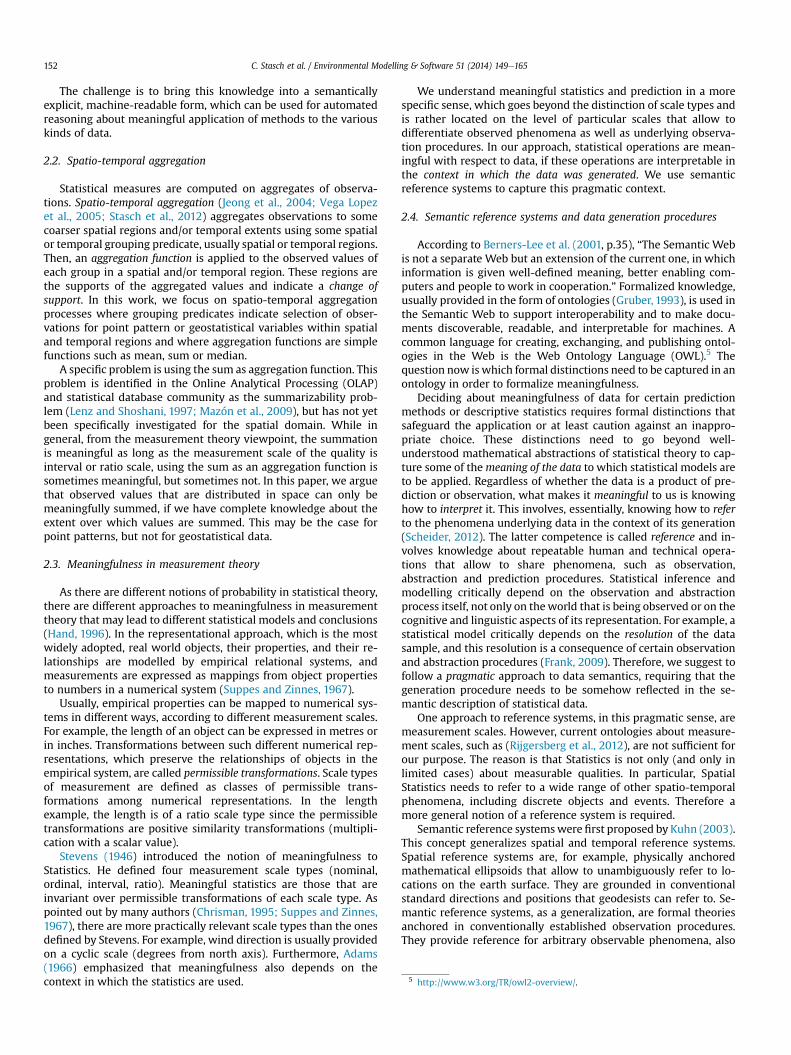
To illustrate the problem, consider two real datasets from theatmospheric domain shown in Fig. 1: (i) total emissions of CO2 forthe year 2007 from power plants in Germany2 and (ii) daily meanconcentrations of fine dust (PM10) measured at air quality stationsin Germany.3 Both datasets have an indistinguishable data struc-ture: records of scalar values indexed by points in space and time.Hence, the datasets are often treated as the same in spatial analysis.However, though both datasets can be easily interpolated spatially(right column of Fig.1), interpolation of points is onlymeaningful forPM10 concentration and not for total emissions of CO2 from powerplants. Users unaware of the data semantics may apply inappro-priate procedures because they do not distinguish between datasetswith equivalent structure representing incommensurable phe-nomena. A comparable problem concerns the application of statis-tical measures in spatio-temporal aggregation, such as summing upobservation valueswithin spatial regions. Computing the sumof thetotal CO2 emissions of power plants over Germany may be mean-ingful, while the sum of PM10 concentrations over an area may not.

Though basic prediction and aggregation functionality forspatial data is often available in Geographical Information System(GIS) or statistical software in an adhoc fashion, the choice of aparticular method is usually up to the user and its appropriatenessis not checked by the system. Furthermore, while measurementscales (Stevens,1946; Suppes and Zinnes,1967; Chrisman,1995) arewell established, in many cases, allowable operations are unknownfor a dataset. It is, e.g., notmeaningful to compute themean value ofa numerical ordinal variable, although it is possible from acomputational viewpoint.

We argue that the problem of meaningful prediction and ag-gregation requires knowledge about the meaning of data, i.e., se-mantic knowledge, in machine readable form to help usersdetermine which prediction or aggregation method can be appliedto which dataset. In this paper, we suggest a way how the notion ofmeaningfulness can be operationalized:

1. Formal specifications make some of the knowledge underlyingmeaningful statistics more explicit and readable for machines.

2. In a rough approximation, a statistical prediction or aggregationmethod can be said to bemeaningfully applicable to a data set, ifit is semantically interpretable in the observation context of thedata. This context can be captured, to a significant degree, by(semantic) reference systems (Kuhn, 2003).

3. On this basis, the well-known conceptual distinction between(marked) point pattern, geostatistical variables and lattice data(Illian et al., 2008; Burrough and Mcdonnell, 1998; Cressie andWikle, 2011), can be made formally explicit.

4. Meaningfulness of prediction can then be checked by testingwhether prediction functions underlying statistical models

1 The SWEET ontologies are accessible at http://sweet.jpl.nasa.gov/ontology/.2 The data is accessible for free at http://www.carma.org.3 The data is available at http://www.eea.europa.eu/themes/air/airbase.

formally correspond to observation functions underlying data,where both are typed by semantic reference systems.

5. Meaningfulness of summation can be checked by testingwhether regions over which the data is aggregated formallycorrespond to the observed window of the data to be aggregated.

6. This shows a way to design a recommender tool in Spatial Sta-tistics,4 in which data and variables can be linked to interpola-tion and aggregation methods.

The contribution of this paper is a formalization of meaning-fulness of spatial prediction and aggregation with respect to data-sets. Out of scope are the semantic description of observableproperties, of statistical models, and of application problems. Wemake the case for our notion of meaningfulness based on the twoscenarios from the atmospheric domain introduced above (airquality and CO2 emissions). We test our theory and prove mean-ingfulness in Isabelle/HOL, a higher-order theorem prover. A pre-liminary Web Ontology Language (OWL) pattern, which can beused by statistical applications on the Web, and a prototypicalimplementation in R illustrate some of its potential.

The remainder of this paper is structured as follows. The nextsection introduces the background of our work including overviewson Spatial Statistics, on spatio-temporal aggregation, on meaning-fulness inmeasurement theory, and on semantic reference systems.Afterwards our functional approach to formalize Spatial Statisticalknowledge is described in detail. Then, a description of a proto-typical implementation, an R package that extends the package sp,is introduced. Finally, after discussion of our approach, conclusionsand directions for future research are presented.

2. Background

This section provides background and a preliminary discussionof the problem of meaningfulness. First, basic variable types areintroduced which are relevant for meaningful Spatial Statistics.Then, we describe our notion of spatio-temporal aggregation. Af-terwards, we discuss the definition of meaningfulness in mea-surement theory. Finally, semantic reference systems for space,time, as well as for thematic domains are described, and it is arguedwhy they are useful for making the necessary distinctions.

2.1. Spatial Statistics

Spatial Statistics (Ripley, 1981; Cressie, 1993; Cressie and Wikle,2011) is a branch of Statistics that deals with spatial and spatio-temporal processes. Although all observations are taken undercircumstances that can be characterized by a location and time, inmany cases location and time do play a minor role, for instancewhere controlled experiments in lab conditions eliminate the roleof space and time. In case of medical experiments, the subject’sidentity and age may form the major reference. However, whenobservations are taken outside a lab, non-controllable factorstypically cause them to be correlated in space and/or over time.Spatial Statistical models address such correlations, allow in-ferences, and are used for the prediction of phenomena in spaceand time.

For spatio-temporal processes, Cressie and Wikle (2011) use thefollowing notation:

4 In this paper, we follow the distinction introduced by Cressie and Wikle (2011),where statistics refers to summaries of data and Statistics to the Statistical Science.The same is applied to Spatial Statistics and Geostatistics.

Fig. 1. Example datasets containing total CO2 emissions of power plants in 2007 (upper left) and PM10 measurements at 7th June 2005 (lower left). Both datasets consists of recordsof scalar values indexed by coordinates in space and can be easily spatially interpolated. However, the interpolated CO2 emissions (upper right) can hardly be interpreted at locationswhere no power plants are located.

C. Stasch et al. / Environmental Modelling & Software 51 (2014) 149e165 151

ZðsÞ; s ˛W; W3Rd (1)

with Z(s) an observed or unobserved value at s, the combination ofspatial location and time; W the spatial and temporal domain orwindowover which Z is defined; and d the dimensionality of space-time (e.g., three in case of two-dimensional space plus time). Thelocation s, the spatial and/or temporal support, is a region in aspatial and/or temporal reference system and may be representedas a point.

Two basic forms can be distinguished. First, Z is defined forevery possible value of s (hence Z is total). In Geostatistics, oneassumes that s is a continuous index. In this case, Z(s) is a geo-statistical variable, and the challenge often lies in predicting valuesZ for unobserved locations s0, based on a limited set of n observa-tions Z(s1),.,Z(sn).

The second form is that of point pattern variables (Illian et al.,2008), where not for every point si Z is defined (hence Z ispartial). A pure point pattern consists only of those locations.Marked point patterns include the Z values (the marks). Typicalquestions in point pattern modelling are whether point densityvariations can be considered random, whether points interact(e.g., attract or repulse), and how point density, interactions, or

marks depend on known covariates. For analysing point patterndata, it is important to know the observation window W(Baddeley and Turner, 2005), as the latter allows discriminatingbetween where we know there are no points from wherenothing is known.

If values are considered results of a random process, the valuescannot be chosen arbitrarily and we call that variable a randomvariable. In contrast, we call a variable a fixed variable, if the valuescan be fixed, i.e., the values can be selected arbitrarily. Point patternanalysis considers s ¼ s1,.,sn as a random set, meaning that loca-tions are random variables. Given the locations, the marks of amarked point process Z(s) are considered random variables. Forgeostatistical variables, only Z is considered random, as observationand prediction locations s can be chosen arbitrarily.

In the case of Lattice data, observed values reflect aggregationsover a set of covering regions rather than (values for) points. Theunion of regions forms the area of studyW. The observed variable isusually modelled as a random field, the regions are not random.Images are often considered as a special case of lattice data. Typicalproblems are modelling spatial dependence, assessing whetherspatial patterns might be completely random, and finding relationswith covariates.

5 http://www.w3.org/TR/owl2-overview/.

C. Stasch et al. / Environmental Modelling & Software 51 (2014) 149e165152

The challenge is to bring this knowledge into a semanticallyexplicit, machine-readable form, which can be used for automatedreasoning about meaningful application of methods to the variouskinds of data.

2.2. Spatio-temporal aggregation

Statistical measures are computed on aggregates of observa-tions. Spatio-temporal aggregation (Jeong et al., 2004; Vega Lopezet al., 2005; Stasch et al., 2012) aggregates observations to somecoarser spatial regions and/or temporal extents using some spatialor temporal grouping predicate, usually spatial or temporal regions.Then, an aggregation function is applied to the observed values ofeach group in a spatial and/or temporal region. These regions arethe supports of the aggregated values and indicate a change ofsupport. In this work, we focus on spatio-temporal aggregationprocesses where grouping predicates indicate selection of obser-vations for point pattern or geostatistical variables within spatialand temporal regions and where aggregation functions are simplefunctions such as mean, sum or median.

A specific problem is using the sum as aggregation function. Thisproblem is identified in the Online Analytical Processing (OLAP)and statistical database community as the summarizability prob-lem (Lenz and Shoshani, 1997; Mazón et al., 2009), but has not yetbeen specifically investigated for the spatial domain. While ingeneral, from the measurement theory viewpoint, the summationis meaningful as long as the measurement scale of the quality isinterval or ratio scale, using the sum as an aggregation function issometimes meaningful, but sometimes not. In this paper, we arguethat observed values that are distributed in space can only bemeaningfully summed, if we have complete knowledge about theextent over which values are summed. This may be the case forpoint patterns, but not for geostatistical data.

2.3. Meaningfulness in measurement theory

As there are different notions of probability in statistical theory,there are different approaches to meaningfulness in measurementtheory that may lead to different statistical models and conclusions(Hand, 1996). In the representational approach, which is the mostwidely adopted, real world objects, their properties, and their re-lationships are modelled by empirical relational systems, andmeasurements are expressed as mappings from object propertiesto numbers in a numerical system (Suppes and Zinnes, 1967).

Usually, empirical properties can be mapped to numerical sys-tems in different ways, according to different measurement scales.For example, the length of an object can be expressed in metres orin inches. Transformations between such different numerical rep-resentations, which preserve the relationships of objects in theempirical system, are called permissible transformations. Scale typesof measurement are defined as classes of permissible trans-formations among numerical representations. In the lengthexample, the length is of a ratio scale type since the permissibletransformations are positive similarity transformations (multipli-cation with a scalar value).

Stevens (1946) introduced the notion of meaningfulness toStatistics. He defined four measurement scale types (nominal,ordinal, interval, ratio). Meaningful statistics are those that areinvariant over permissible transformations of each scale type. Aspointed out by many authors (Chrisman, 1995; Suppes and Zinnes,1967), there are more practically relevant scale types than the onesdefined by Stevens. For example, wind direction is usually providedon a cyclic scale (degrees from north axis). Furthermore, Adams(1966) emphasized that meaningfulness also depends on thecontext in which the statistics are used.

We understand meaningful statistics and prediction in a morespecific sense, which goes beyond the distinction of scale types andis rather located on the level of particular scales that allow todifferentiate observed phenomena as well as underlying observa-tion procedures. In our approach, statistical operations are mean-ingful with respect to data, if these operations are interpretable inthe context in which the data was generated. We use semanticreference systems to capture this pragmatic context.

2.4. Semantic reference systems and data generation procedures

According to Berners-Lee et al. (2001, p.35), “The Semantic Webis not a separate Web but an extension of the current one, in whichinformation is given well-defined meaning, better enabling com-puters and people to work in cooperation.” Formalized knowledge,usually provided in the form of ontologies (Gruber, 1993), is used inthe Semantic Web to support interoperability and to make docu-ments discoverable, readable, and interpretable for machines. Acommon language for creating, exchanging, and publishing ontol-ogies in the Web is the Web Ontology Language (OWL).5 Thequestion now is which formal distinctions need to be captured in anontology in order to formalize meaningfulness.

Deciding about meaningfulness of data for certain predictionmethods or descriptive statistics requires formal distinctions thatsafeguard the application or at least caution against an inappro-priate choice. These distinctions need to go beyond well-understood mathematical abstractions of statistical theory to cap-ture some of themeaning of the data to which statistical models areto be applied. Regardless of whether the data is a product of pre-diction or observation, what makes it meaningful to us is knowinghow to interpret it. This involves, essentially, knowing how to referto the phenomena underlying data in the context of its generation(Scheider, 2012). The latter competence is called reference and in-volves knowledge about repeatable human and technical opera-tions that allow to share phenomena, such as observation,abstraction and prediction procedures. Statistical inference andmodelling critically depend on the observation and abstractionprocess itself, not only on theworld that is being observed or on thecognitive and linguistic aspects of its representation. For example, astatistical model critically depends on the resolution of the datasample, and this resolution is a consequence of certain observationand abstraction procedures (Frank, 2009). Therefore, we suggest tofollow a pragmatic approach to data semantics, requiring that thegeneration procedure needs to be somehow reflected in the se-mantic description of statistical data.

One approach to reference systems, in this pragmatic sense, aremeasurement scales. However, current ontologies about measure-ment scales, such as (Rijgersberg et al., 2012), are not sufficient forour purpose. The reason is that Statistics is not only (and only inlimited cases) about measurable qualities. In particular, SpatialStatistics needs to refer to a wide range of other spatio-temporalphenomena, including discrete objects and events. Therefore amore general notion of a reference system is required.

Semantic reference systemswere first proposed by Kuhn (2003).This concept generalizes spatial and temporal reference systems.Spatial reference systems are, for example, physically anchoredmathematical ellipsoids that allow to unambiguously refer to lo-cations on the earth surface. They are grounded in conventionalstandard directions and positions that geodesists can refer to. Se-mantic reference systems, as a generalization, are formal theoriesanchored in conventionally established observation procedures.They provide reference for arbitrary observable phenomena, also

C. Stasch et al. / Environmental Modelling & Software 51 (2014) 149e165 153

for phenomena described by complex geometries or attributes in aGeographic Information System (GIS). There are, e.g., referencesystems for time in terms of calendars, for places in terms of postaladdresses, as well as for other kinds of observable phenomena. Formany spatio-temporal phenomena, such as geographic objects andevents, reference systems can be constructed in a similar way,based on repeatable observation and abstraction procedures(Scheider, 2012).

In this paper, we will just make use of the discriminative powerof reference systems regarding domains of phenomena of interest,while the question of constructing and grounding them is not infocus. Therefore, we will presuppose that we have reference sys-tems of an appropriate kind at our disposal, and we will preservethe term referent to speak about an individualized phenomenon inthe domain of a reference system. The meaning of the latter isconventionally established.

Since reference systems are formal theories grounded inrepeatable procedures, their domain can be viewed as the struc-tured set of all possible entities that can be the result of such a pro-cedure. For example, the set of all potentially observable coloursmakes a colour space, or the set of all potentially observable loca-tions makes a spatial reference domain. By a procedure, we under-stand in this paper any conventionally shared instruction to generateentities of a reference system, in particular mathematical functions.This is regardless ofwhether this instruction is explicit in the formofa computational rule, such as a prediction algorithm inGeostatistics,or whether it is implicit in the form of human action schemes.

3. A formalization of meaningful prediction and aggregation

In this section, we introduce the formalism that enables to inferwhether applications of prediction and aggregation procedures todatasets are meaningful, provided that their underlying observa-tion procedures are known. First, an overview is given of theapproach (Section 3.1), followed by an introduction to our formalnotation (Section 3.2), and subsections for each core concept in ourformalism (Sections 3.3e3.8).

3.1. Overview

The basic idea of our formalism is a formal distinction betweenrepresentations of procedures as functions, which capture knowledgeabout potential operations such as observing or predicting phe-nomena, and representations of data sets as predicates over functiondomains, which denote limited (finite) results of applying suchoperations. This distinction allows us to compare data and pro-cedures in terms of the underlying data generation capabilities. Weexplain this idea first in an informal way.

An observation procedure is an operational description how toobserve a phenomenon. For example, the observation procedure forobserving PM10 involves localization of the measurement device inspace, time measurement by a clock, and the use of a PM10 sensor,whose technical specification describes the measurement proce-dure in more detail. By executing this procedure, one takes uniquemeasurements at arbitrary points in time and space. Therefore, wecan specify the observation procedure by a continuous observationfunction, a mapping from arbitrary locations and times to concen-trations. Similarly to an observation procedure, a particular pre-diction procedure is specified by a prediction function in ourformalism. An example of a prediction procedure is the descriptionof ordinary kriging in a statistical book (Cressie and Wikle, 2011,p.145), which can be specified as a function from continuous spaceand time to predicted values. Hence, our formalism consists offunctional specifications, shown in yellow colour in Fig. 2, whichallow to distinguish the different types of Spatial Statistical

variables: point pattern, marked point pattern, and geostatisticalvariables, in terms of different types of functions.

The meaning of the functional domains and ranges, i.e., of thetypes of entities being related by a function, is given in terms ofreference systems shown as blue concept in Fig. 2. More precisely,functions are mappings from certain reference domains to otherones, where the latter are specified as formal types.

As an example, the function specifying PM10 observationsin Germany in the year 2008 is a mapping WGS840UTC20080 PM10 from the spatial reference domain given in theWorld Geodetic System 1984 (WGS84), WGS84 coordinates inGermany, and the temporal reference domain UTC2008, the year2008 in Universal Time Coordinated (UTC), to a sensor referencedomain PM10 defining concentration values in mg/m3. Such anobservation function is of a geostatistical type, since it maps pointsin continuous space and time to quality values.

The observation procedure, which is specified as an observationfunction, stands for potential observations, whereas executing theprocedure generates actual observations, i.e., data. Since the pro-cedure can be executed only finitely many times, data is alwaysfinite, in contrast to the corresponding observation function.However, annotating datawith an observation function allows us tolink it with the underlying observation procedure, and thus, to takepossible observations into account when deciding about mean-ingfulness. More precisely, in order to check whether a predictionprocedure can be meaningfully applied to a dataset, we propose tocheck whether the respective observation function corresponds ina certain sense to the prediction function which specifies the pre-diction procedure (compare Fig. 2).

How does this approach help us to distinguish the geostatisticalfrom the point pattern scenario? Since the function formalismcaptures procedures in the sense of potential observations or pre-dictions, it allows, for example, to capture the difference betweencontinuously observable space and discretely observable objects,even though the actual datasets are discrete in both cases and, thus,may not be distinguishable. The difference between continuouslyobservable space and discretely observable objects is, in essence,the difference between a geostatistical and a point pattern variable.Furthermore, a prediction function, which specifies what can bedonewith a prediction procedure such as Kriging interpolation, canonly be considered meaningful with respect to an observationdataset, if the underlying observation procedure supplies possibleobservations for each predictable case. For example, in the case ofCO2 emissions of power plants, a geostatistical interpolation gen-erates values at locations where no power plants are located, and,hence, an interpolation of power plant emissions becomesmeaningless.

In a similar way, the observed window, which is the extent towhich an observation dataset “covers” a spatio-temporal domain,can be used to determine whether an aggregation procedure can bemeaningfully applied to a dataset or not. For example, since theobservation of PM10 cannot cover a continuous spatial aggregationregion, such as the spatial region of Germany, by a discrete datasample, using the sum to aggregate this dataset is meaningless.However, summing up emissions from discrete power plants maybe meaningful, provided that the observed window covers thewhole region of Germany. Note that also in this case, the essentialidea is that a specification of an observation procedure accounts forwhat can be observed in contrast to the limited sample of an actualdataset.

3.2. Formal notation and semi-automated test and proof in Isabelle

The formalism is written, implemented and tested in Isabelle/HOL, a typed higher-order logic (HOL) which allows for reasoning

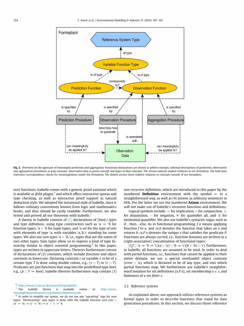
Fig. 2. Overview on the approach of meaningful prediction and aggregation. Functional declarations are shown as yellow concepts, informal descriptions of prediction, observationand aggregation procedures as grey concepts, observation data as green concept and types as blue concepts. The arrows indicate explicit relations in our formalism. The bold linesrepresent correspondence checks for meaningfulness inside the formalism. The dotted arrows show implicit relations to concepts outside of our formalism.

C. Stasch et al. / Environmental Modelling & Software 51 (2014) 149e165154

over functions. Isabelle comes with a generic proof assistant whichis available as jEdit plugin,6 and which offers interactive syntax andtype checking, as well as interactive proof support in naturaldeduction style. We adopted the notational style of Isabelle, since itfollows ordinary conventions known from logic and mathematicsbooks, and thus should be easily readable. Furthermore, we alsotested and proved all our theorems with Isabelle.7

A theory in Isabelle consists of (1) declarations of (basic) typesand type definitions, using type constructors such as 0a 0 0b forfunction types, 0a � 0b for tuple types, and 0a set for the type of setswith elements of type 0a, with variables 0a,0b,0c standing for sometypes. We also use sum types 0a þ 0b, i.e., types that are the union oftwo other types. Sum types allow us to express a kind of type hi-erarchy similar to object oriented programming.8 In this paper,types arewritten in uppercase letters. Theories furthermore consistof declarations of (2) constants, which include functions and objectconstants in lowercase. Declaring constant c or variable v to be of acertain type T is done using double colons, e.g., (v :: T) or (c :: T).Predicates are just functions that map into the predefined type bool,e.g., (p :: T 0 bool). Isabelle theories furthermore may contain (3)

6 http://www.cl.cam.ac.uk/research/hvg/isabelle/.7 The Isabelle theory is available online at: http://www.

meaningfulspatialstatistics.org/theories/Miptheory.thy.8 In order to simplify our syntax, we do not use any “upcasting” sign for sum

types. “Downcasting” sum types is done with the Isabelle function sum_case ::(a0 0 0b) 0 (c0 0 0b) 0 a0 þ 0c 0 0b.

non-recursive definitions, which are introduced in this paper by thenumbered Definition environment with the symbol h in astraightforward way, as well as (4) axioms as arbitrary sentences inHOL. For the latter we use the numbered Axiom environment. Wewill not make use of Isabelle’s recursive functions and definitions.

Logical symbols include/ for implication, ^ for conjunction,nfor disjunction, : for negation, c for quantifier all, and d forexistential quantifier. We also use Isabelle’s syntactic sugar, such asif.then.else. As in functional programming, f a means applyingfunction f to a, and lx.b denotes the function that takes an x andreturns b. ix.P x denotes the unique x that satisfies the predicate P.Functions are always curried, i.e., function domains are written as a(right-associative) concatenation of functional types:

(((f :: 0a 0 0b 0 0c)(a :: 0a) :: 0b 0 0c)(b :: 0b) :: 0c). Furthermore,in Isabelle, all functions are assumed to be total. In order to dealwith partial functions, i.e., functions that cannot be applied to theirentire domain, we use a special overloaded object constant(error :: 0a), which is declared to be of any type, and into whichpartial functions map. We furthermore use Isabelle’s straightfor-ward notation for set definitions {x.P x}, set membership x ˛ s, andfiniteness of a set finite s.

3.3. Reference systems

As explained above, our approach utilizes reference systems asformal types in order to describe functions that stand for datageneration procedures. In this section, we discuss those reference

C. Stasch et al. / Environmental Modelling & Software 51 (2014) 149e165 155

systems that are needed to specify the observation and predictionprocedures in our scenarios, and we introduce basic types forthem.

Table 1 shows types of reference systems that are used in ourapproach. Besides domains of spatial and temporal reference sys-tems, such as coordinate systems and calendars, we assume do-mains for quality reference systems including, for example,measurement scales or observed qualities such as colour, as well asdomains for discrete entities. Discrete entities may be furtherdistinguished into physical objects and events, following top-levelontologies as described in Gangemi et al. (2003). Note, however,that we do not make any further commitment, e.g., as to whetherqualities need to inhere in objects. However, the distinction be-tween spatial, temporal, quality, and discrete domains of referencewill already enable us to introduce a new notion of meaningfulnessin Spatial Statistics.

Each domain of reference comes with its own formal struc-ture, the latter being a result of a data generation procedure.This structure includes formal relations on these domains, suchas the order relation in a calendar, or the metric relation be-tween spatial coordinates, as well as cardinality properties of thedomains, such as finiteness, infinity, density, and continuity. Forexample, spatial and temporal domains of measurement areusually considered infinitely dense, meaning that there areinfinitely many potentially distinguishable locations, such thateach pair of distinguishable ordered locations contains anotherpotentially measurable location in between. The domain struc-ture can be formally specified in Isabelle, and this will be used inSection 3.7 in order to prove for our CO2 and PM10 guidingscenario that continuous interpolation procedures are notmeaningfully applicable in the CO2 case. For this purpose, weneed to formalize strict cardinality orders among reference do-mains, Dd 3c Ds ^ Dd 3c Dt. Even though in Isabelle, we cannotdirectly handle relations on types, we can do this indirectly byrestricting injective functions on them (see Appendix A). That is,even though finiteness, discreteness, and continuity have furtherformal implications, in this paper, we only use the fact that theyimply different set cardinalities, i.e., different sizes, togetherwith the following mathematical fact about finite and infinitesets:

Axiom 1. Infinite sets are bigger than finite sets:“cs s0. finite s ^: finite s0 / (dx.x ˛ s0 ^: x ˛ s) ”

For quality reference systems, the type of measurement scale isanother formal structure which is of importance to decide on theapplicability of statistics (see Section 2.3). As there are, in theory, “anondenumerable infinity of types of scales., but most of them arenot of any real empirical significance” (Suppes and Zinnes, 1967,p.14), we focus exemplary on Stevens’ measurement scale types(Stevens, 1946) and indicate them by nominal (Dn

q), ordinal (Doq),

interval (Diq), and ratio (Dr

q) types.The reference domains Ds, Dt, and Dq include granules (entities

that cannot be divided into smaller entities of that reference sys-tem). However, granules can be aggregated to sets which we callregions.9 Thus, region types of some reference domain D can bedefined in Isabelle simply by the “set” type constructor, i.e., rD ¼ Dset. For example, a spatial reference system WGS84 can be used torefer to locations as singular coordinate tuples, and so WGS84 setcan be used to refer to regions of coordinate tuples. The regions

9 We are aware of the fact that spatio-temporal regions, too, have further formalproperties, such as continuity and regularity. However, for our purpose, thesedistinctions are not necessary.

may be finite as well as infinite sets of granules (regardless of thefact that their computer representation is always finite). Further-more, while a domain of regions rD contains the power set of the setof granules, what is of interest are usually particular finite collec-tions of them. Such collections are specified formally below aspredicates over region domains, similar to other kinds of datasets(Section 3.6).

3.4. Specifying Spatial Statistical variable types as types offunctions

Spatial Statistical variables are representations of spatio-temporal processes. In this section, we show how to distinguishvariable types relevant in Spatial Statistics in terms of types offunctions in our formalism. These types are a key to decidingwhether procedures can be meaningfully applied to data, as dis-cussed in Section 2.1. Spatial Statistical variables can be specified asfunctions, since one normally assumes that there is only one targetvalue for a particular represented process at a particular “support”,i.e., for a particular location or object in time10. The domain of thefunction (left part of the functional type) can be considered fixed(i.e., a matter of choice), whereas the range (the right part) can beconsidered the result of some random process (i.e., it cannot beinfluenced).

Table 2 shows the functional types of point patterns in SpatialStatistics. Spatial point patterns (SPP) provide spatial locations fordiscrete entities, e.g., locations of longleaf pines within 4 ha of anatural forest (Cressie and Wikle, 2011, p.204). In this example,the domain of discrete entities (Dd) is a set of longleaf pines thatare mapped to spatial positions in the forest (Ds 3 R2), the latterbeing considered the result of a random process. If there areadditional attribute values for each location (e.g., the diameter ofthe longleaf pines), the variable is a marked spatial point pattern(MSPP). Temporal point patterns (TPP) are similar to their spatialcounterparts, but their defining function is a mapping fromdiscrete entities to temporal positions. The occurrence of earth-quakes in a particular US state is a temporal point pattern wherethe discrete reference domain Dd is the set of earthquakes andthe temporal reference domain Dt contains the times within theobservation period. In analogy to space, in a marked temporalpoint pattern (MTPP), quality values are attached to the timepositions, e.g., magnitude in addition to the position of anearthquake.

If the locations in space and time are fixed, but the quality valuesare considered being the result of some random process, the vari-ables are called geostatistical or lattice, as defined in Table 3. Geo-statistical variables (GEOST) provide quality values for granularlocations in space. Hence, they are specified as functions that mapfrom points in space and time to quality values that are considereda result of a stochastic process. In the object and field view (see forexample Galton (2004)), the geostatistical variables implement thefield view, whereas point patterns provide values for discrete en-tities, thus implementing the object view.

Examples for a geostatistical variable are PM10 concentrationsmeasured across Europe. The spatial domain consists of positionswithin Europe (Ds 3 R2), the temporal domain contains the timepositions within the observation period (Dt 3 R), and the qualitydomain is the PM10 scale in degree Fahrenheit, thus an intervalscaled quality domain (Di

q3R). If the fixed locations in space arenot granular but regional entities, we call that variable a lattice

10 Stochastic variables (i.e., joint probability distributions) can be specified asfunctions from reference types into probability space. However, probability distri-butions are not in focus in this paper.

Table 2Types of point pattern variables used in Spatial Statistics.

Variable type Functional type Example

Spatial point pattern SPP ¼ “Dd 0 Ds” Locations of longleaf pines in 4 ha of a natural forest in Thomas County, GeorgiaMarked spatial point pattern MSPP ¼ “Dd 0 (Ds � Dq)” Locations of longleaf pines in 4 ha of a natural forest in Thomas County,

Georgia with diameters-at-breast-heights (DBH)Temporal point pattern TPP ¼ “Dd 0 Dt” Occurrence of earthquakes in an American countyMarked temporal point pattern MTPP ¼ “Dd 0 (Dt � Dq)” Occurrence of earthquakes in an American county with magnitudesSpatio-temporal point pattern STPP ¼ “Dd 0 (Dt � Ds)” Occurrence of earthquakes at particular locations in space and timeMarked spatio-temporal

point patternMSTPP ¼ “Dd 0 (Dt � Ds � Dq)” Occurrence of earthquakes at particular locations in space and time with magnitudes

Table 3Types of geostatistical and lattice variables in Spatial Statistics.

Variable type Functional type Example

Geostatistical variable GEOST ¼ “Ds 0 Dt 0 Dq” PM10 concentrations across GermanyLattice variable LAT ¼ “rDs 0 Dt 0 Dq” Number of doctor-prescriptions per consultation

in cantons of the Midi-Pyrenees

Table 1Types of reference system domains.

Reference domain Type Description Example

Domain of a spatialreference system

Ds All possible locations that are defined in a spatialreference system; we restrict Ds to Ds 3 R2

([�90,90] � [�180,180]) 3 R2 defined in WGS84

Domain of a temporalreference system

Dt All possible times defined in a temporalreference system

POSIX time (seconds from 1st January 1970 UTC) with Dt 3 Q

Domain of a qualityreference system

Dq Set of all values that a quality might take [0,106] 3 R with unit ppm as defined in Unified Code forUnits of Measure (UCUM)

Domain of a discreteentities

Dd Set of discrete objects or events. Set of coal power plants in Germany in 2010; set of allearthquakes in Italy in 20th century

C. Stasch et al. / Environmental Modelling & Software 51 (2014) 149e165156

variable (LAT). Often, lattice data is point data that has beenaggregated for particular reasons, e.g., privacy in medical data. Asan example, the doctor-prescription amounts per consultation incantons of the Midi-Pyrenees (Cressie and Wikle, 2011, pp.189e191) are computed from individual doctor-prescriptions at partic-ular locations of the Midi-Pyrenees at particular times.

Another variable type are trajectories (Table 4). Trajectories(TRAJECT) are mappings from discrete objects and times to spatiallocations, e.g., paths of tracked animals. Similar to point patterns,marks may be attached to the spatial positions, e.g., the bodytemperature of the tracked animals. Spatial point patterns can bederived from trajectories by fixing the time.

3.5. Specifying observation procedures as functions

In this subsection, we show how observation functions can bedefined which capture essential knowledge about observationprocedures underlying our example scenarios. Examples of func-tions representing primitive procedures are listed in Table 5. Otherprocedures may be defined on this basis. The object localizationprocedure obsloc locates discrete objects at particular times in space.

Table 4Trajectory variable type in Spatial Statistics.

Variable type Functional type Example

Trajectory TRAJECT ¼“Dd 0 Dt 0 Ds”

Paths of tracked animals

Markedtrajectory

MTRAJECT ¼“Dd 0 Dt 0 (Ds � Dq)”

Paths of tracked animalswith measurementsof body temperature

Another example is themeasurement of an object property, definedas obsprop in our formalism. Note that formal specifications of theseobservation functions represent the observation procedure, butfunctions are not identical with procedures. First, observationfunctions are fictions, as the set of tuples that constitutes thefunction (the functions’ extension) is largely unknown. Second, theprocedures involve a lot more knowledge about conventions andmeasurement operations which are not explicit in the functionalspecification. For example, spatial localization of objects involvesthe whole geodetic apparatus of measurement as well as aperceptual procedure for objects. However, it is these procedureswhich give the observation functions their specific intendedmeaning.

The observation procedures are represented as total functions,meaning that the functions are defined over their whole func-tional domain such that they do not produce any errors. Forexample, the function obsloc always returns a spatial location forall discrete entities. Observation procedures are specified asfunctions because there can only be one observed value for aparticular phenomenon at a particular location in time and space.For example, the surface temperature only takes a certain value ata particular location in space and time. In addition, they are totalfunctions without errors, since observation procedures fully cap-ture observation potentials over a domain of interest. Even thoughwe cannot travel back in time to observe phenomena in the past,and even thoughe for practical reasonse it may not be possible attimes and places in the future, observation procedures representthe potential of generating a response in every single casedescribed by the application domain. Hence, observation func-tions express potential observations, providing a way to talk aboutpotential actions, i.e., actions that may be intended, but, for some

Table 5Functions for basic observation procedures.

Observation procedure Observation function Example

Object localization procedure obsloc :: Dd 0 Dt 0 Ds Location of a coal power plant by centroid (any spatial point pattern)Object property observation procedure obsprop :: Dd 0 Dt 0 Dq CO2 emission rate of a power plant at a series of timesContinuous phenomenon observation procedure obscphen :: Ds 0 Dt 0 Dq Observation of PM10 concentrations across Germany

Table 6Relevant data types in Spatial Statistics.

Data type Formal type Explanation

Spatial point pattern data SPPD ¼ “Dd 0 Ds 0 bool” Locations of coal power plants in Germany.Geostatistical data GEOSTD ¼ “Ds 0 Dt 0 Dq 0 bool” PM10 concentrations measured at monitoring stations in Germany.Lattice data LATTICED ¼ “rDs 0 Dt 0 Dq 0 bool” Number of doctor-prescriptions per consultation in cantons of the Midi-Pyrenees

Table 7Additional data types used in our formalism.

Data type Formal type Explanation

Collection of spatial regions SR ¼ “rDs 0 bool” Federal states of GermanyCollection of temporal regions TR ¼ “rDt 0 bool” Months in 2008Observation data super type OBSD ¼ “GEOSTD þ SPPD þ LATTICED” A shorthand for one of the statistical data types aboveRegion data super type REGIOND ¼ “SR þ TR” A shorthand for one of the region data types aboveData super type DATA ¼ “OBSD þ REGIOND” A shorthand for all of the data types above

11 We use a simplified operator sum_case* for better readability. In Isabelle, thisoperator needs to be implemented as a cascading downcasting.

C. Stasch et al. / Environmental Modelling & Software 51 (2014) 149e165 157

reason, remain unperformed. Isabelle functions are always total,so, the only thing we need to assert is that observation functionsdo not produce errors:

Axiom 2. Totality of observation functions:

“c x y:obsprop x yserror” and

“c x y:obscphen x yserror” and

“c x y:obsloc x yserror”

More complex observation procedures can be generated byfunctional compositions. For example, the observation of total CO2emissions from coal power plants at a particular year, which is amarked spatial point pattern, may be generated by a functionobsmspp as in Definition 1.

Definition 1. (Marked Spatial Point Pattern Observation).obsmspp :: MSPP where

“�obsmspp d

�h�ðobsloc d t1Þ;

�obsprop d t1

��”

with t1 :: Dt standing for a temporal instance.

The function obsmspp is a composition of the object localizationfunction (obsloc) and the object property observation function(obsprop). Note that in this definition, the time of the primitiveobservation functions is implicitly fixed by a constant t1, whichdoes not appear anymore in the defined observation functionobsmspp. In this way, it is possible to derive new observationfunctions from primitive procedures, as well as to prove theirformal properties.

3.6. Specifying data and observed window

Once an observation procedure is executed, data is produced.While an observation function describes potentially limitless

observations, a particular dataset consists of a finite sample.Correspondingly, we specify data as a predicate over an observationfunctionwhich just picks out a finite sample of tuples from the setthat constitutes the total function. For example, while the obser-vation function obscphen specifies observations of PM10 concen-trations for all possible locations and times, a particular dataset,such as datageostat in Table 8, consists of a finite subset of tuples atsome locations in space, namely where monitoring stations arelocated. A selection of relevant data types for Spatial Statistics isshown in Table 6, additional data types used in our formalism aredefined in Table 7 and example instances of data are defined inTable 8.

How can these data properties be formalized? We assume thatdata sets are always finite and non-empty (Definition 2). Definition2 asserts this for the overloaded sum type DATA.11

Definition 2. (Data properties). Data :: “DATA 0 bool” where

“Data mh sum case*

ðlm:ðfinite f ða; b; cÞ: m a b cgÞ ^ ðd a b c: m a b cÞÞðlm:ðfinite f ða; bÞ: m a bgÞ ^ ðd a b: m a bÞÞðlm:ðfinite f a: m agÞ ^ ðd a: m aÞÞm”

Lattices are specified as a special kind of data, namely as a finitecollection of infinite (continuous) regions in space and time (Table 9and Axiom 3). The latter follows from Definition 2, Axiom 3 andAxiom 4.

Axiom 3. Lattice properties:“c l. Lattice l / (c r. l r / : finite r) ^ Data l”

We can now assert data properties defined in Definition 2 for alldata sets introduced in Table 8:

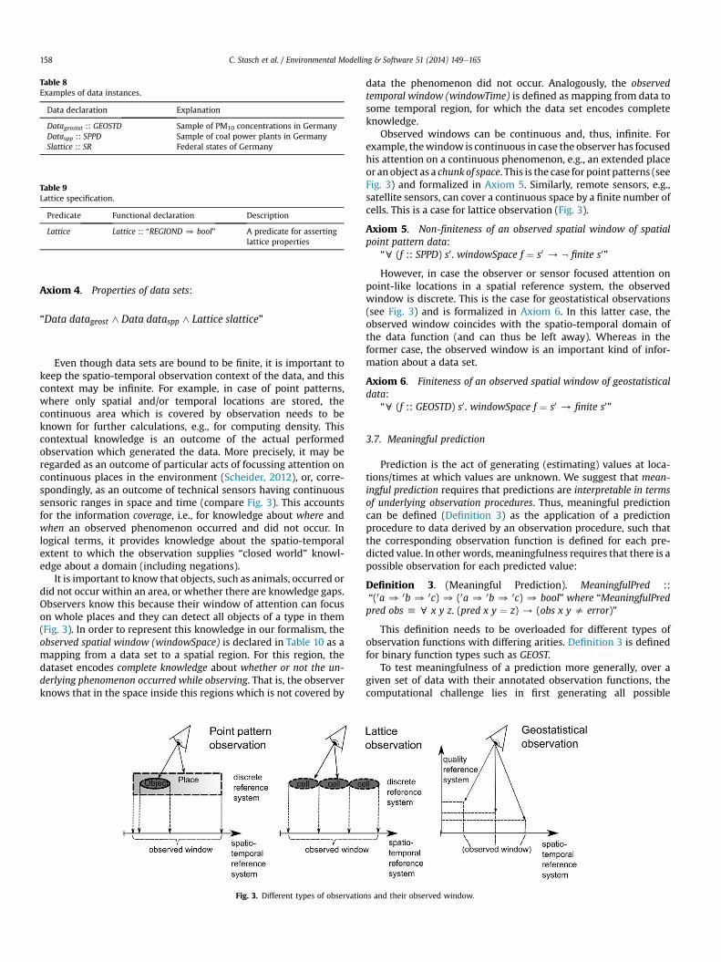
Table 8Examples of data instances.

Data declaration Explanation

Datageostat :: GEOSTD Sample of PM10 concentrations in GermanyDataspp :: SPPD Sample of coal power plants in GermanySlattice :: SR Federal states of Germany

Table 9Lattice specification.

Predicate Functional declaration Description

Lattice Lattice :: “REGIOND 0 bool” A predicate for assertinglattice properties

C. Stasch et al. / Environmental Modelling & Software 51 (2014) 149e165158

Axiom 4. Properties of data sets:

“Data datageost ^ Data dataspp ^ Lattice slattice”

Even though data sets are bound to be finite, it is important tokeep the spatio-temporal observation context of the data, and thiscontext may be infinite. For example, in case of point patterns,where only spatial and/or temporal locations are stored, thecontinuous area which is covered by observation needs to beknown for further calculations, e.g., for computing density. Thiscontextual knowledge is an outcome of the actual performedobservation which generated the data. More precisely, it may beregarded as an outcome of particular acts of focussing attention oncontinuous places in the environment (Scheider, 2012), or, corre-spondingly, as an outcome of technical sensors having continuoussensoric ranges in space and time (compare Fig. 3). This accountsfor the information coverage, i.e., for knowledge about where andwhen an observed phenomenon occurred and did not occur. Inlogical terms, it provides knowledge about the spatio-temporalextent to which the observation supplies “closed world” knowl-edge about a domain (including negations).

It is important to know that objects, such as animals, occurred ordid not occur within an area, or whether there are knowledge gaps.Observers know this because their window of attention can focuson whole places and they can detect all objects of a type in them(Fig. 3). In order to represent this knowledge in our formalism, theobserved spatial window (windowSpace) is declared in Table 10 as amapping from a data set to a spatial region. For this region, thedataset encodes complete knowledge about whether or not the un-derlying phenomenon occurred while observing. That is, the observerknows that in the space inside this regions which is not covered by

Fig. 3. Different types of observatio

data the phenomenon did not occur. Analogously, the observedtemporal window (windowTime) is defined as mapping from data tosome temporal region, for which the data set encodes completeknowledge.

Observed windows can be continuous and, thus, infinite. Forexample, thewindow is continuous in case the observer has focusedhis attention on a continuous phenomenon, e.g., an extended placeor anobject as a chunkof space. This is the case for point patterns (seeFig. 3) and formalized in Axiom 5. Similarly, remote sensors, e.g.,satellite sensors, can cover a continuous space by a finite number ofcells. This is a case for lattice observation (Fig. 3).

Axiom 5. Non-finiteness of an observed spatial window of spatialpoint pattern data:

“c (f :: SPPD) s0. windowSpace f ¼ s0 / : finite s0”

However, in case the observer or sensor focused attention onpoint-like locations in a spatial reference system, the observedwindow is discrete. This is the case for geostatistical observations(see Fig. 3) and is formalized in Axiom 6. In this latter case, theobserved window coincides with the spatio-temporal domain ofthe data function (and can thus be left away). Whereas in theformer case, the observed window is an important kind of infor-mation about a data set.

Axiom 6. Finiteness of an observed spatial window of geostatisticaldata:

“c (f :: GEOSTD) s0. windowSpace f ¼ s0 / finite s0”

3.7. Meaningful prediction

Prediction is the act of generating (estimating) values at loca-tions/times at which values are unknown. We suggest that mean-ingful prediction requires that predictions are interpretable in termsof underlying observation procedures. Thus, meaningful predictioncan be defined (Definition 3) as the application of a predictionprocedure to data derived by an observation procedure, such thatthe corresponding observation function is defined for each pre-dicted value. In other words, meaningfulness requires that there is apossible observation for each predicted value:

Definition 3. (Meaningful Prediction). MeaningfulPred ::“(0a 0 0b 0 0c) 0 (0a 0 0b 0 0c) 0 bool” where “MeaningfulPredpred obs h c x y z. (pred x y ¼ z) / (obs x y s error)”

This definition needs to be overloaded for different types ofobservation functions with differing arities. Definition 3 is definedfor binary function types such as GEOST.

To test meaningfulness of a prediction more generally, over agiven set of data with their annotated observation functions, thecomputational challenge lies in first generating all possible

ns and their observed window.

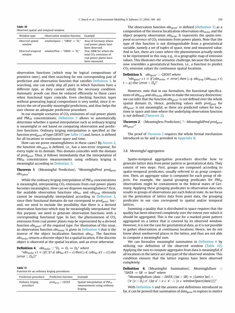
Table 10Observed spatial and temporal window.

Window type Observation window function Example

Observed spatialwindow

windowSpace :: “OBSD 0 rDs” Area of Germany wherecoal power plants havebeen observed.

Observed temporalwindow

windowTime :: “OBSD 0 rDt” Year 2008 for which thetotal CO2 emissions ofcoal power plants havebeen measured.

C. Stasch et al. / Environmental Modelling & Software 51 (2014) 149e165 159

observation functions (which may be logical compositions ofprimitive ones), and then searching for one corresponding pair ofprediction and observation function that satisfies Definition 3. Insearching, one can easily skip all pairs in which functions have adifferent type, as they cannot satisfy the necessary condition.Automatic proofs can thus be reduced efficiently to those caseswhen functional types coincide. Even checking function typeswithout generating logical compositions is very useful, since it re-stricts the set of possibly meaningful predictions, and thus helps theuser choose an adequate prediction procedure.

In our example scenarios of CO2 emissions of coal power plantsand PM10 concentrations, Definition 3 allows to automaticallydetermine whether a spatial interpolation such as ordinary krigingis meaningful or not based on comparing observation and predic-tion functions. Ordinary kriging interpolation is specified as thefunction predgeost of type GEOST (see Table 11) and, hence, is definedfor all locations in continuous space and time.

How can we prove meaningfulness in these cases? By Axiom 2,the function obscphen is defined, i.e., has a non-error response, forevery tuple in its domain. This domain coincides with the domainof predgeost. Thus, it follows immediately that the interpolation ofPM10 concentration measurements using ordinary kriging ismeaningful according to Definition 3:

Theorem 1. (Meaningful Prediction). “MeaningfulPred predgeostobscphen”

While the ordinary kriging interpolation of PM10 concentrationsis meaningful, interpolating CO2 emissions from coal power plantsbecomesmeaningless. How canwe disprovemeaningfulness? First,the available observation functions obsloc and obsprop obviouslycannot be meaningfully interpolated according to Definition 3,since their functional domains do not correspond to predgeost. Sec-ond, we need to exclude the possibility that there is a derivedobservation function which may be meaningfully interpolated. Forthis purpose, we need to generate observation functions with acorresponding functional type. In fact, the phenomenon of CO2emissions from coal power plants may be represented by a derivedfunction obsgeost* of the required type. For illustration of this issue,an observation function obsinvloc is given in Definition 4 that is theinverse of the object localization function obsloc. The functionobsinvloc returns a discrete object for a spatial location, if the discreteobject is observed at the spatial location, and an error otherwise.

Definition 4. obsinvloc :: “Ds 0 Dt 0 Dd” where“obsinvloc s th (if (d! d. obsloc d t¼ s) then (i d. (obsloc d t¼ s)) else

(error :: Dd))”

Table 11Function for an ordinary kriging procedures.

Prediction procedure Prediction function Example

Ordinary krigingprocedure

predgeost :: GEOST Spatial interpolation of PM10

measurements using ordinarykriging.

The observation function obsgeost* is defined (Definition 5) as acomposition of the inverse localization observation obsinvloc and theobject property observation obsprop. It represents the spatio-tem-poral occurrence of CO2 emissions from power plants. Note that thetype of this function is not distinguishable from a geostatisticalvariable, namely a set of tuples of space, time and measured value.And in fact, there are cases where the phenomenon actually needsto be represented in this way, e.g., in a geographic map of emissionvalues. This illustrates the semantic challenge, because the functionnow resembles a geostatistical function, i.e., a function to predictCO2 emission values for continuous spatial locations.

Definition 5. obsgeost* :: GEOST where“obsgeost* s t h if (obsinvloc s error) then (i q. obsprop (obsinvloc s t)

t ¼ q) else (error :: Dq)”

However, note that in our formalism, the functional specifica-tions of obsprop and obsinvloc allow tomake the necessary distinction:we can infer that the function obsgeost* is not defined over thewholespatial domain Ds. Hence, predicting values with predgeost forobsgeost* is not meaningful, as there are predicted values for loca-tions in space and time where the underlying observation functionis not defined (Theorem 2):

Theorem 2. (Meaningless Prediction). “: MeaningfulPred predgeostobsgeost*”

The proof of Theorem 2 requires the whole formal mechanismintroduced so far and is provided in Appendix B.

3.8. Meaningful aggregation

Spatio-temporal aggregation procedures describe how togenerate lattice data from point pattern or geostatistical data. Theyconsist of two steps: First, groups are composed according tospatio-temporal predicates, usually referred to as group composi-tion. Then, an aggregate value is computed for each group of ob-jects. For example, the spatial grouping predicates for PM10observations might be containment in the federal states of Ger-many. Applying these grouping predicates to observation data setsresults in groups of observations per each federal state. As we focuson the generation of lattice data from point data, the groupingpredicates in our case correspond to spatial and/or temporallattices.

Summing a quality that is distributed in space requires that thequality has been observed completely over the extent over which itshould be aggregated. This is the case for a marked point patternaggregated on a lattice that is covered by its observed window.However, it is not the case for geostatistical data, as it is not possibleto gather observations at continuous locations. Hence, we do notknow about unobserved places in the lattice, and thus are not ableto compute a meaningful sum.

We can formalize meaningful summation in Definition 6 byutilizing our definition of the observed window (Table 10).Applying the sum to compute aggregates fromdata is meaningful, ifall locations in the lattice are also part of the observed window. Thiscondition ensures that the lattice regions have been observedcompletely.

Definition 6. (Meaningful Summation). MeaningfulSum ::“DATA 0 SR 0 bool” where

“MeaningfulSum (data :: DATA) (lat :: SR) h (Lattice lat) ^(c (x :: Ds) x0. (lat x0 ^ x ˛ x0 / (x ˛ windowSpace(data))))”

With Definition 6 and the axioms and definitions introduced sofar, it can be proved that summation of datageost to regions in slattice

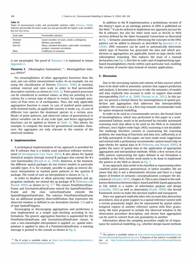
Table 12Types of measurement scales and permissible statistics (after (Stevens, 1946));statistics permissible for lower scales are also permissible for higher scale variables,but not vice-versa.

Scale type Permissible statistics

Nominal Count (number of cases), mode, contingencyOrdinal Median, percentilesInterval Mean, standard deviation, rank-order correlation,

productemoment correlationRatio Coefficient of variation

C. Stasch et al. / Environmental Modelling & Software 51 (2014) 149e165160

is not meaningful. The proof of Theorem 3 is explained in AnnexAppendix C.

Theorem 3. (Meaningless Summation). “: MeaningfulSum data-geost slattice”

For meaningfulness of other aggregation functions than thesum, one can utilize measurement scales. As an example, we areusing the classification of Stevens (Stevens, 1946) in nominal,ordinal, interval and ratio scale in order to find permissibledescriptive statistics as shown in Table 12. Point pattern processescan be considered as nominal values, as they are pointing to lo-cations for a certain type of objects or events, for example posi-tions of Pine trees or of earthquakes. Thus, the only applicableaggregation function is count. In case of marked point patternswith nominal marks, an applicable statistic is mode, e.g., in case ofdifferent tree species the dominant species in a certain area.Marks of point patterns, and observed values of geostatistical orlattice variables can be of any scale type, and hence aggregationfunctions can be applied as shown in Table 12. This allows, forexample, to compute the mean for geostatistical variables. How-ever, the aggregates are only relevant in the context of theobserved window.

4. Implementation

A prototypical implementation of our approach is provided forthe R software that is a widely used statistical software environ-ment (R Development Core Team, 2011). R also allows for SpatialStatistical analysis through several R packages that extend the R’score functionality (Bivand et al., 2008). However, at the moment,the different spatial packages do not restrict models to particularvariable types. It is, for example, possible to apply an inverse dis-tance interpolation to marked point patterns in the spatstat Rpackage. The result of such an interpolation is shown in Fig. 4.

In order to disallow or allow particular interpolation and ag-gregation methods, we extend the sp package of R (Pebesma andBivand, 2005) as shown in Fig. 5.12 The classes PointPatternData-Frame and GeostatisticalDataFrame extend the SpatialPointsData-Frame and the class LatticeDataFrame extends theSpatialPolygonsDataFrame. The subclass PointPatternDataFramehas an additional property observedWindow that represents theobserved window as defined in our formalism (Section 3.6) and isof type SpatialPolygons.

Encouraging or discouraging aggregations and predictions isnow implemented as a simple type-checking according to ourformalism. The generic aggregation function is augmented for thePointPatternDataFrame and GeostatisticalDataFrame classes. Incase a non-meaningful interpolation is applied, i.e., spatial inter-polation is applied to data of a PointatternDataFrame, a warningmessage is printed in the console as shown in Fig. 6.

12 The R script is available online at https://svn.52north.org/svn/geostatistics/main/meaningful/tools/R/implementation.R.

In addition to the R implementation, a preliminary version ofthe theory’s types as an ontology pattern in OWL is published ontheWeb.13 It can be utilized to implement our approach not just forthe R software, but also for other tools such as ArcGIS or Webservices defined by the Open Geospatial Consortium as illustratedin Fig. 7. Semantic annotations referencing the concepts in the OWLpattern can be added to datasets as described by Janowicz et al.(2010). OWL reasoners can be used to automatically determinewhich type of function has generated the data and which pre-dictions or aggregations are applicable, based on type checks withsubsumption reasoning. This replaces the issue of a manualdeclaration (see Fig. 6, first line in code) and of implementing type-based meaningfulness checks within each particular tool, enablingthe creation of smarter data instead of smarter applications.

5. Discussion

Due to the increasing variety and volume of data sources whichhave to be dealt with in automatic systems that support predictionand analysis, it becomes necessary to take the semantics of modelsand data explicitly into account in order to support data-modelinteroperability (Bell et al., 2009; Parsons et al., 2011). In this pa-per, we present a formal theory for meaningfulness of spatial pre-diction and aggregation that addresses this interoperabilityproblem. We consider it as a first step towards recommender toolsfor spatio-temporal modelling.

In order to be used as a recommender service, the formal checkof meaningfulness, which was performed in this paper in a semi-automated fashion, needs to be performed by tractable automatedreasoning tools that allow to be used on the Web or in statisticalsoftware, since higher-order logic (HOL) reasoning is not decidable.The challenge therefore consists in constraining the reasoningproblem, the matching of functions and data sets, sufficiently as tobe fully automated. In this paper, we have made some suggestionsand started with a preliminary recommender system based only ontype-checks for spatial data in R (Pebesma and Bivand, 2005). Itguides the users of spatial data in the application of appropriateaggregation and interpolation methods. While a first version of anOWL pattern representing the types defined in our formalism isavailable in the Web, further work needs to be done to implementthe pattern in the Web as shown in Fig. 7.

In our approach, data needs to be classified as representing either(marked) point patterns, geostatistical, or lattice variables. We areaware that this is not a deterministic decision and there is a largedegree of freedom in semantic conceptualization (compare the dis-cussion in Scheider (2012), Chapter 4). This is also related to thewell-knowndistinctionbetweenobject-basedandfield-based approachesin GIS, which is a matter of information purpose and design(Couclelis, 1992) as well as observation (Frank, 2009). Our formalframework serves to make this decision explicit and transparent.

Since our approach explicitly takes into account data abstractionprocedures, data at point support in a spatial reference systemwitha certain granularity might also be represented by spatial and/ortemporal regions in another reference system with finer granu-larity. We have proposed to include the observed window in theobservation procedure description, and shown how aggregationcan be used to convert from one granularity to another.

Information about the sampling procedure might be of impor-tance for statistical modelling, e.g., whether design-based methods

13 The pattern is available online at http://www.meaningfulspatialstatistics.org/theories/MeaningfulSpatialStatistics.owl. A diagram of the pattern is available on-line at http://www.meaningfulspatialstatistics.org/theories/MeaningfulSpatialStatistics.

Fig. 4. Interpolated marked point pattern (diameters of longleaf pines) with R packagespatstat.

C. Stasch et al. / Environmental Modelling & Software 51 (2014) 149e165 161

can be applied (de Gruijter et al., 2006). This kind of informationwas not included in this paper, but may be incorporated in theobservation procedure description and then used as additional in-formation for reasoning about the meaningfulness of a particularprediction or aggregation.

Our notion of meaningfulness in aggregation requires that theregions over which data should be summed needs to be observedcompletely. In the OLAP and Statistical database community,several authors try to address the issue of summarizability as well(Lenz and Shoshani, 1997; Mazón et al., 2009; Niemi and Niinimäki,2010) and also define a completeness condition. However, theirdefinition of completeness states that each non-aggregated obser-vation needs to be covered by at least one region. Instead, werequire that knowledge is needed for the whole region over whichdata should be summed, which is the case for point pattern vari-ables, but not for geostatistical variables. Our approach for spatio-temporal aggregation can be seen as a complementary contribu-tion to this issue, as thework on the summarizability so far does notexplicitly consider different types of spatial variables.

In our approach, we focus on the aggregation of point data(either point patterns or geostatistical variables) to areal data.However, the resulting areal data might be, in turn, aggregated tolarger areas and so forth. It appears that the distinction betweenpoint patterns (i.e., discrete entities that are represented by some

Fig. 5. Subclasses of the sp package classes used for meaningful interpolation and aggregatioSpatialPointsDataFrame, the LatticeDataFrame class is subclass of the SpatialPolygonsDataFrimplementation are shown as yellow boxes. Regular lattices such as remote sensing imagersubclass of SpatialGridDataFrame or RasterStack. (For interpretation of the references to co

space-time geometry) and geostatistical variables (continuousphenomena in space/time) is still valid also for areal data. As anexample, the sum of discrete entities still makes sense for arealdata, e.g., summing the total CO2 emissions of power plants pereach European country to the sum of Europe, while summing thetemperature appears still not appropriate for polygonal data.

An example of an aggregation of the air quality variable PM10 isshown in Fig. 8, which was published by the EuropeanEnvironmental Agency (2012). In this report, a section on Europe-wide survey of PM shows time trends in PM10 concentrationsaveraged over monitoring network stations with complete mea-surement records. Below the figure it notes that “in the diagrams ageographical bias exists towards central Europewhere there is a higherdensity of stations”, but it is not made clear whether this bias refersto selection, to estimation, or both. We argue that these trendsrelate to the stations selected, rather than an area (Europe). Arealmean values can be predicted, e.g., by block kriging (Journel andHuijbregts, 1978).

While we have proposed meaningfulness of predictions basedon reference systems, we have not yet considered meaningfulnessof statistical models. An example is the decision for which area wemay assume second order stationarity of a phenomenon. Interpo-lating PM10 values measured at traffic stations (Fig. 8) to areas withrural, traffic-free conditions (and vice versa) may not be mean-ingful. Towards such meaningful models, further work is needed todetermine and formalize the additional required information. Ourapproach can be a starting point towards choosing suchmeaningfulmodels. In the context of evaluating model performance (Bennettet al., 2013), our theory covers meaningfulness of spatial predic-tion and aggregation of model residuals. Furthermore, we do notinclude semantic descriptions of concrete application problems. Anexample of this would be predicting air quality over Beijing. Theformalization of this application problem would allow matchingappropriate data and prediction procedures with the applicationgoal.

For meaningfulness of other aggregation functions than thesum, we are using Stevens’ classification scheme (Stevens, 1946)and emphasize that point patterns might be considered as nom-inal data, whereas the application of statistical measures tomarked point patterns, geostatistical and lattice data depends onthe measurement scale of the quality values that are observed. As

n. The PointPatternDataFrame and GeostatisticalDataFrame classes are subclasses of theame. Classes of package sp are shown as blue boxes, classes added in the prototypicaly is formally a subclass of LatticeDataFrame, but will in practice be implemented as alour in this figure legend, the reader is referred to the web version of this article.)

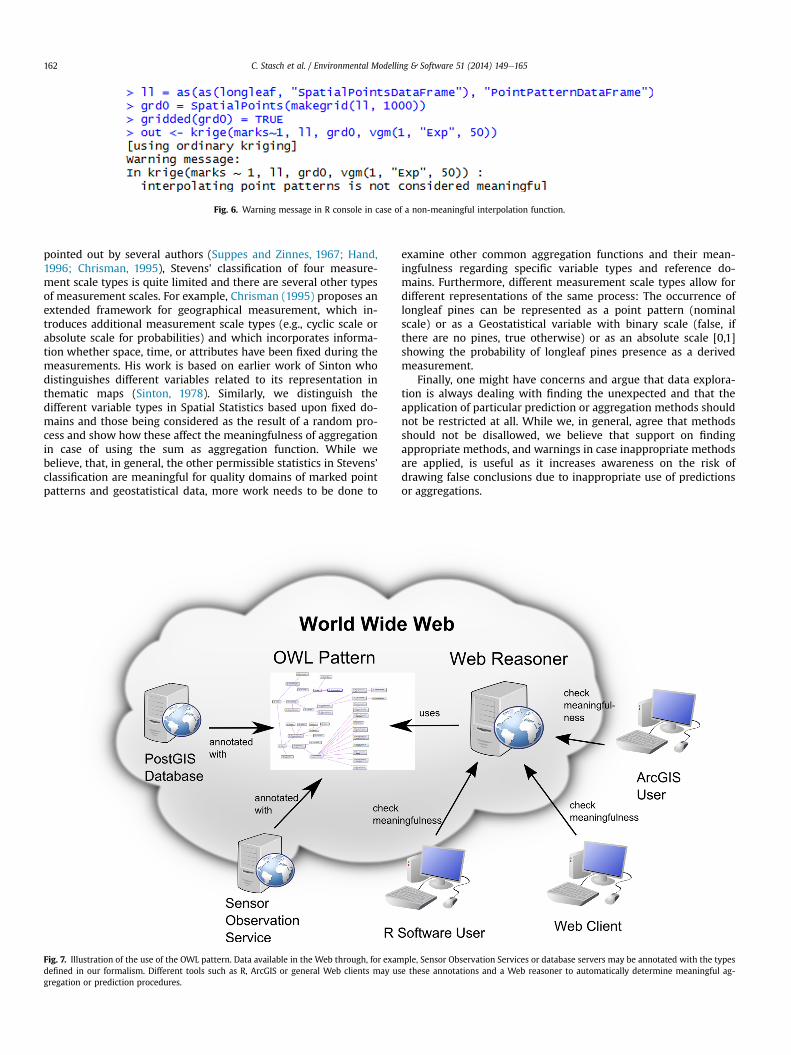
Fig. 6. Warning message in R console in case of a non-meaningful interpolation function.

C. Stasch et al. / Environmental Modelling & Software 51 (2014) 149e165162

pointed out by several authors (Suppes and Zinnes, 1967; Hand,1996; Chrisman, 1995), Stevens’ classification of four measure-ment scale types is quite limited and there are several other typesof measurement scales. For example, Chrisman (1995) proposes anextended framework for geographical measurement, which in-troduces additional measurement scale types (e.g., cyclic scale orabsolute scale for probabilities) and which incorporates informa-tion whether space, time, or attributes have been fixed during themeasurements. His work is based on earlier work of Sinton whodistinguishes different variables related to its representation inthematic maps (Sinton, 1978). Similarly, we distinguish thedifferent variable types in Spatial Statistics based upon fixed do-mains and those being considered as the result of a random pro-cess and show how these affect the meaningfulness of aggregationin case of using the sum as aggregation function. While webelieve, that, in general, the other permissible statistics in Stevens’classification are meaningful for quality domains of marked pointpatterns and geostatistical data, more work needs to be done to

Fig. 7. Illustration of the use of the OWL pattern. Data available in the Web through, for examdefined in our formalism. Different tools such as R, ArcGIS or general Web clients may usgregation or prediction procedures.

examine other common aggregation functions and their mean-ingfulness regarding specific variable types and reference do-mains. Furthermore, different measurement scale types allow fordifferent representations of the same process: The occurrence oflongleaf pines can be represented as a point pattern (nominalscale) or as a Geostatistical variable with binary scale (false, ifthere are no pines, true otherwise) or as an absolute scale [0,1]showing the probability of longleaf pines presence as a derivedmeasurement.

Finally, one might have concerns and argue that data explora-tion is always dealing with finding the unexpected and that theapplication of particular prediction or aggregation methods shouldnot be restricted at all. While we, in general, agree that methodsshould not be disallowed, we believe that support on findingappropriate methods, and warnings in case inappropriate methodsare applied, is useful as it increases awareness on the risk ofdrawing false conclusions due to inappropriate use of predictionsor aggregations.

ple, Sensor Observation Services or database servers may be annotated with the typese these annotations and a Web reasoner to automatically determine meaningful ag-

Fig. 8. Trends in PM10 (mg/m3), 2001e2010, per station type. Source: EuropeanEnvironmental Agency (2012).

C. Stasch et al. / Environmental Modelling & Software 51 (2014) 149e165 163

6. Conclusion

We introduced a new notion of meaningfulness of predictionand aggregation and formally specified it in a semantic theory inhigher order logic (HOL). The theory consists of functional speci-fications of observation procedures, prediction procedures, ag-gregation procedures, as well as datasets based on semanticreference systems as types. Our notion of meaningfulness is basedon the formal distinction between observation, prediction, andaggregation procedures on the one hand, which describe potentialdata, and data on the other hand, which is generated by executingthese procedures. The different procedures are represented asfunctions of different types, which correspond to known variabletypes in Spatial Statistics. Data are represented by predicates onthe domain and range of these functions, i.e., they are a finitesubset of the tuples defined by a function. Meaningfulness checksare implemented in our formalism as correspondence checks:Meaningful prediction is introduced based on a correspondencecheck between observation functions and prediction functionsthat ensures that there is a possible observation for each predic-tion. Meaningful aggregation is based on checking whether anobserved window corresponds to the target regions of an aggre-gation, hence testing the condition, that the target region needs tobe observed completely in case of using the sum as an aggregationfunction. The theory, including definitions, axioms, and theorems,was implemented and tested with Isabelle/HOL, a semi-automated theory prover.

One challenge for future work consists in tractable imple-mentations of meaningfulness checks in open Semantic Web en-vironments as well as in statistical software. As environmentalmodels always deal with uncertain data (Bastin et al., 2013), andsince uncertainty can be seen as a consequence of observation(Frank, 2009), its inclusion in our formalism would be natural.Future work may also address the extension of our theory to coverother related notions of meaningfulness, the incorporation ofsampling procedures, other types of aggregation and prediction, aswell as further measurement scales.

14 http://www.meaningfulspatialstatistics.org/theories/Miptheory.thy.

Acknowledgements

The presented work was developed within the 52� North geo-statistics community, and partly funded by the European Project

UncertWeb (FP7-248488, see http://www.uncertweb.org/) and theInternational Research Training Group on Semantic Integration ofGeospatial Information funded by the DFG (German ResearchFoundation), GRK 1498. Simon Scheider’s contribution was partlyfunded by a research fellowship grant (DFG SCHE 1796/1-1) and theICT-FP7-249120 ENVISION project.

Appendix A. Cardinality order on types

Partial cardinality orders among domains can be formalizedbased on the existence of embeddings, i.e., injective total functionsf :: X0 Y from type X into the one with higher cardinality Y. Partialcardinality order on types, X4c Y, thus, can be expressed in Isabelleas follows:

dðf :: X0YÞ:inj f

A strict cardinality order X 3c Y can be formalized accordingly byrequiring that all mappings f :: X0 Y are non-surjective, i.e., they donot fully cover Y. We formally capture this by an axiom that deniessurjectivity:

Axiom 7. Strict cardinality order on reference domains:

:ðdðf :: Dd0DsÞ:surj f Þ

:ðdðf :: Dd0DtÞ:surj f Þ

Which is how we translate the cardinality differencesDd 3c Ds ^ Dd 3c Dt into Isabelle.

Appendix B. Proof of Theorem 2

In order to prove that the prediction of CO2 emissions of coalpower plants, represented by obsgeost*, with an Ordinary Kriginginterpolation procedure, represented by predgeost, is not meaningful(Theorem 2), it needs to be shown that Definition 3 is not satisfiedby the functions obsgeost* and predgeost, i.e., that there are spatial andtemporal locations at which the prediction function provides aquality value, but where the corresponding observation functionreturns an error. The following is a description of substeps of theautomated proof which is available online.14

Proof. First, using Axiom 7 and the definition of surjectivity, itcan be proved that all functions of type Dd 0 Ds (mappings fromdiscrete entities into space) miss some entity in their range asspecified in Theorem 4.

Theorem 4. Non-surjectivity of object-space mappings: “c

(f :: Dd 0 Ds).(d (s :: Ds).: (d (d :: Dd). s ¼ f d))”

Using only Theorem 4, it can be directly proved that the objectlocalization function obsloc misses entities in its range at all times(Theorem 5):

Theorem 5. Non-surjectivity of obsloc: “c t.(d s.: (d d. s ¼ obslocd t))”

Hence, using Definition 4 and Theorem 5, it can be proved thatthe inverse function obsinvloc generates errors for some spatial lo-cations at all times:

Theorem 6. Errors in obsinvloc: “c t. (d s. obsinvloc s t ¼ error)”

C. Stasch et al. / Environmental Modelling & Software 51 (2014) 149e165164

Thus, the pseudo-geostatistical observation function obsgeost*produces errors, too, as it is constructed with obsinvloc. This can beproved by Theorem 6 and Definition 5:

Theorem 7. Errors in obsgeost* : “(d y x. obsgeost* x y ¼ error)”

Hence, the domain of obsgeost* is of lower cardinality, i.e.,defined only for a true discrete subset of Ds, reflecting the fact thatCO2 emissions (in contrast to concentration) need emitters thatare discrete objects (coal power plants). Thus, there are pre-dictions that are not parallelled by any observation. Our goal wasto show that predicting obsgeost* with predgeost is not meaningful(Theorem 2). This follows immediately from Theorem 7 andDefinition 3. ,

Appendix C. Proof of Theorem 3

In order to show that the computation of a sum of geostatisticalvalues, such as datageost, over spatial lattices, such as slattice, is notmeaningful (Theorem 3), we need to show that there exist locationsin the spatial lattice that are not contained in the observed windowof the observation data, corresponding to Definition 6. Thefollowing is a description of substeps of the automated proof whichis available online.15

Proof. First, based on Axiom 6, we infer that the observed spatialwindow of datageost needs to be finite:

Theorem 8. Finiteness of observed spatial window of datageost:“finite (windowSpace datageost)”

In addition, based on Axioms 3 and 4, we can prove that regionsin the spatial lattice slattice are not finite (actually, they arecontinuous sets of points):

Theorem 9. Non-finiteness of lattice regions: “c x. slattice x / :finite x”

Using the very same axioms together with Definition 2 for dataproperties, it can also be shown that there is at least one region inslattice.

Theorem 10. Existence of region in slattice: “d x. slattice x”

From Theorems 8, 9, and Axiom 1, it follows that there is aspatial location in a region of the spatial lattice that is not part of theobserved spatial window of datageost :

Theorem 11. Cardinality of observed window and regions: “c x.slattice x / (d z. (z ˛ x) ^ : (z: windowSpace datageost))”

Hence, the observed spatial window of datageost is of lowercardinality than the regions in slattice. Theorems 11 and 10 togetherwith Definition 6 for meaningful sum allow to derive Theorem 3immediately. ,

References

Adams, E.W., 1966. On the nature and purpose of measurement. Synthese 16, 125e169. http://dx.doi.org/10.1007/BF00485355.

Baddeley, A., Turner, R., 2005. Spatstat: an R package for analyzing spatial pointpatterns. J. Stat. Softw. 12, 1e42. ISSN 1548e7660.

Bastin, L., Cornford, D., Jones, R., Heuvelink, G.B., Pebesma, E., Stasch, C., Nativi, S.,Mazzetti, P., Williams, M., 2013. Managing uncertainty in integrated environ-mental modelling: the uncertweb framework. Environ. Model. Softw. 39, 116e134 (Thematic Issue on the Future of Integrated Modeling Science andTechnology).

Bell, G., Hey, T., Szalay, A., 2009. Beyond the data deluge. Science 323, 1297e1298.http://www.sciencemag.org/content/323/5919/1297.full.pdf.

Bennett, N.D., Croke, B.F., Guariso, G., Guillaume, J.H., Hamilton, S.H.,Jakeman, A.J., Marsili-Libelli, S., Newham, L.T., Norton, J.P., Perrin, C.,

15 http://www.meaningfulspatialstatistics.org/theories/Miptheory.thy.

Pierce, S.A., Robson, B., Seppelt, R., Voinov, A.A., Fath, B.D., Andreassian, V.,2013. Characterising performance of environmental models. Environ. Model.Softw. 40, 1e20.

Berners-Lee, T., Fielding, R., Lassila, O., 2001. The semantic web. Sci. Am. 284 (5),34e43.

Bivand, R.S., Pebesma, E.J., Góomez-Rubio, V., 2008. Applied Spatial Data Analysiswith R. Springer. ISBN 978-0-387-78170-.

Burrough, P.A., Mcdonnell, R.A., 1998. Principles of Geographical Information Sys-tems. Oxford University Press, USA.

Chrisman, N., 1995. Beyond stevens: a revised approach to measurement ofgeographic information. In: Proceedings Auto-Carto 12, pp. 271e280.

Compton, M., Barnaghi, P., Bermudez, L., Garca-Castro, R., Corcho, O., Cox, S.,Graybeal, J., Hauswirth, M., Henson, C., Herzog, A., Huang, V., Janowicz, K.,Kelsey, W.D., Phuoc, D.L., Lefort, L., Leggieri, M., Neuhaus, H., Nikolov, A.,Page, K., Passant, A., Sheth, A., Taylor, K., 2012. The {SSN} ontology of the {W3C}semantic sensor network incubator group. Web Semant. Sci. Serv. Agents WorldWide Web 17, 25e32.

Couclelis, H., 1992. People manipulate objects (but cultivate fields): beyond theraster-vector debate in GIS. In: Proceedings of the International Conference GIS- from Space to Territory: Theories and Methods of Spatio-temporal Reasoningon Theories and Methods of Spatio-temporal Reasoning in Geographic Space.Springer, pp. 65e77.

Cressie, N., 1993. Statistics for Spatial Data (Revised Edition). Wiley, New York.Cressie, N., Wikle, C., 2011. Statistics for Spatio-temporal Data. Wiley, New York.European Environmental Agency, 2012. Air Quality in Europe 2012 Report (Tech-

nical Report). Office for Official Publications of the European Union,Luxembourg.

Frank, A., 2009. Scale is introduced in spatial datasets by observation processes. In:Spatial Data Quality from Process to Decision(6th ISSDQ 2009). CRC Presss,pp. 17e29.

Galton, A., 2004. Fields and objects in space, time, and space-time. Spat. Cogn.Comput. 4, 39e68.

Gangemi, A., Guarino, N., Masolo, C., Oltramari, A., 2003. Sweetening WordNet withDOLCE. AI Mag. 24 (3), 13e24.

Gray, J., Liu, D., Nieto-Santisteban, M., Szalay, A., DeWitt, D., Heber, G., 2005. Sci-entific data management in the coming decade. SIGMOD Record 34 (4), 34e41.

Gruber, T.R., 1993. A translation approach to portable ontologies. Knowl. Acquis. 5,199e220.

de Gruijter, J., Brus, D., Bierkens, M., Knotters, M., 2006. Sampling for NaturalResource Monitoring. Springer, Berlin, ISBN 978-3-540-22486-0.

Hand, D.J., 1996. Statistics and the theory of measurement. J. R. Stat. Soc. Ser. A Stat.Soc. 159, 445e492.

Illian, J., Penttinen, A., Stoyan, H., Stoyan, D., 2008. Statistical Analysis and Modellingof Spatial Point Patterns. Wiley.

Janowicz, K., Schade, S., Brring, A., Keler, C., Mau, P., Stasch, C., 2010. Semanticenablement for spatial data infrastructures. Trans. GIS 14, 111e129.

Jeong, S.H., Fernandes, A.A.A., Paton, N.W., Griffiths, T., 2004. A generic algorithmicframework for aggregation of spatio-temporal data. In: SSDBM ’04: Proceedingsof the 16th International Conference on Scientific and Statistical DatabaseManagement. IEEE Computer Society, Washington, DC, USA, p. 245.

Journel, A., Huijbregts, C., 1978. Mining Geostatistics. Academic Press.Kuhn, W., 2003. Semantic reference systems (Guest Editorial). Int. J. Geogr. Inf. Sci.

17, 405e409.Laniak, G.F., Olchin, G., Goodall, J., Voinov, A., Hill, M., Glynn, P., Whelan, G.,

Geller, G., Quinn, N., Blind, M., Peckham, S., Reaney, S., Gaber, N., Kennedy, R.,Hughes, A., 2013. Integrated environmental modeling: a vision and roadmap forthe future. Environ. Model. Softw. 39, 3e23 (Thematic Issue on the Future ofIntegrated Modeling Science and Technology).

Lenz, H.J., Shoshani, A., 1997. Summarizability in olap and statistical data bases. In:SSDBM. IEEE Computer Society, pp. 132e143.

Mazón, J.N., Lechtenbörger, J., Trujillo, J., 2009. A survey on summarizability issuesin multidimensional modeling. Data Knowl. Eng. 68, 1452e1469.

National Aeronautics and Space Administration, 2012. A.40 ComputationalModeling Algorithms and Cyberinfrastructure (Technical Report). NationalAeronautics and Space Administration.

Niemi, T., Niinimäki, M., 2010. Ontologies and summarizability in olap. In: Pro-ceedings of the 2010 ACM Symposium on Applied Computing. ACM, New York,NY, USA, pp. 1349e1353.

Parsons, M.A., Godøy, Ø., LeDrew, E., de Bruin, T.F., Danis, B., Tomlinson, S.,Carlson, D., 2011. A conceptual framework for managing very diverse data forcomplex, interdisciplinary science. J. Inf. Sci. 37, 555e569. http://jis.sagepub.com/content/37/6/555.full.pdfþhtml.

Pebesma, E., Cornford, D., Dubois, G., Heuvelink, G.B., Hristopulos, D., Pilz, J.,Stoehlker, U., Morin, G., Skøien, J.O., 2011. Intamap: the design and imple-mentation of an interoperable automated interpolation web service. Comput.Geosci. 37, 343e352.

Pebesma, E.J., Bivand, R.S., 2005. Classes and methods for spatial data in R. R News5, 9e13.

R Development Core Team, 2011. R: a Language and Environment for StatisticalComputing. R Foundation for Statistical Computing, Vienna, Austria, ISBN 3-900051-07-0.

Rijgersberg, H., van Assem, M., Top, J., 2012. Ontology of units of measure andrelated concepts. Semant. Web J. 4, 3e13.

Ripley, B., 1981. Spatial Statistics. Wiley, New York.

C. Stasch et al. / Environmental Modelling & Software 51 (2014) 149e165 165

Scheider, S., 2012. Grounding Geographic Information in Perceptual Operations. In:Frontiers in Artificial Intelligence and Applications, vol. 244. IOS Press,Amsterdam.

Sheth, A., Henson, C., Sahoo, S., 2008. Semantic sensor web. IEEE Internet Comput.,78e83.

Sinton, D.F., 1978. The inherent structure of information as a constraint to analysis:mapped thematic data as a case study. Harv. Pap. Geogr. Inf. Syst. 6, 1e17.

Stasch, C., Foerster, T., Autermann, C., Pebesma, E., 2012. Spatio-temporal aggrega-tion of European air quality observations in the sensor web. Comput. Geosci. 47,111e118.

Stevens, S.S., 1946. On the theory of scales and measurement. Science 103,677e680.

Suppes, P., Zinnes, J., 1967. Handbook of Mathematical Psychology, vol. 1. Wiley,pp. 1e76 (Chapter Basic Measurement Theory).

Vega Lopez, I.F., Snodgrass, R.T., Moon, B., 2005. Spatiotemporal aggregatecomputation: a survey. IEEE Trans. Knowl. Data Eng. 17, 271e286.

Villa, F., Athanasiadis, I.N., Rizzoli, A.E., 2009. Modelling with knowledge: a reviewof emerging semantic approaches to environmental modelling. Environ. Model.Softw. 24, 577e587.

Voinov, A., Shugart, H.H., 2013. integronsters, integral and integrated modeling.Environ. Model. Softw. 39, 149e158 (Thematic Issue on the Future of IntegratedModeling Science and Technology).

Weinberger, D., 2011. The machine that would predict the future. Sci. Am. 305,323e340.