
Orbital Aggregation & Space Infrastructure Systems (OASIS)
283
Revolutionary Aerospace Systems Concepts Orbital Aggregation & Space Infrastructure Systems (OASIS) Preliminary Architecture and Operations Analysis FY2001 Final Report June 10, 2002
-
Upload
khangminh22 -
Category
Documents
-
view
2 -
download
0
Transcript of Orbital Aggregation & Space Infrastructure Systems (OASIS)

Revolutionary Aerospace Systems Concepts Orbital Aggregation & Space Infrastructure Systems (OASIS) Preliminary Architecture and Operations Analysis
FY2001 Final Report June 10, 2002

This page intentionally left blank.

Foreword Just as the early American settlers pushed west beyond the original thirteen colonies, the world today is on the verge of expanding the realm of humanity beyond its terrestrial bounds. The next great frontier lies ahead in low-Earth orbit and beyond. Commercialization of space has recently been mostly limited to communications and remote sensing applications, but materials processing, manufacturing, tourism and servicing opportunities will undoubtedly increase during the first part of the new millennium. Discoveries hinting at the existence of water on Mars and Europa offer additional motivation for establishing a space-based infrastructure that supports extended human exploration of the solar system. If this space-based infrastructure were also utilized to stimulate and support space commercialization, permanent human occupation of low-Earth orbit and beyond could be achieved sooner and more cost effectively. The purpose of this study is to identify synergistic opportunities and concepts among human exploration initiatives and space commercialization activities while taking into account technology assumptions and mission viability in an Orbital Aggregation & Space Infrastructure Systems (OASIS) framework. OASIS is a set of concepts that provide a common infrastructure for enabling a large class of space missions. The concepts include communication, navigation and power systems, propellant modules, tank farms, habitats, and transfer systems using several propulsion technologies. OASIS features in-space aggregation of systems and resources in support of mission objectives. The concepts feature a high level of reusability and are supported by inexpensive launch of propellant and logistics payloads. The anticipated benefits of the synergistic utilization of space infrastructure are reduced mission costs and increased mission flexibility for future space exploration and commercialization initiatives.
i

This page intentionally left blank.
ii
Executive Summary The study was performed under the Revolutionary Aerospace Systems Concepts (RASC) activity led by the NASA Langley Research Center (LaRC). LaRC was chartered by the NASA Administrator to be the lead Center for evaluating revolutionary aerospace systems concepts and architectures to identify new mission approaches and the associated technologies that enable these missions to be implemented. Mission There are many challenges confronting humankind’s exploration of space, and many engineering problems that must be solved in order to provide safe, affordable and efficient in-space transportation of both personnel and equipment. These challenges directly impact the commercialization of space, with cost being the single largest obstacle. One method of reducing cost is to develop reusable transportation systems—both Earth-to-orbit systems and in-space infrastructure. Without reusable systems, sustained exploration or large-scale development beyond low-Earth-orbit (LEO) appears to be economically non-viable. However, reusable in-space transportation systems must be capable of both high fuel efficiency and “high utilization of capacity,” or economic costs will remain unacceptably high. Fixed infrastructures have been suggested as one approach to solving this challenge; for example, rotating tether approaches. However, these systems tend to suffer from high initial costs or unacceptable operational constraints. Another significant challenge is minimizing the in-space travel time for crewed missions. The risks associated with human missions can be significantly reduced by decreasing the time that the crew is in transit. Besides nuclear thermal propulsion systems and the inherent public concerns that accompany the use of these systems near the Earth, the propulsive system that provides a reasonably high thrust and short transit time is one that uses chemical propellants. One significant drawback to chemical systems is the relatively low specific impulse (Isp) requiring large propellant quantities to provide the velocity changes necessary to complete a mission. Solar electric propulsion (SEP) systems can provide high fuel efficiency but only at the cost of low thrust and transit times that are not compatible with crewed missions. An innovative concept that integrates the best features of both chemical and solar electric propulsive systems is proposed in this report. This concept appears to hold the promise of solving the issues associated with other approaches and may provide a new family of capabilities for future exploration and commercial development of near-Earth space and beyond. Study Summary An architecture composed of common in-space transportation elements was derived to support both human exploration and commercial applications in the Earth-moon neighborhood. Mission concepts utilizing this architecture are predicated on the availability of a low-cost launch vehicle for delivery of propellant and re-supply logistics. Infrastructure costs would be shared by Industry, NASA and other users.
iii
The Orbital Aggregation & Space Infrastructure Systems (OASIS) architecture minimizes point designs of elements in support of specific space mission objectives and maximizes modularity, reusability and commonality of elements across many missions, enterprises and organizations. A reusable Hybrid Propellant Module (HPM) that combines both chemical and electrical propellant in conjunction with modular orbital transfer/engine stages was targeted as the core OASIS element. The HPM provides chemical propellant for time critical transfers and provides electrical propellant for pre-positioning or return of the HPM for refueling and reuse. The HPM incorporates zero-boil off technology to maintain its cryogenic propellant load for long periods of time. The Chemical Transfer Module (CTM) is an OASIS element that serves as a high energy injection stage when attached to an HPM. The CTM also functions independently of the HPM as an autonomous orbital maneuvering vehicle for proximity operations such as payload ferrying, refueling and servicing. The Solar Electric Propulsion (SEP) Stage serves as a low thrust transfer stage when attached to an HPM for pre-positioning large/massive elements or for the slow return of elements for refurbishing and refueling. The Crew Transfer Vehicle (CTV) is used to transfer crew in a shirt sleeve environment from LEO to the L1 Earth–Moon Lagrange point and back as well as to the International Space Station (ISS) and any other crewed infrastructure elements. Parametric launch cost analysis of the OASIS architecture supporting NASA Lunar Gateway missions has demonstrated the potential cost advantage of this reusable architecture over an architecture with few reusable elements. When using today’s Space Shuttle for initial launch of the OASIS elements, the cross-over point where the OASIS architecture becomes more cost effective than non-reusable architectures is at approximately 8 lunar missions (4 to 4 ½ years assuming lunar missions every six months). If a high capacity, relatively low cost Delta IV-H is used for initial launch of OASIS elements, this cross-over point occurs at lunar mission #3 (1 ½ years). Analysis of commercial scenarios utilizing the HPM and CTM for satellite delivery and servicing show that a launch cost of $1,000/kg for propellant to re-supply the space-based elements is required for economic viability given a range of assumptions for element development costs and frequency of use. In these scenarios, Industry will leverage government investment in OASIS infrastructure development. Technology Identification
A major assumption in support of the OASIS architecture is the availability of technologies to enable the routine and inexpensive launch of propellant to LEO. These technologies are being identified through NASA’s Space Launch Initiative (SLI). Many advanced technologies also are necessary to make an OASIS architecture a reality, including technologies specifically applicable to the HPM, CTM, CTV, and SEP Stage. With the proper funding levels, many of the technologies could be available within the next 15 years. Accelerated funding levels could make this timeline significantly shorter. The following is a brief description of some of the key technologies needed for the development of an OASIS architecture:
iv

• Zero boil-off cryogenic propellant storage system providing up to 10 years of
storage without boil-off
• Extremely lightweight, integrated primary structure and meteoroid and orbital debris shield incorporating non-metallic hybrids to maximize radiation protection
• High efficiency power systems such as advanced triple junction crystalline solar cells providing at least 250 W/kg (array-level specific power) and 40% efficiency, along with improved radiation tolerance
• Long-term autonomous spacecraft operations including rendezvous and docking, propellant transfer, deep-space navigation and communications, and vehicle health monitoring (miniaturized monitoring systems)
• Reliable on-orbit cryogenic fluid transfer with minimal leakage using fluid transfer interfaces capable of multiple autonomous connections and disconnects
• Lightweight composite cryogenic propellant storage tanks highly resistant to propellant leakage
• Advanced materials such as graphitic foams and syntactic metal foams
• Long-life chemical and electric propulsion systems with high restart ( > 50) capability, or systems with on-orbit replaceable and/or serviceable components
• High thrust electric propulsion systems (greater than 10 N)
• Integrated flywheel energy storage system combining energy storage and attitude control functions.
v

This page intentionally left blank.
vi

Table of Contents
FOREWORD..................................................................................................................... I
EXECUTIVE SUMMARY............................................................................................ III
TABLE OF CONTENTS..............................................................................................VII
LIST OF FIGURES ........................................................................................................XI
LIST OF TABLES ...................................................................................................... XIII
1. INTRODUCTION/BACKGROUND ...................................................................... 1 1.1 ORBITAL AGGREGATION & SPACE INFRASTRUCTURE SYSTEMS (OASIS) ........... 1 1.2 OASIS ELEMENTS ............................................................................................... 1 1.3 STUDY APPROACH AND PARTICIPANTS ................................................................ 3
1.3.1 Approach ..................................................................................................... 3 1.3.2 Responsibilities and Teaming...................................................................... 4
2. ASSUMPTIONS........................................................................................................ 5 2.1 FUTURE VISION, SCENARIO AND ENVIRONMENT ................................................. 5 2.2 GENERAL ASSUMPTIONS ...................................................................................... 5
3. OASIS REQUIREMENTS....................................................................................... 9 3.1 LEVEL 0 REQUIREMENTS...................................................................................... 9 3.2 LEVEL 1 REQUIREMENTS...................................................................................... 9
3.2.1 General Requirements................................................................................. 9 3.2.2 Human Rating Requirements .................................................................... 10
3.2.2.1 General Human Rating.......................................................................... 10 3.2.2.2 Safety and Reliability ............................................................................ 10 3.2.2.3 Human-in-the-Loop............................................................................... 10
4. ARCHITECTURES AND ASSOCIATED MISSIONS....................................... 11 4.1 EXPLORATION .................................................................................................... 11
4.1.1 L1 Mission Description.............................................................................. 13 4.1.2 L1 Mission Traffic Model........................................................................... 16 4.1.3 Comparison with the NEXT Advanced Concepts Team Aerobrake Lunar Architecture............................................................................................................... 18
4.2 COMMERCIAL APPLICATIONS............................................................................. 21 4.2.1 Commercialization Study Objectives ........................................................ 21 4.2.2 Key Assumptions ....................................................................................... 22
4.2.2.1 HPM Design.......................................................................................... 22 4.2.2.2 Low-Cost Earth-to-LEO Transportation ............................................... 22 4.2.2.3 Common Satellite Industry Infrastructure............................................. 23
4.2.3 Study Methodology.................................................................................... 23 4.2.4 Analysis of Projected Satellites/Constellations......................................... 24
4.2.4.1 Commercial Satellite Market Trends .................................................... 25
vii
4.2.4.2 OASIS Commercial Mission Scenarios ................................................ 30 4.2.5 OASIS Performance Analyses ................................................................... 33
4.2.5.1 Quick Look Performance Analysis ....................................................... 33 4.2.5.2 Orbit Transfer Definitions..................................................................... 35 4.2.5.3 Analysis Assumptions .......................................................................... 37 4.2.5.4 Non-Geostationary Orbit Support. ....................................................... 38 4.2.5.5 GEO Support ........................................................................................ 51
4.2.6 Integrated Traffic Model ........................................................................... 53 4.2.7 Operations and Technology Assessment ................................................... 55
4.2.7.1 HPM Sizing for Direct GEO Servicing................................................. 55 4.2.7.2 ELV Propellant Delivery Requirements ............................................... 56 4.2.7.3 Technology Assessment........................................................................ 57
4.3 MILITARY APPLICATIONS................................................................................... 59 4.3.1 Military Satellite Market Trends ............................................................... 59 4.3.2 Current Program Examples ...................................................................... 59
4.3.2.1 DARPA Orbital Express ...................................................................... 59 4.3.2.2 NASA-USAF Reusable Space Launch Development.......................... 61
5 SUPPORTING ELEMENTS ................................................................................. 63 5.1 HYBRID PROPELLANT MODULE.......................................................................... 63
5.1.1 Configuration & System Packaging.......................................................... 63 5.1.1.1 HPM Baseline Block II Configuration................................................. 63 5.1.1.2 HPM ELV Configurations ................................................................... 66
5.1.2 Systems ...................................................................................................... 68 5.1.2.1 Structures and Mechanisms.................................................................. 68 5.1.2.2 Propellant Management System........................................................... 75 5.1.2.3 Guidance, Navigation & Control ......................................................... 83 5.1.2.4 Command and Data Handling/Communication and Tracking System 86 5.1.2.5 Electrical Power System....................................................................... 89
5.1.3 HPM System Mass and Power Summary ................................................. 94 5.1.3 Operations................................................................................................. 97
5.2 CHEMICAL TRANSFER MODULE ......................................................................... 99 5.2.1 Configuration & System Packaging.......................................................... 99 5.2.2 Systems .................................................................................................... 102
5.2.2.1 Structures & Mechanisms ................................................................... 102 5.2.2.2 Guidance Navigation and Control....................................................... 104 5.2.2.3 Command and Data Handling/Communication and Tracking System106 5.2.2.4 Electrical Power System...................................................................... 109 5.2.2.5 Engine Feed/Propellant Management System..................................... 111
5.2.3 CTM System Mass and Power Summary................................................. 116 5.2.4 Operations............................................................................................... 119
5.3 SOLAR ELECTRIC PROPULSION STAGE ............................................................. 121 5.3.1 Configuration and System Packaging ..................................................... 122 5.3.2 Systems .................................................................................................... 125
5.3.2.1 Structures and Mechanisms................................................................. 125 5.3.2.2 Guidance, Navigation & Control ........................................................ 129 5.3.2.3 Electrical Power System...................................................................... 131
viii

5.3.2.4 Propellant Management System/Propulsion System........................... 133 5.3.2.4 Thermal Control System ..................................................................... 135 5.3.2.5 C&DH/C&T........................................................................................ 137
5.3.3 SEP Stage System Mass and Power Summary ........................................ 138 5.3.4 Operations............................................................................................... 141
5.3.4.1 Delivery to LEO.................................................................................. 141 5.3.4.2 Thruster Boom Deployment................................................................ 141 5.3.4.3 Array Deployment............................................................................... 141 5.3.4.4 LEO parking operations ...................................................................... 142 5.3.4.5 HPM Rendezvous................................................................................ 142 5.3.4.6 LEO to L1 Orbit transfer...................................................................... 143 5.3.4.7 L1/Gateway Arrival ............................................................................. 144 5.3.4.8 L1 Parking Operations ........................................................................ 144 5.3.4.9 Return Payload Acquisition ................................................................ 145 5.3.4.10 L1 Departure & LEO Return ........................................................... 145 5.3.4.11 SEP Element Disposal..................................................................... 146
5.4 CREW TRANSFER VEHICLE............................................................................... 147 5.4.1 Configuration & System Packaging........................................................ 148 5.4.2 Systems .................................................................................................... 149
5.4.2.1 Structures and Mechanisms................................................................. 149 5.4.2.2 External Systems and Fixtures ............................................................ 150 5.4.2.3 Human Factors and Habitability ......................................................... 150
5.4.3 CTV System Mass Summary.................................................................... 151
6. TECHNOLOGY SUMMARY AND RECOMMENDATIONS........................ 153
7. PRELIMINARY COST ANALYSIS................................................................... 155 7.1 OASIS VS. NEXT ACT LUNAR GATEWAY ARCHITECTURES.......................... 155
7.1.1 Objectives and Assumptions.................................................................... 155 7.1.2 Sensitivity Analysis and Results .............................................................. 156
7.2 OASIS COMMERCIAL ECONOMIC VIABILITY ASSESSMENT ............................. 159 7.2.1 Objective and Approach.......................................................................... 159 7.2.2 Sensitivity Analysis and Results .............................................................. 159 7.3 HPM Economic Viability Analysis Conclusions ......................................... 163
8. CONCLUSIONS.................................................................................................... 165 8.1 STUDY SUMMARY ............................................................................................ 165 8.2 FUTURE WORK................................................................................................. 166
ACRONYMS ................................................................................................................. 169
REFERENCES.............................................................................................................. 173
APPENDIX A—STUDY CONTRIBUTORS ............................................................. 175
APPENDIX B—METHODS OF ANALYSES ........................................................... 177
ix

This page intentionally left blank.
x
List of Figures Figure 1-1: OASIS Elements (not to scale). ....................................................................... 2 Figure 2-1: Projected Events and Development of Technologies...................................... 6 Figure 4-1: Earth’s Neighborhood Lagrange Point Geometry. ...................................... 11 Figure 4-2: Lunar Gateway. ............................................................................................ 13 Figure 4-3: Typical Lunar L1 HPM Utilization Scenario. ............................................... 14 Figure 4-4: The OASIS Architecture Lunar L1 Mission Scenario. .................................. 17 Figure 4-6: NEXT ACT Aerobrake Architecture Mission Scenario. ............................... 19 Figure 4-7: Comparison of NEXT ACT and OASIS Crew Transfer Vehicles.................. 20 Figure 4-9: OASIS Commercialization Study Methodology. ........................................... 24 Figure 4-11: Comstac Forecast Trends in Payload Mass Distribution........................... 27 Figure 4-12: Current Distribution of GEO Satellites. ..................................................... 29 Figure 4-13: HPM Commercial Satellite Deploy Scenario. ............................................ 31 Figure 4-14: HPM Commercial Satellite Servicing Scenario. ........................................ 32 Figure 4-15: HPM Payload-Velocity “Speed Curve.” .................................................... 34 Figure 4-16: HPM Performance vs. Representative Spacecraft...................................... 35 Figure 4-17: Satellite Orbit Transfer Definitions. ........................................................... 36 Figure 4-18: NGSO Constellation Orbital Distribution. ................................................. 39 Figure 4-19: HPM Capability Analysis. .......................................................................... 40 Figure 4-20: NGSO Analysis “Worst Case” Results....................................................... 43 Figure 4-21: NGSO Analysis “Best Case” Results. ........................................................ 45 Figure 4-22: NGSO Analysis Differential Right Ascension Summary............................. 47 Figure 4-23: NGSO Launch Opportunities for Near ISS Constellations......................... 48 Figure 4-24: NGSO Launch Opportunities for Polar and Sun Synchronous
Constellations............................................................................................................ 49 Figure 4-25: NGSO Average Mission Phase Time. ......................................................... 50 Figure 4-25: GEO/GPS Performance Summary.............................................................. 52 Figure 4-26: Total Annual HPM Propellant Requirement. ............................................. 54 Figure 4-27: “Clean Sheet” ELV Requirements and Design Implications. .................... 56 Figure 4-28: Orbital Express Mission Scenario. ............................................................. 61 Figure 4-29: One Team Integrated Architecture Elements. ............................................ 62 Figure 5-5: HPM Structural Layout ................................................................................ 69 Figure 5-6: HPM Upper Section Cross-Section. ............................................................. 70 Figure 5-7: HPM Lower Section Cross-Section. ............................................................. 71 Figure 5-8: The International Berthing and Docking Mechanism. ................................. 72 Figure 5-11: HPM Propellant Management System Schematic. ..................................... 77 Figure 5-12: Density of Xenon at Candidate Storage Conditions. .................................. 79 Figure 5-13: Mass of a 28 Inch Radius Xenon Tank as a Function of Material and
Pressure..................................................................................................................... 79 Figure 5-14: Possible Zero Boil-off In-Space Configuration. ......................................... 80 Figure 5-15: HPM GN&C System Schematic.................................................................. 84 Figure 5-16: HPM C&DH/C&T System Schematic. ....................................................... 87 Figure 5-17: HPM EPS Schematic. ................................................................................. 89 Figure 5-18: HPM Mass Distribution.............................................................................. 96
xi

Figure 5-19: Chemical Transfer Module. ........................................................................ 99 Figure 5-21: CTM GN&C System Schematic. ............................................................... 105 Figure 5-22: CTM C&DH System Schematic. ............................................................... 107 Figure 5-23: CTM S-Band Communication System Schematic. .................................... 108 Figure 5-24: CTM UHF Communication System Schematic......................................... 108 Figure 5-25: CTM Electrical Power System Schematic. ............................................... 109 Figure 5-26: CTM Propulsion Feed System Schematic................................................. 112 Figure 5-27: CTM Aft Detail. ........................................................................................ 113 Figure 5-28: CTM Integrated Reaction Control System Schematic. ............................. 114 Figure 5-26: CTM Mass Distribution. ........................................................................... 118 Figure 5-28: SEP Stage Configuration and Packaging................................................. 124 Figure 5-29: SEP Stage Mass Distribution.................................................................... 140 Figure 5-30: Crew Transfer Vehicle (attached to CTM). .............................................. 147 Figure 5-31: CTV Internal Layout. ................................................................................ 148 Figure 5-32: CTV Principal Dimensions. ...................................................................... 149 Figure 5-33: CTV Structural Layout.............................................................................. 149 Figure 5-34: CTV External Systems and Fixtures. ........................................................ 150 Figure 7-1: Comparison of Architecture Launch Costs—Space Shuttle Option. .......... 157 Figure 7-2: Comparison of Architecture Launch Costs—Delta IV-H Option. .............. 157 Figure 7-3: Sensitivity to Satellite Deployment Cost. .................................................... 160 Figure 7-5: Sensitivity to HPM/CTM Use Rate for $50 Million Deployment Cost. ...... 162 Figure 7-6: Sensitivity to HPM/CTM Use Rate for $70 Million Deployment Cost. ...... 162
xii
List of Tables Table 1-1: OASIS Study Participants and Responsibilities. .............................................. 4 Table 3-1: OASIS Level 1 Requirements. ......................................................................... 9 Table 4-1: Current NGSO Commercial Constellation Summary..................................... 28 Table 4-2: Current NGSO Military Constellation Summary. .......................................... 28 Table 4-3: OASIS NGSO Nominal Traffic Model. ......................................................... 51 Table 4-4: OASIS Integrated Traffic Model. ................................................................... 53 Table 4-5: OASIS “Refined” Integrated Traffic Model................................................... 54 Table 4-6: Military Technology Initiatives Applicable to a Commercial OASIS. .......... 57 Table 5-1: HPM Structures and Mechanisms System Requirements. ............................. 68 Table 5-2: HPM Structures and Mechanisms Technology Needs. .................................. 74 Table 5-3: HPM Propellant Management System Requirements. ................................... 75 Table 5-4: Tank Mass for Various Materials (kg)............................................................ 78 Table 5-5: HPM Propellant Management System Sizing. ............................................... 81 Table 5-6: HPM Propellant Management System Technology Needs. ........................... 82 Table 5-7: HPM GN&C System Requirements. .............................................................. 83 Table 5-8: HPM GN&C Technology Needs. ................................................................... 85 Table 5-9: HPM C&DH/C&T System Requirements...................................................... 86 Table 5-10: HPM C&DH/C&T Technology Needs......................................................... 88 Table 5-11: HPM EPS Requirements............................................................................... 89 Table 5-12: HPM EPS Performance Specifications......................................................... 90 Table 5-13: HPM EPS Technology Needs....................................................................... 93 Table 5-14: HPM Structures and Mechanisms Mass Summary. ..................................... 94 Table 5-15: HPM Propellant Management System Mass and Power Summary.............. 94 Table 5-16: HPM GN&C Mass and Power Summary. .................................................... 95 Table 5-17: HPM C&DH/C&T Mass and Power Summary............................................ 95 Table 5-18: HPM Thermal Control System Mass and Power Summary. ........................ 95 Table 5-19: HPM EPS Mass and Power Summary.......................................................... 95 Table 5-20: HPM System Mass Breakdown. ................................................................... 96 Table 5-21: CTM Structures and Mechanisms System Requirements. ......................... 102 Table 5-22: CTM GN&C System Requirements. .......................................................... 104 Table 5-23: CTM C&DH/C&T System Requirements.................................................. 106 Table 5-24: CTM EPS System Requirements................................................................ 109 Table 5-25: CTM Engine Feed/Propellant Management System Requirements. .......... 111 Table 5-26: CTM Engine Feed/Propellant Management System Technology Needs. .. 115 Table 5-27: CTM Structures and Mechanisms Mass Summary. ................................... 116 Table 5-28: CTM Propellant Management System Mass Summary.............................. 116 Table 5-29: CTM Engine/Feed System Mass Summary................................................ 116 Table 5-30: CTM TCS Mass Summary. ........................................................................ 117 Table 5-31: CTM EPS Mass and Power Summary........................................................ 117 Table 5-32: CTM C&DH/C&T Mass and Power Summary.......................................... 117 Table 5-33: CTM GN&C Mass and Power Summary. .................................................. 118 Table 5-34: CTM System Mass Breakdown. ................................................................. 118 Table 5-35: SEP Stage Structures and Mechanisms System Requirements. ................. 126
xiii
Table 5-36: SEP Stage Structures and Mechanisms Technology Needs. ...................... 128 Table 5-37: SEP Stage GN&C System Requirements. .................................................. 129 Table 5-38: SEP Stage EPS Requirements. ................................................................... 131 Table 5-39: SEP Stage EPS Technology Needs............................................................. 132 Table 5-40: SEP Stage Propellant Management System/Propulsion System Technology
Needs....................................................................................................................... 134 Table 5-41: SEP Stage TCS Technology Needs. ........................................................... 136 Table 5-42: SEP Stage Structures and Mechanisms Mass Summary. ........................... 138 Table 5-43: SEP Stage EPS Mass Summary.................................................................. 138 Table 5-44: SEP Stage GN&C Mass Summary. ............................................................ 138 Table 5-45: SEP Stage Propellant Management System/Propulsion System Mass
Summary. ................................................................................................................ 139 Table 5-46: SEP Stage TCS Mass Summary. ................................................................ 139 Table 5-47: SEP Stage Structures and Mechanisms Mass Summary. ........................... 139 Table 5-48: SEP Stage System Mass Breakdown.......................................................... 139 Table 5-49: Human Factors and Habitability Design Concept. ..................................... 151 Table 5-50: CTV System Mass Summary...................................................................... 152 Table 6-1: OASIS Element Key Technologies. ............................................................. 154 Table 7-1: Critical Economic Factors. ........................................................................... 159
xiv
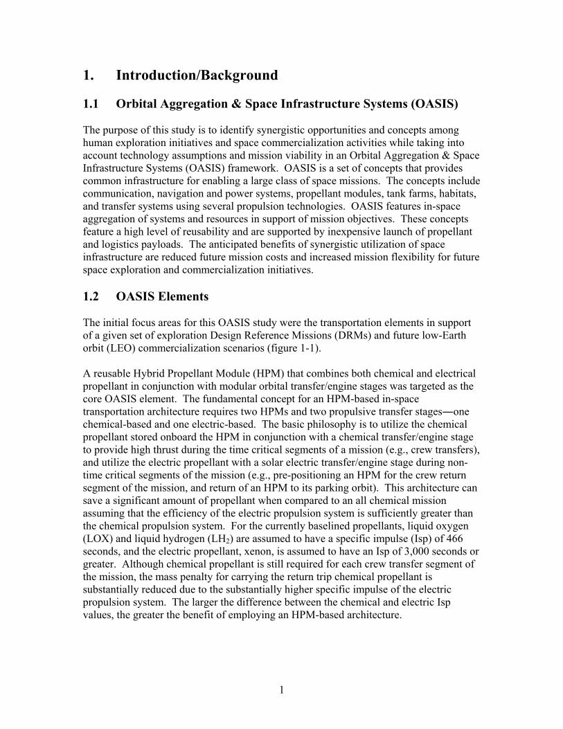
1. Introduction/Background 1.1 Orbital Aggregation & Space Infrastructure Systems (OASIS) The purpose of this study is to identify synergistic opportunities and concepts among human exploration initiatives and space commercialization activities while taking into account technology assumptions and mission viability in an Orbital Aggregation & Space Infrastructure Systems (OASIS) framework. OASIS is a set of concepts that provides common infrastructure for enabling a large class of space missions. The concepts include communication, navigation and power systems, propellant modules, tank farms, habitats, and transfer systems using several propulsion technologies. OASIS features in-space aggregation of systems and resources in support of mission objectives. These concepts feature a high level of reusability and are supported by inexpensive launch of propellant and logistics payloads. The anticipated benefits of synergistic utilization of space infrastructure are reduced future mission costs and increased mission flexibility for future space exploration and commercialization initiatives. 1.2 OASIS Elements The initial focus areas for this OASIS study were the transportation elements in support of a given set of exploration Design Reference Missions (DRMs) and future low-Earth orbit (LEO) commercialization scenarios (figure 1-1). A reusable Hybrid Propellant Module (HPM) that combines both chemical and electrical propellant in conjunction with modular orbital transfer/engine stages was targeted as the core OASIS element. The fundamental concept for an HPM-based in-space transportation architecture requires two HPMs and two propulsive transfer stages―one chemical-based and one electric-based. The basic philosophy is to utilize the chemical propellant stored onboard the HPM in conjunction with a chemical transfer/engine stage to provide high thrust during the time critical segments of a mission (e.g., crew transfers), and utilize the electric propellant with a solar electric transfer/engine stage during non-time critical segments of the mission (e.g., pre-positioning an HPM for the crew return segment of the mission, and return of an HPM to its parking orbit). This architecture can save a significant amount of propellant when compared to an all chemical mission assuming that the efficiency of the electric propulsion system is sufficiently greater than the chemical propulsion system. For the currently baselined propellants, liquid oxygen (LOX) and liquid hydrogen (LH2) are assumed to have a specific impulse (Isp) of 466 seconds, and the electric propellant, xenon, is assumed to have an Isp of 3,000 seconds or greater. Although chemical propellant is still required for each crew transfer segment of the mission, the mass penalty for carrying the return trip chemical propellant is substantially reduced due to the substantially higher specific impulse of the electric propulsion system. The larger the difference between the chemical and electric Isp values, the greater the benefit of employing an HPM-based architecture.
1
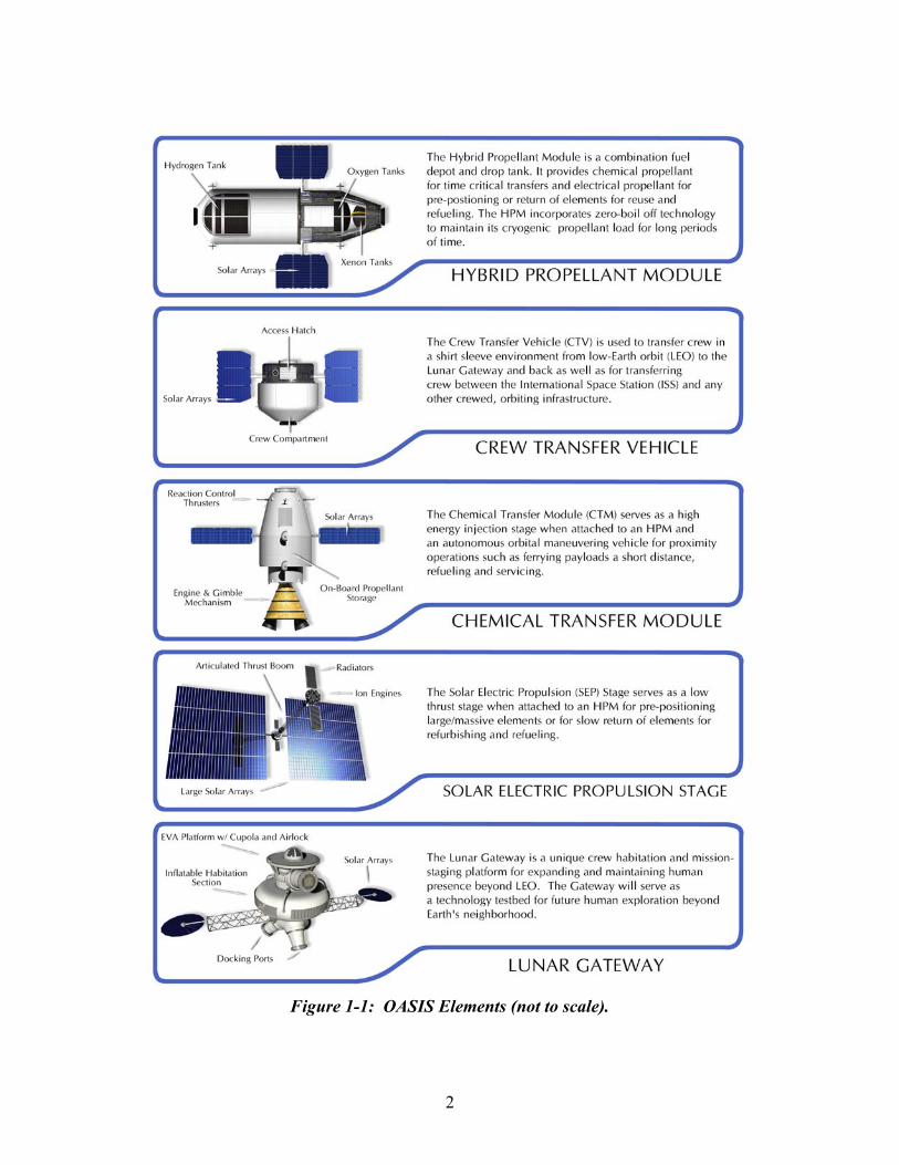
Figure 1-1: OASIS Elements (not to scale).
2
The Chemical Transfer Module (CTM) is an OASIS element that serves as a high energy injection stage when attached to an HPM. The CTM also functions independently of the HPM as an autonomous orbital maneuvering vehicle for proximity operations such as ferrying payloads a short distance, refueling and servicing. The CTM has high thrust cryogenic LOX/LH2 engines for orbit transfers and high-pressure LOX/LH2 thrusters for proximity operations and small delta-V maneuvers. The CTM can store approximately 4,000 kg of LOX/LH2 and a small amount of xenon (Xe) and may utilize the internally stored chemical propellant or burn propellant directly transferred from the HPM. The CTM does not incorporate zero boil-off technology. The Solar Electric Propulsion (SEP) Stage serves as a low-thrust transfer stage when attached to an HPM for pre-positioning large/massive elements or for the slow return of elements for refurbishing and refueling. The Crew Transfer Vehicle (CTV) is used to transfer crew in a shirt sleeve environment from LEO to the Lunar Gateway and back as well as to transfer crew between the International Space Station (ISS) and any other crewed orbiting infrastructure. 1.3 Study Approach and Participants 1.3.1 Approach This study was performed under the Revolutionary Aerospace Systems Concepts (RASC) activity led by the NASA Langley Research Center (LaRC). LaRC was chartered by the NASA Administrator to be the lead Center for evaluating revolutionary aerospace systems concepts and architectures to identify new mission approaches and the associated technologies that enable these missions to be implemented. The key objective of the RASC activity is to look beyond current research and technology (R&T) programs/missions and evolutionary technology development approaches by employing a “top-down” perspective to explore possible new mission capabilities. The accomplishment of this objective will support NASA’s goal of establishing a “go anywhere, anytime” capability for safe, reliable, and affordable human and robotic space exploration. The RASC Team seeks to maximize the cross-Enterprise benefits of these revolutionary capabilities as it defines the needed revolutionary enabling technology areas and performance levels. The product of the RASC Team studies will be revolutionary systems concepts, identification of associated enabling technologies, and definition of payoffs in new mission capabilities which these concepts can provide. These results will be delivered to the NASA Enterprises and the NASA Chief Technologist for use in planning future NASA R&T program investments.
3

1.3.2 Responsibilities and Teaming This OASIS study was performed by a collaborative NASA/contractor/university team. The NASA Langley Research Center (LaRC) served as the lead and was supported by Johnson Space Center (JSC), Glenn Research Center (GRC), and Marshall Spaceflight Center (MSFC). Boeing provided major input for OASIS commercial applications, and Swales, Analytical Mechanics Associates, Inc. and George Washington University supported the study integration effort. Participant responsibilities are given in more detail in table 2-1 below.
Table 1-1: OASIS Study Participants and Responsibilities. Study Participant Responsibilities
LaRC
• Study integration • Mission analysis (including lead for orbital mechanics) • OASIS mission architectures • HPM configuration • Crew Transfer Vehicle
JSC
• NASA Exploration Team (NEXT) design reference missions (DRMs)
• Lunar Gateway concept • Information management • System development • Crew Transfer Vehicle
GRC
• Sizing and layout of HPM cryogenic tanks • Fuel transfer interfaces • Zero boil-off systems • HPM power system sizing using advanced technology arrays • Solar Electric Propulsion Stage sizing and layout • Electric propulsion trajectory simulations
MSFC • Chemical Transfer Module
Boeing • Mission & technology tracking • Economic sensitivities • Commercial applications and missions
Other
• Orbital mechanics • Configuration analysis • Structural analysis • Multimedia visualization
4
2. Assumptions
2.1 Future Vision, Scenario and Environment Successful development of LEO and beyond will require a coalescence of events and technologies anticipated to span decades. Event occurrence and technology development are a function of budgetary, scientific and political variables. The timeframe and order in which these events develop will be gradual and evolutionary in nature unless paradigm shifting technology breakthroughs are introduced. Figure 2-1 attempts to capture the events and a technology development timeline that represent an environment leading to the OASIS architecture. Given an Apollo era budget and a coordinated national mandate, the timeline depicted could perhaps be compressed to 10 years. With current technology investment levels and unfocused long-term strategic plans, this timeline could stretch far beyond 20 years. Two developments that are major drivers in the depicted scenario are cost effective Earth-to-orbit transportation and discovery of commercially viable LEO business opportunities. As an example, there is a school of thought that space tourism will drive the initial development of inexpensive launch capability and space infrastructure. The scenario shown in figure 2-1 is driven by the concurrent needs of the NASA, military and commercial (including space tourism) sectors. 2.2 General Assumptions Through all but the last phases of this scenario, crew transportation to LEO is assumed to be provided by the current or upgraded U.S. Space Shuttle along with Russian Soyuz vehicles and, possibly, Chinese derivatives. “Affordable” human transportation to LEO is essential for space tourism and requires significant improvements in efficiency over current human-rated launch vehicles. However, nearly all mass sent into space is in the form of hardware and propellant that does not require a human-rated launch vehicle. Expendable launch vehicles (ELVs) such as the Delta IV-Heavy can be used in the near future to launch valuable hardware while a new generation of mass-produced, inexpensive ELVs may be developed to launch propellant and raw materials that are aggregated in LEO. The reliability of this new generation of ELVs would not have to be as high as conventional launchers since a lost payload would typically be just a tank of liquid hydrogen or oxygen. If technology permits, a non-human rated reusable launch system for aggregation of propellant in LEO could replace the mass-produced ELVs later in the scenario. Systems for facilitating the aggregation of resources in LEO are already under development through the Department of Defense (DOD) Orbital Express program. Orbital Express is a system for maintaining and refueling satellites in support of military objectives. The technologies (e.g., automated rendezvous and docking, on-orbit refueling) and standards developed for the military are assumed to migrate to the commercial sector. Once automated on-orbit servicing of both military and commercial satellites is the norm, the next natural extension is the ability to deliver and transport satellites utilizing a space based infrastructure. This is a leap in scale beyond Orbital Express requiring a large, reusable Orbital Transfer Vehicle (OTV) with cryogenic
5
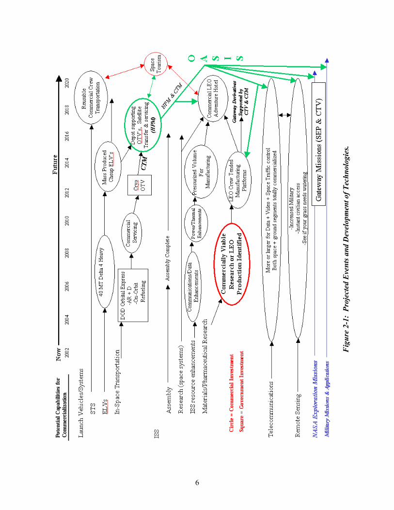
Figure 2-1: Projected Events and Development of Technologies.
Fig
ure
2-1:
Pro
ject
ed E
vent
s and
Dev
elop
men
t of T
echn
olog
ies.
6
propellants. The OASIS HPM and CTM are the next step in the evolution of capabilities beyond a military/commercial OTV. The International Space Station (ISS) offers the potential for reinvigorating the development of space. The key factor is the discovery of processes or products unique to the LEO environment that can form the basis of commercially viable enterprises. Whether these are new wonder drugs or valuable materials difficult to produce on Earth, a commercial demand for ISS resources will quickly follow. It is assumed that when ISS resources can no longer be expanded to accommodate the demand, unpressurized, crew-tended commercial platforms or pressurized, crewed platforms will be deployed in LEO. A reusable on-orbit infrastructure will be required to economically maintain a large number of LEO processing platforms. Economical transportation of materials to and from LEO will also be required if large-scale production occurs. Crewed processing platforms could have much in common with NASA’s Lunar Gateway and could yield a core design that may eventually be utilized as a commercial space hotel in support of space tourism. Satellite systems for telecommunications and remote sensing certainly will be more capable than today’s systems. Communications over more frequencies with higher bandwidth along with increased military and civilian remote sensing applications will either require larger satellites with more power and on-orbit upgrade capability or increased constellations of smaller, more disposable systems. Reality will likely be a combination of the two. Both system concepts will benefit from an on-orbit infrastructure and reduced launch costs. Assumptions for NASA, commercial and military scenarios are discussed in more detail in Sections 4.1, 4.2.2, and 4.3 of this report. A major assumption in support of the OASIS architecture is the availability of routine and inexpensive launch of propellant to LEO. A cursory assessment of an ELV-based approach was made based on the following assumptions:
• A commercial launch services company has built a factory offsite of an east coast launch facility (e.g., Wallops Flight Facility or Kennedy Space Center) that produces one inexpensive ELV a week capable of launching a 100,000 kg payload to 400 km circular at 51.6° inclination.
• A road or rail has been built between the factory and the launch facility for the horizontal transport of the ELV.
• The ELV can be pulled by a typical 18-wheeler cab since it is fueled on the pad with cryogenic oxygen and hydrogen. The ELV also features two strap-on stages that are fueled in the same manner.
• The strap-on configuration results in a shorter ELV that is easy to raise to a vertical position on the pad (similar to Russian launch vehicles).
7
• Once on the pad, one of two payload containers is bolted to the top of the stack.
• The small container carries either cryogenic xenon or liquid oxygen as a payload.
• Xenon is trucked in from the “ACME Xenon Company” and pumped into the payload carrier.
• Liquid oxygen is pumped into the payload carrier shortly before or after the ELV is filled with liquid oxygen.
• The large payload carrier is used for liquid hydrogen or re-supply logistics.
• As with the liquid oxygen, liquid hydrogen is pumped into the payload carrier approximately the same time it is pumped into the ELV as fuel.
• The liquid oxygen and liquid hydrogen are produced and piped in from the same infrastructure that supports other cryogenically fueled vehicles at the launch facility.
• Sealed payload containers with dry logistics are trucked in from other commercial facilities and bolted directly to the top of the stack (prior to fueling).
• Two identical pads exist in close proximity but far enough apart that if an ELV has a catastrophic failure, it will not impact operations at the other pad.
• The launch pads are simple facilities including a concrete square with a combination horizontal to vertical spine that serves as the tower. There may also be a roll away umbilical tower.
A quick summary of this scenario would be 1) transport the ELV to the launch pad, 2) rotate the ELV to vertical, 3) attach the payload carrier (with a Caterpillar type crane), power the ELV and perform pre-flight verification checks, 4) load propellant, 5) launch.
8
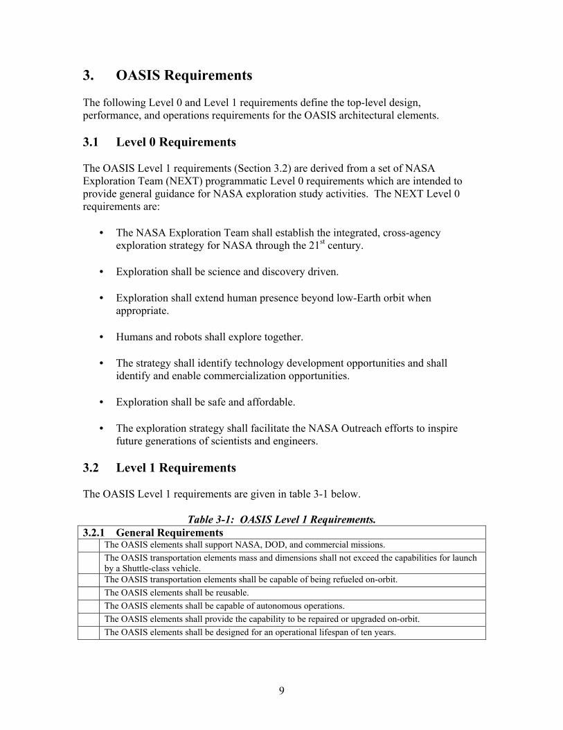
3. OASIS Requirements The following Level 0 and Level 1 requirements define the top-level design, performance, and operations requirements for the OASIS architectural elements. 3.1 Level 0 Requirements The OASIS Level 1 requirements (Section 3.2) are derived from a set of NASA Exploration Team (NEXT) programmatic Level 0 requirements which are intended to provide general guidance for NASA exploration study activities. The NEXT Level 0 requirements are:
• The NASA Exploration Team shall establish the integrated, cross-agency exploration strategy for NASA through the 21st century.
• Exploration shall be science and discovery driven.
• Exploration shall extend human presence beyond low-Earth orbit when
appropriate.
• Humans and robots shall explore together.
• The strategy shall identify technology development opportunities and shall identify and enable commercialization opportunities.
• Exploration shall be safe and affordable.
• The exploration strategy shall facilitate the NASA Outreach efforts to inspire
future generations of scientists and engineers. 3.2 Level 1 Requirements The OASIS Level 1 requirements are given in table 3-1 below.
Table 3-1: OASIS Level 1 Requirements. 3.2.1 General Requirements The OASIS elements shall support NASA, DOD, and commercial missions. The OASIS transportation elements mass and dimensions shall not exceed the capabilities for launch
by a Shuttle-class vehicle. The OASIS transportation elements shall be capable of being refueled on-orbit. The OASIS elements shall be reusable. The OASIS elements shall be capable of autonomous operations. The OASIS elements shall provide the capability to be repaired or upgraded on-orbit. The OASIS elements shall be designed for an operational lifespan of ten years.
9
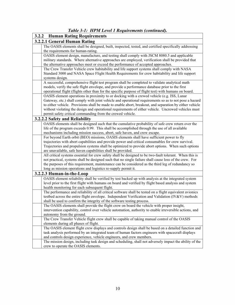
Table 3-1: HPM Level 1 Requirements (continued). 3.2.2 Human Rating Requirements 3.2.2.1 General Human Rating The OASIS elements shall be designed, built, inspected, tested, and certified specifically addressing
the requirements for human-rating. OASIS element design, manufacture, and testing shall comply with JSCM 8080.5 and applicable
military standards. Where alternative approaches are employed, verification shall be provided that the alternative approaches meet or exceed the performance of accepted approaches.
The Crew Transfer Vehicle crew habitability and life support systems shall comply with NASA Standard 3000 and NASA Space Flight Health Requirements for crew habitability and life support systems design.
A successful, comprehensive flight test program shall be completed to validate analytical math models, verify the safe flight envelope, and provide a performance database prior to the first operational flight (flights other than for the specific purpose of flight test) with humans on board.
OASIS element operations in proximity to or docking with a crewed vehicle (e.g. ISS, Lunar Gateway, etc.) shall comply with joint vehicle and operational requirements so as to not pose a hazard to either vehicle. Provisions shall be made to enable abort, breakout, and separation by either vehicle without violating the design and operational requirements of either vehicle. Uncrewed vehicles must permit safety critical commanding from the crewed vehicle.
3.2.2.2 Safety and Reliability OASIS elements shall be designed such that the cumulative probability of safe crew return over the
life of the program exceeds 0.99. This shall be accomplished through the use of all available mechanisms including mission success, abort, safe haven, and crew escape.
For beyond Earth orbit (BEO) missions, OASIS elements shall have sufficient power to fly trajectories with abort capabilities and provide power and critical consumables for crew survival. Trajectories and propulsion systems shall be optimized to provide abort options. When such options are unavailable, safe haven capabilities shall be provided.
All critical systems essential for crew safety shall be designed to be two-fault tolerant. When this is not practical, systems shall be designed such that no single failure shall cause loss of the crew. For the purposes of this requirement, maintenance can be considered as the third leg of redundancy so long as mission operations and logistics re-supply permit it.
3.2.2.3 Human-in-the-Loop OASIS element reliability shall be verified by test backed up with analysis at the integrated system
level prior to the first flight with humans on board and verified by flight based analysis and system health monitoring for each subsequent flight.
The performance and reliability of all critical software shall be tested on a flight equivalent avionics testbed across the entire flight envelope. Independent Verification and Validation (IV&V) methods shall be used to confirm the integrity of the software testing process.
The OASIS elements shall provide the flight crew on board the vehicle with proper insight, intervention capability, control over vehicle automation, authority to enable irreversible actions, and autonomy from the ground.
The Crew Transfer Vehicle flight crew shall be capable of taking manual control of the OASIS elements during all phases of flight.
The OASIS element flight crew displays and controls design shall be based on a detailed function and task analysis performed by an integrated team of human factors engineers with spacecraft displays and controls design experience, vehicle engineers, and crew members.
The mission design, including task design and scheduling, shall not adversely impact the ability of the crew to operate the OASIS elements.
10

4. Architectures and Associated Missions 4.1 Exploration Missions for human exploration of the solar system are an important part of NASA’s future vision. Consequently, reference mission studies are performed to formulate the means by which these missions will be accomplished. These studies utilize “mission architectures” to define the system elements and the methods humans will use to leave Earth, perform their objectives, and subsequently return to Earth. Rationale and justification for human exploration of the Earth’s neighborhood continues to mount. Recent scientific discoveries in the lunar polar regions have sparked renewed interest in human exploration of the Moon. As another example, our goal of exploring the origins of the universe will require the on-orbit assembly of large astronomical facilities with humans and robotic partners. These new opportunities for scientific investigation in the Earth’s neighborhood have led architecture designers to take revolutionary new approaches for accommodating these various missions in a sensible, integrated fashion. In the past, such destinations were considered on their own basis with little thought given to how they fit together. This new approach has led to a particular architecture for exploration within the Earth’s neighborhood known as the Gateway Architecture. Central to this is the emplacement of a mission-staging platform near the Moon―specifically at the Earth-Moon L1 Lagrange point (figure 4-1). This facility, the Lunar Gateway, will serve as a “gateway” to future exploration of space including the lunar surface, other Lagrange points, and Mars.
L2
Sun
1.5 million km 1.5 million km
L4
L1
L3
L5
Sun - EarthL1
Sun - EarthL2
Moon’s Orbit
150 million km
Earth-Moon L1 Lagrange point is327,000 km from Earth’s center,58,000 km from Moon’s center. L2
Sun
1.5 million km 1.5 million km
L4
L1
L3
L5
Sun - EarthL1
Sun - EarthL2
Moon’s Orbit
150 million km
Earth-Moon L1 Lagrange point is327,000 km from Earth’s center,58,000 km from Moon’s center.
Figure 4-1: Earth’s Neighborhood Lagrange Point Geometry.
The primary goal of the Gateway Architecture is to enable both short-duration and extended-stay exploration of the entire lunar surface as well as to enable the on-orbit assembly of large astronomical observatories. Utilizing the collinear Earth-Moon L1 Lagrange point as a mission staging node allows access to all lunar latitudes for essentially the same transportation costs as a direct Earth-to-Moon mission while providing a continuous launch window to and from the lunar surface. As noted, one use of the Gateway Architecture is to provide the extensive infrastructure needed for the on-orbit assembly, calibration and servicing of large-aperture Gossamer telescopes. While construction from the Space Shuttle offers the necessary robotic and
11
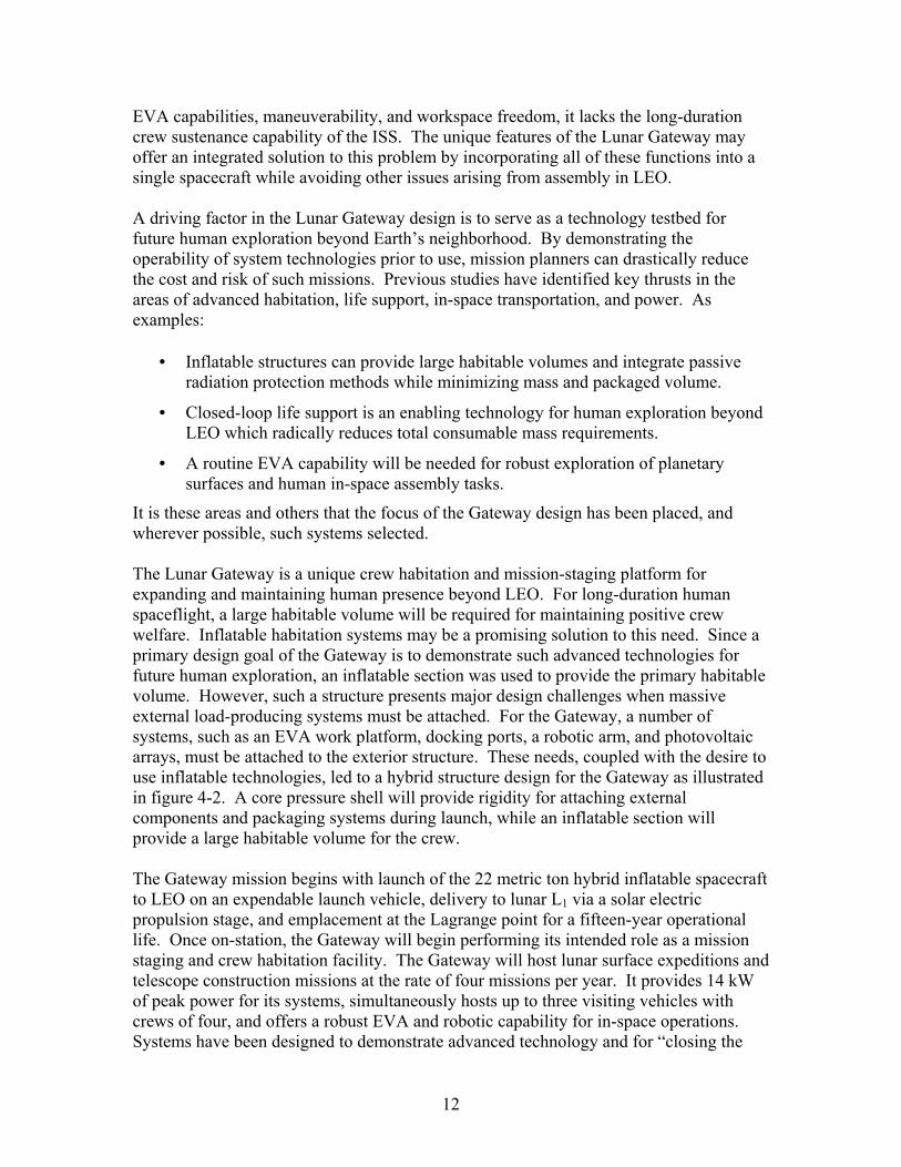
EVA capabilities, maneuverability, and workspace freedom, it lacks the long-duration crew sustenance capability of the ISS. The unique features of the Lunar Gateway may offer an integrated solution to this problem by incorporating all of these functions into a single spacecraft while avoiding other issues arising from assembly in LEO. A driving factor in the Lunar Gateway design is to serve as a technology testbed for future human exploration beyond Earth’s neighborhood. By demonstrating the operability of system technologies prior to use, mission planners can drastically reduce the cost and risk of such missions. Previous studies have identified key thrusts in the areas of advanced habitation, life support, in-space transportation, and power. As examples:
• Inflatable structures can provide large habitable volumes and integrate passive radiation protection methods while minimizing mass and packaged volume.
• Closed-loop life support is an enabling technology for human exploration beyond LEO which radically reduces total consumable mass requirements.
• A routine EVA capability will be needed for robust exploration of planetary surfaces and human in-space assembly tasks.
It is these areas and others that the focus of the Gateway design has been placed, and wherever possible, such systems selected. The Lunar Gateway is a unique crew habitation and mission-staging platform for expanding and maintaining human presence beyond LEO. For long-duration human spaceflight, a large habitable volume will be required for maintaining positive crew welfare. Inflatable habitation systems may be a promising solution to this need. Since a primary design goal of the Gateway is to demonstrate such advanced technologies for future human exploration, an inflatable section was used to provide the primary habitable volume. However, such a structure presents major design challenges when massive external load-producing systems must be attached. For the Gateway, a number of systems, such as an EVA work platform, docking ports, a robotic arm, and photovoltaic arrays, must be attached to the exterior structure. These needs, coupled with the desire to use inflatable technologies, led to a hybrid structure design for the Gateway as illustrated in figure 4-2. A core pressure shell will provide rigidity for attaching external components and packaging systems during launch, while an inflatable section will provide a large habitable volume for the crew. The Gateway mission begins with launch of the 22 metric ton hybrid inflatable spacecraft to LEO on an expendable launch vehicle, delivery to lunar L1 via a solar electric propulsion stage, and emplacement at the Lagrange point for a fifteen-year operational life. Once on-station, the Gateway will begin performing its intended role as a mission staging and crew habitation facility. The Gateway will host lunar surface expeditions and telescope construction missions at the rate of four missions per year. It provides 14 kW of peak power for its systems, simultaneously hosts up to three visiting vehicles with crews of four, and offers a robust EVA and robotic capability for in-space operations. Systems have been designed to demonstrate advanced technology and for “closing the
12
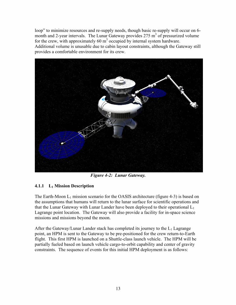
loop” to minimize resources and re-supply needs, though basic re-supply will occur on 6-month and 2-year intervals. The Lunar Gateway provides 275 m3 of pressurized volume for the crew, with approximately 60 m3 occupied by internal system hardware. Additional volume is unusable due to cabin layout constraints, although the Gateway still provides a comfortable environment for its crew.
Figure 4-2: Lunar Gateway.
4.1.1 L1 Mission Description The Earth-Moon L1 mission scenario for the OASIS architecture (figure 4-3) is based on the assumptions that humans will return to the lunar surface for scientific operations and that the Lunar Gateway with Lunar Lander have been deployed to their operational L1 Lagrange point location. The Gateway will also provide a facility for in-space science missions and missions beyond the moon. After the Gateway/Lunar Lander stack has completed its journey to the L1 Lagrange point, an HPM is sent to the Gateway to be pre-positioned for the crew return-to-Earth flight. This first HPM is launched on a Shuttle-class launch vehicle. The HPM will be partially fueled based on launch vehicle cargo-to-orbit capability and center of gravity constraints. The sequence of events for this initial HPM deployment is as follows:
13
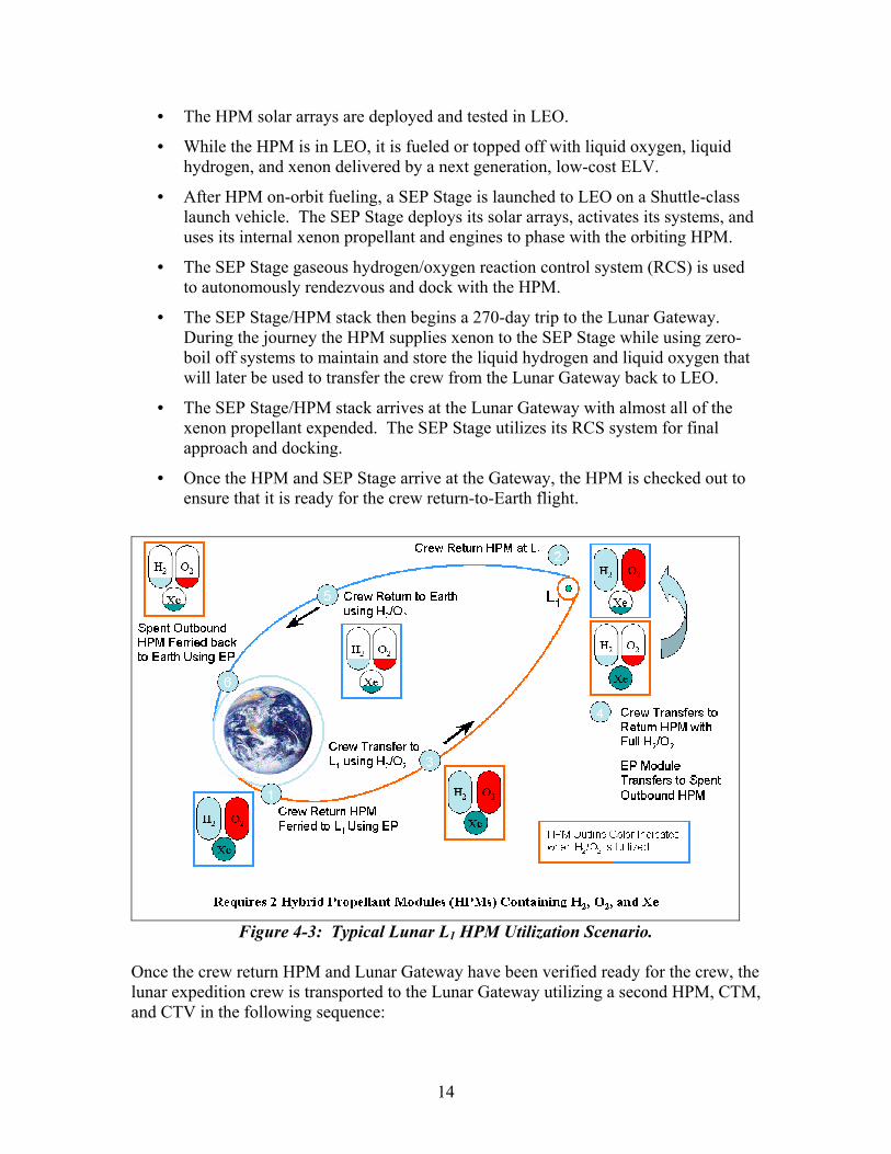
• The HPM solar arrays are deployed and tested in LEO.
• While the HPM is in LEO, it is fueled or topped off with liquid oxygen, liquid hydrogen, and xenon delivered by a next generation, low-cost ELV.
• After HPM on-orbit fueling, a SEP Stage is launched to LEO on a Shuttle-class launch vehicle. The SEP Stage deploys its solar arrays, activates its systems, and uses its internal xenon propellant and engines to phase with the orbiting HPM.
• The SEP Stage gaseous hydrogen/oxygen reaction control system (RCS) is used to autonomously rendezvous and dock with the HPM.
• The SEP Stage/HPM stack then begins a 270-day trip to the Lunar Gateway. During the journey the HPM supplies xenon to the SEP Stage while using zero-boil off systems to maintain and store the liquid hydrogen and liquid oxygen that will later be used to transfer the crew from the Lunar Gateway back to LEO.
• The SEP Stage/HPM stack arrives at the Lunar Gateway with almost all of the xenon propellant expended. The SEP Stage utilizes its RCS system for final approach and docking.
• Once the HPM and SEP Stage arrive at the Gateway, the HPM is checked out to ensure that it is ready for the crew return-to-Earth flight.
Figure 4-3: Typical Lunar L1 HPM Utilization Scenario.
Once the crew return HPM and Lunar Gateway have been verified ready for the crew, the lunar expedition crew is transported to the Lunar Gateway utilizing a second HPM, CTM, and CTV in the following sequence:
14
• A Shuttle-class launch vehicle delivers the CTM and CTV to LEO.
• The CTM is deployed and loiters until the HPM is delivered and fueled.
• After CTM deployment, the Shuttle-class launch vehicle performs a rendezvous with the ISS and berths the CTV to the station via an International Berthing & Docking Mechanism (IBDM) located on the nadir face of the ISS. The CTV is then configured and outfitted for the journey to the Lunar Gateway.
• The HPM for crew transport to the Lunar Gateway is launched to LEO and fueled/topped off with liquid oxygen, liquid hydrogen and xenon delivered to orbit by a next generation, low-cost ELV. This HPM contains enough liquid oxygen and hydrogen to deliver the crew from LEO to the Lunar Gateway in less than four days. The HPM also carries enough xenon propellant so that the HPM can be returned from L1 using a SEP Stage.
• The CTM performs a rendezvous and docks with the HPM.
• The CTM performs a rendezvous and docks the CTM/HPM stack to the CTV on the ISS. The crew enters the CTV from the ISS and is now ready to begin the journey to the Lunar Gateway.
• The CTM/HPM/CTV stack departs from the ISS. The CTM utilizes its RCS to separate the stack a sufficient distance to fire its main engines. Then the CTM/HPM/CTV stack begins a series of engine burns that will transport the crew from LEO to the Lunar Gateway.
• The CTM/HPM/CTV stack arrives and docks to the Lunar Gateway.
Crew and all elements required to perform a lunar excursion are now at the Gateway. Before the lunar excursion is performed, the CTM, SEP Stage and HPMs must be repositioned such that (1) the HPM with the full load of liquid hydrogen and liquid oxygen is connected to the CTV and CTM, and (2) the HPM with the full load of xenon propellant is attached to the SEP Stage. The repositioning begins with the CTM pulling the HPM loaded with xenon off the CTV and holding it a safe distance from the Gateway. Next, the SEP Stage utilizes its RCS to transfer the HPM loaded with liquid hydrogen and liquid oxygen to the Gateway port where the CTV is docked. The HPM stacks approach the desired ports on the Gateway in sequential order. Once this phase is complete, the HPM loaded with hydrogen and oxygen is attached to the CTV. Now, the CTM and SEP Stage separate from the HPMs. They exchange places so that the CTM is attached to the HPM loaded hydrogen and oxygen and the SEP Stage is attached to the xenon-loaded HPM. Once they have been checked out in this configuration, both stacks are ready for the return voyage to LEO. The lunar excursion can now be performed. After the lunar excursion is complete and the crew has returned to the Gateway, the return-to-Earth mission sequence begins:
• The crew enters the CTV from the Gateway.
• The CTM separates the CTM/HPM/CTV stack from the Gateway.
15
• The CTM then propels the HPM and crewed CTV back to LEO. The stack docks to the ISS where the crew will depart for Earth on a Shuttle flight.
• The CTV is refurbished on the ISS.
• The HPM and CTM perform a rendezvous with ELV-delivered propellant carriers, refuel and are ready for the next Gateway mission sortie.
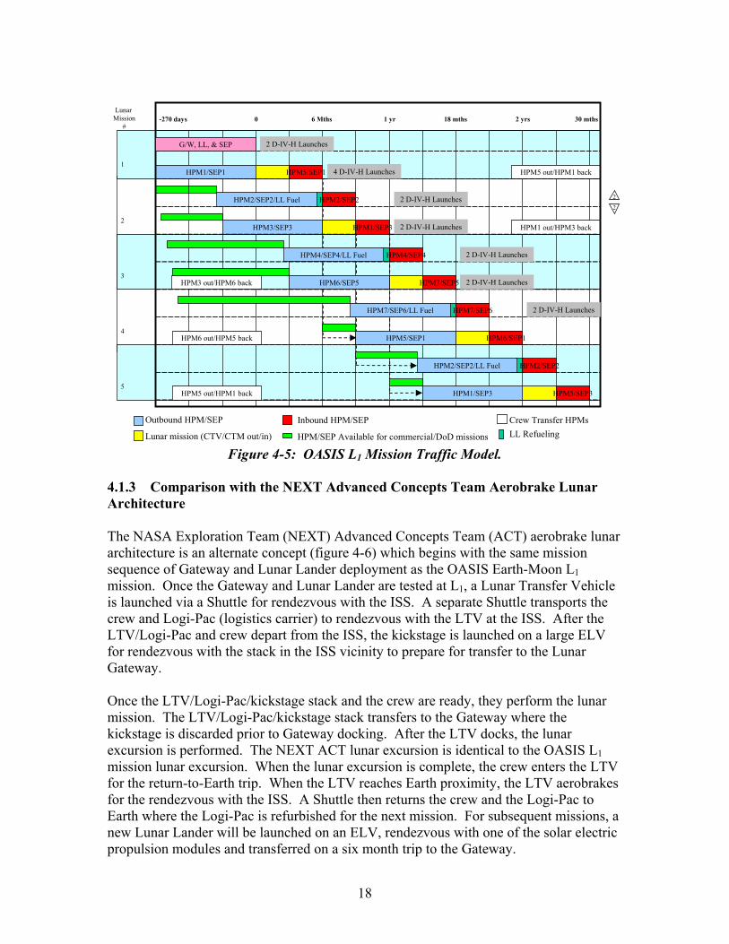
Either prior to or shortly after the crew departs from the Gateway, the SEP Stage and xenon-loaded HPM leave the Gateway for the return to LEO. Once the SEP Stage/HPM stack is back in LEO, the HPM is refueled via the ELV-delivered propellant logistics carriers. The SEP Stage internal tank is also topped off with xenon. The SEP Stage arrays may need replacement at the ISS. At this point, all of the elements that were utilized for crew and supply transfer with the exception of the Lunar Lander have returned to LEO and are ready to support another mission. To perform multiple lunar missions in less than approximately 540 days, multiple HPMs and SEP Stages are required to establish the desired mission frequency. Simultaneous to the crew return HPM and SEP Stage performing their mission, a second HPM/SEP Stage stack will ferry propellant to refuel the Lunar Lander for the next lunar excursion. This stack carries a xenon load to support both the outbound and return trips of the HPM/SEP Stage. Between the two lunar excursions, this stack will auto-rendezvous with the Lunar Lander and perform a fuel transfer. Once the transfer is complete, the empty HPM will use the remaining xenon for the transfer back to LEO. This OASIS architecture lunar L1 mission scenario is illustrated in figure 4-4. 4.1.2 L1 Mission Traffic Model The Earth-Moon L1 mission traffic model shown in figure 4-5 is based on a lunar excursion every six months. The sequence for the first five lunar excursions and the required launches are illustrated. Due to mission sequencing and length of time for the SEP Stage outbound phases, 7 HPMs and 6 SEP Stages are required to support lunar excursion missions at six-month intervals. Also a result of mission sequencing, a greater than three month interval exists between mission sorties for a given HPM. This interval may potentially be used for HPM commercial or military application missions (Sections 4.2 and 4.3). The three-month period shown for the lunar mission time includes HPM and Lunar Lander checkout, lunar mission duration, and contingency. Checkout time is to ensure that the HPM/CTV/CTM stack is ready for the mission once it is assembled on-orbit and to verify Lunar Lander systems after refueling at the Gateway.
16
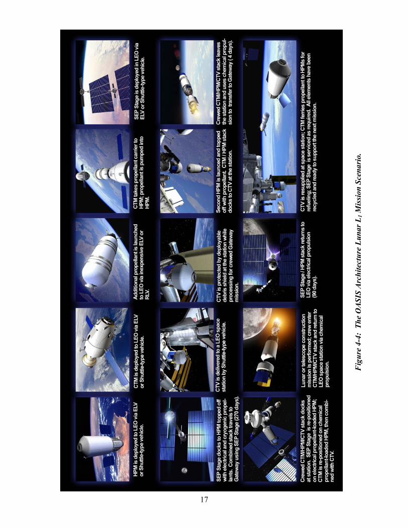
Figure 4-4: The OASIS Architecture Lunar L1 Mission Scenario.
Fig
ure
4-4:
The
OA
SIS
Arc
hite
ctur
e Lu
nar L
1 Mis
sion
Sce
nari
o.
17
Inbound HPM/SEP
HPM/SEP Available for commercial/DoD missions
-270 days 0 6 Mths 1 yr 18 mths 2 yrs 30 mths
Outbound HPM/SEP
Lunar mission (CTV/CTM out/in)
Crew Transfer HPMs
HPM1/SEP1
HPM2/SEP2/LL Fuel
HPM3/SEP3
HPM4/SEP4/LL Fuel
HPM5/SEP1
HPM2/SEP2
HPM4/SEP4
HPM6/SEP5
HPM5 out/HPM1 back
HPM1 out/HPM3 back
HPM3 out/HPM6 back
HPM6 out/HPM5 back
HPM7/SEP6/LL Fuel
HPM5 out/HPM1 back
HPM3/SEP5
HPM7/SEP6
HPM2/SEP2/LL Fuel
HPM1/SEP3
HPM1/SEP3
HPM5/SEP1
HPM6/SEP1
HPM5/SEP3
HPM2/SEP2
2
3
4
5
1
Lunar Mission
#
G/W, LL, & SEP
2
2
LL Refueling
2 D-IV-H Launches
4 D-IV-H Launches
2 D-IV-H Launches
2 D-IV-H Launches
2 D-IV-H Launches
2 D-IV-H Launches
2 D-IV-H Launches
Figure 4-5: OASIS L1 Mission Traffic Model. 4.1.3 Comparison with the NEXT Advanced Concepts Team Aerobrake Lunar Architecture The NASA Exploration Team (NEXT) Advanced Concepts Team (ACT) aerobrake lunar architecture is an alternate concept (figure 4-6) which begins with the same mission sequence of Gateway and Lunar Lander deployment as the OASIS Earth-Moon L1 mission. Once the Gateway and Lunar Lander are tested at L1, a Lunar Transfer Vehicle is launched via a Shuttle for rendezvous with the ISS. A separate Shuttle transports the crew and Logi-Pac (logistics carrier) to rendezvous with the LTV at the ISS. After the LTV/Logi-Pac and crew depart from the ISS, the kickstage is launched on a large ELV for rendezvous with the stack in the ISS vicinity to prepare for transfer to the Lunar Gateway. Once the LTV/Logi-Pac/kickstage stack and the crew are ready, they perform the lunar mission. The LTV/Logi-Pac/kickstage stack transfers to the Gateway where the kickstage is discarded prior to Gateway docking. After the LTV docks, the lunar excursion is performed. The NEXT ACT lunar excursion is identical to the OASIS L1 mission lunar excursion. When the lunar excursion is complete, the crew enters the LTV for the return-to-Earth trip. When the LTV reaches Earth proximity, the LTV aerobrakes for the rendezvous with the ISS. A Shuttle then returns the crew and the Logi-Pac to Earth where the Logi-Pac is refurbished for the next mission. For subsequent missions, a new Lunar Lander will be launched on an ELV, rendezvous with one of the solar electric propulsion modules and transferred on a six month trip to the Gateway.
18
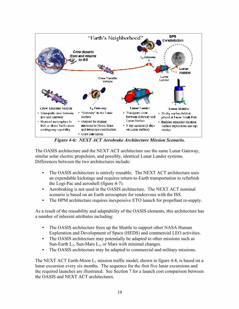
Figure 4-6: NEXT ACT Aerobrake Architecture Mission Scenario.
The OASIS architecture and the NEXT ACT architecture use the same Lunar Gateway, similar solar electric propulsion, and possibly, identical Lunar Lander systems. Differences between the two architectures include:
• The OASIS architecture is entirely reusable. The NEXT ACT architecture uses an expendable kickstage and requires return-to-Earth transportation to refurbish the Logi-Pac and aeroshell (figure 4-7).
• Aerobraking is not used in the OASIS architecture. The NEXT ACT nominal scenario is based on an Earth aerocapture for rendezvous with the ISS.
• The HPM architecture requires inexpensive ETO launch for propellant re-supply.
As a result of the reusability and adaptability of the OASIS elements, this architecture has a number of inherent attributes including:
• The OASIS architecture frees up the Shuttle to support other NASA Human Exploration and Development of Space (HEDS) and commercial LEO activities.
• The OASIS architecture may potentially be adapted to other missions such as Sun-Earth L2, Sun-Mars L1, or Mars with minimal changes.
• The OASIS architecture may be adapted to commercial and military missions. The NEXT ACT Earth-Moon L1 mission traffic model, shown in figure 4-8, is based on a lunar excursion every six months. The sequence for the first five lunar excursions and the required launches are illustrated. See Section 7 for a launch cost comparison between the OASIS and NEXT ACT architectures.
19
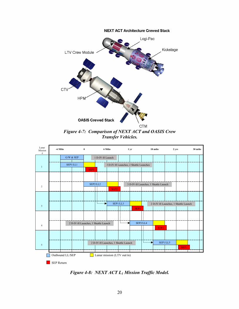
Figure 4-7: Comparison of NEXT ACT and OASIS Crew
Transfer Vehicles.
-6 Mths 0 6 Mths 1 yr 18 mths 2 yrs 30 mths
Outbound LL/SEP
SEP Return
Lunar mission (LTV out/in)
G/W & SEP
SEP1/LL1
SEP2/LL2
SEP2/LL4
SEP1/LL3
SEP1
SEP2
SEP1
SEP2
SEP1
2
3
4
5
1
Lunar Mission
#
SEP1/LL5
1 D-IV-H Launch
3 D-IV-H Launches, 2 Shuttle Launches
3 D-IV-H Launches, 1 Shuttle Launch
2 D-IV-H Launches, 1 Shuttle Launch
2 D-IV-H Launches, 1 Shuttle Launch
2 D-IV-H Launches, 1 Shuttle Launch
Figure 4-8: NEXT ACT L1 Mission Traffic Model.
20
4.2 Commercial Applications Earth orbiting satellites have provided ever increasingly important services both in commercial and military applications since the first satellite launch in 1957. A recent study by the Teal Group of Fairfax, Virginia [World Space Systems Briefing, IAF 52nd International Astronautical Congress,Toulouse, France, October 2, 2001] indicates that of the 5,070 satellites launched to date, 600 to 610 remain operational. Approximately 150 of these are military satellites. Surveys of the commercial satellite industry predict that there will continue to be a need for orbiting commercial and military assets to provide a variety of applications over at least the next two decades. While fluctuations will occur in the predicted number and locations of satellites, the current suite of orbiting constellations is representative of the predicted market. An orbiting constellation of reusable propellant depots when combined with a propulsive capability as envisioned for the OASIS HPM and associated propulsive elements may provide an economically viable concept for supporting the predicted commercial and military market. This section summarizes the results of a commercialization study evaluating the size and cost requirements for a network of OASIS elements that could support the predicted satellite market by deploying new satellites and servicing on-orbit spacecraft. Synergies are identified between technologies required for development of the OASIS elements and those envisioned by NASA, military and industry to enhance space vehicle performance. 4.2.1 Commercialization Study Objectives The objectives of this commercialization study include:
• To assess the OASIS architecture’s potential applicability and benefits for Earth’s Neighborhood commercial and military space missions in the post 2015 time frame by:
o Determining key areas of need for projected commercial/military missions
that OASIS may support (e.g., deployment, refueling/servicing, retrieval/disposal). See Section 4.3, Military Applications, for a description of potential military applications.
o Quantifying the levels of potential HPM commercial utilization (i.e.,
development of an OASIS traffic model).
o Developing rough order of magnitude cost estimates for the resulting economic impacts (see Section 7, Economic Viability Analysis).
• To determine common technology development areas to leverage NASA research
spinoffs and technology transfers, and to identify potential cost saving initiatives that support commercial applications.
21
While there are many issues that will impact the future commercialization of space and, specifically, effect the utility of OASIS elements in supporting commercial applications, there are a few key drivers that impact this study. These are:
• Projected commercial/military satellite market
• OASIS element design (sizing and performance parameters)
• HPM allocation and usage rates to support identified markets (traffic models)
• Earth-to-orbit transportation costs including comparisons between HPM and HPM propellant re-supply vs. current launch architectures.
4.2.2 Key Assumptions Numerous factors will impact the predictions of the commercial space infrastructure more than a decade into the future. Therefore, a number of assumptions have been made based on understanding the current commercial market, current industry infrastructure, and the HPM design. These key assumptions affect the approach taken to analyze the HPM’s performance capability to support the predicted markets and assess its economic viability to compete with current industry standard approaches and competition. This section discusses the major assumptions that impacted the overall study. 4.2.2.1 HPM Design Commercial scenarios analyzed in this section utilize the HPM design (Section 5.1) as defined for the Earth-Moon L1 exploration missions. For performance analyses only, the HPM “performance mass” estimate has been defined which is 20 percent higher than the target mass estimate. See table 5-20, HPM System Mass Breakdown, for the HPM dry target mass estimate. This provides a measure of conservatism in estimating performance for OASIS elements in supporting both exploration and commercial missions. 4.2.2.2 Low-Cost Earth-to-LEO Transportation This analysis is predicated on the assumption that in the 2015+ period, a low-cost launch system will have been developed to provide transportation from Earth launch sites into LEO. These LEO parking orbits are assumed to be circular and between 200 and 400 km in altitude. Orbits below 200 km sustain orbit decay rates that are too rapid to support timelines needed for orbital operations. Launch systems are assumed to be one of two types depending on payload. Highly reliable, reusable launch vehicles (RLVs) or expendable launch vehicles (ELVs) may be developed to provide launch services for high value payloads such as human crews, cargo and satellites. Potentially lower reliability ELVs may be developed to provide very low cost launch services for lesser-valued payloads such as re-supply propellant. Specific LEO delivery cost per kg goals will be assessed as a part of the HPM economic viability analysis discussed in Section 7. In all cases, these lower cost Earth-to-LEO launch
22
systems will not have the capability to go beyond LEO and will require separate orbit-to-orbit transfer systems which may be space-based. 4.2.2.3 Common Satellite Industry Infrastructure For an OASIS architecture to support the broadest market potential, it will be necessary for the satellite industry (preferably both global commercial satellite manufacturers and U.S. military satellite providers) to adopt a common infrastructure that is consistent with OASIS systems. There are a number of satellite systems that would benefit from common interfaces to maximize the utility of an OASIS architecture. This section discusses a few of the important interfaces. The common HPM design would feature a single payload attach fitting that would permit the HPM to hard dock with the many types of satellite models to enable deployment, re-boosting and repositioning missions. This represents a significant departure from present day infrastructure where launch service providers offer numerous payload attach fittings to accommodate differing satellite designs. The HPM is designed to transfer liquid hydrogen and liquid oxygen to the CTM, and xenon to the SEP Stage. This capability will also permit the HPM system to refuel those orbiting satellites with solar electric station keeping propulsion systems that use xenon as propellant thereby extending their useful life. Common satellite refueling ports would be necessary to permit refueling for this class of satellite. It may be possible to use the OASIS elements to extend the life of orbiting satellites by refurbishing components that have degraded or failed. In order to supply and install these components on-orbit, the satellites would require “plug and play” systems that could be easily removed and replaced autonomously. Candidate systems for refurbishment include solar panels and booms, batteries, avionics boxes, and station keeping propulsion systems. 4.2.3 Study Methodology The process employed to conduct the commercialization study is shown in figure 4-9. Inputs for the study involve details of the HPM system baseline design . Specifically, module and propellant masses and propulsion system specific impulse (Isp) were needed. A number of references were utilized to assess trends and predict the potential commercial market in the 2015+ timeframe. Technology initiative databases were consulted to identify efforts underway within NASA and the military regarding technologies that would enable the development of OASIS elements. The figure indicates the flow of the study from analyzing the projected satellite market for HPM application through a performance analysis assessing the ability of the OASIS elements to service the projected market and the subsequent development of an OASIS traffic model.
23
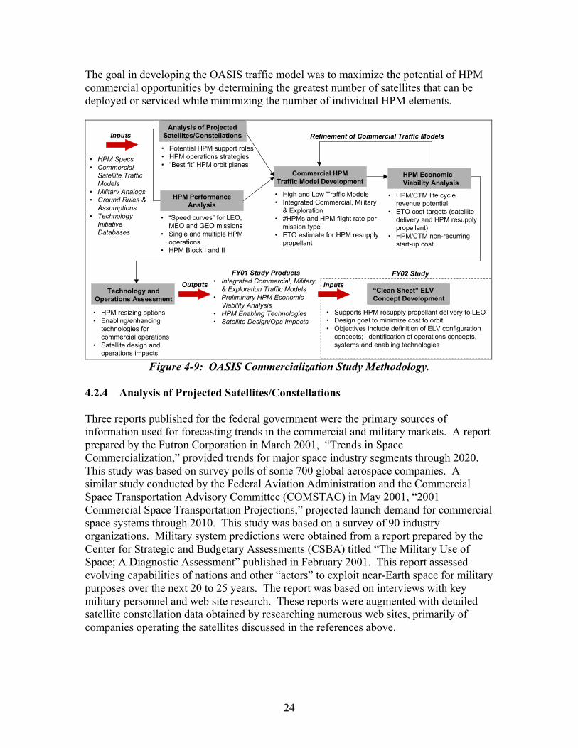
The goal in developing the OASIS traffic model was to maximize the potential of HPM commercial opportunities by determining the greatest number of satellites that can be deployed or serviced while minimizing the number of individual HPM elements.
• HPM Specs• Commercial
Satellite TrafficModels
• Military Analogs• Ground Rules &
Assumptions• Technology
InitiativeDatabases
• “Speed curves” for LEO,MEO and GEO missions
• Single and multiple HPMoperations
• HPM Block I and II
• High and Low Traffic Models• Integrated Commercial, Military
& Exploration• #HPMs and HPM flight rate per
mission type• ETO estimate for HPM resupply
propellant
• HPM/CTM life cyclerevenue potential
• ETO cost targets (satellitedelivery and HPM resupplypropellant)
• HPM/CTM non-recurringstart-up cost
• Supports HPM resupply propellant delivery to LEO• Design goal to minimize cost to orbit• Objectives include definition of ELV configuration
concepts; identification of operations concepts,systems and enabling technologies
• HPM resizing options• Enabling/enhancing
technologies forcommercial operations
• Satellite design andoperations impacts
Refinement of Commercial Traffic Models
FY01 Study Products• Integrated Commercial, Military
& Exploration Traffic Models• Preliminary HPM Economic
Viability Analysis• HPM Enabling Technologies• Satellite Design/Ops Impacts
HPM PerformanceAnalysis
Commercial HPMTraffic Model Development
HPM Economic Viability Analysis
Technology andOperations Assessment
“Clean Sheet” ELVConcept Development
FY02 Study
Inputs
InputsOutputs
• Potential HPM support roles• HPM operations strategies• “Best fit” HPM orbit planes
Analysis of ProjectedSatellites/Constellations
Figure 4-9: OASIS Commercialization Study Methodology.
4.2.4 Analysis of Projected Satellites/Constellations Three reports published for the federal government were the primary sources of information used for forecasting trends in the commercial and military markets. A report prepared by the Futron Corporation in March 2001, “Trends in Space Commercialization,” provided trends for major space industry segments through 2020. This study was based on survey polls of some 700 global aerospace companies. A similar study conducted by the Federal Aviation Administration and the Commercial Space Transportation Advisory Committee (COMSTAC) in May 2001, “2001 Commercial Space Transportation Projections,” projected launch demand for commercial space systems through 2010. This study was based on a survey of 90 industry organizations. Military system predictions were obtained from a report prepared by the Center for Strategic and Budgetary Assessments (CSBA) titled “The Military Use of Space; A Diagnostic Assessment” published in February 2001. This report assessed evolving capabilities of nations and other “actors” to exploit near-Earth space for military purposes over the next 20 to 25 years. The report was based on interviews with key military personnel and web site research. These reports were augmented with detailed satellite constellation data obtained by researching numerous web sites, primarily of companies operating the satellites discussed in the references above.
24

4.2.4.1 Commercial Satellite Market Trends Accurately predicting the highly cyclical market for both the commercial and military satellite industry is difficult even in the short term and especially so out 15 years to the deployment of an OASIS architecture. Particularly volatile is the market for Non-geostationary (NGSO) satellites. For example, the Futron study reports NGSO satellite deployment counts of 35, 19 and 23 for the years 2000, 2001, and 2002, respectively. Previous Futron and Comstac estimates indicated a rapidly growing market for large constellations of LEO satellites to support both narrow and broadband telecommunications systems (e.g., Globalstar, Iridium). Once the orbital infrastructure was in place, pricing, marketing and technical issues reduced the expected revenue for the companies offering these services. A number of them were forced out of business and the assets were sold at considerable financial loss. The current assessments predict little growth in NGSO telecommunication systems over the forecasting periods. However, there has been renewed interest in the capabilities of some of these systems, most recently in response to terrorist actions in New York and Washington DC. Sales of satellite phones have increased considerably and, again, attention is focusing on the unique capabilities offered by NGSO telecommunications systems. Forecasts for the commercial geosynchronous Earth orbit (GEO) satellite market are more stable indicating an increase from an average of 24 annual deployments from 1996 to 1999 to about 30 per year later in the forecasting period. Forecasting military satellite needs, particularly into the next decade, is very difficult as the military responds to rapidly changing global tactical situations. In both commercial and military applications, however, these references discuss trends that can be used to predict the utility of an OASIS architecture in the future. Examples of the types of information provided in these references are shown in this section. Figure 4-10 provides a Futron study estimate of the total number of forecasted launches through 2020. Data are parsed into Commercial GEO, Commercial NGSO, Government GEO, Government NGSO, and Emerging Markets categories. The figure indicates that, while there is fluctuation among the various categories, the overall result is a fairly consistent number of satellite launches throughout the forecast period.
25
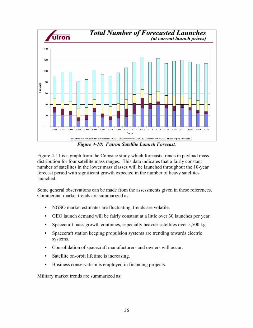
Figure 4-10: Futron Satellite Launch Forecast. Figure 4-11 is a graph from the Comstac study which forecasts trends in payload mass distribution for four satellite mass ranges. This data indicates that a fairly constant number of satellites in the lower mass classes will be launched throughout the 10-year forecast period with significant growth expected in the number of heavy satellites launched. Some general observations can be made from the assessments given in these references. Commercial market trends are summarized as:
• NGSO market estimates are fluctuating, trends are volatile.
• GEO launch demand will be fairly constant at a little over 30 launches per year.
• Spacecraft mass growth continues, especially heavier satellites over 5,500 kg.
• Spacecraft station keeping propulsion systems are trending towards electric systems.
• Consolidation of spacecraft manufacturers and owners will occur.
• Satellite on-orbit lifetime is increasing.
• Business conservatism is employed in financing projects. Military market trends are summarized as:
26
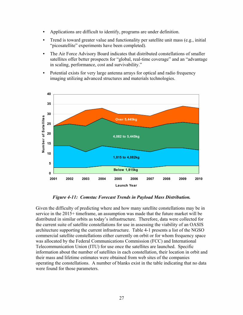
• Applications are difficult to identify, programs are under definition.
• Trend is toward greater value and functionality per satellite unit mass (e.g., initial “picosatellite” experiments have been completed).
• The Air Force Advisory Board indicates that distributed constellations of smaller satellites offer better prospects for “global, real-time coverage” and an “advantage in scaling, performance, cost and survivability.”
• Potential exists for very large antenna arrays for optical and radio frequency imaging utilizing advanced structures and materials technologies.
Below 1,815kg
1,815 to 4,082kg
4,082 to 5,445kg
Over 5,445kg
0
5
10
15
20
25
30
35
40
2001 2002 2003 2004 2005 2006 2007 2008 2009 2010
Launch Year
Num
ber
of S
atel
lites
Figure 4-11: Comstac Forecast Trends in Payload Mass Distribution.
Given the difficulty of predicting where and how many satellite constellations may be in service in the 2015+ timeframe, an assumption was made that the future market will be distributed in similar orbits as today’s infrastructure. Therefore, data were collected for the current suite of satellite constellations for use in assessing the viability of an OASIS architecture supporting the current infrastructure. Table 4-1 presents a list of the NGSO commercial satellite constellations either currently on orbit or for whom frequency space was allocated by the Federal Communications Commission (FCC) and International Telecommunication Union (ITU) for use once the satellites are launched. Specific information about the number of satellites in each constellation, their location in orbit and their mass and lifetime estimates were obtained from web sites of the companies operating the constellations. A number of blanks exist in the table indicating that no data were found for those parameters.
27
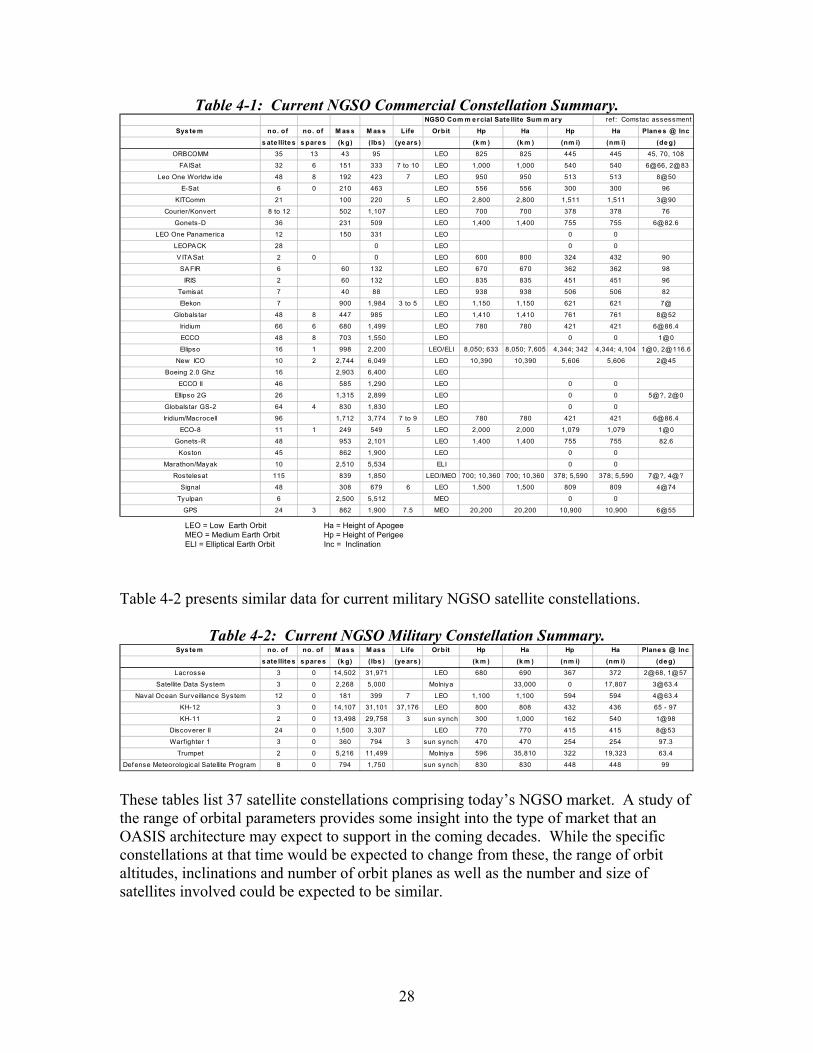
Table 4-1: Current NGSO Commercial Constellation Summary.
LEO = Low Earth OrbitMEO = Medium Earth OrbitELI = Elliptical Earth Orbit
Ha = Height of ApogeeHp = Height of PerigeeInc = Inclination
NGSO Com m e rcial Sate llite Sum m ary ref : Comstac assessment
Sys te m no. of no. of M as s M as s Life Orbit Hp Ha Hp Ha Plane s @ Incs ate llite s s pare s (k g) (lbs ) (ye ars ) (k m ) (k m ) (nm i) (nm i) (de g)
ORBCOMM 35 13 43 95 LEO 825 825 445 445 45, 70, 108
FA ISat 32 6 151 333 7 to 10 LEO 1,000 1,000 540 540 6@66, 2@83
Leo One Worldw ide 48 8 192 423 7 LEO 950 950 513 513 8@50
E-Sat 6 0 210 463 LEO 556 556 300 300 96
KITComm 21 100 220 5 LEO 2,800 2,800 1,511 1,511 3@90
Courier/Konvert 8 to 12 502 1,107 LEO 700 700 378 378 76
Gonets-D 36 231 509 LEO 1,400 1,400 755 755 [email protected]
LEO One Panamerica 12 150 331 LEO 0 0
LEOPA CK 28 0 LEO 0 0
V ITA Sat 2 0 0 LEO 600 800 324 432 90
SA FIR 6 60 132 LEO 670 670 362 362 98
IRIS 2 60 132 LEO 835 835 451 451 96
Temisat 7 40 88 LEO 938 938 506 506 82
Elekon 7 900 1,984 3 to 5 LEO 1,150 1,150 621 621 7@
Globals tar 48 8 447 985 LEO 1,410 1,410 761 761 8@52
Iridium 66 6 680 1,499 LEO 780 780 421 421 [email protected]
ECCO 48 8 703 1,550 LEO 0 0 1@0
Ellipso 16 1 998 2,200 LEO/ELI 8,050; 633 8,050; 7,605 4,344; 342 4,344; 4,104 1@0, [email protected]
New ICO 10 2 2,744 6,049 LEO 10,390 10,390 5,606 5,606 2@45
Boeing 2.0 Ghz 16 2,903 6,400 LEO
ECCO II 46 585 1,290 LEO 0 0
Ellipso 2G 26 1,315 2,899 LEO 0 0 5@?, 2@0
Globals tar GS-2 64 4 830 1,830 LEO 0 0
Iridium/Macrocell 96 1,712 3,774 7 to 9 LEO 780 780 421 421 [email protected]
ECO-8 11 1 249 549 5 LEO 2,000 2,000 1,079 1,079 1@0
Gonets-R 48 953 2,101 LEO 1,400 1,400 755 755 82.6
Koston 45 862 1,900 LEO 0 0
Marathon/Mayak 10 2,510 5,534 ELI 0 0
Rostelesat 115 839 1,850 LEO/MEO 700; 10,360 700; 10,360 378; 5,590 378; 5,590 7@?, 4@?
Signal 48 308 679 6 LEO 1,500 1,500 809 809 4@74
Tyulpan 6 2,500 5,512 MEO 0 0
GPS 24 3 862 1,900 7.5 MEO 20,200 20,200 10,900 10,900 6@55
Table 4-2 presents similar data for current military NGSO satellite constellations.
Table 4-2: Current NGSO Military Constellation Summary. Sys te m no. of no. of M as s M as s Life Orbit Hp Ha Hp Ha Plane s @ Inc
s ate llite s s pare s (k g) (lbs ) (ye ars ) (k m ) (k m ) (nm i) (nm i) (de g)Lacrosse 3 0 14,502 31,971 LEO 680 690 367 372 2@68, 1@57
Satellite Data System 3 0 2,268 5,000 Molniya 33,000 0 17,807 [email protected]
Naval Ocean Surveillance System 12 0 181 399 7 LEO 1,100 1,100 594 594 [email protected]
KH-12 3 0 14,107 31,101 37,176 LEO 800 808 432 436 65 - 97
KH-11 2 0 13,498 29,758 3 sun synch 300 1,000 162 540 1@98
Discoverer II 24 0 1,500 3,307 LEO 770 770 415 415 8@53
Warf ighter 1 3 0 360 794 3 sun synch 470 470 254 254 97.3
Trumpet 2 0 5,216 11,499 Molniya 596 35,810 322 19,323 63.4
Defense Meteorological Satellite Program 8 0 794 1,750 sun synch 830 830 448 448 99 These tables list 37 satellite constellations comprising today’s NGSO market. A study of the range of orbital parameters provides some insight into the type of market that an OASIS architecture may expect to support in the coming decades. While the specific constellations at that time would be expected to change from these, the range of orbit altitudes, inclinations and number of orbit planes as well as the number and size of satellites involved could be expected to be similar.
28

Orbit parameters in the tables range as follows:
• Altitude ranges from 556 to 2,800 km with a few exceptions. The Global Positioning System (GPS) is at half geosynchronous altitude of 20,200 km. New ICO and Rostelesat are located at quarter geosynchronous altitude of 10,390 and 10,360 km, respectively. There are three highly elliptical orbit (Molniya type) constellations.
• Inclination ranges from 45 to 117 degrees. There are three constellations in equatorial (0º inclination) low-Earth orbits—two Brazilian constellations (ECCO and ECO-8), and the Concordia orbit of the Ellipso constellation.
• Orbit planes vary from 1 to 8 with varying numbers of satellites in each orbit plane with planes equally spaced in right ascension.
There are 27 commercial and military constellations for which a complete set of orbital parameters was available with which to conduct a detailed HPM traffic model analysis. GEO satellites are placed in an equatorial orbit at an altitude (35,810 km) that results in the satellite orbit period exactly matching the rotation rate of the Earth. This location allows the satellite to appear to remain over the same location on the Earth facilitating stationary line-of-sight telecommunications. Figure 4-12 shows the distribution of the current suite of 279 GEO satellites. Multiple satellites located within one degree in longitude of each other are shown offset by 2 degree latitude increments for display purposes. The figure indicates that GEO satellites are fairly uniformly distributed in longitude around the Earth. There is some clustering of satellites at the longitudes providing services to the most populous locations around the globe. Specifically, clusters appear near the middle of North America, middle of Europe, India, and the Far East. A gap in coverage can be seen in the mid-Pacific Ocean region.
Figure 4-12: Current Distribution of GEO Satellites.
29
Significant clustering of GEO satellites may have indicated optimal locations to pre-position HPM elements for servicing missions. The nearly uniform distribution seen in the figure tends to obviate that goal, however. 4.2.4.2 OASIS Commercial Mission Scenarios An on-orbit reusable propellant depot could perform a number of missions to support commercial and military orbital assets in the future. Some of these missions are not practical with today’s aerospace infrastructure. This section discusses potential usage of the OASIS elements and illustrates specific scenarios for each mission. The HPM when combined with a propulsion module such as a CTM is envisioned to be used as an upper stage to augment the launch capability of a low cost RLV or ELV that would only provide access to LEO (altitude < 400 km). One potential mission is the deployment of a satellite to its final orbital position. Figure 4-13 illustrates the deployment scenario. With HPMs paired with CTMs and pre-positioned in storage orbits, mission planners would select the HPM/CTM closest to the final orbit position of a payload for use on this mission. Prior to launching the satellite, one or more ELVs would launch LH2 and LOX propellants into LEO. The HPM/CTM (or perhaps CTM only) would rendezvous and dock with the propellant delivery stage and transfer the propellants into the HPM. The satellite would then be launched on another ELV or RLV to LEO. The HPM/CTM would rendezvous and dock with the satellite and use CTM propulsion to move the combined stack to the final deployment orbit position and release the satellite. It may be possible to deliver more than one satellite per mission with the HPM/CTM maneuvering to release each satellite at the correct true anomaly. Following deployment, the HPM/CTM would perform the necessary engine burns to return to the parking orbit to await the next mission. The figure illustrates a satellite delivery to a final orbit requiring no additional propellant usage for maneuvering by the satellite to complete the delivery. For satellites destined for orbits requiring velocity increments (∆V’s) greater than the velocity capability of the HPM/CTM, the system could be used to transfer the satellite(s) from LEO into a transfer orbit (e.g., geosynchronous transfer orbit (GTO)) as is frequently done by the present day launch industry. The scenario would be the same; however, the satellite would be required to carry a propulsion system such as an apogee kick motor with enough propellant to complete delivery to the final orbit position.
30
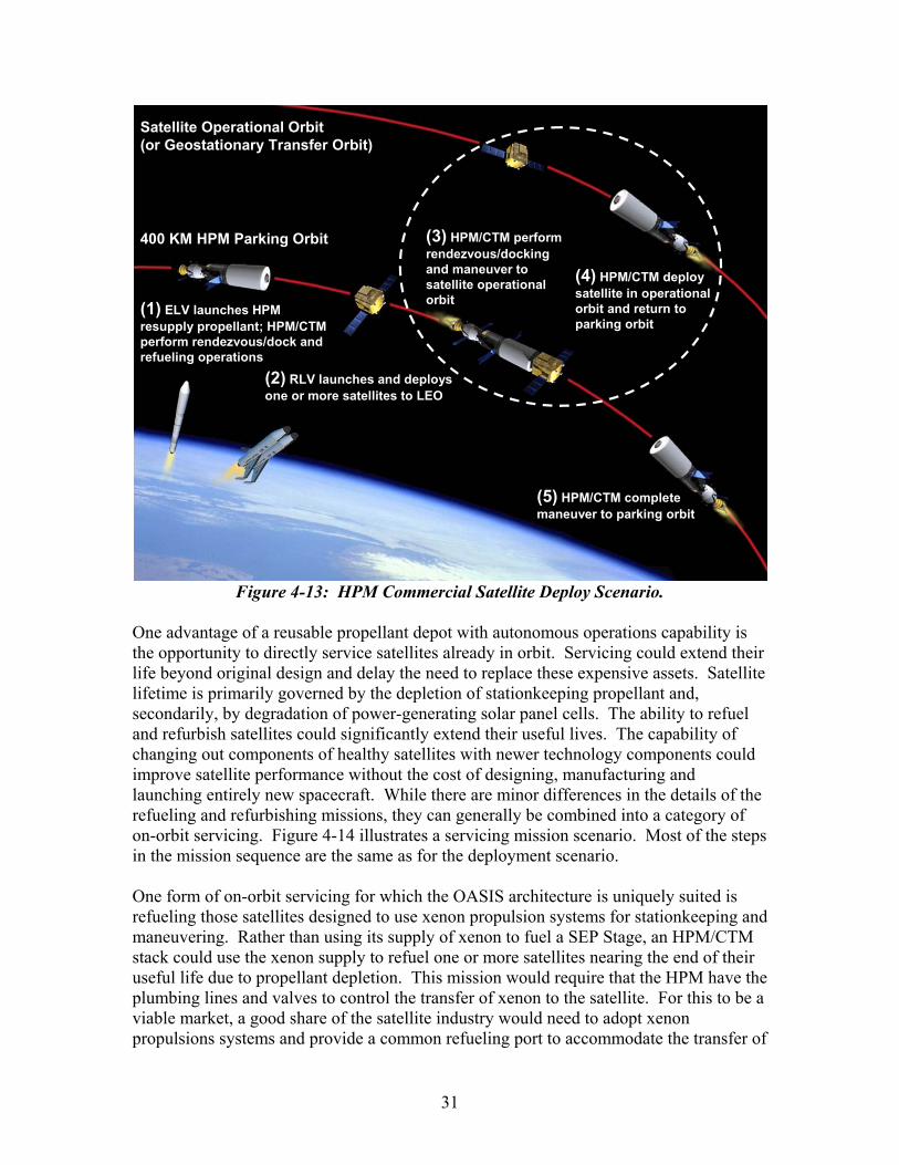
400 KM HPM Parking Orbit
Satellite Operational Orbit (or Geostationary Transfer Orbit)
(1) ELV launches HPM resupply propellant; HPM/CTM perform rendezvous/dock and refueling operations
(2) RLV launches and deploys one or more satellites to LEO
(3) HPM/CTM perform rendezvous/docking and maneuver to satellite operational orbit
(4) HPM/CTM deploy satellite in operational orbit and return to parking orbit
(5) HPM/CTM complete maneuver to parking orbit
Figure 4-13: HPM Commercial Satellite Deploy Scenario.
One advantage of a reusable propellant depot with autonomous operations capability is the opportunity to directly service satellites already in orbit. Servicing could extend their life beyond original design and delay the need to replace these expensive assets. Satellite lifetime is primarily governed by the depletion of stationkeeping propellant and, secondarily, by degradation of power-generating solar panel cells. The ability to refuel and refurbish satellites could significantly extend their useful lives. The capability of changing out components of healthy satellites with newer technology components could improve satellite performance without the cost of designing, manufacturing and launching entirely new spacecraft. While there are minor differences in the details of the refueling and refurbishing missions, they can generally be combined into a category of on-orbit servicing. Figure 4-14 illustrates a servicing mission scenario. Most of the steps in the mission sequence are the same as for the deployment scenario. One form of on-orbit servicing for which the OASIS architecture is uniquely suited is refueling those satellites designed to use xenon propulsion systems for stationkeeping and maneuvering. Rather than using its supply of xenon to fuel a SEP Stage, an HPM/CTM stack could use the xenon supply to refuel one or more satellites nearing the end of their useful life due to propellant depletion. This mission would require that the HPM have the plumbing lines and valves to control the transfer of xenon to the satellite. For this to be a viable market, a good share of the satellite industry would need to adopt xenon propulsions systems and provide a common refueling port to accommodate the transfer of
31

400 KM HPM Parking Orbit
Satellite Operational Orbit
(1) ELV launches HPM resupply propellant; HPM/CTM perform rendezvous/dock and refueling operations (2) RLV or ELV launches
and deploys to LEO satellite propellant and/or refurbish components
(3) HPM/CTM perform LEO rendezvous/docking and maneuver to satellite operational orbit
(4) HPM/CTM refuel and/or refurbish satellite and return to parking orbit
(5) HPM/CTM complete maneuver to parking orbit
Figure 4-14: HPM Commercial Satellite Servicing Scenario.
fuel. The refurbishment mission would be conducted in the same manner; however, the HPM/CTM stack would require the capability of removing old components and installing the replacements. This may be accomplished by formation flying in close proximity to the satellite or by docking with the satellite. In either case, a robotic arm controlled either remotely by ground controller or autonomously would be required to accomplish the mission. Hence, HPM subsystems in addition to those required for the exploration missions may need to be designed and developed to support the variety of potential commercial missions. Additional commercial missions for which the HPM would be suited include rescue and subsequent retrieval or deployment in correct final or transfer orbits. Removal of older satellites into disposal orbits or possibly even self-destructive reentry orbits may be a possible commercial application for OASIS elements. Details of each of these scenarios would differ slightly from those discussed above but the major scenario steps would be similar in all of these missions. See Section 4.3 for a discussion of potential military applications for OASIS elements.
32
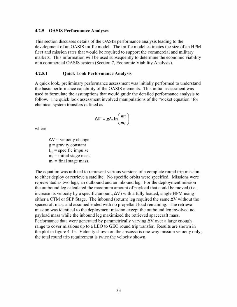
4.2.5 OASIS Performance Analyses This section discusses details of the OASIS performance analysis leading to the development of an OASIS traffic model. The traffic model estimates the size of an HPM fleet and mission rates that would be required to support the commercial and military markets. This information will be used subsequently to determine the economic viability of a commercial OASIS system (Section 7, Economic Viability Analysis). 4.2.5.1 Quick Look Performance Analysis A quick look, preliminary performance assessment was initially performed to understand the basic performance capability of the OASIS elements. This initial assessment was used to formulate the assumptions that would guide the detailed performance analysis to follow. The quick look assessment involved manipulations of the “rocket equation” for chemical system transfers defined as
=∆
f
isp
mmgIV ln
where
∆V = velocity change g = gravity constant Isp = specific impulse mi = initial stage mass mf = final stage mass.
The equation was utilized to represent various versions of a complete round trip mission to either deploy or retrieve a satellite. No specific orbits were specified. Missions were represented as two legs, an outbound and an inbound leg. For the deployment mission the outbound leg calculated the maximum amount of payload that could be moved (i.e., increase its velocity by a specific amount, ∆V) with a fully loaded, single HPM using either a CTM or SEP Stage. The inbound (return) leg required the same ∆V without the spacecraft mass and assumed ended with no propellant load remaining. The retrieval mission was identical to the deployment mission except the outbound leg involved no payload mass while the inbound leg maximized the retrieved spacecraft mass. Performance data were generated by parametrically varying ∆V over a large enough range to cover missions up to a LEO to GEO round trip transfer. Results are shown in the plot in figure 4-15. Velocity shown on the abscissa is one-way mission velocity only; the total round trip requirement is twice the velocity shown.
33
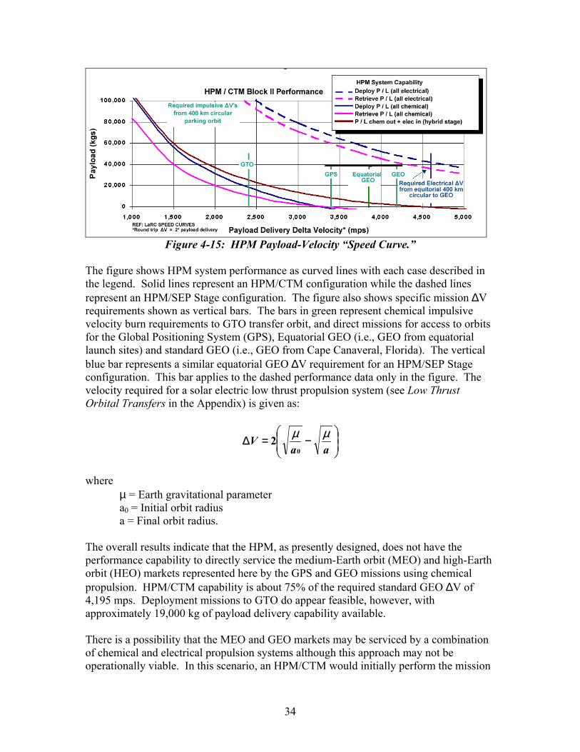
Figure 4-15: HPM Payload-Velocity “Speed Curve.”
The figure shows HPM system performance as curved lines with each case described in the legend. Solid lines represent an HPM/CTM configuration while the dashed lines represent an HPM/SEP Stage configuration. The figure also shows specific mission ∆V requirements shown as vertical bars. The bars in green represent chemical impulsive velocity burn requirements to GTO transfer orbit, and direct missions for access to orbits for the Global Positioning System (GPS), Equatorial GEO (i.e., GEO from equatorial launch sites) and standard GEO (i.e., GEO from Cape Canaveral, Florida). The vertical blue bar represents a similar equatorial GEO ∆V requirement for an HPM/SEP Stage configuration. This bar applies to the dashed performance data only in the figure. The velocity required for a solar electric low thrust propulsion system (see Low Thrust Orbital Transfers in the Appendix) is given as:
−=∆
aaV µµ
02
where µ = Earth gravitational parameter a0 = Initial orbit radius a = Final orbit radius. The overall results indicate that the HPM, as presently designed, does not have the performance capability to directly service the medium-Earth orbit (MEO) and high-Earth orbit (HEO) markets represented here by the GPS and GEO missions using chemical propulsion. HPM/CTM capability is about 75% of the required standard GEO ∆V of 4,195 mps. Deployment missions to GTO do appear feasible, however, with approximately 19,000 kg of payload delivery capability available. There is a possibility that the MEO and GEO markets may be serviced by a combination of chemical and electrical propulsion systems although this approach may not be operationally viable. In this scenario, an HPM/CTM would initially perform the mission
34

using chemical propulsion. Then a pre-positioned SEP Stage would be used to return the HPM to its parking orbit. An equatorial launch site would be required for this scenario since inclination plane changes required from northerly launch sites are difficult to accomplish with low-thrust solar electric systems (see Low Thrust Inclination Changes in the Appendix). Trip times using the SEP Stage would be quite lengthy (more than a half year round trip) which would reduce the mission rate per HPM significantly. Frequent refurbishment of SEP Stage engines and solar cells would also reduce the cost effectiveness of this mission concept. Lower velocity requirement missions such as servicing the NGSO market of satellites in LEO appear to be very feasible as payload capability increases rapidly below 3,000 mps. Figure 4-16 shows a detailed view of the initial payload velocity curve with the masses of a number of LEO satellites overlaid as horizontal bars on the plot.
Figure 4-16: HPM Performance vs. Representative Spacecraft.
Selected satellites representing the range of current satellite masses from tables 5-1 and 5-2 are shown. Most constellations consist of satellites under 3,000 kg and are bounded by the Iridium and New ICO data in this figure. Trumpet represents a larger class of military satellite with the KH-11 and KH-12 Keyhole military satellites representing the upper range of LEO satellite masses. Subsequent detailed performance analyses are based on the chemical payload delivery mission as representing the most stressing HPM mission. Refueling and other mission types are subsets of the delivery mission with respect to performance requirements. The delivery mission corresponds to the solid blue curves in the payload velocity figures. 4.2.5.2 Orbit Transfer Definitions In order to deliver satellites from a LEO parking orbit to their final destination orbits, the HPM/CTM will need to perform a series of maneuvers through three orbital dimensions. Figure 4-17 presents a diagram defining orbital volume terminology and explaining the maneuver sequence.
35
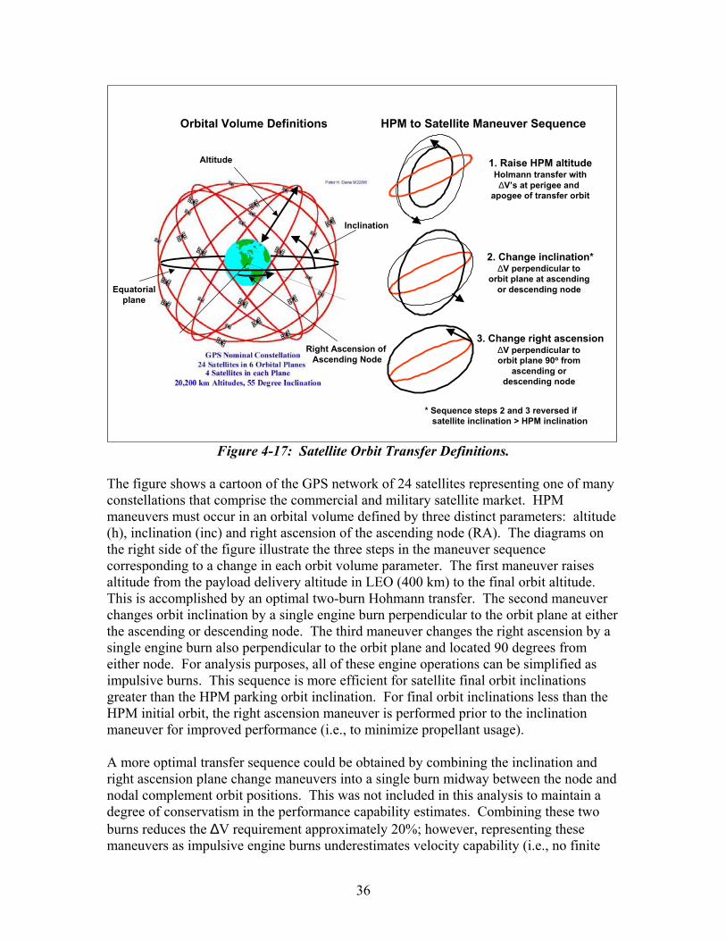
Altitude
Right Ascension of Ascending Node
Equatorialplane
1. Raise HPM altitudeHolmann transfer with∆V’s at perigee and
apogee of transfer orbit
2. Change inclination*∆V perpendicular to
orbit plane at ascending or descending node
3. Change right ascension∆V perpendicular to orbit plane 90o from
ascending or descending node
Orbital Volume Definitions HPM to Satellite Maneuver Sequence
* Sequence steps 2 and 3 reversed if satellite inclination > HPM inclination
Inclination
Figure 4-17: Satellite Orbit Transfer Definitions.
The figure shows a cartoon of the GPS network of 24 satellites representing one of many constellations that comprise the commercial and military satellite market. HPM maneuvers must occur in an orbital volume defined by three distinct parameters: altitude (h), inclination (inc) and right ascension of the ascending node (RA). The diagrams on the right side of the figure illustrate the three steps in the maneuver sequence corresponding to a change in each orbit volume parameter. The first maneuver raises altitude from the payload delivery altitude in LEO (400 km) to the final orbit altitude. This is accomplished by an optimal two-burn Hohmann transfer. The second maneuver changes orbit inclination by a single engine burn perpendicular to the orbit plane at either the ascending or descending node. The third maneuver changes the right ascension by a single engine burn also perpendicular to the orbit plane and located 90 degrees from either node. For analysis purposes, all of these engine operations can be simplified as impulsive burns. This sequence is more efficient for satellite final orbit inclinations greater than the HPM parking orbit inclination. For final orbit inclinations less than the HPM initial orbit, the right ascension maneuver is performed prior to the inclination maneuver for improved performance (i.e., to minimize propellant usage). A more optimal transfer sequence could be obtained by combining the inclination and right ascension plane change maneuvers into a single burn midway between the node and nodal complement orbit positions. This was not included in this analysis to maintain a degree of conservatism in the performance capability estimates. Combining these two burns reduces the ∆V requirement approximately 20%; however, representing these maneuvers as impulsive engine burns underestimates velocity capability (i.e., no finite
36

burn velocity losses) by as much as 5 to 10%. Therefore, the three separate maneuver steps were retained as a conservative compromise. 4.2.5.3 Analysis Assumptions Following the analysis of the current commercial and military satellite markets and having completed a quick look at the performance capability of the HPM and propulsive elements, a number of detailed assumptions may now be made. The following are major considerations affecting the performance analysis and the assumptions made for each. Some of these assumptions are considered fairly conservative while others are not. It is believed that the combined effect of these assumptions will produce a reasonable estimate of HPM performance for traffic model development and economic viability assessment. Market. Future NGSO constellations will exist in similar orbits as current constellations. With the estimate volatility seen in recent studies conducted for the Government, obtaining an accurate prediction of constellation number, size and location in the 2015+ timeframe is not possible. Current constellations, however, cover a wide range of orbital volume such that if the OASIS elements could be shown to be able to service today’s commercial market, there is a high likelihood that OASIS elements will be capable of servicing any future market. Issues that affect this assumption are possible growth in satellite mass that would reduce HPM deployment performance capability and increases in nominal satellite lifetime or a reduction in the number of NGSO constellations that could reduce mission rates to below acceptable levels necessary for economic viability. Launch Vehicle. Delivers payloads to 400 km circular parking orbits at the inclination and right ascension of stored HPM/CTM elements closest to the final orbit. With NGSO constellations occupying a wide range of orbital volume, there will need to be a network of HPM/CTM elements deployed into parking orbits to service this market. Mission planners would select the HPM closest to the final target satellite orbit to minimize performance requirements. The payload delivery orbit altitude of 400 km corresponds to the altitude used by the HPM team for sizing the NASA Earth-Moon L1 mission. HPM/CTM. Chemical engine applies ∆V impulsively at locally optimal locations. The justification for making this assumption is described above in association with figure 4-17. There may actually be additional altitude change maneuvers via Hohmann transfer over those shown in the figure to move the HPM/CTM down from a storage orbit to the payload delivery orbit. The mission would end, though, at this storage orbit such that the total ∆V required would be the same as for the maneuvers described in the figure.
37
A propellant reserve provides a 150 mps velocity reserve for maneuvers (e.g., rendezvous, proximity operations and docking, re-boost in storage orbits, etc). All performance analyses herein assume that nearly all of the HPM cryogenic propellant is consumed in conducting the three maneuvers described in figure 4-17. The 150 mps velocity reserve provides a small allocation of propellant withheld from the HPM capacity with no additional propellant provided in the CTM to permit rendezvous maneuvers, occasional re-boost and for maneuvers associated with refueling the HPM. This estimate is not based on a detailed analysis and may be insufficiently small. The CTM may operate as a standalone vehicle with its own propellant supply to conduct standalone operations or to obtain propellant to refuel the HPM. It is assumed that this propellant is exhausted prior to conducting the HPM/CTM mission. HPM/SEP Stage. The SEP Stage is not considered in these analyses due to mission duration impact and refurbishment costs. As discussed above, low thrust systems such as solar electric propulsion result in very long duration missions that would be unattractive to commercial customers who require quick response to their needs. Providing competitive response times would require larger fleets of OASIS elements resulting in increased cost and complexity. The inability of the SEP Stage to easily change orbit plane makes it an unattractive choice for GEO support missions operating from typical northern latitude launch sites. Estimated refurbishment rates (on the order of once per mission) for the SEP Stage engines and the need to replace solar array cells also add to the cost and complexity of using these elements. Satellite. Battery life is available for about two days of autonomous operation between LEO delivery, HPM docking and mission completion. In today’s launch architecture the launch service provider supplies battery power to the spacecraft while the vehicle is on the launch pad. Just prior to liftoff, spacecraft power is switched to its own internal battery. The spacecraft relies on this power until its solar panels are deployed following delivery to its final orbit location. This timeline may take some eight hours for the longest transfers to GEO. With an OASIS architecture, the payload will be delivered to a parking orbit to await rendezvous and docking by the HPM/CTM. This process may take up to two days of small orbital phasing maneuvers. While a typical spacecraft will not have deployed its arrays during this sequence, some power will be generated through the non-deployed arrays. Therefore, the assumption that a spacecraft can survive on battery power for two days before final deployment is considered to be valid. 4.2.5.4 Non-Geostationary Orbit Support. This section discusses details of the OASIS performance analysis of the NGSO commercial and military market. The assumption guiding this analysis is that the market in the post-2015 time period will be based on the current suite of commercial and military
38
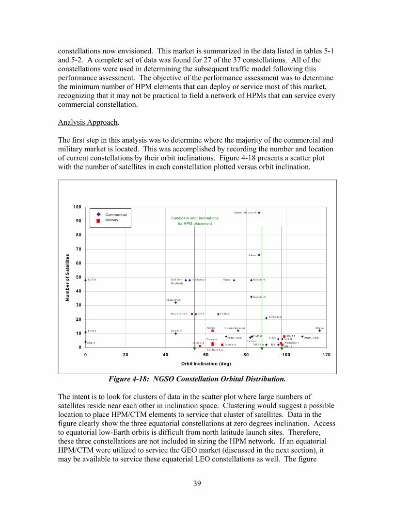
constellations now envisioned. This market is summarized in the data listed in tables 5-1 and 5-2. A complete set of data was found for 27 of the 37 constellations. All of the constellations were used in determining the subsequent traffic model following this performance assessment. The objective of the performance assessment was to determine the minimum number of HPM elements that can deploy or service most of this market, recognizing that it may not be practical to field a network of HPMs that can service every commercial constellation. Analysis Approach. The first step in this analysis was to determine where the majority of the commercial and military market is located. This was accomplished by recording the number and location of current constellations by their orbit inclinations. Figure 4-18 presents a scatter plot with the number of satellites in each constellation plotted versus orbit inclination.
Number of Satellites per Orbit Inclination
0
10
20
30
40
50
60
70
80
90
100
0 20 40 60 80 100 120
Orbit Inclination (deg)
Num
ber o
f Sat
ellit
es
CommercialMilitary
GP S
Glo ba ls ta rLEO O neWo rldwide
O R B C O M M
E C C O
EC O-8
Ellips o
S igna l
Iridium /M a c ro c e ll
Iridium
Go ne ts -R
Go ne ts -D
F AIS a tDis c o ve re r IIKIT C o m m
Ne w IC ON OS S C o urie r/Ko nve rt
La c ro s s eLa c ro s s e
O R B C o m mTrum pe t
S a t Da ta S ys
F AIS a t
Te m is a tVITA S a t
E -S a t
IR IS
DM S P
Wa rfighte r 1KH-11
OR B C o m m
E llips o
S AF IR
Candidate orbit inclinationsfor HPM placement
Figure 4-18: NGSO Constellation Orbital Distribution. The intent is to look for clusters of data in the scatter plot where large numbers of satellites reside near each other in inclination space. Clustering would suggest a possible location to place HPM/CTM elements to service that cluster of satellites. Data in the figure clearly show the three equatorial constellations at zero degrees inclination. Access to equatorial low-Earth orbits is difficult from north latitude launch sites. Therefore, these three constellations are not included in sizing the HPM network. If an equatorial HPM/CTM were utilized to service the GEO market (discussed in the next section), it may be available to service these equatorial LEO constellations as well. The figure
39
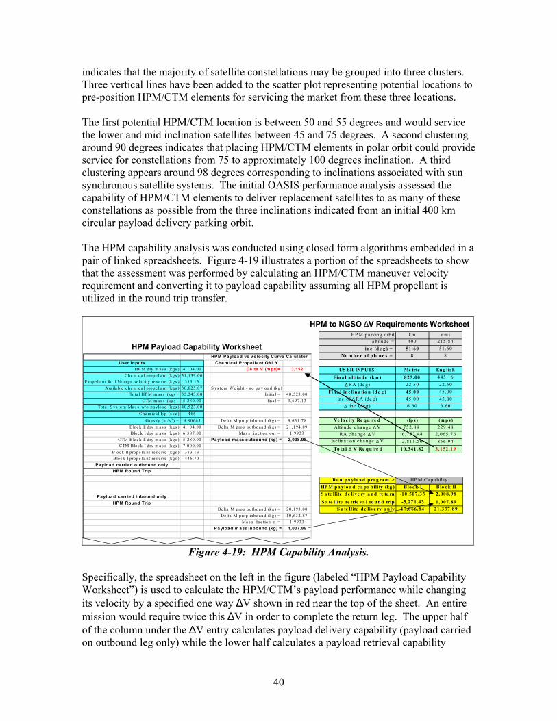
indicates that the majority of satellite constellations may be grouped into three clusters. Three vertical lines have been added to the scatter plot representing potential locations to pre-position HPM/CTM elements for servicing the market from these three locations. The first potential HPM/CTM location is between 50 and 55 degrees and would service the lower and mid inclination satellites between 45 and 75 degrees. A second clustering around 90 degrees indicates that placing HPM/CTM elements in polar orbit could provide service for constellations from 75 to approximately 100 degrees inclination. A third clustering appears around 98 degrees corresponding to inclinations associated with sun synchronous satellite systems. The initial OASIS performance analysis assessed the capability of HPM/CTM elements to deliver replacement satellites to as many of these constellations as possible from the three inclinations indicated from an initial 400 km circular payload delivery parking orbit. The HPM capability analysis was conducted using closed form algorithms embedded in a pair of linked spreadsheets. Figure 4-19 illustrates a portion of the spreadsheets to show that the assessment was performed by calculating an HPM/CTM maneuver velocity requirement and converting it to payload capability assuming all HPM propellant is utilized in the round trip transfer.
HPM Payloa d vs Ve locity Curve Ca lula torUser Inputs Chem ica l Prope lla nt ONLY
HP M dry m a s s (kgs ) 4,104.00Che m ic a l prope lla nt (kgs ) 31,139.00
P rope lla nt for 150 m ps ve loc ity re s e rve (kgs ) 313.13Ava ila ble c he m ic a l prope lla nt (kgs ) 30,825.87 S ys te m W e ight - no pa yloa d (kg)
Tota l HP M m a s s (kgs ) 35,243.00 Initia l = 40,523.00CTM m a s s (kgs ) 5 ,280.00 fina l = 9 ,697.13
Tota l S ys te m Ma s s w/o pa yloa d (kgs ) 40,523.00Che m ic a l Is p (s e c ) 466
G ra vity (m /s 2) = 9.80665 De lta M prop inbound (kg) = 9 ,631.78Bloc k II dry m a s s (kgs ) 4,104.00 De lta M prop outbound (kg) = 21,194.09Bloc k I dry m a s s (kgs ) 6,387.00 Ma s s fra c tion out = 1.9933
CTM Bloc k II dry m a s s (kgs ) 5,280.00 Payloa d m ass outbound (kg) = 2,008.98CTM Bloc k I dry m a s s (kgs ) 7,000.00
Bloc k II prope lla nt re s e rve (kgs ) 313.13 Bloc k I prope lla nt re s e rve (kgs ) 446.70
Payload carrie d outbound onlyHPM Round Trip
Payload ca rried inbound onlyHPM Round Trip
De lta M prop outbound (kg) = 20,193.00De lta M prop inbound (kg) = 10,632.87
Ma s s fra c tion in = 1.9933Pa yload m ass inbound (kg) = 1,007.89
Ru n p a ylo a d p ro g ra m > HP M p a ylo a d c a p a b ility (kg ) Blo c k I Blo c k IIS a te llite d e live ry a n d re tu rn -10,507.33 2,008.98S a te llite re trie va l ro u n d trip -5,271.43 1,007.89
S a te llite d e live ry o n ly 17,066.84 21,337.89
HP M Ca pa bility
HP M pa rking orbit km nm ia ltitude = 400 215.84
in c (d e g ) = 51.60 51.60Nu m b e r o f p la n e s = 8 8
US ER INP UTS Me tric En g lishFin a l a ltitu d e (km ) 825.00 445.16
∆ RA (de g) 22.50 22.50Fin a l in c lin a tio n (d e g ) 45.00 45.00
Inc of ∆ RA (de g) 45.00 45.00∆ inc (de g) 6.60 6.60
Ve lo c ity Re q u ire d (fp s) (m p s )Altitude c ha nge ∆ V 752.89 229.48
RA c ha nge ∆ V 6,777.44 2,065.76Inc lina tion c ha nge ∆ V 2,811.50 856.94 To ta l ∆ V Re q u ire d 10,341.82
HPM to NGSO ∆V Requirements Worksheet
HPM Payload Capability Worksheet
Delta V (m ps)= 3,152
3,152.19
Figure 4-19: HPM Capability Analysis. Specifically, the spreadsheet on the left in the figure (labeled “HPM Payload Capability Worksheet”) is used to calculate the HPM/CTM’s payload performance while changing its velocity by a specified one way ∆V shown in red near the top of the sheet. An entire mission would require twice this ∆V in order to complete the return leg. The upper half of the column under the ∆V entry calculates payload delivery capability (payload carried on outbound leg only) while the lower half calculates a payload retrieval capability
40

(payload carried on inbound leg only—not used for formal performance assessment). The entries in the leftmost column under the blue shaded region capture the basic HPM and CTM design parameters needed for the analysis. The spreadsheet on the right in the figure (labeled “HPM to NGSO ∆V Requirements Worksheet”) is used to calculate the ∆V requirement needed to perform a round trip maneuver from the payload delivery (or parking) orbit to the satellite’s final destination orbit and return. The portion shaded in gray at the top of the worksheet defines the HPM parking orbit conditions. Entries in bold are variables in the analysis; the parking orbit is fixed at 400 km circular. The two variable entries are parking orbit inclination and the number of orbit planes allocated to the HPM/CTM network. There will be one HPM and one CTM located in each orbit plane with all planes equally spaced in right ascension of the ascending node. Hence, an eight orbit plane network would consist of eight HPMs and eight CTMs with each pair spaced 45 degrees apart in right ascension and all oriented at the same inclination (see figure 4-17 for a similar layout of the GPS constellation). The blue shaded region of this worksheet represents the satellite’s destination orbital parameters. Altitude and inclination are the two variable inputs and are taken from the data in tables 5-1 and 5-2 for each constellation being evaluated. The required one-way plane change in right ascension is assumed to be half the spacing between adjacent HPM planes. This is based on the assumption that the “worst case” transfer (i.e., most stressing in performance) would occur when the satellite delivery orbit is exactly half way between adjacent HPM orbit planes such that either the HPM/CTM to the right or left could be used to conduct the mission. The area shaded in green captures the individual ∆V requirements for each of the three maneuvers (∆h, ∆i, ∆RA) required to complete the payload delivery. The impulsive velocity equations for the three maneuvers are as follows. For the altitude change, a two burn Hohmann transfer is assumed with the initial and final velocity increments (∆V1 and ∆V2) computed as:
−
+
=∆ 1
122 2
1
12
1221
11
aaaa
aV µ
+
−
=∆
21
12
21
12
121
aaaV µ
where
µ = Earth gravitational parameter a1 = semi-major axis of initial orbit a2 = semi-major axis of final orbit.
41
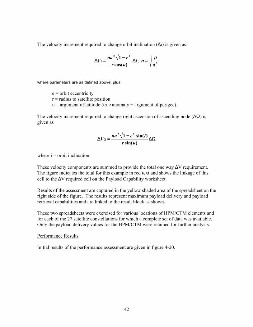
The velocity increment required to change orbit inclination (∆i) is given as:
iur
enaVi ∆−=∆)cos(
1 22
, 3an µ=
where parameters are as defined above, plus e = orbit eccentricity r = radius to satellite position u = argument of latitude (true anomaly + argument of perigee). The velocity increment required to change right ascension of ascending node (∆Ω) is given as
∆Ω−=∆ Ω)sin(
)sin(1 22
urienaV
where i = orbit inclination. These velocity components are summed to provide the total one way ∆V requirement. The figure indicates the total for this example in red text and shows the linkage of this cell to the ∆V required cell on the Payload Capability worksheet. Results of the assessment are captured in the yellow shaded area of the spreadsheet on the right side of the figure. The results represent maximum payload delivery and payload retrieval capabilities and are linked to the result block as shown. These two spreadsheets were exercised for various locations of HPM/CTM elements and for each of the 27 satellite constellations for which a complete set of data was available. Only the payload delivery values for the HPM/CTM were retained for further analysis. Performance Results. Initial results of the performance assessment are given in figure 4-20.
42

Park ing Orbit ConditionsAltitude (k m ) Inc (de g) # plane s Inc (de g) # plane s Inc (de g) # plane s
400 51.6 8 51.6 9 54 10Ne ar ISS cons te llations
Payload M as s (k g) Payload M as s (k g) Payload M as s (k g)Nam e Block I Block II Block I Block II Block I Block II
ORBCOMM (I=45) 2,009 6,339 3,865Leo One Worldw ide 10,664 5,195 16,621 2,213 13,805
Globals tar 9,615 3,850 15,349 3,482 15,002Discoverer II 11,481 6,454 17,816 13,248 24,302
Lacrosse (I=57) 16,897
Altitude (k m ) Inc (de g) # plane s Inc (de g) # plane s Inc (de g) # plane s400 90 8 88 9 90 10
Polar cons te llationsPayload M as s (k g) Payload M as s (k g) Payload M as s (k g)
Nam e Block I Block II Block I Block II Block I Block IIV ITA Sat 2,176 3,386 2,871 14,425
Iridium + Iridium/Macrocell 4,551 4,541KITComm 2,184
Altitude (k m ) Inc (de g) # plane s Inc (de g) # plane s Inc (de g) # plane s400 98 8 98 9 98 10
Sun Synchronous cons te llationsPayload M as s (k g) Payload M as s (k g) Payload M as s (k g)
Nam e Block I Block II Block I Block II Block I Block IISA FIR 3,453 9,999 4,740 16,191
Warf ighter 1 2,873 9,426 4,141 15,624DMSP 6,144 11,625IRIS 3,414 8,513
E-sat 5,143 10,609KH-11 16,513
Approach• HPM propulsively changes RA• HPM inclination and number of planes
adjusted to increase deploy/servicingcandidates
• Record cases with payloads greater thanconstellation’s satellite mass
Trends• Increasing number of planes:
– Improves Block I performance– Marginally improves number of candidate
constellations– But, adds one HPM/CTM per plane
• Adjusting inclination:– Away from ISS captures one military asset– Has minor impact for near polar constellations
Results• 14 of 27 constellations
deployable/serviceablewith 3 constellations of10 HPM/CTMs in each
-10,507 -5,788 -8,476-1,135-2,258-262
-5,486
-10,328 -8,999-7,729 -7,740
-10,315
-8,926 -1,846-9,560 -2,461
-6,000 -108-8,969 -3,443-7,085 -1,193
5,080
Figure 4-20: NGSO Analysis “Worst Case” Results. These results are considered “worst case” since all maneuvers are conducted using HPM propellant through the CTM. Results are presented in tabular blocks for each of the three initial HPM constellation locations labeled “Near ISS” for inclinations near the International Space Station inclination of 51.6 degrees, “Polar” for the 90 degree location and “Sun Synchronous” for the 98 degree location. Each block records the satellite constellations nearest each HPM/CTM location and gives the payload capability as HPM inclination and number of orbit planes are individually (manually) adjusted to increase deployment coverage. Payload mass values in green indicate payload masses that are greater than the specified mass of individual satellites in a constellation and may therefore be delivered by the HPM/CTM to that location. Mass values in red (many of
43

which are negative) are below the satellite mass indicating that the satellite could not be delivered from those HPM locations. Additional columns to the right show that constellation coverage is improved by adjusting the inclination of the HPM and/or increasing the number of orbit planes in the HPM network. Increasing the number of HPM orbit planes improves performance and marginally improves the number of candidate satellite constellations. However, it also adds one HPM/CTM per plane. Adjusting the Near ISS HPM inclination away from the ISS location captures one additional military asset while adjusting the polar inclination has only a minor impact. The general result of this portion of the analysis is that only 14 of 27 satellite constellations are serviceable using three HPM/CTM constellations with 10 HPM/CTMs in each constellation (30 vehicles total). Most of the ∆V required to complete these maneuvers is due to the assumption that the satellite delivery orbit is exactly half way between two adjacent HPM orbit planes. This represents a large propulsive plane change that is very expensive in terms of propellant usage, especially when performed at low orbit altitudes where velocities are high. An advantage can be taken, however, of the fact that, due to the Earth’s oblateness, a satellite’s orbit plane (measured by right ascension) will regress around the Earth’s polar axis. Posigrade orbits less than 90 degrees regress westerly while retrograde orbits greater than 90 degrees regress easterly. Rates of regression depend on orbit altitude and inclination but can amount to 5 degrees per day at low altitude. Since the HPM/CTMs are parked in orbits at a lower altitude and different inclination than most satellite constellations, there will be a differential nodal regression rate between the HPM orbit and each satellite orbit. If commercial customers are able to schedule their missions when the satellite and HPM/CTM orbit planes naturally align, then the propulsive ∆V requirements can be significantly reduced. The previous analysis was performed again to take advantage of this natural nodal alignment. For this assessment it was assumed that all but one degree of right ascension per leg was removed by nodal alignment. Retaining a two degree round-trip right ascension plane change is viewed as a conservative measure to account for the fact that there is a finite time period needed to perform these transfer maneuvers during which nodal regression will continue to occur at some rate. The results of this re-assessment are presented in figure 4-21. These results are considered “best case” since primarily only the altitude and inclination change maneuvers are required using HPM propellant through the CTM. The format of these results is the same as in the previous figure except that the number of HPM orbit planes is no longer a variable in the analysis. Results indicate that 24 of the 27 constellations for which data are available for analysis provide positive payload margins. Both the polar and sun synchronous oriented HPMs provide coverage for the same satellites located in their coverage areas. Therefore, these results imply that possibly only two constellations of HPM/CTM elements would be needed to deploy the majority of commercial and military satellites.
44
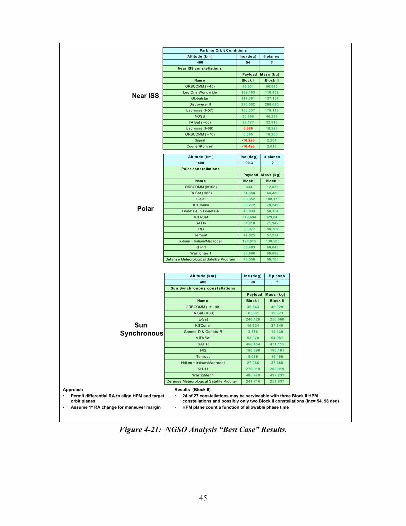
Near ISS
Altitude (k m ) Inc (de g) # plane s400 54 ?
Ne ar ISS cons te llationsPayload M as s (k g)
Nam e Block I Block IIORBCOMM (I=45) 46,631 56,845
Leo One Worldw ide 109,163 118,952Globals tar 117,361 127,137
Discoverer II 278,002 288,025Lacrosse (I=57) 168,337 178,113
NOSS 35,900 46,299FA ISat (I=66) 22,177 32,916
Lacrosse (I=68) 18,228ORBCOMM (I=70) 6,865 18,206
Signal 2,264Courier/Konvert 2,018
Park ing Orbit Conditions
Polar
Altitude (k m ) Inc (de g) # plane s400 90.3 ?
Polar cons te llationsPayload M as s (k g)
Nam e Block I Block IIORBCOMM (i=108) 334 12,039
FA ISat (I=83) 54,368 64,480E-Sat 98,352 108,170
KITComm 68,272 78,249Gonets-D & Gonets-R 40,033 50,354
V ITA Sat 319,694 329,848SA FIR 61,910 71,942
IRIS 80,877 90,769Temisat 47,025 57,234
Iridium + Iridium/Macrocell 120,815 130,585KH-11 50,483 60,643
Warf ighter 1 80,806 90,698Defense Meteorological Satellite Program 46,550 56,765
Sun Synchronous
Altitude (k m ) Inc (de g) # plane s400 98 ?
Sun Synchronous cons te llationsPayload M as s (k g)
Nam e Block I Block IIORBCOMM (i = 108) 36,543 46,929
FA ISat (I=83) 8,092 19,373E-Sat 246,128 256,060
KITComm 16,624 27,548Gonets-D & Gonets-R 2,886 14,439
V ITA Sat 53,970 64,087SA FIR 460,454 471,115
IRIS 180,390 190,181Temisat 5,066 16,499
Iridium + Iridium/Macrocell 27,066 37,668KH-11 270,918 280,919
Warf ighter 1 486,470 497,231Defense Meteorological Satellite Program 241,716 251,637
Approach• Permit differential RA to align HPM and target
orbit planes• Assume 1o RA change for maneuver margin
Results (Block II)• 24 of 27 constellations may be serviceable with three Block II HPM
constellations and possibly only two Block II constellations (inc= 54, 98 deg)• HPM plane count a function of allowable phase time
6,888
-10,228-10,498
Figure 4-21: NGSO Analysis “Best Case” Results.
45

A concern regarding reliance on differential nodal regression rates in the “best case” results presented above arises in recalling that there is no nodal regression for satellites in exactly polar orbits. While there will be small differential nodal regression rates between OASIS elements and satellite constellations near polar orbit, the phase time required to align orbit planes may be quite large resulting in an unacceptably long period between “launch” windows for commercial missions. The next step in the assessment addresses this issue.
Figure 4-22 lists the differential nodal regression rates ( ) in degrees per day for each of the commercial and military satellites and the four HPM/CTM orbit inclinations.
∗Ω∆
Nodal regression rate is calculated as
)cos(R23
2
2e2 i
anJ−=Ω
∗
where parameters are as defined in previous equations above plus J2 = spherical harmonic coefficient representing the flattening of the Earth Re = Earth’s radius. HPM system regression rates for each orbit are given in the yellow region at the top of the figure. Satellite constellation regression rates are given in the fourth column from the left. Differential rates are listed for each HPM system in the rightmost four columns. The data shaded in blue represent the rates for the most likely HPM system to be used with each satellite. The next step in the process is to use these differential nodal regression rates to determine the phase time required to align satellite and HPM orbit planes. These phase times define the frequency of payload delivery launch window openings and are a function of the number of HPM orbit planes needed to satisfy the entire market. Phase time is computed by taking half the distance between adjacent HPM planes and dividing by the differential rate, thus producing a “worst case” alignment time that assumes a satellite’s orbit plane is exactly half way between HPM planes. Figures 4-22 and 4-23 list the phase time in days required to align orbit planes for HPM/CTM element counts from two to ten equally spaced planes. Data are presented in two blocks per figure with each block representing a different HPM/CTM location. Phase times are shown in the right half of each figure. The cells shaded in blue indicate alignment times of less than 30 days. Alignment times between 30 and 60 days are shaded in brown. Unshaded entries indicate that more than 60 days would be required between launch window opportunities.
46
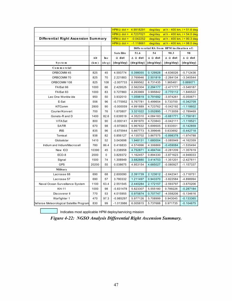
HPM Ω dot = 4.9918291 deg/day at h - 400 km, i = 51.6 degHPM Ω dot = 4.7237021 deg/day at h - 400 km, i = 54.0 degHPM Ω dot = -0.042252 deg/day at h - 400 km, i = 90.3 degHPM Ω dot = -1.118661 deg/day at h - 400 km, i = 98.0 deg
S ate llite 51.6 54 90.3 98
Alt In c Ω dot ∆ Ω dot ∆ Ω dot ∆ Ω dot ∆ Ω dotS ys te m (k m ) (d e g ) (de g/day) (de g/day) (de g/day) (de g/day) (de g/day)
Co m m e rc ial
ORBCOMM 45 825 45 4.593774 0.398055 0.129928 -4.636026 -5.712436
ORBCOMM 70 825 70 2.221883 2.769946 2.501819 -2.264134 -3.340544
ORBCOMM 108 825 108 -2.007733 6.999562 6.731435 1.965481 0.889071
FAISat 66 1000 66 2.429525 2.562304 2.294177 -2.471777 -3.548187
FAISat 83 1000 83 0.727860 4.263969 3.995842 -0.770112 -1.846522
Leo One Worldw ide 950 50 3.932010 1.059819 0.791692 -3.974261 -5.050671
E-Sat 556 96 -0.775952 5.767781 5.499654 0.733700 -0.342709
KITComm 2800 90 -0.000059 4.991889 4.723762 -0.042192 -1.118602
Courier/Konvert 700 76 1.670807 3.321022 3.052895 -1.713059 -2.789469
Gonets-R and D 1400 82.6 0.639519 4.352310 4.084183 -0.681771 -1.758181
VITASat 800 90 -0.000141 4.991970 4.723843 -0.042111 -1.118521
SAFIR 670 98 -0.975803 5.967632 5.699505 0.933551 -0.142859
IRIS 835 96 -0.675944 5.667773 5.399646 0.633692 -0.442718
Temisat 938 82 0.856127 4.135702 3.867575 -0.898378 -1.974788
Globalstar 1410 52 3.043698 1.948131 1.680004 -3.085949 -4.162359
Iridium and Iridium/Macrocell 780 86.4 0.416833 4.574996 4.306869 -0.459084 -1.535494
New ICO 10390 45 0.238958 4.752871 4.484744 -0.281209 -1.357619
ECO-8 2000 0 3.829372 1.162457 0.894330 -3.871623 -4.948033
Signal 1500 74 1.308949 3.682880 3.414753 -1.351201 -2.427611
GPS 20200 55 0.038675 4.953154 4.685027 -0.080927 -1.157337
Military
Lacrosse 68 690 68 2.600090 2.391739 2.123612 -2.642341 -3.718751
Lacrosse 57 690 57 3.780332 1.211497 0.943370 -3.822584 -4.898994
Naval Ocean Surveillance System 1100 63.4 2.551545 2.440284 2.172157 -2.593797 -3.670206
KH-11 1000 98 -0.831478 5.823307 5.555180 0.789226 -0.287184
Discoverer II 770 53 4.015955 0.975874 0.707747 -4.058206 -5.134616
Warf ighter 1 470 97.3 -0.985297 5.977126 5.708999 0.943045 -0.133365
Defense Meteorological Satellite Program 830 99 -1.013986 6.005815 5.737688 0.971735 -0.104675
Diffe re n tial RA fro m HPM in c lin atio n o f:
Differentia l Right Ascension Summary
Indicates most applicable HPM deploy/servicing mission Figure 4-22: NGSO Analysis Differential Right Ascension Summary.
47

HPM Ω dot = 4.9918291 deg/day at h - 400 km, i = 51.6 deg Phase TimeHPM Ω dot = 4.7237021 deg/day at h - 400 km, i = 54.0 deg Less than 30 days
Betw een 30 and 60 daysfor near ISS conste lla tions
Sys te m Sate llite Phas e tim e to align HPM and Sate llite r ight as ce ns ions (days )Com m e rcial Alt Inc Ω dot ∆ Ω dot Num be r of plane s
(k m ) (de g) (de g/day) (de g/day) 10 9 8 7 6 5 4 3 2
ORBCOMM 45 825 45 4.5937741 0.129928 138.54 153.93 173.17 197.91 230.90 277.08 346.35 461.79 692.69
ORBCOMM 70 825 70 2.2218827 2.501819 7.19 7.99 8.99 10.28 11.99 14.39 17.99 23.98 35.97
FA ISat 66 1000 66 2.429525 2.294177 7.85 8.72 9.81 11.21 13.08 15.69 19.61 26.15 39.23
Leo One Worldw ide 950 50 3.9320098 0.791692 22.74 25.26 28.42 32.48 37.89 45.47 56.84 75.79 113.68
Courier/Konvert 700 76 1.6708071 3.052895 5.90 6.55 7.37 8.42 9.83 11.79 14.74 19.65 29.48
Globals tar 1410 52 3.0436979 1.680004 10.71 11.90 13.39 15.31 17.86 21.43 26.79 35.71 53.57
New ICO 10390 45 0.2389579 4.484744 4.01 4.46 5.02 5.73 6.69 8.03 10.03 13.38 20.07
Signal 1500 74 1.3089491 3.414753 5.27 5.86 6.59 7.53 8.79 10.54 13.18 17.57 26.36
GPS 20200 55 0.038675 4.685027 3.84 4.27 4.80 5.49 6.40 7.68 9.61 12.81 19.21
690 68 2.6000897 2.123612 8.48 9.42 10.60 12.11 14.13 16.95 21.19 28.25 42.38
690 57 3.7803324 0.943370 19.08 21.20 23.85 27.26 31.80 38.16 47.70 63.60 95.40
1100 63.4 2.5515449 2.172157 8.29 9.21 10.36 11.84 13.81 16.57 20.72 27.62 41.43
770 53 4.0159548 0.707747 25.43 28.26 31.79 36.33 42.39 50.87 63.58 84.78 127.16
ORBCOMM 45 825 45 4.5937741 0.398055 45.22 50.24 56.52 64.60 75.37 90.44 113.05 150.73 226.10
ORBCOMM 70 825 70 2.2218827 2.769946 6.50 7.22 8.12 9.28 10.83 13.00 16.25 21.66 32.49
FA ISat 66 1000 66 2.429525 2.562304 7.02 7.81 8.78 10.04 11.71 14.05 17.56 23.42 35.12
Leo One Worldw ide 950 50 3.9320098 1.059819 16.98 18.87 21.23 24.26 28.31 33.97 42.46 56.61 84.92
Courier/Konvert 700 76 1.6708071 3.321022 5.42 6.02 6.78 7.74 9.03 10.84 13.55 18.07 27.10
Globals tar 1410 52 3.0436979 1.948131 9.24 10.27 11.55 13.20 15.40 18.48 23.10 30.80 46.20
New ICO 10390 45 0.2389579 4.752871 3.79 4.21 4.73 5.41 6.31 7.57 9.47 12.62 18.94
Signal 1500 74 1.3089491 3.682880 4.89 5.43 6.11 6.98 8.15 9.77 12.22 16.29 24.44
GPS 20200 55 0.038675 4.953154 3.63 4.04 4.54 5.19 6.06 7.27 9.09 12.11 18.17
690 68 2.6000897 2.391739 7.53 8.36 9.41 10.75 12.54 15.05 18.81 25.09 37.63
690 57 3.7803324 1.211497 14.86 16.51 18.57 21.23 24.76 29.72 37.14 49.53 74.29
1100 63.4 2.5515449 2.440284 7.38 8.20 9.22 10.54 12.29 14.75 18.44 24.59 36.88
770 53 4.0159548 0.975874 18.44 20.49 23.06 26.35 30.74 36.89 46.11 61.48 92.22
Diffe rentia l Right Ascension Ana lysis
54
M ilitary
Lacrosse 68
Lacrosse 57
Naval Ocean Surveillance System
Discoverer II
51.6
Lacrosse 68
Lacrosse 57
Naval Ocean Surveillance System
Discoverer II
Diffe re ntial RA fromHPM inclination of:
Figure 4-23: NGSO Launch Opportunities for Near ISS Constellations. Data in figure 4-22 apply to the two near-ISS HPM payload delivery locations of 54 and 51.6 degrees. Satellites with planar alignment times greater than 30 days even at larger HPM plane counts such as the ORBCOMM constellation represent “outliers” in the analysis. These represent the most difficult satellites to deploy from an HPM performance perspective. These are the cases that drive the sizing of the HPM network. Lengthy alignment times will require reliance on full propulsive maneuvers recorded in the “worst case” performance analysis to accomplish timely deployment/servicing missions. Data in figure 4-24 apply to the polar and sun synchronous HPM/CTM locations. These two blocks especially show the difficulty of relying on nodal regression to reduce propellant usage requirements. Satellites located nearly at the same inclination as the HPM/CTM such as the three military constellations and KITComm and VITASat will require unacceptably long delays for planar alignment. Missions for these constellations will require full propulsive maneuvers for timely deployment and servicing. By combining the information from the “worst case” and “best case” propulsive maneuver analyses and the planar alignment times in the above figures, a minimum HPM system allocation may be determined for each HPM/CTM constellation. A minimum of eight HPM/CTMs will be required at 54 degrees inclination to service the Near ISS satellite constellations and ten HPM/CTMs will be required in a near 90 degree inclination orbit to service the polar market. The conclusion can now be made that most of the NGSO satellite market may be serviced by a total of 18 HPM/CTM elements.
48
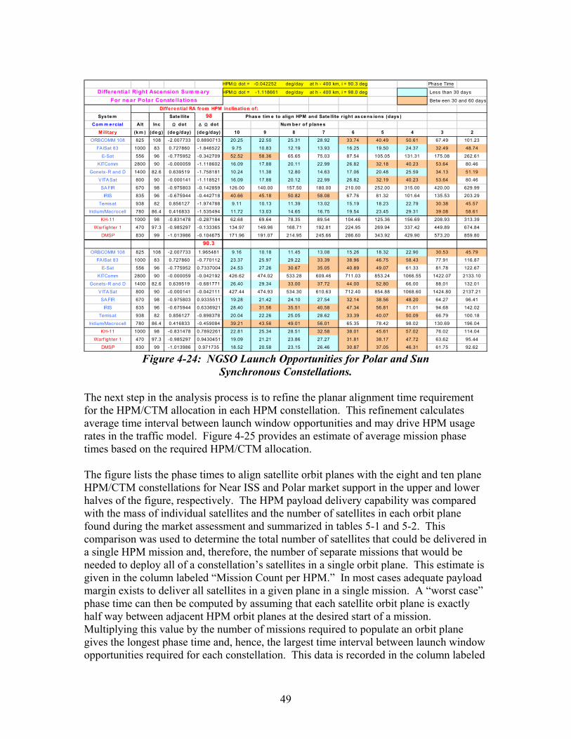
HPM Ω dot = -0.042252 deg/day at h - 400 km, i = 90.3 deg Phase Time
HPM Ω dot = -1.118661 deg/day at h - 400 km, i = 98.0 deg Less than 30 days
Betw een 30 and 60 days
Sys te m Sate llite Phas e tim e to align HPM and Sate llite r ight as ce ns ions (days )Com m e rcial Alt Inc Ω dot ∆ Ω dot Num be r of plane s
(k m ) (de g) (de g/day) (de g/day) 10 9 8 7 6 5 4 3 2ORBCOMM 108 825 108 -2.007733 0.8890713 20.25 22.50 25.31 28.92 33.74 40.49 50.61 67.49 101.23
FA ISat 83 1000 83 0.727860 -1.846522 9.75 10.83 12.19 13.93 16.25 19.50 24.37 32.49 48.74
E-Sat 556 96 -0.775952 -0.342709 52.52 58.36 65.65 75.03 87.54 105.05 131.31 175.08 262.61
KITComm 2800 90 -0.000059 -1.118602 16.09 17.88 20.11 22.99 26.82 32.18 40.23 53.64 80.46
Gonets-R and D 1400 82.6 0.639519 -1.758181 10.24 11.38 12.80 14.63 17.06 20.48 25.59 34.13 51.19
V ITA Sat 800 90 -0.000141 -1.118521 16.09 17.88 20.12 22.99 26.82 32.19 40.23 53.64 80.46
SA FIR 670 98 -0.975803 -0.142859 126.00 140.00 157.50 180.00 210.00 252.00 315.00 420.00 629.99
IRIS 835 96 -0.675944 -0.442718 40.66 45.18 50.82 58.08 67.76 81.32 101.64 135.53 203.29
Temisat 938 82 0.856127 -1.974788 9.11 10.13 11.39 13.02 15.19 18.23 22.79 30.38 45.57
Iridium/Macrocell 780 86.4 0.416833 -1.535494 11.72 13.03 14.65 16.75 19.54 23.45 29.31 39.08 58.61
1000 98 -0.831478 -0.287184 62.68 69.64 78.35 89.54 104.46 125.36 156.69 208.93 313.39
470 97.3 -0.985297 -0.133365 134.97 149.96 168.71 192.81 224.95 269.94 337.42 449.89 674.84
830 99 -1.013986 -0.104675 171.96 191.07 214.95 245.66 286.60 343.92 429.90 573.20 859.80
ORBCOMM 108 825 108 -2.007733 1.965481 9.16 10.18 11.45 13.08 15.26 18.32 22.90 30.53 45.79
FA ISat 83 1000 83 0.727860 -0.770112 23.37 25.97 29.22 33.39 38.96 46.75 58.43 77.91 116.87
E-Sat 556 96 -0.775952 0.7337004 24.53 27.26 30.67 35.05 40.89 49.07 61.33 81.78 122.67
KITComm 2800 90 -0.000059 -0.042192 426.62 474.02 533.28 609.46 711.03 853.24 1066.55 1422.07 2133.10
Gonets-R and D 1400 82.6 0.639519 -0.681771 26.40 29.34 33.00 37.72 44.00 52.80 66.00 88.01 132.01
V ITA Sat 800 90 -0.000141 -0.042111 427.44 474.93 534.30 610.63 712.40 854.88 1068.60 1424.80 2137.21
SA FIR 670 98 -0.975803 0.9335511 19.28 21.42 24.10 27.54 32.14 38.56 48.20 64.27 96.41
IRIS 835 96 -0.675944 0.6336921 28.40 31.56 35.51 40.58 47.34 56.81 71.01 94.68 142.02
Temisat 938 82 0.856127 -0.898378 20.04 22.26 25.05 28.62 33.39 40.07 50.09 66.79 100.18
Iridium/Macrocell 780 86.4 0.416833 -0.459084 39.21 43.56 49.01 56.01 65.35 78.42 98.02 130.69 196.04
1000 98 -0.831478 0.7892261 22.81 25.34 28.51 32.58 38.01 45.61 57.02 76.02 114.04
470 97.3 -0.985297 0.9430451 19.09 21.21 23.86 27.27 31.81 38.17 47.72 63.62 95.44
830 99 -1.013986 0.971735 18.52 20.58 23.15 26.46 30.87 37.05 46.31 61.75 92.62
Diffe rentia l Right Ascension Sum m aryFor near Pola r Conste lla tions
Diffe re ntial RA from HPM inclination of:98
M ilitary
KH-11
Warf ighter 1
DMSP
90.3
KH-11
Warf ighter 1
DMSP
Figure 4-24: NGSO Launch Opportunities for Polar and Sun Synchronous Constellations.
The next step in the analysis process is to refine the planar alignment time requirement for the HPM/CTM allocation in each HPM constellation. This refinement calculates average time interval between launch window opportunities and may drive HPM usage rates in the traffic model. Figure 4-25 provides an estimate of average mission phase times based on the required HPM/CTM allocation. The figure lists the phase times to align satellite orbit planes with the eight and ten plane HPM/CTM constellations for Near ISS and Polar market support in the upper and lower halves of the figure, respectively. The HPM payload delivery capability was compared with the mass of individual satellites and the number of satellites in each orbit plane found during the market assessment and summarized in tables 5-1 and 5-2. This comparison was used to determine the total number of satellites that could be delivered in a single HPM mission and, therefore, the number of separate missions that would be needed to deploy all of a constellation’s satellites in a single orbit plane. This estimate is given in the column labeled “Mission Count per HPM.” In most cases adequate payload margin exists to deliver all satellites in a given plane in a single mission. A “worst case” phase time can then be computed by assuming that each satellite orbit plane is exactly half way between adjacent HPM orbit planes at the desired start of a mission. Multiplying this value by the number of missions required to populate an orbit plane gives the longest phase time and, hence, the largest time interval between launch window opportunities required for each constellation. This data is recorded in the column labeled
49

“Worst Case Phase Time” expressed in days. Note that phase times are zeroed for cases where full propulsive maneuvers are required. Since the differences in right ascension between an HPM orbit and a satellite orbit will lie between zero degrees and the midpoint between adjacent HPM planes at the desired start of a mission, phase times will be uniformly distributed between these worst case times and no delay time. An average phase time is then determined by dividing the worst case value by two. These values are listed in the final column of data in the figure. The individual average phase times were then averaged over all the satellites in each group to determine HPM constellation averages of 4.5 and 8.4 days for the Near ISS and Polar constellations, respectively.
HPM Ω dot = -0.0422516 deg/day at h - 400 km, i = 90.3 deg Phase TimeHPM Ω dot = 4.7237021 deg/day at h - 400 km, i = 54.0 deg Les s than 30 days
Betw een 30 and 60 daysHPM Constellation Allocation
System Satellite Phas e Time (days ) Worst case AverageCommercial Alt Inc Ω dot ∆ Ω dot Number of planes Mission Count Phase Time* Phase Time*
(km) (deg) (deg/day) (deg/day) 8 per HPM (days) (days)ORBCOMM 45 825 45 4.5937741 0.129928 173.17 1 0.00 0.00ORBCOMM 70 825 70 2.2218827 2.501819 8.99 1 8.99 4.50
FAISat 66 1000 66 2.429525 2.294177 9.81 1 9.81 4.90Leo One Worldw ide 950 50 3.9320098 0.791692 28.42 1 28.42 14.21
Courier/Konvert 700 76 1.6708071 3.052895 7.37 2 14.74 7.37Globalstar 1410 52 3.0436979 1.680004 13.39 1 13.39 6.70New ICO 10390 45 0.2389579 4.484744 5.02 1 5.02 2.51
Signal 1500 74 1.3089491 3.414753 6.59 2 13.18 6.59GPS 20200 55 0.038675 4.685027 4.80 1 4.80 2.40
690 68 2.6000897 2.123612 10.60 1 10.60 5.30690 57 3.7803324 0.943370 23.85 1 23.85 11.93
1100 63.4 2.5515449 2.172157 10.36 2 20.72 10.36770 53 4.0159548 0.707747 31.79 2 0.00 0.00
17 9.03 4.52 < Total10
ORBCOMM 108 825 108 -2.0077328 1.965481 9.16 1 9.16 4.58FAISat 83 1000 83 0.7278604 -0.770112 23.37 1 23.37 11.69
E-Sat 556 96 -0.775952 0.733700 24.53 1 24.53 12.27KITComm 2800 90 -5.948E-05 -0.042192 426.62 1 0.00 0.00
Gonets-R and D 1400 82.6 0.6395194 -0.681771 26.40 5 132.01 66.00VITASat 800 90 -0.000141 -0.042111 427.44 1 0.00 0.00SAFIR 670 98 -0.9758027 0.933551 19.28 1 19.28 9.64IRIS 835 96 -0.6759437 0.633692 28.40 1 28.40 14.20
Temisat 938 82 0.8561266 -0.898378 20.04 1 20.04 10.02Iridium/Macrocell 780 86.4 0.4168327 -0.459084 39.21 3 0.00 0.00
1000 98 -0.8314776 0.789226 22.81 1 22.81 11.40470 97.3 -0.9852967 0.943045 19.09 1 19.09 9.54830 99 -1.0139862 0.971735 18.52 1 18.52 9.26
19 16.70 8.35 < Total* Phas e times greater than 30 days operate propuls ively w ith no phas ing required
Mission Count Based on "Optimal"
54
Military
Lacrosse 68Lacrosse 57
Naval Ocean Surveillance SystemDiscoverer II
90.3
KH-11Warfighter 1
DMSP
Differential RA fromHPM inclination of:
Figure 4-25: NGSO Average Mission Phase Time. Non-Geosynchronous Orbit Traffic Model. The OASIS traffic model may now be completed from the performance analysis results and from assumptions regarding average satellite operational lifetime. Only limited information was found for satellite lifetime estimates in the market assessment. Available information is recorded in tables 4-1 and 4-2. From the limited data, an upper lifetime estimate of 10 years and lower estimate of 5 years were assumed. An average satellite lifetime of 10 years would result in fewer HPM missions to replenish or refuel satellites while the 5-year estimate would require more frequent deployment and servicing missions. Averaging these limits produces a “nominal” traffic model satellite lifetime estimate of 7.5 years. Table 4-3 summarizes the OASIS nominal traffic model.
50
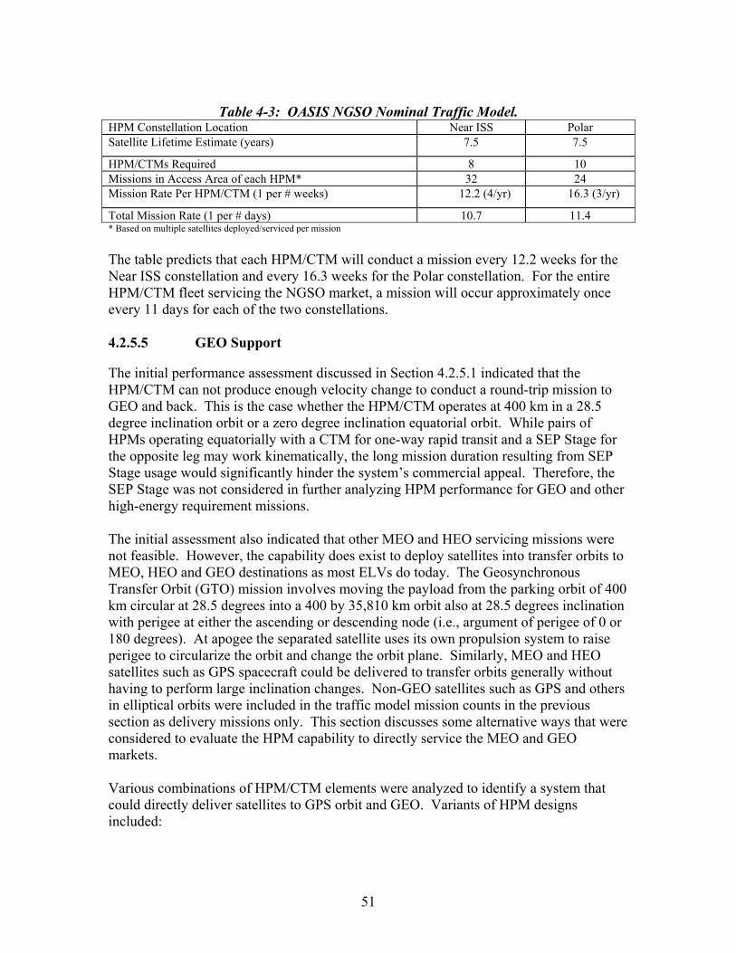
Table 4-3: OASIS NGSO Nominal Traffic Model.
HPM Constellation Location Near ISS Polar Satellite Lifetime Estimate (years) 7.5 7.5
HPM/CTMs Required 8 10 Missions in Access Area of each HPM* 32 24 Mission Rate Per HPM/CTM (1 per # weeks) 12.2 (4/yr) 16.3 (3/yr)
Total Mission Rate (1 per # days) 10.7 11.4 * Based on multiple satellites deployed/serviced per mission
The table predicts that each HPM/CTM will conduct a mission every 12.2 weeks for the Near ISS constellation and every 16.3 weeks for the Polar constellation. For the entire HPM/CTM fleet servicing the NGSO market, a mission will occur approximately once every 11 days for each of the two constellations. 4.2.5.5 GEO Support The initial performance assessment discussed in Section 4.2.5.1 indicated that the HPM/CTM can not produce enough velocity change to conduct a round-trip mission to GEO and back. This is the case whether the HPM/CTM operates at 400 km in a 28.5 degree inclination orbit or a zero degree inclination equatorial orbit. While pairs of HPMs operating equatorially with a CTM for one-way rapid transit and a SEP Stage for the opposite leg may work kinematically, the long mission duration resulting from SEP Stage usage would significantly hinder the system’s commercial appeal. Therefore, the SEP Stage was not considered in further analyzing HPM performance for GEO and other high-energy requirement missions. The initial assessment also indicated that other MEO and HEO servicing missions were not feasible. However, the capability does exist to deploy satellites into transfer orbits to MEO, HEO and GEO destinations as most ELVs do today. The Geosynchronous Transfer Orbit (GTO) mission involves moving the payload from the parking orbit of 400 km circular at 28.5 degrees into a 400 by 35,810 km orbit also at 28.5 degrees inclination with perigee at either the ascending or descending node (i.e., argument of perigee of 0 or 180 degrees). At apogee the separated satellite uses its own propulsion system to raise perigee to circularize the orbit and change the orbit plane. Similarly, MEO and HEO satellites such as GPS spacecraft could be delivered to transfer orbits generally without having to perform large inclination changes. Non-GEO satellites such as GPS and others in elliptical orbits were included in the traffic model mission counts in the previous section as delivery missions only. This section discusses some alternative ways that were considered to evaluate the HPM capability to directly service the MEO and GEO markets. Various combinations of HPM/CTM elements were analyzed to identify a system that could directly deliver satellites to GPS orbit and GEO. Variants of HPM designs included:
51

• Single―the same designs used in the preceding NGSO analysis.
• Paired―two fully loaded HPM/CTM elements operating separately outbound; one carrying the payload, the other without a payload. Following payload delivery, the two stacks (2 HPM/CTMs) dock and return as one combined stack using remaining propellant in both HPMs.
• Tandem―multiple HPMs (up to four evaluated) with one CTM, docked end-to-end with propellant crossfed from one HPM to the next.
• Paired/Tandem―two pairs of tandem HPMs each with a single CTM operating as defined above for Paired.
HPM designs were identical to those in the NGSO analysis except for the tandem HPMs where the dry weights were increased by 10 percent to account for modifications needed for the flow-through propellant feed system. Results of this analysis are presented in figure 4-25.
Mission/ ∆V*HPM configuration
GTO2,400 mps
GEO-28 deg4,200 mps
GEO-0 deg3,856 mps
GPS 51.63,429 mps
GPS transfer2,159 mps
19,376 26,610Paired 38,753 53,219Tandem
2 HPMs 50,751 10,547 64,8313 HPMs 83,231 24,052 104,1204 HPMs 115,710 37,556 143,410
Paired/Tandem2 HPMs per pair 101,503 21,094 129,661
* One way Preferred Configuration
Single -12,453 -7,941 -1,678-24,906 -15,882 -3,355
-9,267 -1,054-4,643
-18
-18,534 -2,108
Single -12,453 -7,941 -1,678-24,906 -15,882 -3,355
-9,267 -1,054-4,643
-18
-18,534 -2,108
7,19715,449
7,19715,449
Figure 4-25: GEO/GPS Performance Summary. Based on the results in the figure, the following conclusions may be summarized:
• Single HPMs are only capable of performing GTO and GPS transfer missions.
• None of the configurations studied can deliver payloads to GEO from a 28 degree inclination orbit.
• Only HPM tandem configurations have useful payload capability for either GEO (equatorial launch) or GPS (launch to 51.6 degree inclination) missions.
• The use of three or more HPMs in tandem (required for equatorial GEO) should be considered operationally problematical at best.
• Tandem HPM configurations outperform comparable Paired HPM configurations.
• The current HPM design (sized for the Earth-Moon L1 mission) is undersized in propellant for GEO missions and has inherent inefficiencies due to the extra dry weight associated with xenon propellant accommodations.
52

Based on payload delivery missions only, an HPM GEO traffic model is established requiring two HPM/CTMs delivering up to 15 payloads each to GTO per year. This allocation will satisfy the forecasted 30 GEO satellite deliveries per year. 4.2.6 Integrated Traffic Model This section compiles the results of the NGSO, GEO and OASIS exploration traffic models to form an integrated OASIS traffic model (table 4-4) and presents rationale for a “refined” OASIS traffic model.
Table 4-4: OASIS Integrated Traffic Model. NGSO Near ISS Constellation Support – 8 HPM/CTMs
• Average mission rate of 1 every 11 days <= one per 12.2 weeks for each HPM/CTM (4 per year/HPM)
• Planar launch windows every 4.5 days (average) for nodal alignment (Does not impact mission rate)
• Launches from Eastern Test Range NGSO Near Polar Constellation Support – 10 HPM/CTMs
• Average mission rate of 1 every 11 days <= one per 16.3 weeks for each HPM/CTM (3 per year/HPM)
• Planar launch windows every 8.4 days (average) for nodal alignment (Does not impact mission rate)
• Launches from Vandenburg Air Force Base GEO Constellation Support (GTO delivery) – 2 HPM/CTMs
• Average mission rate of 1 every 12 days <= 15 per year for each HPM/CTM • Launch on demand from Eastern Test Range
NASA Exploration (Lunar Gateway) Support – 7 HPMs
• 7 HPMs, 6 SEP Stages, 1-2 CTMs and CTVs • 1 lunar excursion every 6 months • Launch from Eastern Test Range
Total – 27 HPMs, 21-22 CTMs, 1-2 CTVs
The OASIS integrated traffic model requires a fleet of 20 HPM/CTM elements for commercial/military satellite support. Assuming an average satellite lifetime of 7.5 years, the fleet will conduct a combined 96 missions per year for an average of one commercial mission every 4.8 days. Table 4-5 provides a high and low traffic model estimate based on 5 and 10 year satellite lifetime extremes. This table also presents a “refined” traffic model by considering a number of key operational factors in fielding and operating such a fleet. This refined model retains only higher usage rate missions at greater than 3 per year; lesser usage reduces the economic viability of the system as discussed in the Section 7. Polar market support was excluded from the refined model due to low usage rates and because access to those orbits requires a second launch site (e.g., Vandenburg, California) with duplication of associated HPM support infrastructure. A 50 percent market share of the high traffic model was assumed and only the commercial industry support was included in this refined model.
53
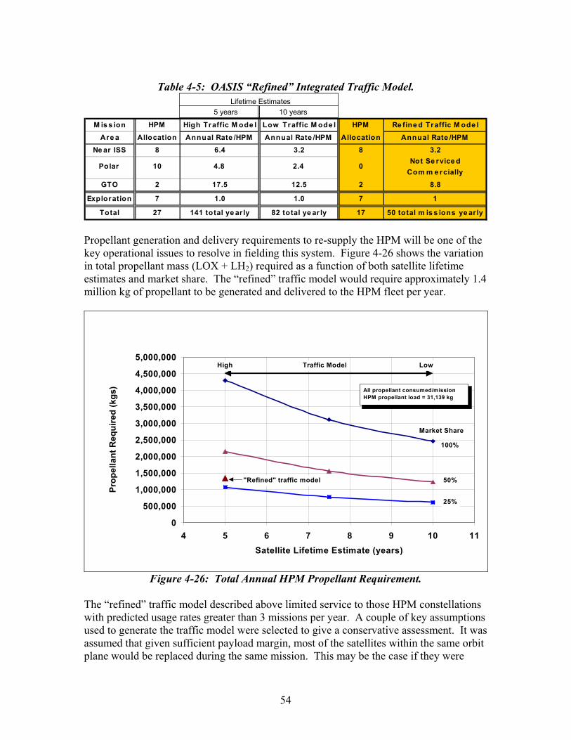
Table 4-5: OASIS “Refined” Integrated Traffic Model.
M is s ion HPM High Traffic M ode l Low Traffic M ode l HPM Re fine d Traffic M ode lAre a Allocation Annual Rate /HPM Annual Rate /HPM Allocation Annual Rate /HPM
Ne ar ISS 8 6.4 3.2 8 3.2
Polar 10 4.8 2.4 0 Not Se rvice d Com m e rcially
GTO 2 17.5 12.5 2 8.8
Exploration 7 1.0 1.0 7 1
Total 27 141 total ye ar ly 82 total ye ar ly 17 50 total m is s ions ye ar ly
Lifetime Estimates5 years 10 years
Propellant generation and delivery requirements to re-supply the HPM will be one of the key operational issues to resolve in fielding this system. Figure 4-26 shows the variation in total propellant mass (LOX + LH2) required as a function of both satellite lifetime estimates and market share. The “refined” traffic model would require approximately 1.4 million kg of propellant to be generated and delivered to the HPM fleet per year.
0
500,000
1,000,000
1,500,000
2,000,000
2,500,000
3,000,000
3,500,000
4,000,000
4,500,000
5,000,000
4 5 6 7 8 9 10Satellite Lifetime Estimate (years)
Prop
ella
nt R
equi
red
(kgs
)
11
100%
All propellant consumed/missionHPM propellant load = 31,139 kg
Market Share
Traffic ModelHigh Low
50%
25%
"Refined" traffic model
Figure 4-26: Total Annual HPM Propellant Requirement.
The “refined” traffic model described above limited service to those HPM constellations with predicted usage rates greater than 3 missions per year. A couple of key assumptions used to generate the traffic model were selected to give a conservative assessment. It was assumed that given sufficient payload margin, most of the satellites within the same orbit plane would be replaced during the same mission. This may be the case if they were
54

initially deployed during the same mission. However, there may be many cases where separate missions to the same orbit plane may be more practical. This would increase the usage rate per HPM and make the system more economically attractive. Conversely, it may be possible to deliver or service satellites in more than one orbit plane in a single mission which could reduce usage rates. This seems unlikely, though, given that satellites in nearby orbit planes would be operated by different companies independently of each other. The likelihood of two companys’ assets needing replacement or servicing at the same time appears remote. Another conservative assumption is the depletion of all HPM propellant during every mission. Significant mission payload margin would translate into propellant savings that may lower propellant re-supply frequency. Reducing launches for propellant re-supply would reduce overall system operating costs and improve the economic viability of the concept. 4.2.7 Operations and Technology Assessment With a revolutionary conceptual architecture such as OASIS, a variety of operations and technology development issues will need to be resolved as the system evolves. This section discusses several major operational issues to be addressed and summarizes the result of an assessment conducted of industry and military technology initiatives underway that may benefit the development of OASIS elements for commercial applications. 4.2.7.1 HPM Sizing for Direct GEO Servicing As discussed in Section 4.2.5.1, the current HPM design does not have the performance capability to support the MEO, HEO, or GEO servicing markets. The capability exists to deliver new or replacement satellites to transfer orbits. However, to fully utilize the capabilities offered by autonomous OASIS elements, it is desirable to rendezvous with and directly service satellites already in orbits up to GEO altitude. A quick look performance study was performed to determine the size required of a single HPM when used with a single, current-design CTM to directly service the GEO market. The requirements for this study were to carry a 5,000 kg satellite from the nominal 400 km circular orbit at 28.5 degree inclination to GEO altitude at equatorial inclination for deployment, and then return the HPM/CTM to the original orbit. Assumptions included use of the current HPM/CTM design concept, same propellant reserve as used for previous performance studies, and an increase in HPM dry mass to account for additional propellant while maintaining a 0.94 propellant tank mass fraction. The result of this study was that the HPM propellant load would have to more than double from 30,826 kg to 70,513 kg—an increase of 39,687 kg—to perform this mission. To satisfy the propellant tank mass fraction assumption, the HPM dry mass would have to increase by 2,533 kg from 4,104 kg to 6,637 kg.
55
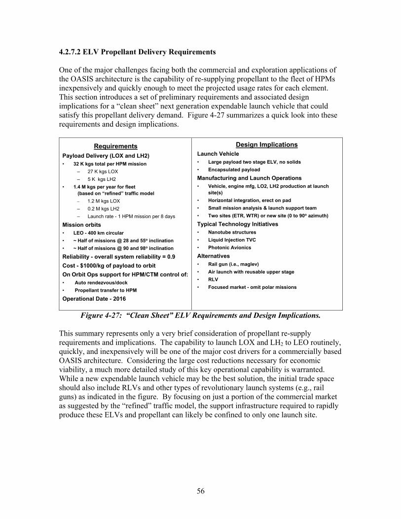
4.2.7.2 ELV Propellant Delivery Requirements One of the major challenges facing both the commercial and exploration applications of the OASIS architecture is the capability of re-supplying propellant to the fleet of HPMs inexpensively and quickly enough to meet the projected usage rates for each element. This section introduces a set of preliminary requirements and associated design implications for a “clean sheet” next generation expendable launch vehicle that could satisfy this propellant delivery demand. Figure 4-27 summarizes a quick look into these requirements and design implications. RequirementsPayload Delivery (LOX and LH2)• 32 K kgs total per HPM mission
– 27 K kgs LOX– 5 K kgs LH2
• 1.4 M kgs per year for fleet (based on “refined” traffic model
– 1.2 M kgs LOX– 0.2 M kgs LH2– Launch rate - 1 HPM mission per 8 days
Mission orbits• LEO - 400 km circular• ~ Half of missions @ 28 and 55o inclination• ~ Half of missions @ 90 and 98o inclinationReliability - overall system reliability = 0.9Cost - $1000/kg of payload to orbitOn Orbit Ops support for HPM/CTM control of:• Auto rendezvous/dock• Propellant transfer to HPMOperational Date - 2016
Design ImplicationsLaunch Vehicle• Large payload two stage ELV, no solids• Encapsulated payloadManufacturing and Launch Operations• Vehicle, engine mfg, LO2, LH2 production at launch
site(s)• Horizontal integration, erect on pad• Small mission analysis & launch support team• Two sites (ETR, WTR) or new site (0 to 90o azimuth)Typical Technology Initiatives• Nanotube structures• Liquid Injection TVC• Photonic AvionicsAlternatives• Rail gun (i.e., maglev)• Air launch with reusable upper stage• RLV• Focused market - omit polar missions
Figure 4-27: “Clean Sheet” ELV Requirements and Design Implications.
This summary represents only a very brief consideration of propellant re-supply requirements and implications. The capability to launch LOX and LH2 to LEO routinely, quickly, and inexpensively will be one of the major cost drivers for a commercially based OASIS architecture. Considering the large cost reductions necessary for economic viability, a much more detailed study of this key operational capability is warranted. While a new expendable launch vehicle may be the best solution, the initial trade space should also include RLVs and other types of revolutionary launch systems (e.g., rail guns) as indicated in the figure. By focusing on just a portion of the commercial market as suggested by the “refined” traffic model, the support infrastructure required to rapidly produce these ELVs and propellant can likely be confined to only one launch site.
56
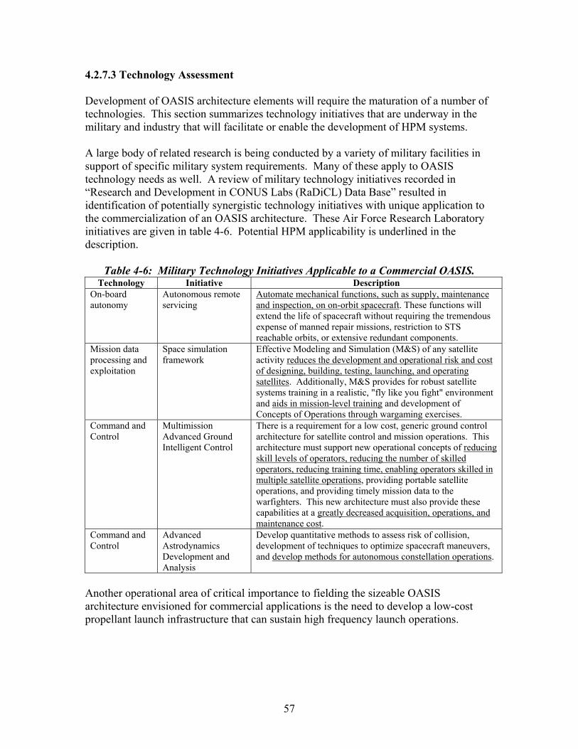
4.2.7.3 Technology Assessment Development of OASIS architecture elements will require the maturation of a number of technologies. This section summarizes technology initiatives that are underway in the military and industry that will facilitate or enable the development of HPM systems. A large body of related research is being conducted by a variety of military facilities in support of specific military system requirements. Many of these apply to OASIS technology needs as well. A review of military technology initiatives recorded in “Research and Development in CONUS Labs (RaDiCL) Data Base” resulted in identification of potentially synergistic technology initiatives with unique application to the commercialization of an OASIS architecture. These Air Force Research Laboratory initiatives are given in table 4-6. Potential HPM applicability is underlined in the description.
Table 4-6: Military Technology Initiatives Applicable to a Commercial OASIS. Technology Initiative Description
On-board autonomy
Autonomous remote servicing
Automate mechanical functions, such as supply, maintenance and inspection, on on-orbit spacecraft. These functions will extend the life of spacecraft without requiring the tremendous expense of manned repair missions, restriction to STS reachable orbits, or extensive redundant components.
Mission data processing and exploitation
Space simulation framework
Effective Modeling and Simulation (M&S) of any satellite activity reduces the development and operational risk and cost of designing, building, testing, launching, and operating satellites. Additionally, M&S provides for robust satellite systems training in a realistic, "fly like you fight" environment and aids in mission-level training and development of Concepts of Operations through wargaming exercises.
Command and Control
Multimission Advanced Ground Intelligent Control
There is a requirement for a low cost, generic ground control architecture for satellite control and mission operations. This architecture must support new operational concepts of reducing skill levels of operators, reducing the number of skilled operators, reducing training time, enabling operators skilled in multiple satellite operations, providing portable satellite operations, and providing timely mission data to the warfighters. This new architecture must also provide these capabilities at a greatly decreased acquisition, operations, and maintenance cost.
Command and Control
Advanced Astrodynamics Development and Analysis
Develop quantitative methods to assess risk of collision, development of techniques to optimize spacecraft maneuvers, and develop methods for autonomous constellation operations.
Another operational area of critical importance to fielding the sizeable OASIS architecture envisioned for commercial applications is the need to develop a low-cost propellant launch infrastructure that can sustain high frequency launch operations.
57

Technology areas in work by the Boeing Company that could enable routine, low-cost ELV development and manufacture are:
• Advanced digital enterprise processes and tools
• Knowledge management
• Virtual manufacturing
• Integrated vehicle design systems.
58

4.3 Military Applications Future Department of Defense (DOD) missions will likely provide additional applications and increased usage rates for OASIS elements. In addition to servicing, refueling and ORU/equipment upgrades which are potential OASIS applications for the commercial sector, a mission with potential military application involves the repositioning of military satellites. There may be value in response to tactical situations of repositioning an orbital asset either by changing its orbit inclination or by lowering its orbit perigee over a military theater of operation to provide better surveillance or improved communication throughout a region. Ongoing OASIS activities supporting analyses of potential military applications include:
• Identifying/refining conceptual operational missions that would benefit from a servicing infrastructure by review of current DOD program (unclassified) requirements
• Refining mission utility analyses and life cycle cost estimates to understand economic viability issues.
4.3.1 Military Satellite Market Trends Future military satellite applications are difficult to identify since numerous programs are currently under conceptual definition. Predicted or observed military satellite market trends [from The Military Use of Space; A Diagnostic Assessment, Center for Strategic and Budgetary Assessments (CSBA), February 2001] include:
• A trend toward greater value and functionality per satellite unit mass. Initial “picosatellite” experiments have been completed.
• Distributed constellations of smaller satellites will offer better prospects for “global, real-time coverage” and “advantages in scaling, performance, cost and survivability” (recent comments from the Air Force Science Advisory Board).
• The potential for very large antenna arrays for optical and radio-frequency imaging utilizing advanced structures and materials technologies.
See table 4-2 (Section 4.2.4.1) for a summary of current non-geostationary orbit military satellite constellations. 4.3.2 Current Program Examples 4.3.2.1 DARPA Orbital Express The Defense Advanced Research Projects Agency (DARPA) is currently developing a system within the Orbital Express Advanced Technology Demonstration Program that will demonstrate robotic techniques for satellites. These include preplanned electronics
59

upgrades, refueling, repositioning and reconfiguration. Orbital Express is incorporating “industry standard” non-proprietary satellite-to-satellite electrical and mechanical interfaces. A demonstration of the Orbital Express spacecraft is planned for launch in 2006. Figure 4-28 illustrates an Orbital Express mission scenario. OASIS may enable approaches to military satellite design and constellation management beyond those envisioned through the Orbital Express program. As examples, in addition to enabling routine, automated on-orbit satellite refueling and facilitating technology insertion during the operating life of a satellite, OASIS can provide orbit repositioning, including height adjust and plane change, for large military assets. The Orbital Express development efforts currently underway will help to resolve numerous issues that would impact an OASIS commercial system. The establishment of common interfaces for military systems may be particularly useful in providing a standard that might carry over to the commercial industry. The following excerpts from the DARPA Orbital Express Advanced Technology Demonstration Phase II Program Selection Process Document describe the rationale for military satellite servicing, refueling and selected bus/payload equipment upgrades that is also directly relevant to potential OASIS applications:
“Today’s Department of Defense (DOD) space architecture has significant limitions that would be substantially mitigated―perhaps eliminated―by the adoption of on-orbit satellite servicing. The lack of an on-orbit servicing capability forces satellite designers to trade propellant (and other consumable) mass, payload mass, and bus mass to meet required satellite lifetimes or launch vehicle limitations. As a result, DOD satellites have minimal maneuverability, resulting in easily predictable orbital characteristics, allowing adversaries to schedule their activities around satellite access opportunities. The absence of maneuverability also severely limits the ability of DOD constellations to quickly respond to real world operational contingencies by modifying their orbits to optimize coverage. Finite quantities of onboard fuel and cryogenic consumables also impose absolute limits on the mission lifetime of satellites. In addition, lengthy satellite development and deployment timeframes result in obsolescent technology on-orbit, with no timely means to upgrade performance. DARPA strongly believes that routine automated on-orbit satellite servicing, refueling and selected bus/payload equipment upgrades can extend the useful lifetime of satellites and provide spacecraft with unprecedented freedom of maneuver. This newly enabled freedom would allow satellite coverage to be adjusted or optimized at will or, alternatively, would enable spacecraft to employ unpredictable maneuvers to counter possible threats or adversary activity scheduling. DARPA also anticipates that routine autonomous preplanned upgrades or reconfiguration of spacecraft components can significantly reduce the time
60

required to insert new technology into operational spacecraft, improving performance and providing flexibility to respond to an evolving threat environment.”
Other military satellite applications relevant to OASIS described in the DARPA Orbital Express Advanced Technology Demonstration Phase II Program Selection Process Document include:
• Ferrying and other operations with microsatellites as a secondary mission
• Potential requirements for a “super-sized” Orbital Express Demonstration System (OEDS) referred to as OEDS “Grande.”
Figure 4-28: Orbital Express Mission Scenario.
4.3.2.2 NASA-USAF Reusable Space Launch Development A joint NASA and U.S. Air Force (USAF) study team, named the One Team, was chartered in October 2001 by the NASA Administrator and the Secretary of the Air Force to study options for cooperative development of a new generation of reusable launch vehicles (RLVs) to meet national needs. Study objectives include the formulation of a
61

credible, comprehensive plan to develop RLVs, and to define and converge (where possible) NASA and Air Force requirements. This One Team study activity has defined requirements for architectural elements which could be met by OASIS (figure 4-29). These architectural elements include on-orbit transfer and servicing elements (upper stages, orbital transfer vehicles, and refueling/servicing vehicles) and reusable orbital vehicles such as space maneuver vehicles. As described in One Team industry briefing material, the general utility of the new generation RLV and associated architectural elements for national security, civil, and U.S. commercial space sectors include:
• Enabling new approaches to satellite design and constellation management
• Extending satellite operating life and improving maneuverability through on-orbit refueling
• Enabling technology insertion during operating life of a satellite block, and
• Reducing cost to build, insure, and operate satellites by up to two-thirds.
Launch Vehicle Systems
Reusable Orbital Vehicles Payloads
On-Orbit Transfer & Servicing
ELV’s
2nd Gen RLVs
3rd Gen RLVs
Upper Stages
Re-fueling/ Servicing
Crew Transfer
Cargo Transfer
Space Maneuver Vehicles
Commercial
Strategic
Tactical
HumanHuman
Scientific
GroundFacilities
Orbital Transfer Vehicles
Spaceport
AutomatedMission
Processing
Potential OASIS Elements
Figure 4-29: One Team Integrated Architecture Elements.
62
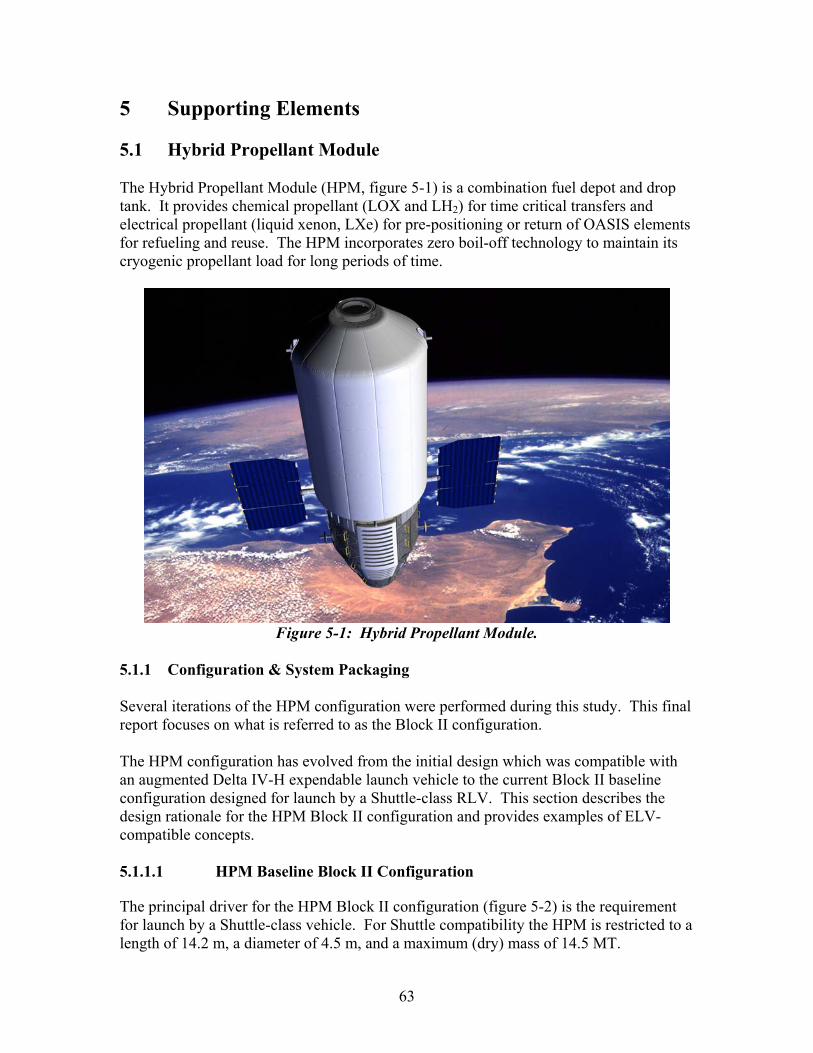
5 Supporting Elements 5.1 Hybrid Propellant Module The Hybrid Propellant Module (HPM, figure 5-1) is a combination fuel depot and drop tank. It provides chemical propellant (LOX and LH2) for time critical transfers and electrical propellant (liquid xenon, LXe) for pre-positioning or return of OASIS elements for refueling and reuse. The HPM incorporates zero boil-off technology to maintain its cryogenic propellant load for long periods of time.
Figure 5-1: Hybrid Propellant Module.
5.1.1 Configuration & System Packaging Several iterations of the HPM configuration were performed during this study. This final report focuses on what is referred to as the Block II configuration. The HPM configuration has evolved from the initial design which was compatible with an augmented Delta IV-H expendable launch vehicle to the current Block II baseline configuration designed for launch by a Shuttle-class RLV. This section describes the design rationale for the HPM Block II configuration and provides examples of ELV-compatible concepts. 5.1.1.1 HPM Baseline Block II Configuration The principal driver for the HPM Block II configuration (figure 5-2) is the requirement for launch by a Shuttle-class vehicle. For Shuttle compatibility the HPM is restricted to a length of 14.2 m, a diameter of 4.5 m, and a maximum (dry) mass of 14.5 MT.
63
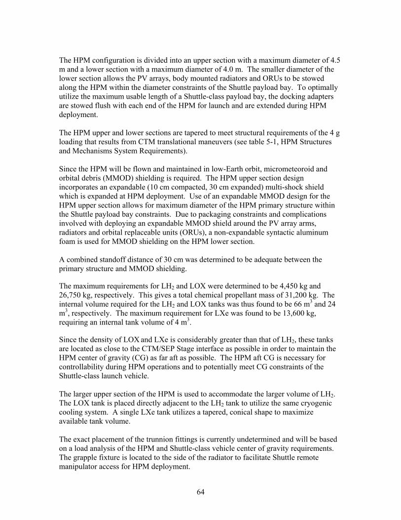
The HPM configuration is divided into an upper section with a maximum diameter of 4.5 m and a lower section with a maximum diameter of 4.0 m. The smaller diameter of the lower section allows the PV arrays, body mounted radiators and ORUs to be stowed along the HPM within the diameter constraints of the Shuttle payload bay. To optimally utilize the maximum usable length of a Shuttle-class payload bay, the docking adapters are stowed flush with each end of the HPM for launch and are extended during HPM deployment. The HPM upper and lower sections are tapered to meet structural requirements of the 4 g loading that results from CTM translational maneuvers (see table 5-1, HPM Structures and Mechanisms System Requirements). Since the HPM will be flown and maintained in low-Earth orbit, micrometeoroid and orbital debris (MMOD) shielding is required. The HPM upper section design incorporates an expandable (10 cm compacted, 30 cm expanded) multi-shock shield which is expanded at HPM deployment. Use of an expandable MMOD design for the HPM upper section allows for maximum diameter of the HPM primary structure within the Shuttle payload bay constraints. Due to packaging constraints and complications involved with deploying an expandable MMOD shield around the PV array arms, radiators and orbital replaceable units (ORUs), a non-expandable syntactic aluminum foam is used for MMOD shielding on the HPM lower section. A combined standoff distance of 30 cm was determined to be adequate between the primary structure and MMOD shielding. The maximum requirements for LH2 and LOX were determined to be 4,450 kg and 26,750 kg, respectively. This gives a total chemical propellant mass of 31,200 kg. The internal volume required for the LH2 and LOX tanks was thus found to be 66 m3 and 24 m3, respectively. The maximum requirement for LXe was found to be 13,600 kg, requiring an internal tank volume of 4 m3. Since the density of LOX and LXe is considerably greater than that of LH2, these tanks are located as close to the CTM/SEP Stage interface as possible in order to maintain the HPM center of gravity (CG) as far aft as possible. The HPM aft CG is necessary for controllability during HPM operations and to potentially meet CG constraints of the Shuttle-class launch vehicle. The larger upper section of the HPM is used to accommodate the larger volume of LH2. The LOX tank is placed directly adjacent to the LH2 tank to utilize the same cryogenic cooling system. A single LXe tank utilizes a tapered, conical shape to maximize available tank volume. The exact placement of the trunnion fittings is currently undetermined and will be based on a load analysis of the HPM and Shuttle-class vehicle center of gravity requirements. The grapple fixture is located to the side of the radiator to facilitate Shuttle remote manipulator access for HPM deployment.
64
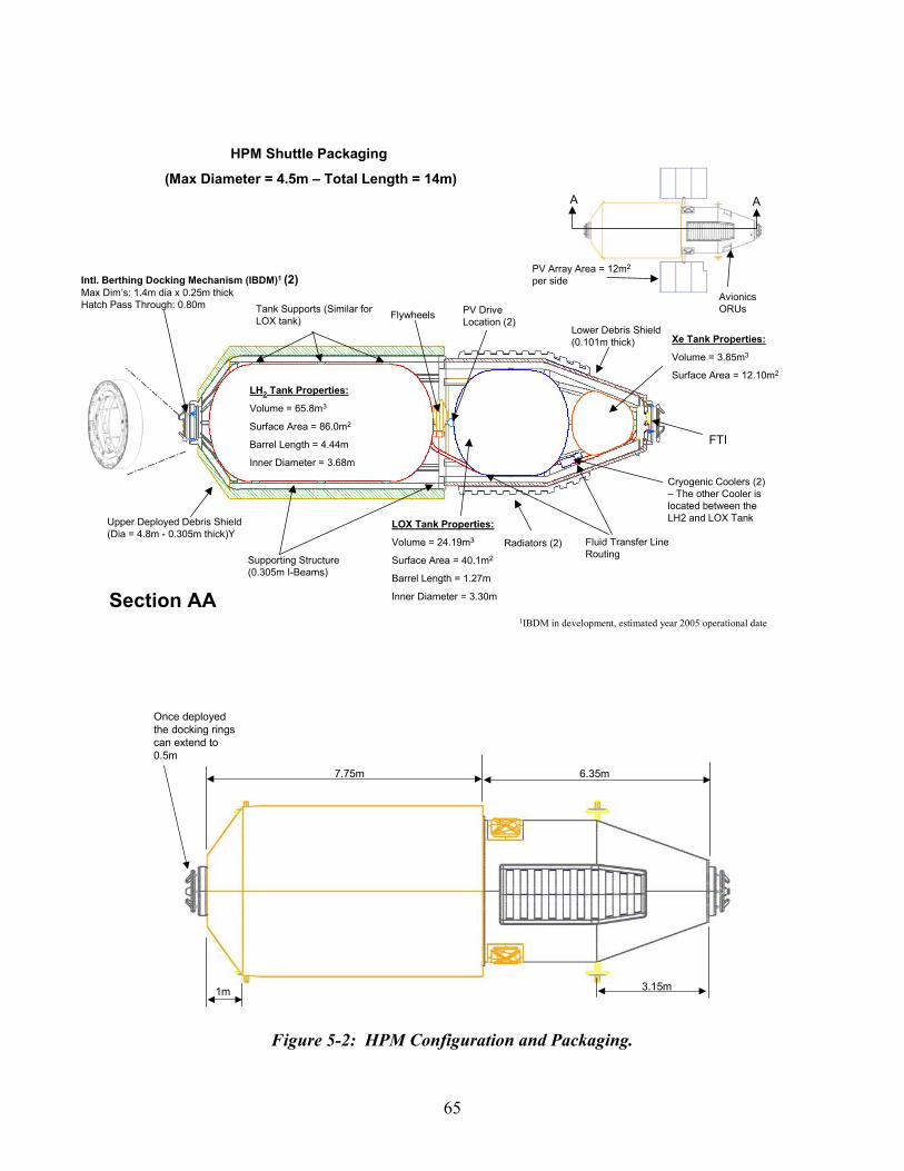
A A
Section AA
LH2 Tank Properties:
Volume = 65.8m3
Surface Area = 86.0m2
Barrel Length = 4.44m
Inner Diameter = 3.68m
LOX Tank Properties:
Volume = 24.19m3
Surface Area = 40.1m2
Barrel Length = 1.27m
Inner Diameter = 3.30m
Intl. Berthing Docking Mechanism (IBDM)1 (2)Max Dim’s: 1.4m dia x 0.25m thickHatch Pass Through: 0.80m
1IBDM in development, estimated year 2005 operational date
PV Drive Location (2)
AvionicsORUsFlywheels
Cryogenic Coolers (2) – The other Cooler is located between the LH2 and LOX Tank
Fluid Transfer Line Routing
Xe Tank Properties:
Volume = 3.85m3
Surface Area = 12.10m2
Upper Deployed Debris Shield (Dia = 4.8m - 0.305m thick)Y
PV Array Area = 12m2
per side
HPM Shuttle Packaging
(Max Diameter = 4.5m – Total Length = 14m)
Radiators (2)
Lower Debris Shield (0.101m thick)
Tank Supports (Similar for LOX tank)
Supporting Structure (0.305m I-Beams)
FTI
6.35m7.75m
1m 3.15m
Once deployed the docking rings can extend to 0.5m
Figure 5-2: HPM Configuration and Packaging.
65

The cryogenic-coolers, flywheels, and PV array drives are located in the volume between the LH2 and LOX tanks (figure 5-3). Orbital replaceable units (ORUs), which include the computers, data recorders and communication hardware, are located on the tapered section of the HPM for easy access by a servicing vehicle. 5.1.1.2 HPM ELV Configurations Preliminary analysis has been performed to define ELV compatible HPM configurations. A “Shuttle capacity equivalent” configuration with the same propellant capacities as the baseline Block II HPM has been designed to fit within a Delta IV-H payload envelope of 5.0 m diameter x 11.5 m length. This HPM configuration can be launched with the full propellant load required for any L1 transfer mission. A “maximum shroud configuration” has been designed for a Delta IV-H payload envelope of 5.0 m diameter x 15.0 m length. This HPM, configured to utilize the maximum allowable Delta IV-H shroud, could offer enhanced performance for both exploration and commercial missions. Figure 5-4 illustrates launch vehicle packaging for the HPM “maximum shroud” and baseline Shuttle compatible configurations.
ORUs (Computers, Data Storage, Communications)
Flywheels
Cryogenic Coolers
Fluid Transfer Line Routing
FTI and Docking Adaptor
PV Drives and Conditioners
ORUs (Computers, Data Storage, Communications)
Flywheels
Cryogenic Coolers
Fluid Transfer Line Routing
FTI and Docking Adaptor
PV Drives and Conditioners
Figure 5-3: HPM Internal Systems.
66
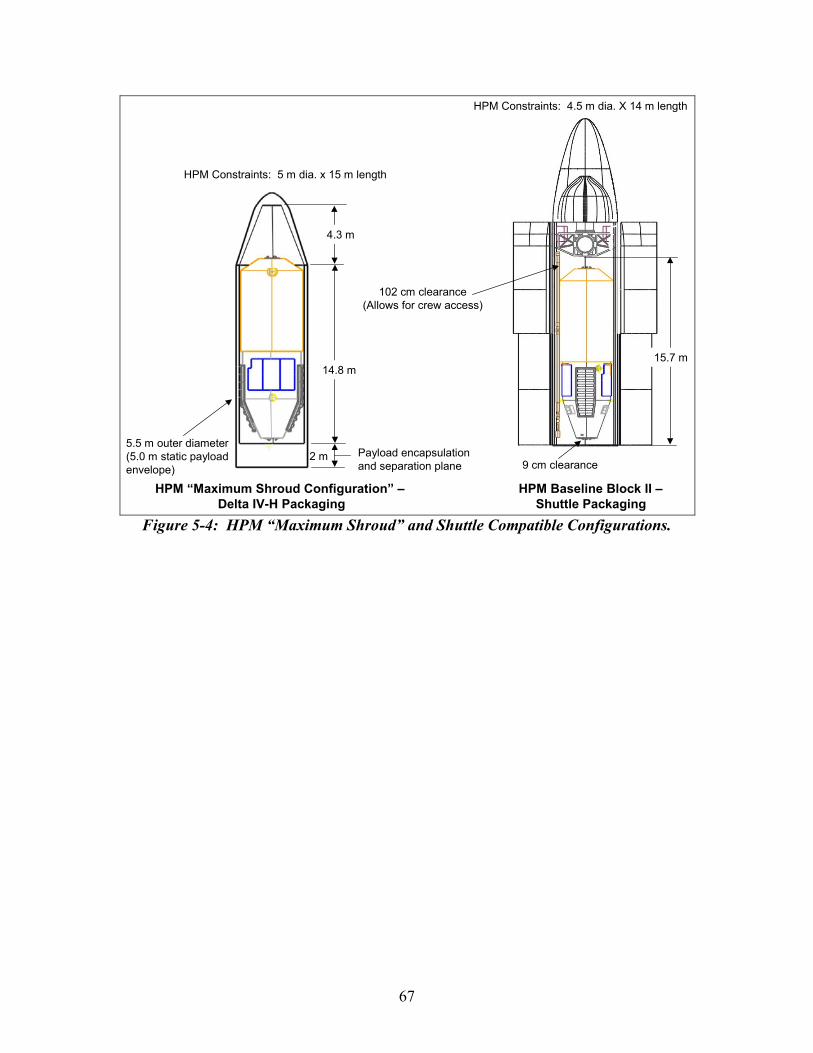
2 m Payload encapsulation and separation plane
5.5 m outer diameter (5.0 m static payload envelope)
14.8 m
4.3 m
15.7 m
9 cm clearance
102 cm clearance (Allows for crew access)
HPM Constraints: 5 m dia. x 15 m length
HPM Constraints: 4.5 m dia. X 14 m length
HPM “Maximum Shroud Configuration” –Delta IV-H Packaging
HPM Baseline Block II –Shuttle Packaging
Figure 5-4: HPM “Maximum Shroud” and Shuttle Compatible Configurations.
67

5.1.2 Systems 5.1.2.1 Structures and Mechanisms The structures and mechanisms system of the HPM transfers and supports loads from one OASIS element to another while acting as a rigid skeleton for HPM interior component attachment. The HPM structures and mechanisms system also provides the outer shell for micrometeoroid and orbital debris protection. The design is considered as two main structural sections composed of beam longerons: the upper section and the smaller diameter lower section. Each section transfers loads from the other section through the mid span ring to the docking rings located at each end of the HPM, as shown in figure 5-5. Both structural sections are tapered at the ends to improve load transfer from docked OASIS elements. System Requirements. Mechanical Loads. The primary requirements of the HPM structural system are to provide a load transfer path for the launch and in-space loads and to serve as a backbone to attach all other subsystems. The structural system design meets the requirements of NASA Standard 5001, Structural Design and Test Factors of Safety for Space Flight Hardware. The structural system is designed to withstand the launch loads from either a Shuttle-class RLV or an augmented Delta IV-Heavy ELV and their corresponding load values and vectors. The in-service maximum loads are dictated by the specific HPM mission and mission phase. The maximum mission load occurs during a CTM engine burn which thrusts the HPM at an axial load of 4 Gs.
Table 5-1: HPM Structures and Mechanisms System Requirements. Mechanical Loads
• Provide a load transfer path for launch and in-space operations loads: o Shuttle launch (maximum): -2.0 to +3.0 g axial, -1.0 to +1.0 g lateral; -2.5 to +2.0 g normal o CTM thrust (maximum): +4.0 g axial
• Provide attach structure for HPM systems. Thermal Control
• Protect HPM systems from exterior heat during launch and in-space operations. • Provide safe operating environment for the HPM EPS. • Insulate HPM propellant tanks from internally generated heat.
Radiation Protection • Provide radiation protection to HPM systems/components.
Micrometeoroid and Orbital Debris Protection • Protect HPM systems/components from micrometeoroid/orbital debris throughout 10-year design
life (no penetration from a 0.4 cm diameter aluminum projectile with an impact velocity of 7 km/sec).
Thermal Control and Radiation Protection. The thermal protection subsystem (TPS) protects the interior components from exterior heat during launch and in-space operations. The TPS also provides a safe operating environment for the EPS and
68
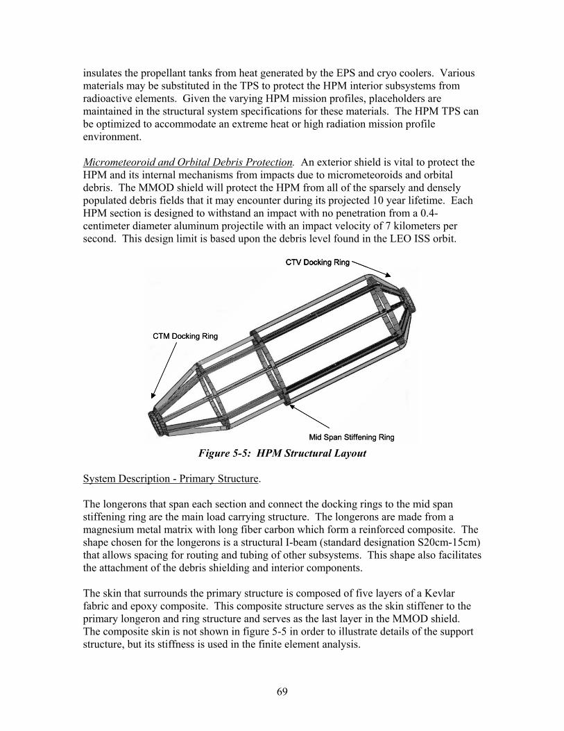
insulates the propellant tanks from heat generated by the EPS and cryo coolers. Various materials may be substituted in the TPS to protect the HPM interior subsystems from radioactive elements. Given the varying HPM mission profiles, placeholders are maintained in the structural system specifications for these materials. The HPM TPS can be optimized to accommodate an extreme heat or high radiation mission profile environment. Micrometeoroid and Orbital Debris Protection. An exterior shield is vital to protect the HPM and its internal mechanisms from impacts due to micrometeoroids and orbital debris. The MMOD shield will protect the HPM from all of the sparsely and densely populated debris fields that it may encounter during its projected 10 year lifetime. Each HPM section is designed to withstand an impact with no penetration from a 0.4-centimeter diameter aluminum projectile with an impact velocity of 7 kilometers per second. This design limit is based upon the debris level found in the LEO ISS orbit.
Mid Span Stiffening Ring
CTV Docking Ring
CTM Docking Ring
Mid Span Stiffening Ring Mid Span Stiffening Ring
CTV Docking RingCTV Docking Ring
CTM Docking RingCTM Docking Ring
Figure 5-5: HPM Structural Layout
System Description - Primary Structure. The longerons that span each section and connect the docking rings to the mid span stiffening ring are the main load carrying structure. The longerons are made from a magnesium metal matrix with long fiber carbon which form a reinforced composite. The shape chosen for the longerons is a structural I-beam (standard designation S20cm-15cm) that allows spacing for routing and tubing of other subsystems. This shape also facilitates the attachment of the debris shielding and interior components. The skin that surrounds the primary structure is composed of five layers of a Kevlar fabric and epoxy composite. This composite structure serves as the skin stiffener to the primary longeron and ring structure and serves as the last layer in the MMOD shield. The composite skin is not shown in figure 5-5 in order to illustrate details of the support structure, but its stiffness is used in the finite element analysis.
69

Upper Section. The structural design layout for the upper section, shown in figure 5-6, includes eight longerons spaced 45 degrees apart. The longeron beams are the connection between the MMOD shielding and the liquid oxygen tank. The spaces between the beams, the MMOD shielding and the tank are used for routing of fluid transfer pipes and electrical conduits. Internal volume is available for layers of radiation protective material or thermal insulation depending on which material is needed for the specific HPM mission. The MMOD shielding on the upper section is an expandable concept based on the design of the NASA Mars Trans Habitat. At launch the shielding can be compressed to 10 centimeters and then expanded to 30 centimeters once the HPM is deployed.
Upper Debris Shielding (Deployed)
Longerons
LOX Tank Wall and Insulation
Radiation and Thermal Shielding Place Holder
Upper Debris Shielding (Deployed)
Longerons
LOX Tank Wall and Insulation
Radiation and Thermal Shielding Place Holder
Upper Debris Shielding (Deployed)
Longerons
LOX Tank Wall and Insulation
Radiation and Thermal Shielding Place Holder
Upper Debris Shielding (Deployed)
Longerons
LOX Tank Wall and Insulation
Radiation and Thermal Shielding Place Holder
R 1.87m
R 1.84m R 2.40m
R 2.10m
R 1.87m
R 1.84m R 2.40m
R 2.10m
Figure 5-6: HPM Upper Section Cross-Section. Lower Section. The lower section of the HPM (figure 5-7) is similar in design to the upper section with a few notable differences. The largest distinction is that the overall diameter of the structure is smaller. This is needed for the launch configuration of the solar arrays which are stowed in a folded position alongside the lower section before deployment. The lower section also includes integrated panels used for interior access (e.g., to replace ORUs). Due to these requirements, the MMOD shielding is not the expandable design used in the upper section. A fixed diameter Whipple type shield is chosen for the lower section for these reasons. This shield type uses a sacrificial thin outer layer that fragments and slows down any orbital debris before it impacts the inner composite skin. The overall standoff, identical to the upper section, is 10 centimeters. The lower section longeron beams are of the same shape and use the same material as the upper section for commonality to simplify manufacturing.
70

Radiators
Lower Debris Shielding
LOX Tank Wall and Insulation Radiation and Thermal
Shielding Place Holder
Radiators
Lower Debris Shielding
LOX Tank Wall and Insulation Radiation and Thermal
Shielding Place Holder
Radiators
Lower Debris Shielding
LOX Tank Wall and Insulation Radiation and Thermal
Shielding Place Holder
Radiators
Lower Debris Shielding
LOX Tank Wall and Insulation Radiation and Thermal
Shielding Place Holder
R 1.65mR 1.71m
R 2.00m
R 1.90m
R 1.65mR 1.71m
R 2.00m
R 1.90m
Figure 5-7: HPM Lower Section Cross-Section. Mid-Span and Docking Rings. The mid span ring serves as a stiff connection between the upper and lower longerons and also as a connection point for trunion fittings for a Shuttle-class RLV. It is made from the same metal matrix composite as the longerons. The rectangular section of the tube is 20 by 40 centimeters which is wide enough to accommodate the upper and lower offset and transfer the loads between the sections. Docking rings are located at each end of the HPM to enable mating with other OASIS elements and the ISS. These rings serve as the connection between the International Berthing and Docking Mechanism (IBDM, figure 5-8) and the longerons providing a stiff foundation for docking. They also transfer all of the longitudinal loads from the attached vehicle into the beam structure of the HPM. The docking support rings are constructed of the metal matrix composite that is used throughout the primary structure. These docking rings are made of 20 centimeter square structural tubes to provide the proper interface surface with the longerons. The lower section of the HPM (i.e., the CTM mating location) also provides a fluid transfer interface.
71
Figure 5-8: The International Berthing and Docking Mechanism.
System Description - Secondary Structure. The secondary structures of the HPM consist of thermal protection, MMOD shielding and the attachment structures of each sub-component. The thermal protection and MMOD shielding are combined as a single subelement. Meteoroid and Orbital Debris Shielding. Each section of the HPM utilizes a different concept for MMOD and thermal protection. The upper section includes three layers of Nextel ceramic cloth that provide thermal protection in the debris shield (figure 5-9). These cloth layers and open cell foam within the standoff spacing provide MMOD shielding by slowing the velocity of the debris impact. This foam is a carbon-based graphitic material that also has excellent thermal properties. During launch the shielding is compacted to a height of 10 centimeters and deployed in service to its full height of 30 centimeters. The inner Kevlar wall attaches to the flanges on the longerons of the primary structure for the upper section of the HPM. Other material may be used in addition to, or in place of, the graphitic foam to aid in radiation protection or provide other protection as required for a given HPM mission.
Nextel (AF10) Ceramic ClothLow-density, open cell foam
Nextel (AF10) Ceramic ClothLow-density, open cell foam
Nextel (AF10) Ceramic ClothLow density, open cell foam
Kevlar (5 layers)
12” (30 cm)standoff
Figure 5-9: HPM Upper Section Debris and Thermal Protection.
72

The lower section MMOD shielding and thermal protection is a Whipple shield design (figure 5-10). This shielding design, with a fixed outer diameter, was selected to allow EVA access of subsystem components through removable trays. Each wall of the Whipple shield is made of syntactic aluminum metal foam to minimize material density while retaining strength. Hypervelocity impact testing is necessary to verify MMOD protective capability. Multi-layer insulation (MLI) is incorporated between the walls in the stand off area to provide thermal protection.
Bumper Thickness
Rear Wall Thickness
Aluminum Rear Wall
Aluminum Bu mper
Stand-Off Dis tance
Bumper Thickness
Rear Wall Thickness
Aluminum Rear Wall
Aluminum Bu mper
Stand-Off Dis tance
Bumper Thickness
Rear Wall Thickness
Aluminum Rear Wall
Aluminum Bu mper
Stand-Off Dis tance
Bumper Thickness
Rear Wall Thickness
Aluminum Rear Wall
Aluminum Bu mper
Stand-Off Dis tance
Bumper Thickness
Rear Wall Thickness
Aluminum Rear Wall
Aluminum Bu mper
Stand-Off Dis tance
Figure 5-10: HPM Lower Section Whipple Debris Shield.
Technology Needs. The following table of structures technology needs (table 5-2) is listed in three sections by order of significance. The first section of the table lists the four most important technologies that are essential to fulfill the requirements and assumptions for this design. The HPM structures and mechanisms system design is based on these technologies including carbon composites, metal matrix composites, graphitic foam, and syntactic metal foam. The next section lists those areas of research that could either greatly enhance or replace the first group of technologies. Novel technologies are listed in the third group. These technologies have the potential of revolutionary functional impact to the HPM design.
73

Table 5-2: HPM Structures and Mechanisms Technology Needs.
Technology
Summary Description of
Desired Technology and
Key Performance Metrics
Current TRL Where Who
Current Funding
($k)
Funding Increase Required
Applications of the
Technology other than
HPM
Carbon Composites
High stiffness to low weight ratio 5 Various Various 12,824 None Various
Metal Matrix Composites
High stiffness to low weight ratio and MMOD protection
3 Various Various 3,877 Small Various
Graphitic Foam
Lightweight filler for debris shielding that also adds thermal protection
5 Various Various 300 Small Various
Syntactic Metal Foam
High stiffness to low weight ratio 4 Various Various 70 Small Various
Multi-function Structure
Secondary structure of all subsystems incorporated into primary structure
5 Various Various 5,394 None Various
Ceramic Matrix Composites
High stiffness to low weight ratio and high thermal protection
3 Various Various 11,246 None Various
Advanced Micro-Meteoroid & Orbital Debris Shielding
Technology to mitigate the threat of meteoroid damage
3 Various Various 500 Major Various
Advanced Insulation Materials
Thermal protection from space environment and cryogenic thermal stability
2 Various Various 140 Major Various
Self-Healing Materials
Ability to repair pressure/structure walls after debris impact
2 Various Various 70 Small Various
Biomimetic Materials
Mimicking structures found in nature to help reduce loads and stress concentrations
3 Various Various 2,433 None Various
Carbon Nanotubes
High stiffness to low weight ratio 2 Various Various 5,539 None Various
74
5.1.2.2 Propellant Management System The HPM is designed to be self-sufficient and provide a reliable source of propellants for the OASIS propulsive elements at any potential mission location in LEO or deep space. The HPM propellant management system must provide long term storage of propellants—on the order of years—and provide the appropriate rate of propellant transfer to allow the propulsive maneuvers of the mated OASIS elements to be performed properly. The propellant management system, like all HPM systems, is designed for a useable lifetime of 10 years. System Requirements. The top-level HPM propellant management system requirements are given in table 5-3.
Table 5-3: HPM Propellant Management System Requirements. Key Performance Requirements
• The HPM shall accommodate 4 fill and drain cycles per year for 10 years with no refurbishment. • The HPM shall accommodate 4,450 kg of LH2 propellant. • The HPM shall accommodate 26,750 kg of LOX propellant. • The HPM shall accommodate 13,600 kg of LXe propellant.
Tanks • The HPM propellant tanks shall maintain structural integrity between 2% and 100% of maximum
capacity. Zero Boil-Off Cryogenic Propellant Storage
• The HPM shall be capable of providing 2 years of propellant storage at all potential mission locations with a maximum 100 kg/year leakage.
Propellant Delivery • HPM propellant delivery subsystem shall manage liquid propellants under zero gravity to ensure
that propellant is expelled from the storage tanks. Propellant Feed System (Zero-G Management)
• The HPM propellant feed subsystem shall provide vapor free liquid to OASIS element engines at TBD flow rate.
Propellant Gauging and Health Monitoring • The HPM propellant gauging and health monitoring subsystem shall interface with the HPM
C&DH system to provide tank propellant loading, pressure and temperature information during all mission phases.
Lines • HPM propellant lines shall be sized to provide proper flow rates for all OASIS element propulsive
maneuvers. • HPM propellant lines shall maintain the phase state of the propellant during transfer to/from
propulsive or refueling elements. • HPM propellant line leakage shall be less than ½% of stored fluid per year.
Fluid Transfer Interfaces • The HPM fluid transfer interfaces shall provide standard interfaces for the automated connection
to OASIS propulsive elements or refueling elements. Standard Interface Quick Disconnects
• The HPM propellant management system quick disconnects shall provide 100 mating and de-mating cycles.
75

Tanks. The HPM propellant storage tanks must be capable of retaining the cryogenically stored liquids (LH2, LOX and xenon electric propellant) for extended periods of time with very minimal leakage through the tank walls and connection seals. All tanks must be capable of being refilled via the bi-directional fluid transfer interface. All tanks must be capable of withstanding launch loads either fully or partially loaded and must be capable of maintaining structural integrity between 2.5% and 100% of the maximum capacity. The maximum propellant storage requirements for the HPM propellant storage tanks are:
• LH2: 4,450 kg
• LOX: 26,750 kg
• LXe: 13,600 kg. Zero Boil-Off Cryogenic Propellant Storage. The zero boil-off cryogenic storage subsystem must be capable of providing two years of propellant storage at all potential mission locations. The cryogenic cooler and insulation will be optimized to provide a minimum weight system capable of storing cryogens indefinitely. Cryocooler input power will be a maximum of TBD Watts. Waste heat from the cryocooler will be dissipated via a radiator capable of dissipating TBD Watts.
Propellant Delivery. The propellant delivery subsystem will be designed to manage the liquid propellants under zero gravity to ensure that liquid propellant is expelled from the storage tanks. Propellant Feed System (Zero-G Management). The propellant feed subsystem will use autogenous pressurization and a propellant management device to provide vapor free liquid to OASIS element engines at a TBD flow rate. The xenon tanks will use a total communication liquid acquisition device to continuously provide liquid in a low thrust environment. The main propellant tanks may use either a total communication liquid acquisition device or a refillable trap capable of holding enough liquid during engine startup to insure that vapor free liquid is fed to the main engines until propellant settling is achieved. Propellant Gauging and Health Monitoring. The propellant gauging and health monitoring subsystem will interface with the HPM C&DH system to provide tank propellant loading, pressure and temperature information during all mission phases. Lines. Propellant lines will be sized to provide proper flow rates for all propulsive maneuvers. Lines will be insulated to properly maintain phase state of the propellant during transfer to/from attached OASIS elements or refueling vehicles. Leakage from lines will be less than ½% of stored fluid per year. Lines will be vented and purged after maneuvers to prevent trapped liquid from over pressurizing systems. Hardware is expected to include:
76
• Liquid hydrogen lines
• Liquid oxygen lines
• Electric propellant lines
• Isolation valves
• Pressure relief valves
• Fill and purge valves
• Pressure regulators.
Fluid Transfer Interfaces. The fluid transfer interfaces (FTIs) will provide the automated connection of the appropriate transfer stage and the transfer of the proper type and amount of propellant for propulsive maneuvers. The FTIs will also allow the refilling of the HPM to be performed by an orbital maneuvering vehicle (or other equivalent system). The FTIs are designed to provide the standardized interface for all propellant transfer between the HPM and external elements/vehicles.
Standard Interface Quick Disconnects. The quick disconnects (QDs) will provide for the automated propellant transfer interface between the HPM and the attached OASIS element or refueling vehicle. The QDs must be capable of providing 100 mating and de-mating cycles. System Description. A flow schematic of the HPM propellant management system is shown in figure 5-11.
LOX
LH 2
H2 Vent
Pressure Building
Coil
Pressure Building
Coil
O 2 Vent
Xe
Xe Vent
Key Valve Relief Valve Burst Disk
Key Valve Relief Valve Burst Disk
LH2 Cryocooler
LOX/Xe Cryocooler
Figure 5-11: HPM Propellant Management System Schematic.
77

Tank pressure will be maintained with an autogenous pressurization system. Small quantities of propellant are withdrawn from the tank and warmed by heat exchange with the ambient environment to produce vapor that is injected back into tank to raise tank pressure. Pressure lowering options include a settle and vent procedure or, if operationally necessary, a thermodynamic vent system which can operate in a low thrust environment. Emergency overpressure protection is provided by a fault tolerant relief valve and burst disk system. Shutoff valves at both the fluid transfer interface and tank allow the operational flexibility to drain trapped cryogen back into the main tank as well as store the cryogen without the large heat load of a long liquid-filled line. Tank Material Trades. Table 5-4 shows tank mass as a function of various tank materials. 301 stainless steel and 2219 aluminum are conventional materials used in current vehicles. A fiberglass S glass epoxy system is listed as representative of composite construction performance.
Table 5-4: Tank Mass for Various Materials (kg). LH2 Tank LOX Tank 2219 Aluminum 353.5 104.9 301 Stainless Steel 399.5 118.6 S-Glass Epoxy Fiberglass 161.8 48.0 A 50 psi operating pressure was selected as a typical tank pressure. Tank masses are based on calculation of the minimum shell thickness for each material. Real tanks will have greater mass due to manufacturing inefficiencies, reinforcements at supports, penetrations, and weld allowances (metal tanks only). The mass of these items is accounted for in a 10% overall mass contingency for the HPM element. For comparison purposes in this design trade, the absence of this mass does not impact ranking of the material performance. Composite construction shows a clear mass savings for all tanks. Cryogenic versus Non-Cryogenic Xenon Storage. Current electric propulsion stages rely on ambient temperature, high pressure storage of their xenon propellant. Cryogenic storage of xenon results in a substantial increase in xenon density resulting in a proportional decrease in tank size. Figure 5-12 shows xenon density at various storage conditions. In addition, reduction of the xenon storage pressure results in a substantial reduction in tank mass. Figure 5-13 shows xenon tank mass as a function of tank pressure. Design of xenon cryogenic storage and fluid management systems pose some additional complexity. However, the same system concept for HPM cryogenic hydrogen and oxygen storage is potentially applicable for xenon storage. For example, it is believed the xenon tank can use the same cryocooler system used to refrigerate the HPM cryogenic oxygen.
78

0
1,000
2,000
3,000
13790 Kpa, 294 K 5516 Kpa, 294 K 345 Kpa, 167K
Den
sity
(kg/
cu m
)
Figure 5-12: Density of Xenon at Candidate Storage Conditions.
0
50
100
150
S glass Epoxysphere 345
Kpa
2219aluminum
sphere 345Kpa
301 stainlesssteel sphere
345 Kpa
S glass Epoxysphere 5,516
Kpa
S glass Epoxysphere 13,790
KPa
Mas
s (k
g)
Figure 5-13: Mass of a 28 Inch Radius Xenon Tank as a Function of
Material and Pressure.
79

Design of Zero Boiloff System. Zero boiloff systems use a cryocooler to remove all thermal energy that leaks into the storage system through the tank insulation (figure 5-14). The thermodynamic state of stored fluid will not change with a well-designed zero boiloff system as long as the cryocooler is functional. One-stage cryocoolers capable of cooling xenon and oxygen systems are currently available with lifetimes approaching 10 years. Hydrogen cooling requires a two-stage system due to the lower temperature. Although two-stage systems are available, some technology development is necessary to scale up existing designs to the size needed for HPM hydrogen zero boiloff storage. The potential exists to use the first stage of the hydrogen cooler to cool the oxygen tank. Zero boiloff systems for the HPM were sized using a spreadsheet tool which selects cryocoolers and insulation systems for zero boiloff given a tank size and cryocooler target temperatures. Results of this analysis are shown in table 5-5.
Cryocooler
ColdFinger
MLI Blankets
VaporVapor
Cryogen
Space
Heat Exchanger
RadiatorSolarArray
Figure 5-14: Possible Zero Boil-off In-Space Configuration.
80
Table 5-5: HPM Propellant Management System Sizing. Description Units Reference note
Propellant Hydrogen Oxygen
Propellant Quantity 4378.958 26273.75 kg
Ullage 3 3 % Off load to prevent tank rupture, assumption by Plachta
Residual 2 2 % Unaccessible propellant at bottom of tank, assumption by Plachta
Pressure 207 207 KPa
Liquid Temperature 22.8 97 K Fluid properties at 207 KPa
Density 67.7 1105 kg/m3 Fluid properties at 207 KPa
Minimum Tank Volume 67.92 24.97 m3 Mass divided by density, multiplied by 1 plus ullage and residual factors
Tank Diameter (inside) 3.81 3.3 m
Cylindrical Length 3.316195 0.951157 m If applicable
Cylinder End Cap Surface Area 37.21 37.21 m2
Tank Surface Area 76.91 47.07 m2 If cylinder length is specified, then oblate spheroid endcaps are assumed, with an a/b ratio of 1.4
No. of MLI layers 45 35 Assumption, total mass of system is somewhat independent of this variable for ZBO
Insulation Density 0.81 0.63 kg/m2 Paper by Hasting/Martin, MSFC, 1998
Insulation Mass 62.3 29.7 kg
Insulation Heat Leak 0.21 0.25 w/m2
Using 243K as reference temperature in LEO, using 1.7 Lockheed Scale Factor, Tcold for H2 set at 70K (using 2 stage cooler)
Other Heat Leak 0.0005 0.0005 w/kg Penetration losses, based on 1990 flight design by Astronautics Lab, AL-TR-90
Total Heating Rate 19.7 28.4 w Includes a 25% margin on tank system mass
Environmental temperature 243 243 K Estimate of LEO conditions, worst case from S. Tucker analysis, 1993
1st Stage applicable? yes no
1st Stage Cooler rejection temp 243 -n/a- K
1st Stage Cold Head temp 70 -n/a- K
2nd Stage Cold Head temp 21.8 96 K Assumes a 1 Kelvin temperature drop from tank to cooler
2nd Stage Cooler rejection temp 80 243 K Assumes 2 coolers, to simulate 2 stage cooler, with intermediate shield being used to reject heat
Mixer Heat Added 10 10 % Assumes 10% of heat added to tank
1st Stage Cooler Thermal Power 21.62 0.00
Ist Stage Cooler Input Power 1241.87 0.00
Applicable for LH2 only. This approach assumes one cooler to reduce the shield temp to 70K, and a second cooler to cool the bulk liquid. Calculation from "Propellant Preservation for Mars Missions," P. Kittel, Advances in Cryo Engineering, Vol. 45, pg. 443, Plenum Publishers, 2000.
Cooler Mass 49.50 0.00 kg
2nd Stage Cooler Thermal Power 0.63 31.20
2nd Stage Cooler Input Power 49.02 242.58
2nd Stage Cooler Input Mass 7.14 4.12
1st Stage Shield Mass 192.27 0.00 kg 2.5 kg/m2 assumption, from "Long Term Cryogenic System Study," R. T. Giellis, AFRPL TR-82-071
81
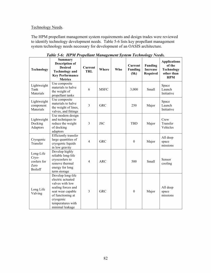
Technology Needs. The HPM propellant management system requirements and design trades were reviewed to identify technology development needs. Table 5-6 lists key propellant management system technology needs necessary for development of an OASIS architecture.
Table 5-6: HPM Propellant Management System Technology Needs.
Technology
Summary Description of
Desired Technology and
Key Performance Metrics
Current TRL Where Who
Current Funding
($k)
Funding Increase Required
Applications of the
Technology other than
HPM
Lightweight Tank Materials
Use composite materials to halve the weight of propellant tanks
6 MSFC
3,000 Small Space Launch Initiative
Lightweight component Materials
Use composite materials to halve the weight of lines, valves, and fittings
3 GRC
Major Space Launch Initiative
Lightweight Docking Adaptors
Use modern design and techniques to reduce the weight of docking adaptors
3 JSC
TBD Major Crew Transfer Vehicles
Cryogenic Transfer
Efficiently transfer large quantities of cryogenic liquids in low gravity
4 GRC
0 Major All deep space missions
Long-Life Cryo-coolers for Zero Boiloff
Develop highly reliable long-life cryocoolers to remove thermal energy for long term storage
4 ARC
500 Small Sensor cooling
Long Life Valving
Develop long-life electric actuated valves with low sealing forces and seat wear capable of functioning at cryogenic temperatures with minimal leakage
3 GRC
0 Major All deep space missions
250
82

5.1.2.3 Guidance, Navigation & Control The HPM has to operate in low-Earth orbit and at locations such as the Earth-Moon Lagrange points or the Sun-Earth Lagrange points. (See figure 4-1 for the Lagrange point geometry.) The HPM Guidance, Navigation and Control (GN&C) system will maintain HPM attitude in free flight mode and during automatic rendezvous and docking (AR&D) with other OASIS elements at these locations. System Requirements. The HPM GN&C system provides attitude (rotational) control in free flight but does not perform any positional (translation) maneuvers. During AR&D operations with OASIS elements including the CTM and SEP Stage, the HPM is the passive vehicle and communicates state vector information to the active vehicle. In a stack configuration with the CTM or SEP Stage, the HPM is passive with respect to the guidance and attitude control requirements of the stack. GN&C functions are performed by the attached vehicle. These requirements impose stringent attitude control and precise position knowledge requirements for the HPM as summarized in table 5-7.
Table 5-7: HPM GN&C System Requirements. The HPM GN&C system shall provide position and attitude information at any location. The HPM shall be capable of communicating its position and attitude to ground and/or transfer vehicles. The HPM GN&C system shall hold attitude to within +/- 0.5 degrees during automatic rendezvous and docking operations. The HPM shall be capable of attitude control to within +/- 5 degrees of torque equilibrium attitude (TEA) using flywheels for momentum management during LEO/GEO parking orbit mode. System Description. Figure 5-15 provides a schematic of the HPM GN&C system. Attitude, attitude rates, position, velocity, and sun pointing of the HPM will be determined/provided using the Microcosm Autonomous Navigation System (MANS) sensor suite comprised of star sensor and Earth sensor with inertial measurement unit (IMU) as backup. The MANS suite can currently provide 100 m position information and 0.03 degree attitude information. The MANS suite is also lightweight and uses little power. While MANS is currently in use for Earth orbit applications, its extension to deep space is a new application which may require technology development and demonstration. Use of MANS as a component of the HPM GN&C system can replace radiometric and optical navigation methods. The HPM-baselined GN&C technology of MANS with a backup IMU for navigation and attitude determination is chosen over radiometric and optical navigation options since the
83
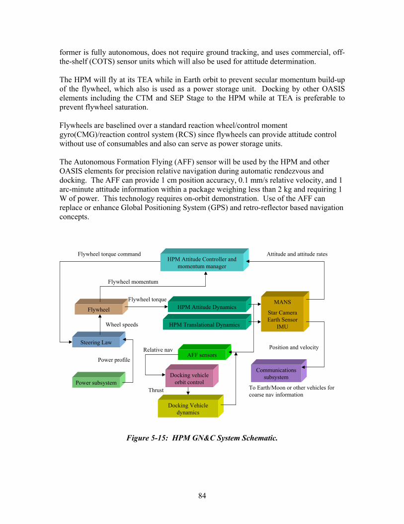
former is fully autonomous, does not require ground tracking, and uses commercial, off-the-shelf (COTS) sensor units which will also be used for attitude determination. The HPM will fly at its TEA while in Earth orbit to prevent secular momentum build-up of the flywheel, which also is used as a power storage unit. Docking by other OASIS elements including the CTM and SEP Stage to the HPM while at TEA is preferable to prevent flywheel saturation. Flywheels are baselined over a standard reaction wheel/control moment gyro(CMG)/reaction control system (RCS) since flywheels can provide attitude control without use of consumables and also can serve as power storage units. The Autonomous Formation Flying (AFF) sensor will be used by the HPM and other OASIS elements for precision relative navigation during automatic rendezvous and docking. The AFF can provide 1 cm position accuracy, 0.1 mm/s relative velocity, and 1 arc-minute attitude information within a package weighing less than 2 kg and requiring 1 W of power. This technology requires on-orbit demonstration. Use of the AFF can replace or enhance Global Positioning System (GPS) and retro-reflector based navigation concepts.
HPM Attitude Dynamics
HPM Translational Dynamics
MANS
Star Camera Earth Sensor
IMU
HPM Attitude Controller and momentum manager
Communications subsystem
To Earth/Moon or other vehicles for coarse nav information
Attitude and attitude rates
Position and velocity
Flywheel
Flywheel momentum
Flywheel torque
Steering Law
Flywheel torque command
Power subsystem
AFF sensors
Docking Vehicle dynamics
Docking vehicle orbit control
Power profile
Wheel speeds
Thrust
Relative nav
Figure 5-15: HPM GN&C System Schematic.
84

The AFF sensors for AR&D are baselined over GPS and retro-reflectors since these are fully autonomous, derived from GPS concepts, provide excellent accuracy, and can function outside of Earth orbit. AFF sensors are also low mass and require very little power. Technology Needs. A summary of the technology status of the MANS and AFF GN&C sensor suites is provided in table 5-8 below.
Table 5-8: HPM GN&C Technology Needs.
Technology
Summary Description of
Desired Technology and Key
Performance Metrics
Current TRL Where Who
Current Funding
($k)
Funding Increase Required
Applications of the
Technology other than
HPM
Microcosm Autonomous Navigation System (MANS)
Requires development of software, hardware definitions/interfaces, testing for deep space platforms. • 100 m position
information • 0.03 deg. Attitude
information • 11 kg and 28 W
based on sensor suite used
5 Micro-cosm, Inc.
Gwynne Gurevich
TBD; may use NASA SBIR
Small
Attitude and position info for any near-Earth or deep space space craft
Autonomous Formation Flying (AFF)
Based on GPS technology and can work in deep space with or without GPS satellites. Needs onboard implementation and testing. • 1 cm relative
position • 0.1 mm/sec
relative velocity • 1 arc-minute
attitude • 1 W average
power • < 2 kg mass
3 JPL Kenneth Lau
Initial NASA funding complete
Small
In-space rendezvous and docking applications; formation flying applications
85

5.1.2.4 Command and Data Handling/Communication and Tracking System The HPM Command and Data Handling (C&DH)/Communications and Tracking (C&T) system provides health and status information for the onboard systems and supports minimal command capability and standard Deep Space Network (DSN) tracking services. This system must also support GN&C functions while the HPM is in free flight mode. The HPM C&DH system must be capable of storing telemetry and command data for up to one day to provide communication link outage protection and for commands that are stored for later execution during autonomous operations or failure situations. When the HPM is attached to crewed vehicles including the CTV and ISS, it must interface with these vehicles for data transfer. Since these vehicles will have much higher data rate requirements, it is assumed that they will be responsible for transferring data to the ground when the HPM is attached since only a single vehicle at a time should have an active link with the ground. When the HPM is not attached to a crewed vehicle and in free flight mode, it will transfer data via the DSN. The HPM C&DH/C&T systems will also interface with uncrewed OASIS propulsive elements including the CTM and SEP Stage. When in a stack configuration, these propulsive elements will be responsible for command and data transfer functions. System Requirements. The HPM top-level C&T and C&DH system requirements are listed in table 5-9 below.
Table 5-9: HPM C&DH/C&T System Requirements. The HPM C&T system shall provide communications with the Earth during all critical phases. HPM shall have the capability to communicate from any mission location with a 3 dB link margin. The HPM C&T system shall transmit data through a DSN compatible transmitter. During the usable communications window, transmitted data shall be capable of being received by the DSN with a bit error rate (BER) no greater than 10-6 after error detection and correction. The HPM communications system shall support a maximum uplink rate of 1 kbps. The HPM communications system shall support a maximum downlink rate of 2 kbps. The HPM C&DH system shall control all HPM functions autonomously and/or by command. The HPM C&DH/C&T systems shall autonomously detect, report, and recover from hardware and software failures to ensure the continued operation and safety of the HPM. The HPM C&DH system shall be capable of storing telemetry and command data for up to one day. The HPM C&DH system shall provide a housekeeping data set for health and status of all systems. HPM telemetry data shall be provided in sufficient detail to evaluate the health and operating status of the HPM and to diagnose any problems that might arise. System Description. Given the system requirements for the HPM C&DH/C&T systems, these will be relatively simple with low mass and power requirements. The data rate requirements of the systems are low allowing the use of low gain patch antennas and medium gain horn
86
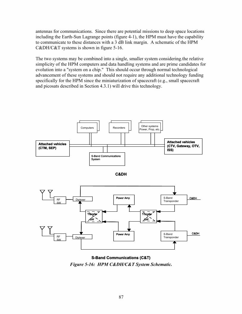
antennas for communications. Since there are potential missions to deep space locations including the Earth-Sun Lagrange points (figure 4-1), the HPM must have the capability to communicate to these distances with a 3 dB link margin. A schematic of the HPM C&DH/C&T systems is shown in figure 5-16. The two systems may be combined into a single, smaller system considering.the relative simplicity of the HPM computers and data handling systems and are prime candidates for evolution into a "system on a chip." This should occur through normal technological advancement of these systems and should not require any additional technology funding specifically for the HPM since the miniaturization of spacecraft (e.g., small spacecraft and picosats described in Section 4.3.1) will drive this technology.
Attached vehicles(CTM, SEP)
S-Band Communications System
Computers Recorders Other systemsPower, Prop, etc.
Attached vehicles(CTV, Gateway, OTV, ISS)
Power Amp
Transfer
SW
Power Amp C&DH
Diplexer
DiplexerRF SW
RF SW
S-Band Transponder
S-Band Transponder
C&DH
SW
Transfer
C&DH
S-Band Communications (C&T)
Attached vehicles(CTM, SEP)
S-Band Communications System
Computers Recorders Other systemsPower, Prop, etc.
Attached vehicles(CTV, Gateway, OTV, ISS)
Power Amp
Transfer
SW
Power Amp C&DH
Diplexer
DiplexerRF SW
RF SW
S-Band Transponder
S-Band Transponder
C&DH
SW
Transfer
Power Amp
Transfer
SW
Power Amp C&DH
Diplexer
DiplexerRF SW
RF SW
S-Band Transponder
S-Band Transponder
C&DH
SW
Transfer
C&DH
S-Band Communications (C&T) Figure 5-16: HPM C&DH/C&T System Schematic.
87
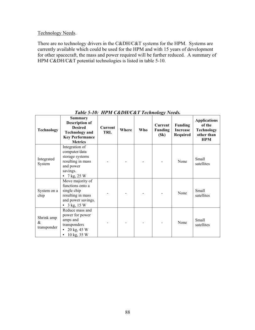
Technology Needs. There are no technology drivers in the C&DH/C&T systems for the HPM. Systems are currently available which could be used for the HPM and with 15 years of development for other spacecraft, the mass and power required will be further reduced. A summary of HPM C&DH/C&T potential technologies is listed in table 5-10.
Table 5-10: HPM C&DH/C&T Technology Needs.
Technology
Summary Description of
Desired Technology and
Key Performance Metrics
Current TRL Where Who
Current Funding
($k)
Funding Increase Required
Applications of the
Technology other than
HPM
Integrated System
Integration of computer/data storage systems resulting in mass and power savings. • 7 kg, 25 W
- - - - None Small satellites
System on a chip
Move majority of functions onto a single chip resulting in mass and power savings. • 3 kg, 15 W
- - - - None Small satellites
Shrink amp & transponder
Reduce mass and power for power amps and transponders • 20 kg, 45 W • 10 kg, 35 W
- - - - None Small satellites
88

5.1.2.5 Electrical Power System The HPM electrical power system (EPS) provides power generation for the HPM (housekeeping); energy storage for the HPM during shadow, and power processing. The thermal control subsystem of the HPM EPS provides the required heat rejection capability. As a means to maximize the efficiency of the HPM systems, the flywheel-based energy storage system also provides momentum management in LEO for attitude control. System Requirements. The principal EPS requirements are given in table 5-11.
Table 5-11: HPM EPS Requirements. System Performance
• 10.1 KWe power generation capacity • 0.5 KWt heat rejection capacity • 5.5 KWh energy storage capacity • 1,000 N-m-sec momentum control
Minimal system mass and volume. High reliability; cycling capability. Radiation degradation resistant for system lifetime of 10 years. Capable of power generation with arrays stowed (at reduced level). Redeployable photovoltaic arrays (stowed during CTM maneuvers). System Design. A schematic of the HPM EPS is shown in figure 5-17. EPS performance specifications as a function of technology availability (i.e., funding level and development schedule) is given in table 5-12.
Flywheels
Solar Array
Charge/Discharge
System
Thermal control
Solar Array
Power ProcessingPower Regulation & Control
Power Distribution
To Spacecraft Bus
Figure 5-17: HPM EPS Schematic.
89

Table 5-12: HPM EPS Performance Specifications. Power Generation Specific Power
(Array-level) Efficiency
Multiple Band Gap (MBG) Crystalline PV Thin Film PV
200 W/kg 200 W/kg
30% 10%
MBG Crystalline PV Thin Film PV
250 W/kg 270 W/kg
40% 15%
Thin Film PV Advanced Array Designs Quantum Dots (high risk/high potential technology)
600 W/kg >400 W/kg >500 W/kg
20% >40% 60%
Energy Storage Specific Energy Cycle Lifetime/ Efficiency Depth of Discharge
Li-based Batteries1
Century Flywheel2
Active Dedicated RFC3
100 Wh/kg 45 Wh/kg
400 Wh/kg
30 kCyc. 75 kCyc. 55% Eff.
60% 89%
- Li-based Batteries1 Advanced Flywheel2 Passive Unitized RFC3
200 Wh/kg 100 Wh/kg
1000 Wh/kg
30 kCyc. 75 kCyc. 65% Eff.
70% 89%
- Full Polymer Batteries1 Future Flywheel2 Passive Unitized RFC3
300 Wh/kg 150 Wh/kg
>1000 Wh/kg
20 Yrs. (Geo) >95 kCyc. 80% Eff.
70% 90%
- Power Processing Specific Energy Efficiency Temperature
Converter w/Active Control 300V Power Distribution
0.5 kW/kg 0.3 kW/kg
90% -
125° C -
Modular, High-Temp. Converters 600V Power Distribution
1.5 kW/kg 0.7 kW/kg
95% -
225° C -
High-Temp. PMAD System 1200 V Power Distribution
3.0 kW/kg 1.4kW/kg
95% -
350° C -
Technologies expected to be available on schedule with current funding profile. Technologies requiring additional funding beyond current funding profile for on-schedule availability. Technologies requiring substantial funding and additional development time beyond HPM schedule. 1Does not include power electronics mass. 2Includes power electronics mass. 3Regenerative fuel cell: specific energy is a function of discharge time. Solar Arrays. The solar arrays utilize advanced high efficiency GaAs-based multi-junction photovoltaic cells to reduce the array mass. The cells are encapsulated in a protective coating to prevent arcing. The cells are assumed to have an efficiency of 41% at AM0 and 28 °C. This efficiency is projected to drop to approximately 32% in space due to beginning of life (BOL) knockdowns and environmental factors. The cells are mounted on the panel blanket with a packing factor of 85%. The specific energy of the photovoltaic (PV) cells at this blanket level is estimated to be 587 W/kg. The cells are mounted on an aluminum honey-comb rigid panel that will provide the strength required during launch and high thrust chemical transfers. The two solar array wings are composed of three parallel sections each. Each section is 3.4 m long by 1.1 m wide. Sections are attached to its neighbor with hinge connections that allow the wing to be deformed for secure attachment to the exterior surface of the HPM body for packaging during launch and high thrust chemical transfer.
90

Each wing is attached to a solar array drive assembly (SADA) which provides single-axis gimbaling capability and power transfer. The SADA is attached to a short rigid boom that positions the wing at a safe distance from the HPM structure. On the opposite end of the boom is a single axis wrist joint that moves the wing from its secured position to the operating position orthogonal to the HPM surface. The specific energy of the photovoltaic arrays including the SADA is estimated to be 91 W/kg. When the wings are folded along the HPM surface, they will be mechanically secured by a series of latching mechanisms. These mechanisms grab the edge of the arrays to hold them in place. Power Management and Distribution. The power management and distribution (PMAD) subsystem for the arrays consist of a power distribution unit that distributes current collected from the array to the power inputs in the HPM. The arrays and PMAD are assumed to be operating nominally at 120 V to reduce the mass contribution of power distribution (i.e., cabling). Cabling into the PMAD unit is included in this system. The efficiency of the PMAD is projected to be 95%. Heat generated by the PMAD will be removed from the systems through the thermal control system. Thermal Control Subsystem. The thermal control subsystem (TCS) serves to remove heat generated by the PMAD boxes. A simplified TCS is used which consists of two elements:
• A Radiator. A single radiator panel, approximately 1 m wide by 0.6 m long, is mounted to the base pallet and oriented so that it can radiate to space for a majority of each orbit.
• A Loop Heat Pipe System. Heat from each PMAD box is transferred to the
radiator wing by a passive loop heat pipe system. Energy Storage System. The energy storage requirements for the HPM EPS are supplied by a flywheel-based system known as the integrated power and attitude control system (IPACS). The IPACS uses the characteristics of a flywheel to provide both energy storage and momentum bias for attitude control. The IPACS is expected to provide capability for both functions more efficiently than having two separate systems on the spacecraft. The IPACS is required to provide 1,000 N-m-sec of momentum control and 5,500 W-hrs of energy storage. An IPACS composite rotor wheel system was sized for the HPM vehicle. The combined energy storage requirement, momentum control requirement, and wheel material characteristics establish the IPACS mass. The wheels selected are made of carbon composite with an ultimate strength de-rating of 2.0 to ensure long life operation. The
91
wheels are arranged in a skew symmetric configuration which has a wheel located on each of the upright faces of a pyramid and redundant wheel facing downward on the base. This configuration allows momentum control and energy storage to be controlled independently. An optimization was performed which traded maximum/minimum speed of the wheel and the motor size based on torque output. As the max/min speed range increases, more energy is extracted from each flywheel. However, the motor size for each wheel is based on the torque so that decreases in motor speed lead to increases in torque and, therefore, increases in mass of the motor for the same power extraction. The IPACS designed for this mission has a total system mass of 136 kg. The specific energy of the IPACS is projected to be 37 W-hrs/kg. A representative aluminum housing was assumed for the IPACS and incorporated into the system mass. On-board electronics will control the motors on each of the flywheels within the IPACS to spin up or down to meet the attitude and/or energy handling requirements. A set of one-time use batteries to be used for initial flywheel spin-up is incorporated into this system. Technology Needs. A summary of technology development requirements for the HPM EPS is listed in table 5-13.
92
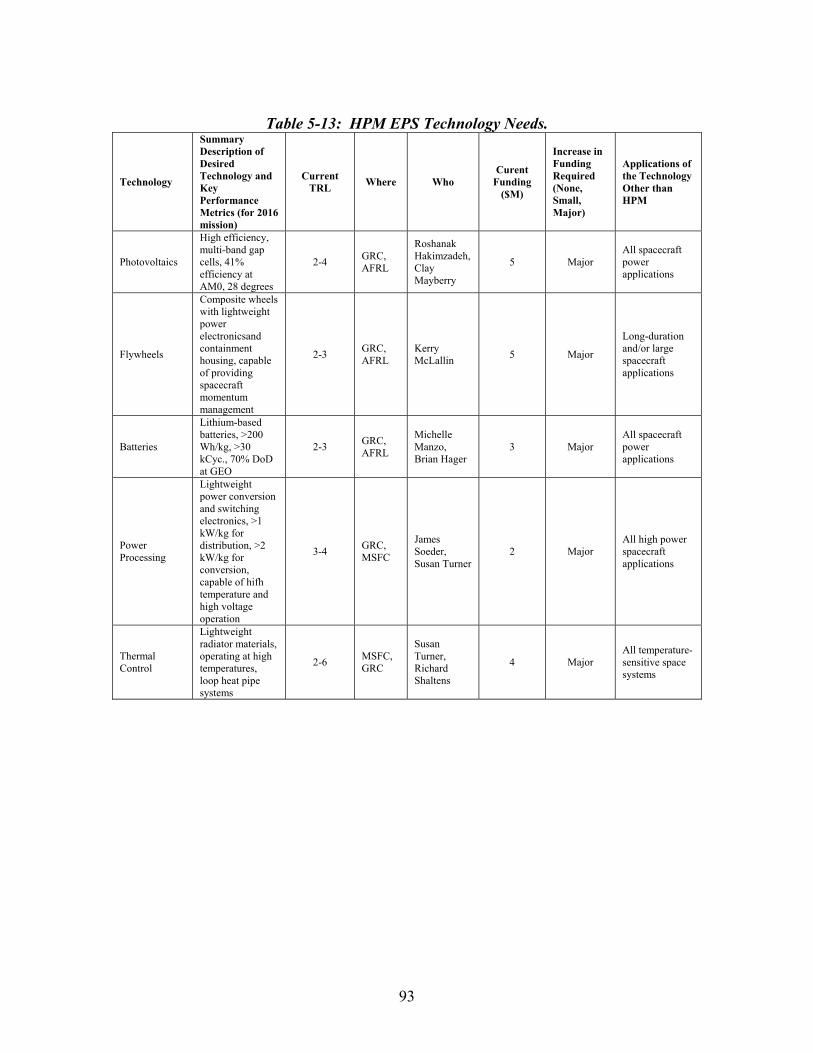
Table 5-13: HPM EPS Technology Needs.
Technology
Summary Description of Desired Technology and Key Performance Metrics (for 2016 mission)
Current TRL Where Who
Curent Funding
($M)
Increase in Funding Required (None, Small, Major)
Applications of the Technology Other than HPM
Photovoltaics
High efficiency, multi-band gap cells, 41% efficiency at AM0, 28 degrees
2-4 GRC, AFRL
Roshanak Hakimzadeh, Clay Mayberry
5 Major All spacecraft power applications
Flywheels
Composite wheels with lightweight power electronicsand containment housing, capable of providing spacecraft momentum management
2-3 GRC, AFRL
Kerry McLallin 5 Major
Long-duration and/or large spacecraft applications
Batteries
Lithium-based batteries, >200 Wh/kg, >30 kCyc., 70% DoD at GEO
2-3 GRC, AFRL
Michelle Manzo, Brian Hager
3 Major All spacecraft power applications
Power Processing
Lightweight power conversion and switching electronics, >1 kW/kg for distribution, >2 kW/kg for conversion, capable of hifh temperature and high voltage operation
3-4 GRC, MSFC
James Soeder, Susan Turner
2 Major All high power spacecraft applications
Thermal Control
Lightweight radiator materials, operating at high temperatures, loop heat pipe systems
2-6 MSFC, GRC
Susan Turner, Richard Shaltens
4 Major All temperature-sensitive space systems
93
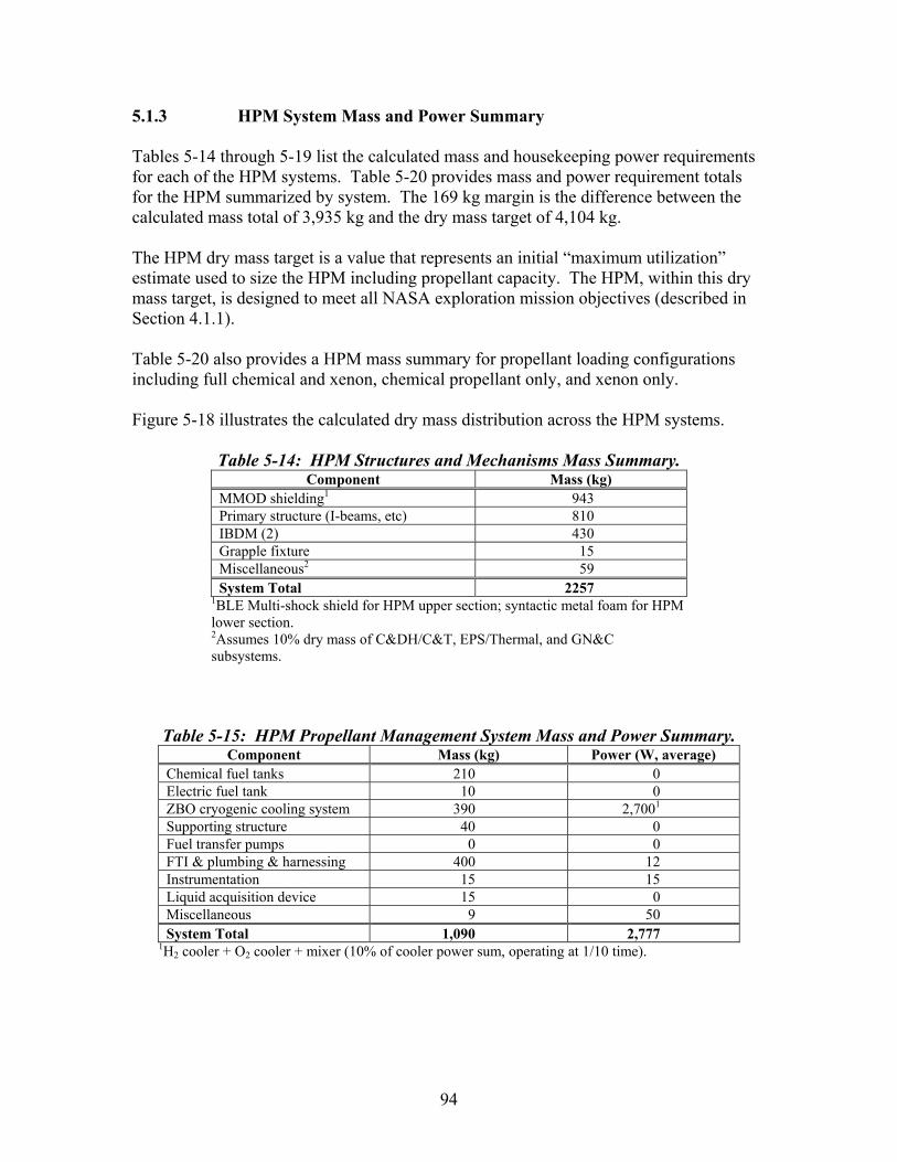
5.1.3 HPM System Mass and Power Summary Tables 5-14 through 5-19 list the calculated mass and housekeeping power requirements for each of the HPM systems. Table 5-20 provides mass and power requirement totals for the HPM summarized by system. The 169 kg margin is the difference between the calculated mass total of 3,935 kg and the dry mass target of 4,104 kg. The HPM dry mass target is a value that represents an initial “maximum utilization” estimate used to size the HPM including propellant capacity. The HPM, within this dry mass target, is designed to meet all NASA exploration mission objectives (described in Section 4.1.1). Table 5-20 also provides a HPM mass summary for propellant loading configurations including full chemical and xenon, chemical propellant only, and xenon only. Figure 5-18 illustrates the calculated dry mass distribution across the HPM systems.
Table 5-14: HPM Structures and Mechanisms Mass Summary. Component Mass (kg)
MMOD shielding1 943
Primary structure (I-beams, etc) 810 IBDM (2) 430 Grapple fixture 15 Miscellaneous2 59 System Total 2257
1BLE Multi-shock shield for HPM upper section; syntactic metal foam for HPM lower section. 2Assumes 10% dry mass of C&DH/C&T, EPS/Thermal, and GN&C subsystems.
Table 5-15: HPM Propellant Management System Mass and Power Summary. Component Mass (kg) Power (W, average)
Chemical fuel tanks 210 0 Electric fuel tank 10 0 ZBO cryogenic cooling system 390 2,7001
Supporting structure 40 0 Fuel transfer pumps 0 0 FTI & plumbing & harnessing 400 12 Instrumentation 15 15 Liquid acquisition device 15 0 Miscellaneous 9 50 System Total 1,090 2,777
1H2 cooler + O2 cooler + mixer (10% of cooler power sum, operating at 1/10 time).
94
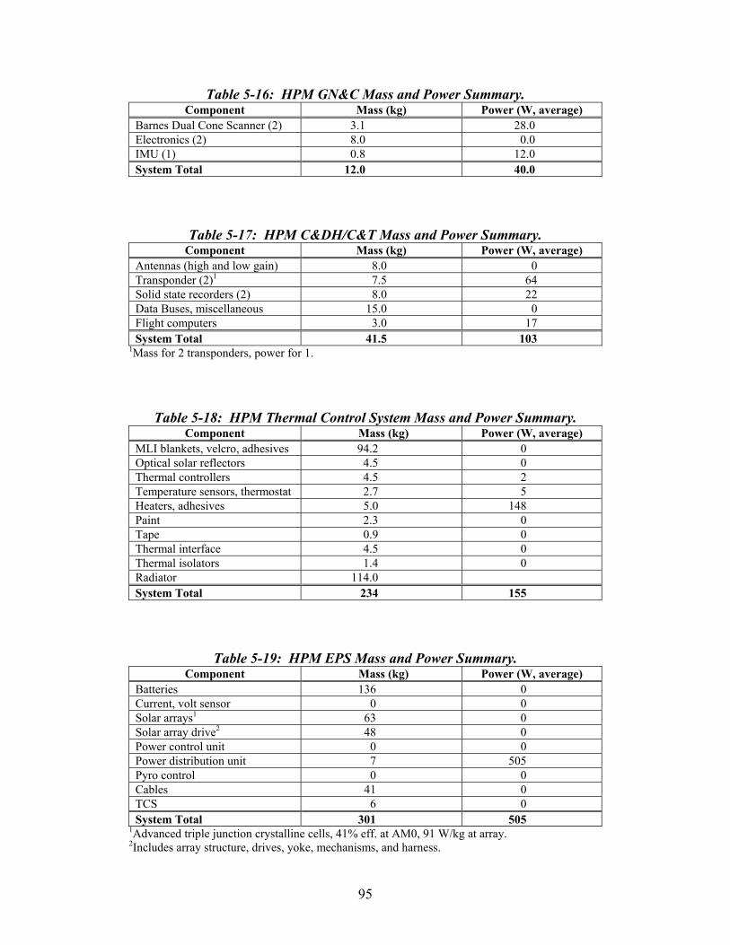
Table 5-16: HPM GN&C Mass and Power Summary. Component Mass (kg) Power (W, average)
Barnes Dual Cone Scanner (2) 3.1 28.0 Electronics (2) 8.0 0.0 IMU (1) 0.8 12.0 System Total 12.0 40.0
Table 5-17: HPM C&DH/C&T Mass and Power Summary. Component Mass (kg) Power (W, average)
Antennas (high and low gain) 8.0 0 Transponder (2)1 7.5 64 Solid state recorders (2) 8.0 22 Data Buses, miscellaneous 15.0 0 Flight computers 3.0 17 System Total 41.5 103
1Mass for 2 transponders, power for 1.
Table 5-18: HPM Thermal Control System Mass and Power Summary. Component Mass (kg) Power (W, average)
MLI blankets, velcro, adhesives 94.2 0 Optical solar reflectors 4.5 0 Thermal controllers 4.5 2 Temperature sensors, thermostat 2.7 5 Heaters, adhesives 5.0 148 Paint 2.3 0 Tape 0.9 0 Thermal interface 4.5 0 Thermal isolators 1.4 0 Radiator 114.0 System Total 234 155
Table 5-19: HPM EPS Mass and Power Summary. Component Mass (kg) Power (W, average)
Batteries 136 0 Current, volt sensor 0 0 Solar arrays1 63 0 Solar array drive2 48 0 Power control unit 0 0 Power distribution unit 7 505 Pyro control 0 0 Cables 41 0 TCS 6 0 System Total 301 505
1Advanced triple junction crystalline cells, 41% eff. at AM0, 91 W/kg at array. 2Includes array structure, drives, yoke, mechanisms, and harness.
95
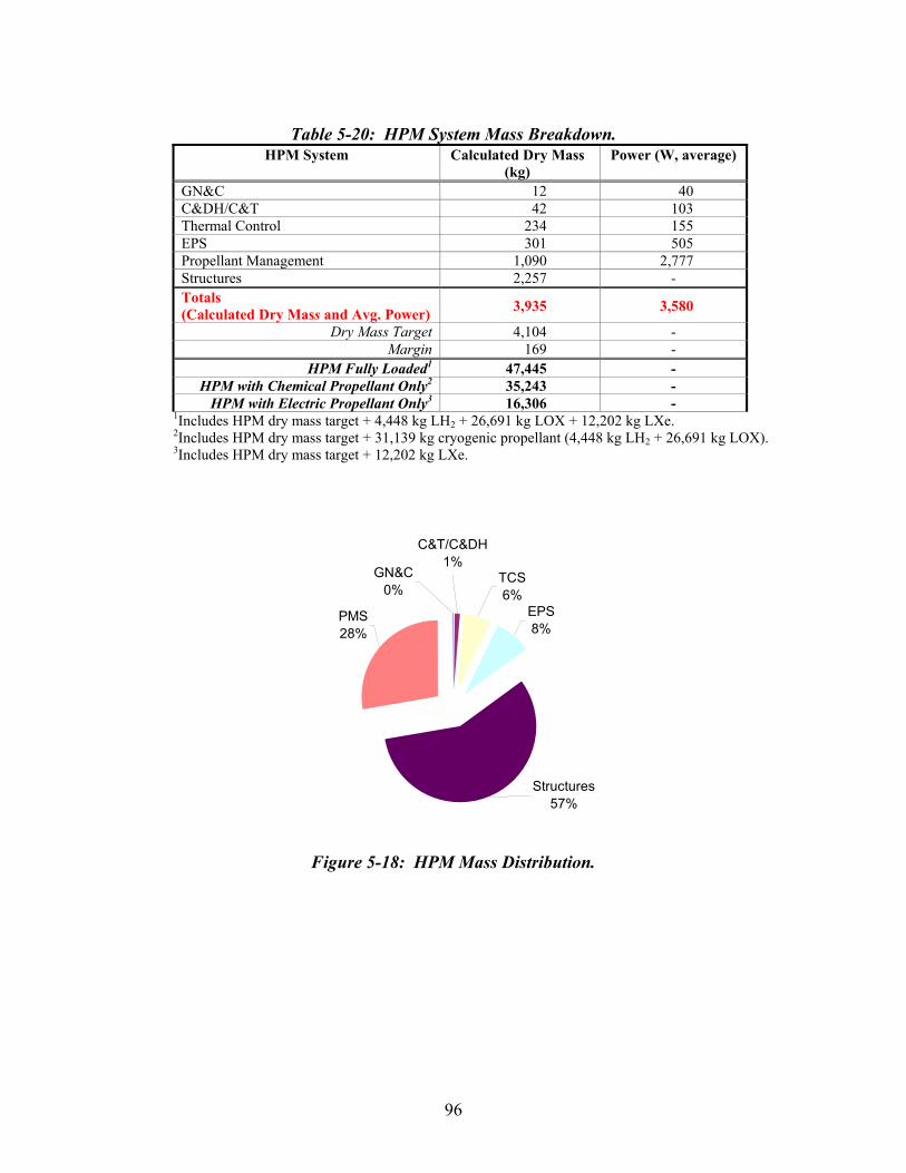
Table 5-20: HPM System Mass Breakdown.
HPM System Calculated Dry Mass (kg)
Power (W, average)
GN&C 12 40 C&DH/C&T 42 103 Thermal Control 234 155 EPS 301 505 Propellant Management 1,090 2,777 Structures 2,257 - Totals (Calculated Dry Mass and Avg. Power) 3,935 3,580
Dry Mass Target 4,104 - Margin 169 -
HPM Fully Loaded1 47,445 - HPM with Chemical Propellant Only2 35,243 -
HPM with Electric Propellant Only3 16,306 - 1Includes HPM dry mass target + 4,448 kg LH2 + 26,691 kg LOX + 12,202 kg LXe. 2Includes HPM dry mass target + 31,139 kg cryogenic propellant (4,448 kg LH2 + 26,691 kg LOX). 3Includes HPM dry mass target + 12,202 kg LXe.
Structures57%
PMS28%
EPS8%
C&T/C&DH1%
TCS6%
GN&C0%
Figure 5-18: HPM Mass Distribution.
96

5.1.3 Operations See Section 4.1.1 for a discussion of HPM operations in support of the Earth-Moon L1 mission.
97

This page intentionally left blank
98

5.2 Chemical Transfer Module The Chemical Transfer Module (CTM, figure 5-19) serves as a high energy injection stage when attached to an HPM and an autonomous orbital maneuvering vehicle for proximity operations such as ferrying payloads a short distance, refueling and servicing. It has high thrust H2O2 engines for orbit transfers and high-pressure H2O2 thrusters for proximity operations and small delta-V translational or rotational maneuvers. It is capable of transferring and storing approximately 3,000 kg of cryogenic hydrogen and oxygen. The main engines can use the stored cryogens or utilize propellant directly transferred from the HPM. Unlike the HPM, the CTM does not incorporate zero boil-off technology.
Figure 5-19: Chemical Transfer Module.
5.2.1 Configuration & System Packaging The CTM is designed for launch by a Shuttle-class launch vehicle. Four active longeron trunnions and a single keel trunnion support the CTM in the launch vehicle cargo bay. The CTM configuration and packaging concept is shown in figure 5-20.
99

Solar Array (2 plcs) (410 cm x 100 cm)
Docking Adapter
Active Longeron Trunnions (4 plcs)
Tri-Pod RCS Thrusters (2 plcs)
RL10 67 KN Class Engine (2 plcs)
Thrust Structure MMOD
Interstage MMOD
Forward Skirt MMOD
Approx. Overall Deployed Dimensions: 9.4 m long x 12.6 m width
Radiator (2 plcs) (127 cm x 91 cm)
Tri-Pod RCS Thrusters (2 plcs)
Tri-Pod Cold Gas Thrusters (2 plcs)
Tri-Pod Cold Gas Thrusters (2 plcs)
Star Sensor (Earth Sensor Located 180 deg)
AFF Receive Antenna (3 plcs)
Avionics ORUs
AFF Transmit AntennaMANS Scanners (4 plcs)
AFF Receive Antenna (3 plcs)
AFF Transmit Antenna
Thrust Structure MMOD
Solar Array (2 plcs) (410 cm x 100 cm)
Docking Adapter
Active Longeron Trunnions (4 plcs)
Tri-Pod RCS Thrusters (2 plcs)
RL10 67 KN Class Engine (2 plcs)
LH2 Tank (279 cm dia. x 210 cm long)
Xenon Tank (2 plcs) (91 cm dia. x 94 cm long)
LOX Tank (201 cm dia. x 150 cm long)
NOTE: MMOD SHOWN TRANSPARENT FOR CLARITY.
Tri-Pod RCS Thrusters(2 plcs)
Tri-Pod Cold Gas Thrusters (2 plcs)
Tri-Pod Cold Gas Thrusters (2 plcs)
RCS Tank (74 cm dia.) (GO2 Tank 1 plc and GH2 Tank 6 plcs)
LOX Feedline (6.4 cm dia.)
LH2 Feedline (6.4 cm dia.)
AFF Transmit Antenna
MANS Scanners (4 plcs)
Star Sensor (Earth Sensor Located 180 deg)
AFF Transmit Antenna
AFF Receive Antenna (3 plcs)
AFF Receive Antenna (3 plcs)
Solar Array (2 plcs) (410 cm x 100 cm)
Docking Adapter
Active Longeron Trunnions (4 plcs)Active Longeron Trunnions (4 plcs)
Tri-Pod RCS Thrusters (2 plcs)
RL10 67 KN Class Engine (2 plcs)
LH2 Tank (279 cm dia. x 210 cm long)
Xenon Tank (2 plcs) (91 cm dia. x 94 cm long)Xenon Tank (2 plcs) (91 cm dia. x 94 cm long)
LOX Tank (201 cm dia. x 150 cm long)
NOTE: MMOD SHOWN TRANSPARENT FOR CLARITY.
Tri-Pod RCS Thrusters(2 plcs)
Tri-Pod Cold Gas Thrusters (2 plcs)
Tri-Pod Cold Gas Thrusters (2 plcs)
RCS Tank (74 cm dia.) (GO2 Tank 1 plc and GH2 Tank 6 plcs)
LOX Feedline (6.4 cm dia.)
LH2 Feedline (6.4 cm dia.)
AFF Transmit Antenna
MANS Scanners (4 plcs)
Star Sensor (Earth Sensor Located 180 deg)Star Sensor (Earth Sensor Located 180 deg)
AFF Transmit Antenna
AFF Receive Antenna (3 plcs)
AFF Receive Antenna (3 plcs)
Figure 20: CTM Configuration and Packaging.
100

The CTM deployed length is approximately 9.4 meters. The CTM width, with solar arrays deployed, is approximately 12.6 meters. The major components of the CTM are:
• Dual RL10 67 kN-class engines
• Liquid oxygen (LOX) tank
• Liquid hydrogen (LH2) tank
• Gaseous oxygen (GOX) RCS tank
• Six gaseous hydrogen (GH2) RCS tanks
• Two deployable solar arrays
• Avionics ORUs
• Two radiator panels
• Four sets of tri-pod RCS thrusters
• Four sets of tri-pod cold gas thrusters
• Docking adapter. The dual RL10 engines are mounted twenty degrees off the CTM centerline on a fixed thrust structure. Two engines are required to satisfy reliability requirements. Since only one engine is used at a time, the thrust structure and the two engines are rotated as a single unit such that the firing engine thrust vector is aligned with the vehicle center of gravity. A new development gimbal system is required to accomplish this operation. Two sets of tri-pod RCS thrusters and two sets of tri-pod cold gas thrusters are mounted on the aft end of the CTM. The thruster pods are all canted forty-five degrees to avoid plume impingement on the CTM thrust structure MMOD shield. Two sets of tri-pod RCS thrusters and two sets of tri-pod cold gas thrusters are mounted on the forward end of the CTM. These thruster pods are mounted on fixed booms and canted forty-five degrees to prevent plume impingement on an attached HPM. MMOD shielding encloses the CTM tankage and plumbing to satisfy safety requirements. The avionics ORUs are packaged in the forward skirt to avoid the adverse thermal environment in the vicinity of the RL10 engines.
101
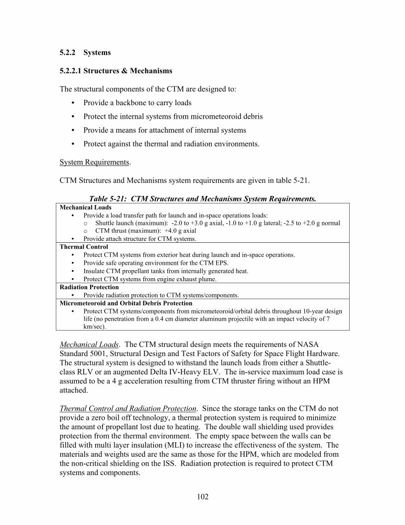
5.2.2 Systems 5.2.2.1 Structures & Mechanisms The structural components of the CTM are designed to:
• Provide a backbone to carry loads
• Protect the internal systems from micrometeoroid debris
• Provide a means for attachment of internal systems
• Protect against the thermal and radiation environments. System Requirements. CTM Structures and Mechanisms system requirements are given in table 5-21.
Table 5-21: CTM Structures and Mechanisms System Requirements. Mechanical Loads
• Provide a load transfer path for launch and in-space operations loads: o Shuttle launch (maximum): -2.0 to +3.0 g axial, -1.0 to +1.0 g lateral; -2.5 to +2.0 g normal o CTM thrust (maximum): +4.0 g axial
• Provide attach structure for CTM systems. Thermal Control
• Protect CTM systems from exterior heat during launch and in-space operations. • Provide safe operating environment for the CTM EPS. • Insulate CTM propellant tanks from internally generated heat. • Protect CTM systems from engine exhaust plume.
Radiation Protection • Provide radiation protection to CTM systems/components.
Micrometeoroid and Orbital Debris Protection • Protect CTM systems/components from micrometeoroid/orbital debris throughout 10-year design
life (no penetration from a 0.4 cm diameter aluminum projectile with an impact velocity of 7 km/sec).
Mechanical Loads. The CTM structural design meets the requirements of NASA Standard 5001, Structural Design and Test Factors of Safety for Space Flight Hardware. The structural system is designed to withstand the launch loads from either a Shuttle-class RLV or an augmented Delta IV-Heavy ELV. The in-service maximum load case is assumed to be a 4 g acceleration resulting from CTM thruster firing without an HPM attached. Thermal Control and Radiation Protection. Since the storage tanks on the CTM do not provide a zero boil off technology, a thermal protection system is required to minimize the amount of propellant lost due to heating. The double wall shielding used provides protection from the thermal environment. The empty space between the walls can be filled with multi layer insulation (MLI) to increase the effectiveness of the system. The materials and weights used are the same as those for the HPM, which are modeled from the non-critical shielding on the ISS. Radiation protection is required to protect CTM systems and components.
102
Micrometeoroid and Orbital Debris Protection. The exterior of the CTM is comprised of two layers of syntactic aluminum foam filled with thermal blankets to protect the central elements of the CTM from MMOD impacts. To allow on orbit accessibility to the internal ORUs, a constant outer shell diameter is required. A Whipple shield system is used on the CTM similar to the lower section of the HPM. System Description. The CTM primary structure is made of long carbon fiber metal matrix composites (MMC) that provide a strength to weight ratio three times better than spacecraft aluminum. A Whipple type debris shield is used to protect the CTM from MMOD and incorporates materials to help with thermal control and radiation protection. The CTM connects to the HPM or ISS through the IBDM and is outfitted with a fluid transfer interface so that it may utilizeHPM-provided propellant. An engine mount gimbal mechanism is used to rotate the thrust structure/engine assembly for proper engine alignment. The engines mounts, engine alignment struts and IBDM connection points are MMC structural shapes that allow the loads to transfer into the reinforced shell structure. Trunion fittings are required for launch systems and connect directly to the ring frames under the shield skin. Technology Needs. An integrated primary multifunction structure including radiation protection and MMOD shielding is a structural system technology requirement for all OASIS elements. See table 5-2, HPM Structures and Mechanisms Technology Needs, for a list of structures technologies also applicable to the CTM.
103
5.2.2.2 Guidance Navigation and Control The CTM guidance, navigation and control (GN&C) system will maintain CTM attitude in free flight mode and during automatic rendezvous and docking (AR&D) with other OASIS elements at these locations. System Requirements. The CTM GN&C system provides attitude (rotational) control in free flight and also performs positional (translation) maneuvers to rendezvous with other OASIS elements such as the HPM. During AR&D operations with the HPM, the CTM is the active vehicle and HPM is the passive vehicle, which performs only attitude control. In a stack configuration with the HPM, the CTM is active with respect to the guidance and attitude control requirements of the stack. No GN&C functions are performed by the HPM. These requirements impose stringent attitude control and precise position knowledge requirements for the CTM as summarized in table 5-22.
Table 5-22: CTM GN&C System Requirements. The CTM GN&C system shall provide position and attitude information at any location. The CTM shall be capable of communicating its position and attitude to ground and/or transfer vehicles. The CTM GN&C system shall hold attitude to within +/- 0.5 degrees during automatic rendezvous and docking operations. The CTM shall be capable of attitude control to within +/- 5 degrees of any commanded attitude using Reaction Control System. System Description. Figure 5-21 provides a schematic of the CTM GN&C system. Attitude, attitude rates, position, velocity, and sun pointing of the CTM will be determined/provided using the Microcosm Autonomous Navigation System (MANS) sensor suite comprised of star sensor and Earth sensor with inertial measurement unit (IMU) as backup. The MANS suite can currently provide 100 m position information and 0.03 degree attitude information. The MANS suite is also lightweight and uses little power. While MANS is currently in use for Earth orbit applications, its extension to deep space is a new application which may require technology development and demonstration. Use of MANS as a component of the CTM GN&C system can replace radiometric and optical navigation methods. For fine relative navigation requirements during automatic rendezvous and docking, the CTM will utilize the Autonomous Formation Flyer (AFF) sensor. All orbit and attitude control will be performed by the CTM thrusters. Orbit & Attitude Control. Four sets GOX/GH2 thrusters with a 556 N thrust level, Isp of 385 seconds and minimum pulse duration of 30 ms are used for attitude control. Four
104
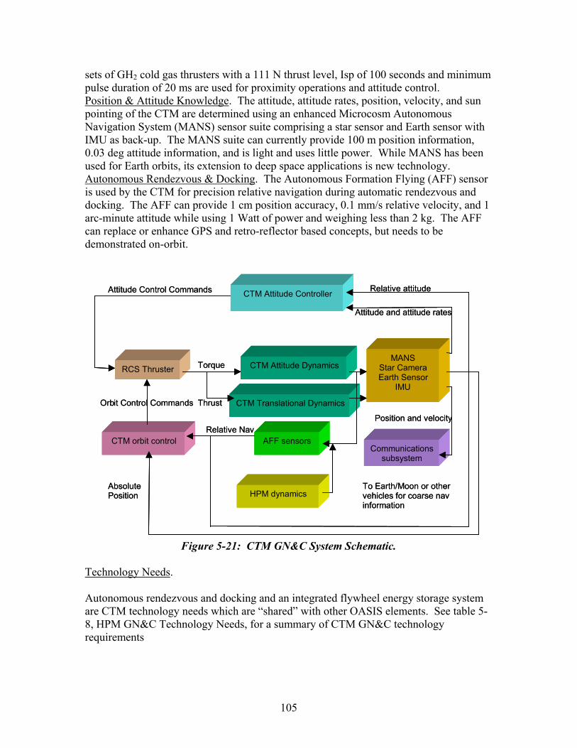
sets of GH2 cold gas thrusters with a 111 N thrust level, Isp of 100 seconds and minimum pulse duration of 20 ms are used for proximity operations and attitude control. Position & Attitude Knowledge. The attitude, attitude rates, position, velocity, and sun pointing of the CTM are determined using an enhanced Microcosm Autonomous Navigation System (MANS) sensor suite comprising a star sensor and Earth sensor with IMU as back-up. The MANS suite can currently provide 100 m position information, 0.03 deg attitude information, and is light and uses little power. While MANS has been used for Earth orbits, its extension to deep space applications is new technology. Autonomous Rendezvous & Docking. The Autonomous Formation Flying (AFF) sensor is used by the CTM for precision relative navigation during automatic rendezvous and docking. The AFF can provide 1 cm position accuracy, 0.1 mm/s relative velocity, and 1 arc-minute attitude while using 1 Watt of power and weighing less than 2 kg. The AFF can replace or enhance GPS and retro-reflector based concepts, but needs to be demonstrated on-orbit.
CTM Attitude Dynamics
CTM Translational Dynamics
MANSStar Camera Earth Sensor
IMU
CTM Attitude Controller
Communications subsystem
To Earth/Moon or other vehicles for coarse nav information
Attitude and attitude rates
Position and velocity
RCS Thruster Torque
Attitude Control Commands
AFF sensors
HPM dynamics
CTM orbit controlRelative Nav
Relative attitude
Orbit Control Commands
Absolute Position
Thrust
Figure 5-21: CTM GN&C System Schematic.
Technology Needs. Autonomous rendezvous and docking and an integrated flywheel energy storage system are CTM technology needs which are “shared” with other OASIS elements. See table 5-8, HPM GN&C Technology Needs, for a summary of CTM GN&C technology requirements
105

5.2.2.3 Command and Data Handling/Communication and Tracking System The CTM C&DH/C&T system provides health and status information for the onboard systems and supports GN&C functions, minimal command capability and standard Deep Space Network (DSN) tracking services. When the CTM is attached to the HPM and ISS, it must interface with these vehicles for data transfer. When the CTM is attached to the HPM, the CTM will be responsible for transferring data to the ground since only a single vehicle at a time should have an active ground link. System Requirements. CTM C&DH/C&T system requirements are listed in table 5-23.
Table 5-23: CTM C&DH/C&T System Requirements. The CTM C&T system shall provide communications with the Earth during all critical phases. The CTM shall have the capability to communicate from any mission location with a 3 dB link margin. The CTM C&T system shall transmit data through a DSN compatible transmitter. During the usable communications window, transmitted data shall be capable of being received by the DSN with a bit error rate (BER) no greater than 10-6 after error detection and correction. The CTM communications system shall support a maximum uplink rate of 1 kbps. The CTM communications system shall support a maximum downlink rate of 16 kbps. The CTM C&DH system shall control all CTM functions autonomously and/or by command. The CTM C&DH/C&T systems shall autonomously detect, report, and recover from hardware and software failures to ensure the continued operation and safety of the CTM. TheCTM C&DH system shall be capable of storing telemetry and command data for up to one day. The CTM C&DH system shall provide a housekeeping data set for health and status of all systems. CTM telemetry data shall be provided in sufficient detail to evaluate the health and operating status of the CTM and to diagnose any problems that might arise. System Description. The CTM C&DH system (figure 5-22) consists of three flight control computers, two remote multiplexers/demultiplexers (RMDMs), a collision-avoidance maneuver (CAM) MDM, a command and telemetry unit, and three dual redundant 1553 data buses. The flight control computers utilize an R3000/R3010 data processor with a throughput of approximately 20 million instructions per second. The RMDMs are smart remote terminals connected to each of the three buses and provide input/output (I/O) channels for interfacing with sensors and effectors that do not interface directly with the buses. The RMDMs are each housed in an MDM-10 chassis that can support up to 10 I/O cards. These boxes were chosen for commonality with the International Space Station.
106
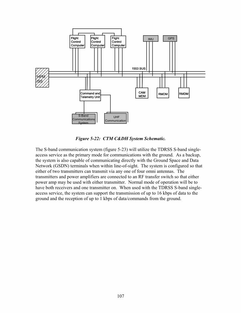
FlightControlComputer
FlightControlComputer
FlightControlComputer
1553 BUS
IMU
Command andTelemetry Unit
S-BandCommunications
System
UHFCommunication
CAMMDM
RMDM RMDM
HPMISS
GPSFlightControlComputer
FlightControlComputer
FlightControlComputer
1553 BUS
IMU
Command andTelemetry Unit
S-BandCommunications
System
UHFCommunication
CAMMDM
RMDM RMDM
HPMISS
GPS
Figure 5-22: CTM C&DH System Schematic.
The S-band communication system (figure 5-23) will utilize the TDRSS S-band single-access service as the primary mode for communications with the ground. As a backup, the system is also capable of communicating directly with the Ground Space and Data Network (GSDN) terminals when within line-of-sight. The system is configured so that either of two transmitters can transmit via any one of four omni antennas. The transmitters and power amplifiers are connected to an RF transfer switch so that either power amp may be used with either transmitter. Normal mode of operation will be to have both receivers and one transmitter on. When used with the TDRSS S-band single-access service, the system can support the transmission of up to 16 kbps of data to the ground and the reception of up to 1 kbps of data/commands from the ground.
107
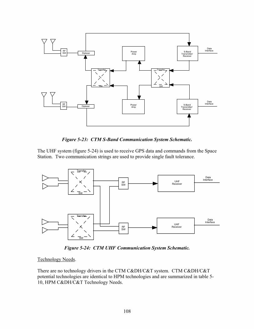
RF SW Diplexer Power
AmpS-Band
Transmitter/ Receiver
Data Interface
Transfer Transfer
SW SW
RF SW Diplexer Power
AmpS-Band
Transmitter/ Receiver
Data Interface
Figure 5-23: CTM S-Band Communication System Schematic. The UHF system (figure 5-24) is used to receive GPS data and commands from the Space Station. Two communication strings are used to provide single fault tolerance.
Transfer
SW
Transfer
SW
RF SW
RF SW
UHF Receiver
UHF Receiver
Data Interface
Data Interface
Figure 5-24: CTM UHF Communication System Schematic.
Technology Needs. There are no technology drivers in the CTM C&DH/C&T system. CTM C&DH/C&T potential technologies are identical to HPM technologies and are summarized in table 5-10, HPM C&DH/C&T Technology Needs.
108
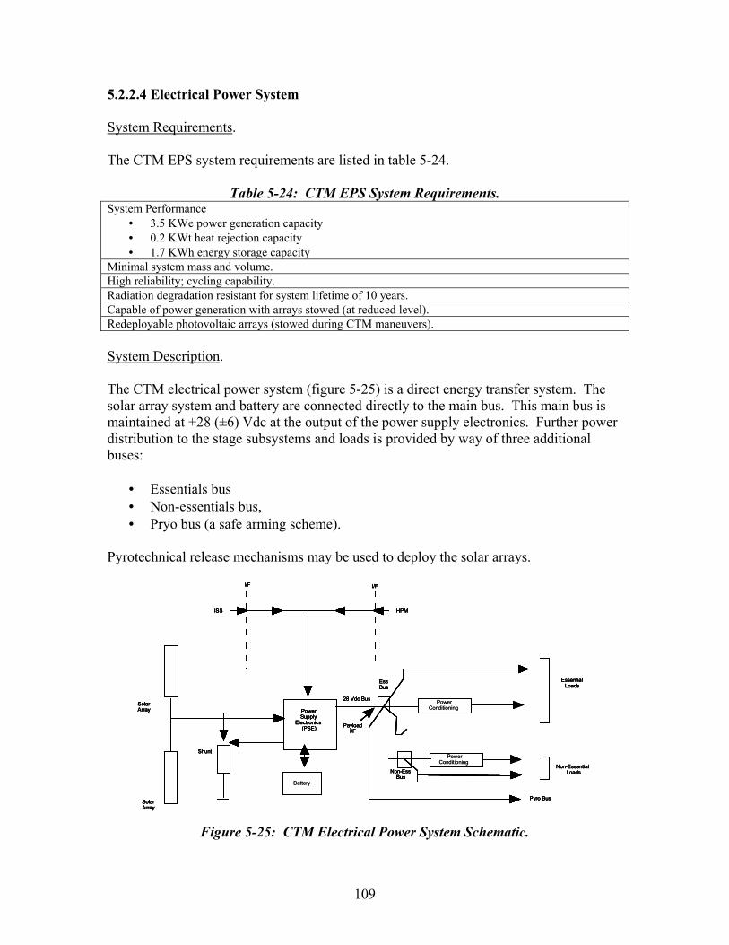
5.2.2.4 Electrical Power System System Requirements. The CTM EPS system requirements are listed in table 5-24.
Table 5-24: CTM EPS System Requirements. System Performance
• 3.5 KWe power generation capacity • 0.2 KWt heat rejection capacity • 1.7 KWh energy storage capacity
Minimal system mass and volume. High reliability; cycling capability. Radiation degradation resistant for system lifetime of 10 years. Capable of power generation with arrays stowed (at reduced level). Redeployable photovoltaic arrays (stowed during CTM maneuvers). System Description. The CTM electrical power system (figure 5-25) is a direct energy transfer system. The solar array system and battery are connected directly to the main bus. This main bus is maintained at +28 (±6) Vdc at the output of the power supply electronics. Further power distribution to the stage subsystems and loads is provided by way of three additional buses:
• Essentials bus • Non-essentials bus, • Pryo bus (a safe arming scheme).
Pyrotechnical release mechanisms may be used to deploy the solar arrays.
Pyro Bus
Solar Array
ISS HPM
Solar Array
Shunt
Power Supply
Electronics (PSE) Payload
I/F
28 Vdc Bus
Ess Bus
Non-Ess Bus
Essential Loads
Non-Essential Loads
I/F I/F
Pyro Bus
Solar Array
ISS HPM
Solar Array
Shunt
Power Supply
Electronics (PSE)
Battery
Payload I/F
28 Vdc Bus
Ess Bus
Power Conditioning
Power Conditioning
Non-Ess Bus
Essential Loads
Non-Essential Loads
I/F I/F
Pyro Bus
Solar Array
ISS HPM
Solar Array
Shunt
Power Supply
Electronics (PSE) Payload
I/F
28 Vdc Bus
Ess Bus
Non-Ess Bus
Essential Loads
Non-Essential Loads
I/F I/F
Pyro Bus
Solar Array
ISS HPM
Solar Array
Shunt
Power Supply
Electronics (PSE)
Battery
Payload I/F
28 Vdc Bus
Ess Bus
Power Conditioning
Power Conditioning
Non-Ess Bus
Essential Loads
Non-Essential Loads
I/F I/F
Figure 5-25: CTM Electrical Power System Schematic.
109

Technology Needs. There are no technology drivers in the CTM EPS system. For a summary of CTM EPS technology needs, refer to table 5-13, HPM EPS Technology Needs. With the exception of advanced flywheel technology, all HPM EPS technology needs are applicable to the CTM.
110
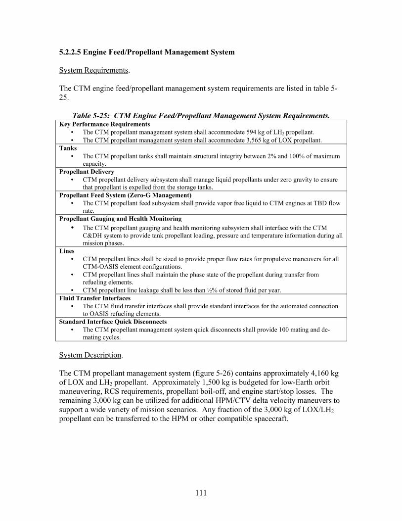
5.2.2.5 Engine Feed/Propellant Management System System Requirements. The CTM engine feed/propellant management system requirements are listed in table 5-25.
Table 5-25: CTM Engine Feed/Propellant Management System Requirements. Key Performance Requirements
• The CTM propellant management system shall accommodate 594 kg of LH2 propellant. • The CTM propellant management system shall accommodate 3,565 kg of LOX propellant.
Tanks • The CTM propellant tanks shall maintain structural integrity between 2% and 100% of maximum
capacity. Propellant Delivery
• CTM propellant delivery subsystem shall manage liquid propellants under zero gravity to ensure that propellant is expelled from the storage tanks.
Propellant Feed System (Zero-G Management) • The CTM propellant feed subsystem shall provide vapor free liquid to CTM engines at TBD flow
rate. Propellant Gauging and Health Monitoring
• The CTM propellant gauging and health monitoring subsystem shall interface with the CTM C&DH system to provide tank propellant loading, pressure and temperature information during all mission phases.
Lines • CTM propellant lines shall be sized to provide proper flow rates for propulsive maneuvers for all
CTM-OASIS element configurations. • CTM propellant lines shall maintain the phase state of the propellant during transfer from
refueling elements. • CTM propellant line leakage shall be less than ½% of stored fluid per year.
Fluid Transfer Interfaces • The CTM fluid transfer interfaces shall provide standard interfaces for the automated connection
to OASIS refueling elements. Standard Interface Quick Disconnects
• The CTM propellant management system quick disconnects shall provide 100 mating and de-mating cycles.
System Description. The CTM propellant management system (figure 5-26) contains approximately 4,160 kg of LOX and LH2 propellant. Approximately 1,500 kg is budgeted for low-Earth orbit maneuvering, RCS requirements, propellant boil-off, and engine start/stop losses. The remaining 3,000 kg can be utilized for additional HPM/CTV delta velocity maneuvers to support a wide variety of mission scenarios. Any fraction of the 3,000 kg of LOX/LH2 propellant can be transferred to the HPM or other compatible spacecraft.
111

A
D
B
C
SELF REGULATED VENT VALVE
ORIFICE
SOLENOID VALVE
CHECK VALVE
QUICK DISCONNECT
HEAT EXCHANGER
FILTER
DIFFUSRE/DISSIPATOR
HIGH PRESSURE PUMP
REGULATOR
RELIEF VALVE
GAS GENERATOR
LH2 FILL, DRAIN, TRANSFER LINE
LH2 RCS TRANSFER LINE
GH2 REPRESS
GH2 VENT, TRANSFER PRESUIZATION LINE
GH2 BLEEDPRESSURIZATION
LOX FILL, DRAIN, TRANSFER LINE
LHOX RCS TRANSFER LINE
GH2 VENT, TRANSFER PRESUIZATION LINE
GH2 REPRESS
GH2 BLEEDPRESSURIZATION
LOX FEED LINE
LOX FEED LINE
eNGINE CONDITIONINGOVERBOARDDUMP
He VALVE PNUMATICS
He ENGINE PURGE
N/C
N/O
N/C
N/CN/C
N/C
N/C
N/C
N/C
N/CN/O
N/O N/O
N/C
N/C
MLI PURGE
ENGINE PURGE
ENGINE VALVE PNUMATICS
LIQUID OXYGEN (LOX)
LIQUID FLUIDSENSOR
LIQUID FLUIDSENSOR
LIQUID HYDROGEN (LH2)
He 4000 PSI
Figure 5-26: CTM Propulsion Feed System Schematic.
To meet the safety and mission assurance requirements, two 67,000 N LOX/LH2 main engines are mounted to a single, twenty-degree positional armature (figure 5-27). The armature is capable of aligning either of the two main engines with the center-of-gravity of the entire vehicle stack, thereby providing engine out redundancy in the unlikely event of a main engine failure. Only one engine is used at a time.
112
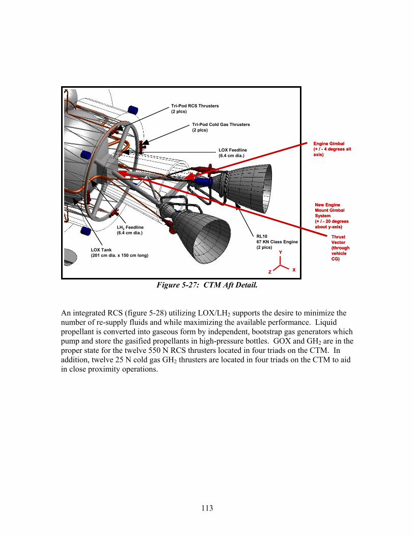
Tri-Pod RCS Thrusters (2 plcs)
RL10 67 KN Class Engine (2 plcs)
LOX Feedline (6.4 cm dia.)
LH2 Feedline (6.4 cm dia.)
LOX Tank (201 cm dia. x 150 cm long)
Tri-Pod Cold Gas Thrusters (2 plcs)
Tri-Pod RCS Thrusters (2 plcs)
RL10 67 KN Class Engine (2 plcs)
LOX Feedline (6.4 cm dia.)
LH2 Feedline (6.4 cm dia.)
LOX Tank (201 cm dia. x 150 cm long)
Tri-Pod Cold Gas Thrusters (2 plcs)
Engine Gimbal (+ / - 4 degrees all axis)
New Engine Mount Gimbal System (+ / - 20 degrees about y-axis)
Y
XZ
ThrustVector (through vehicle CG)
Engine Gimbal (+ / - 4 degrees all axis)
New Engine Mount Gimbal System (+ / - 20 degrees about y-axis)
Y
XZ
ThrustVector (through vehicle CG)
Figure 5-27: CTM Aft Detail. An integrated RCS (figure 5-28) utilizing LOX/LH2 supports the desire to minimize the number of re-supply fluids and while maximizing the available performance. Liquid propellant is converted into gaseous form by independent, bootstrap gas generators which pump and store the gasified propellants in high-pressure bottles. GOX and GH2 are in the proper state for the twelve 550 N RCS thrusters located in four triads on the CTM. In addition, twelve 25 N cold gas GH2 thrusters are located in four triads on the CTM to aid in close proximity operations.
113

GO2
A
B
C
REACTION CONTROL THRUSTERS
COLD GAS THRUSTER
2 F/T N/C
2 F/T N/C
2 F/T N/C
2 F/T N/C
2 F/T N/C
2 F/T N/C
2 F/T N/C
2 F/T N/C
2 F/T N/C
2 F/T N/C
2 F/T N/C
2 F/T N/C
2 F/T N/C
2 F/T N/C
2 F/T Dual-Seat
N/C
2 F/T N/C
2 F/T N/C
2 F/T N/C
2 F/T N/C
1 F/T Single-Seat
N/C
D
GH2
Figure 5-28: CTM Integrated Reaction Control System Schematic.
Technology Needs. The CTM propulsion system requires two advanced propulsion-related technologies. A LOX/LH2 main propulsion engine with a vacuum specific impulse greater than 455 seconds requires advances in engine materials, integrated vehicle health monitoring and turbopump design to reach the required 50+ start/stop cycles and 10 year on-orbit life requirement. The overall propulsion system, which includes the propellant feed system; pressurization system; on-orbit propellant re-supply valving, plumbing and interface hardware; and engine and thrust structure gimble actuators, is required to have a lifetime reliability greater than 0.995. The major components of the propulsion system, such as the main engine and actuators, should ideally be designed as orbital replacement units (ORUs) for ease of repair and/or replacement. The second major technology requirement is a two-fault tolerant, six degree-of -freedom RCS utilizing the same propellant combination as the main propulsion system. This will require the development of a gaseous oxygen and gaseous hydrogen thruster with a cycle life greater than 100,000. The thruster will require a steady-state vacuum Isp greater than 385 seconds with associated valving hardware designed to provide an impulse-bit
114

acceptable for attitude control, station keeping, propellant settling and rendezvous operations. In order to provide RCS propellants on-demand from liquid propellants stored in the main propellant tanks, a highly reliable, lightweight, high-pressure cryogenic propellant gasification storage and distribution system is necessary to support the on-orbit 10-year life requirement. These technology requirements are summarized in table 5-26.
Table 5-26: CTM Engine Feed/Propellant Management System Technology Needs.
Technology
Summary Description of Desired
Technology and Key
Performance Metrics
Current TRL Where Who
Current Funding
($K)
Increase in Funding Required
(none, small, large)
Applications other than HPM/CTM
High Performance, High Cycle Life LH2/LOX Main Engine
Main propulsion engine with Isp > 445 sec., capable of > 50 on-orbit starts over a 10 year period with reliability > 0.995.
5 - Pratt & Whitney, Rocketdyne
TBD TBD Upper stage applications
Integrated GH2/GOX Reaction Control System
Two-fault tolerant system to gasify and maintain RCS propellants with thruster Isp > 385 sec. And 100,000 cycle life.
6 MSFC, JSC
Space Station Freedom, SSTO
TBD TBD
Upper stage, HEDS, SSTO, ISS applications
Electro-Mechanical Valve Actuators
Lightweight, high-efficiency electro-mechanical valve actuators and engine gimbal motors
6 MSFC Pratt & Whitney, MOOG
TBD TBD
Upper stage, HEDS, launch vehicles
115
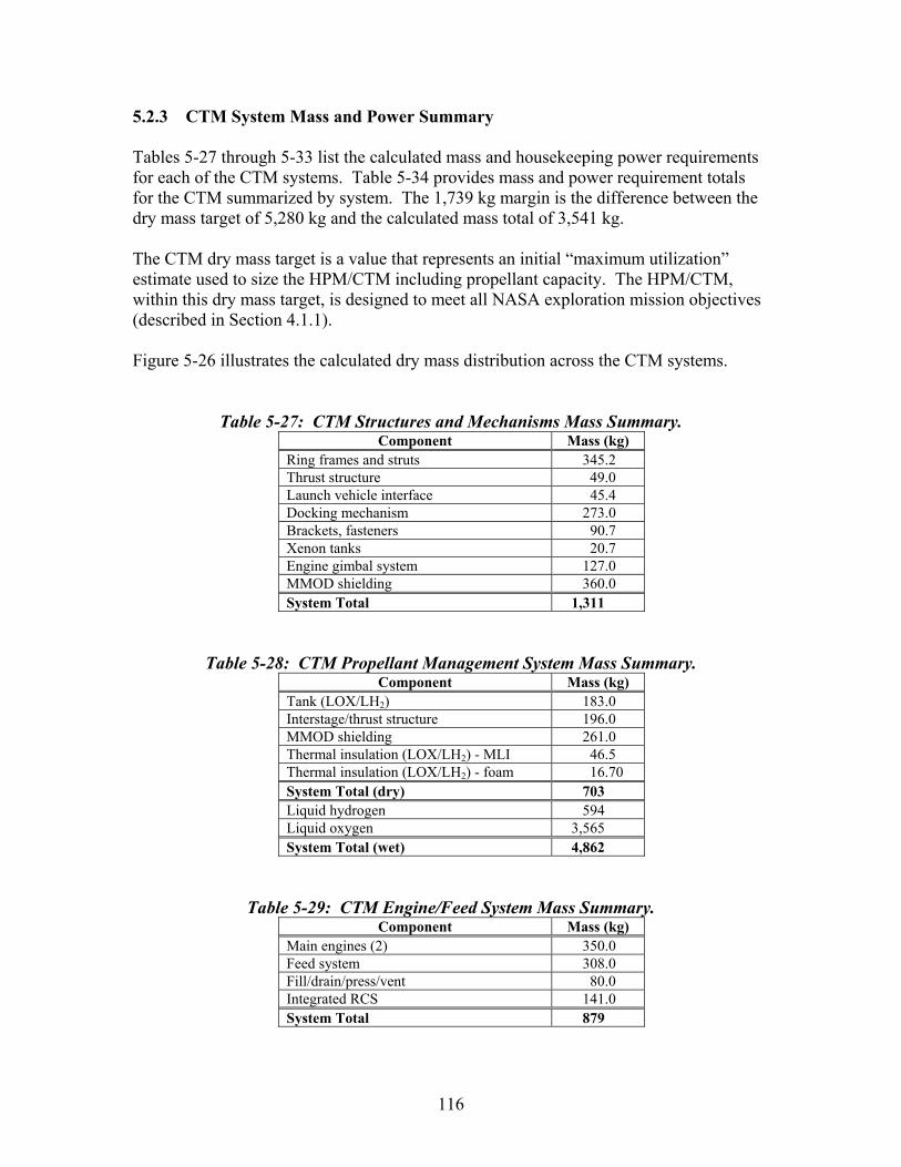
5.2.3 CTM System Mass and Power Summary Tables 5-27 through 5-33 list the calculated mass and housekeeping power requirements for each of the CTM systems. Table 5-34 provides mass and power requirement totals for the CTM summarized by system. The 1,739 kg margin is the difference between the dry mass target of 5,280 kg and the calculated mass total of 3,541 kg. The CTM dry mass target is a value that represents an initial “maximum utilization” estimate used to size the HPM/CTM including propellant capacity. The HPM/CTM, within this dry mass target, is designed to meet all NASA exploration mission objectives (described in Section 4.1.1). Figure 5-26 illustrates the calculated dry mass distribution across the CTM systems.
Table 5-27: CTM Structures and Mechanisms Mass Summary. Component Mass (kg)
Ring frames and struts 345.2 Thrust structure 49.0 Launch vehicle interface 45.4 Docking mechanism 273.0 Brackets, fasteners 90.7 Xenon tanks 20.7 Engine gimbal system 127.0 MMOD shielding 360.0 System Total 1,311
Table 5-28: CTM Propellant Management System Mass Summary. Component Mass (kg)
Tank (LOX/LH2) 183.0 Interstage/thrust structure 196.0 MMOD shielding 261.0 Thermal insulation (LOX/LH2) - MLI 46.5 Thermal insulation (LOX/LH2) - foam 16.70 System Total (dry) 703 Liquid hydrogen 594 Liquid oxygen 3,565 System Total (wet) 4,862
Table 5-29: CTM Engine/Feed System Mass Summary. Component Mass (kg)
Main engines (2) 350.0 Feed system 308.0 Fill/drain/press/vent 80.0 Integrated RCS 141.0 System Total 879
116
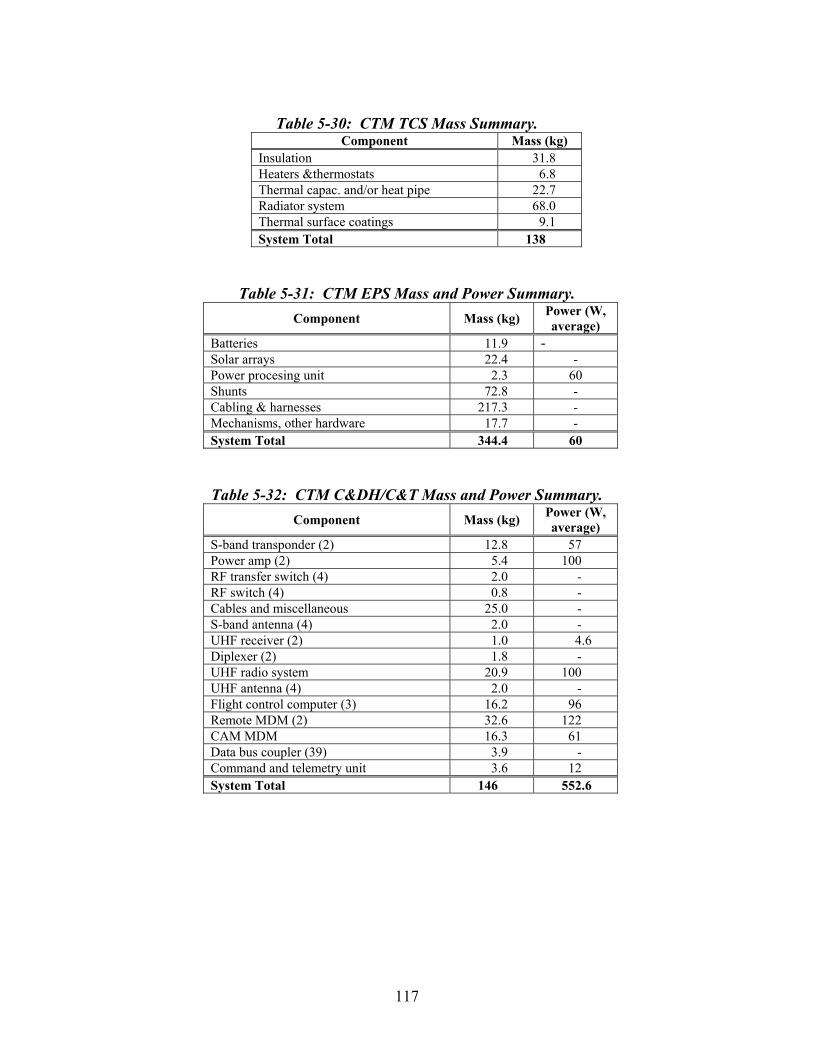
Table 5-30: CTM TCS Mass Summary.
Component Mass (kg) Insulation 31.8 Heaters &thermostats 6.8 Thermal capac. and/or heat pipe 22.7 Radiator system 68.0 Thermal surface coatings 9.1 System Total 138
Table 5-31: CTM EPS Mass and Power Summary. Component Mass (kg) Power (W,
average) Batteries 11.9 - Solar arrays 22.4 - Power procesing unit 2.3 60 Shunts 72.8 - Cabling & harnesses 217.3 - Mechanisms, other hardware 17.7 - System Total 344.4 60
Table 5-32: CTM C&DH/C&T Mass and Power Summary. Component Mass (kg) Power (W,
average) S-band transponder (2) 12.8 57 Power amp (2) 5.4 100 RF transfer switch (4) 2.0 - RF switch (4) 0.8 - Cables and miscellaneous 25.0 - S-band antenna (4) 2.0 - UHF receiver (2) 1.0 4.6 Diplexer (2) 1.8 - UHF radio system 20.9 100 UHF antenna (4) 2.0 - Flight control computer (3) 16.2 96 Remote MDM (2) 32.6 122 CAM MDM 16.3 61 Data bus coupler (39) 3.9 - Command and telemetry unit 3.6 12 System Total 146 552.6
117
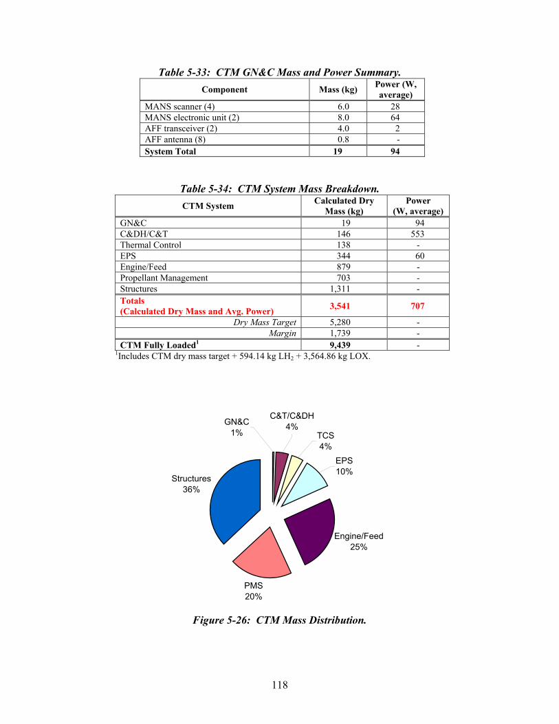
Table 5-33: CTM GN&C Mass and Power Summary. Component Mass (kg) Power (W,
average) MANS scanner (4) 6.0 28 MANS electronic unit (2) 8.0 64 AFF transceiver (2) 4.0 2 AFF antenna (8) 0.8 - System Total 19 94
Table 5-34: CTM System Mass Breakdown. CTM System Calculated Dry
Mass (kg) Power
(W, average) GN&C 19 94 C&DH/C&T 146 553 Thermal Control 138 - EPS 344 60 Engine/Feed 879 - Propellant Management 703 - Structures 1,311 - Totals (Calculated Dry Mass and Avg. Power) 3,541 707
Dry Mass Target 5,280 - Margin 1,739 -
CTM Fully Loaded1 9,439 - 1Includes CTM dry mass target + 594.14 kg LH2 + 3,564.86 kg LOX.
Engine/Feed25%
PMS20%
Structures36%
EPS10%
GN&C1%
C&T/C&DH4%
TCS4%
Figure 5-26: CTM Mass Distribution.
118

5.2.4 Operations See Section 4.1.1 for a discussion of CTM operations in support of the Earth-Moon L1 mission.
119

This page intentionally left blank.
120
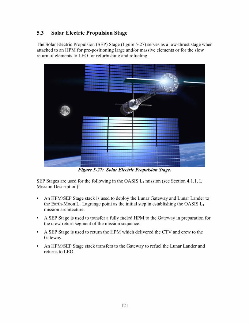
5.3 Solar Electric Propulsion Stage The Solar Electric Propulsion (SEP) Stage (figure 5-27) serves as a low-thrust stage when attached to an HPM for pre-positioning large and/or massive elements or for the slow return of elements to LEO for refurbishing and refueling.
Figure 5-27: Solar Electric Propulsion Stage.
SEP Stages are used for the following in the OASIS L1 mission (see Section 4.1.1, L1 Mission Description): • An HPM/SEP Stage stack is used to deploy the Lunar Gateway and Lunar Lander to
the Earth-Moon L1 Lagrange point as the initial step in establishing the OASIS L1 mission architecture.
• A SEP Stage is used to transfer a fully fueled HPM to the Gateway in preparation for the crew return segment of the mission sequence.
• A SEP Stage is used to return the HPM which delivered the CTV and crew to the Gateway.
• An HPM/SEP Stage stack transfers to the Gateway to refuel the Lunar Lander and returns to LEO.
121

5.3.1 Configuration and System Packaging A primary driver for the SEP Stage configuration and packaging concept is the requirement for launch by a Shuttle-class vehicle (figure 5-28). The SEP Stage is comprised of three elements:
• Thruster Pallet
• Deployable Boom
• Base Pallet The Thruster Pallet is a circular plate used to mount multiple electric thrusters on lightweight gimbals. The gimbals are incorporated to enable small pointing corrections to offset any beam aberrations in each thruster. A power processing unit (PPU), one per thruster, converts input power from the arrays into the required thruster power. A gas distribution unit (GDU), located on the thruster face of the pallet, serves as a manifold for propellant delivery to the thrusters. Each engine includes a propellant feed system that regulates input flow as required for engine operation. A loop heat pipe system is mounted on the Thruster Pallet to reject waste heat from the PPUs. The rejected heat is conducted to two radiator wings attached to the Thruster Pallet. The Thruster Pallet is attached to the Deployable Boom. This structure:
• Enables the Thruster Pallet to be articulated over large angles while the Base Pallet and the HPM are maintained in a solar inertial attitude for solar array pointing. The Thruster Pallet position is continually adjusted to maintain a relatively constant thrust vector through the spacecraft center of mass in order to maximize effective thrust.
• Provides sufficient distance between the thrusters and the solar arrays to prevent degradation due to exhaust plume impingement and erosion.
To achieve the proper range of motion, the boom arm consists of three sections: two rigid boom arms at each end and a coilable, deployable central mast section which provides most of the boom length. The end elements are required to allow the Thruster Pallet to reach around the Base Pallet and HPM structures. The elements of the boom are connected to each other and the pallets at each end with multiple-axis wrist joints to enable the required range of 180°. Structurally similar to the Shuttle Remote Manipulator System (SRMS) and the ISS Remote Manipulator System (ISSRMS), the rigid elements have an open internal structure through which an umbilical is run. Included in this umbilical are two flexible propellant lines (1 main, 1 spare), 24 1/0 gauge cables, and a command/control cable bundle. These lines are enclosed in a flexible cover for MMOD protection. The coilable mast concept is derived from the mast used for the Shuttle Radar Topography Mission (SRTM). It has an open lattice structure that is collapsed and coiled
122

for canister packaging and is deployed on orbit. Since the mast can be stored compactly, it enables a relatively large structure to be launched on a vehicle with Shuttle-like payload size constraints. The Base Pallet houses the solar arrays and associated power management and distribution components, the docking mechanism and fluid transfer interfaces, and other systems. This pallet is a cylindrical structure with a rigid boom attached at the center of one face. On the opposite face is the docking mechanism and fluid transfer interface which mate with the HPM. Two large, rectangular-shaped solar arrays are attached to the Base Pallet sides as illustrated in figure 5-28. These arrays are on stand-off booms to provide the necessary clearance with the HPM structure. The solar arrays consist of advanced, thin-film cells on a lightweight substrate supported on a collapsible, cell-structure wing architecture. This architecture has the advantage of packing very compactly and does not impose size limitations impacting launch vehicle manifesting. The arrays are required to accommodate a one-time deployment only. Other elements inside the Base Pallet include:
• A gas distribution unit to handle xenon flow through the pallet from the HPM to the thrusters
• A reaction wheel-based system for attitude control during electric thruster operation
• A GN&C unit
• A C&DH unit
• A battery system to power deployment of the solar arrays
• A xenon tank loaded with 2,000 kg of xenon for free-flying operations during SEP Stage orbital parking
• A reaction control system (RCS) for docking maneuvers consisting of four thruster pods and two propellant tanks (containing gaseous hydrogen and gaseous oxygen)
• A thermal control system comprised of two radiator wings attached to the outside of the base pallet and a loop heat pipe system mounted inside that conducts waste heat from the PPUs.
123

Figure 5-28: SEP Stage Configuration and Packaging.
124
5.3.2 Systems 5.3.2.1 Structures and Mechanisms The main components of the SEP Stage structures and mechanisms system are the Thruster Pallet, Deployable Boom, and Base Pallet. Each component is connected to allow full 180° articulation between the two respective parts. The design provides for xenon transfer from the HPM to the thrusters and allows thruster loads to transfer to the HPM. The Thruster Pallet reacts to the load from the thrusters and transmits the load to the Deployable Boom through the spherical connection. The thruster load is carried the length of the boom through a truss structure to the Base Pallet. A spherical connection is used to transmit the load through the joint into the Base Pallet where it connects to the HPM berthing mechanism and the fluid transfer interface. System Requirements. Table 5-35 summarizes the SEP Stage structures and mechanisms top-level requirements. Mechanical Loads. Since the boom is packaged in a coiled position during launch, the only mechanical loads on the structure are those imposed during SEP Stage in-flight conditions. The structural system design meets the requirements of NASA Standard 5001, Structural Design and Test Factors of Safety for Space Flight Hardware. Two of the worst case loading scenarios are when the boom is directly in line with the HPM and when it is perpendicular to the HPM. The Thruster Pallet consists of eight operating ion engines (plus one spare) that provide two Newtons of thrust each. The resulting load conditions are given in table 5-35. Thermal Control and Radiation Protection. The SEP Stage thermal protection subsystem (TPS) is required for xenon transfer from the Base Pallet to the Thruster Pallet. The conduit for the fluid transfer is wrapped in insulating material to protect against heat loss and radiation exposure. Micrometeoroid and Orbital Debris Protection. The structural components of the Deployable Boom are designed to withstand impact from micrometeoroids, but additional protection will be necessary if the SEP Stages spend significant time in LEO and are subjected to the ISS orbital debris environment. The MMOD design will be updated as necessary as the OASIS L1 mission traffic model is revised.
125
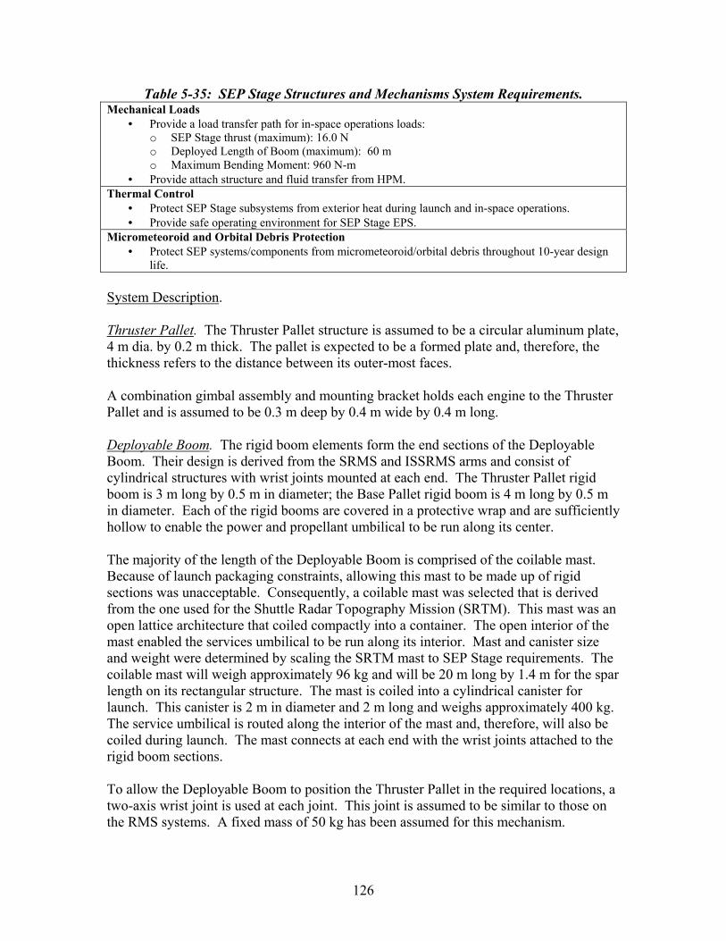
Table 5-35: SEP Stage Structures and Mechanisms System Requirements. Mechanical Loads
• Provide a load transfer path for in-space operations loads: o SEP Stage thrust (maximum): 16.0 N o Deployed Length of Boom (maximum): 60 m o Maximum Bending Moment: 960 N-m
• Provide attach structure and fluid transfer from HPM. Thermal Control
• Protect SEP Stage subsystems from exterior heat during launch and in-space operations. • Provide safe operating environment for SEP Stage EPS.
Micrometeoroid and Orbital Debris Protection • Protect SEP systems/components from micrometeoroid/orbital debris throughout 10-year design
life. System Description. Thruster Pallet. The Thruster Pallet structure is assumed to be a circular aluminum plate, 4 m dia. by 0.2 m thick. The pallet is expected to be a formed plate and, therefore, the thickness refers to the distance between its outer-most faces. A combination gimbal assembly and mounting bracket holds each engine to the Thruster Pallet and is assumed to be 0.3 m deep by 0.4 m wide by 0.4 m long. Deployable Boom. The rigid boom elements form the end sections of the Deployable Boom. Their design is derived from the SRMS and ISSRMS arms and consist of cylindrical structures with wrist joints mounted at each end. The Thruster Pallet rigid boom is 3 m long by 0.5 m in diameter; the Base Pallet rigid boom is 4 m long by 0.5 m in diameter. Each of the rigid booms are covered in a protective wrap and are sufficiently hollow to enable the power and propellant umbilical to be run along its center. The majority of the length of the Deployable Boom is comprised of the coilable mast. Because of launch packaging constraints, allowing this mast to be made up of rigid sections was unacceptable. Consequently, a coilable mast was selected that is derived from the one used for the Shuttle Radar Topography Mission (SRTM). This mast was an open lattice architecture that coiled compactly into a container. The open interior of the mast enabled the services umbilical to be run along its interior. Mast and canister size and weight were determined by scaling the SRTM mast to SEP Stage requirements. The coilable mast will weigh approximately 96 kg and will be 20 m long by 1.4 m for the spar length on its rectangular structure. The mast is coiled into a cylindrical canister for launch. This canister is 2 m in diameter and 2 m long and weighs approximately 400 kg. The service umbilical is routed along the interior of the mast and, therefore, will also be coiled during launch. The mast connects at each end with the wrist joints attached to the rigid boom sections. To allow the Deployable Boom to position the Thruster Pallet in the required locations, a two-axis wrist joint is used at each joint. This joint is assumed to be similar to those on the RMS systems. A fixed mass of 50 kg has been assumed for this mechanism.
126
The services umbilical is a combined bundle of power, propellant, and command lines that is passed through the center of the Deployable Boom. These various lines have been bundled for the following reasons:
• Since the mast section is coiled, the umbilical is required to be packed into the reduced volume of the collapsed mast. It is expected that fitting one bundle into the coiled mast would be the most efficient use of the limited space. This also requires that the lines be flexible at in-space conditions.
• The parasitic heat generated in the power lines during thruster operation can serve to keep the propellant lines sufficiently heated to prevent xenon condensation/freezing.
• The bundling of all of these lines reduces the amount, and therefore weight, of the overwrap layer of material for MMOD protection.
The elements of the bundle consist of:
• Power cabling. To simplify PMAD and cabling requirements, it is assumed that the generated power is conducted to the thrusters at high voltage (~500 V). At the target power level of 450 kW, this means that the power lines have to be capable of handling at least 900 A DC. The cabling selected was 0/1 gauge copper wire of which there were 12 twisted pairs.
• Gas lines. Two flexible metallic hoses are used for propellant transfer from the
Base Pallet to the Thruster Pallet. One line is required to support all of the engines, with the second as back-up. It is assumed that the hose will be bellows-type stainless steel tubing that will remain flexible without loss of material integrity over the duration of the mission as well as withstand the high delivery pressure of the propellant. A flexible, leak-tight joint mechanism was assumed to be part of the propellant line at each of the wrist joints to better meet the integrity requirements.
• Command/control lines. A wire bundle is included in the umbilical that will
contain the command signals for the thruster PPUs, the propellant feed systems at each thruster, and for the gas distribution unit. Along with the control signals, any return telemetry will be contained in this bundle.
Base Pallet. The Base Pallet is a cylindrical aluminum structure that is derived from the HPM primary structure. The base pallet is 4 m in diameter by 2 m long. It is sized to hold the elements listed below. The base pallet has a docking mechanism and fluid transfer interface on the face opposite the boom attachment point. Permanent MMOD shielding is assumed to be on the base pallet. The structure was derived from the HPM design.
127
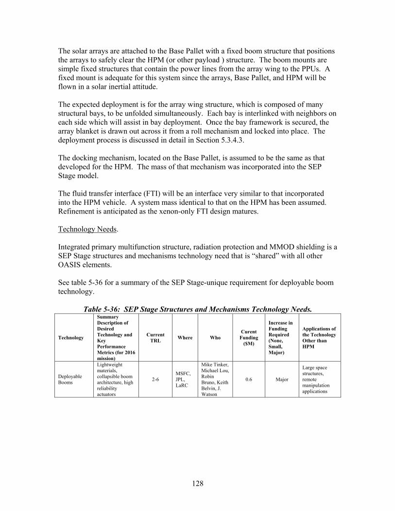
The solar arrays are attached to the Base Pallet with a fixed boom structure that positions the arrays to safely clear the HPM (or other payload ) structure. The boom mounts are simple fixed structures that contain the power lines from the array wing to the PPUs. A fixed mount is adequate for this system since the arrays, Base Pallet, and HPM will be flown in a solar inertial attitude. The expected deployment is for the array wing structure, which is composed of many structural bays, to be unfolded simultaneously. Each bay is interlinked with neighbors on each side which will assist in bay deployment. Once the bay framework is secured, the array blanket is drawn out across it from a roll mechanism and locked into place. The deployment process is discussed in detail in Section 5.3.4.3. The docking mechanism, located on the Base Pallet, is assumed to be the same as that developed for the HPM. The mass of that mechanism was incorporated into the SEP Stage model. The fluid transfer interface (FTI) will be an interface very similar to that incorporated into the HPM vehicle. A system mass identical to that on the HPM has been assumed. Refinement is anticipated as the xenon-only FTI design matures. Technology Needs. Integrated primary multifunction structure, radiation protection and MMOD shielding is a SEP Stage structures and mechanisms technology need that is “shared” with all other OASIS elements. See table 5-36 for a summary of the SEP Stage-unique requirement for deployable boom technology.
Table 5-36: SEP Stage Structures and Mechanisms Technology Needs.
Technology
Summary Description of Desired Technology and Key Performance Metrics (for 2016 mission)
Current TRL Where Who
Curent Funding
($M)
Increase in Funding Required (None, Small, Major)
Applications of the Technology Other than HPM
Deployable Booms
Lightweight materials, collapsible boom architecture, high reliability actuators
2-6 MSFC, JPL, LaRC
Mike Tinker, Michael Lou, Robin Bruno, Keith Belvin, J. Watson
0.6 Major
Large space structures, remote manipulation applications
128

5.3.2.2 Guidance, Navigation & Control The SEP Stage has to operate in low-Earth orbit and at locations such as the Earth-Moon Lagrange points or the Sun-Earth Lagrange points. (See figure 4-1 for the Lagrange point geometry.) The SEP Stage Guidance, Navigation and Control (GN&C) system will maintain the SEP Stage attitude in free flight mode and during automatic rendezvous and docking (AR&D) with other OASIS elements at these locations. System Requirements. The SEP Stage GN&C system provides attitude (rotational) control in free flight and also performs positional (translation) maneuvers to rendezvous with other OASIS elements such as the HPM. During AR&D operations with the HPM, the SEP Stage is the active vehicle and HPM is the passive vehicle (which performs only attitude control). The SEP Stage and CTM have very similar GN&C architecture, with the caveat that thrust and torque magnitudes may be significantly different. In a stack configuration with the HPM, the SEP Stage is active with respect to the guidance and attitude control requirements of the stack. No GN&C functions are performed by the HPM. These requirements impose stringent attitude control and precise position knowledge requirements for the SEP Stage as summarized in table 5-37.
Table 5-37: SEP Stage GN&C System Requirements. The SEP Stage GN&C system shall provide position and attitude information at any location. The SEP Stage shall be capable of communicating its position and attitude to ground and/or transfer vehicles. The SEP Stage GN&C system shall hold attitude to within +/- 0.5 degrees during automatic rendezvous and docking operations. The SEP Stage shall be capable of attitude control to within +/- 5 degrees of any commanded attitude using Reaction Control System. System Description. A representative G&NC system was used based on the configuration planned for the CTM design (figure 5-21). The mass of that system was incorporated into the SEP Stage model. Attitude Control System. An attitude control system (ACS) has been incorporated into the Base Pallet to compensate for any disturbances induced by non-optimal thrusting. While the deployable boom was designed to maintain a constant and maximum thrust vector, off-axis disturbance torques will occur because of limits on the precision and accuracy of the positioning capability of this boom arm, spatially and temporally. Additionally, compensation for external perturbations and secular disturbances is required. These include: solar radiation pressure, atmospheric drag, and orbit perturbations due to a nonspherical Earth and third-body interactions. Specific ACS
129

design requirements have not been quantified because the attitude variations of the SEP Stage with the HPM vehicle have not been determined. Once these parameters have been characterized, further refinements of the ACS design will be made. Reaction Wheel System. The ACS consists of four reaction wheels with masses of 25 kg each. Three wheels are arranged orthogonally with the fourth wheel serving as a spare. The wheels are spun up and down as required for attitude maintenance. It is assumed that desaturation of the wheels can be performed with the electric propulsion system. Technology Needs. Autonomous rendezvous and docking and an integrated flywheel energy storage system are SEP Stage technology needs which are “shared” with other OASIS elements. See table 5-8, HPM GN&C Technology Needs, for a summary of SEP Stage GN&C technology requirements.
130

5.3.2.3 Electrical Power System System Requirements. Top-level SEP Stage EPS requirements are given in table 5-38.
Table 5-38: SEP Stage EPS Requirements. The SEP Stage EPS shall provide 450 KWe. The SEP Stage EPS shall provide conditioned power to the thrusters. The SEP Stage photovoltaic array wings shall be capable of a one-time deployment. System Description. Power Processing Units. The Power Processing Units (PPUs), located on the Thruster Pallet, contain the power conversion and control electronics for the associated thruster. The electronics are high voltage DC compatible and have been hardened for long-term space operation. The input power is a constant (during illumination) high voltage (500 V) input arriving at the Thruster Pallet from the boom, where it is supplied to each PPU. The input power is conditioned into the multiple power inputs required at the thruster. The PPU housing is fabricated from aluminum. The PPUs are expected to operate at 94% efficiency. The units are required to have sufficient life and radiation resistance to survive multiple Van Allen belt transits and solar storms. Photovoltaic Array Wings. The solar arrays, located on the Base Pallet, consist of advanced high efficiency CIGS thin film cells to reduce the array. The cells are encapsulated in a protective coating to prevent arcing.
The cells are assumed to have an efficiency of 20% at AM0 and 28°. This efficiency is projected to reduce to approximately 13% in space including beginning of life (BOL) knockdowns and environmental factors. The cells are mounted on the panel blanket with a packing factor of 85%. The arrays operate at approximately 500 V. Additionally, a fixed amount of 5 kW of power shall be generated for SEP Stage housekeeping power. The cells are mounted on a light-weight polyimide backing. This cell blanket will be kept packed during launch and deployment of the array structure. Once the array structure is deployed, the cell blankets are drawn into place and secured. The array structure is a one-time only deployable structure. This design is under development by AEC-Able via an Air Force Research Lab (AFRL) SBIR. Power management and distribution (PMAD) for the arrays consist of power distribution units that distribute current collected from the arrays to the power leads going to the Thruster Pallet. The arrays and PMAD are assumed to be operating at 500 V to reduce the mass contribution of power distribution (i.e., cabling). The mass of the cabling into the PMAD unit along with the power leads going to the Thruster Pallet are included in the PMAD mass.
131
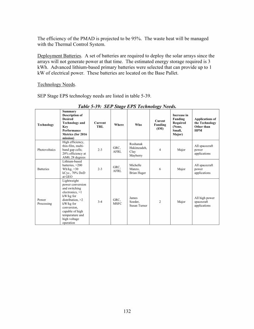
The efficiency of the PMAD is projected to be 95%. The waste heat will be managed with the Thermal Control System. Deployment Batteries. A set of batteries are required to deploy the solar arrays since the arrays will not generate power at that time. The estimated energy storage required is 3 kWh. Advanced lithium-based primary batteries were selected that can provide up to 1 kW of electrical power. These batteries are located on the Base Pallet. Technology Needs. SEP Stage EPS technology needs are listed in table 5-39.
Table 5-39: SEP Stage EPS Technology Needs.
Technology
Summary Description of Desired Technology and Key Performance Metrics (for 2016 mission)
Current TRL Where Who
Curent Funding
($M)
Increase in Funding Required (None, Small, Major)
Applications of the Technology Other than HPM
Photovoltaics
High efficiency, thin-film, multi-band gap cells; 20% efficiency at AM0, 28 degrees
2-3 GRC, AFRL
Roshanak Hakimzadeh, Clay Mayberry
4 Major All spacecraft power applications
Batteries
Lithium-based batteries, >200 Wh/kg, >30 kCyc., 70% DoD at GEO
2-3 GRC, AFRL
Michelle Manzo, Brian Hager
6 Major All spacecraft power applications
Power Processing
Lightweight power conversion and switching electronics, >1 kW/kg for distribution, >2 kW/kg for conversion, capable of high temperature and high voltage operation
3-4 GRC, MSFC
James Soeder, Susan Turner
2 Major All high power spacecraft applications
132
5.3.2.4 Propellant Management System/Propulsion System The SEP Stage propellant management system/propulsion system provides propulsive capability for HPM/SEP Stage operations and for autonomous, free-flight operations. System Description. Gas Distribution Unit. The purpose of the gas distribution unit (GDU) is to divide the single propellant flow arriving at the thruster pallet into separate and equal flows that are directed to each of the engines. The propellant is delivered to the GDU at high pressure from the Base Pallet and reduced to the required input pressure at the thruster. The GDU is contained in an aluminum box mounted on the thruster side of the pallet. Thrusters. The thrusters selected for the SEP Stage are gridded electrostatic (Kaufman) ion engines. Preliminary analysis indicates that a thruster with a diameter of at least 0.6 m is required. The thruster depth is set to 0.35 m. Mounted on the thruster body are the necessary electrical leads and propellant feed lines. The ion thrusters are assumed to perform at the following conditions:
• Specific Impulse: 3,300 seconds
• Input Power: 50 kW (to the PPUs)
• Operating Efficiency: 65%
• Throughput per engine: 3,320 kg Xe
• Number of engines: 8 required, 1 spare included. Propellant for Free-Flying Operations. It is expected that there will be extended periods at LEO, and possibly at L1, when the SEP Stage will be parked. Consequently, the stage will be moved in and out of the parking location, and moved autonomously to join with the target payload vehicle. To facilitate this repositioning, a supply of xenon propellant is located on the Base Pallet. This reserve will be used only when the SEP Stage is flying autonomously without an HPM. A target amount of 2,000 kg of xenon was selected. The exact requirements depend on the positioning requirements that have not been determined. The xenon will be stored supercritically to minimize the complexity, mass, management, and power requirements of the storage system. The storage tank for the xenon is assumed to be light-weight composite material. For this preliminary design, the tank mass is assumed to be 2.5% of the stored propellant, and the tank support structure mass and associated propellant feed system hardware is assumed to be 5.0% of the stored propellant
133
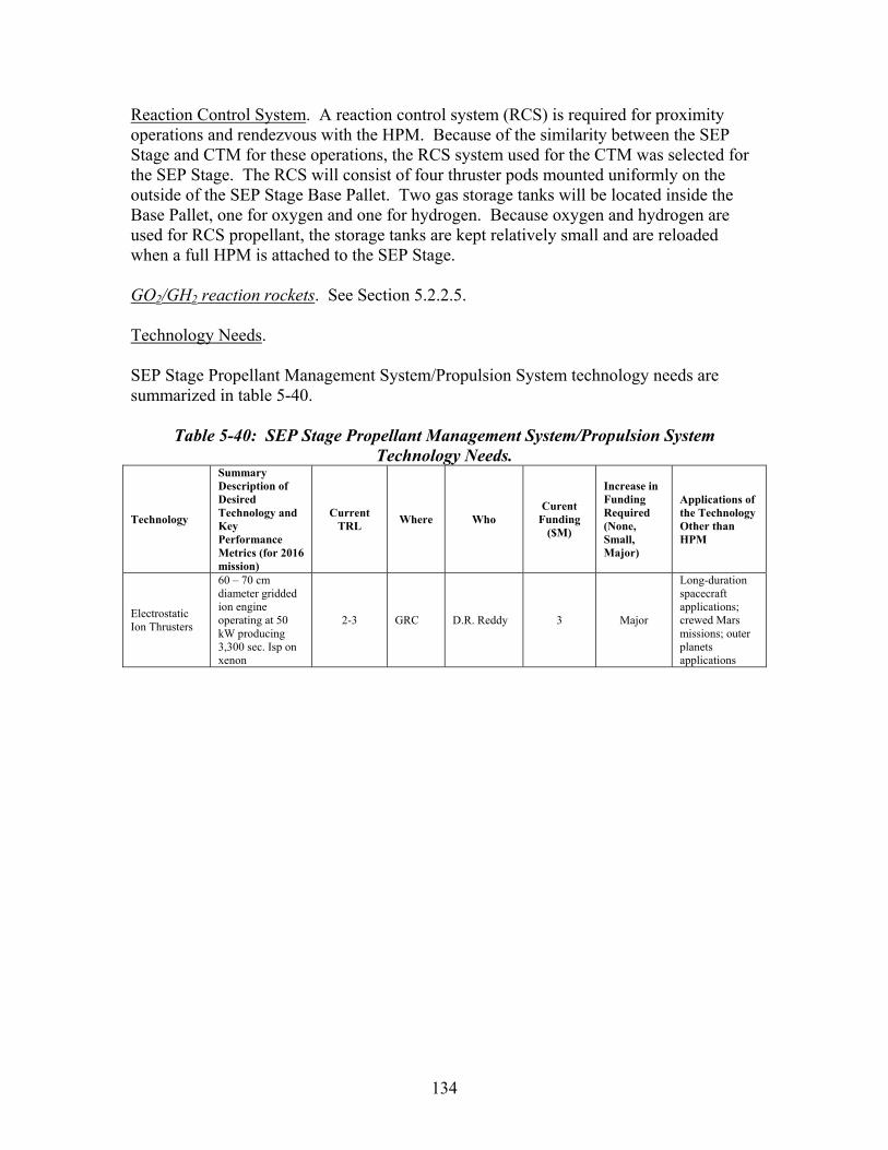
Reaction Control System. A reaction control system (RCS) is required for proximity operations and rendezvous with the HPM. Because of the similarity between the SEP Stage and CTM for these operations, the RCS system used for the CTM was selected for the SEP Stage. The RCS will consist of four thruster pods mounted uniformly on the outside of the SEP Stage Base Pallet. Two gas storage tanks will be located inside the Base Pallet, one for oxygen and one for hydrogen. Because oxygen and hydrogen are used for RCS propellant, the storage tanks are kept relatively small and are reloaded when a full HPM is attached to the SEP Stage. GO2/GH2 reaction rockets. See Section 5.2.2.5. Technology Needs. SEP Stage Propellant Management System/Propulsion System technology needs are summarized in table 5-40.
Table 5-40: SEP Stage Propellant Management System/Propulsion System Technology Needs.
Technology
Summary Description of Desired Technology and Key Performance Metrics (for 2016 mission)
Current TRL Where Who
Curent Funding
($M)
Increase in Funding Required (None, Small, Major)
Applications of the Technology Other than HPM
Electrostatic Ion Thrusters
60 – 70 cm diameter gridded ion engine operating at 50 kW producing 3,300 sec. Isp on xenon
2-3 GRC D.R. Reddy 3 Major
Long-duration spacecraft applications; crewed Mars missions; outer planets applications
134

5.3.2.4 Thermal Control System The SEP Stage TCS provides thermal regulation for element systems and components. The design consists of a TCS for the Thruster Pallet and a similar TCS for the Base Pallet. System Description. The thermal control system (TCS) on the Thruster Pallet manages heat rejected from the PPUs. The TCS can also provide a portion of the waste heat to the gas distribution unit (GDU) to maintain that unit at a temperature above the condensation point for the xenon propellant. A simplified TCS has been selected which consists of two elements: Radiators. Two radiator panels are mounted on opposite sides of the Thruster Pallet. Each panel is approximately 2 m wide by 7.6 m long. The panels are oriented so that they radiate to space for a majority of each orbit. Loop Heat Pipe System. Heat from each PPU is transferred to the radiator wings via a passive heat pipe system. The thermal control system (TCS) on the Base Pallet manages heat rejected from the PMAD boxes. The Base Pallet TCS is also a simplified system consisting of two elements: Radiators. Two radiator panels are mounted on opposite sides of the Base Pallet. Each panel is approximately 2 m wide by 6.3 m long. The panels are oriented so that they radiate to space for a majority of each orbit. Loop Heat Pipe System. Heat from each PMAD box is transferred to the radiator wings by a passive heat pipe system. Technology Needs. SEP Stage TCS technology needs are summarized in table 5-41.
135

Table 5-41: SEP Stage TCS Technology Needs.
Technology
Summary Description of Desired Technology and Key Performance Metrics (for 2016 mission)
Current TRL Where Who
Curent Funding
($M)
Increase in Funding Required (None, Small, Major)
Applications of the Technology Other than HPM
Thermal Control
Lightweight radiator materials, operating at high temperatures, loop heat pipe systems
2-6 MSFC, GRC
Susan Turner, Richard Shaltens
4 Major All temperature-sensitive space systems
136

5.3.2.5 C&DH/C&T The SEP Stage C&DH/C&T system is identical to the CTM C&DH/C&T system. See Section 5.2.2.3 for a description.
137
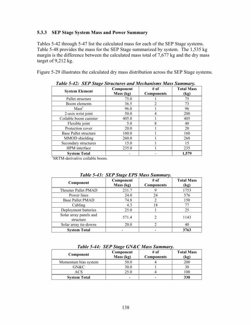
5.3.3 SEP Stage System Mass and Power Summary Tables 5-42 through 5-47 list the calculated mass for each of the SEP Stage systems. Table 5-48 provides the mass for the SEP Stage summarized by system. The 1,535 kg margin is the difference between the calculated mass total of 7,677 kg and the dry mass target of 9,212 kg. Figure 5-29 illustrates the calculated dry mass distribution across the SEP Stage systems.
Table 5-42: SEP Stage Structures and Mechanisms Mass Summary.
System Element Component Mass (kg)
# of Components
Total Mass (kg)
Pallet structure 75.0 1 75 Boom elements 36.5 2 73
Mast1 96.0 1 96 2-axis wrist joint 50.0 4 200
Coilable boom canister 405.0 1 405 Flexible joint 5.0 8 40
Protection cover 20.0 1 20 Base Pallet structure 160.0 1 160
MMOD shielding 260.0 1 260 Secondary structures 15.0 1 15
HPM interface 235.0 1 235 System Total - - 1,579
1SRTM-derivative coilable boom.
Table 5-43: SEP Stage EPS Mass Summary.
Component Component Mass (kg)
# of Components
Total Mass (kg)
Thruster Pallet PMAD 231.7 9 1753 Power lines 24.0 24 576
Base Pallet PMAD 74.8 2 150 Cabling 4.3 18 77
Deployment batteries 25.0 1 25 Solar array panels and
structure 571.4 2 1143
Solar array tie-downs 20.0 2 40 System Total - - 3763
Table 5-44: SEP Stage GN&C Mass Summary. Component Component
Mass (kg) # of
Components Total Mass
(kg) Momentum bias system 50.0 4 200
GN&C 30.0 1 30 ACS 25.0 4 100
System Total - - 330
138
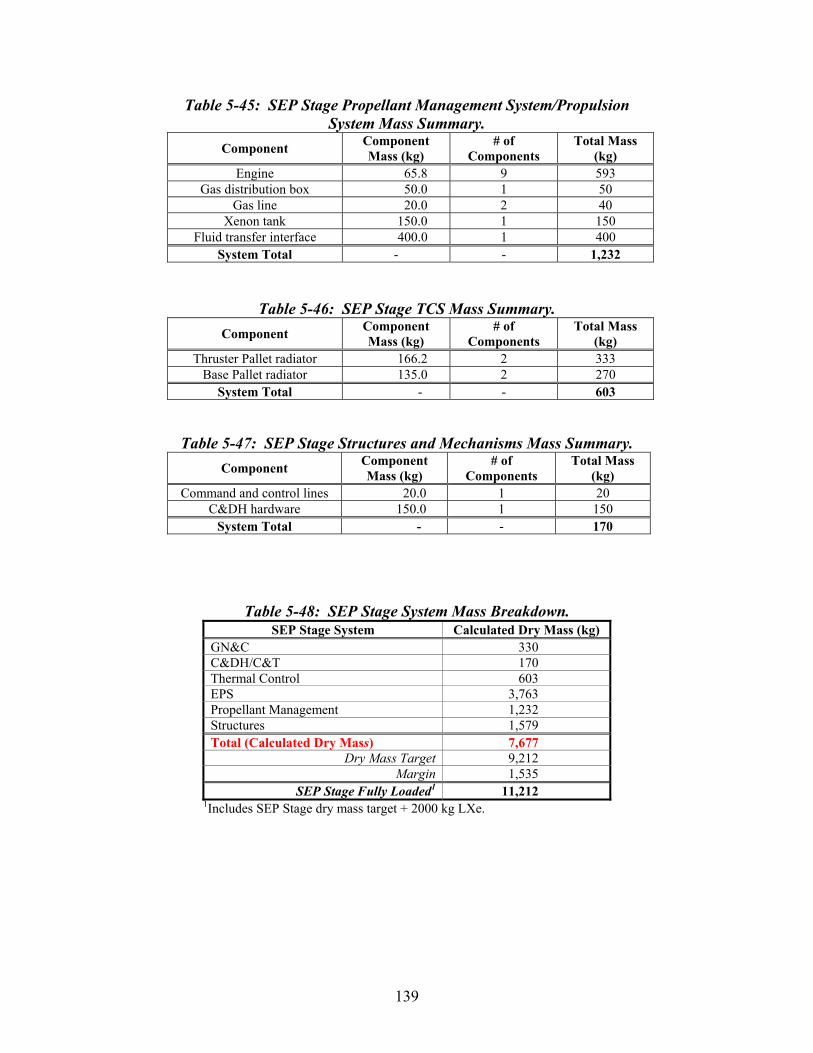
Table 5-45: SEP Stage Propellant Management System/Propulsion System Mass Summary.
Component Component Mass (kg)
# of Components
Total Mass (kg)
Engine 65.8 9 593 Gas distribution box 50.0 1 50
Gas line 20.0 2 40 Xenon tank 150.0 1 150
Fluid transfer interface 400.0 1 400 System Total - - 1,232
Table 5-46: SEP Stage TCS Mass Summary. Component Component
Mass (kg) # of
Components Total Mass
(kg) Thruster Pallet radiator 166.2 2 333
Base Pallet radiator 135.0 2 270 System Total - - 603
Table 5-47: SEP Stage Structures and Mechanisms Mass Summary. Component Component
Mass (kg) # of
Components Total Mass
(kg) Command and control lines 20.0 1 20
C&DH hardware 150.0 1 150 System Total - - 170
Table 5-48: SEP Stage System Mass Breakdown. SEP Stage System Calculated Dry Mass (kg)
GN&C 330 C&DH/C&T 170 Thermal Control 603 EPS 3,763 Propellant Management 1,232 Structures 1,579 Total (Calculated Dry Mass) 7,677
Dry Mass Target 9,212 Margin 1,535
SEP Stage Fully Loaded1 11,212 1Includes SEP Stage dry mass target + 2000 kg LXe.
139
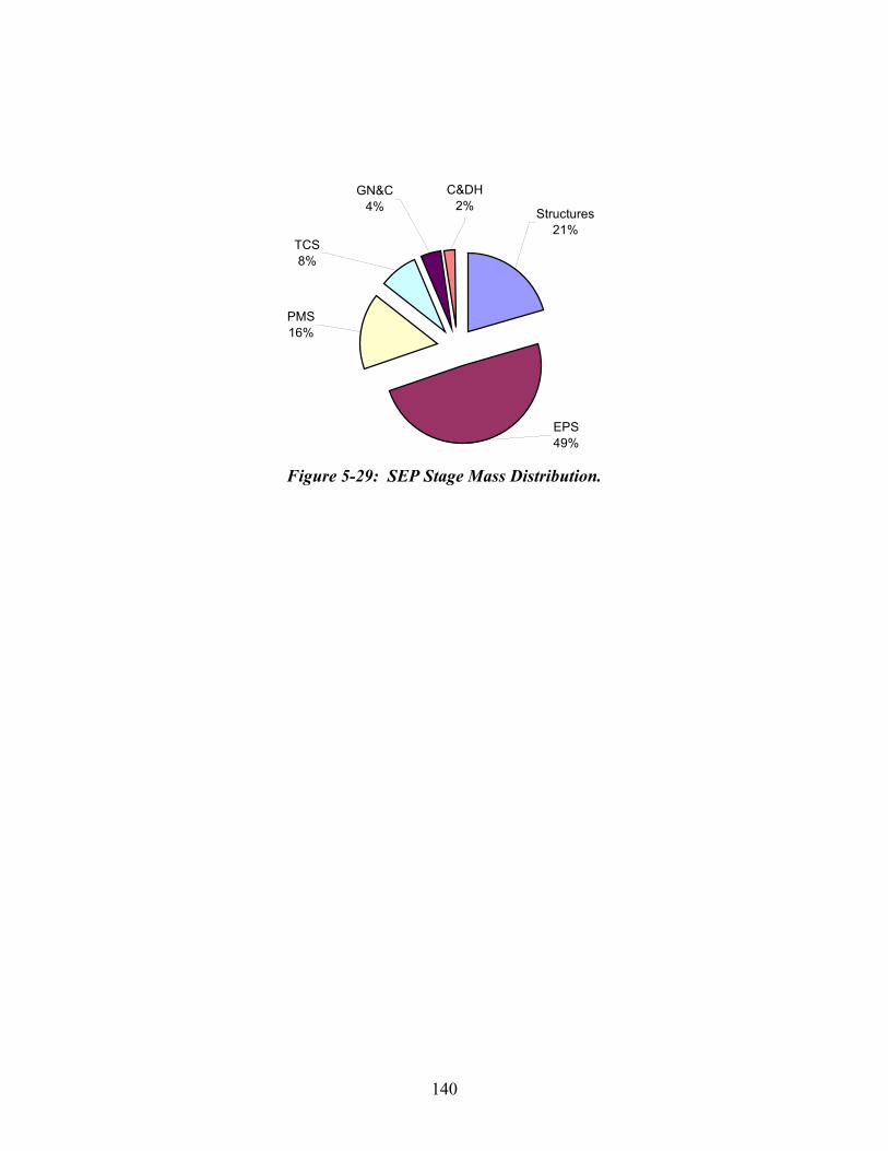
Structures21%
EPS49%
PMS16%
TCS8%
GN&C4%
C&DH2%
Figure 5-29: SEP Stage Mass Distribution.
140
5.3.4 Operations 5.3.4.1 Delivery to LEO The SEP Stage is delivered as a single package in the Space Shuttle. The SEP Stage package is launched into an ISS orbit of 400 km altitude, 51.6° inclination. The launch will target an orbit that is in safe proximity to the HPM. 5.3.4.2 Thruster Boom Deployment Once released from the launch supports, the Deployable Boom will be positioned so that the two rigid elements and the canister are aligned along a single axis so that the Thruster Pallet is at is maximum distance from the Base Pallet with the mast retracted. The coilable mast is then deployed until it reaches its proscribed length. The coiling mechanisms are secured to prevent collapse and/or bending distortions. Once secured, the boom is at its operating length of 28 m. To verify operation, each wrist joint, starting at the Base Pallet, is tracked through 180° of rotation on each of its two axes. After completion of this test, the boom is returned to the single axis alignment along the main axis of the Base Pallet. This orientation is referred to as the “off state.” 5.3.4.3 Array Deployment Array deployment is initiated by the release of the structural tie-downs (mechanical or pyrotechnic) that secured the array structure during launch. The arrays are deployed through the simultaneous deployment of the bays that make up each wing. The bay is deployed when electric motors located at the midpoint of the top and bottom spars of each rectangular bay are powered on and unfold the two halves of that spar. The spar sections are stored in a parallel configuration during launch. The motors move the spar sections apart by 180° so that these sections align in a single line to form one side of the bay. The two other sides of the bay are single sections. When the top and bottom spars are moved by the motors, the sides are also moved. When the motors have fully extended the bays, the sides of the bays form a flat, rectangular shape. All of the elements of the bays are shared with adjacent bays (except for the edge bays), so all of the bays are deployed in concert. This arrangement allows adjacent bays to ‘assist’ if a single bay is not opening normally. Once these bays are deployed and secured, the framework is ready for array blanket deployment. For each bay, the photovoltaic cell blanket at launch is rolled up on a reel mechanism attached to one of the solid sides of the bay. The array blanket is drawn off the reel via a cable and pulley system until is reaches the other side of the bay. The array blanket is sized to cover the bay structure completely. With the blanket fully extended, mechanical latches distributed uniformly around three sides of the bay grab the edge of the blanket and secure it in place. Once all of the bays are covered and secure, the arrays are ready for use.
141

5.3.4.4 LEO parking operations Orbit maintenance. Between trips to the Lunar Gateway, the SEP Stage will be maintained in a parking orbit at a higher altitude than the ISS. The parking altitude will be selected so that operations support and monitoring are minimized without jeopardizing the vehicle. This location insures that the SEP Stage does not interfere with ISS operations and reduces reboost requirements. In this parking orbit, the SEP Stage orbital altitude will decrease slowly due to atmospheric drag. This drag-induced decay rate will be minimized by flying the SEP Stage with the arrays “feathered” or in-line with the direction of travel so that the vehicle cross-section is minimized. Since power will not be used for a majority of the parking time, the arrays will not need to be sun-pointing. Besides altitude change, there will be slow changes in inclination and right ascension due to typical orbit perturbations. The SEP Stage will orbit in this orientation until the orbit has decayed to near the ISS altitude. Once the drift limit has been reached, the SEP Stage will be oriented for power generation and the electric thrusters will be turned on. The thrusters will be operated until the SEP Stage has returned to its parking location. At that point, the vehicle will then be put back into parking mode. It is envisioned that a majority of the free-flying xenon on the SEP Stage will be used for these maneuvers. Orbit matching for rendezvous. Once a SEP Stage is required for an orbit transfer starting at LEO, it is moved out of its parking mode in two steps. First, the SEP Stage is commanded to stop orbit maintenance operations. Second, it is commanded to move to a rendezvous target location using its electric propulsion system. This target location is a position and time where the SEP Stage and an HPM (or other payload) will be in close proximity and co-orbiting. 5.3.4.5 HPM Rendezvous Proximity operations. Once the SEP Stage and HPM are at the rendezvous target location, the electric thrusters are turned off and the deployable boom is moved to and secured in an off state. The SEP Stage GN&C system contacts the HPM GN&C system and synchronizes with a set of proximity sensors. Once the GN&C systems have achieved full synchronization, the rendezvous can proceed. Under full synchronization, the relative locations of each vehicle are fully determined and the required series of reaction control system burns to achieve docking are calculated. With the firing sequence computed and verified by mission operators, the RCS on the SEP Stage is activated and the planned sequence of firings is initiated. After each burn, the relative states (location, velocity, and orientation) are checked and verified before initiating the next step.
142

HPM-SEP Stage Docking. The last burn will bring the two vehicles into close enough proximity so that the docking mechanisms in each can mate and lock. After vehicles are secured, the fluid transfer interfaces will be activated and the propellant fluid line will be joined between the two interfaces. The FTIs will have electronics on-board to insure that the fluid lines are properly interfaced and secured. Only after the propellant line integrity is verified will transition to flight mode proceed. Transition to flight mode. Once the docking mechanisms are secured, the RCS will be fired so that the now coupled vehicle will reorient into a solar inertial attitude. The SEP Stage with HPM is ready for orbit transfer. 5.3.4.6 LEO to L1 Orbit transfer The SEP Stage performs the orbit transfer of payloads from a circular LEO orbit at 407 km altitude to a halo orbit about Earth-Moon L1. The orbit transfer requires an inclination change from 51.6° to 23.44 ± 5° at L1. Throughout the transfer, the vehicle maintains a solar inertial attitude with the array plane perpendicular to the Sun vector. While the thrusters are operating, the thruster boom points the resultant thrust vector through the vehicle center of mass to maintain vehicle attitude. These two design considerations allow the thrust direction to vary optimally while minimizing any periodic attitude changes for the HPM/SEP Stage stack itself. The transfer can be described in several phases. The first phase is a geocentric spiral where the thrust vector direction is defined by the weighted blend of three steering laws: tangential steering, eccentricity change steering, and inclination change steering. Each steering law defines the varying thrust direction throughout each orbit passage that, for a given amount of thrust, provides a maximum change in semi-major axis, eccentricity, and inclination, respectively. The unit thrust vectors instantaneously defined by each law are weighted and combined to obtain the appropriate thrust vector direction at a given point in the orbit. The instantaneous weight of each steering law is optimized so that the transfer is accomplished for a minimal propellant mass. Transit time is also minimized at the expense of increased power level. The thrust vector magnitude is always defined by the thrusters output, which is maximized except when the Sun’s illumination of the SEP Stage is blocked by the Earth. During shadow periods the thrusters are turned off. Optimally, the dominance of one law over the others changes during the transit. Tangential steering dominates the trajectory from LEO out to a semi-major axis of approximately 13,000 km to minimize the time spent in the radiation belts, after which eccentricity change steering is phased in with increasing weight as orbit eccentricity increases. Once the orbit becomes eccentric, thrusting to change inclination is efficient near apogee. Here inclination change steering is blended for each orbit when the vehicle true anomaly is such that maximum eccentricity steering is inefficient. The final phase of the transfer occurs after the HPM/SEP Stage orbit reaches an apogee of about 300,000 km to 325,000 km where, when apogee passage is phased with the Moon, the Moon’s
143
gravity pulls the stack into the L1 libration point. When this happens, the HPM/SEP Stage stack is inserted into a halo orbit about L1. Again, thrust vector steering is defined to accomplish this optimally for a minimal propellant mass. 5.3.4.7 L1/Gateway Arrival L1 Halo orbit acquisition. When the HPM/SEP Stage stack arrives at its maximum altitude, it will be close to the target halo orbit at Earth-Moon L1. As mentioned above, the HPM/SEP Stage will move into that halo orbit with very little propulsive effort when the orbit is properly phased with the Moon. Orbit matching for rendezvous. After stabilization, the SEP Stage RCS is used to adjust the velocity of the HPM/SEP Stage stack so that it will be moved into relatively close proximity with the Lunar Gateway. This is expected to occur by thrusting to slow the HPM/SEP Stage until it matches velocities with the Lunar Gateway when the vehicle is in relatively close, but safe, proximity to the station. Proximity operations for HPM transfer to Gateway. Once the HPM/SEP Stage and Lunar Gateway are properly co-located, the HPM is ready for transfer to the station. The fluid transfer interface and docking mechanisms are disengaged between the SEP Stage and the HPM. The SEP Stage RCS is used to move the SEP Stage away from the HPM vehicle. Once a safe distance is achieved, the SEP Stage RCS is used to move the SEP Stage to a designated parking location in the L1 halo orbit. 5.3.4.8 L1 Parking Operations Orbit maintenance. The orbit maintenance requirements for the SEP Stage are expected to be relatively minimal and will be executed in a similar fashion to the parking operations in LEO. Orbit matching for return trip. When the SEP Stage is required for the return transfer to LEO, it is moved out of its parking mode in two steps. First, the SEP Stage is commanded to stop orbit maintenance operations. Second, it is commanded to move to a rendezvous target location using the SEP RCS. This target location is a position and time where the SEP Stage and an empty HPM (or other payload) will be in close proximity and co-orbiting.
144
5.3.4.9 Return Payload Acquisition Proximity operations. Once the SEP Stage and HPM are at the rendezvous target location, the electric thrusters are turned off and the Deployable Boom is moved to and secured in an off state. The SEP Stage GN&C system contacts the HPM GN&C system and synchronizes with a set of proximity sensors. Once the GN&C systems have achieved full synchronization, the rendezvous can proceed. Under full synchronization, the relative locations of each vehicle are fully determined and the required series of reaction control system burns to achieve docking are estimated. With the firing sequence computed and verified by mission operators, the SEP Stage RCS is activated and the planned sequence of firings is initiated. After each burn, the relative states (location, velocity, and orientation) are checked and verified before initiating the next step. Payload-SEP Stage Docking. The last burn of the planned sequence will bring the two vehicles into contact so that the docking mechanisms in each can mate and lock. After vehicles are secured, the fluid transfer interfaces will be activated and the propellant fluid line will be joined between the two interfaces. The FTIs will have electronics on-board to insure that the fluid lines are properly interfaced and secured. Only after the propellant line integrity is verified will transition to flight mode proceed. Transition to flight mode. Once the docking and FTI mechanisms are secured, the RCS will be fired so that the now coupled vehicle will reorient into a solar inertial attitude. The SEP Stage with an empty HPM vehicle is ready for orbit transfer. 5.3.4.10 L1 Departure & LEO Return L1-LEO orbit transfer. The SEP Stage performs the inbound transit with the empty HPM from Earth-Moon L1 to LEO in the same way as the outbound transit, albeit with the thrust phases in reverse. The SEP Stage thrusts to move the stack out of L1 halo orbit and the stack then falls into a geocentric orbit. Again, the thrust vector follows an optimized blend of tangential steering, eccentricity change steering, and inclination change steering laws to move the stack down to circular low-Earth orbit at 407 km circular altitude at 51.6° inclination. LEO orbit acquisition. After the orbit transfer is completed and the HPM/SEP Stage is at the target orbit, the SEP Stage RCS is used to shift the phase of the orbit until the HPM/SEP Stage moves into close proximity to the ISS. At the proper distance, the SEP system is turned off.
145
The HPM/SEP Stage attitude control system is then operated to position the vehicle for HPM release to the OASIS station. HPM payload release. With the proper attitude achieved, the FTI and docking mechanisms are disengaged. Once the on-board systems indicate successful separation, the SEP Stage RCS is used to move it away from the HPM. The SEP Stage is moved a sufficient distance so that the electric thrusters can now be engaged without risk to the HPM or ISS. The SEP Stage is subsequently moved into its LEO parking orbit and placed in parking mode. 5.3.4.11 SEP Element Disposal Replacement of several elements of the SEP Stage will be performed on-orbit to extend the lifetime of the vehicle. It is expected that the engines will require replacement every other mission because of the 18,000 hour lifetime rating. The thrusters will be recovered and disposed of manually after replacement. The solar arrays are expected to require replacement after every other mission. The old arrays will be disconnected and released from the SEP Stage. Because of their size and low mass, the arrays will quickly deorbit and disintegrate on entry. At its end of life, the SEP Stage will be placed in a higher altitude long-life orbit for disposal.
146
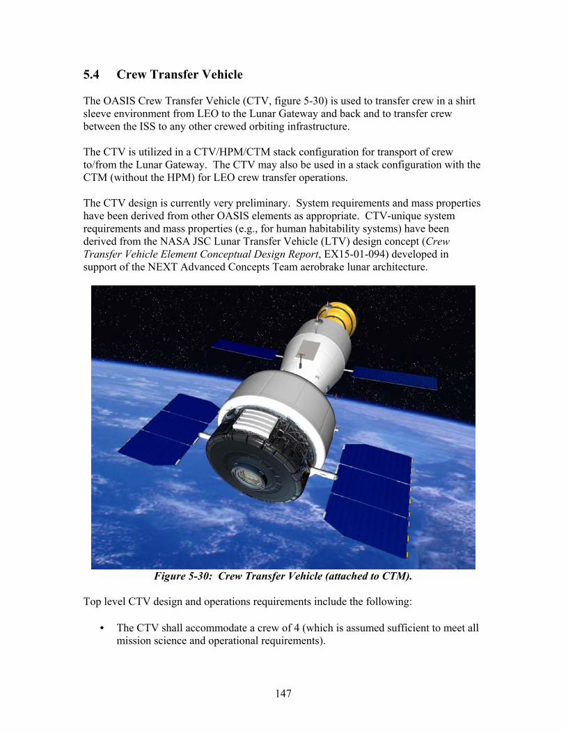
5.4 Crew Transfer Vehicle The OASIS Crew Transfer Vehicle (CTV, figure 5-30) is used to transfer crew in a shirt sleeve environment from LEO to the Lunar Gateway and back and to transfer crew between the ISS to any other crewed orbiting infrastructure. The CTV is utilized in a CTV/HPM/CTM stack configuration for transport of crew to/from the Lunar Gateway. The CTV may also be used in a stack configuration with the CTM (without the HPM) for LEO crew transfer operations. The CTV design is currently very preliminary. System requirements and mass properties have been derived from other OASIS elements as appropriate. CTV-unique system requirements and mass properties (e.g., for human habitability systems) have been derived from the NASA JSC Lunar Transfer Vehicle (LTV) design concept (Crew Transfer Vehicle Element Conceptual Design Report, EX15-01-094) developed in support of the NEXT Advanced Concepts Team aerobrake lunar architecture.
Figure 5-30: Crew Transfer Vehicle (attached to CTM).
Top level CTV design and operations requirements include the following:
• The CTV shall accommodate a crew of 4 (which is assumed sufficient to meet all mission science and operational requirements).
147
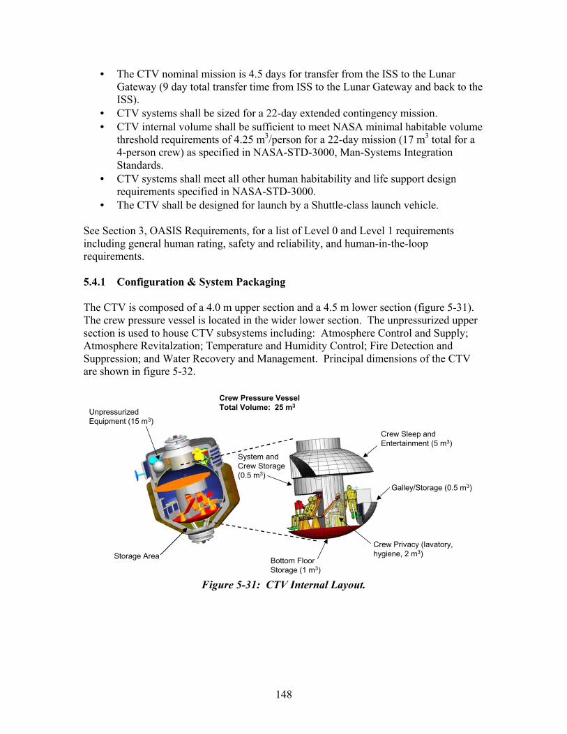
• The CTV nominal mission is 4.5 days for transfer from the ISS to the Lunar Gateway (9 day total transfer time from ISS to the Lunar Gateway and back to the ISS).
• CTV systems shall be sized for a 22-day extended contingency mission. • CTV internal volume shall be sufficient to meet NASA minimal habitable volume
threshold requirements of 4.25 m3/person for a 22-day mission (17 m3 total for a 4-person crew) as specified in NASA-STD-3000, Man-Systems Integration Standards.
• CTV systems shall meet all other human habitability and life support design requirements specified in NASA-STD-3000.
• The CTV shall be designed for launch by a Shuttle-class launch vehicle. See Section 3, OASIS Requirements, for a list of Level 0 and Level 1 requirements including general human rating, safety and reliability, and human-in-the-loop requirements. 5.4.1 Configuration & System Packaging The CTV is composed of a 4.0 m upper section and a 4.5 m lower section (figure 5-31). The crew pressure vessel is located in the wider lower section. The unpressurized upper section is used to house CTV subsystems including: Atmosphere Control and Supply; Atmosphere Revitalzation; Temperature and Humidity Control; Fire Detection and Suppression; and Water Recovery and Management. Principal dimensions of the CTV are shown in figure 5-32.
Storage Area
Unpressurized Equipment (15 m3)
Bottom Floor Storage (1 m3)
Crew Privacy (lavatory, hygiene, 2 m3)
Galley/Storage (0.5 m3)
System and Crew Storage (0.5 m3)
Crew Sleep and Entertainment (5 m3)
Crew Pressure Vessel Total Volume: 25 m3
Figure 5-31: CTV Internal Layout.
148
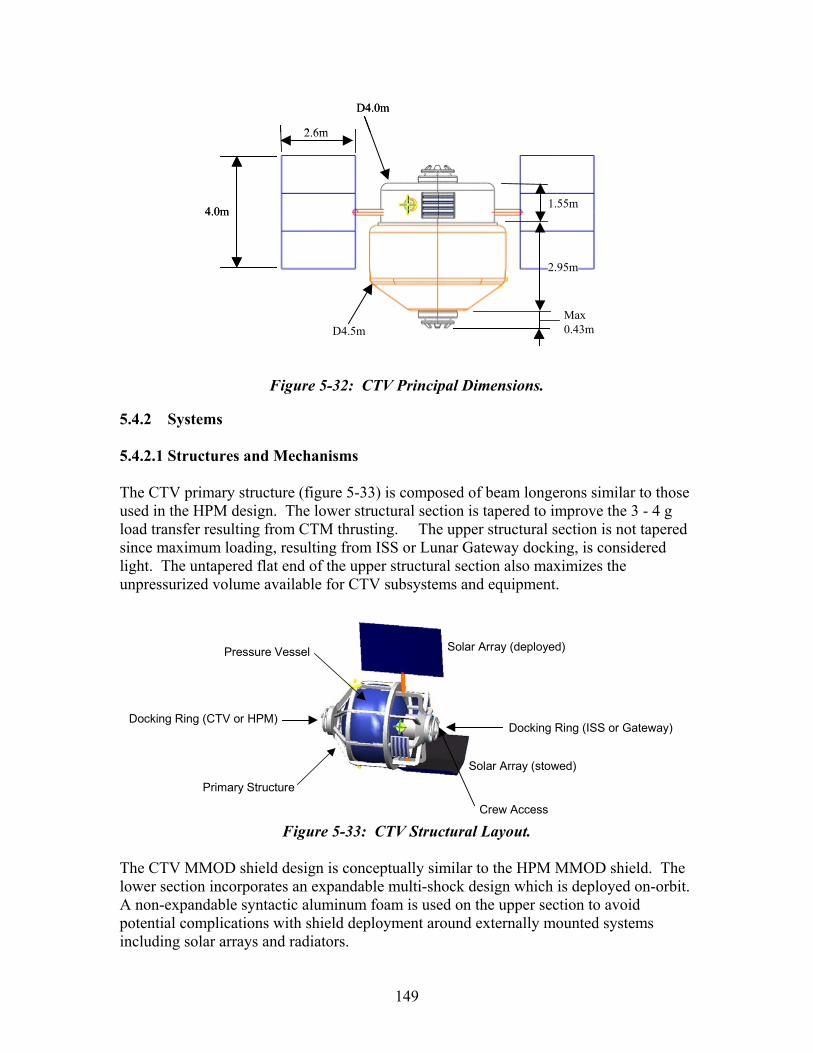
1.55m
Max0.43m
D4.0m
D4.5m
2.6m
4.0m
2.95m
1.55m
Max0.43m
D4.0m
D4.5m
2.6m
4.0m
2.95m
Figure 5-32: CTV Principal Dimensions.
5.4.2 Systems 5.4.2.1 Structures and Mechanisms The CTV primary structure (figure 5-33) is composed of beam longerons similar to those used in the HPM design. The lower structural section is tapered to improve the 3 - 4 g load transfer resulting from CTM thrusting. The upper structural section is not tapered since maximum loading, resulting from ISS or Lunar Gateway docking, is considered light. The untapered flat end of the upper structural section also maximizes the unpressurized volume available for CTV subsystems and equipment.
Pressure Vessel
Primary Structure
Crew Access
Solar Array (deployed)
Solar Array (stowed)
Docking Ring (CTV or HPM)Docking Ring (ISS or Gateway)
Figure 5-33: CTV Structural Layout.
The CTV MMOD shield design is conceptually similar to the HPM MMOD shield. The lower section incorporates an expandable multi-shock design which is deployed on-orbit. A non-expandable syntactic aluminum foam is used on the upper section to avoid potential complications with shield deployment around externally mounted systems including solar arrays and radiators.
149
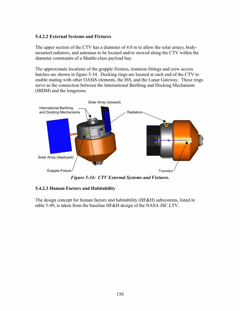
5.4.2.2 External Systems and Fixtures The upper section of the CTV has a diameter of 4.0 m to allow the solar arrays, body-mounted radiators, and antennas to be located and/or stowed along the CTV within the diameter constraints of a Shuttle-class payload bay. The approximate locations of the grapple fixtures, trunnion fittings and crew access hatches are shown in figure 5-34. Docking rings are located at each end of the CTV to enable mating with other OASIS elements, the ISS, and the Lunar Gateway. These rings serve as the connection between the International Berthing and Docking Mechanism (IBDM) and the longerons.
Grapple Fixture
Radiators
Trunnion
Solar Array (deployed)
Solar Array (stowed)International Berthingand Docking Mechanisms
Figure 5-34: CTV External Systems and Fixtures.
5.4.2.3 Human Factors and Habitability The design concept for human factors and habitability (HF&H) subsystems, listed in table 5-49, is taken from the baseline HF&H design of the NASA JSC LTV.
150
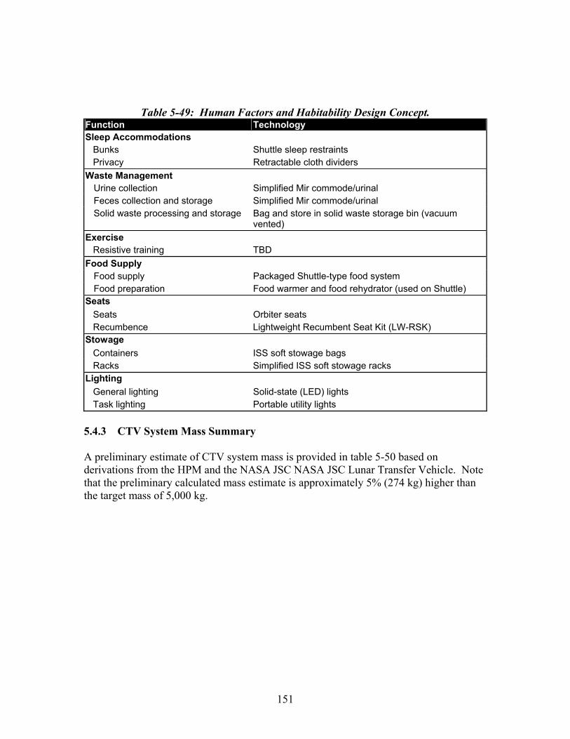
Table 5-49: Human Factors and Habitability Design Concept. Function Technology Sleep Accommodations Bunks Shuttle sleep restraints Privacy Retractable cloth dividers Waste Management Urine collection Simplified Mir commode/urinal Feces collection and storage Simplified Mir commode/urinal Solid waste processing and storage Bag and store in solid waste storage bin (vacuum
vented) Exercise Resistive training TBD Food Supply Food supply Packaged Shuttle-type food system Food preparation Food warmer and food rehydrator (used on Shuttle) Seats Seats Orbiter seats Recumbence Lightweight Recumbent Seat Kit (LW-RSK) Stowage Containers ISS soft stowage bags Racks Simplified ISS soft stowage racks Lighting General lighting Solid-state (LED) lights Task lighting Portable utility lights 5.4.3 CTV System Mass Summary A preliminary estimate of CTV system mass is provided in table 5-50 based on derivations from the HPM and the NASA JSC NASA JSC Lunar Transfer Vehicle. Note that the preliminary calculated mass estimate is approximately 5% (274 kg) higher than the target mass of 5,000 kg.
151
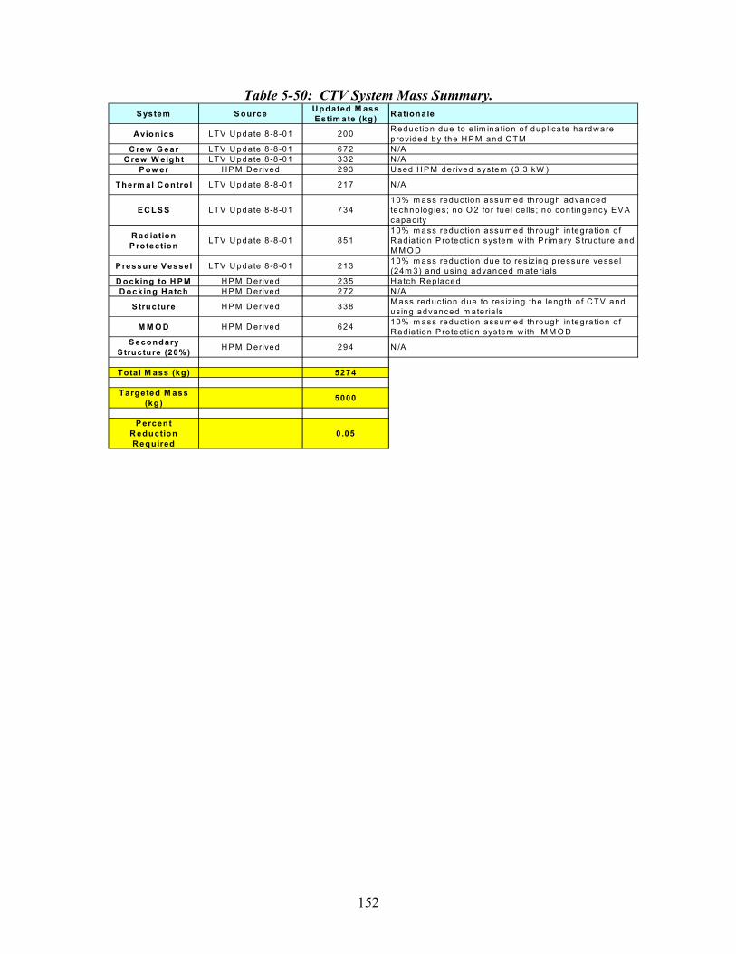
Table 5-50: CTV System Mass Summary. S ystem S ource U pdated M ass
E stim ate (kg ) R ationale
Avion ics LTV U pdate 8 -8-01 200 R eduction due to e lim ina tion o f dup lica te hardw are p rovided by the H P M and C TM
C rew G ear LTV U pdate 8 -8-01 672 N /AC rew W eight LTV U pdate 8 -8-01 332 N /A
P ow er H P M D erived 293 U sed H P M derived sys tem (3 .3 kW )
Therm al C ontro l LTV U pdate 8 -8-01 217 N /A
E C LS S LTV U pdate 8 -8-01 73410% m ass reduction assum ed th rough advanced technolog ies; no O 2 fo r fue l ce lls ; no con tingency E V A capacity
R adiation P ro tection LTV U pdate 8 -8-01 851
10% m ass reduction assum ed th rough in tegra tion o f R adia tion P rotec tion system w ith P rim ary S truc ture and M M O D
P ressure V essel LTV U pdate 8 -8-01 213 10% m ass reduction due to res iz ing p ressure vesse l (24m 3) and us ing advanced m ateria ls
D ocking to H P M H P M D erived 235 H atch R eplacedD ocking H atch H P M D erived 272 N /A
S tructure H P M D erived 338 M ass reduction due to res iz ing the length o f C TV and us ing advanced m ateria ls
M M O D H P M D erived 624 10% m ass reduction assum ed th rough in tegra tion o f R adia tion P rotec tion system w ith M M O D
S econdary S tructure (20% ) H P M D erived 294 N /A
Tota l M ass (kg) 5274
Targeted M ass (kg ) 5000
P ercent R eduction R equired
0.05
152
6. Technology Summary and Recommendations The advanced technologies necessary to make the OASIS architecture a reality, including technologies specifically applicable to the HPM, CTM, CTV, and SEP Stage, are listed in table 6-1 and described below:
• Zero boil-off cryogenic propellant storage system for the HPM providing up to 10 years of storage without boil-off.
• Extremely lightweight, integrated primary structure and micrometeoroid and orbital debris shield incorporating non-metallic hybrids to maximize radiation protection. This is required for all OASIS elements.
• High efficiency power systems such as advanced triple junction crystalline solar cells providing at least 250 W/kg (array-level specific power) and 40% efficiency, along with improved radiation tolerance. Required for the HPM, CTM, and CTV.
• Long-term autonomous spacecraft operations including rendezvous and docking, propellant transfer, deep-space navigation and communications, and vehicle health monitoring (miniaturized monitoring systems). Applicable for all OASIS elements.
• Reliable on-orbit cryogenic fluid transfer with minimal leakage using fluid transfer interfaces capable of multiple autonomous connections and disconnects
• Lightweight composite cryogenic propellant storage tanks highly resistant to propellant leakage
• Advanced materials such as graphitic foams and syntactic metal foams. Required for all OASIS elements.
• Long-life chemical and electric propulsion systems with high restart ( > 50) capability, or systems with on-orbit replaceable and/or serviceable components.
• High thrust electric propulsion systems (greater than 10 N).
• Integrated flywheel energy storage system combining energy storage and attitude control functions.
These technologies needed to enable the OASIS elements require targeted research and development. With the proper funding levels, many of the technologies could be available within the next 15 years. Accelerated funding levels could make this timeline significantly shorter. See the system discussions for each OASIS element for additional description of technology needs.
153

Table 6-1: OASIS Element Key Technologies. Key Technologies HPM CTM SEP Stage CTV Integrated flywheel energy storage system
3-axis control 3-axis control 3-axis control Possible
Advanced triple junction crystalline solar cells
> 30% eff >30% eff NA >30% eff
Large deployable thin film arrays* NA NA 167W/m2, rad hard NA
Zero boil-off (ZBO) system* Multistage NA NA NA
Integrated primary multifunction structure, radiation & micrometeoroid and orbital debris shielding
Also provides thermal insulation
Also provides thermal insulation Yes Also provides
radiation shielding
Autonomous operations including rendezvous and docking*
MANS/AFF MANS/AFF MANS/AFF MANS/AFF
On-orbit cryogenic fluid transfer* LH2/LOX/Xenon LH2/LOX/Xenon Xenon/GH2/GO2 NA
Lightweight cryogenic propellant tanks
Composite Aluminum Composite NA
Graphitic foams and syntactic metal foams
YES YES YES YES
Carbon-carbon composite radiators
YES YES YES YES
High performance, high cycle life LH2/LOX main engine*
NA 50-100 Starts, 0.995 Reliability NA NA
Integrated GH2/GO2 reaction control system (RCS)*
NA Yes YES NA
Advanced ECLSS CO2 removal system
NA NA NA YES
High power gridded ion engines*
NA NA >15k-hours life NA
* Critical technology requiring accelerated funding beyond current levels to enable development of OASIS systems within 15-year timeframe.
154
7. Preliminary Cost Analysis 7.1 OASIS vs. NEXT ACT Lunar Gateway Architectures 7.1.1 Objectives and Assumptions A comparison of launch costs between the OASIS and NEXT Advanced Concepts Team Lunar Gateway architectures has been performed to (1) establish cost trends between a reusable vs. a non-reusable architecture over a period of years, and (2) to compare the impacts of the current Space Shuttle vs. Delta IV-H for launch of architecture elements. This analysis was based on the following assumptions:
• Operations, development, and manufacturing costs for both architectures are assumed to be equivalent.
• Return of crews on Space Shuttle ISS logistics flights are not shown for either case. Since the frequency of lunar missions and crew size are identical for both architectures, these flights do not impact cost trends.
• SEP Stage, HPM, CTM and Lunar Lander logistics flights are not counted in either case since it is assumed that these reusable systems are designed for low maintenance and that most maintenance may be performed on routine Shuttle to ISS logistics flights.
• Launch vehicle performance:
o Space Shuttle cargo capacity to LEO is 15,000 kg.
o Delta IV-Heavy capacity to LEO is 35,000 kg.
• The NEXT ACT architecture requires Space Shuttle launch for Logi-Pac and crew (see figure 4-7).
• The OASIS architecture assumes crew is launched on a Space Shuttle ISS logistics flight. This Space Shuttle launch is not counted as part of the OASIS traffic model.
• The NEXT ACT architecture uses disposable (single use) Lunar Landers and reusable solar electric propulsion elements.
• The OASIS architecture uses reusable Lunar Landers and reusable SEP Stages.
• Fuel capacity for the OASIS reusable Lunar Lander is 25,000 kg.
• 90 days is assumed required for HPM and Lunar Lander checkout + Lunar Lander mission + contingency for ISS return.
• SEP Stages used for Lunar Lander refueling stay attached to HPMs for ease of planning and execution. The number of HPMs and SEP Stages could be reduced by changing this assumption.
155
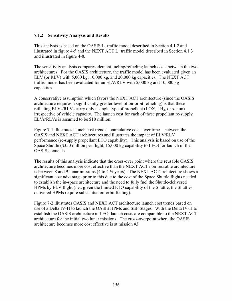
7.1.2 Sensitivity Analysis and Results This analysis is based on the OASIS L1 traffic model described in Section 4.1.2 and illustrated in figure 4-5 and the NEXT ACT L1 traffic model described in Section 4.1.3 and illustrated in figure 4-8. The sensitivity analysis compares element fueling/refueling launch costs between the two architectures. For the OASIS architecture, the traffic model has been evaluated given an ELV (or RLV) with 5,000 kg, 10,000 kg, and 20,000 kg capacities. The NEXT ACT traffic model has been evaluated for an ELV/RLV with 5,000 kg and 10,000 kg capacities. A conservative assumption which favors the NEXT ACT architecture (since the OASIS architecture requires a significantly greater level of on-orbit refueling) is that these refueling ELVs/RLVs carry only a single type of propellant (LOX, LH2, or xenon) irrespective of vehicle capacity. The launch cost for each of these propellant re-supply ELVs/RLVs is assumed to be $10 million. Figure 7-1 illustrates launch cost trends—cumulative costs over time—between the OASIS and NEXT ACT architectures and illustrates the impact of ELV/RLV performance (re-supply propellant ETO capability). This analysis is based on use of the Space Shuttle ($350 million per flight; 15,000 kg capability to LEO) for launch of the OASIS elements. The results of this analysis indicate that the cross-over point where the reusable OASIS architecture becomes more cost effective than the NEXT ACT non-reusable architecture is between 8 and 9 lunar missions (4 to 4 ½ years). The NEXT ACT architecture shows a significant cost advantage prior to this due to the cost of the Space Shuttle flights needed to establish the in-space architecture and the need to fully fuel the Shuttle-delivered HPMs by ELV flight (i.e., given the limited ETO capability of the Shuttle, the Shuttle-delivered HPMs require substantial on-orbit fueling). Figure 7-2 illustrates OASIS and NEXT ACT architecture launch cost trends based on use of a Delta IV-H to launch the OASIS HPMs and SEP Stages. With the Delta IV-H to establish the OASIS architecture in LEO, launch costs are comparable to the NEXT ACT architecture for the initial two lunar missions. The cross-overpoint where the OASIS architecture becomes more cost effective is at mission #3.
156
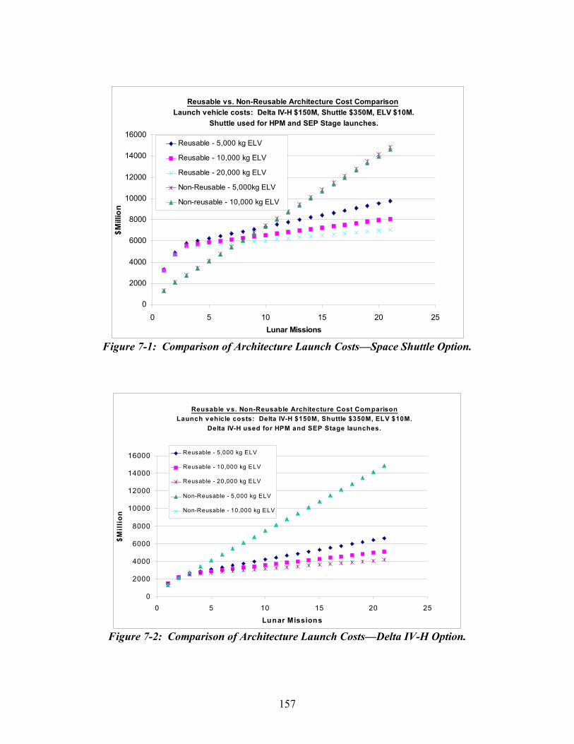
Reusable vs. Non-Reusable Architecture Cost Comparison Launch vehicle costs: Delta IV-H $150M, Shuttle $350M, ELV $10M.
Shuttle used for HPM and SEP Stage launches.
0
2000
4000
6000
8000
10000
12000
14000
16000
0 5 10 15 20 25Lunar Missions
$Mill
ion
Reusable - 5,000 kg ELV
Reusable - 10,000 kg ELV
Reusable - 20,000 kg ELV
Non-Reusable - 5,000kg ELV
Non-reusable - 10,000 kg ELV
Figure 7-1: Comparison of Architecture Launch Costs—Space Shuttle Option.
Reusable vs. Non-Reusable Architecture Cost ComparisonLaunch vehicle costs: Delta IV-H $150M, Shuttle $350M, ELV $10M.
Delta IV-H used for HPM and SEP Stage launches.
0
2000
4000
6000
8000
10000
12000
14000
16000
0 5 10 15 20 25Lunar Missions
$Mill
ion
Reusable - 5,000 kg ELV
Reusable - 10,000 kg ELV
Reusable - 20,000 kg ELV
Non-Reusable - 5,000 kg ELV
Non-Reusable - 10,000 kg ELV
Figure 7-2: Comparison of Architecture Launch Costs—Delta IV-H Option.
157

This analysis has demonstrated, through parametric assessment of launch cost variables, the potential cost advantage of a reusable lunar mission architecture over an architecture with few reusable elements. Use of a next generation RLV in place of the Space Shuttle or Delta IV-H to initially deliver OASIS elements would likely result in a cost-effective cross-over point between the two cases presented—i.e., between 3 and 8 missions—since this future RLV will likely have performance similar to the Space Shuttle at substantially reduced launch costs.
158
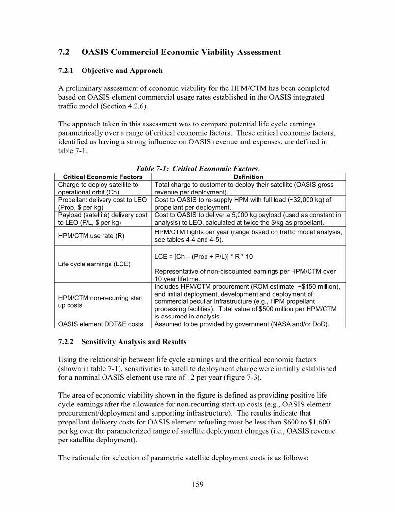
7.2 OASIS Commercial Economic Viability Assessment 7.2.1 Objective and Approach A preliminary assessment of economic viability for the HPM/CTM has been completed based on OASIS element commercial usage rates established in the OASIS integrated traffic model (Section 4.2.6). The approach taken in this assessment was to compare potential life cycle earnings parametrically over a range of critical economic factors. These critical economic factors, identified as having a strong influence on OASIS revenue and expenses, are defined in table 7-1.
Table 7-1: Critical Economic Factors. Critical Economic Factors Definition
Charge to deploy satellite to operational orbit (Ch)
Total charge to customer to deploy their satellite (OASIS gross revenue per deployment).
Propellant delivery cost to LEO (Prop, $ per kg)
Cost to OASIS to re-supply HPM with full load (~32,000 kg) of propellant per deployment.
Payload (satellite) delivery cost to LEO (P/L, $ per kg)
Cost to OASIS to deliver a 5,000 kg payload (used as constant in analysis) to LEO, calculated at twice the $/kg as propellant.
HPM/CTM use rate (R) HPM/CTM flights per year (range based on traffic model analysis, see tables 4-4 and 4-5).
Life cycle earnings (LCE)
LCE = [Ch – (Prop + P/L)] * R * 10 Representative of non-discounted earnings per HPM/CTM over 10 year lifetime.
HPM/CTM non-recurring start up costs
Includes HPM/CTM procurement (ROM estimate ~$150 million), and initial deployment, development and deployment of commercial peculiar infrastructure (e.g., HPM propellant processing facilities). Total value of $500 million per HPM/CTM is assumed in analysis.
OASIS element DDT&E costs Assumed to be provided by government (NASA and/or DoD). 7.2.2 Sensitivity Analysis and Results Using the relationship between life cycle earnings and the critical economic factors (shown in table 7-1), sensitivities to satellite deployment charge were initially established for a nominal OASIS element use rate of 12 per year (figure 7-3). The area of economic viability shown in the figure is defined as providing positive life cycle earnings after the allowance for non-recurring start-up costs (e.g., OASIS element procurement/deployment and supporting infrastructure). The results indicate that propellant delivery costs for OASIS element refueling must be less than $600 to $1,600 per kg over the parameterized range of satellite deployment charges (i.e., OASIS revenue per satellite deployment). The rationale for selection of parametric satellite deployment costs is as follows:
159

• The $70 million upper value of the range offers a $15 to $30 million dollar cost advantage over an existing launch vehicle capable of deploying 5,000 kg to GTO (e.g., Delta IV medium + 4,2).
• The $50 million nominal value is cost competitive with a Delta III class vehicle, but offers substantially greater payload capability to GTO or multi-payloads to lower energy orbits.
• The $30 million minimum deployment cost represents a highly competitive option which can deploy Delta IV medium +4,2 class payloads for less than the cost of a Delta II.
-8
-6
-4
-2
0
2
4
6
8
0 500 1,000 1,500 2,000 2,500
Propellant Delivery Cost to LEO ($ per kg)
Use Rate = 12 Flights per Year
30
50
70
Life
Cyc
le E
arni
ngs
($ B
illion
s)
Charge to Deploy 5,000 kg Satellite to Operational Orbit (Ch, $Millions)
Area of EconomicViability
Note: 5,000 kg P/L delivery to LEO assumed twice propellant delivery cost/kg.
Figure 7-3: Sensitivity to Satellite Deployment Cost.
Sensitivities to HPM/CTM use rates were established over a range of use rates that encompass those of the OASIS integrated traffic model (table 4-5). Use rate sensitivity was determined for each of the previously discussed satellite deployment charges of $30, $50, and $70 million. As shown in figure 7-4, which assumes a satellite deployment charge of $30 million, OASIS earnings are not realized at propellant delivery costs higher than $700 per kg independent of use rate. This zero earnings point (at $700 per kg propellant delivery cost) represents the point where the cost to the OASIS owner of delivering propellant and payload is equivalent to the $30 million OASIS revenue received for the satellite deployment service.
160
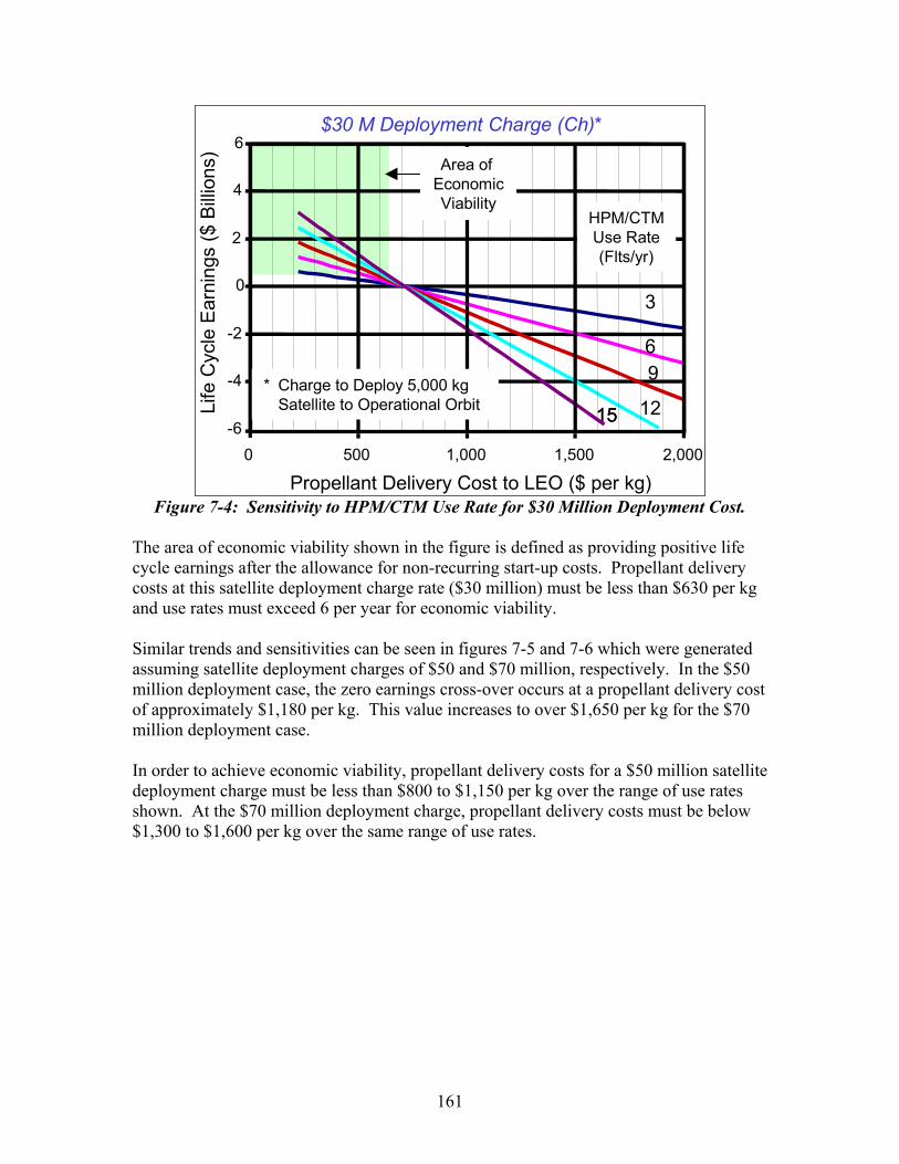
$30 M Deployment Charge (Ch)*
-6
-4
-2
0
2
4
6
0 500 1,000 1,500 2,000
Life
Cyc
le E
arni
ngs
($ B
illion
s)
3
69
121515
HPM/CTMUse Rate(Flts/yr)
Area of EconomicViability
Propellant Delivery Cost to LEO ($ per kg)
* Charge to Deploy 5,000 kg Satellite to Operational Orbit
Figure 7-4: Sensitivity to HPM/CTM Use Rate for $30 Million Deployment Cost.
The area of economic viability shown in the figure is defined as providing positive life cycle earnings after the allowance for non-recurring start-up costs. Propellant delivery costs at this satellite deployment charge rate ($30 million) must be less than $630 per kg and use rates must exceed 6 per year for economic viability. Similar trends and sensitivities can be seen in figures 7-5 and 7-6 which were generated assuming satellite deployment charges of $50 and $70 million, respectively. In the $50 million deployment case, the zero earnings cross-over occurs at a propellant delivery cost of approximately $1,180 per kg. This value increases to over $1,650 per kg for the $70 million deployment case. In order to achieve economic viability, propellant delivery costs for a $50 million satellite deployment charge must be less than $800 to $1,150 per kg over the range of use rates shown. At the $70 million deployment charge, propellant delivery costs must be below $1,300 to $1,600 per kg over the same range of use rates.
161

$50 Million Deployment Charge (Ch)*
-6
-4
-2
0
2
4
6
8
0 500 1,000 1,500Propellant Delivery Cost to LEO ($ per kg)
2,000
1818Life
Cyc
le E
arni
ngs
($ B
illion
s)
3
9* Charge to Deploy 5,000 kg Satellite to Operational Orbit
HPM/CTMUse Rate(Flts/yr)
Area of EconomicViability
Figure 7-5: Sensitivity to HPM/CTM Use Rate for $50 Million Deployment Cost.
$70 M Deployment Charge (Ch)*
-4
-2
0
2
4
6
8
10
0 500 1,000 1,500 2,000
3
15
HPM/CTMUse Rate(Flts/yr)
Area of EconomicViability
Life
Cyc
le E
arni
ngs
($ B
illion
s)
9
Propellant Delivery Cost to LEO ($ per kg)
* Charge to Deploy 5,000 kg Satellite to Operational Orbit
Figure 7-6: Sensitivity to HPM/CTM Use Rate for $70 Million Deployment Cost.
162
7.3 HPM Economic Viability Analysis Conclusions This assessment shows that OASIS commercial viability requires:
• Government (NASA or DOD) provides OASIS element DDT&E funding. Industry will leverage government investment in infrastructure development.
• Enough lifecycle revenue to:
o Cover start-up costs including HPM/CTM procurement/launch, and development and deployment of commercial peculiar infrastructure (e.g., HPM propellant processing facilities). These start-up costs are estimated to be as much as $0.5 billion per HPM/CTM.
o Provide the desired commercial return on investment.
• Low propellant delivery cost, less than $1,000/kg for the nominal $50 million OASIS satellite deployment charge.
• HPM use rates greater than 3 flights per year.
163

This page intentionally left blank.
164
8. Conclusions 8.1 Study Summary There are many challenges confronting humankind’s exploration of space, and many engineering problems that must be solved in order to provide safe, affordable and efficient in-space transportation of both personnel and equipment. These challenges directly impact the commercialization of space, with cost being the single largest obstacle. One method of reducing cost is to develop reusable transportation systems—both Earth-to-orbit systems and in-space infrastructure. Without reusable systems, sustained exploration or large-scale development beyond low-Earth-orbit may not be viable. Orbital Aggregation & Space Infrastructure Systems (referred to as OASIS) is a set of concepts that provide a common infrastructure for enabling a large class of space missions. The OASIS architecture maximizes modularity, reusability and commonality of elements across many missions and organizations. Mission concepts utilizing this architecture are predicated on the availability of a low-cost launch vehicle for delivery of propellant and re-supply logistics. Infrastructure costs would be shared by Industry, NASA and other users. A reusable Hybrid Propellant Module that combines storage of liquid hydrogen and oxygen for chemical propulsion and xenon for electrical propulsion is the core OASIS element. The HPM works in conjunction with modular propulsion modules to maximize efficiency. The liquid hydrogen and oxygen stored onboard the HPM is used in conjunction with a chemical propulsion module to provide high thrust during the time critical segments of a mission such as crew transfers. The more efficient xenon propellant is used with a solar electric propulsion module during non-time critical segments of the mission such as pre-positioning logistics or returning an empty HPM for refueling. The Chemical Transfer Module is an OASIS element that serves as a high-energy injection stage when attached to an HPM. The CTM has high-thrust cryogenic LOX/LH2 engines for orbit transfers and high-pressure oxygen/hydrogen thrusters for proximity operations and small maneuvers. The CTM also functions independently of the HPM as an autonomous orbital maneuvering vehicle for proximity operations such as ferrying payloads a short distance, refueling and servicing. Profitable commercial utilization of the HPM and CTM for satellite deployment, repositioning and servicing would require a launch cost on the order of $1,000/kg for the LOX and LH2 propellants. Launch costs for satellites and other sensitive payloads could be significantly higher without impacting commercial viability of the space-based elements. In these commercial scenarios, Industry would leverage government investment in OASIS infrastructure development.
165
Additional infrastructure is required to support crewed missions to a Lunar Gateway located at the Earth-Moon L1 Lagrange point nearly two thirds of the distance from the Earth to the moon. The Solar Electric Propulsion (SEP) Stage serves as a low-thrust transfer stage when attached to an HPM for pre-positioning large, massive elements and for the slow return of elements for refurbishing and refueling. The SEP Stage solar arrays generate hundreds of kilowatts of power to drive ion engines using the efficient xenon propellant. The last OASIS element required to support NASA crewed exploration missions is the Crew Transfer Vehicle (CTV). The CTV is used to transfer crew in a shirt sleeve environment to and from the Lunar Gateway as well as to the International Space Station (ISS) and any other crewed infrastructure elements. It uses the same multifunction structure as developed for the HPM with integrated life support systems to safely support a crew of 4 for transfer to and from the Lunar Gateway. The potential cost advantage of the reusable OASIS architecture over an architecture with few reusable elements will be realized at approximately 8 lunar missions (4 to 4 ½ years assuming lunar missions every six months) using today’s Space Shuttle for initial launch of the OASIS elements. With the more cost effective and higher capacity Delta IV-H, this OASIS cost advantage occurs as early as lunar mission #3 (1 ½ years). The technologies needed to enable the OASIS elements require targeted research and development. The key technology enablers are zero boil-off cryogenic propellant storage, cryogenic fluid transfer and high cycle reusable cryogenic engines. High efficiency solar cells and advances in electrical propulsion are also required. Lightweight multi-function structures and advanced composite propellant tanks also greatly contribute to the efficiency of the elements. Long-term autonomous spacecraft operations including rendezvous & docking and vehicle health monitoring are also necessary to provide safe, affordable and efficient in-space transportation in support of human exploration and development of space. 8.2 Future Work FY02 work developing the OASIS in-space architecture concept will include:
• Additional cost analysis to establish rough order of magnitude (ROM) estimates for OASIS element technology development costs and theoretical first unit costs
• Developing additional, industry-defined in-space commercial applications into OASIS architecture mission scenarios.
With additional funding it is desired to optimize OASIS element design and refine operations concepts for a multi-role capability to support NASA human exploration initiatives, commercial satellite applications as well as DOD applications.
166
The goal of this OASIS element design optimization will be to refine system performance for commercial and DOD missions without eliminating the ability to evolve the elements to support NASA exploration missions. Analysis will likely include an assessment of element resizing options including repackaging of the HPM and CTM for expected commercial ELVs. Design work will also develop the HPM and CTM systems to the next level of detail. This design and operations analysis will ideally include an initial assessment of OASIS element utilization for human Earth-Sun L2 and Mars missions. Future work may also include concept definition of a high-thrust nuclear-powered OASIS stage, derived from NASA human Mars mission system studies, to support deployment and in-situ servicing of commercial and military geostationary satellites. Since delivery of propellants to LEO at the $1000/kilogram level has been identified as the breakeven point for a commercially OASIS architecture, a “from scratch” study has been proposed to derive requirements and define (conventional and unconventional) concepts for the ultra-low cost orbital aggregation of propellant.
167

This page intentionally left blank.
168
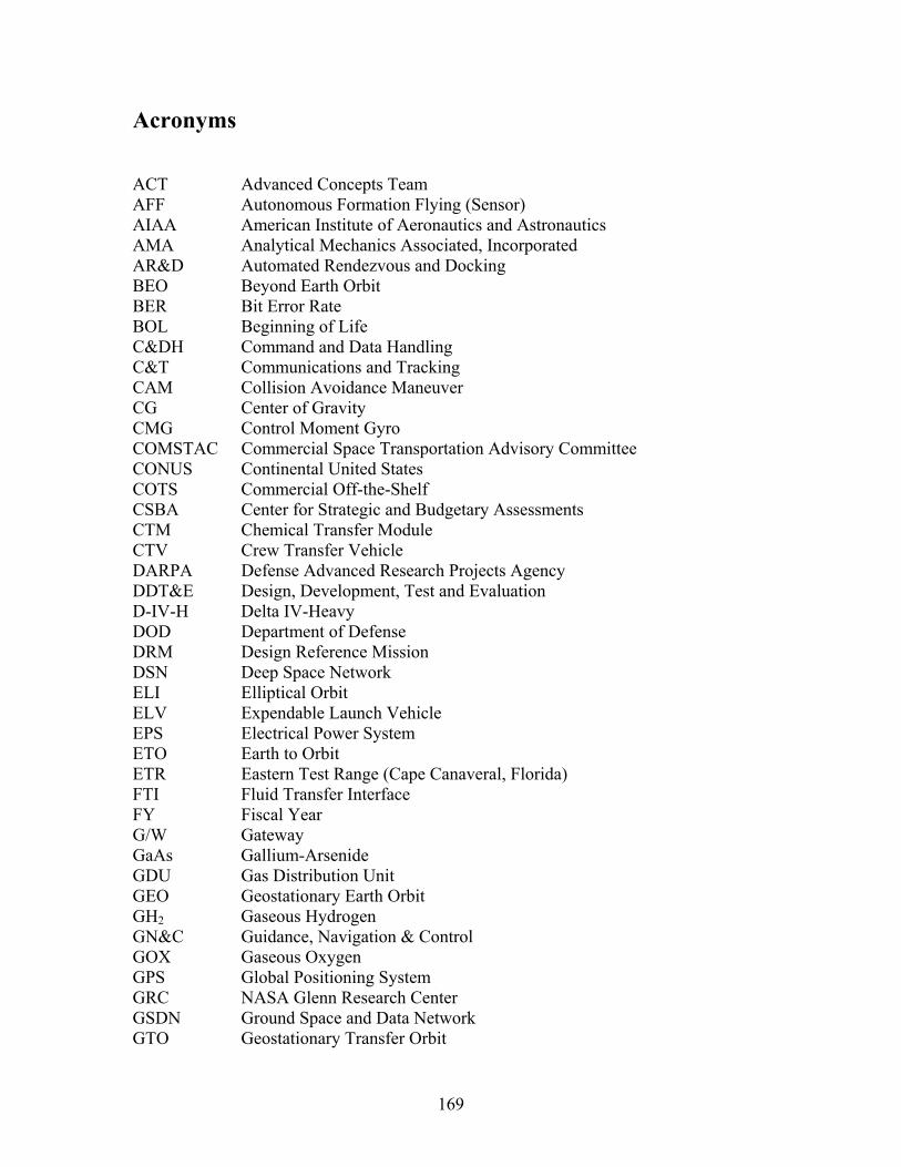
Acronyms ACT Advanced Concepts Team AFF Autonomous Formation Flying (Sensor) AIAA American Institute of Aeronautics and Astronautics AMA Analytical Mechanics Associated, Incorporated AR&D Automated Rendezvous and Docking BEO Beyond Earth Orbit BER Bit Error Rate BOL Beginning of Life C&DH Command and Data Handling C&T Communications and Tracking CAM Collision Avoidance Maneuver CG Center of Gravity CMG Control Moment Gyro COMSTAC Commercial Space Transportation Advisory Committee CONUS Continental United States COTS Commercial Off-the-Shelf CSBA Center for Strategic and Budgetary Assessments CTM Chemical Transfer Module CTV Crew Transfer Vehicle DARPA Defense Advanced Research Projects Agency DDT&E Design, Development, Test and Evaluation D-IV-H Delta IV-Heavy DOD Department of Defense DRM Design Reference Mission DSN Deep Space Network ELI Elliptical Orbit ELV Expendable Launch Vehicle EPS Electrical Power System ETO Earth to Orbit ETR Eastern Test Range (Cape Canaveral, Florida) FTI Fluid Transfer Interface FY Fiscal Year G/W Gateway GaAs Gallium-Arsenide GDU Gas Distribution Unit GEO Geostationary Earth Orbit GH2 Gaseous Hydrogen GN&C Guidance, Navigation & Control GOX Gaseous Oxygen GPS Global Positioning System GRC NASA Glenn Research Center GSDN Ground Space and Data Network GTO Geostationary Transfer Orbit
169

Ha Height of Apogee HEDS Human Exploration and Development of Space HF&H Human Factors and Habitability Hp Height of Perigee HPM Hybrid Propellant Module I/O Input/Output IAF International Astronautics Federation IBDM International Berthing and Docking Mechanism IMU Intertial Measurement Unit Inc Inclination of Orbit IPACS Integrated Power and Attitude Control System Isp Specific Impulse ISS International Space Station ISSRMS International Space Station Remote Manipulator System ITU International Telecommunication Union IV&V Independent Verification and Validation JSC NASA Johnson Space Center kg Kilogram km Kilometer kW Kilowatt LaRC NASA Langley Research Center LEO Low-Earth Orbit LH2 Liquid Hydrogen LL Lunar Lander LOX Liquid Oxygen LTV Lunar Transfer Vehicle LXe Liquid Xenon M&S Modeling and Simulation MANS Microcosm Autonomous Navigation System MDM Multiplexer/Demultiplexer MEO Medium Earth Orbit MLI Multi-layer Insulation MMC Metal Matrix Composites MMOD Micrometeoroid and Orbital Debris mps Meters per Second MSFC NASA Marshall Space Flight Center MT Metric Ton NASA National Aeronautics and Space Administration NEXT NASA Exploration Team NGSO Non-Geostationary Orbit OASIS Orbital Aggregation & Space Infrastructure OE Orbital Express OEDS Orbital Express Demonstration System ORU Orbital Replacement Unit OTV Orbital Transfer Vehicle P/L Payload
170
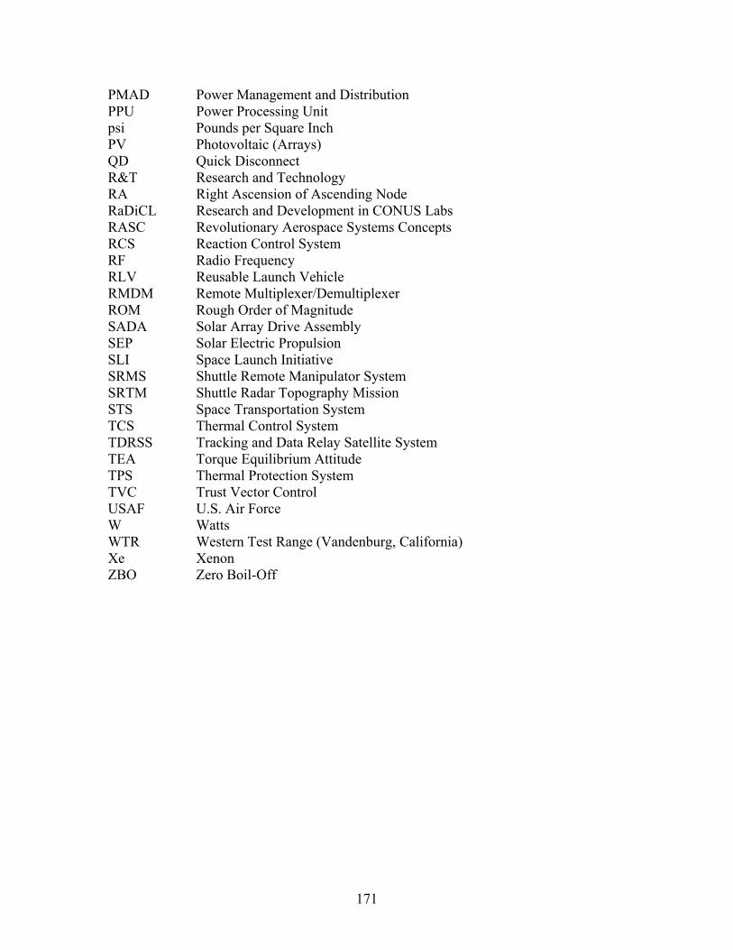
PMAD Power Management and Distribution PPU Power Processing Unit psi Pounds per Square Inch PV Photovoltaic (Arrays) QD Quick Disconnect R&T Research and Technology RA Right Ascension of Ascending Node RaDiCL Research and Development in CONUS Labs RASC Revolutionary Aerospace Systems Concepts RCS Reaction Control System RF Radio
Solar Electric Propulsion
Shuttle Remote Manipulator System SRTM
Space Transportation System TCS
Watts
Frequency RLV Reusable Launch Vehicle RMDM Remote Multiplexer/Demultiplexer ROM Rough Order of Magnitude SADA Solar Array Drive Assembly SEP SLI Space Launch Initiative SRMS
Shuttle Radar Topography Mission STS
Thermal Control System TDRSS Tracking and Data Relay Satellite System TEA Torque Equilibrium Attitude TPS Thermal Protection System TVC Trust Vector Control USAF U.S. Air Force W WTR Western Test Range (Vandenburg, California) Xe Xenon ZBO Zero Boil-Off
171

This page intentionally left blank
172
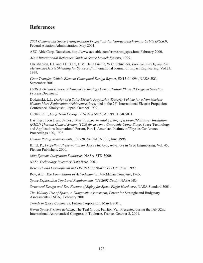
References
2001 Commercial Space Transportation Projections for Non-geosynchronous Orbits (NGSO), Federal Aviation Administration, May 2001.
Giellis, R.T., Long Term Cryogenic System Study, AFRPL TR-82-071.
Kittel, P., Propellant Preservation for Mars Missions, Advances in Cryo Engineering, Vol. 45, Plenum Publishers, 2000.
NASA Technology Inventory Data Base, 2001.
Trends in Space Commerce, Futron Corporation, March 2001.
World Space Systems Briefing, The Teal Group, Fairfax, Va., Presented during the IAF 52nd International Astronautical Congress in Toulouse, France, October 2, 2001.
AEC-Able Corp. Datasheet, http://www.aec-able.com/srtm/srtm_spex.htm, February 2000.
AIAA International Reference Guide to Space Launch Systems, 1999.
Christiansen, E.L and J.H. Kerr, H.M. De la Fuente, W.C. Schneider, Flexible and Deployable Meteoroid/Debris Shielding for Spacecraft, International Journal of Impact Engineering, Vol.23, 1999.
Crew Transfer Vehicle Element Conceptual Design Report, EX15-01-094, NASA JSC, September 2001.
DARPA Orbital Express Advanced Technology Demonstration Phase II Program Selection Process Document.
Dudzinski, L.J., Design of a Solar Electric Propulsion Transfer Vehicle for a Non-Nuclear Human Mars Exploration Architecture, Presented at the 26th International Electric Propulsion Conference, Kitakyushu, Japan, October 1999.
Hastings, Leon J. and James J. Martin, Experimental Testing of a Foam/Multilayer Insulation (FMLI) Thermal Control System (TCS) for use on a Cryogenic Upper Stage, Space Technology and Applications International Forum, Part 1, American Institute of Physics Conference Proceedings 420, 1998.
Human Rating Requirements, JSC-28354, NASA JSC, June 1998.
Man-Systems Integration Standards, NASA-STD-3000.
Research and Development in CONUS Labs (RaDiCL) Data Base, 1999.
Roy, A.E., The Foundations of Astrodynamics, MacMillan Company, 1965. Space Exploration Top Level Requirements (6/4/2002 Draft), NASA HQ.
Structural Design and Test Factors of Safety for Space Flight Hardware, NASA Standard 5001.
The Military Use of Space; A Diagnostic Assessment, Center for Strategic and Budgetary Assessments (CSBA), February 2001.
173

This page intentionally left blank
174
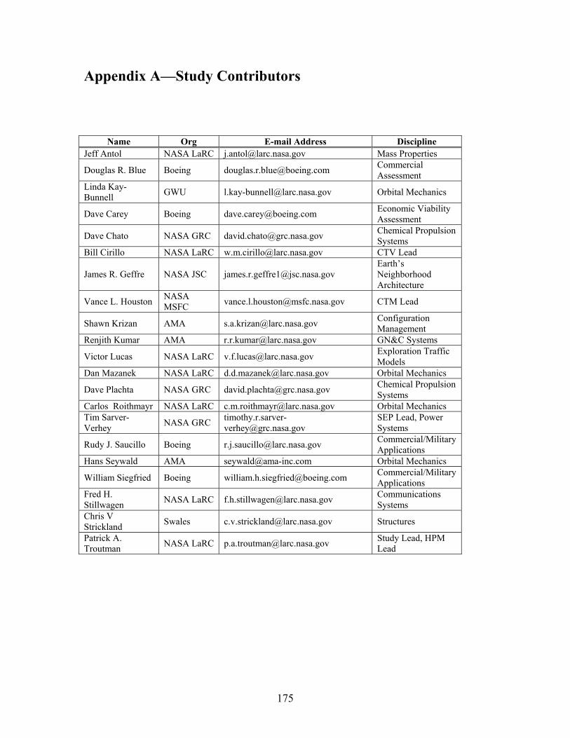
Appendix A—Study Contributors
Name Org Discipline
E-mail Address NASA LaRC [email protected] Mass Properties
Douglas R. Blue Boeing [email protected] Commercial Assessment
Linda Kay-Bunnell GWU [email protected] Orbital Mechanics
Dave Carey Boeing [email protected] Economic Viability Assessment
Dave Chato NASA GRC [email protected] Chemical Propulsion Systems
Bill Cirillo NASA LaRC [email protected] CTV Lead
James R. Geffre NASA JSC [email protected] Earth’s Neighborhood Architecture
Vance L. Houston NASA MSFC [email protected] CTM Lead
AMA Configuration Management
Renjith Kumar AMA [email protected] GN&C Systems
Victor Lucas NASA LaRC [email protected] Exploration Traffic Models
NASA LaRC [email protected] Orbital Mechanics
Dave Plachta NASA GRC [email protected] Chemical Propulsion Systems
Carlos Roithmayr NASA LaRC [email protected] Orbital Mechanics Tim Sarver-Verhey NASA GRC timothy.r.sarver-
[email protected] SEP Lead, Power Systems
Rudy J. Saucillo Boeing [email protected] Commercial/Military Applications
Hans Seywald AMA Orbital Mechanics [email protected]
William Siegfried Boeing [email protected] Commercial/Military Applications
Fred H. Stillwagen NASA LaRC [email protected] Communications
Systems Chris V Strickland Swales [email protected] Structures
Patrick A. Troutman NASA LaRC [email protected] Study Lead, HPM
Lead
Jeff Antol
Shawn Krizan [email protected]
Dan Mazanek
175

This page intentionally left blank
176

Appendix B—Methods of Analyses
177

This page intentionally left blank.
178

November 20, 2001
CM McCleskey/YA-C
Hybrid Propulsion Module Assessment with Vision Spaceport Model Release 1.0 (Initial Run) Run: 1.1.1_HPM.01 Assumes Element not Reusable per submitted survey sheet Assumes Earth-based figures of merit not space-based Figures of Merit (FOM) Interpretation:
6 ~ Worse than Shuttle Orbiter 5 ~ Shuttle Orbiter 4 ~ One order magnitude improvement from FOM = 5 (i.e., 2nd Gen) 3 ~ Two order magnitude improvement from FOM = 5 (i.e., 3rd Gen) 2 ~ Concorde-like 1 ~ Commercial Airline-like Results:
Conclusions/Recommendations: Concept looked promising, however, several potential operational improvements were noted. Run was made with inputs as is—no changes made. Recommend completing survey for each element of the proposed architecture, rather than combining all the elements together. Results will be easier to interpret and trade (HPM, CTM, CTV). The model is set up to provide such results. Note that a second release of Vision Spaceport will be available to produce quantitative results rather than qualitative FOMs in early 2002.
Reference Used : E-mail correspondence and Mankins, J. C. and Mazanek, D., IAF-01-V.3.03 “The Hybrid Propulsion Module (HPM): A New Concept for Space Transfer in Earth’s Neighborhood and Beyond.”
Element Independent Operations
Module Name
Facility Acquisition Cost FOM
GSE Acquisition Cost FOM
Fixed Laber
Cost FOM
Fixed Materials Cost FOM
Variable Labor
Cost FOM
Variable Materials Cost FOM
Cycle Time FOM
Payload/Cargo Processing Functions 3.36 2.05 3.06 3.28 3.53 3.16 3.18Traffic/Flight Control Functions 1.87 2.13 2.39 1.45 1.49 1.46 3.00Launch Functions 4.19 4.06 3.63 3.94 3.31 3.77 2.96Landing/Recovery Functions 1.20 1.20 1.20 1.20 1.20 1.20 1.20Vehicle Turnaround Functions 2.88 2.89 1.80 1.41 1.79 1.92 3.10Vehicle Assembly/Integration Functions 4.24 4.18 4.24 4.49 3.45 4.18 3.04Vehicle Depot Maintenance Functions 3.05 3.45 1.82 1.41 1.76 1.92 2.71Spaceport Support Infrastructure Functions 4.42 4.29 4.16 3.61 3.64 3.58 1.00Concept-Unique Logistics Functions 4.17 4.26 3.40 3.36 3.31 3.79 1.00Transportation System Ops Planning and Management 3.07 3.29 3.13 2.96 3.11 3.32 1.00
Element-Specific (HPM) Operations
Payload/Cargo Processing Functions 1.30 1.28 1.23 1.00 1.23 1.18 1.24Traffic/Flight Control Functions 2.99 3.13 3.16 3.27 2.92 1.73 3.18Launch Functions 3.38 3.20 3.15 3.04 3.16 3.50 3.22Landing/Recovery Functions 0.00 0.00 0.00 0.00 0.00 0.00 0.00Vehicle Turnaround Functions 0.00 0.00 0.00 0.00 0.00 0.00 0.00Vehicle Assembly/Integration Functions 3.00 2.88 2.59 2.52 3.02 3.12 3.05Vehicle Depot Maintenance Functions 3.89 3.32 3.54 4.03 3.50 4.15 3.66Spaceport Support Infrastructure Functions 3.41 3.02 3.02 2.90 3.04 3.45 1.00Concept-Unique Logistics Functions 3.51 3.07 3.00 3.13 3.16 3.78 1.00Transportation System Ops Planning and Management 3.44 3.11 3.13 3.24 3.12 3.67 1.00Element Receipt & Acceptance 3.62 3.02 3.15 3.75 3.07 4.04 3.17

November 20, 2001
CM McCleskey/YA-C
This page intentionally left blank.

HPM: Chemical Transfer from LEO to Earth/Moon L1 Point Author: R.M. Kolacinski
Case Description and Focus A power analysis is presented demonstrating the feasibility of producing sufficient power to power the HPM via solar arrays. It is shown that by fixing the HPM's attitude in an optimal orientation sufficient power can be produced using a single solar panel in an undeployed state. The optimal orientation is determined via an unconstrained minimization that minimizes the inner product between the sun incidence vector and the unit normal of the solar panel during the orbit transfer. It is also shown that the evolution of the optimum orientation is sufficiently slow that a single orientation can provide nearly perfect pointing during the entire orbit transfer. A Hohmann transfer with a terminal plane change from a LEO orbit (of altitude 400 km) to EML1 at a distance of 332,771 km with an initial inclination relative to the ecliptic of 56.1 is assumed for all transfers examined. A conjugate gradient search algorithm (Polack-Ribiere) is used to determine the minimum of the cost functional. Case 1: In the first case, the default position of the spacecraft relative to its trajectory is used. The positive z-axis is normal to the trajectory (initially pointed toward the earth's center) and the positive y-axis points in the direction of the spacecraft's trajectory (fig. 1). The trajectory is selected so that the transfer is begun while in the earth's shadow (fig. 2). The orbit data is given in table 1. The solar arrays are assumed to lie flat, in one piece against the body of the HPM (i.e. the entire array area shares a common normal).
Figure 1 Figure 2
CASE PARAMETERS Central Body Earth Periapsis (km) 400 Apoapsis (km) 332771 Inclination (deg) 51.6 Argument of Periapsis (deg) 90 Longitude of Ascending Node (deg) 90 Initial True Anomaly (deg) 90 Orbital Period (sec) 7.1588e+005 Simulation Specific Event Date (yyyy mm dd hr min sec)
2015 7 18 0 0 0
Table 1
1/22 LEO_FNL_RPT Last Modified: 10/19/01 11:39 AM
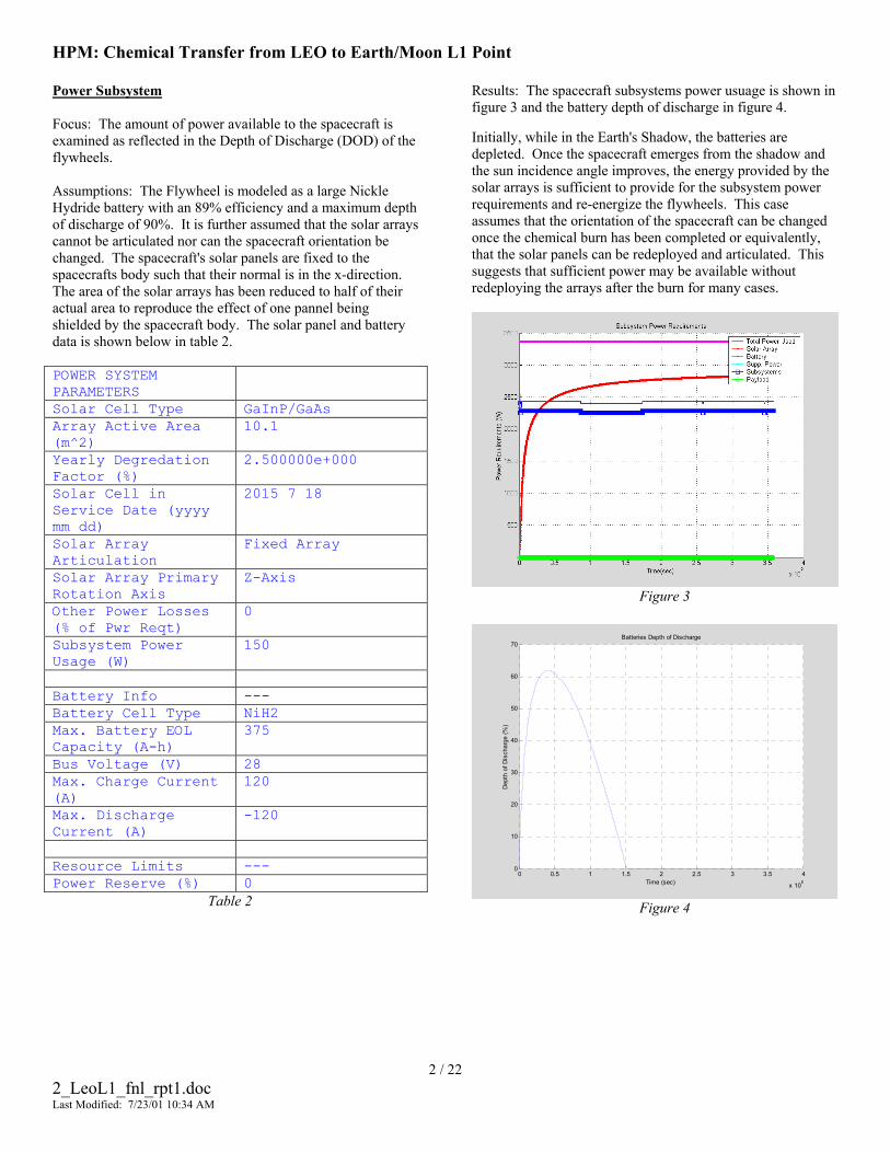
HPM: Chemical Transfer from LEO to Earth/Moon L1 Point Power Subsystem Focus: The amount of power available to the spacecraft is examined as reflected in the Depth of Discharge (DOD) of the flywheels. Assumptions: The Flywheel is modeled as a large Nickle Hydride battery with an 89% efficiency and a maximum depth of discharge of 90%. It is further assumed that the solar arrays cannot be articulated nor can the spacecraft orientation be changed. The spacecraft's solar panels are fixed to the spacecrafts body such that their normal is in the x-direction. The area of the solar arrays has been reduced to half of their actual area to reproduce the effect of one pannel being shielded by the spacecraft body. The solar panel and battery data is shown below in table 2. POWER SYSTEM PARAMETERS
Solar Cell Type GaInP/GaAs Array Active Area (m^2)
10.1
Yearly Degredation Factor (%)
2.500000e+000
Solar Cell in Service Date (yyyy mm dd)
2015 7 18
Solar Array Articulation
Fixed Array
Solar Array Primary Rotation Axis
Z-Axis
Other Power Losses (% of Pwr Reqt)
0
Subsystem Power Usage (W)
150
Battery Info --- Battery Cell Type NiH2 Max. Battery EOL Capacity (A-h)
375
Bus Voltage (V) 28 Max. Charge Current (A)
120
Max. Discharge Current (A)
-120
Resource Limits --- Power Reserve (%) 0 Table 2
Results: The spacecraft subsystems power usuage is shown in figure 3 and the battery depth of discharge in figure 4. Initially, while in the Earth's Shadow, the batteries are depleted. Once the spacecraft emerges from the shadow and the sun incidence angle improves, the energy provided by the solar arrays is sufficient to provide for the subsystem power requirements and re-energize the flywheels. This case assumes that the orientation of the spacecraft can be changed once the chemical burn has been completed or equivalently, that the solar panels can be redeployed and articulated. This suggests that sufficient power may be available without redeploying the arrays after the burn for many cases.
Figure 3
0 0.5 1 1.5 2 2.5 3 3.5 4
x 105
0
10
20
30
40
50
60
70Batteries Depth of Discharge
Time (sec)
Dep
th o
f Dis
char
ge (%
)
Figure 4
2 / 22 2_LeoL1_fnl_rpt1.doc Last Modified: 7/23/01 10:34 AM
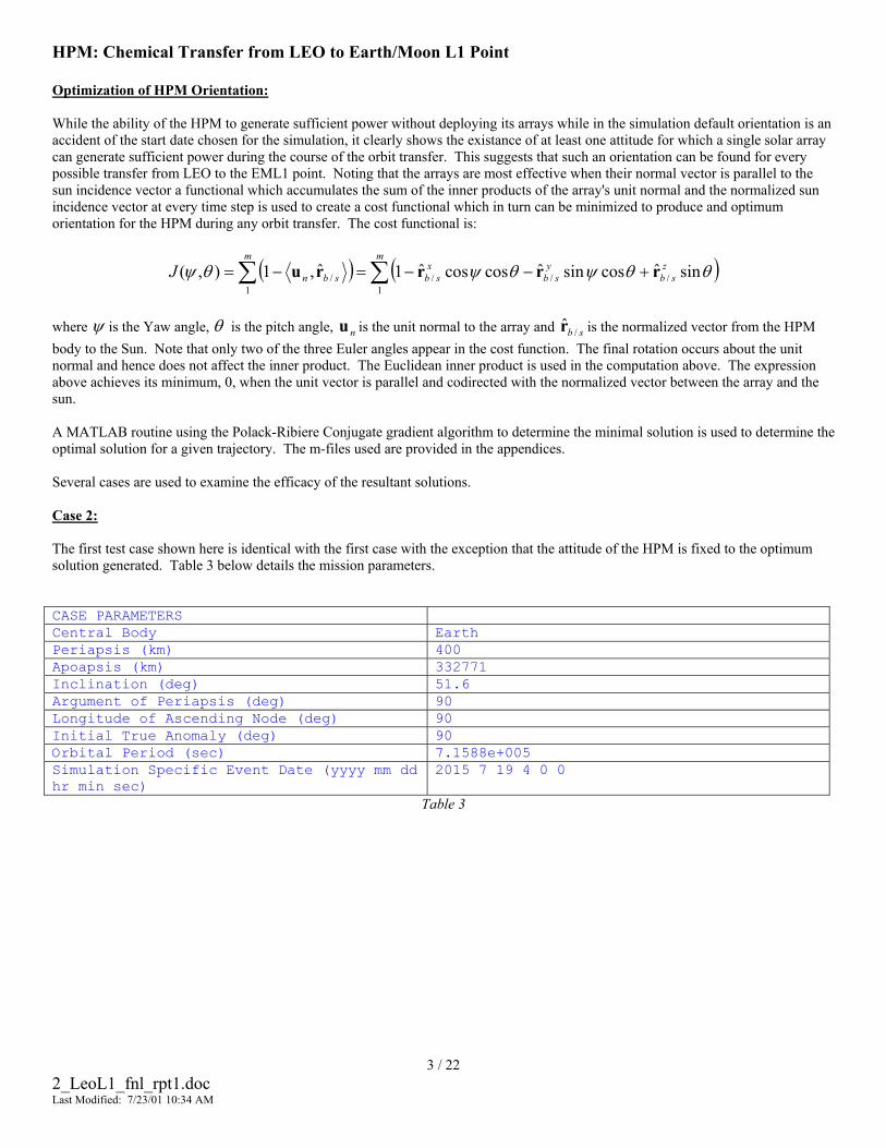
HPM: Chemical Transfer from LEO to Earth/Moon L1 Point Optimization of HPM Orientation: While the ability of the HPM to generate sufficient power without deploying its arrays while in the simulation default orientation is an accident of the start date chosen for the simulation, it clearly shows the existance of at least one attitude for which a single solar array can generate sufficient power during the course of the orbit transfer. This suggests that such an orientation can be found for every possible transfer from LEO to the EML1 point. Noting that the arrays are most effective when their normal vector is parallel to the sun incidence vector a functional which accumulates the sum of the inner products of the array's unit normal and the normalized sun incidence vector at every time step is used to create a cost functional which in turn can be minimized to produce and optimum orientation for the HPM during any orbit transfer. The cost functional is:
( ) ( )∑∑ +−−=−=m
zsb
ysb
xsb
m
sbnJ1
///1
/ sinˆcossinˆcoscosˆ1ˆ,1),( θθψθψθψ rrrru
where ψ is the Yaw angle, θ is the pitch angle, u is the unit normal to the array and r is the normalized vector from the HPM body to the Sun. Note that only two of the three Euler angles appear in the cost function. The final rotation occurs about the unit normal and hence does not affect the inner product. The Euclidean inner product is used in the computation above. The expression above achieves its minimum, 0, when the unit vector is parallel and codirected with the normalized vector between the array and the sun.
n sb /ˆ
A MATLAB routine using the Polack-Ribiere Conjugate gradient algorithm to determine the minimal solution is used to determine the optimal solution for a given trajectory. The m-files used are provided in the appendices. Several cases are used to examine the efficacy of the resultant solutions. Case 2: The first test case shown here is identical with the first case with the exception that the attitude of the HPM is fixed to the optimum solution generated. Table 3 below details the mission parameters. CASE PARAMETERS Central Body Earth Periapsis (km) 400 Apoapsis (km) 332771 Inclination (deg) 51.6 Argument of Periapsis (deg) 90 Longitude of Ascending Node (deg) 90 Initial True Anomaly (deg) 90 Orbital Period (sec) 7.1588e+005 Simulation Specific Event Date (yyyy mm dd hr min sec)
2015 7 19 4 0 0
Table 3
3 / 22 2_LeoL1_fnl_rpt1.doc Last Modified: 7/23/01 10:34 AM
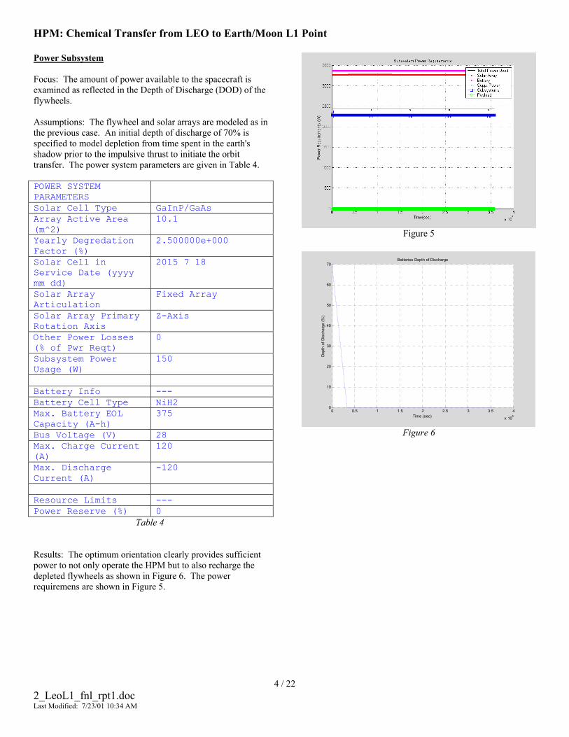
HPM: Chemical Transfer from LEO to Earth/Moon L1 Point Power Subsystem Focus: The amount of power available to the spacecraft is examined as reflected in the Depth of Discharge (DOD) of the flywheels. Assumptions: The flywheel and solar arrays are modeled as in the previous case. An initial depth of discharge of 70% is specified to model depletion from time spent in the earth's shadow prior to the impulsive thrust to initiate the orbit transfer. The power system parameters are given in Table 4. POWER SYSTEM PARAMETERS
Solar Cell Type GaInP/GaAs Array Active Area (m^2)
10.1
Yearly Degredation Factor (%)
2.500000e+000
Solar Cell in Service Date (yyyy mm dd)
2015 7 18
Solar Array Articulation
Fixed Array
Solar Array Primary Rotation Axis
Z-Axis
Other Power Losses (% of Pwr Reqt)
0
Subsystem Power Usage (W)
150
Battery Info --- Battery Cell Type NiH2 Max. Battery EOL Capacity (A-h)
375
Bus Voltage (V) 28 Max. Charge Current (A)
120
Max. Discharge Current (A)
-120
Resource Limits --- Power Reserve (%) 0 Table 4 Results: The optimum orientation clearly provides sufficient power to not only operate the HPM but to also recharge the depleted flywheels as shown in Figure 6. The power requiremens are shown in Figure 5.
Figure 5
0 0.5 1 1.5 2 2.5 3 3.5 4
x 105
0
10
20
30
40
50
60
70Batteries Depth of Discharge
Time (sec)
Dep
th o
f Dis
char
ge (%
)
Figure 6
4 / 22 2_LeoL1_fnl_rpt1.doc Last Modified: 7/23/01 10:34 AM

HPM: Chemical Transfer from LEO to Earth/Moon L1 Point Optimization Study: A series of cases are examined, varying the start time of simulation to examine the evolution of the solution and its effectiveness. Table 5 shows the otimization results over approximately one quarter of a lunar cycle. Additionally, the total area of the arrays is decreased to 9.25 m2 in order to model the effect of allowing the solar arrays to wrap around the body of the HPM when not deployed. The results obtained using the optimal attitude are virtually identical with the results shown in figures 5 and 6.
Start Date Start Time )( οω (arg. of Per.) )( οψ (Yaw) )( οθ (Pitch) ),( θψJ July 18, 2015 0:00:00 90 157.9602 -9.021 0.00020453 July 19, 2015 4:00:00 105 159.0363 -8.6106 0.00020626 July 20, 2015 8:00:00 120 160.1038 -8.1942 0.00020831 July 21, 2015 12:00:00 135 161.165 -7.7716 0.00020954 July 22, 2015 16:00:00 150 162.2176 -7.3446 0.00021049 July 23, 2015 20:00:00 165 -196.7363 -6.9139 0.00021045 July 25, 2015 0:00:00 189 -195.7001 -6.4822 0.00020971
Table 5 The evolution of the optimal solution is slow relative to the times scale of the orbit transfer and therefore the attitude remains very close to the optimum for the duration of the transfer. Next, a series of cases are examined, varying the start time of simulation over the course of one year. The start time is varied three months each time to investigate the solution and it's effectiveness over the course of the Earth's orbit about the Sun. Again, the results obtained for each cae are virtually identical with the results depicted in figures 5 and 6. Table 6 shows the optimization results.
Start Date Start Time )( οω (arg. of Per.) )( οψ (Yaw) )( οθ (Pitch) ),( θψJ Jan. 18, 2015 0:00:00 90 -22.3145 8.964 0.00022102 Apr. 18, 2015 0:00:00 90 -294.2927 -20.9923 0.00022509 July 18, 2015 0:00:00 90 157.9602 -9.021 0.00020453 Oct. 18, 2015 0:00:00 90 -117.5436 20.3181 0.00020006
Conclusions: Nearly ideal pointing over the duration of the orbit transfer can be obtained using a fixed attitude. Furthermore, once the HPM has left the Earth's shadow, a single array in its stowed configuration is sufficient to produce enough power to operate the HPM and re-energize the flywheels. This means that the arrays need not be deployed (and hence restowed during the transfer's terminal impulse) during the orbit transfer.
5 / 22 2_LeoL1_fnl_rpt1.doc Last Modified: 7/23/01 10:34 AM
HPM: Chemical Transfer from LEO to Earth/Moon L1 Point
Appendix: Optimization Routines
Opt_orient_drv.m % % Script to determine optimal orientation of HPM with solar arrays retracted % using the Polak-Ribiere Minimization % % % Set initial values % global r_hat Col load rbsn % Create unit vector pointing from space craft to the sun Col = size(rbsn,2); % Number of steps in rbsn r_hat = rbsn(2:4,:); % First row is the time X_init = [-.7, 1]; % Initial guess tol = 5.0e-08; % Convergence Tolerance % [x_min,f_extrema] = Polak_Ribiere(X_init,tol,'opt_orient_fun','opt_orient_dfun'); r2d = 180/pi; x_min x_min_deg = x_min*r2d f_extrema
6 / 22 2_LeoL1_fnl_rpt1.doc Last Modified: 7/23/01 10:34 AM
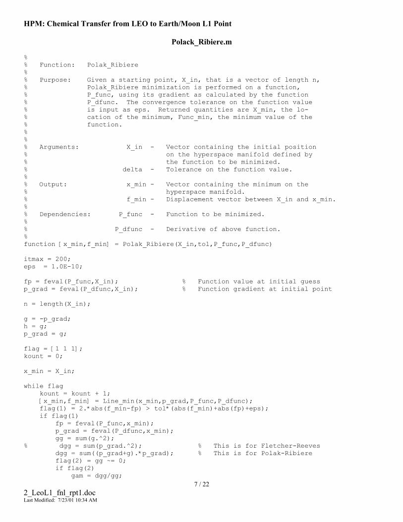
HPM: Chemical Transfer from LEO to Earth/Moon L1 Point
Polack_Ribiere.m % % Function: Polak_Ribiere % % Purpose: Given a starting point, X_in, that is a vector of length n, % Polak_Ribiere minimization is performed on a function, % P_func, using its gradient as calculated by the function % P_dfunc. The convergence tolerance on the function value % is input as eps. Returned quantities are X_min, the lo- % cation of the minimum, Func_min, the minimum value of the % function. % % % Arguments: X_in - Vector containing the initial position % on the hyperspace manifold defined by % the function to be minimized. % delta - Tolerance on the function value. % % Output: x_min - Vector containing the minimum on the % hyperspace manifold. % f_min - Displacement vector between X_in and x_min. % % Dependencies: P_func - Function to be minimized. % % P_dfunc - Derivative of above function. % function [x_min,f_min] = Polak_Ribiere(X_in,tol,P_func,P_dfunc) itmax = 200; eps = 1.0E-10; fp = feval(P_func,X_in); % Function value at initial guess p_grad = feval(P_dfunc,X_in); % Function gradient at initial point n = length(X_in); g = -p_grad; h = g; p_grad = g; flag = [1 1 1]; kount = 0; x_min = X_in; while flag kount = kount + 1; [x_min,f_min] = Line_min(x_min,p_grad,P_func,P_dfunc); flag(1) = 2.*abs(f_min-fp) > tol*(abs(f_min)+abs(fp)+eps); if flag(1) fp = feval(P_func,x_min); p_grad = feval(P_dfunc,x_min); gg = sum(g.^2); % dgg = sum(p_grad.^2); % This is for Fletcher-Reeves dgg = sum((p_grad+g).*p_grad); % This is for Polak-Ribiere flag(2) = gg ~= 0; if flag(2)
7 / 22 2_LeoL1_fnl_rpt1.doc Last Modified: 7/23/01 10:34 AM
gam = dgg/gg;

HPM: Chemical Transfer from LEO to Earth/Moon L1 Point g = -p_grad; h = g + gam*h; p_grad = h; end end flag(3) = kount < itmax; end if ~flag(3) disp('WARNING: Maximum iterations in Polak-Ribiere exceeded'); end
8 / 22 2_LeoL1_fnl_rpt1.doc Last Modified: 7/23/01 10:34 AM
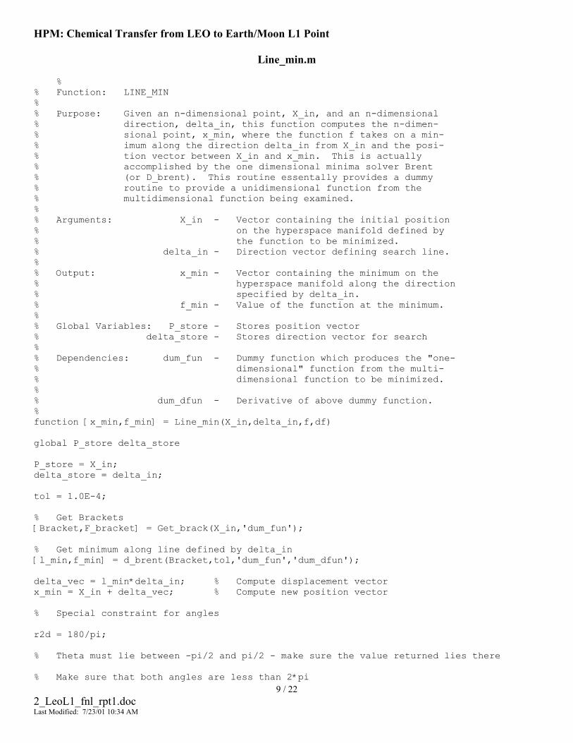
HPM: Chemical Transfer from LEO to Earth/Moon L1 Point
Line_min.m % % Function: LINE_MIN % % Purpose: Given an n-dimensional point, X_in, and an n-dimensional % direction, delta_in, this function computes the n-dimen- % sional point, x_min, where the function f takes on a min- % imum along the direction delta_in from X_in and the posi- % tion vector between X_in and x_min. This is actually % accomplished by the one dimensional minima solver Brent % (or D_brent). This routine essentally provides a dummy % routine to provide a unidimensional function from the % multidimensional function being examined. % % Arguments: X_in - Vector containing the initial position % on the hyperspace manifold defined by % the function to be minimized. % delta_in - Direction vector defining search line. % % Output: x_min - Vector containing the minimum on the % hyperspace manifold along the direction % specified by delta_in. % f_min - Value of the function at the minimum. % % Global Variables: P_store - Stores position vector % delta_store - Stores direction vector for search % % Dependencies: dum_fun - Dummy function which produces the "one- % dimensional" function from the multi- % dimensional function to be minimized. % % dum_dfun - Derivative of above dummy function. % function [x_min,f_min] = Line_min(X_in,delta_in,f,df) global P_store delta_store P_store = X_in; delta_store = delta_in; tol = 1.0E-4; % Get Brackets [Bracket,F_bracket] = Get_brack(X_in,'dum_fun'); % Get minimum along line defined by delta_in [l_min,f_min] = d_brent(Bracket,tol,'dum_fun','dum_dfun'); delta_vec = l_min*delta_in; % Compute displacement vector x_min = X_in + delta_vec; % Compute new position vector % Special constraint for angles r2d = 180/pi; % Theta must lie between -pi/2 and pi/2 - make sure the value returned lies there
9 / 22 2_LeoL1_fnl_rpt1.doc Last Modified: 7/23/01 10:34 AM
% Make sure that both angles are less than 2*pi
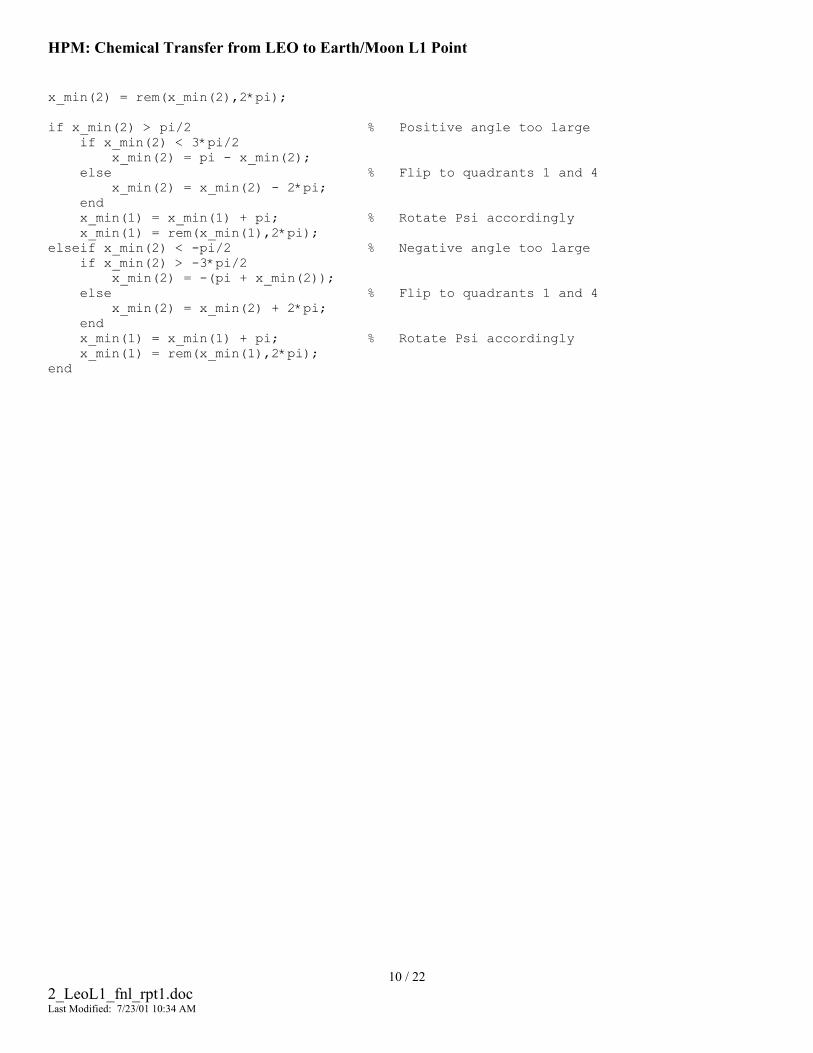
HPM: Chemical Transfer from LEO to Earth/Moon L1 Point x_min(2) = rem(x_min(2),2*pi); if x_min(2) > pi/2 % Positive angle too large if x_min(2) < 3*pi/2 x_min(2) = pi - x_min(2); else % Flip to quadrants 1 and 4 x_min(2) = x_min(2) - 2*pi; end x_min(1) = x_min(1) + pi; % Rotate Psi accordingly x_min(1) = rem(x_min(1),2*pi); elseif x_min(2) < -pi/2 % Negative angle too large if x_min(2) > -3*pi/2 x_min(2) = -(pi + x_min(2)); else % Flip to quadrants 1 and 4 x_min(2) = x_min(2) + 2*pi; end x_min(1) = x_min(1) + pi; % Rotate Psi accordingly x_min(1) = rem(x_min(1),2*pi); end
10 / 22 2_LeoL1_fnl_rpt1.doc Last Modified: 7/23/01 10:34 AM

HPM: Chemical Transfer from LEO to Earth/Moon L1 Point
Get_brack.m % % Function: Get_brack % % Purpose: Given a function f, and given distinct initial points ax and % bx, this function searches in the downhill direction (defined % by the function as evaluated at the initial points) and returns % new points, ax, bx, and cx that bracket a minimum of the func- % tion. Also returned are the function values at the three points % fa, fb and fc. % % This implementation is based upon the implementation % given in Numerical Recipes, Press et. al. % % Arguments: X_in - Vector containing the initial points % [ax,bx] % % f - Function to be minimized % % Bracket - Vector containing the bracketing points % of the extrema, [ax,bx,cx] where: % ax = "Leftmost" bracketing abscissa % bx = Central abscissa % cx = "Rightmost" bracketing abscissa % % F_bracket - Vector containing the function values % corresponding to the above bracket points % function [Bracket,F_bracket] = Get_brack(X_in,f) gold = 1.618034; % Golden ratio g_limit = 100; % Maximum magnification allowed max_brack = 2*pi; % Added just for angle search tiny = 1.0E-20; % Avoid division by zero % May wish to change this part around to perform computations more in situ ax = X_in(1); bx = X_in(2); fa = feval(f,ax); fb = feval(f,bx); if fb > fa % Make sure that steps are going downhill temp = ax; ax = bx; % Switch if necessary bx = temp; temp = fa; fa = fb; fb = temp; end cx = bx + gold*(bx-ax); % Use golden section method for first guess at cx fc = feval(f,cx); con_flag = fb > fc;
11 / 22 2_LeoL1_fnl_rpt1.doc Last Modified: 7/23/01 10:34 AM
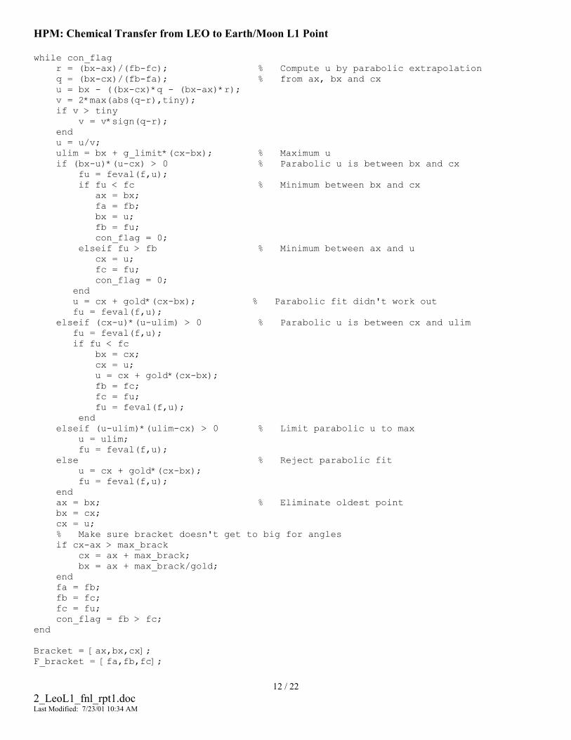
HPM: Chemical Transfer from LEO to Earth/Moon L1 Point while con_flag r = (bx-ax)/(fb-fc); % Compute u by parabolic extrapolation q = (bx-cx)/(fb-fa); % from ax, bx and cx u = bx - ((bx-cx)*q - (bx-ax)*r); v = 2*max(abs(q-r),tiny); if v > tiny v = v*sign(q-r); end u = u/v; ulim = bx + g_limit*(cx-bx); % Maximum u if (bx-u)*(u-cx) > 0 % Parabolic u is between bx and cx fu = feval(f,u); if fu < fc % Minimum between bx and cx ax = bx; fa = fb; bx = u; fb = fu; con_flag = 0; elseif fu > fb % Minimum between ax and u cx = u; fc = fu; con_flag = 0; end u = cx + gold*(cx-bx); % Parabolic fit didn't work out fu = feval(f,u); elseif (cx-u)*(u-ulim) > 0 % Parabolic u is between cx and ulim fu = feval(f,u); if fu < fc bx = cx; cx = u; u = cx + gold*(cx-bx); fb = fc; fc = fu; fu = feval(f,u); end elseif (u-ulim)*(ulim-cx) > 0 % Limit parabolic u to max u = ulim; fu = feval(f,u); else % Reject parabolic fit u = cx + gold*(cx-bx); fu = feval(f,u); end ax = bx; % Eliminate oldest point bx = cx; cx = u; % Make sure bracket doesn't get to big for angles if cx-ax > max_brack cx = ax + max_brack; bx = ax + max_brack/gold; end fa = fb; fb = fc; fc = fu; con_flag = fb > fc; end Bracket = [ax,bx,cx]; F_bracket = [fa,fb,fc];
12 / 22 2_LeoL1_fnl_rpt1.doc Last Modified: 7/23/01 10:34 AM

HPM: Chemical Transfer from LEO to Earth/Moon L1 Point
dum_fun.m % % Function: DUM_FUN % % Purpose: Dummy function used by Line_min to find a minimum along % a givin direction in n-dimensional space. % % Arguments: X_in - Displacement along the given direction % from the initial point. % function f = dum_fun(x) global P_store delta_store x_temp = P_store + x*delta_store; % % This line will need to be modified to accomodate different function % or, this name can be used for whatever routine will contain the function % to be minimized. % f = opt_orient_fun(x_temp);
13 / 22 2_LeoL1_fnl_rpt1.doc Last Modified: 7/23/01 10:34 AM
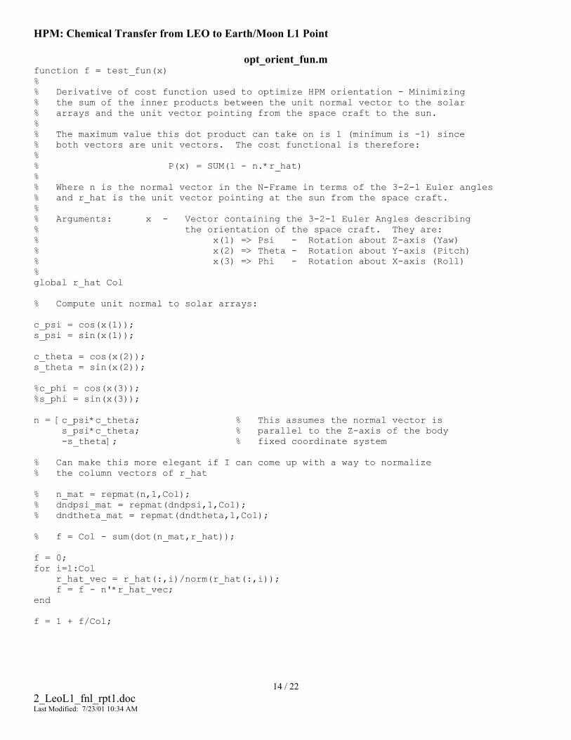
HPM: Chemical Transfer from LEO to Earth/Moon L1 Point
opt_orient_fun.m function f = test_fun(x) % % Derivative of cost function used to optimize HPM orientation - Minimizing % the sum of the inner products between the unit normal vector to the solar % arrays and the unit vector pointing from the space craft to the sun. % % The maximum value this dot product can take on is 1 (minimum is -1) since % both vectors are unit vectors. The cost functional is therefore: % % P(x) = SUM(1 - n.*r_hat) % % Where n is the normal vector in the N-Frame in terms of the 3-2-1 Euler angles % and r_hat is the unit vector pointing at the sun from the space craft. % % Arguments: x - Vector containing the 3-2-1 Euler Angles describing % the orientation of the space craft. They are: % x(1) => Psi - Rotation about Z-axis (Yaw) % x(2) => Theta - Rotation about Y-axis (Pitch) % x(3) => Phi - Rotation about X-axis (Roll) % global r_hat Col % Compute unit normal to solar arrays: c_psi = cos(x(1)); s_psi = sin(x(1)); c_theta = cos(x(2)); s_theta = sin(x(2)); %c_phi = cos(x(3)); %s_phi = sin(x(3)); n = [c_psi*c_theta; % This assumes the normal vector is s_psi*c_theta; % parallel to the Z-axis of the body -s_theta]; % fixed coordinate system % Can make this more elegant if I can come up with a way to normalize % the column vectors of r_hat % n_mat = repmat(n,1,Col); % dndpsi_mat = repmat(dndpsi,1,Col); % dndtheta_mat = repmat(dndtheta,1,Col); % f = Col - sum(dot(n_mat,r_hat)); f = 0; for i=1:Col r_hat_vec = r_hat(:,i)/norm(r_hat(:,i)); f = f - n'*r_hat_vec; end f = 1 + f/Col;
14 / 22 2_LeoL1_fnl_rpt1.doc Last Modified: 7/23/01 10:34 AM
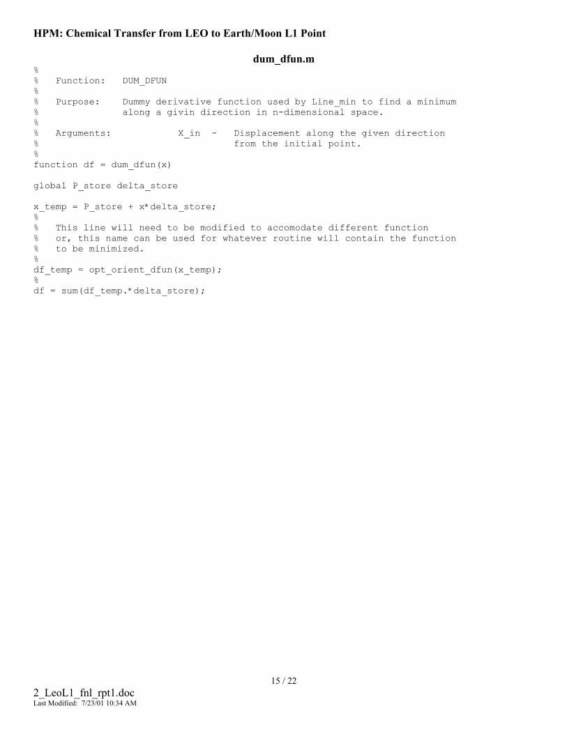
HPM: Chemical Transfer from LEO to Earth/Moon L1 Point
dum_dfun.m % % Function: DUM_DFUN % % Purpose: Dummy derivative function used by Line_min to find a minimum % along a givin direction in n-dimensional space. % % Arguments: X_in - Displacement along the given direction % from the initial point. % function df = dum_dfun(x) global P_store delta_store x_temp = P_store + x*delta_store; % % This line will need to be modified to accomodate different function % or, this name can be used for whatever routine will contain the function % to be minimized. % df_temp = opt_orient_dfun(x_temp); % df = sum(df_temp.*delta_store);
15 / 22 2_LeoL1_fnl_rpt1.doc Last Modified: 7/23/01 10:34 AM
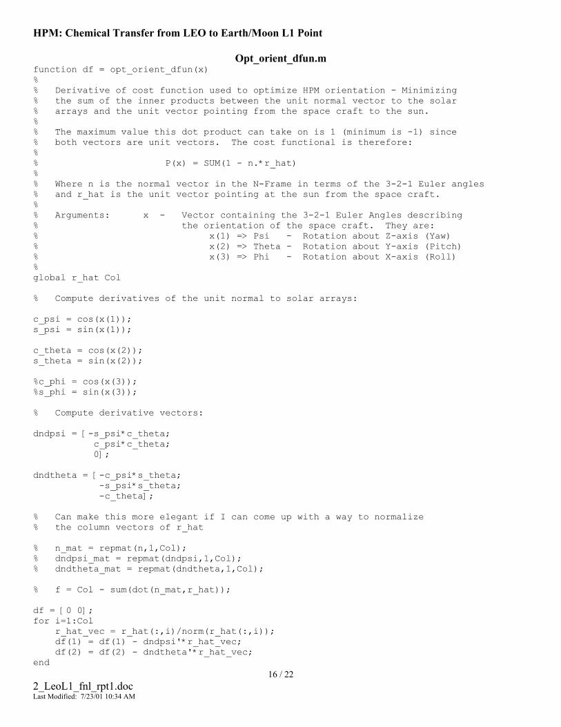
HPM: Chemical Transfer from LEO to Earth/Moon L1 Point
Opt_orient_dfun.m function df = opt_orient_dfun(x) % % Derivative of cost function used to optimize HPM orientation - Minimizing % the sum of the inner products between the unit normal vector to the solar % arrays and the unit vector pointing from the space craft to the sun. % % The maximum value this dot product can take on is 1 (minimum is -1) since % both vectors are unit vectors. The cost functional is therefore: % % P(x) = SUM(1 - n.*r_hat) % % Where n is the normal vector in the N-Frame in terms of the 3-2-1 Euler angles % and r_hat is the unit vector pointing at the sun from the space craft. % % Arguments: x - Vector containing the 3-2-1 Euler Angles describing % the orientation of the space craft. They are: % x(1) => Psi - Rotation about Z-axis (Yaw) % x(2) => Theta - Rotation about Y-axis (Pitch) % x(3) => Phi - Rotation about X-axis (Roll) % global r_hat Col % Compute derivatives of the unit normal to solar arrays: c_psi = cos(x(1)); s_psi = sin(x(1)); c_theta = cos(x(2)); s_theta = sin(x(2)); %c_phi = cos(x(3)); %s_phi = sin(x(3)); % Compute derivative vectors: dndpsi = [-s_psi*c_theta; c_psi*c_theta; 0]; dndtheta = [-c_psi*s_theta; -s_psi*s_theta; -c_theta]; % Can make this more elegant if I can come up with a way to normalize % the column vectors of r_hat % n_mat = repmat(n,1,Col); % dndpsi_mat = repmat(dndpsi,1,Col); % dndtheta_mat = repmat(dndtheta,1,Col); % f = Col - sum(dot(n_mat,r_hat)); df = [0 0]; for i=1:Col r_hat_vec = r_hat(:,i)/norm(r_hat(:,i)); df(1) = df(1) - dndpsi'*r_hat_vec; df(2) = df(2) - dndtheta'*r_hat_vec;
16 / 22 2_LeoL1_fnl_rpt1.doc Last Modified: 7/23/01 10:34 AM
end

HPM: Chemical Transfer from LEO to Earth/Moon L1 Point df = df/Col;
17 / 22 2_LeoL1_fnl_rpt1.doc Last Modified: 7/23/01 10:34 AM
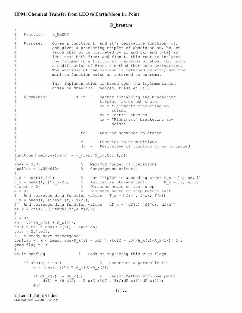
HPM: Chemical Transfer from LEO to Earth/Moon L1 Point
D_brent.m % % Function: D_BRENT % % Purpose: Given a function f, and it's derivative function, df, % and given a bracketing triplet of abscissas ax, bx, cx % (such that bx is bracketed by ax and cx, and f(bx) is % less than both f(ax) and f(cx)), this routine isolates % the minimum fo a fractional precision of about tol using % a modification of Brent's method that uses derivatives. % The abscissa of the minimum is returned as xmin, and the % minimum function value as returned as extrema. % % This implementation is based upon the implementation % given in Numerical Recipes, Press et. al. % % Arguments: X_in - Vector containing the bracketing % triplet [ax,bx,cx] where: % ax = "Leftmost" bracketing ab- % scissa % bx = Central absciss % cx = "Rightmost" bracketing ab- % scissa % % tol - Desired accurace tolerance % % f - Function to be minimized % df - Derivative of function to be minimized % function [xmin,extrema] = d_brent(X_in,tol,f,df) % kmax = 200; % Maximum number of iterations epsilon = 1.0E-010; % Convergence criteria % A_x = sort(X_in); % Put Triplet in ascending order A_x = [a, bx, b] B_x = ones(1,3)*A_x(2); % Initialize Storage vector B_x = [v, w, x] d_used = 0; % Distance moved on last step e = 0; % Distance moved on step before last % And corresponding function values F_x = [f(v), f(w), f(x)] F_x = ones(1,3)*feval(f,A_x(2)); % And corresponding function values dF_x = [df(v), df(w), df(x)] dF_x = ones(1,3)*feval(df,A_x(2)); % k = 0; xm = .5*(A_x(1) + A_x(3)); tol1 = tol * abs(B_x(3)) + epsilon; tol2 = 2.*tol1; % Already have convergence? conflag = [k < kmax, abs(B_x(3) - xm) > (tol2 - .5*(A_x(3)-A_x(1))) 1]; grad_flag = 1; % while conflag % Look at replacing this with flags if abs(e) > tol1 % Construct a parabolic fit d = ones(1,2)*2.*(A_x(3)-A_x(1)); if dF_x(2) ~= dF_x(3) % Secant Method with one point d(1) = (B_x(2) - B_x(3))*dF_x(3)/(dF_x(3)-dF_x(2));
18 / 22 2_LeoL1_fnl_rpt1.doc Last Modified: 7/23/01 10:34 AM
end
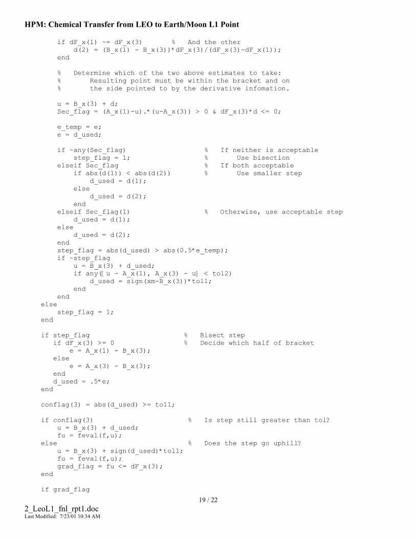
HPM: Chemical Transfer from LEO to Earth/Moon L1 Point if dF_x(1) ~= dF_x(3) % And the other d(2) = (B_x(1) - B_x(3))*dF_x(3)/(dF_x(3)-dF_x(1)); end % Determine which of the two above estimates to take: % Resulting point must be within the bracket and on % the side pointed to by the derivative infomation. u = B_x(3) + d; Sec_flag = (A_x(1)-u).*(u-A_x(3)) > 0 & dF_x(3)*d <= 0; e_temp = e; e = d_used; if ~any(Sec_flag) % If neither is acceptable step_flag = 1; % Use bisection elseif Sec_flag % If both acceptable if abs(d(1)) < abs(d(2)) % Use smaller step d_used = d(1); else d_used = d(2); end elseif Sec_flag(1) % Otherwise, use acceptable step d_used = d(1); else d_used = d(2); end step_flag = abs(d_used) > abs(0.5*e_temp); if ~step_flag u = B_x(3) + d_used; if any([u - A_x(1), A_x(3) - u] < tol2) d_used = sign(xm-B_x(3))*tol1; end end else step_flag = 1; end if step_flag % Bisect step if dF_x(3) >= 0 % Decide which half of bracket e = A_x(1) - B_x(3); else e = A_x(3) - B_x(3); end d_used = .5*e; end conflag(3) = abs(d_used) >= tol1; if conflag(3) % Is step still greater than tol? u = B_x(3) + d_used; fu = feval(f,u); else % Does the step go uphill? u = B_x(3) + sign(d_used)*tol1; fu = feval(f,u); grad_flag = fu <= dF_x(3); end
19 / 22 2_LeoL1_fnl_rpt1.doc Last Modified: 7/23/01 10:34 AM
if grad_flag

HPM: Chemical Transfer from LEO to Earth/Moon L1 Point du = feval(df,u); if fu <= F_x(3) if u >= B_x(3) A_x(1) = B_x(3); else A_x(3) = B_x(3); end B_x(1) = B_x(2); F_x(1) = F_x(2); dF_x(1) = dF_x(2); B_x(2) = B_x(3); F_x(2) = F_x(3); dF_x(2) = dF_x(3); B_x(3) = u; F_x(3) = fu; dF_x(3) = du; else if u < B_x(3) A_x(1) = u; else A_x(3) = u; end if fu <= F_x(2) | B_x(2) == B_x(3) B_x(1) = B_x(2); F_x(1) = F_x(2); dF_x(1) = dF_x(2); B_x(2) = u; F_x(2) = fu; dF_x(2) = du; elseif any([fu <= F_x(1), B_x(1) == B_x(3), B_x(1) == B_x(2)]) B_x(1) = u; F_x(1) = fu; dF_x(1) = du; end end end k = k + 1; xm = .5*(A_x(1) + A_x(3)); tol1 = tol * abs(B_x(3)) + epsilon; tol2 = 2.*tol1; % Have convergence? conflag(1:2) = [k < kmax, abs(B_x(3) - xm) > (tol2 - .5*(A_x(3)-A_x(1)))]; end % % Here are the results % xmin = B_x(3); extrema = F_x(3);
20 / 22 2_LeoL1_fnl_rpt1.doc Last Modified: 7/23/01 10:34 AM
if conflag(2:3) % Exit because exceeded maximum iterations

HPM: Chemical Transfer from LEO to Earth/Moon L1 Point warning('Maximum iterations exceeded in Brent'); end
21 / 22 2_LeoL1_fnl_rpt1.doc Last Modified: 7/23/01 10:34 AM

HPM: Chemical Transfer from LEO to Earth/Moon L1 Point
This page intentionally left blank.
22 / 22 2_LeoL1_fnl_rpt1.doc Last Modified: 7/23/01 10:34 AM

V e r s i o n - 0 8 - 2 8 - 0 1
Low Thrust Orbital Transfers
1
TABLE OF CONTENTS
Table of Contents.......................................................................................................................................1
Summary .......................................................................................................................................................2
Nomenclature..............................................................................................................................................2
1. Original Problem.................................................................................................................3
2. Differential Equation for Semi Major Axis..................................................................3
3. Analytical Solution ..............................................................................................................6
4. Analytical Solution Expressed in Different Useful Forms......................................7
5. Domain of Applicability ....................................................................................................9
6. Comparison with Hohmann Transfer.........................................................................10
7. High-Thrust and Low-Thrust Escape........................................................................11
8. Interesting Observations and Rules of Thumb .......................................................13
Numerical Results ...................................................................................................................................15
2
SUMMARY
An analytical formula is derived that approximates the semi major axis as a function of time for the case of a low thrust orbital transfers with circular initial orbit, circular target orbit, and constant thrust directed either always along or always opposite the velocity vector. It is assumed that the thrust and the gravitational attraction stemming from the central body are the only forces acting on the vehicle. A criterion is derived to determine the range within which the approximation should be expected to yield good agreement with the precise solution. A comparison of the analytical approximations derived here to precise numerical integration results is presented.
NOMENCLATURE
a semi-major axis ][m
0a initial semi-major axis ][m
µ gravitational constant times mass of central body;
for earth, ][103.9843912 2314 sm⋅=µ
E total energy ][Nm
kinE kinetic energy ][Nm
potE potential energy ][Nm
T (constant) thrust magnitude ][N
ev (constant) exhaust velocity ][ sm
m mass of satellite ][kg
0m initial mass of satellite ][kg
m& mass rate of change due to thruster firing ][ skg

3
1. Original Problem Given is a satellite orbiting in a circular orbit around the earth (or another central body). The satellite is driven by an electric propulsion system. That means, we have high exhaust velocity but only low thrust. The desire is to perform an orbital transfer to another circular orbit, but with larger or smaller semi-major axis, within a reasonable amount of time.
Our approach is to leave the thrusters on all the time, and to fire the thrusters always along the velocity vector. The assumption that the thrust acceleration is small compared to the gravitational acceleration allows for certain simplifications that enable the approximate analytical integration as shown below.
In the analysis below, we always assume that the only forces acting on the satellite are the thrust and the gravitation stemming from the central body.
2. Differential Equation for Semi Major Axis Consider a satellite of mass m in an orbit of semi major axis a about an inertially fixed central body with gravitational constant .µ We state the following well known equations of physics and orbital mechanics without proof:
potkin EEE += (1)
,21 2mvEkin = (2)
r
mEpotµ
−= (3)
amE2µ
−= (4)
−=
arv 122 µ (5)
Differentiating (4), we get
ama
amE
22 2
µµ &&& −⋅= (6)
Equations (1)-(6) hold for arbitrary orbits of semi major axis .a In the absence of any external forces other than the gravitational force exerted by the central body, the left-hand side of (6) is identically zero.
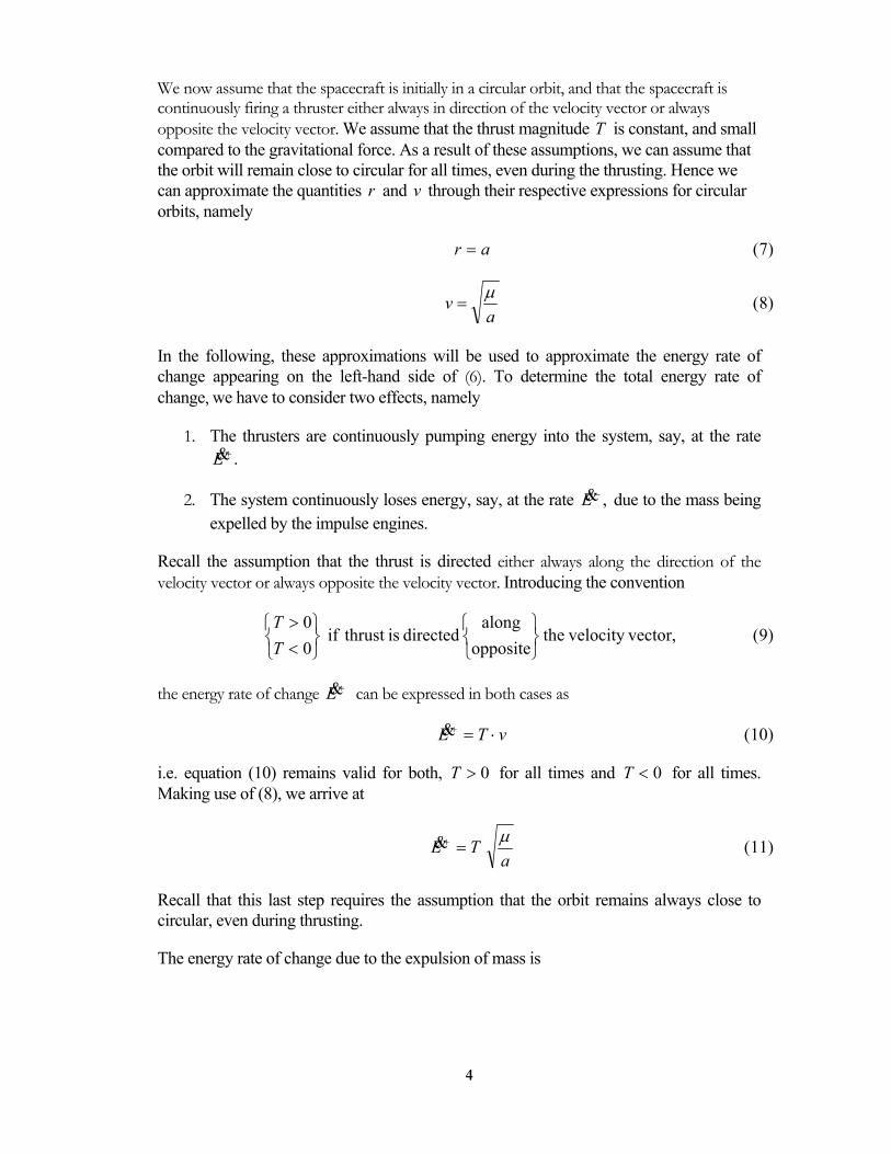
4
We now assume that the spacecraft is initially in a circular orbit, and that the spacecraft is continuously firing a thruster either always in direction of the velocity vector or always opposite the velocity vector. We assume that the thrust magnitude T is constant, and small compared to the gravitational force. As a result of these assumptions, we can assume that the orbit will remain close to circular for all times, even during the thrusting. Hence we can approximate the quantities r and v through their respective expressions for circular orbits, namely
ar = (7)
a
v µ= (8)
In the following, these approximations will be used to approximate the energy rate of change appearing on the left-hand side of (6). To determine the total energy rate of change, we have to consider two effects, namely
1. The thrusters are continuously pumping energy into the system, say, at the rate .+E&
2. The system continuously loses energy, say, at the rate ,−E& due to the mass being expelled by the impulse engines.
Recall the assumption that the thrust is directed either always along the direction of the velocity vector or always opposite the velocity vector. Introducing the convention
vector, velocity theopposite
along directed is thrust if
00
<>
TT
(9)
the energy rate of change +E& can be expressed in both cases as
vTE ⋅=+& (10)
i.e. equation (10) remains valid for both, 0>T for all times and 0<T for all times. Making use of (8), we arrive at
a
TE µ=+& (11)
Recall that this last step requires the assumption that the orbit remains always close to circular, even during thrusting.
The energy rate of change due to the expulsion of mass is

5
mmEE&& ⋅=− (12)
Using ammvE22
1 2 µ−= obtained from (1), (2), (3), and using the approximations (7), (8),
this yields
ma
E && ⋅−=−
2µ (13)
Inserting the sum of (11) and (13) for E& on the left-hand side of (6) yields
ama
amm
aaT
222 2
µµµµ &&& −⋅=⋅− (14)
Solving for ,a& we get
32 amTa ⋅=µ
& (15)
Clearly, the quantities ,T ,µ and m& are constants, and the satellite mass m is a known function of time, namely
tmmtm ⋅+= &0)( (16)
In summary, equation (15) represents an ordinary differential equation in the scalar quantity ).(ta Explicitly showing all dependencies, this differential equation can be stated in the form
( )
3
0
)(2)( tatmm
Tta ⋅⋅+
=µ&
& (17)
where
locityexhaust veconstant
change of rate massconstant v
|T|mass initialconstant
constant nalgravitatioconstant (9) also see ;maginitudehrust constant t
timeaxismajor semi
e
0
=
=−=
=====
ev
m
m
Tta
&
µ (18)
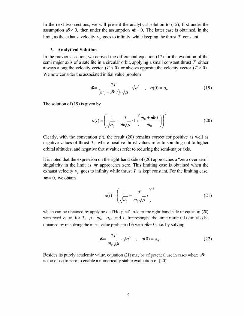
6
In the next two sections, we will present the analytical solution to (15), first under the assumption ,0<m& then under the assumption .0=m& The latter case is obtained, in the limit, as the exhaust velocity ev goes to infinity, while keeping the thrust T constant.
3. Analytical Solution In the previous section, we derived the differential equation (17) for the evolution of the semi major axis of a satellite in a circular orbit, applying a small constant thrust T either always along the velocity vector )0( >T or always opposite the velocity vector ).0( <T We now consider the associated initial value problem
( ) 0
3
0
)0(,2 aaatmmTa =⋅
⋅⋅+=
µ&& (19)
The solution of (19) is given by
2
0
0
0
ln1)(−
⋅+⋅−=
mtmm
mT
ata
&
& µ (20)
Clearly, with the convention (9), the result (20) remains correct for positive as well as negative values of thrust ,T where positive thrust values refer to spiraling out to higher orbital altitudes, and negative thrust values refer to reducing the semi-major axis.
It is noted that the expression on the right-hand side of (20) approaches a “zero over zero” singularity in the limit as m& approaches zero. This limiting case is obtained when the exhaust velocity ev goes to infinity while thrust T is kept constant. For the limiting case,
,0=m& we obtain
2
00
1)(−
−= tmT
ata
µ (21)
which can be obtained by applying de l’Hospital’s rule to the right-hand side of equation (20) with fixed values for ,T ,µ ,0m ,0a and .t Interestingly, the same result (21) can also be obtained by re-solving the initial value problem (19) with ,0=m& i.e. by solving
03
0
)0(,2 aaamTa =⋅=µ
& (22)
Besides its purely academic value, equation (21) may be of practical use in cases where m& is too close to zero to enable a numerically stable evaluation of (20).
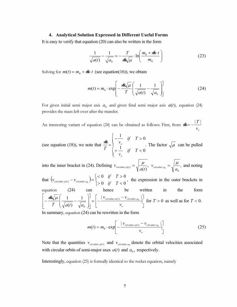
7
4. Analytical Solution Expressed in Different Useful Forms It is easy to verify that equation (20) can also be written in the form
⋅+⋅−=−
0
0
0
ln1)(
1m
tmmmT
ata&
& µ (23)
Solving for tmmtm ⋅+= &0)( (see equation(16)), we obtain
−−⋅=
00
1)(
1exp)(ataT
mmtm
µ& (24)
For given initial semi major axis 0a and given final semi major axis ),(ta equation (24) provides the mass left over after the transfer.
An interesting variant of equation (24) can be obtained as follows: First, from evTm ||
−=&
(see equation (18)), we note that .01
01
<+
>−=
Tifv
Tifv
Tm
e
e& The factor µ can be pulled
into the inner bracket in (24). Defining ,)()(, ta
v tacircularµ
= ,0
, 0 av acircular
µ= and noting
that ( ) ,0000
0,)(,
<>><
=−TifTif
vv acirculartacircular the expression in the outer brackets in
equation (24) can hence be written in the form
−−=
−−
e
acirculartacircular
vvv
ataTm ||1
)(1 0,)(,
0
µ& for 0>T as well as for .0<T
In summary, equation (24) can be rewritten in the form
−−⋅=
e
acirculartacircular
vvv
mtm||
exp)( 0,)(,0 (25)
Note that the quantities )(, tacircularv and 0,acircularv denote the orbital velocities associated
with circular orbits of semi-major axes )(ta and ,0a respectively.
Interestingly, equation (25) is formally identical to the rocket equation, namely

8
−−⋅=
evvtv
mtm|)(|
exp)( 00 (26)
That means that the vehicle mass after a circular-to-circular low-thrust orbital transfer can be formally obtained from the rocket equation. Note that the rocket equation (26) is derived for linear accelerations in inertial space without gravitation or other perturbing forces. Thrust is assumed as the only acting force, and this thrust is directed either always along the velocity vector or always opposite the velocity vector. For the assumptions underlying the rocket equation, thrust along/opposite the velocity vector causes the velocity to increase/decrease. The situation is precisely reversed in the case of our low thrust orbital transfers. There, thrust along/opposite the velocity vector causes the velocity to increase/decrease. Nevertheless, this sign change remains without effect in the mass equations (25), (26), as it appears inside the absolute values, and formally, the mass evolution for our low thrust orbital transfer is identical to that in the case of the rocket equation (26).
Obviously, the transfer time, ,t and the fuel mass, ,tmm fuel ⋅−= & can be easily obtained from (24), namely
−−−⋅−=
0
0 1)(
1exp1ataT
mmm
tµ&
& (27)
−−−⋅=
00
1)(
1exp1ataT
mmm fuel
µ& (28)
Using arguments similar to the ones used above, these two equations can be written in the form
−−−⋅=
ee v
vtvTm
vt|)(|
exp1||
00 (29)
−−−⋅=
efuel v
vtvmm
|)(|exp1 0
0 (30)
Note that all equations derived above are valid for positive as well as negative values of thrust ,T as long as we follow the conventions defined in equation (9).

9
5. Domain of Applicability The results (20), (21) can be expected to yield good approximations only as long as the assumptions used in the derivation remain satisfied. The key assumption in the derivation of (20), (21) was that the orbit remains close to circular at all times during the orbital transfer. This is tantamount to the assumption that the orbital transfer occurs gradually, i.e. that the semi major axis increases only by a small factor over each orbit. Clearly, as the semi major axis increases, the gravitational acceleration reduces, and the constant thrust magnitude becomes more significant compared to the gravitational force. Intuitively, it must be expected that the semi major axis starts increasing more rapidly, then.
Comparisons between the analytical approximation (20) and solutions obtained through precise numerical integration show that excellent agreement is obtained as long as the semi major axis increases by up to 10% per orbit. Acceptable results are achieved even as long as the semi major axis increases by up to 50% per orbit.
Now let p denote a percentage increase in the semi major axis per orbit with which the user feels comfortable. Then the condition that the semi major axis increases by no more than a factor (1+p) per orbit can be written in the form
pa
a orbitoneover ≤∆
|| (31)
Approximating orbitoneovera∆ by ,orbitTa ⋅& and using for orbitT the expression for the orbital
period, i.e. ,23
µπ aTorbit ⋅= (31) yields
paa ≤⋅⋅ |2|µ
π & (32)
Inserting the right-hand side of (15) for ,a& we get from (32)
ptatmT
≤⋅ |)()(
4| 2
µπ (33)
The left -hand side of equation (33) gives us the fraction by which the semi major axis changes within one orbit, given the semi-major axis a and the mass m at the beginning of that orbit. Equation (33) is useful to determine up to what semi-major axis the low-thrust assumption can be used. But some guessing is necessary to come up with an approximation for the mass .m Equation (33) remains correct without changes even for the singular case of constant mass, i.e. for the case .0=m&
Multiplying the left -hand side of equation (33) with 100 gives us the percentage change in semi major axis per orbit.
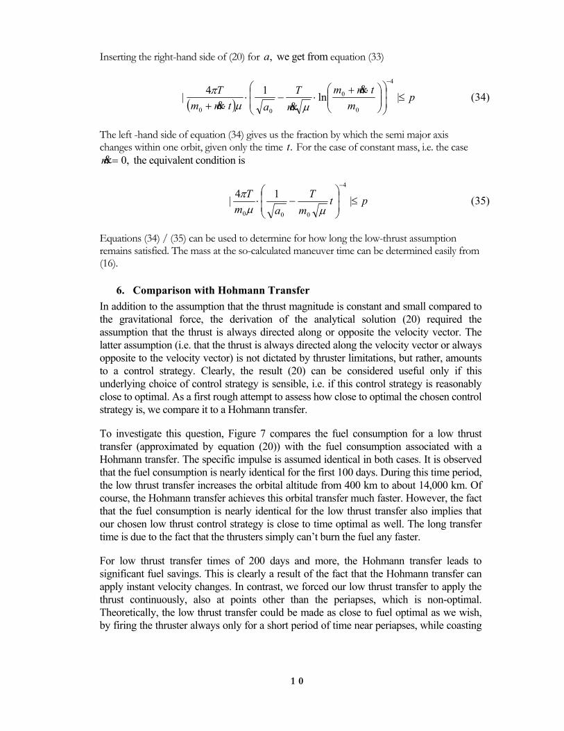
1 0
Inserting the right-hand side of (20) for ,a we get from equation (33)
( ) pm
tmmmT
atmmT
≤
⋅+⋅−⋅
⋅+
−
|ln14|4
0
0
00
&
&& µµπ (34)
The left -hand side of equation (34) gives us the fraction by which the semi major axis changes within one orbit, given only the time .t For the case of constant mass, i.e. the case
,0=m& the equivalent condition is
ptmT
amT
≤
−⋅
−
|14|4
000 µµπ (35)
Equations (34) / (35) can be used to determine for how long the low-thrust assumption remains satisfied. The mass at the so-calculated maneuver time can be determined easily from (16).
6. Comparison with Hohmann Transfer In addition to the assumption that the thrust magnitude is constant and small compared to the gravitational force, the derivation of the analytical solution (20) required the assumption that the thrust is always directed along or opposite the velocity vector. The latter assumption (i.e. that the thrust is always directed along the velocity vector or always opposite to the velocity vector) is not dictated by thruster limitations, but rather, amounts to a control strategy. Clearly, the result (20) can be considered useful only if this underlying choice of control strategy is sensible, i.e. if this control strategy is reasonably close to optimal. As a first rough attempt to assess how close to optimal the chosen control strategy is, we compare it to a Hohmann transfer.
To investigate this question, Figure 7 compares the fuel consumption for a low thrust transfer (approximated by equation (20)) with the fuel consumption associated with a Hohmann transfer. The specific impulse is assumed identical in both cases. It is observed that the fuel consumption is nearly identical for the first 100 days. During this time period, the low thrust transfer increases the orbital altitude from 400 km to about 14,000 km. Of course, the Hohmann transfer achieves this orbital transfer much faster. However, the fact that the fuel consumption is nearly identical for the low thrust transfer also implies that our chosen low thrust control strategy is close to time optimal as well. The long transfer time is due to the fact that the thrusters simply can’t burn the fuel any faster.
For low thrust transfer times of 200 days and more, the Hohmann transfer leads to significant fuel savings. This is clearly a result of the fact that the Hohmann transfer can apply instant velocity changes. In contrast, we forced our low thrust transfer to apply the thrust continuously, also at points other than the periapses, which is non-optimal. Theoretically, the low thrust transfer could be made as close to fuel optimal as we wish, by firing the thruster always only for a short period of time near periapses, while coasting

1 1
in between. In the limit, as the thruster on-times go to zero, this strategy approaches the fuel consumption associated with the Hohmann transfer. Obviously, a huge penalty is paid in terms of the overall transfer time due to long coast arcs.
Altogether, it can be concluded that, all operational constraints considered, the control strategy underlying the derivation of equation (20) is sensible (close to fuel optimal and close to time optimal), i.e. equation (20) can be considered a useful tool for low thrust trajectory prototyping.
While Figure 7 was helpful in assessing the degree of non-optimality of the low thrust transfer, Figure 7 does not provide a fair comparison of the overall performance of low thrust and high thrust transfers, because we assumed the same specific impulse in both cases. Figure 7 repeats the comparison of Figure 7 with a range of different specific impulse values assumed for the Hohmann transfer. Note that current state-of-the-art chemical propulsion systems yield a specific impulse of about 250 s. For this value, we see from Figure 8 that the low thrust transfer offers substantial fuel savings.
It is well known that Hohmann transfers are optimal only as long as the initial and final semi major axes differ by a factor of less than 11.8. For “larger” orbital changes, Hohmann transfers are no longer optimal, but they are still very close to optimal, and any fuel savings over the Hohmann transfer have to be paid for by a huge increase in maneuver time. Hence, all statements made above in our assessment how close our low thrust transfer is to optimal remain valid, even though the Hohmann transfer that we used for comparison is, strictly speaking, not necessarily always optimal.
7. High-Thrust and Low-Thrust Escape Assume a spacecraft is initially orbiting in a circular earth orbit of semi-major axis .0a In the following, we will determine the velocity increment that is required for the spacecraft to leave the earth’s gravitational field. We will derive the associated velocity increment first for the case of high-thrust transfers, then for the case of low-thrust transfers. Note that the results obtained below hold for all central bodies of gravitational constant .µ The influence of celestial bodies other than the central body is not taken into account.
For impulsive transfers, the well-known relation
−=
arv 122 µ (36)
can be used to determine the velocity increment required to achieve an orbit of infinite semi-major axis. Assuming an initial circular orbit of semi-major axis ,0a the initial radial distance r before the delta-v burn is equal .0a Immediately after the delta-v burn, the semi-major axis is “infinity”, while the radial distance is still equal .0a Inserting this in (36) yields the required velocity immediately after the delta-v burn, namely

1 2
0
2a
v µ⋅= (37)
In light of the initial velocity
0
0 av µ
= (38)
i.e. the orbital velocity for a circular orbit of semi-major axis ,0a the total required impulsive velocity increment is given by
( )0
12a
v µ⋅−=∆ (39)
or equivalently by
( ) 012 vv ⋅−=∆ (40)
To recap, the impulsive velocity increment needed to escape from a circular initial orbit of semi-major axis 0a around a central body of gravitational constant µ is given by equation
(40). The required velocity increment is ( )12 − times the orbital velocity associated with the circular initial orbit.
To obtain the equivalent result for low-thrust spiral transfers, we first use equation (25) to determine the mass fraction associated with an escape to infinity. In a second step, we then use the rocket equation (26) to determine the associated total velocity increment. Explicitly,
using 0)(, →tacircularv and 0
, 0 av acircular
µ= in equation (25), we obtain
−=
00
1exp)(avm
tm
e
µ (41)
which is the ratio of the final mass after the transfer to the initial mass just before the transfer. Inserting this result into the rocket equation (26) and solving for |,)(| 0vtvv −=∆ we obtain the total velocity increment to perform the transfer, namely
0a
v µ=∆ (42)
or equivalently

1 3
0vv =∆ (43)
Again using the rocket equation (26), we can calculate the time required to achieve escape.
Explicitly, inserting ,)( 0 escapeescape tmmtm ⋅+= & ,0
0 av µ
= and 0)( =escapetv in equation
(26), we get
−⋅=⋅+
eescape va
mtmm 1exp0
00µ& (44)
Solving for the escape time ,escapet this yields
−−⋅−=
eescape vam
mt 1exp1
0
0 µ&
(45)
To recap, the total velocity increment required to perform a low-thrust spiral transfer from a circular initial orbit of semi-major axis 0a around a central body of gravitational constant µ all the way to infinity (escape) is given by equation (43), i.e. the required velocity increment to escape from the gravitational field is equal the orbital velocity associated with the circular initial orbit.
8. Interesting Observations and Rules of Thumb Assume we are performing a circular-to-circular low-thrust orbital transfer with the thrust either always directed along the velocity vector or always directed opposite the velocity vector. Let the initial and final semi-major axes be denoted by 0a and ,1a respectively,
and the associated orbital velocities by 0v and ,1v respectively. (i.e. 0
0 av µ
= and
11 av µ= ). Then
• The mass ratio 0
1
mm is independent of the thrust .T (see equation (25))

1 4
• The mass ratio 0
1
mm changes exponentially with the exhaust velocity .ev
Explicitly, let superscripts (1) and (2) denote quantities associated with the transfers performed with the two different exhaust velocities )1(
ev and .)2(ev
Then, from equation (25), we can see that
)2(
)1(
)1(
0
1
)2(
0
1e
e
vv
mm
mm
=
and
⋅
−⋅−−= )2()1(
)2()1(
01)1(0
)2(1 ||exp
ee
ee
vvvv
vvmm
• For constant exhaust velocity ev the transfer time is inversely proportional to the thrust .T (see equation (29)).
• For constant thrust T the transfer time always increases with the exhaust velocity .ev The reason for this non-intuitive fact is as follows: higher exhaust velocity means higher efficiency, which means more mass reaches the final destination, which means the flight time increases if the thrust remains unchanged. For sufficiently short transfers, i.e. for transfers where initial and final semi-major axes are sufficiently close to each other, the transfer time increases only unnoticeably when the exhaust velocity is increased.
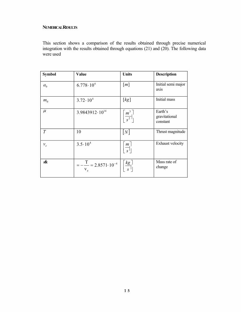
1 5
NUMERICAL RESULTS
This section shows a comparison of the results obtained through precise numerical integration with the results obtained through equations (21) and (20). The following data were used
Symbol Value Units Description
0a 610778.6 ⋅ ][m Initial semi major axis
0m 41072.3 ⋅ ][kg Initial mass
µ 14103.9843912 ⋅
2
3
sm
Earth’s gravitational constant
T 10 [ ]N Thrust magnitude
ev 4103.5 ⋅
sm
Exhaust velocity
m& 4
e
102.8571vT −⋅=−=
skg
Mass rate of change

1 6
0 50 100 150 200time [days]
0
10000
20000
30000
40000
50000
60000a
[km
]analytical (time varying mass)precise numerical integration
Figure 1: Comparison of analytical approximation and precise numerical integration for a flight time of 200 days
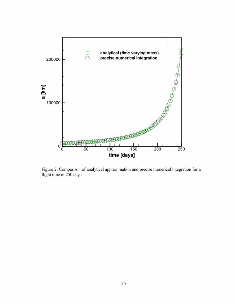
1 7
0 50 100 150 200 250time [days]
0
100000
200000
a[k
m]
analytical (time varying mass)precise numerical integration
Figure 2: Comparison of analytical approximation and precise numerical integration for a flight time of 250 days
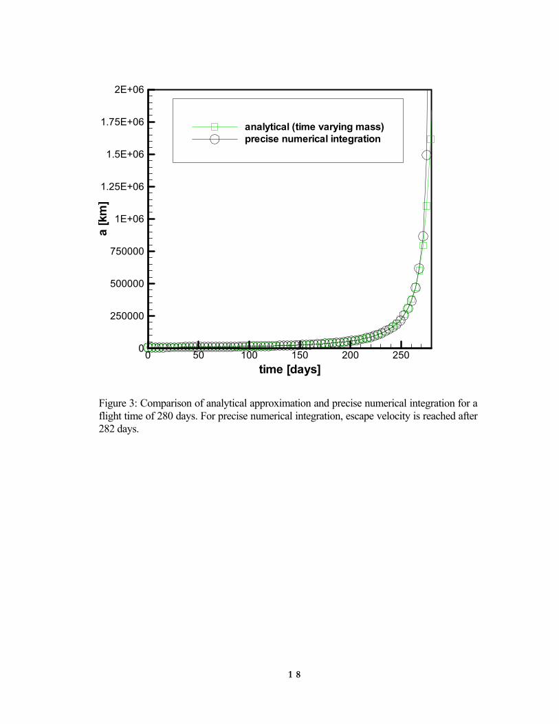
1 8
0 50 100 150 200 250time [days]
0
250000
500000
750000
1E+06
1.25E+06
1.5E+06
1.75E+06
2E+06a
[km
]
analytical (time varying mass)precise numerical integration
Figure 3: Comparison of analytical approximation and precise numerical integration for a flight time of 280 days. For precise numerical integration, escape velocity is reached after 282 days.
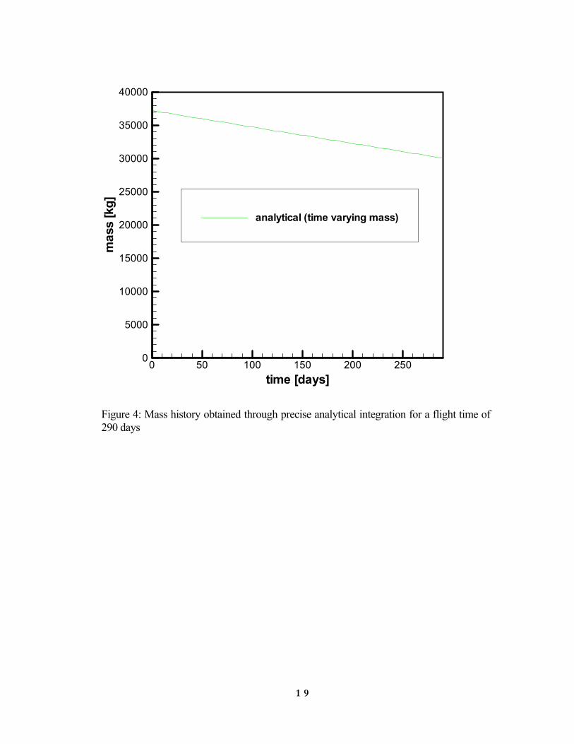
1 9
0 50 100 150 200 250time [days]
0
5000
10000
15000
20000
25000
30000
35000
40000m
ass
[kg]
analytical (time varying mass)
Figure 4: Mass history obtained through precise analytical integration for a flight time of 290 days

2 0
0 50 100 150 200 250time [days]
0
0.1
0.2
0.3
0.4
0.5
0.6
0.7
0.8
0.9
1
1.1
norm
aliz
edm
ass
analytical (time varying mass)
Figure 5: Normalized mass history obtained through precise analytical integration for a flight time of 290 days
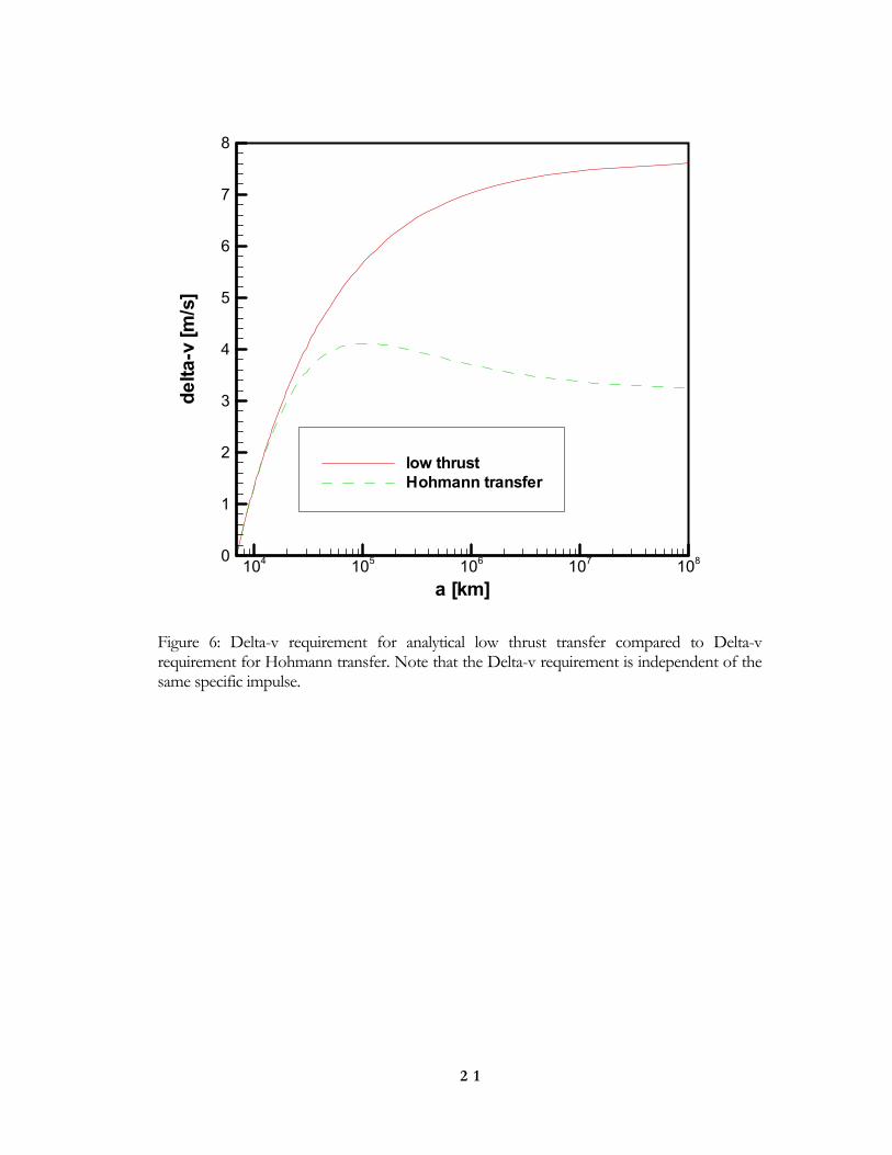
2 1
104 105 106 107 108
a [km]
0
1
2
3
4
5
6
7
8
delta
-v[m
/s]
low thrustHohmann transfer
Figure 6: Delta-v requirement for analytical low thrust transfer compared to Delta-v requirement for Hohmann transfer. Note that the Delta-v requirement is independent of the same specific impulse.

2 2
104 105 106 107 108
a [km]
0.8
0.825
0.85
0.875
0.9
0.925
0.95
0.975
1m
ass
fract
ion
low thrustHohmann transfer
Figure 7: Fuel consumption for analytical low thrust transfer compared to fuel consumption for Hohmann transfer. The same specific impulse is assumed for both cases, namely
].[500,3 sI sp =
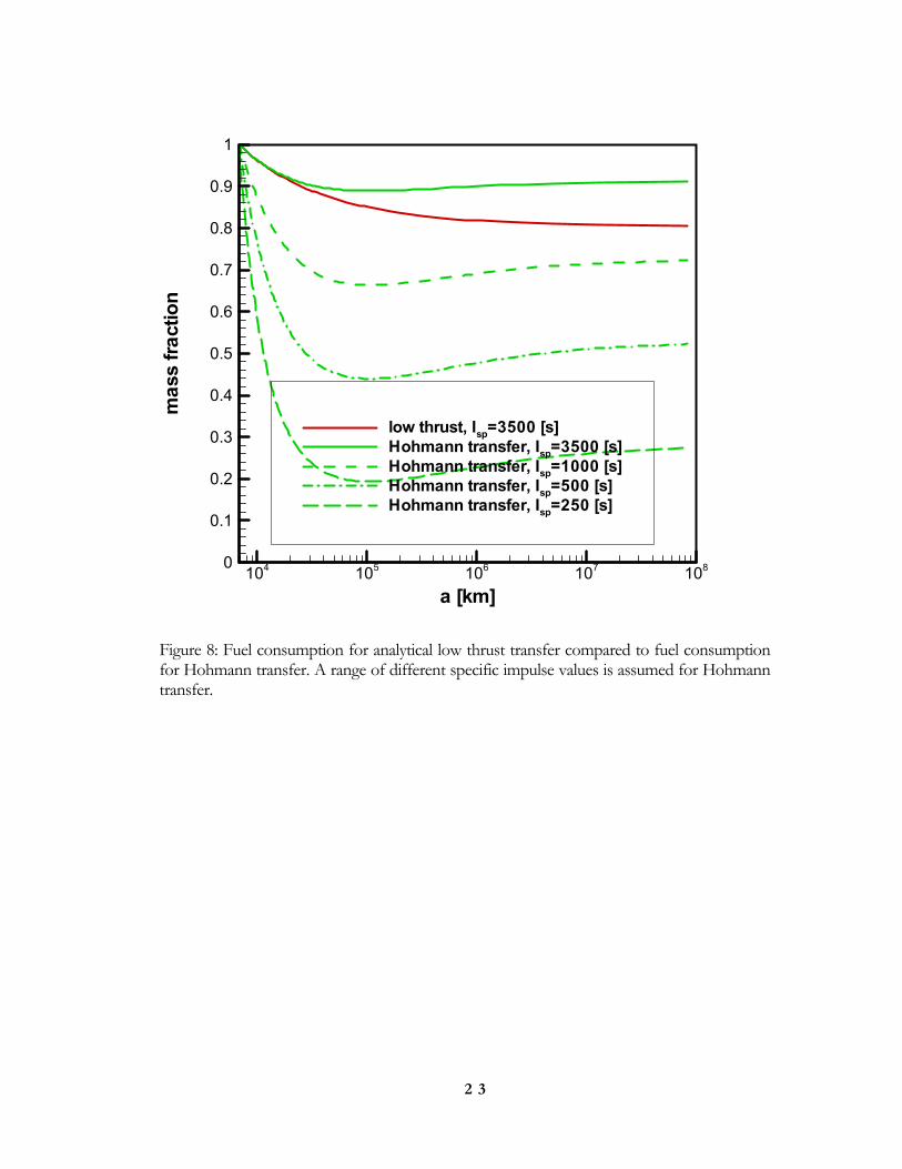
2 3
104 105 106 107 108
a [km]
0
0.1
0.2
0.3
0.4
0.5
0.6
0.7
0.8
0.9
1m
ass
fract
ion
low thrust, Isp=3500 [s]Hohmann transfer, Isp=3500 [s]Hohmann transfer, Isp=1000 [s]Hohmann transfer, Isp=500 [s]Hohmann transfer, Isp=250 [s]
Figure 8: Fuel consumption for analytical low thrust transfer compared to fuel consumption for Hohmann transfer. A range of different specific impulse values is assumed for Hohmann transfer.

2 4
104 105 106 107 108
a [km]
0
0.5
1
1.5
2
2.5
3
3.5
4
4.5ra
tioof
mas
sfra
ctio
ns:m
Hoh
man
n/mel
ectri
c
Hohmann transfer, Isp=3500 [s]Hohmann transfer, Isp=1000 [s]Hohmann transfer, Isp=500 [s]Hohmann transfer, Isp=250 [s]
Figure 9: Mass fraction achieved for low thrust transfer divided through mass fraction achieved through Hohmann transfer.

2 5
This page intentionally left blank.
V e r s i o n - 0 9 - 0 7 - 0 1
Low Thrust Inclination Changes
Questions, comments?
Please contact:
Hans Seywald
AMA, Inc.
Phone: (757) 865-0944
Email: [email protected]
1
TABLE OF CONTENTS
Table of Contents.......................................................................................................................................1
Summary .......................................................................................................................................................2
Nomenclature..............................................................................................................................................3
1. Problem Formulation .........................................................................................................4
2. Differential Equation for Inclination Rate of Change .............................................4
3. Assumptions .........................................................................................................................4
4. Thrust Profile........................................................................................................................5
5. Inclination Change Over One Orbit..............................................................................6
6. Discussion ...........................................................................................................................10
7. Comparison to High-Thrust Inclination Change ...................................................11
2
SUMMARY
An analytical formula is derived for the approximate inclination change achieved through low-thrust orbital transfers with circular initial orbit and circular target orbit of the same semi-major axis. During each orbit, the transfer maneuver consists of two thrust arcs centered at the two nodes, with coast arcs in between. On the thrust arcs, the thrust magnitude is constant and is always directed normal to the current orbital plane. However, the thrust direction is opposite along two subsequent thrust arcs.
The overall fraction of time, ],1,0[∈p that the thrusters are on during each orbit is carried along as a design parameter in our analytical results. In the limit, as this time fraction approaches zero, the fuel efficiency of the low-thrust inclination change maneuver approaches that of an impulsive, high-thrust maneuver, subject to the constraint that the thrust is always directed normal to the current orbital plane. As the thruster on-time ratio p is gradually increased from zero to one, the v∆ -requirement
increases by a factor of ( ) .2/sin2/
ππp
p This implies that the fuel consumption increases
by a factor of 2/π when the thrusters are on all the time.
By allowing the thrusters to be fired into a direction other than normal to the current orbital plane, additional fuel savings can be achieved. Such strategies are easy to consider in impulsive transfers, but for low-thrust transfers they lead to some difficulties, and we did not include such strategies. Explicitly, for high-thrust transfers, thrusting always normal to the current orbital plane increases the total
required velocity increment by a factor of ( ) .2sin2i
i∆
∆ For small inclination changes,
this factor approaches unity. On the other end of the spectrum, assuming that the largest reasonable inclination change is 90 degrees, the worst possible increase in
velocity increment is given by ( ) ,11.1224sin
4≈=
ππ
π i.e. an increase of 11%.

3
NOMENCLATURE
i inclination ][rad
W thrust acceleration normal to orbital plane ]/[ 2sm
WF thrust force normal to orbital plane (in direction of )W ][N
u =+= fω argument of perigee plus true anomaly ][rad
r radial distance from central body ][m
n ===Taπµ 2
3 orbit rate ][ 1−s
T µ
ππ 3
22 an
== orbit rate ][s
a semi-major axis ][m
e eccentricity ]1[
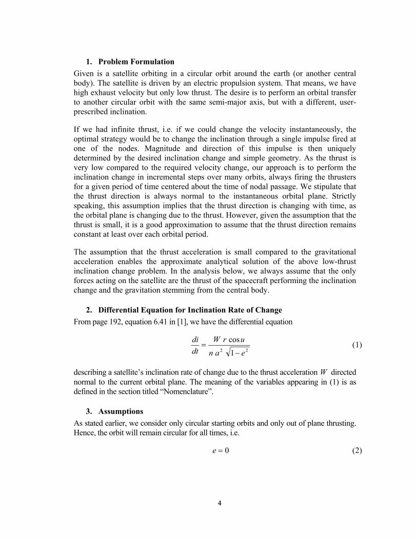
4
1. Problem Formulation Given is a satellite orbiting in a circular orbit around the earth (or another central body). The satellite is driven by an electric propulsion system. That means, we have high exhaust velocity but only low thrust. The desire is to perform an orbital transfer to another circular orbit with the same semi-major axis, but with a different, user-prescribed inclination.
If we had infinite thrust, i.e. if we could change the velocity instantaneously, the optimal strategy would be to change the inclination through a single impulse fired at one of the nodes. Magnitude and direction of this impulse is then uniquely determined by the desired inclination change and simple geometry. As the thrust is very low compared to the required velocity change, our approach is to perform the inclination change in incremental steps over many orbits, always firing the thrusters for a given period of time centered about the time of nodal passage. We stipulate that the thrust direction is always normal to the instantaneous orbital plane. Strictly speaking, this assumption implies that the thrust direction is changing with time, as the orbital plane is changing due to the thrust. However, given the assumption that the thrust is small, it is a good approximation to assume that the thrust direction remains constant at least over each orbital period.
The assumption that the thrust acceleration is small compared to the gravitational acceleration enables the approximate analytical solution of the above low-thrust inclination change problem. In the analysis below, we always assume that the only forces acting on the satellite are the thrust of the spacecraft performing the inclination change and the gravitation stemming from the central body.
2. Differential Equation for Inclination Rate of Change From page 192, equation 6.41 in [1], we have the differential equation
22 1
cos
ean
urWdtdi
−= (1)
describing a satellite’s inclination rate of change due to the thrust acceleration W directed normal to the current orbital plane. The meaning of the variables appearing in (1) is as defined in the section titled “Nomenclature”.
3. Assumptions As stated earlier, we consider only circular starting orbits and only out of plane thrusting. Hence, the orbit will remain circular for all times, i.e.
0=e (2)

5
Equation (2) also implies that we can set the argument of perigee equal zero, i.e.
0=ω (3)
Equation (3) is not really an assumption. Given (2), the argument of perigee ω loses its meaning. We can then pick ω arbitrarily. If we pick ,0=ω then the true anomaly f is the angle measured from the ascending node to the satellite in orbit.
From (2) and (3) it also follows that
ar = (4)
and
ntu = (5)
Note that W denotes the thrust acceleration, not the thrust itself. Let WF denote the thrust normal to the orbital plane (directed along W ), then
mF
W W= (6)
Inserting (2), (3), (4), (5) in (1) and using ,3an µ= we get
= 3cos
aa
mF
dtdi W µ
µ (7)
Before integrating this equation, we first define a strategy for our thrust history .WF Once that is done we will make the simplifying assumption that the mass changes only insignificantly over the course of one orbit. This will be the point where the low-thrust assumption enters our analysis.
4. Thrust Profile The basic idea is to fire the thrusters only normal to the orbital plane. For ,WF the component of the thrust vector normal to the orbital plane, we choose the following step function
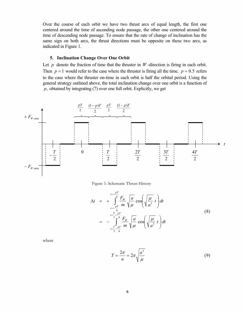
6
Over the course of each orbit we have two thrust arcs of equal length, the first one centered around the time of ascending node passage, the other one centered around the time of descending node passage. To ensure that the rate of change of inclination has the same sign on both arcs, the thrust directions must be opposite on these two arcs, as indicated in Figure 1.
5. Inclination Change Over One Orbit Let p denote the fraction of time that the thruster in W -direction is firing in each orbit. Then 1=p would refer to the case where the thruster is firing all the time. 5.0=p refers to the case where the thruster on-time in each orbit is half the orbital period. Using the general strategy outlined above, the total inclination change over one orbit is a function of
,p obtained by integrating (7) over one full orbit. Explicitly, we get
∫
∫
+=
−=
+=
−=
−=
+=∆
42
42
3
4
4
3
cos
cos
pTTt
pTTt
W
pTt
pTt
W
dtta
amF
dtta
amF
i
µµ
µµ
(8)
where
µ
ππ 3
22 an
T == (9)
2T
23T
24T
22T
2T
−
max,WF+
max,WF−
0
2pT
2)1( Tp−
2pT
2)1( Tp−
t
Figure 1: Schematic Thrust History

7
denotes the orbital period.
Equation (8) cannot be integrated analytically unless we consider the integral
∫=x
dtt
tx0
sinintsin as given. To obtain an approximate solution for i∆ without using the
function ,intsin x we make the low-thrust assumption that the mass of the satellite changes only insignificantly over the course of one orbit. For integration over one single orbit, the mass )(tm can then be considered constant and can be pulled outside the integrals in (8). The remaining cosine function can then be integrated analytically. Explicitly, we get
42
42
3
3
4
4
3
3
sin
sin
pTTt
pTTt
W
pTt
pTt
Worbitoneover
ta
aamF
ta
aamF
i
+=
−=
+=
−=
−=
+=∆
µµµ
µµµ
(10)
Simple manipulations yield
⋅=
⋅=
+
=
−
=∆
+=
−=
+=
−=
+=
−=
+=
−=
+=
−=
4sin4
2
sin
sin
3
2
4
4
3
2
4
4
3
4
4
3
2
42
42
3
4
4
3
2
pTa
amF
ta
insamF
ta
ta
insamF
ta
ta
insamF
i
W
pTt
pTt
W
pTt
pTt
pTt
pTt
W
pTTt
pTTt
pTt
pTt
Worbitoneover
µµ
µµ
µµµ
µµµ
Using (9), the last line above can also be written in the form
⋅=∆
2sin4
2 πµ
pamF
i Worbitoneover (11)
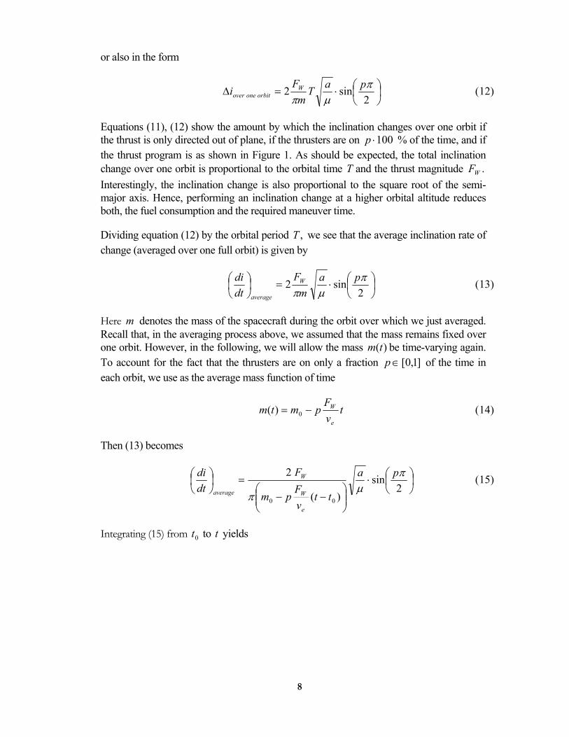
8
or also in the form
⋅=∆
2sin2 π
µπpaT
mF
i Worbitoneover (12)
Equations (11), (12) show the amount by which the inclination changes over one orbit if the thrust is only directed out of plane, if the thrusters are on 100⋅p % of the time, and if the thrust program is as shown in Figure 1. As should be expected, the total inclination change over one orbit is proportional to the orbital time T and the thrust magnitude .WF Interestingly, the inclination change is also proportional to the square root of the semi-major axis. Hence, performing an inclination change at a higher orbital altitude reduces both, the fuel consumption and the required maneuver time.
Dividing equation (12) by the orbital period ,T we see that the average inclination rate of change (averaged over one full orbit) is given by
⋅=
2sin2 π
µπpa
mF
dtdi W
average
(13)
Here m denotes the mass of the spacecraft during the orbit over which we just averaged. Recall that, in the averaging process above, we assumed that the mass remains fixed over one orbit. However, in the following, we will allow the mass )(tm be time-varying again. To account for the fact that the thrusters are on only a fraction ]1,0[∈p of the time in each orbit, we use as the average mass function of time
tvF
pmtme
W−= 0)( (14)
Then (13) becomes
⋅
−−
=
2sin
)(
2
00
πµ
π
pa
ttvF
pm
Fdtdi
e
W
W
average
(15)
Integrating (15) from 0t to t yields

9
( ) ( )
( ) ( ) ( )( )
( )
⋅⋅=
−⋅⋅=
−−−⋅⋅=
−−⋅
−⋅
⋅=
−−⋅
⋅=
=∆
=
=
−
∫
∫
)(ln
2/2/sin
)(lnln2/
2/sin
)(lnln2/sin2
)(ln2
sin2
)(2
sin2
0
0
000
00
1
00
0
0
0
tmm
ppav
tmmp
pav
ttvF
pmmp
pav
ttvF
pmpFvpaF
dtttvF
pmpaF
dtdtdii
e
e
e
We
tt
tte
W
W
eW
t
t e
WW
t
t average
ππ
µ
ππ
µ
πµπ
πµπ
πµπ
(16)
From the rocket equation
||
0)( evv
emtm∆
−
= (17)
which relates the mass ratio, the velocity increment, and the exhaust velocity, we obtain by inserting in the last line of the expression for i∆ obtained in (16)
( )2/
2/sinππ
µ ppavi ⋅∆=∆ (18)
or, after solving for v∆
( )2/sin2/
ππµp
pa
iv ⋅∆=∆ (19)
In equations (18) and (19) we did not keep track of the correct sign. Instead, we arbitrarily chose the plus sign. This is not a big issue. Equation (19) shows the velocity increment
v∆ required to achieve a given inclination change i∆ for a circular orbit of semi-major axis a in a gravitational field of strength .µ Additionally, it I s assumed in (19) that the thrusters are fired always normal to the latest orbital plane, and that the thruster on-time during each orbit is a fixed fraction p of the overall orbital period.
Equation (16) can also be used to solve for the mass fraction as a function of the inclination change. We get

1 0
( )
⋅∆−=
2/sin2/1exp
)()(
0 ππµp
pav
itmtm
e
(20)
From equation (20) and the fundamental equation for the evolution of mass,
( ),)( 00 ttvF
pmtme
W −−= we can calculate the maneuver time required to achieve an
inclination change ,i∆ namely
( )
( )
⋅∆−=
−−
2/sin2/1exp
)( 0
00
ππµp
pav
itm
ttvF
pm
e
e
W
( )
⋅∆−−=−
2/sin2/1exp100 π
πµp
pav
ivpF
vmtt
eeW
e (21)
The factor ( )2/sin2/)(
ππp
ppf = appears in (21) and in several equations before that. It has
the following properties:
( )
→⇒→→⇒→
∈=
2/)(11)(0
)1,0[for increasinglly monotonica
2/sin2/)(
ππ
π
pfppfp
p
pppf (22)
Recall that the variable p denotes the fraction of time that the thrusters are on (and are firing normal to the current orbital plane) during the inclination change maneuver. For
,1=p the thrusters are on all the time. This control strategy is time optimal, but the least fuel efficient. For ,0→p the thrusters are firing only at the times of nodal passage. This control strategy is fuel optimal (in the limit), but the inclination change takes infinitely long (in the limit).
6. Discussion Equations (19), (20) show the v∆ -requirement and the resulting mass fraction as a function of the inclination change (inclination given in radians). Recall that )1,0[∈p denotes the fraction of time that the thrusters are on over the period of an orbit, with the thruster on-times centered at the nodes and distributed equally but with opposite signs over both nodes.

1 1
In the limit, for ,0→p the inclination change is most efficient, with ( ) .12/sin
2/lim0
=→ π
πp
pp
In this limit case, the thrusters are on only at the nodes. In this case, equations (19), (20) become expressions for impulsive burns at the nodes. However, we have made the stipulation that the thrust be always normal to the orbital plane, even as the orientation of the orbital plane in space changes due to the inclination change maneuver. (The effects of this assumption for high-thrust inclination changes are discussed in the next section). As indicated above, this strategy is most efficient in terms of fuel usage and v∆ -requirement. For low-thrust transfers, the penalty comes in terms of maneuver time. As p is gradually increased from zero to one, the v∆ -requirement goes up by a factor of .2/π The fastest way to achieve a given inclination change with low-thrust engines is to select ,1=p even though this is the least efficient choice in terms of fuel consumption. The total maneuver time is roughly inversely proportional to the selected value of ].1,0[∈p
7. Comparison to High-Thrust Inclination Change If the thrust magnitude is sufficiently large such that the desired velocity changes can be executed on a time scale that is much smaller than the time scale at which all other significant states change, then we can make the “high-thrust” assumption that the velocity can be changed instantaneously.
High-thrust inclination changes are quite straightforward compared to low-thrust inclination changes. From simple geometry, it is easy to see that high-thrust inclination changes are most efficiently performed at the instant of nodal passage. Explicitly, the desired inclination change and the required velocity increment are related by
( )2sin2 ia
v ∆⋅⋅=∆µ (23)
This equation can be derived from simple geometry. As the orbit is assumed to be circular, the velocity vector has the magnitude
av µ=2|||| both, before and after the inclination change maneuver. Equation (23) then follows from the geometry depicted in Figure 2 for the special case of a 90 degree inclination change.
Note that the overall velocity increment v∆ is such that the magnitude of the velocity vector after the inclination change maneuver is the
N
S
v1
v2
∆v
Equator
Figure 2: Impulsive inclination change
∆i
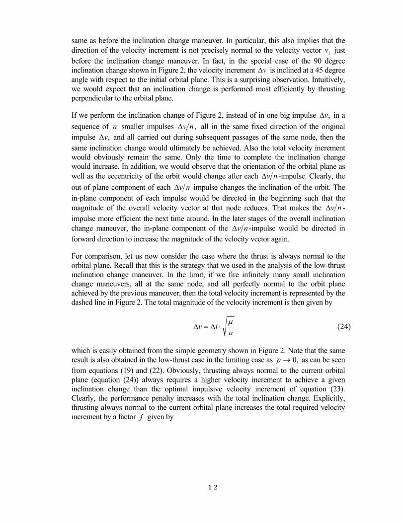
1 2
same as before the inclination change maneuver. In particular, this also implies that the direction of the velocity increment is not precisely normal to the velocity vector 1v just before the inclination change maneuver. In fact, in the special case of the 90 degree inclination change shown in Figure 2, the velocity increment v∆ is inclined at a 45 degree angle with respect to the initial orbital plane. This is a surprising observation. Intuitively, we would expect that an inclination change is performed most efficiently by thrusting perpendicular to the orbital plane.
If we perform the inclination change of Figure 2, instead of in one big impulse ,v∆ in a sequence of n smaller impulses ,nv∆ all in the same fixed direction of the original impulse ,v∆ and all carried out during subsequent passages of the same node, then the same inclination change would ultimately be achieved. Also the total velocity increment would obviously remain the same. Only the time to complete the inclination change would increase. In addition, we would observe that the orientation of the orbital plane as well as the eccentricity of the orbit would change after each nv∆ -impulse. Clearly, the out-of-plane component of each nv∆ -impulse changes the inclination of the orbit. The in-plane component of each impulse would be directed in the beginning such that the magnitude of the overall velocity vector at that node reduces. That makes the nv∆ -impulse more efficient the next time around. In the later stages of the overall inclination change maneuver, the in-plane component of the nv∆ -impulse would be directed in forward direction to increase the magnitude of the velocity vector again.
For comparison, let us now consider the case where the thrust is always normal to the orbital plane. Recall that this is the strategy that we used in the analysis of the low-thrust inclination change maneuver. In the limit, if we fire infinitely many small inclination change maneuvers, all at the same node, and all perfectly normal to the orbit plane achieved by the previous maneuver, then the total velocity increment is represented by the dashed line in Figure 2. The total magnitude of the velocity increment is then given by
a
iv µ⋅∆=∆ (24)
which is easily obtained from the simple geometry shown in Figure 2. Note that the same result is also obtained in the low-thrust case in the limiting case as ,0→p as can be seen from equations (19) and (22). Obviously, thrusting always normal to the current orbital plane (equation (24)) always requires a higher velocity increment to achieve a given inclination change than the optimal impulsive velocity increment of equation (23). Clearly, the performance penalty increases with the total inclination change. Explicitly, thrusting always normal to the current orbital plane increases the total required velocity increment by a factor f given by
1 3
( ) .2sin2i
iv
vf
optimal
normalalways
∆∆
=∆
∆= (25)
For small inclination changes this factor approaches unity, which means that it does not matter which strategy is picked for small inclination changes. As the inclination change i∆ increases, the factor f in (25) increases monotonically. Assuming that the largest reasonable inclination change is 90 degrees, the worst possible increase in velocity increment
is given by the factor ( ) .11.1224sin
4≈==
ππ
πf

1 4
References
[1] Roy, A. E., Orbital Motion, Adam Hilger, Bristol and Philadelphia, 1988.

1 5
This page intentionally left blank.
RASC HPM Docking Fuel Budget Introduction This study was prepared in support of the Orbital Aggregation & Space Infrastructure Systems (OASIS) project, under the Revolutionary Aerospace Systems Concepts (RASC) activity. The Chemical Transfer Module (CTM) was evaluated to determine if the proposed reaction control system was capable of supporting the provided reference missions, and to predict the propellant requirements in each scenario. The analysis was performed using the recently enhanced version of DOCKSIM, a six degree of freedom simulator that calculates either fuel1 or time optimal trajectories for docking one orbiting vehicle to another. The model properties for the CTM craft were obtained from Marshall Space Flight Center. The models properties for the HPM and CTV, and the descriptions of the five reference missions were provided by NASA Langley. The Reference Missions The reference missions were selected based on their relevance to the OASIS operations plan. The configurations and propellant fill fractions in these cases are intended to serve as bounding values for the proximity operations propellant budget analysis: Case 1: The CTM and fully loaded HPM are stacked together. This stack docks in an r-bar
approach to the CTV, which is attached to the ISS in low earth orbit. Case 2: The CTM and fully loaded HPM are stacked together. This stack docks to the CTV,
which is attached to the L1 gateway station. Case3: The CTM, a nearly empty HPM and the CTV are stacked together. This stack
docks in an r-bar approach to the ISS in low earth orbit. Case 4: The CTM docks to the HPM in low earth orbit. Case 5: The CTM docks to the HPM. The HPM is attached to the L1 gateway station. In all cases the HPM solar wings are deployed, and the approach corridor is identical to the one used for STS docking to the ISS. DOCKSIM Analysis
1 Note that when DOCKSIM calculates the “fuel” optimal trajectory, a 3 DOF point mass model is used. The actual optimization is based on minimizing the control forces acting on the point mass. Jets (and their layout configuration) are not considered during the optimization process. Then, during the 6 DOF simulation process, DOCKSIM selects appropriate jet firing combinations, subject to other constraints, which force the docking vehicle’s cm to “ride” along the optimized trajectory as closely as possible. Consequently, while DOCKSIM’s optimized trajectory should result in less fuel used, it may not yield the absolute minimal amount of fuel necessary to perform the rendezvous operation.
1
The DOCKSIM program was originally designed to analyze the dynamics of proximity vehicles executing low earth orbits. Although recent enhancements have improved DOCKSIM’s overall capabilities and accuracy, the initial analysis for the two L1 cases raised some concern about the validity of the results for high altitude trajectories. Consequently, in order to provide preliminary results for this study, the L1 trajectories were approximated by using the same trajectories used for the three LEO case with the exception that gravity gradient torques and atmospheric drag terms were removed from the system. The mass, area properties, and jet configurations of the docking vehicles were obtained from I-DEAS CAD models, and entered as inputs into DOCKSIM. SSMRBS was used to generate a low Earth orbit, LVLH hold flight mode trajectory for the target vehicle. This data was used for the target vehicle in each of the five cases. The initial conditions of the docking vehicle in each case included a 0.1 degree yaw, pitch and roll offset, a 0.01 m/s angular velocity offset along each axis, a X0,Y0,Z0 = 5.0,1.0,100.0 position offset, and a 0.01 m/s velocity offset along each axis. The DOCKSIM outputs include time histories of the RCS jet firings, vehicle position/orientation for both the optimal trajectory and the achieved trajectory, and the mass of propellants consumed during the docking. Plots of the position and orientation time histories and propellant consumption are included in this report. A visual simulation of Case 3 was performed by importing the model geometry and DOCKSIM analysis results into the ISS Synergistic Engineering Environment (SEE). An SEE simulation of the originally proposed CTM thruster configuration showed that the canted thrusters on the forward side of the CTM were significantly impinging on the aft side of the HPM. The CTM model was then updated to change the cant angle of the forward thrusters and to place the four forward thruster tripods out on booms. The results presented in this report refer to the updated CTM model. Results The DOCKSIM analysis of the three LEO missions showed that the CTM reaction control system is capable of maintaining control of the vehicle stack during the docking maneuver, with steady state oscillations held to within a yaw, pitch and roll of 0.5 degrees, or better, in all cases. Cases 4 and 5 proved to be the most difficult to control, which suggests that the jets provide more thrust than necessary for controlling the CTM vehicle by itself. The maximum propellant usage was 94.27 kg in the time optimal trajectory for case 1. This was expected since the configuration (CTM, and full HPM) in case 1 (and case 2) has the largest mass. The minimum propellant usage was 10.61 kg in the control optimal trajectory for case 5, which corresponds to a configuration (CTM only) with the least mass. A spreadsheet detailing the propellant usage for each scenario is attached to this report. Conclusions The design of the RCS for the CTM is capable of performing the proximity operations described by the five reference missions. Further analysis using a modified version of the DOCKSIM code tailored to the environment at the LaGrange points would increase the fidelity of the propellant budget results for the L1 cases.
2
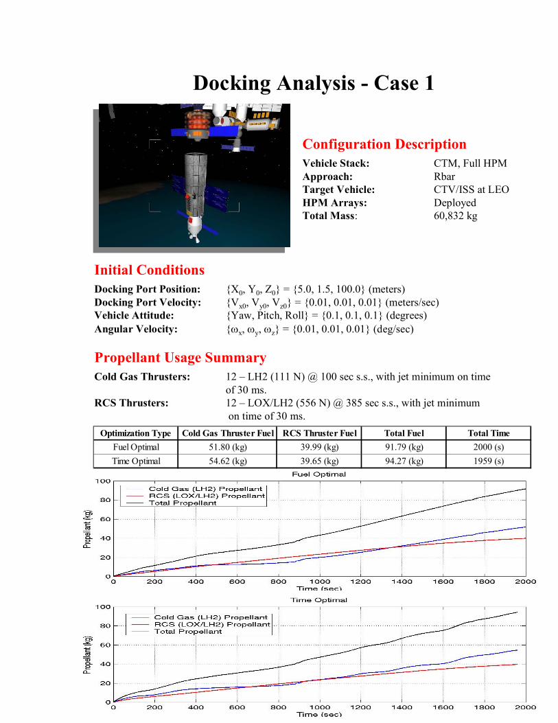
3
Vehicle Stack: CTM, Full HPMApproach: RbarTarget Vehicle: CTV/ISS at LEOHPM Arrays: DeployedTotal Mass: 60,832 kg
Docking Analysis - Case 1
Docking Port Position: X0, Y0, Z0 = 5.0, 1.5, 100.0 (meters)Docking Port Velocity: Vx0, Vy0, Vz0 = 0.01, 0.01, 0.01 (meters/sec)Vehicle Attitude: Yaw, Pitch, Roll = 0.1, 0.1, 0.1 (degrees)Angular Velocity: ωx, ωy, ωz = 0.01, 0.01, 0.01 (deg/sec)
Cold Gas Thrusters: 12 – LH2 (111 N) @ 100 sec s.s., with jet minimum on time of 30 ms.
RCS Thrusters: 12 – LOX/LH2 (556 N) @ 385 sec s.s., with jet minimumon time of 30 ms.
Optimization Type Cold Gas Thruster Fuel RCS Thruster Fuel Total Fuel Total TimeFuel Optimal 51.80 (kg) 39.99 (kg) 91.79 (kg) 2000 (s)Time Optimal 54.62 (kg) 39.65 (kg) 94.27 (kg) 1959 (s)
Configuration Description
Initial Conditions
Propellant Usage Summary
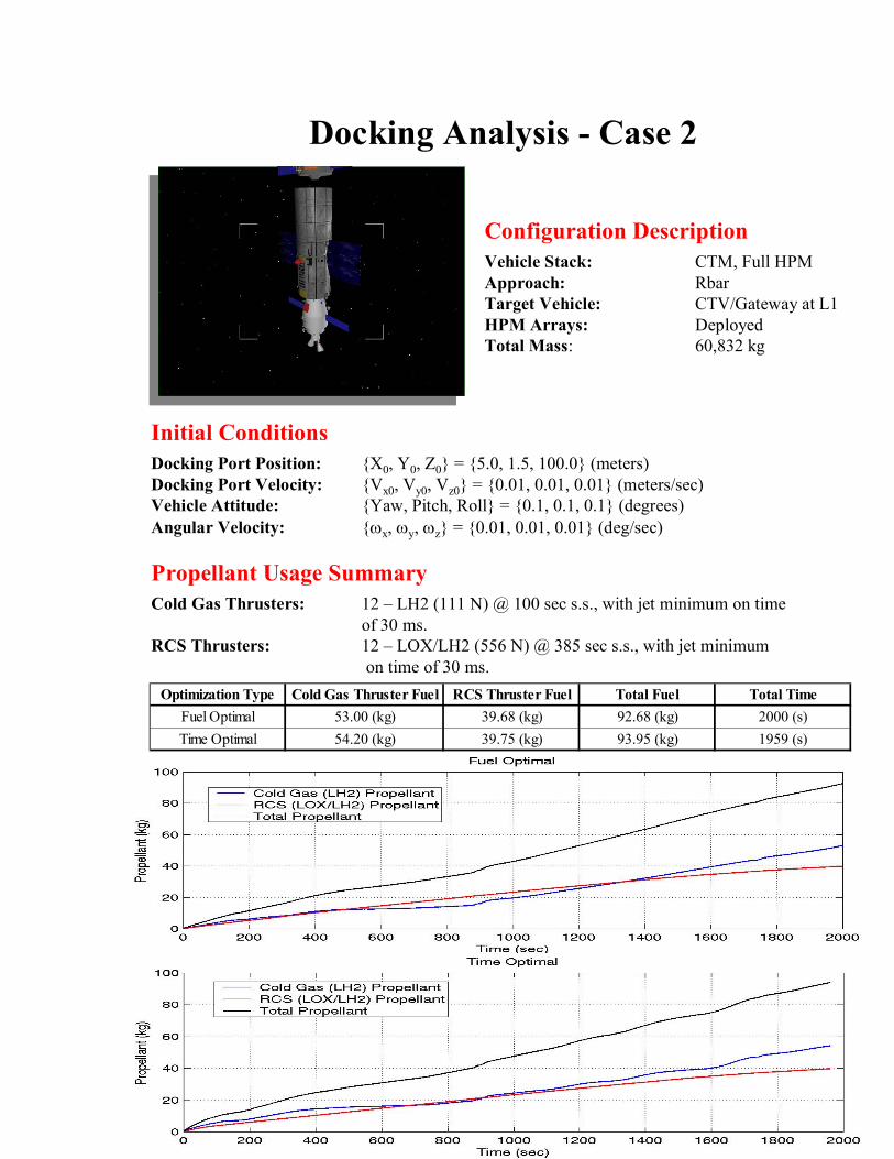
4
Vehicle Stack: CTM, Full HPMApproach: RbarTarget Vehicle: CTV/Gateway at L1HPM Arrays: DeployedTotal Mass: 60,832 kg
Docking Analysis - Case 2
Docking Port Position: X0, Y0, Z0 = 5.0, 1.5, 100.0 (meters)Docking Port Velocity: Vx0, Vy0, Vz0 = 0.01, 0.01, 0.01 (meters/sec)Vehicle Attitude: Yaw, Pitch, Roll = 0.1, 0.1, 0.1 (degrees)Angular Velocity: ωx, ωy, ωz = 0.01, 0.01, 0.01 (deg/sec)
Cold Gas Thrusters: 12 – LH2 (111 N) @ 100 sec s.s., with jet minimum on time of 30 ms.
RCS Thrusters: 12 – LOX/LH2 (556 N) @ 385 sec s.s., with jet minimumon time of 30 ms.
Optimization Type Cold Gas Thruster Fuel RCS Thruster Fuel Total Fuel Total TimeFuel Optimal 53.00 (kg) 39.68 (kg) 92.68 (kg) 2000 (s)Time Optimal 54.20 (kg) 39.75 (kg) 93.95 (kg) 1959 (s)
Configuration Description
Initial Conditions
Propellant Usage Summary
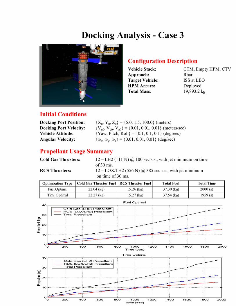
5
Vehicle Stack: CTM, Empty HPM, CTVApproach: RbarTarget Vehicle: ISS at LEOHPM Arrays: DeployedTotal Mass: 19,893.2 kg
Docking Analysis - Case 3
Docking Port Position: X0, Y0, Z0 = 5.0, 1.5, 100.0 (meters)Docking Port Velocity: Vx0, Vy0, Vz0 = 0.01, 0.01, 0.01 (meters/sec)Vehicle Attitude: Yaw, Pitch, Roll = 0.1, 0.1, 0.1 (degrees)Angular Velocity: ωx, ωy, ωz = 0.01, 0.01, 0.01 (deg/sec)
Cold Gas Thrusters: 12 – LH2 (111 N) @ 100 sec s.s., with jet minimum on time of 30 ms.
RCS Thrusters: 12 – LOX/LH2 (556 N) @ 385 sec s.s., with jet minimumon time of 30 ms.
Optimization Type Cold Gas Thruster Fuel RCS Thruster Fuel Total Fuel Total TimeFuel Optimal 22.04 (kg) 15.26 (kg) 37.30 (kg) 2000 (s)Time Optimal 22.27 (kg) 15.27 (kg) 37.54 (kg) 1959 (s)
Configuration Description
Initial Conditions
Propellant Usage Summary
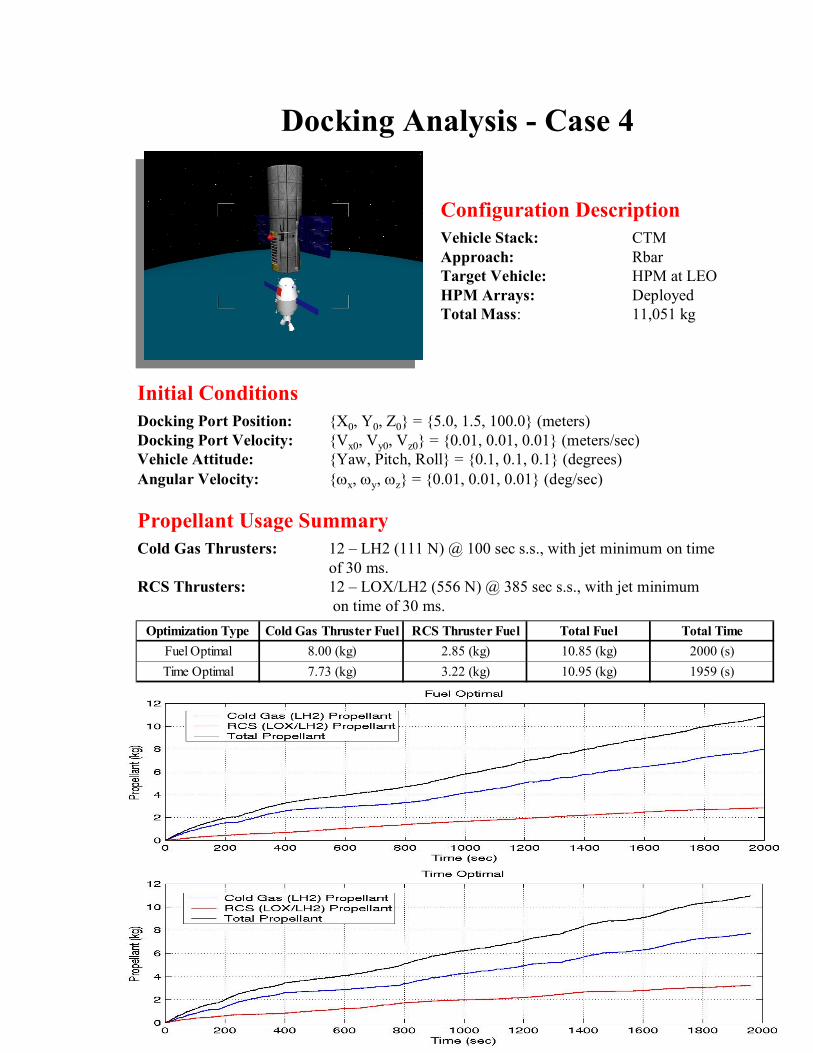
6
Vehicle Stack: CTMApproach: RbarTarget Vehicle: HPM at LEOHPM Arrays: DeployedTotal Mass: 11,051 kg
Docking Analysis - Case 4
Docking Port Position: X0, Y0, Z0 = 5.0, 1.5, 100.0 (meters)Docking Port Velocity: Vx0, Vy0, Vz0 = 0.01, 0.01, 0.01 (meters/sec)Vehicle Attitude: Yaw, Pitch, Roll = 0.1, 0.1, 0.1 (degrees)Angular Velocity: ωx, ωy, ωz = 0.01, 0.01, 0.01 (deg/sec)
Cold Gas Thrusters: 12 – LH2 (111 N) @ 100 sec s.s., with jet minimum on time of 30 ms.
RCS Thrusters: 12 – LOX/LH2 (556 N) @ 385 sec s.s., with jet minimumon time of 30 ms.
Optimization Type Cold Gas Thruster Fuel RCS Thruster Fuel Total Fuel Total TimeFuel Optimal 8.00 (kg) 2.85 (kg) 10.85 (kg) 2000 (s)Time Optimal 7.73 (kg) 3.22 (kg) 10.95 (kg) 1959 (s)
Configuration Description
Initial Conditions
Propellant Usage Summary
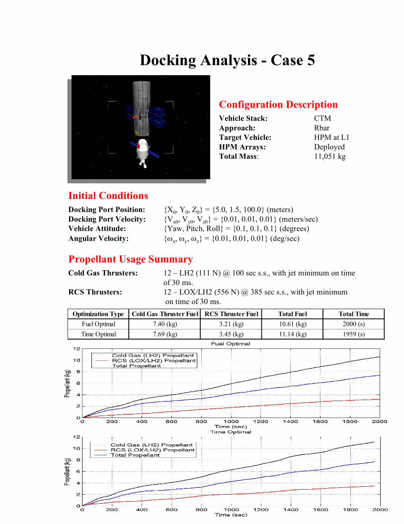
7
Vehicle Stack: CTMApproach: RbarTarget Vehicle: HPM at L1HPM Arrays: DeployedTotal Mass: 11,051 kg
Docking Analysis - Case 5
Docking Port Position: X0, Y0, Z0 = 5.0, 1.5, 100.0 (meters)Docking Port Velocity: Vx0, Vy0, Vz0 = 0.01, 0.01, 0.01 (meters/sec)Vehicle Attitude: Yaw, Pitch, Roll = 0.1, 0.1, 0.1 (degrees)Angular Velocity: ωx, ωy, ωz = 0.01, 0.01, 0.01 (deg/sec)
Cold Gas Thrusters: 12 – LH2 (111 N) @ 100 sec s.s., with jet minimum on time of 30 ms.
RCS Thrusters: 12 – LOX/LH2 (556 N) @ 385 sec s.s., with jet minimumon time of 30 ms.
Optimization Type Cold Gas Thruster Fuel RCS Thruster Fuel Total Fuel Total TimeFuel Optimal 7.40 (kg) 3.21 (kg) 10.61 (kg) 2000 (s)Time Optimal 7.69 (kg) 3.45 (kg) 11.14 (kg) 1959 (s)
Configuration Description
Initial Conditions
Propellant Usage Summary
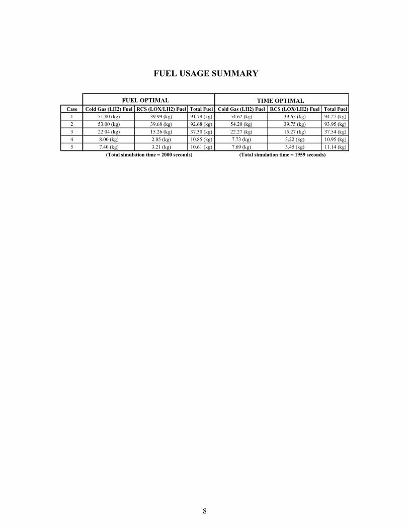
8
FUEL USAGE SUMMARY
FUEL OPTIMAL TIME OPTIMALCase Cold Gas (LH2) Fuel RCS (LOX/LH2) Fuel Total Fuel Cold Gas (LH2) Fuel RCS (LOX/LH2) Fuel Total Fuel
1 51.80 (kg) 39.99 (kg) 91.79 (kg) 54.62 (kg) 39.65 (kg) 94.27 (kg)2 53.00 (kg) 39.68 (kg) 92.68 (kg) 54.20 (kg) 39.75 (kg) 93.95 (kg)3 22.04 (kg) 15.26 (kg) 37.30 (kg) 22.27 (kg) 15.27 (kg) 37.54 (kg)4 8.00 (kg) 2.85 (kg) 10.85 (kg) 7.73 (kg) 3.22 (kg) 10.95 (kg)5 7.40 (kg) 3.21 (kg) 10.61 (kg) 7.69 (kg) 3.45 (kg) 11.14 (kg)
(Total simulation time = 2000 seconds) (Total simulation time = 1959 seconds)
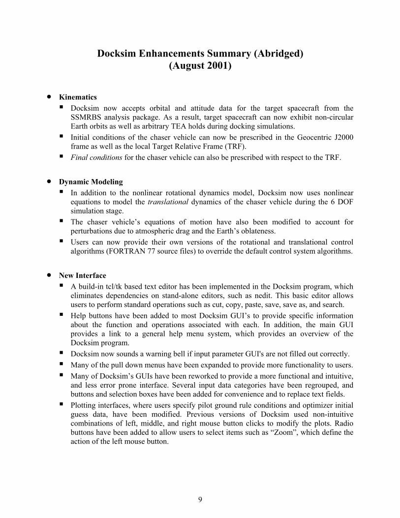
Docksim Enhancements Summary (Abridged) (August 2001)
• Kinematics
Docksim now accepts orbital and attitude data for the target spacecraft from the SSMRBS analysis package. As a result, target spacecraft can now exhibit non-circular Earth orbits as well as arbitrary TEA holds during docking simulations.
Initial conditions of the chaser vehicle can now be prescribed in the Geocentric J2000 frame as well as the local Target Relative Frame (TRF).
Final conditions for the chaser vehicle can also be prescribed with respect to the TRF.
• Dynamic Modeling In addition to the nonlinear rotational dynamics model, Docksim now uses nonlinear
equations to model the translational dynamics of the chaser vehicle during the 6 DOF simulation stage.
The chaser vehicle’s equations of motion have also been modified to account for perturbations due to atmospheric drag and the Earth’s oblateness.
Users can now provide their own versions of the rotational and translational control algorithms (FORTRAN 77 source files) to override the default control system algorithms.
• New Interface
A build-in tcl/tk based text editor has been implemented in the Docksim program, which eliminates dependencies on stand-alone editors, such as nedit. This basic editor allows users to perform standard operations such as cut, copy, paste, save, save as, and search.
Help buttons have been added to most Docksim GUI’s to provide specific information about the function and operations associated with each. In addition, the main GUI provides a link to a general help menu system, which provides an overview of the Docksim program.
Docksim now sounds a warning bell if input parameter GUI's are not filled out correctly. Many of the pull down menus have been expanded to provide more functionality to users. Many of Docksim’s GUIs have been reworked to provide a more functional and intuitive,
and less error prone interface. Several input data categories have been regrouped, and buttons and selection boxes have been added for convenience and to replace text fields.
Plotting interfaces, where users specify pilot ground rule conditions and optimizer initial guess data, have been modified. Previous versions of Docksim used non-intuitive combinations of left, middle, and right mouse button clicks to modify the plots. Radio buttons have been added to allow users to select items such as “Zoom”, which define the action of the left mouse button.
9

This page intentionally left blank.
10

Calculation of Payload Mass and Propellant Mass
Carlos M. RoithmayrLinda Kay-Bunnell
NASA Langley Research Center, Hampton, Virginia, 23681
September 7, 2001
1 Introduction
The Hybrid Propellant Module is currently being designed to work in pairs to ferry propellantand crews from low Earth orbit to the cislunar or interior Earth-Moon Lagrange pointL1, and back, using a combination of electric propellant for low-thrust trajectories, andchemical propellant for impulsive maneuvers. In addition to playing this role, the vehiclemay prove useful in other endeavors. In order to investigate such possibilities, it is importantto determine the maximum payload that can be carried on one leg of a round trip by a singleHPM if it uses only one kind of propellant, and by an HPM working as part of a pair andusing both propellants. Another scheme of interest involves two HPMs using only chemicalpropellant; a payload is delivered by one HPM which then returns in tandem with anotherHPM. Curves showing the maximum payload mass as a function of velocity change, ∆V ,are contained herein, preceded by derivations of the governing expressions. The materialconcludes with a discussion on calculation of propellant mass when requirements must bemet for keeping residual propellant in the tanks.
2 A Single HPM
A single HPM using a single propellant to carry a payload is simpler to analyse than apair of HPMs working together and using two types of propellants; therefore we begin bystudying the former case, and then examine the latter. Consider the “backward” form ofthe rocket equation (ignoring any requirements for “residual” propellant that must remainin the tanks), given by
∆m = mf (eγ − 1) (1)
where mf is the final mass of the rocket after a change of amount ∆V is made in velocity,∆m is the mass of fuel required to make the velocity change, and γ is defined as
γ=
∆V
g Isp
(2)
Since the rocket’s mass changes when a payload is jettisoned (or retrieved), the rocket equa-tion must be applied twice; first over the inbound leg, and then over the outbound leg. The
1

change of velocity for the round trip, ∆V , must be regarded as the sum of the velocity changerequired for the outbound leg, ∆V1, and the velocity change required for the inbound leg,∆V2,
∆V = ∆V1 + ∆V2 (3)
or, in view of Eq. (2),γ = γ1 + γ2 (4)
2.1 Payload Delivered on Outbound Leg
Let us consider first the case in which a payload is delivered at the end of the outboundleg; the mass of the rocket at the end of the inbound leg, denoted by mf , is simply thesum of the dry mass of the HPM and the mass of an engine (either an engine used to burnchemical propellant, or an engine used to burn electric propellant). According to Eq. (1),the propellant mass required for the inbound leg is given by
∆m2 = mf (eγ2 − 1) (5)
At the end of the outbound leg the rocket mass must consist of the dry mass of the HPM,the engine mass, the mass of the payload being delivered, mP/L, and the propellant massrequired for the inbound leg, ∆m2. Applying Eq. (1) to the outbound leg, the requiredpropellant mass is
∆m1 = (mf + mP/L + ∆m2) (eγ1 − 1) (6)
The total propellant mass required for the round trip, ∆m1 + ∆m2, can not exceed thecapacity of the propellant tank; denoting this capacity by c, we write
c = ∆m1 + ∆m2 (7)
Substitution from Eq. (7) into (6) yields
c − ∆m2 = (mf + mP/L + ∆m2) (eγ1 − 1) (8)
which can be solved for the payload mass,
mP/L =c − ∆m2 eγ1
(eγ1 − 1)− mf (9)
In the interest of simplicity, it is assumed that the outbound leg requires the same velocitychange as the inbound leg; that is, ∆V1 = ∆V2, and we can then write
γ1 = γ2 = γ/2 (10)
Upon substitution from Eqs. (5), (4), and (10), Eq. (9) can be rewritten as
mP/L =c − mf (e
γ − 1)
(eγ2 − 1)
(11)
giving the maximum payload that can be carried by an HPM on the outbound leg of a roundtrip whose total velocity change is ∆V .
2

2.2 Payload Retrieved on Inbound Leg
Instead of delivering a payload on the outbound leg of a round trip, it may be desireable tosend an HPM to retrieve a payload that is already in orbit, and carry it on the inbound legfor refurbishment or rescue. In this case, the mass of the rocket at the end of the inboundleg consists of the dry mass of the HPM, the mass of an engine, and the mass of the payload.Therefore, we write
∆m2 = (mf + mP/L) (eγ2 − 1) (12)
in place of Eq. (5) and consequently express the payload mass as
mP/L =∆m2
(eγ2 − 1)− mf (13)
At the end of the outbound leg the rocket mass must include the dry mass of the HPM, theengine mass, and the propellant mass required for the inbound leg. The required propellantmass for the outbound leg is thus given by
∆m1 = (mf + ∆m2) (eγ1 − 1) (14)
instead of Eq. (6); after taking the capacity of the propellant tank into account with Eq. (7),∆m1 is eliminated from this expression and ∆m2 is given by
∆m2 =c − mf (e
γ1 − 1)
eγ1(15)
Substitution from Eqs. (15), (4), and (10) into (13) then gives
mP/L =c − mf (e
γ − 1)
eγ2 (e
γ2 − 1)
(16)
the maximum payload that can be carried by an HPM on the inbound leg of a round tripwhose total velocity change is ∆V . A comparison of Eqs. (11) and (16) reveals that themaximum payload delivered on the outbound leg is a factor of e
γ2 larger than the maximum
payload that can be carried on the inbound leg.Eqs. (11) and (16) can be used in the case of impulsive burns made with chemical fuel; as
we shall see in the following section, they are applicable also to a special kind of continuous,low-thrust burn made with electrical propellant.
3 Low Thrust Spiral Trajectories
In Eq. (23) of Ref. [1], Melbourne gives an expression for the approximate value of thesemimajor axis a as a function of time, assuming that a rocket using constant low-thrustpropulsion travels on a spiral trajectory that remains nearly circular. This expression can berearranged so that it has the form of Eq. (1), where ∆m, mf , and γ have the same meaningsas before, and the velocity change is defined as
∆V=
∣∣∣∣∣
√
µ
a0
−√
µ
a
∣∣∣∣∣
(17)
3

where a0 is the radius of the initial circular orbit, a is the radius of the circular orbit ofinterest (a > a0 corresponds to an outbound trip, whereas a < a0 corresponds to an inboundtrip), and µ is the gravitational parameter of the primary body. Since we require the totalvelocity change for a round trip between circular orbits of radii a0 and a, and we assumethat the outbound velocity change is identical to the inbound velocity change, we can write
∆V = 2
(√
µ
a0
−√
µ
a
)
(18)
where a > a0. As long as ∆V is calculated in this way, we can employ Eqs. (11) and (16)to calculate, respectively, the maximum payload that can be transferred on the outboundleg or the inbound leg of a round trip made by the HPM via a low-thrust, spiral trajectorybetween circular orbits of radii a0 and a.
4 A Pair of HPMs
Having studied two ways of using a single HPM with one kind of propellant, we now turnour attention to the more complicated procedure involving two HPMs. One rocket, A, useselectric propellant and leaves in advance of a second rocket, B, to reach an orbit where apayload is to be delivered or retrieved. Rocket B departs after A but uses chemical propellantto travel more quickly so that it may overtake and rendezvous with A, at which point Aexchanges its electric engine for the chemical engine of B. Rocket A then returns quicklywith chemical propellant carried on the outbound trip, and B returns slowly with electricpropellant. It is assumed that the payload is to be carried on the faster of the two rockets;therefore a payload is either delivered by B, or retrieved by A. Each possibility is examinedin turn. It is important to note that the calculation of maximum payload mass does notinvolve the rocket that does not carry the payload.
4.1 Payload Delivered on Outbound Leg
If rocket B is to deliver a payload on its outbound journey, the mass of electric propellantneeded to return is given by
∆me = (md + pe) (eγe − 1) (19)
where md is the dry mass of an HPM, pe is the mass of an engine (obtained from rocketA) used for electric propulsion, and γe = ∆Ve/gIsp with ∆Ve denoting low thrust velocitychange given by the right hand member of Eq. (17). The mass of chemical propellant neededfor the outbound trip is given by
∆mc = (md + pc + mP/L + ∆me) (eγc − 1) (20)
where pc is the mass of an engine used for chemical propulsion, mP/L is the payload mass,∆me is given by Eq. (19), and γc = ∆Vc/gIsp with ∆Vc representing impulsive velocitychange. The largest payload mass is delivered when the chemical propellant tank is filled to
4
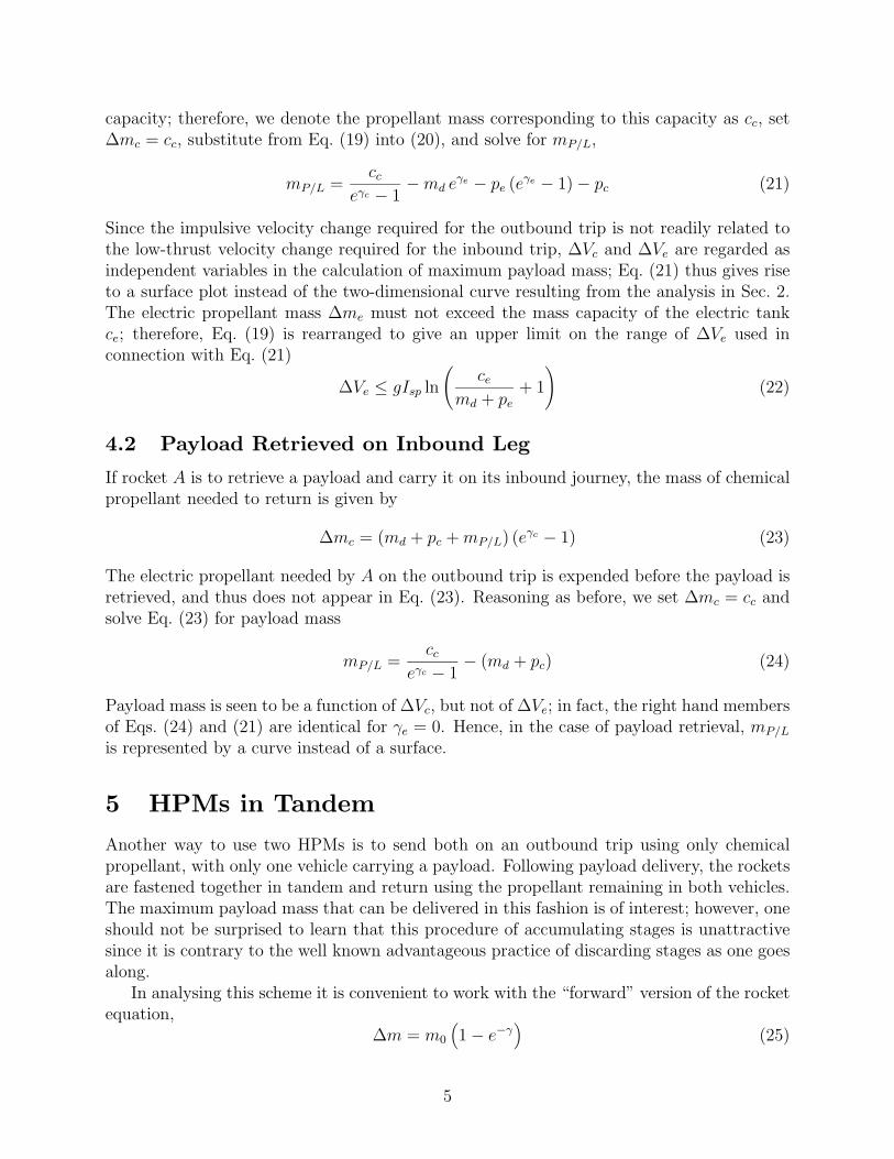
capacity; therefore, we denote the propellant mass corresponding to this capacity as cc, set∆mc = cc, substitute from Eq. (19) into (20), and solve for mP/L,
mP/L =cc
eγc − 1− md eγe − pe (eγe − 1) − pc (21)
Since the impulsive velocity change required for the outbound trip is not readily related tothe low-thrust velocity change required for the inbound trip, ∆Vc and ∆Ve are regarded asindependent variables in the calculation of maximum payload mass; Eq. (21) thus gives riseto a surface plot instead of the two-dimensional curve resulting from the analysis in Sec. 2.The electric propellant mass ∆me must not exceed the mass capacity of the electric tankce; therefore, Eq. (19) is rearranged to give an upper limit on the range of ∆Ve used inconnection with Eq. (21)
∆Ve ≤ gIsp ln
(
ce
md + pe
+ 1
)
(22)
4.2 Payload Retrieved on Inbound Leg
If rocket A is to retrieve a payload and carry it on its inbound journey, the mass of chemicalpropellant needed to return is given by
∆mc = (md + pc + mP/L) (eγc − 1) (23)
The electric propellant needed by A on the outbound trip is expended before the payload isretrieved, and thus does not appear in Eq. (23). Reasoning as before, we set ∆mc = cc andsolve Eq. (23) for payload mass
mP/L =cc
eγc − 1− (md + pc) (24)
Payload mass is seen to be a function of ∆Vc, but not of ∆Ve; in fact, the right hand membersof Eqs. (24) and (21) are identical for γe = 0. Hence, in the case of payload retrieval, mP/L
is represented by a curve instead of a surface.
5 HPMs in Tandem
Another way to use two HPMs is to send both on an outbound trip using only chemicalpropellant, with only one vehicle carrying a payload. Following payload delivery, the rocketsare fastened together in tandem and return using the propellant remaining in both vehicles.The maximum payload mass that can be delivered in this fashion is of interest; however, oneshould not be surprised to learn that this procedure of accumulating stages is unattractivesince it is contrary to the well known advantageous practice of discarding stages as one goesalong.
In analysing this scheme it is convenient to work with the “forward” version of the rocketequation,
∆m = m0
(
1 − e−γ)
(25)
5

where m0 is the total mass of the rocket (and payload) before a change of amount ∆V ismade in velocity, ∆m is the mass of fuel required to make the velocity change, and γ hasthe same meaning as in Eq. (2).
The rocket that does not carry the payload has an initial mass m0 that includes therocket’s dry mass md, mass of a chemical engine pc, and a full tank with chemcial propellantmass of cc. Using Eq. (25), the propellant mass required for an outbound trip requiring avelocity change of ∆V1 is given by
∆m1 = (md + pc + cc)(
1 − e−γ1
)
(26)
The rocket that carries the payload has an initial mass that includes the payload mass, sothe propellant mass required for its outbound trip is
∆m2 = (md + pc + cc + mP/L)(
1 − e−γ1
)
(27)
The two rockets return togther with empty propellant tanks and without the payload, so themass of the tandem configuration when it returns is simply 2(md + pc), and this is used asmf in the backward form of the rocket equation, Eq. (1), to obtain the mass of propellantneeded to return,
∆m = 2(md + pc) (eγ2 − 1) (28)
where the inbound trip requires a velocity change of ∆V2. For the sake of simplicity weassume that ∆V1 = ∆V2, therefore Eq. (10) applies.
Now, the amount of propellant available for the return trip must equal the propellantremaining on the rockets after the outbound trip,
∆m = (cc − ∆m1) + (cc − ∆m2) = 2cc − ∆m1 − ∆m2 (29)
so that Eq. 28 becomes
2(md + pc)(
eγ2 − 1
)
= 2cc − ∆m1 − ∆m2
= 2cc − (md + pc + cc)(
1 − e−γ2
)
− (md + pc + cc + mP/L)(
1 − e−γ2
)
= 2[
cc − (md + pc + cc)(
1 − e−γ2
)]
− mP/L
(
1 − e−γ2
)
(30)
which can be solved for mP/L,
mP/L =2
[
cce− γ
2 − (md + pc)(
eγ2 − e−
γ2
)]
(
1 − e−γ2
) (31)
where γ is associated with the roundtrip velocity change, assumed to consist of two equalone-way velocity changes, either of which is associated with γ/2.
6 Numerical Results
The preceding relationships can now be used to calculate maximum payload mass as afunction of velocity change by using numerical values for HPM dry mass md, engine mass p,propellant mass capacity c, and specific impulse Isp, as reported in Table 1.
6
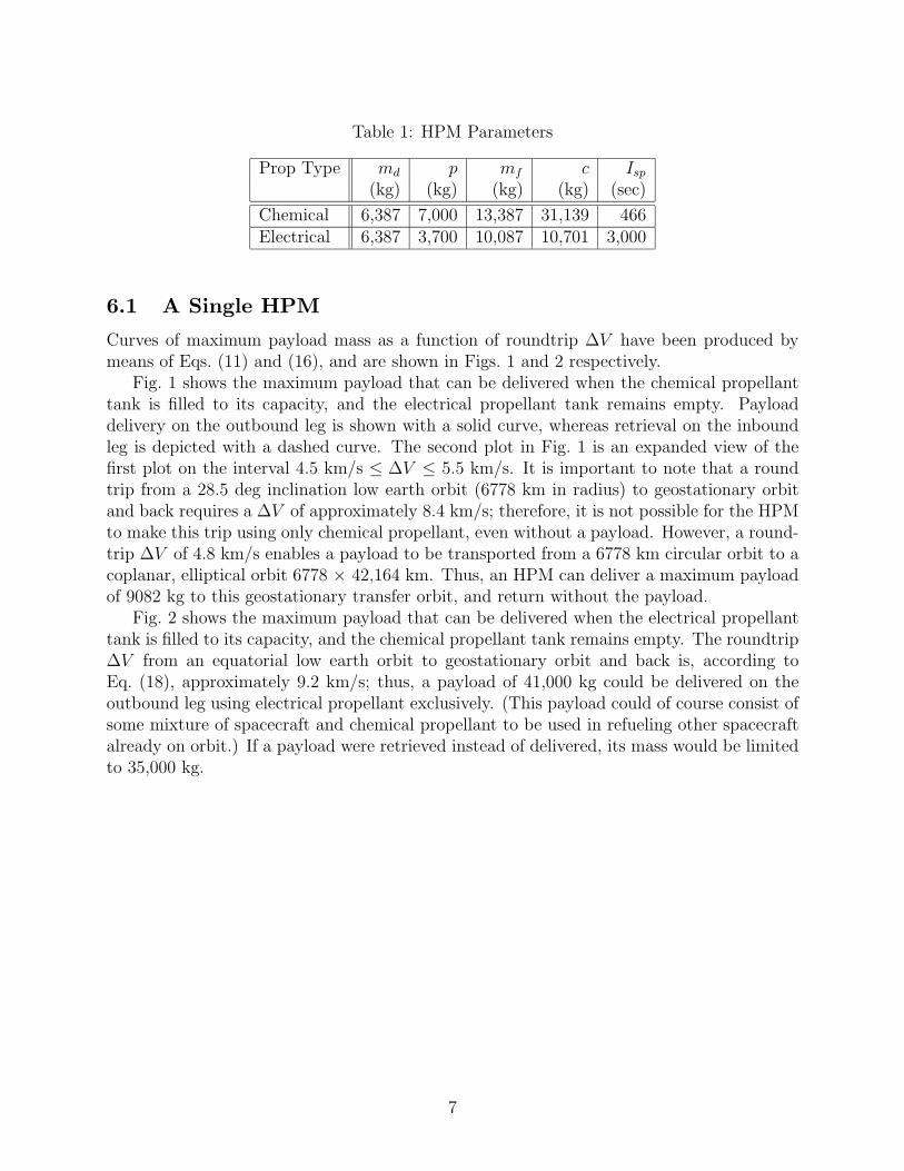
Table 1: HPM Parameters
Prop Type md p mf c Isp
(kg) (kg) (kg) (kg) (sec)
Chemical 6,387 7,000 13,387 31,139 466Electrical 6,387 3,700 10,087 10,701 3,000
6.1 A Single HPM
Curves of maximum payload mass as a function of roundtrip ∆V have been produced bymeans of Eqs. (11) and (16), and are shown in Figs. 1 and 2 respectively.
Fig. 1 shows the maximum payload that can be delivered when the chemical propellanttank is filled to its capacity, and the electrical propellant tank remains empty. Payloaddelivery on the outbound leg is shown with a solid curve, whereas retrieval on the inboundleg is depicted with a dashed curve. The second plot in Fig. 1 is an expanded view of thefirst plot on the interval 4.5 km/s ≤ ∆V ≤ 5.5 km/s. It is important to note that a roundtrip from a 28.5 deg inclination low earth orbit (6778 km in radius) to geostationary orbitand back requires a ∆V of approximately 8.4 km/s; therefore, it is not possible for the HPMto make this trip using only chemical propellant, even without a payload. However, a round-trip ∆V of 4.8 km/s enables a payload to be transported from a 6778 km circular orbit to acoplanar, elliptical orbit 6778 × 42,164 km. Thus, an HPM can deliver a maximum payloadof 9082 kg to this geostationary transfer orbit, and return without the payload.
Fig. 2 shows the maximum payload that can be delivered when the electrical propellanttank is filled to its capacity, and the chemical propellant tank remains empty. The roundtrip∆V from an equatorial low earth orbit to geostationary orbit and back is, according toEq. (18), approximately 9.2 km/s; thus, a payload of 41,000 kg could be delivered on theoutbound leg using electrical propellant exclusively. (This payload could of course consist ofsome mixture of spacecraft and chemical propellant to be used in refueling other spacecraftalready on orbit.) If a payload were retrieved instead of delivered, its mass would be limitedto 35,000 kg.
7

0 0.5 1 1.5 2 2.5 3 3.5 4 4.5 5 5.50
1
2
3
4
5
6x 10
5
Round Trip ∆V (km/s)
Max
imum
Pay
load
(kg
)
Chemical HPM P/L vs ∆V
Outbound P/L (Delivery)Inbound P/L (Retrieval)
4.5 4.6 4.7 4.8 4.9 5 5.1 5.2 5.3 5.4 5.50
5000
10000
15000
Round Trip ∆V (km/s)
Max
imum
Pay
load
(kg
)
Figure 1: Maximum Payload Mass vs. Roundtrip ∆V , with Chemical Propellant.
0 1 2 3 4 5 6 7 8 9 100
2
4
6
8
10
12
14x 10
5
Round Trip ∆V (km/s)
Max
imum
Pay
load
(kg
)
Electrical HPM P/L vs ∆V
Outbound P/L (Delivery)Inbound P/L (Retrieval)
9 9.1 9.2 9.3 9.4 9.5 9.6 9.7 9.8 9.9 102.5
2.7
2.9
3.1
3.3
3.5
3.7
3.9
4.1
4.3
4.5x 10
4
Round Trip ∆V (km/s)
Max
imum
Pay
load
(kg
)
Figure 2: Maximum Payload Mass vs. Roundtrip ∆V , with Electrical Propellant.
8
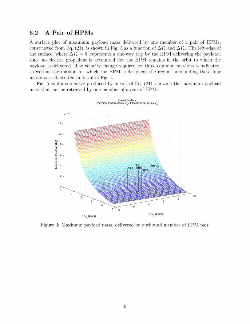
6.2 A Pair of HPMs
A surface plot of maximum payload mass delivered by one member of a pair of HPMs,constructed from Eq. (21), is shown in Fig. 3 as a function of ∆Vc and ∆Ve. The left edge ofthe surface, where ∆Ve = 0, represents a one-way trip by the HPM delivering the payload;since no electric propellant is accounted for, the HPM remains in the orbit to which thepayload is delivered. The velocity change required for three common missions is indicated,as well as the mission for which the HPM is designed; the region surrounding these fourmissions is illustrated in detail in Fig. 4.
Fig. 5 contains a curve produced by means of Eq. (24), showing the maximum payloadmass that can be retrieved by one member of a pair of HPMs.
01
23
45 0
24
68
10
0
2
4
6
8
10
12
x 104
EML1
∆ Ve (km/s)
GEOGEOEq.
GPS
Speed SurfaceChemical Outbound (∆ V
c), Electric Inbound (∆ V
e)
∆ Vc (km/s)
Max
imum
Pay
load
(kg
)
Figure 3: Maximum payload mass, delivered by outbound member of HPM pair.
9
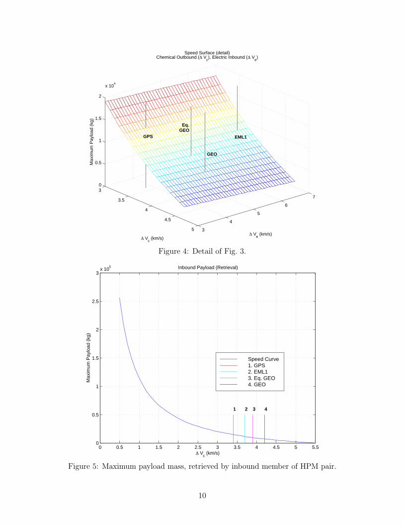
3
3.5
4
4.5
5 3
4
5
6
7
0
0.5
1
1.5
2
x 104
∆ Ve (km/s)
EML1
GEO
Speed Surface (detail)Chemical Outbound (∆ V
c), Electric Inbound (∆ V
e)
Eq.GEO
∆ Vc (km/s)
GPS
Max
imum
Pay
load
(kg
)
Figure 4: Detail of Fig. 3.
0 0.5 1 1.5 2 2.5 3 3.5 4 4.5 5 5.50
0.5
1
1.5
2
2.5
3x 10
5 Inbound Payload (Retrieval)
∆ Vc (km/s)
Max
imum
Pay
load
(kg
)
1 2 3 4
Speed Curve1. GPS2. EML13. Eq. GEO4. GEO
Figure 5: Maximum payload mass, retrieved by inbound member of HPM pair.
10
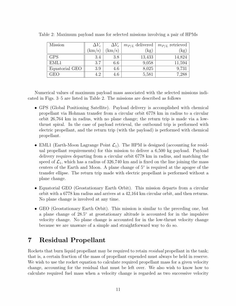
Table 2: Maximum payload mass for selected missions involving a pair of HPMs
Mission ∆Vc ∆Ve mP/L delivered mP/L retrieved(km/s) (km/s) (kg) (kg)
GPS 3.4 3.8 13,433 14,824EML1 3.7 6.6 9,058 11,594Equatorial GEO 3.9 4.6 8,025 9,731GEO 4.2 4.6 5,581 7,288
Numerical values of maximum payload mass associated with the selected missions indi-cated in Figs. 3–5 are listed in Table 2. The missions are described as follows
• GPS (Global Positioning Satellite). Payload delivery is accomplished with chemicalpropellant via Hohman transfer from a circular orbit 6778 km in radius to a circularorbit 26,764 km in radius, with no plane change; the return trip is made via a low-thrust spiral. In the case of payload retrieval, the outbound trip is performed withelectric propellant, and the return trip (with the payload) is performed with chemicalpropellant.
• EML1 (Earth-Moon Lagrange Point L1). The HPM is designed (accounting for resid-ual propellant requirements) for this mission to deliver a 6,500 kg payload. Payloaddelivery requires departing from a circular orbit 6778 km in radius, and matching thespeed of L1, which has a radius of 326,740 km and is fixed on the line joining the masscenters of the Earth and Moon. A plane change of 5 is required at the apogee of thetransfer ellipse. The return trip made with electric propellant is performed without aplane change.
• Equatorial GEO (Geostationary Earth Orbit). This mission departs from a circularorbit with a 6778 km radius and arrives at a 42,164 km circular orbit, and then returns.No plane change is involved at any time.
• GEO (Geostationary Earth Orbit). This mission is similar to the preceding one, buta plane change of 28.5 at geostationary altitude is accounted for in the impulsivevelocity change. No plane change is accounted for in the low-thrust velocity changebecause we are unaware of a simple and straightforward way to do so.
7 Residual Propellant
Rockets that burn liquid propellant may be required to retain residual propellant in the tank;that is, a certain fraction of the mass of propellant expended must always be held in reserve.We wish to use the rocket equation to calculate required propellant mass for a given velocitychange, accounting for the residual that must be left over. We also wish to know how tocalculate required fuel mass when a velocity change is regarded as two successive velocity
11
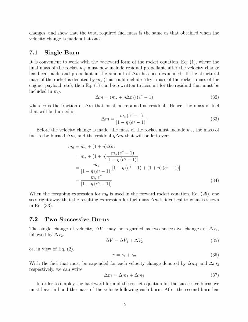
changes, and show that the total required fuel mass is the same as that obtained when thevelocity change is made all at once.
7.1 Single Burn
It is convenient to work with the backward form of the rocket equation, Eq. (1), where thefinal mass of the rocket mf must now include residual propellant, after the velocity changehas been made and propellant in the amount of ∆m has been expended. If the structuralmass of the rocket is denoted by ms (this could include “dry” mass of the rocket, mass of theengine, payload, etc), then Eq. (1) can be rewritten to account for the residual that must beincluded in mf .
∆m = (ms + η∆m) (eγ − 1) (32)
where η is the fraction of ∆m that must be retained as residual. Hence, the mass of fuelthat will be burned is
∆m =ms (eγ − 1)
[1 − η (eγ − 1)](33)
Before the velocity change is made, the mass of the rocket must include ms, the mass offuel to be burned ∆m, and the residual η∆m that will be left over:
m0 = ms + (1 + η)∆m
= ms + (1 + η)ms (eγ − 1)
[1 − η (eγ − 1)]
=ms
[1 − η (eγ − 1)][1 − η (eγ − 1) + (1 + η) (eγ − 1)]
=ms eγ
[1 − η (eγ − 1)](34)
When the foregoing expression for m0 is used in the forward rocket equation, Eq. (25), onesees right away that the resulting expression for fuel mass ∆m is identical to what is shownin Eq. (33).
7.2 Two Successive Burns
The single change of velocity, ∆V , may be regarded as two successive changes of ∆V1,followed by ∆V2.
∆V = ∆V1 + ∆V2 (35)
or, in view of Eq. (2),γ = γ1 + γ2 (36)
With the fuel that must be expended for each velocity change denoted by ∆m1 and ∆m2
respectively, we can write∆m = ∆m1 + ∆m2 (37)
In order to employ the backward form of the rocket equation for the successive burns wemust have in hand the mass of the vehicle following each burn. After the second burn has
12

been accomplished the total vehicle mass, including the residual from both burns, is given[as in Eq. (32)] by
mf = ms + η∆m = ms + η(∆m1 + ∆m2) (38)
After the first burn has been accomplished the mass of the vehicle must be the sum of mf
and the mass of the fuel that will be expended in the second burn,
m1 = ms + η(∆m1 + ∆m2) + ∆m2 = ms + (1 + η)∆m2 + η∆m1 (39)
These expressions for mass are used in successive applications of the backward rocket equa-tion for each of the burns,
∆m2 = mf (eγ2 − 1) = [ms + η(∆m1 + ∆m2)] (eγ2 − 1) (40)
∆m1 = m1 (eγ1 − 1) = [ms + (1 + η)∆m2 + η∆m1] (eγ1 − 1) (41)
yielding two equations that must be solved simultaneously for ∆m1 and ∆m2. SolvingEq. (40) for ∆m2, one obtains
∆m2 = [ms + η∆m1](eγ2 − 1)
[1 − η (eγ2 − 1)](42)
from which one may substitute into Eq. (41)
∆m1[1 − η (eγ1 − 1)] = [ms + (1 + η)∆m2] (eγ1 − 1)
=
ms + (1 + η)[ms + η∆m1](eγ2 − 1)
[1 − η (eγ2 − 1)]
(eγ1 − 1) (43)
or
∆m1
[1 − η (eγ1 − 1)] − (1 + η)η(eγ2 − 1)(eγ1 − 1)
[1 − η (eγ2 − 1)]
=
ms + (1 + η)ms(eγ2 − 1)
[1 − η (eγ2 − 1)]
(eγ1 − 1) (44)
After some algebraic manipulation, one obtains
∆m1 =ms eγ2(eγ1 − 1)
[1 − η(eγ − 1)](45)
and, after substitution into Eqn. (42),
∆m2 =ms (eγ2 − 1)
[1 − η(eγ − 1)](46)
It is easily verified that the sum of the fuel mass required for the two successive burns isidentical to that obtained earlier in Eq. (33) for a single burn:
∆m = ∆m1 + ∆m2 =ms (eγ − 1)
[1 − η (eγ − 1)](47)
References
[1] Melbourne, W. G., “Interplanetary Trajectories and Payload Capabilities of AdvancedPropulsion Vehicles”, Jet Propulsion Laboratory Technical Report No. 32-68, CaliforniaInstitute of Technology, Pasadena, CA, March 31, 1961.
13