Orbital shrinking

Matteo Fischetti1, Leo Liberti2

1 DEI, Universita di Padova, ItalyEmail:matteo.fischetti@unipd.it

2 LIX, Ecole Polytechnique, F-91128 Palaiseau, FranceEmail:liberti@lix.polytechnique.fr

July 12, 2011

Abstract

Symmetry plays an important role in optimization. The usual approach to cope with symme-try in discrete optimization is to try to eliminate it by introducing artificial symmetry-breakingconditions into the problem, and/or by using an ad-hoc search strategy. In this paper we arguethat symmetry is instead a beneficial feature that we should preserve and exploit as much aspossible, breaking it only as a last resort. To this end, we outline a new approach, that wecall orbital shrinking, where additional integer variables expressing variable sums within eachsymmetry orbit are introduces and used to “encapsulate” model symmetry. This leads to adiscrete relaxation of the original problem, whose solution yields a bound on its optimal value.Encouraging preliminary computational experiments on the tightness and solution speed of thisrelaxation are presented.

Keywords: Mathematical programming, discrete optimization, algebra, symmetry, relaxation,MILP, convex MINLP.

1 Introduction

Nature loves symmetry. Artists love symmetry. People love symmetry. Mathematicians andcomputer scientists also love symmetry, with the only exception of people working in discreteoptimization who always want to break it. Why? The answer is that symmetry is of great help insimplifying optimization in a convex setting, but in the discrete case it can trick search algorithmsbecause symmetric solutions are visited again and again. The usual approach to cope with thisredundancy source is to destroy symmetry by introducing artificial conditions into the problem,or by using a clever branching strategy such as isomorphism pruning [6, 7] or orbital branching[10]. We will outline a different approach, that we call orbital shrinking, where additional integervariables expressing variable sums within each orbit are introduces and used to “encapsulate” modelsymmetry. This leads to a discrete relaxation of the original problem, whose solution yields a boundon its optimal value. The underlying idea here is that we see symmetry as a positive feature of ourmodel, so we want to preserve it as much as possible, breaking it only as a last resort. Preliminarycomputational experiments are presented.

2 Symmetry

We next review some main results about symmetry groups; we refer the reader to, e.g., [1] (pp.189-190) and [6, 7, 4] for more details. For any positive integer n we use notation [n] := 1, · · · , n.

For any optimization problem (Z) we let v(Z) and F (Z) denote the optimal objective function valueand the feasible solution set of (Z), respectively. To ease presentation, all problems considered inthis paper are assumed to be feasible and bounded.

Our order of business is to study the role of symmetry when addressing a generic optimizationproblem of the form

(P ) v(P ) := minf(x) : x ∈ F (P ) (1)

where F (P ) ⊆ Rn and f : Rn → R. To this end, let G = Q1, · · · , QK ⊂ Rn×n be a finite group,i.e., a finite set of nonsingular n×n matrices closed under matrix product and inverse, and assumethat, for all x ∈ Rn and for all k ∈ [K]:

(C1) the function f is G-invariant (or symmetric w.r.t. G), i.e., f(Qkx) = f(x);

(C2) x ∈ F (P ) ⇒ Qkx ∈ F (P ).

Let the fixed subspace of G be defined as F := x : ∀k ∈ [K] Qkx = x. Given a point x, we define

x :=1

K

K∑k=1

Qkx (2)

as the new point obtained by “averaging x along G”. By elementary group theory, left-multiplyingG by any of its elements Qk leaves G unchanged, hence one has x ∈ F because

∀k ∈ [K] Qkx =1

K

K∑h=1

(QkQh)x =1

K

K∑h=1

Qhx = x. (3)

In this paper we always consider the case where all Qk’s in G are permutation matrices, i.e.,0-1 matrices with exactly one entry equal to 1 in each row and in each column. In this case,y = Qkx if and only if there exists a permutation πk of [n] such that yj = xi and j = πk(i) for alli ∈ [n]. In other words, the elements of group G are just permutations πk that simply relabel thecomponents of x. This naturally leads to a partition of the index set [n] into m ≥ 1 disjoint setsω1, · · · , ωm = Ω, called the orbits of G, where i and j (i < j) belong to a same orbit ω ∈ Ω ifand only if there exists k ∈ [K] such that j = πk(i).

From an algorithmic point of view, we can visualize the action of a permutation group G asfollows. Consider a digraph D = (V,A) whose n nodes are associated with the indices of thexj variables. Each πk in the group then corresponds to the digraph Dk = (V,Ak) whose arcsetAk := (i, j) : i ∈ V, j = πk(i) defines a family of arc-disjoint circuits covering all the nodes ofD. By definition, (i, j) ∈ Ak implies that i and j belong to a same orbit. So the orbits are justthe connected component of D when taking A =

∪Kk=1A

k. In practice, the group is defined bya limited set of “basic” elements (called generators) whose product and inverse lead to the entiregroup, and the orbits are quickly computed by initializing ωi = i for all i ∈ [n], scanning thegenerators πk, in turn, and merging the two orbits containing the endpoints of each arc (i, πk(i))for all i ∈ V [11].

In practical applications, the permutation group is detected automatically by analyzing theproblem formulation, i.e., the specific constraints used to define F (P ). In particular, a permutationπ is part of the permutation groups only if there exist an associated permutation σ of the indicesof the constraints defining F (P ), that makes it trivial to verify condition (C2); see e.g. [4].

2

A key property of permutation groups is that, because of (3), the average point x defined in (2)must have xj constant within each orbit, so it can be computed efficiently by just taking x-averagesinside the orbits, i.e.,

∀ω ∈ Ω, ∀j ∈ ω xj =1

|ω|∑i∈ω

xi. (4)

3 Optimization under symmetry

We next address the role of symmetry in optimization.

3.1 Convex optimization

Assume first that (P ) is a convex problem, i.e., f is a convex function and F (P ) is a convex set.Then x ∈ F (P ) implies x ∈ F (P ) and f(x) = f(

∑Kk=1Q

kx/K) ≤∑K

k=1 f(Qkx)/K = f(x), so

one needs only consider average points x when looking for an optimal solution to (P ). Because of(4), for permutation groups this means that the only unknowns for (P ) are the average x-valuesinside each orbit or, equivalently, the sums zω =

∑j∈ω xj for each ω ∈ Ω. It is known that (P )

can therefore be reformulated as follows (see Cor. 3.2): (i) introduce a new variable zω for eachorbit ω, (ii) replace variables xj for all j ∈ ω with their optimal expression zω/|ω|. Optimizingthe resulting projected problem on the space of the z variables yields the same optimal objectivefunction value as for the original problem. As a result, symmetry is a very useful property in aconvex optimization setting, in that it allows one to simplify the optimization problem—providedof course that the symmetry group (or a subgroup thereof) can be found effectively, as is often thecase [4].

3.2 Discrete optimization

We now address a discrete optimization setting where the objective function f is still convex butthe feasible set is defined as

F (P ) = x ∈ X : ∀j ∈ J xj ∈ Z,

where X ⊂ Rn is a convex set and J ⊆ [n] identifies the variables with integrality requirement. Ascustomary, we assume X be defined as

X = x ∈ Rn : ∀i ∈ [r] fi(x) ≤ 0,

where fi : Rn → R, i ∈ [r], are convex functions. This framework is quite general in that it coversMixed-Integer Linear Programming (MILP) as well many relevant cases of Mixed-Integer NonlinearProgramming (MINLP).

A natural way to exploit symmetry in the above setting is based on the observation that thewell known Branch-and-Bound (BB) tree search can be seen as a way to subdivide (P ) into anumber of convex subproblems, which provide relaxations of (P ) that are then used to computebounds and henceforth prune the search tree. At each tree node one needs to solve a convexsubproblem corresponding to X subject to the branching conditions—that we assume be expressedby additional convex constraints—hence symmetry can exploited to simplify this task. Note howeverthat branching conditions alter the symmetry group of the convex subproblem computed at the

3

root node of the search tree, so its recomputation (or heuristic update, as e.g. in [10]) at each nodebecomes necessary. In addition, the use of symmetry inside each node does not prevent the treesearch to possibly enumerate symmetric solutions again and again, so ad-hoc branching strategiesare still of fundamental importance.

3.3 Orbital shrinking relaxation

We next propose a different approach, intended to eliminate problem symmetry by “encapsulating”it in a new (relaxed) formulation. More specifically, instead of trying to break symmetries as isstandard in the current literature [12, 6, 7, 10, 9, 4], our approach is to solve a discrete relaxationof the original problem, defined on a shrunken space with just one variable for each orbit.

Let G be the group for (P ) (found e.g. as in [4]) and let Ω = ω1, . . . , ωm be its set of orbits(by construction integer and continuous variables will be in different orbits). WLOG, assume thefirst m orbits involve integer variables only, and let Θ = ω1, . . . , ωm, while the remaining orbits(if any) involve continuous variables only (if any). In addition, for each x ∈ Rn, let z(x) ∈ Rm bedefined as

∀ω ∈ Ω zω(x) :=∑j∈ω

xj .

For any g : Rn → R let g : Rm → R be obtained from g(x) by replacing each xj by zω/|ω| (j ∈ ω,ω ∈ Ω). Note that g(z(x)) = g(x) holds whenever xj is constant within each orbit, hence becauseof (4) one has the identity

g(z(x)) = g(x). (5)

Our Orbital Shrinking Relaxation (OSR) is constructed from (P ) in two steps:

1. Let (PREL) be the relaxed problem obtained from (P ) by replacing the integrality conditionsxj ∈ Z (j ∈ J) by their surrogate version

∀ω ∈ Θ (∑j∈ω

xj) ∈ Z ; (6)

2. Reformulate (PREL) as

(POSR) v(POSR) := minf(z) : ∀i ∈ [r] f i(z) ≤ 0,∀ω ∈ Θ zω ∈ Z (7)

3.1 Theoremv(POSR) = v(PREL) ≤ v(P ).

Proof. Inequality v(PREL) ≤ v(P ) is obvious, so we only need to prove v(POSR) = v(PREL).Let x be any optimal solution to (PREL). We claim that x is an equivalent optimal solution to

(PREL). Indeed, because of (C2) one has Qkx ∈ X for all k ∈ [K], hence x =(

1K

∑k∈[K]Q

kx)∈ X

because of the convexity of X. In addition, because of (4),∑

j∈ω xj =∑

j∈ω xj for all ω ∈Θ, hence x also satisfies (6) and is therefore feasible for (PREL). The optimality of x for (PREL)

then follows immediately from the convexity of f , which implies f(x) = f(

1K

∑k∈[K]Q

kx)

≤1K

∑k∈[K] f(Q

kx) = f(x), i.e., f(x) = v(PREL).

4

Now take the point z(x). Because of (5) and since x ∈ X, for all i ∈ [r] we have f i(z(x)) =fi(x) ≤ 0. In addition, zω(x) ∈ Z for all ω ∈ Θ because x ∈ F (PREL) satisfies (6), hence z(x) ∈F (POSR) and then v(POSR) ≤ f(z(x)) = f(x) = v(PREL), thus proving v(POSR) ≤ v(PREL).

To show v(POSR) ≥ v(PREL), let z be any optimal solution to (POSR) and consider the point x ∈ Rn

with xj := zω/|ω| for all j ∈ ω and ω ∈ Ω. By construction, x = x and z(x) = z. Because of (5),for all i ∈ [r] one then has fi(x) = fi(x) = f i(z(x)) = f i(z) ≤ 0, i.e., x ∈ X. In addition, for allω ∈ Θ,

∑j∈ω xj = zω ∈ Z, i.e., x also satisfies (6) and therefore x ∈ F (PREL). Finally, again because

of (5), v(PREL) ≤ f(x) = f(x) = f(z(x)) = f(z) = v(POSR), i.e., v(PREL) ≤ v(POSR) as required. 2

3.2 CorollaryFor convex optimization (case J = ∅), (POSR) is a reformulation of (P ), in the sense that v(POSR) =v(P ).

Proof. Just observe that (PREL) coincides with (P ) when J = ∅. 2

4 Experiments on finding the best subgroup

Theorem 3.1 remains obviously valid if a subgroup G′ of G is used (instead of G) in the constructionof (POSR). Different choices of G′ lead to different relaxations and hence to different bounds v(POSR).If G′ is the trivial group induced by the identity permutation, no shrinking at all is performedand the relaxation coincides with the original problem. As G′ grows in size, it generates longerorbits and the relaxation becomes more compact and easier to solve (also because more symmetryis encapsulated into the relaxation), but the lower bound quality decreases.

Ideally, we wish the relaxation to be (a) as tight as possible and (b) as efficient as possiblewith respect to the CPU time taken to solve it. In this section we discuss and computationallyevaluate a few ideas for generating subgroups G′ which should intuitively yield “good” relaxationsin a MILP context. All experiments were conducted on a 1.4GHz Intel Core 2 Duo 64bit with 3GBof RAM. The MILP solver of choice is IBM ILOG Cplex 12.2.

4.1 Automatic generation of the whole symmetry group

The formulation group is detected automatically using the techniques discussed in [4]: the MILP istransformed into a Directed Acyclic Graph (DAG) encoding the incidence of variables in objectiveand constraints, and a graph automorphism software (nauty [8]) is then called on the DAG. Theorbital-shrinking relaxation is constructed automatically using a mixture of bash scripting, GAP[3], AMPL [2], and ROSE [5].

4.2 The instance set

We considered the following 39 symmetric MILP instances:

ca36243 ca57245 ca77247 clique9 cod105 cod105r cod83 cod83r cod93 cod93r cov1053

cov1054 cov1075 cov1076 cov1174 cov954 flosn52 flosn60 flosn84 jgt18 jgt30 mered

O4 35 oa25332 oa26332 oa36243 oa57245 oa77247 of5 14 7 of7 18 9 ofsub9 pa36243 pa57245

pa77247 sts135 sts27 sts45 sts63 sts81

5

all taken from F. Margot’s website.

4.3 Generator ranking

Using orbital shrinking with the whole symmetry group G has the merit of yielding the mostcompact relaxation. On our test set, however, this approach yields a relaxation bound which is notbetter than the LP bound 31 times out of 39, and for the remaining 8 times it is not better thanthe root-node Cplex’s bound (i.e., LP plus root node cuts)—although this will not necessarily bethe case for other symmetric instances (e.g., for instances with small symmetry groups).

We observe that the final OSR only depends on the orbits of G′ rather than on G′ itself, andthe smaller G′ the more (and/or shorter) orbits it yields. We therefore consider the idea of testingsubgroups with orbits of varying size, from small to large. Since testing all subgroups of G is outof the question, we look at its generator list Π = (π0, . . . , πk) (including the identity permutation).For any permutation π we let fix(π) be the subset of [n] fixed by π, i.e., containing those i suchthat π(i) = i. We then reorder our list Π so that

|fix(π0)| ≥ · · · ≥ |fix(πk)|

and for all ℓ ≤ k we define Gℓ as the subgroup of G induced by the sublist (π0, · · · , πℓ). This leadsto a subgroup chain

G0, G1, · · · , Gk = G

with increasing number of generators and hence larger and larger orbits (G0 being the trivialgroup induced by the identity permutation). In our view, the first generators in the list are themost attractive ones in terms of bound quality—having a large fix(π) implies that the generatedsubgroup is likely to remain valid for (P ) even when several variables are fixed by branching.

For each instance in our test set, we generated the relaxations corresponding to each Gℓ andrecorded bound values and CPU times, plotting the results against ℓ. We set a maximum user CPUtime of 1800s, as we deemed a relaxation useless if it takes too long to solve. The typical behaviorof the relaxation in terms of bound value and CPU time was observed to be mostly monotonicallydecreasing in function of the number ℓ of involved generators. Figure 1 shows an example of theseresults on the sts81 instance.

4.4 Choosing a good set of generators

Our generator ranking provides a “dial” to trade bound quality versus CPU time. We now considerthe question of how to set this dial automatically, i.e., how to choose a value of ℓ ∈ [k] leading toa good subgroup Gℓ.

Out of the 39 instances in our test set, 16 yields the same bound independently of ℓ, and werehence discarded from this test. The remaining 23 instances:

ca36243 clique9 cod105 cod105r cod83 cod83r cod93 cod93r cov1075 cov1076 cov954 mered

O4 35 oa36243 oa77247 of5 14 7 of7 18 9 pa36243 sts135 sts27 sts45 sts63 sts81

yields a nonzero decrease in bound value as ℓ increases, so they are of interest for our test.Having generated and solved relaxations for all ℓ ≤ k, we hand-picked good values of ℓ for each

instance, based on these prioritized criteria:

1. bound provided by Gℓ strictly tighter than LP bound;

6

sts81

ℓ/k obj CPU

1/14 45 3.602/14 45 1.513/14 45 1.184/14 45 1.135/14 33 0.016/14 33 0.017/14 33 0.028/14 33 0.009/14 29 0.0210/14 29 0.0011/14 29 0.0112/14 28 0.0113/14 28 0.0014/14 27 0.00

26

28

30

32

34

36

38

40

42

44

46

0 2 4 6 8 10 12 14

obj

0

0.5

1

1.5

2

2.5

3

3.5

4

0 2 4 6 8 10 12 14

CPU

Figure 1: Bound values and CPU times against the number ℓ of generators for instance sts81.

7

2. minimize user CPU time, with strong penalty for choices of ℓ leading to excess of 10 seconds;

3. on lack of other priorities, choose ℓ leading to bounds around midrange in [bnd(Gk),bnd(G1)],where bnd(G′) denotes the bound value obtained by solving the orbital-shrinking relaxationbased on the subgroup G′.

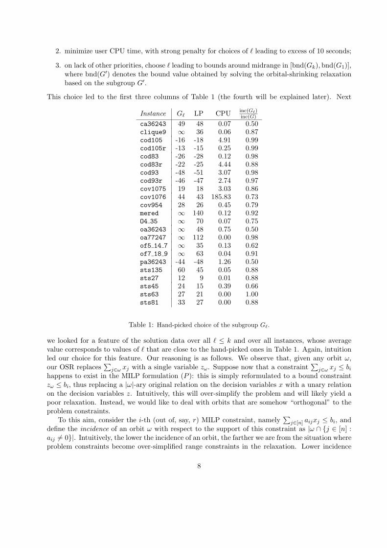
This choice led to the first three columns of Table 1 (the fourth will be explained later). Next

Instance Gℓ LP CPU inc(Gℓ)inc(G)

ca36243 49 48 0.07 0.50clique9 ∞ 36 0.06 0.87cod105 -16 -18 4.91 0.99cod105r -13 -15 0.25 0.99cod83 -26 -28 0.12 0.98cod83r -22 -25 4.44 0.88cod93 -48 -51 3.07 0.98cod93r -46 -47 2.74 0.97cov1075 19 18 3.03 0.86cov1076 44 43 185.83 0.73cov954 28 26 0.45 0.79mered ∞ 140 0.12 0.92O4 35 ∞ 70 0.07 0.75oa36243 ∞ 48 0.75 0.50oa77247 ∞ 112 0.00 0.98of5 14 7 ∞ 35 0.13 0.62of7 18 9 ∞ 63 0.04 0.91pa36243 -44 -48 1.26 0.50sts135 60 45 0.05 0.88sts27 12 9 0.01 0.88sts45 24 15 0.39 0.66sts63 27 21 0.00 1.00sts81 33 27 0.00 0.88

Table 1: Hand-picked choice of the subgroup Gℓ.

we looked for a feature of the solution data over all ℓ ≤ k and over all instances, whose averagevalue corresponds to values of ℓ that are close to the hand-picked ones in Table 1. Again, intuitionled our choice for this feature. Our reasoning is as follows. We observe that, given any orbit ω,our OSR replaces

∑j∈ω xj with a single variable zω. Suppose now that a constraint

∑j∈ω xj ≤ bi

happens to exist in the MILP formulation (P ): this is simply reformulated to a bound constraintzω ≤ bi, thus replacing a |ω|-ary original relation on the decision variables x with a unary relationon the decision variables z. Intuitively, this will over-simplify the problem and will likely yield apoor relaxation. Instead, we would like to deal with orbits that are somehow “orthogonal” to theproblem constraints.

To this aim, consider the i-th (out of, say, r) MILP constraint, namely∑

j∈[n] aijxj ≤ bi, anddefine the incidence of an orbit ω with respect to the support of this constraint as |ω ∩ j ∈ [n] :aij = 0|. Intuitively, the lower the incidence of an orbit, the farther we are from the situation whereproblem constraints become over-simplified range constraints in the relaxation. Lower incidence

8

orbits should yield tighter relaxations, albeit perhaps harder to solve. Given a subgroup G′ withorbits Ω′ = ω′

1, · · · , ω′m′, we then extend the incidence notion to G′

inc(G′, i) :=

∣∣∣∣∣ ∪ω′∈Ω′

ω′ ∩ j ∈ [n] : aij = 0

∣∣∣∣∣ , (8)

and finally to the whole MILP formulation

inc(G′) =∑i∈[r]

inc(G′, i). (9)

The rightmost column of Table 1 reports the relative incidence of Gℓ, computed as inc(Gℓ)/ inc(G),for those ℓ that were hand-chosen to be “best” according to the prioritized criteria listed above. Itsaverage is 0.82 with standard deviation 0.17. This value allows us to generate a relaxation whichis hopefully “good”, by automatically selecting the value of ℓ such that inc(Gℓ)/ inc(G) is as closeto 0.82 as possible.

5 Computational experiments

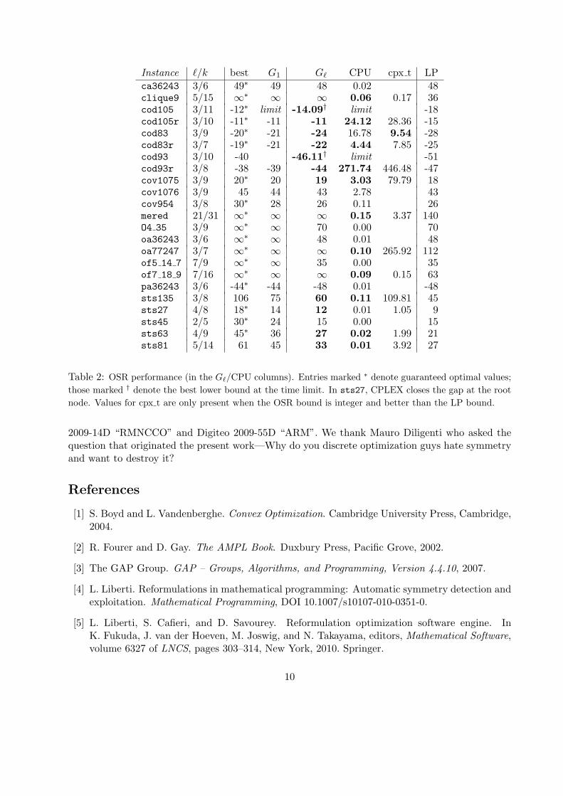
The quality of the OSR we obtain with the method of Section 4.4 is reported in Table 2 whosecolumns include: the instance name, the automatically determined value of ℓ and the total numberk of generators, the best-known optimal objective function value for the instance (starred valuescorrespond to guaranteed optima), the bound given by G1 which provides the tightest non-trivialOSR bound, the bound given by Gℓ and the associated CPU time, the CPU time “cpx t” spentby CPLEX 12.2 (default settings) on the original formulation to get the same bound as OSR (onlyreported when the OSR bound is strictly better than the LP bound), and the LP bound. Entrylimit marks an exceeded time limit of 1800 sec.s, while boldface highlights the best results for eachinstance.

The results are quite encouraging: our bound is very often stronger than the LP bound, whilstoften taking only a fraction of a second to solve. The effect of orbital shrinking can be noticed bylooking at the “cpx t” column, where it is evident that normal branching takes significantly longerto reach the bound given by our relaxation.

6 Conclusions

We discussed a new methodology for deriving a tight relaxation of a given discrete optimizationproblem, based on orbit shrinking. Results on a testbed of MILP instances are quite encouraging.Our work opens up several directions: how to find a good generator set, whether it is possible tofind extensions to general MINLPs, how will the relaxation perform when used within a Branch-and-Bound algorithm and how to dynamically change it along the search tree, and which insightsfor heuristics can be derived from the integer solution of the relaxed problem.

Acknowledgements

The first author was supported by the Progetto di Ateneo on “Computational Integer Programming”of the University of Padova. The second author was partially supported by grants Digiteo Chair

9

Instance ℓ/k best G1 Gℓ CPU cpx t LP

ca36243 3/6 49∗ 49 48 0.02 48clique9 5/15 ∞∗ ∞ ∞ 0.06 0.17 36cod105 3/11 -12∗ limit -14.09† limit -18cod105r 3/10 -11∗ -11 -11 24.12 28.36 -15cod83 3/9 -20∗ -21 -24 16.78 9.54 -28cod83r 3/7 -19∗ -21 -22 4.44 7.85 -25cod93 3/10 -40 -46.11† limit -51cod93r 3/8 -38 -39 -44 271.74 446.48 -47cov1075 3/9 20∗ 20 19 3.03 79.79 18cov1076 3/9 45 44 43 2.78 43cov954 3/8 30∗ 28 26 0.11 26mered 21/31 ∞∗ ∞ ∞ 0.15 3.37 140O4 35 3/9 ∞∗ ∞ 70 0.00 70oa36243 3/6 ∞∗ ∞ 48 0.01 48oa77247 3/7 ∞∗ ∞ ∞ 0.10 265.92 112of5 14 7 7/9 ∞∗ ∞ 35 0.00 35of7 18 9 7/16 ∞∗ ∞ ∞ 0.09 0.15 63pa36243 3/6 -44∗ -44 -48 0.01 -48sts135 3/8 106 75 60 0.11 109.81 45sts27 4/8 18∗ 14 12 0.01 1.05 9sts45 2/5 30∗ 24 15 0.00 15sts63 4/9 45∗ 36 27 0.02 1.99 21sts81 5/14 61 45 33 0.01 3.92 27

Table 2: OSR performance (in the Gℓ/CPU columns). Entries marked ∗ denote guaranteed optimal values;

those marked † denote the best lower bound at the time limit. In sts27, CPLEX closes the gap at the root

node. Values for cpx t are only present when the OSR bound is integer and better than the LP bound.

2009-14D “RMNCCO” and Digiteo 2009-55D “ARM”. We thank Mauro Diligenti who asked thequestion that originated the present work—Why do you discrete optimization guys hate symmetryand want to destroy it?

References

[1] S. Boyd and L. Vandenberghe. Convex Optimization. Cambridge University Press, Cambridge,2004.

[2] R. Fourer and D. Gay. The AMPL Book. Duxbury Press, Pacific Grove, 2002.

[3] The GAP Group. GAP – Groups, Algorithms, and Programming, Version 4.4.10, 2007.

[4] L. Liberti. Reformulations in mathematical programming: Automatic symmetry detection andexploitation. Mathematical Programming, DOI 10.1007/s10107-010-0351-0.

[5] L. Liberti, S. Cafieri, and D. Savourey. Reformulation optimization software engine. InK. Fukuda, J. van der Hoeven, M. Joswig, and N. Takayama, editors, Mathematical Software,volume 6327 of LNCS, pages 303–314, New York, 2010. Springer.

10

[6] F. Margot. Pruning by isomorphism in branch-and-cut. Mathematical Programming, 94:71–90,2002.

[7] F. Margot. Exploiting orbits in symmetric ILP. Mathematical Programming B, 98:3–21, 2003.

[8] B. McKay. nauty User’s Guide (Version 2.4). Computer Science Dept. , Australian NationalUniversity, 2007.

[9] J. Ostrowski, J. Linderoth, F. Rossi, and S. Smriglio. Constraint orbital branching. In A. Lodi,A. Panconesi, and G. Rinaldi, editors, IPCO, volume 5035 of LNCS, pages 225–239. Springer,2008.

[10] J. Ostrowski, J. Linderoth, F. Rossi, and S. Smriglio. Orbital branching. Mathematical Pro-gramming, 126:147–178, 2011.

[11] A. Seress. Permutation Group Algorithms. Cambridge University Press, Cambridge, 2003.

[12] H. Sherali and C. Smith. Improving discrete model representations via symmetry considera-tions. Management Science, 47(10):1396–1407, 2001.

11