Evolution of the eccentricity and orbital inclination caused by ...
139
HAL Id: tel-01081966 https://tel.archives-ouvertes.fr/tel-01081966 Submitted on 12 Nov 2014 HAL is a multi-disciplinary open access archive for the deposit and dissemination of sci- entific research documents, whether they are pub- lished or not. The documents may come from teaching and research institutions in France or abroad, or from public or private research centers. L’archive ouverte pluridisciplinaire HAL, est destinée au dépôt et à la diffusion de documents scientifiques de niveau recherche, publiés ou non, émanant des établissements d’enseignement et de recherche français ou étrangers, des laboratoires publics ou privés. Evolution of the eccentricity and orbital inclination caused by planet-disc interactions Jean Teyssandier To cite this version: Jean Teyssandier. Evolution of the eccentricity and orbital inclination caused by planet-disc interac- tions. Galactic Astrophysics [astro-ph.GA]. Université Pierre et Marie Curie - Paris VI, 2014. English. NNT : 2014PA066205. tel-01081966
-
Upload
khangminh22 -
Category
Documents
-
view
1 -
download
0
Transcript of Evolution of the eccentricity and orbital inclination caused by ...

HAL Id: tel-01081966https://tel.archives-ouvertes.fr/tel-01081966
Submitted on 12 Nov 2014
HAL is a multi-disciplinary open accessarchive for the deposit and dissemination of sci-entific research documents, whether they are pub-lished or not. The documents may come fromteaching and research institutions in France orabroad, or from public or private research centers.
L’archive ouverte pluridisciplinaire HAL, estdestinée au dépôt et à la diffusion de documentsscientifiques de niveau recherche, publiés ou non,émanant des établissements d’enseignement et derecherche français ou étrangers, des laboratoirespublics ou privés.
Evolution of the eccentricity and orbital inclinationcaused by planet-disc interactions
Jean Teyssandier
To cite this version:Jean Teyssandier. Evolution of the eccentricity and orbital inclination caused by planet-disc interac-tions. Galactic Astrophysics [astro-ph.GA]. Université Pierre et Marie Curie - Paris VI, 2014. English.NNT : 2014PA066205. tel-01081966

THÈSE DE DOCTORATDE L’UNIVERSITÉ PIERRE ET MARIE CURIE
Spécialité : Physique
École doctorale : ASTRONOMIE ET ASTROPHYSIQUED’ÎLE-DE-FRANCE
réalisée à
l’Institut d’Astrophysique de Paris
présentée par
Jean TEYSSANDIER
pour obtenir le grade de :
DOCTEUR DE L’UNIVERSITÉ PIERRE ET MARIE CURIE
Sujet de la thèse :
Évolution de l’excentricité et de l’inclinaisonorbitale due aux interactions planètes-disque
soutenue le 16 Septembre 2014
devant le jury composé de :
Bruno Sicardy PrésidentCarl Murray RapporteurSean Raymond RapporteurAlessandro Morbidelli ExaminateurClément Baruteau ExaminateurCaroline Terquem Directrice de thèse


Une mathématique bleue
Dans cette mer jamais étale
D’où nous remonte peu à peu
Cette mémoire des étoiles
Léo Ferré, La mémoire et la mer

2
Remerciements
Mes remerciements vont tout d’abord à Caroline, pour avoir accepté de dirigercette thèse. Ca a été un plaisir de pouvoir profiter du large spectre de ses con-naissances, et de tant apprendre à son contact. Je lui suis aussi redevable pourla rigueur qu’elle a imposée à mon travail et qui ne pourra que m’être bénéfiquepour la suite. Je la remercie enfin de m’avoir laissé une grande liberté dans mesrecherches, m’encourageant à explorer mes propres pistes et développer mesidées, et de toujours avoir laissé sa porte ouverte à la discussion. C’est aussigrâce à elle et Steve Balbus que j’ai pu passer deux si belles années à Oxford.Les aléas de la recherche ont parfois du bon!
Je remercie aussi Carl Murray et Sean Raymond d’avoir accepté de servir entant que rapporteurs de cette thèse, ainsi que Bruno Sicardy, Alessandro Mor-bidelli et Clément Baruteau pour avoir accepté d’en être les examinateurs.
Je remercie aussi Frederic Rasio et Smadar Naoz de m’avoir accueilli àl’Université de Northwestern durant les stages qui ont précédé ma thèse. Ce sonteux qui m’ont définitivement donné le goût pour la dynamique des exoplanètes.Je remercie aussi John Papaloizou pour la collaboration qu’il a apportée à l’undes papiers publiés dans cette thèse.
Cette thèse n’aurait pas été une si belle expérience sans toutes les rencon-tres qu’elle a occasionnées en chemin. Il y a d’abord les anciens du M2 del’Observatoire, Élodie, Andy, Jessica, Claire-Line, Alex, Élise et les autres. Àl’IAP, c’est toujours un plaisir de revenir passer du temps avec Vincent, Flavienet tous les autres doctorants. À Oxford, je remercie Suzanne Aigrain de m’avoiraccueilli dans son groupe, avec à la clé les fameux déjeuners du vendredi! C’estun plaisir d’avoir côtoyé ses étudiants, en particulier Tom, Ed et Ruth. Enfin, lavie à Oxford n’aurait pas été la même sans Thibaut, Rich et Shravan. Un grandmerci au passage à Rich, pour avoir relu quelques bouts de ma thèse. Plusgénéralement, ce fut un plaisir de partager durant deux ans la vie du grouped’astrophysique d’Oxford.
3

4
Peu de choses durant mon séjour à Oxford m’ont fait plus plaisir que derecevoir la visite de mon frère et ma soeur. J’espère qu’ils auront l’occasion devenir à Cambridge voir si les pubs sont si différents de ceux d’Oxford. . . Enfin,cette thèse est dédiée à mes parents, pour leur soutien inconditionnel duranttoute la poursuite de mes études. Si j’en suis arrivé là, c’est surtout grâce à eux.

Abstract
Since the discovery of the first planet orbiting a main-sequence star outside thesolar system in 1995, the field of exoplanet studies has grown rapidly, both fromthe observational and theoretical sides. Despite the fact that we are still lackinga global picture for the formation and evolution of planetary systems, it is nowcommonly accepted that planets form in protoplanetary discs and interact withthem in the early stages of their evolution. This thesis aims at studying some ofthese interactions.
The observations of extrasolar planets have brought several puzzling resultsto the attention of the community. One of them is the existence of hot Jupiters,giant gaseous planets which orbit their parent star with a period of a few daysonly. The commonly accepted scenario is that they formed in the outer partsof the disc and migrated inward. Furthermore, a significant number of planetsdetected so far, especially by the method of radial velocities, have high eccen-tricities. This is in contrast with our own solar system where giant planets havequasi-circular orbits. Such a distribution of eccentricities may be the signatureof strong dynamical interactions between the different components of a sameplanetary system. Finally, there are short-period planets whose orbits is mis-aligned with the axis of rotation of their host star, which could possibly argueagainst the smooth migration of planets in their disc.
Therefore, it is important to disentangle between the orbital characteristicsthat planets acquired through mutual dynamical interactions, and the ones theyacquired when they interacted with the disc. Firstly, it gives constraints on thephysical parameters of protoplanetary discs. Secondly, it is interesting to knowthe properties of the system of planets after the disc has dissipated, and whatsort of initial conditions one can expect when planets start to interact freely onewith each other. For instance, one can ask if it is possible for planets to reachlarge eccentricities and inclinations when the disc was still present, and whetherthey could maintain them or not.
5

6
The first topic that we study in this thesis is the interaction between a planetand a disc, when the orbit of the planet has a large inclination with respect tothe mid-plane of the disc. If the initial inclination of the orbit is larger thansome critical value, the gravitational force exerted by the disc on the planetleads to a Kozai cycle in which the eccentricity of the orbit is pumped up tolarge values and oscillates with time in antiphase with the inclination. On theother hand, both the inclination and the eccentricity are damped by the frictionalforce that the planet is subject to when it crosses the disc. Typically, Neptuneor lower mass planets would remain on inclined and eccentric orbits over thedisc lifetime, whereas orbits of Jupiter or higher mass planets would align andcircularize.
A mechanism that could explain this primordial misalignment between plan-ets and discs, and more generally, the population of planets with large spin-orbitmisalignments, is that of resonant migration. When two planets migrate in adisc, it is possible that they enter a configuration where the ratio of their orbitalperiods is equal to the ratio between two small integers. This configuration isreferred to as mean motion resonance. If the resonance is maintained during themigration, the eccentricities can grow to high values. Simulations have shownthat, in some cases, the inclinations could also grow to high values. However,the disc tends to damp the eccentricities and inclinations and keep them to lowvalues. In this thesis we study, analytically and numerically, the conditionsneeded for a system of two migrating planets trapped in a 2:1 mean motion res-onance to enter an inclination–type resonance. We show that this resonance canbe achieved only after the eccentricities have reached a critical value. Howeverthe maximum value reached by the eccentricities is limited by the disc damp-ing. We show that the criterion for triggering an inclination–type resonance isa function of the ratio between the eccentricity damping timescale and the or-bital migration timescale. If this ratio is larger than a few tenths, the system canenter an inclination–type resonance. However, both observations and theorysuggest that this ratio probably cannot exceed a few hundredths. We concludethat excitation of inclinations through the type of resonance described here isvery unlikely to happen in a system of two planets migrating in a disc.

Résumé
Depuis la découverte de la première planète orbitant une étoile de la séquenceprincipale autre que le Soleil en 1995, ce champ de recherche a connu une crois-sance vertigineuse, tant au niveau des observations, que des modèles théoriquesdéveloppés en parallèle. Même si la formation et l’évolution des systèmesplanétaires restent encore mal comprises dans leur globalité, Il est à peu prèscertain que les planètes se forment dans des disques protoplanétaires et inter-agissent avec ces derniers durant la phase primordiale de leur évolution. Cettethèse s’attache à décrire certains aspects de ces interactions.
Parmi les problèmes soulevés par les nombreuses observations d’exoplanètes,on peut citer l’existence des Jupiter chaudes, géantes gazeuses dont la révolu-tion autour de leur étoile s’effectue en quelques jours à peine. Il est communé-ment admis qu’elles se sont formées dans les parties externes du disque, pourensuite migrer vers l’intérieur. Cependant , les processus de migration restentencore débattus. On pourra aussi noter qu’un nombre important de planètesdétectées, notamment par la méthode des vitesses radiales, présentent de fortesexcentricités. Cette observation contraste avec celle de notre propre SystèmeSolaire, où les planètes géantes ont des orbites quasi-circulaires. Cette distri-bution d’excentricités témoigne probablement d’une certaine richesse dans lesinteractions dynamiques entre les planètes d’un même système. Un autre résul-tat majeur des quelques dernières années est l’observation de planètes à faiblepériode orbitale dont l’orbite n’est pas alignée avec l’axe de rotation de leurétoile. Cette observation pourrait potentiellement remettre en question l’idéeselon laquelle ces planètes acquièrent leur faible période par le biais de la mi-gration au sein du disque.
Par conséquent, il est important de pouvoir différencier quelles sont les car-actéristiques observationelles des exoplanètes qui sont le fruit de leurs interac-tions mutuelles, et celles qui peuvent être expliquées lors de la phase d’interactionavec le disque protoplanétaire. D’une part, cela permet d’imposer des con-traintes sur la physique des disques protoplanétaires. D’autre part, il est in-
7

8
téressant de savoir à quoi ressemble le système de planètes une fois que ledisque se dissipe, et à quelles conditions intiales peut-on s’attendre lorsque lesplanétes commencent à interagir entre elles sans la présence du disque. Par ex-emple, est-il possible pour une ou des planètes d’acquérir de l’excentricité et del’inclinaison au sein du disque, et de les maintenir par la suite? De plus, il estcertain que le disque domine l’évolution des planètes au stage primordial de leurvie, mais jusqu’à quel point cela limite-t-il les interactions entre les planètes?
Le premier effet étudié dans cette thèse concerne l’évolution d’une planètedont l’orbite serait inclinée par rapport au plan du disque protoplanétaire. Sil’inclinaison relative entre les deux plans est plus grande qu’une certaine valeurcritique, le potentiel gravitationnel du disque provoque d’importantes variationsde l’excentricité et de l’inclinaison de la planète, par le biais de cycles de Kozai.Cependant, l’excentricité et l’inclinaison sont tous deux amorties par la forcede friction qui s’exerce sur la planète quand elle traverse le plan du disque. Laplanète a donc tendance à se réaligner avec le disque, sur une orbite circulaire.Nous montrons que pour des planètes de la taille de Jupiter et plus, ce réaligne-ment se fait en un temps plus court que la durée de vie du disque. Cependant, lesplanètes de la taille de Neptune restent inclinées par rapport au plan du disque,et acquièrent même de l’excentricité grâce à l’effet Kozai.
Un mécanisme pouvant expliquer ce non-alignement primordial entre ledisque et la planète, et qui pourrait plus généralement expliquer l’observation deplanètes dont l’orbite est inclinée par rapport à l’axe de rotation de l’étoile, estconnu sous le nom de migration résonante. Lorsque deux planètes migrent dansun disque, il peut arriver qu’elles entrent dans une configuration où le rapport deleurs périodes orbitales est aussi le rapport entre deux petits nombres entiers. Cephénomène est connu sous le nom de résonance de moyen mouvement. Lorsquela résonance est maintenue au cours de la migration, l’excentricité des planètesaugmente. Dans certains cas, des simulations ont montré que l’inclinaison pou-vait aussi augmenter significativement. Cependant, là encore, le disque chercheà maintenir l’excentricité et l’inclinaison à des faibles valeurs. Dans cette thèse,nous étudions, analytiquement et numériquement, les conditions requises pourque le système rentre dans une résonance d’inclinaison au cours de la migration.Nous montrons que cette résonance ne peut être atteinte que si l’excentricité estplus grande qu’une certaine valeur critique. Cependant, la valeur maximaleque peut atteindre l’excentricité est limitée par l’amortissement dû au disque,qui freine la croissance. Nous montrons que la possibilité d’entrer en réso-nance d’inclinaison est fonction du rapport entre le temps d’amortissement del’excentricité et le temps de migration orbitale. Si le rapport entre ces deux

9
temps est plus grand que quelques dixièmes, alors il devient possible pour lesystème d’entrer en résonance d’inclinaison. Cependant, un certain nombred’études, appuyées par des observations, ont montré que le rapport entre cesdeux temps n’excède probablement pas quelques centièmes. Par conséquent, ilsemble difficile pour deux planètes d’atteindre de fortes excentricités et incli-naisons lors de la phase où elles interagissent avec le disque.

10

Table of symbols and abbreviations
Symbol Signification Value in International System of Units
AU Astronomical unit 1.4960× 10¹¹ mG Gravitational constant 6.6738× 10⁻¹¹ m3 kg−1 s−2
c Speed of light in vacuum 299792458 m s−1
M Solar Mass 1.9891× 1030 kgMJ Jupiter Mass 1.8981× 1030 kgMN Neptune Mass 1.0243× 1026 kgM⊕ Earth Mass 5.9722× 1024 kg
R Solar radius 6.963× 10⁸ mRJ Jupiter radius 6.991× 10⁷ mRN Neptune radius 2.462× 10⁷ mR⊕ Earth radius 6.371× 10⁶ m
11

12

Contents
1 Introduction 171.1 Historical overview . . . . . . . . . . . . . . . . . . . . . . . . . . . . . . 17
1.2 Problematic . . . . . . . . . . . . . . . . . . . . . . . . . . . . . . . . . . 19
1.3 Plan of the thesis . . . . . . . . . . . . . . . . . . . . . . . . . . . . . . . 20
2 Extrasolar planets 212.1 Detection methods . . . . . . . . . . . . . . . . . . . . . . . . . . . . . . 22
2.1.1 Direct Imaging . . . . . . . . . . . . . . . . . . . . . . . . . . . . 22
2.1.2 Transit Photometry . . . . . . . . . . . . . . . . . . . . . . . . . . 22
2.1.3 Radial velocities . . . . . . . . . . . . . . . . . . . . . . . . . . . 23
2.1.4 Astrometry . . . . . . . . . . . . . . . . . . . . . . . . . . . . . . 24
2.1.5 Gravitational microlensing . . . . . . . . . . . . . . . . . . . . . . 24
2.1.6 Transit Timing Variations . . . . . . . . . . . . . . . . . . . . . . 25
2.1.7 Other methods . . . . . . . . . . . . . . . . . . . . . . . . . . . . 25
2.1.8 The Rossiter-McLaughlin effect . . . . . . . . . . . . . . . . . . . 25
2.2 The diversity of exoplanets . . . . . . . . . . . . . . . . . . . . . . . . . . 26
2.2.1 Period distribution . . . . . . . . . . . . . . . . . . . . . . . . . . 26
2.2.2 Mass distribution . . . . . . . . . . . . . . . . . . . . . . . . . . . 27
2.2.3 Eccentricity distribution . . . . . . . . . . . . . . . . . . . . . . . 28
2.2.4 Spin-orbit angle distribution . . . . . . . . . . . . . . . . . . . . . 29
2.2.5 Multiple systems . . . . . . . . . . . . . . . . . . . . . . . . . . . 30
2.2.6 Statistical properties of exoplanets . . . . . . . . . . . . . . . . . . 31
2.3 Planet Formation . . . . . . . . . . . . . . . . . . . . . . . . . . . . . . . 32
2.3.1 The protostellar nebulae . . . . . . . . . . . . . . . . . . . . . . . 32
2.3.2 Properties of protoplanetary discs . . . . . . . . . . . . . . . . . . 32
2.3.3 Grains and planetesimals formation . . . . . . . . . . . . . . . . . 33
2.3.4 Rocky planets formation . . . . . . . . . . . . . . . . . . . . . . . 33
2.3.5 Giant planets formation . . . . . . . . . . . . . . . . . . . . . . . . 33
2.4 Planet migration . . . . . . . . . . . . . . . . . . . . . . . . . . . . . . . . 34
2.4.1 Disc migration . . . . . . . . . . . . . . . . . . . . . . . . . . . . 35
2.4.2 Migration via scattering of planetesimals . . . . . . . . . . . . . . 40
13

14 CONTENTS
2.4.3 High-eccentricity induced migration . . . . . . . . . . . . . . . . . 41
3 Basics of celestial mechanics 433.1 The two-body problem . . . . . . . . . . . . . . . . . . . . . . . . . . . . 43
3.1.1 The planar case . . . . . . . . . . . . . . . . . . . . . . . . . . . . 43
3.1.2 Three-dimensional orbit . . . . . . . . . . . . . . . . . . . . . . . 46
3.2 Perturbation theory . . . . . . . . . . . . . . . . . . . . . . . . . . . . . . 47
3.2.1 Keplerian orbits perturbed by an extra force . . . . . . . . . . . . . 48
3.2.2 The disturbing function and Lagrange’s equations . . . . . . . . . . 49
3.2.3 Laplace-Lagrange theory of secular perturbations . . . . . . . . . . 50
3.2.4 Hierarchical systems and the Kozai mechanism . . . . . . . . . . . 52
3.2.5 Resonant perturbations . . . . . . . . . . . . . . . . . . . . . . . . 57
3.2.6 Post-Newtonian perturbations . . . . . . . . . . . . . . . . . . . . 60
4 Interactions between an inclined planet and a disc 634.1 Planets on inclined orbits . . . . . . . . . . . . . . . . . . . . . . . . . . . 63
4.2 The disc potential . . . . . . . . . . . . . . . . . . . . . . . . . . . . . . . 64
4.2.1 The 2D case . . . . . . . . . . . . . . . . . . . . . . . . . . . . . . 65
4.2.2 The 3D case . . . . . . . . . . . . . . . . . . . . . . . . . . . . . . 66
4.3 Frictional forces . . . . . . . . . . . . . . . . . . . . . . . . . . . . . . . . 67
4.3.1 Aerodynamic drag . . . . . . . . . . . . . . . . . . . . . . . . . . 67
4.3.2 Dynamical Friction . . . . . . . . . . . . . . . . . . . . . . . . . . 68
4.3.3 Comparison of the two forces . . . . . . . . . . . . . . . . . . . . 70
4.4 Publication I - Orbital evolution of a planet on an inclined orbit interactingwith a disc . . . . . . . . . . . . . . . . . . . . . . . . . . . . . . . . . . . 71
4.5 Interplay between eccentricity and inclination . . . . . . . . . . . . . . . . 85
4.6 Systems of two planets . . . . . . . . . . . . . . . . . . . . . . . . . . . . 85
5 Resonant Migration 935.1 Migration and the capture in resonance . . . . . . . . . . . . . . . . . . . . 93
5.1.1 Observational evidences . . . . . . . . . . . . . . . . . . . . . . . 93
5.1.2 Disc–driven migration of two planets . . . . . . . . . . . . . . . . 94
5.2 Resonant migration and orbital evolution . . . . . . . . . . . . . . . . . . . 95
5.2.1 Probability of capture in resonance . . . . . . . . . . . . . . . . . . 96
5.2.2 Physics of the resonant migration . . . . . . . . . . . . . . . . . . 97
5.2.3 Damping of the orbital elements by the disc . . . . . . . . . . . . . 97
5.3 Publication II - Evolution of eccentricity and orbital inclination of migratingplanets in 2:1 mean motion resonance . . . . . . . . . . . . . . . . . . . . 98
5.4 Complete solution in the case of strong eccentricity damping . . . . . . . . 116

CONTENTS 15
6 Conclusions 1196.1 Summary . . . . . . . . . . . . . . . . . . . . . . . . . . . . . . . . . . . 1196.2 Perspectives . . . . . . . . . . . . . . . . . . . . . . . . . . . . . . . . . . 121
Bibliography 123
A Laplace coefficients 131
B Complements on the Kozai mechanism 133

16 CONTENTS

Chapter 1
Introduction
Contents1.1 Historical overview . . . . . . . . . . . . . . . . . . . . . . . . . . . . 17
1.2 Problematic . . . . . . . . . . . . . . . . . . . . . . . . . . . . . . . . 19
1.3 Plan of the thesis . . . . . . . . . . . . . . . . . . . . . . . . . . . . . . 20
1.1 Historical overview
The thrilling idea that other worlds may exist in the Universe is not new, and has fascinatedMankind for a long time. In fact, it can be traced back to ancient times. For instance,Metrodorus of Chios (4th century BC) reportedly wrote that “to suppose that Earth is theonly populated world in infinite space is as absurd as to believe that in an entire field sownwith millet, only one grain will grow”. According to some writings by Archimedes, anotherGreek astronomer, Aristarchus of Samos, presented around 300 BC the first heliocentricmodel. However, the prevalent model remained for centuries the geocentric constructionof Ptolemy. While his work was improved and criticized by Arab astronomers throughoutthe Middle Ages, the revolution in Europe came from Copernicus, who proposed the firstcomplete heliocentric model during the sixteenth century. The monk Giordano Bruno sawfurther application to this model and imagined the Sun as being a small star among manyothers. He famously wrote “ [God] is glorified not in one, but in countless suns; not in asingle earth, a single world, but in a thousand thousand, I say in an infinity of worlds” inDe l’infinito universo et Mondi (1584). At the same time, Galileo Galilei first pointed atelescope to the sky and showed that Jupiter was itself orbited by many moons, stronglyarguing against the geocentric view of the Universe. The centuries that followed were agolden age for astronomy, with Kepler and Newton understanding the motion of planets.Improvements in optics and observation methods lead to the detection of Uranus by WilliamHerschel in 1781. In parallel, Laplace published his Traité de Mécanique Céleste, the firstmodern treaty of celestial mechanics, based on calculus rather than geometry (a point of
17

18 1. INTRODUCTION
view which Newton adopted). The triumph of celestial mechanics in the 19th century camewith the discovery of Neptune by Adams and Le Verrier in the 1840’s, based only on obser-vations of irregularities in the motion of Uranus.
However, for most of the 19th and 20th century, celestial mechanics mainly remaineddevoted to the study of the solar system. The possibility of detecting life outside the solarsystem, however philosophically important, has not become a major goal of science untilrecently, mainly because of the technical difficulties that go along with it. However, the ideathat planets could be detected around other stars is also quite old. As noted by Howell et al.(1999), Dionysius Lardner noted in his Lardner’s Handbooks of Natural Philosophy and
Astronomy (1858) that “periodical obscuration or total disappearance of the star, may arisefrom transits of the star by its attendant planets”, which is the underlying idea for the transitdetection method (see section 2.1.2). Belorizky (1938) later noted that, seen from outsidethe solar system, Jupiter would induce a variation of the radial velocity curve of the Sunof about 13 m/s, which was far beyond the detection limit of its instruments, and its lightwould be completely shadowed by that of the Sun, making direct observation impossible.He was also aware of the fact that the transit of Jupiter would induce a photometric varia-tion of about 1% in the light curve of the Sun. He concluded “ Toutes ces considérationsnous incitent à penser que c’est peut-être dans la photométrie des étoiles avec une précisionde 1/100 de magnitude que se trouve le moyen de découvrir l’existence d’autres systèmes
planétaires” 1
The confirmed discovery of the first exoplanets was made by Wolszczan and Frail (1992),with at least two planets orbiting the pulsar PSR1257+12. It relied on a detection methodcalled pulsar timing and that can therefore only be applied to pulsars. Given the extremeregularity of the pulsar rotation period, any variation could be easily detected, which leadto this discovery. It allowed the discovery of small objects (2.8 and 3.4 Earth masses) withrelatively long periods (66.6 and 98.2 days). Because of the rather unusual method andresult, and because planets around pulsars could hardly sustain life, the discovery had lit-tle impact. The discovery that really set a milestone in exoplanet astronomy was that ofMayor and Queloz (1995) of a planet around the star 51 Peg. First, the method utilized todetect this planet, the so-called radial velocity method, would remain the main method fordetecting exoplanets for at least a decade. Second, the host star 51 Peg is a main-sequencestar, which looks very much like our own Sun, with a mass of 1.06 solar mass. Howeverthe orbital properties of the planet 51 Peg b has opened a new era in our understanding ofplanet formation and evolution. Indeed the rather massive planet (at least 0.47 Jupiter mass)has a very short period of 4.23 days, making it the first member of subset of planets nowknown as the hot Jupiters. As we will see, such planets could hardly form so close to their
1All these considerations encourage us to think that it is maybe in the photometry of stars with a precisionof 1/100 is the way to discover the existence of other planetary systems.

1.2. PROBLEMATIC 19
star, and a migration mechanism must be invoked to explain their presence. During the twodecades that follow this first discoveries, the number of planets detected has being growingexponentially, dramatically changing our view of planet formation and evolution.
1.2 Problematic
Before the detection of the first exoplanet, the only constraints we had on planet formationand evolution came from the solar system. The latter consists in well-spaced, quasi-alignedand circular to moderately eccentric planets. In addition, the four inner planets are small andtelluric, whereas the four outer ones are giant and gaseous. The good alignment between allthe orbits argues in favour of all the planets forming in the same, thin disc. Abundance ofmaterial in the outer parts allowed for formation of the giant planets, while the growth of theinner planets was limited by the lack of material. The discovery of 51 Peg in 1995, a giantplanet on a short-period orbit, did not argue in favour of this idealistic picture. Fortunately,theories developed in the 1980’s were able to give a natural description of this phenomenon:planets interact with their disc, which usually causes inward migration on a timescale shorterthan the disc’s lifetime. This scenario usually implies that the planet maintains a low eccen-tricity and remains in the plane of the disc. Some planets were found to be on eccentric andinclined orbits, and could be explained by a competing scenario in which planets acquireshort periods by dynamical interactions: a system of several planets would evolve throughtheir mutual interactions until one of them is put on a very eccentric orbit. At this point,close encounters with the star dissipate its orbital energy by tidal effects, resulting in its pe-riod shrinking to the observed value. Such scenario naturally forms inclined and eccentricorbits, but also comes with drawbacks, which we will review in the next chapter.
Therefore, one of the majors goals of exoplanetary sciences nowadays is to provide ageneral framework that can conciliate all theses theories and reproduce the wide diversity ofexoplanets. It should be noted that, for instance, the two competing scenarios for the forma-tion of hot Jupiter are not incompatible. It is possible that some of these planets form by discmigration, while the others form by high-eccentricity migration. A global theory, however,should be able to answer the question: “what fraction is formed by which scenario?”. Inaddition, observations (of our own solar system, to start with), indicate that planet migrationdoes not always take place, or at least does not always form a hot Jupiter. A possibilitywould be that the planets interact with each other as they interact with the disc. The goal ofthis thesis is to highlight some of the disc-planet interactions, and derive constraints on theinteractions that may have taken place in the early stages of planet formation and evolution,while they cohabit with the disc.

20 1. INTRODUCTION
1.3 Plan of the thesis
Because this thesis has been motivated by the harvest of exoplanets and their huge diversity,we devote the second chapter to give a summary of the detection techniques, and the statis-tical properties of exoplanets that can be deduced from the current sample. We also reviewthe main theories regarding the formation and evolution of extrasolar planets, and see howthey can be related to the observations. In the third chapter we introduce some of the maintools of celestial mechanics that we use in this thesis. We focus on some applications ofperturbation theory in order to correctly model the resonant and secular evolution of plane-tary systems. In the fourth chapter we study the interaction between a planet on an inclinedorbit and a disc. We make use of an aspect of secular theory developed in chapter 3, the so-called Kozai mechanism, and how it is triggered by the disc gravitational potential when theinclination is above a critical value. Because the planet crosses the disc, its eccentricity andinclination are damped, and we show that massive planets realign with the disc. However,low-mass planets remain on inclined and eccentric orbits throughout the disc’s lifetime. Inthe fifth chapter, we study the resonant interaction between two planets migrating in a disc.We investigate, analytically and numerically, how this process can naturally lead to eccentricorbits. When the eccentricity reaches a critical value, inclinations can be excited to high val-ues through a second-order resonant effect. However the growth of eccentricity is limited bythe damping from the disc, and we derive a criterion for the onset of inclination resonances.We show that this criterion is unlikely to be fulfilled for realistic disc parameters. Finally, inthe sixth chapter, we conclude and give perspectives for future works.

Chapter 2
Extrasolar planets
Contents2.1 Detection methods . . . . . . . . . . . . . . . . . . . . . . . . . . . . . 22
2.1.1 Direct Imaging . . . . . . . . . . . . . . . . . . . . . . . . . . . 22
2.1.2 Transit Photometry . . . . . . . . . . . . . . . . . . . . . . . . . 22
2.1.3 Radial velocities . . . . . . . . . . . . . . . . . . . . . . . . . . 23
2.1.4 Astrometry . . . . . . . . . . . . . . . . . . . . . . . . . . . . . 24
2.1.5 Gravitational microlensing . . . . . . . . . . . . . . . . . . . . . 24
2.1.6 Transit Timing Variations . . . . . . . . . . . . . . . . . . . . . 25
2.1.7 Other methods . . . . . . . . . . . . . . . . . . . . . . . . . . . 25
2.1.8 The Rossiter-McLaughlin effect . . . . . . . . . . . . . . . . . . 25
2.2 The diversity of exoplanets . . . . . . . . . . . . . . . . . . . . . . . . 26
2.2.1 Period distribution . . . . . . . . . . . . . . . . . . . . . . . . . 26
2.2.2 Mass distribution . . . . . . . . . . . . . . . . . . . . . . . . . . 27
2.2.3 Eccentricity distribution . . . . . . . . . . . . . . . . . . . . . . 28
2.2.4 Spin-orbit angle distribution . . . . . . . . . . . . . . . . . . . . 29
2.2.5 Multiple systems . . . . . . . . . . . . . . . . . . . . . . . . . . 30
2.2.6 Statistical properties of exoplanets . . . . . . . . . . . . . . . . . 31
2.3 Planet Formation . . . . . . . . . . . . . . . . . . . . . . . . . . . . . 32
2.3.1 The protostellar nebulae . . . . . . . . . . . . . . . . . . . . . . 32
2.3.2 Properties of protoplanetary discs . . . . . . . . . . . . . . . . . 32
2.3.3 Grains and planetesimals formation . . . . . . . . . . . . . . . . 33
2.3.4 Rocky planets formation . . . . . . . . . . . . . . . . . . . . . . 33
2.3.5 Giant planets formation . . . . . . . . . . . . . . . . . . . . . . . 33
2.4 Planet migration . . . . . . . . . . . . . . . . . . . . . . . . . . . . . . 34
21

22 2. EXTRASOLAR PLANETS
2.4.1 Disc migration . . . . . . . . . . . . . . . . . . . . . . . . . . . 35
2.4.2 Migration via scattering of planetesimals . . . . . . . . . . . . . 40
2.4.3 High-eccentricity induced migration . . . . . . . . . . . . . . . . 41
In this section we review some of the main results that 20 years of study of exoplanetshave taught us. We start with the detection methods and some statistical properties that canbe learnt from the current sample of exoplanets. Then we summarize the mains theoriesabout planet formation and planet migration.
2.1 Detection methods
2.1.1 Direct Imaging
This method is perhaps the most natural to apprehend, as it simply consists in measuring thelight we directly receive from a planet. Its advantage is that it can, in principle, give accurateinformation about the orbit of the planet. Moreover the direct observation of the planetaryspectrum gives access to its atmospheric composition. The improvement in adaptive opticstechnologies allows us, for near-by stars, to obtain an angular resolution high enough toresolve planetary systems. The main problem comes from the very high contrast betweenthe luminous flux from the star and that of the planet, which results in the light of the latteroften being hidden. Moreover, estimations of the planetary mass rely on the knowledgeof the stellar age, and can be poorly constrained. So far, this method can account for thediscovery of Jupiter-mass (and higher) planets with orbital separations of several tens orhundreds of astronomical units (AU1). In the very near future, the Gemini Planet Imagerwill achieve high contrast resolution, aiming at detecting gas giants with semi-major axes of5-30 AU.
2.1.2 Transit Photometry
The principle behind the transit method is known for a long time in the Solar System. Whenan object passes between an observer and the Sun, the luminosity of the latter decreases.It is the principle of solar eclipses and Venus transits, for instance. The same principlecan be applied to extrasolar planets. If the orbital plane of a planet is well aligned withthe line of sight from the observer to the star, the former can measure a decrease in thelight flux of the latter. This decrease is proportional to the surface ratio of the stellar andplanetary discs, thus the square of the ratio of the radii. Therefore this method favoursplanets with large radii: a Jupiter-like planet around a Sun-like star will lead to a decrease ofluminosity of about 1% in the light curve of the star. For an Earth-size planet the decrease
1For a list of symbols and abbreviations used throughout this thesis, and their meaning, see the table page11

2.1. DETECTION METHODS 23
will only be of 0.01%. In addition, active bright stars will have proper luminosity variations,which can mimic a planetary transit. In addition to properly model the stellar activity, itis necessary to observe a large number of transits, which requires long-term follow-up forlong-period planets. Moreover, other periodic phenomena, like a stellar companion witha grazing orbit, or an eclipsing binary in the field of view can produce the same signal asa transiting planet. Therefore, because of the limited lifetime of observational programs,only short-period planets can be easily detected (an observer outside our own Solar Systemwill have to wait at least 12 years in order to observe 2 transits of Jupiter). This techniquegives access to the period of the planet, and to its radius. In addition, observing the transitat different wavelengths can tell us about the atmospheric composition of the planet. Thefirst planet detected by transit was the hot Jupiter transiting HD 209458 (Henry et al., 2000;Charbonneau et al., 2000). Since then, this method has been successfully applied by ground-based telescopes such as SuperWASP, and by the space-based telescopes CoRoT and Kepler.Despite the small probability of observing a planet transiting around a given star, the largenumber of planets observed by these telescopes has allowed for the detection of a largenumber of planets.
2.1.3 Radial velocities
This is an indirect method for which we detect the planet through the gravitational influenceit exerts on the star around which it gravitates. In a N -body system (here, the star and oneor several planets), the motion of each body occurs around the centre of mass of the system.For the central star, this motion is small but detectable. Indeed the radial component of thestellar velocity will lead to a shift in the stellar spectrum: a blue shift if the star is comingtoward the observer, or a red shift if it is going away from it. It is a direct application ofthe Doppler-Fizeau effect. This method (hereafter radial velocity method, or RV) led to thefirst detection of a planet around a main-sequence star, 51 Peg (Mayor and Queloz, 1995).It favours the detection of massive planets on short-period orbits. It is also more efficientfor low-mass, nearby, main-sequence stars. Indeed, low-mass stars will be more sensitiveto the planet’s influence. Main-sequence stars will also tend to rotate slower than youngactive star, producing a clearer spectrum. A degeneracy exists because the inclination of theorbital plane with respect to the line of sight is not known. As a consequence the true massMp of the planet is unknown, only the the quantity Mp sin(io) can be measured, where io isthe inclination of the orbital plane with respect to the plane of the sky. The degeneracy canbe broken if the planet also transits the star, In this case io ∼ 90 and we get a very goodestimation of the planetary mass.
For a single planet around a star of mass M∗, the semi-amplitude of the sinusoidal vari-ations is given by
K =
(2πG
P
)1/3Mp sin(io)
M2/3∗
1√1− e2
, (2.1)

24 2. EXTRASOLAR PLANETS
where G is the gravitational constant, and P and e are the orbital period and eccentricity ofthe planet, respectively. From this formula, it clearly appears that the RV method will bemore sensitive to massive planets on short-period orbits. For a circular Jupiter-mass planetwith orbital period of a year around a Sun-like star, the semi-amplitude variation of the RVcurve is K = 28.4 m s−1. For an Earth-like planet with the same characteristics, it falls to9 cm s−1. At the time of writing, spectrometer like HARPS at the ESO 3.6 meter telescopein La Silla Observatory, Chile, or HIRES at the Keck telescopes are reaching accuracy ofabout 1 m s−1 and somewhat below. Next-generation spectrometers such as ESPRESSO(successor of HARPS) will aim to detect variations of 10 cm s−1 and below, giving accessto Earth-like planets in the habitable zone.
2.1.4 Astrometry
As we just saw, the presence of planets around a star leads to a small stellar motion whichcauses variations in the stellar spectrum. However it only gives access to the radial velocitycomponent of the motion. The so-called astrometric measurement of a star tracks the motionof the star on the plane of the sky. Therefore two components of the motion are known andit breaks the degeneracy caused by the unknown orbital inclination with respect to the lineof sight. Therefore it gives access to all the orbital parameters and the planetary mass. Con-trary to the transit or radial velocity method, the astrometric detection is more sensitive tomassive planets far away from their star. At the moment, the transit and RV methods hardlyreach this population of planets, and astrometric detections could represent an interestingcomplementary method. It is expected that the Gaia mission will detect some planets viathis method.
2.1.5 Gravitational microlensing
The light from a distant star, as observed from Earth, can be magnified when another starpasses in front of it. This is because the gravitational field from the foremost star acts likea lens when the two stars and the observer are exactly aligned. This effect is called gravi-tational microlensing. The gravitational field of an hypothetical planet around the foremoststar will also contribute to the lensing. The method has proved successful for planets withlarge orbital separations around distant stars, and does not rely on the system being seenedge-on. Therefore it is a good complement to the transit and RV methods. The majordrawback of this method relies in the uniqueness of the event. Because such events arealso usually quite distant, it is hard to do follow-up observations with a more conventionalmethod. It gives access to the physical distance between the star and the planet at the timeof observation. For an eccentric orbit, this distance could be quite different from the semi-major axis. The mass estimated with this method usually comes with large error bars. How-ever the occurrence of gravitational microlensing events could tell us about the abundance

2.1. DETECTION METHODS 25
of planets around stars in our galaxy, as well as the abundance of free-floating planets. Forinstance, Cassan et al. (2012) have inferred from microlensing surveys that there could beas high as one or more bound planets per star in our Galaxy.
2.1.6 Transit Timing Variations
If a star is orbited by a single, non-perturbed planet, the frequency at which transits oc-curs remains constant. Irregularities in the periodicity of the transit occurrence (usuallycalled transit timing variations, hereafter TTV) can reveal the presence of an unseen, nontransiting companion. Notably, companions on orbits in mean motion resonance producelarge-amplitude TTV. It can also give a good estimate on the mass and eccentricity of theunseen planet. It has proven useful in order to get more informations for a system containingat least one transiting planet, especially regarding the Kepler mission.
2.1.7 Other methods
Other methods exist, and are often used to confirm and constraint the previously mentionedmethods (mainly RV and transits). Such methods usually rely on the variation of the bright-ness of the star as the planet orbits around it. They are only of marginal importance in thecurrent arsenal of detection methods, and we shall only mention them: variation of the totalbrightness caused by the thermal emission of the reflected light of the planet, relativisticbeaming effect which changes the density of photons, and ellipsoidal variations caused bymassive planets tidally distorting their parent stars. In addition, a few methods will applyonly in specific cases. This is the case of the pulsar timing method, used to discover thefirst exoplanet. However its range of applications being rather limited, we will not developit further in the present work.
2.1.8 The Rossiter-McLaughlin effect
Here we also mention an interesting measurement that can be made when we can obtainradial velocity data for a transiting planet. As we observe the rotating star, one of its hemi-spheres is coming toward us, appearing blueshifted in the spectrum, while the other is go-ing away from us, appearing redshifted. Planets transiting in the prograde direction willfirst occult the blue part of the spectrum, then the red part, and vice-versa for retrogradeplanets. This is called the Rossiter-McLaughlin effect (hereafter RM effect; Rossiter, 1924;McLaughlin, 1924). Asymmetries in the RM effect provide informations about the projectedangle between the stellar spin and the orbital inclination (see figure 2.1 for an illustration).As we will see, the spin-orbit angle, measured using the RM effect, gives important con-straints about planet formation and evolution. We note here that the spin-orbit angle canalso be obtained via asteroseismologic measurements.

26 2. EXTRASOLAR PLANETS
Figure 2.1: Illustration of the Rossiter-McLaughlin Effect. c©Subaru Telescope, NAOJ
2.2 The diversity of exoplanets
As of June 2014, 1518 exoplanets have been found, forming a total of 926 planetary systems.Among them, 1037 have been detected using the transit photometry method, and 439 usingthe RV method2. The range of masses, periods, eccentricities and inclinations they spanis so wide that planet formation and evolution theories had to be revised and completed inorder to try to provide a more global picture. Here we review the main features of exoplanetsystems.
2.2.1 Period distribution
Probably the most surprising result that came along with the detection of 51 Peg b was itsvery short orbital period of 4.23 days (orbital separation of 0.0527 AU). This is twenty timesshorter than Mercury’s period. At the time of writing, the current sample of exoplanets spansabout 6 orders of magnitudes in periods, ranging from a few hours to several hundred years.
On figure 2.2 we show the current distribution of periods for all the known extrasolarplanetary systems, including data from all the detection methods (thick black line). This dis-tribution looks roughly bimodal, with a peak between at 3-4 days, and another one, smaller,at around 1 year. The lack of planets beyond periods of∼ 103 yr is more of an observationalbias than a real dearth of planets. Indeed, we saw that most detection methods fail to detectlong-period planets, because of a lack of sensitivity and the inability to repeat observations.
2Data extracted from http://exoplanets.org

2.2. THE DIVERSITY OF EXOPLANETS 27
0.01 0.1 1 10 100 103 104 105
150
100
50
0
Orbital Period [Days]
Dis
tribu
tion
exoplanets.org | 4/22/2014
Figure 2.2: Period distribution for the current catalogue of exoplanets. The thick black curve showsthe period distribution of all exoplanets, regardless of the detection method. The blue histogramshows the planets detected by the transits method, and the red histogram shows the planets detectedby the RV method. Plot made using tools provided by exoplanets.org
The peak at a few days is more interesting. A lot of planets in this peak come from the over-abundance of short-period planets detected by the transit method. Although the RV methodis more sensitive to short-period planets, it has detected a large number of planets with pe-riods larger than 100 days. However, the RV method still finds a slight over-abundance ofshort-period planets (period smaller than 10 days). This is illustrated in figure 2.2 whereplanets detected by the RV method are shown by the red histogram. This figure also showsthat the RV and transit methods account for the vast majority of the planets detected so far.
It is very unlikely that these short-period planets have formed so close to their host star,as we will explain in section §2.3. Hence, one must invoke some migration scenario to bringthem here from the outer parts of the system (typically at period of a few hundred days andabove, in the region where RV observation seem to find a significant number of planets). Wewill detail these processes in section §2.4
2.2.2 Mass distribution
In figure 2.3 we represent the mass of exoplanets as a function of their orbital period. The bi-modal distribution seen in figure 2.2 is still apparent, but additional features are also present.First, we remark that the sample of detected planets is biased toward massive planets (aroundone Jupiter mass), which is not surprising: RV measurements are sensitive to the planetary

28 2. EXTRASOLAR PLANETS
0.0001
0.001
0.01
0.1
1
10
100
0.1 1 10 100 1000 10000 100000 1e+06
mas
s [J
upite
r mas
s]
Period [days]
Figure 2.3: Mass vs. period relation for the current catalogue of exoplanets. Blue triangles representthe Solar System planets. Data extracted from exoplanets.org
mass (see eq. (2.1)) and transits are sensitive to the radius (which usually correlates with themass). The group of planets at periods of a few days and Jovian masses are the so-called hot
Jupiters. They have attracted considerable attention since the discovery of the first memberof their kind, 51 Peg b. This is because not only were they the easiest planets to detect, butthey also challenged formation theories in several ways, as we will see later in this chapter.
On figure 2.3 we also represent the planets of the Solar System with blue triangle. Thecurrent level of accuracy of detection methods fails to find equivalents to our own SolarSystem. Especially, Earth-like planets (small mass and moderate periods) and Neptune-likeplanets (long-period subgiants) are out of reach for our current instruments.
2.2.3 Eccentricity distribution
One surprising result revealed by the observation of extrasolar planets is the large range oforbital eccentricities, as shown in figure 2.4. The highest known eccentricity is that of HD20782 b (O’Toole et al., 2009), reported to be 0.97. By comparison, the most eccentricplanet in the Solar System is Mercury with 0.2, and all the other ones are below 0.1 (andbasically below 0.05, apart from Mars). As we will see, high eccentricities can hardly beachieved in the configuration of a single planet migrating in a disc, and are likely to becaused by gravitational interaction in multiple systems. The architecture of systems with aneccentric planet is likely to be quite different from that of systems with quasi-circular orbits,for stability reasons. We will investigate this point in more details later in this chapter.
A noticeable feature of figure 2.4 is the dearth of very eccentric planets at short periods.More precisely, the higher the eccentricity, the further from the star the innermost planetis located. Eccentric planets on short-period orbits will either: i) have their eccentricitydamped to zero through tidal interactions with the star, or ii) be tidally disrupted or even

2.2. THE DIVERSITY OF EXOPLANETS 29
0
0.1
0.2
0.3
0.4
0.5
0.6
0.7
0.8
0.9
1
0.1 1 10 100 1000 10000 100000 1e+06
Ecce
ntric
ity
Period [days]
Figure 2.4: Eccentricity vs. period relation for the current catalogue of exoplanets. Blue trianglesrepresent the Solar System planets. Data extracted from exoplanets.org
swallowed by the star.
2.2.4 Spin-orbit angle distribution
As we have seen in section §2.1.8, in some cases we can access the angle between the spin ofthe star and the orbital angular momentum of the planet around it. As we will see in sections§2.3 and §2.4, if a planet has formed in a disc, it can naturally undergo disc migrationwhich would bring it on a closer orbit. However, when the disc forms by the flatteningof the protostellar envelop, one can assume that it is roughly aligned with the equatorialplane, by mean of total angular momentum conservation. This statement is supported by i)our own Solar System, where all the planets lie within a few degrees of the Sun’s equator,and ii) measurements of the angle between the stellar rotation axis inclination angles andthe geometrically measured debris–disc inclinations for a sample of eight debris-disc byWatson et al. (2011), which shows no evidence for a misalignment between the two (seealso Greaves et al., 2014).
The first measurement of the spin–orbit angle during a planetary transit was made byQueloz et al. (2000), who found no significant evidence of misalignment for the planet HD209458 b, supporting the disc-migration scenario. Later on, Hébrard et al. (2008) suggestedthat the planet XO-3 b was possibly significantly misaligned, a result soon confirmed byWinn et al. (2009). Since then, many more hot Jupiters have proved to be misaligned (see,e.g., Triaud et al., 2010; Albrecht et al., 2012). The current distribution is represented infigure 2.5. Some measurements come with large error bars and it is hard to define theminimum angle from which we can classify a system as being misaligned. At the time ofwriting, out of the 66 exoplanets for which the spin-orbit angle has been measured, 33 showa misalignment larger than 15, and 10 are in retrograde orbits (spin–orbit angle larger than
30 2. EXTRASOLAR PLANETS
-200
-150
-100
-50
0
50
100
150
200
0.1 1 10 100 1000
Spin
-orb
it an
gle
Period [days]
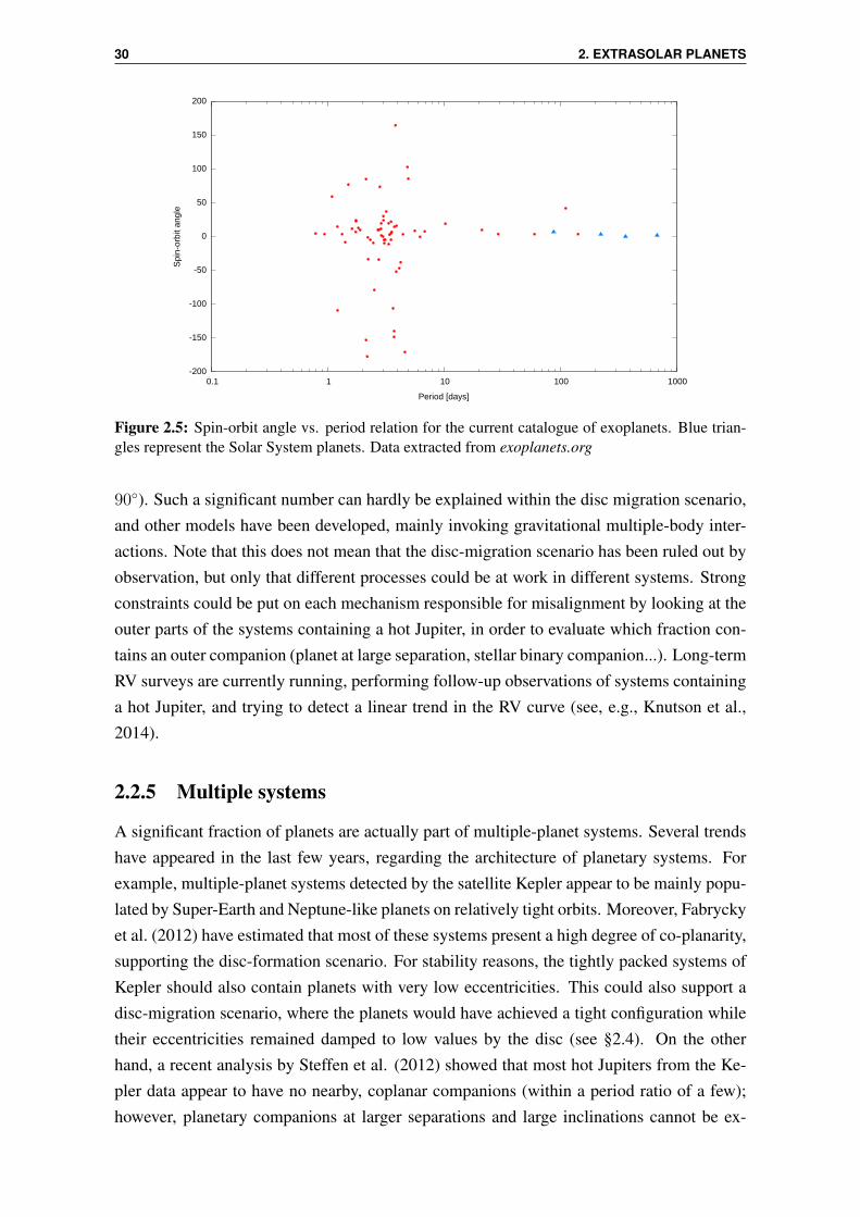
Figure 2.5: Spin-orbit angle vs. period relation for the current catalogue of exoplanets. Blue trian-gles represent the Solar System planets. Data extracted from exoplanets.org
90). Such a significant number can hardly be explained within the disc migration scenario,and other models have been developed, mainly invoking gravitational multiple-body inter-actions. Note that this does not mean that the disc-migration scenario has been ruled out byobservation, but only that different processes could be at work in different systems. Strongconstraints could be put on each mechanism responsible for misalignment by looking at theouter parts of the systems containing a hot Jupiter, in order to evaluate which fraction con-tains an outer companion (planet at large separation, stellar binary companion...). Long-termRV surveys are currently running, performing follow-up observations of systems containinga hot Jupiter, and trying to detect a linear trend in the RV curve (see, e.g., Knutson et al.,2014).
2.2.5 Multiple systems
A significant fraction of planets are actually part of multiple-planet systems. Several trendshave appeared in the last few years, regarding the architecture of planetary systems. Forexample, multiple-planet systems detected by the satellite Kepler appear to be mainly popu-lated by Super-Earth and Neptune-like planets on relatively tight orbits. Moreover, Fabryckyet al. (2012) have estimated that most of these systems present a high degree of co-planarity,supporting the disc-formation scenario. For stability reasons, the tightly packed systems ofKepler should also contain planets with very low eccentricities. This could also support adisc-migration scenario, where the planets would have achieved a tight configuration whiletheir eccentricities remained damped to low values by the disc (see §2.4). On the otherhand, a recent analysis by Steffen et al. (2012) showed that most hot Jupiters from the Ke-pler data appear to have no nearby, coplanar companions (within a period ratio of a few);however, planetary companions at larger separations and large inclinations cannot be ex-

2.2. THE DIVERSITY OF EXOPLANETS 31
cluded (especially since an outer companion with an orbital period ratio of ∼10 and a 60
mutual inclination would have a detection likelihood of less than 5% by transit methods).This suggests a different evolutionary path for hot Jupiters and smaller planets. For instance,independently of the process by which a Jupiter-like planet will migrate, it is likely to scatteraway most planetesimals and small-mass planets.
Although pairs of planets mostly have random orbital period ratios, some of them arelocated near mean motion resonance. For these planets, the ratios seem to have a smallexcess just outside the resonance, and a small deficit just inside. These multiple-planetsystems (mainly consisting of super-Earth and Neptune-like planets) are also more tightlypacked than our own Solar System. Note that the period ratio of two adjacent planets can bequite similar compared to that of the planets in the Solar System, but their physical mutualdistance is much smaller. This requires very low eccentricities in order for the systems toremain stable.
2.2.6 Statistical properties of exoplanets
Combining results from the different detection methods, we are now able to draw a fewconclusions on the content and architecture of planetary systems. More details can be foundin Fischer et al. (2013) and references therein. When considering planets with periods of lessthan 50 days, small planets (Earth to Neptune size) outnumber large ones (gas giants). Forinstance, hot Jupiters are found around only 0.5 to 1% of Sun–like stars, despite the fact thatthey are easy to detect and therefore well characterized. They also tend to be the only planetorbiting their star, within observational limits. On the other hand, RV surveys indicate that15% of Sun-like stars are orbited by planets with projected mass Mp sin io in the range 3−30M⊕ at less than 0.25 AU. The HARPS survey also found that, in total, at least 50% of starscontain a planet at a period of less than 100 days, regardless of the mass of the planet. Resultsfrom the Kepler mission indicate that small-mass planets remain abundant up to periodsof 250 days. 23% of the stars in the Kepler catalogue that contain one transiting planetactually host two or more planets. Hence, although finding an analogue of our Solar Systemremains challenging at the time of writing, mainly because of observational limitations,it makes little doubts now that planetary objects populate a large number of stars in ourGalaxy. The large range of properties and architectures that they already exhibit, and theconstant improvements in observational techniques have challenged, and keeps challenging,our views on planet formation and evolution. In the next section, we review some of themain results in this field.
32 2. EXTRASOLAR PLANETS
2.3 Planet Formation
2.3.1 The protostellar nebulae
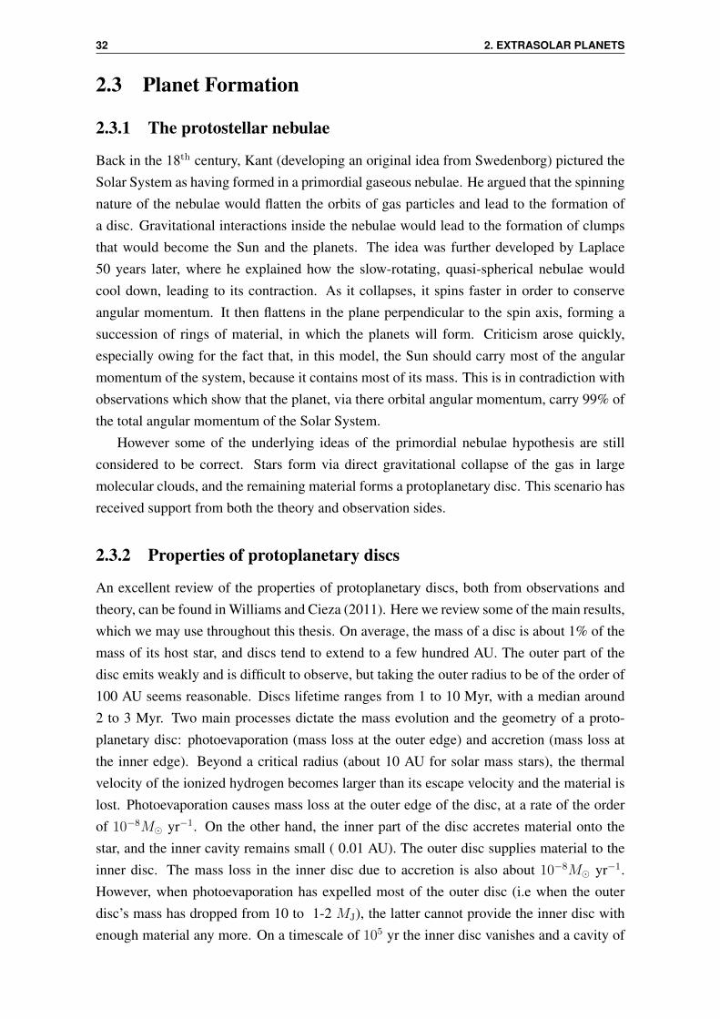
Back in the 18th century, Kant (developing an original idea from Swedenborg) pictured theSolar System as having formed in a primordial gaseous nebulae. He argued that the spinningnature of the nebulae would flatten the orbits of gas particles and lead to the formation ofa disc. Gravitational interactions inside the nebulae would lead to the formation of clumpsthat would become the Sun and the planets. The idea was further developed by Laplace50 years later, where he explained how the slow-rotating, quasi-spherical nebulae wouldcool down, leading to its contraction. As it collapses, it spins faster in order to conserveangular momentum. It then flattens in the plane perpendicular to the spin axis, forming asuccession of rings of material, in which the planets will form. Criticism arose quickly,especially owing for the fact that, in this model, the Sun should carry most of the angularmomentum of the system, because it contains most of its mass. This is in contradiction withobservations which show that the planet, via there orbital angular momentum, carry 99% ofthe total angular momentum of the Solar System.
However some of the underlying ideas of the primordial nebulae hypothesis are stillconsidered to be correct. Stars form via direct gravitational collapse of the gas in largemolecular clouds, and the remaining material forms a protoplanetary disc. This scenario hasreceived support from both the theory and observation sides.
2.3.2 Properties of protoplanetary discs
An excellent review of the properties of protoplanetary discs, both from observations andtheory, can be found in Williams and Cieza (2011). Here we review some of the main results,which we may use throughout this thesis. On average, the mass of a disc is about 1% of themass of its host star, and discs tend to extend to a few hundred AU. The outer part of thedisc emits weakly and is difficult to observe, but taking the outer radius to be of the order of100 AU seems reasonable. Discs lifetime ranges from 1 to 10 Myr, with a median around2 to 3 Myr. Two main processes dictate the mass evolution and the geometry of a proto-planetary disc: photoevaporation (mass loss at the outer edge) and accretion (mass loss atthe inner edge). Beyond a critical radius (about 10 AU for solar mass stars), the thermalvelocity of the ionized hydrogen becomes larger than its escape velocity and the material islost. Photoevaporation causes mass loss at the outer edge of the disc, at a rate of the orderof 10−8M yr−1. On the other hand, the inner part of the disc accretes material onto thestar, and the inner cavity remains small ( 0.01 AU). The outer disc supplies material to theinner disc. The mass loss in the inner disc due to accretion is also about 10−8M yr−1.However, when photoevaporation has expelled most of the outer disc (i.e when the outerdisc’s mass has dropped from 10 to 1-2 MJ), the latter cannot provide the inner disc withenough material any more. On a timescale of 105 yr the inner disc vanishes and a cavity of

2.3. PLANET FORMATION 33
a few AU is formed.
2.3.3 Grains and planetesimals formation
The disc originally contains gas and small grains, of micrometer size. This dust tends tobe slowed down by the gaseous medium as it goes through the equatorial plane of the disc.Overall, it tends to condensate in this plane. The cooling down and condensation of icegrains is only possible at distances larger than the so-called snow line. Inside the snowline, radiation and temperature are too important and prevent condensation of ice to occur(however, heavier elements such as silicates and metals can condensate in the inner parts, butthey are not the dominant elements of the disc’s material). When grains can condensate, theygrow by accumulating more materials, through collisions with each others. On a relativelyshort timescale (a few 103 yr) centimeter to meter-sized particle are formed. The processwhich leads from these grains to kilometer-sized planetesimals remains unclear, and is stillan active domain of research. Because gas drag causes an important orbital decay for meter-sized grains, the process has to occur rather quickly (a meter-sized body at 1 AU would drifttowards the Sun in a few hundred years). Another issue is that an important collision-rate athigh relative velocities would prevent the growth of planetesimals.
2.3.4 Rocky planets formation
When kilometer-sized bodies are formed, they are big enough to become decoupled from thegas. They now have Keplerian speeds around the central star, and their evolution is that of agravitational N -body system (if we neglect the tidal interactions with the gaseous medium;we will review this process later, in the framework of disc migration). Planetesimals eccen-tricities increase as they encounter each others, leading to collisions and agglomerations.It follows that a so-called “runaway accretion” takes place, where the more massive bodyaccrete faster than the less massive ones. These few massive embryos accrete most of thematerial inside their sphere of influence, and reach the state of protoplanets after a few 104
years. This process leaves the system with a small number of rocky cores that interact witheach others. A last phase of merging, from embryos of typical masses of about 10−2 M⊕,to Earth-mass rocky planets, then takes place on a much longer timescale. Some of thesecores will then accrete gas by a process described below in order to form giant planets, ona timescale limited by the disc’s lifetime (∼ 106 yr). After the disc dissipates, collisionsbetween rocky planetesimals continue for a few 108 years.
2.3.5 Giant planets formation
Observations show that the gas in the disc dissipates on a timescale of a few million years.Hence, while rocky planets can keep forming on a much longer timescale via merger ofrocky planetesimals, giant gaseous planets have to form rapidly, as they need to accrete gas

34 2. EXTRASOLAR PLANETS
from the disc. There are currently two main scenarios aiming at explaining the formationof giant planets. The first one is called the “core accretion” model (Pollack et al., 1996). Inthis scenario it is assumed that a solid core of a few Earth masses has formed according tothe scenario described above. In addition to the accretion of planetesimals, the solid corealso gravitationally accretes gas, which forms an atmosphere. At first, the gas accretion israther slow, up to a few million years. However, when the mass of gas contained in theatmosphere becomes comparable to the mass of the solid core (around 10 M⊕), the growthbecomes much quicker, and a Jupiter–mass planet can be formed before the disc dissipates.The growth stops when the planet has accreted all the gas on its orbit. This scenario can alsoexplain Neptune-like planets, who can be described as “failed” giants, whose growth wasstopped by the lack of gas, probably because they started accreting too late and the disc hasbeen dissipated before they could reach a larger size.
The second scenario for forming giant planets is usually referred to as the “gravitationalinstability” scenario (see, e.g., Boss, 1997, and references therein), which is similar to thatenvisioned by Laplace, and that is at work in star formation processes. In this scenario,the disc (or, at an even earlier stage, the protostellar envelop) would start to fragment intodense clumps under gravitational instabilities. The gravitational collapse of these over-denseregions can potentially form giant planets in a few thousand years. However, in its currentform, it suffers several major drawbacks, and remains less commonly accepted than thecore accretion model. First, it requires a massive disc, whose mass would be 10% of thestellar mass. However we saw that the mass of the disc is estimated to be about 1% of thestellar mass. In addition this scenario tends to form massive gaseous planets far from thestar (& 50 AU), and cannot explain Neptune-mass gaseous planets. Finally, it struggles toexplain the lack of heavy elements in the chemical composition of the atmosphere of Jupiterand Saturn.
2.4 Planet migration
As we saw, planets have to form in a region where condensation of the grains is possible(i.e., for giant planets, further than the snow line, located at a few AU from the star), andhave to accrete the gas quickly, in gas-rich regions. In addition, the inner part of the disc(<0.1 AU) has a complicated structure: high temperatures tend to cause evaporation andionization, stellar winds blow away material (making the region rather gas-poor), and thestellar magnetic field is thought to truncate the disc at a distance of a few stellar radii.Hence, the formation of giant, gaseous, planets seems very unlikely so close to the star. Inconsequence, it seems natural to invoke a migration scenario to explain the population ofgiant planets at orbital distances below 0.1 AU (the hot Jupiters population)
2.4. PLANET MIGRATION 35
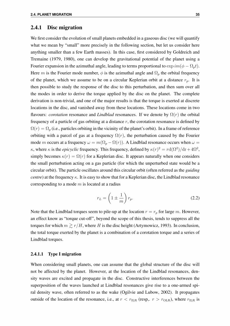
2.4.1 Disc migration
We first consider the evolution of small planets embedded in a gaseous disc (we will quantifywhat we mean by “small” more precisely in the following section, but let us consider hereanything smaller than a few Earth masses). In this case, first considered by Goldreich andTremaine (1979, 1980), one can develop the gravitational potential of the planet using aFourier expansion in the azimuthal angle, leading to terms proportional to exp im(φ− Ωpt).Here m is the Fourier mode number, φ is the azimuthal angle and Ωp the orbital frequencyof the planet, which we assume to be on a circular Keplerian orbit at a distance rp. It isthen possible to study the response of the disc to this perturbation, and then sum over allthe modes in order to derive the torque applied by the disc on the planet. The completederivation is non-trivial, and one of the major results is that the torque is exerted at discretelocations in the disc, and vanished away from these locations. These locations come in twoflavours: corotation resonance and Lindblad resonances. If we denote by Ω(r) the orbitalfrequency of a particle of gas orbiting at a distance r, the corotation resonance is defined byΩ(r) = Ωp (i.e., particles orbiting in the vicinity of the planet’s orbit). In a frame of referenceorbiting with a parcel of gas at a frequency Ω(r), the perturbation caused by the Fouriermode m occurs at a frequency ω = m(Ωp−Ω(r)). A Lindblad resonance occurs when ω =
κ, where κ is the epicyclic frequency. This frequency, defined by κ(r)2 = rd(Ω2)/dr+4Ω2,simply becomes κ(r) = Ω(r) for a Keplerian disc. It appears naturally when one considersthe small perturbation acting on a gas particle (for which the unperturbed state would be acircular orbit). The particle oscillates around this circular orbit (often referred as the guiding
centre) at the frequency κ. It is easy to show that for a Keplerian disc, the Lindblad resonancecorresponding to a mode m is located at a radius
rL =
(1± 1
m
)rp. (2.2)
Note that the Lindblad torques seem to pile-up at the location r = rp for large m. However,an effect know as “torque cut-off”, beyond the scope of this thesis, tends to suppress all thetorques for whichm & r/H , whereH is the disc height (Artymowicz, 1993). In conclusion,the total torque exerted by the planet is a combination of a corotation torque and a series ofLindblad torques.
2.4.1.1 Type I migration
When considering small planets, one can assume that the global structure of the disc willnot be affected by the planet. However, at the location of the Lindblad resonances, den-sity waves are excited and propagate in the disc. Constructive interferences between thesuperposition of the waves launched at Lindblad resonances give rise to a one-armed spi-ral density wave, often referred to as the wake (Ogilvie and Lubow, 2002). It propagatesoutside of the location of the resonance, i.e., at r < rILR (resp,. r > rOLR), where rILR is

36 2. EXTRASOLAR PLANETS
the location of the inner Lindblad resonance (resp., where rOLR is the location of the outerLindblad resonance). Because of the differential rotation, the outer density wave trails be-hind the planet, therefore exerting a negative torque on the planet (and the opposite for theinner density wave). This is illustrated in the left panel of figure 2.6. Ward (1997) showedthat the torque exerted by the outer part of the disc is larger than the inner torque. This isbecause the outer Lindblad resonance is located slightly closer to the planet than the innerone, because of the disc geometry. Therefore, the planet tends to loose angular momentumto the disc and migrate inward. The typical migration timescale, given by Ward (1997) is
tmig ≈ 108
(Mp
M⊕
)−1(Σ
g cm−2
)−1 ( r
AU
)−1/2
× 102
(H
r
)yr, (2.3)
where Σ is the disc’s surface density. Type I migration typically occurs on a timescale of105 years for a 1 M⊕ planet at 1 AU. The torque acting on the planet will also modify itseccentricity. For small eccentricities, the net effect will be a damping of the eccentricity.Papaloizou and Larwood (2000) provide a fit for the migration timescale tmig and the eccen-tricity damping te the 2D case, given by (see also Papaloizou and Terquem, 2010):
tmig = 146.0
[1 +
(e
1.3H/r
)5][
1−(
e
1.1H/r
)4]−1
×(H/r
0.05
)2MMd
M⊕Mp
a
1auyr,
(2.4)
te = 0.362
[1 + 0.25
(e
H/r
)3](
H/r
0.05
)4MMd
M⊕Mp
a
1auyr, (2.5)
where a and e are the semi-major axis and eccentricity of the planet, respectively, and Md
is the disc mass contained within the planetary orbit. These authors also estimated thatthe orbital inclination of the planet should be damped on a timescale ti similar to te. Thedamping timescale is much shorter than the migration timescale, so we can conclude thatlow-mass planets will tend to remain on circular and planar orbits as they migrate.
2.4.1.2 Type II migration
Type I migration causes small planets to migrate inward but leaves most of the disc unaf-fected by the planet’s presence. However we can expect massive planets to affect the gas, atleast in the vicinity of their orbit. When a particle is orbiting inside the orbital radius of theplanet (r < rp), the net effect of the planet will be to speed it up. Thus, angular momentumis transferred from the particle to the planet, and the particle is pushed inward. If one simplyconsiders the impulse received by a particle as it approaches the planet, and the subsequentdeflection, one can deduce that the rate of transfer of angular momentum between the disc’s

2.4. PLANET MIGRATION 37
Figure 2.6: Left panel: a low mass planet embedded in a protoplanetary disc launches a trail-ing spiral wave in the disc. The surface density of the disc is not significantly modified bythe presence of the planet. Right panel: a massive planet has cleared a large gap in the disc,where the surface density is almost zero. In each panel, the bottom left corner shows the sur-face density of the disc. The gap opening is clearly apparent for massive planets. Plot fromhttp://jila.colorado.edu/~pja/planet_migration.html.
particles inside the planetary orbit and the planet is given by:
dJ
dt=
8G2M2prΣ
27Ω2pa
3min
, (2.6)
where amin is the distance of minimal approach between the particles and the planet (Linand Papaloizou, 1979). Note that the sign is positive, leading indeed to the particles beingpushed inward. A similar analysis can be done for the particle exterior to the planet’s orbitalradius (r > rp), with a similar result, except that the sign is opposite. Hence material outsidethe orbit of the planet is pushed outward. In conclusion the planet tends to push the materialaway, and can clear a gap in the disc, where the density drops significantly. However, viscousdiffusion in the disc tends to transport angular momentum, at a rate
dJvisc
dt= 3πνΣr2Ωp (2.7)
where ν is the kinematic viscosity. The viscous timescale associated with this flow of angu-lar momentum is given by
tvisc =r2
ν=
(H
r
)−21
αΩ(2.8)
Here we have assumed that the viscosity follows the model developed by Shakura and Sun-yaev (1973). In this model, viscosity is dominated by turbulence in the gas. The largestturbulence scale should be of the order of disc height H , and propagates with a characteris-tic speed smaller than the sound speed cs = H/Ω. Hence we write ν = αcsH , where α is a

38 2. EXTRASOLAR PLANETS
dimensionless constant parameter, which can be constrained to be in the range 10−3 − 10−2
in order for type II migration to occur within the lifetime of protoplanetary discs.
The net effect of this viscous transport will be to refill the gap. Hence, from theseconsiderations, we can deduce that a gap will open if
dJ
dt>
dJvisc
dt. (2.9)
This condition can be re-written as
Mp
M∗>
40ν
r2Ωp
. (2.10)
For typical disc models, a gap can be opened for planets of the mass of Saturn and higher(see illustration in the right panel of figure 2.6, where a massive planet opens a large gap).
Once the gap is opened, the corotation torque is cancelled due to the lack of materialin the vicinity of the planet, and the total Lindblad torque exerted on the planet is zero,because the latter positions itself at the equilibrium point in the gap where the inner torquecancels the outer one. In the inner parts of the disc, accretion onto the central star causesthe gas to move inward. The planet will simply follow this accretion flow, because thereis still transfer of angular momentum from the inner parts to the outer parts, and migrateinward on the viscous timescale. For a planet starting at 5 to 10 AU, the viscous timescaleis of the order of a few 105 years, and the planet is therefore expected to migrate inwardon a timescale shorter than the disc’s lifetime. It is important to remark the fundamentaldifference between type I and type II migration. In the case of type I migration, low-massplanets migrate in the disc, leaving the latter mostly unaffected. In type II migration, massiveplanets migrate with the disc, and affect its structure by opening a gap. Type II migrationis often invoked to explain the population of hot Jupiters. It is interesting to notice that thisprocess (as well as type I migration), was foreseen long before the detection of the first hotJupiter, mainly by Lin and Papaloizou (1986).
Even if disc-driven eccentricity growth seems possible, in particular for planets of sev-eral Jupiter masses (see, e.g., Papaloizou et al., 2001), in general the outcome of disc–planetinteractions is to damp the eccentricity of the planet (Bitsch and Kley, 2010). Eccentricitydamping is often related to the migration timescale through the following parametrization:
∣∣∣∣e
e
∣∣∣∣ = K
∣∣∣∣a
a
∣∣∣∣ , (2.11)
where K is a dimensionless constant. Numerical investigations find K > 1, with valuespossibly as high as K = 100. Hence, like in the case of type I migration, the eccentricityis damped quicker than the migration timescale. In addition, Bitsch and Kley (2011) findthat the orbital inclination is also damped on a timescale that is shorter than the migrationtimescale, for moderate inclinations (of the order of the disc aspect ratio). The evolution of

2.4. PLANET MIGRATION 39
eccentricity and inclination for planets with large initial inclinations is studied in detail inTeyssandier et al. (2013b), which is the subject of Chapter 4 of this thesis.
If hot Jupiters are really the result of type II migration, then it requires that the migra-tion stops before the planet falls into the star. Several mechanisms have been proposed inorder to stop type II migration. For instance, it is likely that the disc is truncated at a fewstellar radii because of the stellar magnetic field (Bouvier et al., 2007). In addition, Terquem(2003) argued that the presence of a magnetic field in the disc could change the total torqueand slow down the migration. Trilling et al. (1998) suggested that a planet affected by tidesfrom the star would overflow its Roche lobe and transfer part of its mass to the star. Con-servation of angular momentum would then cause the planet to move away from the star.It is also thought that the first generation of planets would eventually merge with their star,and only planets that have been formed later could survive, because of the subsequent lackof material in the disc. One should also keep in mind that we have studied the migrationof a single planet in a disc. However, observations support the idea of multiple-planet sys-tems. Mutual interactions between migrating planets could affect the migration. One aspectof the mutual interaction between two migrating planets is the possibility of mean motionresonance locking. This effect and its consequences on the eccentricities and inclinationsare studied by Teyssandier and Terquem (2014), presented in Chapter 5.
2.4.1.3 Type III migration
So far we have mostly neglected the corotation torque: For type I migration, the main con-tribution to the total torque comes from the Lindblad torque, and for type II migration, theplanet has opened a gap and cleared all the material that could give rise to a corotationtorque.
Material that is in corotation with the planet exhibits so-called horseshoe orbits (as seenfrom a reference frame rotating with the planet, see illustration in figure 2.7), which corre-sponds to libration around the Lagrange equilibrium points L4 and L5. Particles originallylocated at a distance rp + δr experience a U-turn in the vicinity of the planet, which bringsthem to a distance rp − δr. By doing so, they loose angular momentum, which is commu-nicated to the planet. Symmetrically, particles originally located at a distance rp − δr takeangular momentum away from the planet. By symmetry, the net effect should be zero.
As we saw, low-mass planets do not clear a gap, contrary to massive planets. The tran-sition occurs for Saturn-mass planets. Such planets are expected to clear only a partial gap,and material will keep flowing through the orbit, passing by the corotation radius, and there-fore exerting a strong corotation torque. Masset and Papaloizou (2003) were the first tostudy this effect. As the planet migrates inward, material from the inner disc get trappedin the horseshoe streamline and goes to the outer disc. In doing so, they remove angularmomentum from the planet. On the other hand, as the material is trapped in the corota-tion region, it drifts inward with the planet, loosing angular momentum. The two effects

40 2. EXTRASOLAR PLANETS
Figure 2.7: Different trajectories of gas particles as seen in a frame of reference where the planet(represented by the black dot) remains fixed. Particles trapped in horseshoe trajectories make a U-turn in the vicinity of the planet. Figure extracted from Kley and Nelson (2012)
do not cancel out, and give rise to a net torque which acts to assist the migration. This iswhy this effect is often referred to as runaway migration. This process is likely to occur forSaturn-mass planets embedded in massive discs, and causes migration on the timescale of afew hundred orbits. Note that if the planet was originally migrating outward, the net torquewould again act to assist outward migration.
2.4.2 Migration via scattering of planetesimals
In our Solar System, the existence of the Kuiper Belt and the Oort cloud provide evidencesthat planetesimals have been gravitationally scattered by the giant planets. For instance onecould imagine that Neptune, as the outermost planet, perturbs some planetesimals and in-creases their eccentricities. Their small perihelion brings them closer to second outermostplanet (Uranus), which then dominates their evolution. Because the planetesimal migratedinward, Neptune had to migrate outward. The process is likely to continue until Jupiterfinally sends the planetesimals into almost parabolic orbits, hence creating the Oort cloud.Because of its high mass, Jupiter would be only weakly affected, while Neptune could mi-grate outward by a few AU. By doing so, it can enter a mean-motion resonance with someplanetesimals, as observed in the Kuiper Belt (e.g., the 3:2 resonance with Pluto) and excitetheir eccentricities (also an observational fact in the Kuiper Belt). Note that in this scenario,Saturn, Uranus and Neptune would migrate outward as they send the planetesimals to theinner parts of the system, while Jupiter would (slightly) migrate inward as it sends them tothe Oort Cloud. This scenario (see, e.g., Fernandez and Ip, 1984; Hahn and Malhotra, 1999)is one of the underlying ideas behind the so-called Nice model (Morbidelli et al., 2007),

2.4. PLANET MIGRATION 41
which aims to explain the formation of the Solar System. More generally, Levison et al.(2007) found that when two planets interact with a disc of planetesimals, the inner one islikely to migrate inward while the outer one would migrate outward.
2.4.3 High-eccentricity induced migration
There exists an alternative theory for planet migration, which does not rely on disc-planetinteractions. The underlying idea behind this mechanism would be as follows: Once thedisc has been swept out, only the planets (and some planetesimals, which we ignore here)would remain. Therefore the dynamical evolution of the system is dominated by planet–planet gravitational interactions. If such interactions could excite the eccentricity of one ofthe planet to large values, the perihelion of this planet would be located very close to thestar. At each perihelion passage, the planet would loose orbital energy to the star, becauseof tidal interactions. As a result, it would circularize at a short period, possibly forming ahot Jupiter. The ways the eccentricity of a planet can be pumped up to high values come indifferent flavours, which we briefly review here.
2.4.3.1 Orbital relaxation
Papaloizou and Terquem (2001) considered a scenario in which a large number of giant plan-ets (several Jupiter masses) rapidly form through the fragmentation of a thick protoplanetarydisc or a protostellar envelope (due to gravitational instabilities), and start interacting witheach other, leading to rapid dynamical relaxation on a timescale of a few hundred orbits.They found that, almost independently of the initial number of planet (between 5 and 100),most objects escape, and only 2 or 3 planets remain bound to the star, with various eccentrici-ties and inclinations. Interestingly, the innermost planet often undergoes tidal circularizationand ends up having a short period. Such scenario could then account for the eccentric plan-ets, as well as some of the hot Jupiters. Terquem and Papaloizou (2002) refined the scenarioby including low-mass, inner planets. Such planets were assumed to have formed via thecore accretion model, and remain tidally bound to the disc, before being perturbed by theouter, dynamically relaxed, planets, leading again to eccentric, close-in planets. Adams andLaughlin (2003) considered a similar scenario and focused on the statistical outcome of alarge number of simulations of dynamical relaxations. They found that it is difficult to ex-actly reproduce the distribution of short–period planets, because in order for the planet tomove inward (losing orbital energy), it requires to scatter away a large number of low-massobjects (hence increasing their orbital energy).
2.4.3.2 Planet–planet scattering
Shortly after the discovery of the planet around 51 Peg, Rasio and Ford (1996) and Wei-denschilling and Marzari (1996) proposed the following mechanism to explain this unusual

42 2. EXTRASOLAR PLANETS
discovery: shortly after the protoplanetary disc dissipates, the system is left with severalplanets in a tight configuration. Because the disc is not here any more to damp the eccen-tricities and inclinations, the planets now interact freely one with each other. In some case,this leads to strong gravitational interactions, where the semi-major axis, eccentricities andinclinations of the planets change dramatically on a short timescale. The outcome is quitesimilar to that of orbital relaxation, with most planets being expelled from the system, andonly a few left on eccentric and inclined orbits. This scenario also struggles to explain alonesome of the observed properties of extrasolar planets (see, e.g., Davies et al., 2013, andreferences therein)
2.4.3.3 Secular chaos
Wu and Lithwick (2011) proposed an alternative scenario for the formation of hot Jupiters.They set up a system of 3 massive planets, where the outer planet is the most massive andmost eccentric. On a secular timescale, much longer than that of planet–planet scattering,the outer planet chaotically diffuses its eccentricity and inclination to the inner parts of thesystem. The innermost planet eventually reaches a quasi-parabolic orbit and is subsequentlytidally locked to the star, at large inclination. Note that the initial conditions required forsuch mechanism to occur could be the result of an early phase of planet–planet scattering.The diffusion of eccentricity from outer, massive, planets, to inner, less massive ones, couldaslo explain why Mercury has the highest eccentricity of all the planets in the Solar System(Lithwick and Wu, 2011)
2.4.3.4 The Kozai mechanism
The Kozai mechanism (Kozai, 1962; Lidov, 1962) will be studied in details in the next chap-ter. In this scenario, an inner planet is perturbed by an outer, far-away, more massive body,such as a planet, a brown-dwarf, or a star. If the inclination between the two orbits is largerthan a critical value (∼ 40), the inner planet reaches very high eccentricities and can eventu-ally be tidally circularized to its host star. Naoz et al. (2011) showed that when the perturberis on an eccentric orbit, the inner planet can naturally flip from prograde to retrograde or-bits, which could naturally account for some of the highly misaligned hot Jupiters. Becausea significant number of stars are thought to be part of binary systems, a stellar companioncould naturally raise Kozai oscillations on a planet (see, e.g., Fabrycky and Tremaine, 2007).However this mechanism could be killed by the presence of additional planets in the system.Teyssandier et al. (2013a) showed that a planetary companion, at orbital distances rangingfrom 50 to 150 AU, eccentricities between 0.25 and 0.7 and a mass larger than 2 MJ coulddrive an inner Jupiter-mass planet at 5 AU from a circular to a quasi-parabolic orbit, wheretidal circularization at periastron could take place.

Chapter 3
Basics of celestial mechanics
Contents3.1 The two-body problem . . . . . . . . . . . . . . . . . . . . . . . . . . 43
3.1.1 The planar case . . . . . . . . . . . . . . . . . . . . . . . . . . . 43
3.1.2 Three-dimensional orbit . . . . . . . . . . . . . . . . . . . . . . 46
3.2 Perturbation theory . . . . . . . . . . . . . . . . . . . . . . . . . . . . 47
3.2.1 Keplerian orbits perturbed by an extra force . . . . . . . . . . . . 48
3.2.2 The disturbing function and Lagrange’s equations . . . . . . . . . 49
3.2.3 Laplace-Lagrange theory of secular perturbations . . . . . . . . . 50
3.2.4 Hierarchical systems and the Kozai mechanism . . . . . . . . . . 52
3.2.5 Resonant perturbations . . . . . . . . . . . . . . . . . . . . . . . 57
3.2.6 Post-Newtonian perturbations . . . . . . . . . . . . . . . . . . . 60
3.1 The two-body problem
In this thesis we are interested in the orbital evolution of planetary systems. In this sec-tion we recall some of the main results of celestial mechanics that we will use throughoutthis work. First, we quickly present the point mass two-body problem, which allows usto introduce our notations. This introduction roughly follows that of Murray and Dermott(1999)
3.1.1 The planar case
We consider the evolution of two point mass of mass m1 et m2, for which the positions withrespect to an originO are respectively given by the vectors r1 and r2. Similarly we can studythe motion ofm2 with respect tom1. The relative position vector r is defined by r = r2−r1.
43

44 3. BASICS OF CELESTIAL MECHANICS
The motion of r with time is the solution of the following equation:
d2rdt2
= −µ rr3, (3.1)
where µ = G(m1 + m2), with G the gravitational constant. It is straightforward to showthat the quantity h ≡ r × r is a constant of the motion, because of the radial nature of theforce involved in equation (3.1). Therefore the motion is restricted to the plan defined by thevectors r and r. In a polar coordinate system where the vector r is given by the coordinates(r, θ), we get that the norm of h is h = r2θ, which is a constant of motion.
The solution of equation (3.1) is well known: it is a conic of equation:
r =h2/µ
1 + Ah2
µcos(θ − θ0)
. (3.2)
Here, A et θ0 are two constants of integration. We can define the conic parameter p byp = h2/µ, and the eccentricity by e = Ah2/µ. We also define the true anomalyf byf = θ − θ0. Hence:
r =p
1 + e cos f. (3.3)
The nature of the trajectory will depend on the value of e. Indeed the total energy of thesystem E, divided by the reduced mass, takes the form:
E =1
2
(drdt
)2
− µ
r. (3.4)
The total energy is then:E = − µ
2p(1− e2). (3.5)
We will focus on closed trajectories only (negative total energy), i.e, solutions for which e ∈[0; 1[. The trajectory is an ellipse (or a circle if e = 0) of semi-major axis a = (1/2)(rmax +
rmin), where rmax and rmin are the values of r for which f = π and f = 0 respectively. Itfollows that a = p/(1− e2). rmin = a(1− e) is called the pericenter, while rmax = a(1 + e)
is the apocenter. We indicate them respectively by P and Q on figure 3.1 We note that thetotal energy is now simply:
E = − µ
2a. (3.6)
During an infinitesimal increment along the ellipse, the area swept out by the orbitalradius vector is dA = 1
2r2dθ. This leads to the so-called Kepler’s second law:
dA
dt=
1
2h. (3.7)
Because h is constant, equal areas are swept out in equal times. If we define T as theorbital period, we find that the total area of the ellipse is A = hT/2. Geometrically, the area
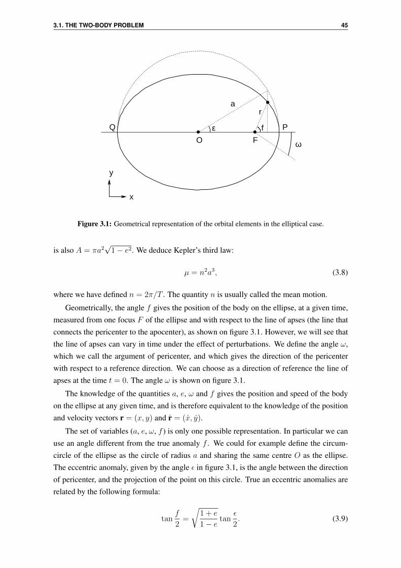
3.1. THE TWO-BODY PROBLEM 45
O F
fε
ra
ω
x
y
PQ
Figure 3.1: Geometrical representation of the orbital elements in the elliptical case.
is also A = πa2√
1− e2. We deduce Kepler’s third law:
µ = n2a3, (3.8)
where we have defined n = 2π/T . The quantity n is usually called the mean motion.
Geometrically, the angle f gives the position of the body on the ellipse, at a given time,measured from one focus F of the ellipse and with respect to the line of apses (the line thatconnects the pericenter to the apocenter), as shown on figure 3.1. However, we will see thatthe line of apses can vary in time under the effect of perturbations. We define the angle ω,which we call the argument of pericenter, and which gives the direction of the pericenterwith respect to a reference direction. We can choose as a direction of reference the line ofapses at the time t = 0. The angle ω is shown on figure 3.1.
The knowledge of the quantities a, e, ω and f gives the position and speed of the bodyon the ellipse at any given time, and is therefore equivalent to the knowledge of the positionand velocity vectors r = (x, y) and r = (x, y).
The set of variables (a, e, ω, f ) is only one possible representation. In particular we canuse an angle different from the true anomaly f . We could for example define the circum-circle of the ellipse as the circle of radius a and sharing the same centre O as the ellipse.The eccentric anomaly, given by the angle ε in figure 3.1, is the angle between the directionof pericenter, and the projection of the point on this circle. True an eccentric anomalies arerelated by the following formula:
tanf
2=
√1 + e
1− etan
ε
2. (3.9)

46 3. BASICS OF CELESTIAL MECHANICS
We also have the useful relation:
r = a(1− e cos ε). (3.10)
Note that, while the set of variables (a, e, ω, f ) can give the position of the body on theellipse, the time variable does not explicitly appear in the equations of motion. In celestialmechanics it is common to replace the time variable by a dimensionless variable called themean anomaly, noted M and defined by:
M = n(t− t0). (3.11)
Here t0 is the time of passage at pericenter. This variable does not have a simple geometricalinterpretation, but has the dimension of an angle and is an increasing linear function of time.It is related to the eccentric anomaly through Kepler’s equation:
M = ε− e sin ε. (3.12)
This equation is fundamental as it gives the position of the body on the ellipse (given by ε)as a function of time (given by M ).
Finally we give some useful relations. Differentiating Kepler’s equation, we get
dM = (1− e cos ε)dε. (3.13)
Then, it can be shown that :
dM =(1− e2)3/2
(1 + e cos f)2df. (3.14)
These relations will prove useful every time we wish to average a quantity over its orbitalperiod.
3.1.2 Three-dimensional orbit
We saw that the two-body problem for mass point objects is a planar problem, and it wastherefore natural to choose a coordinate system in which the vertical component z and theassociated velocity z are thoroughly zero. The motion is characterized by a, e, ω and f .In space, the motion needs to be characterized by two additional variable. The set of sixvariable will be equivalent to the six Cartesian components that form the position and ve-locity vectors. First we can define the inclination I between the plane of the orbit and aplane of reference. Then we define the longitude of ascending node Ω as the angle betweenthe intersection of the orbital plane and the plane of reference, with respect to a referencedirection (see figure 3.2). In space, we define the longitude of pericenter $ as $ = Ω + ω,even though the angles ω and Ω do not lie in the same plane. We can also define the meanlongitude λ as λ = M+$. The set of variables a, e, I, $, Ω and λ allows us to characterize
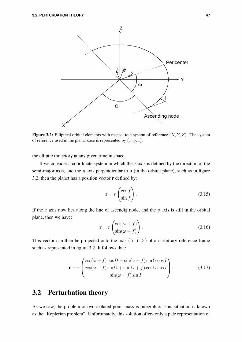
3.2. PERTURBATION THEORY 47
ω
Ω
I
X
Y
Z
xyz
Pericenter
Ascending node
Figure 3.2: Elliptical orbital elements with respect to a system of reference (X,Y, Z). The systemof reference used in the planar case is represented by (x, y, z).
the elliptic trajectory at any given time in space.
If we consider a coordinate system in which the x axis is defined by the direction of thesemi-major axis, and the y axis perpendicular to it (in the orbital plane), such as in figure3.2, then the planet has a position vector r defined by:
r = r
(cos f
sin f
). (3.15)
If the x axis now lies along the line of ascendig node, and the y axis is still in the orbitalplane, then we have:
r = r
(cos(ω + f)
sin(ω + f)
). (3.16)
This vector can then be projected onto the axis (X, Y, Z) of an arbitrary reference framesuch as represented in figure 3.2. It follows that:
r = r
cos(ω + f) cos Ω− sin(ω + f) sin Ω cos I
cos(ω + f) sin Ω + sin(Ω + f) cos Ω cos I
sin(ω + f) sin I
. (3.17)
3.2 Perturbation theory
As we saw, the problem of two isolated point mass is integrable. This situation is knownas the “Keplerian problem”. Unfortunately, this solution offers only a pale representation of

48 3. BASICS OF CELESTIAL MECHANICS
the dynamics of celestial bodies. When studying, for example, the long term evolution of thesolar system, it is necessary to take into account (at least) the mutual interactions betweenthe 8 planets, in addition to their Keplerian motion around the Sun. Furthermore, if one triesto correctly model the motion of an artificial satellite around the Earth, the latter cannot beconsidered as a point mass: its deviation from a perfect sphere has to be taken into account,in order to correctly model its gravitational field. Unfortunately, the general N -body prob-lem does not offer simple solutions. This is why the main effort of celestial mechanics inthe last centuries has been to focus on so-called “perturbed” solutions. Starting from an in-tegrable problem, for instance the Keplerian motion of a planet around a star, we add a smallperturbation, arising for instance from an external planet. By modelling the perturbation asa small deviation from the integrable problem, we will try to seek approximate solutions.
3.2.1 Keplerian orbits perturbed by an extra force
We wish to know how an orbit changes when a small extra force is acting on it. FollowingBurns (1976) we start with the equation of motion
d2rdt2
= −µ rr3, (3.18)
and add a little perturbation in the form of a small force dF. We write dF = ReR + T eT +
NeN where eR pointing radially outwards, eT is orthogonal to eR, lying in the orbital planeand positive in the direction of the motion, and eN normal to the orbital plane such as thethree vectors form a direct set of unit base vectors. The variation of energy E = −µ/2a andangular momentum H = r2θeN (per unit of mass) is given by:
dE
dt= r.dF, (3.19)
dH
dt= r× dF. (3.20)
It follows that the orbital energy E varies as:
dE
dt=
õ
a(1− e2)[Re sin f + T (1 + e cos f)] , (3.21)
The angular momentum H changes as H = rT eN − rNeT . Since H lies along ez, the rNcomponent changes its direction, and the change of magnitude is H = rT . Hence:
dH
dt=
a(1− e2)
1 + e cos fT (3.22)

3.2. PERTURBATION THEORY 49
It follows that the six orbital elements can be written as a function of the components R, Tand N . We give here the equations for a, e, I and ω:
da
dt= 2
√a3
µ(1− e2)[Re sin f + T (1 + e cos f)] , (3.23)
de
dt=
√a
µ(1− e2) [R sin f + T (cos f + cos ε)] , (3.24)
dI
dt=rN cos(ω + f)
H, (3.25)
dω
dt=
1
e
√a(1− e2)
µ[−R cos f + T sin f(2 + e cos f)]− Ω cos I. (3.26)
Equations (3.23)–(3.26) will prove very useful when dealing with dissipative forces. How-ever, in the case of the point mass three-body problem, an other set of equations is prefered,which we present now.
3.2.2 The disturbing function and Lagrange’s equations
Let us consider the motion of two planets around a central star. For j = 1, 2, we note rjthe position vector between the planet j (mass mj) and the central star of mass M . Theequations of motion for planet 1 and 2 take the form;
d2r1
dt2+G(M +m1)
r1
r31
= Gm2
(r2 − r1
|r2 − r1|3− r2
r32
), (3.27)
d2r2
dt2+G(M +m2)
r2
r32
= Gm1
(r1 − r2
|r1 − r2|3− r1
r31
). (3.28)
The right-hand side of equation (3.27) (resp., equation [3.28]) derives from a potentialR1 (resp. R2), with:
R1 = Gm2
(1
|r2 − r1|− r1.r2
r32
), (3.29)
R2 = Gm1
(1
|r1 − r2|− r1.r2
r31
). (3.30)
If Ψ is the angle between r1 and r2, it is well-known that the quantity |r2 − r1|−1 can bewritten in term of the Legendre polynonials Pl:
1
|r2 − r1|=
1
r2
∞∑
l=0
(r1
r2
)lPl(cos Ψ). (3.31)
Similarly, the term involving r1.r2 is also a function of Ψ. Using these developments,considerable efforts have been put to express the disturbing function using orbital elementsonly. We will skip the details, but it has been shown that the disturbing function can take the

50 3. BASICS OF CELESTIAL MECHANICS
very general form (Murray and Dermott, 1999)
R1 = Gm2
∑
j1,...,j6
f(α)
a2
e|j3|1 e
|j4|2 s
|j5|1 s
|j6|2 cos(j1λ1+j2λ2+j3$1+j4$2+j5Ω1+j6Ω2) (3.32)
and a similar form forR2. Here α = a1/a2 and f(α) is a function of the Laplace coefficients(see appendix §A). We also have introduce the notation sk = sin(Ik/2) for k = 1, 2.Summation is made over the six integers j’, which obey the d’Alembert relation:
6∑
i=1
ji = 0, (3.33)
coming from the fact that the disturbing function has to remain invariant under global rota-tion.
In order to conveniently use the disturbing function, one needs to know the variationof the orbital elements under the action of the disturbing function. We shall go straight toresult, which is referred to as the Lagrange’s planetary equations:
da
dt=
2
na
∂R
∂λ, (3.34)
de
dt= −√
1− e2
na2e
∂R
∂$− e
√1− e2
na2(1 +√
1− e2)
∂R
∂λ, (3.35)
dI
dt= − 1
na2√
1− e2 sin I
∂R
∂Ω− tan(I/2)
na2√
1− e2
(∂R
∂$+∂R
∂λ
), (3.36)
d$
dt=
√1− e2
na2e
∂R
∂e+
tan(I/2)
na2√
1− e2
∂R
∂I, (3.37)
dΩ
dt=
1
na2√
1− e2 sin I
∂R
∂I, (3.38)
dλ
dt= n− 2
na
∂R
∂a+
e√
1− e2
na2(1 +√
1− e2)
∂R
∂e+
tan I/2
na2√
1− e2
∂R
∂I. (3.39)
Note that these equations can be used with any disturbing function, not only with that arisingfrom the three-body problem. A complete derivation of these equations can be found, e.g.,in Brouwer and Clemence (1961).
3.2.3 Laplace-Lagrange theory of secular perturbations
We consider the evolution of two planets of mass m1 and m2 orbiting a central star of massm0 (m0 m1 and m0 m2) and we only take into account the secular interactionsbetween the two planets.
We follow Murray & Dermott (1999): for j = 1, 2, let aj , ej , Ij , nj , $j and Ωj be thesemi-major axis, eccentricity, inclination, mean motion, longitude of pericenter and longi-

3.2. PERTURBATION THEORY 51
tude of ascending node of planet j, respectively. Let also Rj be the disturbing function ofplanet j, in this case the secular perturbation from planet k = 1, 2, k 6= j. To second orderin inclinations and eccentricities we have
Rj = nja2j
[1
2Ajje
2j + Ajke1e2 cos($1 −$2)
+1
2BjjI
2j +BjkI1I2 cos(Ω1 − Ω2)
] (3.40)
where the A’s and B’s are functions of the Laplace coefficients (see appendix A)
Because we are only interested in the secular variations of the system, we have averagedout to zero all the terms containing the mean longitudes λ. Therefore, given the Lagrange’sequations, the semi-major axis remain constant throughout secular evolution. We have onlykept the lowest order terms in eccentricities and inclinations, and the disturbing functionbecomes fully decoupled: the variations of the (e;$) variables is independent from the vari-ation of the (I; Ω) variables. The problem reduces to that of finding two sets of eigenvaluesand eigenfrequencies. The general solution reads, for planet j:
ej sin$j =2∑
k=1
ejk sin(gkt+ βk), ej cos$j =2∑
k=1
ejk cos(gkt+ βk), (3.41)
and
Ij sin Ωj =2∑
k=1
Ijk sin(fkt+ γk), Ij cos Ωj =2∑
k=1
Ijk cos(fkt+ γk). (3.42)
The ejk and Ijk are components of the kth eigenvector, and the gk and fk the correspondingeigenvalues. The phases βk and γk, as well as the amplitude of the eigenvectors, are givenby the initial conditions. Note that in the case of the inclination vectors, one eigenfrequencyis zero, owing for the conservation of total angular momentum. Note also that the formulasabove can be generalized to N planets.
The eccentricities and inclinations of each planet vary sinusoidally with time, and thelongitudes of pericenters and ascending nodes precess on timescales of order g−1
k and f−1k ,
respectively. A secular resonance arises when two secular frequencies match each other,or are equal to a precession frequency induced by another mechanism (e.g., the precessioninduced by the oblateness of the central star).
This theory applied well in the early studies of the Solar System, where the major plan-ets have moderate eccentricities and inclinations, and are not locked into any first-ordermean-motion resonances. The simple, long-term, exchange of angular momentum whicharise from this theory let astronomers to believe that the Solar System could be long-termstable. In extrasolar planetary systems, however, planets can have large eccentricities and/orinclinations, and be very close to mean-motion resonances, making this theory poorly ap-

52 3. BASICS OF CELESTIAL MECHANICS
plicable. However the precession timescales are very useful, as they can be compared toother timescales arising from other kind of perturbations. Such first-order analysis can givea quick glance at which mechanism is going to dominate the evolution of the system.
3.2.4 Hierarchical systems and the Kozai mechanism
Here we review another example of secular interaction that does not fit in the frameworkof the Laplace-Lagrange theory. We wish to study a system in which a tight binary (e.g., aplanet of mass m1 around a star of mass m0) is orbited by an outer, far-away, companion(e.g., a planet of mass m2), such as the ratio of semi-major axis remains small (a1/a2 1). Such system is called hierarchical. Once again we will average out over the orbitalperiods, in order to focus on the secular evolution only. However, the system studied herepresents a major difference with the Laplace-Lagrange theory. Here we restrict ourselvesto the case a1/a2 1 but we have no restrictions on the values which can be taken bythe eccentricities and inclinations. In the Laplace-Lagrange theory, the expansion would bevalid for any a1/a2 (as long as it is not located on a low-order MMR) but would be valid forsmall eccentricities and inclinations only.
Perturbation theory in the framework of hierarchical systems is discussed in Valtonenand Karttunen (2006), and some applications can be found in Innanen et al. (1997). Let usconsider the case where m1 m2, therefore the disturbing function that is of interest for usis:
R = Gm2
(1
|r2 − r1|− r1.r2
r32
). (3.43)
We note ψ the angle between r1 and r2. The quantity |r2 − r1|−1 can be expanded tosecond order in r1/r2 to give
1
|r2 − r1|=
1
r2
[1 +
r1
r2
cosψ − 1
2
(r1
r2
)2 (1− 3 cos2 ψ
)]. (3.44)
It follows that:
R =Gm2
r2
[1− 1
2
(r1
r2
)2 (1− 3 cos2 ψ
)]. (3.45)
In order to study the secular interaction between the two planets, we have to average thedisturbing function R over the orbital period of the two planets, in order to get the seculardisturbing functionRsec:
Rsec =
∫ 2π
0
∫ 2π
0
RdM1dM2.
First of all we need to expressR as a function of the orbital elements of the two planets.

3.2. PERTURBATION THEORY 53
We can use eq. (3.17) to calculate the term cosψ = r1.r2/(r1r2). We obtain:
cosψ = (cosω1 cosω2 + sinω1 sinω2 cos I1 cos I2) cos(Ω1 − Ω2)
+ (cosω1 sinω2 cos I2 − sinω1 cosω2 cos I1) sin(Ω1 − Ω2) (3.46)
+ sinω1 sinω2 sin I1 sin I2.
We can choose a plane of reference (X, Y, Z) such as Z is aligned with the (constant) totalangular momentum of the system (in this case, the sum of the orbital angular momentum ofthe two planets), and X and Y lie in the plane perpendicular to this axis. Conservation ofangular momentum imposes Ω2 − Ω1 = π, such as
cosψ = −(cosω1 cosω2 + sinω1 sinω2 cos I1 cos I2) + sinω1 sinω2 sin I1 sin I2. (3.47)
In addition we have assumed that m1 m2 and a1 a2. Thus m2 carries most of theangular momentum of the system, and we have sin I2 ' 0. Finally we get
cosψ = −(cosω1 cosω2 + sinω1 sinω2 cos I1) (3.48)
Using equations (3.3), (3.14) and (3.48) we can carry the integration over the outer orbit’speriod. After some tedious algebra, or making use of a symbolic computational software likeMathematica we get:
1
2π
∫ 2π
0
RdM2 =Gm2
a2
[1 +
(r1
a2
)21 + 3 cos(2I1) + 6 cos 2(ω1 + f1) sin2 I1
16 (1− e22)
3/2
](3.49)
Because the semi-major axis are constant in the secular approximation, we can drop theadditive term Gm2/a2, and carry the integration over the inner orbit’s period to get:
Rsec =Gm2a
21
32a32(1 + e2
2)3/2
[(2 + 3e2
1)(1 + 3 cos(2I1)) + 30e21 cos(2ω1) sin2 I1
]. (3.50)
which we can re-write, using trigonometric formulas:
Rsec =Gm2a
21
8a32(1 + e2
2)3/2
[2 + 3e2
1 − 3 sin2 I1(1− e21 + 5e2
1 sin2 ω1)]. (3.51)
In this disturbing function, the orbital elements of the perturbing body appear only in theoverall multiplicative factor. Therefore they will only change the timescale on which the in-teractions take place. Because we have averaged over the orbital periods, we have eliminatedall short-term interactions in the disturbing function (3.51).
Using eq. (3.51), Lagrange planetary equations for the secular problem give:

54 3. BASICS OF CELESTIAL MECHANICS
dIdτ
= −15
8
e2
√1− e2
sin 2ω sin I cos I,
dedτ
=15
8e√
1− e2 sin 2ω sin2 I,
dωdτ
=3
4
1√1− e2
[2(1− e2) + 5 sin2 ω(e2 − sin2 I)
].
(3.52)
where we have dropped the subscript “1” for the inner planet, and where we have defined adimentionless time parameter τ as
τ =Gm2
a32(1− e2
2)3/2nt.
We assume that the inner eccentricity is initially small, so that we can neglect all the termsin e2:
dIdτ
= 0,
dedτ
=15
8e sin 2ω sin2 I,
dωdτ
=3
4
[2− 5 sin2 ω sin2 I)
].
(3.53)
Since dI/dτ = 0, we can define a new constant quantity A by
A = 5 sin2 I − 2.
In appendix B, we show that the equation dω/dτ = a+ b sin2 ω can be solved to give
ω =
arctan[√
2A
e32
√2Aτ+1
e32
√2Aτ−1
]if I > 39.23
arctan[√
2−A tan
(34
√−2Aτ
)]if I < 39.23.
(3.54)
We now study the behavior of this solution, depending whether I < 39.23 or I >
39.23.
Case I < 39.23
We first consider the case I < 39.23, the solution for ω is
tanω = tan
[√2
−Atan
(3
4
√−2Aτ
)].
Therefore ω periodically circulates. As I is constant, the Lagrange equation for e takes theform
dee
= C sin(2ω)dω
3.2. PERTURBATION THEORY 55
where C is a constant. The solution for e will take the form
e = e0 exp
[−C
2cos 2ω
].
and therefore e will remain bounded around its initial small value.
Case I > 39.23
We now consider the case I > 39.23. When looking at the secular evolution of the system,we consider timescales much larger than the orbital period, i.e. t T . Therefore we canuse the approximation e
32
√2Aτ+1
e32
√2Aτ−1
' 1. With this approximation, ω becomes a constant and
therefore dωdτ = 0. Given the Lagrange planetary equation for ω we deduce
5 sin2 ω sin2 I = 2
Hence the Lagrange equation for e is:
dedτ
=15
4e
√2
5
(sin2 I − 2
5
). (3.55)
Note that there is also a negative solution if cosω and sinω are of opposite signs. Noting e0
the initial (small) eccentricity, this equation is easily integrated to give
e(t) = e0 exp15
4
√2
5
(sin2 I − 2
5
)τ . (3.56)
Therefore the growth of e from e0 is exponential. Very quickly the approximation statingthat I is constant is not valid anymore. However, as e increases, the quantity
√1− e2 cos I (3.57)
has to remain constant. It can be seen from calculating ddt
√1− e2 cos I using Eq.(3.34). This
quantity is sometimes referred to as the Kozai integrale. Physically it is the dimensionlessz-component of the angular momentum of the inner orbit. Equation (3.57) clearly indicatesthat when e is maximum, I is minimum and vice-versa. We saw that the minimum of Ioccurs for sin2 I = 2/5, therefore cos I =
√3/5. At this point the eccentricity reaches its
maximal value emax: √1− e2
0 cos I0 =√
1− e2max
√3
5
where I0 is the initial inclination. Therefore, recalling that e0 is very small, one gets
emax =
√1− 5
3cos2 I0 (3.58)

56 3. BASICS OF CELESTIAL MECHANICS
After reaching its maximum, e will decrease until it reaches e0, and so on. Meanwhile,I will vary accordingly, in order to keep
√1− e2 cos I constant. This long-term periodic
variations are call Kozai cycles. On figure 3.3 we show an example of such cycles. We carryout the numerical integration of equations (3.52) for a system of two planets around a starof 1 M. The inner planet has a mass of 0.1 MJ at 4 AU on a circular orbit, and is inclinedby 60. The perturber is a planet of 10 MJ on a circular orbit at 80 AU, with no inclination.Numerically, the eccentricity reaches a maximum e1,max = 0.7638, in very good agreementwith eq. (3.58). When this maximum is reached, the inclination reaches a minimum of39.23, which is the Kozai critical angle.
0 0.1 0.2 0.3 0.4 0.5 0.6 0.7 0.8
0 1e+07 2e+07 3e+07 4e+07 5e+07 6e+07 7e+07 8e+07 9e+07 1e+08
e
time (years)
30 35 40 45 50 55 60 65 70
0 1e+07 2e+07 3e+07 4e+07 5e+07 6e+07 7e+07 8e+07 9e+07 1e+08
I (de
g)
time (years)
Figure 3.3: Evolution of the eccentricity (top panel) and inclination (bottom panel) for a planetundergoing Kozai cycles. The planet has a mass of 0.1 MJ at 4 AU on a circular orbit, and isinclined by 60. The perturber is a planet of 10 MJ on a circular orbit at 80 AU, with no inclination.The cycles of equal period clearly appear. As the eccentricity reaches its maximum, the inclinationreaches its minimum, and vice-versa. These maximum and minimum values satisfy those predictedby the theory.
According to equation (3.56) the eccentricity increases to reach its maximum on a timescaleτe given by
τe = 0.42
(sin2 I0 −
2
5
)−1/2
ln
(emax
e0
). (3.59)
Therefore a complete cycle will take place on a timescale at least twice as large as this. Inunits of times, we can define the Kozai timescale as
TK =
(a2
a1
)3m0
m2
(1− e22)3/2 T1
2π(3.60)
where T1 is the orbital period of the inner planet. Therefore the period of a Kozai oscillationis at least 2τeTK (Innanen et al., 1997, found that the period of oscillations is actually slightlylarger than that). For example, when applied to the system in figure 3.3, it gives a period of

3.2. PERTURBATION THEORY 57
1.3 107 yr, which is in good agreement with the numerical period.
The first applications of this so-called Kozai (or Kozai-Lidov) mechanism can be foundin Kozai (1962) and Lidov (1962). Kozai’s work was motivated by the dynamical study ofasteroids orbiting the Sun and perturbed by Jupiter, while Lidov was interested in artificialsatellites in the Earth-Moon system. Since then, this mechanism has been applied to alarge variety of astrophysical problems, from solar system dynamics to binary black holes,and of course including extrasolar planets (for an extensive bibliographical review of theastrophysical applications of secular dynamics in hierarchical three-body system, we referthe reader to Naoz et al., 2013).
To conclude, we remark that the onset of the Kozai mechanism is based on a very slowprecession of the argument of pericenter. This is therefore possible in systems in whichthere are no other sources of strong variations of the argument of pericenter. For instance,the action of a fourth body, the oblateness of the star, or post-Newtonian effects (see §3.2.6),could lead to rapid variations of this argument, and hence suppress the Kozai mechanism.
We note that the author has participated in series of papers devoted to the Kozai mecha-nism (Naoz et al., 2011, 2013; Teyssandier et al., 2013a) at a higher level of approximation.When relaxing the assumptions of test particle for the inner body and circular orbit for theouter body, higher-order terms in the Hamiltonian become important (often referred to asoctupole terms). The inner planet can reach eccentricities arbitrary close to unity, and spansa wide spectrum of inclinations. The high value reached by the eccentricity means that whentides arising from the star are taken into account, the planet undergoes strong orbital energydissipation at pericenter. The result is a circularized, highly inclined planets on a very shortorbit. This can account for the population of observed misaligned hot Jupiters.
3.2.5 Resonant perturbations
A mean motion resonance (hereafter MMR) arises when the ratio of the mean motions oftwo bodies (say, two planets orbiting a star) is close to the ratio of two integers. Namely, a(p+ q) : p MMR is a configuration that will obey
n2
n1
=p
p+ q(3.61)
where p and q are positive integers, with p 6= 0, and n denotes the mean motion. The simplestcase is the case q = 0. This is often referred to as a corotation (or co-orbital) resonance.An example of such resonance can be found in the Solar System, with the Trojan asteroidswhich share the orbit of Jupiter, but are situated roughly ±60 away from the planet. Ingeneral, q is called the order of the resonance. For instance, in a 2:1 MMR, the inner planetwill orbit the star twice while the outer planet orbits it once. Every qth conjunction occur atthe same longitude, which results in the planets exerting a strong gravitational influence oneach other, causing important exchanges of angular momentum, which can gradually lead to
58 3. BASICS OF CELESTIAL MECHANICS
unstable orbits. In other circumstances the resonant configuration helps the orbits to remainstable.
Following the excellent review of Peale (1976) (see also Greenberg, 1977), we introducesome important physical concepts of MMRs. Let us consider the case of two planets orbitinga central star and experiencing repeated conjunctions. We assume that the two planets havemasses m1 and m2, with m1 m2. The two orbits are coplanar, and the inner massis assumed to on a circular orbit, unaffected by the lower mass outer planet (hereafter, theparticle) on an eccentric orbit. We are interested in exchange of angular momentum betweenthe planets and the stable configuration that could arise. It is useful to keep in mind equation(3.22), which gives the relation between the variation of orbital angular momentum, orbitalradius and tangential force as
dH
dt= rT.
Let us first consider the case where conjunction occurs exactly at apocenter or pericenter.By symmetry, the tangential force exerted by the massive planet on the particle before andafter conjunction will be of equal magnitude and opposite sign. Hence the effect of thetangential force averages out to zero and there is no net transfer of angular momentum.
Now, let us examine the situation where conjunctions occur at any other location on theorbits. On figure 3.4 we show one such example where the conjunction occurs slightly be-fore apocenter. As the particle is coming toward apocenter, its angular velocity will be fasterbefore conjunction than after. Therefore it will be closer to the inner planet’s angular veloc-ity before than after. Hence the tangential force is applied longer before conjunction thanafter. In addition, the tangential force will tend to be larger before conjunction than after,as the two orbits quickly diverge one from the other after conjunction passage. Thereforethe largest tangential force will be the one acting against the motion of the particle, leadingto a total torque being negative. Hence, angular momentum is lost by the particle, slowingdown its period. This causes the next conjunction to occur slightly later, i.e, closer to theapocenter.
Similarly, let us consider the situation where conjunction occurs just before pericenter.The particle coming toward pericenter, its angular velocity increases, being faster just afterconjunction. Hence the tangential force will act longer after conjunction than before. Be-cause the two orbits diverge slowly, the net torque is positive, and the period of the particle’sorbits shrinks. Thus the next conjunction occurs slightly sooner, i.e, closer to apocenteragain.
The same argument can be applied to show that conjunctions occurring just after apoc-enter and just after pericenter will also bring the followings conjunctions to occur closer toapocenter. Conjunction at apocenter then appears to be the stable equilibrium configurationof the system. Murray and Dermott (1999) showed that in the other configuration, i.e, theparticle being on the inner eccentric orbit, then pericenter conjunction is the stable equilib-rium configuration.

3.2. PERTURBATION THEORY 59
A
P
Figure 3.4: Resonant encounter at conjunction at point A, just before pericenter (point P ). Arrowpointing up and down are the tangential forces, whereas arrows pointing to the right are radial forcesexerted by the inner planet on the outer one, just before and just after conjunction.
Much like a pendulum can oscillate around its equilibrium position or go around it doinga full circle, the resonant conjunction can oscillate around the line of apses (libration) or doa full 360 motion around it (circularization). As long as the conjunction is maintained, sowill be the ratio of orbital periods.
Conjunction will occur at a longitude given by λconj = (p + q)λ2 − pλ1. As we justsaw, the longitude of conjunction tends to align with the line of apses. However the later canprecess because of the interactions between the two planets. Therefore, provided the line ofapses varies on timescale longer than the orbital periods, the longitude of conjunction willmatch its variations, such as the angle (p + q)λ2 − pλ1 − q$1 remains roughly constant.Note that the coefficients of this argument follow the relation (3.33). Such angle is calleda resonant argument, and measures the displacement of the longitude of conjunction withrespect to the line of apses. Although the relation n2/n1 = p/(p + q) denotes a nominal
resonance, an exact resonance will occur when the time derivative of a resonant argumentis exactly zero. The exact location of a resonance will hence be slightly shifted from theposition of the exact resonance. In the case of two massive planets, $2 can also be subjectto variations, and several distinct resonances can arise. For instance, in the 2:1 resonance,the two obvious resonant angles will be 2λ2 − λ1 − $1 and 2λ2 − λ1 − $2. However,other resonant angles exist which can be formed as linear combination of these ones, suchas 4λ2 − 2λ1 − 2$1, 4λ2 − 2λ1 − 2$2 and the mixed angle 4λ2 − 2λ1 −$1 −$2.
However, a term like 4λ2 − 2λ1 − 2$1 will contribute to a lower extend than a termlike 2λ2 − λ1 −$1. Indeed we saw in equation (3.32) that a general term of the disturbing
60 3. BASICS OF CELESTIAL MECHANICS
function takes the form
f(α)
a2
e|j3|1 e
|j4|2 s
|j5|1 s
|j6|2 cos(j1λ1 + j2λ2 + j3ω1 + j4ω2 + j5Ω1 + j6Ω2).
Therefore, 4λ2 − 2λ1 − 2$1, having q = 2, has an amplitude of the order e2, comparedto 2λ2 − λ1 − $1 which has an amplitude of order e. For low eccentricities, the latter willdominate. For the same reason, a 31:15 MMR, although in appearance very similar to a 2:1MMR, has an order q = 16, meaning that the associated terms in the disturbing function,being of order e16 at least, will be of insignificant contribution.
Similarly to the eccentricity-type resonance we have just presented, there exists inclination-type resonances. They are characterized by libration of the conjunction around the longi-tudes of nodes. As we saw in equation (3.25), only the normal component of perturbativeforces will affect the inclinations. The normal component of the force being very small forlow inclinations, there are no inclination-type resonances for low inclinations (Greenberg,1977). More generally, inclinations terms only appear in even powers of the disturbingfunction, in order to insure physical invariance under the permutation of the vertical axis.
3.2.6 Post-Newtonian perturbations
In 1859, Urbain le Verrier analysed 150 years of Solar System observations and comparedthem with the existing theory for the motion of planets (basically, an expansion of theLaplace-Lagrange theory including higher-order terms). He found that the gravitationalprecession of Mercury was about 40 arcsec/century faster than the theoretical value, whichincluded perturbation by the seven other planets. The result stood against all theories untilEinstein applied its newly created General Relativity and solved the problem.
This effect is now taken into account in every theory that aims at studying the long-termstability of the Solar System. It was also found to play a part in the dynamics of someexoplanets. Indeed, hot Jupiters are orbiting so close to their star that this effect is greatlyenhanced. As we saw, the Kozai mechanism is based on the slow variation of the argumentof pericenter. Therefore, if the relativistic precession were occurring on a timescale shorterthan the Kozai timescale, the latter would be “killed”. Here we quickly introduce the mainresults of this effect.
We consider a planet of massm1 orbiting a star of massm0 at a distance r1. The potentialdue to the first-order post-Newtonian term reads (see, e.g., Nobili and Roxburgh, 1986):
ΦGR = −3G2m20
r21c
2, (3.62)
where c is the speed of light. The force that derives from this potential reads:
ΓGR = −6G2m20
c2
r1
|r1|4. (3.63)

3.2. PERTURBATION THEORY 61
The long-term variation of the argument of pericenter ω1 caused by this force is
⟨dω1
dt
⟩=
1
2π
∫ 2π
0
dω1
dtdM1. (3.64)
where ω1 is given by equation (3.26). The integration can be carried out once we substitutedM1 by df1 via equation (3.14). We get
⟨dω1
dt
⟩=
3G3/2m3/20
a5/21 c2(1− e2
1). (3.65)
The argument of pericentre is the only element affected by this precession. For all the otherelements, the effect averages out to zero. It follows that an estimate for the relativisticprecession timescale is
τGR = 2πa
5/21 c2(1− e2
1)
3G3/2m3/20
. (3.66)
This timescale can then be compared with other timescales (Kozai, Laplace-Lagrange...) inorder to determine the dominant effect.

62 3. BASICS OF CELESTIAL MECHANICS

Chapter 4
Interactions between an inclined planetand a disc
Contents4.1 Planets on inclined orbits . . . . . . . . . . . . . . . . . . . . . . . . . 63
4.2 The disc potential . . . . . . . . . . . . . . . . . . . . . . . . . . . . . 64
4.2.1 The 2D case . . . . . . . . . . . . . . . . . . . . . . . . . . . . . 65
4.2.2 The 3D case . . . . . . . . . . . . . . . . . . . . . . . . . . . . . 66
4.3 Frictional forces . . . . . . . . . . . . . . . . . . . . . . . . . . . . . . 67
4.3.1 Aerodynamic drag . . . . . . . . . . . . . . . . . . . . . . . . . 67
4.3.2 Dynamical Friction . . . . . . . . . . . . . . . . . . . . . . . . . 68
4.3.3 Comparison of the two forces . . . . . . . . . . . . . . . . . . . 70
4.4 Publication I - Orbital evolution of a planet on an inclined orbit in-teracting with a disc . . . . . . . . . . . . . . . . . . . . . . . . . . . . 71
4.5 Interplay between eccentricity and inclination . . . . . . . . . . . . . 85
4.6 Systems of two planets . . . . . . . . . . . . . . . . . . . . . . . . . . . 85
4.1 Planets on inclined orbits
In this chapter we are interested in planets whose orbit is misaligned with respect to a pro-toplanetary disc. In chapter 2, we have seen that some planets have been observed with alarge angle between their orbital plane and the stellar equatorial plane. If the total angularmomentum of the protoplanetary disc is aligned with the stellar spin (a statement currentlysupported by observations, see, e.g., Watson et al., 2011), this would indicate that the orbitalplane of the planet, as we observe it today, is no longer in the plane where the disc was oncelocated. In this chapter, we aim at determining the fate of a planet whose orbit is inclined
63

64 4. INTERACTIONS BETWEEN AN INCLINED PLANET AND A DISC
with respect to the disc. Mainly, we examine under which conditions will it realign with theplane of the disc, and whether it could leave some observational evidences.
The evolution of a planet whose orbit is inclined with respect to a disc has been studiedby Terquem and Ajmia (2010) and Rein (2012). We note that Vokrouhlicky and Karas(1998) have also used the same approach when looking at stellar orbits around a centralgalactic black hole, surrounded by an accretion disc. In particular, both Vokrouhlicky andKaras (1998) and Terquem and Ajmia (2010) have shown that the gravitational potentialof the disc can raise Kozai oscillations on the planet (or any other orbiting celestial body),provided that the angle between the orbital plane and the mid-plane of the disc is above acritical angle.
There is currently no evidence of such a primordial misalignment between a disc anda planet, but Barnes et al. (2013) reported a possible misaligned hot Jupiter orbiting thepre-main-sequence star PTFO 8-8695, whose age of less than 3 Myr could be compatiblewith the presence of a disc. In addition, models suggest that a primordial misalignmentcould be possible. For instance Papaloizou and Terquem (2001) envisioned a scenario inwhich a large number of massive planetary size objects formed out of the disc through afragmentation process occurring in the protostellar envelope while it collapses on to theprotostar. Most of them are rapidly ejected during a phase of dynamical relaxation, and onlya handful remain, with various inclinations and eccentricities. They could later on interactwith the protoplanetary disc. Another scenario could invoke interactions in dense stellarclusters where the system originated: capture of free-floating planets, or of planets fromanother system during a stellar flyby are possible (Malmberg et al., 2011), and could resultin the planet being inclined and eccentric. In the next chapter we will also study a scenarioin which planets can be put on inclined orbits with respect to a disc, via resonant migrationof a pair of planets.
In the present chapter we first study the gravitational perturbation that the disc induceson the planet, and show that it naturally leads to Kozai oscillations. Then we study thedissipative processes that result from the frictional forces exerted by the disc particles on theplanet, as its orbit crosses the plane of the disc. We then combine these effects to study theinteractions between an inclined planet and a disc. These results are presented in a paperpublished in MNRAS in 2013 (Teyssandier, Terquem & Papaloizou). Finally we look atsystems of two planets and a disc.
4.2 The disc potential
We study a system of a star of mass M∗, orbited by a planet of mass Mp. The star is alsosurrounded by a protoplanetary disc of mass Md. In all this chapter, we assume that theangular momentum of the disc is large compared to that of the planet’s orbit. Thereforethe disc is not affected by the planet. We justify this more precisely in the appendix of

4.2. THE DISC POTENTIAL 65
Teyssandier et al. (2013b). We work in a coordinate system centred on the star.
4.2.1 The 2D case
The gravitational interaction between a two-dimensional disc and an inclined planet wasstudied in Terquem and Ajmia (2010). Here, we review in details some of their results. Wefirst assume that the disc is a two-dimensional ring of material, located in the equatorial planeof the star. We choose this plane to be the plane of reference, so that the disc’s inclinationis zero. The disc extends from an inner radius Ri to an outer radius Ro. Using sphericalcoordinates, the planet is at a location (rp, φp, θp), where φp is the azimuthal angle and θpthe polar angle. If we consider a small portion of material in the disc at the location (r, φ),then the distance between this material and the planet is (r2 + r2
p − 2rrp cosφ sin θp)1/2.
Therefore, the gravitational potential exerted by the disc on the planet is
Φ = −∫ Ro
Ri
∫ 2π
0
GΣ(r)r
(r2 + r2p − 2rrp cosφ sin θp)1/2
drdφ. (4.1)
Here Σ(r) is the surface density of the disc. We assume that the density profile follows:
Σ(r) = Σ0
(r
R0
)−n. (4.2)
The constant Σ0 is defined through the total mass of the disc. We have
Md =
∫ Ro
Ri
∫ 2π
0
Σ(r)rdrdφ, (4.3)
which imposes
Σo =(−n+ 2)Md
2πR2o (1− η−n+2)
. (4.4)
Here η ≡ Ri/Ro. The quantity n, which characterizes the density profile, usually variesbetween 1/2 and 3/2.
In order to capture the main features of the gravitational interaction, we assume that theplanet is gravitating inside the inner cavity of the disc, so that rp Ri, thus rp r for anyr in the disc. A similar reasoning, although less restrictive, can be applied if we assume thatmost of the disc’s mass is contained in the outer parts of the disc, so that the gravitationalinteraction mainly arises from the parts of the disc satisfying r rp. In any case, we get,to second order in r/rp:
(r2 + r2p − rrp cosα sin θp)
−1/2 =1
r
[1 +
rpr
cosα sin θp −r2p
2r2
(1− 3 cos2 α sin2 θp
)].
(4.5)

66 4. INTERACTIONS BETWEEN AN INCLINED PLANET AND A DISC
It follows that
∫ 2π
0
(r2 + r2p − rrp cosα sin θp)
−1/2 =1
r
[1−
r2p
2r2
(1− 3
2sin2 θp
)]. (4.6)
The integration on dr can be completed, and we finally get:
Φ = − 2− n1− η−n+2
GMd
Ro
[1− η1−n
1− n− −1 + η−1−n
1 + n
r2p
2R2o
(1 +
3
2sin2 θp
)](4.7)
If the planet has a semi-major a, eccentricity e, inclination I , argument of periapsis ωand true anomaly f , we get the following relation:
cos θp = sin(ω + f) sin I. (4.8)
If we want to study the secular evolution of the planet perturbed by the disc, we have toaverage Φ over the orbital period of the planet. We have to calculate the quantity:
1
2π
∫ 2π
0
r2p
(1− 3
2sin2 θp
)dM.
We use relations (3.3), (3.14) and (4.8), and compute the final integrale to get the averagepotential:
〈Φ〉 =(2− n)(−1 + η−1−n)
(1 + n)(1− η−n+2)
GMda2
8R3o
(2 + 3e2 − 3 sin2 I(1− e2 + 5e2 sin2 ω)
), (4.9)
where we have dropped a constant additive term. Up to a constant multiplicative factor, thispotential is equivalent to that given by eq. (3.51) if the perturber was a planet of massMd ona circular orbit at a distance Ro. Therefore we can expect that the disc should raise Kozai-like oscillations on an inclined planet. The multiplicative factor in equation (4.9) gives usthe modified timescale of the disc-Kozai cycles:
TK,disc =(1 + n)(1− η−n+2)
(2− n)(−1 + η−1−n)
(Ro
a
)3M∗Md
T
2π. (4.10)
4.2.2 The 3D case
Previously, we modelled the disc as a two-dimensional ring of material without any verticalstructure. This assumption could prove to be useful when studying a planetary ring, suchas that of Saturn. However, protoplanetary discs, which we are interested in, can have asignificant vertical structure. We define the aspect ratio H0 ≡ H(r)/r, where H(r) is theheight of the disc at the radius r. Both observation and theory suggest that the disc aspectratio is quite small, in the range 10−2 − 10−1. It has been suggested that H ∝ rγ , with γ ofthe order unity (D’Alessio et al., 1998, for example, suggest γ ≈ 5/4). Here we will assume

4.3. FRICTIONAL FORCES 67
that H ∝ r, such as H0 is constant. Note that we define H from the mid-plane of the disc,so that the total thickness of the disc is 2H .
We consider again a planet of massMp, orbiting a star of massM∗, and whose position isgiven, in cylindrical coordinates, by (rp, φp, zp), in a coordinate system centred on the star.The star is also surrounded by a disc of mass Md, whose mid-plane lies in the equatorialplane defined by z = 0. The disc has a vertical structure defined by its semi-thickness H(r).It extends from an inner radius Ri to an outer radius Ro. This disc exerts a gravitationalpotential on the planet, which takes the form
Φ(rp, zp) = −G∫ Ro
Ri
∫ H
−H
∫ 2π
0
ρ(r′, z′)r′dr′dz′dφ′(r2p + r′2 − 2rpr′ cosφ′ + (zp − z′)2
)1/2, (4.11)
where ρ(r, z) is the mass density in the disc.If one wants to integrate numerically the orbit of a planet perturbed by the disc, then one
needs to express the gravitational force that derives from equation (4.11), which is −∇Φ.This is detailed in Teyssandier et al. (2013b).
4.3 Frictional forces
When the planet crosses the disc, it has a relative velocity with respect to the particles inthe disc, and thus suffers a frictional force. We will assume that the disc particles have aKeplerian speed. At the distance r from the disc, their angular velocity is given by Ω =√GM∗/r3, where M∗ is the stellar mass. If the planet has a position r = (xp, yp, zp) and
a velocity v = (xp, yp, zp), the relative velocity between the planet and the disc particles atlocation r = |r| is vrel = xp + Ωyp, yp − Ωxp, zp, with vrel = |vrel|.
4.3.1 Aerodynamic drag
The first kind of friction that acts on the planet is caused by direct collisions with the particlesof the gaseous medium. This effect, called the aerodynamic drag, is proportional to thesurface of the planet. It is also likely to be a function of the relative speed between the planetand the gas particles vrel, the fluid density ρ and the viscosity ν. A dimensional analysis,usually referred as the Buckingham π theorem, can be conducted in order to arrange thesequantities in order to write down a functional form for the drag force. One finds that theforce per unit of mass reads:
Γaero = − 1
2Mp
CπR2pρ(r, z)vrelvrel, (4.12)
where C is a dimensionless coefficient related to the Reynolds number, and therefore depen-dant on the viscosity and geometry of the problem. In our case we will adopt a coefficientof unity.

68 4. INTERACTIONS BETWEEN AN INCLINED PLANET AND A DISC
b
b
b θd
θθ0
V0
Figure 4.1: Geometry of a close encounter between the planet and a particle, and the subsequentdeflection of the trajectory.
4.3.2 Dynamical Friction
We consider the motion of a planet of mass Mp in a gaseous medium consisting of particleof masses m Mp. In order to evaluate the outcome of an encounter between the planetan a single particle, we follow Binney and Tremaine (1987). Then we will integrate to takeinto account the interaction with the entire medium.
Let (xp, vp) and (xm, vm) be the positions and velocities of the planet and the particle,respectively. Their relative position is r = xm − xp, and their relative speed is V = r.The relative motion of the reduced system follow the equation of motion (3.1). During theencounter, the velocities are going to change by a value ∆vp and ∆vm. We note ∆V =
∆vm−∆vp. The position R of the center mass of the two bodies is given by (m+Mp)R =
mxm +Mpxp. Because R = 0, it follows that
m∆vm +Mp∆vp = 0. (4.13)
Hence we havem∆vm = −
(m
m+Mp
)∆V. (4.14)
As represented on figure 4.1, we note Vo the initial relative velocity and b the impactparameter. In such a reduced system, the angular momentum per unit of mass h is conserved.Evaluated at t→ −∞ (assuming the encounter occurs at t = 0), it gives h = bVo. Rewritingeq. (3.2), the hyperbolic trajectory reads:
1
r= A cos(θ − θ0) +
G(Mp +m)
b2V 20
, (4.15)
where A and θ0 are set by initial conditions. It follows that
dr
dt= Ar2θ sin(θ − θ0). (4.16)
We assume θ(t → ∞) = 0 and drdt
(t → −∞) = −V0 and we recall that h = r2θ. Thus we
4.3. FRICTIONAL FORCES 69
have−V0 = AbV0 sin−θ0. (4.17)
In addition we assume r−1(t→∞) = 0, such as
A cos θ0 +G(Mp +m)
b2V 20
= 0. (4.18)
Finally we obtain:
tan θ0 =−bV 2
0
G(Mp +m). (4.19)
Because the encounter is symmetrical about the point of closest approach (given byθ = θ0, solution of r = 0), the geometry of the problem gives the relation between θ0 andthe deflection angle θd as 2(π − θ0) + θd = π, which can be written
θd = 2θ0 − π. (4.20)
If we write∆V = V0 cos θdex − V0 sin θdey − V0ex (4.21)
it is natural to define the two components of ∆V, ∆V⊥ and ∆V‖ as being perpendicular andparallel to the initial V0. It follows that
|∆V⊥| = |V0 sin θd|, (4.22)
|∆V‖| = |V0(1− cos θd)|. (4.23)
Using eq. (4.19), we get:
|∆V⊥| =2bV 3
0
G(Mp +m)
(1 +
b2V 40
G2(Mp +m)2
)−1
, (4.24)
|∆V‖| = 2V0
(1 +
b2V 40
G2(Mp +m)2
)−1
. (4.25)
Using eq. (4.14) we can write:
|∆vp⊥| =2mbV 3
0
G(Mp +m)2
(1 +
b2V 40
G2(Mp +m)2
)−1
, (4.26)
|∆vp‖| =2mV0
Mp +m
(1 +
b2V 40
G2(Mp +m)2
)−1
. (4.27)
These equations give the variation of the velocity of the planet after an encounter witha particle of mass m. Although very tiny, this effect will be amplified if Mp is travelling inhomogeneous medium consisting in a large number of particles of masses m. By symmetry,the average change of velocity 〈∆vp⊥〉 will be zero. On the other hand, the change
⟨∆vp‖
⟩

70 4. INTERACTIONS BETWEEN AN INCLINED PLANET AND A DISC
does not average out to zero. It forms a density wake trailing behind the planet, which willtend to slow it down. This effect is called dynamical friction.
As it travels at a speed V relative to the medium, the planet encounters particles in acylinder of radius b+ db at a rate 2πbdb×V ×n(r, z). Here n is the number of particles perunit of volume, and we use cylindrical coordinates. The total variation of vp is then:
dvpdt
= −∫ bmax
bmin
Vn(r, z)|∆vp‖|2πbdb (4.28)
where the − sign represents the fact that dynamical friction opposes the motion. Carryingthe integration gives
dvpdt
= −2πVn(r, z)G2m(m+Mp)
V 3ln
1 + b2maxV
4
G2(Mp+m)2
1 +b2minV
4
G2(Mp+m)2
(4.29)
The minimum impact parameter can be taken as bmin = Rp, the planetary radius. Theminimum orbital velocity, Vmin is given by (GMp/Rp)
1/2, and represents the minimum ve-locity necessary to keep a body in orbit. Therefore bminV
2/(GMp) = V 2/V 2min and this
quantity is much larger than 1. In a disc of heightH , it is natural to choose bmax = H , and wecan assume that H > Rp. Therefore the two quantities bminV
2/(GMp) and bmaxV2/(GMp)
are larger than 1, so that the logarithm can be approximated by 2 ln(H/Rp).
In addition, if there are N particles of mass m in the medium, then the quantity n(r, z)×m is the density ρ(r, z). Finally the dynamical friction force per unit of mass takes the form:
Γdyn = −4πG2Mpρ(r, z) ln
(H
Rp
)vrel
v3rel
, (4.30)
where we now use the notation vrel for the relative velocity, and we have use the approxima-tion m+Mp 'Mp.
4.3.3 Comparison of the two forces
The aerodynamic drag and the dynamical friction differ in several ways. For instance Γaero
is proportional to v2rel whereas Γdyn is proportional to v−2
rel . In addition Γaero is stronglydependant on the size of the planet, through R2
p, but scales down with Mp. Therefore wecould expect Γaero to be more important for planetesimals and small mass planets.
If we assume that the disc particles and the planet are on circular keplerian orbits, theirorbital velocity at an orbital distance r will be
√GM∗/r. If we note I the inclination
between the midplane of the disc and the orbital plane of the planet, then we get
v2rel =
2GM∗r
sin2 I. (4.31)
When the orbital inclination is significantly large, we get that the relative speed is of the

4.4. PUBLICATION I - ORBITAL EVOLUTION OF A PLANET ON AN INCLINED ORBIT INTERACTINGWITH A DISC 71
order v2rel ' GM∗/r. Thus, the ratio of the two frictional forces can be written as:
Γaero
Γdyn
=1
8 ln HRp
(M∗Mp
)2(Rp
r
)2
. (4.32)
Here H is the height for the disc at location r. We assume the ratio H/r, called the discaspect ratio, to be constant. Values of H/r for protoplanetary discs are usually of a few10−2. On figure 4.2 we show the variation of the ratio given by eq. (4.32) as a function ofthe orbital distance, for different three different planets, for which we have taken the massand radius of the Earth, Neptune and Jupiter. We also take H/r = 0.025 and M∗ = 1M.The aerodynamical drag is only significant for Earth-like planets at orbital separations lowerthan 2 AU. Here we focus on planets with masses equal to or larger than that of Neptune.Therefore, despite the fact that we include both forces in our model and in our simulations,any quantitative analysis, such as finding the damping timescales associated with friction,can be done taking only the dynamical friction into account.
10-6
10-5
10-4
10-3
10-2
10-1
100
101
2 4 6 8 10 12 14 16 18 20
Γ aer
o / Γ
dyn
r [AU]
Earth
Neptune
Jupiter
Figure 4.2: Ratio of the aerodynamic drag over the dynamical friction as a function of the orbitaldistance, for planets with the mass and radius of the Earth, Neptune and Jupiter.
4.4 Publication I - Orbital evolution of a planet on an in-clined orbit interacting with a disc
In the previous sections of this chapter we have introduced different forces that can be ex-erted by a disc on a planet. The forces introduced here are well suited if one wants to studythe evolution of a planet whose orbit is significantly inclined with regard to the mid-plane ofa protoplanetary disc. First, let us consider the gravitational potential of a disc. We showedthat it takes the same form, at least up to the first order, as the Kozai potential in the case of a
72 4. INTERACTIONS BETWEEN AN INCLINED PLANET AND A DISC
three-body problem. It is not surprising if one remembers that the Kozai effect was derivedin the secular approximation. The averaging over the orbital periods reduces the problemto that of two rings of mass exchanging angular momentum. A protoplanetary disc can beseen, approximatively, as a continuum of such rings of mass. Specifically, in both cases,the potential is considered to be axisymmetric. Therefore we expect the disc to raise Kozaicycles on the planet, which will excite its eccentricity and inclination. However, depend-ing on the location of the inner radius of the disc compared to the orbital parameters of theplanet, it is possible that, when crossing the plane of the disc, the planet encounters somegas, and thus suffers friction, as previously described. Friction is expected to damp the ec-centricity and inclination of the planet. These parameters are expected to be excited by theKozai mechanism, and the following publication aims at studying the combined effects ofthese two processes and what constraints does it give on a possible primordial misalignmentbetween a planet and the disc.
Note that in our approach, the disc is modelled only by its gravitational potential andfrictional forces. We make the underlying assumption that it preserves the same structureduring the simulations. The first thing that could perturb the disc’s structure is the planetitself, that could potentially generate a warp, or carve a gap at the location where it crossesthe disc. In the appendix of the following paper, we study the response of the disc to a linearperturbation from the planet. We show that the torque exerted by the planet rapidly vanishesaway from it. Therefore the deformation is just local and does not affect the global structureof the disc. Different authors (Xiang-Gruess and Papaloizou, 2013; Bitsch et al., 2013) havealso shown that only massive planets (several Jupiter mass) can open a partial gap in a discwhen they are inclined with respect to the latter. Thus we neglect the perturbations raisedby the disc on the planet. The second effect that could modify the structure of the disc isits own evolution. Mass loss of the disc usually comes in two ways: photoevaporation ofthe outer parts, and accretion of the inner parts onto the star. However, neglecting theseeffects should not massively change the results presented below: if planets realign on atimescale much shorter than the disc’s lifetime, then accretion and photoevaporation do nothave time to significantly affect the structure of the disc. If planets realign on a timescalemuch longer than the disc’s lifetime, then the disc’s mass loss will only enhance this process.The only situation where it could become significant is if the planet realigns on a timescalecomparable to the disc’s lifetime. However, as we will see, it is not the case for the planetswe study here.

MNRAS 428, 658–669 (2013) doi:10.1093/mnras/sts064
Orbital evolution of a planet on an inclined orbit interacting with a disc
Jean Teyssandier,1‹ Caroline Terquem1‹ and John C. B. Papaloizou2‹1Institut d’Astrophysique de Paris, UMR 7095, CNRS, UPMC Univ Paris 06, 98 bis bd Arago, F-75014 Paris, France2Department of Applied Mathematics and Theoretical Physics, Centre for Mathematical Sciences, University of Cambridge, Wilberforce Road, CambridgeCB3 0WA
Accepted 2012 September 21. Received 2012 September 14; in original form 2012 July 25
ABSTRACTWe study the dynamics of a planet on an orbit inclined with respect to a disc. If the initialinclination of the orbit is larger than some critical value, the gravitational force exerted by thedisc on the planet leads to a Kozai cycle in which the eccentricity of the orbit is pumped upto large values and oscillates with time in antiphase with the inclination. On the other hand,both the inclination and the eccentricity are damped by the frictional force that the planet issubject to when it crosses the disc. We show that, by maintaining either the inclination orthe eccentricity at large values, the Kozai effect provides a way of delaying alignment withthe disc and circularization of the orbit. We find the critical value to be characteristically assmall as about 20. Typically, Neptune or lower mass planets would remain on inclined andeccentric orbits over the disc lifetime, whereas orbits of Jupiter or higher mass planets wouldalign and circularize. This could play a significant role in planet formation scenarios.
Key words: celestial mechanics – planets and satellites: general – planetary systems – planetsand satellites: formation – planet-disc interactions.
1 IN T RODUCT I ON
At the time of writing, more than 800 extrasolar planets have beendetected around main-sequence stars. Most of these objects havebeen observed through radial velocity measurements, and aboutone-third of them have also been detected through transit measure-ments. In addition, the Kepler mission has so far released about2300 planet candidates (Borucki et al. 2011; Batalha et al. 2012).Only a few of these objects have been confirmed by radial velocitymeasurements so far, but the number of false positives is expectedto be very small. The rate at which extrasolar planets are beingdiscovered is accordingly increasing very sharply.
The angle between the sky projections of the stellar spin axis andthe orbit normal (that we will call hereafter the projected inclinationangle) has been measured using the Rossiter–McLaughlin effect for53 planets (Albrecht et al. 2012, and references therein). About one-third display significant misalignment with retrograde orbits beingindicated in some cases. Misalignment, therefore, is common, atleast for short-period systems for which measurements have beenmade. Note however that the planets in this sample are rather mas-sive. The lightest one has a mass of about 25 M⊕, whereas the otherplanets in the sample have masses ranging from a few tenths of aJupiter mass to several Jupiter masses. By performing duration ratiostatistics on the Kepler planetary candidates, Fabrycky et al. (2012)
E-mail: [email protected] (JT); [email protected] (CT);[email protected] (JCBP)
have concluded that pairs of planets in their sample are alignedto within a few degrees. As the Kepler catalogue contains a ma-jority of super-Earth and Neptune-like planets, it is possible thatmisalignment is less common for lower mass planets.
According to the commonly accepted core accretion scenario, inwhich planets form in a disc through the accretion of solid materialinto a core followed, in the case of giant planets, by the capture ofa gaseous atmosphere, the orbit of planets should lie in the disc,and therefore in the equatorial plane of the star. In this model,migration due to tidal interaction between disc and planets can beinvoked to explain the presence of giant planets on very short orbits.However, such an interaction would not account for the occurrenceof any inclination of the orbit. Therefore, this scenario is not likelyto apply to the hot Jupiters that are observed to be on inclinedorbits. Planet formation through fragmentation of the disc might beconsidered, but in that case the orbits are also expected to lie in theplane of the disc.
One scenario that has been proposed for misaligning the orbits ofhot Jupiters that have formed in a disc lying in the stellar equatorialplane relies on gravitational interaction with a distant stellar or plan-etary companion that takes place after the disc has dissipated. Whenthe two orbits are not coplanar, the secular perturbation exerted bythe companion produces a Kozai cycle in which the eccentricityand the inclination of the inner planet’s orbit vary in antiphase. Ifthe pericentre distance gets small enough, the orbit may becomecircularized because of the tidal interaction with the central star,and the orbit shrinks while, in some circumstances, keeping a highinclination (Fabrycky & Tremaine 2007; Wu, Murray & Ramsahai
C© 2012 The AuthorsPublished by Oxford University Press on behalf of the Royal Astronomical Society
at Oxford U
niversity on March 3, 2014
http://mnras.oxfordjournals.org/
Dow
nloaded from

Orbital evolution of a planet on an inclined orbit 659
2007; Naoz et al. 2011). In this model, a distant companion is neededwhich, however, may not always be present in reality. Other modelsrely on planet–planet scattering (Chatterjee et al. 2008) or secularchaos (Wu & Lithwick 2011).
It has been proposed that the disc itself may be misaligned withrespect to the stellar equatorial plane. This could happen if the disc,at later times, were accreting material with angular momentum mis-aligned with that of the star, as considered by Bate, Lodato & Pringle(2010). If at that stage there was enough mass in the disc to formplanets, their orbits would naturally be inclined with respect to thestellar equatorial plane. A similar scenario was studied by Thieset al. (2011), who pointed out that close encounters of a disc ac-creting from an extended envelope with another star could result inthe disc plane becoming tilted, possibly even to a retrograde orien-tation with respect to its original one. Planetary orbits inclined withrespect to the stellar equatorial plane would also result if the stellarspin axis were tilted due to interaction with the disc (Foucart & Lai2011; Lai, Foucart & Lin 2011). Note however that by comparingstellar rotation axis inclination angles with the geometrically mea-sured disc inclinations for a sample of eight debris discs, Watsonet al. (2011) have seen no evidence of a misalignment between thetwo.
Another possibility would be that the misaligned planets haveformed out of the disc through a fragmentation process occurringin the protostellar envelope while it collapses on to the protostar,as envisioned by Papaloizou & Terquem (2001) and Terquem &Papaloizou (2002). In this scenario, a population of planetary ob-jects form rapidly enough that their orbits can undergo dynamicalrelaxation on a time-scale of the order of a few 104 yr. During therelaxation process, most of the objects are ejected, while one to afew planets become more bound to the central star. Formation of hotJupiters through tidal circularization by the central star of a highlyeccentric orbit may occur (Papaloizou & Terquem 2001). The orbitsof the planets that are left in the system at the end of the relaxationprocess display a range of eccentricities and inclinations (Adams& Laughlin 2003). In this context, the misaligned planets interactwith the disc that has formed around the star during the protostellarenvelope collapse. It is the subsequent dynamics of a system ofthis type, consisting of a gaseous disc together with a planet withan orbital plane misaligned with its mid-plane, that we propose toinvestigate here. Note that we do not expect low-mass planets toform according to the scenario of Papaloizou & Terquem (2001).On the other hand, in the scenario proposed by Bate et al. (2010), itmay happen that subsequent discs with different inclinations formand dissipate, so that planets formed early in a disc may interact atlater time with a disc with different orientation.
In this paper, we focus on a system with only one planet. Multiplesystems will be studied in future publications. Some preliminarywork on the interaction of a planet on an inclined orbit with a dischas been carried out by Terquem & Ajmia (2010). It was found thatthe gravitational force exerted by the disc on to the planet leadsto a Kozai cycle in which the eccentricity and the inclination ofthe orbit vary periodically with large amplitudes. This indicatesthat a planet’s orbit which is inclined to start with may achieve higheccentricity. In their calculations, Terquem & Ajmia (2010) adopteda two-dimensional flat disc model and ignored the frictional forcefelt by the planet as it passes through the disc. In this paper, weextend this work by modelling the disc in three dimensions andincluding the frictional force. Our goal is to understand under whatcircumstances inclined orbits can be maintained when the disc ispresent. We consider planets with masses ranging from Neptunemass to several Jupiter masses. The plan of the paper is as follows.
In Section 2.1, we describe the three-dimensional disc modelused in the numerical simulations and the calculation of the grav-itational force exerted by the disc on a planet in an inclined orbit.A computationally convenient formulation, in terms of elliptic in-tegrals, is presented in Appendix B. We go on to give a brief reviewof the Kozai mechanism in Section 2.2. In Section 2.3, we give anexpression for the frictional force exerted by the disc on the planetand derive a damping time-scale based on a simplified analysis inSection 2.4. In Section 3, we present the results of numerical simu-lations of the interaction between a planet on an inclined orbit anda disc. We first perform simulations without the frictional force inSection 3.1 and compare the results to those of Terquem & Ajmia(2010) that were obtained for a two-dimensional flat disc model. InSection 3.2, we include friction. We show that when the planet’sorbit starts with a low inclination (less than about 23) with respectto the disc, it becomes aligned with the disc plane and circularizedby the frictional force. However, when the inclination is initiallyhigh enough, the Kozai effect is present. This pumps up the eccen-tricity of the planet’s orbit maintaining either the inclination or theeccentricity at large values. As a consequence, alignment of the or-bital and disc planes, as well as circularization of the orbit resultingfrom the frictional force, is delayed. In some cases, the orbit staysmisaligned over the disc lifetime. More massive planets and planetsfurther away from the star align faster. In addition, more massivediscs favour alignment. In Section 4, we discuss our results in thelight of the observations that have been reported so far.
2 INTERACTION BETWEEN A PLANETON AN INCLINED ORBIT AND A DISC
2.1 Gravitational potential and disc model
We consider a planet of mass Mp orbiting around a star of massM which is itself surrounded by a disc of mass Md. The disc’smid-plane is in the equatorial plane of the star, whereas the orbit ofthe planet is inclined with respect to this plane. We denote by I theangle between the orbital plane and the disc’s plane. We supposethat the angular momentum of the disc is large compared to thatof the planet’s orbit so that the effect of the planet on the disc isnegligible: the disc does not precess and its orientation is invariable(see Appendix A). We denote by (x, y, z) the Cartesian coordinatesystem centred on the star and by (r, ϕ, z) the associated cylindricalcoordinates. The (axisymmetric) disc is in the (x, y) plane, its innerradius is Ri, its outer radius is Ro and its thickness (defining theregion within which the mass is confined) at radius r is 2H(r).
The gravitational potential exerted by the disc at the location (r,z) of the planet is
(r, z) = −G
∫ Ro
Ri
∫ H
−H
∫ 2π
0
ρ(r ′, z′) r ′dr ′dz′dφ′√
r2 + r ′2 − 2rr ′ cos φ′ + (z − z′)2,
(1)
where G is the gravitational constant and ρ is the mass density inthe disc.
We assume that ρ falls off exponentially with z2 near the mid-plane with a cutoff at |z| = H(r), while decreasing as a power of r.Thus, we adopt
ρ(r, z) =[e
12 (1−z2/H (r)2) − 1
] ( r
Ro
) −nρ0
e1/2 − 1, (2)
where ρ0 is a constant. We have ρ = 0 at the surface of the disc, i.e.when |z| = H and ρ(r, 0) = ρ0(r/Ro)−n in the mid-plane. This z
at Oxford U
niversity on March 3, 2014
http://mnras.oxfordjournals.org/
Dow
nloaded from

660 J. Teyssandier, C. Terquem and J. C. B. Papaloizou
dependence of ρ has been chosen for simplicity, but we note that thedetails of how ρ varies with z do not matter. What is important is thelocal disc surface density at the location the planet passes through.This largely determines the change in orbital energy resulting fromthe dynamical drag force (as is apparent from equation 11 ofSection 2.3).
The mass density given above is discontinuous at r = Ri andRo, as ρ is zero outside the disc. We have found that this couldintroduce some numerical artefacts in the calculation of the disc’sgravitational force, so that in some runs we have replaced ρ by ρ ×f(r) with
f (r) =[
1 −(
Ri
r
) 10] [
1 −(
r
Ro
) 20]
. (3)
The exponents 10 and 20 ensure that the edges are rather sharp, sothat we get quantitatively the same orbital evolution whether thefactor f is used or not.
In the calculations presented below, we choose a value of the discmass Md and calculate ρ0 using Md = ∫ ∫ ∫
disc ρdV . For the disc’ssemithickness, we choose a constant aspect ratio,
H (r) = H0r, (4)
where H0 is a constant. The gravitational force per unit mass exertedby the disc on to the planet is −∇. In Appendix B, we giveconvenient expressions for −∇ in terms of elliptic integrals whichcan be readily computed.
2.2 The Kozai mechanism
The Kozai effect (Kozai 1962; Lidov 1962) arises when an innerbody on an inclined orbit is perturbed by a distant companion. Firstderived by Kozai to study the motion of inclined asteroids aroundthe Sun under perturbations from Jupiter, it has since found manyapplications in astrophysics. We are interested here in the caseswhere the inner body is a planet of mass Mp. We denote by a itssemimajor axis, M′ the mass of the outer companion, assumed to beon a circular orbit, and a′ its semimajor axis. We consider the casea′ a. The secular perturbation from the outer companion causesthe eccentricity e of the inner planet and the mutual inclination Iof the two orbits to oscillate in time in antiphase provided that theinitial inclination angle I0 is larger than the critical angle Ic givenby
cos2 Ic = 3
5. (5)
The maximum value reached by the eccentricity is then given by
emax =(
1 − 5
3cos2 I0
) 1/2
, (6)
and the time tevol it takes to reach emax starting from e0 is (Innanenet al. 1997)
tevol
τ= 0.42
(sin2 I0 − 2
5
) −1/2
ln
(emax
e0
), (7)
with the time τ defined by
τ =(
a′
a
) 3 (M
M ′
)T
2π, (8)
where T is the orbital period of the inner planet. If the eccentricityoscillates between emin and emax, then the period of the oscillationsPosc is given by Posc = 2tevol with e0 = emin in equation (7).
Since the two orbits are well separated, the component of theangular momentum of the inner orbit perpendicular to the orbitalplane is constant. As it is proportional to
√1 − e2 cos I , the oscil-
lations of I and e are in antiphase. Hereafter, we will refer to thismechanism as the classical Kozai effect.
Terquem & Ajmia (2010) found that the Kozai effect extendsto the case where the inner orbit is perturbed by the gravitationalpotential of a disc, even when the orbit of the planet crosses thedisc, provided most of the disc mass is beyond the planet’s orbit.In that case, I is the angle between the orbital plane and the disc’splane. They also showed that, in agreement with equations (7) and(8), the period of the oscillations decreased with a. It was also foundto decrease with increasing disc mass. When the semimajor axis ofthe planet is small compared to the disc’s inner radius, the evolutiontime-scale is of the same form as that given by equation (7) butwith
τ ∝(
Ro
a
) 3 (M
Md
)T
2π, (9)
where the coefficient of proportionality depends on the functionalform of ρ and on the ratio Ri/Ro.
2.3 Friction
When the planet crosses the disc, as it has a relative velocity withrespect to the particles in the disc, it suffers a frictional force. Thereare two types of drag acting on the planet: (i) an aerodynamic drag,due to the fact that the planet has a finite size and suffers directcollisions with the particles in the disc, and (ii) a dynamical drag,due to the fact that particles in the disc are gravitationally scatteredby the planet.
Adopting a drag coefficient of unity, the aerodynamic drag forceper unit mass exerted on the planet located at (r, ϕ, z), or equivalently(x, y, z), can be written as
aero = − 1
2Mpπ R2
pρ(r, z)vrelvrel, (10)
where Rp is the planet’s radius and vrel is the relative velocity of theplanet with respect to the particles in the disc at the location (x, y,z). If we denote by v = (vx, vy, vz) the velocity of the planet, thenvrel = (vx + y, vy − x, vz), where =
√GM/r3.
The dynamical drag is the gravitational force exerted by theparticles in the disc on the planet that is associated with the scatteringand change of location that occurs as a result of the passage of theplanet. The main contribution to this force comes from the particleslocated in the vicinity of the planet at the time it crosses the disc.Note that the gravitational force from these particles has alreadybeen included in −∇ (see Section 2.1), but as we have ignoredthe motion of the particles in the disc relative to the planet whencalculating this force, it is conservative and does not capture thechange of energy of the planet’s orbital motion. The problem issimilar to dynamical friction in a collisionless medium (e.g. Binney& Tremaine 1987).
When the inclination angle of the planet’s orbit with respect to thedisc is not very small, vrel ∼ √
GM/a, with a being the semimajoraxis of the planet’s orbit, is supersonic. In this case, the dynamicalfriction force per unit mass acting on the planet can be written as(Ruderman & Spiegel 1971; Rephaeli & Salpeter 1980; Ostriker1999)
dyn = −4π G2Mpρ(r, z)
∣∣∣∣ lnH (r)
Rp
∣∣∣∣vrel
v3rel
. (11)
at Oxford U
niversity on March 3, 2014
http://mnras.oxfordjournals.org/
Dow
nloaded from

Orbital evolution of a planet on an inclined orbit 661
The ratio of the two frictional forces is thus
aero
dyn∼ 1
8∣∣∣ ln H (r)
Rp
∣∣∣
(Rp
a
) 2 (M
Mp
) 2
, (12)
where we have replaced v2rel by GM/a. In this paper, we will focus
on planets with masses at least that of Neptune, for which theprevious expression gives aero/dyn 1 for the orbital parameterswe consider. Therefore, friction is dominated by the dynamicalterm even though a large value of unity was adopted for the dragcoefficient.
2.4 Evolution time-scale
The velocity v of the planet is, in first approximation, the Keplerianvelocity around the star, i.e. v √
GM/a. To simplify matters, weapproximate the relative velocity by its vertical component so thatvrel ∼ vz v sin I √
GM/a sin I .When the planet’s orbit has a significant eccentricity, the relative
velocity is in general larger as the planet crosses the disc closerto pericentre than apocentre and its horizontal components (in thedisc’s plane) are then important. We define a damping time-scalefor the planet in the absence of forces other than friction as
τdamp =(
1
v
dv
dt
) −1
= v
dyn. (13)
This is the characteristic time-scale in which the frictional force dyn
damps the velocity of the planet. Note that τ damp = 2a(da/dt)−1.With the above approximation for vrel and | ln(H/Rp)| 6, whichcorresponds to giant planets at around 10 au in a disc with H(r) =2.5 × 10⁻²r, as we consider below in the numerical calculations,we get
τdamp ∼ M2 sin2 I
24π Mpa3ρ(r, z)
T
2π, (14)
where T is the orbital period of the planet.To proceed further, for the purpose of getting a convenient
analytical estimate of τ damp, we approximate the vertical depen-dence of the mass density by a δ function in z and set ρ(r, z) =2δ(z)H (r)ρ0(r/Ro)−n. Then, we get (r) = ∫ H
−Hρ(r, z) dz =
2ρ0(r/Ro)−nH (r). Using equation (4), we can then calculate thedisc mass to be Md = ∫ Ro
Ri(r)2π rdr 8π ρ0H0R
3o/3, where we
have used n = 3/2, as in the numerical simulations below. This al-lows us to express ρ0 in term of Md, such that ρ0 3Md/(8π H0R
3o).
In accordance with equation (2), we identify the mid-plane massdensity as ρ(r, 0) = ρ0(r/Ro)−n 3Md(r/Ro)−n/(8π H0R
3o).
We now suppose that the planet’s orbit is not too eccentric sothat ρ can be evaluated at r = a in the expression of τ damp. Finally,equation (14) gives
τdamp ∼ M2
9MpMd
(Ro
a
) 3/2
H0 sin2 IT
2π. (15)
This expression may not give the correct quantitative value of thedamping time-scale, because of the approximations that have beenused in deriving it, but it gives the scaling of τ damp with the differentparameters. Also, although the dependence on the eccentricity hasnot been taken into account in this expression, as pointed out above,we expect the damping time-scale to be larger when the eccentricityis larger.
3 NUMERICAL SIMULATIONS
To study the evolution of the system (star, planet, disc), we use theN-body code described in Papaloizou & Terquem (2001) in whichwe have added the gravitational and frictional forces exerted by thedisc on the planet.
The equation of motion for the planet is
d2rdt2
= −GMr|r|3 − ∇ + aero + dyn + t,r − GMpr
|r|3 . (16)
The last term on the right-hand side is the acceleration of the coor-dinate system based on the central star. It arises because the centreof mass of the system does not coincide with that of the star. Thisterm takes into account only the force exerted by the planet on tothe star and neglects the net force of the disc on the central star,which would of course require a calculation of the disc response tothe planet’s perturbation. Tides raised by the star in the planet andrelativistic effects are included through t,r , but they are unimpor-tant here as the planet does not approach the star closely. Equation(16) is integrated using the Bulirsch–Stoer method. The integralsover φ involved in ∇ are calculated using elliptic integrals (seeAppendix B). The integrals over r and z are calculated with theRomberg method (Press et al. 1993).
The planet is set on a circular orbit at the distance rp from thestar. When the planet does not pass through the disc, e.g. when thereis no friction, the orbital energy is conserved and rp is equal to theplanet’s semimajor axis a throughout the evolution of the system.The initial inclination angle of the orbit with respect to the disc isI0. In the simulations reported here, we have taken M = 1 M , aradial power law with exponent n = 3/2 for the disc mass densityρ (see equation 2), a disc aspect ratio H0 = 2.5 × 10⁻² and a discouter radius Ro = 100 au.
We will consider a planet with either (i) Mp = 10−3 M ≡1 MJ and Rp = 7 × 109 cm (Jupiter), (ii) Mp = 5 × 10⁻⁵ M ≡1 MN and Rp = 2.5 × 109 cm (Neptune) or (iii) Mp = 10−2 M =10 MJ and Rp = 8.4 × 109 cm, i.e. 1.2 times Jupiter’s radius. Theselatter values approximately correspond to the mass and radius of theplanet XO–3 b, which has been detected both in transit and usingradial velocity measurements (Johns-Krull et al. 2008; Winn et al.2008).
3.1 Gravitation only
To get a benchmark, we first consider the evolution of the planet’sorbit in the case where friction is ignored (i.e. aero and dyn areset to zero in equation 16). This applies when the planet’s distanceto the star is at all times smaller than the disc inner radius (e.g.planet orbiting in a cavity). These calculations are similar to thoseperformed by Terquem & Ajmia (2010), and a comparison is madebelow.
Fig. 1 shows the time evolution of the eccentricity e and inclina-tion I for Mp = 1 MJ, rp = 5 au, Md = 10−2 M , Ri = 10 au andI0 = 50.
The inclination angle varies between Imin = Ic and Imax, whereIc is the critical value of I0 below which eccentricity growth is notobserved. The fact that Imin = Ic is illustrated in Fig. 2, which showsthe time evolution of the inclination I for Mp = 1 MJ, rp = 7 au,Md = 10−2 M , Ri = 1 au and I0 varying between 23 and 50.For these parameters, oscillations of the eccentricity and inclinationdisappear once I0 becomes smaller than 23, which means thatIc = 23. For values of I0 well above Ic, the inclination is seen tooscillate between Imin = Ic and Imax. When I0 decreases, however,
at Oxford U
niversity on March 3, 2014
http://mnras.oxfordjournals.org/
Dow
nloaded from

662 J. Teyssandier, C. Terquem and J. C. B. Papaloizou
Figure 1. Eccentricity e (dotted line) and inclination angle I (in degrees,solid line) versus time (in yr) in the absence of friction for Mp = 1 MJ,rp = 5 au, Md = 10−2 M , Ri = 10 au and I0 = 50.
Figure 2. Inclination I (in degrees) versus time (in yr) in the absence offriction for Mp = 1 MJ, rp = 7 au, Md = 10−2 M , Ri = 1 au and I0 =50 (solid line), 40 (dotted line), 30 (short dashed line) and 23 (longdashed line). For these parameters, Ic = 23. No oscillations are present forI0 < Ic.
the amplitudes of the oscillations are such that Imin gets a bit largerthan Ic.
As already noted by Terquem & Ajmia (2010), since Ic dependson the gravitational force exerted on to the planet, it varies withthe initial position of the planet rp. When rp Ri, the conditionsare similar to the classical Kozai effect and the gravitational forcefrom the disc can be approximated by a quadrupole term. In thiscase, it can be shown that Ic = 39 (equation 5). When rp is larger
Figure 3. Ic (in degrees) versus rp (in au) in the absence of friction forMp = 1 MJ, Md = 10−2 M , Ri = 10 au and rp varying between 1 and35 au. For rp Ri au, we recover the classical Kozai value Ic = 39.
though, the quadrupole approximation is not valid anymore and Ic
gets smaller. This is illustrated in Fig. 3, which shows the criticalangle Ic as a function of rp, which here is the same as the planet’ssemimajor axis since the orbit is initially circular and there is noenergy dissipation. These calculations are done for Mp = 1 MJ,Md = 10−2 M , Ri = 10 au and rp varying between 1 and 35 au.For these parameters, the Kozai effect disappears when rp becomeslarger than ∼40 au, as most of the mass is then no longer outsidethe orbit of the planet (Terquem & Ajmia 2010).
For comparison, we have also run the case displayed in Fig. 1 bymodelling the disc in two dimensions only, as in Terquem & Ajmia(2010). The gravitational potential is then calculated as arising froma distribution of mass with surface density 2D(r) ∝ r−p. We takep = 1/2 as in the three-dimensional calculations we have (r) ∼ρ(r)H(r) ∝ r−1/2. There is very good agreement between the twosets of calculations. The extrema of I and e and the period of theoscillations are roughly the same.
In the three-dimensional case, we have also checked that thevertical structure of the disc does not affect the oscillations. Indeed,when the disc mass is kept constant but H0 is varied in equation (4),the oscillations are unchanged.
3.2 The effect of friction
We are now going to study the effect of friction on the evolution ofthe planet’s orbit by taking into account aero and dyn in equation(16).
Fig. 4 shows the time evolution of the orbital parameters I, e,semimajor axis a and distance to pericentre a(1 − e) for Mp = 1 MN,rp = 7 au, Md = 10−2 M , Ri = 1 au and for two different valuesof I0. For these parameters, Ic = 23 (the critical angle does notdepend on the mass of the planet and therefore is the same asin Fig. 2). As discussed in Section 2.4, the damping time-scaleincreases with I and e. Therefore, when I0 > Ic, as at all times oneof these parameters has a large value because of the Kozai cycle,
at Oxford U
niversity on March 3, 2014
http://mnras.oxfordjournals.org/
Dow
nloaded from

Orbital evolution of a planet on an inclined orbit 663
Figure 4. Inclination I (in degrees, upper-left plot), eccentricity e (upper-right plot), semimajor axis a (in au, lower-left plot) and pericentre distance a(1 − e)(in au, lower-right plot) versus time (in yr) for Mp = 1 MN, rp = 7 au, Md = 10−2 M , Ri = 1 au and I0 = 50 (solid line) and 20 (dotted line). For theseparameters, Ic = 23. When I0 = 20, e = 0 throughout the evolution so the curve does not show on the plot. The Kozai effect provides a way of pumping upe and maintaining either e or I at large values, and therefore delays circularization and alignment with the disc of the orbit.
the damping time-scale is longer than in the case I0 < Ic and e =0. This is illustrated in Fig. 4, where we see that a decreases muchmore rapidly when I0 = 20 than when I0 = 50. In the case wherethere is no Kozai cycle, the orbit stays circular and I is damped fasteras it becomes smaller, so that the orbit aligns with the disc on a veryshort time-scale. When I0 > Ic, Kozai oscillations are present asexpected, but the oscillations are damped because of friction. Weobserve that damping is much less efficient than in the I0 = 20
case, even though the inclination I does reach values that are notmuch larger than 20 and for which the damping time-scale wouldbe similar if the orbit were circular. When the Kozai cycle is presentthough, the eccentricity of the orbit is large when I is minimum,which results in the damping time-scale being maintained at largevalues. Contrary to what happens when I0 < Ic then, the dampingtime-scale stays roughly constant. This is illustrated in the plot ofFig. 4 that shows a versus time. Ultimately, if the disc were presentlong enough, the orbit of the planet would align with the disc andwould be circularized (I and e vanish). For a Neptune mass planetand the parameters used here though, we find that misalignmentcan be maintained over the disc lifetime, which is of a few millionyears. A Jupiter mass planet would align faster, as discussed below.
These calculations show that, by pumping up the eccentricity ofthe planet’s orbit and maintaining either I or e at large values, theKozai effect provides a way of delaying alignment with the disc andcircularization of the orbit.
We see in Fig. 4 that the period of the oscillations decreases withtime. If there were no dissipation, this period would stay constant.In the classical Kozai cycle, when the orbit of the inner planethas a semimajor axis a, the time it takes to reach emax startingfrom emin is proportional to a−3/2ln (emax/emin) (see equations 7and 8). Although this formula has been derived for a quadrupolargravitational potential, it may be expected to give a general trendin the disc case as well. Friction reduces a, which tends to increasethis time-scale. But the amplitude of the cycle also decreases (emin
increases and emax decreases), so that the net effect is a shortertime-scale.
As pointed out in Section 2.3, the expression for dynamical fric-tion given by equation (11) is valid only when the relative velocity ofthe planet with respect to the particles in the disc is supersonic. Thisis not the case when I is close to zero and, therefore, the part of thecurves in Fig. 4 corresponding to I close to zero can be interpretedonly qualitatively.
at Oxford U
niversity on March 3, 2014
http://mnras.oxfordjournals.org/
Dow
nloaded from

664 J. Teyssandier, C. Terquem and J. C. B. Papaloizou
Figure 5. Inclination I (in degrees, upper plot), eccentricity (middle plot) and semimajor axis a (in au, lower plot) versus time (in yr) for rp = 7 au,Md = 10−2 M , Ri = 1 au, I0 = 50 (same parameters as in Fig. 4) and Mp = 1 MN (solid line), 1 MJ (dotted line) and 10 MJ (dashed line). For theseparameters, Ic = 23 < I0 so that we are in the regime where Kozai cycles are present. Friction damps the oscillations more efficiently for larger mass planets.Alignment of the orbit with the disc may not happen over the disc lifetime for smaller mass planets.
3.2.1 Influence of the planet’s mass
We now study the influence of the planet’s mass on the evolutionof the orbit. Fig. 5 shows the time evolution of the inclination I,eccentricity e and semimajor axis a for the same parameters as inFig. 4, i.e. rp = 7 au, Md = 10−2 M , Ri = 1 au, I0 = 50 and threedifferent values of Mp. As Ic = 23 for these parameters, we are inthe regime where Kozai cycles are present. As shown by equation(15), the damping time-scale τ damp is proportional to 1/Mp. Theperiod Posc of the Kozai cycle, on the other hand, does not dependon the planet’s mass (see equations 8 and 9). We therefore expectfriction to be very efficient for high-mass planets for which thedamping time-scale τ damp would be smaller than Posc, and muchless efficient for low-mass planets for which τ damp Posc. Thisis borne out by the results displayed in Fig. 5. Friction dominatesthe evolution for the planet with Mp = 10 MJ, for which τ damp issmaller than Posc. For a Jupiter mass planet, the two time-scales arecomparable and the orbit aligns after a few oscillations, i.e. after afew 105 yr. For a Neptune mass planet, τ damp Posc and I decreasesvery slowly. In that case, the orbit would stay misaligned over thedisc lifetime.
As stated above, Posc does not depend on the planet’s mass.However, we see from Fig. 5 that the oscillations for Mp = 1 MJ
and Mp = 1 MN do not have the same period. This is because, asnoted above, Posc decreases as damping reduces the amplitudes ofthe oscillations.
The fact that dynamical drag leads to faster alignment of the orbitsfor more massive planets was seen in the numerical simulations of
Rein (2012) who considered planets on highly inclined orbits butwithout taking into account the gravitational interaction with thedisc.
3.2.2 Influence of the disc’s mass
Fig. 6 shows the time evolution of the inclination I and semimajoraxis a for Mp = 1 MN, rp = 7 au, Ri = 1 au, I0 = 50 (as in Fig. 4)and three different values of Md ranging from 10−2 to 0.1 M .Terquem & Ajmia (2010) showed that Ic does not depend on Md
when the other parameters are kept fixed, so that we have Ic = 23
here. Since I0 = 50, we are therefore in the regime of Kozai cycles.From equation (15), we see that τdamp ∝ M−1
d . On the other hand,we also have Posc ∝ M−1
d , as expected from the classical Kozaieffect and verified in the disc’s case by Terquem & Ajmia (2010).It follows that alignment of the orbit with the disc, when it occurs,should happen after the same number of oscillations whatever thedisc’s mass. This is confirmed by the curves in Fig. 6 which areall a time-scaled version of each other, with the more massive discshowing the shortest evolution time-scale. It is therefore easier tokeep a planet on an inclined orbit in the presence of a less massivedisc.
3.2.3 Influence of the planet’s initial semimajor axis
Finally, we study the effect of the initial semimajor axis on theorbital evolution. Fig. 7 shows the time evolution of the inclination
at Oxford U
niversity on March 3, 2014
http://mnras.oxfordjournals.org/
Dow
nloaded from

Orbital evolution of a planet on an inclined orbit 665
Figure 6. Inclination I (in degrees, upper plot) and semimajor axis a (in au, lower plot) versus time (in yr) for Mp = 1 MN, rp = 7 au, Ri = 1 au,I0 = 50 (same parameters as in Fig. 4) and Md = 0.1 M (dashed line), 5 × 10⁻² M (dotted line) and 10−2 M (solid line). For these parameters,Ic = 23 < I0 so that we are in the regime where Kozai cycles are present. It is easier to keep a planet on an inclined orbit in the presence of a less massivedisc.
Figure 7. Inclination I (in degrees) versus time (in yr) for Mp = 1 MJ,Md = 10−2 M , Ri = 10 au, I0 = 60 and rp = 20 au (solid line), 12 au(dotted line), 8 au (short dashed line) and 5 au (long dashed line). For theseparameters, we are in the regime of Kozai cycles. Alignment of the orbitwith the disc is faster at larger distances from the star.
I for Mp = 1 MJ, Md = 10−2 M , Ri = 10 au, I0 = 60 and fourdifferent values of rp ranging from 5 to 20 au. For these parameters,we are in the regime of Kozai cycles. For rp = 5 au, the planetstays in the disc’s inner cavity so that it never experiences frictionalforces when it goes through the disc’s plane. The orbital evolutionis therefore that of a Kozai cycle with no friction and a minimumangle of 37, consistent with the results of Fig. 3. For rp = 8 au,although the distance to the star does get larger than Ri when e >
0.25, as it happens the planet is always in the disc’s inner cavitywhen it crosses the disc’s plane, so that here again friction doesnot play a role. Like in the previous case, the minimum angle forthis cycle is consistent with the results of Fig. 3. As noted above,Posc ∝ a−3/2 in the classical Kozai case. We verify here that Posc
does indeed decrease when a increases [in agreement with Terquem& Ajmia (2010). For rp = 12 and 20 au, the planet crosses thedisc so that the oscillations are damped by the frictional force.As shown by equation (15), the damping time-scale τ damp doesnot depend on a. This is consistent with the curves displayed inFig. 7 at early times, before the eccentricity of the orbits grows,as they show that the damping time-scale is indeed the same forrp = 12 and 20 au. But as the inclination gets smaller for the largervalue of rp (Imin is smaller and the planet spends more time in thedisc), τ damp also gets shorter for this value of rp. Alignment ofthe orbit with the disc is then faster at larger distances from thestar.
at Oxford U
niversity on March 3, 2014
http://mnras.oxfordjournals.org/
Dow
nloaded from

666 J. Teyssandier, C. Terquem and J. C. B. Papaloizou
4 DI S CUS S I ON
We have investigated the dynamics of a planet on an orbit in-clined with respect to a disc. If the initial inclination of the or-bit is larger than some critical value, the gravitational force ex-erted by the disc on the planet leads to a Kozai cycle in whichthe eccentricity of the orbit is pumped up to large values and os-cillates with time in antiphase with the inclination. On the otherhand, when the planet goes through the disc, it suffers a frictionalforce that results in a loss of orbital energy. As a consequence, theinclination and the eccentricity of the orbit are damped and thesemimajor axis decreases. The goal of this paper was to study onwhat time-scale orbits inclined with respect to a disc would alignwith it.
The calculations presented in this paper show that, by pump-ing up the eccentricity of the planet’s orbit and maintaining eitherI or e at large values, planets in orbits undergoing Kozai cyclesmaintain large velocities relative to the disc as they pass throughit, so delaying alignment with the disc and circularization of theorbit.
For the parameters used in this paper, which are typical of pro-tostellar discs, it was found that Neptune mass planets would re-main on inclined orbits over the disc lifetime. Jupiter mass plan-ets, however, tend to align faster, as the damping time-scale isshorter for more massive planets. Note however that we havenot taken into account the fact that the disc dissipates pro-gressively over time. As damping is less efficient in less mas-sive discs, Jupiter mass planets could remain misaligned if thedisc’s mass were decreasing sufficiently fast. We have also foundthat alignment of the orbits was faster at larger distances fromthe star.
So far, the only planets that have been found on inclined orbitsare rather massive (with a mass ∼ MJ) and on short-period orbits.This of course is a result of observational bias, as the inclinationis measured so far only for transiting planets. As the results ofthis paper suggest, if these planets had been on inclined orbitswhen the disc was present, they probably would have aligned ifthey had crossed the disc. Therefore, either (i) the orbits becameinclined after the disc had dissipated, (ii) the disc in which theplanets formed was misaligned with the stellar equatorial planeor (iii) the planets formed on inclined orbits with short enoughperiods that they crossed the disc’s plane only in an inner cavity.Jupiter mass planets formed on inclined orbits at large distancesfrom the star would be expected to have aligned with the discunless the formation took place near the end of the life of thedisc.
The planets in the Kepler sample seem to have both low in-clinations (Fabrycky et al. 2012) and low eccentricities (Kaneet al. 2012). Radial velocity surveys also show lower eccentrici-ties for lower mass planets. According to the results of our pa-per, this strongly suggests that these planets, with masses mainlyat most ∼ MN, have formed and stayed in the original disc.Had they been in a sufficiently inclined orbit at some point,this would have recurred over the disc lifetime, and the orbitwould have had episodes of high eccentricity. Thus, a popula-tion in both highly eccentric and inclined orbits would be ex-pected. Measurement of inclination angles for longer period orbitswill enable the evaluation of proposed aspects of planet formationscenarios.
Finally, we remark that in this paper we have considered onlyone planet interacting with the disc. In a subsequent paper, we willinvestigate the dynamics of multiple systems.
REFERENCES
Adams F. C., Laughlin G., 2003, Icarus, 163, 290Albrecht S., Winn J. N., Johnson J. A. et al., 2012, ApJ, 757, 18Batalha N. M., Rowe J. F., Bryson S. T. et al., 2012, eprint arXiv:1202.5852Bate M. R., Lodato G., Pringle J. E., 2010, MNRAS, 401, 1505Binney J., Tremaine S., 1987, Galactic dynamics. Princeton Univ. Press,
Princeton, NJBorucki W. J., Koch D. G., Basri G. et al., 2011, ApJ, 736, 19Chatterjee S., Ford E. B., Matsumura S., Rasio F. A., 2008, ApJ, 686, 580Fabrycky D. C., Tremaine S., 2007, ApJ, 669, 1298Fabrycky D. C., Lissauer J. J., Ragozzine D. et al., 2012, ApJ, eprint
arXiv:1202.6328Foucart F., Lai D., 2011, MNRAS, 412, 2799Innanen K. A., Zheng J. Q., Mikkola S., Valtonen M. J., 1997, AJ, 113, 1915Johns-Krull C. M. et al., 2008, ApJ, 677, 657Kane S. R., Ciardi D. R., Gelino D. M., von Braun K., 2012, MNRAS, 425,
757Kozai Y., 1962, AJ, 67, 591Lai D., Foucart F., Lin D. N. C., 2011, MNRAS, 412, 2790Larwood J. D., Nelson R. P., Papaloizou J. C. B., Terquem C., 1996, MN-
RAS, 282, 597Lidov M. L., 1962, Planet. Space Sci., 9, 719Naoz S., Farr W. M., Lithwick Y., Rasio F. A., Teyssandier J., 2011, Nat,
473, 187Nelson R. P., Papaloizou J. C. B., 1999, MNRAS, 309, 929Ostriker E. C., 1999, ApJ, 513, 252Papaloizou J. C. B., Terquem C., 1995, MNRAS, 274, 987Papaloizou J. C. B., Terquem C., 2001, MNRAS, 325, 221Press W. H., Teukolsky S. A., Vetterling W. T., Flannery B. P, 1993, Nu-
merical Recipes in Fortran. Cambridge Univ. Press, CambridgeRein H., 2012, MNRAS, 422, 3611Rephaeli Y., Salpeter E. E., 1980, ApJ, 240, 20Ruderman M. A., Spiegel E. A., 1971, ApJ, 165, 1Terquem C., Ajmia A., 2010, MNRAS, 404, 409Terquem C., Papaloizou J. C. B., 2002, MNRAS, 332, L39Thies I., Kroupa P., Goodwin S. P., Stamatellos D., Whitworth A. P., 2011,
MNRAS, 417, 1817Watson C. A., Littlefair S. P., Diamond C., Collier Cameron A., Fitzsimmons
A., Simpson E., Moulds V., Pollacco D., 2011, MNRAS, 413, L71Winn J. N. et al., 2008, ApJ, 683, 1076Wu Y., Lithwick Y., 2011, ApJ, 735, 109Wu Y., Murray N. W., Ramsahai J. M., 2007, ApJ, 670, 820
APPENDIX A: RESPONSE OF THE DISC TOTHE GRAVITATIONAL INTERACTION WITHTHE PLANET
We here estimate the warping response of a disc of the type weconsider to a planet in an inclined circular orbit. The disc is assumedto contain significantly more angular momentum than the planetand obey a barotropic equation of state. We show that provided theinverse of the orbital precession frequency is less than the localdisc sound crossing time and the mass of the planet is less than thedisc mass in its neighbourhood, the range of inclinations excited isexpected to be small.
A1 Governing equations
The basic governing equations are the equations of continuity andmotion for a barotropic gas in the form
∂ ρ
∂ t+ ∇ · ρv = 0, (A1)
at Oxford U
niversity on March 3, 2014
http://mnras.oxfordjournals.org/
Dow
nloaded from

Orbital evolution of a planet on an inclined orbit 667
∂ v
∂ t+ v · ∇v = − 1
ρ∇P − ∇ − ∇, (A2)
where = −GM/|r| is the gravitational potential due to thecentral star and
= − GMp√r2 + R2 − 2rR cos(φ − φp) + (z − zp)2
(A3)
is the potential due to the planet which is treated as a perturbationfor which we calculate the linear response below (the indirect termdoes not contribute to the warping and so may be dropped). Herethe cylindrical coordinates of the planet are (R, φp, zp).
We adopt a Fourier decomposition in azimuth and time of theform
=∑
m>0
m exp[i(mφ + ωp,mt)] + cc, (A4)
where +cc indicates the addition of the complex conjugate, m isthe azimuthal mode number and ωp, m is an associated frequencycorresponding to a pattern speed −ωp, m/m. For global warps weare interested in m = 1 and pattern speeds that correspond to a slowprecession of the planetary orbit. The precession period of the line ofnodes, which for the purposes of this section is assumed to be given,is related and comparable to the period of Kozai oscillations whenthese occur. We adopt the time or orbit average of the coefficient1 which is appropriate for a discussion of the secular evolution ofglobal warps. We perform a corresponding Fourier decompositionfor the response perturbations to the disc which are taken to haveφ and t dependences through a multiplicative factor exp [i(mφ +ωp, mt)]. From now on, this factor will be taken as read and we dropthe subscript m on quantities as this is taken to be unity.
A2 The disc inclination response
Denoting perturbations with a prime, linearization of the equationsof motion (A2) for the response to the perturbing potential, ,gives
i(ωp + )v′r − 2v′
φ = − ∂ W
∂ r
i(ωp + )v′φ + κ2
2v′
r = − iW
r
i(ωp + )v′z = − ∂ W
∂ z, (A5)
where W = P′/ρ + and κ is the epicyclic frequency. Solving forthe velocity perturbations, we obtain
v′r = −i
(ωp + )∂ W/∂ r + 2W/r
κ2 − (ωp + )2
v′φ = (κ2/(2))∂ W/∂ r + (ωp + )W/r
κ2 − (ωp + )2. (A6)
As we are interested in a disc that is close to Keplerian rotation,with ωp and κ ∼ , we neglect ωp and set κ = in thenumerators above, and replace κ2 − (ωp + )2 by 2(κ − ωp − )in the denominators to obtain
v′r = −i
∂ W/∂ r + 2W/r
2(κ − ωp − )
v′φ = ∂ W/∂ r + 2W/r
4(κ − ωp − ). (A7)
Following our previous work (e.g. Papaloizou & Terquem 1995;Larwood et al. 1996; Nelson & Papaloizou 1999), we seek a solution
for which v′z is independent of z to within a correction of the order of
(H/r)2. Then to within the same order of accuracy we may integratethe linearized z component of the equation of motion to give
W = −i(ωp + )zv′z. (A8)
We now write down the linearized continuity equation in the form
i(ωp + )ρ(W − )
c2s
= −∇ · (ρv′), (A9)
where we have used P ′ = c2s ρ
′, with c2s = dP/dρ. Multiplying (A9)
by z and integrating over the vertical extent of the disc, we get∫ ∞
−∞
i(ωp + )ρz
c2s
dz =∫ ∞
−∞
(ωp + )2v′zρz2
c2s
dz
−∫ ∞
−∞v′
zρdz + ∇⊥ ·( ∫ ∞
−∞zv′
⊥ρdz
),
(A10)
where the perpendicular velocity perturbation is v′⊥ = (v′
r , v′φ, 0).
Making use of equations (A7) and (A8) with ωp neglected in thelatter, and vertical hydrostatic equilibrium for the unperturbed state,we obtain
∂
∂ r
(μ
ωp + − κ
∂ g
∂ r
)+ 4ωpg
= 2ir2
GM
∫ ∞
−∞ρ∂
∂ zdz ∼ 2ir2
GM
(∂
∂ z
)
z=0
, (A11)
where
μ =∫ ∞
−∞ρz2dz, (A12)
g = r2v′z/(r32) ≡ v′
z/(r), and terms of the order of ω2p have
been neglected. Note that consistently with the approximations usedhere, where possible, we have adopted Keplerian rotation and takenr32 = GM to be a constant in this expression. Thus, 2g becomesthe local inclination of the disc [the factor of 2 arises from the formof the Fourier decomposition (A4)]. We remark that (A11) may alsobe written as
∂
∂ r
(μ
ωp + − κ
∂ g
∂ r
)+ 4ωpg
= 1
π GM
dT
dr, (A13)
where, for orbits with line of nodes coinciding with the y-axis asconsidered below, T is the torque due to the planet acting on thedisc in the radial interval (r, ∞) in the x direction. Thus, T → 0 asr → ∞.
A3 Solution for the disc inclination
We wish to solve (A13) for the inclination of the disc induced by aplanet on an inclined orbit. As the unforced problem has solutionsconsisting of long-wavelength bending waves propagating with aspeed that is a multiple of the sound speed (Nelson & Papaloizou1999), a complete solution requires knowledge of the completestructure of the disc including boundary details which are beyondthe scope of the modelling in this paper. To deal with this situationwe assume that the disc extends to large radii and has much largerangular momentum content than the planet. We then look for asolution for which the inclination response is localized away fromlarge radii having g → 0, and dg/dr → 0, for r → ∞. Thesesolutions are in fact regular as r → 0 for the power-law discs weadopt here. However, inner boundary effects could possibly causethe excitation of a freely propagating bending wave that should
at Oxford U
niversity on March 3, 2014
http://mnras.oxfordjournals.org/
Dow
nloaded from

668 J. Teyssandier, C. Terquem and J. C. B. Papaloizou
Figure A1. The left-hand panel shows the inclination, normalized by the factor 103(Mp/M)(0.05R/H (R))2ωpR3/2/
√GM, as a function of r/R for the
calculation described in the text. This was calculated under the condition that it tended to zero as r → ∞. The right-hand panel shows the function T(r/R)/T(0)which represents the magnitude of the torque due to the planet acting on the disc in the radial interval (r, ∞) normalized by its value as r → 0. For both panelsthe inclination of the circular planetary orbit of radius R to the plane of the disc was π /4.
be added. But this should not affect an estimate of the scale ofthe warping. To simplify matters further, we shall take κ = asexpected for a constant aspect ratio disc, under the gravitationalpotential due to a central point mass, and assume that ωp/ ismuch less than H/r. The latter assumption, which is expected tolead to mild warping (e.g. Larwood et al. 1996 and see below),enables us to neglect the term ∝ g in equation (A13) which can thenbe easily integrated to give
μ
ωp
∂ g
∂ r= 1
π GM
T , (A14)
and accordingly
g = −ωp
∫ ∞
r
T
π μGM
dr. (A15)
We make a rough estimate of g as determined by (A15) by settingμ = H2 and T ∼ π GMpr ∼ Mpr
2ωp, where r is evaluated ata location where the planet intersects the disc. Then, we estimate
g ∼ ωpMpr2
M H 2∼
(ω2
pr2
2H 2
) (Mp
Mωp
). (A16)
This implies that the inclination range is in general small. The firstfactor in brackets measures the square of the product of the preces-sion frequency and local sound crossing time which is expected tobe less than unity and so leads to only small warping (see Papaloizou& Terquem 1995; Larwood et al. 1996; Nelson & Papaloizou 1999).The second factor in brackets is expected to be the ratio of the planetmass to the characteristic disc mass contained within a length scalecomparable to that of the orbit, which is expected to be less than oforder unity particularly for low-mass planets.
We have evaluated the solution given by (A15) for a planet ina circular orbit of radius R, inclined at 45 to the plane of thedisc and with line of nodes coinciding with the y-axis. We took ∝ r−1/2 as in the main text and as the solution scales with theinverse square of the disc aspect ratio, H/r, that is left as a pa-rameter. The left-hand panel of Fig. A1 shows the inclination inunits of 103(Mp/M)(0.05R/H (R))2ωpR
3/2/√
GM, as a functionof r/R. The maximum value of this is of order unity indicating
that, even for a Jovian mass planet in a disc with an aspect ra-tio of 0.05, the characteristic value of the inclination range is ofthe order of ωpR
3/2/√
GM which is expected to be of the orderof the ratio of the mass of the disc to that of the central star andthus a small quantity. The right-hand panel of Fig. A1 shows thecumulative torque T(r/R)/T(0) measured in the sense of increas-ing inwards. This indicates that the torque falls off rapidly at largeradii.
APPENDIX B: EXPRESSION OF THEGRAVITATIONAL FORCE DUE TO THE DISCIN TERMS OF ELLIPTIC INTEGRALS
Here we develop expressions for the gravitational force per unitmass exerted by a disc on a planet that may be passing throughit in terms of elliptic integrals. The resulting expressions requirethe evaluation of two-dimensional integrals with integrands that atworst contain a logarithmic singularity which is readily manageablenumerically.
The gravitational potential exerted by the disc at the location(r, z) of the planet is given by equation (1) as
(r, zp) = −G
∫ Ro
Ri
∫ H
−H
∫ 2π
0
ρ(r ′, z′) r ′dr ′dz′dφ′√
r2 + r ′2 − 2rr ′ cos φ′ + (z − z′)2.
(B1)
As the disc is axisymmetric, the gravitational force per unit massexerted by the disc on the planet has only a radial and a vertical com-ponent, given by −∂ /∂ r and −∂ /∂ z, respectively. To calculatethese, we first note that is the solution of Poisson’s equation,which is given by
∂ 2
∂ r2+ 1
r
∂
∂ r+ ∂ 2
∂ z2− m2
r2= 4π Gρ(r, z), (B2)
with m = 0. In the general non-axisymmetric case, when theϕ dependence of ρ is through a factor exp (iϕ), the azimuthalnumber m is non-zero and we have ∂ 2/∂ ϕ2 = −m2. We nowdifferentiate equation (B2), with m = 0, with respect to r to
at Oxford U
niversity on March 3, 2014
http://mnras.oxfordjournals.org/
Dow
nloaded from

Orbital evolution of a planet on an inclined orbit 669
obtain
∂ 2
∂ r2
(∂
∂ r
)+ 1
r
∂
∂ r
(∂
∂ r
)− 1
r2
∂
∂ r+ ∂ 2
∂ z2
(∂
∂ r
)= 4π G
∂ ρ
∂ r.
(B3)
This shows that ∂ /∂ r satisfies Poisson’s equation with m =1 and ∂ ρ/∂ r as the source term. The solution can be writtenas
∂
∂ r= −G
∫ Ro
Ri
∫ H
−H
∫ 2π
0
∂ ρ∂ r
(r ′, z′) r ′dr ′ cos φ′dz′dφ′√
r2 + r ′2 − 2rr ′ cos φ′ + (z − z′)2
+ Bi + Bo. (B4)
Here the domain of integration is the interior of the domain con-taining the mass distribution, and Bi and Bo are boundary termsthat have to be taken into account when the disc’s mass densityis given by equation (2), as in that case ∂ ρ/∂ r is infinite at theradial boundaries of the disc. When the disc’s mass density is madecontinuous by multiplication by the factor f defined in equation (3),these boundary terms are not included.
Expression (B4) can be recast in the form
∂
∂ r= −G
∫ Ro
Ri
∫ H
−H
∂ ρ
∂ r(r ′, z′)Hr (r, r ′, z − z′) r ′dr ′dz′ + Bi + Bo,
(B5)
with
Hr (r, r ′, z − z′) =∫ 2π
0
cos φ′dφ′√
r2 + r ′2 − 2rr ′ cos φ′ + (z − z′)2.
(B6)
We define a2 = r2 + r′2 + (z − z′)2, b2 = 2rr′ and u = 2b2/(a2 +b2). It is then straightforward to show that
Hr (r, r ′, z − z′) = 4√
a2 + b2
b2
[a2
a2 + b2K(u) − E(u)
], (B7)
where K and E are the elliptic integrals of the first and second kind,defined as
K(m) =∫ π /2
0
dθ√1 − m sin2 θ
, (B8)
E(m) =∫ π /2
0
√1 − m sin2 θdθ, (B9)
with m < 1.
We calculate the boundary terms Bi and Bo by assuming that ρ iscontinuous and supposing that ρ increases from 0 to ρ(Ri, z) overa distance r → 0 at the inner edge and decreases from ρ(Ro, z) to0 over the same distance at the outer edge, i.e.
Bi = −G
∫ Ri
Ri−r
∫ H
−H
∂ ρ
∂ r(r ′, z′)Hr (r, r ′, z − z′) r ′dr ′dz′, (B10)
= −G
∫ H (Ri)
−H (Ri)ρ(Ri, z
′)RiHr (r, Ri, z − z′) dz′. (B11)
Similarly,
Bo = −G
∫ Ro+r
Ro
∫ H
−H
∂ ρ
∂ r(r ′, z′)Hr (r, r ′, z − z′) r ′dr ′dz′, (B12)
= +G
∫ H (Ro)
−H (Ro)ρ(Ro, z
′)RoHr (r, Ro, z − z′) dz′. (B13)
We calculate ∂ /∂ z in a similar way by differentiating Poisson’sequation (B2), with m = 0, with respect to z, which leads to
∂ 2
∂ r2
(∂
∂ z
)+ 1
r
∂
∂ r
(∂
∂ z
)+ ∂ 2
∂ z2
(∂
∂ z
)= 4π G
∂ ρ
∂ z. (B14)
This shows that ∂ /∂ z satisfies Poisson’s equation with m = 0 and∂ ρ/∂ z as the source term. The solution can be written as
∂
∂ z= −G
∫ Ro
Ri
∫ H
−H
∫ 2π
0
∂ ρ∂ z
(r ′, z′) r ′dr ′dφ′dz′√
r2 + r ′2 − 2rr ′ cos φ′ + (z − z′)2.
(B15)
This expression can be recast in the form
∂
∂ z= −G
∫ Ro
Ri
∫ H
−H
∂ ρ
∂ z(r ′, z′)Hz(r, r
′, z − z′) r ′dr ′dz′, (B16)
with
Hz(r, r′, z − z′) =
∫ 2π
0
dφ′√
r2 + r ′2 − 2rr ′ cos φ′ + (z − z′)2,
(B17)
or in terms of the elliptic function K as
Hz(r, r′, z − z′) = 4√
a2 + b2K(u). (B18)
This paper has been typeset from a TEX/LATEX file prepared by the author.
at Oxford U
niversity on March 3, 2014
http://mnras.oxfordjournals.org/
Dow
nloaded from

4.5. INTERPLAY BETWEEN ECCENTRICITY AND INCLINATION 85
4.5 Interplay between eccentricity and inclination
In this section, we wish to clarify a statement we have made in the publication above. In theabstract, we stated that “by maintaining either the inclination or the eccentricity at large val-ues, the Kozai effect provides a way of delaying alignment with the disc and circularizationof the orbit”. Previous studies (see, e.g., Fendyke and Nelson, 2014, for low-mass plan-ets) showed that eccentric planets embedded in discs are damped less rapidly than those onquasi-circular orbits. Here, the fact that the eccentricity is excited to high values by the discargues in favour of the statement we made in the abstract. However, we remark that, becauseof the nature of the Kozai mechanism, the increase of eccentricity is correlated with a de-crease of inclination. And the lower the inclination, the more time is spent in the disc duringeach orbit, and therefore the longer the planet undergoes dynamical friction. Hence, eveninside the Kozai mechanism itself, two effects compete to decide how quickly the planet isgoing to realign. On figure 4.3 we show, in arbitrary units, the semi major axis, inclinationand eccentricity of the run depicted in figure 5 of Teyssandier et al. (2013b) for a planet of1 MJ. As expected, the semi major axis decreases more rapidly at the peak of the Kozaimechanism (maximum eccentricity and minimum inclination). In figure 4.4 we redo thesame run, removing the disc’s gravitational potential (and therefore suppressing the Kozaioscillations, leaving only the friction). We show that inclination is damped slower with-out the Kozai oscillations. However the time on which the planet realigns with the disc isonly slightly larger, and it does not affect our conclusion that massive planets realign withinthe disc’s lifetime. Therefore we conclude that Kozai oscillations do not necessarily delayalignment.
4.6 Systems of two planets
Until now we have always assumed that there was only one planet orbiting around the star.Here we explore the possibility of having a system containing two planets misaligned withrespect to a disc. We expect that additional planets will also be mainly perturbed by thedisc. However, mutual perturbations between the planets could affect their evolution. Themain source of mutual perturbations arises from the secular exchange of angular momen-tum between the two planets, which we have introduced in chapter 3 in the framework of theLaplace-Lagrange theory (see §3.2.3). We saw that the eccentricities and inclinations peri-odically vary in time, on a timescale given by the eigenfrequencies gi and fi, related to theprecession of the argument of pericenter and longitude of ascending node, respectively. Inchapter 2, we also saw that the Kozai mechanism can only be triggered if the variation of theargument of pericenter is slow. Hence, in the case where the variation of the arguments ofpericenter caused by the mutual interaction between the planets would occur on a timescaleshorter than the disc-Kozai induced variation, one could expect the planet-planet interactionto dominate the disc-planet interaction.

86 4. INTERACTIONS BETWEEN AN INCLINED PLANET AND A DISC
0
Figure 4.3: Semimajor axis (solid line, in units of the initial semimajor axis), eccentricity (dottedline) and inclination (dashed line, in units of the initial inclination) as a function of time, for thesame set up at in figure 5 of Teyssandier et al. (2013b). The semimajor axis decreases because of thefriction. At the peak of the Kozai cycle (maximum eccentricity, minimum inclination), the decreaseof the semimajor axis is steeper (hence the friction is more important).
Takeda et al. (2008) proposed a dynamical classification for systems of two planetsaround a star, perturbed by a binary star companion. In our case, the pertuber is no longera star, but the disc. Still, a similar classification can be done. For the i-th planet, wherei = 1 , 2 (with 1 denoting the inner planet), we note tK,i the timescale of the Kozai oscilla-tions raised by the disc on planet i. In addition, we note tω,i the timescale of the Laplace-Lagrange precession of the argument of pericenter of planet i caused by the other planet.Similarly, tΩ,i is the Laplace-Lagrange precession timescale of the longitude of ascendingnode of planet i. With the notations of section 3.2.3, we can write, for i = 1, 2:
tω,i =2π
gi, tΩ,i =
2π
fi. (4.33)
We recall that the inclination part of the problem is degenerate, which leads to f1 = f2.Therefore we have only one precession timescale of the ascending nodes, which we notetΩ.With these notations, we classify the systems as follows:
• Decoupled systems: the two planets are not coupled one to each other, and are fullydominated by perturbations from the disc. In this case, tK,i < tω,i for i = 1, 2,and the planets can develop independent disc-driven Kozai oscillations, provided theirinclination with respect to the disc is above the critical angle. In this configuration,

4.6. SYSTEMS OF TWO PLANETS 87
0
Figure 4.4: Solid line: inclination as a function of time for the same set up at in figure 5 ofTeyssandier et al. (2013b). The dashed line shows the inclination for the same set up, but with-out the disc’s gravitational potential. Because the Kozai cycles periodically bring the inclination tolow values, where friction is more important (as the planet spends more time in the disc), the inclina-tion is damped more rapidly in the presence of Kozai cycles. However in both cases, the inclinationis damped much more rapidly than the disc’s lifetime.
the ascending nodes of the two planets precess independently (tΩ tK,i), meaningthat the planets can reach a large mutual inclination. However, even if this inclinationis larger than the critical Kozai angle, Kozai oscillations between the two planets willnot appear, as they are both independently evolving in the gravitational potential ofthe disc.
• Weakly coupled systems: here, the outer planet is dominated by the secular pertur-bations from the disc, and can undergo disc-Kozai osscillations. Meanwhile the in-ner planet is affected mainly by the outer planet. Large-amplitude nodal libration ofthe inner planet can lead to large mutual inclination and eccentricity. Because theinclination and eccentricity of the outer planet are already excited by the disc, thisconfiguration can rapidly lead to chaotic behaviour.
• Strongly coupled systems: The two planets act as a “rigid body” and remain roughlycoplanar, which is characterized by the two nodes varying at the same speed. Because,in the Kozai mechanism, the longitude of ascending node precesses at a speed similar

88 4. INTERACTIONS BETWEEN AN INCLINED PLANET AND A DISC
10 20 30 40
Figure 4.5: Comparison of different timescales as a function of the initial semi major axis of theouter planet. The inner planet is located at 2 AU. In this case, both planets have a mass of 0.5 MJ.The disc extends from 50 to 500 AU with a mass of 5MJ. tω,1 and tω,2 are timescales associated withthe precession of the pericenters, and tΩ the nodal precession timescale, all derived in the frameworkof the Laplace-Lagrange theory. tK,1 and tK,2 are the timescale of the Kozai oscillations raised bythe disc on planet 1 and 2, respectively. tGR,1 is General Relativity pericenter precession timescaleof planet 1. We see two clear distinct regimes: when a2 < 14 AU, the planets evolve through theirmutual Laplace-Lagrange perturbations. When a2 > 14 AU the shorter, dominant, timescale will bethat of the Kozai oscillations raised by the disc on the outer planet.
to that of the argument of pericenter, a system will be strongly coupled when tΩ tK,i.
On figure 4.5 we show an example of such timescale analysis, where we compare thetimescales of the pericenter and longitudes of ascending nodes precessions, in the frameworkof the Laplace-Lagrange theory, with the timescale of the Kozai oscillations raised by thedisc on the planets. We also plot tGR,1, the timescale of the general relativity precessionof the inner planet. Note that we have chosen a specific set of parameters to illustrate ouranalysis. In particular, we have assumed that the disc, despite being relatively massive, hascleared out a large inner cavity at Ri = 50 AU, which allows us to ignore the dynamicalfriction that we studied above. The disc extends to 500 AU with a mass of 5 MJ. It appearsthat, as soon as the outer planet is sufficiently far away from the inner one, the disc isexpected to dominate the evolution of the later.
On figure 4.6 we show an example where the disc has a mass of 5 MJ and extendsfrom 50 to 500 AU. The star is orbited by two planets, both of them having a mass of0.5 MJ, eccentricities of 10−3 and inclinations of 50 and 55, at 2 and 6 AU initially.
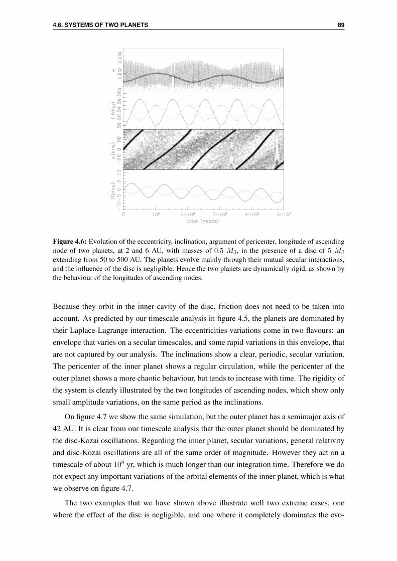
4.6. SYSTEMS OF TWO PLANETS 89
Figure 4.6: Evolution of the eccentricity, inclination, argument of pericenter, longitude of ascendingnode of two planets, at 2 and 6 AU, with masses of 0.5 MJ, in the presence of a disc of 5 MJ
extending from 50 to 500 AU. The planets evolve mainly through their mutual secular interactions,and the influence of the disc is negligible. Hence the two planets are dynamically rigid, as shown bythe behaviour of the longitudes of ascending nodes.
Because they orbit in the inner cavity of the disc, friction does not need to be taken intoaccount. As predicted by our timescale analysis in figure 4.5, the planets are dominated bytheir Laplace-Lagrange interaction. The eccentricities variations come in two flavours: anenvelope that varies on a secular timescales, and some rapid variations in this envelope, thatare not captured by our analysis. The inclinations show a clear, periodic, secular variation.The pericenter of the inner planet shows a regular circulation, while the pericenter of theouter planet shows a more chaotic behaviour, but tends to increase with time. The rigidity ofthe system is clearly illustrated by the two longitudes of ascending nodes, which show onlysmall amplitude variations, on the same period as the inclinations.
On figure 4.7 we show the same simulation, but the outer planet has a semimajor axis of42 AU. It is clear from our timescale analysis that the outer planet should be dominated bythe disc-Kozai oscillations. Regarding the inner planet, secular variations, general relativityand disc-Kozai oscillations are all of the same order of magnitude. However they act on atimescale of about 108 yr, which is much longer than our integration time. Therefore we donot expect any important variations of the orbital elements of the inner planet, which is whatwe observe on figure 4.7.
The two examples that we have shown above illustrate well two extreme cases, onewhere the effect of the disc is negligible, and one where it completely dominates the evo-

90 4. INTERACTIONS BETWEEN AN INCLINED PLANET AND A DISC
Figure 4.7: Evolution of the eccentricity, inclination, argument of pericenter, longitude of ascendingnode of two planets, at 2 and 42 AU, with masses of 0.5 MJ, in the presence of a disc of 5 MJ ex-tending from 50 to 500 AU. The outer planet exhibits large variations of eccentricity and inclination,caused by Kozai oscillations from the disc. The inner planet’s eccentricity and inclination merelyvary during the integration time (the eccentricity is invisible as it remains close to its initial value of0.001).
lution of one of the planet, leaving the other unaffected on the timescale of the simulation.Note that we have chosen initial conditions (in particular the disc’s parameters) that are con-venient to illustrate our point. On figure 4.8 we show an example with a more realistic disc(but still ignoring friction). The disc extends from 10 to 100 AU, with a mass of 10 MJ.The inner planet is located at 3 AU with a mass of 0.1 MJ and an inclination of 55, whilethe outer planet has a mass of 1 MJ and inclination of 65. Both planets are on circularorbits. In this case it clearly appears that the outer planet will always be dominated by Kozaioscillations from the disc, because it is too massive to be strongly perturbed by the innerplanet. In addition, as the separation between the planets increases, the secular influence ofthe outer one on the inner one decreases and we expect that when a2 & 10 AU, the innerplanet would also be dominated by Kozai-disc oscillations. Note that their could be someintermediate cases with interesting behavior: the inner planet would be dominated by sec-ular perturbations from the outer one, causing the system to be rigid. In the meantime, theouter planet would be dominated by disc-Kozai variations. In this case the inner planet could“follow” the Kozai oscillations of the outer planet and undergo large eccentricity variations.However such configuration is expected to be quite unstable, because of the various sourcesof eccentricity excitation.

4.6. SYSTEMS OF TWO PLANETS 91
10 20 30 40100
Figure 4.8: Comparison of different timescales as a function of the initial semi major axis of the outerplanet. The inner planet is located at 3 AU. In this case, the inner planet has a mass of 0.1 MJ, andthe outer one 1MJ. tω,1 and tω,2 are timescales associated with the precession of the pericenters, andtΩ the nodal precession timescale, all derived in the framework of the Laplace-Lagrange theory. tK,1and tK,2 are the timescales of the Kozai oscillations raised by the disc on planet 1 and 2, respectively.tGR,1 is General Relativity pericenter precession timescale of the inner planet. The outer planetis dominated by the Kozai oscillations from the disc, mainly because the inner planet has a lowermass. When the two planets are well separated (a2 > 10 AU), we expect the inner planet to also bedominated by disc-Kozai oscillations
Finally we remark that we have neglected friction, mainly because we have consideredsimplistic cases where the planets orbit in an inner cavity. When friction is included, itwill act to decrease the semi-major axis of the planets, meaning that the timescales wehave derived will evolve in time. This makes the evolution of the system hard to predict,especially if the planets cross some secular resonances that could lead to chaotic behaviour.

92 4. INTERACTIONS BETWEEN AN INCLINED PLANET AND A DISC

Chapter 5
Resonant Migration
Contents5.1 Migration and the capture in resonance . . . . . . . . . . . . . . . . . 93
5.1.1 Observational evidences . . . . . . . . . . . . . . . . . . . . . . 93
5.1.2 Disc–driven migration of two planets . . . . . . . . . . . . . . . 94
5.2 Resonant migration and orbital evolution . . . . . . . . . . . . . . . . 95
5.2.1 Probability of capture in resonance . . . . . . . . . . . . . . . . . 96
5.2.2 Physics of the resonant migration . . . . . . . . . . . . . . . . . 97
5.2.3 Damping of the orbital elements by the disc . . . . . . . . . . . . 97
5.3 Publication II - Evolution of eccentricity and orbital inclination ofmigrating planets in 2:1 mean motion resonance . . . . . . . . . . . . 98
5.4 Complete solution in the case of strong eccentricity damping . . . . . 116
5.1 Migration and the capture in resonance
In the previous chapter we have analysed a configuration where a planet is inclined withrespect to the mid-plane of a disc. In the present chapter, we study a mechanism that has beenthought by several authors to cause a primordial misalignment between a pair of planets andtheir native disc. This mechanism, which also excites eccentricities, is referred to as resonant
migration. It involves the planets being locked in a mean motion resonance (hereafter MMR,see section 3.2.5), where the ratio of their orbital period is the ratio of two small integers.
5.1.1 Observational evidences
Several stars have been found to be orbited by pairs of planets in, or close to, mean motionresonances. In particular, the star GJ 876 was found to host two giant planets in a 2:1 MMR(Marcy et al., 2001). The best-fit orbital solution (Rivera et al., 2010) gives periods of 30.4
93

94 5. RESONANT MIGRATION
and 61.1 days, with the inner planet having a mass of 0.7 MJ and an eccentricity of 0.26,while the outer one has a mass of 2.3 MJ and an eccentricity of 0.03. As pointed out by Leeand Peale (2002), this system contrasted with an other example of a 2:1 MMR, involvingthe satellites Io and Europa of Jupiter. In this case the resonant angles librate about 0 and180, and the apses are therefore anti-aligned. In the GJ 876 system, both resonant angleslibrate around 0 and the apses are aligned.
An other example consists in the two Saturn-like planets orbiting HD 45364, which werefound to be in a 3:2 MMR (Correia et al., 2009). Because a system in a 3:2 MMR is likely tohave crossed the 2:1 MMR first, fast migration is required in order to avoid trapping in thisconfiguration (see section 5.2.1 below). Rein et al. (2010) argued that fast type III migrationcould account for this, and managed to produce an orbital solution and the associated light-curve that could fit the observations. There solution differs from that of Correia et al. (2009)and only subsequent observations will be able to disentangle between the two solutions.
The Kepler mission has revealed a large population of multiple systems, and a smallfraction of them appear to be located in, or at least close to, MMRs. For these systems, thegeneral trend is that the period ratio (outer period over inner period) is slightly larger than theexact resonant value. Terquem and Papaloizou (2007), Lithwick and Wu (2012), and Baty-gin and Morbidelli (2013) argued that tidal interactions with the star can increase the periodratio of two planets otherwise in a resonant configuration. However, this mechanism cannotexplain why this trend is still observed for systems with the inner planet’s period larger than10 days, where tides are almost insignificant. More generally, the processes which, at theplanet-disc level of interactions, can help or prevent the formation of resonances are still anactive area of research.
5.1.2 Disc–driven migration of two planets
It is very unlikely that the pairs of resonant planets where formed in this configuration.The most natural explanation invokes convergent migration of the planets (Snellgrove et al.,2001). In fact, because the formation of MMR configurations is a natural outcome of themigration of a pair of planets, the observation of such systems could argue in support of discmigration. However, note that MMRs could also be an outcome of planet-planet scattering(Raymond et al., 2008).
If the orbits decay at rates such as the mutual separation between the two planets in-creases, then resonant capture cannot occur. However, if the two orbits converge, numericalsimulations of planets embedded in protoplanetary discs reveal that resonant capture is pos-sible. Figure 5.1 (from Kley and Nelson, 2012) shows an example of such hydrodynamicalsimulation where two giants planets clear out a mutual gap. The inner planet is pushed out-ward by the inner disc, while the outer planet is pushed inwards by the outer disc, resultingin convergent migration. Subsequently, the planets enter a resonant configuration. The 2:1MMR is the first first-order resonance that two initially well-spaced planets may encounter,

5.2. RESONANT MIGRATION AND ORBITAL EVOLUTION 95
Figure 5.1: Disc-migration of two planets trapped in a 2:1 resonance, and the formation of a jointgap. The simulation is 2D, represented in a fixed Cartesian reference frame after 1400 orbits of theinner planet. Figure extracted from Kley and Nelson (2012).
and therefore represents the most likely outcome.
Note that in figure 5.1, there is still a flow of material from the outer disc to the innerone, mainly driven by the wake in the vicinity of the planets. Numerical simulations (Lubowand D’Angelo, 2006) indicate that the gap formation can significantly reduce this flow ofmaterial. In this case, the inner disc might accrete onto the star, significantly reducing thetorque on the inner planet.
5.2 Resonant migration and orbital evolution
In this section we describe in details how the resonant migration can affect the orbital el-ements of the planets. We show that it can be associated with eccentricity and inclinationgrowth. We first recall how the the disc affects the orbital elements and how we can modelthese effects. Then we use a more general model that takes into account first and second-order terms in eccentricities and inclinations. This development allows us to conduct aparametric study of the resonant migration. These results are presented in a paper pub-lished in MNRAS (Teyssandier and Terquem, 2014), in which we determine, analytically

96 5. RESONANT MIGRATION
and numerically, the conditions needed for a system of two migrating planets trapped in a2:1 MMR to enter an inclination–type resonance, in which the inclinations can grow to highvalues, and eject the planets out of the plane of the disc. We also present a simple analyticalsolution for the eccentricities and semi-major axis in the case of of two planar orbits andstrong eccentricity damping.
5.2.1 Probability of capture in resonance
In section 3.2.5, we have noted that the behaviour of a resonant angle resembles that of apendulum. Close to the equilibrium point, the resonant angle librates, and circulates furtheraway. To a given resonance, we can associate a libration width, which gives the size ofthe libration area. For a planet with a semi-major axis a2, we note ∆a the extent of thelibration in terms of semi-major axis. Following Rein et al. (2010), we can get a first-orderestimate of the possibility of capture in resonance for a migrating planet, based on simplephysical considerations. If we consider that the planet is migrating inward at a constant rateon a timescale ta, it can capture an inner planet in resonance, provided the time spent in thelibration width is bigger than the period associated with the libration. More precisely, for aconstant migration rate, the time ∆t spent in the libration zone is given by
∆t =∆a
a2
ta. (5.1)
Hence, if Plib is the libration period, resonant capture is possible as long as
ta >a2
∆aPlib. (5.2)
The variation ∆a can be related to the variation of the mean motion by Kepler’s third law,to give:
2
3∆n =
n2
a2
∆a, (5.3)
and for a resonant system, ∆n can be directly related to 2π/Plib, such as the resonant capturecondition reads:
ta >P 2
lib
P2
. (5.4)
where P2 is the period of the outer planet.
However, expressing Plib as a function of the orbital parameters is not trivial (see, e.g.,Rein and Papaloizou, 2009). Quillen (2006) used a Hamiltonian model to study the proba-bility of capture into mean motion resonance by a migrating planet, and give a simple ex-pression for the minimum migration timescale that permits capture. Precisely, she showedthat resonant capture can occur if the migration timescale ta satisfies, in the case of the 2:1MMR:
ta & 0.4µ−4/3P2 (5.5)

5.2. RESONANT MIGRATION AND ORBITAL EVOLUTION 97
where µ is the outer planet to star mass ratio. The resonant capture of an inner planet by anouter migrating planet of 1 MJ at 5 AU is possible as long as the migration timescale of thelatter is larger than 4.7× 10⁴ yr. Because the viscous timescale, on which type II migrationis supposed to occur, is of the order of a few 105 yr, resonant capture is likely to happen.
5.2.2 Physics of the resonant migration
As we have seen in section 3.2.5, resonant conjunctions tend to stabilize near one apse,and therefore librate around 0 or 180. If the outer planet is now migrating inward, thenext conjunction will be located slightly after the stable longitude. The net tangential forcethat results from this configuration leads to a small exchange of angular momentum. Thisexchange acts to prevent the conjunction to depart from the stable longitude. Therefore,the resonant configuration is maintained and the inner planet migrates inward along withthe outer one. A similar reasoning shows that an inner planet that is migrating outwardcan capture another planet exterior to its orbit in a MMR. In the solar system, outwardmigration of natural satellites due to tidal interaction with their giant planet host can explainthe large number of resonant configurations, for example around Saturn (Goldreich, 1965).However, an inner planet migrating inward cannot drag along with it an outer planet, becausecommensurability cannot be maintained.
Even if the commensurability is maintained, the conjunction for a libration state of therelevant argument of resonance still tends to occur after longitude of the line of apse. Wouldthe conjunction happen exactly at apocenter or pericenter, the transfer of angular momentumfrom apocenter to pericenter would be exactly compensated by the transfer from pericenterto apocenter. The net transfer of angular momentum would average out to zero over oneorbit, and their would be no change of eccentricity. Here, the symmetry is broken by themigration of the outer planet, which causes the conjunction to occur away from the apse.The radial impulse that results from this configuration will act to increase the eccentricities.
To summarize, one can expect the net effect of resonant capture of an inner planet byan outer, migrating one, to maintain the resonant commensurability, while exciting the twoeccentricities. As we will see, such process can also, under specific conditions, excite theinclinations to large values.
5.2.3 Damping of the orbital elements by the disc
We have mentioned in section 2.4.1.2 that under disc migration, the disc tends to damp theorbital eccentricities and inclinations. The eccentricity damping is often parametrized in thefollowing way ∣∣∣∣
e
e
∣∣∣∣ = K
∣∣∣∣a
a
∣∣∣∣ , (5.6)
where K is a dimensionless parameter. The orbital decay on the right-hand side occurs ona viscous timescale of a few 105 years. Numerical simulations have put constraints on K,

98 5. RESONANT MIGRATION
ranging between 1 and 100. For instance, Lee and Peale (2002) showed that the GJ 876system can only be reproduced with K ∼ 100, whereas 2D hydrodynamical simulationsfrom Kley et al. (2004) indicate K of the order unity.
Results from hydrodynamical simulations (see, e.g., Snellgrove et al., 2001; Kley et al.,2004) have shown that a prescription can be used to model the migration, which reproducesthe same results. This prescription consists in adding extra forces to an N -body code, whichallows for faster computation. Precisely, let us define the two following forces per unit ofmass:
Γd,a = − 1
tm
drdt, (5.7)
Γd,e = − 2
te|r|2
(drdt· r)
r, (5.8)
where r is the orbital distance from the planet to the star, tm parametrizes the orbital decay,and te the eccentricity damping timescale. It is possible to show, using the equations ofsection 3.2.1, that Γd,a leads to an exponential damping of the semi-major axis, of the form
da
dt= − 2
tma, (5.9)
while Γd,e leads to an exponential damping of the eccentricity, of the form
de
dt= − 1
tee. (5.10)
Note that Γd,e also contributes to the evolution of the semi-major axis, adding a term of theform
da
dt= − 2
teae2. (5.11)
The details of the calculation can be found in the appendix of Teyssandier and Terquem(2014). We remark that the orbital decays of a single planet actually occurs on a timescaletm/2, and we define ta = tm/2 as the effective migration timescale.
5.3 Publication II - Evolution of eccentricity and orbital in-clination of migrating planets in 2:1 mean motion res-onance
As we have mentioned earlier in this chapter, the resonant capture of a planet while it mi-grates in a disc is a well-known mechanism, and has been applied to real planetary systemssuch as GJ 876 and HD 45364. However, these studies remained focused on the planarevolution of migrating planets, without taking into consideration the possibility of verti-cal motion. This can be justified by the fact that planets are expected to remain in their

5.3. PUBLICATION II - EVOLUTION OF ECCENTRICITY AND ORBITAL INCLINATION OF MIGRATINGPLANETS IN 2:1 MEAN MOTION RESONANCE 99
thin disc will migrating. However, Thommes and Lissauer (2003) found that if the planetsreach high eccentricities, an inclination–type resonance can be triggered, and the inclina-tions grow to large values, of the order of several tens of degrees. They concluded thatthis could be responsible for a high degree of non-coplanarity in planetary systems. Theirresults were further developed by Lee and Thommes (2009), and extended to higher-orderresonances by Libert and Tsiganis (2009). These works showed that the onset of inclination–type resonance was only possible if the eccentricity damping caused by the disc occurred ona timescale of the order of, or larger than, the migration timescale. In addition, their resultswere mostly numerical, and an in-depth analytical understanding was lacking.
In the following publication, we study the evolution of a pair of planets under the com-bined effect of the 2:1 MMR and disc-migration. Our work contains both an analyticaland a numerical part. In order to analytically model the resonant effects, we follow section3.2.5, and use a disturbing function that contains all the resonant and secular terms up to,and including, the second order in eccentricities and inclinations. This disturbing functionis tabulated in Murray and Dermott (1999). The disc-migration mechanism is modelled bythe forces introduced in section 5.2.3 above. Numerical integration can be done for themotion of the two planets, using a N-body integrator with a Bulirsch–Stoer scheme. UsingN-body simulation instead of hydrodynamical simulations is less computational expensive,and allow us to conduct a large number of simulations and map the parameter space.

MNRAS 443, 568–583 (2014) doi:10.1093/mnras/stu1137
Evolution of eccentricity and orbital inclination of migrating planets in2:1 mean motion resonance
Jean Teyssandier1‹ and Caroline Terquem1,2
1Institut d’Astrophysique de Paris, UPMC Univ Paris 06, CNRS, UMR7095, 98 bis bd Arago, F-75014 Paris, France2Department of Astrophysics, University of Oxford, Keble Road, Oxford OX1 3RH, UK
Accepted 2014 June 5. Received 2014 May 16; in original form 2014 March 26
ABSTRACTWe determine, analytically and numerically, the conditions needed for a system of two mi-grating planets trapped in a 2:1 mean motion resonance to enter an inclination-type resonance.We provide an expression for the asymptotic equilibrium value that the eccentricity ei of theinner planet reaches under the combined effects of migration and eccentricity damping. Wealso show that, for a ratio q of inner to outer masses below unity, ei has to pass through a valueei, res of the order of 0.3 for the system to enter an inclination-type resonance. Numerically,we confirm that such a resonance may also be excited at another, larger, value ei, res 0.6,as found by previous authors. A necessary condition for onset of an inclination-type reso-nance is that the asymptotic equilibrium value of ei is larger than ei, res. We find that, forq ≤ 1, the system cannot enter an inclination-type resonance if the ratio of eccentricity tosemimajor axis damping time-scales te/ta is smaller than 0.2. This result still holds if onlythe eccentricity of the outer planet is damped and q . 1. As the disc/planet interaction ischaracterized by te/ta ∼ 10−2, we conclude that excitation of inclination through the type ofresonance described here is very unlikely to happen in a system of two planets migrating ina disc.
Key words: celestial mechanics – planets and satellites: dynamical evolution and stability –planetary systems.
1 IN T RODUCT I O N
At the time of writing, 98 extrasolar multiple-planet systems havebeen detected by radial velocity surveys and 420 by the Keplermission (Lissauer et al. 2014; Rowe et al. 2014). A significantfraction of these systems contain planet pairs in or near a 2:1 meanmotion resonance (MMR; Lissauer et al. 2011; Fabrycky et al. 2012,see also Petrovich, Malhotra & Tremaine 2013).
Capture in MMR is thought to be the result of convergent mi-gration of planets (Snellgrove, Papaloizou & Nelson 2001). Severalstudies (Lee & Peale 2002; Beauge, Ferraz-Mello & Michtchenko2003; Lee 2004; Kley et al. 2005), focusing on the dynamics ofthe two planets in 2:1 MMR in the system GJ 876, were publishedsoon after the discovery of this system (Marcy et al. 2001). Theyassume coplanar orbits and focus on explaining the unusual factthat the orbits of the two planets librate about apsidal alignmentin this system (as opposed to anti-alignment in the Io–Europa sys-tem). The evolution of planetary systems in MMR has also beenstudied with three-dimensional simulations (Thommes & Lissauer2003; Lee & Thommes 2009; Libert & Tsiganis 2009). It has
E-mail: [email protected]
been found that a system of planets in an eccentricity-type reso-nance may enter an inclination-type resonance if the eccentricity ofthe inner planet becomes large enough. In this context, very highorbital inclinations can be reached starting from nearly coplanarconfigurations.
Studies of resonant inclination excitation are important as thismechanism has been proposed to explain the fact that some extra-solar planets have an orbit which is inclined with respect to thestellar equatorial plane.
Other processes which have been put forward to produce such aninclination include interactions between the planet and a compan-ion (Fabrycky & Tremaine 2007; Wu, Murray & Ramsahai 2007;Chatterjee et al. 2008; Naoz et al. 2011; Wu & Lithwick 2011),misalignment of the disc in which the planet forms (Bate, Lodato& Pringle 2010; Batygin 2012; Terquem 2013), tilting of the stellarspin axis due to interaction with the disc (Foucart & Lai 2011; Lai,Foucart & Lin 2011) or dynamical relaxation of a population ofplanets (Papaloizou & Terquem 2001).
The studies of inclination-type resonances published so far, whichare numerical, have mapped to some extent the parameter space andhave shown that the onset of resonant inclination excitation dependssensitively on the eccentricity damping time-scale and the ratio ofthe planets’ masses.
C© 2014 The AuthorsPublished by Oxford University Press on behalf of the Royal Astronomical Society
at Bodleian Library on A
ugust 11, 2014http://m
nras.oxfordjournals.org/D
ownloaded from
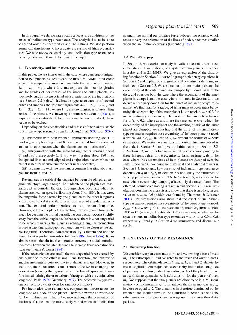
Migrating planets in 2:1 MMR 569
In this paper, we derive analytically a necessary condition for theonset of inclination-type resonance. The analysis has to be doneto second order in eccentricities and inclinations. We also performnumerical simulations to investigate the regime of high eccentric-ities. We now review eccentricity- and inclination-type resonancesbefore giving an outline of the plan of the paper.
1.1 Eccentricity- and inclination- type resonances
In this paper, we are interested in the case where convergent migra-tion of two planets has led to capture into a 2:1 MMR. First-ordereccentricity-type resonance involves only the resonant arguments2λo − λi − i, o, where λi, o and i, o are the mean longitudesand longitudes of pericentres of the inner and outer planets, re-spectively, and is not associated with a variation of the inclinations(see Section 2.2 below). Inclination-type resonance is of secondorder and involves the resonant arguments 4λo − 2λi − 2i, o and4λo − 2λi − i − o, where i, o are the longitudes of ascendingnodes of the planets. As shown by Thommes & Lissauer (2003), itrequires the eccentricity of the inner planet to reach relatively largevalues to be excited.
Depending on the eccentricities and masses of the planets, stableeccentricity-type resonances can be (Beauge et al. 2003; Lee 2004):
(i) symmetric with both resonant arguments librating about 0
(and o − i librating about 0, i.e. the apsidal lines are alignedand conjunction occurs when the planets are near pericentre),
(ii) antisymmetric with the resonant arguments librating about0 and 180, respectively (and o − i librating about 180, i.e.the apsidal lines are anti-aligned and conjunction occurs when oneplanet is near pericentre and the other near apocentre),
(iii) asymmetric with the resonant arguments librating about an-gles far from 0 and 180.
Resonances are stable if the distance between the planets at con-junctions stays large enough. To understand the physics of reso-nance, let us consider the case of conjunction occurring when theplanets are near an apse, i.e. librating about 0 or 180. In that case,the tangential force exerted by one planet on to the other integratesto zero over an orbit and there is no exchange of angular momen-tum. The next conjunction therefore occurs at the same longitude.However, if the outer planet is migrating inwards (over a time-scalemuch longer than the orbital period), the conjunction occurs slightlyaway from the stable longitude. In that case, there is a net tangentialforce which results in the planets exchanging angular momentumin such a way that subsequent conjunctions will be closer to the sta-ble longitude. Therefore, commensurability is maintained and theinner planet is pushed inwards (Goldreich 1965; Peale 1976). It canalso be shown that during the migration process the radial perturba-tive force between the planets tends to increase their eccentricities(Lissauer, Peale & Cuzzi 1984).
If the eccentricities are small, the net tangential force exerted byone planet on to the other is small, and therefore, the transfer ofangular momentum between the two planets is weak. However, inthat case, the radial force is much more effective in changing theorientation (causing the regression) of the line of apses and there-fore in maintaining the orientation of the apses with the conjunctionlongitude (Peale 1976; Greenberg 1977). The eccentricity-type res-onance therefore exists even for small eccentricities.
For inclination-type resonances, conjunctions librate about thelongitude of a node of one planet. There is however no resonancefor low inclinations. This is because although the orientation ofthe lines of nodes can be more easily varied when the inclination
is small, the normal perturbative force between the planets, whichtends to vary the orientation of the lines of nodes, becomes smallerwhen the inclination decreases (Greenberg 1977).
1.2 Plan of the paper
In Section 2, we develop an analysis, valid to second order in ec-centricities and inclinations, of a system of two planets embeddedin a disc and in 2:1 MMR. We give an expression of the disturb-ing function in Section 2.1, write Lagrange’s planetary equations inSection 2.2 and explain how migration and eccentricity damping areincluded in Section 2.3. We assume that the semimajor axis and theeccentricity of the outer planet are damped by interaction with thedisc, and consider both the case where the eccentricity of the innerplanet is damped and the case where it is not. In Section 2.4, wederive a necessary condition for the onset of inclination-type reso-nance. We find that, for a ratio q of inner mass to outer mass belowunity, the eccentricity of the inner planet has to reach ei, res ∼ 0.3 foran inclination-type resonance to be excited. This cannot be achievedfor tei/ta < 0.2, where tei and ta are the time-scales over which theeccentricity of the inner planet and the semimajor axis of the outerplanet are damped. We also find that the onset of the inclination-type resonance requires the eccentricity of the outer planet to reacha critical value eo, res. In Section 3, we present the results of N-bodysimulations. We write the equations of motion which are solved inthe code in Section 3.1 and give the initial setting in Section 3.2.In Section 3.3, we describe three illustrative cases corresponding tothree different values of the eccentricity damping time-scale in thecase where the eccentricities of both planets are damped over thesame time-scale te. We compare numerical and analytical results inSection 3.4, investigate how the onset of inclination-type resonancedepends on q and te/ta in Section 3.5 and study the influence ofvarying parameters in Section 3.6. In Section 3.7, we consider thecase where eccentricity damping affects only the outer planet. Theeffect of inclination damping is discussed in Section 3.8. These sim-ulations confirm the analysis and show that there is another, larger,value of ei, res 0.6 (which was found by Thommes & Lissauer2003). The simulations also show that the onset of inclination-type resonance requires the eccentricity of the outer planet to reacheo, res ∼ 0.2 when q . 1. The resonant argument φ2 librates about180 or 0 (while φ1 librates about 0) depending on whether thesystem enters an inclination-type resonance with ei, res 0.3 or 0.6,respectively. Finally, in Section 4 we summarize and discuss ourresults.
2 ANALYSIS OF THE RESONANCE
2.1 Disturbing function
We consider two planets of masses mi and mo orbiting a star of massm. The subscripts ‘i’ and ‘o’ refer to the inner and outer planets,respectively. The orbital elements λi, ai, ei, Ii, i and i denote themean longitude, semimajor axis, eccentricity, inclination, longitudeof pericentre and longitude of ascending node of the planet of massmi, with same quantities with subscript ‘o’ for the planet of massmo. We suppose that the two planets are close to or in a 2:1 meanmotion commensurability, i.e. the ratio of the mean motions, ni/no,is close or equal to 2. The dynamics is therefore dominated by theresonant and secular terms in the disturbing function, since all theother terms are short period and average out to zero over the orbitalperiods.
MNRAS 443, 568–583 (2014)
at Bodleian Library on A
ugust 11, 2014http://m
nras.oxfordjournals.org/D
ownloaded from

570 J. Teyssandier and C. Terquem
The perturbing functions for the inner and outer planets can bewritten under the form (Murray & Dermott 1999)
〈Ri〉 = Gmo
ao
( ⟨Rsec
D
⟩ + ⟨Rres
D
⟩ + α 〈RE〉) , (1)
〈Ro〉 = Gmi
ao
( ⟨Rsec
D
⟩ + ⟨Rres
D
⟩ + 1
α2〈RI〉
), (2)
where G is the constant of gravitation, α ≡ ai/ao,⟨Rsec
D
⟩and⟨
RresD
⟩are the secular and resonant contributions to the direct part
of the disturbing function, respectively, 〈RE〉 is the indirect partdue to an external perturber and 〈RI〉 is the indirect part due to aninternal perturber. The brackets indicate that the quantities are timeaveraged. Note that there is no secular contribution to 〈RE〉 and〈RI〉.
When an expansion of the perturbing function in the orbital el-ements is carried out, the lowest orders at which eccentricities andinclinations appear are the first and second, respectively, and at sec-ond order, there are no terms in which eccentricities and inclinationsare coupled. To study the inclination-type resonance, second-orderterms in eccentricities need to be included. The expansion of theperturbing function to second order is (Murray & Dermott 1999)⟨Rsec
D
⟩ = K1
(e2
i + e2o
) + K2eieo cos (i − o)
+ K3
(s2
i + s2o
) + K4siso cos (i − o) , (3)
⟨Rres
D
⟩ = eif1 cos φ1 + eof2 cos φ2 + e2i f3 cos φ3
+eieof4 cos φ4 + e2of5 cos φ5 + s2
i f6 cos φ6
+sisof7 cos φ7 + s2of8 cos φ8, (4)
〈RE〉 = −2eo cos φ2, (5)
〈RI〉 = −1
2eo cos φ2, (6)
where si, o = sin (Ii, o/2), and the fi (i = 1, . . . , 8) and Ki (i =1, . . . , 4) are expressed in term of the Laplace coefficients andα. Their expression is given in Appendix A. The resonant anglesφi (i = 1, . . . , 8) are defined by
φ1 = 2λo − λi − i, (7)
φ2 = 2λo − λi − o, (8)
φ3 = 4λo − 2λi − 2i, (9)
φ4 = 4λo − 2λi − o − i, (10)
φ5 = 4λo − 2λi − 2o, (11)
φ6 = 4λo − 2λi − 2i, (12)
φ7 = 4λo − 2λi − i − o, (13)
φ8 = 4λo − 2λi − 2o. (14)
2.2 Lagrange’s planetary equations
When the perturbing function is expanded to second order in theeccentricities and inclinations, Lagrange equations can be writtenas follows:
daβ
dt= 2
nβaβ
∂⟨Rβ
⟩
∂ λβ
, (15)
deβ
dt= −1
nβa2βeβ
∂⟨Rβ
⟩
∂ β
, (16)
dβ
dt= 1
nβa2βeβ
∂⟨Rβ
⟩
∂ eβ
, (17)
dλβ
dt= nβ + 1
nβa2β
(− 2aβ
∂⟨Rβ
⟩
∂ aβ
+ eβ
2
∂⟨Rβ
⟩
∂ eβ
+ tanIβ
2
∂⟨Rβ
⟩
∂ Iβ
), (18)
dβ
dt= 1
nβa2β sin Iβ
∂⟨Rβ
⟩
∂ Iβ
, (19)
dIβ
dt= −1
nβa2β sin Iβ
∂⟨Rβ
⟩
∂ β
, (20)
where β = i, o. In equation (18), the derivative with respect to aβ
has to be carried out by ignoring the fact that the angles φi (i =1, . . . , 8) depend on aβ through λi and λo (Roy 1978). We define atime-scale T such that
T = n−1o0
m
mi, (21)
where the subscript ‘0’ denotes initial value. We consider planetswith masses mi, o m, so that the mean motions are approximated
by ni,o = (Gm/a
3i,o
) 1/2.
Using the expression of the perturbing function given by equa-tions (1)–(6), we can rewrite Lagrange equations (15)–(20) in thefollowing dimensionless form:
dai
dτ= Ci2ai [eiF1 + eoF2 − eo2α sin φ2 + F3 + O(3)] , (22)
dao
dτ= Co(−4ao)
[eiF1 + eoF2 − eo
2α2sin φ2 + F3 + O(3)
], (23)
dei
dτ= Ci [−F1 + O(2)] , (24)
deo
dτ= Co
[−F2 + 1
2α2sin φ2 + O(2)
], (25)
di
dτ= Ci
[1
eif1 cos φ1 + 2f3 cos φ3 + eo
eif4 cos φ4 + 2K1
+K2eo
eicos (i − o) + O(1)
], (26)
MNRAS 443, 568–583 (2014)
at Bodleian Library on A
ugust 11, 2014http://m
nras.oxfordjournals.org/D
ownloaded from

Migrating planets in 2:1 MMR 571
do
dτ= Co
[1
eo
(f2 − 1
2α2
)cos φ2 + ei
eof4 cos φ4 + 2f5 cos φ5
+ 2K1 + K2ei
eocos (i − o) + O(1)
], (27)
dλi
dτ= Ci
[1
α
m
mo+ 1
2eif1 cos φ1 + 4αeo cos φ2 − + O(2)
],
(28)
dλo
dτ= Co
[m
mi+ 2eif1 cos φ1
+1
2eo
(5f2 + 3
2α2
)cos φ2 + + O(2)
], (29)
di
dτ= Ci
2
[K3 + 1
2
so
si(K4 cos(i − o) + f7 cos φ7)
+ f6 cos φ6 + O(1)] , (30)
do
dτ= Co
2
[K3 + 1
2
si
so(K4 cos(i − o) + f7 cos φ7)
+ f8 cos φ8 + O(1)] , (31)
dIi
dτ= Ci
[1
2
so
ci(K4 sin(i − o) − f7 sin φ7)
− si
cif6 sin φ6 + O(2)
], (32)
dIo
dτ= Co
[−1
2
si
co(K4 sin(i − o) + f7 sin φ7)
− so
cof8 sin φ8 + O(2)
], (33)
where τ = t/T, ci, o = cos (Ii, o/2), Ci = (ao0/ao)3/2 mo/(mi√
α),Co = (ao0/ao)3/2,
F1 = f1 sin φ1 + 2eif3 sin φ3 + eof4 sin φ4
− K2eo sin (i − o) , (34)
F2 = f2 sin φ2 + 2eof5 sin φ5 + eif4 sin φ4
+ K2ei sin (i − o) , (35)
F3 = 2s2i f6 sin φ6 + 2sisof7 sin φ7 + 2s2
of8 sin φ8 (36)
and
= 2α
(ei∂ f1
∂ αcos φ1 + eo
∂ f2
∂ αcos φ2
). (37)
Note that, with a perturbing function expanded to second order ineccentricities and inclinations, the rate of change of i, o and i, o
can be obtained only to zeroth order in eccentricities and inclina-tions.
The only orbital elements which are relevant when the orbits arecoplanar are ai, o, ei, o, i, o and λi, o. At the order at which the aboveequations are valid, we note that their evolution is decoupled fromthat of i, o and Ii, o. Similarly, when the semimajor axes do not varysignificantly, the variations of i, o and Ii, o are decoupled from thatof the other orbital elements.
2.3 Modelling of migration and eccentricity damping
We are interested in the case where the two planets capture eachother in an MMR, which happens for instance if the outer planetmigrates inwards due to its interaction with the disc at least asfast as the inner planet. To model this, we artificially decreasethe semimajor axis of the outer planet by adding a damping term−ao/τ a on the right-hand side of equation (23), where τ a is the(dimensionless) migration time-scale that can be freely specified.In principle, due to its interaction with the disc, the inner planet alsomigrates independently of the outer one. For simplicity, this is nottaken into account here. It would not change the results presented inthis paper as long as the inner planet were not migrating faster thanthe outer one. In this context, the time-scale τ a can be thought ofas the time-scale over which the outer planet migrates with respectto the inner one. Note that a diminution of ai, although not beingadded artificially, will be induced by that of ao (see below).
Interaction with the disc also leads to damping of the plan-ets eccentricities. This is taken into account by adding a damp-ing term −ei/τ ei and −eo/τ eo on the right-hand side of equations(24) and (25), respectively, where τ ei and τ eo are the (dimension-less) eccentricity damping time-scales. Eccentricity damping doesin turn contribute to the damping of the semimajor axis by a term−2ai,oe
2i,o/τei,o (see Appendix B).
With migration and eccentricity damping taken into account,equations (22)–(25) become
dai
dτ= Ci2ai [eiF1 + eoF2 − eo2α sin φ2 + F3 + O(3)] − 2aie
2i
τei,
(38)
dao
dτ= Co(−4ao)
[eiF1 + eoF2 − eo
2α2sin φ2 + F3 + O(3)
]
− ao
τa− 2aoe
2o
τeo, (39)
dei
dτ= Ci [−F1 + O(2)] − ei
τei, (40)
deo
dτ= Co
[−F2 + 1
2α2sin φ2 + O(2)
]− eo
τeo. (41)
In this paper, we will consider either the case τ ei = τ eo or the caseof infinite τ ei (no damping on the inner planet) and finite τ eo.
Inclination damping has not been included, as it is not relevanthere (see Section 3.8).
2.4 Necessary condition for the onsetof inclination-type resonance
In this section, we derive a necessary condition for a pair of planetsin 2:1 MMR to enter an inclination-type resonance. We assume thatthe planets have captured each other in an exact resonance, so that
MNRAS 443, 568–583 (2014)
at Bodleian Library on A
ugust 11, 2014http://m
nras.oxfordjournals.org/D
ownloaded from

572 J. Teyssandier and C. Terquem
α ≡ ai/ao = 2−2/3 remains constant in time. In that case, it is usefulto note that 2α = 1/(2α2). We also define the mass ratio q ≡ mi/mo.
In this context, equations (38) and (39) can be combined to give
2
ai
dai
dτ+ 1
q√
α
1
ao
dao
dτ= − 1
q√
ατa− 4
e2i
τei− 2
q√
α
e2o
τeo. (42)
Using α = ai/ao, we obtain the following differential equation forai and ao:
(1 + 2q
√α) 1
ai,o
dai,o
dτ= − 1
τa− 4q
√α
e2i
τei− 2
e2o
τeo. (43)
To first order in eccentricities, the solutions are
ai,o(τ ) = ai0,o0 e−τ/[(1+2q√
α)τa]. (44)
This shows that, when q = 0, i.e. when the inner planet is treated asa test particle, both planets migrate at a rate τ a. When q is non-zero,the migration is slightly slowed down by the mutual interactionbetween the two planets.
2.4.1 Eccentricity-type resonance
As a first step, we calculate the equilibrium values reached by theeccentricities under the combined effects of migration and eccen-tricity damping when the system is in an eccentricity-type resonancewith zero inclinations.
Equations (40) and (41) can be combined to give
eidei
dτ+ e2
i
τei+ 1
q√
α
(eo
deo
dτ+ e2
o
τeo
)
= −Ci
[eiF1 + eoF2 − eo
2α2sin φ2 + O(3)
]. (45)
When the inclinations are zero, F3 = 0. Using equations (39) and(43), we can then rewrite equation (45) under the form
de2i
dτ+ 1 + q
√α
1 + 2q√
α
4e2i
τei+ 1
q√
α
[de2
o
dτ+ 1 + q
√α
1 + 2q√
α
2e2o
τeo
]
= 1
τa(1 + 2q√
α). (46)
When q → 0, eo has to satisfy de2o/dτ + 2e2
o/τeo = 0, which meansthat eo is damped to zero whereas, in this limit, ei reaches theequilibrium value [τ ei/(4τ a)]1/2.
2.4.1.1 Finite values of τ ei and τ eo: When the eccentricities ofboth planets are damped and q ≤ 1, i.e. the outer planet is at leasta massive as the inner one, we expect the eccentricity of the outerplanet to grow less than that of the inner planet. We therefore neglectthe terms involving eo in equation (46), which then leads to thefollowing equilibrium value (corresponding to τ τ ei) for ei:
ei,eq = 1
2
(τei/τa
1 + q√
α
) 1/2
. (47)
In Fig. 1, we plot ei, eq as a function of q for τ ei/τ a = 1, 0.2 and0.1.
The numerical simulations presented in the next section confirmthat neglecting eo in equation (46) is a valid approximation for theparameters of interest in this paper. The numerical values foundfor ei, eq also agree very well with that given by equation (47), asindicated in Fig. 6.
2.4.1.2 Finite value of τ eo and τ ei → ∞ : In some conditions thatwill be discussed in Section 3.7, damping due to tidal interactionwith the disc acts only on the eccentricity of the outer planet, not onthat of the inner planet. In that case, as the planets are in resonance,ei still reaches an equilibrium value. This is shown by equation (24)in which F1 = 0 when the resonant angles librate about 0 or 180.By substituting de2
i /dτ = 0 and τ ei → ∞ in equation (46), weobtain the following equilibrium value (corresponding to τ τ eo)for eo:
eo,eq =[
q√
α τeo/τa
2(1 + q
√α)] 1/2
. (48)
In Fig. 2, we plot eo, eq as a function of q for τ eo/τ a = 0.2, 0.05and 0.01.
The numerical values found for eo, eq agree very well with thatgiven by equation (48), as indicated in Fig. 10.
2.4.2 Inclination-type resonance
We now calculate the values ei, res and eo, res that ei and eo, re-spectively, have to reach for the inclinations to start growing. Anecessary condition for the system to enter an inclination-type res-onance when both τ ei and τ eo are finite is ei, res < ei, eq, where ei, eq
is given by equation (47). When τ ei → ∞, a necessary condition iseo, res < eo, eq, where eo, eq is given by equation (48).
Inclination-type resonance can be reached only after aneccentricity-type resonance has been established (Thommes & Lis-sauer 2003) and therefore all the resonant angles librate about somevalues. Due to eccentricity damping, libration of the resonant anglesis actually offset from a fixed value (generally 0 or 180) by a termof the order of ei/τ ei or eo/τ eo (Goldreich & Schlichting 2014).Because of the 1/τ ei or 1/τ eo factor, this term is much smaller thanthose retained in the analysis here, so that we will ignore it. There-fore, the time-derivative of the resonant angles is close to zero.Equations (7), (8), (12) and (14) then yield
di
dτ= do
dτ= di
dτ= do
dτ, (49)
i.e. the nodes and pericentres all precess at the same rate. In theinclination-type resonance we consider here, as shown in the nu-merical simulations presented below, the resonant angles φ6, φ7 andφ8 librate about 180, 0 and 180, respectively, and i − o li-brates about 180, in agreement with Thommes & Lissauer (2003).In the analysis that follows, we therefore use φ7 = 0, φ6 = 180,φ8 = 180 and i − o = 180.
We first write di/dτ = do/dτ by equating equations (30) and(31). This leads to an algebraic equation for si/so. Using the factthat f6 = f8 and K3 − f8 = (− K4 + f7)/2 (see Appendix A), we canwrite the solution of this equation as
so
si= q
√α. (50)
For values of q less than unity, the inclination of the inner planet ismore easily excited than that of the outer planet. Note that the ratioof the inclinations does not depend on τ a nor τ ei or τ eo.
We now write d o/dτ = do/dτ by equating equations (27) and(31) and d i/dτ = di/dτ by equating equations (26) and (30). Inthe resulting set of equations, we replace si/so by the value foundabove. This set of two equations can now be solved to calculateei, res and eo, res, which are the values of ei and eo, respectively, whenthe inclination-type resonance is reached. This calculation requiresthe knowledge of φ1 and φ2 at the time when the inclination-type
MNRAS 443, 568–583 (2014)
at Bodleian Library on A
ugust 11, 2014http://m
nras.oxfordjournals.org/D
ownloaded from

Migrating planets in 2:1 MMR 573
Figure 1. Solid line: eccentricity ei, res of the inner planet when the system enters an inclination-type resonance versus q in logarithmic scale. This curvecorresponds to equation (51) with cos 2φ2 = 1. Also shown is the equilibrium eccentricity for τ ei/τ a = 0.1 (long dashed line), τ ei/τ a = 0.2 (short dashed line)and τ ei/τ a = 1 ( dotted line). These curves correspond to equation (47). The system cannot enter an inclination-type resonance when τ ei/τ a < 0.2.
resonance is triggered. For two planets in 2:1 MMR, it has beenfound (e.g. Lee & Peale 2002) that, in general, (φ1, φ2) = (0, 180)or (0, 0), depending on whether the eccentricities are small orlarge, respectively (‘large’ meaning that second-order terms in theeccentricities are not negligible). Fixing φ1 = 0 and cos 2φ2 = 1,we obtain
ei,res = −f13 + (f2 − 1
2α2
)(f4 + K2)
− (f4 + K2)2 + 34, (51)
eo,res = f1 (f4 + K2) − 4
(f2 − 1
2α2
)
34 − (f4 + K2)2 cos φ2, (52)
where we have defined 1 = K3 + q√
α(f7 − K4)/2 − f6, 2 =K3 + (f7 − K4)/(2q
√α) − f8, 3 = 2f5 + 2K1 − 2/2 and
4 = 2f3 + 2K1 − 1/2.We note that ei, res and eo, res do not depend on the damp-
ing time-scales. When q → 0, equations (51) and (52) giveei, res = f1/[(K3 − f6)/2 − 2(f3 + K1)] 0.22 and eo, res = 0,respectively.
Equation (52) gives a positive value of the eccentricity for φ2 = 0
but a negative value for φ2 = 180. When φ2 evolves from librationabout 0 to libration about 180, the apsidal lines evolve from beingaligned to being anti-aligned, i.e. the pericentre of the outer orbitis changed to apocentre. In that case, for the equation of the outerellipse which was used in deriving Lagrange’s equations to be pre-served, eo should be changed to −eo. The value of eo correspondingto φ2 = 180 is therefore the opposite as that given by equation (52).
In Fig. 1, we plot the eccentricity ei, res given by equation (51)as a function of q. For q varying between 0.1 and 1, we see thatei, res 0.3. The eccentricity eo, res given by equation (52) is shownin Fig. 2. We see that eo, res varies much more with q than ei, res.
The numerical results presented in the next section show thatthere are two regimes in which the system may enter an inclination-type resonance: (i) a small eccentricity regime, which is describedby the analysis above (although the value of eo, res found numericallyis about twice as large as that found analytically), and (ii) a largeeccentricity regime, in which inclination-type resonance is obtainedfor ei, res 0.6 and eo, res 0.2 for q . 1. The large eccentricityregime cannot be captured by the analysis above, as our equationsare not developed up to a sufficient order in ei, o. As noted above, byexpanding the perturbing function to second order in ei, o, we obtaindi,o/dt and di,o/dt to zeroth order only in ei, o.
When both τ ei and τ eo are finite, we can find the values of q andτ ei/τ a for which inclination-type resonance may occur by writingthe necessary condition ei, res < ei, eq. Using equations (47) and (51)and ignoring the (weak) variation of ei, res with q, this leads to
τei/τa
1 + q√
α> 4e2
i,res. (53)
Note that the above condition is necessary but not sufficient, aswe have not taken into account the fact that eo must also reacheo, res (we cannot write this condition as we have not calculated eo, eq
when τ ei is finite). Fig. 1 shows that the system cannot enter aninclination-type resonance when τ ei/τ a < 0.2. When q decreases,the inclination-type resonance is reached for shorter eccentricity
MNRAS 443, 568–583 (2014)
at Bodleian Library on A
ugust 11, 2014http://m
nras.oxfordjournals.org/D
ownloaded from
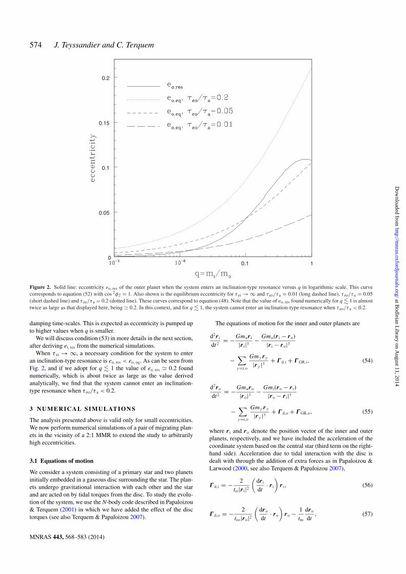
574 J. Teyssandier and C. Terquem
Figure 2. Solid line: eccentricity eo, res of the outer planet when the system enters an inclination-type resonance versus q in logarithmic scale. This curvecorresponds to equation (52) with cos 2φ2 = 1. Also shown is the equilibrium eccentricity for τ ei → ∞ and τ eo/τ a = 0.01 (long dashed line), τ eo/τ a = 0.05(short dashed line) and τ eo/τ a = 0.2 (dotted line). These curves correspond to equation (48). Note that the value of eo, res found numerically for q . 1 is almosttwice as large as that displayed here, being 0.2. In this context, and for q . 1, the system cannot enter an inclination-type resonance when τ eo/τ a < 0.2.
damping time-scales. This is expected as eccentricity is pumped upto higher values when q is smaller.
We will discuss condition (53) in more details in the next section,after deriving ei, res from the numerical simulations.
When τ ei → ∞, a necessary condition for the system to enteran inclination-type resonance is eo, res < eo, eq. As can be seen fromFig. 2, and if we adopt for q . 1 the value of eo, res 0.2 foundnumerically, which is about twice as large as the value derivedanalytically, we find that the system cannot enter an inclination-type resonance when τ eo/τ a < 0.2.
3 NUM E RI CAL SIMULATIONS
The analysis presented above is valid only for small eccentricities.We now perform numerical simulations of a pair of migrating plan-ets in the vicinity of a 2:1 MMR to extend the study to arbitrarilyhigh eccentricities.
3.1 Equations of motion
We consider a system consisting of a primary star and two planetsinitially embedded in a gaseous disc surrounding the star. The plan-ets undergo gravitational interaction with each other and the starand are acted on by tidal torques from the disc. To study the evolu-tion of the system, we use the N-body code described in Papaloizou& Terquem (2001) in which we have added the effect of the disctorques (see also Terquem & Papaloizou 2007).
The equations of motion for the inner and outer planets are
d2r i
dt2= −Gmr i
|r i|3 − Gmo(r i − ro)
|r i − ro|3
−∑
γ=i,o
Gmγ rγ
|rγ |3 + Γ d,i + Γ GR,i, (54)
d2ro
dt2= −Gmro
|ro|3 − Gmi(ro − r i)
|ro − r i|3
−∑
γ=i,o
Gmγ rγ
|rγ |3 + Γ d,o + Γ GR,o, (55)
where r i and ro denote the position vector of the inner and outerplanets, respectively, and we have included the acceleration of thecoordinate system based on the central star (third term on the right-hand side). Acceleration due to tidal interaction with the disc isdealt with through the addition of extra forces as in Papaloizou &Larwood (2000, see also Terquem & Papaloizou 2007),
Γ d,i = − 2
tei|r i|2(
dr i
dt· r i
)r i, (56)
Γ d,o = − 2
teo|ro|2(
dro
dt· ro
)ro − 1
tm
dro
dt, (57)
MNRAS 443, 568–583 (2014)
at Bodleian Library on A
ugust 11, 2014http://m
nras.oxfordjournals.org/D
ownloaded from

Migrating planets in 2:1 MMR 575
where tm, teo and tei are the time-scales over which the angularmomentum of the outer planet, its eccentricity and the eccentricity ofthe inner planet, respectively, are damped through tidal interactionwith the disc. As mentioned in Section 2.3, the 1/tm term is appliedto the outer planet only. We show in Appendix B that these forcesdo indeed lead to exponential damping of the eccentricities andouter semimajor axis. Note however that the migration time-scaletm defined through equation (57) is equal to twice the semimajoraxis damping time-scale defined through equation (39). In otherwords, tm = 2ta, where ta = τaT and T is given by equation (21).For the eccentricity damping time-scales, we simply have that tei
and teo defined through equations (56) and (57) are equal to τ eiT andτ eoT, respectively, where τ ei and τ eo are the dimensionless dampingtime-scales defined in Section 2.3.
Relativistic effects are included through the following accelera-tion:
Γ GR,i,o = −6G2m2
c2
r i,o
|r i,o|4 , (58)
with c being the speed of light. It is found that this term, which in-duces a precession of the arguments of pericentres, does not affectsignificantly the results. This is because the planets do not approachthe star closely enough. For this reason also, tidal interaction be-tween the planets and the star can be neglected.
The effect of inclination damping due to planet–disc interaction,which also has not been included here, will be discussed in Sec-tion 3.8 below.
3.2 Initial setting
In all the runs presented below, unless mentioned otherwise, weconsider a one Jupiter-mass outer planet (mo = 1 MJ) and start thetwo planets slightly outside a 2:1 MMR at ai0 = 3.05 au and ao0 = 5au, corresponding to a period ratio of 2.1. The initial eccentricitiesand inclinations are small: ei0 = eo0 = 5 × 10⁻³, Ii0 = 0.01 andIo0 = 0.02. The longitudes of pericentres and of ascending nodes areall equal to 0 initially. We fix tm = 1.4 × 10⁶ yr which correspondsto a semimajor axis damping time-scale ta = 7 × 10⁵ yr. This isroughly equal to the disc evolution time-scale at 3 au, as should bethe case for type II migration. To start with, we fix for simplicitytei = teo ≡ te, i.e. τ ei = τ eo ≡ τ e, and consider different values ofte ranging from ∼105 to ∼106 yr. In Section 3.7, we will considertei → ∞ and finite values of teo. The dependence of our results onthe choice of initial conditions will be discussed in Section 3.6.
3.3 Illustrative cases
In this section, we illustrate the main features of the dynamicalevolution of two planets migrating in 2:1 MMR as a function ofthe damping eccentricity time-scale. We consider strong, moderateand weak eccentricity damping, corresponding to te/ta ≡ τe/τa =0.25, 0.8 and 4, respectively. Here, the inner planet has a massmi = 0.7 MJ, so that the mass ratio is q = 0.7.
3.3.1 Strong eccentricity damping: no inclination-type resonance
We first consider the case te = 1.75 × 10⁵ yr, corresponding toτ e/τ a = 0.25. Fig. 3 shows the evolution of ai, o, ei, o, Ii, o, = i − o, = i − o, φ1, φ2, φ6, φ7 and φ8 between0 and 106 yr. Very quickly after the beginning of the simulation,the planets capture each other in a 2:1 eccentricity-type resonance.From equation (47), we expect the eccentricity of the inner planet
to reach an equilibrium value ei, eq = 0.2, in good agreement withthe value observed in the simulation. At first, the resonant anglesφ1 and φ2 librate about 0. However, after about 8 × 10⁵ yr, asthe planets get closer to each other during their convergent mi-gration, eo starts to increase significantly while ei decreases, andthe value about which φ2 librates switches rather abruptly to 180,which is indicative of a regime with smaller eccentricities. As ex-pected from the analysis, ei does not become large enough for aninclination-type resonance to develop. Accordingly, the inclinationsremain small and the resonant angles φ6, φ7 and φ8, associated withinclination-type resonances, behave chaotically.
3.3.2 Moderate eccentricity damping: inclination-type resonancewith small eccentricities
We now consider the case te = 5.6 × 10⁵ yr, corresponding toτ e/τ a = 0.8. The evolution of ai, o, ei, o, Ii, o, , and theresonant angles between 0 and 4 × 10⁶ yr are displayed in Fig. 4.In this case, equation (47) predicts that the eccentricity of the in-ner planet should reach an equilibrium value ei, eq = 0.35, in goodagreement with the numerical result. We see that, at first, ei growsvery quickly, until it reaches the equilibrium value. At the sametime, φ1 and φ2 librate about 0. Like in the previous case, after acertain time (here t 3.2 × 10⁶ yr), ei starts decreasing while eo
gets larger, and the value about which φ2 librates switches to 180.When ei 0.3, an inclination-type resonance starts to develop, invery good agreement with the expectation from equation (51). Ac-cordingly, the resonant angles φ6, φ7 and φ8 start librating about180, 0 and 180, respectively, while librates about 180. Theinclinations grow quickly, maintaining a ratio in agreement withequation (50). The inclination-type resonance is triggered wheneo 0.18, which is a bit larger than the value of 0.1 predicted byequation (52).
Note that, in this particular case, the inclination-type resonanceoccurs at t ∼ 3.5 × 10⁶ yr, which is likely to be longer than thedisc’s lifetime.
We observe that the system does not enter an inclination-typeresonance when ei first reaches 0.3, at about t = 2 × 10⁵ yr. This isbecause at that point eo is still smaller than eo, res. For q < 1, eo canreach eo, res only when the two planets get close enough during theirconvergent migration for the perturbation on to the outer planet tobecome significant.
3.3.3 Weak eccentricity damping: inclination-type resonance withlarge eccentricities
We finally consider the case te = 2.8 × 10⁶ yr, corresponding toτ e/τ a = 4. The evolution of ai, o, ei, o, Ii, o, , and the resonantangles between 0 and 3 × 10⁶ yr are displayed in Fig. 5. In thiscase, equation (47) predicts that the eccentricity of the inner planetshould reach an equilibrium value ei, eq = 0.8. As this is very large,the analysis presented in Section 2.4 is probably not valid. In anycase, equilibrium is not attained during the time of the simulation.Here, φ1 and φ2 librate about 0 throughout the simulation, which isexpected for a regime with high eccentricities. Both ei and eo growfrom the beginning of the simulation. When ei 0.6, at t 1.2 × 10⁶
yr, the system enters an inclination-type resonance, characterizedby , φ6, φ7 and φ8 librating about 180, 180, 0 and 180,respectively. This case is similar to those investigated by Thommes& Lissauer (2003).
MNRAS 443, 568–583 (2014)
at Bodleian Library on A
ugust 11, 2014http://m
nras.oxfordjournals.org/D
ownloaded from

576 J. Teyssandier and C. Terquem
Figure 3. Evolution of a system in 2:1 MMR for q = 0.7 and τ e/τ a = 0.25 in the case τ ei = τ eo ≡ τ e. Left column, from top to bottom: semimajor axes(in au), eccentricities and inclinations of the two planets, = i − o and = i − o versus time (in years). Right column, from top to bottom:resonant angles φ1, φ2, φ6, φ7 and φ8 versus time (in years). All the angles are given in degrees. In the plot displaying the eccentricities, the upper and lowercurves represent ei and eo, respectively. Shortly after the beginning of the simulation, the planets are captured into an eccentricity-type resonance: ei growsuntil it reaches ei, eq = 0.2 and , φ1 and φ2 librate about 0. After t 8 × 10⁵ yr, ei starts decreasing while eo gets larger, and the value about which φ2
librates switches rather abruptly to 180. Throughout the evolution, ei stays too small to allow for inclination-type resonance. Accordingly, the inclinationsremain small, the resonant angles φ6, φ7 and φ8 behave chaotically and = 0 throughout the evolution.
We observe that the system does not enter an inclination-typeresonance when ei reaches 0.3 at about t = 2 × 10⁵ yr, as eo is stillsmaller than eo, res at that time.
In the simulation reported here, the inclination of the outer planetstays smaller than the disc aspect ratio, so that migration is notinterrupted. However, we expect the inclination to become larger atsome later time, so that the outer planet loses contact with the discand stops migrating.
3.4 Comparison with analytical results
In this section, we compare the numerical values of ei, eq, ei, res,eo, res and of the ratio so/si when the system is in an inclination-typeresonance, with the analytical values given by equations (47), (51),(52) and (50), respectively.
3.4.1 Equilibrium eccentricity of the inner planet
In Section 2.4, we derived an analytical expression for the equilib-rium value of ei assuming eo to be negligible compared to ei. As can
be seen from Figs 3 to 5, this approximation is at least marginallyvalid.
In Fig. 6, we compare the analytical value of ei, eq given byequation (47) with the results of the numerical integration. Weconsider two eccentricity damping time-scales, corresponding toτ e/τ a = 0.5 and 1, and different values of q ranging from 0.2 to 1.We obtain very good agreement between numerical and analyticalresults for these values of τ e/τ a, even for rather large values ofei, eq ∼ 0.5.
Equation (47) cannot be used for larger values of τ e/τ a as itwould then give values of ei too high for the second-order analysisto be valid. Anyway, as will be discussed below, larger values ofτ e/τ a are not realistic in the context of planets migrating in discs.
3.4.2 Eccentricities of the planets when the system enters aninclination-type resonance
In the analysis conducted in Section 2.4, we found that inclination-type resonance would occur for ei ≡ ei, res ∼ 0.3 (equation 51 andFig. 1). As we have already noted, our analysis, which gives the rate
MNRAS 443, 568–583 (2014)
at Bodleian Library on A
ugust 11, 2014http://m
nras.oxfordjournals.org/D
ownloaded from

Migrating planets in 2:1 MMR 577
Figure 4. Same as Fig. 3 but for τ e/τ a = 0.8. In the plots displaying the eccentricities and inclinations, the upper curves represent ei and Ii, respectively, whereasthe lower curves represent eo and Io, respectively. Here again, shortly after the beginning of the simulation, the planets are captured into an eccentricity-typeresonance: ei grows until it reaches ei, eq = 0.35 and , φ1 and φ2 librate about 0. After t 3.2 × 10⁶ yr, ei starts decreasing while eo gets larger, and thevalue about which φ2 librates switches to 180. When ei 0.3, an inclination-type resonance starts to develop. Accordingly, the resonant angles φ6, φ7 andφ8 start librating about 180, 0 and 180, respectively, while librates about 180. The inclinations grow quickly.
of change of i, o and i, o only to zeroth order in ei, o, is not validin the regime of large eccentricities. The numerical simulationspresented here do indeed confirm that there is a low-eccentricityregime with ei, res 0.3, which corresponds to φ1 and φ2 libratingabout 0 and 180, respectively. In addition, they show that there isa large eccentricity regime with ei, res 0.6, which corresponds toφ1 and φ2 both librating about 0.
The analysis also predicted that inclination-type resonance wouldoccur for eo ≡ eo, res 0.1 for q = 0.7 (equation 52). This valueshould not be used in the regime φ2 = 0, as in that case ei is largewhen the resonance is triggered and the equations are therefore notdeveloped up to sufficient order in the eccentricities. In the low-eccentricity regime, the value found numerically for eo, res, 0.18,is almost twice as large as the value derived analytically. In thelarge eccentricity regime, the simulations give a similar value ofeo, res ∼ 0.2.
3.4.3 Evolution of the inclinations
After the system enters an inclination-type resonance, according toequation (50), the inclinations evolve while maintaining a constant
ratio Io/Ii = q√
α (where we have used si, o Ii, o/2, valid for smallinclinations).
Numerically, we find this relation to be reasonably well satisfied.This is illustrated for τ e/τ a = 0.8 and q = 0.7 in Fig. 7, which showsthe evolution of Io/Ii after the system has entered an inclination-typeresonance. We have also verified that the ratio of the inclinationsis essentially independent of τ a and τ e for the values of τ e/τ a forwhich the analysis is valid.
3.5 Conditions for the onset of inclination-type resonance
In Section 2.4, we derived a necessary condition (equation 53) forthe system to enter an inclination-type resonance, which can bewritten as τe/τa > 4e2
i,res
(1 + q
√α). With ei, res = 0.3, the right-
hand side of this inequality varies between 0.35 and 0.65 as qvaries between 0 and 1, whereas it varies between 1.4 and 2.6 forei, res = 0.6. We now investigate whether this condition agrees withnumerical results.
We performed a series of runs with q =0.2, 0.3, 0.4, 0.7, 1 and 2and τ e/τ a =0.2, 0.4, 0.5, 0.6, 0.7, 0.8, 1, 1.4, 2, 2.4, 4, 10 and 20.We integrated the equations for up to t = 6 × 10⁶ yr, which is longerthan or comparable to the age of the disc. For each run, we indicate
MNRAS 443, 568–583 (2014)
at Bodleian Library on A
ugust 11, 2014http://m
nras.oxfordjournals.org/D
ownloaded from

578 J. Teyssandier and C. Terquem
Figure 5. Same as Fig. 3 but for τ e/τ a = 4. In the plots displaying the eccentricities and inclinations, the upper curves represent ei and Ii, respectively, whereasthe lower curves represent eo and Io, respectively. Here again, shortly after the beginning of the simulation, the planets are captured into an eccentricity-typeresonance and ei and eo grow. In the present case, φ1 and φ2 librate about 0 throughout the simulation. When ei ∼ 0.6, the system enters an inclination-typeresonance and , φ6, φ7 and φ8 start librating about 180, 180, 0 and 180, respectively, while the inclinations start growing.
Figure 6. Equilibrium eccentricity of the inner planet versus mass ratioq for τ e/τ a = 1 (dotted line, triangles), and τ e/τ a = 0.5 (dashed line,squares) in the case τ ei = τ eo ≡ τ e. The lines represent ei, eq, calculatedusing equation (47) whereas the symbols represent the numerical values.
in Fig. 8 whether the system entered an inclination-type resonanceor not. Crosses represent runs in which there was no inclination-type resonance, open and filled symbols represent runs in whichthere was an inclination-type resonance with (φ1, φ2) = (0, 180)or (φ1, φ2) = (0, 0), respectively. Circles and triangles representsystems that entered an inclination-type resonance before or aftert = 3 × 10⁶ yr, respectively.
On this diagram, the lower dashed line is the curve τe/τa =4e2
i,res
(1 + q
√α)
(analytical condition 53) with ei, res = 0.3. Forq ≤ 0.7, this curve approximates very well the boundary betweensystems which do not enter an inclination-type resonance and sys-tems which do enter such a resonance with (φ1, φ2) = (0, 180),i.e. while maintaining small eccentricities. These results confirmthe analytical result ei, res 0.3 (equation 51 and Fig. 1). We notethat, as q gets larger (heavier inner planet), it takes longer for aninclination-type resonance to be excited, which is consistent withthe fact that it takes longer for the eccentricity of the inner planet togrow. This probably explains why systems above the dashed curvehave not entered an inclination-type resonance for the largest valuesof q. We would expect these systems to enter such a resonance ifwe carried on the integration beyond 6 Myr.
The upper dashed line is the curve τe/τa = 4e2i,res
(1 + q
√α)
(analytical condition 53) with ei, res = 0.57, value which gives the
MNRAS 443, 568–583 (2014)
at Bodleian Library on A
ugust 11, 2014http://m
nras.oxfordjournals.org/D
ownloaded from

Migrating planets in 2:1 MMR 579
Figure 7. Io/Ii versus time (in years) for q = 0.7 and τ e/τ a = 0.8 in the caseτ ei = τ eo ≡ τ e. At t 3.7 × 10⁶ yr, the system enters an inclination-typeresonance. The horizontal line represents q
√α, which is the value of Io/Ii
expected from the analysis. There is a reasonably good agreement betweenthe numerical and analytical results.
best fit to the boundary between runs which enter an inclination-type resonance for (φ1, φ2) = (0, 180) and those which enterthe resonance for (φ1, φ2) = (0, 0). The fact that this boundarycan be fitted with this curve indicates that the analysis leading tothe expression (47) of the equilibrium value of ei (which is usedin deriving equation 53) is still valid in the regime of rather largeeccentricities, as already noted in Section 3.4.1, and also that ei, res
is essentially independent of q and τ e/τ a in the large eccentricityregime (see also Thommes & Lissauer 2003).
3.6 Influence of varying ta and mo
In the simulations presented above, we fixed mo = 1 MJ and ta =7 × 10⁵ yr (consistent with type II migration time-scale at a few aufrom the star). Then q ≡ mi/mo and τe/τa ≡ te/ta were varied.
We have checked that the results reported above are unaffected ifwe take ta to be 5 × 10⁵ or 106 yr and mo to be 0.5 MJ.
The Kepler mission has found planets with a mass comparableto or lower than that of Neptune to be very common. Fig. 9 showsthe evolution of two Neptune-mass planets (mo = mi = 0.05 MJ)with ta = 2 × 10⁵ yr and τ e/τ a = 4. As in the case of two Jupiter-mass planets illustrated above, the system enters an inclination-typeresonance when ei ∼ 0.6.
3.7 Case where the eccentricity of the inner planet is notdamped
So far, we have assumed that both planets were interacting with thedisc so that both eccentricities were damped (tei and teo both finite).In this section, we consider the case where the planets evolve ina cavity, with only the outer planet maintaining contact with thedisc. Eccentricity damping therefore acts only on the outer planet(tei → ∞ and teo finite). This situation may arise if the planets clear-out a gap which is deep enough that the parts of the disc interior to
Figure 8. Occurrence of inclination-type resonance as a function of q andτ e/τ a in systems evolved between 0 and 6 Myr. Here, τ ei = τ eo ≡ τ e.Crosses represent systems that did not enter an inclination-type resonance,open and filled symbols represent systems that entered an inclination-typeresonance with (φ1, φ2) = (0, 180) or (φ1, φ2) = (0, 0), respectively.Circles and triangles represent systems that entered an inclination-type reso-nance before or after t = 3 Myr, respectively. The dashed lines are the curvesτe/τa = 4e2
i,res
(1 + q
√α)
with ei, res = 0.3 (lower line) and ei, res = 0.57(upper line). In agreement with theoretical expectations, systems in be-tween those two lines entered an inclination-type resonance with (φ1, φ2) =(0, 180) if evolved long enough, whereas systems above the upper lineentered an inclination-type resonance with (φ1, φ2) = (0, 0).
the orbits are no longer replenished efficiently from the outer disc.The inner disc accretes on to the star over a viscous time-scale.If the outer planet migrates in over a similar time-scale, pushingin the inner planet, contact between the disc and the inner planetis maintained. However, is the outer planet migrates over a slowertime-scale, which happens when the mass of the planet is largerthan that of the disc in the vicinity of its orbit, the inner planetloses contact with the disc. Note that, if the pair of planets entersan inner cavity carved, e.g. by photoevaporation, migration of theouter planet ceases and eccentricities cannot grow anymore, whichwould prevent the onset of inclination-type resonance.
We perform the same numerical simulations as above except thatnow Γ d,i in equation (54) is set to zero, whereas Γ d,o in equation (55)remains unchanged.
Fig. 10 shows the eccentricities, inclinations and resonant angleφ2 for τe/τa = 0.25, 0.3 and 0.01, where τ e ≡ τ eo.
The case τe/τa = 0.25 is the same as that shown on Fig. 3 witha finite τ ei. When τ ei → ∞, the eccentricities reach much largervalues. However, ei saturates just below 0.6, which is not sufficientto trigger an inclination-type resonance with (φ1, φ2) = (0, 0).Note that ei passed through the value 0.3, which we found to be,in principle, sufficient to trigger an inclination-type resonance with(φ1, φ2) = (0, 180). However, when ei = 0.3, eo is only about0.05, below the value eo, res required for the resonance to be excited.
For τ e/τ a = 0.3, the inclination-type resonance is not excitedwhen the eccentricity of the inner planet is damped (see Fig. 8).Here, however, we see that ei grows to large values and eventu-ally reaches 0.6, at which point an inclination-type resonance with(φ1, φ2) = (0, 0) is triggered. Therefore, in this case, suppressingeccentricity damping on the inner planet significantly affects theevolution of the system.
Fig. 10 also shows the case τe/τa = 0.01. Damping of the outerplanet eccentricity is too strong for either ei, res or eo, res to be reached.
MNRAS 443, 568–583 (2014)
at Bodleian Library on A
ugust 11, 2014http://m
nras.oxfordjournals.org/D
ownloaded from

580 J. Teyssandier and C. Terquem
Figure 9. Same as Fig. 5 but for mo = mi = 0.05 MJ and ta = 2 × 10⁵ yr (and τ e/τ a = 4 as in Fig. 5). The evolution is very similar to that observed in Fig. 5for two Jupiter-mass planets.
We see on Fig. 10 that the values at which eo saturates agree verywell with the expectation from equation (48).
The value of eo, res we have calculated analytically is not valid inthe regime φ2 = 0 which is observed here. In this regime however,numerical simulations performed for finite values of τ ei and q = 0.7indicate that eo, res 0.2. We see on Fig. 2 that eo cannot reach thisvalue for τ e/τ a < 0.2, which is in good agreement with the resultsdisplayed in Fig. 10.
3.8 Effect of inclination damping
So far, we have ignored damping of the inclinations due to interac-tion with the disc. For the range of inclinations and eccentricitiesconsidered here, inclination and eccentricity damping are expectedto occur over similar time-scales (Bitsch et al. 2013 for gap openingplanets, Cresswell et al. 2007 for non-gap opening planets). Incli-nation damping can therefore be taken into account by adding thefollowing term on the right-hand side of equations (56) and (57)(Papaloizou & Larwood 2000):
− 2
ti
(dr i,o
dt· ez
)ez, (59)
where ez is the unit vector perpendicular to the disc mid-plane, andti the inclination damping time-scale, which is of the same order as
the eccentricity damping time-scale. We have run a few simulationswhich show that the addition of this extra force does not stronglyaffect the dynamics of the system. Inclination-type resonances arefound to occur for the same values of the parameters as above, andare characterized by libration of the resonant angles about the samevalues as when there is no inclination damping.
Inclination damping has little effect because it happens overthe same time-scale as eccentricity damping. When te is small,inclination-type resonances do not occur, and therefore inclinationdamping is irrelevant. In contrast, when te is large enough thatinclination-type resonances are excited, inclination damping is tooweak to affect the sudden increase of the inclinations. It would how-ever limit the growth of the inclinations over a time-scale longerthan the time during which the simulations were run.
4 DISCUSSION
4.1 Summary of the main results
In this paper, we have studied analytically the evolution of theeccentricities of a pair of planets locked in a 2:1 MMR. In theearly stages of the evolution, the planets are in an eccentricity-typeresonance, in which the orbits are in the plane of the disc. We have
MNRAS 443, 568–583 (2014)
at Bodleian Library on A
ugust 11, 2014http://m
nras.oxfordjournals.org/D
ownloaded from

Migrating planets in 2:1 MMR 581
Figure 10. Evolution of a system in 2:1 MMR for q = 0.7 and τ ei → ∞. Here, τ e ≡ τ eo. From top to bottom: eccentricities and inclinations (in degrees) ofthe two planets and resonant angle φ2 (in degrees) versus time (in years) for τe/τa = 0.25 (left column), 0.3 ( middle column) and 0.01 (right column). In theplots displaying the eccentricities, the upper and lower curves correspond to ei and eo, respectively. The case with τe/τa = 0.25 is the same as that displayedon Fig. 3 except for τ ei which is infinite here.
derived the equilibrium eccentricity ei, eq reached by the inner planetafter a time large compared to the eccentricity damping time-scale(equation 47) in the case where the eccentricities of both planetsare damped. In the case where only the eccentricity of the outerplanet is damped, we have calculated its equilibrium value eo, eq
(equation 48).We have shown that, for the system to enter an inclination-type
resonance, the eccentricity of the inner planet has to reach a valueei, res ∼ 0.3, independent of the migration and eccentricity dampingtime-scales and only weakly dependent on the mass ratio q forq ≤ 1 (equation 51 and Fig. 1). Numerically, we have also shownthat there is another, larger, value of ei, res 0.6 (which was found byThommes & Lissauer 2003). When the system enters an inclination-type resonance with ei, res 0.3 (small eccentricity regime), theresonant angles φ1 and φ2 librate about 0 and 180, respectively.In the large eccentricity regime (ei, res 0.6), φ1 and φ2 both librateabout 0.
We have also derived analytically the value eo, res that the ec-centricity of the outer planet has to reach for an inclination-typeresonance to be excited. In the low-eccentricity regime, we findeo, res 0.1 for a mass ratio q . 1. This value is somewhat smaller
than that found numerically, which is 0.2. In the large eccen-tricity regime, the numerical simulations also give eo, res 0.2for q . 1.
If ei reaches ei,res while eo is still below eo,res, the systemkeeps evolving in the eccentricity-type resonance. As the plan-ets approach each other during their convergent migration, eo
increases and may at some point reach eo,res. The system maythen enter an inclination-type resonance with either ei 0.3or 0.6 if the eccentricity of the inner planet has continued toincrease.
Necessary conditions for the system to enter an inclination-typeresonance are ei, res < ei, eq and eo, res < eo, eq. This leads to a con-dition on the ratio of the eccentricity damping time-scale to thesemimajor axis damping time-scale, te/ta, as a function of the massratio q = mi/mo (equation 53 and Fig. 1 for the case where botheccentricities are damped and Fig. 2 for the case where only theeccentricity of the outer planet is damped). For q ≤ 1 and whenboth eccentricities are damped, we find that the system cannot enteran inclination-type resonance if te/ta < 0.2. This result still holdswhen only the eccentricity of the outer planet is damped, at leastfor q . 1.
MNRAS 443, 568–583 (2014)
at Bodleian Library on A
ugust 11, 2014http://m
nras.oxfordjournals.org/D
ownloaded from

582 J. Teyssandier and C. Terquem
4.2 Implication for extrasolar planetary systems
Whether or not the orbit of an extrasolar planet embedded in a discand locked in an MMR with a heavier outer companion may becomeinclined due to an inclination-type resonance depends on whetherthe eccentricity of the planet can become as high as 0.3. This in turndepends (weakly) on the mass ratio q and (strongly) on te/ta.
For a wide range of planet masses, the eccentricity dampingtime-scale due to planet/disc interaction is of the order of a hundredorbits (see Papaloizou & Larwood 2000; Cresswell et al. 2007 andBitsch & Kley 2010 for masses ∼ 1−10 M⊕, 20 M⊕ and 0.1–1 MJ,respectively), i.e. shorter than 103 yr for a planet at a few au fromthe central star. As type I and type II migration time-scales at thislocation are of the order of 105 yr, this implies that te/ta ∼ 10−2,much smaller than the value needed for ei, res to be reached.
Even when the eccentricity of the inner planet is not damped, andfor q . 1, disc torques acting on the outer planet are still too strongfor enabling its eccentricity to reach the value required for the onsetof an inclination-type resonance.
Lee & Peale (2002) calculated the value of τe/τa consistent withthe observed eccentricities of the two giant planets around GJ 876,which are found to be in a 2:1 MMR, assuming the system hadmigrated inwards. They found that in the case where the semimajoraxes and eccentricities of both planets were assumed to be damped,τe/τa had to be about 0.1, whereas it had to be about 0.01 in thecase where only the semimajor axis and eccentricity of the outerplanet were damped. According to the results presented in thispaper, in neither of these cases could an inclination-type resonancebe triggered.
We conclude that the excitation of inclination through the type ofresonance described here is very unlikely to happen in a system oftwo planets migrating in a disc. If the eccentricities of both planetsare damped, this conclusion does not depend on the mass ratio ofthe planets. If only the eccentricity of the outer planet is damped,this conclusion holds for at least q . 1. This is consistent withthe fact that orbits in the multiplanet systems detected by Keplerseem to have both low inclinations (Fabrycky et al. 2012) and loweccentricities (Kane et al. 2012). It is also therefore very unlikelythat inclination-type resonance is the cause of the orbital inclinationobserved for a number of hot Jupiters.
ACKNOWL E DGEMENTS
We thank our anonymous referee for helpful comments and sugges-tions that improved the manuscript.
REFE RE NCE S
Bate M., Lodato G., Pringle J., 2010, MNRAS, 401, 1505Batygin K., 2012, Nature, 491, 418Beauge C., Ferraz-Mello S., Michtchenko T., 2003, ApJ, 593, 1124Bitsch B., Kley W., 2010, A&A, 523, 30Bitsch B., Crida A., Libert A.-S., Lega E., 2013, A&A, 555, 124Burns J. A., 1976, Am. J. Phys., 44, 944Chatterjee S., Ford E., Matsumura S., Rasio F., 2008, ApJ, 686, 580Cresswell P., Dirksen G., Kley W., Nelson R., 2007, A&A, 473, 329Fabrycky D., Tremaine S., 2007, ApJ, 669, 1298Fabrycky D. et al., 2012, ApJ, 750, 114Foucart F., Lai D., 2011, MNRAS, 412, 2799Goldreich P., 1965, MNRAS, 130, 159Goldreich P., Schlichting H., 2014, Astron. J., 147, 32Greenberg R., 1977, Vistas Astron., 21, 209Kane S., Ciardi D., Gelino D., von Braun K., 2012, MNRAS, 425, 757
Kley W., Lee M., Murray N., Peale S., 2005, A&A, 437, 727Lai D., Foucart F., Lin D., 2011, MNRAS, 412, 2790Lee M., 2004, ApJ, 611, 517Lee M., Peale S., 2002, ApJ, 567, 596Lee M., Thommes E., 2009, ApJ, 702, 1662Libert A.-S., Tsiganis K., 2009, MNRAS, 400, 1373Lissauer J., Peale S., Cuzzi J., 1984, Icarus, 58, 159Lissauer J. et al., 2011, ApJS, 197, 8Lissauer J. et al., 2014, ApJ, 784, 44Marcy G., Butler R., Fischer D., Vogt S., Lissauer J., Rivera E., 2001, ApJ,
556, 296Murray C., Dermott S., 1999, Solar System Dynamics. Cambridge Univ.
Press, CambridgeNaoz S., Farr W., Lithwick Y., Rasio F., Teyssandier J., 2011, Nature, 473,
187Papaloizou J., Larwood J., 2000, MNRAS, 315, 823Papaloizou J., Terquem C., 2001, MNRAS, 325, 221Peale S., 1976, ARA&A, 14, 215Petrovich C., Malhotra R., Tremaine S., 2013, ApJ, 770, 24Rowe J. et al., 2014, ApJ, 784, 45Roy A. E., 1978, Orbital Motion, 4th edn. Institute of Physics, London,
p. 212Snellgrove M., Papaloizou J., Nelson R., 2001, A&A, 374, 1092Terquem C., 2013, MNRAS, 435, 798Terquem C., Papaloizou J., 2007, ApJ, 654, 1110Thommes E., Lissauer J., 2003, ApJ, 597, 566Wu Y., Lithwick Y., 2011, ApJ, 735, 109Wu Y., Murray N., Ramsahai J., 2007, ApJ, 670, 820
APPENDIX A: COEFFICIENTS IN THEDISTURBING FUNCTION
In Table A1, we give the expression of the coefficients fi (i =1, . . . , 8) and Ki (i = 1, . . . , 4) which enter the expression ofthe direct part of the disturbing function in equations (3) and (4).We denote b(j )
s (α) the Laplace coefficient defined by
b(j )s (α) = 1
π
∫ 2π
0
cos(jψ)(1 − 2α cos ψ + α2
) s dψ, (A1)
where j is an integer and s is a half integer. We define D ≡ d/dα. InTable A1, we also give the numerical value of the fi (i = 1, . . . , 8)and Ki (i = 1, . . . , 4) evaluated at the 2:1 MMR, where α = 2−2/3.
Table A1. Expression and numerical value at the 2:1 MMR of thecoefficients which enter the expression of the disturbing function.
Coefficient Expression Numerical value atthe 2:1 resonance
f1 − 12 (4 + αD) b
(2)1/2 − 1.190 49
f212 (3 + αD) b
(1)1/2 1.688 31
f m2 f2 − 2α 0.428 39f3
18
(44 + 14αD + α2D2
)b
(4)1/2 1.695 73
f4 − 14
(42 + 14αD + α2D2
)b
(3)1/2 − 4.966 85
f518
(38 + 14αD + α2D2
)b
(2)1/2 3.593 80
f612 αb
(3)3/2 0.819 88
f7 −αb(3)3/2 − 1.639 76
f812 αb
(3)3/2 0.819 88
K118
(2αD + α2D2
)b
(0)1/2 0.387 63
K214
(2 − 2αD − α2D2
)b
(1)1/2 − 0.575 70
K3 − 12 αb
(1)3/2 − 1.550 51
K4 αb(1)3/2 3.101 02
MNRAS 443, 568–583 (2014)
at Bodleian Library on A
ugust 11, 2014http://m
nras.oxfordjournals.org/D
ownloaded from

Migrating planets in 2:1 MMR 583
APPE NDI X B : DA MP ING F O RCES
In the N-body simulations performed in this paper, the dampingforce due to the interaction between the outer planet and the disc isgiven by equation (57), which we can rewrite under the form
Γ d = −(
1
tm+ 2
te
)r er − 1
tmrθ eθ , (B1)
where we have dropped the subscript ‘o’ which we have used for theouter planet. Here, r and θ are the polar coordinates referred to thecentral star, er and eθ are the unit vectors along and perpendicularto the radius vector r , respectively, in the orbital plane, and the dotdenotes a time-derivative.
We now show that adding this force to the equation of motionis equivalent to adding the terms −a/ta − 2ae2/te, with ta = tm/2,in the expression of da/dt and the term −e/te in the expression ofde/dt, as done in Section 2.3 (see equations 39 and 41).
The total energy and angular momentum vector per unit mass ofthe planet are E = −Gm/(2a) and H = r2θez, respectively, whereez = er × eθ . Because the planet is acted on by the perturbativeforce (B1), E and H vary with time according to
E = r · Γ d,= −(
1
tm+ 2
te
)r2 − 1
tm(rθ)2, (B2)
H = r × Γ d, = − 1
tmr2θez. (B3)
The rate of change of a and e is related to that of E and H through(e.g. Burns 1976)
da
dt= 2a2
Gm
E, (B4)
de
dt= 1
2e(e2 − 1)
(2H
H+ E
E
). (B5)
Substituting equation (B2) into equation (B4), we obtain⟨
da
dt
⟩= 2a2
Gm
[−(
1
tm+ 2
te
) ⟨r2⟩ − 1
tm
⟨(rθ)2
⟩ ], (B6)
where the brackets denote time-averaging over an orbital period. Toperform the time-averaging, we first write r and rθ in terms of thetrue anomaly f
r = na√1 − e2
e sin f , (B7)
rθ = na√1 − e2
(1 + e cos f ) . (B8)
We then use the expansion of cos f and sin f in terms of the meananomaly M, which is 2π -periodic and a linear function of time. Toobtain 〈da/dt〉 and 〈de/dt〉 to second order in e, we only need toexpand cos f and sin f to first order in e. This gives
cos f = cos M + e (cos 2M − 1) , (B9)
sin f = sin M + e sin 2M, (B10)
so that⟨r2⟩ = n2a2e2/2 and
⟨(rθ)2
⟩ = n2a2(1 − e2/2). Substitut-ing into equation (B6) and using Gm = n2a3, we finally obtain⟨
da
dt
⟩= −2a
(1
tm+ e2
te
). (B11)
To calculate the rate of change of e, we now substitute equations(B3) and (B4) into equation (B5), and use the expression of E andH to obtain⟨
de
dt
⟩= 1
2e(e2 − 1)
(− 2
tm− 1
a
⟨da
dt
⟩ ). (B12)
Substituting equation (B11), this gives⟨
de
dt
⟩= − 1
tee. (B13)
Therefore, as anticipated, adding the damping force (equation B1)to the equation of motion is equivalent to adding the terms inequations (B11) and (B13) to the rate of change of a and e.
This paper has been typeset from a TEX/LATEX file prepared by the author.
MNRAS 443, 568–583 (2014)
at Bodleian Library on A
ugust 11, 2014http://m
nras.oxfordjournals.org/D
ownloaded from

116 5. RESONANT MIGRATION
5.4 Complete solution in the case of strong eccentricity damp-ing
We consider the case where the eccentricity damping is strong (τe τa), in order to use aset of equations valid at lowest order in eccentricities. When the two planets are locked inresonance, φ1 = 0, φ2 = π, and the relation d$i/dτ = d$o/dτ can be rewritten:
eo = −q√αfei (5.12)
where f = fm2 /f1.
The equations for the semi-major axis and eccentricities now read:
dai
dτ= Ci2ai [eif1 sinφ1 + eof
m2 sinφ2]− 2aie
2i
τe, (5.13)
dao
dτ= Co(−4ao) [eif1 sinφ1 + eof
m2 sinφ2]− ao
τa− 2aoe
2o
τe, (5.14)
dei
dτ= −Cif1 sinφ1 −
ei
τe, (5.15)
deo
dτ= −Cof
m2 sinφ2 −
eo
τe, (5.16)
where we define fm2 ≡ f2 − 2α = f2 − 1/(2α2)
Using the relation (5.12) and α = ai/ao, we obtain the following differential equationfor ai and ao:
(1 + 2q
√α) 1
ai,o
dai,o
dτ= − 1
τa− 2q√α(2 + q
√αf 2)
e2i
te(5.17)
Combining equations (5.15) and (5.16) we also get
(eidei
dτ+e2
i
τe
)(1 + q
√αf 2
)= −Ci
[eiF1 + eoF2 −
eo
2α2sinφ2 +O(3)
](5.18)
which can be injected in (5.14) to give
1
ao
dao
dτ= 2q√α(1 + q
√αf 2)
de2i
dτ+ 2q√α[2(1 + q
√αf 2)− q
√αf 2
] e2i
τe− 1
τa(5.19)
By combining equations (5.17) and (5.19) we get the following differential equation:
de2i
dτ+ µ(q)
e2i
τe= η(q)
1
τa(5.20)
whereµ(q) =
2 + q√αf 2
1 + q√αf 2
(1 +
1
1 + 2q√α
)
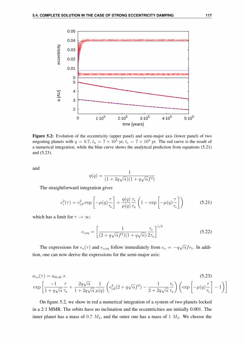
5.4. COMPLETE SOLUTION IN THE CASE OF STRONG ECCENTRICITY DAMPING 117
0
0.01
0.02
0.03
0.04
0.05
ecce
ntric
ity
2
3
4
5
0 1⋅105 2⋅105 3⋅105 4⋅105 5⋅105
a [A
U]
time [years]
Figure 5.2: Evolution of the eccentricity (upper panel) and semi-major axis (lower panel) of twomigrating planets with q = 0.7, ta = 7 × 10⁵ yr, te = 7 × 10³ yr. The red curve is the result ofa numerical integration, while the blue curve shows the analytical prediction from equations (5.21)and (5.23).
andη(q) =
1
(1 + 2q√α)(1 + q
√αf 2)
The straightforward integration gives
e2i (τ) = e2
i,0 exp
[−µ(q)
τ
τe
]+η(q)
µ(q)
τeτa
(1− exp
[−µ(q)
τ
τe
])(5.21)
which has a limit for τ →∞:
ei,eq =
[1
(2 + q√αf 2)(1 + q
√α)
τe2τa
]1/2
(5.22)
The expressions for eo(τ) and eo,eq follow immediately from eo = −q√αfei. In addi-
tion, one can now derive the expressions for the semi-major axis:
ai,o(τ) = ai0,o0× (5.23)
exp
[−1
1 + q√α
τ
τa+
2q√α
1 + 2q√α
1
µ(q)
(e2
i,0(2 + q√αf 2)− 1
2 + 2q√α
τeτa
)(exp
[−µ(q)
τ
τe
]− 1
)]
On figure 5.2, we show in red a numerical integration of a system of two planets lockedin a 2:1 MMR. The orbits have no inclination and the eccentricities are initially 0.001. Theinner planet has a mass of 0.7 MJ, and the outer one has a mass of 1 MJ. We choose the
118 5. RESONANT MIGRATION
timescales to be ta = 7 × 10⁵ yr and te = 7 × 10³ yr (equivalent to K = 100, regimeof strong damping). Not surprisingly, we find that the eccentricities are kept to very lowvalues throughout the integration. In blue, we also plot the analytical results given by equa-tions (5.21) and (5.23). Regarding the semi-major axis, the agreement is very good. Theinner eccentricity (upper curve) reaches an equilibrium value that agrees with the analyticalestimate to within a few percent. The only major disagreement comes from the outer eccen-tricity, which reaches an equilibrium whose value is roughly half of that predicted by thetheory. Recall that our calculation is based on the assumption that d$i/dτ = d$o/dτ , butthe evolutions of the apses are known only to zero-th order.

Chapter 6
Conclusions
Contents6.1 Summary . . . . . . . . . . . . . . . . . . . . . . . . . . . . . . . . . . 119
6.2 Perspectives . . . . . . . . . . . . . . . . . . . . . . . . . . . . . . . . 121
6.1 Summary
In this thesis we have studied some aspects of the planet-disc interactions. We have focused,both analytically and numerically, on the possibility for the disc to excite and/or maintain aplanet, or a system of planets, at large eccentricities and inclinations.
The fate of planets inclined with respect to a disc
The first problem that we have investigated is the evolution of a planet whose orbit is mis-aligned with respect to a disc. We have modelled the disc as a 3D potential and included thefriction that the planet undergoes when crossing the disc, twice per orbit. We have ignoredthe back reaction of the planet on the disc, an assumption well justified as long as the discis more massive than the planet. We show that the disc naturally excites the eccentricity andinclination of the planet when the inclination between the two is larger than a critical angle,whose value can be as low as 20. This is equivalent to the well-known Kozai mechanismin 3-body systems. The orbital elements of the planet are damped to low values by the fric-tion, but also undergo periodic variations caused by the Kozai mechanism. These variationsexcite the eccentricity that would otherwise be kept at low values by the friction. However,the same variations cause the inclination to go to low values, where it spends more time inthe disc (i.e., where it is more affected by friction). Therefore, damping by friction is overallenhanced by this process.
We find that Jupiter mass planets and above realign with the plane of the disc on atimescale shorter than the disc’s lifetime. However, Neptune mass planets are kept on in-clined orbits for longer than the disc’s lifetime. In addition, the Kozai mechanism causes
119

120 6. CONCLUSIONS
their eccentricity to reach high values. Therefore, Neptune mass planets can naturally re-main misaligned and eccentric. Currently, there is no observational evidence of a populationof Neptune mass planets on inclined and eccentric orbits. For instance, the Kepler samplesupports the idea that low-mass planets have low inclinations and low eccentricities. Oncewe will have removed the observational bias that does not favour the detection of long-period, low mass planets, we expect this to be confirmed. On the other hand, it is possiblethat Jupiter mass planets have been misaligned; their fast realignment would make it im-possible for us to disentangle between them and the population of planets that formed andstayed in their disc. However, it seems that the disc-induced Kozai oscillations of a massiveplanet on an inclined orbit cannot explain the population of misaligned hot Jupiters.
We have also shown that when two planets orbit the star and are perturbed by the disc, thelatter usually dominated their evolution. Planet-planet interaction, however, can sometimeslead to chaotic evolution of the system.
A possible mechanism to generate inclined orbits using disc migration
The second problem that we have studied naturally arises when studying planets which aremisaligned with respect to their disc: “how did the planet(s) get this primordial inclinationin the first place”. In Teyssandier et al. (2013b) we have given a few suggestions regard-ing when this situation could occur. In Teyssandier and Terquem (2014), we have studiedone specific scenario in details. In this scenario, two planets migrate in a disc, and entera mean motion resonance. Exchange of angular momentum while the planets are lockedin resonance leads to an increase of the eccentricities. Under the combined effects of res-onant migration and damping from the disc, eccentricities eventually reach an equilibriumvalue. In addition, an other type of resonance can also appear when second-order termsin the disturbing function are included. They correspond to an inclination-type resonance,in which the inclinations rapidly reach very high values. We have shown that the onsetof this inclination-type resonance can only be achieved if the eccentricities become higherthan a critical value. This allows us to derive a criterion for the onset of inclination–typeresonance: the equilibrium value reached by the eccentricity because of the disc dampinghas to be higher than the critical value needed to trigger the inclination–type resonance.We find that this criterion is weakly dependant on the mass ratio between the two planets.However, it is strongly dependant on the ratio of the eccentricity damping timescale and theorbital decay timescale. We find that this ratio has to be larger than a few 10−1 in order forinclination–type resonances to become possible. However, both observations and numeri-cal simulations tend to indicate that this ratio cannot exceed a few 10−2. We conclude thatthe excitation of inclinations through resonant migration of a pair of planets embedded ina disc is very unlikely. This seems to be supported by the fact that multiple systems in theKepler sample, including those in, or close to, mean motion resonances, appear to have lowinclinations and eccentricities.

6.2. PERSPECTIVES 121
Final remarks
The conclusions of this thesis seem to indicate that it is unlikely that planets as massiveas Jupiter have been strongly misaligned with the disc, or that they could maintain suchinclination. First, strong eccentricity damping prevents them from being kicked out of theplane of the disc through resonant migration mechanisms. In addition, even if the planetmanages to become misaligned (for instance if they have formed by fragmentation of theenvelope, or if they are captured during a close encounter with another star), they wouldtend to realign quickly with the disc. Only low mass planets could remain inclined andeccentric.
These results give constraints on the early stages of the evolution of planetary systems.They support the evidence that eccentricity damping in a disc is strong enough to keepthe planets in the disc. They also indicate that Neptune mass planets are not expected tohave been misaligned with their disc, otherwise we could still see consequences of thismisalignment today. However, if massive planets have formed through gravitational collapsein the protostellar envelope, their should be very little evidence to support this theory, asthey are expected to realign with the disc, and therefore mix with the population of massiveplanets formed in a disc.
6.2 Perspectives
There are several points in this thesis that currently remain unsolved. As we have seen, itis hard to do a global parametric survey of the interactions between two planets on orbitsthat are inclined with respect to a disc. If those planets formed via gravitational collapseof a protostellar envelope, then we can actually expect more than two massive planets to beformed, making the evolution even harder to predict. In addition, the action of a populationof massive planets on a disc could significantly alter the structure of the latter, making ourmodel unreliable. A way of avoiding this issue could be to properly model the response ofthe disc using hydrodynamical simulations. Such simulations have already been conductedfor a single massive planet (see, e.g., Xiang-Gruess and Papaloizou, 2013; Bitsch et al.,2013), but could be extended to the low-mass planets regime. It should also be noted thatthese simulations have note explored yet multiplanet systems.
Following on the work we have presented in section 4.6, we have noticed that numericalsimulations of systems of two planets inclined with respect to a disc often lead to unstableorbits. The question of the stability of such systems should be addressed more carefully,and requires high-precision numerical simulations, in order to insure a good conservation ofenergy.
In addition, we have noted in our simulations that the resonant capture of an inner planetby an outer, inward migrating planet can also happen if the mutual inclination between thetwo planets is initially high. Hence, if an inner planet has cleared a cavity between the inner

122 6. CONCLUSIONS
edge of the disc and the star, and is highly inclined with respect to the plane of the disc(because of some possible scattering event), it could in principle be pushed even further infollowing its subsequent capture in resonance by an outer planet. This could further increaseits inclination and eccentricity and produce a short-period misaligned planet. However, theprobability of such event to occur is expected to be rather low, but should be tested in moredetails.
To finish, our work could also be extended to other types of resonances. It could beinteresting, for instance, to test configurations like the 3:2 MMR of the planets orbiting HD45364. The 3:2 MMR being interior to the 2:1, this configuration probably required a fastmigration, which would reduce the probability of capture in the 2:1 MMR. As we have seen,the onset of inclination-type resonance strongly depends on the ratio between the eccentric-ity damping timescale and the migration timescale. For a fast type III migration, this ratiocould be closer to unity than in the case of the “slow” type II migration, and it would beinteresting the investigate the behaviour of the inclinations in this regime. In addition, wehave not investigated higher order resonances such as the 3:1 MMR. While they are difficultto investigate analytically, because of the necessity of including several high-order termsin inclinations and eccentricities, they can be studied numerically. Finally, we remark thatwe have used prescriptions for the migration and damping. However, planet migration canbe more complicated, with stochastic terms that depart from the smooth inward migrationscenario we have envisioned here. Again, it would be interesting to see if full 3D hydrody-namical simulations also reveal the onset of inclination-type resonances in specific regimes.
More globally, the study of planetary systems (including that of our own solar system)still comes with many unsolved problems. Many of them require a good understandingof planet-disc interactions. For instance, the importance of the corotation torque on theevolution of migrating planets was only fully appreciated in the last few years and is now avery active field of research. In addition, complex physical behaviours, resulting for instancefrom magnetic fields or turbulence in the disc, can affect the migration. As a result, theresonant locking of a pair of planets might be complicated, and brief episodes of divergentmigration might explain some of the observed statistical properties of exoplanets, such asthe excess of pairs just outside mean-motion resonances seen by Kepler. More generally, it iscertain that planet-disc interactions will shape the planetary system, by distributing the semi-major axis, eccentricities and inclinations in a way that is not fully understood today. Assuch, they are a key component to understand the subsequent evolution of planetary systemsonce the disc has vanished, and to explain the wonderful variety of planetary systems as wepresently see them.

Bibliography
Adams, F. C. and Laughlin, G. (2003). Migration and dynamical relaxation in crowdedsystems of giant planets. Icarus, 163:290–306.
Albrecht, S., Winn, J. N., Johnson, J. A., Howard, A. W., Marcy, G. W., Butler, R. P.,Arriagada, P., Crane, J. D., Shectman, S. A., Thompson, I. B., Hirano, T., Bakos, G.,and Hartman, J. D. (2012). Obliquities of Hot Jupiter Host Stars: Evidence for TidalInteractions and Primordial Misalignments. ApJ, 757:18.
Artymowicz, P. (1993). On the Wave Excitation and a Generalized Torque Formula forLindblad Resonances Excited by External Potential. ApJ, 419:155.
Barnes, J. W., van Eyken, J. C., Jackson, B. K., Ciardi, D. R., and Fortney, J. J. (2013).Measurement of Spin-orbit Misalignment and Nodal Precession for the Planet aroundPre-main-sequence Star PTFO 8-8695 from Gravity Darkening. ApJ, 774:53.
Batygin, K. and Morbidelli, A. (2013). Dissipative Divergence of Resonant Orbits. Astro-
nomical Journal, 145:1.
Belorizky, D. (1938). Le Soleil, Etoile Variable. L’Astronomie, 52:359–361.
Binney, J. and Tremaine, S. (1987). Galactic dynamics.
Bitsch, B., Crida, A., Libert, A.-S., and Lega, E. (2013). Highly inclined and eccentricmassive planets. I. Planet-disc interactions. A&A, 555:A124.
Bitsch, B. and Kley, W. (2010). Orbital evolution of eccentric planets in radiative discs.A&A, 523:A30.
Bitsch, B. and Kley, W. (2011). Evolution of inclined planets in three-dimensional radiativediscs. A&A, 530:A41.
Boss, A. P. (1997). Giant planet formation by gravitational instability. Science, 276:1836–1839.
Bouvier, J., Alencar, S. H. P., Boutelier, T., Dougados, C., Balog, Z., Grankin, K., Hodgkin,S. T., Ibrahimov, M. A., Kun, M., Magakian, T. Y., and Pinte, C. (2007). Magnetosphericaccretion-ejection processes in the classical T Tauri star AA Tauri. A&A, 463:1017–1028.
123

124 BIBLIOGRAPHY
Brouwer, D. and Clemence, G. M. (1961). Methods of celestial mechanics. Academic Press.
Burns, J. A. (1976). Elementary derivation of the perturbation equations of celestial me-chanics. American Journal of Physics, 44:944–949.
Cassan, A., Kubas, D., Beaulieu, J.-P., Dominik, M., Horne, K., Greenhill, J., Wambsganss,J., Menzies, J., Williams, A., Jørgensen, U. G., Udalski, A., Bennett, D. P., Albrow, M. D.,Batista, V., Brillant, S., Caldwell, J. A. R., Cole, A., Coutures, C., Cook, K. H., Dieters,S., Prester, D. D., Donatowicz, J., Fouqué, P., Hill, K., Kains, N., Kane, S., Marquette,J.-B., Martin, R., Pollard, K. R., Sahu, K. C., Vinter, C., Warren, D., Watson, B., Zub,M., Sumi, T., Szymanski, M. K., Kubiak, M., Poleski, R., Soszynski, I., Ulaczyk, K.,Pietrzynski, G., and Wyrzykowski, Ł. (2012). One or more bound planets per Milky Waystar from microlensing observations. Nature, 481:167–169.
Charbonneau, D., Brown, T. M., Latham, D. W., and Mayor, M. (2000). Detection ofPlanetary Transits Across a Sun-like Star. ApJL, 529:L45–L48.
Correia, A. C. M., Udry, S., Mayor, M., Benz, W., Bertaux, J.-L., Bouchy, F., Laskar,J., Lovis, C., Mordasini, C., Pepe, F., and Queloz, D. (2009). The HARPS search forsouthern extra-solar planets. XVI. HD 45364, a pair of planets in a 3:2 mean motionresonance. A&A, 496:521–526.
D’Alessio, P., Canto, J., Calvet, N., and Lizano, S. (1998). Accretion Disks around YoungObjects. I. The Detailed Vertical Structure. ApJ, 500:411.
Davies, M. B., Adams, F. C., Armitage, P., Chambers, J., Ford, E., Morbidelli, A., Raymond,S. N., and Veras, D. (2013). The Long-Term Dynamical Evolution of Planetary Systems.ArXiv e-prints.
Fabrycky, D. and Tremaine, S. (2007). Shrinking Binary and Planetary Orbits by KozaiCycles with Tidal Friction. ApJ, 669:1298–1315.
Fabrycky, D. C., Lissauer, J. J., Ragozzine, D., Rowe, J. F., Agol, E., Barclay, T., Batalha,N., Borucki, W., Ciardi, D. R., Ford, E. B., Geary, J. C., Holman, M. J., Jenkins, J. M.,Li, J., Morehead, R. C., Shporer, A., Smith, J. C., Steffen, J. H., and Still, M. (2012).Architecture of Kepler’s Multi-transiting Systems: II. New investigations with twice asmany candidates. ArXiv e-prints.
Fendyke, S. M. and Nelson, R. P. (2014). On the corotation torque for low-mass eccentricplanets. MNRAS, 437:96–107.
Fernandez, J. A. and Ip, W.-H. (1984). Some dynamical aspects of the accretion of Uranusand Neptune - The exchange of orbital angular momentum with planetesimals. Icarus,58:109–120.

BIBLIOGRAPHY 125
Fischer, D., Howard, A., Laughlin, G., Macintosh, B., Mahadevan, S., Sahlmann, J., andYee, J. (2013). Exoplanet Detection Techniques. Protostars and Planet VI.
Goldreich, P. (1965). An explanation of the frequent occurrence of commensurable meanmotions in the solar system. MNRAS, 130:159.
Goldreich, P. and Tremaine, S. (1979). The excitation of density waves at the Lindblad andcorotation resonances by an external potential. ApJ, 233:857–871.
Goldreich, P. and Tremaine, S. (1980). Disk-satellite interactions. ApJ, 241:425–441.
Greaves, J. S., Kennedy, G. M., Thureau, N., Eiroa, C., Marshall, J. P., Maldonado, J.,Matthews, B. C., Olofsson, G., Barlow, M. J., Moro-Martín, A., Sibthorpe, B., Absil, O.,Ardila, D. R., Booth, M., Broekhoven-Fiene, H., Brown, D. J. A., Cameron, A. C., delBurgo, C., Di Francesco, J., Eislöffel, J., Duchêne, G., Ertel, S., Holland, W. S., Horner,J., Kalas, P., Kavelaars, J. J., Lestrade, J.-F., Vican, L., Wilner, D. J., Wolf, S., and Wyatt,M. C. (2014). Alignment in star-debris disc systems seen by Herschel. MNRAS, 438:L31–L35.
Greenberg, R. (1977). Orbit-orbit resonances in the solar system - Varieties and similarities.Vistas in Astronomy, 21:209–239.
Hahn, J. M. and Malhotra, R. (1999). Orbital Evolution of Planets Embedded in a Planetes-imal Disk. Astronomical Journal, 117:3041–3053.
Hébrard, G., Bouchy, F., Pont, F., Loeillet, B., Rabus, M., Bonfils, X., Moutou, C., Boisse,I., Delfosse, X., Desort, M., Eggenberger, A., Ehrenreich, D., Forveille, T., Lagrange,A.-M., Lovis, C., Mayor, M., Pepe, F., Perrier, C., Queloz, D., Santos, N. C., Ségransan,D., Udry, S., and Vidal-Madjar, A. (2008). Misaligned spin-orbit in the XO-3 planetarysystem? A&A, 488:763–770.
Henry, G. W., Marcy, G. W., Butler, R. P., and Vogt, S. S. (2000). A Transiting “51 Peg-like”Planet. ApJL, 529:L41–L44.
Howell, S. B., Everett, M. E., Esquerdo, G., Davis, D. R., Weidenschilling, S., and van Lew,T. (1999). Photometric Search for Extra-Solar Planets. In Craine, E. R., Crawford, D. L.,and Tucker, R. A., editors, Precision CCD Photometry, volume 189 of Astronomical So-
ciety of the Pacific Conference Series, page 170.
Innanen, K. A., Zheng, J. Q., Mikkola, S., and Valtonen, M. J. (1997). The Kozai Mecha-nism and the Stability of Planetary Orbits in Binary Star Systems. Astronomical Journal,113:1915.
Kley, W. and Nelson, R. P. (2012). Planet-Disk Interaction and Orbital Evolution. Annual
Review of Astronomy and Astrophysics, 50:211–249.
126 BIBLIOGRAPHY
Kley, W., Peitz, J., and Bryden, G. (2004). Evolution of planetary systems in resonance.A&A, 414:735–747.
Knutson, H. A., Fulton, B. J., Montet, B. T., Kao, M., Ngo, H., Howard, A. W., Crepp, J. R.,Hinkley, S., Bakos, G. Á., Batygin, K., Johnson, J. A., Morton, T. D., and Muirhead, P. S.(2014). Friends of Hot Jupiters. I. A Radial Velocity Search for Massive, Long-periodCompanions to Close-in Gas Giant Planets. ApJ, 785:126.
Kozai, Y. (1962). Secular perturbations of asteroids with high inclination and eccentricity.Astronomical Journal, 67:591.
Lee, M. H. and Peale, S. J. (2002). Dynamics and Origin of the 2:1 Orbital Resonances ofthe GJ 876 Planets. ApJ, 567:596–609.
Lee, M. H. and Thommes, E. W. (2009). Planetary Migration and Eccentricity and Inclina-tion Resonances in Extrasolar Planetary Systems. ApJ, 702:1662–1672.
Levison, H. F., Morbidelli, A., Gomes, R., and Backman, D. (2007). Planet Migration inPlanetesimal Disks. Protostars and Planets V, pages 669–684.
Libert, A.-S. and Tsiganis, K. (2009). Trapping in high-order orbital resonances and incli-nation excitation in extrasolar systems. MNRAS, 400:1373–1382.
Lidov, M. L. (1962). The evolution of orbits of artificial satellites of planets under theaction of gravitational perturbations of external bodies. Planetary and Space Science,9:719–759.
Lin, D. N. C. and Papaloizou, J. (1979). Tidal torques on accretion discs in binary systemswith extreme mass ratios. MNRAS, 186:799–812.
Lin, D. N. C. and Papaloizou, J. (1986). On the tidal interaction between protoplanets andthe protoplanetary disk. III - Orbital migration of protoplanets. ApJ, 309:846–857.
Lithwick, Y. and Wu, Y. (2011). Theory of Secular Chaos and Mercury’s Orbit. ApJ, 739:31.
Lithwick, Y. and Wu, Y. (2012). Resonant Repulsion of Kepler Planet Pairs. ApJL, 756:L11.
Lubow, S. H. and D’Angelo, G. (2006). Gas Flow across Gaps in Protoplanetary Disks.ApJ, 641:526–533.
Malmberg, D., Davies, M. B., and Heggie, D. C. (2011). The effects of fly-bys on planetarysystems. MNRAS, 411:859–877.
Marcy, G. W., Butler, R. P., Fischer, D., Vogt, S. S., Lissauer, J. J., and Rivera, E. J. (2001).A Pair of Resonant Planets Orbiting GJ 876. ApJ, 556:296–301.

BIBLIOGRAPHY 127
Masset, F. S. and Papaloizou, J. C. B. (2003). Runaway Migration and the Formation of HotJupiters. ApJ, 588:494–508.
Mayor, M. and Queloz, D. (1995). A Jupiter-mass companion to a solar-type star. Nature,378:355–359.
McLaughlin, D. B. (1924). Some results of a spectrographic study of the Algol system. ApJ,60:22–31.
Morbidelli, A., Tsiganis, K., Crida, A., Levison, H. F., and Gomes, R. (2007). Dynamicsof the Giant Planets of the Solar System in the Gaseous Protoplanetary Disk and TheirRelationship to the Current Orbital Architecture. Astronomical Journal, 134:1790–1798.
Murray, C. D. and Dermott, S. F. (1999). Solar system dynamics. Cambridge UniversityPress.
Naoz, S., Farr, W. M., Lithwick, Y., Rasio, F. A., and Teyssandier, J. (2011). Hot Jupitersfrom secular planet-planet interactions. Nature, 473:187–189.
Naoz, S., Farr, W. M., Lithwick, Y., Rasio, F. A., and Teyssandier, J. (2013). Seculardynamics in hierarchical three-body systems. MNRAS, 431:2155–2171.
Nobili, A. and Roxburgh, I. W. (1986). Simulation of general relativistic corrections in longterm numerical integrations of planetary orbits. In Kovalevsky, J. and Brumberg, V. A.,editors, Relativity in Celestial Mechanics and Astrometry. High Precision Dynamical The-
ories and Observational Verifications, volume 114 of IAU Symposium, pages 105–110.
Ogilvie, G. I. and Lubow, S. H. (2002). On the wake generated by a planet in a disc. MNRAS,330:950–954.
O’Toole, S. J., Tinney, C. G., Jones, H. R. A., Butler, R. P., Marcy, G. W., Carter, B., andBailey, J. (2009). Selection functions in doppler planet searches. MNRAS, 392:641–654.
Papaloizou, J. C. B. and Larwood, J. D. (2000). On the orbital evolution and growth ofprotoplanets embedded in a gaseous disc. MNRAS, 315:823–833.
Papaloizou, J. C. B., Nelson, R. P., and Masset, F. (2001). Orbital eccentricity growththrough disc-companion tidal interaction. A&A, 366:263–275.
Papaloizou, J. C. B. and Terquem, C. (2001). Dynamical relaxation and massive extrasolarplanets. MNRAS, 325:221–230.
Papaloizou, J. C. B. and Terquem, C. (2010). On the dynamics of multiple systems of hotsuper-Earths and Neptunes: tidal circularization, resonance and the HD 40307 system.MNRAS, 405:573–592.
128 BIBLIOGRAPHY
Peale, S. J. (1976). Orbital resonances in the solar system. Annual Review of Astronomy and
Astrophysics, 14:215–246.
Pollack, J. B., Hubickyj, O., Bodenheimer, P., Lissauer, J. J., Podolak, M., and Greenzweig,Y. (1996). Formation of the Giant Planets by Concurrent Accretion of Solids and Gas.Icarus, 124:62–85.
Queloz, D., Eggenberger, A., Mayor, M., Perrier, C., Beuzit, J. L., Naef, D., Sivan, J. P.,and Udry, S. (2000). Detection of a spectroscopic transit by the planet orbiting the starHD209458. A&A, 359:L13–L17.
Quillen, A. C. (2006). Reducing the probability of capture into resonance. MNRAS,365:1367–1382.
Rasio, F. A. and Ford, E. B. (1996). Dynamical instabilities and the formation of extrasolarplanetary systems. Science, 274:954–956.
Raymond, S. N., Barnes, R., Armitage, P. J., and Gorelick, N. (2008). Mean Motion Reso-nances from Planet-Planet Scattering. ApJL, 687:L107–L110.
Rein, H. (2012). Planet-disc interaction in highly inclined systems. MNRAS, 422:3611–3616.
Rein, H. and Papaloizou, J. C. B. (2009). On the evolution of mean motion resonancesthrough stochastic forcing: fast and slow libration modes and the origin of HD 128311.A& A, 497:595–609.
Rein, H., Papaloizou, J. C. B., and Kley, W. (2010). The dynamical origin of the multi-planetary system HD 45364. A&A, 510:A4.
Rivera, E. J., Laughlin, G., Butler, R. P., Vogt, S. S., Haghighipour, N., and Meschiari, S.(2010). The Lick-Carnegie Exoplanet Survey: a Uranus-Mass Fourth Planet for GJ 876in an Extrasolar Laplace Configuration. ApJ, 719:890–899.
Rossiter, R. A. (1924). On the detection of an effect of rotation during eclipse in the velocityof the brigher component of beta Lyrae, and on the constancy of velocity of this system.ApJ, 60:15–21.
Shakura, N. I. and Sunyaev, R. A. (1973). Black holes in binary systems. Observationalappearance. A&A, 24:337–355.
Snellgrove, M. D., Papaloizou, J. C. B., and Nelson, R. P. (2001). On disc driven inwardmigration of resonantly coupled planets with application to the system around GJ876.A&A, 374:1092–1099.

BIBLIOGRAPHY 129
Takeda, G., Kita, R., and Rasio, F. A. (2008). Planetary Systems in Binaries. I. DynamicalClassification. ApJ, 683:1063–1075.
Terquem, C. and Ajmia, A. (2010). Eccentricity pumping of a planet on an inclined orbit bya disc. MNRAS, 404:409–414.
Terquem, C. and Papaloizou, J. C. B. (2002). Dynamical relaxation and the orbits of low-mass extrasolar planets. MNRAS, 332:L39–L43.
Terquem, C. and Papaloizou, J. C. B. (2007). Migration and the Formation of Systems ofHot Super-Earths and Neptunes. ApJ, 654:1110–1120.
Terquem, C. E. J. M. L. J. (2003). Stopping inward planetary migration by a toroidal mag-netic field. MNRAS, 341:1157–1173.
Teyssandier, J., Naoz, S., Lizarraga, I., and Rasio, F. A. (2013a). Extreme Orbital Evolutionfrom Hierarchical Secular Coupling of Two Giant Planets. ApJ, 779:166.
Teyssandier, J. and Terquem, C. (2014). Evolution of eccentricity and orbital inclination ofmigrating planets in 2:1 mean motion resonance. To appear in MNRAS.
Teyssandier, J., Terquem, C., and Papaloizou, J. C. B. (2013b). Orbital evolution of a planeton an inclined orbit interacting with a disc. MNRAS, 428:658–669.
Thommes, E. W. and Lissauer, J. J. (2003). Resonant Inclination Excitation of MigratingGiant Planets. ApJ, 597:566–580.
Triaud, A. H. M. J., Collier Cameron, A., Queloz, D., Anderson, D. R., Gillon, M., Hebb, L.,Hellier, C., Loeillet, B., Maxted, P. F. L., Mayor, M., Pepe, F., Pollacco, D., Ségransan,D., Smalley, B., Udry, S., West, R. G., and Wheatley, P. J. (2010). Spin-orbit anglemeasurements for six southern transiting planets. New insights into the dynamical originsof hot Jupiters. A&A, 524:A25.
Trilling, D. E., Benz, W., Guillot, T., Lunine, J. I., Hubbard, W. B., and Burrows, A. (1998).Orbital Evolution and Migration of Giant Planets: Modeling Extrasolar Planets. ApJ,500:428.
Valtonen, M. and Karttunen, H. (2006). The Three-Body Problem.
Vokrouhlicky, D. and Karas, V. (1998). Stellar dynamics in a galactic centre surrounded bya massive accretion disc - I. Newtonian description. MNRAS, 298:53–66.
Ward, W. R. (1997). Protoplanet Migration by Nebula Tides. Icarus, 126:261–281.

130 BIBLIOGRAPHY
Watson, C. A., Littlefair, S. P., Diamond, C., Collier Cameron, A., Fitzsimmons, A., Simp-son, E., Moulds, V., and Pollacco, D. (2011). On the alignment of debris discs and theirhost stars’ rotation axis - implications for spin-orbit misalignment in exoplanetary sys-tems. MNRAS, 413:L71–L75.
Weidenschilling, S. J. and Marzari, F. (1996). Gravitational scattering as a possible originfor giant planets at small stellar distances. Nature, 384:619–621.
Williams, J. P. and Cieza, L. A. (2011). Protoplanetary Disks and Their Evolution. Annual
Review of Astronomy and Astrophysics, 49:67–117.
Winn, J. N., Johnson, J. A., Fabrycky, D., Howard, A. W., Marcy, G. W., Narita, N., Cross-field, I. J., Suto, Y., Turner, E. L., Esquerdo, G., and Holman, M. J. (2009). On theSpin-Orbit Misalignment of the XO-3 Exoplanetary System. ApJ, 700:302–308.
Wolszczan, A. and Frail, D. A. (1992). A planetary system around the millisecond pulsarPSR1257 + 12. Nature, 355:145–147.
Wu, Y. and Lithwick, Y. (2011). Secular Chaos and the Production of Hot Jupiters. ApJ,735:109.
Xiang-Gruess, M. and Papaloizou, J. C. B. (2013). Interaction between massive planets oninclined orbits and circumstellar discs. MNRAS, 431:1320–1336.

Appendix A
Laplace coefficients
We saw that writting down the disturbing function leads to terms of the following form:
(r2
1 + r22 − 2r1r2 cosφ
)−1/2.
Using a Taylor series expansion, some terms appear of the form
ρ(α) =(1 + α2 − 2α cosψ
)−s, (A.1)
where α, in this case, would be the semi-major axis ratio (see, e.g., Murray and Dermott,1999, for more details). The function ρ is 2π periodic in ψ.
We recall that if fs is a periodic function of period P , then it can be expanded in Fourierseries:
fs(x) =1
2a0s +
∞∑
j=1
ajs cos(kψ). (A.2)
where the ajs are the Fourier coefficients, defined by:
ajs =2
P
∫ P
0
fs(x) cos
(2πjx
P
)dx. (A.3)
In our case we have
(1 + α2 − 2α cosψ
)−s=
1
2b(0)s (α) +
∞∑
j=1
b(j)s (α) cos(jψ) (A.4)
where the Laplace coefficients, noted b(j)s are defined by:
b(j)s (α) =
1
π
∫ 2π
0
cos(jψ)dψ(1− 2α cosψ + α2)s
(A.5)
where s is a half-integer. They can also be expressed by a series always convergent for
131
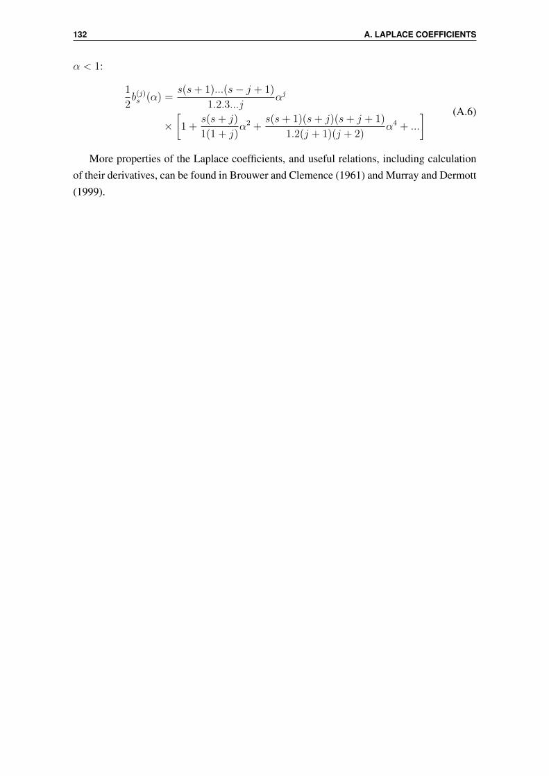
132 A. LAPLACE COEFFICIENTS
α < 1:
1
2b(j)s (α) =
s(s+ 1)...(s− j + 1)
1.2.3...jαj
×[1 +
s(s+ j)
1(1 + j)α2 +
s(s+ 1)(s+ j)(s+ j + 1)
1.2(j + 1)(j + 2)α4 + ...
] (A.6)
More properties of the Laplace coefficients, and useful relations, including calculationof their derivatives, can be found in Brouwer and Clemence (1961) and Murray and Dermott(1999).

Appendix B
Complements on the Kozai mechanism
In this appendix we solve the integral which gives the relation between the argument of peri-center ω and the time τ , and show that its solution depends upon the value of the inclinationwith respect to a critical value of 39.23.
The argument of pericenter is linked to the time variable τ via the following equation:
τ =
∫ ω
ω0
dω′
a+ b sin2 ω′, (B.1)
where a = 3/2 and b = −(15/4) sin2 I . We therefore seek the solutions of the followingintegral:
I =
∫ x2
x1
dxa+ b sin2 x
. (B.2)
Using the relation sin2 x = (1− cos 2x)/2, this integrale can be re-written
I =
∫ 2x2
2x1
dxc+ d cosx
, (B.3)
with c = 2a + b and d = −b. We now set t = tan(x/2), such as cosx = (1− t2)/(1 + t2)
and dx = 2dt/(1 + t2). It follows that:
I =2
c+ d
∫ t2
t1
dt1 + c−d
c+dt2. (B.4)
From here we have two distinct cases, depending on the sign of (c− d)/(c+ d).
Case (c− d)/(c+ d) > 0
If (c− d)/(c+ d) > 0, we set y = βt, with β =√
(c− d)/(c+ d). Hence:
I =2√
(c+ d)(c− d)
∫ y2
y1
dy1 + y2
. (B.5)
133

134 B. COMPLEMENTS ON THE KOZAI MECHANISM
Finally, in terms of the initial variables, we get
I =1√
a(a+ b)
[arctan
(√a+ b
atan(x
2
))]2x2
2x1
. (B.6)
Case (c− d)/(c+ d) < 0
If (c− d)/(c+ d) < 0, we set y = βt, with β =√−(c− d)/(c+ d). Hence:
I =2√
−(c+ d)(c− d)
∫ y2
y1
dy1− y2
. (B.7)
Using the identity1
1− y2=
1
2(1− y)+
1
2(1 + y), (B.8)
we findI =
2√d2 − c2
[lny + 1
y − 1
]y2
y1
, (B.9)
which we re-write:
I =1
2√−a(a+ b)
[ln
(a+ b) tan x2−√−a(a+ b)
(a+ b) tan x2
+√−a(a+ b)
]2x2
2x1
. (B.10)
We note that the condition (c − d)/(c + d) > 0 is equivalent to c2 > d2, which in turnis the same as a(a + b) > 0. Similarly, (c − d)/(c + d) < 0 is equivalent to a(a − b) < 0.Therefore, all the quantities in the square roots and logarithms are well-defined. Hence wehave:
∫ ω
ω0
dωa+ b sin2 ω
=
1√a(a+b)
arctan
[(a+b) tanω√
a(a+b)
]if a(a+ b) > 0
1
2√−a(a+b)
ln
[(a+b) tanω−
√−a(a+b)
(a+b) tanω+√−a(a+b)
]if a(a+ b) < 0.
(B.11)
To derive this solution we have assumed w0 = π/2 when τ = 0 for the case I > 39.23,and w0 = 0 when τ = 0 for the case I < 39.23. This allows us to get rid of integrationconstants without loss of generality.
Futhermore, we have:
a(a+b) > 0 ⇐⇒ 3
2
(3
2− 15
4sin2 I
)> 0 ⇐⇒ sin2 I <
2
5⇐⇒ I < 39.23 or I > 140.77
and similarlya(a+ b) < 0 ⇐⇒ 39.23 < I < 140.77.
We restrict ourselves to the case I < 90 but symmetrical results yield for I > 90. The
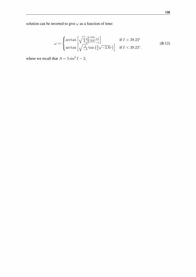
135
solution can be inverted to give ω as a function of time:
ω =
arctan[√
2A
e32
√2Aτ+1
e32
√2Aτ−1
]if I > 39.23
arctan[√
2−A tan
(34
√−2Aτ
)]if I < 39.23.
(B.12)
where we recall that A = 5 sin2 I − 2.

136 B. COMPLEMENTS ON THE KOZAI MECHANISM