Aerodynamic Analysis of a Winged Sub-Orbital Spaceplane

B. Geiben∗, F. Götten∗†, M. Havermann∗

∗ Department of Aerospace Engineering, FH Aachen University of Applied Sciences, Aachen, Germany† School of Engineering, RMIT University, Melbourne, Australia

Abstract

This paper primarily presents an aerodynamic CFD analysis of a winged spaceplane geometry based on theJapanese Space Walker proposal. StarCCM+ was used to calculate aerodynamic coefficients for a typicalspace flight trajectory including super-, trans- and subsonic Mach numbers and two angles of attack. Since thesolution of the RANS equations in such supersonic flight regimes is still computationally expensive, inviscidEuler simulations can principally lead to a significant reduction in computational effort. The impact on accuracyof aerodynamic properties is further analysed by comparing both methods for different flight regimes up to aMach number of 4.

KeywordsSpaceplane; Sub-Orbital; CFD; RANS; Euler; Supersonic Flow

NOMENCLATURE

Latin Letters

AoA ° Angle of attackCD [-] Coefficient of dragCL [-] Coefficient of liftCM [-] Coefficient of momentH km AltitudeL/D [-] Lift-to-drag ratioM [-] Mach numberM kg kmol−1 Molar massp Pa PressureR J kg−1 K−1 Specific gas constantR Jmol−1 K−1 Universal gas constantT K Temperatureu ms−1 Velocityy+ [-] Normalised wall distance

Greek Letters

α ° Angle of attackγ [-] Isentropic exponentµ Pa s Dynamic viscosityρ kgm−3 Densityτ Pa Stress tensor

Subscripts & Superscripts

( )∞ Freestream condition( )′ Fluctuating state

( ) Averaged state

Acronyms & Abbreviations

BC Boundary conditionCFL Courant-Friedrichs-Lewy No.C.O.G. Centre of gravityLEO Low Earth orbit

MAC Mean aerodynamic chordN-S Navier-StokesRANS Reynolds-averaged N-SS-A Spalart-AllmarasSTSO Space Shuttle OrbiterWISP Studied Winged Spaceplane

1. INTRODUCTION

The study and development of spaceplane-like vehi-cles for various applications, ranging from scientificto commercial proposals, has gained popularity in thelast decades. While many spaceplanes have beenproposed in the last century, very few vehicles haveachieved operational status or entered full-size test-ing. With increasing space commercialisation by pri-vate companies and launch providers, the demandfor space return vehicles has increased considerably.This is partly based on the imminent exit and lack ofcompetitiveness within government-driven space util-isation. With that and the emergent hope for spacetourism as the next step in space commercialisation,spaceplane-like vehicles will play a major role in suchventures. This increases the demand for fast and reli-able prototyping and development, which can be pro-vided by means of modern CFD studies.

©2022 doi: 10.25967/530170

Deutscher Luft- und Raumfahrtkongress 2020DocumentID: 530170

1

This paper aims to deliver an aerodynamic CFDanalysis on a generic spaceplane geometry, basedon one of three openly available Space Walker pro-posals supported by JAXA [1], Figure 1. This classof sub-orbital vehicles can be used and adaptedfor various applications, including space tourismand smallsat launch services, concerning altitudesand Mach numbers of up to 120 km and M∞ = 4,respectively.A Reynolds-averaged Navier-Stokes (RANS) ap-proach is used in the CFD calculations to studyaerodynamic parameters at different flight regimes.Since these calculations are still time-consumingboth in preprocessing and processing, an Euler ap-proach is evaluated as a possibly faster alternative.The theoretical foundation suggest good results forreduced computational effort, due to lower resolvedmeshes, no boundary layer and less equations periteration to be solved. Nonetheless, the usefulness ofthe Euler approach has to be studied on a per casebasis to compare and compete with the inherentlymore accurate RANS calculations.

2. CFD SETUP AND METHODOLOGY

2.1. Model Geometry

The WISP geometry is partially based on the pub-licly available data from the Spacewalker project [1].In this case the specific geometry is modelled aftertheir smallest spaceplane proposal designed for sci-entific missions in sub-orbital or LEO configurations,Figure 1. The base geometry has a wingspan of 5.9mand an overall length of 9.5m and therefore resemblesa generic class of currently developed spaceplanes.From here on most design decisions in creating theWISP geometry were chosen to represent the gen-eral class of vehicles for an aerodynamic CFD study.

FIG 1. Top down view of the root geometry Spacewalkerscience mission spaceplane [1].

The entire vehicle, including the delta-wing-like struc-ture and dual rear stabilisers, has been modelled inOpenVSP (see Figures 2a and 2b) and exported as astereolithography file to be meshed and simulated inStarCCM+ [2]. Within OpenVSP a very fine discreti-sation has been chosen both to capture all geometricdetails and deliver a fine baseline model for the CFD

meshing [3]. Based on similar projects and the SpaceTransportation System Orbiter (STSO) configuration,the main wing profile was chosen to be a NACA four-digit series zero lift profile, NACA 0008, with the rearstabiliser profile being a NACA 0012 [4].

(a) Top down view of 3D model

(b) Side view of 3D model

FIG 2. Different model views from OpenVSP software

2.2. Meshing in StarCCM+

The stereolithography file of the Winged Spaceplane(WISP) model, containing the tessellation meshcreated by OpenVSP, is imported into StarCCM+ asa surface mesh. In this case, before meshing, somesurface repair operations had to be performed inorder to present a coherent and closed manifold tothe internal StarCCM+ mesher. The specific meshingprocedure is dependent on the corresponding CFDsimulation and setup. The following meshing setupis performed with a half spherical flow field aroundthe WISP model, Figure 3. The sphere is createdwith a diameter roughly twenty times the charac-teristic length of the craft [5] [6]. This results in ahalf spherical flow field, using the symmetry of thestudied problem, with a radius of 100m. The rear ofthe Spaceplane is located at the origin of the sphere.Particularly for sonic and supersonic operations, thefocus of the simulations, a non-central positioningof the craft can be advantageous. In these cases itallows for a larger downstream flow field, while theupstream flow field should not be affected due thephysical nature of supersonic flows.For this study, three different general meshes wereused, all based on the integrated unstructuredtrimmed cell mesher of StarCCM+ [7]: first, a flowdirection orientated high y+ mesh for RANS simu-lations; secondly, based on the first mesh, a shockadaptive mesh, refining cells with large density gra-dients and finally, a lower cell count mesh without aprism layer mesh for the Euler simulations. The Eulersimulation workflow is discussed further in section 4.

©2022

Deutscher Luft- und Raumfahrtkongress 2020

2

FIG 3. Half spherical flow field with 100 m radius.

In addition to the volume meshes, a surface remesherwas used in all cases ensuring full depiction of allgeometric features.

2.2.1. RANS Meshing

The RANS CFD meshing pipeline is based on a twostep system. The target is to create a coarser basemesh, which is computationally less expensive to theninitialise a density gradient refinement function overO(102) iterations. This adaptive mesh refinement isthen fed back into the trimmed cell mesher to cre-ate a second level mesh. Depending on the qual-ity of the results and the convergence behaviour, athird level mesh, Figure 4, might be created using thesame process. The refinement function is created asa field function in StarCCM+ 13.04, which calculatesthe density gradient of every cell in the mesh nor-malised to its size. The refinement function assignsa value to every cell, which is then exported into a re-finement table that in turn is loaded into the trimmedcell mesher.

def CellWidth:

pow(${Volume}, (1/3))

def DenGrad:

mag(grad(${Density}))*${CellWidth}

def Refinement:

((${WallDistance} < 0.02) ? 0 :

(${DenGrad} > 0.04) ?

max(${CellWidth}/2, 0.005) : 0)

The base mesh is constructed with multiple surfaceand volumetric refinements, a full surface remesh anda prism layer mesh. Most surface cells are between15mm and 60mm. The maximum cell size is only lim-ited by the cell size at the boundaries of the flow fieldand not artificially. Especially curves and other finegeometric features are further refined, which is effec-tively demonstrated by the span of cell size presenton the wing surface. From the largest cells on the up-per and lower side of the wing with 30mm, the featuresize is halved three times, over smaller cells (7.5mm)on the leading edge to the smallest cells on the wingtips at 3.75mm.The prism layer mesher discretises the boundarylayer region to be described by wall functions witha high y+ wall treatment. In this case eight to ten

FIG 4. Exemplary level three adaptive mesh.

prism layers are used with a target y+ = 30 firstcell height distributed by a “Hyperbolic Tangent”stretching function, as recommended in [6]. Both thetotal boundary layer thickness and the size of thelowest layer can be approximated beforehand. Whilethe (dynamic) viscosity, density and velocity (as afunction of the Mach number and temperature) arevariable on all tested configurations, the referencelength is constant and has been defined to be theoverall vehicle length of 9.5m. The different flightconfigurations and related atmospheric values canbe obtained from Table 1. After the initial meshing,the adaptive mesh procedure is carried out, whichresults in a level two adapted mesh with ∼ 2.5 · 106

cells. This can be seen in Figures 5a and 5b. Afteran additional iteration in the mesh adaption process,a level three adaptive mesh is generated. Such alevel three mesh can contain between ∼ 5 · 106 and∼ 12 · 106 cells, depending on the occurring shocksand density gradients.

(a) Near mesh view

(b) Mid mesh view

FIG 5. Different near-field views of a level two adaptedmesh with prism layers and rotated mesh.

2.3. CFD Setup in StarCCM+

From the internal StarCCM+ mesher the simulationfiles are prepared for both the different flight config-urations as well as the two solvers. All of the flight

©2022

Deutscher Luft- und Raumfahrtkongress 2020

3

configurations are derived from a typical descent of asub-orbital spaceplane, such as our WISP, with a ser-vice ceiling of around 100 km [1]. Such a flight profileallows mainly for two types of missions, either a self-powered payload acting as a boosted second stage(resulting in rather small final payload capacities) or ashort-term mission using the time in a low gravity andthin atmosphere environment. The time spent in suchconditions can range from seconds to a few minutes.The flight configurations tested during the descent ofthe craft are listed in Table 1, where missing valuessuch as density and velocity can be computed un-der the assumption of an ideal gas. The atmosphericconditions have been taken from the MSIS-E-90 at-mospheric model for mean solar activity [8].

TAB 1. WISP flight configurations for AoA = 20° andAoA = 40°.

M∞ H [km] T∞ [K] p∞ [kPa] µ∞ [Pa · s]

4 50 250 0.165 16.15 · 10−6

3 25 230 3.555 15.07 · 10−6

2.5 20 205 5.620 13.65 · 10−6

1.3 20 205 5.620 13.65 · 10−6

0.8 10 223 26.20 14.68 · 10−6

0.3 0 288.15 101.325 18.12 · 10−6

Most general settings in the StarCCM+ simulationfiles are identical for the RANS and Euler calcu-lations, specific solver and physics settings areoutlined in subsection 2.3.1 and 4.2, respectively.All simulations were set up for a steady state, usingthe three-dimensional coupled flow solver with airas an ideal gas. The reference pressure and initialconditions were all set according to the tested flightconfiguration from Table 1. The magnitude of thevelocity is computed as a function of the Mach num-ber and temperature (equation (1)), where γair = 1.4is the isentropic exponent and R is the specific gasconstant Rair = RM−1 = 287.1 J kg−1 K−1 [9]. (In theupper atmosphere the molar mass of air can deviateslightly, however, in the tested regimes this does nothave a significant impact [8].)

(1) u∞ = M∞ ·√γRT∞

The direction of the velocity vector is controlled glob-ally with a rotated coordinate system for AoA = 20° or40° operations. This global coordinate system is usedsimilarly in any related settings as well as the direc-tional meshing discussed in section 2.2.Due to the spherical shape of the flow field only threegeneral boundary conditions are in use. First, the“Wall” BC, applied to all surfaces of the WISP geom-etry; second, a “Symmetry” BC present at the mid-plane creating the half-spherical flow field. And fi-nally, the shell of the spherical flow field is set to a“Free Stream” BC with the flow direction, Mach num-ber, pressure and temperature defining it [7].

2.3.1. Spalart-Allmaras Turbulence Model

In addition to the physics models that are part of allsimulations, a RANS approach with a “High-ReynoldsNumber Spalart-Allmaras” to model the turbulencehas been chosen. The S-A model for external aero-dynamics both in incompressible and compressibleflow configurations is widely adopted and has beenvalidated extensively for such cases [10]. It is usedwith a modified high y+ approach to induce the use ofwall functions to model the lower part of the boundarylayer. The initial turbulence is specified as a turbulentviscosity ratio of 10.The convergence behaviour is evaluated under mul-tiple criteria. The weaker criterion is represented bya drop in residuals of three orders of magnitude ormore (≤ 1 · 10−3), whereas the stronger criterion isevaluated on the convergence of actual aerodynamiccoefficients. The lift coefficient and the lift-to-drag ra-tio are monitored during all simulations to determinethe convergence behaviour under consideration of theoverall residual behaviour.

3. RESULTS AND DISCUSSION

The major quantitative analyses of this study includelift, drag and moment coefficients plotted over a Machnumber sweep, a lift-to-drag ratio analysis, also as afunction of the Mach number and multiple lift and dragpolars for a landing configuration. For further insight apressure coefficient analysis is also performed at var-ious configurations. The landing configuration is com-posed of three additional RANS simulations at M = 0.3with varying angles of attack [11].Specific configuration values or definitions, such asthe landing Mach number or the definition of thereference area, are chosen in accordance with theSpace Shuttle Orbiter (STSO). The descent phaseof the STSO is aerodynamically well studied andhas delivered a lot of experimental and reliable datafor comparisons. Furthermore the STSO is, apartfrom the classified X37-B [12] and the Soviet Buran,the only generically shaped winged spaceplane withextensive datasets available [11] [13]. Therefore itrepresents a well-documented comparison point for apreliminary analysis [14].

3.1. Analysis of Aerodynamic Characteristics

Aerodynamic coefficients are computed for optimalcompatibility to other studies. The coefficients of lift,drag and momentum are functions of the referencearea, which is chosen in accordance with the maincomparison point STSO. The moment coefficient isalso dependent on a reference length and a workingpoint of the acting moments. For the delta-wing-likestructure of the WISP the reference length is calcu-lated as the mean aerodynamic chord (MAC) with1.814m. The working point of the acting moments isusually represented by the centre of gravity / mass(C.O.G.) of the craft and is designed to be of minimaldistance to the pressure point of the wing or lifting

©2022

Deutscher Luft- und Raumfahrtkongress 2020

4

body. Due to a lack of representative mass distribu-tion data, for this analysis the C.O.G. of the WISPis determined by the centre of volume, computed inOpenVSP. Therefore the momentum coefficient datain this analysis is only qualitative, but can be linearlytransformed for future reference, if the true C.O.G.is determined. The reference area is defined to bethe entire projected area of the WISP in accordanceto the reference area definition of the STSO, whichresults in SWISP = 21.04m2 and SSTSO = 249.9m2 [11].The first RANS analysis concerns the lift and drag be-haviour over the studied Mach number range at bothangles of attack, Figure 6. First of all, all graphs showthe expected general behaviour concerning a peak invalue around and after M = 1, conforming with thePrandtl-Glauert rule [15]. Therefore the overall qual-itative behaviour between the WISP and STSO coin-cide, with differences in the quantitative data. TheSTSO produces higher coefficients of lift in all con-figurations with its advantage ranging between 40%and 66%, Figure 6a. This is most easily attributed tothe large difference in the wing-to-fuselage ratio. (Thewing area is defined as stated previously.) Whereasthe STSO has a wing-to-fuselage ratio

SWing

SFuse

∣∣∣∣STSO

' 1.25 ,(2)

the WISP only presents a wing-to-fuselage ratio of

SWing

SFuse

∣∣∣∣WISP

= 0.53 .(3)

This effect is more predominant in low Mach numberscenarios (see landing configuration, Figure 8a and8b) and creates a significant difference in lift over theentire Mach number range.The larger wing area of the STSO, which is greatlybased on the much more elongated delta wing struc-ture than present at the WISP, does also create moredrag. This specific difference in the wing shape isalso clearly demonstrated in Figure 6b when compar-ing the difference in drag coefficients between AoA= 20° and 40°. With an increase in the angle of at-tack the elongated wing structure is further orientatedagainst the flow direction.With these two overlapping effects the lift-to-drag ra-tio, shown in Figure 7a, presents as expected. Theoverall behaviour is very similar in all configurations,but deviates most notably in the subsonic regime. Forlow Mach numbers the pressure distribution is dis-tinctly different than for supersonic Mach numbers,which indicates greater benefits from a larger wing-to-fuselage ratio for subsonic velocities. At 40° (. 45°)angle of attack the lift-to-drag ratio shows nearly Machindependent behaviour at around L/D ∼ 1. Suchstatic behaviour is also expected, especially in thesupersonic range, where the pressure drag (mostlywave drag) is much more dominant than shear relateddrag forces [9].

The moment coefficient plot, shown in Figure 7b,presents the qualitative pitching moment data gath-ered in the RANS CFD analysis. The negativepitching moment coefficients, which are importantstatic and dynamic stability parameters, especiallyduring the high-load atmospheric entry / descentphase, follow the generally expected behaviour [16].By the Prandtl-Glauert rule, particularly at AoA = 20°,the WISP and STSO coincide qualitatively. A quanti-tative analysis would require reliable data regardingthe C.O.G., which might be available in later phasesof the development.

3.1.1. Landing Configuration

The study of the landing configuration, Figure 8a, un-derlines the prior results and closure, where the lift co-efficient of the WISP is generally lower and decreasesrelative to the STSO further with an increasing angleof attack. The same behaviour can be seen whenintroducing the drag polar in Figure 8b, which indi-cates again that the increasing angle of attack raisesthe drag more strongly on the STSO. At very low an-gles of attack the greater thickness of the STSO’sNACA 0012 can delay stall conditions, but also intro-duces larger pressure drag in comparison to the thin-ner NACA 0008 used in the WISP design. This partof the overall analysis was not a major study pointand the authors recommend further simulations, pos-sibly with a better-suited segregated flow solver andtwo-equations RANS turbulence model such as k-ωSST [5].Figures 9 and 10 also supports the results from sec-tion 3.1, where the distribution of the pressure coef-ficient demonstrates the difference in lift creation byover- and underpressure between low subsonic andhigh supersonic flight. The results are supported bystagnation point Cp values, which are limited to Cp =1 in incompressible flow and Cp ' 1.6 at M = 4.

FIG 9. WISP pressure coefficient Cp distribution atM = 0.3; AoA = 40°.

©2022

Deutscher Luft- und Raumfahrtkongress 2020

5

0 1 2 3 4

0

0.4

0.8

1.2

1.6

Mach number M [-]

Lift

coef

ficie

ntC

L[-

]WISP α = 40◦ WISP α = 20◦

STSO α = 40◦ STSO α = 20◦

(a) Coefficient of lift

0 1 2 3 4

0

0.4

0.8

1.2

1.6

Mach number M [-]

Dra

gco

effic

ientC

D[-

]

WISP α = 40◦ WISP α = 20◦

STSO α = 40◦ STSO α = 20◦

(b) Coefficient of drag

FIG 6. Lift and drag coefficient Mach number sweep.

0 1 2 3 40

0.4

0.8

1.2

1.6

2

2.4

2.8

3.2

Mach number M [-]

Lift

-to-

drag

ratio

L/D

[-]

WISP α = 40◦ WISP α = 20◦

STSO α = 40◦ STSO α = 20◦

(a) Lift-to-drag ratio

0 1 2 3 4

−0.75

−0.5

−0.25

0

Mach number M [-]

Mom

entc

oeffi

cien

tCM

[-]

WISP α = 40◦ WISP α = 20◦

STSO α = 40◦ STSO α = 20◦

(b) Moment coefficient

FIG 7. Lift-to-drag ratio and moment coefficient Mach number sweep.

0 10 20 30

0

0.4

0.8

1.2

1.6

Angle of attack α [°]

Lift

coef

ficie

ntC

L[-

]

WISP M = 0.3 STSO M = 0.3

(a) Lift polar, with CL over α

0 0.1 0.2 0.3 0.4 0.5

0

0.4

0.8

1.2

1.6

Drag coefficient CD [-]

Lift

coef

ficie

ntC

L[-

]

WISP M = 0.3 STSO M = 0.3

(b) Drag polar, with CL over CD

FIG 8. Lift and drag polars for landing configuration at M = 0.3.

©2022

Deutscher Luft- und Raumfahrtkongress 2020

6

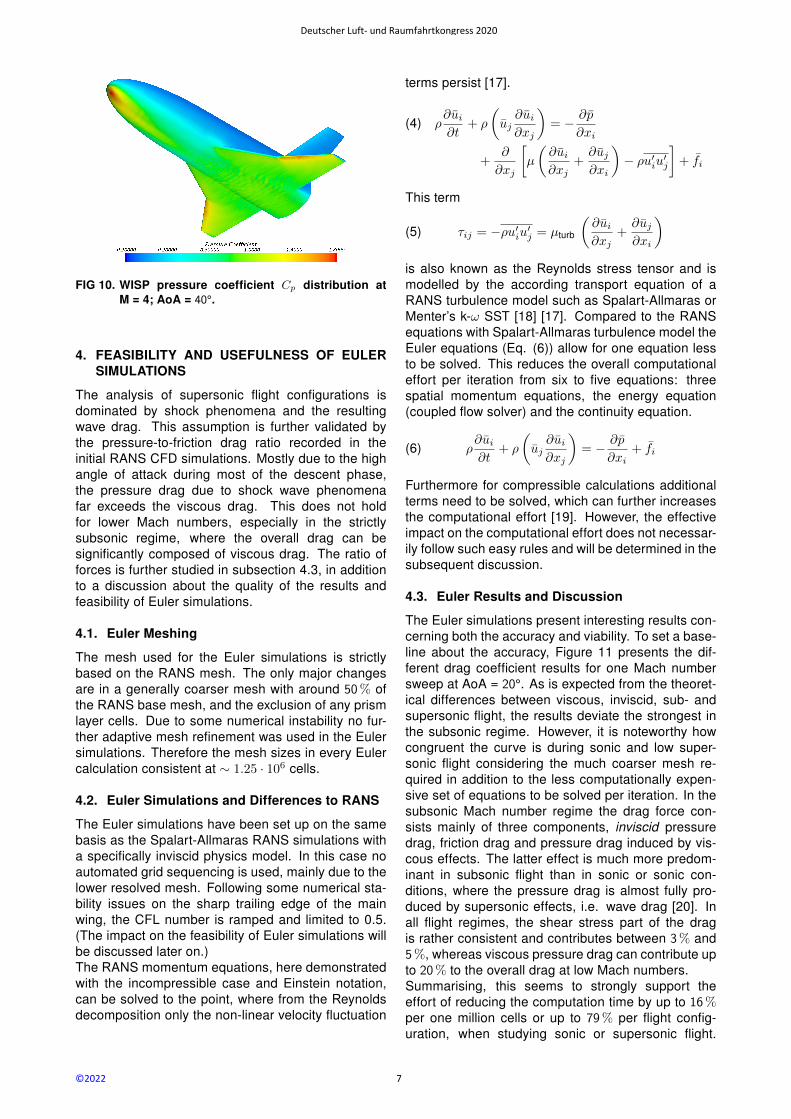
FIG 10. WISP pressure coefficient Cp distribution atM = 4; AoA = 40°.

4. FEASIBILITY AND USEFULNESS OF EULERSIMULATIONS

The analysis of supersonic flight configurations isdominated by shock phenomena and the resultingwave drag. This assumption is further validated bythe pressure-to-friction drag ratio recorded in theinitial RANS CFD simulations. Mostly due to the highangle of attack during most of the descent phase,the pressure drag due to shock wave phenomenafar exceeds the viscous drag. This does not holdfor lower Mach numbers, especially in the strictlysubsonic regime, where the overall drag can besignificantly composed of viscous drag. The ratio offorces is further studied in subsection 4.3, in additionto a discussion about the quality of the results andfeasibility of Euler simulations.

4.1. Euler Meshing

The mesh used for the Euler simulations is strictlybased on the RANS mesh. The only major changesare in a generally coarser mesh with around 50% ofthe RANS base mesh, and the exclusion of any prismlayer cells. Due to some numerical instability no fur-ther adaptive mesh refinement was used in the Eulersimulations. Therefore the mesh sizes in every Eulercalculation consistent at ∼ 1.25 · 106 cells.

4.2. Euler Simulations and Differences to RANS

The Euler simulations have been set up on the samebasis as the Spalart-Allmaras RANS simulations witha specifically inviscid physics model. In this case noautomated grid sequencing is used, mainly due to thelower resolved mesh. Following some numerical sta-bility issues on the sharp trailing edge of the mainwing, the CFL number is ramped and limited to 0.5.(The impact on the feasibility of Euler simulations willbe discussed later on.)The RANS momentum equations, here demonstratedwith the incompressible case and Einstein notation,can be solved to the point, where from the Reynoldsdecomposition only the non-linear velocity fluctuation

terms persist [17].

(4) ρ∂ui∂t

+ ρ

(uj∂ui∂xj

)= − ∂p

∂xi

+∂

∂xj

[µ

(∂ui∂xj

+∂uj∂xi

)− ρu′iu′j

]+ fi

This term

(5) τij = −ρu′iu′j = µturb

(∂ui∂xj

+∂uj∂xi

)is also known as the Reynolds stress tensor and ismodelled by the according transport equation of aRANS turbulence model such as Spalart-Allmaras orMenter’s k-ω SST [18] [17]. Compared to the RANSequations with Spalart-Allmaras turbulence model theEuler equations (Eq. (6)) allow for one equation lessto be solved. This reduces the overall computationaleffort per iteration from six to five equations: threespatial momentum equations, the energy equation(coupled flow solver) and the continuity equation.

(6) ρ∂ui∂t

+ ρ

(uj∂ui∂xj

)= − ∂p

∂xi+ fi

Furthermore for compressible calculations additionalterms need to be solved, which can further increasesthe computational effort [19]. However, the effectiveimpact on the computational effort does not necessar-ily follow such easy rules and will be determined in thesubsequent discussion.

4.3. Euler Results and Discussion

The Euler simulations present interesting results con-cerning both the accuracy and viability. To set a base-line about the accuracy, Figure 11 presents the dif-ferent drag coefficient results for one Mach numbersweep at AoA = 20°. As is expected from the theoret-ical differences between viscous, inviscid, sub- andsupersonic flight, the results deviate the strongest inthe subsonic regime. However, it is noteworthy howcongruent the curve is during sonic and low super-sonic flight considering the much coarser mesh re-quired in addition to the less computationally expen-sive set of equations to be solved per iteration. In thesubsonic Mach number regime the drag force con-sists mainly of three components, inviscid pressuredrag, friction drag and pressure drag induced by vis-cous effects. The latter effect is much more predom-inant in subsonic flight than in sonic or sonic con-ditions, where the pressure drag is almost fully pro-duced by supersonic effects, i.e. wave drag [20]. Inall flight regimes, the shear stress part of the dragis rather consistent and contributes between 3% and5%, whereas viscous pressure drag can contribute upto 20% to the overall drag at low Mach numbers.Summarising, this seems to strongly support theeffort of reducing the computation time by up to 16%per one million cells or up to 79% per flight config-uration, when studying sonic or supersonic flight.

©2022

Deutscher Luft- und Raumfahrtkongress 2020

7

0 1 2 3 4

0

0.1

0.2

0.3

0.4

Mach number M [-]

Dra

gco

effic

ientC

D[-

]RANS EULER

FIG 11. Drag coefficient at AoA 20° for RANS and Eulercalculations.

Unfortunately, during the additional Euler simulationssome stability and convergence issues occurred,which were later supposedly found to be caused bythe geometry and mesh injection into StarCCM+.Therefore in our case, all Euler simulations requiredmore iterations and solver tweaking than expected.Such problems did not occur during any RANS cal-culations, where presumably the viscous boundarylayer dampened many of the geometry inducedextreme-condition-cells and resulting stability issues.

5. CONCLUSION

The paper presents an aerodynamic CFD studyon a generic spaceplane geometry based on theSpacewalker project. The results show good validitywith existing studies and results both from experi-mental and CFD studies. Especially in the trans-and supersonic regime the Spalart-Allmaras RANSturbulence model delivers good results for a com-putationally inexpensive one-equation model. In thesubsonic regime, mostly demonstrated in the landingconfiguration angle of attack sweep, a two-equationRANS model might be better suited to further resolveflow separation effects.

Overall, the WISP geometry shows reasonableaerodynamic characteristics and is similar to otherflight-tested and in-development spaceplane-likevehicles. It trades some aerodynamic lift for betterdrag characteristics, especially during high angle ofattack phases. Depending on the exact flight path,this could be advantageous to lower the mechanicalloads on the craft’s structure, but also unfavourableconcerning aerothermal loads during the early su-personic return phase. Furthermore, the preliminarystudy of the pitching moment coefficient presentsfavourable results for both the static and dynamic sta-bility during all descent phases. (Only the magnitudeof the results is preliminary due to the missing dataconcerning the WISP’s centre of mass.)

Regarding the use of Euler simulations for trans- andsupersonic flight configurations in spaceplane appli-cations, the authors conclude, that even in times ofexponentially increasing computational resources theuse of Euler simulations can be time saving if para-metric studies are required. However, a very smoothCAD geometry and a proper CFD setup for the Eu-ler calculations is absolutely necessary to gain pro-cessing time benefits. Nonetheless, the potential forfaster turn-around and rapid prototyping in early de-velopment and research stages can be significant.

6. ACKNOWLEDGEMENT

The authors like to express their gratitude to SiemensPLM Software for providing academic licenses of theirsoftware StarCCM+.

Contact address:

geiben@fh-aachen.dehavermann@fh-aachen.de

References

[1] Spacewalker Project. https://www.

space-walker.co.jp/en. Accessed: 2020-03-13.

[2] OpenVSP Software. http://openvsp.org. Ac-cessed: 2020-08-12.

[3] F. Götten, F. Finger, M. Havermann, C. Braun,M. Marino, and C. Bil. A highly automatedmethod for simulating airfoil characteristics atlow reynolds number using a rans - transition ap-proach. 2020. DOI: 10.25967/490026.

[4] J. W. Paulson Jr. Aerodynamic characteristics ofa large aircraft to transport space shuttle orbiteror other external payloads. National Aeronauticsand Space Administration, 1975.

[5] F. Götten, F. Finger, M. Marino, C. Bil, M. Haver-mann, and C. Braun. A review of guidelines andbest practices for subsonic aerodynamic sim-ulations using RANS CFD. Asia-Pacific Inter-national Symposium on Aerospace Technology2019, Gold Coast, Australia, December 2019.ISBN: 978-1-925627-40-4.

[6] P. Ewing. Best practices for aerospace aero-dynamics. Star South East Asian Conference,2015.

[7] Simcenter STAR-CCM+ Documentation. CD-adapco.

[8] M. Kuznetsova, A. Chulaki, N. Papitashvili,et al. MSIS-E-90 Atmosphere Model.https://ccmc.gsfc.nasa.gov/modelweb/

models/msis_vitmo.php.

©2022

Deutscher Luft- und Raumfahrtkongress 2020

8

[9] J. D. Anderson. Modern CompressibleFlow. McGraw-Hill Education, New York, 1990.ISBN: 978-0-072-42443-0.

[10] Siemens CD-adapco. Validation of Star-CCM+for external aerodynamics in the aerospaceindustry. http://mdx2.plm.automation.

siemens.com/sites/default/files/

Presentation/CD-adapco_AeroValidation_

v7.pdf. Accessed: 2020-08-14.

[11] Claus Weiland. Aerodynamic data of space ve-hicles. Springer, Heidelberg, 2014. ISBN: 978-3-642-54167-4.

[12] John Pienkowski et al. Analysis of the aero-dynamic orbital transfer capabilities of the x-37space maneuvering vehicle. In 41st AerospaceSciences Meeting and Exhibit. American Insti-tute of Aeronautics and Astronautics, 1 2003.DOI: 10.2514/6.2003-908.

[13] N.N. Aerodynamic Design Data Book - OrbiterVehicle STS-1. Rockwell International, 1980.

[14] K. W. Iliff and M. F. Shafer. Space Shuttle Hy-personic Aerodynamic and AerothermodynamicFlight Research and the Comparison to GroundTest Results. NASA Dryden Flight ResearchFacility, 1993. NASA Technical Memorandum4499.

[15] Fritz Dubs. Hochgeschwindigkeits-Aerodynamik.Birkhäuser, 1975. ISBN: 3764307145.

[16] Mark Drela. Flight Vehicle Aerodynamics. TheMIT Press, 02 2014. ISBN: 978-0-262-52644-9.

[17] W. K. George. Lectures in Turbulence for the21st Century. Imperial College of London, 2013.

[18] H. Tennekes. A First Course in Turbulence. TheMIT Press, Cambridge, Massachusetts, 1992.ISBN: 978-0-262-20019-6.

[19] J. Ferziger. Numerische Stroemungsmechanik.Springer, Berlin Heidelberg, 2008. ISBN: 978-3-540-67586-0.

[20] F. Janser, M. Havermann, B. Hoeveler, andC. Hertz. Inkompressible Profil- und Tragfluege-laerodynamik. Verlagshaus Mainz GmbH,Aachen, 2016. ISBN: 978-38107-0261-6.

©2022

Deutscher Luft- und Raumfahrtkongress 2020

9