ANALYSIS OF DRAG REDUCTION USING AERODYNAMIC

DEVICES ON COMMERCIAL BUSES BY COMPUTATIONAL FLUID

DYNAMIC SIMULATION

BY

RACHEL BROWN

A THESIS

SUBMITTED TO THE FACULTY OF

ALFRED UNIVERSITY

IN PARTIAL FULFILLMENT OF THE REQUIREMENTS

FOR THE DEGREE OF

MASTER OF SCIENCE

IN

MECHANICAL ENGINEERING

ALFRED, NEW YORK

September, 2015

Alfred University theses are copyright protected and may be used for education or personal research only. Reproduction or distribution in part or whole is prohibited without written permission from the author.

Signature page may be viewed at Scholes Library, New York State College of Ceramics, Alfred University, Alfred, New York.

COMPUTATIONAL SIMULATION OF DRAG REDUCTION USING

AERODYNAMIC DEVICES ON COMMERCIAL BUSES

BY

RACHEL BROWN

B.S. UNION COLLEGE (2013)

SIGNATURE OF AUTHOR___________________________________

APPROVED BY____________________________________________

DR. SEONG-JIN LEE, ADVISOR

_______________________________________________

DR. WALLACE LEIGH, ADVISORY COMMITTEE

_______________________________________________

DR. JOE ROSICZKOWSKI, ADVISORY COMMITTEE

_______________________________________________

CHAIR, ORAL THESIS DEFENSE

ACCEPTED BY ____________________________________________

DOREEN D. EDWARDS, DEAN

KAZUO INAMORI SCHOOL OF ENGINEERING

iii

ACKNOWLEDGMENTS

Foremost, the author of this study would like to express her sincere gratitude to her

advisor Dr. Seong-Jin Lee for the continuous support of her Master's study and research,

for his patience, motivation, and enthusiasm. His guidance helped her throughout all the

research and writing of this thesis. Research could also not have been completed without

the financial support of the Kazuo Inamori School of Engineering and Dean Edwards. The

author would also like to acknowledge her thesis committee members Dr. Wallace Leigh

and Dr. Joe Rosiczkowski in their time and support of this study. Lastly she would like to

acknowledge the continued support of her parents throughout her education.

iv

TABLE OF CONTENTS

Page

Acknowledgements ...................................................................................................... iii

Table of Contents ......................................................................................................... iv

List of Tables ............................................................................................................... vi

List of Figures ............................................................................................................ viii

Abstract ....................................................................................................................... xii

I INTRODUCTION....................................................................................................... 1

A. Aerodynamics of Commercial Buses .................................................................................. 3

1. Flow Field around a Bus ...................................................................................................... 3

2. Turbulence ........................................................................................................................... 5

B. Computational Fluid Dynamics (CFD) Software ............................................................... 7

C. Reynolds Averaged Navier-Stokes Equations (RANS) ...................................................... 9

1. Boundary-Layer Equations ................................................................................................ 13

D. Turbulence Models ........................................................................................................... 16

A. Previous Studies on Turbulence Modeling .................................................................... 16

B. Modeling Terminology .................................................................................................. 17

C. Two-Equation Turbulence Models ................................................................................ 18

E. Aerodynamic Drag Reduction Devices ............................................................................ 27

1. Airvane as a Drag Reduction Device ............................................................................. 29

II EXPERIMENTAL PROCEDURE.......................................................................... 34

A. SolidWorks Scaled-Down Model ..................................................................................... 34

B. Parameter Study to Reach Optimized Airvane Devices ................................................... 36

C. ANSYS Fluent Setup and Procedure ................................................................................ 41

1. Geometry Setup ............................................................................................................. 41

2. Meshing Procedure ........................................................................................................ 43

3. Fluent Procedure ............................................................................................................ 48

D. Calibration of Fluent Simulations ..................................................................................... 49

III RESULTS AND DISCUSSION ............................................................................... 50

A. Calibration of Fluent ......................................................................................................... 50

B. Bus Model without Airvane .............................................................................................. 55

C. Bus Model with Airvane ................................................................................................... 61

v

1. Top Airvane Only .......................................................................................................... 62

2. Top and Side Airvanes ................................................................................................... 74

3. Different Configurations ................................................................................................ 85

IV CONCLUSION ......................................................................................................... 91

V FUTURE WORK ...................................................................................................... 93

REFERENCES ................................................................................................................ 94

APPENDIX A: Dimensions of Full Sized Bus and 1/35th Scale Model ..................... 97

APPENDIX B: Blueprint of Side View of MCI D4505 ................................................ 98

APPENDIX C: SolidWorks 1/35th Scaled Model of Commercial Bus ....................... 99

APPENDIX D: ANSYS Fluent Set-up and Procedure .............................................. 100

APPENDIX E: Calibration Raw Data ........................................................................ 106

APPENDIX F: Raw Data of Parameter Study Performed on Top Airvane ........... 108

APPENDIX G: Raw Data of Parameter Study Performed on Side Airvane .......... 113

APPENDIX H: Raw Data of Different Configurations, Bottom Airvane and

Deflection Plate.............................................................................................................. 118

vi

LIST OF TABLES

Page

Table I: Model Constants for k-e Two Equation Turbulence Model ................................ 20

Table II: Closure Constants for Wilcox’s Standard k-ω Equation. .................................. 22

Table III: Model Constants for the RKE Turbulence Model ............................................ 23

Table IV: Model Constants for the Outer Layer for the SST Turbulence Model ............. 25

Table V: Model Constants for the Inner Layer for the SST Turbulence Model ............... 26

Table VI: Dimensions for Wind Tunnel Enclosure Designed in ANSYS Fluent............. 42

Table VII: Dimensions for Refinement Box. .................................................................... 42

Table VIII: A Set of Simulations was Run with Different Combinations. ....................... 86

Table IX: A Set of Simulations was Run with Different Configurations ......................... 87

Table X: Important Dimensions of MCI D4505 Commercial Bus ................................... 97

Table XI: First Run of the Calibration of the Fluent simulations. .................................. 106

Table XII: Second Run of the Calibration of the Fluent simulations. ............................ 107

Table XIII: Raw Data of Refined Angle Tests Run on the Top Airvane ....................... 108

Table XIV: Raw Data of General Expansion Ratio Tests Run on the Top Airvane ...... 108

Table XV: Raw Data of the Refined Expansion Ratios on the Top Airvane ................. 109

Table XVI: Data of the Radius of the Curved Portion of the Top Airvane. ................... 110

Table XVII: Raw Data of the Inlet Gap for the Top Airvane ......................................... 110

Table XVIII: Raw Data for the Angle of the Planar Portion of the Top Airvane........... 111

Table XIX: Raw Data of the Planar Length of the Top Airvane .................................... 112

Table XX: Raw Data of the General Angle of the Side Airvane .................................... 113

Table XXI: Raw Data of the Refined Angle of the Side Airvane .................................. 114

Table XXII: Raw Data of the General Expansion Ratio of the Side Airvane ................ 114

vii

Table XXIII: Raw Data of the Refined Expansion Ratio of the Side Airvane ............... 115

Table XXIV: Raw Data Radius of Curvature of the Side Airvane ................................. 115

Table XXV: Raw Data of the Inlet Gap of the Side Airvane ......................................... 116

Table XXVI: Raw Data of the Angle of the Inlet of the Side Airvane ........................... 117

Table XXVII: Raw Data of the Planar Length of the Side Airvane ............................... 117

Table XXVIII: Raw Data of the Different Combinations .............................................. 118

Table XXIX: Raw Data of Different Configurations. .................................................... 118

viii

LIST OF FIGURES

Page

Figure 1: Relation of aerodynamic and rolling drag to velocity of a bluff body ............... 2

Figure 2: Flow around a bluff body .................................................................................... 4

Figure 3: Relationship between time-averaged variables, fluctuations and average: (a)

steady flow and (b) unsteady flow ..................................................................... 10

Figure 4: Boundary layer notation and coordinate system on a flat plate ........................ 13

Figure 5: Visual representation of the SST turbulence model .......................................... 25

Figure 6: Aivane kit created by Kirsch with important aspects numbered ....................... 29

Figure 7: Different configurations of airvanes that were mounted on the top leeward

corner of the body .............................................................................................. 31

Figure 8: SolidWorks 1/35th scaled CAD model of commercial bus ............................... 36

Figure 9: Optimized airvane attached to the top horizontal edge ..................................... 39

Figure 10: Optimized airvane attached to the side vertical edges .................................... 40

Figure 11: Different element types for three-dimensional meshes ................................... 44

Figure 12: Cutcell mesh created in ANSYS for the bus model without a drag reduction

device attached ................................................................................................... 46

Figure 13: Enhanced view of CutCell mesh created in ANSYS. ..................................... 47

Figure 14: Polyhedral mesh created in ANSYS Fluent .................................................... 47

Figure 15: Calibration tests run for the Realizable k-ε turbulence model utilizing a

polyhedral mesh ................................................................................................. 51

Figure 16: Calibration tests run for the Realizable k-ε turbulence model utilizing a

CutCell mesh ...................................................................................................... 52

ix

Figure 17: Calibration tests run for the SST k-ω turbulence model utilizing a polyhedral

mesh ................................................................................................................... 53

Figure 18: Graph of calibration tests run for the SST k-ω turbulence model utilizing a

CutCell mesh ...................................................................................................... 54

Figure 19: Velocity contour of bus model without an airvane employed ......................... 55

Figure 20: Pressure contour found for the bus without an airvane employed .................. 57

Figure 21: Contour of turbulence kinetic energy .............................................................. 58

Figure 22: Velocity contour of the bus model without an airvane employed ................... 59

Figure 23: Pressure contour found for the bus without an airvane ................................... 60

Figure 24: Contour of turbulence kinetic energy .............................................................. 61

Figure 25: Percent reduction in the drag coefficients versus the general angles .............. 63

Figure 26: Percent reduction in the drag coefficients versus the more refined angles ..... 64

Figure 27: Percent reduction in the drag coefficients versus the general expansion ratios

tested .................................................................................................................. 65

Figure 28: Percent reduction in the drag coefficients versus the more refined expansion

ratios ................................................................................................................... 67

Figure 29: Percent reductions in the drag coefficient versus the radius of curvatures ..... 68

Figure 30: Percent reduction in the drag coefficients versus the inlet gaps ...................... 69

Figure 31: Percent reduction in the drag coefficients versus the angles of the planar

portion of the airvane ......................................................................................... 70

Figure 32: Percent reduction in the drag coefficients versus the lengths of the planar

portion ................................................................................................................ 71

Figure 33: Velocity contour of the wake of the bus model with a top airvane ................. 72

x

Figure 34: Pressure contour of the bus with a top airvane ................................................ 73

Figure 35: Contour of turbulence kinetic energy with a top airvane ................................ 74

Figure 36: Percent reduction in the drag coefficients versus the general angles .............. 75

Figure 37: Percent reduction in the drag coefficients versus the more refined angles ..... 76

Figure 38: Percent reduction in the drag coefficients versus the general expansion ratios

employed ............................................................................................................ 77

Figure 39: Percent reduction in the drag coefficients versus the more refined expansion

ratios ................................................................................................................... 78

Figure 40: Percent reductions in the drag coefficient versus the radius of curvatures ..... 79

Figure 41: Percent reduction in the drag coefficients versus the inlet gaps ...................... 80

Figure 42: Percent reduction in the drag coefficients versus the angles of the planar

portion ................................................................................................................ 81

Figure 43: Percent reduction in the drag coefficients versus the lengths of the planar

portion ................................................................................................................ 82

Figure 44: Velocity contour of the bus model with top and side airvanes employed ....... 83

Figure 45: Pressure contour of the bus with top and side airvanes ................................... 84

Figure 46: Contour of turbulence kinetic energy with top and side airvanes ................... 85

Figure 47: Percent reduction in the different combinations of deflection plate, bottom

airvanes .............................................................................................................. 86

Figure 48: Percent reduction in the different configurations of airvanes employed......... 88

Figure 49: Velocity contour of the bus model with top, side, and bottom airvanes ......... 89

Figure 50: Pressure contour of the bus with top, side and bottom airvanes ..................... 89

Figure 51: Contour of turbulence kinetic energy with top, bottom, and side airvanes ..... 90

xi

Figure 52: Side view of MCI D4505 commercial bus ...................................................... 98

Figure 53: Right view (a), left view (b), front view (c), and rear view (d) of 1/35th scaled

model bus ........................................................................................................... 99

xii

ABSTRACT

A large percentage of the usable fuel employed in a commercial bus is utilized to

overcome the aerodynamic drag at highway speeds and therefore if reduced could produce

a large reduction in the total fuel consumption of the vehicle and reduce the negative

environmental effects. MCI's D4505 coach bus was modeled in this study and airvanes,

drag reduction devices, were employed on the model bus to reduce the drag coefficient of

the bus. Each airvane, attached to edges of the leeward face of the bus, was optimized by

a parameter study were each individual dimension of the device was tested to determine

the optimal design. The airflow surrounding the bus models with and without the airvanes

attached were modeled using a computational fluid dynamics software. In this software

different turbulence models and meshes were employed to observe the effect of these

changes on the predicted airflow and optimization of the aerodynamic devices. Two

separate sets of simulations were run on each dimension tested. The first simulation

utilized a polyhedral mesh with the Realizable k-ε turbulence model, while the second set

of simulations used a CutCell mesh and the Shear Stress Transport k-ω turbulence model.

It was found that to reach a maximum reduction of the drag coefficient of the bus airvanes

were placed on all edges of the leeward face and optimized for the specific placement on

the bus. A drag coefficient of 0.54351 was produced which was a reduction of 12.37% for

the polyhedral RKE model while the CutCell SST model produced a drag coefficient of

0.54021 a reduction of 14.55%. This reduction in the drag coefficient lead to a maximum

reduction of 1.5% in the fuel consumption, which if applied to all commercial buses would

have a significant effect on the total national fuel consumption and a positive impact on

the environment.

1

INTRODUCTION

Aerodynamics is the section of fluid dynamics focused explicitly on the motion of

air, primarily when interacting with solid objects in its path. The study of aerodynamics

has existed for a long time and the understanding of how aerodynamics works has greatly

enhanced and continues to develop, even today. Over time the aerodynamics of

commercial vehicles, such as tractor-trailers, trains, and buses, has advanced immensely,

starting with Labatt Brewing Company over sixty-five years ago. Improving the

aerodynamics of a vehicle has considerable effects on the maximum velocity the vehicle is

able to reach, but also on the environmental impact due to fuel consumption of the vehicle.

While in the past, the goal of producing more aerodynamic vehicles was increasing the top

cruising speed of the vehicle. Today, the focus is no longer the speed of the vehicle but on

energy conservation.

Decreasing the fuel consumption of vehicles is particularly important when looking

at commercial vehicles, due to the fact that they constitute for a large portion of the total

domestic fuel consumption used each day.1 Large fuel consumption implies even larger

emissions, which have an adverse effect on the environment. Previous aerodynamic

studies, for example David W. Pointer’s study on heavy vehicles, have determined at a

velocity of approximately 70 miles per hour up to 65% of the total energy consumed by a

large ground vehicle is employed to overcome the aerodynamic drag. Aerodynamic drag

is defined as the work required overcoming the force of air hindering the motion of the

object at a given velocity along a given distance. As the vehicle's velocity increases so

does the aerodynamic drag present on the vehicle. Since the rolling resistance, the force

resisting motion of the body due to frictional force on the tires, remains constant at varying

velocities as the aerodynamic drag increases, so does the percentage of the total energy

used to overcome that drag force.2 Figure 1 illustrates this characteristic, as the speed of

the bluff body increases the aerodynamic drag overtakes the rolling resistance as the main

component of the total drag present on the vehicle around 65 km/h.3

2

Figure 1: Relation of aerodynamic and rolling drag to the velocity of a bluff body. This graph

demonstrates that as the velocity increases the rolling drag remains constant, but the aerodynamic

drag increases exponentially. At a velocity of approximately 65 km/h the aerodynamic drag

overcomes the rolling resistance as the main force on the body.3

Even a small reduction in the total force due to aerodynamic drag, while at a

velocity above 65 km/h, would lead to a significant reduction in fuel consumption and

when applied to all commercial buses would lead to an extreme reduction of the total

domestic fuel consumption. If the vehicle’s drag coefficient is reduced by 50% it could

lead to a 25% decrease of the total fuel consumption.2 A 1% reduction in fuel consumption

would lead to, in only one year, approximately 245 million gallons of fuel being saved in

the U.S. alone. Larger reductions in fuel consumption would lead to even more substantial

amounts of fuel saved and less negative impact on the environment.

Several governmental programs have been enacted to encourage companies to

reduce their products’ overall fuel consumption. The importance of reducing fuel

consumption emanates from the rising fuel prices due to deterioration of fuel, demand for

crude oil, and worldwide extreme consumption, among other conditions including

environmental concerns.4 These environmental issues include an impact on the climate,

with an increase in Greenhouse Gases which increase global warming. As fuel prices

continue to climb the push for even more aerodynamic vehicles also increases, but this

improvement has become a greater and greater effort for a smaller and smaller gain.1

Numerous studies have been conducted involving reduction of drag on tractor-

trailers, but few studies have been performed on drag reduction of commercial buses. Drag

reduction denotes streamlined flow has become steadier, in other words, the flow field has

3

less unsteadiness or turbulence.5 This study aimed to better understand the unique

aerodynamic forces present on buses, and investigate a simple add-on device to reduce

aerodynamic drag and by relation the fuel consumption used. Reducing fuel consumption

of commercial buses is important due to the fact that large fleets of buses are used every

day to transport large numbers of people extended distances. The amount of fuel

consumption due to buses alone is substantial.

The goal of this research is to diminish fuel consumption of a commercial bus by

reducing the drag coefficient of the vehicle. To reduce the aerodynamic drag on the bus

simple add-on drag reduction devices called airvanes were placed on the rear edges of the

bus. The airvanes placed on the leeward face of the bus were used to decelerate the airflow

into the wake behind the bus and thus mostly increase the pressure and decrease the total

force drag on the bus. To ensure that the airvanes maximized the reduction in the drag

coefficient parameter studies were run on each individual airvane to optimize the

dimensions of the devices. The airflow and drag coefficient were predicted utilizing a

computational fluid dynamics program. Once the drag coefficient was determined the total

reduction in fuel consumption could be found.

A. Aerodynamics of Commercial Buses

1. Flow Field around a Bus

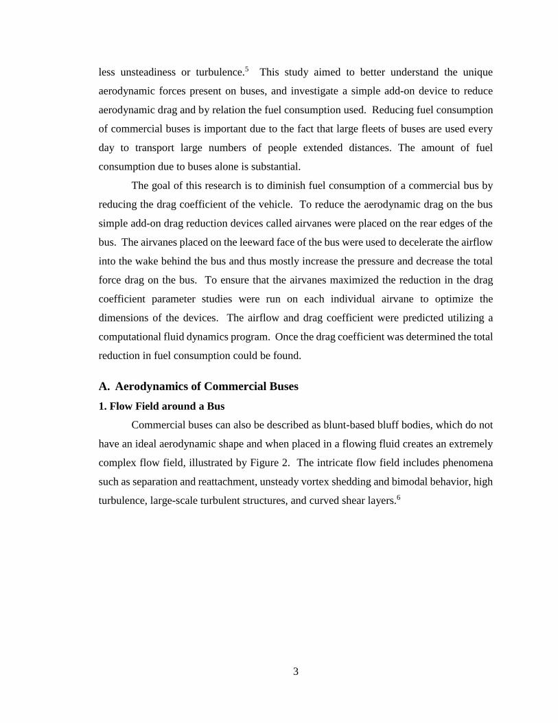
Commercial buses can also be described as blunt-based bluff bodies, which do not

have an ideal aerodynamic shape and when placed in a flowing fluid creates an extremely

complex flow field, illustrated by Figure 2. The intricate flow field includes phenomena

such as separation and reattachment, unsteady vortex shedding and bimodal behavior, high

turbulence, large-scale turbulent structures, and curved shear layers.6

4

Figure 2: Flow around a bluff body (a) far from ground (b) constrained by ground. It can be

observed that there is a separation point at the front of each body causing a high pressure zone in

front of the body. The air flows around the front corners and causes separation bubbles which

reattaches further down the body. Another set of separation bubbles form around the back corners

and feed into a turbulent wake at the back of the body, creating a low pressure zone.7

When a bluff body is placed in a flowing fluid an axially symmetrical flow pattern

can be witnessed (Figure 2 (a)). A stagnation point can be observed on the windward face

of the bluff body and the boundary layer separates around the leading edges where

separation bubbles then develop on the forepart of the sides of the bluff body. The flow

then reattaches to the side walls and remains attached until the trailing edges where another

set of separation bubbles form. These separation bubbles occur in the wake surrounded by

a shear layer. Farther beyond the wake the flow reattaches at the symmetry axis. If the

bluff body is constrained by the ground, as in Figure 2(b), flow is similar to the flow field

existing on the top side of Figure 2(a). The stagnation point is shifted slightly downward

and the separation bubble present in the wake is surrounded by a shear boundary layer on

all sides, except the bottom, which is constrained by the ground.

Due to the fact that buses are slightly raised off the ground, about 10% of the total

height of the bus, there is flow under the bus to consider as well. Air flow decelerates as

it flows under the bus and flows out beside the bus laterally. This outward flow displaces

the air flowing along the sides of the bus upward and laterally. Air that flows out the rear

of the underbody separates on the ground and feeds the separation bubble in the wake as it

flows backward.7

a.)

b.)

5

Being bluff bodies, buses have large frontal areas which create an area of high

pressure on the windward face. A low pressure area is also present on the leeward face of

the bus creating a large pressure differential that forms a vacuum-like “suction” that pulls

the bus backward, hindering forward motion.8 Forces caused by this pressure differential

are called pressure forces. Pressure forces present on buses are found to account for up to

80% of the total wind-averaged aerodynamic drag.9 Since pressure drag accounts for such

a large percentage of the overall aerodynamic drag it makes it the ideal area to examine for

reduction in drag. Increasing pressure in the low pressure wake region behind the body

would in turn reduce the adverse pressure differential present on the bus. Reduction in

pressure differential would have a major effect on reducing the total force drag.8 This flow

pattern is very important in understanding the aerodynamics of buses and how drag

reduction can be achieved by reducing the separation bubbles and wake present.

2. Turbulence

Flow fields around bluff bodies, such as the buses described above, can be

considered to have extremely turbulent flow patterns. Separation bubbles, boundary

layers, and wakes present on bluff bodies are examples of turbulence within a flow field.

Most fluid flows encountered in everyday life can be considered to be turbulent.

Turbulence itself does not have an exact definition and can prove to be enigmatic. The

most accurate definition available to concisely explain turbulence is, "a dissipative flow

state characterized by nonlinear fluctuating three-dimensional vorticity".10 Fluctuations

that take place in turbulent flows are unpredictable in detail and have not been able to be

solved by deterministic or statistical methods. Useful predictions for turbulent flows may

be found using dimensional arguments, direct numerical simulations, or empirical models

and computational methods.

Although there is no exact definition for turbulence there are several characteristics

that help to identify turbulence. Turbulence’s first characteristic is the fluctuations that

take place in the flow field. Even in turbulent flows that contain steady boundary

conditions the dependent-flow quantities such as pressure, velocity, temperature, among

others, fluctuate. These fluctuations make the turbulent flow appear irregular and

unpredictable, because of its irregularity is often considered to be random. This assumption

is a misconception. Turbulence is not random, since its flow is governed by the Navier-

6

Stokes equation. Unlike a purely random time-dependent vector field, a turbulent flow

field must conserve mass, momentum, and energy.

Nonlinearity is the second main characteristic of turbulence. When the critical

nonlinear parameter, such as the Reynolds number, the Rayleigh number, or the inverse

Richardson number exceeds a critical value turbulent flow ensues. This nonlinearity is

apparent in turbulent flow because it is the last step in the nonlinear transition process.

When the nonlinear constraint has surpassed the maximum value small disturbances begin

to grow spontaneously and may come to equilibrium as fixed amplitude disturbances.

More instability and intricate disturbances can occur in this new equilibrium state,

continuing in this fashion until a final non-repeating unpredictable flow field is reached

which can be called turbulence.

Vorticity describes the local revolving motion of the fluid as would be seen from a

point along the flow path of the fluid. In turbulent flows vorticity fluctuates. When

observing turbulent flow fields it can be witnessed that various structures can be identified

such as streaks, strain regions, and swirls of varying sizes that spin, deform, and split.

There structures, specifically the ones that rotate, are identified as eddies. Eddies present

in turbulence flows vary in size and as the Reynolds number increases so does the range in

the sizes of eddies present. The width of the turbulent region is the characteristic size of

the largest eddies; these eddies can be several orders of magnitude larger than the smallest

eddies and contain the largest amount of fluctuation energy in the turbulent flow.10

It is believed that turbulent eddies exist for a certain amount of time in a certain

region of space and due to cascade process or dissipation are destroyed. This dissipation is

another specific characteristic of turbulent flow. Smaller eddies, which are dissipated into

thermal energy, are enclosed in the region covered by the larger eddies. In the cascade

process smaller turbulent eddies receive fluctuation energy from the slightly larger eddies,

while those eddies receive fluctuation energy from even larger turbulent eddies. Energy is

extracted from the mean flow to supply the largest eddies.11 Due to this dissipation of

energy a constant supply of energy must be present to maintain turbulence

One last feature of turbulent flow is diffusivity, fluctuations in the flow field cause

quick mixing and circulation of species, momentum, and heat. Diffusivity is much higher

7

in turbulent flows than in laminar flows due to the large fluctuation characteristics of

turbulent flows.10

Turbulent flows often have higher values of pressure drop and friction drag as well

as a greater diffusion rate of a scalar quantity and noise. When dealing with an adverse

pressure gradient a turbulent boundary layer is able to deal with a considerably larger

region before separation than a laminar boundary layer is able to.12 Turbulent flow is much

more complex than laminar flow due to the complex characteristics and equations that

govern its flow, therefore it is much harder to analyze and model. Consequently, different

methods are utilized to solve these intricate fluid problems.

B. Computational Fluid Dynamics (CFD) Software

Three main methods to analyzing fluid dynamic problems exist; theoretical,

experimental, and numerical, which can also be referred to as computational fluid

dynamics. The theoretical method can also be referred to as the analytical approach, which

infers that the problem is solved using known mathematical equations. Since most fluid

dynamic problems are complex and cannot be solved directly, assumptions must be made

to employ this approach. The main advantage of the theoretical methodology is that

“clean” general information is able to be solved for using simple formulas. Reasonable

numbers are able to be found and are often are used for preliminary work. One

disadvantage of this method is it is restricted to linear problems, simple geometry, and

simple physics. Complex flows cannot be solved for without major assumptions that

reduce the accuracy of the tests and the solutions found. Along with the fact that it is

widely accepted that turbulent flows are mostly not understood, this makes it impossible

to solve for theoretically.

Experimental methods are often the primary approach for testing aerodynamic flow

fields past buses. Evaluating the performance of a scaled-down model of a prototype

device is the main objective of the experimental method. Scaled-down models of the

device are relatively inexpensive and therefore it is realistic for companies to use this

method. One problem this method faces is that the wind tunnel facility must be able to

produce the required free stream conditions which can be difficult to obtain, especially for

cases that model large aircrafts or space vehicles. Large scale wind tunnel facilities also

8

require large amounts of energy to run high-speed tests; therefore the run-times must be

kept at a minimum for economic reasons. The results of these tests would then be analyzed

and a new model would have to be created and tested, this process would continue until an

acceptable design was engineered. Experimental methods achieve the most accurate

results for most fluid dynamic problems, but the costs of this approach are large and

increase every day. In the meantime computational methods are becoming more popular

for analyzing complex fluid dynamic problems.

As computers gained popularity a new method of solving complex fluid problems

was developed called computational fluid dynamics. The governing equations of fluid

motion, including the conservation of mass, momentum, and energy, usually in partial

differential or integral form, are solved numerically using this approach to predict the fluid

flow. With computational methods few assumptions are needed and a high-speed computer

is utilized to solve the resulting governing equations for the fluid dynamic problem.

Advantages of this method are that the user is not constrained to linear problems,

complicated problems can be solved, and time evolution of flow can be obtained. There

are disadvantages to this method which include boundary condition problems and the high

costs of a computer that is able to run the complex problems. As CFD becomes more

prevalent in industrial applications the disadvantages decrease due to cheaper computers

and turbulence models able to reduce boundary condition issues.12

Computational fluid dynamics (CFD) software was utilized in this study to determine

the effectiveness of specific aerodynamic devices, which are explained in a later section,

to reduce the total force drag present on a model bus and in turn reduce the total fuel

consumption. There is a wide range of CFD software to choose from today and there are

several advantages and disadvantages for each type of software. ANSYS Fluent13 a widely

used CFD software which contains the capability to model flow, turbulence, reactions, and

heat transfer problems, was chosen for this study. Advantages of this software are the large

selection of turbulence models available for simulation and the high level of accuracy this

software is able to model fluid dynamic problems. One disadvantage of this software is

the extensive hardware requirements and computing time that is necessary to model the

complex problems. Despite this disadvantage ANSYS Fluent was used in this study and

the equations behind the simulations were studied.

9

C. Reynolds Averaged Navier-Stokes Equations (RANS)

Due to the immense range of time and length scales of turbulent flows at high Reynolds

numbers, it is nearly impossible to predict the flow in any great level of detail using the

Navier-Stokes equations. To alleviate this problem the Navier-Stokes equations are

derived for a mean state in the turbulent flow.10 Most turbulence models employed in

present day simulations of turbulent flow are based off of these time-averaged Navier-

Stokes equations, which are also known as Reynolds equations of motions or the Reynolds

Averaged Navier-Stokes (RANS) equations. When the equations of motions are time-

averaged new terms are formed, which can be defined as “apparent” stress gradients due

to turbulent flow patterns. Further assumptions and approximations must be made to

produce turbulence models that can relate these terms to the mean flow variables. Since

this process of solving the closure problem with the Reynolds equations of motion makes

additional assumptions it does not fully abide by the first principles.

Time-mean and fluctuating components are found by decomposing the dependent flow

variables in the conservation equations and then the whole equation is time-averaged to

derive the Reynolds equations. This decomposition is known as Reynolds decomposition.

Using the Cartesian coordinate system the time averages and fluctuations around the

average can be written as shown below where the represent the time-averaged value:

𝒖 = �� + 𝒖′ 𝒗 = �� + 𝒗′ 𝒘 = �� + 𝒘′ 𝝆 = �� + 𝝆′ 𝒑 = �� + 𝒑′ (1)

In the above equation u, v, and w represent the velocities in the x, y, and z direction

respectively, while ρ is the density and p is the pressure. Fluid properties such as viscosity

have such small fluctuations as to be neglected in the derivation of the RANS equations.

Figure 3 illustrates the relationship between the time averages (��), fluctuations around the

average (𝑢′), and the total flow variables (𝑢). Time averaging of fluctuating quantities will

equal zero as illustrated in Equation 2.

𝒇′ =𝟏

𝜟𝒕∫ 𝒇′𝒅𝒕 = 𝟎

𝒕𝟎+𝜟𝒕

𝒕𝟎 (2)

It should be noted that for compressible flows the velocity components would be mass-

weighted averaged to develop more appropriate equations, but for the purpose of this

10

experiment an incompressible flow was studied consequently, mass-weighted averaging

was unnessescary.12

Figure 3: Relationship between time-averaged variables, fluctuations and average: (a) steady flow

and (b) unsteady flow. The time-averaged variables are denoted by (��) while the fluctuations are

denoted as (𝒖′). The total flow variable, (𝒖), is defined as the time-average variables added to the

fluctuations. It can be observed that in steady flow the time-averaged variables remain constant, but

in unsteady flow they do not.12

There are three fundamental equations of fluid dynamics that are averaged to place

them in a Reynolds form; the continuity equation, momentum equation, and the energy

equation. The energy equation is not looked at in this paper due to the fact that is only

necessary for heat transfer problems and not aerodynamic ones. The continuity equation

is formed when the conservation of mass law is applied to an inconsequential fixed volume

with a fluid passing through shown, in Cartesian coordinates, by Equation 3.

𝝏𝝆

𝝏𝒕+

𝝏

𝝏𝒙(𝝆𝒖) +

𝝏

𝝏𝒚(𝝆𝒗) +

𝝏

𝝏𝒛(𝝆𝒘) = 𝟎 (3)

After Reynolds decomposition is completed on Equation 3 and the variables are in

the form shown in Equation 1 the entire continuity equation is then time averaged resulting

in Equation 4.

𝝏��

𝝏𝒕+

𝝏𝝆′

𝝏𝒕+

𝝏

𝝏𝒙𝒋(𝝆𝒖𝒋 ) +

𝝏

𝝏𝒙𝒋(𝝆′𝒖𝒋 ) +

𝝏

𝝏𝒙𝒋(𝝆𝒖𝒋

′ ) +𝝏

𝝏𝒙𝒋(𝝆′𝒖𝒋

′) = 𝟎 (4)

The second, fourth and fifth terms are equal to zero based on the principle shown

in Equation 2, leaving Equation 5 below.

𝝏��

𝝏𝒕+

𝝏

𝝏𝒙𝒋(𝝆𝒖𝒋 + 𝝆′𝒖𝒋

′ ) (5)

While looking at incompressible flows ρ' = 0 therefore the Reynolds form

continuity equation becomes Equation 6.

11

𝝏𝒖𝒋

𝝏𝒙𝒋= 𝟎 (6)

The second set of fluid dynamics equations to be placed in Reynolds form is the

momentum equations, which are also known as the Navier-Stokes equations. The

momentum equations are developed when a fluid passing through an infinitesimally small,

fixed control volume has Newton's second law applied to it. The easiest method to develop

the momentum equations in Reynolds form is to beginning with the Navier-Stokes

momentum equations which are in conservation-law form as shown in Equation 7.

𝜕𝜌𝑢

𝜕𝑡+

𝜕

𝜕𝑥(𝜌𝑢2 + 𝑝 − 𝜏𝑥𝑥) +

𝜕

𝜕𝑦(𝜌𝑢𝑣 − 𝜏𝑥𝑦) +

𝜕

𝜕𝑧(𝜌𝑢𝑤 − 𝜏𝑥𝑧) = 𝜌𝑓𝑥

𝝏𝝆𝒗

𝝏𝒕+

𝝏

𝝏𝒙(𝝆𝒖𝒗 − 𝝉𝒙𝒚) +

𝝏

𝝏𝒚(𝝆𝒗𝟐 + 𝒑 − 𝝉𝒚𝒚) +

𝝏

𝝏𝒛(𝝆𝒗𝒘 − 𝝉𝒚𝒛) = 𝝆𝒇𝒚 (7)

𝜕𝜌𝑤

𝜕𝑡+

𝜕

𝜕𝑥(𝜌𝑢𝑤 − 𝜏𝑥𝑧) +

𝜕

𝜕𝑦(𝜌𝑣𝑤 − 𝜏𝑦𝑧) +

𝜕

𝜕𝑧(𝜌𝑤2 + 𝑝 − 𝜏𝑧𝑧) = 𝜌𝑓𝑧

Using Equation 1 the dependent variables in Equation 7 are replaced with the time-

averaged variables with the fluctuation and all body forces neglected. The entire equation

is then time-averaged. Looking back at Equation 2 when linear fluctuation terms become

zero when time-averaged, several terms equal zero, while other terms can be cancelled out

using the continuity equation, Equation 6. All three components of the momentum

equations in Reynolds form can be written in the form shown in Equation 8.

𝜕

𝜕𝑡(��𝑢�� + 𝜌′𝑢𝑗

′ ) +𝜕

𝜕𝑥𝑗(��𝑢��𝑢�� + 𝑢��𝜌′𝑢𝑗

′)

= −𝝏��

𝝏𝒙𝒊+

𝝏

𝝏𝒙𝒋(��𝒊𝒋 − 𝒖𝒋 𝝆′𝒖𝒊

′ − ��𝒖𝒊′ 𝒖𝒋

′ − 𝝆′𝒖𝒊′ 𝒖𝒋

′ ) (8)

where:

𝝉𝒊𝒋 = 𝝁 [(𝝏𝒖𝒊

𝝏𝒙𝒋+

𝝏𝒖𝒋

𝝏𝒙𝒊) −

𝟐

𝟑𝜹𝒊𝒋

𝝏𝒖𝒌

𝝏𝒙𝒌] (9)

In the equation above μ is the viscosity of the fluid. Once again doubly primed

fluctuations of viscous terms can be assumed small and therefore terms that can be

neglected. As before for incompressible flows ρ' = 0. These conditions reduce Equation 8

to Equation 10 and Equation 9 to Equation 11.

𝝏

𝝏𝒕(𝝆𝒖𝒊) +

𝝏

𝝏𝒙𝒋(𝝆𝒖𝒊𝒖𝒋 ) = −

𝝏��

𝝏𝒙𝒊+

𝝏

𝝏𝒙𝒋(��𝒊𝒋 − 𝝆𝒖𝒊

′ 𝒖𝒋′ ) (10)

12

𝝉𝒊𝒋 = 𝝁 (𝝏��𝒊

𝝏𝒙𝒋+

𝝏��𝒋

𝝏𝒙𝒊) (11)

This Reynolds form of the momentum equation, Equation 10, contains several

terms that help to govern the time-mean motion of an incompressible fluid flow including

momentum flux and laminar-like stress terms as well as turbulent stresses shown by the

new fluctuation terms. Turbulent stresses can be derived from the Navier-Stokes

equations, in particular from the momentum flux terms. This means that the particle

acceleration can be related to stress gradients using the equations of mean motion.

Knowing the expression for acceleration of the time-mean motion, it can be assumed that

any new terms in the equations are the turbulent motion stress gradients. Using the

continuity equation, Equation 10 can be expressed as shown in Equation 12, where the

particle derivative is the term on the left-hand side. Equation 12 also illustrates the meaning

of each term in the Reynolds form of the momentum equation for incompressible flow.12

𝝆𝑫��𝒊

𝑫𝒕 = −

𝝏��

𝝏𝒙𝒊 +

𝝏(��𝒊𝒋)𝒍𝒂𝒎

𝝏𝒙𝒋 +

𝝏(��𝒊𝒋)𝒕𝒖𝒓𝒃

𝝏𝒙𝒋 (12)

The term (𝜏��𝑗)𝑙𝑎𝑚

is defined by Equation 11, while (𝜏��𝑗)𝑡𝑢𝑟𝑏

, the turbulent stresses

also known as Reynolds stresses, can be expressed as:

(��𝒊𝒋)𝒕𝒖𝒓𝒃

= −𝝆𝒖𝒊′ 𝒖𝒋

′ (13)

Due to the new unknowns, the turbulent stresses, the Reynolds equations cannot be

solved as is. There are ten unknowns including three velocity terms, a pressure term, and

six stress terms compared to the four equations, the continuity equation and the three

components of the Navier-Stokes equations. To solve this closure problem, additional

equations, including assumptions relating the turbulent qualities and time-mean flow

variables or new unknown variables need to be defined. This is done through turbulence

modeling, which is discussed further in Section D.11, 12

Particle acceleration of

mean motion

Mean

pressure

gradient

Laminar-like stress gradients

for the mean

motion

Apparent stress

gradients due to transport of

momentum by

turbulent

fluctuations

13

1. Boundary-Layer Equations

Boundary layers can be defined as a thin region that develops near a solid boundary,

for flows with adequately high Reynolds numbers, where, no matter the viscosity of the

fluid, the viscous forces are just as important as the inertial forces if not more important.

Using two main constraints the governing equations can be employed in these regions.

The first main constraint is that compared to the characteristic streamwise dimension of the

object while it is submerged in the fluid, the viscous layer that forms must be relatively

thin; 𝛿/𝐿 ≪ 1. The second constraint that must be placed on the system is that the largest

viscous term present has to be roughly equivalent to any of the particle acceleration (or

inertia) terms. Ludwig Prandt discovered this in 1904 and used an order of magnitude

analysis method to reduce the governing equations to make them applicable to the

boundary-layer. Today this method is known as "boundary-layer approximation" and can

be used for different types of flows such as wakes, jets, mixing layers, and flow around

solid boundaries. To better understand “boundary-layer approximation” the methodology

is applied to the Reynolds and Navier-Stokes equations for a turbulent, two-dimensional

incompressible flow. This flow also is assumed to have constant properties. Turbulent

flow is only chosen to be examined here due to the fact that this study aims to reduce the

drag coefficient of commercial buses due to the turbulence. Figure 4 illustrates the

boundary layer on a flat plate and can be used to further understand the “boundary-layer

approximation”.12

Figure 4: Boundary layer notation and coordinate system on a flat plate. This region is called the boundary

layer which is created when fluid flows over a solid boundary. A new set of equations is developed to solve the

flow which is called the boundary-layer approximation The velocity profile can be observed and the boundary

layer thickness, δ, is labeled. 12

14

Non-dimensional variables need to be defined as the first step and are shown in

Equation 14.

𝒖∗ =��

𝒖∞ 𝒗∗ =

��

𝒖∞ 𝒙∗ =

𝒙

𝑳 𝒚∗ =

𝒚

𝑳 𝒑∗ =

��

𝝆𝒖𝟐∞

(𝒖′)∗ =𝒖′

𝒖∞ (𝒗′)∗ =

𝒗′

𝒖∞ (14)

These terms are then substituted into the continuity and momentum equations.

Equation 15 illustrates the continuity equation and Equation 16 shows the momentum

equations in the x and y coordinates respectively.

𝝏𝒖∗

𝝏𝒙∗+

𝝏𝒗∗

𝝏𝒚∗= 𝟎 (15)

𝒖∗ 𝝏𝒖∗

𝝏𝒙∗ + 𝒗∗ 𝝏𝒖∗

𝝏𝒚∗ = −𝝏𝒑∗

𝝏𝒙∗ +𝟏

𝑹𝒆𝑳(

𝝏𝟐𝒖∗

𝝏𝒙∗𝟐 +𝝏𝟐𝒖∗

𝝏𝒚∗𝟐) −𝝏

𝝏𝒚∗ (𝒖′𝒗′ )∗

−𝝏

𝝏𝒙∗ (𝒖′𝟐 )

∗

(16a)

𝒖∗ 𝝏𝒗∗

𝝏𝒙∗ + 𝒗∗ 𝝏𝒗∗

𝝏𝒚∗ = −𝝏𝒑∗

𝝏𝒚∗ +𝟏

𝑹𝒆𝑳(

𝝏𝟐𝒗∗

𝝏𝒙∗𝟐 +𝝏𝟐𝒗∗

𝝏𝒚∗𝟐) −𝝏(𝒗′𝒖′ )

∗

𝝏𝒙∗ −𝝏(𝒗′𝟐

)∗

𝝏𝒚∗ (16b)

where:

𝑹𝒆𝑳 = 𝑹𝒆𝒚𝒏𝒐𝒍𝒅𝒔 𝒏𝒖𝒎𝒃𝒆𝒓 =𝝆𝒖∞𝑳

𝝁 (17)

Using the first constraint, 𝛿/𝐿 ≪ 1 and 𝛿𝑡/𝐿 ≪ 1 , we can assign 휀 = 𝛿/𝐿 and

휀𝑡 = 𝛿𝑡/𝐿. Since both ε and εt are assumed to be small it can be said that they are of the

same magnitude. In order to determine the Reynolds stresses experimental data must be

used, which demonstrate that these stresses have the ability to be nearly as large as the

laminar stresses where (𝑢′𝑣 ′)∗~휀.

When looking at the boundary layers the order of magnitude of a derivative is

normally estimated by replacing the derivative by the finite difference over the expected

range of the variable while in the boundary layer. Orders of magnitudes between 10 and

100 are considered important. While in the boundary layer, experimental evidence exhibits

that (𝑢′2 )

∗

, (𝑢′𝑣 ′ )∗, and (𝑣 ′2

)∗

are on the same order of magnitude despite having different

magnitudes and distributions. This being known it is unable to stipulate that these terms

have magnitudes that are different by a factor of ten or more. It can be said that 𝑢∗ranges

between 1 and 0 while 𝑥∗ranges between 0 and 1, therefore the order of magnitude of 𝜕𝑢∗

𝜕𝑥∗

can be found as shown in Equation 18.

15

|𝝏𝒖∗

𝝏𝒙∗| ≈ |𝟎−𝟏

𝟏−𝟎| = 𝟏 (18)

The next term to consider is the other half of the continuity equation, 𝜕𝑣∗

𝜕𝑦∗ , in order

to conserve mass this term must have the same order of magnitude. In this term 𝑣∗ ranges

from 0 to ε, while 𝑦∗ also ranges from 0 to ε. Using these orders of magnitudes the

incompressible non-dimensional Reynolds equations shown in Equations 15-16 can be

assigned orders of magnitudes for each term as shown in Equations 19 and 20.

𝝏𝒖∗

𝝏𝒙∗ +𝝏𝒗∗

𝝏𝒚∗ = 𝟎 (19)

1 1

𝒖∗ 𝝏𝒖∗

𝝏𝒙∗ + 𝒗∗ 𝝏𝒖∗

𝝏𝒚∗ = −𝝏𝒑∗

𝝏𝒙∗ +𝟏

𝑹𝒆𝑳(

𝝏𝟐𝒖∗

𝝏𝒙∗𝟐 +𝝏𝟐𝒖∗

𝝏𝒚∗𝟐) −𝝏

𝝏𝒚∗ (𝒖′𝒗′ )∗

−𝝏

𝝏𝒙∗ (𝒖′𝟐 )

∗

(20a)

1 1 ε 1

𝜀 1 ε2 1

1

𝜀2 𝜀

𝜀 ε

𝒖∗ 𝝏𝒗∗

𝝏𝒙∗ + 𝒗∗ 𝝏𝒗∗

𝝏𝒚∗ = −𝝏𝒑∗

𝝏𝒚∗ +𝟏

𝑹𝒆𝑳(

𝝏𝟐𝒗∗

𝝏𝒙∗𝟐 +𝝏𝟐𝒗∗

𝝏𝒚∗𝟐) −𝝏(𝒗′𝒖′ )

∗

𝝏𝒙∗ −𝝏(𝒗′𝟐

)∗

𝝏𝒚∗ (20b)

1 ε ε 1 1 ε2 ε 1

𝜀 ε 1

To change these equations into the final boundary layer equations terms that have

an order of magnitude of 1 are the only terms that are kept due to the fact that terms with ε

as their order of magnitude are consider to have such a small effect as to be negligible.

This leaves the final boundary layer continuity and momentum equations shown in

Equations 21 and 22 respectively.

𝝏��

𝝏𝒙+

𝝏��

𝝏𝒙= 𝟎 (21)

𝝆��𝝏��

𝝏𝒙+ 𝝆��

𝝏��

𝝏𝒚= −

𝝏��

𝝏𝒙+ 𝝁

𝝏𝟐��

𝝏𝒚𝟐 − 𝝆𝝏

𝝏𝒚(𝒖′𝒗′ ) (22)

When looking at the boundary layer momentum equation, the largest term that is

neglected is the Reynolds normal stress term which was found to be an order of magnitude

larger than the normal stress term neglected in the laminar equations. Only one Reynolds

stress remains in the governing equations while examining the boundary layer.12

16

D. Turbulence Models

Turbulence models are defined as the sets of approximate equations CFD software

employs to accurately model and simulate flow fields in and around complex objects.

There are a wide range of turbulence models CFD software can utilize to model different

fluid dynamic problems under varying conditions and assumptions. The idea of these

models was developed long before computers were invented due to the need to predict

weather patterns and performance patterns of engineered devices, but has only recently

come into play with the designing of computational fluid dynamics software. Simpler

laminar flow problems have been modeled and solutions developed and determined to be

accurate, but turbulent flows prove to be more difficult. Development of turbulence models

has greatly increased in recent years with the goal of producing increasingly accurate

numerical solutions for fluid dynamic problems including complex turbulent flows.

Turbulence models aim to predict solutions to turbulent flows employing fully closed

numerical solutions to the Reynolds equations.12

1. Previous Studies on Turbulence Modeling

Numerous turbulence models have been utilized in previous studies of

aerodynamics around bluff bodies to predict the fluid flow, mainly the turbulence. Pointer

(2004) employed the following models to test the drag coefficients around a tractor trailer;

the Standard High Reynolds number k-ε model (STD), the Menter SST k-ω model, the

(RNG) Renormalization Group Formation of the k-ε model, and the Quadratic k-ε model

(QUAD). It was concluded that the SST model was able to most accurately determine the

drag coefficient of the vehicle.2 When simulating the drag reduction on a large-scale bus

Kim (2005) utilized three of the same turbulence models as Pointer, the STD k-ε model ,

RNG k-ε model, and QUAD. In this study it was found that the RNG model was able to

yield a nearly exact solution for the fluid flow and converges nicely when compared to the

STD model, it was recommended to not use the STD model. The QUAD model's strength

was in modeling the wake behind the vehicle, but its error rate was highly dependent on

the discretization scheme.14 When looking at commercial buses Godwin et al. (2014)

utilized several different models including Standard k-ε model, Realizable k-ε two layer

model (RKE), SST Menter k-ω model (SST), and AKN k-ε model, among others. It was

found that AKN k-ε model gave the best results, but that the RKE and SST models also

17

gave relatively accurate results.4 Wahba et al. (2012) decided to employ the Standard k-ε

turbulence model as well as the SST k-ω model. Simulation results illustrated that the SST

k-ω model was able to more accurately predict the drag coefficient of the vehicle.9

Rodi (1997) tested several different k-ε models including the Standard k-ε model

which was found to be unable to accurately simulate the turbulent kinetic energy in

stagnation regions, actually over predicting the energy. Rodi also modeled flow using the

Large Eddy Simulation (LES) method and found that this method was much more

successful in modeling the complex flows involved with bluff bodies.6 Ӧsth et al. (2012)

also chose to use LES and found that this method of turbulence modeling was highly

accurate in predicting the flow field around a bluff body.15

Based on these previous studies two different turbulence models were chosen to be

employed in modeling the fluid motion around a commercial bus for this study. The bus

model was tested with and without the drag reduction devices for both models. The two

turbulence models chosen for this study included the Realizable k-ε model (RKE) and the

Menter Shear Stress Transport (SST) k-ω model. Both models have proven their abilities

to provide accurate simulations of fluid flow around bluff bodies as well as having a

reasonable computational time. LES and Detached Eddy Simulation (DES), a hybrid

RANS/LES model, were briefly research for use in this study, due to their advanced

abilities to accurately model turbulence in fluid flow. Due to the large computational

expense for each of these models they were not utilized for this study.

2. Modeling Terminology

When looking at the equations of fluid motion, after Reynolds-averaging is utilized

to develop equations, as shown in Section C, a closure problem develops. To solve this

problem approximate methods have been developed to fully close the system of Reynolds

Averaged Navier-Stokes equations. The main idea behind this closure system is to develop

a relationship between the Reynolds stress terms and the mean velocity field.10 In order to

fully close the Reynolds equations it is necessary to make assumptions involving the

apparent turbulent flow. All current turbulence models have limitations on their abilities

to model flows under different conditions. Previous studies have determined that there will

be no ultimate turbulence model developed in the near future; therefore it is the aim of

scientists to improve the models to have solutions that have reasonable accuracy over

18

limited range of flow conditions. Different turbulence models should be used for different

problem constraints, but RANS has been proven to be satisfactorily precise for most

computational fluids dynamics problems.

Two major categories exist for turbulence models that are used to close the Reynolds

equations; those that use the Boussinesq assumption and those that do not. The Boussinesq

assumption (1877) states that using an apparent scalar turbulent or “eddy” viscosity the

apparent turbulent shearing stresses can be related to the rate of mean strain. Equation 23

illustrates the Boussinesq assumption:

−𝝆𝒖𝒊′𝒖𝒋

′ = 𝟐𝝁𝑻𝑺𝒊𝒋 − 𝜹𝒊𝒋 (𝝁𝑻𝝏𝒖𝒌

𝝏𝒙𝒌+ 𝝆��) (23)

where:

𝜇𝑇 represents the turbulent viscosity, 𝜇𝑇 = 𝜌𝜐𝑇𝑙

�� represents the kinetic energy of turbulence, �� = 𝑢𝑖′𝑢𝑗

′/2

The rate of the mean strain tensor 𝑆𝑖𝑗 is:

𝑺𝒊𝒋 =𝟏

𝟐(

𝝏𝒖𝒊

𝝏𝒙𝒋+

𝝏𝒖𝒋

𝝏𝒙𝒊) (24)

Most turbulence models that are used today are called turbulent viscosity models or

Category 1 models which use the Boussinesq assumption. Category 1 turbulence models

are also known as first-order models and through experimental tests have been found to be

effective in many cases of flow. Category 2 models, which are also known as Reynolds

stress models do not employ the Boussinesq assumption to fully close the Reynolds-

averaged equations. These models are known as second-order equations. A third, smaller

category exists that contains turbulence models that are not completely based on the

Reynolds equations.12

3. Two-Equation Turbulence Models

Both models chosen for this study, the Realizable k-ε model and the Menter SST

k-ω model are two-equation turbulence models. This means that two different model

parameters are allowed to vary throughout the flow. Simple algebraic or zero-equations

are the simplest turbulence models, in that they do not allow for any model parameters to

depend on the fluid flow. Researchers decided that this was not adequate enough for all

19

flows therefore one-equation models were made. These models allow for one model

parameter, governed by its own partial derivative equation, to vary throughout the fluid

flow. Researchers found fault with these models due to the fact that the length scale

depends only on the local flow conditions instead of the upstream “history” of the flow, as

it should when looking at turbulent flow. To pacify this problem a more complex

dependence of the length scales was developed that derived a transport equation for the

varying length scale. If the equation that is used to find the length scale is a partial

derivative equation the turbulence model is then considered a two-equation model.12

The solved turbulent quantities for all two-equation models are 𝑘, the turbulent

kinetic energy. The other equation that makes up two-equation models comes from a

transport quantity.16 Different variables can be used as the transported quantity, including

ε, the dissipation rate, and ω, the specific dissipation rate, where 𝜔 = 휀/𝑘 and 𝑘 is the

kinetic energy of turbulence.12 The kinetic turbulent energy can be defined as the sum of

all the normal Reynolds stresses.11 Dissipation rate is the most commonly used transported

quantity due to the fact it allows for an exact equation, making k-ε turbulence models the

most widely accepted models in CFD.16 The equation to find the length scales can be found

using Equations 25 and 26 using their respective transported quantities.

𝒍 = 𝑪𝑫𝒌𝟑/𝟐/𝜺 (25)

𝒍 = 𝑪 𝑫𝒌𝟏/𝟐/𝝎 (26)

When using the dissipation rate as the transported quantity the k-ε turbulent

viscosity can be found using Equation 27 when, 𝐶𝜇 = 𝐶𝐷4/3

.

𝝁𝑻 = 𝑪𝝁𝝆𝒌𝟐/𝜺 (27)

The first step to getting the complete set of equations for the standard k-ε turbulence

model is, using the Navier-Stokes equations, develop a transport partial derivative equation

for the turbulent kinetic energy. When looking at an incompressible flow Equation 28 is

the equation that is found.

𝝆𝝏𝒌

𝝏𝒕+ 𝝆𝒖𝒋

𝝏𝒌

𝝏𝒙𝒋=

𝝏

𝝏𝒙𝒋(𝝁

𝝏𝒌

𝝏𝒙𝒋−

𝟏

𝟐𝝆𝒖𝒊

′ 𝒖𝒊′ 𝒖𝒋

′ − 𝒑′𝒖𝒋′ ) − 𝝆𝒖𝒊

′ 𝒖𝒋′ 𝝏𝒖𝒊

𝝏𝒙𝒋− 𝝁

𝝏𝒖𝒊′

𝝏𝒙𝒌

𝝏𝒖𝒊′

𝝏𝒙𝒌

(28)

20

To further simplify Equation 28 the following substitution can be made to model

this part of the equation as a gradient diffusion process:

−𝟏

𝟐𝝆𝒖𝒊

′ 𝒖𝒊′ 𝒖𝒋

′ − 𝒑′𝒖𝒋′ =

𝝁𝑻

𝑷𝒓𝒌

𝝏𝒌

𝝏𝒙𝒋 (29)

In Equation 29 Prk, a purely closure constant, can be defined as the turbulent Prandt

number for turbulent kinetic energy. Another substitution that can be made is using the

Boussinesq eddy viscosity assumption shown in Equation 23. The following can be said:

−𝝆𝒖𝒊′ 𝒖𝒋

′ 𝝏𝒖𝒊

𝝏𝒙𝒋= (𝟐𝝁𝑻𝑺𝒊𝒋 −

𝟐

𝟑𝝆𝒌𝜹𝒊𝒋)

𝝏𝒖𝒊

𝝏𝒙𝒋 (30)

Therefore the final turbulent kinetic energy, 𝑘 equation can be written as shown in

Equation 31.

𝝆𝑫𝒌

𝑫𝒕=

𝝏

𝝏𝒙𝒋[(𝝁 + 𝝁𝑻/𝑷𝒓𝒌)

𝝏𝒌

𝝏𝒙𝒋] + (𝟐𝝁𝑻𝜹𝒊𝒋 −

𝟐

𝟑𝝆𝒌𝜹𝒊𝒋)

𝝏𝒖𝒊

𝝏𝒙𝒋− 𝝆𝜺 (31)

The dissipation rate equation, represented by ε in the k- ε, is found using the same

method as was used to find the 𝑘 equation and is shown in Equation 32.

𝝆𝑫𝜺

𝑫𝒕=

𝝏

𝝏𝒙𝒋[(𝝁 + 𝝁𝑻/𝑷𝒓𝜺)

𝝏𝜺

𝝏𝒙𝒋] + 𝑪𝒆𝟏

𝜺

��(𝟐𝝁𝑻𝜹𝒊𝒋 −

𝟐

𝟑𝝆𝒌𝜹𝒊𝒋)

𝝏𝒖𝒊

𝝏𝒙𝒋− 𝑪𝜺𝟐𝝆

𝜺𝟐

�� (32)

When Equations 31 and 32 are used in combination the k- ε turbulence model is

created. Table I contains the typical values for the model constants for the k-ε equations.

Table I: Model Constants for k-e Two Equation Turbulence Model12

Cμ Cε1 Cε2 Prk Prε

`0.09 1.44 1.92 1.0 1.3

When using the standard k-ε model further closure is needed due to the fact that

this model does not address the damping factor associated with solid boundaries and

Particle rate of increase

of 𝑘

Diffusion rate for 𝑘 Generation rate for 𝑘 Dissipation

rate for 𝑘

Particle rate

of increase

of ε

Diffusion rate for ε Generation rate for ε Dissipation

rate for ε

21

therefore is not fitting for the viscous sub-layer. To close the system of equations it must

be assumed that in the inner region, the law of the wall holds true and by matching a

traditional damped mixing-length algebraic model or wall functions, as described by

Launder and Spalding, with the k-ε model equations while neglecting the convection and

diffusion of ε and k the model can be fully closed. A boundary condition is thus created

within the law-of-the-wall region, show in Equation 33, at point yc for k. The final closure

solution is shown in Equation 34.12

𝒌(𝒙, 𝒚𝒄) =𝝉(𝒚𝒄)

𝝆𝑪𝑫𝟐/𝟑 (33)

𝜺 =𝑪𝑫𝒌𝟑/𝟐

𝒍=

𝑪𝑫[𝒌(𝒚𝒄)]𝟑/𝟐

К𝒚 (34)

Any of the wall functions that allow the k-ε model to perform more accurately are

also of questionable strength when modeling separating and adverse pressure gradient fluid

flows that are present when looking at the flow around a bluff body. Therefore, another

transport quantity is more appropriate for these types of flows.10

The other transport quantity that is often used as the secondary quantity is the

specific dissipation rate of the turbulent kinetic energy, ω. Unlike the dissipation rate the

specific dissipation rate does not yield an exact equation and in order to use this transport

quantity the equation must be developed. There are multiple ways of developing the ω-

equation the first being relatively straight forward and very similar to the method shown

above for modeling the ε-equation. In this method ω/k is multiplied through the k-equation

to yield a dimensionally changed secondary transport equation. The second method is

more complicated than the first method and is done by replacing ω in the k- and ε-equations

with ε/k. This technique adds several new terms to the transport equation, but provides an

equation very similar to the original k-ε model with a much improved near-wall behavior.

The turbulent eddy viscosity for the ω-equation is modeled in Equation 35, where

α* is a closure constant.16

𝝁𝑻 = 𝜶∗𝝆𝒌/𝝎 (35)

Looking at Wilcox’s original k-ω model the k-equation was found to be Equation

36 while the ω-equation was found to be as shown in Equation 37, where β and β* are

closure constants.

22

𝝏(𝝆𝒖𝒋𝒌)

𝝏𝒙𝒋= 𝑷𝒌 − 𝜷∗𝝆𝝎𝒌 +

𝝏

𝝏𝒙𝒋[(𝝁 +

𝝁𝑻

𝝈𝒌)

𝝏𝒌

𝝏𝒙𝒋] (36)

𝝏(𝝆𝒖𝒋𝝎)

𝝏𝒙𝒋= 𝜶

𝝎

��𝑷𝒌 − 𝜷𝝆𝝎𝟐 +

𝝏

𝝏𝒙𝒋[(𝝁 +

𝝁𝑻

𝝈𝝎)

𝝏𝝎

𝝏𝒙𝒋] (37)

Pk, also known as the production of kinetic energy of the system, can be defined as

shown in Equation 38 for incompressible flows.

𝑷𝒌 = 𝝁𝑻 (𝝏𝒖𝒊

𝝏𝒙𝒋+

𝝏𝒖𝒋

𝝏𝒙𝒊)

𝝏𝒖𝒊

𝝏𝒙𝒋 (38)

Using these turbulence model equations the closure constants are found to be as

shown in Table II.

Table II: Closure Constants for Wilcox’s Standard k-ω-Equation17

α* β* Α β σk = σω

1.0 0.09 0.56 0.075 2.0

The k-ω two-equation turbulence model has been proven to produce more accurate

results when modeling adverse pressure gradients and separated flow, both present in fluid

flow around a commercial bus, than other two-equation models. Where the k-ε model

needs a further equation for near-wall treatment, the k-ω model does not due to the fact

that it can be integrated directly to the near wall region. It was found that this model has a

tendency to underestimate the near-wall eddy viscosity. Different modifications allow this

turbulence model to more accurately predict the viscosity.17

a. Realizable k-ε Turbulence Model (RKE)

There are two main constraints that the standard k-ε model is unable to overcome,

including the fact that the normal stresses are not guaranteed to be positive and the

Schwartz inequality of the shear stresses. The Realizable k-ε (RKE) turbulence model was

developed to overcome these constraints, to produce this model adjustments needed to be

made to the governing equations. Several modifications of the standard k-ε model are

made to try and overcome these constraints, including a new equation for the turbulent

viscosity, new model constants, and a new dissipation rate equation, while the equation for

the turbulent kinetic energy stays the same as in Equation 31. Deriving a transport equation

for the mean-square vorticity fluctuation provides the new ε-equation. One last change

23

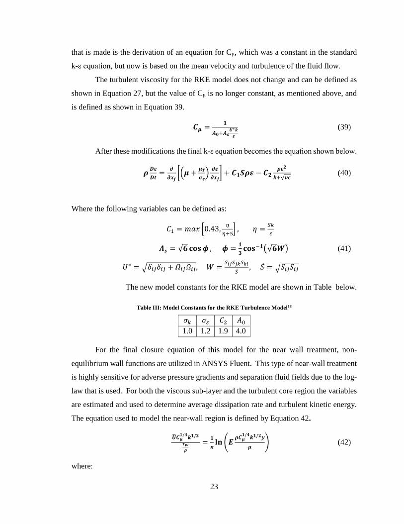
that is made is the derivation of an equation for Cμ, which was a constant in the standard

k-ε equation, but now is based on the mean velocity and turbulence of the fluid flow.

The turbulent viscosity for the RKE model does not change and can be defined as

shown in Equation 27, but the value of Cμ is no longer constant, as mentioned above, and

is defined as shown in Equation 39.

𝑪𝝁 =𝟏

𝑨𝟎+𝑨𝒔𝑼∗𝒌

𝜺

(39)

After these modifications the final k-ε equation becomes the equation shown below.

𝝆𝑫𝜺

𝑫𝒕=

𝝏

𝝏𝒙𝒋[(𝝁 +

𝝁𝑻

𝝈𝜺)

𝝏𝜺

𝝏𝒙𝒋] + 𝑪𝟏𝑺𝝆𝜺 − 𝑪𝟐

𝝆𝜺𝟐

𝒌+√𝒗𝝐 (40)

Where the following variables can be defined as:

𝐶1 = 𝑚𝑎𝑥 [0.43,𝜂

𝜂+5] , 𝜂 =

𝑆𝑘

𝜀

𝑨𝒔 = √𝟔 𝐜𝐨𝐬 𝝓 , 𝝓 =𝟏

𝟑𝐜𝐨𝐬−𝟏(√𝟔𝑾) (41)

𝑈∗ = √𝛿𝑖𝑗𝛿𝑖𝑗 + 𝛺𝑖𝑗𝛺𝑖𝑗, 𝑊 =𝑆𝑖𝑗𝑆𝑗𝑘𝑆𝑘𝑖

��, �� = √𝑆𝑖𝑗𝑆𝑖𝑗

The new model constants for the RKE model are shown in Table below.

Table III: Model Constants for the RKE Turbulence Model18

𝜎𝑘 𝜎𝜀 𝐶2 𝐴0

1.0 1.2 1.9 4.0

For the final closure equation of this model for the near wall treatment, non-

equilibrium wall functions are utilized in ANSYS Fluent. This type of near-wall treatment

is highly sensitive for adverse pressure gradients and separation fluid fields due to the log-

law that is used. For both the viscous sub-layer and the turbulent core region the variables

are estimated and used to determine average dissipation rate and turbulent kinetic energy.

The equation used to model the near-wall region is defined by Equation 42.

��𝑪𝝁𝟏/𝟒

𝒌𝟏/𝟐

𝝉𝒘𝝆

=𝟏

𝜿𝐥𝐧 (𝑬

𝝆𝑪𝝁𝟏/𝟒

𝒌𝟏/𝟐𝒚

𝝁) (42)

where:

24

�� = 𝑼 −𝟏

𝟐

𝒅𝒑

𝒅𝒙[

𝒚𝒗

𝝆𝜿𝒌𝟏/𝟐 𝐥𝐧 (𝒚

𝒚𝒗) +

𝒚−𝒚𝒗

𝝆𝜿𝒌𝟏/𝟐 +𝒚𝒗

𝟐

𝝁] (43)

Overall, the RKE turbulence model performs better than the standard k-ε model as

well as allowing several additional terms to be added if needed, including buoyancy and

compressibility terms. There is one main weakness that it is still present in the RKE

turbulence model that was not fixed with the present modifications and that is the model

still is limited being an isotropic eddy viscosity model. Despite this weakness, this model

performs much better for more complex flows including recirculation, rotation, separation,

and large adverse pressure gradients, which are largely present in the flow field around a

bus making this model more suitable for this study than the standard 𝑘-ε model.19

b. Shear Stress Transport k-ω Model (SST)

The Shear Stress Transport (SST) eddy-viscosity turbulence model combines both

a k-ε model and a k-ω equation. Using the SST model the inner boundary is modeled using

a k-ω equation while the outer region of the boundary layer and remain parts of the fluid

flow are modeled using a k-ε equation. This model allows for the shear stress in the adverse

pressure gradient region to be limited. There is one major disadvantage of the k-ω model,

the fact that it is dependent on the free stream value of ω. This mixing of different

turbulence models allows for this weakness and the two main weakness of the k-ε equation

to be avoided, the over predicting of the shear stress in adverse pressure gradients and the

need for near-wall modifications. The k-ω model does a much better job of modeling the

shear stress in the adverse pressure gradient region and no damping functions are needed

in the near-wall boundary layer.11 Figure 5 illustrates the blending of the two models into

one successful turbulence model, the SST model.19

25

Figure 5: Visual representation of the SST turbulence model. In this model for the inner layer near the wall a

modified version of the Wilcox k-ω model is used, the outer layer uses a k-ω model that is formed from the

standard k-ε model. These two models are blended together to form the final SST turbulence model. 19

Converting the k-ε equation into a k-ω equation using a simple change-of-variable,

is the first step to creating the SST model, using the relationship shown in Equation 44

when β* = Cμ.

𝝎 =𝝐

(𝜷∗𝒌) (44)

Using this relationship and the chain rule the following k- and ω-equations are

found for the outer layer of the fluid flow.

𝝆𝑫𝒌

𝑫𝒕= 𝝉𝒊𝒋

𝝏𝑼𝒊

𝝏𝒙𝒋− 𝜷∗𝒌𝝆𝝎 +

𝝏

𝝏𝒙𝒋[(𝝁 +

𝝁𝑻

𝝈𝒌𝟐)

𝝏𝒌

𝝏𝒙𝒋] (45)

𝝆𝑫𝝎

𝑫𝒕=

𝜸𝟐

𝒗𝒕𝝉𝒊𝒋

𝝏𝑼𝒊

𝝏𝒙𝒋− 𝜷𝟐𝝆𝝎𝟐 +

𝝏

𝝏𝒙𝒋[(𝝁 +

𝝁𝑻

𝝈𝝎𝟐)

𝝏𝝎

𝝏𝒙𝒋] + 𝟐𝝆𝝈𝝎𝟐

𝟏

𝝎

𝝏𝒌

𝝏𝒙𝒋

𝝏𝝎

𝝏𝒙𝒋 (46)

The turbulent viscosity can be defined as shown in Equation 47, while Equation 48

illustrates the equation for γ2 in Equation 46.

𝝁𝑻 = 𝝆𝒌

𝝎 (47)

𝜸𝟐 =𝜷𝟐

𝜷∗ −𝜿𝟐

(√𝜷∗𝝈𝝎𝟐) (48)

Table IV below defines the model constants for the outer layer.

Table IV: Model Constants for the Outer Layer for the SST Turbulence Model19

𝛽2 𝜎𝑘2 𝜎𝜔2 𝛽∗ κ

26

0.0828 1.0 1.168 0.09 0.41

The inner layer uses the original Wilcox k-ω model, shown in Equations 36 and 37,

with modified constants shown in Table V.

Table V: Model Constants for the Inner Layer for the SST Turbulence Model19

𝛽 𝜎𝑘 𝜎𝜔 𝛽∗ 𝜅

0.075 1.176 2.0 0.09 0.41

The turbulent viscosity for this part of the model can be defined as shown in

Equation 49.

𝝁𝑻 = 𝝆𝒂𝟏𝒌

𝒎𝒂𝒙(𝒂𝟏𝝎,𝜴𝑭𝟐) (49)

where:

𝐅𝟐 = 𝐭𝐚𝐧𝐡(𝐚𝐫𝐠𝟐𝟐), 𝐚𝐫𝐠𝟐 = 𝐦𝐚𝐱 (

𝟐√𝐤

𝟎.𝟎𝟗𝛚𝐲,

𝟓𝟎𝟎𝐯

𝐲𝟐𝛚) (50)

Once these two regions are defined they can be blended smoothly into one set of

equations for the whole fluid flow. This theory can be shown on Equation 51 with Equation

52 illustrating the variables defined, under the assumption that in the inner layer F1=1 and

in the outer region F1 approaches zero.

𝑭𝟏 [𝝆𝑫𝒌

𝑫𝒕+ ⋯ ]

𝒊𝒏𝒏𝒆𝒓+ (𝟏 − 𝑭𝟏) [𝝆

𝑫𝒌

𝑫𝒕+ ⋯ ]

𝒐𝒖𝒕𝒆𝒓 (51)

𝑭𝟏 = 𝐭𝐚𝐧𝐡(𝒂𝒓𝒈𝟏𝟒) , 𝒂𝒓𝒈𝟏 = 𝒎𝒊𝒏 [𝒎𝒂𝒙 (

√𝒌

𝜷∗𝝎𝒚,

𝟓𝟎𝟎𝒗

𝒚𝟐𝝎) ,

𝟒𝝆𝝈𝝎𝟐𝒌

𝑪𝑫𝒌𝝎𝒚𝟐,] (52)

𝐶𝐷𝑘𝜔 = 𝑚𝑎𝑥 (2𝜌𝜎𝜔21

𝜔

𝜕𝑘

𝜕𝑥𝑗

𝜕𝜔

𝜕𝑥𝑗, 10−20)

Using these equations the final k- and ε-equations for the SST turbulence model

come to the following equations:

𝝆𝑫𝒌

𝑫𝒕= 𝝉𝒊𝒋

𝝏𝑼𝒊

𝝏𝒙𝒋− 𝜷∗𝒌𝝆𝝎 +

𝝏

𝝏𝒙𝒋[(𝝁 +

𝝁𝑻

𝝈𝒌)

𝝏𝒌

𝝏𝒙𝒋] (53)

𝝆𝑫𝝎

𝑫𝒕=

𝜸

𝒗𝒕𝝉𝒊𝒋

𝝏𝑼𝒊

𝝏𝒙𝒋− 𝜷𝝆𝝎𝟐 +

𝝏

𝝏𝒙𝒋[(𝝁 +

𝝁𝑻

𝝈𝝎)

𝝏𝝎

𝝏𝒙𝒋] + 𝟐𝝆(𝟏 − 𝑭𝟏)𝝈𝝎𝟐

𝟏

𝝎

𝝏𝒌

𝝏𝒙𝒋

𝝏𝝎

𝝏𝒙𝒋 (54)

27

The turbulent eddy viscosity can be defined as shown in Equation 55.

𝝁𝑻 = 𝝆𝒂𝟏𝒌

𝒎𝒂𝒙(𝒂𝟏𝝎,𝜴𝑭𝟐)= 𝒎𝒊𝒏 (

𝒌

𝝎,

𝒂𝟏𝒌

𝜴𝑭𝟐) (55)

where:19

𝑭𝟐 = 𝐭𝐚𝐧𝐡(𝒂𝒓𝒈𝟐𝟐), 𝒂𝒓𝒈𝟐 = 𝒎𝒂𝒙 (

𝟐√𝒌

𝟎.𝟎𝟗𝝎𝒚,

𝟓𝟎𝟎𝒗

𝒚𝟐𝝎) , 𝜴 = √𝟐𝜴𝒊𝒋𝜴𝒊𝒋 (56)

This equation allows the Boussinesq assumption and −𝑣2′ 𝑣2

′ = 𝑎1𝑘 to be used in

only the boundary layer, for this reason it is multiplied by F2 which is 1 in the near-wall

region and nowhere else, while the turbulent eddy viscosity from the original k-ω model is

used everywhere else.

The SST turbulence model has proven, under adverse pressure gradients, to be able

to provide more accurate results in boundary layers. It has proven to be the most accurate

RANS model for aerodynamic fluid flows, making it the best choice for this study.11

E. Aerodynamic Drag Reduction Devices

When examining the aerodynamics of personal automobiles there is a large amount

of freedom to change the geometry of the vehicle to make it more aerodynamic, but this is

no longer possible with large ground vehicles.5 Originally buses had squared edges which

resulted in a coefficient of drag between 0.8 and 0.9. To reduce this drag all corners,

especially leading edges were rounded with a radius of about 10% the total width of the

bus. Inclining the entire front face of the bus allowed for an additional drag reduction of

about 8%. These changes led to the current geometry of commercial buses.7 Current bus

geometry is not as easily changed due to the fact that the internal volume needs to be

maximized for passengers, while external dimensions need to stay consistent with legal

limits.5 Current bus models have a drag coefficient in the range of 0.4 ≤ cd ≤ 0.7 depending

on the yaw angle.7

Since the basic bus geometry of today is not able to be changed simple add-on

aerodynamic devices have been examined. These devices have proven to modify the flow

field around the vehicle in a way such as to reduce the drag force. Another reason

aerodynamic add-on devices have become the prominent mode of drag reduction for

commercial vehicles is due to the large cost it would be to replace all vehicles compared

28

to the smaller cost of simple devices that could be attached to the vehicles already in

commission.14 Several aerodynamic add-on devices that have been produced for large

ground vehicles, especially tractor-trailers, include side skirts, spoilers, airvanes, vortex

generators, boat-tails, and cab extensions. Commercial buses do not have a cab therefore a

cab extension is not applicable and buses are general closer to the ground than tractor-

trailers therefore side skirts are also not a practical add-on device.

Most progress has been made on the windward face of the bus, attempting to

introduce large radii to the top and side edges to reduce the separation bubble created by

the sharp change in geometry. There have not been as many studies applied to the leeward

face of the bus; where a more aerodynamic shape could reduce the large pressure gradient

present on the bus and consequently reduce the overall drag.5

In 2001 Khalighi et al. performed a study on a bluff body hoping to reduce the

pressure losses near wake area using four extension plates on the base of the bluff body. It

was found that the addition of these plates allowed for the intensity off the recirculation

velocity to be reduced in the base region, the large-scaled turbulent motions to be

suppressed in the wake, and an increase in the pressure at the back of the bluff body. The

total drag coefficient was able to be reduced by about 20% and a reduction of 10% for the

turbulent intensity with the addition of these plates.18

Kim (2003) added a rear-spoiler to a large-sized bus model to reduce the wake

behind the bus. The addition of this drag reduction device produced a total drag reduction

of up to 16%, by reducing the extreme vortex that is created behind a bluff body, as well

as increasing the driving stability of the bus.14

When air flow is guided into the low-pressure wake region that develops behind a

bluff body, the pressure is increased, decreasing the adverse pressure gradient present on

the body. This reduction in pressure drag creates a reduction in the overall aerodynamic

drag present on the vehicle. One add-on drag reduction device that provides this

phenomenon is lateral guide vanes. Wahba et al. (2012) studied lateral guide vanes on a

large ground vehicle that was similar to a bluff body. It was found using these lateral guide

vanes could reduce the drag coefficient of a bluff body by up to 18%.9

29

1. Airvane as a Drag Reduction Device

The aerodynamic add-on devices examined in this study were airvane devices,

which are very similar to lateral air guides. Kirsch submitted patents in 1977 and 1976

introducing airvanes as a method of drag reduction on bluff bodies. Kirsch's 1977 patent

was very similar to his 1976 patent will minor differences. Airvanes are nozzle-like

devices, which are mounted along the corner edges of both the windward and leeward face

of the bluff body. The main goal of utilizing these airvanes was to reduce the drag force

on a body by preventing the separation that takes place on the sharp windward corners and

along the adjacent top and lateral faces that are rearward extending. The airvanes were

also able to create a forward thrust which reduces the adverse pressure gradient, which in

turn reduces the total drag on the vehicle. Figure 6 illustrates the airvane kit from the 1977

patent, that was presented in Kirsch’s patent and important aspects of the designed can be

referenced by the numbers present.

Figure 6: Airvane kit created by Kirsch with important aspects numbered. This device was specifically was

made for vehicle with rounded corners like buses. This device is made of two parts bolted together; the air flow

guide and the airvane itself. As the air flows through the airvane, if placed on the leeward face, decelerates into

the wake increasing the pressure in the wake zone. This reduces the adverse pressure gradient and the total

drag on the body.20

This drag reduction device consists of two separate parts, an air flow guide portion

(34) and an airvane portion (36). The air flow guide portion has the shape of an inverted

L-shape and is attached directly to the bluff body along the top windward corner with the

30

longitudinal planar portion (34b) and the downwardly dependent piece (34a). The airvane

component of the device has a planar portion that extends along the top horizontal face of

the bluff body (36b) and a concave curved element (36a) that is attached directly to the air

flow guide using brackets (38).

Based on a standard trailer with a height of 8-13 ft and a width of about 8 ft the

planar portion of the airvane should be approximately 1 inch above the air flow guide or

2-3 cm. The inlet of the airvane has a larger height than the outlet allowing for a contraction

that increases the velocity, the difference between the heights is called the expansion ratio.

Kirsch found that the ideal expansion ratio, b/c, to be 5.5 ± 0.5 while the vehicle travels 70

mph or 3.5 when traveling approximately 120 mph, where c is 2-3 cm as mentioned above.

The optimal included angle between a tangent line to the curve of the airvane and a

horizontal line was found to be 86º. It was found that the radius of the curved portion be

equal to or less than 12% of the distance between the stagnation point and the upper edge

of the windward face. The length of the planar portion of the airvane was found to be

between 1/2 and 3/2 the radius of curvature to ensure proper mixing of the air flow to

prevent turbulence. A similar airvane can be placed on the top leeward corner with the one

alteration, that the inlet is smaller than the outlet. It was also found that maximum drag

reduction was achieved when vertical airvanes were utilized on the vertical windward

edges which have identical geometry to the airvane described above.

Airvanes placed on the windward corners work by allowing the air flow to pass

from the stagnation point around the corners with little to no separation. The air that hits

the stagnation point spreads outward toward the edges of the windward face and therefore

to the airvanes that are mounted on those edges. The prevention of separation is achieved

by the constriction of the air flow through the airvane causing the velocity of the air to

increase. The air flow is discharged through the outlet between the air flow guide and

airvane which causes the air to flow along the faces of the vehicle with minimal separation.

When mounted on the leeward corners of the bluff body the air passing though the airvanes

is caused to decelerate which reduces the wake and increases the pressure behind the

vehicle therefore decreasing the adverse pressure gradient. The total drag reduction that

was found from using the airvanes on all corners on both the windward and leeward faces

was up to 30%.

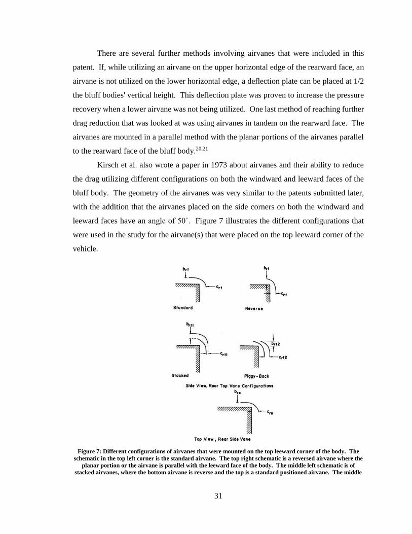
31

There are several further methods involving airvanes that were included in this

patent. If, while utilizing an airvane on the upper horizontal edge of the rearward face, an

airvane is not utilized on the lower horizontal edge, a deflection plate can be placed at 1/2

the bluff bodies' vertical height. This deflection plate was proven to increase the pressure

recovery when a lower airvane was not being utilized. One last method of reaching further

drag reduction that was looked at was using airvanes in tandem on the rearward face. The

airvanes are mounted in a parallel method with the planar portions of the airvanes parallel

to the rearward face of the bluff body.20,21

Kirsch et al. also wrote a paper in 1973 about airvanes and their ability to reduce

the drag utilizing different configurations on both the windward and leeward faces of the

bluff body. The geometry of the airvanes was very similar to the patents submitted later,

with the addition that the airvanes placed on the side corners on both the windward and

leeward faces have an angle of 50˚. Figure 7 illustrates the different configurations that

were used in the study for the airvane(s) that were placed on the top leeward corner of the

vehicle.

Figure 7: Different configurations of airvanes that were mounted on the top leeward corner of the body. The

schematic in the top left corner is the standard airvane. The top right schematic is a reversed airvane where the

planar portion or the airvane is parallel with the leeward face of the body. The middle left schematic is of

stacked airvanes, where the bottom airvane is reverse and the top is a standard positioned airvane. The middle

32

right picture is "piggy-back" airvanes; two reverse airvanes lined up with each other. The bottom most

schematic is of a standard airvane placed on the side edges of the body.25

These different configurations included the standard airvane that was described

above, with the planar portion of the airvane parallel with the top face of the bus. The

second configuration is the reverse airvane that has the planar part of the airvane parallel

with the back leeward face of the body. Airvanes were also stacked on top of each other,

where the bottom airvane is positioned similar to the reverse airvane while the top airvane

is positioned similar to the standard airvane, making sure that the top airvane is protruding

past the bottom airvane. The last configuration was the “piggy-back” formation that

contains two reverse airvanes in line with each other. The last part of Figure 7 illustrates

the alignment of the airvane that was mounted on the side corners of the vehicle.

In this study it was found that while utilizing an airvane on the top windward corner

of the body a drag reduction of approximately 10.8% was observed. When 50˚ airvanes

were mounted on the side corners of the windward face a total drag reduction of 8% was

attributed to the side airvanes alone. In this study it was found the rear-mounted airvanes

had little effect on the turbulence present in the wake behind a bluff body and only about

1% drag reduction was observed. When an airvane was placed on the lower horizontal

edge a total drag reduction of 2.5% was calculated. The optimal configuration for the

windward face was found to be a “piggy-back” arrangement that produced a total drag

reduction of 3% without a stagnation plate and 4% with one. When side airvanes where

mounted to the body a total drag reduction of 6% was observed. These studies illustrate

that airvanes are a successful type of add-on drag reduction device that can be employed

on commercial buses.22

Once the total reduction in drag coefficient was found it could be used to find the

reduction in fuel consumption that would be produced by the airvanes employed. The

reduction in fuel consumption could be calculated using Equation 57 below.

𝜟𝑭𝑪

𝑭𝑪=

𝜟𝑷

𝑷= 𝜼 ∗ (

𝜟𝑪𝑫

𝑪𝑫+

𝜟𝑺

𝑺+

𝟑𝜟𝑼

𝑼) (57)

In this equation CD was the drag coefficient, S was the frontal area and U was the

velocity of the vehicle. A property of the diving cycle, η, was used in this equation and it

often ranges between 0.5 and 0.7 for vehicles at highway speeds, such as those used in this

study. A value of 0.7 was utilized for this study.23

33

Using Kirsch’s studies on airvanes as drag reduction devices for bluff bodies and

the turbulence models outlined in Section I-D, a study was conducted to utilize airvane

systems as add-on drag reduction devices to reduce the aerodynamic drag force on

commercial buses. ANSYS Fluent was employed as the Computational Fluid Dynamics

software and the method and different configurations studied are outlined in the

Experimental Procedure section of this paper.

34

EXPERIMENTAL PROCEDURE

Parameter studies were conducted to determine the optimal geometries and

configuration for the add-on airvane devices implemented on the bus model. An optimal

design and configuration would produce maximum drag reduction. A scaled-down model

bus was designed and constructed, using computer aided design (CAD). Dassault

Systèmes’ SolidWorks was employed for this study. 24 Once the CAD models of the bus,

with and without airvane devices, were designed they were imported into the computational

fluid dynamics (CFD) program, ANSYS Fluent.13 ANSYS Fluent was utilized to perform

external fluid flow simulations, predicting the drag coefficient of each bus model with

different airvane configurations. These drag coefficients were compared and studied to

determine the optimal airvane design. To further reduce computational time required for

each simulation the CAD model was scaled down to a 1/35th scaled model. This size model

was chosen based off of other studies’ scaling and the ability of the model to fit into a wind

tunnel box that would later be modeled in Fluent. The process that was taken, for both

SolidWorks and Fluent, is outlined in this section.

A. SolidWorks Scaled-Down Model

Today’s industry offers several different styles of buses, all with unique geometry

and drag coefficients. Subsequently, a specific model of bus had to be chosen to study.

Motor Coach Industries Int’l, Inc.’s D4505 commercial bus was chosen, although it should

be noted that the CAD model used was not an exact replica of the D4505 bus, but an

approximate model. The MCI D4505 model was chosen for the basis of this study because

it is currently one of the most popular models of commercial bus used. The D-Series

commercial bus was introduced to the market in 2010 and by May 2014 there were over

188 D4505 buses in the Greyhound fleet.25 The entire bus was designed as one part rather

than as an assembly to reduce the possibility of errors when exported to Fluent.

The MCI D4505 bus used as the basis for this study was 13.84 m from bumper to

bumper, had an overall width of 2.59 m and an overall height of 3.48 m. The distance

between the front wheels and the rear driving wheels was 8.08 m, while the front overhang

was 1.93 m, and the rear overhang was 2.68 m. The front overhang was the distance

between the front wheels and the windward face, while the rear overhang was defined as

35

the distance between the rear driving wheels and the leeward face. The bus contained three

wheel axles, one in the front with one set of wheels, and two wheel axles in the back. The

rear drive axle had two sets of wheels and the rear trailing axle had only one set of wheels.

The rear track for the drive axle, or distance between the wheels on the same axle was 1.94

m, while the tracks of both the front axle and rear trailing axle were 2.17 m. All wheels on

the bus were 22.5 x 9 in, which was equal to 0.5715 x 0.2286 m.26 These dimensions were

then scaled down to create a 1/35th scaled model. The base scaled dimensions used to

design the model are shown in Table X of Appendix A.

The dimensions given above give the basic geometry of the bus, but further

geometry was need to accurately produce a realistic model of a bus. Simple blueprints

were found and utilized in SolidWorks to project the side contour of the bus, the front and

back blueprints were not used due to the fact that it was unable to be determined if the top

face was rounded along the entire bus or only at the end. Using the contour of the side of

the bus allowed for the windward face to be inclined similar to the real model of the D4505

commercial bus shown in Figure 8.

Figure 8: Motor Coach Industries Int'l. Inc. D4505 commercial bus that was used as a loose model for the bus

studied in this paper.26 This model of bus was used as a base for the 1/35th model that was created in

SolidWorks and tested in ANSYS Fluent.

Figure 53 in Appendix B displays the side view of the D4505 bus that was used in

SolidWorks.27 Since it could not be fully determined if the entire top of the bus was

rounded, or if so the proper radius, Kim's14 study was followed and the top of the bus was

kept flat and the top rearward extending edges and top windward edge were filleted with a

0.005 m radius, which on the full scale bus would be 0.175 m.

36

All edges on the bus were filleted to help air flow more easily around sharp changes

in geometry. Edges present on the bottom of the bus, the leeward face, and the wheels and

wheelbases were filleted with a radius of 0.001 m, which on the full sized bus would be

0.035 m. Edges present on the bumper and vertical leeward edges were filleted to 0.0025

m, which on a full size bus would be 0.0875 m. These fillets, however small, reduced the

size of the separation bubbles that were produced when there was a sharp change in

geometry.

Figure 9: SolidWorks 1/35th scaled CAD model of commercial bus studied in this paper. This model bus was

based loosely off of MCI’s D4505 bus. This figure illustrates the finalized bus, but the model that was used in

the ANSYS Fluent simulations did not have the reflectors, headlights, windshield wipers, windows, etc.. Further

views are shown in Figure 54 in Appendix C.

Once the basic CAD model was designed and constructed it was imported into

ANSYS Fluent where simulations could be performed to determine the drag coefficient of

the vehicle. After the model was tested and the drag coefficient for the bus without any

drag reduction devices generated, airvanes could be designed and added to the model.

Parameter studies were implemented for the addition of airvane devices on the model bus,

determining the optimal dimensions that would maximize the reduction in drag. This

process is further explained in Section B below.

B. Parameter Study to Reach Optimized Airvane Devices

SolidWorks was employed to design airvanes added directly to the bus model and

to change dimensions of the airvanes for the parameter studies run. As the parameter

studies were run and completed, individual models were made for each parameter

37

examined. The airvane was added to the SolidWorks part file rather than attached as an

assembly, to avoid errors when imported into Fluent. The airvanes consisted of three loft

features, one over the flat top face of the bus and one over each curved edge of the top

rearward extending face. Two vertical plates were designed, placed between the three lofts,

attaching them to each other and to the bus itself. All three lofts were created using the

same dimensions, those which were tested in the parameter study.

The dimensions of the airvane that was used as the original start point for the study

was based off of Kirch et al.’s studies, as described in Section E of the Introduction.20,21,22

The inlet gap was set at 2.5 cm, which for the 1/35th scale was 0.7143 mm. For the curved

the portion of the airvane that extended past the top horizontal leeward corner, the radius

was set at approximately 12% of the distance between the stagnation point and the top

windward edge. This came to a dimension of approximately 7.886 mm on the 1/35th scale.

The planar portion of the airvane parallel to the top face of the bus was set to one times the

radius of the curvature. An additional portion of the planar section extended past the

leeward face of the bus, before the curved portion began. This extension, which was set as

the same dimension as the inlet gap, 0.7143 mm, was implemented to reduce the chance of

a constriction of the air passage due to the curved edge of the bus model itself. When the

inlet gap was examined in the parameter study this extension was also changed. The

expansion ratio was set to approximately 5.1 to account for the fact that the velocity used

in this study was slightly higher than the 70 mph which gave an expansion ratio of 5.5.

This expansion ratio gave the dimension of 3.651 mm for the outlet gap. The angle between

the line tangent to the radius of curvature and the horizontal from the planar section was

set as 86˚. After the base airvane was constructed a parameter study was implemented that

isolated a single parameter at a time to determine the optimal dimension for that parameter

before testing another parameter.

The first parameter examined was the angle between the tangent line to the curved

portion and the horizontal from the planar section. The angle was changed from 80˚ to 35˚

in increments of 5˚. In place of the 85˚ test the original model of 86˚ was implemented.

Once the simulations were run the angle that provided the highest drag reduction, 55˚, was

set as the new dimension for the airvane. To further test the angle a more refined set of

simulations were run for the angles between 60˚ and 50˚ in increments of 1˚. Since 60˚,

38

55˚, and 50˚ were already run in the previous set of simulations those angles were not rerun.

It was found that 53˚ was the optimal angle and that was set as the angle for the top airvane

for the rest of the study.

The next parameter studied was the expansion ratio, the ratio between the inlet gap

and the outlet gap. The expansion ratio was changed from 1:2 to 1:6.5 with increments of

1:0.5. It was found that 1:6 was the best expansion ratio; therefore a refinement set of

simulations was run for the expansion ratios from 1:5.6 to 1:6.4 with an increment of 1:0.1.

The optimal expansion ratio was found to be 1:6 and was set as the expansion ratio for the

top airvane for the rest of the study.

The radius of the curvature was the third parameter tested and a set of simulations

was run to test the radius of curvature from 5% of the distance from the stagnation point to

the top windward face to 15%. It was found that 8% was the optimal percentage of the

distance between the stagnation point and the top windward face. This dimension was

utilized for the rest of the study. The inlet gap was then studied, which in turn changed the

outlet gap, but it was ensured that the expansion was kept at the 1:6 ratio. The inlet gap

was changed from 2 cm to 4.5 cm in increments of 0.5 cm, which on the 1/35th scale was

approximately 0.5714 mm to 1.286 mm, in increments of 0.143 mm. An inlet gap of 4.5

cm was found to be optimal and was employed as the inlet gap of the rest of the study.

The angle of the planar length was tested next. This was the angle downward from

the horizontal that the planar section of the airvane was set at. A set of simulations was

run from 0˚ to 6˚ in increments of 0.5˚ and it was established that an angle of 4˚ produced

the highest drag reduction and therefore was set as the angle of the planar section for the

airvane. Lastly, the length of the planar section was examined from 0.25 times the radius

of curvature to 2.5 times the radius of curvature. It was found that 2.5 times the radius of

curvature was ideal and was therefore implemented. This was the final parameter that was

studied for the optimization of the top airvane. Figure 10 illustrates the optimized top

airvane that was designed during this parameter study, as it is attached to the top horizontal

leeward edge of the bus.

39

Figure 10: Optimized airvane attached to the top horizontal edge of the leeward face of the bus. SolidWorks was

utilized to model the airvane that was studied during the parameter study. The parameter study looked at one

parameter of the airvane at a time and a range of dimensions for that parameter was tested. This parameter

study led to the optimized airvane shown.

Once the optimal airvane was designed for the top horizontal edge on the leeward

face of the bus, airvanes were added to the side vertical edges of the leeward face. Only

one side airvane was modeled in SolidWorks and studied in Fluent due to the fact that the

bus was symmetrical. The same parameter study that was run on the top airvane, detailed

above, was employed for the side airvane parameter study with one major difference. This

difference was for the base airvane that the parameter study was started with; the tangent

angle for the radius of curvature was changed from 86˚ to 50˚ as recommended by Kirch

et al..20,21,22 The inlet gap was also set parallel and equal with the inlet gap of the top

airvane with the same inlet gap height, 4 cm, and planar length. The last change was the

expansion ratio and was set at approximately 1:3.3.

For the first test in the parameter study, the general angle change, an angle of 35˚

was found as the optimal angle for both the Realizable k-ε turbulence model and the SST

k-ω turbulence model therefore the refined angle set of simulations was run from 30˚ to

40˚ in increments of 1˚. After this set of simulations 33˚ was found to be the optimal angle

for the side airvanes and was utilized for the remaining studies. The same range, for the

top airvane, was used for the general expansion ratio parameter study and 1:6 was found

as the optimal one. Therefore the refined parameter study for expansion ratio was run from

1:5.6 to 1:6.4 in increments of 1:0.1. It was found that 1:6 was the optimal expansion ratio

and was employed as the final expansion ratio for the side airvanes. A range of 7% to 15%

of the distance between the stagnation point and the top edge, in increments of 1% was run

for the radius of the curved portion of the airvane. The optimal dimension was found to be

12% of the distance between the stagnation point and the top horizontal edge of the

40

windward face. The same range was utilized for the inlet gap and a gap of 3.5 cm was

found as the optimal inlet gap. The angle between the planar portion of the airvane and the

horizontal was tested from 0˚ to 5˚ in increments of 1˚ and it was found that no angle, 0˚,

was the optimal angle for the planar section. The same range was used for planar length

as was used for the top airvane, from 0.25 times the radius of curvature to 2.5 times the

radius. It should be noted that the radius of curvature for the side airvane was found to be

different than the top airvane, therefore the magnitude of the dimensions were different. A

planar length of 0.5 times the radius of curvature was found as optimal dimension for the

side airvane. This test was the last set of simulations ran for the parameter study of the

side airvane. The optimal side airvane, as it was attached to the bus, is shown below in

Figure 11.

Figure 11: Optimized airvane attached to the side vertical edges of the leeward face of the bus. SolidWorks was

utilized to model the airvane that was studied during the parameter study. The parameter study looked at one

parameter of the airvane at a time and a range of dimensions for that parameter was tested. This parameter

study led to the optimized airvane shown.

To further optimize the reduction in drag coefficient additional tests were run

employing airvanes in the different configurations. The first set of simulations run added

a bottom airvane to the bottom horizontal edge and/or a deflection plate on the leeward

face of the bus. The deflection plate was first addition tested with and without side airvanes

41

attached. Two different bottom airvanes were then tested, one with the same dimensions

as the top airvane and one with the same dimensions as the side airvanes. The bottom

airvane was tested with and without the side airvanes in place. The last set of these

simulations tested the deflection plate and bottom airvane used in tandem, with and without

the side airvanes attached. Once it was determined the best combination the last set of

simulations could be started with the combination in place.

The different configurations presented in Figure 7 were then implemented for the

top airvane. These configurations included an airvane positioned in a reverse position as

the original airvane, meaning the planar portion was placed along the leeward face of the

bus. The second configuration was the stacked alignment; this consisted of two airvanes

one on top of the other. The bottom airvane was a reversed position airvane, while the top

airvane was the standard positioned airvane. The last configuration tested was the piggy-

back positioning, where two reversed airvanes were place in line with each other. These

simulations were the final tests of the parameter studies and once designed in SolidWorks

the models could be placed into Fluent for simulations to be run as described below.

C. ANSYS Fluent Setup and Procedure

ANSYS Fluent was utilized, as the computational fluid dynamics software, to run

fluid flow simulations on the SolidWorks CAD models. The simulation process was split

up into four separate sections; Geometry, Meshing, Setup, and Solution. For all

simulations, for models with and without the airvane, the process that was followed was

the same. Appendix D shows the step-by-step procedure followed for the simulations

performed.

1. Geometry Setup

Step one of the Fluent setup was to define the geometry that would be modeled.

Once the SolidWorks model was uploaded an enclosure was designed surrounding the bus

model to represent the air neighboring the bus. For accurate results the enclosure was

designed to represent the size of an actual wind tunnel, one which would be used for an

experimental study. Rodi found, in his study of computational methods, that the

dimensions for an appropriately sized computational wind tunnel were; three and a half

times the overall height of the model bus for the upstream length, nine times the height for

42

the width, ten times the height for the downstream length, and six times the height for the

height of the wind tunnel.6 The dimensions used for the 1/35th scaled wind tunnel model

are shown below in Table VI.

Table VI: Dimensions for Wind Tunnel Enclosure Designed in ANSYS Fluent (These dimensions for the

computational wind tunnel, on the 1/35th scale, were found using Rodi's study. The width dimension was only

used in the +x direction because the bus was symmetrical, therefore only half the bus was modeled in Fluent.

The height was only used in the +y direction because the bus sits on the ground, therefore there was no air

present below the wheels.6)

Length (Upstream) Width Height Length (Downstream)

0.348 m 0.4474305 m 0.596574 m 0.99429 m

1.141665 ft 1.46795 ft 1.95714 ft 3.2619 ft

Commercial buses, like all vehicles, have symmetrical geometry longitudinally;

therefore the enclosure feature was also used to only extract the air on the right side of the

model bus, thus reducing the computational time for the simulations that were run. This

was done by inserting a symmetry plane along the YZ Plane, which cut the bus in half

longitudinally. The same theory could be used to produce the road boundary below the

bus. It was found that a symmetry plane could not be used to produce the road boundary

condition, because an error would be present; therefore a dimension of 1E-6 m was used

in the –y direction. Once the wind tunnel enclosure was constructed the Boolean feature

was employed to subtract the volume of the bus from the volume of enclosure. This process

created a new volume that represented only the air that surrounded the bus. This volume

was the fluid that was looked at in when simulating the fluid field around the bus.

A refinement box was then built around the outline of the bus. This refinement box

allowed, when looking at meshing of the volume, a finer mesh to be implemented for only

the air closer to the bus. The box was designed so it was large enough to provide

appropriate refinement, but not to large that unnecessary refinement was used that greatly

increased computational time. The dimensions that were used can be shown below in Table

VII.

Table VII: Dimensions for Refinement Box that Allowed for a More Refined Mesh for the Air Closely

Surrounding the Bus (The total length represents the length of the box, while the downstream from origin is the

portion of the total length that was behind the origin that was present at the front of the bus. The height is from

the bottom of the wheels to the top of the refinement box. The extrusion was from the center of the bus out

laterally to the outside of the refinement box.)

43

Total Length Height Downstream from Origin Extrusion

0.881425 m 0.15 m 0.528855 m 0.15 m

2.89181 ft 0.492126 ft 1.735089 ft 0.492126 ft

Once the refinement box was created the Geometry Setup was complete and

meshing was started.

2. Meshing Procedure

Two different mesh types were developed in this study, polyhedral and CutCell.

ANSYS recommended hexahedral or polyhedral meshes, or a hybrid of both, be used for

moderately complex geometry similar to the model bus in this study. Due to the large

number of hex cells present, CutCell meshes often produce better results than tetrahedral

meshes.28 Pointer employed hexahedral elements, in a polyhedral “cut” cell mesh, finding

that it was able to accurately simulate the air flow around a tractor trailer.2 The CutCell

mesh used in this study was similar to Pointer’s polyhedral “cut” cell mesh, containing

mostly hexahedral elements, with other elements, such as tetrahedron, wedge, and pyramid

elements, being utilized that were better suited to reduce the skewness. Skewness can be

defined as the measure of how close to ideal a specific cell is. Skewness was measured

from zero to one, where zero defined a cell that was ideal, for example an equilateral

triangle, and one was a cell that was highly degenerated, for example a triangle that has

sides that are nearly coplanar. It should be noted that once the CutCell mesh was imported

into Fluent the elements that were connected to parent faces and hanging nodes were

converted to polyhedral elements. Figure 12 illustrates the different element types

available in ANSYS Fluent.28

44

Figure 12: Different element types for three-dimensional meshes available in ANSYS Fluent. CutCell meshes

used in this study contained between 80 and 95 percent hexahedron elements while the final percentage was

made up of tetrahedron, wedge, and pyramid elements where appropriate. When the CutCell mesh was

imported into Fluent the elements connected to parent faces and all hanging nodes were converted to

polyhedron elements. The second type of mesh used was fully polyhedral meshes, which were originally

tetrahedral meshes that were converted to polyhedral.28

Polyhedral mesh was chosen as the second type of mesh to be utilized in this study.

It was found in Pointer et al.’s study that an unstructured polyhedral mesh was successful

in producing accurate results for external fluid flows.29 Polyhedral meshes were converted

in Fluent rather than constructed in the Mesh component of the setup. When converting

from a tetrahedral mesh to a polyhedral mesh the cell count was reduced and therefore

required less computational time to converge. Although, in general the polyhedral meshes

were coarser they held higher quality elements and therefore needed less improvements.

Both the CutCell and polyhedral meshes were setup using the same method to maintain

consistency for better comparison of results.

Several meshing parameters were changed to better suit this study. Relevance of

each mesh was set to 100. Relevance allowed for the adjustment of the fineness of the

entire mesh as a whole. Relevance of 100 meant high accuracy while a relevance of -100

meant high speed, the higher the accuracy the slower the speed and the lower the accuracy

the higher the speed. A higher accuracy was chosen for this study, which caused the

simulations to take a longer amount of time. The advanced size function was set to

proximity and curvature, which allowed for the progression from minimum size elements,

closer to the bus and around the curvature of the bus, to maximum size elements farther

away from the bus toward the walls of the wind tunnel box. The relevance center was then

45

set to medium, ensuring that the entire mesh was of medium fineness, giving higher

accuracy then a coarse mesh, but higher speed then a fine mesh. Smoothing was changed

to high, increasing the number of smoothing iterations, which improved element quality by

moving nodes with respect to other nodes and elements in the vicinity.

There was only one difference in mesh setup between the CutCell meshes and the

polyhedral meshes. This difference was the setting that was chosen for the method of the

assembly meshing. Assembly meshing applied a specific mesh to the entire assembly

rather that to a specific part of the model. There were three choices None, CutCell, and

Tetrahedron. CutCell was selected to create the CutCell mesh, while Tetrahedron was

chosen for the mesh that was later converted into a polyhedral mesh. Tetrahedron was

chosen for the mesh type for the polyhedral due to the fact it is an unstructured mesh and

therefore was able to be converted to a polyhedral mesh much easier with better quality

elements. This type of assembly mesh was able to provide a medium coarse mesh, after

converted to polyhedral, which was desired for this study.

These parameter changes provided a default minimum element size of 0.46295 mm

and a maximum element size of 59.258 mm, with the small elements closer to the bus and

the larger elements closer to the wind tunnel walls. The default growth rate of 1.10 was

used, meaning in each subsequent layer of the mesh the element edge length was increased

by 10%. The default minimum element length for this study was 1.9783e-004 mm. The

default curvature normal angle, the maximum angle that a single element was allowed to

span, of 12˚ was employed. The number of layers used in gaps in the mesh was defaulted

at five and the proximity size function source was set to edges. Using this setting edge-to-

edge proximity would be used when proximity sized function calculations were completed.

These settings provided a base mesh, but further refinement was employed to increase the

fineness of the mesh near the bus itself.

Two local mesh sizing controls were generated to further refine the mesh, in order

to produce a more accurate simulation. Sizing controls allowed for the defining of precise

element size for a specified area rather than the entire mesh. The first type of sizing that

was used was a body of influence. Body of influence sizing allowed one body, in this study

the Boolean feature, to influence the mesh density of another body, in this study the

refinement box, while not being influenced itself. Default element sizes were accepted.

46

Element sizing was also employed, with the faces that were influenced being the entire bus

contour. This further increased the mesh density on the faces of the bus, where the fluid

flow was most important. The default settings were again used for this sizing, meaning

that either the global minimum size or the local element size was used depending on which

was smaller. Figure 13 illustrates the CutCell mesh that was produced and employed for

the bus model without any drag reduction device. On average the CutCell meshes

contained approximately 1.02 million to 1.07 million elements.

Figure 13: CutCell mesh created in ANSYS for the bus model without a drag reduction device attached. This

mesh was repeated for all simulations run for the bus models with the drag reduction devices. The growth rate

of the mesh can be observed. Closer to the bus the mesh is much finer, while farther away the mesh becomes

coarser.

Figure 14 illustrates an enhanced view of the CutCell mesh surrounding the contour

of the bus. The growth rate can be seen around the bus. The elements in close proximity

to the contour are much smaller and around the curvature the elements become even

smaller. The tetrahedral mesh that was created to be converted into the polyhedral mesh

was very similar to the CutCell mesh shown with the exception that tetrahedrons were used

rather than hexahedrons.

47

Figure 14: Enhanced view of CutCell mesh created in ANSYS. In close proximity to the buses contour and

around the curvature the mesh is finer and each succeeding layer of elements is 10% larger where the

refinement is unnecessary. The tetrahedron mesh that was produced to later be converted into the polyhedral

was similar to the CutCell design with the exception that tetrahedrons were used in place of hexahedrons.

Figure 15 illustrates the polyhedral mesh that was created when the tetrahedral

mesh was converted. The polyhedral meshes ranged, on average from 950,000 to

1,010,000 elements.

Figure 15: Polyhedral mesh created in ANSYS Fluent. Tetrahedral mesh was converted into a polyhedral mesh

increasing accuracy and reducing total cell count, which in turn reduced the total computational time.

Lastly, named sections were created that were referenced in Fluent when

performing simulations. The plane in front of the bus was the velocity inlet while the plane

behind was the pressure outlet. The face underneath the bus was the road, while all faces

of the bus were their own section, both were considered walls. All other sides of the wind

tunnel were symmetry planes. Once the meshes were created the fluid flow simulations

could be run.

48

3. Fluent Procedure

Both the Realizable k-ε model and SST k-ω model were employed in the Fluent

simulations for all models of the bus with and without the airvane attached. Based off of

the calibration that was run on the Fluent simulations, explained in Section D below, the

Realizable k-ε turbulence model was run with a polyhedral mesh and the SST k-ω

turbulence model was run with a CutCell mesh. While using the Realizable k-ε turbulence

model a non-equilibrium near-wall treatment was also employed.

All simulations were run with a velocity of 75 mph or 33.528 m/s impeding the

motion of the bus. The velocity’s origin was set at the named section “Velocity Inlet” in

the direction of the named section “Pressure Outlet” in reference to the “Air”. The

turbulence intensity for the velocity inlet was reduced to 1%. Turbulence intensity can be

defined as the root-mean-square of the velocity fluctuations over the mean flow velocity.

A turbulence intensity of 1% is relatively low meaning steady air flow and the velocity

introduced to the simulation had very low fluctuations and therefore very little turbulence.

The area of each specific model was found using Fluent’s project area feature and was

utilized in determining the drag coefficient of the bus model from the force that was

calculated during the simulation.

A coupled scheme was chosen for the pressure-velocity coupling. This scheme is

more robust and efficient than other schemes for steady-state flows, such as the flow in this

study. While employing a coupled scheme the flow Courant number was set to 50 while

both the explicit relaxation factors for momentum and pressure to 0.25. The flow Courant

number is the ratio between the computational distance step and the distance a disturbance

travels in one time step. Reducing this value improves the accuracy and steadiness of the

simulation. The reduction in the explicit relaxation factors allowed for a more skewed

mesh to be converged easier. They represent the percent of the solution being used from

iteration to iteration throughout the simulation. The turbulent viscosity relaxation factor

was set to 0.95 for the Realizable k-ε model and 0.8 for the SST k-ω turbulence model.

In order to monitor the calculation and simulation of the drag coefficient a monitor

was created for drag on the bus, due to the velocity impeding the motion of the vehicle.

Once the drag monitor was created it could be used to set the convergence criterion for the

simulation. Convergence was defined as the drag coefficient remaining constant at the 1e-

49

5 value for ten consecutive iterations. Once this convergence was met the simulation was

complete and was stopped.

The simulations were run for varying times. Simulations employing the Realizable

k-ε turbulence model were run for 500 iterations and often converged before those

iterations were completed. Simulations utilizing the SST k-ω turbulence model were run

for between 1000 and 3000 iterations depending on the computational time it took to reach

convergence. Once convergence was reached the solution could be analyze to determine

the effectiveness of the airvane being studied.

After the simulations were complete the post-simulation part of Fluent was utilized

to fully analyze the solution and the air flow through and around the airvane and bus.

Contours of the pressure, turbulence, and velocity magnitudes were created using this

software. Other visual aids where created in CFD-Post such as pathlines.

D. Calibration of Fluent Simulations

When comparing the drag coefficients, the uncertainty of the simulations had to be

considered to ensure that the optimal parameter was in fact the optimal choice and not an

error in calculations. To determine the accuracy of the Fluent simulations run a calibration

study was performed on both the Realizable k-ε model and the SST k-ω model. The

calibration was run on the first set of simulations of the parameter study, the original

airvane with only the angle between the tangent line and the horizontal changing. Four

sets of simulations were run; a set with the CutCell mesh and the Realizable k-ε turbulence

model, a set with the CutCell mesh and the SST k-ω model, a set with the polyhedral mesh

and the Realizable k-ε turbulence model and lastly a set with the polyhedral mesh utilizing

the SST k-ω turbulence model.

Once all simulations were run the values found for the drag coefficients were

compared and repeatability examined. Similar meshes and turbulence models were

compared; meaning the first run of the Realizable k-ε model utilizing a polyhedral mesh

was compared with the second run of Realizable k-ε model utilizing a polyhedral mesh.

This comparison showed the reliability of the convergence of the simulations for all

combinations of mesh and turbulence model. This calibration also helped to determine that

Realizable k-ε with a polyhedral mesh and SST k-ω with a CutCell mesh were the two

most reliable combinations and were used for the rest of the study.

50

RESULTS AND DISCUSSION

A. Calibration of Fluent

While comparing multiple sets of data produced, the uncertainties and repeatability

of those data sets were examined first. This examination was able to conclude whether the

small differences in the drag coefficient were from the addition of the airvanes or the error

in software used to find the solutions. Appendix E contains the raw data collected from

the simulations which were run for the calibration tests. This data, as stated in the previous

section, was run on the first set of tests in the parameter study; the change in the angle

between the line tangent to the curved portion of the airvane and the line on the horizontal.

The raw data includes the drag coefficients that were calculated during the simulations and

the percent reductions in the drag coefficient. Percent reductions were calculated between

the drag coefficient calculated for the bus without an airvane attached and the drag

coefficient found for each bus model with the airvane attached, including the angle

changes.

To determine the repeatability runs were compared to like runs, meaning the RKE

turbulence model employing the polyhedral mesh in the first run was compared to the RKE

turbulence model employing the polyhedral mesh in the second run. This was repeated for

the RKE turbulence model employing the CutCell mesh, the SST model employing the

polyhedral mesh, and lastly the SST model employing the CutCell mesh. Polyhedral RKE

calibration simulations were analyzed first. Figure 16 illustrates a graph of the drag

coefficients found during the simulations versus the angle the airvane was set to, for both

the first and second run. The blue line was the first calibration run, while the red line

represents the second calibration run.

51

Figure 16: Calibration tests run for the Realizable k-ε turbulence model utilizing a polyhedral mesh. This graph

represents drag coefficients found in simulations for varying angles between the line tangent to the curved

portion of the airvane and the line on the horizontal. The blue line represents the first run of the simulations

and the red line represents the second run of the calibration simulations.

Regarding Figure 16, it can be observed that the first and second calibrations runs

were nearly identical. If there was a error in the Fluent simulations the two graphs would

not be identical, showing a slight difference in values. The average standard deviation

between runs for the coefficient of drag was found to be ± 0.00006. Convergence criterion

was set to 1E-5, therefore it could be assumed that the standard deviation for this

combination of mesh and turbulence model was very small. These observations, in

cohesion, determined that when employed together, the polyhedral mesh and the RKE

turbulence model, were almost completely repeatable and the amount of uncertainty

present in the simulations was negligible.

A combination of CutCell mesh and RKE turbulence model was the next set of

simulations to be analyzed. Figure 17 displays the calibration for these simulations. The

blue line represents the first set of simulations run and the red line was the second set of

simulations run. The graph represents the drag coefficient found from Fluent simulations

versus the angle that the airvane was changed to.

0.5860.588

0.590.5920.5940.5960.598

0.60.6020.6040.6060.608

30 50 70 90

Dra

g C

oe

ffic

ien

t

Angle (Degrees)

Polyhedral RKE

First Run

Secoond Run

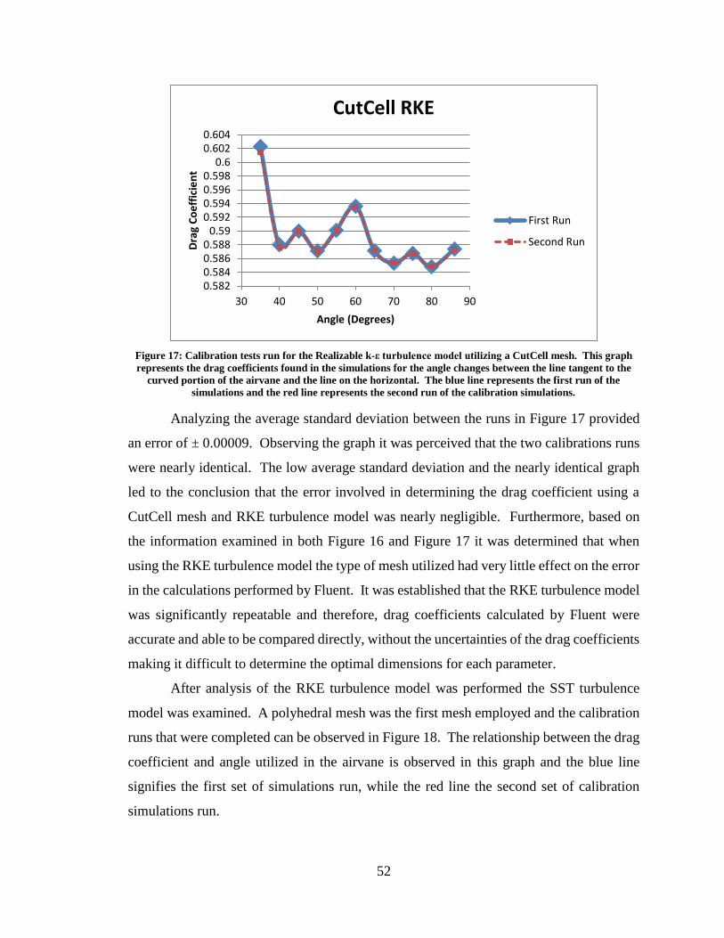
52

Figure 17: Calibration tests run for the Realizable k-ε turbulence model utilizing a CutCell mesh. This graph

represents the drag coefficients found in the simulations for the angle changes between the line tangent to the

curved portion of the airvane and the line on the horizontal. The blue line represents the first run of the

simulations and the red line represents the second run of the calibration simulations.

Analyzing the average standard deviation between the runs in Figure 17 provided

an error of ± 0.00009. Observing the graph it was perceived that the two calibrations runs

were nearly identical. The low average standard deviation and the nearly identical graph

led to the conclusion that the error involved in determining the drag coefficient using a

CutCell mesh and RKE turbulence model was nearly negligible. Furthermore, based on

the information examined in both Figure 16 and Figure 17 it was determined that when

using the RKE turbulence model the type of mesh utilized had very little effect on the error

in the calculations performed by Fluent. It was established that the RKE turbulence model

was significantly repeatable and therefore, drag coefficients calculated by Fluent were

accurate and able to be compared directly, without the uncertainties of the drag coefficients

making it difficult to determine the optimal dimensions for each parameter.

After analysis of the RKE turbulence model was performed the SST turbulence

model was examined. A polyhedral mesh was the first mesh employed and the calibration

runs that were completed can be observed in Figure 18. The relationship between the drag

coefficient and angle utilized in the airvane is observed in this graph and the blue line

signifies the first set of simulations run, while the red line the second set of calibration

simulations run.

0.5820.5840.5860.588

0.590.5920.5940.5960.598

0.60.6020.604

30 40 50 60 70 80 90

Dra

g C

oe

ffic

ien

t

Angle (Degrees)

CutCell RKE

First Run

Second Run

53

Figure 18: Calibration tests run for the SST k-ω turbulence model utilizing a polyhedral mesh. This graph

represents drag coefficients found in simulations run for varying angles between the line tangent to the curved

portion of the airvane and the line from the horizontal. The blue line represents the first run of the simulations

and the red line represents the second run of the calibration simulations.

It can be observed, although not as repeatable as the polyhedral RKE calibration,

shown in Figure 16, the polyhedral SST calibration run was also highly repeatable. The

two sets of simulations run for this combination were nearly identical. An average standard

deviation of ± 0.00023 in drag coefficients was calculated between the two sets of

simulations. This standard deviation is slightly higher than the ± 0.00006 that was found

for the polyhedral RKE calibration. This again implies that the SST turbulence model,

although highly repeatable was not as repeatable as the RKE turbulence model.

A CutCell mesh employed with the SST turbulence model was the last set of

calibration simulations run. The two sets of simulations that were used in this calibration

can be seen in Figure 19. Represented in this graph is the drag coefficient due to the angle

that was employed on the airvane. In this graph the solid blue line was the first run, while

the dotted red line was the second set of simulations run.

0.6

0.605

0.61

0.615

0.62

0.625

30 40 50 60 70 80 90

Dra

g C

oe

ffic

ien

t

Angle (Degrees)

Polyhedral SST

First Run

Second Run

54

Figure 19: Graph of calibration tests run for the SST k-ω turbulence model utilizing a CutCell mesh. This

graph represents drag coefficients found in simulations run for angles tested between the line tangent to the

curved portion of the airvane and the line on the horizontal. The blue line represents the first run of the

simulations and the red line represents the second run of the calibration simulations.

When compared, as shown in Figure 19, the SST turbulence model when employed

with a CutCell mesh was found to be highly repeatable. The drag coefficients found for

both sets of simulations were nearly identical for every set angle. The standard deviation

for the drag coefficient was calculated to be ± 0.00034. Being higher that the standard

deviation of ± 0.00009 associated with the CutCell RKE simulations, it again can be

deduced that the RKE turbulence model is more repeatable, but the SST turbulence model

is also adequate in determining the optimal dimension when running the parameter studies

without the need to consider the uncertainty.

When analyzing the meshes themselves, apart from the turbulence models, it could

be observed that the standard deviations for the simulations using the CutCell mesh were

slightly higher than the simulations employing the polyhedral mesh. With this observation

it could be determined that the polyhedral mesh was marginally more repeatable that the

CutCell mesh. Due to the fact that the errors in Fluent simulations were almost negligible

the errors were not considered when examining the drag coefficients and percent reductions

found

0.58

0.585

0.59

0.595

0.6

0.605

0.61

0.615

30 40 50 60 70 80 90

Dra

g C

oe

ffic

en

t

Angle (Degrees)

CutCell SST

Frist Run

Second Run

55

B. Bus Model without Airvane

To determine the reduction in the drag coefficient from the addition of a specific

airvane, the drag coefficient and flow field of the bus without an airvane was examined

first. These simulations provided the base drag coefficient for the study. All simulations

run for the parameter studies of the airvanes were compared to the flow field and drag

coefficient found in this simulation. To determine the percent reduction due to the airvane

employed on the bus the drag coefficients were compared. Two different simulations were

completed for the bus model, the polyhedral mesh employing the RKE turbulence model

and the CutCell mesh combined with the SST turbulence model.

When the bus was placed into air flowing with a velocity of 75 mph or 33.528 m/s,

utilizing a polyhedral mesh and RKE turbulence model the drag coefficient was calculated

to be 0.62026. As noted in the Introduction section of this paper the drag coefficients of

current commercial buses range from 0.4 ≥ cd ≥ 0.7, therefore the drag coefficient found in

this simulation is accurate for a commercial bus. When analyzing the flow field around

the bus, due to the velocity impeding the motion of the vehicle, it was important to look at

the velocity field present on the bus. This analysis was able to provide important

information about the turbulence and air flow present on the bus. Figure 20 illustrates the

velocity contour found using Fluent for the bus without an airvane employed.

Figure 20: Velocity contour of bus model without an airvane employed, found using Fluent at a velocity of

33.528 m/s. This simulation was run using a polyhedral mesh and the RKE turbulence model. The legend on

the left displays the magnitude of the velocity; red represents the higher velocity while dark blue represents no

velocity, or a dead zone.

A legend can be observed in Figure 20, representing the magnitude of the velocity

of the air flow in m/s, with colors corresponding to the velocity contour shown. It should

be noted that while the velocity impeding the motion of the bus was 33.528 m/s, the

56

maximum velocity in the flow field was nearly twice that at 56.89 m/s and the minimum

velocity was 0 m/s, meaning stagnant air. The varying colors of green in the contour

represent the velocities close to the input velocity, meaning that the bus’s geometry had

very little effect on the fluid flow in that area of the flow field.

Sudden changes in geometry created sections of maximum velocities. Such

sections can be seen around the top and bottom horizontal edges of the windward face.

High velocities, red areas of the contour, were surrounded by layers of slowly decreasing

velocities, the orange through yellow colored sections in the contour. This was continued

until, farther away from the bus, the velocity evened out at the magnitude of the input

velocity. This increases in velocity from the input velocity to the maximum velocity causes

separation bubbles along the rearward extending surfaces, which can be observed in Figure

22, below. Separation bubbles, as described in the Introduction section, are types of

turbulence and thus impede motion and increase the drag present on the bus.

Blue colored sections in the contour represent low velocity areas present on the

body. The major point of low velocity on the bus was called the stagnation point and was

present on the windward face of the bus. This point was found to be 67.0418 mm from the

top horizontal edge of the bus. This dimension was later used to determine the radius of

curvature of the airvane. The other major area of low velocity is in the wake behind the

bus. This low velocity area present in the wake contained high levels of turbulence and

this turbulence increased the drag coefficient present on the bus. There also were viscous

boundary layers along the rearward extending faces of the bus that contain areas of low

velocity and recirculation which increased the drag present on the bus.

Pressure drag present on the bus constitutes for the largest percent of aerodynamic

drag impeding the motion of the bus. Therefore it was important to analyze the high and

low areas of pressure present on the bus and how these sections affected the air flow and

coefficient of drag. Figure 21 contains the pressure contour that was produced for the

model bus without an airvane employed when a simulation with a polyhedral mesh and

RKE turbulence model was used.

57

Figure 21: Pressure contour found in Fluent for the bus without an airvane employed at a velocity of 33.528 m/s.

This simulation utilized a polyhedral mesh and the RKE turbulence model. The legend on the left represents the

magnitude of the pressure in Pa, with red being a high pressure and blue being a low pressure.

The stagnation point which, as described above, was the point on the windward

face which had a velocity of 0 m/s can be seen as the area of high pressure, red section.

The magnitude of this high pressure area was approximately 731.1 Pa, with each

subsequent layer decreasing in pressure until the ambient pressure, approximately 33.49

Pa, was reached. The pressure behind the bus, on the leeward face, was at the ambient

pressure of 33.49 Pa, as can be seen by the yellow color. This significant difference in

pressure, between the windward and leeward faces of the bus, created a large pressure drag

described in the Introduction section. This large pressure differential caused a suction-like

vacuum behind the bus that caused the pressure drag and thus increased the drag coefficient

of the vehicle.

The pressure present near the separation bubbles, that were caused by the high

velocities near the top and bottom horizontal edges of windward face, were slightly lower

than the ambient pressure in the wind tunnel box. The magnitude of this low pressure was

approximately -66.47 Pa, as shown by the green sections of the contour. As with the high

pressure area each subsequent layer surrounding the low pressure area increased until the

ambient pressure was reached.

The last property that was important to examine was the turbulence kinetic energy.

The turbulent kinetic energy contour, seen in Figure 22, illustrates the amount of turbulence

that was present on the bus based on how the air flowed past the changing geometry of the

model. A polyhedral mesh and RKE turbulence model was employed to determine the

value of this property and produce the contour shown.

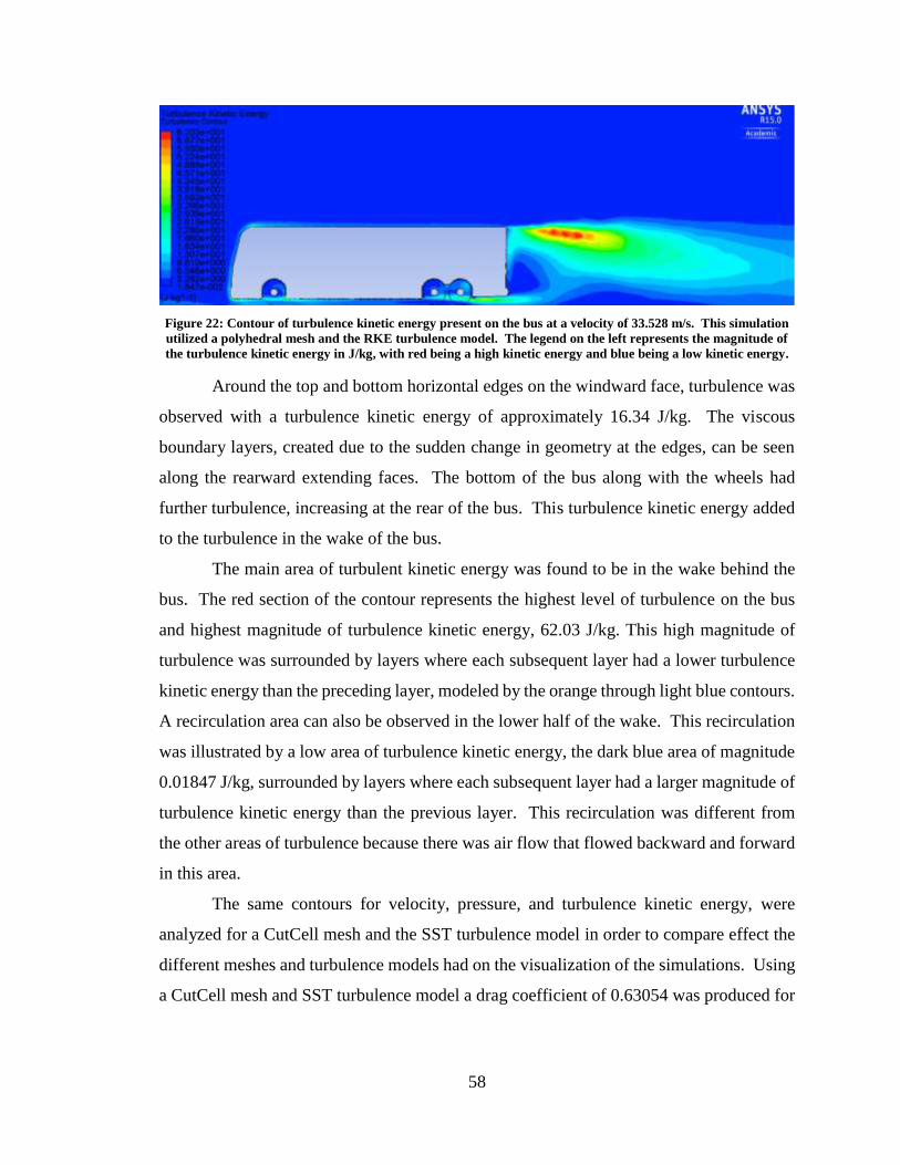
58

Figure 22: Contour of turbulence kinetic energy present on the bus at a velocity of 33.528 m/s. This simulation

utilized a polyhedral mesh and the RKE turbulence model. The legend on the left represents the magnitude of

the turbulence kinetic energy in J/kg, with red being a high kinetic energy and blue being a low kinetic energy.

Around the top and bottom horizontal edges on the windward face, turbulence was

observed with a turbulence kinetic energy of approximately 16.34 J/kg. The viscous

boundary layers, created due to the sudden change in geometry at the edges, can be seen

along the rearward extending faces. The bottom of the bus along with the wheels had

further turbulence, increasing at the rear of the bus. This turbulence kinetic energy added

to the turbulence in the wake of the bus.

The main area of turbulent kinetic energy was found to be in the wake behind the

bus. The red section of the contour represents the highest level of turbulence on the bus

and highest magnitude of turbulence kinetic energy, 62.03 J/kg. This high magnitude of

turbulence was surrounded by layers where each subsequent layer had a lower turbulence

kinetic energy than the preceding layer, modeled by the orange through light blue contours.

A recirculation area can also be observed in the lower half of the wake. This recirculation

was illustrated by a low area of turbulence kinetic energy, the dark blue area of magnitude

0.01847 J/kg, surrounded by layers where each subsequent layer had a larger magnitude of

turbulence kinetic energy than the previous layer. This recirculation was different from

the other areas of turbulence because there was air flow that flowed backward and forward

in this area.

The same contours for velocity, pressure, and turbulence kinetic energy, were

analyzed for a CutCell mesh and the SST turbulence model in order to compare effect the

different meshes and turbulence models had on the visualization of the simulations. Using

a CutCell mesh and SST turbulence model a drag coefficient of 0.63054 was produced for

59

the model bus without any airvanes attached to the model. Figure 23 illustrates the velocity

contour found for this simulation and was compared to the contour shown in Figure 20.

Figure 23: Velocity contour of the bus model without an airvane employed, found using the Fluent simulation at

a velocity of 33.528 m/s. This simulation was run using a CutCell mesh and the SST turbulence model. The

legend on the left side displays the magnitude of the velocity; red represents the higher velocity while dark blue

represents no velocity, or a dead zone.

As with the previous contour, areas of high velocities were observed on the top and

bottom horizontal edges on the windward face. The major difference in the modeling of

these high velocities was that the contour shown above better illustrated the transition from

the viscous boundary layer to the ambient velocity. It can also be seen that the magnitude

of the maximum velocity was found to be slightly lower at 56.09 m/s. The low velocity

stagnation point can be seen on the windward face and, like in the previous contour, has a

magnitude of 0 m/s. The wake behind the bus was found to be highly similar when

compared contours with minor differences. It can be said, after comparing the velocity

contours that the polyhedral mesh and RKE turbulence model tend to produce a more

estimated contour, while the CutCell mesh and SST turbulence model provides a more

realistic contour.

Figure 24 is the pressure contour that was created for the simulation of the bus

employing a CutCell mesh and the SST turbulence model. While analyzing the contour it

was compared to the pressure contour that was found when using a polyhedral mesh and

RKE turbulence model, as shown in Figure 21.

60

Figure 24: Pressure contour found in Fluent for the simulation of the bus without an airvane employed at a

velocity of 33.528 m/s. This simulation utilized a CutCell mesh and the SST turbulence model. The legend on

the left represents the magnitude of the pressure in Pa, with red being a high pressure and blue being a low

pressure.

When comparing the pressure contour from the different simulations run the same

basic features can be seen. The major difference in the contours was that in the contour

shown above it can be seen that the pressure in the wake of the bus was not found, as in

the previous simulation, to be the ambient pressure but at a slightly lower pressure of -

192.1 Pa. This difference in the pressure behind the bus increases the pressure differential

from the windward face of the bus to the leeward face of the bus. This increase in the

pressure differential increases the total drag coefficient on the bus. The magnitudes of

pressure were also slightly different with the maximum pressure of 727.7 Pa and an

ambient pressure of approximately 70.73 Pa. Overall, the different simulations that were

run produced very similar contours, but the CutCell mesh and SST turbulence model

produced a slightly more in-depth picture of the pressure present on the bus. This was due

to two main facts, first the CutCell mesh utilized different shaped elements based on the

best shape for the geometry of the object present, reducing the skewness of the mesh. The

second reason this combination provided a more accurate result was the SST turbulence

model was able to better model the turbulence present in the fluid field than the RKE

turbulence model.

Turbulence kinetic energy was the last property contour to be compared and

analyzed. Figure 25 is the contour of turbulence kinetic energy for the simulation run using

a CutCell mesh and SST turbulence model and was compared to the contour found for the

previous shown in Figure 22.

61

Figure 25: Contour of turbulence kinetic energy present on the bus at a velocity of 33.528 m/s. This simulation

utilized a CutCell mesh and the SST turbulence model. The legend on the left represents the magnitude of the

turbulence kinetic energy in J/kg, with red being a high kinetic energy and blue being a low kinetic energy.

When comparing contours it can be observed that they contain the same areas of

turbulence, with different magnitudes. The maximum turbulent kinetic energy for this

contour was 83.81 J/kg; this was significantly higher than the maximum turbulent kinetic

energy found in the previous contour. The ambient turbulent kinetic energy was found to

be 0.00222 J/kg which was closer to zero turbulence than the previous contour. This

difference made the contour above more reliable than the previous simulation due to the

fact that in areas where the bus geometry does not affect the air flow the turbulent kinetic

energy should be zero.

Overall when comparing the property contours from the two different simulations

the CutCell mesh and SST turbulence model appears to provide more complete contours.

The polyhedral RKE turbulence model simulations provided a more rounded contour that

the other simulation. Since the CutCell mesh and SST turbulence model combination

provided better contours this model was used when analyzing further contours, but both

simulations were examined when comparing the percentage reduction in drag coefficients

for each parameter.

C. Bus Model with Airvane

Once the bus model itself, without any airvanes attached, was modeled and

analyzed the parameter studies could be implemented. The first airvane that was tested

was the airvane attached to the top horizontal face of the bus. The second set of airvanes

62

to be examined were the airvanes attached to the side faces of the bus. The parameter study

performed on all airvanes tested each parameter, one at a time, on a range of dimensions.

The drag coefficients found were compared to the drag coefficient of the bus without an

airvane. After the top and side airvanes parameter studies were performed and analyzed

further tests were run using the different configurations shown in Figure 7, an airvane

attached to the bottom horizontal edge on the leeward face, and a deflection plate attached

to the leeward face. The raw data for the first set of tests run in the top airvane parameter

study can be seen in Appendix E, while the rest of the raw data for the top airvane parameter

study is given in Appendix F. The raw data for the side airvane parameter study is shown

in Appendix G and the data for the different configurations is shown in Appendix H.

1. Top Airvane Only

The first set of simulations completed for the parameter study of the top airvane

was run for a general range of angles for the angle between the line tangent to the curved

portion of the airvane and the horizontal. As described in the calibration section of this

paper, two sets of simulations were run for this parameter, only the first set of simulations

was analyzed here. For all graphs in this section the solid blue line represents the set of

simulations run with a polyhedral mesh and the RKE turbulence model, while the dotted

red line represents the simulations run with a CutCell mesh and SST turbulence model.

Comparing the values calculated for the two sets of simulations, the profiles of the

drag coefficients versus angles were observed to have very low correspondence with each

other. This lack of correlation led to the conclusion that different combinations of mesh

and turbulence did not always agree on which angles produced the best drag coefficients.

Simulations run with a polyhedral mesh and RKE turbulence model found that an angle of

55˚ provided the lowest drag coefficient. Although, as stated above, the overall contour of

the simulations run for the CutCell mesh and SST turbulence model were not completely

identical to the other set of simulations 55˚ was found as the angle which produced the

lowest drag coefficient for this set of simulations as well. This correlation between the

different simulations proved that 55˚ was the optimal angle for the airvane employed on

the top leeward edge of the bus.

As well as examining the drag coefficients directly the total percent reduction in

the drag coefficients were found for each angle tested utilizing the coefficients found for

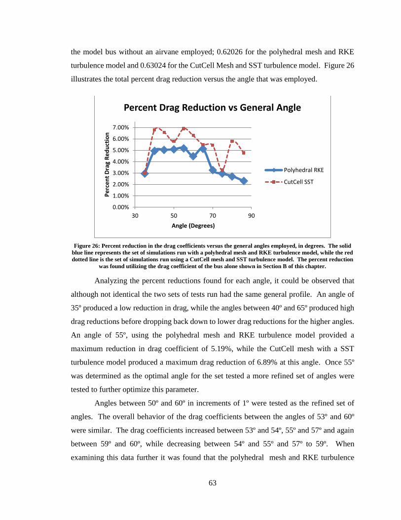
63

the model bus without an airvane employed; 0.62026 for the polyhedral mesh and RKE

turbulence model and 0.63024 for the CutCell Mesh and SST turbulence model. Figure 26

illustrates the total percent drag reduction versus the angle that was employed.

Figure 26: Percent reduction in the drag coefficients versus the general angles employed, in degrees. The solid

blue line represents the set of simulations run with a polyhedral mesh and RKE turbulence model, while the red

dotted line is the set of simulations run using a CutCell mesh and SST turbulence model. The percent reduction

was found utilizing the drag coefficient of the bus alone shown in Section B of this chapter.

Analyzing the percent reductions found for each angle, it could be observed that

although not identical the two sets of tests run had the same general profile. An angle of

35º produced a low reduction in drag, while the angles between 40º and 65º produced high

drag reductions before dropping back down to lower drag reductions for the higher angles.

An angle of 55º, using the polyhedral mesh and RKE turbulence model provided a

maximum reduction in drag coefficient of 5.19%, while the CutCell mesh with a SST

turbulence model produced a maximum drag reduction of 6.89% at this angle. Once 55º

was determined as the optimal angle for the set tested a more refined set of angles were

tested to further optimize this parameter.

Angles between 50º and 60º in increments of 1º were tested as the refined set of

angles. The overall behavior of the drag coefficients between the angles of 53º and 60º

were similar. The drag coefficients increased between 53º and 54º, 55º and 57º and again

between 59º and 60º, while decreasing between 54º and 55º and 57º to 59º. When

examining this data further it was found that the polyhedral mesh and RKE turbulence

0.00%

1.00%

2.00%

3.00%

4.00%

5.00%

6.00%

7.00%

30 50 70 90

Pe

rce

nt

Dra

g R

ed

uct

ion

Angle (Degrees)

Percent Drag Reduction vs General Angle

Polyhedral RKE

CutCell SST

64

model produced an angle of 51º as the optimal angle with a drag coefficient of 0.58779.

Employing a CutCell mesh and a SST turbulence model produced an angle of 53º as the

optimal angle with a drag coefficient of 0.58637. Since the two simulations did not agree

on an optimal angle a third simulation was run for the two optimal angles, 51º and 53º.

This simulation was run with a polyhedral mesh and a SST turbulence model and the values

produced were compared to the values of the other simulations to determine the optimal

angle. Using the third simulation a drag coefficient of 0.60147 was found for 51º, while a

value of 0.59997 was found for an angle of 53º. Comparing the simulation run using a

polyhedral mesh and a SST turbulence agreed with the simulation run using a CutCell mesh

and SST turbulence model 53º was determined as the optimal angle between the tangent

line to the radius of curvature and the horizontal.

To further examine the results of the simulations run for the refined angles the total

percent reduction in the drag coefficient was graphed, as shown in Figure 27.

Figure 27: Percent reduction in the drag coefficients versus the more refined angles employed, in degrees. The

solid blue line represents the set of simulations run with a polyhedral mesh and RKE turbulence model, while

the red dotted line is the set of simulations run using a CutCell mesh and SST turbulence model. The percent

reduction was found utilizing the drag coefficient of the bus alone shown in Section B of this chapter.

The profiles of the percent reductions in drag coefficients of the two simulations

run did not correlate very well. The maximum drag reduction for the polyhedral RKE

simulation, at 51º, was a reduction of 5.28% while the CutCell SST combination produced

a maximum drag reduction of 7.01% at 53º. When the third set of simulations were run a

0.00%

1.00%

2.00%

3.00%

4.00%

5.00%

6.00%

7.00%

8.00%

49 54 59

Pe

rce

nt

Dra

g R

ed

uct

ion

Angle (Degrees)

Percent Drag Reduction vs Refined Angle

Polyhedral RKE

CutCell SST

65

drag reduction of 5.01% was found for 51º, while the maximum reduction in the drag

coefficient was found to be 5.25% at 53º. Since the third set of simulations found an angle

of 53º to produce a high drag reduction rate than 51º an angle of 53º was utilized as the

final angle between the line tangent to the radius of curvature and the horizontal, which

was employed for the remainder of the study.

The expansion ratio of the airvane, the ratio between the inlet gap and the outlet

gap, was the second parameter to be tested. A general set of expansion ratios was tested

first. The different simulations run shared a basic profile. Although not identical, a clear

relationship between the expansion ratio and the behavior of the drag coefficient found

could be seen. After increasing from an expansion ratio of 1:2 to 1:2.5 the drag coefficient

decreased from 1:2.5 to 1:4. The different simulation models disagreed on the behavior of

the drag coefficient between 1:4 and 1:5, but agreed that it decreased from 1:5 to 1:6 and

increase again between 1:6 and 1:6.5. The polyhedral mesh and RKE turbulence model

produced 1:6 as the optimal expansion ratio while the CutCell SST turbulence model found

1:2 as the optimal expansion ratio. To better determine the difference between these two

optimal expansion ratios the percent drag reductions were examined in comparison to the

expansion ratio employed. These relations are illustrated in Figure 28 below.

Figure 28: Percent reduction in the drag coefficients versus the general expansion ratios employed, in the form

1:X. The solid blue line represents the set of simulations run with a polyhedral mesh and RKE turbulence

model, while the red dotted line is the set of simulations run using a CutCell mesh and SST turbulence model.

The percent reduction was found utilizing the drag coefficient of the bus alone shown in Section B.

0.00%

1.00%

2.00%

3.00%

4.00%

5.00%

6.00%

7.00%

8.00%

1.5 3.5 5.5

Pe

rce

nt

Dra

g R

ed

uct

ion

Expansion Ratio (1:X)

Percent Drag Reduction vs General Expansion Ratio

Polyhedral RKE

CutCell SST

66

When analyzing the percent drag reductions it was observed that the profiles were

very similar, except for the expansion ratios between 1:4 and 1:5. Even with this

discrepancy the expansion ratios of 1:2 and 1:6 were found as the two optimal expansion

ratios for both sets of simulations. The polyhedral RKE simulations found 1:6 as the

optimal ratio, with a percent reduction of 5.34%, while an expansion ratio of 1:2 was found

as the optimal expansion ratio for the CutCell SST turbulence model simulations, with a

percent reduction of 7.48%. Kirch recommended an expansion ratio around 1:5.5 ± 0.5,

therefore it was determined that the expansion ratio of 1:6 should be chosen as the optimal

expansion ratio for these tests.21

Once the optimal general expansion ratio was determine a more refined set of

expansion ratios were tested to further optimize the parameter. When analyzing the data

found, the drag coefficients for the refined expansion ratios run with a polyhedral mesh

and RKE turbulence model remained relatively constant, with only slight increases and

decreases for the simulations. Using a CutCell mesh and SST turbulence model produced

larger fluctuations in the drag coefficients calculated. An optimal expansion ratio of 1:5.6

was found for the polyhedral RKE simulations, with a drag coefficient of 0.58722. It was

determined that the optimal expansion ratio was 1:5.7 for the CutCell SST simulations,

with a drag coefficient of 0.58630. It should also be noted that the expansion ratio of 1:6,

although not the optimal dimension for either simulation, produced drag coefficients that

were the best option when considering both simulation methods. At this expansion ratio a

drag coefficient of 0.58788 was calculated for the polyhedral RKE method and 0.58644

for the CutCell SST method.

To better understand this discrepancy and determine the optimal expansion ratio

for the airvane the percent reductions in the drag coefficient were examined. The graph of

the percent drag reduction versus the expansion ratio used can be seen below in Figure 29.

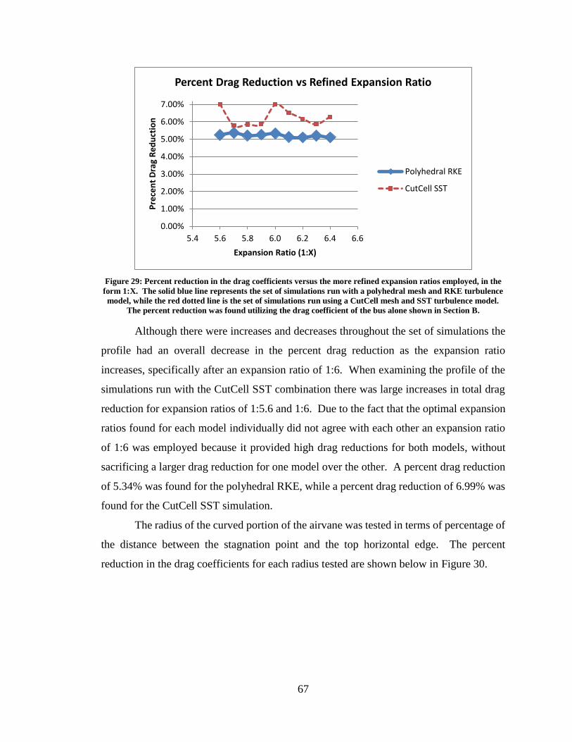
67

Figure 29: Percent reduction in the drag coefficients versus the more refined expansion ratios employed, in the

form 1:X. The solid blue line represents the set of simulations run with a polyhedral mesh and RKE turbulence

model, while the red dotted line is the set of simulations run using a CutCell mesh and SST turbulence model.

The percent reduction was found utilizing the drag coefficient of the bus alone shown in Section B.

Although there were increases and decreases throughout the set of simulations the

profile had an overall decrease in the percent drag reduction as the expansion ratio

increases, specifically after an expansion ratio of 1:6. When examining the profile of the

simulations run with the CutCell SST combination there was large increases in total drag

reduction for expansion ratios of 1:5.6 and 1:6. Due to the fact that the optimal expansion

ratios found for each model individually did not agree with each other an expansion ratio

of 1:6 was employed because it provided high drag reductions for both models, without

sacrificing a larger drag reduction for one model over the other. A percent drag reduction

of 5.34% was found for the polyhedral RKE, while a percent drag reduction of 6.99% was

found for the CutCell SST simulation.

The radius of the curved portion of the airvane was tested in terms of percentage of

the distance between the stagnation point and the top horizontal edge. The percent

reduction in the drag coefficients for each radius tested are shown below in Figure 30.

0.00%

1.00%

2.00%

3.00%

4.00%

5.00%

6.00%

7.00%

5.4 5.6 5.8 6.0 6.2 6.4 6.6

Pre

cen

t D

rag

Re

du

ctio

n

Expansion Ratio (1:X)

Percent Drag Reduction vs Refined Expansion Ratio

Polyhedral RKE

CutCell SST

68

Figure 30: Percent reductions in the drag coefficient versus the radius of curvatures employed, found by the

percent of the distance between the stagnation point and the top windward edge of the bus. The solid blue line

represents the set of simulations run with a polyhedral mesh and RKE turbulence model, while the red dotted

line is the set of simulations run using a CutCell mesh and SST turbulence model. The percent reduction was

found utilizing the drag coefficient of the bus alone shown in Section B of this chapter.

When analyzing the contours of the drag reduction versus the radii tested it can be

seen that for the polyhedral RKE simulations as the radius was increased from 5% to 8%

the reduction in the drag coefficient found was increased to a maximum of 5.48% at a

radius of 8%. As the radius was further increased the drag force on the bus increased as

well, meaning that the reduction in the coefficient due to the radius change was decreased.

Comparing the CutCell SST simulation results to the polyhedral RKE simulation results

showed a common general contour, with the acceptations that the drag reduction increased

between a radius dimension of 13% and 14%. Although there were minor discrepancies in

the behavior of the drag coefficient, the CutCell SST simulation also found a radius of 8%

to be the optimal radius, with a drag reduction of 7.86%.

The gap between the inlet of the airvane and the horizontal top face was the next

dimension to be tested. The percent reduction in the drag coefficient found for each inlet

gap tested are shown in Figure 31.

0.00%

1.00%

2.00%

3.00%

4.00%

5.00%

6.00%

7.00%

8.00%

4% 9% 14%

Pe

rce

nt

Dra

g R

ed

uct

ion

Radius (%)

Percent Drag Reduction vs Radius

Polyhedral RKE

CutCell SST

69

Figure 31: Percent reduction in the drag coefficients versus the inlet gaps employed, in cm. This dimension was

in reference to the full-scaled model bus and was scaled down to the 1/35th scale. The solid blue line represents

the set of simulations run with a polyhedral mesh and RKE turbulence model, while the red dotted line is the set

of simulations run using a CutCell mesh and SST turbulence model. The percent reduction was found utilizing

the drag coefficient of the bus alone shown in Section B of this chapter.

It was found in Figure 31, for the simulations run utilizing a polyhedral mesh and

RKE turbulence model, that as the dimension of the inlet gap increased so did the percent

reduction in the drag coefficient found for each dimension tested. An inlet gap of 4.5 cm

on the full scale was found as the optimal dimension, with a drag coefficient of 0.56666

and a percent reduction of 8.69%. Although the drag coefficient continued to decrease up

to the last dimension tested, 4.5 cm was set as the last dimension due to the fact that as the

drag was decreasing the frontal area was increasing and therefore would offset the effect

of the drag reduction when looking at the fuel consumption used. The other set of

simulations run agreed with the general increase in drag reduction as the inlet gap increase,

but fluctuated more between 2 cm and 3 cm, which were not present in the first set of

simulations. The CutCell SST simulations found 4.25 cm as the optimal dimension which

produced a minimum drag coefficient of 0.56671 and a maximum drag reduction of

10.12%. Since the two simulations did not agree on an exact optimal dimension for the

inlet gap a set of simulations with a polyhedral mesh and SST turbulence model was run

for dimensions of 4.25 and 4.5 cm. A drag coefficient of 0.56225 and reduction of 11.20%

was found for 4.25 cm and a drag coefficient of 0.5594 which was a reduction of 11.65%

was found for an inlet gap of 4.5 cm. Comparing these results led to an inlet gap of 4.5 cm

0.00%

2.00%

4.00%

6.00%

8.00%

10.00%

1.5 2.5 3.5 4.5

Pe

rce

nt

Dra

g R

ed

uct

ion

Inlet Gap (cm)

Percent Drag Reduction vs Inlet Gap

Polyhedral RKE

CutCell SST

70

being determined as the optimal angle, which provided a drag coefficient of 0.57117 and

9.42% reduction for the CutCell SST simulation.

The next parameter that was analyzed was the angle tested between the top

horizontal face of the bus and the planar portion of the airvane. The percent reductions in

the drag coefficients that were found for the angles that were tested in this parameter study

are shown below in Figure 32.

Figure 32: Percent reduction in the drag coefficients versus the angles of the planar portion of the airvane

employed, in degrees. The solid blue line represents the set of simulations run with a polyhedral mesh and RKE

turbulence model, while the red dotted line is the set of simulations run using a CutCell mesh and SST

turbulence model. The percent reduction was found utilizing the drag coefficient of the bus alone shown in

Section B of this chapter.

The two contours produced, using the different simulations, for the percent

reductions of the different inlet angles tested did not correlate with each other. The

behavior of the drag coefficients for the different angles modeled did not agree between

the turbulence models and meshes used. Both models had fluctuations throughout the sets

of simulations run on the inlet angle. While the polyhedral RKE simulation found 4.5˚ as

the optimal angle with a drag coefficient of 0.55407 and a percent reduction of 10.71%,

the CutCell SST simulation found 4˚ as the optimal angle with a maximum reduction of

11.89% with a drag coefficient of 0.55557. An angle that was optimal for both sets of

simulations was not found, but it was determined that an angle of 4˚ was the optimal for

the CutCell SST model and limited the reduction in drag sacrificed for the polyhedral RKE

0.00%

2.00%

4.00%

6.00%

8.00%

10.00%

12.00%

14.00%

0 2 4 6

Pe

rce

nt

Dra

g R

ed

uct

ion

Inlet Angle (Degrees)

Percent Drag Reduction vs Inlet Angle

Polyhedral RKE

CutCell SST

71

model. For an angle of 4˚ the polyhedral RKE model produced a drag coefficient of

0.55533 and a reduction in the coefficient of 10.51%.

The last parameter that was examined in this parameter study was the length of the

planar portion of the airvane. The contours of the percent reductions found for the different

planar lengths tested are shown in Figure 33

Figure 33: Percent reduction in the drag coefficients versus the lengths of the planar portion of the airvane

employed. The solid blue line represents the set of simulations run with a polyhedral mesh and RKE turbulence

model, while the red dotted line is the set of simulations run using a CutCell mesh and SST turbulence model.

The percent reduction was found utilizing the drag coefficient of the bus alone shown in Section B of this

chapter.

The contours for the two sets of simulations run correlated very well with each

other and the behavior of the drag coefficient was nearly identical between the polyhedral

RKE model and the CutCell SST model. There was a sharp decrease and then a sharp

increase in the percent drag reduction between the planar lengths of 0.25 and 0.75 times

the radius of curvature. There were smaller fluctuations between the tests run for the planar

lengths between 0.75 and 2.5 times the radius of curvature, but there was an overall increase

in the percent reduction in the drag coefficient up to the optimal point of 2.5 times the

radius of curvature that was found. This was a length of 13.41 mm on the 1/35th scale

model. Utilizing the polyhedral RKE model produced a drag coefficient of 0.54972 which

led to a total reduction in the coefficient of 11.42 % for the top airvane. For the optimal

top airvane the CutCell SST simulation provided a reduction in the drag coefficient of

13.26% with a value of 0.54694. Using Equation 57 the total reduction in fuel consumption

0.00%

2.00%

4.00%

6.00%

8.00%

10.00%

12.00%

0 0.5 1 1.5 2 2.5

Pe

rce

nt

Dra

g R

ed

uct

ion

Planar Length

Percent Drag Reduction vs Planar Length

Polyhedarl RKE

CutCell SST

72

when the velocity was kept the same, the CutCell SST produced a reduction of 1.13%,

while the polyhedral RKE actually led to an increase of 0.5% fuel consumption. This

increase in fuel consumption was due to the increase in the area being larger that the

reduction in the drag coefficient. It was observed that the polyhedral k-ε simulation often

produced lower drag coefficients and percent reduction than the SST k-ω simulations. This

was believed to be because the k-ε turbulence model was not as adequate at modeling the

turbulence present on the bus which lead to assumptions being made,

To fully examine how the top airvane changed the airflow surrounding the bus to

reduce the drag present on the bus, contours of the velocity, pressure, and turbulence kinetic

energy were created and are compared to the contours of the airflow around the bus without

an airvane attached. Figure 34 illustrates the velocity contour that was found using the

CutCell SST simulation for the bus with a top airvane employed, optimized by the

parameter study. The contour shown was of the wake area of the bus due to the fact the

velocity contour of the rest of the bus did not change with the addition of the airvane. This

contour can be compared to Figure 23, the velocity contour of the bus with no airvane

employed.

Figure 34: Velocity contour of the wake of the bus model with a top airvane employed, found using the Fluent

simulation at a velocity of 33.528 m/s. This simulation was run using a CutCell mesh and the SST turbulence

model. The legend on the left side displays the magnitude of the velocity; red represents the higher velocity

while dark blue represents no velocity, or a dead zone.

Comparing the velocity contours produced for the bus with and without the top

airvane employed it could be observed that the magnitudes found for the different colors

of the contour were nearly the same with only minor negligible differences. When

examining the wake of the bus on which the top airvane was employed it was observed that

73

the total area of low velocity in the wake was greatly decreased. Without the airvane the

low velocity wake area with recirculation was more of a square shape extending past the

leeward face of the bus. When the airvane was added to the bus the low velocity wake was

reduced to a smaller triangular area. The airvane channeled the faster air flow from the top

of the bus in a downward angle toward the recirculation of the wake. This reduced the size

of the wake as well as the areas were completely stagnate air was present.

The pressure contour found for this simulation is shown in Figure 35 and can be

compared to the pressure contour found for the bus without any devices added shown in

Figure 24.

Figure 35: Pressure contour found in Fluent for the simulation of the bus with a top airvane employed at a

velocity of 33.528 m/s. This simulation utilized a CutCell mesh and the SST turbulence model. The legend on

the left represents the magnitude of the pressure in Pa, with red being a high pressure and blue being a low

pressure.

Comparing the magnitudes present in the legend for the figure above with the

legend of the pressure contour of the bus without an airvane in place it could be seen that

there was small differences in the pressures that would provide slight differences in the

pressure differential of the bus. The major difference between the simulations was the area

of higher, yellowish-green, pressure on the leeward face of the bus in Figure 35. This area

was not present in the wake of the bus without the airvane and this higher pressure was

created due to the airvane guiding the air flow from the top of the bus to the wake and the

expansion of the air allowed for the decrease in velocity and in turn the increase of pressure.

This increase in pressure decreased the pressure differential and as mention previous, since

the pressure drag is the largest portion of the aerodynamic drag present on the bus this

change significantly reduced the drag coefficient of the bus.

74

The last contour to be examined was the turbulent kinetic energy present on the bus

shown in Figure 36. This contour was compared to the turbulent kinetic energy contour of

the bus without any drag reduction devices added shown in Figure 25.

Figure 36: Contour of turbulence kinetic energy present on the bus at a velocity of 33.528 m/s when a top

airvane was utilized. This simulation utilized a CutCell mesh and the SST turbulence model. The legend on the

left represents the magnitude of the turbulence kinetic energy in J/kg, with red being a high kinetic energy and

blue being a low kinetic energy.

Turbulence kinetic energy present on the front half of the bus was the same

therefore only the wake area of the bus was examined. Comparing the magnitudes found

in the legends for both the figure above and the contour of the turbulent kinetic energy for

the bus with not airvanes attached it could be seen that there was a major difference in the

values produced. The maximum turbulent kinetic energy present in the above contour, the

red section, was found to be 35.01 J/kg. Compared to the value of 83.31 J/kg for the

original bus this value was significantly lower. It was also observed that the more turbulent

area of the wake, the colors ranging from red to light green, was much larger with lower

magnitudes than the bus without the airvane present. This showed that the airvane was

able to disperse the high intensity area of turbulence into a larger area with lower intensity.

This in turn reduced the drag present at the back of the bus and decreased the overall drag

coefficient of the bus.

2. Top and Side Airvanes

Once the top airvane was optimized airvanes were placed on the vertical edges of

the leeward face of the bus in conjunction with the top airvane. The same parameter study

was run on the side airvanes as was run on the top airvane, it was believed that the

difference in the radii of the top and side edges could led to different optimal dimensions.

The first dimension that was tested and analyzed was the general set of angles that was

75

tested for the curved portion of the airvane. The percent reduction in the drag coefficients

of the bus for the angles tested are shown in Figure 37.

Figure 37: Percent reduction in the drag coefficients versus the general angles employed, in degrees, between the

line tangent to the radius of curvature and the horizontal. The solid blue line represents the set of simulations

run with a polyhedral mesh and RKE turbulence model, while the red dotted line is the set of simulations run

using a CutCell mesh and SST turbulence model. The percent reduction was found utilizing the drag coefficient

of the bus alone shown in Section B of this chapter.

Examining the profiles of the reduction in drag coefficient for both sets of

simulations showed that they were nearly identical, not in the magnitudes, but the behavior

of the drag coefficient as the angle was changed. While the angle was increased from 35º

to 60º the reduction in the drag coefficient decreased, meaning the larger the angle the less

optimal the angle. The angles between 60º and 86º produced fluctuations in the reduction

in the drag coefficient, but at a lower average reduction than the optimal angle. For both

sets of simulations the optimal angle was found to be 35º and produced a drag coefficient

of 0.54835 and a percent reduction of 11.64% for the polyhedral RKE simulation. The

CutCell SST simulation produced a drag coefficient of 0.54827 and a reduction in the drag

coefficient of 13.05% for the optimal angle.

After a general optimal angle of 35º was determine a more refined set of simulations

were examined between the angles of 30º and 40º. The graphs of the drag coefficients

produced for the different angles tested can be seen in Figure 38 below.

0.00%

2.00%

4.00%

6.00%

8.00%

10.00%

12.00%

30 50 70 90

Pe

rce

nt

Dra

g R

ed

uct

ion

Angle (Degrees)

Percent Drag Reduction vs General Angle

Polyhedral RKE

CutCell SST

76

Figure 38: Percent reduction in the drag coefficients versus the more refined angles employed, in degrees,

between the line tangent to the radius of curvature and the horizontal. The solid blue line represents the set of

simulations run with a polyhedral mesh and RKE turbulence model, while the red dotted line is the set of

simulations run using a CutCell mesh and SST turbulence model. The percent reduction was found utilizing the

drag coefficient of the bus alone shown in Section B of this chapter.

The two sets of simulations disagreed in the behavior of the drag coefficient as the

angle of the curved portion of the airvane was changed. The polyhedral RKE simulations

decreased in drag reduction between the angles of 33º and 36º and between 38º and 40º.

Percent reduction in the drag coefficient was found to increase between angles of 30º and

33º and then from 36º to the optimal angle of 38º. At an angle of 38º a drag coefficient of

0.54620 was found, which produced a reduction in drag of 11.98%. Using the CutCell

SST simulations there were minor fluctuations in the drag coefficient with an overall

general decrease in the reduction of drag as the angle increased. An optimal angle of 33º

was found for this simulation with a drag coefficient of 0.54446 and percent reduction of

13.65% was calculated. Although the simulations did not agree on the optimal angle it was

observed that at an angle of 33º the polyhedral RKE simulation produced a nearly identical

reduction in the drag coefficient, of 11.94%, to the optimal angle and therefore the angle

of the curved portion of the side airvane was set to 33º.

The next tests of the parameter study that were examined were the simulations run

on the general range of expansion ratios. Reductions in drag coefficients calculated for the

different expansion ratios tested are illustrated below in Figure 39.

0.00%

2.00%

4.00%

6.00%

8.00%

10.00%

12.00%

14.00%

16.00%

29 34 39

Pe

rce

nt

Dra

g R

ed

uct

ion

Angle (Degrees)

Percent Drag Reduction vs Refined Angle

Polyhedral RKE

CutCell SST

77

Figure 39: Percent reduction in the drag coefficients versus the general expansion ratios employed, in the form

1:X, between the inlet gap and the outlet gap. The solid blue line represents the set of simulations run with a

polyhedral mesh and RKE turbulence model, while the red dotted line is the set of simulations run using a

CutCell mesh and SST turbulence model. The percent reduction was found utilizing the drag coefficient of the

bus alone shown in Section B of this chapter.

The general behavior of the drag coefficient agreed for both sets of simulations

utilized. The drag coefficient stayed relatively the same for the expansion ratios tested up

to 1:4 and then proceeded to fluctuate between 1:4 and 1:6.5. Both simulations found an

expansion ratio of 1:6 to be the optimal ratio for the dimensions tested. The polyhedral

RKE simulation found that this expansion ratio produced a drag coefficient of 0.54687

which was a percent reduction of 11.87%, while the CutCell SST simulation produced a

drag coefficient of 0.54286 and a percent reduction of 13.91% in the drag present on the

bus.

After a general expansion ratio of 1:6 was found as the optimal ratio between the

inlet and the outlet gap a more refined set of expansion ratios was examined to determine

if a more optimal expansion ratio existed. Figure 40 illustrates the percent reductions in

the drag coefficients that were found for the refined expansion ratios that were tested.

0.00%

2.00%

4.00%

6.00%

8.00%

10.00%

12.00%

14.00%

1.5 3.5 5.5

Pe

rce

nt

Dra

g R

ed

uct

ion

Expansion Ratio (1:X)

Percent Drag Reduction vs General Expansion Ratio

Polyhedral RKE

CutCell SST

78

Figure 40: Percent reduction in the drag coefficients versus the more refined expansion ratios employed, in the

form 1:X, between the inlet gap and the outlet gap. The solid blue line represents the set of simulations run with

a polyhedral mesh and RKE turbulence model, while the red dotted line is the set of simulations run using a

CutCell mesh and SST turbulence model. The percent reduction was found utilizing the drag coefficient of the

bus alone shown in Section B of this chapter.

Although it was observed when analyzing the profiles of the percent reductions for

the expansion ratios tested, that the different simulations did not agree completely on the

behavior of the drag coefficient they did agree on the optimal expansion ratio of the airvane.

It was found that the optimal expansion ratio for the side airvane, like the top airvane, was

1:6. This was the same dimension as found in the previous and therefore the same drag

coefficients and percent reductions in the drag present on the bus were found for this set of

simulations.

After the expansion ratio was optimized the next parameter to be studied was the

percent of the distance between the stagnation point and top edge that was used for the

radius of the curved portion of the airvane. The contours of the behavior of the percent

reduction of the drag coefficients found for the range of percentages tested are shown

below in Figure 41.

0.00%

2.00%

4.00%

6.00%

8.00%

10.00%

12.00%

14.00%

5.5 5.7 5.9 6.1 6.3 6.5

Pe

rce

nt

Dra

g R

ed

uct

ion

Expansion Ratio (1:X)

Percent Drag Reduction vs Refined Expansion Ratio

Polyhedral RKE

CutCell SST

79

Figure 41: Percent reductions in the drag coefficient versus the radius of curvatures employed, found by the

percent of the distance between the stagnation point and the top windward edge of the bus. The solid blue line

represents the set of simulations run with a polyhedral mesh and RKE turbulence model, while the red dotted

line is the set of simulations run using a CutCell mesh and SST turbulence model. The percent reduction was

found utilizing the drag coefficient of the bus alone shown in Section B of this chapter.

The plots for the reductions in the drag coefficients for the radii tested for both the

polyhedral RKE and CutCell SST simulations were identical, although not in magnitudes,

but in the profiles found. The plots agreed that as the radius was changed from 7% to 9%

the drag coefficient decreased and in turn the percent reduction increase and a then there

was a quick decrease when the radius was set to 10%. Although the plots agreed that there

was a decrease in the percent reduction from a radius of 12% to 13% and then an increase

from 13% to 15% the plots disagreed on the behavior of drag coefficient for the radii of

11% and 12%. Both simulations found these two dimensions to be the two best options

for the radius of curvature, but disagreed on which dimension provided a lower drag force.

The polyhedral RKE simulation found that a radius of 11% produced the optimal

dimension while the CutCell SST simulation found that a radius of 12% was the optimal

dimension. Due to the small difference in the percent reduction for the polyhedral RKE

simulations for the radii of 11% and 12% compared to the larger difference in the CutCell

SST simulations, a optimal radius of 12% was used for the airvanes employed on the sides

of the bus. This dimension provided the same drag coefficient and percent reductions as

the previous two tests in the parameter study.

0.00%

2.00%

4.00%

6.00%

8.00%

10.00%

12.00%

14.00%

6% 8% 10% 12% 14% 16%

Pe

rce

nt

Dra

g R

ed

uct

ion

Radius (%)

Percent Drag Reduction vs Radius

Polyhedral RKE

CutCell SST

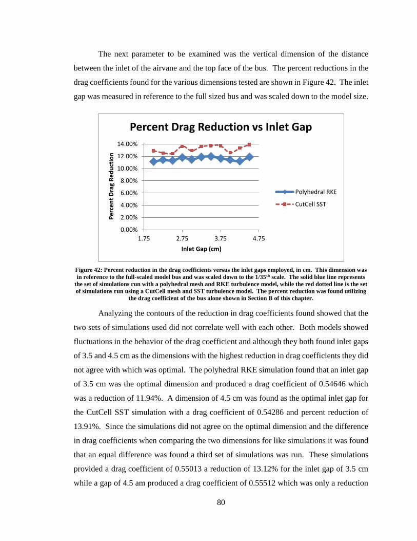
80

The next parameter to be examined was the vertical dimension of the distance

between the inlet of the airvane and the top face of the bus. The percent reductions in the

drag coefficients found for the various dimensions tested are shown in Figure 42. The inlet

gap was measured in reference to the full sized bus and was scaled down to the model size.

Figure 42: Percent reduction in the drag coefficients versus the inlet gaps employed, in cm. This dimension was

in reference to the full-scaled model bus and was scaled down to the 1/35th scale. The solid blue line represents

the set of simulations run with a polyhedral mesh and RKE turbulence model, while the red dotted line is the set

of simulations run using a CutCell mesh and SST turbulence model. The percent reduction was found utilizing

the drag coefficient of the bus alone shown in Section B of this chapter.

Analyzing the contours of the reduction in drag coefficients found showed that the

two sets of simulations used did not correlate well with each other. Both models showed

fluctuations in the behavior of the drag coefficient and although they both found inlet gaps

of 3.5 and 4.5 cm as the dimensions with the highest reduction in drag coefficients they did

not agree with which was optimal. The polyhedral RKE simulation found that an inlet gap

of 3.5 cm was the optimal dimension and produced a drag coefficient of 0.54646 which

was a reduction of 11.94%. A dimension of 4.5 cm was found as the optimal inlet gap for

the CutCell SST simulation with a drag coefficient of 0.54286 and percent reduction of

13.91%. Since the simulations did not agree on the optimal dimension and the difference

in drag coefficients when comparing the two dimensions for like simulations it was found

that an equal difference was found a third set of simulations was run. These simulations

provided a drag coefficient of 0.55013 a reduction of 13.12% for the inlet gap of 3.5 cm

while a gap of 4.5 am produced a drag coefficient of 0.55512 which was only a reduction

0.00%

2.00%

4.00%

6.00%

8.00%

10.00%

12.00%

14.00%

1.75 2.75 3.75 4.75

Pe

rce

nt

Dra

g R

ed

uct

ion

Inlet Gap (cm)

Percent Drag Reduction vs Inlet Gap

Polyhedral RKE

CutCell SST

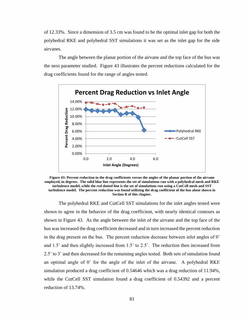
81

of 12.33%. Since a dimension of 3.5 cm was found to be the optimal inlet gap for both the

polyhedral RKE and polyhedral SST simulations it was set as the inlet gap for the side

airvanes.

The angle between the planar portion of the airvane and the top face of the bus was

the next parameter studied. Figure 43 illustrates the percent reductions calculated for the

drag coefficients found for the range of angles tested.

Figure 43: Percent reduction in the drag coefficients versus the angles of the planar portion of the airvane

employed, in degrees. The solid blue line represents the set of simulations run with a polyhedral mesh and RKE

turbulence model, while the red dotted line is the set of simulations run using a CutCell mesh and SST

turbulence model. The percent reduction was found utilizing the drag coefficient of the bus alone shown in

Section B of this chapter.

The polyhedral RKE and CutCell SST simulations for the inlet angles tested were

shown to agree in the behavior of the drag coefficient, with nearly identical contours as

shown in Figure 43. As the angle between the inlet of the airvane and the top face of the

bus was increased the drag coefficient decreased and in turn increased the percent reduction

in the drag present on the bus. The percent reduction decrease between inlet angles of 0˚

and 1.5˚ and then slightly increased from 1.5˚ to 2.5˚. The reduction then increased from

2.5˚ to 3˚ and then decreased for the remaining angles tested. Both sets of simulation found

an optimal angle of 0˚ for the angle of the inlet of the airvane. A polyhedral RKE

simulation produced a drag coefficient of 0.54646 which was a drag reduction of 11.94%,

while the CutCell SST simulation found a drag coefficient of 0.54392 and a percent

reduction of 13.74%.

0.00%

2.00%

4.00%

6.00%

8.00%

10.00%

12.00%

14.00%

0.0 2.0 4.0 6.0

Pe

rce

nt

Dra

g R

ed

uct

ion

Inlet Angle (Degrees)

Percent Drag Reduction vs Inlet Angle

Polyhedral RKE

CutCell SST

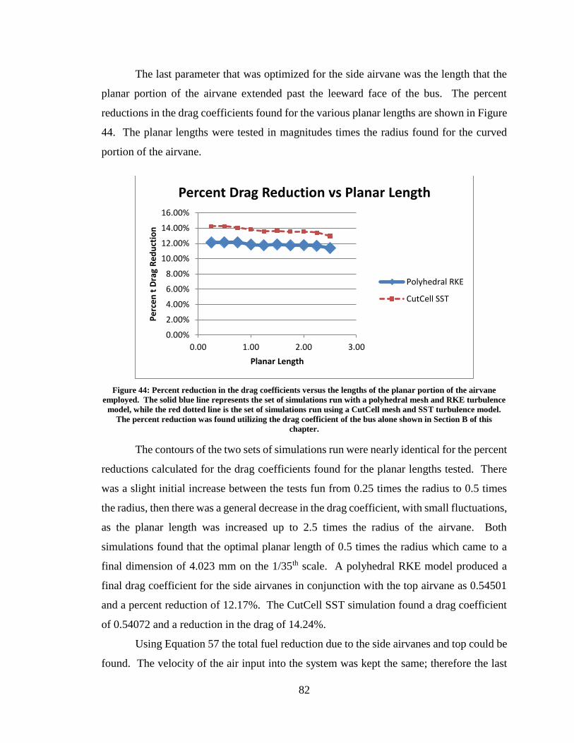
82

The last parameter that was optimized for the side airvane was the length that the

planar portion of the airvane extended past the leeward face of the bus. The percent

reductions in the drag coefficients found for the various planar lengths are shown in Figure

44. The planar lengths were tested in magnitudes times the radius found for the curved

portion of the airvane.

Figure 44: Percent reduction in the drag coefficients versus the lengths of the planar portion of the airvane

employed. The solid blue line represents the set of simulations run with a polyhedral mesh and RKE turbulence

model, while the red dotted line is the set of simulations run using a CutCell mesh and SST turbulence model.

The percent reduction was found utilizing the drag coefficient of the bus alone shown in Section B of this

chapter.

The contours of the two sets of simulations run were nearly identical for the percent

reductions calculated for the drag coefficients found for the planar lengths tested. There

was a slight initial increase between the tests fun from 0.25 times the radius to 0.5 times

the radius, then there was a general decrease in the drag coefficient, with small fluctuations,

as the planar length was increased up to 2.5 times the radius of the airvane. Both

simulations found that the optimal planar length of 0.5 times the radius which came to a

final dimension of 4.023 mm on the 1/35th scale. A polyhedral RKE model produced a

final drag coefficient for the side airvanes in conjunction with the top airvane as 0.54501

and a percent reduction of 12.17%. The CutCell SST simulation found a drag coefficient

of 0.54072 and a reduction in the drag of 14.24%.

Using Equation 57 the total fuel reduction due to the side airvanes and top could be

found. The velocity of the air input into the system was kept the same; therefore the last

0.00%

2.00%

4.00%

6.00%

8.00%

10.00%

12.00%

14.00%

16.00%

0.00 1.00 2.00 3.00

Pe

rce

n t

Dra

g R

ed

uct

ion

Planar Length

Percent Drag Reduction vs Planar Length

Polyhedral RKE

CutCell SST

83

term in the equation was neglected. The change in area for the polyhedral RKE simulation

was an increase of 0.43446 mm2 and 0.43475 mm2 for the CutCell SST simulation. This

change in frontal area in addition to the change in drag coefficient led to a reduction in fuel

consumption of 0.0023% for the polyhedral RKE simulation, which was a change of

0.5023% for the side airvanes alone. The CutCell SST simulation produced a fuel

consumption reduction of 1.45%, which was an additional reduction of 0.32% due to the

addition of side airvanes alone.

Once the parameter study for the side airvanes was completed the airflow around

the bus could be examined to determine the effect of the airvane of the airflow to produce

the drag reduction found. A velocity contour was the first thing looked at, since the front

of the bus remained the same the wake was focused on as shown in Figure 45. This was

compared to the velocity contour of the bus with only the top airvane attached as shown in

Figure 34.

Figure 45: Velocity contour of the bus model with top and side airvanes employed, found using the Fluent

simulation at a velocity of 33.528 m/s. This simulation was run using a CutCell mesh and the SST turbulence

model. The legend on the left side displays the magnitude of the velocity; red represents the higher velocity

while dark blue represents no velocity, or a dead zone.

When comparing the legends of the two simulations it was observed that the

magnitudes of the contours were nearly identical and the small differences were negligible

when comparing the wake region of the contour. The addition of the side airvanes slightly

changed the shape of the wake, channeling the air flow further down on the leeward face

of the bus. The major change produced by the addition of the side airvanes was the

reduction in the range of velocities present in the recirculation area in the wake. It was

found in the recirculation area of wake of the bus the velocities ranged from 0 m/s to 8.842

84

m/s for the bus with the side airvanes attached, while without the side airvanes attached the

velocities ranged from 0 m/s to 14.74 m/s. This reduction in the range of velocities present

reduced the turbulence present in the wake as well as increasing the pressure which in turn

reduced the total drag coefficient of the bus.

As stated above the pressure present on the bus was important and therefore the

contour for the bus with side airvanes, as shown in Figure 46, was compared to the pressure

contour of the bus with only the top airvane present as shown in Figure 35.

Figure 46: Pressure contour found in Fluent for the simulation of the bus with top and side airvanes employed at

a velocity of 33.528 m/s. This simulation utilized a CutCell mesh and the SST turbulence model. The legend on

the left represents the magnitude of the pressure in Pa, with red being a high pressure and blue being a low

pressure.

When examining the legend of the two contours it was observed that the magnitudes

of the contour were nearly identical as well as the contour of the front of the bus. The

major difference in the pressure contour was in the wake area. The previous pressure

contour had a pressure between -75.53 Pa and -206 Pa except for a small bubble that had a

slightly higher pressure bubble. The contour for the bus with the side airvanes had a

pressure between 60.9 Pa and -72.51 Pa in the wake. This higher pressure, due to the

decrease in the magnitude and range of velocities in the wake zone because of the

expansion of the airflow from the airvane, decreased the overall pressure differential from

the windward and leeward faces of the bus. Since pressure drag is responsible for the

largest contribution to aerodynamic drag on the bus, the drag was reduced and the drag

coefficient of the bus was found to be even smaller than the previous bus model.

Kinetic energy due to the turbulence present on the bus was compared next to better

understand were the major areas of turbulence were and how they changed due to the

85

airvanes employed. The contour for the bus with only the top airvane, as seen in Figure

36, was compared to the contour for the bus with the side airvanes added to the top airvane,

as seen in Figure 47.

Figure 47: Contour of turbulence kinetic energy present on the bus at a velocity of 33.528 m/s when top and side

airvanes were utilized. This simulation utilized a CutCell mesh and the SST turbulence model. The legend on

the left represents the magnitude of the turbulence kinetic energy in J/kg, with red being a high kinetic energy

and blue being a low kinetic energy.

Examining the legends of the contours it was seen that there was a same reduction

in the magnitudes with the maximum kinetic energy from turbulence being 31.17 K/kg

while it was 35.01 J/kg before the side airvanes were added. There was also a major

difference in the turbulent kinetic energy contour for the wake of the bus. The maximum

energy was no longer in the recirculation portion of the wake, but in the lower part of the

bus. Lower levels of turbulent kinetic energy were present in the recirculation and the

higher portions of turbulent kinetic energy in present in this area where much smaller and

the lower magnitudes of turbulent kinetic energy were larger. This reduction in the higher

levels of turbulence reduce the drag force present on the bus and the drag coefficient of the

bus.

3. Different Configurations

After parameter studies were completed for the top and side airvanes further

simulations were run with different combinations of deflection plates, bottom airvanes,

and/or side airvanes employed. The deflection plate was a flat plate that was attached half

way up the leeward face of the face. The bottom airvane was tested with two different sets

of dimensions, either an airvane with the same dimensions as the top airvane or as the side

airvanes. Table VIII illustrates the reference numbers given to the different combinations

that were tested.

86

Table VIII: A Set of Simulations was Run with Different Combinations; With a Deflection Plate, Bottom

Airvane and/or Side Airvanes Employed (Each configuration was given a reference number in order to graph

and analyze the different configurations.)

The reductions in the drag coefficients produced in the simulations run for the

different combinations shown in Table VIII are illustrates in Figure 48.

Figure 48: Percent reduction in the different combinations of deflection plate, bottom airvanes with either the

dimensions of the top or side airvane, and sides airvanes employed. The solid blue line represents the set of

simulations run with a polyhedral mesh and RKE turbulence model, while the red dotted line is the set of

simulations run using a CutCell mesh and SST turbulence model.

Both sets of simulations agree on the behavior of the drag coefficient of the bus

when different combinations were tested. When observing the fluctuations in the percent

reductions for the different combinations tested it could be seen that for every combination

tested, including an airvane employed on the bottom horizontal edge of the leeward face,

Combination Reference Number

With Deflection Plate and Sides and Bottom-Side 1

With Deflection Plate and Sides and Bottom-Top 2

Without Deflection Plate With Sides and Bottom-Side 3

Without Deflection Plate With Sides and Bottom-Top 4

Without Deflection Plate or Sides With Bottom-Top 5

Without Deflection Plate or Sides With Bottom-Side 6

With Deflection Plate Without Sides With Bottom-Side 7

With Deflection Plate Without Sides With Bottom-Top 8

With Deflection Plate and Sides Without Bottom 9

With Deflection Plate Without Sides or Bottom 10

0.00%

2.00%

4.00%

6.00%

8.00%

10.00%

12.00%

14.00%

0 5 10

Pe

rce

nt

Dra

g R

ed

uct

ion

Configuration Reference Number

Percent Drag Reduction vs Configuration

Polyhedral RKE

CutCell SST

87

the bottom airvane with the dimensions similar to the side airvane produced larger

reductions in the drag coefficient than the bottom airvane with the same dimensions as the

top airvane. It could also be observed that the combinations without the side airvanes also

produced very low reductions in the drag coefficient and were not found as optimal

combinations. The combinations without a deflection plate, but with both sides and bottom

airvanes were found to produce the lowest drag coefficients. In combination with the

observation that the bottom airvane with the dimensions of the side airvanes producing

better drag reduction it was found that number 3 was the best combination. This

combination employed both the optimal top and side airvanes with the addition of a bottom

airvane with the same dimensions as the side airvanes. A drag coefficient of 0.54351 was

produced which was a reduction of 12.37% for the polyhedral RKE model while the

CutCell SST model produced a drag coefficient of 0.54021 a reduction of 14.55%.

Once the best combination was determined different configurations were than

examined. The configurations shown in Figure 7 were tested and reference numbers were

given to each configuration and are shown in Table .

Table IX: A Set of Simulations was Run with Different Configurations; a Reverse Airvane, Piggy-back

Airvanes, and Stacked Airvanes (Each configuration was given a reference number in order to graph and

analyze the different configurations. A reverse airvane was where the planar portion of the airvane was parallel

to the leeward face of the bus rather than the top face. The piggy-back configuration was two reverse airvanes

applied on top of each other in line with the top face. The stacked configuration consisted of a reverse airvane

closet to the bus with a standard airvane on top of the reverse airvane.)

Percent reductions in the drag coefficients found for the different configurations

shown above are illustrated in Figure 49. The contours of the two different meshes and

turbulence models agree for both sets of simulations run.

Configurations Reference Number

Standard 1

Reverse 2

Piggy-Back 3

Stacked 4

88

Figure 49: Percent reduction in the different configurations of airvanes employed. The solid blue line represents

the set of simulations run with a polyhedral mesh and RKE turbulence model, while the red dotted line is the set

of simulations run using a CutCell mesh and SST turbulence model.

It could be observed that all three additional configurations tested; piggy-back,

reverse, and stacked, produced significantly lower reductions in the drag present on the bus

than the previous configuration. Therefore the final configuration for this study was the

employment of airvanes on all sides of the leeward face of the bus. The side and bottom

airvanes were of identical dimensions which were found in the second parameter study run,

while the top airvane used the dimensions of optimal in the first parameter study.

The addition of the bottom airvane was compared to the bus with the top and side

airvanes first with the velocity contours. The velocity contour shown below in Figure 50

represents the bus with the bottom airvane employed and was compared to Figure 45.

0.00%

2.00%

4.00%

6.00%

8.00%

10.00%

12.00%

14.00%

0 1 2 3 4 5

Pe

rce

nt

Dra

g R

ed

uct

ion

Configuration Reference Number

Percent Drag Reduction vs Configuration

Polyhedral RKE

CutCell SST

89

Figure 50: Velocity contour of the bus model with top, side, and bottom airvanes employed, found using the

Fluent simulation at a velocity of 33.528 m/s. This simulation was run using a CutCell mesh and the SST

turbulence model. The legend on the left side displays the magnitude of the velocity; red represents the higher

velocity while dark blue represents no velocity, or a dead zone.

The magnitudes of the velocity contour above were found to be nearly identical to

the previous contours with negligibly larger velocities. The contour itself when compared

with Figure 45 was found to be identical with no changes due to the addition of the bottom

airvane. To better understand the effect of the addition of the bottom airvane the pressure

contour was examined and compared to the pressure contour of the bus model with only

the top and side airvanes. The contour for the model with the bottom airvane is shown in

Figure 51, while the pressure contour of the bus without the bottom airvane was shown in

Figure 47.

Figure 51: Pressure contour found in Fluent for the simulation of the bus with top, side and bottom airvanes

employed at a velocity of 33.528 m/s. This simulation utilized a CutCell mesh and the SST turbulence model.

The legend on the left represents the magnitude of the pressure in Pa, with red being a high pressure and blue

being a low pressure.

In the pressure contour above the magnitudes that were produced in the contour

were found to be nearly identical to the previous contour with negligibly larger pressures.

When compared the contours were found to be nearly identical as well, the only difference

was in the previous contour there was a small bubble of lower pressure directly behind the

airvane which was not present in the contour above. Lastly the turbulent kinetic energy

contour found for the bus without the bottom airvane was compared to the previous contour

produced shown in Figure 47.

90

Figure 52: Contour of turbulence kinetic energy present on the bus at a velocity of 33.528 m/s when top, bottom,

and side airvanes were utilized. This simulation utilized a CutCell mesh and the SST turbulence model. The

legend on the left represents the magnitude of the turbulence kinetic energy in J/kg, with red being a high

kinetic energy and blue being a low kinetic energy.

Comparing the legends it was seen that the magnitudes were slightly different, with

the maximum kinetic energy due to turbulence being 32.05 J/kg compared to 31.17 J/kg of

the previous contour. When comparing the contours it was observed that they were nearly

identical with one major difference. The bottom edge of the recirculation area had lower

turbulence magnitudes and area, as well as the inner wake area having one less layer of

higher turbulence. Although there were only minor differences noted between the contours

with and without the bottom airvane employed there was a noticeable difference in the drag

coefficient which in turn reduced the fuel consumption of the bus. Using the drag

coefficients found it was calculated that the polyhedral RKE model resulted in a reduction

of 0.17% in the fuel consumption while the CutCell SST model produced a reduction of

1.5%. Therefore to produce the maximum reduction in fuel consumption an optimized

airvane should be employed on all edges of the leeward face of the bus.

91

CONCLUSION

This study aimed to reduce the fuel consumption of a model bus by employing

simple airvane devices on the leeward face of the bus to reduce the aerodynamic drag of

the bus. Aerodynamic drag present on bluff bodies constitutes for the most significant

portion of force resisting the forward motion of the vehicle. The largest percentage of the

usable mechanical energy in the fuel, between 35% and 45%, goes to countering the

aerodynamic drag alone.23 Since aerodynamic drag constitutes for the largest portion of

fuel consumption the reduction in this force would lead to a significant reductions in fuel

consumption and when applied to all ground vehicles would led to large reductions in fuel

demand and environment effects.

In this study airvanes, add-on drag reduction devices, were employed on a model

of a commercial bus to study the effects of this device on the reduction in drag force.

Airvanes were separately placed on the top horizontal edge and side vertical edges of the

leeward face of the bus. These devices were placed at the back of the bus to reduce the

turbulence present in the wake produced by the airflow around the bus. Parameter studies

were run on the airvanes to determine the optimal dimensions of the devices to produce the

maximum reduction in the drag coefficient of the model bus. Each individual dimensions

was isolated one at a time to run this study.

While analyzing the optimized top airvane it was found that it produced a reduction

in the drag coefficient of 11.42% for the simulation utilizing a polyhedral mesh and

Realizable k-ε turbulence model, while a CutCell mesh and SST k-ω turbulence model

produced a reduction in the drag coefficient of 13.26%. Utilizing this device without any

reduction in the speed of the vehicle led to an increase in fuel consumption of 0.49% when

the polyhedral RKE model was used. This increase was due to the increase of the frontal

area being greater than the decrease in drag coefficient. A reduction of 1.13% fuel

consumption was calculated for the CutCell SST simulation. The difference in percent

reductions was caused by the ability of the SST turbulence model to more accurately model

the drag forces present on the body and the differences in the drag coefficient caused by

the addition of the airvane.

The addition of side airvanes led to a total drag reduction of 12.17% for the

polyhedral RKE simulation, while the CutCell SST simulation produced a total reduction

92

in drag coefficient of 14.24%. The polyhedral RKE simulation produced a total reduction

of fuel consumption of 0.0023. The reduction in drag forces led to a total of 1.45%

reduction for the simulation run with a CutCell mesh and SST turbulence model. When an

airvane with the dimensions of the side airvanes was placed on the bottom horizontal edge

of the leeward face of the bus a total reduction of 0.71% for the fuel consumption was

found using a polyhedral mesh and RKE turbulence model. A total reduction of 1.5% in

fuel consumption for the addition of a bottom airvane was found using the CutCell SST

model. It was found that this configuration was the optimal configuration for the airvanes

and if employed on all commercial buses could led to a large decrease in the impact of fuel

consumption on the environment by lowering the Greenhouse Gas emissions produced by

the bus.

93

FUTURE WORK

To further the study performed in this paper several different actions could be taken.

All dimensions of the airvane were dependent on each other; once one dimension was

changed it could potentially affect the optimization of a dimension that was already tested.

Therefore, to further optimize the airvanes it could be examined how the optimization of a

dimension effected the optimization of a dimension that was already tested.

Further turbulence models could be applied to the parameter studies that were run.

Large Eddy Simulations and Detached Eddy Simulations have recently been employed to

predict airflow around bluff bodies and the types of turbulence present. Although these

models require a large computational time they would provide an accurate picture of how

the airvanes affect the drag force. When compared with the turbulence models used in this

studied these new turbulence models could possibly provide different dimensions and

configurations for further optimization of the devices.

Experimental studies, using a wind tunnel, could be run on the final model found

in this study to compare the values found to the values produced in this study. This

comparison would allow for further analysis of which model and mesh was able to provide

a more realistic value for the drag coefficient and how accurate the tests were.

One last future study that could be completed is the testing of other add-on devices

that reduce the aerodynamic drag present on the bus. It would be beneficial to specifically

look at devices that would have an effect on the airflow around the front of the bus and the

underbody of the vehicle. Devices in either of these places could significantly reduce the

drag coefficient and in turn the fuel consumption of the vehicle. Reducing the increase in

the frontal area and reducing the speed of the vehicle would as reduce the fuel consumption

of the body. All of these things are tests that could further the total reduction in the fuel

consumption of the bus and when applied to all buses have a major impact on the negative

effect on the environment.

94

REFERENCES

1. K. R. Cooper, “Commercial Vehicle Aerodynamic Drag Reduction: Historical

Perspective as a Guide”; pp. 9-28 in The Aerodynamics of Heavy Vehicles II: Trucks,

Buses, and Trains, Vol. 19, Lecture Notes in Applied and Computational Mechanics.

Edited by R. McCallen. Springer Berlin, Germany, 2004.

2. D. Pointer, “Evaluation of Commercial CFD Code Capabilities for Prediction of

Heavy Vehicle Drag Coefficients,” AIAA Fluid Dynamics Conference and Exhibit,

AIAA 2254, Portland, OR, 2004.

3. Y. Takemori, S. Kato, Y. Masumitsu, Y. Kaya, and T. Mizutani, “Drag Reduction of

Bluff-Based Body by Wake Control Vanes (Effective Utilization of Under Floor

Flow),” Tech. Rept. 2000-05-0527, Mie University and Honda Motor Co, Ltd., Seoul,

Korea, June 2000.

4. J. G. John, A. Muthuvel, and N. Prakash, “Numerical Analysis for Drag Reduction in

Commercial Buses,” IOSR Journal of Mechanical and Civil Engineering, 2320-334

(2014).

5. C. A. J. Fletcher and G. D. H. Stewart, “Bus Drag Reduction by the Trapped Vortex

Concept for a Single Bus and Two Buses in Tandem,” Journal of Wind Engineering

and Industrial Aerodynamics, 24 [2] 143-68 (1986).

6. W. Rodi, “Comparison of LES and RANS Calculations of the Flow around Bluff

Bodies,” Journal of Wind Engineering and Industrial Aerodynamics, 69-71 55-75

(1997).

7. T Lajos., L. Preszler, and L. Finta, “Styling and Aerodynamics of Buses,” Int. J. of

Vehicle Design, 9 [1] 1-15 (1988).

8. T. B. Hilleman, “Vehicle Drag Reduction with Air Scoop Vortex Impeller and

Trailing Edge Surface Texture Treatment,” U.S. Pat. 7,192,077, May 2003.

9. E. M. Wahba, H. Al-Marzooqi, M. Shahin, and T. El-Dhmashawy, “Aerodynamic

Drag Reduction for Ground Vehicles using Lateral Vanes,” CFD Letters, 4 [2] 68-79

(2012).

10. P. K. Kundu, I. M. Cohen, and D. R. Dowling, Fluid Mechanics, 5th ed.; Ch. 12 pp.

541-596. Academic Press, Boston, MA, 2012.

11. L. Davidson, "Fluid Mechanics, Turbulent Flow and Turbulence Modeling," Lecture

Notes, Department of Applied Mechanics, Chalmers University of Technology,

Göteborg, Sweden, 2014.

12. R. H. Pletcher, J. C. Tannehill, and, D. A. Anderson, Computational Fluid Mechanics

and Heat Transfer, 3rd ed.; Ch. 5 pp. 247-309. CRC Press, New York, NY, 2013.

13. ANSYS, Fluent, 15.0. [Download]. ANSYS, Inc., Canonsburg, PA, 2014.

95

14. M. Kim, “Aerodynamic Simulation on the Drag Reduction Device of a Large-Sized

Bus Model,” Int. J. Heavy Vehicle Systems, 12 [3] 207-24 (2005).

15. J. Östh and S. Krajnović, “The Flow around a Simplified Tractor-Trailer Model

Studied by Large Eddy Simulation,” Journal of Wind Engineering and Industrial

Aerodynamics, 102 36-47 (2012).

16. J. Bredberg, "On Two-equation Eddy Viscosity Models," Department of Thermo and

Fluid Dynamics, Chambers University of Technology, Göteberg, Sweden, 2001.

17. S. Peng, L. Davidson, and S. Holmberg, “The Two-Equation k-ω Model Applied to

Recirculating Ventilation Flows,” Department of Thermo and Fluid Dynamics,

Chambers University of Technology, Göteberg, Sweden, February 1996.

18. B. Khalighi, S. Zhang, C. Koromilas, S. R. Balkanyi, L.P. Bernal, G. Iaccarino, and

P. Moin, "Experimental and Computational Study of Unsteady Wake Flow Behind a

Bluff Body with a Drag Reduction Device," SAE Tech. Rept., 2001-01-1042, General

Motors R&D Center, University of Michigan, and Cascade Technologies, Inc., March

2001.

19. ANSYS, Inc, ANSYS Fluent, “Turbulence Modeling using ANSYS Fluent”. The

Corporation, Canonsburg, Pennsylvania, 2014.

20. J. W. Kirch and E. A. Day, “Air Drag Reducing Means for Bluff Vehicles and the

Like,” U.S. Pat. 4,022,508, March 1977.

21. J. W. Kirch and S. K. Garg, “Airvane Device for Bluff Vehicles and the Like,” U.S.

Pat. 3,999,797, December 1976.

22. J. W. Kirch, “Drag Reduction of Bluff Vehicles with Airvanes,” Tech. Rep. 730686,

Society of Automotive Engineers, Fleet Owner, New York, NY, February 1973.

23. R. K. Agarwal, "Sustainable Ground Transportation - Review of Technologies,

Challenges and Opportunities," Int. J. Energy Environ., 4 [6] 1061-78 (2013).

24. SolidWorks Corporation, SolidWorks, 2014. [Download]. Dassault Systemes,

Waltham, MA, 2014.

25. “Greyhoud Facts and Figures” (2014) Greyhound. Accessed on: June 2015. Available

at <https://www.greyhound.com/en/about/factsandfigures.aspx>

26. “MCI D-Series” (2004-2015) Motor Coach Industries Int’l, Inc.. Accessed on:

November 2014. Available at <http://www.mcicoach.com/luxury-

coaches/passengerDseries.htm>

27. "MCI D4505 Bus Parts and Components" IBP Industries, Inc.. Accessed on:

November 2014. Available at <http://www.ibpindustries.com/mci-d4505.html>

28. ANSYS, Inc., ANSYS Fluent. The Corporation, Canonsburg, Pennsylvania, 2014.

96

29. D. Pointer, T. Sofu, J. Chang, and D. Weber, “Applicability of Commercial CFD

Tools for Assessment of Heavy Vehicle Aerodynamic Characteristics”; pp. 349-61 in

The Aerodynamics of Heavy Vehicles II: Trucks, Buses, and Trains, Vol. 41, Lecture

Notes in Applied and Computational Mechanics. Edited by R. McCallen. Springer

Berlin, Germany, 2009.

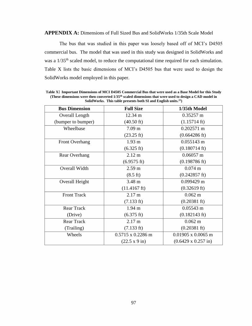
97

APPENDIX A: Dimensions of Full Sized Bus and SolidWorks 1/35th Scale Model

The bus that was studied in this paper was loosely based off of MCI’s D4505

commercial bus. The model that was used in this study was designed in SolidWorks and

was a 1/35th scaled model, to reduce the computational time required for each simulation.

Table X lists the basic dimensions of MCI’s D4505 bus that were used to design the

SolidWorks model employed in this paper.

Table X: Important Dimensions of MCI D4505 Commercial Bus that were used as a Base Model for this Study

(These dimensions were then converted 1/35th scaled dimensions that were used to design a CAD model in

SolidWorks. This table presents both SI and English units.22)

Bus Dimension Full Size 1/35th Model

Overall Length

(bumper to bumper)

12.34 m

(40.50 ft)

0.35257 m

(1.15714 ft)

Wheelbase 7.09 m

(23.25 ft)

0.202571 m

(0.664286 ft)

Front Overhang 1.93 m

(6.325 ft)

0.055143 m

(0.180714 ft)

Rear Overhang 2.12 m

(6.9575 ft)

0.06057 m

(0.198786 ft)

Overall Width 2.59 m

(8.5 ft)

0.074 m

(0.242857 ft)

Overall Height 3.48 m

(11.4167 ft)

0.099429 m

(0.32619 ft)

Front Track 2.17 m

(7.133 ft)

0.062 m

(0.20381 ft)

Rear Track

(Drive)

1.94 m

(6.375 ft)

0.05543 m

(0.182143 ft)

Rear Track

(Trailing)

2.17 m

(7.133 ft)

0.062 m

(0.20381 ft)

Wheels 0.5715 x 0.2286 m

(22.5 x 9 in)

0.01905 x 0.0065 m

(0.6429 x 0.257 in)

98

APPENDIX B: Blueprint of Side View of MCI D4505

To model the bus in SolidWorks Figure 53 was used to project the side contour of

the bus. This allowed for the incline of the windward face of the bus to be properly

modeled. The blueprints of the windward and leeward faces of the bus were not utilized

due to the fact that it could not be determined if the top face of the bus was curved all along

the bus or only at the ends. This figure was blown up to match the dimensions listed in

Appendix A.

Figure 53: Side view of MCI D4505 commercial bus, which was used as the reference for the bus model

examined in this study. The contour of this figure was utilized in SolidWorks to project the estimated contour of

the bus onto a CAD model that had the dimensions stated in Appendix A. This figure allowed for the correct

approximation of the incline of the windward face.23

99

APPENDIX C: SolidWorks 1/35th Scaled Model of Commercial Bus Used in Study

The model examined in this study was constructed using SolidWorks and is shown

in Figure 54. Part (a) shows the right view of the bus, while part (b) illustrates the left side.

Part (c) shows the windward face of the bus and part (d) the leeward face. When

simulations were run the headlights, windshield wipers, etc. were not included, only the

basic bus model was employed.

Figure 54: Right view (a), left view (b), front view (c), and rear view (d) of 1/35th scaled model bus . It can be

seen in both the right and left views that the windward face is inclined, while the front and rear views show that

the rest of the bus is relatively square like the classic bluff body. All edges are filleted to reduce the separation

bubbles that occur when air flows around sharp changes in geometry.

a.)

b.)

c.) d.)

100

APPENDIX D: ANSYS Fluent Set-up and Procedure

Step 1: Open ANSYS Workbench and select and drag Fluid Flow (Fluent) from under

Analysis Systems onto the Workbench area. Rename simulation to the appropriate title.

Geometry:

Step 2: Right-click on the Geometry line and click Import Geometry → Browse. Select

the file that you would like to run a simulation on.

Step 3: Double-click on the Geometry line to open DesignModeler. Once DesignModeler

is open press the Generate button, , to full attach the file.

Step 4: Under Tools select Enclosure and make the following changes under the Detail

View box:

Change the Number of Planes to 1.

Click the yellow box on the Symmetry Plane1 box. Select the YZ Plane under the

Tree Outline box and click the Apply button next to the Symmetry Plane1 line.

Type the following dimensions into the Details of Enclosure1 box:

Rename

Drag

101

Step 5: Press the Generate button to create the Enclosure.

Step 6: Select the Boolean button under the Create menu. Under the Details of Boolean1

select the Subtract option from the drop-down menu next to the Operation line.

Step 7: Click the yellow box next to the Target Bodies option, select the entire Boolean

Enclosure and click the Apply box for the Target Bodies.

Step 8: Click the yellow box next to the Tool Bodies option, select the button from

the tool bar and select the box select option. Highlight the entire bus and click the Apply

box for the Tool Bodies. Click the Generate button. When Generated change the name of

the part to “Air” by right clicking under the tree.

Step 9: Select the Sketching tab from the Sketching Toolboxes menu and choose Rectangle

under the Draw tab. Draw a rectangle on the back place around the bus, with the bottom of

the rectangle coincident with the symmetry plane. Result shown below.

102

Step 10: Click the Dimensions tab and dimension the length and height of the refinement

box. Then select the Length/Distance button from the dimension options and dimension

the distance between the y-axis and the back vertical edge of the refinement box. Input the

follow dimensions:

Step 11: Select the Extrude feature from toolbar and extrude the sketch 0.15m by inputting

the dimension in the depth line of the details of Extrude1. Click Generate the produce the

refinement box. This concludes the Geometry setup and the DesignModeler can be closed.

Mesh:

Step 12: Double-click on the Mesh line to open Meshing. The geometry that was defined

will be automatically attached.

Step 13: Click Mesh under the Outline tree on the left side of the screen. Under Details of

“Mesh” make the following changes.

Change Relevance to 100.

Under Sizing change:

o Use Advanced Size Function to Proximity and Curvature.

o Change Relevance Center to Medium.

o Change Smoothing to High.

Under Assembly Meshing change Method to either CutCell or Tetrahedron

depending on what mesh you are designing.

Step 14: Right click on mesh choose Insert and select Sizing. Repeat one more time.

Step 15: Click on the first Sizing under Mesh and click the yellow box next to Geometry

under Scope. Click the button on the toolbar and click on the enclosure and click Apply

next to the Geometry line.

103

Step 16: Select Body of Influence from under the Type pull down menu in the Details of

“Body Sizing” – Sizing box.

Step 17: Under Geometry on the outline right click on the Air and select Hide Body.

Step 18: Click the yellow box next to Bodies of Influence and select the refinement box in

the viewing window. Click Apply next to Bodies of Influence.

Step 19: Under Geometry on the outline right click on the Air and select Show Body and

right click on Solid and select Hide Body.

Step 20: Select the second Sizing. Click the button and select the Box Select and

shown above. Click the yellow box next to Geometry, highlight the faces of the bus contour

and click Apply next to Geometry under Scope.

Step 21: Under Connections delete the unknown connection.

Step 22: Highlight the contour of the bus and right click. Select Create Named Section

and name it “Bus”.

Step 23: Select Single Select in replace of Box Select. Name other planes in similar

manner as described above:

Plane in front of bus should be named “Velocity Inlet”.

Plane in back of bus should be named “Pressure Outlet”.

Plane underneath bus should be named “Road”.

Plane with bus contour on it should be named “Symmetry”.

Plane above bus and far side of wind tunnel should be combined and named

“Symmetry 2”.

Step 24: Click Generate button to create the mesh. Once the mesh is loaded the Mesh

section of the setup and can be closed out.

Step 25: Once closed right click on the Mesh line of the setup and select Update.

Setup:

Step 26: Double-click on the Setup line to open Fluent. The geometry and mesh that was

defined will be automatically attached.

Step 27: The first step of Fluent setup is dependent on which mesh was used:

CutCell – type “mesh/polyhedral/convert-hanging-nodes” in text box to convert all

hanging nodes to polyhedral elements.

104

Polyhedral – Go under Mesh on toolbar, select Convert Domain from Polyhedral

option.

Step 28: Once the mesh is converted select the Check button under General tab.

Step 29: Under the Models tab double click on Viscous-Laminar. Depending on which

turbulence model you are using make the following selections:

Realizable k-ε Model – Select k-epsilon from under Models, Realizable under k-

epsilon Model, Non-equilibrium under Near-Wall Treatment, and keep all other

settings on the default. Click OK.

SST Model – Select k-omega from under Models, SST under k-omega Model and

keep all other settings on the default. Click OK.

Step 30: Under Boundary Conditions click Velocity Inlet and choose Edit. Select

Magnitude and Direction from the dropdown menu next to Velocity Specification Method.

Set the X- and Y-Component of Flow Direction to 0 and Z-Component of Flow Direction

to 33.528 m/s. Set Turbulent Intensity to 1%. Click OK.

Step 31: Under Reports double click on Projected Area. Select the bus and Z Direction,

click compute. You will use this area in the next step.

Step 32: Under Reference Values change the Compute From to Velocity Inlet and the

Reference Zone to Air. In the Area box input the area found in Step 31. Leave all other

boxes on the default.

Step 33: Under Solution Methods change the Scheme to Coupled, the Turbulent Kinetic

energy to Second Order Upwind, and Turbulent Dissipation Rate to Second Order Upwind.

Step 34: Select Solution Controls and input the following parameters, leaving all others on

the default:

Courant Number – 50

Momentum – 0.25

Pressure – 0.25

Energy – 0.953

Step 35: Under Monitors select Residuals and click Edit button. Under Convergence

Criterion choose none. Click OK.

Step 36: Under the Monitor tab in the Residuals, Statistics, and Force Monitors, select

Create and choose Drag. Under the Drag Monitor select the Bus from the Wall Zone and

105

check the boxes next to Print to Console, Plot, and Write. Next to the File Name add”.txt”

and change the X Force Vector to 0 and the Z Force Vector to -1. Click OK.

Step 37: Double click the Convergence Manger on the Monitor tab check the box next to

line, change the Stop Criterion to 1e-05 and the Previous Iterations to Consider to 10. Click

OK.

Step 38: Click Initialize under the Solution Initialization.

Step 39: Once Initialized select the Calculation Activities and change the Autosave Every

(Iterations) to 100.

Step 40: Under the Run Calculation tab change the Number of Iterations to 500 for RKE

and 1000 to SST. Click Calculate to run simulation. Once simulation is run and the drag

coefficient has converged close the simulation making sure to allow Fluent to save.

106

APPENDIX E: Calibration Raw Data

To determine the repeatability of the simulations run in ANSYS Fluent a calibration

study was conducted. The first part of the parameter study was utilized as the calibration

test. The angle between the line drawn tangent to the radius of curvature and the line on

the horizontal was changed from 80˚ to 35˚ in increments of 5˚ with an additional test run

at 86˚, the angle recommended by Kirch et al.’s study.20 The study was run for all four

combinations of turbulence models and meshes. Table XI shows the raw data that was

found when the simulations were run. The drag coefficient was found in the simulation

and the percent was the percent reduction in the drag coefficient that was calculated.

Table XI: First Run of the Calibration of the Fluent Simulations (All four sets of simulations were run; CutCell

Realizable k-ε, CutCell SST k-ω, polyhedral Realizable k-ε, and polyhedral SST k-ω. It can be seen, as

highlighted, that the CutCell SST k-ω and polyhedral k-ε both found 55˚ as the optimal angle while CutCell

Realizable k-ε found 80˚ to be optimal and polyhedral SST k-ω found 50˚ to be the best.)

A second identical run was completed to be able to compare the rests to test the

repeatability of the solution found by the simulations, depending on the turbulence model

and mesh employed. It was also noted how much the different models and turbulence

models compared to each other. Table XII illustrates the raw data that was found for the

second run of simulations. Once both sets were found they could be compared to each

other.

Percent Drag Percent Drag Percent Drag Percent Drag

86 5.31% 0.58734 4.78% 0.6004 2.32% 0.60614 2.05% 0.62018

80 5.71% 0.58485 5.80% 0.594 2.72% 0.60367 2.84% 0.61523

75 5.40% 0.58676 3.26% 0.61 2.97% 0.60214 2.83% 0.61526

70 5.63% 0.58536 5.45% 0.5962 3.26% 0.60035 2.73% 0.61589

65 5.33% 0.58719 5.50% 0.59588 5.13% 0.58873 4.13% 0.60701

60 4.30% 0.59359 6.30% 0.59081 4.50% 0.59266 3.77% 0.60931

55 4.86% 0.5901 6.89% 0.58707 5.19% 0.58836 3.87% 0.60866

50 5.35% 0.58709 5.79% 0.59403 5.08% 0.58906 4.93% 0.60195

45 4.88% 0.59001 6.59% 0.589 5.02% 0.58939 4.48% 0.60482

40 5.20% 0.58799 6.80% 0.58765 4.94% 0.5899 4.67% 0.60359

35 2.89% 0.60232 3.02% 0.61152 2.96% 0.6022 3.14% 0.61328

RKE SST RKE SST

CutCell Polyhedral

107

Table XII: Second Run of the Calibration of the Fluent Simulations (All four sets of simulations were run;

CutCell Realizable k-ε, CutCell SST k-ω, polyhedral Realizable k-ε, and polyhedral SST k-ω. It can be seen, as

highlighted, that the CutCell SST k-ω and polyhedral k-ε both found 55˚ as the optimal angle while CutCell

Realizable k-ε found 80˚ to be optimal and polyhedral SST k-ω found 50˚ to be the best.)

Percent Drag Percent Drag Percent Drag Percent Drag

Without 0.62026 0.63054 0.62056 0.63319

86 5.31% 0.58733 4.78% 0.6004 2.38% 0.60582 2.09% 0.61994

80 5.71% 0.58485 5.94% 0.59309 2.71% 0.60374 2.85% 0.61515

75 5.40% 0.58678 3.24% 0.61013 2.97% 0.60213 2.83% 0.61525

70 5.63% 0.58536 5.48% 0.59599 3.26% 0.60035 2.71% 0.616

65 5.33% 0.58719 5.53% 0.5957 5.13% 0.58873 4.14% 0.60696

60 4.31% 0.5935 6.31% 0.59076 4.46% 0.59291 3.62% 0.61027

55 4.86% 0.59009 6.65% 0.58863 5.19% 0.58836 4.03% 0.60765

50 5.34% 0.58711 5.78% 0.59408 5.08% 0.58905 4.94% 0.60189

45 4.88% 0.59 6.57% 0.5891 5.01% 0.58948 4.49% 0.60478

40 5.25% 0.58767 6.78% 0.58776 4.93% 0.58997 4.53% 0.6045

35 3.03% 0.60145 3.32% 0.6096 2.97% 0.60212 3.15% 0.61324

RKE SST RKE SST

CutCell Polyhedral

108

APPENDIX F: Raw Data of Parameter Study Performed on Top Airvane

The first parameter that was examined in the parameter study was the angle that

was measured between the horizontal and the line tangent to the curved portion of the

airvane. This raw data was presented in Appendix E After the general angles were tested

and it was found that the optimal angle was 55˚, a more refined set of angles was tested

around this angle, from 60˚ to 50˚ in increments of 1˚. The raw data for the set of refined

angles can be seen in Table XII.

Table XIII: Raw Data of Refined Angle Tests Run for the Parameter Run on the Top Airvane (The angle

measured was between the horizontal and the line tangent to the curved portion of the airvane. The drag

coefficient was found using the Fluent simulations and the percent reduction was found using the drag

coefficient of the bus without an airvane attached.)

c

The expansion ratio was the second parameter that was tested in the parameter

study. The expansion ratio was the ratio between the inlet gap and the outlet gap. The test

was run from 1:2 to 1:6.5 in increments of 1:0.5. The raw data can be seen in Table XIV.

Table XIV: Raw Data of General Expansion Ratio Tests Run for the Parameter Test of the Top Airvane (The

expansion ratio was the ratio between the inlet gap and the outlet gap. The drag coefficient was found using the

Angle Drag Percent Drag Percent

60 0.59291 4.46% 0.59873 5.04%

59 0.58889 5.10% 0.58865 6.64%

58 0.59285 4.47% 0.58879 6.62%

57 0.59265 4.50% 0.59791 5.17%

56 0.58949 5.01% 0.59433 5.74%

55 0.58836 5.19% 0.58863 6.65%

54 0.59423 4.24% 0.59004 6.42%

53 0.5894 5.02% 0.58637 7.01%

52 0.58793 5.26% 0.59656 5.39%

51 0.58779 5.28% 0.59676 5.36%

50 0.58905 5.08% 0.59408 5.78%

Polyhedral RKE CutCell SST

109

Fluent simulations and the percent reduction was found using the drag coefficient of the bus without an airvane

attached.)

Once 1:6 was determined as the optimal expansion ratio, to further optimize the

parameter another set of simulations were run with more refined dimensions. The

expansion ratio was testes from 1:5.6 to 1:6.4 in increments of 1:0.1, the raw data from

these simulations can be seen in Table XV.

Table XV: Raw Data Produced From the Simulations Run to Test the Refined Expansion Ratios in the

Parameter Study of the Top Airvane (The drag coefficient was found using the Fluent simulations and the

percent reduction was found using the drag coefficient of the bus without an airvane attached.)

The third parameter examined in the parameter study of the top airvane was the

dimension of the radius of the curved portion of the airvane. The dimension of the radius

was tested as a percentage of the distance from the stagnation point to the top horizontal

Expansion Ratio Drag Percent Drag Percent

2 0.58819 5.22% 0.58338 7.48%

2.5 0.60118 3.12% 0.593 5.95%

3 0.59605 3.95% 0.5958 5.51%

3.5 0.595 4.12% 0.59611 5.46%

4 0.59154 4.68% 0.59 6.43%

4.5 0.58799 5.25% 0.5975 5.24%

5 0.595 4.12% 0.59294 5.96%

5.5 0.5926 4.51% 0.59486 5.66%

6 0.58743 5.34% 0.58644 6.99%

6.5 0.5884 5.18% 0.59332 5.90%

Polyhedral RKE CutCell SST

Expansion Ratio Drag Percent Drag Percent

5.6 0.58799 5.25% 0.5863 7.02%

5.7 0.58722 5.37% 0.59409 5.78%

5.8 0.58814 5.22% 0.59364 5.85%

5.9 0.58788 5.27% 0.59351 5.87%

6.0 0.58743 5.34% 0.58644 6.99%

6.1 0.58865 5.14% 0.58936 6.53%

6.2 0.58889 5.10% 0.59169 6.16%

6.3 0.58831 5.20% 0.59356 5.86%

6.4 0.58888 5.11% 0.59089 6.29%

Polyhedral RKE CutCell SST

110

edge of the windward face of the bus. Table XVI contains the raw data that was found for

the simulations run for the optimization of the radius of the curved portion of the airvane.

Table XVI: Data Produced from the Testing of the Radius of the Curved Potion of the Airvane for the

Parameter Study of the Top Airvane (The drag coefficient was found using the Fluent simulations and the

percent reduction was found using the drag coefficient of the bus without an airvane attached.)

After the radius of the curved portion of the airvane was tested the inlet gap could be tested.

While testing the inlet gap the expansion was kept at 1:6, meaning that as the inlet gap was

increased so was the outlet gap. The inlet gap was tested from 2 cm to 4.5 cm in increments

of 0.5 cm; these dimensions were on a full sized model. On the 1/35th scaled model it was

0.057 cm to 0.13 cm in increments of 0.014 cm. The raw data that was found using Fluent

is shown in Table XVII.

Table XVII: Raw Data Collected for the Testing of the Inlet Gap for the Parameter Study of the Top Airvane

(As the inlet gap was increased the outlet was also to ensure that an expansion ratio of 1:6 was maintained. The

Radius Drag Percent Drag Percent

5% 0.59281 4.47% 0.59692 5.33%

6% 0.5915 4.68% 0.59368 5.85%

7% 0.5888 5.12% 0.59363 5.85%

8% 0.58655 5.48% 0.58099 7.86%

9% 0.58677 5.45% 0.58777 6.78%

10% 0.58868 5.14% 0.58749 6.83%

11% 0.58906 5.08% 0.58744 6.84%

12% 0.58944 5.01% 0.58673 6.95%

13% 0.58905 5.08% 0.58858 6.65%

14% 0.59005 4.92% 0.58571 7.11%

15% 0.58997 4.93% 0.58877 6.62%

Polyhedral RKE CutCell SST

111

drag coefficient was found using the Fluent simulations and the percent reduction was found using the drag

coefficient of the bus without an airvane attached.)

The angle between the planar portion of the airvane and the top horizontal face of

the bus was the next parameter that was analyzed. The angle was tested from 0˚ to 5˚ in

increments of 0.5˚. Table XVIII contains the raw data that was collected for the testing of

the angle of planar portion of the top airvane.

Table XVIII: Raw Data Collected for the Angle Changes of the Planar Portion of the Top Airvane (The drag

coefficient was found using the Fluent simulations and the percent reduction was found using the drag

coefficient of the bus without an airvane attached.)

Table XIX contains the last set of raw data for the parameter study run on the top

airvane. The length of the planar portion of the airvane was tested from 0.25 times the

radius of curvature to 2.5 times in increments of 0.25 times the radius of curvature.

Inlet Height (cm) Drag Percent Drag Percent

2 0.5909 4.78% 0.59468 5.69%

2.25 0.58814 5.22% 0.59418 5.77%

2.5 0.58725 5.37% 0.58347 7.47%

2.75 0.58615 5.54% 0.5926 6.02%

3 0.58115 6.35% 0.5858 7.10%

3.25 0.57834 6.80% 0.5936 5.86%

3.5 0.57724 6.98% 0.57742 8.42%

3.75 0.576 7.18% 0.57128 9.40%

4 0.57853 6.77% 0.57828 8.29%

4.25 0.57032 8.10% 0.56671 10.12%

4.5 0.56666 8.69% 0.57117 9.42%

Polyhedral RKE CutCell SST

Inlet Angle (degrees) Drag Percent Drag Percent

0 0.56666 8.69% 0.57117 9.42%

0.5 0.57061 8.05% 0.56861 9.82%

1 0.57019 8.12% 0.57129 9.40%

1.5 0.56649 8.71% 0.57307 9.11%

2 0.5671 8.61% 0.5757 8.70%

2.5 0.56851 8.39% 0.57243 9.22%

3 0.55955 9.83% 0.56774 9.96%

3.5 0.55546 10.49% 0.56151 10.95%

4 0.55533 10.51% 0.55557 11.89%

4.5 0.55407 10.71% 0.5625 10.79%

5 0.55697 10.25% 0.55762 11.56%

5.5 0.55704 10.24% 0.55601 11.82%

6 0.5609 9.61% 0.55993 11.20%

Polyhedral RKE CutCell SST

112

Table XIX: Raw Data of the Simulations Run for the Change in Planar Length of the Top Airvane (The drag

coefficient was found using the Fluent simulations and the percent reduction was found using the drag

coefficient of the bus without an airvane attached.)

Planar Length Drag Percent Drag Percent

0.25 0.56373 9.16% 0.57616 8.62%

0.5 0.59562 4.02% 0.588558 6.66%

0.75 0.55896 9.93% 0.56545 10.32%

1 0.56192 9.45% 0.56586 10.26%

1.25 0.55829 10.03% 0.55425 12.10%

1.5 0.55568 10.46% 0.55445 12.07%

1.75 0.55908 9.91% 0.55645 11.75%

2 0.55317 10.86% 0.55207 12.44%

2.25 0.55161 11.11% 0.5506 12.68%

2.5 0.54972 11.42% 0.54694 13.26%

CutCell SSTPolyhedarl RKE

113

APPENDIX G: Raw Data of Parameter Study Performed on Side Airvane

The first parameter that was examined in the parameter study was the angle that

was measured between the horizontal and the line tangent to the curved portion of the

airvane. The tests were run from 80˚ to 35˚ in increments of 5˚, with an additional test ran

at 86˚ as the initial airvane angle. The raw data for the set of refined angles can be seen in

Table XX.

Table XX: Raw Data of the Simulations Run for the General Change in the Angle Between the Line Tangent to

the Radius of Curvature and the Horizontal of the Side Airvane (The drag coefficient was found using the

Fluent simulations and the percent reduction was found using the drag coefficient of the bus without an airvane

attached.)

After the general angles were tested and it was found that the optimal angle was

35˚, a more refined set of angles was tested around this angle, from 40˚ to 30˚ in increments

of 1˚. The raw data for the set of refined angles can be seen in Table XXI.

Angle Drag Percent Drag Percent

86 0.56774 8.51% 0.5622 10.84%

80 0.56209 9.42% 0.56172 10.91%

75 0.57093 8.00% 0.56374 10.59%

70 0.57154 7.90% 0.56062 11.09%

65 0.56387 9.14% 0.5627 10.76%

60 0.567551 8.54% 0.56459 10.46%

55 0.55865 9.98% 0.56125 10.99%

50 0.55613 10.38% 0.55842 11.44%

45 0.55302 10.88% 0.55506 11.97%

40 0.549 11.53% 0.54993 12.78%

35 0.54835 11.64% 0.54827 13.05%

CutCell SSTPolyhedral RKE

114

Table XXI: Raw Data of the Simulations Run for the Refined Angle of the Side Airvane (The drag coefficient

was found using the Fluent simulations and the percent reduction was found using the drag coefficient of the bus

without an airvane attached.)

The expansion ratio was the second parameter that was tested in the parameter

study. The expansion ratio was the ratio between the inlet gap and the outlet gap. The test

was run from 1:2 to 1:6.5 in increments of 1:0.5. The raw data can be seen in Table XXII.

Table XXII: Raw Data of the Simulations Run for the General Expansion Ratio of the Side Airvane (The drag

coefficient was found using the Fluent simulations and the percent reduction was found using the drag

coefficient of the bus without an airvane attached.)

Once 1:6 was determined as the optimal expansion ratio, to further optimize the

parameter another set of simulations were run with more refined dimensions. The

Angle Drag Percent Drag Percent

40 0.549 11.53% 0.54993 12.78%

39 0.5486 11.60% 0.54818 13.06%

38 0.5462 11.98% 0.54836 13.03%

37 0.54926 11.49% 0.549 12.93%

36 0.54954 11.44% 0.5476 13.15%

35 0.54835 11.64% 0.54827 13.05%

34 0.54695 11.86% 0.54695 13.26%

33 0.54648 11.94% 0.54446 13.65%

32 0.54791 11.71% 0.54675 13.29%

31 0.54864 11.59% 0.54655 13.32%

30 0.54957 11.44% 0.54636 13.35%

CutCell SSTPolyhedral RKE

Eaxpansion Ratio Drag Percent Drag Percent

2 0.54843 11.62% 0.54522 13.53%

2.5 0.54843 11.62% 0.54532 13.52%

3 0.54811 11.67% 0.54497 13.57%

3.5 0.54799 11.69% 0.54545 13.49%

4 0.54848 11.62% 0.54576 13.45%

4.5 0.55047 11.29% 0.54826 13.05%

5 0.54854 11.61% 0.54454 13.64%

5.5 0.54825 11.65% 0.55011 12.76%

6 0.54687 11.87% 0.54286 13.91%

6.5 0.55126 11.17% 0.54813 13.07%

CutCell SSTPolyhedral RKE

115

expansion ratio was testes from 1:5.6 to 1:6.4 in increments of 1:0.1, the raw data from

these simulations can be seen in Table XXIII.

Table XXIII: Raw Data of the Simulations Run for the Refined Expansion Ratio of the Side Airvane (The drag

coefficient was found using the Fluent simulations and the percent reduction was found using the drag

coefficient of the bus without an airvane attached.)

The third parameter examined in the parameter study of the side airvane was the

dimension of the radius of the curved portion of the airvane. The dimension of the radius

was tested as a percentage of the distance from the stagnation point to the top horizontal

edge of the windward face of the bus. Table XXIV contains the raw data that was found

for the simulations run for the optimization of the radius of the curved portion of the

airvane. The tests were run from 7% to 15% in increments of 1%.

Table XXIV: Raw Data of the Simulations Run for the Radius of Curvature of the Side Airvane (The drag

coefficient was found using the Fluent simulations and the percent reduction was found using the drag

coefficient of the bus without an airvane attached.)

Expansion Ratio Drag Percent Drag Percent

5.6 0.5488 11.56% 0.54536 13.51%

5.7 0.54719 11.82% 0.54523 13.53%

5.8 0.54918 11.50% 0.54433 13.67%

5.9 0.54816 11.67% 0.5445 13.65%

6.0 0.54687 11.87% 0.54286 13.91%

6.1 0.54904 11.53% 0.54865 12.99%

6.2 0.55156 11.12% 0.54885 12.96%

6.3 0.55085 11.23% 0.55592 11.83%

6.4 0.550873 11.23% 0.54823 13.05%

CutCell SSTPolyhedral RKE

Radius Drag Percent Drag Percent

7% 0.56059 9.66% 0.55492 11.99%

8% 0.55393 10.74% 0.54827 13.05%

9% 0.55081 11.24% 0.54745 13.18%

10% 0.55413 10.70% 0.5518 12.49%

11% 0.54659 11.92% 0.54483 13.59%

12% 0.54687 11.87% 0.54286 13.91%

13% 0.54932 11.48% 0.54682 13.28%

14% 0.54939 11.47% 0.54683 13.28%

15% 0.54798 11.70% 0.54467 13.62%

CutCell SSTPolyhedral RKE

116

After the radius of the curved portion of the airvane was tested the inlet gap could

be tested. While testing the inlet gap the expansion was kept at 1:6, meaning that as the

inlet gap was increased so was the outlet gap. The inlet gap was tested from 2 cm to 4.5

cm in increments of 0.5 cm; these dimensions were on a full sized model. On the 1/35th

scaled model it was 0.057 cm to 0.13 cm in increments of 0.014 cm. The raw data that was

found using Fluent is shown in Table XXV.

Table XXV: Raw Data of the Simulations Run for the Inlet Gap of the Side Airvane (The drag coefficient was

found using the Fluent simulations and the percent reduction was found using the drag coefficient of the bus

without an airvane attached.)

The angle between the planar portion of the airvane and the top horizontal face of

the bus was the next parameter that was analyzed. The angle was tested from 0˚ to 5˚ in

increments of 0.5˚. Table XXVI contains the raw data that was collected for the testing of

the angle of planar portion of the top airvane.

Inlet Gap (cm) Drag Percent Drag Percent

2.00 0.55142 11.14% 0.54929 12.89%

2.25 0.54965 11.43% 0.55146 12.54%

2.50 0.55023 11.33% 0.55206 12.45%

2.75 0.54745 11.78% 0.54457 13.63%

3.00 0.54919 11.50% 0.54894 12.94%

3.25 0.54699 11.86% 0.5449 13.58%

3.50 0.54646 11.94% 0.54392 13.74%

3.75 0.54826 11.65% 0.544 13.72%

4.00 0.54961 11.43% 0.55129 12.57%

4.25 0.5511 11.19% 0.54634 13.35%

4.50 0.54687 11.87% 0.54286 13.91%

CutCell SSTPolyhedral RKE

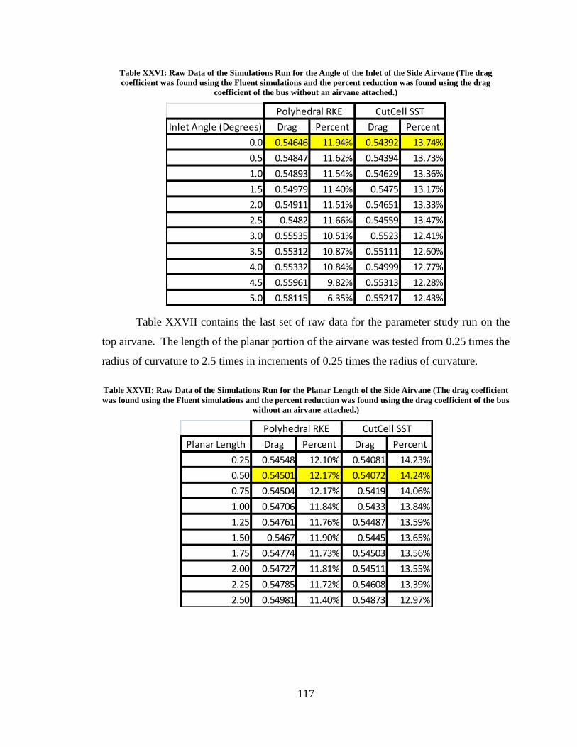
117

Table XXVI: Raw Data of the Simulations Run for the Angle of the Inlet of the Side Airvane (The drag

coefficient was found using the Fluent simulations and the percent reduction was found using the drag

coefficient of the bus without an airvane attached.)

Table XXVII contains the last set of raw data for the parameter study run on the

top airvane. The length of the planar portion of the airvane was tested from 0.25 times the

radius of curvature to 2.5 times in increments of 0.25 times the radius of curvature.

Table XXVII: Raw Data of the Simulations Run for the Planar Length of the Side Airvane (The drag coefficient

was found using the Fluent simulations and the percent reduction was found using the drag coefficient of the bus

without an airvane attached.)

Inlet Angle (Degrees) Drag Percent Drag Percent

0.0 0.54646 11.94% 0.54392 13.74%

0.5 0.54847 11.62% 0.54394 13.73%

1.0 0.54893 11.54% 0.54629 13.36%

1.5 0.54979 11.40% 0.5475 13.17%

2.0 0.54911 11.51% 0.54651 13.33%

2.5 0.5482 11.66% 0.54559 13.47%

3.0 0.55535 10.51% 0.5523 12.41%

3.5 0.55312 10.87% 0.55111 12.60%

4.0 0.55332 10.84% 0.54999 12.77%

4.5 0.55961 9.82% 0.55313 12.28%

5.0 0.58115 6.35% 0.55217 12.43%

CutCell SSTPolyhedral RKE

Planar Length Drag Percent Drag Percent

0.25 0.54548 12.10% 0.54081 14.23%

0.50 0.54501 12.17% 0.54072 14.24%

0.75 0.54504 12.17% 0.5419 14.06%

1.00 0.54706 11.84% 0.5433 13.84%

1.25 0.54761 11.76% 0.54487 13.59%

1.50 0.5467 11.90% 0.5445 13.65%

1.75 0.54774 11.73% 0.54503 13.56%

2.00 0.54727 11.81% 0.54511 13.55%

2.25 0.54785 11.72% 0.54608 13.39%

2.50 0.54981 11.40% 0.54873 12.97%

CutCell SSTPolyhedral RKE

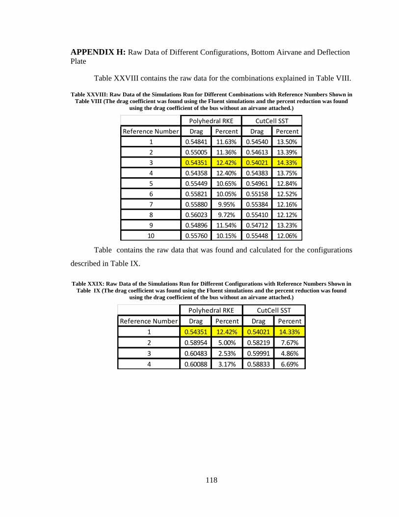
118

APPENDIX H: Raw Data of Different Configurations, Bottom Airvane and Deflection

Plate

Table XXVIII contains the raw data for the combinations explained in Table VIII.

Table XXVIII: Raw Data of the Simulations Run for Different Combinations with Reference Numbers Shown in

Table VIII (The drag coefficient was found using the Fluent simulations and the percent reduction was found

using the drag coefficient of the bus without an airvane attached.)

Table contains the raw data that was found and calculated for the configurations

described in Table IX.

Table XXIX: Raw Data of the Simulations Run for Different Configurations with Reference Numbers Shown in

Table IX (The drag coefficient was found using the Fluent simulations and the percent reduction was found

using the drag coefficient of the bus without an airvane attached.)

Reference Number Drag Percent Drag Percent

1 0.54841 11.63% 0.54540 13.50%

2 0.55005 11.36% 0.54613 13.39%

3 0.54351 12.42% 0.54021 14.33%

4 0.54358 12.40% 0.54383 13.75%

5 0.55449 10.65% 0.54961 12.84%

6 0.55821 10.05% 0.55158 12.52%

7 0.55880 9.95% 0.55384 12.16%

8 0.56023 9.72% 0.55410 12.12%

9 0.54896 11.54% 0.54712 13.23%

10 0.55760 10.15% 0.55448 12.06%

CutCell SSTPolyhedral RKE

Reference Number Drag Percent Drag Percent

1 0.54351 12.42% 0.54021 14.33%

2 0.58954 5.00% 0.58219 7.67%

3 0.60483 2.53% 0.59991 4.86%

4 0.60088 3.17% 0.58833 6.69%

CutCell SSTPolyhedral RKE