aerodynamic drag coefficients of
76
AERODYNAMIC DRAG COEFFICIENTS OF A VARIETY OF ELECTRICAL CONDUCTORS by JEFFREY C. STROMAN, B.S.M.E. A THESIS IN MECHANICAL ENGINEERING Submitted to the Graduate Faculty of Texas Tech University in Partial Fulfillment of the Requirements for the Degree of MASTER OF SCIENCE IN MECHANICAL ENGINEERING Approved May, 1997
-
Upload
khangminh22 -
Category
Documents
-
view
1 -
download
0
Transcript of aerodynamic drag coefficients of

AERODYNAMIC DRAG COEFFICIENTS OF
A VARIETY OF ELECTRICAL CONDUCTORS
by
JEFFREY C. STROMAN, B.S.M.E.
A THESIS
IN
MECHANICAL ENGINEERING
Submitted to the Graduate Facul ty of Texas Tech University in
Par t ia l Fulfillment of the Requirements for
the Degree of
MASTER OF SCIENCE
IN
MECHANICAL ENGINEERING
Approved
May, 1997

/^ / A /
TABLE OF CONTENTS
LIST OF TABLES iii
LIST OF FIGURES iv
CHAPTER
1. INTRODUCTION 1
1.1. Objective 1
1.2. Application of Results 1
1.3. Methodology Overview 1
2. BACKGROUND 3
2.1. Theoretical Considerations 3
2.2. Literature Survey 8
3. EXPERIMENTAL APPARATUS 13
3.1. End Plate Design 13
3.2. Towtank Apparatus 17
3.3. Wind Tunnel Apparatus 20
3.4. Uncertainty Analysis 22
4. RESULTS AND DISCUSSION 26
4.1. Conductors in Normal Crossflow 26
4.2. Conductors in Yawed Flow 42
5. CONCLUSIONS AND RECOMMENDATIONS 51
SOURCES 53
APPENDICES
A TABULATED DATA 54
B CONDUCTOR INFORMATION 69
11

LIST OF TABLES
3.1. Towtank Uncertainty Analysis Results 24
3.2. Wind Tunnel Uncertainty Analysis Results 25
A.l. Smooth Cylinder Data 55
A.2. Conductor 100-58600-3 Data 56
A.3. Conductor 100-58604-6 Data 57
A.4. Conductor 100-58650-0 Data 58
A.5. Conductor 100-61200-4 Data 59
A.6. Conductor 142-15026-2 Data 60
A.7. Conductor 142-14100-0 Data 61
A.8. Conductor 100-57900-7 Data 62
A.9. Conductor 100-58200-8 Data 63
A.10. Conductor 100-58104-4 Data 64
A.11. Conductor 100-58300-4 Data 64
A. 12. Conductor 100-61200-4 Yaw Data 65
A. 13. Conductor 100-58650-0 Yaw Data 66
A. 14. Conductor 100-58600-3 Yaw Data 67
A.15. Conductor 100-58200-8 Yaw Data 68
B.l. Conductor Information 70
111

LIST OF FIGURES
2.1. Regimes of the Drag Coefficient versus Reynolds Number Plot 4
2.2. Laminar (a) and Turbulent (b) Boundary Layer Separation Points 5
2.3. Surface Pressure Distribution on a Cylinder in Crossflow 6
2.4. Variation of Drag Coefficient with Surface Roughness 7
2.5. Conductor, as Seen from Above, in Yawed Flow 8
2.6. Cross-Sections of Round Wire (a) and Trapezoidal Wire (b) Conductors 10
2.7. Comparison of Drag Coefficient Data Collected in Wind Tunnels
and Field 10
3.1. Saddle Clamp Block 13
3.2. End Plate 14
3.3. Saddle Block, Unflexed (a) Flexed (b) 14
3.4. End Plates in Untensioned (a) and Tensioned (b) Configurations 15
3.5. End Plate vAth Shroud Installed 16
3.6. End Plate Slot 16
3.7. End Plate Slot, Taped for Tare (a) and for Conductors (b) 17
3.8. Texas Tech Towtank Facility 18
3.9. Load Cells in Their Upright (a) and Testing (b) Positions 18
3.10. End Plate Installation in the Wind Tunnel 21
3.11. End Plate with Conductor in Yaw, Unshrouded (a), and Shrouded (b) 22
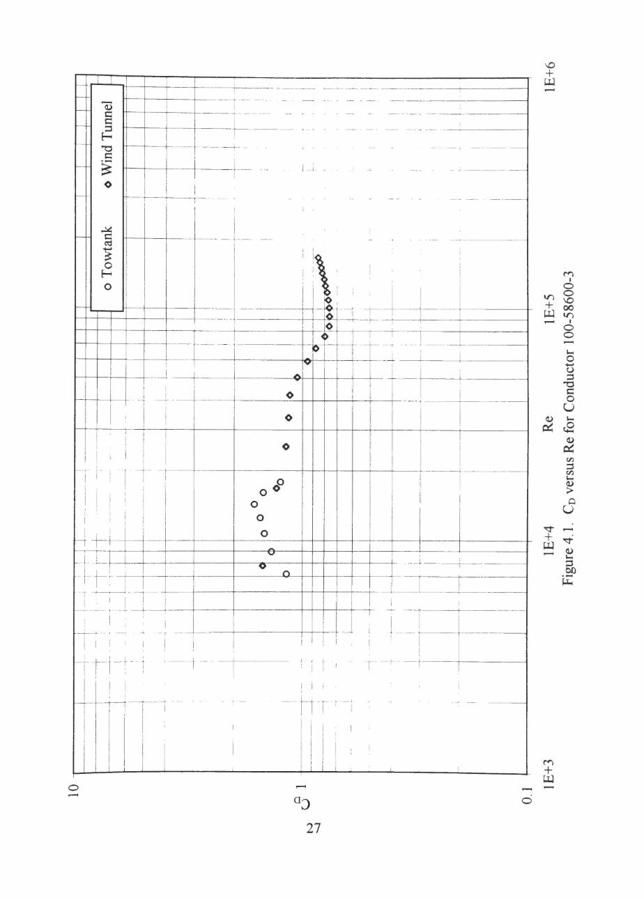
4.1. CD versus Re for Conductor 100-58600-3 27
4.2. CD versus Re for Conductor 100-58604-6 28
4.3. CD versus Re for Conductor 100-58650-0 29
4.4. CD versus Re for Conductor 100-61200-4 31
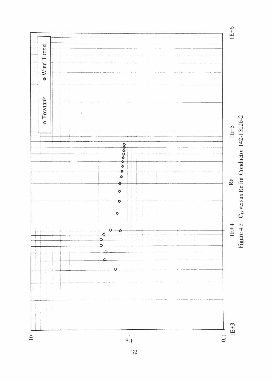
4.5. CD versus Re for Conductor 142-15026-2 32
4.6. CD versus Re for Conductor 142-14100-0 33
4.7. CD versus Re for Conductor 100-57900-7 34
4.8. CD versus Re for Conductor 100-58200-8 35
iv

4.9. CD versus Re for Conductor 100-58104-4 36
4.10. CD versus Re for Conductor 100-58300-4 37
4.11. Comparison of Round and Trapezoidal Strand Conductors 40
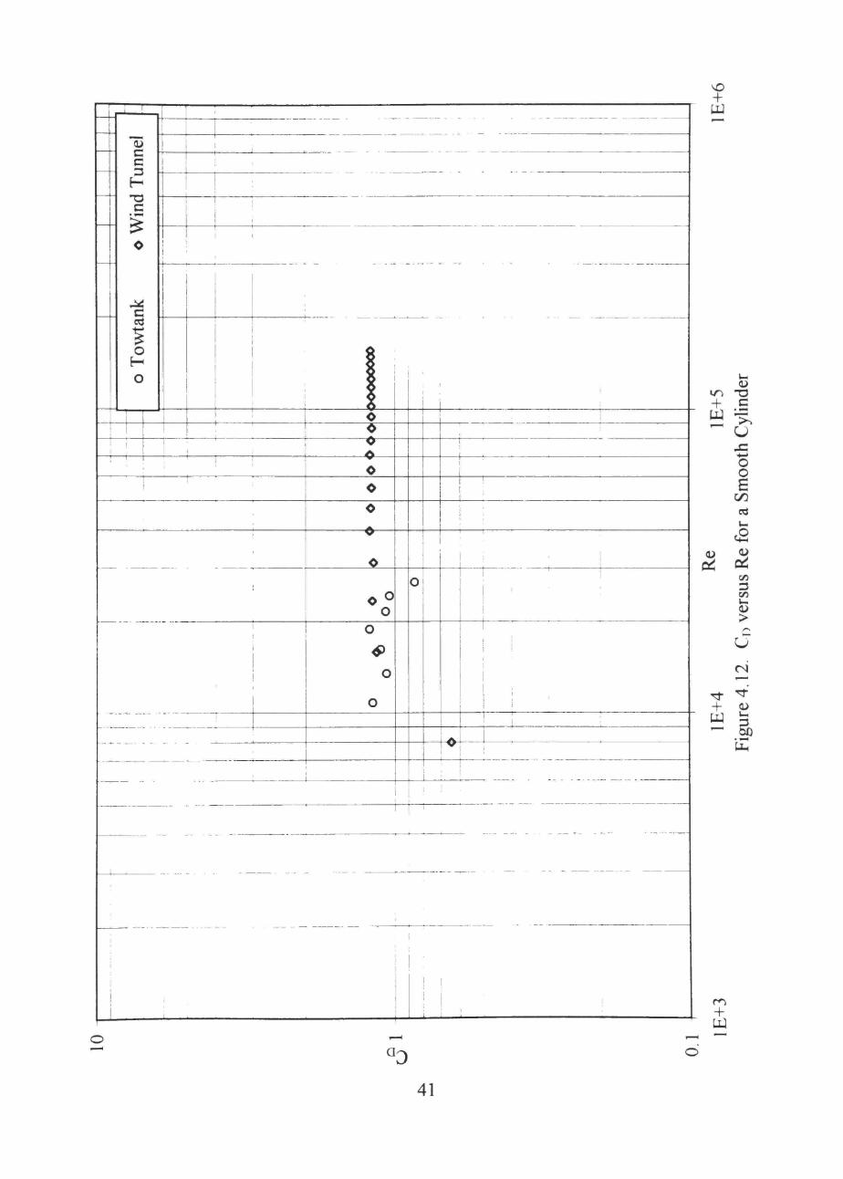
4.12. CD versus Re for a Smooth Cylinder 41
4.13. CD,yaw versus Re for Conductor 100-61200-4 43
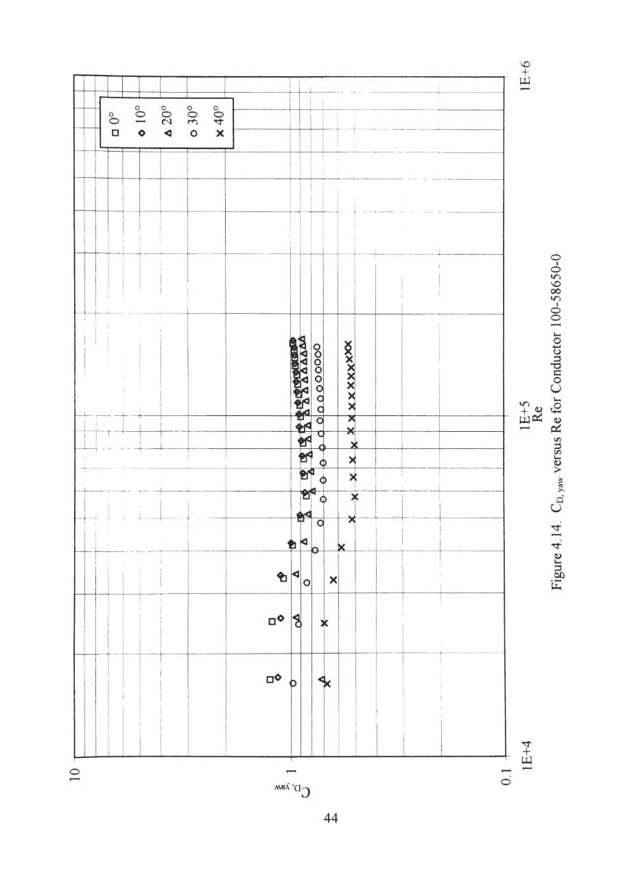
4.14. CD,yaw versus Re for Conductor 100-58650-0 44
4.15. CD,yaw versus Re for Conductor 100-58600-3 45
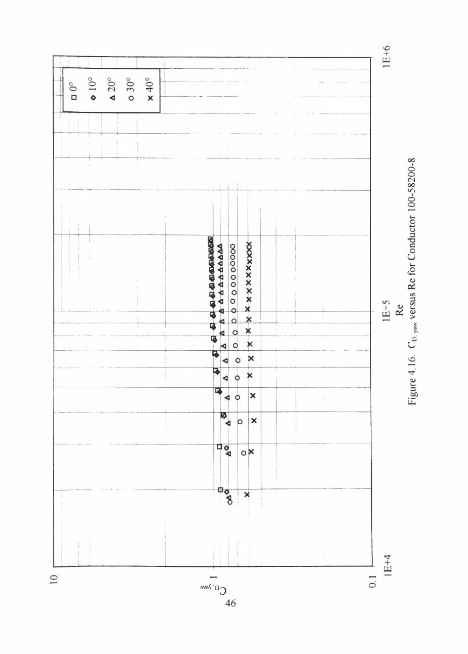
4.16. CD,yaw versus Re for Conductor 100-58200-8 46
4.17. CD, yaw/cosV versus Re for Conductor 100-61200-4 47
4.18. CD, yaw/cosV versus Re for Conductor 100-58650-0 48
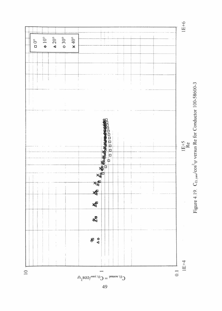
2 4.19. CD,yaw/cos vj/versus Re for Conductor 100-58600-3 49 .2 4.20. CD,yaw /cos> versus Re for Conductor 100-58200-8 50

CHAPTER 1
INTRODUCTION
1.1 Objective
The objective of this study is to determine accurately the aerodynamic drag
coefficients of several different conductors, also called electric transmission lines The
study was handed by Florida Power & Light in hopes of acquiring better data with which
to design transmission line towers. The reason that Florida Power & Light has funded this
research is that recent legislation changes in Florida require a higher tolerance to hurricane
wind loading for structures. This includes transmission line towers, and thus the wind's
drag force on the conductors is paramount to design.
1.2 Application of Results
The author hopes that the results contained in this paper may be used to design and
construct safer electric transmission lines and structures, not only in Florida, but in any
region with high storm wind speeds. The data presented are applicable to any
transmission line loading design problem involving the conductors tested in this study.
1.3 Methodology Overview
The drag coefficient data were collected using two methods. First was the Low
Speed Wind Tunnel Facility operated by Texas A&M University's Aerospace Engineering
Department. Second was the Water Towtank Facihty at the Mechanical Engineering
Department of Texas Tech University. In both tests, actual conductor samples were used
instead of models of conductors. Also, in opposition to the traditional wind tunnel testing
technique for conductors, the samples were not mounted through the walls of the wind
tunnel to external balances but were mounted between two end plates in the center of the
wind tunnel test section on the facihty's internal force balance. Mounting the conductors
in the center of the free stream circumvented the traditional problem of boundary layer

effects along the wind tunnel walls and also provided the flexibility required for testing
under yawed flow conditions.
The drag forces encountered in the wind tunnel and the water towtank tests were
measured, and the drag coefficients calculated for a range of Reynolds numbers. In the
wind tunnel, drag coefficients were obtained for normal and yawed wind conditions. In
both v^nd tunnel and towtank experiments, the drag force on the end plates alone was
measured and subtracted from the total drag force of the conductor and end supports.
This was done in order to isolate the drag due to the conductors. This subtracted quantity
is referred to as the tare drag.

CHAPTER 2
BACKGROUND
2.1 Theoretical Considerations
Many factors affect the drag coefficient of a conductor. Several important factors
are Reynolds number, roughness, turbulence, and wind direction. The equation defining
the drag coefficient may be found in any standard fluids or aerodynamics reference. The
equation states:
C D = - J — ^ 2 (2.1)
In Equation 2.1, FD is the drag force, p is the density of the fluid, Voo is the free
stream velocity, and Af is the frontal area. This equation may be used to calculate drag
coefficients for any object subjected to a fluid flow, including conductors. Notice that the
equation is nondimensional, i.e., unitless. A second nondimensional parameter of some
importance is Reynolds number. It is calculated in the following fashion:
V D Re = - ^ - . (2.2)
V
In Equation 2.2, Voo once again represents the free stream velocity. The
characteristic dimension, D, for this study is the outer diameter of the conductor. And
finally, the kinematic viscosity of the fluid is represented by v. The major resuhs of this
study are plots of the drag coefficient, CD, as a fiinction of the Reynolds number. Re.
Reynolds number represents a balance of the relative magnitudes of inertial and
viscous forces on an object subjected to a fluid flow. Low Reynolds numbers indicate that
viscous effects, along with stable, laminar flow are dominant. High Reynolds numbers
indicate that inertial (pressure) forces, along with unstable, titrbulent flow are dominant.
Several regimes of the drag coefficient versus Reynolds number plot may be defined by the
relative magnitude of Reynolds number. Low Reynolds numbers refer to the subcritical
regime, while high Reynolds numbers refer to the supercritical regime. Intermediate

values of Reynolds number refer to the critical regime. These subcritical, critical, and
supercritical regimes are illustrated in Figure 2.1.
CD
Subcritical Critical Supercritical
Re
Figure 2.1 Regimes of the Drag Coefficient versus Reynolds Number Plot
The sharp drop of the drag coefficient in the critical regime occurs due to a
transition from laminar to turbulent boundary layer separation. Laminar and turbulent
boundary layer separation are illustrated on the next page in Figure 2 2 The subcritical
regime is characterized by a broad downstream wake associated with early separation of
the laminar boundary layer at approximately 82° on the front side of the cylinder. The
supercritical regime is characterized by a narrow downstream wake associated with
delayed turbulent boundary layer separation at approximately 120° on the aft side of the
cyhnder.
The high drag coefficient of the cyhnder with laminar boundary layer separation
and subcritical flow is caused by early separation and the subsequent broad downstream
wake. The region of separated flow behind the cylinder is at a much lower relative
pressure than the stagnation point (6 = 0°) on the fi-ont of the cylinder. Laminar boundary

(a)
~ ^
Broad Wake
J> (b)
Figure 2.2. Laminar (a) and Turbulent (b) Boundary Layer Separation Points
Narrow ^ o Wake r ^ 9
layer flow is vulnerable to separation in the presence of this adverse pressure gradient
Figure 2.3 on the next page shows the pressure distribution on a cylinder in cross flow as a
function of circular angle. On the front of the cylinder (6 < 90°), there is a steep drop in
surface pressure as the flow progresses through approximately 80°. The laminar boundary
layer, being very susceptible to separation in this adverse pressure gradient, diverges from
the surface at an angular position of 82°, just aft of the point with the lowest surface
pressure.
The lower drag coefficient of the cylinder with turbulent boundary layer separation
and supercritical flow occurs because turbulent flow is more resistant to separation in the
presence of the adverse pressure gradient. The turbulent separation point is farther
downstream (9 = 120°) than the separation point for laminar flow. The delayed separation
results in a narrower wake, providing less area for the wake's low pressure to act upon.
The drag coefficient is not only affected by the Reynolds number; it is also affected
by surface roughness of the cyhnder and turbulence in the free stream. The Reynolds
number at which the critical regime transition occurs is affected by the surface roughness
of the cylinder or conductor. The roughness parameter is defined by:
8 r = —.
D (2.3)
The roughness, r, is defined in Equation 2.3 by the outside or overall diameter of the
conductor, D, and the wall roughness, e. The critical regime transition occurs earlier (at

8
Ii
90
i9
135°
Figure 2.3. Surface Pressure Distribution on a Cylinder in Crossflow (White 414)
180°
lower Reynolds number) for conductors with large roughness values (see Fig. 2.4, next
page). Conductors with small values of roughness behave more like smooth cylinders.
Note in Figure 2.4 that the drag coefficient of rough cylinders does not decrease as much
as that of smooth ones. This early transition behavior for rough cylinders occurs because
the roughness element trips the boundary layer. In other words, the roughness element
perturbs the flow, causing enough turbulence for the boundary layer to make the early
transition from laminar to turbulent. The more rough a cylinder is, the earlier this
transition occurs. This concept is illustrated on the next page in Figure 2.4.
6

D 0.7 i f
0 .5 - 0.004 ojore
Figure 2.4. Variation of Drag Coefficient with Surface Roughness (White 227)
Also of importance to the drag coefficient is the turbulence of the fluid moving
around the conductor. The information presented above concerning critical regimes,
boundary layer separation, etc., is for smooth laminar flow in the free stream. However, if
the free stream is very turbulent, the critical regime is shifted to lower Reynolds numbers.
In this sense, turbulence has the same effect as surface roughness: high turbulence in the
free stream (or surface roughness of the cylinder) causes an early transition. The same
boundary layer transition trends occur with increasing turbulence as with increasing
surface roughness. The general trend of earlier transhion for increasmg surface roughness
shown in Figure 2.4 apphes for increasing free stream turbulence as well. A high quahty
wind tunnel will keep free stream turbulence to a minimum in order to prevent this early
turbulent transition phenomenon from affectmg drag force measurements.
The last consideration in the drag of a circular cylinder is the angular difference
between the longitudinal axis and the direction normal to the flow. This angle is caUed the
yaw angle, \\f, and is illustrated in Figure 2.5 on the next page. The drag force on the
cylmder can be expected to vary with the normal velocity component, or the inverse of the
cosine of psi, squared. Equation 2.4 shows this dependence.

'D , normal 'D.yaw
cos \\J
(2.4)
In Equation 2.4, CD,nonnai represents the drag coefficient aX\\f = 0°, while CD,yaw represents
the drag coefficient calculated from measurements of the drag force on a conductor at the
Normal velocity component
V
Flow direction
Direction A normal to flow t
Conductor's longitudinal axis
Figure 2.5. Conductor, as Seen from Above, in Yawed Flow
yaw angle, v|/. Note that the measured drag force, FD,yaw is the drag force in the direction
perpendicular to the conductor's longitudinal axis. Yaw angle may be critical in
determining the actual force on a conductor, as compared to the predicted force calculated
from drag coefficients for normal flow.
2.2 Literature Survey
Much research in the area of conductor wind loading has been done. The majority
of the information available is focused on characterization of the random wind loads
8

generated during storm conditions. However, the focus of this paper is characterization of
the aerodynamic drag coefficients of conductors. The majority of pubhshed research has
been performed by the power industry in hopes of better understanding wind loads on
transmission lines. Contributions in the field of aerodynamic drag on conductors have
been made by Krishnasamy of Ontario Hydro, Shan of Sverdrup Technology Incorporated
for the Electric Power Research Institute, and Wardlaw of the National Research Council
Canada.
The Ontario Hydro Research Division has conducted wind tunnel and field tests of
round wire and trapezoidal wire conductors (Krishnasamy). Due to their supposed lower
drag coefficients at high speeds, trapezoidal wire conductors were considered as a
replacement for aging round wire conductors. The difference between trapezoidal and
round wire conductors is shown in Figure 2.6 on the next page.
Wind tunnel tests were performed on four Aluminum Conductor Steel Reinforced
(ACSR) conductor samples at wind speeds between 20 and 190 km/hr. One important
conclusion was drawn by Ontario Hydro concerning the results of wind tunnel testing.
Trapezoidal wire conductors may have significantly lower drag coefficients than round
wire conductors at supercritical Reynolds numbers. Transition for the trapezoidal
conductor occurred at a Reynolds number of approximately 8 x lO' .
Sverdrup Technology, Incorporated of Haslet, Texas, has conducted research on
conductor drag coefficients for the Electric Power Research Institute's Transmission Line
Mechanical Research Center (Potter and Boylan, Shan). Shan used a "free-air-wind-
tunnel" to obtain drag coefficients of several conductor samples in an attempt to rectify
the marked differences between field data and wind tunnel data noted by Potter and
Boylan. This difference is illustrated in Figure 2.7 on the next page.
The difference between wind tunnel and field measurements is large, and the exact
cause of the discrepancy is unknovm. However, Potter and Boylan list and discuss several
possible explanations for the differences. Among these are conductor roughness,
atmospheric turbulence, spanwise variations in wind speed and direction, unsteady flow,
and wmd tunnel end effects and blockage. They conclude that two of these factors are

Core with circular steel strands
Outer layers with circular aluminum strands
Core with circular steel strands
Outer layers with trapezoidal aluminum strands
(a) (b)
Figure 2.6. Cross-Sections of Round Wire (a) and Trapezoidal Wire (b) Conductors (Krishnasamy 9)
O
1.4
1.2
1
0.8
0.6
0.4
0.2U
»
-
-
-
-
-
."A
'
\ »•—
\ \ - ^
1V»
\
Wind TVinnel Data
^ -
' • • • 1
1 -
FUid T«sts
'
Counlhan Imp Coll Sci & T«ch
Pr ic* Bristol Unlv
NRC Roport LA-110 (20 OL Strands)
MRC/FFL/ACPC 6' X 9' TUnnol
NRC/FPL/ACPC 30' X 30' Tiinnsl
Ont Hydro Fiold Data
Harrison Fiold Data
2 3 4 5 6 7 Reynolds Number xio^
Figure 2.7. Comparison of Drag Coefficient Data Collected in Wind Tunnels and Field (Shan 8)
paramount. First is the roughness and its associated early boundary layer transition, which
has been thoroughly studied and reported in the literature. The second, more important
factor is accurate wind definition. In field studies which use the maximum wind gust
10

speed to calculate drag, an apparent 40% drop in the drag coefficient may arise because
the maximum wind speed does not exist at all points along a span. Using averaging
procedures for wind speed between spans does not accurately characterize the wind either.
Wind direction, or yaw angle, and wind turbulence are also included in the difficulty of
wind definition. Additionally, in the field there are vertical and horizontal components of
the wind. If the vertical component of the field wind has a yaw angle, (j), then the drag
coefficient is affected by two yaw angles, one for the horizontal component, and one for
the vertical component. The overall drag coefficient of the conductor in the field could
then be described by the following equation.
CD = T - F - ^ T^^ : T— • (2.5) 1 2^
2 2 2
V cos (\|/)cos ((p) A,
In Equation 2.5 the wind speed's absolute magnitude is represented by V with an overbar.
The yaw angle of the horizontal component of wind is \\J, while that of the vertical wind
component is ^. Notice that the original frontal area, Af, is used. This double dependence
on yaw angles further comphcates the issue of resolving differences between wind tunnel
and field studies, because in normal wind tunnel tests the vertical component of wind is
not studied
Potter and Boylan conclude by writing that "accuracy and uncertainty bands of the
field-measured Ca associated with ... variable wind conditions may deserve additional
study as part of the effort to resolve discrepancies between field and wind tunnel data"
(Potter and Boylan 37). Therefore, apphcation of wind tunnel measurements of the drag
coefficient to actual field structures is difficult because wind speed and direction in the
field are not regular or simple to quantify.
Sverdrup's "free-air-wmd-tunnel," used to collect data for Shan's paper, consisted
of a 66 ft tower with a rotatable frame attached to the top. The 12 ft conductor models
were attached at either end of the frame to load cells for data collection. Shan concludes,
by comparison of "free-air-wmd-tunnel" data, field data, and wind tunnel data, that
"quality wind tunnel drag coefficients are correct and can be used to calculate the drag
11

force on transmission line conductors if the wind velocity is accurately known" (Shan 26).
This statement is not encouraging to the engineer faced with the problem of designing
transmission line towers, due to the difficulty in accurately characterizing the wind
velocity.
The National Research Council Canada conducted tests in a wind tunnel in order
to "determine the significance of some of the errors associated with the wind tunnel"
(Wardlaw, Phase I). They assessed, among other things, the effect of the wind tunnel wall
boundary layer, the end condition effects, and the aspect ratio (length divided by diameter)
of the conductor models. The end conditions used in their testing were open holes through
the walls of the wind tunnel test section. This allowed air to leak through the small gap
between the cable and the wind tunnel wall at both ends. They also added rough materials
to the walls of the wind tunnel in order to determine the effect of the boundary layer on
measurements of the drag coefficient. They concluded that the wall boundary layer and
end conditions play large roles in the measurement of the drag coefficient. Their data also
seem to imply that the aft centerhne pressure is most constant on conductor sections near
the center of the wind tunnel and that there is more variation near the walls.
In a second National Research Council Canada paper, the effect of tension on the
measurement of the drag coefficient was studied (Wardlaw, Phase II). The data suggest
that the amount of tension in the conductor is immaterial to the measurement of drag
coefficient m the wind tunnel, especially at supercritical Reynolds nimiber. This is to be
expected, as the shape and diameter of the conductor do not change significantly when
tension is applied.
12
CHAPTER 3
EXPERIMENTAL APPARATUS
3.1 End Plate Design
The same pair of end plates was used in both the wind tunnel and towtank phases
of the study. The end plates were constructed of aluminum in the Mechanical Engineering
Shops of Texas Tech University by the author. The abihty of the conductor to flex in the
direction of the wind force was determined to be important in obtaining high quality
measurements of the drag force. This flexure was accomphshed with a saddle clamp block
in each end plate, shown in Figure 3.1. One of the pair of end plates is shovm in Figure
3.2. The unflexed and flexed positions of the saddle block are shown, as mstalled in the
end plate, in Figure 3.3.
Figure 3.1. Saddle Clamp Block 13

Figure 3.2. End Plate
(a) (b)
Figure 3.3. Saddle Block, Unflexed (a) and Flexed (b)
14

Also important in the design of the end plates was the abihty to apply tension to
the conductor. Although the tension applied in the laboratory was very small compared to
tension used in actual applications, h was necessary in order to prevent oscillation and
vibration of the conductor during experiments. The tension was apphed by separating the
"saddle" block clamps from the end plates after the conductor was clamped. Each plate
allowed for approximately 0.5 inch elongation of the conductor. The tensiomng
mechanism's operation is shown in Figure 3.4.
^^Httji j i^X
wooaoo^>MgFy J^H^^^^^^^^^^^W
«^V/>. m
(a) (b)
Figure 3.4. End Plates in Untensioned (a) and Tensioned (b) Configurations
The tensioning mechanism and saddle clamps were covered during experiments
with semi-spherical fiberglass shrouds. The shape of the end plate shrouds was chosen to
reduce the overall drag force on the end plate assembly. An end plate with the shroud
installed is shown in Figure 3.5. Also important to the design of the end plates was
interference-free motion of the conductors, especially during experiments with yaw. This
was accomphshed with slots in the end plates which, when combined with the saddle block
clamp's capability to rotate, allowed for mterference-free motion of the conductor. The
slot in one of the end plates is shown in Figure 3.6. During tests, the portion of the slot
not occupied by conductor was covered with adhesive-backed aluminum tape. Durmg
15

measurements of the tare force on the end plates alone, the entire slot was covered with
the aluminum tape. The plate is shown, as taped during tests, in Figure 3.7 (next page)
Figure 3.5. End Plate with Shroud Installed
Figure 3.6. End Plate Slot
16

(a) (b) Figure 3.7. End Plate Slot, Taped for
Tare (a) and for Conductors (b)
3.2 Towtank Apparatus
The water towtank in the Mechanical Engineering Department at Texas Tech
University was used for the towtank phase of the experiment. The towtank is 80 ft long,
15 ft wide, and 10 ft deep. Unlike wmd tunnel and water tunnel arrangements, the water
in the towtank is static while the experiment model is moved through the water. A cart
spanning the width of the towtank moves on steel tracks along the top edges of the
longest dimension of the towtank. A panoramic photograph of the towtank facility is
included in Figure 3.8. Experimental apparatus are suspended from the cart, which has a
maximum speed of 5.0 ft/s. Using the dimensionless Reynolds number, this speed
corresponds to approximately 50 mph in standard air for the same size model.
The drag force on the conductors was measured using two load cells, which were
suspended from the front of the cart. In order to facilitate model changes, the load cells
were buih with the capacity to be lifted out of the water with a hinge mechanism. The two
load cells were bound together with a steel member parallel to the conductor in order to
prevent side force contamination of drag force measurement resuhs. The two load cells
are shown in their upright (for model changes) and testing positions in Figure 3.9.
17

Figure 3.8. Texas Tech Towtank Facility
(a)
Figure 3.9. Load Cells in Their Upright (a) and Testing (b) Positions
(b)
18

Both load cells had four strain gages mounted longitudinally on their surfaces. The
four strain gages on each load cell were connected in a full Wheatstone bridge
configuration and were used to measure the drag force. The strain gage configuration
filtered out the effects of temperature variation. Each full bridge circuit, also called a
channel, was connected to a strain gage balancing and amphfying device. The output of
the amplifier was connected to an analog to digital circuit board in a personal computer.
Data were recorded by the computer during experiments in the towtank.
The loadcells were calibrated in the following way. Known weights were hung at
three positions on a rigid bar in the saddle clamp blocks. This was done while the
loadceUs were in their upright, or model change, position so that the weight force
direction would be the same as the drag force direction. While each individual weight was
apphed, the voltage output of the strain gage amplifier was recorded for both loadcells.
Since the loadcells were connected with a steel member during conductor tests, the
calibration was also done with the member connecting the loadceUs. While the member
prevented side force contamination of the drag force, it also had the effect of coupling the
individual forces apphed to the loadcells. That is, a force applied to one loadcell caused a
voltage output from both loadcells. This was not a problem, however, as the calibration
procedure was designed to account for this coupling.
The calibration resuhed in a 2 x 2 calibration matrix, relating the known forces to
measured voltages. The diagonal terms were dominant, indicating that there was little
coupling between the loadcells. Voltages were recorded during tests, averaged over the
duration, and then muUiplied by the calibration matrix to calculate the drag force. The
tare drag associated with the test speed was subtracted from the total drag force, and the
drag coefficient calculated. The loadcell's force resolution was approximately 0.1 lb.
Each test was executed with the foUowing steps. Fhst, the cart's speed was
gradually increased to the test speed. Second, the cart ran for 10 ft before any data was
taken to ensure that any transients and residual vibration had been damped. Third, one
thousand data points were coUected at a samplmg frequency proportional to the speed.
Fourth, the speed was gradually reduced to rest. Fifth, the cart retumed to the front of the
19
tank at 1.0 ft/s in order to avoid causing extra turbulence in the water. The cart remained
stationary for two minutes before performing the next test, to allow any residual
turbulence in the water to abate. The range of speeds tested in the towtank was 2.0 to 5.0
ft/s, with tests done at each 0.5 ft/s. The uncertainty in the velocity of the towtank cart
was approximately ±0.1 ft/s.
3.3 Wind Tunnel Apparatus
The Low Speed Wind Tunnel Facility at Texas A&M University in CoUege
Station, Texas, was used for the wind tunnel phase of this experiment. The experimental
test section of the wind tunnel had a 10 ft by 7 ft cross section. The approximate
maximum wmd velocity used in this study was 200 mph. Drag force was measured using
a six component pyramidal balance located directly under the test section. The drag force
resolution of the facUity was ± 0.10 lbs with repeatability to within 0.10%. The average
dynamic pressure variation in the test section was no greater than ± 0.4%. The flow
angularity was no more than ± 0.25% from straight. These statistics lead one to believe
that the results from the wind tunnel are very accurate. However, the statistics hsted
above concerning the wind tunnel do not take into account the individual setup for this
study.
The conductors were mounted in the center of the wind tunnel's test section. As
described previously, the conductor samples were mounted between two shrouded end
plates. The end plates were in turn connected to the facUity's mtemal force balance,
located under the floor of the wind tunnel test section. The end plates are shown in Figure
3.10 on the next page as they were installed in the wmd tunneL
During tests at nonzero yaw angles, the internal force balance was rotated 10°,
20°, 30°, and 40°. For each yaw angle, a new tare force measurement was taken. The
end plates were also rotated so that their flat surface was parallel to the wind direction.
During yaw tests, the conductors were stUl connected to the end plates in the same manner
as normal tests, with the exception of the saddle block flexure joint. During this portion of
the testing the saddle clamp block flexure was most hnportant in order to prevent a large
20

Figure 3.10. End Plate InstaUation in the Wind Tunnel
bending moment from being applied at the ends of the conductor samples. An end plate
with a conductor installed in yaw is shown on the next page in Figure 3.11.
The wind tunnel setup for this study also circumvented all three of the error
sources studied by the National Research Council Canada (Wardlaw, Phase I). The
conductors in this study were not mounted through the walls of the wind tunnel, so
boundary layer thickness on the test section waU did not affect the measurements. The
end condition in which air leaks through gaps between wind tunnel walls and conductors
also did not exist since the conductor samples were mounted in the center of the tunnel
between end plates. This mounting also seemed to take advantage of a near-constant aft
centerhne pressure for the conductor near the center of the wind tunnel. The amount of
tension applied to the conductor in the wind tunnel was insignificant compared to actual
field conditions, being on the order of 50 lb. However, the low tension is unimportant
because drag coefficient is independent of cable tension according to Wardlaw (Phase II).
21

(a) (b)
Figure 3.11. End Plate with Conductor in Yaw, Unshrouded (a), and Shrouded (b)
3.4 Uncertainty Analysis
The uncertainty of the drag coefficient and Reynolds number will be calculated in
the standard manner. In the following equations, the uncertainty of a variable x is Ux. In
Equation 3.1, y is a function of n independent variables. Its uncertainty is represented in
Equation 3.2.
y "~ l ( X i ? ^ 2 ' ' " ' ^ n / • (3.1)
f U y H
ay v5x,
^ •
u, f
+ U. +...+ y
y J
(3.2)
Using these general expressions which define the uncertainty of a fijnction, the uncertainty
for the drag coefficient calculation can be derived. In reference to Equation 2.1, the drag
coefficient is dependent upon drag force, free stream velocity, fluid density, and frontal
area. The drag force for this study is defined by the difference between the drag of the
conductor with end plates and the drag of the end plates alone. The second quanthy, the
22
drag of the end supports alone, is the tare drag. The frontal area is defined by the product
of the conductor's outer diameter and the conductor's length. Equation 3.3 shows these
modifications of the drag coefficient from Equation 2.1.
c . = ^ D
pV/A,
F _ ^ total
tare
^PV.^LD (3.3)
In Equation 3.3, L represents the length of the conductor under test, and D represents the
outer diameter of the conductor. Other notation is famUiar, with the exception of Ftotai and
Ftare- These represent respectively the total drag of conductor and end plates, and the tare
drag of the end plates alone, respectively. As per Equation 2.2, the Reynolds number is
dependent upon the velocity, diameter, and kinematic viscosity. The uncertainties in the
drag coefficient and Reynolds number are as foUows:
UCD=CD ^total ftare
V (F, total Ftare) J +
r
V
u. ^' ru„V f^^\'• v . ; + +
V p ; \ \ . ) +
UD.^
^ D J (3.4)
URe = Re V J + ru„^ .f""^ V D y V V y
(3.5)
The first two terms of the bracketed multipher in Equation 3.4 are notable. The
tare force, Fure, is subtracted from the total force, Ftotai, and thus their uncertainties are
added in a root mean square sense. The uncertainty in the velocity measurement appears
twice due to its power of two m Equations 2.1 and 3.3. The other terms in Equations 3.4
and 3.5 are uncertainty approximations of the usual sort because the variables are not
additive and do not have exponents.
For the towtank resuhs, a complete uncertainty analysis was performed for two
cases: the smaUest diameter cable and one of the largest diameter cables. These two
analyses yield, respectively, upper and lower boimd uncertamties for the study. The
resuhs are listed with approxunately a 90% confidence level m Table 3.1 on the next page.
Uncertainty in the towtank for small diameters and low speeds is obviously a major
23

Table 3.1
Speed
2.0 2.5 3.0 3.5 4.0 4.5 5.0
. Towtank Uncertainty Analysis Resuhs 142-14100-0 (smallest diameter) Re
2380 2975 3570 4165 4760 5355 5950
%URe
5.74 4.89 4.37 4.02 3.77 3.59 3.46
CD
1.35 2.16 2.16 2.37 2.57 2.60 2.19
%UcD
146.24 202.51 41.97 32.52 19.53 13.41 18.77
100-57900-7 (larger diameter) Re
9287 11608 13930 16252 18573 20895 23217
%URe
5.05 4.06 3.41 2.95 2.60 2.34 2.13
CD
1.10 1.13 1.19 1.26 1.28 1.26 1.07
%UcD
56.66 17.31 13.57 8.99 7.30 7.51 9.21
concern. The large uncertainties at these condictions are caused because the magnitude of
the drag force measurement is of the same order as the resolution of the data acquisition
equipment.
Also a large component of uncertainty exists because two "large" numbers (total
drag and tare drag) are being subtracted to calculate a "small" number (conductor drag
alone). Another component of the uncertamty that is magnified at low speed is the
uncertainty in the speed of the cart. At low speeds the 0.1 fl/s uncertainty is a larger
portion of the overall speed, and thus uncertainty is mcreased. It should also be noted that
constant values for water density and kinematic viscosity were used throughout the
calculations, due to the mability in the towtank facihty to measure these quantities for each
test. The density used was 1.937 slug/ft with an uncertainty of 0.005 slug/ft^ The
kmematic viscosity used was 2.5 x 10" ft^/s with an uncertainty of 1 x 10" ft^/s.
The towtank data show a consistent trend in the range of Reynolds numbers
tested. The trend is "bell" shaped and may be observed in figures in the next chapter.
This "bell" shaped trend is not thought to accurately represent the drag coefficient or any
physical phenomenon of the drag on a conductor. The trend is thought to occur due to
some systematic uncertainty in the velocity of the towtank cart, and the towtank data
should be considered only as a luniting case for the drag coefficient. In other words, it is
thought that the true drag coefficient lies somewhere between the upper and lower bounds
ofthe "bell" trend.
24

Uncertainty analysis was also completed for the same two conductors in the wind
tunnel. The results of this analysis are shown with approximately a 95% confidence level
on the next page in Table 3.2. As with the towtank, there is a concern with large
uncertainties at low speeds. This uncertainty is due to the small forces involved at low
speed. The difference of two "large" measurements to obtain a "small" resuh is also
applicable for the wind tuimel uncertainty. The uncertainties in dynamic pressure and drag
force measurement described in the wind tunnel apparatus section were used to calculate
the drag coefficient uncertainty. These uncertainties are ± 0.4% for the dynamic pressure
and ±0.1 lb for the drag force.
Table 3.2. Wind Tunnel Uncertainty Analysis Resuhs 142-14100-0 (smallest diameter)
V wind, free stream
29.29 43.59 58.08 72.61 87.04 101.78 116.54 131.04 145.91 160.29 174.71 189.38 203.97 218.56
%UcD
471.41 428.56 83.23 78.18 101.05 106.37 56.63 27.86 44.55 31.13 34.60 22.26 15.18 15.22
100-57900-7 (larger diameter)
V windj free stream
29.4 43.64 57.91 72.52 87.03 101.61 116.28 130.66 145.52 159.85 174.43 188.96 203.38 218.02
%UcD
50.51 88.39 196.42 543.93 404.06 211.08 64.29 28.64 43.79 23.31 17.18 16.26 11.95 10.71
25

CHAPTER 4
RESULTS AND DISCUSSION
4.1 Conductors in Normal Crossflow
The drag coefficient data resulting from the experimental force measurement
results and subsequent calculations show some interesting trends. The conductors may be
divided into two general categories for study: trapezoidal wire conductors and round wire
conductors. Trapezoidal and round wire conductors are discussed below at length.
The conductors with trapezoidal stranding have serial numbers: 100-58600-3, 100-
58604-6, and 100-58650-0. The last of these three trapezoidal strand conductors, 100-
58650-0, was manufactured with dimples at regular intervals on each strand. The dimples
were most likely added in hopes of decreasing the drag coefficient in the same manner as
dimpled golf balls do. By increasing the roughness ofthe surface shghtiy, the
manufacturer hoped to cause an earlier critical regime transition for the conductor and
thus reduce its drag coefficient and drag force at high wind speeds. Noting earlier
discussion in Chapter 2, this is a reasonable notion for conductor design. Drag
coefficients of dimpled and undimpled trapezoidal conductors should differ at equal Avind
speed and Reynolds number, with dimpled models having lower drag due to slightly
increased roughness.
Plots ofthe drag coefficient as a function of Reynolds number for the three
trapezoidal strand conductors are included on the next three pages in Figures 4.1, 4.2, and
4.3. Inspection of Figures 4.1 and 4.2 yields some interesting information about
conductors 100-58600-3 and 100-58604-6. These two conductors behave similarly in
most respects. The critical regime transition appears to begin at a Reynolds number of
approximately 3.5 x lO' for both conductors. The minimum drag coefficient at the
juncture ofthe critical and supercritical regimes appears to be approximately 0.8 at a
Reynolds number of approximately 9 x lO' . Also, the maximum drag coefficients of these
conductors appear to have a near constant value of 1.2 in the subcritical region.
26
—
1
! 1
o T
owta
nk
o W
ind
Tunn
el
• : 1
.. ! \
: , i i
1
j i
'<
1
1
!
1
1
J
i
1
^
o
o
o
oO° o o o
/^ \J
o o
I
o
]
i
&
o o o >
-^--^
,
i
1
i
i :
1
1
1
i : : ,
+
I
o
s " '"' o o
o c o
+
1/5
> Q
+
^3
27

- T
—
1 1
] o
Tow
tank
o
Win
d Tu
nnel
i
1 1
1
i
! i ! •
1 '
^
1
, ' I
I 1
i
"i '— i I 1
i
— 1 — \ —
!
- _- ,
:
<
o
o
o
. < ? o o o o
o
>
1 o 0 < o
&
• ! ' 1
i i i : ! 1
' i
I
1 —
i
:
! 1
-
\
+
I
W ^ ^ O
o I—I
U I
o o 3
-O c o
c2
3 U i
> Q
u
3
^3
28

o T
owta
nk
o W
ind
Tunn
el
i 1
— - - +
1
•
- - - ' - -
• 1
\
i
'
1 , j
1 1 ' ! 1
1
i
— \—' i
i
i i
'— - L, y
<
o
o
o » o o o
o o
o 0
^ I 0
o o >
0
j..-—
--I 1 ! ; ! ; !
1
1
i
' ;
J
! j
i I ' :
VO
+
o IT) VO + 00 W «^ ^ o
o
o 3
T3 C o
3 t/i
>
W <u
^3 29

Now consider Figure 4.3, in which the drag coefficient is plotted as a function of
Reynolds number for the dimpled trapezoidal conductor, 100-58650-0. The critical
regime for this conductor appears to start at a much lower Reynolds number than that of
the other trapezoidal conductors: approximately 2 x 10" . The drag coefficient also does
not appear to drop as low in the critical regime as the undimpled conductors, reaching a
minimum value of approximately 0.85 at a Reynolds number of approximately 6 x 10"*.
Comparison ofthe two trapezoidal undimpled conductors to the trapezoidal
dimpled conductor is particularly interesting. The critical regime ofthe dimpled conductor
appears to occur at a lower Reynolds number than the undimpled conductors. This is to
be expected because the dimpled conductor is slightly rougher than the undimpled
conductors, and the literature suggests that h will have an earlier transhion. Another
interesting comparison is the minimum drag coefficient in the critical/supercritical regime.
According to the literature, the drag coefficient ofthe rougher conductor wiU not be
reduced in the critical regime as much as the smoother conductors. This is verified by
inspection ofthe minimum drag coefficients. The rougher, dimpled conductor's drag
coefficient appears to drop to approximately 0.9, while the smoother, undimpled
conductors' drag appears to drop to approximately 0.8. This concludes discussion ofthe
trapezoidal conductors.
The remaining conductors have round wire stranding. Their serial numbers are:
100-58104-4, 100-61200-4, 142-15026-2, 100-57900-7, 100-58200-8, 100-58300-4, and
142-14100-0. Plots ofthe drag coefficient as a function of Reynolds number are shown
for these conductors in Figures 4.4 through 4.10. All of these conductors, whh the
exception of 142-14100-0, have either steel or aluminum cores with aluminum outside
strands. Conductor 142-14100-0 is a seven-strand galvanized steel conductor. The round
conductors can be divided into two groups for discussion. The first of these groups
contains round wire conductors whose drag coefficient does not appear to drop below a
value of 1.0. This group includes conductors 100-61200-4, 142-15026-2, and 142-14100-
0. The second group consists of round wire conductors whose drag coefficient does
30

o
c c 3
-o c
c
O
H
o o
- I — I -
-Q-
+
+ Ui
I o o
VO I o o
o 3 -o c o U u.
c< Vi 3 Vi u. >
U ' ^ '^'
3 00
+
^3 31
c 3
c
O H O
4
O—
O
UJ
+
I VO
o I
r f
3 -o c o
cS
3 c« u.
>
U
+ rr UJ <y
3 00
+ UJ
Q'
32

c c 3 H c
C BJ
o
o
T ~0~ o o
o o
! o
o
-o-
o o
, S + rr
O 3
T3 C
o
a: Vi
3 O)
u.
>
c ^, rr UJ <u — u.
3 00
UJ
^3
33

1
o T
owta
nk
o W
ind
Tunn
el
r 1''' 1
'
•
1
i
1
- '
- — - —
OO
OO
OO
o
O: Ck
1 i /i
i W
) 1 •
: i '
! 1
1
•
• • " —-:
i
1
i
j 1 1
._.._.. ^
1 j T
j
-
<
o o o o o o
o
>
o
o
t
- - - - - - -
' 1
1 ' '
i
i '•
—'
1
I
: I
i
•
i
•
- -
- -
-
VO + UJ
+
I o o
UJ «A)
"~ o o
o 3 C o
U a Vi 3 Vi
>
O
+ rr UJ CD '—' u-
3 00
+
^3
34

— 1 1 i- , 1
1 h
rtl o
Win
d Tu
nn(
o T
owta
nk
1 I
i i
1 I
1 1 \
, I i
1 :
o o o O^ o o o
i t , o • 1 ! • i , .
o
o o o o
o s
\J
i ; ]
" < i
^
>
<
'
j
,
' '
i
'•
— -
! ;
i j i
1 :
L _ J ^ \ , :
i
-
1 ' ' '
-
VO + UJ
i n + UJ
00 I o o
<N OO
I o o
o 3
-o a o
fl) WH
Vi
3 Vi 0)
+ UJ
00 '^'
3 00
UH
+ UJ
^3
35

—
I
1 r o
Tow
tank
o
Win
d Tu
nnel
1
i
- - - -
- - - - - -
oooo
L .
.
V O ' '
" ' '" • - - - ' -- - - - - v r— - -
1
i 1
. j
i
:
i
1 i i
i ;
i 1
H
i' i
J
6
<t <•
<
o
o o o o
o
1
1
1
I , , , 1 ,
:
i : • '.
i i ,
1 i
i
__J
;
i
I
1 ;
1
i
, . - . 1
VO + UJ
«/) + w )
(1> p<
r f
+ w '—'
rr <-)
00 t n
1
o o — UH
o • » - »
CJ 3
-o c o U
V-i
o <^
<u pci c« 3 w u (U > Q
u OS Tt a> u. 3 00
b
+ UJ
^3
36

UJ
c
O
rr I
o o
+ 00 UJ '^' -' o
o
^
o o o
o 3 c o
c2
Vi
3
> U
T 2 UJ rr — (U
u, 3 00
1 + " UJ
^3
37
appear to drop below a value of 1.0. The second group includes conductors 100-57900-7,
100-58200-8, 100-58104-4, and 100-58300-4.
The plots of drag coefficient as a function of Reynolds number for the first group
described above, containing conductors 100-61200-4, 142-15026-2 and 142-14100-0, are
shown in Figures 4.4 through 4.6. In Figure 4.4, conductor 100-61200-4 appears to have
a drag coefficient of approximately 1.2 in the subcritical critical regime with a critical
Reynolds number of approximately 2 x 10" . The second conductor in the first group is
conductor 142-15026-2. In Figure 4.5, hs drag coefficient appears to have a subcritical
value of approximately 1.3 and a critical Reynolds number of approximately 1.5 x 10" .
The last conductor in the first group, shown in Figure 4.6, is 142-14100-0. This is the
smallest conductor tested. It appears that this conductor's roughness is so large that h has
no transition and does not behave as a circular cylinder.
The most conspicuous trend observed in all three ofthe plots for conductors in the
first group is that the drag coefficient decreases slightly with Reynolds number. This trend
is not characteristic ofthe literature concerning drag on circular cyhnders. The literature
states that the drag coefficient should begin to rise at the junction ofthe critical and
subcritical regimes. There are no other trends in the data for these conductors that can be
stated conclusively. This concludes discussion ofthe first group of round wire
conductors.
The drag coefficients ofthe second group of round wire conductors to be studied
appear to drop below a value of 1.0 in the critical regime. Figures 4.7 through 4.10 show
plots ofthe drag coefficient as a function of Reynolds number for conductors 100-57900-
7, 100-58200-8, 100-58104-4, and 100-58300-4, respectively. Note that wind tunnel data
for conductor 100-58300-4 was not coUected and therefore is not included in Figure 4.10.
Conductor 100-57900-7 appears to have a subcritical regime drag coefficient of 0.95 and
a critical Reynolds number of approximately 2.5 x 10" . Conductor 100-58200-8 appears
to have a drag coefficient in the subcritical regime of 0.9 and a critical Reynolds number of
approximately 3.0 x 10" . The third conductor, 100-58104-4, appears to have a subcritical
drag coefficient of 1.2 and a critical Reynolds number of approximately 1.9 x 10" . The
38

drag coefficient for this conductor appears to reach a minimum of 1.0 in the critical
regime. The last conductor in the second group is 100-58300-4,
The conductors in the second group exhibh an interesting trend. The trend is that,
unlike the first group of round wire conductors, the drag coefficients of conductors 100-
57900-7 and 100-58200-8 increase slightly with Reynolds number in the supercritical
range. Conductor 100-58104-4 appears to behave similarly to the first group of
conductors in that ks drag coefficient decreases slightly with Reynolds number in the
supercritical regime. The behavior of conductor 100-58300-4 in the supercritical regime
is unknown due to the absence of wind tunnel data.
A comparison of trapezoidal strand conductors to round strand conductors is the
next logical step m the study ofthe conductors. Figure 4.11 on the next page is a
compilation of two representative conductors, one trapezoidal, the other round. Although
neither representative exactly portrays all the characteristics of its classification, some
trends may be observed. Generally, the drag coefficient of trapezoidally stranded
conductors drops more than round stranded models in the critical region. Not well
depicted in Figure 4.11 is another trend suggesting that the critical Reynolds numbers of
trapezoidally stranded conductors are larger than those of round stranded conductors.
The last tests in normal crossflow were done on a smooth cyhnder in order to
verify the accuracy of drag coefficient data taken in the wind tunnel and towtank. Results
from tests ofthe conductors may be verified by comparing smooth cylinder resuhs from
the wind tunnel and towtank to the classical values reported in the literature. Figure 4.12
is a plot ofthe drag coefficient as a fiinction of Reynolds number for a smooth cylinder.
The drag coefficient data from the wmd tunnel is relatively constant throughout the range
of Reynolds numbers tested. The towtank data appears to have much more drift. The
classical drag coefficient value for subcritical flow (10"* < Re < 3 x 10 ) around a smooth
circular cyhnder is approximately 1.2. The resuhs ofthe testing on a smooth cyhnder
verify that the wind tunnel resuhs are accurate because the wind tunnel resuhs show a
constant value of 1.2 for the drag coefficient ofthe smooth cylinder. Note that the critical
39

^
-B-T
rape
zoid
al S
tran
d R
epre
sent
ativ
e (1
00-5
8650
-0)
-&-R
ound
Str
and
Rep
rese
ntat
ive
(100
-581
04-4
)
i I
i
j t
1 1 1 1 1 !
• 1
1 1
i
I i i
1 ^ • ,'
1 —
1
( () <) \ 1
() (
<
<
\ LJ 1
m
u i • !
/ f i 1 1
1 ^
U l
V
i
i
1
1
-
!
1 i
^ • - J
i
: 1 •
1 i i
1.
i
VO +
Vi
o 3
o
+ " UJ S " ^ CO
'o N 0)
a-cd
c u cd
3 O
a: o c o Vi
cd
" a, + S UJ o
u 3 00
tin
+ UJ
^3
40
1 r -
0 T
owta
nk
o W
ind
Tunn
el
—1
i •'
1
1 i 1 '
1 ;
! 1 1
i
i
I
: <> ' 0
1 ; V ! ' • ' ; 1
'
\ i
i
i
i
- - -
- —
o o o
o
oO o o
o
o
o
i 1 1 ' I
i : • 1
i
\
>^: : i 1
,
i '
,
-
1 1 1 . . \
VO + UJ
IT) + UJ
Pi
-o c * > . U
o o S cd
c2 <U
c< Vi 3 1/3 k.
>
CNJ
''^
+ UJ '""'
-^ <u 3 00
tin
+ UJ
^3
41

Reynolds number was not reached in the tests performed in the wind tunnel. The towtank
data appear to hover near the correct value, but are inconsistent.
When considering the plots in Figures 4.1 through 4.12, the uncertainty ofthe drag
coefficient calculation should be taken into account. In several ofthe figures, outlying
data points are obvious. The outhers have been plotted for completeness, but should be
disregarded as means for serious design work.
4.2 Conductors in Yawed Flow
Four conductors were tested in the wind tunnel in yawed flow conditions. They
are conductors 100-61200-4, 100-58650-0, 100-58600-3, and 100-58200-8. It is
expected from the theory discussed in Chapter 2 that the drag coefficients measured m
yawed flow conditions will be equal to the drag coefficient for normal flow muhiplied by
the square ofthe cosine ofthe yaw angle. Plots ofthe drag coefficient measured in yawed
flow for the four conductors tested are shown in Figures 4.13 through 4.16. Plots ofthe
yawed flow drag coefficient normalized by cos \\f are shown in Figures 4.17 through 4.20.
The most important resuh of Figures 4.13 through 4.16 is that the drag coefficient
is strongly affected by the angle ofthe wind (yaw angle). Consideration of this factor in
calculating the drag force on a conductor is critical. As yaw angle increases for each
conductor tested, the overall drag force is reduced by an amount proportional to the
wind's normal velocity component, squared. The drag coefficient is similarly reduced.
Figures 4.17 through 4.20 serve mostly as a check on previous resuhs obtained for
conductors in normal flow. The overlapping ofthe points for each yaw angle tested
shows that the cosine squared phenomenon for the drag in yawed flow conditions holds
for conductors as well as smooth cyhnders. The overlap also verifies the accuracy ofthe
wind tunnel measurements.
42

o o o o o o o o o o ^1 (N m - ^ D O < O X
ll-n 1 \ \ < r ! 1
!
j : '
j i • -
i i 1 1 '
i
i
'
i • • i
i i
j 1
!
1 : i •
1
• :
1
i s] i' i <
^1
%
°«1
i 1 1
i ^ C
\ — • '
—
- • - •
I
< < c c c _x c
"0
o o
o
o
o
o
) 5
)
>
c
X V
X X
X X
X
X
X
X
X
1
i
1 1
[
i
i
i
V O
+
I o o tN
VO I o o
o 3
-o c o
a t n
+ o Vi 3 Vi
>
a
Q
m
U l
tin
+ UJ
MBX 'Q^
43
i 1
1
nO
°
o 10
°
A 20
°
o3
0°
x4
0°
1
; i
i '•
1 1 '
!
1 i
1 1
_ j
'
1 ;
1 1
i
4 ••
i !
:
i
^
nO
DO ,
1
j
i
i
1
^I^
T^
AA
AA
AO
o o o o o o 0 G O
r
^TM <:
<
<
1
D
1
)
<
O
«i
0
3
<
X
(
K
X X X X X X
X X
>
>
>
>
X
c
1
i !
c i
' 1 I
' 1
1
VO
+ UJ
UJP^
o I
o VO 0 0
o o
o 3
T3 o
O c2
Vi 3 U l
>
Q U
<L> u
+ UJ
MBit ' Q ^
44

=1=
o o o o o o o o o o .—1 CN m - ^
VO + UJ
+ UJ
I O o VO 00
I o o
3 C o u a oi 3 Vi u <U >
eg
d
i n
u
UJ
AVBiC ' Q ,
45
VO + UJ
o o O O O O -H (SJ
o o O O
-i h
00 I o o
(N 00
I o o
o O O o o o o o o -a
X :< :<
X
_0_J<_ <t) ><
i n + UJ oi
o 3
T3 C o u
a> oi 3 u
>
a
u VO
<l <)
u 3 00
^ <\ 0
"crr
MBX 'Q^
+ UJ
46

" ^ ] 1 1
: n
O°
o 10
°
. A
20°
o3
0°
x4
0°
! 1
1
1 '•
1 ' ! 1 •
1
1 i
i ;
' '
!
'
— • -
—
— - • - - '
50 1 i
1
; ! ^ ^ #
!
1 :
j 1
1 i yt
i 1 1 i
1 *
«
> « *
:
1
; }
i 1
i
i
VO +
ujo^
o o (N
VO I o o
o 3 C o u
c2 oi Vi 3 c/3 u >
W5 O
Q
u 3 00
+ UJ
/t\ SOD/' rAVB;{ ' Q ^ |BUUOU 'Q. ,
47

u:
UJP^
o I o
i n VO 00 m
I O o
o 3 -o c o U u
c2 (U oi Vi 3 c/3 u >
Vi O o
a
u ob
Tf (U u 3 00
+ UJ
48
I ">—1 1
— o o o o o O O O O O ^ CN ro - ^ • O < O X
1 j l 1 1 1 1 ! t t ! I
j
' r i
i
' ' ' j i
' ' ' 1
1 i
!
I
- - • - —
1
i
1
! I _ J<
^ ! 1 y^'^
..^n i i
1
t
:
^
^
^
«5
1
r f° J
2 3 1 i D n D
O
1
i
i 1
1 1
:
i
!
1 i
vO + UJ
(U
CO
O
o VO OO «n
I o o
o 3
-a c o
U
Oi c/3 3 c/3 U
>
c/3
o
Q
u
Tf
u 3 00
Tf
+ UJ
/tv soo/'^*'^ 'Q'^ = iBouou ' a ^
4 9

VO + UJ
o o o o o O ^ CN
o o O O ro -^
00 I
O o (N 00 i n
I o o
o 3
-o c o
CJ u a
UJO^ 3 ^^ en
u >
c/3 o o
o
Q
X o
-£%-
Tf + UJ
/tv SOO/'^^'^ ' Q ' ^ = IBnuou ' a ^
50
o CN Tf U
§>

CHAPTER 5
CONCLUSIONS AND RECOMMENDATIONS
The results of this study lead to several conclusions. The obvious first conclusion
is that trapezoidal wire conductors can achieve lower drag coefficients than round wire
conductors. However, this lower drag coefficient is not realized until a higher critical
Reynolds number than that of round wire conductors. This has unphcations for the design
of structures that carry conductors. Trapezoidal conductors may not be practical for an
area in which the wind does not produce flow with a Reynolds number high enough to
reach the critical point. In these areas, round wire conductors may be more practical and
economical.
Another conclusion that can be reached from the hterature surveyed is that the
results of quahty wind tunnel studies ofthe drag coefficient are correct for the wind
condhions in which they are obtained. In the field, the exact wind velocity, direction, and
turbulence are difficult to characterize over an entire span of conductor. The marked
difference between field- and laboratory-collected data has not been resolved by this study
due to its limited scope. In the ideal conditions ofthe laboratory, drag coefficient resuhs
acquired are correct. However, this is not to say that field results are incorrect. Both
types of studies produce correct, yet different results for different conditions. The difficuh
problem faced by engineers in this field is apphcation of laboratory data to design
problems m the field, where the same ideal laboratory condhions do not exist.
Resuhs ofthe wind tunnel tests in this study are accurate. This is confirmed best
by the test ofthe smooth cyhnder. The drag coefficient ofthe smooth cylinder tested in
the wind tunnel matched with the data quoted in White's reference The resuhs ofthe
towtank tests are not highly accurate. The uncertainties of mdividual data points ranged
from approximately 5%) to 200%. The "bell" shape of aU ofthe data acquired in the
towtank is thought to be the resuh of a systematic uncertamty in the velocity, and not the
true representation of physical phenomena. OveraU, the resuhs are quite good, and h is
hoped that the resuhs obtained in this study can be used to design safer transmission lines.
51

Two recommendations for further study are in order. The first recommendation is
to conduct a field study in which the wind's characteristics are measured at several points
along a span. If wind speed, direction, and turbulence are measured at regular intervals
along a span of conductor in the field, a reconcihation between field and laboratory resuhs
may be forthcoming. The second recommendation is to repeat the towtank tests on
conductors. Several steps could be taken to improve the accuracy ofthe resuhs. The use
of a professionally buih load ceU with high accuracy could decrease the uncertainty.
Flatter end plates would reduce the tare drag appreciably and thus decrease uncertainty.
Finally, a longer waiting time between consecutive runs in the towtank would allow the
water to settle and avoid the precision problem associated whh residual turbulence in the
water.
52

SOURCES
Krishnasamy, S. G. "Response of Smooth Body, Trapezoidal Wire Compact Conductors to Wind Loading." Ontario Hydro Research Division Report No. B91-44-K, Progress Report No. 1, File 825.151. October 10, 1991.
Potter, J. Lehh, and David E. Boylan. "Aerodynamic Force Coefficients for the Prediction of Wind Loads on Electrical Transmission Lines." Final Report of Sverdrup Corporation to The University of Oklahoma and the Electric Power Research Institute. March, 1981.
Shan, L. "Measurement of Electrical Conductor Drag Coefficients in a 'Free-Air-Wind-Tunnel.'" Draft Report of Sverdrup Technology, Inc., of Haslet, Texas, to the Transmission Line Mechanical Research Center, Electric Power Research Institute. October, 1991.
Wardlaw, R. L. "Determination ofthe Aerodynamic Drag of Overhead Electric Power Cables : Phase I." Report from National Research CouncU Canada to the Aluminum Company of America, LTR - LA - 313, ALCOA Purchase Order #MB 213520 MB, Phase I. April, 1990.
Wardlaw, R. L. "Determination ofthe Aerodynamic Drag of Overhead Electric Power Cables : Phase II." Report from National Research CouncU Canada to the Aluminum Company of America, LTR - LA - 314, ALCOA Purchase Order #MB 213520 MB, Phase H. April, 1990.
White, Frank M. Fluid Mechanics. 3rd ed. New York: McGraw-HUl, 1994.
53

APPENDIX A
TABULATED DATA
54

Table A. 1
Re
7995
15860
23380
31330
39680
47250
55150
63090
70940
78830
86710
94460
102300
110000
117900
125600
133300
141000
148600
156000
Re
10820
13525
16230
18935
21640
24345
27050
Smooth Cylinder Data
Smooth, 0'
Wind Tunnel: D =
CD 1 V 0.644
1.151
1.191
1.180
1.216
1.207
1.198
1.202
1.215
1.204
1.194
1.198
1.199
1.200
1.199
1.199
1.202
1.205
1.200
1.205
Towta
CD
1.19 1.07
1.12
1.22
1.07
1.04
0.85
10.330
20.393
30.027
40.186
50.925
60.661
70.834
81.164
91.336
101.516
111.702
121.820
132.027
142.139
152.352
162.559
172.732
183.075
193.445
203.680
n k : D = l
V
1.36
1.70
2.05
2.39
2.73
3.07
3.41
0.0833 ft
q
0.27
1.06
2.31
4.13
6.63
9.41
12.83
16.83
21.30
26.31
31.85
37.86
44.45
51.48
59.13
67.27
75.90
85.18
94.97
105.10
.623 in
q 3.87
6.05
8.72
11.86
15.50
19.61
24.21
FD/L
0.014
0.102
0.229
0.406
0.671
0.946
1.280
1.685
2.155
2.638
3.169
3.779
4.438
5.146
5.904
6.720
7.599
8.547
9.496
10.545
FD/L
0.62
0.87
1.32
1.95
2.25
2.76
2.80
Note : V is free stream velocity (miles / hour)
q is dynamic pressure = 0.5 * p ' V (lb / ft ) FD/L is drag force per length conductor (lb / ft)
55
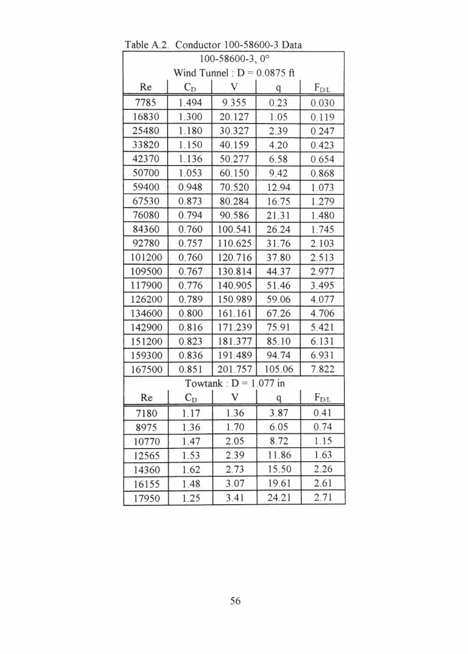
Table A.2
Re
7785
16830
25480
33820
42370
50700
59400
67530
76080
84360
92780
101200
109500
117900
126200
134600
142900
151200
159300
167500
Re
7180
8975
10770
12565
14360
16155
17950
Conductor 100-58600-3 Data
10(
Wind Tui
CD
1.494
1.300
1.180
1.150
1.136
1.053
0.948
0.873
0.794
0.760
0.757
0.760
0.767
0.776
0.789
0.800
0.816
0.823
0.836
0.851
Towta
CD
1.17 1.36
1.47
1.53
1.62
1.48
1.25
)-58600-3,
nnel: D =
V
9.355
20.127
30.327
40.159
50.277
60.150
70.520
80.284
90.586
100.541
110.625
120.716
130.814
140.905
150.989
161.161
171.239
181.377
191.489
201.757
n k : D = l
V
1.36
1.70
2.05
2.39
2.73
3.07
3.41
0°
0.0875 ft
q
0.23
1.05
2.39
4.20
6.58
9.42
12.94
16.75
21.31
26.24
31.76
37.80
44.37
51.46
59.06
67.26
75.91
85.10
94.74
105.06
.077 in
q
3.87
6.05
8.72
11.86
15.50
19.61
24.21
I
FD/L
0.030
0.119
0.247
0.423
0.654
0.868
1.073
1.279
1.480
1.745
2.103
2.513
2.977
3.495
4.077
4.706
5.421
6.131
6.931
7.822
FD/L
0.41
0.74
1.15
1.63
2.26
2.61
2.71
56

Table A.3. Conductor 100-58604-6 Data
Re
21460
32660
43170
54050
64370
75480
86020
97010
107600
118400
129000
139700
150300
160900
Re
9100
11375
13650
15925
18200
20475
22750
10(
Wind Tu]
CD
1.125
1.205
1.159
1.117
1.001
0.875
0.823
0.815
0.818
0.833
0.849
0.861
0.868
0.874
Towta
CD
1.07
1.29
1.33
1.36
1.36
1.28
1.08
)-58604-6,
nnel: D =
V
20.175
30.655
40.459
50.639
60.327
70.786
80.700
91.070
100.936
111.150
121.214
131.284
141.436
151.541
n k : D = l
V
1.36
1.70
2.05
2.39
2.73
3.07
3.41
0°
0.1125 ft
q
1.05
2.43
4.23
6.63
9.40
12.94
16.82
21.41
26.31
31.89
37.91
44.47
51.58
59.18
.365 in
q 3.87
6.05
8.72
11.86
15.50
19.61
24.21
FD/L
0.133
0.329
0.552
0.833
1.058
1.273
1.558
1.963
2.422
2.988
3.619
4.307
5.036
5.818
FD/L
0.47
0.89
1.32
1.84
2.39
2.85
2.98
57

Table A.4
Re
8339
16850
24890
33270
41550
49830
58130
66430
74750
83020
91190
99350
107600
115900
124100
132300
140500
148500
156400
164200
Re
7047
8808
10570
12332
14093
15855
17617
Conductor 100-58650-0 Data
100-58650-0,
Wind Tunnel : D =
CD 1 V 0.827
1.250
1.222
1.078
0.980
0.894
0.844
0.861
0.868
0.874
0.883
0.896
0.904
0.912
0.923
0.932
0.946
0.954
0.960
0.973
Towta
CD
1.61 1.53
1.60
1.69
1.67
1.52
1.26
10.200
20.530
30.211
40.343
50.373
60.443
70.541
80.720
90.968
101.059
111.027
121.084
131.195
141.395
151.493
161.645
171.893
182.011
192.239
202.582
n k : D = l
V
1.36
1.70
2.05
2.39
2.73
3.07
3.41
0°
0.0867 ft
q 0.27
1.09
2.36
4.21
6.56
9.44
12.85
16.82
21.34
26.33
31.78
37.78
44.33
51.48
59.07
67.22
75.98
85.10
94.78
105.02
.057 in
q
3.87
6.05
8.72
11.86
15.50
19.61
24.21
I
FD/L
0.019
0.118
0.250
0.394
0.557
0.732
0.940
1.256
1.607
1.994
2.434
2.936
3.476
4.069
4.728
5.432
6.232
7.035
7.891
8.855
FD/L
0.55
0.82
1.23
1.77
2.28
2.62
2.68
58
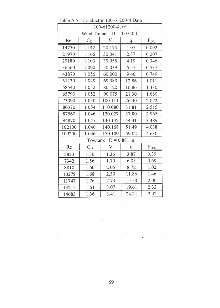
Table A. 5.
Re 1 14770
21970
29180
36560
43870
51130
58540
65790
73090
80370
87560
94870
102100
109200
Re
5873
7342
8810
10278
11747
13215
14683
Conductor 100-61200-4 Data
100-61200-4,
Wind Tunnel: D =
CD 1 V 1.142
1.166
1.103
1.090
1.056
1.049
1.052
1.052
1.050
1.054
1.046
1.047
1.046
1.046
Towta
CD
1.36
1.56
1.60
1.68
1.76
1.61
1.36
20.175
30.041
39.955
50.039
60.000
69.989
80.120
90.075
100.111
110.080
120.027
130.132
140.168
150.109
nk:D = 0
V
1.36
1.70
2.05
2.39
2.73
3.07
3.41
0°
0.0750 ft
q
1.07
2.37
4.19
6.57
9.46
12.86
16.86
21.30
26.30
31.81
37.80
44.41
51.49
59.02
.881 in
q
3.87
6.05
8.72
11.86
15.50
19.61
24.21
L
FD/L
0.092
0.207
0.346
0.537
0.749
1.011
1.330
1.680
2.072
2.515
2.965
3.489
4.038
4.630
FD/L
0.39
0.69
1.02
1.46
2.00
2.32
2.42
59

Table A.6
Re 1 9986
15020
19950
25030
29990
35180
40080
45080
50100
55060
60030
65000
69980
74840
Re
4080
5100
6120
7140
8160
9180
10200
Conductor 142-15026-2 Data
142-15026-2,
Wind Tunnel : D =
CD 1 V 1.191
1.284
1.222
1.213
1.203
1.159
1.141
1.123
1.121
1.107
1.097
1.091
1.082
1.081
Towta
CD
1.34
1.72
1.68
1.88
1.88
1.77
1.51
20.114
29.939
39.457
49.343
59.168
69.464
79.180
89.107
99.055
108.968
118.950
128.898
138.880
148.616
nk:D = 0
V
1.36
1.70
2.05
2.39
2.73
3.07
3.41
0°
0.0500 ft
q
1.07
2.39
4.16
6.52
9.37
12.91
16.77
21.23
26.24
31.73
37.78
44.35
51.47
58.91
.612 in
q 3.87
6.05
8.72
11.86
15.50
19.61
24.21
L
FD/L
0.064
0.153
0.254
0.395
0.564
0.748
0.957
1.192
1.470
1.756
2.072
2.418
2.783
3.184
FD/I.
0.26
0.53
0.75
1.14
1.49
1.77
1.86
60

Table A.7.
Re J 6409
9645
12910
16160
19370
22640
25900
29090
32370
35520
38700
41920
45110
48300
Re
2380
2975
3570
4165
4760
5355
5950
Concuctor 142-14100-0 Data
142-14100-0,
Wind Tunnel: D =
CD 1 V 1.260
1.184
1.169
1.166
1.180
1.158
1.148
1.165
1.144
1.155
1.148
1.153
1.153
1.144
Towta
CD
1.35
2.16
2.16
2.37
2.57
2.60
2.19
19.970
29.720
39.600
49.507
59.345
69.395
79.459
89.345
99.484
109.289
119.120
129.123
139.070
149.018
nk:D = 0
V
1.36
1.70
2.05
2.39
2.73
3.07
3.41
0°
0.0325 ft
q
1.05
2.34
4.17
6.53
9.38
12.82
16.80
21.23
26.31
31.73
37.68
44.26
51.32
58.90
.357 in
q 3.87
6.05
8.72
11.86
15.50
19.61
24.21
F D L
0.043
0.090
0.158
0.248
0.360
0.482
0.627
0.804
0.979
1.191
1.406
1.659
1.923
2.190
FD/L
0.16
0.39
0.56
0.84
1.18
1.52
1.57
61

Table A. 8.
Re 1 23480
35220
46890
58880
70740
82590
94470
106100
118100
129600
141400
153100
164600
176300
Re
9287
11608
13930
16252
18573
20895
23217
Conductor 100-57900-7 Data
100-57900-7,
Wind Tunnel: D =
CD 1 V 1 0.951
0.945
0.998
1.036
1.030
1.034
1.040
1.048
1.045
1.046
1.049
1.056
1.053
1.054
Towta
CD
1.10 1.13 1.19 1.26
1.28
1.26
1.07
20.045
29.755
39.484
49.445
59.339
69.280
79.282
89.086
99.218
108.989
118.930
128.836
138.668
148.650
n k : D = l
V
1.36
1.70
2.05
2.39
2.73
3.07
3.41
0°
0.1167ft
q 1.07
2.37
4.18
6.57
9.47
12.90
16.89
21.33
26.44
31.89
37.97
44.55
51.58
59.24
.393 in
q 3.87
6.05
8.72
11.86
15.50
19.61
24.21
I
FD/L
0.119
0.261
0.487
0.794
1.138
1.557
2.050
2.609
3.224
3.894
4.647
5.488
6.340
7.288
FD/L
0.49
0.80
1.21
1.73
2.30
2.87
3.00
62

Table A.9. Conductor 100-58200-8 Data
Re
9926
19940
29410
39130
48900
58550
68400
78280
87940
97590
107300
116800
126600
136400
146100
155500
165300
174500
184100
193100
Re
7980
9975
11970
13965
15960
17955
19950
101
Wind Tu
CD
1.000
0.903
0.914
0.864
0.934
0.966
0.977
0.992
1.006
1.004
1.005
1.016
1.018
1.018
1.021
1.025
1.030
1.030
1.035
1.040
Towta
CD
1.09
1.29
1.33
1.39
1.46
1.34
1.04
3-58200-8
nnel: D =
V
10.268
20.509
30.143
40.084
50.059
59.966
70.057
80.257
90.293
100.289
110.298
120.232
130.364
140.516
150.620
160.548
170.768
180.750
191.141
201.136
nk:D=l
V
1.36
1.70
2.05
2.39
2.73
3.07
3.41
,0°
0.1000 ft
q 1 FDL 0.27
1.10
2.38
4.21
6.57
9.43
12.87
16.88
21.35
26.32
31.83
37.80
44.43
51.60
59.26
67.27
76.09
85.13
95.08
105.10
.197 in
q
3.87
6.05
8.72
11.86
15.50
19.61
24.21
0.027
0.099
0.218
0.364
0.614
0.911
1.258
1.675
2.149
2.642
3.200
3.842
4.522
5.250
6.047
6.898
7.837
8.768
9.838
10.935
FDL
0.42
0.78
1.15
1.65
2.26
2.61
2.52
63

Table A. 10. Conductor 100-58104-4 Data 100-58104-4, 0°
Wind Tunnel : D = 0.0933 ft
Re 1 CD 1 V 1 q 17960
27150
36040
44640
53570
62790
71480
80410
89350
98260
107100
116000
124900
133600
Re
7460
9325
11190
13055
14920
16785
18650
1.212
1.039
0.998
1.021
1.014
1.025
1.036
1.041
1.037
1.037
1.036
1.036
1.033
1.030
Towta
CD
1.54
1.58
1.54
1.62
1.56
1.49
1.25
20.332
30.655
40.636
50.264
60.361
70.814
80.639
90.743
100.834
110.932
120.941
131.093
141.327
151.377
nk:D=l
V
1.36
1.70
2.05
2.39
2.73
3.07
3.41
1.07
2.43
4.27
6.54
9.43
12.97
16.82
21.30
26.30
31.82
37.81
44.41
51.57
59.14
.119m
q 3.87
6.05
8.72
11.86
15.50
19.61
24.21
FD/L
0.121
0.235
0.397
0.623
0.892
1.240
1.626
2.069
2.544
3.079
3.654
4.292
4.969
5.682
FD/L
0.55
0.89
1.25
1.79
2.25
2.72
2.83
Table A l l . Conductor 100-58300-4 Data
Re
9540
11925
14310
16695
19080
21465
23850
10(
Towta
CD
1.06
1.30
1.21
1.25
1.19
1.08
0.89
)-58300-4,
nk:D=l
V
1.36
1.70
2.05
2.39
2.73
3.07
3.41
0°
431 in
q 1 FD/L 3.87
6.05
8.72
11.86
15.50
19.61
24.21
0.49
0.94
1.26
1.77
2.20
2.53
2.57
64

Table A. 12. Conductor 100-61200-4 Yaw Data
0°
Ke [ CD,yaw
14770
21970
29180
36560
43870
51130
58540
65790
73090
80370
87560
94870
102100
109200
1.142
1.166
1.103
1.090
1.056
1.049
1.052
1.052
1.050
1.054
1.046
1.047
1.046
1.046
10°
Rp 1 C
7054
14440
21490
28560
35640
42880
50230
57100
64280
71420
78550
85580
92650
99900
106800
113900
121000
128000
135000
141800
1.052
1.124
1.070
1.050
1.057
1.060
1.041
1.053
1.054
1.053
1.065
1.061
1.055
1.058
1.056
1.057
1.061
1.063
1.064
1.061
100-61200-4
20°
Re 1 CDJ^HW
7214
13910
21080
27630
34290
41190
48270
55030
61810
68820
75740
82520
89410
96140
103000
109800
116600
123300
130000
136400
1.606
1.118
1.051
1.011
1.009
1.021
1.007
1.007
1.012
1.008
1.006
1.006
0.999
0.996
0.993
0.990
0.988
0.986
0.987
0.982
30
Re
7536
13640
20620
33960
47510
54390
61000
67890
74720
81450
88040
94810
101700
108300
115000
121400
127900
134300
^D.yau
0.649
0.957
0.844
0.837
0.834
0.845
0.842
0.836
0.837
0.839
0.824
0.818
0.815
0.816
0.823
0.814
0.802
0.799
40
Re
7995
13860
20910
27890
34680
41550
48570
55270
62130
69170
75930
82880
89750
96660
103300
110300
117100
123900
130400
137100
^D.vaw
1.263
0.803
0.709
0.629
0.644
0.644
0.647
0.630
0.649
0.634
0.646
0.628
0.621
0.623
0.618
0.617
0.604
0.608
0.616
0.606
65

Table A. 13. Conductor 100-58650-0 Yaw Data
0'
Re
8339
16850
24890
33270
41550
49830
58130
66430
74750
83020
91190
99350
107600
115900
124100
132300
140500
148500
156400
164200
3
^D,yaw
0.827
1.250
1.222
1.078
0.980
0.894
0.844
0.861
0.868
0.874
0.883
0.896
0.904
0.912
0.923
0.932
0.946
0.954
0.960
0.973
10
Re
9092
17090
25420
33910
42220
50930
59330
67680
76160
84490
92880
101200
109500
118000
126300
134700
142900
151100
159200
167100
^D.yaw
0.716
1.151
1.117
1.118
0.997
0.907
0.861
0.876
0.884
0.893
0.913
0.915
0.926
0.935
0.941
0.945
0.953
0.957
0.963
0.973
100-58
20
Re
16800
25510
34150
42590
51220
59920
68370
76970
85420
93820
102200
110800
119100
127700
136100
144500
152800
161100
168900
650-0
°
^D,yaw
0.721
0.946
0.951
0.872
0.835
0.793
0.806
0.819
0.830
0.834
0.848
0.851
0.857
0.861
0.868
0.869
0.868
0.879
0.888
30
Re
8717
16430
24380
32290
40170
48370
56800
64560
72610
80640
88810
96820
104700
112700
120600
128800
136700
144400
152200
159900
^D,yaw
0.804
0.978
0.921
0.841
0.769
0.726
0.704
0.704
0.702
0.710
0.719
0.727
0.720
0.724
0.729
0.738
0.740
0.745
0.742
0.750
4C
Re
7898
16320
24540
32830
40940
49500
57680
65860
74090
82090
90360
98450
106700
114800
123000
131100
139100
147000
155000
162900
^D.vau
1.102
0.679
0.699
0.633
0.580
0.518
0.502
0.508
0.513
0.502
0.524
0.517
0.516
0.518
0.522
0.521
0.521
0.530
0.536
0.537
66

Table A. 14. Conductor 100-58600-3 Yaw Data
0
Re
7785
16830
25480
33820
42370
50700
59400
67530
76080
84360
92780
101200
109500
117900
126200
134600
142900
151200
159300
167500
3
^D,yaw
1.494
1.300
1.180
1.150
1.136
1.053
0.948
0.873
0.794
0.760
0.757
0.760
0.767
0.776
0.789
0.800
0.816
0.823
0.836
0.851
10
Re
8371
16890
25450
33490
42020
50430
58970
67350
75780
84090
92540
100900
109200
117500
125800
134300
142600
150800
158900
167000
'-'Djyaw
0.597
1.067
1.144
1.147
1.134
1.058
0.980
0.944
0.900
0.872
0.858
0.847
0.846
0.851
0.856
0.862
0.872
0.878
0.886
0.894
100-58
20
Re
8628
15800
23850
31740
39820
47560
55760
63560
71560
79370
87360
95330
103200
111100
119100
126900
134700
142600
150400
157900
600-3
p ^^D,yaw 0.996
0.984
1.044
1.059
1.037
0.982
0.916
0.872
0.842
0.817
0.799
0.785
0.780
0.779
0.779
0.780
0.787
0.792
0.796
0.803
30
Re
8702
16290
24210
32530
40550
48380
56550
64850
72800
81010
88770
96820
104900
112900
119700
128700
136700
144400
152100
159700
° ^D,yaw
0.881
1.009
0.949
0.937
0.899
0.868
0.786
0.722
0.691
0.674
0.672
0.674
0.661
0.670
0.671
0.679
0.681
0.682
0.688
0.690
4C
Re
8475
16590
24410
32590
41000
49350
57520
65490
73670
81760
89990
97990
106200
114400
122400
130500
138600
146500
154300
162100
1°
^D,yaw
1.030
0.782
0.734
0.745
0.735
0.718
0.657
0.605
0.575
0.552
0.551
0.535
0.529
0.523
0.518
0.525
0.519
0.516
0.522
0.525
67
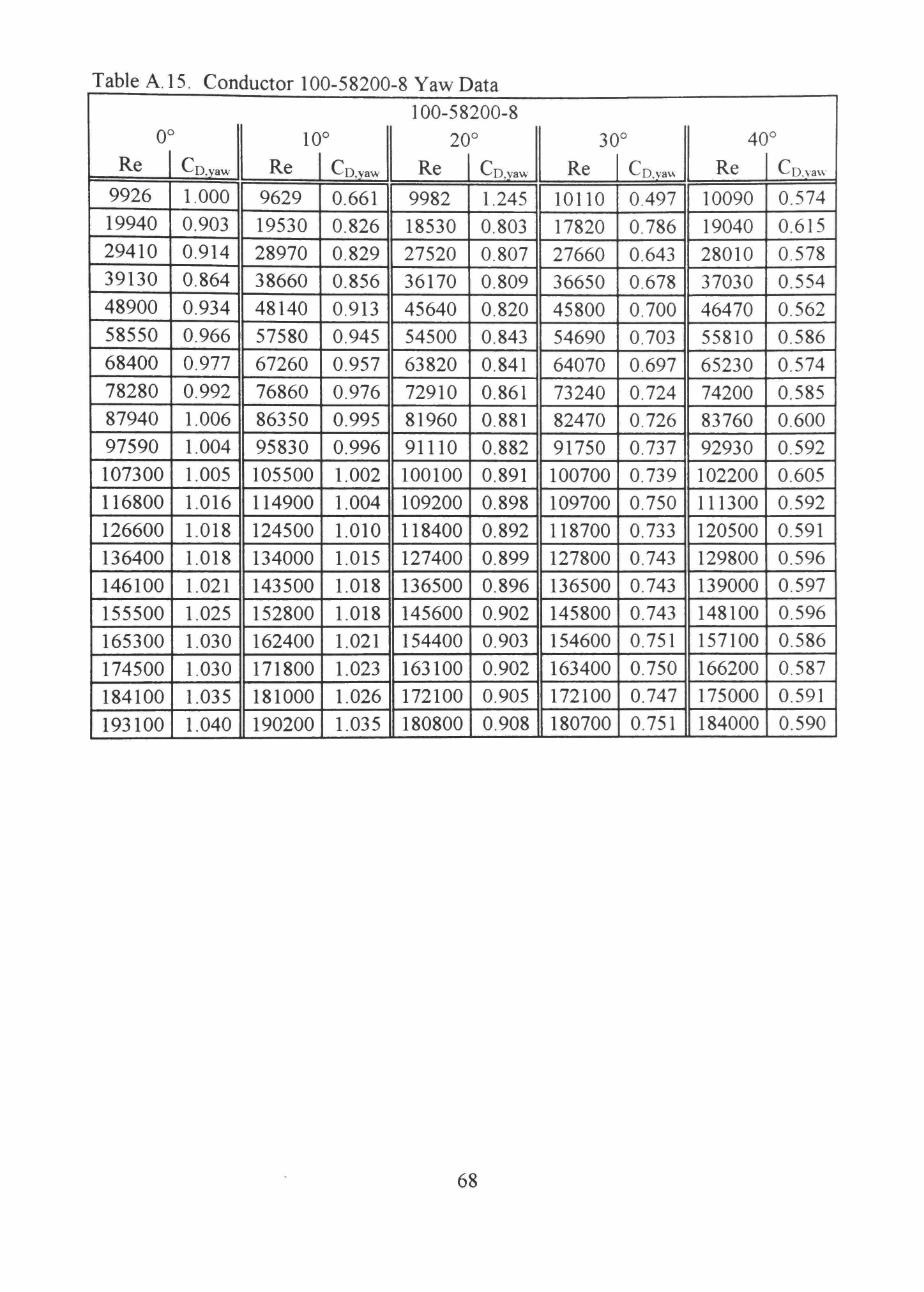
Table A. 15. Conductor 100-58200-8 Yaw Data
0
R e I 9926
19940
29410
39130
48900
58550
68400
78280
87940
97590
107300
116800
126600
136400
146100
155500
165300
174500
184100
193100
3
^^D.yaw
1.000
0.903
0.914
0.864
0.934
0.966
0.977
0.992
1.006
1.004
1.005
1.016
1.018
1.018
1.021
1.025
1.030
1.030
1.035
1.040
10
Re
9629
19530
28970
38660
48140
57580
67260
76860
86350
95830
105500
114900
124500
134000
143500
152800
162400
171800
181000
190200
'^D.yaw
0.661
0.826
0.829
0.856
0.913
0.945
0.957
0.976
0.995
0.996
1.002
1.004
1.010
1.015
1.018
1.018
1.021
1.023
1.026
1.035
100-58200-8
20°
Re 1 CD^THW
9982
18530
27520
36170
45640
54500
63820
72910
81960
91110
100100
109200
118400
127400
136500
145600
154400
163100
172100
180800
1.245
0.803
0.807
0.809
0.820
0.843
0.841
0.861
0.881
0.882
0.891
0.898
0.892
0.899
0.896
0.902
0.903
0.902
0.905
0.908
30
Re
10110
17820
27660
36650
45800
54690
64070
73240
82470
91750
100700
109700
118700
127800
136500
145800
154600
163400
172100
180700
^D.vavv
0.497
0.786
0.643
0.678
0.700
0.703
0.697
0.724
0.726
0.737
0.739
0.750
0.733
0.743
0.743
0.743
0.751
0.750
0.747
0.751
40
Re
10090
19040
28010
37030
46470
55810
65230
74200
83760
92930
102200
111300
120500
129800
139000
148100
157100
166200
175000
184000
1°
^D.vaw
0.574
0.615
0.578
0.554
0.562
0.586
0.574
0.585
0.600
0.592
0.605
0.592
0.591
0.596
0.597
0.596
0.586
0.587
0.591
0.590
68

APPENDIX B
CONDUCTOR INFORMATION
69
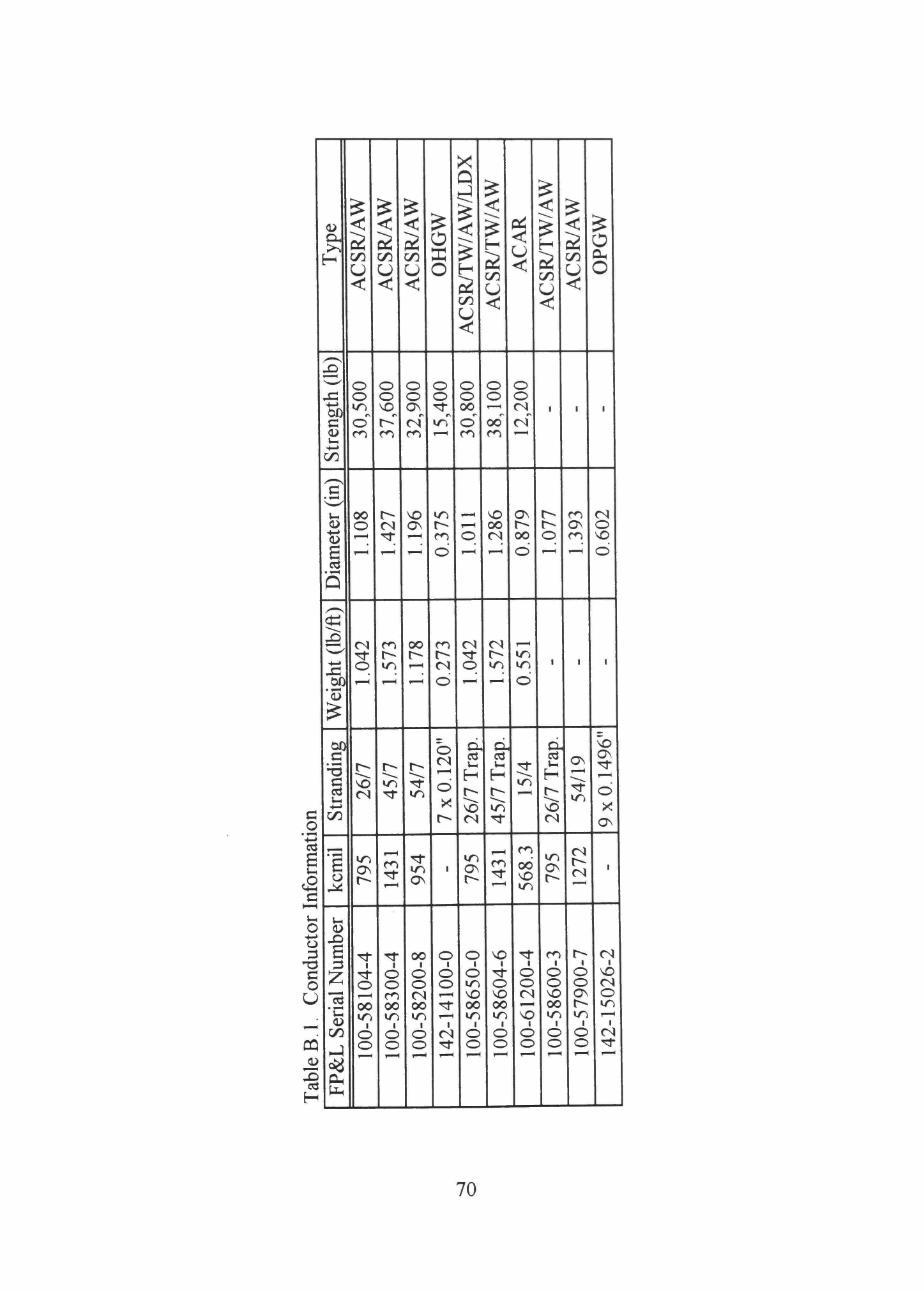
c o
nfor
mat
] T
able
B.l
. C
ondu
ctor
1
ex
Stre
ngth
(lb
) D
iam
eter
(in
) St
rand
ing
Wei
ght
(lb/
ft)
kcm
il FP
&L
Ser
ial N
umbe
r 1
AC
SR/A
W
30,5
00
1.10
8 1.
042
26/7
79
5 10
0-58
104-
4 A
CSR
/AW
37
,600
1.
427
1.57
3 45
/7
1431
10
0-58
300-
4 A
CSR
/AW
32
,900
VO ON r-H
1.17
8 54
/7
954
100-
5820
0-8
OH
GW
15
,400
0.
375
0.27
3 7x
0.12
0"
1
142-
1410
0-0
AC
SR/T
W/A
W/L
DX
30
,800
1 — <
o
1.04
2 26
/7 T
rap.
79
5 10
0-58
650-
0 A
CSR
/TW
/AW
38
,100
1.
286
1.57
2 45
/7 T
rap.
14
31
100-
5860
4-6
AC
AR
12
,200
0.
879
0.55
1 15
/4
568.
3 10
0-61
200-
4 A
CSR
/TW
/AW
1
1.07
7
1
26/7
Tra
p.
795
100-
5860
0-3
AC
SR/A
W
1
1.39
3
1
54/1
9 12
72
100-
5790
0-7
OPG
W
'
0.60
2
•
9x0.
1496
"
1
142-
1502
6-2
70

PERMISSION TO COPY
In presenting this thesis in partial fulfillment of the requirements for a
master's degree at Texas Tech University or Texas Tech University Health Sciences
Center, I agree that the Library and my major department shall make it freely
available for research purposes. Permission to copy this thesis for scholarly
purposes may be granted by the Director of the Library or my major professor.
It is understood that any copying or publication of this thesis for financial gain
shall not be allowed without my further written permission and that any user
may be liable for copyright infringement.
Agree (Permission is granted.)
.^
(. student's Signature / / j Date
Disagree (Permission is not granted.)
Student's Signature Date
71