processes

Article

Design of Aerodynamic Ball Levitation Laboratory Plant

Tomáš Tkácik 1, Milan Tkácik 1,*, Slávka Jadlovská 2 and Anna Jadlovská 1

Citation: Tkácik, T.; Tkácik, M.;

Jadlovská, S.; Jadlovská, A. Design of

Aerodynamic Ball Levitation

Laboratory Plant. Processes 2021, 9,

1950. https://doi.org/10.3390/

pr9111950

Academic Editor:

Krzysztof Rogowski

Received: 16 September 2021

Accepted: 25 October 2021

Published: 30 October 2021

Publisher’s Note: MDPI stays neutral

with regard to jurisdictional claims in

published maps and institutional affil-

iations.

Copyright: © 2021 by the authors.

Licensee MDPI, Basel, Switzerland.

This article is an open access article

distributed under the terms and

conditions of the Creative Commons

Attribution (CC BY) license (https://

creativecommons.org/licenses/by/

4.0/).

1 Department of Cybernetics and Artificial Intelligence, Faculty of Electrical Engineering and Informatics,Technical University of Košice, Letná 9, 042 00 Košice, Slovakia; tomas.tkacik@tuke.sk (T.T.);anna.jadlovska@tuke.sk (A.J.)

2 Department of Industrial Engineering and Informatics, Faculty of Manufacturing Technologies with a Seat inPrešov, Technical University of Košice, Bayerova 1, 080 01 Prešov, Slovakia; slavka.jadlovska@tuke.sk

* Correspondence: milan.tkacik@tuke.sk; Tel.: +421-55-602-4214

Abstract: This paper presents the development of a new Aerodynamic Ball Levitation LaboratoryPlant at the Center of Modern Control Techniques and Industrial Informatics (CMCT&II). The entiredesign process of the plant is described, including the component selection process, the physicalconstruction of the plant, the design of a printed circuit board (PCB) powered by a microcontroller,and the implementation of its firmware. A parametric mathematical model of the laboratory plantis created, whose parameters are then estimated using a nonlinear least-squares method based onacquired experimental data. The Kalman filter and the optimal state-space feedback control aredesigned based on the obtained mathematical model. The designed controller is then validated usingthe physical plant.

Keywords: aerodynamic levitation; experimental identification; system state estimation; linearoptimal control; noise filtration; motor control

1. Introduction

The core principle of aerodynamic levitation is based on suspending an arbitraryobject in the air using airflow. The practical use-case of this phenomenon can be seen inapplications where physical contact between objects must be avoided. It is usually utilizedon a microscopic scale to prevent oxidation or crystal formation upon object contact withits container. This method allows studying materials under unusual conditions and evenallows the formation of new glass materials [1].

The goal of our design of an Aerodynamic Ball Levitation Plant is to levitate a ping-pong ball inside a tube using the stream of air produced by a fan. From a control engi-neering aspect, this model is interesting for its simplicity of modeling and its low price.Similar to the Magnetic Levitation Plant, which uses a magnetic force to levitate a steelball [2], the Aerodynamic Levitation Plant could also be a part of control engineeringcourses provided by the Center of Modern Control Techniques and Industrial Informatics(CMCT&II) at the Department of Cybernetics and Artificial Intelligence (DCAI), Faculty ofElectrical Engineering and Informatics (FEEI), Technical University of Košice (TUKE). Asthe commercial availability of such plant types is limited, we opted to construct one. Themain advantage of the Aerodynamic Levitation Plant over the Magnetic Levitation Plantis its slower dynamics. It allows the use of a larger sampling period and consequentlymore computationally expensive control algorithms. This model also provides a wider ballposition operation range that makes experimental identification simpler.

Several world scientists have already worked on a similar Aerodynamic Ball LevitationPlant. The authors of [3] focused mainly on the physical construction of the plant, the choiceof the most suitable sensor for measuring the ball’s position, and its analytical modeling.Apart from the physical construction, the authors of [4] focused more on controller designbased on the experimentally identified Autoregressive model with Exogenous Variable(ARX model) in the input–output form. In this case, an Arduino Mega equipped with

Processes 2021, 9, 1950. https://doi.org/10.3390/pr9111950 https://www.mdpi.com/journal/processes

Processes 2021, 9, 1950 2 of 19

an ATmega2560 microcontroller was used as an analog-to-digital interface of the controlcomputer. Others contributed mainly to the application of a nonlinear modification ofthe Proportional-Integral-Derivative (PID) controller in the context of the AerodynamicLevitation Plant [5]. Papers [6–8] were more focused on making this type of plant availablein virtual and remote laboratories and used classical controllers like the PID controller. Theauthors of [9] had taken a more experimental approach in the controller design and utilizeda simple switched controller inspired by the sliding window controller. Although the noisefiltration and proper state estimation are purposefully left out in this design method, thedesigned control algorithm performed well in the simulation and on the real plant. Up tothis point, all authors used airflow to levitate a ball inside a tube. A different approach wasused in [10–12], where the ball was not placed inside a tube. This arrangement is morechallenging in terms of both measuring the ball’s position and the power requirements.On the other hand, the plant is inherently stable from a control engineering aspect, as theairflow speed gradually decreases over distance. The authors of [13] presented a model-freebased control algorithm design for a similar plant (the Magnetic Levitation Plant). Thismethod uses an experimental approach to fine-tune controller parameters for a targetapplication. Another option is to use a nonlinear state-space controller as in [14]. Thiscontroller provides the robustness needed for systems with varying parameters. From ourown experience [2] with a similar magnetic levitation plant, we decided to start with alinear state-space controller instead of a PID controller. Although linear controllers arenot as robust as their nonlinear counterparts, they are easier to design. The authors of [15]used the exact linearization approach to design a controller for the Magnetic LevitationPlant. This method combines linear controller synthesis with nonlinear compensation. Anotable drawback of this method is finding a suitable mathematical transformation thattransforms the nonlinear system model into a linear one.

While facing the task of experimental identification, most authors have chosen linearapproximations of a mathematical model, such as the ARX model [4,5,7,16]. From thecontrol design aspect, this is not an issue, since they proved the ARX model to be sufficientfor this application. The main limitation seen in this approach is that the nonlinear mathe-matical model obtained from analytical identification is more suitable for the controllerverification in a simulation environment. This is the reason why the authors of [17] optedfor nonlinear parameter estimation. Their focus was to create an open-source design thatcan be adopted by others. Although filtration is mentioned in figures, no more informationabout the used filtration method is provided. Considering that noise is the natural phe-nomenon of all physical systems, room for improvement is present. Only [16] utilized alow-pass filter to reduce sensory noise. There are a few papers [5,7,16] that included dy-namics of a fan in the mathematical model, but they did not utilize state-space control. Thegoal of this paper is to solve presented open problems, mainly the parameter identificationof the mathematical model, noise filtration, and utilization of the state-space control.

In this paper, we present the improved Aerodynamic Ball Levitation Plant with a fanspeed sensor. We consider the addition of this sensor important for better plant control as itenables the use of more sophisticated control and state estimation algorithms. Furthermore,the additional sensor helps with the experimental estimation of the mathematical model’sparameters. The proposed methodology of the Aerodynamic Ball Levitation Plant modelingand control design is incorporated in the entire paper layout. This includes subtasks in thefollowing order: mathematical modeling, creation of physical plant, experiment design,data acquisition, nonlinear parameter estimation, design of Kalman filter, controller design,validation in the simulation environment, and validation on the real plant. Methodologyverification is presented in this paper using sets of experiment and their results.

The paper consists of several sections. Section 2 deals with the construction of theAerodynamic Ball Levitation Plant, whereas Section 3 describes the analytical modelingand parameter identification of the mathematical model using the nonlinear least-squaresmethod. Section 4 deals with the design and validation of the Kalman filter and the optimalstate-space controller with integrator (Linear-Quadratic-Integral control—LQI). Finally,

Processes 2021, 9, 1950 3 of 19

Section 5 describes the inclusion of the laboratory plant into the Distributed Control System(DCS) architecture at the CMCT&II.

2. Hardware Design

The main reason for the construction of a custom plant over buying one was to reducecosts and to adjust all its aspects to our needs. Components like enclosure and connectionfittings were designed in Fusion 360 (a 3D modeling software) and later 3D printed using aPLA filament. Our goal was to create a portable laboratory plant that can be easily moved.

Besides the already mentioned basic principles of the plant, there are a few designconsiderations that one needs to take into account. A sensor must be placed inside the tubeto determine the ball’s position. There is also a need to dynamically adjust the fan speed toachieve the desired effect of levitation. The rest of this section is designated to present theplant’s physical, electrical, and firmware design.

2.1. Physical Construction of the Plant

Firstly, the type of ball for levitation had to be selected. From all available options, aping-pong ball was chosen due to the strict standardization of its parameters. Regardingthe tube selection, two constraints were considered—transparency of its walls and innerdiameter to be slightly larger than the ball’s diameter. A slightly larger inner diameter of thetube will allow the ball to move freely in the vertical direction while avoiding unnecessaryhorizontal movement. In our case, the inner diameter is about 4 mm wider than the ball. Ina fan selection process, a computer fan was considered at the first, since it can be controlledusing a pulse-width modulated (PWM) signal and often includes a tachometer to measureits speed. However, modern computer fans are optimized for silent operation using higherstatic pressure and lower air velocity. As low air velocity is undesirable for our application,we opted for a fan extracted from a hairdryer. It is powered by a 24 V DC motor and itsdiameter is close enough to the diameter of the tube. Additionally, it provides sufficientoutput air velocity to push the ball up in the tube. Because of the missing tachometer onthe fan, we attached a Pololu 20D magnetic encoder to its back shaft. This modificationenables the possibility to directly measure the fan’s angular velocity. To power the fan, wedecided to use a 19 V DC laptop charger to keep the plant portable. Finally, we added aVL53L0X laser rangefinder to measure the ball’s position within the tube. This choice wasmotivated by the sensor’s accuracy and simple interface, similar to the solution describedin [3].

A simple user interface is added to the plant so that it can be used without an addi-tional computer. This includes a 4-digit 7-segment display and a rotary encoder with apush-button that allows the user to change parameters on the fly. Additionally, a scale wasengraved onto the tube with an LED backlight to easily determine the ball’s position. Thefinal 3D assembly of the plant is shown in Figure 1.

2.2. Design of Electronic Components

To make the plant operational on its own, a microcontroller was needed. For thistask, the Arduino Nano development board with an ATmega328P microcontroller waschosen. Since no microcontroller can handle currents large enough to power a DC motor,additional components were necessary. As connecting all components using jumper wiresis impractical, we decided to create a plant control unit—a printed circuit board (PCB)designed in the Autodesk EAGLE software. This PCB interconnects a 5 V regulator(LM7805), an NPN BJT transistor (BC547) used as a MOSFET driver, an n-channel MOSFET(IRF530) to drive the fan, and a number of JST XH connectors. Connectors are used toconnect other components (motor, motor speed sensor, 7-segment display, rotary encoder,and ball position sensor) that cannot be placed onto the main PCB. To futureproof our PCBdesign, we added several connectors of various interfaces in case more sensors or actuatorsare added in the future. The Arduino Nano development board is directly soldered ontothe control unit. The PCB design is shown in Figure 2.

Processes 2021, 9, 1950 4 of 19

Figure 1. Component assembly of the Aerodynamic Ball Levitation Laboratory Plant.

Figure 2. PCB design of plant’s control unit.

2.3. Firmware Design

Our firmware design comprises four modules, as shown in Figure 3. All informationexchanged between these modules is preprocessed and uses standard units where applica-ble. The firmware itself is implemented in the C++ language and is compiled using theArduino IDE.

The communication module is used as a communication interface between a computerand the plant using a Universal Asynchronous Receiver–Transmitter (UART) serial link.For this task, a simple packet-based communication protocol was created that uses the mostsignificant bit of each byte to control communication. In addition, a 28-bit fixed-precision

Processes 2021, 9, 1950 5 of 19

data type was proposed to allow the exchange of real numbers using this protocol. Thecommunication interface running on the computer that handles this protocol is written inthe Python programming language. It is easier to work with binary data in Python than inMatlab while keeping the interface platform-independent.

The driver module is used as an interface between the plant and peripherals such as sen-sors and actuators that require the use of timers or interrupts. Its interface is programmedto work with physical units to prevent information misinterpretation. It allows for easierhardware changes as the hardware-specific code is isolated.

The UI module handles user input from the rotary encoder and the push-button toallow parameter changes without the need for a computer. It enables a user to enter/exitparameter editor by long button push and to change currently selected parameter usinga short push. Rotation action is handled by selected parameter type: for example, aBoolParameter switches its state, whereas a FloatParameter increments or decrements itsvalue according to rotational speed.

The control module estimates and filters values of the state vector using the Kalman filter.It also implements polynomial and LQI controllers, whose parameters can be changedusing the mentioned communication protocol. Both implemented control algorithmsinherited from the AbstractController interface making it easier to implement differentcontrol algorithms in the future.

Figure 3. Firmware design diagram.

3. Mathematical Modeling

In research papers [4,9,16], a mathematical model of the Aerodynamic Ball LevitationPlant is presented as a single-input and single-output (SISO) system, with input beingthe fan’s voltage u(t) and output the ball position x(t). Even though this representationdoes not affect the mathematical model itself, it is problematic during the experimentalparameter estimation task. This is due to a high number of parameters and insufficientinsight into internal system states. To overcome this limitation, our plant includes a fanspeed sensor that enables us to model the system as a single-input and multiple-output(SIMO) system. To make the modeling task simpler, we are going to model two mainsubsystems (a fan and a ball in the tube) separately according to the diagram shown inFigure 4.

Processes 2021, 9, 1950 6 of 19

Figure 4. Diagram of subsystem interaction of Aerodynamic Ball Levitation Plant.

Since our fan is driven by a DC motor, we can create its mathematical model usingthe kinematic equation for the rotational motion and Kirchhoff’s second law. Ignoring allnonlinearities, the resulting mathematical model is described by two first-order differentialequations (Equation (1)). State variables of this model are an armature current i(t) and anangular velocity ω(t) [18].

Jω(t) + blω(t) = KMi(t)

Ldi(t)

dt+ Ri(t) + Keω(t) = u(t)

(1)

where: J - rotor’s moment of inertia [kg.m2]ω(t) - rotor’s angular acceleration [rad.s−2]bl - rotor’s friction constant [N.m.s]ω(t) - rotor’s angular velocity [rad.s−1]KM - motor’s torque constant [N.m.A−1]i(t) - armature current [A]L - armature inductance [H]R - armature resistance [Ω]Ke - motor’s back electromotive force constant [V.rad−1.s−1]u(t) - motor’s input voltage [V]

To be able to use the proposed mathematical model (1) of the fan for the parameteridentification task, it is crucial to measure both of its state variables (i(t) and ω(t)). Havingsensors to measure both state variables (armature current i(t) and rotor’s angular velocityω(t)), it would be possible to use state-space control algorithms to control this subsystem.However, our hardware design does not include a current sensing circuit, so a slight modelmodification is needed. An approximation of the fan model in form of a linear first-orderdifferential equation (Equation (2)) was chosen for this task. Such a model has only onestate variable (ω(t)) that can be measured with a rotary encoder included in our hardwaredesign. Limitations of this approximation include slightly different system dynamics, themerger of system parameters, and the use of input–output based control algorithms. Theparameter merging poses a problem if the physical interpretation of parameter value isrequired. This is not a problem as long as we intend to create a stabilizing controller.

ω(t) + bmω(t) = Kmu(t) (2)

where: bm - fan’s damping factor [s−1]Km - motor constant [rad.s−2.V−1]

The ball in the tube subsystem shown in Figure 5 can be modeled using Newton’ssecond law if all forces acting on the ball are identified. To make it simpler, we consideronly two major forces—a force of aerodynamic drag Fo(t) and a gravitational force Fg thatcan be calculated using Formula (3).

Processes 2021, 9, 1950 7 of 19

Fg = mgg (3)

where: Fg - gravitational force [N]mg - ball’s weight [kg]g - gravitational acceleration [m.s−2]

The aerodynamic drag force depends on a ball’s drag coefficient Cg, ball’s cross sectionarea Sg, density of the air ρv, and square of ball’s relative velocity as in (4). The relativevelocity is defined as a difference between air velocity vv(t) and ball’s velocity x(t).

Fo(t) =12

CgSgρv(vv(t)− x(t))2 (4)

where: Fo(t) - aerodynamic drag force [N]Cg - ball’s drag coefficient [−]Sg - ball’s cross section area [m2]ρv - air density [kg.m−3]vv(t) - air velocity [m.s−1]x(t) - ball’s velocity [m.s−1]

Figure 5. Simplified diagram of Aerodynamic ball levitation plant.

Since air velocity vv(t) in the tube is relatively low, all mentioned factors except therelative velocity can be combined into a single constant bv as in (5).

bv =12

CgSgρv (5)

where: bv - ball’s drag factor [kg.m−1]

According to the diagram in Figure 5, both acting forces have opposing direction ofthe effect (6).

F(t) = Fo(t)− Fg (6)

where: F(t) - force acting on the ball [N]

During normal operation, the aerodynamic drag force Fo(t) is always acting in op-posite direction to the gravitational force Fg. To make its direction of influence physicallycorrect under all conditions, we added the sign function to the model Equation (7).

mg x(t) = bv(vv(t)− x(t))2sgn(vv(t)− x(t))−mgg (7)

Processes 2021, 9, 1950 8 of 19

where: x(t) - ball’s linear acceleration [m.s−2]sgn(...) - sign function

Finally, it is needed to find a link between the fan’s angular velocity ω(t) and airvelocity vv(t). According to our experiments shown in Figure 6, the air velocity vv(t) haslinear dependency on the fan’s angular velocity ω(t) as in (8). A constant term is added tocompensate for nonlinear behavior around zero.

Figure 6. Air velocity vv(t) as a function of fan’s angular velocity ω(t).

vv(t) = Kvω(t) + Cv (8)

where: Kv - fan’s coefficient [m.rad−1]Cv - fan’s constant [m.s−1]

The complete mathematical model of the Aerodynamic Ball Levitation Plant is shownin (9). Since this model contains several unknown parameters (bm, Km, bv, Kv, Cv) thatcannot be measured directly, we are going to estimate their values by means of experimen-tal identification.

ω(t) + bmω(t) = Kmu(t)

x(t) =bv

mg(Kvω(t) + Cv − x(t))2sgn(Kvω(t) + Cv − x(t))− g

(9)

3.1. Experimental Identification and Model Validation

Experimental identification techniques can be divided by the type of resulting modelinto two major groups—grey-box and black-box model identification [19]. As quite a fewauthors [4,5,7,16] have already put their effort into black-box model estimation [20], wedecided to focus on the first option and identify parameters of the plant model (9) to createa grey-box model. The general schema of the identification topology is shown in Figure 7,where in our case the approximation model is replaced with the analytical model (9). Thenan optimization algorithm is used to tune the model’s parameters to minimize the quadraticcost function (10). This topology can be used for both online and offline identification tasks.Due to the fast dynamics of our plant, we opted for the offline variant.

J(φ) =1N

N

∑k=1

(eT(k, φ)W(φ)e(k, φ)

)(10)

where: J(φ) - quadratic cost functionφ - vector of model’s parameterse(k, φ) = y(k)− y(k, φ) - output prediction error vectorW(φ) - weighting matrix

Processes 2021, 9, 1950 9 of 19

Figure 7. General schema for experimental parameter identification driven by output prediction error.

Like the modeling, the parameter identification task can be also split into two partsaccording to the model subsystems. From the control engineering aspect, the fan subsystemis stable, and thus the identification can be performed in the open-loop using a pseudo-random rectangular input signal with varying amplitude. Because the ball’s presenceaffects airflow inside the tube, it was fixed inside the tube during the experiment. Obtainedexperimental data were used to estimate parameter values (bm, Km) of the fan’s modelusing tfest function in MATLAB. The normalized root mean squared error of this modelis 12.55% (the lower the better) and the adjusted R-squared value of this fit is 98.42%.Graphical model validation is shown in Figure 8.

(a) (b)Figure 8. Fan’s mathematical model validation. (a) Real plant compared to modeled fan angularvelocity ω(t); (b) fan’s input voltage u(t).

Parameter identification of the ball in the tube subsystem is a bit more challengingbecause this subsystem is inherently unstable [5]. To overcome this issue, a closed-loopfeedback controller must be used to avoid the ball’s position saturation at its physicallimits. Instead of designing a full-fledged controller, we decided to go with a simple rule-based algorithm. This algorithm oscillates the ball around the center point by switchinginput value between ±10% of equilibrium value. The time at which the input value isswitched is always random to prevent harmonic oscillations. The parameters (bv, Kv, Cv) ofmathematical model (9) are estimated by nonlinear least-squares method using a nlgreyestfunction in MATLAB.

Results in Figure 9 do not look promising at the first glance since the ball’s positionof the identified model does not follow the position of the real ball precisely. This can becaused by a slight deviation in the value of some parameters and since the system behavesas an integrator, this error accumulates quickly over time. From the control engineeringaspect, this should not be an issue in controller design as controllers must be robust enoughto cope with system uncertainty. Values of estimated parameters are shown in Table 1.

Processes 2021, 9, 1950 10 of 19

(a) (b)Figure 9. Validation of the ball in tube subsystem. (a) Real plant compared to modeled ball positionx(t); (b) fan’s input voltage u(t).

Table 1. Estimated model parameters.

Label Name Value Unit

bm fan’s damping factor 2.491 s−1

Km motor constant 203.270 rad.s−2.V−1

bv ball’s drag factor 9.202 × 10−3 kg.m−1

mg ball’s weight 2.700 × 10−3 kgKv fan’s coefficient 1.979 × 10−3 m.rad−1

Cv fan’s constant 0.369 m.s−1

3.2. Linearization and Discretization

The mathematical model (9) is not suitable for designing a discrete LQI controller,because this method is based on a linear discrete model in state-space form. To get thecorrect form, the model (9) must be linearized first and then discretized. To make thenotation of state vector cleaner, a substitution (11) is proposed.

x(t) =[ω(t) x(t) x(t)

]T=[x1(t) x2(t) x3(t)

]T (11)

where: x(t) - system’s state vectorx1(t) = ω(t) - fan’s angular velocity [rad.s−1]x2(t) = x(t) - ball’s position [m]x3(t) = x(t) - ball’s speed [m.s−1]

The mathematical model (9) can be rewritten accordingly (12).

x1(t) = −bmx1(t) + Kmu(t)

x2(t) = x3(t)

x3(t) =bv

mg(Kvx1(t) + Cv − x3(t))2sgn(Kvx1(t) + Cv − x3(t))− g

(12)

In our case, the nonlinear model (9) is linearized at a operating point selected in thecenter of the tube, while other values are calculated by substituting all derivatives (9) withzero. Finally, the operating point can be defined by (13).

OP =[x10 x20 x30 u0

]=[670.819 0.25 0 8.222

](13)

Processes 2021, 9, 1950 11 of 19

where: OP - linearization operating point vectorx10 - operating point fan’s angular velocity [rad.s−1]x20 - operating point ball’s position [m]x30 - operating point ball’s linear velocity [m.s−1]u0 - operating point fan’s input voltage [V]

Linearization at the operating point OP can be performed by expanding nonlinearmodel (12) into first order approximation using Taylor series as shown in (14), where y(t)denotes output vector of a linear model [21].

∆x(t) =

−2.491 0 00 0 1

0.023 0 −11.565

∆x(t) +

203.27000

∆u(t)

∆y(t) =[

1 0 00 1 0

]∆x(t)

(14)

where: ∆x(t) = x(t)− x0∆u(t) = u(t)− u0

Based on the sampling period Tsp of the ball’s position sensor (Tsp = 0.04 s), the linearmodel (14) is discretized using the same sampling period value. The linear discrete modelin state-space form is shown in (15). This model is used to design an LQI controller.

∆x(k + 1) = Ad∆x(k) + Bd∆u(k)∆y(k) = Cd∆x(k)

(15)

where: Ad - discrete linear state matrixBd - discrete linear input matrixCd - discrete linear output matrix

4. Controller Design and Verification

Thanks to the integrated fan speed sensor of our plant, a wide range of controlalgorithms can be utilized. Since plenty of previously mentioned authors have alreadyworked on control algorithms based on the input-output model, the state-space controlbased on LQI has been selected.

Even with the addition of the fan speed sensor, it is not possible to measure the ball’sspeed x3(k). To overcome this limitation, some kind of estimation is needed. The simplestsolution is to estimate the ball’s speed x3(k) using the difference of its position x2(k). Sincedata from the position sensor is quite noisy, the Kalman filter is used as both an estimatorand a noise filter.

4.1. Noise Filtration

The Kalman filter uses a discrete linear model (15) of the system with the additionof a system noise (w(k)) and a sensory noise (z(k)) (16). System noise (w(k)) is used asthe result of ignored or approximated parts of the physical system’s dynamics, whereassensory noise (z(k)) is caused by the sensor itself or by the ADC conversion. It is expectedthat both system and sensory noise have a zero mean value and noise covariance matrices(QE, RE) are known. The extended Kalman filter is a modification that allows noise filteringof non-linear systems, as system matrices (Ad(k), Bd(k), Cd(k)) are being updated in everystep [22]. From the perspective of the model (12), it is sufficient to use the Kalman filter(not its non-linear variant) as the change in the ball’s position does not affect the linearizedmodel, and the ball’s velocity is expected to have near-zero value.

x(k + 1) = Adx(k) + Bdu(k) + w(k)y(k) = Cdx(k) + z(k)

(16)

Processes 2021, 9, 1950 12 of 19

where: Ad - discrete state matrixBd - discrete input matrixCd - discrete output matrix

Each iteration of the Kalman filter algorithm is divided into two phases—predictionand correction [22]. During the prediction phase, a new system state is predicted using thesystem’s model, the previous state, and the value of the input (17). The second phase usesmeasurements to correct the predicted states to get an estimate of the real system state (18).

x−(k) = Ad x+(k− 1) + Bdu(k− 1)

P−(k) = AdP+(k− 1)ATd + QE

(17)

where: x−(k) - predicted value of the state vectorx+(k) - corrected value of the state vectorP−(k) - predicted value of error covariance matrixP+(k) - corrected value of error covariance matrixQE - covariance matrix of the system noise

KE(k) = P−(k)CTd

(RE + CdP−(k)CT

d

)−1

x+(k) = x−(k) + KE(k)(y(k)− Cd x−(k)

)P+(k) = (I − KE(k)Cd)P

−(k)

(18)

where: KE(k) - Kalman gain matixRE - covariance matrix of the measurement (sensory) noisey(k) - measured system outputI - identity matrix

The discrete linear model (15) was used to design a Kalman filter. Noise covariancematrices (QE, RE) were fine-tuned using an experimental approach, so that measured noiseis reduced while not affecting the dynamics of the physical plant. Exact values used areshown in (19).

QE =

1 0 00 10 00 0 10

; RE =

[90 00 30

](19)

In Figure 10, one can see the application of the Kalman filter in the task of noisefiltration of the ball’s position x(k) measurement. The visible noise reduction will have apositive effect on the control of the plant.

Figure 10. An application of Kalman filter in task of ball’s position x(k) estimation.

Processes 2021, 9, 1950 13 of 19

4.2. LQI Controller

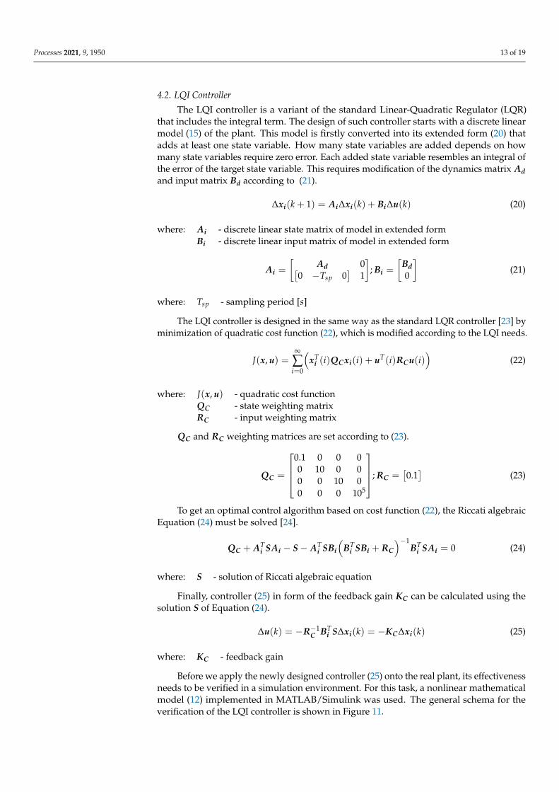
The LQI controller is a variant of the standard Linear-Quadratic Regulator (LQR)that includes the integral term. The design of such controller starts with a discrete linearmodel (15) of the plant. This model is firstly converted into its extended form (20) thatadds at least one state variable. How many state variables are added depends on howmany state variables require zero error. Each added state variable resembles an integral ofthe error of the target state variable. This requires modification of the dynamics matrix Adand input matrix Bd according to (21).

∆xi(k + 1) = Ai∆xi(k) + Bi∆u(k) (20)

where: Ai - discrete linear state matrix of model in extended formBi - discrete linear input matrix of model in extended form

Ai =

[Ad 0[

0 −Tsp 0]

1

]; Bi =

[Bd0

](21)

where: Tsp - sampling period [s]

The LQI controller is designed in the same way as the standard LQR controller [23] byminimization of quadratic cost function (22), which is modified according to the LQI needs.

J(x, u) =∞

∑i=0

(xT

i (i)QCxi(i) + uT(i)RCu(i))

(22)

where: J(x, u) - quadratic cost functionQC - state weighting matrixRC - input weighting matrix

QC and RC weighting matrices are set according to (23).

QC =

0.1 0 0 00 10 0 00 0 10 00 0 0 105

; RC =[0.1]

(23)

To get an optimal control algorithm based on cost function (22), the Riccati algebraicEquation (24) must be solved [24].

QC + ATi SAi − S− AT

i SBi

(BT

i SBi + RC

)−1BT

i SAi = 0 (24)

where: S - solution of Riccati algebraic equation

Finally, controller (25) in form of the feedback gain KC can be calculated using thesolution S of Equation (24).

∆u(k) = −R−1C BT

i S∆xi(k) = −KC∆xi(k) (25)

where: KC - feedback gain

Before we apply the newly designed controller (25) onto the real plant, its effectivenessneeds to be verified in a simulation environment. For this task, a nonlinear mathematicalmodel (12) implemented in MATLAB/Simulink was used. The general schema for theverification of the LQI controller is shown in Figure 11.

Processes 2021, 9, 1950 14 of 19

Plantxref(k)

x(k)

xi(k)−KC

Figure 11. General schema of LQI controller.

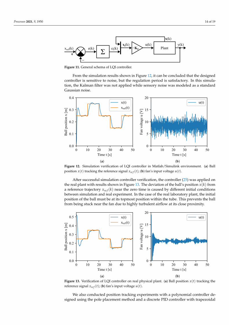
From the simulation results shown in Figure 12, it can be concluded that the designedcontroller is sensitive to noise, but the regulation period is satisfactory. In this simula-tion, the Kalman filter was not applied while sensory noise was modeled as a standardGaussian noise.

(a) (b)Figure 12. Simulation verification of LQI controller in Matlab/Simulink environment. (a) Ballposition x(t) tracking the reference signal xre f (t); (b) fan’s input voltage u(t).

After successful simulation controller verification, the controller (25) was applied onthe real plant with results shown in Figure 13. The deviation of the ball’s position x(k) froma reference trajectory xre f (k) near the zero time is caused by different initial conditionsbetween simulation and real experiment. In the case of the real laboratory plant, the initialposition of the ball must be at its topmost position within the tube. This prevents the ballfrom being stuck near the fan due to highly turbulent airflow at its close proximity.

(a) (b)Figure 13. Verification of LQI controller on real physical plant. (a) Ball position x(t) tracking thereference signal xre f (t); (b) fan’s input voltage u(t).

We also conducted position tracking experiments with a polynomial controller de-signed using the pole placement method and a discrete PID controller with trapezoidal

Processes 2021, 9, 1950 15 of 19

integral approximation. Results shown in Figure 14 depict a comparison of these controlalgorithms with the previously presented LQI control algorithm. The following parameterswere used in the design of these controllers:

• Polynomial controller using pole placement method (poles in continuous time):s =

[−1 −1.5 −2 −3± 0.5i −6

]• Discrete PID using Naslin method: δmax = 5%→ α = 2

Figure 14. Comparison of various control algorithms applied on real plant.

A quantitative comparison of the selected set of control algorithms is shown in Table 2.Metric J(∆e) quantifies how well the ball position x(t) tracks the reference position xre f (t)and its formula is in (26). Metric J(∆u) quantifies how stable is the fan’s voltage u(t) andits formula is in (27). The regulation time is the timespan it takes the ball position to reach±5% of reference the reference signal from the start of the experiment.

Table 2. Quantitative comparison of various control algorithms on simulation and real plant.

Control AlgorithmRegulation Time [s]

(Lower Is Better) Samples J(∆e)(Lower Is Better)

J(∆u)(Lower Is Better)

Simulation Real Simulation Real Simulation Real Simulation Real

LQI 3.44 5.44 1251 1251 2.04 2.87 13,493.94 1177.73PID (Pole placement) 3.24 5.80 1251 1251 1.66 4.77 775.35 1767.94

PID (Naslin) 2.20 6.12 1251 1251 1.92 5.80 56,660.30 4738.40

J(∆e) =N

∑n=1

(x(i)− xre f (i)

)2(26)

where: x(i) - i-th sample of ball positionxre f (i) - i-th sample of ball reference position

J(∆u) =N

∑n=2

(u(i)− u(i− 1))2 (27)

where: u(i) - i-th sample of fan voltage

5. Implementation of the Laboratory Plant within the DCS at CMCT&II

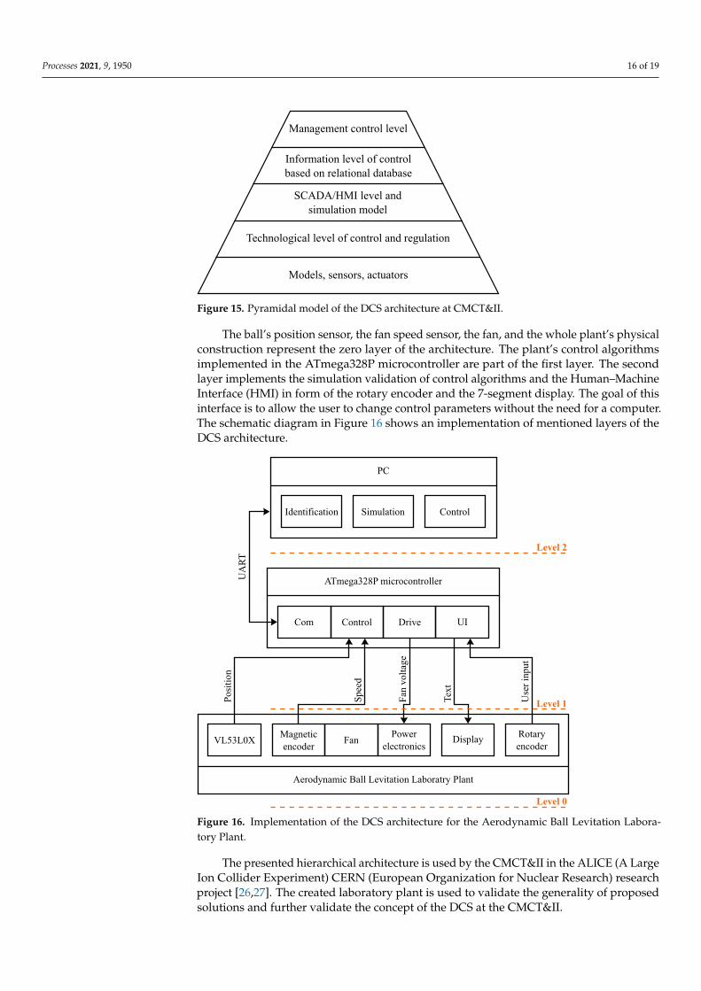
The newly created laboratory plant is implemented into a Distributed Control System(DCS) [25] at the CMCT&II. The hierarchical model of the DCS architecture shown inFigure 15 is divided into five layers of which the first three layers are currently applied tothis plant. Implementation of the remaining two topmost layers of the pyramidal model isthe subject of further research.

Processes 2021, 9, 1950 16 of 19

Figure 15. Pyramidal model of the DCS architecture at CMCT&II.

The ball’s position sensor, the fan speed sensor, the fan, and the whole plant’s physicalconstruction represent the zero layer of the architecture. The plant’s control algorithmsimplemented in the ATmega328P microcontroller are part of the first layer. The secondlayer implements the simulation validation of control algorithms and the Human–MachineInterface (HMI) in form of the rotary encoder and the 7-segment display. The goal of thisinterface is to allow the user to change control parameters without the need for a computer.The schematic diagram in Figure 16 shows an implementation of mentioned layers of theDCS architecture.

Figure 16. Implementation of the DCS architecture for the Aerodynamic Ball Levitation Labora-tory Plant.

The presented hierarchical architecture is used by the CMCT&II in the ALICE (A LargeIon Collider Experiment) CERN (European Organization for Nuclear Research) researchproject [26,27]. The created laboratory plant is used to validate the generality of proposedsolutions and further validate the concept of the DCS at the CMCT&II.

Processes 2021, 9, 1950 17 of 19

6. Conclusions

The main goal of this paper is to present obtained experimental results from the newlycreated Aerodynamic Ball Levitation plant. This includes the design and verification ofa methodology for modeling, identification, control, simulation, and implementation onthe real nonlinear laboratory plant. Additionally, details about hardware and softwareimplementations are provided with the emphasis on design improvements. The mainimprovement of our design is the addition of the fan speed sensor that enabled us touse a broader range of available control algorithms. These control algorithms can beeasily validated on the simulation model that acts as a digital twin for the real plant. Thedigital twin can be used for predictive control algorithms or to generate training data forAI-based controllers.

Another improvement was made in the use of the Kalman filter to filter the sensorynoise, which in turn reduced the fluctuation of the control voltage. Lastly, the onboardcontrol mechanism was added in form of the display and the rotary encoder with a push-button to control the plant without the need for a computer. Obtained results are presentedin visual form supplemented with quantitative evaluation. The laboratory plant can befurther improved, e.g., with the addition of a current sensing circuit. This circuit canimprove the results of the experimental identification especially in the case of the fansubsystem. Additionally, a different set of control algorithms such as Model PredictiveControl, Model Reference Adaptive Control, or Robust Tracking Control can be evaluatedon this plant.

The newly created laboratory plant will be used in the education process duringcontrol engineering courses provided by CMCT&II, for example, Basics of AutomaticControl, Optimal Control of Hybrid Systems, or Control and Artificial Intelligence. Theplant creates a solid foundation for standard control engineering tasks, such as analyticalmodeling, parameter identification, and design of various types of controllers. It alsoenables the members of the CMCT&II to implement the laboratory plant into similar DCSarchitecture that is used at the CERN.

Author Contributions: Conceptualization, T.T.; methodology, T.T., M.T. and A.J. and S.J.; software,T.T. and M.T.; validation, T.T., A.J. and S.J.; formal analysis, A.J. and S.J.; investigation, T.T.; resources,T.T.; data curation, T.T. and M.T.; writing—original draft preparation, T.T.; writing—review andediting, M.T., A.J. and S.J.; visualization, T.T.; supervision, A.J. and S.J.; project administration, A.J.;funding acquisition, A.J. and S.J. All authors have read and agreed to the published version ofthe manuscript.

Funding: This research was funded by the project ALICE experiment at the CERN LHC: The studyof strongly interacting matter under extreme conditions (ALICE KE FEI TU 0195/2021).

Acknowledgments: This publication is the result of project implementations: Modular multifunc-tional control workplace using computational intelligence techniques (APVV-19-0590) and ALICEexperiment at the CERN LHC: The study of strongly interacting matter under extreme conditions(ALICE KE FEI TU 0195/2021).

Conflicts of Interest: The authors declare no conflict of interest.

AbbreviationsThe following abbreviations are used in this manuscript:

ADC Analog to Digital ConverterALICE A Large Ion Collider ExperimentARX Autoregressive Model with Exogenous VariableCERN European Organization for Nuclear ResearchCMCT&II Center of Modern Control Techniques and IndustrialDCAI Department of Cybernetics and Artificial IntelligenceDCS Distributed Control System

Processes 2021, 9, 1950 18 of 19

FEEI Faculty of Electrical Engineering and InformaticsHMI Human–Machine InterfaceLQI Linear Quadratic Integral (regulator)LQR Linear-Quadratic RegulatorPCB Printed Circuit BoardPID Proportional-Integral-Derivative (regulator)PLA Polylactic Acid (popular material used for 3D printing)PWM Pulse-Width Modulated (signal)SISO Single-Input Single-Output (system)SIMO Single-Input Multiple-Output (system)TUKE Technical University of KošiceUART Universal Asynchronous Receiver–Transmitter

References1. Benmore, C.; Weber, J. Aerodynamic levitation, supercooled liquids and glass formation. Adv. Phys. X 2017, 2, 717–736. [CrossRef]2. Šuster, P.; Jadlovská, A. Modeling and control design of magnetic levitation system. In Proceedings of the 2012 IEEE 10th

International Symposium on Applied Machine Intelligence and Informatics (SAMI), Herl’any, Slovakia, 26–28 January 2012;pp. 295–299. [CrossRef]

3. Rábek, M.; Žáková, K. Building of the fan driven ball levitation system. IFAC-PapersOnLine 2019, 52, 283–287. [CrossRef]4. Chołodowicz, E.; Orłowski, P. Low-cost air levitation laboratory stand using MATLAB/Simulink and Arduino. Pomiary

Automatyka Robotyka 2017, 21, 33–39. [CrossRef]5. Chacón, J.; Vargas, H.; Dormido, S.; Sánchez, J. Experimental study of nonlinear PID controllers in an air levitation system.

IFAC-PapersOnLine 2018, 51, 304–309. [CrossRef]6. Saenz, J.; Chacon, J.; de la Torre, L.; Dormido, S. An open software-open hardware lab of the air levitation system. IFAC-

PapersOnLine 2017, 50, 9168–9173. [CrossRef]7. Chacon, J.; Saenz, J.; Torre, L.D.l.; Diaz, J.M.; Esquembre, F. Design of a low-cost air levitation system for teaching control

engineering. Sensors 2017, 17, 2321. [CrossRef] [PubMed]8. Rábek, M.; Žáková, K. Development of Control Experiments for an Online Laboratory System. Information 2020, 11, 131.

[CrossRef]9. Chaos, D.; Chacón, J.; Aranda-Escolástico, E.; Dormido, S. Robust switched control of an air levitation system with minimum

sensing. ISA Trans. 2020, 96, 327–336. [CrossRef]10. Jernigan, S.R.; Fahmy, Y.; Buckner, G.D. Implementing a remote laboratory experience into a joint engineering degree program:

Aerodynamic levitation of a beach ball. IEEE Trans. Educ. 2008, 52, 205–213. [CrossRef]11. Kuzhandairaj, J.C. Development, control and testing of an air levitation system for educational purpose. Master’s Degree Thesis,

Polytechnic University of Milan, Milan, Italy, 19 April 2018.12. Escano, J.M.; Ortega, M.G.; Rubio, F.R. Position control of a pneumatic levitation system. In Proceedings of the 2005 IEEE

Conference on Emerging Technologies and Factory Automation, Catania, Italy, 19–22 September 2005; Volume 1, pp. 523–528.[CrossRef]

13. Pujol-Vázquez, G.; Vargas, A.N.; Mobayen, S.; Acho, L. Semi-Active Magnetic Levitation System for Education. Appl. Sci. 2021,11, 5330. [CrossRef]

14. Mobayen, S.; Tchier, F. An LMI approach to adaptive robust tracker design for uncertain nonlinear systems with time-delays andinput nonlinearities. Nonlinear Dyn. 2016, 85, 1965–1978. [CrossRef]

15. Barie, W.; Chiasson, J. Linear and nonlinear state-space controllers for magnetic levitation. Int. J. Syst. Sci. 1996, 27, 1153–1163.[CrossRef]

16. Tootchi, A.; Amirkhani, S.; Chaibakhsh, A. Modeling and Control of an Air Levitation Ball and Pipe Laboratory Setup. InProceedings of the 2019 7th International Conference on Robotics and Mechatronics (ICRoM), Tehran, Iran, 20–21 November2019; pp. 29–34.[CrossRef]

17. Takács, G.; Chmurciak, P.; Gulan, M.; Mikuláš, E.; Kulhánek, J.; Penzinger, G.; Vdolecek, M.; Podbielancík, M.; Lucan, M.;Šálka, P.; et al. FloatShield: An Open Source Air Levitation Device for Control Engineering Education. IFAC-PapersOnLine 2020,53, 17288–17295. [CrossRef]

18. Emhemed, A.A.; Mamat, R.B. Modelling and simulation for industrial DC motor using intelligent control. Procedia Eng. 2012,41, 420–425. [CrossRef]

19. Brastein, O.; Perera, D.; Pfeifer, C.; Skeie, N.O. Parameter estimation for grey-box models of building thermal behaviour. EnergyBuild. 2018, 169, 58–68. [CrossRef]

20. Ljung, L. System Identification: Theory for the User, 2nd ed.; Prentice-Hall: Englewood Cliffs, NJ, USA, 1999; ISBN 978-0136566953.21. Wang, D.; Meng, F.; Meng, S. Linearization Method of Nonlinear Magnetic Levitation System. Math. Probl. Eng. 2020,

2020, 9873651. [CrossRef]22. Kim, Y.; Bang, H. Introduction to Kalman filter and its applications. Introd. Implement. Kalman Filter 2018, 1, 1–16. [CrossRef]

Processes 2021, 9, 1950 19 of 19

23. Young, P.C.; Willems, J. An approach to the linear multivariable servomechanism problem. Int. J. Control 1972, 15, 961–979.[CrossRef]

24. Kirk, D.E. Optimal Control Theory: An Introduction; Dover Publications: Mineola, New York, USA, 2012; ISBN 978-0486135076.25. Jadlovský, J.; Jadlovská, A.; Jadlovská, S.; Cerkala, J.; Kopcík, M.; Cabala, J.; Oravec, M.; Varga, M.; Vošcek, D. Research activities

of the center of modern control techniques and industrial informatics. In Proceedings of the 2016 IEEE 14th InternationalSymposium on Applied Machine Intelligence and Informatics (SAMI), Herl’any, Slovakia, 21–23 January 2016; pp. 279–285.[CrossRef]

26. Jadlovský, J.; Jadlovská, A.; Jadlovská, S.; Oravec, M.; Vošcek, D.; Kopcík, M.; Cabala, J.; Tkácik, M.; Chochula, P.; Pinazza, O.Communication Architecture of the Detector Control System for the Inner Tracking System. In Proceedings of the 16thInternational Conference on Accelerator and Large Experimental Physics Control Systems (ICALEPCS 2017), Barcelona, Spain,8–13 October 2017; p. THPHA208. [CrossRef]

27. Tkácik, M.; Jadlovský, J.; Jadlovská, S.; Koska, L.; Jadlovská, A.; Donadoni, M. FRED—Flexible Framework for FrontendElectronics Control in ALICE Experiment at CERN. Processes 2020, 8, 565. [CrossRef]