On Aerodynamic Models for Flutter Analysis - MDPI

Article

On Aerodynamic Models for Flutter Analysis: A SystematicOverview and Comparative Assessment

Marco Berci

��

Citation: Berci, M. On Aerodynamic

Models for Flutter Analysis: A

Systematic Overview and

Comparative Assessment. Appl. Mech.

2021, 2, 516–541. https://doi.org/

10.3390/applmech2030029

Received: 27 May 2021

Accepted: 8 July 2021

Published: 29 July 2021

Publisher’s Note: MDPI stays neutral

with regard to jurisdictional claims in

published maps and institutional affil-

iations.

Copyright: © 2021 by the author.

Licensee MDPI, Basel, Switzerland.

This article is an open access article

distributed under the terms and

conditions of the Creative Commons

Attribution (CC BY) license (https://

creativecommons.org/licenses/by/

4.0/).

Pilatus Aircraft Ltd., 6370 Stans, Switzerland; [email protected]

Abstract: This work reviews different analytical formulations for the time-dependent aerodynamicload of a thin aerofoil and clarifies numerical flutter results available in the literature for the typicalsection of a flexible wing; inviscid, two-dimensional, incompressible, potential flow is consideredin all test cases. The latter are investigated using the exact theory for small airflow perturbations,which involves both circulatory and non-circulatory effects of different nature, complemented by thep-k flutter analysis. Starting from unsteady aerodynamics and ending with steady aerodynamics,quasi-unsteady and quasi-steady aerodynamic models are systematically derived by successivesimplifications within a unified approach. The influence of the aerodynamic approximations onthe aeroelastic stability boundary is then rigorously assessed from both physical and mathematicalperspectives. All aerodynamic models are critically discussed and compared in the light of thenumerical results as well, within a comprehensive theoretical framework in practice. In all cases,results accuracy depends on the aero-structural arrangement of the flexible wing; however, simplifiedunsteady and simplified quasi-unsteady aerodynamic approximations are suggested for robust flutteranalysis whenever the wing’s elastic axis lies ahead of the aerofoil’s control point.

Keywords: aerodynamic approximation; flutter analysis; subsonic flow; incompressible fluid

1. Introduction

Semi-analytical formulations of the aerodynamic loads for the flutter analysis of thinwing sections in subsonic potential flow have been available for a long time [1]; nevertheless,some definitions are not universal and the relative models are still under discussion [2]: thisis the case of quasi-steady aerodynamics. In this respect, it is immediately clarified that, atleast in the present work, the attributes “unsteady”, “quasi-unsteady”, “quasi-steady” and“steady” refer to the type of flow, which is generally time-dependent (as indeed requiredfor aeroelastic flutter calculations) [3].

All airload approximations involve both circulatory and non-circulatory contributions,except for the case of steady aerodynamics, which includes circulatory contributions onlyand considers the same instantaneous angle of attack along the entire aerofoil chord [4].Within the proposed theoretical framework, unsteady and quasi-unsteady aerodynamicsaccount for a wake being shed from the aerofoil’s trailing edge with the reference airspeedand influencing the airload in turn, due to the inflow from the travelling wake’s vorticity [5].Unsteady aerodynamics also includes apparent inertia terms of non-circulatory nature;these are instead coherently disregarded by quasi-steady and steady aerodynamics, whichassume slow variations in the airflow [6]. In these quasi-static cases, dynamic effectsare neglected and the airflow evolution is treated as a continuous series of subsequentindependent steady states where the airload reacts instantaneously to variations in theboundary condition [7]. On the contrary, unsteady aerodynamics involves a convolutionprocess where the current flow state depends on the previous ones, due to the feedbackmechanism enforced by the wake’s inflow resulting from the shed vorticity and governedby Kutta’s condition [8].

Although inherently limited in applicability [9,10], explicit airload expressions andtheoretical solutions grant a clear overview of the underlying phenomena and offer rigor-

Appl. Mech. 2021, 2, 516–541. https://doi.org/10.3390/applmech2030029 https://www.mdpi.com/journal/applmech

https://www.mdpi.com/journal/applmech

https://www.mdpi.com

https://doi.org/10.3390/applmech2030029


https://creativecommons.org/

https://creativecommons.org/licenses/by/4.0/

https://creativecommons.org/licenses/by/4.0/


https://www.mdpi.com/journal/applmech

https://www.mdpi.com/article/10.3390/applmech2030029?type=check_update&version=1

Appl. Mech. 2021, 2 517

ous validation as well as fundamental insights for both educational and practical scopes inboth academic and industrial activities, with a convenient trade-off between reliability andaffordability [11–13]. Focusing on two-dimensional, incompressible, potential flow withoutloss of generality for the fundamental purpose of this conceptual work, the unsteady aero-dynamic model is first reviewed by adopting a vorticity-based approach [14,15], showingits formal equivalence with Thodorsen’s and Wagner’s models [16,17]. All previouslymentioned approximations for the aerofoil’s airload are hence systematically derived bysuccessive simplifications of physical effects and mathematical terms within a unifiedapproach, ranging from the more complex unsteady aerodynamics to the more straight-forward steady aerodynamics. Aeroelastic flutter calculations are then performed usingall presented aerodynamic models and critically compared with numerical results alreadyavailable in the literature for the typical section of a flexible wing [18], which are ex-plained and clarified in light of the proposed theoretical derivation within a comprehensiveassessment.

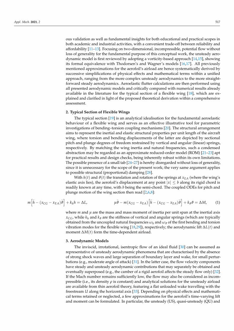
2. Typical Section of Flexible Wings

The typical section [19] is an analytical idealisation for the fundamental aeroelasticbehaviour of a flexible wing and serves as an effective illustrative tool for parametricinvestigations of bending–torsion coupling mechanisms [20]. The structural arrangementaims to represent the inertial and elastic structural properties per unit length of the aircraftwing, where torsion and bending displacements of the latter are depicted by sectionalpitch and plunge degrees of freedom restrained by vertical and angular (linear) springs,respectively. By matching the wing inertia and natural frequencies, such a condensedabstraction may be regarded as an approximate reduced-order model (ROM) [21–23] aptfor practical results and design checks, being inherently robust within its own limitations.The possible presence of a small tab [24–27] is hereby disregarded without loss of generality,since it is unnecessary for the scope of the present work; the very same argument appliesto possible structural (proportional) damping [28].

With h(t) and ϑ(t) the translation and rotation of the springs at xEA (where the wing’selastic axis lies), the aerofoil’s displacement at any point |x| ≤ b along its rigid chord isreadily known at any time, with b being the semi-chord. The coupled ODEs for pitch andplunge motion of the wing section then read [2,6,8]:

m[ ..

h− (xCG − xEA)..ϑ]+ khh = ∆L, µ

..ϑ−m(xCG − xEA)

[ ..h− (xCG − xEA)

..ϑ]+ kϑϑ = ∆M, (1)

where m and µ are the mass and mass moment of inertia per unit span at the inertial axisxCG, while kh and kϑ are the stiffness of vertical and angular springs (which are typicallyobtained from the uncoupled natural frequencies ωh and ωϑ of the first bending and torsionvibration modes for the flexible wing [18,29]), respectively; the aerodynamic lift ∆L(t) andmoment ∆M(t) form the time-dependent airload.

3. Aerodynamic Models

The inviscid, irrotational, isentropic flow of an ideal fluid [30] can be assumed asrepresentative of unsteady aerodynamic phenomena that are characterised by the absenceof strong shock waves and large separation of boundary layer and wake, for small pertur-bations (e.g., moderate angle of attack) [31]. In the latter case, the flow velocity componentshave steady and unsteady aerodynamic contributions that may separately be obtained andeventually superposed (e.g., the camber of a rigid aerofoil affects the steady flow only) [32].If the Mach number remains sufficiently low, the flow may also be considered as incom-pressible (i.e., its density ρ is constant) and analytical solutions for the unsteady airloadare available from thin aerofoil theory, featuring a flat unloaded wake travelling with thefreestream U along the horizontal axis [33]. Depending on physical effects and mathemati-cal terms retained or neglected, a few approximations for the aerofoil’s time-varying liftand moment can be formulated. In particular, the unsteady (US), quasi-unsteady (QU) and

Appl. Mech. 2021, 2 518

simplified quasi-unsteady (SQU), quasi-steady (QS) and simplified quasi-steady (SQS),degenerate unsteady (DU), and steady (SS) airload models for incompressible potentialflow will thoroughly be considered hereafter.

3.1. Exact Solution for Unsteady Flow

Adopting a vorticity-based approach for incompressible potential flow [14,15], theunsteady airload was divided into circulatory and non-circulatory contributions [4,16]:the former one originates from pairs of counter-rotating bound and wake vortices with astretching distance given by Joukowski’s conformal transformation [33] (mapping a circleinto a slit [34]) in the complex plane, whereas the latter one originates from fixed pairs ofsymmetric sources and sinks placed along a complex circle (representing a streamline). Dueto the linearity of the fluid dynamics equations for small irrotational perturbations [35], theprinciple of superposition applies. This ideal arrangement of “virtual” singular elementsgrants upper and lower surfaces of the flat aerofoil as streamlines for inviscid flow anddemonstrates as formally equivalent to unsteady thin aerofoil theory [36–38].

In particular, two vortex sheets γa(x, t) and γw(x, t) are placed along the aerofoil’schord (i.e., |x| ≤ b) and its shed wake (i.e., x > b), giving rise to the respective equal andopposite circulations Γa(t) and Γw(t) as [4,33]:

Γa ≡+b∫−b

γadx, Γw ≡∞∫

b

γwdx, Γ ≡ Γa + Γw = 0,dΓdt≡ dΓa

dt+

dΓw

dt= 0, (2)

which satisfies Helmholtz’s and Kelvin’s theorems for the conservation of the total (null)circulation Γ(t) on all streamlines of the simply connected region including the wakediscontinuity. Thus, with infinitesimal vortices dΓw = γwdx counteracting infinitesimalvariations of bound circulation dΓa, the condition for an unloaded wake results in atransport equation for the shed vorticity as it stretches with dx = Udt, namely [14]:

∂γw

∂t+ U

∂γw

∂x= 0, γw = γw(x−Ut), γw(b, t) = − 1

UdΓa

dt, (3)

where Kutta’s condition [39] and Joukowski’s theorem [40] grant that the airflow leaves theaerofoil’s trailing edge smoothly with finite velocity and finds a unique bound circulationwhile relating its rate of change with the wake’s vorticity. With Dirichlet’s boundary condi-tion for the asymptotic airflow inherently embedded in the freestream [7], the Neumann’stype impermeability condition accomplishes the fluid–structure interaction (FSI) [41] alongthe thin aerofoil and involves its own kinematics vn(x, t) by imposing the airflow as alwaystangential to its mean surface za(x, t), namely [4,14]:

vn ≡∂za

∂t+ U

∂za

∂x= − 1

2π

+b∫−b

γadξ

x− ξ− 1

2π

∞∫b

γwdξ

x− ξ≡ va + vw, za = h− (x− xEA)ϑ, (4)

which drive the aerodynamic flow and pressure load while being affected by the latter inturn, with va(x, t) the vertical perturbation velocity and vw(x, t) the wake’s inflow.

Within this framework for incompressible inviscid flow, the fluid potential functionφ(x, t) satisfies Laplace’s equation [28], the horizontal perturbation velocity u(x, t) is givenby its longitudinal derivative and Bernoulli’s unsteady linearised equation [4,14] thenprovides the net pressure airload ∆p(x, t) acting across upper and lower surfaces of theaerofoil, namely [16]:

∆p = −2ρ

(U

∂φ

∂x+

∂φ

∂t

), γ = 2u, u =

∂φ

∂x, ∇2φ = 0, (5)

Appl. Mech. 2021, 2 519

where Kutta’s, Dirichlet’s and Neumann’s conditions must be fulfilled [7]. The pressureairload can eventually be integrated to obtain the unsteady lift and moment around theelastic axis as [4,14]:

∆L = −+b∫−b

∆pdx, ∆M =

+b∫−b

∆p(x− xEA)dx, (6)

which drive the aerofoil’s motion while being strongly affected by the latter in turn. How-ever, by exploiting linear superposition, the problem formulation is conveniently split intocirculatory and non-circulatory parts, namely [16]:

φ ≡ φC + φN , u ≡ uC + uN , γ ≡ γC + γN , (7)

∆p ≡ ∆pC + ∆pN , ∆L ≡ ∆LC + ∆LN , ∆M ≡ ∆MC + ∆MN , (8)

where the definition of the respective contributions is straightforward; the latter are thentreated separately, based on their physical nature. Thus, taking advantage of the aero-foil’s impermeability condition and Joukowski’s conformal transformation as the wakestretches [34], the proposed arrangement of vortices, sources and sinks gives [16]:

φNa =

[Uϑ−

.h +

( x2− xEA

) .ϑ]√

b2 − x2, uNa =

1√b2 − x2

{x[ .

h− (x− xEA).ϑ−Uϑ

]+

b2

2

.ϑ

}, (9)

φCa =

12π

∞∫b

arctan

(√b2 − x2

√ξ2 − b2

b2 − xξ

)γwdξ, uC

a =1

2π

∞∫b

√ξ2 − b2

b2 − x2γwdξ

x− ξ, (10)

which correspond to the theoretical solutions found by unsteady thin aerofoil theory [15]:

γNa ≡

_γ

Na =

2√b2 − x2

+b∫−b

√b2 − ξ2

π(x− ξ)vndξ, γC

a ≡_γ

Ca + γ̃a =

1π

∞∫b

√ξ2 − b2

b2 − x2γwdξ

x− ξ, (11)

where the wake’s inflow induces a circulatory perturbation γ̃a(x, t) to a quasi-steady state_γ a(x, t), namely [4,14]:

γNa ≡

_γ

Na =

2√b2 − x2

+b∫−b

√b2 − ξ2

π(x− ξ)vndξ, γC

a ≡_γ

Ca + γ̃a =

1π

∞∫b

√ξ2 − b2

b2 − x2γwdξ

x− ξ, (12)

with a stagnation point at the unloaded trailing edge (i.e., γa(b, t) = 0 with ∆p(b, t) = 0).These provide the aerofoil with a unique bound circulation also given by an unsteady

perturbation Γ̃a(t) to a quasi-steady state_Γ a(t), namely [4,14,16,33]:

Γa ≡_Γ a + Γ̃a, Γ̃a ≡

+b∫−b

γ̃adx =

∞∫b

(√x + bx− b

− 1

)γwdx,

_Γ a ≡

+b∫−b

_γ adx = −2

+b∫−b

√b + xb− x

vndx, (13)

where the last equality is granted by Kutta’s condition and relates the wake’s vortic-

ity with the aerofoil’s kinematics while implicitly allowing the circulatory_γ

Ca (x, t) and

non-circulatory_γ

Na (x, t) parts of the quasi-steady vorticity (i.e., what does and does not

contribute to the bound circulation, respectively) to be separated as [15]:

_γ

Na =

2

π√

b2 − x2

+b∫−b

√b2 − ξ2

x− ξvndξ,

_γ

Ca = − 2

π√

b2 − x2

+b∫−b

√b + ξ

b− ξvndx, (14)

Appl. Mech. 2021, 2 520

as rigorously confirmed by exact conformal solutions specialised for flat aerofoil [7,14].Thus, for the unsteady pressure airload it can readily be identified that [15,16,36]:

∆pN = −ρ

U_γ

Na +

∂

∂t

x∫−b

_γ

Na dξ

, ∆pC = −ρU

_γ

Ca +

1π

√b− xb + x

∞∫b

γwdξ√ξ2 − b2

, (15)

which then give the non-circulatory unsteady lift and moment around the elastic axisas [4,15,16,36]:

∆LN = −ρ ddt

+b∫−b

_γ

Na xdx = −2ρ

+b∫−b

∂vn∂t

√b2 − x2dx,

∆MN = ρ

[ddt

+b∫−b

_γ

Na( x

2 − xEA)

xdx−U+b∫−b

_γ

Na xdx

]= −2ρ

+b∫−b

[Uvn −

( x2 − xEA

) ∂vn∂t

]√b2 − x2dx,

(16)

where the shed wake plays no role and all double integrals are reduced to standard integralsby interchanging the order of quadrature [14], whereas the circulatory unsteady lift andmoment read [4,15,16,36]:

∆LC = −ρU∞∫b

γwxdx√x2−b2 = ρU

(_Γ a +

∞∫b

bγwdx√x2−b2

),

∆MC = ρU∞∫b

(b2

2 − xEAx)

γwdx√x2−b2 = ρU

[xEA

_Γ a +

(b2 + xEA

)∞∫b

bγwdx√x2−b2

],

(17)

respectively. Note that the net effect of the airfoil’s quasi-steady vorticity is indeed notlimited to the quasi-steady circulation per se, as the non-circulatory contributions do giverise to apparent flow inertia loads (including centrifugal ones [28]). The total unsteadypressure airload is then found as [4,42]:

∆p = −ρ

U_γ a +

∂

∂t

x∫−b

_γ

Na dξ +

Uπ

√b− xb + x

∞∫b

γwdξ√ξ2 − b2

, (18)

and integrated [15] to give the aerofoil’s total unsteady lift and moment around the elasticaxis as [4,33,36,42]:

∆L = ρ

(U

_Γ a − d

dt

+b∫−b

_γ

Na xdx + Ub

∞∫b

γwdx√x2−b2

),

∆M = −ρ

(U

+b∫−b

_γ

Na xdx− 1

2ddt

+b∫−b

_γ

Na x2dx−U b2

2

∞∫b

γwdx√x2−b2

)+ xEA∆L.

(19)

After substituting the aerofoil’s kinematics, the contributions to the quasi-steadyvorticity read [15,16]:

_γ

Na =

2√b2 − x2

{x[ .


]+

b2

2

.ϑ

},

_γ

Ca =

2b√b2 − x2

[Uϑ−

.h +

(b2− xEA

).ϑ

], (20)

_γ a = 2

√b− xb + x

[Uϑ−

.h + (b + x− xEA)

.ϑ],

_Γ a = 2πb

[Uϑ−

.h +

(b2− xEA

).ϑ

], (21)

and the non-circulatory airload has an explicit expression with respect to the aerofoil’sdegrees of freedom [15,16]:

∆LN = πρb2(

U.ϑ−

..h− xEA

..ϑ)

, ∆MN = πρb2[

U(

Uϑ−.h)− xEA

..h−

(b2

8+ x2

EA

)..ϑ

], (22)

which include quasi-unsteady contributions only. Note that apparent flow inertia effects(particularly important in the presence of a tab [18]) pertain to both vertical acceleration

Appl. Mech. 2021, 2 521

at the aerofoil’s mid-chord and centrifugal acceleration [28], while the pitch rate does notcontribute to the moment (as equal and opposite terms cancel out among those from thenon-circulatory vorticity and its time derivative), regardless of the position of the elasticaxis. On the contrary, the wake vorticity in the circulatory airload is generally not availablein explicit analytical form; however, assuming harmonic motion (as indeed suitable forflutter investigations) simplifies the problem formulation and the circulatory airload isfound multiplied by Theodorsen’s lift-deficiency function C(k) [16], namely:

C(k) ≡

∞∫1

ζe−ikζ√ζ2−1

dζ

∞∫1

√ζ+1ζ−1 e−ikζdζ

=H(2)

1 (k)

H(2)1 (k) + iH(2)

0 (k), k =

bω

U, (23)

where H(2)n (k) are Hankel’s functions of the n-th order and second kind [4], with k the

reduced frequency (i.e., Strouhal’s number in terms of travelled semichords [3]). Note thatKutta’s condition is implicit in the definition of Theodorsen’s function, which multipliesthe bound circulation acting at the aerodynamic centre (i.e., the first-quarter chord) but isnot necessary to depict the wake’s inflow mechanism per se [5,43] (rather driven by thecounter-rotating vorticity in the shed wake [33,44]). Thus, for the circulatory flow (alwayscontributing to the bound circulation) over the aerofoil’s surface it is [4,16]:

∆LC = ρUC(k)_Γ a = 2πρUbC(k)

[Uϑ−

.h +

(b2 − xEA

) .ϑ], αe f f =

VU ,

∆MC = ρU[(

b2 + xEA

)C(k)− b

2

]_Γ a = 2πρUb

[(b2 + xEA

)C(k)− b

2

][Uϑ−

.h +

(b2 − xEA

) .ϑ],

(24)

where the vertical flow speed at the aerofoil’s control point (i.e., third-quarter chord) V(t)gives the instantaneous effective angle of attack αe f f (t) [7], whereas CL/α = 2π representsthe sectional steady lift derivative for flat aerofoil, according to thin aerofoil theory [32].Theodorsen’s (complex transfer) function can then be considered as the Fourier transform ofthe (unit) unsteady airload due to impulsive plunging of the aerofoil at its control point [5]in the reduced-frequency domain: it introduces a lag in the airload build-up because of thecounteracting vorticity that is shed in the wake from infinitesimal variations of the boundcirculation according to Kelvin’s and Helmholtz’s theorems [7]. Theodorsen’s functiongeneralises for the swept wing and subsonic compressible flow [45–47] by considering theeffective freestream relative to the aerodynamic axis and Prandtl-Glauert’s compressibilityfactor [10,32]; for finite wings [34,48], it is modified by unsteady downwash effects (whichreduce the sectional effective angle of attack and the related airload as well as its build-uprate [49,50]) within modified strip theory [12].

Finally, the total “unsteady” airload acting on the oscillating aerofoil reads [4,16]:

∆L = 2πρUbC(k)V + πρb2(

U.ϑ−

..h− xEA

..ϑ)

, V = Uϑ−.h +

(b2 − xEA

) .ϑ,

∆M = 2πρUb(

b2 + xEA

)C(k)V − πρb2

[(b2 − xEA

)U

.ϑ + xEA

..h +

(b2

8 + x2EA

) ..ϑ],

(25)

where cancellations occurred between some circulatory and non-circulatory terms, still dueto Kelvin’s theorem; this is formally equivalent to Wagner’s solution employing Duhamel’sconvolution in the reduced time τ, since [18]:

C(k)V = V0Φ +

τ∫0

dVdς

Φ(τ − ς)dς, Φ =1

2π

+∞∫−∞

(eikτ

ik

)C(k)dk, τ =

Utb

, (26)

where Wagner’s indicial-admittance function Φ(τ) from a unit step-change in the angleof attack modulates the vertical flow speed at the aerofoil’s control point [17], which hasan initial value V0 directly related to the initial conditions of the aerofoil motion. Whenadded aerodynamic states are conveniently defined [51], a state-space formulation is thenpossible [52] and often useful to study stable sub- or super-critical limit cycles oscillations ofnonlinear aeroelastic systems [53]. Finally, it is worth stressing that several research studies

Appl. Mech. 2021, 2 522

did build (and still build) on this fundamental model [54–57], including linear effects dueto morphing capabilities [36–38,43,58,59] and flow compressibility [60,61] or nonlineareffects due to aerofoil thickness [62,63], large angles of attack and free wake [64,65], viscousboundary layer [66], flow separation and stall [67,68].

For the sake of completeness, note that the wing’s gust response is also importantin aircraft design and certification [69]. In particular, a “frozen” approach [70,71] is typ-ically adopted for lower-fidelity analytical models [49,72] (where the aerofoil’s presenceis assumed not to affect the wind gust [15]), which relate Kussners’s function for theindicial lift from a unit sharp-edge gust to the indicial circulation relative to Wagner’s func-tion [73,74]; an arbitrary gust can then be considered by exploiting Duhamel’s convolutionwith Kussners’s indicial-admittance function directly [75]. Later numerical studies [76] andhigher-fidelity simulations [77] confirmed that quasi-steady aerodynamics is not appro-priate for calculating gust responses unless the wind gust is very smooth and its length ismuch longer than the aerofoil’s chord [75].

3.2. Degenerate Unsteady and Quasi-Steady Approximations

In order to simplify the unsteady airload’ expression and avoid a mixed formulation inboth time and frequency domains, different aerodynamic models have been proposed in theliterature as approximate ROMs (e.g., to estimate the stability margin in robust MDO [13]and safe flight tests [78]) that neglect the shed wake’s inflow. In particular, let the potentialincompressible flow around the thin aerofoil undergo small quasi-steady perturbations (e.g.,due to a moderate and slowly-varying angle of attack). In the absence of wake vorticity, anequal and opposite lumped vortex of intensity Γw counteracts the instantaneous (quasi-steady) circulation infinitely far behind the aerofoil to satisfy Helmholtz’s and Kelvin’stheorems [7] for the conservation of the total (null) circulation at all times, with:

γw = 0, γ̃a = 0, γa =_γ a = 2

√b− xb + x

[Uϑ−

.h + (b + x− xEA)

.ϑ], (27)

_γ

Na =

2√b2 − x2

{x[ .


]+

b2

2

.ϑ

},

_γ

Ca =

2b√b2 − x2

[Uϑ−

.h +

(b2− xEA

).ϑ

], (28)

Γ̃a = 0, Γa =_Γ a = 2πb

[Uϑ−

.h +

(b2− xEA

).ϑ

], vn =

.h− (x− xEA)

.ϑ−Uϑ, (29)

where an unloaded wake is still implicitly assumed but its vorticity and inflow are neglectedin the proximity of the aerofoil. From the exact solution for unsteady flow [16], simplyimposing C(k) = 1 for k << 1 (i.e., neglecting any feedback from the wake’s inflow atlow reduced frequencies) while retaining all non-circulatory terms results in a “degenerateunsteady” aerodynamic model [4] where pressure distribution and circulatory loads read:

∆p = −ρ

U_γ a +

∂

∂t

x∫−b

_γ

Na dξ

, ∆LC = ρU_Γ a, ∆MC = ρUxEA

_Γ a, (30)

and the total lift and moment around the elastic axis result in:

∆L = ρ

U_Γ a −

ddt

+b∫−b

_γ

Na xdx

, ∆M = ρ

U

xEA_Γ a −

+b∫−b

_γ

Na xdx

+12

ddt

+b∫−b

_γ

Na x2dx

, (31)

with both circulatory and non-circulatory contributions directly related to the aerofoil’smotion, namely:

∆LN = −2ρ

+b∫−b

∂vn

∂t

√b2 − x2dx, ∆MN = −2ρ

+b∫−b

[Uvn −

( x2− xEA

)∂vn

∂t

]√b2 − x2dx, (32)

Appl. Mech. 2021, 2 523

∆LC = −2ρU+b∫−b

√b + xb− x

vndx, ∆MC = −2ρUxEA

+b∫−b

√b + xb− x

vndx, (33)

where double integrals have been reduced to standard ones by interchanging the order ofquadrature [14] and the non-circulatory airload is that of unsteady flow. Finally, substitutingthe aerofoil’s kinematics in terms of its degrees of freedom gives:

∆LN = πρb2(

U.ϑ−

..h− xEA

..ϑ)

, ∆MN = πρb2[

U(

Uϑ−.h)− xEA

..h−

(b2

8+ x2

EA

)..ϑ

], (34)

∆LC = 2πρUb[

Uϑ−.h +

(b2− xEA

).ϑ

], ∆MC = 2πρUbxEA

[Uϑ−

.h +

(b2− xEA

).ϑ

], (35)

and the total lift and moment around the elastic axis reduce to [4]:

∆L = 2πρb{

U[Uϑ−

.h + (b− xEA)

.ϑ]− b

2

( ..h + xEA

..ϑ)}

,

∆M = 2πρb{

U[(

b2 + xEA

)(Uϑ−

.h)+(

b2 − xEA

)xEA

.ϑ]− b

2

[xEA

..h +

(b2

8 + x2EA

) ..ϑ]}

,(36)

with aerodynamic inertia, damping and stiffness terms. However, some cancellationsbetween circulatory and non-circulatory contributions to the airload do not occur in theabsence of wake vorticity [36]. A second-order Taylor expansion of Theodorsen’s functionhas then been considered for low reduced frequencies [79] but revealed an inconvenientlogarithmic singularity that tends to trigger an unphysical behaviour for harmonic mo-tion [80–82] (e.g., on the flutter boundary) especially through the undamped pitch rate [9];moreover, inaccurate extrapolation for k > 0.05 would lead to unrealistic results. At highreduced frequencies, imposing C(k) = 1/2 for k � 1 also eliminates lag effects but stillincludes the wake’s influence on the unsteady airload (which is in fact halved) and there-fore cannot be considered as a proper quasi-unsteady approximation within the presenttheoretical framework. In any case, the relative position of elastic axis and centre of gravity(typically forward of the mid-chord) was found to have a significant influence on theaccuracy of flutter analyses [83–85], especially at low reduced frequencies with negligibleapparent flow inertia. An alternative formulation has been proposed where the time rateof the circulatory vorticity was also included [7] (see the Appendix A); however, this is notinvestigated further, because the trailing edge becomes questionably loaded (i.e., still astagnation point with γa(b, t) = 0 yet with ∆p(b, t) 6= 0) but for marginal variations of thebound circulation.

In fact, neglecting all apparent inertia terms by assuming very slow variations of theairflow speed provides the airload with damping and stiffness features only and results ina “quasi-steady” aerodynamic model where the pressure distribution becomes:

∆p = −ρU_γ a,

∂vn

∂t= 0, αe f f = ϑ−

.hU

+

(b2− xEA

) .ϑ

U, C(k) = 1, (37)

while the non-circulatory and circulatory components of the airload simplify as:

∆LN = 0, ∆MN = −2ρU+b∫−b

√b2 − x2vndx = πρUb2

(Uϑ−

.h− xEA

.ϑ)

, (38)

∆LC = 2πρUb[

Uϑ−.h +

(b2− xEA

).ϑ

], ∆MC = 2πρUbxEA

[Uϑ−

.h +

(b2− xEA

).ϑ

], (39)

and the total lift and moment around the elastic axis reduce to [28]:

∆L = 2πρUb[

Uϑ−.h +

(b2− xEA

).ϑ

], ∆M = 2πρUb

[(b2+ xEA

)(Uϑ−

.h)− x2

EA

.ϑ

], (40)

where the circulatory term proportional to the pitch rate in the moment always contributesto stabilising the aeroelastic response. However, note that disregarding the flow’s accel-

Appl. Mech. 2021, 2 524

eration would require the pitch rate to be negligible as well (and also centrifugal loads),from a rigorous mathematical standpoint (see the Appendix A too). It is worth anticipatingthat both degenerate unsteady and quasi-steady aerodynamic approximations have beencoupled with an Euler-Bernoulli beam for flutter analyses of flexible wings in subsonicflow, but eventually not suggested to this purpose [86].

3.3. Simplified Quasi-Steady and Steady Approximations

A “simplified quasi-steady” approximation was also formulated that neglects thecontribution of the pitch rate to the aerofoil’s kinematics [9,80] and thus features a uniformeffective instantaneous angle of attack [4] along the entire chord, as for the case of steadyflow; in fact, this is fully consistent with disregarding the flow’s acceleration and relatedapparent inertia. Thus, pressure distribution and vertical flow velocity read:

∆p = −ρU_γ a, vn =

.h−Uϑ, αe f f = ϑ−

.hU

, C(k) = 1, (41)

while the vorticity contributions and bound circulation become:

_γ a = 2

√b− xb + x

(Uϑ−

.h)

,_Γ a = 2πb

(Uϑ−

.h)

, (42)

_γ

Na =

2x( .

h−Uϑ)

√b2 − x2

,_γ

Ca =

2b(

Uϑ−.h)

√b2 − x2

, (43)

and the relative non-circulatory and circulatory contributions to the quasi-steady airloadsimplify as:

∆LN = 0, ∆MN = πρUb2(

Uϑ−.h)

, (44)

∆LC = 2πρUb(

Uϑ−.h)

, ∆MC = 2πρUbxEA

(Uϑ−

.h)

; (45)

the total lift and moment around the elastic axis then reduce to [2,8]:

∆L = 2πρUb(

Uϑ−.h)

, ∆M = 2πρUb(

b2+ xEA

)(Uϑ−

.h)

, (46)

with aerodynamic damping and stiffness terms only, the former depending solely on theplunge velocity.

If the latter is also neglected, the typical section is left aerodynamically undampedand the “steady” aerodynamic approximation is eventually obtained where only stiffnessterms related to the instantaneous pitch angle remain, namely:

∆p = −ρU_γ a, vn = −Uϑ, αe f f = ϑ, C(k) = 1, (47)

while the vorticity contributions and bound circulation become:

_γ a = 2Uϑ

√b− xb + x

,_Γ a = 2πUbϑ, (48)

_γ

Na = − 2Uxϑ√

b2 − x2,

_γ

Ca =

2Ubϑ√b2 − x2

; (49)

the relative non-circulatory and circulatory contributions to the airload simplify as:

∆LN = 0, ∆MN = πρU2b2ϑ, (50)

∆LC = 2πρU2bϑ, ∆MC = 2πρU2bxEAϑ, (51)

Appl. Mech. 2021, 2 525

and the total lift and moment around the elastic axis then reduce to [6]:

∆L = 2πρU2bϑ, ∆M = 2πρU2b(

b2+ xEA

)ϑ, (52)

which are typically employed for rough loads estimations and illustrative flutter purposes

only [13]. It is worth stressing that_Γ a = 2πUbαe f f , as per the lumped-vortex model in

steady flow (also holding in quasi-steady flow); moreover, the circulatory contribution tothe moment transfers the lift from the aerodynamic centre (i.e., the first quarter chord) tothe aerofoil’s mid-chord (i.e., the origin of the Cartesian plane), while the non-circulatorycontribution moves it further to the elastic axis.

3.4. Quasi-Unsteady, Simplified Quasi-Unsteady and Simplified Unsteady Approximations

Recently, a “quasi-unsteady” aerodynamic model was published where the circulatorywake’s inflow is kept whereas the non-circulatory apparent inertia is neglected [3]; thus,this approximation maintains a mixed formulation in both time and frequency domains,where Theodorsen’s (complex) function multiplies the circulatory quasi-steady airloadrelated to the wake’s inflow. In particular, from the exact solutions for unsteady flow, it is:

∆p = −ρ

U_γ a +

Uπ

√b− xb + x

∞∫b

γwdξ√ξ2 − b2

,_γ a = 2

√b− xb + x

[Uϑ−

.h + (b + x− xEA)

.ϑ], (53)

_γ

Na =

2√b2 − x2

{x[ .


]+

b2

2

.ϑ

},

_γ

Ca =

2b√b2 − x2

[Uϑ−

.h +

(b2− xEA

).ϑ

], (54)

and the non-circulatory airload coincides with the quasi-steady one directly as:

∆LN = 0, ∆MN = πρUb2(

Uϑ−.h− xEA

.ϑ)

, (55)

whereas the circulatory airload involves Theodorsen’s lift-deficiency function as:

∆LC = ρUC(k)_Γ a, ∆MC = ρU

[(b2+ xEA

)C(k)− b

2

]_Γ a, (56)

C(k) =H(2)

1 (k)

H(2)1 (k) + iH(2)

0 (k),

_Γ a = 2πb

[Uϑ−

.h +

(b2− xEA

).ϑ

], (57)

where Hankel’s functions are a combination of Bessel’s functions [4]. The total lift andmoment around the elastic axis then reduce to [3]:

∆L = 2πρUbC(k)[Uϑ−

.h +

(b2 − xEA

) .ϑ],

∆M = 2πρUb{(

b2 + xEA

)C(k)

[Uϑ−

.h +

(b2 − xEA

) .ϑ]− b2

4

.ϑ}

,(58)

with aerodynamic damping and stiffness terms only.More recently, the unsteady airload perturbation was found due to non-circulatory

effects induced by the wake’s vorticity [36,37]; this is rather counterintuitive indeed (asTheodorsen’s function modulates the amplitude and phase of the circulatory airload relatedto the wake with the reduced frequency of the flow perturbations), yet embedded in thedefinition of Theodorsen’s function exploiting Kutta’s condition [16]. A “simplified quasi-unsteady” aerodynamic model was then proposed that disregards the contribution of thepitch rate (often seen as a “morphing camber” effect [4]) to the instantaneous effectiveangle of attack while keeping all non-circulatory terms, including apparent inertia [87].

Appl. Mech. 2021, 2 526

From the unsteady airload directly, the pressure distribution without contribution from thewake’s inflow reads as (but is not) the degenerate unsteady one, namely:

∆p = −ρ

U_γ a +

∂

∂t

x∫−b

_γ

Na dξ

, αe f f = ϑ−.hU

, C(k) = 1, (59)

but the total lift and moment around the elastic axis then reduce to [87]:

∆L = 2πρb[U(

Uϑ−.h + b

2

.ϑ)− b

2

( ..h + xEA

..ϑ)]

,

∆M = 2πρb{

U[(

b2 + xEA

)(Uϑ−

.h)+ b

2

(b2 − xEA

) .ϑ]− b

2

[xEA

..h +

(b2

8 + x2EA

) ..ϑ]}

,(60)

with aerodynamic inertia, damping and stiffness contributions to the aeroelastic responseof the typical section. Within the framework of flutter analysis using tuned strip theory [12](i.e., scaling the circulatory contributions by the ratio between wing’s and aerofoil’s liftcoefficient derivatives with respect to the angle of attack in order to account for the overallsteady effect of the three-dimensional downwash [11]), it is worth stressing that this lower-fidelity aerodynamic approximation did compare favourably with higher-fidelity toolscoupling a beam-based finite element model with doublet lattice or boundary elementaerodynamics [87], as the latter provides a faster development of the indicial airload thanWagner’s model and approaches a quasi-steady behaviour while decreasing the wing’saspect ratio (i.e., increasing unsteady downwash effects) [49,50].

Isolating the bound circulation within the total quasi-unsteady airload, a “simplifiedunsteady” aerodynamic model was also formulated that still neglects the contributionof the pitch rate to the instantaneous effective angle of attack [9], avoiding unphysicalbehaviours from inconvenient singularities related to some circulatory terms that involvethe pitch rate [80]. Neglecting all apparent inertia terms as well, the pressure distributionbecomes:

∆p = −ρU_γ a,

∂vn

∂t= 0, αe f f = ϑ−

.hU

, C(k) = 1, (61)

and the total lift and moment around the elastic axis then reduce to [9]:

∆L = 2πρUb(

Uϑ−.h)

, ∆M = 2πρbU[(

b2+ xEA

)(Uϑ−

.h)− b2

4

.ϑ

], (62)

with aerodynamic damping and stiffness terms only. In particular, a stabilising coupleproportional to the pitch rate remains and does play a key role in damping the aeroelasticresponse of the typical section within a consistent analytical framework where the natureof all terms can be traced.

3.5. Summary and Comparison

Table 1 summarises the main physical features of the different aerodynamic modelsintroduced earlier, ranked in order of increasing complexity (with the wake’s inflowintroducing the highest one); note that higher complexity does not imply higher accuracyand generality, depending on the application.

Recall that non-circulatory contributions involve but are not limited to apparent inertiaeffects, which are separately considered; of course, when the effective instantaneous angleof attack is given at the elastic axis, then it is uniform along the aerofoil’s chord anddisregards contributions from the pitch rate. Figures 1 and 2 then show the normalisedcoefficients of the aerodynamic damping terms for both lift and moment as a function ofthe elastic axis position along the aerofoil’s chord, as they both provide key insights onaeroelastic stability; of course, positive values are destabilising whereas negative ones arestabilising (with the total airload appearing on the right side of the aeroelastic equations).First of all, note that the plunge rate provides all approximations with the same effects:

Appl. Mech. 2021, 2 527

the lift derivative is independent of the position of the elastic axis and always stabilising,whereas the moment derivative decreases with moving the elastic axis backwards andbecomes stabilising only when the latter is beyond the aerodynamic centre (i.e., the firstquarter chord).

Table 1. Main physical features of the presented aerodynamic models.

Model Contributions Wake Inflow Apparent Inertia Effective AoA Plunge DoF Pitch DoF

US Circ & Noncirc x x @ CP x xQU Circ & Noncirc x - @ CP x xDU Circ & Noncirc - x @ CP x x

SQU Circ & Noncirc - x @ EA x xSU Circ & Noncirc - - @ EA x xQS Circ & Noncirc - - @ CP x x

SQS Circulatory - - @ EA x xSS Circulatory - - @ EA - x

Appl. Mech. 2021, 2, FOR PEER REVIEW 13

Figure 1. Normalised aerodynamic damping derivatives for the aerofoil’s lift: plunge rate (left), pitch rate (right).

Figure 2. Normalised aerodynamic damping derivatives for the aerofoil’s moment: plunge rate (left), pitch rate (right).

Variations in the characterisation of the aeroelastic stability of the typical section are then mostly driven by the pitch rate, the contribution of which differs among almost all aerodynamic models. In particular, the lift derivative of the DU model decreases with the elastic axis moving backwards but does remain always destabilising, whereas the mo-ment derivative shows a parabolic dependence on the position of the elastic axis and is destabilising when the latter lies between the aerofoil’s mid-chord and control point (i.e., between the second and third quarter chord). Thus, this aerodynamic approximation gave controversial flutter results [4], since some cancellations between the circulatory and non-circulatory contributions to the unsteady airload do not hold in the absence of wake vorticity [15] and such inconsistencies can lead to very unrealistic results. The lift derivative of the QS model also decreases with the elastic axis moving backwards, but it becomes stabilising only when the latter lies beyond the aerofoil’s control point, whereas the moment derivative shows a parabolic dependence on the position of the elastic axis and is always stabilising but at the aerofoil’s mid-chord; however, this aerodynamic ap-proximation also gave controversial flutter results [2]. The derivatives of the SQS model are always zero and thus do not contribute to the stability, which can lead to unrealistic results; the lift derivative of the SU model is also always zero, but the moment derivative is constant and always stabilising. Finally, the lift derivative of the SQU model is constant and always destabilising, whereas the moment derivative increases with the elastic axis moving backwards and becomes destabilized when the latter lies beyond the aerofoil’s





Variations in the characterisation of the aeroelastic stability of the typical section are then mostly driven by the pitch rate, the contribution of which differs among almost all aerodynamic models. In particular, the lift derivative of the DU model decreases with the elastic axis moving backwards but does remain always destabilising, whereas the mo-ment derivative shows a parabolic dependence on the position of the elastic axis and is destabilising when the latter lies between the aerofoil’s mid-chord and control point (i.e., between the second and third quarter chord). Thus, this aerodynamic approximation gave controversial flutter results [4], since some cancellations between the circulatory and non-circulatory contributions to the unsteady airload do not hold in the absence of wake vorticity [15] and such inconsistencies can lead to very unrealistic results. The lift derivative of the QS model also decreases with the elastic axis moving backwards, but it becomes stabilising only when the latter lies beyond the aerofoil’s control point, whereas the moment derivative shows a parabolic dependence on the position of the elastic axis and is always stabilising but at the aerofoil’s mid-chord; however, this aerodynamic ap-proximation also gave controversial flutter results [2]. The derivatives of the SQS model are always zero and thus do not contribute to the stability, which can lead to unrealistic results; the lift derivative of the SU model is also always zero, but the moment derivative is constant and always stabilising. Finally, the lift derivative of the SQU model is constant and always destabilising, whereas the moment derivative increases with the elastic axis moving backwards and becomes destabilized when the latter lies beyond the aerofoil’s


Variations in the characterisation of the aeroelastic stability of the typical section arethen mostly driven by the pitch rate, the contribution of which differs among almost allaerodynamic models. In particular, the lift derivative of the DU model decreases withthe elastic axis moving backwards but does remain always destabilising, whereas the

Appl. Mech. 2021, 2 528

moment derivative shows a parabolic dependence on the position of the elastic axis andis destabilising when the latter lies between the aerofoil’s mid-chord and control point(i.e., between the second and third quarter chord). Thus, this aerodynamic approximationgave controversial flutter results [4], since some cancellations between the circulatoryand non-circulatory contributions to the unsteady airload do not hold in the absenceof wake vorticity [15] and such inconsistencies can lead to very unrealistic results. Thelift derivative of the QS model also decreases with the elastic axis moving backwards,but it becomes stabilising only when the latter lies beyond the aerofoil’s control point,whereas the moment derivative shows a parabolic dependence on the position of the elasticaxis and is always stabilising but at the aerofoil’s mid-chord; however, this aerodynamicapproximation also gave controversial flutter results [2]. The derivatives of the SQS modelare always zero and thus do not contribute to the stability, which can lead to unrealisticresults; the lift derivative of the SU model is also always zero, but the moment derivative isconstant and always stabilising. Finally, the lift derivative of the SQU model is constant andalways destabilising, whereas the moment derivative increases with the elastic axis movingbackwards and becomes destabilized when the latter lies beyond the aerofoil’s controlpoint (where SQU and DU models, as well as SU and QS models, are equivalent). TheSQU aerodynamic approximation shall then not be used in such a case, which is, however,unlikely for practical application (due to both the geometrical features of real wings andstatic divergence issues in the first place).

Note that an iterative process where the value of these aerodynamic derivatives isrefined based on successive flutter solutions was also proposed [9,80] (e.g., by updatingthe real part of Theodorsen’s function with a predictor-corrector scheme using the flutterreduced-frequency calculated at the last iteration, rather than just fixing the unitary valuea priori). However, this approach is not considered here, since it is deemed ultimatelyinefficient in terms of computational cost when compared to that of the exact US model.

4. Flutter Analysis

From combining structural and aerodynamic models in vector-matrix form, the gov-erning coupled ODEs become [2]:

[Ms]

{ ..h..ϑ

}+ [Cs]

{ .h.ϑ

}+ [Ks]

{hϑ

}=

{∆L∆M

},{

∆L∆M

}= [Ma]

{ ..h..ϑ

}+ [Ca]

{ .h.ϑ

}+ [Ka]

{hϑ

}, (63)

where the structural inertia and stiffness matrices are constant, whereas the aerodynamicinertia, damping and stiffness matrices depend on the airload model adopted; as stated,two-dimensional, incompressible, inviscid flow is hereby assumed. With s ≡ σ + iωLaplace’s complex variable (where σ and ω relate to damping and frequency of the oscilla-tions, respectively), the flutter instability may generally be investigated as [6]:

det([Ms]s2 + [Cs]s + [Ks]− [Qa]

)= 0, [Qa] = [Ma]s2 + [Ca]s + [Ka], (64)

and the parametric aeroelastic stability boundary is obtained by monitoring the root locusas the reference airspeed increases in the low-subsonic regime using the p-k method [88].The latter is appropriate for lightly damped modes only, since structural dynamics andaerodynamic load are separately expressed in Laplace’s and Fourier’s domains, with s= iω on the flutter boundary (i.e., for resonant harmonic motion). When the airload isentirely expressed in the time domain only, the aeroelastic equations are formulated inthe state space directly [10] and the continuation method [89] is particularly suitable; thecharacteristic equation for the flutter determinant is then a high-order polynomial in thereference airspeed, for which an exact quasi-steady solution exists at the flutter point [28].

Appl. Mech. 2021, 2 529

In the absence of aerodynamic load, the coupled and uncoupled natural vibrationfrequencies are explicitly found as:

ω = ±√

µϑ

2µ

√√√√ω2h + ω2

ϑ ±

√(ω2

h + ω2ϑ

)2 − 4(

µ

µϑ

)ω2

hω2ϑ, U = 0, (65)

ωh =

√khm

, ωϑ =

√kϑ

µϑ, µϑ = µ + m(xCG − xEA)

2, (66)

respectively, whereas retaining steady airload and structural stiffness only results in thestatic aeroelastic divergence speed UD being [2]:

det([Ks]− [Ka]) = 0, UD =

√kϑ

2πρb(xEA − xAC), ωD = 0. (67)

Note that the typical section has extensively been used to study and understand theflutter mechanism of flexible slender wings [90–93], both numerically [94,95] and experi-mentally [96,97]; steady and quasi-steady aerodynamics have been used to derive exactanalytical solutions and grasp fundamental theoretical insights on the aeroelastic stabilityboundary [83–85]. In particular, such formulations grant a clear and complete overviewof the problem at a conceptual level, which is essential for any engineering application,providing full control in terms of both results and their underlying assumptions. Althoughinherently limited, analytical approaches offer a wealth of qualitative information andquantitative details, as well as rigorous validation, for both educational and practicalpurposes [12,13]. As far as the p-k method is adopted for flutter analyses in the reducedfrequency domain, all presented aerodynamic approximations lead to similar negligiblecomputational cost with modern computers; however, unsteady and quasi-unsteady aero-dynamics become more expensive as soon as added aerodynamic states are defined to writethe unsteady airload in the time domain [18] within a state-space formulation (typicallyrequired to study the stability of nonlinear aeroelastic equations) where the p method canthen be directly adopted for flutter analyses in Laplace’s domain [6]. Of course, the exactanalytical expressions available for the stability boundary of linear aeroelastic equationswithin the lowest fidelity models come at no computational cost and ideal efficiency.

5. Results and Discussion

Numerical flutter test cases found in the literature for the typical section of a flexiblewing are now analysed and clarified, specifying the input data and then critically assessingthe influence of different aerodynamic approximations on the aeroelastic stability boundary,from both physical and mathematical perspectives. All relevant data are given in Table 2,where the position of elastic axis and gravity centre are expressed as the percentage of theaerofoil’s chord from the leading edge; incompressible flow is assumed in all cases withair density at sea level from the standard atmosphere [98]. Note that data for Case B [2]originally came from a previous book [8] where the centre of gravity (i.e., the static momentof inertia) is also stated incorrectly and has hence been amended here.

Table 2. Aero-structural properties of test cases from the literature for flutter of a typical section in incompressible flow.

Case m (kg/m) µ (kg·m) xCG (%) kh (N/m) kθ (N·m/rad) ωh (rad/s) ωθ (rad/s) c (m) xEA (%) ρ (kg/m3)

A [6] 76.97 17.70 45.0 12.32 18.47 0.400 1.000 2.0 40.0 1.225

B [2] 38.49 8.082 55.0 9.621 9.621 0.500 1.000 2.0 45.0 1.225

C [9] 200.0 66.67 50.0 197,392 263,189 31.42 62.83 2.0 50.0 1.225

Flutter results for Case A [6] are given in Table 3; the related flutter diagrams for theevolution of the nondimensional complex eigenvalues are shown in Figures 3 and 4, for

Appl. Mech. 2021, 2 530

selected aerodynamic models. In particular, the results from DU and SS models are notplotted since they are less relevant, as anticipated in the dedicated sections: those fromthe former model are questionable from a physical standpoint, while those from the lattermodel are already available in the references and provide no realistic evolution of modaldamping.

Table 3. Flutter analysis results for Case A using different aerodynamic models.

Case A US QU DU SQU SU QS SQS SS

UF (rad/s) 2.19 2.11 0.94 1.81 1.71 0.39 0.95 1.84

ωF (rad/s) 0.65 0.67 0.94 0.71 0.73 1.01 0.94 0.56

kF (-) 0.30 0.32 1.00 0.39 0.43 2.60 0.99 0.30


Figure 3. Evolution of the complex eigenvalues for Case A: real part (left), imaginary part (right); continuous, dashed and dotted lines for US, SU and SQU aerodynamic models, respectively.

Figure 4. Evolution of the complex eigenvalues for Case A: real part (left), imaginary part (right); continuous, dashed and dotted lines for QU, QS and SQS aerodynamic models, respectively.

With ωh = 0.398 rad/s and ωθ = 1.026 rad/s as the coupled natural vibration frequen-cies for the plunge and pitch modes, respectively, the static divergence speed is then found as UD = 2.83 m/s by all models, whereas the flutter speed varies considerably (note that these very low speeds satisfy the hypothesis of incompressible flow but are not meant to be practical per se, since they are only due to the convenient yet unrealistic choices of unitary semi-chord as well as uncoupled natural vibration frequency for the pitch mode). While flutter results from the QU and US models are rather close, all other aerodynamic approximations are quite conservative with respect to the latter but draw the same flutter mechanism, where the pitch modes become unstable and extract energy from the airflow through the plunge mode. Employing either the SU or SQU model leads to very similar flutter results, which are remarkably better than those obtained with the DU, SQS or QS model. This difference is confirmed by the evolution of the complex ei-genvalues in the flutter diagrams (where the effect of the apparent flow inertia reducing the eigen-frequencies can be appreciated even at rest and the stability branches then de-part progressively from the exact ones of the US model) and is exacerbated in the flutter reduced-frequency. Although quite higher than theoretically suitable for all quasi-steady

Figure 3. Evolution of the complex eigenvalues for Case A: real part (left), imaginary part (right); continuous, dashed anddotted lines for US, SU and SQU aerodynamic models, respectively.


Figure 3. Evolution of the complex eigenvalues for Case A: real part (left), imaginary part (right); continuous, dashed and dotted lines for US, SU and SQU aerodynamic models, respectively.

Figure 4. Evolution of the complex eigenvalues for Case A: real part (left), imaginary part (right); continuous, dashed and dotted lines for QU, QS and SQS aerodynamic models, respectively.

With ωh = 0.398 rad/s and ωθ = 1.026 rad/s as the coupled natural vibration frequen-cies for the plunge and pitch modes, respectively, the static divergence speed is then found as UD = 2.83 m/s by all models, whereas the flutter speed varies considerably (note that these very low speeds satisfy the hypothesis of incompressible flow but are not meant to be practical per se, since they are only due to the convenient yet unrealistic choices of unitary semi-chord as well as uncoupled natural vibration frequency for the pitch mode). While flutter results from the QU and US models are rather close, all other aerodynamic approximations are quite conservative with respect to the latter but draw the same flutter mechanism, where the pitch modes become unstable and extract energy from the airflow through the plunge mode. Employing either the SU or SQU model leads to very similar flutter results, which are remarkably better than those obtained with the DU, SQS or QS model. This difference is confirmed by the evolution of the complex ei-genvalues in the flutter diagrams (where the effect of the apparent flow inertia reducing the eigen-frequencies can be appreciated even at rest and the stability branches then de-part progressively from the exact ones of the US model) and is exacerbated in the flutter reduced-frequency. Although quite higher than theoretically suitable for all quasi-steady

Figure 4. Evolution of the complex eigenvalues for Case A: real part (left), imaginary part (right); continuous, dashed anddotted lines for QU, QS and SQS aerodynamic models, respectively.

With ωh = 0.398 rad/s and ωθ = 1.026 rad/s as the coupled natural vibration frequen-cies for the plunge and pitch modes, respectively, the static divergence speed is then foundas UD = 2.83 m/s by all models, whereas the flutter speed varies considerably (note thatthese very low speeds satisfy the hypothesis of incompressible flow but are not meant

Appl. Mech. 2021, 2 531

to be practical per se, since they are only due to the convenient yet unrealistic choices ofunitary semi-chord as well as uncoupled natural vibration frequency for the pitch mode).While flutter results from the QU and US models are rather close, all other aerodynamicapproximations are quite conservative with respect to the latter but draw the same fluttermechanism, where the pitch modes become unstable and extract energy from the airflowthrough the plunge mode. Employing either the SU or SQU model leads to very similarflutter results, which are remarkably better than those obtained with the DU, SQS or QSmodel. This difference is confirmed by the evolution of the complex eigenvalues in the flut-ter diagrams (where the effect of the apparent flow inertia reducing the eigen-frequenciescan be appreciated even at rest and the stability branches then depart progressively fromthe exact ones of the US model) and is exacerbated in the flutter reduced-frequency. Al-though quite higher than theoretically suitable for all quasi-steady aerodynamic models(especially for the QS one), the latter can still be used as a key indicator of the quality of theaerodynamic approximation with respect to the US model. The SS model is a special casethough, as it provides a good approximation of the flutter point but brings no informationabout the evolution of the damping (which is essential to understand the evolution of theaeroelastic stability and run safe flight tests, for instance).

Flutter results for Case B [2] are given in Table 4; the related flutter diagrams forthe evolution of the nondimensional complex eigenvalues are shown in Figures 5 and 6for the selected aerodynamic models. With ωh = 0.488 rad/s and ωθ = 1.118 rad/s, thecoupled natural vibration frequencies for plunge and pitch modes, respectively, the staticdivergence speed is found as UD = 1.77 m/s by all models, while the flutter speed variesconsiderably (still, these very low speeds also satisfy the hypothesis of incompressibleflow but are not meant to be any practical per se, since just due to the convenient yetunrealistic choices of unitary semi-chord as well as uncoupled natural vibration frequencyfor the pitch mode). The same general discussion as per Case A applies; nevertheless, itis worth stressing that the DU model is inherently unstable, the absence of apparent flowinertia lowers the flutter frequency calculated by the QU model significantly, whereas theSS model gives more conservative results than SU and SQU models.

Table 4. Flutter analysis results for Case B using different aerodynamic models.

Case B US QU DU SQU SU QS SQS SS

UF (rad/s) 1.30 1.31 - 1.11 1.07 0.43 0.88 1.02

ωF (rad/s) 0.80 0.73 - 0.75 0.73 1.07 0.87 0.67

kF (-) 0.62 0.56 - 0.68 0.69 2.49 0.98 0.65


aerodynamic models (especially for the QS one), the latter can still be used as a key in-dicator of the quality of the aerodynamic approximation with respect to the US model. The SS model is a special case though, as it provides a good approximation of the flutter point but brings no information about the evolution of the damping (which is essential to understand the evolution of the aeroelastic stability and run safe flight tests, for instance).

Flutter results for Case B [2] are given in Table 4; the related flutter diagrams for the evolution of the nondimensional complex eigenvalues are shown in Figures 5 and 6 for the selected aerodynamic models. With ωh = 0.488 rad/s and ωθ = 1.118 rad/s, the coupled natural vibration frequencies for plunge and pitch modes, respectively, the static diver-gence speed is found as UD = 1.77 m/s by all models, while the flutter speed varies con-siderably (still, these very low speeds also satisfy the hypothesis of incompressible flow but are not meant to be any practical per se, since just due to the convenient yet unreal-istic choices of unitary semi-chord as well as uncoupled natural vibration frequency for the pitch mode). The same general discussion as per Case A applies; nevertheless, it is worth stressing that the DU model is inherently unstable, the absence of apparent flow inertia lowers the flutter frequency calculated by the QU model significantly, whereas the SS model gives more conservative results than SU and SQU models.

Figure 5. Evolution of the complex eigenvalues for Case B: real part (left), imaginary part (right); continuous, dashed and dotted lines for US, SU and SQU aerodynamic models, respectively.

Figure 6. Evolution of the complex eigenvalues for Case B: real part (left), imaginary part (right); continuous, dashed and dotted lines for QU, QS and SQS aerodynamic models, respectively.

Figure 5. Evolution of the complex eigenvalues for Case B: real part (left), imaginary part (right); continuous, dashed anddotted lines for US, SU and SQU aerodynamic models, respectively.

Appl. Mech. 2021, 2 532


aerodynamic models (especially for the QS one), the latter can still be used as a key in-dicator of the quality of the aerodynamic approximation with respect to the US model. The SS model is a special case though, as it provides a good approximation of the flutter point but brings no information about the evolution of the damping (which is essential to understand the evolution of the aeroelastic stability and run safe flight tests, for instance).

Flutter results for Case B [2] are given in Table 4; the related flutter diagrams for the evolution of the nondimensional complex eigenvalues are shown in Figures 5 and 6 for the selected aerodynamic models. With ωh = 0.488 rad/s and ωθ = 1.118 rad/s, the coupled natural vibration frequencies for plunge and pitch modes, respectively, the static diver-gence speed is found as UD = 1.77 m/s by all models, while the flutter speed varies con-siderably (still, these very low speeds also satisfy the hypothesis of incompressible flow but are not meant to be any practical per se, since just due to the convenient yet unreal-istic choices of unitary semi-chord as well as uncoupled natural vibration frequency for the pitch mode). The same general discussion as per Case A applies; nevertheless, it is worth stressing that the DU model is inherently unstable, the absence of apparent flow inertia lowers the flutter frequency calculated by the QU model significantly, whereas the SS model gives more conservative results than SU and SQU models.

Figure 5. Evolution of the complex eigenvalues for Case B: real part (left), imaginary part (right); continuous, dashed and dotted lines for US, SU and SQU aerodynamic models, respectively.

Figure 6. Evolution of the complex eigenvalues for Case B: real part (left), imaginary part (right); continuous, dashed and dotted lines for QU, QS and SQS aerodynamic models, respectively.

Figure 6. Evolution of the complex eigenvalues for Case B: real part (left), imaginary part (right); continuous, dashed anddotted lines for QU, QS and SQS aerodynamic models, respectively.

Flutter results for Case C [9] are given in Table 5; the related flutter diagrams forthe evolution of the complex eigenvalues are shown in Figures 7 and 8 for the selectedaerodynamic models. The coupled natural vibration frequencies for plunge and pitchmodes coincide with the uncoupled ones (since elastic axis and centre of gravity coincide),and the static divergence speed is found as UD = 261.5 m/s by all models, whereas thesubsonic flutter speed varies considerably. The same general discussion as per Case Astill applies; nevertheless, it is worth stressing that DU, QS and SQS models are inherentlyunstable, whereas the SS model finds no coalescence between plunge and pitch modes.Finally, Tables 6 and 7 show a sensitivity analysis where the elastic axis is moved at theaerodynamic centre (where no static divergence occurs) and at the control point (where UD= 244.6 m/s), respectively. In the former case, a significant improvement is observed forthe results obtained with all aerodynamic approximations (especially the SQS model) butthe DU one; in the latter case, flutter would actually occur at a speed much higher thanstatic divergence speed, but this is not foreseen by any quasi-steady approximation, as theDU and SQU models (which give same flutter results, as expected), as well as the QS andSQS models (which also give same flutter results, as expected), behave conservatively.

Table 5. Flutter analysis results for Case C using different aerodynamic models; elastic axis at midchord.

Case C US QU DU SQU SU QS SQS SS

UF (rad/s) 216.6 212.8 - 153.8 150.6 - - -

ωF (rad/s) 43.9 44.1 - 51.4 51.8 - - -

kF (-) 0.20 0.21 - 0.33 0.34 - - -

Table 6. Flutter analysis results for Case C using different aerodynamic models; elastic axis at aerodynamic centre.


UF (rad/s) 278.8 272.4 - 242.7 243.2 41.1 226.5 243.2

ωF (rad/s) 52.0 48.6 - 57.5 55.3 87.5 62.8 51.1

kF (-) 0.19 0.18 - 0.24 0.23 2.13 0.28 0.21

Appl. Mech. 2021, 2 533

Table 7. Flutter analysis results for Case C using different aerodynamic models; elastic axis at control point.


UF (rad/s) 428.5 392.7 137.4 137.4 47.9 47.9 - -

ωF (rad/s) 56.5 59.4 82.8 82.8 87.5 87.5 - -

kF (-) 0.13 0.15 0.60 0.60 1.83 1.83 - -


Table 4. Flutter analysis results for Case B using different aerodynamic models.

Case B US QU DU SQU SU QS SQS SS UF (rad/s) 1.30 1.31 - 1.11 1.07 0.43 0.88 1.02 ωF (rad/s) 0.80 0.73 - 0.75 0.73 1.07 0.87 0.67

kF (-) 0.62 0.56 - 0.68 0.69 2.49 0.98 0.65

Flutter results for Case C [9] are given in Table 5; the related flutter diagrams for the evolution of the complex eigenvalues are shown in Figures 7 and 8 for the selected aer-odynamic models. The coupled natural vibration frequencies for plunge and pitch modes coincide with the uncoupled ones (since elastic axis and centre of gravity coincide), and the static divergence speed is found as UD = 261.5 m/s by all models, whereas the subsonic flutter speed varies considerably. The same general discussion as per Case A still applies; nevertheless, it is worth stressing that DU, QS and SQS models are inherently unstable, whereas the SS model finds no coalescence between plunge and pitch modes. Finally, Tables 6 and 7 show a sensitivity analysis where the elastic axis is moved at the aerody-namic centre (where no static divergence occurs) and at the control point (where UD = 244.6 m/s), respectively. In the former case, a significant improvement is observed for the results obtained with all aerodynamic approximations (especially the SQS model) but the DU one; in the latter case, flutter would actually occur at a speed much higher than static divergence speed, but this is not foreseen by any quasi-steady approximation, as the DU and SQU models (which give same flutter results, as expected), as well as the QS and SQS models (which also give same flutter results, as expected), behave conservatively.

Table 5. Flutter analysis results for Case C using different aerodynamic models; elastic axis at midchord.

Case C US QU DU SQU SU QS SQS SS UF (rad/s) 216.6 212.8 - 153.8 150.6 - - - ωF (rad/s) 43.9 44.1 - 51.4 51.8 - - -

kF (-) 0.20 0.21 - 0.33 0.34 - - -

Figure 7. Evolution of the complex eigenvalues for Case C: real part (left), imaginary part (right); continuous, dashed and dotted lines for US, SU and SQU aerodynamic models, respectively.

Figure 7. Evolution of the complex eigenvalues for Case C: real part (left), imaginary part (right); continuous, dashed anddotted lines for US, SU and SQU aerodynamic models, respectively.


Figure 8. Evolution of the complex eigenvalues for Case C: real part (left), imaginary part (right); continuous, dashed and dotted lines for QU, QS and SQS aerodynamic models, respectively.

Table 6. Flutter analysis results for Case C using different aerodynamic models; elastic axis at aerodynamic centre.

Case C US QU DU SQU SU QS SQS SS UF (rad/s) 278.8 272.4 - 242.7 243.2 41.1 226.5 243.2 ωF (rad/s) 52.0 48.6 - 57.5 55.3 87.5 62.8 51.1

kF (-) 0.19 0.18 - 0.24 0.23 2.13 0.28 0.21

Table 7. Flutter analysis results for Case C using different aerodynamic models; elastic axis at control point.

Case C US QU DU SQU SU QS SQS SS UF (rad/s) 428.5 392.7 137.4 137.4 47.9 47.9 - - ωF (rad/s) 56.5 59.4 82.8 82.8 87.5 87.5 - -

kF (-) 0.13 0.15 0.60 0.60 1.83 1.83 - -

Within the proposed unified theoretical framework, the accuracy and robustness of all aerodynamic approximations presented have been assessed with respect to the exact unsteady theory for thin aerofoil. Goland’s wing [99,100] is now considered as a standard benchmark for validation and practical source of comparison with higher-fidelity data, since it has widely been used to assess many numerical methods and tools ranging from a Euler–Bernoulli beam coupled with unsteady [101] or quasi-steady [86] aerodynamics, an intrinsic beam formulation coupled with inflow theory [102,103], a beam-based finite element model coupled with doublet lattice [104] or unsteady vortex lattice [104,105], or boundary element [87] aerodynamics. It is a uniform, thin, flat, rectangular and cantile-vered wing with its root clamped at its elastic axis; the properties of its typical section idealisation are given in Table 8. The wing is aligned with the horizontal freestream and exhibits the prototypical flutter mechanism coupling its fundamental bending and tor-sion modes, with the latter becoming unstable and extracting energy from the airstream through the former. Assuming standard atmosphere at sea level [98] and multiplying the off-diagonal terms of all aero-structural matrices by the modal cross-projection factor r≈0.959 [6,87], Table 9 and Figures 9 and 10 show the flutter results for all aerodynamic approximations. With ωh = 48.16 rad/s and ωθ = 95.78 rad/s, the coupled natural vibration frequencies for the plunge and pitch modes, respectively, the static divergence speed is readily found as UD = 252.3 m/s by all models whereas the flutter speed varies consider-ably, as expected. In particular, the present results for the US model are in perfect agreement with those already found in the literature for two-dimensional flow [99–103], providing full higher-fidelity validation as well as confirming the assumption of incom-

Figure 8. Evolution of the complex eigenvalues for Case C: real part (left), imaginary part (right); continuous, dashed anddotted lines for QU, QS and SQS aerodynamic models, respectively.

Within the proposed unified theoretical framework, the accuracy and robustness ofall aerodynamic approximations presented have been assessed with respect to the exactunsteady theory for thin aerofoil. Goland’s wing [99,100] is now considered as a standardbenchmark for validation and practical source of comparison with higher-fidelity data,since it has widely been used to assess many numerical methods and tools ranging froma Euler–Bernoulli beam coupled with unsteady [101] or quasi-steady [86] aerodynamics,an intrinsic beam formulation coupled with inflow theory [102,103], a beam-based finiteelement model coupled with doublet lattice [104] or unsteady vortex lattice [104,105], orboundary element [87] aerodynamics. It is a uniform, thin, flat, rectangular and cantilevered

Appl. Mech. 2021, 2 534

wing with its root clamped at its elastic axis; the properties of its typical section idealisationare given in Table 8. The wing is aligned with the horizontal freestream and exhibitsthe prototypical flutter mechanism coupling its fundamental bending and torsion modes,with the latter becoming unstable and extracting energy from the airstream through theformer. Assuming standard atmosphere at sea level [98] and multiplying the off-diagonalterms of all aero-structural matrices by the modal cross-projection factor r ≈ 0.959 [6,87],Table 9 and Figures 9 and 10 show the flutter results for all aerodynamic approximations.With ωh = 48.16 rad/s and ωθ = 95.78 rad/s, the coupled natural vibration frequencies forthe plunge and pitch modes, respectively, the static divergence speed is readily found asUD = 252.3 m/s by all models whereas the flutter speed varies considerably, as expected. Inparticular, the present results for the US model are in perfect agreement with those alreadyfound in the literature for two-dimensional flow [99–103], providing full higher-fidelityvalidation as well as confirming the assumption of incompressible fluid at low speeds [7].Note that the present results for DU and QS models are also in exact agreement with higher-fidelity ones based on a Euler–Bernoulli beam model [86], granting further validation aswell as confirming the typical section concept is suitable for flutter analysis of slenderwings in subsonic flow when their aero-structural properties are rather homogeneous andtheir natural vibration modes are well separated [13].

Table 8. Aero-structural properties for the typical section of Goland’s wing in incompressible flow.

Goland m (kg/m) µ (kg·m) xCG (%) kh (N/m) kθ (N·m/rad) ωh (rad/s) ωθ (rad/s) c (m) xEA (%) ρ (kg/m3)

TS [87] 35.72 7.452 43.0 87,480 65,573 49.49 87.08 1.829 33.0 1.225

Table 9. Flutter analysis results for Goland’s wing using different aerodynamic models.

Goland US QU DU SQU SU QS SQS SS

UF (rad/s) 136.8 128.4 62.9 119.6 110.0 33.6 79.7 102.1

ωF (rad/s) 70.0 71.6 88.0 67.6 69.8 94.0 82.6 64.9

kF (-) 0.47 0.51 1.28 0.52 0.58 2.56 0.95 0.58


pressible fluid at low speeds [7]. Note that the present results for DU and QS models are also in exact agreement with higher-fidelity ones based on a Euler–Bernoulli beam model [86], granting further validation as well as confirming the typical section concept is suit-able for flutter analysis of slender wings in subsonic flow when their aero-structural properties are rather homogeneous and their natural vibration modes are well separated [13].


Goland m (kg/m) μ (kg∙m) xCG (%) kh (N/m) kθ (N∙m/rad) ωh (rad/s) ωθ (rad/s) c (m) xEA (%) ρ (kg/m3) TS [87] 35.72 7.452 43.0 87,480 65,573 49.49 87.08 1.829 33.0 1.225


Goland US QU DU SQU SU QS SQS SS UF (rad/s) 136.8 128.4 62.9 119.6 110.0 33.6 79.7 102.1 ωF (rad/s) 70.0 71.6 88.0 67.6 69.8 94.0 82.6 64.9

kF (-) 0.47 0.51 1.28 0.52 0.58 2.56 0.95 0.58

Figure 9. Evolution of the complex eigenvalues for Goland’s wing: real part (left), imaginary part (right); continuous, dashed and dotted lines for US, SU and SQU aerodynamic models, respectively.

Figure 10. Evolution of the complex eigenvalues for Goland’s wing: real part (left), imaginary part (right); continuous, dashed and dotted lines for QU, QS and SQS aerodynamic models, respectively.

Figure 9. Evolution of the complex eigenvalues for Goland’s wing: real part (left), imaginary part (right); continuous,dashed and dotted lines for US, SU and SQU aerodynamic models, respectively.

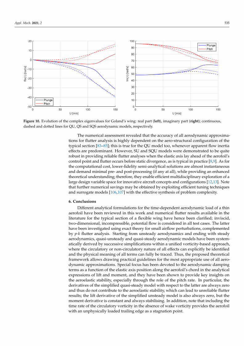
Appl. Mech. 2021, 2 535


pressible fluid at low speeds [7]. Note that the present results for DU and QS models are also in exact agreement with higher-fidelity ones based on a Euler–Bernoulli beam model [86], granting further validation as well as confirming the typical section concept is suit-able for flutter analysis of slender wings in subsonic flow when their aero-structural properties are rather homogeneous and their natural vibration modes are well separated [13].


Goland m (kg/m) μ (kg∙m) xCG (%) kh (N/m) kθ (N∙m/rad) ωh (rad/s) ωθ (rad/s) c (m) xEA (%) ρ (kg/m3) TS [87] 35.72 7.452 43.0 87,480 65,573 49.49 87.08 1.829 33.0 1.225


Goland US QU DU SQU SU QS SQS SS UF (rad/s) 136.8 128.4 62.9 119.6 110.0 33.6 79.7 102.1 ωF (rad/s) 70.0 71.6 88.0 67.6 69.8 94.0 82.6 64.9

kF (-) 0.47 0.51 1.28 0.52 0.58 2.56 0.95 0.58

Figure 9. Evolution of the complex eigenvalues for Goland’s wing: real part (left), imaginary part (right); continuous, dashed and dotted lines for US, SU and SQU aerodynamic models, respectively.

Figure 10. Evolution of the complex eigenvalues for Goland’s wing: real part (left), imaginary part (right); continuous, dashed and dotted lines for QU, QS and SQS aerodynamic models, respectively. Figure 10. Evolution of the complex eigenvalues for Goland’s wing: real part (left), imaginary part (right); continuous,dashed and dotted lines for QU, QS and SQS aerodynamic models, respectively.

The numerical assessment revealed that the accuracy of all aerodynamic approxima-tions for flutter analysis is highly dependent on the aero-structural configuration of thetypical section [83–85]; this is true for the QU model too, whenever apparent flow inertiaeffects are predominant. However, SU and SQU models were demonstrated to be quiterobust in providing reliable flutter analyses when the elastic axis lay ahead of the aerofoil’scontrol point and flutter occurs before static divergence, as is typical in practice [8,9]. As forthe computational cost, lower-fidelity semi-analytical solutions are almost instantaneousand demand minimal pre- and post-processing (if any at all), while providing an enhancedtheoretical understanding; therefore, they enable efficient multidisciplinary exploration of alarge design variable space for innovative aircraft concepts and configurations [12,13]. Notethat further numerical savings may be obtained by exploiting efficient tuning techniquesand surrogate models [106,107] with the effective synthesis of problem complexity.

6. Conclusions

Different analytical formulations for the time-dependent aerodynamic load of a thinaerofoil have been reviewed in this work and numerical flutter results available in theliterature for the typical section of a flexible wing have hence been clarified; inviscid,two-dimensional, incompressible, potential flow is considered in all test cases. The latterhave been investigated using exact theory for small airflow perturbations, complementedby p-k flutter analysis. Starting from unsteady aerodynamics and ending with steadyaerodynamics, quasi-unsteady and quasi-steady aerodynamic models have been system-atically derived by successive simplifications within a unified vorticity-based approach,where the circulatory or non-circulatory nature of all effects can explicitly be identifiedand the physical meaning of all terms can fully be traced. Thus, the proposed theoreticalframework allows drawing practical guidelines for the most appropriate use of all aero-dynamic approximations. Special focus has been devoted to the aerodynamic dampingterms as a function of the elastic axis position along the aerofoil’s chord in the analyticalexpressions of lift and moment, and they have been shown to provide key insights onthe aeroelastic stability, especially through the role of the pitch rate. In particular, thederivatives of the simplified quasi-steady model with respect to the latter are always zeroand thus do not contribute to the aeroelastic stability, which can lead to unreliable flutterresults; the lift derivative of the simplified unsteady model is also always zero, but themoment derivative is constant and always stabilising. In addition, note that including thetime rate of the circulatory vorticity in the absence of wake vorticity provides the aerofoilwith an unphysically loaded trailing edge as a stagnation point.

Appl. Mech. 2021, 2 536

The non-circulatory contributions involve but are not limited to apparent flow inertiaeffects: while the former have been found essential for a reliable representation of bothaeroelastic stability root locus and flutter mechanism, the latter tend to lower the flutterfrequency and become important in the presence of light damping. Neglecting the wake’sinflow eliminates lag effects on the circulatory flow around the aerofoil due to feedbackfrom the shed vorticity (governed by Kutta’s condition at the unloaded trailing edge)and thus avoids an inconvenient formulation for the unsteady airload in both time andfrequency domains. However, some cancellations between circulatory and non-circulatorycontributions do not occur anymore: a degenerate model results that is inherently incon-sistent as well as unstable when the elastic axis lies between the aerofoil’s mid-chord andits control point (i.e., between the second and third quarter chord) and often gives contro-versial flutter results otherwise. It has also been found that higher complexity does notimply higher accuracy and generality, depending on the specific application. In particular,the plunge rate provides all approximations with the same effects: the lift derivative isindependent of the position of the elastic axis and always stabilising, while the momentderivative decreases with the elastic axis moving backward and becomes stabilised onlywhen the latter is beyond the aerodynamic centre (i.e., the first quarter chord). Thus,the aeroelastic stability of a typical section is mostly characterised by the pitch rate, thecontribution of which differs among almost all aerodynamic models. Disregarding thepitch rate in the effective instantaneous angle of attack makes the latter uniform along theaerofoil’s chord and avoids inconvenient singularities, which tend to trigger unphysicalbehaviours for harmonic motion at low reduced frequency: this choice was found to pro-vide the typical section with a more realistic aeroelastic stability boundary even beyondthe hypothesis of quasi-steady flow, especially when either the simplified unsteady orsimplified quasi-unsteady aerodynamic model is employed.

The latter aerodynamic approximations are hence suggested for robust estimationsof the aeroelastic response of a flexible wing in practical cases, whenever the elastic axislies ahead of the control point (i.e., the third quarter chord): they both feature a stabilisingcouple proportional to the pitch rate, but the simplified quasi-unsteady model also embedsapparent flow inertia effects (which are important, as some non-circulatory effects werefound to be induced by the wake’s vorticity within the exact unsteady model). However,within a rigorous assessment from both physical and mathematical perspectives supportedby comprehensive numerical results and sensitivity analyses, their accuracy for flutteranalysis is still found to be dependent on the specific aero-structural configuration, evenwhen the airflow is actually quasi-steady with small aerofoil’s oscillations at a very lowreduced frequency.

Funding: This research received no external funding.

Conflicts of Interest: The author declares no conflict of interest.

Nomenclature

b aerofoil semi-chordc aerofoil chordC(k) Theodorsen’s lift-deficiency functionCL/α sectional lift derivative with respect to angle of attack[Ca], [Cs] aerodynamic and structural damping matricesh sectional plunge displacement (positive upwards)

H(m)n (k) Hankel’s function of n-th order and m-th kind

k, kF reduced frequency of aerofoil oscillations and flutterkh, kϑ stiffness of vertical/flexural and angular/torsional springs[Ka], [Ks] aerodynamic and structural stiffness matrices∆L sectional aerodynamic lift (positive upwards)m sectional mass per unit span

Appl. Mech. 2021, 2 537

∆M sectional aerodynamic moment (positive clockwise)[Ma], [Ms] aerodynamic and structural stiffness matrices∆p sectional net pressure airload along the aerofoil[Qa] aerodynamic load matrixs Laplace’s complex variablet physical timeTj Chebyshev’s polynomialsu, ua horizontal flow velocity (flow perturbation)U horizontal reference airspeedsUF, UD flutter and divergence airspeedsvn vertical aerofoil velocity (flow perturbation)va, vw vertical flow velocity and wake’s inflow (flow perturbation)V vertical velocity of aerofoil’s control pointx, ξ longitudinal coordinates from aerofoil’s mid-chord (positive aft)xCG, xEA longitudinal coordinates of the sectional centre of gravity and elastic axisza aerofoil’s vertical displacementαe f f , αj instantaneous effective angle of attack and Glauert’s coefficientsγ, γa, γw global, aerofoil and wake vorticity distributionsΓ, Γa, Γw global, aerofoil and wake vorticity circulationsζ normalised longitudinal coordinate from aerofoil’s mid-chord (positive aft)ϑ sectional pitch displacement (positive clockwise)µ, µϑ sectional mass moments of inertia at centre of gravity and elastic axisρ air densityσ damping of aerofoil oscillations (real Laplace variable)τ, ς reduced timeφ, φa fluid potential function (flow perturbation)Φ Wagner’s indicial lift functionψ Glauert’s angle along aerofoil chordω, ωF frequencies of aerofoil oscillations and flutter (imaginary Laplace variable)ωh, ωϑ natural frequencies of sectional plunge and pitch modes_χ , χ̃ quasi-steady and unsteady contributions (for any aerodynamic quantity)χC, χN circulatory and non-circulatory contributions (for any aerodynamic quantity)

Appendix A

The overall analytical strategy for modelling unsteady aerodynamic loads may besummarised as follows. Adopting a vorticity-based approach for the incompressiblepotential flow around a thin rigid aerofoil [1,32], the horizontal component of the instan-taneous perturbation velocity is found to be directly proportional to the local vorticityalong the latter [4], whereas the vertical component is given by Hilbert’s formula andmust satisfy both Neumann’s and Kutta–Joukowski’s conditions for inviscid irrotationalflow [3,4]. While Dirichlet’s boundary condition for the asymptotic airflow is inherentlyembedded in the freestream [7], Neumann’s impermeability boundary condition imposesthe airflow as always tangential to aerofoil’s mean line [14]. Kutta’s and Joukowski’stheorems [39,40] establish the resultant aerodynamic force as being normal to freestreamand proportional to circulation, as the airflow leaves the aerofoil’s trailing edge smoothlywith finite speed [7,15]. While Kutta’s condition enforces physical consistence withoutflow singularity at the trailing edge [16,17], Bernoulli’s unsteady linearised equation [4,14]provides the net pressure airload acting across upper and lower surfaces of the aerofoil.Finally, the aerodynamic lift and moment are obtained by integrating such pressure airloadas an explicit function of the aerofoil’s kinematic [5,10].

In particular, for a flat aerofoil the vertical perturbation velocity may alternatively beexpressed using the aerofoil’s impermeability condition and Glauert’s expansion as [7]:

va = vn − vw ≈ U

[∞

∑j=1

αj cos(jψ)− α0

], x = −b cos ψ, (A1)

Appl. Mech. 2021, 2 538

α0 = − 1π

π∫0

(va

U

)dψ, αj =

2π

π∫0

(va

U

)cos(jψ)dψ, Tj = cos(jψ), (A2)

where the latter are Chebyshev’s polynomials of the first kind [32,43], with 0 ≤ ψ ≤ π;these are consistent with a generalised form of the unsteady bound vorticity and circulationthat satisfy Kutta’s condition at the aerofoil’s trailing edge, namely [7]:

γa ≈ 2U

[α0

(1 + cos ψ

sin ψ

)+

∞

∑j=1

αj sin(jψ)

], Γa = 2πbU

(α0 +

α1

2

), (A3)

and can eventually be integrated to give the unsteady airload in terms of Glauert’s coef-ficients αj(t) directly, which include the wake’s inflow [5,33]. Note that this model wasrecently generalised for a thin aerofoil with morphing camber [36–38,43].

However, when the wake’s inflow is marginal, the solution is solely driven by theaerofoil’s kinematics as [7]:

Uα0 = Uϑ−.h− xEA

.ϑ, Uα1 = b

.ϑ, αj = 0, vw = 0, (A4)

and the vorticity distribution along the aerofoil’s chord reduces to:_γ a = 2U

[α0

(1 + cos ψ

sin ψ

)+ α1 sin ψ

],

1 + cos ψ

sin ψ=

√b− xb + x

, sin ψ =

√1− x2

b2 , (A5)

which coincides with the expression found by thin aerofoil theory [15,36] and provides theaerofoil’s trailing edge with a stagnation point (i.e.,

_γ a(b, t) = 0 regardless of the motion of

the typical section). After integration of the pressure distribution [7]:

∆p = ρ

U_γ a +

∂

∂t

x∫−b

_γ adξ

, αe f f = α0 +α1

2, (A6)

the total lift and moment around the elastic axis read:

∆L = 2πρUb[U(α0 +

α12)+ b

2(3

.α0 +

.α1)]

,

∆M = 2πρUb{

U[(

b2 + xEA

)α0 +

xEA2 α1

]+ b

2

[(3xEA − b

2

) .α0 +

(xEA − b

2

) .α1

]};

(A7)

however, note that the aerofoil’s trailing edge is loaded unless the rate of change of thebound circulation is marginal. It is also worth stressing that the bound circulation isindeed proportional to the airfoil’s instantaneous kinematics at the control point, as per anequivalent lumped-vortex model in steady airflow [30] where the counter-rotating wakevortex is infinitely far behind the aerofoil.

When all apparent inertia terms are also negligible, the pressure distribution grantsan unloaded trailing edge and the aerofoil’s quasi-steady airload simplifies to [28]:

∆p = ρU_γ a, ∆L = 2πρU2b

(α0 +

α1

2

), ∆M = 2πρU2b

[(b2+ xEA

)α0 +

xEA2

α1

], (A8)

where the rate of change of the bound circulation is also disregarded.

References1. Jones, R.T. Classical Aerodynamic Theory; NASA-RP-1050; NASA: Washington, DC, USA, 1979.2. Dowell, E.H. A Modern Course in Aeroelasticity; Springer: Berlin/Heidelberg, Germany, 2004.3. Gulcat, U. Fundamentals of Modern Unsteady Aerodynamics; Springer: Berlin/Heidelberg, Germany, 2011.4. Bisplinghoff, R.L.; Ashley, H.; Halfman, R.L. Aeroelasticity; Dover: Mineola, NY, USA, 1996.5. Peters, D.A. Two-Dimensional Incompressible Unsteady Airfoil Theory–A Review. J. Fluids Struct. 2008, 24, 295–312. [CrossRef]6. Hodges, D.; Pierce, G. Introduction to Structural Dynamics and Aeroelasticity; Cambridge University Press: Cambridge, UK, 2002.7. Katz, J.; Plotkin, A. Low-Speed Aerodynamics; Cambridge University Press: Cambridge, UK, 2001.8. Bisplinghoff, R.L.; Ashley, H. Principles of Aeroelasticity; Dover: Mineola, NY, USA, 2013.9. Wright, J.R.; Cooper, J.E. Introduction to Aircraft Aeroelasticity and Loads; Wiley: Hoboken, NJ, USA, 2014.

http://doi.org/10.1016/j.jfluidstructs.2007.09.001

Appl. Mech. 2021, 2 539

10. Leishman, J.G. Principles of Helicopter Aerodynamics; Cambridge University Press: Cambridge, UK, 2006.11. Berci, M. Semi-analytical static aeroelastic analysis and response of flexible subsonic wings. Appl. Math. Comput. 2015, 267,

148–169. [CrossRef]12. Berci, M.; Cavallaro, R. A Hybrid Reduced-Order Model for the Aeroelastic Analysis of Flexible Subsonic Wings—A Parametric

Assessment. Aerospace 2018, 5, 76. [CrossRef]13. Berci, M.; Torrigiani, F. Multifidelity Sensitivity Study of Subsonic Wing Flutter for Hybrid Approaches in Aircraft Multidisci-

plinary Design and Optimisation. Aerospace 2020, 7, 161. [CrossRef]14. Newman, J.N. Marine Hydrodynamics; MIT Press: Cambridge, MA, USA, 1977.15. Epps, B.P.; Roesler, B.T. Vortex Sheet Strength in the Sears, Küssner, Theodorsen, and Wagner Aerodynamics Problems. AIAA J.

2018, 56, 889–904. [CrossRef]16. Theodorsen, T. General Theory of Aerodynamic Instability and the Mechanism of Flutter; NACA-TR-496; NACA: Washington, DC,

USA, 1935.17. Wagner, H. Uber die Entstenhung des Dynamischen Auftriebes von Tragflugeln. Z. Angew. Math. und Mech. 1925, 5, 17–35.

[CrossRef]18. Dimitriadis, G. Introduction to Nonlinear Aeroelasticity; Wiley: Hoboken, NJ, USA, 2017.19. Dennis, S.T. Undergraduate Aeroelasticity: The Typical Section Idealization Re-Examined. Int. J. Mech. Eng. Educ. 2013, 41, 72–91.

[CrossRef]20. Weisshaar, T.A. Static and Dynamic Aeroelasticity. In Encyclopedia of Aerospace Engineering; Wiley: Hoboken, NJ, USA, 2010.21. Quarteroni, A.; Rozza, G. Reduced Order Methods for Modeling and Computational Reduction; Springer International Publishing:

Cham, Switzerland, 2014.22. Qu, Z.Q. Model. Order Reduction Techniques with Applications in Finite Element Analysis; Springer: Berlin/Heidelberg, Germany,

2004.23. Silva, W.A. AEROM: NASA’s Unsteady Aerodynamic and Aeroelastic Reduced-Order Modeling Software. Aerospace 2018, 5, 41.

[CrossRef]24. Theodorsen, T.; Garrick, L.E. Flutter Calculations in Three Degrees of Freedom; NACA-TR-741; NASA: Washington, DC, USA, 1942.25. Theodorsen, T.; Garrick, L.E. Nonstationary Flow about a Wing-Aileron-Tab Combination Including Aerodynamic Balance; NACA-736;

NASA: Washington, DC, USA, 1942.26. Zeiler, T.A. Results of Theodorsen and Garrick Revisited. J. Aircr. 2000, 37, 918–920. [CrossRef]27. Kussner, H.G.; Schwartz, I. The Oscillating Wing with Aerodynamically Balanced Elevator; NACA-TM-991; NASA: Washington, DC,

USA, 1941.28. Fung, Y.C. An Introduction to the Theory of Aeroelasticity; Dover: Mineola, NY, USA, 1993.29. Yang, B. Strain, Stress and Structural Dynamics; Elsevier: Amsterdam, The Netherlands, 2005.30. Karamcheti, K. Principles of Ideal-Fluid Aerodynamics; Wiley: New York, NY, USA, 1967.31. Prandtl, L. Applications of Modern Hydrodynamics to Aeronautics; NACA-TR-116; NASA: Washington, DC, USA, 1921.32. Glauert, H. The Elements of Aerofoil and Airscrew Theory; Cambridge University Press: Cambridge, UK, 1983.33. Von Karman, T.; Sears, W.R. Airfoil Theory for Non-Uniform Motion. J. Aeronaut. Sci. 1938, 5, 379–390. [CrossRef]34. Jones, R.T. The Unsteady Lift of a Wing of Finite Aspect Ratio; NACA-TR-681; NASA: Washington, DC, USA, 1940.35. Anderson, J.D. Fundamentals of Aerodynamics; McGraw-Hill: New York, NY, USA, 2017.36. Johnston, C.O. Review, Extension and Application of Unsteady Thin Airfoil Theory; CIMSS-04-101; CIMSS: Madison, WI, USA, 2004.37. Johnston, C.O.; Mason, W.H.; Han, C. Unsteady thin airfoil theory revisited for a general deforming airfoil. J. Mech. Sci. Technol.

2010, 24, 2451–2460. [CrossRef]38. Gaunaa, M. Unsteady 2D Potential-Flow Forces on a Thin Variable Geometry Airfoil Undergoing Arbitrary Motion; Risø–R–1478; Risø:

Roskilde, Denmark, 2006.39. Kutta, W.M. Auftriebskräfte in Strömenden Flüssigkeiten. Illus. Aeronaut. Mitt. 1902, 6, 133–135.40. Joukowski, N.E. Sur les Tourbillons Adjionts. Traraux Sect. Phys. Soc. Imp. Amis Sci. Nat. 1906, 13, 261–284.41. Bungartz, H.J.; Schafer, M. Fluid-Structure Interaction: Modelling, Simulation, Optimization; Springer: Berlin/Heidelberg, Germany,

2006.42. Neumark, S. Vortex Pressure Distribution on an Airfoil in Nonuniform Motion. J. Aeronaut. Sci. 1952, 19, 214–215. [CrossRef]43. Peters, D.A.; Hsieh, M.-C.A.; Torrero, A. A State-Space Airloads Theory for Flexible Airfoils. J. Am. Helicopter Soc. 2007, 52,

329–342. [CrossRef]44. Queijo, M.J.; Wells, W.R.; Keskar, D.A. Approximate Indicial Lift Function for Tapered, Swept Wings in Incompressible Flow; NASA-TP-

1241; NASA: Washington, DC, USA, 1978.45. Berci, M.; Righi, M. An enhanced analytical method for the subsonic indicial lift of two-dimensional aerofoils–with numerical

cross-validation. Aerosp. Sci. Technol. 2017, 67, 354–365. [CrossRef]46. Righi, M.; Berci, M. On Elliptical Wings in Subsonic Flow: Indicial Lift Generation via CFD Simulations-with Parametric Analytical

Approximations. ASD J. 2019, 7, 1–17.47. Ronch, A.D.A.; Ventura, A.; Righi, M.; Franciolini, M.; Berci, M.; Kharlamov, D. Extension of analytical indicial aerodynamics to

generic trapezoidal wings in subsonic flow. Chin. J. Aeronaut. 2018, 31, 617–631. [CrossRef]48. Jones, W.P. Aerodynamic Forces on Wings in Non-Uniform Motion; ARC-R&M-2117; ARC: London, UK, 1945.

http://doi.org/10.1016/j.amc.2015.04.095

http://doi.org/10.3390/aerospace5030076


http://doi.org/10.2514/1.J056399

http://doi.org/10.1002/zamm.19250050103

http://doi.org/10.7227/IJMEE.41.1.7


http://doi.org/10.2514/2.2691

http://doi.org/10.2514/8.674

http://doi.org/10.1007/s12206-010-0920-4

http://doi.org/10.2514/8.2219

http://doi.org/10.4050/JAHS.52.329

http://doi.org/10.1016/j.ast.2017.03.004

http://doi.org/10.1016/j.cja.2018.02.008

Appl. Mech. 2021, 2 540

49. Berci, M. Lift-Deficiency Functions of Elliptical Wings in Incompressible Potential Flow: Jones’ Theory Revisited. J. Aircr. 2016, 53,599–602, Erratum in 2017, 54, 1–2. [CrossRef]

50. Boutet, J.; Dimitriadis, G. Unsteady Lifting Line Theory Using the Wagner Function for the Aerodynamic and AeroelasticModeling of 3D Wings. Aerospace 2018, 5, 92. [CrossRef]

51. Sears, W.R. Operational methods in the theory of airfoils in non-uniform motion. J. Frankl. Inst. 1940, 230, 95–111. [CrossRef]52. Vepa, R. Finite State Modeling of Aeroelastic Systems; NASA-CR-2779; NASA: Washington, DC, USA, 1977.53. Berci, M.; Dimitriadis, G. A combined Multiple Time Scales and Harmonic Balance approach for the transient and steady-state

response of nonlinear aeroelastic systems. J. Fluids Struct. 2018, 80, 132–144. [CrossRef]54. Reissner, E. On the General Theory of Thin Airfoils for Non-Uniform Motion; NACA-TN-946; NASA: Washington, DC, USA, 1944.55. Radok, J.R.M. The Theory of Aerofoils in Unsteady Motion. Aeronaut. Q. 1952, 3, 297–320. [CrossRef]56. Van De Vooren, A.I. Unsteady Aerofoil Theory. Adv. Appl. Mech. 1958, 5, 35–89.57. Perry, B. Comparison of Theodorsen’s Unsteady Aerodynamic Forces with Doublet Lattice Generalized Aerodynamic Forces; NASA/TM–

2017-219667; NASA: Washington, DC, USA, 2017.58. Mateescu, D.; Abdo, M. Theoretical Solutions for Unsteady Flows Past Oscillating Flexible Airfoils Using Velocity Singularities.

J. Aircr. 2003, 40, 153–163. [CrossRef]59. Berci, M.; Gaskell, P.H.; Hewson, R.W.; Toropov, V.V. A semi-analytical model for the combined aeroelastic behaviour and gust

response of a flexible aerofoil. J. Fluids Struct. 2013, 38, 3–21. [CrossRef]60. Kemp, N.H.; Homicz, G. Approximate unsteady thin-airfoil theory for subsonic flow. AIAA J. 1976, 14, 1083–1089. [CrossRef]61. Mateescu, D. Theoretical Solutions for Unsteady Compressible Subsonic Flows Past Oscillating Rigid and Flexible Airfoils. Math.

Eng. Sci. Aerosp. 2011, 2, 1–27.62. Hewson-Browne, R.C. The Oscillation of a Thick Aerofoil in an Incompressible Flow. Q. J. Mech. Appl. Math. 1963, 16, 79–92.

[CrossRef]63. Woods, L.C. The Lift and Moment Acting on a Thick Aerofoil in Unsteady Motion. Philosophical Transactions of the Royal

Soci-ety of London-Series, A. Math. Phys. Sci. 1954, 247, 131–162.64. Giesing, J.P. Nonlinear two-dimensional unsteady potential flow with lift. J. Aircr. 1968, 5, 135–143. [CrossRef]65. Riso, C.; Riccardi, G.; Mastroddi, F. Semi-analytical unsteady aerodynamic model of a flexible thin airfoil. J. Fluids Struct. 2018, 80,

288–315. [CrossRef]66. Liu, T.; Wang, S.; Zhang, X.; He, G. Unsteady Thin-Airfoil Theory Revisited: Application of a Simple Lift Formula. AIAA J. 2015,

53, 1492–1502. [CrossRef]67. Ericsson, L.E.; Reding, J.P. Unsteady Airfoil Stall, Review and Extension. J. Aircr. 1971, 8, 609–616. [CrossRef]68. Ahaus, L. An Airloads Theory for Morphing Airfoils in Dynamic Stall with Experimental Correlation; Washington University in St.

Louis: St. Louis, MO, USA, 2010.69. Hoblit, F.M. Gust Loads on Aircraft: Concepts and Applications; American Institute of Aeronautics and Astronautics (AIAA): Reston,

VA, USA, 1988.70. Kussner, H.G. Zusammenfassender Beritch uber den Instationaren Auftrieb von Flugeln. Luftfahrtforsch 1936, 13, 410–424.71. Kayran, A. Kussner’s Function in the Sharp Edged Gust Problem–A Correction. J. Aircr. 2006, 43, 1596–1599. [CrossRef]72. Jones, A.R.; Cetiner, O. Overview of Unsteady Aerodynamic Response of Rigid Wings in Gust Encounters. AIAA J. 2021, 59,

731–736. [CrossRef]73. Garrick, L.E. On Some Reciprocal Relations in the Theory of Nonstationary Flows; NACA-TR-629; NASA: Washington, DC, USA, 1938.74. Sears, W.R.; Kuethe, A.M. The Growth of the Circulation of an Airfoil Flying through a Gust. J. Aeronaut. Sci. 1939, 6, 376–378.

[CrossRef]75. Pratt, K.G. A Revised Formula for the Calculation of Gust Loads; NACA-TN-2964; NASA: Washington, DC, USA, 1953.76. Basu, B.C.; Hancock, G.J. The unsteady motion of a two-dimensional aerofoil in incompressible inviscid flow. J. Fluid Mech. 1978,

87, 159–178. [CrossRef]77. Berci, M.; Mascetti, S.; Incognito, A.; Gaskell, P.H.; Toropov, V.V. Dynamic Response of Typical Section Using Variable-Fidelity

Fluid Dynamics and Gust-Modeling Ap-proaches–With Correction Methods. J. Aerosp. Eng. 2014, 27, 1–24. [CrossRef]78. Zimmerman, N.H.; Weissenburger, J.T. Prediction of flutter onset speed based on flight testing at subcritical speeds. J. Aircr. 1964,

1, 190–202. [CrossRef]79. Rodden, W.P. Theoretical and Computational Aeroelasticity; Crest Publishing: Los Angeles, CA, USA, 2011.80. Hancock, G.J.; Wright, J.R.; Simpson, A. On the Teaching of the Principles of Wing Flexure-Torsion Flutter. Aeronaut. J. 1985, 89,

285–305.81. Miles, J.W. Quasi-stationary airfoil theory. J. Aeronaut. Sci. 1949, 16, 440.82. Miles, J.W. Quasi-stationary airfoil theory in subsonic compressible flow. J. Aeronaut. Sci. 1949, 16, 509. [CrossRef]83. Goland, M. The Quasi-Steady Air Forces for Use in Low-Frequency Stability Calculations. J. Aeronaut. Sci. 1950, 17, 601–608.

[CrossRef]84. Dugundji, J. Effect of Quasi-Steady Air Forces on Incompressible Bending-Torsion Flutter. J. Aerosp. Sci. 1958, 25, 119–121.

[CrossRef]85. Gravitz, S.I.; Laidlaw, W.R.; Bryce, W.W.; Cooper, R.E. Development of a Quasi-Steady Approach to Flutter and Correlation With

Kernel-Function Results. J. Aerosp. Sci. 1962, 29, 445–459. [CrossRef]

http://doi.org/10.2514/1.C033515


http://doi.org/10.1016/S0016-0032(40)90651-2


http://doi.org/10.1017/S000192590000072X

http://doi.org/10.2514/2.3070


http://doi.org/10.2514/3.7188

http://doi.org/10.1093/qjmam/16.1.79

http://doi.org/10.2514/3.43920


http://doi.org/10.2514/1.J053439

http://doi.org/10.2514/3.59146

http://doi.org/10.2514/1.20298

http://doi.org/10.2514/1.J059602

http://doi.org/10.2514/8.897

http://doi.org/10.1017/S0022112078002980

http://doi.org/10.1061/(ASCE)AS.1943-5525.0000336

http://doi.org/10.2514/3.43581

http://doi.org/10.1090/qam/38195

http://doi.org/10.2514/8.1747

http://doi.org/10.2514/8.7525

http://doi.org/10.2514/8.9485

Appl. Mech. 2021, 2 541

86. Haddadpour, H.; Firouz-Abadi, R. Evaluation of quasi-steady aerodynamic modeling for flutter prediction of aircraft wings inincompressible flow. Thin-Walled Struct. 2006, 44, 931–936. [CrossRef]

87. Torrigiani, F.; Berci, M. Multifidelity Parametric Aeroelastic Stability Analyses of Goland’s Wing. In AIAA Scitech 2021 Forum;American Institute of Aeronautics and Astronautics (AIAA): Reston, VA, USA, 2021.

88. Hassig, H.J. An approximate true damping solution of the flutter equation by determinant iteration. J. Aircr. 1971, 8, 885–889.[CrossRef]

89. Mantegazza, P.; Cardani, C. Continuation and Direct Solution of the Flutter Equation. Comput. Struct. 1978, 8, 185–192. [CrossRef]90. Theodorsen, T.; Garrick, L.E. Mechanism of Flutter–A Theoretical and Experimental Investigation of the Flutter Problem; NACA-TR-685;

NASA: Washington, DC, USA, 1938.91. Biot, M.A.; Arnold, L. Low-Speed Flutter and Its Physical Interpretation. J. Aeronaut. Sci. 1948, 15, 232–236. [CrossRef]92. Dugundji, J. A Nyquist Approach to Flutter. J. Aeronaut. Sci. 1952, 19, 422–423. [CrossRef]93. Rheinfurth, M.; Swift, F. A New Approach to the Explanation of the Flutter Mechanism; NASA-TN-D-3125; NASA: Washington, DC,

USA, 1966.94. Goland, M.; Luke, Y.L. A Study of the Bending-Torsion Aeroelastic Modes for Aircraft Wings. J. Aeronaut. Sci. 1949, 16, 389–396.

[CrossRef]95. Balakrishnan, A.V.; Iliff, K.W. Continuum Aeroelastic Model for Inviscid Subsonic Bending-Torsion Wing Flutter. J. Aerosp. Eng.

2007, 20, 152–164. [CrossRef]96. Cicala, P. Comparison of Theory with Experiment in the Phenomenon of Wing Flutter; NACA-TM-887; NASA: Washington, DC, USA,

1939.97. Bollay, W.; Brown, C.D. Some Experimental Results on Wing Flutter. J. Aeronaut. Sci. 1941, 8, 313–318. [CrossRef]98. National Oceanic and Atmospheric Administration. US Standard Atmosphere; NASA TM-X-74335; NASA: Washington, DC, USA,

1976.99. Goland, M. The Flutter of a Uniform Cantilever Wing. J. Appl. Mech. 1945, 12, A197–A208. [CrossRef]100. Goland, M.; Luke, Y.L. The Flutter of a Uniform Wing with Tip Weights. J. Appl. Mech. 1948, 15, 13–20. [CrossRef]101. Banerjee, J.R. Flutter Sensitivity Studies of High Aspect Ratio Aircraft Wings. WIT Trans. Built Environ. 1993, 2, 374–387.102. Sotoudeh, Z.; Hodges, D.H.; Chang, C.S. Validation Studies for Aeroelastic Trim and Stability Analysis of Highly Flexible Aircraft.

J. Aircr. 2010, 47, 1240–1247. [CrossRef]103. Palacios, R.; Epureanu, B. An Intrinsic Description of the Nonlinear Aeroelasticity of Very Flexible Wings. In Proceedings of the

52nd AIAA/ASME/ASCE/AHS/ASC Structures, Structural Dynamics and Materials Conference, Denver, CO, USA, 4–7 April2011; American Institute of Aeronautics and Astronautics (AIAA): Reston, VA, USA, 2011.

104. Wang, Z.; Chen, P.C.; Liu, D.D.; Mook, D.T.; Patil, M. Time Domain Nonlinear Aeroelastic Analysis for HALE Wings. InProceedings of the 47th AIAA/ASME/ASCE/AHS/ASC Structures, Structural Dynamics, and Materials Conference 14thAIAA/ASME/AHS Adaptive Structures Conference 7th, Newport, RI, USA, 1–4 May 2006; American Institute of Aeronauticsand Astronautics (AIAA): Reston, VA, USA, 2006.

105. Murua, J.; Palacios, R.; Graham, J.M. Modeling of Nonlinear Flexible Aircraft Dynamics Including Free-Wake Effects. InProceedings of the AIAA Atmospheric Flight Mechanics Conference, Grapevine, TX, USA, 9–13 January 2017; American Instituteof Aeronautics and Astronautics (AIAA): Reston, VA, USA, 2010.

106. Berci, M.; Gaskell, P.H.; Hewson, R.W.; Toropov, V.V. Multifidelity metamodel building as a route to aeroelastic optimization offlexible wings. Proc. Inst. Mech. Eng. Part C J. Mech. Eng. Sci. 2011, 225, 2115–2137. [CrossRef]

107. Berci, M.; Toropov, V.V.; Hewson, R.W.; Gaskell, P.H. Multidisciplinary multifidelity optimisation of a flexible wing aerofoil withreference to a small UAV. Struct. Multidiscip. Optim. 2014, 50, 683–699. [CrossRef]

http://doi.org/10.1016/j.tws.2006.08.020

http://doi.org/10.2514/3.44311

http://doi.org/10.1016/0045-7949(78)90021-4

http://doi.org/10.2514/8.11552

http://doi.org/10.2514/8.2314

http://doi.org/10.2514/8.11818

http://doi.org/10.1061/(ASCE)0893-1321(2007)20:3(152)

http://doi.org/10.2514/8.10724

http://doi.org/10.1115/1.4009489

http://doi.org/10.1115/1.4009753

http://doi.org/10.2514/1.46974

http://doi.org/10.1177/0954406211403549

http://doi.org/10.1007/s00158-014-1066-2

On Aerodynamic Models for Flutter Analysis - MDPI

Documents

Transcript of On Aerodynamic Models for Flutter Analysis - MDPI