TORSION FLUTTER Philip Curtis Wheeler, Master of Science
150
ABSTRACT Title of Thesis: AN EXPLICATION OF AI RFOIL SECTION BENDIN G- TORSION FLUTTER Philip Curtis Wheeler, Master of Science, 2004 Thesis directed by: Professor Ricardo Medina Department of Civil and Environmental Engineering This thesis examines the dynamic instability known as flutter using a two-degree-of-freedom airfoil section model in both quasi-steady and unsteady flow. It explains the fundamental forces and moments involved in the bending-torsion flutter of an airfoil section, and demonstrates a solution method for determining the critical flutter frequency and speed for
-
Upload
khangminh22 -
Category
Documents
-
view
0 -
download
0
Transcript of TORSION FLUTTER Philip Curtis Wheeler, Master of Science

ABSTRACT
Title of Thesis: AN EXPLICATION OF AIRFOIL SECTION BENDIN G-
TORSION FLUTTER
Philip Curtis Wheeler, Master of Science, 2004
Thesis directed by: Professor Ricardo Medina
Department of Civil and Environmental Engineering
This thesis examines the dynamic instability known as flutter using
a two-degree-of-freedom airfoil section model in both quasi-steady and
unsteady flow. It explains the fundamental forces and moments involved
in the bending-torsion flutter of an airfoil section, and demonstrates a
solution method for determining the critical flutter frequency and speed for

both flow cases. Additionally, through the use of a programmed Mathcad
11 worksheet, it evaluates the flutter characteristics of six example
sections, illustrating the effects of the elastic, inertial and aerodynamic
properties of an airfoil section. For each section, a parametric study of the
effect of the section Center of Gravity position along the section chord is
performed. The flutter frequency and speed are calculated using both
quasi-steady and unsteady aerodynamic forces and moments, and the
results compared. Software used was MathSoft Mathcad 11, Microsoft
Word and Intergraph Smart Sketch LE.

AN EXPLICATION OF AIRFOIL SECTION BENDING-TORSION
FLUTTER
by
Philip Curtis Wheeler
Thesis submitted to the Faculty of the Graduate School of the
University of Maryland, College Park in partial fulfillment
of the requirements for the degree of
Master of Science
2004
Advisory Committee:
Professor Ricardo Medina, Chair
Professor Pedro Albrecht
Professor Bruce K. Donaldson

©Copyright by
Philip Curtis Wheeler
2004

ii
Acknowledgements
The author wishes to thank Dr. Bruce Donaldson for his assistance
in preparing this scholarly paper.
The author also wishes to thank Dr. Ricardo Medina and Dr. Pedro
Albrecht for their review of this paper.

iii
This Page Intentionally Left Blank

iv
Table of Contents
List of Tables..................................................................................... xList of Figures.................................................................................... xiList of Symbols and Abbreviations .................................................... xii
Chapter 1.0: Introduction................................................................... 1
1.1 Motivation for the thesis................................................... 11.2 Objectives of the thesis ................................................... 21.3 Thesis Organization......................................................... 31.4 Chapter Summary ........................................................... 3
Chapter 2.0: A Fundamental Description of Flutter ........................... 5
2.1 Types of Aeroelasticity ..................................................... 5
2.2 Distinctive Characteristics of Classical Airfoil Section Flutter ........................................................................ 8
2.3 Types of Airfoil Section Flutter ......................................... 10
2.3.1 Vibratory modes.................................................. 11
2.3.2 Examples of Airfoil Section Flutter withIncreasing Numbers of Types of Motion ...................... 11
2.4 Bending-torsion Flutter of an Airfoil Section as Described in this Thesis ......................................................... 12
2.4.1 Defining the Degrees of Freedom...................... 14
2.5 Chapter Summary ........................................................... 15

v
Chapter 3.0: Solutions for the Flutter Frequency and Speed ............ 17
3.1 Derivation of the Lagrange Equations of Motion.............. 17
3.1.1 Strain Energy of Elastic Forces.......................... 193.1.2 Kinetic Energy of Inertial Forces ........................ 193.1.3 Generalized Forces ........................................... 20
3.2 Writing the Lagrange Equations of Motion....................... 21
3.3 Energy Transfer and Coupling......................................... 24
3.3.1 Energy Transfer from the Airstream................... 243.3.2 Inertial coupling due to Center of Gravity location ............................................................ 253.3.3 Phasing of the Motions ...................................... 263.3.4 Aerodynamic Coupling via Phasing ................... 26
3.4 Frequency Coalescence.................................................. 28
3.5 Phasing Diagrams ........................................................... 29
3.5.1 Stable Condition ................................................ 293.5.2 Critical Flutter Condition..................................... 303.5.3 Full Flutter Condition.......................................... 31
3.6 Aerodynamic Forces........................................................ 32
3.6.1 Fluid Properties................................................... 333.6.2 Basic strip theory ............................................... 353.6.3 Two Dimensional Airfoil Section Properties ....... 363.6.4 Development of the Quasi-steady Aerodynamic Forces.................................................... 37
3.6.4.1 Aerodynamic Moment .......................... 383.6.4.2 Forming the Lagrange Equations of Motion using Quasi-steady AerodynamicForces ............................................................... 40
3.6.5 Development of the Unsteady Aerodynamic Forces.................................................... 42

vi
3.6.5.1 Forming the Lagrange Equations of Motion using Unsteady Aerodynamic Forcesand Moments .................................................... 43
3.6.5.1.1 Finding the flutter frequency and speed – Theodorsen’s Method............... 443.6.5.1.2 Finding the flutter frequency and speed – Materiel Center Method ............ 45
3.7 Solution of the Double Eigenvalue Problem .................... 46
3.7.1 Placing the System in Simple Harmonic Motion.......................................................... 47
3.7.1.1 Flutter Solution in the case of Quasi-steady Aerodynamic Forces ................... 493.7.1.2 Flutter Solution in the Case of Unsteady Aerodynamic Forces and Moments .. 51
3.8 Chapter Summary ........................................................... 61
Chapter 4.0: Calculation of Flutter Properties by Mathcad Worksheet ..... . .......... ................................................... 63
4.1 Mathcad Worksheet Methodology ................................... 63
4.1.1 Program inputs .................................................. 644.1.2 Supporting calculations...................................... 65
4.1.2.1 Quasi-steady Case................................ 654.1.2.2 Unsteady Case...................................... 65
4.1.3 Primary calculations........................................... 67
4.1.3.1 Quasi-steady Case............................... 674.1.3.2 Unsteady Case..................................... 67
4.1.4 Program Outputs ............................................... 68
4.2 Example Calculations . .................................................... 69
4.2.1 Example One: Ryan NYP prototype

vii
(Blevins, 1990)........ .................................................... 70
4.2.1.1 Inputs, Intermediate Calculations and Output .................................................... 704.2.1.2 Section Characteristics ......................... 714.2.1.3. Flutter Calculations for the Quasi-steady Case............................................ 724.2.1.4 Flutter Calculations for the Unsteady Case ................................................. 724.2.1.5 Comparison of Results in the Quasi-steady and Unsteady Cases ............................. 734.2.1.6 CG Variation Survey ............................ 73
4.2.2 Example Two: Ryan NYP Final Design (Blevins, 1990)........ .................................................... 75
4.2.2.1 Inputs, Intermediate Calculations and Outputs .................................................... 754.2.2.2 Section Characteristics ......................... 764.2.2.3. Flutter Calculations for the Quasi-steady Case............................................ 764.2.2.4 Flutter Calculations for the Unsteady Case ................................................. 774.2.2.5 Comparison of Results in the Quasi-steady and Unsteady Cases ............................. 784.2.2.6 CG Variation Survey ............................ 78
4.2.3 Example Three: MD3-160 Aircraft Section(Usmani, Ho, 2003). .................................................... 79
4.2.3.1 Inputs, Intermediate Calculations and Outputs .................................................... 794.2.3.2 Section Characteristics ......................... 804.2.3.3. Flutter Calculations for the Quasi-steady Case............................................ 814.2.3.4 Flutter Calculations for the Unsteady Case ................................................. 814.2.3.5 Comparison of Results in the Quasi-steady and Unsteady Cases ............................. 824.2.3.6 Altitude Variation Survey...................... 824.2.2.7 CG Variation Survey ............................ 84

viii
4.2.4 Example Four: Example from NACA TechnicalReport 685, (Theodorsen, Garrick, 1938) .................. 85
4.2.4.1 Inputs, Intermediate Calculations and Outputs .................................................... 854.2.4.2 Section Characteristics ......................... 864.2.4.3. Flutter Calculations for the Quasi-steady Case............................................ 874.2.4.4 Flutter Calculations for the Unsteady Case ................................................. 874.2.4.5 Comparison of Results in the Quasi-steady and Unsteady Cases ............................. 874.2.4.6 CG Variation Survey .......................... 88
4.2.5 Example Five: Example from USAAF Technical Report 4798, (Smilg, Wasserman, 1942).................... 89
4.2.5.1 Inputs, Intermediate Calculations and Outputs .................................................... 894.2.5.2 Section Characteristics ......................... 904.2.5.3. Flutter Calculations for the Quasi-steady Case............................................ 914.2.5.4 Flutter Calculations for the Unsteady Case ................................................. 914.2.5.5 Comparison of Results in the Quasi-steady and Unsteady Cases ............................. 914.2.5.6 CG Variation Survey .......................... 92
4.2.6 Example Six: Example from Reference 5, page 203 (Scanlan, Rosenbaum, 1968) .................... 93
4.2.6.1 Inputs, Intermediate Calculations and Outputs .................................................... 934.2.6.2 Section Characteristics ......................... 944.2.6.3. Flutter Calculations for the Quasi-steady Case............................................ 944.2.6.4 Flutter Calculations for the Unsteady Case ................................................. 954.2.6.5 Comparison of Results in the Quasi-steady and Unsteady Cases ............................. 954.2.6.6 CG Variation Survey .......................... 95
4.3 Chapter Summary ...... .................................................... 97

ix
Appendix .......... .......... .......... .................................................... 103References .......... .......... .......... .................................................... 125

x
List of Tables
Table 3.6.3: Airfoil Section Data .................................................... 36
Table 4.2.3.7: Flutter Speed Variation with Altitude ......................... 83
Table 4.3: Summary of Program Inputs, Calculations and Outputs.. 99

xi
List of Figures
Figure 2.1: Summary of Forces and Responses .............................. 6
Figure 2.4: Two DOF Model ........ .................................................... 14
Figure 3.3.2: Inertial Coupling as a Function of CG Position............ 26
Figure 3.5.1: Stable Vertical and Torsional Oscillations ................... 30
Figure 3.5.2: Critical Flutter (Stability Boundary) Condition.............. 31
Figure 3.5.3: Full Flutter Condition ................................................... 32
Figure 3.6.2: Basic Strip Theory .................................................... 35
Figure 3.6.3: Lift Curve and Aerodynamic Moment Slopes .............. 40
Figure 3.7.1.2.1: Artificial Damping versus Reduced Frequency...... 60
Figure 3.7.1.2.2: Artificial Damping versus Velocity ......................... 61
Figure 4.2.3.7: Graph of Flutter Speed Variation with Altitude ......... 83

xii
List of Symbols and Abbreviations
Symbol Definition Unit
a Distance from section elastic axis
to section aerodynamic center, positive
forward of elastic axis.
in
ah Location of section elastic axis
from section midchord, positive aft
of midchord.
Non-
Dimensional
b Distance from section elastic axis
to section center of gravity, positive
forward of elastic axis, equal to ah xα−( ) b'⋅
in
b' Section semi-chord, equal to c/2. in
c Section chord; distance from the leading
edge to trailing edge, positive aft of leading
edge.
in
fb Uncoupled bending frequency Hz
ffl Coupled flutter frequency using unsteady
aerodynamics
Hz
ffQS Coupled flutter frequency using
quasi-steady aerodynamics
Hz
fT Uncoupled torsional frequency Hz
g Artificial damping coefficient, a variable
used in the solution of the flutter stability
determinant.
Non- Dimensional
deg Degrees

xiii
h Vertical translation of section; first
degree of freedom of section, measured
for the Quasi-steady case positive up
from the elastic axis, and for the
Unsteady case positive down.
in
Non - Dimensionalized vertical translation
of section
i 1−
k Reduced frequency, the ratio between the
section oscillation frequency and the
fictitious frequency equal to the number of
times per second the section, due to its
forward speed, traverses a distance equal
to its semi-schord; equal toωfl b'⋅
Vfl.
Non- Dimensional
kb Section bending stiffness per
unit span
knots Nautical miles per hour
lbf Pound force pounds
m Section mass per unit span
q Dynamic pressurelbf
in2
qD Static divergence dynamic pressurelbf
in2
rα Dimensionless section radius of
gyration per unit span about the
EA, equal to Hea
m b'2⋅
Non- Dimensional
Non- Dimensional hb'
in lbf⋅in
slug

xiv
rad Radians
t Time seconds
w Section span in
w.r.t. Abbreviation for "with respect to"
xα Location of section CG, positive aft
of EA.
Non- Dimensional
A Bending flutter determinant element
for h/b'
Non- Dimensional
A0 Aerodynamic lift factor , equal to 12ρ⋅ S⋅ Clα⋅
slug in⋅rad
B Bending flutter determinant elementfor α
Non- Dimensional
C(k) Theodorsen's Circulation function, equal to F k( ) i G k( )⋅+
Non- Dimensional
CG Location of section center of gravity,
positive aft of leading edge.
in
Cl Section lift coefficient Non- Dimensional
Clα Section lift curve slope1
rad
AC Location of section aerodynamic center;
the point along the section chord where
all changes in lift take place and where
the aerodynamic moment is a constant,
positive aft of the leading edge.
in

xv
D Torsional flutter determinant element
for h/b'
Non- Dimensional
DOF Degree of freedom Non- Dimensional
E Torsional flutter determinant elementfor α
Non- Dimensional
EA Location of section elastic axis,
positive aft of leading edge
in
EOM Equation(s) of Motion
F(k) Real part of Theodorsen's function Non- Dimensional
iG(k) Imaginary part of Theodorsen's function Non- Dimensional
Hcg Section mass moment of inertia per
unit span about center of gravity
slug in2⋅
Hea Section mass moment of inertia
per unit span about elastic axis
slug in2⋅
Im Imaginary part of complex number Non- Dimensional
J0 Zeroeth order Bessel function of the
first kind
J1 First order Bessel function of the
first kind
KT Section torsional stiffness per
unit span
lbfrad
KTAS Knots True Air Speed knots

xvi
L Lift force acting perpendicular to the
airstream at the AC, per unit span,
positive up.
lbf
Lh Lift force coefficient due to bending
oscillations per unit span using unsteady
aerodynamics
Non-
Dimensional
Lα Lift force coefficient due to torsional
oscillations per unit span using unsteady
aerodynamics
Non-
Dimensional
LE Abbreviation for the leading edge of
the airfoil section
Non-
Dimensional
M Aerodynamic moment about the AC
per unit span
Non-
Dimensional
Mh Aerodynamic moment coefficient due to
section bending oscillations per unit span
using unsteady aerodynamics
Non-
Dimensional
Mα Aerodynamic moment coefficient due to
section torsional oscillations per unit span
using unsteady aerodynamics
Non-
Dimensional
QS Abbreviation for "Quasi-Steady"
Re Real part of complex number Non- Dimensional
S Section strip area in2
Sα Section static imbalance per unit span, equal to m b'⋅ xα⋅
slug in⋅
T Kinetic energy lbf in⋅
U Strain energy lbf in⋅
US Abbreviation for "Unsteady" in
secknots,

xvii
Critical flutter speed, the speed at which
the oscillations of the section occur at
constant amplitude, using unsteady
aerodynamics
insec
knots,
VfQS Critical flutter speed using quasi-steady
aerodynamics
insec
knots,
Wt Section weight per unit span lbf
X Square of the real part of the flutter
frequency ratio, equal to ωT
ωfl
2
radsec
2
Y0 Zeroeth order Bessel function of the
second kind
Y1 First order Bessel function of the
second kind
Z Square of the real and imaginary parts of
the flutter frequency ratio, equal to
ωT
ωfl
2
1 i g⋅+( )⋅
radsec
2
α Section angle of attack; torsional spring
rotation; second (rotational) degree of
freedom, positive leading edge up.
radians,
degrees
δ Density ratio, equal to ρρ0
Non- Dimensional
Airstream velocity, a true airspeedV
insec
knots,Static divergence speedVD
Vfl
xviii
δW Virtual work of wing bending and
torsion
lbf in⋅
µ Mass ratio of the airfoil section to a
cylinder of air circumscribed about the
section chord, equal to m
π ρ b'2⋅
Non- Dimensional
ρ Air density at test condition pressure
and temperature
slug
in 3
ρ0 Air density at International Standard
Atmosphere pressure and temperature
slug
in 3
φ Phase angle between the bending
and torsional DOF
rad deg,
ωfl Coupled flutter frequency using unsteady
aerodynamics
radsec
ωfQS Coupled flutter frequency using quasi-
steady aerodynamics
radsec
ωb Uncoupled natural bending
frequency in the vertical planeradsec
ωT Uncoupled natural torsional
frequency about the elastic axis
radsec
• Differentiation with respect to time
Aerodynamic center
Center of gravity
Elastic axis

xix
Column matrix
( ) Row matrix
Square matrix
Determinant

1
Chapter 1.0: Introduction
This thesis is intended to explain one type of the aeroelastic
phenomenon known as flutter. The thesis examines two methods for
determining the bending-torsion flutter frequency and speed of a one-
dimensional, two degree-of-freedom airfoil section. It points out the
assumptions, approximations and errors inherent in these methods, and
demonstrates their use to determine the flutter frequency and speed of six
example airfoil sections. Finally, the thesis examines the effects of
changing the section Center of Gravity (CG) location on the flutter
frequency and speed of the six airfoil sections.
1.1 Motivation for the thesis
A good deal of information about flutter is readily available in the
literature. However, there is a need for an engineering analysis of the
fundamental flutter mechanism combined with a convenient calculation
program (in this case, a Mathcad 11 worksheet) that includes as program
inputs all of the critical characteristics of an airfoil section and produces as
the output the critical flutter frequency and speed. The critical flutter
speed is the speed of airflow that will result in simple harmonic vibration of
the airfoil section, where the amplitude of vibration is neither increasing

2
nor decreasing. The critical flutter frequency is the coupled frequency of
vibration that accompanies this condition. To provide a meaningful
comparison of the effects of using quasi-steady or unsteady aerodynamic
forces, this methodology must calculate the flutter frequency and speed
using both methods of defining the aerodynamic forces and moments.
(Section 3.6 provides details of the aerodynamic forces and moments for
each case.) This thesis seeks to fulfill this requirement by providing a
parallel analysis of flutter characteristics for all six airfoil sections.
1.2 Objectives of the thesis
The four primary goals of this thesis are: 1) To show how the
elastic, inertial and aerodynamic forces and moments acting on a one-
dimensional airfoil section in two-dimensional airflow interplay to produce
bending-torsion flutter; 2) To demonstrate two methods of calculating the
critical flutter frequency and speed by the use of a programmed Mathcad
11 worksheet; 3) To determine the critical flutter frequency and speed of
six example sections and compare the results of using quasi-steady and
unsteady aerodynamic forces; and 4) To study the effects of Center of
Gravity shift along the section chord for each section.

3
1.3 Thesis Organization
In support of these primary goals, Section Two provides a
description of the basic characteristics of flutter, with a particular emphasis
on those which distinguish it from other types of vibrations. The
characteristics of the basic model and its limitations are described.
Section Three derives two solution methods for determining the flutter
frequency and speed. Lagrange’s Equation provides the basis for the
equations of motion. With the applicable quasi-steady or unsteady
aerodynamic forces, the characteristic equation is produced. In both force
cases, the solution to this equation yields the flutter frequency and speed.
Additionally, the approximations, assumptions, limitations and sources of
error in each of the two methods are identified and explained. Section
Four examines six example sections, with the flutter frequency and speed
calculated using both quasi-steady and unsteady aerodynamic forces. In
support of the Center of Gravity study, plots of flutter speed as a function
of CG position are provided for both cases.
1.4 Chapter Summary
It is hoped that this thesis will provide an overall understanding of
what flutter is, how the critical flutter frequency and speed may be

4
mathematically determined, and how the structural, inertial, and
aerodynamic parameters of the section determine the critical flutter
frequency and speed. Through knowledge of these relationships, better
design choices are made and greater understanding of flutter is promoted.

5
Chapter 2.0: A Fundamental Description of Flutter
Many people have had firsthand opportunity to observe the
phenomenon of aeroelasticity, which is the structural deformation of an
airframe due to aerodynamic forces. For example, as an airline
passenger, one frequently witnesses the bending of the aircraft wing while
in flight. A less obvious aerodynamic structural deflection of the airframe,
not so readily observed but equally real, is the torsional rotation of the
wing under the same conditions. It is the relationship between the
bending and torsional motions of the wing that is the basis for bending-
torsion flutter.
2.1 Types of Aeroelasticity
To fully appreciate the forces and structural responses involved in
flutter, it is important to distinguish it among the different types of possible
aeroelasticity phenomena. Figure 2.1, adapted from Reference 17,
illustrates the multiple relationships that exist among the forces and
responses involved in static and dynamic aeroelasticity.

6
Aerodynamic Forces
ElasticForces
InertialForcesStructural
Vibrations
DynamicAeroelasticity
Aircraft dynamic stability
StaticAeroelasticity
FlutterBuffetingDynamic responseAeroelastic effects ondynamic stability
Static divergenceLoad redistributionControl reversal andeffectivenessAeroelastic effects onstatic stability
Figure 2.1: Summary of forces and responses.
This diagram is helpful in discerning between flutter (a dynamic
structural response characterized by divergent oscillations) and the other
types of aeroelastic structural responses possible, such as structural
vibrations and static aeroelasticity. The main difference is that flutter
involves the interplay of all three forces shown (elastic, inertial, and
aerodynamic), where the structural response is, as a function of the speed
of the airflow, in the form of a harmonic (constant amplitude) oscillation or
a divergent oscillation of the structure.
Since aircraft structures must be light, they are flexible.
Additionally, the thin airfoils sections required for high design speeds

7
encourage flexibility. This lack of stiffness leads to vibration, simply
defined as any periodic motion of the structure. Vibration is the origin of
flutter. A vibratory mode is a particular way all the components of the
airframe structure vibrate at the same frequency. The vibratory modes of
a given aircraft are often identified through a combination of analysis and
ground vibration tests. After predicting the natural frequencies of vibration
analytically, the ground vibration tests confirm the actual natural
frequencies arising as a function of the configuration of the airplane. A
conventionally configured airplane is defined in this thesis as a braced or
cantilever monoplane with the tail assembly located at the aft end of the
fuselage. In such an airplane, the combination of bending and torsional
vibrations of the wings, fuselage and control surfaces lead to the most
common forms of flutter, as described below. After the vibratory modes
are determined, the analyst decides what degrees of freedom (DOF) will
be necessary in a given analysis, and then uses generalized coordinates
to mathematically define the motions of the structure. A generalized
coordinate is defined as any coordinate required to completely specify the
configuration of the system at any particular time.
Coupling unites the motions of the DOF to produce a new, unique
coupled frequency of vibration, which is a function of the elastic, inertial
and aerodynamic forces and moments in combination within the structure.

8
Thus, the vibratory modes of the components of the airframe are the
foundations of the structural vibrations that lead to flutter. Vibration itself
is not flutter, but vibration, combined by coupling to affect energy transfer
from the airstream, is required for two degree-of-freedom flutter to occur.
This important distinction is made by Figure 2.1, since unforced structural
vibrations alone are not the equivalent of flutter, because they lack the
component of aerodynamic forces. Similarly, static divergence lacks the
inertial component, as it involves only aerodynamic and elastic forces.
Although it shares many of the forces seen in flutter in its basic
mechanics, it must be distinguished from flutter since it is not a dynamic
aeroelastic phenomenon. Only flutter, and the other forms of dynamic
aeroelasticity shown, combine all three forces in the structural response.
2.2 Distinctive Characteristics of Classical Airfoil Section Flutter
Certain characteristics of the classical flutter of an airfoil section
may be identified. In this thesis, the flutter of a flag, or that of other
systems which involve large deflections, is not considered. Examples of
these excluded types of flutter are stall flutter, vortex shedding from bluff
bodies, and the effects of flow separation on structures. This discussion is
limited to the small deflections of a one-dimensional airfoil section in two-
dimensional potential (unseparated) flow. Such flutter is:

9
-a self-exciting phenomenon, where the airfoil’s own deflections
induce the aerodynamic forces and moments that lead to further
deflections;
-determined by the interplay of elastic, inertial and aerodynamic
forces;
-dependent on the energy balance between the immediate
airstream and the airfoil structure, and the subsequent energy transfer
from the airstream to the structure;
-dependent on the phasing of the various motions of the structure;
-a dynamic instability, defined by a particular critical velocity of the
airstream, at which the energy transferred from the airstream is equal to
the structural damping. Stability is defined as the tendency of the system
to return to a state of equilibrium following a disturbance. As the problem
is mathematically a stability problem and not one of forced response, this
critical stability condition defines a stability boundary. The boundary may
be located by finding the solution to the system of the linear differential
equations of motion of the section, as it vibrates in simple harmonic
motion.
-determined by the values of specific parameters, including:
-the locations of the section aerodynamic center (AC), center
of gravity (CG), and elastic axis (EA);
-the section mass, and therefore its weight;

10
-the section mass moment of inertia about the elastic axis
( H ea ) and therefore the distribution of that weight, and,
-the section elastic properties, as defined by the bending
( kb ) and torsional ( KT) stiffnesses.
Thus, to understand exactly what flutter is, it is important to
recognize what it is not. Flutter must be distinguished from simpler forms
of vibration. The critical concept is the existence, for this simple system,
of at least two degrees of freedom, which, due to the effects of increasing
velocity, become mutually reinforcing through the phasing of their motions.
Flutter, in its fully developed state, is a divergent structural response. As
such, the magnitude of the structural deflections increases without bound
as time progresses. This is to be distinguished from the case of non-
divergent structural vibrations, which do not constitute flutter because of
the decreasing amplitude of deflections observed over time.
2.3 Types of Airfoil Section Flutter
The range of possible modes by which flutter may occur is
extensive, limited only by the configuration of the airframe and its vibratory
modes. A few examples of the combinations of vibratory modes that
typically lead to flutter are discussed below.

11
2.3.1 Vibratory modes
For airplanes of conventional configuration, some examples of
possible combinations of natural vibratory modes which may lead to flutter
include wing bending and torsion, fuselage bending and torsion, stabilizer
bending and torsion, and control surface deflection modes. The flutter
may be symmetric or anti-symmetric about the primary axes of the aircraft.
2.3.2 Examples of Airfoil Section Flutter with Increasing Numbers of
Types of Motion
Flutter modes involving two types of motion (binary flutter) are
typified by wing bending-torsion, fuselage bending-elevator rotation,
fuselage torsion-rudder rotation, fuselage torsion-elevator rotation, and
stabilizer bending-torsion flutter. For flutter involving three types of motion
(ternary flutter), a control surface frequently provides the additional
component of movement. Examples are wing bending-torsion-aileron
rotation, fuselage bending-rudder-tab rotation, fuselage bending-elevator-
tab rotation, fuselage torsion-rudder-tab rotation, fuselage torsion-
elevator-tab rotation, and stabilizer bending-torsion-elevator rotation.
Flutter involving four types of motion requires four components capable of
movement. Two examples of such flutter are wing bending-torsion-

12
aileron-tab rotation and stabilizer bending-torsion-elevator-tab rotation
flutter. This list is intended to give a few examples of typical types of
flutter possible on an aircraft of conventional configuration. It is by no
means all-inclusive. Any two vibratory modes may theoretically combine
to produce flutter if input energy and coupling are available. Binary flutter
is the basis for all higher flutter modes, such as those involving control
surfaces and tabs. It is for that reason examination of the binary case
provides an adequate basis for understanding all flutter types and their
solution methodologies.
2.4 Bending-torsion Flutter of an Airfoil Section as Described in this
Thesis
The model used in this thesis describes an airfoil section, as
representative of a complete wing, in bending-torsion flutter. It cannot be
used to confidently evaluate the flutter characteristics of an entire wing,
but can give insights into the fundamental mechanism of flutter. Figure
2.4 is a diagram of the one-dimensional (having the dimension of the
chord length, c, only) airfoil section, showing the two degrees of freedom
of motion: h, the vertical displacement; andα, the torsional displacement
(Donaldson, 1993). These degrees of freedom are further discussed in
Section 2.4.1. Also, the locations of the aerodynamic center (AC), the

13
center of gravity (CG), and the elastic axis (EA) of the two-dimensional
section are shown. The airstream velocity (V), the lift force (L) generated
by the section, the aerodynamic moment (M) and the bending and
torsional stiffnesses are seen. These parameters represent the
properties of the system and in combination determine its dynamic
response. Since this model represents an airfoil section, it is necessary to
make some assumptions in order to estimate the flutter properties of an
entire wing. The elastic (bending and torsional stiffness), inertial (mass
and mass distribution), and dimensional (section chord length) properties
of the entire infinite span, untapered wing are represented by those
properties found at the 70-75% wing semi-span position. This “rule of
thumb” is the result of observation in testing of actual aircraft wings
(Bisplinghoff, Ashley, and Halfman, 1955). Since the wing is assumed to
be of constant cross section, at all points along the span, the sections are
identical and the stiffnesses are constant. They are assumed to be
perfectly linear, with the elastic restoring forces directly proportional to the
structural displacements. Also, the structure is perfectly elastic, in that it
will return completely to its original shape after load application and
removal. Since the work of deformation is completely converted into strain
energy, the elastic forces are conservative, as no frictional losses due to
internal structural damping occur.

14
K
k
T
b
ba
h
V
Elastic axis
Aerodynamic center
Center of gravity
Figure 2.4. Two degree of freedom model for bending-torsionflutter.
L
b`
c
α
M
2.4.1. Defining the Degrees of Freedom
In bending-torsion flutter, two fundamental vibratory modes may
occur. One is wing vertical bending, and the other is wing torsion about
the wing’s elastic axis. The two generalized coordinates required to
completely and unambiguously describe the vibratory motions of this thin,
one-dimensional airfoil section (a “thin” foil section is one having an
infinitesimal thickness to chord ratio) in this two degree-of-freedom system

15
are (1) the section vertical translation, h, positive up for the quasi-steady
case (and positive down for the unsteady case); and (2) the section
rotation about the elastic axis, α, positive leading edge up. The
generalized coordinates specify the exact configuration3 of the system at
any time. The generalized coordinates are used with Lagrange’s Equation
to form the equations of motion of the system.
2.5 Chapter Summary
Flutter is a divergent, coupled oscillation. For clarity of
understanding, one must be able to identify other types of vibrations and
why they do not qualify as flutter since they lack one or more components
of the three forces involved in flutter. This simple flutter model is adequate
to the task of describing airfoil section flutter, but falls short of being able
to represent an actual wing without the sacrifice of accuracy. The two
degree of freedom model provides a complete description of the motions
of the system through the generalized coordinates. These are then used
with Lagrange’s Equation to build the equations of motion.

16
This Page Intentionally Left Blank

17
Chapter 3.0: Solutions for the Flutter Frequency and Speed
This section describes two elementary means by which the flutter
frequency and speed may be found. By examining the derivation of the
equations of motion and the solution of the resulting characteristic
equation, the factors affecting the flutter solution are examined and
explained. In the first case, aerodynamic forces are described by quasi-
steady two dimensional (2-D) aerodynamics, while in the second,
unsteady 2-D aerodynamics are used. In each, the assumptions and
limitations of the respective method are described, and the errors
evaluated.
As the objective of this thesis is to bring about an understanding of
flutter, the process of determining the equations of motions and finding the
solution to the flutter frequency and speed is essential. Examining and
comparing these two solution methods, and the errors that arise from
them, support the goal of developing a comprehensive understanding of
flutter and the factors that affect it.
3.1 Derivation of the Lagrange Equations of Motion
Solution of the classical two-degree-of-freedom bending-
torsion flutter problem requires the solution of a system of second-order
18
linear differential equations of motion. By arranging this system of
equations with the appropriate aerodynamic forces in matrix form, and
requiring the resulting determinant to equal zero, a characteristic equation
results. The roots of this characteristic equation are then used to
determine the flutter frequency and speed. This solution method is limited
to small displacements due to the requirement that the equations of
motion be linear. This is a result of the requirement that the elastic
properties and the aerodynamic lift curve slope be linear.
Lagrange’s Equation, a restatement of Newton’s Second Law,
provides the basis for forming the equations of motion using energy terms.
Lagrange’s equation, in general, is:
where qi is the i th generalized coordinated, T is the kinetic energy, U is
the strain energy, and Qi is the i th generalized external force (Scanlon,
Rosenbaum, 1968).
To write the Lagrange equations of motion, the kinetic energy and
strain energy of the oscillating section are required. These are easily
obtained from inertial and elastic forces. The external generalized forces,

19
which in this case will be aerodynamic forces and moments, are then
determined by calculating the virtual work of bending and torsion. After
taking the appropriate derivatives and determining the generalized forces,
these values are substituted into Lagrange's equation and the system of
the equations of motion is formed.
3.1.1 Strain Energy of Elastic Forces
Hooke’s Law is the constitutive law of the strain energy of the
elastic forces when the deflections are small. In terms of the DOF's h and
α , the strain energy is (Hurty, Rubinstein, 1964):
U12
kb⋅ h2⋅ 12
KT α2⋅+=
3.1.2 Kinetic Energy of Inertial Forces
The kinetic energy represents the inertial energy of the system
(Bisplinghoff, Ashley, and Halfman, 1955):
or,

20
3.1.3 Generalized Forces
The non-conservative external forces applied to the system are the
aerodynamic forces and moments. The generalized forces and moments
in this system are calculated by determining the work done during a virtual
displacement of each one of the generalized coordinates, while the other
generalized coordinates remain undisplaced. To obtain the generalized
forces and moments acting on the airfoil section, the virtual work (δW) of
the section is calculated. In terms of DOF's h and α, the virtual work is
the summation of work associated with the bending and torsional motions
(Bisplinghoff, Ashley, and Halfman, 1955):
δW δWh δWα+=
For small bending displacements, Lift is the applied force:
For small torsional displacements, the product of Lift and the
moment arm (a) is the applied moment. As discussed in section 3.6.4.1,
δWh Lδh=
Qh L=

21
in the case of quasi-steady 2-D aerodynamics, the aerodynamic moment
is a static moment and thus is omitted from this calculation of dynamic
forces:
The total virtual work of the section is described by the
superposition of the bending and torsional virtual work:
The detailed description of the quasi-steady and unsteady
aerodynamic forces will be provided in sections 3.6.4 and 3.6.5. These
forces and moments will then be applied as appropriate to Lagrange’s
Equation to complete the equations of motion, as applicable.
3.2 Writing the Lagrange Equations of Motion
In preparation for substitution into Lagrange's equation, we now
take the partial derivatives of the strain energy with respect to DOF's h
and α :
δWα L a⋅ δα⋅=
Qα L a⋅=
δW Lδh L a⋅ δα⋅+=

22
hU∂
∂kb h⋅=
αU∂
∂KT α⋅=
Similarly, taking the partial derivatives of the kinetic energy with
respect to DOF's h and α ,
Taking the time derivative of the variation of the kinetic energy with
respect to DOF's h and α ,
Since T contains no h or α terms,
q iT∂
∂=0
Substituting each of the above results into Lagrange's equation,

23
and including the generalized aerodynamic forces, the equations of motion
are:
or, using the mass moment of inertia about the section elastic axis, the
second equation of motion becomesordinary differential equations with constant coefficients, where
Hea Hcg mb2+= ,,
Inertial coupling may be readily observed in this system of
equations of motion. The coupling terms are , which couples
torsion to the bending equation of motion, and , which couples
bending to the torsional equation. Inertial de-coupling therefore occurs
when the “b” term, the lever arm distance from the Center of Gravity (CG)
to the Elastic Axis (EA), is zero. This is, of course, the case when the CG
and the EA are co-located.

24
3.3 Energy Transfer and Coupling
Energy transfer is required for flutter to occur, and coupling is the
means by which energy transfer is facilitated. Flutter cannot occur if either
coupling or energy transfer is absent.
3.3.1 Energy Transfer from the Airstream
The fundamental driver of flutter is the energy transfer from the
airstream to the structure via coupling of the two degrees of freedom. The
balance of the energies in the system, elastic (strain), inertial (kinetic), and
aerodynamic (kinetic), governs the speed at which flutter will occur. If
viewed as a flutter engine, the wing can be observed to do net work on the
airstream, or to have the airstream do net work upon it. (Fung, 1969). In
the stable condition, the wing is doing net work on the airstream. In this
case, the elastic and inertial energies of the oscillating structure exceed
the energy input of the airstream. In the critical flutter condition, the
energies of the airstream (aerodynamic) and the structure (elastic and
inertial), are exactly balanced. In the full flutter condition, the airstream is
doing positive net work on the structure, since the aerodynamic energy
input of the airstream exceeds the elastic restoring energy of the structure
together with its inherent inertial energies. Coupling is the interaction of

25
the two degrees of freedom which serves as the path by which energy
transfer occurs. In this system, both inertial and aerodynamic coupling are
present.
3.3.2 Inertial coupling due to Center of Gravity location
In inertial coupling, the location of the section center of gravity
(CG), determines whether the section’s flutter properties will be enhanced
(higher flutter speed) or diminished (lower flutter speed). Figures 3.3.2 (a)
and (b) demonstrate the combinations of the bending motion, the torsional
deflection and the inertial moment. In Figure 3.3.2 (a), the CG is located
ahead of the EA (defined here as “positive” inertial coupling). When the
section is displaced upward in bending, the inertial moment (M) opposes
torsional rotation, reducing the angle of attack and thus the lift force.
Figure 3.3.2(b), defined as “negative” inertial coupling, demonstrates the
effect of the CG when it is located aft of the EA. When the section is
vertically displaced upward, the inertial moment (-M) acts to increase the
torsional deflection. Such torsional deflections, by increasing the angle of
attack, lead to generation of greater aerodynamic forces and further
bending and torsional deflections. This is a very pro-flutter condition.

26
Elastic axis
Center of gravity
Figure 3.3.2. Inertial coupling as a function of CG position.a) Positve b) Negative.
-b
h
b
h
M Inertial moment
a)
b)
M
-M
V
V
α
α
3.3.3 Phasing of the Motions
Phasing, (the variation of the phase angle between the degrees of
freedom as a function of coupling) is the result of combining the elastic,
inertial, and aerodynamic forces in such a way so as to either suppress or
encourage flutter. The phase angle indicates whether the motions of each
separate DOF opposes or reinforces the other’s deflections.
3.3.4 Aerodynamic Coupling via Phasing
Aerodynamic coupling may occur as the result of the action of
either the bending or torsional degree of freedom. The aerodynamic
coupling resulting from the action of the bending degree of freedom is

27
always stable. When the wing is bending down, the effective angle of
attack is increased by the vertical velocity, increasing the lift force, and
assisting the elastic forces in restoring the wing to its point of zero vertical
displacement. Conversely, when the wing is bending up, the upward
velocity reduces the effective angle of attack. This decreases the lift force,
and once again helps the elastic forces restore the wing to its point of zero
vertical displacement.
Aerodynamic coupling of the torsional degree of freedom can be
stabilizing, neutral, or destabilizing, depending on the phase angle
between the bending and torsional degrees of freedom. An example of
the stable condition is when the phase angle is 180 degrees. Such a case
occurs when the angle of attack is at its maximum negative value when
the bending is at its maximum positive value. The stable condition exists
when the phase angle is from 180 to just over 90 degrees. The neutral
(critical flutter) condition occurs when the phase angle is precisely 90
degrees, where the torsional displacement (angle of attack) is maximum
when the bending displacement is zero; and zero when the bending
displacement is maximum (Fung, 1968). This condition is marked by the
sinusoidal, harmonic motions of the DOF’s. The unstable full flutter
condition occurs as a result of aerodynamic coupling when the phase
angle is less than 90 degrees. In this condition, the angle of attack

28
increases as the bending increases, leading to further bending, and so on.
In this divergent condition, the amplitudes of the DOF’s can increase
rapidly, leading to structural failure in a few cycles of motion.
Torsion is the unstable vibratory mode in this system, and it is
through the torsional DOF that energy passes to the bending mode. This
is the energy transfer that leads to structural failure as the divergent cycle
in the full flutter condition progresses (Fung, 1969).
3.4 Frequency Coalescence
Frequency coalescence, or the convergence of the coupled
frequencies of each DOF towards each other, is also exhibited in flutter.
Fundamental to the process is the uncoupled natural frequency of each
DOF. In a two-degree-of-freedom system, there are two natural,
uncoupled frequencies of vibration. These two distinct frequencies are
functions of, for bending, the bending stiffness and the mass; and for
torsion, the torsional stiffness, and the mass moment of inertia. As the
velocity of the airflow increases and the energy input to the system
increases, the coupled vibratory frequency of each DOF converges
towards, or coalesces upon, a common coupled flutter frequency. The
flutter frequency determined by the Mathcad worksheet, ωfQS or ωfl ,is

29
this coupled frequency.
3.5 Phasing Diagrams
Three phasing diagrams are provided below to depict the process
of phase shift as the velocity of the airflow increases and frequency
coalescence occurs. In each diagram, the stable, critical, and unstable
flutter conditions are depicted.
3.5.1 Stable Condition
The stable condition is depicted in Figure 3.5.1, a phase and
frequency diagram of the vertical and torsional oscillations of the section,
where the coupled frequency ratio of the bending oscillation to the
torsional oscillation is equal to 0.5. In other words, the cyclic torsional
motion is twice as fast as the cyclic vertical motion. The diagram shows
that the torsional oscillation completes two cycles, from zero deflection, to
positive maximum, to zero, and negative maximum and back to zero, in
the same amount of time that the vertical oscillation completes one full
cycle.

30
0 degrees 90 180 270 360
h+
_
+
-
Figure 3.5.1. Stable vertical and torsional oscillations, where the natural torsionalfrequency is equal to twice the natural bending frequency (Frequency ratioequal to 0.5).
V
α
As airflow velocity increases, the stable bending mode coupled
frequency remains relatively constant, but the unstable torsional coupled
frequency decreases. This occurs as the strength of the “aerodynamic
spring” approaches the torsional stiffness of the wing as a result of the
increased aerodynamic force (Fung, 1969). The torsion to bending
frequency ratio thus reduces, in this example, from 2.0 to approaching
unity.
3.5.2 Critical Flutter Condition
The critical flutter condition is shown in Figure 3.5.2, a phase and
frequency diagram of the DOF oscillations where the motions are 90
degrees out of phase and the frequency ratio is 1.0, in the condition of
frequency coalescence. In this diagram, the two DOF’s are reaching their
maximum displacements, either positive or negative, at different times (90

31
degrees out of phase), while the coupled frequencies of the bending and
torsional oscillations are equal or nearly equal. Any increase in velocity
will cause the phase angle between the DOF’s to become less than 90
degrees, allowing aerodynamic coupling, and hence divergent oscillations,
to occur. This phase shift occurs quite rapidly as the coupled frequency
ratio approaches unity. In fact, in the case of no damping, as assumed in
this case, the phase shift is instantaneous (Scanlon, Rosenbaum, 1968).
0 degrees 90 180 270 360
h+
_
+
-
Figure 3.5.2: Critical flutter (stability boundary) condition, where the vertical andtorsional oscillations are 90 degrees out of phase, and where the coupled torsionalfrequency nearly equals the coupled bending frequency (Frequency Coalescence).
V
α
3.5.3 Full Flutter Condition
In the unstable full flutter condition, both degrees of freedom are
reaching their maximum displacements at the same time (moving in-
phase), and each DOF is aerodynamically reinforcing the motions of the
other. Figure 3.5.3 is a phase and frequency diagram of the full flutter
condition, where the two DOF’s are moving in-phase and at the same
coupled frequency. Such angular displacement at its maximum tends to

32
drive the vertical displacement h even higher with each cycle.
0 degrees 90 180 270 360
h
+
_
+
-
Figure 3.5.3. Full flutter condition, where the vertical and torsional oscillations aremoving in phase at the flutter frequency.
V
α
3.6 Aerodynamic Forces
All of the aerodynamic forces and moments generated by the
section arise only as a result of the section’s oscillation. The aerodynamic
forces and moments included in this analysis are thus limited to dynamic
forces and moments, and any static forces and moments required to
maintain equilibrium are excluded (Scanlon, Rosenbaum, 1968).
Also, in both the quasi-steady and unsteady cases, a number of
simplifying assumptions regarding the air have been made. Fluid
properties, two-dimensional flow and lift curve slope are all simplified as
follows.

33
3.6.1 Fluid Properties
In this analysis, the air is considered to be a perfect fluid. As such,
the air is an inviscid (frictionless) fluid, leading to an overstatement of the
aerodynamic forces. The Reynolds Number, which is the non-dimensional
ratio of the fluid’s inertial forces to its viscous forces, is infinite. This
means that at every point on the airfoil, no boundary layer is formed, so
potential flow is assured, and no separation of the air from the airfoil
occurs. The potential flow lift curve slope of the airfoil is also slightly
overstated as a consequence. This fictitious efficiency of the airflow leads
to an overstatement of the aerodynamic forces generated. The inviscid
assumption also means that no drag forces are generated by this model
(Milne-Thompson, 1958).
Also, since here the air is considered incompressible, no changes
in air density occur as the flow velocity increases. The Mach Number, the
ratio of the airflow velocity to the local speed of sound, is therefore zero.
This assumption will limit the range of valid speeds to those below about
250 knots. This non-conservative error would progressively degrade the
accuracy of flutter speed predictions at higher speeds.
Environmental conditions are assumed to be International Standard

34
Atmospheric (ISA) conditions of sea level pressure and the standard
temperature of 15 degrees centigrade. Neglecting compressibility effects,
the flutter speed, as a true airspeed, is inversely proportional to the
density ratio (the ratio of the density of air at a given altitude to the
standard air density), and so a higher altitude, having a lower density ratio
than sea level, results in a higher flutter speed. ISA conditions are thus
the most conservative in terms of the resulting critical flutter speed. See
Section 4.2.3 for an example of flutter calculations at increasing altitudes.
Finally, an inviscid fluid provides no fluid damping to impede the
vibrations of the structure. This conservative error is considered
acceptable due to the minimal amount of damping that would occur as the
section oscillates in a real fluid, and also since the calculated critical flutter
speed will be below the actual flutter speed. Basic section flutter behavior
is not profoundly influenced by the lack of fluid damping, since flutter
arises from the energy transfer that occurs via the coupling between the
DOF, rather than from the energy dissipation that accompanies damping.

35
3.6.2 Basic strip theory
Two-dimensional (2-D) aerodynamic theory, where the flow occurs
in the xy plane only, is used in both the Quasi-steady and Unsteady
cases. Figure 3.6.2 depicts the external, non-conservative aerodynamic
forces estimated by basic strip theory.
Figure 3.6.2. Basic strip theory.
Strip Width w
Chord c
L
V
(y)
(x)
Strip theory is a means of approximating the lift force generated by
a wing of finite span using two-dimensional flow over a strip of arbitrary
width. By dividing the wing into such strips, and then using two-
dimensional flow properties to generate the lift force attributable to that

36
strip’s width, vertical motion and local angle of attack, the strip’s tributary
lift force is determined. Adding the lift force of all the strips for the entire
wing would yield the wing’s total lift force, but would neglect the effects of
true three dimensional flow, such as those resulting from tip vortices.
This one-dimensional structural model thus approximates a wing of infinite
length. These assumptions cause conservative errors in the calculations
of the aerodynamic forces since there is no accounting for interference
effects of adjacent structures and flow patterns (Smilg, Wasserman,
1942).
3.6.3 Two Dimensional Airfoil Section Properties
The following table is provided as a reference of representative
airfoil properties, where aerodynamic center (AC) location is in tenths of
chord length, and where the lift curve slope and aerodynamic moment are
per degree (Perkins, Hage, 1949):
Section
Number
AC
Location
Lift Curve
Slope
Aerodynamic
Moment
0009 0.250 0.110 0.000
1412 0.252 0.103 -0.023
2412 0.247 0.104 -0.040
4412 0.247 0.106 -0.090
23012 0.247 0.104 -0.013

37
64-012 0.262 0.110 0.000
64-412 0.267 0.112 -0.073
64-415 0.264 0.114 -0.070
64A212 0.262 0.108 -0.040
64A215 0.265 0.111 -0.037
65-212 0.261 0.108 -0.035
65-412 0.265 0.109 -0.070
65-415 0.268 0.107 -0.068
Table 3.6.3 Airfoil Section Properties
These two-dimensional properties include no corrections for finite
span effects and are valid for a Reynolds Number of 6,000,000, and are
thus appropriate for use in this two-dimensional analysis using basic strip
theory. Aerodynamic center location is seen to be typically in the quarter-
chord region, and the lift curve slope is assumed to be constant and linear
within the small range of angle of attack (+/- 10 degrees). The rigid airfoil
profile is considered to remain undeformed, and thus there is no variation
in the lift force generated as a result of section deflections.
3.6.4 Development of the Quasi-steady Aerodynamic Forces
In this thesis, the lift force is described in two fundamental ways. It
may be considered as a force generated by the airfoil at a particular angle
of attack, with the wing bending at a particular rate in a certain airstream

38
velocity, without regard for the fact that the airfoil section is torsionally
oscillating in the flow. This is the basic scenario employed in quasi-steady
2-D aerodynamics, where the effects of the wake downstream of the airfoil
are disregarded (Bisplinghoff, Ashley, 1962). As will be explained in
Section 3.6.5.1, this results in an overstated lift force and a conservative
calculation of the flutter speed.
3.6.4.1 Aerodynamic Moment
An asymmetrical airfoil section generates changes in both the lift
force and an aerodynamic moment (the pitching moment), about the
quarter chord point, as a result of changes in the angle of attack while in
an airflow. In quasi-steady 2-D aerodynamics, the lift force varies with
time as the section oscillates vertically and torsionally. The quasi-steady
lift therefore produces dynamic deflections and is thus included as a
dynamic force in this analysis. The aerodynamic pitching moment of the
airfoil, however, is essentially a constant with respect to changes in angle
of attack, as demonstrated by the low value of the slope of the pitching
moment coefficient in Figure 3.6.3 below. Therefore, in quasi-steady flow,
the pitching moment is a static moment and is thus omitted from the
aerodynamic forces and moments. The only moment attributable to
aerodynamic forces in the quasi-steady analysis is that due to the

39
application of the section lift force (L) at the distance (a) from the elastic
axis (EA).
In unsteady flow, the section aerodynamic moment is a dynamic
moment producing dynamic deflections as a function of the reduced
frequency of oscillation of the section. The unsteady aerodynamic
moment is not a static moment and is therefore included in the dynamic
forces and moments acting on the oscillating section. Unsteady
aerodynamic forces are further considered in Section 3.6.5.
Figure 3.6.3, from Reference 18, illustrates the low value of the
aerodynamic moment curve slope for a NACA 23012 airfoil. Moreover, for
symmetrical airfoil sections, the aerodynamic moment curve slope is zero.

40
Figure 3.6.3 Lift curve and aerodynamic moment curve slopes
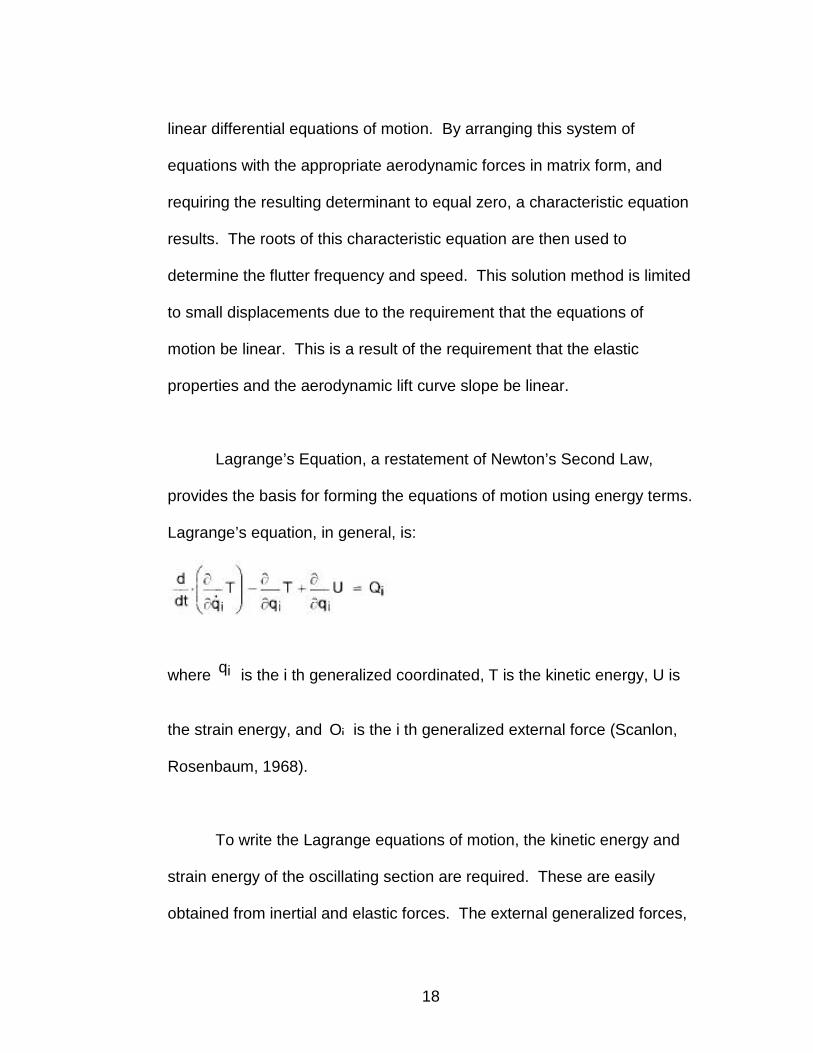
3.6.4.2 Forming the Lagrange Equations of Motion using Quasi-steady
Aerodynamic Forces
The quasi-steady lift force (L) of the airfoil section is defined as the
product of dynamic pressure (q), section planform area (S), the quasi-
steady lift curve slope (Clα), and the angle of attack (α). Stating the
41
quasi-steady lift force as a function of time, and defining the effective lift
force as a function of h and α :
L t( )12ρ⋅ S⋅ Clα⋅ V2⋅ αeff⋅=
where α eff is:
The above equation reflects the fact that the geometric angle of
attack between the airstream and the section chord line is not the only
variable important in determining the lift force. The vertical motion of the
section affects the local angle of attack as well. Including the vertical
translation of the airfoil section due to bending, the lift force becomes:
Substituting for constants, the aerodynamic lift factor is:
A012ρ⋅ S⋅ Clα⋅=
The dynamic lift force resulting from bending and torsion is thus:

42
Adding this expression to the equations of motion completes the
system of linear ordinary differential equations with constant coefficients
for the quasi-steady case:
Rearranging and transposing, the homogeneous equations of
motion for the quasi-steady case are:
3.6.5 Development of the Unsteady Aerodynamic Forces
The alternative to quasi-steady flow is to account for the torsional
oscillations of the airfoil in the calculation of the lift force. In that case,
unsteady 2-D aerodynamics is used, where the magnitude of the lift force
is dependent on the frequency of the oscillation of the airfoil section. The

43
unsteady lift force is a function of the reduced frequency (k), which is the
non-dimensionalized oscillation rate of the airfoil. The reduced frequency
may be regarded as a measure of the unsteadiness of the airflow. As the
reduced frequency increases, the error inherent in quasi-steady 2-D
aerodynamics becomes greater and greater, and the use of unsteady 2-D
aerodynamics becomes increasingly significant in the calculation of an
accurate flutter speed.
3.6.5.1 Forming the Lagrange Equations of Motion using Unsteady
Aerodynamic Forces and Moments
In unsteady flow, the reduced frequency of the section's oscillation
is used to determine the effect that motion has on the lift force generated.
As the airfoil section oscillates in the airstream, a changing trailing vortex
is generated. This vortex acts in opposition to the circulation around the
section. For example, when the section pitches nose up, the wake curls
around the trailing edge in a direction opposite to the pitching motion.
This reduces the lift force by reducing the circulation (Bisplinghoff, Ashley,
1962). Theodorsen’s circulation function is a means of quantifying this
wake-induced lift loss, where the values range from 1.0 to 0.5 as a
function of the reduced frequency. In contrast, no reduction in lift force
due to section oscillation occurs in quasi-steady flow, since the out-of-

44
phase component of lift force that results from the effects of the trailing
vortices is, as we have seen in Section 3.6.4, omitted. Two basic
approaches, both based on the determinant method for solving for the
system’s eigenvalues, are used to solve for the flutter frequency and
speed when using unsteady 2-D aerodynamics.
3.6.5.1.1 Finding the flutter frequency and speed – Theodorsen’s Method
Theodorsen's method is based on the simultaneous solution of the
real and imaginary parts of the flutter determinant. The flutter determinant
arises from the same equations of motion used in the quasi-steady case,
with the modification of the lift forces by the use of unsteady 2-D
aerodynamics. The basic solution procedure is to choose a series of
values of reduced frequency and find the corresponding roots of the real
and imaginary characteristic equations. These roots, the eigenvalues of
the system of equations of motion, are then plotted as functions of the
reciprocal of the reduced frequency, (1/k). The point on the graph where
the two plots of the roots intersect is the point where the required condition
of both the real and imaginary determinants equaling zero is
simultaneously satisfied. Both the flutter frequency and the flutter speed
are found at the intersection of the real and imaginary plots (Fung, 1969).

45
3.6.5.1.2 Finding the flutter frequency and speed – Materiel Center
Method
In Smilg and Wasserman's “Materiel Center” method, an artificial
damping factor, g, (equal for both bending and torsional degrees of
freedom) is introduced into the equations of motion. The attached
Mathcad worksheets use this method, where the solution to the flutter
frequency and speed is found when the artificial damping changes sign
from negative to positive as a function of the reciprocal of the reduced
frequency (1/k). When the artificial damping factor is positive, the system
is unstable, and therefore in a condition of flutter. This is due to the
balance of forces needed to maintain system stability, as a positive
artificial damping factor indicates a need for positive damping to be
present in order to prevent instability. A negative artificial damping factor
indicates a stable system, since there is, in its presence, an excess of
damping available in the system. An artificial damping factor of zero
implies the critical flutter condition (Donaldson, 1993).
The artificial damping factor is applied to the stiffness matrix, where
it effectively supplements the system's resistance to deflection. It is
inserted into the same equations of motion developed in Section 3.2, with
the substitution of the lift and moment of unsteady aerodynamic forces. It

46
should be noted that in these equations, DOF h is oriented positive down
(Smilg, Wasserman, 1942). The equations of motion for the case of
unsteady 2-D aerodynamics are thus:
The lift and moment expressions for unsteady 2-D aerodynamics
are further discussed in Section 3.7.1.2. After rearranging to make the
system of equation homogeneous, the equations of motion are thus:
3.7 Solution of the Double Eigenvalue Problem
Having derived the equations of motion, it is now necessary to
solve the system of the equations of motion for its two eigenvalues.
These are the values which cause the characteristic equation to equal
zero, and are the squares of the flutter frequency and speed.

47
3.7.1 Placing the System in Simple Harmonic Motion
In both the quasi-steady and the unsteady 2-D aerodynamics case,
the objective of the analysis is to locate the system's stability boundary,
which is the airfoil section's critical flutter speed. This is determined by the
critical speed of airflow at which the magnitudes of the bending and
torsional oscillations are neither increasing nor decreasing. Since the
neutral stability condition is to be tested, a logical approach is to insert
solutions for simple harmonic motion into the equations of motion and then
solve the system for the eigenvalues which will cause this condition to be
satisfied. In the critical flutter condition, the bending and torsional
motions, being constant in amplitude, are neither increasing nor
decreasing, so it is appropriate to represent them as sinusoidal motions,
as shown below, where A1 A2, , and B1 are the amplitudes of the
torsional and bending motions, respectively. The motions of the two DOF
are described by the sine function, and the cosine function provides a
component with a 90-degree phase angle between the bending and
torsional motions:
To be clear on the matter pf phase angles, note that if:
h t( ) B 1 sin ω t⋅=
α t( ) A 1 sin ω t⋅ A 2 cos⋅ ω t⋅+=

48
A1 A0 cos⋅ φ⋅=
and
A 2 A 0 sin φ⋅=
Then,
α t( ) A0 sinω t cos⋅ φ⋅ cos ω t⋅ sinφ⋅+( )⋅=
or
α t( ) A 0 sinω t φ+( )⋅=
where φ can be seen as the phase angle between bending and torsion.
Alternately, using complex notation, the multiplication of A2 by i
also provides the 90-degree phase angle component between the bending
and torsional motions:
Using the complex algebra form, and taking the first and second
time derivatives of the two DOF:
h B 1 e iω t⋅=
α A 1 i A 2⋅+( ) eiω t⋅=

49
Substituting these solutions into the equations of motion, canceling
eiωt for all terms, and casting in matrix form results in the matrix equations
of motion. The solution to this system satisfies the condition of simple
harmonic motion.
3.7.1.1 Flutter Solution in the case of Quasi-steady Aerodynamic Forces
Using the Equations of Motion derived in Section 3.2, forming the
determinant, and separating into real and imaginary parts:
m− ω 2⋅ b⋅ A0 V2⋅−KT Hea ω 2⋅− a A0⋅ V2⋅−
kb m ω 2⋅−mω2− b⋅
A1
B1
⋅
iω A0⋅ V⋅
a ω⋅ A0⋅ V⋅m ω 2⋅ b⋅ A0 V2⋅+
KT Hea ω 2⋅− a A0⋅ V2⋅−( )
⋅ B1
A2
⋅+
...
0
0
=
It is now necessary to determine the eigenvalues of this system,
that is, the frequency and velocity for which the required condition of both

50
the real and imaginary determinants equaling zero, is true. For this two
DOF system, the determinant method is a convenient means of finding the
eigenvalues. After expanding the complex determinant and solving the
characteristic equation, the flutter frequency is:
ω fKT
Hea m a⋅ b⋅−=
Similarly, the real determinant yields the flutter speed:
V fkb m ω f
2⋅−( ) K T Hea ω f2⋅−( )⋅ m b⋅ ω f
2⋅( )2−
A 0 a kb m ω f2⋅−( )⋅ m b⋅ ω f
2⋅+ ⋅=
It should be noted here that when the CG is co-located with the EA,
the lever arm distance (b) will be zero. In that case, the flutter frequency
will be equal to the uncoupled torsional frequency, and the flutter speed
will be zero. This result is compared with the flutter speed calculated by
use of unsteady aerodynamics below, and illustrates a fundamental flaw in
the use of quasi-steady aerodynamics.

51
3.7.1.2 Flutter Solution in the Case of Unsteady Aerodynamic Forces and
Moments
The homogeneous equations of motion using the Materiel Center
method were derived in Section 3.6.5.1.2. They are:
The lift force and the aerodynamic moment per unit span moment
about the elastic axis resulting from the use of unsteady 2-D
aerodynamics are functions of α V, ω, , and Theodorsen's
circulation function, C(k) (Scanlon, Rosenbaum, 1968) :

52
Using the reduced frequency (k), Theodorsen's circulation function
is calculated by use of Bessel Functions. The values for the lift and
moment determined are then used to determine the values of the
coefficients in the flutter determinant (Theodorsen, 1934).
C k( ) F k( ) i G k( )⋅+=
Again assuming harmonic motion, we use the substitutions of:
h h0 eiωt⋅=
and
F k( )J1 k( ) J1 k( ) Y0 k( )+( )⋅ Y1 k( ) Y1 k( ) J0 k( )−( )⋅+
J1 k( ) Y0 k( )+( )2 Y1 k( ) J0 k( )−( )2+=
G k( )Y1 k( )− Y0 k( )⋅ J1 k( ) J0 k( )⋅−
J1 k( ) Y0 k( )+( )2 Y1 k( ) J0 k( )−( )2+=

53
α α0 eiωt⋅= and their derivatives to replace the terms in the Lift and
Moment equations, resulting in the equation of motion being stated in
terms of the non-dimensional DOF
hb' and α . The lift and moment
coefficients for bending and torsion are functions of the reduced frequency
(Kussner, Schwartz, 1935):
In these equations, Lh , Lα , and M α are the lift and aerodynamic
moment coefficients about the elastic axis as functions of the reduced
frequency, while Mh is a constant, ½. These values are also substituted
into the equations of motion:
L π− ρb'3 ω 2
L hhb'⋅ Lα 1
2a h+
L h⋅−
α⋅+⋅=
Lh k( ) 1 2 i⋅ 1k
C k( )⋅−=
Lα k( )12
i1k
⋅ 1 2 C k( )⋅+( )⋅− 2
1k
2⋅ C k( )⋅−=
M h12
=
Mα k( )38
i1k
⋅−=

54
M π ρb'4⋅ ω 2⋅ Mh( 1
2ah+ Lh⋅−
hb'⋅
Mα 12
ah+ Lα Mh+( )⋅−
12
ah+
2Lh⋅+
...
α⋅+
...
⋅=
Dividing out π ρ b'3⋅ ω 2⋅ from the bending equation, and
π ρb4⋅ ω 2⋅ from the torsional equation to express the Lift and Moment
coefficients in non-dimensional form:
L Lhhb'⋅ Lα 1
2ah+ Lh⋅−
α⋅+−=
M Mh12
ah+ Lh⋅−
hb'⋅
Mα 12
ah+ Lα Mh+( )⋅− 1
2ah+
2Lh⋅+
α⋅+
...=
Defining the complex variable Z:
ZωT
ω
2
1 i g⋅+( )⋅= (Smilg, Wasserman, 1942).
and substituting into the equations of motion, after transposing, results in:

55
µ 1 Zω b
ω T
2
⋅ 1 i g⋅+( )⋅−
⋅ L h k( )⋅ h
b'⋅
µ xα⋅ L α k( )+ L h k( )12
a h+⋅− α⋅+
...
0=
µ xα⋅ Mh+ Lh k( )12
ah+⋅−
hb'⋅
µ rα 2⋅ 1 X 1 i g⋅+( )⋅−[ ]12
12
ah+⋅−
Mα k( ) Lα k( )12
ah+⋅− Lh k( )
12
ah+
2⋅++
...
α⋅+
...
0=
Casting the system of equations of motion in matrix form,
µ 1 Zωb
ωT
2
⋅ 1 i g⋅+( )⋅−
⋅ Lh k( )⋅
µ xα⋅ Mh+ Lh k( )12
ah+⋅−
µ xα⋅ Lα k( )+ Lh k( )12
ah+⋅−
µ rα2⋅ 1 X 1 i g⋅+( )⋅−[ ]⋅ 12
12
ah+⋅−
Mα k( ) Lα k( )12
ah+⋅− Lh k( )
12
ah+
2⋅++
...
hb'
α
⋅ 0=

56
Setting the determinant equal to zero,
µ 1 Zωb
ωT
2
⋅ 1 i g⋅+( )⋅−
⋅ Lh k( )⋅
µ xα⋅ Mh+ Lh k( )1
2ah+⋅−
µ xα⋅ Lα k( )+ Lh k( )12
ah+⋅−
µ rα2⋅ 1 X 1 i g⋅+( )⋅−[ ]⋅ 1
2
1
2ah+⋅−
Mα k( ) Lα k( )12
ah+⋅− Lh k( )
12
ah+
2⋅++
...
0=
The flutter determinant elements may be simplified by using the
following substitutions (A, B, D & E):
A µ 1 Zωb
ωT
2
⋅ 1 i g⋅+( )⋅−
⋅ Lh k( )⋅=
B µ xα⋅ Lα k( )+ Lh k( )12
ah+⋅−=
E µ rα 2⋅ 1 X 1 i g⋅+( )⋅−[ ]12
12
ah+⋅− Mα k( )+ Lα k( )
12
ah+⋅−
Lh k( )12
ah+
2⋅+
...=
D µ xα⋅ Mh+ Lh k( )12
ah+⋅−=

57
The equations of motion, in terms of the above, are thus:
Casting in matrix form:
A
D
B
E
hb'
α
⋅ 0=
Setting the determinant of the system to zero:
A
D
B
E
0=
The characteristic equation, including the real and imaginary
values, is thus:
A E⋅ B D⋅− 0=
The Mathcad worksheet calculates the values of the determinant
elements A, B, D and E instead of using the tabular values found in
Ahb'⋅ Bα+ 0=
Dhb'⋅ Eα+ 0=

58
USAAF Technical Report 4798. The complex characteristic equation is
then formed, and the Polyroots function of Mathcad is used to determine
the real and complex roots of the resulting quadratic equation. The lesser
of these two roots, which represents the unstable torsional motion, will
always contain the imaginary component which changes sign from
negative to positive as the reciprocal of the reduced frequency increases
(Bisplinghoff, Ashley, and Halfman, 1955).
Since ω and g always appear together in the determinantal
elements A and E, by solving for Z, both ω and g can be determined.
Representing the unstable torsional motion, the first root of Z, as a
function of reduced frequency (k), Z k( )1, is used in the calculation of the
artificial damping. The system damping is determined by taking the ratio
of the imaginary part to the real part of the first root of the frequency
quadratic. When the sign of g changes from negative to positive as a
function of the sign of Z k( )1, instability is indicated, where a positive g
indicates flutter:
gIm Z k( )1( )Re Z k( )1( )=
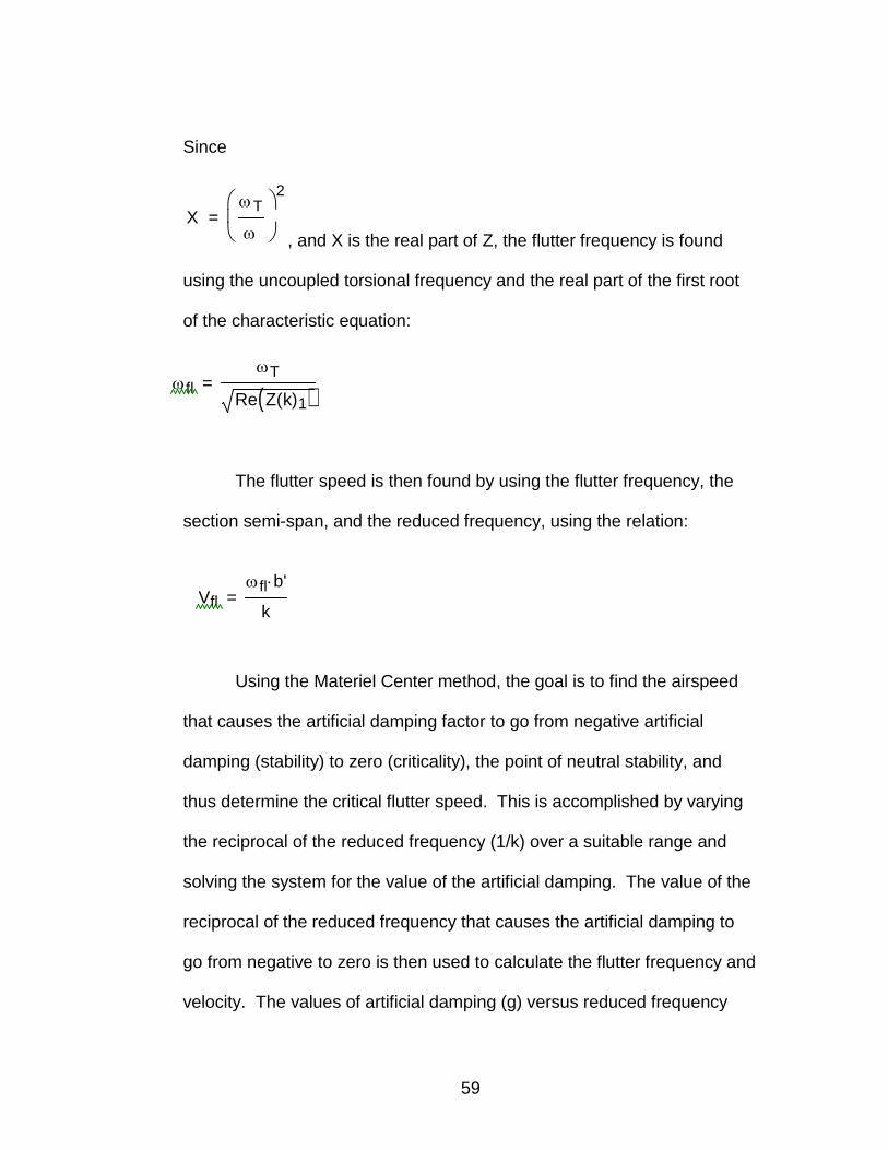
59
Since
XωT
ω
2
=, and X is the real part of Z, the flutter frequency is found
using the uncoupled torsional frequency and the real part of the first root
of the characteristic equation:
The flutter speed is then found by using the flutter frequency, the
section semi-span, and the reduced frequency, using the relation:
Using the Materiel Center method, the goal is to find the airspeed
that causes the artificial damping factor to go from negative artificial
damping (stability) to zero (criticality), the point of neutral stability, and
thus determine the critical flutter speed. This is accomplished by varying
the reciprocal of the reduced frequency (1/k) over a suitable range and
solving the system for the value of the artificial damping. The value of the
reciprocal of the reduced frequency that causes the artificial damping to
go from negative to zero is then used to calculate the flutter frequency and
velocity. The values of artificial damping (g) versus reduced frequency
Vflωfl b'⋅
k=
ωflωT
Re Z k( )1( )=

60
may be plotted to observe the trend in damping as the reduced frequency
is increased. This is illustrated in Figure 3.7.1.2.1.
1 1.5 2 2.5 3 3.5 4
0.1
0.1
0.2
0.3
0.4Damping vs. Reduced Frequency
Reciprocal of Reduced Frequency
Art
ifici
al D
ampi
ng
g k( )
1
k
Figure 3.7.1.2.1 Artificial damping versus reduced frequency
The slope of the damping curve gives an indication of the severity
of the onset of flutter in that the rate of the instability may be predicted. A
shallow slope indicates a less severe onset of flutter, whereas a steep
slope implies that a violent encounter with flutter may be expected
(Bisplinghoff, Ashley, and Halfman, 1955). The attached Mathcad
worksheets carry out these calculations as a result of the input variables

61
provided. Figure 3.7.1.2.2 depicts the artificial damping versus the speed
of the airflow in knots.
150 200 250 300 350 400 450 500 550 600
0.1
0.1
0.2
0.3
0.4Damping vs. Velocity
Velocity (knots)
Art
ifici
al D
ampi
ng
g k( )
0.0494 Vfl k( )
Figure 3.7.1.2.2 Artificial damping versus velocity
3.8 Chapter Summary
The basic means of establishing the equations of motion is the
same in both the quasi-steady and the unsteady cases. Using Lagrange’s
equation and the appropriate expressions for (1) the strain energy, (2) the
kinetic energy, and (3) the aerodynamic forces leads to the homogeneous
equations of motion. The two descriptions of the aerodynamic forces
considered here are quasi-steady and unsteady 2-D aerodynamic forces

62
and moments. Both the quasi-steady and unsteady 2-D cases use the
determinant method to establish the characteristic equation, which is then
solved for its roots. Accuracy is improved by the use of the unsteady
aerodynamic forces and moments, while the quasi-steady solution
method, within its range of validity with respect to CG position, is more
rapidly solved and results in a conservative calculation (Bisplinghoff,
Ashley, and Halfman, 1955).

63
Chapter 4.0: Calculation of Flutter Properties by Mathcad
Worksheets
This section describes the calculation methodology used in the
attached Mathcad worksheet to determine the flutter frequency and the
critical flutter speed of six example sections. Using both quasi-steady and
unsteady aerodynamics, flutter properties of the example sections are
calculated in the worksheet using a common set of section parameters.
The objective is to input the key structural and inertial parameters that
affect the value of the flutter frequency and speed and compare the
section’s flutter properties using quasi-steady and unsteady aerodynamic
forces. For the case of center of gravity (CG) variation, results are plotted
for both cases and compared. An example of flutter speed variation with
altitude is also performed in one example.
4.1 Mathcad Worksheet Methodology
The Mathcad Worksheet processing flow follows the pattern of
inputs, intermediate or supporting calculations, and outputs. The means
by which each of these is carried is as follows.

64
4.1.1 Program inputs
User inputs (the boxed quantities on the worksheet) define the
primary airfoil section elastic, inertial and aerodynamic parameters
common to both the quasi-steady and unsteady cases. The basic section
parameters of section chord, section aerodynamic center, center of gravity
and elastic axis location, the section weight per inch of span length (Wt),
the section mass moment of inertia about the center of gravity per inch
( Hcg ), and the section bending and torsional stiffnesses per inch are
input. For the quasi-steady calculation, the section lift curve slope for a
given airfoil ( Clα ), drawn from Table 3.6.3, and the strip width (w, an
arbitrary value) are also inputs. Additionally, the air properties are
included as inputs, such as the International Standard Atmosphere (ISA)
air density (ρ) and the density ratio (δ) as required for test altitude. The
user may vary any input as desired to test for flutter frequency and speed
sensitivity with respect to that particular parameter or any combination of
input parameters.

65
4.1.2 Supporting calculations
The worksheet prepares intermediate calculations for use in both
the quasi-steady and unsteady cases. The lever arm distances from the
section aerodynamic center to the elastic axis (a), and from the section
elastic axis to the center of gravity (b), the section mass (m), and the
section mass moment of inertia about the elastic axis ( Hea ) are calculated
for internal program use. The air density ratio as a function of altitude and
the air density at test condition are provided to allow test altitudes above
Sea Level.
4.1.2.1 Quasi-steady Case
For the quasi-steady case, the strip properties of strip area,
stiffness and mass moment of inertia are calculated. These are used to
define the elastic, inertial and aerodynamic forces arising from any given
strip width.
4.1.2.2 Unsteady Case
For the unsteady case, several additional non-dimensional
quantities are derived from the basic program inputs. These include the

66
section semi-chord (b`), the uncoupled bending and torsional natural
frequencies (ωb ,ωT ), the dimensionless center of gravity ( xα ) and
elastic axis positions (ah ), the dimensionless radius of gyration ( rα ) and
the section mass ratio (µ). Many of the references cited in this thesis use
the uncoupled bending-torsional natural frequency ratio to define the
section properties. It is thus calculated in order to cross check these
values with the section input parameters. The section static
imbalance, Sα , similarly provides an input cross-check. As these
quantities are often presented in the literature in this non-dimensional
form, this feature allows convenient comparison of dimensional and non-
dimensional inputs, as applicable. It also allows direct entry of all non-
dimensional parameters, if desired.
A final supporting calculation useful for both cases is the check of
the section static divergence speed (VD ). This value provides an upper
limit on the range of flutter speeds to be evaluated, as any flutter speed
calculated above this value would be unattainable, since the section would
have failed in static divergence prior to experiencing flutter.

67
4.1.3 Primary calculations
4.1.3.1 Quasi-steady Case
The flutter frequency and speed are found by direct calculation of
the closed form equations of Section 3.7.1.1. For the CG variation study,
the CG position is varied from the aerodynamic center location at the
quarter chord to the trailing edge of the airfoil and plotted.
4.1.3.2 Unsteady Case
For the unsteady flutter calculation, the program uses an initial
value of the reduced frequency (k). It calculates the value of
Theodorsen’s function, C(k), and the unsteady lift and moments due to
section bending and torsion. The determinant elements are then
calculated and the resulting characteristic quadratic equation solved for its
roots using the Polyroots root finder function of Mathcad. This process is
carried out for a series of reciprocals of the reduced frequency until the
program finds the reciprocal of the reduced frequency (1/k) that causes
the artificial damping (g) to become zero. These values are plotted to
show the trend of damping versus the reciprocal of the reduced frequency.
A similar calculation loop is carried out to find the flutter frequency and

68
speed, both graphically and numerically. A plot of damping versus
velocity of airflow then is used to depict the artificial damping and also the
flutter speed.
CG variation is again accomplished by the use of the same
program operating on a series of CG change increments. The results of
the flutter speed as a function of CG position is plotted.
4.1.4 Program Outputs
The program outputs are shown as the boxed and shaded
quantities on the Mathcad worksheet. The quasi-steady flutter frequency
and speed are the imaginary and real eigenvalues of the system of the
equations of motion of the section. Unsteady case program outputs (all
functions of reduced frequency) are the artificial damping (g), the phase
angle at zero artificial damping (φ), the flutter frequency (ωfl ), and the
critical flutter speed (Vfl ).

69
4.2 Example Calculations
The following six airfoil sections were evaluated using the Mathcad
worksheet to determine their flutter characteristics. The sources for these
sections range from published technical reports and textbooks to
information located on the Internet in the case of a newly-designed
aircraft. In all cases, a check of the static divergence speed confirmed
that all sections would experience flutter at speeds below the divergence
speed.

70
4.2.1 Example One: Ryan NYP prototype (Blevins, 1990)
4.2.1.1 Inputs, Intermediate Calculations and Outputs
Program Inputs
Section Chord 84 Inch
Strip Width 10 Inch
AC location 0.25 Tenths of chord
CG Location 0.4 Tenths of chord
EA Location 0.26 Tenths of chord
Section Bending Stiffness 12.25 Pounds per Inch
Section Torsional Stiffness 6084 Inch-Pounds per
Radian
Section Weight per unit span 0.81 Pounds per Inch
Section Mass Moment of Inertia
about CG
8.75 Slug-inch^2 per
inch
Air Density at ISA conditions 0.002378 Slugs/cubic foot
Test Altitude 0 (Sea
Level)
Feet
Airfoil Lift Curve Slope 0.084 Per degree
Intermediate Calculations
Air Density Ratio at Test
Condition
1.0 Non Dimensional
Uncoupled Natural Bending
Frequency
22.1 Radians/Sec
Uncoupled Natural Torsional
Frequency
22.3 Radians/Sec
CG Position 0.28 Non Dimensional
EA Position -0.48 Non Dimensional
Section Static Imbalance 0.296 Slug-inch
Radius of Gyration 0.525 Non Dimensional
Mass ratio 3.3 Non Dimensional

71
Static Divergence Speed 252.1 Knots
Program Outputs
Quasi-steady (QS) Flutter
Frequency
22.08 Radians/Sec
Quasi-steady (QS) Flutter
Speed
35.6 Knots
Reduced Frequency (k) at Zero
Damping
1.0 Non Dimensional
Unsteady (US) Flutter
Frequency
27.32 Radians/Sec
Unsteady (US) Flutter Speed 53.5 Knots
Ratio of QS to US flutter
frequency
0.81 Non Dimensional
Ratio of QS to US flutter speed 0.63 Non Dimensional
4.2.1.2 Section Characteristics
This wing section is the preliminary design of wood and fabric
construction for the single-engine, special-purpose aircraft, “The Spirit of
St. Louis”. It is typical of the design and construction methodology of the
late 1920’s. The braced wing section is composed of two main spars,
both made of wood, with a covering of doped fabric which acts as the non-
load bearing skin. The parameters listed are found on pages 141-144 of
Reference Nine. The section is exceptionally light, with the mass ratio of
3.3 being the lowest of all sections tested. A low mass ratio typically

72
indicates a low flutter speed due to the high propensity for the section to
experience flow-induced vibration. The torsional natural frequency is the
lowest of all the example sections. Also, little frequency separation
between the natural bending and torsional frequencies is present,
suggesting the possibility of a low flutter speed. Finally, the section has
the most aft CG of all the sections.
4.2.1.3. Flutter Calculations for the Quasi-steady Case
The flutter frequency of 22.08 Rad/sec is approximately equal to
the natural bending frequency. The flutter speed of 35.6 knots is within
4% of that published in Reference Nine of 37.0 knots.
4.2.1.4 Flutter Calculations for the Unsteady Case
The reduced frequency at zero damping is found to be 1.0. This
indicates a relatively slow rate of section oscillation. Notably, the coupled
flutter frequency of 27.14 Rad/sec is greater than both the natural bending
and torsional frequencies. This is unusual, but not unheard of
(Bisplinghoff, Ashley, and Halfman, 1955). The critical flutter speed of
56.3 knots falls short of the design requirement of 112 knots. In this case,
it is necessary to make changes in the section torsional stiffness and /or

73
the CG position to increase the critical flutter speed.
The low flutter speed found in this example shows how flutter may
occur at low speeds. A common misconception is that if an aircraft is
“slow”, it will not be subject to the effects of flutter. This is seen to be
false, as the combination of the elastic, inertial and aerodynamic forces
are responsible for flutter occurrence, and not merely the range of
airspeed values attainable.
4.2.1.5 Comparison of Results in the Quasi-steady and Unsteady Cases
The quasi-steady flutter frequency is 81% of the unsteady flutter
frequency, while the quasi-steady flutter speed is 63% of the unsteady
flutter speed. These are typical values for this comparison (Bisplinghoff,
Ashley, and Halfman, 1955).
4.2.1.6 CG Variation Survey
The sharp decrease in the critical flutter speed indicates a great
sensitivity to CG position. Also, at the design condition of CG at 0.4c, the
flutter speed using quasi-steady aerodynamics is seen. The two speeds
are equal at a CG position of about 0.6c.

74
0.3 0.4 0.5 0.6 0.7 0.8 0.9 1
20
40
60
80
100Flutter Speed Variation (US & QS)
CG Location (tenths of chord)
Flu
tter
Spe
ed (
knot
s)
Vfl' CG( )
VfQS' CG( )
CG
c

75
4.2.2 Example Two: Ryan NYP Final Design (Blevins, 1990)
4.2.2.1 Inputs, Intermediate Calculations and Outputs
Program Inputs
Section Chord 84 Inch
Strip Width 10 Inch
AC location 0.25 Tenths of chord
CG Location 0.4 Tenths of chord
EA Location 0.26 Tenths of chord
Section Bending Stiffness 49 Pounds per Inch
Section Torsional Stiffness 24336 Inch-Pounds per
Radian
Section Weight per unit span 0.81 Pounds per Inch
Section Mass Moment of Inertia
about CG
8.75 Slug-inch^2 per
inch
Air Density at ISA conditions 0.002378 Slugs/cubic foot
Test Altitude 0 (Sea
Level)
Feet
Airfoil Lift Curve Slope 0.084 Per degree
Intermediate Calculations
Air Density Ratio at Test
Condition
1.0 Non Dimensional
Uncoupled Natural Bending
Frequency
44.14 Radians/Sec
Uncoupled Natural Torsional
Frequency
44.61 Radians/Sec
CG Position 0.28 Non Dimensional
EA Position -0.48 Non Dimensional
Section Static Imbalance 0.296 Slug-inch
Radius of Gyration 0.525 Non Dimensional
Mass ratio 3.3 Non Dimensional
Static Divergence Speed 504.1 Knots

76
Program Outputs
Quasi-steady (QS) Flutter
Frequency
44.16 Radians/Sec
Quasi-steady (QS) Flutter
Speed
71.1 Knots
Reduced Frequency (k) at Zero
Damping
1.06 Non Dimensional
Unsteady (US) Flutter
Frequency
54.64 Radians/Sec
Unsteady (US) Flutter Speed 107.1 Knots
Ratio of QS to US flutter
frequency
0.81 Non Dimensional
Ratio of QS to US flutter speed 0.66 Non Dimensional
4.2.2.2 Section Characteristics
In this case, the same input parameters given in Example One are
repeated, with the design modification of the bending and torsional
stiffnesses. These have been quadrupled by the addition of four external
wing struts in order to meet the design requirement of a maximum speed
of 107 knots, as described in Reference Nine.
4.2.2.3 Flutter Calculations for the Quasi-steady Case
The flutter frequency of 44.16 rad/sec is twice that found in

77
Example One, as a result of the quadrupled stiffnesses. This value
remains approximately equal to the natural bending frequency. The flutter
speed of 107 knots is also twice that found in Example One.
4.2.2.4 Flutter Calculations for the Unsteady Case
The reduced frequency for zero artificial damping in the unsteady
case is 1.06. The unsteady flutter frequency remains greater than both
the natural bending and torsional frequencies at 54.64 rad /sec. The
flutter speed of 107 knots now meets the design requirement of 120 miles
per hour as a result of the quadrupled stiffnesses. These results may be
generalized to conclude that flutter speed increases as the square root of
the stiffness.

78
4.2.2.5 Comparison of Results in the Quasi-steady and Unsteady Cases.
The quasi-steady flutter frequency is 81% of unsteady flutter
frequency, while the quasi-steady flutter speed is 63% of the unsteady
flutter speed. This is identical to the results found in the prototype
(Example 1) despite the quadrupled bending and torsional stiffnesses.
4.2.2.6 CG Variation Survey
The increased flutter speeds for all CG positions is noted. Again
the quasi-steady and unsteady flutter speeds are equal at about 0.6c.
0.3 0.4 0.5 0.6 0.7 0.8 0.9 140
60
80
100
120
140
Flutter Speed Variation (US & QS)
CG Location (tenths of chord)
Flu
tter
Spe
ed (
knot
s)
Vfl' CG( )
VfQS' CG( )
CG
c

79
4.2.3 Example Three: MD3-160 Aircraft Section (Usmani, Ho, 2003)
4.2.3.1 Inputs, Intermediate Calculations and Outputs
Program Inputs
Section Chord 60 Inch
Strip Width 10 Inch
AC location 0.25 Tenths of chord
CG Location 0.5 Tenths of chord
EA Location 0.4 Tenths of chord
Section Bending Stiffness 114 Pounds per Inch
Section Torsional Stiffness 132756 Inch-Pounds per
Radian
Section Weight per unit span 0.83 Pounds per Inch
Section Mass Moment of Inertia
about CG
13.74 Slug-inch^2 per
inch
Air Density at ISA conditions 0.002378 Slugs/cubic foot
Test Altitude 0 (Sea
Level)
Feet
Airfoil Lift Curve Slope 0.104 Per degree
Intermediate Calculations
Air Density Ratio at Test
Condition
1.0 Non Dimensional
Uncoupled Natural Bending
Frequency
66.5 Radians/Sec
Uncoupled Natural Torsional
Frequency
95.14 Radians/Sec
CG Position 0.2 Non Dimensional
EA Position -0.2 Non Dimensional
Section Static Imbalance 0.155 Slug-inch
Radius of Gyration 0.7952 Non Dimensional
Mass ratio 6.62 Non Dimensional
Static Divergence Speed 382.5 Knots

80
Program Outputs
Quasi-steady (QS) Flutter
Frequency
90.92 Radians/Sec
Quasi-steady (QS) Flutter
Speed
112.6 Knots
Reduced Frequency (k) at Zero
Damping
0.85 Non Dimensional
Unsteady (US) Flutter
Frequency
91.34 Radians/Sec
Unsteady (US) Flutter Speed 159.3 Knots
Ratio of QS to US flutter
frequency
1.00 Non Dimensional
Ratio of QS to US flutter speed 0.71 Non Dimensional
4.2.3.2 Section Characteristics
This section is from a light two-place, single-engine sport and
training aircraft. It uses an all-aluminum, semi-monocoque (stressed skin,
load bearing) cantilever wing design. This section is the least statically
imbalanced of all the sections tested, while the radius of gyration is the
highest. The CG position for the test case is located fairly far aft at 0.5c.
In addition to the CG study, this section is used to carry out an altitude
variation study. The increase in the critical flutter speed as test altitude is
increased is determined and plotted.

81
4.2.3.3 Flutter Calculations for the Quasi-steady Case
The flutter frequency 90.92 Rad/sec, falling between the bending
and torsional uncoupled natural frequencies as expected. The flutter
speed is 112.6 knots.
4.2.3.4 Flutter Calculations for the Unsteady Case
The reduced frequency for zero artificial damping in the unsteady
case is 0.9. The flutter frequency is 91.34 rad/sec, and the flutter speed
is calculated at 159.3 knots.

82
4.2.3.5 Comparison of Results in the Quasi-steady and Unsteady Cases
The quasi-steady flutter frequency is 100% of the unsteady flutter
frequency, while the quasi-steady flutter speed is 71% of the unsteady
flutter speed. This was the closest conformance of quasi-steady to
unsteady flutter speed calculations of all six examples.
The design criteria stated in Reference 15 was for freedom from
flutter for airspeeds up to 120 knots. These results indicate that design
target has been achieved. Flight testing would be required to verify these
calculations.
4.2.3.6 Altitude Variation Survey
The increase in flutter speed predicted in Section 3.6.1 is
demonstrated in Table 4.2.3 7 and Figure 4.2.3 7. Both the quasi-steady
and unsteady flutter speeds (as true airspeeds) increase as altitude
increases from Sea Level to 25,000 feet. The quasi-steady flutter speed
remains approximately 71% of the unsteady flutter speed throughout this
altitude range.

83
Table 4.2.3.7
Flutter Speed Variation with Altitude
Test
Altitude
(feet)
Quasi-steady
(QS) Flutter
Speed
(KTAS)
Unsteady
(US) Flutter
speed (KTAS)
QS/US
Speed
Ratio
Unsteady
(US) Flutter
speed
(KIAS)
0 112.6 159.3 0.71 159.3
5000 121.3 167.3 0.73 155.3
10000 131.1 178.1 0.74 153.0
15000 142.0 192.6 0.74 152.8
20000 154.3 209.6 0.74 153.0
25000 168.3 229.8 0.73 153.8
Figure 4.2.3.7Flutter Speed Variation w ith Altitude
MD3-160 Aircraft Section
112.6
121.3
131.1
142.0
154.3
168.3
159.3
167.3
192.6
209.6
229.8
178.1
110.0
130.0
150.0
170.0
190.0
210.0
230.0
0 5000 10000 15000 20000 25000Altitude (fee t)
Flu
tter
Sp
eed
(K
TA
S)
Quasi-steady(QS) FlutterSpeed (KTAS)
Unsteady (US)Flutter speed(KTAS)

84
4.2.3.7 CG Variation Survey
0.3 0.4 0.5 0.6 0.7 0.8 0.9 150
100
150
200
250
300Flutter Speed Variation (US & QS)
CG Location (tenths of chord)
Flu
tter
Spe
ed (
knot
s)
Vfl' CG( )
VfQS' CG( )
CG
c

85
4.2.4 Example Four: Example from NACA Technical Report 685,
(Theodorsen, Garrick, 1938)
4.2.4.1 Inputs, Intermediate Calculations and Outputs
Program Inputs
Section Chord 144 Inch
Strip Width 10 Inch
AC location 0.25 Tenths of chord
CG Location 0.4 Tenths of chord
EA Location 0.3 Tenths of chord
Section Bending Stiffness 45.4 Pounds per Inch
Section Torsional Stiffness 948572 Inch-Pounds per
Radian
Section Weight per unit span 2.9 Pounds per Inch
Section Mass Moment of Inertia
about CG
97.6 Slug-inch^2 per
inch
Air Density at ISA conditions 0.002378 Slugs/cubic foot
Test Altitude 0 (Sea
Level)
Feet
Airfoil Lift Curve Slope 0.104 Per degree
Intermediate Calculations
Air Density Ratio at Test
Condition
1.0 Non Dimensional
Uncoupled Natural Bending
Frequency
22.45 Radians/Sec
Uncoupled Natural Torsional
Frequency
90.32 Radians/Sec
CG Position 0.2 Non Dimensional
EA Position -0.4 Non Dimensional
Section Static Imbalance 1.297 Slug-inch
Radius of Gyration 0.499 Non Dimensional
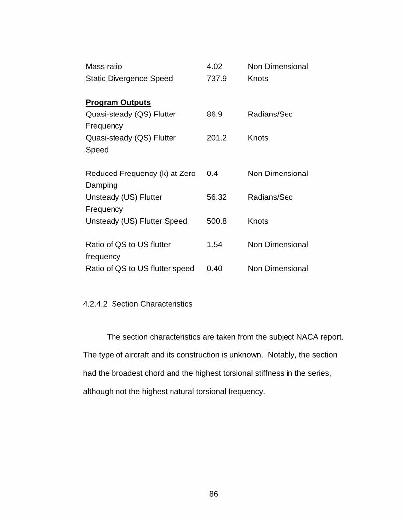
86
Mass ratio 4.02 Non Dimensional
Static Divergence Speed 737.9 Knots
Program Outputs
Quasi-steady (QS) Flutter
Frequency
86.9 Radians/Sec
Quasi-steady (QS) Flutter
Speed
201.2 Knots
Reduced Frequency (k) at Zero
Damping
0.4 Non Dimensional
Unsteady (US) Flutter
Frequency
56.32 Radians/Sec
Unsteady (US) Flutter Speed 500.8 Knots
Ratio of QS to US flutter
frequency
1.54 Non Dimensional
Ratio of QS to US flutter speed 0.40 Non Dimensional
4.2.4.2 Section Characteristics
The section characteristics are taken from the subject NACA report.
The type of aircraft and its construction is unknown. Notably, the section
had the broadest chord and the highest torsional stiffness in the series,
although not the highest natural torsional frequency.

87
4.2.4.3 Flutter Calculations for the Quasi-steady Case
The flutter frequency is 86.9 Rad/sec, coalescing between the
bending and torsional uncoupled natural frequencies. The flutter speed is
calculated at 201.2 knots.
4.2.4.4 Flutter Calculations for the Unsteady Case
In contrast to previous examples, a significantly lower reduced
frequency (k) at zero artificial damping is found for this airfoil section. The
reduced frequency is found to be 0.4 at zero artificial damping.
The unsteady flutter frequency is greater than both the natural
bending and torsional frequencies at 56.32 rad/sec. The flutter speed is
500.8 knots, well into the compressible range and above the valid range of
incompressible speeds for which this methodology is intended.
Corrections for compressibility would be required.
4.2.4.5 Comparison of Results in the Quasi-steady and Unsteady Cases
The quasi-steady flutter frequency is 154% of the unsteady flutter
frequency, while the quasi-steady flutter speed is just 40% of the unsteady
flutter speed. These results thus differ the most of all the examples

88
presented. Nevertheless, the unsteady flutter speed calculation is within
2% of that published in NACA TR 685 (Reference 14) of 492.7 knots.
4.2.4.6 CG Variation Survey
This section shows a markedly lower slope for the flutter speed
variation curve. This indicates a reduced sensitivity to CG shift due to the
high torsional stiffness. The quasi-steady and unsteady flutter speeds are
seen to agree at the CG position of about 0.7c.
0.3 0.4 0.5 0.6 0.7 0.8 0.9 1
100
200
300
400
500
600Flutter Speed Variation (US & QS)
CG Location (tenths of chord)
Flu
tter
Spe
ed (
knot
s)
Vfl' CG( )
VfQS' CG( )
CG
c

89
4.2.5 Example Five: Example from USAAF Technical Report 4798,
(Smilg, Wasserman, 1942)
4.2.5.1 Inputs, Intermediate Calculations and Outputs
Program Inputs
Section Chord 132 Inch
Strip Width 10 Inch
AC location 0.25 Tenths of chord
CG Location 0.39 Tenths of chord
EA Location 0.31 Tenths of chord
Section Bending Stiffness 114 Pounds per Inch
Section Torsional Stiffness 279963 Inch-Pounds per
Radian
Section Weight per unit span 8.5 Pounds per Inch
Section Mass Moment of Inertia
about CG
198 Slug-inch^2 per
inch
Air Density at ISA conditions 0.00237
8
Slugs/cubic foot
Test Altitude 10000 Feet
Airfoil Lift Curve Slope 0.109 Per degree
Intermediate Calculations
Air Density Ratio at Test
Condition
0.7383 Non Dimensional
Uncoupled Natural Bending
Frequency
20.78 Radians/Sec
Uncoupled Natural Torsional
Frequency
35.08 Radians/Sec
CG Position 0.16 Non Dimensional
EA Position -0.38 Non Dimensional
Section Static Imbalance 2.788 Slug-inch

90
Radius of Gyration 0.4447 Non Dimensional
Mass ratio 18.98 Non Dimensional
Static Divergence Speed 453.9 Knots
Program Outputs
Quasi-steady (QS) Flutter
Frequency
33.5 Radians/Sec
Quasi-steady (QS) Flutter
Speed
135.0 Knots
Reduced Frequency (k) at Zero
Damping
0.4 Non Dimensional
Unsteady (US) Flutter
Frequency
27.08 Radians/Sec
Unsteady (US) Flutter Speed 220.7 Knots
Ratio of QS to US flutter
frequency
1.24 Non Dimensional
Ratio of QS to US flutter speed 0.61 Non Dimensional
4.2.5.2 Section Characteristics
This section appeared to be taken from an all-aluminum, semi-
monocoque construction multi-engine transport or bomber aircraft.
This section has the highest mass ratio of the series, suggesting
greater flutter resistance. The section is also the most massive of the
series sections, probably due to contribution of the wing mounted engine
in the section weight. Test altitude was 10,000 feet. No published results
for the bending-torsion flutter frequency or speed for this airfoil section

91
were available in Technical Report 4798.
4.2.5.3 Flutter Calculations for the Quasi-steady Case
The flutter frequency of 33.5 rad/sec is between the bending and
torsional natural frequencies. The flutter speed is calculated at 135 knots.
4.2.5.4 Flutter Calculations for the Unsteady Case
The reduced frequency at zero artificial damping is 0.4. The
unsteady flutter frequency is between both the natural bending and
torsional frequencies, coming in at 27.08 rad/sec. This section had the
lowest coupled flutter frequency of the series. The flutter speed is 220.7
knots.
4.2.5.5 Comparison of Results in the Quasi-steady and Unsteady Cases
The quasi-steady flutter frequency is 124% of the unsteady flutter
frequency, while the quasi-steady flutter speed is 61% of the unsteady
flutter speed. This continues the typical trend of results for the quasi-
steady case of about 60% of the calculated critical flutter speed when
compared to the unsteady case.

92
4.2.5.6 CG Variation Survey
The section shows profound sensitivity to CG location. The high
mass of the section seems to predominate among the three forces as far
as sensitivity to flutter speed change.
0.3 0.4 0.5 0.6 0.7 0.8 0.9 1
200
400
600
800Flutter Speed Variation (US & QS)
CG Location (tenths of chord)
Flu
tter
Spe
ed (
knot
s)
Vfl' CG( )
VfQS' CG( )
CG
c

93
4.2.6 Example Six: Example from Reference 5, page 203 (Scanlan,
Rosenbaum, 1968)
4.2.6.1 Inputs, Intermediate Calculations and Outputs
Program Inputs
Section Chord 75 Inch
Strip Width 10 Inch
AC location 0.25 Tenths of chord
CG Location 0.46 Tenths of chord
EA Location 0.35 Tenths of chord
Section Bending Stiffness 210 Pounds per Inch
Section Torsional Stiffness 409875 Inch-Pounds per
Radian
Section Weight per unit span 1.75 Pounds per Inch
Section Mass Moment of Inertia
about CG
36.7 Slug-inch^2 per
inch
Air Density at ISA conditions 0.002378 Slugs/cubic foot
Test Altitude 20000 Feet
Airfoil Lift Curve Slope 0.104 Per degree
Intermediate Calculations
Air Density Ratio at Test
Condition
0.5326 Non Dimensional
Uncoupled Natural Bending
Frequency
62.16 Radians/Sec
Uncoupled Natural Torsional
Frequency
100.73 Radians/Sec
CG Position 0.22 Non Dimensional
EA Position -0.3 Non Dimensional
Section Static Imbalance 0.488 Slug-inch
Radius of Gyration 0.727 Non Dimensional
Mass ratio 16.79 Non Dimensional
Static Divergence Speed 902.4 Knots

94
Program Outputs
Quasi-steady (QS) Flutter
Frequency
96.78 Radians/Sec
Quasi-steady (QS) Flutter
Speed
250.2 Knots
Reduced Frequency (k) at Zero
Damping
0.4 Non Dimensional
Unsteady (US) Flutter
Frequency
89.29 Radians/Sec
Unsteady (US) Flutter Speed 384.7 Knots
Ratio of QS to US flutter
frequency
1.08 Non Dimensional
Ratio of QS to US flutter speed 0.65 Non Dimensional
4.2.6.2 Section Characteristics
This section is taken from the textbook listed above. The aircraft
type is unknown. Test altitude was 20,000 feet. The section has the
highest natural torsional frequency of the six section tested.
4.2.6.3 Flutter Calculations for the Quasi-steady Case
Flutter frequency is 96.78 rad/sec, falling between the bending and
torsional natural frequencies. The flutter speed is 250.2 knots.

95
4.2.6.4 Flutter Calculations for the Unsteady Case
The reduced frequency for zero artificial damping in the unsteady case is
0.4. The flutter frequency is 89.29 Rad/sec, and the flutter speed is 384.7
knots. The flutter speed range is above the range of validity for
incompressible flow. Further evaluation would be required to refine the
flutter speeds determined here.
4.2.6.5 Comparison of Results in the Quasi-steady and Unsteady Cases
The quasi-steady flutter frequency is 108 % of the unsteady flutter
frequency, while the quasi-steady flutter speed is 61% of the unsteady
flutter speed for the given conditions.
4.2.6.6 CG Variation Survey
The high natural torsional frequency here seems to reduce the
slope of the flutter speed variation curve. This section had the highest
Divergence speed, the highest quasi-steady flutter frequency and the
highest quasi-steady flutter speed of all the tested sections.

96
0.3 0.4 0.5 0.6 0.7 0.8 0.9 1
200
400
600
800Flutter Speed Variation (US & QS)
CG Location (tenths of chord)
Flu
tter
Spe
ed (
knot
s)
Vfl' CG( )
VfQS' CG( )
CG
c

97
4.3 Chapter Summary
The attached spreadsheet summarizes the results of five test
sections. Comparison of the quasi-steady to the unsteady flutter speeds
typically shows the quasi-steady speeds to be about 60-65% of those
when unsteady aerodynamic forces are used. In one case the quasi-
steady flutter speed was only 40% of the unsteady flutter speed.
The results of the CG study were in agreement only when the value
of the lever arm distance from the CG to the EA was about 0.25 in non-
dimensional terms. For this range, the 60-70% trend found in the quasi-
steady to unsteady flutter speeds is supported.
The Mathcad worksheet may be used to investigate potential
solutions to unacceptably low flutter speeds. The results of trial
calculations may then be reviewed by use of the worksheets to determine
the most favorable method to change the flutter speed according to the
design requirements and the options available to the designer.
Prevention or mitigation of flutter can be accomplished by
adjustment of key structural and aerodynamic parameters, such as:

98
1. Section geometric properties, including section chord and airfoil
section profile;
2. Structural properties, including the bending and the torsional
stiffnesses and elastic axis location;
3. Inertial properties, including section mass, mass moment of
inertia, and center of gravity position.
4. Aerodynamic properties for the desired test condition, i.e., Sea
Level or at altitude.
Active flutter suppression measures, such a smart structures, can
alter stiffness on demand, thereby altering the structural variables as
required by operational conditions. This increases flutter speed while
keeping weight growth in control. This approach has been investigated
using a wind tunnel model in the Piezoelectric Aeroelastic Response
Tailoring Investigation (PARTI) program cited in Reference 16.

99
Table 4.3
Summary of Program Inputs, Calculations and Outputs
Ryan
NYP
Proto-
type
(1)
MD3-
160 (3)
Ref 14,
p. 108
(4)
Ref 11,
p. 155
(5)
Ref 5,
p. 203
(6)
Unit
Program Inputs
Section Chord 84 60 144 132 75 Inch
Strip Width 10 10 10 10 10 Inch
AC location 0.25 0.25 0.25 0.25 0.25 Tenths of
chord
CG Location 0.4 0.5 0.4 0.39 0.46 Tenths of
chord
EA Location 0.26 0.4 0.3 0.31 0.35 Tenths of
chord
Section Bending
Stiffness
12.25 114 45.4 114 210 Pounds
/Inch
Section Torsional
Stiffness
6084 132756 948572 279963 409875 Inch-
Pounds
/Radian
Section Weight per
unit span
0.81 0.83 2.9 8.5 1.75 Pounds
/Inch
Section Mass
Moment of Inertia
about CG
8.75 13.74 97.6 198 36.7 Slug-
inch^2
per inch
Air Density at ISA
conditions
0.0024 0.0024 0.0024 0.0024 0.0024 Slugs
/cubic ft
Test Altitude 0 0 0 10000 20000 Feet
Airfoil Lift Curve
Slope
0.084 0.104 0.104 0.109 0.104 Per
degree

100
Intermediate Calculations
Air Density Ratio
at Test Condition
1.0 1.0 1.0 0.7383 0.5326 Non
Dimens.
Uncoupled Natural
Bending
Frequency
22.1 66.5 22.45 20.78 62.16 Radians
/Sec
Uncoupled Natural
Torsional
Frequency
22.3 95.14 90.32 35.08 100.73 Radians
/Sec
CG Position 0.28 0.2 0.2 0.16 0.22 Non
Dimens.
EA Position -0.48 -0.2 -0.4 -0.38 -0.3 Non
Dimens.
Section Static
Imbalance
0.296 0.155 1.297 2.788 0.488 Slug-inch
Radius of Gyration 0.525 0.7952 0.499 0.4447 0.727 Non
Dimens.
Mass ratio 3.3 6.62 4.02 18.98 16.79 Non
Dimens.
Static Divergence
Speed
252.1 382.5 737.9 453.9 902.4 Knots
Program Outputs
Quasi-steady
Aerodynamics
Quasi-steady (QS)
Flutter Frequency
22.08 90.92 86.9 33.5 96.78 Radians
/Sec
Quasi-steady (QS)
Flutter Speed
35.6 112.6 201.2 135.0 250.2 Knots

101
Unsteady Aerodynamics
Reduced
Frequency (k) at
Zero Damping
1.06 0.85 0.40 0.40 0.43 Non
Dimens.
Phase Angle at
Zero Damping
8.3 60.2 68.00 72.00 72.50 Degrees
Unsteady (US)
Flutter Frequency
27.32 91.34 56.32 27.08 89.29 Radians/
Sec
Unsteady (US)
Flutter Speed
53.5 159.3 500.8 220.7 384.7 Knots
Ratio of QS to US
flutter frequency
0.81 1.00 1.54 1.24 1.08 Non
Dimens.
Ratio of QS to US
flutter speed
0.67 0.71 0.40 0.61 0.65 Non
Dimens.

102
This Page Intentionally Left Blank

103
Appendix
Sample Mathcad Bending-Torsion Flutter Worksheet....................... 105

104
This Page Intentionally Left Blank

105

106

107

108

109

110

111
0.25 0.34 0.44 0.53 0.63 0.72 0.81 0.91 1
66.67
133.33
200
266.67
333.33
400Flutter Speed Variation (QS Aero)
CG Location (tenths of chord)
Flu
tter
Spe
ed (
knot
s)
VfQS' CG( )
CG
c

112

113
1.6 1.8 2 2.2 2.4 2.6 2.8
0.05
0.05
0.1Damping vs. Reciprocal of k
Reciprocal of Reduced Frequency
Art
ifici
al D
ampi
ng
g k( )
1
k

114

115
Flutter Frequency (Radians/sec) Flutter Speed (Inches/sec)
ωfl k( )ωT
Z k( )= Vfl k( )
ωfl k( ) b'⋅k
=
300 320 340 360 380 400 420 440
0.05
0.05
0.1Damping vs. Airflow Velocity
Air Velocity (knots)
Art
ifici
al D
ampi
ng
g k( )
0.0494 Vfl k( )

116

117

118

119

120

121

122
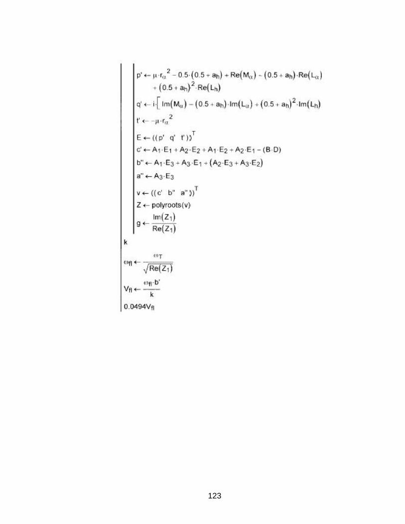
123

124
0.3 0.4 0.5 0.6 0.7 0.8 0.9 1
200
400
600
800Flutter Speed Variation (US & QS)
CG Location (tenths of chord)
Flu
tter
Spe
ed (
knot
s)
Vfl' CG( )
VfQS' CG( )
CG
c

125
References
1. Aeroelasticity, Bisplinghoff, R.L., Ashley, H., Halfman, R.L., Dover
Publications, Inc., Mineola, NY, 1955
2. Principles of Aeroelasticity, Bisplinghoff, R.L., Ashley, H., Dover
Publications, Inc., Mineola, NY, 1962
3. An Introduction to the Theory of Aeroelasticity, Y.C. Fung, Dover
Publications, Inc., New York, NY, 1969
4. Dynamics of Structures, Hurty, W.C., Rubinstein, M.F., Prentice Hall,
Inc., Englewood Cliffs, NJ, 1964
5. Introduction to the Study of Aircraft Vibration and Flutter, Scanlon,
R.H., Rosenbaum, R., Dover Publications, Inc, New York, NY, 1968
6. Theoretical Aerodynamics, Milne-Thompson, L.M., C.B.E., Fourth
Edition, Dover Publications, New York, NY, 1958.
7. Analysis of Aircraft Structures, An Introduction, Donaldson, B.K.,
McGraw-Hill, Inc., 1993
8. Aerodynamics of Wings and Bodies, Ashley, H., Landahl, M., Dover
Publications, Inc., Mineola, NY, 1965
9. Flow-Induced Vibration, Blevins, R.D., Krieger Publishing Co., Malabar,
FL, 1990
10. Airplane Performance, Stability and Control, Perkins, C.D., Hage,
R.E., John Wiley and Sons, Inc., New York, NY, 1949

126
11. Air Corps Technical Report No, 4798, Application of Three-
Dimensional Flutter Theory to Aircraft Structures (with Corrections for the
Effects of Control Surface Aerodynamic Balance and Geared Tabs),
Smilg, B., Wasserman, L., War Department, Air Corps Materiel Division,
Dayton, OH, 1942
12. The Oscillating Wing with Aerodynamically Balanced Elevator,
Kussner, H.G., Schwartz, L., NACA Technical Manual No. 991, 1940
13. NACA Technical Report No. 496, General Theory of Aerodynamic
Instability and the Mechanism of Flutter, Theodorsen, T., Langley
Memorial Aeronautical Laboratory, Langley Field, VA, 1934
14. NACA Technical Report No. 685, Mechanism of Flutter; A Theoretical
and Experimental Investigation of the Flutter Problem , Theodorsen, T.,
Garrick, I.E., Langley Memorial Aeronautical Laboratory, Langley Field,
VA, 1938
15. Dynamic Response of the MD3-160 Aircraft’s Wing Model in Steady
Flow, Usmani, M.A.W., Ho,. T.C., Department of Aerospace Engineering,
University Putra Malaysia, Malaysia, 2003
16. NASA Technical Memorandum 112852, Research and Applications in
Aeroelasticity and Structural Dynamics at the NASA Langley Research
Center, Abel, I., Langley Research Center, Hampton, VA, 1997
17. Article on aeroelasticity found on the Internet at
http://asdl.kaist.ac.kr/intro/ae1.htm
18. NACA Technical Report No. 824, Summary of Airfoil Data , Abbott,
I.H., von Doenhoff, A.E., Stivers, L.S., Langley Memorial Aeronautical
Laboratory, Langley Field, VA, 1945

127
19. A Manual for Writers of Term Papers, Theses, and Dissertations,
Turabian, Kate L., Sixth Edition, Revised by John Grossman and Alice
Bennett, The University of Chicago Press, Chicago, 1996

128
This Page Intentionally Left Blank