Basics of Aeroelasticity and Flutter AnalysisGertjan LooyeGerman Aerospace Research Center, (DLR) Oberpfa�enhofenFebruary 4, 1998

IntroductionAeroelasticity is:Discipline focusing on problems concerning the deformations ofelastomechanic bodies (elasticity) in an air ow (aero).Deformations interact with ow through e.g. change in angle of attack of anair foil, leading to change in the aerodynamic loads ...

VA

α + αd

L+dL

undeformed

deformedA complete functional diagram for an oscillating aircraft structurelooks like:

motion-induced

aircraft structure

damping

stiffness

aerodynamics

aircraftexcitation

inertia

ContentsBasics of aeroelasticity and utter analysis� basic aeroelastic stability problems;� principles of unsteady aerodynamic modeling;� the utter equation;� utter analysis methods;� "robust" utter analysis;� conclusions and outlook.

The typical sectionBasic aeroelastic principles can best be explained using the'Typical wing section', used in all aeroelasticity textbooks.... basically 2-D wing, that approximately matches aeroelastic properties at70-75% of actual wing semi-span

2 I2

e2

eh

δc

e1Kθ

Kh

m1 I

m

1

ACh

Kδ

δ

θ

We will use data from the 'Benchmark Active Control Technology' (BACT)wind tunnel model [Waszak, 1996, Waszak, 1997]. an experimental facilityof NASA Langley used for validation of CFD codes, and utter suppressioncontrol laws.Equations of motion derived using Lagrange's Equations, andPrinciple of Virtual Work ...

BACT equations of motion

1 I1

m2 I2

δc

xb

yb

xe

ye

xd

yd

m

equilibrium position

θ

h

δ

We choose 3 generalized coordinates to describe system motions: h, �, and �Kinetic energy:T = 12m1( _h + e1 _�)2 + 12I1 _�2 + 12m2( _h + e2 _� + e� _�)2 + 12I2 _� + _�2Potential energy Ue = 12Khh2 + 12K��2 + 12K��2Lagrange's equation: ddt �@T@ _qi�� �@T@qi� + �@U@qi� = Qqiq = [q1; q2; q3]T = [h; �; �]T ,Qqi is generalized force associated with qi.

BACT Equations of Motion:Equations of motion:24 m sh� sh�sh� I� s��sh� s�� I� 35

264 �h����375 + 24 Kh 0 00 K� 00 0 K� 3524 h�� 35 = 24 00K� 35 �c + 24 QhQ�Q� 35... generalized masses, and inertial coupling terms are:m = m1 +m2 sh� = m1e1 +m2e2I� = I1 + I2 +m1e21 +m2e22 sh� = m2e�I� = I2 +m2e22 s�� = I2 +m2e2e�Assuming K� is very sti� (so that � = �c), we may write:� m sh�sh� I� � � �h�� � + � Kh 00 K� � � h� � = � QhQ� �

Assume nonconservative damping forces:(!h, �h, !�, �� are in vacuo vibration characteristics)� QnchQnc� � = � � m sh�sh� I� � � 2�h!h 00 2��!� � � _h_� �The equations of motion become:(with L, M generalized aerodynamic forces)Ms � �h�� � +Ds � _h_� � +Ks � h� � = � �LM �

BACT equations of motionAerodynamic generalized forces:

L = qS hCL�� + CL�� + �c2V (CL _� _� + CLq _�)iM = qS�c hCM�� + CM�� + �c2V (CM _� _� + CMq _�)iwith q = 12�V 2Coe�cients have been determined from wind tunnel experiments and compu-tational aerodynamics.The angle of attack is:(l is dist. to aerodynamic center)� = � + _hV + l _�V... obviously a linear combination of the chosen generalized coordinates andderivatives.

BACT equations of motionSubstitution of � gives:� �LM � = qS � 0 �CL�0 �cCM� � � h� � "sti�ness"+ qSV " �CL� �lCL� � �c2V (CL _� + CLq)�cCM� �l�cCM� � �c22V (CM _� + CMq) # � _h_� � "damping"+ qS�c2V � �CL _� �lCL _��cCM _� �l�cCM _� � � �h�� � "inertia"+ qS � �CL��cCM� � � controlin short: � �LM � = Ma � �h�� � +Da � _h_� � +Ka � h� � +B��Finally, the complete equations of motion look like:

(Ms �Ma) � �h�� � + (Ds �Da) � _h_� � + (Ks �Ka) � h� � = B��

Static aeroelasticityWe will start with two static phenomena:� Torsional divergence� Control reversal

Kθ

l

Mac = 0

θ

V

θT+ θ m,I

L

zero lift

Torsional divergenceWe consider the torsional motion of the typical section:I�(�� + 2��!� _�) +K�� = MQuestion: for which pitch angle � is system in equilibrium?Time derivative terms are set to zero, and � = �T + �:K�� = M = qS�cCM�� = qS�c CM�(�T + �)Equilibrium between restoring torque in wing structure and aerodynamic mo-ment for: � = qS�cK� CM��T1� qS�cK�CM�

Static aeroelasticity� = qS�cK� CM��T1� qS�cK�CM�Increasing the speed V , and therefore the dynamic pressure q, a singularitymay occur: qS�cCM� = K�... increase in "aerodynamic" sti�ness exceeds restoring structural sti�ness.

This phenomenon is called divergence, and the corresponding dynamic pressurethe critical divergence dynamic pressure:qD = K�S�cCM�... a major design consideration, e.g. for forward swept wings.BACT: qD = 30003:556 1:333 1:490 = 424:8 psi = 20:34 kPa

0 1 2 3 4 5 6 7 8 9 10−0.01

−0.008

−0.006

−0.004

−0.002

0

0.002

0.004

0.006

0.008

0.01

time (sec)

thet

a (d

eg)

q = 424 Psi

q = 425 Psi

Static aeroelasticityControl reversalFind static equilibrium, but now the control surface has some de ection �: (weassume �T = 0)K�� = M = qS�c[(CL�� + CL��)l=�c + CMAC��]The angle of twist is: � = qS�cK� CL�l=�c + CMAC�1� qS�cK�CL�l=�c �The total lift becomes:L = qS "CL� qS�cK� CL�l=�c + CMAC�1� qS�cK�CL�l=�c + CL�# �... this expression may change sign.At the critical aileron reversal dynamic pressure:qR = �K�S�c CL�=CL�CMAC�a downward control de ection unintendedly causes negative lift

R

L L = 0 -L

q < q q = q q > qR RBACT: qD = 169 kPa (!)

FlutterWe assume a steady aerodynamic model:� �LM � = qS � 0 �CL�0 �cCM� � � h� �... only a�ecting sti�ness.Also neglecting structural damping, we obtain:� m sh�sh� I� � � �h�� � + � Kh 00 K� � � h� � = qS � 0 �CL�0 �cCM� � � h� �We keep all matrices constant, and start increasing the airspeed, and thus q.In a root locus plot this looks like:

−5 −4 −3 −2 −1 0 1 2 3 4 50

5

10

15

20

25

30

35

real

imag

V = 111

locus: x −−> o, for V: 0 −−> 200 m/s

Flutter... or in Flutter diagrams:

0 20 40 60 80 100 120 140 160 180 2005

10

15

20

25

30

35

flutter

V (m/s)

freq

. (ra

d/s)

0 20 40 60 80 100 120 140 160 180 200−0.25

−0.2

−0.15

−0.1

−0.05

0

0.05

0.1

0.15

0.2

0.25

flutter

V (m/s)

zeta

FlutterA physical interpretation can be given by looking at the work by the airloadson the structure: W = � Z T0 L dh = � Z T0 L _h dtConsider utter mode:

.

θ ~ L

h

T

W = ++- ++ -

0

The net work per cycle is positive: unstable

Unsteady aerodynamicsFirst: a VERY FREE interpretation:

superpositionV dt

oscillationSteady aerodynamics

Unsteady aerodynamics

The BACT model principally has a steady aerodynamic model, except for the_� termsBUT: in practice this is not enough!A common measure for "unsteadiness" is k = !�c2V :for k > 0:05 unsteady aerodynamics can no longer be neglected (BACT:k � 0:044).Aircraft: unsteady aerodynamics play a crucial role in ( utter) behaviorof higher modes.We will again stick to the basics, using the typical wing section.

Unsteady aerodynamicsSeveral methods are available for computational uid dynamics:� Navier-Stokes� Euler, ...� Linear Potential Theory... where Navier-Stokes Stokes is most accurate, but requires some 10 000time more CPU time than LPT.Fortunately, Linear Potential Theory has appeared to be a su�cient basis foraeroelastic computations.Assumptions that are made:� linearity� the ow is rotation free� no viscosity (no friction)� small perturbationsOnly HARMONICALLY OSCILLATING motions are considered

Basic modeling elementsz (x,t)l

z (x,t)u

w (x,t)a

u (x,t)a

airfoil

-b b0

z

x

Oscillating

* Flow equationsFlow irrotational, except in wake.... which allows the ow to be described by a potential function �(x; z).We can derive three ow equations:� velocity: [u(x; z); w(x; z)]T = grad�(x; z)� continuity: @2�@x2 + @2�@z2 = 0� dynamics: p� p1 = ��(@�@t + V @�@x) = �� * Boundary conditionsThe airfoil contour is F(x,z,t) = 0, and consists of:total thickness angle of attack,

camber

+vibrationmode

unsteady

= +

By good approximation we only need to consider the linearized condition:@�(x; z; t)@z = wa(x; t) = @za@t + V @za@x... wa(x; t) is known vertical velocity component over airfoil contour.

Basic modeling elements* Additional ow boundary conditions:� at in�nity: disturbances u0, w0 ! 0� no pressure jump across wake� Kutta condition at trailing edge (pressure continuous)* Aerodynamic forces

-b b0 x

p+

p-AC

z

V

LM

Pressure distribution along airfoil:cp(x; t) = p(x; t)� p112�V 2Lift force (positive up):L(t) = 12�V 2 Z b�b[c�p (x; t)� c+p (x; t)]dxMoment about 14�c:M(t) = 12�V 2 Z b�b[c�p (x; t)� c+p (x; t)](x+ 12b)dx

Basic modeling elementsWe already Assumed harmonic motions:za(t) = zaei!t cp(t) = cpei!t�a(t) = �aei!t L(t) = Lei!t (t) = ei!t M(t) = Mei!tNow we can start thinking of solution methods ....� Velocity potential method; Theodorsen (1935)� Vortex distribution method; K�ussner (1936), Schwarz (1940)� Integral equation method; Possio (1938)

Integral equation methodγw(x,t)

wake

z

xb0-b

γ (x,t)a

airfoilIntegral equation with wa(x; t) known:wa(x; t) = � 12� I b�b a(�; t)x� � d� �� 12� Z 1�b w(�; t)x� � d� w and a are related by Kelvin's theorem: circulation remains constantIn e.g. [Bisplingho� and Ashley, 1962, F�orsching, 1974] some additionalelementary transformation elimination is applied, leading to :wa(x)V = Z b�b�cp(�)K(x� �; k)d�... where K(x� �; k) is a (very scary) kernel function.Numerical solution methods:� Kernel function method (linear combination of pressure modes)� Doublet Lattice (DL) method

Doublet LatticeProcedure (2D case):The chord is divided into N+1 segments� At the 14�c locations a concentrated, unknown �cp is assumed (generatedwith doublet ow elements)�cp(x) = NXi=0 cp(xi)�(x� xi)� Integral equation applied at 34�c of segments

p1

cp2

cp3c

collocation points

b-b 0

N=2

� By sensible choice of cp, requires only integration over kernel function.� Integral equation reduces to matrix equation:�waV � = [D] fcpg... which is solved for fcpg for di�erent k values.DL is very exible: extends to 3D structures, compressible ow. Method isused in most available software packages.

ComplicationsUp to now we assumed incompressible ow. However for Mach numbers(Ma > 0:5) this assumption is no longer valid.The linearized equations let themselves be corrected for Mach e�ects, but wewill not further detail this.An important point however: every Mach number requires new computation,e.g. with Doublet Lattice method...Transonic aeroelastics is (even for 2D case) a continuing research topic.

Analytical exampleFor a 2D structure in incompressible ow an analytic solution for unsteadyaerodynamics exists:L = 14���c2(j!V �� � !2�h + !2l��) + ��V �cC(k)(V �� + j!�h + (�c4 � l)j!��)... C(k) is the complex valued Theodorsen function.By approximation [Dowell and Others, 1995]: (remember k = !�c2V )C(k) = 1 + �0:4544ikik + 0:1902... where the fractional part is nothing more than a lag function.Further remarks:� L basically has the form:L = A0 + A1 � k + A2 � k2 + additional lag term... adding an additional aerodynamic state to the model.� more accurate approximation for C(k) adds more lag states.� oscillatory aerodynamics are useful for estimation of unsteady stabilityderivatives (CL _�, Cm _�, etc.) for rigid aircraft [Rodden and Giesing, 1970].

Transformation into time domainCombining the structural dynamics model with aerodynamics leadsto the utter equation:(Mss2 +Dss +Ks)q = Qq(Ma; k)q... for BACT: q = [h; �]T , Qq = [�L; M ]T .In practice, computation of Qq(Ma; k)...� is done mode by mode, using DL;� for a set of values of k and Ma;� ....is only valid on the imaginary axis.An approximate transformation into time domain is needed.From a physical point of view, using lag functions is most obvious.Procedure:� for given Ma, compute Qq(Ma; k) for a range of k-values;� choose a number of lag functions in Laplace domain;� �t coe�cients, for computed Qq(Ma; k)'s.

Transformation into time domainWell-known methods:� Non-critical pole functions [Roger, 1977]� Modi�ed matrix Pad�e method [Vepa, 1977]� Minimum state method [Karpel and Hoadley, 1990]For a comparison, refer to [Schuler, 1997]: latter method gives lowest order...and most accurate results.For example, modi�ed matrix Pad�e method:

Qq(Ma; k)j = A0j + A1jp + A2jp2 + nlXr=1 p�rj + pAr+2jwith p = s�c2V = + ik.This is for j'th mode: nq � nl additional states in model ....Furthermore: we have to pay attention to location of 'arti�cial poles'.

Flutter analysisFor the aeroelastician, the main motivation for all this modeling work is utter analysis:�nd the lowest speed for which the �rst mode goes unstable.The starting point is the utter equation:Mss2 +Dss +Ks = Qq(Ma; k) = 12�V 2Cq(Ma; k)� this is an eigenvalue problem� solve as a function of q (or V ), for di�erent mach numbers, alt.� complication: Qq(Ma; k) is only available on imaginary axis!

Flutter analysis� K-method [Bisplingho� and Ashley, 1962];{ introduce arti�cial damping to enforce harmonic solution, �nd velocityfor which this term is zero.{ sometimes anomalous utter curves.� PK-method [Hassig, 1971];{ iteratively match k in eigenvalue p = + ik with the corresponding kin Qq(Ma; k).{ ight control system may be included.{ solution is only exact on imaginary axis ( utter point)� p-method [Abel, 1979]; apply transformation into time domain, computeeigenvalues of state-space A-matrix.{ ight control system may be included.{ use of standard control analysis tools.Brand new method [Lind and Brenner, 1998]:� �-methodObtain state space model, write in LFT-form with �q as free parameter,perform �-analysis.{ modeled uncertainties �t in LFT model;{ compute local worst-case utter margin.{ used in ight.All analyses valid at speci�c Mach number, aircraft con�guration, altitude ....

BACT Flutter diagram

FlutterIn root locus plot:

−6 −4 −2 0 2 4 60

5

10

15

20

25

30

35

real

imag

V = 113

locus: x −−> o, for V: 0 −−> 200 m/s

Robust utter analysisRecall the BACT equations of motion (implicit form):0 = Ms � �h�� � +Ks � h� �� qS � �CL�cCM �All parameters are constant, except for the dynamic pressure q:q = q0 + sq�q; j�qj < 1We may write:0 = Ms � �h�� � +Ks � h� �� (q0 + sq�q)S � �CL�cCM �

= Ms � �h�� � +Ks � h� �� q0S � �CL�cCM �� �qzq= Ms � �h�� � +Ks � h� �� q0S � �CL�cCM �� wqwith wq = zq�q, and: zq = sqS � �CL�cCM �δ Iq

P

z wq q

... this is a Linear Fractional Transformation (LFT)

Robust utter analysisAgain, the BACT equations of motion:0 = � m sh�sh� I� ��� �h�� � + � 2�h!h 00 2��!� � � _h_� �� + � Kh 00 K� � � h� ��12�V 2S � �CL(�; h; V; :::)�cCM(�; h; V; :::) �All parameters are constant, excepting V :V = 91:44 + 18:29 �V m=s; j�V j < 1using the software from [Varga et al., 1997], we obtain:

δ I

zv

wv v

P

Next, we compute the frequency response:δ I

z

ω

wv vv

P(j )

Robust utter analysisWe are looking for the smallest �V for which instability occurs:� this is the case when the �rst pole walks over the j!-axis;� at that very moment, the LFT is singular;� this is nothing else than a �-computation!The structured singular value � is in general de�ned as:�(P (j!)) = 1min�2�f��(�) : det(I � P (j!)�) = 0g... we are only able to compute upper and lower bounds:

101

102

0

0.2

0.4

0.6

0.8

1

freq. (rad)We have seen the location of the peak before ...... as well as the critical V : V = 91:44 + 21:58 � 1:0 = 113 m=s

Robust utter analysisIn our LFT modeling, we are not limited to velocity, but we may model uncer-tainties in exactly the same way, e.g.:!h = 21:0 + 2:0 �!h rad=s!p = 32:7 + 3:0 �!p rad=s�h = 0:01 + 0:005 ��h�p = 0:01 + 0:005 ��pAgain, by hand, or using [Varga et al., 1997]:

w

ω2

0

∆0Ivδ

P (j )

z

∆p

... now with � = diag(�V I4; �!hI3; �!pI3; ��h; ��pInstead of a nominal model, we are looking at a set of models.

Robust utter analysisAs � will �nd the lowest destabilizing �, we obtain the worst-casemodel parameters, for which the utter speed is lowest.

10−2

10−1

100

101

102

0

0.5

1

1.5

2

2.5

3

We �nd: !h = 21:0 + 2:0 0:4 = 21:8 rad=s!p = 32:7 + 3:0 �0:4 = 31:5 rad=s�h = 0:01 + 0:005 0:4 = 0:0120�p = 0:01 + 0:005 �0:4 = 0:008In the worst case, utter will already occur atV = 91:44 + 21:58 � 0:40 = 100:1 m=s

Robust utter analysisWe can check our result via a root locus:

−6 −4 −2 0 2 4 60

5

10

15

20

25

30

35

real

imag

V = 100

locus: x −−> o, for V: 0 −−> 200 m/s

Robust utter analysis... and via simulations:

0 1 2 3 4 5 6 7 8 9 10−1.5

−1

−0.5

0

0.5

1

1.5x 10

−4

time (s)

thet

a (d

eg)

V = 99.4 m/s

0 1 2 3 4 5 6 7 8 9 10−4

−3

−2

−1

0

1

2

3

4x 10

−4

time (s)

thet

a (d

eg)

V = 100.8 m/s

Robust utter analysis� analysis with a control system can be done easlily;� LFT modeling has been automated;� computing �(j!) gives a guaranteed upper bound;� additionally, worst cases derived� is used in ight by NASA-Dryden ( utterometer).Problems with the method:� Frequency gridding;� Parameters must occur in a rational way;� LFT order reduction.

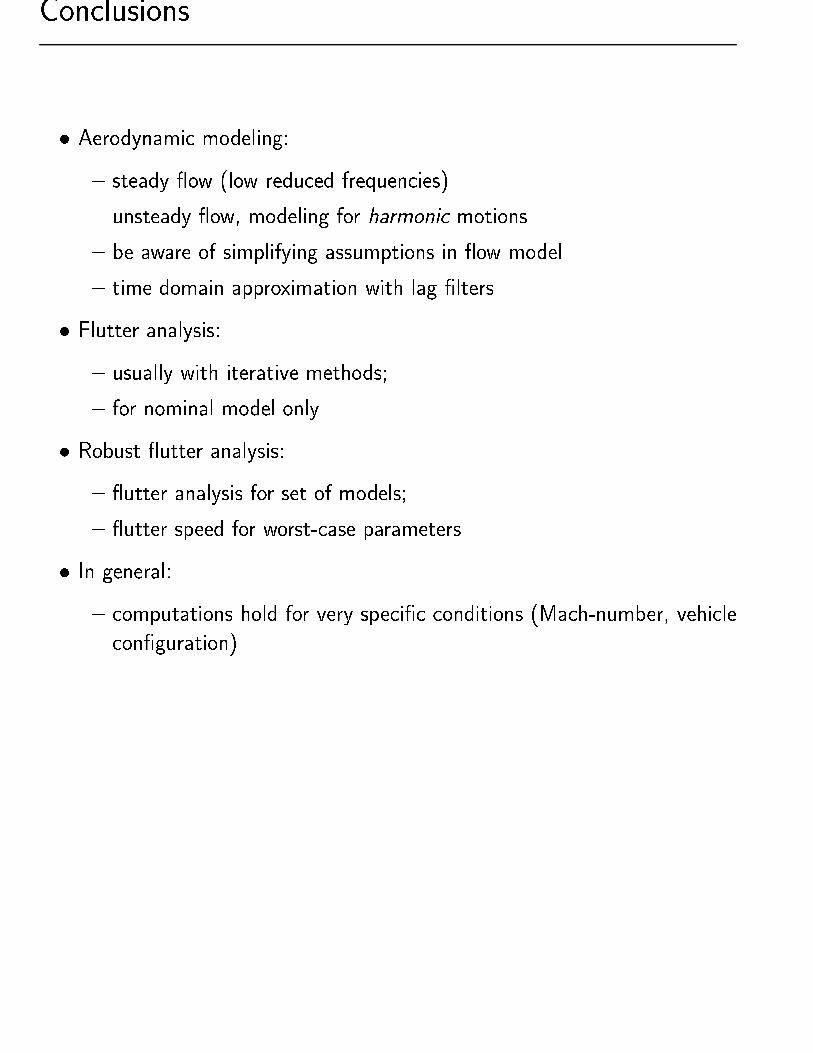
Conclusions� Aerodynamic modeling:{ steady ow (low reduced frequencies){ unsteady ow, modeling for harmonic motions{ be aware of simplifying assumptions in ow model{ time domain approximation with lag �lters� Flutter analysis:{ usually with iterative methods;{ for nominal model only.� Robust utter analysis:{ utter analysis for set of models;{ utter speed for worst-case parameters.� In general:{ computations hold for very speci�c conditions (Mach-number, vehiclecon�guration)

Bibliography[Abel, 1979] Abel, I. (1979). An analytical technique for predicting the characteristics of a exible wingequipped with an active utter-suppression system and comparison with wind-tunnel data. TechnicalReport NASA TP-1367, NASA.[Bisplingho� and Ashley, 1962] Bisplingho�, R. L. and Ashley, H. (1962). Principles of Aeroelasticity. DoverPublications Inc., New York.[Dowell and Others, 1995] Dowell, E. H. and Others (1995). A Modern Course in Aeroelasticity. KluwerAcademic Publishers, Dordrecht, The Netherlands, third edition. editions from 1975,1989 as well.[F�orsching, 1974] F�orsching, H. (1974). Grundlagen der Aeroelastik. Springer-Verlag.[Hassig, 1971] Hassig, H. (1971). An Approximate True Damping Solution of the Flutter Equation byDeterminant Iteration. Journal of Aircraft, 8(11):885{889.[Karpel and Hoadley, 1990] Karpel, M. and Hoadley, S. (1990). Physically Weighted Minimum State Un-steady Aerodynamic Approximation. Technical Report NASA-TP-3025, NASA. to be published (1990)NOT AVAILABLE.[Lind and Brenner, 1998] Lind, R. and Brenner, M. J. (1998). Robust Flutter Margin Analysis that Incor-porates Flight Data. Technical Report NASA TP-????, NASA, Dryden Flight Research Center, EdwardsCA. draft version available.[Rodden and Giesing, 1970] Rodden, W. P. and Giesing, J. P. (1970). Application of Oscillatory AerodynamicTheory to Estimation of Dynamic Stability Derivatives. Journal of Aircraft, 7(3):272{275.[Roger, 1977] Roger, K. (1977). Airplane Math Modeling Methods for Active Control Design. AGARD,(CP-228).[Schuler, 1997] Schuler, J. (1997). Flugregelung und aktive Schwingungsd�ampfung f�ur exible Gro�raum- ugzeuge { Modellbildung und Simulation. PhD thesis, Institut f�ur Flugmechanik und Flugregelung,Universit�at Stuttgart, Stuttgart.[Varga et al., 1997] Varga, A., Looye, G., Moormann, D., and Gr�ubel, G. (1997). Automated Generation ofLFT-Based Parametric Uncertainty Descriptions from Generic Aircraft Models. Technical Report TP-088-36, GARTEUR.[Vepa, 1977] Vepa, R. (1977). Finite State Modeling of Aeroelastic Systems. Technical Report NASACR-2779, NASA.[Waszak, 1996] Waszak, M. R. (1996). Modeling the Benchmark Active Controls Technology Wind-TunnelModel for Application to Flutter Suppression. In Proceedings of the AIAA Atmospheric Flight MechanicsConference, number AIAA Paper 96-3437, San Diego. AIAA.[Waszak, 1997] Waszak, M. R. (1997). Bact simulation user guide (version 7.0). Technical Report NASATM-97-206252, NASA Langley Research Center, Hampton.38