Effect of uncertainty on the bifurcation

behavior of pitching airfoil stall flutter

S. Sarkar a,∗, J.A.S. Witteveen b, A. Loeven b, H. Bijl b

aDepartment of Aerospace Engineering, IIT Madras, Chennai 600036, India.

bFaculty of Aerospace Engineering, Delft University of Technology, Kluyverweg 1,

2629 HS Delft, The Netherlands

Abstract

In this paper the effect of system parametric uncertainty on the stall flutter bi-

furcation behavior of a pitching airfoil is studied. The aerodynamic moment on the

two-dimensional rigid airfoil with nonlinear torsional stiffness is computed using the

Onera dynamic stall model. The pitch natural frequency, a cubic structural nonlin-

earity parameter, and the structural equilibrium angle are assumed to be uncertain.

The effect on the amplitude of the response, the bifurcation of the probability distri-

bution, and the flutter boundary is considered. It is demonstrated that the system

parametric uncertainty results already in 5% probability of pitching stall flutter at

an 12.5% earlier position than the point where a deterministic analysis would pre-

dict unstable behavior. Probabilistic Collocation is found to be more efficient than

the Galerkin Polynomial Chaos method and Monte Carlo simulation for modeling

uncertainty in the post-bifurcation domain.

Key words: Stall flutter, Uncertainty quantification, Galerkin Polynomial Chaos,

Probabilistic Collocation, Flutter boundary

Preprint submitted to Elsevier Science 2 June 2008

1 Introduction

It is increasingly acknowledged that flutter analysis should include the quan-

tification of the effects of system parametric uncertainty. Dynamical systems

are known to be sensitive to physical uncertainties, since they often amplify

this random variability with time. A stable response of a nonlinear dynamical

system can change at a bifurcation boundary into an oscillatory instability that

can grow in an unbounded fashion, which is known as flutter (Fung, 1955).

Flutter of aircraft and rotor structures is of practical interest to engineers,

since it can lead to fatigue damage or failure of the structure. System para-

metric uncertainties can significantly affect the onset and properties of flutter.

The added value of modeling these uncertainties with probabilistic methods

compared to deterministic approaches to robustness is that they quantify the

effect of uncertainties in a probabilistic sense. Based on the resulting detailed

probabilistic information well-balanced decisions can be made in a robust de-

sign optimization process.

Monte Carlo (MC) simulation and perturbation techniques are classical prob-

abilistic methods for uncertainty quantification. However, stochastic spectral

methods based on the Polynomial Chaos expansion may be more efficient

and accurate alternatives. The Polynomial Chaos expansion by Wiener (1938)

is a polynomial expansion in probability space in terms of independent ran-

dom variables and deterministic coefficients. The Galerkin Polynomial Chaos

(GPC) method proposed by Ghanem and Spanos (1991) employs a Galerkin

stochastic finite element approach to solve for the deterministic coefficients.

∗ Corresponding author. Tel.: +914422574024; fax: +914422574002Email address: sunetra.sarkar@gmail.com (S. Sarkar ).

2

The Galerkin projection in probability space results in a coupled set of de-

terministic equations. This type of methods are called intrusive methods,

since the deterministic solver has to be altered to solve for the coupled equa-

tions. The method can achieve exponential convergence for Gaussian distribu-

tions, since it is based on Gaussian random variables and Hermite polynomi-

als (Ghanem, 1999). The exponential convergence has been extended to more

distributions in the generalized Polynomial Chaos by Xiu and Karniadakis

(2002) and for arbitrary distributions by Wan and Karniadakis (2006a) and

Witteveen and Bijl (2006a). Other non-polynomial expansions are the wavelet

based Wiener-Haar expansion of Le Maıtre et al. (2004) and the Fourier Chaos

expansion of Millman et al. (2003).

In order to avoid solving the coupled set of equations of the Galerkin Polyno-

mial Chaos method intrusively, several non-intrusive uncoupled alternatives

have been proposed. In non-intrusive Polynomial Chaos methods a determin-

istic solver is used as a black-box like in Monte Carlo simulation. The Prob-

abilistic Collocation (PC) method is such a non-intrusive Polynomial Chaos

method in which the deterministic coefficients are solved for by collocating the

problem in Gauss points in probability space (Babuska et al., 2007; Loeven

et al., 2007). Suitable Gauss points are the zeros of polynomials orthogonal

with respect to the probability density of the uncertain system parameter.

Exponential convergence with respect to the order of approximation can be

obtained for arbitrary probability distributions. Babuska et al. (2007) have

proven that for elliptic partial differential equations the Probabilistic Collo-

cation method is equivalent to the Galerkin Polynomial Chaos method. The

non-intrusive Polynomial Chaos method proposed by Hosder et al. (2006)

and Walters (2003) is based on approximating the Polynomial Chaos coeffi-

3

cients. A similar approach called non-intrusive Spectral Projection is used by

Reagan et al. (2003). The Stochastic Collocation method proposed by Math-

elin and Hussaini (2003); Mathelin et al. (2005) showed a significant decrease

in computational time compared to the Galerkin Polynomial Chaos method.

When multiple uncertain parameters are involved the collocation grids are

constructed using tensor products of one-dimensional quadrature grids. The

amount of collocation point, and therefore the number of required determin-

istic solves, increases rapidly. As an alternative, sparse grid collocation ap-

proaches are used (Ganappathysubramanian and Zabaras, 2007; Gerstner and

Griebel, 1998; Xiu and Hesthaven, 2005).

Although Polynomial Chaos methods have been successful in many problems,

often Monte Carlo simulation or perturbation techniques are used for model-

ing uncertainty in flutter analysis. Monte Carlo simulations have, for example,

been used by Lindsley et al. (2002, 2006) to study the periodic response of

nonlinear plate equations under supersonic flow subject to uncertain modu-

lus of elasticity and boundary conditions. The effect of uncertainties on panel

flutter has been analyzed by Liaw and Yang (1993) using a second moment

perturbation based stochastic finite element model. A first order perturbation

method has been applied to a bending-torsion flutter model in an unpublished

report by Poirion, [see Lind and Brenner (1998); Pettit (2004a)], to predict

flutter probability with uncertain structural mass and stiffness. Poirion (2000)

has also investigated nonlinear random oscillations with application to aeroser-

voelastic systems using simulation techniques for Gaussian and non-Gaussian

random processes and random delay modeling of control systems. Poirel and

Price (2003) have solved random bending-torsion flutter equations under tur-

bulent flow conditions with a linear structural model using a Monte Carlo type

4

approach. Choi and Namachchivaya (2006) have found qualitatively different

response density functions in nonlinear panel flutter under supersonic flow

subject to random fluctuations in the turbulent boundary layer using non-

standard reduction through stochastic averaging. Ibrahim et al. (2005) and

Beloiu et al. (2005) have investigated the effects of boundary condition and

joint condition uncertainties on a panel flutter system. De Rosa and Franco

(2008) have presented the response of a plate subjected to stochastic flow-field

due to the effect of turbulent boundary layer using numerical and analytical

approach. Pettit (2004a,b) has outlined that small uncertainties in the system

parameters, external loads and boundary conditions can significantly modify

the static and dynamic aeroelastic system response. Various uncertain aeroe-

lastic analyses for plate-like structures are discussed in Dowell et al. (1989)

and Nigam and Narayanan (1994).

Studies that use Polynomial Chaos methods to predict the effect of uncertain-

ties in flutter analysis report that the Polynomial Chaos expansion can have

difficulty capturing the uncertain response after long-term time integration.

Pettit and Beran (2004, 2006) have found that the Wiener-Hermite expan-

sion suffers from energy loss in representing the periodic response of bending-

torsion flutter model for long integration times. For the wavelet based Wiener-

Haar expansion of Le Maıtre et al. (2004), this problem is less dominant (Pettit

and Beran, 2006). Millman et al. (2003) demonstrated that a Fourier-Chaos

expansion can be computationally more efficient for a bending-torsion flutter

problem subjected to Gaussian distributions than the regular Wiener-Hermite

expansion. Lucor and Karniadakis (2004) and Wan and Karniadakis (2006b)

have observed that the effect of uncertainties on the frequency of the response

is of major influence on long-term integration accuracy of Polynomial Chaos

5

approximations.

In this paper, the effect of parametric uncertainty on the stall flutter behavior

of a pitching airfoil is studied using Polynomial Chaos expansion methods.

This study can be considered a qualitative assessment of the effect of uncer-

tainty on the bifurcation behavior of the system. Stall flutter is, for example,

of interest to wind turbine research community. In the present deterministic

model, the blade structure is modeled as a two-dimensional rigid airfoil with

torsional degree-of-freedom. The structural stiffness (Fragiskatos, 1999) in the

torsional direction is modeled using a combination of a linear and a cubic

nonlinear spring (Lee and Tron, 1989; Lee et al., 1999), since a blade section

which is being twisted is likely to behave as a cubic stiffness hardening spring

(Lee et al., 1999). The stall aerodynamic moment is computed using the On-

era semi-empirical dynamic stall model as shown by Beedy et al. (2003), and,

Dunn and Dugundji (1992). This approach is commonly used in many engi-

neering aeroelastic applications (Lee et al., 1999; Sheta et al., 2002; Tang and

Dowell, 1993a,b). Tang and Dowell (2004) have also used the Onera dynamic

stall model to investigate the effects of structural nonlinearity on a high aspect

ratio binary wing flutter. In another recent work, Svacek et al. (2007) have in-

vestigated two-dimensional flutter in the dynamic stall regime; however, they

have not used a semi-empirical model to compute the aerodynamic loads, but

with a finite element based discretization of the Navier-Stokes equations.

An earlier deterministic study by Sarkar and Bijl (2008) on a stall flutter

system has pointed out that the response is sensitive to model parameter

variations. In this paper the Galerkin Polynomial Chaos method and the Prob-

abilistic Collocation method are applied to study the effect of uncertainty in

several model parameters. The pitch natural frequency, the cubic structural

6

nonlinearity parameter, and the structural equilibrium angle are assumed to

be uncertain.

The efficiency of both the Galerkin Polynomial Chaos method and the Proba-

bilistic Collocation method are compared for the case with the uncertain pitch

natural frequency. The effect of the Polynomial Chaos expansion order on the

accuracy of the long-term time integration results is studied. A comparison

of the computational costs of the two methods shows that the Probabilis-

tic Collocation method is more efficient for the highly nonlinear model. The

Probabilistic Collocation method is further employed to study the effect of

the uncertain cubic structural nonlinearity parameter and the structural equi-

librium angle on the bifurcation behavior of the system. In these cases the

effect on the amplitude of the response, the bifurcation of the probability

distribution, and the flutter boundary is considered.

The Polynomial Chaos method and the Probabilistic Collocation method are

briefly reviewed in section 2. In section 3 the equation of motion and the

aerodynamic model for the stall flutter problem are given. Numerical results

are presented in section 4 and the conclusions are summarized in section 5.

2 Polynomial Chaos expansion methods

Modeling uncertainties in the stall flutter problem results in a system of

stochastic differential equations based on a probability space (Ω, F , P ). Let

ω ∈ U(0, 1) be an element of the sample space Ω, F ⊂ 2Ω the σ-algebra of

events and P a probability measure. Random event ω is defined as uniformly

distributed on [0, 1] in accordance with the standard technique for gener-

7

ating random numbers of an arbitrary distribution by projecting uniformly

distributed numbers ω onto probability measure P , as in Bhattacharya and

Waymire (2007). The argument ω is used for an uncertain variable u(t, ω) to

emphasize the fact that an uncertain variable is a function of a random event.

Suppose that the stall flutter model is described by the following equation for

u(t, ω) with an nonlinear operator L and a source term S

L(t, ω; u(t, ω)) = S(t, ω), (1)

Let us consider the operator to be a differential operator and the system is

described by a nonlinear stochastic differential equation for u(t, ω) with a

nonlinear function g(u(t, ω))

d(u(t, ω))

dt+ c1(ω)u(t, ω) + c2(ω)g(u(t, ω)) = f(t) (2)

with time t and appropriate initial conditions. The system is assumed to have

parametric uncertainty through c1, c2 with known probability distribution.

The Galerkin Polynomial Chaos method and the Probabilistic Collocation

method to propagate the uncertainty through (1) are discussed in this section.

2.1 Galerkin Polynomial Chaos method

The uncertain variable u(t, ω) and the uncertain parameter can be represented

by a Polynomial Chaos expansion

u(t, ω) =∞∑

i=0

ui(t)Ψi(ξ(ω)), (3)

where ui(t) denote the deterministic polynomial chaos coefficients and Ψi(ξ(ω))denote orthogonal polynomials in terms of a random variable ξ(ω). The ran-

dom variable ξ(ω) is obtained from a linear transformation of the uncertain

8

physical parameter to a corresponding standard domain, i.e. [−1, 1], [0, ∞)

or (−∞, ∞). The polynomials Ψi(ξ(ω)) satisfy the following orthogonality

relation

〈Ψi(ξ), Ψj(ξ)〉 =∫

suppξ

Ψi(ξ)Ψj(ξ)wξ(ξ)dξ = 〈Ψ2i (ξ)〉δij, (4)

where δij denotes the Kronecker delta and 〈·, ·〉 denotes an inner product,

wξ(ξ) is a weighting function, and suppξ is the support of ξ(ω). To be able to

obtain exponential convergence for sufficiently smooth solutions, the weighting

function of the integration is chosen to be equal to the probability density fξ(ξ)

of ξ(ω), i.e. wξ(ξ) = fξ(ξ) (Wan and Karniadakis, 2006a; Witteveen and Bijl,

2006a).

The deterministic coefficients ui(t) in (3) can be solved for numerically using

a stochastic finite element approach, as shown by Ghanem and Spanos (1991).

For the numerical implementation the infinite summation in ξ in (3)is replaced

by a truncated finite-term summation

u(t, ω) =N∑

i=0

ui(t)Ψi(ξ(ω)). (5)

We also assume,

c1,2 =1∑

i=0

c1,2iΨi(ξ(ω)) (6)

Substituting the above into the governing equation (2)

N∑

i=0

d

dtuiΨi +

1∑

j=0

N∑

i=0

uic1jΨiΨj +1∑

j=0

c2jg( N∑

i=0

uiΨi

)= f(t). (7)

For g(u) being a cubic nonlinear function, g(∑N

i=0 uiΨi) will take the following

form:

g(u) = u3 = (N∑

i=0

uiΨi)3 =

N∑

i1=0

N∑

i2=0

N∑

i3=0

ui1Ψi1ui2Ψi2ui3Ψi3 (8)

9

A stochastic Galerkin projection is employed to obtain a system of coupled

N + 1 deterministic equations for the N + 1 deterministic coefficients. The

Galerkin projection in probability space of (7) onto each polynomial basis

Ψk(ξ(ω))Nk=0 in the sense of inner product (4) yields

⟨[ N∑

i=0

d

dtuiΨi +

N∑

i=0

1∑

j=0

uic1jΨiΨj +1∑

j=0

c2jg( N∑

i=0

uiΨi

)], Ψk(ξ)

⟩= 〈f(t), Ψk(ξ)〉,

(9)

for k = 0, 1, . . . , N . The Galerkin projection results in a coupled set of N + 1

deterministic equations as shown below:

duk

dt+

1

〈Ψ2k〉

1∑

j=0

N∑

i=0

uic1j〈ΨiΨjΨk〉+⟨[ 1∑

j=0

c2jg( N∑

i=0

uiΨi

)], Ψk(ξ)

⟩= 〈f(t), Ψk(ξ)〉

(10)

The inner product term 〈ΨiΨjΨk〉 along with1

〈Ψ2k〉

can be evaluated analyti-

cally. For analytic nonlinearities like a cubic function shown in (8), the third

term in the left hand side of (10) will also have inner product terms which can

be evaluated analytically before the time marching process. For non-analytic

forms the term needs to be evaluated numerically using some numerical inte-

gration process like Simpson’s rule etc.

The original homogeneous Polynomial Chaos (Ghanem and Spanos, 1991) is

based on a Gaussian probability measure P and a Gaussian random variable

ξ(ω). For that case Hermite polynomials satisfy orthogonality relation (4). For

any arbitrary distributions the orthogonal polynomials are constructed using

other classical polynomials or an orthogonalization method (Wan and Kar-

niadakis, 2006a; Witteveen and Bijl, 2006a; Xiu and Karniadakis, 2002). In

this work the uncertain system parameters are assumed to be lognormally dis-

tributed. A lognormal distribution is often a good model for non-negative phys-

ical parameters. The orthogonal polynomials Ψi(ξ(ω))Ni=0 are constructed

10

using Gram-Schmidt orthogonalization (Gautschi, 2004), in which the inner

products are written as summations of the analytically known raw moments

of the lognormal distribution. Constructing the polynomials in this way re-

sults in negligible additional computational costs compared to using classical

polynomials.

2.2 Probabilistic Collocation method

Another approach to obtain a Polynomial Chaos approximation of the un-

certain response u(t, ω) is the Probabilistic Collocation method of Babuska

et al. (2007), [also see Loeven et al. (2007)]. In this non-intrusive approach the

Polynomial Chaos coefficients are computed by solving uncoupled determinis-

tic problems for various parameter values. The uncertain system parameter is

written in terms of an N th order Polynomial Chaos expansion with Lagrange

basis polynomials hi(ξ(ω))

u(t, ω) =N+1∑

i=1

u∗i (t)hi (ξ(ω)) , (11)

where u∗i (t)N+1i=1 are the realizations of u(t, ω) at the N +1 collocation points

ξiN+1i=1 , with ξi = ξ(ωi). The Lagrange interpolating polynomial chaoses

hi(ξ(ω))N+1i=1 of order N through the collocation points ξi are given by

hi (ξ(ω)) =N+1∏

j=1j 6=i

ξ(ω)− ξj

ξi − ξj

, (12)

such that hi (ξj) = δij. Suitable collocation points are the Gaussian quadrature

points corresponding to the inner product (4) with weighting function wξ(ξ) =

fξ(ξ). These collocation points are the roots of the orthogonal polynomial

ΨN+2(ξ(ω)) given by (4). The Gauss quadrature points can be computed for

11

any arbitrary distributions using, for example, the Golub-Welsch algorithm,

as shown by Golub and Welsch (1969). This algorithm employs the recurrence

coefficients (Gautschi, 2005) of the orthogonal polynomials Ψi(ξ).

The uncoupled set of N+1 equations for the deterministic coefficients u∗i (t)N+1i=1

can be derived by substituting expansion (11) into the governing equation (2)

d

dt(N+1∑

i=1

u∗i (t)hi(ξ))+c1(ω)N+1∑

i=1

u∗i (t)hi(ξ)+c2(ω)g(N+1∑

i=1

u∗i (t)hi(ξ)) ≈ f(t) (13)

A Galerkin projection of each Lagrangian basis hj (ξ(ω))N+1j=1 results in

⟨ d

dt(N+1∑

i=1

u∗i (t)hi(ξ)) + c1(ω)N+1∑

i=1

u∗i (t)hi(ξ) + c2(ω)g(N+1∑

i=1

u∗i (t)hi(ξ))

, hj(ξ)

⟩= 〈f(t), hj(ξ)〉,

(14)

for j = 1, 2, . . . , N +1. Approximating the inner product in (14) using numer-

ical integration and using property hi (ξj) = δij of the Lagrange polynomials

results in the following set of uncoupled deterministic equations

d(u∗j(t))

dt+ c1(ωj)u

∗j(t) + c2(ωj)g(u∗j(t)) = f(t), (15)

for j = 1, 2, . . . , N + 1. The distribution function can be constructed from the

expansion coefficients u∗i (t) using expansion (11).

3 Stall flutter model

In this section the single degree-of-freedom pitching airfoil stall flutter model

is described. It consists of an equation of motion for the two-dimensional

rigid airfoil with nonlinear torsional spring stiffness. The aerodynamic moment

including the stall behavior is modeled using the Onera dynamic stall model.

12

3.1 Equation of motion

A schematic plot of the two-dimensional blade section of unit span and the

coordinate system is given in Figure 1. The equation of motion for the single

degree-of-freedom pitching oscillation is given by Fragiskatos (1999) and Fung

(1955):

Iαα + Iαω2αα + Knl1α

3 = M(t). (16)

Here, Iα is the wing mass moment of inertia, α is the effective angle of at-

tack, ωα is the natural frequency of the pitch elastic mode, Knl1 is a nonlinear

stiffness term accounting for concentrated structural nonlinearities in the tor-

sional direction, and M(t) is the time dependent aerodynamic moment. A

nondimensional form of the governing equation is often useful in aeroelastic

analysis to investigate the effect of system parameters. The nondimensional

form of (16) is given below (Fragiskatos, 1999):

α′′ + α/(U2) + Knlα3 = 2Cm/(πµr2

α). (17)

Here, (′) denotes a derivative with respect to nondimensional time τ = tV /b, V

is the resultant velocity of the wind velocity U and the rotational velocity Ωr

as shown in Figure 1, b is the semi-chord of the blade, Cm is the aerodynamic

moment coefficient, U is the nondimensional airspeed defined as U = V /bωα,

µ and rα are nondimensional structural parameters, mass ratio µ = m/(πρb2),

radius of gyration rα = Iα/(mb2), Knl is the nondimensional form of Knl1.

Typical data for a 1000 KW capacity wind turbine are used with a semi-chord

of b = 0.8m at 0.75 blade radius and a representative resultant wind speed of

V = 50m/s (Cheney and Migliore, 2000; Stiesdal, 1999).

The uncertain parameters in the structural model are the pitch natural fre-

13

quency ωα, the cubic structural nonlinearity parameter Knl, and the struc-

tural equilibrium angle αm. The uncertainty in ωα is introduced in the model

through U . The deterministic value of the structural nonlinearity Knl is as-

sumed to be zero. The parameter αm is introduced in the same way as shown

by Fragiskatos (1999) and Price and Fragiskatos (2000). The airfoil is given

its initial perturbation about this angle. An extra moment is used to maintain

this angle for the structure.

3.2 Aerodynamic stall model

The aerodynamic moment coefficient Cm in (17) is computed using the Onera

semi-empirical dynamic stall model, as shown in Beedy et al. (2003) and Dunn

and Dugundji (1992). This model gives a system of ordinary differential equa-

tions for the aerodynamic loads. Using this type of semi-empirical aerodynamic

models is common practice in engineering aeroelastic problems. The physical

process of dynamic stall involves leading and trailing edge vortex development

and their subsequent separation and shedding into the wake. Vortex growth

increases suction and helps increase the aerodynamic loads beyond their static

stall values. Vortex separation from the body triggers a rapid decrease of the

loads. The Onera model takes into account this complex unsteady phenomena

step by step. A detailed discussion on the Onera dynamic stall model is given

by Dunn and Dugundji (1992) and Tran and Petot (1981). The differential

equations are of the following form:

Cz = szα′ + kvzθ

′′ + Cz1 + Cz2 (18)

C ′z1

+ λzCz1 = λz (aozα + σzθ′) + αz (aozα

′ + σzθ′′) (19)

C ′′z2

+ 2dωC ′z2

+ w2(1 + d2

)Cz2 = −w2

(1 + d2

)(∆Cz|α + e∆C ′

z|α) , (20)

14

where the coefficients sz, kvz, λz, αz, aoz, σz, d, w and e are empirically

determined by parameter identification techniques using experimental data.

The values for the coefficients for the NACA0012 airfoil have been obtained

from Dunn and Dugundji (1992). The pitch angle θ and the total angle of

attack α = θ − h′, are equal in this case since only torsional oscillations are

considered. Here, h is the nondimensional flapping displacement normalized

with the airfoil chord.

The coefficients Cz are the aerodynamic coefficient Cl, Cd or Cm for z =

l, d, m. In this case, only the moment coefficient Cm is of interest. The aero-

dynamic moment consists of two contributions: (i) the inviscid circulatory

part Cm1 given by (19) and (ii) the viscous stall part Cm2 given by (20),

which becomes important above the static stall angle. The stall behavior is

modeled in Eq. (20) by the ∆Cm term. The ∆Cm part is a nonlinear function

which is identically zero below the static stall angle of 12o at which it exhibits

a discontinuous step to a finite value.

The nonlinear ∆Cm term has a major influence on the implementation of the

Galerkin Polynomial Chaos method for the stall flutter model. The Galerkin

projection (9) applied to the dynamic stall flutter model (17) to (20) results

in inner products (4) containing nonlinear functions for the nonlinear terms

involving Knl and ∆Cm. The inner product with Knl can be tabulated in a

preprocessing step, since it contains polynomial nonlinearities only. The inner

product of the terms containing ∆Cm involves a non-polynomial nonlinearity

in terms of a step function, which cannot be tabulated in a similar way. It is

known that the application of the Galerkin Polynomial Chaos formulation is

difficult for nonpolynomial nonlinearities [see some proposed methods in De-

busschere et al. (2004); Witteveen and Bijl (2006b)]. Here the inner products

15

containing ∆Cm are evaluated numerically using Simpson’s rule at each time

level. A trial and error approach has been used to select the sufficiently high

number of integration points of 2500. The numerical integration contributes

significantly towards making the coupled Galerkin Polynomial Chaos approach

much slower compared to non-intrusive Probabilistic Collocation method.

A 4th order Runge-Kutta scheme is used with a time step size of ∆τ = 0.01.

This step size satisfies the criteria of convergence of the time integration tech-

nique and is also commensurate with the frequency of oscillation. The sim-

ulations are run up to τ = 800, by which the transient effects are well past

and the response reaches time stationarity. The simulation uses an initial per-

turbation of α0 = 10o about a structural equilibrium mean angle of attack of

αm = 4o.

4 Results

Numerical results are presented for the effect of uncertainty in three model

parameters on the stall flutter response. Uncertainty in the pitch natural fre-

quency ωα, the cubic structural nonlinearity parameter Knl, and the structural

equilibrium angle αm is considered. For the first uncertain parameter, ωα, the

Galerkin Polynomial Chaos (GPC) method and the Probabilistic Collocation

(PC) method are compared. For the other two uncertain parameters, Knl and

αm, the Probabilistic Collocation method is used, which proved to be the more

efficient method for the current problem. GPC and PC results are compared

with a 2500 point Monte Carlo simulations. It is well known that Monte Carlo

results go to the exact solution asymptotically as the sample size becomes

infinitely large. However, a very large sample size makes the computation

16

prohibitively slow. In this work, sample size of 2500 is chosen based on the

feasibility of the computational cost involved.

4.1 Comparison of GPC and PC for uncertain pitch natural frequency ωα

Galerkin Polynomial Chaos and Probabilistic Collocation are compared for

two test cases with an uncertain pitch natural frequency ωα. The uncertainty

in ωα effects the model through the bifurcation parameter U . The pitch natural

frequency ωα is varied corresponding to pre-bifurcation and post-bifurcation

values of U separately.

4.1.1 Uncertain pitch natural frequency ωα in the pre-bifurcation domain

The deterministic bifurcation plot with respect to bifurcation parameter U

is given in Figure 2. The bifurcation plot is given in terms of the maximum

and minimum values of an oscillating response, which are those where the

time derivative of the response α(τ) is zero. The deterministic model shows

a supercritical Hopf bifurcation at approximately U = 16, where the angle

of attack of the damped response reaches the stall angle of 12o. In the pre-

bifurcation domain the angle of attack at which the damped response stabilizes

increases with U . Beyond the bifurcation point the system exhibits a periodic

response, which is known as a limit cycle oscillation (LCO), with increasing

amplitude as U increases.

The uncertainty of the non-negative pitch natural frequency ωα is described

by a lognormal distribution with mean µωα = 6.25 rad/s, with a coefficient of

variation of CVωα = 1.5%. This corresponds to U = 10 using the test data of

17

V = 50m/s and b = 0.8m, as was mentioned in Section 3.1. In Figure 3 the

distribution of ωα and the corresponding U values are shown. The variation

of U is well below the critical U = 15.5 value, such that α(τ) exhibits a

non-oscillatory damped solution.

The propagation of uncertainty through the model is computed using the

Galerkin Polynomial Chaos method and the Probabilistic Collocation method

with a fourth order expansion with N = 4. In Figure 4 the approximations

of the distribution function of the response α(τ) at τ = 800 are compared

to Monte Carlo (MC) simulation results based on 2500 realizations. For this

pre-bifurcation case, the results of Galerkin Polynomial Chaos and Probabilis-

tic Collocation both compare well with the Monte Carlo results already for

relatively low order expansions.

In Figure 5 the reconstruction of a typical time history from the Galerkin

Polynomial Chaos and Probabilistic Collocation results is compared with the

deterministic realization for U = 10.2 in the lower tail of the probability

distribution of ωα. The response α(τ) stays below the stall angle of 12o and

shows a decaying solution as expected. The reconstructed time histories match

accurately with the deterministic realization.

4.1.2 Uncertain pitch natural frequency ωα in the post-bifurcation domain

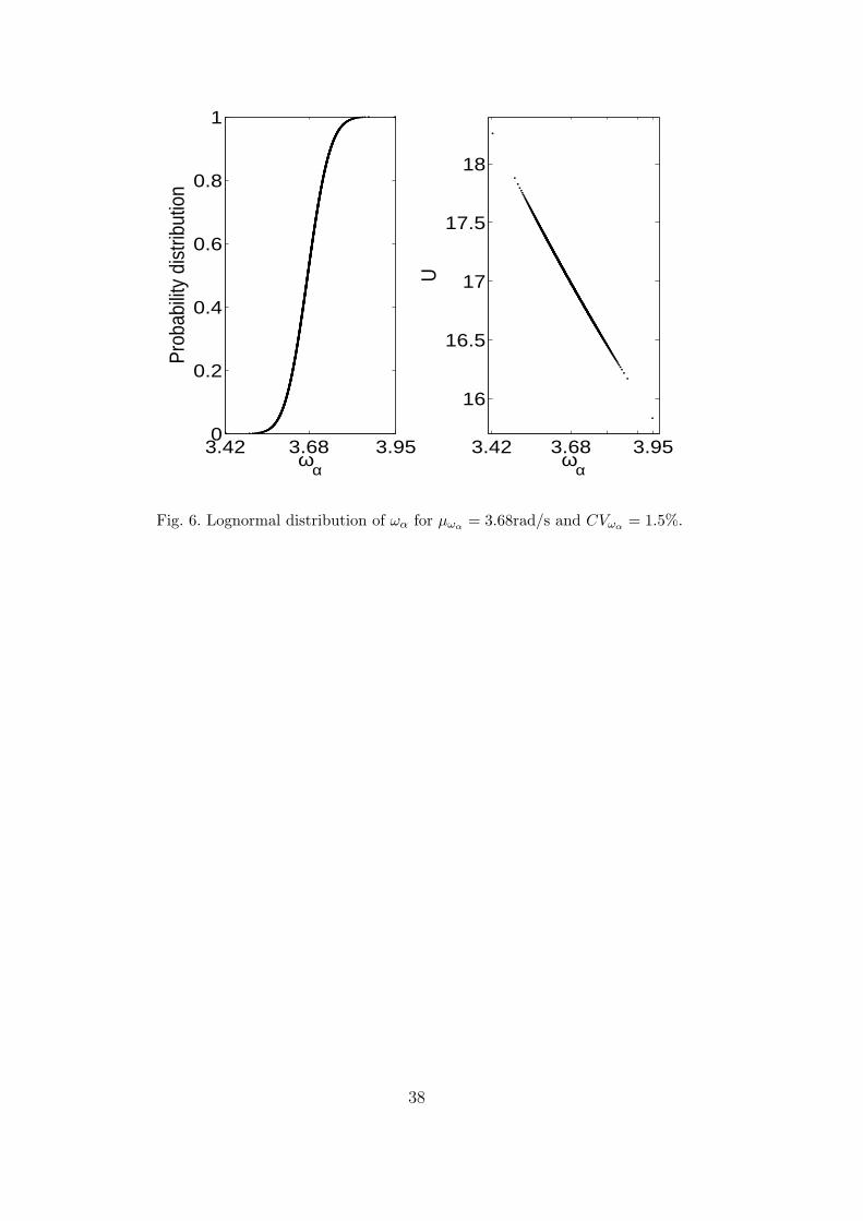
For the post-bifurcation case the mean of the pitch natural frequency ωα is

given by ωα = 3.68 rad/s, which corresponds to U = 17 using the test data of

V = 50m/s and b = 0.8m. In Figure 6 the probability distribution of ωα and

the variation of U is shown. The realizations of U are well in the determin-

istic post-bifurcation range, see Figure 2. In Figure 7 the results of Galerkin

18

Polynomial Chaos, Probabilistic Collocation and Monte Carlo simulation are

presented in terms of the minimum and maximum values of the oscillating pe-

riodic response, αmin and αmax, during one period as function of ωα. Galerkin

Polynomial Chaos response results are compared for increasing expansion or-

der N = 2, 4, 8 in Figure 8. The Galerkin Polynomial Chaos method with

N = 2 results in an inaccurate representation of the response. For increasing

N the results become better and for N = 8 the approximation matches the

Monte Carlo results almost exactly (Figure 7). The Probabilistic Collocation

results match both with the Galerkin Polynomial Chaos results for N = 8 and

the Monte Carlo simulation results.

The approximation of a typical time history for U = 17.3, is shown in Figure 9.

It is known that Polynomial Chaos expansions have difficulty resolving a pe-

riodic time history, because of the increasing nonlinearity of the response for

long-term time integration (Pettit and Beran, 2006). The low order Polyno-

mial Chaos expansion with N = 2 falls indeed short in modeling the periodic

response after short-term time integration at τ = 300. It has been reported

by Pettit and Beran (2006) and Wan and Karniadakis (2006b) that increas-

ing the Polynomial Chaos order does not increase the accuracy significantly.

However, in this case a relatively small increase of the order of the expansion

to N = 8 results in an accurate prediction of the time series up till τ = 800.

This could be attributed to the relatively small effect of uncertain ωα on the

frequency of the system response (Wan and Karniadakis, 2006b).

The accuracy of the Galerkin Polynomial Chaos method and the Probabilistic

Collocation method of the same order N is comparable. The relative compu-

tational efficiency of the methods is compared to that of Monte Carlo simu-

lation in Table 1. For a Monte Carlo simulation of comparable accuracy up

19

to τ = 500 a number of 2500 realizations is employed. For the pre-bifurcation

case of section 4.1.1, both methods are at least a factor 40 faster than the

standard Monte Carlo technique, for which it takes approximately 4.5 hours

to complete the 2500 deterministic simulations. The computational time for

solving the coupled equations in Galerkin Polynomial Chaos is for this case

relatively close to that of the non-intrusive Probabilistic Collocation, because

explicit time integration is used and the system response remains in the linear

pre-stall domain.

The nonlinear stall model containing non-polynomial step function nonlin-

earity is important in the post-bifurcation domain. The CPU time for the

Probabilistic Collocation approach is not affected significantly by the nonlin-

ear terms. Probabilistic Collocation uses 9 deterministic runs only and the

post processing using the Lagrange polynomial chaos is also not much time

consuming. In contrast, Galerkin Polynomial Chaos is a factor of 75 slower

than for the pre-bifurcation case. This is caused by numerical integration of

the inner products containing the nonlinear terms at every time level. For

this highly nonlinear case Galerkin Polynomial Chaos is even twice as slow as

Monte Carlo simulation. These results demonstrate for this case an decrease of

computational time of two orders of magnitude for Probabilistic Collocation

compared to Galerkin Polynomial Chaos. Therefore, in the rest of this paper

the Probabilistic Collocation approach is used.

4.2 Uncertain cubic structural nonlinearity parameter Knl

In the earlier part, the structural nonlinearity parameter Knl was assumed to

be zero. In this section, Knl is non-zero and assumed to be uncertain described

20

by a lognormal distribution with a mean of µKnl= 0.001 and a coefficient of

variation of CVKnl= 15%. The effect on the overall bifurcation behavior of the

system with respect to bifurcation parameter U is considered. Due to the high

coefficient of variation at least 15 collocation points are required in order to

achieve convergence. This is rather high compared to the previous case where

a maximum of 9 points were used (corresponding to order 8). However, the

coefficient of variation CVKnlis higher than the earlier case which requires

such a choice in order to match deterministic solutions. A convergence study

was performed in such a way that time histories corresponding to 99.8% of the

domain match with that of deterministic results. This results in a minimum

value of 15 collocation points; below which PC results show discrepancies with

the deterministic solution.

The bifurcation diagram with the 99.8% uncertainty bars is shown in Fig-

ure 10. The bifurcation parameter U is varied with 0.05 intervals between

U = 15.5 and U = 16.5. With this resolution the closest estimate of the shift

of the supercritical Hopf bifurcation point due to the nonzero nonlinear stiff-

ness indicated in the figure is at Ucr = 15.85. Above the bifurcation point the

systems exhibits limit cycle oscillations and below U = 15.85 the response

shows damped oscillations or stable fixed points. The uncertainty bar sug-

gests that the overall effect of the uncertainty in the structural nonlinearity

parameter Kn on the bifurcation behavior is weak. The effect is smallest for

the post-bifurcation values of αmax.

In Figure 11 a zoom of the critical range of U with smaller intervals of 0.01 is

shown. In this plot it is examined whether a shift in the stall flutter boundary

occurs as a result of the uncertainty in Knl. To that end the bifurcation plot

for three realizations for ω = 0.002; 0.5; 0.998 are reconstructed from the

21

Probabilistic Collocation results. The ω value of 0.5 corresponds to the median

of uncertain parameter Knl and the two other realizations correspond to two

realizations in the tails. The figure indicates that the effect of the uncertainty

in Knl on the stall flutter boundary is small. The flutter boundary shifts from

U = 15.81 to U = 15.83 between the three branches.

4.3 Uncertain structural equilibrium angle αm

The structural equilibrium angle αm (Fragiskatos, 1999) is considered to be

uncertain with a mean µαm = 4o, a coefficient of variation of CVαm = 15%

and a lognormal distribution. The number of collocation points is chosen as 15

following a similar The bifurcation plot with 99.8% uncertainty bars is shown

in Fig. 12. In the post-bifurcation domain both the minimum and maximum

response, and thus the amplitude of the periodic response, are sensitive to the

system parametric uncertainty. The uncertain αm has the largest effect on the

minimum response αmin in the post-bifurcation domain, which is demonstrated

by the uncertainty bars with length 6o. The resulting uncertain maximum

response αmax in the post-bifurcation domain is described by a 3o uncertainty

bar. The uncertainty bar in the pre-bifurcation domain has a length of 4o.

In Figures 13 to 15 the probability distribution function and probability den-

sity function of the response are presented at three characteristic U values

U = 12.5; 15.5; 21 to identify the bifurcation trend in the probability den-

sity function. At U = 12.5, shown in Figure 13, the response is damped in the

entire domain. For that case the probability density of the damped response

shows a maximum around α = 7.3o.

22

For U = 15.5 shown in Figure 14 both damped and oscillatory realizations

are present. This results in a clearly nonlinear propagation of uncertainty to

the response. Due to the oscillatory realizations the system shows different

values for the minimum and maximum response. The probability density of

αmin is highly deformed due to the non-monotonic dependence on αm. The

probability of αmax shows a maximum around 12.3o.

A third type of behavior is encountered further at U = 21. In that case,

the entire domain shows oscillatory behavior. As a result, both the maximum

and the minimum response exhibit monotonic behavior as function of αm.

The probability density functions of the minimum and maximum response

show two clearly distinguishable maxima, shown in Figure 15. The proba-

bility of the minimum response has a maximum around 7.7o and the max-

imum response around 13.9o. These results are summarized in Figure 16 in

the form of a bifurcation diagram in combination with three realizations for

ω = 0.002; 0.5; 0.998. The minimum and maximum response show qualita-

tively different probability density functions in different bifurcation domains.

Near the deterministic bifurcation point of U = 16 the effect of the parametric

uncertainty on the response is most nonlinear.

The uncertainty in the structural equilibrium angle αm also affects the position

of the flutter point. In Figure 17 the probability distribution of the bifurcation

point is given. Based on the probability distribution it can be concluded that

the flutter point is reduced by 12.5% to U=14 due to the uncertain αm, if a 5%

probability of flutter is deemed acceptable. This demonstrates the importance

of the probabilistic modeling of uncertainties in the analysis of pitching stall

flutter, since this approach can quantify the earlier onset of unstable behavior

compared to the deterministic bifurcation point in a probabilistic sense.

23

5 Concluding Remarks

The bifurcation behavior of pitching airfoil stall flutter subject to uncertain

variation of system parameters is studied. The structure is modeled as a two-

dimensional rigid airfoil with cubic nonlinear torsional stiffness. The Onera

dynamic stall model is used to compute the aerodynamic loading. An uncertain

pitch natural frequency ωα, cubic structural nonlinearity parameter Knl, and

structural equilibrium angle αm are considered.

The problem is a simple model problem to understand the mechanism of

stall flutter in a stochastic framework. The choice of the uncertain parame-

ters is however, more practical. The parameters which have been assumed to

be random are torsional frequency ωα which is determined from laboratory

dynamical experiments and it could encounter various sources of uncertainty

based on the laboratory conditions. Knl stands for various sources of ana-

lytic nonlinearities. According to some aeroelasticity literature (Lee and Tron,

1989; Tang and Dowell, 1993b), these often represents different control mech-

anisms. Therefore Knl could face modeling uncertainties. Similarly there could

be uncertain sources of error in implementing the structural equilibrium angle.

The Galerkin Polynomial Chaos method and the Probabilistic Collocation

method are applied to propagate the uncertainty through the system. The

focus of this work is to investigate the success of these techniques for a stall

flutter problem in linear and nonlinear regime and also with high level of

uncertainty. It was to see how the flutter stability characteristics are altered

due to these effects. The choice of some of the parameters like the coefficient

of variation (CV) is made so as to make the system adequately sensitive to

24

the uncertain variation of the chosen parameters.

The results of both the methods are compared to a Monte Carlo reference so-

lution for the case with uncertainty in the pitch natural frequency ωα. In the

pre-bifurcation domain the Polynomial Chaos methods are both significantly

more efficient than Monte Carlo simulation. The computational costs of the

Galerkin Polynomial Chaos method in the post-bifurcation domain are of the

same order as Monte Carlo simulation owing to the non-polynomial nonlinear-

ity of the model above the static stall angle. The bifurcation does not affect

the computational costs of the Probabilistic Collocation method significantly.

In the post-bifurcation case low order Polynomial Chaos expansions fail to

predict the periodic response after short-term time integration up to τ = 300.

An 8th order Polynomial Chaos expansion is sufficient to maintain an accurate

solution till around τ = 800, well after the system reaches time stationarity.

The effect of the uncertain cubic structural nonlinearity parameter Knl and

structural equilibrium angle αm are studied using the Probabilistic Collocation

method. Uncertainty in αm has the largest effect on the bifurcation behavior

of the system. It results in 3o to 6o uncertainty bars for the response, which

affects the amplitude of the periodic response in the post-bifurcation domain.

The minimum and maximum response show qualitatively different probability

density functions at different domains of the bifurcation plot. The uncertainty

in αm results in a flutter point which is 12.5% lower than the deterministic

prediction if 5% probability of flutter is deemed acceptable. This demonstrates

that parametric uncertainties in pitching airfoil stall flutter can lead to an

earlier onset of unstable behavior than a deterministic analysis would point

out.

25

This study successfully uses the uncoupled and non-intrusive Probabilistic

Collocation approach to quantify the effect of uncertain parametric variation

of a stall flutter system. The stall flutter model is simple and yet can predict

the nature of instabilities that can occur in an actual system. Therefore, the

stochastic modeling of the present system will be helpful towards the aeroelas-

tic design of a real-life stall flutter device without being too computationally

intensive. In this work, the Probabilistic Collocation approach is used to cap-

ture the period-1 limit cycle oscillations. As a next step, we would like to

investigate capturing higher periodic responses as well.

26

References

Babuska, I. M., Nobile, F., Tempone, R., 2007. A stochastic collocation method

for elliptic partial differential equations with random input data. SIAM

Journal on Numerical Analysis 45 (3), 1005–1034.

Beedy, J. A., Barakos, G., Badcock, K. J., Richards, B. E., 2003. Nonlinear

analysis of stall flutter based on the onera aerodynamic model. The Aero-

nautical Journal 107 (1074), 495–509.

Beloiu, D. M., Ibrahim, R. A., Pettit, C. L., 2005. Influence of boundary con-

ditions relaxation on panel flutter with compressive in-plane loads. Journal

of Fluids and Structures 21, 743–767.

Bhattacharya, R., Waymire, E. C., 2007. A basic course on probability theory.

Springer, Berlin.

Cheney, M. C., Migliore, P. G., 2000. Feasibility study of pultruded blades for

wind turbine rotors. 38th Aerospace Sciences Meeting and Exhibit, Reno,

NV, Paper no. AIAA-2000-0061.

Choi, S., Namachchivaya, N. S., 2006. Stochastic dynamics of a nonlinear

aeroelastic system. AIAA Journal 44 (9), 1921–1931.

De Rosa, S., Franco, F., 2008. Exact and numerical responses of a plate under

a turbulent boundary layer excitation. Journal of Fluids and Structures 24,

212–230.

Debusschere, B. J., Najm, H. N., Pebay, P., Knio, O. M., Ghanem, R. G.,

Le Maıtre, O. P., 2004. Numerical challenges in the use of polynomial chaos

representations for stochastic processes. SIAM Journal on Scientific Com-

puting 26, 698–719.

Dowell, E. H., Curtiss, H. C. J., Scanlan, R. H., Sisto, F., 1989. A modern

course in aeroelasticity. Kluwer Academic Publisher, Dordrecht.

27

Dunn, P., Dugundji, J., 1992. Nonlinear stall flutter and divergence analysis

of cantilevered graphite/epoxy wings. AIAA Journal 30 (1), 153–162.

Fragiskatos, G., 1999. Nonlinear response and instabilities of a two-degree-of-

freedom airfoil oscillating in dynamic stall. M.Eng. Masters Thesis, McGill

University, Montreal, Canada.

Fung, Y. C., 1955. An introduction to the theory of aeroelasticity. John Wiley

& Sons, Inc., New York.

Ganappathysubramanian, B., Zabaras, N., 2007. Sparse grid collocation

schemes for stochastic natural convection problems. Journal of Computa-

tional Physics 225, 652–685.

Gautschi, W., 2004. Orthogonal polynomials; computation and approxima-

tion. Oxford University Press, Oxford.

Gautschi, W., 2005. Orthogonal polynomials (in matlab). Journal of Compu-

tational and Applied Mathematics 178, 215–234.

Gerstner, T., Griebel, M., 1998. Numerical integration using sparse grids. Nu-

merical Algorithms 18, 209–232.

Ghanem, R., 1999. Stochastic finite elements with multiple random non-

gaussian properties. Journal of Engineering Mechanics 125, 26–40.

Ghanem, R. G., Spanos, P., 1991. Stochastic finite elements: a spectral ap-

proach. Springer-Verlag, New York.

Golub, G. H., Welsch, J. H., 1969. Calculation of gauss quadrature rules.

Mathematics of Computation 23, 221–230.

Hosder, S., Walters, R. W., Perez, R., 2006. A non-intrusive polynomial

chaos method for uncertainty propagation in CFD simulations. 44th AIAA

Aerospace Sciences Meeting and Exhibit, Reno, NV, Paper no. AIAA-2006-

891.

Ibrahim, R. A., Beloiu, D. M., Pettit, C. L., 2005. Influence of joint relaxation

28

on deterministic and stochastic panel flutter. AIAA Journal 43 (7), 1444–

1454.

Le Maıtre, O. P., Knio, O. M., Najm, H. N., Ghanem, R. G., 2004. Uncer-

tainty propagation using wiener-haar expansions. Journal of Computational

Physics 197, 28–57.

Lee, B. H. K., Price, S. J., Wong, Y. S., 1999. Nonlinear aeroelastic analysis of

airfoils: bifurcation and chaos. Progress in Aerospace Sciences 35, 205–334.

Lee, B. H. K., Tron, A., 1989. Effects of structural nonlinearities on flutter

characteristics of the cf-18 aircraft. Journal of Aircraft 26 (8), 781–786.

Liaw, D. G., Yang, H. T. Y., 1993. Reliability and nonlinear supersonic flutter

of uncertain laminated plates. AIAA Journal 31 (12), 2304–2311.

Lind, R., Brenner, M. J., 1998. Robust flutter margin analysis that incorpo-

rates flight data. NASA/TP-1998-206543.

Lindsley, N. J., Beran, P. S., Pettit, C. L., 2002. Effects of uncertainty on

nonlinear plate aeroelastic response. 43rd AIAA/ASME/ASCE/AHS/ASC

Structures, Structural Dynamics, and Materials conference, Denver, Col-

orado, Paper no. AIAA 2002-1271.

Lindsley, N. J., Pettit, C. L., Beran, P. S., 2006. Nonlinear plate aeroelastic

response with uncertain stiffness and boundary conditions. Structure and

Infrastructure Engineering 2, 201–220.

Loeven, G., Witteveen, J. A. S., Bijl, H., 2007. Probabilistic collocation: an

efficient non-intrusive approach for arbitrarily distributed parametric un-

certainties. 45th AIAA Aerospace Sciences Meeting and Exhibit, Reno, NV,

Paper no. AIAA-2007-317.

Lucor, D., Karniadakis, G. E., 2004. Noisy inflows cause a shedding-mode

switching in flow past an oscillating cylinder. Physical Review Letters 92,

4501.

29

Mathelin, L., Hussaini, M. Y., 2003. A stochastic collocation algorithm for

uncertainty analysis. Technical Report NASA/CR-2003-212153 NASA Lan-

gley Research Center.

Mathelin, L., Hussaini, M. Y., Zang, T. A., 2005. Stochastic approaches to

uncertainty quantification in CFD simulations. Numerical Algorithms 38,

209–236.

Millman, D. R., King, P. I., Beran, P. S., 2003. A stochastic approach for

predicting bifurcation of a pitch and plung airfoil. 21st AIAA Applied Aero-

dynamics Conference, Orlando, FL, Paper no. AIAA-2003-3515.

Nigam, N. C., Narayanan, S., 1994. Applications of Random Vibrations.

Narosa Publishing House, New Delhi.

Pettit, C. L., 2004a. Uncertainty in aeroelasticity analysis, design and testing,

Engineering Design Reliability Handbook, E. Nicolaidis, D. Ghiocel (Eds.).

CRC Press, Boca Raton, FL.

Pettit, C. L., 2004b. Uncertainty quantification in aeroelasticity: recent results

and research challenges. Journal of Aircraft 41 (5), 1217–1229.

Pettit, C. L., Beran, P. S., 2004. Polynomial chaos expansion applied to airfoil

limit cycle oscillations. 45th AIAA/ASME/ASCE/AHS/ASC Structures,

Structural Dynamics & Materials Conference, California, Paper no. AIAA

2004-1691.

Pettit, C. L., Beran, P. S., 2006. Spectral and multiresolution wiener expan-

sions of oscillatory stochastic process. Journal of Sound and Vibrtion 294,

752–779.

Poirel, D., Price, S. J., 2003. Random binary (coalescence) flutter of a two-

dimensional linear airfoil. Journal of Fluids and Structures 18, 23–42.

Poirion, F., 2000. On some stochastic method applied to aeroservoelasticity.

Aerospace Science and Technology 4, 201–214.

30

Price, S. J., Fragiskatos, G., 2000. Nonlinear aeroelastic response of a two-

degree-of-freedom airfoil oscillating in dynamic stall. In: Proceedings of Flow

Induced Vibration, Eds. Ziada and Staubli, Bakelma, Rotterdam.

Reagan, M. T., Najm, H. N., Ghanem, R. G., Knio, O. M., 2003. Uncertainty

quantification in reacting-flow simulations through non-intrusive spectral

projection. Combustion and Flame 132, 545–555.

Sarkar, S., Bijl, H., 2008. Nonlinear aeroelastic behavior of an oscillating airfoil

during stall induced vibration. Journal of Fluids and Structures, in press.

Sheta, E. F., Harrand, V. J., Thompson, D. E., W., S. T., 2002. Computa-

tional and experimental investigation of limit cycle oscillations of nonlinear

aeroelastic systems. Journal of Aircraft 39 (1), 133–141.

Stiesdal, H., 1999. The wind turbine components and operation. Bonus-Info,

Newsletter, http://www.windmission.dk/workshop/BonusTurbine.pdf.

Svacek, P., Feistauer, M., Horacek, J., 2007. Numerical simulation of flow in-

duced airfoil vibrations with large amplitudes. Journal of Fluids and Struc-

tures 23, 391–411.

Tang, D. M., Dowell, E. H., 1993a. Comparison of theory and experiment for

nonlinear flutter and stall response of a helicopter blade. Journal of Sound

and Vibration 165 (2), 251–276.

Tang, D. M., Dowell, E. H., 1993b. Nonlinear aeroelasticity in rotorcraft.

Mathematical and Computer modelling 18, 157–184.

Tang, D. M., Dowell, E. H., 2004. Effects of geometric structural nonlinearity

on flutter and limit cycle oscillations of high-aspect-ratio wings. Journal of

Fluids and Structures 19, 291–306.

Tran, C. T., Petot, T., 1981. Semi-empirical model for the dynamic stall of air-

foils in view of the application to the calculation of responses of a helicopter

blade in forward flight. Vertica 5, 35–53.

31

Walters, R. W., 2003. Towards stochastic fluid mechanics via polynomial

chaos. 41st AIAA Aerospace Sciences Meeting and Exhibit, Reno, NV, Paper

no. AIAA-2003-0413.

Wan, X., Karniadakis, G., 2006a. Beyond wiener-askey expansions: Handling

arbitrary pdfs. Journal of Scientific Computing 27, 455–464.

Wan, X., Karniadakis, G. E., 2006b. Long-term behavior of polynomial chaos

in stochastic flow simulations. Computer Methods in Applied Mechanics

and Engineering 195, 5582–5596.

Wiener, N., 1938. The homogeneous chaos. American Journal of Mathematics

60, 897–936.

Witteveen, J. A. S., Bijl, H., 2006a. Modeling arbitrary uncertainties using

gram-schmidt polynomial chaos. 44th AIAA Aerospace Sciences Meeting

and Exhibit, Reno, NV, Paper no. AIAA-2006-896.

Witteveen, J. A. S., Bijl, H., 2006b. Using polynomial chaos for

uncertainty quantification in problems with nonlinearities. 47th

AIAA/ASME/ASCE/AHS/ASC Structures, Structural Dynamics, and

Materials Conference, Newport, RI, Paper no. AIAA-2006-2066.

Xiu, D., Karniadakis, G. E., 2002. The wiener-askey polynomial chaos for

stochastic differential equations. SIAM Journal on Scientific Computing

24 (2), 619–644.

Xiu, D. B., Hesthaven, J. S., 2005. High-order collocation methods for differen-

tial equations with random inputs. SIAM Journal on Scientific Computing

27, 1118–1139.

32

pitch

2ba

VU

Or

elastic axis

Fig. 1. Schematic plot of the airfoil coordinate system and oscillation degree-of-free-

dom.

33

5 10 15 20 25 302

4

6

8

10

12

14

16

U

αo at α

’ = 0

Fig. 2. Bifurcation diagram for the deterministic aeroelastic system.

34

5.8 6.25 6.750

0.2

0.4

0.6

0.8

1

ωα

Pro

babi

lity

dist

ribut

ion

5.8 6.25 6.75

9.4

9.6

9.8

10

10.2

10.4

10.6

10.8

ωα

U

Fig. 3. Lognormal distribution of ωα for µωα = 6.25rad/s and CVωα = 1.5%.

35

4.4 4.6 4.8 5 5.2

0.1

0.2

0.3

0.4

0.5

0.6

0.7

0.8

0.9

1

α

Pro

babi

lity

dist

ribut

ion

GPC(N=4)

PC(N=4)

+ + + MC (2500)

Fig. 4. Probability distribution of response αo for µωα = 6.25rad/s and

CVωα = 1.5%.

36

0 200 400 600 8000

2

4

6

8

10

τ

α(τ)

U=10.2

MCGPC (N=4)PC (N=4)

Fig. 5. Comparison of a typical time history for µωα = 6.25 rad/s,CV = 1.5% .

37

3.42 3.68 3.950

0.2

0.4

0.6

0.8

1

ωα

Pro

babi

lity

dist

ribut

ion

3.42 3.68 3.95

16

16.5

17

17.5

18

ωα

U

Fig. 6. Lognormal distribution of ωα for µωα = 3.68rad/s and CVωα = 1.5%.

38

9 10 11 12 13 143.5

3.56

3.63

3.69

3.75

3.81

max,min α

ωα

GPC(N=8)

PC(N=8)

+ + + MC (2500)

Fig. 7. Response of the maximum and minimum αo for µωα = 3.68rad/s and

CVωα = 1.5%.

39

8 9 10 11 12 13 143.5

3.56

3.63

3.69

3.75

3.81

max,min α

ωα

GPC(N=2)

GPC(N=4)

GPC(N=8)

Fig. 8. Response of the maximum and minimum αo for µωα = 3.68rad/s and

CVωα = 1.5% with increasing order of GPC.

40

50 100 150 200 250 300 350 4007

8

9

10

11

12

13

τ

α(τ)

U=17.3

MCGPC (N=2)GPC (N=4)GPC (N=8)PC (N=8)

Fig. 9. Comparison of a typical time history for µωα = 3.68rad/s and CV = 1.5%.

41

15.4 15.6 15.8 16 16.2 16.4 16.6

11.2

11.4

11.6

11.8

12

12.2

12.4

U

α

Fig. 10. Response 99.8% uncertainty bars for µKnl= 0.001 and CVKnl

= 15%.

42

15.75 15.8 15.85 15.9 15.9511.8

11.9

12

12.1

12.2

U

α at

α′=

0

max amp(ω=0.5)min amp(ω=0.5)max amp(ω=0.002)min amp(ω=0.002)max amp(ω=0.998)min amp(ω=0.998)

Fig. 11. Stall flutter boundaries shown as spanned in the uncertainty domain for

µKnl= 0.001 and CVKnl

= 15%.

43

12 14 16 18 20 222

4

6

8

10

12

14

16

U

α

Fig. 12. Response 95% uncertainty bars for µαm = 4 and CVαm = 15%.

44

4 6 8 10 1212.50

0.2

0.4

0.6

0.8

1

α

Pro

babi

lity

dist

ribut

ion

U=12.5

4 6 8 10 1212.50

0.05

0.1

0.15

0.2

0.25

0.3

0.35

0.4

α

Pro

babi

lity

dens

ity

U=12.5

Fig. 13. Probability distribution and density of the damped response at U = 12.5

for µαm = 4o and CVαm = 15%.

45

5 10 150

0.2

0.4

0.6

0.8

1

max,min α

Pro

babi

lity

dist

ribut

ion

U=15.5

max(α)

min(α)

5 10 150

0.2

0.4

0.6

0.8

1

max,min α

Pro

babi

lity

dens

ity

U=15.5

max(α)

min(α)

Fig. 14. Probability distribution and density of the maximum and minimum re-

sponse at U = 15.5 for µαm = 4o and CVαm = 15%.

46

0 10 200

0.2

0.4

0.6

0.8

1

max, min α

Prob

abilit

y di

strib

utio

n

max(α)min(α)

U=21

0 10 200

0.1

0.2

0.3

0.4

0.5

0.6

0.7

max, min αPr

obab

ility

dens

ity

max(α)min(α)

U=21

Fig. 15. Probability distribution and density of the LCO response at U = 21 for

µαm = 4o and CVαm = 15%.

47

12.5 15.5 18 210

5

10

15

20

U

max

and

min

α

domain mean

pdf, max(α)pdf, min(α)

max/min,ω=0.002max/min,ω=0.998

Fig. 16. Qualitative changes shown in the response probability density at three

characteristic U values for µαm = 4o and CVαm = 15%.

48

10 15 200

0.2

0.4

0.6

0.8

1

Bifurcation onset U cr

Pro

babi

lity

dist

ribut

ion

10 15 200

0.05

0.1

0.15

0.2

0.25

0.3

0.35

Bifurcation onset U cr

Pro

babi

lity

dens

ity

Fig. 17. Probability distribution and density of the bifurcation point for µαm = 4o

and CVαm = 15%.

49

Table 1

Comparison of the order of the CPU times by Galerkin Polynomial Chaos, Proba-

bilistic Collocation and Monte Carlo simulation till τ = 500.

GPC PC MC

pre-bifurcation 7 min (N = 4) 2 min (N = 4) ≈ 4.5 hrs (2500 realizations)

post-bifurcation 8.9 hrs (N = 8) 3 min (N = 8) ≈ 4.5 hrs (2500 realizations)

50