ATVD UncertaintyQuantificationMethod withBounded Error Applied to Transonic Airfoil Flutter

COMMUNICATIONS IN COMPUTATIONAL PHYSICSVol. 6, No. 2, pp. 406-432

Commun. Comput. Phys.August 2009

A TVD Uncertainty Quantification Method with Bounded

Error Applied to Transonic Airfoil Flutter

Jeroen A. S. Witteveen∗ and Hester Bijl

Faculty of Aerospace Engineering, Delft University of Technology, Kluyverweg 1,2629HS Delft, The Netherlands.

Received 26 September 2008; Accepted (in revised version) 30 October 2008

Communicated by Jan S. Hesthaven

Available online 15 December 2008

Abstract. The Unsteady Adaptive Stochastic Finite Elements (UASFE) approach is arobust and efficient uncertainty quantification method for resolving the effect of ran-dom parameters in unsteady simulations. In this paper, it is shown that the underly-ing Adaptive Stochastic Finite Elements (ASFE) method for steady problems based onNewton-Cotes quadrature in simplex elements is extrema diminishing (ED). It is alsoshown that the method is total variation diminishing (TVD) for one random parameterand for multiple random parameters for first degree Newton-Cotes quadrature. It isproven that the interpolation of oscillatory samples at constant phase in the UASFEmethod for unsteady problems results in a bounded error as function of the phase forperiodic responses and under certain conditions also in a bounded error in time. Thetwo methods are applied to a steady transonic airfoil flow and a transonic airfoil flutterproblem.

AMS subject classifications: 60H35, 65C30, 65N15, 65P99, 76M35

Key words: Total variation diminishing, extrema diminishing, error bounds, stochastic finite ele-ments, uncertainty quantification, transonic flow, transonic flutter.

1 Introduction

Deterministic numerical solutions of engineering flow and fluid-structure interactionproblems contain no information about the influence of parameter variations on the out-puts of interest. Physical uncertainties are, however, present in practically all engineer-ing applications due to, for example, varying atmospheric conditions, and production

∗Corresponding author. Email addresses: [email protected] (J. A. S. Witteveen), h.bijl@

tudelft.nl (H. Bijl)

http://www.global-sci.com/ 406 c©2009 Global-Science Press

J. A. S. Witteveen and H. Bijl / Commun. Comput. Phys., 6 (2009), pp. 406-432 407

tolerances affecting material properties and the geometry. These inherent physical vari-ations enter the computational problem through physical input parameters, and initialand boundary conditions. Especially, discontinuous solutions of shock waves in super-sonic flow and bifurcation phenomena of aeroelastic systems are highly sensitive to thisinput variability. Dynamic fluid-structure interaction systems also amplify input varia-tions with time.

Physical variability is here described in a probabilistic framework by random pa-rameters with known probability density. The distribution functions and the statisticalmoments of outputs of interest are determined in order to obtain more reliable compu-tational predictions, which can be utilized in robust design optimization and reducingdesign safety factors. In contrast, in structural reliability analysis input randomness ispropagated to compute the probability of failure [4]. Failure probabilities are often smallsuch that in that case the tails of the distribution are of interest.

The resulting mathematical formulation of the uncertainty quantification problem foroutput of interest u(x,t,ω) is

L(x,t,ω;u(x,t,ω))=S(x,t,ω), (1.1)

with appropriate initial and boundary conditions. Operator L and source term S are de-fined on domain D×T×Ω, where x∈D and t∈T are the spatial and temporal dimensionswith D⊂R

d, d=1,2,3, and T⊂R. The argument ω emphasizes that u(x,t,ω) is a ran-dom event with the set of outcomes Ω of the probability space (Ω, F , P) with F ⊂2Ω theσ-algebra of events and P a probability measure. The probability space originates fromna uncorrelated second order random parameters

a(ω)=a1(ω),··· ,ana(ω)∈A,

with probability density fa(a) in Eq. (1.1) and its initial and boundary conditions, withparameter space A⊂R

na .For a single realization ω=ωk, u(x,t,ωk) reduces to the deterministic function uk(x,t)

in terms of the spatial coordinates x and time t. The numerical approximation of uk(x,t)can be obtained using standard spatial discretization methods and time marching schemes.A weighted approximation of the response surface u∗(x,t,a) based on ns deterministic so-lutions uk(x,t)ns

k=1 is considered a solution of uncertainty quantification problem (1.1).Integration and sorting of u∗(x,t,a) results in the statistical moments µui

(x,t)

µui(x,t)=

∫

Au∗(x,t,a)i fa(a)da, (1.2)

and its probability distribution.The classical approach of solving (1.1) by computing many deterministic solutions

for randomly sampled parameter values in a Monte Carlo simulation [9] leads to im-practically high computational costs for flow and fluid-structure simulations, which arealready computationally intensive in the deterministic case. Non-intrusive Polynomial

408 J. A. S. Witteveen and H. Bijl / Commun. Comput. Phys., 6 (2009), pp. 406-432

Chaos methods [1, 8, 12, 20, 24, 30] aim at reducing the number of deterministic solvesby using a global polynomial interpolation of the samples in parameter space. An effec-tive sampling in suitable Gauss quadrature points is employed in Stochastic Collocationapproaches [2, 17, 22, 31]. Current challenges in uncertainty quantification for computa-tional fluid dynamics and fluid-structure interaction simulations include problems withdiscontinuities and unsteadiness [32].

Global polynomial approximations of discontinuities in probability space can resultin oscillatory predictions and unphysical realizations. A more robust approximation isachieved by piecewise polynomial approximations of the response in adaptive finite el-ements discretizations of probability space [6, 15, 16, 23]. These Adaptive Stochastic Fi-nite Elements (ASFE) methods employ local Polynomial Chaos or Stochastic Collocationapproximations in hypercube elements. An alternative Adaptive Stochastic Finite Ele-ments formulation based on Newton-Cotes quadrature in simplex elements was recentlyalso proposed [28]. Since the main motivation for performing uncertainty analysis is toobtain reliable computational predictions, it is important to assure the robustness of un-certainty quantification methods. In the deterministic finite volume community the totalvariation diminishing (TVD) and extrema diminishing (ED) properties [10, 13] of finitevolume methods ascertain that no unphysical solutions are predicted due to overshootsand undershoots near discontinuities. It is, therefore, useful to extend these concepts touncertainty quantification methods in probability space.

In unsteady problems, uncertainty quantification methods usually require a fast in-creasing number of samples with time to maintain a constant accuracy. This effect isespecially profound in problems with oscillatory solutions in which the frequency of theresponse is affected by the random parameters [19]. The random frequency results inincreasing phase differences in the response, which consequently lead to an increasinglyoscillatory response surface and more required samples. A Fourier Chaos basis can bea suitable alternative for approximating oscillatory responses [18]. Frequency domainmethods have also been considered for solving linear stochastic operator equations [21].

Two Unsteady Adaptive Stochastic Finite Elements (UASFE) methods for oscillatoryproblems were proposed based on Newton-Cotes quadrature in simplex elements. Thefirst approach is based on applying the uncertainty quantification interpolation to a time-independent parameterization of oscillatory samples instead of to the unsteady samplesthemselves [25, 26]. This results in a time-independent uncertainty quantification inter-polation accuracy for the time-independent functionals. In the second method the oscil-latory samples are scaled with their phase [27]. The uncertainty quantification interpo-lation of the samples is then performed at constant phase, which eliminates the effect ofthe increasing phase differences on the increase of the number of required samples. Thelatter method is not subject to a parameterization error, which improves the convergencebehavior of the method, and it can resolve time-dependent functionals such as transientbehavior. The formulation was also extended to multi-frequency responses of continuousstructures by using a wavelet decomposition preprocessing step [29].

In this paper, it is shown that the Adaptive Stochastic Finite Elements method with


Newton-Cotes quadrature in simplex elements is an extrema diminishing uncertaintyquantification method in Section 2. It is also shown that the method is total variation di-minishing for one random parameter and for multiple random parameters for first degreeNewton-Cotes quadrature. It is proven in Section 3 that the Unsteady Adaptive Stochas-tic Finite Elements method with interpolation at constant phase results in a boundederror as function of the phase for periodic responses and under certain conditions also ina bounded error in time. The two methods are applied to a steady transonic airfoil flowand a transonic airfoil flutter problem in Section 4. The conclusions are summarized inSection 5.

2 Adaptive Stochastic Finite Elements

The Adaptive Stochastic Finite Elements method based on Newton-Cotes quadrature insimplex elements is presented in Section 2.1. It is shown under which conditions theapproach is total variation diminishing in probability space in Section 2.2. In Section 2.3it is proven that the method is extrema diminishing in probability space.

2.1 Newton-Cotes quadrature in simplex elements

Adaptive Stochastic Finite Elements with Newton-Cotes quadrature and simplex ele-ments evaluate integral (1.2) by dividing parameter space A in ne non-overlapping sim-plex elements Aj

µui(x,t)=

ne

∑j=1

∫

Aj

u∗(x,t,a)i fa(a)da. (2.1)

A piecewise polynomial approximation w∗(x,t,a) of the response u∗(x,t,a) is constructedbased on ns deterministic solutions vj,k(x,t) = u∗(x,t,aj,k) for the values of the randomparameters aj,k that correspond to the ns Newton-Cotes quadrature points of degree d inthe element Aj

µui(x,t)≈µwi

(x,t)=ne

∑j=1

ns

∑k=1

cj,kvj,k(x,t)i, (2.2)

where cj,k is the weighted integral of the Lagrange interpolation polynomial Lj,k(a) throughNewton-Cotes quadrature point k in element Aj

cj,k =∫

Aj

Lj,k(a) fa(a)da, (2.3)

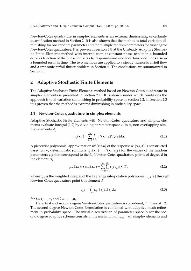
for j=1,··· ,ne and k=1,··· ,ns.Here, first and second degree Newton-Cotes quadrature is considered, d=1 and d=2.

The second degree Newton-Cotes formulation is combined with adaptive mesh refine-ment in probability space. The initial discretization of parameter space A for the sec-ond degree adaptive scheme consists of the minimum of neini =na! simplex elements and


(a) Element (b) Initial grid (c) Adapted grid

Figure 1: Discretization of two-dimensional parameter space A using 2-simplex elements and second-degreeNewton-Cotes quadrature points given by the dots.

nsini = 3na samples, see Fig. 1. The example of Fig. 1 for two random input parameterscan geometrically be extended to higher dimensional probability spaces. The elementsAj are adaptively refined using a refinement measure ρj based on the largest absoluteeigenvalue of the Hessian Hj, as measure of the curvature of the response surface ap-proximation in the elements, weighted by the probability f j contained by the elements

f j =∫

Aj

fa(a)da, (2.4)

with ∑nej=1 f j =1. The stochastic grid refinement is terminated when δne < δ, where conver-

gence measure δne is defined as

δne =max

(

|µu⌊ne/2⌋(x,t)−µune

(x,t)|∞

|µune(x,t)|∞

,|σu⌊ne/2⌋

(x,t)−σune(x,t)|∞

|σune(x,t)|∞

)

, (2.5)

with µu(x,t) and σu(x,t) the mean and standard deviation of u(x,t,ω), or when a thresh-old for the maximum number of samples ns is reached. Convergence measure δne can beextended to include higher statistical moments of the output.

Due to the location of the Newton-Cotes quadrature points the deterministic sam-ples are reused in successive refinements and the samples are used in approximating theresponse in multiple elements. In elements where the quadratic second degree interpola-tion results in an extremum other than in a quadrature point, the element is subdividedinto ne = 2na subelements with a linear first degree Newton-Cotes approximation of theresponse without performing additional deterministic solves.

As is common in multi-element methods, the probability of the random parametersa(ω) is assumed to be zero outside a finite domain. Probability distributions on infinitedomains are truncated at a small enough threshold value for the probability, such thatthe truncation error is small compared to other numerical errors that occur in practicalapplications.


2.2 Total variation diminishing

It is shown that Adaptive Stochastic Finite Elements based on Newton-Cotes quadra-ture in simplex elements is total variation diminishing for one random parameter in Sec-tion 2.2.1. In Section 2.2.2 it is argued that the method is also total variation diminishingin higher dimensional probability spaces up to first degree Newton-Cotes quadrature.

2.2.1 One-dimensional probability space

Consider uncertainty quantification problem (1.1) with one random input parametera(ω), na = 1, on a bounded connected domain a ∈ A, with one-dimensional parameterspace A = [min(a),max(a)]. Let response surface u∗(x,t,a) be a continuously differen-tiable function. The arguments x and t, and the index ∗ are omitted in the following forsimplicity of the notation. Let sampling method g result in a discrete set of ns samplesv=v1,··· ,vns= g(u(a)) of response surface u(a), with

vk = gk(u(a))=u(ak), ak = a(ωk), k=1,··· ,ns,

anda1≤ a2 ≤···≤ ans , (2.6)

with a1 =min(a) and ans =max(a). Let interpolation method h of the samples v result ina piecewise continuously differentiable interpolation function w(a)= h(v) with w(ak)=vk, which is continuously differentiable on subdomains Aj of A and continuous on thesubdomain boundaries ∂Aj with j = 1,··· ,ne. Let uncertainty quantification method levaluate (1.2) by approximating response surface u(a) with interpolation

w(a)= l(u(a))=h(g(u(a)))

of the samples v. Then the concepts total variation, total variation diminishing, and totalvariation conserving are defined in probability space as follows in correspondence totheir definitions for finite volume methods in physical space in [10].

Definition 2.1. (Total variation) The total variation TV of response surface u(a) in thespace A of random parameter a(ω) is

TV(u)=∫

A

∣

∣

∣

∣

∂u

∂a

∣

∣

∣

∣

da. (2.7)

The total variation of the continuous and piecewise continuously differentiable approxi-mation w(a) is

TV(w)=ne

∑j=1

TV(wj)=ne

∑j=1

∫

Aj

∣

∣

∣

∣

∂wj

∂a

∣

∣

∣

∣

da. (2.8)

The total variation of the discrete set of samples v is

TV(v)=ns−1

∑k=1

|vk+1−vk|. (2.9)


Definition 2.2. (Total variation diminishing) A set of samples v is total variation dimin-ishing (TVD) with respect to response surface u(a) if

TV(v)≤TV(u). (2.10)

Sampling method g is TVD if the resulting set of samples v is TVD for all u(a). Approxi-mation w(a) of response surface u(a) is TVD if

TV(w)≤TV(u). (2.11)

Uncertainty quantification method l is TVD if the resulting approximation w(a) is TVDfor all u(a).

Definition 2.3. (Total variation conserving) Interpolation w(a) of samples v is total vari-ation conserving (TVC) if

TV(w)=TV(v). (2.12)

Interpolation method h is TVC if the resulting interpolation w(a) is TVC for all v.

Based on these definitions it is proven below that Stochastic Finite Elements withNewton-Cotes quadrature in simplex elements is a TVD uncertainty quantification methodfor random parameter a(ω).

Lemma 2.1. Sampling method g is TVD for random parameter a(ω).

Proof. For the total variation of the samples v= g(u(a)) holds according to Definition 2.1

TV(v)=ns−1

∑k=1

|vk+1−vk|=ns−1

∑k=1

|u(ak+1)−u(ak)|

≤ns−1

∑k=1

∫ ak+1

ak

∣

∣

∣

∣

∂u

∂a

∣

∣

∣

∣

da=∫

A

∣

∣

∣

∣

∂u

∂a

∣

∣

∣

∣

da=TV(u). (2.13)

Since (2.13) holds for all u(a), sampling method g is TVD according to Definition 2.2.

Consider Stochastic Finite Elements uncertainty quantification method l1 with firstdegree Newton-Cotes quadrature in simplex elements. Sampling method g1 then resultsin ns samples v1 in the vertices of the ne simplex elements. Interpolation method h1

results in a linear interpolation w1j (a) of the samples v1

j in the elements Aj. For one ran-

dom parameter a(ω) sampling method g1 results in ns =ne+1 samples v1. Interpolationmethod h1 then results in the piecewise linear interpolation w1(a)

w1(a)=w1j (a)=

v1j (aj+1−a)+v1

j+1(a−aj)

aj+1−aj, for a∈Aj =[aj,aj+1], j=1,··· ,ne. (2.14)

Theorem 2.1. Uncertainty quantification method l1 based on first degree Newton-Cotes quadra-ture in simplex elements is TVD for random parameter a(ω).


Proof. The total variation of w1(a) is according to Definition 2.1 and (2.14)

TV(w1)=ne

∑j=1

∫

Aj

∣

∣

∣

∣

∣

∂w1j

∂a

∣

∣

∣

∣

∣

da=ne

∑j=1

∣

∣

∣

∣

∣

v1j+1−v1

j

aj+1−aj

∣

∣

∣

∣

∣

(aj+1−aj)

=ns−1

∑k=1

∣

∣

∣v1

k+1−v1k

∣

∣

∣=TV(v1). (2.15)

Since (2.15) holds for all v1, interpolation method h1 is TVC according to Definition 2.3.Lemma 2.1 gives

TV(w1)=TV(v1)≤TV(u). (2.16)

Since (2.16) holds for all u(a), uncertainty quantification method l1 is TVD according toDefinition 2.2.

Consider Stochastic Finite Elements uncertainty quantification method l2 with seconddegree Newton-Cotes quadrature in simplex elements. Sampling method g2 then resultsin ns samples v2 in the middle of the edges and in the vertices of the ne simplex elements.Interpolation method h2 results in a quadratic interpolation w2

j (a) of the samples v2j in the

elements Aj. For one random parameter a(ω) sampling method g2 results in ns =2ne+1samples. Interpolation method h2 then results in quadratic approximation w2

j (a) in the

element Aj through the samples v2k for k = 2j−1,2j,2j+1, j = 1,··· ,ne. If the quadratic

approximation w2j (a) in an element Aj has an extremum other than in a quadrature point

ak, i.e.,

minAj

(w2j (a))<min(v2

2j−1,v22j,v

22j+1) ∨ max

Aj

(w2j (a))>max(v2

2j−1,v22j,v

22j+1), (2.17)

then element Aj is subdivided into ne =2 subelements with a linear first degree Newton-Cotes approximation based on the samples vk with k=2j−1,2j,2j+1

w2j (a)=

v22j−1(a2j−a)+v2

2j(a−a2j−1)

a2j−a2j−1, a∈ [a2j−1 ,a2j],

v22j(a2j+1−a)+v2

2j+1(a−a2j)

a2j+1−a2j, a∈ [a2j ,a2j+1],

(2.18)

Theorem 2.2. Uncertainty quantification method l2 based on second degree Newton-Cotes quadra-ture in simplex elements is TVD for random parameter a(ω).

Proof. Two cases have to be considered to prove Theorem 2.2. In case (i) the quadraticapproximation w2

j (a) in element Aj has an extremum other than in a quadrature point ak

(2.17)

minAj

(w2j (a))<min(v2

2j−1,v22j,v

22j+1) ∨ max

Aj

(w2j (a))>max(v2

2j−1,v22j,v

22j+1).


The approximation w2j (a) in element Aj is then given by the piecewise linear function

(2.18). The total variation of w2j (a) in element Aj is then according to Definition 2.1

TV(w2j (a))=

∫

Aj

∣

∣

∣

∣

∂w2j

∂a

∣

∣

∣

∣

da=∣

∣

∣v2

2j−v22j−1

∣

∣

∣+∣

∣

∣v2

2j+1−v22j

∣

∣

∣

=TV(v22j−1,v2

2j,v22j+1). (2.19)

In case (ii) the quadratic approximation w2j (a) has its extrema in element Aj in quadrature

points

minAj

(w2j (a))=min(v2

2j−1,v22j,v

22j+1) ∧ max

Aj

(w2j (a))=max(v2

2j−1,v22j,v

22j+1). (2.20)

The total variation of w2j (a) in element Aj is then

TV(w2j (a))=

∫

Aj

∣

∣

∣

∣

∂w2j

∂a

∣

∣

∣

∣

da=∣

∣

∣v2

2j−v22j−1

∣

∣

∣+∣

∣

∣v2

2j+1−v22j

∣

∣

∣

=TV(v22j−1,v2

2j,v22j+1), (2.21)

which is equal to the result of case (i). For the interpolation w2(a) of the samples v2 overall ne elements then holds

TV(w2)=ne

∑j=1

TV(w2j )=

ne

∑j=1

TV(v22j−1,v2

2j,v22j+1)=TV(v2). (2.22)

Since (2.22) holds for all v2, interpolation method h2 is TVC according to Definition 2.3.Lemma 2.1 gives

TV(w2)=TV(v2)≤TV(u). (2.23)

Since (2.23) holds for all u(a), uncertainty quantification method l2 is TVD according toDefinition 2.2.

Similarly, it can be proven that zero degree Newton-Cotes quadrature in simplex ele-ments is also a TVD uncertainty quantification method for random parameter a(ω).

2.2.2 Multi-dimensional probability space

Consider an uncertainty quantification problem with an arbitrary number of na randominput parameters a(ω) = a1(ω),··· ,ana(ω) on a bounded connected domain a∈ A. Inthis section it is argued that Stochastic Finite Elements with Newton-Cotes quadrature insimplex elements is also a TVD uncertainty quantification method in the resulting multi-dimensional probability space for first degree Newton-Cotes.


Also for an arbitrary number of random parameters a(ω) holds that a samplingmethod g is TVD, since the resulting set of samples v cannot result in larger total variationthan response surface u(a).

Uncertainty quantification method l1 based on first degree Newton-Cotes quadraturein simplex elements is also TVD in multi-dimensional probability spaces. The linear in-terpolation w1

j (a) of the samples v1j in the vertices of simplex element Aj conserves the

total variation of the samples vj in element Aj. Since the piecewise linear interpolation

w1(a) of the samples v1 is continuous over the element boundaries ∂Aj, interpolation

w1(a) is TVC with respect to the TVD samples v.Uncertainty quantification method l2 based on second degree Newton-Cotes quadra-

ture in simplex elements results for multi-dimensional probability spaces in an approxi-mation w2(a), which is not everywhere continuous on the element boundaries ∂Aj. Un-certainty quantification method l2 is, therefore, not TVD for multi-dimensional probabil-ity spaces.

Zero degree Newton-Cotes quadrature in simplex elements also results in an approx-imation which is discontinuous at the element boundaries ∂Aj.

2.3 Extrema diminishing

Another important property for uncertainty quantification methods is the extrema di-minishing concept. This property eliminates the possibility of predicting non-zero prob-abilities for unphysical outcomes due to overshoots and undershoots near discontinu-ities. Consider again an uncertainty quantification problem with an arbitrary number ofna random input parameters a(ω) = a1(ω),··· ,ana(ω) ∈ A. The concepts extrema di-minishing and extrema conserving are defined for probability space below in accordancewith their definitions in the context of finite volume methods for physical space [13].

Definition 2.4. (Extrema diminishing) A set of samples v is extrema diminishing (ED)with respect to response surface u(a) if

min(v)≥minA

(u(a)) ∧ max(v)≤maxA

(u(a)). (2.24)

Sampling method g is ED if the resulting set of samples v is ED for all u(a). Approxima-tion w(a) of response surface u(a) is ED if

minA

(w(a))≥minA

(u(a)) ∧ maxA

(w(a))≤maxA

(u(a)). (2.25)

Uncertainty quantification method l is ED if the resulting approximation w(a) is ED forall u(a).

Definition 2.5. (Extrema conserving) Interpolation w(a) of samples v is extrema con-serving (EC) if

minA

(w(a))=min(v) ∧ maxA

(w(a))=max(v). (2.26)

Interpolation method h is EC if the resulting interpolation w(a) is EC for all v.


It is proven below that the Stochastic Finite Elements method with Newton-Cotesquadrature in simplex elements satisfies the definition of an ED uncertainty quantifica-tion method.

Lemma 2.2. Sampling method g is ED.

Proof. For the minimum of the samples v holds

min(v)=mink

(vk)=mink

(u(ak))≥minA

(u(a)), (2.27)

and equivalently for the maximum

max(v)≤maxA

(u(a)). (2.28)

Since (2.27) and (2.28) hold for all u(a), sampling method g is ED according to Defini-tion 2.4.

Theorem 2.3. Uncertainty quantification method l1 based on first degree Newton-Cotes quadra-ture in simplex elements is ED.

Proof. For the minimum of the linear interpolation w1j (a) of the samples v1

j in the vertices

of simplex element Aj holds

minAj

(w1j (a))=min(v1

j ). (2.29)

For the minimum of the piecewise linear interpolation w1(a) of the samples v1 then holds

minA

(w1(a))=minj

(

minAj

(w1j (a))

)

=minj

(min(v1j ))=min(v1), (2.30)

and equivalently for the maximum

maxA

(w1(a))=max(v1). (2.31)

Since (2.30) and (2.31) hold for all v1, interpolation method h1 is EC according to Defini-tion 2.5. Lemma 2.2 gives

minA

(w1(a))=min(v1)≥minA

(u(a)), maxA

(w1(a))=max(v1)≤maxA

(u(a)). (2.32)

Since (2.32) holds for all u(a), uncertainty quantification method l1 is ED according toDefinition 2.4.

Theorem 2.4. Uncertainty quantification method l2 based on second degree Newton-Cotes quadra-ture in simplex elements is ED.


Proof. The two cases (i) and (ii) again have to be considered to prove Theorem 2.4. Incase (i) the quadratic approximation w2

j (a) in element Aj has an extremum other than in

a quadrature point ak (2.17)

minAj

(w2j (a))<min(v2

j ) ∨ maxAj

(w2j (a))>max(v2

j ). (2.33)

The approximation w2j (a) in element Aj is then given by a piecewise linear interpolation

of the samples v2j , for which holds according to (2.30) and (2.31)

minAj

(w2j (a))=min(v2

j ), maxAj

(w2j (a))=max(v2

j ). (2.34)

In case (ii) the quadratic approximation w2(a) in element Aj has its extrema in quadraturepoints

minAj

(w2j (a))=min(v2

j ) ∧ maxAj

(w2j (a))=max(v2

j ), (2.35)

which is equivalent to the result of case (i). For the minimum and maximum of interpo-lation w2(a) of samples v2 on A then holds

minA

(w2(a))=min(v2), maxA

(w2(a))=max(v2). (2.36)

Since (2.36) holds for all v2, interpolation h2 is EC according to Definition 2.5. Lemma 2.2gives

minA

(w2(a))=min(v2)≥minA

(u(a)), maxA

(w2(a))=max(v2)≤maxA

(u(a)). (2.37)

Since (2.37) holds for all u(a), uncertainty quantification method l2 is ED according toDefinition 2.4.

Similarly, it can be shown that zero degree Newton-Cotes quadrature in simplex ele-ments is also ED.

3 Unsteady Adaptive Stochastic Finite Elements

The Unsteady Adaptive Stochastic Finite Elements method based on interpolation of os-cillatory samples at constant phase φ is introduced in Section 3.1. In Section 3.2 it isproven that the method results in a bounded error as function of the phase for periodicresponses. It is also shown under which conditions the error is bounded in time.


3.1 Interpolation at constant phase

Assume that solving Eq. (1.1) for realizations of the random parameters ak results in oscil-latory samples vk(t)=u(ak), of which the phase vφk

(t)=φ(t,ak) is a well-defined functionof time t. In order to interpolate the samples v(t)= v1(t),··· ,vna(t) at constant phase,first, their phase as function of time vφ(t)= vφ1

(t),··· ,vφna(t) is extracted from the de-

terministic solves v(t). Second, the time series for the phase vφ(t) are used to transformthe samples v(t) to functions of their phase v(vφ(t)) = v1(vφ1

(t)),··· ,vna(vφna(t)) in-

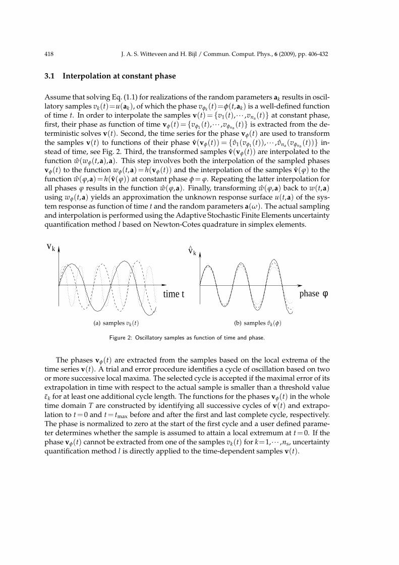
stead of time, see Fig. 2. Third, the transformed samples v(vφ(t)) are interpolated to thefunction w(wφ(t,a),a). This step involves both the interpolation of the sampled phasesvφ(t) to the function wφ(t,a)= h(vφ(t)) and the interpolation of the samples v(ϕ) to thefunction w(ϕ,a)=h(v(ϕ)) at constant phase φ= ϕ. Repeating the latter interpolation forall phases ϕ results in the function w(ϕ,a). Finally, transforming w(ϕ,a) back to w(t,a)using wφ(t,a) yields an approximation the unknown response surface u(t,a) of the sys-tem response as function of time t and the random parameters a(ω). The actual samplingand interpolation is performed using the Adaptive Stochastic Finite Elements uncertaintyquantification method l based on Newton-Cotes quadrature in simplex elements.

kv

time t

(a) samples vk(t)

kv^

φphase

(b) samples vk(φ)

Figure 2: Oscillatory samples as function of time and phase.

The phases vφ(t) are extracted from the samples based on the local extrema of thetime series v(t). A trial and error procedure identifies a cycle of oscillation based on twoor more successive local maxima. The selected cycle is accepted if the maximal error of itsextrapolation in time with respect to the actual sample is smaller than a threshold valueεk for at least one additional cycle length. The functions for the phases vφ(t) in the wholetime domain T are constructed by identifying all successive cycles of v(t) and extrapo-lation to t =0 and t = tmax before and after the first and last complete cycle, respectively.The phase is normalized to zero at the start of the first cycle and a user defined parame-ter determines whether the sample is assumed to attain a local extremum at t =0. If thephase vφ(t) cannot be extracted from one of the samples vk(t) for k=1,··· ,ns, uncertaintyquantification method l is directly applied to the time-dependent samples v(t).


3.2 Bounded error

It is shown below that the uncertainty quantification interpolation of periodic samples atconstant phase results in a bounded error. Let u(t,a) be a periodic response as functionof time t for t∈R

u(t+zT(a),a)=u(t,a), for all z∈Z and a∈A, (3.1)

with T(a)=1/ f (a)>0 the period length and f (a) the frequency affected by the randominput a(ω). The phase φ(t,a) of the response u(t,a) is given by

φ(t,a)=φ0(a)+t

T(a), (3.2)

with φ0(a) = φ(0,a). Consider uncertainty quantification method l which results in anapproximation w(t,a) of u(t,a) based on applying interpolation method h at constantphase to ns samples v(t)=v1(t),··· ,vns for parameter values ak for k=1,··· ,ns resultedfrom sampling method g.

Theorem 3.1. The error ε(ϕ,a) = w(ϕ,a)−u(ϕ,a) in approximation w(ϕ,a) with respect toperiodic response surface u(ϕ,a) as resulted from uncertainty quantification method l applied atconstant phase ϕ is bounded for all ϕ∈R and a∈A by δ for which holds

ε(ϕ,a)<δ, for all ϕ∈ [0,1] and a∈A. (3.3)

Proof. Sampling method g results in samples

vk(t)= gk(u(t,a))=u(t,ak), (3.4)

for k = 1,··· ,ns. The samples vk(t) are periodic signals with period length vTk= T(ak),

since using (3.1)

vk(t+zvTk)=u(t+zT(ak),ak)

=u(t,ak)=vk(t) for all z∈Z, (3.5)

for k=1,··· ,ns. The phase vφk(t)=φ(t,ak) of the samples vk(t) is then in correspondence

with (3.2) given byvφk

(t)=vφ0k+t/vTk

, for k=1,··· ,ns, (3.6)

with vφ0k=vφk

(0). Scaling the samples vk(t) with their phase vφk(t) results in

vk(t)= vk(vφk(t))= vk

(

vφ0k+t/vTk

)

, (3.7)

for k=1,··· ,ns. Periodicity of vk(t) gives

vk(vφk(t)+z)= vk

(

vφ0k+t/vTk

+z)

= vk

(

vφ0k+

t+zvTk

vTk

)

=vk(t+zvTk)=vk(t)= vk(vφk

(t)), for all z∈Z, (3.8)


for k =1,··· ,ns. Uncertainty quantification method l results in approximation w(ϕ,a) byapplying interpolation method h of the samples v(t) at a constant phase ϕ

w(ϕ,a)=h(v(ϕ))=h(v1(ϕ),··· ,vns(ϕ)). (3.9)

The error ε(ϕ,a) as function of phase ϕ in approximation w(ϕ,a) with respect to u(ϕ,a)is defined as

ε(ϕ,a)= w(ϕ,a)−u(ϕ,a), (3.10)

withu(t,a)= u(φ(t,a),a), (3.11)

and

u(φ+z,a)= u

(

φ0(a)+t+zT(a)

T(a),a

)

=u(t+zT(a),a)

=u(t,a)= u(φ,a), for all z∈Z and a∈A. (3.12)

For error ε(ϕ,a) then holds using (3.8), (3.9), and (3.12)

ε(ϕ+z,a)= w(ϕ+z,a)−u(ϕ+z,a)

=h(v1(ϕ+z),··· ,vns(ϕ+z))−u(ϕ+z,a)

=h(v1(ϕ),··· ,vns(ϕ))−u(ϕ,a)

= w(ϕ,a)−u(ϕ,a)= ε(ϕ,a), for all z∈Z and ϕ∈R and a∈A. (3.13)

Error ε(ϕ,a) is, therefore, a periodic function of ϕ. Define δ for which holds (3.3)

ε(ϕ,a)<δ for all ϕ∈ [0,1] and a∈A,

then holds

ε(ϕ+z,a)= ε(ϕ,a)<δ for all z∈Z and ϕ∈ [0,1] and a∈A, (3.14)

andε(ϕ,a)<δ for all ϕ∈R and a∈A, (3.15)

Error ε(ϕ,a) in approximation w(ϕ,a) is, therefore, bounded by δ for all ϕ∈R and a ∈A.

Notice that the proof of Theorem 3.1 is independent of uncertainty quantificationmethod l, sampling method g, and interpolation method h.

The bounded error ε(ϕ,a) as function of phase ϕ also results in a bounded error ε(t,a)in time for the Unsteady Adaptive Stochastic Finite Elements method l1 based on first de-gree Newton-Cotes quadrature, if initial phase φ0(a) and frequency f (a) depend linearlyon a. Let initial phase φ0(a), therefore, depend linearly on the random parameters a

φ0(a)= cφ0 ,0+cφ0,1 ·a. (3.16)


where · denotes the vector inner product, with cφ0,0 constant and cφ0 ,1 a vector containingna constants. And let frequency f (a) also depend linearly on a(ω)

f (a)= cf,0+cf,1 ·a, (3.17)

with cf,0 constant and cf,1 an na-dimensional constant vector. Consider uncertainty quan-tification method l1 based on piecewise linear interpolation method h1 of samples in thefirst degree Newton-Cotes quadrature points in the vertices of simplex elements of sam-pling method g1.

Theorem 3.2. The error ε(t,a)=w(t,a)−u(t,a) in approximation w(t,a) with respect to periodicresponse surface u(t,a) as resulted from uncertainty quantification method l1 applied at constantphase ϕ is bounded for all t∈R and a∈A by δ for which holds (3.3)

ε(ϕ,a)<δ, for all ϕ∈ [0,1] and a∈A,

if initial phase φ0(a) and frequency f (a) depend linearly on a.

Proof. The phase φ(t,a) of the periodic response u(t,a) is given by (3.2)

φ(t,a)=φ0(a)+t

T(a)=φ0(a)+ f (a)t.

The linear dependence of φ0(a) and f (a) on a given by (3.16) and (3.17) results in

φ(t,a)= cφ0 ,0+cf,0t+(cφ0 ,1+cf,1t)·a (3.18)

The ns sampled phases v1φ(t) = vφ1

(t),··· ,vφns(t) resulting from sampling method g1

are, therefore,v1

φk(t)= cφ0 ,0+cf,0t+(cφ0 ,1+cf,1t)·ak , (3.19)

for k =1,··· ,ns. The resulting w1φ(t,a) of piecewise linear interpolation h1 of the samples

v1φ(t) then exactly reconstructs the function φ(t,a)

w1φ(t,a)=h1(v1

φ(t))= cφ0 ,0+cf,0t+(cφ0 ,1+cf,1t)·a=φ(t,a). (3.20)

Therefore, error ε(φ(t,a),a) in the approximation w1(w1φ(t,a),a) of response u(φ(t,a),a)

becomes

ε(φ(t,a),a)= w1(w1φ(t,a),a)−u(φ(t,a),a)

= w1(φ(t,a),a)−u(φ(t,a),a)

=w1(t,a)−u(t,a)

= ε(t,a)<δ for all φ∈R and a∈A, (3.21)

according to Theorem 3.1. Using (3.2) gives

ε(t,a)<δ for all t∈R and a∈A. (3.22)

This completes the proof of the theorem.


Unsteady Adaptive Stochastic Finite Elements method l2 based on a piecewise quadraticinterpolation method h2 of samples in the second degree Newton-Cotes quadrature pointsin simplex elements of sampling method g2 consequently gives ε(t,a)<δ for all t∈R anda∈A up to quadratic dependence of φ0(a) and f (a) on a.

For periodic responses the interpolation of the samples at constant phase eliminatesthe effect of the increasing phase differences in time, which usually causes the fast in-crease of the number of required samples. The error is even bounded in time for periodicproblems with an up to quadratic dependence of initial phase φ0(a) and frequency f (a)on random parameters a. For non-periodic responses the interpolation at constant phasealso eliminates the effect of the increasing phase differences on the increase of the num-ber of required samples. The error is for non-periodic responses not bounded in time dueto, for example, increasing amplitudes with time. In practice, interpolation of oscillatorysamples in time results, however, in an approximately constant accuracy in time with aconstant number of samples for periodic and non-periodic responses of which the phaseis well-defined.

4 Numerical results

The developed uncertainty quantification methods are applied to transonic airfoil flows.Adaptive Stochastic Finite Elements with Newton-Cotes quadrature in simplex elementsis applied to a steady transonic airfoil flow in Section 4.1. A transonic airfoil flutter prob-lem is analyzed in Section 4.2 using Unsteady Adaptive Stochastic Finite Elements withinterpolation at constant phase.

4.1 Steady transonic airfoil flow

The steady transonic flow over a NACA0012 airfoil is considered with randomness inthe angle of attack α(ω). The randomness around the mean angle of attack µα = 2o isgiven by a symmetrical beta distribution with β1 = β2 = 2 in domain α ∈ [1o,3o], whichcorresponds to an input coefficient of variation of cvα = 22.4%. Standard atmosphericfree stream pressure p∞ = 101300Pa and temperature T∞ = 293K results for free streamvelocity V∞ =276.27m/s in a Mach number of M∞ =0.8. The flow is modeled here by thecompressible Euler equations [5] mainly to demonstrate the properties of the uncertaintyquantification method. The two-dimensional flow domain is discretized by an unstruc-tured hexahedral mesh of 12·103 cells, which was selected based on a grid convergencestudy. The Euler equations are discretized using a second order central finite volume dis-cretization stabilized with artificial dissipation [11]. The steady state solution is obtainedby time integration with a CFL number of 1.5.

The deterministic flow for the mean angle of attack µα =2o is transonic with a shockwave at 70.2% of the upper surface, as can be identified in the pressure field and thepressure distribution over the airfoil surface in Fig. 3. This shock wave in physical space


(a) Pressure field

0 0.2 0.4 0.6 0.8 1−1.6

−1.4

−1.2

−1

−0.8

−0.6

−0.4x 105

surface coordinate s

pres

sure

−p

[Pa]

upper surfacelower surface

(b) Surface distribution

Figure 3: Deterministic pressure for mean angle of attack µα =2o for the steady transonic airfoil flow.

1 1.5 2 2.5 31

1.5

2

2.5

3

3.5x 104

lift [

N]

ns=17

angle of attack [deg]

1st degree NC2nd degree NCsamples

(a) Lift

1 1.5 2 2.5 3

1000

1500

2000

2500

3000

drag

[N]

ns=17



(b) Drag

1 1.5 2 2.5 3−5500

−5000

−4500

−4000

−3500

−3000

−2500

−2000

−1500

mom

ent [

Nm

]

ns=17



(c) Moment

1 1.5 2 2.5 30.6

0.62

0.64

0.66

0.68

0.7

0.72

0.74

0.76

0.78

shoc

k lo

catio

n [s

]

ns=17



(d) Shock location

Figure 4: Response surfaces of lift, drag, pitching moment, and shock location for the steady transonic airfoilflow with random angle of attack α(ω).


1 1.5 2 2.5 3 3.5x 10

4

0

0.1

0.2

0.3

0.4

0.5

0.6

0.7

0.8

0.9

1

lift [N]

ns=17

cum

ulat

ive

prob

abili

ty

1st degree NC2nd degree NC

(a) Lift

1000 1500 2000 2500 3000

0

0.1

0.2

0.3

0.4

0.5

0.6

0.7

0.8

0.9

1

drag [N]

ns=17

cum

ulat

ive

prob

abili

ty


(b) Drag

−5500 −5000 −4500 −4000 −3500 −3000 −2500 −2000 −1500

0

0.1

0.2

0.3

0.4

0.5

0.6

0.7

0.8

0.9

1

moment [Nm]

ns=17

cum

ulat

ive

prob

abili

ty


(c) Moment

0.6 0.65 0.7 0.75

0

0.1

0.2

0.3

0.4

0.5

0.6

0.7

0.8

0.9

1

shock location [s]

ns=17

cum

ulat

ive

prob

abili

ty


(d) Shock location

Figure 5: Cumulative probability distributions of lift, drag, pitching moment, and shock location for the steadytransonic airfoil flow with random angle of attack α(ω).

results in a discontinuity in probability space. On the lower surface there is also a smallsupersonic region present.

Adaptive Stochastic Finite Elements with first and second degree Newton-Cotes (NC)quadrature in simplex elements are employed to resolve the response surfaces and prob-ability distributions of the functionals lift, drag, pitching moment, and shock location inFigs. 4 and 5. The first and second degree Newton-Cotes approximations of the responsesurfaces based on ns=17 samples are in close agreement in Fig. 4. Both discretizations re-sult in an interpolation that preserves the extrema of the samples. The response surfaceof the shock location is less smooth than that of the other functionals, because the shocklocation attains discrete values of the locations of the volume faces on the airfoil surface.Since the multi-element approximations are piecewise continuously differentiable, it ismore appropriate to study the variation in the functionals in terms of the resulting cu-mulative probability distributions in Fig. 5 than in terms of their probability densities.The convergence for the mean and standard deviation of the lift, drag, pitching moment,


Table 1: Mean and standard deviation of lift L(ω) for the steady transonic airfoil flow with random angle ofattack α(ω).

1st degree NC 2nd degree NCns ne mean µL st.dev. σL ne mean µL st.dev. σL

2 1 2.244·104 4.676·103 - - -3 2 2.290·104 4.679·103 1 2.303·104 4.679·103

5 4 2.299·104 4.703·103 2 2.302·104 4.710·103

9 8 2.301·104 4.711·103 4 2.302·104 4.714·103

17 16 2.302·104 4.712·103 8 2.302·104 4.712·103

Table 2: Mean and standard deviation of drag D(ω) for the steady transonic airfoil flow with random angle ofattack α(ω).

1st degree NC 2nd degree NCns ne mean µD st.dev. σD ne mean µD st.dev. σD

2 1 2.108·103 5.132·102 - - -3 2 2.010·103 5.146·102 1 1.982·103 5.143·102

5 4 1.988·103 5.231·102 2 1.981·103 5.256·102

9 8 1.982·103 5.254·102 4 1.981·103 5.261·102

17 16 1.981·103 5.258·102 8 1.981·103 5.259·102

Table 3: Mean and standard deviation of pitching moment M(ω) for the steady transonic airfoil flow with

random angle of attack α(ω).

1st degree NC 2nd degree NCns ne mean µM st.dev. σM ne mean µM st.dev. σM

2 1 −3.479·103 9.003·102 - - -3 2 −3.406·103 9.008·102 1 −3.386·103 9.007·102

5 4 −3.390·103 9.219·102 2 −3.385·103 9.279·102

9 8 −3.385·103 9.275·102 4 −3.383·103 9.292·102

17 16 −3.384·103 9.282·102 8 −3.384·103 9.285·102

Table 4: Mean and standard deviation of shock location sshock(ω) for the steady transonic airfoil flow withrandom angle of attack α(ω).

1st degree NC 2nd degree NCns ne mean µs st.dev. σs ne mean µs st.dev. σs

2 1 6.908·10−1 3.108·10−2 - - -3 2 6.976·10−1 3.120·10−2 1 6.995·10−1 3.117·10−2

5 4 6.985·10−1 3.118·10−2 2 6.988·10−1 3.118·10−2

9 8 6.994·10−1 3.166·10−2 4 6.997·10−1 3.181·10−2

17 16 6.992·10−1 3.184·10−2 8 6.991·10−1 3.190·10−2

and shock location given in Tables 1 to 4 shows a higher accuracy for second degreeNewton-Cotes quadrature compared to first degree quadrature especially for the mean.The standard deviation ranges from 4.6% of the mean for the shock location to 27.4% forthe pitching moment.


The effect of the random α(ω) on the surface pressure distribution in terms of themean and the 99% uncertainty interval is given in Fig. 6 for the more accurate seconddegree Newton-Cotes quadrature. The discretization based on ns=17 samples and ne=8elements in Fig. 6a shows that the shock wave on the upper surface is smeared out inthe mean sense compared to the deterministic case of Fig. 3b. The uncertainty intervalin the shock region indicates that α(ω) has more effect on the shock wave location thanon the shock wave strength. This Euler computation also indicates a significantly largeruncertainty interval upstream of the shock than downstream of the shock. The 99% un-certainty interval falls within the range of the sampled minimum and maximum givenby the dotted line in Fig. 6a, which demonstrates the extrema diminishing property ofthe method. The result for the pressure distribution on the lower surface of Fig. 6b pre-dicts a shock wave only for a fraction of the realizations. Discretizations with ns=3,5,9show in Fig. 6c convergence of a staircase approximation of the mean and the uncer-tainty interval to a smooth behavior. Uniform stochastic grid refinement is used here inthe examples.

0 0.2 0.4 0.6 0.8 1−1.6

−1.4

−1.2

−1

−0.8

−0.6

−0.4x 105


pres

sure

−p

[Pa]

ns=17

mean99% intervalsampled min/max

(a) Upper surface

0 0.2 0.4 0.6 0.8 1−1.6

−1.4

−1.2

−1

−0.8

−0.6

−0.4x 105


pres

sure

−p

[Pa]

ns=17

mean99% intervalsampled min/max

(b) Lower surface

0 0.2 0.4 0.6 0.8 1−1.6

−1.4

−1.2

−1

−0.8

−0.6

−0.4x 105


pres

sure

−p

[Pa]

ns=3

ns=5

ns=9

sampled min/max

(c) Convergence

Figure 6: Mean surface pressure and 99% uncertaintyinterval of second degree Newton-Cotes quadraturefor the steady transonic airfoil flow with random angleof attack α(ω).

Fig. 7 shows an approximation of the mean and standard deviation of the pressurefield relative to the airfoil. In the mean pressure field the smearing of the shock wave


(a) Mean (b) Standard deviation

Figure 7: Mean and standard deviation of the pressure field for second degree Newton-Cotes quadrature withns =17 for the steady transonic airfoil flow with random angle of attack α(ω).

can again be identified. The standard deviation field shows that standard deviation isproduced in the shock region with a maximum coefficient of variation of cvp = 37.1%at 68.9% of the upper surface. This corresponds to a maximum amplification of inputrandomness α(ω) by 65.6%.

4.2 Transonic airfoil flutter

The combined effect of independent randomness in the ratio of natural frequencies ω(ω)and the free stream velocity U∞(ω) on the post-flutter behavior of an elastically mountedairfoil is analyzed. The structural model of the pitch-plunge airfoil with cubic nonlinearspring stiffness is given by [7, 14]:

ξ′′+xαα′′+

(

ω

U∗

)2

(ξ+βξ ξ3)=−1

πµCl(τ), (4.1)

xα

r2α

ξ′′+α′′+1

U∗2(α+βαα3)=

2

πµr2α

Cm(τ), (4.2)

where βξ=0m−2 and βα=300rad−2 are the cubic spring parameters, ξ(τ)=h/b is the non-dimensional plunge displacement of the elastic axis, see Fig. 8, α(τ) is the pitch angle,and (′) denotes differentiation with respect to non-dimensional time τ =Ut/b, with half-chord length b=c/2=0.5m. The radius of gyration around the elastic axis is rαb=0.25m,bifurcation parameter U∗ is defined as U∗ = U/(bωα), and the airfoil-air mass ratio isµ=m/πρ∞b2 =100, with m the airfoil mass. The elastic axis is located at a distance ahb=−0.25m from the mid-chord position and the mass center is located at a distance xαb =0.125m from the elastic axis. The ratio of natural frequencies is defined as ω(ω)=ωξ/ωα,with ωξ and ωα the natural frequencies of the airfoil in pitch and plunge, respectively. Therandomness in ω(ω) is described by a uniform distribution around mean value µω =0.25with a coefficient of variation of 10%. The free stream velocity U∞(ω) is subject to a


ahb xα b

h

mid−chordelastic axis

centre of mass

reference position

cb

α

Figure 8: The elastically mounted pitch-plunge airfoil model.

symmetric unimodal beta distribution with β1 = β2 = 2 with a coefficient of variation of1% around mean µU∞

=276.27m/s, which corresponds to M∞ =0.8.

The non-dimensional aerodynamic lift and moment coefficients, Cl(τ) and Cm(τ), aredetermined by solving the Euler equations as for the steady transonic airfoil flow. An Ar-bitrary Lagrangian-Eulerian formulation is employed to couple the fluid mesh with themovement of the structure. The fluid mesh is deformed using radial basis function inter-polation of the boundary displacements [3]. Time integration is performed using the sec-ond order BDF-2 method until t=3 with time step ∆t=0.002, which was established aftera time step refinement study. Initially the airfoil is at rest at a deflection of α(0)=0.1degand ξ(0)=0 from its equilibrium position. In order to study the post-bifurcation behav-ior, the bifurcation parameter U∗ is fixed at 130% of the deterministic linear bifurcationpoint for the mean values of the random parameters. The stochastic behavior of the angleof attack α(t,ω) is resolved as indicator for the post-flutter airfoil behavior.

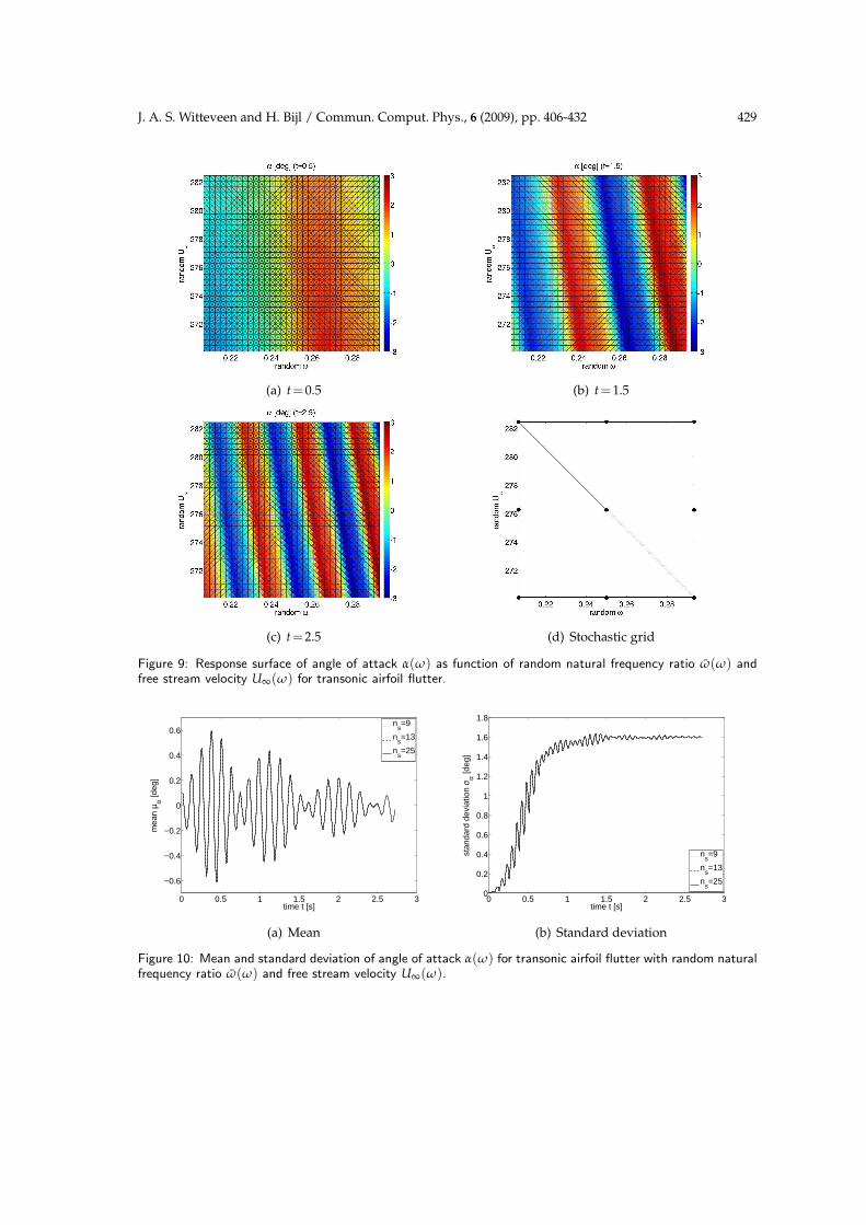
The Unsteady Adaptive Stochastic Finite Elements response surface approximationof the angle of attack α(t,ω) as function of the random parameters ω(ω) and U∞(ω) att = 0.5;1.5;2.5 given in Fig. 9 shows an increasingly oscillatory response surface withtime. The 10% variation in ω(ω) has a larger effect on the frequency of the response thanU∞(ω) with 1% variation. Both parameters have a small effect on the amplitude of theoscillation of α(t,ω) of approximately 3o. At t=0.5 the airfoil exhibits transient behaviorfrom its initial perturbation of α(0)=0.1o, which is indicated by the smaller amplitude ofthe response surface variations of approximately 2o. These results are obtained using thetime-independent grid in probability space shown in Fig. 9d with ns =9 samples, ne =2elements, and nesub

=4096 post-processing subelements.

The resulting UASFE approximation of the mean µα(t) and standard deviation σα(t)of the angle of attack α(t,ω) in Fig. 10 shows two frequency signals due to the effect ofthe two random parameters on the frequency of the response. The mean µα(t) exhibitsinitially an increasing oscillation caused by the deterministic transient of the samples, af-ter which it develops a decaying oscillation due to the effect of the random parameterson the frequency of the response. The large effect of the random parameters on the dy-


(a) t=0.5 (b) t=1.5

(c) t=2.5 (d) Stochastic grid

Figure 9: Response surface of angle of attack α(ω) as function of random natural frequency ratio ω(ω) andfree stream velocity U∞(ω) for transonic airfoil flutter.

0 0.5 1 1.5 2 2.5 3

−0.6

−0.4

−0.2

0

0.2

0.4

0.6

time t [s]

mea

n µ α [d

eg]

ns=9

ns=13

ns=25

(a) Mean

0 0.5 1 1.5 2 2.5 30

0.2

0.4

0.6

0.8

1

1.2

1.4

1.6

1.8

time t [s]

stan

dard

dev

iatio

n σ α [d

eg]

ns=9

ns=13

ns=25

(b) Standard deviation

Figure 10: Mean and standard deviation of angle of attack α(ω) for transonic airfoil flutter with random naturalfrequency ratio ω(ω) and free stream velocity U∞(ω).


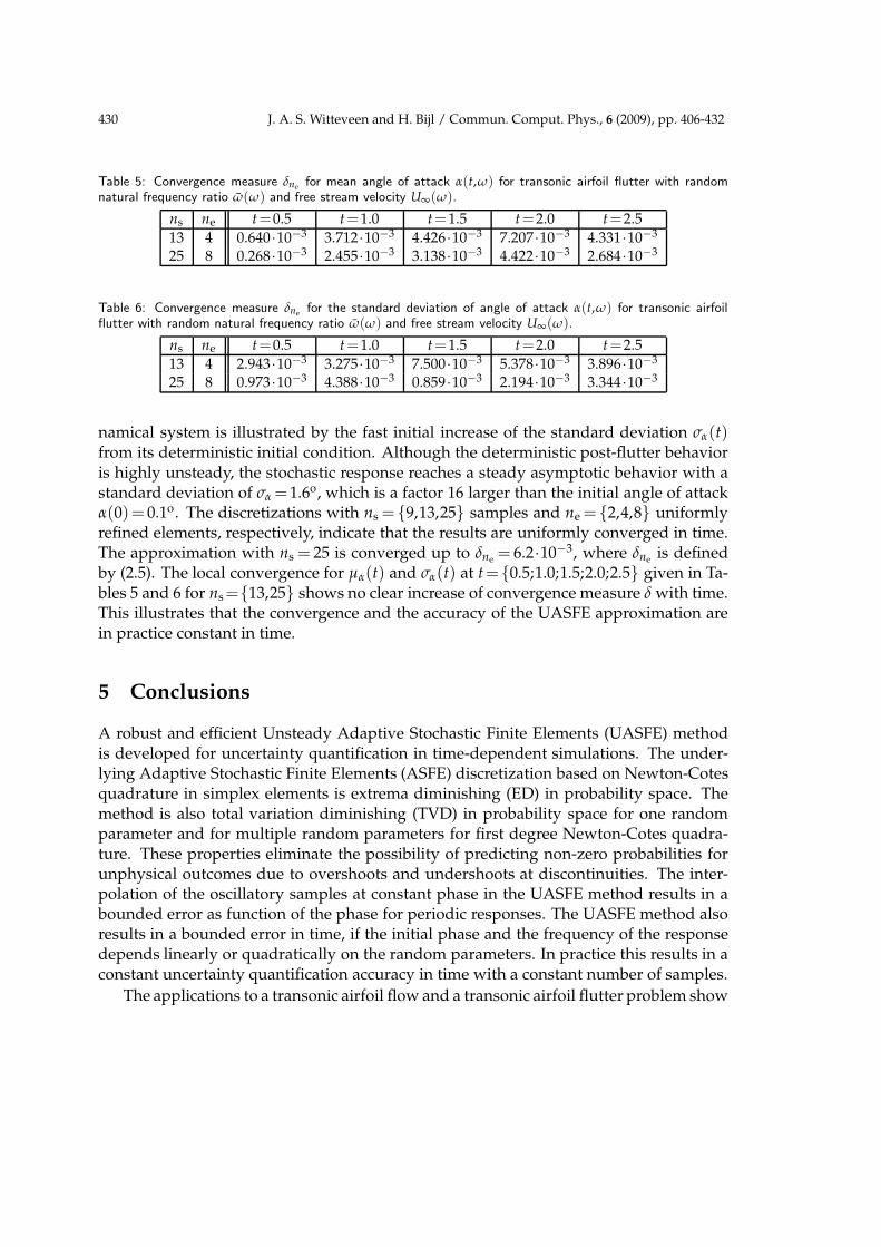
Table 5: Convergence measure δne for mean angle of attack α(t,ω) for transonic airfoil flutter with random

natural frequency ratio ω(ω) and free stream velocity U∞(ω).

ns ne t=0.5 t=1.0 t=1.5 t=2.0 t=2.5

13 4 0.640·10−3 3.712·10−3 4.426·10−3 7.207·10−3 4.331·10−3

25 8 0.268·10−3 2.455·10−3 3.138·10−3 4.422·10−3 2.684·10−3

Table 6: Convergence measure δne for the standard deviation of angle of attack α(t,ω) for transonic airfoil

flutter with random natural frequency ratio ω(ω) and free stream velocity U∞(ω).

ns ne t=0.5 t=1.0 t=1.5 t=2.0 t=2.5

13 4 2.943·10−3 3.275·10−3 7.500·10−3 5.378·10−3 3.896·10−3

25 8 0.973·10−3 4.388·10−3 0.859·10−3 2.194·10−3 3.344·10−3

namical system is illustrated by the fast initial increase of the standard deviation σα(t)from its deterministic initial condition. Although the deterministic post-flutter behavioris highly unsteady, the stochastic response reaches a steady asymptotic behavior with astandard deviation of σα =1.6o, which is a factor 16 larger than the initial angle of attackα(0)= 0.1o. The discretizations with ns = 9,13,25 samples and ne = 2,4,8 uniformlyrefined elements, respectively, indicate that the results are uniformly converged in time.The approximation with ns = 25 is converged up to δne = 6.2·10−3, where δne is definedby (2.5). The local convergence for µα(t) and σα(t) at t=0.5;1.0;1.5;2.0;2.5 given in Ta-bles 5 and 6 for ns=13,25 shows no clear increase of convergence measure δ with time.This illustrates that the convergence and the accuracy of the UASFE approximation arein practice constant in time.

5 Conclusions

A robust and efficient Unsteady Adaptive Stochastic Finite Elements (UASFE) methodis developed for uncertainty quantification in time-dependent simulations. The under-lying Adaptive Stochastic Finite Elements (ASFE) discretization based on Newton-Cotesquadrature in simplex elements is extrema diminishing (ED) in probability space. Themethod is also total variation diminishing (TVD) in probability space for one randomparameter and for multiple random parameters for first degree Newton-Cotes quadra-ture. These properties eliminate the possibility of predicting non-zero probabilities forunphysical outcomes due to overshoots and undershoots at discontinuities. The inter-polation of the oscillatory samples at constant phase in the UASFE method results in abounded error as function of the phase for periodic responses. The UASFE method alsoresults in a bounded error in time, if the initial phase and the frequency of the responsedepends linearly or quadratically on the random parameters. In practice this results in aconstant uncertainty quantification accuracy in time with a constant number of samples.

The applications to a transonic airfoil flow and a transonic airfoil flutter problem show


a significant effect of input randomness. In the steady transonic airfoil flow randomnessin the angle of attack results in production of standard deviation in the shock region witha maximum coefficient of variation cvp = 37.1% at 68.9% of the upper surface, whichcorresponds to an amplification of input randomness by 65.6%. The unsteady transonicairfoil flutter problem shows a steady asymptotic stochastic behavior with a standarddeviation of 1.6o, which is a factor 16 larger than the deterministic initial condition.

Acknowledgments

This research was supported by the Technology Foundation STW, applied science divi-sion of NWO and the technology programme of the Ministry of Economic Affairs.

References

[1] I. Babuska, R. Tempone and G. E. Zouraris, Galerkin finite element approximations ofstochastic elliptic partial differential equations, SIAM J. Numer. Anal., 42 (2004), 800-825.

[2] I. Babuska, F. Nobile and R. Tempone, A stochastic collocation method for elliptic partialdifferential equations with random input data, SIAM J. Numer. Anal., 45 (2007), 1005-1034.

[3] A. de Boer, M. S. van der Schoot and H. Bijl, Mesh deformation based on radial basis functioninterpolation, Comput. Struct., 85 (2007), 784-795.

[4] F. Casciati and B. Roberts, Mathematical Models for Structural Reliability Analysis, CRCPress, Boca Raton, 1996.

[5] A. J. Chorin and J. E. Marsden, A Mathematical Introduction to Fluid Mechanics, Springer-Verlag, New York, 1979.

[6] M. Deb, I. Babuska and J. Oden, Solution of stochastic partial differential equations usingGalerkin finite element techniques, Comput. Methods Appl. Mech. Eng., 190 (2001), 6359-6372.

[7] Y. Fung, An Introduction to Aeroelasticity, Dover Publications, New York, 1969.[8] R. G. Ghanem and P. Spanos, Stochastic Finite Elements: A Spectral Approach, Springer-

Verlag, New York, 1991.[9] J. M. Hammersley and D. C. Handscomb, Monte Carlo Methods, Methuen’s Monographs

on Applied Probability and Statistics, Fletcher & Son Ltd., Norwich, 1964.[10] A. Harten, High resolution schemes for hyperbolic conservation laws, J. Comput. Phys., 49

(1983), 357-393.[11] C. Hirsch, Numerical Computation of Internal and External Flows: Fundamentals of Com-

putational Fluid Dynamics, Elsevier, Amsterdam, 2007.[12] S. Hosder, R. W. Walters and R. Perez, A non-intrusive polynomial chaos method for un-

certainty propagation in CFD simulations, AIAA-2006-891, 44th AIAA Aerospace SciencesMeeting and Exhibit, Reno, Nevada, 2006.

[13] A. Jameson, Positive schemes and shock modelling for compressible flows, Int. J. Num.Meth. Fluids, 20 (1995), 743-776.

[14] B. H. K. Lee, L. Y. Jiang and Y. S. Wong, Flutter of an airfoil with a cubic nonlinear restor-ing force, AIAA-1998-1725, 39th AIAA/ASME/ASCE/AHS/ASC Structures, Structural Dy-namics, and Materials Conference, Long Beach, CA, 1998.


[15] O. P. Le Maıtre, O. M. Knio, H. N. Najm and R. G. Ghanem, Uncertainty propagation usingWiener-Haar expansions, J. Comput. Phys., 197 (2004), 28-57.

[16] O. P. Le Maıtre, H. N. Najm, R. G. Ghanem and O. M. Knio, Multi-resolution analysis ofWiener-type uncertainty propagation schemes, J. Comput. Phys., 197 (2004), 502-531.

[17] L. Mathelin, M. Y. Hussaini and Th. A. Zang, Stochastic approaches to uncertainty quantifi-cation in CFD simulations, Num. Alg., 38 (2005), 209-236.

[18] D. R. Millman and P. I. King, Airfoil pitch-and-plunge bifurcation behavior with Fourierchaos expansions, J. Aircraft, 42 (2005), 376-384.

[19] C. L. Pettit and P. S. Beran, Spectral and multiresolution Wiener expansions of oscillatorystochastic processes, J. Sound Vib., 294 (2006), 752-779.

[20] M. T. Reagan, H. N. Najm, R. G. Ghanem and O. M. Knio, Uncertainty quantification inreacting-flow simulations through non-intrusive spectral projection, Combust. Flame, 132(2003), 545-555.

[21] A. Sarkar and R. G. Ghanem, Mid-frequency structural dynamics with parameter uncer-tainty, Comput. Method. Appl. Mech. Eng., 191 (2002), 5499-5513.

[22] M. A. Tatang, Direct incorporation of uncertainty in chemical and environmental engineer-ing systems, Ph.D Thesis, MIT, Cambridge, 1995.

[23] X. Wan and G. E. Karniadakis, An adaptive multi-element generalized polynomial chaosmethod for stochastic differential equations, J. Comput. Phys., 209 (2005), 617-642.

[24] J. A. S. Witteveen and H. Bijl, A monomial chaos approach for efficient uncertainty quantifi-cation in nonlinear problems, SIAM J. Sci. Comput., 30 (2008), 1296-1317.

[25] J. A. S. Witteveen, G. J. A. Loeven, S. Sarkar and H. Bijl, Probabilistic collocation for period-1limit cycle oscillations, J. Sound Vib., 311 (2008), 421-439.

[26] J. A. S. Witteveen and H. Bijl, An unsteady adaptive stochastic finite elements formulationfor rigid-body fluid-structure interaction, Comput. Struct., 86 (2008), 2123-2140.

[27] J. A. S. Witteveen and H. Bijl, An alternative unsteady adaptive stochastic finite elementsformulation based on interpolation at constant phase, Comput. Method. Appl. Mech. Eng.,198 (2008), 578-591.

[28] J. A. S. Witteveen, G. J. A. Loeven and H. Bijl, An adaptive stochastic finite elements formu-lation based on Newton-Cotes quadrature in simplex elements, (2008) submitted.

[29] J. A. S. Witteveen and H. Bijl, Effect of randomness on multi-frequency aeroelastic responsesresolved by unsteady adaptive stochastic finite elements, (2008) submitted.

[30] D. Xiu and G. E. Karniadakis, The Wiener-Askey polynomial chaos for stochastic differentialequations, SIAM J. Sci. Comput., 24 (2002), 619-644.

[31] D. Xiu and J. S. Hesthaven, High-order collocation methods for differential equations withrandom inputs, SIAM J. Sci. Comput., 27 (2005), 1118-1139.

[32] D. Xiu, Fast numerical methods for stochastic computations: A review, Commun. Comput.Phys., 5 (2009), 242-272.

ATVD UncertaintyQuantificationMethod withBounded Error Applied to Transonic Airfoil Flutter

Documents

Transcript of ATVD UncertaintyQuantificationMethod withBounded Error Applied to Transonic Airfoil Flutter