A computational study of vortex-airfoil

interaction using high-order finite difference

methods

Magnus Svärd, Johan Lundberg and Jan Nordström

Post Print

N.B.: When citing this work, cite the original article.

Original Publication:

Magnus Svärd, Johan Lundberg and Jan Nordström, A computational study of vortex-airfoil

interaction using high-order finite difference methods, 2010, Computers & Fluids, (39),

1267-1274.

http://dx.doi.org/10.1016/j.compfluid.2010.03.009

Copyright: Elsevier Science B.V., Amsterdam.

http://www.elsevier.com/

Postprint available at: Linköping University Electronic Press

http://urn.kb.se/resolve?urn=urn:nbn:se:liu:diva-68614

A computational study of vortex-airfoil

interaction using high-order finite difference

methods

Magnus Svard ∗, Johan Lundberg †and Jan Nordstrom ‡

January 11, 2010

Abstract

Simulations of the interaction between a vortex and a NACA0012airfoil are performed with a stable, high-order accurate (in space andtime), multi-block finite-difference solver for the compressible Navier-Stokes Equations.

We begin by computing a benchmark test case to validate the code.Next, the flow with steady inflow conditions are computed on severaldifferent grids. The resolution of the boundary layer as well as theamount of the artificial dissipation is studied to establish the necessaryresolution requirements. We propose an accuracy test based on theweak imposition of the boundary conditions that does not require agrid refinement.

Finally, we compute the vortex-airfoil interaction and calculate thelift and drag coefficients. It is shown that the viscous terms add theeffect of detailed small scale structures to the lift and drag coefficients.

1 Introduction

Flows around multiple bodies are common in aerodynamic computations.Each body will disturb the free stream and the disturbances interact down-stream of the body. To obtain good solutions for multi-body configurations,

∗School of Mathematics, University of Edinburgh, King’s Buildings, Mayfield Road,Edinburgh, EH9 3JZ, United Kingdom; e-mail: Magnus.Svard@ed.ac.uk

†Department of Information Technology, Uppsala University, SE-751 05 Uppsala, Swe-den; ABB AB, Natverksgatan 3, Building 391, SE-721 59 Vasteras, Sweden

‡Department of Computational Physics, The Swedish Defense Research Agency, SE-164 90 Stockholm, Sweden; Department of Information Technology, Uppsala University,SE-751 05 Uppsala, Sweden; e-mail jan.nordstrom@foi.se

1

the numerical scheme must accurately compute the flow around the bodies,as well as the wave propagation between the bodies. As a prototype of suchproblems, we will study a vortex-airfoil interaction. The vortex represents astructure generated by a body upstream of the airfoil.

In [3], the vortex-airfoil interaction problem governed by the Euler equa-tions was studied. It was shown that high-order accuracy in space results insuperior computational efficiency. However, while the Euler equations mightbe a good model for the vortex transport, it is less likely to be a good modelin the interaction phase since viscosity plays an important role. The purposeof the present work is to study vortex-airfoil interaction governed by theNavier-Stokes equations and take viscous effects into account. Previouslypublished results on vortex-airfoil interaction concern the inviscid case, [14].

The simulations have been carried out with a stable, high-order accu-rate (in both space and time), multi-block finite difference solver for thecompressible Navier-Stokes and Euler equations, described in [9] and [11].The finite difference scheme satisfies a Summation-by-Parts rule (SBP) andthe Simultaneous Approximation Term (SAT) technique is used to weaklyenforce the boundary conditions. The entire scheme for the Navier-Stokesequations can be proven linearly stable for the constant coefficient problem(see [9] and [11] and references therein). Linear stability of the constantcoefficient problem leads to stability of the variable coefficient problem (see[5]) and stability of the linear variable coefficient problem leads to stabilityof non-linear problems with smooth solutions (see [8]). Hence, the proofs ofstability in [9, 11] implies, via a mathematically stringent chain of arguments,stability of the problems we will study in this paper. This is corroboratedin [10], where design order of accuracy (up to 5) was demonstrated for thepresent implementation.

In this article, we present a delicate validation test case to further demon-strate the accuracy of the code: the flow around a NACA0012 airfoil at Machnumber (Ma) 0.5 and Reynolds number (Re) 5000.

Next, we will increase the Reynolds number to 10000 and run with free-stream inflow data (without a vortex). We will use that solution to quantifythe accuracy of the present computations. This is done by studying the sep-aration point, the resolution of the boundary layers and the effective amountof artificial diffusion.

Finally, we will compute the vortex-airfoil interaction at Ma = 0.5 andRe = 10000. We monitor the lift and drag and show the differences from aninviscid computation.

2

2 The numerical method

The numerical method (from now on referred to as SBP-SAT schemes) isdescribed at length in [9] and [11]. Nevertheless, we will present its theoreticalproperties using the advection-diffusion equation and prove stability via anenergy estimate. We will use two different boundary conditions; one mimicinga far-field boundary and the other one a wall.

We define the L2-norm on [xA, xB] as

‖u‖2

2 =

∫ xB

xA

u2 dx.

The x-axis is discretized with N + 1 grid points such that xi = ih + xA,i = 0..N and h = (xB−xA)/N . A first-derivative approximation of a functionu is written as

P−1Qu = ux + Te,

where u is the vector function

u = [u(x0, t), u(x1, t) . . . u(xN , t)]T

and Te is the truncation error. The derivative approximation, P−1Qu, is saidto have the Summation-by-parts (SBP) property if:

1. P is symmetric and positive definite. (In this article, we will onlyconsider diagonal P :s.)

2. Q + QT = B where B = diag [−1, 0 . . . 0, 1].

Second-derivatives will be approximated with the operator D2 = P−1QP−1Q.We will also need the auxiliary vectors eN = [0 . . . 0, 1]T and e0 = [1, 0, . . . 0]T .

2.1 Energy estimates

Consider the one-dimensional advection-diffusion equation

ut + aux = ǫuxx,

αu(xA, t) + βux(xA, t) = gA(t), (1)

u(xB, t) = 0,

where the boundary condition at xA models an inflow or outflow boundaryand the boundary condition at xB models a wall. We derive an energy

3

estimate for (1) by multiplying by u and integrating in space.

d

dt‖u‖2 + 2ǫ‖ux‖

2 =

(

a +2α

βǫ

) (

u(xA, t) −ǫ

β(a + 2αβ

ǫ)gA(t)

)2

−

(ǫ

β

)2(

1

a + 2αβ

ǫ

)

gA(t)2.

An energy estimate is obtained if

a +2α

βǫ < 0. (2)

We proceed to derive an energy estimate for the semi-discrete SBP-SATscheme. Let v denote the approximate solution, v = [v0(t), ..., vN(t)]. Wediscretize (1) as

vt + aP−1Qv − ǫD2v = σAP−1e0

[αv0 + β

(P−1Qv

)

0− gA

](3)

+ σBP−1eN [vN − 0] ,

where the terms on the right-hand side are the Simultaneous ApproximationTerms (also referred to as SAT’s or penalty terms) that will enforce theboundary conditions. The penalty parameters σA and σB will be determinedwith respect to stability. To simplify the analysis it will be useful to introduceσB = σB

V +σBI . Furthermore, we define ‖v‖2

P = vT Pv. Multiply equation (3)by vT P from the left and add the transpose of the equation. We obtain

d

dt‖v‖2

P + 2ǫ‖P−1Qv‖2

P = BTL + BTIR + BTV R, (4)

where the boundary terms are

BTL = av2

0 − 2ǫv0

(P−1Qv

)

0+ 2σAαv2

0 + (5)

2σAβv0

(P−1Qv

)

0− 2σAv0g

A,

BTIR = −av2

N + 2σBI v2

N , (6)

BTV R = 2ǫvN

(P−1Qv

)

N+ 2σB

V v2

N . (7)

For stability, we require that the right-hand side is bounded from above bydata. Beginning with (6) we see that

σBI ≤

a

2, (8)

4

is a necessary condition. Next, we consider (5). The terms with u0 (P−1Qu)0

must cancel exactly since it is not possible to bound them in a quadraticform. Hence, we require that

σA = ǫ/β. (9)

For gA 6= 0 and using (9), (5) results in condition (2).The viscous part of the wall boundary penalty (7), can be expressed as a

quadratic form

BTV R = −2(vN

(P−1Qv

)

N)

(−σB

V − ǫ2

− ǫ2

0

)

︸ ︷︷ ︸

AV

(vN

(P−1Qv)N

)

. (10)

The expression (10) is negative if the matrix AV on the right-hand sideis positive semi-definite. That can not be achieved in the present form.Therefore, we performed a mathematical manipulation (introduced in [1]) toobtain an energy estimate.

The idea is to borrow a quadratic term from 2ǫ‖P−1Qu‖2P on the left-

hand side of (4). Recalling that P is diagonal with elements Pii = pih, we canrewrite ‖v‖2

P =∑N

i=0v2

i pih =∑N−1

i=0v2

i pih+ pNv2Nh = ‖v‖2

P+ pNv2

Nh. Carry-ing out these changes, the term 2ǫ‖P−1Qv‖2

P in (4) turns into 2ǫ‖P−1Qv‖2

P

and (10) becomes

BTV R = BTV R − 2ǫhpN

(P−1Qv

)2

N(11)

= −2(vN

(P−1Qv

)

N)

(−σB

V − ǫ2

ǫ2

ǫhpN

)

︸ ︷︷ ︸

AV

(vN

(P−1Qv)N

)

.

AV is positive definite if

σBV < −

ǫ

4hpN

. (12)

The above derivation can be summarized in the following proposition.

Proposition 2.1 The scheme (3) is stable if (2), (8), (9) and (12) hold.

Without going into detail, we conclude that when ǫ → 0, some terms ofthe penalty parameters will vanish, leaving only the conditions that enforcethe well-posed boundary conditions for the inviscid equation. We also pointto the fact that the effect of the ǫ dependent terms of the penalty parameterswill diminish as h grows, suggesting that the boundary conditions behave astheir inviscid counterparts on coarse meshes.

5

Details of the above argument, generalized to the Navier-Stokes equations,can be found in [9] and [11]. For the Navier-Stokes equations computed ona fixed grid, the wall boundary condition will approach a slip condition asRe → ∞. Moreover, if the grid is coarsened and Re is kept fixed, the solutionwill behave more like a slip condition.

2.2 Artificial dissipation

The following form of artificial dissipation was derived in [4],

A2p = (−1)p+1P−1DTp BpDp, (13)

where P = ∆x−1P and Dp = hpDp (Dp is a pth-order derivative). The(symmetric part of the) matrix Bp is required to be positive semi-definite.

We choose (Bp)ii = |vi|+ci, where ci is the local speed of sound and |vi| isthe magnitude of the local velocity vector. The artificial dissipation, A2pv, isadded to a 2pth-order accurate discretization of the Navier-Stokes equations.This choice will not increase the width of the stencil and it preserves theoverall order of accuracy.

Furthermore, it is trivial to show that the proposed form results in adamping term in the energy estimate and hence it conforms precisely withthe SBP theory. (We refer to [4] for more details.)

2.3 Grid generation and parallelization

Various grids around the NACA0012 airfoil will be used. They all have thesame principal structure and consist of 12 blocks (see Figure 1). Each blockis a smooth grid. The only requirement is that the grid lines match alongeach interface, but they need not be smooth across the interface. (See [7] fora stability proof.)

6

−15 −10 −5 0 5 10 15−15

−10

−5

0

5

10

15GRID around NACA 0012, 12 block.

x

y

3

1 2

9 8 7

4 6

5

10 11 12

Airfoil

(a) The entire domain

−2.5 −2 −1.5 −1 −0.5 0 0.5 1 1.5−2

−1.5

−1

−0.5

0

0.5

1

1.5

2GRID around NACA 0012, 12 block.

x

y

3

1

2

Airfoil

(b) Zoom of the airfoil

Figure 1: The multi-block computional grid.7

Name ∆min Nodes on airfoilReference 5e-5 350Grid A 1e-4 350

Grid A (coarse) 2e-4 175Grid B 4e-4 350Grid C 16e-4 350Grid D 64e-4 350

Table 1: Computational grids. The normal resolution (and hence the numberof grid points) changes in the grid blocks surrounding the airfoil.

To study the resolution requirements close to the airfoil, we use severaldifferent grids in the blocks 1,2,3 in Figure 1. We will only change theresolution in the normal direction and keep the number of grid points aroundthe airfoil constant. Moreover, the resolution near the outer boundary ofblocks 1,2,3 is also kept constant such that the resolution only changes inthe boundary layer. Finally, the resolution in the y-direction in blocks 5and 6 will change as a consequence of the changes in 1,2 and 3 due to therequirement that grid lines match across an interface. The different gridsused in this article are listed in Table 1.

To obtain solutions in a reasonable amount of time, the 12-block grid wassplit and run on 28 processors (14 AMD Opteron nodes). We stress that thesubdivision is purely artificial and does not change the numerical results.

The splitting was done to achieve a good load balance on Grid A. On allother grids we use the same splitting, which results in a non-optimal loadbalance since Grids B,C,D contain fewer points in some of the blocks.

3 Computations

Throughout this section, we will use two different SBP-SAT schemes. Thefirst is a scheme with internal fourth-order accuracy in space. The truncationerrors near the boundaries are of order two for the inviscid terms and one forthe viscous terms. As a consequence, the global order of accuracy is threeand we will refer to this scheme as the 3rd-order scheme. The other schemehas internal order of eight with truncation errors of order four (inviscid) andthree (viscous) near the boundaries, and the global order is five in space.It will be termed the 5th-order scheme. (For a derivation of global orderof accuracy see [10].) We remark that the global orders of accuracy (5 and3, in our cases) are the convergence rates that can be observed pointwiseeverywhere in the domain, including the boundaries.

8

Furthermore, all computations have been carried with a 4th-order accu-rate low-storage explicit Runge-Kutta scheme for the temporal discretization.

Remark There is a globally second-order accurate version of the SBP-SATscheme available that is the standard central finite-difference scheme with aspecific boundary closure. However, we choose to not include computationswith that scheme since second-order of accuracy is not sufficiently accuratefor vortex propagation, see [3].

3.1 Validation test case

It was shown in [10] that the present technique indeed converges with thecorrect convergence rates for the different orders of accuracy. Moreover, thecode has been validated in [11] for the flow around a cylinder and goodagreement with previously published data was reported.

To further demonstrate the strength of this technique, we have includedthe following benchmark case: flow around the NACA0012 airfoil at Re =5000 , Ma = 0.5 and 0 degrees angle of attack. We compute this flow usingthe 3rd-order scheme on Grid A (fine) and on every second point of Grid A(coarse). At the far-field boundaries we enforce the free-stream data usingthe characteristic boundary conditions derived in [9]. On the airfoil, no-slipboundary conditions proposed in [11] are applied.

This flow case has previously been studied in [12, 13, 15, 6] and we willrefer to it as the Swanson and Turkel (or S&T) test case. For this test case,the flow separates but no wake instabilities should appear. Excessive artificialdiffusion increases the effective Reynolds number and moves the separationpoint downstream. Furthermore, the test case is sensitive to asymmetries inthe solution procedure, which easily can trigger vortices and a steady statewould not be obtained.

We define the separation point as the first grid point at which the flowturns backwards. The separation points computed with our scheme are shownin Table 2 along with previously published data. Our results agree to withinone grid point of the reference data, which is the best we can achieve. InFigure 2, we observe that no wake instabilities occur.

Remark Our way of defining the separation point is conservative and leavesno ambiguity as to how it is obtained. Of course, one may use differentinterpolation techniques to estimate the separation point between grid points,but we prefer this stricter method.

9

Grid Nodes on airfoil ∆y,min Separation point ∆x

Coarse 175 2e-4 0.828 0.018Fine 350 1e-4 0.819 0.009

S&T 85 128 3e-4,6e-4 0.817 -S&T 87 129 6e-4 0.811 -

Venkatakrishnan - - 0.81-0.824 -Mittal - - 0.813 -

Table 2: Results for the validation test (NACA0012, Ma = 0.5, Re = 5000)compared with [12] (S&T85), [13] (S&T87), [15] (Venkatakrishnan) and [6](Mittal). ∆y,min is the minimum grid size in the normal direction of theairfoil. ∆x is the grid size along the airoifl. The fine grid is Grid A and thecoarse is every second point of Grid A. Our results are within one grid cellof those of the references.

(a) Velocity in the x-direction

x

y

0.85 0.9 0.95 1 1.05 1.1 1.15

-0.05

0

0.05

(b) Separation and back flow

Figure 2: The validation test case (NACA0012 at Re = 5000, Ma = 0.5)computed with a 3rd-order scheme.

10

In Figure 3 a zoom of the separation region can be seen. In both the coarseand the fine grid the separation occurs in the cell immediately followingx = 0.81. We also point to the fact that in all plots the velocity vectorat the boundary is too short to be seen, despite the substantial zoom level.(Compare with the reference vector of length 1e − 5.) The no-slip conditionis almost exactly fulfilled even with the weak enforcement of the boundarycondition. We emphasize that with this methodology, no optimization ofany parameters is needed. The test was setup and computed once. Weconclude that this is a very powerful feature and strongly supports that ourcode accurately computes approximations to the correct solution also in caseswhere the solution is not known.

3.2 Steady inflow data

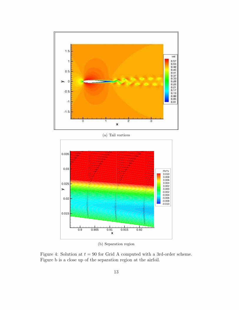
Next, we consider the case with steady inflow data at Ma = 0.5 and Re =10000. Again, we employ the 3rd-order scheme. Solutions were computed forall grids in Table 1. The computations were initialized with constant free-stream values in the entire domain. Tail vortices and back flow appeared inthe numerical solution after some time as is seen in Figure 4 for Grid A. (Thesolutions on the other grids behave similarly.) The computations were rununtil a constant frequency vortex shedding was achieved at about 90 timeunits.

11

x

y

0.81 0.8105 0.811 0.8115

0.024

0.0245

0.025

0.0255

1E-05

(a) The point before separation. Coarsegrid.

xy

0.8275 0.828 0.8285 0.829 0.8295 0.83 0.8305 0.831

0.0215

0.022

0.0225

0.023

0.0235

0.024

0.0245

1E-05

(b) The point after separation. Coarse grid.

x

y

0.81 0.8105 0.811 0.8115

0.0245

0.025

0.0255

1E-05

(c) [The point before separation. Fine grid.

x

y

0.819 0.8195 0.82 0.8205

0.023

0.0235

0.024

0.0245

1E-05

(d) [The point after separation. Fine grid.

Figure 3: The validation test case (NACA0012 at Re = 5000, Ma = 0.5)computed with a 3rd-order scheme. Zoom of velocity vectors at the separa-tion region (including a reference vector).

12

(a) Tail vortices

x

y

0.9 0.905 0.91 0.915 0.92

0.015

0.02

0.025

0.03

0.035

rho*u0.0100.0080.0060.0040.0020.000

-0.002-0.004-0.006-0.008-0.010

(b) Separation region

Figure 4: Solution at t = 90 for Grid A computed with a 3rd-order scheme.Figure b is a close up of the separation region at the airfoil.

13

The reference grid, Grid A and B all have similar boundary layer profilesand the no-slip condition is enforced along the airfoil. It is tempting toassume that the boundary layers are well resolved on those grids. (See Figures5, 6 and 7, 8.) We also observe that for the two coarser grids (C and D),the wall boundary condition behaves more like a slip condition, i.e., theyare likely to be less resolved. Below we will show that the error of the no-slip condition, indeed is a way to quantify the accuracy of a given solutioncomputed with this technique.

In Table 3 the points of separation are listed for the different grids. ForGrid A and B the separation points are the same as for the reference gridand then it moves slightly towards the tail for the coarser grids (C and D).This measure of accuracy suggests that for the 3rd-order scheme, Grids Aand B are resolved, while Grid C is on the verge of being resolved. This isconsistent with the observation in the Figures 5, 6 and 7, 8 regarding theenforcement of the no-slip condition.

Remark We emphasize that the weak imposition is a very robust technique.Despite the boundary layer being under-resolved, the scheme produces areasonably accurate solution on both Grid C and D. This was reported in[11], where it also was shown that more standard techniques often fail in suchcases and become unstable.

14

x

y

-0.005 0 0.0050.004

0.006

0.008

0.01

0.012

vel

0.520.430.340.250.160.07

-0.02

(a) Grid A

x

y

-0.005 0 0.0050.004

0.006

0.008

0.01

0.012

vel

0.520.430.340.250.160.07

-0.02

(b) Grid B

Figure 5: Solutions computed with a 3rd-order scheme on different grids.The figures show a region close to the nose of the airfoil.

15

x

y

-0.005 0 0.0050.004

0.006

0.008

0.01

0.012

vel

0.520.430.340.250.160.07

-0.02

(a) Grid C

x

y

-0.005 0 0.0050.004

0.006

0.008

0.01

0.012

vel

0.520.430.340.250.160.07

-0.02

(b) Grid D

x

y

-0.005 0 0.0050.004

0.006

0.008

0.01

0.012

vel

0.520.430.340.250.160.07

-0.02

(c) Reference grid

Figure 6: Solutions computed with a 3rd-order scheme on different grids.The figures show a region close to the nose of the airfoil.

16

x

y

0.23 0.24 0.25

0.06

0.065

0.07

0.075

vel

0.520.430.340.250.160.07

-0.02

(a) Grid A

x

y

0.23 0.24 0.25

0.06

0.065

0.07

0.075

vel

0.520.430.340.250.160.07

-0.02

(b) Grid B

Figure 7: Solutions computed with a 3rd-order scheme on different grids.The figures show a region in the middle of the airfoil

17

x

y

0.23 0.24 0.25

0.06

0.065

0.07

0.075

vel

0.520.430.340.250.160.07

-0.02

(a) Grid C

x

y

0.23 0.24 0.25

0.06

0.065

0.07

0.075

vel

0.520.430.340.250.160.07

-0.02

(b) Grid D

x

y

0.23 0.24 0.25

0.06

0.065

0.07

0.075

vel

0.520.430.340.250.160.07

-0.02

(c) Reference grid

Figure 8: Solutions computed with a 3rd-order scheme on different grids.The figures show a region in the middle of the airfoil

18

Grid Reference A B C DPoint of separation 0.739 0.739 0.739 0.756 0.747

Table 3: Point of separation with steady inflow condition computed with the3rd-order scheme on different grids.

In [11] it was shown that the 5th-order scheme was the most efficientscheme (in terms of computational time and accuracy) to compute the shed-ding behind a circular cylinder. To study the impact on the solution by orderof accuracy, we have run the 5th-order scheme on Grid C. Without showingthe results, we just state that the separation point is the same as for the3rd-order scheme on Grid C. This is also reflected in the boundary layers,which are only slightly better resolved than for the 3rd-order scheme.

As a final measure of accuracy, we compare the ratio, artifical diffu-sion/total diffusion. If the ratio is small, the physical viscosity dominates,which indicates that the accuracy is good. If the artificial diffusion dominatesit is a sign of under-resolution. We calculated the ratio at 4 different pointsin the boundary layer on the airfoil and at 1 point in the wake behind theairfoil. The results support the previous conclusion. The 3rd-order schemeon Grid A has a very low contribution from the artificial viscosity and thesolution is determined by the physical terms. (The range of the ratio is:0.000-0.072) The same scheme in Grid C shows the artificial diffusion has asubstantial impact. (0.028-0.965) The 5th-order scheme on Grid C resultsin the ratios, 0.017-0.955, which again is consistent with the previous con-clusion that the 5th-order scheme is about as accurate as the 3rd-order onGrid C for this particular problem. (Still this does not necessarily rule outthe 5th-order scheme, since it might be more efficient when time dependentstructures, such as the vortex, appear in the solution.)

Returning to our inital assumption that the resolution of the no-slip con-dition is an indicator of the overall accuracy, we conclude that all the aboveaccuracy tests support that. By looking at the boundary layers and the ex-tent to which the no-slip condition is satisfied, we drew the conclusion thatthe solutions on Grid A and B were resolved, Grid D under-resolved andGrid C somewhere in between. The separation points and the sizes of theartificial diffusion also pointed at the same conclusion. The impact of thisis significant. Computing the solution on a series of finer grids is a standardway of assessing the quality of a solution. But for practical computationsthat is most often not feasible due to the computational costs. What is de-sirable is a way to measure the accuracy of a given computation. With thepresent technique of imposing the boundary conditions weakly, we have sucha measurement at hand. The above observations shows a strong correla-

19

tion between the resolution of the boundary layers and the no-slip condition(which can be evaluated for a single computation), and the accuracy of thesolution.

Remark In [11], the flow around a circular cylinder was computed with thesame numerical schemes. The weak enforcement was studied and convergenceat no-slip boundaries was shown. The results in [11] supports the conclusionsin the present article.

3.3 Vortex-airfoil interaction

To study the vortex-airfoil interaction, we will use an exact vortex solutionto the Euler equations in free space. The full expressions for the Euler vortexare found in [2]. To indicate its properties we show the tangential velocity

vθ =ǫr

2πexp

(1 − r2

2

)

. (14)

We will use the radius r = 0.5 and strength ǫ = 0.5. The solution is usedas inflow data with the vortex center starting 3 length units outside theleft boundary (at (x, y) = (−18, 0)). The vortex propagates with the flowMa = 0.5 towards the airfoil at x = 0. We compute the solution using the3rd-order scheme.

In Table 4, we show the movement of the separation point. The unaffectedseparation point is 0.739 (see Table 3), which is the value before and afterthe vortex passage. Note also that t = 0 refers to the time the center of thevortex enters the domain and in a free stream the vortex will be at the noseat about t = 30, but the effect on the airfoil is seen earlier.

Next, we study the forces on the airfoil by integrating the pressure, p,and viscous stress, ¯τ , over the surface of the airfoil, ∂W ,

F =

∫

∂W

(¯τn − pn) ds. (15)

The lift and drag forces are the x and y components of the total force. (x isthe flow direction.)

F = FDx + FLy. (16)

The lift and drag coefficients are defined as

CL =FL

1

2ρ∞u2

∞lC

, CD =FD

1

2ρ∞u2

∞lC

, (17)

20

20 22 24 26 28 30 32 34 36 38 40−0.03

−0.02

−0.01

0

0.01

0.02

0.03

0.04

0.05

time

CD

1e−4

4e−4

16e−4

64e−4

1e−4 Euler

Figure 9: The drag coefficient of solutions computed with the 3rd-orderscheme on Grids A-D. As a reference we show the Euler solution on GridA.

21

Time Point of separa-tion on upper side

Point of separa-tion on lower side

26 0.756 0.74527 0.756 0.74528 0.765 0.71829 1.000 0.64130 No separation 0.41931 0.922 0.49032 0.756 0.76333 0.515 0.818

Table 4: Point of separation during the vortex passage computed with the3rd-order scheme on Grid B. The point of separation before and after thevortex is at 0.739

where ρ∞ and u∞ are the free stream density and velocity, and lC is the chordlength. The drag coefficient is shown in Figure 9. The drag coefficient curvesfor the two finest grids (A and B) are almost indistinguishable, implyingthat the solutions are well-resolved. We would like to draw attention to theappearance of small scale variations for the fine grids, which diminish as thegrids coarsen and are absent in the Euler computation. Furthermore, wenote that the drag coefficient for the under-resolved grids quickly decreasestowards 0 (away from the interaction phase). However, Grid D still has asubstantial free-stream drag since the boundary layers are not under-resolvedeverywhere. Nevertheless, this is another indication that the wall boundaryconditions behaves increasingly like a slip condition as the grid is coarsened.

The lift coefficient is plotted in Figure 10 and shows that the three finestgrids (A,B and C) seem to resolve the interaction well. The lift coefficienton Grid D lacks a lot of finer structures implying that some of the dynamicsinduced by the viscosity is not captured on this grid. The lack of finerstructures is even more pronounced in the Euler solution, which is clearlydifferent.

Remark In the above study we have excluded the reference grid, since thesimulation time was too long and the results from steady inflow indicatedthat Grid A is sufficiently fine. This is also confirmed by the fact that thesolutions on Grid A and B are very similar.

22

20 22 24 26 28 30 32 34 36 38 40−0.5

−0.4

−0.3

−0.2

−0.1

0

0.1

0.2

0.3

0.4

time

CL

1e−4

4e−4

16e−4

64e−4

1e−4 Euler

(a) Lift coefficients

30 31 32 33 34 35 36 37 38 39−0.05

0

0.05

0.1

0.15

0.2

0.25

0.3

time

CL

1e−4

4e−4

16e−4

64e−4

1e−4 Euler

(b) A zoom on the lift coefficients

Figure 10: The lift coefficient of solutions computed with the 3rd-orderscheme on Grids A-D. As a reference we show the Euler solution on GridA.

23

4 Conclusions

Finite difference methods satisfying the SBP property with boundary con-ditions enforced by the SAT procedure are used to solve the compressibleNavier-Stokes and Euler equations on multi-block grids. To validate the code,we ran the benchmark case, Ma = 0.5, Re = 5000 around a NACA0012, andshowed that it was accurately computed. Next, we moved on to study thecase Ma = 0.5 and Re = 10000.

We studied the accuracy of solutions on several different grids and com-puted with the 3rd- or the 5th-order schemes. We measured the separationpoint as well as the effective amount of artificial diffusion. The accuracy ofthose quantities correlated well with the resolution of the boundary layer. Bythat we conclude that by evaluating the enforcement of the no-slip conditionone can get a good indication of the accuracy of a computation. This is veryuseful in practice since an expensive grid refinement study is not required toassess the accuracy of the scheme.

The Euler equations have earlier been shown to be a good model forvortex propagation [3], but when it interacts with the airfoil the viscouseffects become important. We computed the lift and drag coefficients asthe vortex passed the airfoil and although on a large scale the Euler andNavier-Stokes equations suggest roughly the same behavior, the viscosity ofthe Navier-Stokes equations adds small scale structures to the flow.

References

[1] M. H. Carpenter, J. Nordstrom, and D. Gottlieb. A Stable and Conser-vative Interface Treatment of Arbitrary Spatial Accuracy. J. Comput.Phys., 148, 1999.

[2] G. Erlebacher, M. Y. Hussaini, and C.-W. Shu. Interaction of a shockwith a longitudinal vortex. J. Fluid. Mech., 337:129–153, 1997.

[3] K. Mattsson, M. Svard, M.H. Carpenter, and J. Nordstrom. High-orderaccurate computations for unsteady aerodynamics. Computers and Flu-ids, 36(3):636–649, 2007.

[4] K. Mattsson, M. Svard, and J. Nordstrom. Stable and Accurate Artifi-cial Dissipation. Journal of Scientific Computing, 21(1):57–79, August2004.

24

[5] S. Mishra and M. Svard. On stability of numerical schemes via frozencoefficients and the magnetic induction equations. under review Mathe-matics of Computations, 2008.

[6] S. Mittal. Finite element computation of unsteady viscous compressibleflows. Comput. Methods Appl. Engrg., 157:151–175, 1998.

[7] J. Nordstrom and M. H. Carpenter. High-order finite difference meth-ods, multidimensional linear problems, and curvilinear coordinates. J.Comput. Phys., 173, 2001.

[8] G. Strang. Accurate partial difference methods II. non-linear problems.Num. Math., 6:37–46, 1964.

[9] M. Svard, M.H. Carpenter, and J. Nordstrom. A stable high-order finitedifference scheme for the compressible Navier-Stokes equations, far-fieldboundary conditions. Journal of Computational Physics, 225:1020–1038,2007.

[10] M. Svard and J. Nordstrom. On the order of accuracy for differenceapproximations of initial-boundary value problems. J. Comput. Physics,218(1):333–352, October 2006.

[11] M. Svard and J. Nordstrom. A stable high-order finite difference schemefor the compressible Navier-Stokes equations, wall boundary conditions.J. Comput. Phys., 227:4805–4824, 2008.

[12] R. C. Swanson and E. Turkel. A multistage time-stepping scheme forthe Navier-stokes equations. In AIAA 23rd Aerospace sciences meeting,Reno, Nevada, USA, January 1985. AIAA.

[13] R. C. Swanson and E. Turkel. Artificial dissipation and central differenceschemes for the Euler and Navier-stokes equations. In ComputationalFluid Dynamics Conference, 8th, Honolulu, USA, June 1987. AIAA.

[14] L. Tang and J.D. Baeder. Adaptive Euler simulations of airfoil-vortexinteraction. International Journal for Numerical Methods in Fluids,53:777–792, 2007.

[15] V. Venkatakrishnan. Viscous computations using a direct solver. Com-put. Fluids, 18(2):191–204, 1990.

25