Exercise 3: Pressure Distribution on an Airfoil (Version 2)25OCT2012

Geoffrey DeSena

United States Naval AcademyAnnapolis, Maryland

Midshipman First Class, Aerospace Engineering Department, EA303 Laboratory report© 2012, Geoffrey S. DeSena.

Abstract

The team conducted the experiment to determine the effects of

pressure distribution on lift and pitching moment and the behavior of

stall for laminar and turbulent boundary layers in the USNA Closed-

Circuit Wing Tunnel (CCWT) with an NACA 65-012 airfoil at a Reynolds

number of 1,000,000. The airfoil was tested in a clean configuration

at angles of attack of 0, 5, 8, 10, and 12 degrees. Tape added to the

leading edge tripped the boundary layer, and pressure distributions

were taken at 8, 10, and 12 degrees angle of attack. Experimental

results showed a suction peak at less than 1% of chord, providing a

beneficial test article for contrast between smooth and laminar

boundary layer behavior at the stall condition. The maximum lift

coefficient for the clean airfoil was 0.9 at 10 degrees angle of

attack, and tripped airfoil reached a maximum lift coefficient of 1.03

at 12 degrees angle of attack, a 14% increase. These data were 10%

lower than the empirical airfoil data found in Theory of Wing Sections from

Abbott and von Doenhoff. Pitching moment coefficient about the

quarter chord remained near zero below stall as expected for a

symmetrical airfoil, but rapidly became negative after stall for

experimental and empirical data. The airfoil exhibited a leading edge

stall for both laminar and turbulent boundary layers.

ii

Table of Contents

Abstract......................................................iiTable of Contents............................................iiiList of Figures................................................vList of Tables................................................viList of Symbols...............................................vi1 Introduction................................................7

1.1 Background.............................................71.1.1...............................................Inviscid Flow71.1.2........................Viscous Flow in the Boundary Layer101.2 Purpose...............................................151.3 Theory................................................161.3.1..............................................Stall Behavior181.3.2............................................XFOIL Comparison20

2 Experimental Setup and Procedure...........................222.1 Equipment.............................................222.2 Wind Tunnel Model.....................................242.3 Experimental Setup and Data Collection................262.4 Procedure.............................................272.5 Error Analysis........................................28

3 Results....................................................293.1 Reference Data........................................293.2 Pressure Coefficient..................................303.2.1...................................................Stall Mode313.2.2.....................Airfoil Behavior with Turbulence Tape333.2.3.............Comparison of Pressure Coefficients to XFOIL353.2.4......................Implications of Stall and Transition363.3 Lift Coefficient......................................373.3.1....Effects of Tripped Boundary Layer on Lift Coefficient373.3.2.............................Comparison with Empirical Data383.3.3.................Implications of Lift Coefficient Behavior403.4 Moment Coefficients...................................403.4.1Moment Coefficient Behavior in Linear and Stalled Regions

40

iii

3.4.2...............Implications of Moment Coefficient Behavior423.5 Error Analysis........................................43

4 Conclusions................................................444.1.1......................................................Purpose444.1.2................................................Expectations444.1.3........................................Pressure Coefficient444.1.4............................................Lift Coefficient454.1.5..........................................Moment Coefficient464.1.6................................................Implications46

References....................................................47APPENDIX A: Raw Data..........................................48APPENDIX B: XFOIL Data........................................56APPENDIX C: Local Absolute Pressures..........................58APPENDIX D: Pressure Coefficients.............................60APPENDIX E: MATLAB Scripts....................................62

iv

List of Figures

Figure 1. Streamlines about a Lifting Body .........................7Figure 2. Angle of Attack and Pressure Distribution ................9Figure 3. Boundary Layer Velocity Profiles ........................11Figure 4. Boundary Layer Transition ...............................11Figure 5. Boundary Layer Separation ...............................12Figure 6. Stages of Stall Development .............................13Figure 7. Streamlines of Inviscid Flow Around a Cylinder ..........13Figure 8. Streamlines of Viscous Flow Around a Cylinder ...........14Figure 9. Pressure Distribution on a Real Sphere Compared to an Inviscid Sphere ...................................................14Figure 10. Wake Size on Smooth and Rough Spheres ..................15Figure 11. Forces on an Airfoil....................................16Figure 12. Simplified Pressure Coefficient Plot....................18Figure 13. Leading Edge Stall .....................................19Figure 14. Laminar Separation Bubble...............................20Figure 15. USNA CCWT Layout........................................23Figure 16. Pressure Systems, Inc. System 8400 Mainframe............24Figure 17. NACA 65-012 Airfoil with Pressure Ports.................24Figure 18. Airfoil Mount in Wind Tunnel............................26Figure 19. Tape Application........................................27Figure 20. Clean Airfoil Pressure Coefficient Distribution.........30Figure 21. Location of Max Suction and Laminar Separation Bubble. . .31Figure 22. Pressure Coefficients at 10° AoA........................32Figure 23. Laminar Separation Contradiction........................33Figure 24. Turbulence Tape Airfoil Pressure Distribution...........34Figure 25. Pressure Coefficient Distribution on Clean Airfoil at 5° AoA ...............................................................35Figure 26. XFOIL Predicted Laminar Separation Bubble...............36Figure 27. Clean and Tripped Airfoil Lift Coefficients.............38Figure 28. Lift Coefficients of Experimental and Empirical Data. . . .39Figure 29. Moment Coefficient as a Function of Angle of Attack.....41Figure 30. Moment Coefficient as a Function of Lift Coefficient. . . .42

v

List of Tables

Table 1. USNA CCWT Technical Details...............................22Table 2. Pressure Port Locations...................................25Table 3. Free Stream Properties....................................29Table 4. Experimental Lift Coefficients............................37Table 5. Experimental Moment Coefficients about the Quarter Chord. .40Table 6. Local Pressure and Local Pressure Coefficient Uncertainties...................................................................43

List of Symbols

A .................. axial forceCL ................. lift coefficientCm,c/4.............. pitching moment about the quarter chordCN ................ normal coefficientCp ................. pressure coefficientCp,l................. pressure coefficient on the lower surfaceCp,u................ pressure coefficient on the upper surfaceL................... liftN ................. normal force

vi

R .................. resultant forceS .................. dynamic pressurec .................. chord lengthp0 ................. total pressureps.................. static pressureq .................. dynamic pressureα .................. angle of attackρ .................. density

vii

1 Introduction

1.1 Background

1.1.1 Inviscid Flow

As air flows around a body, it creates forces on that body, which

can be determined via measurement of the pressures on the body’s

surface. Specifically in the case of a lifting body, the force

perpendicular to the velocity of the flow is lift, and the parallel

force is drag. The phenomenon can most easily be explained using a

body-centered reference system, in which the body is stationary in

relation to the observer, and the air flows around it. Following a

fluid element in the flow in which the air is moving parallel at a

constant velocity, the element must change direction because of the

presence of the obstruction. The aggregate movement of fluid elements

results in the concept of streamlines as depicted in Figure 1.

Figure 1. Streamlines about a Lifting Body [1]

The fluid elements on one streamline will continue to follow the

same streamline as long as the flow remains steady and the airfoil is

8

∙ 1

∙ 2

static. Figure 1 shows that the distance between the streamlines at

points 1and 2 has been reduced as the element travels downstream, and

the distance between the streamlines at the same streamwise location

below the airfoil has been increased. In three dimensions, the

distances between streamlines are called stream tubes. By the law of

conservation of mass, mass cannot be created nor destroyed, so the air

must move through the smaller stream tube on the upper surface of the

airfoil at higher speed than the air flowing under the lower surface.

This principle is shown mathematically in Equation (1), where ρ is the

density of the air, V is the velocity of the air, and A is the stream

tube cross sectional area.

ρ1A1V1=ρ2A2V2

(1)

For low-speed flows, density can be assumed to be constant. The

velocity of the flow along a streamline can be related to the pressure

at a given location using the momentum equation, shown in Equation

(2), where dp is a differential pressure.

dp=−ρVdV(2)

∫p1

p2

dp+ρ∫V1

V2

VdV=0

(3)

pT=p1+12ρV1

2=p2+12ρV2

2

(4)9

Integrating Equation (2) over the distance between points 1 and 2

along a streamline yields Equation (3), and solving gives Equation

(4), which is known as Bernoulli’s Principle. pT is the total pressure

of the flow. Equation (4) can be used to find accurately the static

pressure at a given location in any fluid flow as long as the

following assumptions can be reasonably made: the effect of flow

viscosity is negligible (inviscid), the flow density is constant

(incompressible), the flow is steady, points 1 and 2 are along the

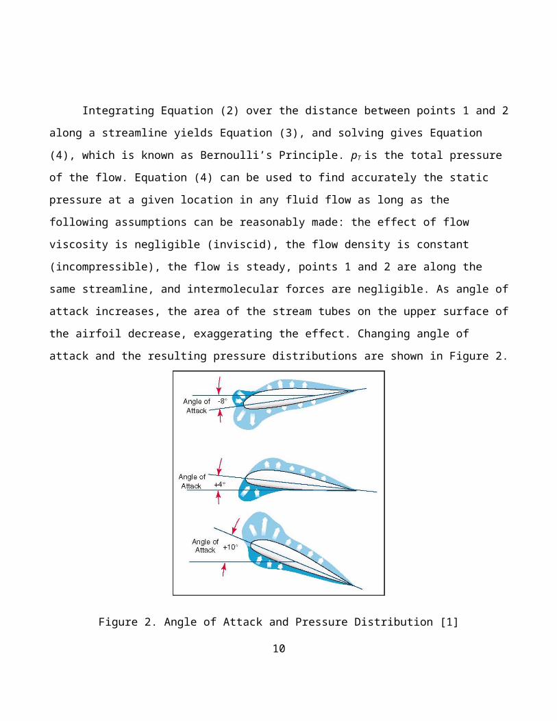
same streamline, and intermolecular forces are negligible. As angle of

attack increases, the area of the stream tubes on the upper surface of

the airfoil decrease, exaggerating the effect. Changing angle of

attack and the resulting pressure distributions are shown in Figure 2.

Figure 2. Angle of Attack and Pressure Distribution [1]

10

The pressure representations in Figure 2 connote gauge pressures,

which are in reference to the static pressure in the free stream. The

varying pressure across the airfoil will cause a pitching moment. The

point at which this moment is constant with changing angle of attack

is the aerodynamic center. The negative gauge pressure near the

leading edge of the airfoil at 10° angle of attack in Figure 2

indicates that this point will be forward of the half chord because

the sum of the pressure over the leeward half of the airfoil is

considerably weaker. For symmetric airfoils, the aerodynamic center is

exactly at the quarter chord. At 10° angle of attack, Figure 2 shows a

point near the leading edge on the upper surface of the airfoil with a

minimum pressure (highest magnitude pointed away from the airfoil).

From the leading edge to this point, the pressure is decreasing, which

is known as a favorable pressure gradient because this is the natural

direction of flow when work is not added to the system. From the point

of minimum pressure to the trailing edge, the pressure is increasing,

causing an adverse pressure gradient. The momentum of the air carries

it through this region, but the flow loses velocity over this region.

The inviscid assumption implies that the velocity, and thus the

momentum, is constant across streamlines. However, near the airfoil,

this assumption breaks down in a region known as the boundary layer.

1.1.2 Viscous Flow in the Boundary Layer

The viscosity of a fluid causes fluid particles that are directly

in contact with an object to become attached to the object. The

11

particles directly adjacent to those at the surface will be held back

by the viscous forces as the particles interact, and the speed of the

air will gradually increase with distance from the surface. This

effect perpetuates away from the object indefinitely, but viscous

effects need only be treated while the speed of the fluid is less than

99% of the speed stream far from the surface [2]. This region is

called the boundary layer. For the scale of an airfoil in a wind

tunnel, the thickness of the boundary layer ranges from approximately

1/8 in to 1/2 in.

The boundary layer can be categorized into two types: laminar and

turbulent. In a laminar boundary layer, the flow is characterized by

“smooth regular streamlines” [3]. Without obstructions, the boundary

layer at the leading edge of an airfoil will be laminar. The laminar

boundary layer will continue downstream until the viscous forces of

the flow outside the boundary layer on the slower-moving air within

the boundary layer causes the flow to tumble and become unstable. This

is the region of the turbulent boundary layer, which will have a much

higher rate of velocity increase with distance from the surface than

that of the laminar boundary layer. This rapid acceleration of the

fluid causes a greater amount of skin friction on the airfoil, but it

also allows the turbulent boundary layer to retain a greater amount of

momentum, which is critical when moving through an adverse pressure

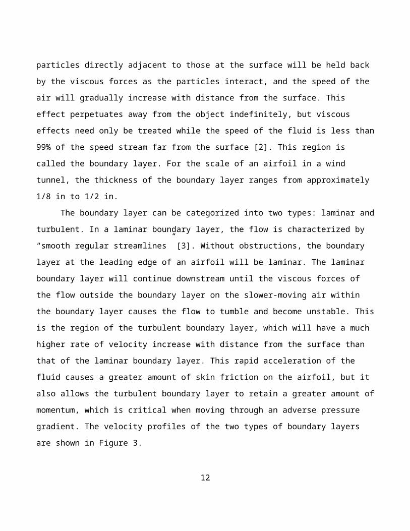
gradient. The velocity profiles of the two types of boundary layers

are shown in Figure 3.

12

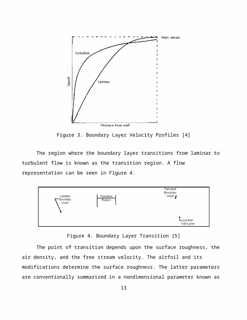
Figure 3. Boundary Layer Velocity Profiles [4]

The region where the boundary layer transitions from laminar to

turbulent flow is known as the transition region. A flow

representation can be seen in Figure 4.

Figure 4. Boundary Layer Transition [5]

The point of transition depends upon the surface roughness, the

air density, and the free stream velocity. The airfoil and its

modifications determine the surface roughness. The latter parameters

are conventionally summarized in a nondimensional parameter known as

13

the Reynolds number. Assuming constant density and viscosity

throughout the flow, Reynolds number is defined in Equation (5), where

V∞ is the free stream velocity, x is the distance from the leading

edge, and μ is the dynamic viscosity of the fluid.

ℜ≡ρV∞xμ(5)

For a smooth, flat plate like the one in Figure 3, the Reynolds

number at which transition occurs is approximately 5x105 [6]. The

geometry and surface of the airfoil influence the critical Reynolds

number at which the flow transitions. As the flow moves along the

airfoil in the adverse pressure gradient, the air velocity is

accelerating in the upwind direction as the kinetic energy of the flow

is converted into static pressure. The main stream airflow has the

momentum to overcome this adverse pressure gradient and continue in

the downstream direction. In the boundary layer, the flow has lost

energy through the viscous friction. When the adverse pressure

gradient becomes too great, the boundary layer flow will come to a

stop and reverse direction. The flow moving in the streamwise

direction is now separated from the airfoil surface, so this

phenomenon is called separation. The velocity profile of the boundary

layer through the stages of separation is shown in Figure 5.

14

Figure 5. Boundary Layer Separation [7]

As the angle of attack of the airfoil increases, the adverse

pressure gradient will become stronger. This will force the separation

to occur nearer to the leading edge. The stages of separation are

shown in Figure 6.

Figure 6. Stages of Stall Development [9]

15

At angles of attack greater than that which produces the greatest

amount of lift, the airfoil is said to be stalled. In Figure 6, this

occurs at 16° angle of attack. The increase in static pressure on the

upper surface dramatically reduces lift and increases drag.

1.1.3 Separation Control

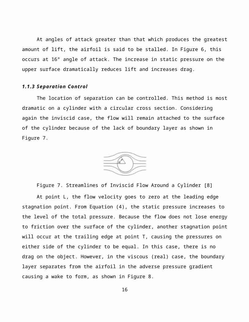
The location of separation can be controlled. This method is most

dramatic on a cylinder with a circular cross section. Considering

again the inviscid case, the flow will remain attached to the surface

of the cylinder because of the lack of boundary layer as shown in

Figure 7.

Figure 7. Streamlines of Inviscid Flow Around a Cylinder [8]

At point L, the flow velocity goes to zero at the leading edge

stagnation point. From Equation (4), the static pressure increases to

the level of the total pressure. Because the flow does not lose energy

to friction over the surface of the cylinder, another stagnation point

will occur at the trailing edge at point T, causing the pressures on

either side of the cylinder to be equal. In this case, there is no

drag on the object. However, in the viscous (real) case, the boundary

layer separates from the airfoil in the adverse pressure gradient

causing a wake to form, as shown in Figure 8.

16

L T

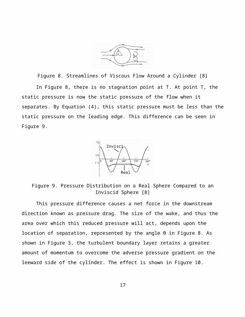
Figure 8. Streamlines of Viscous Flow Around a Cylinder [8]

In Figure 8, there is no stagnation point at T. At point T, the

static pressure is now the static pressure of the flow when it

separates. By Equation (4), this static pressure must be less than the

static pressure on the leading edge. This difference can be seen in

Figure 9.

Figure 9. Pressure Distribution on a Real Sphere Compared to anInviscid Sphere [8]

This pressure difference causes a net force in the downstream

direction known as pressure drag. The size of the wake, and thus the

area over which this reduced pressure will act, depends upon the

location of separation, represented by the angle θ in Figure 8. As

shown in Figure 3, the turbulent boundary layer retains a greater

amount of momentum to overcome the adverse pressure gradient on the

leeward side of the cylinder. The effect is shown in Figure 10.

17

L T

Inviscid

Real

Figure 10. Wake Size on Smooth and Rough Spheres [9]

In the lower image, the dimples of the golf ball forced the

boundary layer to transition to turbulent flow in a process known as

tripping the boundary layer. The result is a smaller wake and less

pressure drag. Separation on an airfoil can be delayed in exactly the

same manner as the golf ball with surface roughness or

inconsistencies. The boundary layer will transition through an

increase in Reynolds number as in Figure 5 or with surface roughness

as in Figure 10. For an airfoil, this also means that an airfoil with

a turbulent boundary layer will be able to achieve higher angles of

attack, and thus greater lift, before stall.

1.2 Purpose

The purpose of the experiment was to accurately collect a

pressure distribution on a NACA 65-012 airfoil section and determine

its effects on lift, pitching moment, and stall characteristics. These

results were to be validated via comparison with empirical data and

18

theoretical modeling using XFOIL. Additions to the airfoil were used

to determine the effects of forcing a turbulent boundary layer as

compared to a laminar boundary layer over a lifting surface. The

pressure port method was used to determine the distribution of lift

production on the airfoil. The results of high angle of attack would

be analyzed to determine the type of stall the airfoil would

experience.

1.3 Theory

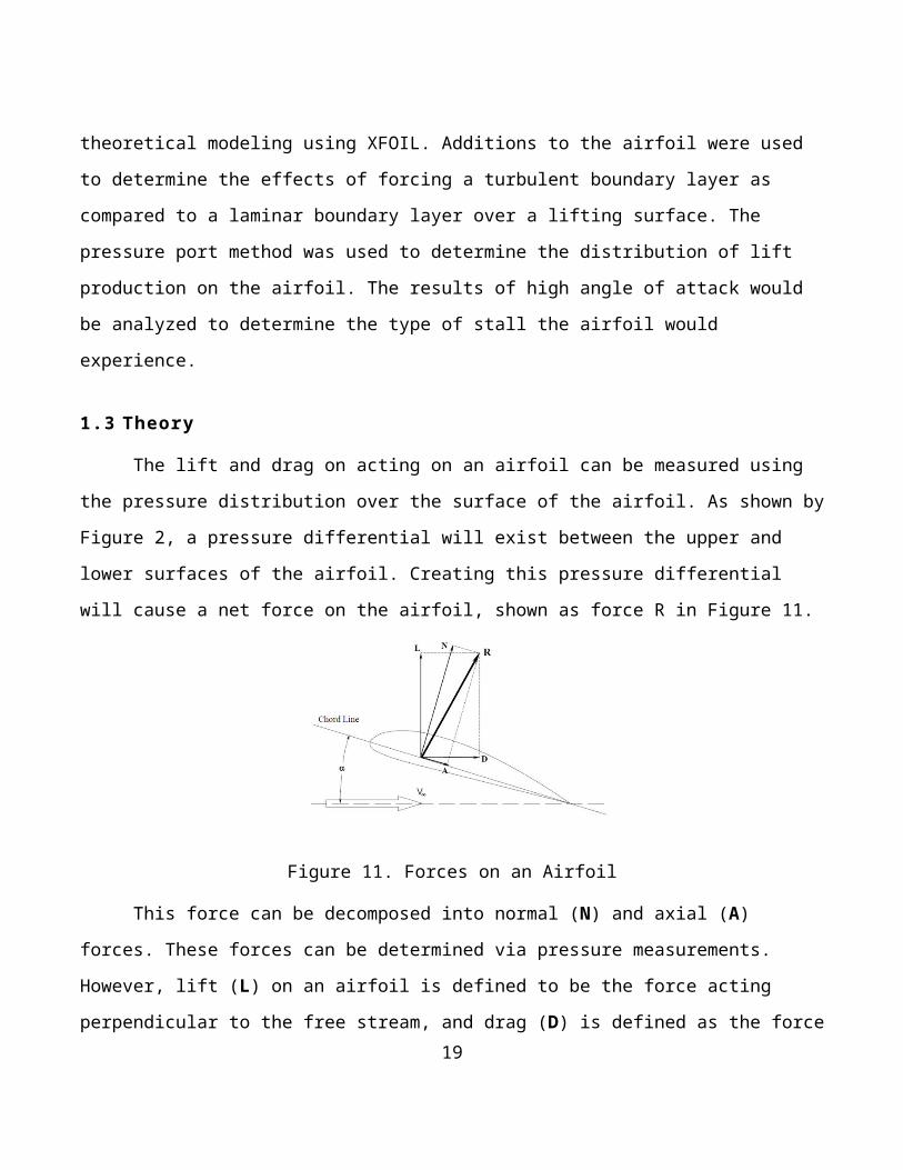
The lift and drag on acting on an airfoil can be measured using

the pressure distribution over the surface of the airfoil. As shown by

Figure 2, a pressure differential will exist between the upper and

lower surfaces of the airfoil. Creating this pressure differential

will cause a net force on the airfoil, shown as force R in Figure 11.

Figure 11. Forces on an Airfoil

This force can be decomposed into normal (N) and axial (A)

forces. These forces can be determined via pressure measurements.

However, lift (L) on an airfoil is defined to be the force acting

perpendicular to the free stream, and drag (D) is defined as the force19

acting parallel to the free stream. These forces can be related

through Equation (5).

L=Ncosα−Asinα≈Ncosα(6)

In order to nondimensionalize the terms, data reduction will use

coefficients of lift (CL), and normal force (CN). Using the definition

of CL in Equation (7) gives Equation (8) where S is the reference area

of the airfoil.

CL≡L∙q∙S

(7)

CL≈CNcosα

(8)

In order to determine the pressure distribution along the

airfoil, a coefficient of pressure (Cp) is defined in Equation (9)

where p is the local pressure, p∞ is the free stream static pressure,

and q∞ is the free stream dynamic pressure.

20

Cp≡p−p∞

q∞=p−p∞

12ρV∞

2

(9)

Local pressures can be measured using pressure ports along the

surface of the airfoil, providing a pressure distribution. In effect,

the pressure coefficients are a measure of the speed of the air over

the surface of the airfoil. More negative Cp indicates a higher local

velocity relative to the free stream. The maximum Cp will occur at the

leading edge stagnation point where the velocity goes to zero. The

pressure ports on the surface of the airfoil will are not affected by

their location within the boundary layer. Pressure remains constant in

the direction normal to the flow within the boundary layer, so the

pressure at the airfoil surface is equal to the static pressure in the

local stream. Using the assumptions in developing Equation (4),

Equation (9) can be simplified to a form that is more useful for

finding the local velocity, as shown in Equation (10).

Cp=1−V2

V∞2

(10)

The net normal force is simply the difference of the pressure

over the lower surface of the airfoil and the pressure over the upper

surface of the airfoil, which can be expressed in coefficients on the

21

upper (Cp,u) and lower (Cp,l) surfaces. Cp can be used to determine CN as

shown in Equation (11).

CN=∫0

1

(Cp,l−Cp,u )d(xc )=¿∫0

1

(Cp,l)d(xc )−∫01

(Cp,u )d(xc )¿(11)

The locations along the chord have been divided by the chord

length such that the locations are now expressed in fractions of the

total chord length. Similarly, the pitching moment about the quarter

chord can be determined by determining the difference in the products

of the pressure and respective moment arms over the lower and upper

surfaces. The relationship is expressed in Equation (12).

Cmc4

=∫0

1

(Cp,l )∙(14−xc )d(xc )−∫0

1

(Cp,u )∙(14−xc )d(xc ) (12)

This defines a nose-up pitching moment to be positive. The center

of pressure is the point about which the moment coefficient is

constant. For a symmetrical airfoil, this point is expected to be at

c/4, and the moment is expected to be nearly zero or slightly

negative. The pressure coefficients can be plotted against the

fraction of chord length to provide a visual representation of the

pressure distribution. The y-axis is inverted to clearly show the

22

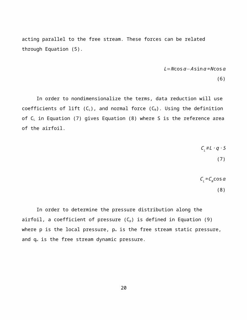
pressure coefficients upper and lower surfaces. A simple

interpretation of an expected Cp plot is shown in Figure 2.

Figure 12. Simplified Pressure Coefficient Plot

The y-axis has been inverted to represent the negative pressure

coefficients on the upper surface of the airfoil. The normal force

coefficient can be determined geometrically from Figure 2 by finding

the area of the two triangles. In this case CN = 1.5 . The increasing

value of Cp for the upper surface indicates an adverse pressure

gradient. It is expected that the minimum pressure coefficients

(suction peaks) will decrease (become more negative) as angle of

attack increases.

1.3.1 Stall Behavior

The airfoil will reach an angle of attack at which the flow over

the upper surface cannot overcome the adverse pressure gradient, and

lift will decrease. This will result in one of three stall scenarios:

23

trailing edge stall, leading edge stall, or a laminar separation

bubble. In a trailing edge stall, the flow will separate toward the

trailing initially, and the reversed flow will move toward the leading

edge as the angle of attack increases, as shown in Figure 6. This is

the most favorable mode of stall because it can provide the pilot with

feedback via buffet in the airframe as the separated flow washes over

the tail section. After trailing edge stall, the flow will reattach

with minimal hysteresis, the reduction in angle of attack required to

reestablish attached flow. This is generally seen with airfoils with a

large radius of curvature at the leading edge.

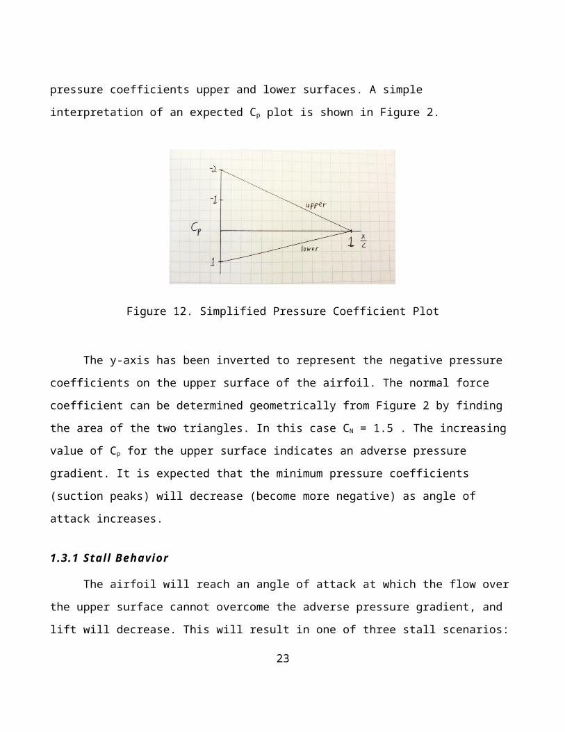
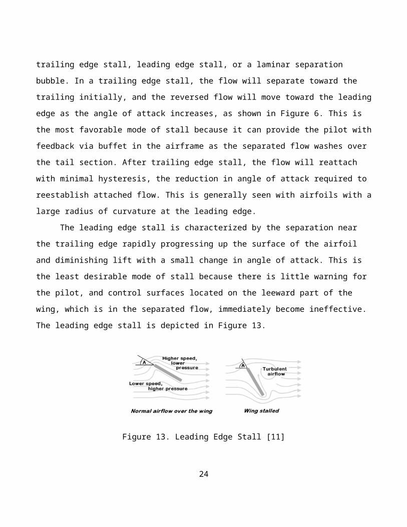
The leading edge stall is characterized by the separation near

the trailing edge rapidly progressing up the surface of the airfoil

and diminishing lift with a small change in angle of attack. This is

the least desirable mode of stall because there is little warning for

the pilot, and control surfaces located on the leeward part of the

wing, which is in the separated flow, immediately become ineffective.

The leading edge stall is depicted in Figure 13.

Figure 13. Leading Edge Stall [11]

24

Leading edge stalls are most common in airfoils with a small

leading edge radius like the flat plate in Figure 13. Airfoils known

to exhibit leading edge stalls are symmetric sections with thickness

between 9% and 15% of the chord [12]. The sharp turn at the leading

edge at high angles of attack causes a large adverse pressure

gradient, taking the majority of the boundary layer momentum to

overcome.

The laminar separation bubble is depicted in Figure 14.

Figure 14. Laminar Separation Bubble

The laminar separation bubble is a form of stall in which laminar

flow separates from the airfoil immediately aft of the peak pressure.

The flow transitions to turbulent flow outside of the bubble, and the

increased energy reattaches the flow before reaching the trailing

edge. The size of the bubble depends upon the Reynolds number of the

experiment. Longer separation bubbles will arise in low speed, low

Reynolds number flows, and higher speeds will decrease the length.

25

[13] The laminar separation bubble mode of stall will evolve into a

leading edge stall with an increase in angle of attack. This mode of

stall is undesirable because it does not offer any feedback to the

pilot, but there is a significant loss of lift. Roughness near the

leading edge of the airfoil will trip the boundary layer and force it

to transition to turbulent flow. As discussed, the turbulent flow has

more momentum to overcome the adverse pressure gradient at the leading

edge and eliminates the possibility of a laminar separation bubble.

1.3.2 XFOIL Comparison

The results are to be verified using the program XFOIL [12], a

subsonic airfoil modeling program. XFOIL bases calculations on the

vortex panel method to approximate the pressure distribution around an

airfoil. The vortex panel method is a product of potential flow theory

in which real airflows can be modeled using algebraic combinations of

mathematical representations. The theory, however, only represents

inviscid flow. Viscous effects such as separation do not appear in

potential flow solutions. XFOIL has been modified to handle limited

trailing edge separation and separation bubbles. XFOIL solutions are

calculated using a Reynolds number of 15x106. As seen above, the

Reynolds number can have a large impact on separation and stall, so

XFOIL solutions will only be used in low angle of attack cases in

which separation is not expected.

26

2 Experimental Setup and Procedure

2.1 Equipment

The experiment was conducted in the USNA Closed-Circuit Wind

Tunnel (CCWT). The CCWT is a closed circuit, single return, research-

quality wind tunnel. The test section is a vented jet, meaning that

the section is physically closed but vented to atmospheric pressure.

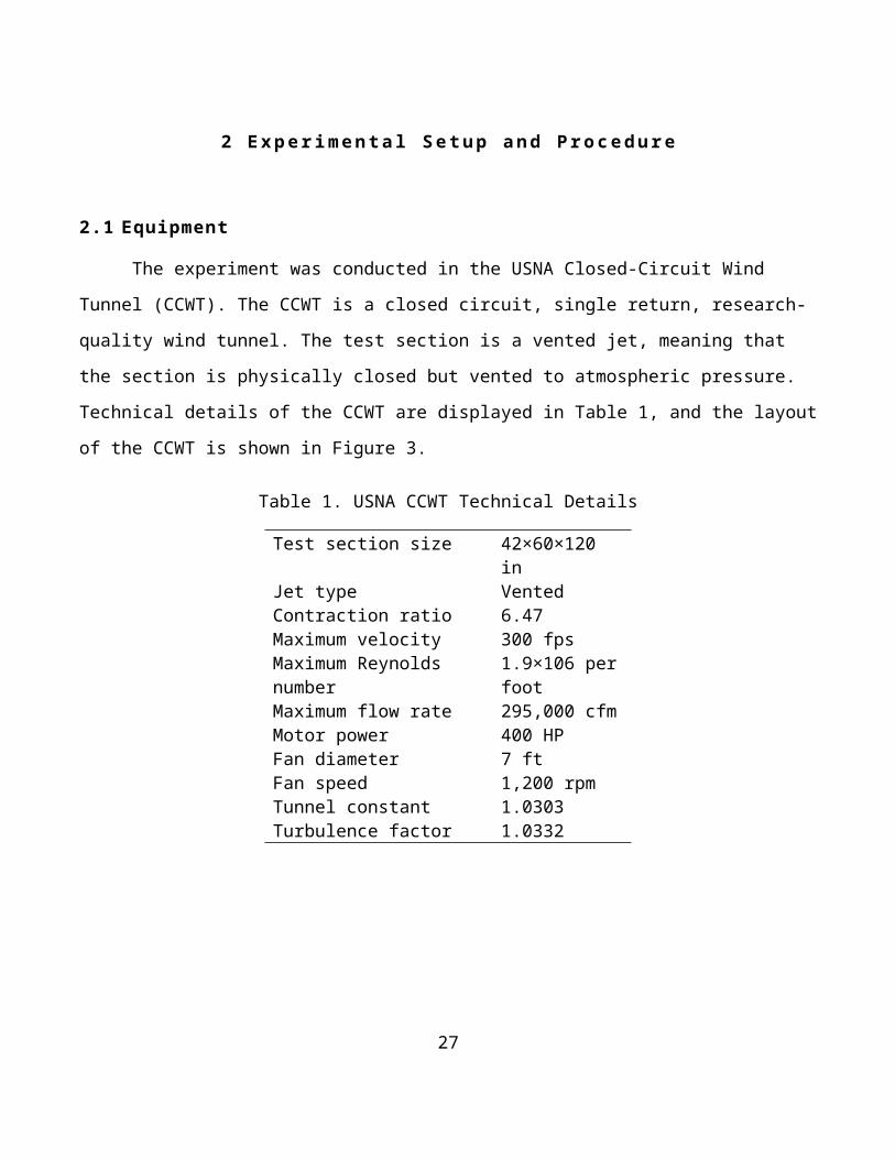
Technical details of the CCWT are displayed in Table 1, and the layout

of the CCWT is shown in Figure 3.

Table 1. USNA CCWT Technical Details

Test section size 42×60×120 in

Jet type VentedContraction ratio 6.47Maximum velocity 300 fpsMaximum Reynolds number

1.9×106 perfoot

Maximum flow rate 295,000 cfmMotor power 400 HPFan diameter 7 ftFan speed 1,200 rpmTunnel constant 1.0303Turbulence factor 1.0332

27

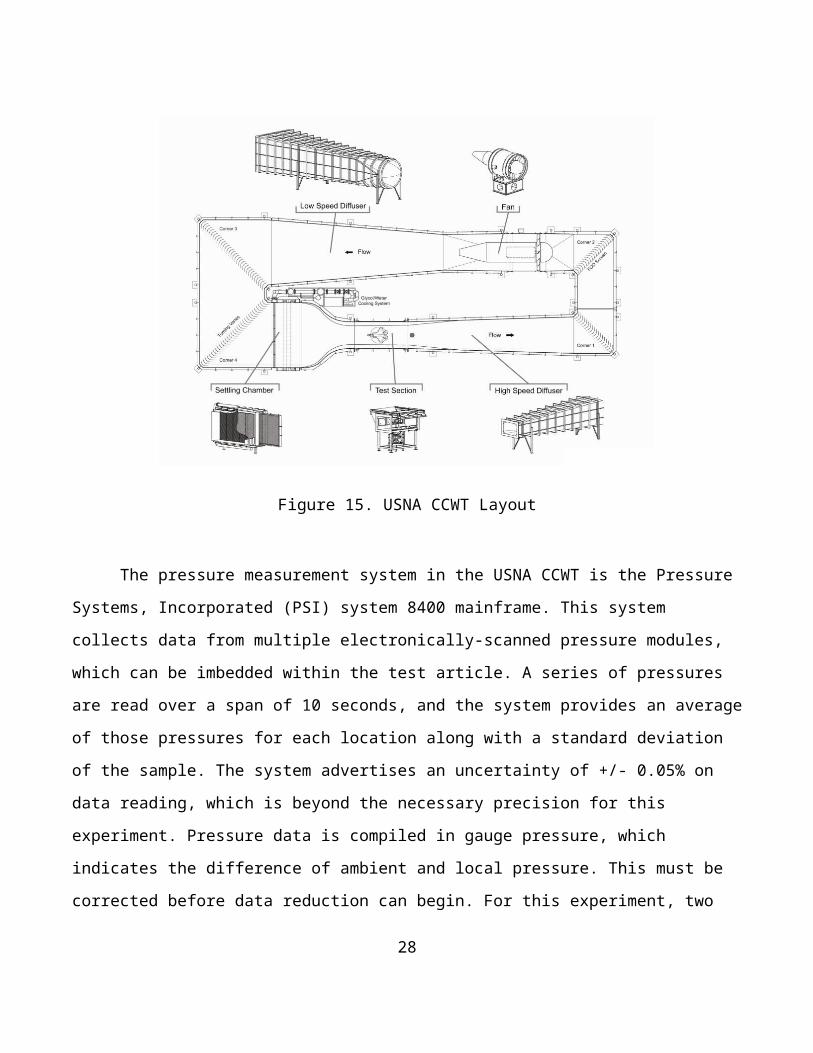
Figure 15. USNA CCWT Layout

The pressure measurement system in the USNA CCWT is the Pressure

Systems, Incorporated (PSI) system 8400 mainframe. This system

collects data from multiple electronically-scanned pressure modules,

which can be imbedded within the test article. A series of pressures

are read over a span of 10 seconds, and the system provides an average

of those pressures for each location along with a standard deviation

of the sample. The system advertises an uncertainty of +/- 0.05% on

data reading, which is beyond the necessary precision for this

experiment. Pressure data is compiled in gauge pressure, which

indicates the difference of ambient and local pressure. This must be

corrected before data reduction can begin. For this experiment, two

28

modules were used, 100 and 300, which were mounted within the airfoil

to measure pressure along the upper and lower surface, respectively.

The system 8400 mainframe and test ports are shown in Figure 16.

Figure 16. Pressure Systems, Inc. System 8400 Mainframe

2.2 Wind Tunnel Model

The airfoil used was the NACA 65-012, one of the 6-series

airfoils developed in the 1940s to reduce drag by encouraging laminar

flow over a greater portion of the wing [8]. The 65-012 is a

symmetrical airfoil with a maximum thickness of 12% of the chord

located at 40.5% chord length. The wind tunnel model has a chord of 16

in and a span of 42 in. The airfoil is fitted with 27 pressure taps on

each surface along the half span. Figure 17 shows the shape of the

airfoil and the location of the pressure ports. Corresponding pressure

port locations are presented in Table 2.

29

Figure 17. NACA 65-012 Airfoil with Pressure Ports

Table 2. Pressure Port Locations

x/cUpper

SurfaceLowerSurface

Port No. Port No.0.0000 101 3010.0020 102 3020.0040 103 3030.0060 104 3040.0080 105 3050.0100 106 3060.0150 107 3070.0200 108 3080.0300 109 3090.0400 110 3100.0600 111 3110.0800 112 3120.1000 113 3130.1500 114 3140.2000 115 3150.2500 116 3160.3000 117 3170.3500 118 3180.4000 119 3190.4500 120 320

30

0.5000 121 3210.5500 122 3220.6000 123 3230.7000 124 3240.8000 125 3250.9000 126 3260.9500 127 3271.0000 128 328p1 -patm

129 329

p2 -patm

130 330

The port’s distance from the chord line was not considered in

data reduction and has been omitted in Table 2. Ports 101 and 301 are

measuring the same location at the leading edge, and ports 128 and 328

are measuring the same location at the trailing edge. p1 denotes the

pressure at the beginning of the wind tunnel contraction, and p2 is

the static pressure at the entrance to the test section. For this

experiment, p2 was used as the free stream pressure, p∞.

2.3 Experimental Setup and Data Collection

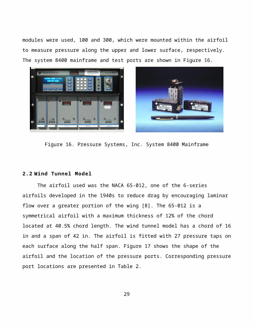
The airfoil was placed vertically in the USNA CCWT test section as shown in Figure 6.

31

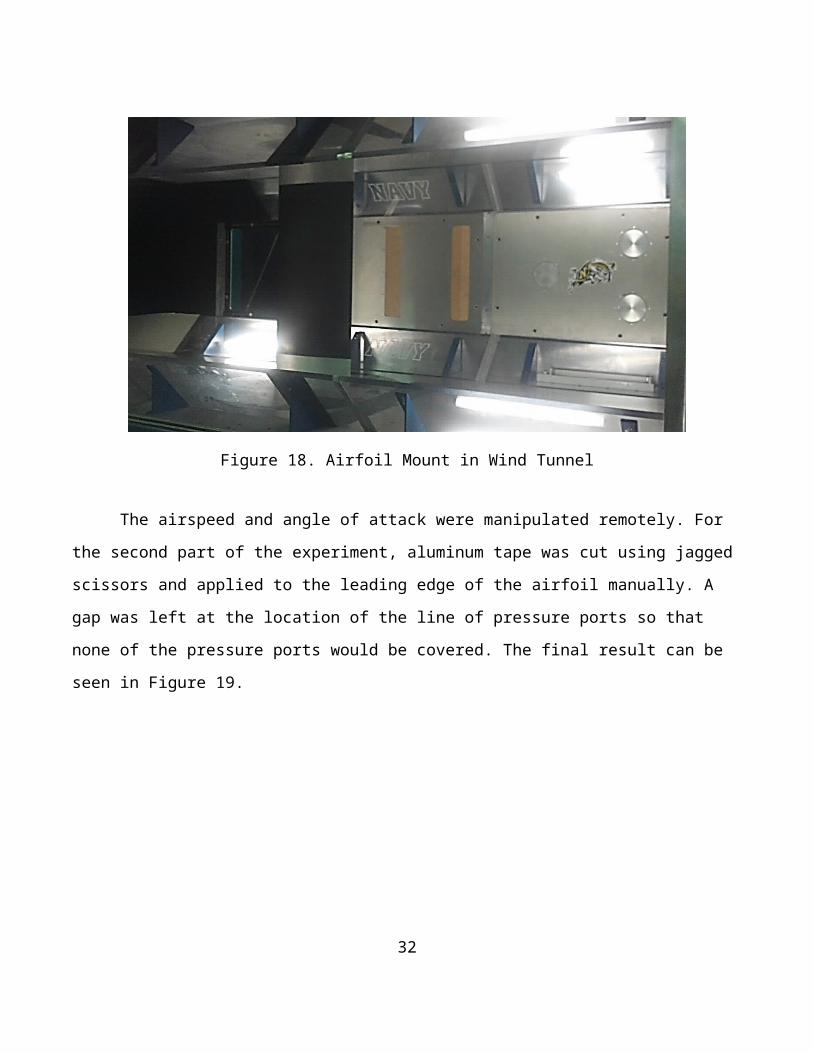
Figure 18. Airfoil Mount in Wind Tunnel

The airspeed and angle of attack were manipulated remotely. For

the second part of the experiment, aluminum tape was cut using jagged

scissors and applied to the leading edge of the airfoil manually. A

gap was left at the location of the line of pressure ports so that

none of the pressure ports would be covered. The final result can be

seen in Figure 19.

32

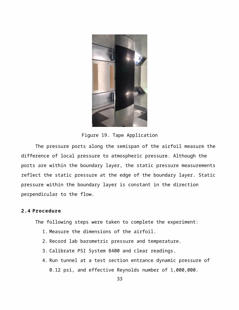
Figure 19. Tape Application

The pressure ports along the semispan of the airfoil measure the

difference of local pressure to atmospheric pressure. Although the

ports are within the boundary layer, the static pressure measurements

reflect the static pressure at the edge of the boundary layer. Static

pressure within the boundary layer is constant in the direction

perpendicular to the flow.

2.4 Procedure

The following steps were taken to complete the experiment:

1. Measure the dimensions of the airfoil.

2. Record lab barometric pressure and temperature.

3. Calibrate PSI System 8400 and clear readings.

4. Run tunnel at a test section entrance dynamic pressure of

0.12 psi, and effective Reynolds number of 1,000,000.33

5. Record pressure data at 0, 5, 8, 10, and 12 degrees angle of

attack.

6. Shut down wind tunnel.

7. Apply tape to leading edge.

8. Run tunnel at a test section entrance dynamic pressure of

0.12 psi.

9. Record pressure data at 8, 10, and 12 degrees angle of

attack.

10. Stop wind tunnel, remove tape, and secure equipment.

After the experiment was complete, the team used the program

XFOIL the simulate flow that had been tested. Because of the viscous

limitations of XFOIL, the team used results only from the 0° and 5°

angle of attack configurations. Information was also extracted from

airfoil data compiled in Theory of Wing Sections from Abbott & von

Doenhoff, which will be abbreviated as “AVD” throughout the remainder

of this report. The AVD data comes from a series of NACA experiments

conducted in the 1930s and 1940s to examine the performance of several

airfoil shapes. Data used are the averages of many tests. The

experiments referenced were run at a Reynolds number of 3x106, so

separation characteristics are expected to vary from experimental

results.

2.5 Error Analysis

The System 8400 returned a standard deviation of each data sample

collected. These raw data are displayed in Appendix A. One sigma error

34

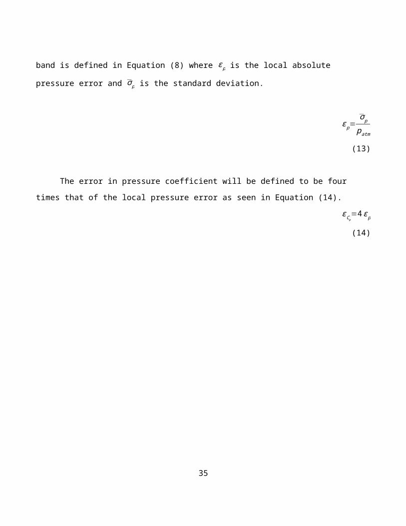
band is defined in Equation (8) where εp is the local absolute

pressure error and σp is the standard deviation.

εp=σp

patm

(13)

The error in pressure coefficient will be defined to be four

times that of the local pressure error as seen in Equation (14).

εCp=4εp

(14)

35

3 Results

The raw data extracted from the pressure ports can be found in

Appendix A. The data are grouped by angle of attack and runs with and

without the turbulence tape. These data represent the pressure

distribution over the upper and lower surfaces of the airfoil. MATLAB

was used for data reduction and plot generation. MATLAB script can be

found in Appendix E. The reference area used in calculations is the

chord length 16 in because the experiment is considered a 2-

dimensional wing. Data using XFoil to simulate the behavior of the

airfoil is presented in Appendix B. Cp1 indicates the pressure

coefficient on the upper surface and Cp2 indicates the pressure

coefficient on the lower surface.

3.1 Reference Data

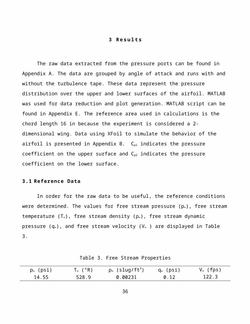
In order for the raw data to be useful, the reference conditions

were determined. The values for free stream pressure (p∞), free stream

temperature (T∞), free stream density (ρ∞), free stream dynamic

pressure (q∞), and free stream velocity (V∞ ) are displayed in Table

3.

Table 3. Free Stream Properties

p∞ (psi) T∞ (°R) ρ∞ (slug/ft3) q∞ (psi) V∞ (fps)14.55 528.9 0.00231 0.12 122.3

36

These values are necessary to determine the Reynolds number of

operation, which has been determined to be 1,000,000. The first step

to working with the data was to convert the gage pressures to absolute

local pressures (pi). The local pressures from the raw data were added

to the ambient pressure as shown in Equation (15).

pi=patm+pg=14.56+pg (15)

Data for the local absolute pressures are displayed in Appendix

C.

3.2 Pressure Coefficient

The local absolute pressures were used to determine the

coefficients of pressure at each point on the airfoil using Equation

(9). The pressure coefficients of the clean airfoil testing are

displayed in Figure 20. The pressure coefficient data is presented in

tabular form in Appendix D.

37

0 0.1 0.2 0.3 0.4 0.5 0.6 0.7 0.8 0.9 1

-6

-5

-4

-3

-2

-1

0

1

2

x/c

Cp

0 degrees

5 degrees

8 degrees

10 degrees

12 degrees

x/c = 0.25

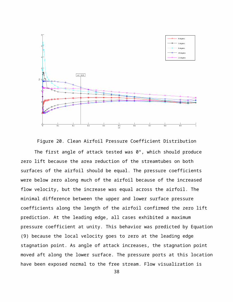
Figure 20. Clean Airfoil Pressure Coefficient Distribution

The first angle of attack tested was 0°, which should produce

zero lift because the area reduction of the streamtubes on both

surfaces of the airfoil should be equal. The pressure coefficients

were below zero along much of the airfoil because of the increased

flow velocity, but the increase was equal across the airfoil. The

minimal difference between the upper and lower surface pressure

coefficients along the length of the airfoil confirmed the zero lift

prediction. At the leading edge, all cases exhibited a maximum

pressure coefficient at unity. This behavior was predicted by Equation

(9) because the local velocity goes to zero at the leading edge

stagnation point. As angle of attack increases, the stagnation point

moved aft along the lower surface. The pressure ports at this location

have been exposed normal to the free stream. Flow visualization is 38

provided in Figures 1 & 13. The movement of the stagnation point under

the leading edge contributes a strong nose up pitching moment,

reinforcing the prediction of an aerodynamic center forward of the

half chord. The combination of the suction peak on the upper surface

of the airfoil and the location of the stagnation point on the lower

surface of the airfoil resulted in a force much larger than any

concentration further aft on the airfoil. The location about which the

forces are balanced, the aerodynamic center, was moved toward this

pressure concentration. Figure 20 shows the expected location of the

aerodynamic center at 25% of the chord. The location of the peak

suction occurs at less than 1% of the chord at 5° and 8° angle of

attack. The minimum pressure is reached at 8° angle of attack with a

pressure coefficient of -5.37. By Equation (10), the local velocity at

the point is found to be 308 fps. This local velocity is nearly three

times the free stream velocity. Aft of the point, the flow entered the

adverse pressure gradient, rapidly losing momentum and decreasing

velocity.

3.2.1 Stall Mode

The data showed decreasing minimum pressure coefficient with

increasing angle of attack up to 8°. Downstream of this initial

expansion, the airflow faced an adverse pressure gradient. The

pressure rapidly increased in the downstream direction. At 5 and 8

angle of attack, the data revealed an area of constant pressure as

39

shown in Figure 21, which initially suggested a laminar separation

bubble.

0 0.01 0.02 0.03 0.04 0.05 0.06 0.07 0.08 0.09 0.1

-6

-5

-4

-3

-2

-1

0

1

2

x/c

Pressure Coefficie

nt

5 degrees8 degrees

M ax SuctionLam inar Separation Bubble

Figure 21. Location of Max Suction and Laminar Separation Bubble

40

A separation bubble is reasonable at this location because it is

immediately aft of the peak suction point, indicated by ports 5 and 6

on the upper surface. A bubble here would trip the boundary layer to

turbulent flow and allow the boundary layer to reestablish downstream

flow at the airfoil surface. Figure 20 shows that the pressure

distribution along the aft half of the airfoil changes very little

between angles of attack at which attached flow is known to be present

at the leading edge due to the defined suction peak. This suggests

that the flow remained attached over nearly all of the upper surface.

A laminar separation bubble would be consistent with the prediction

that it will lead to leading edge stall. The suspect region spans less

than 0.5% of the chord in both cases, which is expectedly smaller than

cases in experiments of Reynolds numbers below 100,000 [13]. At 10°

angle of attack, the suction peak was significantly decreased,

indicating that the separation bubble had burst, developing into a

leading edge stall. At 12° angle of attack, the pressure variation

along the chord was minimal indicating a fully developed stall. The

laminar separation bubble, however, can only exist when the boundary

layer is initially laminar. Examination of the second part of the

experiment using the turbulence tape indicates that this pressure

anomaly is a result of the shape of the airfoil instead of flow

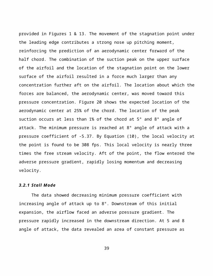
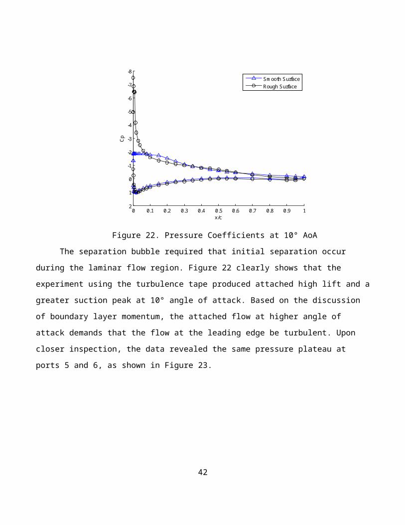
reversal. Figure 22 shows the dramatic increase in local pressure as

the flow separated near the leading edge at 10° angle of attack.

41

0 0.1 0.2 0.3 0.4 0.5 0.6 0.7 0.8 0.9 1

-8

-7

-6

-5

-4

-3

-2

-1

0

1

2

x/c

Cp

Sm ooth SurfaceRough Surface

Figure 22. Pressure Coefficients at 10° AoA

The separation bubble required that initial separation occur

during the laminar flow region. Figure 22 clearly shows that the

experiment using the turbulence tape produced attached high lift and a

greater suction peak at 10° angle of attack. Based on the discussion

of boundary layer momentum, the attached flow at higher angle of

attack demands that the flow at the leading edge be turbulent. Upon

closer inspection, the data revealed the same pressure plateau at

ports 5 and 6, as shown in Figure 23.

42

0 0.01 0.02 0.03 0.04 0.05 0.06 0.07 0.08 0.09 0.1

-8

-7

-6

-5

-4

-3

-2

-1

0

1

2

x/c

Cp

Sm ooth SurfaceRough Surface

Suspected Lam inar Separation Bubble

Attached Turbulent Flow

Lam inar Flow Separation

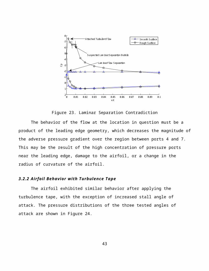
Figure 23. Laminar Separation Contradiction

The behavior of the flow at the location in question must be a

product of the leading edge geometry, which decreases the magnitude of

the adverse pressure gradient over the region between ports 4 and 7.

This may be the result of the high concentration of pressure ports

near the leading edge, damage to the airfoil, or a change in the

radius of curvature of the airfoil.

3.2.2 Airfoil Behavior with Turbulence Tape

The airfoil exhibited similar behavior after applying the

turbulence tape, with the exception of increased stall angle of

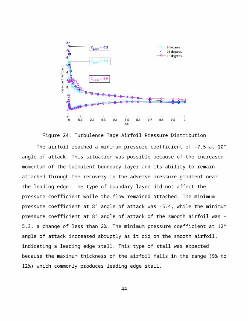
attack. The pressure distributions of the three tested angles of

attack are shown in Figure 24.

43

0 0.1 0.2 0.3 0.4 0.5 0.6 0.7 0.8 0.9 1

-8

-7

-6

-5

-4

-3

-2

-1

0

1

2

x/c

Pressure Coefficie

nt

8 degrees10 degrees12 degrees

Cp,min = -3.0

Cp,min = -5.4

Cp,min = -7.5

Figure 24. Turbulence Tape Airfoil Pressure Distribution

The airfoil reached a minimum pressure coefficient of -7.5 at 10°

angle of attack. This situation was possible because of the increased

momentum of the turbulent boundary layer and its ability to remain

attached through the recovery in the adverse pressure gradient near

the leading edge. The type of boundary layer did not affect the

pressure coefficient while the flow remained attached. The minimum

pressure coefficient at 8° angle of attack was -5.4, while the minimum

pressure coefficient at 8° angle of attack of the smooth airfoil was -

5.3, a change of less than 2%. The minimum pressure coefficient at 12°

angle of attack increased abruptly as it did on the smooth airfoil,

indicating a leading edge stall. This type of stall was expected

because the maximum thickness of the airfoil falls in the range (9% to

12%) which commonly produces leading edge stall.

44

3.2.3 Comparison of Pressure Coeffi cients to XFOIL

Figure 25. Pressure Coefficient Distribution on Clean Airfoil at 5°AoA [13]

The coefficient of pressure data generated using XFOIL is plotted

with the experimental data in Figure 24. Figure 24 shows the close

correlation of the experimental data and the data generated using

XFOIL. The data loosely resembled the simplified scheme shown in

Figure 12. The pressure coefficients reached a minimum value of -2.7

at 0.4% of the chord and a maximum value of 0.93 at 0.06% of the

chord. The pressure coefficients converged rapidly as chord length

increased. The pressure coefficient on the upper surface of the

airfoil remained above -1.0 for all locations aft of 10% of the chord.

This shows the concentration of the lifting location and the large

adverse pressure gradient near the leading edge of the airfoil. The

modeling technique used by XFOIL, the vortex panel method, makes the

45

inviscid assumption, so the XFOIL solution could not show large

separation effects. The close agreement of the experimental data along

the length of the airfoil indicates that no large separation was

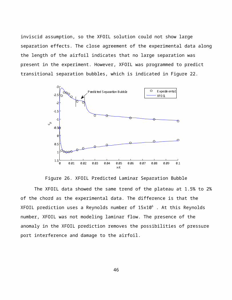
present in the experiment. However, XFOIL was programmed to predict

transitional separation bubbles, which is indicated in Figure 22.

0 0.01 0.02 0.03 0.04 0.05 0.06 0.07 0.08 0.09 0.1

-3

-2.5

-2

-1.5

-1

-0.5

0

0.5

1

1.5

x/c

c p

Experim entalXFOIL

Predicted Separation Bubble

Figure 26. XFOIL Predicted Laminar Separation Bubble

The XFOIL data showed the same trend of the plateau at 1.5% to 2%

of the chord as the experimental data. The difference is that the

XFOIL prediction uses a Reynolds number of 15x106 . At this Reynolds

number, XFOIL was not modeling laminar flow. The presence of the

anomaly in the XFOIL prediction removes the possibilities of pressure

port interference and damage to the airfoil.

46

3.2.4 Implications of Stall and Transition

The data showed that the airfoil tends to stall at the leading

edge at the given Reynolds number. This is detrimental to aircraft use

because of rapid loss of lift, loss of control surface effectiveness,

and increased pressure drag. Between 8° and 10° angle of attack, the

airfoil loses most of its lift in the clean configuration. With the

presence of the turbulence tape, the loss of lift is also abrupt, but

the flow remains attached until 12° angle of attack. This situation is

more likely to happen in practical application due to higher Reynolds

number of full scale aircraft and dirt or bug collection on the

leading edge. The smooth airfoil may have exhibited a lower friction

drag while the flow remained attached, but the smooth airfoil was not

able to sustain attached flow at increased angles of attack.

3.3 Lift Coefficient

3.3.1 Eff ects of Tripped Boundary Layer on Lift Coeffi cient

The lift coefficients for each angle of attack were calculated

using the summation in Equation (11) and the transformation in

Equation (8). The data for the experimental lift coefficients are

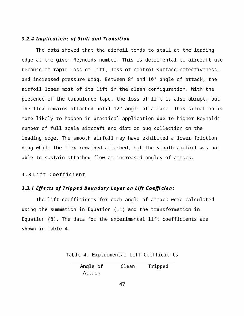
shown in Table 4.

Table 4. Experimental Lift Coefficients

Angle ofAttack

Clean Tripped

47

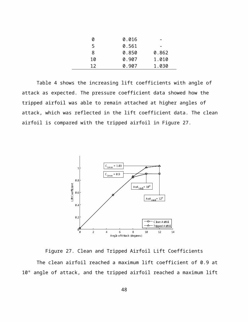
0 0.016 -5 0.561 -8 0.850 0.86210 0.907 1.01012 0.907 1.030

Table 4 shows the increasing lift coefficients with angle of

attack as expected. The pressure coefficient data showed how the

tripped airfoil was able to remain attached at higher angles of

attack, which was reflected in the lift coefficient data. The clean

airfoil is compared with the tripped airfoil in Figure 27.

0 2 4 6 8 10 12 140

0.2

0.4

0.6

0.8

1

Angle of Attack (degrees)

Lift C

oefficie

nt

Clean AirfoilTripped Airfoil

CLmax = 1.03

CLmax = 0.9

AoAstall = 10o

AoAstall = 12o

Figure 27. Clean and Tripped Airfoil Lift Coefficients

The clean airfoil reached a maximum lift coefficient of 0.9 at

10° angle of attack, and the tripped airfoil reached a maximum lift

48

coefficient of 1.03 at 12° angle of attack, a 14% increase. As the

pressure coefficient distribution showed, the turbulent boundary layer

was able to overcome the adverse pressure gradient at 10° angle of

attack, continuing to produce more lift. The tripped airfoil did not

include data from the linear region of the lift curve, but the

agreement of the lift coefficients at 8° angle of attack indicates

that the linear region was almost identical. This was expected because

the lift of attached flow is dependent on the airfoil, not the type of

boundary layer. Predictions cannot be made about the stall behavior

beyond the maximum lift coefficient because data was only taken up to

the maximum lift coefficient. With the leading edge stall indicated by

the pressure distribution, stall was expected to greatly reduce lift

over a small span of angles of attack.

3.3.2 Comparison with Empirical Data

The lift coefficients for the clean airfoil are plotted with

empirical data from AVD in Figure 28.

49

0 2 4 6 8 10 12 140

0.2

0.4

0.6

0.8

1

1.2

1.4

Angle of Attack (degrees)

Lift C

oefficie

nt

Clean AirfoilAVD

CL,AoA = 0.109

CL,AoA = 0.11

AoAstall = 10o

AoAstall = 12o

CLm ax = 1.15

CLm ax = 0.9

Figure 28. Lift Coefficients of Experimental and Empirical Data

Figure 28 shows the lift curves for the NACA 65-012 airfoil from

different sources. The experimental data and the empirical data from

AVD agree closely before the experimental data shows signs of stall.

The maximum lift coefficient of the experimental data is 0.9 at 10°

angle of attack, and the maximum lift coefficient of the empirical

data is 1.15 at 12° angle of attack. The early stall in the

experimental data was a result of the lowered Reynolds number. The

experiment was conducted at Re = 1x106, and the empirical data was

collected at Re = 3x106. As Reynolds number increases, the flow

behaves more like inviscid flow, in which separation does not occur

[7]. Thus, at a lower Reynolds number, separation is more likely given

the same adverse pressure gradient. The stall of the empirical data

shows a sharp drop indicative of a leading edge stall predicted by the

pressure coefficient distribution. The stall of the experimental data 50

developed over a larger range of angles of attack, so a quick stall is

not visible in the data. Further experimentation at higher angles of

attack is necessary to conclude this stall characteristic. In the

linear region of the lift curve, the slope is 0.109 per degree for the

experimental data and 0.11 per degree for the empirical data. These

data agree to within 1%.

3.3.3 Implications of Lift Coeffi cient Behavior

The primary conclusion of the lift coefficient data is that the

airfoil will stall at a lower angle of attack and achieve a lower

maximum lift coefficient with a laminar boundary layer. The peak

suction of the pressure distribution directly correlated with the lift

coefficient. While the flow remained attached, the lift coefficient

increased linearly. This makes prediction of performance of a given

angle of attack very reliable while inside the linear region. After

the airfoil reached stall and the peak suction decreased, the airfoil

behavior became unpredictable with the data points taken. The

experimental data was not conclusive in the type of stall experienced,

but the empirical data suggests that this type of airfoil is prone to

a leading edge stall.

3.4 Moment Coefficients

3.4.1 Moment Coeffi cient Behavior in Linear and Stalled Regions

The coefficients of the moments about the quarter chord, which

was expected to be the aerodynamic center for the symmetric airfoil, 51

were calculated using Equation (12). The reduced data are displayed in

Table 5 plotted as a function of angle of attack in Figure 29.

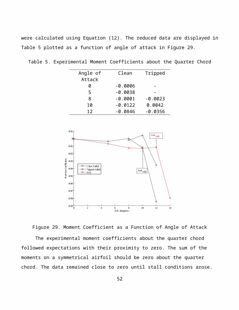
Table 5. Experimental Moment Coefficients about the Quarter Chord

Angle ofAttack

Clean Tripped

0 -0.0006 -5 -0.0038 -8 -0.0001 -0.002310 -0.0122 0.004212 -0.0846 -0.0356

0 2 4 6 8 10 12 14-0.09

-0.08

-0.07

-0.06

-0.05

-0.04

-0.03

-0.02

-0.01

0

0.01

AoA (degrees)

Mom

ent C

oefficie

nt

Clean AirfoilTripped AirfoilAVD

AoAstall

AoAstall

Figure 29. Moment Coefficient as a Function of Angle of Attack

The experimental moment coefficients about the quarter chord

followed expectations with their proximity to zero. The sum of the

moments on a symmetrical airfoil should be zero about the quarter

chord. The data remained close to zero until stall conditions arose.

52

The clean airfoil showed stall developing at 10° angle of attack, and

the tripped airfoil showed stall developing at or before 12° angle of

attack. Figure 29 shows how the rise in pressure near the leading edge

during stall conditions cause a strong negative moment about the

quarter chord. Figure 30 further illustrates the drop manifestation

of a nose-down pitching moment after reaching maximum lift

coefficient.

0 0.5 1 1.5-0.1

-0.09

-0.08

-0.07

-0.06

-0.05

-0.04

-0.03

-0.02

-0.01

0

0.01

Lift Coefficient

Mom

ent C

oefficie

nt

Clean AirfoilTripped AirfoilAVD

CLmax

CLmax

CLmax

Figure 30. Moment Coefficient as a Function of Lift Coefficient

The moment coefficient decreased to -0.0846 for the clean

airfoil. The empirical data from AVD showed the same characteristics

as the clean airfoil, decreasing to -0.08 upon reaching maximum lift

coefficient. The tripped airfoil moment coefficients began to decrease

53

at the point where stall had been identified, but minimum moment

coefficient was -0.0356, indicating that the tripped airfoil developed

the same type of stall as the clean airfoil, but at an angle of attack

not tested.

3.4.2 Implications of Moment Coeffi cient Behavior

The data confirmed the estimation of the aerodynamic center at

25% of the chord because of the moment coefficient of effectively zero

at this point while flow remained attached. In normal flight

conditions, the airfoil does not create a moment about the aerodynamic

center, and the aerodynamic center can be expected to remain at this

location. If used as a wing, aircraft loading locations should be

referenced to this point. In order to minimize moment production in

flight, high mass loads (fuel, weapons, or passengers) should be

located near the quarter chord of the wing. The airfoil experienced a

large nose-down moment after reaching its maximum lift coefficient in

the experimental and empirical cases. From a practical standpoint,

this is beneficial because an aircraft will tend to pitch nose down

when stalled. A nose down moment is required to increase airspeed and

allow for the boundary layer to reattach to the upper surface of the

wing. The horizontal tail and elevator exists to provide the nose-down

pitching moment, but the airfoil pitching moment aids in the stall

recovery. The moment arm depends upon the location of the aerodynamic

center of the horizontal stabilizer. Using a symmetric airfoil section

(as is often the case) indicates that the aerodynamic center is

54

located at the quarter chord of the stabilizer. This is where the

force the horizontal stabilizer creates will act. From a design

perspective, the moment arm of the horizontal stabilizer will

determine the necessary stabilizer size to provide the nose down

moment or vice versa.

3.5 Error Analysis

The pressure measurements were analyzed for error as described

using Equations (13) & (14). The average uncertainty in pressure and

pressure coefficient are displayed in Table 7.

Table 6. Local Pressure and Local Pressure Coefficient Uncertainties

Angle of Attack Ɛp (psi) ƐCp

0° Clean 1.4 x 10-5 5.6 x 10-6

5° Clean 2.3 x 10-5 9.1 x 10-5

8° Clean 2.0 x 10-5 8.1 x 10-5

10° Clean 1.9 x 10-4 7.6 x 10-4

12° Clean 4.0 x 10-4 1.6 x 10-3

8° Tripped 2.5 x 10-5 9.9 x 10-5

10° Tripped 4.7 x 10-5 1.9 x 10-4

12° Tripped 3.5 x 10-4 1.4 x 10-3

The highest coefficient of pressure uncertainty 1.6 x 10-3 gives

an average error of 6%. All other values can be expected to be more

accurate. Carried through, this uncertainty propagates as

approximately 6% uncertainty in lift and moment coefficient. Although

noticeable, these errors do not change the trends discussed previously

in this report.

55

56

4 Conclusions

4.1.1 Purpose

The experiment was conducted to determine the pressure

distribution on a NACA 65-012 airfoil section and the effect of

pressure distribution on lift and moment behavior. The experiment was

also to validate the method of testing in the USNA CCWT with

predictions of the XFOIL simulation and empirical data from AVD. The

pressure port method was used to determine the distribution of lift

production on the airfoil.

4.1.2 Expectations

The team expected to find that the airfoil would exhibit constant

increasing peak suction with increasing angle of attack until stall.

The stall behavior was expected to be one of three types: trailing

edge stall, leading edge stall, or a laminar separation bubble. The

boundary layer characteristics were to determine the type and location

of stall. A turbulent boundary layer would remain attached in a

greater adverse pressure gradient, thus be able to produce more lift.

The laminar boundary layer would produce less drag, but the experiment

did not measure drag. The team expected a linear increase in lift

coefficient with increasing angle of attack and zero moment about the

quarter chord with increasing angle of attack in the region of an

attached boundary layer.

57

4.1.3 Pressure Coeffi cient

The primary purpose of the experiment to determine the pressure

distribution on the airfoil was accomplished for the smooth airfoil

from 0° to 12° angle of attack and for the airfoil with a turbulence

strip at the leading edge from 8° to 12° angle of attack. Coefficient

of pressure analysis revealed the concentration of the pressure on the

airfoil at the leading edge. The minimum pressure coefficient achieved

was -7.56 at 10° angle of attack while tripping the flow. This

indicates that the flow had been accelerated to approximately three

times the free stream velocity at peak suction. As the flow slowed to

free stream velocity, the pressure increased, causing an adverse

pressure gradient. For the clean airfoil, the minimum pressure

coefficient was -5.37 at 8° angle of attack. At the given Reynolds

number, a laminar boundary layer could not overcome the adverse

pressure gradient created at angles of attack greater than 10°. The

pressure coefficient trend near the leading edge showed an ambiguous

anomaly of constant pressure in the recovery region aft of the peak

suction. This initially suggested a laminar separation bubble, but the

presence of the same plateau between pressure ports 4 and 6 on the

upper surface of the airfoil in the presence of a turbulent leading

edge boundary layer and in the high Reynolds number XFOIL prediction

indicate that the anomaly was a product of the leading edge shape. The

team concluded that the airfoil experienced leading edge stall because

pressure at the leading edge on the upper surface increased in a very

58

short distance, and the pressure distribution over the aft section of

the airfoil remained similar with changing angle of attack.

4.1.4 Lift Coeffi cient

The purpose of the experiment to determine the effect of pressure

distribution on lift production was accomplished, and the lift

coefficient was determined to be directly related to the peak suction.

The point at which the suction region collapses indicated the region

in which maximum lift had been achieved. The experimental data was not

conclusive in determining the stall behavior, but the agreement of the

empirical data from AVD and pressure coefficient conclusions indicated

that the airfoil experienced a leading edge stall.

The primary conclusion of the lift coefficient data is that the

airfoil stalled at a lower angle of attack and achieved a lower

maximum lift coefficient with a laminar boundary layer. The peak

suction of the pressure distribution directly correlated with the lift

coefficient. While the flow remained attached, the lift coefficient

increased linearly. This makes prediction of performance of a given

angle of attack very reliable while inside the linear region. After

the airfoil reached stall, and the peak suction decreased, the airfoil

behavior became unpredictable with the data points taken. The

experimental data was not conclusive in the type of stall experienced,

but the empirical data suggests that this type of airfoil is prone to

a leading edge stall. The maximum lift coefficient achieved was 1.03,

corresponding with the minimum pressure coefficient at 10° angle of

59

attack using the tripped airfoil. The maximum lift coefficient

achieved using the clean airfoil was 0.9, a 10% decrease in available

lift coefficient at the given Reynolds number. The experiment was not

taken to an angle of attack which would have revealed the stall

characteristics, but data from AVD show a sharp decrease in lift

coefficient after reaching maximum lift coefficient, which supports

the conclusion that the airfoil experienced a leading edge stall.

4.1.5 Moment Coeffi cient

The dramatic decrease in pressure at the leading edge with little

variation in pressure coefficient distribution after of the

aerodynamic center indicated that the airfoil experienced leading edge

stall without a laminar separation bubble at the examined angles of

attack. The pitching moment coefficient about the quarter chord

remained within +/- 0.005 of the expected zero value while the

boundary layer was attached across the airfoil, indicating that the

aerodynamic center remained at the quarter chord as expected for a

symmetrical airfoil. Experimental and empirical data revealed a large

nose-down pitching moment after reaching maximum lift coefficient. The

clean airfoil and the AVD data showed a pitching moment coefficient on

the order of -0.08. In practice, this pitching moment will help regain

attached flow and suitable flight conditions.

60

4.1.6 Implications

The NACA 65-012 airfoil was designed to maintain a laminar

boundary layer over the length of the airfoil for relatively high

Reynolds numbers. The experimental method was validated by the

favorable comparison with empirical data and modeling predictions. The

experiment validated the claim of a laminar boundary layer throughout

the range of angles of attack. The laminar boundary layer limited the

maximum lift coefficient and stall angle of attack. The pitching

moment data revealed a tendency to pitch nose-down after establishing

stall conditions, but the laminar boundary layer also caused

undesirable stall characteristics that do not give physical feedback

to the pilot before the stall break. The team recommends the airfoil

for its design use at low angles of attack to achieve low drag flight.

Use at high angles of attack will invoke an undesirably sharp stall

break.

61

References

[1]M. Belisle, " Potential-flow streamlines around a NACA 0012 airfoil at 11° angle of attack, with upper and lower streamtubes identified. Computed using the Wolfram Demonstrations Project CodePotential Flow over a NACA Four-Digit Airfoil by Richard L. Fearn," 2008.

[2]"Chapter 2: Principles of Flight," American Flyers, [Online]. Available: http://www.americanflyers.net/aviationlibrary/pilots_handbook/chapter_2.htm. [Accessed 16 October 2012].

[3]J. A. Schetz, Boundary Layer Analysis, Englewood Cliffs, NJ: Prentice-Hall, 1993.

[4]C. E. Lole and J. E. Lewis, Flight Theory and Aerodynamics, 2nd Ed., New York: John Wiley & Sons, 2000.

[5]E. L. Houghton and N. B. Carruthers, Wind Forces on Buildings and Structures: An Introduction, New York: Wiley, 1976.

[6]"Airplane aerodynamics: fundamentals and flight principles.," FreeOnline Private Pilot Ground School, 2006. [Online]. Available: http://www.free-online-private-pilot-ground-school.com/aerodynamics.html. [Accessed 17 October 2012].

[7]D. P. De Witt, Fundamentals of Heat and Mass Transfer, New York: Wiley, 1990.

[8]J. D. Anderson, Introduction to Flight, New York: McGraw-Hill, 2008.

[9]NASA, "Aeronautics: Tutorial," [Online]. Available: http://quest.arc.nasa.gov/aero/virtual/demo/aeronautics/tutorial/wings.html. [Accessed 21 October 2012].

[10]

J. Scott, "Golf Ball Dimples & Drag," 13 February 2005. [Online]. Available: http://www.aerospaceweb.org/question/aerodynamics/q0215.shtml. [Accessed 21 October 2012].

[11]

J. Hearfield, "Windmill sails - an engineer's thoughts," 2007. [Online]. Available:

62

http://www.johnhearfield.com/Wind/Windmills.htm. [Accessed 21 October 2012].

[12]

G. B. McCullough and D. E. Gault, "Examples of Three RepresetativeTypes of Airfoil-Section Stalls at Low Speed," National Advisory Committee for Aeronautics, Moffet Field, CA, 1951.

[13]

M. Jahanmiri, "Laminar Separation Bubble: Its Structure, Dynamics and Control," CHALMERS UNIVERSITY OF TECHNOLOGY, Göteborg, Sweden,2011.

[14]

M. Drela, XFOIL Subsonic Airfoil Development, Cambridge, MA, 2007.

[15]

I. H. Abbot and A. E. von Doenhoff, Theory of Wing Sections, Toronto: General Publishing Company, 1959.

[16]

T. CHKLOVSKI, "POINTED-TIP WINGS AT LOW REYNOLDS NUMBERS," [Online]. Available: http://www.wfis.uni.lodz.pl/edu/Proposal.htm#_Toc110650472. [Accessed 17 October 2012].

63

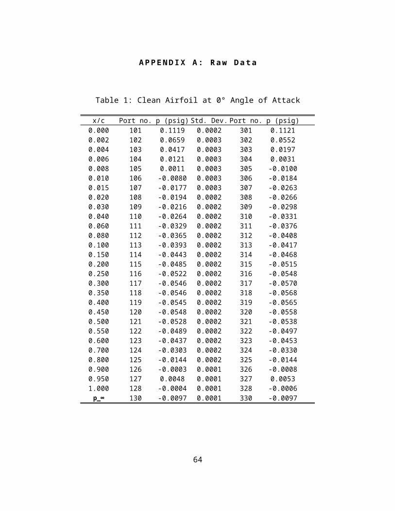
APPENDIX A: Raw Data

Table 1: Clean Airfoil at 0° Angle of Attack

x/c Port no. p (psig) Std. Dev. Port no. p (psig)0.000 101 0.1119 0.0002 301 0.11210.002 102 0.0659 0.0003 302 0.05520.004 103 0.0417 0.0003 303 0.01970.006 104 0.0121 0.0003 304 0.00310.008 105 0.0011 0.0003 305 -0.01000.010 106 -0.0080 0.0003 306 -0.01840.015 107 -0.0177 0.0003 307 -0.02630.020 108 -0.0194 0.0002 308 -0.02660.030 109 -0.0216 0.0002 309 -0.02980.040 110 -0.0264 0.0002 310 -0.03310.060 111 -0.0329 0.0002 311 -0.03760.080 112 -0.0365 0.0002 312 -0.04080.100 113 -0.0393 0.0002 313 -0.04170.150 114 -0.0443 0.0002 314 -0.04680.200 115 -0.0485 0.0002 315 -0.05150.250 116 -0.0522 0.0002 316 -0.05480.300 117 -0.0546 0.0002 317 -0.05700.350 118 -0.0546 0.0002 318 -0.05680.400 119 -0.0545 0.0002 319 -0.05650.450 120 -0.0548 0.0002 320 -0.05580.500 121 -0.0528 0.0002 321 -0.05380.550 122 -0.0489 0.0002 322 -0.04970.600 123 -0.0437 0.0002 323 -0.04530.700 124 -0.0303 0.0002 324 -0.03300.800 125 -0.0144 0.0002 325 -0.01440.900 126 -0.0003 0.0001 326 -0.00080.950 127 0.0048 0.0001 327 0.00531.000 128 -0.0004 0.0001 328 -0.0006

130 -0.0097 0.0001 330 -0.0097p_∞

64

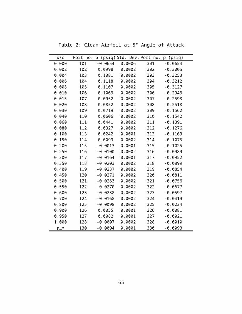
Table 2: Clean Airfoil at 5° Angle of Attack

x/c Port no. p (psig) Std. Dev. Port no. p (psig)0.000 101 -0.0654 0.0006 301 -0.06540.002 102 0.0998 0.0002 302 -0.30050.004 103 0.1081 0.0002 303 -0.32530.006 104 0.1118 0.0002 304 -0.32120.008 105 0.1107 0.0002 305 -0.31270.010 106 0.1063 0.0002 306 -0.29430.015 107 0.0952 0.0002 307 -0.25930.020 108 0.0852 0.0002 308 -0.25180.030 109 0.0719 0.0002 309 -0.15620.040 110 0.0606 0.0002 310 -0.15420.060 111 0.0441 0.0002 311 -0.13910.080 112 0.0327 0.0002 312 -0.12760.100 113 0.0242 0.0001 313 -0.11630.150 114 0.0099 0.0002 314 -0.10750.200 115 -0.0013 0.0001 315 -0.10250.250 116 -0.0100 0.0002 316 -0.09890.300 117 -0.0164 0.0001 317 -0.09520.350 118 -0.0203 0.0002 318 -0.08990.400 119 -0.0237 0.0002 319 -0.08540.450 120 -0.0271 0.0002 320 -0.08110.500 121 -0.0283 0.0002 321 -0.07560.550 122 -0.0270 0.0002 322 -0.06770.600 123 -0.0238 0.0002 323 -0.05970.700 124 -0.0168 0.0002 324 -0.04190.800 125 -0.0098 0.0002 325 -0.02340.900 126 0.0055 0.0001 326 -0.00810.950 127 0.0082 0.0001 327 -0.00211.000 128 -0.0007 0.0002 328 -0.0010

130 -0.0094 0.0001 330 -0.0093p_∞

65

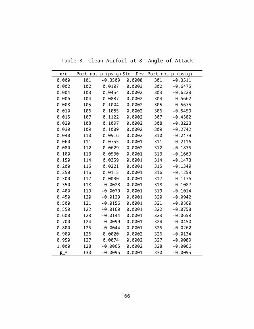
Table 3: Clean Airfoil at 8° Angle of Attack

x/c Port no. p (psig) Std. Dev. Port no. p (psig)0.000 101 -0.3509 0.0008 301 -0.35110.002 102 0.0107 0.0003 302 -0.64750.004 103 0.0454 0.0002 303 -0.62280.006 104 0.0887 0.0002 304 -0.56620.008 105 0.1004 0.0002 305 -0.56750.010 106 0.1085 0.0002 306 -0.54590.015 107 0.1122 0.0002 307 -0.45820.020 108 0.1097 0.0002 308 -0.32230.030 109 0.1009 0.0002 309 -0.27420.040 110 0.0916 0.0002 310 -0.24790.060 111 0.0755 0.0001 311 -0.21160.080 112 0.0629 0.0002 312 -0.18750.100 113 0.0530 0.0001 313 -0.16690.150 114 0.0359 0.0001 314 -0.14730.200 115 0.0221 0.0001 315 -0.13490.250 116 0.0115 0.0001 316 -0.12580.300 117 0.0030 0.0001 317 -0.11760.350 118 -0.0028 0.0001 318 -0.10870.400 119 -0.0079 0.0001 319 -0.10140.450 120 -0.0129 0.0001 320 -0.09420.500 121 -0.0156 0.0001 321 -0.08600.550 122 -0.0160 0.0001 322 -0.07580.600 123 -0.0144 0.0001 323 -0.06580.700 124 -0.0099 0.0001 324 -0.04500.800 125 -0.0044 0.0001 325 -0.02620.900 126 0.0020 0.0002 326 -0.01340.950 127 0.0074 0.0002 327 -0.00891.000 128 -0.0065 0.0002 328 -0.0066

130 -0.0095 0.0001 330 -0.0095p_∞

66

Table 4: Clean Airfoil at 10° Angle of Attack

x/c Port no. p (psig) Std. Dev. Port no. p (psig)0.000 101 -0.1685 0.0065 301 -0.16860.002 102 0.0516 0.0021 302 -0.23320.004 103 0.0741 0.0015 303 -0.22660.006 104 0.1017 0.0007 304 -0.22530.008 105 0.1088 0.0005 305 -0.22820.010 106 0.1131 0.0003 306 -0.22730.015 107 0.1140 0.0003 307 -0.22820.020 108 0.1104 0.0004 308 -0.22850.030 109 0.1017 0.0004 309 -0.22770.040 110 0.0930 0.0005 310 -0.22690.060 111 0.0779 0.0005 311 -0.22730.080 112 0.0659 0.0005 312 -0.22770.100 113 0.0564 0.0004 313 -0.22070.150 114 0.0397 0.0004 314 -0.21320.200 115 0.0258 0.0004 315 -0.18990.250 116 0.0148 0.0004 316 -0.16260.300 117 0.0059 0.0004 317 -0.13720.350 118 -0.0004 0.0003 318 -0.11600.400 119 -0.0062 0.0003 319 -0.10010.450 120 -0.0119 0.0003 320 -0.08710.500 121 -0.0153 0.0003 321 -0.07710.550 122 -0.0165 0.0003 322 -0.06820.600 123 -0.0156 0.0004 323 -0.06120.700 124 -0.0127 0.0004 324 -0.04890.800 125 -0.0085 0.0004 325 -0.03860.900 126 -0.0039 0.0004 326 -0.03040.950 127 -0.0045 0.0005 327 -0.02651.000 128 -0.0233 0.0011 328 -0.0237

130 -0.0069 0.0001 330 -0.0069p_∞

67

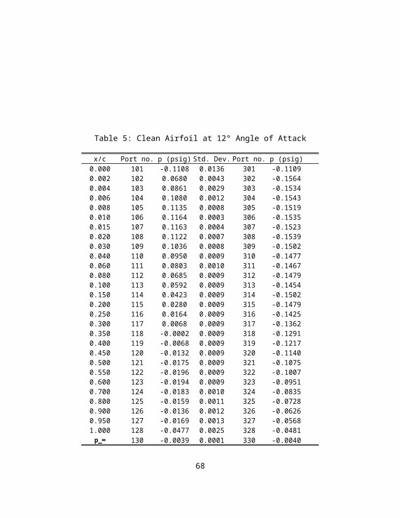
Table 5: Clean Airfoil at 12° Angle of Attack

x/c Port no. p (psig) Std. Dev. Port no. p (psig)0.000 101 -0.1108 0.0136 301 -0.11090.002 102 0.0680 0.0043 302 -0.15640.004 103 0.0861 0.0029 303 -0.15340.006 104 0.1080 0.0012 304 -0.15430.008 105 0.1135 0.0008 305 -0.15190.010 106 0.1164 0.0003 306 -0.15350.015 107 0.1163 0.0004 307 -0.15230.020 108 0.1122 0.0007 308 -0.15390.030 109 0.1036 0.0008 309 -0.15020.040 110 0.0950 0.0009 310 -0.14770.060 111 0.0803 0.0010 311 -0.14670.080 112 0.0685 0.0009 312 -0.14790.100 113 0.0592 0.0009 313 -0.14540.150 114 0.0423 0.0009 314 -0.15020.200 115 0.0280 0.0009 315 -0.14790.250 116 0.0164 0.0009 316 -0.14250.300 117 0.0068 0.0009 317 -0.13620.350 118 -0.0002 0.0009 318 -0.12910.400 119 -0.0068 0.0009 319 -0.12170.450 120 -0.0132 0.0009 320 -0.11400.500 121 -0.0175 0.0009 321 -0.10750.550 122 -0.0196 0.0009 322 -0.10070.600 123 -0.0194 0.0009 323 -0.09510.700 124 -0.0183 0.0010 324 -0.08350.800 125 -0.0159 0.0011 325 -0.07280.900 126 -0.0136 0.0012 326 -0.06260.950 127 -0.0169 0.0013 327 -0.05681.000 128 -0.0477 0.0025 328 -0.0481

130 -0.0039 0.0001 330 -0.0040p_∞

68

Table 6: Tripped Airfoil at 8° Angle of Attack

69

x/c Port no. p (psig) Std. Dev. Port no.0.000 101 -0.3680 0.0010 3010.002 102 0.0036 0.0003 3020.004 103 0.0400 0.0002 3030.006 104 0.0858 0.0002 3040.008 105 0.0982 0.0002 3050.010 106 0.1069 0.0002 3060.015 107 0.1115 0.0002 3070.020 108 0.1094 0.0002 3080.030 109 0.1009 0.0002 3090.040 110 0.0919 0.0002 3100.060 111 0.0760 0.0002 3110.080 112 0.0634 0.0002 3120.100 113 0.0536 0.0002 3130.150 114 0.0365 0.0001 3140.200 115 0.0228 0.0001 3150.250 116 0.0122 0.0001 3160.300 117 0.0037 0.0001 3170.350 118 -0.0019 0.0002 3180.400 119 -0.0072 0.0001 3190.450 120 -0.0121 0.0001 3200.500 121 -0.0147 0.0001 3210.550 122 -0.0151 0.0002 3220.600 123 -0.0135 0.0001 3230.700 124 -0.0090 0.0001 3240.800 125 -0.0035 0.0001 3250.900 126 0.0032 0.0001 3260.950 127 0.0088 0.0002 3271.000 128 -0.0044 0.0001 328

130 -0.0095 0.0001 330p_∞

70

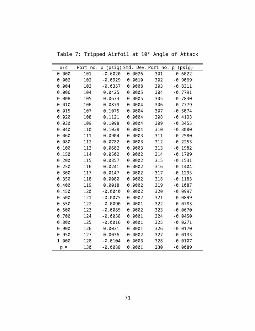
Table 7: Tripped Airfoil at 10° Angle of Attack

x/c Port no. p (psig) Std. Dev. Port no. p (psig)0.000 101 -0.6020 0.0026 301 -0.60220.002 102 -0.0929 0.0010 302 -0.90690.004 103 -0.0357 0.0008 303 -0.83110.006 104 0.0425 0.0005 304 -0.77910.008 105 0.0673 0.0005 305 -0.78300.010 106 0.0879 0.0004 306 -0.77790.015 107 0.1075 0.0004 307 -0.50740.020 108 0.1121 0.0004 308 -0.41930.030 109 0.1098 0.0004 309 -0.34550.040 110 0.1038 0.0004 310 -0.30800.060 111 0.0904 0.0003 311 -0.25800.080 112 0.0782 0.0003 312 -0.22530.100 113 0.0682 0.0003 313 -0.19820.150 114 0.0502 0.0002 314 -0.17090.200 115 0.0357 0.0002 315 -0.15310.250 116 0.0241 0.0002 316 -0.14040.300 117 0.0147 0.0002 317 -0.12930.350 118 0.0080 0.0002 318 -0.11830.400 119 0.0018 0.0002 319 -0.10870.450 120 -0.0040 0.0002 320 -0.09970.500 121 -0.0075 0.0002 321 -0.08990.550 122 -0.0090 0.0001 322 -0.07830.600 123 -0.0085 0.0002 323 -0.06700.700 124 -0.0058 0.0001 324 -0.04500.800 125 -0.0016 0.0001 325 -0.02710.900 126 0.0031 0.0001 326 -0.01700.950 127 0.0036 0.0002 327 -0.01331.000 128 -0.0104 0.0003 328 -0.0107

130 -0.0088 0.0001 330 -0.0089p_∞

71

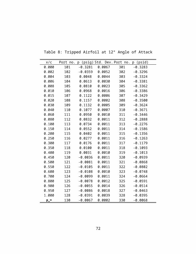
Table 8: Tripped Airfoil at 12° Angle of Attack

x/c Port no. p (psig) Std. Dev. Port no. p (psid)0.000 101 -0.3281 0.0067 301 -0.32830.002 102 -0.0359 0.0052 302 -0.32960.004 103 0.0048 0.0044 303 -0.33240.006 104 0.0613 0.0030 304 -0.33810.008 105 0.0810 0.0023 305 -0.33620.010 106 0.0968 0.0016 306 -0.33860.015 107 0.1122 0.0006 307 -0.34290.020 108 0.1157 0.0002 308 -0.35000.030 109 0.1132 0.0005 309 -0.36240.040 110 0.1077 0.0007 310 -0.36710.060 111 0.0950 0.0010 311 -0.34460.080 112 0.0832 0.0011 312 -0.28880.100 113 0.0734 0.0011 313 -0.22760.150 114 0.0552 0.0011 314 -0.15860.200 115 0.0402 0.0011 315 -0.13560.250 116 0.0277 0.0011 316 -0.12630.300 117 0.0176 0.0011 317 -0.11790.350 118 0.0100 0.0011 318 -0.10930.400 119 0.0031 0.0010 319 -0.10130.450 120 -0.0036 0.0011 320 -0.09390.500 121 -0.0081 0.0011 321 -0.08680.550 122 -0.0105 0.0011 322 -0.08020.600 123 -0.0108 0.0010 323 -0.07480.700 124 -0.0099 0.0011 324 -0.06640.800 125 -0.0078 0.0012 325 -0.05910.900 126 -0.0055 0.0014 326 -0.05140.950 127 -0.0086 0.0018 327 -0.04631.000 128 -0.0391 0.0039 328 -0.0395

130 -0.0067 0.0002 330 -0.0068p_∞

72

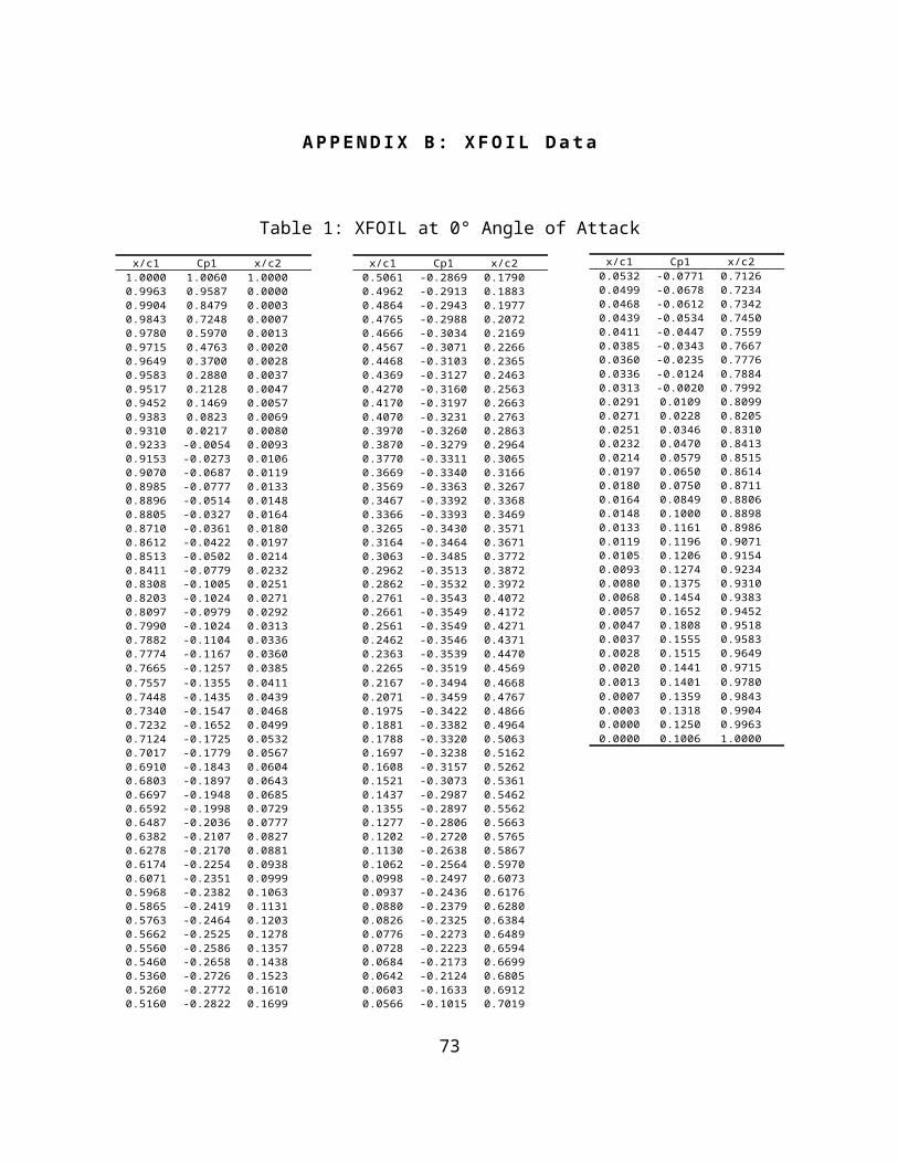
APPENDIX B: XFOIL Data

Table 1: XFOIL at 0° Angle of Attackx/c1 Cp1 x/c2

1.0000 1.0060 1.00000.9963 0.9587 0.00000.9904 0.8479 0.00030.9843 0.7248 0.00070.9780 0.5970 0.00130.9715 0.4763 0.00200.9649 0.3700 0.00280.9583 0.2880 0.00370.9517 0.2128 0.00470.9452 0.1469 0.00570.9383 0.0823 0.00690.9310 0.0217 0.00800.9233 -0.0054 0.00930.9153 -0.0273 0.01060.9070 -0.0687 0.01190.8985 -0.0777 0.01330.8896 -0.0514 0.01480.8805 -0.0327 0.01640.8710 -0.0361 0.01800.8612 -0.0422 0.01970.8513 -0.0502 0.02140.8411 -0.0779 0.02320.8308 -0.1005 0.02510.8203 -0.1024 0.02710.8097 -0.0979 0.02920.7990 -0.1024 0.03130.7882 -0.1104 0.03360.7774 -0.1167 0.03600.7665 -0.1257 0.03850.7557 -0.1355 0.04110.7448 -0.1435 0.04390.7340 -0.1547 0.04680.7232 -0.1652 0.04990.7124 -0.1725 0.05320.7017 -0.1779 0.05670.6910 -0.1843 0.06040.6803 -0.1897 0.06430.6697 -0.1948 0.06850.6592 -0.1998 0.07290.6487 -0.2036 0.07770.6382 -0.2107 0.08270.6278 -0.2170 0.08810.6174 -0.2254 0.09380.6071 -0.2351 0.09990.5968 -0.2382 0.10630.5865 -0.2419 0.11310.5763 -0.2464 0.12030.5662 -0.2525 0.12780.5560 -0.2586 0.13570.5460 -0.2658 0.14380.5360 -0.2726 0.15230.5260 -0.2772 0.16100.5160 -0.2822 0.1699

x/c1 Cp1 x/c20.5061 -0.2869 0.17900.4962 -0.2913 0.18830.4864 -0.2943 0.19770.4765 -0.2988 0.20720.4666 -0.3034 0.21690.4567 -0.3071 0.22660.4468 -0.3103 0.23650.4369 -0.3127 0.24630.4270 -0.3160 0.25630.4170 -0.3197 0.26630.4070 -0.3231 0.27630.3970 -0.3260 0.28630.3870 -0.3279 0.29640.3770 -0.3311 0.30650.3669 -0.3340 0.31660.3569 -0.3363 0.32670.3467 -0.3392 0.33680.3366 -0.3393 0.34690.3265 -0.3430 0.35710.3164 -0.3464 0.36710.3063 -0.3485 0.37720.2962 -0.3513 0.38720.2862 -0.3532 0.39720.2761 -0.3543 0.40720.2661 -0.3549 0.41720.2561 -0.3549 0.42710.2462 -0.3546 0.43710.2363 -0.3539 0.44700.2265 -0.3519 0.45690.2167 -0.3494 0.46680.2071 -0.3459 0.47670.1975 -0.3422 0.48660.1881 -0.3382 0.49640.1788 -0.3320 0.50630.1697 -0.3238 0.51620.1608 -0.3157 0.52620.1521 -0.3073 0.53610.1437 -0.2987 0.54620.1355 -0.2897 0.55620.1277 -0.2806 0.56630.1202 -0.2720 0.57650.1130 -0.2638 0.58670.1062 -0.2564 0.59700.0998 -0.2497 0.60730.0937 -0.2436 0.61760.0880 -0.2379 0.62800.0826 -0.2325 0.63840.0776 -0.2273 0.64890.0728 -0.2223 0.65940.0684 -0.2173 0.66990.0642 -0.2124 0.68050.0603 -0.1633 0.69120.0566 -0.1015 0.7019

x/c1 Cp1 x/c20.0532 -0.0771 0.71260.0499 -0.0678 0.72340.0468 -0.0612 0.73420.0439 -0.0534 0.74500.0411 -0.0447 0.75590.0385 -0.0343 0.76670.0360 -0.0235 0.77760.0336 -0.0124 0.78840.0313 -0.0020 0.79920.0291 0.0109 0.80990.0271 0.0228 0.82050.0251 0.0346 0.83100.0232 0.0470 0.84130.0214 0.0579 0.85150.0197 0.0650 0.86140.0180 0.0750 0.87110.0164 0.0849 0.88060.0148 0.1000 0.88980.0133 0.1161 0.89860.0119 0.1196 0.90710.0105 0.1206 0.91540.0093 0.1274 0.92340.0080 0.1375 0.93100.0068 0.1454 0.93830.0057 0.1652 0.94520.0047 0.1808 0.95180.0037 0.1555 0.95830.0028 0.1515 0.96490.0020 0.1441 0.97150.0013 0.1401 0.97800.0007 0.1359 0.98430.0003 0.1318 0.99040.0000 0.1250 0.99630.0000 0.1006 1.0000

73

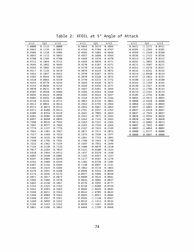
Table 2: XFOIL at 5° Angle of Attackx/c1 Cp1 x/c2

1.0000 0.1116 1.00000.9963 0.1139 0.99630.9904 0.1128 0.99040.9843 0.1115 0.98430.9780 0.1103 0.97800.9715 0.1094 0.97150.9649 0.1092 0.96490.9583 0.1082 0.95830.9517 0.1126 0.95180.9452 0.1047 0.94520.9383 0.0944 0.93830.9310 0.0865 0.93100.9233 0.0778 0.92340.9153 0.0696 0.91540.9070 0.0631 0.90710.8985 0.0550 0.89860.8896 0.0422 0.88980.8805 0.0292 0.88060.8710 0.0169 0.87110.8612 0.0044 0.86140.8513 -0.0073 0.85150.8411 -0.0208 0.84130.8308 -0.0354 0.83100.8203 -0.0506 0.82050.8097 -0.0660 0.80990.7990 -0.0818 0.79920.7882 -0.0977 0.78840.7774 -0.1137 0.77760.7665 -0.1301 0.76670.7557 -0.1468 0.75590.7448 -0.1635 0.74500.7340 -0.1796 0.73420.7232 -0.1962 0.72340.7124 -0.2130 0.71260.7017 -0.2293 0.70190.6910 -0.2464 0.69120.6803 -0.2640 0.68050.6697 -0.2809 0.66990.6592 -0.2988 0.65940.6487 -0.3156 0.64890.6382 -0.3325 0.63840.6278 -0.3491 0.62800.6174 -0.3656 0.61760.6071 -0.3817 0.60730.5968 -0.3986 0.59700.5865 -0.4150 0.58670.5763 -0.4325 0.57650.5662 -0.4483 0.56630.5560 -0.4651 0.55620.5460 -0.4804 0.54620.5360 -0.4957 0.53610.5260 -0.5099 0.52620.5160 -0.5247 0.51620.5061 -0.5396 0.5063

x/c1 Cp1 x/c20.4864 -0.5619 0.48660.4765 -0.5704 0.47670.4666 -0.5802 0.46680.4567 -0.5888 0.45690.4468 -0.5976 0.44700.4369 -0.6035 0.43710.4270 -0.6107 0.42710.4170 -0.6168 0.41720.4070 -0.6229 0.40720.3970 -0.6287 0.39720.3870 -0.6328 0.38720.3770 -0.6372 0.37720.3669 -0.6420 0.36710.3569 -0.6456 0.35710.3467 -0.6481 0.34690.3366 -0.6563 0.33680.3265 -0.6624 0.32670.3164 -0.6679 0.31660.3063 -0.6734 0.30650.2962 -0.6793 0.29640.2862 -0.6867 0.28630.2761 -0.6937 0.27630.2661 -0.7003 0.26630.2561 -0.7071 0.25630.2462 -0.7145 0.24630.2363 -0.7241 0.23650.2265 -0.7339 0.22660.2167 -0.7415 0.21690.2071 -0.7511 0.20720.1975 -0.7599 0.19770.1881 -0.7723 0.18830.1788 -0.7843 0.17900.1697 -0.7952 0.16990.1608 -0.8078 0.16100.1521 -0.8208 0.15230.1437 -0.8329 0.14380.1355 -0.8447 0.13570.1277 -0.8587 0.12780.1202 -0.8738 0.12030.1130 -0.8897 0.11310.1062 -0.9118 0.10630.0998 -0.9343 0.09990.0937 -0.9486 0.09380.0880 -0.9625 0.08810.0826 -0.9802 0.08270.0776 -0.9995 0.07770.0728 -1.0208 0.07290.0684 -1.0449 0.06850.0642 -1.0709 0.06430.0603 -1.0941 0.06040.0566 -1.1138 0.05670.0532 -1.1412 0.05320.0499 -1.1661 0.04990.0468 -1.1799 0.0468

x/c1 Cp1 x/c20.0411 -1.2171 0.04110.0385 -1.2369 0.03850.0360 -1.2548 0.03600.0336 -1.2722 0.03360.0313 -1.2914 0.03130.0291 -1.3045 0.02920.0271 -1.3507 0.02710.0251 -1.4278 0.02510.0232 -1.6241 0.02320.0214 -2.0440 0.02140.0197 -2.1022 0.01970.0180 -2.1219 0.01800.0164 -2.1399 0.01640.0148 -2.1567 0.01480.0133 -2.1786 0.01330.0119 -2.2181 0.01190.0105 -2.2756 0.01060.0093 -2.3473 0.00930.0080 -2.4420 0.00800.0068 -2.5266 0.00690.0057 -2.6083 0.00570.0047 -2.6918 0.00470.0037 -2.7943 0.00370.0028 -2.8556 0.00280.0020 -2.9047 0.00200.0013 -2.8802 0.00130.0007 -2.7842 0.00070.0003 -2.6064 0.00030.0000 -1.8177 0.00000.0000 -0.8887 0.0000

74

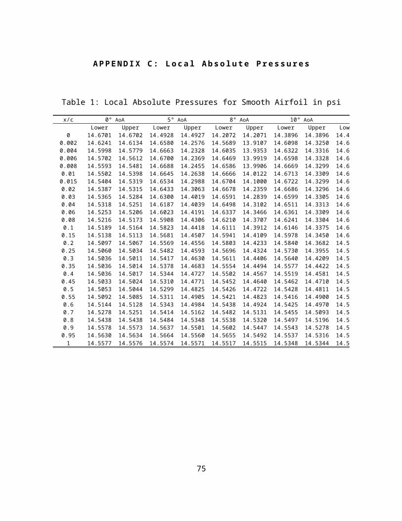
APPENDIX C: Local Absolute Pressures

Table 1: Local Absolute Pressures for Smooth Airfoil in psi

x/cLower Upper Lower Upper Lower Upper Lower Upper Lower

0 14.6701 14.6702 14.4928 14.4927 14.2072 14.2071 14.3896 14.3896 14.44740.002 14.6241 14.6134 14.6580 14.2576 14.5689 13.9107 14.6098 14.3250 14.62610.004 14.5998 14.5779 14.6663 14.2328 14.6035 13.9353 14.6322 14.3316 14.64430.006 14.5702 14.5612 14.6700 14.2369 14.6469 13.9919 14.6598 14.3328 14.66620.008 14.5593 14.5481 14.6688 14.2455 14.6586 13.9906 14.6669 14.3299 14.67160.01 14.5502 14.5398 14.6645 14.2638 14.6666 14.0122 14.6713 14.3309 14.67460.015 14.5404 14.5319 14.6534 14.2988 14.6704 14.1000 14.6722 14.3299 14.67440.02 14.5387 14.5315 14.6433 14.3063 14.6678 14.2359 14.6686 14.3296 14.67040.03 14.5365 14.5284 14.6300 14.4019 14.6591 14.2839 14.6599 14.3305 14.66170.04 14.5318 14.5251 14.6187 14.4039 14.6498 14.3102 14.6511 14.3313 14.65320.06 14.5253 14.5206 14.6023 14.4191 14.6337 14.3466 14.6361 14.3309 14.63850.08 14.5216 14.5173 14.5908 14.4306 14.6210 14.3707 14.6241 14.3304 14.62670.1 14.5189 14.5164 14.5823 14.4418 14.6111 14.3912 14.6146 14.3375 14.61730.15 14.5138 14.5113 14.5681 14.4507 14.5941 14.4109 14.5978 14.3450 14.60040.2 14.5097 14.5067 14.5569 14.4556 14.5803 14.4233 14.5840 14.3682 14.58620.25 14.5060 14.5034 14.5482 14.4593 14.5696 14.4324 14.5730 14.3955 14.57460.3 14.5036 14.5011 14.5417 14.4630 14.5611 14.4406 14.5640 14.4209 14.56490.35 14.5036 14.5014 14.5378 14.4683 14.5554 14.4494 14.5577 14.4422 14.55800.4 14.5036 14.5017 14.5344 14.4727 14.5502 14.4567 14.5519 14.4581 14.55140.45 14.5033 14.5024 14.5310 14.4771 14.5452 14.4640 14.5462 14.4710 14.54490.5 14.5053 14.5044 14.5299 14.4825 14.5426 14.4722 14.5428 14.4811 14.54060.55 14.5092 14.5085 14.5311 14.4905 14.5421 14.4823 14.5416 14.4900 14.53850.6 14.5144 14.5128 14.5343 14.4984 14.5438 14.4924 14.5425 14.4970 14.53870.7 14.5278 14.5251 14.5414 14.5162 14.5482 14.5131 14.5455 14.5093 14.53990.8 14.5438 14.5438 14.5484 14.5348 14.5538 14.5320 14.5497 14.5196 14.54230.9 14.5578 14.5573 14.5637 14.5501 14.5602 14.5447 14.5543 14.5278 14.54460.95 14.5630 14.5634 14.5664 14.5560 14.5655 14.5492 14.5537 14.5316 14.54131 14.5577 14.5576 14.5574 14.5571 14.5517 14.5515 14.5348 14.5344 14.5105

0° AoA 5° AoA 8° AoA 10° AoA 12° AoA

75

Table 1: Local Absolute Pressures for Tripped Airfoil in psi

x/cLower Upper Lower Upper

0 14.1901 14.1901 13.9561 13.95600.002 14.5618 13.8978 14.4653 13.65130.004 14.5982 13.9232 14.5224 13.72710.006 14.6439 13.9796 14.6007 13.77910.008 14.6563 13.9833 14.6254 13.77520.01 14.6651 14.0013 14.6461 13.78030.015 14.6696 14.1300 14.6656 14.05080.02 14.6675 14.2370 14.6702 14.13890.03 14.6591 14.2813 14.6679 14.21260.04 14.6501 14.3080 14.6620 14.25020.06 14.6342 14.3445 14.6485 14.30020.08 14.6216 14.3691 14.6363 14.33290.1 14.6117 14.3899 14.6264 14.36000.15 14.5947 14.4098 14.6084 14.38730.2 14.5809 14.4224 14.5939 14.40500.25 14.5703 14.4314 14.5822 14.41770.3 14.5619 14.4396 14.5728 14.42880.35 14.5562 14.4483 14.5661 14.43990.4 14.5510 14.4556 14.5600 14.44950.45 14.5461 14.4627 14.5541 14.45840.5 14.5435 14.4707 14.5506 14.46820.55 14.5430 14.4809 14.5491 14.47990.6 14.5446 14.4909 14.5496 14.49110.7 14.5491 14.5118 14.5524 14.51320.8 14.5547 14.5316 14.5565 14.53100.9 14.5614 14.5461 14.5613 14.54120.95 14.5669 14.5514 14.5617 14.54491 14.5537 14.5534 14.5478 14.5474

8° AoA 10° AoA

76

APPENDIX D: Pressure Coefficients

Table 1: Pressure Coefficients on Smooth Airfoil

77

x/cLower Upper Lower Upper Lower Upper Lower Upper Lower Upper

0 0.93 0.93 -0.54 -0.54 -2.91 -2.91 -1.40 -1.40 -0.92 -0.920.002 0.55 0.46 0.83 -2.49 0.09 -5.37 0.43 -1.94 0.56 -1.300.004 0.35 0.16 0.90 -2.70 0.38 -5.17 0.61 -1.88 0.71 -1.270.006 0.10 0.03 0.93 -2.67 0.74 -4.70 0.84 -1.87 0.90 -1.280.008 0.01 -0.08 0.92 -2.59 0.83 -4.71 0.90 -1.89 0.94 -1.260.01 -0.07 -0.15 0.88 -2.44 0.90 -4.53 0.94 -1.89 0.97 -1.270.015 -0.15 -0.22 0.79 -2.15 0.93 -3.80 0.95 -1.89 0.96 -1.260.02 -0.16 -0.22 0.71 -2.09 0.91 -2.67 0.92 -1.90 0.93 -1.280.03 -0.18 -0.25 0.60 -1.30 0.84 -2.28 0.84 -1.89 0.86 -1.250.04 -0.22 -0.27 0.50 -1.28 0.76 -2.06 0.77 -1.88 0.79 -1.230.06 -0.27 -0.31 0.37 -1.15 0.63 -1.76 0.65 -1.89 0.67 -1.220.08 -0.30 -0.34 0.27 -1.06 0.52 -1.56 0.55 -1.89 0.57 -1.230.1 -0.33 -0.35 0.20 -0.97 0.44 -1.39 0.47 -1.83 0.49 -1.210.15 -0.37 -0.39 0.08 -0.89 0.30 -1.22 0.33 -1.77 0.35 -1.250.2 -0.40 -0.43 -0.01 -0.85 0.18 -1.12 0.21 -1.58 0.23 -1.230.25 -0.43 -0.45 -0.08 -0.82 0.10 -1.04 0.12 -1.35 0.14 -1.180.3 -0.45 -0.47 -0.14 -0.79 0.02 -0.98 0.05 -1.14 0.06 -1.130.35 -0.45 -0.47 -0.17 -0.75 -0.02 -0.90 0.00 -0.96 0.00 -1.070.4 -0.45 -0.47 -0.20 -0.71 -0.07 -0.84 -0.05 -0.83 -0.06 -1.010.45 -0.45 -0.46 -0.23 -0.67 -0.11 -0.78 -0.10 -0.72 -0.11 -0.950.5 -0.44 -0.45 -0.23 -0.63 -0.13 -0.71 -0.13 -0.64 -0.15 -0.890.55 -0.41 -0.41 -0.22 -0.56 -0.13 -0.63 -0.14 -0.57 -0.16 -0.840.6 -0.36 -0.38 -0.20 -0.50 -0.12 -0.55 -0.13 -0.51 -0.16 -0.790.7 -0.25 -0.27 -0.14 -0.35 -0.08 -0.37 -0.11 -0.41 -0.15 -0.690.8 -0.12 -0.12 -0.08 -0.19 -0.04 -0.22 -0.07 -0.32 -0.13 -0.600.9 0.00 -0.01 0.05 -0.07 0.02 -0.11 -0.03 -0.25 -0.11 -0.520.95 0.04 0.04 0.07 -0.02 0.06 -0.07 -0.04 -0.22 -0.14 -0.471 0.00 0.00 -0.01 -0.01 -0.05 -0.05 -0.19 -0.20 -0.40 -0.40

0° AoA 5° AoA 8° AoA 10° AoA 12° AoA

Table 2: Pressure Coefficients on Tripped Airfoil

x/cLower Upper Lower Upper Lower

0 -3.0669 -3.0669 -5.0171 -5.0180 -2.73450.002 0.0300 -5.5033 -0.7740 -7.5574 -0.29910.004 0.3337 -5.2915 -0.2975 -6.9254 0.04040.006 0.7149 -4.8209 0.3542 -6.4923 0.51080.008 0.8182 -4.7906 0.5607 -6.5248 0.67530.01 0.8910 -4.6408 0.7326 -6.4824 0.80640.015 0.9290 -3.5675 0.8956 -4.2280 0.93460.02 0.9116 -2.6761 0.9341 -3.4938 0.96380.03 0.8410 -2.3071 0.9147 -2.8796 0.94350.04 0.7660 -2.0846 0.8653 -2.5666 0.89740.06 0.6337 -1.7805 0.7529 -2.1497 0.79150.08 0.5286 -1.5758 0.6513 -1.8773 0.69310.1 0.4464 -1.4022 0.5686 -1.6515 0.61200.15 0.3045 -1.2366 0.4186 -1.4239 0.45970.2 0.1899 -1.1315 0.2977 -1.2762 0.33470.25 0.1015 -1.0563 0.2006 -1.1703 0.23120.3 0.0309 -0.9881 0.1222 -1.0775 0.14630.35 -0.0161 -0.9154 0.0666 -0.9854 0.08370.4 -0.0597 -0.8547 0.0152 -0.9057 0.02600.45 -0.1006 -0.7956 -0.0337 -0.8310 -0.03040.5 -0.1224 -0.7284 -0.0628 -0.7492 -0.06750.55 -0.1262 -0.6439 -0.0754 -0.6524 -0.08770.6 -0.1128 -0.5607 -0.0709 -0.5587 -0.08970.7 -0.0753 -0.3863 -0.0480 -0.3747 -0.08270.8 -0.0290 -0.2209 -0.0134 -0.2260 -0.06480.9 0.0269 -0.1006 0.0261 -0.1415 -0.04620.95 0.0729 -0.0566 0.0297 -0.1107 -0.07171 -0.0369 -0.0397 -0.0866 -0.0895 -0.3260

8° AoA 10° AoA 12° AoA

78

APPENDIX E: MATLAB Scripts

%**************************************************************************% EA303_Lab3.m%% This program calculates the pressure coefficients, lift coefficients,% and moment coefficients from gage pressure data extracted from a .xls% file for the purposes of generating data and figures for EA303 Lab 3.% % Author: MIDN Geoffrey DeSena, 04OCT2012%% References: Theory of Wing Sections by Ira Abbott & Albert von Doenhoff%% Documentation: Code used to generate XFOIL data for the group% presentation was integrated into this code for figure generation.%%************************************************************************** %% Workspace cleanup format compactclearclc %% Data input % Import pressure port raw dataClean0 = xlsread('clean 0 AOA.xls',1);Clean5 = xlsread('clean 5 AOA.xls',1);

79

Clean8 = xlsread('clean 8 AOA.xls',1);Clean10 = xlsread('clean 10 AOA.xls',1);Clean12 = xlsread('clean 12 AOA.xls',1);Trip8 = xlsread('tripped 8 AOA.xls',1);Trip10 = xlsread('tripped 10 AOA.xls',1);Trip12 = xlsread('tripped 12 AOA.xls',1); % Load pressure coefficient data into vectorsPup0 = Clean0(7:34,6);Plo0 = Clean0(7:34,13);Pup5 = Clean5(7:34,6);Plo5 = Clean5(7:34,13);Pup8 = Clean8(7:34,6);Plo8 = Clean8(7:34,13);Pup10 = Clean10(7:34,6);Plo10 = Clean10(7:34,13);Pup12 = Clean12(7:34,6)*1.06;Plo12 = Clean12(7:34,13)*1.06;Pupt8 = Trip8(7:34,6);Plot8 = Trip8(7:34,13);Pupt10 = Trip10(7:34,6);Plot10 = Trip10(7:34,13);Pupt12 = Trip12(7:34,6);Plot12 = Trip12(7:34,13); xlocs = Clean0(7:34,1); %port locations in % of chord %% Normal coefficient CN0 = -trapz(xlocs,Plo0)+trapz(xlocs,Pup0);CN5 = -trapz(xlocs,Plo5)+trapz(xlocs,Pup5);CN8 = -trapz(xlocs,Plo8)+trapz(xlocs,Pup8);CN10 = -trapz(xlocs,Plo10)+trapz(xlocs,Pup10);CN12 = -trapz(xlocs,Plo12)+trapz(xlocs,Pup12);CNt8 = -trapz(xlocs,Plot8)+trapz(xlocs,Pupt8); CNt10 = -trapz(xlocs,Plot10)+trapz(xlocs,Pupt10);

80

CNt12 = -trapz(xlocs,Plot12)+trapz(xlocs,Pupt12); %% Lift Coefficient %Experimental dataCL0 = CN0*cosd(0); CL5 = CN5*cosd(5); CL8 = CN8*cosd(8); CL10 = CN10*cosd(10); CL12 = CN12*cosd(12); CLt8 = CNt8*cosd(8); CLt10 = CNt10*cosd(10); CLt12 = CNt12*cosd(12); CLs = [CL0,CL5,CL8,CL10,CL12];CLts = [CLt8,CLt10,CLt12];alphas = [0,5,8,10,12];CLalpha = (CL5-CL0)/5;CLtalpha = (CLt10-CLt8)/2; %Empirical data from Abbot & von DoenhoffCL0avd = 0; CL5avd = 0.55; CL8avd = 0.88; CL10avd = 1.05; CL12avd = 1.15;CL13avd = 0.86;CLavds = [CL0avd,CL5avd,CL8avd,CL10avd,CL12avd,CL13avd];alphasavd = [0 5 8 10 12 13];CLalphaavd = (CL5avd-CL0avd)/5 %% Moment Coefficient arms = ones(length(xlocs),1)*.25-xlocs; %moment arm distance from c/4 % Integrands of moment equationgrandup0 = Pup0.*arms;

81

grandlo0 = Plo0.*arms;grandup5 = Pup5.*arms;grandlo5 = Plo5.*arms;grandup8 = Pup8.*arms;grandlo8 = Plo8.*arms;grandup10 = Pup10.*arms;grandlo10 = Plo10.*arms;grandup12 = Pup12.*arms;grandlo12 = Plo12.*arms;grandupt8 = Pupt8.*arms;grandlot8 = Plot8.*arms;grandupt10 = Pupt10.*arms;grandlot10 = Plot10.*arms;grandupt12 = Pupt12.*arms;grandlot12 = Plot12.*arms; % Experimental moment coefficientsCM0 = trapz(xlocs,grandup0)-trapz(xlocs,grandlo0);CM5 = trapz(xlocs,grandup5)-trapz(xlocs,grandlo5);CM8 = trapz(xlocs,grandup8)-trapz(xlocs,grandlo8);CM10 = trapz(xlocs,grandup10)-trapz(xlocs,grandlo10);CM12 = trapz(xlocs,grandup12)-trapz(xlocs,grandlo12);CMt8 = trapz(xlocs,grandupt8)-trapz(xlocs,grandlot8);CMt10 = trapz(xlocs,grandupt10)-trapz(xlocs,grandlot10);CMt12 = trapz(xlocs,grandupt12)-trapz(xlocs,grandlot12);CMs = [CM0,CM5,CM8,CM10,CM12];CMts = [CMt8, CMt10,CMt12];CMalpha = (CM5-CM0)/5;CMtalpha = (CMt10-CMt12)/2; % Moment coefficients from Abbott & von DoenhoffCM0avd = 0;CM5avd = -.007;CM8avd = -0.0125;CM10avd = -0.013;CM12avd = -0.012;CM14avd = -0.08;

82

CMavds = [CM0avd,CM5avd,CM8avd,CM10avd,CM12avd,CM14avd];CMalphaavd = (CM5avd-CM0avd)/5 %% Plotting Xfoil at 0 degree AoAdata1= xlsread('Lab_2_AOA00_1.xls');data2= xlsread('Lab_2_AOA05_1.xls'); figure(11)hold onplot(data1(:,1),data1(:,2),'-rs',data1(:,3),data1(:,4),'--k');set(gca, 'ydir', 'reverse')axis ([0 1 -0.4 1.2])xlabel('x/c')ylabel('c_p')legend('upper surface','lower surface')title('Xfoil 0^o AoA')hold off %% Plotting Xfoil at 5 degree AoA figure(22)hold onplot(xlocs,Pup5,'ok')plot(data2(:,1),data2(:,2),'-b')plot(data2(:,3),data2(:,4),'-b')plot(xlocs,Plo5,'ok')set(gca, 'ydir', 'reverse')legend('Experimental', 'XFOIL')xlabel('x/c')ylabel('c_p')hold off %% Finding Cl for Xfoil at 0 degree AoA Cn0=trapz(data1(:,3),data1(:,4))+trapz(data1(:,1),data1(:,2)) %% Finding Cl for Xfoil at 5 degree AoA

83

Cn5=trapz(data2(:,3),data2(:,4))+trapz(data2(:,1),data2(:,2)) %% Cl for Xfoil at 0 deg AoA Cl0=Cn0 % since AoA is 0 degrees and Cl=Cn*cos(AoA) %% Cl for Xfoil at 5 deg AoA Cl5=Cn5*cosd(5) Clalpha = (Cl5-Cl0)/5;%% Cm,c/y for Xfoil at 0 deg AoA x= data1(:,3); x1=x';xlocsx= x1; armsx=ones(1,(length(xlocsx)))*.25-xlocsx; cp0U=(data1(:,2)');cp0L=(data1(:,4)');mom0_up=cp0U.*armsx;mom0_low=cp0L.*armsx; cp5U=(data2(:,2)');cp5L=(data2(:,4)');mom5_up=cp5U.*armsx;mom5_low=cp5L.*armsx; Cm0= trapz(xlocsx,mom0_up)-trapz(xlocsx,mom0_low)Cm5= trapz(xlocsx,mom5_up)-trapz(xlocsx,mom5_low) %% Plot Data % Plot Lift vs Moment Coefficientsfigure(1)hold on

84

plot(CLs,[CM0,CM5,CM8,CM10,CM12],'-ok')plot(CLts,CMts,'-^k')plot(CLavds,CMavds,'-or')xlabel('Lift Coefficient')ylabel('Moment Coefficient')legend('Clean Airfoil','Tripped Airfoil','AVD',3)axis([0 1.5 -0.1 0.01]) % Plot moment coefficients vs Alphafigure(2)hold onplot([0,5,8,10,12],[CM0,CM5,CM8,CM10,CM12],'-ok')plot([8 10 12],CMts,'-^k')xlabel('AoA (degrees)')ylabel('Moment Coefficient')legend('Clean Airfoil','Tripped Airfoil') %Plot Turbulent Pressures vs chordwise locationsfigure(3)hold onplot(xlocs,Pupt8,'-oc')plot(xlocs,Pupt10,'-ob')plot(xlocs,Pupt12,'-om')plot(xlocs,Plot8,'-oc')plot(xlocs,Plot10,'-ob')plot(xlocs,Plot12,'-om')set(gca,'ydir','reverse')xlabel('x/c')ylabel('Cp')legend('8 degrees','10 degrees','12 degrees') % Plot Clean Preussures vs chordwise locationsfigure(4)hold onplot(xlocs,Pup0,'-or')plot(xlocs,Pup5,'-ok')plot(xlocs,Pup8,'-oc')

85

plot(xlocs,Pup10,'-ob')plot(xlocs,Pup12,'-om')plot(xlocs,Plo0,'-or')plot(xlocs,Plo5,'-ok')plot(xlocs,Plo8,'-oc')plot(xlocs,Plo10,'-ob')plot(xlocs,Plo12,'-om')set(gca,'ydir','reverse')xlabel('x/c')ylabel('Cp')legend('0 degrees','5 degrees','8 degrees','10 degrees','12 degrees') % Plot smooth vs rough surface pressures coefficientsfigure(5)hold onplot(xlocs,Pup10,'-^b')plot(xlocs,Pupt10,'-ok')plot(xlocs,Plo10,'-^b')plot(xlocs,Plot10,'-ok')set(gca,'ydir','reverse')xlabel('x/c')ylabel('Cp')legend('Smooth Surface','Rough Surface') % Plot 8 and 10 degree smooth pressure coefficientsfigure(6)hold onplot(xlocs,Pup8,'-ok')plot(xlocs,Pup10,'-^b')plot(xlocs,Plo8,'-ok')plot(xlocs,Plo10,'-^b')set(gca,'ydir','reverse')xlabel('x/c')ylabel('Cp')legend('8 degrees','10 degrees') %Plot clean, tripped, and AVD data for lift coefficients

86

figure(7)hold onplot(alphas, CLs,'-ok')plot([8 10 12], CLts,'-ob')plot(alphasavd, CLavds,'-or')xlabel('Angle of Attack (degrees)')ylabel('Lift Coefficient')legend('Clean Airfoil','Tripped Airfoil','AVD',4) % Plot clean vs tripped lift coefficientsfigure(8)hold onplot(alphas, CLs,'-ok')plot([8 10 12], CLts,'-^k')axis([0 14 0 1.2])xlabel('Angle of Attack (degrees)')ylabel('Lift Coefficient')legend('Clean Airfoil','Tripped Airfoil',4)

87