AIAA 2004–0259Prediction of the Flow over an Airfoilat Maximum LiftRupesh B. Kotapati-Apparao, Kyle D. SquiresMAE Department, Arizona State University, Tempe, AZ

James R. ForsytheCobalt Solutions LLC, 4636 New Carlisle Pike,Springfield, OH

Aerospace Sciences Meeting 20045–8 January 2004 / Reno, Nevada

For permission to copy or republish, contact the American Institute of Aeronautics and Astronautics1801 Alexander Bell Drive, Suite 500, Reston, VA 20191–4344

Prediction of the Flow over an Airfoil at

Maximum Lift

Rupesh B. Kotapati-Apparao∗, Kyle D. Squires†

MAE Department, Arizona State University, Tempe, AZ

James R. Forsythe‡

Cobalt Solutions LLC, 4636 New Carlisle Pike, Springfield, OH

Predictions of the flow around the Aerospatiale A-airfoil at maximum lift, α = 13.3,and Re = 2 × 106 are obtained using solutions of the steady Reynolds-averaged Navier-Stokes (RANS) equations and using Detached-Eddy Simulation (DES). RANS predictionsof the two-dimensional flow are computed using the Spalart-Allmaras and SST turbulencemodels. Solutions of the fully-turbulent flow are computed using both RANS models inaddition to prediction of the flow with laminar separation near the leading edge usingthe tripless approach within the Spalart-Allmaras model. For the tripless case, transitionfrom laminar-to-turbulent flow along the lower (pressure) surface was fixed by trippingthe boundary layer at x/C = 0.3. The pressure coefficient in the RANS solutions are inreasonable agreement with measurements prior to the trailing edge separation. The trip-less solution using the Spalart-Allmaras model predicts laminar separation at x/C = 0.088with turbulent reattachment at x/C = 0.124 and followed by separation of the turbulentboundary layer near the trailing edge at x/C = 0.96. Trailing edge separation in the fullyturbulent solutions is also further aft compared to the location reported in experiments,predicted at x/C = 0.88 using the Spalart-Allmaras model and at x/C = 0.92 using SST.Comparison of the mean velocity predictions to measurements shows a behavior consis-tent with the mismatch in separation location compared to measurements. PreliminaryDES predictions are presented and aspects requiring future research are identified.

Introduction

PREDICTION of complex flows that includelaminar-to-turbulent transition, adverse pressure

gradient, streamline curvature, and boundary layerseparation remain among the most challenging for tur-bulence simulation strategies. A prototypical examplethat is the focus of the present investigation is theflow over an airfoil at maximum lift. Flow regimes aresensitive to the airfoil geometry, angle of attack, andReynolds number and motivate various hierarchies ofsimulation strategies.

Reynolds-averaged Navier-Stokes (RANS) ap-proaches remain the most widely applied simulationtechnique for complex flows. For flows that are notfar from the thin shear layers used to calibrate themodels, RANS approaches are often sufficient. Inother regimes, e.g., flows with significant effects of sep-aration and which are characterized by flow structuresatypical compared to the thin (and usually attached)shear layers predicted by RANS models, techniquessuch as Large-Eddy Simulation (LES) are attractive.While LES carries a prohibitive computational cost forresolving boundary layer turbulence at high Reynolds

∗Research Assistant, present affiliation: Mechanical and

Aerospace Engineering Department, The George Washington

University†Professor, AIAA Member‡Director of Research, Senior Member AIAA

Copyright c© 2004 by the American Institute of Aeronauticsand Astronautics, Inc. All rights reserved.

numbers, the technique offers many advantages overRANS methods for predicting separated flows. Thisin turn provides strong incentive for the merging ofthese techniques in hybrid RANS-LES approaches.

Detached-Eddy Simulation (DES) is among themore well known and actively applied hybridRANS-LES strategies. The method was proposedby Spalart et al. [1] as a numerically feasible andplausibly accurate approach for prediction of mas-sively separated flows at high Reynolds numbers. Todate, there have been a range of flows predictedusing DES. These investigations have been largelysuccessful, yielding predictions superior to those ob-tained using RANS approaches while resolving three-dimensional, time-dependent features because of theLES treatment of separated regions (e.g., [2], [3], [4]).In “natural” applications of the technique, boundarylayer growth and separation is under control of theRANS model, the method becomes an LES in regionsaway from solid surfaces provided the grid density issufficient. The approach has proven especially effec-tive for prediction of massively separated flows, in turnmotivating extension of the method to the accurateprediction of other complex flow regimes.

The work reported in this manuscript constitutespart of a longer-term project aimed at improving DESfor predicting flows outside the design-range of mas-sive separations. The specific flow of interest is thatover the Aerospatiale-A airfoil at an angle of attack

1 of 13

American Institute of Aeronautics and Astronautics Paper 2004–0259

of 13.3 and Reynolds number of 2× 106, correspond-ing to maximum lift. The flow has been measured inseparate experiments [5], [6] and was the subject ofan coordinated set of investigations through the LES-FOIL project (e.g., see Mellen et al. [7] for a recentoverview).

The objective of the LESFOIL project was to ad-vance Large-Eddy Simulation in particular, and Com-putational Fluid Dynamics in general, for predictingcomplex flows. Advantages of LES for the generalcase include the reduced sensitivity to modeling er-rors than occurring in RANS methods and the useof grid refinement as a means for increasing the fi-delity of the predictions. Such features are quiteunlike those in RANS approaches given the fixed mod-eling errors that exist, even in the fine-grid limit.The flow over an airfoil near maximum lift stronglychallenges RANS methods, the inter-mingling of ef-fects such as laminar-to-turbulent transition, adversepressure gradient, streamline curvature, shallow sep-aration, and reattachment complicating analysis andmodeling. Unfortunately, one of the findings of theLESFOIL project is that even a narrow section of theairfoil, at a moderate Reynolds number and unswept,continues to pose an extreme cost challenge to LES.Mellen et al. [7] also noted that other aspects such asthe numerical method, grid generation and mesh reso-lution requirements, especially in the near-wall region,coupled with considerations of the spanwise period inthree-dimensional eddy-resolving computations stressessentially all elements of any simulation strategy.

Reported below are RANS predictions of the steady-state solution and DES of the time-dependent andthree-dimensional flow. RANS predictions are ob-tained using two turbulence models – the Spalart-Allmaras one-equation model [8] (referred to as S-A throughout) and the two-equation SST modelof Menter [9]. As described below, a laminar separa-tion (and subsequent transition to turbulence) alongthe suction surface occurs not far from the leadingedge in the experiments. Using the S-A model, thetripless approach of Travin et al. [10], which has theeffect of disabling the turbulence model upstream ofseparation is employed for prediction of the flow withlaminar separation. Both S-A and SST models are alsoused in fully turbulent simulations of the domain, i.e.,for which the boundary layers from the leading edge ofthe airfoil are turbulent. Inter-comparisons are shownof the models and against experimental measurementsof the mean flow. The S-A model forms the base forthe DES predictions shown in the following sections.

Presented in the next section is a summary of theflow features over the Aerospatiale-A airfoil at maxi-mum lift, followed by an outline of the computationalapproach, including grid construction and turbulencemodels. Properties of the RANS and DES predic-tions are then evaluated against measurements of the

U∞

Laminar Boundary Layer

Separation Bubble, Transition

Attached Turbulent Boundary Layer

Turbulent Separation

Tripped Transition

Wake

Fig. 1 Flow regimes on the Aerospatiale-A airfoilat 13.3 (adapted from Mellen et al. [7]).

velocity field, surface pressure, and skin friction distri-butions.

Approach

Flow Description

The flow considered is the same as used as the testcase for the LESFOIL project: the Aerospatiale A-airfoil at an angle of attack α = 13.3, correspondingto the maximum lift configuration, and at a chord-based Reynolds number of 2 × 106. The general char-acteristics of the flow are illustrated in Figure 1. Assummarized in Mellen et al. [7], along the upper suc-tion surface the laminar boundary layer experiencesa free transition in a small laminar separation bubblewith turbulent reattachment at around x/C = 0.12.The turbulent boundary layer grows along the suctionside of the airfoil, separating at x/C = 0.83, result-ing in a recirculation that extends to the trailing edge.Measurements show that the reverse-flow region ex-tends to roughly a wall-normal location y/C = 0.016where y defines the coordinate normal to the suctionsurface and that the location of maximum reverse flowoccurs at y/C = 0.003. Transition from laminar-to-turbulent flow along the lower (pressure) surface wasfixed in experiments by tripping the boundary layerat x/C = 0.3. Measurements were acquired in twodifferent wind tunnels, the airfoil lift and drag weremeasured along with the skin friction and pressure dis-tributions as well as mean velocity and Reynolds stressprofiles at several stations along the airfoil and into thenear-wake [5], [6].

One of the more difficult aspects of the prediction isthe relatively high sensitivity of such flows with incip-ient and then shallow separation to details of the flowdevelopment. Small differences between simulationsand experiments in the upstream flow can amplify withdownstream development. Consequently, the flow is amore difficult case compared to other flows experienc-ing massive separation (e.g., airfoils at high angle ofattack) or where separation is fixed by the geometry,e.g., as occurs at a sharp edge.

2 of 13

American Institute of Aeronautics and Astronautics Paper 2004–0259

Turbulence Models

Spalart-Allmaras

The Spalart-Allmaras RANS model solves an equa-tion for the variable ν which is dependent on theturbulent viscosity [8]. The model is derived basedon empiricism and arguments of Galilean invariance,dimensional analysis and dependence on molecular vis-cosity. The model includes a wall destruction termthat reduces the turbulent viscosity in the laminar sub-layer and trip terms to provide smooth transition toturbulence. The transport equation for the workingvariable ν used to form the eddy viscosity is writtenas,

Dν

Dt= cb1(1 − ft2)S ν −

[cw1fw −

cb1

κ2ft2

] [ ν

d

]2

+1

σ

[∇ · ((ν + ν)∇ν) + cb2 (∇ν)2

]

+ ft1 ∆U2 , (1)

where ν is the working variable. The eddy viscosity νt

is obtained from,

νt = ν fv1 , fv1 =χ3

χ3 + c3v1

, χ ≡ ν

ν, (2)

where ν is the molecular viscosity. The productionterm is expressed as,

S ≡ S +ν

κ2d2fv2 , fv2 = 1 − χ

1 + χfv1

, (3)

where S is the magnitude of the vorticity. The functionfw is given by,

fw = g

[1 + c6

w3

g6 + c6w3

]1/6

,

g = r + cw2 (r6 − r) , r ≡ ν

Sκ2d2, (4)

with large values of r truncated to 10. The trip func-tion ft2 is defined as,

ft2 = ct3exp(−ct4χ2) . (5)

The trip function ft1 is specified in terms of the dis-tance dt from the field point to the trip, the wallvorticity ωt at the trip, and ∆U which is the differ-ence between the velocity at the field point and thatat the trip,

ft1 = ct1gtexp

(−ct2

ω2t

∆U2

[d2 + g2

t d2t

]), (6)

where gt = min(0.1, ∆U/ωt∆x) where ∆x is the gridspacing along the wall at the trip.

The wall boundary condition is ν = 0. The con-stants are cb1 = 0.1355, σ = 2/3, cb2 = 0.622,κ = 0.41, cw1 = cb1/κ2 + (1 + cb2)/σ, cw2 = 0.3,cw3 = 2, cv1 = 7.1, cv2 = 5, ct1 = 1, ct2 = 2, ct3 = 1.1,and ct4 = 2.

Shear Stress Transport

The Shear Stress Transport (SST) model was devel-oped by Menter [9] to improve the accuracy of the k–ωmodel for prediction of separated flows. The baselineform combines k–ε and k–ω formulations, using a pa-rameter F1 to bridge from k–ω near the wall to k–ε inthe freestream. The transport equations governing kand ω take the form,

D

Dt(ρk) = τij

∂ui

∂xj− β∗ρωk

+∂

∂xj

[(µ + σkµt)

∂k

∂xj

], (7)

D

Dt(ρω) =

γρ

µtτij

∂ui

∂xj− βρω2

+∂

∂xj

[(µ + σωµt)

∂ω

∂xj

]

+ 2ρ (1 − F1) σω2

1

ω

∂k

∂xj

∂ω

∂xj, (8)

where τij above is the (modeled) turbulent shearstress. The switching function F1 is given by,

F1 = tanh(arg4

1

), (9)

arg1 = min

(max

( √k

0.09ωy;500µ

ρωy2

);

4ρσω2k

CDkωy2

),

CDkω = max

[2ρσω2

1

ω

∂k

∂xi

∂ω

∂xi; 10−20

]. (10)

The switching function F1 is also used to determinethe values of the model constants. If φ1 representsa generic constant in the k–ω equations and φ2 rep-resents the same constant in the k–ε equations, thenthe model constants employed in (7) and (8) are de-termined by,

φ = F1φ1 + (1 − F1)φ2 . (11)

In the baseline version of the model the turbulent eddyviscosity is determined as µt = ρk/ω. The SST modellimits the turbulent shear stress to ρa1k where a1 =0.31. This in turn leads to an expression for the eddyviscosity,

µt =ρa1k

max (a1ω; ΩF2), (12)

where Ω is the absolute value of vorticity. The func-tion F2 is included to prevent singular behavior in thefreestream where Ω goes to zero and is given by,

F2 = tanh(arg2

2

), (13)

arg2 = max

(2

√k

0.09ωy;400ν

y2ω

).

The k–ω model constants are given by σk1 = 0.85,σω1 = 0.5, β1 = 0.0750, β∗ = 0.09, κ = 0.41,γ1 = β1/β∗−σω1κ

2/√

β∗. The values of the k–ε modelconstants are σk2 = 1.0, σω2 = 0.856, β1 = 0.0828,β∗ = 0.09, κ = 0.41, γ2 = β2/β∗ − σω2κ

2/√

β∗.

3 of 13

American Institute of Aeronautics and Astronautics Paper 2004–0259

Detached-Eddy Simulation

The DES formulation is obtained by replacing in theS-A model the distance to the nearest wall, d, by d,where d is defined as,

d ≡ min(d, CDES∆) , (14)

with the value of the additional model constantCDES = 0.65 set in simulations of homogeneous turbu-lence [11]. In (14), ∆ is the largest distance betweenthe cell center under consideration and the cell cen-ter of the neighbors (i.e., those cells sharing a facewith the cell in question). In “natural” applications ofDES, the wall-parallel grid spacings (e.g., streamwiseand spanwise) are on the order of the boundary layerthickness, the S-A RANS model is retained through-out most or all of the boundary layer, i.e., d = d,and prediction of boundary layer separation is deter-mined in the “RANS mode” of DES. Away from solidboundaries, the closure is a one-equation model forthe subgrid scale eddy viscosity. When the productionand destruction terms of the model are balanced, thelength scale d = CDES∆ in the LES region yields aSmagorinsky-like eddy viscosity ν ∝ S∆2. Analogousto classical LES, the role of ∆ is to allow the energycascade down to the grid size.

While most natural applications of DES treat theentire boundary layer in RANS mode, grid refinementin the wall-parallel directions (both streamwise andspanwise) layer will cause the RANS-LES interface tomove nearer the wall, activating the DES limiter andreducing the eddy viscosity below its RANS levels.This process can degrade predictions if mesh densi-ties are insufficient to support eddy content within theboundary layer, resulting in lower Reynolds stress lev-els compared to that provided by the RANS model [1].

Flow solver and grid

In this work, the compressible Navier-Stokes equa-tions are solved on unstructured grids using Cobalt.The numerical method is a cell-centered finite vol-ume approach applicable to arbitrary cell topologies(e.g, hexahedra, prisms, tetrahedra) and described inStrang et al. [12]. The spatial operator uses the ex-act Riemann Solver of Gottlieb and Groth [13], least-squares gradient calculations using QR factorizationto provide second order accuracy in space, and TVDflux limiters to limit extremes at cell faces. A pointimplicit method using analytic first-order inviscid andviscous Jacobians is used for advancement of the dis-cretized system. For time-accurate computations, aNewton sub-iteration scheme is employed, the methodis second order accurate in time. The domain decom-position library ParMETIS [14] is used for parallelimplementation and provides optimal load balancingwith a minimal surface interface between zones. Com-munication between processors is achieved using Mes-sage Passing Interface.

Fig. 2 Grid in the vicinity of the Aerospatiale-Aairfoil, 946 × 117 points in the surface-tangent andsurface-normal directions, respectively.

Calculations were carried out on a domain that ex-tends approximately eight chord lengths upstream ofthe leading edge of the airfoil. The domain down-stream of the trailing edge extends about 20 chordlengths. In the cross-stream direction the grid ex-tends ten chord lengths both above and below theairfoil. The computations reported in this manuscriptwere performed using structured C-type grids gener-ated using Gridgen [15]. A view of the mesh in thevicinity of the airfoil is shown in Figure 2. The gridis comprised of 945 points along the airfoil surfaceand 117 points normal to the wall. Of the 945 pointsalong the airfoil, 693 are on the leading edge and up-per (suction) surface with the remainder along thebranch cut and the lower (pressure) surface. The meshwas designed to possess sufficient density to supportboundary layer turbulence and the coordinate alongthe airfoil surface is resolved with approximately 10-12 points per boundary layer thickness beginning atroughly the half chord (x/C ≈ 0.50) – this determinesthe DES length scale (∆ = 0.0015C). The grids areclustered near the airfoil surface with the average dis-tance from the wall to the first cell center less thanone viscous unit (∆y/C = 4.7x10−6). The cells werestretched at a geometric growth rate of 1.2 for the first32 layers. At this point the wall normal spacing wasabout 0.0011C, slightly below the target grid spacingof 0.0015C. This wall normal spacing was maintaineduntil outside the expected boundary layer thicknessand separation bubble. After that, the wall normalspacing was stretched at a geometric growth rate of1.1.

While possessing finer mesh spacing than typical forRANS calculations, the two-dimensional RANS pre-dictions shown below were computed using the gridpossessing 945 × 117 points. As also described be-low, for the DES the spanwise grid spacing is specifiedto yield comparable resolution, i.e., 10-12 points perboundary layer thickness beginning at x/C ≈ 0.50.

4 of 13

American Institute of Aeronautics and Astronautics Paper 2004–0259

ResultsRANS

Measurements show that the flow over theAerospatiale-A airfoil experiences a laminar separationin the vicinity of the leading edge region, just down-stream of the peak negative pressure along the suctionside. Transition occurs in the separated shear layerwith the reattached turbulent boundary layer evolv-ing further along the suction side prior to a subsequentseparation near the trailing edge. The laminar sepa-ration and transition is accounted for in the presentS-A predictions using the “tripless” approach outlinedby Travin et al. [10]. The tripless approach providesa means to accommodate the laminar separation andtransition in the separated shear layer, in the presentcalculations represented by an activation of the tur-bulence model. The eddy viscosity upstream of theairfoil is zero, non-zero values are seeded into the suc-tion side of the airfoil using a boundary layer trip atx/C = 0.2, which is downstream of the location ofthe laminar separation. In the initial stages before thecalculation reaches steady state, reversing flow sweepsupstream eddy viscosity from regions downstream ofthe trip, bringing this fluid into contact with regionsof zero eddy viscosity. The recirculation in the separa-tion bubble near the leading edge then sustains themodel and at steady state the turbulence model isactive slightly downstream of the point of flow sep-aration. A second boundary layer trip is located atx/C = 0.3 along the pressure surface, the same loca-tion as used in the experiments.

Predictions are also obtained of the fully-turbulentflow using the S-A and SST turbulence models. Thefully-turbulent solutions are computed by seeding asmall level of eddy viscosity into the upstream flow,sufficient to ignite the turbulence model as the fluidenters the boundary layers. As shown in Figure 4,the initial (laminar) separation near the leading edgedoes not occur in the fully turbulent solutions. Otheraspects of these calculations are also different from thetripless solutions and are described below.

Streamlines from the tripless S-A RANS predic-tions are shown in Figure 3. The zoomed view inthe lower frame highlights the small separation bubblewhich is initiated at x/C = 0.0088, the figure showingvelocity vectors colored by the eddy viscosity ratio.The turbulent flow then reattaches at x/C = 0.124,in good agreement with experimental measurements(e.g., see Mellen et al. [7]). A second separation is pre-dicted in the tripless S-A result near the trailing edge,beginning at at x/C = 0.96. The trailing edge (turbu-lent) separation is further aft of the value reported inexperiments, x/C = 0.83 [7].

Streamlines and contours of the velocity magnitudefrom each of the RANS predictions are shown in Fig-ure 4. The airfoil has been extruded in the directionnormal to the plane showing the velocity magnitude in

Fig. 3 Streamlines over the Aerospatiale-A airfoilat 13.3 angle of attack and chord Reynolds numberof 2 × 10

6. Result shown in the figure from thetripless S-A prediction. Lower frame is an enlargedview showing the laminar separation bubble nearthe leading edge (x/C ≈ 0.1).

Fig. 4 Streamlines and contours of the velocitymagnitude. The isosurface of zero streamwise ve-locity is also shown on the airfoil surface. Upperframe: tripless S-A. Middle frame: fully-turbulentS-A. Lower frame: fully-turbulent SST.

5 of 13

American Institute of Aeronautics and Astronautics Paper 2004–0259

order to also plot the contour (isosurface in the figure)of zero streamwise velocity. This view shows the sepa-ration bubble beginning at x/C = 0.088 in the triplessS-A prediction (upper frame). Figure 4 also shows thatthere is no leading edge separation in the fully tur-bulent S-A and SST predictions, the turbulent stateof the boundary layer in these simulations possessingsufficient momentum to resist leading-edge separation.The fully-turbulent S-A result (middle frame) predictsseparation at x/C = 0.88 and SST (lower frame) pre-dicts boundary layer separation at x/C = 0.92. Theseparation locations in the fully turbulent runs areboth closer to that deduced in experiments comparedto the tripless result. Figure 4 also indicates that thedisplacement effects deduced from the velocity magni-tude in the tripless result (top frame) appear slightlysmaller than in either of the fully turbulent solutions,with the largest differences visible between the triplessS-A and fully turbulent SST predictions. As tabulatedbelow, the lift and drag predictions from the triplessS-A calculation are consistent with a smaller effect ofthe separation compared to the fully turbulent runs.

The pressure coefficient over the airfoil on both thepressure and suction sides and an enlarged view of thetrailing edge region is shown in Figure 5. The fig-ures show that compared to the experimental measure-ments, the overall pressure distribution is adequatelycaptured by both fully turbulent solutions over thepressure side and for the suction side upstream of theregion strongly influenced by the trailing edge separa-tion (x/C > 0.8). The enlarged view of the pressurecoefficient distribution in the lower frame of Figure 5shows the fully turbulent solutions are closer to the ex-perimental measurements than the tripless prediction.The mismatch between the RANS and measurementsdepicted in the lower frame of the figure illustrates oneof the outcomes of the differences in the separation pre-diction. Differences in the location of separation andin the characteristics of the separated flow region bothcontributing to the less negative Cp predicted by theRANS models along the suction surface and illustratedin Figure 5. The tripless S-A result shown in Figure 5also yields a larger peak pressure near the leading edgeof the suction side than measured or predicted by ei-ther of the fully turbulent S-A or SST runs. The largerpeak suction is similar to the behavior observed in pre-vious computations which also showed larger suctionpressures in predictions with delayed trailing edge sep-aration, a result attributed to changes in the airfoilcirculation [7].

A notable difference between the fully turbulent andtripless predictions is apparent for the suction-sidepressure distribution near the airfoil leading edge. Inthe vicinity x/C ≈ 0.1 the tripless prediction showsa slight plateau in the pressure distribution, a resultof the laminar separation bubble captured in this cal-culation (c.f., Figure 4), though not in either of the

x/C

Cp

0 0.2 0.4 0.6 0.8 1

-5

-4

-3

-2

-1

0

1

2

S-A FTS-A triplessSST FTMeasurements

x/C

Cp

0.6 0.7 0.8 0.9 1

-1

-0.5

0

0.5

S-A FTS-A triplessSST FTMeasurements

Fig. 5 Pressure coefficient. Upper frame showsthe distribution over both the pressure and suc-tion sides of the airfoil. The lower frame shows anenlarged view of the trailing edge region. Measure-ments from Gleyzes [6].

fully turbulent runs. Previous LES calculations of theflow were also able to resolve the laminar separation,in addition to details of the transition process, thoughat a substantially increased cost [16].

The skin friction coefficient over the suction sideof the airfoil is shown in the upper frame of Fig-ure 6 and with an enlarged view of the trailing edgedistribution in the lower frame. Analogous to the be-havior observed in the pressure coefficient, the fullyturbulent calculations yield similar predictions of theskin friction, both S-A and SST in reasonable agree-ment with measurements for chordwise stations pastx/C = 0.4. The tripless S-A result predicts a lam-inar boundary layer prior to separation and yieldsa substantially lower Cf compared to the fully tur-bulent runs upstream of x/C ≈ 0.1. The negative

6 of 13

American Institute of Aeronautics and Astronautics Paper 2004–0259

x/C

Cf

0 0.2 0.4 0.6 0.8 1-0.005

0

0.005

0.01

0.015

0.02

S-A FTS-A triplessSST FTMeasurements, F2, Re = 2.0 x 106

Measurements, F1, Re = 2.1 x 106

x/C

Cf

0.6 0.7 0.8 0.9 1-0.0025

0

0.0025

0.005

S-A FTS-A triplessSST FTMeasurements, F2, Re = 2.0 x 106

Measurements, F1, Re = 2.1 x 106

Fig. 6 Skin friction coefficient. Upper frameshows the distribution over the suction side of theairfoil. The lower frame shows an enlarged viewof the trailing edge region. Measurements “F1”from Huddeville et al. [5], “F2” from Gleyzes [6].

region in Cf near x/C ≈ 0.1 identifies the separationpoint and length of the reverse-flow region. Followingreattachment, the skin friction in the tripless solutionsharply increases to values slightly higher than in thefully turbulent predictions. The trailing edge distri-bution shown in the lower frame of the figure shows abetter agreement between experimental measurementsand the fully turbulent predictions as compared to thetripless result. The later separation in the tripless pre-diction compared to both fully turbulent solutions andthe experimental measurements is also evident in theCf distributions.

The mean velocity components in coordinates lo-cally tangent and normal to the airfoil surface weremeasured in experiments [6], a representative com-parison of the simulations to the data are shown in

u/U∞

y/C

-0.3 0 0.3 0.6 0.9 1.2 1.5 1.8

0

0.02

0.04

0.06

0.08

0.1

0.12

S-A triplessS-A FTSST FTMeasurements

x/C = 0.400

v/U∞

y/C

-0.1 -0.05 0 0.05 0.1 0.15 0.2 0.25

0

0.02

0.04

0.06

0.08

0.1

0.12

S-A triplessS-A FTSST FTMeasurements

x/C = 0.400

Fig. 7 Mean streamwise (upper frame) and wall-normal (lower frame) velocity at x/c = 0.40. Mea-surements from Gleyzes [6].

Figures 7-13. Figures 7-9 show the comparison be-tween RANS and experimental measurements at threestreamwise locations – x/C = 0.4, 0.5, and 0.7 – priorto trailing edge separation. The tripless calculationhas reattached following the laminar separation, ini-tiating a turbulent boundary layer from x/C = 0.124while the fully turbulent solutions initiate boundarylayers from the leading edge (without any separationuntil the trailing edge region). Each of Figures 7-9show that the fully turbulent S-A and SST predic-tions of the mean streamwise velocity are in reasonableagreement with measurements, with larger differencesvisible between the runs at x/C = 0.7 and the SSTresult closer to the measured profile than S-A. Thefigures also show that for these chordwise stations themean streamwise velocity predicted in the tripless cal-culation leads that of the fully turbulent solutions andalso exceeds the experimentally measured profiles. At

7 of 13

American Institute of Aeronautics and Astronautics Paper 2004–0259

u/U∞

y/C

-0.3 0 0.3 0.6 0.9 1.2 1.5 1.8

0

0.02

0.04

0.06

0.08

0.1

0.12

S-A triplessS-A FTSST FTMeasurements

x/C = 0.500

v/U∞

y/C

-0.1 -0.05 0 0.05 0.1 0.15 0.2 0.25

0

0.02

0.04

0.06

0.08

0.1

0.12

S-A triplessS-A FTSST FTMeasurements

x/C = 0.500

Fig. 8 Mean streamwise (upper frame) and wall-normal (lower frame) velocity at x/c = 0.50. Mea-surements from Gleyzes [6].

x/C = 0.4 and x/C = 0.5, the tripless S-A predictionof the mean streamwise velocity show an overshootthat is not apparent in the experimental measurementsand less pronounced in the fully turbulent S-A andSST predictions. This difference in the streamwisemean velocities is in turn consistent with a weakertrailing edge separation and larger suction near theleading edge as discussed above, aspects that slightlyincrease the circulation of the airfoil.

At x/C = 0.4 and x/C = 0.5, Figure 7 and Fig-ure 8 show good agreement between the fully turbulentRANS predictions and measurements for most of thewall-normal profile, the SST results yielding the clos-est match to the data. At x/C = 0.7, the wall-normalmean flow in Figure 9 (lower frame) depicts a largerdifference between each of the RANS predictions andthe measured profile. The under-prediction of theRANS solution indicative of a relatively weaker dis-

u/U∞

y/C

-0.3 0 0.3 0.6 0.9 1.2 1.5 1.8

0

0.02

0.04

0.06

0.08

0.1

0.12

S-A triplessS-A FTSST FTMeasurements

x/C = 0.700

v/U∞

y/C

-0.1 -0.05 0 0.05 0.1 0.15 0.2 0.25

0

0.02

0.04

0.06

0.08

0.1

0.12

S-A triplessS-A FTSST FTMeasurements

x/C = 0.700

Fig. 9 Mean streamwise (upper frame) and wall-normal (lower frame) velocity at x/c = 0.70. Mea-surements from Gleyzes [6].

placement of the mean flow under the action of theadverse pressure gradient developing over the suctionside of the airfoil.

The remaining profiles, beginning with those mea-sured and predicted at x/C = 0.825 in Figure 10 showlarger differences between the predictions and mea-surements and more substantial differences amongstthe RANS models. This is anticipated based on thepressure and skin friction distributions, showing thatthe RANS and measurements are increasingly differ-ent towards the trailing edge region. The profiles atx/C = 0.825 are close to the location of boundary layerseparation in the experiments. Both the mean stream-wise and wall-normal velocities measured in the exper-iments and depicted in Figure 10 show the boundarylayer on the verge of separation. The RANS predic-tions, with separation further aft, yield streamwisemean velocities that lead the measurements and wall-

8 of 13

American Institute of Aeronautics and Astronautics Paper 2004–0259

u/U∞

y/C

-0.3 0 0.3 0.6 0.9 1.2 1.5 1.8

0

0.02

0.04

0.06

0.08

0.1

0.12

S-A triplessS-A FTSST FTMeasurements

x/C = 0.825

v/U∞

y/C

-0.05 0 0.05 0.1 0.15 0.2 0.25 0.3

0

0.02

0.04

0.06

0.08

0.1

0.12

S-A triplessS-A FTSST FTMeasurements

x/C = 0.825

Fig. 10 Mean streamwise (upper frame) and wall-normal (lower frame) velocity at x/c = 0.825. Mea-surements from Gleyzes [6].

normal means that lag the data in the outer region ofthe boundary layer. The tripless S-A prediction showsthe largest difference compared to measurements inboth profiles, the fully turbulent SST solution is clos-est to the measured distributions.

At x/C = 0.87 in Figure 11, the measured profiles ofthe mean streamwise velocity indicate a weak reverseflow. There is also relatively mild change in the meanwall-normal velocity compared to the measurementsat x/C = 0.825. The RANS predictions are also sim-ilar to those at the upstream station x/C = 0.825 –none of the RANS predictions indicate boundary layerseparation and the mean wall-normal velocity lags themeasured values in the outer region.

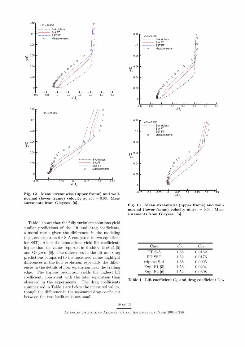
Compared to the flow upstream, an increase inthe peak reverse velocity in the measurements of thestreamwise mean is observed at x/C = 0.96 in Fig-ure 12. The fully turbulent S-A and SST prediction

u/U∞

z/C

-0.3 0 0.3 0.6 0.9 1.2 1.5 1.8

0

0.02

0.04

0.06

0.08

0.1

0.12

S-A triplessS-A FTSST FTMeasurements

x/C = 0.870

v/U∞

z/C

-0.05 0 0.05 0.1 0.15 0.2 0.25 0.3

0

0.02

0.04

0.06

0.08

0.1

0.12

S-A triplessS-A FTSST FTMeasurements

x/C = 0.870

Fig. 11 Mean streamwise (upper frame) and wall-normal (lower frame) velocity at x/c = 0.87. Mea-surements from Gleyzes [6].

indicate flow separation prior to this streamwise loca-tion. Figure 12 shows that the reversed flow in thestreamwise component predicted by both models ismuch smaller than observed in the measured profile,consistent with the later separation predicted by themodels compared to the experiments. As also observedin the profiles upstream of this location, the tripless S-A result over-predicts the measured profile over nearlyall of the boundary layer. The mean wall-normal veloc-ities in the lower frame of Figure 12 show the closestagreement between the measurements and fully tur-bulent RANS solutions, though the profiles show lesspeak-to-peak variation than indicated in the measure-ments. The last streamwise station along the airfoilfor which measurements were acquired, x/C = 0.99, inFigure 13 shows the SST prediction closest to the mea-sured profile in both the streamwise and wall-normalcomponents.

9 of 13

American Institute of Aeronautics and Astronautics Paper 2004–0259

u/U∞

y/C

-0.6 -0.3 0 0.3 0.6 0.9 1.2 1.5

0

0.02

0.04

0.06

0.08

0.1

0.12

S-A triplessS-A FTSST FTMeasurements

x/C = 0.960

v/U∞

y/C

-0.05 0 0.05 0.1 0.15 0.2 0.25

0

0.02

0.04

0.06

0.08

0.1

0.12

S-A triplessS-A FTSST FTMeasurements

x/C = 0.960

Fig. 12 Mean streamwise (upper frame) and wall-normal (lower frame) velocity at x/c = 0.96. Mea-surements from Gleyzes [6].

Table 1 shows that the fully turbulent solutions yieldsimilar predictions of the lift and drag coefficients,a useful result given the differences in the modeling(e.g., one equation for S-A compared to two equationsfor SST). All of the simulations yield lift coefficientshigher than the values reported in Huddeville et al. [5]and Gleyzes [6]. The differences in the lift and dragpredictions compared to the measured values highlightdifferences in the flow evolution, especially the differ-ences in the details of flow separation near the trailingedge. The tripless prediction yields the highest liftcoefficient, consistent with the later separation thanobserved in the experiments. The drag coefficientssummarized in Table 1 are below the measured values,though the difference in the measured drag coefficientbetween the two facilities is not small.

u/U∞

y/C

-0.6 -0.3 0 0.3 0.6 0.9 1.2 1.5

0

0.02

0.04

0.06

0.08

0.1

0.12

S-A triplessS-A FTSST FTMeasurements

x/C = 0.990

v/U∞

y/C

-0.15 -0.1 -0.05 0 0.05 0.1 0.15 0.2 0.25

0

0.02

0.04

0.06

0.08

0.1

0.12

S-A triplessS-A FTSST FTMeasurements

x/C = 0.990

Fig. 13 Mean streamwise (upper frame) and wall-normal (lower frame) velocity at x/c = 0.99. Mea-surements from Gleyzes [6].

Case CL CD

FT S-A 1.58 0.0162FT SST 1.52 0.0176

tripless S-A 1.68 0.0095Exp. F1 [5] 1.56 0.0204Exp. F2 [6] 1.52 0.0308

Table 1 Lift coefficient CL and drag coefficient CD.

10 of 13

American Institute of Aeronautics and Astronautics Paper 2004–0259

Fig. 14 Contours of the instantaneous vorticity inthe DES. Cutting planes at x/C = 0.4, 0.65, 0.8, and0.9.

DES

For the three-dimensional, time-dependent and fullyturbulent DES predictions the grid (c.f., Figure 2)was extruded into the spanwise (z) direction using 68points and with a constant spanwise spacing ∆z/C =0.0015. Periodic boundary conditions are applied, thespanwise period being 0.1C for the current grid spac-ing. The timestep used in the DES when made dimen-sionless using the chord length and freestream speedis 7.8 × 10−4, yielding a CFL number based on thespanwise (target) grid spacing of approximately 0.5.

As summarized above for the current grid, the wall-parallel directions near the airfoil surface are resolvedwith 10-12 points per boundary layer thickness begin-ning at roughly the half-chord, x/C = 0.5. Previousapplications of DES in channel flow indicate such reso-lution corresponds to the coarser range of grid spacingscapable of supporting eddy content in the boundarylayer [17], [18]. Grids with sufficient density to re-solve boundary layer turbulence are not the norm forthe design range of applications aimed at massivelyseparated flows. For the current mesh the interfacebetween the RANS and LES regions is within theboundary layer, activating the DES limiter and lower-ing the Reynolds stresses near the interface comparedto the levels that would be given by the RANS model.

Solutions include development of techniques thatseed the boundary layer with eddy content, in anattempt to develop resolved Reynolds stress to sup-plement the modeled values that are decreased on finemeshes when the RANS-LES interface is close to thewall. One example is the inclusion of backscatter mod-els, e.g., through stochastic forcing of the momentumequations, which has been applied in DES of turbu-lent channel flow [19]. Control over the location of theRANS-LES interface is an alternative approach andtested in the current simulations. The objective is tomaintain RANS behavior in specific regions of the flow,irrespective of the mesh density.

In the present effort, a simple approach is applied bymaintaining the RANS model to x/C = 0.5 since the

Fig. 15 Isosurfaces of the instantaneous fluctu-ating pressure in the DES prediction. Alternatingsigns in the pressure fluctuations indicated by thered (positive) and gray (negative) isosurfaces.

grid density is not sufficient to support eddy contentprior to this chordwise station. Shown in Figure 14 arecontours of the instantaneous vorticity in four planesalong the airfoil. At x/C = 0.4, the RANS modelis retained and the figure illustrates that the solutionpossesses weak spanwise variation. At the subsequentplanes a range of scales is resolved as the flow de-velops eddies in the separating shear layer. Anotherview is provided in Figure 15 which shows isosurfacesof the instantaneous pressure, the red isosurface indi-cating positively signed pressure fluctuations and grayisosurface indicating regions of negative pressure fluc-tuations. The figure shows a relatively large spanwisestructure and a range of three-dimensional structuresdeveloping downstream.

For the present configuration, unlike flows exhibit-ing massive separation, the development of three-dimensional eddy content is not rapid as the solutionconvects downstream from the structureless RANS re-gion maintained upstream of x/C = 0.5. The lack ofeddy content leads to lower Reynolds stress levels and,in the current case, to a separation of the boundarylayer upstream of the location observed in experiments(or predicted in the RANS calculations). This featurehighlights the need to seed the flow in order to de-velop eddy content to replace Reynolds stress reducedvia the action of the DES limiter, in addition to moreautomated means to monitor and control the locationof the RANS-LES interface.

Summary

RANS and DES have been applied to the predictionof the flow over the Aerospatiale-A airfoil at maximumlift. Experimental measurements show that the flow ischaracterized by a laminar separation followed by tur-bulent reattachment near the leading edge and witha subsequent separation in the trailing edge region.The laminar separation and turbulent reattachmentwere accurately predicted using the tripless approachwithin the S-A model, with the reattachment locationat x/C = 0.124 in the simulations agreeing well withexperimental measurements. Subsequent developmentof the tripless solution, however, was farther from ex-perimental measurements of the pressure coefficient,

11 of 13

American Institute of Aeronautics and Astronautics Paper 2004–0259

skin friction, and velocity distributions compared tofully turbulent predictions obtained using the S-A andSST models.

All of the RANS models predict separation aft ofthe location indicated in the experimental measure-ments. Consequently, the mean velocities in the sep-arated region is not as accurately re-produced by anyof the RANS models, e.g., differences are noted inthe pressure distribution and mean flow near the trail-ing edge. Measurements and predictions of the wall-normal mean velocity indicate the displacement of theflow by the adverse pressure gradient upstream is notsimilar in the computations. The delayed separationeffectively increases the circulation in tripless S-A pre-diction, leading to larger suction near the leading edgeand higher lift.

Preliminary DES predictions were obtained bymaintaining the RANS model over the airfoil to x/C =0.5, which constitutes the region upstream of that withsufficient grid spacing to adequately resolve eddy con-tent within the boundary layer. The calculations didnot utilize any means of seeding fluctuations withinthe boundary layer that would more efficiently developresolved Reynolds stress. Such strategies are not re-quired in natural applications of the technique to mas-sively separated flows since the entire boundary layer isusually treated by the RANS model and the explosivegrowth of instabilities in the separated region providesan efficient mechanism for creating three-dimensionaleddy structure. The process of generating eddy struc-ture within the boundary layer represents a steeperchallenge than encountered in natural DES applica-tions and is an important area of future work. Inaddition, the flow places many other demands on themodeling and numerical treatments, all of which re-quire additional research.

Acknowledgments

The authors gratefully acknowledge the support ofthe Air Force Office of Scientific Research (GrantF49620-02-1-0117, Program Officers: Dr. ThomasBeutner and Dr. John Schmisseur). Mr. Kul-winder Singh and Mr. Vivek Krishnan assisted withpost-processing and analysis. The work was performedas part of a DoD Challenge project, on the Aeronau-tical Systems Center Major Shared Resource Centerand the Maui High Performance Computing Center.

References1 Spalart, P. R. , Jou W-H. , Strelets M. , and

Allmaras, S. R., “Comments on the Feasibilityof LES for Wings, and on a Hybrid RANS/LESApproach,” Advances in DNS/LES, 1st AFOSRInt. Conf. on DNS/LES, Aug. 4-8, 1997, GreydenPress, Columbus Oh.

2 Strelets, M., “Detached Eddy Simulation of Mas-

sively Separated Flows”, AIAA Paper 2001-0879,2001.

3 Squires, K.D., Forsythe, J.R., Morton, S.A.,Strang, W.Z., Wurtzler, K.E., Tomaro, R.F.,Grismer, M.J. and P.R. Spalart, “Progress onDetached-Eddy Simulation of massively separatedflows”, AIAA Paper 2002-1021, 2002.

4 Forsythe, J.R. and Woodson, S.H., “UnsteadyCFD calculations of abrupt wing stall usingDetached-Eddy Simulation”, AIAA 2003-0594,2003.

5 Huddeville, R., Piccin, O. and Cassoudesalle, D.,“Operation decrochage – mesurement de frotte-ment sur profiles AS 239 et A 240 a la soufflerieF1 du CFM”, Tech. Rep. RT-OA 19/5025 (RT-DERAT 19/5025 DN), ONERA, 1987.

6 Gleyzes, C., “Operation decrochage – resultats dela 2eme campagne d’essais a F2 – Mesures depression et velocimetrie laster”, Tech. Rep. RT-DERAT 55/5004, ONERA, 1989.

7 Mellen, C.P., Froolich, J. and Rodi, W., “Lessonsfrom the European LESFOIL project on LES offlow around an airfoil”, AIAA 2002-0111, 2002.

8 Spalart, P.R., and Allmaras, S.R., “ A One-Equation Turbulence model for AerodynamicFlows”, La Recherche Aerospatiale, 1, pp. 5-21,1994.

9 Menter, F.R., “Two-Equation Eddy-ViscosityTurbulence Models for Engineering Applications,”AIAA Journal, 32(8) pp. 1598-1605, 1994.

10 Travin, A., Shur, M., Strelets, M. and Spalart,P.R., “Detached-eddy simulations past a circularcylinder”, Flow, Turbulence, and Combustion, 63,pp. 293-313, 2000.

11 Shur, M., Spalart, P. R., Strelets, M., and Travin,A, “Detached-Eddy Simulation of an Airfoil atHigh Angle of Attack, 4th Int. Symp. Eng. Turb.Modelling and Measurements, Corsica, May 24-26,1999.

12 Strang, W. Z., Tomaro, R. F. and Grismer, M. J.,“The Defining Methods of Cobalt60: a Parallel,Implicit, Unstructured Euler/Navier-Stokes FlowSolver,” AIAA 99-0786, 1999.

13 Gottlieb, J.J. and Groth, C.P., “Assessment ofRiemann solvers for unsteady one-dimensional in-viscid flows of perfect gases”, J. Comp. Physics,78, pp. 437-458, 1998.

14 Karypis, G., Schloegel, K., and Kumar, V,ParMETIS: Parallel Graph Partitioning and

12 of 13

American Institute of Aeronautics and Astronautics Paper 2004–0259

Sparse Matrix Ordering Library Version 1.0. Uni-versity of Minnesota, Department of ComputerScience, Minneapolis, MN 55455, July 1997.

15 Steinbrenner, J., Wyman, N., Chawner, J., “De-velopment and Implementation of Gridgen’s Hy-perbolic PDE and Extrusion Methods,” AIAA 00-0679.

16 Mary, I. and Sagaut, P., “Large Eddy Simulationof Flow around an Airfoil Near Stall”, AIAA J.,40(6), pp. 1139-1145, 2002.

17 Nikitin, N.V. Nicoud, F., Wasistho, B., Squires,K.D. and Spalart, P.R., “An approach to wall layermodeling in Large-Eddy Simulations”, Phys. Flu-ids, 12(7), pp. 1629-1632, 2000.

18 Spalart, P.R., “Strategies for Turbulence Mod-elling and Simulations”, Int. J. Heat and FluidFlow, 21, 252-263, 2000.

19 Piomelli, U., Balaras, E., Pasinato, H., Squires,K.D. Spalart, P.R., “The inner-outer layer inter-face in Large-Eddy Simulations with wall-layermodels”, Int. J. Heat and Fluid Flow, 24, pp. 538-550, 2003.

13 of 13

American Institute of Aeronautics and Astronautics Paper 2004–0259