Aerodynamic Design Optimization of Range Extension Kit of a ...

Paper: ASAT-17-139-AF

17th

International Conference on

AEROSPACE SCIENCES & AVIATION TECHNOLOGY,

ASAT - 17 – April 11 - 13, 2017, E-Mail: [email protected]

Military Technical College, Kobry Elkobbah, Cairo, Egypt

Tel: +(202) 24025292 – 24036138, Fax: +(202) 22621908

Aerodynamic Design Optimization of Range Extension Kit of a

Subsonic Flying Body

A. M. Elsherbiny*, A. M. Bayoumy

†, A. M. Elshabka

‡ and M. M. Abdelrahman

§

Abstract: This paper aims to convert the aerodynamic shape of a conventional aerial subsonic

flying body into a glide one by providing a range extension kit and fins. It describes the

selection of configuration and airfoils depending on the tactical requirements and flight

regimes. The wing and fins sizing is obtained using three different methods subjected to

geometric constraints. The first method is an iterative optimization method using linear

aerodynamic data. The second method is a genetic algorithm multi-objective function aims to

maximize stability, controllability and lift-drag ratio within certain weights using linear

aerodynamic data. The third method is a genetic algorithm optimization function integrated

with MISSILE DATCOM aims to maximize lift-drag ratio. Then perform a direct

uncontrolled six degree of freedom simulation for the three optimized designs and the

conventional flying body. Comparing the results of ranges for these bodies reveals that the

third method has the best range over the other designs including the conventional flying body.

Keywords: Aerodynamic Design, Subsonic Flying body, Range Extension Kit, Optimization,

Genetic algorithm, MISSILE DATCOM, 6DoF simulation.

Nomenclature Lift, drag, and pitching

moment coefficients Lateral force, rolling, and

yawing moment coefficients

Lift, drag, and pitching

moment coefficients at

zero values of , q, ,

and

Lateral force, rolling, and

yawing moment coefficients at

zero values of , p, r, and

Derivatives of lift

coefficient w.r.t. , q,

, and

Derivatives of lateral force

coefficient w.r.t. , p, r, and

* M.Sc. Student, MTC, Cairo, Egypt, [email protected]

† Assistant Prof, MSA University, Giza, Egypt, [email protected]

‡ Assistant Prof, MTC, Cairo, Egypt, [email protected]

§ Prof, Cairo University, Cairo, Egypt, [email protected]

mailto:[email protected]





Derivatives of moment

coefficient w.r.t. , q,

, and

Derivatives of rolling moment

coefficient w.r.t. , p, r, and

Derivatives of yawing

moment coefficient

w.r.t. , p, r, and

Wing, root, and tip chords [m]

Directional cosines

matrix Resultant external force vector

applied on the flying body in

body axes [N]

Gravity acceleration

vector [m/s2]

Neutral and maneuver points

Inertia matrix in body

axes [N.m2]

Flying body mass [Kg]

Scalar components of

angular velocity in body

axis [rad/sec]

Scalar components of linear

velocity in body axis [m/s]

velocity vector in body

axis [m/s] Horizontal-tail volume ratio

Total velocity [m/s] Components of vehicle

trajectory [m]

Wind angles [deg] Air density at (H) altitude

Roll, pitch, and yaw fin

deflection angles [deg] Relative mass parameter

Roll, pitch, and yaw

angles (Euler angles)

[deg]

Angular velocity vector in

body axis [rad/s]

1. Introduction In the last 40 years, there are a global need for long range air-to-surface munitions which are

associated with low cost-effectiveness, and standoff. So, a glide flying bodies are developed

which is a category between conventional aerial bomb and tactical air-to-ground missile featured

with a high benefit-cost ratio. These munitions can be loaded on bomb carriers, fighters and

other combat aircrafts which are capable of carrying aerial bombs. In 1980, Randall [14]

introduced an aerodynamic design of an extended range bomb to provide a low altitude, 15 km

stand-off, a 2.5 km turn radius, and return-to-target (RTT) delivery capability from aircraft at

release speeds of 330-800 KCAS. The bomb is a canard configuration, this canard is used for

attitude control and lift. The optimization of canard design is performed using wind tunnel tests.

In 1994, Wakayama and Kroo [11] introduced subsonic wing design using multidisciplinary

optimization. The objective function was to minimize the drag subject to maximum lift and

minimum structural weight and the design parameters was the wing planform. In 1995, Anderson

[12] introduced the potential of genetic algorithms for subsonic wing design to determine high

efficiency wing planform geometries. The objective function was to maximize aerodynamic

efficiency (lift-drag ratio). In 1996, Anderson and Gebert [10] introduced the using of Pareto

genetic algorithms to determine high efficiency wing geometries, and demonstrates the capability

of pareto genetic algorithms to determine highly efficient and robust wing designs given a variety


of design goals and constraints. The design goals are maximizing lift-drag ratio and minimizing

structure weight. The design parameters are wing planform, height of wing along span, and wing

twist. In 1998, Austin [9] introduced an investigation of range extension with a genetic algorithm.

The optimization is aimed to increase the range depending on the inputs to a six degree of

freedom simulation. The parameters to be optimized were the inputs to this motion generator and

the simulator's output (terminal range) was the fitness measure. The parameters of interest were

initial launch altitude, initial launch speed, wing angle-of-attack, and engine ignition time. In

1999, Vicini and Queagliarella [8] introduced airfoil and wing design through hybrid optimization

strategies. This hybrid optimization algorithm has been obtained by adding a gradient based

technique among the set of operators of a multi-objective genetic algorithm. In 2007, Lei Tang et

al. [7] introduced extension of projectile range using oblique-wing concept. A body-conformal

oblique wing/tails with smart-structure control has been proposed to achieve an extended range

with full optimal scheduling of L/D from subsonic to supersonic speeds using an intensive thin-

layer Reynolds-averaged Navier-Stokes computations. In 2008, Takahashi [6] described a

comprehensive study of wing sizing and configuration for subsonic cruise air-vehicles by

maximizing (L/D) at the design speed. In 2015, Andrews and Perez [4] introduced a parametric

study of box-wing aerodynamics for minimum drag under stability and maneuverability

constraints. They aim to optimize the wing planform by maximizing the aerodynamic

efficiency while enforcing three constraints: the ability to maintain inherent static stability at

cruise, the ability to perform a maneuver without stalling, and the ability to generate sufficient

lift to support the aircraft at cruise conditions. In 2016, Viti et al. [1] introduced a preliminary

aircraft design procedure in a multidisciplinary context for new aircraft configurations by

optimizing top level variables that directly impact both aerodynamics and structure. A CFD-

CSM model with a DAKOTA gradient based optimization method is used to perform the

optimization process. In 2016, Russell M. Cummings et al. [2] introduced an aerodynamics and

conceptual design studies on an unmanned combat aerial vehicle configuration by predicting both

static and dynamic stability characteristics of air vehicles using computational fluid dynamics

methods aiming to reduce the number of ground tests required to verify vehicle concepts. In this paper, a comprehensive study is introduced for extension kit and fins design

optimization. The design optimization is done through two main steps. First step is the

configuration and airfoils selections subject to the tactical requirements. Second step is the

range extension kit and fins sizing optimization using three different methods subjected to

geometric constraints. The first method is an iterative method aims to reach a certain stability

characteristics using theoretical aerodynamic data. The second method is a multi-objective

genetic algorithm, aims to maximize the aerodynamic efficiency, stability and

maneuverability. In this method a pareto front is introduced showing the effect of changing

wing and fins parameters on the required objective functions. Third method is an optimization

using integration between multiple softwares. This method introduce a developed Matlab

code that integrates MISSILE DATCOM and Matlab genetic algorithm to obtain maximum

aerodynamic efficiency subject to stability constraints. A six degree of freedom (6DoF)

simulations for the conventional flying body and the three optimized designs are performed

and comparisons between the results are introduced. Using the output of these methods as an

initial guess to a high level optimization will decrease the cost and time in wing and fins

designs.

2. Configuration and Airfoils Selections

To start the design, the technical requirements should be specified by knowing the tactical

requirements. Tactical requirements are Stand-off attack flying body (range ≥ 60 Km), high

subsonic release velocity, and attacking enemy fixed target such as command center, runways,

naval ports, etc. The technical requirements can be stated as a high lift-drag ratio and a

cruising subsonic Mach number ( ) to meet the tactical requirements.


Aerodynamic design mainly has two objectives, the first is to achieve small zero-lift drag and high

lift-drag ratio to make sure the flying body's range is far enough, the other is to achieve control

and stability characteristic which meet the requirements to enable the flying body to fly reliable

and stable.

2.1. Configuration Selection Flying body configurations can be divided into plane symmetrical configuration and axis

symmetrical configuration as shown in Figure 1. The plane-symmetrical configuration

(symmetry about vertical plane) has a largest lift plane. The flying body generates a large

normal force, a large load factor and a high lift-drag ratio in the normal direction in this plane.

But it has a rather weak maneuver capability in the lateral direction. So, the plane symmetrical

configuration is suitable for attacking fixed targets. The axis-symmetrical configuration

(symmetry about longitudinal axis) usually has the fin and the wing arranged crossly along

the flying body. In this case, the normal force has the isotropy which is suitable for attacking

the high maneuver target. Consequently, the plane-symmetrical configuration is the best

configuration to achieve the specified tactical requirements.

Figure 1 Plane-symmetrical configuration (left) and axis symmetrical configuration (right)

2.2. Airfoil Selection There are many classifications of airfoils according to speed range employed such as low

speed, subsonic, transonic and supersonic airfoils and the corresponding airfoil. According to

the technical requirements, main flight scope is flight altitude is 0-12 Km, major flight

altitude is 6000 m, and major flight Mach number is 0.7. So, a high speed subsonic airfoil

would be selected. The requirements of minimizing the zero-lift drag coefficient and increasing

the critical Mach number can be achieved using laminar airfoil profile. These laminar airfoils

are the rather perfect subsonic airfoils. Because the airfoil drag is mainly friction when flying

with low angle of attack, studies indicates that the drag of laminar airfoil can be reduced more

than half compared with the drag of common turbulent airfoil. Therefore, it is significant that

the method of increasing scope of airfoil laminar surface flow is used to reduce the airfoil

drag and increase the lift-drag ratio. The best known laminar airfoil includes airfoil in

NACA6 series. Choosing inside NACA6 series should be considered from several aspects

which are lift coefficient, lift line slope, drag characteristics, and moment characteristics.

Depending on these factors, NACA 64A212 airfoil is chosen for the wing, and NACA 65006

symmetric airfoil is chosen for the fin.

3. Range Extension Kit Sizing The longitudinal stability and maneuverability dynamics can be used to obtain the wing kit

and fins dimensions to achieve a desired trimming angle. The optimization is subjected to

technical requirement, geometric, and stability constraints. Technical requirement constraint is


maximum range which can be transformed to maximum lift-drag ratio in gliding. Geometric

constraints are wing span, wing chord, fin span, and fin trailing edge location. Wing semi-span

must be less than the distance between wing leading edge and fin leading edge positions with a

clearance 1 cm ( ) to ensure a clear unfolding of wing. Wing chord in folded position must not

exceed the component of fin span in lateral direction. Fin span limitation results from the aircraft

pylon dimensions and position w.r.t. airplane and other suspension systems, so the maximum fin

span can be chosen as 3 times of flying body diameter. Fin trailing edge location must not exceed

the flying body length ( ), so the aerodynamic center position of the fin root chord must not

exceed the flying body length minus 0.75 fin chord. Stability constraints are positive pitch

stiffness (negative pitch moment curve slope), and aerodynamic center location must be behind

the flying body center of gravity ( ) which is located at 1105±15 mm from flying body nose.

3.1. Range Extension Kit Optimization Using Iterative Process

Theoretical stability equations (3.1 – 3.18) are used in wing and fins sizing to achieve a

desired value of trimming angle [13]. The optimization is subjected to technical requirement,

geometric, and stability constraints. This method has many assumed parameters, these

parameters are wing leading edge position, sweepback angles for both wing and fins ,

and fins span . The advantage of this method is obtaining the wing and fins dimensions

and locations in an easy and simple manner. The procedures of this method are as follows:

1. From airfoil’s polar curve, maximum (CL/CD) is obtained at optimum glide angle.

2. From the lift curve, optimum angle of attack can be obtained using the value of

CL optimum.

3. Assume an initial value for the wing chord ( ), and leading edge position for fins

( ).

4. Calculate wing span from geometric restriction using equation (3.1).

5. Calculate wing aspect ratio .

6. Calculate the wing lift curve slope with compressibility effect using equation (3.2).

7. From the trimming condition calculate the wing area using equation (3.3).

8. Calculate the new values of wing span and chord from the calculated area and aspect

ratio.

9. Calculate the aerodynamic center at the mid of semi span using equation (3.4).

10. Obtain the value of fin tip chord that satisfy the desired trimming angle by

getting all coefficients in equation (3.5) using equations (3.6 – 3.15) as function of fin

tip chord.

11. Calculate the new values of fin leading edge position using equation (3.16).

12. Repeat procedures from step 3 to 11 till the process converges at error < 10-5

using

equation (3.19).

13. During each iteration, pitch deflection angle per g [ ⁄ ] is calculated using

equation (3.17) where is the load factor.

(3.1)

√

⁄ (3.2)

(3.3)

(3.4)

(3.5)

(3.6)


(3.7)

⁄ , ⁄ (3.8)

⁄ (3.9)

(3.10)

(3.11)

( ) (3.12)

(3.13)

(3.14)

(3.15)

( ) (3.16)

⁄

(3.17)

⁄

(3.18)

(3.19)

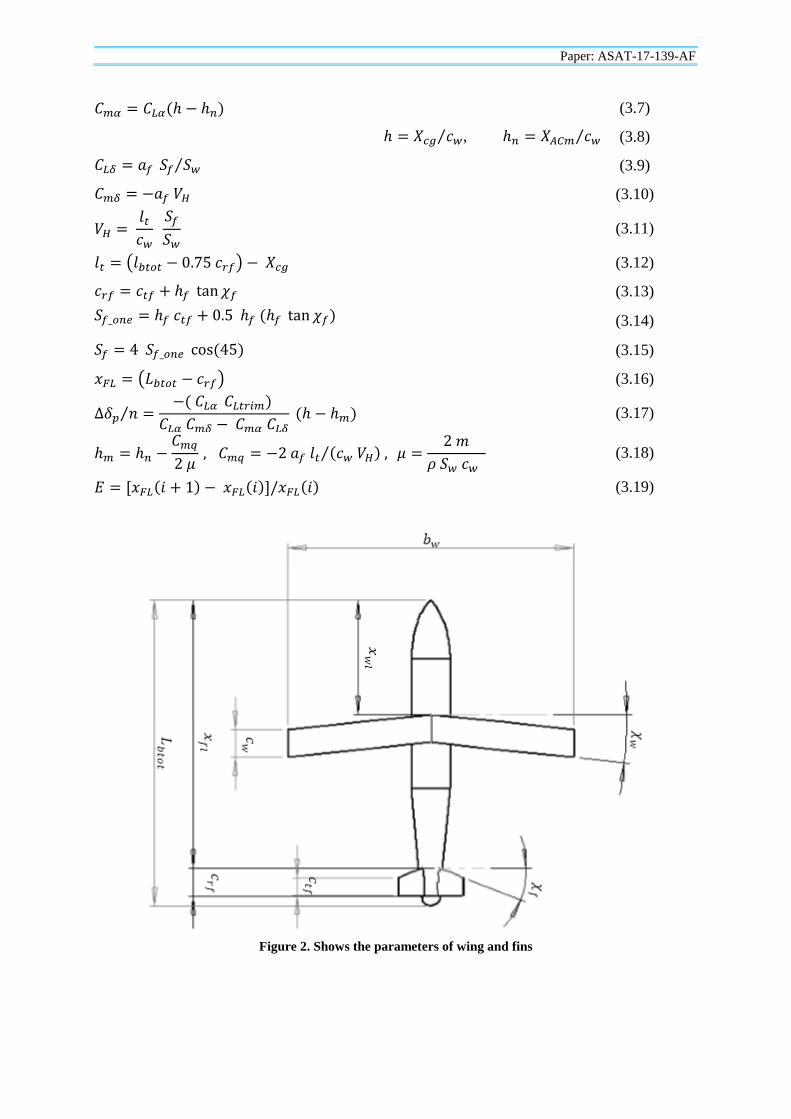
Figure 2. Shows the parameters of wing and fins


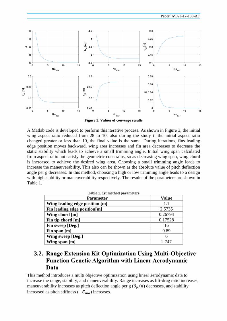
Figure 3. Values of converge results

A Matlab code is developed to perform this iterative process. As shown in Figure 3, the initial

wing aspect ratio reduced from 28 to 10, also during the study if the initial aspect ratio

changed greater or less than 10, the final value is the same. During iterations, fins leading

edge position moves backward, wing area increases and fin area decreases to decrease the

static stability which leads to achieve a small trimming angle. Initial wing span calculated

from aspect ratio not satisfy the geometric constrains, so as decreasing wing span, wing chord

is increased to achieve the desired wing area. Choosing a small trimming angle leads to

increase the maneuverability. This also can be shown as the absolute value of pitch deflection

angle per g decreases. In this method, choosing a high or low trimming angle leads to a design

with high stability or maneuverability respectively. The results of the parameters are shown in

Table 1.

Table 1. 1st method parameters

Parameter Value

Wing leading edge position [m] 1.1

Fin leading edge position[m] 2.5735

Wing chord [m] 0.26794

Fin tip chord [m] 0.17528

Fin sweep [Deg.] 16

Fin span [m] 0.89

Wing sweep [Deg.] 6

Wing span [m] 2.747

3.2. Range Extension Kit Optimization Using Multi-Objective

Function Genetic Algorithm with Linear Aerodynamic

Data

This method introduces a multi objective optimization using linear aerodynamic data to

increase the range, stability, and maneuverability. Range increases as lift-drag ratio increases,

maneuverability increases as pitch deflection angle per g ( ⁄ ) decreases, and stability

increased as pitch stiffness ( ) increases.


The optimization problem can be defined as: the objective functions is to minimize drag-lift

ratio ( ⁄ ), pitch deflection angle per g, and pitching moment curve slope ( ) using

the same theoretical equations used in the first method, subjected to the geometric and

stability constraints . The problem can be mathematically defined as:

Minimize ⁄

Minimize

Minimize ⁄

Subject to

The optimization parameters are the wing leading edge position, fin leading edge position,

wing chord, fin tip chord, and wing span, while fin span, wing and fins sweepback angles are

assumed.

[

( )

( )

]

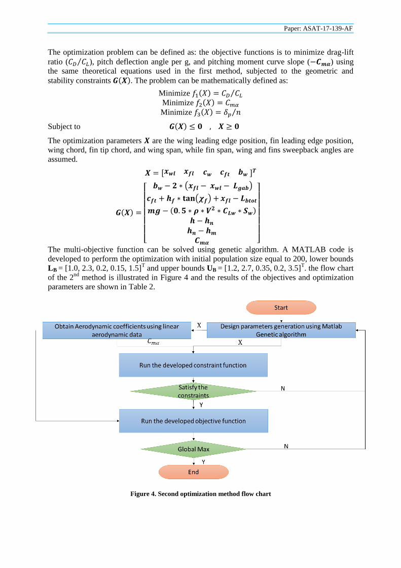
The multi-objective function can be solved using genetic algorithm. A MATLAB code is

developed to perform the optimization with initial population size equal to 200, lower bounds

LB = [1.0, 2.3, 0.2, 0.15, 1.5]T and upper bounds UB = [1.2, 2.7, 0.35, 0.2, 3.5]

T. the flow chart

of the 2nd

method is illustrated in Figure 4 and the results of the objectives and optimization

parameters are shown in Table 2.

Figure 4. Second optimization method flow chart


Table 2. Objective and optimization parameters using 2nd

method

Point

No.

Objectives Optimization Parameters

⁄ ⁄

1 0.0263 -0.0386 -0.0115 1.1000 2.5778 0.2732 0.1523 2.8045

2 0.0253 -0.0259 -0.0065 1.0719 2.5807 0.2553 0.1652 2.8353

3 0.0256 -0.0421 -0.0109 1.0999 2.5821 0.2585 0.1633 2.8107

4 0.0253 -0.0351 -0.0089 1.0869 2.5807 0.2553 0.1628 2.8340

5 0.0253 -0.0318 -0.0080 1.0815 2.5807 0.2553 0.1649 2.8353

6 0.0257 -0.0410 -0.0114 1.0999 2.5786 0.2614 0.1537 2.8074

7 0.0254 -0.0403 -0.0101 1.0958 2.5809 0.2567 0.1674 2.8205

8 0.0253 -0.0341 -0.0087 1.0853 2.5809 0.2553 0.1620 2.8340

9 0.0253 -0.0342 -0.0086 1.0854 2.5810 0.2553 0.1637 2.8344

10 0.0253 -0.0259 -0.0065 1.0719 2.5807 0.2553 0.1652 2.8353

11 0.0261 -0.0396 -0.0115 1.0999 2.5785 0.2679 0.1524 2.8057

12 0.0256 -0.0421 -0.0109 1.0999 2.5821 0.2585 0.1633 2.8107

13 0.0253 -0.0353 -0.0090 1.0873 2.5810 0.2554 0.1628 2.8340

14 0.0253 -0.0366 -0.0093 1.0893 2.5813 0.2555 0.1628 2.8340

15 0.0254 -0.0385 -0.0099 1.0930 2.5807 0.2563 0.1614 2.8252

16 0.0253 -0.0290 -0.0073 1.0769 2.5807 0.2553 0.1651 2.8353

17 0.0253 -0.0317 -0.0081 1.0814 2.5809 0.2553 0.1625 2.8344

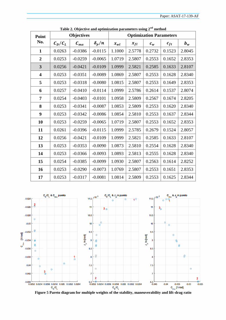
Figure 5 Pareto diagram for multiple weights of the stability, maneuverability and lift-drag ratio


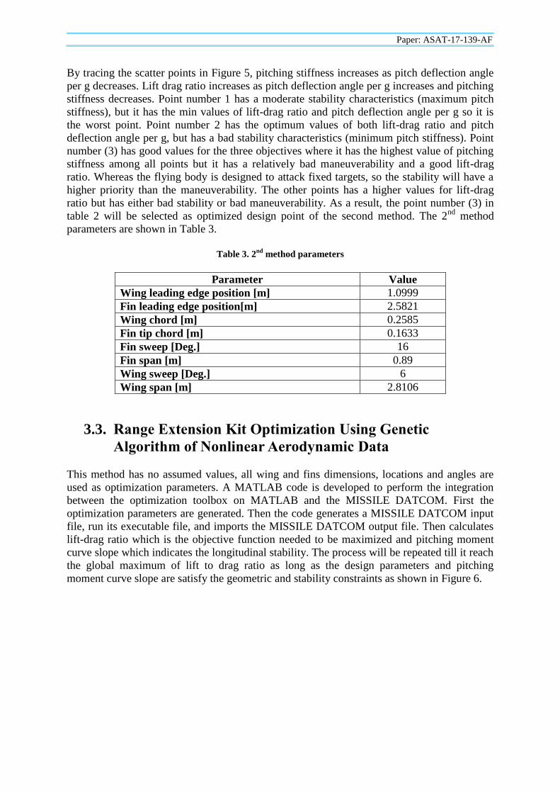
By tracing the scatter points in Figure 5, pitching stiffness increases as pitch deflection angle

per g decreases. Lift drag ratio increases as pitch deflection angle per g increases and pitching

stiffness decreases. Point number 1 has a moderate stability characteristics (maximum pitch

stiffness), but it has the min values of lift-drag ratio and pitch deflection angle per g so it is

the worst point. Point number 2 has the optimum values of both lift-drag ratio and pitch

deflection angle per g, but has a bad stability characteristics (minimum pitch stiffness). Point

number (3) has good values for the three objectives where it has the highest value of pitching

stiffness among all points but it has a relatively bad maneuverability and a good lift-drag

ratio. Whereas the flying body is designed to attack fixed targets, so the stability will have a

higher priority than the maneuverability. The other points has a higher values for lift-drag

ratio but has either bad stability or bad maneuverability. As a result, the point number (3) in

table 2 will be selected as optimized design point of the second method. The 2nd

method

parameters are shown in Table 3.

Table 3. 2

nd method parameters

Parameter Value





Fin sweep [Deg.] 16

Fin span [m] 0.89

Wing sweep [Deg.] 6

Wing span [m] 2.8106

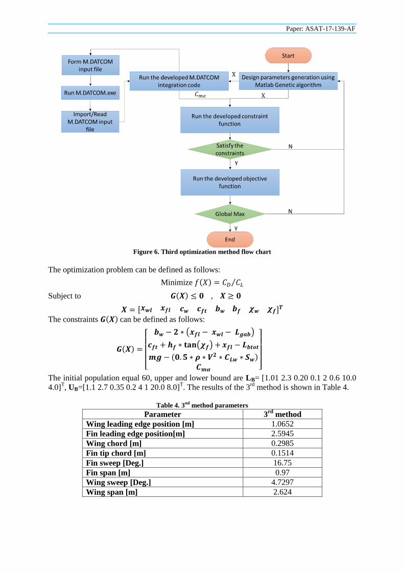
3.3. Range Extension Kit Optimization Using Genetic

Algorithm of Nonlinear Aerodynamic Data

This method has no assumed values, all wing and fins dimensions, locations and angles are

used as optimization parameters. A MATLAB code is developed to perform the integration

between the optimization toolbox on MATLAB and the MISSILE DATCOM. First the

optimization parameters are generated. Then the code generates a MISSILE DATCOM input

file, run its executable file, and imports the MISSILE DATCOM output file. Then calculates

lift-drag ratio which is the objective function needed to be maximized and pitching moment

curve slope which indicates the longitudinal stability. The process will be repeated till it reach

the global maximum of lift to drag ratio as long as the design parameters and pitching

moment curve slope are satisfy the geometric and stability constraints as shown in Figure 6.


Figure 6. Third optimization method flow chart

The optimization problem can be defined as follows:

Minimize ⁄

Subject to

The constraints can be defined as follows:

[

( )

( )

]

The initial population equal 60, upper and lower bound are LB= [1.01 2.3 0.20 0.1 2 0.6 10.0

4.0]T, UB=[1.1 2.7 0.35 0.2 4 1 20.0 8.0]

T. The results of the 3

rd method is shown in Table 4.

Table 4. 3

nd method parameters

Parameter 3rd

method





Fin sweep [Deg.] 16.75

Fin span [m] 0.97

Wing sweep [Deg.] 4.7297

Wing span [m] 2.624


3.4. Aerodynamic Characteristics and Design Parameters

Comparison of the Three Methods

The aerodynamic characteristics and design parameters comparisons are shown in

Figure 7 and Table 5 respectively.

Table 5. Parameters comparison between the three design methods. ()* means assumed values

Parameter 1st method 2

nd method 3

rd method

Wing leading edge position [m] 1.1* 1.0999 1.0652

Fin leading edge position[m] 2.5735 2.5821 2.5945

Wing chord [m] 0.26794 0.2585 0.2985

Fin tip chord [m] 0.17528 0.1633 0.1514

Fin sweep [Deg.] 16* 16* 16.75

Fin span [m] 0.89* 0.89* 0.97

Wing sweep [Deg.] 6* 6* 4.7297

Wing span [m] 2.747 2.8106 2.624

Figure 7. Aerodynamic characteristics comparison of the three design methods

By comparing the design parameters of the three methods from table 5. The 1st method has

four assumed values, 2nd

method has three assumed values and 3rd

method doesn’t have any

assumed values. From polar curve shown in Figure 7, the lift-drag ratio of the third method is

much more than the two other methods at the range of applied angles of attack, then the 2nd

method comes in the second place although it has a high lift-drag ratio but at very high angles

of attack. From the pitching moment curve shown in Figure 7, all the three methods have a

positive pitch stiffness and the second curve has the steepest slope and zero pitching moment

coefficient equal zero ( ), so the 2nd

method has the most favorable stability

characteristics. Since ( ) for the three cases, a control surface deflection must be

applied to obtain trimming angle of attack that leads to the maximum aerodynamic efficiency.

The elapsed time of the 3rd

optimization method is greater than the other methods, because of

the increment of design parameters and the integration between the multiple software to

obtain the nonlinear aerodynamic data. But it produces more accurate aerodynamic data and

more design parameters. To have more evaluation, an uncontrolled six degree of freedom

simulation has been performed.


4. Flying body Modeling and Simulation

4.1. Mathematical Modeling

The first step to develop a six degree of freedom nonlinear flight simulation model for a

flying body is to develop the mathematical model that describes the flying body dynamics and

its surroundings. The mathematical model includes the flying body Dynamic model

(equations of motion) which describes the flying body dynamics [3], the aerodynamic model

which describes the aerodynamic forces and moments represented in the body frame, gravity

model which describes the gravity force, mass-inertia model which describes the mass and

inertia properties of the total configuration of the flying body, and atmosphere model which

describes the change in atmosphere parameters along the flight.

4.1.1. Dynamic model

This dynamic model contains the nonlinear differential equations. These equations of motion

are developed assuming that the flying body is a rigid body, Earth is flat and non-rotating, and

x-z plane is the flying body plane of symmetry.

These equations can be classified into four main vector equations (force, moment, attitude,

and trajectory equations), force and moment equations are developed from Newton’s second

law and they are applied in the flying body axis, attitude equations are derived from Euler

method, and since the flying body position updates occur in the Earth frame so the trajectory

equation is used by transforming the flying body velocities to linear position rates in the Earth

axis.

The standard six degrees of freedom nonlinear differential equations for a flying body, using

Euler’s angles are as follows:

Force equation: ⁄ (4.1)

Moment equation: (4.2)

Attitude equation: (4.3)

Trajectory equation: (4.4)

These vector equations are in the form of a state space vector , each vector

equation include three unidirectional equations, so it represent twelve equations with twelve

state vectors where and is the

control input vector.

In our case study, the forces are represented in the body frame due to aerodynamic forces

and gravity forces

(no thrust) and the moment represented also in body frame due

to aerodynamic moments only.

4.1.2. Aerodynamic Model

The aerodynamic model introduces the total aerodynamic forces and moments, the forces and

moments can be written as follows:

(4.5)

These aerodynamic forces and moments can be classified into longitudinal and lateral forces

and moments [5]. The longitudinal forces and moments are affected by the angle of attack

and its derivative , pitch deflection angle and pitch rate . The lateral forces and


moments are affected by the sideslip angle , rolling deflection angle , roll rate , yaw

deflection angle , and yaw rate .

The longitudinal loads are lift force , drag force , and pitching moment are given by:

(4.6)

Also, lateral loads are side force , roll moment , and yaw moment are given by:

(4.7)

Equations (4.6) and (4.7) can be rewritten using linear approximation as:

⁄ ⁄

(4.8)

⁄ ⁄

⁄ ⁄

⁄ ⁄

⁄ ⁄ (4.9)

All the aerodynamic coefficient in equations (4.8) and (4.9) is calculated using MISSILE

DATCOM through a developed Matlab code that reads the geometry data of the flying body

from an excel sheet. This process is done for different Mach numbers, altitudes, roll deflection

angles and pitch deflection angles to give a full representation of aerodynamic coefficients

through the flight for both conventional and optimized flying bodies. The aerodynamic forces

are transformed from wind frame to body frame using the direction cosine matrix:

(4.10)

4.1.3. Gravity Model

Gravity model introduces the gravity forces of the flying body in body frame

by

converting the gravity force from Earth frame

to body frame where:

[

] (4.11)

4.1.4. Mass-Inertia Model

The mass and inertia of the flying body are 500 [Kg] and

[Kg.m2].

4.1.5. Atmosphere Model

The maximum release altitude of the flying body is 11 [Km], so the flight will be in

Troposphere layer where the temperature changes linearly with rate of -6.5 [K/Km].


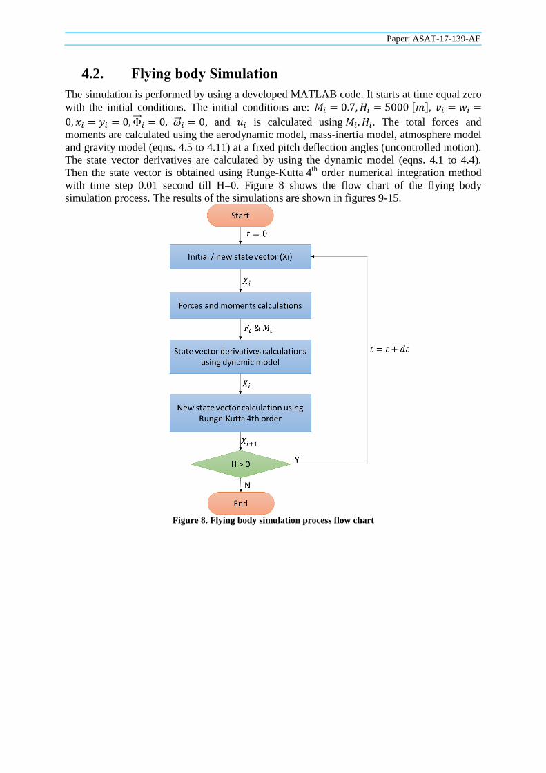
4.2. Flying body Simulation

The simulation is performed by using a developed MATLAB code. It starts at time equal zero

with the initial conditions. The initial conditions are:

, and is calculated using . The total forces and

moments are calculated using the aerodynamic model, mass-inertia model, atmosphere model

and gravity model (eqns. 4.5 to 4.11) at a fixed pitch deflection angles (uncontrolled motion).

The state vector derivatives are calculated by using the dynamic model (eqns. 4.1 to 4.4).

Then the state vector is obtained using Runge-Kutta 4th

order numerical integration method

with time step 0.01 second till H=0. Figure 8 shows the flow chart of the flying body

simulation process. The results of the simulations are shown in figures 9-15.

Figure 8. Flying body simulation process flow chart


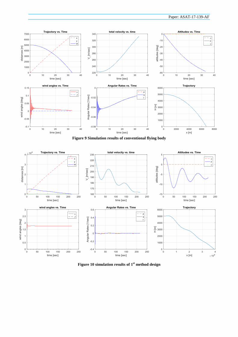
Figure 9 Simulation results of conventional flying body

Figure 10 simulation results of 1

st method design


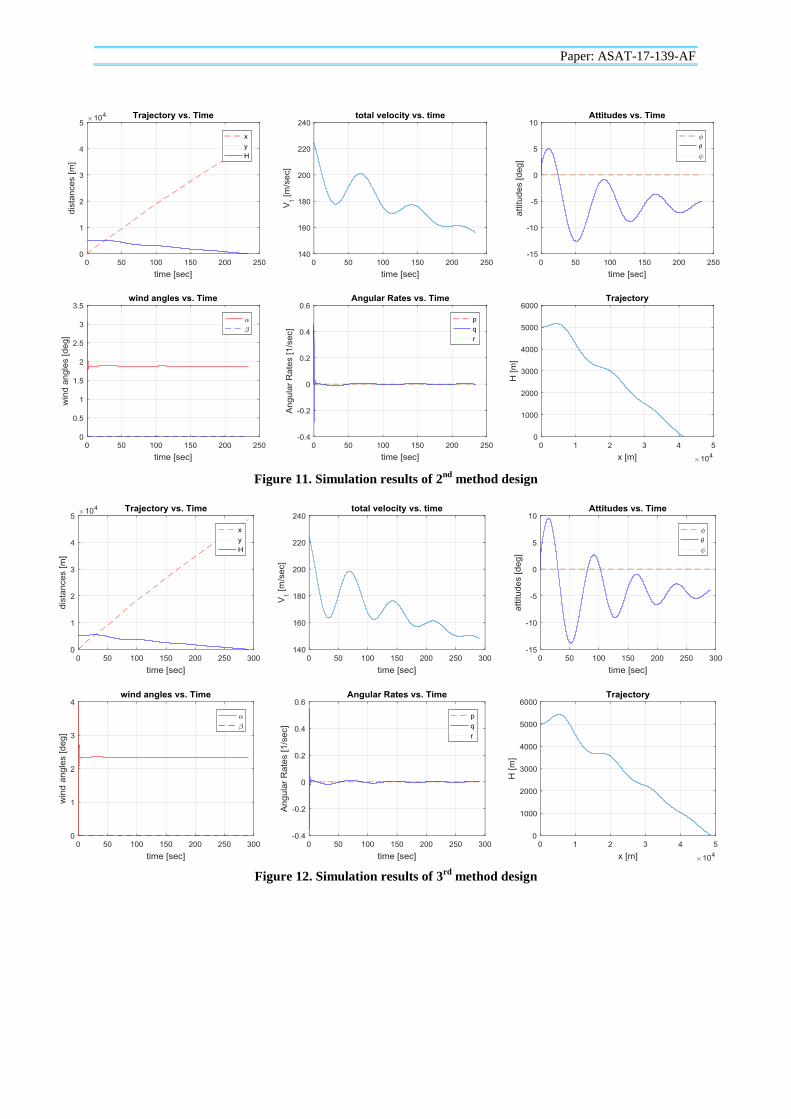
Figure 11. Simulation results of 2

nd method design

Figure 12. Simulation results of 3

rd method design


Figure 13. Comparison of Ranges

Figure 14. The three designs ranges comparison at 11 [Km] release altitude

Figure 15. Trajectories of the 3

rd method design and conventional flying body

The range of the conventional flying body reaches 6.8 Km, the total velocity increases along

the trajectory, but the pitch angle and angle of attack are not stable along the trajectory and

the flight time is 33 seconds as shown in Figure 9. The three designs are simulated with a

fixed pitch deflection angle equals 6 degrees (1.5 for each fin). The range of the 1st method is

39 Km with increment (474%), so the range is highly increases than the conventional. Also,


the flying body pitch angle and rate is fluctuating around 6 degrees and 0 sec-1

respectively

which mean that it is dynamically stable, the angle of attack stabilized at 1.758 degrees, and

flight time is 216 seconds as shown in Figure 10. The 2nd

method range is 41.24 Km with

increment (506.5%), pitch angle and pitch rate fluctuate around 6 degrees and 0 sec-1

respectively, angle of attack stabilized at 1.88 degrees, and flight time is about 234 seconds as

shown in Figure 11. The 3rd

method range is 48.6 Km with increment (614.7%), pitch angle

and pitch rate fluctuate around 4 degrees and 0 sec-1

respectively, angle of attack stabilized at

2.335 degrees, and flight time is 291 seconds as shown in Figure 12. This simulations shows

that the ranges of the 1st and 2

nd are very close to each other whereas they differs only 2.24

Km, the 3rd

method pitch angle is less than the 1st and 2

nd methods, and the angle of attack

stabilized at the highest one which indicates that the 3rd

method range should be more than the

others. By comparing the ranges, the 3rd

method range is higher than the 2nd

methods by 7.4

Km as shown in Figure 13. The 3rd

method and conventional flying bodies 3D trajectories are

shown with attitudes change in Figure 15.

The maximum release altitude of the conventional flying body is 5 Km, but adding the wing

and fins allow to increase the release altitude of the flying body. Another simulation is

performed for the three designs at [11 Km] release altitude. The ranges of the flying vehicles

is extremely increased where the ranges of the first, second and third designs are 72.6, 76.4,

and 90.06 km with an increment of (967.65%), (1023.53%), and (1224.41%) respectively as

shown in Figure 14.

5. Conclusion

A completely generic aerodynamic optimization tool with a new geometric parameterization

technique for application to nonlinear aerodynamic data has been developed and applied to

wing and fins optimization. Linear methods (1st and 2

nd methods) is used as initial steps for

the nonlinear method (3rd

method) and they give an indication of parametric changing and

reduce the 3rd

method running time.

The 1st method is effective in choosing the dominant characteristics between stability and

maneuverability. If the maneuverability/stability characteristics are the dominant, select a

low/high trimming deflection angle respectively. The 2nd

method shows more detailed results

and has the ability to select a specified characteristic between stability, maneuverability and

lift-drag ratio. The 3rd

method uses the nonlinear aerodynamic data, and it has many design

parameters such as wing and fins sweepback angles. Wing and fins sweepback angles are very

effective in drag calculations at high speed. The increase of sweepback angles lead to the

increase of the divergence drag Mach number. Consequently, choosing the sweepback angles

as design parameters will surly increase the range. The best method is the nonlinear method

(3rd

method) with range increment is 614.7% at 5 [Km] release altitude. Also the output of the

third method can be used as an initial guess for a CFD gradient based optimization method

which will magnificently decrease the number of CFD’s runs, time and cost.

Adding a range extension kit leads to increase the range with low glide angle. So, if it flies

without control, it would hit the target with very low impact angle. The solution of this

problem is discussed in details in a next paper under processing where the flying body must

trace a designed trajectory. This trajectory has minimum glide angle to get a maximum range,

also it has the maximum velocity and impact angle at the collusion. This can be achieved by

using inverse dynamics approach to obtain the control deflection angles along the trajectory

which allow the flying body to follow the designed trajectory.


6. References

[1] A. Viti, T. Druot, and A. Dumont, "Aero-structural approach coupled with direct

operative cost optimization for new aircraft concept in preliminary design," in 17th

AIAA/ISSMO Multidisciplinary Analysis and Optimization Conference, 2016, p. 3512.

[2] R. M. Cummings, C. M. Liersch, A. Schütte, and K. C. Huber, "Aerodynamics and

conceptual design studies on an unmanned combat aerial vehicle configuration,"

Journal of Aircraft, pp. 1-21, 2016.

[3] A. M. Kamal, A. Bayoumy, and A. Elshabka, "Modeling and flight simulation of

unmanned aerial vehicle enhanced with fine tuning," Aerospace Science and

Technology, vol. 51, pp. 106-117, 2016.

[4] S. A. Andrews and R. E. Perez, "Parametric study of box-wing aerodynamics for

minimum drag under stability and maneuverability constraints," in 33rd AIAA Applied

Aerodynamics Conference, 2015, p. 3291.

[5] A. Kamal, A. M. Aly, and A. Elshabka, "Modeling, analysis and validation of a small

airplane flight dynamics," in AIAA Modeling and Simulation Technologies

Conference, 2015, p. 1138.

[6] T. Takahashi, "The search for the optimal wing configuration for small subsonic air

vehicles," in 12th AIAA/ISSMO Multidisciplinary Analysis and Optimization

Conference, 2008, p. 5915.

[7] L. Tang, D. Liu, and P.-C. Chen, "Extension of projectile range using oblique-wing

concept," Journal of aircraft, vol. 44, pp. 774-779, 2007.

[8] A. Vicini and D. Quagliarella, "Airfoil and wing design through hybrid optimization

strategies," AIAA journal, vol. 37, pp. 634-641, 1999.

[9] S. Austin, "Investigation of range extension with a genetic algorithm," in 7th

AIAA/USAF/NASA/ISSMO Symposium on Multidisciplinary Analysis and

Optimization, 1998, p. 4880.

[10] M. Anderson and G. Gebert, "Using pareto genetic algorithms for preliminary

subsonic wing design," in 6th Symposium on Multidisciplinary Analysis and

Optimization, 1996, p. 4023.

[11] S. Wakayama and I. Kroo, "Subsonic wing planform design using multidisciplinary

optimization," Journal of Aircraft, vol. 32, pp. 746-753, 1995.

[12] M. Anderson, "The potential of genetic algorithms for subsonic wing design," in

Aircraft Engineering, Technology, and Operations Congress, 1995, p. 3925.

[13] B. Etkin, Dynamics of flight: stability and control vol. 3: Wiley New York, 1982.

[14] R. G. . Maydew, "Aerodynamic design of an extended range bomb," Journal of

Aircraft, vol. 17, pp. 385-386, 1980.

Aerodynamic Design Optimization of Range Extension Kit of a ...

Documents

Transcript of Aerodynamic Design Optimization of Range Extension Kit of a ...