Aerodynamic Centers of Arbitrary Airfoils

Utah State University Utah State University

DigitalCommons@USU DigitalCommons@USU

All Graduate Theses and Dissertations Graduate Studies

12-2017

Aerodynamic Centers of Arbitrary Airfoils Aerodynamic Centers of Arbitrary Airfoils

Orrin Dean Pope Utah State University

Follow this and additional works at: https://digitalcommons.usu.edu/etd

Part of the Mechanical Engineering Commons

Recommended Citation Recommended Citation Pope, Orrin Dean, "Aerodynamic Centers of Arbitrary Airfoils" (2017). All Graduate Theses and Dissertations. 6890. https://digitalcommons.usu.edu/etd/6890

This Thesis is brought to you for free and open access by the Graduate Studies at DigitalCommons@USU. It has been accepted for inclusion in All Graduate Theses and Dissertations by an authorized administrator of DigitalCommons@USU. For more information, please contact [email protected].

https://digitalcommons.usu.edu/

https://digitalcommons.usu.edu/etd

https://digitalcommons.usu.edu/gradstudies

https://digitalcommons.usu.edu/etd?utm_source=digitalcommons.usu.edu%2Fetd%2F6890&utm_medium=PDF&utm_campaign=PDFCoverPages

http://network.bepress.com/hgg/discipline/293?utm_source=digitalcommons.usu.edu%2Fetd%2F6890&utm_medium=PDF&utm_campaign=PDFCoverPages

https://digitalcommons.usu.edu/etd/6890?utm_source=digitalcommons.usu.edu%2Fetd%2F6890&utm_medium=PDF&utm_campaign=PDFCoverPages

mailto:[email protected]

http://library.usu.edu/

http://library.usu.edu/

AERODYNAMIC CENTERS OF ARBITRARY AIRFOILS

by

Orrin Dean Pope

A thesis submitted in partial fulfillment of the requirements of the degree

of

MASTER OF SCIENCE

in

Mechanical Engineering

Approved: ______________________ ____________________ Douglas Hunsaker, Ph.D. Stephan A. Whitmore, Ph.D. Major Professor Committee Member ______________________ ____________________ Geordi Richards, Ph.D. Mark R. McLellan, Ph.D. Committee Member Vice President for Research and Dean of the School of Graduate Studies

UTAH STATE UNIVERSITY Logan, Utah

2017

ii

Copyright © Orrin Dean Pope 2017

All Rights Reserved

iii

ABSTRACT

Aerodynamic Centers of Arbitrary Airfoils

by

Orrin Dean Pope, Master of Science

Utah State University, 2017

Major Professor: Douglas Hunsaker, Ph.D. Department: Mechanical and Aerospace Engineering

A method for accurately predicting the aerodynamic center of an airfoil is

presented based on a general form for the nonlinear lift and pitching-moment of an airfoil

as a function of angle of attack. This method does not suffer from small-angle, small-

camber, and thin-airfoil approximations, and is shown to match inviscid results to much

higher accuracy than the traditional methods. It is shown that the aerodynamic center of

an airfoil with arbitrary amounts of thickness and camber in an inviscid flow does not, in

general, lie at the quarter-chord. Rather, it is a single, deterministic point, independent of

angle of attack, which lies at the quarter chord only in the limit as the airfoil thickness

and camber approach zero. Furthermore, it is shown that once viscous effects are

included, the aerodynamic center is not in general a single point as predicted by

traditional thin airfoil theory, but is a function of angle of attack. Differences between

nonlinear predictions and those based on thin airfoil theory are on the order of 1-5%,

which can be significant when predicting aircraft stability.

(135 pages)

iv

PUBLIC ABSTRACT

Aerodynamic Centers of Arbitrary Airfoils

Orrin Dean Pope

The study of designing stable aircraft has been widespread and ongoing since the

early days of Orville and Wilbur Wright and their famous Wright Flyer airplane. All

aircraft as they fly through the air are subject to minor changes in the forces acting on

them. The field of aircraft stability seeks to understand and predict how aircraft will

respond to these changes in forces and to design aircraft such that when these forces

change the aircraft remains stable. The mathematical equations used to predict aircraft

stability rely on knowledge of the location of the aerodynamic center, the point through

which aerodynamic forces act on an aircraft. The aerodynamic center of an aircraft is a

function of the aerodynamic centers of each individual wing, and the aerodynamic center

of each wing is a function of the aerodynamic centers of the individual airfoils from

which the wing is made. The ability to more accurately predict the location of the airfoil

aerodynamic center corresponds directly to an increase in the accuracy of aircraft stability

calculations.

The Aerolab at Utah State University has develop new analytic mathematical

expressions to describe the location of the airfoil aerodynamic center. These new

expressions do not suffer from any of the restrictions, or approximations found in

traditional methods, and therefore result in more accurate predictions of airfoil

aerodynamic centers and by extension, more accurate aircraft stability predictions.

v

ACKNOWLEDGMENTS

I would like to specifically thank Dr. Doug Hunsaker for his guidance, support,

and unending passion for aircraft and aeronautics. I am also thankful to the Utah NASA

Space Grant Consortium (award NNX15A124H) for funding this research.

I give special thanks to my colleagues, friends, and especially my family who

have always supported me throughout my Master’s program and through all of my

engineering education.

Orrin Dean Pope

vi

CONTENTS

Page

ABSTRACT ....................................................................................................................... iii

PUBLIC ABSTRACT ....................................................................................................... iv

ACKNOWLEDGMENTS ...................................................................................................v

LIST OF TABLES ........................................................................................................... viii

LIST OF FIGURES ........................................................................................................... ix

NOTATION .........................................................................................................................x

CHAPTER 1 INTRODUCTION .........................................................................................................1

1.1 Research Motivation ..............................................................................................1 1.2 Literature Review ...................................................................................................2

1.2.1 Traditional Thin Airfoil Theory Relations for the Aerodynamic Center .........2 1.2.2 General Relations for the Aerodynamic Center ..............................................5

2 ALTERNATIVE APPROACH TO FINDING THE LOCATION OF THE AERODYNAMIC CENTER .......................................................................................8 2.1 The Aerodynamic Center as a Function of Coefficient of Lift ..............................8 2.2 The Aerodynamic Center as a Function of Normal-force Coefficient .................12

2.2.1 Equivalence Proof ..........................................................................................15 2.3 Sample Results ......................................................................................................18

2.3.1 Vortex Panel Method .....................................................................................18 2.3.2 Finite Difference Method ...............................................................................20

3 THE AERODYNAMIC CENTER OF INVISCID AIRFOILS ..................................24 3.1 Classical Thin Airfoil Theory ...............................................................................24 3.2 General Airfoil Theory .........................................................................................27

3.2.1 Theory Development .....................................................................................28 3.2.2 Comparison to Inviscid Computational Results ............................................38

vii

3.3 Least Squares Regression Fit Coefficients-Inviscid Flow ....................................44 3.3.1 Fit to Thin Airfoil Theory Equations ........................................................44 3.3.2 Fit to General Airfoil Theory Equations ...................................................46

3.4 The Aerodynamic Center of Airfoils in Inviscid Flow .........................................48 3.4.1 Thin Airfoil Theory with Trigonometric Nonlinearities ................................48 3.4.2 General Airfoil Theory ..................................................................................49

4 THE AERODYNAMIC CENTER OF VISCOUS AIRFOILS ..................................54 4.1 The Aerodynamic Center of Airfoils in Viscous Flow .........................................54 4.2 Third Order Approximation ..................................................................................58 4.3 Sample Results ......................................................................................................60 4.4 Least Squares Regression Fit Coefficients-Viscous Flow ....................................70

5 CONCLUSION ...........................................................................................................74

REFERENCES ..................................................................................................................77

APPENDICES ...................................................................................................................80 A Viscous Least Squares Regression Fit Coefficients ...................................................81 B Vortex Panel Method Code .......................................................................................86 C Analytical Symbolic Solver Code ..............................................................................93 D Inviscid Aerodynamic Center NACA Airfoil Camber/Thickness Code ..................117

viii

LIST OF TABLES

Table Page

1 Vortex panel method data for NACA 8415 airfoil, 107 ≤≤− α ......................19

2 Vortex panel method data for NACA 8415 airfoil, 1510 ≤≤− α ....................40

3 Least squares regression coefficients for NACA 8415 airfoil ..........................41

4 Viscous least squares regression fit coefficient data for a series of NACA four digit airfoils ................................................................................................61

5 RMS error of high order solution and third order approximation using XFOIL data ..............................................................................................63

6 RMS error of high order solution and third order approximation using XFOIL data ..............................................................................................66

ix

LIST OF FIGURES

Figure Page

1 Forces and pitching moment on an airfoil...........................................................3

2 The aerodynamic center of a NACA 8415 airfoil in inviscid flow as a function of angle of attack and the normal-force ..............................................21

3 Superposition of a uniform flow and a curved vortex sheet along the camber line of a thin airfoil section ...................................................................26

4 Circular cylinder in the complexζ - plane ........................................................31

5 RMS error for thin airfoil theory and general airfoil theory lift predictions for 250 NACA airfoils in inviscid flow .............................................................42

6 RMS error for thin airfoil theory and general airfoil theory pitching moment predictions for 250 NACA airfoils in inviscid flow ............................42

7 The aerodynamic center of a NACA 8415 airfoil in inviscid flow predicted by thin airfoil theory, general airfoil theory, and finite differencing .......................................................................................................51

8 The pitching moment about the aerodynamic center of a NACA 8415 airfoil in inviscid flow predicted by thin airfoil theory, general airfoil theory, and finite differencing ...........................................................................51

9 The aerodynamic center of 250 NACA airfoils in inviscid flow as a function of airfoil thickness and camber ...........................................................52

10 The aerodynamic center location of a selection of NACA airfoils in viscous flow comparing the high order solution and third order approximation using Abbott & Von Doenhoff data ..........................................62

11 The aerodynamic center location of a selection of NACA airfoils in viscous flow comparing the high order solution and third order approximation using XFOIL data ......................................................................65

12 Aerodynamic center locations for a NACA 1408 airfoil in viscous flow data ....................................................................................................................68

13 Pitching moment about the aerodynamic center of a NACA 1408 airfoil in viscous flow ...................................................................................................69

x

NOTATION

nB = coefficients in the expansion given in Eq. (47)

AC~ = section axial-force coefficient

α,~

AC = first derivative of AC~ with respect to α

αα ,,~

AC = second derivative of AC~ with respect to α

DC~ = section drag coefficient

0

~DC = section drag coefficient at zero lift, Eq. (67)

LDC ,0

~ = coefficient of LC~ in the parabolic relation for DC~ , Eq. (67)

20 ,

~LDC = coefficient of 2~

LC in the parabolic relation for DC~ , Eq. (67)

LC~ = section lift coefficient

α,~

LC = first derivative of LC~ with respect to α

α,0~

LC = first derivative of LC~ with respect to α, at α =0

mC~ = section moment coefficient about the point (x, y)

acmC~ = section moment coefficient about the aerodynamic center

4

~cmC = section moment coefficient about the quarter-chord

lemC~ = section moment coefficient about the leading-edge

OmC~ = section moment coefficient about the origin

α,~

OmC = first derivative of OmC~ with respect to α

αα ,,~

OmC = second derivative of OmC~ with respect to α

xi

AmC ,~ = constant coefficient used in Eqs. (55) and (68)

NmC ,~ = constant coefficient used in Eqs. (55) and (68)

α,0~

mC = constant coefficient used in Eqs. (55) and (68)

NC~ = section normal-force coefficient

α,~

NC = first derivative of NC~ with respect to α

αα ,,~

NC = second derivative of NC~ with respect to α

nC = complex constants in the Laurent series expansion

c = section chord length

F1, F2 = Laurent series expansions used in Eqs. (44) and (45)

K1, K2 = constants defined in Eq. (78)

L~ = section lift

Om~ = pitching moment about the origin

n = term in the Laurent series expansion

R = radius of the circular cylinder used for the conformal transformation

∞V = freestream airspeed

w = complex velocity field

w1 = complex velocity in the plane of the circular cylinder

w2 = complex velocity in the plane of the airfoil

yx, = axial and upward-normal coordinates relative to the leading edge

0x = real coordinate of the center of the circular cylinder in the complex plane

acac yx , = x and y coordinates of the aerodynamic center

xii

cy = y coordinate of the camber line

0y = imaginary coordinate of the center of the circular cylinder in the complex plane

z = coordinate in the complex plane

lz = leading edge of the airfoil in the z-plane

tz = trailing edge of the airfoil in the z-plane

0z = center of the circular cylinder in the complex plane, 000 iyxz +=

α = angle of attack

0Lα = zero-lift angle of attack

Γ = circulation strength

ζ = analytic transformation function

lζ = point in the complex plane that maps to the airfoil leading edge

surfaceζ = coordinates of the cylinder surface

tζ = point in the complex plane that maps to the airfoil trailing edge

Θ = change of variables for the axial coordinate of an airfoil

θ = angle relative to the horizontal axis in the complex plane

θt = value of θ at the airfoil trailing edge

ρ = fluid density

Φ1 = complex potential in the plane of the circular cylinder

Φ2 = complex potential in the plane of the airfoil

φ = local camber angle

CHAPTER 1

INTRODUCTION

1.1 Research Motivation

Correctly identifying the location of the aerodynamic center of a lifting surface is

extremely important in aircraft design and analysis. For example, the location of the

aerodynamic center of a complete aircraft relative to the center of gravity is an important

measure of longitudinal pitch stability [1-2]. This location, often referred to as the neutral

point, is a function of the aerodynamic center of each lifting surface or wing. In addition

to longitudinal pitch stability, accurate knowledge of the location of the aerodynamic

center of a lifting surface or wing has been shown to be a fundamental parameter in

aeroelastic analysis as well as flutter and divergence speed calculations [3]. The

importance of correctly identifying the location of the aerodynamic center of a lifting

surface is also apparent in supersonic aircraft design. Efforts to minimize trim drag,

maximize load factor capability, and to provide acceptable handling qualities, rely on

accurate knowledge of the location of the aerodynamic center of a supersonic lifting

surface [4]. The aerodynamic center of a wing is a function of the aerodynamic center of

the individual airfoils from which the wing is made, as well as wing sweep, dihedral, and

planform. Thus, correctly predicting the aerodynamic center or neutral point of a

complete airframe during preliminary design depends on the accuracy to which we can

predict the aerodynamic centers of airfoils and finite wings.

2 1.2 Literature Review

1.2.1 Traditional Thin Airfoil Theory Relations for the Aerodynamic Center

The aerodynamic center is traditionally defined to be the point about which the

pitching moment is invariant to small changes in angle of attack, i.e.

0~

≡∂

∂α

acmC (1.1)

The pitching moment about any point in the airfoil plane can be found from a simple

transformation of forces and moments about the origin to the point of interest, i.e.,

ANmm CcyC

cxCC

O

~~~~−+= (1.2)

where OmC~ is the pitching moment about the origin, AC~ is the axial force coefficient, and

NC~ is the normal force coefficient. The axial and normal force coefficients are related to

the lift and drag coefficients through a transformation in angle of attack, as shown in Fig.

1

αα sin~cos~~LDA CCC −= (1.3)

αα sin~cos~~DLN CCC += (1.4)

Using Eqs. (1.3) and (1.4) in Eq. (1.2), the pitching moment about the aerodynamic

center is

)sin~cos~()sin~cos~(~~ αααα LDac

DLac

mm CCc

yCC

cx

CCOac

−−++= (1.5)

3 For a typical airfoil, the vertical offset of the aerodynamic center from the airfoil chord

line is small, and the drag is much less than the lift. Additionally, the angle of attack is

small for normal flight conditions. Therefore, applying the traditional approximations,

αα sin~cos~DL CC >> , 0sin ≅αacy , 0~

≅DacCy , 1cos ≅α , gives

Lac

mm Cc

xCC

Oac

~~~+= (1.6)

Taking the derivative of Eq. (1.6) with respect to angle of attack, applying the constraint

given by Eq. (1.1), and rearranging gives the traditional approximation for the

aerodynamic center

α

α

,

,~

~

L

mac

C

Cc

x O−= , 0=c

yac (1.7)

Note that the y-coordinate is traditionally assumed to be zero due to the approximations

applied in the development of Eq. (1.6).

Figure 1. Forces and pitching moment on an airfoil.

4 Equation (1.7) gives the traditional approximation for the location of the

aerodynamic center of an airfoil. These relations require knowledge of the lift and

pitching moment slopes of a given airfoil. This prediction for the location of the

aerodynamic center of an airfoil is widely used today across the aerospace industry and

academia. Furthermore, these relations are traditionally used to approximate the location

of the neutral point of an aircraft, and are used to evaluate aircraft static stability. The

traditional thin airfoil theory approach as developed by Max Munk [5-9] predicts

solutions to Eq. (1.7) as lying at the airfoil quarter chord, or 25% aft of the airfoil leading

edge, and directly on the chord line. However, solutions to Eq. (1.7) suffer from small-

angle, small-camber, and thin-airfoil approximations. What’s more, the assumptions

leading to the result given by Eq. (1.7) include a linear lift slope and a moment slope

below stall, and therefore neglect nonlinearities in lift, pitching moment, and drag.

Furthermore, this traditional approach reduces the nonlinear trigonometric relations in

Eq. (1.5) to linear functions of angle of attack. These linearizing approximations

significantly hinder our understanding of the effects of nonlinearities associated with

pitch stability of airfoils and aircraft. Attempts have been made to develop less restrictive

definitions for the location of the airfoil aerodynamic center, however do not account for

all of the trigonometric and aerodynamic nonlinearities, nor remove all small-angle,

small-camber, and thin-airfoil approximations [10-11].

In order to provide a more accurate solution for the location of the aerodynamic

center, we shall now relax the linearizing assumptions in a more general development of

the aerodynamic center.

5

1.2.2 General Relations for the Aerodynamic Center

Phillips, Alley, and Niewoehner [12] presented general relations for the

aerodynamic center, which do not include the linearizing approximations used in the

traditional approach. From Eq. (1.2) or (1.5), the pitching moment about the aerodynamic

center can be written

Aac

Nac

mm Cc

yC

cx

CCOac

~~~~−+= (1.8)

Taking the derivative of Eq. (1.8) with respect to angle of attack and applying the

traditional constraints given in Eq. (1.1) gives

ααα ,,,~~~

OmAac

Nac CC

cy

Cc

x−=− (1.9)

Note that application of the constraint given in Eq. (1.1) produces an equation for a line,

not a point. The line given in Eq. (1.9) is the neutral axis of the airfoil [12]. All points

along this line satisfy the constraint given in Eq. (1.1). Therefore, the single constraint

given in Eq. (1.1) is not sufficient to specify a single point as the aerodynamic center.

Phillips, Alley, and Niewoehner [12] suggest a second constraint to isolate the location of

the aerodynamic center, namely, that the location of the aerodynamic center must be

invariant to small changes in angle of attack, i.e.,

0≡∂∂

αacx

, 0≡∂∂

αacy

(1.10)

Differentiating Eq. (1.9) with respect to angle of attack, and applying Eq. (1.10) gives

6

αααααα ,,,,,,~~~

OmAac

Nac CC

cy

Cc

x−=− (1.11)

The intersection of the two lines specified by Eqs. (1.9) and (1.11) defines a

unique point where both of the constraints are simultaneously satisfied, and therefore

defines the location of the aerodynamic center. Solving Eqs. (1.9) and (1.11) for xac and

yac, and using the result in Eq. (1.8) gives the location of the aerodynamic center and the

pitching moment coefficient about the aerodynamic center

αααααα

αααααα

,,,,,,

,,,,,,~~~~

~~~~

NAAN

AmmAac

CCCC

CCCCc

x OO

−

−= (1.12)

αααααα

αααααα

,,,,,,

,,,,,,~~~~

~~~~

NAAN

NmmNac

CCCC

CCCCc

y OO

−

−= (1.13)

Aac

Nac

mm Cc

yC

cx

CCOac

~~~~−+= (1.14)

Equations (1.12) and (1.13) offer a more accurate description of the location of

the aerodynamic center for any lifting surface. They allow both the x and y coordinates of

the aerodynamic center to be evaluated, unlike the traditional approximations given in

Eq. (1.7), which always predicts a y-coordinate for the aerodynamic center that lies on the

chord line. Furthermore, Eqs. (1.12) and (1.13) correctly include the effects of vertical

offsets as well as trigonometric nonlinearities and aerodynamic nonlinearities such as

drag.

Note that Eqs. (1.12) and (1.13) are dependent on first and second aerodynamic

derivatives with respect to angle of attack, while the traditional approximation given in

7 Eq. (1.7) depends only on first derivatives of aerodynamic properties. Therefore, this

general solution for the aerodynamic center depends on accurately predicting any second-

order aerodynamic nonlinearities, even below stall. To estimate the aerodynamic center

of airfoils, thin airfoil theory is often applied, which, as will be shown in Chapter 3,

neglects these second-order nonlinearities.

Two unique alternative forms of Eqs. (1.12) and (1.13) can be developed which

do not rely on first and second aerodynamic derivatives with respect to angle of attack,

but rather rely on first and second derivatives with respect to coefficient of lift and the

normal-force coefficient respectively. These alternative forms may be useful when

comparing the aerodynamic centers of two different lifting surfaces where one desires to

fix the design for a given value of lift or normal-force while allowing variation in angle

of attack.

8

CHAPTER 2

ALTERNATIVE APPROACH TO FINDING THE LOCATION OF THE

AERODYNAMIC CENTER

2.1 The Aerodynamic Center as a Function of Coefficient of Lift

The relations developed for the location of the aerodynamic center using

traditional thin airfoil theory and the more general approach as developed by Phillips [12]

both are functions of angle of attack as can be seen in Eq. (1.7) and Eqs. (1.12-1.13)

respectively. The value of these relations depend largely on wing and airfoil geometry.

Consider two wings with different geometry, both at the same angle of attack. Each of

these wings will have a unique coefficient of lift and therefore unique locations of their

respective aerodynamic centers. This is due to the fact that the lift distribution generated

over a range of angles of attack varies from wing to wing based on section and span

geometry. It is advantageous therefore to be able to describe the location of the

aerodynamic center independent of wing or airfoil geometry.

In order to accomplish this, we modify the method presented by Phillips [12]

whereby we redefine the change in pitching moment coefficient and the location of the

aerodynamic center to depend not on small changes in angle of attack, but rather on small

changes in coefficient of lift. We redefine the original two constraints given by Eq. (1.1)

and Eq. (1.10) as follows

1. The pitching moment about the aerodynamic center must be invariant to small

changes in coefficient of lift

9

0~~

≡∂

∂

L

mac

CC (2.1)

2. The location of the aerodynamic center must be invariant to small changes in

coefficient of lift

0~ ≡∂∂

L

ac

Cx

, 0~ ≡∂∂

L

ac

Cy

(2.2)

Using these two new definitions, the location of the aerodynamic center as a

function of coefficient of lift will be developed. Consider the definition of the pitching

moment and force components normalized by span and divided by dynamic pressure

∫

∫ ∫=

−=

=

−=

=

−=∞

−

−+−=

2/

2/

2/

2/

2/

2/

22

21

0

~)cos~sin~(

~)sin~cos~(~

bz

bzacDL

bz

bz

bz

bzacDLm

dzycCC

dzxcCCdzcCV

mac

αα

ααρ

(2.3)

Applying the definition for the mean moment coefficient and the mean aerodynamic

chord length and dividing by the planform area S, we arrive at the modified definition for

the pitching moment about the origin of an arbitrary wing.

αα

αρ

cos~sin~sin~

cos~~~2

21

DDLLDD

LLrefmO

refm

yCyCxC

xCcCSV

mcCacO

+−−

−=∞ (2.4)

where ∫=

≡2/

0

2~2~ b

zmac

mm dzcC

cSC

ac

ac and ∫

=

≡2/

0

22 b

zmac dzc

Sc

10

Using the definition of the pitching moment about the aerodynamic center and dividing it

by dynamic pressure and the planform area S gives

)cossin()sincos( ααα DLacDLacrefacmrefm CCyCCxcCcCO

−−−−= (2.5)

Combining Eq. (2.4) and Eq. (2.5), we obtain

acac

ac

mm

LDLDDLLLLL

refmDLacDLac

cC

CyCxCCyCxC

cCCCyCCx

~)~cos~sin(~)~sin~cos(~

~)cos~sin~()sin~cos~(

−

−++

=−−+− ααα

(2.6)

Modifying the definition of the section change in pitching moment about the

aerodynamic center defined by Eq. (2.1) to be with respect to coefficient of lift is given as

0~

~≡

∂

∂

L

m

CC

ac (2.7)

Using Eqs. (2.1), (2.2) and (2.7), in the first derivatives of Eqs. (2.4) and (2.6) with

respect to coefficient of lift we obtain

L

mref

LDLDDLLLLLL

DLL

acDLL

ac

CC

c

CyCxCCyCxCC

CCC

yCCC

x

O~~

)]~cos~sin(~)~sin~cos(~[~

)cos~sin~()sin~cos~(~

∂

∂−=

−++∂

∂

=−∂

∂++

∂∂ ααα

(2.8)

As previously stated, the location of the aerodynamic center is not defined by a

single point but rather by the intersection of two lines. The first line is defined by Eq.

11 (2.8). This equation describes a line in the plane of symmetry along which every point

satisfies the first constraint on the location of the aerodynamic center (Eq. (2.1)). To

uniquely define a point along this line a second equation is need that satisfies the second

constraint given by Eq. (2.2). To obtain this additional equation we first rewrite Eqs. (2.5)

and (2.8) in terms of axial and normal coefficients

αα sin~cos~~LDA CCC −= (2.9)

αα sin~cos~~DLN CCC −= (2.10)

which yields

AacNacrefmrefm CyCxcCcCacO

~~~~+−= (2.11)

refCmCAacCNac cCCyCxLOLL

~,~,~,

~~~−=− (2.12)

Equation. (2.12) is equivalent to Eq. (2.8) and defines a line which satisfies the first

constraint for given coefficients of lift. To obtain the second line, which is necessary to

define the location of the aerodynamic center, we differentiate Eq. (2.12) with respect to

coefficient of lift and apply the second constraint. This gives

refCCmCCAacCCNac cCCyCxLLOLLLL

~,~,~,~,~,~,

~~~−=− (2.13)

As is the case for the line defined by Eq. (2.12), where every point along the line

satisfies the first constraint, every point along the line defined by Eq. (2.13) satisfies the

second constraint on the location of the aerodynamic center. The intersection of these two

lines uniquely defines a point where both of the constraints are simultaneously satisfied,

12 and therefore defines the location of the aerodynamic center. Solving Eqs. (2.12) and

(2.13) for cxac and cyac , and using the results in Eq. (2.11) we obtain

LLLLLL

LLLOLLOL

CCNCACCACN

CCACmCCmCAac

CCCC

CCCC

cx

~,~,~,~,~,~,

~,~,~,~,~,~,~~~~

~~~~

−

−= (2.14)

LLLLLL

LLLOLLOL

CCNCACCACN

CCNCmCCmCNac

CCCC

CCCC

cy

~,~,~,~,~,~,

~,~,~,~,~,~,~~~~

~~~~

−

−= (2.15)

Aac

Nac

mm Cc

yCc

xCCOac

~~~~−+= (2.16)

Thus we see that the location of the aerodynamic center can be written as a function of

coefficient of lift. Eqs. (2.14-2.16) are functions of coefficient of lift and are analogous to

Eqs. (1.12-1.14), which as previously stated define the location of the aerodynamic center

as a function of angle of attack.

2.2 The Aerodynamic Center as a Function of Normal-force Coefficient

Another alternative approach to finding the location of the aerodynamic center

involves calculating its location as a function of the normal-force coefficient instead of

the traditional approach, which depends on changes in angle of attack (Eq. (1.7) and Eqs.

(1.12-1.13) respectively). As stated previously in Section 2.1, the traditional relations

depend largely on wing and airfoil geometry and are therefore limited when attempting to

compare multiple airfoils or wings at a given angle of attack.

13

In order to determine the location of the aerodynamic center and the associated

pitching moment independent of wing or airfoil geometry, we modify the method

presented by Phillips [12]. We redefine the original two constraints for the change in

pitching moment coefficient and the location of the aerodynamic center given by Eqs.

(1.1) and (1.10) to depend not on small changes in angle of attack but rather on small

changes in the normal-force coefficient as follows.

1. The pitching moment about the aerodynamic center must be invariant to small

changes in coefficient of lift

0~~

≡∂∂

N

mac

CC

(2.17)

2. The location of the aerodynamic center must be invariant to small changes in

coefficient of lift

0~ ≡∂∂

N

ac

Cx

, 0~ ≡∂∂

N

ac

Cy

(2.18)

Using these two new definitions, the location of the aerodynamic center as a

function of normal-force coefficient is developed. Consider the following equation which

describes the pitching moment coefficient about the aerodynamic center given in terms of

the axial and normal-force coefficients AC~ and NC~ .

AacNacrefmrefm CyCxcCcCac

~~~~0 −+= (2.19)

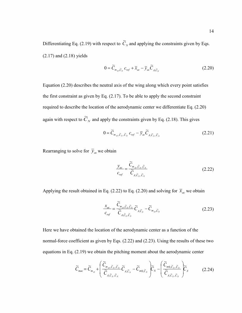
14 Differentiating Eq. (2.19) with respect to NC~ and applying the constraints given by Eqs.

(2.17) and (2.18) yields

NNO CAacacrefCm CyxcC ~,

~,~~0 −+= (2.20)

Equation (2.20) describes the neutral axis of the wing along which every point satisfies

the first constraint as given by Eq. (2.17). To be able to apply the second constraint

required to describe the location of the aerodynamic center we differentiate Eq. (2.20)

again with respect to NC~ and apply the constraints given by Eq. (2.18). This gives

NNNNO CCAacrefCCm CycC ~,~,

~,~,~~0 −= (2.21)

Rearranging to solve for acy we obtain

NN

NNO

CCA

CCm

ref

ac

CC

cy

~,~,

~,~,~

~= (2.22)

Applying the result obtained in Eq. (2.22) to Eq. (2.20) and solving for acx we obtain

NON

NN

NNOCmCA

CCA

CCm

ref

ac CCCC

cx

~,~,~,~,

~,~, ~~~~

−= (2.23)

Here we have obtained the location of the aerodynamic center as a function of the

normal-force coefficient as given by Eqs. (2.22) and (2.23). Using the results of these two

equations in Eq. (2.19) we obtain the pitching moment about the aerodynamic center

ACCA

CCmNCmCA

CCA

CCmmmac C

CC

CCCC

CCC

NN

NN

NN

NN

NNO

O

~~~

~~~~

~~~

~,~,

~,~,0~,0~,

~,~,

~,~,

−

−+= (2.24)

15

While Eqs. (2.23) and (2.22) are analogous to Eqs.(1.12) and (1.13) they appear to

be of a different form. In order to verify the correctness of Eqs. (2.23) and (2.22), an

equivalence proof is given here to show that the location of the aerodynamic center as a

function of the normal-force coefficient is equivalent to the location of the aerodynamic

center as a function of angle attack. This is important as sample results comparing these

two methods will be presented in Section 2.3.

2.2.1 Equivalence Proof

In the alternative approach presented in Section 2.2 the location of the

aerodynamic center was derived using constraints which enforce invariance of the

pitching moment about the aerodynamic center and the location ),( yx of the

aerodynamic center with respect to the normal force coefficient.

NON

NN

NNOCmCA

CCA

CCm

ref

ac CCC

Ccx

~,~,~,~,

~,~, ~~~

~−= (2.25)

NN

NNO

CCA

CCm

ref

ac

CC

cy

~,~,

~,~,~~

= (2.26)

These equations appear to be of a significantly different form compared to the analogous

relations given by Eqs. (1.12) and (1.13) which are functions of angle of attack. Here an

equivalence proof is given to show that the location of the aerodynamic center as a

function of normal-force coefficient is indeed equivalent to the location of the

aerodynamic center as a function of angle attack.

16

First, we define the numerator of the fraction in the first term of Eq. (2.25) as

“∗ ” and its denominator as “ ∗∗ .” Notice that the numerator and denominator of this

term are the same as in the case of Eq. (2.26). Starting with ∗ and expanding its partial

derivatives with respect to angle of attack, α gives

2

20,0 ~

~~~

~~

~~~

~~

N

m

NN

m

N

m

NN

m

N CC

CCC

CC

CCC

COO

∂∂

∂∂

+∂∂

∂

∂=

∂∂

∂

∂

∂∂

=∂

∂

∂∂ α

ααα

αα (2.27)

By expanding the partial derivate on the right hand side of Eq. (2.27) again with respect

to angle of attack, α we obtain

( )

( ) ( ) ∗=−=

∂

∂∂∂

+=

∂∂

∂∂

+

∂

∂∂∂

∂

∂=

3,

,,,2

,

,,

,2,

,,

~

~~

~

~

~1

~~

~

~

~~~

~1

~~

~

,

,

α

ααα

α

αα

α

α

αα

α

α

α

α

αα

α

N

Nom

N

om

NNm

N

om

NNm

NN

m

C

CC

C

C

CCC

C

C

CCC

CCC

C

O

O

O

(2.28)

Applying the same procedure to ** yields

( ) ( )3,

,,,2

,

,,~

~~

~

~

α

ααα

α

αα

N

NA

N

A

C

CC

C

C−=∗∗ (2.29)

Dividing ∗ by ∗∗ results in the following relation

17

αααααα

αααααα

,,,,,,

,,,,,,~~~~~~~~

NAAN

NmmN

CCCCCCCC

OO

−

−=

∗∗∗

(2.30)

Notice that the relation given by Eq. (2.30) is equal to Eq. (1.13) which is the vertical

component of the aerodynamic center as obtained by Phillips. Therefore, we see that Eq.

(2.26) which describes the vertical location of the aerodynamic center as a function of the

normal-force coefficient is indeed equivalent to Eq. (1.13). We can use the result

obtained in Eq. (2.30) in Eq. (2.25) to obtain

NCON

OOmCA

NAAN

NmmN

ref

ac CCCCCCCCCC

cx

,

~~~~~~~~~~

,,,,,,,

,,,,,, −

−

−=

αααααα

αααααα (2.31)

Expanding the remaining partial derivatives with respect to angle of attack yields

αα

α

αααααα

αααααα α

,,

,

,,,,,,

,,,,,,~

~

~~

~~~~~~~~

,

N

m

N

A

NAAN

NmmN

ref

ac

C

C

CC

CCCCCCCC

cx OOO −

−

−= (2.32)

We manipulate this relation further by performing all multiplicative distributions,

combining each term by the lowest common denominator, and cancelling common

factors to obtain

αααααα

αααααα

,,,,,,

,,,,,,~~~~~~~~

NAAN

AmmA

ref

ac

CCCCCCCC

cx OO

−

−= (2.33)

Notice that we have recovered exactly Eq. (1.12) as derived by Phillips. Therefore, we

see that Eq. (2.25) is equivalent to Eq. (1.12). We see furthermore that the location of the

aerodynamic center can indeed be described as purely a function of the normal-force

coefficient. This equivalence can further be shown by calculating values for acx and acy

18 using Eqs. (1.12) and (1.13) as functions of angle of attack and Eqs. (2.25) and (2.26) as

functions of the normal-force coefficient.

2.3 Sample Results

Using the relations describing the location of the aerodynamic center as a function

of angle of attack and those which describe it as a function of the normal-force

coefficient respectively, values can be obtained which show the equivalence of the two

methods. In both cases neither of these sets of relations make restrictions about the type

of flow, whether inviscid or viscous, for which they calculate the location of the

aerodynamic center. The sample results presented here reflect purely inviscid flow for

which the effects of drag are ignored. Inviscid flow data can be obtained by a number of

different methods, both analytical and numerical. One such numerical method, the Vortex

Panel Method [Appendix B] provides accurate and fast results for inviscid flow over

airfoils.

2.3.1 Vortex Panel Method

The vortex panel method uses a synthesis of straight-line segments and control

points along the top and bottom surface of an airfoil. By using a sufficiently high number

of straight line segments and control points this method can accurately predict the

coefficient of lift and the pitching moment of a given airfoil as functions of angle of

attack. Values for coefficient of lift can be related to the axial and normal force

coefficients via the inviscid transformations

19 αsin~~

LA CC −= (2.34)

αcos~~LN CC = (2.35)

The following data was generated for a NACA 8415 airfoil using a vortex panel method

with 400 nodes, cosine clustering, and a non-closed trailing edge.

Table 1 Vortex Panel Method data for a NACA 8415 airfoil

Angle of Attack (degrees) LC~ NC~ AC~ mC~

10 2.2845 2.2498 -0.39607 0.81502 9 2.1655 2.1388 -0.33875 0.78408 8 2.0457 2.0258 -0.28471 0.75269 7 1.9254 1.9110 -0.23464 0.72091 6 1.8044 1.7945 -0.18861 0.68876 5 1.6830 1.6765 -0.14668 0.65629 4 1.5609 1.5571 -0.10888 0.62353 3 1.4384 1.4364 -0.07528 0.59052 2 1.3155 1.3147 -0.04591 0.55731 1 1.1922 1.1920 -0.02081 0.52393 0 1.0685 1.0685 0.000000 0.49043 -1 0.94447 0.94433 0.01648 0.45684 -2 0.82017 0.81967 0.02862 0.42321 -3 0.69562 0.69467 0.03641 0.38958 -4 0.57086 0.56947 0.03982 0.35599 -5 0.44592 0.44423 0.03887 0.32248 -6 0.32085 0.31909 0.03354 0.28909 -7 0.19568 0.19423 0.02385 0.25586

Using this data, the first and second derivatives in Eqs. (1.12) and (1.13) and Eqs. (2.25)

and (2.26) can be approximated numerically in order to find solutions to the location of

the aerodynamic center. This numerical approximation can be achieved by means of a

second order finite differencing method.

20

2.3.2 Finite Difference Method

In order to approximate the first and second derivatives required to compute

values of the location of the aerodynamic center in Eqs. (1.12) and (1.13) and Eqs. (2.25)

and (2.26) discrete approximations using the Taylor series expansion about a point may

be employed. The Taylor series expansion of a function )(yφ about a point y for the

value yy ∆+ can be written as

+∆+

∆

∂∂

+

∆

∂∂

+∆

∂∂

+=∆+

)(6

2)()(

43

3

3

2

2

2

yOyy

yy

yy

yyy

y

yy

φ

φφφφ

(2.36)

The second order approximation of the first derivative of )(yφ at a point j is given by

)(

)(22

2222

baab

abjabba

j yyyyyyyy

y ∆∆−∆∆∆−∆−∆−∆

=

∂∂ φφφφ (2.37)

Where a and b represent the points before and after j respectively.

The second order approximation of the second derivative of )(yφ at a point j is given by

)())((

)(2))((

)(2

))(()(2)(2

2yOyyyyy

yyyyyyy

yy

yyyyyyy

yyyyyy

y

caccbc

ba

bbacbb

ac

aacbaa

cbj

cba

cba

j

∆+∆−∆∆−∆∆

∆+∆+

∆−∆∆−∆∆∆+∆

+

∆−∆∆−∆∆∆+∆

+∆∆∆

∆+∆+∆=

∂∂

φ

φ

φφφ

(2.38)

21 Where a represents the point before j and b and c represent the first and second point

after j respectively.

Using the data from Table 1 in Eq. (2.37) and Eq. (2.38) we can generate

approximations of the first and second derivatives of mC~ , AC~ , and NC~ as functions of the

traditionally used angle of attack, as well as the normal-force coefficient as discussed in

Section 2.2. Using these derivatives in their corresponding equations for the location of

the aerodynamic center results in Fig 2.

Figure 2. The ),( yx location of the aerodynamic center of a NACA 8415 airfoil using the traditional method as a function of angle of attack, Eqs. (1.12) and (1.13) and the modified method as a function of the normal-force coefficient, Eqs. (2.25) and (2.26).

From the figure we see that both methods give identical results to machine

precision. Noting the scale on the axes, for all practical usages the x and y coordinates of

22 the aerodynamic center given in this figure describe a single point. The scatter in the data

can be attributed to the numerical method used. The results of this figure further verify

the conclusion given in Section 2.2.1, that the location of the aerodynamic center as a

function of angle of attack can be equivalently described as a function of the normal-

force coefficient. However, the true significance of this figure is not that the two

methods are equivalent. The true significance of this figure is that the aerodynamic

center of an airfoil in an inviscid flow is described by a single point.

Recall that both the general method for finding the location of the aerodynamic

center, given by Eqs. (1.12) and (1.13), and the modified method, given by Eqs. (2.25)

and (2.26), allow for evaluation of both the x and y coordinates and include the effects of

vertical offsets as well as trigonometric and aerodynamic nonlinearities. Therefore, the

fact that in the case of an airfoil in a purely inviscid flow the location of the aerodynamic

center collapse to a single point is rather remarkable. This cannot readily be seen by

examining Eqs. (1.12) and (1.13) or Eqs. (2.25) and (2.26) as in both cases the relations

appear to be highly dependent on changes in angle of attack. However, as has been

shown in Fig. 2 the location of the aerodynamic center in purely inviscid flow is in

fact a single point, independent of angle of attack.

We desire to be able to describe the location of this point for any inviscid airfoil

analytically with new, more simple relations, without the need for numerical

approximations such as the finite differencing method in order to determine values of

unknown derivatives. Additionally, we desire that these new relations analytically

demonstrate the angle of attack independence observed in the sample results, while still

23 including the effects of vertical offsets as well as any trigonometric and or aerodynamic

nonlinearities.

24

CHAPTER 3

THE AERODYNAMIC CENTER OF INVISCID AIRFOILS

As shown in Section 1.2.2, Eqs. (1.12) and (1.13) offer a more accurate

description of the location of the aerodynamic center for any lifting surface. They allow

for evaluation of both the x and y coordinates of the aerodynamic center, unlike the

traditional approximations given in Eq. (1.7), which always predicts a y-coordinate for

the aerodynamic center that lies on the chord line. Furthermore, Eqs. (1.12) and (1.13)

correctly include the effects of vertical offsets as well as trigonometric and aerodynamic

nonlinearities such as drag. These two equations are dependent on first and second

aerodynamic derivatives with respect to angle of attack, while the traditional

approximation given in Eq. (1.7) depends only on first derivatives of aerodynamic

properties. Therefore, the general solution for the aerodynamic center depends on

accurately predicting any second-order aerodynamic nonlinearities, even below stall. To

estimate the aerodynamic center of airfoils, thin airfoil theory is often applied, which

neglects these second-order nonlinearities.

3.1 Classical Thin Airfoil Theory

Thin airfoil theory was developed by Max Munk during the period between 1914

and 1922 [5–9]. In this classical theory, an airfoil is synthesized as the superposition of a

uniform flow and a vortex sheet placed along the camber line of the airfoil as shown in

Fig. 3. Small camber and small angle-of-attack approximations are applied such that

25 higher-order terms can be neglected. This results in the classical thin-airfoil lift and

pitching-moment relations

)(~~0, LLL CC ααα −= (3.1)

4

~~~4

Lmm

CCCcO

−= (3.2)

where α,~

LC is the lift slope, 0Lα is the zero-lift angle of attack, and 4

~cmC is the pitching

moment about the quarter chord. The coefficients 0Lα and 4

~cmC are constants that can be

obtained from the camber line distribution,

∫=

−=π

θ

θθπ

α0

0 )cos1(1 ddxdyc

L (3.3)

∫=

−=π

θ

θθθ0

]cos)2[cos(21~

4d

dxdy

C cmc

(3.4)

where θ represents the change of variables for the axial coordinate given by

)cos1)(2()( θθ −≡ cx . The coefficient α,~

LC is a constant, which from thin-airfoil theory

is predicted to be

26

Figure 3. Synthesis of a thin airfoil section from superposition of a uniform flow and a curved vortex sheet distributed along the camber line.

πα 2~, =LC (3.5)

The development of thin airfoil theory can be found in most engineering text books on

aerodynamics [13-18]. Using Eq. (3.1) in Eq. (3.2) and applying the result to the

traditional relation for the aerodynamic center given in Eq. (1.7) gives the aerodynamic

center as predicted by thin airfoil theory,

41

=c

xac , 0=c

yac (3.6)

Notice from Eqs. (3.1) and (3.2) that the lift and pitching moment are predicted by

this theory to be linear functions of angle of attack. All higher-order nonlinearities in

angle of attack were neglected in the development of this theory. Strictly speaking, Eqs.

(3.1)–(3.5) are only accurate in the limit as the airfoil geometry and operating conditions

approach those of the approximations applied in the development of classical thin airfoil

theory. These assumptions include an infinitely thin airfoil, small camber, and small

27 angles of attack. However, it is commonly assumed that the form of Eqs. (3.1) and (3.2)

are correct for arbitrary airfoils at angles of attack below stall. Therefore, α,~

LC , 0Lα , and

4

~cmC are often used as coefficients to fit Eqs. (3.1) and (3.2) to airfoil data obtained from

experimental measurements or numerical simulations. This results in predictions for lift

and pitching moment that are linear functions of angle of attack, and do not contain any

higher-order dependence on angle of attack below stall. However, as was discussed

above, the location of the aerodynamic center is dependent on second-order aerodynamic

effects with respect to angle of attack. Thus, in order to better understand the influence of

nonlinear aerodynamics on the location of the aerodynamic center, we now consider a

more general airfoil theory that does not include any approximations for thickness,

camber, or angle of attack.

3.2 General Airfoil Theory

A general airfoil theory that does not include the approximations of small camber,

small thickness, and small angles of attack can be developed from the method of

conformal mapping [19, 20]. The theory presented here can be used to map flow about a

circular cylinder to flow about any arbitrary two-dimensional surface. Pressure

distributions can then be integrated to evaluate the resulting lift and pitching moment, as

shown in the following development.

28 3.2.1 Theory Development

Flow about a circular cylinder of radius R centered at the point z0,including the

effects of angle of attack, α , and finite circulation, Γ , can be described by

−−

−+=

Φ=

∞

−∞ 2

0

2

0

11 )(

1)(

12

)(zz

eRzzV

ΓieVdz

dzw ii αα

π (3.7)

where 1Φ is the complex potential and w1 is the complex velocity in the plane of the

circular cylinder. Using the method of conformal mapping, we can apply an arbitrary

transformation of this flow from the plane of the cylinder to the plane of an airfoil of the

form

)]([)( 12 zz ζΦ=Φ (3.8)

where )(zζ is an analytic transformation function. The complex velocity in the airfoil

plane corresponding to this complex potential is

ζ

ζζζζζζ d

dzzwdzdzw

dzdz

dd

dzd

zw )]([)]([)]([)( 1112

2 ==Φ=Φ

= (3.9)

Thus, the complex velocity for the transformed flow field can be expressed as

ζζζπ

αα

ddz

zeR

zVΓieV

dzd

zw ii

−−

−+=

Φ=

∞

−∞ 2

0

2

0

22 )(

1)(

12

)( (3.10)

The potential-flow solution about a circular cylinder can be transformed to obtain the

potential-flow solution about a cylinder with any arbitrary cross section. In general, an

29 arbitrary transformation requires an infinite number of degrees of freedom, and can be

expressed in terms of the Laurent series expansion [20],

∑∞

=

+=1

)(n

nnC

zζ

ζζ (3.11)

where the coefficients, Cn, are complex constants. The first derivative of this general

transformation is

∑∞

=+−=

111

nn

nnCddz

ζζ (3.12)

The equation for the surface of the circular cylinder in the ζ -plane can be written as

0 zeR isurface += θζ (3.13)

Using Eq. (3.13) in Eq. (3.11), the transformed surface of the cylinder in the z-plane is

given by the relation

∑∞

= +++=

1 00 ) (

)(n

nini

surface zeRC

zeRz θθζ (3.14)

The derivative of the conformal transformation given in Eq. (3.12) can be zero at

multiple points, depending on the values of the complex coefficients, Cn. These values of

ζ are often referred to as the critical points of the transformation, at which the

transformed velocity field given by Eq. (3.10) is singular. In order to map the flow of a

circular cylinder to that over an airfoil, one of the critical points must lie on the circular

cylinder in the ζ -plane at the point that maps to the airfoil’s trailing edge in the ζ -plane.

30 All remaining critical points must lie inside the circular cylinder in the ζ -plane in order

for the flow external to the cylinder to remain conformal. Here we denote the critical

point in the ζ -plane that maps to the airfoil’s trailing edge in the ζ -plane as tζ . It is

convenient to choose tζ to be on the positive real axis, as shown in Fig. 4. This requires

002

02 zeRxyR ti

t +=+−= θζ (3.15)

where tθ is the value of θ at tζζ = , i.e.,

−−=−= −− 2

02

01

01 tan)(sin yRyRytθ (3.16)

Similarly, the left-hand real-axis intercept of the parent circular cylinder is

02

02 xyRl +−−=ζ (3.17)

31

Figure 4. Circular cylinder in the complex ζ -plane, centered at 000 iyxz +==ζ .

Note that for a symmetric airfoil, 00 =y . The Kutta condition must be satisfied at the

trailing edge of the airfoil, and requires that tζ be a stagnation point for the flow in the

ζ -plane. The complex velocity field is given in Eq. (3.10) and will have a stagnation

point at the point on the parent circular cylinder that maps to the airfoil trailing edge if

0)(

1)(

12 2

0

2

0

=−

−−

+∞

−

zeR

zVΓie

t

i

t

i

ζζπαα (3.18)

Solving this relation for Γ gives the circulation that will satisfy the Kutta condition at the

trailing edge,

32

−−

−= −∞ αα ζ

ζπ i

tt

i ezz

eRiVΓ )(

)(12

00

2 (3.19)

Using Eq. (3.15) we can evaluate

02

02

0002

02

0 )( iyyRiyxxyRzt −−=+−+−=−ζ (3.20)

Using Eq. (3.20) in Eq. (3.19) gives an alternate form for the circulation

+−= ∞ ααπ cossin4 0

20

2 yyRVΓ (3.21)

From the Kutta-Joukowski law [21,22], the section lift can be computed from the section

circulation, i.e.,

ΓVL ∞= ρ~ (3.22)

Using the circulation from Eq. (3.21) in Eq. (3.22) gives

+−= ∞ ααπρ cossin4~

02

022 yyRVL (3.23)

Notice that the predicted section lift given in Eq. (3.23) is independent of any

particular transformation, and is a function only of the radius and vertical offset of the

circular cylinder. On the other hand, the leading and trailing edges of the airfoil in the z-

plane are dependent on the transformation, and are needed in order to compute the chord

length and lift coefficient. For any given transformation, the section lift coefficient can be

obtained from Eq. (3.23)

33

−+

−

−=

−≡

∞

ααπ

ρcossin

)(8

)(

~~2

02

02

02

221

yR

yzz

yRzzV

LCltlt

L (3.24)

where lt zzc −= is the airfoil chord length. Thus, regardless of the transformation, the lift

coefficient will be of the form

)costan(sin~~0,0 αααα LLL CC −= (3.25)

where α,0~

LC is the lift slope at zero angle of attack and 0Lα is the zero-lift angle of attack.

From Eq. (3.24),

,)(

8~ 20

2

,0lt

L zzyR

C−

−=

πα

−−== − 2

02

01

0 tan yRytL θα (3.26)

Notice that from Eqs. (3.23) and (3.26) that the lift and zero-lift angle of attack do not

depend on either the transformation or the real part of the cylinder offset, x0. On the other

hand, the lift coefficient and lift slope at zero angle of attack depend on the

transformation, which in turn depends on x0. In any case, Eq. (3.25) is a general form for

the lift coefficient of an arbitrary airfoil. No assumptions of camber, thickness, or small

angle of attack were made in the development of Eq. (3.25). Therefore, we would expect

this form of equation to fit the inviscid lift properties of any airfoil at arbitrary angles of

attack.

From the Blasius relations [23-24], the pitching moment about the origin for an

arbitrary geometry is

34 [ ]{ }∫=

CO dzzzwm 221 )(real~ ρ (3.27)

Using Eq. (3.12) in Eq. (3.10), the square of the complex velocity of the transformed flow

field is

[ ]2

11

2

20

2

0

22 1)(

1)(

12

)(

−

−

−−

+= ∑∞

=+

∞

−∞

nn

nii nCz

eRzV

ΓieVzwζζζπ

αα

(3.28)

Using Eq. (3.28) in Eq. (3.27) and expanding in a Laurent series of gives

[ ]{ }∫∞=CO dFFVm ζζζρ )()(real~

22

12

21 (3.29)

where

[ ] +

−−++=

∞∞

−

∞

−−

22

22

2022

112

41)(

ζππζπζ

ααα R

VΓ

VeΓz

iV

ΓeieFii

i

(3.30)

++

+++=

−

+= ∑∑

∞

=+

∞

=3

213

221

11

12

24321)(ζζζ

ζζζ

ζζCCCCnCC

Fn

nn

nnn

(3.31)

and

[ ] +

+−−++= −

∞∞

−

∞

−−

ζπππζζζ α

ααα 122

4)()( 2

12

22

202

22

1i

iii eCR

VΓ

VeΓz

iV

ΓeieFF

ζ1

35

(3.32)

Therefore, the pitching moment about the origin can be written in terms of the series

= ∫ ∑∞

=−∞ C

nnn

O dBVm ζζ

ρ0

12

21 real~

` (3.33)

where

α20

ieB −= , ∞

−

=V

ΓeiBi

π

α

1 , ,224

21

222

20

2α

α

ππi

i

eCRVΓ

VeΓz

iB −

∞∞

−

+−−=

(3.34)

Using Eq. (3.34) in Eq. (3.33) and integrating shows that the pitching moment is only a

function of the first constant in the Laurent series,

( )αα ρπρ iiO eΓzVeCVim −

∞−

∞ −= 02

122real~ (3.35)

After applying the Kutta-Joukowski law given in Eq. (3.22), the pitching moment about

the origin can be written as

( )ααπρ iiO ezLeCVim −−

∞ −= 02

12 ~2real~ (3.36)

Using the identity as well as the definition in Eq. (3.36) gives

( )αααπρ sincos~)2sin(2~001

2 yxLCVmO +−= ∞ (3.37)

Because the constant C1 depends on the transformation, we see that unlike the section lift,

the section pitching moment does depend on the transformation. Dividing Eq. (3.37) by

ααα sincos iei += 000 iyxz +=

36 the dynamic pressure and chord length squared, the section pitching moment coefficient

relative to the origin used in the transformation can be expressed as

ltL

lt

ltm

zzyxC

zzC

zzVmC

O

−+

−−

=−

≡∞

αααπ

ρ

sincos~)2sin()(

4)(

~~

002

1

2221

0

(3.38)

The moment coefficient about an arbitrary point in the z-plane can be found from the

moment coefficient relative to the origin and the lift coefficient,

lt

Lmm zzyxCCC

O −+

+=αα sincos~~~ (3.39)

Using Eq. (3.38) in Eq. (3.39) gives

lt

Llt

m zzyyxx

Czz

CC

−−+−

+−

=αα

απ sin)(cos)(~)2sin(

)(4~ 00

21 (3.40)

In order to compute the pitching-moment coefficient, we need to know C1, zt, and zl,

which must be found from the transformation. However, regardless of the transformation,

the pitching-moment coefficient for an airfoil in inviscid flow about any point in the

domain is a function of angle of attack of the form

αααα sin~~cos~~)2sin(~~,,,0 LAmLNmmm CCCCCC −+= (3.41)

where α,0~

mC , NmC ,~ , and AmC ,

~ are constant coefficients. As can be seen from Eq. (3.40), the

values for the coefficients NmC ,~ , and AmC ,

~ are a function of the x , and y location of the

pitching moment relative to the origin used in the transformation. Since the origin of the

37 transformation has little physical meaning in the traditional airfoil coordinate system, we

will define NmC ,~ , and AmC ,

~ to be the coefficients with the pitching moment evaluated at the

airfoil leading edge, i.e. lzx = , and 0=y , which is the origin of the traditional airfoil

coordinate system. For any given transformation, the pitching moment of an airfoil in an

inviscid flowfield about the airfoil leading edge can be evaluated from Eq. (3.41) with the

coefficients

lt

Amlt

lNm

ltm zz

yCzzxzC

zzCC

−=

−−

=−

= 0,

0,2

1,0

~ ,~ ,)(

4~ πα (3.42)

The form of Eqs. (3.25) and (3.41) hold for any airfoil transformation, and therefore, for

any arbitrary airfoil shape. These relations were developed without any approximations

for airfoil thickness, camber, or angle of attack, and are therefore not constrained under

the same limitations that were used in the development of the traditional small-camber

and small-angle relations given in Eqs. (3.1) and (3.2).

The coefficients α,0~

LC , 0Lα , α,0~


~ required in Eqs. (3.25) and (3.41)

can be evaluated analytically from a known parent cylinder offset and transformation by

using Eqs. (3.26) and (3.42). For example, the Joukowski transformation is defined as a

special case of Eq. (3.11) where

ζ

ζζ

2

020

2

)(

+−

+=xyR

z (3.43)

Using Eq. (3.43) as well as a given parent circular cylinder offset of z0, the method

described above gives the coefficients for a Joukowski airfoil

38

( ) ( )

( )

( ) ( ))(4

)(~ ,)(4

)(~

,4

~

tan ,1

2~

2 ,2 ,

20

20

20

20

,20

20

20

20

,

2

20

2

20

20

2

,0

20

20

10

020

20

,0

020

2

20

20

2

020

22

020

21

)(

yRxyRyy

CyR

xyRxxC

yRxyRC

yRyxyRx

C

xyRxyRzxyRzxyRC

AmNm

m

LL

lt

−−−−

−=−

−−−=

−−−

=

−−=−−+

=

−−

+−−=+−=+−=

−

π

απ

α

α

(3.44)

The analytical solution for the coefficients given in Eq. (3.44) for a Joukowski airfoil

sheds significant insight on an important aspect of the coefficients required in Eqs. (3.25)

and (3.41). Note that for a Joukowski airfoil, the entire airfoil and transformation can be

defined by only three variables, R , 0x , and 0y . All coefficients in Eq. (3.44) are

functions of these three variables. Hence, the aerodynamic coefficients are not entirely

independent. For example, after some algebraic manipulation, NmC ,~ can alternatively be

expressed as 12)~()8(~~ 2/1,0,0, −+= ππ αα mLNm CCC . Although the number of variables

required to define an airfoil may vary depending on the transformation, the aerodynamic

coefficients of Eqs (3.25) and (3.41) will in general not be entirely independent.

3.2.2 Comparison to Inviscid Computational Results

For airfoil geometries that were not generated from conformal mapping

techniques, the coefficients α,0~

LC , 0Lα , α,0~

mC , NmC ,~

, and AmC ,~

required for Eqs. (3.25) and

(3.41) can be evaluated numerically. This can be accomplished by fitting Eqs. (3.25) and

(3.41) to a set of airfoil data obtained from experimental or numerical results. A vertical

39 least squares regression method for fitting these coefficients to a set of data is outlined in

Section 3.3. This method can be used to evaluate appropriate coefficients for Eqs. (3.1)

and (3.2) or Eqs. (3.25) and (3.41) for cambered airfoils. Because the general airfoil

theory relations given in Eqs. (3.25) and (3.41) were developed without any assumptions

for airfoil geometry other than that of a single trailing edge, we should expect the form of

these equations to match inviscid airfoil aerodynamic data more accurately than Eqs.

(3.1) and (3.2), which were obtained from thin airfoil theory. Here we consider the

accuracy of each of these equations for the NACA 4-digit series over a range of camber

and thickness magnitudes.

Inviscid incompressible aerodynamic lift and pitching moment coefficient data for

250 NACA 4-digit series airfoils were generated over a wide range of camber and

thickness using a numerical vortex panel method [Appendix B] employing linear vortex

sheets along the airfoil surface [25]. The airfoil surfaces were discretized using 400

panels, which produced grid-resolved solutions. The panels were clustered near the

leading and trailing edges of the airfoil using standard cosine clustering. Results were

computed for each airfoil at angles of attack ranging from -10 to +15 degrees in

increments of 1 degree. At each angle of attack, the lift and pitching moment coefficient

about the airfoil leading edge were recorded. Table 2 shows a sample data set for the

NACA 8415 airfoil.

40

Table 2. Inviscid lift and pitching-moment data generated from a vortex panel method for a NACA 8415 airfoil.

Angle of Attack

(degrees) LC~ mC~

15 2.86876 -0.96179 14 2.75352 -0.93361 13 2.63744 -0.90481 12 2.52056 -0.87542 11 2.40291 -0.84548 10 2.28453 -0.81502 9 2.16545 -0.78408 8 2.04571 -0.75269 7 1.92535 -0.72091 6 1.80441 -0.68876 5 1.68291 -0.65629 4 1.56090 -0.62353 3 1.43842 -0.59052 2 1.31549 -0.55731 1 1.19217 -0.52393 0 1.06848 -0.49043 -1 0.94447 -0.45684 -2 0.82017 -0.42321 -3 0.69562 -0.38958 -4 0.57086 -0.35599 -5 0.44592 -0.32248 -6 0.32085 -0.28909 -7 0.19568 -0.25586 -8 0.07045 -0.22284 -9 -0.05480 -0.19005 -10 -0.18003 -0.15755

The least-squares regression method was used to fit the aerodynamic data for each

airfoil to the thin-airfoil equations given in Eqs. (3.1) and (3.2), and the RMS value for

each case was recorded. Similarly, the least-squares regression method was used to fit the

aerodynamic data for each airfoil to the general airfoil theory equations given in Eqs.

(3.25) and (3.41), and the RMS value for each case was recorded. Table 3 shows sample

resulting coefficients for the NACA 8415 airfoil, along with the associated RMS error

from both thin airfoil theory and general airfoil theory. Figures 5 and 6 show the RMS

41 values for all 250 airfoils as a function of airfoil thickness and varying camber. It should

be noted that Eq (3.55) which can be used for fitting data from symmetric airfoils to Eq.

(3.41) produces a system of equations that has an infinite number of solutions. The

anomaly for symmetric airfoils will be investigated in future work.

Table 3. Least-squares regression coefficients for a NACA 8415 airfoil using relations from thin and general airfoil theory respectively. Root-mean-square error values are also given for each theory compared against results from the vortex panel method.

Coefficient Thin Airfoil Theory Coefficient General Airfoil Theory

α,~

LC 7.00698 α,0~

LC 7.09641

0Lα -0.15121 0Lα -0.14944

4/

~cmC -0.22746 α,0

~mC 0.69403

NmC ,~ -0.45900

AmC ,~ 0.04973

Room Mean

Squared Error Thin Airfoil Theory General Airfoil Theory

LC~ 0.01069 machine zero

mC~ 0.01495 machine zero

42

Figure 5. RMS error for lift predictions from thin airfoil theory and general airfoil theory for 250 NACA 4-digit airfoils.

Figure 6. RMS error for pitching-moment predictions from thin airfoil theory and general airfoil theory for 250 NACA 4-digit airfoils.

43 Note that the RMS error from the general airfoil theory is several orders of

magnitude smaller than that of the traditional relations based on thin airfoil theory. In

fact, the RMS error from the general airfoil theory is on the order of machine precision.

This indicates that the general airfoil theory equations can be fit exactly to the inviscid

solutions, and therefore, are of the correct form. The error associated with the least-

squares regression fits to the thin airfoil theory equations indicate that the form of the thin

airfoil theory equations are not exactly correct. With current measurement technology for

experimental setups, the accuracy gained from the general airfoil theory equations for lift

and pitching moment predictions is clearly unwarranted. Experimental data is generally

only known to 2 or 3 significant figures, which is the same order of accuracy as that

obtained from thin airfoil theory. Therefore, the significance of the general airfoil

theory is not that it can more accurately fit experimental data or CFD simulations.

Indeed, the error in experimental data or CFD simulations often falls outside the range of

accuracy to be found in either the general airfoil theory or thin airfoil theory. Thus, using

one theory over the other will not give significantly improved results if we wish only

to predict lift or pitching moment over a range of angles of attack below stall.

Rather, the significance of the general airfoil theory becomes apparent when second

derivatives for lift or pitching moment as a function of angle of attack are needed.

Such is the case in the estimation of the location of the aerodynamic center.

44 3.3 Least-Squares Regression Fit Coefficients – Inviscid Flow

The method of least-squares regression was used to fit the aerodynamic data for

each airfoil to the thin-airfoil equations given in Eqs. (3.1) and (3.2), and the general

airfoil theory equations given in Eqs. (3.25) and (3.41). The least-squares regression

method is commonly used in regression analysis, most importantly in data fitting. In

general, the sum of the squares, S, of the vertical deviations between the best-fit equation

and a set of n data points is given by

∑=

−≡n

iii xfyS

1

2],([ a) (3.45)

where ),( ii yx are discrete data points, a is a vector of the unknown coefficients to be

determined, and ),( aixf is the analytical expression to which the data is to be fitted. The

vertical least-squares method seeks to minimize S for a given data set and expression

),( aixf . The RMS error for a given solution can be computed from

nS

≡RMS (3.46)

3.3.1 Fit to Thin Airfoil Theory Equations

Applying the traditional lift relation given in Eq. (3.1) to Eq. (3.45) yields

[ ]∑=

−−=n

iLiLLC CCS

iL1

20,~ )(~~ ααα (3.47)

45 Best-fit values for α,

~LC and 0Lα can be determined by setting the partial derivatives of Eq.

(3.47) with respect to α,~

LC and 0Lα equal to zero. Expressions for the partial derivatives

are

[ ]( ){ } 0)(~~2~1

00,,

~=−−−−=

∂

∂∑

=

n

iLiLiLL

L

C CCC

Si

L αααααα

(3.48)

[ ]{ } 0~)(~~21

,0,0

~=−−=

∂

∂∑

=

n

iLLiLiL

L

C CCCS

Lαα αα

α (3.49)

Solving Eqs. (3.48) and (3.49) simultaneously for α,~

LC and 0Lα yield the best-fit values

for these two coefficients for the traditional lift equation given in Eq. (3.1),

∑ ∑

∑ ∑

= =

= =

+−

−= n

iL

n

iiLi

n

i

n

iLLiL

L

n

CCC

ii

1

20

10

2

1 10

,

2

~)~(~

αααα

ααα (3.50)

∑∑∑

∑∑∑∑

===

====

⋅−⋅

⋅−⋅= n

iiL

n

ii

n

iL

n

iiL

n

ii

n

ii

n

iL

L

ii

ii

CnC

CC

111

111

2

10

)~(~

)~(~

αα

αααα (3.51)

Using the results from Eqs. (3.50) and (3.51) in Eq. (3.1), an estimate for the lift

coefficient as a function of angle of attack can be obtained. This vertical least-squares

fitting process can also be used to evaluate the best-fit quarter-chord pitching moment for

the traditional equation given in Eq. (3.2), i.e.,

nCCCn

i

iLimm Oc ∑

=

+=

1 4

~~~4/

(3.52)

46 3.3.2 Fit to General Airfoil Theory Equations

The best-fit coefficients required to fit Eq. (3.25) to a data set can be solved using

the process described above, which yields the following expressions for α,0~

LC and 0Lα

⋅−⋅

⋅−⋅=

∑ ∑∑∑

∑∑∑∑

= ===

====−n

i

n

iiiL

n

iii

n

iiL

n

iii

n

iiL

n

ii

n

iiL

L

ii

ii

CC

CC

1 1

2

11

111

2

110

cos)sin~()cos(sin)cos~(

)cos(sin)sin~(sin)cos~(tan

ααααα

αααααα

(3.53)

∑

∑

=

=

−

−

= n

iiLi

n

iiLiL

L

iC

C

1

20

10

,0

)costan(sin

)costan(sin~~

ααα

ααα

α (3.54)

Using the results from Eqs. (3.53) and (3.54) in Eq. (3.25) an estimate for the lift

coefficient as a function of angle of attack can be obtained. The least-squares process can

then be repeated to evaluate the best-fit coefficients for Eq. (3.41) as a function of angle

of attack and lift coefficient. After some algebraic manipulation, this yields the following

linear system of equations, which can be solved to evaluate α,0~


~

47

( ) ( )( ) ( ) ( )( ) ( ) ( )

( )( )( )

=

−

−

−

∑

∑

∑

∑∑∑

∑∑∑

∑∑∑

=

=

=

===

===

===

n

iiLm

n

iiLm

n

iim

Am

Nm

m

n

iiL

n

iiiL

n

iiiL

n

iiiL

n

iiL

n

iiiL

n

iiiL

n

iiiL

n

ii

iiO

iiO

iO

iii

iii

ii

CC

CC

C

CCC

CCC

CCC

CC

1

1

1

,

,

,0

1

22

1

2

1

1

2

1

22

1

111

2

sin~~

cos~~

)2sin(~

~~~

sin~sincos~)2sin(sin~

sincos~cos~)2sin(cos~

)2sin(sin~)2sin(cos~)2(sin

α

α

α

ααααα

ααααα

αααααα

(3.55)

For symmetric airfoils, Eq. (3.55) becomes singular. The reason for this singularity is at

this time not fully understood, but could be related to the fact that α,0~


~

are not linearly independent, as discussed in Section 3.2.1. From general airfoil theory, it

can be shown that 0~, =AmC for symmetric airfoils. However, there potentially exists an

unknown number of solutions for α,0~

mC , and NmC ,~ that satisfy Eq. (3.55). Therefore while

AmC ,~ is known in the case of symmetric airfoils, the relation between α,0

~mC , and NmC ,

~ is not

presently known and we conclude

( ) ~~ ,0~,,0, NmmAm CfCC == α (3.56)

A method for uniquely evaluating these two coefficients for symmetric airfoils will be the

topic of future research.

48 3.4 The Aerodynamic Center of Airfoils in Inviscid Flow

In general, the location of the aerodynamic center can be correctly predicted using

Eqs. (1.12) and (1.13). Recall that this definition for the location of the aerodynamic

center is a general definition, in that it does not include any linearizing or small-angle

approximations. We shall now consider the location of the aerodynamic center of inviscid

airfoils as predicted by the relations developed from classical thin airfoil theory, given in

Eqs. (3.1) and (3.2), compared with the relations developed from general airfoil theory,

given in Eqs. (3.25) and (3.41). First we consider only the case of inviscid flow, i.e.,

0~=DC . From Eqs. (1.3) and (1.4), this gives

αsin~~LA CC −= (3.57)

αcos~~LN CC = (3.58)

3.4.1 Thin Airfoil Theory with Trigonometric Nonlinearities

Predictions for the aerodynamic center from thin airfoil theory are traditionally

obtained by applying aerodynamic and trigonometric linearizing approximations to Eqs.

(1.12) and (1.13). This method was outlined previously, and results in an aerodynamic

center location given in Eq. (1.7). After the discussion surrounding the general definition

of the aerodynamic center given by Eqs. (1.12)-(1.14), one may be inclined to apply the

linear aerodynamic equations from thin airfoil theory while retaining the geometric

nonlinearities of Eqs. (3.57) and (3.58). Here we examine the results of such an approach.

Using Eq. (3.1) in Eqs. (3.57) and (3.58), differentiating the result twice along with Eq.

(3.2), and applying the resulting derivatives to Eqs. (1.12)–(1.14) gives

49

8)(4cos2sin)(

20

0

+−+−

=L

Lac

cx

αααααα

(3.59)

8)(4sin2cos)(

20

0

+−+−

=L

Lac

cy

αααααα

(3.60)

]2)[(4

]2)[(~)(~~

20

20

30, 4

+−

+−+−−=

L

LmLLm

c

ac

CCC

αα

ααααα (3.61)

Note that the aerodynamic center and associated pitching moment given by Eqs. (3.59)–

(3.61) is a nonlinear function of angle of attack. We now compare this result to that from

general airfoil theory.

3.4.2 General Airfoil Theory

The aerodynamic center of an arbitrary inviscid airfoil can be more accurately

found by using the lift and pitching-moment relations from general airfoil theory. Using

Eqs. (3.25) and (3.41) in Eqs. (3.57) and (3.58), differentiating twice, and applying the

resulting derivatives to Eqs. (1.12)–(1.14) gives

NmLL

mac CCC

cx

,02

,0

,0 ~cos~~

2 −−= αα

α (3.62)

AmLL

mac CCC

cy

,0,0

,0 ~)2sin(~~

+= αα

α (3.63)

)2sin(~~0,0 Lmm CC

acαα= (3.64)

50 Notice that Eqs. (3.62)–(3.64) are independent of angle of attack. Therefore, the

location of the aerodynamic center for an arbitrary airfoil in inviscid flow is a single

point, independent of angle of attack. This point does not in general lie at the airfoil

quarter chord, but is a single point dependent on airfoil thickness and camber. This

solution was developed from general airfoil theory, which does not make any

assumptions for small angles of attack, small camber, or small thickness. It is rather

remarkable that when all geometric and aerodynamic nonlinearities are retained in the lift

and pitching moment equations, along with those in the definition of the aerodynamic

center, the relations for the aerodynamic center reduce to such a simple expression,

independent of angle of attack, for inviscid flow.

Figure 7 shows the aerodynamic center for the NACA 8415 airfoil as predicted by the

traditional thin airfoil theory given in Eq. (1.7), thin airfoil theory with trigonometric

nonlinearities given in Eqs. (3.59) and (3.60), and the general airfoil theory given in Eqs.

(3.62) and (3.63). Figure 8 shows the pitching moment about the aerodynamic center

predicted by each theory as a function of angle of attack. Figures 7 and 8 also include

results from second-order finite difference approximations obtained from inviscid

numerical solutions for the NACA 8415 airfoil and Eqs. (1.12)–(1.14).

Equations (3.59)-(3.61) represent a mix of using linear aerodynamics from thin airfoil

theory while retaining the trigonometric nonlinearities given in Eqs. (3.57) and (3.58).

This produces non-physical results and should never be used to approximate the

aerodynamic center and the associated pitching moment. Note that the aerodynamic

center predicted by Eqs. (3.62) and (3.63) does not lie at the quarter-chord, but is a single

51 point 1.8% chord aft and 2.1% chord above the quarter-chord point. Equations (3.62)-

(3.64) match the finite-difference computational results exactly.

Figure 7. The location of the aerodynamic center for a NACA 8415 airfoil as predicted by thin airfoil theory, Eqs. (3.59)-(3.60), general airfoil theory, and finite differencing.

Figure 8. Pitching moment about the aerodynamic center as predicted by thin airfoil theory, Eq. (3.61), general airfoil theory, and finite differencing.

52

Figure 9. The aerodynamic center location as predicted from Eqs. (3.62) and (3.63) for 250 NACA 4-digit airfoils as a function of camber and thickness. Filled markers represent airfoil thickness increments of 10%.

Figure 9 shows the aerodynamic center as predicted from Eqs. (3.62) and (3.63)

for 250 NACA 4-digit-series airfoils as a function of camber and thickness [Appendix D].

These results show that increasing thicknesses tends to shift the aerodynamic center aft,

while camber tends to shift the aerodynamic center normal to the chord line. Notice that

airfoils of 10% thickness can have up to 1% deviation in both axial and normal directions

relative to the quarter-chord. Because the static margin is often on the order of 5% for a

stable aircraft, the difference in these approximations for the location of the aerodynamic

center can be somewhat significant. We have thus far considered characteristics of

53 airfoils only in inviscid flow. As will be shown, viscosity also significantly impacts the

location of the aerodynamic center.

54

CHAPTER 4

THE AERODYNAMIC CENTER OF VISCOUS AIRFOILS

4.1 The Aerodynamic Center of Airfoils in Viscous Airflows

Up to this point, we have neglected the influence of viscosity on the aerodynamic

forces and moments created by an airfoil. The largest effect of viscosity on airfoils at

angles of attack below stall is the production of friction along the surface of the airfoil.

Below stall, this skin friction generally does not significantly impact the lift but does

produce drag and alters the pitching moment relative to the inviscid scenario. The section

drag coefficient is traditionally related to the section lift coefficient using a quadratic

equation. Here we use the traditional relation

2,,

~~~~~~2

000 LLDLLDDD CCCCCC ++= (4.1)

where 0

~DC , LDC ,0

~ , and 20 ,

~LDC are constant coefficients for a given airfoil drag polar. Note

that the second term on the right-hand side is required to adequately model drag polars

that do not have a minimum at zero lift. Such is the case for most non-symmetric airfoils.

Viscosity also affects the pitching moment produced by the airfoil. Recall that Eq.

(3.41) was developed from airfoil theory based on conformal mapping, which is built on

the assumption of an inviscid flow. This equation for the pitching moment can be

extended to account for viscous effects by including the drag-component acting in the

normal and axial directions,

AAmNNmmm CCCCCC ~~~~)2sin(~~,,,0 ++= αα (4.2)

55 or, in light of Eqs. (1.3) and (1.4),

)sin~cos~(~

)sin~cos~(~)2sin(~~

,

,,0

αα

αααα

LDAm

DLNmmm

CCC

CCCCC

−+

++= (4.3)

Differentiating Eq. (4.2) and applying the result to Eqs. (1.12) and (1.13) gives the exact

solution for the location of the aerodynamic center including viscous effects

NmNAAN

AAm

ac CCCCC

CCC

cx

,,,,,,,

,,,,0

~~~~~

~)2cos(~)2sin(2~2 −−

+−=

αααααα

αααα

αα (4.4)

AmNAAN

NNm

ac CCCCC

CCC

cy

,,,,,,,

,,,,0

~~~~~

~)2cos(~)2sin(2~2 +−

+−=

αααααα

αααα

αα (4.5)

Applying Eqs. (4.2), (4.4), and (4.5) to Eq. (1.14) gives the associated pitching moment

−

−+−+=

αααααα

ααααααα

ααα

,,,,,,

,,,,,,,0 ~~~~

)~~~~)(2cos()~~~~)(2sin(22)2sin(~~

NAAN

ANNAANANmm CCCC

CCCCCCCCCC

ac

(4.6)

Equations. (4.4), (4.5), and (4.6) can be used to find the exact location of the

aerodynamic center and the associated pitching moment for any airfoil including viscous

effects.

In order to be able to compute solutions to Eqs. (4.4-4.6) we need expressions for

the normal and axial forces and their respective first and second derivatives with respect

56 to angle of attack. These can be found analytically by using Eqs. (3.25) and (4.1) in Eqs.

(1.3) and (1.4) and differentiating to give

)tancos(sinsin~])tancos(sin~~

)tancos(sin~~~[cos~

0,0

20

2,0,

0,0,

20

00

LL

LLLD

LLLDDA

C

CC

CCCC

αααα

ααα

αααα

α

α

α

−−

−+

−+=

(4.7)

)tancos(sincos~])tancos(sin~~

)tancos(sin~~~[sin~

0,0

20

2,0,

0,0,

20

00

LL

LLLD

LLLDDN

C

CC

CCCC

αααα

ααα

αααα

α

α

α

−+

−+

−+=

(4.8)

)tansin(cossin~)tancos(sincos~

])tancos(sin~~)tancos(sin~~~[sin

]~)tansin(cos~

~)tancos)(sintansin(cos~2[cos~

0,0

0,0

20

2,0,

0,0,

,00,

2,000,,

20

00

0

20

LL

LL

LLLD

LLLDD

LLLD

LLLLDA

C

C

CC

CCC

CC

CCC

αααα

αααα

ααα

αααα

ααα

ααααααα

α

α

α

α

α

αα

+−

−−

−+

−+−

++

−+=

(4.9)

)tancos(sinsin~)tansin(coscos~

])tancos(sin~~)tancos(sin~~~[cos

]~)tansin(cos~

~)tancos)(sintansin(cos~2[sin~

0,0

0,0

20

2,0,

0,0,

,00,

2,000,,

20

00

0

20

LL

LL

LLLD

LLLDD

LLLD

LLLLDN

C

C

CC

CCC

CC

CCC

αααα

αααα

ααα

αααα

ααα

ααααααα

α

α

α

α

α

αα

−−

++

−+

−++

++

−+=

(4.10)

57

]~)tansin(cos~

~)tancos)(sintansin(cos~~2[sin2

])tancos(sin~~)tancos(sin~~~[cos

])tancos(sin~~2

)tansin(cos~~2

)tancos(sin~~[cos

)tansin(coscos~2)tancos(sinsin~2~

,00,

2,000

2,0,

20

2,0,

0,0,

20

2,0,

20

2,0,

0,0,

0,00,0,,

0

20

20

00

20

20

0

α

αα

α

α

α

α

α

αααα

ααα

ααααααα

ααα

αααα

ααα

ααα

αααα

αααααααα

LLLD

LLLLLD

LLLD

LLLDD

LLLD

LLLD

LLLD

LLLLA

CC

CCC

CC

CCC

CC

CC

CC

CCC

++

−+−

−+

−+−

−+

+−

−−

+−−=

(4.11)

]~)tansin(cos~

~)tancos)(sintansin(cos~~2[cos2

])tancos(sin~~)tancos(sin~~~[sin

])tancos(sin~~2

)tansin(cos~~2

)tancos(sin~~[sin

)tansin(cossin~2)tancos(sincos~2~

,00,

2,000

2,0,

20

2,0,

0,0,

20

2,0,

20

2,0,

0,0,

0,00,0,,

0

20

20

00

20

20

0

α

αα

α

α

α

α

α

αααα

ααα

ααααααα

ααα

αααα

ααα

ααα

αααα

αααααααα

LLLD

LLLLLD

LLLD

LLLDD

LLLD

LLLD

LLLD

LLLLN

CC

CCC

CC

CCC

CC

CC

CC

CCC

++

−++

−+

−+−

−+

+−

−−

+−−−=

(4.12)

Using Eqs. (4.7-4.12) in Eqs. (4.4), (4.5), and (4.6) yields solutions for the exact location

of the aerodynamic center and the associated pitching moment including viscous effects

for any airfoil. As can be seen from Eqs. (4.4) and (4.5), the x and y locations of the

aerodynamic center are both functions of angle of attack. This differs from the inviscid

solution given in Eqs. (3.62) and (3.63), which yield a single point independent of angle

of attack.

58 These analytical expressions are quite cumbersome, and can be difficult to use in

practical applications. However, they can be obtained symbolically using an analytical

solver [Appendix C], which can be very useful if applied in a computational framework.

The use of a third order approximation is much simpler, while remaining quite accurate

as compared to the full higher-order analytical solutions.

4.2 Third Order Approximation

A third-order approximation for the exact location of the aerodynamic center and

the associated pitching moment can be obtained using a series of higher order reductions.

This is accomplished first by using small-angle-of-attack approximations

3tan ,291)3cos(

,21)2cos( ,21cos,293)3sin( ,342)2sin( ,6sin

3000

2

22

333

LLL ααααα

αααα

ααααααααα

+≅−≅

−≅−≅

−≅−≅−≅

(4.13)

in Eqs. (4.7)-(4.12) and applying the results to Eqs. (4.4)-(4.6). This yields an

intermediate result for the now reduced location of the aerodynamic center and the

associated pitching moment. Because the angle of attack, α , zero-lift angle of attack, 0Lα ,

and drag are small compared to the section lift slope, α,0~

LC , we apply the second reduction

which is to neglect any terms that include fourth-order and higher combinations of α , 0Lα

, 0

~DC , LDC ,0

~ , and 20 ,

~LDC . For airfoils at angles of attack below stall, values for these

coefficients generally fall in the ranges 3.02.0 <<− α , 1.01.0 0 <<− Lα ,

59

010.0~004.00

<< DC , 0~003.0 ,0<<− LDC , 015.0~003.0 2

0 , << LDC . Therefore, we also

apply the following simplifying approximations

1~ ,1~ ,1~~

,1~ ,1~

2,

2,

,0,

00200

00

<<<<<<

<<<<

LDDLDD

LDLLD

CCCC

CC αα (4.14)

This process produces what will be referred to here as the third-order

approximation for the aerodynamic center and associated pitching moment, and can be

written as

NmLLL

LL

L

mac CKKK

KKCC

cx

,2020

22

201

22

20

201

,0

,0 ~1)1322(3)231(

1)231(]1)2(3[~~

2 −

−−−−−++

−+−+−−−=

αααααααααα

α

α

(4.15)

AmLLL

LLLDL

L

mac CKKK

KCKCC

cy

,2020

22

201

2002,01

,0

,0 ~1)1322(3)231(

)31(3~)23(~~

2 0 +

−−−−−++++++−

−=ααααα

ααααα

α

α

(4.16)

−−−−−++

++−−+=

1)1322(3)231()(6)13(~2~

2020

22

201

2122

0210,0

LLL

LLmm KKK

KKKKKCCac ααααα

αααα

(4.17)

where )~2(~ ,~~,02,,01 02

0αα LDLDL CCKCCK ≡≡

60 Notice that Eqs. (4.15-4.17) are of the same form of Eqs. (3.62-3.64), however, they

remain functions of angle of attack and drag. This can further be seen by setting all drag

term in Eqs. (4.15-4.17) to zero and applying the approximation 120 <<Lα to obtain

NmL

mac CCC

cx

,2,0

,0 ~~~

2 −−=α

α (4.18)

( ) AmLL

mac CCC

cy

,0,0

,0 ~2~~

+= αα

α (4.19)

( )0,0 2~~Lmm CC

acαα= (4.20)

Here we have recovered exactly the small angle approximation of Eqs. (3.62-3.64). This

result at first glance seems somewhat remarkable; however, it is to be expected as the

results obtained in Eqs. (4.18-4.20) include the small-angle-of-attack approximations

given by Eq. (4.13) and upon removal of all remaining viscous drag terms should result

in the small angle approximation of the inviscid solution obtained in Chapter 3. Solutions

for Eqs. (4.15-4.17) were obtained symbolically using an analytical solver [Appendix C].

4.3 Sample Results

Equations (4.15)–(4.17) can be used as a rather accurate estimate for the

aerodynamic center and associated pitching moment for any airfoil. Of course, the

accuracy of any estimate for the aerodynamic center is also dependent on the accuracy to

which the coefficients in Eqs. (3.25), (4.1), and (4.3) are known. These coefficients can

be obtained from a set of data using the least-squares regression method outlined in

61 Section 4.4. For example, data for several NACA 4-digit airfoils were digitized from

plots of lift, drag, and pitching moment published by Abbott and von Doenhoff [26].

These data were fit to Eqs. (3.25), (4.1), and (4.3) using the least-squares regression

method outlined in Section 4.4. The resulting aerodynamic coefficients for these airfoils

are shown in Table 4.

Table 4. Coefficients for several NACA airfoils as computed from the least-squares algorithm outlined in Section 4.4 using data from Abbott and von Doenhoff [26].

NACA 1408 1412 2412 2424 4415 4418 4424

0Lα -0.01457 -0.02160 -0.04556 -0.03540 -0.07343 -0.06851 -0.06285

α,~

LC 6.18977 6.02468 5.75810 5.18830 5.68654 5.71103 5.38038

0

~DC 0.00515 0.00587 0.00640 0.00845 0.00751 0.00790 0.00879

LDC ,0

~ -0.00176 -0.00135 -0.00208 -0.00076 -0.00254 -0.00256 -0.00178

20 ,

~LDC 0.00802 0.00537 0.00619 0.00636 0.00419 0.00401 0.00533

α,0~

mC 0.86774 0.54239 0.49412 0.56386 0.64057 0.66330 0.68051

AmC ,~ -0.03221 -0.01838 -0.02634 0.02839 -0.02452 -0.02351 -0.00591

NmC ,~ -0.53493 -0.42972 -0.41442 -0.43311 -0.46852 -0.47075 -0.47971

Figure 10 shows the aerodynamic center location for each of these airfoils over

the range 1515 <<− α as computed from the exact solution obtained from analytical

derivatives applied to Eqs. (4.4) and (4.5), as well as the estimated aerodynamic center

predicted by Eqs. (4.15) and (4.16). As can be seen from these results, Eqs. (4.15) and

(4.16) quite accurately match the exact solutions for each of the airfoils considered. Note

that for the airfoils shown in Fig. 10 at positive angles of attack, the aerodynamic center

is positioned higher than at negative angles of attack. This vertical deviation can be as

large as 2% of the chord. The aerodynamic center predicted by thin airfoil theory is the

62 quarter-chord location for all airfoils, and is also included in the plot for reference. Notice

that the aerodynamic center predictions including viscous effects deviate from the quarter

chord by as much as 3.5% in the axial direction and 4.5% in the normal direction as a

percentage of chord.

Figure 10. The aerodynamic center location as predicted by the full viscous higher order solution and the third order viscous approximation given by Eqs. (4.15) and (4.16) over a range of angles of attack below stall.

Table 5 gives results for the root-mean-square error between solutions for the

location of the aerodynamic center and the associated pitching moment obtained using

the full higher order relations and the third order approximation respectively for the

selection of NACA 4-digit airfoils. This table also gives the root-mean-square error

63 between the acyx ),( pairs using the full higher order relations and the third order

approximation. It can be seen from this table that indeed the third order approximation is

quite accurate when compared to the much more complicated and cumbersome higher

order solution with the largest RMS error on the order of 1E-03.

Table 5. Root-mean-square error between the full higher order exact location of the aerodynamic center and the associated pitching moment, and the third order approximations given by Eqs. (4.15-4.17) respectively using data obtained from Abbott and Von Doenhoff [26]. Root-mean-square error between the high order and third order acyx ),( pairs for a selection of NACA 4 digit airfoils. Percent deviation between the average high order acyx ),( pair and the traditional quarter chord location of the aerodynamic center for a selection of NACA 4 digit airfoils.

Root Mean Squared Error % Deviation

4/c Airfoil cxac cyac acmC~ acyx ),(

1408 2.02E-04 5.20E-04 1.04E-03 5.58E-04 3.68% 1412 7.51E-05 2.15E-04 4.21E-04 2.27E-04 2.24% 2412 9.18E-05 2.32E-04 4.43E-04 2.50E-04 3.50% 2424 9.30E-05 2.69E-04 4.59E-04 2.84E-04 4.00% 4415 1.02E-04 2.12E-04 3.99E-04 2.35E-04 4.16% 4418 9.81E-05 2.08E-04 3.90E-04 2.30E-04 4.10% 4424 1.14E-04 2.82E-04 5.07E-04 3.04E-04 3.12%

The rightmost column in Table 5 shows the deviation of the solution in percent chord for

the location of the aerodynamic center as obtained from the full higher order relations

compared to the quarter chord location predicted by thin airfoil theory. Notice that the

percent deviation varies for the selection of NACA airfoils, with the majority between

approximately 2-4%. While the deviation of the aerodynamic center from the

commonly used approximation of the quarter chord may seem insignificant for most

64 airfoils, results have strong implications for the pitch stability of complete aircraft,

which generally have a static margin on the order of 5%.

Results shown in Fig. 9 for the numerically obtained location of the aerodynamic

center in inviscid flow show definite trends for the location of the aerodynamic center as

a function of airfoil camber and thickness. It can be seen from Fig. 9 as camber increases

the location of the aerodynamic center increases in the y direction. As thickness

increases the aerodynamic center location shifts rearward of the quarter chord location.

With the addition of viscous effects as shown in Fig. 10, it is difficult to exactly discern a

trend as a function of camber and airfoil thickness. However, the addition of camber or

thickness appear to move the location of the aerodynamic center forward and down

below the quarter chord location predicted by thin airfoil theory. Given that the results

in Fig. 10 were predicted using experimental viscous data, we can expect that correctly

predicting the location of the aerodynamic center for any airfoil depends greatly on the

method used and accuracy to which we can obtain data.

Viscous aerodynamic data can also be predicted numerical through the utilization

of an integral boundary layer method such as is done in the MIT airfoil development code

XFOIL [27]. This widely available tool is used for preliminary airfoil analysis and

design. More detail on the methods employed within XFOIL can be found from a number

of sources [28-30]. Numerical data for the same selection of NACA 4-digit airfoils as

discussed above was independently obtained using XFOIL. These data were fit to Eqs.

(3.25), (4.1), and (4.3) using the least-squares regression method outlined in Section 4.4.

Figure 11 shows results for the aerodynamic center location for each of the airfoils over

65 the range 1515 <<− α as computed from the exact solution obtained from analytical

derivatives applied to Eqs. (4.4) and (4.5), as well as the estimated aerodynamic center

predicted by Eqs. (4.15) and (4.16). In both the case of the full higher order analytical

solution and the third order approximation, the location of the aerodynamic center in

general remains a function of angle of attack. As can be seen from these results, Eqs.

(4.15) and (4.16) quite accurately match the exact solutions for each of the airfoils

considered. Note that for the airfoils shown in Fig. 11 at positive angles of attack, the

aerodynamic center is positioned higher than at negative angles of attack.

Figure 11. The aerodynamic center location as predicted by the full viscous higher order solution and the third order viscous approximation given by Eqs. (4.15) and (4.16) over a range of angle of attack below stall.

66

Table 6 shows results for the root-mean-square errors and percent deviations

described for Table 5, however, using data obtained from XFOIL.

Table 6. Root-mean-square error between the full higher order exact location of the aerodynamic center and the associated pitching moment, and the second order approximations given by Eqs. (4.15-4.17) respectively using data obtained from XFOIL [27]. Root-mean-square error between the high order and third order acyx ),( pairs for a selection of NACA 4 digit airfoils. Percent deviation between the average high order acyx ),( pair and the traditional quarter chord location of the aerodynamic center for a selection of NACA 4 digit airfoils.

Root Mean Squared Error % Deviation

4/c Airfoil cxac cyac acmC~ acyx ),(

1408 1.53E-04 4.01E-04 8.21E-04 4.29E-04 2.12% 1412 8.61E-05 2.50E-04 5.18E-04 2.65E-04 2.05% 2412 1.06E-04 2.79E-04 5.80E-04 2.99E-04 1.10% 2424 6.01E-05 1.77E-04 3.43E-04 1.87E-04 3.85% 4415 1.16E-04 2.24E-04 4.71E-04 2.52E-04 4.64% 4418 8.98E-05 1.73E-04 3.54E-04 1.95E-04 4.62% 4424 8.27E-05 1.79E-04 3.48E-04 1.97E-04 3.58%

Notice that the percent deviation across all of the airfoils examined varies between

approximately 1-5%. As was stated before, while the deviation of the aerodynamic

center from the commonly used approximation of the quarter chord may seem

insignificant for most airfoils, results have strong implications for the pitch stability

of complete aircraft, which generally have a static margin on the order of 5%.

As was the case in Fig. 10, it is difficult from Fig. 11 to determine exactly a

definite trend to the location of the aerodynamic center as a function of airfoil camber

and thickness. However, while the results in both Fig.10 and Fig. 11 follow the same

general trend, it is apparent that their results are different. From this observation we

67 conclude that the ability to correctly predict the location of the aerodynamic center

for any airfoil using the full higher order analytical solution or the third order

approximations depends greatly on the method used and accuracy to which we can

obtain data.

To understand how large the deviation of the aerodynamic center as a function of

angle of attack can be in comparison to the airfoil geometry, results for the NACA 1408

airfoil are shown in Fig. 12. Predictions for the aerodynamic center from three methods are

included. These are thin airfoil theory, the inviscid prediction from Eqs. (3.62) and (3.63)

using data from the vortex panel method [Appendix B], and full viscous results from Eqs.

(4.4) and (4.5) using data from Abbott and von Doenhoff [26]. Included is the estimate

given in Eqs. (4.15) and (4.16), which overlap the exact solution from Eqs. (4.4) and (4.5).

Note that while thin airfoil theory and the inviscid solution predict an aerodynamic center

that is independent of angle of attack, the full viscous solution predicts that the

aerodynamic center is a function of angle of attack. For this airfoil, experimental results

show that the aerodynamic center falls below the geometry of the airfoil at angles of attack

within normal operating conditions.

Figure 13 shows the pitching moment for the same airfoil as a function of angle of

attack predicted from thin airfoil theory, the inviscid prediction from Eq. (3.64) using data

from the vortex panel method [Appendix B], and full viscous results from Eq. (4.6)

compared to the estimate given in Eq. (4.17) using data from Abbott and von Doenhoff

[26]. In this case, thin airfoil theory matches the full viscous solution surprisingly well,

partially due to the fact that viscosity tends to cancel thickness effects [31].

68

Figure 12. Aerodynamic center locations for the NACA 1408 airfoil as predicted by

thin airfoil theory, inviscid computations, and experimental data.

69

Figure 13. Pitching moment about the aerodynamic center of the NACA 1408 airfoil

as predicted by thin airfoil theory, inviscid computations, and experimental data.

The process of finding values for the location of the aerodynamic center and the

associated pitching moment from the full higher order solution, or the third order

approximation given by Eqs. (4.15-4.17) can be done in general for any airfoil. This

requires knowledge of the coefficients α,0~

LC , 0Lα , α,0~

mC , NmC ,~

, AmC ,~

, 0

~DC , LDC ,0

~ , and

20 ,

~LDC to be used in Eqs. (3.25), (4.1), and (4.3). Values for these coefficients must be

evaluated numerically. This can be done using the method of Least Squares Regression in

a manner similar to that which was done in Section 3.3, however for airfoils in viscous

flow.

70 4.4 Least Squares Regression Fit Coefficients – Viscous Flow

A vertical least squares regression method was used in Section 3.3 to develop

inviscid fit equations for α,~

LC , 0Lα , and4/

~cmC to be used in the classical thin-airfoil

relations for LC~ and OmC~ , given by Eqs. (3.1) and (3.2). These inviscid fit equations,

given by Eqs. (3.50)-(3.52) can also be used for a thin-airfoil approximation of airfoils in

viscous flow as Eqs. (3.1) and (3.2) are not functions of drag and therefore are not altered

by the inclusion of viscous effects. Inviscid fit equations for α,0~

LC , and 0Lα used in the

general airfoil theory relation for LC~ (Eq. (3.25)) were also developed in Section 3.3.

These general airfoil theory inviscid fit equations, given by Eqs. (3.54) and (3.53) can be

used for airfoils in viscous flow as Eq. (3.25) is not a function of drag and therefore is not

altered by the inclusion of viscous effects. However, the pitching moment fit coefficients

α,0~

mC , NmC ,~

, and AmC ,~

given in Section 3.3 cannot be used for airfoils in viscous flow.

Equation (3.55) provides solutions for these pitching moment coefficients and can only

be applied to Eq. (3.41), which is the pitching moment of an airfoil in an inviscid

flowfield, but does not include the effects of drag.

The pitching moment of an airfoil in a viscous flowfield including the effects of

drag is defined by Eq. (4.3). Applying the least squares regression process to Eq. (4.3)

yields the following linear system of equations, which can be solved to evaluate α,0~

mC ,

NmC ,~ , and AmC ,

~

71

( ) ( )( ) ( ) ( )( ) ( ) ( )

( )( )( )

=

∑

∑

∑

∑∑∑

∑∑∑

∑∑∑

=

=

=

===

===

===

n

iAm

n

iNm

n

iim

Am

Nm

m

n

iA

n

iAN

n

iAi

n

iAN

n

iN

n

iNi

n

iAi

n

iNi

n

ii

iiO

iiO

iO

iiii

iiii

ii

CC

CC

C

CCC

CCCC

CCCC

CC

1

1

1

,

,

,0

1

2

11

11

2

1

111

2

~~

~~

)2sin(~

~~~

~~~~)2sin(

~~~~)2sin(

~)2sin(~)2sin()2(sin

α

α

α

αααα

(4.21)

where )sin(~)cos(~~iLiDiA ii

CCC αα −= and )sin(~)cos(~~iDiLiN ii

CCC αα += .

In order to evaluate Eq. (4.21), which includes the effects of drag, the three

unknown coefficients from Eq. (4.1) must first be obtained from the least squares

process. This yields the following linear system of equations, which can be solved to

evaluate 0

~DC , LDC ,0

~ , and 20 ,

~LDC .

( )( )

=

∑

∑

∑

∑∑∑

∑∑∑

∑∑

=

=

=

===

===

==

n

iLiD

n

iLiD

n

iiD

LD

LD

D

n

iL

n

iL

n

iL

n

iL

n

iL

n

iL

n

iL

n

iL

i

i

iii

iii

ii

CC

CC

C

CCC

CCC

CCC

CCn

1

2

1

1

,

,

4

1

3

1

2

1

3

1

2

11

2

11

~~

~~

~

~~~

~~~

~~~

~~

0

0

0

20

0

0

(4.22)

For the special case of a symmetric airfoil in viscous flow, several modifications

to the least squares regression fit coefficient relations must be made. The thin airfoil

72 theory fit coefficient relations given by Eqs. (3.50)-(3.52) for α,

~LC , 0Lα , and

4/

~cmC reduce

to

∑

∑

=

==== n

ii

n

iiL

LLm

i

c

CCC

1

2

1,0

)~(~,0~

4/

α

αα α (4.23)

Similarly the general airfoil theory fit coefficient relations for α,0~

LC , and 0Lα , given by

Eqs. (3.54) and (3.53), reduce to

∑

∑

=

=== n

ii

n

iiL

LL

iC

C

1

2

1,00

sin

)sin~(~,0

α

αα α (4.24)

Additionally, the linear system of equations given by Eq. (4.22) for a symmetric airfoil

reduces to

( )

=

=∑

∑

∑∑

∑

=

=

==

=n

iLiD

n

iiD

LD

D

n

iL

n

iL

n

iL

LD

iii

i

CC

C

CC

CC

CnC

1

2

1

,4

1

2

1

2

1, ~~

~

~~

~~

~

,0~

0

0

20

0

0 (4.25)

As was the case for Eq. (3.55) in Section 3.3.2 for symmetric airfoils, the linear system of

equations given by Eq. (4.21) becomes singular for symmetric airfoils. The reason for

this singularity is at this time not fully understood, but could be related to the fact that

α,0~

mC , NmC ,~

, and AmC ,~ are not linearly independent, as discussed in Section 3.2.1. From

general airfoil theory, it can be shown that 0~, =AmC for symmetric airfoils. However, there

73 potentially exists an unknown number of solutions for α,0

~mC , and NmC ,

~ that satisfy Eq.

(4.21). Therefore while AmC ,~ is known in the case of symmetric airfoils, the relation

between α,0~

mC , and NmC ,~ is not presently known and we conclude

( ) ~~ ,0~,,0, NmmAm CfCC == α (4.26)

A method for uniquely evaluating these two coefficients for symmetric airfoils will be the

topic of future research.

Appendix A contains results for the thin airfoil theory and general airfoil

theory least squares regression fit coefficients for a wide range of NACA 4, 5, and 6

digit airfoils in viscous flow. These coefficients can be used in order to evaluate the

location of the aerodynamic center and the associated pitching moment from the full

higher order analytical solution or the third order approximations given by Eqs.

(4.15)-(4.17).

74

CHAPTER 5

CONCLUSION

Although thin airfoil theory predicts that the aerodynamic center of an airfoil lies

at the quarter chord, it is widely acknowledged that this is, in general, not correct. Rather,

the aerodynamic center lies at the quarter chord only in the limit as the airfoil thickness

and camber both approach zero. Traditional linear methods of predicting the lift and

pitching moment coefficients of airfoils as a function of angle of attack neglect

trigonometric and aerodynamic nonlinearities associated with the aerodynamics of

airfoils. Hence, traditional approximations do not accurately predict the location of the

aerodynamic center, even below stall.

General nonlinear relations for the lift and pitching moment of arbitrary airfoils as

a function of angle of attack have been developed here, which include the trigonometric

and aerodynamic nonlinearities of airfoils with arbitrary thickness and camber at arbitrary

angles of attack. These general relations are given in Eqs. (3.25) and (3.41). These have

been shown to match airfoil data for arbitrary airfoils to much higher accuracy than the

traditional lift and pitching-moment equations based on thin-airfoil theory, as

demonstrated in Figs. 5 and 6. However, the significance of general airfoil formulation

is not that it more accurately fits experimental data or CFD simulations. Indeed, the

accuracy of the traditional equations based on thin airfoil theory is well within the

accuracy of experimental or CFD results. Rather the significance of the general airfoil

formulation becomes apparent when second derivatives for lift or pitching moment

75 as a function of angle of attack are needed, which is the case in the estimation of the

location of the aerodynamic center.

Using the general airfoil theory formulation, it has been shown that the

aerodynamic center of any arbitrary airfoil in inviscid flow is a single point, independent

of angle of attack, given by Eqs. (3.62) and (3.63). The corresponding pitching moment

about the aerodynamic center is given in Eq. (3.64). This matches results predicted by

second order finite difference approximations from numerical vortex panel data to

machine precision and differs from estimations based on thin airfoil theory, as shown in

Fig. 7.

Estimates for the aerodynamic center based on thin airfoil theory also neglect any

effects due to viscosity. It has been shown that, once viscous effects are included, the

aerodynamic center is no longer a single point, but is in general a function of angle

of attack. The degree to which we can accurately calculate the location of the

aerodynamic center depends greatly on the method used and accuracy to which we

can obtain viscous aerodynamic data, whether experimentally or numerically.

A database of least squares regression fit coefficients has been obtained for a wide

range of NACA 4, 5, and 6 digit airfoils in viscous flow. These fit coefficients for both

thin airfoil theory and general airfoil theory can be used in order to predict the location of

the aerodynamic center and the associated pitching moment.

While the difference in the location of the aerodynamic center predicted using

thin airfoil theory and general airfoil theory is typically only on the order of one to four

percent, this becomes significant when predicting important aircraft static stability

76 parameters, such as the static margin, which is generally less than 10 percent of the mean

chord.

77

REFERENCES

[1] Diehl, W. S., “The Mean Aerodynamic Chord and the Aerodynamic Center of a

Tapered Wing,” NACA TR-751, Jan. 1942.

[2] Mathews, C. W., and Kurbjun M. C., “An Analysis of the Factors Affecting the Loss

in Lift and Shift in Aerodynamic Center Produced by the Distortion of a Swept Wing

Under Aerodynamic Load,” NACA TN-2901, Mar. 1953.

[3] Rodden, W. P., “Methods for Calculating the Subsonic Aerodynamic Center of Finite

Wings,” Journal of Aircraft, Vol. 40, No. 5, 2003, pp. 1003.

[4] Alford, J. E., and Lamar, J. E., “Aerodynamic-Center Considerations of Wings and

Wing-Body Combinations,” NASA-TN-D-3581, Oct. 1966.

[5] Munk, M. M., “General Theory of Thin Wing Sections,” NACA TR-142, Jan. 1922.

[6] Birnbaum, W., “Die tragende Wirbelfläche als Hilfsmittel zur Behandlung des ebenen

Problems der Tragflügeltheorie,” Zeitschrift für Angewandte Mathematik und

Mechanik, Vol. 3, No. 4, 1923, pp. 290–297.

[7] Glauert, H., “A Theory of Thin Aerofoils,” Aeronautical Research Council, Reports

and Memoranda 910, London,

Feb. 1924.

[8] Glauert, H., “Thin Aerofoils,” The Elements of Aerofoil and Airscrew Theory,

Cambridge Univ. Press, Cambridge, England, UK, 1926, pp. 87–93.

[9] Abbott, I. H., and von Doenhoff, A. E., “Theory of Thin Wing Sections,” Theory of

Wing Sections, McGraw–Hill,

New York, 1949, (republished by Dover, New York, 1959), pp. 64–79.

[10] Anderson, J. D., “Incompressible Flow over Airfoils,” Fundamentals of

Aerodynamics, McGraw–Hill, New York, 2011, pp. 357–361

[11] Thompson, M. J., “A Simple Method for Determining the Aerodynamic Center of an

Airfoil,” Journal of the Aeronautical Sciences, Vol. 5, No. 4, 1938, pp. 138-140.

78 [12] Phillips, W. F., Alley, N. R., and Niewoehner, R. J., “Effects of Nonlinearities on

Subsonic Aerodynamic Center,” Journal of Aircraft, Vol. 45, No. 4, July–Aug, 2008,

pp. 1244–1255.

[13] Anderson, J. D., “Classical Thin Airfoil Theory,” Fundamentals of Aerodynamics,

5th ed., McGraw–Hill, New York, 2011, pp. 338–357.

[14] Bertin, J. J., and Cummings, R. M., “Thin-Airfoil Theory,” Aerodynamics for

Engineers, 6th ed., Prentice–Hall, Upper Saddle River, NJ, 2014, pp. 298–317.

[15] Katz, J., and Plotkin, A., “Small-Disturbance Flow over Two-dimensional Airfoils,”

Low-Speed Aerodynamics, 2nd ed., Cambridge Univ. Press, Cambridge, England,

U.K., 2001, pp. 94–121.

[16] Kuethe, A. M., and Chow, C. Y., “Aerodynamic Characteristics of Airfoils,”

Foundations of Aerodynamics: Bases of Aerodynamic Design, 5th ed., Wiley, New

York, 1998, pp. 136–150.

[17] McCormick, B. W., “Thin Airfoil Theory,” Aerodynamics, Aeronautics, and Flight

Mechanics, 2nd ed., Wiley, New York, 1995, pp. 73–84.

[18] Phillips, W. F., “Incompressible Flow over Airfoils,” Mechanics of Flight, 2nd ed.,

Wiley, Hoboken, NJ, 2010, pp. 26–39.

[19] Abbott, I. H., and Von Doenhoff, A. E., “Theory of Wing Sections of Finite

Thickness,” Theory of Wing Sections, Dover Publications, Inc., New York, 1959,

pp. 46–63.

[20] Karamcheti, K., “Problem of the Airfoil,” Principles of Ideal-Fluid Aerodynamics,

Krieger, Malabar, Florida, 1980, pp. 466–491.

[21] Kutta, M. W., “Auftriebskrafte in Stromenenden Flussigkeiten,” Illustrierte

Aeronautische Mitteilungen, Vol. 6, No. 133, 1902.

[22] Joukowski, N. E., “Sur les Tourbillons Adjionts,” Traraux de la Section Physique de

la Societe Imperiale des Amis des Sciences Naturales, Vol. 13, No. 2, 1906.

79 [23] Blasius, H., “Funktionentheoretische Methoden in der Hydrodynamik,” Zeitschrift

für Mathematik und Physik, Vol. 58, 1910, pp. 90-110.

[24] Hager, W. H., “Blasius: A life in research and education,” Experiments in Fluids,

Vol. 34, 2003, pp. 566-571.

[25] Phillips, W. F., “Incompressible Flow over Airfoils,” Mechanics of Flight, 2nd ed.,

Wiley, Hoboken NJ, 2010, pp. 32–36.

[26]Abbott, I. H., and von Doenhoff, A. E., “Aerodynamic Characteristics of Wing

Sections,” Theory of Wing Sections, McGraw–Hill, New York, 1949, (republished

by Dover, New York, 1959), pp. 449-687.

[27] Drela, M., and Youngren, H., “XFOIL 6.9 User Primer,” User Guide in Plain Text,

Nov. 30, 2001

[28] Drela, M., “XFOIL: An Analysis and Design System for Low Reynolds Number

Airfoils,” Conference on Low Reynolds Number Airfoil Aerodynamics, University

of Notre Dame, June 1989.

[29] Drela, M. and Giles, M.B., “Viscous-Inviscid Analysis of Transonic and Low

Reynolds Number Airfoils,” AIAA Journal, Vol. 25, No. 10, October 1987,

pp.1347–1355.

[30] Drela, M., “Integral Boundary Layer Formulation for Blunt Trailing Edges,” AIAA

Paper AIAA-89-2166, August 1989.

[31] Phillips, W. F., “The Vortex Panel Method,” Mechanics of Flight, 2nd ed., Wiley,

Hoboken NJ, 2010, pp. 32–39.

80

APPENDICES

81

APPENDIX A

Coefficients obtained from Experimental Data, Abbott and von Doenhoff [26]

NA

CA

A

irfoi

l

Thin Airfoil Theory General Airfoil Theory Drag

Re CL,a aL0 Cmc/4 CL0,a aL0 Cm0,α Cm,A Cm,N CD0 CD0,L CD0,L

2 α

0006

3E+6 6.181421 0.000000 0.000000 6.189582 0.000000 - 0.000000 - 0.004605 0.000000 0.010322 -6 to 7º 6E+6 6.100116 0.000000 0.000000 6.112849 0.000000 - 0.000000 - 0.004932 0.000000 0.006375 -7 to 9º

9E+6 6.205852 0.000000 0.000000 6.216357 0.000000 - 0.000000 - 0.005218 0.000000 0.004296 -7 to 7º

0009

3E+6 6.089632 0.000000 0.000000 6.103080 0.000000 - 0.000000 - 0.005508 0.000000 0.005776 -8 to 8º

6E+6 6.344274 0.000000 0.000000 6.357797 0.000000 - 0.000000 - 0.005672 0.000000 0.003633 -8 to 8º

9E+6 6.289587 0.000000 0.000000 6.305649 0.000000 - 0.000000 - 0.005724 0.000000 0.002693 -8 to 8º

0012

3E+6 6.118259 0.000000 0.000000 6.149872 0.000000 - 0.000000 - 0.005790 0.000000 0.005896 -12 to 12º

6E+6 6.183314 0.000000 0.000000 6.214021 0.000000 - 0.000000 - 0.005765 0.000000 0.004433 -11 to 12º

9E+6 6.177693 0.000000 0.000000 6.206802 0.000000 - 0.000000 - 0.005741 0.000000 0.003659 -12 to 12º

1408

3E+6 6.168086 -0.014590 -0.023982 6.189772 -0.014568 0.867737 -0.032207 -0.534927 0.005151 -0.001759 0.008015 -8 to 10º

6E+6 6.301070 -0.015595 -0.020854 6.314351 -0.015616 0.657319 0.016932 -0.457367 0.005628 -0.001324 0.004731 -8 to 10º

9E+6 6.261541 -0.014387 -0.022490 6.276694 -0.014417 0.786238 0.006101 -0.499470 0.005452 -0.000871 0.003754 -9 to 10º

1410

3E+6 6.090839 -0.019132 -0.013013 6.111727 -0.019172 0.380982 -0.015116 -0.372816 0.005596 -0.001388 0.006575 -10 to 10º

6E+6 6.170836 -0.015147 -0.016562 6.194926 -0.015158 0.613587 -0.010143 -0.446676 0.005586 -0.000938 0.004934 -11 to 12º

9E+6 6.118072 -0.015833 -0.014208 6.138984 -0.015888 0.557532 -0.004581 -0.429428 0.005466 -0.001177 0.004469 -10 to 13º

1412

3E+6 6.001755 -0.021536 -0.021405 6.024677 -0.021601 0.542386 -0.018384 -0.429724 0.005874 -0.001349 0.005367 -10 to 11º

6E+6 6.091784 -0.016802 -0.024162 6.119747 -0.016853 0.752251 0.011942 -0.493578 0.005647 -0.000234 0.003854 -10 to 12º

9E+6 6.133597 -0.015878 -0.025978 6.155697 -0.015923 0.823418 0.001949 -0.518380 0.005612 -0.000413 0.003618 -10 to 10º

2408

3E+6 6.091846 -0.032610 -0.041816 6.110525 -0.032682 0.702485 -0.030144 -0.475019 0.005342 -0.001752 0.006456 -8 to 9º

6E+6 6.073660 -0.030098 -0.047586 6.095314 -0.030130 0.849237 -0.017421 -0.525911 0.005410 -0.001553 0.004769 -8 to 10º

9E+6 6.095589 -0.028866 -0.048982 6.117383 -0.028918 0.878380 -0.007438 -0.534153 0.005266 -0.001212 0.004401 -8 to 10º

2410

3E+6 6.221635 -0.034988 -0.045486 6.235686 -0.035010 0.696673 -0.012175 -0.471751 0.005809 -0.002028 0.006576 -9 to 12º

6E+6 6.251356 -0.034312 -0.044758 6.265188 -0.034359 0.703542 -0.010119 -0.472714 0.005564 -0.001365 0.004977 -9 to 12º

9E+6 6.239127 -0.034324 -0.045221 6.252557 -0.034349 0.704642 -0.014919 -0.475254 0.005516 -0.001074 0.004153 -8 to 12º

82 24

12 3E+6 5.735879 -0.045493 -0.038841 5.758102 -0.045558 0.494124 -0.026337 -0.414420 0.006400 -0.002082 0.006188 -8 to 12º

6E+6 5.726450 -0.042593 -0.039865 5.748630 -0.042669 0.503643 -0.002176 -0.419038 0.006127 -0.001044 0.004288 -8 to 10º 9E+6 5.942871 -0.036513 -0.040618 5.965259 -0.036666 0.583567 0.010841 -0.439381 0.005789 -0.000889 0.004053 -8 to 10º

2415

3E+6 5.673667 -0.032895 -0.049724 5.688055 -0.032973 0.825610 -0.007745 -0.528454 0.006668 -0.001301 0.004762 -8 to 10º 6E+6 5.776581 -0.030134 -0.047428 5.802051 -0.030312 0.824218 0.003879 -0.528124 0.005967 -0.000648 0.004677 -12 to 12º 9E+6 6.060433 -0.028849 -0.047768 6.084060 -0.028982 0.893157 0.001861 -0.536979 0.006032 -0.000497 0.003724 -10 to 12º

2418

3E+6 5.690563 -0.041339 -0.040239 5.705331 -0.041378 0.535882 -0.002243 -0.426241 0.007403 -0.001636 0.004916 -8 to 8º 6E+6 5.747011 -0.039935 -0.040612 5.773990 -0.039976 0.580398 -0.008685 -0.436021 0.006735 -0.000788 0.004581 -13 to 12º 9E+6 5.853511 -0.037723 -0.038116 5.868849 -0.037785 0.607039 -0.004419 -0.445511 0.006768 -0.000695 0.003672 -10 to 12º

2421

3E+6 5.482827 -0.028982 -0.042323 5.498960 -0.028997 0.815568 -0.037512 -0.525707 0.007632 -0.000838 0.004986 -10 to 8º 6E+6 5.713580 -0.030407 -0.040514 5.727586 -0.030463 0.726069 -0.021705 -0.489988 0.007334 -0.000569 0.003890 -8 to 8º 9E+6 5.785282 -0.029825 -0.040106 5.800076 -0.029873 0.685713 0.009042 -0.477229 0.007079 -0.000464 0.003418 -8 to 8º

2424

3E+6 5.175580 -0.035389 -0.037437 5.188299 -0.035403 0.563858 0.028392 -0.433109 0.008448 -0.000758 0.006356 -8 to 8º 6E+6 5.350890 -0.032789 -0.045521 5.373682 -0.032961 0.633593 -0.019616 -0.460110 0.007809 0.000012 0.004896 -12 to 10º 9E+6 5.610325 -0.033106 -0.037235 5.626174 -0.033163 0.594102 0.022710 -0.440452 0.007935 -0.000054 0.004354 -10 to 10º

4412

3E+6 5.843108 -0.066762 -0.090013 5.859192 -0.066813 0.688557 -0.110713 -0.491349 0.006453 -0.003365 0.007242 -8 to 8º 6E+6 6.057261 -0.067199 -0.089448 6.051318 -0.067214 0.702923 0.012215 -0.472179 0.006145 -0.002666 0.004725 -8 to 10º 9E+6 6.012884 -0.067075 -0.092156 6.037428 -0.067063 0.713035 -0.009479 -0.483424 0.005847 -0.002491 0.004867 -9 to 10º

4415

3E+6 5.673553 -0.073398 -0.090258 5.686539 -0.073430 0.640571 -0.024522 -0.468523 0.007506 -0.002540 0.004190 -10 to 8º 6E06 5.716730 -0.075196 -0.086808 5.720777 -0.075246 0.626418 -0.016697 -0.459590 0.006401 -0.002415 0.005108 -10 to 10º 9E+6 5.796120 -0.071852 -0.090048 5.811326 -0.071862 0.662697 -0.004711 -0.470227 0.006122 -0.001896 0.004183 -10 to 10º

4418

3E+6 5.706191 -0.068478 -0.084508 5.711032 -0.068508 0.663301 -0.023506 -0.470753 0.007900 -0.002560 0.004011 -10 to 8º 6E+6 5.718503 -0.064300 -0.083977 5.733114 -0.064363 0.693895 0.008571 -0.479265 0.007046 -0.002218 0.004647 -8 to 8º 6E+6 5.798059 -0.064913 -0.082845 5.810737 -0.064985 0.682779 0.001780 -0.476071 0.006525 -0.001724 0.004529 -8 to 8º

4421

3E+6 5.534859 -0.065228 -0.078026 5.545927 -0.065266 0.667796 0.012813 -0.467814 0.008336 -0.001958 0.004871 -12 to 12º 6E+6 5.693683 -0.065589 -0.077986 5.705878 -0.065621 0.629405 0.014778 -0.453952 0.007577 -0.001511 0.003834 -12 to 10º 9E+6 5.852726 -0.065733 -0.081660 5.862931 -0.065732 0.631135 0.033698 -0.450134 0.007321 -0.001302 0.003362 -12 to 8º

4424

3E+6 5.375882 -0.062803 -0.076719 5.380375 -0.062847 0.680507 -0.005914 -0.479714 0.008792 -0.001781 0.005330 -10 to 8º 6E+6 5.572906 -0.060265 -0.079361 5.578377 -0.060305 0.673568 0.030947 -0.470261 0.007901 -0.000985 0.004075 -12 to 8º 9E+6 5.700749 -0.060103 -0.077360 5.706967 -0.060148 0.672613 0.042659 -0.469273 0.007456 -0.000936 0.003755 -10 to 8º

2301

2 3E+6 5.979710 -0.019216 -0.012753 6.000759 -0.019264 0.336826 0.015158 -0.358299 0.006988 -0.002303 0.005238 -10 to 12º

6E+6 6.017477 -0.020185 -0.012110 6.052772 -0.020274 0.319013 0.014421 -0.350984 0.006204 -0.001394 0.004294 -12 to 12º

9E+6 6.045419 -0.020622 -0.008444 6.075906 -0.020749 0.262420 0.000879 -0.336407 0.006018 -0.001191 0.003785 -10 to 14º

83 23

015 3E+6 5.938874 -0.018845 -0.005843 5.957677 -0.018911 0.179111 0.019991 -0.296773 0.007177 -0.002109 0.005745 -10 to 12º

6E+6 5.955494 -0.018042 -0.006619 5.989454 -0.018160 0.206994 0.023113 -0.310226 0.006277 -0.000981 0.004422 -10 to 12º

9E+6 6.051603 -0.016673 -0.006509 6.081734 -0.016773 0.236275 0.030306 -0.318413 0.006209 -0.000690 0.003684 -10 to 14º

2301

8 3E+6 5.666324 -0.028672 -0.012240 5.686134 -0.028728 0.134011 0.021702 -0.284113 0.007502 -0.001445 0.004915 -13 to 10º

6E+6 5.901569 -0.024154 -0.005806 5.922443 -0.024202 0.145350 0.017164 -0.288819 0.006939 -0.000901 0.003773 -11 to 12º

9E+6 5.972945 -0.024113 -0.006768 6.001261 -0.024236 0.153323 0.017369 -0.294219 0.006868 -0.000667 0.003080 -11 to 12º

2302

1 3E+6 5.292591 -0.013700 -0.007753 5.307409 -0.013725 0.162467 0.043692 -0.290738 0.007698 -0.001933 0.006848 -12 to 10º

6E+6 5.581320 -0.017372 -0.008857 5.602794 -0.017395 0.200770 0.036733 -0.302184 0.007136 -0.000854 0.005001 -12 to 12º

9E+6 5.812017 -0.018011 -0.005844 5.832891 -0.018016 0.260178 0.023671 -0.321054 0.007064 -0.000776 0.003765 -10 to 13º

2302

4 3E+6 5.145307 -0.019800 0.003153 5.163103 -0.019864 0.060366 0.032572 -0.237427 0.008119 0.000464 0.006599 -8 to 10º

6E+6 5.336206 -0.019260 -0.005488 5.351846 -0.019281 0.027999 0.031523 -0.233952 0.007721 0.000156 0.004959 -10 to 8º

9E+6 5.600812 -0.021085 -0.001784 5.620946 -0.021129 0.052746 0.025534 -0.250493 0.007429 0.000219 0.003576 -10 to 10º

632-

015

3E+6 6.610284 0.000000 0.000000 6.624243 0.000000 - 0.000000 - 0.005444 0.000000 0.005917 ± 0 to 4.2º

0.006812 0.000000 0.006056 ± 4.2 to 10º

6E+6 6.522596 0.000000 0.000000 6.544813 0.000000 - 0.000000 - 0.005117 0.000000 0.005335 ± 0 to 3.8º

0.006412 0.000000 0.004515 ± 3.8 to 11º

9E+6 6.591281 0.000000 0.000000 6.613621 0.000000 - 0.000000 - 0.004827 0.000000 0.009516 ± 0 to 4.3º

0.006123 0.000000 0.004327 ± 4.3 to 12º

641-

012

3E+6 6.432701 0.000000 0.000000 6.446674 0.000000 - 0.000000 - 0.004955 0.000000 0.006401 ± 0 to 2.9º

0.006733 0.000000 0.006217 ± 2.9 to 11º

6E+6 6.409336 0.000000 0.000000 6.423554 0.000000 - 0.000000 - 0.004461 0.000000 0.020149 ± 0 to 3.0º

0.006252 0.000000 0.004444 ± 3.0 to 11º

9E+6 6.386475 0.000000 0.000000 6.400883 0.000000 - 0.000000 - 0.004168 0.000000 0.026835 ± 0 to 2.2º

0.005457 0.000000 0.004516 ± 2.2 to 11º

84 64

2-01

5

3E+6 6.284688 0.000000 0.000000 6.299905 0.000000 - 0.000000 - 0.005420 0.000000 0.003999 ± 0 to 4.1º

0.006465 0.000000 0.007108 ± 4.1 to 10º

6E+6 6.307967 0.000000 0.000000 6.322507 0.000000 - 0.000000 - 0.004557 0.000000 0.007069 ± 0 to 3.1º

0.005900 0.000000 0.005261 ± 3.1 to 12º

9E+6 6.351646 0.000000 0.000000 6.365895 0.000000 - 0.000000 - 0.004242 0.000000 0.014563 ± 0 to 3.7º

0.005982 0.000000 0.004563 ± 3.7 to 12º

643-

018

3E+6 6.088551 0.000000 0.000000 6.103873 0.000000 - 0.000000 - 0.005902 0.000000 0.001455 ± 0 to 3.7º

0.004802 0.000000 0.010974 ± 3.7 to 10º

6E+6 6.147039 0.000000 0.000000 6.162439 0.000000 - 0.000000 - 0.004929 0.000000 0.002372 ± 0 to 3.7º

0.005968 0.000000 0.005974 ± 3.7 to 11º

9E+6 6.357993 0.000000 0.000000 6.373660 0.000000 - 0.000000 - 0.004598 0.000000 0.003845 ± 0 to 3.6º

0.006077 0.000000 0.005080 ± 3.6 to 12º

651-

012

3E+6 6.240483 0.000000 0.000000 6.254937 0.000000 - 0.000000 - 0.003914 0.000000 0.007907 ± 0 to 3.0º

0.006444 0.000000 0.005926 ± 3.0 to 10º

6E+6 6.252728 0.000000 0.000000 6.266979 0.000000 - 0.000000 - 0.003771 0.000000 0.023150 ± 0 to 2.5º

0.005755 0.000000 0.005422 ± 2.5 to 11º

9E+6 6.264319 0.000000 0.000000 6.278622 0.000000 - 0.000000 - 0.003705 0.000000 0.014162 ± 0 to 1.7º

0.005495 0.000000 0.004594 ± 1.7 to 11º

651-

212

0.006072 -0.001970 0.006479 -10 to -1.6º

3E+6 6.198918 -0.014102 -0.038737 6.214146 -0.014118 1.335019 0.038239 -0.680002 0.004664 -0.002224 0.009535 -1.6 to 3.8º

0.010585 -0.010807 0.012718 3.8 to 10º

0.005999 -0.001015 0.005052 -10 to -1.1º

6E+6 6.278492 -0.015401 -0.035940 6.293619 -0.015419 1.162492 0.002331 -0.628835 0.004205 -0.005527 0.019424 -1.1 to 3.2º

0.007369 -0.004373 0.006767 3.2 to 10º

0.005747 -0.000762 0.004336 -10 to -1.4º

9E+6 6.286199 -0.013423 -0.038645 6.301603 -0.013440 1.349683 -0.015975 -0.688873 0.005151 -0.015126 0.037611 -1.4 to 3.5º

0.007075 -0.004410 0.006538 3.5 to 11º

85 65

2-01

5

3E+6 6.199212 0.000000 0.000000 6.213161 0.000000 - 0.000000 - 0.004937 0.000000 0.001957 ± 0 to 3.6º

0.006322 0.000000 0.007255 ± 3.6 to 10º

6E+6 6.290727 0.000000 0.000000 6.305509 0.000000 - 0.000000 - 0.004100 0.000000 0.003314 ± 0 to 3.0º

0.005826 0.000000 0.005518 ± 3.0 to 11º

9E+6 6.342150 0.000000 0.000000 6.355733 0.000000 - 0.000000 - 0.003948 0.000000 0.002935 ± 0 to 2.6º

0.005655 0.000000 0.004866 ± 2.6 to 11º

661-

012

3E+6 6.017035 0.000000 0.000000 6.030681 0.000000 - 0.000000 - 0.004033 0.000000 0.010373 ± 0 to 2.7º

0.006497 0.000000 0.007556 ± 2.7 to 10º

6E+6 6.131810 0.000000 0.000000 6.146134 0.000000 - 0.000000 - 0.003564 0.000000 0.012201 ± 0 to 1.8º

0.005791 0.000000 0.005753 ± 1.8 to 10º

9E+6 6.166211 0.000000 0.000000 6.173896 0.000000 - 0.000000 - 0.003164 0.000000 0.044701 ± 0 to 1.6º

0.005544 0.000000 0.005136 ± 1.6 to 10º

662-

015

3E+6 5.783112 0.000000 0.000000 5.791156 0.000000 - 0.000000 - 0.004582 0.000000 0.001936 ± 0 to 3.3º

0.007468 0.000000 0.008278 ± 3.3 to 8º

6E+6 6.001973 0.000000 0.000000 6.015151 0.000000 - 0.000000 - 0.003626 0.000000 0.010872 ± 0 to 2.6º

0.006057 0.000000 0.007059 ± 2.6 to 9º

9E+6 6.031154 0.000000 0.000000 6.044237 0.000000 - 0.000000 - 0.003362 0.000000 0.024016 ± 0 to 2.2º

0.006045 0.000000 0.005356 ± 2.2 to 10º

663-

018

3E+6 5.552828 0.000000 0.000000 5.565584 0.000000 - 0.000000 - 0.004781 0.000000 0.003304 ± 0 to 4.4º

0.003118 0.000000 0.024523 ± 4.4 to 8º

6E+6 5.917977 0.000000 0.000000 5.931538 0.000000 - 0.000000 - 0.003795 0.000000 0.005105 ± 0 to 3.5º

0.005225 0.000000 0.011594 ± 3.5 to 8º

9E+6 5.971148 0.000000 0.000000 5.984244 0.000000 - 0.000000 - 0.003099 0.000000 0.021320 ± 0 to 4.1º

0.006318 0.000000 0.004715 ± 4.1 to 9º

86

APPENDIX B

VORTEX PANEL METHOD

The following program is a numerical vortex panel method designed to predict lift and pitching moment coefficients for any 4-digit NACA airfoil in inviscid flow. Additionally, the results for coefficient of lift are compared against those from thin airfoil theory. ----------------------------------------------------------------------- %%%%%%%%%%%%%%%%%%%%%%%%%%%%%%% MAIN CODE %%%%%%%%%%%%%%%%%%%%%%%%%%%%% ----------------------------------------------------------------------- %% Freestream Conditions v00=1; % m/s, incoming freestream velocity prompt = 'Enter the desired free stream velocity [m/s] '; v00 = input(prompt); % incoming freestream velocity % Airfoil Properties prompt = 'Enter an even number of nodes you would like to use for the 4-Digit NACA airfoil '; N = input(prompt); % Total number of nodes to be used prompt = 'Enter the lowest angle of attack value (deg) to be examined '; AOA_low = input(prompt); prompt = 'Enter the highest angle of attack value (deg) to be examined '; AOA_high = input(prompt); prompt = 'Do you want to use cosine clustering? (y) yes, (n) no '; flag = input(prompt,'s'); prompt = 'Do you want to close the airfoil trailing edge? (y/n) '; tailFlag = input(prompt,'s'); % Total number of nodes to be used AOA_Range = AOA_low:1:AOA_high; % Series of user prompts for the specific NACA airfoil prompt = 'What is the first digit of the 4-Digit NACA airfoil? '; m = input(prompt); % a1 m=m/100; prompt = 'What is the second digit of the 4-Digit NACA airfoil? '; p = input(prompt); % a2 p=p/10; prompt = 'What are the last two digits of the 4-Digit NACA airfoil? '; t = input(prompt); % a3 t=t/100; prompt = 'Input the desired chord length '; c = input(prompt); % % Total chord length foilNameNum = [m*100,p*10,t*100]; a1 = num2str(foilNameNum(1,1)); a2 = num2str(foilNameNum(1,2));

87

a3 = num2str(foilNameNum(1,3)); foilNameStr = strcat(a1,a2,a3); % Airfoil geometry generation [ X,Y,xC,yC] = airFoilGeometry( N,c,p,m,t,foilNameStr, flag, tailFlag ); % Thin Airfoil Theory [ cl_thinAirfoil ] = thinAirfoilTheory( m,p,c,AOA_Range ); % Vortex Strength Distribution [ gamma, V, L ] = vortexStrength( X,Y,xC,yC,AOA_Range,N,v00 ); % Calculated Coefficient of lift from vortex panels [ cL, cMLE,] = aeroCoefficient( X,Y,c,L,v00,gamma,AOA_Range,N); % Plots and Tables figure(2) %Coefficient of Lift p1 = plot(AOA_Range,cL,'-or'); % calculated CL hold on p2 = plot(AOA_Range,cl_thinAirfoil,'-.d'); %alpha in degrees plotted against coefficient of lift for the thinairfoil theory xlabel('Angle of Attack, Alpha') ylabel('Coefficient of Lift, cL') %title('Coefficient of Lift vs Angle of Attack') legend([p1,p2],['cL NACA ' foilNameStr ' (calculated)'],'cL Thin Airfoil Theory','Location','northwest') figure(3) %Coefficient of Moment p3 = plot(AOA_Range,cMLE,'-ob'); xlabel('Angle of Attack, Alpha') ylabel('Coefficient of Moment leading edge, cM') title('Coefficient of Moment vs Angle of Attack') legend([p3],['cM (Leading Edge) NACA ' foilNameStr ' Calculated'],'Location','northeast') ----------------------------------------------------------------------- %%%%%%%%%%%%%%%%%%%%%%%%% SUPPORTING FUNCTIONS %%%%%%%%%%%%%%%%%%%%%%%% ----------------------------------------------------------------------- function [ X,Y,xC,yC,x1pull,y1pull] = airFoilGeometry( N,c,p,m,t,foilNameStr, flag, tailFlag ) %AIRFOILGEOMETRY Summary of this function goes here % Detailed explanation goes here dtheta = pi/((N/2)-0.5); %designation of delta theta values for i=1:N/2 if flag == 'y' % Cosine Clustering for x values along the chord line

88

x(i) = ( c*(0.5)*(1-cos(i*dtheta-0.5*dtheta))); distribution = '(cosine clustered)'; elseif flag == 'n' x(i) = (2*c/N)*i; distribution = '(uniform distribution)'; end %half thickness of the airfoil if tailFlag == 'y' %Yt(i) = (5*t*c*(0.2969*sqrt(x(i)/c)+(-0.1260)*(x(i)/c)+(-0.3516)*(x(i)/c)^2+0.2843*(x(i)/c)^3+(-0.1036)*(x(i)/c)^4)); Yt(i) = (5*t*c*(0.2969*sqrt(x(i)/c)+(-0.1260)*(x(i)/c)+(-0.3523)*(x(i)/c)^2+0.2836*(x(i)/c)^3+(-0.1022)*(x(i)/c)^4)); elseif tailFlag == 'n' Yt(i) = (5*t*c*(0.2969*sqrt(x(i)/c)+(-0.1260)*(x(i)/c)+(-0.3516)*(x(i)/c)^2+0.2843*(x(i)/c)^3+(-0.1015)*(x(i)/c)^4)); end if x(i) <= (p*c) dYc(i) = 2*m*(p-(x(i)/c))/(p^2); else dYc(i) = ((2*m)/(1-p)^2)*(p-(x(i)/c)); end theta(i) = atan(dYc(i)); % angle distribution around the airfoil if x(i) <= p*c Yc(i) = (m*(x(i)/p^2)*(2*p-(x(i)/c))); %mean chamber line else Yc(i) = (m*((c-x(i))/(1-p)^2)*(1+(x(i)/c)-2*p)); %mean chamber line end %physical structure of the airfoil XL(i) = (x(i)+Yt(i)*sin(theta(i))); % x position along the lower surface YL(i) = (Yc(i)-Yt(i)*cos(theta(i))); % y position along the lower surface XU(i) = (x(i)-Yt(i)*sin(theta(i))); % x position along the upper surface YU(i) = (Yc(i)+Yt(i)*cos(theta(i))); % y position along the upper surface %Normal points along the panels, normalized by chord length xN(N/2+i) = XU(i)/c; yN(N/2+i) = YU(i)/c; xN(N/2+1-i) = XL(i)/c; yN(N/2+1-i) = YL(i)/c; end j=1; for i=N/2:-1: 1

89

XLt(j) = XL(i); YLt(j) = YL(i); j=j+1; end X=[XLt,XU]/c; % x along the foil, normalized by chord length Y=[YLt,YU]/c; % y along the foil, normalized by chord length for i=1:N-1 xC(i) = (X(i)+X(i+1))/2; %control points yC(i) = (Y(i)+Y(i+1))/2; %control points end figure(1); plot(X,Y,'--b') % airfoil profile hold on plot(x/c,Yc/c,'k') % mean camber line plot(xN,yN,'ok') % panel intersection points plot(xC,yC,'*r') % mid-panel control points xlabel('x') ylabel('y') title(['NACA ' foilNameStr ' Airfoil ' distribution]) legend('Airfoil Profile','Mean Camber Line','Panel Intersection Point','Control Point') axis equal ch = get(gca,'children'); x1pull = get(ch(1),'xdata'); y1pull = get(ch(1),'ydata'); hold off end function [ clT ] = thinAirfoilTheory( m,p,c,AOA_Range ) %THINAIRFOILTHEORY Summary of this function goes here % Detailed explanation goes here syms cT xT T z1 = ((m*xT)/p^2) * (2*p-(xT/cT)); %eq for mean camber line z2 = m*((cT-xT)/(1-p)^2)*(1+(xT/cT)-2*p); %eq for mean camber line dZ1 = diff(z1,xT); %dz/dx dZ2 = diff(z2,xT); %dz/dx xT = (cT/2)*(1-cos(T)); dZ1 = 1/5 - ((cT/2)*(1-cos(T)))/(2*cT);

90

dZ2 = (cT/9 - ((cT/2)*(1-cos(T)))/9)/cT - ((cT/2)*(1-cos(T)))/(9*cT) - 1/45; cT=1; test1 = eval(dZ1); test2 = eval(dZ2); %dz/dt integrated between bounds given in wiki handout part1 = eval( int(dZ1*(cos(T)-1),T,0,1.36944) ); %eq 4.61 Anderson Aerodynamics part2 = eval( int(dZ2*(cos(T)-1),T,1.36944,pi)); %eq 4.61 Anderson Aerodynamics alphaZero = (-1/pi) * part1 -(1/pi)* part2; %eq 4.61 % Anderson Aerodynamics for i=1:length(AOA_Range) alphaT(i)=AOA_Range(i); %alpha values in degrees alpharT(i)= alphaT(i)*(pi/180); %alpha values in radians clT(i)=2*pi*(alpharT(i)-alphaZero); %coefficent of lift for each values of alpha eq 4.60 end end function [ gamma, V, L ] = vortexStrength( X,Y,xC,yC,AOA_Range,N,v00 ) %VORTEXSTRENGTH Summary of this function goes here % Detailed explanation goes here for j=1:N-1 L(j) = sqrt((X(j+1)-X(j))^2 + (Y(j+1)-Y(j))^2); %length of each panel end A=zeros(N);% set all elements to zero for i=1:N-1 for j=1:N-1 xi = (1/L(j)) * ((X(j+1)-X(j))*(xC(i)-X(j)) + (Y(j+1)-Y(j))*(yC(i)-Y(j))); eta = (-(Y(j+1)-Y(j))*(xC(i)-X(j)) + (X(j+1)-X(j))*(yC(i)-Y(j)))/L(j); phi = atan2(eta*L(j),eta^2+xi^2-xi*L(j)); psi = (1/2)*log((xi^2+eta^2)/((xi-L(j))^2+eta^2)); a11 = (X(j+1)-X(j));

91

a12 = (-Y(j+1)+Y(j)); a21 = (Y(j+1)-Y(j)); a22 = (X(j+1)-X(j)); b11 = ((L(j)-xi)*phi+eta*psi); b12 = (xi*phi-eta*psi); b21 = (eta*phi-(L(j)-xi)*psi-L(j)); b22 = (-eta*phi-xi*psi+L(j)); p11 = (1/(2 * pi * L(j)^2)) * (a11*b11 + a12*b21); p12 = (1/(2 * pi * L(j)^2)) * (a11*b12 + a12*b22); p21 = (1/(2 * pi * L(j)^2)) * (a21*b11 + a22*b21); p22 = (1/(2 * pi * L(j)^2)) * (a21*b12 + a22*b22); A(i,j) = A(i,j) + ((X(i+1)-X(i))/L(i))*p21 - ((Y(i+1)-Y(i))/L(i))*p11; A(i,j+1) = A(i,j+1) + ((X(i+1)-X(i))/L(i))*p22 - ((Y(i+1)-Y(i))/L(i))*p12; end % Application of the kutta condition A(N,1)=1; A(N,N)=1; end %%%%%%%%%%%%%%%%%%%%%%%%%%%%%%%%%%%%%%%%%%%%%%%%%%%%%%%%%%%%%%%%%%%%%%%%%%% %Formation of the Right Hand Side count=1; for k = 1:1:length(AOA_Range) alphar=AOA_Range(1,k)*pi/180; for i=1:N-1 B(i) = v00 * (((Y(i+1)-Y(i))*cos(alphar)-(X(i+1)-X(i))*sin(alphar))/L(i)); %solution matrix end B(N)=0; if count ==1 B = B'; end gamma(:,count) = A\B; %solving for vortex panel strenght, gamma, at each panel control point V(:,count)=abs(gamma(:,count)); count=count+1; end end

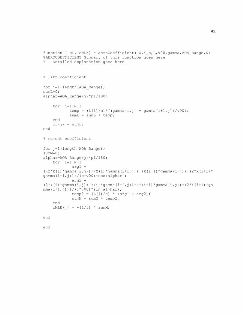
92

function [ cL, cMLE] = aeroCoefficient( X,Y,c,L,v00,gamma,AOA_Range,N) %AEROCOEFFICIENT Summary of this function goes here % Detailed explanation goes here % lift coefficient for j=1:length(AOA_Range); sumL=0; alphar=AOA_Range(j)*pi/180; for i=1:N-1 temp = (L(i)/c)*((gamma(i,j) + gamma(i+1,j))/v00); sumL = sumL + temp; end cL(j) = sumL; end % moment coefficient for j=1:length(AOA_Range); sumM=0; alphar=AOA_Range(j)*pi/180; for i=1:N-1 arg1 = ((2*X(i)*gamma(i,j))+(X(i)*gamma(i+1,j))+(X(i+1)*gamma(i,j))+(2*X(i+1)*gamma(i+1,j)))/(c*v00)*cos(alphar); arg2 = (2*Y(i)*gamma(i,j)+(Y(i)*gamma(i+1,j))+(Y(i+1)*gamma(i,j))+(2*Y(i+1)*gamma(i+1,j)))/(c*v00)*sin(alphar); temp2 = (L(i)/c) * (arg1 + arg2); sumM = sumM + temp2; end cMLE(j) = -(1/3) * sumM; end end

93

APPENDIX C

The following program is a symbolic solver designed to analytically solve the full high order location of the aerodynamic center and the associated pitching moment in viscous flow using the general airfoil theory equations. This solver also solves for the second order approximation of the aerodynamic center and the associated pitching moment. ----------------------------------------------------------------------- %%%%%%%%%%%%%%%%%%%%%%%%%%%%%%%% MAIN CODE %%%%%%%%%%%%%%%%%%%%%%%%%%%% ----------------------------------------------------------------------- syms a alo cloa cmo cma CD0 CD0L CD0L2 CMLEa CMLEN CMLEA CMc4 K1 K2 syms cl(a) syms CM(cl) CD(cl) % prompt = ('Inviscid (i) or Viscous (v) ? '); % flag = input(prompt,'s'); % prompt = ('Small angle approximation (s), General Airfoil Theory? (g), Thin Airfoil w/o small angle (t) '); % flagAngle = input(prompt,'s'); % % prompt = ('Run Test? (y/n)'); % testFlag = input(prompt,'s'); flag = 'v' flagAngle = 'g' testFlag = 'y' if flag == 'i' % inviscid flow if flagAngle == 's' cl(a) = cloa*(a-alo); % small angle approximation CA = -cl*a; % inviscid axial force coeff w/small angle approx CN = cl; % inviscid normal force coeff w/small angle approx %CM = cma*a+cmo; % traditional pitching moment equation CM = CMc4-cl/4; elseif flagAngle == 't' cl(a) = cloa*(a-alo); % small angle approximation CA = -cl*sin(a); % inviscid axial force coeff w/o small angle approx CN = cl*cos(a); % inviscid normal force coeff w/o small angle approx %CM = cma*a+cmo; CM = CMc4-cl/4; % traditional pitching moment equation elseif flagAngle == 'g' cl(a) = cloa*(sin(a)-tan(alo)*cos(a)); % non-small angle approximation

94

CA = -cl*sin(a); % inviscid axial force coefficient (Phillips 4.8.24) CN = cl*cos(a); % inviscid normal force coefficient (Phillips 4.8.25) CM = CMLEa*sin(2*a)+cl*CMLEN*cos(a)-cl*CMLEA*sin(a); % pitching moment equation modified in paper %CM = CMLEa*sin(2*a)-cl*CMLEN*cos(a)+cl*CMLEA*tan(alo)*sin(a); % joukowski pitching moment equation end cla(a) = diff(cl,a); claa(a) = diff(cla,a); CAa = diff(CA,a); CAaa = diff(CAa,a); CNa = diff(CN,a); CNaa = diff(CNa,a); CMa = diff(CM,a); CMaa = diff(CMa,a); elseif flag == 'v' % viscous flow if flagAngle == 's' cl(a) = cloa*(a-alo); % small angle approximation CD = CD0 + CD0L*cl + CD0L2*cl*cl; % parabolic drag model CA = -cl*a+CD; % viscous axial force coeff w/small angle approx CN = cl+CD*a; % viscous normal force coeff w/small angle approx %CM = cma*a+cmo; % traditional pitching moment equation CM = CMc4-cl/4; % traditional pitching moment equation elseif flagAngle == 't' cl(a) = cloa*(a-alo); % small angle approximation CD = CD0 + CD0L*cl + CD0L2*cl*cl; % parabolic drag model CA = -cl*sin(a)+CD*cos(a); % viscous axial force coeff w/o small angle approx CN = cl*cos(a)+CD*sin(a); % viscous normal force coeff w/o small angle approx %CM = cma*a+cmo; CM = CMc4-cl/4; % traditional pitching moment equation elseif flagAngle == 'g' cl(a) = cloa*(sin(a)-tan(alo)*cos(a)); % non-small angle approximation CD = CD0 + CD0L*cl + CD0L2*cl*cl; % parabolic drag model CA = -cl*sin(a) + CD*cos(a); % viscous axial force coefficient (Phillips 4.8.24) CN = cl*cos(a) + CD*sin(a); % viscous normal force coefficient (Phillips 4.8.25)

95

CM = CMLEa*sin(2*a)+CMLEN*(cl*cos(a)+CD*sin(a))+CMLEA*(CD*cos(a)-cl*sin(a)); % (corrected) joukowski pitching moment equation end cla(a) = diff(cl,a); claa(a) = diff(cla,a); %claa(a) = -cl(a) CAa = diff(CA,a); CAaa = diff(CAa,a); CNa = diff(CN,a); CNaa = diff(CNa,a); CMa = diff(CM,a); CMaa = diff(CMa,a); end % inviscid vs viscous disp('Non-Reduced standard----------------------------------------------------') disp(' ') Xac = (CAa*CMaa-CMa*CAaa)/(CNa*CAaa-CAa*CNaa); % aerodynamic center (Phillips 4.8.29) XacO = Xac; % Yac = (CNa*CMaa-CMa*CNaa)/(CNa*CAaa-CAa*CNaa); % aerodynamic center (Phillips 4.8.30) YacO = Yac; % cmAC = CM + Xac*CN - Yac*CA; % moment coefficient (Phillips 4.8.31) cmACO = cmAC; % ????????????????????????????? % Xac = -2*CMLEa*((2*sin(2*a)*CAa+cos(2*a)*CAaa)/(CNa*CAaa-CAa*CNaa))-CMLEN; % Xac = simplify(Xac) % % Yac = -2*CMLEa*((2*sin(2*a)*CNa+cos(2*a)*CNaa)/(CNa*CAaa-CAa*CNaa))+CMLEA; % Yac = simplify(Yac) % % cmAC = CM + Xac*CN - Yac*CA; % moment coefficient (Phillips 4.8.31) % cmAC = simplify(cmAC) %disp('Non-Reduced pretty-------------------------------------------------------')

96

%disp(' ') % disp('Xac_original') % pretty(Xac); % disp('Yac_original') % pretty(Yac); % disp('cMAC_original') % pretty(cmAC); %% Full high order solution if testFlag == 'y' cpass = 'k'; % color mpass = '.'; % marker [ xsave,ysave,cmsave ] = plotting( Xac,Yac,cmAC, cpass, mpass); dataSave(:,1) = xsave(:); dataSave(:,2) = ysave(:); dataSave(:,3) = cmsave(:); end %% Order Reduction if flag == 'v' % EqOrderReduction( CAa,CAaa,CNa,CNaa,CMa,CMaa,CN,CA,CM,a,alo,CD0,CD0L,CD0L2,cl, testFlag ) [CAa,CAaa,CNa,CNaa,CMa,CMaa,CN,CA,CM,a,alo,CD0,CD0L,CD0L2,cl, Xac, Yac, cmAC,dataSave] = EqOrderReduction4( CAa,CAaa,CNa,CNaa,CMa,CMaa,CN,CA,CM,a,alo,CD0,CD0L,CD0L2,cl,dataSave, testFlag ); end disp('post reduction equations-------------------------------------------') % Xac = subs(Xac,cloa*CD0L2,K1); % Xac = subs(Xac,CD0/(2*cloa),K2); Xac = simplify(Xac); % Yac = subs(Yac,cloa*CD0L2,K1); % Yac = subs(Yac,CD0/(2*cloa),K2); Yac = simplify(Yac); % cmAC = subs(cmAC,cloa*CD0L2,K1); % cmAC = subs(cmAC,CD0/(2*cloa),K2) cmAC = simplify(cmAC); % Xac % Yac % cmAC [Xac,Yac,cmAC] = OrderReduction_Post( Xac,Yac,cmAC ); cpass = 'k'; % color mpass = '*'; % marker [ xsave,ysave,cmsave ] = plotting( Xac,Yac,cmAC, cpass, mpass ); dataSave(:,10) = xsave(:);

97

dataSave(:,11) = ysave(:); dataSave(:,12) = cmsave(:); % Check on final paper versions of 3rd order reduction k1 = cloa*CD0L2 ; k2 = CD0/(2*cloa); xknum = k1*(3*(a*alo-a^2-alo^2/2)+1)-k2*(1+3*a^2/2)-1; kden = k1*(1+3*alo^2/2)+3*k2*(a^2/2-a*alo-2*k2/3-1)-alo^2-1; XacK = -2*CMLEa/cloa*(xknum/kden)-CMLEN; yknum = k1*(3*a-2*alo)+CD0L+3*a*k2+alo*(1+alo^2/3); YacK = -2*CMLEa/cloa*(yknum/kden)+CMLEA; cmacknum = alo*(k1+k2-alo^2/3-1)+6*a*k2*(k1+k2); cmACK = 2*CMLEa*(cmacknum/kden); % final reduced equations after hand simplification cpass = 'c'; % color mpass = '^'; % marker [ xsave,ysave,cmsave ] = plotting( XacK,YacK,cmACK, cpass, mpass ); dataSave(:,7) = xsave(:); dataSave(:,8) = ysave(:); dataSave(:,9) = cmsave(:); % Comparison to Dr.Hunsaker code xu = -3.0*cloa*CD0L2*a^2 + 3*cloa*CD0L2*a*alo - 3*cloa*CD0L2*alo^2/2 + cloa*CD0L2 + CD0L*alo - 1 - 3*CD0*a^2/(4*cloa) - CD0/(2*cloa); yu = 3*cloa*CD0L2*a - 2*cloa*CD0L2*alo + CD0L + alo^3/3 + alo + 3*CD0*a/(2*cloa); denom = - 3*cloa*CD0L*CD0L2*a + 3*cloa*CD0L*CD0L2*alo + 3*cloa*CD0L2*alo^2/2 + cloa*CD0L2 + CD0*CD0L2 - CD0L^2 - alo^2 - 1 - 3*CD0*CD0L*a/(2*cloa) + 3*CD0*CD0L*alo/(2*cloa) + 3*CD0*a^2/(4*cloa) - 3*CD0*a*alo/(2*cloa) - 3*CD0/(2*cloa) - CD0^2/(2*cloa^2); xu = xu*2*cloa; yu = yu*2*cloa; denom = denom*2*cloa*cloa; XacTest = -2*CMLEa* xu/denom - CMLEN; YacTest = -2*CMLEa* yu/denom + CMLEA; %cmCATest = %%%%%%%%%%%%%%%%%%%%%%%%%%%%%%%%%%%%%%%%%%%%%%%%%%%%%%%%%%%%%%%%%%%%%%%%%%% % NACA 1408 data from Airfoil Appendix foilName = '1408'; a = 5*(pi/180);

98

alo = -0.0145678; cloa = 6.1897717; CD0 = 0.0051515; CD0L = -0.0017593; CD0L2 = 0.0080154; CMLEa = 0.8677365; CMLEA = -0.0322065; CMLEN = -0.5349267; % Third Order + manual reduction Hunsaker code format long XacDk = eval(subs(XacK)); YacDk = eval(subs(YacK)); cmACDk = eval(subs(cmACK)); % Third Order Reduction Final of Pope code format long XacP = eval(subs(Xac)); YacP = eval(subs(Yac)); cmACP = eval(subs(cmAC)); format long XacTest = eval(subs(XacTest)); YacTest = eval(subs(YacTest)); %cmACTest = eval(subs(cmACTest)) figure(2) plot(dataSave(:,1),dataSave(:,2),'.-b',dataSave(:,7),dataSave(:,8),'.-r') xlabel('Xac') ylabel('Yac') title(['AC(alpha) for NACA ',foilName]) legend('Original','Reduced') axis equal figure(3) plot((-15:1:15),dataSave(:,3),'.-b') hold on plot((-15:1:15),dataSave(:,6),'.-g') plot((-15:1:15),dataSave(:,12),'.-k') plot((-15:1:15),dataSave(:,9),'.-r') xlabel('alpha') ylabel('cmAC') title(['cmAC(alpha) for NACA ',foilName]) legend('full','matlab','matlab R','paper') XacP-XacTest YacP-YacTest XacP-XacDk YacP-YacDk

99

----------------------------------------------------------------------- %%%%%%%%%%%%%%%%%%%%%%%%% SUPPORTING FUNCTIONS %%%%%%%%%%%%%%%%%%%%%%%% ----------------------------------------------------------------------- function [ CAa,CAaa,CNa,CNaa,CMa,CMaa,CN,CA,CM,a,alo,CD0,CD0L,CD0L2,cl, Xac, Yac, cmAC,dataSave] = EqOrderReduction4( CAa,CAaa,CNa,CNaa,CMa,CMaa,CN,CA,CM,a,alo,CD0,CD0L,CD0L2,cl,dataSave, testFlag ) %EQORDERREDUCTION4 disp('RUN EQUATION REDUCTION FUNCTION -------------------------------') disp(' ') % Expand %disp('Expanded Equations') %disp(' ') CA = expand(CA); CAa = expand(CAa); CAaa = expand(CAaa); CN = expand(CN); CNa = expand(CNa); CNaa = expand(CNaa); CM = expand(CM); CMa = expand(CMa); CMaa = expand(CMaa); % Using Reduced Equations in Aerodynamic Center Equations (12,13) disp('1st Reduction ----------------------------------------------------') disp(' ') CA = subs(CA, sin(a),a-a^3/6); CA = subs(CA, sin(2*a),2*a-4*a^3/3); CA = subs(CA, sin(3*a),3*a-9*a^3/2); CA = subs(CA, cos(a),1-a^2/2); CA = subs(CA, cos(2*a),1-2*a^2); CA = subs(CA, cos(3*a),1-9*a^2/2); CA = subs(CA, tan(alo),alo+alo^3/3); CAa = subs(CAa, sin(a),a-a^3/6); CAa = subs(CAa, sin(2*a),2*a-4*a^3/3); CAa = subs(CAa, sin(3*a),3*a-9*a^3/2); CAa = subs(CAa, cos(a),1-a^2/2); CAa = subs(CAa, cos(2*a),1-2*a^2); CAa = subs(CAa, cos(3*a),1-9*a^2/2); CAa = subs(CAa, tan(alo),alo+alo^3/3); CAaa = subs(CAaa, sin(a),a-a^3/6);

100

CAaa = subs(CAaa, sin(2*a),2*a-4*a^3/3); CAaa = subs(CAaa, sin(3*a),3*a-9*a^3/2); CAaa = subs(CAaa, cos(a),1-a^2/2); CAaa = subs(CAaa, cos(2*a),1-2*a^2); CAaa = subs(CAaa, cos(3*a),1-9*a^2/2); CAaa = subs(CAaa, tan(alo),alo+alo^3/3); CN = subs(CN, sin(a),a-a^3/6); CN = subs(CN, sin(2*a),2*a-4*a^3/3); CN = subs(CN, sin(3*a),3*a-9*a^3/2); CN = subs(CN, cos(a),1-a^2/2); CN = subs(CN, cos(2*a),1-2*a^2); CN = subs(CN, cos(3*a),1-9*a^2/2); CN = subs(CN, tan(alo),alo+alo^3/3); CNa = subs(CNa, sin(a),a-a^3/6); CNa = subs(CNa, sin(2*a),2*a-4*a^3/3); CNa = subs(CNa, sin(3*a),3*a-9*a^3/2); CNa = subs(CNa, cos(a),1-a^2/2); CNa = subs(CNa, cos(2*a),1-2*a^2); CNa = subs(CNa, cos(3*a),1-9*a^2/2); CNa = subs(CNa, tan(alo),alo+alo^3/3); CNaa = subs(CNaa, sin(a),a-a^3/6); CNaa = subs(CNaa, sin(2*a),2*a-4*a^3/3); CNaa = subs(CNaa, sin(3*a),3*a-9*a^3/2); CNaa = subs(CNaa, cos(a),1-a^2/2); CNaa = subs(CNaa, cos(2*a),1-2*a^2); CNaa = subs(CNaa, cos(3*a),1-9*a^2/2); CNaa = subs(CNaa, tan(alo),alo+alo^3/3); CM = subs(CM, sin(a),a-a^3/6); CM = subs(CM, sin(2*a),2*a-4*a^3/3); CM = subs(CM, sin(3*a),3*a-9*a^3/2); CM = subs(CM, cos(a),1-a^2/2); CM = subs(CM, cos(2*a),1-2*a^2); CM = subs(CM, cos(3*a),1-9*a^2/2); CM = subs(CM, tan(alo),alo+alo^3/3); CMa = subs(CMa, sin(a),a-a^3/6); CMa = subs(CMa, sin(2*a),2*a-4*a^3/3); CMa = subs(CMa, sin(3*a),3*a-9*a^3/2); CMa = subs(CMa, cos(a),1-a^2/2); CMa = subs(CMa, cos(2*a),1-2*a^2); CMa = subs(CMa, cos(3*a),1-9*a^2/2); CMa = subs(CMa, tan(alo),alo+alo^3/3); CMaa = subs(CMaa, sin(a),a-a^3/6); CMaa = subs(CMaa, sin(2*a),2*a-4*a^3/3); CMaa = subs(CMaa, sin(3*a),3*a-9*a^3/2); CMaa = subs(CMaa, cos(a),1-a^2/2); CMaa = subs(CMaa, cos(2*a),1-2*a^2); CMaa = subs(CMaa, cos(3*a),1-9*a^2/2);

101

CMaa = subs(CMaa, tan(alo),alo+alo^3/3); xDL = (CAa*CMaa); xDR = (CMa*CAaa); xNL = (CNa*CAaa); xNR = (CAa*CNaa); yDL = (CNa*CMaa); yDR = (CMa*CNaa); yNL = (CNa*CAaa); yNR = (CAa*CNaa); Xac = (xDL-xDR)/(xNL-xNR); % aerodynamic center (Phillips 4.8.29) Yac = (yDL-yDR )/(yNL-yNR ); % aerodynamic center (Phillips 4.8.30) cmAC = CM + Xac*CN - Yac*CA; % moment coefficient (Phillips 4.8.31) cpass = 'g'; % color mpass = '.'; % marker plotting( Xac,Yac,cmAC, cpass, mpass ); disp('Second Reduction (alpha)---------------------------------------------------') disp(' ') % Xac = simplify(Xac); % Yac = simplify(Yac); % cmAC = simplify(cmAC); Xac = expand(Xac); Yac = expand(Yac); cmAC = expand(cmAC); Xac = subs(Xac, a*a*a*a*a*a*a*a*a*a*a*a*a*a*a*a, 0); % 16a Xac = subs(Xac, a*a*a*a*a*a*a*a*a*a*a*a*a*a*a, 0); % 15a Xac = subs(Xac, a*a*a*a*a*a*a*a*a*a*a*a*a*a, 0); % 14a Xac = subs(Xac, a*a*a*a*a*a*a*a*a*a*a*a*a, 0); % 13a Xac = subs(Xac, a*a*a*a*a*a*a*a*a*a*a*a, 0); % 12a Xac = subs(Xac, a*a*a*a*a*a*a*a*a*a*a, 0); % 11a Xac = subs(Xac, a*a*a*a*a*a*a*a*a*a, 0); % 10a Xac = subs(Xac, a*a*a*a*a*a*a*a*a, 0); % 9a Xac = subs(Xac, a*a*a*a*a*a*a*a, 0); % 8a Xac = subs(Xac, a*a*a*a*a*a*a, 0); % 7a Xac = subs(Xac, a*a*a*a*a*a, 0); % 6a Xac = subs(Xac, a*a*a*a*a, 0); % 5a Xac = subs(Xac, a*a*a*a, 0); % 4a Xac = subs(Xac, alo*alo*alo*alo*alo*alo*alo*alo*alo, 0); % 9alo Xac = subs(Xac, alo*alo*alo*alo*alo*alo*alo*alo, 0); % 8alo Xac = subs(Xac, alo*alo*alo*alo*alo*alo*alo, 0); % 7alo Xac = subs(Xac, alo*alo*alo*alo*alo*alo, 0); % 6alo Xac = subs(Xac, alo*alo*alo*alo*alo, 0); % 5alo Xac = subs(Xac, alo*alo*alo*alo, 0); % 4alo

102

Yac = subs(Yac, a*a*a*a*a*a*a*a*a*a*a*a*a*a*a*a, 0); % 16a Yac = subs(Yac, a*a*a*a*a*a*a*a*a*a*a*a*a*a*a, 0); % 15a Yac = subs(Yac, a*a*a*a*a*a*a*a*a*a*a*a*a*a, 0); % 14a Yac = subs(Yac, a*a*a*a*a*a*a*a*a*a*a*a*a, 0); % 13a Yac = subs(Yac, a*a*a*a*a*a*a*a*a*a*a*a, 0); % 12a Yac = subs(Yac, a*a*a*a*a*a*a*a*a*a*a, 0); % 11a Yac = subs(Yac, a*a*a*a*a*a*a*a*a*a, 0); % 10a Yac = subs(Yac, a*a*a*a*a*a*a*a*a, 0); % 9a Yac = subs(Yac, a*a*a*a*a*a*a*a, 0); % 8a Yac = subs(Yac, a*a*a*a*a*a*a, 0); % 7a Yac = subs(Yac, a*a*a*a*a*a, 0); % 6a Yac = subs(Yac, a*a*a*a*a, 0); % 5a Yac = subs(Yac, a*a*a*a, 0); % 4a Yac = subs(Yac, alo*alo*alo*alo*alo*alo*alo*alo*alo, 0); % 9alo Yac = subs(Yac, alo*alo*alo*alo*alo*alo*alo*alo, 0); % 8alo Yac = subs(Yac, alo*alo*alo*alo*alo*alo*alo, 0); % 7alo Yac = subs(Yac, alo*alo*alo*alo*alo*alo, 0); % 6alo Yac = subs(Yac, alo*alo*alo*alo*alo, 0); % 5alo Yac = subs(Yac, alo*alo*alo*alo, 0); % 4alo cmAC = subs(cmAC, a*a*a*a*a*a*a*a*a*a*a*a*a*a*a*a*a*a, 0); % 18a cmAC = subs(cmAC, a*a*a*a*a*a*a*a*a*a*a*a*a*a*a*a*a, 0); % 17a cmAC = subs(cmAC, a*a*a*a*a*a*a*a*a*a*a*a*a*a*a*a, 0); % 16a cmAC = subs(cmAC, a*a*a*a*a*a*a*a*a*a*a*a*a*a*a, 0); % 15a cmAC = subs(cmAC, a*a*a*a*a*a*a*a*a*a*a*a*a*a, 0); % 14a cmAC = subs(cmAC, a*a*a*a*a*a*a*a*a*a*a*a*a, 0); % 13a cmAC = subs(cmAC, a*a*a*a*a*a*a*a*a*a*a*a, 0); % 12a cmAC = subs(cmAC, a*a*a*a*a*a*a*a*a*a*a, 0); % 11a cmAC = subs(cmAC, a*a*a*a*a*a*a*a*a*a, 0); % 10a cmAC = subs(cmAC, a*a*a*a*a*a*a*a*a, 0); % 9a cmAC = subs(cmAC, a*a*a*a*a*a*a*a, 0); % 8a cmAC = subs(cmAC, a*a*a*a*a*a*a, 0); % 7a cmAC = subs(cmAC, a*a*a*a*a*a, 0); % 6a cmAC = subs(cmAC, a*a*a*a*a, 0); % 5a cmAC = subs(cmAC, a*a*a*a, 0); % 4a cmAC = subs(cmAC, alo*alo*alo*alo*alo*alo*alo*alo*alo, 0); % 9alo cmAC = subs(cmAC, alo*alo*alo*alo*alo*alo*alo*alo, 0); % 8alo cmAC = subs(cmAC, alo*alo*alo*alo*alo*alo*alo, 0); % 7alo cmAC = subs(cmAC, alo*alo*alo*alo*alo*alo, 0); % 6alo cmAC = subs(cmAC, alo*alo*alo*alo*alo, 0); % 5alo cmAC = subs(cmAC, alo*alo*alo*alo, 0); % 4alo cpass = 'm'; % color mpass = '.'; % marker plotting( Xac,Yac,cmAC, cpass, mpass); disp('3rd Reduction (alpha+alo)---------------------------------------------------') disp(' ')

103

% Xac = simplify(Xac); % Yac = simplify(Yac); % cmAC = simplify(cmAC); Xac = subs(Xac, a*a*a*alo, 0); Xac = subs(Xac, a*a*alo*alo, 0); Xac = subs(Xac, a*alo*alo*alo, 0); Yac = subs(Yac, a*a*a*alo, 0); Yac = subs(Yac, a*a*alo*alo, 0); Yac = subs(Yac, a*alo*alo*alo, 0); cmAC = subs(cmAC, a*a*a*alo, 0); cmAC = subs(cmAC, a*a*alo*alo, 0); cmAC = subs(cmAC, a*alo*alo*alo, 0); cpass = 'r'; % color mpass = '.'; % marker plotting( Xac,Yac,cmAC, cpass, mpass); disp('4th Reduction (drag combos)---------------------------------------------------') disp(' ') Xac = expand(Xac); Yac = expand(Yac); cmAC = expand(cmAC); % Xac = simplify(Xac); % Yac = simplify(Yac); % cmAC = simplify(cmAC); Xac = subs(Xac, CD0L*CD0L2*alo*alo, 0); Xac = subs(Xac, CD0*CD0L2*alo*alo, 0); Xac = subs(Xac, CD0L2*CD0L2*alo*alo, 0); Xac = subs(Xac, CD0L*CD0L*alo*alo, 0); %Xac = subs(Xac, CD0*CD0L2*alo, 0); Xac = subs(Xac, CD0*CD0L2*alo*alo*alo, 0); Xac = subs(Xac, CD0*CD0L*alo*alo*alo, 0); Xac = subs(Xac, CD0L*alo*alo*alo, 0); Xac = subs(Xac, CD0L*CD0L2*a*alo, 0); Xac = subs(Xac, CD0*CD0L2*a*alo, 0); Xac = subs(Xac, CD0*CD0L2*a*a*a, 0); Xac = subs(Xac, CD0*CD0L2*a*a, 0); Xac = subs(Xac, CD0*CD0L*a*a*a, 0); Xac = subs(Xac, CD0*CD0L*a*a, 0); Xac = subs(Xac, CD0L2*CD0L2*alo*alo, 0); Xac = subs(Xac, CD0L2*CD0L2*a*a, 0); Xac = subs(Xac, CD0L2*CD0L2*a*alo, 0); Xac = subs(Xac, CD0*a*a*a, 0); Xac = subs(Xac, CD0L*a*a*a, 0); Xac = subs(Xac, CD0L2*a*a*a, 0); Xac = subs(Xac, CD0L2*alo*alo*alo, 0); Xac = subs(Xac, CD0L2*alo*alo*a, 0);

104

Xac = subs(Xac, CD0L2*alo*a*a, 0); Yac = subs(Yac, CD0L*CD0L2*alo*alo, 0); Yac = subs(Yac, CD0*CD0L2*alo*alo, 0); Yac = subs(Yac, CD0L2*CD0L2*alo*alo, 0); Yac = subs(Yac, CD0L*CD0L*alo*alo, 0); %Yac = subs(Yac, CD0*CD0L2*alo, 0); Yac = subs(Yac, CD0*CD0L2*alo*alo*alo, 0); Yac = subs(Yac, CD0*CD0L*alo*alo*alo, 0); Yac = subs(Yac, CD0L*alo*alo*alo, 0); Yac = subs(Yac, CD0L*CD0L2*a*alo, 0); Yac = subs(Yac, CD0*CD0L2*a*alo, 0); Yac = subs(Yac, CD0*CD0L2*a*a*a, 0); Yac = subs(Yac, CD0*CD0L2*a*a, 0); Yac = subs(Yac, CD0*CD0L*a*a*a, 0); Yac = subs(Yac, CD0*CD0L*a*a, 0); Yac = subs(Yac, CD0L2*CD0L2*alo*alo, 0); Yac = subs(Yac, CD0L2*CD0L2*a*a, 0); Yac = subs(Yac, CD0L2*CD0L2*a*alo, 0); Yac = subs(Yac, CD0*a*a*a, 0); Yac = subs(Yac, CD0L*a*a*a, 0); Yac = subs(Yac, CD0L2*a*a*a, 0); Yac = subs(Yac, CD0L2*alo*alo*alo, 0); Yac = subs(Yac, CD0L2*alo*alo*a, 0); Yac = subs(Yac, CD0L2*alo*a*a, 0); cmAC = subs(cmAC, CD0L*CD0L2*alo*alo, 0); cmAC = subs(cmAC, CD0*CD0L2*alo*alo, 0); cmAC = subs(cmAC, CD0L2*CD0L2*alo*alo, 0); cmAC = subs(cmAC, CD0L*CD0L*alo*alo, 0); cmAC = subs(cmAC, CD0*CD0L2*alo, 0); cmAC = subs(cmAC, CD0*CD0L2*alo*alo*alo, 0); cmAC = subs(cmAC, CD0*CD0L*alo*alo*alo, 0); cmAC = subs(cmAC, CD0L*alo*alo*alo, 0); cmAC = subs(cmAC, CD0L*CD0L2*a*alo, 0); cmAC = subs(cmAC, CD0*CD0L2*a*alo, 0); cmAC = subs(cmAC, CD0*CD0L2*a*a*a, 0); cmAC = subs(cmAC, CD0*CD0L2*a*a, 0); cmAC = subs(cmAC, CD0*CD0L*a*a*a, 0); cmAC = subs(cmAC, CD0*CD0L*a*a, 0); cmAC = subs(cmAC, CD0L2*CD0L2*alo*alo, 0); cmAC = subs(cmAC, CD0L2*CD0L2*a*a, 0); cmAC = subs(cmAC, CD0L2*CD0L2*a*alo, 0); cmAC = subs(cmAC, CD0*a*a*a, 0); cmAC = subs(cmAC, CD0L*a*a*a, 0); cmAC = subs(cmAC, CD0L2*a*a*a, 0); cmAC = subs(cmAC, CD0L2*alo*alo*alo, 0); cmAC = subs(cmAC, CD0L2*alo*alo*a, 0); cmAC = subs(cmAC, CD0L2*alo*a*a, 0); cmAC = subs(cmAC, CD0*alo*alo*alo, 0);

105

cmAC = subs(cmAC, CD0*CD0L*alo*alo, 0); cmAC = subs(cmAC, CD0*CD0L*a*alo, 0); cmAC = subs(cmAC, CD0*CD0L*CD0L2*a, 0); cmAC = subs(cmAC, CD0*CD0L*CD0L*a*alo, 0); cmAC = subs(cmAC, CD0*CD0L*a*alo*alo, 0); cmAC = subs(cmAC, CD0*a*alo*alo, 0); cmAC = subs(cmAC, CD0*a*a*alo, 0); cmAC = subs(cmAC, CD0*CD0*a*a, 0); cmAC = subs(cmAC, CD0*CD0*a*alo, 0); cmAC = subs(cmAC, CD0*CD0*CD0L*a, 0); cmAC = subs(cmAC, CD0*CD0*CD0L*a*alo, 0); cmAC = subs(cmAC, CD0*CD0*CD0L*alo, 0); cmAC = subs(cmAC, CD0*CD0*CD0*a, 0); cmAC = subs(cmAC, CD0*CD0*CD0*a*a, 0); cmAC = subs(cmAC, CD0*CD0*a*a*alo, 0); cmAC = subs(cmAC, CD0*CD0*CD0L2*a, 0); cmAC = subs(cmAC, CD0*CD0*alo*alo*alo, 0); cmAC = subs(cmAC, CD0L*a*a*alo, 0); cmAC = subs(cmAC, CD0L*a*alo*alo, 0); cmAC = subs(cmAC, CD0L*CD0L2*a*a, 0); cmAC = subs(cmAC, CD0L*CD0L*a*a, 0); cmAC = subs(cmAC, CD0L*CD0L*a*a*alo, 0); cmAC = subs(cmAC, CD0L*CD0L*a*alo, 0); cmAC = subs(cmAC, CD0L*CD0L*CD0*a, 0); cmAC = subs(cmAC, CD0L*CD0L*CD0L2*a*a, 0); cmAC = subs(cmAC, CD0L*CD0L*CD0L*a, 0); cmAC = subs(cmAC, CD0L*CD0L*CD0L*alo, 0); cmAC = subs(cmAC, CD0L*CD0L*CD0L*a*a, 0); cmAC = subs(cmAC, CD0L*CD0L*CD0L*a*alo, 0); cmAC = subs(cmAC, CD0L*CD0L*CD0L*a*a*alo, 0); disp('%%%%%%%%%%%%%%%%%%%%%%%%%%%%%%%%%%%%%%%%%%%%%%%%%%%%%%%%%%%%%%%%%%%%') % Reduced model after equation reduction cpass = 'c'; % color mpass = '.'; % marker [ xsave,ysave,cmsave ] = plotting( Xac,Yac,cmAC, cpass, mpass ); dataSave(:,4) = xsave(:); dataSave(:,5) = ysave(:); dataSave(:,6) = cmsave(:); end

106

function [ xsave,ysave,cmsave ] = plotting( Xac,Yac,cmAC, cpass, mpass ) %PLOTTING Summary of this function goes here % Detailed explanation goes here disp('test case----------------------------------------------------') j=1; for i = -15:1:15 %%%%%%%%%%%%%%%%%%%%%%%%%%%%%%%%%%%%%%%%%%%%%%% % % NACA 0006 data from Airfoil Appendix % foilName = '0006'; % a = i*(pi/180); % alo = 0; % cloa = 6.18958236335962; % CD0 = 0.00460455864601409; % CD0L = 0; % CD0L2 = 0.010321990400509; % CMLEa = 0; % CMLEA = 0; % CMLEN = -0.250178140301351; %%%%%%%%%%%%%%%%%%%%%%%%%%%%%%%%%%%%%%%%%%%%%%% %%%%%%%%%%%%%%%%%%%%%%%%%%%%%%%%%%%%%%%%%%%%%%% % % NACA 0012 data from Airfoil Appendix % foilName = '0012'; % a = i*(pi/180); % alo = 0; % cloa = 6.14987213746803; % CD0 = 0.00578980686984839; % CD0L = 0; % CD0L2 = 0.00589558911360464; % CMLEa = 0; % CMLEA = 0; % CMLEN = -0.248792267683901; %%%%%%%%%%%%%%%%%%%%%%%%%%%%%%%%%%%%%%%%%%%%%%% %%%%%%%%%%%%%%%%%%%%%%%%%%%%%%%%%%%%%%%%%%%%%%% % NACA 1408 data from Airfoil Appendix foilName = '1408'; a = i*(pi/180); alo = -0.0145678; cloa = 6.1897717; CD0 = 0.0051515; CD0L = -0.0017593; CD0L2 = 0.0080154; CMLEa = 0.8677365; CMLEA = -0.0322065; CMLEN = -0.5349267; %cmo = 1; %cma = 1; %Cmc4 = 1; %%%%%%%%%%%%%%%%%%%%%%%%%%%%%%%%%%%%%%%%%%%%%%% %%%%%%%%%%%%%%%%%%%%%%%%%%%%%%%%%%%%%%%%%%%%%%%

107

% % NACA 1412 data from Airfoil Appendix % foilName = '1412'; % a = i*(pi/180); % alo = -0.0216014394282236; % cloa = 6.02467660173922; % CD0 = 0.00587402293302405; % CD0L = -0.00134903274883071; % CD0L2 = 0.00536741319382652; % CMLEa = 0.542385993671305; % CMLEA = -0.0183836491952911; % CMLEN = -0.429724431443849; %%%%%%%%%%%%%%%%%%%%%%%%%%%%%%%%%%%%%%%%%%%%%%% %%%%%%%%%%%%%%%%%%%%%%%%%%%%%%%%%%%%%%%%%%%%%%% % % NACA 2410 data from Airfoil Appendix % foilName = '2410'; % a = i*(pi/180); % alo = -0.0350101171310758; % cloa = 6.23568559320461; % CD0 = 0.00580887637682987; % CD0L = -0.00202820935139267; % CD0L2 = 0.00657649746862038; % CMLEa = 0.696673178623474; % CMLEA = -0.0121747099302256; % CMLEN = -0.471751212453014; %%%%%%%%%%%%%%%%%%%%%%%%%%%%%%%%%%%%%%%%%%%%%%% %%%%%%%%%%%%%%%%%%%%%%%%%%%%%%%%%%%%%%%%%%%%%%% % % NACA 2412 data from Airfoil Appendix % foilName = '2412'; % a = i*(pi/180); % alo = -0.0455580244243206; % cloa = 5.75810202691551; % CD0 = 0.00640032868295237; % CD0L = -0.00208181252700775; % CD0L2 = 0.00618775485134525; % CMLEa = 0.494123897109009; % CMLEA = -0.0263366838973971; % CMLEN = -0.414419608257138; %%%%%%%%%%%%%%%%%%%%%%%%%%%%%%%%%%%%%%%%%%%%%%% %%%%%%%%%%%%%%%%%%%%%%%%%%%%%%%%%%%%%%%%%%%%%%% % % NACA 2424 data from Airfoil Appendix % foilName = '2424'; % a = i*(pi/180); % alo = -0.0354033949938163; % cloa = 5.18829911765801; % CD0 = 0.00844763624697131; % CD0L = -0.00075778327782238; % CD0L2 = 0.00635556970934001; % CMLEa = 0.563857762725431; % CMLEA = 0.0283921893758112; % CMLEN = -0.433109250719577; %%%%%%%%%%%%%%%%%%%%%%%%%%%%%%%%%%%%%%%%%%%%%%% %%%%%%%%%%%%%%%%%%%%%%%%%%%%%%%%%%%%%%%%%%%%%%% % % NACA 4412 data from Airfoil Appendix % foilName = '4412';

108

% a = i*(pi/180); % alo = -0.066813366237402; % cloa = 5.85919194114081; % CD0 = 0.00645256725654991; % CD0L = -0.00336480754312331; % CD0L2 = 0.00724157881965858; % CMLEa = 0.68855712967518; % CMLEA = -0.110712686814761; % CMLEN = -0.491349229675727; %%%%%%%%%%%%%%%%%%%%%%%%%%%%%%%%%%%%%%%%%%%%%%% %%%%%%%%%%%%%%%%%%%%%%%%%%%%%%%%%%%%%%%%%%%%%%% % % NACA 4415 data from Airfoil Appendix % foilName = '4415'; % a = i*(pi/180); % alo = -0.0734303832901057; % cloa = 5.68653896493843; % CD0 = 0.0075058042036877; % CD0L = -0.00254026404822751; % CD0L2 = 0.00419036888285099; % CMLEa = 0.640570566841305; % CMLEA = -0.0245218565708409; % CMLEN = -0.468522511921671; %%%%%%%%%%%%%%%%%%%%%%%%%%%%%%%%%%%%%%%%%%%%%%% %%%%%%%%%%%%%%%%%%%%%%%%%%%%%%%%%%%%%%%%%%%%%%% % % NACA 4418 data from Airfoil Appendix % foilName = '4418'; % a = i*(pi/180); % alo = -0.0685079303321731; % cloa = 5.71103186575275; % CD0 = 0.00790011856241665; % CD0L = -0.00256047509045299; % CD0L2 = 0.00401065120084031; % CMLEa = 0.663301464170368; % CMLEA = -0.0235063201303145; % CMLEN = -0.470752522108866; %%%%%%%%%%%%%%%%%%%%%%%%%%%%%%%%%%%%%%%%%%%%%%% %%%%%%%%%%%%%%%%%%%%%%%%%%%%%%%%%%%%%%%%%%%%%%% % % NACA 4424 data from Airfoil Appendix % foilName = '4424'; % a = i*(pi/180); % alo = -0.0628467630852301; % cloa = 5.38037549620744; % CD0 = 0.008792211847361; % CD0L = -0.00178071313927388; % CD0L2 = 0.0053300138585352; % CMLEa = 0.680507117895762; % CMLEA = -0.00591426748485269; % CMLEN = -0.479713535634107; %%%%%%%%%%%%%%%%%%%%%%%%%%%%%%%%%%%%%%%%%%%%%%% %%%%%%%%%%%%%%%%%%%%%%%%%%%%%%%%%%%%%%%%%%%%%%% % % NACA 2412Dustin compressible data from Airfoil Appendix % foilName = '2412'; % a = i*(pi/180); % alo = -0.035876678458286425;

109

% cloa = 11.392192346341583; % CD0 = 0.02056918358643251; % CD0L = -0.026492229858322114; % CD0L2 = 0.11743008498986997; % CMLEa = 0.7257122234947719; % CMLEA = -1.2715452269152567; % CMLEN = -0.5147128651813082; %%%%%%%%%%%%%%%%%%%%%%%%%%%%%%%%%%%%%%%%%%%%%%% %%%%%%%%%%%%%%%%%%% X FOIL %%%%%%%%%%%%%%%%%%%% %%%%%%%%%%%%%%%%%%%%%%%%%%%%%%%%%%%%%%%%%%%%%%% % % XNACA 0006 data from Airfoil Appendix % foilName = '0006'; % a = i*(pi/180); % alo = 0; % cloa = 6.24725277916935; % CD0 = 0.00317816842440291; % CD0L = 0; % CD0L2 = 0.0127851315547638; % CMLEa = 0; % CMLEA = 0; % CMLEN = -0.24556228409321; %%%%%%%%%%%%%%%%%%%%%%%%%%%%%%%%%%%%%%%%%%%%%%% %%%%%%%%%%%%%%%%%%%%%%%%%%%%%%%%%%%%%%%%%%%%%%% % % xNACA 0012 data from Airfoil Appendix % foilName = '0012'; % a = i*(pi/180); % alo = 0; % cloa = 6.4126395802572; % CD0 = 0.00520318347755638; % CD0L = 0; % CD0L2 = 0.00493201029734306; % CMLEa = 0; % CMLEA = 0; % CMLEN = -0.249436912071791; %%%%%%%%%%%%%%%%%%%%%%%%%%%%%%%%%%%%%%%%%%%%%%% %%%%%%%%%%%%%%%%%%%%%%%%%%%%%%%%%%%%%%%%%%%%%%% % % xNACA 1408 data from Airfoil Appendix % foilName = '1408'; % a = i*(pi/180); % alo = -0.0180652358272032; % cloa = 6.32226645998854; % CD0 = 0.00461237846328006; % CD0L = -0.00136642750620477; % CD0L2 = 0.00717274422939727; % CMLEa = 0.750138280491661; % CMLEA = -0.0166962861688784; % CMLEN = -0.485906892418554; %%%%%%%%%%%%%%%%%%%%%%%%%%%%%%%%%%%%%%%%%%%%%%% %%%%%%%%%%%%%%%%%%%%%%%%%%%%%%%%%%%%%%%%%%%%%%% % % xNACA 1412 data from Airfoil Appendix % foilName = '1412'; % a = i*(pi/180);

110

% alo = -0.0178982511770066; % cloa = 6.36814143933405; % CD0 = 0.00521938900679535; % CD0L = -0.000876001965110274; % CD0L2 = 0.00505246982460321; % CMLEa = 0.673506992898865; % CMLEA = 0.0241548514697989; % CMLEN = -0.458825322979267; %%%%%%%%%%%%%%%%%%%%%%%%%%%%%%%%%%%%%%%%%%%%%%% %%%%%%%%%%%%%%%%%%%%%%%%%%%%%%%%%%%%%%%%%%%%%%% % % xNACA 2412 data from Airfoil Appendix % foilName = '2412'; % a = i*(pi/180); % alo = -0.0373895121688584; % cloa = 6.3253620978506; % CD0 = 0.00532949246530466; % CD0L = -0.00182506208560641; % CD0L2 = 0.00522268362548347; % CMLEa = 0.714522309708262; % CMLEA = -0.00184803325645788; % CMLEN = -0.472541777595804; %%%%%%%%%%%%%%%%%%%%%%%%%%%%%%%%%%%%%%%%%%%%%%% %%%%%%%%%%%%%%%%%%%%%%%%%%%%%%%%%%%%%%%%%%%%%% % % xNACA 2424 data from Airfoil Appendix % foilName = '2424'; % a = i*(pi/180); % alo = -0.0356187169129064; % cloa = 6.02088351998069; % CD0 = 0.00726457301719901; % CD0L = -0.00118756576598667; % CD0L2 = 0.00340876822456072; % CMLEa = 0.699560535536618; % CMLEA = -0.0279009300010138; % CMLEN = -0.46936193044925; %%%%%%%%%%%%%%%%%%%%%%%%%%%%%%%%%%%%%%%%%%%%%%% %%%%%%%%%%%%%%%%%%%%%%%%%%%%%%%%%%%%%%%%%%%%%% % % xNACA 4415 data from Airfoil Appendix % foilName = '4415'; % a = i*(pi/180); % alo = -0.0738471950476704; % cloa = 6.31439243010206; % CD0 = 0.00648995198238606; % CD0L = -0.00310050333854929; % CD0L2 = 0.00400685412224384; % CMLEa = 0.707460219355764; % CMLEA = -0.0295899801763886; % CMLEN = -0.472658242541987; %%%%%%%%%%%%%%%%%%%%%%%%%%%%%%%%%%%%%%%%%%%%%%% %%%%%%%%%%%%%%%%%%%%%%%%%%%%%%%%%%%%%%%%%%%%%% % % xNACA 4418 data from Airfoil Appendix % foilName = '4418'; % a = i*(pi/180); % alo = -0.0734820440836776; % cloa = 6.29539227696611;

111

% CD0 = 0.00703366550835054; % CD0L = -0.00259656735970565; % CD0L2 = 0.0031449907696781; % CMLEa = 0.699822363875463; % CMLEA = -0.029676210380603; % CMLEN = -0.469847771314208; %%%%%%%%%%%%%%%%%%%%%%%%%%%%%%%%%%%%%%%%%%%%%%% %%%%%%%%%%%%%%%%%%%%%%%%%%%%%%%%%%%%%%%%%%%%%% % % xNACA 4424 data from Airfoil Appendix % foilName = '4424'; % a = i*(pi/180); % alo = -0.0709059112140821; % cloa = 5.9874308077726; % CD0 = 0.00786583384450818; % CD0L = -0.00205551523231613; % CD0L2 = 0.00336950600880986; % CMLEa = 0.678651851542374; % CMLEA = -0.0178801645616264; % CMLEN = -0.464528574908379; %%%%%%%%%%%%%%%%%%%%%%%%%%%%%%%%%%%%%%%%%%%%%%% %%%%%%%%%%% SYMMETRIC ISSUE TEST %%%%%%%%%%%%%% %%%%%%%%%%%%%%%%%%%%%%%%%%%%%%%%%%%%%%%%%%%%%%% % % NACA 0012S data from Airfoil Appendix % foilName = '0012'; % a = i*(pi/180); % alo = 0; % cloa = 6.14987213746803; % CD0 = 0.00578980686984839; % CD0L = 0; % CD0L2 = 0.00589558911360464; % CMLEa = 0; % CMLEA = 0; % CMLEN = -0.248792267683901; %%%%%%%%%%%%%%%%%%%%%%%%%%%%%%%%%%%%%%%%%%%%%%% % substitute symbolic variables for double numbers into symbolic % expressions and evaluate to decimals XacT = eval(subs(Xac)); YacT = eval(subs(Yac)); cmACT = eval(subs(cmAC)); xsave(j) = XacT; ysave(j) = YacT; cmsave(j) = cmACT; j=j+1; end figure(1)

112

plot(xsave,ysave,'color',cpass,'marker',mpass) xlabel('Xac') ylabel('Yac') title(['AC(alpha) for NACA ',foilName]) axis equal hold on legend('Original','1st Reduction', '2nd Reduction', '3rd Reduction','4th Reduction','5th Reduction') end function [Xac,Yac,cmAC] = OrderReduction_Post( Xac,Yac,cmAC ) syms a alo cloa CD0 CD0L CD0L2 CMLEa CMLEN CMLEA Xac = expand(Xac); Yac = expand(Yac); cmAC = expand(cmAC); %%%%%%%%%%%%%%%%%%%%%%%%%%%%%%%%%%%%%%%%%%%%%%%%%%%%%%%%%%%%%%%%%%%%%%%%%%% Xac = subs(Xac, a*a*a*a*a*a*a*a*a*a*a*a*a*a*a*a, 0); % 16a Xac = subs(Xac, a*a*a*a*a*a*a*a*a*a*a*a*a*a*a, 0); % 15a Xac = subs(Xac, a*a*a*a*a*a*a*a*a*a*a*a*a*a, 0); % 14a Xac = subs(Xac, a*a*a*a*a*a*a*a*a*a*a*a*a, 0); % 13a Xac = subs(Xac, a*a*a*a*a*a*a*a*a*a*a*a, 0); % 12a Xac = subs(Xac, a*a*a*a*a*a*a*a*a*a*a, 0); % 11a Xac = subs(Xac, a*a*a*a*a*a*a*a*a*a, 0); % 10a Xac = subs(Xac, a*a*a*a*a*a*a*a*a, 0); % 9a Xac = subs(Xac, a*a*a*a*a*a*a*a, 0); % 8a Xac = subs(Xac, a*a*a*a*a*a*a, 0); % 7a Xac = subs(Xac, a*a*a*a*a*a, 0); % 6a Xac = subs(Xac, a*a*a*a*a, 0); % 5a Xac = subs(Xac, a*a*a*a, 0); % 4a Xac = subs(Xac, alo*alo*alo*alo*alo*alo*alo*alo*alo, 0); % 9alo Xac = subs(Xac, alo*alo*alo*alo*alo*alo*alo*alo, 0); % 8alo Xac = subs(Xac, alo*alo*alo*alo*alo*alo*alo, 0); % 7alo Xac = subs(Xac, alo*alo*alo*alo*alo*alo, 0); % 6alo Xac = subs(Xac, alo*alo*alo*alo*alo, 0); % 5alo Xac = subs(Xac, alo*alo*alo*alo, 0); % 4alo Yac = subs(Yac, a*a*a*a*a*a*a*a*a*a*a*a*a*a*a*a, 0); % 16a Yac = subs(Yac, a*a*a*a*a*a*a*a*a*a*a*a*a*a*a, 0); % 15a Yac = subs(Yac, a*a*a*a*a*a*a*a*a*a*a*a*a*a, 0); % 14a Yac = subs(Yac, a*a*a*a*a*a*a*a*a*a*a*a*a, 0); % 13a Yac = subs(Yac, a*a*a*a*a*a*a*a*a*a*a*a, 0); % 12a Yac = subs(Yac, a*a*a*a*a*a*a*a*a*a*a, 0); % 11a Yac = subs(Yac, a*a*a*a*a*a*a*a*a*a, 0); % 10a Yac = subs(Yac, a*a*a*a*a*a*a*a*a, 0); % 9a

113

Yac = subs(Yac, a*a*a*a*a*a*a*a, 0); % 8a Yac = subs(Yac, a*a*a*a*a*a*a, 0); % 7a Yac = subs(Yac, a*a*a*a*a*a, 0); % 6a Yac = subs(Yac, a*a*a*a*a, 0); % 5a Yac = subs(Yac, a*a*a*a, 0); % 4a Yac = subs(Yac, alo*alo*alo*alo*alo*alo*alo*alo*alo, 0); % 9alo Yac = subs(Yac, alo*alo*alo*alo*alo*alo*alo*alo, 0); % 8alo Yac = subs(Yac, alo*alo*alo*alo*alo*alo*alo, 0); % 7alo Yac = subs(Yac, alo*alo*alo*alo*alo*alo, 0); % 6alo Yac = subs(Yac, alo*alo*alo*alo*alo, 0); % 5alo Yac = subs(Yac, alo*alo*alo*alo, 0); % 4alo cmAC = subs(cmAC, a*a*a*a*a*a*a*a*a*a*a*a*a*a*a*a*a*a, 0); % 18a cmAC = subs(cmAC, a*a*a*a*a*a*a*a*a*a*a*a*a*a*a*a*a, 0); % 17a cmAC = subs(cmAC, a*a*a*a*a*a*a*a*a*a*a*a*a*a*a*a, 0); % 16a cmAC = subs(cmAC, a*a*a*a*a*a*a*a*a*a*a*a*a*a*a, 0); % 15a cmAC = subs(cmAC, a*a*a*a*a*a*a*a*a*a*a*a*a*a, 0); % 14a cmAC = subs(cmAC, a*a*a*a*a*a*a*a*a*a*a*a*a, 0); % 13a cmAC = subs(cmAC, a*a*a*a*a*a*a*a*a*a*a*a, 0); % 12a cmAC = subs(cmAC, a*a*a*a*a*a*a*a*a*a*a, 0); % 11a cmAC = subs(cmAC, a*a*a*a*a*a*a*a*a*a, 0); % 10a cmAC = subs(cmAC, a*a*a*a*a*a*a*a*a, 0); % 9a cmAC = subs(cmAC, a*a*a*a*a*a*a*a, 0); % 8a cmAC = subs(cmAC, a*a*a*a*a*a*a, 0); % 7a cmAC = subs(cmAC, a*a*a*a*a*a, 0); % 6a cmAC = subs(cmAC, a*a*a*a*a, 0); % 5a cmAC = subs(cmAC, a*a*a*a, 0); % 4a cmAC = subs(cmAC, alo*alo*alo*alo*alo*alo*alo*alo*alo, 0); % 9alo cmAC = subs(cmAC, alo*alo*alo*alo*alo*alo*alo*alo, 0); % 8alo cmAC = subs(cmAC, alo*alo*alo*alo*alo*alo*alo, 0); % 7alo cmAC = subs(cmAC, alo*alo*alo*alo*alo*alo, 0); % 6alo cmAC = subs(cmAC, alo*alo*alo*alo*alo, 0); % 5alo cmAC = subs(cmAC, alo*alo*alo*alo, 0); % 4alo %%%%%%%%%%%%%%%%%%%%%%%%%%%%%%%%%%%%%%%%%%%%%%%%%%%%%%%%%%%%%%%%%%%%%%%%%%% Xac = expand(Xac); Yac = expand(Yac); cmAC = expand(cmAC); Xac = subs(Xac, a*a*a*alo, 0); Xac = subs(Xac, a*a*alo*alo, 0); Xac = subs(Xac, a*alo*alo*alo, 0); Yac = subs(Yac, a*a*a*alo, 0); Yac = subs(Yac, a*a*alo*alo, 0); Yac = subs(Yac, a*alo*alo*alo, 0); cmAC = subs(cmAC, a*a*a*alo, 0); cmAC = subs(cmAC, a*a*alo*alo, 0);

114

cmAC = subs(cmAC, a*alo*alo*alo, 0); %%%%%%%%%%%%%%%%%%%%%%%%%%%%%%%%%%%%%%%%%%%%%%%%%%%%%%%%%%%%%%%%%%%%%%%%%%% Xac = expand(Xac); Yac = expand(Yac); cmAC = expand(cmAC); Xac = subs(Xac, CD0L*CD0L2*alo*alo, 0); Xac = subs(Xac, CD0*CD0L2*alo*alo, 0); Xac = subs(Xac, CD0L2*CD0L2*alo*alo, 0); Xac = subs(Xac, CD0L*CD0L*alo*alo, 0); Xac = subs(Xac, CD0*CD0L2*alo*alo*alo, 0); Xac = subs(Xac, CD0*CD0L*alo*alo*alo, 0); Xac = subs(Xac, CD0L*alo*alo*alo, 0); Xac = subs(Xac, CD0L*CD0L2*a*alo, 0); Xac = subs(Xac, CD0*CD0L2*a*alo, 0); Xac = subs(Xac, CD0*CD0L2*a*a*a, 0); Xac = subs(Xac, CD0*CD0L2*a*a, 0); Xac = subs(Xac, CD0*CD0L*a*a*a, 0); Xac = subs(Xac, CD0*CD0L*a*a, 0); Xac = subs(Xac, CD0L2*CD0L2*alo*alo, 0); Xac = subs(Xac, CD0L2*CD0L2*a*a, 0); Xac = subs(Xac, CD0L2*CD0L2*a*alo, 0); Xac = subs(Xac, CD0*a*a*a, 0); Xac = subs(Xac, CD0L*a*a*a, 0); Xac = subs(Xac, CD0L2*a*a*a, 0); Xac = subs(Xac, CD0L2*alo*alo*alo, 0); Xac = subs(Xac, CD0L2*alo*alo*a, 0); Xac = subs(Xac, CD0L2*alo*a*a, 0); Yac = subs(Yac, CD0L*CD0L2*alo*alo, 0); Yac = subs(Yac, CD0*CD0L2*alo*alo, 0); Yac = subs(Yac, CD0L2*CD0L2*alo*alo, 0); Yac = subs(Yac, CD0L*CD0L*alo*alo, 0); Yac = subs(Yac, CD0*CD0L2*alo*alo*alo, 0); Yac = subs(Yac, CD0*CD0L*alo*alo*alo, 0); Yac = subs(Yac, CD0L*alo*alo*alo, 0); Yac = subs(Yac, CD0L*CD0L2*a*alo, 0); Yac = subs(Yac, CD0*CD0L2*a*alo, 0); Yac = subs(Yac, CD0*CD0L2*a*a*a, 0); Yac = subs(Yac, CD0*CD0L2*a*a, 0); Yac = subs(Yac, CD0*CD0L*a*a*a, 0); Yac = subs(Yac, CD0*CD0L*a*a, 0); Yac = subs(Yac, CD0L2*CD0L2*alo*alo, 0); Yac = subs(Yac, CD0L2*CD0L2*a*a, 0); Yac = subs(Yac, CD0L2*CD0L2*a*alo, 0); Yac = subs(Yac, CD0*a*a*a, 0); Yac = subs(Yac, CD0L*a*a*a, 0); Yac = subs(Yac, CD0L2*a*a*a, 0); Yac = subs(Yac, CD0L2*alo*alo*alo, 0); Yac = subs(Yac, CD0L2*alo*alo*a, 0);

115

Yac = subs(Yac, CD0L2*alo*a*a, 0); cmAC = subs(cmAC, CD0L*CD0L2*alo*alo, 0); cmAC = subs(cmAC, CD0*CD0L2*alo*alo, 0); cmAC = subs(cmAC, CD0L2*CD0L2*alo*alo, 0); cmAC = subs(cmAC, CD0L*CD0L*alo*alo, 0); cmAC = subs(cmAC, CD0*CD0L2*alo, 0); cmAC = subs(cmAC, CD0*CD0L2*alo*alo*alo, 0); cmAC = subs(cmAC, CD0*CD0L*alo*alo*alo, 0); cmAC = subs(cmAC, CD0L*alo*alo*alo, 0); cmAC = subs(cmAC, CD0L*CD0L2*a*alo, 0); cmAC = subs(cmAC, CD0*CD0L2*a*alo, 0); cmAC = subs(cmAC, CD0*CD0L2*a*a*a, 0); cmAC = subs(cmAC, CD0*CD0L2*a*a, 0); cmAC = subs(cmAC, CD0*CD0L*a*a*a, 0); cmAC = subs(cmAC, CD0*CD0L*a*a, 0); cmAC = subs(cmAC, CD0L2*CD0L2*alo*alo, 0); cmAC = subs(cmAC, CD0L2*CD0L2*a*a, 0); cmAC = subs(cmAC, CD0L2*CD0L2*a*alo, 0); cmAC = subs(cmAC, CD0*a*a*a, 0); cmAC = subs(cmAC, CD0L*a*a*a, 0); cmAC = subs(cmAC, CD0L2*a*a*a, 0); cmAC = subs(cmAC, CD0L2*alo*alo*alo, 0); cmAC = subs(cmAC, CD0L2*alo*alo*a, 0); cmAC = subs(cmAC, CD0L2*alo*a*a, 0); cmAC = subs(cmAC, CD0*alo*alo*alo, 0); cmAC = subs(cmAC, CD0*CD0L*alo*alo, 0); cmAC = subs(cmAC, CD0*CD0L*a*alo, 0); cmAC = subs(cmAC, CD0*CD0L*CD0L2*a, 0); cmAC = subs(cmAC, CD0*CD0L*CD0L*a*alo, 0); cmAC = subs(cmAC, CD0*CD0L*a*alo*alo, 0); cmAC = subs(cmAC, CD0*a*alo*alo, 0); cmAC = subs(cmAC, CD0*a*a*alo, 0); cmAC = subs(cmAC, CD0*CD0*a*a, 0); cmAC = subs(cmAC, CD0*CD0*a*alo, 0); cmAC = subs(cmAC, CD0*CD0*CD0L*a, 0); cmAC = subs(cmAC, CD0*CD0*CD0L*a*alo, 0); cmAC = subs(cmAC, CD0*CD0*CD0L*alo, 0); cmAC = subs(cmAC, CD0*CD0*CD0*a, 0); cmAC = subs(cmAC, CD0*CD0*CD0*a*a, 0); cmAC = subs(cmAC, CD0*CD0*a*a*alo, 0); cmAC = subs(cmAC, CD0*CD0*CD0L2*a, 0); cmAC = subs(cmAC, CD0*CD0*alo*alo*alo, 0); cmAC = subs(cmAC, CD0L*a*a*alo, 0); cmAC = subs(cmAC, CD0L*a*alo*alo, 0); cmAC = subs(cmAC, CD0L*CD0L2*a*a, 0); cmAC = subs(cmAC, CD0L*CD0L*a*a, 0); cmAC = subs(cmAC, CD0L*CD0L*a*a*alo, 0); cmAC = subs(cmAC, CD0L*CD0L*a*alo, 0); cmAC = subs(cmAC, CD0L*CD0L*CD0*a, 0); cmAC = subs(cmAC, CD0L*CD0L*CD0L2*a*a, 0); cmAC = subs(cmAC, CD0L*CD0L*CD0L*a, 0); cmAC = subs(cmAC, CD0L*CD0L*CD0L*alo, 0);

116

cmAC = subs(cmAC, CD0L*CD0L*CD0L*a*a, 0); cmAC = subs(cmAC, CD0L*CD0L*CD0L*a*alo, 0); cmAC = subs(cmAC, CD0L*CD0L*CD0L*a*a*alo, 0); %%%%%%%%%%%%%%%%%%%%%%%%%%%%%%%%%%%%%%%%%%%%%%%%%%%%%%%%%%%%%%%%%%%%%%%%%%% end

117

APPENDIX D

The following program was used to calculate the location of the aerodynamic center for 250 NACA 4-digit airfoils as a function of airfoil camber and thickness in inviscid flow. This program uses the numerical vortex panel method from Appendix B. ----------------------------------------------------------------------- %%%%%%%%%%%%%%%%%%%%%%%%%%%%%%%% MAIN CODE %%%%%%%%%%%%%%%%%%%%%%%%%%%% ----------------------------------------------------------------------- % The purpose of this script is to sweep through a range of NACA 4-digit airfoils and solve for coefficient of lift and moment over a range of angles of attack using the vortex panel method. After collecting the RMS error is computed to compare the VPM data results against the traditional and alternative line fitting equations both using a least squares regression technique. % suffix "hunsaker" refers to relations developed from general airfoil % theory and conformal mapping techniques % suffix "traditional" refers to relations developed from thin airfoil % theory % suffix "traditional mod" refers to relations developed from thin airfoiltheory, however, removes the small angle approximations msweep = [0:2:8]; % first digit [2:2:8] psweep = [0]; % second digit [4] tsweep = [1:1:50]; % last two digits c = 1; % chord length v00 = 1; % free stream velocity N = 400; % number of panels to be used (even) tailFlag = 'y'; % close the trailing edge? (y/n) AOA_low = -5; % low angle of attack (degrees) AOA_high = 5; % high angle of attack (degrees) A0Aincrement = 5; % increment of the angles of attack flag = 'y'; % use cosine clustering? (y/n) k =1; for i=1:length(msweep) % first digit loop for j=1:1:length(tsweep) % last two digit loop % import raw data [ cLVortex, cMVortex, AOARangeVortex, cl_thinAirfoil] = vortexPanelMethodFunction(v00,N,tailFlag,AOA_low,AOA_high,flag,msweep(i),psweep(1),tsweep(j),c,A0Aincrement); % filename = 'joukowskiAirfoilData.csv'; % data = csvread(filename,2,0); CAvortex = -cLVortex.*sind(AOARangeVortex);

118

CNvortex = cLVortex.*cosd(AOARangeVortex); data = vertcat(AOARangeVortex,CNvortex,CAvortex,cMVortex,cLVortex)'; datasweep(:,:,k) = data; % records vortex panel method data for each airfoil k = k+1; end % last 2 digit loops psweep = [4]; end % first digit loop disp('Data Collection Complete') %% Coefficient Solver disp('running solver...') limit = (k-1); col1 = linspace(1,50,50); col2 = linspace(51,100,50); col3 = linspace(101,150,50); col4 = linspace(151,200,50); col5 = linspace(201,250,50); guide = [col1;col2;col3;col4;col5]'; for k=1:limit alpha = datasweep(:,1,k); alphaRad = alpha*(pi/180); CL = datasweep(:,5,k); Cm = datasweep(:,4,k); % CL Coefficient Solver Traditional alphaL0SolvedTRAD(k) = (sum(CL)*sum(alphaRad.*alphaRad)-sum(alphaRad)*sum(CL.*alphaRad))/(sum(CL)*sum(alphaRad)-length(alphaRad)*sum(CL.*alphaRad)); CLalphaSolvedTRAD(k) = sum(CL)/(sum(alphaRad)-length(alphaRad)*alphaL0SolvedTRAD(k)); % CL Coefficient Solver Hunsaker alphaL0Solved(k) = atan((sum(CL.*cos(alphaRad))*sum(sin(alphaRad).*sin(alphaRad))-sum(CL.*sin(alphaRad))*sum(sin(alphaRad).*cos(alphaRad)))/(sum(sin(alphaRad).*cos(alphaRad))*sum(CL.*cos(alphaRad))-sum(CL.*sin(alphaRad))*sum(cos(alphaRad).*cos(alphaRad)))); CLalphaSolved(k) = sum(CL.*cos(alphaRad))/(sum(sin(alphaRad).*cos(alphaRad))-tan(alphaL0Solved(k))*sum(cos(alphaRad).*cos(alphaRad))); % CM Coefficient Solver Hunsaker if k>50

119

A = [sum(sin(2*alphaRad).*sin(2*alphaRad)), sum(CL.*cos(alphaRad).*sin(2*alphaRad)), sum(-CL.*sin(alphaRad).*sin(2*alphaRad)); sum(sin(2*alphaRad).*CL.*cos(alphaRad)),sum(CL.*CL.*cos(alphaRad).*cos(alphaRad)),sum(-CL.*CL.*sin(alphaRad).*cos(alphaRad)); sum(sin(2*alphaRad).*CL.*sin(alphaRad)),sum(CL.*CL.*cos(alphaRad).*sin(alphaRad)),sum(-CL.*CL.*sin(alphaRad).*sin(alphaRad)); ]; B = [sum(Cm.*sin(2*alphaRad)); sum(Cm.*CL.*cos(alphaRad)); sum(Cm.*CL.*sin(alphaRad))]; CMCoeffSolved = A^(-1)*B; CmLEAlpha(k) = CMCoeffSolved(1); CmLENormal(k) = CMCoeffSolved(2); CmLEAxial(k) = CMCoeffSolved(3); else CmLEAlpha(k) = 0; CmLENormal(k) = sum(Cm.*CL.*cos(alphaRad))/sum(CL.*CL.*cos(alphaRad).*cos(alphaRad)); CmLEAxial(k) = 0; end % CM Coefficient Solver Traditional cmC4(k) = sum(Cm+CL./4)/length(alphaRad); for i=1:length(alphaRad) CL_Hunsaker(i) = CLalphaSolved(k)*(sin(alphaRad(i))-tan(alphaL0Solved(k))*cos(alphaRad(i))); CL_Traditional(i) = CLalphaSolvedTRAD(k)*(alphaRad(i)-alphaL0SolvedTRAD(k)); Cm_Hunsaker(i) = CmLEAlpha(k)*sin(2*alphaRad(i)) + CmLENormal(k)*CL_Hunsaker(i)*cos(alphaRad(i)) - CmLEAxial(k)*CL_Hunsaker(i)*sin(alphaRad(i)); Cm0_Traditional(i) = cmC4(k)-CL(i)/4; end % save data for the NACA 8415 case if k == 215 cL8415Hunsaker = CL_Hunsaker; cL8415Traditional = CL_Traditional; cm8415Hunsaker = Cm_Hunsaker; cm8415Traditional = Cm0_Traditional; end

120

% Calculate RMS Error values for each airfoil configuration CL_RMSE_Hunsaker(k) = RMSE( CL, CL_Hunsaker, length(CL)); CM_RMSE_Traditional(k) = RMSE( Cm, Cm0_Traditional, length(Cm)); CL_RMSE_Traditional(k) = RMSE( CL, CL_Traditional, length(CL)); CM_RMSE_Hunsaker(k) = RMSE( Cm, Cm_Hunsaker, length(Cm)); % Calculate aerodynamic center location for each airfoil configuration XAC_hunsaker(k) = -2*CmLEAlpha(k)/CLalphaSolved(k)*cos(alphaL0Solved(k))^2-CmLENormal(k); YAC_hunsaker(k) = CmLEAlpha(k)/CLalphaSolved(k)*sin(2*alphaL0Solved(k))+CmLEAxial(k); end %% Plotting disp('Plotting...') figure(1) %%%%%%%%%%%%%%%%%%%%%%%%%%%%%%%%%%%%%%%%%%%%%%%% p11 = semilogy(tsweep,CL_RMSE_Traditional( 1:50 ),'-r'); hold on semilogy(tsweep,CL_RMSE_Traditional( 51:100),'-r') semilogy(tsweep,CL_RMSE_Traditional(101:150),'-r') semilogy(tsweep,CL_RMSE_Traditional(151:200),'-r') semilogy(tsweep,CL_RMSE_Traditional(201:250),'-r') p12 = semilogy(tsweep,CL_RMSE_Hunsaker(1:50),'-b'); semilogy(tsweep,CL_RMSE_Hunsaker( 51:100),'-b') semilogy(tsweep,CL_RMSE_Hunsaker(101:150),'-b') semilogy(tsweep,CL_RMSE_Hunsaker(151:200),'-b') semilogy(tsweep,CL_RMSE_Hunsaker(201:250),'-b') hold off set(gca,'FontName','Times New Roman','FontSize',10) xlabel('airfoil thickness','Fontname','Times New Roman') ylabel('RMS Error','Fontname','Times New Roman') title('CL') legend([p11,p12],'traditional','hunsaker','location','southeast') figure(2) %%%%%%%%%%%%%%%%%%%%%%%%%%%%%%%%%%%%%%%%%%%%%%%% p21 = semilogy(tsweep,CM_RMSE_Traditional( 1:50),'-r'); hold on semilogy(tsweep,CM_RMSE_Traditional( 51:100),'-r') semilogy(tsweep,CM_RMSE_Traditional(101:150),'-r') semilogy(tsweep,CM_RMSE_Traditional(151:200),'-r') semilogy(tsweep,CM_RMSE_Traditional(201:250),'-r') p22 = semilogy(tsweep,CM_RMSE_Hunsaker( 1:50 ),'-b'); semilogy(tsweep,CM_RMSE_Hunsaker( 51:100),'-b')

121

semilogy(tsweep,CM_RMSE_Hunsaker(101:150),'-b') semilogy(tsweep,CM_RMSE_Hunsaker(151:200),'-b') semilogy(tsweep,CM_RMSE_Hunsaker(201:250),'-b') set(gca,'FontName','Times New Roman','FontSize',10) xlabel('airfoil thickness','Fontname','Times New Roman') ylabel('RMS Error','Fontname','Times New Roman') title('CM','Fontname','Times New Roman') legend([p21,p22],'Thin Airfoil Theory','General Airfoil Theory','location','southeast') hold off figure(3) %%%%%%%%%%%%%%%%%%%%%%%%%%%%%%%%%%%%%%%%%%%%%%%% semilogy(tsweep,CL_RMSE_Traditional( 1:50),'-'); hold on semilogy(tsweep,CL_RMSE_Traditional( 51:100),'-') semilogy(tsweep,CL_RMSE_Traditional(101:150),'-') semilogy(tsweep,CL_RMSE_Traditional(151:200),'-') semilogy(tsweep,CL_RMSE_Traditional(201:250),'-') set(gca,'FontName','Times New Roman','FontSize',10) xlabel('airfoil thickness','Fontname','Times New Roman') ylabel('RMS Error','Fontname','Times New Roman') title('CL Thin Airfoil Theory','Fontname','Times New Roman') legend('00XX','24XX','44XX','64XX','84XX') hold off figure(4) %%%%%%%%%%%%%%%%%%%%%%%%%%%%%%%%%%%%%%%%%%%%%%%% semilogy(tsweep,CL_RMSE_Hunsaker( 1:50),'-') hold on semilogy(tsweep,CL_RMSE_Hunsaker( 51:100),'-') semilogy(tsweep,CL_RMSE_Hunsaker(101:150),'-') semilogy(tsweep,CL_RMSE_Hunsaker(151:200),'-') semilogy(tsweep,CL_RMSE_Hunsaker(201:250),'-') set(gca,'FontName','Times New Roman','FontSize',10) xlabel('airfoil thickness','Fontname','Times New Roman') ylabel('RMS Error','Fontname','Times New Roman') title('CL General Airfoil Theory','Fontname','Times New Roman') legend('00XX','24XX','44XX','64XX','84XX') hold off figure(5) %%%%%%%%%%%%%%%%%%%%%%%%%%%%%%%%%%%%%%%%%%%%%%%% semilogy(tsweep,CM_RMSE_Traditional( 1:50),'-'); hold on semilogy(tsweep,CM_RMSE_Traditional( 51:100),'-') semilogy(tsweep,CM_RMSE_Traditional(101:150),'-') semilogy(tsweep,CM_RMSE_Traditional(151:200),'-') semilogy(tsweep,CM_RMSE_Traditional(201:250),'-') set(gca,'FontName','Times New Roman','FontSize',10) xlabel('airfoil thickness','Fontname','Times New Roman') ylabel('RMS Error','Fontname','Times New Roman') title('CM Thin Airfoil Theory','Fontname','Times New Roman') legend('00XX','24XX','44XX','64XX','84XX') hold off

122

figure(6) %%%%%%%%%%%%%%%%%%%%%%%%%%%%%%%%%%%%%%%%%%%%%%%% semilogy(tsweep,CM_RMSE_Hunsaker( 1:50),'-') hold on semilogy(tsweep,CM_RMSE_Hunsaker( 51:100),'-') semilogy(tsweep,CM_RMSE_Hunsaker(101:150),'-') semilogy(tsweep,CM_RMSE_Hunsaker(151:200),'-') semilogy(tsweep,CM_RMSE_Hunsaker(201:250),'-') set(gca,'FontName','Times New Roman','FontSize',10) xlabel('airfoil thickness','Fontname','Times New Roman') ylabel('RMS Error','Fontname','Times New Roman') title('CM General Airfoil Theory','Fontname','Times New Roman') legend('00XX','24XX','44XX','64XX','84XX') hold off figure(7) %%%%%%%%%%%%%%%%%%%%%%%%%%%%%%%%%%%%%%%%%%%%%%%% cL8415Vortex = datasweep(:,5,215); plot(alpha ,cL8415Vortex,'^k') hold on plot(alpha ,cL8415Traditional,'or') plot(alpha ,cL8415Hunsaker,'sb') xlabel('angle of attack (degrees)','Fontname','Times New Roman') ylabel('Coefficient of Lift','Fontname','Times New Roman') title('NACA 8415','Fontname','Times New Roman') legend('Vortex Panel Method','Thin Airfoil Theory','General Airfoil Theory','location','southeast') hold off figure(8) %%%%%%%%%%%%%%%%%%%%%%%%%%%%%%%%%%%%%%%%%%%%%%%% cm8415Vortex = datasweep(:,4,215); plot(alpha ,cm8415Vortex,'^k') hold on plot(alpha ,cm8415Traditional,'or') plot(alpha ,cm8415Hunsaker,'sb') xlabel('angle of attack (degrees)','Fontname','Times New Roman') ylabel('Pitching Moment Coefficient','Fontname','Times New Roman') title('NACA 8415','Fontname','Times New Roman') legend('Vortex Panel Code','Thin Airfoil Theory','General Airfoil Theory','location','northeast') hold off figure(9) plot(XAC_hunsaker(1:50),YAC_hunsaker(1:50),'bo') hold on plot(XAC_hunsaker(51:100),YAC_hunsaker(51:100),'r+') plot(XAC_hunsaker(101:150),YAC_hunsaker(101:150),'k^') plot(XAC_hunsaker(151:200),YAC_hunsaker(151:200),'ms') plot(XAC_hunsaker(151:200),YAC_hunsaker(201:250),'g>') xlabel('x Position') ylabel('y Position') legend('00XX','24XX','44XX','64XX','84XX','location','northwest') hold off

123

% General airfoil theory for NACA 8415 format long datasweep(:,:,62) alphaL0Solved(62) CLalphaSolved(62) CmLEAlpha(62) CmLENormal(62) CmLEAxial(62) %% for i=1:length(XAC_hunsaker) extract(:,i) = datasweep(:,5,i); end ----------------------------------------------------------------------- %%%%%%%%%%%%%%%%%%%%%%%%% SUPPORTING FUNCTIONS %%%%%%%%%%%%%%%%%%%%%%%% ----------------------------------------------------------------------- function [ RMSE ] = RMSE( A, B, bound) %RMSE Summary of this function goes here % Detailed explanation goes here sum = 0; for i=1:bound diffsq(i) = (A(i) - B(i))^2; sum = sum + diffsq(i); end RMSE = sqrt(sum/bound); end

Aerodynamic Centers of Arbitrary Airfoils

Documents

Transcript of Aerodynamic Centers of Arbitrary Airfoils