fluids

Article

RANS Simulations of Aerodynamic Performance ofNACA 0015 Flapped Airfoil

Sohaib Obeid 1,*, Ratneshwar Jha 2,* and Goodarz Ahmadi 1,*1 Mechanical & Aeronautical Engineering Department, Clarkson University, Potsdam, NY 13699, USA2 Aerospace Engineering, Mississippi State University, Starkville, MS 39762, USA* Correspondence: sobied@clarkson.edu (S.O.); jha@ae.msstate.edu (R.J.); ahamdi@clarkson.edu (G.A.);

Tel.: +1-315-212-4474 (S.O.); +1-662-325-2911 (R.J.); +1-315-268-2322 (G.A.)

Academic Editor: Asterios PantokratorasReceived: 8 August 2016; Accepted: 23 December 2016; Published: 5 January 2017

Abstract: An analysis of 2D subsonic flow over an NACA 0015 airfoil with a 30% trailing edge flapat a constant Reynolds number of 106 for various incidence angles and a range of flap deflectionsis presented. The steady-state governing equations of continuity and momentum conservation aresolved combined with the realizable k-ε turbulence model using the ANSYS-Fluent code (Version 13.7,ANSYS, Inc., Canonsburg, PA, USA). The primary objective of the study is to provide a comprehensiveunderstanding of flow characteristics around the NACA 0015 airfoil as a function of the angle of attackand flap deflection at Re = 106 using the realizable k-ε turbulence model. The results are validatedthrough comparison of the predictions with the free field experimental measurements. Consistentwith the experimental observations, the numerical results show that increased flap deflectionsincrease the maximum lift coefficient, move the zero-lift angle of attack (AoA) to a more negativevalue, decrease the stall AoA, while the slope of the lift curve remains unchanged and the curvejust shifts upwards. In addition, the numerical simulations provide limits for lift increment ∆Cl andCl, max values to be 1.1 and 2.2, respectively, obtained at a flap deflection of 50. This investigationdemonstrates that the realizable k-ε turbulence model is capable of predicting flow features over anairfoil with and without flap deflections with reasonable accuracy.

Keywords: aerodynamics; lift; drag; NACA 0015; flap; k-ε

1. Introduction

The aerodynamic shape of lifting objects is one of their most important design parameters.This parameter affects the amount of the lift and the drag forces that the airfoil can generate. Aircraftwings are mainly intended to provide the maximum value of the lift-to-drag ratio L/D. The L/D ratiois deemed as a measure of the efficiency of an aircraft [1] and can be stated as the amount of power(thrust) that is required to impel an aircraft of a certain weight. The aircraft wing performance isseriously impaired if flow separation occurs [2]. Commonly, flow separation results in a loss of lift, anincrease of drag, diminished pressure recovery, etc. Therefore, a considerable amount of research efforthas been devoted to the control of flow separation, and many methods to attain separation controlhave been suggested. Among the most promising active flow control approaches are suction, blowing,synthetic jet actuation and wall movement.

Proper flow control methods have the ability to reduce skin friction and form drag, increase liftand improve flight controllability. The potential benefits of flow control include enhanced range andpayload, short runway landing capability, improved ecological compliance and savings in overall fuelconsumption. For instance, maintaining laminar flow over the entire wing surface can reduce totalaircraft drag by as much as 15% [3].

Fluids 2017, 2, 2; doi:10.3390/fluids2010002 www.mdpi.com/journal/fluids

Fluids 2017, 2, 2 2 of 27

Recently, there has been considerable interest in flow control, especially in the field ofaerodynamics with the intent of increasing lift and decreasing the drag of airfoils. To allow landingand take-off from short runways at reduced ground speeds, some modern airplanes are equipped withmulti-element high-lift devices that generate the required high lift. Slat and single or multiple flaps aretypical examples of such devices [4]. Multi-element wing designs, however, are found unfavorablefrom a weight and complexity point of view. That is the reason for replacing the multi-element flapwith a single-hinged flap in the current designs to reduce the complexity while increasing the efficiencyof the wing. While reducing the complexity of the wing, the single-hinged flap increases the chance forflow separation on the flap at large deflection angles. To prevent or at least to minimize the effectsof flow separation, the air flowing over the wing near the surface must be energized so that it couldovercome the effects of the adverse pressure gradient encountered along the flap.

In recent years, the possible application of trailing edge flaps as a potential vibration and noisecontrol tool has gained considerable attention for application to the helicopter blades and wind turbines.Applications of trailing edge flap systems in helicopter rotors have been the subject of much research,both in the context of individual blade control [5], as well as smart rotor development [6–8], for thepurposes of vibration reduction [9].

The employment of plain flaps in wind turbines has been also a topic of interest to manyresearchers. The efficacy of plain flaps in wind turbines is considered favorable both in relationto load alleviation, as well as power generation [10]. Furthermore, small flap deflections could delaythe laminar-turbulent transition [11].

A wide range of engineering applications utilize airfoils operating at relatively low and mediumchord Reynolds numbers ranging from 104 to 106. As noted before, helicopter rotor blades,small-to-medium-scale wind turbines and unmanned aerial vehicles are typical examples [12]. In thisReynolds number range, the boundary layer on the upper surface of an airfoil is prone to experienceflow separation, even at a low incidence angle. While there is a number of published works on airfoilperformance at low Reynolds numbers, still there are not many studies, either experimentally ornumerically, that cover the range of Re = 106. In addition, despite numerous publications on the liftand drag of NACA airfoils, better understanding of airfoils with one hinged flap is still of interest [13].

Symmetric NACA airfoils with a thickness range from 9% to 18% also have many applicationsin industry and for demonstration purposes [14]. Gault [15] classified the stalling characteristics ofthe low speed NACA airfoil sections into: thin airfoil stall, leading edge stall, trailing edge stall and acombination of leading edge and trailing edge stall. Based on this classification, the NACA 0015 airfoilwas selected for this study as it is classified as a medium thickness airfoil, which is susceptible only totrailing edge stall at Re = 106.

Numerical studies of the aerodynamic performance of the NACA 0015 airfoil with an integral-typetrailing edge flap were reported by Hassan [16] using the 2D ARC2D Navier–Stokes flow solverdeveloped at the NASA Ames Research Center. Zhang et al. [17] studied the aerodynamic performanceof the NACA 0015 airfoil at different speeds using the FLUENT code. They reported the flow patterns,pressure distributions, velocity vector fields and turbulence intensities around the airfoil. Numericalstudies for plain (un-flapped) airfoils were presented by Srinivasan et al. [18]. They investigatedvarious turbulence models for unsteady flows around a NACA 0015 oscillating airfoil.

The main goal of the numerical simulations presented in this paper is to provide a thoroughunderstanding of flow features around the NACA 0015 airfoil as a function of both angle of attackand flap deflection at Re = 106 by using the realizable k-ε turbulence model. The other objective is tovalidate the computational model by comparison of the results with the experimental data and earliernumerical simulation results. The flow problem here is of a boundary layer nature; therefore, thefluid motions near the airfoil surfaces are of interest. The Reynolds Averaged Navier–Stokes (RANS)models have been used extensively for wall-bounded flows [19]. On the other hand, many researchersconsider the realizable k-εmodel a suitable choice for analyzing the boundary layer flows under strongadverse pressure gradients or with separation [18].

Fluids 2017, 2, 2 3 of 27

The realizable k-εmodel shares the same turbulent kinetic energy equation as the standard k-εmodel, but has an improved equation for the energy dissipation term, ε, and uses a variable coefficientCµ instead of the constant value that is used in the standard k-εmodel.

The realizable k-ε model has been extensively validated for a wide range of flows [20,21].The realizable k-εmodel is found to provide more accurate predictions compared to the standard k-εmodel for the cases of rotating homogeneous shear flows, free shear flows in jets and mixing layers,channel and boundary layer flows and separated flows. In addition, the realizable k-ε model properlypredicts the spreading rate for axisymmetric jets, as well as that for planar jets [18].

In the present study, the 2D subsonic flows over a NACA 0015 flapped airfoil were analyzedusing the realizable k-ε turbulence model of the ANSYS-Fluent (Version 13.7) computational code.The static pressure distribution, the lift and the skin friction coefficient, as well as the drag force overthe flapped airfoils were studied. Attention was also given to the details of the airflow turbulenceintensity distribution around the airfoil with and without flap deflection.

An analysis of the flow over the NACA 0015 airfoil with zero flap deflection is first presented.The details of the mathematical model, meshing schemes utilized and the computational analyses aredescribed. This is followed by simulations of flapped airfoils. Validations of the computational resultsfor cases with and without flap deflection are also presented. It is concluded that the realizable k-εturbulence model is capable of capturing the flow conditions over the airfoils with and without flapswith reasonable accuracy.

2. Computational Modeling

2.1. Formulation

In this study, the ANSYS-Fluent (Version 13.7) code is used as the solver along with the realizablek-ε turbulence model for solving the Reynolds Average Navier–Stokes (RANS) equations for flowaround the NACA 0015 airfoil with and without a hinged flap. The code solves the equations of theconservation of mass and balance of momentum. Additionally, the transport equations are also solvedfor turbulence properties. The realizable k-εmodel has the following transport equations [20]

∂

∂t(ρk) +

∂

∂xj

(ρkuj

)=

∂

∂xj

[(µ+

µt

σk)

∂k∂xj

]+ Pk + Pb − ρε−YM + Sk (1)

∂

∂t(ρε) +

∂

∂xj

(ρεuj

)=

∂

∂xj

[(µ+

µt

σε)

∂ε

∂xj

]+ ρC1Sε− ρC2

ε2

k +√

γε+ C1ε

ε

kC3εPb + Sε (2)

where C1 = max[0.43 + η

η+5

], η = S k

ε , S =√

2SijSij.In these equations, Pk represents the generation of turbulence kinetic energy due to the mean

velocity gradient. Pb is the generation of turblence kinetic energy due to buoyancy. The turbulent

eddy viscosity is given as µt = ρCµ kε

2, where Cµ = 1

Ao+ AskU∗ε

, U∗ ≡√

SijSij + ΩijΩij, Ωij =

Ωij − 2εijkωk, Ωij = Ωij − εijkωk. Here, Ωij is the mean rate of the rotation tensor viewed in arotating reference frame with the angular velocity ωk. The model constants Ao and As are given as:

Ao = 4.04, As =√

6 cosφ, where φ = 13 cos−1

(√6W)

, W =SijSjkSki

S3 , S =√

SijSij, Sij =12

[∂uj∂xi

+ ∂ui∂xj

];

and the model constants are: C1ε = 1.44, C2 = 1.9, σk = 1.0 and σε = 1.2.

2.2. Evaluation of Cp, Cl and C f

The pressure coefficient, Cp, and the lift coefficient, Cl, are evaluated as,

Cp =p− p∞

q∞(3)

Fluids 2017, 2, 2 4 of 27

Cl ≈∫ 1

0

[[Cp]Pressure Side − [Cp]Suction Side

]d( x

c

)(4)

In these equations, p is the surface static pressure; p∞ is the free stream static pressure; q∞ is thefree stream dynamic pressure, which is defined as q∞ = 1

2 ρv2∞; and x/c is the normalized chord-wise

position. The skin friction coefficient Cf is the ratio of the surface shear stress, τ, to freestream dynamicpressure. That is,

C f =τ

q∞(5)

2.3. Computational Domain and Boundary Conditions

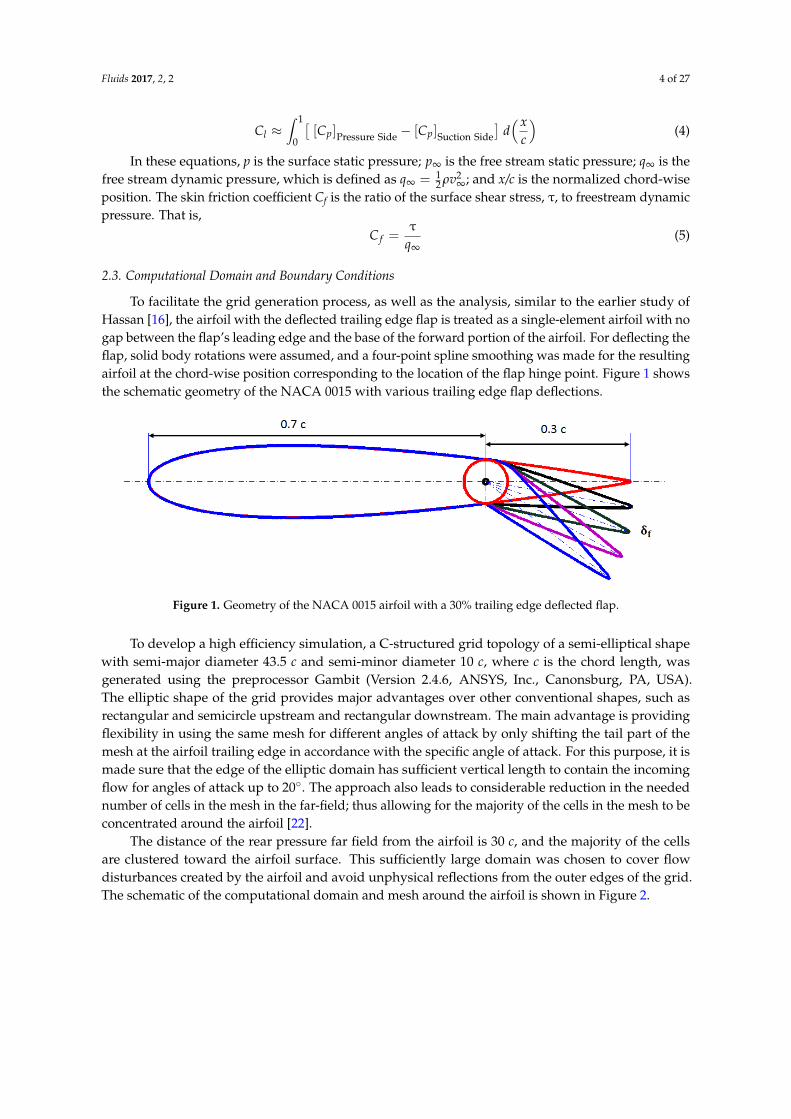
To facilitate the grid generation process, as well as the analysis, similar to the earlier study ofHassan [16], the airfoil with the deflected trailing edge flap is treated as a single-element airfoil with nogap between the flap’s leading edge and the base of the forward portion of the airfoil. For deflecting theflap, solid body rotations were assumed, and a four-point spline smoothing was made for the resultingairfoil at the chord-wise position corresponding to the location of the flap hinge point. Figure 1 showsthe schematic geometry of the NACA 0015 with various trailing edge flap deflections.

Fluids 2017, 2, 2 4 of 27

𝐶𝑙 ≈ ∫ [ [𝐶𝑝]Pressure Side − [𝐶𝑝]Suction Side] 𝑑 (𝑥

𝑐)

1

0

(4)

In these equations, p is the surface static pressure; 𝑝∞ is the free stream static pressure; 𝑞∞ is the

free stream dynamic pressure, which is defined as 𝑞∞ =1

2𝜌𝑣∞

2 ; and x/c is the normalized

chord-wise position. The skin friction coefficient Cf is the ratio of the surface shear stress, τ, to

freestream dynamic pressure. That is,

𝐶𝑓 =τ

𝑞∞ (5)

2.3. Computational Domain and Boundary Conditions

To facilitate the grid generation process, as well as the analysis, similar to the earlier study of

Hassan [16], the airfoil with the deflected trailing edge flap is treated as a single-element airfoil with

no gap between the flap’s leading edge and the base of the forward portion of the airfoil. For

deflecting the flap, solid body rotations were assumed, and a four-point spline smoothing was made

for the resulting airfoil at the chord-wise position corresponding to the location of the flap hinge

point. Figure 1 shows the schematic geometry of the NACA 0015 with various trailing edge

flap deflections.

Figure 1. Geometry of the NACA 0015 airfoil with a 30% trailing edge deflected flap.

To develop a high efficiency simulation, a C-structured grid topology of a semi-elliptical shape

with semi-major diameter 43.5 c and semi-minor diameter 10 c, where c is the chord length, was

generated using the preprocessor Gambit (Version 2.4.6, ANSYS, Inc., Canonsburg, PA, USA). The

elliptic shape of the grid provides major advantages over other conventional shapes, such as

rectangular and semicircle upstream and rectangular downstream. The main advantage is providing

flexibility in using the same mesh for different angles of attack by only shifting the tail part of the

mesh at the airfoil trailing edge in accordance with the specific angle of attack. For this purpose, it is

made sure that the edge of the elliptic domain has sufficient vertical length to contain the incoming

flow for angles of attack up to 20°. The approach also leads to considerable reduction in the needed

number of cells in the mesh in the far-field; thus allowing for the majority of the cells in the mesh to

be concentrated around the airfoil [22].

The distance of the rear pressure far field from the airfoil is 30 c, and the majority of the cells are

clustered toward the airfoil surface. This sufficiently large domain was chosen to cover flow

disturbances created by the airfoil and avoid unphysical reflections from the outer edges of the grid.

The schematic of the computational domain and mesh around the airfoil is shown in Figure 2.

Figure 1. Geometry of the NACA 0015 airfoil with a 30% trailing edge deflected flap.

To develop a high efficiency simulation, a C-structured grid topology of a semi-elliptical shapewith semi-major diameter 43.5 c and semi-minor diameter 10 c, where c is the chord length, wasgenerated using the preprocessor Gambit (Version 2.4.6, ANSYS, Inc., Canonsburg, PA, USA).The elliptic shape of the grid provides major advantages over other conventional shapes, such asrectangular and semicircle upstream and rectangular downstream. The main advantage is providingflexibility in using the same mesh for different angles of attack by only shifting the tail part of themesh at the airfoil trailing edge in accordance with the specific angle of attack. For this purpose, it ismade sure that the edge of the elliptic domain has sufficient vertical length to contain the incomingflow for angles of attack up to 20. The approach also leads to considerable reduction in the needednumber of cells in the mesh in the far-field; thus allowing for the majority of the cells in the mesh to beconcentrated around the airfoil [22].

The distance of the rear pressure far field from the airfoil is 30 c, and the majority of the cellsare clustered toward the airfoil surface. This sufficiently large domain was chosen to cover flowdisturbances created by the airfoil and avoid unphysical reflections from the outer edges of the grid.The schematic of the computational domain and mesh around the airfoil is shown in Figure 2.

Fluids 2017, 2, 2 5 of 27

Fluids 2017, 2, 2 5 of 27

Figure 2. Domain of calculations and boundary conditions.

The grids constructed for this study have about 104,000 cells with a four-node quadrilateral

element. To simulate the wake area correctly, Dolle [22] recommended using a fine grid with

quadrilateral cells in these areas rather than other type of cells. Therefore, refined quadrilateral cells

were placed on top of the boundary layer grid on the upper side and lower side of the airfoil outline.

Figure 3 shows the details of the structured mesh, which is highly clustered toward the airfoil

surface, and it is fine in the vicinity of wake regions and deflected flaps.

(a)

(b)

(c)

Figure 3. Mesh clustering toward airfoil surface and deflected flap regions. (a) Airfoil with 0° flap

deflection; (b) airfoil with 10° flap deflection; (c) airfoil with 40° flap deflection.

The boundary conditions for this simulation were the pressure far-field at the computational

domain periphery and stationary wall condition at the airfoil surface. The pressure far-field

boundary is a non-reflecting boundary condition based on “Riemann invariants” used to model a

free-stream condition at infinity, with the free-stream Mach number and static conditions being

specified. At the wall, the standard wall function boundary condition was used. The calculation

procedures at the pressure far-field boundaries, as well as the shear-stress calculations at wall

Figure 2. Domain of calculations and boundary conditions.

The grids constructed for this study have about 104,000 cells with a four-node quadrilateralelement. To simulate the wake area correctly, Dolle [22] recommended using a fine grid withquadrilateral cells in these areas rather than other type of cells. Therefore, refined quadrilateralcells were placed on top of the boundary layer grid on the upper side and lower side of the airfoiloutline. Figure 3 shows the details of the structured mesh, which is highly clustered toward the airfoilsurface, and it is fine in the vicinity of wake regions and deflected flaps.

Fluids 2017, 2, 2 5 of 27

Figure 2. Domain of calculations and boundary conditions.

The grids constructed for this study have about 104,000 cells with a four-node quadrilateral

element. To simulate the wake area correctly, Dolle [22] recommended using a fine grid with

quadrilateral cells in these areas rather than other type of cells. Therefore, refined quadrilateral cells

were placed on top of the boundary layer grid on the upper side and lower side of the airfoil outline.

Figure 3 shows the details of the structured mesh, which is highly clustered toward the airfoil

surface, and it is fine in the vicinity of wake regions and deflected flaps.

(a)

(b)

(c)

Figure 3. Mesh clustering toward airfoil surface and deflected flap regions. (a) Airfoil with 0° flap

deflection; (b) airfoil with 10° flap deflection; (c) airfoil with 40° flap deflection.

The boundary conditions for this simulation were the pressure far-field at the computational

domain periphery and stationary wall condition at the airfoil surface. The pressure far-field

boundary is a non-reflecting boundary condition based on “Riemann invariants” used to model a

free-stream condition at infinity, with the free-stream Mach number and static conditions being

specified. At the wall, the standard wall function boundary condition was used. The calculation

procedures at the pressure far-field boundaries, as well as the shear-stress calculations at wall

Figure 3. Mesh clustering toward airfoil surface and deflected flap regions. (a) Airfoil with 0 flapdeflection; (b) airfoil with 10 flap deflection; (c) airfoil with 40 flap deflection.

The boundary conditions for this simulation were the pressure far-field at the computationaldomain periphery and stationary wall condition at the airfoil surface. The pressure far-field boundaryis a non-reflecting boundary condition based on “Riemann invariants” used to model a free-streamcondition at infinity, with the free-stream Mach number and static conditions being specified. At thewall, the standard wall function boundary condition was used. The calculation procedures at thepressure far-field boundaries, as well as the shear-stress calculations at wall boundaries were describedin the Fluent lecture notes [23]. In some cases, the mesh is adapted based on the static pressure gradient,

Fluids 2017, 2, 2 6 of 27

using the default mesh adaptation control settings, so the solver periodically refines the mesh in theregions of high pressure gradients.

2.4. Setting up of the Numerical Simulation Parameters

Time independent pressure-based solver is used within ANSYS-Fluent (Version 13.7) for theanalysis. The realizable k-ε turbulence model is selected for analyzing the boundary layer flow overthe airfoil. The airflow is assumed to be incompressible. A simple scheme with the Green-Gausscell-based gradient implicit formulation of pressure velocity coupling is utilized [23]. For spatialdiscretization, the second order upwind differencing scheme which offers several advantagesover a central-differencing formulation for computing viscous flows is used in this work [24].The ANSYS-Fluent code solves the coupled governing equations of fluid motion simultaneouslyand provides updating correction for the pressure value in each iteration [25]. A convergence criterionof 1 × 10−8 was used for the continuity, x-velocity, y-velocity, k and ε. All solutions converged withthe standard interpolation scheme for calculating cell-face pressure and second order up-wind density,momentum, turbulent kinetic energy, turbulent dissipation rate and energy interpolation schemes forturbulent flow.

3. Results and Discussion

3.1. Mesh Independence Tests

To ensure that the simulation results are independent of grid size, different computational mesheswere inspected. This is done by running cases with increasing number of grid cells until the simulationresults did not change with the use of progressively finer grids. Table 1 lists the properties of sixdifferent grids with varying density that have been inspected for the flow pattern around the NACA0015 airfoil with zero flap deflection. This table lists some details of the grids, including the totalnumber of cells, the number of nodes Nx and Ny placed, respectively, in the x and y directions and themaximum, minimum and average values of non-dimensional normal distance from the wall, y+, foreach grid. It is observed that all of the grids inspected have considerably low y+ values, particularlyGrids III–VI, to sufficiently resolve the viscous sub-layer.

Table 1. Details of grids used in mesh sensitivity testing.

Grid No. of Cells Nx Ny Max y+ Min y+ Aver y+

I 24,910 690 35 32.5 4.8 13.85II 53,040 884 50 16.5 3.4 06.55III 76,128 976 65 12 1 05.50IV 103,192 1184 75 9.2 0.8 04.20V 141,168 1384 85 8.8 0.7 04.05VI 367,235 1850 90 1.01 0.01 0.500

Table 2 provides more details on the distribution of cells for different inspected meshes along thex and y directions. To have a better control of the distribution of the mesh, the airfoil body was dividedinto two parts; the front portion of the airfoil, which extends from the leading edge up to 30% of thechord length, and the rear portion of the airfoil, which includes the rest of the airfoil body. The wakeregion extends from the airfoil trailing edge up to the right far-field end. In each case, the first 30% ofthe airfoil was meshed with non-uniform grid spacing along the x-axis, while the last 70% of the airfoilmeshed with uniform grid spacing. The number of grid cells located in the airfoil rear portion is morethan three-times that located at the front part.

Fluids 2017, 2, 2 7 of 27

Table 2. Details of the grid cells distribution along the x-axis and y-axis.

Grid Leading Edge up to 30% of Chord Trailing Edge up to 70% of Chord Wake Region Height

I 90 325 275 35II 110 374 400 50III 112 384 480 65IV 116 468 600 75V 120 544 720 85VI 128 597 1125 90

The mesh size near the airfoil surface is a critical parameter for proper simulation of boundarylayer flow properties. The size of the first cell height near the wall ∆y was estimated based on thephysical properties of the fluid used and the selected values of the non-dimensional normal distancefrom the wall y+. Table 3 gives values for estimated size of this first cell height as a fraction of airfoilchord length. The mesh growth factor that controls the transition of cell size and specifies the increasein element size for each succeeding layer is found to be 1.2.

Table 3. Estimated size of the first cell height near the wall as a fraction of airfoil chord length.

Grid Max y+ Min y+ Aver y+ Max ∆y Min ∆y Aver ∆y

I 32.5 4.8 13.85 7.65× 10−4 c 1.00× 10−4 c 3.17 × 10−4 cII 16.5 3.4 6.55 3.78× 10−4 c 7.80× 10−5 c 1.50 × 10−4 cIII 12 1 5.50 2.75× 10−4 c 2.30× 10−5 c 1.26 × 10−4 cIV 9.2 0.8 4.20 2.11× 10−4 c 1.83× 10−5 c 9.93 × 10−5 cV 8.8 0.7 4.05 2.02× 10−4 c 1.60× 10−5 c 9.27 × 10−5 cVI 1.01 0.01 0.500 2.38× 10−5 c 2.35× 10−7 c 1.18 × 10−5 c

In this section, the grid inspection studies for flows at Reynolds numbers of 105 and 106 areperformed. The results of the two-equation realizable k-εmodel of Shih et al. [20] were compared withthose of the one-equation closure model of the Spalart–Allmaras (SA). The SA model was developedmainly for simulating aerodynamic flows. This model solves the modeled transport equation for thekinematic eddy (turbulent) viscosity [26]. The results obtained from SA and R-k-ε numerical modelswere compared with the experimental data of Rethmel [27]. Tables 4 and 5 show the predicted values ofthe lift coefficients for six different meshes by using the Spalart–Allmaras (SA) and the R-k-ε turbulencemodels for Re = 105 and 106, respectively. It is apparent that the realizable k-ε solutions obtained byGrids IV, V and VI are in good agreement with the experimental data. Despite the fact that the numberof cells in Grid VI is approximately 3.7-times that of Grid IV, these grids provided nearly the sameresults for the lift coefficient. It is also seen that the SA model yields significantly higher Cl valuescompared to the experiments. Regardless of the turbulence model used, the numerical results for theselast three grids remain almost the same with increasing the number of cells from Grid IV–Grid VI.

Table 4. Lift coefficient values for the NACA 0015 airfoil at α = 12, δ = 0 and Re = 105 using RANSmodels. SA, Spalart–Allmaras.

Grid Cl Exp. Cl (R-k-ε Model) Cl (SA Model)

I 0.90 ± 0.005 0.7654 0.9845II 0.90 ± 0.005 0.8292 1.0276III 0.90 ± 0.005 0.8412 1.0988IV 0.90 ± 0.005 0.9091 1.1169V 0.90 ± 0.005 0.9016 1.1199VI 0.90 ± 0.005 0.9073 1.1178

Fluids 2017, 2, 2 8 of 27

Table 5. Lift coefficient values for the NACA 0015 airfoil at α = 12, δ = 0 and Re = 106 usingRANS models.

Grid Cl Exp. Cl (R-k-ε Model) Cl (SA Model)

I 1.12 ± 0.005 8.546 × 10−1 1.0034II 1.12 ± 0.005 9.655× 10−1 1.1642III 1.12 ± 0.005 9.891× 10−1 1.2521IV 1.12 ± 0.005 1.1463 1.316V 1.12 ± 0.005 1.1491 1.3230VI 1.12 ± 0.005 1.1484 1.3201

The last step in the grid convergence inspection was focused on the analysis of the distribution ofthe pressure coefficient along the airfoil chord, as well as the velocity profiles on the upper surfaceof the airfoil in some selected sections. Figure 4 presents the chordwise distributions of the pressurecoefficient (Cp) profile for the airfoil predicted by Grids I, IV and VI using the R-k-ε turbulencemodel for α = 12, δ = 0 and Re = 105 (a) and Re = 106 (b). Here, the predicted distributions ofthe pressure coefficient are compared with the experimental data of Rethmel [27]. It is seen that themodel predictions for the pressure coefficient are generally comparable with the experimental data.In particular, the predictions obtained by Grids IV and VI are very close to each other and to thedistribution of the experimental data for both Reynolds numbers.

Fluids 2017, 2, 2 8 of 27

Table 5. Lift coefficient values for the NACA 0015 airfoil at α = 12°, δ = 0° and Re = 106 using

RANS models.

Grid lC Exp. lC (R-k-ε Model) lC (SA Model)

I 1.12 ± 0.005 8.546 × 10−1 1.0034

II 1.12 ± 0.005 9.655× 10−1 1.1642

III 1.12 ± 0.005 9.891× 10−1 1.2521

IV 1.12 ± 0.005 1.1463 1.316

V 1.12 ± 0.005 1.1491 1.3230

VI 1.12 ± 0.005 1.1484 1.3201

The last step in the grid convergence inspection was focused on the analysis of the distribution

of the pressure coefficient along the airfoil chord, as well as the velocity profiles on the upper surface

of the airfoil in some selected sections. Figure 4 presents the chordwise distributions of the pressure

coefficient (Cp) profile for the airfoil predicted by Grids I, IV and VI using the R-k-ε turbulence model

for α = 12°, δ = 0° and Re = 105 (a) and Re = 106 (b). Here, the predicted distributions of the pressure

coefficient are compared with the experimental data of Rethmel [27]. It is seen that the model

predictions for the pressure coefficient are generally comparable with the experimental data. In

particular, the predictions obtained by Grids IV and VI are very close to each other and to the

distribution of the experimental data for both Reynolds numbers.

Figure 4. Comparison of pressure coefficient curves along the sides of airfoil from different grids at

α = 12° and δ = 0° with the experimental data of Rethmel [27] at (a) Re = 105 and (b) Re = 106.

Figure 5 shows the velocity profiles on the upper surface of airfoil at the 20% cord location

from the leading edge as predicted by the realizable k-ε model using Grids I, IV and VI for α = 12°

and δ = 0° for Re = 105 and Re = 106. The vertical axis (y) in Figure 5 denotes the vertical distance from

the surface of the airfoil as a fraction of the chord length. It is seen that the model predictions for

Grids IV and VI are almost identical. That is, further refinement of Grid IV does not have a

noticeable effect on the velocity profile.

Figure 4. Comparison of pressure coefficient curves along the sides of airfoil from different grids at α =12 and δ = 0 with the experimental data of Rethmel [27] at (a) Re = 105 and (b) Re = 106.

Figure 5 shows the velocity profiles on the upper surface of airfoil at the 20% cord location fromthe leading edge as predicted by the realizable k-ε model using Grids I, IV and VI for α = 12 andδ = 0 for Re = 105 and Re = 106. The vertical axis (y) in Figure 5 denotes the vertical distance from thesurface of the airfoil as a fraction of the chord length. It is seen that the model predictions for Grids IVand VI are almost identical. That is, further refinement of Grid IV does not have a noticeable effect onthe velocity profile.

Fluids 2017, 2, 2 9 of 27

Fluids 2017, 2, 2 9 of 27

Figure 5. Velocity profiles on the upper surface of airfoil at a 20% cord location from the leading edge

at α = 12° and δ = 0° and for (a) Re = 105 and (b) Re = 106.

The presented grid sensitivity analysis shows that the model predictions with the use of

Grids IV and VI are very close to each other and to the experimental data. Due to the high

computational cost associated with the use of Grid VI, Grid IV with a total number of 103,192 cells

was used in the subsequent analyses.

3.2. NACA 0015 Airfoil with Zero Flap Deflection

The airflow properties around the NACA 0015 with zero flap deflection are first studied, and

the corresponding distributions of static pressure and velocity magnitude at different incidence

angles are evaluated and compared with the published numerical results and/or experimental data.

Figure 6 shows the static pressure and velocity magnitude contours around the NACA 0015

airfoil for a few selected incidence angles. As NACA 0015 is a symmetric airfoil, at zero incidence

angle, the static pressure and velocity distribution over the airfoil are symmetric, which results in

zero lift force and a stagnation point, exactly at the nose of the airfoil. There are regions of

accelerated flows over and under the airfoil that reach the highest speed at the airfoil maximum

thickness point. The velocity is high (marked by red spots) in the low pressure region and vice versa.

The maximum pressure occurs at the stagnation point when the velocity is zero.

At an incidence angle of 5°, the contours of static pressure over the airfoil become asymmetric;

the pressure on the upper surface becomes lower than the pressure on the lower surface; regions of

high pressure on the airfoil lower surface become dominant; and a lift coefficient of 0.531 is

generated due to the pressure imbalance.

Figure 6 shows that as the angle of attack increases, the stagnation point is shifted towards the

trailing edge on the bottom surface; hence, it creates a low velocity region at the lower surface of the

airfoil and a high velocity region on the upper side of the airfoil. Thus, the pressure on the upper

side of the airfoil is lower than the ambient pressure, whereas the pressure on the lower side is

higher than the ambient pressure. Therefore, increasing the incidence angle is associated with the

increase of the lift coefficient, as well as the increase of the drag coefficient. This increase in the lift

coefficient continues up to a maximum, after which the lift coefficient decreases.

It is also seen that the flow field around the airfoil varies markedly with the incidence angle. In

addition to the changes in velocity and pressure distributions, the properties of the boundary layer

flow along the airfoil surface also change. At low incidence angles up to about 12°, the boundary

layer is fully attached to the surface of the airfoil, and the lift coefficient increases with angle of

attack, while the drag is relatively low. With the increase of incidence angle, the boundary layer is

thickened. When the incidence angle of the airfoil is increased to about 13° or larger, the adverse

Figure 5. Velocity profiles on the upper surface of airfoil at a 20% cord location from the leading edgeat α = 12 and δ = 0 and for (a) Re = 105 and (b) Re = 106.

The presented grid sensitivity analysis shows that the model predictions with the use of GridsIV and VI are very close to each other and to the experimental data. Due to the high computationalcost associated with the use of Grid VI, Grid IV with a total number of 103,192 cells was used in thesubsequent analyses.

3.2. NACA 0015 Airfoil with Zero Flap Deflection

The airflow properties around the NACA 0015 with zero flap deflection are first studied, and thecorresponding distributions of static pressure and velocity magnitude at different incidence angles areevaluated and compared with the published numerical results and/or experimental data.

Figure 6 shows the static pressure and velocity magnitude contours around the NACA 0015 airfoilfor a few selected incidence angles. As NACA 0015 is a symmetric airfoil, at zero incidence angle, thestatic pressure and velocity distribution over the airfoil are symmetric, which results in zero lift forceand a stagnation point, exactly at the nose of the airfoil. There are regions of accelerated flows overand under the airfoil that reach the highest speed at the airfoil maximum thickness point. The velocityis high (marked by red spots) in the low pressure region and vice versa. The maximum pressure occursat the stagnation point when the velocity is zero.

At an incidence angle of 5, the contours of static pressure over the airfoil become asymmetric;the pressure on the upper surface becomes lower than the pressure on the lower surface; regions ofhigh pressure on the airfoil lower surface become dominant; and a lift coefficient of 0.531 is generateddue to the pressure imbalance.

Figure 6 shows that as the angle of attack increases, the stagnation point is shifted towards thetrailing edge on the bottom surface; hence, it creates a low velocity region at the lower surface of theairfoil and a high velocity region on the upper side of the airfoil. Thus, the pressure on the upperside of the airfoil is lower than the ambient pressure, whereas the pressure on the lower side is higherthan the ambient pressure. Therefore, increasing the incidence angle is associated with the increaseof the lift coefficient, as well as the increase of the drag coefficient. This increase in the lift coefficientcontinues up to a maximum, after which the lift coefficient decreases.

It is also seen that the flow field around the airfoil varies markedly with the incidence angle.In addition to the changes in velocity and pressure distributions, the properties of the boundary layerflow along the airfoil surface also change. At low incidence angles up to about 12, the boundarylayer is fully attached to the surface of the airfoil, and the lift coefficient increases with angle of attack,while the drag is relatively low. With the increase of incidence angle, the boundary layer is thickened.

Fluids 2017, 2, 2 10 of 27

When the incidence angle of the airfoil is increased to about 13 or larger, the adverse pressure gradientimposed on the boundary layers become so large that separation of the boundary layer occurs. A regionof recirculating flow over the entire upper surface of the airfoil forms, and the region of higher pressureon the lower surface of the airfoil becomes smaller. Consequently, the lift decreases markedly, and thedrag increases sharply. This is a typical condition in which the airfoil is stalled.

Fluids 2017, 2, 2 10 of 27

pressure gradient imposed on the boundary layers become so large that separation of the boundary

layer occurs. A region of recirculating flow over the entire upper surface of the airfoil forms, and the

region of higher pressure on the lower surface of the airfoil becomes smaller. Consequently, the lift

decreases markedly, and the drag increases sharply. This is a typical condition in which the airfoil is

stalled.

Figure 6. Static pressure and velocity magnitude contours around the NACA 0015 airfoil at different

incidence angles.

For a further increase of the airfoil incidence angle to 20°, the stagnation point shifts

significantly further towards the trailing edge on the bottom surface. The recirculating flow region

becomes dominant and covers the entire upper surface of the airfoil, and the airflow is fully

separated from the upper surface of the airfoil. This leads to further reduction of the lift force and a

severe increase of the drag force.

The air flowing along the top of the airfoil surface experiences a change in pressure, moving

from the ambient pressure in front of the airfoil, to a lower pressure over the surface of the airfoil,

then back to the ambient pressure behind the airfoil. The region where fluid must flow from low to

high pressure (adverse pressure gradient) could cause flow separation. If the adverse pressure

Figure 6. Static pressure and velocity magnitude contours around the NACA 0015 airfoil at differentincidence angles.

For a further increase of the airfoil incidence angle to 20, the stagnation point shifts significantlyfurther towards the trailing edge on the bottom surface. The recirculating flow region becomesdominant and covers the entire upper surface of the airfoil, and the airflow is fully separated from theupper surface of the airfoil. This leads to further reduction of the lift force and a severe increase of thedrag force.

The air flowing along the top of the airfoil surface experiences a change in pressure, moving fromthe ambient pressure in front of the airfoil, to a lower pressure over the surface of the airfoil, thenback to the ambient pressure behind the airfoil. The region where fluid must flow from low to highpressure (adverse pressure gradient) could cause flow separation. If the adverse pressure gradient istoo high, the pressure forces overcome the fluid inertial forces, and the flow separates from the airfoil

Fluids 2017, 2, 2 11 of 27

upper surface. As noted before, the pressure gradient increases with incidence angle, and there is amaximum angle of attack for keeping the flow attached to the airfoil. If the critical incidence angle isexceeded, separation occurs, and the lift force decreases sharply.

Figure 7 shows how the predicted position of the stagnation point varies for different angles ofattack. It is apparent that with positive angle of attack (AoA) the stagnation point moves toward thetrailing edge on the lower surface of the airfoil, while this movement would be on the upper surface ofthe airfoil at negative angles. The variation of the stagnation point position with the angle of attackobtained in this study is compared with the results obtained by Ahmed et al. [28] for the NACA 0012airfoil. Although the NACA 0012 airfoil is thinner, the present results match well up to an AoA of 12

and then follow the same trend.

Fluids 2017, 2, 2 11 of 27

gradient is too high, the pressure forces overcome the fluid inertial forces, and the flow separates

from the airfoil upper surface. As noted before, the pressure gradient increases with incidence angle,

and there is a maximum angle of attack for keeping the flow attached to the airfoil. If the critical

incidence angle is exceeded, separation occurs, and the lift force decreases sharply.

Figure 7 shows how the predicted position of the stagnation point varies for different angles of

attack. It is apparent that with positive angle of attack (AoA) the stagnation point moves toward the

trailing edge on the lower surface of the airfoil, while this movement would be on the upper surface

of the airfoil at negative angles. The variation of the stagnation point position with the angle of

attack obtained in this study is compared with the results obtained by Ahmed et al. [28] for the

NACA 0012 airfoil. Although the NACA 0012 airfoil is thinner, the present results match well up to

an AoA of 12° and then follow the same trend.

Figure 7. Variation of the stagnation point position with the angle of attack.

Figure 8 presents the chordwise distributions of the pressure coefficient (Cp) profile for the

airfoil at some selected incidence angles. For small angles of attack, the Cp distribution is

characterized by a negative pressure peak near the leading edge on the suction side. Beyond this

point, the Cp value gradually increases along the chord of the airfoil. On the pressure side of the

airfoil, the Cp value reaches a maximum of Cp = 1 at the stagnation line. This point is near the leading

edge, but shifts slightly depending on the incidence angle. Further down the chord length of the

airfoil, the pressure side Cp value increases gradually until it equals the suction side value at the

trailing edge.

Figure 8. Pressure coefficient curves along the upper and lower surfaces of the airfoil with 0° flap

deflection for different incidence at Re = 106.

Figure 7. Variation of the stagnation point position with the angle of attack.

Figure 8 presents the chordwise distributions of the pressure coefficient (Cp) profile for the airfoilat some selected incidence angles. For small angles of attack, the Cp distribution is characterized bya negative pressure peak near the leading edge on the suction side. Beyond this point, the Cp valuegradually increases along the chord of the airfoil. On the pressure side of the airfoil, the Cp valuereaches a maximum of Cp = 1 at the stagnation line. This point is near the leading edge, but shiftsslightly depending on the incidence angle. Further down the chord length of the airfoil, the pressureside Cp value increases gradually until it equals the suction side value at the trailing edge.

Fluids 2017, 2, 2 11 of 27

gradient is too high, the pressure forces overcome the fluid inertial forces, and the flow separates

from the airfoil upper surface. As noted before, the pressure gradient increases with incidence angle,

and there is a maximum angle of attack for keeping the flow attached to the airfoil. If the critical

incidence angle is exceeded, separation occurs, and the lift force decreases sharply.

Figure 7 shows how the predicted position of the stagnation point varies for different angles of

attack. It is apparent that with positive angle of attack (AoA) the stagnation point moves toward the

trailing edge on the lower surface of the airfoil, while this movement would be on the upper surface

of the airfoil at negative angles. The variation of the stagnation point position with the angle of

attack obtained in this study is compared with the results obtained by Ahmed et al. [28] for the

NACA 0012 airfoil. Although the NACA 0012 airfoil is thinner, the present results match well up to

an AoA of 12° and then follow the same trend.

Figure 7. Variation of the stagnation point position with the angle of attack.

Figure 8 presents the chordwise distributions of the pressure coefficient (Cp) profile for the

airfoil at some selected incidence angles. For small angles of attack, the Cp distribution is

characterized by a negative pressure peak near the leading edge on the suction side. Beyond this

point, the Cp value gradually increases along the chord of the airfoil. On the pressure side of the

airfoil, the Cp value reaches a maximum of Cp = 1 at the stagnation line. This point is near the leading

edge, but shifts slightly depending on the incidence angle. Further down the chord length of the

airfoil, the pressure side Cp value increases gradually until it equals the suction side value at the

trailing edge.

Figure 8. Pressure coefficient curves along the upper and lower surfaces of the airfoil with 0° flap

deflection for different incidence at Re = 106. Figure 8. Pressure coefficient curves along the upper and lower surfaces of the airfoil with 0 flapdeflection for different incidence at Re = 106.

Fluids 2017, 2, 2 12 of 27

Figure 8 also shows that the flow remains attached to the suction surface up to α = 13 after whichflow begins to separate. The separation line starts near the trailing edge and moves forward towardthe leading edge as incidence increases. The flow becomes fully separated over almost the entire chordof the airfoil for α greater than 15. For α > 13, the maximum Cp negative value decreases on theairfoil upper side, and a pronounced shift of the stagnation position toward the trailing edge is found.This situation continues until α = 17, at which the Cp value starts to vary in an irregular manner.

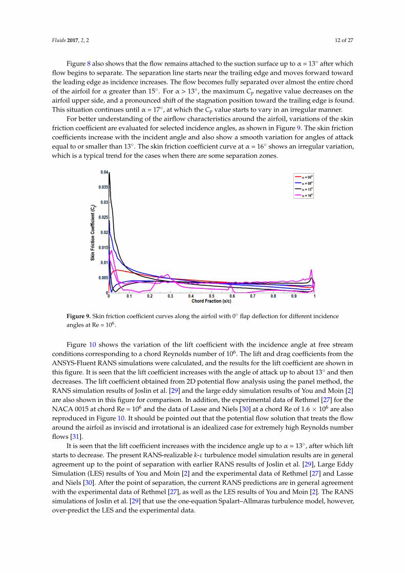
For better understanding of the airflow characteristics around the airfoil, variations of the skinfriction coefficient are evaluated for selected incidence angles, as shown in Figure 9. The skin frictioncoefficients increase with the incident angle and also show a smooth variation for angles of attackequal to or smaller than 13. The skin friction coefficient curve at α = 16 shows an irregular variation,which is a typical trend for the cases when there are some separation zones.

Fluids 2017, 2, 2 12 of 27

Figure 8 also shows that the flow remains attached to the suction surface up to α = 13° after

which flow begins to separate. The separation line starts near the trailing edge and moves forward

toward the leading edge as incidence increases. The flow becomes fully separated over almost the

entire chord of the airfoil for α greater than 15°. For α > 13°, the maximum Cp negative value

decreases on the airfoil upper side, and a pronounced shift of the stagnation position toward the

trailing edge is found. This situation continues until α = 17°, at which the Cp value starts to vary in an

irregular manner.

For better understanding of the airflow characteristics around the airfoil, variations of the skin

friction coefficient are evaluated for selected incidence angles, as shown in Figure 9. The skin

friction coefficients increase with the incident angle and also show a smooth variation for angles of

attack equal to or smaller than 13°. The skin friction coefficient curve at α = 16° shows an irregular

variation, which is a typical trend for the cases when there are some separation zones.

Figure 9. Skin friction coefficient curves along the airfoil with 0° flap deflection for different

incidence angles at Re = 106.

Figure 10 shows the variation of the lift coefficient with the incidence angle at free stream

conditions corresponding to a chord Reynolds number of 106. The lift and drag coefficients from the

ANSYS-Fluent RANS simulations were calculated, and the results for the lift coefficient are shown in

this figure. It is seen that the lift coefficient increases with the angle of attack up to about 13° and

then decreases. The lift coefficient obtained from 2D potential flow analysis using the panel method,

the RANS simulation results of Joslin et al. [29] and the large eddy simulation results of You and

Moin [2] are also shown in this figure for comparison. In addition, the experimental data of Rethmel

[27] for the NACA 0015 at chord Re = 106 and the data of Lasse and Niels [30] at a chord Re of 1.6 ×

106 are also reproduced in Figure 10. It should be pointed out that the potential flow solution that

treats the flow around the airfoil as inviscid and irrotational is an idealized case for extremely high

Reynolds number flows [31].

It is seen that the lift coefficient increases with the incidence angle up to α = 13°, after which lift

starts to decrease. The present RANS-realizable k-ε turbulence model simulation results are in

general agreement up to the point of separation with earlier RANS results of Joslin et al. [29], Large

Eddy Simulation (LES) results of You and Moin [2] and the experimental data of Rethmel [27] and

Lasse and Niels [30]. After the point of separation, the current RANS predictions are in general

agreement with the experimental data of Rethmel [27], as well as the LES results of You and Moin

[2]. The RANS simulations of Joslin et al. [29] that use the one-equation Spalart–Allmaras turbulence

model, however, over-predict the LES and the experimental data.

Figure 9. Skin friction coefficient curves along the airfoil with 0 flap deflection for different incidenceangles at Re = 106.

Figure 10 shows the variation of the lift coefficient with the incidence angle at free streamconditions corresponding to a chord Reynolds number of 106. The lift and drag coefficients from theANSYS-Fluent RANS simulations were calculated, and the results for the lift coefficient are shown inthis figure. It is seen that the lift coefficient increases with the angle of attack up to about 13 and thendecreases. The lift coefficient obtained from 2D potential flow analysis using the panel method, theRANS simulation results of Joslin et al. [29] and the large eddy simulation results of You and Moin [2]are also shown in this figure for comparison. In addition, the experimental data of Rethmel [27] for theNACA 0015 at chord Re = 106 and the data of Lasse and Niels [30] at a chord Re of 1.6 × 106 are alsoreproduced in Figure 10. It should be pointed out that the potential flow solution that treats the flowaround the airfoil as inviscid and irrotational is an idealized case for extremely high Reynolds numberflows [31].

It is seen that the lift coefficient increases with the incidence angle up to α = 13, after which liftstarts to decrease. The present RANS-realizable k-ε turbulence model simulation results are in generalagreement up to the point of separation with earlier RANS results of Joslin et al. [29], Large EddySimulation (LES) results of You and Moin [2] and the experimental data of Rethmel [27] and Lasseand Niels [30]. After the point of separation, the current RANS predictions are in general agreementwith the experimental data of Rethmel [27], as well as the LES results of You and Moin [2]. The RANSsimulations of Joslin et al. [29] that use the one-equation Spalart–Allmaras turbulence model, however,over-predict the LES and the experimental data.

Fluids 2017, 2, 2 13 of 27Fluids 2017, 2, 2 13 of 27

Figure 10. Comparison of lift coefficient Cl values of the airfoil at 0° flap deflection as a function of (α)

at chord Re = 106 with experimental and numerical results.

While the present RANS simulations for the lift coefficient are in good agreement with the

experimental data of Rethmel [27], the matching of the integrated lift coefficients does not

necessarily ensure agreement in the pressure distribution around the airfoil. Figure 11a shows the

chord-wise distribution of pressure coefficient Cp on the airfoil as predicted by the present RANS

simulation at the onset of stall (α = 12°). The experimental data of Rethmel [27] are reproduced in this

figure for comparison. Excellent agreement in the chord-wise distributions of the predicted pressure

coefficient with the experimental data is seen from this figure. This emphasizes the observation that

the realizable k-ε turbulence model provides an accurate description of the pressure distribution

around the airfoil at this incidence angle.

For angles of incidence in the stalled regime (α > 13°), the flow separation occurs, and the

accuracy of the realizable k-ε turbulence model in predicting the separated flow structures becomes

somewhat questionable. In fact, a careful examination of Figure 10 reveals that the k-ε turbulence

model slightly over-predicts the experimental lift coefficient at high angles of attack of α = 13°–14°.

To examine this trend, Figure 11b shows the distribution of Cp as predicted from the current RANS

simulation at the fully-developed stall regime (α = 16°) and compares them with the experimental

data of Rethmel [27]. There are noticeable differences between these pressure distributions.

Figure 11. Comparison of predicted pressure coefficients around the airfoil at angle of attack

(AoA) = 12° and AoA = 16° with the experimental data of Rethmel [27].

Figure 10. Comparison of lift coefficient Cl values of the airfoil at 0 flap deflection as a function of (α)at chord Re = 106 with experimental and numerical results.

While the present RANS simulations for the lift coefficient are in good agreement with theexperimental data of Rethmel [27], the matching of the integrated lift coefficients does not necessarilyensure agreement in the pressure distribution around the airfoil. Figure 11a shows the chord-wisedistribution of pressure coefficient Cp on the airfoil as predicted by the present RANS simulation atthe onset of stall (α = 12). The experimental data of Rethmel [27] are reproduced in this figure forcomparison. Excellent agreement in the chord-wise distributions of the predicted pressure coefficientwith the experimental data is seen from this figure. This emphasizes the observation that the realizablek-ε turbulence model provides an accurate description of the pressure distribution around the airfoil atthis incidence angle.

For angles of incidence in the stalled regime (α > 13), the flow separation occurs, and the accuracyof the realizable k-ε turbulence model in predicting the separated flow structures becomes somewhatquestionable. In fact, a careful examination of Figure 10 reveals that the k-ε turbulence model slightlyover-predicts the experimental lift coefficient at high angles of attack of α = 13–14. To examine thistrend, Figure 11b shows the distribution of Cp as predicted from the current RANS simulation at thefully-developed stall regime (α = 16) and compares them with the experimental data of Rethmel [27].There are noticeable differences between these pressure distributions.

Fluids 2017, 2, 2 13 of 27

Figure 10. Comparison of lift coefficient Cl values of the airfoil at 0° flap deflection as a function of (α)

at chord Re = 106 with experimental and numerical results.

While the present RANS simulations for the lift coefficient are in good agreement with the

experimental data of Rethmel [27], the matching of the integrated lift coefficients does not

necessarily ensure agreement in the pressure distribution around the airfoil. Figure 11a shows the

chord-wise distribution of pressure coefficient Cp on the airfoil as predicted by the present RANS

simulation at the onset of stall (α = 12°). The experimental data of Rethmel [27] are reproduced in this

figure for comparison. Excellent agreement in the chord-wise distributions of the predicted pressure

coefficient with the experimental data is seen from this figure. This emphasizes the observation that

the realizable k-ε turbulence model provides an accurate description of the pressure distribution

around the airfoil at this incidence angle.

For angles of incidence in the stalled regime (α > 13°), the flow separation occurs, and the

accuracy of the realizable k-ε turbulence model in predicting the separated flow structures becomes

somewhat questionable. In fact, a careful examination of Figure 10 reveals that the k-ε turbulence

model slightly over-predicts the experimental lift coefficient at high angles of attack of α = 13°–14°.

To examine this trend, Figure 11b shows the distribution of Cp as predicted from the current RANS

simulation at the fully-developed stall regime (α = 16°) and compares them with the experimental

data of Rethmel [27]. There are noticeable differences between these pressure distributions.

Figure 11. Comparison of predicted pressure coefficients around the airfoil at angle of attack

(AoA) = 12° and AoA = 16° with the experimental data of Rethmel [27]. Figure 11. Comparison of predicted pressure coefficients around the airfoil at angle of attack(AoA) = 12 and AoA = 16 with the experimental data of Rethmel [27].

Fluids 2017, 2, 2 14 of 27

It is worth mentioning that the maximum lift coefficient predicted by the present simulations is1.15 for α = 13. The slope of the lift curve obtained from the current study, as well as those for theearlier numerical results and experimental data is ∂Cl

∂α = 0.101 for low AoA, which remains constantfor incidence angles up to about 11. The slope of the lift curve is ∂Cl

∂α = 0.11 for the potential flow case.Figure 12 exhibits the predicted variation of drag coefficients with the incidence angles and

provides comparison with the earlier RANS simulations and the experimental data. As expected,the drag coefficient increases with the increase of incidence angle. The RANS simulation results ofSchroeder [32] for the NACA 0012 airfoil at Re = 106 and the drag coefficient measurements’ dataof Sharma [33] for the NACA 0015 at Re = 0.7 × 106 are reproduced in this figure for comparison.In addition, the drag coefficient data of Sheldahl and Klimas [34] for the NACA 0015 at Re = 106

and those of Lasse and Niels [30] at Re = 1.6 × 106 are also shown in this figure. It is seen that thedrag coefficient values predicted by the realizable k-ε model are in reasonable agreement with theexperimental data and earlier numerical results for incident angle less than 13. The drag coefficient islow at zero incidence angles and increases slowly with the angle of attack to the value of 0.038 at thestall condition. The slope of the drag coefficient with respect to incidence angle, ∂Cd

∂α , remains roughlyconstant at about 0.003. After the stall condition, the drag coefficient increases rapidly with the furtherincrease of the angle of attack and reaches a value of 0.28 at α = 20, which is more than seven-timesthe drag coefficient at the stall condition. The slope of the drag coefficient versus incidence angle, ∂Cd

∂α ,jumps to a value of 0.04 after the stall condition. It is also seen that the value of the drag coefficientdecreases with the increase of the Reynolds number. It is also observed that for an incident anglebeyond separation, the present model overestimates the experimental data for the drag coefficient.Further study of the accuracy of various turbulence models including the realizable k-ε turbulencemodel are left for a future work.

Fluids 2017, 2, 2 14 of 27

It is worth mentioning that the maximum lift coefficient predicted by the present simulations is

1.15 for α = 13°. The slope of the lift curve obtained from the current study, as well as those for the

earlier numerical results and experimental data is 𝜕𝐶𝑙

𝜕α= 0.101 for low AoA, which remains constant

for incidence angles up to about 11°. The slope of the lift curve is 𝜕𝐶𝑙

𝜕α= 0.11 for the potential

flow case.

Figure 12 exhibits the predicted variation of drag coefficients with the incidence angles and

provides comparison with the earlier RANS simulations and the experimental data. As expected, the

drag coefficient increases with the increase of incidence angle. The RANS simulation results of

Schroeder [32] for the NACA 0012 airfoil at Re = 106 and the drag coefficient measurements’ data of

Sharma [33] for the NACA 0015 at Re = 0.7 × 106 are reproduced in this figure for comparison. In

addition, the drag coefficient data of Sheldahl and Klimas [34] for the NACA 0015 at Re = 106 and

those of Lasse and Niels [30] at Re = 1.6 × 106 are also shown in this figure. It is seen that the drag

coefficient values predicted by the realizable k-ε model are in reasonable agreement with the

experimental data and earlier numerical results for incident angle less than 13°. The drag coefficient

is low at zero incidence angles and increases slowly with the angle of attack to the value of 0.038 at

the stall condition. The slope of the drag coefficient with respect to incidence angle, 𝜕𝐶𝑑

𝜕𝛼, remains

roughly constant at about 0.003. After the stall condition, the drag coefficient increases rapidly with

the further increase of the angle of attack and reaches a value of 0.28 at α = 20°, which is more than

seven-times the drag coefficient at the stall condition. The slope of the drag coefficient versus

incidence angle, 𝜕𝐶𝑑

𝜕α, jumps to a value of 0.04 after the stall condition. It is also seen that the value of

the drag coefficient decreases with the increase of the Reynolds number. It is also observed that for

an incident angle beyond separation, the present model overestimates the experimental data for the

drag coefficient. Further study of the accuracy of various turbulence models including the realizable

k-ε turbulence model are left for a future work.

Figure 12. Comparison of drag coefficient of airfoil at 0° flap deflection versus angle of attack at

chord Reynolds number Re = 106 with the experimental data and earlier numerical results.

Figure 13 shows the variation of the lift-to-drag ratio (𝐶𝑙 /𝐶𝑑 ) with the incidence angle as

predicted by the realizable k-ε model and the comparison with the available experimental data and

earlier simulations. It is seen that the lift-to-drag ratio increases rapidly from zero at α = 0° toward its

maximum value with the increase in incidence angle. This is because for small angles of attack, both

𝐶𝑙 and 𝐶𝑑 increase, but 𝐶𝑙 increases faster than 𝐶𝑑 [35]. Then, as the angle of attack further

increases, the lift-to-drag ratio decreases, and the decreasing trends are continuous to beyond the

stall angle.

While the trend of variations of the lift-to-drag ratio of the present simulations is in qualitative

agreement with the experimental data and earlier simulations, there are quantitative differences in

Figure 12. Comparison of drag coefficient of airfoil at 0 flap deflection versus angle of attack at chordReynolds number Re = 106 with the experimental data and earlier numerical results.

Figure 13 shows the variation of the lift-to-drag ratio (Cl/Cd) with the incidence angle as predictedby the realizable k-ε model and the comparison with the available experimental data and earliersimulations. It is seen that the lift-to-drag ratio increases rapidly from zero at α = 0 toward itsmaximum value with the increase in incidence angle. This is because for small angles of attack, bothCl and Cd increase, but Cl increases faster than Cd [35]. Then, as the angle of attack further increases,the lift-to-drag ratio decreases, and the decreasing trends are continuous to beyond the stall angle.

Fluids 2017, 2, 2 15 of 27

While the trend of variations of the lift-to-drag ratio of the present simulations is in qualitativeagreement with the experimental data and earlier simulations, there are quantitative differences in thepeak value of this ratio. The maximum value of lift-to-drag ratio found for the present simulations is48.2, which occurs at AoA of 8.5. Figure 13 shows that the maximum value of lift-to-drag ratio formost cases occurs at AoA of 8–8.5, except for the data of Sheldahl and Klimas [34], for which thepeak occurs at AoA of 10. This figure also shows that the lift-to-drag ratio could reach a peak value ofabout 65.

Fluids 2017, 2, 2 15 of 27

the peak value of this ratio. The maximum value of lift-to-drag ratio found for the present

simulations is 48.2, which occurs at AoA of 8.5°. Figure 13 shows that the maximum value of

lift-to-drag ratio for most cases occurs at AoA of 8°–8.5°, except for the data of Sheldahl and Klimas

[34], for which the peak occurs at AoA of 10°. This figure also shows that the lift-to-drag ratio could

reach a peak value of about 65.

Figure 13. Comparison of the lift-to-drag 𝐶𝑙/𝐶𝑑 ratio of the airfoil at 0° flap deflection versus the

angle of attack at chord Re = 106 with experimental data and earlier numerical results.

Another result obtained from this study is the behavior of the turbulence intensity of the flow

around the airfoil. Here, the turbulence intensity (TI) is defined as the ratio of root mean square

velocity fluctuation 𝑢′, to the mean local flow velocity 𝑈𝑎𝑣𝑒𝑟 (Fluent lecture notes [23]). Figure 14

shows the turbulence intensity contours around the airfoil for selected incidence angles as a

percentage. It is seen that the turbulence level increases with incident angle and could reach a

maximum of 49% for the range of incidence angles considered. At zero incidence angle, the

maximum turbulence intensity occurs near the leading edge of the airfoil. At an incidence angle of

5°, the contour map of turbulence intensity shows a slight shift of the location of the maximum

intensity region toward the trailing edge on the upper surface of the airfoil.

Figure 14 also indicates that at low incidence angles up to about 12°, a turbulent boundary layer

is attached to the airfoil, and only a thin wake is formed behind the airfoil. When the airfoil incidence

angle is increased to 13° or larger (where the flow separation is expected to occur), the wake becomes

much larger, and the region with maximum turbulent intensity becomes larger and departs further

from the airfoil surface. For the airfoil incidence angle of 20°, the airfoil is passing through a deep

stall, where the airflow on its upper surface separates right after the leading edge and produces a

wide wake. In this case, the maximum turbulence intensity region occupies a large zone off the

airfoil surface, but close to the trailing edge.

Figure 13. Comparison of the lift-to-drag Cl/Cd ratio of the airfoil at 0 flap deflection versus the angleof attack at chord Re = 106 with experimental data and earlier numerical results.

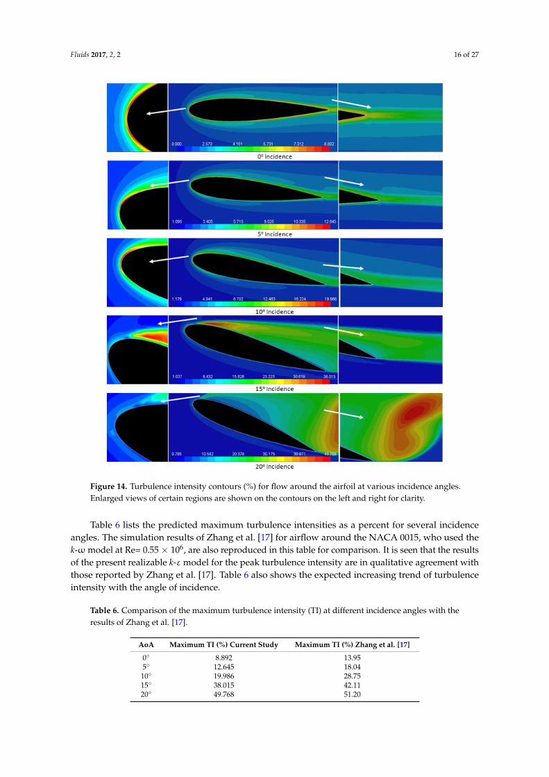
Another result obtained from this study is the behavior of the turbulence intensity of the flowaround the airfoil. Here, the turbulence intensity (TI) is defined as the ratio of root mean squarevelocity fluctuation u′, to the mean local flow velocity Uaver (Fluent lecture notes [23]). Figure 14 showsthe turbulence intensity contours around the airfoil for selected incidence angles as a percentage. It isseen that the turbulence level increases with incident angle and could reach a maximum of 49% forthe range of incidence angles considered. At zero incidence angle, the maximum turbulence intensityoccurs near the leading edge of the airfoil. At an incidence angle of 5, the contour map of turbulenceintensity shows a slight shift of the location of the maximum intensity region toward the trailing edgeon the upper surface of the airfoil.

Figure 14 also indicates that at low incidence angles up to about 12, a turbulent boundary layeris attached to the airfoil, and only a thin wake is formed behind the airfoil. When the airfoil incidenceangle is increased to 13 or larger (where the flow separation is expected to occur), the wake becomesmuch larger, and the region with maximum turbulent intensity becomes larger and departs furtherfrom the airfoil surface. For the airfoil incidence angle of 20, the airfoil is passing through a deepstall, where the airflow on its upper surface separates right after the leading edge and produces awide wake. In this case, the maximum turbulence intensity region occupies a large zone off the airfoilsurface, but close to the trailing edge.

Fluids 2017, 2, 2 16 of 27

Fluids 2017, 2, 2 16 of 27

Figure 14. Turbulence intensity contours (%) for flow around the airfoil at various incidence angles.

Enlarged views of certain regions are shown on the contours on the left and right for clarity.

Table 6 lists the predicted maximum turbulence intensities as a percent for several incidence

angles. The simulation results of Zhang et al. [17] for airflow around the NACA 0015, who used the

k- model at Re= 0.55 × 106, are also reproduced in this table for comparison. It is seen that the results

of the present realizable k-ε model for the peak turbulence intensity are in qualitative agreement

with those reported by Zhang et al. [17]. Table 6 also shows the expected increasing trend of

turbulence intensity with the angle of incidence.

Table 6. Comparison of the maximum turbulence intensity (TI) at different incidence angles with the

results of Zhang et al. [17].

AoA Maximum TI (%) Current Study Maximum TI (%) Zhang et al. [17]

0° 8.892 13.95

5° 12.645 18.04

10° 19.986 28.75

15° 38.015 42.11

20° 49.768 51.20

Figure 14. Turbulence intensity contours (%) for flow around the airfoil at various incidence angles.Enlarged views of certain regions are shown on the contours on the left and right for clarity.

Table 6 lists the predicted maximum turbulence intensities as a percent for several incidenceangles. The simulation results of Zhang et al. [17] for airflow around the NACA 0015, who used thek-ωmodel at Re= 0.55 × 106, are also reproduced in this table for comparison. It is seen that the resultsof the present realizable k-εmodel for the peak turbulence intensity are in qualitative agreement withthose reported by Zhang et al. [17]. Table 6 also shows the expected increasing trend of turbulenceintensity with the angle of incidence.

Table 6. Comparison of the maximum turbulence intensity (TI) at different incidence angles with theresults of Zhang et al. [17].

AoA Maximum TI (%) Current Study Maximum TI (%) Zhang et al. [17]

0 8.892 13.955 12.645 18.04

10 19.986 28.7515 38.015 42.1120 49.768 51.20

Fluids 2017, 2, 2 17 of 27

3.3. NACA 0015 Airfoil with Flap Deflection

The effect of downward flap deflection on the aerodynamic performance of the airfoil is studied foreight different flap positions of 2, 5, 10, 15, 20, 25, 30 and 40. For zero AoA, the static pressureand velocity contours for different flap deflections (δf) are presented in Figure 15. The comparison ofthe static pressure contours for zero flap deflection and for the deflected flap at the same angle of attackshows that the flap deflection increases the negative pressure over the entire upper surface of the mainairfoil and increases the positive pressure on the lower surface near the trailing edge. The pressureon the lower surface increases rapidly with flap deflection, while the pressure on the upper surfaceincreases gradually. The pressures on both the upper and the lower surfaces of the flap increase withflap deflection.

Fluids 2017, 2, 2 17 of 27

3.3. NACA 0015 Airfoil with Flap Deflection

The effect of downward flap deflection on the aerodynamic performance of the airfoil is studied

for eight different flap positions of 2°, 5°, 10°, 15°, 20°, 25°, 30° and 40°. For zero AoA, the static

pressure and velocity contours for different flap deflections (δf) are presented in Figure 15. The

comparison of the static pressure contours for zero flap deflection and for the deflected flap at the

same angle of attack shows that the flap deflection increases the negative pressure over the entire

upper surface of the main airfoil and increases the positive pressure on the lower surface near the

trailing edge. The pressure on the lower surface increases rapidly with flap deflection, while the

pressure on the upper surface increases gradually. The pressures on both the upper and the lower

surfaces of the flap increase with flap deflection.

Figure 15. Cont.

Fluids 2017, 2, 2 18 of 27

Fluids 2017, 2, 2 18 of 27

Figure 15. Static pressure and velocity magnitude contours around the NACA 0015 flapped airfoil at

an angle of attack of 0° for different flap deflections.

One other interesting observation is the progressive increase of the velocity magnitude over the

upper surface of the main airfoil as the flap deflection increases. The flap deflection changes the

velocity and pressure distributions on the airfoil upper and lower surfaces, causing higher pressure

to be built over the rear portion, generating a net lift force at AoA = 0°, and increases the airfoil

maximum lift coefficient. The flap deflection also moves the zero lift angle-of-attack of the airfoil to a

lower negative value and greatly increases the drag force.

Figure 16 shows the predicted variation of the lift coefficient with the flap deflection at two

different angles of attack of α = 5° and α = 10°. Here, the realizable k-ε predictions are compared with

the simulation results of Hassan [16] and Luchian [36], as well as the experimental data of

Williamson [37]. Hassan [16] studied the aerodynamic performance of the NACA 0015 airfoil with a

25% trailing edge flap at Re = 3 × 106 and for different Mach numbers. Luchian [36] investigated the

aerodynamic performance of the NACA 0015 airfoil with a 27.5% trailing edge plain flap for

different flap deflection angles at Re = 106 by using three different codes (Javafoil 2.20, Martin

Hepperle, Braunschweig, Germany, Profili2.20, Stefano Duranti, Feltre, Italy, and XFLR5 6.06,

techwinder, Paris, France). Williamson [37] conducted experiments on the W1015 airfoil, which is

identical to the NACA 0015 airfoil for wide range of low Reynolds numbers and trailing edge flap

deflections. It is evident that the lift coefficient increases sharply with the increase of the flap

deflection up to about 10°–15°, and then, the rate of increase becomes slower up to δf = 40°. The

present model predictions are in general agreement with the results of Hassan [16] for high

Reynolds numbers for flap deflections up to δf = 20°, the results of Luchian [36] at low Reynold

numbers for flap deflections up to δf = 30° and the experimental data of Williamson [37] for low

Reynolds numbers for a wide range of flap deflections up to δf = 40°.

Figure 15. Static pressure and velocity magnitude contours around the NACA 0015 flapped airfoil atan angle of attack of 0 for different flap deflections.

One other interesting observation is the progressive increase of the velocity magnitude over theupper surface of the main airfoil as the flap deflection increases. The flap deflection changes thevelocity and pressure distributions on the airfoil upper and lower surfaces, causing higher pressure tobe built over the rear portion, generating a net lift force at AoA = 0, and increases the airfoil maximumlift coefficient. The flap deflection also moves the zero lift angle-of-attack of the airfoil to a lowernegative value and greatly increases the drag force.

Figure 16 shows the predicted variation of the lift coefficient with the flap deflection at twodifferent angles of attack of α = 5 and α = 10. Here, the realizable k-ε predictions are comparedwith the simulation results of Hassan [16] and Luchian [36], as well as the experimental data ofWilliamson [37]. Hassan [16] studied the aerodynamic performance of the NACA 0015 airfoil with a25% trailing edge flap at Re = 3 × 106 and for different Mach numbers. Luchian [36] investigated theaerodynamic performance of the NACA 0015 airfoil with a 27.5% trailing edge plain flap for differentflap deflection angles at Re = 106 by using three different codes (Javafoil 2.20, Martin Hepperle,Braunschweig, Germany, Profili2.20, Stefano Duranti, Feltre, Italy, and XFLR5 6.06, techwinder, Paris,France). Williamson [37] conducted experiments on the W1015 airfoil, which is identical to the NACA0015 airfoil for wide range of low Reynolds numbers and trailing edge flap deflections. It is evidentthat the lift coefficient increases sharply with the increase of the flap deflection up to about 10–15,and then, the rate of increase becomes slower up to δf = 40. The present model predictions are ingeneral agreement with the results of Hassan [16] for high Reynolds numbers for flap deflections up toδf = 20, the results of Luchian [36] at low Reynold numbers for flap deflections up to δf = 30 and theexperimental data of Williamson [37] for low Reynolds numbers for a wide range of flap deflectionsup to δf = 40.

Fluids 2017, 2, 2 19 of 27

Fluids 2017, 2, 2 19 of 27

Figure 16. Comparison of effect of flap deflection on lift coefficient for AoA = 5° and AoA = 10° with

Hassan’s [16] simulations, Luchian’s [36] results and Williamson’s [37] experiments.

Figure 17 shows the predicted variation of the drag coefficient with the flap deflection at two

different angles of attack of α = 5° and α = 10°. For α = 5°, the drag coefficient of the flapped airfoil

increases gradually with the flap deflection up to a flap angle of δf = 20°, and then, the rate of increase

becomes much shaper. For example, the drag coefficient at δf = 30° is more than two-times its value

at δf = 15°. The trend is somewhat different for the AoA of α = 10°, where the drag coefficient

increases gradually with the flap deflection up to δf = 15°, and then, the drag coefficient increases

sharply. The drag coefficient for δf = 30° in this case is more than five-times its value at (δf = 10°).

When compared with the earlier results, the drag coefficients obtained by the realizable k-ε model in

this study are reasonably accurate for the AoA = 5° and in the entire range of flap deflections up to δf

= 30°. It is clear that for the AoA = 10° and δf > 15°, the predicted drag values are somewhat higher

than those predicted by both the Profili and XFLR5 codes, but below the values obtained by the

Javafoil code.

Figure 17. Comparison of the effect of flap deflection on drag coefficient values at AoA = 5° and

AoA = 10° with Hassan’s [16] simulations, Luchian’ [36] results and Williamson’s [37] experiments.

The effect of flap deflection on lift increment is presented next. A lift increment ∆ 𝐶𝑙 is the

amount of lift that is gained or lost due to a flap deflection measured from a reference configuration.

The airfoil with zero flap deflection is taken as the reference case. The trend in these plots is

compared with the experimental data of Williamson [37] for the W1015 symmetrical airfoil tested at

Re = 4 × 105 at zero flap deflection and 10° flap deflection.

Figure 16. Comparison of effect of flap deflection on lift coefficient for AoA = 5 and AoA = 10 withHassan’s [16] simulations, Luchian’s [36] results and Williamson’s [37] experiments.

Figure 17 shows the predicted variation of the drag coefficient with the flap deflection at twodifferent angles of attack of α = 5 and α = 10. For α = 5, the drag coefficient of the flapped airfoilincreases gradually with the flap deflection up to a flap angle of δf = 20, and then, the rate of increasebecomes much shaper. For example, the drag coefficient at δf = 30 is more than two-times its valueat δf = 15. The trend is somewhat different for the AoA of α = 10, where the drag coefficientincreases gradually with the flap deflection up to δf = 15, and then, the drag coefficient increasessharply. The drag coefficient for δf = 30 in this case is more than five-times its value at (δf = 10).When compared with the earlier results, the drag coefficients obtained by the realizable k-ε modelin this study are reasonably accurate for the AoA = 5 and in the entire range of flap deflections upto δf = 30. It is clear that for the AoA = 10 and δf > 15, the predicted drag values are somewhathigher than those predicted by both the Profili and XFLR5 codes, but below the values obtained by theJavafoil code.

Fluids 2017, 2, 2 19 of 27

Figure 16. Comparison of effect of flap deflection on lift coefficient for AoA = 5° and AoA = 10° with

Hassan’s [16] simulations, Luchian’s [36] results and Williamson’s [37] experiments.

Figure 17 shows the predicted variation of the drag coefficient with the flap deflection at two

different angles of attack of α = 5° and α = 10°. For α = 5°, the drag coefficient of the flapped airfoil

increases gradually with the flap deflection up to a flap angle of δf = 20°, and then, the rate of increase

becomes much shaper. For example, the drag coefficient at δf = 30° is more than two-times its value

at δf = 15°. The trend is somewhat different for the AoA of α = 10°, where the drag coefficient

increases gradually with the flap deflection up to δf = 15°, and then, the drag coefficient increases

sharply. The drag coefficient for δf = 30° in this case is more than five-times its value at (δf = 10°).

When compared with the earlier results, the drag coefficients obtained by the realizable k-ε model in

this study are reasonably accurate for the AoA = 5° and in the entire range of flap deflections up to δf

= 30°. It is clear that for the AoA = 10° and δf > 15°, the predicted drag values are somewhat higher

than those predicted by both the Profili and XFLR5 codes, but below the values obtained by the

Javafoil code.

Figure 17. Comparison of the effect of flap deflection on drag coefficient values at AoA = 5° and

AoA = 10° with Hassan’s [16] simulations, Luchian’ [36] results and Williamson’s [37] experiments.

The effect of flap deflection on lift increment is presented next. A lift increment ∆ 𝐶𝑙 is the

amount of lift that is gained or lost due to a flap deflection measured from a reference configuration.

The airfoil with zero flap deflection is taken as the reference case. The trend in these plots is

compared with the experimental data of Williamson [37] for the W1015 symmetrical airfoil tested at

Re = 4 × 105 at zero flap deflection and 10° flap deflection.

Figure 17. Comparison of the effect of flap deflection on drag coefficient values at AoA = 5 andAoA = 10 with Hassan’s [16] simulations, Luchian’ [36] results and Williamson’s [37] experiments.

The effect of flap deflection on lift increment is presented next. A lift increment ∆ Cl is the amountof lift that is gained or lost due to a flap deflection measured from a reference configuration. The airfoilwith zero flap deflection is taken as the reference case. The trend in these plots is compared with theexperimental data of Williamson [37] for the W1015 symmetrical airfoil tested at Re = 4 × 105 at zeroflap deflection and 10 flap deflection.

Fluids 2017, 2, 2 20 of 27

Figure 18a exhibits the variation of the lift coefficient with the angle of attack at a flap deflection ofδf = 10 together with their corresponding reference values at δf = 0. Figure 18b presents an enlargedsection of the lift coefficient for small angles of attack. In addition, the increments in the values ofthe lift coefficient are shown in Figure 18b. It is seen that the lift increment value ∆ Cl due to theflap angle is roughly the same for a large range of incidence angles below the stall angle. That is,(∆ Cl)1

∼= (∆ Cl)2 for the airfoils with zero and 10 flap angle.

Fluids 2017, 2, 2 20 of 27

Figure 18a exhibits the variation of the lift coefficient with the angle of attack at a flap deflection

of δf = 10° together with their corresponding reference values at δf = 0°. Figure 18b presents an

enlarged section of the lift coefficient for small angles of attack. In addition, the increments in the

values of the lift coefficient are shown in Figure18b. It is seen that the lift increment value ∆ 𝐶𝑙 due

to the flap angle is roughly the same for a large range of incidence angles below the stall angle. That

is, (∆ 𝐶𝑙)1 ≅ (∆ 𝐶𝑙)2 for the airfoils with zero and 10° flap angle.

Figure 18. Lift increment at flap deflection of 10° and validation with the experimental data of

Williamson [37].

In Figure 18b, it can be seen that at δf = 0°, the slope of the lift curve for the W1015 airfoil is

slightly lower than the slope of the lift curve for the NACA 0015. It should also be pointed out that

the W1015 airfoil was tested at Re = 4 × 105, and the NACA 0015 results are for Re = 106. It is also

known that for the same angle of attack, a higher Reynolds number gives higher lift coefficient and

consequently a greater slope of the lift curve. The lift curves for both airfoils are nearly linear at low

angles of attack (below 10°).

Due to the flap deflection, it is observed that the lift coefficient has a nonzero value at zero AoA

for both airfoils. For both airfoils, the lift increment is nearly constant at low angles of attack. The lift

increment is slightly higher for the NACA 0015 due to the higher Reynolds number for the flow

computations. Table 7 shows the values of the increments in the lift coefficient obtained due to a flap

deflection of 10° for both airfoils.

Table 7. The Increment in the value of the lift coefficient due to a flap deflection of 10°.

AoA ∆Cl ∆Cl

W1015 (Re = 4 × 105) NACA 0015 (Re = 106)

0 0.435 0.477

4.0 0.433 0.476

8.0 0.430 0.463

12.0 0.420 0.441

Simulation results for the lift increment due to flap deflection at zero angle of attack for a wide

range of flap deflections are plotted in Figure 19, and the results are compared with the experimental

data. There are three distinct regions that define different trends of ∆Cl values. A linear region is

Figure 18. Lift increment at flap deflection of 10 and validation with the experimental data ofWilliamson [37].

In Figure 18b, it can be seen that at δf = 0, the slope of the lift curve for the W1015 airfoil isslightly lower than the slope of the lift curve for the NACA 0015. It should also be pointed out thatthe W1015 airfoil was tested at Re = 4 × 105, and the NACA 0015 results are for Re = 106. It is alsoknown that for the same angle of attack, a higher Reynolds number gives higher lift coefficient andconsequently a greater slope of the lift curve. The lift curves for both airfoils are nearly linear at lowangles of attack (below 10).

Due to the flap deflection, it is observed that the lift coefficient has a nonzero value at zero AoAfor both airfoils. For both airfoils, the lift increment is nearly constant at low angles of attack. The liftincrement is slightly higher for the NACA 0015 due to the higher Reynolds number for the flowcomputations. Table 7 shows the values of the increments in the lift coefficient obtained due to a flapdeflection of 10 for both airfoils.

Table 7. The Increment in the value of the lift coefficient due to a flap deflection of 10.

AoA∆Cl ∆Cl

W1015 (Re = 4 × 105) NACA 0015 (Re = 106)

0 0.435 0.4774.0 0.433 0.4768.0 0.430 0.463

12.0 0.420 0.441

Fluids 2017, 2, 2 21 of 27

Simulation results for the lift increment due to flap deflection at zero angle of attack for a widerange of flap deflections are plotted in Figure 19, and the results are compared with the experimentaldata. There are three distinct regions that define different trends of ∆Cl values. A linear region isobserved at smaller flap deflections of 0≤ δf ≤ 15. In this region, the slope of the ∆Cl curve is constant,indicating fully-attached flow conditions. The second region is the transitional region, as it acts as aconnection between linear and nonlinear regions. It is normally marked as the leveling or decreasing of∆Cl values that is caused by the separation of flow from the upper surface of the flap. Separation fromthe upper surface normally occurs around a flap deflection of 10–20 deg. The actual flap deflection forflow separation depends on the Reynolds number, airfoil thickness, flap-chord ratio, angle of attackand the size of the gap around the nose of the flap. The third region is nonlinear in nature due tothe reduced nonlinear increase of ∆Cl values with flap deflection. In this region, the flow is largelyseparated over the upper surface of the flap.

Figure 19 shows that the current realizable k-εmodel predictions for the lift increment are in closeagreement with the experimental data of Williamson [37]. For flap deflection angles δf ≤ 20, it is seenthat the lift increment ∆Cl varies linearly in the simulations. The simulations of Hassan [16] were fora high Reynolds number flow and have a linear trend, but a higher slope. For high flap deflections(δf > 20) and a high Reynolds number, Hassan [16] did not provide any data. From Figure 19, it isconcluded that the present model predictions are reasonably accurate at least for low Reynoldsnumber flows.

Fluids 2017, 2, 2 21 of 27

observed at smaller flap deflections of 0 ≤ δf ≤ 15°. In this region, the slope of the ∆Cl curve is

constant, indicating fully-attached flow conditions. The second region is the transitional region, as it

acts as a connection between linear and nonlinear regions. It is normally marked as the leveling or

decreasing of ∆Cl values that is caused by the separation of flow from the upper surface of the flap.

Separation from the upper surface normally occurs around a flap deflection of 10–20 deg. The actual

flap deflection for flow separation depends on the Reynolds number, airfoil thickness, flap-chord

ratio, angle of attack and the size of the gap around the nose of the flap. The third region is nonlinear

in nature due to the reduced nonlinear increase of ∆Cl values with flap deflection. In this region, the

flow is largely separated over the upper surface of the flap.

Figure 19 shows that the current realizable k-ε model predictions for the lift increment are in

close agreement with the experimental data of Williamson [37]. For flap deflection angles δf ≤ 20°, it

is seen that the lift increment ∆Cl varies linearly in the simulations. The simulations of Hassan [16]

were for a high Reynolds number flow and have a linear trend, but a higher slope. For high flap

deflections (δf > 20°) and a high Reynolds number, Hassan [16] did not provide any data. From

Figure 19, it is concluded that the present model predictions are reasonably accurate at least for low

Reynolds number flows.

Figure 19. Variation of ∆Cl with flap deflection at zero AoA and comparison with the experimental

data of Williamson [34] and simulations of Hassan [16].

It is of interest to study the effect of the flap deflection on both the maximum lift coefficient and

the corresponding angle of attack (critical or stall AoA). The variation of the predicted maximum lift

coefficient versus flap deflection is shown in Figure 20a, while the variation of the stall angle of

attack is illustrated in Figure 20b. In these figures, the corresponding results of Williamson [37] and

Hassan [16] are reproduced for comparison. Figure 20a shows that the maximum lift coefficient

increases linearly for small flap deflections 0 ≤ δf ≤ 15°. For flap deflections larger than 15°, however,

the increasing slope of the maximum lift coefficient is reduced and reaches a plateau for the flap

deflection in the range of 40° < δf < 60°. Thus, it can be concluded that deflection of the flap δf > 40°

does not provide additional benefit in regard to the maximum lift coefficient. Figure 19a also shows

that the trends of the maximum lift coefficient obtained by the present realizable k-ε model are

comparable to those of the experimental data of Williamson [37] for the W1015 airfoil, as well as the

results of Hassan [16] for the NACA 0015 airfoil. The magnitudes are, however, somewhat different,

and the present simulation results lie in between the results of Williamson [37] and Hassan [16].

Figure 20b shows the variation of the stall angle versus flap angle. It is seen that the current

model predictions follow the general trend of the published results, as the stall angle of attack at

which Cl, max is achieved decreases with increasing the flap deflection. Deflecting the flap by 20°

decreases the stall angle of attack by 1.75° in the present study, while leading to a decrease of 1.5° in

the experimental study of Williamson [37] and 0.75° in the results of Hassan [16]. The further

Figure 19. Variation of ∆Cl with flap deflection at zero AoA and comparison with the experimentaldata of Williamson [34] and simulations of Hassan [16].

It is of interest to study the effect of the flap deflection on both the maximum lift coefficient andthe corresponding angle of attack (critical or stall AoA). The variation of the predicted maximum liftcoefficient versus flap deflection is shown in Figure 20a, while the variation of the stall angle of attack isillustrated in Figure 20b. In these figures, the corresponding results of Williamson [37] and Hassan [16]are reproduced for comparison. Figure 20a shows that the maximum lift coefficient increases linearlyfor small flap deflections 0 ≤ δf ≤ 15. For flap deflections larger than 15, however, the increasingslope of the maximum lift coefficient is reduced and reaches a plateau for the flap deflection in therange of 40 < δf < 60. Thus, it can be concluded that deflection of the flap δf > 40 does not provideadditional benefit in regard to the maximum lift coefficient. Figure 19a also shows that the trends ofthe maximum lift coefficient obtained by the present realizable k-εmodel are comparable to those ofthe experimental data of Williamson [37] for the W1015 airfoil, as well as the results of Hassan [16] for

Fluids 2017, 2, 2 22 of 27

the NACA 0015 airfoil. The magnitudes are, however, somewhat different, and the present simulationresults lie in between the results of Williamson [37] and Hassan [16].

Figure 20b shows the variation of the stall angle versus flap angle. It is seen that the currentmodel predictions follow the general trend of the published results, as the stall angle of attack atwhich Cl, max is achieved decreases with increasing the flap deflection. Deflecting the flap by 20

decreases the stall angle of attack by 1.75 in the present study, while leading to a decrease of 1.5 inthe experimental study of Williamson [37] and 0.75 in the results of Hassan [16]. The further increasein the flap deflection decreases the stall angle of attack. The present model predicts that lowering theflap by 40 decreases the stall angle of attack by 2, while Williamson’s [37] data suggest a decrease ofthe stall angle of attack by 4.

Fluids 2017, 2, 2 22 of 27

increase in the flap deflection decreases the stall angle of attack. The present model predicts that

lowering the flap by 40° decreases the stall angle of attack by 2°, while Williamson’s [37] data

suggest a decrease of the stall angle of attack by 4°.

Figure 20. Comparison of effect of flap deflection on (a) the maximum lift coefficient and (b) the stall

angle of attack with the experimental data of Williamson [37] and Hassan [16].

The turbulence intensity contours of the flow around the flapped airfoil at some selected

deflection angles and zero incidence are also evaluated. Figure 21 presents the contours of

turbulence intensity at δf 2°, 5°, 10°, 15°, 20°, 25°, 30° and 40° and for zero incidence angle. It is

observed that at the zero incidence angle, the flap deflection has a pronounced influence on the

turbulence intensity around the flapped airfoil. Even a small deflection in flap angle disturbs the

flow and creates regions of high turbulence intensity in the upper surface of the flapped airfoil.

These regions expand with increasing of the flap deflection and shift from the main airfoil towards

the flap section. For δf ≤ 15°, the realizable k-ε model predicts that the peak turbulence intensity

occurs in the boundary layer near both the upper and lower surfaces of the main airfoil close to the

leading edge and with a lower level of turbulence intensity in the wake region. For δf ≥ 15°, however,

the maximum turbulence intensity occurs in the wake region close to the flap in addition to the

boundary layer regions. This is due to the fact that the region with recirculating flow becomes larger

as the wake width increases with the flap deflection. At high flap deflections, the flow separates

from the flap, and high pressure acting on the pressure side of the flapped airfoil and consequently

marked increase in the drag occur compared to situations where the flow remains attach to the

surface.

Figure 20. Comparison of effect of flap deflection on (a) the maximum lift coefficient and (b) the stallangle of attack with the experimental data of Williamson [37] and Hassan [16].

The turbulence intensity contours of the flow around the flapped airfoil at some selected deflectionangles and zero incidence are also evaluated. Figure 21 presents the contours of turbulence intensityat δf 2, 5, 10, 15, 20, 25, 30 and 40 and for zero incidence angle. It is observed that at the zeroincidence angle, the flap deflection has a pronounced influence on the turbulence intensity aroundthe flapped airfoil. Even a small deflection in flap angle disturbs the flow and creates regions of highturbulence intensity in the upper surface of the flapped airfoil. These regions expand with increasing ofthe flap deflection and shift from the main airfoil towards the flap section. For δf ≤ 15, the realizablek-ε model predicts that the peak turbulence intensity occurs in the boundary layer near both the upperand lower surfaces of the main airfoil close to the leading edge and with a lower level of turbulenceintensity in the wake region. For δf ≥ 15, however, the maximum turbulence intensity occurs in thewake region close to the flap in addition to the boundary layer regions. This is due to the fact that theregion with recirculating flow becomes larger as the wake width increases with the flap deflection.At high flap deflections, the flow separates from the flap, and high pressure acting on the pressureside of the flapped airfoil and consequently marked increase in the drag occur compared to situationswhere the flow remains attach to the surface.

Fluids 2017, 2, 2 23 of 27Fluids 2017, 2, 2 23 of 27

Figure 21. Cont.

Fluids 2017, 2, 2 24 of 27

Fluids 2017, 2, 2 24 of 27

Figure 21. Contours of turbulence intensity (%) around the flapped airfoil at AoA = 0° and various

flap deflections.

4. Conclusions

Using the realizable k-ε turbulence model, a numerical investigation of flow characteristics over

the NACA 0015 airfoil at Re = 106 at different flap deflections was conducted. The airfoil with the

deflected trailing edge flap was treated as a single element with no gap between the airfoil and the

flap leading edge. A parabolic computational domain with 104,000 structured cells along with 10%

turbulence intensity at the far-pressure field at its boundaries was used in the analysis. The grid

sensitivity was performed to satisfy the mesh independence condition. For different configurations

with and without flap deflections, flows over the airfoil were simulated, and the resulting lift and

drag coefficients were validated by comparison with earlier experimental data and numerical

simulation results. Based on the presented results, the following conclusions are drawn:

The simulation results showed that the realizable k-ε model is a suitable turbulence model for

simulating the flow characteristics around an airfoil at different angle of attacks and

flap deflections.

Results showed that the increasing incidence angle was associated with the increasing lift

coefficient up to the maximum of 1.15 at α = 13°, after which the lift coefficient sharply

decreases. Before stall, the slope of the lift versus incidence angle curve, 𝜕𝐶𝑙

𝜕α, remained roughly

constant at about 0.101. After the stall angle of attack, the lift coefficient decreased sharply with

further increase of the incident angle, leading to a lift coefficient of 0.79 at α = 17°.

Figure 21. Contours of turbulence intensity (%) around the flapped airfoil at AoA = 0 and variousflap deflections.

4. Conclusions

Using the realizable k-ε turbulence model, a numerical investigation of flow characteristics overthe NACA 0015 airfoil at Re = 106 at different flap deflections was conducted. The airfoil with thedeflected trailing edge flap was treated as a single element with no gap between the airfoil and theflap leading edge. A parabolic computational domain with 104,000 structured cells along with 10%turbulence intensity at the far-pressure field at its boundaries was used in the analysis. The gridsensitivity was performed to satisfy the mesh independence condition. For different configurationswith and without flap deflections, flows over the airfoil were simulated, and the resulting lift and dragcoefficients were validated by comparison with earlier experimental data and numerical simulationresults. Based on the presented results, the following conclusions are drawn:

• The simulation results showed that the realizable k-ε model is a suitable turbulence modelfor simulating the flow characteristics around an airfoil at different angle of attacks andflap deflections.

• Results showed that the increasing incidence angle was associated with the increasing liftcoefficient up to the maximum of 1.15 at α = 13, after which the lift coefficient sharply decreases.Before stall, the slope of the lift versus incidence angle curve, ∂Cl

∂α , remained roughly constant

Fluids 2017, 2, 2 25 of 27

at about 0.101. After the stall angle of attack, the lift coefficient decreased sharply with furtherincrease of the incident angle, leading to a lift coefficient of 0.79 at α = 17.

• The value of the drag coefficient was low at zero incidence angles and increased slowly with theangle of attack to the value of 0.038 at the stall condition. The slope of the drag versus incidenceangle curve, ∂Cd

∂α , remained roughly constant at about 0.003. After the stall condition, the dragincreased rapidly with the further increase of the angle of attack to reach a value of 0.28 at α = 20,which was more than seven-times the drag coefficient at the stall condition. The slope of the dragversus incidence angle curve, ∂Cd

∂α , jumped to a value of 0.04 after the stall condition.• For the case with zero flap deflection, the turbulence intensity around the airfoil increased with

incident angle and would reach a maximum of 49% at α = 20.• The presented results showed that flap deflection significantly affected the aerodynamic

performance of the airfoil. For the same angle of attack, increasing δf enhanced both the liftand drag coefficients.

• The lift increment (∆Cl) increased with the flap deflection angle. This trend continued until amaximum value was reached, and then, the lift increment remained constant. The maximum liftcoefficient was 2.02 for the range of parameters studied.

• Increased flap deflection moved the zero-lift incidence angle of the airfoil from 0 to negativevalues. For δf = 5 and δf = 10, the zero-lift incidence angle were, respectively, α = −1.9 andα = −2.7.

• Increased flap deflection decreased the stalling angle of attack (αstall) for which the maximum liftcoefficient was reached. The stalled angles of attack were α = 13, 12.25 and 11.25, respectively,for flap deflections of δf = 0, 10 and 20.

• For all investigated flap deflections, the slope of the lift versus incidence angle, ∂Cl∂α , remained

roughly constant at about 0.1, and the lift curve just shifts upwards due to increased flap deflection.• For the zero incident angle, the turbulence level increased with the increase of flap deflection and

reached to 27% at δf = 40.

Acknowledgments: The authors gratefully acknowledge the financial support of the U.S. Air Force Office ofScientific Research through Grant No. FA9550-09-1-0051.

Author Contributions: This study was a part of the PhD research work of Sohaib Obeid who was responsible fordeveloping the computational model and for performing the simulations and data analysis. Ratneshwar Jha andGoodarz Ahmadi contributed to the interpretation of the results and to the critical revision of the article.

Conflicts of Interest: The authors declare no conflict of interest.

References

1. Anderson, J.D., Jr. Fundamentals of Aerodynamics, 3rd ed.; McGraw-Hill Series in Aeronautical and AerospaceEngineering; McGraw-Hill: New York, NY, USA, 2001; pp. 283–335.

2. You, D.; Moin, P. Active control of flow separation over an airfoil using synthetic jets. J. Fluids Struct. 2008,24, 1349–1357. [CrossRef]

3. Schrauf, G. Application of laminar flow technology on transport aircraft. In Proceedings of the CEAS DragReduction Conference, Potsdam, Germany, 19–21 June 2000.

4. Günther, B.; Carnarius, A.; Thiele, F. Numerical investigation of active flow control applied to an airfoilwith a camber flap. In Active Flow Control II; King, R., Ed.; Notes on Numerical Fluid Mechanics andMultidisciplinary Design; Springer: Berlin/Heidelberg, Germany, 2010; Volume 108, pp. 45–61.

5. Ham, N.D. Helicopter individual blade control research at MIT 1977–1985. Vertica 1987, 11, 109–122.6. Hall, S.R.; Spangler, R.L., Jr. Piezoelectric Helicopter Blade Flap Actuator. US Patent 5,224,826, 6 July 1993.7. Hall, S.R.; Prechtl, E.F. Development of piezoelectric servo-flap for helicopter rotor control.

Smart Mater. Struct. 1996, 5, 26–34. [CrossRef]8. Chopra, I. Status of application of smart structures technology to rotorcraft systems. J. Am. Helicopter Soc.

2000, 45, 228–252. [CrossRef]

Fluids 2017, 2, 2 26 of 27

9. Hall, S.R.; Wereley, N.M. Performance of higher harmonic control algorithms for helicopter vibrationreduction. AIAA J. Guid. Control Dyn. 1993, 16, 794–797. [CrossRef]

10. Van Kuik, G. The application of smart structures for large wind turbine rotor. In Proceedings of the 50th IEATopical Expert Meeting, Delft University of Technology, Delft, The Netherland, 11–12 December 2006.

11. Somers, D.M. Effect of Flap Deflection on Section Characteristics of S813 Airfoil (Period of Performance: 1993–1994);NREL/SR-500–36335; National Renewable Energy Laboratory: Golden, CO, USA, 2005.

12. McCroskey, W.J. A Critical Assessment of Wind Tunnel Results for the NACA 0012 Airfoil; NASA TechnicalMemorandum 100019; NASA Technical Reports Server (NTRS): Hampton, VA, USA, 1989.

13. Little, J.; Samimy, M. High-Lift airfoil separation with dielectric barrier discharge plasma actuation. AIAA J.2010, 48, 2884–2898. [CrossRef]

14. Gerakpoulos, R.; Boutier, M.S.H.; Yarusevych, S. Aerodynamic characteristics of NACA 0018 airfoil at lowreynolds numbers. In Proceedings of the 40th Fluid Dynamic Conference and Exhibit, Chicago, IL, USA,28 June–1 July 2010.

15. Gault, D.E. A Correlation of Low-Speed, Airfoil-Section Stalling Characteristics with Reynolds Number and AirfoilGeometry; NACA Technical Note 3963; NACA Technical: Washington, DC, USA, 1957.

16. Hassan, A. Predicted Aerodynamic Characteristics of a NACA 0015 Airfoil Having a 25% Integral Type TrailingEdge Flap; NACA CR/-1999–209328; NASA Technical Reports Server (NTRS): Hampton, VA, USA, 1999;pp. 209–328.

17. Zhang, G.; Jiang, J.; Liu, C. Numerical simulation of aerodynamic performance for wind turbines. J. EastChina Electric Power 2009, 37, 449–452.

18. Srinivasan, G.R.; Ekaterinaris, J.A.; McCroskey, W.J. Evaluation of turbulence models for unsteady flows ofan oscillating airfoil. Comput. Fluids 1995, 24, 833–861. [CrossRef]

19. Menter, F.R. Best Practice: Scale-Resolving Simulations in ANSYS CFD, Version 1; ANSYS Germany GmbH, Inc.:Canonsburg, PA, USA, 2012; pp. 3–5.

20. Shih, T.H.; Liou, W.W.; Shabbir, A.; Yang, Z.; Zhu, J. A new k-ε eddy viscosity model for high reynoldsnumber turbulent flows. Comput. Fluids 1995, 24, 227–238. [CrossRef]

21. Kim, S.E.; Choudhury, D.; Patel, B. Computations of complex turbulent flows using the commercial codeFLUENT. In Proceedings of the ICASE/LaRC/AFOSR Symposium on Modeling Complex Turbulent Flows,Hampton, VA, USA, 11–13 August 1997; pp. 259–276.

22. Dolle, T.J.A. Flap Performance Improvement by Surface Excitation. Master’s Thesis, Aerospace Engineering,Delft University of Technology, The Netherlands, 2009; pp. 23–27.

23. ANSYS, Inc. Introduction to ANSYS FLUENT 12.0. “Lecture 5 Solver Setting” ANSYS, Release 13; ANSYS, Inc.:Canonsburg, PA, USA, 2010; pp. 8–30.

24. Anderson, W.K.; Bonhaus, D.L. An implicit upwind algorithm for computing turbulent flows on unstructuredgrids. Comput. Fluids 1994, 23, 1–21. [CrossRef]

25. Bakker, A. Lecture 5—Solution Methods Applied Computational Fluid Dynamics; Lectures of Fluent Instructor;Fluent Inc.: New York, NY, USA, 2002; pp. 41–43.

26. Spalart, P.; Allmaras, S. A one-equation turbulence model for aerodynamic flows. In Proceedings of the30th Aerospace Sciences Meeting and Exhibit, Aerospace Sciences Meetings, Reno, NV, USA, 6–9 January 1992.

27. Rethmel, C.C. Airfoil Leading Edge Flow Separation Control Using Nanosecond Pulse DBD PlasmaActuators. Master’s Thesis, Mechanical Engineering, The Ohio State University, Columbus, OH, USA,2011; pp. 25–30.

28. Ahmed, T.; Amin, M.T.; Islam, S.M.R.; Ahmed, S. Computational study of flow around a NACA 0012 wingflapped at different flap angles with varying mach numbers. Glob. J. Res. Eng. Gen. Eng. 2013, 13, 4–16.

29. Joslin, R.D.; Horta, L.G.; Chen, F.J. Transiting action control to application. In Proceedings of the 30th AIAAFluid Dynamics Conference, Norfolk, VA, USA, 28 June–18 July 1999.

30. Lasse, G.; Niels, S. Large eddy simulations of an airfoil in turbulent inflow. In 4th PhD Seminar on Wind Energyin Europe: Book of Abstracts; The European Wind Energy Association: Brussels, Belgium, 2008; pp. 33–36.

31. Joseph, D.D.; Funada, T.; Wang, J. Potential Flows of Viscous and Viscoelastic Fluids; Notes to Fluid MechanicsStudents; University of Minnesota: Minneapolis, MN, USA, 2010; pp. 1–25.

32. Schroeder, E.J. Low Reynolds Number Flow Validation Using Computational Fluid Dynamics withApplication to micro Air Vehicles. Master’s Thesis, Aeronautical Engineering, University of Maryland,College Park, MD, USA, 2005; pp. 20–23.

Fluids 2017, 2, 2 27 of 27

33. Sharma, D.M. Experimental Investigations of Dynamic Stall for an Oscillating Airfoil. Ph.D. Thesis,Aeronautical Engineering, Indian Institute of Technology Kanpur, Kanpur, India, 2010; pp. 90–102.

34. Sheldahl, R.E.; Klimas, P.C. Aerodynamic Characteristics of Seven Symmetrical Airfoil sections Through 180 DegreeAngle of Attack for Use in Aerodynamic Analysis of Vertical Axis Wind Turbines; Sandia National Laboratories:Albuquerque, NM, USA, 1981; pp. 20–36.

35. Sahin, I.; Acir, A. Numerical and experimental investigations of lift and drag performances of NACA 0015wind turbine airfoil. Int. J. Mater. Mech. Manuf. 2015, 3, 22–25. [CrossRef]

36. Luchian, A. Numerical and Experimental Study on the Effect of High Lift Devices on NACA 0015Aerodynamics. Ph.D. Thesis, Mechanical Engineering, Polytechnic University of Bucharest, Bucharest,Romania, 2014; pp. 54–61.

37. Williamson, G.A. Experimental Wind Tunnel Study of Airfoils with Large Flap Deflections at Low ReynoldsNumbers. Master’s Thesis, Aerospace Engineering, The University of Illinois at Urbana-Champaign,Champaign, IL, USA, 2012; pp. 14–60.

© 2017 by the authors; licensee MDPI, Basel, Switzerland. This article is an open accessarticle distributed under the terms and conditions of the Creative Commons Attribution(CC-BY) license (http://creativecommons.org/licenses/by/4.0/).