Improving Aerodynamic Performance of a Truck:a Numerical Based Analysis

JOHAN MALMBERG

Master’s Thesis at KTH: Mechanical DepartmentSupervisor: Mihai Mihaescu

Examiner: Laszlo Fuchs

TRITA xxx 2015-06

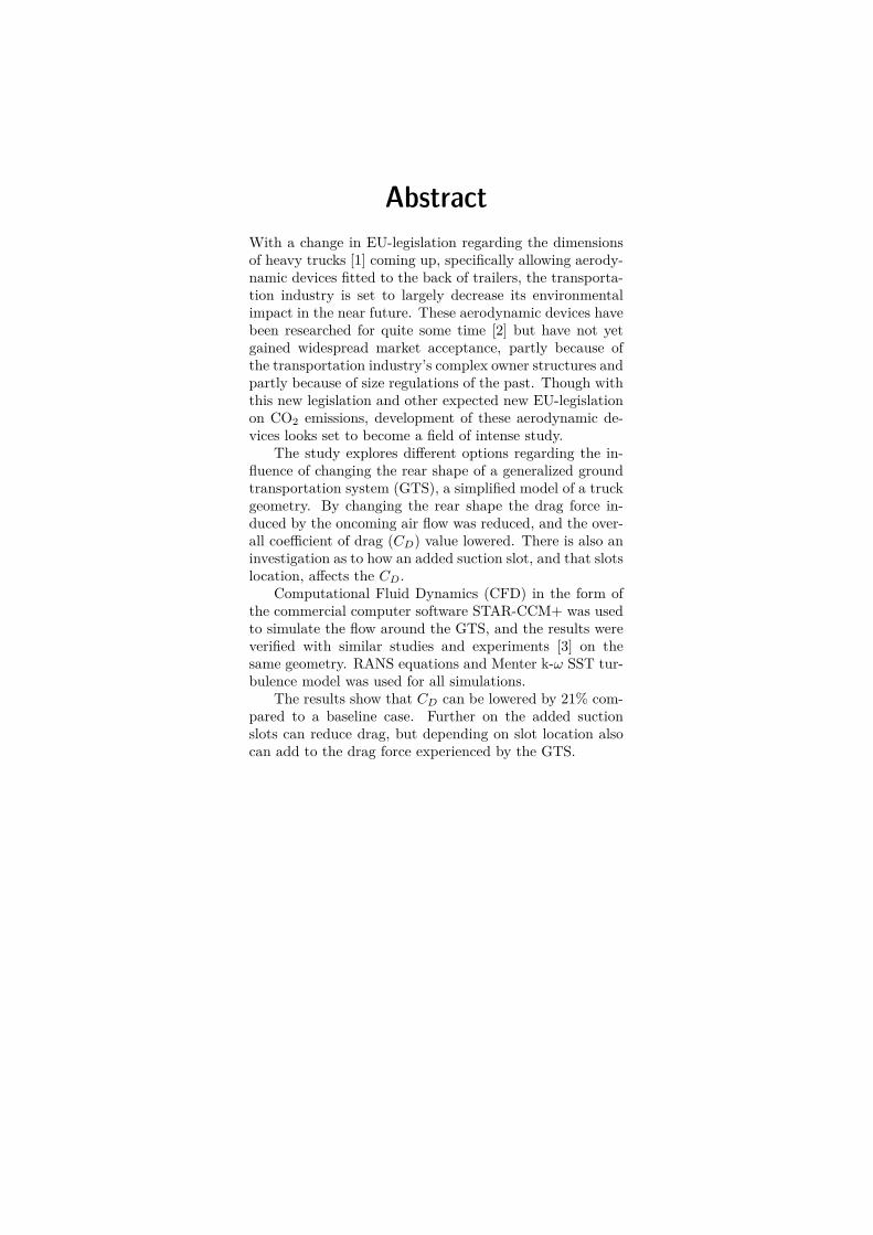
AbstractWith a change in EU-legislation regarding the dimensionsof heavy trucks [1] coming up, specifically allowing aerody-namic devices fitted to the back of trailers, the transporta-tion industry is set to largely decrease its environmentalimpact in the near future. These aerodynamic devices havebeen researched for quite some time [2] but have not yetgained widespread market acceptance, partly because ofthe transportation industry’s complex owner structures andpartly because of size regulations of the past. Though withthis new legislation and other expected new EU-legislationon CO2 emissions, development of these aerodynamic de-vices looks set to become a field of intense study.

The study explores different options regarding the in-fluence of changing the rear shape of a generalized groundtransportation system (GTS), a simplified model of a truckgeometry. By changing the rear shape the drag force in-duced by the oncoming air flow was reduced, and the over-all coefficient of drag (CD) value lowered. There is also aninvestigation as to how an added suction slot, and that slotslocation, affects the CD.

Computational Fluid Dynamics (CFD) in the form ofthe commercial computer software STAR-CCM+ was usedto simulate the flow around the GTS, and the results wereverified with similar studies and experiments [3] on thesame geometry. RANS equations and Menter k-ω SST tur-bulence model was used for all simulations.

The results show that CD can be lowered by 21% com-pared to a baseline case. Further on the added suctionslots can reduce drag, but depending on slot location alsocan add to the drag force experienced by the GTS.

AcknowledgementsI would like to thank my supervisor Mihai Mihaescu for allhis encouragement and feedback during my work with thisthesis. Elias Sundström has been invaluable as support forall questions regarding CFD.

I have Anna Svensson, Peter Georén and Per Gyllen-spetz to thank for getting me started on the thesis idea.

Thanks to Mustafa Güdücü for bringing some spirit toour work room, without him the place would have been waytoo quiet.

Finally, a huge thank you to my family who have beensupportive all throughout my, unbelievably long, school ca-reer as they have never given up on me.

And Kristina, who I can’t live without.

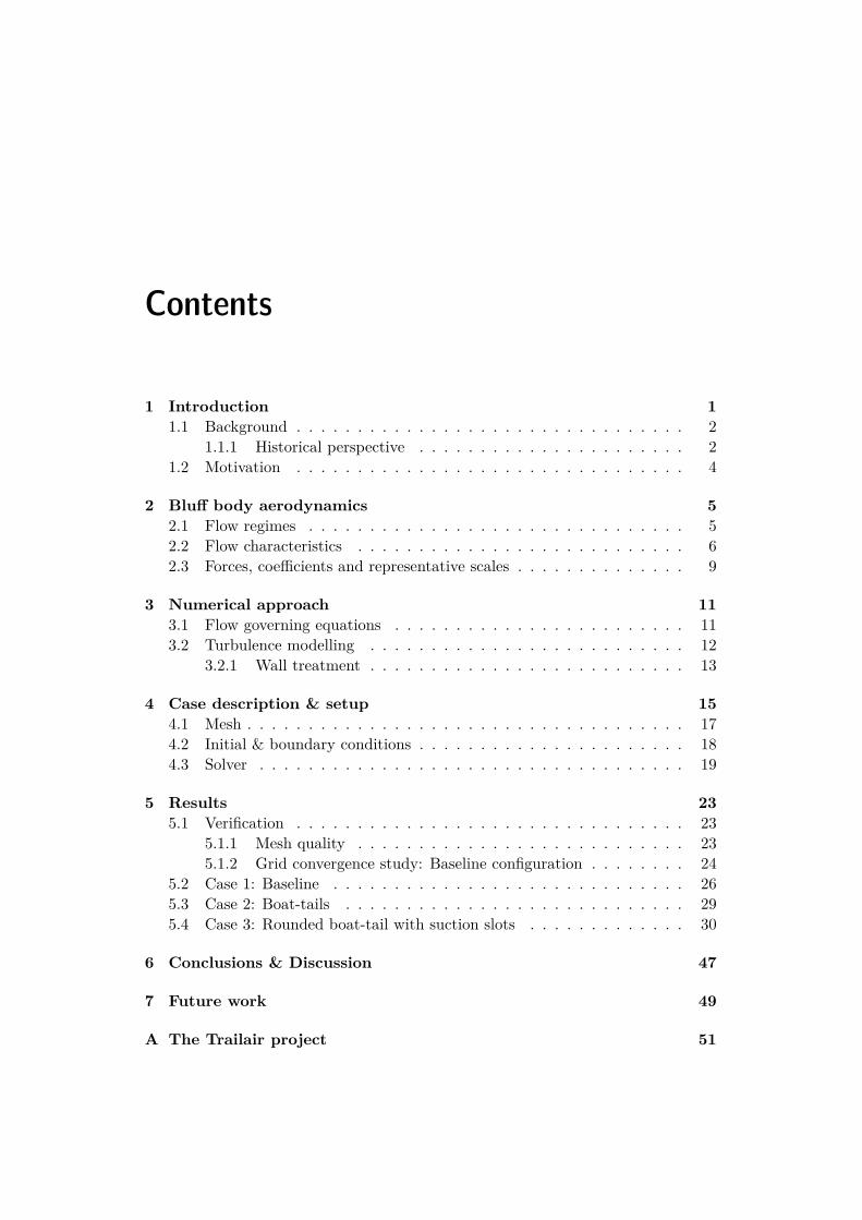
Contents

1 Introduction 11.1 Background . . . . . . . . . . . . . . . . . . . . . . . . . . . . . . . . 2

1.1.1 Historical perspective . . . . . . . . . . . . . . . . . . . . . . 21.2 Motivation . . . . . . . . . . . . . . . . . . . . . . . . . . . . . . . . 4

2 Bluff body aerodynamics 52.1 Flow regimes . . . . . . . . . . . . . . . . . . . . . . . . . . . . . . . 52.2 Flow characteristics . . . . . . . . . . . . . . . . . . . . . . . . . . . 62.3 Forces, coefficients and representative scales . . . . . . . . . . . . . . 9

3 Numerical approach 113.1 Flow governing equations . . . . . . . . . . . . . . . . . . . . . . . . 113.2 Turbulence modelling . . . . . . . . . . . . . . . . . . . . . . . . . . 12

3.2.1 Wall treatment . . . . . . . . . . . . . . . . . . . . . . . . . . 13

4 Case description & setup 154.1 Mesh . . . . . . . . . . . . . . . . . . . . . . . . . . . . . . . . . . . . 174.2 Initial & boundary conditions . . . . . . . . . . . . . . . . . . . . . . 184.3 Solver . . . . . . . . . . . . . . . . . . . . . . . . . . . . . . . . . . . 19

5 Results 235.1 Verification . . . . . . . . . . . . . . . . . . . . . . . . . . . . . . . . 23

5.1.1 Mesh quality . . . . . . . . . . . . . . . . . . . . . . . . . . . 235.1.2 Grid convergence study: Baseline configuration . . . . . . . . 24

5.2 Case 1: Baseline . . . . . . . . . . . . . . . . . . . . . . . . . . . . . 265.3 Case 2: Boat-tails . . . . . . . . . . . . . . . . . . . . . . . . . . . . 295.4 Case 3: Rounded boat-tail with suction slots . . . . . . . . . . . . . 30

6 Conclusions & Discussion 47

7 Future work 49

A The Trailair project 51

B Case 2: Additional plots 53

C Case 3: Additional plots 69

D GTS Geometries 75

Bibliography 77

Chapter 1

Introduction

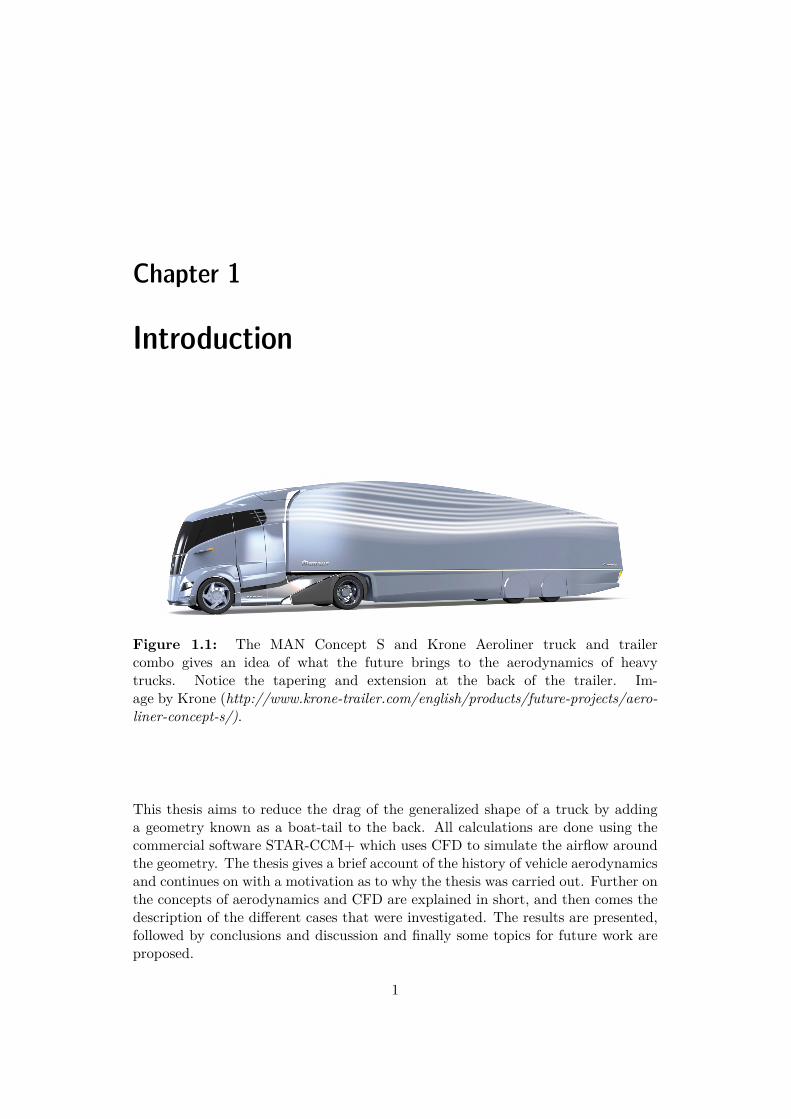
Figure 1.1: The MAN Concept S and Krone Aeroliner truck and trailercombo gives an idea of what the future brings to the aerodynamics of heavytrucks. Notice the tapering and extension at the back of the trailer. Im-age by Krone (http://www.krone-trailer.com/english/products/future-projects/aero-liner-concept-s/).

This thesis aims to reduce the drag of the generalized shape of a truck by addinga geometry known as a boat-tail to the back. All calculations are done using thecommercial software STAR-CCM+ which uses CFD to simulate the airflow aroundthe geometry. The thesis gives a brief account of the history of vehicle aerodynamicsand continues on with a motivation as to why the thesis was carried out. Further onthe concepts of aerodynamics and CFD are explained in short, and then comes thedescription of the different cases that were investigated. The results are presented,followed by conclusions and discussion and finally some topics for future work areproposed.

1

1.1 Background

1.1.1 Historical perspective

The field of aerodynamics traces its origins back to the first wind tunnels of thelate 1890s. The Wright brothers, credited with building the first aeroplane, built awind tunnel to examine lift for wing profiles, and in Sweden Carl Richard Nybergused a wind tunnel to construct his aeroplane Flugan, although it never really flew.

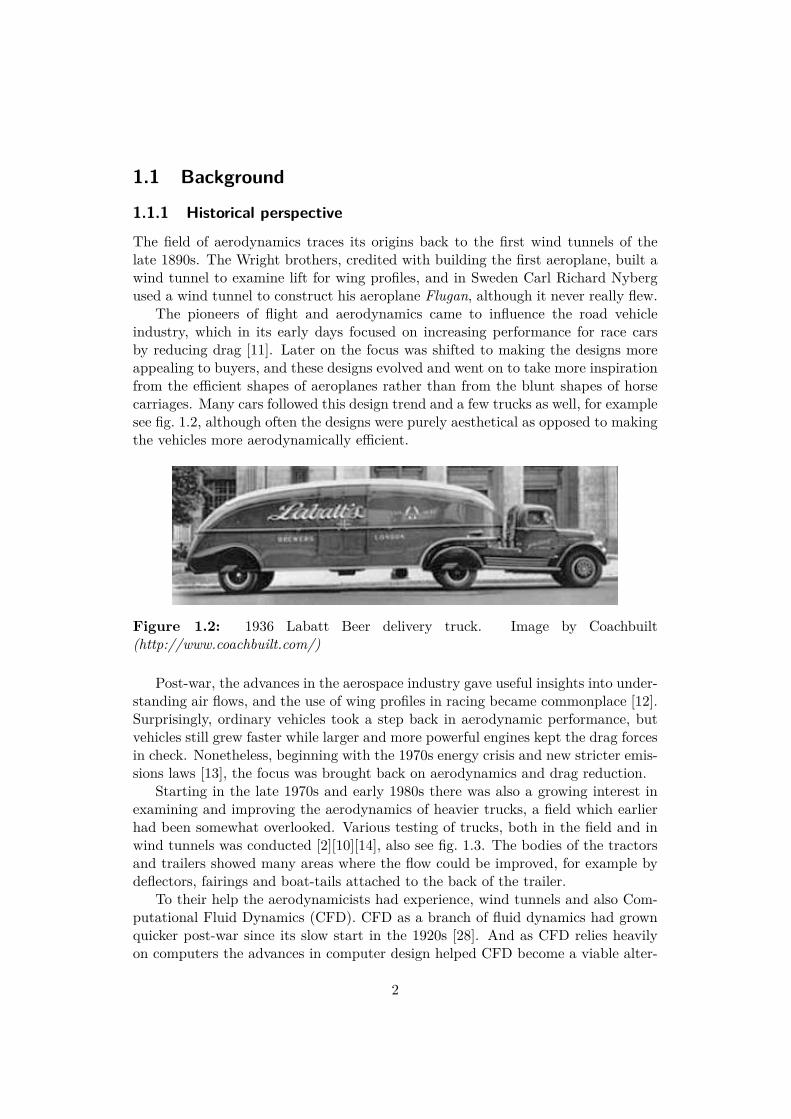
The pioneers of flight and aerodynamics came to influence the road vehicleindustry, which in its early days focused on increasing performance for race carsby reducing drag [11]. Later on the focus was shifted to making the designs moreappealing to buyers, and these designs evolved and went on to take more inspirationfrom the efficient shapes of aeroplanes rather than from the blunt shapes of horsecarriages. Many cars followed this design trend and a few trucks as well, for examplesee fig. 1.2, although often the designs were purely aesthetical as opposed to makingthe vehicles more aerodynamically efficient.

Figure 1.2: 1936 Labatt Beer delivery truck. Image by Coachbuilt(http://www.coachbuilt.com/)

Post-war, the advances in the aerospace industry gave useful insights into under-standing air flows, and the use of wing profiles in racing became commonplace [12].Surprisingly, ordinary vehicles took a step back in aerodynamic performance, butvehicles still grew faster while larger and more powerful engines kept the drag forcesin check. Nonetheless, beginning with the 1970s energy crisis and new stricter emis-sions laws [13], the focus was brought back on aerodynamics and drag reduction.

Starting in the late 1970s and early 1980s there was also a growing interest inexamining and improving the aerodynamics of heavier trucks, a field which earlierhad been somewhat overlooked. Various testing of trucks, both in the field and inwind tunnels was conducted [2][10][14], also see fig. 1.3. The bodies of the tractorsand trailers showed many areas where the flow could be improved, for example bydeflectors, fairings and boat-tails attached to the back of the trailer.

To their help the aerodynamicists had experience, wind tunnels and also Com-putational Fluid Dynamics (CFD). CFD as a branch of fluid dynamics had grownquicker post-war since its slow start in the 1920s [28]. And as CFD relies heavilyon computers the advances in computer design helped CFD become a viable alter-

2

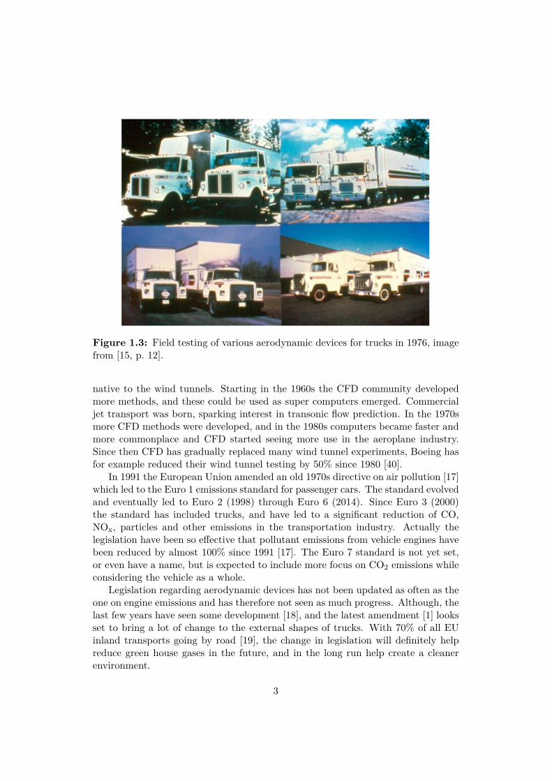
Figure 1.3: Field testing of various aerodynamic devices for trucks in 1976, imagefrom [15, p. 12].

native to the wind tunnels. Starting in the 1960s the CFD community developedmore methods, and these could be used as super computers emerged. Commercialjet transport was born, sparking interest in transonic flow prediction. In the 1970smore CFD methods were developed, and in the 1980s computers became faster andmore commonplace and CFD started seeing more use in the aeroplane industry.Since then CFD has gradually replaced many wind tunnel experiments, Boeing hasfor example reduced their wind tunnel testing by 50% since 1980 [40].

In 1991 the European Union amended an old 1970s directive on air pollution [17]which led to the Euro 1 emissions standard for passenger cars. The standard evolvedand eventually led to Euro 2 (1998) through Euro 6 (2014). Since Euro 3 (2000)the standard has included trucks, and have led to a significant reduction of CO,NOx, particles and other emissions in the transportation industry. Actually thelegislation have been so effective that pollutant emissions from vehicle engines havebeen reduced by almost 100% since 1991 [17]. The Euro 7 standard is not yet set,or even have a name, but is expected to include more focus on CO2 emissions whileconsidering the vehicle as a whole.

Legislation regarding aerodynamic devices has not been updated as often as theone on engine emissions and has therefore not seen as much progress. Although, thelast few years have seen some development [18], and the latest amendment [1] looksset to bring a lot of change to the external shapes of trucks. With 70% of all EUinland transports going by road [19], the change in legislation will definitely helpreduce green house gases in the future, and in the long run help create a cleanerenvironment.

3

1.2 MotivationSociety can make large savings, both economical and environmental, by improvingthe aerodynamic performance of a truck. A reduction by 12.5% of CD for a typicalsized truck running 80 km/hr leads to an approximate reduction in fuel consumptionby 5%, and cost savings for a typical long-haul truck driver [22] in the range of5000 EUR/year [23]. These reductions in fuel would be the same for CO2 and othergreenhouse gases, helping considerably with the goals of both EU and manufacturersassociations in reducing the environmental impact of heavy duty trucks.

There have been a lot of development of the design of tractors in the last 40years, but from manufacturers there has not been very much focus on the trailersthat are pulled. The drag created at the base of a trailer accounts for 29% ofthe total drag of a tractor-trailer-combo [25] so an improvement can make a largeimpact on fuel economy.

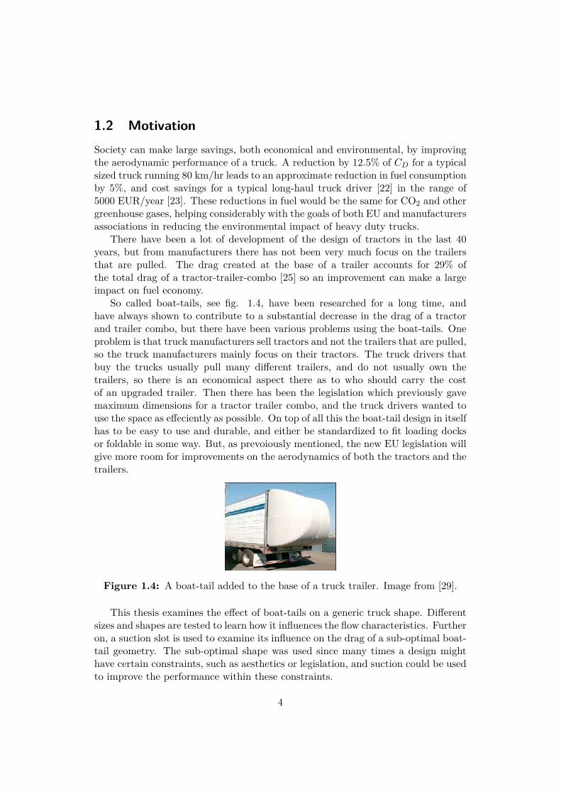
So called boat-tails, see fig. 1.4, have been researched for a long time, andhave always shown to contribute to a substantial decrease in the drag of a tractorand trailer combo, but there have been various problems using the boat-tails. Oneproblem is that truck manufacturers sell tractors and not the trailers that are pulled,so the truck manufacturers mainly focus on their tractors. The truck drivers thatbuy the trucks usually pull many different trailers, and do not usually own thetrailers, so there is an economical aspect there as to who should carry the costof an upgraded trailer. Then there has been the legislation which previously gavemaximum dimensions for a tractor trailer combo, and the truck drivers wanted touse the space as effeciently as possible. On top of all this the boat-tail design in itselfhas to be easy to use and durable, and either be standardized to fit loading docksor foldable in some way. But, as prevoiously mentioned, the new EU legislation willgive more room for improvements on the aerodynamics of both the tractors and thetrailers.

Figure 1.4: A boat-tail added to the base of a truck trailer. Image from [29].

This thesis examines the effect of boat-tails on a generic truck shape. Differentsizes and shapes are tested to learn how it influences the flow characteristics. Furtheron, a suction slot is used to examine its influence on the drag of a sub-optimal boat-tail geometry. The sub-optimal shape was used since many times a design mighthave certain constraints, such as aesthetics or legislation, and suction could be usedto improve the performance within these constraints.

4

Chapter 2

Bluff body aerodynamics

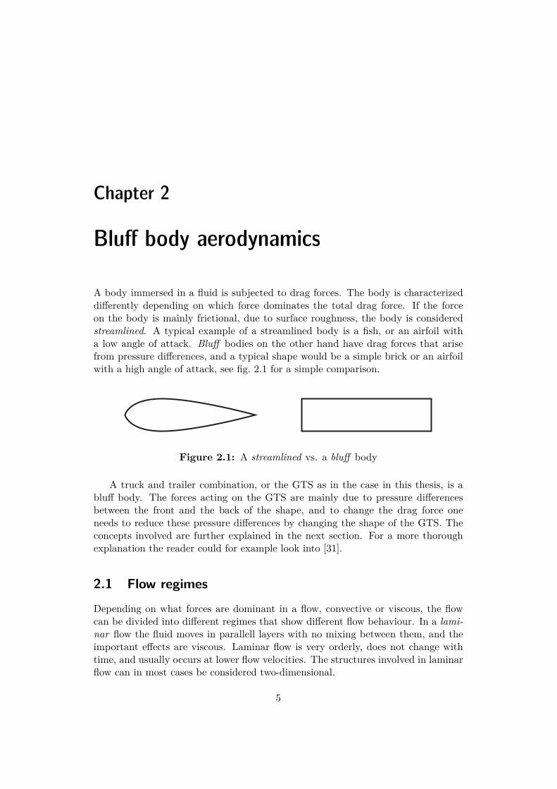
A body immersed in a fluid is subjected to drag forces. The body is characterizeddifferently depending on which force dominates the total drag force. If the forceon the body is mainly frictional, due to surface roughness, the body is consideredstreamlined. A typical example of a streamlined body is a fish, or an airfoil witha low angle of attack. Bluff bodies on the other hand have drag forces that arisefrom pressure differences, and a typical shape would be a simple brick or an airfoilwith a high angle of attack, see fig. 2.1 for a simple comparison.

Figure 2.1: A streamlined vs. a bluff body

A truck and trailer combination, or the GTS as in the case in this thesis, is abluff body. The forces acting on the GTS are mainly due to pressure differencesbetween the front and the back of the shape, and to change the drag force oneneeds to reduce these pressure differences by changing the shape of the GTS. Theconcepts involved are further explained in the next section. For a more thoroughexplanation the reader could for example look into [31].

2.1 Flow regimes

Depending on what forces are dominant in a flow, convective or viscous, the flowcan be divided into different regimes that show different flow behaviour. In a lami-nar flow the fluid moves in parallell layers with no mixing between them, and theimportant effects are viscous. Laminar flow is very orderly, does not change withtime, and usually occurs at lower flow velocities. The structures involved in laminarflow can in most cases be considered two-dimensional.

5

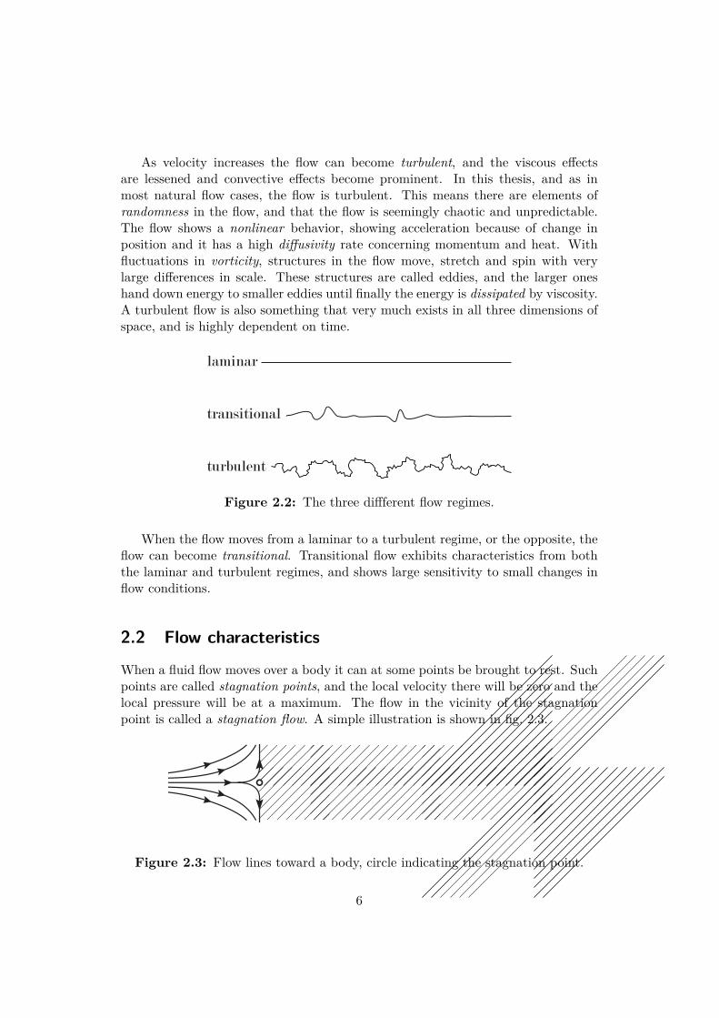
As velocity increases the flow can become turbulent, and the viscous effectsare lessened and convective effects become prominent. In this thesis, and as inmost natural flow cases, the flow is turbulent. This means there are elements ofrandomness in the flow, and that the flow is seemingly chaotic and unpredictable.The flow shows a nonlinear behavior, showing acceleration because of change inposition and it has a high diffusivity rate concerning momentum and heat. Withfluctuations in vorticity, structures in the flow move, stretch and spin with verylarge differences in scale. These structures are called eddies, and the larger oneshand down energy to smaller eddies until finally the energy is dissipated by viscosity.A turbulent flow is also something that very much exists in all three dimensions ofspace, and is highly dependent on time.

Figure 2.2: The three diffferent flow regimes.

When the flow moves from a laminar to a turbulent regime, or the opposite, theflow can become transitional. Transitional flow exhibits characteristics from boththe laminar and turbulent regimes, and shows large sensitivity to small changes inflow conditions.

2.2 Flow characteristics

When a fluid flow moves over a body it can at some points be brought to rest. Suchpoints are called stagnation points, and the local velocity there will be zero and thelocal pressure will be at a maximum. The flow in the vicinity of the stagnationpoint is called a stagnation flow. A simple illustration is shown in fig. 2.3.

Figure 2.3: Flow lines toward a body, circle indicating the stagnation point.

6

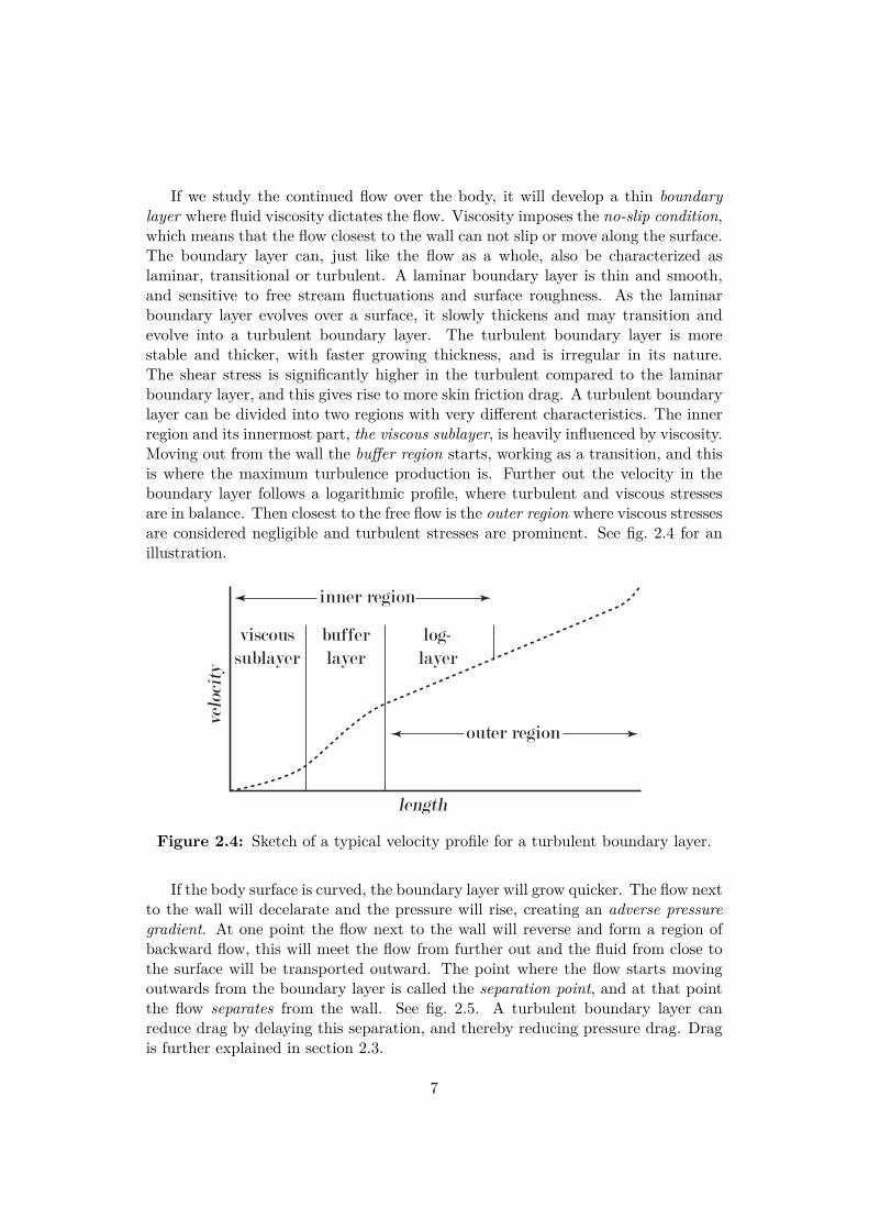
If we study the continued flow over the body, it will develop a thin boundarylayer where fluid viscosity dictates the flow. Viscosity imposes the no-slip condition,which means that the flow closest to the wall can not slip or move along the surface.The boundary layer can, just like the flow as a whole, also be characterized aslaminar, transitional or turbulent. A laminar boundary layer is thin and smooth,and sensitive to free stream fluctuations and surface roughness. As the laminarboundary layer evolves over a surface, it slowly thickens and may transition andevolve into a turbulent boundary layer. The turbulent boundary layer is morestable and thicker, with faster growing thickness, and is irregular in its nature.The shear stress is significantly higher in the turbulent compared to the laminarboundary layer, and this gives rise to more skin friction drag. A turbulent boundarylayer can be divided into two regions with very different characteristics. The innerregion and its innermost part, the viscous sublayer, is heavily influenced by viscosity.Moving out from the wall the buffer region starts, working as a transition, and thisis where the maximum turbulence production is. Further out the velocity in theboundary layer follows a logarithmic profile, where turbulent and viscous stressesare in balance. Then closest to the free flow is the outer region where viscous stressesare considered negligible and turbulent stresses are prominent. See fig. 2.4 for anillustration.

viscoussublayer

bufferlayer

log-layer

outer region

inner region

Figure 2.4: Sketch of a typical velocity profile for a turbulent boundary layer.

If the body surface is curved, the boundary layer will grow quicker. The flow nextto the wall will decelarate and the pressure will rise, creating an adverse pressuregradient. At one point the flow next to the wall will reverse and form a region ofbackward flow, this will meet the flow from further out and the fluid from close tothe surface will be transported outward. The point where the flow starts movingoutwards from the boundary layer is called the separation point, and at that pointthe flow separates from the wall. See fig. 2.5. A turbulent boundary layer canreduce drag by delaying this separation, and thereby reducing pressure drag. Dragis further explained in section 2.3.

7

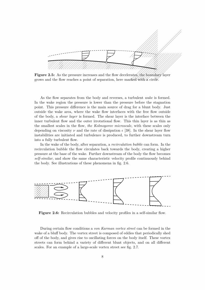
Figure 2.5: As the pressure increases and the flow decelerates, the boundary layergrows and the flow reaches a point of separation, here marked with a circle.

As the flow separates from the body and reverses, a turbulent wake is formed.In the wake region the pressure is lower than the pressure before the stagnationpoint. This pressure difference is the main source of drag for a blunt body. Justoutside the wake area, where the wake flow interfaces with the free flow outsideof the body, a shear layer is formed. The shear layer is the interface between theinner turbulent flow and the outer irrotational flow. This thin layer is as thin asthe smallest scales in the flow, the Kolmogorov microscale, with these scales onlydepending on viscosity ν and the rate of dissipation ε [38]. In the shear layer flowinstabilities are initiated and turbulence is produced, to further downstream turninto a fully turbulent flow.

In the wake of the body, after separation, a recirculation bubble can form. In therecirculation bubble the flow circulates back towards the body, creating a higherpressure at the base of the wake. Further downstream of the body the flow becomesself-similar, and show the same characteristic velocity profile continuously behindthe body. See illustrations of these phenomena in fig. 2.6.

Figure 2.6: Recirculation bubbles and velocity profiles in a self-similar flow.

During certain flow conditions a von Karman vortex street can be formed in thewake of a bluff body. The vortex street is composed of eddies that periodically shedoff of the body, and gives rise to oscillating forces on the body itself. These vortexstreets can form behind a variety of different blunt objects, and on all differentscales. For an example of a large-scale vortex street see fig. 2.7.

8

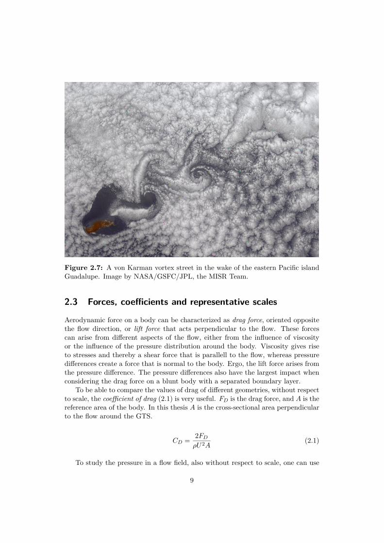
Figure 2.7: A von Karman vortex street in the wake of the eastern Pacific islandGuadalupe. Image by NASA/GSFC/JPL, the MISR Team.

2.3 Forces, coefficients and representative scales

Aerodynamic force on a body can be characterized as drag force, oriented oppositethe flow direction, or lift force that acts perpendicular to the flow. These forcescan arise from different aspects of the flow, either from the influence of viscosityor the influence of the pressure distribution around the body. Viscosity gives riseto stresses and thereby a shear force that is parallell to the flow, whereas pressuredifferences create a force that is normal to the body. Ergo, the lift force arises fromthe pressure difference. The pressure differences also have the largest impact whenconsidering the drag force on a blunt body with a separated boundary layer.

To be able to compare the values of drag of different geometries, without respectto scale, the coefficient of drag (2.1) is very useful. FD is the drag force, and A is thereference area of the body. In this thesis A is the cross-sectional area perpendicularto the flow around the GTS.

CD = 2FD

ρU2A(2.1)

To study the pressure in a flow field, also without respect to scale, one can use

9

the coefficient of pressure (2.2)

CP = 2(p− p∞)ρU2 , (2.2)

where p is the local pressure and p∞ is the ambient pressure. CP describes howthe local pressure in every point of a flow field relates to the pressure far away.Consequently, if CP is zero, the local pressure is the same as the ambient pressureand if CP is 1, the local pressure is the stagnation pressure and that point is astagnation point.

In order to compare different flows and predict flow behaviour Reynolds numberRe (2.3) can be used. Re is a non-dimensional quantity that is a function of densityρ, mean velocity U , characteristic length L and dynamic viscosity µ. For exactvalues used in the thesis see table 4.1.

Re = ρUL

µ(2.3)

Re is essentially the ratio of inertial forces to viscous forces, and can therefore beused to predict flow regime and behaviour. A laminar flow depends highly on viscousforces and hence it occurs for low Re which can be attributed to either low inertia orhigh viscosity. As the flow moves into the transitional regime the ratio of inertia toviscosity balances, and depending on small changes in any parameter the balancecan change quickly. As either velocity or any other parameter in the numeratorgrows, or if viscosity decreases, the flow becomes turbulent and the inertial forcesare most dominant. Because of the non-dimensionality of Re, transitions betweenflow regimes occur at the same value of Re.

Re can be used as a scaling parameter, and is very useful when the size of a bodyis too large to fit in a wind tunnel. Since the flow behaviour depends only on Re,the different parameters can be varied but still create the same flow characteristic.For the case of the GTS, a 1/8th scale model is used, but in order to have the sameRe as for a full scale model the speed of the flow is increased.

Another dimensionsless number that is useful is the Strouhal number (2.4),

St = fL

U, (2.4)

where f is the frequency of vortex shedding, previously explained in 2.2. Thefrequency f can be an important number when building structures or designingvehicles. If f is close to the natural frequency of a body, the shedding can induceoscillations which can lead instabilities, even breakdown of a structure, or to soundemissions with a specific tone.

10

Chapter 3

Numerical approach

3.1 Flow governing equationsCFD aims to numerically solve problems concerning fluid flow. Nowadays the calcu-lations are done by computer, although it did not start out that way some 100 oddyears ago [28]. Since the 1950s and the advent of the modern digital computer CFDhas evolved almost just as quickly as the processing speed of computers, making ita more powerful tool every day.

The basis for most CFD problems, and certainly the problems in this thesis,are the Navier-Stokes equations, here for an incompressible Newtonian fluid (withviscosity independent of stress), omitting the energy equation

ρ

(∂ui

∂t+ uj

∂ui

∂xj

)= − ∂p

∂xi+ µ

∂2ui

∂xjxj, (3.1)

∂ui

∂xi= 0 (3.2)

where u is velocity, ρ is density, p is pressure, ν is the kinematic viscosity. Bodyforces, such as g are omitted. The equations follow incompressibility if the speed ofthe flow is low enough, that is if the Mach number (3.3) is below 0.3.

Ma = U

c, (3.3)

with c being the local speed of sound.The Navier-Stokes equations are derived from the basic fundamental principles

of conservation of mass, momentum and energy. By converting these partial differ-ential equations to a system of algebraic equations the solutions can be obtained bymeans of a computer. STAR-CCM+, the software utilised in this thesis, uses theFinite Volume Method (FVM) to convert, or discretize, the Navier-Stokes equationsat discrete points on a meshed geometry. Each point in the mesh has a surroundingvolume and then the flux on each corresponding surface is calculated, conservingthe fluxes all throughout.

11

The Navier-Stokes equations can be solved directly by numerical simulation(DNS), and the results are very accurate. But, solving directly is extremely timeconsuming, and for the majority of flow cases it is just not feasable. The numberof operations involved in a DNS grow as Re3, which means that the computationalcosts are very high for more turbulent flows, for example like the one conducted inthis thesis.

3.2 Turbulence modellingA turbulent flow, and all the different scales involved, is time consuming to calculatedirectly with numerical simulation. The equations that govern the flow need tomodel turbulence somehow to cut the computing costs. So if one does not concernoneself with all the different scales of a turbulent flow, and is just interested inthe gross characteristics of it, the Navier-Stokes equations (3.1) can be averagedso they are easier to solve. The averaging is done using Reynolds decomposition,which divides an instantenous quantity in to one part that is time-averaged and onepart that is fluctuating, for example velocity as in the following:

u = u+ u′, (3.4)

where the mean of the fluctuating component u′= 0. If the flow is considered incom-pressible and Newtonian, the Navier-Stokes equations (3.1) together with Reynoldsdecomposition (3.4) results in the Reynolds-Averaged Navier-Stokes (RANS) equa-tions

ρ

(∂ui

∂t+ uj

∂ui

∂xj

)= − ∂p

∂xi+ ∂

∂xj

(µ∂ui

∂xj− ρu′iu′j

)(3.5)

∂ui

∂xi= 0 (3.6)

which look very similar to the ordinary Navier-Stokes equations (3.1), with theexception of an additional term with the Reynolds stress tensor

−ρu′iu′j (3.7)

This gives rise to six extra variables, and the resulting equations need to be closedsomehow, which is done differently depending on turbulence model.

There are many different ways to provide closure to the RANS-equations (3.5);zero-, one-, two-equation, second-order closure and algebraic stress models. Thisthesis uses the SST k-ω-model. The choice of this model was based on resultsfrom [32] and [6], who worked on the same geometry, and the STAR-CCM+ UserGuides[34] suggested best practices for vehicle simulations.

The SST k-ω-model (by Menter[35]) is a two-equation model that is a hybridbetween the classic k-ω and the k-ε-model. All these models use the Boussinesqhypothesis which assumes that the turbulent shear stress is linearly related to themean rate of strain and the proportionality factor is called the eddy-viscosity.

12

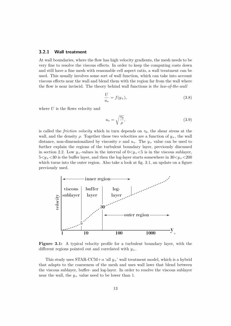
3.2.1 Wall treatmentAt wall boundaries, where the flow has high velocity gradients, the mesh needs to bevery fine to resolve the viscous effects. In order to keep the computing costs downand still have a fine mesh with reasonable cell aspect ratio, a wall treatment can beused. This usually involves some sort of wall function, which can take into accountviscous effects near the wall and blend them with the region far from the wall wherethe flow is near inviscid. The theory behind wall functions is the law-of-the-wall

U

u∗= f(y+), (3.8)

where U is the flows velocity and

u∗ =√τ0ρ, (3.9)

is called the friction velocity which in turn depends on τ0, the shear stress at thewall, and the density ρ. Together these two velocities are a function of y+, the walldistance, non-dimensionalized by viscosity ν and u∗. The y+ value can be used tofurther explain the regions of the turbulent boundary layer, previously discussedin section 2.2. Low y+-values in the interval of 0<y+<5 is in the viscous sublayer,5<y+<30 is the buffer layer, and then the log-layer starts somewhere in 30<y+<200which turns into the outer region. Also take a look at fig. 3.1, an update on a figurepreviously used.

viscoussublayer

bufferlayer

y+

log-layer

outer region

101 100 1000

inner region

5

30

Figure 3.1: A typical velocity profile for a turbulent boundary layer, with thedifferent regions pointed out and correlated with y+.

This study uses STAR-CCM+:s ‘all y+’ wall treatment model, which is a hybridthat adapts to the coarseness of the mesh and uses wall laws that blend betweenthe viscous sublayer, buffer- and log-layer. In order to resolve the viscous sublayernear the wall, the y+ value need to be lower than 1.

13

Chapter 4

Case description & setup

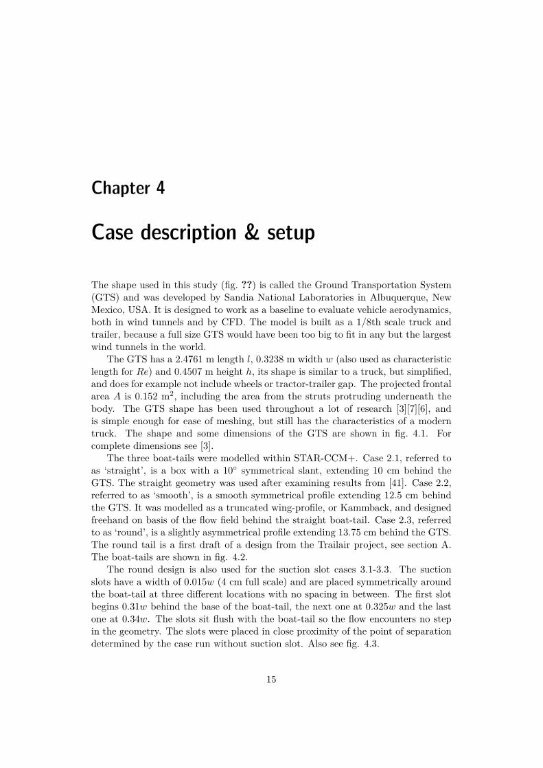
The shape used in this study (fig. ??) is called the Ground Transportation System(GTS) and was developed by Sandia National Laboratories in Albuquerque, NewMexico, USA. It is designed to work as a baseline to evaluate vehicle aerodynamics,both in wind tunnels and by CFD. The model is built as a 1/8th scale truck andtrailer, because a full size GTS would have been too big to fit in any but the largestwind tunnels in the world.

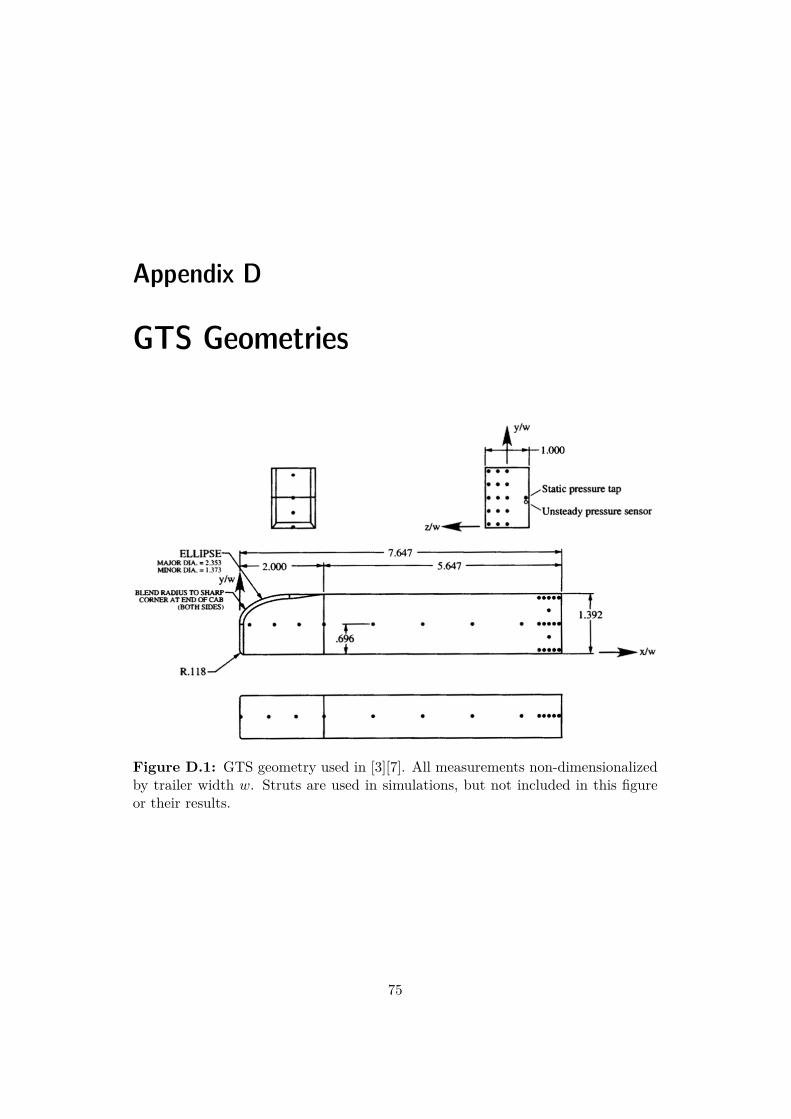
The GTS has a 2.4761 m length l, 0.3238 m width w (also used as characteristiclength for Re) and 0.4507 m height h, its shape is similar to a truck, but simplified,and does for example not include wheels or tractor-trailer gap. The projected frontalarea A is 0.152 m2, including the area from the struts protruding underneath thebody. The GTS shape has been used throughout a lot of research [3][7][6], andis simple enough for ease of meshing, but still has the characteristics of a moderntruck. The shape and some dimensions of the GTS are shown in fig. 4.1. Forcomplete dimensions see [3].

The three boat-tails were modelled within STAR-CCM+. Case 2.1, referred toas ‘straight’, is a box with a 10◦ symmetrical slant, extending 10 cm behind theGTS. The straight geometry was used after examining results from [41]. Case 2.2,referred to as ‘smooth’, is a smooth symmetrical profile extending 12.5 cm behindthe GTS. It was modelled as a truncated wing-profile, or Kammback, and designedfreehand on basis of the flow field behind the straight boat-tail. Case 2.3, referredto as ‘round’, is a slightly asymmetrical profile extending 13.75 cm behind the GTS.The round tail is a first draft of a design from the Trailair project, see section A.The boat-tails are shown in fig. 4.2.

The round design is also used for the suction slot cases 3.1-3.3. The suctionslots have a width of 0.015w (4 cm full scale) and are placed symmetrically aroundthe boat-tail at three different locations with no spacing in between. The first slotbegins 0.31w behind the base of the boat-tail, the next one at 0.325w and the lastone at 0.34w. The slots sit flush with the boat-tail so the flow encounters no stepin the geometry. The slots were placed in close proximity of the point of separationdetermined by the case run without suction slot. Also see fig. 4.3.

15

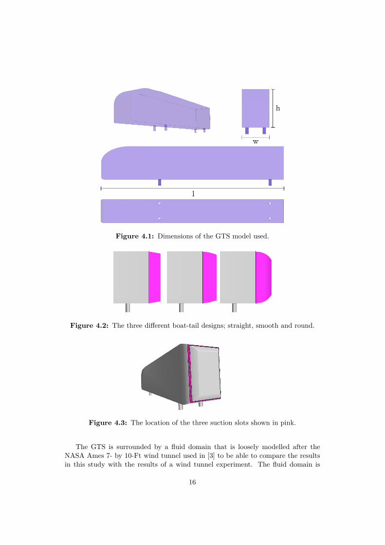
Figure 4.1: Dimensions of the GTS model used.

Figure 4.2: The three different boat-tail designs; straight, smooth and round.

Figure 4.3: The location of the three suction slots shown in pink.

The GTS is surrounded by a fluid domain that is loosely modelled after theNASA Ames 7- by 10-Ft wind tunnel used in [3] to be able to compare the resultsin this study with the results of a wind tunnel experiment. The fluid domain is

16

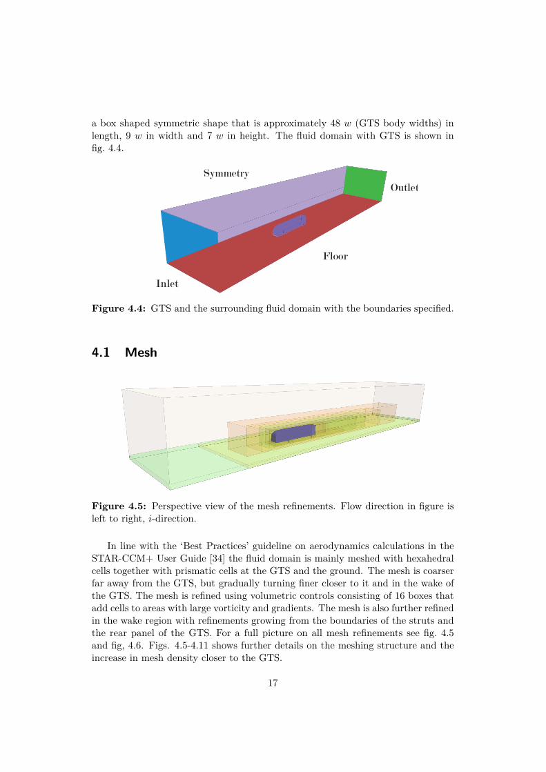
a box shaped symmetric shape that is approximately 48 w (GTS body widths) inlength, 9 w in width and 7 w in height. The fluid domain with GTS is shown infig. 4.4.

Inlet

Outlet

Floor

Symmetry

Figure 4.4: GTS and the surrounding fluid domain with the boundaries specified.

4.1 Mesh

Figure 4.5: Perspective view of the mesh refinements. Flow direction in figure isleft to right, i-direction.

In line with the ‘Best Practices’ guideline on aerodynamics calculations in theSTAR-CCM+ User Guide [34] the fluid domain is mainly meshed with hexahedralcells together with prismatic cells at the GTS and the ground. The mesh is coarserfar away from the GTS, but gradually turning finer closer to it and in the wake ofthe GTS. The mesh is refined using volumetric controls consisting of 16 boxes thatadd cells to areas with large vorticity and gradients. The mesh is also further refinedin the wake region with refinements growing from the boundaries of the struts andthe rear panel of the GTS. For a full picture on all mesh refinements see fig. 4.5and fig, 4.6. Figs. 4.5-4.11 shows further details on the meshing structure and theincrease in mesh density closer to the GTS.

17

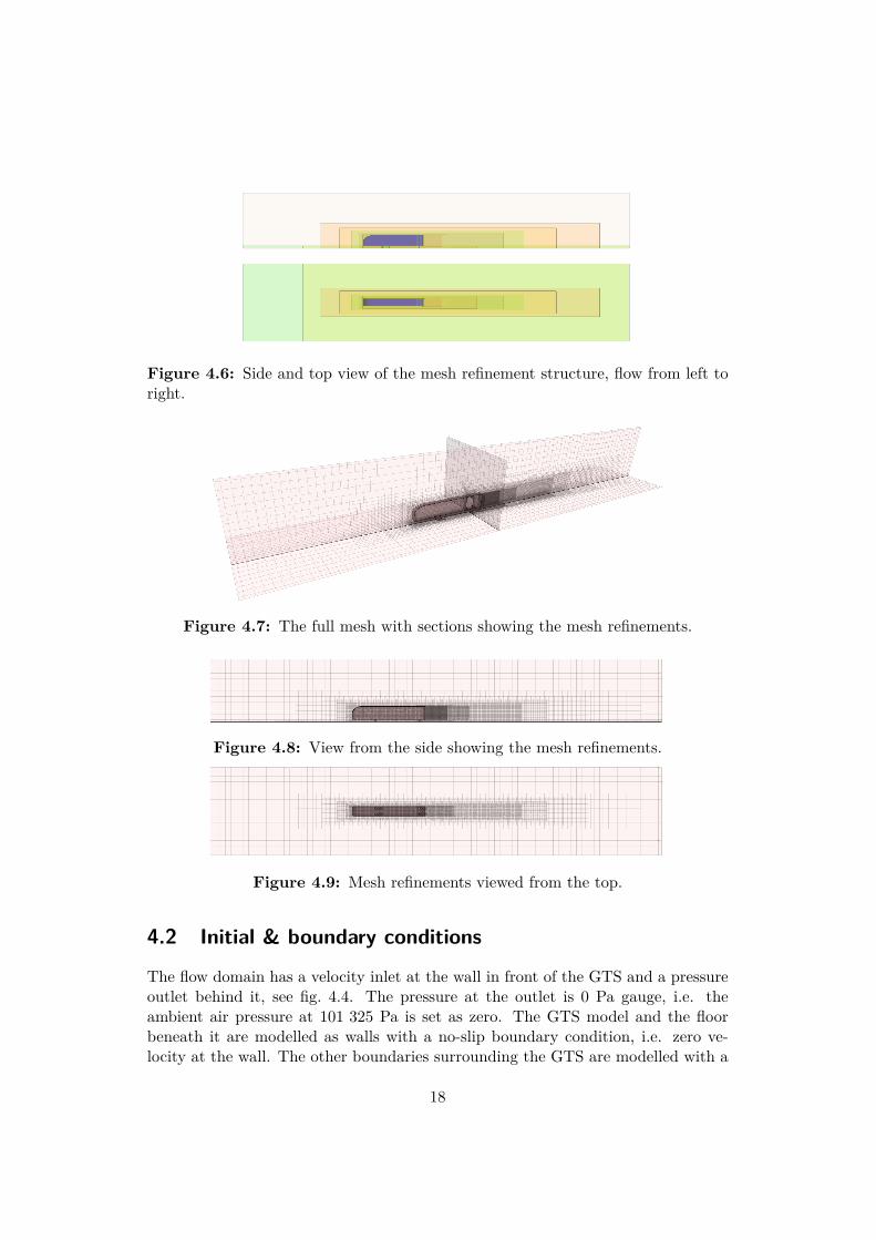
Figure 4.6: Side and top view of the mesh refinement structure, flow from left toright.

Figure 4.7: The full mesh with sections showing the mesh refinements.

Figure 4.8: View from the side showing the mesh refinements.

Figure 4.9: Mesh refinements viewed from the top.

4.2 Initial & boundary conditions

The flow domain has a velocity inlet at the wall in front of the GTS and a pressureoutlet behind it, see fig. 4.4. The pressure at the outlet is 0 Pa gauge, i.e. theambient air pressure at 101 325 Pa is set as zero. The GTS model and the floorbeneath it are modelled as walls with a no-slip boundary condition, i.e. zero ve-locity at the wall. The other boundaries surrounding the GTS are modelled with a

18

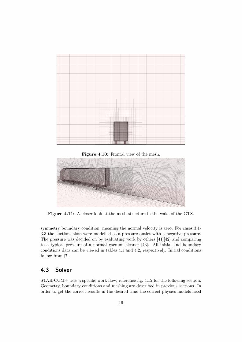
Figure 4.10: Frontal view of the mesh.

Figure 4.11: A closer look at the mesh structure in the wake of the GTS.

symmetry boundary condition, meaning the normal velocity is zero. For cases 3.1-3.3 the suctions slots were modelled as a pressure outlet with a negative pressure.The pressure was decided on by evaluating work by others [41][42] and comparingto a typical pressure of a normal vacuum cleaner [43]. All initial and boundaryconditions data can be viewed in tables 4.1 and 4.2, respectively. Initial conditionsfollow from [7].

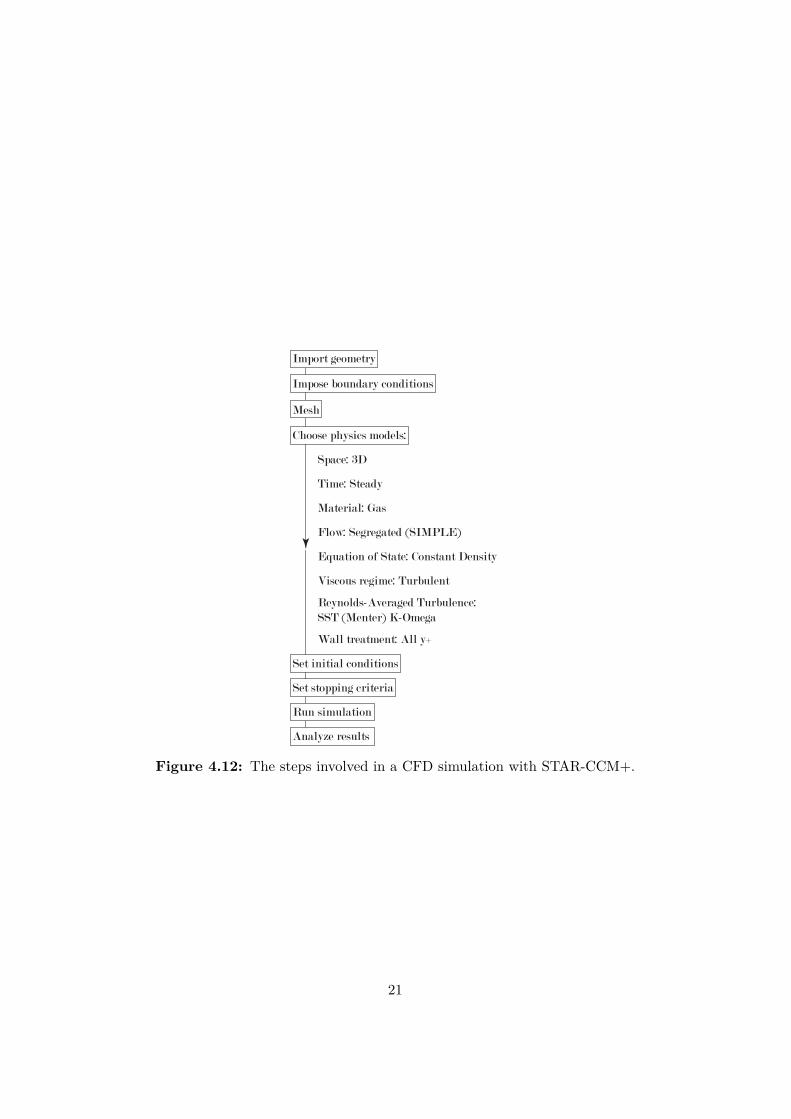
4.3 SolverSTAR-CCM+ uses a specific work flow, reference fig. 4.12 for the following section.Geometry, boundary conditions and meshing are described in previous sections. Inorder to get the correct results in the desired time the correct physics models need

19

Table 4.1: Initial conditions and values derived therefrom.

Name Denotion ValueAir density ρ 1.225 kg/m3

Freestream velocity U∞ 91.64 m/sCharacteristic length w 0.3238 mDynamic viscosity µ 1.85508·10-5 Pa·sReynolds number Re 1.96·106

Table 4.2: Boundary parameters.

Boundary Boundary condition ValueInlet Velocity inlet 91.64 m/sOutlet Pressure outlet 0 Pa (gauge)GTS Wall -Floor Wall -Ceiling and tunnel walls Symmetry -Suction slot Pressure outlet -7.5 kPa

to be chosen. First off, as the flow is highly turbulent with a high Re, and structuresin a turbulent wake are to be examined, a 3D model of space is chosen. A steady-state time model is chosen as it has the least computational cost compared to theresults. The material is gaseous air.

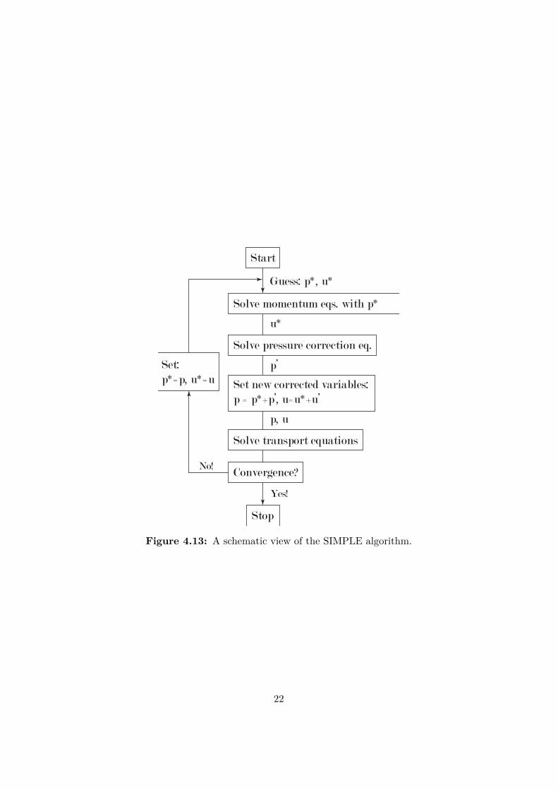
The user manual [34] suggests using a segregated flow model and a constantdensity equation of state for incompressible external aerodynamics. The segregatedsolver uses an Algebraic Multigrid (AMG) linear approach for velocity, pressureand the transport variables k and ω. The use of AMG dampens both high and lowfrequency errors in the solution. The segregated solver calculates the flow parame-ters uncoupled, and mass and momentum iterates independently with a predictor-corrector linkage combined with the SIMPLE algorithm. The solver solves thediscretized momentum equation and the discrete equation for pressure correction,see the flow chart in fig. 4.13 for a schematic view. To promote convergence anunder-relaxation factor (URF) is used to control how big a portion of the old so-lution should be used for the next iteration. The URF ranges from 0 to 1, where1 means that no part of the old solution is used. So a larger URF means moredrastical changes for every iteration, but it may also lead to numerical instability.

The viscous regime is chosen as turbulent. The turbulence model chosen is theSST (Menter) k-ω, as previously explained (section 3.2.1), as is the ‘all y+’ walltreatment used. Initial conditions are presented in section 4.1. The simulationswere stopped when convergence was reached, which is explained in the next section.

All analyzations of the results were carried out either with STAR-CCM+ orMATLAB.

20

Import geometry

Impose boundary conditions

Mesh

Set initial conditions

Set stopping criteria

Run simulation

Analyze results

Choose physics models:

Reynolds-Averaged Turbulence:SST (Menter) K-Omega

Wall treatment: All y+

Space: 3D

Time: Steady

Material: Gas

Flow: Segregated (SIMPLE)

Equation of State: Constant Density

Viscous regime: Turbulent

Figure 4.12: The steps involved in a CFD simulation with STAR-CCM+.

21

Guess: p*, u*

u*

p’

p, u

Solve momentum eqs. with p*

Solve pressure correction eq.

Solve transport equations

Start

Convergence?

Stop

Set new corrected variables:p = p*+p’, u=u*+u’

Set:p*=p, u*=u

Yes!

No!

Figure 4.13: A schematic view of the SIMPLE algorithm.

22

Chapter 5

Results

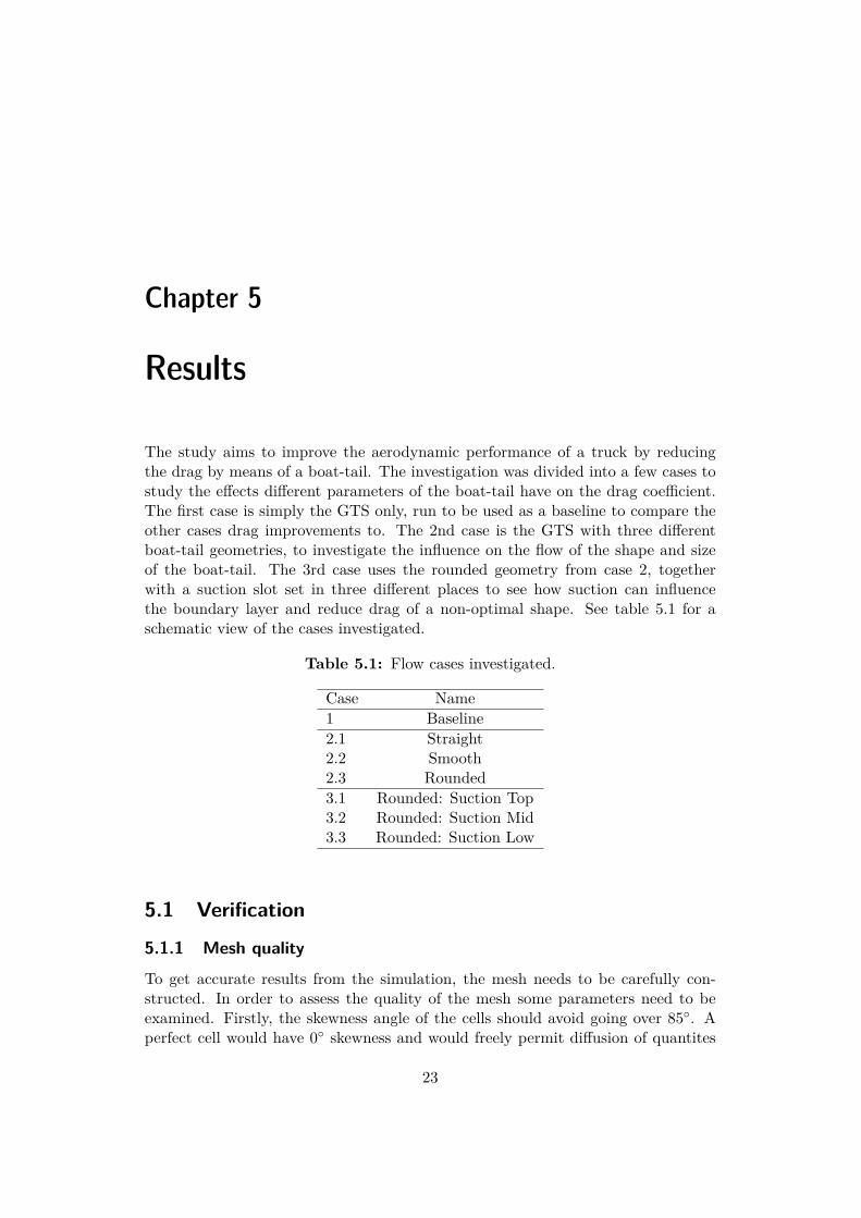
The study aims to improve the aerodynamic performance of a truck by reducingthe drag by means of a boat-tail. The investigation was divided into a few cases tostudy the effects different parameters of the boat-tail have on the drag coefficient.The first case is simply the GTS only, run to be used as a baseline to compare theother cases drag improvements to. The 2nd case is the GTS with three differentboat-tail geometries, to investigate the influence on the flow of the shape and sizeof the boat-tail. The 3rd case uses the rounded geometry from case 2, togetherwith a suction slot set in three different places to see how suction can influencethe boundary layer and reduce drag of a non-optimal shape. See table 5.1 for aschematic view of the cases investigated.

Table 5.1: Flow cases investigated.

Case Name1 Baseline2.1 Straight2.2 Smooth2.3 Rounded3.1 Rounded: Suction Top3.2 Rounded: Suction Mid3.3 Rounded: Suction Low

5.1 Verification

5.1.1 Mesh quality

To get accurate results from the simulation, the mesh needs to be carefully con-structed. In order to assess the quality of the mesh some parameters need to beexamined. Firstly, the skewness angle of the cells should avoid going over 85◦. Aperfect cell would have 0◦ skewness and would freely permit diffusion of quantites

23

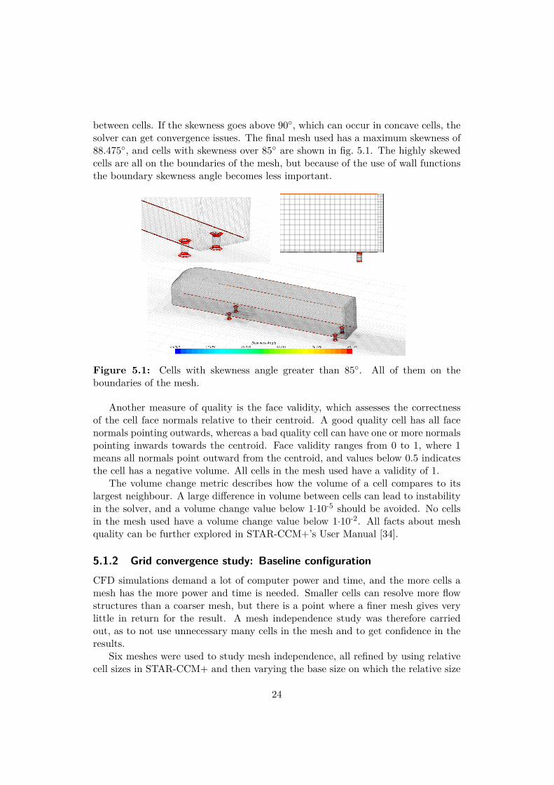
between cells. If the skewness goes above 90◦, which can occur in concave cells, thesolver can get convergence issues. The final mesh used has a maximum skewness of88.475◦, and cells with skewness over 85◦ are shown in fig. 5.1. The highly skewedcells are all on the boundaries of the mesh, but because of the use of wall functionsthe boundary skewness angle becomes less important.

Figure 5.1: Cells with skewness angle greater than 85◦. All of them on theboundaries of the mesh.

Another measure of quality is the face validity, which assesses the correctnessof the cell face normals relative to their centroid. A good quality cell has all facenormals pointing outwards, whereas a bad quality cell can have one or more normalspointing inwards towards the centroid. Face validity ranges from 0 to 1, where 1means all normals point outward from the centroid, and values below 0.5 indicatesthe cell has a negative volume. All cells in the mesh used have a validity of 1.

The volume change metric describes how the volume of a cell compares to itslargest neighbour. A large difference in volume between cells can lead to instabilityin the solver, and a volume change value below 1·10-5 should be avoided. No cellsin the mesh used have a volume change value below 1·10-2. All facts about meshquality can be further explored in STAR-CCM+’s User Manual [34].

5.1.2 Grid convergence study: Baseline configurationCFD simulations demand a lot of computer power and time, and the more cells amesh has the more power and time is needed. Smaller cells can resolve more flowstructures than a coarser mesh, but there is a point where a finer mesh gives verylittle in return for the result. A mesh independence study was therefore carriedout, as to not use unnecessary many cells in the mesh and to get confidence in theresults.

Six meshes were used to study mesh independence, all refined by using relativecell sizes in STAR-CCM+ and then varying the base size on which the relative size

24

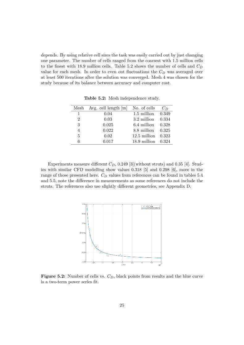
depends. By using relative cell sizes the task was easily carried out by just changingone parameter. The number of cells ranged from the coarsest with 1.5 million cellsto the finest with 18.9 million cells. Table 5.2 shows the number of cells and CD

value for each mesh. In order to even out fluctuations the CD was averaged overat least 500 iterations after the solution was converged. Mesh 4 was chosen for thestudy because of its balance between accuracy and computer cost.

Table 5.2: Mesh independence study.

Mesh Avg. cell length [m] No. of cells CD

1 0.04 1.5 million 0.3492 0.03 3.2 million 0.3343 0.025 6.4 million 0.3284 0.022 8.8 million 0.3255 0.02 12.5 million 0.3236 0.017 18.9 million 0.324

Experiments measure different CD, 0.249 [3](without struts) and 0.35 [4]. Stud-ies with similar CFD modelling show values 0.318 [5] and 0.298 [6], more in therange of those presented here. CD values from references can be found in tables 5.4and 5.5, note the difference in measurements as some references do not include thestruts. The references also use slightly different geometries, see Appendix D.

Figure 5.2: Number of cells vs. CD, black points from results and the blue curveis a two-term power series fit.

25

5.2 Case 1: Baseline

The first case is run as a baseline, or reference, case to compare the other casesto. Since the work is carried out numerically, with errors from a wide range ofparameters such as numerical method, model, round-off errors etc. one has to keepin mind that the results may not be the same as for an experiment. That said, thetrends for the results should be reflected in reality. The baseline case has also beeninvestigated by others, see ref. [3]-[6], so the results in this thesis are compared withthose.

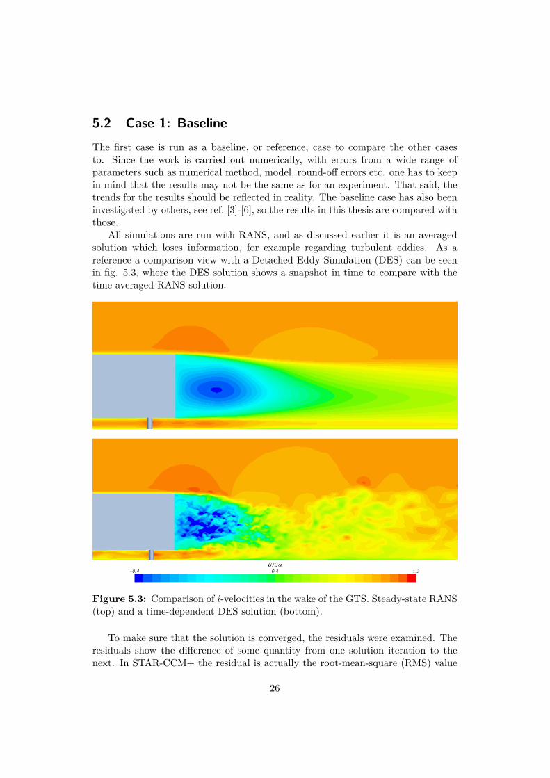
All simulations are run with RANS, and as discussed earlier it is an averagedsolution which loses information, for example regarding turbulent eddies. As areference a comparison view with a Detached Eddy Simulation (DES) can be seenin fig. 5.3, where the DES solution shows a snapshot in time to compare with thetime-averaged RANS solution.

Figure 5.3: Comparison of i-velocities in the wake of the GTS. Steady-state RANS(top) and a time-dependent DES solution (bottom).

To make sure that the solution is converged, the residuals were examined. Theresiduals show the difference of some quantity from one solution iteration to thenext. In STAR-CCM+ the residual is actually the root-mean-square (RMS) value

26

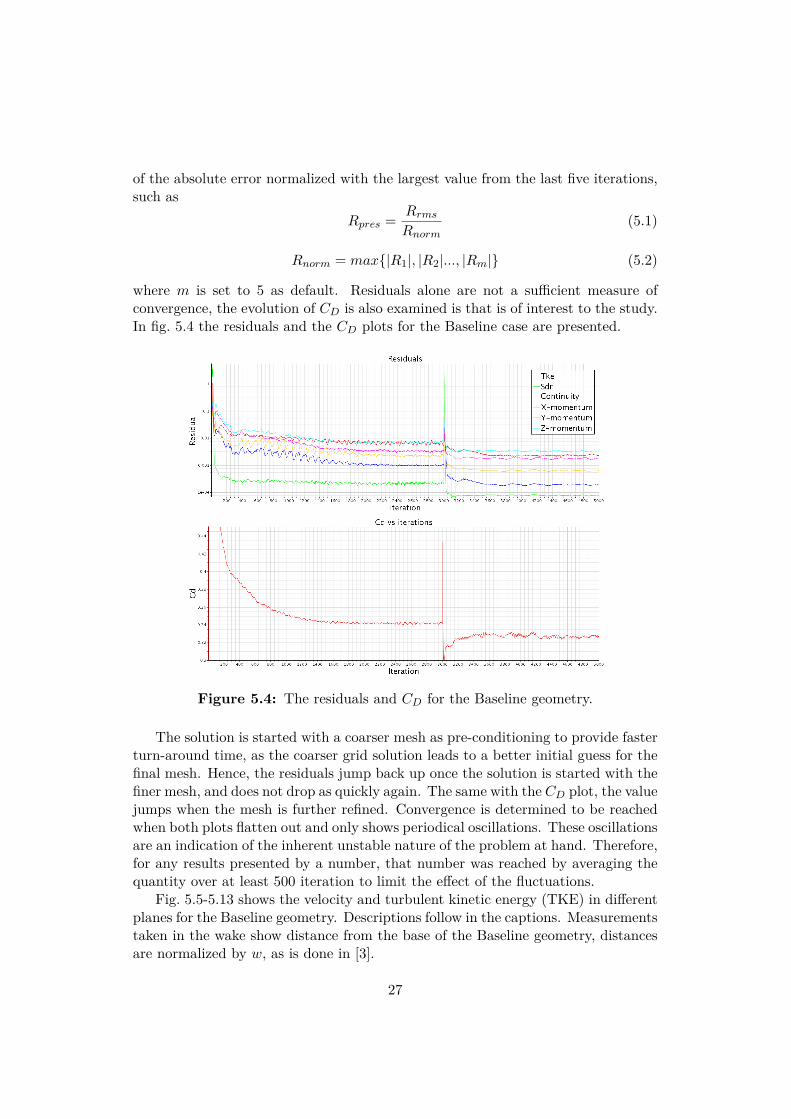
of the absolute error normalized with the largest value from the last five iterations,such as

Rpres = Rrms

Rnorm(5.1)

Rnorm = max{|R1|, |R2|..., |Rm|} (5.2)

where m is set to 5 as default. Residuals alone are not a sufficient measure ofconvergence, the evolution of CD is also examined is that is of interest to the study.In fig. 5.4 the residuals and the CD plots for the Baseline case are presented.

Figure 5.4: The residuals and CD for the Baseline geometry.

The solution is started with a coarser mesh as pre-conditioning to provide fasterturn-around time, as the coarser grid solution leads to a better initial guess for thefinal mesh. Hence, the residuals jump back up once the solution is started with thefiner mesh, and does not drop as quickly again. The same with the CD plot, the valuejumps when the mesh is further refined. Convergence is determined to be reachedwhen both plots flatten out and only shows periodical oscillations. These oscillationsare an indication of the inherent unstable nature of the problem at hand. Therefore,for any results presented by a number, that number was reached by averaging thequantity over at least 500 iteration to limit the effect of the fluctuations.

Fig. 5.5-5.13 shows the velocity and turbulent kinetic energy (TKE) in differentplanes for the Baseline geometry. Descriptions follow in the captions. Measurementstaken in the wake show distance from the base of the Baseline geometry, distancesare normalized by w, as is done in [3].

27

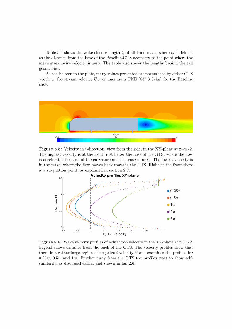
Table 5.6 shows the wake closure length lc of all tried cases, where lc is definedas the distance from the base of the Baseline-GTS geometry to the point where themean streamwise velocity is zero. The table also shows the lengths behind the tailgeometries.

As can be seen in the plots, many values presented are normalized by either GTSwidth w, freestream velocity U∞ or maximum TKE (637.3 J/kg) for the Baselinecase.

Figure 5.5: Velocity in i-direction, view from the side, in the XY-plane at z=w/2.The highest velocity is at the front, just below the nose of the GTS, where the flowis accelerated because of the curvature and decrease in area. The lowest velocity isin the wake, where the flow moves back towards the GTS. Right at the front thereis a stagnation point, as explained in section 2.2.

Figure 5.6: Wake velocity profiles of i-direction velocity in the XY-plane at z=w/2.Legend shows distance from the back of the GTS. The velocity profiles show thatthere is a rather large region of negative i-velocity if one examines the profiles for0.25w, 0.5w and 1w. Further away from the GTS the profiles start to show self-similarity, as discussed earlier and shown in fig. 2.6.

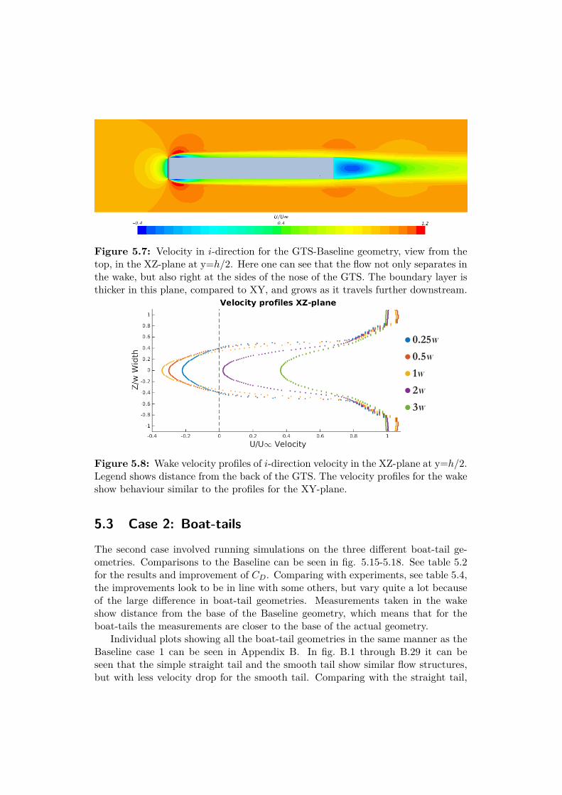
Figure 5.7: Velocity in i-direction for the GTS-Baseline geometry, view from thetop, in the XZ-plane at y=h/2. Here one can see that the flow not only separates inthe wake, but also right at the sides of the nose of the GTS. The boundary layer isthicker in this plane, compared to XY, and grows as it travels further downstream.

Figure 5.8: Wake velocity profiles of i-direction velocity in the XZ-plane at y=h/2.Legend shows distance from the back of the GTS. The velocity profiles for the wakeshow behaviour similar to the profiles for the XY-plane.

5.3 Case 2: Boat-tails

The second case involved running simulations on the three different boat-tail ge-ometries. Comparisons to the Baseline can be seen in fig. 5.15-5.18. See table 5.2for the results and improvement of CD. Comparing with experiments, see table 5.4,the improvements look to be in line with some others, but vary quite a lot becauseof the large difference in boat-tail geometries. Measurements taken in the wakeshow distance from the base of the Baseline geometry, which means that for theboat-tails the measurements are closer to the base of the actual geometry.

Individual plots showing all the boat-tail geometries in the same manner as theBaseline case 1 can be seen in Appendix B. In fig. B.1 through B.29 it can beseen that the simple straight tail and the smooth tail show similar flow structures,but with less velocity drop for the smooth tail. Comparing with the straight tail,

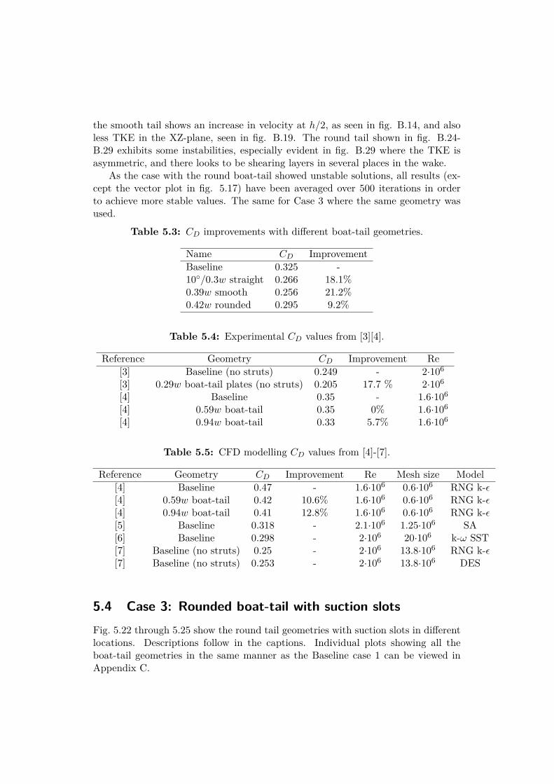
the smooth tail shows an increase in velocity at h/2, as seen in fig. B.14, and alsoless TKE in the XZ-plane, seen in fig. B.19. The round tail shown in fig. B.24-B.29 exhibits some instabilities, especially evident in fig. B.29 where the TKE isasymmetric, and there looks to be shearing layers in several places in the wake.

As the case with the round boat-tail showed unstable solutions, all results (ex-cept the vector plot in fig. 5.17) have been averaged over 500 iterations in orderto achieve more stable values. The same for Case 3 where the same geometry wasused.

Table 5.3: CD improvements with different boat-tail geometries.

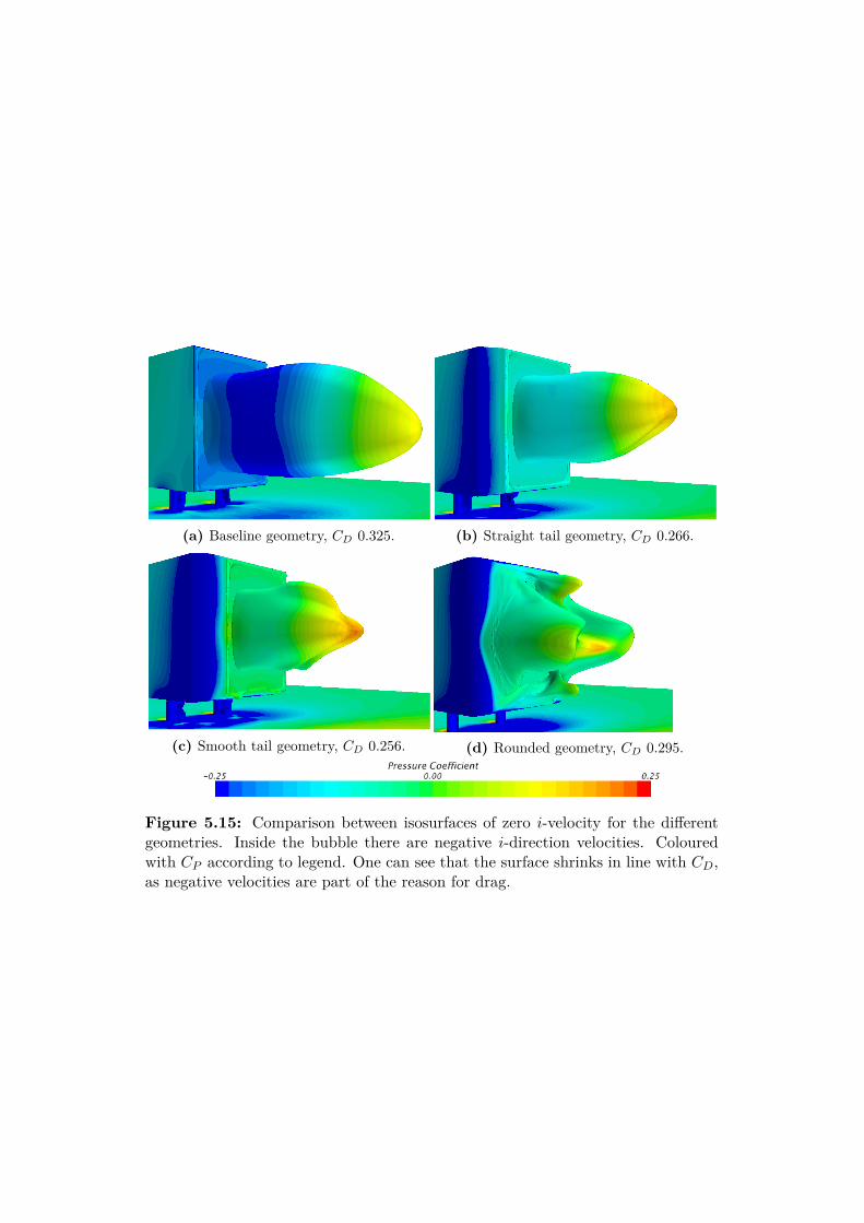
Name CD ImprovementBaseline 0.325 -10◦/0.3w straight 0.266 18.1%0.39w smooth 0.256 21.2%0.42w rounded 0.295 9.2%

Table 5.4: Experimental CD values from [3][4].

Reference Geometry CD Improvement Re[3] Baseline (no struts) 0.249 - 2·106

[3] 0.29w boat-tail plates (no struts) 0.205 17.7 % 2·106

[4] Baseline 0.35 - 1.6·106

[4] 0.59w boat-tail 0.35 0% 1.6·106

[4] 0.94w boat-tail 0.33 5.7% 1.6·106

Table 5.5: CFD modelling CD values from [4]-[7].

Reference Geometry CD Improvement Re Mesh size Model[4] Baseline 0.47 - 1.6·106 0.6·106 RNG k-ε[4] 0.59w boat-tail 0.42 10.6% 1.6·106 0.6·106 RNG k-ε[4] 0.94w boat-tail 0.41 12.8% 1.6·106 0.6·106 RNG k-ε[5] Baseline 0.318 - 2.1·106 1.25·106 SA[6] Baseline 0.298 - 2·106 20·106 k-ω SST[7] Baseline (no struts) 0.25 - 2·106 13.8·106 RNG k-ε[7] Baseline (no struts) 0.253 - 2·106 13.8·106 DES

5.4 Case 3: Rounded boat-tail with suction slotsFig. 5.22 through 5.25 show the round tail geometries with suction slots in differentlocations. Descriptions follow in the captions. Individual plots showing all theboat-tail geometries in the same manner as the Baseline case 1 can be viewed inAppendix C.

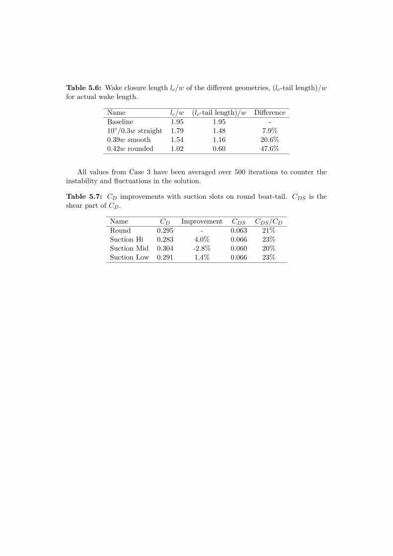
Table 5.6: Wake closure length lc/w of the different geometries, (lc-tail length)/wfor actual wake length.

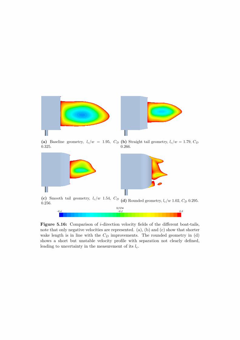
Name lc/w (lc-tail length)/w DifferenceBaseline 1.95 1.95 -10◦/0.3w straight 1.79 1.48 7.9%0.39w smooth 1.54 1.16 20.6%0.42w rounded 1.02 0.60 47.6%

All values from Case 3 have been averaged over 500 iterations to counter theinstability and fluctuations in the solution.

Table 5.7: CD improvements with suction slots on round boat-tail. CDS is theshear part of CD.

Name CD Improvement CDS CDS/CD

Round 0.295 - 0.063 21%Suction Hi 0.283 4.0% 0.066 23%Suction Mid 0.304 -2.8% 0.060 20%Suction Low 0.291 1.4% 0.066 23%

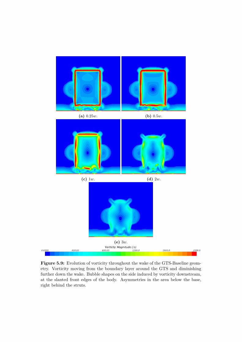
(a) 0.25w. (b) 0.5w.

(c) 1w. (d) 2w.

(e) 3w.

Figure 5.9: Evolution of vorticity throughout the wake of the GTS-Baseline geom-etry. Vorticity moving from the boundary layer around the GTS and diminishingfurther down the wake. Bubble shapes on the side induced by vorticity downstream,at the slanted front edges of the body. Asymmetries in the area below the base,right behind the struts.

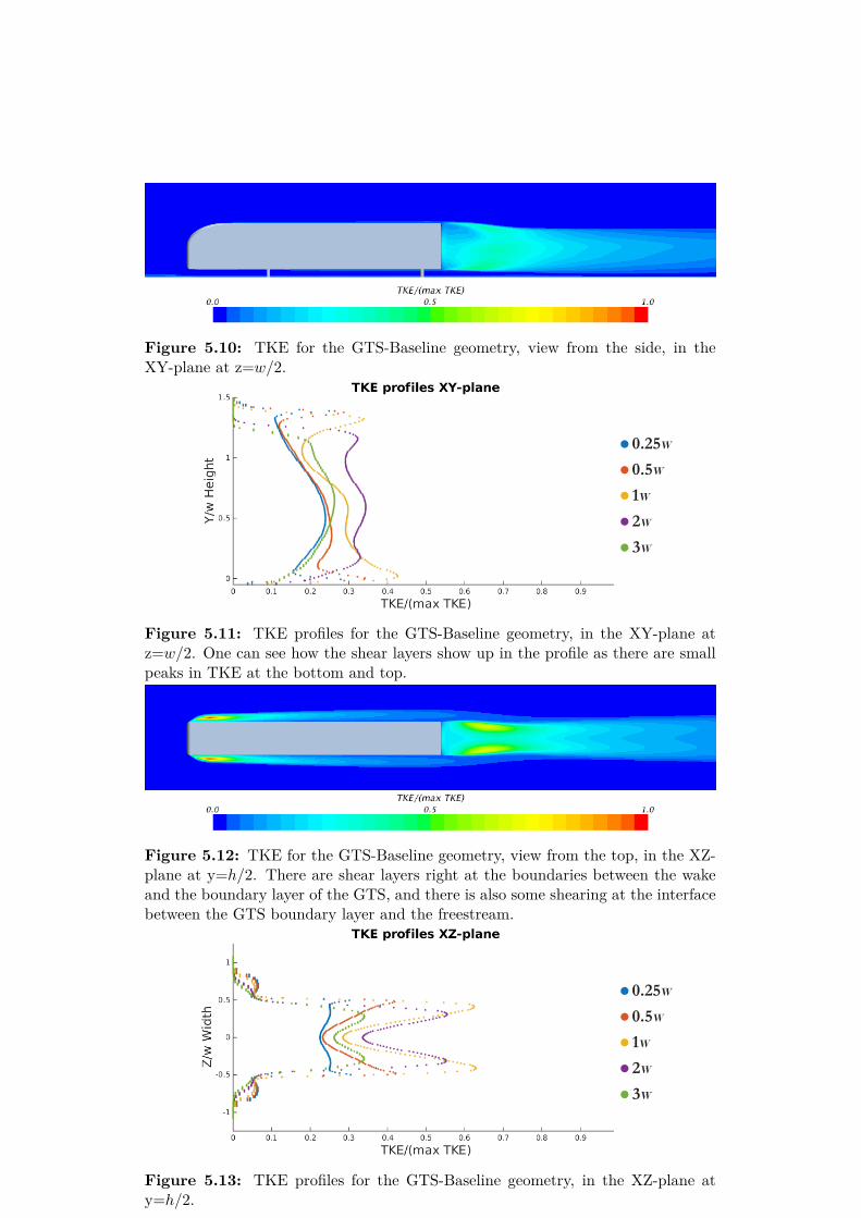
Figure 5.10: TKE for the GTS-Baseline geometry, view from the side, in theXY-plane at z=w/2.

Figure 5.11: TKE profiles for the GTS-Baseline geometry, in the XY-plane atz=w/2. One can see how the shear layers show up in the profile as there are smallpeaks in TKE at the bottom and top.

Figure 5.12: TKE for the GTS-Baseline geometry, view from the top, in the XZ-plane at y=h/2. There are shear layers right at the boundaries between the wakeand the boundary layer of the GTS, and there is also some shearing at the interfacebetween the GTS boundary layer and the freestream.

Figure 5.13: TKE profiles for the GTS-Baseline geometry, in the XZ-plane aty=h/2.

Figure 5.14: Pressure for the GTS-Baseline geometry, in XY-plane at z=w/2and XZ-plane at y=h/2. High pressure at the stagnation point in the front and lowpressure at the base of the wake. The wake also shows a raised pressure downstreamof the GTS, where velocities in j- and k-direction decelarate. Between the high andlow pressure regions is a saddle point with ambient pressure.

(a) Baseline geometry, CD 0.325. (b) Straight tail geometry, CD 0.266.

(c) Smooth tail geometry, CD 0.256. (d) Rounded geometry, CD 0.295.

Figure 5.15: Comparison between isosurfaces of zero i-velocity for the differentgeometries. Inside the bubble there are negative i-direction velocities. Colouredwith CP according to legend. One can see that the surface shrinks in line with CD,as negative velocities are part of the reason for drag.

(a) Baseline geometry, lc/w = 1.95, CD

0.325.(b) Straight tail geometry, lc/w = 1.79, CD

0.266.

(c) Smooth tail geometry, lc/w 1.54, CD

0.256. (d) Rounded geometry, lc/w 1.02, CD 0.295.

Figure 5.16: Comparison of i-direction velocity fields of the different boat-tails,note that only negative velocities are represented. (a), (b) and (c) show that shorterwake length is in line with the CD improvements. The rounded geometry in (d)shows a short but unstable velocity profile with separation not clearly defined,leading to uncertainty in the measurement of its lc.

(a) Baseline geometry, XY-plane (b) Baseline geometry, XZ-plane.

(c) Straight tail geometry, XY-plane. (d) Straight tail geometry, XZ-plane.

(e) Smooth tail geometry, XY-plane. (f) Smooth tail geometry, XZ-plane.

(g) Rounded geometry, XY-plane. (h) Rounded geometry, XZ-plane.

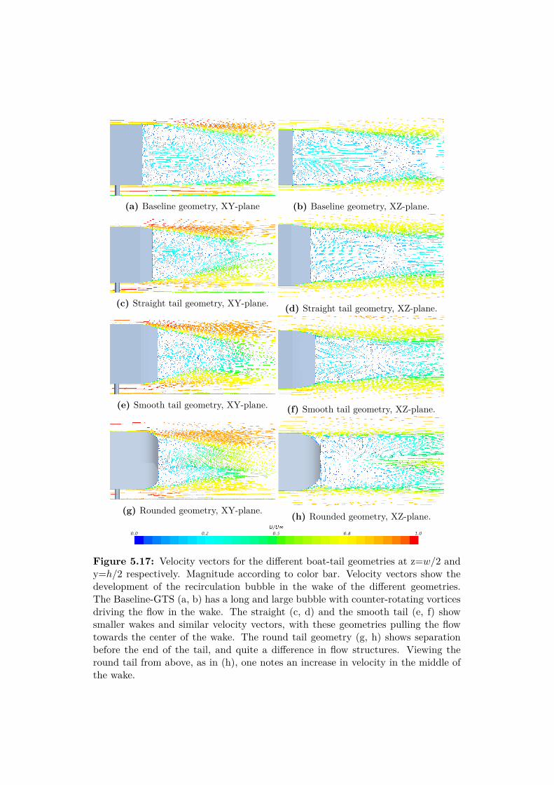
Figure 5.17: Velocity vectors for the different boat-tail geometries at z=w/2 andy=h/2 respectively. Magnitude according to color bar. Velocity vectors show thedevelopment of the recirculation bubble in the wake of the different geometries.The Baseline-GTS (a, b) has a long and large bubble with counter-rotating vorticesdriving the flow in the wake. The straight (c, d) and the smooth tail (e, f) showsmaller wakes and similar velocity vectors, with these geometries pulling the flowtowards the center of the wake. The round tail geometry (g, h) shows separationbefore the end of the tail, and quite a difference in flow structures. Viewing theround tail from above, as in (h), one notes an increase in velocity in the middle ofthe wake.

(a) Baseline geometry, XY-plane (b) Baseline geometry, XZ-plane.

(c) Straight tail geometry, XY-plane.

(d) Straight tail geometry, XZ-plane.

(e) Smooth tail geometry, XY-plane. (f) Smooth tail geometry, XZ-plane.

(g) Rounded geometry, XY-plane. (h) Rounded geometry, XZ-plane.

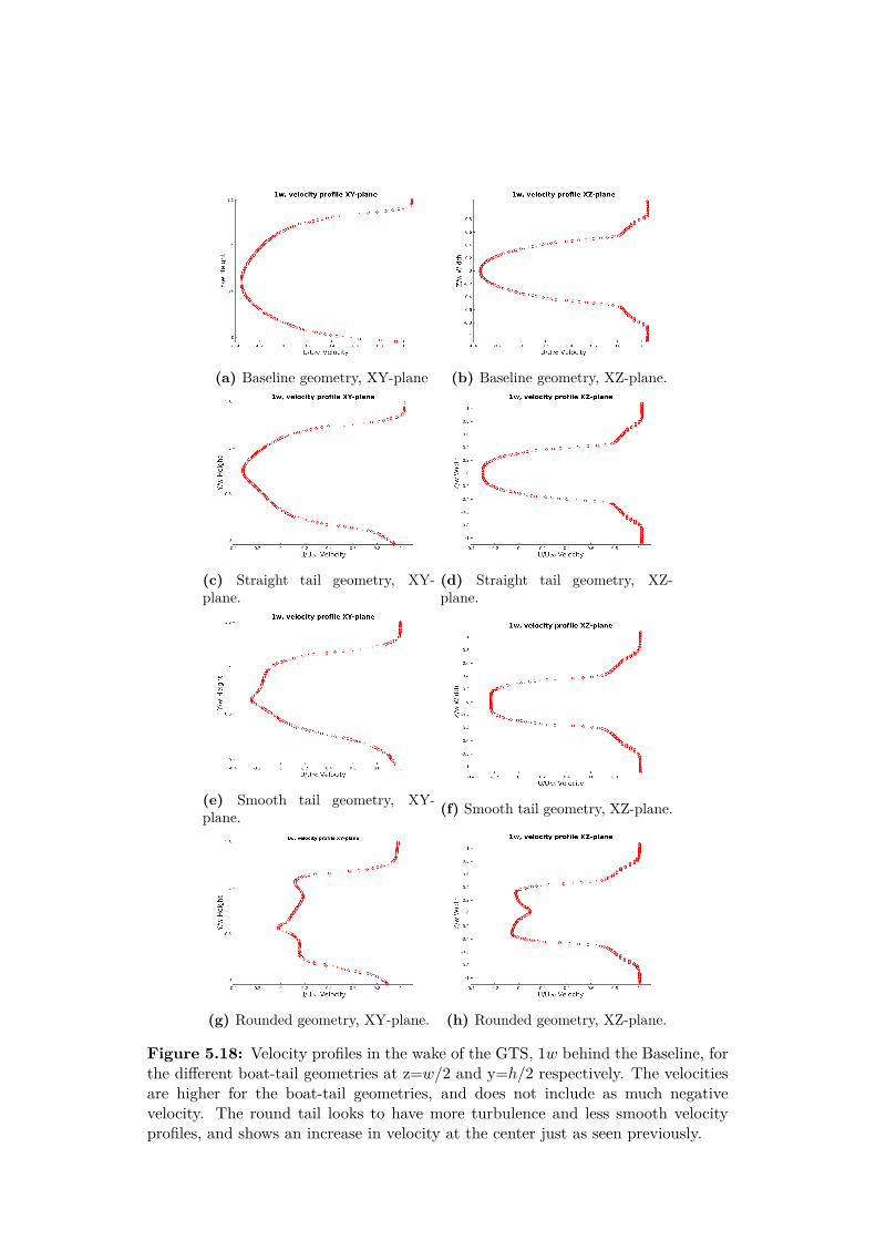
Figure 5.18: Velocity profiles in the wake of the GTS, 1w behind the Baseline, forthe different boat-tail geometries at z=w/2 and y=h/2 respectively. The velocitiesare higher for the boat-tail geometries, and does not include as much negativevelocity. The round tail looks to have more turbulence and less smooth velocityprofiles, and shows an increase in velocity at the center just as seen previously.

(a) Baseline. (b) Straight tail.

(c) Smooth tail. (d) Round tail.

Figure 5.19: Comparison of the vorticity in the wake at x=1w. With narrowertail the shear layers forming from the boundary layer of the GTS moves further intowards the centerline. All images show large disturbances in the bottom of thewake, an area heavily influenced by the struts below the GTS.

(a) Baseline geometry, XY-plane (b) Baseline geometry, XZ-plane.

(c) Straight tail geometry, XY-plane.

(d) Straight tail geometry, XZ-plane.

(e) Smooth tail geometry, XY-plane. (f) Smooth tail geometry, XZ-plane.

(g) Rounded geometry, XY-plane. (h) Rounded geometry, XZ-plane.

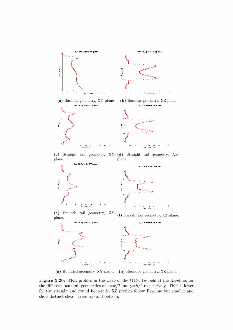
Figure 5.20: TKE profiles in the wake of the GTS, 1w behind the Baseline, forthe different boat-tail geometries at z=w/2 and y=h/2 respectively. TKE is lowerfor the straight and round boat-tails, XZ profiles follow Baseline but smaller andshow distinct shear layers top and bottom.

(a) Baseline geometry.

(b) Straight boat-tail.

(c) Smooth boat-tail.

(d) Round boat-tail.

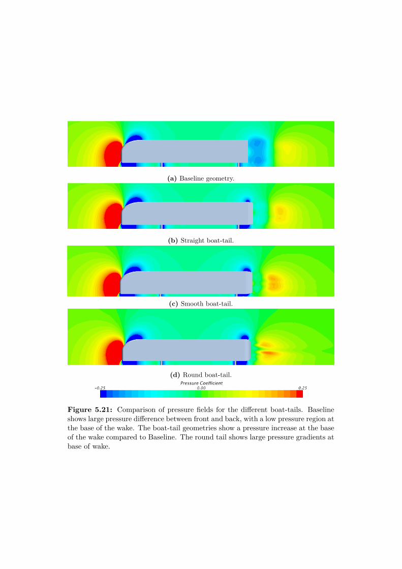
Figure 5.21: Comparison of pressure fields for the different boat-tails. Baselineshows large pressure difference between front and back, with a low pressure region atthe base of the wake. The boat-tail geometries show a pressure increase at the baseof the wake compared to Baseline. The round tail shows large pressure gradients atbase of wake.

(a) No suction, XY-plane. (b) No suction, XZ-plane.

(c) High suction slot, XY-plane. (d) High suction slot, XZ-plane.

(e) Mid suction slot, XY-plane. (f) Mid suction slot, XZ-plane.

(g) Low suction slot, XY-plane. (h) Low suction slot, XZ-plane.

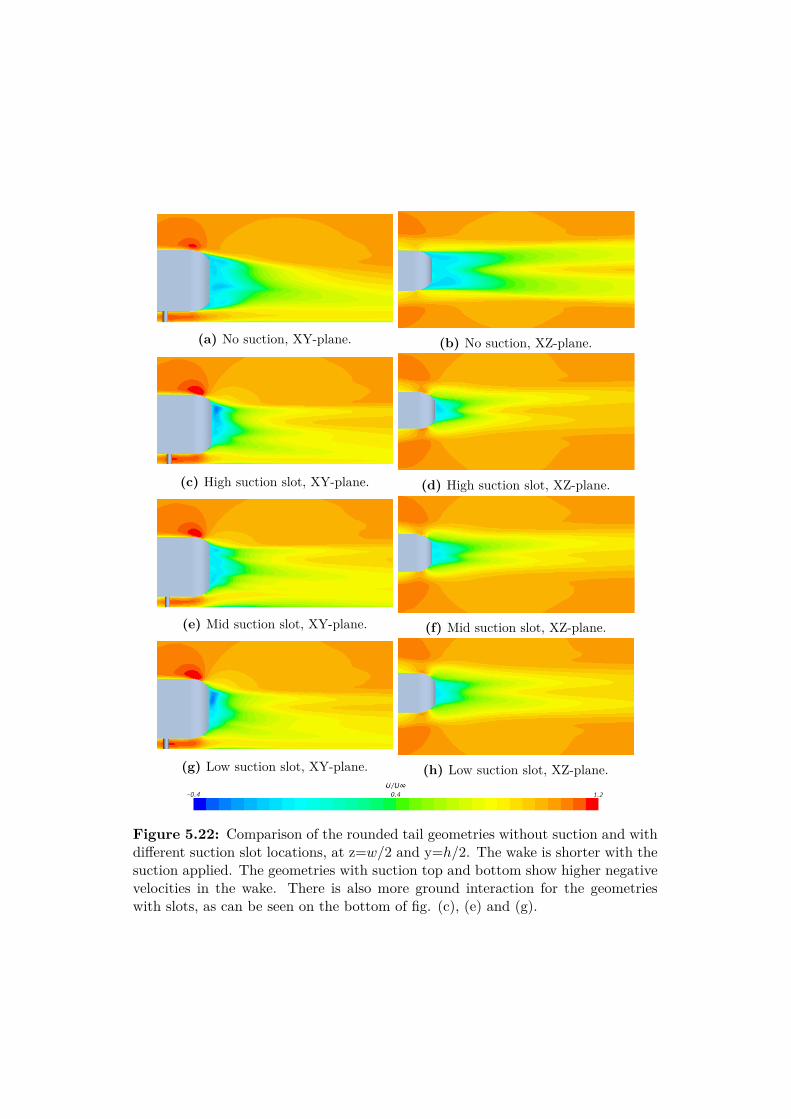
Figure 5.22: Comparison of the rounded tail geometries without suction and withdifferent suction slot locations, at z=w/2 and y=h/2. The wake is shorter with thesuction applied. The geometries with suction top and bottom show higher negativevelocities in the wake. There is also more ground interaction for the geometrieswith slots, as can be seen on the bottom of fig. (c), (e) and (g).

(a) No suction.

(b) High slot location.

(c) Mid slot location.

(d) Low slot location.

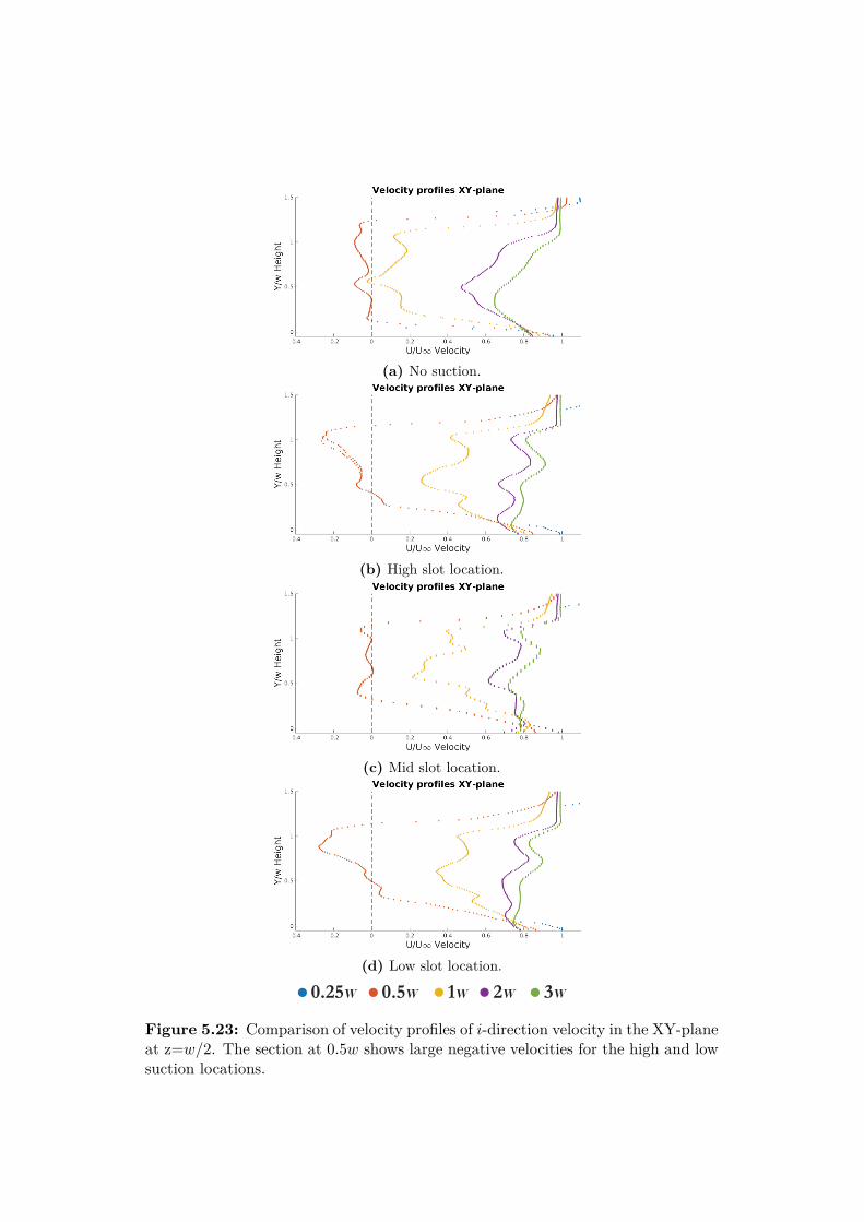
Figure 5.23: Comparison of velocity profiles of i-direction velocity in the XY-planeat z=w/2. The section at 0.5w shows large negative velocities for the high and lowsuction locations.

(a) No suction.

(b) High slot location.

(c) Mid slot location.

(d) Low slot location.

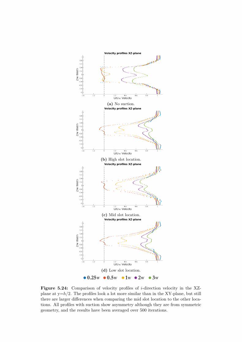
Figure 5.24: Comparison of velocity profiles of i-direction velocity in the XZ-plane at y=h/2. The profiles look a lot more similar than in the XY-plane, but stillthere are larger differences when comparing the mid slot location to the other loca-tions. All profiles with suction show asymmetry although they are from symmetricgeometry, and the results have been averaged over 500 iterations.

(a) Round tail, no suction.

(b) Suction slot top.

(c) Suction slot mid.

(d) Suction slot low.

Figure 5.25: Comparison of pressure fields for different suction slot locations.With suction there is a large increase in pressure at the base of the wake. Instabilitesin the solution showing in the wake area.

Chapter 6

Conclusions & Discussion

CFD was used to simulate the flow behind a 1/8th scale GTS modelof a simplifed tractor and trailer geometry. Three different boat-tailswere added to the GTS to assess their impact on velocity, pressure, dragforce and overall flow field structures. Further on suction slots wereadded to one boat-tail geometry, and three different slot locations wereinvestigated to determine their effect on drag and flow behaviour.

There is no contest to the benefits of adding a boat-tail the back of a bluntshape. Both this study and others show that the improvements are quite drastic.The results in this study showed a reduction of drag by 22%, and other studiesshow results that are similar. The shape does not even need to be that complexto be efficient, which case 2.2 with the straight tail showed with its 18% decreasein drag. Hopefully the new EU legislation will urge manufacturers and truckers towork towards using boat-tails to effectively save the environment, and reduce thecosts both for society and themselves.

The different boat-tail shapes showed the design process can not always be in-tuitive. A shape that looks smooth and streamlined may not always have thosequalities, as evidenced by case 2.3 with the round tail. By using CFD the effec-tiveness of a design can be easily measured and some of its qualities be deduced.Designers and CFD engineers working together cross-disciplanary would probablybenefit the design process and lead to more efficient geometries quicker.

In cases 3.1-3.3 it was investigated how a suction slot could be used to improvea sub-optimal design of a boat-tail. The results showed that the location of the slothighly influenced the outcome, even if the location was only shifted slightly. Theeffect of suction on trucks, and similarly pressure, is a field that has garnered a lotof study in recent years [41][44], and will probably be the next step in optimizingthe aerodynamics of trucks and trailers.

The results from cases 3.1-3.3 are a bit questionable, as the flow field looksunstable. The round tail profile does not have a clearly defined separation pointwhich leads to instabilities in the flow field. Residuals and CD plots (fig. D.2)does not show big differences in convergence compared to the Baseline (fig. 5.4).

47

Probably the RANS model has a hard time reaching a stable solution and whenthe suction slots are added a clear solution is even harder to reach. These caseswould benefit from using a DES simulation which is more accurate in predictingwake flows [34].

Chapter 7

Future work

The work started in this thesis could be continued by running more simulations onthe different geometries, but instead using more accurate numerical models such asthe DES modification of RANS. Better models would lead to more accurate resultsand the complex flow field could be more faithfully captured, in turn leading to abetter prediction of the real life flow field.

The cases involving suction would also benefit from a more accurate numericalmodel which can resolve fluctuations in an unstable wake. Suction slots could beinvestigated with different pressures and slot angles. Further on a pressure outletcould be added, as this would be closer to a situation in reality and would also bea more efficient use of the power needed for such a device. Other flow controllingtechniques such as the use of pulsing flow or using a plasma actuator could be ofinterest too. With accurate enough models, a feedback loop could be used thatmodelled the pressures to the frequencies of the vortex shedding of the shape andactively promote a more stable and efficient flow, for example in crosswinds.

Another approach would be to use a geometry that resembles reality more, andthe interaction between trailer and complex geometry like side mirrors, wheels andtractor-trailer gap would be invstigated. This could in turn lead to an optimizedboat-tail shape that could be used for a full scale experiment with a real truck.

Building directly on this thesis, and moving on to a real, full-size truck exper-iment, the easiest route would probably be to use the straight tail shape. Thestraight tail shape is easy to build, can easily be modified, and still shows goodimprovements on drag. The straight tail shape could first be used for a parametricstudy with a Design of Experiments approach together with CFD to investigate theeffect of slant angle on side, top and bottom, together with the length of the tail.Then with the results from the study the full-size experiment would have more datato build a model boat-tail from.

All of the above would be more easily performed once legislation has been setso the optimizations can be done with the proper constraints.

49

Appendix A

The Trailair project

This thesis started with the help of Peter Georén, project manager at KTH Trans-port Labs, who put me in contact with Per Gyllenspetz who works with the Trailairproject. Trailair targets the reduction of fuel consumption of trucks by focusingon the aerodynamic drag of the trailer. Trailair is not only about reducing drag,but also about making a product that can be easily implemented, used and puton market. Within the project a business analysis has been made, and there areparallell studies such as [23] on logistics.

My part has been to investigate what kind of geometries could be used for aboat-tail. The findings from this thesis will come to use later in the Trailair projectwhen there could be a real size field-testing of a boat-tail on a tractor-trailer combo.

51

Appendix B

Case 2: Additional plots

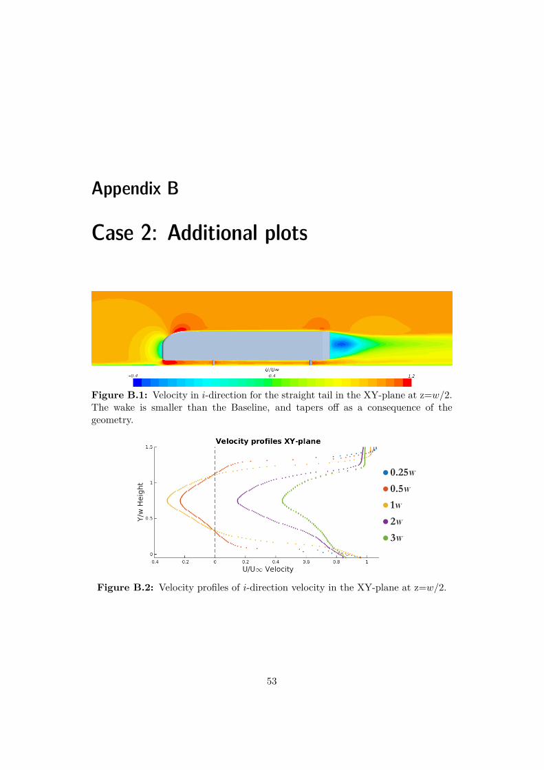
Figure B.1: Velocity in i-direction for the straight tail in the XY-plane at z=w/2.The wake is smaller than the Baseline, and tapers off as a consequence of thegeometry.

Figure B.2: Velocity profiles of i-direction velocity in the XY-plane at z=w/2.

53

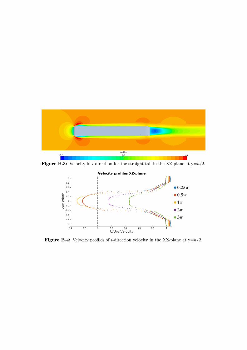
Figure B.3: Velocity in i-direction for the straight tail in the XZ-plane at y=h/2.

Figure B.4: Velocity profiles of i-direction velocity in the XZ-plane at y=h/2.

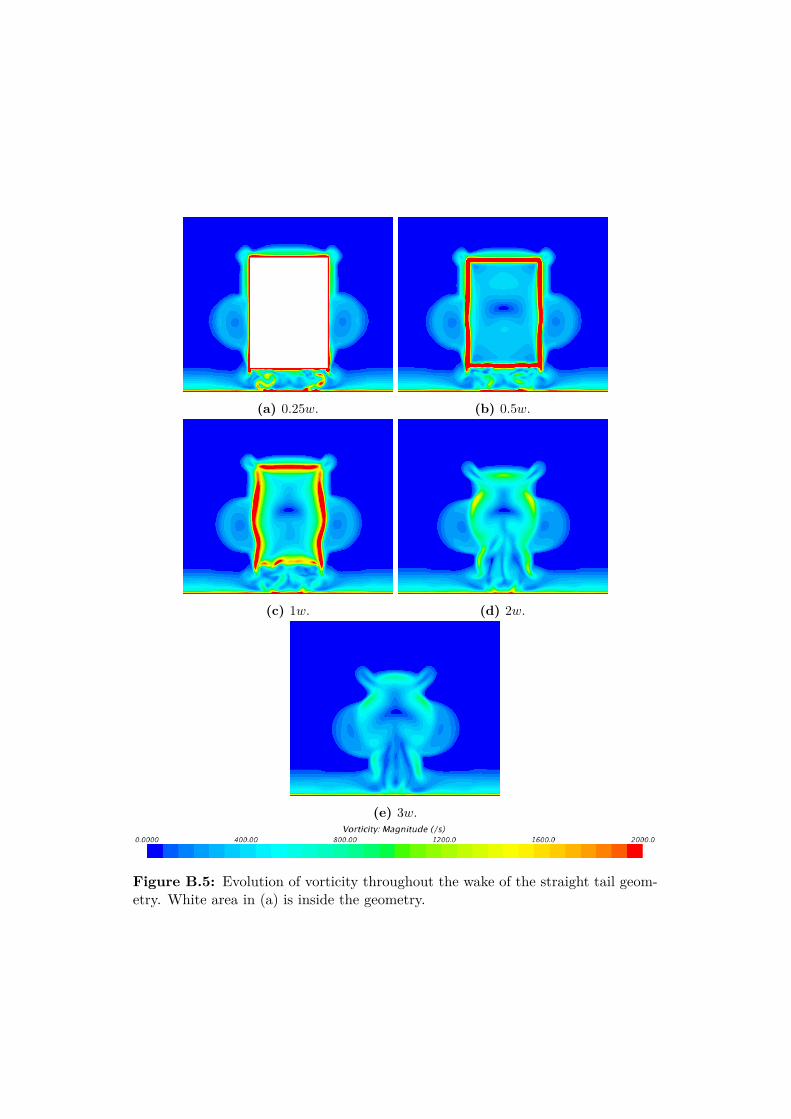
(a) 0.25w. (b) 0.5w.

(c) 1w. (d) 2w.

(e) 3w.

Figure B.5: Evolution of vorticity throughout the wake of the straight tail geom-etry. White area in (a) is inside the geometry.

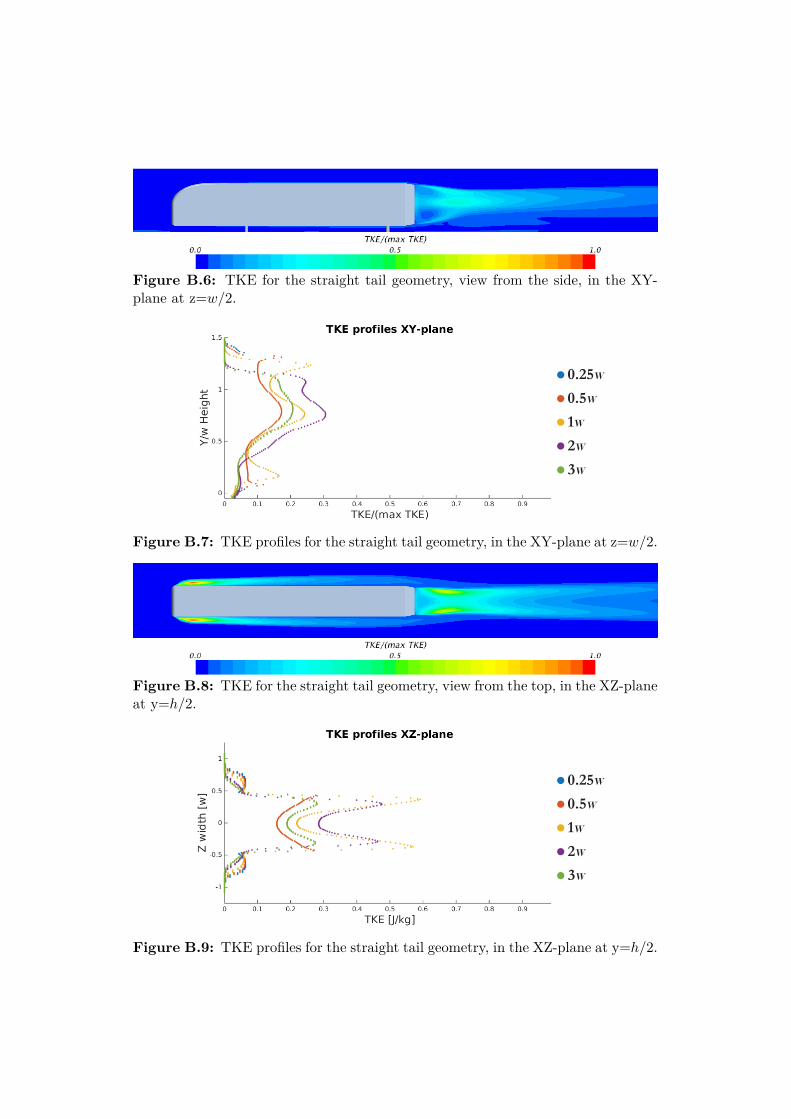
Figure B.6: TKE for the straight tail geometry, view from the side, in the XY-plane at z=w/2.

Figure B.7: TKE profiles for the straight tail geometry, in the XY-plane at z=w/2.

Figure B.8: TKE for the straight tail geometry, view from the top, in the XZ-planeat y=h/2.

Figure B.9: TKE profiles for the straight tail geometry, in the XZ-plane at y=h/2.

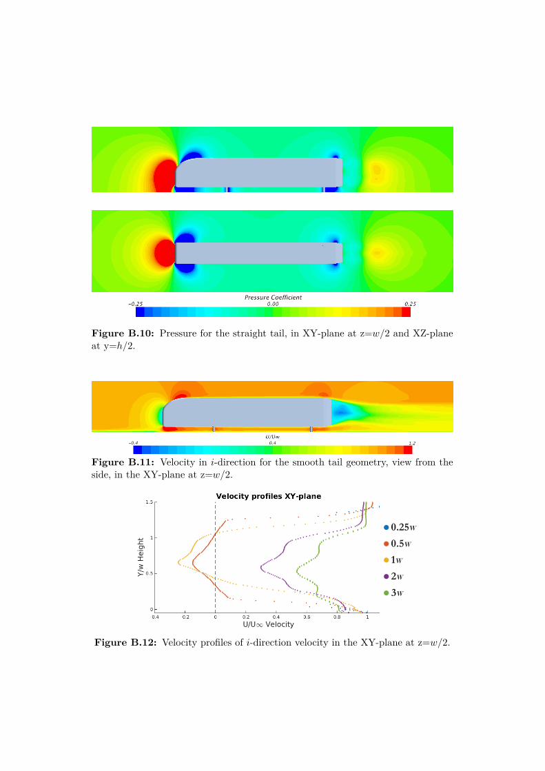
Figure B.10: Pressure for the straight tail, in XY-plane at z=w/2 and XZ-planeat y=h/2.

Figure B.11: Velocity in i-direction for the smooth tail geometry, view from theside, in the XY-plane at z=w/2.

Figure B.12: Velocity profiles of i-direction velocity in the XY-plane at z=w/2.

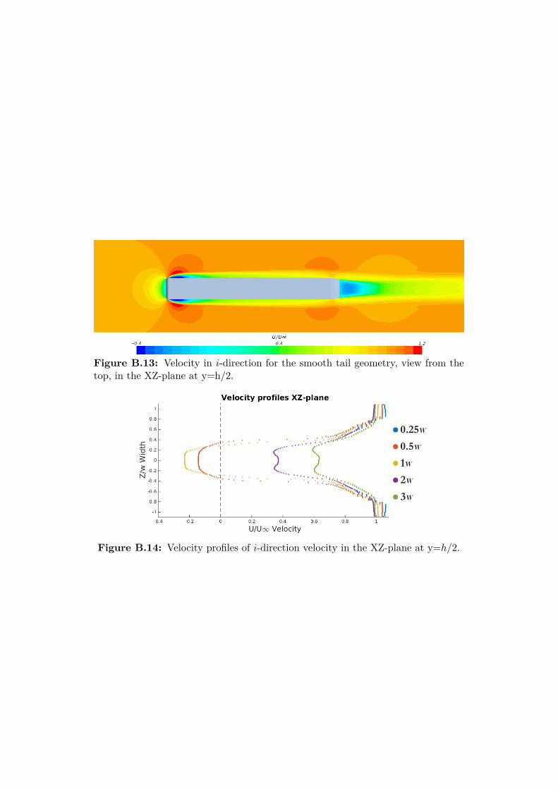
Figure B.13: Velocity in i-direction for the smooth tail geometry, view from thetop, in the XZ-plane at y=h/2.

Figure B.14: Velocity profiles of i-direction velocity in the XZ-plane at y=h/2.

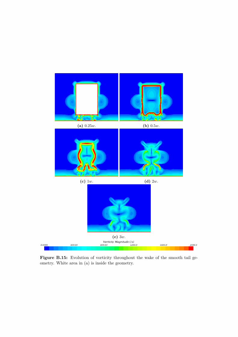
(a) 0.25w. (b) 0.5w.

(c) 1w. (d) 2w.

(e) 3w.

Figure B.15: Evolution of vorticity throughout the wake of the smooth tail ge-ometry. White area in (a) is inside the geometry.

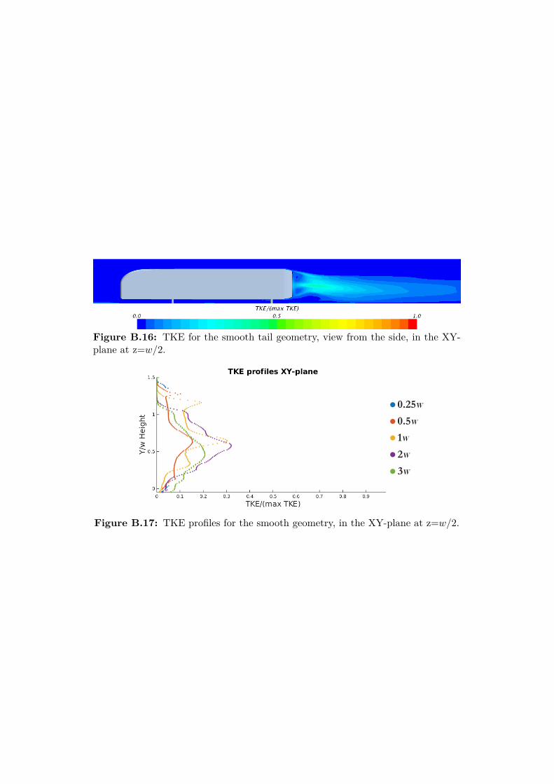
Figure B.16: TKE for the smooth tail geometry, view from the side, in the XY-plane at z=w/2.

Figure B.17: TKE profiles for the smooth geometry, in the XY-plane at z=w/2.

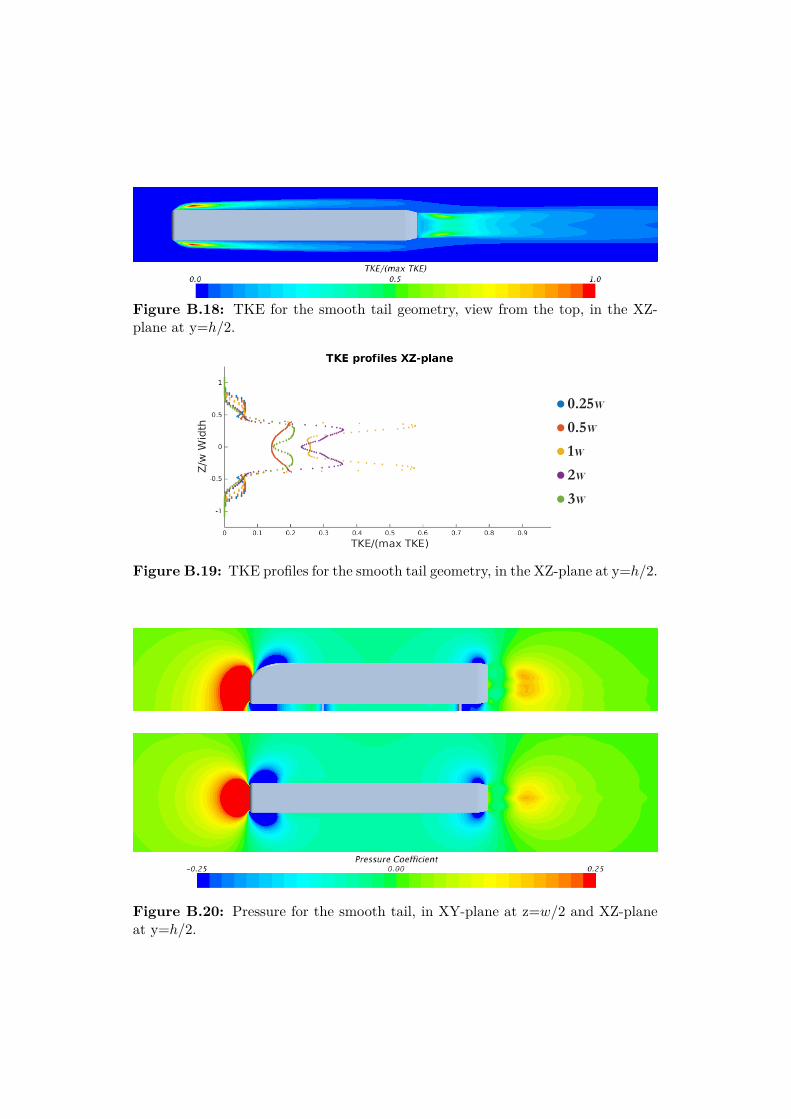
Figure B.18: TKE for the smooth tail geometry, view from the top, in the XZ-plane at y=h/2.

Figure B.19: TKE profiles for the smooth tail geometry, in the XZ-plane at y=h/2.

Figure B.20: Pressure for the smooth tail, in XY-plane at z=w/2 and XZ-planeat y=h/2.

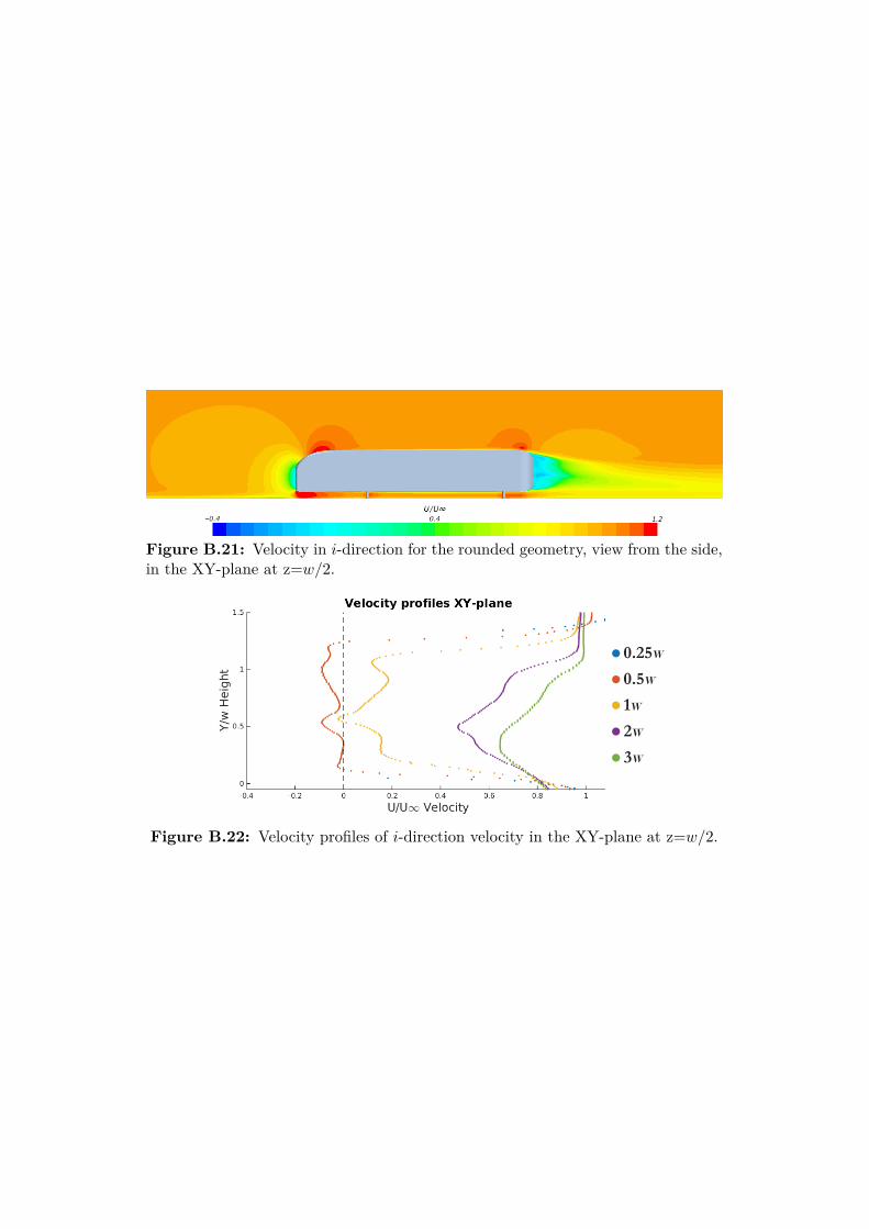
Figure B.21: Velocity in i-direction for the rounded geometry, view from the side,in the XY-plane at z=w/2.

Figure B.22: Velocity profiles of i-direction velocity in the XY-plane at z=w/2.

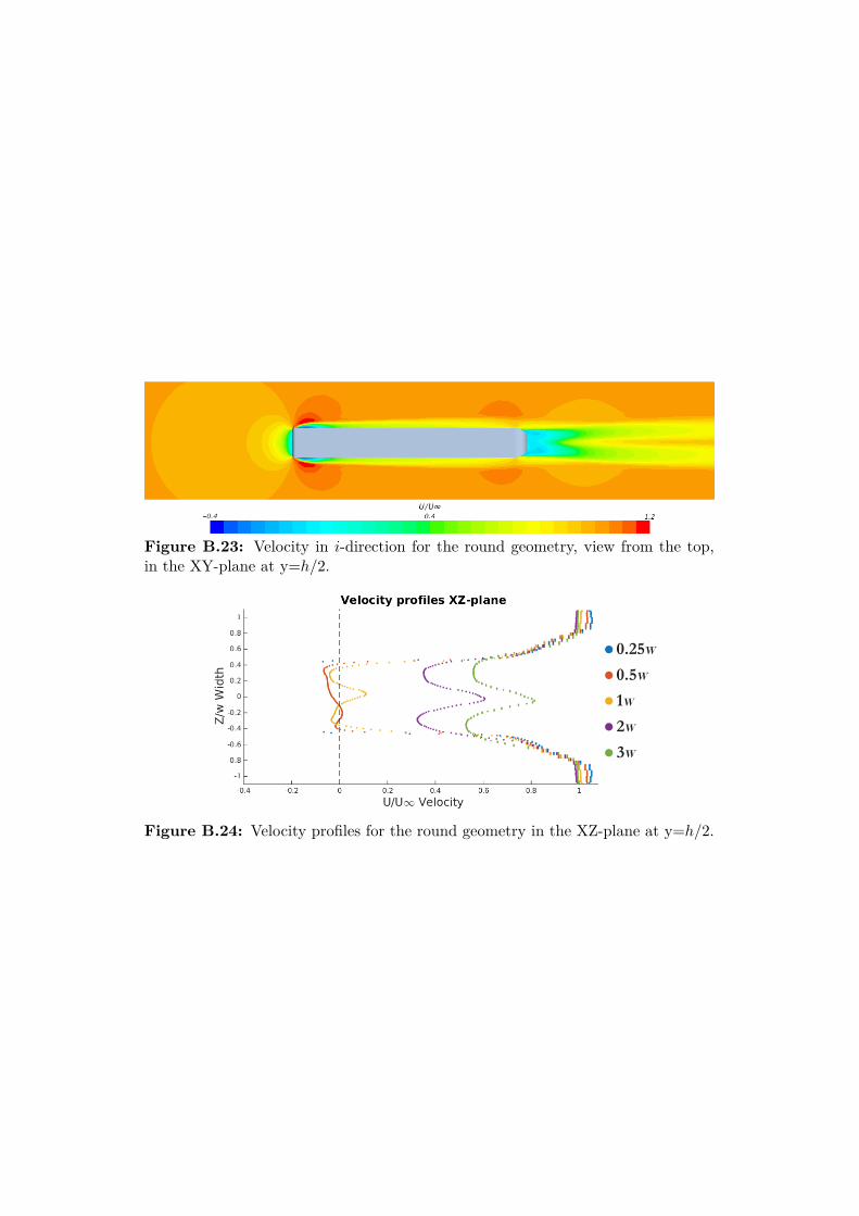
Figure B.23: Velocity in i-direction for the round geometry, view from the top,in the XY-plane at y=h/2.

Figure B.24: Velocity profiles for the round geometry in the XZ-plane at y=h/2.

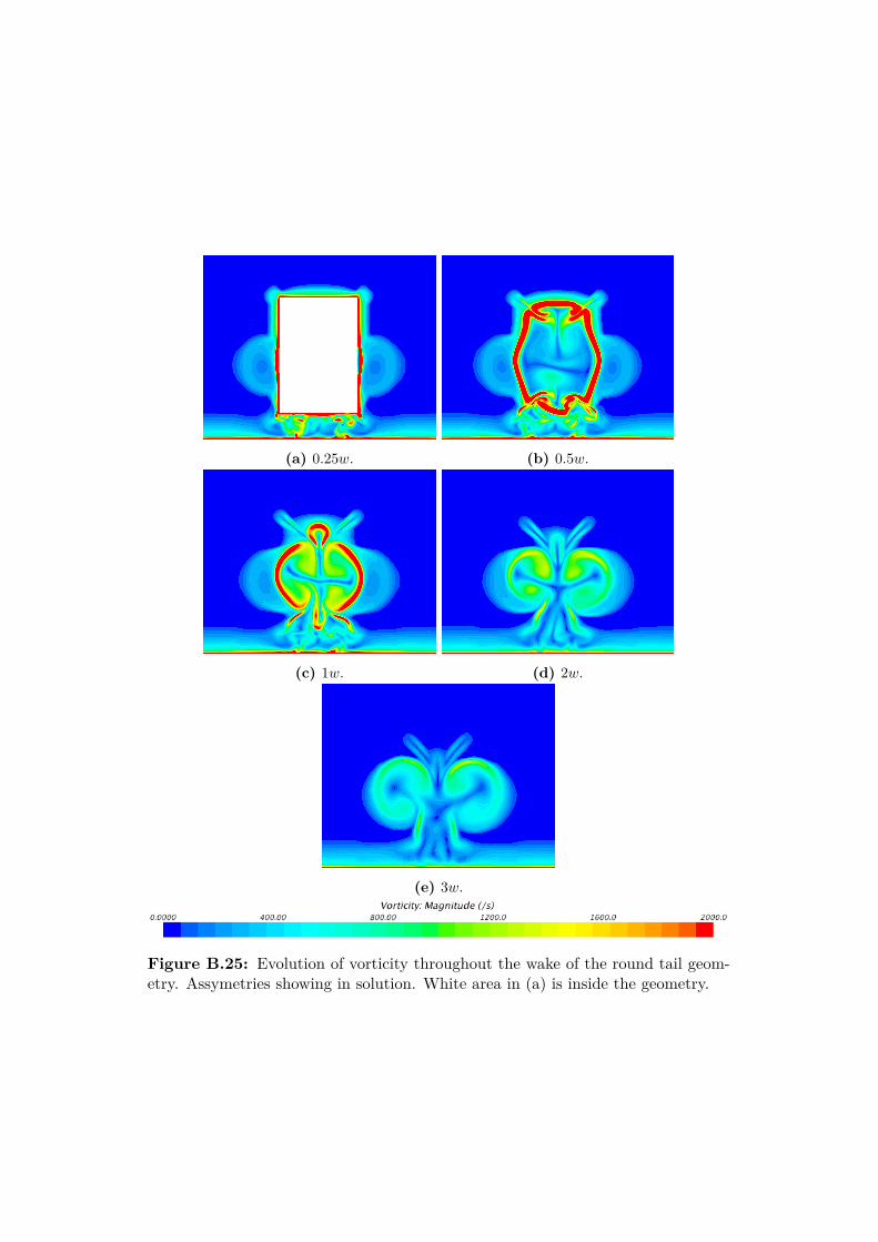
(a) 0.25w. (b) 0.5w.

(c) 1w. (d) 2w.

(e) 3w.

Figure B.25: Evolution of vorticity throughout the wake of the round tail geom-etry. Assymetries showing in solution. White area in (a) is inside the geometry.

Figure B.26: TKE for the round geometry, view from the top, in the XY-planeat z=w/2.

Figure B.27: TKE profiles for the round geometry, in the XY-plane at z=w/2.

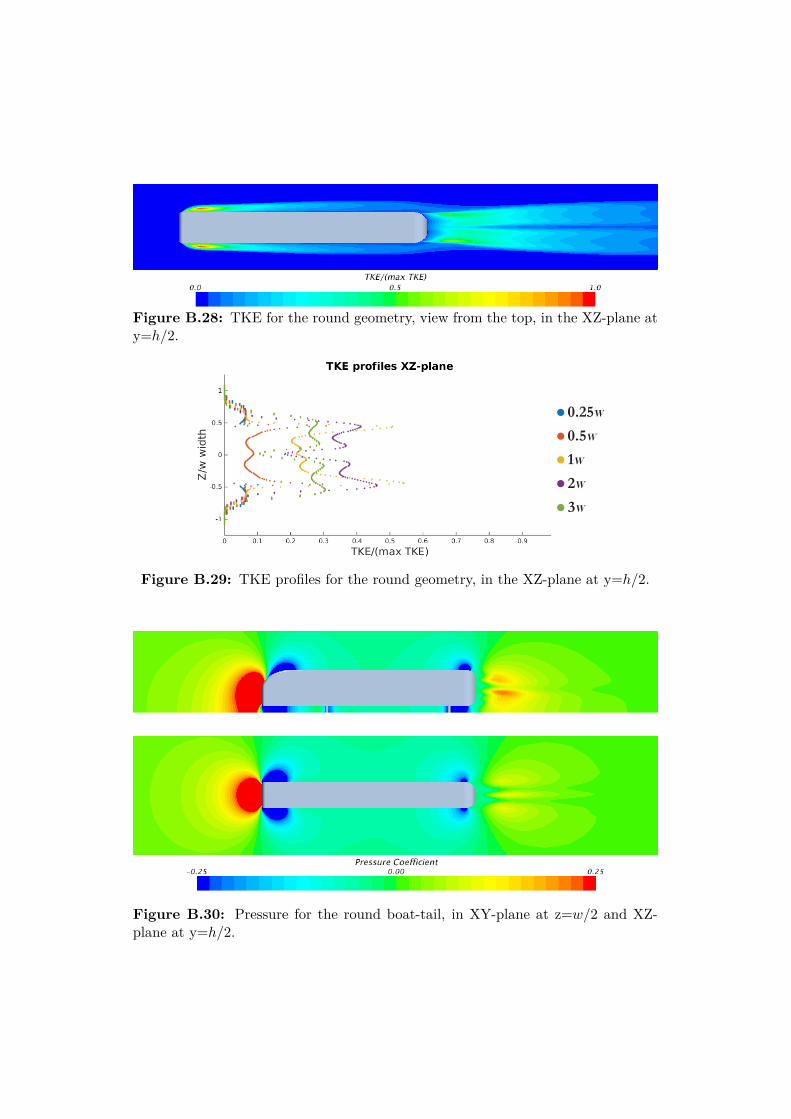
Figure B.28: TKE for the round geometry, view from the top, in the XZ-plane aty=h/2.

Figure B.29: TKE profiles for the round geometry, in the XZ-plane at y=h/2.

Figure B.30: Pressure for the round boat-tail, in XY-plane at z=w/2 and XZ-plane at y=h/2.

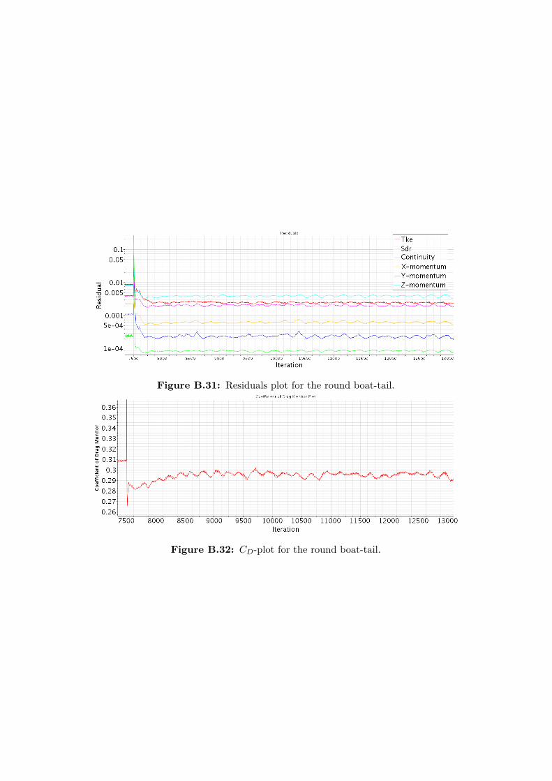
Figure B.31: Residuals plot for the round boat-tail.

Figure B.32: CD-plot for the round boat-tail.

Appendix C

Case 3: Additional plots

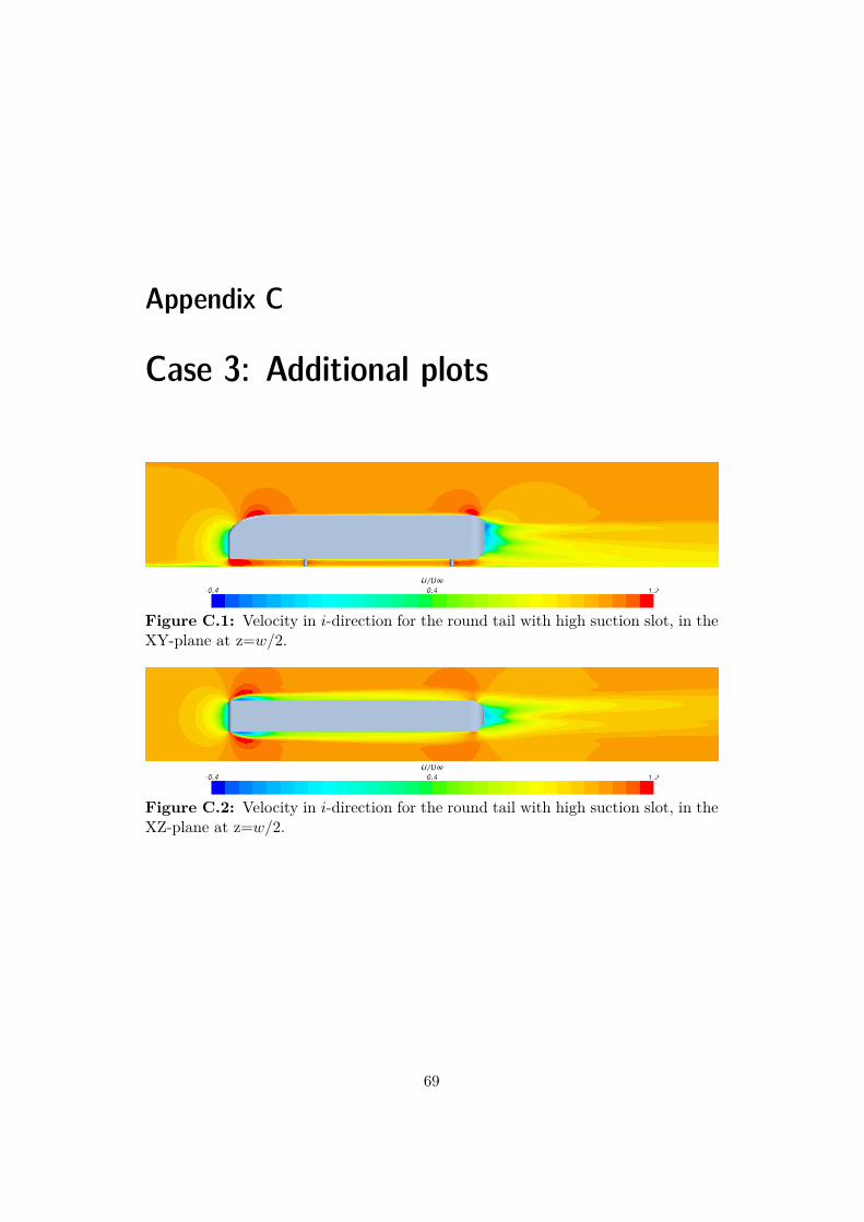
Figure C.1: Velocity in i-direction for the round tail with high suction slot, in theXY-plane at z=w/2.

Figure C.2: Velocity in i-direction for the round tail with high suction slot, in theXZ-plane at z=w/2.

69

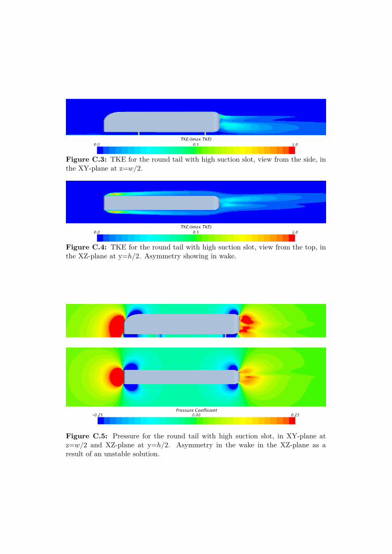
Figure C.3: TKE for the round tail with high suction slot, view from the side, inthe XY-plane at z=w/2.

Figure C.4: TKE for the round tail with high suction slot, view from the top, inthe XZ-plane at y=h/2. Asymmetry showing in wake.

Figure C.5: Pressure for the round tail with high suction slot, in XY-plane atz=w/2 and XZ-plane at y=h/2. Asymmetry in the wake in the XZ-plane as aresult of an unstable solution.

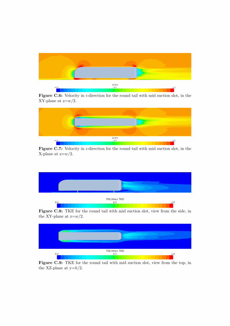
Figure C.6: Velocity in i-direction for the round tail with mid suction slot, in theXY-plane at z=w/2.

Figure C.7: Velocity in i-direction for the round tail with mid suction slot, in theX-plane at z=w/2.

Figure C.8: TKE for the round tail with mid suction slot, view from the side, inthe XY-plane at z=w/2.

Figure C.9: TKE for the round tail with mid suction slot, view from the top, inthe XZ-plane at y=h/2.

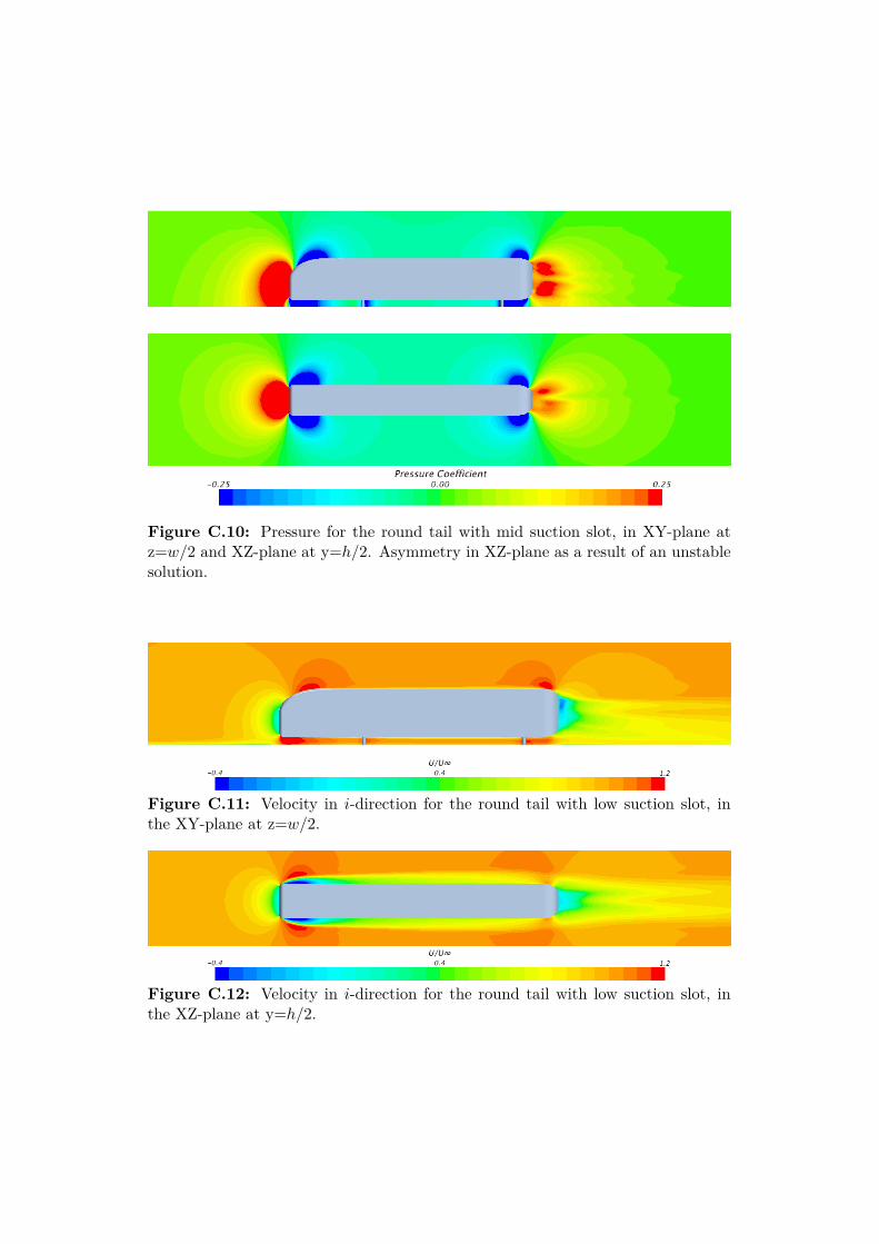
Figure C.10: Pressure for the round tail with mid suction slot, in XY-plane atz=w/2 and XZ-plane at y=h/2. Asymmetry in XZ-plane as a result of an unstablesolution.

Figure C.11: Velocity in i-direction for the round tail with low suction slot, inthe XY-plane at z=w/2.

Figure C.12: Velocity in i-direction for the round tail with low suction slot, inthe XZ-plane at y=h/2.

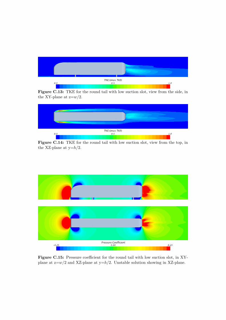
Figure C.13: TKE for the round tail with low suction slot, view from the side, inthe XY-plane at z=w/2.

Figure C.14: TKE for the round tail with low suction slot, view from the top, inthe XZ-plane at y=h/2.

Figure C.15: Pressure coefficient for the round tail with low suction slot, in XY-plane at z=w/2 and XZ-plane at y=h/2. Unstable solution showing in XZ-plane.

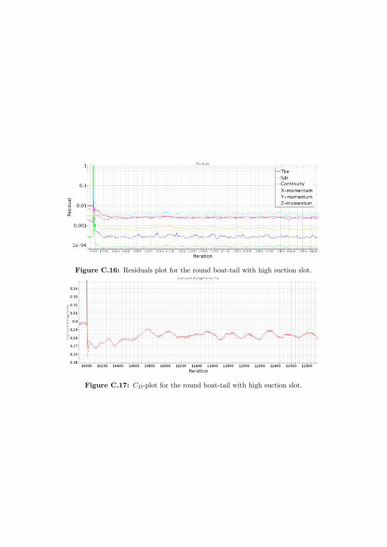
Figure C.16: Residuals plot for the round boat-tail with high suction slot.

Figure C.17: CD-plot for the round boat-tail with high suction slot.

Appendix D

GTS Geometries

Figure D.1: GTS geometry used in [3][7]. All measurements non-dimensionalizedby trailer width w. Struts are used in simulations, but not included in this figureor their results.

75

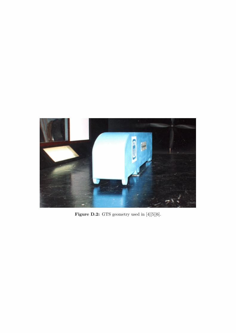
Figure D.2: GTS geometry used in [4][5][6].

Bibliography

[1] COM (2015) 169 def. COD 2013/0105, "Amendment to Council Directive96/53/EC laying down for certain road vehicles circulating within the Com-munity the maximum authorized dimensions in national and internationaltraffic and the maximum authorized weights in international traffic." 2015

[2] K. R. Cooper, "A Wind Tunnel Investigation into the Fuel Savings Availablefrom the Aerodynamic Drag Reduction of Trucks". 1976

[3] Storms et al., "An Experimental Study of the Ground Transportation System(GTS) Model in the NASA Ames 7- by 10-Ft Wind Tunnel". NASA/TM-2001-209621. 2001

[4] W. T. Gutierrez et al., "Aerodynamics Overview of the Ground TransportationSystems (GTS) Project for Heavy Vehicle Drag Reduction". 1996

[5] K. Salari, M. McWherter-Payne, "Computational Flow Modeling of a Simpli-fied Integrated Tractor-Trailer Geometry". 2003

[6] C. J. Roy, J. Payne & M. McWherter-Payne, "RANS Simulations of a Sim-plified Tractor/Trailer Geometry". J. Fluids Eng. 128(5), p. 1083-1089. 2006

[7] Sunil V. Unaune, Sandeep D. Sovani & Sung Eun Kim, "Aerodynamics ofa Generic Ground Transportation System: Detached Eddy Simulation". SAE2005-01-0548. 2005

[8] "Council Directive 96/53/EC of 25 July 1996 laying down for certain road ve-hicles circulating within the Community the maximum authorized dimensionsin national and international traffic and the maximum authorized weights ininternational traffic". 1996

[9] "Annual European Community greenhouse gas inventory 1990-2005 and in-ventory report 2007 ". European Environment Agency. 2007

[10] A. Wiley Sherwood, "Wind Tunnel test of Trailmobile Trailers, 3rd Series".University of Maryland Wind Tunnel Report No. 85. College Park, Maryland,USA. 1974

77

[11] See for example the Indianapolis 500 winners 1915 vs. 1916, the 1924 DjelmoLand Speed Record Car or Louis Coatalen’s 1927 1000 bhp Sunbeam.

[12] See for example the Chaparral 2B or 2E.

[13] US 94th Congress, "S.622 - Energy Policy and Conservation Act". 1975

[14] K. R. Cooper "The Wind Tunnel Testing of Heavy Trucks to Reduce FuelConsumption". SAE 821285. 1982

[15] R. McCallen, F. Browand, J. Ross "The Aerodynamics of Heavy Vehicles:Trucks, Buses, and Trains". 2004

[16] R. McCallen, F. Browand, J. Ross "The Aerodynamics of Heavy Vehicles II:Trucks, Buses, and Trains". 2009

[17] "Council Directive 70/220/EEC of 20 March 1970 on the approximation ofthe laws of the Member States relating to measures to be taken against airpollution by gases from positive-ignition engines of motor vehicles ". 1970

[18] "Commission Regulation (EU) No 1230/2012 of 12 December 2012 imple-menting Regulation (EC) No 661/2009 of the European Parliament and ofthe Council with regard to type-approval requirements for masses and dimen-sions of motor vehicles and their trailers and amending Directive 2007/46/ECof the European Parliament and of the Council ". 2012

[19] COM (2014) 222 def. "Report from the Commission to the European Parlia-ment and the Council on the State of the Union Road Transport Market".2014

[20] R. Hogg, "Life Beyond Euro 7" (http://www.automotiveworld.com/megatrends-articles/life-beyond-euro-vi/). 2014

[21] Cummins "The World After Euro 6". (http://www.cumminseuro6.com/euro-6-blog)

[22] Trucking.org, "Trucking Industry Fact Sheet", 2014

[23] J. Zaya, "Effektivare transportkedjor för näringslivet - Förstudie Aerody-namik", 2014

[24] Eurostat, "Number of lorries, road tractors, trailers and semi-trailers in theEU 2012", (Eurostat, online data code: road_eqs_lrstn) 2012

[25] R. M. Wood, S. X. S. Bauer, "Simple and Low-Cost Aerodynamic Drag Re-duction Devices for Tractor-Trailer Trucks", SAE 2003-01-3377. 2003

[26] EEA "Annual European Union greenhouse gas inventory 1990-2012 and in-ventory report 2014", 2014

[27] OECD Glossary (https://stats.oecd.org/glossary/detail.asp?ID=285)

[28] Lewis F. Richardson, "Weather Prediction by Numerical Process". 1922

[29] Kenworth Trucking/Seattle PI http://www.seattlepi.com/business/article/Rounded-add-on-makes-driving-truck-less-of-a-drag-1104980.php. 2003

[30] T. Chung, "Computational Fluid Dynamics". 2002

[31] P. K. Kundu, I. M. Cohen, "Fluid Mechanics. Third Edition". 2004

[32] K. Salari, M. Ortega, P.J. Castellucci, "Computational Prediction of Aerody-namic Forces for a Simplified Integrated Tractor - Trailer Geometry", AIAA2004-2253. 2004

[33] A.V. Johansson, S. Wallin "Turbulence Lecture Notes", 2012

[34] CD-adapco, "STAR-CCM+ User Guide v9.06".

[35] F. R. Menter, "Two-Equation Eddy-Viscosity Turbulence Models for Engineer-ing Applications". AIAA Paper 93-2906, 1993

[36] G. Kalitzin et al., "Near-wall behavior of RANS turbulence models and impli-cations for wall functions". Journal of Computational Physics 204, p. 265-291.2005

[37] D. Norrby, "A CFD study Of The Aerodynamic Effects Of PlattooningTrucks", diploma work, KTH, 2014

[38] A. N. Kolmogorov, "Dissipation of energy in the locally isotropicturbulence". (Available online through The Royal Society athttp://www.jstor.org/stable/51981), 1941

[39] NPARC Computational Fluid Dynamics (CFD) Verifica-tion and Validation, "Examining Spatial (Grid) Convergence",(http://www.grc.nasa.gov/WWW/wind/valid/tutorial/spatconv.html)

[40] Antony Jameson, "Computational Fluid Dynam-ics: Past, Present and Future". (Available online at:http://aerocomlab.stanford.edu/Papers/NASA_Presentation_20121030.pdf),2012

[41] P. M. van Leeuwen "Computational Analysis of Base Drag Reduction UsingActive Flow Control". Master thesis, University of Delft, 2009.

[42] M. Mihaescu (Personal communication per e-mail, non-official report on suc-tion slots), 2015-04-30

[43] Why I hate Physics blog: "How a Vacuum Cleaner REALLY Works".(http://marty-green.blogspot.ca/2013/09/how-vacuum-cleaner-really-works.html), 2013

[44] M. El-Alti, V. Chernoray, M. Jahanmiri, L. Davidson "Experimental and Com-putational Studied of Active Flow Control on a Model Truck-Trailer". 2012

[45] CFD Online http://www.cfd-online.com