eScholarship provides open access, scholarly publishingservices to the University of California and delivers a dynamicresearch platform to scholars worldwide.

California Partners for Advanced Transitand Highways (PATH)

UC Berkeley

Title:The Aerodynamic Performance Of Platoons: A Final Report

Author:Zabat, MichaelStabile, NickFarascaroli, StefanoBrowand, Frederick

Publication Date:01-01-1995

Series:Research Reports

Publication Info:California Partners for Advanced Transit and Highways (PATH)

Permalink:http://www.escholarship.org/uc/item/8ph187fw

Keywords:Automobiles--Automatic control, Motor vehicles--Aerodynamics

Abstract:This report details the aerodynamic performance of individual members of 2, 3, and 4-vehicleplatoons. The primary purpose of the tests described is to quantify the behavior of vehicle dragas a function of vehicle spacing.

Copyright Information:All rights reserved unless otherwise indicated. Contact the author or original publisher for anynecessary permissions. eScholarship is not the copyright owner for deposited works. Learn moreat http://www.escholarship.org/help_copyright.html#reuse

ISSN 1055-1425

October 1995

This work was performed as part of the California PATH Program of theUniversity of California, in cooperation with the State of California Business,Transportation, and Housing Agency, Department of Transportation; and theUnited States Department of Transportation, Federal Highway Administration.

The contents of this report reflect the views of the authors who are responsiblefor the facts and the accuracy of the data presented herein. The contents do notnecessarily reflect the official views or policies of the State of California. Thisreport does not constitute a standard, specification, or regulation.

CALIFORNIA PATH PROGRAMINSTITUTE OF TRANSPORTATION STUDIESUNIVERSITY OF CALIFORNIA, BERKELEY

The Aerodynamic Performance ofPlatoons: Final Report

UCB-ITS-PRR-95-35California PATH Research Report

Michael ZabatNick StabileStefano FrascaroliFrederick Browand

The Aerodynamic Performance of PlatoonsA Final Report

Presented to the California Department of TransportationPartners for Advanced Transit and Highways (PATH) Program

by,Michael ZabatNick Stabile

Stefano Frascaroliand

Frederick Browand

18 May 1995CD-ROM edition, 10 October 1995

The Aerodynamic Performance of PlatoonsA Final Report

Presented to the California Department of Transportation

Partners for Advanced Transit and Highways(PATH) Program

by

Michael Zabat

Nick Stabile

Stefano Frascaroli

Frederick Browand

Department of Aerospace Engineering

University of Southern California

Los Angeles, California 90089-1191

9 October, 1995

ABSTRACT

This report details the aerodynamic performance of individual members of 2, 3 and 4-vehicle platoons. Theprimary purpose of the tests described here is to quantify the behavior of vehicle drag as a function ofvehicle spacing. One-eighth scale models of the 1991 GM Lumina APV are used as the prototype vehicle.Each model is fitted with a force balance capable of measuring drag, side force and yawing moment. Aporous ground plane equipped with suction is used to simulate the road surface. Results show a reductionin average drag for all platoon members as a function of both inter-vehicle spacing and the number ofvehicles in the platoon. The average drag coefficient for a platoon of four vehicles is measured to be about55% of the drag coefficient in isolation at spacings in the range 0.1-0.3. Extrapolating the experimentalresults to platoons of greater length suggests even lower average drag coefficients are possible. These lowaverage drag coefficients for platoon operation translate directly to increased fuel savings and to lesspollution per mile traveled.

Keywords: Platoon, Drag, Close-following

1

I. OVERVIEW

A. Establishing Confidence in Wind Tunnel Test Results

When bodies under aerodynamic study are modeled in a wind tunnel test, all possible care must be taken to

establish conditions consistent with full-scale operation. In principle, the model test should reflect perfect

dynamic similarity as well as perfect geometric similarity. Such perfection is never realized in practice.

Even if the model tested is a full-scale vehicle, complete in every detail, the presence of the wind tunnel

walls destroys perfect geometric similarity. In most wind tunnel tests, dynamic and geometric similarity are

only approximately established for a variety of reasons. Wind tunnel tests still give valuable information

about aerodynamic performance, provided the limitations of the test are kept in mind.

Dynamic similarity first requires the definition of force coefficients for the body. Since we are

primarily interested in drag force, a drag coefficient is defined,

CD

U AD =

12

2ρ(1)

where D = measured drag

ρ = air density

U = vehicle forward speed, wind tunnel speed

A = Maximum cross-sectional area of the body perpendicular to the flow

Couching discussion in terms of drag coefficient rather than in terms of drag automatically accounts

for differences in vehicle size and vehicle relative velocity. It allows one to make predictions for the

performance of the full-scale vehicle from wind tunnel model measurements. In addition, perfect dynamic

similarity requires that the Reynolds number of the model flow be made to match the Reynolds number in

the full scale operation.

Re= Ud

ν(2)

where d = characteristic length scale

ν = kinematic viscosity of air

The magnitude of the Reynolds number expresses the ratio of fluid inertia force to fluid viscous effect,

or shear stress. When the Reynolds number is large, the fluid moves in response to differences in pressure

2

within the flow field. Only in very thin boundary layer regions adjacent to surfaces are viscous shearing

stresses important. The characteristic length scale of our vehicle model is 1/8th that of the full-scale

vehicle. Since the test is conducted with air as the fluid, the viscosity ν is the same for both cases. To keep

Re constant, the freestream velocity in the test case must be 8 times higher than the full-scale vehicle

velocity. This, of course, is not possiblemodel Reynolds numbers are lower than Reynolds numbers for

full-scale operation. An automobile traveling at highway speed may correspond to Re = O(106-107), while

our wind tunnel tests are conducted at Reynolds numbers about one order of magnitude lower. To account

for these differences, and to judge the sensitivity of the force measurements to changes in Reynolds number,

we will frequently present measurements at several Reynolds numbers. Another simulation technique is to

utilize a series of small roughness elements to artificially "trip" the boundary layer on the model. Tripping

insures a turbulent boundary layer more nearly in character with a boundary layer at higher Reynolds

number.

The model and full-scale vehicle are geometrically similar in the sense that all body dimensions have

been scaled by the same ratio. The mold used to cast the models is fashioned by a stereo-lithographic

process using computer-generated coordinates. For all practical purposes, the model is an exact replica.

However, all minor external features such as window frames, side mirrors, door handles, windshield

wipers, etc., have been removed. Also, the details of the undercarriage have been left out, and the wheels

are stationary.

B. The Unwanted Presence of the Ground Plane Boundary Layer

In the case of ground vehicles, an additional effect is introduced by the presence of the road surface. If one

uses a flat plate to model the road surface in a wind-tunnel, a layer of slow moving fluid (the ground plane

boundary layer) grows continuously in the downstream direction. This layer does not exist on the actual

road surface since it is the vehicle that is in motion and not the medium (air). It is necessary then to

minimize the thickness of the ground plane boundary layer, δ, in wind-tunnel tests. The growth of a

turbulent boundary layer on a flat plate can be approximated by

δ = 0370 2

..

x

xRe(3)

where x is the distance from the leading edge. Based upon the above expression, the thickness of the

boundary layer at 4 model lengths (1.22m) from the start of the ground plane at 25m/s would be about 2.46

cm. Four model lengths would correspond to a case where 2 models are in the tunnel at 1 length spacing,

3

the first model being placed 1 length from the leading edge. Further down the plate, say at x=5 m, δ would

be about 7.71 cm.

Hucho and Sovran (1993) suggest that for a passenger car model affixed to a ground plane, the

displacement thickness, δ*, should be less than 10% of the model ground clearance, H, (in our case H is

about 37 mm). The displacement thickness can be thought of as the amount by which an outer flow

streamline is displaced due to the presence of the boundary layer. For turbulent boundary layers, δ* is

approximately (1/8)δ. The range of δ*/H for our tests would generally be greater than the accepted value

of 0.10, unless some means for controlling boundary layer growth is adopted.

Control of boundary layer thickness can be achieved by several methods. Conceptually, the simplest

way to eliminate the unwanted boundary layer is to move the ground plane at the wind tunnel speed, U.

Unfortunately, this scheme is mechanically complex and impractical for the long ground plane length

required to test a platoon of vehicles. Our choice is to siphon off the boundary layer through a uniformly

porous ground plane surface. This is a much simpler method to implement. Other possibilities, such as

tangential blowing or single slot suction, are not viable because their effectiveness would not extend over

the entire length of the ground plane.

C. Organization of the Manuscript

This report, and the earlier PATH report Zabat et al. (1994), are repositories for all the experimental data

we presently have available. In our concern for completeness, we have sacrificed some of the natural flow

of a well-balanced, shorter manuscript. What we believe to be the most important portions of this work to

date have been summarized in three published papers Zabat et al. (1994b), Zabat et al. (1995), and Zabat

et al. (1995b). These papers, although they contain the data which is included in Zabat et al. (1994), as

well as in this report, should be considered an important part of the written record for this project. Copies

of these papers will be on file with CALTRANS and with PATH, or they can be obtained directly from

conventional SAE and ITS sources.

This report serves as the final report for the three-year project. It is more complete than the earlier

PATH report in that it contains a considerable addition to the experimental results. For the sake of a single

source for all the drag data, we have included in the appendix of this report, the results contained in the

appendix B of Zabat et al. (1994). Please note however, that much of the discussion has not been repeated,

4

so this earlier report remains an important source of information—particularly with regard to wind-tunnel

flow uniformity and the design and testing of the force balances and ground plane.

The various sections of this report are arranged as follows. Section II contains a discussion of the

improvements made to the force balance, and the general procedure followed when taking measurements.

Section III presents the results for all the single vehicle measurements made and discusses the effectiveness

of the blockage correction used, the effects of the ground plane surface, Reynolds number and boundary

layer trips on the model. Section IV contains the drag measurements on 2, 3 & 4 vehicle platoons. The

data from the 2, 3, and 4-vehicle platoon cases are used to predict the drag performance of an n-vehicle

platoon through extrapolation. Section V presents the drag measurements for a 2-vehicle platoon with

variations in geometry and ground plane surface condition. The results of the various geometries are used

to define an average CD ratio that takes account of geometry. In section VI, the fuel-savings benefits that

precipitate from the drag reduction are examined. Section VII presents model surface flow visualizations

and measurements of the floor pressure distributions which will ultimately help explain the drag behavior

as a function of spacing. In section VIII , results from tests on misaligned platoons are presented and the

effects of misalignment on platoon operation are discussed. Section IX outlines future studies that will

further the understanding of platoon aerodynamics. The raw data discussed in sections III, IV, V, VII and

VIII are tabulated in the appendices. All the data−including the surface streamline photographs−are stored

in digital format and can be retrieved and transmitted upon request to PATH.

5

II. EXPERIMENTAL METHOD

Tests are conducted at the USC Dryden Wind Tunnel. This facility has a test section that is hexagonal

in cross-section, 1.37 m wide and 7.4 m long. Ground simulation is accomplished using a porous plate and

suction system to control the boundary layer growth on the ground plane. The majority of the tests are run

at a nominal velocity of 23 m/s. Further details of the wind tunnel and ground plane are provided in Zabat

et al. (1994) and Zabat et al. (1994b).

A. Improving Force Balance Performance

The internally mounted, 3-component force sensors used previously have been designed for nominal loads

of 9.8N with an accuracy estimated at ±0.035N0.35% of the full scale load, and well above the analog-

to-digital converter least count resolution of ±0.006N. This kind of sensitivity requires that the flexures be

very thin (0.6mm). Several significant modes of oscillation have been observed for the sensor alone,

particularly at 45 and 80 Hz. When models are attached to the sensors, the additional weight reduces the

lowest resonant frequency to about 20 Hz.

For a bluff body, the major unsteady loads will probably be due to vortex shedding in the wake. The

frequency of this shedding can be approximated by

fd

U≅ 02. (4)

where f = the shedding frequencyd = the effective diameter (A, the cross- sectional area)

U = the wind speed

Equation (4) results in a shedding frequency of about 19 Hz for a nominal velocity of 23 m/s. This

value is very close to the natural frequency exhibited by the force sensor. The original balance had very

little natural damping which prevented measurements at close spacingswhere significant unsteady

fluctuations are present. It was previously documented that the mean values of force measured by the

sensor were not affected by the fluctuations experienced by the model at spacings greater than 0.5 vehicle

lengths. At smaller spacings, the oscillations became much larger in amplitude, presumably because of

larger pressure fluctuations in the region between the models. Since we felt the mean measurements might

be unreliable in the presence of significant oscillations, no measurements at close spacing were presented

earlier.

6

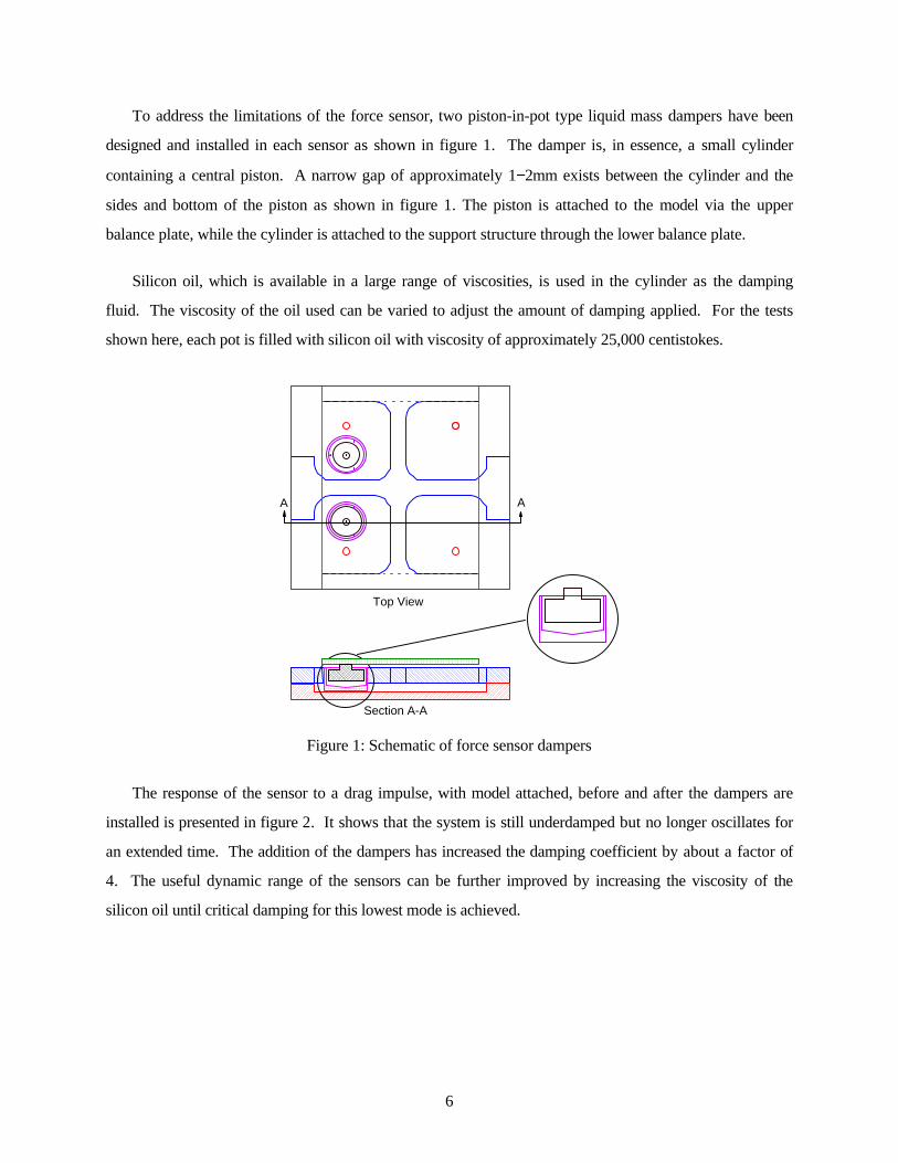
To address the limitations of the force sensor, two piston-in-pot type liquid mass dampers have been

designed and installed in each sensor as shown in figure 1. The damper is, in essence, a small cylinder

containing a central piston. A narrow gap of approximately 1−2mm exists between the cylinder and the

sides and bottom of the piston as shown in figure 1. The piston is attached to the model via the upper

balance plate, while the cylinder is attached to the support structure through the lower balance plate.

Silicon oil, which is available in a large range of viscosities, is used in the cylinder as the damping

fluid. The viscosity of the oil used can be varied to adjust the amount of damping applied. For the tests

shown here, each pot is filled with silicon oil with viscosity of approximately 25,000 centistokes.

A A

Top View

Section A-A

Figure 1: Schematic of force sensor dampers

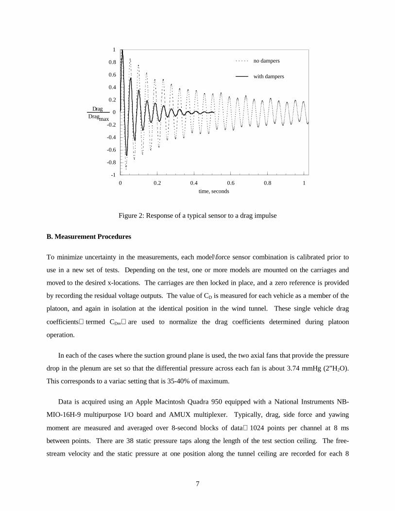
The response of the sensor to a drag impulse, with model attached, before and after the dampers are

installed is presented in figure 2. It shows that the system is still underdamped but no longer oscillates for

an extended time. The addition of the dampers has increased the damping coefficient by about a factor of

4. The useful dynamic range of the sensors can be further improved by increasing the viscosity of the

silicon oil until critical damping for this lowest mode is achieved.

7

-1

-0.8

-0.6

-0.4

-0.2

0

0.2

0.4

0.6

0.8

1

0 0.2 0.4 0.6 0.8 1

Dragmax

time, seconds

no dampers

with dampers

Drag

Figure 2: Response of a typical sensor to a drag impulse

B. Measurement Procedures

To minimize uncertainty in the measurements, each model\force sensor combination is calibrated prior to

use in a new set of tests. Depending on the test, one or more models are mounted on the carriages and

moved to the desired x-locations. The carriages are then locked in place, and a zero reference is provided

by recording the residual voltage outputs. The value of CD is measured for each vehicle as a member of the

platoon, and again in isolation at the identical position in the wind tunnel. These single vehicle drag

coefficientstermed CD∞are used to normalize the drag coefficients determined during platoon

operation.

In each of the cases where the suction ground plane is used, the two axial fans that provide the pressure

drop in the plenum are set so that the differential pressure across each fan is about 3.74 mmHg (2”H2O).

This corresponds to a variac setting that is 35-40% of maximum.

Data is acquired using an Apple Macintosh Quadra 950 equipped with a National Instruments NB-

MIO-16H-9 multipurpose I/O board and AMUX multiplexer. Typically, drag, side force and yawing

moment are measured and averaged over 8-second blocks of data1024 points per channel at 8 ms

between points. There are 38 static pressure taps along the length of the test section ceiling. The free-

stream velocity and the static pressure at one position along the tunnel ceiling are recorded for each 8

8

second data block. A Scanivalve is commanded to step between static taps, and the entire procedure is

repeated until all 38 taps have been sampled. Each run then consists of a measurement of the static

pressure distribution along the test section and a set of 38 force measurementsdrag, side force, yawing

momentfor each of the vehicles in the tunnel. The 38 force values are eventually averaged to produce a

single measurement point. The entire procedure is computer-controlled using LabVIEW. Updated real

time results (at 8 second intervals) are displayed on the computer screen, and are stored in permanent files.

After each run of approximately 7-8 minutes, the vehicles are repositioned and data recording continues

until all spacings are explored.

9

III. SINGLE VEHICLE DRAG MEASUREMENTS

A. Measurement Accuracy Estimates

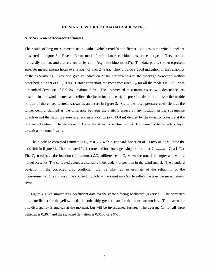
The results of drag measurements on individual vehicle models at different locations in the wind tunnel are

presented in figure 3. Five different model-force balance combinations are employed. They are all

outwardly similar, and are referred to by color (e.g. “the blue model”). The data points shown represent

separate measurements taken over a span of over 2 years. They provide a good indication of the reliability

of the experiments. They also give an indication of the effectiveness of the blockage correction method

described in Zabat et al. (1994). Before correction, the mean measured CD for all the models is 0.361 with

a standard deviation of 0.0126 or about 3.5%. The uncorrected measurements show a dependence on

position in the wind tunnel, and reflect the behavior of the static pressure distribution over the usable

portion of the empty tunnelshown as an insert in figure 3. CP is the local pressure coefficient at the

tunnel ceiling, defined as the difference between the static pressure at any location in the streamwise

direction and the static pressure at a reference location (x=0.864 m) divided by the dynamic pressure at the

reference location. The decrease in CP in the streamwise direction is due primarily to boundary layer

growth at the tunnel walls.

The blockage-corrected estimate is CD = 0.332 with a standard deviation of 0.0085 or 2.6% (note the

axis shift in figure 3). The measured CD is corrected for blockage using the formula, CDcorrected = CD/(1-CP).

The CP used is at the location of maximum ∆CP (difference in CP when the tunnel is empty and with a

model present). The corrected values are sensibly independent of position in the wind tunnel. The standard

deviation in the corrected drag coefficient will be taken as an estimate of the reliability of the

measurements. It is shown in the succeeding plots as the reliability bar to reflect the possible measurement

error.

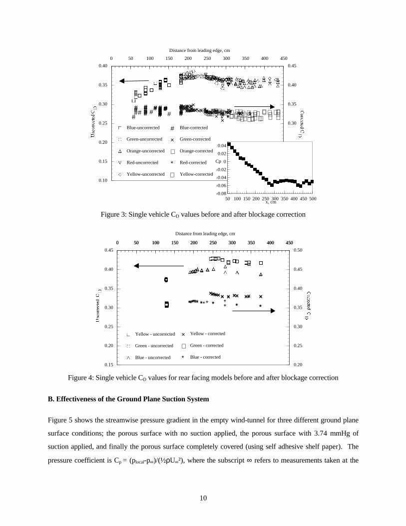
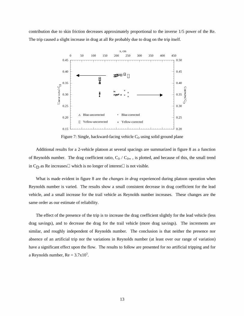
Figure 4 gives similar drag coefficient data for the vehicle facing backward (reversed). The corrected

drag coefficient for the yellow model is noticeably greater than for the other two models. The reason for

this discrepancy is unclear at the moment, but will be investigated further. The average CD for all three

vehicles is 0.367, and the standard deviation is 0.0108 or 2.9% .

10

#### ###

##### ######################## ############

###############

## # # #

× ×× ×××××××××××××××××××××××

××××××××××××××××××××××××××××××

××××

×××××××× ××× ×× × × × ++++++++++++

+++ +++++++++++

+++++++

++ ++++

++ ++++

∗∗∗∗∗∗∗∗∗ ∗∗∗∗∗∗∗∗∗∗∗∗∗∗∗∗∗ ∗∗ ∗∗ ∗∗∗

∈∈∈∈∈ ∈ ∈ ∈

0.15

0.20

0.25

0.30

0.35

0.40

0.45

0 50 100 150 200 250 300 350 400 450

Distance from leading edge, cm

# Blue-corrected

× Green-corrected

+ Orange-corrected

∗ Red-corrected

∈ Yellow-corrected

G

GGG GGG

GGGGG

GGGGGGGGGGGGGGGGGGGGGGGG

GGGGGGGGGGGGGGGGGG

GGGGGGGGG

G

G GG

GÉÉÉ

ÉÉÉÉÉÉÉÉÉÉÉÉÉÉ

ÉÉÉ

ÉÉÉÉÉÉ

ÉÉÉÉÉÉ

É

ÉÉÉÉÉÉÉÉÉÉÉÉÉÉÉÉÉÉÉÉÉ

ÉÉ

ÉÉÉÉ

É

ÉÉÉÉÉÉÉ ÉÉÉ É

ÉÉ É É CCCCCCCCCCC

C

CCC

CC

C

CCCC

C

C

CCC

CCC

C

CCCC

CC

CC

CC

C

CCC

SSSSSSSSS

SSSSSSSSSSSSSSSSS SS S

S SSS

ÅÅÅÅÅ ÅÅ Å

0.10

0.15

0.20

0.25

0.30

0.35

0.40

0 50 100 150 200 250 300 350 400 450

G Blue-uncorrected

É Green-uncorrected

C Orange-uncorrected

S Red-uncorrected

Å Yellow-uncorrected

BBBB

BB

BBBBBB

BBBBBBBB

BBBBBBBBB

B

-0.08

-0.06

-0.04

-0.02

0

0.02

0.04

50 100 150 200 250 300 350 400 450 500

Cp

x, cm

Figure 3: Single vehicle CD values before and after blockage correction

GGGGGGGGGG

GGG

GGG GGGGGGG

GGG

ÉÉÉÉÉÉÉÉÉÉÉÉÉÉÉÉÉÉÉÉÉÉÉÉÉÉÉÉÉÉÉÉÉÉÉÉÉÉÉÉÉÉÉÉÉÉÉÉ

CCCCCCC C C

C C

C

CCCCCCCC C C

C

C

C

C

0.15

0.20

0.25

0.30

0.35

0.40

0.45

0 50 100 150 200 250 300 350 400 450

G Yellow - uncorrected

É Green - uncorrected

C Blue - uncorrected

××××××××××××× ××× ××××××××××

++++++++++++++++++++++++++++++++++++++++++++++++ ∗∗∗∗∗∗ ∗ ∗ ∗ ∗ ∗∗

∗∗∗∗∗∗∗ ∗ ∗ ∗ ∗ ∗∗

∗

0.20

0.25

0.30

0.35

0.40

0.45

0.50

0 50 100 150 200 250 300 350 400 450

Distance from leading edge, cm

× Yellow - corrected

+ Green - corrected

∗ Blue - corrected

Figure 4: Single vehicle CD values for rear facing models before and after blockage correction

B. Effectiveness of the Ground Plane Suction System

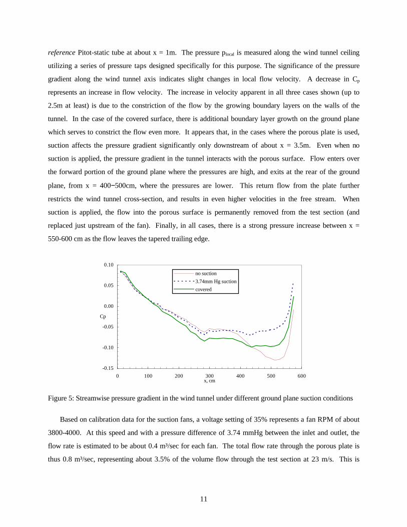
Figure 5 shows the streamwise pressure gradient in the empty wind-tunnel for three different ground plane

surface conditions; the porous surface with no suction applied, the porous surface with 3.74 mmHg of

suction applied, and finally the porous surface completely covered (using self adhesive shelf paper). The

pressure coefficient is Cp = (plocal-p∞)/(½ρU∞²), where the subscript ∞ refers to measurements taken at the

11

reference Pitot-static tube at about x = 1m. The pressure plocal is measured along the wind tunnel ceiling

utilizing a series of pressure taps designed specifically for this purpose. The significance of the pressure

gradient along the wind tunnel axis indicates slight changes in local flow velocity. A decrease in Cp

represents an increase in flow velocity. The increase in velocity apparent in all three cases shown (up to

2.5m at least) is due to the constriction of the flow by the growing boundary layers on the walls of the

tunnel. In the case of the covered surface, there is additional boundary layer growth on the ground plane

which serves to constrict the flow even more. It appears that, in the cases where the porous plate is used,

suction affects the pressure gradient significantly only downstream of about x = 3.5m. Even when no

suction is applied, the pressure gradient in the tunnel interacts with the porous surface. Flow enters over

the forward portion of the ground plane where the pressures are high, and exits at the rear of the ground

plane, from x = 400−500cm, where the pressures are lower. This return flow from the plate further

restricts the wind tunnel cross-section, and results in even higher velocities in the free stream. When

suction is applied, the flow into the porous surface is permanently removed from the test section (and

replaced just upstream of the fan). Finally, in all cases, there is a strong pressure increase between x =

550-600 cm as the flow leaves the tapered trailing edge.

-0.15

-0.10

-0.05

0.00

0.05

0.10

0 100 200 300 400 500 600x, cm

Cp

no suction

3.74mm Hg suction

covered

Figure 5: Streamwise pressure gradient in the wind tunnel under different ground plane suction conditions

Based on calibration data for the suction fans, a voltage setting of 35% represents a fan RPM of about

3800-4000. At this speed and with a pressure difference of 3.74 mmHg between the inlet and outlet, the

flow rate is estimated to be about 0.4 m³/sec for each fan. The total flow rate through the porous plate is

thus 0.8 m³/sec, representing about 3.5% of the volume flow through the test section at 23 m/s. This is

12

about twice the volume flux contained in the covered plate boundary layer, and represents an acceptable

level of flow removal.

In Zabat et al. (1994) and Zabat et al. (1994b), it was shown that for a single vehicle model, the CD

measured using this ground plane surface was 15% higher than if the surface were solid. This indicates

that the flowfields for the two conditions are slightly different, although no details are known. The single

vehicle drag coefficients measured over a covered surface are shown in figure 6 and figure 7 for forward

and rear facing models respectively.

CCCCCCCCCCCCCCCCCCCCCCCCCCCCCCCC

CCCCCCC C CG

GGGGGGGGG

GG

GG

GGGGGGGGG

∗∗∗∗∗∗∗∗∗∗∗∗∗∗∗∗∗∗∗∗∗∗∗∗∗∗∗∗∗∗∗∗

∗∗∗∗∗∗ ∗ ∗ ∗ ××××××××××

×××××××××××××

0.10

0.15

0.20

0.25

0.30

0.35

0.40

0.15

0.20

0.25

0.30

0.35

0.40

0.45

0 50 100 150 200 250 300 350 400 450

x, cm

C Blue-uncorrected

G Yellow-uncorrected

∗ Blue-corrected

× Yellow-corrected

Figure 6: Single, forward-facing vehicle CD using solid ground plane

C. The Effect of Reynolds Number and Boundary Layer Trips

The dependence of the results upon Reynolds number (Re is based on the effective diameter,

d FrontalArea= 4( ) π ) is checked by varying the freestream velocity between 8 m/s and 32 m/s for a

selected number of 2-vehicle platoon tests. Admittedly, this range of variation is limited, and lies well

below full scale Reynolds numbers which are a factor of 7-8 higher than can be reached in the wind tunnel.

In some cases, the flow on the models is tripped using a serrated rubber strip which is stretched over the

nose of the model and positioned about 153 mm from the leading edge of the front bumper. The thickness

of the strip is approximately 0.6 mm. It is of the order of the estimated boundary layer displacement

thickness at that location on the model at U∞ =23 m/s. The dependence of the single vehicle CD on Re and

tripping was presented in Zabat et al. (1994) and Zabat et al. (1994b). A decrease of approximately 3% in

CD was found when the Re is increased from 2.4x105 to 4.1x105. This is expected since the drag

13

contribution due to skin friction decreases approximately proportional to the inverse 1/5 power of the Re.

The trip caused a slight increase in drag at all Re probably due to drag on the trip itself.

CCCCCCCCC

GGGGGGG G

G

GGGGGGGGG

GGGGGGG G G

∗∗∗∗∗∗∗∗∗

×××××× ×

××××××××××× ×××××× × × ×

0.15

0.20

0.25

0.30

0.35

0.40

0.45

0.20

0.25

0.30

0.35

0.40

0.45

0.50

0 50 100 150 200 250 300 350 400 450

x, cm

C Blue-uncorrected

G Yellow-uncorrected

∗ Blue-corrected

× Yellow-corrected

Figure 7: Single, backward-facing vehicle CD using solid ground plane

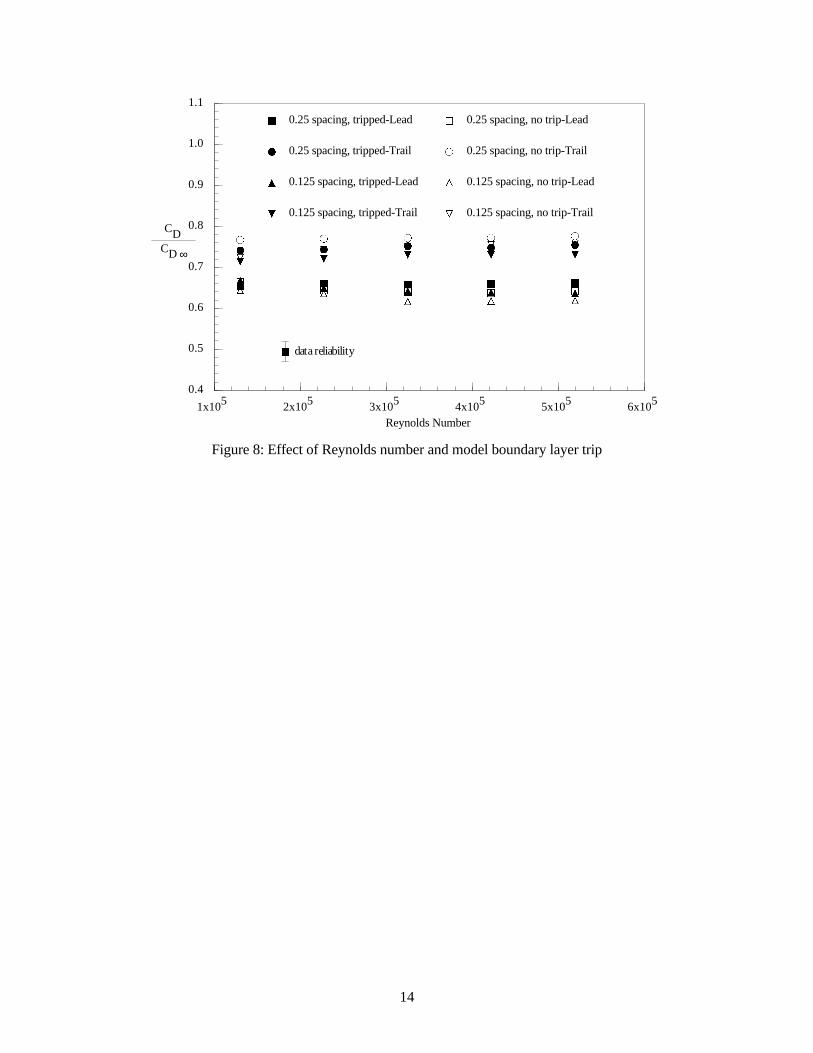
Additional results for a 2-vehicle platoon at several spacings are summarized in figure 8 as a function

of Reynolds number. The drag coefficient ratio, CD / CD∞ , is plotted, and because of this, the small trend

in CD as Re increaseswhich is no longer of interestis not visible.

What is made evident in figure 8 are the changes in drag experienced during platoon operation when

Reynolds number is varied. The results show a small consistent decrease in drag coefficient for the lead

vehicle, and a small increase for the trail vehicle as Reynolds number increases. These changes are the

same order as our estimate of reliability.

The effect of the presence of the trip is to increase the drag coefficient slightly for the lead vehicle (less

drag savings), and to decrease the drag for the trail vehicle (more drag savings). The increments are

similar, and roughly independent of Reynolds number. The conclusion is that neither the presence nor

absence of an artificial trip nor the variations in Reynolds number (at least over our range of variation)

have a significant effect upon the flow. The results to follow are presented for no artificial tripping and for

a Reynolds number, Re = 3.7x105.

14

B B B B B

J J J J J

HH H H H

P PP P P

GG G G G

É É É É É

C CC C C

SS S S S

0.4

0.5

0.6

0.7

0.8

0.9

1.0

1.1

1x105 2x105 3x105 4x105 5x105 6x105

CD

Reynolds Number

B 0.25 spacing, tripped-Lead

J 0.25 spacing, tripped-Trail

H 0.125 spacing, tripped-Lead

P 0.125 spacing, tripped-Trail

G 0.25 spacing, no trip-Lead

É 0.25 spacing, no trip-Trail

C 0.125 spacing, no trip-Lead

S 0.125 spacing, no trip-Trail

CD ∞

data reliabilityB

Figure 8: Effect of Reynolds number and model boundary layer trip

15

IV. THE DRAG OF 2, 3 & 4-VEHICLE PLATOONS

A. Drag on a 2-Vehicle Platoon

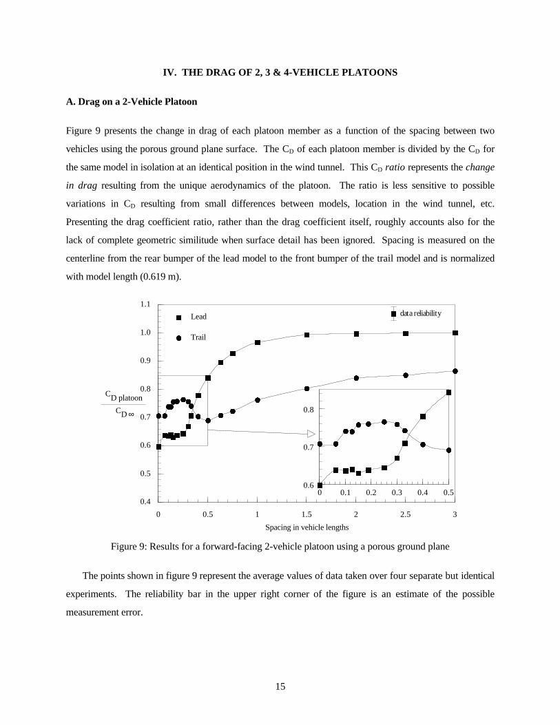
Figure 9 presents the change in drag of each platoon member as a function of the spacing between two

vehicles using the porous ground plane surface. The CD of each platoon member is divided by the CD for

the same model in isolation at an identical position in the wind tunnel. This CD ratio represents the change

in drag resulting from the unique aerodynamics of the platoon. The ratio is less sensitive to possible

variations in CD resulting from small differences between models, location in the wind tunnel, etc.

Presenting the drag coefficient ratio, rather than the drag coefficient itself, roughly accounts also for the

lack of complete geometric similitude when surface detail has been ignored. Spacing is measured on the

centerline from the rear bumper of the lead model to the front bumper of the trail model and is normalized

with model length (0.619 m).

B

BBBBBB

B

B

B

B

B

B

B

B B B B

JJ

JJJJJJ

J

JJ

JJ

J

J

JJ

J

0.4

0.5

0.6

0.7

0.8

0.9

1.0

1.1

0 0.5 1 1.5 2 2.5 3

CD platoon

Spacing in vehicle lengths

B Lead

J Trail

B

B BBBB B

B

B

B

B

J J

JJ

J J JJJ

JJ

0.6

0.7

0.8

0 0.1 0.2 0.3 0.4 0.5

CD ∞

data reliabilityB

Figure 9: Results for a forward-facing 2-vehicle platoon using a porous ground plane

The points shown in figure 9 represent the average values of data taken over four separate but identical

experiments. The reliability bar in the upper right corner of the figure is an estimate of the possible

measurement error.

16

Several important qualitative features can be seen in figure 9. At spacings greater than unity, the lead

vehicle is unaware of the presence of the trail vehicle (this is also true when more than two vehicles are

present). The trail vehicle, which is contained in the wake of the lead vehicle, experiences a decrease in

drag as expected. Extrapolation of these results to greater spacings suggests that a measurable decrease in

drag will persist perhaps to a spacing of ten. This circumstance may be termed weak interaction because it

is one-sidednot mutualand is entirely understandable. As spacing decreases below a value of unity,

the drag of the lead vehicle begins a substantial decrease. The drag of the trail vehicle is also decreased, in

what might now be termed the strong interaction regime. As spacing continues to decrease below the

value one-half, the drag of the trail vehicle abruptly turns upward, crosses the lead vehicle drag curve at

about 0.35 spacing, and remains the greater of the two drags all the way to zero spacing! For two vehicles

of equal performance and throttle setting, the crossover position is a stable fixed pointmeaning that the

distance between the two vehicles will naturally equilibrate to this separation. The observation that

separations of approximately this valueor slightly greater separationsare often observed in the drafting

of stock cars on race tracks lends support to the wind tunnel result.

B. Drag on 3 & 4-Vehicle Platoons

The results of drag measurements as a function of spacing on 3 and 4-vehicle platoons using the porous

surface ground plane are presented in figure 10 and figure 11. The intervehicle spacing within the platoon

is uniform and is measured in the same manner. As in the 2-vehicle case, the points presented here are

averaged over four data sets. The data reliability bar is an estimate based on the root mean square of the

data scatter.

As far as we know, these are unique measurements which document the remarkably large drag savings

obtainable in platoon operation. At first glance they may appear "noisy" because of the numerous small

and unexpected variationsparticularly at short spacings. Much of this variation is in fact greater than

our estimated error and reflects, we believe, the actual physical changes taking place in the flow field at

short spacings. Many of the details show consistent trends as the number of vehicles within the platoon

increases.

17

BBBBB

B

B

B

B

B B

J

J

JJJ

J J

J

J

JJ

HH

HHHHH H

H

H H

0.4

0.5

0.6

0.7

0.8

0.9

1.0

1.1

0 0.5 1 1.5 2 2.5 3

CD platoon

Spacing in vehicle lengths

B Vehicle 1

J Vehicle 2

H Vehicle 3

BB B B B

B

B

J

J

J JJ

J J

H H

H H H HH

0.4

0.5

0.6

0.7

0.8

0 0.1 0.2 0.3 0.4 0.5

CD ∞

data reliabilityB

Figure 10: Results for 3-vehicle platoon

BBBBBBB

B

B

B

B

B

B

B

J

J

JJJJJ

JJJ J

J

J

J

H

H

HHH

HHHH

H

H

HH

H

FFFFF

FFFFFF F

FF

0.4

0.5

0.6

0.7

0.8

0.9

1.0

1.1

0 0.5 1 1.5 2 2.5 3

CD platoon

Spacing in vehicle lengths

B Vehicle 1

J Vehicle 2

H Vehicle 3

F Vehicle 4

BB

B BB B

B

B

B

B

J

J

JJJ J

J

JJ J

J

H

H

H HH

H

HH H

H

HF F

FF

F

F FF F

FF

0.4

0.5

0.6

0.7

0.8

0 0.1 0.2 0.3 0.4 0.5

CD ∞

data reliabilityB

Figure 11: Results for 4-vehicle platoon

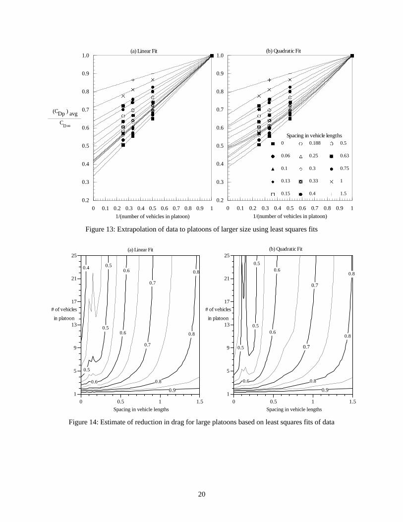
As the number of vehicles in the platoon increases, one observes more complex behaviors in the strong

interaction regime (figures 10 and 11). As might be expected, the interior vehicles have the lower drags,

18

but there are also curious small plateau regions which form. For example, the drag of the lead vehicle

decreases steadily with decreasing separation until a value of about 0.25 is reached, and thereafter drag

remains roughly constant. The drag of the second vehicle in a three-vehicle platoon contains two small

plateau regionsextending from 0.1-0.2 and from 0.3-0.5. The second vehicle experiences similar

behavior in the four-vehicle platoon, and the third vehicle exhibits even more dramatic drag variationa

plateau at 0.6-0.7, a decrease to a relative minimum (plateau) at 0.2-0.3, then a dramatic rise (to a plateau)

at 0.1-0.2 before finally decreasing to an absolute minimum. The narrowness of the plateau peak in drag

at 0.1-0.2 suggests a flow-induced resonance which is quite sensitive to vehicle spacing and to position

within the platoon. Such steep drag gradient regions will be of importance to control system modelers, and

therefore warrant our further study.

C. The Platoon-Averaged Drag Coefficient: Extrapolation to Large Platoons

A closer study of the 2, 3 and 4-vehicle platoon behaviors allow several general conclusions to be made

regarding the possible behavior of a larger platoon.

(1) The drag coefficient ratio for the lead vehicle and for each succeeding vehiclesay the

nth vehicleis independent of the number of vehicles in the platoon provided there are at

least (n+1) vehicles.

(2) Each vehicle added to the platoon experiences a lower drag over most of the strong and

weak interaction range, but may be subject to rather sharp, local drag changes (flowfield

resonances).

(3) The final vehicle in the platoon experiences the least drag variation as vehicle spacing

varies.

An overall measure of platoon drag performance may be obtained by defining an average drag

coefficient ratio.

( ) ( )C Cn

C CDp avg D Di Di

n

∞ ∞=

=

∑

1

1

(5)

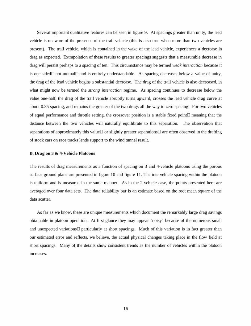
This ratio is shown in figure 12. As might be expected, platoon-averaged drag coefficient ratios possess

much smoother behavior than the drags of individual vehicles. In a platoon containing just four vehicles,

the average drag has been reduced by a factor of 1/2 at zero spacing! More importantly perhaps, the

19

average drag coefficients are dramatically lowered, and vary only moderately, in the range of spacings 0.1-

0.3 where platooning could be implemented. The addition of each succeeding vehicle decreases the platoon

drag, but as the number of vehicles increases the increments become smaller. One would expect the

average drag ratio to approach a limit as the number of platoon members increases indefinitely.

JJJJJJJJJJ

J

J

J

J

JJ J J

HH

HHHHH

HH

H

H

HH

H

HH

B

B

BBBBB

BB

B

B

BB

B

0.4

0.5

0.6

0.7

0.8

0.9

1.0

1.1

0 0.5 1 1.5 2 2.5 3

(CDp )avg

Spacing in vehicle lengths

J 2-vehicle

H 3-vehicle

B 4-vehicle

J

JJJJ

J JJJ

J

J

HH

HHHH

H

HH

H

H

B

B

BBBB

B

BB

B

B

0.5

0.6

0.7

0 0.1 0.2 0.3 0.4 0.5

CD ∞

data reliabilityB

Figure 12: Average drag for 2, 3 & 4-vehicle platoons

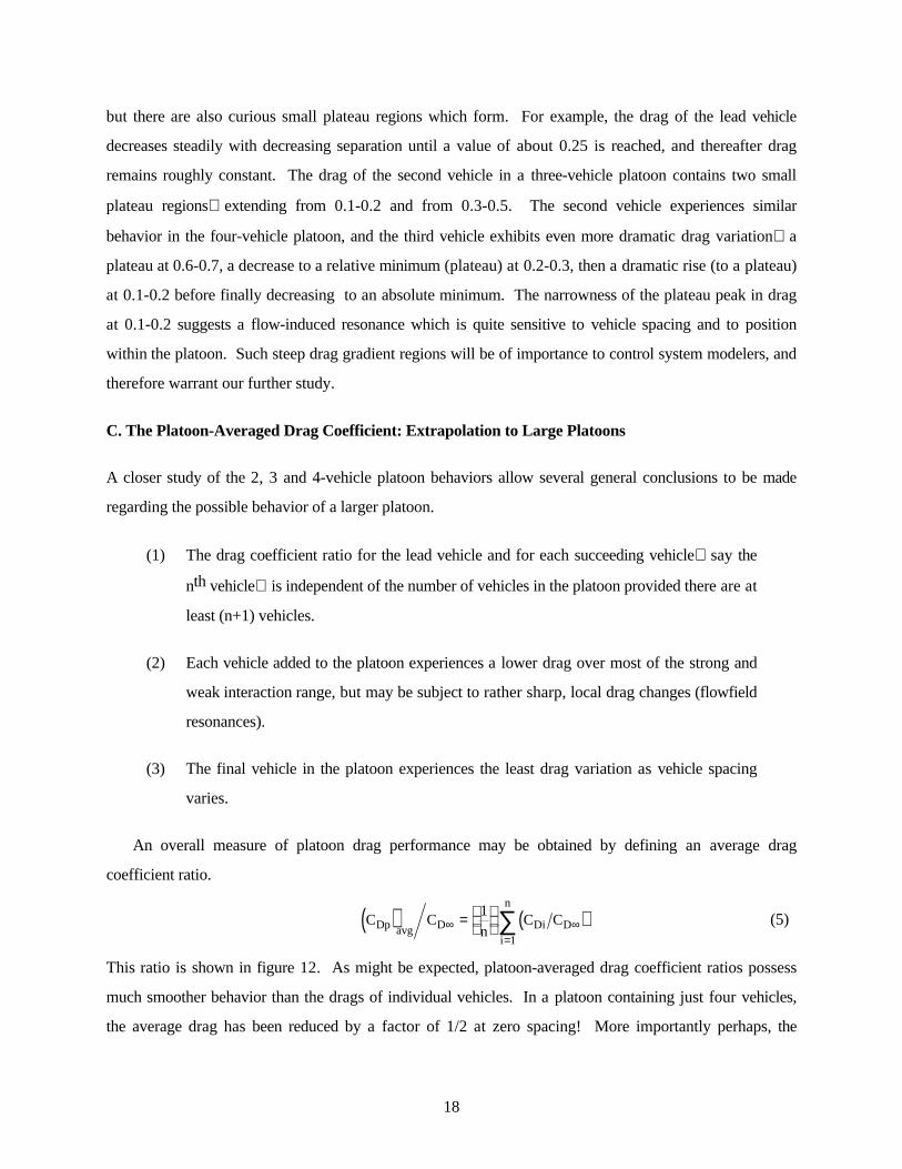
An extrapolation to larger platoon size may be obtained by the following procedure. The platoon-

averaged drag coefficient ratios are plotted for a series of separations as a function of the inverse of the

number of vehicles in the platoon. Continuing the drag coefficient ratio into the domain between one-

quarter (1/n = 1/4) and zero gives the desired behavior. This is accomplished in figure 13 using both linear

and quadratic fits to the four data points at 1/n = 1/1, 1/2, 1/3, 1/4. The difference in the results from these

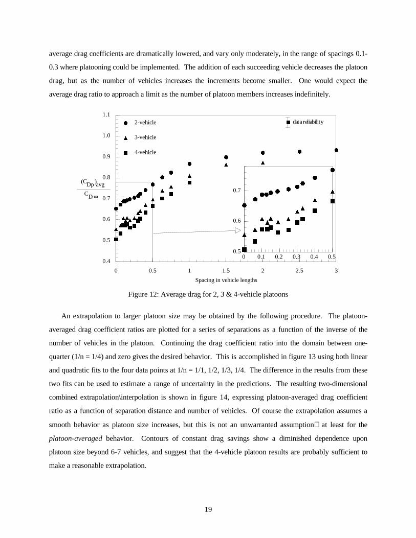
two fits can be used to estimate a range of uncertainty in the predictions. The resulting two-dimensional

combined extrapolation\interpolation is shown in figure 14, expressing platoon-averaged drag coefficient

ratio as a function of separation distance and number of vehicles. Of course the extrapolation assumes a

smooth behavior as platoon size increases, but this is not an unwarranted assumptionat least for the

platoon-averaged behavior. Contours of constant drag savings show a diminished dependence upon

platoon size beyond 6-7 vehicles, and suggest that the 4-vehicle platoon results are probably sufficient to

make a reasonable extrapolation.

20

B

B

B

B

J

J

J

J

H

H

H

H

F

F

FF

G

G

G

G

E

E

E

E

C

C

C

C

A

A

A

A

M

M

M

M

;

;

;

;

O

O

O

O

7

7

7

7

9

9

9

9

I

I

I

I

D

D

D

0.2

0.3

0.4

0.5

0.6

0.7

0.8

0.9

1.0

0 0.1 0.2 0.3 0.4 0.5 0.6 0.7 0.8 0.9 1

1/(number of vehicles in platoon)

(a) Linear Fit (b) Quadratic Fit

CD ∞

B

B

B

B

J

J

J

J

H

H

H

H

F

F

FF

G

G

G

G

E

E

E

E

C

C

C

C

A

A

A

A

M

M

M

M

;

;

;

;

O

O

O

O

7

7

7

7

9

9

9

9

I

I

I

I

D

D

D

0.2

0.3

0.4

0.5

0.6

0.7

0.8

0.9

1.0

0 0.1 0.2 0.3 0.4 0.5 0.6 0.7 0.8 0.9 1

(CDp ) avg

1/(number of vehicles in platoon)

B 0

J 0.06

H 0.1

F 0.13

G 0.15

E 0.188

C 0.25

A 0.3

M 0.33

; 0.4

O 0.5

7 0.63

9 0.75

I 1

D 1.5

Spacing in vehicle lengths

Figure 13: Extrapolation of data to platoons of larger size using least squares fits

0.4

0.5

0.5

0.5

0.6

0.6

0.6

0.7

0.7

0.8

0.8

0.8

0.91

5

9

13

17

21

25

0 0.5 1 1.5

Spacing in vehicle lengths

(a) Linear Fit

0.5

0.5

0.5

0.6

0.6

0.6

0.7

0.7

0.8

0.8

0.8

0.91

5

9

13

17

21

25

0 0.5 1 1.5

Spacing in vehicle lengths

(b) Quadratic Fit

# of vehicles

in platoon

# of vehicles

in platoon

Figure 14: Estimate of reduction in drag for large platoons based on least squares fits of data

21

V. DEFINING THE IMPORTANCE OF VEHICLE SHAPE:

2-VEHICLE PLATOONS IN OTHER ORIENTATIONS

A most important variable in estimating possible platoon drag savings is the geometry of the vehicles

themselves. It was anticipated early-on that some means for judging the sensitivity to changes in vehicle

shape would be needed. The Lumina APV was originally chosen for testing because it presented a strongly

raked windshield and a blunt base. The model can be tested in the conventional forward facing condition,

or be reversed to provide quite a different front-to-back geometry. In fact, these two geometries are

probably more extreme than would be encountered in a group of contemporary automobile vehicles.

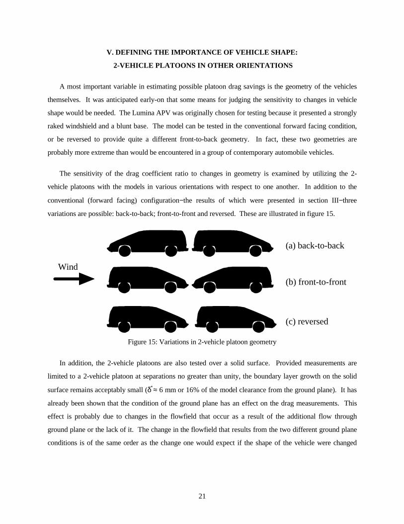
The sensitivity of the drag coefficient ratio to changes in geometry is examined by utilizing the 2-

vehicle platoons with the models in various orientations with respect to one another. In addition to the

conventional (forward facing) configuration−the results of which were presented in section III−three

variations are possible: back-to-back; front-to-front and reversed. These are illustrated in figure 15.

(a) back-to-back

(b) front-to-front

(c) reversed

Wind

Figure 15: Variations in 2-vehicle platoon geometry

In addition, the 2-vehicle platoons are also tested over a solid surface. Provided measurements are

limited to a 2-vehicle platoon at separations no greater than unity, the boundary layer growth on the solid

surface remains acceptably small (δ∗≈ 6 mm or 16% of the model clearance from the ground plane). It has

already been shown that the condition of the ground plane has an effect on the drag measurements. This

effect is probably due to changes in the flowfield that occur as a result of the additional flow through

ground plane or the lack of it. The change in the flowfield that results from the two different ground plane

conditions is of the same order as the change one would expect if the shape of the vehicle were changed

22

slightly. Because of this, measurements with the modified ground plane are presented here as if they had

been another change in geometry.

The results for all the 2-vehicle platoons with different geometries can be consolidated to provide an

estimate of the variation possible, in the results of drag as a function of spacing, due to changes in

geometry. This estimate is in the form of a variability envelope which is also a function of spacing and is

based on the standard deviation from the mean of the data for all geometries tested. Although this estimate

is obtained using only a 2-vehicle platoon, it would not be unreasonable to apply it to the 3 & 4-vehicle

data as well.

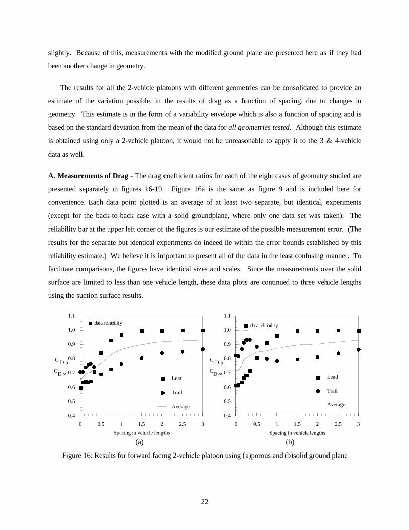
A. Measurements of Drag - The drag coefficient ratios for each of the eight cases of geometry studied are

presented separately in figures 16-19. Figure 16a is the same as figure 9 and is included here for

convenience. Each data point plotted is an average of at least two separate, but identical, experiments

(except for the back-to-back case with a solid groundplane, where only one data set was taken). The

reliability bar at the upper left corner of the figures is our estimate of the possible measurement error. (The

results for the separate but identical experiments do indeed lie within the error bounds established by this

reliability estimate.) We believe it is important to present all of the data in the least confusing manner. To

facilitate comparisons, the figures have identical sizes and scales. Since the measurements over the solid

surface are limited to less than one vehicle length, these data plots are continued to three vehicle lengths

using the suction surface results.

BBBB

B

B

B

BBBBBB

JJ

JJJ

J

J

JJJ

J

JJ

0.4

0.5

0.6

0.7

0.8

0.9

1.0

1.1

0 0.5 1 1.5 2 2.5 3

C D p

Spacing in vehicle lengths

B Lead

J Trail

ÿ Average

data reliabilityB

CD ∞

BBBBB

B

B

B

BBBB

B

JJJ

J

J

J

J

JJJ

JJJ

0.4

0.5

0.6

0.7

0.8

0.9

1.0

1.1

0 0.5 1 1.5 2 2.5 3

C D p

Spacing in vehicle lengths

B Lead

J Trail

ÿ Average

data reliabilityB

CD ∞

(a) (b)

Figure 16: Results for forward facing 2-vehicle platoon using (a)porous and (b)solid ground plane

23

BBBBB

B

B

B

B

B

B

B

B

JJJJJ

J

J

JJJJJJ

0.4

0.5

0.6

0.7

0.8

0.9

1.0

1.1

0 0.5 1 1.5 2 2.5 3

C D p

Spacing in vehicle lengths

B Lead

J Trail

ÿ Average

CD ∞

BB

B

B

B

B

B

B

B

J

J

JJJJJ

J

J

GGGG

ÉÉÉÉ

0.4

0.5

0.6

0.7

0.8

0.9

1.0

1.1

0 0.5 1 1.5 2 2.5 3

C D p

Spacing in vehicle lengths

B Lead-solid

J Trail-solid

G Lead-porous

É Trail-porous

ÿ Average

CD ∞

data reliabilityB data reliabilityB

(a) (b)

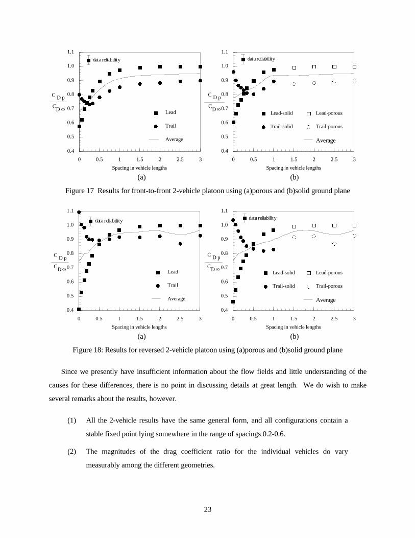
Figure 17 Results for front-to-front 2-vehicle platoon using (a)porous and (b)solid ground plane

BBBBB

B

B

B

B

B

B

B

B

J

J

JJJJJJJ

J

JJ

J

0.4

0.5

0.6

0.7

0.8

0.9

1.0

1.1

0 0.5 1 1.5 2 2.5 3

C D p

Spacing in vehicle lengths

B Lead

J Trail

ÿ Average

CD ∞

data reliabilityB

CD ∞

BB

B

B

B

B

B

B

B

JJJ

J

JJ

J

J

J

GGGG

É

É

ÉÉ

0.4

0.5

0.6

0.7

0.8

0.9

1.0

1.1

0 0.5 1 1.5 2 2.5 3

C D p

Spacing in vehicle lengths

B Lead-solid

J Trail-solid

G Lead-porous

É Trail-porous

ÿ Average

data reliabilityB

(a) (b)

Figure 18: Results for reversed 2-vehicle platoon using (a)porous and (b)solid ground plane

Since we presently have insufficient information about the flow fields and little understanding of the

causes for these differences, there is no point in discussing details at great length. We do wish to make

several remarks about the results, however.

(1) All the 2-vehicle results have the same general form, and all configurations contain a

stable fixed point lying somewhere in the range of spacings 0.2-0.6.

(2) The magnitudes of the drag coefficient ratio for the individual vehicles do vary

measurably among the different geometries.

24

BBBBB

B

B

B

BBB

B

B

B

JJJJJJ

J

JJJJJJ

J

0.4

0.5

0.6

0.7

0.8

0.9

1.0

1.1

0 0.5 1 1.5 2 2.5 3

C D p

Spacing in vehicle lengths

B Lead

J Trail

ÿ Average

CD ∞

BB

B

B

BB

B

B

B

J

J

J

JJ

JJ

J

J

GGGG

ÉÉÉÉ

0.4

0.5

0.6

0.7

0.8

0.9

1.0

1.1

0 0.5 1 1.5 2 2.5 3

C D p

Spacing in vehicle lengths

B Lead-solid

J Trail-solid

G Lead-porous

É Trail-porous

ÿ Average

CD ∞

1.22

data reliabilityB data reliabilityB

(a) (b)

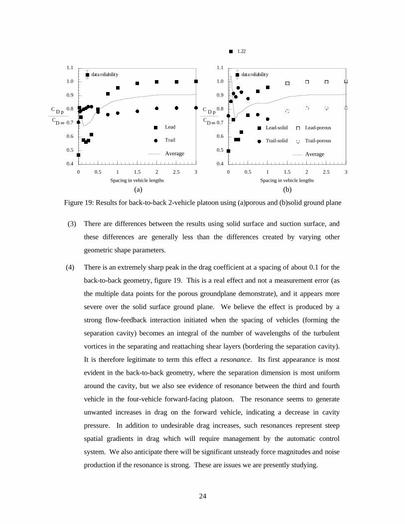
Figure 19: Results for back-to-back 2-vehicle platoon using (a)porous and (b)solid ground plane

(3) There are differences between the results using solid surface and suction surface, and

these differences are generally less than the differences created by varying other

geometric shape parameters.

(4) There is an extremely sharp peak in the drag coefficient at a spacing of about 0.1 for the

back-to-back geometry, figure 19. This is a real effect and not a measurement error (as

the multiple data points for the porous groundplane demonstrate), and it appears more

severe over the solid surface ground plane. We believe the effect is produced by a

strong flow-feedback interaction initiated when the spacing of vehicles (forming the

separation cavity) becomes an integral of the number of wavelengths of the turbulent

vortices in the separating and reattaching shear layers (bordering the separation cavity).

It is therefore legitimate to term this effect a resonance. Its first appearance is most

evident in the back-to-back geometry, where the separation dimension is most uniform

around the cavity, but we also see evidence of resonance between the third and fourth

vehicle in the four-vehicle forward-facing platoon. The resonance seems to generate

unwanted increases in drag on the forward vehicle, indicating a decrease in cavity

pressure. In addition to undesirable drag increases, such resonances represent steep

spatial gradients in drag which will require management by the automatic control

system. We also anticipate there will be significant unsteady force magnitudes and noise

production if the resonance is strong. These are issues we are presently studying.

25

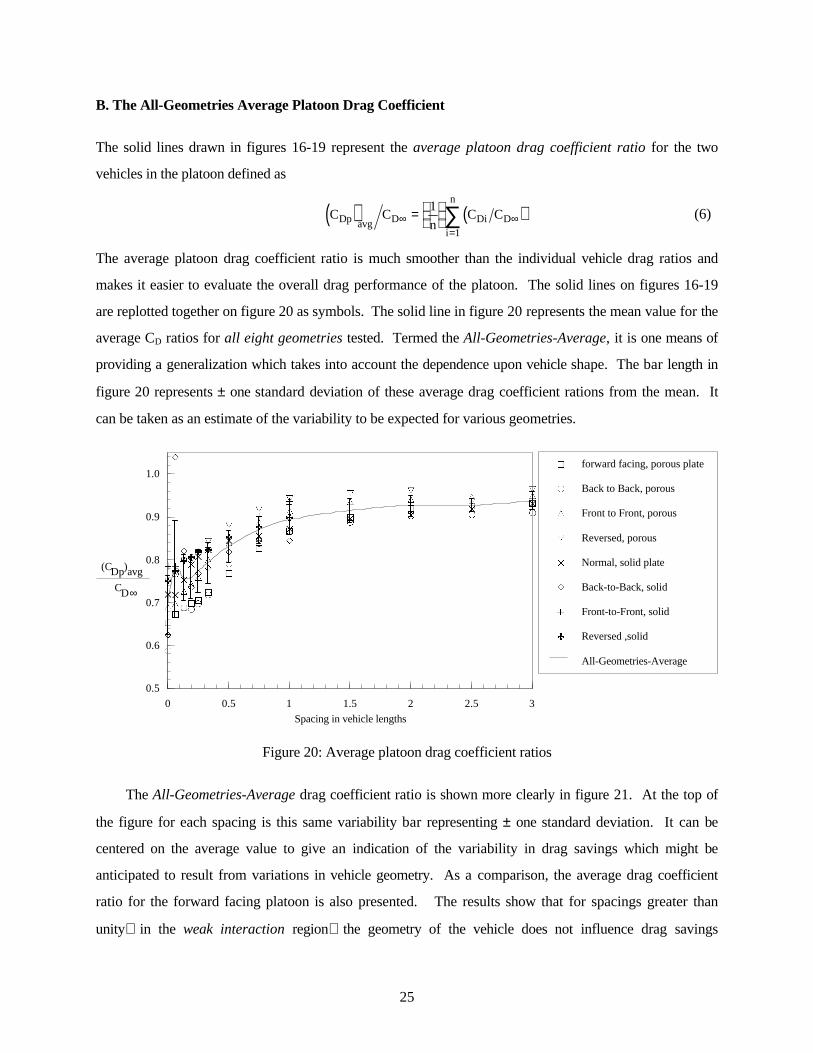
B. The All-Geometries Average Platoon Drag Coefficient

The solid lines drawn in figures 16-19 represent the average platoon drag coefficient ratio for the two

vehicles in the platoon defined as

( ) ( )C Cn

C CDp avg D Di Di

n

∞ ∞=

=

∑

1

1

(6)

The average platoon drag coefficient ratio is much smoother than the individual vehicle drag ratios and

makes it easier to evaluate the overall drag performance of the platoon. The solid lines on figures 16-19

are replotted together on figure 20 as symbols. The solid line in figure 20 represents the mean value for the

average CD ratios for all eight geometries tested. Termed the All-Geometries-Average, it is one means of

providing a generalization which takes into account the dependence upon vehicle shape. The bar length in

figure 20 represents ± one standard deviation of these average drag coefficient rations from the mean. It

can be taken as an estimate of the variability to be expected for various geometries.

GGG

G

G

G

G

G

GGG

G

G

ÉÉÉÉ

É

É

É

É

ÉÉÉ

É

É

ÇÇÇÇ

Ç

Ç

Ç

Ç

ÇÇÇ

ÇÇ

Ü

Ü

ÜÜÜ

Ü

Ü

Ü

ÜÜÜ

ÜÜ

II

II

II

I

III

I

II

AA

A

AA

A

A

A

A

D

D

D

DDDD

DD

Z

Z

Z

ZZZZ

Z

Z

0.5

0.6

0.7

0.8

0.9

1.0

0 0.5 1 1.5 2 2.5 3

(CDp)avg

Spacing in vehicle lengths

G forward facing, porous plate

É Back to Back, porous

Ç Front to Front, porous

Ü Reversed, porous

I Normal, solid plate

A Back-to-Back, solid

D Front-to-Front, solid

Z Reversed ,solid

ÿ All-Geometries-Average

CD ∞

Figure 20: Average platoon drag coefficient ratios

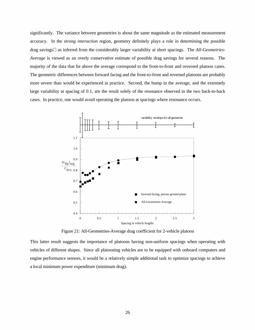
The All-Geometries-Average drag coefficient ratio is shown more clearly in figure 21. At the top of

the figure for each spacing is this same variability bar representing ± one standard deviation. It can be

centered on the average value to give an indication of the variability in drag savings which might be

anticipated to result from variations in vehicle geometry. As a comparison, the average drag coefficient

ratio for the forward facing platoon is also presented. The results show that for spacings greater than

unityin the weak interaction regionthe geometry of the vehicle does not influence drag savings

26

significantly. The variance between geometries is about the same magnitude as the estimated measurement

accuracy. In the strong interaction region, geometry definitely plays a role in determining the possible

drag savingsas inferred from the considerably larger variability at short spacings. The All-Geometries-

Average is viewed as an overly conservative estimate of possible drag savings for several reasons. The

majority of the data that lie above the average correspond to the front-to-front and reversed platoon cases.

The geometric differences between forward facing and the front-to-front and reversed platoons are probably

more severe than would be experienced in practice. Second, the bump in the average, and the extremely

large variability at spacing of 0.1, are the result solely of the resonance observed in the two back-to-back

cases. In practice, one would avoid operating the platoon at spacings where resonance occurs.

BBBB

B

B

B

BBBB

BB

JJJ

JJ

J

J

JJJJ

J

J

0.4

0.5

0.6

0.7

0.8

0.9

1.0

1.1

0 0.5 1 1.5 2 2.5 3

(CDp )avg

Spacing in vehicle lengths

B forward facing, porous ground plane

J All-Geometries-Average

ÿ

CD ∞

variability envelope for all geometries

Figure 21: All-Geometries-Average drag coefficient for 2-vehicle platoon

This latter result suggests the importance of platoons having non-uniform spacings when operating with

vehicles of different shapes. Since all platooning vehicles are to be equipped with onboard computers and

engine performance sensors, it would be a relatively simple additional task to optimize spacings to achieve

a local minimum power expenditure (minimum drag).

27

VI. FUEL SAVING BENEFITS DERIVED FROM PLATOONING

A. The Relationship Between Aerodynamic Drag and Fuel Expenditure

The total resistance encountered by a vehicle in unsteady forward motion can be described by the following

equation

TOTAL RESISTANCE D R R RR g A= + + + (7)

D is the aerodynamic drag and is expressed as

D C V AD= 12

2ρ , (8)

where ρ is the density of air, V is the driving speed (assuming no relative wind) and A is the cross-sectional

area of the vehicle. CD is the non-dimensional coefficient of drag. Aerodynamicists use the drag coefficient

as the comparison quantity rather than the drag itself, because CD is relatively independent of size and

speed. The drag coefficient does depend upon vehicle shape, and in our case, CD also depends upon the

proximity of other vehicles in the platoon. The rolling resistance, RR, is a function of vehicle mass, Μ, and

tire rolling resistance coefficient, ro, which in turn depends upon speed.

R r gR o= Μ , (9)

g is acceleration due to gravity. Rg is referred to as the gravitational or climbing resistance, and is a

function of vehicle mass and the road grade, φ.

R gg = sinφ Μ (10)

RA is the acceleration resistance depending upon mass and rate of change of speed (acceleration).

RdV

dtA i= +Μ( )1 ε (11)

εi accounts for the rotating masses in the various gears. The only component of the total resistance which

is appreciably affected by platooning is the aerodynamic drag.

The engine power output required to overcome total resistance at speed V is

[ ]Ρ =TOTAL RESISTANCE V

Tη(12)

where ηT is a number typically of the order of 0.9, and accounts for losses in the engine powertrain

(transmission). Combining equations (7)-(12) gives the power required for operation at speed V.

Ρ Μ=

+ + + +

1 112

3

ηρ φ ε

TD o

iC AV gV rg

dV

dtsin

( )(13)

28

The fuel consumption of an automobile in liters per kilometer (liters/km) or gallons per mile (GPM)

depends upon the specific fuel consumption (sfc), the engine power level, and velocity.

liters/km or GPMsfc

V= ×Ρ

(14)

(A conversion factor should appear in (14) to keep the units consistent). Finally, combining (13) and (14)

yields the following relation between fuel consumption and the various components comprising the total

resistance.

liters/km or GPM C AV g rg

dV

dtsfc

TD o

i=

+ + + +

×1 11

22

ηρ φ εΜ sin

( )(15)

If one considers unaccelerated travel on a level road, equation (15) simplifies further, and an equation

for the fuel used to overcome aerodynamic drag, (liters/km)DRAG or GPMDRAG , as a percentage of the total

consumption can be written

][l i t e r s km

l i t e r s kmDRAG

/

/ =

[ ][ ]

GPMGPM

C AV

C AV grDRAG D

D o

=+

12

2

12

2

ρ

ρ Μ(16)

A similar equation, representing the rolling resistance contribution to the fuel consumption,

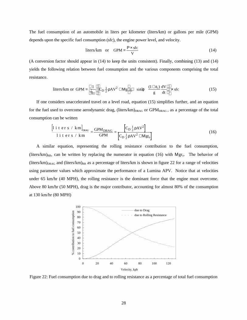
(liters/km)RR, can be written by replacing the numerator in equation (16) with Μgro. The behavior of

(liters/km)DRAG and (liters/km)RR as a percentage of liters/km is shown in figure 22 for a range of velocities

using parameter values which approximate the performance of a Lumina APV. Notice that at velocities

under 65 km/hr (40 MPH), the rolling resistance is the dominant force that the engine must overcome.

Above 80 km/hr (50 MPH), drag is the major contributor, accounting for almost 80% of the consumption

at 130 km/hr (80 MPH)

0

10

20

30

40

50

60

70

80

90

100

0 20 40 60 80 100 120

Velocity, kph

% c

ontr

ibut

ion

to fu

el c

onsu

mpt

ion

due to Drag

due to Rolling Resistance

Figure 22: Fuel consumption due to drag and to rolling resistance as a percentage of total fuel consumption

29

B. The Fuel Consumption Estimates of Sovran

Sovran (1983), suggested a general method for determining the effect of aerodynamic drag on fuel

consumption. It is based upon an extension of equation (15) to include engine performance during breaking

and idling, and utilizes the standard Environmental Protection Agency (EPA) driving cycle model for 1983.

A determination of the actual rate of fuel consumption requires detailed information about the engine and

drivetrain for a particular vehicle. Sovran, in his paper, limits his analysis to changes in the fuel consumed

per unit distance, ∆(liters/km) or ∆GPM, as a result of specific changes in the vehicle drag.

The result of Sovran’s analysis applied to platoon operation is the linear relationship

( ) ( )

( )( )liter km liter km

liter km

GPM GPM

GPM

C C

Cplatoon platoon

A

D Dplatoon avg

D

/ /

/∞

∞

∞

∞

∞

∞

−

=−

=

−

ξ (17)

where, for the EPA urban driving schedule

( ){ }

ξAU

oDr

C A* .

. .=

+ + ∞

074

1 00683 000134Μ

(18)

and for the EPA highway driving schedule

( ){ }

ξAH

oDr

C A* .

. .=

+ + ∞

089

1 00310 0000126Μ

(19)

ξA is the influence coefficient that relates percentage changes in CD to changes in fuel expenditure, and

depends upon the particular vehicle chassis, the engine, the fuel, the drivetrain, and the accessories. These

items are reflected in the various coefficient values in expressions (18) and (19). ξA* represents the highest

attainable value of ξA . When a vehicle traveling at its cruising speed is subjected to a smaller load, say

due to a change in drag, the driver can use the extra power available to speed up or, he/she can maintain the

original speed by reducing the throttle setting. In opting for the latter, the engine is subsequently operated

at a less than optimum condition (lower efficiency) where its specific fuel consumption is slightly higher.

This will be reflected in the above equations by a value of ξA which will be lower than ξA* . To maintain

ξA* , the driver should instead be able to shift to a different gear that would recover the original engine

operating condition.

30

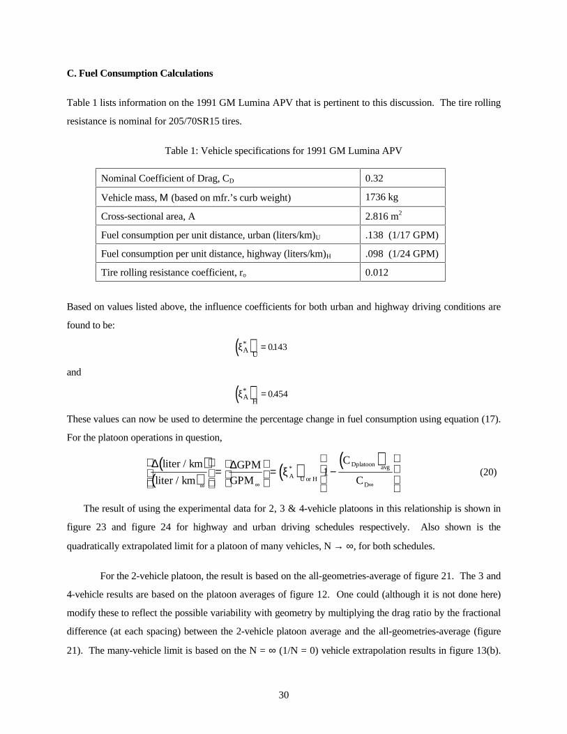
C. Fuel Consumption Calculations

Table 1 lists information on the 1991 GM Lumina APV that is pertinent to this discussion. The tire rolling

resistance is nominal for 205/70SR15 tires.

Table 1: Vehicle specifications for 1991 GM Lumina APV

Nominal Coefficient of Drag, CD 0.32

Vehicle mass, Μ (based on mfr.’s curb weight) 1736 kg

Cross-sectional area, A 2.816 m2

Fuel consumption per unit distance, urban (liters/km)U .138 (1/17 GPM)

Fuel consumption per unit distance, highway (liters/km)H .098 (1/24 GPM)

Tire rolling resistance coefficient, ro 0.012

Based on values listed above, the influence coefficients for both urban and highway driving conditions are

found to be:

( )ξAU

* .= 0143

and

( )ξAH

* .= 0454

These values can now be used to determine the percentage change in fuel consumption using equation (17).

For the platoon operations in question,

( )

( ) ( ) ( )∆ ∆liter km

liter km

GPM

GPM

C

CA U or H

Dplatoon avg

D

/

/*

∞ ∞ ∞

=

= −

ξ 1 (20)

The result of using the experimental data for 2, 3 & 4-vehicle platoons in this relationship is shown in

figure 23 and figure 24 for highway and urban driving schedules respectively. Also shown is the

quadratically extrapolated limit for a platoon of many vehicles, N → ∞, for both schedules.

For the 2-vehicle platoon, the result is based on the all-geometries-average of figure 21. The 3 and

4-vehicle results are based on the platoon averages of figure 12. One could (although it is not done here)

modify these to reflect the possible variability with geometry by multiplying the drag ratio by the fractional

difference (at each spacing) between the 2-vehicle platoon average and the all-geometries-average (figure

21). The many-vehicle limit is based on the N = ∞ (1/N = 0) vehicle extrapolation results in figure 13(b).

31

The variability bar given at the top of the figure for particular spacings is a measure of the possible

variability due to the differences in vehicle geometry. It is based on the standard deviation of the drag data

for all geometries from the all-geometries-average. We believe this estimated variability to be

conservative.

As expected, there is a considerable savings in fuel as a result of the reduction in drag due to

platooning; as much as a 27% reduction from the isolated vehicle consumption is possible at spacings of

0.1−0.2 for very large platoons on the highway. Using the envelope at the top of the figure suggests that

the saving is likely to lie within the range 22–32% regardless of geometry at this spacing.

J

JJJJJ

J

JJ

JJ

J

BB

BBBBBBB

B

B

BB

B

B B

H

H

HHHHHHH

H

H

HH

H

P

P

PPPPP

PP

P

P

P

P

P

P

0%

5%

10%

15%

20%

25%

30%

35%

0 0.5 1 1.5 2 2.5 3

Spacing in vehicle lengths

J 2 vehicles

B 3 vehicles

H 4 vehicles

P many vehicles

ÿ

Decrease in fuel

consumption

Variability envelope for all geometries

Figure 23: All-geometries-average decrease in fuel consumption for platooning vehicles in highwayoperation

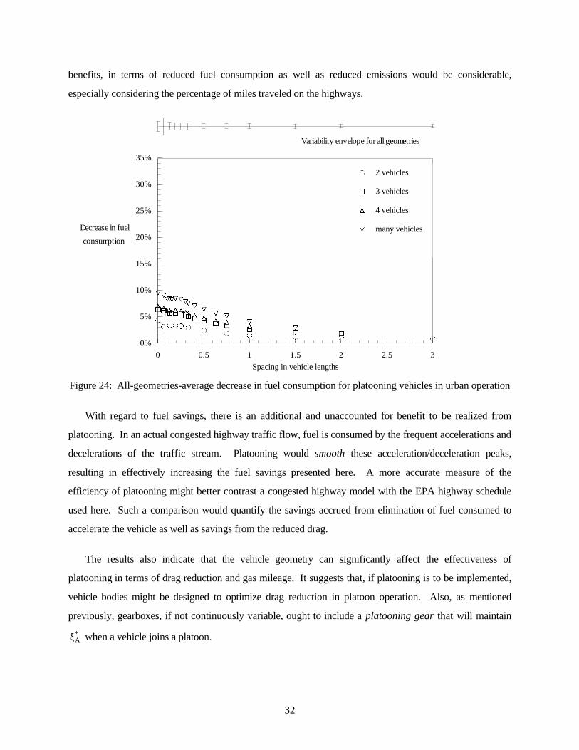
In the city, the savings is not as great since drag is a much smaller percentage of the overall vehicle

resistance at low speeds. Platooning in urban stop and go traffic is not contemplated, but savings

nonetheless amount to a respectable 5-10%.

It is clear from the results shown that the reductions in drag as a result of platooning can be significant.

The development of AVCS technology that will permit platoon operation should be pursued since the

32

benefits, in terms of reduced fuel consumption as well as reduced emissions would be considerable,

especially considering the percentage of miles traveled on the highways.

É

ÉÉÉÉÉÉ

É É É É É

GGGGGGGGGG GG G

GG G

CCCCCCCCCC C

C CC

SSSSSSSSS

SSS S

S

S

0%

5%

10%

15%

20%

25%

30%

35%

0 0.5 1 1.5 2 2.5 3

Spacing in vehicle lengths

É 2 vehicles

G 3 vehicles

C 4 vehicles

S many vehicles

ÿ

Decrease in fuel

consumption

Variability envelope for all geometries

Figure 24: All-geometries-average decrease in fuel consumption for platooning vehicles in urban operation

With regard to fuel savings, there is an additional and unaccounted for benefit to be realized from

platooning. In an actual congested highway traffic flow, fuel is consumed by the frequent accelerations and

decelerations of the traffic stream. Platooning would smooth these acceleration/deceleration peaks,

resulting in effectively increasing the fuel savings presented here. A more accurate measure of the

efficiency of platooning might better contrast a congested highway model with the EPA highway schedule

used here. Such a comparison would quantify the savings accrued from elimination of fuel consumed to

accelerate the vehicle as well as savings from the reduced drag.

The results also indicate that the vehicle geometry can significantly affect the effectiveness of

platooning in terms of drag reduction and gas mileage. It suggests that, if platooning is to be implemented,

vehicle bodies might be designed to optimize drag reduction in platoon operation. Also, as mentioned

previously, gearboxes, if not continuously variable, ought to include a platooning gear that will maintain

ξA* when a vehicle joins a platoon.

33

VII. SURFACE STREAMLINE PATTERNS AND

GROUND PLANE PRESSURE DISTRIBUTIONS

In order to better understand the drag behavior of platoons, it is important to know the behavior of the

flowfield around the vehicle. Numerical methods are still a long way from being able to correctly model a

high Reynolds number separated flow, such as that about an automobile. Of course, complete flowfield

measurements, accurately resolved in space and time, are also beyond practical possibility. However, two

types of experiments have been conducted that might provide clues for the differences between vehicle

flowfields in platoon operation compared to operation in isolation. The work in this section is insufficient

to provide definitive descriptions of the intervehicle flowfields, but it will be incorporated with additional

results from the future studies outlined in section IX.

A. Surface Flow Visualizations

A mixture of kerosene, oleic acid and 5µ-size titanium dioxide particles is brushed evenly onto the models

in both single vehicle operation and in a 2-vehicle platoon. When the wind tunnel is turned on, the airflow

about the models causes the mixture to move in the direction of the airflow. After about ten minutes of

operation, the kerosene has evaporated leaving the titanium dioxide in a pattern that can allow some

inferences to be drawn regarding flow along the vehicle surface. The models are removed from the tunnel

and photographed from the front, back, top and sides. The photographs are digitized for later processing

and storage. This procedure is quite tedious and is performed only for a limited set of test conditions. A

complete set of digitized photographs is included in the appendix. Presented here are three cases showing

evidence that dramatic changes occur in the flowfield under platoon operation.

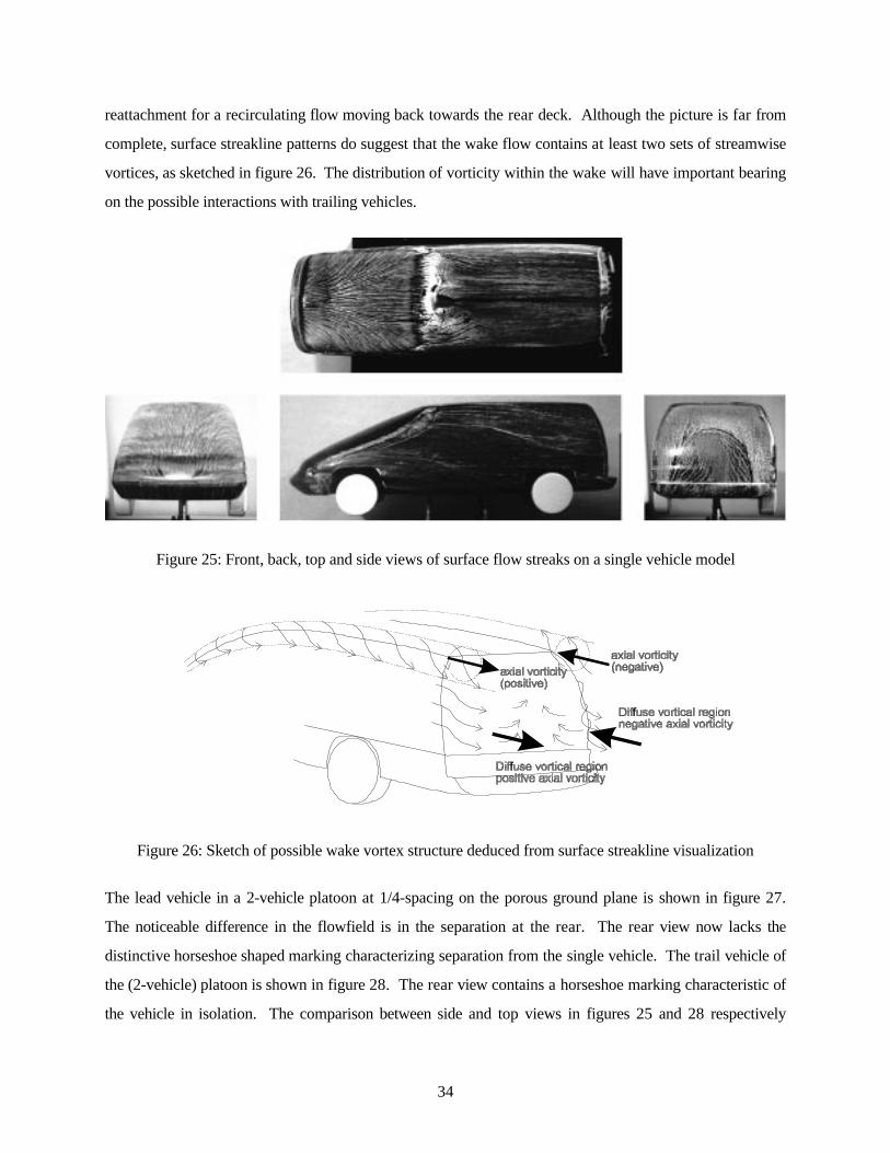
Figure 25 shows the resulting front, top, rear and side views of a single model after following the

procedure described above. In the side view, note the streaks, which indicate a vortex, along the hood-body

panel junction continuing to the top of the A-pillar. The top view shows the flow moving outboard along

the hood which is consistent with the formation of a vortex structure just downstream of the A-pillar. The

top view also gives indication of a local separation bubble on the forward portion of the roof, just behind

the top of the windshield. It is probable that vortical flow is shed from the surface of the vehicle in the

vicinity of the roof A-pillar juncture to form a pair of wake vortices. Farther back, the slight downward

slant of the surface streaklines along the sides of the vehicle indicates that vorticity of the same sign is also

shed at the juncture of the side and read deck. The rear deck itself contains an interesting horseshoe shaped

pattern (see rear view). The present, tentative interpretation is that the horseshoe represents a line of

34

reattachment for a recirculating flow moving back towards the rear deck. Although the picture is far from

complete, surface streakline patterns do suggest that the wake flow contains at least two sets of streamwise

vortices, as sketched in figure 26. The distribution of vorticity within the wake will have important bearing

on the possible interactions with trailing vehicles.

Figure 25: Front, back, top and side views of surface flow streaks on a single vehicle model

Figure 26: Sketch of possible wake vortex structure deduced from surface streakline visualization

The lead vehicle in a 2-vehicle platoon at 1/4-spacing on the porous ground plane is shown in figure 27.

The noticeable difference in the flowfield is in the separation at the rear. The rear view now lacks the

distinctive horseshoe shaped marking characterizing separation from the single vehicle. The trail vehicle of

the (2-vehicle) platoon is shown in figure 28. The rear view contains a horseshoe marking characteristic of

the vehicle in isolation. The comparison between side and top views in figures 25 and 28 respectively

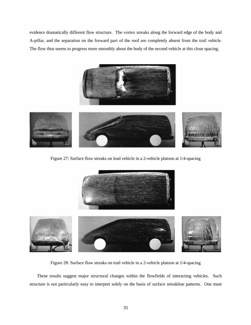
35

evidence dramatically different flow structure. The vortex streaks along the forward edge of the body and

A-pillar, and the separation on the forward part of the roof are completely absent from the trail vehicle.

The flow thus seems to progress more smoothly about the body of the second vehicle at this close spacing.

Figure 27: Surface flow streaks on lead vehicle in a 2-vehicle platoon at 1/4-spacing

Figure 28: Surface flow streaks on trail vehicle in a 2-vehicle platoon at 1/4-spacing

These results suggest major structural changes within the flowfields of interacting vehicles. Such

structure is not particularly easy to interpret solely on the basis of surface streakline patterns. One must

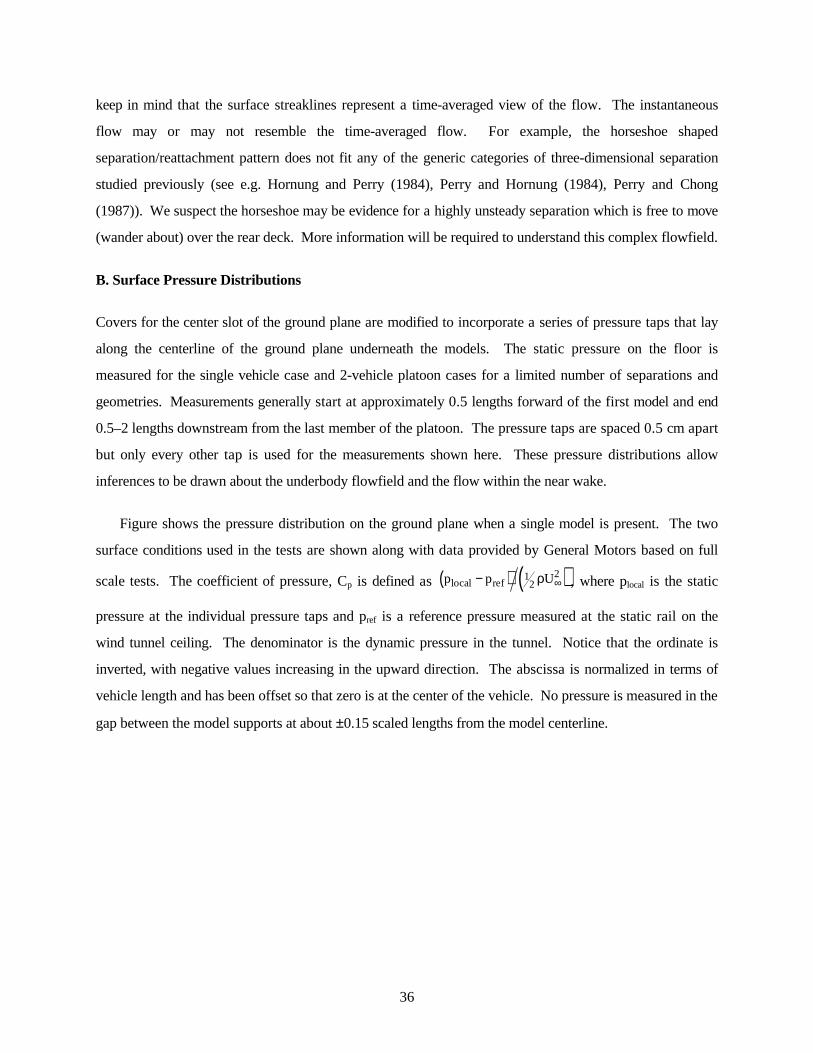
36

keep in mind that the surface streaklines represent a time-averaged view of the flow. The instantaneous

flow may or may not resemble the time-averaged flow. For example, the horseshoe shaped

separation/reattachment pattern does not fit any of the generic categories of three-dimensional separation

studied previously (see e.g. Hornung and Perry (1984), Perry and Hornung (1984), Perry and Chong

(1987)). We suspect the horseshoe may be evidence for a highly unsteady separation which is free to move

(wander about) over the rear deck. More information will be required to understand this complex flowfield.

B. Surface Pressure Distributions

Covers for the center slot of the ground plane are modified to incorporate a series of pressure taps that lay

along the centerline of the ground plane underneath the models. The static pressure on the floor is

measured for the single vehicle case and 2-vehicle platoon cases for a limited number of separations and

geometries. Measurements generally start at approximately 0.5 lengths forward of the first model and end

0.5–2 lengths downstream from the last member of the platoon. The pressure taps are spaced 0.5 cm apart

but only every other tap is used for the measurements shown here. These pressure distributions allow

inferences to be drawn about the underbody flowfield and the flow within the near wake.

Figure shows the pressure distribution on the ground plane when a single model is present. The two

surface conditions used in the tests are shown along with data provided by General Motors based on full

scale tests. The coefficient of pressure, Cp is defined as ( ) ( )p p Ulocal ref− ∞12

2ρ , where plocal is the static

pressure at the individual pressure taps and pref is a reference pressure measured at the static rail on the

wind tunnel ceiling. The denominator is the dynamic pressure in the tunnel. Notice that the ordinate is

inverted, with negative values increasing in the upward direction. The abscissa is normalized in terms of

vehicle length and has been offset so that zero is at the center of the vehicle. No pressure is measured in the

gap between the model supports at about ±0.15 scaled lengths from the model centerline.

37

CCCCCCCCC

C

C

C

CC

C

C

C

CC

C

CC

C

CCC

CCCCCCCCCCCCCCCCCCCC

CCCCCCCCCCCCCCCCCC

CCCCC

GGGGGGGGGG

G

GGG

G

G

GGG

G

GGG

GGG

GGGGG

G

G

G

G

G

GGGGGGGG

GGGGGGGGGGGG

GGGGGGGGGGGGGG

I

I

I

II

I

I

II

I

I

I

IIIIIIIII

I

I

I

0.5

0.4

0.3

0.2

0.1

0

-0.1

-0.2

-0.3

-0.4

-0.5

-1.5 -1 -0.5 0 0.5 1 1.5 2 2.5

Cp

Distance from center of vehicle in vehicle lengths

C Porous Plate

G Solid Plate

I GM Data

Figure 29: Ground plane surface pressure distribution in the presence of a single model

The behavior of Cp forward and just aft of the front bumper of the vehicle is consistent in all three

cases. They all show a sharp increase in Cp indicating a deceleration of the flow as the vehicle is

approached. Shortly beyond the front bumper, the flow accelerates rapidly as indicated by negative values

of Cp. The data from the model tests seem to indicate two negative pressure peaks underneath the vehicle

close to the position of the wheels (and axles). The increased speed can be understood by noting that the

presence of the wheels decreases the cross-sectional area available to the underbody flow, thus flow speed

must increase locally. The General Motors data does not extend much beyond the vehicle centerline, and

cannot verify the presence of the second peak.

The difference between the flows over the porous and solid ground planes can be seen particularly well

in this data. Generally speaking, the effect of the porous ground plane is to smooth out the pressure highs

and lows. That is, the low pressures are not as low and the high pressures are not as high over the porous

surface (compared to the solid surface). The smoothing is undoubtedly accomplished by small flows into,

or out of the surface. Smoothing is most noticeable as the flow exits the undercarriage (see figure 29).

Over the solid ground plane, pressure coefficient increases rapidly from a negative peak (near the axle) to

small positive values at a distance of 0.2−0.3 vehicle lengths from the rear bumper before relaxing to the

value of the undisturbed stream at about one vehicle length downstream. Over the porous surface, the

pressure coefficient relaxes more gradually to the freestream value in about the same distance, but the

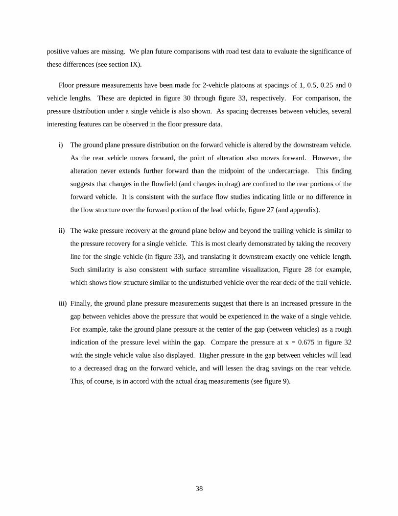
38

positive values are missing. We plan future comparisons with road test data to evaluate the significance of

these differences (see section IX).

Floor pressure measurements have been made for 2-vehicle platoons at spacings of 1, 0.5, 0.25 and 0

vehicle lengths. These are depicted in figure 30 through figure 33, respectively. For comparison, the

pressure distribution under a single vehicle is also shown. As spacing decreases between vehicles, several

interesting features can be observed in the floor pressure data.

i) The ground plane pressure distribution on the forward vehicle is altered by the downstream vehicle.

As the rear vehicle moves forward, the point of alteration also moves forward. However, the

alteration never extends further forward than the midpoint of the undercarriage. This finding

suggests that changes in the flowfield (and changes in drag) are confined to the rear portions of the

forward vehicle. It is consistent with the surface flow studies indicating little or no difference in

the flow structure over the forward portion of the lead vehicle, figure 27 (and appendix).

ii) The wake pressure recovery at the ground plane below and beyond the trailing vehicle is similar to

the pressure recovery for a single vehicle. This is most clearly demonstrated by taking the recovery

line for the single vehicle (in figure 33), and translating it downstream exactly one vehicle length.

Such similarity is also consistent with surface streamline visualization, Figure 28 for example,

which shows flow structure similar to the undisturbed vehicle over the rear deck of the trail vehicle.

iii) Finally, the ground plane pressure measurements suggest that there is an increased pressure in the

gap between vehicles above the pressure that would be experienced in the wake of a single vehicle.

For example, take the ground plane pressure at the center of the gap (between vehicles) as a rough

indication of the pressure level within the gap. Compare the pressure at x = 0.675 in figure 32

with the single vehicle value also displayed. Higher pressure in the gap between vehicles will lead

to a decreased drag on the forward vehicle, and will lessen the drag savings on the rear vehicle.

This, of course, is in accord with the actual drag measurements (see figure 9).

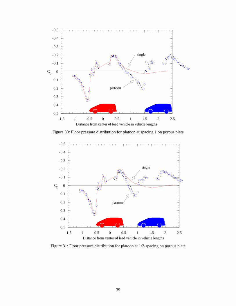
39

ÉÉÉÉÉÉÉÉÉ

É

É

É

ÉÉ

É

É

É

ÉÉ

É

ÉÉ

É

ÉÉÉ

ÉÉÉÉÉÉÉÉÉÉÉÉÉÉÉÉÉÉÉÉÉÉÉÉÉÉÉÉÉ

É

É

ÉÉ

ÉÉ

ÉÉÉ ÉÉ

É

ÉÉÉÉÉÉÉÉÉÉÉ

ÉÉÉÉÉÉÉÉÉ

0.5

0.4

0.3

0.2

0.1

0

-0.1

-0.2

-0.3

-0.4

-0.5

-1.5 -1 -0.5 0 0.5 1 1.5 2 2.5

Cp

Distance from center of lead vehicle in vehicle lengths

single

platoon

Figure 30: Floor pressure distribution for platoon at spacing 1 on porous plate

ÉÉÉÉÉÉÉÉÉ

É

É

É

ÉÉ

É

É

É

ÉÉ

É

ÉÉ

ÉÉÉÉ

ÉÉÉÉÉÉÉÉÉÉÉÉÉÉÉÉÉ

É

É

ÉÉÉÉ

ÉÉÉ ÉÉÉ

É

ÉÉÉÉÉÉÉÉÉÉ

ÉÉÉÉÉÉÉÉÉ

0.5

0.4

0.3

0.2

0.1

0

-0.1

-0.2

-0.3

-0.4

-0.5

-1.5 -1 -0.5 0 0.5 1 1.5 2 2.5

Cp

Distance from center of lead vehicle in vehicle lengths

platoon

single

Figure 31: Floor pressure distribution for platoon at 1/2-spacing on porous plate

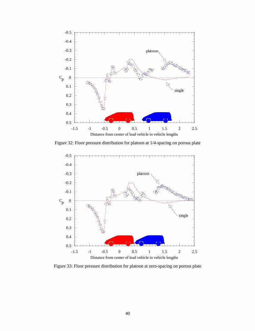
40

ÉÉÉÉÉÉÉÉÉ

É

É

É

ÉÉ

É

É

É

ÉÉ

É

ÉÉ

É

ÉÉÉ

ÉÉÉÉÉÉÉÉÉ

ÉÉÉ

ÉÉÉÉÉÉÉÉÉ

ÉÉÉÉÉÉÉÉÉÉÉÉÉÉÉÉÉÉÉÉÉÉÉ

0.5

0.4

0.3

0.2

0.1

0

-0.1

-0.2

-0.3

-0.4

-0.5

-1.5 -1 -0.5 0 0.5 1 1.5 2 2.5

Cp

Distance from center of lead vehicle in vehicle lengths

single

platoon

Figure 32: Floor pressure distribution for platoon at 1/4-spacing on porous plate

ÉÉÉÉÉÉÉÉÉ

É

É

É

ÉÉ

É

É

É

ÉÉ

É

ÉÉ

ÉÉÉÉ

ÉÉÉÉÉÉÉÉ

ÉÉÉ

ÉÉÉÉ

ÉÉÉ

É

ÉÉÉ

ÉÉÉ

ÉÉÉÉÉÉÉÉÉÉÉÉÉÉÉÉÉÉ

ÉÉÉÉÉÉÉÉÉÉ

0.5

0.4

0.3

0.2

0.1

0

-0.1

-0.2

-0.3

-0.4

-0.5

-1.5 -1 -0.5 0 0.5 1 1.5 2 2.5

Cp

Distance from center of lead vehicle in vehicle lengths

single

platoon

Figure 33: Floor pressure distribution for platoon at zero-spacing on porous plate

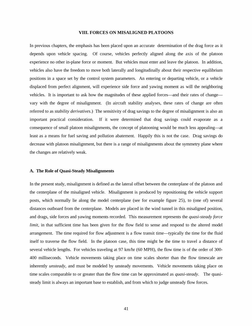
41

VIII. FORCES ON MISALIGNED PLATOONS

In previous chapters, the emphasis has been placed upon an accurate determination of the drag force as it

depends upon vehicle spacing. Of course, vehicles perfectly aligned along the axis of the platoon

experience no other in-plane force or moment. But vehicles must enter and leave the platoon. In addition,

vehicles also have the freedom to move both laterally and longitudinally about their respective equilibrium

positions in a space set by the control system parameters. An entering or departing vehicle, or a vehicle

displaced from perfect alignment, will experience side force and yawing moment as will the neighboring

vehicles. It is important to ask how the magnitudes of these applied forces—and their rates of change—

vary with the degree of misalignment. (In aircraft stability analyses, these rates of change are often

referred to as stability derivatives.) The sensitivity of drag savings to the degree of misalignment is also an

important practical consideration. If it were determined that drag savings could evaporate as a

consequence of small platoon misalignments, the concept of platooning would be much less appealing—at

least as a means for fuel saving and pollution abatement. Happily this is not the case. Drag savings do

decrease with platoon misalignment, but there is a range of misalignments about the symmetry plane where

the changes are relatively weak.

A. The Role of Quasi-Steady Misalignments

In the present study, misalignment is defined as the lateral offset between the centerplane of the platoon and

the centerplane of the misaligned vehicle. Misalignment is produced by repositioning the vehicle support

posts, which normally lie along the model centerplane (see for example figure 25), to (one of) several

distances outboard from the centerplane. Models are placed in the wind tunnel in this misaligned position,

and drags, side forces and yawing moments recorded. This measurement represents the quasi-steady force

limit, in that sufficient time has been given for the flow field to sense and respond to the altered model

arrangement. The time required for flow adjustment is a flow transit time—typically the time for the fluid

itself to traverse the flow field. In the platoon case, this time might be the time to travel a distance of

several vehicle lengths. For vehicles traveling at 97 km/hr (60 MPH), the flow time is of the order of 300-

400 milliseconds. Vehicle movements taking place on time scales shorter than the flow timescale are

inherently unsteady, and must be modeled by unsteady movements. Vehicle movements taking place on

time scales comparable to or greater than the flow time can be approximated as quasi-steady. The quasi-

steady limit is always an important base to establish, and from which to judge unsteady flow forces.

42

Drag, side force, and yawing moment are measured following the same sign conventions described in

section IIB. The yawing moment is measured about the center of the force balance. This point lies in the

vehicle centerplane at a distance of 0.535±.003 vehicle lengths behind the front bumper. Forces are non-

dimensionalized in the usual manner, except that the yawing moment requires an extra length. This scale is

taken to be the square root of the model frontal area, so the following equation is obtained for moment

coefficient.

CYAWING MOMENT

V AY =

12

2 32ρ

When presenting results, it is desired to have the side forces and yawing moments expressed as a

percentage of model drag (in isolation in the wind tunnel). This is accomplished simply by dividing the side

force and yawing moment coefficients by the single vehicle drag coefficient.

B. Special Procedures

It is possible to misalign one vehicle in the platoon by 0.032, 0.067, 0.099 and 0.135 meters from the

centerplane, corresponding to 0.135, 0.287, 0.423 and 0.575 vehicle widths respectively. These odd

distances are a limitation imposed by the necessity of finding satisfactory positions for new holes in the

bottom of the force balance. After altering the mounting post positions, the models are calibrated, making

sure that the drag force is applied along the centerline of the models. The resulting calibrations for all

misalignments show good repeatability—comparable to the previous cases discussed in Zabat et al. (1994).

The bulk of the measurements—those presented in the appendix in tabular form—have been recorded

for the three-vehicle platoon. The three-vehicle platoon, consisting of a lead, a trail, and one interior

vehicle, is the shortest platoon to contain all the essential platoon elements. Even with only three vehicles,

the number of possible misalignment arrangements is large. We have chosen what we think to be the most

representative case—the interior vehicle is misaligned while the lead and trail vehicles remain aligned.

Drag, side force and yawing moment are measured on each of the three vehicles as the central (interior)

vehicle is progressively misaligned. The process is repeated for all eight values of vehicle spacing lying

within the range 0-1.0. Values of vehicle spacing are always the same between the lead and interior vehicle

and between the interior and trail vehicle.

The results are presented in the form of contour maps in the two-dimensional space represented by

vehicle spacing and misalignment. Contours are either drag coefficient ratio, side force coefficient ratio, or

43

yawing moment coefficient ratio. The maps are generated from the discrete data by means of linear

interpolation in two dimensions. The present results should be viewed as preliminary—particularly for side

force and yawing moment, because the values observed are small and difficult to measure. Typical side

force and yawing moment values are of the order of 0.05−0.10 of the single vehicle drag value, which is a

small fraction of the design range of the instrument. A typical measurement error of 0.005x(Full Scale)

becomes an error twenty times larger when judged against an amplitude of 0.05x(Full Scale). In addition,

the number of measurement points—typically forty per plot—are insufficient to provide smooth

contouring. We have since determined a better way to make the measurements, which involves

modification of the vehicle supports to allow positioning of the models under computer control. The

expanded results will be more complete and more accurate, and will be accomplished as a part of the

unsteady force measurement program discussed in section IX.

C. Drag Contour Maps

Drag contours for each of the three vehicles in the platoon are presented separately in figure 34 (a), (b) and

(c). Several tentative conclusions can be drawn.

i) For any spacing and for all three vehicles, the lowest value of drag occurs at zero misalignment. This

is to be expected. The single exception might be in the region 0.75-1.0 spacing, where the interior

vehicle shows a slight off-axis minimum at a misalignment of about 0.15 vehicle widths. We are not

presently convinced this is a real effect. More importantly, since the drag coefficient ratio must be an

even function of misalignment, there will always be a region of modest drag variation near the

centerplane. Our measurements suggest that for values of misalignment less that about ±0.1 vehicle

widths, the drag coefficients variation is small.

ii) Over most of the range of spacings, the drag ratio for the lead vehicle is more sensitive to changes in

spacing than to changes in misalignment. This is reflected in contours which appear mostly horizontal.

The drag ratio for the interior vehicle is much more sensitive to misalignment; this sensitivity is

reflected in contours which are mostly vertical. The drag ratio for the trail vehicle falls between these

behaviors, and displays the least variation with either spacing or misalignment.

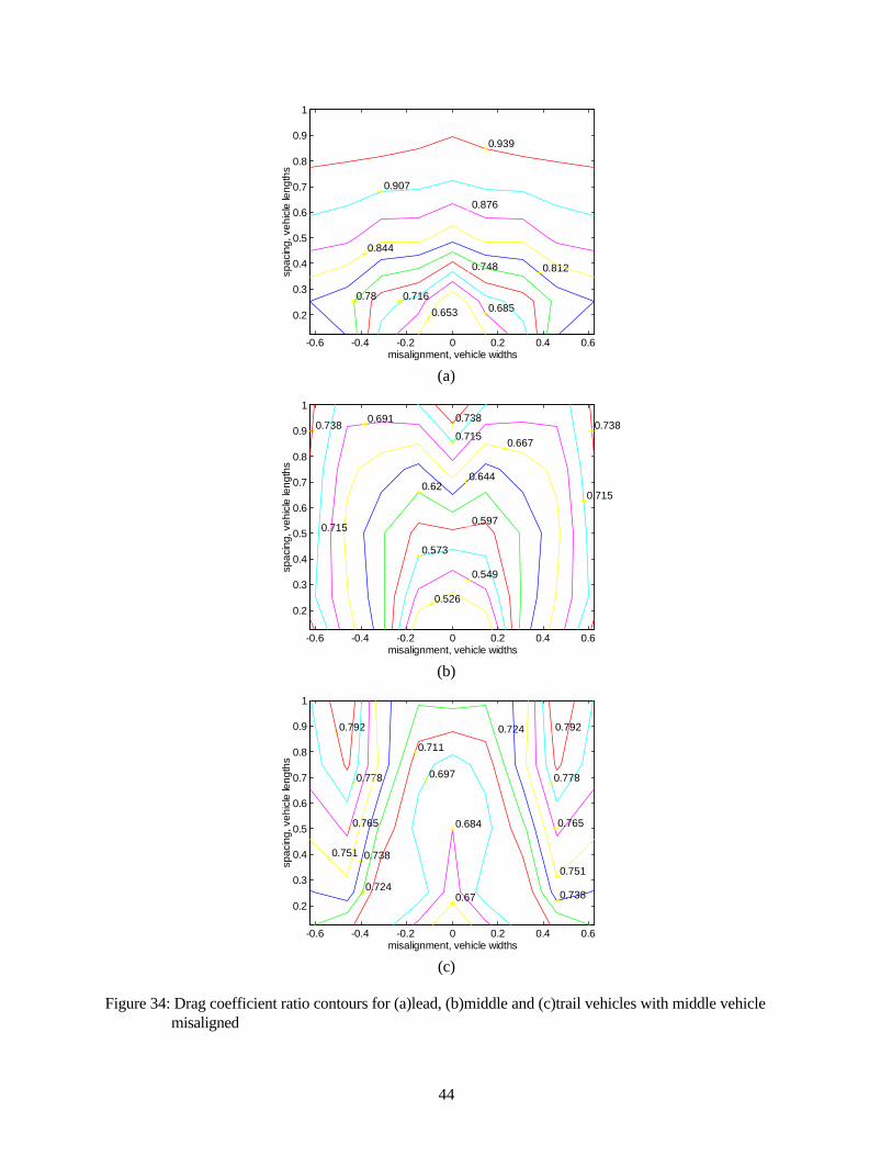
44

-0.6 -0.4 -0.2 0 0.2 0.4 0.6

0.2

0.3

0.4

0.5

0.6

0.7

0.8

0.9

1

misalignment, vehicle widths

spac

ing,

veh

icle

leng

ths

0.653 0.685 0.716

0.748

0.78

0.812

0.844

0.876

0.907

0.939

(a)

-0.6 -0.4 -0.2 0 0.2 0.4 0.6

0.2

0.3

0.4

0.5

0.6

0.7

0.8

0.9

1

misalignment, vehicle widths

spac

ing,

veh

icle

leng

ths

0.738

0.715

0.691

0.667

0.644 0.62

0.597

0.573

0.549

0.526

0.738

0.715

0.715

0.738

(b)

-0.6 -0.4 -0.2 0 0.2 0.4 0.6

0.2

0.3

0.4

0.5

0.6

0.7

0.8

0.9

1

misalignment, vehicle widths

spac

ing,

veh

icle

leng

ths

0.792

0.778

0.765

0.738 0.751

0.724

0.711

0.697

0.684

0.67

0.724 0.792

0.778

0.765

0.751

0.738

(c)

Figure 34: Drag coefficient ratio contours for (a)lead, (b)middle and (c)trail vehicles with middle vehiclemisaligned

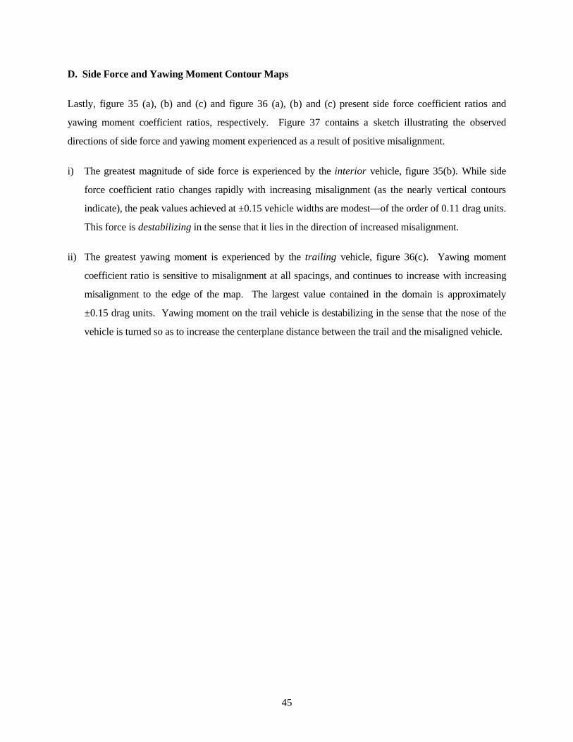
45

D. Side Force and Yawing Moment Contour Maps

Lastly, figure 35 (a), (b) and (c) and figure 36 (a), (b) and (c) present side force coefficient ratios and

yawing moment coefficient ratios, respectively. Figure 37 contains a sketch illustrating the observed

directions of side force and yawing moment experienced as a result of positive misalignment.

i) The greatest magnitude of side force is experienced by the interior vehicle, figure 35(b). While side

force coefficient ratio changes rapidly with increasing misalignment (as the nearly vertical contours

indicate), the peak values achieved at ±0.15 vehicle widths are modest—of the order of 0.11 drag units.

This force is destabilizing in the sense that it lies in the direction of increased misalignment.

ii) The greatest yawing moment is experienced by the trailing vehicle, figure 36(c). Yawing moment

coefficient ratio is sensitive to misalignment at all spacings, and continues to increase with increasing

misalignment to the edge of the map. The largest value contained in the domain is approximately

±0.15 drag units. Yawing moment on the trail vehicle is destabilizing in the sense that the nose of the

vehicle is turned so as to increase the centerplane distance between the trail and the misaligned vehicle.

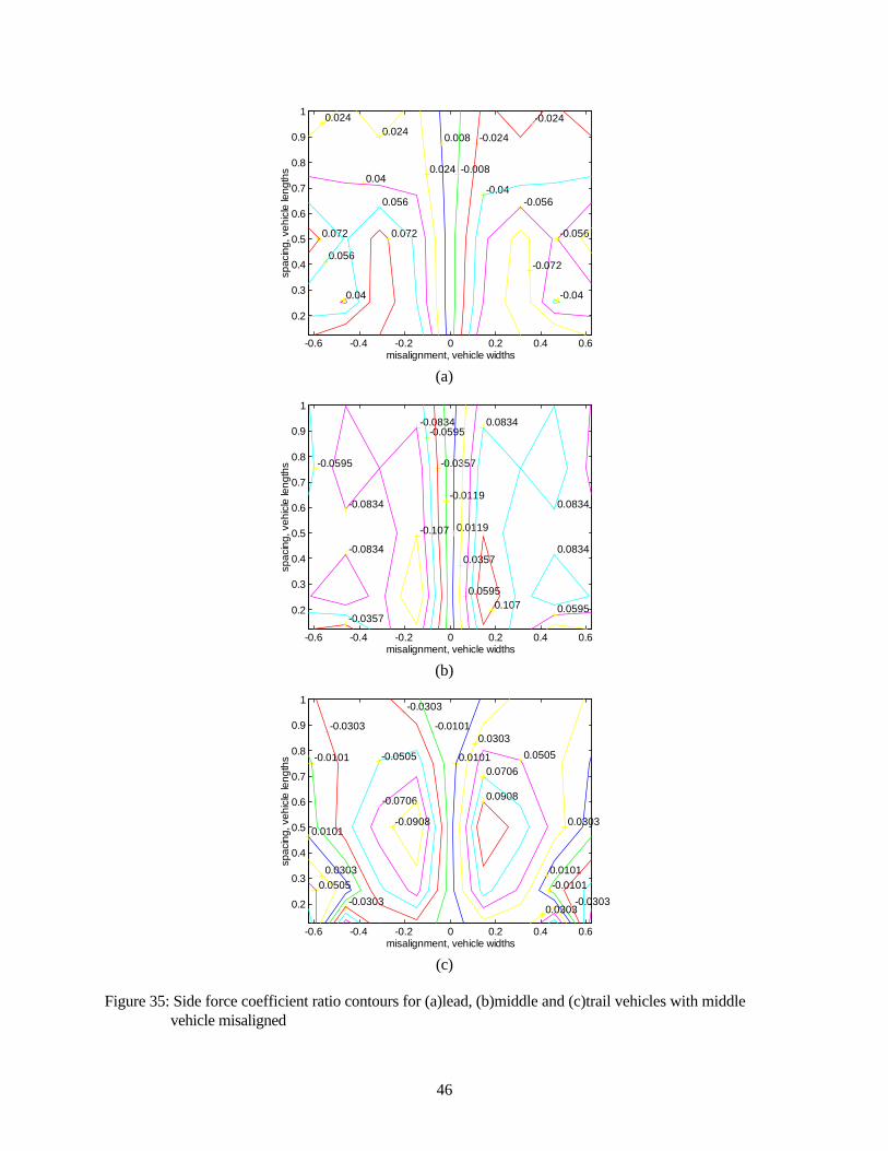
46

-0.6 -0.4 -0.2 0 0.2 0.4 0.6

0.2

0.3

0.4

0.5

0.6

0.7

0.8

0.9

1

misalignment, vehicle widths

spac

ing,

veh

icle

leng

ths

0.008

-0.008 0.024

-0.04

-0.024

0.04

-0.056

-0.056

-0.072 0.056

0.072 0.072

0.056

0.024 -0.024 0.024

0.04 -0.04

(a)

-0.6 -0.4 -0.2 0 0.2 0.4 0.6

0.2

0.3

0.4

0.5

0.6

0.7

0.8

0.9

1

misalignment, vehicle widths

spac

ing,

veh

icle

leng

ths

-0.0834 -0.0595

-0.0357

-0.0119

0.0119

0.0357

0.0595 0.107

0.0834

0.0834

0.0834

0.0595 -0.0357

-0.0834

-0.0834

-0.107

-0.0595

(b)

-0.6 -0.4 -0.2 0 0.2 0.4 0.6

0.2

0.3

0.4

0.5

0.6

0.7

0.8

0.9

1

misalignment, vehicle widths

spac

ing,

veh

icle

leng

ths

-0.0101

-0.0303

0.0303

0.0101

-0.0303

-0.0101

0.0101

0.0303 0.0505

-0.0303

-0.0505

-0.0706

-0.0908

0.0908

0.0706

0.0505

0.0303

0.0101 -0.0101

-0.0303 0.0303

(c)

Figure 35: Side force coefficient ratio contours for (a)lead, (b)middle and (c)trail vehicles with middlevehicle misaligned

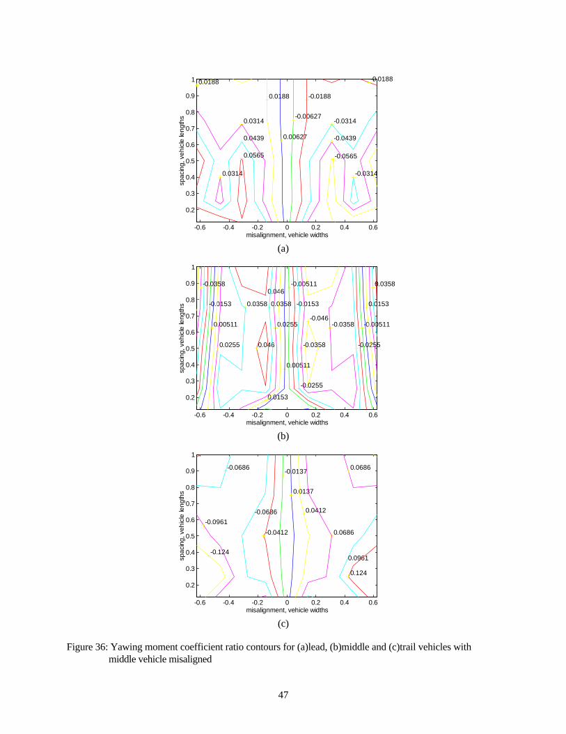
47

-0.6 -0.4 -0.2 0 0.2 0.4 0.6

0.2

0.3

0.4

0.5

0.6

0.7

0.8

0.9

1

misalignment, vehicle widths

spac

ing,

veh

icle

leng

ths

0.0188

0.00627

-0.00627

-0.0188

-0.0314

-0.0439

-0.0565

-0.0314

0.0314

0.0439

0.0314

0.0565

0.0188 -0.0188

(a)

-0.6 -0.4 -0.2 0 0.2 0.4 0.6

0.2

0.3

0.4

0.5

0.6

0.7

0.8

0.9

1

misalignment, vehicle widths

spac

ing,

veh

icle

leng

ths

-0.00511

-0.0153

-0.046

-0.0358

-0.0255

0.0153

0.00511

0.0255

0.046

0.0358

0.046

0.0358

-0.0358

0.0255 -0.0255

0.00511 -0.00511

-0.0153 0.0153

-0.0358 0.0358

(b)

-0.6 -0.4 -0.2 0 0.2 0.4 0.6

0.2

0.3

0.4

0.5

0.6

0.7

0.8

0.9

1

misalignment, vehicle widths

spac

ing,

veh

icle

leng

ths

-0.0137

0.0137

0.0412

0.0686

0.0961

0.124

0.0686 -0.0686

-0.0961

-0.124

-0.0686

-0.0412

(c)

Figure 36: Yawing moment coefficient ratio contours for (a)lead, (b)middle and (c)trail vehicles withmiddle vehicle misaligned

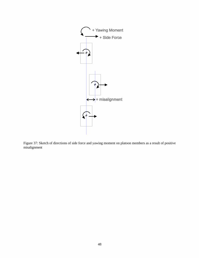
48

Figure 37: Sketch of directions of side force and yawing moment on platoon members as a result of positivemisalignment

49

IX. ADDITIONAL RESEARCH GOALS

This report and the earlier PATH report summarize a three-year project on experimental measurements of

the aerodynamics of platoons. Three papers emphasizing the most important findings to date have been

presented at conferences, and should be considered part of the written record. They are Zabat et al.

(1994b), (1995) and (1995b). Additional results will be added to the present findings over the coming

several years to provide a more complete picture of platoon operation. The following items have either

been proposed for study or are actually underway.

i) Definition of intervehicle flowfields. Measurements presented here document forces and yawing

moments, but do not provide explanations for how these forces and moments are achieved. A more

detailed understanding is required to extrapolate the present results with confidence to other, related

situations. Knowledge of inter-vehicle flowfields is also important to insure adequate engine and

passenger compartment airflows. Several means for determining the detailed inter-vehicle flowfield

include: additional investigations of surface streamline flow patterns; flowfield visualizations

utilizing "fog juice"; and the mapping of local flow velocity and flow direction in regions between

vehicles using 7-hole cone probes and hot wires.

ii) Characterization of unsteady forces. The steady forces we have discussed represent the mean or

averaged values. There are additional unsteady force components which can be significant at high

speedsparticularly for vehicles traveling in the near wake of another vehicle. For platoon

operation, the unsteady force components are expected to be significant for control system design

when vehicles are operating within the strongly interacting regime (spacing less than one vehicle

length). We have also identified certain, unusual spacings for which gap width and turbulent

structure in the separating flow "resonate" to produce dramatic variations in drag coefficient over

very short distances (see page 27). For control system purposes, it will be particularly important to

document the aerodynamic loads associated with such resonances. As an additional part of this

study, the forces and moments arising from platoon misalignment will be repeated with better spatial

resolution. These results will extend the preliminary results described in section VIII.

iii) Measurements of aerodynamic forces in a crosswind. The presence of a crosswind is another

important platoon misalignment. The present wind tunnel set-up has provision for a ten degree yaw

50

of the platoon direction with respect to the axis of the wind tunnel. At 100 km/hr (60 MPH), ten

degrees of yaw simulates the effect of an 18 km/hr (11 MPH) sidewind.

iv) Full-scale platoon measurements of drag and cooling flow. The wind tunnel tests described here

are being conducted at Reynolds numbers about an order of magnitude lower than those experienced

under full-scale conditions. Other differences between model and full-scale include: the lack of

model underbody and trim detail, the lack of rotating wheels, and the unwanted wind tunnel ground

plane boundary layer. In spite of the high quality of the measurements taken in the wind tunnel, these

differences will always reflect uncertainty in translating model results to full-scale operating

conditions. To make a stronger connection between model and prototype, we propose a limited series

of drag measurements for 2, 3 and 4 vehicle platoons operating at full-scale on a roadway (a test

track). Additional valuable information on cooling flow rate and engine compartment temperature

can be collected during platoon operation. This will provide actual data for corroboration of the

wind tunnel intervehicle flow field studies. Ground plane pressure distributions will also be recorded

by driving the platoon over a fixed pressure sensor located on the roadway (test track). These

ground plane pressure distributions provide information about the underbody flow field, and can

readily be compared to the pressure distributions measured in the wind tunnel.

51

REFERENCES

Hornung, H. G., Perry, A. E., 1984, Some Aspects of Three-Dimensional Separation, Part I:Streamsurface Bifurcations, Z. Flugwiss. Weltraumforsch. 8: 77-87

Hucho, W.-H., Sovran, G., 1993, Aerodynamics of Road Vehicles, Annu. Rev. Fluid Mech. 25: 485-537

Perry, A. E., Hornung, H. G., 1984, Some Aspects of Three-Dimensional Separation, Part II: VortexSkeletons, Z. Flugwiss. Weltraumforsch. 8: 155-160

Perry, A. E., Chong, M. S., 1987, A Description of Eddying Motions and Flow Patterns Using Critical-Point Concepts, Annu. Rev. Fluid Mech. 19: 125-155

Sovran, G., 1983, Tractive-Energy-Based Formulae for the Impact of Aerodynamics on Fuel EconomyOver the EPA Driving Schedules, SAE Paper No. 830304

Zabat, M., Frascaroli, S., Browand, F., 1994, Drag Measurements on a Platoon of Vehicles, PATHResearch Paper No. UCB-ITS-PRR-93-27

Zabat, M., Frascaroli, S., Browand, F., 1994b, Drag Measurements on 2, 3 & 4-Car Platoons, SAE PaperNo. 940421

Zabat, M., Stabile, N., Frascaroli, S., Browand, F., 1995, Drag Forces Experienced by 2, 3 & 4-VehiclePlatoons at Close Spacings, SAE Paper No. 950632

Zabat, M., Stabile, N., Browand, F., 1995b, Estimates of Fuel Savings from Platooning, Proceedings ofthe 5th Annual ITS America Meeting, Washington, D. C.

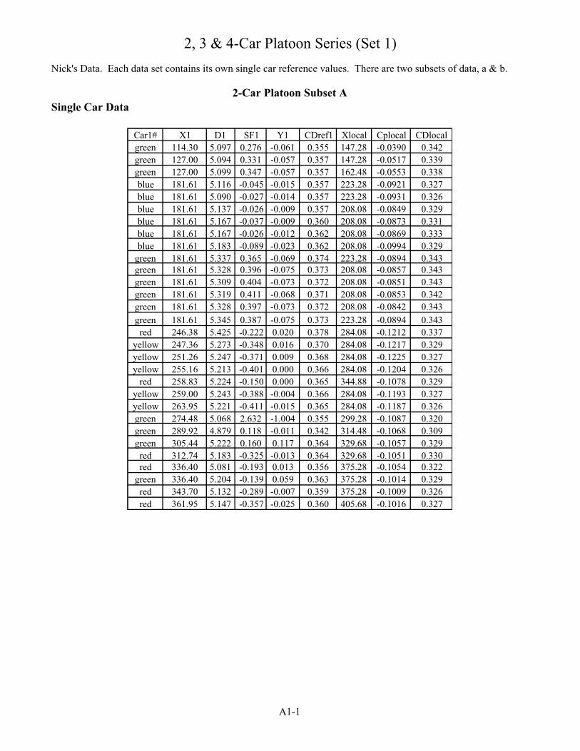
A1-1

2, 3 & 4-Car Platoon Series (Set 1)

Nick's Data. Each data set contains its own single car reference values. There are two subsets of data, a & b.

2-Car Platoon Subset ASingle Car Data

Car1# X1 D1 SF1 Y1 CDref1 Xlocal Cplocal CDlocalgreen 114.30 5.097 0.276 -0.061 0.355 147.28 -0.0390 0.342green 127.00 5.094 0.331 -0.057 0.357 147.28 -0.0517 0.339green 127.00 5.099 0.347 -0.057 0.357 162.48 -0.0553 0.338blue 181.61 5.116 -0.045 -0.015 0.357 223.28 -0.0921 0.327blue 181.61 5.090 -0.027 -0.014 0.357 223.28 -0.0931 0.326blue 181.61 5.137 -0.026 -0.009 0.357 208.08 -0.0849 0.329blue 181.61 5.167 -0.037 -0.009 0.360 208.08 -0.0873 0.331blue 181.61 5.167 -0.026 -0.012 0.362 208.08 -0.0869 0.333blue 181.61 5.183 -0.089 -0.023 0.362 208.08 -0.0994 0.329

green 181.61 5.337 0.365 -0.069 0.374 223.28 -0.0894 0.343green 181.61 5.328 0.396 -0.075 0.373 208.08 -0.0857 0.343green 181.61 5.309 0.404 -0.073 0.372 208.08 -0.0851 0.343green 181.61 5.319 0.411 -0.068 0.371 208.08 -0.0853 0.342green 181.61 5.328 0.397 -0.073 0.372 208.08 -0.0842 0.343green 181.61 5.345 0.387 -0.075 0.373 223.28 -0.0894 0.343red 246.38 5.425 -0.222 0.020 0.378 284.08 -0.1212 0.337

yellow 247.36 5.273 -0.348 0.016 0.370 284.08 -0.1217 0.329yellow 251.26 5.247 -0.371 0.009 0.368 284.08 -0.1225 0.327yellow 255.16 5.213 -0.401 0.000 0.366 284.08 -0.1204 0.326

red 258.83 5.224 -0.150 0.000 0.365 344.88 -0.1078 0.329yellow 259.00 5.243 -0.388 -0.004 0.366 284.08 -0.1193 0.327yellow 263.95 5.221 -0.411 -0.015 0.365 284.08 -0.1187 0.326green 274.48 5.068 2.632 -1.004 0.355 299.28 -0.1087 0.320green 289.92 4.879 0.118 -0.011 0.342 314.48 -0.1068 0.309green 305.44 5.222 0.160 0.117 0.364 329.68 -0.1057 0.329red 312.74 5.183 -0.325 -0.013 0.364 329.68 -0.1051 0.330red 336.40 5.081 -0.193 0.013 0.356 375.28 -0.1054 0.322

green 336.40 5.204 -0.139 0.059 0.363 375.28 -0.1014 0.329red 343.70 5.132 -0.289 -0.007 0.359 375.28 -0.1009 0.326red 361.95 5.147 -0.357 -0.025 0.360 405.68 -0.1016 0.327

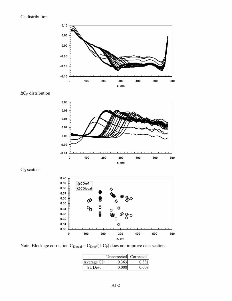
A1-2

CP distribution

x, cm

-0.15

-0.10

-0.05

0.00

0.05

0.10

0 100 200 300 400 500 600

∆CP distribution

x, cm

DC

-0.04

-0.02

0.00

0.02

0.04

0.06

0.08

0 100 200 300 400 500 600

CD scatter

x, cm

0.30

0.31

0.32

0.33

0.34

0.35

0.36

0.37

0.38

0.39

0.40

0 100 200 300 400 500 600

CDref

CDlocal

Note: Blockage correction CDlocal = CDref/(1-CP) does not improve data scatter.

Uncorrected CorrectedAverage CD 0.363 0.331

St. Dev. 0.008 0.008

A1-3

2-Car Platoon Data

Spacing Car1 X1 D1 SF1 Y1 CDref1 CDref_inf1 CD/CDref1 Xlocal1 Cplocal1 CDloc1 CDloc_inf1 CD/CDloc10.046 green 181.61 3.120 1.066 0.558 0.219 0.373 0.586 208.08 -0.0943 0.200 0.343 0.5820.062 green 181.61 3.504 -0.556 -0.207 0.245 0.373 0.657 208.08 -0.0949 0.224 0.343 0.6530.125 green 181.61 3.488 -0.389 -0.173 0.244 0.373 0.655 208.08 -0.0934 0.223 0.343 0.6510.188 green 181.61 3.410 0.209 -0.096 0.239 0.373 0.640 208.08 -0.0930 0.218 0.343 0.6370.250 blue 181.61 4.943 -0.042 -0.016 0.344 0.358 0.961 208.08 -0.0857 0.317 0.329 0.9640.250 green 181.61 3.432 0.392 -0.075 0.241 0.373 0.645 208.08 -0.0897 0.221 0.343 0.6430.330 green 181.61 3.812 0.354 -0.073 0.266 0.373 0.714 208.08 -0.0894 0.244 0.343 0.7130.500 blue 181.61 4.392 -0.107 -0.020 0.306 0.358 0.854 208.08 -0.0878 0.281 0.329 0.8550.750 blue 181.61 4.811 -0.057 -0.018 0.336 0.358 0.937 208.08 -0.0857 0.309 0.329 0.9391.000 blue 181.61 4.994 -0.038 -0.012 0.348 0.358 0.973 208.08 -0.0844 0.321 0.329 0.9761.499 blue 181.61 5.045 -0.036 -0.015 0.354 0.358 0.989 208.08 -0.0853 0.326 0.329 0.9921.501 blue 181.61 5.098 -0.047 -0.017 0.354 0.358 0.989 208.08 -0.0837 0.327 0.329 0.9932.001 green 127.00 5.079 0.323 -0.057 0.356 0.357 0.997 162.48 -0.0530 0.338 0.338 1.0002.501 green 127.00 5.082 0.348 -0.056 0.357 0.357 0.999 162.48 -0.0538 0.338 0.338 1.0013.001 green 114.30 5.068 0.272 -0.060 0.355 0.355 0.998 147.28 -0.0380 0.342 0.342 0.999

Spacing Car2 X2 D2 SF2 Y2 CDref2 CDref_inf2 CD/CDref2 Xloc2 Cploc2 CDloc2 CDloc_inf2 CD/CDloc20.046 red 246.38 3.849 0.533 -0.055 0.270 0.378 0.714 268.91 -0.1414 0.236 0.337 0.7010.062 yellow 247.36 3.783 0.285 -0.060 0.265 0.370 0.715 268.91 -0.1420 0.232 0.329 0.7040.125 yellow 251.26 3.962 0.191 -0.040 0.278 0.368 0.754 268.91 -0.1435 0.243 0.327 0.7420.188 yellow 255.16 4.042 -0.096 0.001 0.283 0.366 0.773 268.91 -0.1426 0.248 0.326 0.7600.250 red 258.98 4.001 -0.134 -0.012 0.279 0.365 0.763 329.72 -0.1405 0.244 0.329 0.7420.250 yellow 259.00 4.096 -0.189 0.012 0.287 0.366 0.784 268.91 -0.1432 0.251 0.327 0.7680.330 yellow 263.95 3.985 -0.160 0.012 0.278 0.365 0.763 284.11 -0.1490 0.242 0.326 0.7430.500 green 274.48 3.611 1.796 -0.740 0.251 0.355 0.708 299.31 -0.1404 0.220 0.32 0.6890.750 green 289.92 3.612 0.008 -0.037 0.252 0.342 0.737 299.31 -0.1393 0.221 0.309 0.7161.000 green 305.44 4.168 -0.065 0.108 0.291 0.364 0.799 329.72 -0.1374 0.256 0.329 0.7771.499 red 336.30 4.150 -0.242 0.002 0.291 0.356 0.818 375.32 -0.1375 0.256 0.322 0.7951.501 green 336.40 4.310 -0.236 0.035 0.299 0.329 0.910 375.32 -0.1334 0.264 0.329 0.8032.001 red 312.74 4.463 -0.404 -0.013 0.313 0.364 0.859 344.92 -0.1207 0.279 0.33 0.8462.501 red 343.70 4.430 -0.405 -0.002 0.311 0.359 0.866 390.53 -0.1194 0.278 0.326 0.8523.001 red 361.95 4.458 -0.403 -0.009 0.312 0.360 0.867 390.53 -0.1032 0.283 0.327 0.865

* Note: Shaded items are not plotted below

Uncorrected CD ratios

spacing

CD

0.5

0.6

0.7

0.8

0.9

1

1.1

0 1 2 3 4 5

Car1

Car2

A1-4

CP distribution

x, cm

-0.20

-0.15

-0.10

-0.05

0.00

0.05

0.10

0.15

0 100 200 300 400 500 600

∆CP distribution

x, cm

DC

-0.02

0.00

0.02

0.04

0.06

0.08

0.10

0 100 200 300 400 500 600

Corrected CD ratios

spacing

CDl

0.5

0.6

0.7

0.8

0.9

1.0

1.1

0 1 2 3 4 5

Car 1

Car2

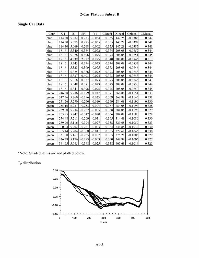
A1-5

2-Car Platoon Subset B

Single Car Data

Car# X 1 D1 SF1 Y1 CDref1 Xlocal Cplocal CDlocalblue 114.30 5.082 0.283 -0.064 0.355 147.28 -0.0388 0.342blue 114.30 5.075 0.293 -0.065 0.355 147.28 -0.0392 0.341blue 114.30 5.069 0.268 -0.062 0.355 147.28 -0.0387 0.341blue 181.61 5.340 0.384 -0.072 0.374 208.08 -0.0857 0.344blue 181.61 5.328 0.406 -0.075 0.374 208.08 -0.0851 0.345blue 181.61 4.839 2.717 0.995 0.340 208.08 -0.0846 0.313blue 181.61 5.343 0.394 -0.073 0.374 208.08 -0.0853 0.344blue 181.61 5.323 0.390 -0.075 0.373 208.08 -0.0846 0.344blue 181.61 5.325 0.386 -0.072 0.373 208.08 -0.0848 0.344blue 181.61 5.337 0.403 -0.074 0.373 208.08 -0.0843 0.344blue 181.61 5.318 0.387 -0.073 0.373 208.08 -0.0845 0.343blue 181.61 5.348 0.381 -0.073 0.373 208.08 -0.0850 0.344blue 181.61 5.341 0.398 -0.075 0.375 208.08 -0.0850 0.345green 246.38 5.286 -0.199 0.017 0.371 268.88 -0.1151 0.333green 247.36 5.260 -0.196 0.023 0.369 268.88 -0.1145 0.331green 251.26 5.270 -0.260 0.010 0.369 284.08 -0.1190 0.330green 255.16 5.257 -0.253 0.004 0.367 284.08 -0.1194 0.328green 259.00 5.234 -0.282 -0.005 0.368 284.08 -0.1193 0.329green 263.95 5.242 -0.342 -0.020 0.366 284.08 -0.1180 0.328green 274.48 5.211 -0.209 -0.031 0.365 314.48 -0.1080 0.330green 289.96 5.116 -0.394 -0.027 0.358 329.68 -0.1059 0.323green 300.04 5.202 -0.281 -0.003 0.364 344.88 -0.1032 0.330green 305.44 5.204 -0.308 -0.011 0.365 329.68 -0.1046 0.330green 331.00 5.167 -0.255 0.002 0.363 375.28 -0.1006 0.329green 336.39 5.176 -0.193 -0.003 0.360 344.88 -0.1006 0.327green 361.95 5.085 -0.368 -0.025 0.358 405.68 -0.1016 0.325

*Note: Shaded items are not plotted below.

CP distribution

x, cm

C

-0.15

-0.10

-0.05

0.00

0.05

0.10

0 100 200 300 400 500 600

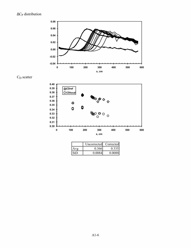
A1-6

∆CP distribution

x, cm

DC

-0.04

-0.02

0.00

0.02

0.04

0.06

0.08

0 100 200 300 400 500 600

CD scatter

x, cm

0.30

0.31

0.32

0.33

0.34

0.35

0.36

0.37

0.38

0.39

0.40

0 100 200 300 400 500 600

CDref

CDlocal

Uncorrected CorrectedAvg 0.366 0.335StD 0.0084 0.0088

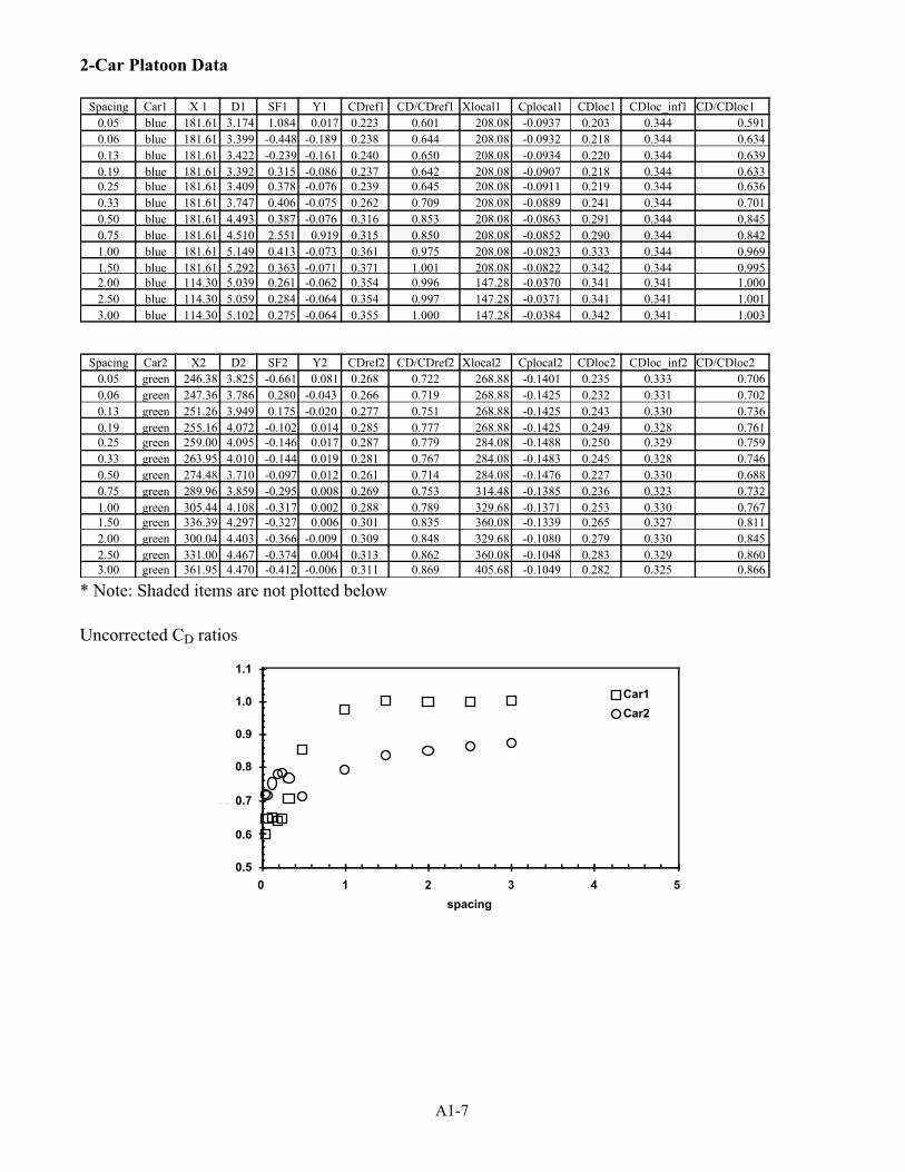
A1-7

2-Car Platoon Data

Spacing Car1 X 1 D1 SF1 Y1 CDref1 CD/CDref1 Xlocal1 Cplocal1 CDloc1 CDloc_inf1 CD/CDloc10.05 blue 181.61 3.174 1.084 0.017 0.223 0.601 208.08 -0.0937 0.203 0.344 0.5910.06 blue 181.61 3.399 -0.448 -0.189 0.238 0.644 208.08 -0.0932 0.218 0.344 0.6340.13 blue 181.61 3.422 -0.239 -0.161 0.240 0.650 208.08 -0.0934 0.220 0.344 0.6390.19 blue 181.61 3.392 0.315 -0.086 0.237 0.642 208.08 -0.0907 0.218 0.344 0.6330.25 blue 181.61 3.409 0.378 -0.076 0.239 0.645 208.08 -0.0911 0.219 0.344 0.6360.33 blue 181.61 3.747 0.406 -0.075 0.262 0.709 208.08 -0.0889 0.241 0.344 0.7010.50 blue 181.61 4.493 0.387 -0.076 0.316 0.853 208.08 -0.0863 0.291 0.344 0.8450.75 blue 181.61 4.510 2.551 0.919 0.315 0.850 208.08 -0.0852 0.290 0.344 0.8421.00 blue 181.61 5.149 0.413 -0.073 0.361 0.975 208.08 -0.0823 0.333 0.344 0.9691.50 blue 181.61 5.292 0.363 -0.071 0.371 1.001 208.08 -0.0822 0.342 0.344 0.9952.00 blue 114.30 5.039 0.261 -0.062 0.354 0.996 147.28 -0.0370 0.341 0.341 1.0002.50 blue 114.30 5.059 0.284 -0.064 0.354 0.997 147.28 -0.0371 0.341 0.341 1.0013.00 blue 114.30 5.102 0.275 -0.064 0.355 1.000 147.28 -0.0384 0.342 0.341 1.003

Spacing Car2 X2 D2 SF2 Y2 CDref2 CD/CDref2 Xlocal2 Cplocal2 CDloc2 CDloc_inf2 CD/CDloc20.05 green 246.38 3.825 -0.661 0.081 0.268 0.722 268.88 -0.1401 0.235 0.333 0.7060.06 green 247.36 3.786 0.280 -0.043 0.266 0.719 268.88 -0.1425 0.232 0.331 0.7020.13 green 251.26 3.949 0.175 -0.020 0.277 0.751 268.88 -0.1425 0.243 0.330 0.7360.19 green 255.16 4.072 -0.102 0.014 0.285 0.777 268.88 -0.1425 0.249 0.328 0.7610.25 green 259.00 4.095 -0.146 0.017 0.287 0.779 284.08 -0.1488 0.250 0.329 0.7590.33 green 263.95 4.010 -0.144 0.019 0.281 0.767 284.08 -0.1483 0.245 0.328 0.7460.50 green 274.48 3.710 -0.097 0.012 0.261 0.714 284.08 -0.1476 0.227 0.330 0.6880.75 green 289.96 3.859 -0.295 0.008 0.269 0.753 314.48 -0.1385 0.236 0.323 0.7321.00 green 305.44 4.108 -0.317 0.002 0.288 0.789 329.68 -0.1371 0.253 0.330 0.7671.50 green 336.39 4.297 -0.327 0.006 0.301 0.835 360.08 -0.1339 0.265 0.327 0.8112.00 green 300.04 4.403 -0.366 -0.009 0.309 0.848 329.68 -0.1080 0.279 0.330 0.8452.50 green 331.00 4.467 -0.374 0.004 0.313 0.862 360.08 -0.1048 0.283 0.329 0.8603.00 green 361.95 4.470 -0.412 -0.006 0.311 0.869 405.68 -0.1049 0.282 0.325 0.866

* Note: Shaded items are not plotted below

Uncorrected CD ratios

spacing

CD

0.5

0.6

0.7

0.8

0.9

1.0

1.1

0 1 2 3 4 5

Car1

Car2

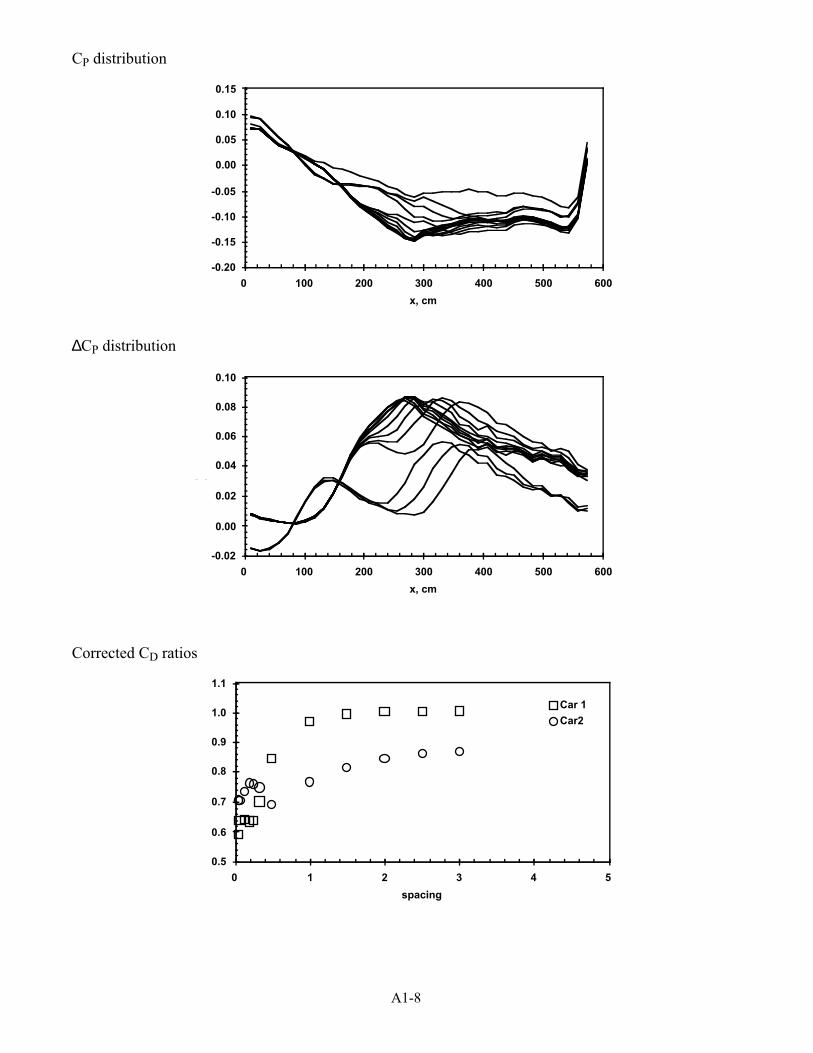
A1-8

CP distribution

x, cm

-0.20

-0.15

-0.10

-0.05

0.00

0.05

0.10

0.15

0 100 200 300 400 500 600

∆CP distribution

x, cm

DC

-0.02

0.00

0.02

0.04

0.06

0.08

0.10

0 100 200 300 400 500 600

Corrected CD ratios

spacing

CDl

0.5

0.6

0.7

0.8

0.9

1.0

1.1

0 1 2 3 4 5

Car 1

Car2

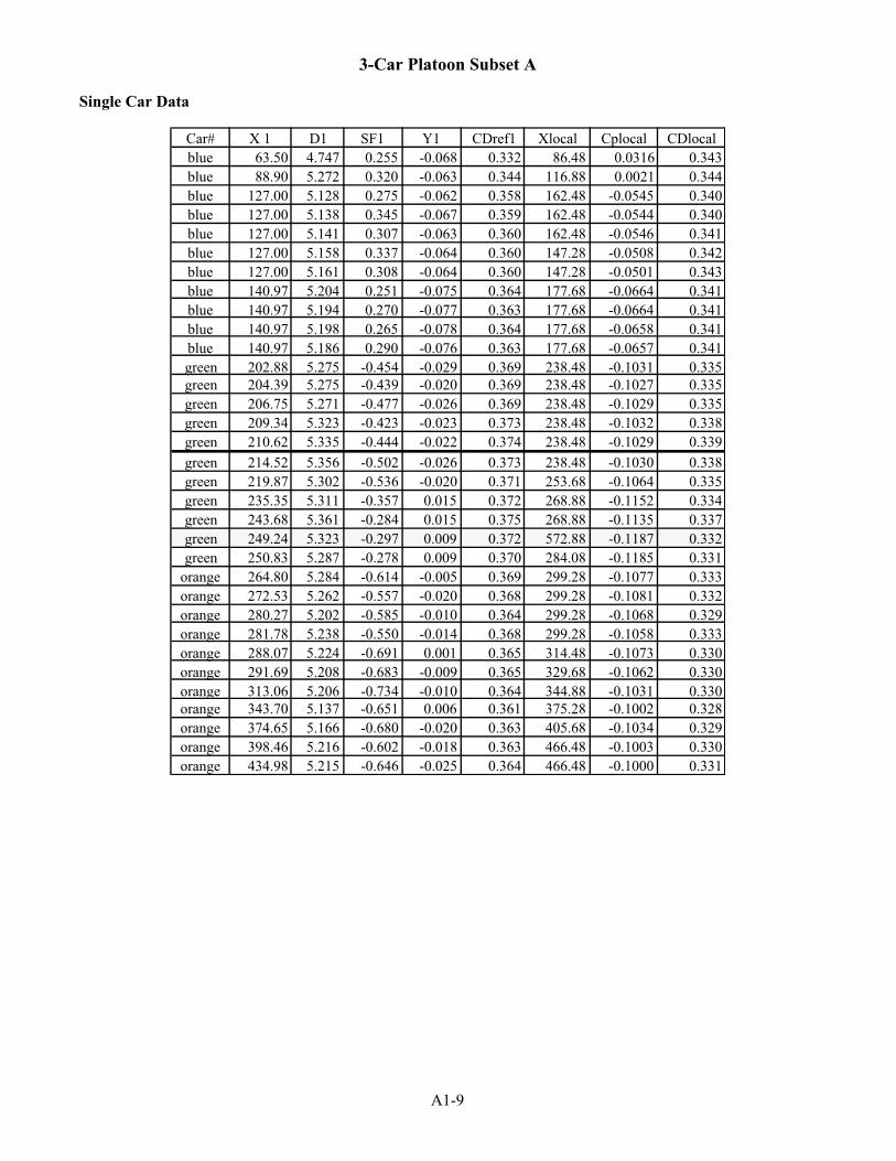
A1-9

3-Car Platoon Subset A

Single Car Data

Car# X 1 D1 SF1 Y1 CDref1 Xlocal Cplocal CDlocalblue 63.50 4.747 0.255 -0.068 0.332 86.48 0.0316 0.343blue 88.90 5.272 0.320 -0.063 0.344 116.88 0.0021 0.344blue 127.00 5.128 0.275 -0.062 0.358 162.48 -0.0545 0.340blue 127.00 5.138 0.345 -0.067 0.359 162.48 -0.0544 0.340blue 127.00 5.141 0.307 -0.063 0.360 162.48 -0.0546 0.341blue 127.00 5.158 0.337 -0.064 0.360 147.28 -0.0508 0.342blue 127.00 5.161 0.308 -0.064 0.360 147.28 -0.0501 0.343blue 140.97 5.204 0.251 -0.075 0.364 177.68 -0.0664 0.341blue 140.97 5.194 0.270 -0.077 0.363 177.68 -0.0664 0.341blue 140.97 5.198 0.265 -0.078 0.364 177.68 -0.0658 0.341blue 140.97 5.186 0.290 -0.076 0.363 177.68 -0.0657 0.341green 202.88 5.275 -0.454 -0.029 0.369 238.48 -0.1031 0.335green 204.39 5.275 -0.439 -0.020 0.369 238.48 -0.1027 0.335green 206.75 5.271 -0.477 -0.026 0.369 238.48 -0.1029 0.335green 209.34 5.323 -0.423 -0.023 0.373 238.48 -0.1032 0.338green 210.62 5.335 -0.444 -0.022 0.374 238.48 -0.1029 0.339green 214.52 5.356 -0.502 -0.026 0.373 238.48 -0.1030 0.338green 219.87 5.302 -0.536 -0.020 0.371 253.68 -0.1064 0.335green 235.35 5.311 -0.357 0.015 0.372 268.88 -0.1152 0.334green 243.68 5.361 -0.284 0.015 0.375 268.88 -0.1135 0.337green 249.24 5.323 -0.297 0.009 0.372 572.88 -0.1187 0.332green 250.83 5.287 -0.278 0.009 0.370 284.08 -0.1185 0.331

orange 264.80 5.284 -0.614 -0.005 0.369 299.28 -0.1077 0.333orange 272.53 5.262 -0.557 -0.020 0.368 299.28 -0.1081 0.332orange 280.27 5.202 -0.585 -0.010 0.364 299.28 -0.1068 0.329orange 281.78 5.238 -0.550 -0.014 0.368 299.28 -0.1058 0.333orange 288.07 5.224 -0.691 0.001 0.365 314.48 -0.1073 0.330orange 291.69 5.208 -0.683 -0.009 0.365 329.68 -0.1062 0.330orange 313.06 5.206 -0.734 -0.010 0.364 344.88 -0.1031 0.330orange 343.70 5.137 -0.651 0.006 0.361 375.28 -0.1002 0.328orange 374.65 5.166 -0.680 -0.020 0.363 405.68 -0.1034 0.329orange 398.46 5.216 -0.602 -0.018 0.363 466.48 -0.1003 0.330orange 434.98 5.215 -0.646 -0.025 0.364 466.48 -0.1000 0.331

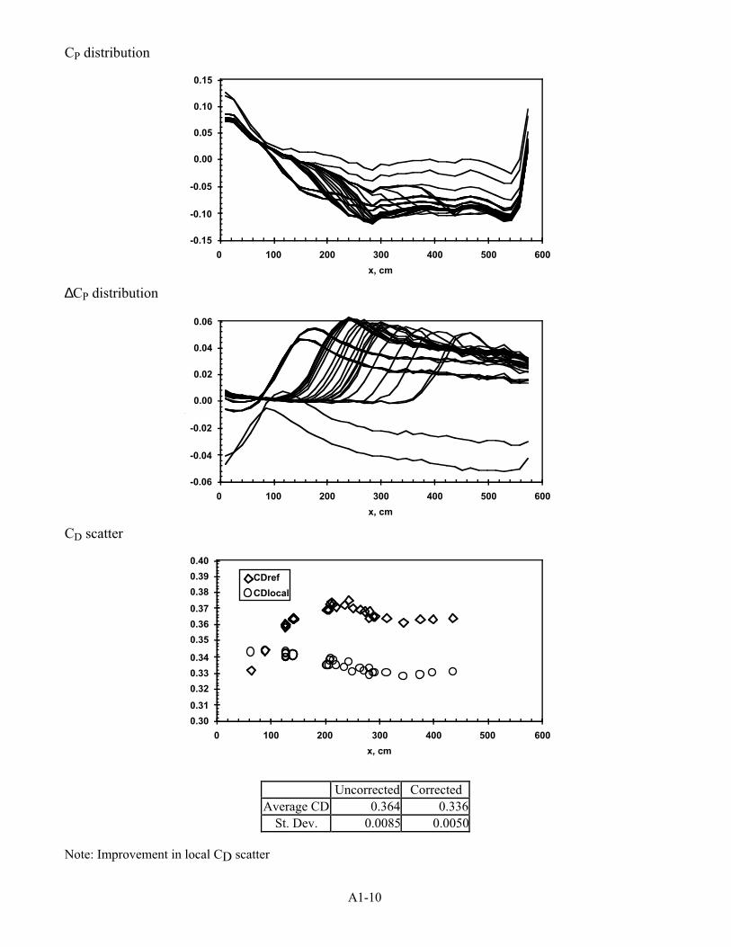
A1-10

CP distribution

x, cm

-0.15

-0.10

-0.05

0.00

0.05

0.10

0.15

0 100 200 300 400 500 600

∆CP distribution

x, cm

DC

-0.06

-0.04

-0.02

0.00

0.02

0.04

0.06

0 100 200 300 400 500 600

CD scatter

x, cm

0.30

0.31

0.32

0.33

0.34

0.35

0.36

0.37

0.38

0.39

0.40

0 100 200 300 400 500 600

CDref

CDlocal

Uncorrected CorrectedAverage CD 0.364 0.336

St. Dev. 0.0085 0.0050

Note: Improvement in local CD scatter

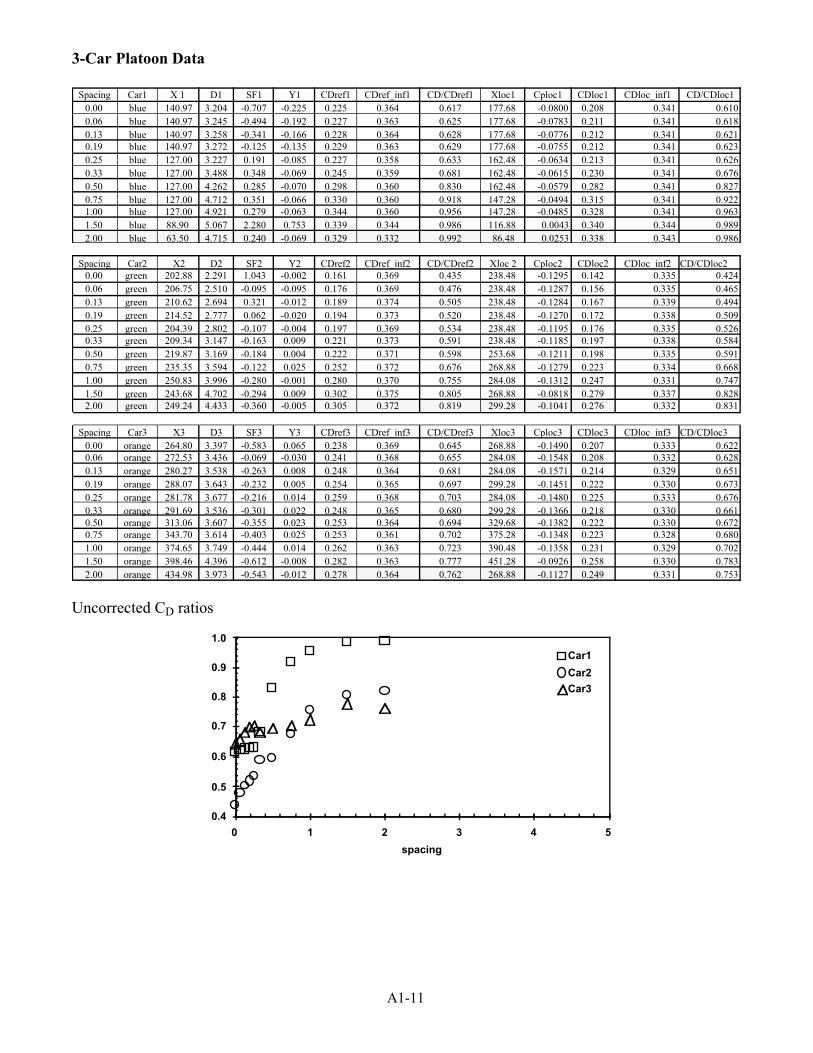
A1-11

3-Car Platoon Data

Spacing Car1 X 1 D1 SF1 Y1 CDref1 CDref_inf1 CD/CDref1 Xloc1 Cploc1 CDloc1 CDloc_inf1 CD/CDloc10.00 blue 140.97 3.204 -0.707 -0.225 0.225 0.364 0.617 177.68 -0.0800 0.208 0.341 0.6100.06 blue 140.97 3.245 -0.494 -0.192 0.227 0.363 0.625 177.68 -0.0783 0.211 0.341 0.6180.13 blue 140.97 3.258 -0.341 -0.166 0.228 0.364 0.628 177.68 -0.0776 0.212 0.341 0.6210.19 blue 140.97 3.272 -0.125 -0.135 0.229 0.363 0.629 177.68 -0.0755 0.212 0.341 0.6230.25 blue 127.00 3.227 0.191 -0.085 0.227 0.358 0.633 162.48 -0.0634 0.213 0.341 0.6260.33 blue 127.00 3.488 0.348 -0.069 0.245 0.359 0.681 162.48 -0.0615 0.230 0.341 0.6760.50 blue 127.00 4.262 0.285 -0.070 0.298 0.360 0.830 162.48 -0.0579 0.282 0.341 0.8270.75 blue 127.00 4.712 0.351 -0.066 0.330 0.360 0.918 147.28 -0.0494 0.315 0.341 0.9221.00 blue 127.00 4.921 0.279 -0.063 0.344 0.360 0.956 147.28 -0.0485 0.328 0.341 0.9631.50 blue 88.90 5.067 2.280 0.753 0.339 0.344 0.986 116.88 0.0043 0.340 0.344 0.9892.00 blue 63.50 4.715 0.240 -0.069 0.329 0.332 0.992 86.48 0.0253 0.338 0.343 0.986

Spacing Car2 X2 D2 SF2 Y2 CDref2 CDref_inf2 CD/CDref2 Xloc 2 Cploc2 CDloc2 CDloc_inf2 CD/CDloc20.00 green 202.88 2.291 1.043 -0.002 0.161 0.369 0.435 238.48 -0.1295 0.142 0.335 0.4240.06 green 206.75 2.510 -0.095 -0.095 0.176 0.369 0.476 238.48 -0.1287 0.156 0.335 0.4650.13 green 210.62 2.694 0.321 -0.012 0.189 0.374 0.505 238.48 -0.1284 0.167 0.339 0.4940.19 green 214.52 2.777 0.062 -0.020 0.194 0.373 0.520 238.48 -0.1270 0.172 0.338 0.5090.25 green 204.39 2.802 -0.107 -0.004 0.197 0.369 0.534 238.48 -0.1195 0.176 0.335 0.5260.33 green 209.34 3.147 -0.163 0.009 0.221 0.373 0.591 238.48 -0.1185 0.197 0.338 0.5840.50 green 219.87 3.169 -0.184 0.004 0.222 0.371 0.598 253.68 -0.1211 0.198 0.335 0.5910.75 green 235.35 3.594 -0.122 0.025 0.252 0.372 0.676 268.88 -0.1279 0.223 0.334 0.6681.00 green 250.83 3.996 -0.280 -0.001 0.280 0.370 0.755 284.08 -0.1312 0.247 0.331 0.7471.50 green 243.68 4.702 -0.294 0.009 0.302 0.375 0.805 268.88 -0.0818 0.279 0.337 0.8282.00 green 249.24 4.433 -0.360 -0.005 0.305 0.372 0.819 299.28 -0.1041 0.276 0.332 0.831

Spacing Car3 X3 D3 SF3 Y3 CDref3 CDref_inf3 CD/CDref3 Xloc3 Cploc3 CDloc3 CDloc_inf3 CD/CDloc30.00 orange 264.80 3.397 -0.583 0.065 0.238 0.369 0.645 268.88 -0.1490 0.207 0.333 0.6220.06 orange 272.53 3.436 -0.069 -0.030 0.241 0.368 0.655 284.08 -0.1548 0.208 0.332 0.6280.13 orange 280.27 3.538 -0.263 0.008 0.248 0.364 0.681 284.08 -0.1571 0.214 0.329 0.6510.19 orange 288.07 3.643 -0.232 0.005 0.254 0.365 0.697 299.28 -0.1451 0.222 0.330 0.6730.25 orange 281.78 3.677 -0.216 0.014 0.259 0.368 0.703 284.08 -0.1480 0.225 0.333 0.6760.33 orange 291.69 3.536 -0.301 0.022 0.248 0.365 0.680 299.28 -0.1366 0.218 0.330 0.6610.50 orange 313.06 3.607 -0.355 0.023 0.253 0.364 0.694 329.68 -0.1382 0.222 0.330 0.6720.75 orange 343.70 3.614 -0.403 0.025 0.253 0.361 0.702 375.28 -0.1348 0.223 0.328 0.6801.00 orange 374.65 3.749 -0.444 0.014 0.262 0.363 0.723 390.48 -0.1358 0.231 0.329 0.7021.50 orange 398.46 4.396 -0.612 -0.008 0.282 0.363 0.777 451.28 -0.0926 0.258 0.330 0.7832.00 orange 434.98 3.973 -0.543 -0.012 0.278 0.364 0.762 268.88 -0.1127 0.249 0.331 0.753

Uncorrected CD ratios

spacing

CD

0.4

0.5

0.6

0.7

0.8

0.9

1.0

0 1 2 3 4 5

Car1

Car2

Car3

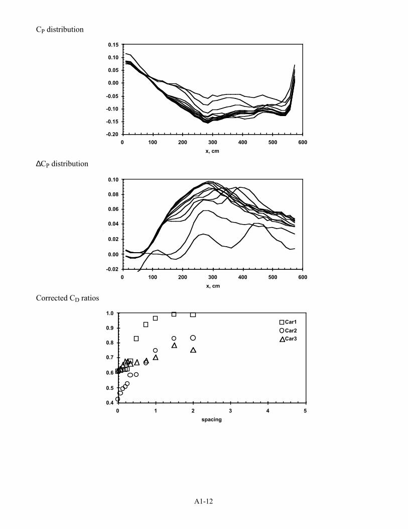
A1-12

CP distribution

x, cm

-0.20

-0.15

-0.10

-0.05

0.00

0.05

0.10

0.15

0 100 200 300 400 500 600

∆CP distribution

x, cm

DC

-0.02

0.00

0.02

0.04

0.06

0.08

0.10

0 100 200 300 400 500 600

Corrected CD ratios

spacing

CD

0.4

0.5

0.6

0.7

0.8

0.9

1.0

0 1 2 3 4 5

Car1

Car2

Car3

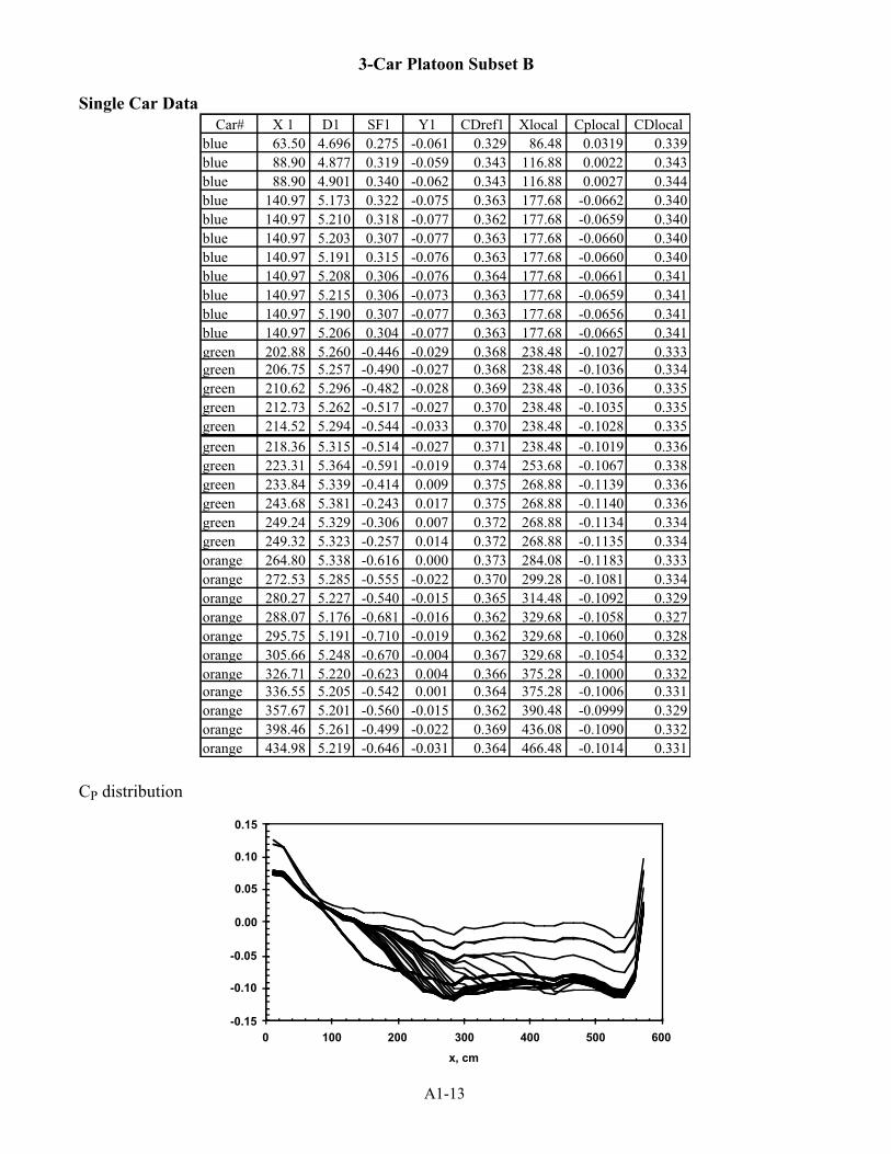
A1-13

3-Car Platoon Subset B

Single Car DataCar# X 1 D1 SF1 Y1 CDref1 Xlocal Cplocal CDlocal

blue 63.50 4.696 0.275 -0.061 0.329 86.48 0.0319 0.339blue 88.90 4.877 0.319 -0.059 0.343 116.88 0.0022 0.343blue 88.90 4.901 0.340 -0.062 0.343 116.88 0.0027 0.344blue 140.97 5.173 0.322 -0.075 0.363 177.68 -0.0662 0.340blue 140.97 5.210 0.318 -0.077 0.362 177.68 -0.0659 0.340blue 140.97 5.203 0.307 -0.077 0.363 177.68 -0.0660 0.340blue 140.97 5.191 0.315 -0.076 0.363 177.68 -0.0660 0.340blue 140.97 5.208 0.306 -0.076 0.364 177.68 -0.0661 0.341blue 140.97 5.215 0.306 -0.073 0.363 177.68 -0.0659 0.341blue 140.97 5.190 0.307 -0.077 0.363 177.68 -0.0656 0.341blue 140.97 5.206 0.304 -0.077 0.363 177.68 -0.0665 0.341green 202.88 5.260 -0.446 -0.029 0.368 238.48 -0.1027 0.333green 206.75 5.257 -0.490 -0.027 0.368 238.48 -0.1036 0.334green 210.62 5.296 -0.482 -0.028 0.369 238.48 -0.1036 0.335green 212.73 5.262 -0.517 -0.027 0.370 238.48 -0.1035 0.335green 214.52 5.294 -0.544 -0.033 0.370 238.48 -0.1028 0.335green 218.36 5.315 -0.514 -0.027 0.371 238.48 -0.1019 0.336green 223.31 5.364 -0.591 -0.019 0.374 253.68 -0.1067 0.338green 233.84 5.339 -0.414 0.009 0.375 268.88 -0.1139 0.336green 243.68 5.381 -0.243 0.017 0.375 268.88 -0.1140 0.336green 249.24 5.329 -0.306 0.007 0.372 268.88 -0.1134 0.334green 249.32 5.323 -0.257 0.014 0.372 268.88 -0.1135 0.334orange 264.80 5.338 -0.616 0.000 0.373 284.08 -0.1183 0.333orange 272.53 5.285 -0.555 -0.022 0.370 299.28 -0.1081 0.334orange 280.27 5.227 -0.540 -0.015 0.365 314.48 -0.1092 0.329orange 288.07 5.176 -0.681 -0.016 0.362 329.68 -0.1058 0.327orange 295.75 5.191 -0.710 -0.019 0.362 329.68 -0.1060 0.328orange 305.66 5.248 -0.670 -0.004 0.367 329.68 -0.1054 0.332orange 326.71 5.220 -0.623 0.004 0.366 375.28 -0.1000 0.332orange 336.55 5.205 -0.542 0.001 0.364 375.28 -0.1006 0.331orange 357.67 5.201 -0.560 -0.015 0.362 390.48 -0.0999 0.329orange 398.46 5.261 -0.499 -0.022 0.369 436.08 -0.1090 0.332orange 434.98 5.219 -0.646 -0.031 0.364 466.48 -0.1014 0.331

CP distribution

x, cm

-0.15

-0.10

-0.05

0.00

0.05

0.10

0.15

0 100 200 300 400 500 600

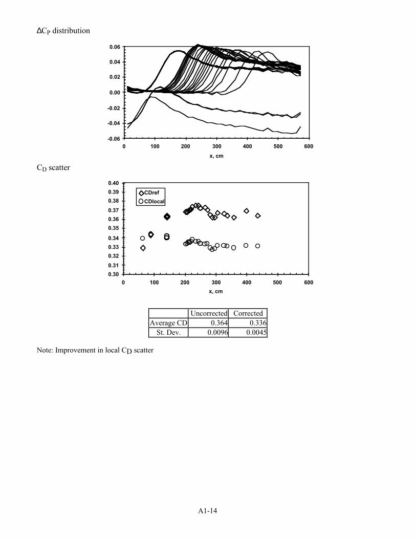
A1-14

∆CP distribution

x, cm

DC

-0.06

-0.04

-0.02

0.00

0.02

0.04

0.06

0 100 200 300 400 500 600

CD scatter

x, cm

0.30

0.31

0.32

0.33

0.34

0.35

0.36

0.37

0.38

0.39

0.40

0 100 200 300 400 500 600

CDref

CDlocal

Uncorrected CorrectedAverage CD 0.364 0.336

St. Dev. 0.0096 0.0045

Note: Improvement in local CD scatter

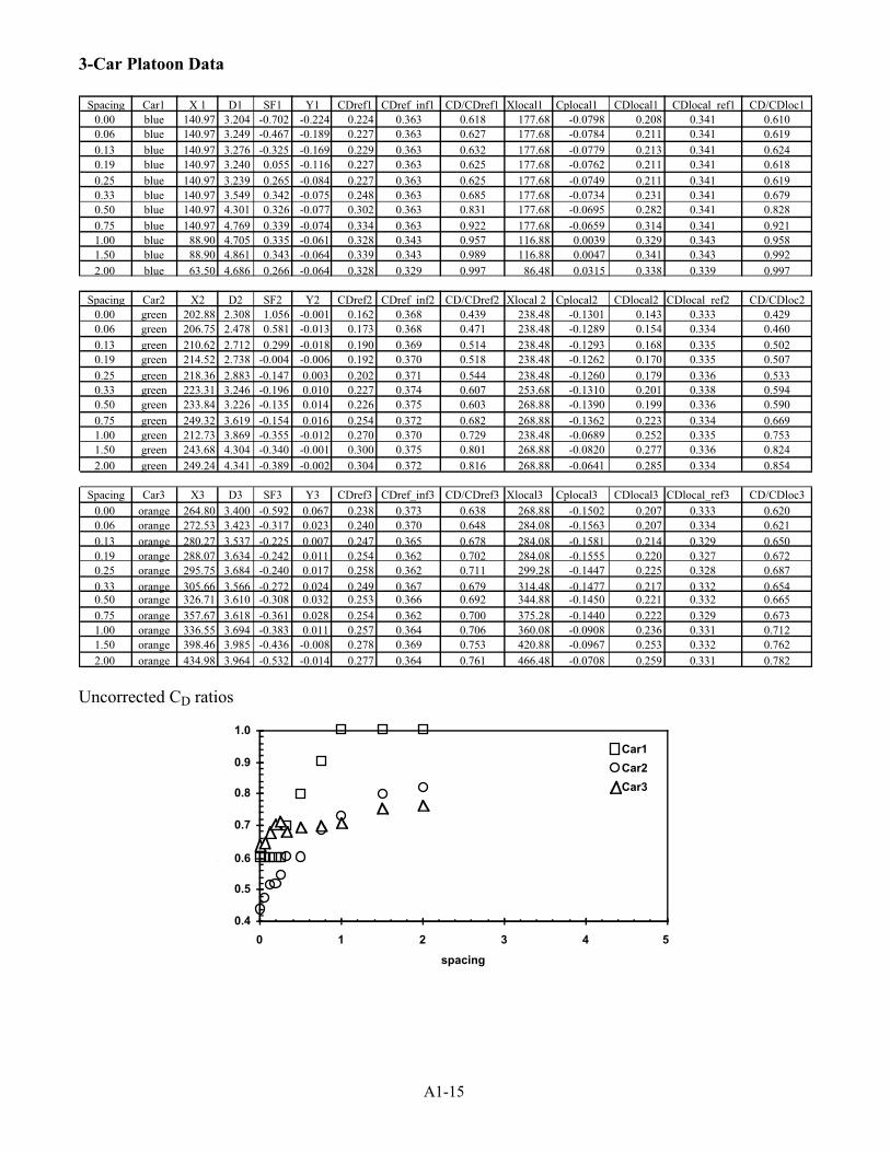
A1-15

3-Car Platoon Data

Spacing Car1 X 1 D1 SF1 Y1 CDref1 CDref_inf1 CD/CDref1 Xlocal1 Cplocal1 CDlocal1 CDlocal_ref1 CD/CDloc10.00 blue 140.97 3.204 -0.702 -0.224 0.224 0.363 0.618 177.68 -0.0798 0.208 0.341 0.6100.06 blue 140.97 3.249 -0.467 -0.189 0.227 0.363 0.627 177.68 -0.0784 0.211 0.341 0.6190.13 blue 140.97 3.276 -0.325 -0.169 0.229 0.363 0.632 177.68 -0.0779 0.213 0.341 0.6240.19 blue 140.97 3.240 0.055 -0.116 0.227 0.363 0.625 177.68 -0.0762 0.211 0.341 0.6180.25 blue 140.97 3.239 0.265 -0.084 0.227 0.363 0.625 177.68 -0.0749 0.211 0.341 0.6190.33 blue 140.97 3.549 0.342 -0.075 0.248 0.363 0.685 177.68 -0.0734 0.231 0.341 0.6790.50 blue 140.97 4.301 0.326 -0.077 0.302 0.363 0.831 177.68 -0.0695 0.282 0.341 0.8280.75 blue 140.97 4.769 0.339 -0.074 0.334 0.363 0.922 177.68 -0.0659 0.314 0.341 0.9211.00 blue 88.90 4.705 0.335 -0.061 0.328 0.343 0.957 116.88 0.0039 0.329 0.343 0.9581.50 blue 88.90 4.861 0.343 -0.064 0.339 0.343 0.989 116.88 0.0047 0.341 0.343 0.9922.00 blue 63.50 4.686 0.266 -0.064 0.328 0.329 0.997 86.48 0.0315 0.338 0.339 0.997

Spacing Car2 X2 D2 SF2 Y2 CDref2 CDref_inf2 CD/CDref2 Xlocal 2 Cplocal2 CDlocal2 CDlocal_ref2 CD/CDloc20.00 green 202.88 2.308 1.056 -0.001 0.162 0.368 0.439 238.48 -0.1301 0.143 0.333 0.4290.06 green 206.75 2.478 0.581 -0.013 0.173 0.368 0.471 238.48 -0.1289 0.154 0.334 0.4600.13 green 210.62 2.712 0.299 -0.018 0.190 0.369 0.514 238.48 -0.1293 0.168 0.335 0.5020.19 green 214.52 2.738 -0.004 -0.006 0.192 0.370 0.518 238.48 -0.1262 0.170 0.335 0.5070.25 green 218.36 2.883 -0.147 0.003 0.202 0.371 0.544 238.48 -0.1260 0.179 0.336 0.5330.33 green 223.31 3.246 -0.196 0.010 0.227 0.374 0.607 253.68 -0.1310 0.201 0.338 0.5940.50 green 233.84 3.226 -0.135 0.014 0.226 0.375 0.603 268.88 -0.1390 0.199 0.336 0.5900.75 green 249.32 3.619 -0.154 0.016 0.254 0.372 0.682 268.88 -0.1362 0.223 0.334 0.6691.00 green 212.73 3.869 -0.355 -0.012 0.270 0.370 0.729 238.48 -0.0689 0.252 0.335 0.7531.50 green 243.68 4.304 -0.340 -0.001 0.300 0.375 0.801 268.88 -0.0820 0.277 0.336 0.8242.00 green 249.24 4.341 -0.389 -0.002 0.304 0.372 0.816 268.88 -0.0641 0.285 0.334 0.854

Spacing Car3 X3 D3 SF3 Y3 CDref3 CDref_inf3 CD/CDref3 Xlocal3 Cplocal3 CDlocal3 CDlocal_ref3 CD/CDloc30.00 orange 264.80 3.400 -0.592 0.067 0.238 0.373 0.638 268.88 -0.1502 0.207 0.333 0.6200.06 orange 272.53 3.423 -0.317 0.023 0.240 0.370 0.648 284.08 -0.1563 0.207 0.334 0.6210.13 orange 280.27 3.537 -0.225 0.007 0.247 0.365 0.678 284.08 -0.1581 0.214 0.329 0.6500.19 orange 288.07 3.634 -0.242 0.011 0.254 0.362 0.702 284.08 -0.1555 0.220 0.327 0.6720.25 orange 295.75 3.684 -0.240 0.017 0.258 0.362 0.711 299.28 -0.1447 0.225 0.328 0.6870.33 orange 305.66 3.566 -0.272 0.024 0.249 0.367 0.679 314.48 -0.1477 0.217 0.332 0.6540.50 orange 326.71 3.610 -0.308 0.032 0.253 0.366 0.692 344.88 -0.1450 0.221 0.332 0.6650.75 orange 357.67 3.618 -0.361 0.028 0.254 0.362 0.700 375.28 -0.1440 0.222 0.329 0.6731.00 orange 336.55 3.694 -0.383 0.011 0.257 0.364 0.706 360.08 -0.0908 0.236 0.331 0.7121.50 orange 398.46 3.985 -0.436 -0.008 0.278 0.369 0.753 420.88 -0.0967 0.253 0.332 0.7622.00 orange 434.98 3.964 -0.532 -0.014 0.277 0.364 0.761 466.48 -0.0708 0.259 0.331 0.782

Uncorrected CD ratios

spacing

CD

0.4

0.5

0.6

0.7

0.8

0.9

1.0

0 1 2 3 4 5

Car1

Car2

Car3

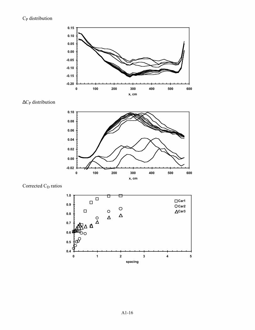
A1-16

CP distribution

x, cm

-0.20

-0.15

-0.10

-0.05

0.00

0.05

0.10

0.15

0 100 200 300 400 500 600

∆CP distribution

x, cm

DC

-0.02

0.00

0.02

0.04

0.06

0.08

0.10

0 100 200 300 400 500 600

Corrected CD ratios

spacing

CD

0.4

0.5

0.6

0.7

0.8

0.9

1.0

0 1 2 3 4 5

Car1

Car2

Car3

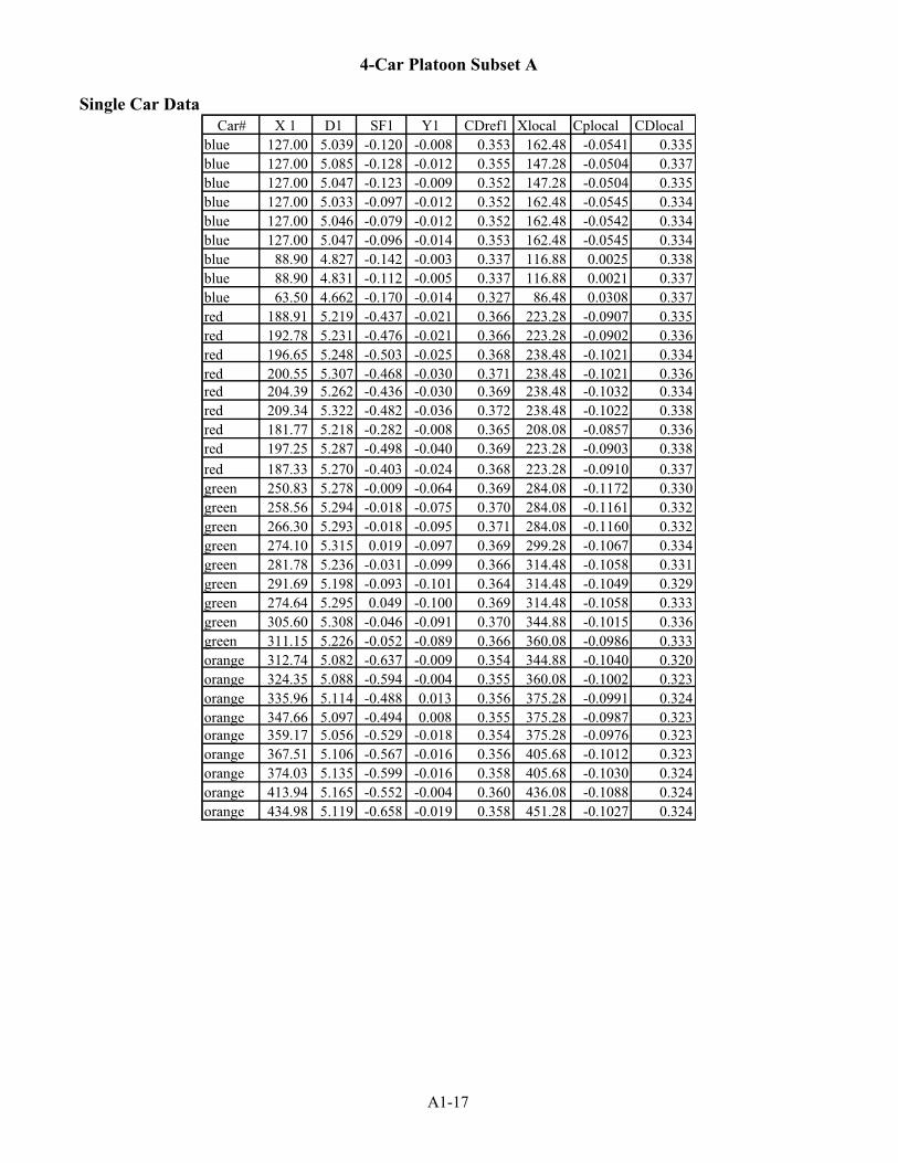
A1-17

4-Car Platoon Subset A

Single Car DataCar# X 1 D1 SF1 Y1 CDref1 Xlocal Cplocal CDlocal

blue 127.00 5.039 -0.120 -0.008 0.353 162.48 -0.0541 0.335blue 127.00 5.085 -0.128 -0.012 0.355 147.28 -0.0504 0.337blue 127.00 5.047 -0.123 -0.009 0.352 147.28 -0.0504 0.335blue 127.00 5.033 -0.097 -0.012 0.352 162.48 -0.0545 0.334blue 127.00 5.046 -0.079 -0.012 0.352 162.48 -0.0542 0.334blue 127.00 5.047 -0.096 -0.014 0.353 162.48 -0.0545 0.334blue 88.90 4.827 -0.142 -0.003 0.337 116.88 0.0025 0.338blue 88.90 4.831 -0.112 -0.005 0.337 116.88 0.0021 0.337blue 63.50 4.662 -0.170 -0.014 0.327 86.48 0.0308 0.337red 188.91 5.219 -0.437 -0.021 0.366 223.28 -0.0907 0.335red 192.78 5.231 -0.476 -0.021 0.366 223.28 -0.0902 0.336red 196.65 5.248 -0.503 -0.025 0.368 238.48 -0.1021 0.334red 200.55 5.307 -0.468 -0.030 0.371 238.48 -0.1021 0.336red 204.39 5.262 -0.436 -0.030 0.369 238.48 -0.1032 0.334red 209.34 5.322 -0.482 -0.036 0.372 238.48 -0.1022 0.338red 181.77 5.218 -0.282 -0.008 0.365 208.08 -0.0857 0.336red 197.25 5.287 -0.498 -0.040 0.369 223.28 -0.0903 0.338red 187.33 5.270 -0.403 -0.024 0.368 223.28 -0.0910 0.337green 250.83 5.278 -0.009 -0.064 0.369 284.08 -0.1172 0.330green 258.56 5.294 -0.018 -0.075 0.370 284.08 -0.1161 0.332green 266.30 5.293 -0.018 -0.095 0.371 284.08 -0.1160 0.332green 274.10 5.315 0.019 -0.097 0.369 299.28 -0.1067 0.334green 281.78 5.236 -0.031 -0.099 0.366 314.48 -0.1058 0.331green 291.69 5.198 -0.093 -0.101 0.364 314.48 -0.1049 0.329green 274.64 5.295 0.049 -0.100 0.369 314.48 -0.1058 0.333green 305.60 5.308 -0.046 -0.091 0.370 344.88 -0.1015 0.336green 311.15 5.226 -0.052 -0.089 0.366 360.08 -0.0986 0.333orange 312.74 5.082 -0.637 -0.009 0.354 344.88 -0.1040 0.320orange 324.35 5.088 -0.594 -0.004 0.355 360.08 -0.1002 0.323orange 335.96 5.114 -0.488 0.013 0.356 375.28 -0.0991 0.324orange 347.66 5.097 -0.494 0.008 0.355 375.28 -0.0987 0.323orange 359.17 5.056 -0.529 -0.018 0.354 375.28 -0.0976 0.323orange 367.51 5.106 -0.567 -0.016 0.356 405.68 -0.1012 0.323orange 374.03 5.135 -0.599 -0.016 0.358 405.68 -0.1030 0.324orange 413.94 5.165 -0.552 -0.004 0.360 436.08 -0.1088 0.324orange 434.98 5.119 -0.658 -0.019 0.358 451.28 -0.1027 0.324

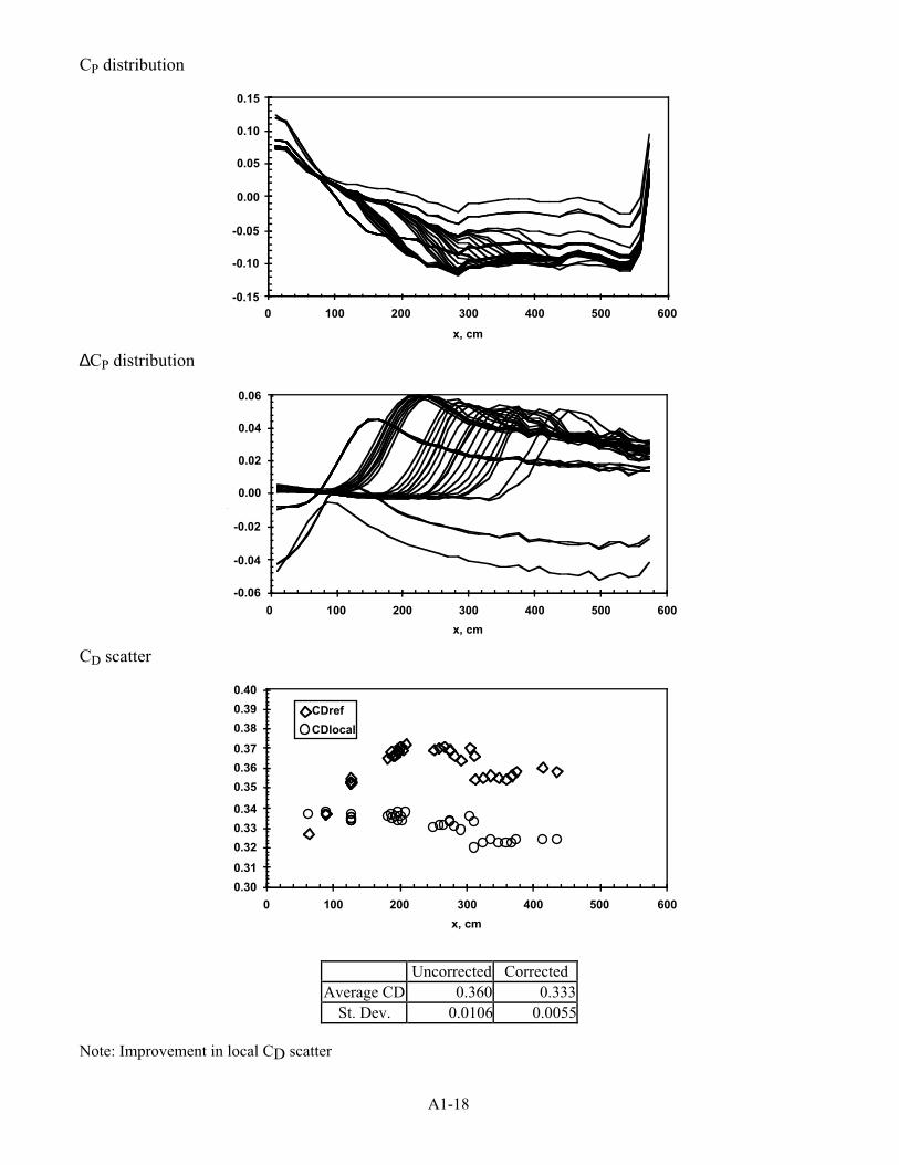
A1-18

CP distribution

x, cm

-0.15

-0.10

-0.05

0.00

0.05

0.10

0.15

0 100 200 300 400 500 600

∆CP distribution

x, cm

DC

-0.06

-0.04

-0.02

0.00

0.02

0.04

0.06

0 100 200 300 400 500 600

CD scatter

x, cm

0.30

0.31

0.32

0.33

0.34

0.35

0.36

0.37

0.38

0.39

0.40

0 100 200 300 400 500 600

CDref

CDlocal

Uncorrected CorrectedAverage CD 0.360 0.333

St. Dev. 0.0106 0.0055

Note: Improvement in local CD scatter

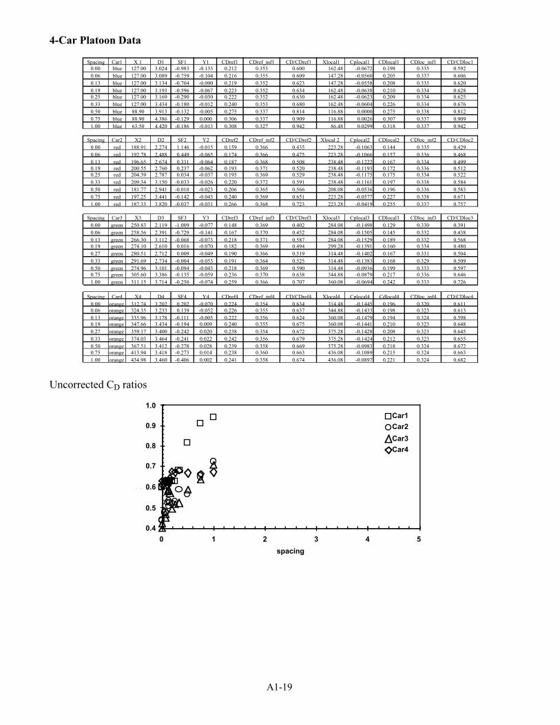
A1-19

4-Car Platoon Data

Spacing Car1 X 1 D1 SF1 Y1 CDref1 CDref_inf1 CD/CDref1 Xlocal1 Cplocal1 CDlocal1 CDloc_inf1 CD/CDloc10.00 blue 127.00 3.024 -0.983 -0.133 0.212 0.353 0.600 162.48 -0.0672 0.198 0.335 0.5920.06 blue 127.00 3.089 -0.759 -0.104 0.216 0.355 0.609 147.28 -0.0560 0.205 0.337 0.6060.13 blue 127.00 3.134 -0.704 -0.090 0.219 0.352 0.623 147.28 -0.0558 0.208 0.335 0.6200.19 blue 127.00 3.193 -0.596 -0.067 0.223 0.352 0.634 162.48 -0.0638 0.210 0.334 0.6280.25 blue 127.00 3.169 -0.290 -0.030 0.222 0.352 0.630 162.48 -0.0623 0.209 0.334 0.6250.33 blue 127.00 3.434 -0.180 -0.012 0.240 0.353 0.680 162.48 -0.0604 0.226 0.334 0.6760.50 blue 88.90 3.913 -0.132 -0.005 0.275 0.337 0.814 116.88 0.0000 0.275 0.338 0.8120.75 blue 88.90 4.386 -0.129 0.000 0.306 0.337 0.909 116.88 0.0026 0.307 0.337 0.9091.00 blue 63.50 4.420 -0.186 -0.013 0.308 0.327 0.942 86.48 0.0299 0.318 0.337 0.942

Spacing Car2 X2 D2 SF2 Y2 CDref2 CDref_inf2 CD/CDref2 Xlocal 2 Cplocal2 CDlocal2 CDloc_inf2 CD/CDloc20.00 red 188.91 2.274 1.146 -0.015 0.159 0.366 0.435 223.28 -0.1063 0.144 0.335 0.4290.06 red 192.78 2.488 0.449 -0.065 0.174 0.366 0.475 223.28 -0.1066 0.157 0.336 0.4680.13 red 196.65 2.674 0.331 -0.064 0.187 0.368 0.508 238.48 -0.1222 0.167 0.334 0.4990.19 red 200.55 2.760 0.237 -0.062 0.193 0.371 0.520 238.48 -0.1193 0.172 0.336 0.5120.25 red 204.39 2.787 0.034 -0.037 0.195 0.369 0.529 238.48 -0.1175 0.175 0.334 0.5220.33 red 209.34 3.150 -0.033 -0.026 0.220 0.372 0.591 238.48 -0.1161 0.197 0.338 0.5840.50 red 181.77 2.941 -0.010 -0.023 0.206 0.365 0.566 208.08 -0.0536 0.196 0.336 0.5830.75 red 197.25 3.441 -0.142 -0.043 0.240 0.369 0.651 223.28 -0.0577 0.227 0.338 0.6711.00 red 187.33 3.820 -0.037 -0.031 0.266 0.368 0.723 223.28 -0.0419 0.255 0.337 0.757

Spacing Car3 X3 D3 SF3 Y3 CDref3 CDref_inf3 CD/CDref3 Xlocal3 Cplocal3 CDlocal3 CDloc_inf3 CD/CDloc30.00 green 250.83 2.119 -1.009 -0.077 0.148 0.369 0.402 284.08 -0.1498 0.129 0.330 0.3910.06 green 258.56 2.391 -0.729 -0.141 0.167 0.370 0.452 284.08 -0.1505 0.145 0.332 0.4380.13 green 266.30 3.112 -0.068 -0.073 0.218 0.371 0.587 284.08 -0.1529 0.189 0.332 0.5680.19 green 274.10 2.610 0.016 -0.070 0.182 0.369 0.494 299.28 -0.1391 0.160 0.334 0.4800.27 green 280.51 2.712 0.009 -0.049 0.190 0.366 0.519 314.48 -0.1402 0.167 0.331 0.5040.33 green 291.69 2.734 -0.004 -0.053 0.191 0.364 0.525 314.48 -0.1383 0.168 0.329 0.5090.50 green 274.96 3.101 -0.094 -0.043 0.218 0.369 0.590 314.48 -0.0936 0.199 0.333 0.5970.75 green 305.60 3.386 -0.135 -0.059 0.236 0.370 0.638 344.88 -0.0879 0.217 0.336 0.6461.00 green 311.15 3.714 -0.250 -0.074 0.259 0.366 0.707 360.08 -0.0694 0.242 0.333 0.726

Spacing Car4 X4 D4 SF4 Y4 CDref4 CDref_inf4 CD/CDref4 Xlocal4 Cplocal4 Cdlocal4 CDloc_inf4 CD/CDloc40.00 orange 312.74 3.202 0.202 -0.070 0.224 0.354 0.634 314.48 -0.1445 0.196 0.320 0.6110.06 orange 324.35 3.233 0.139 -0.052 0.226 0.355 0.637 344.88 -0.1433 0.198 0.323 0.6130.13 orange 335.96 3.178 -0.111 -0.005 0.222 0.356 0.624 360.08 -0.1479 0.194 0.324 0.5980.19 orange 347.66 3.434 -0.194 0.009 0.240 0.355 0.675 360.08 -0.1441 0.210 0.323 0.6480.27 orange 359.17 3.400 -0.242 0.020 0.238 0.354 0.672 375.28 -0.1428 0.208 0.323 0.6450.33 orange 374.03 3.464 -0.241 0.022 0.242 0.356 0.679 375.28 -0.1424 0.212 0.323 0.6550.50 orange 367.51 3.412 -0.278 0.028 0.239 0.358 0.669 375.28 -0.0983 0.218 0.324 0.6720.75 orange 413.94 3.418 -0.273 0.014 0.238 0.360 0.663 436.08 -0.1089 0.215 0.324 0.6631.00 orange 434.98 3.460 -0.406 0.002 0.241 0.358 0.674 436.08 -0.0897 0.221 0.324 0.682

Uncorrected CD ratios

spacing

CD

0.4

0.5

0.6

0.7

0.8

0.9

1.0

0 1 2 3 4 5

Car1

Car2

Car3

Car4

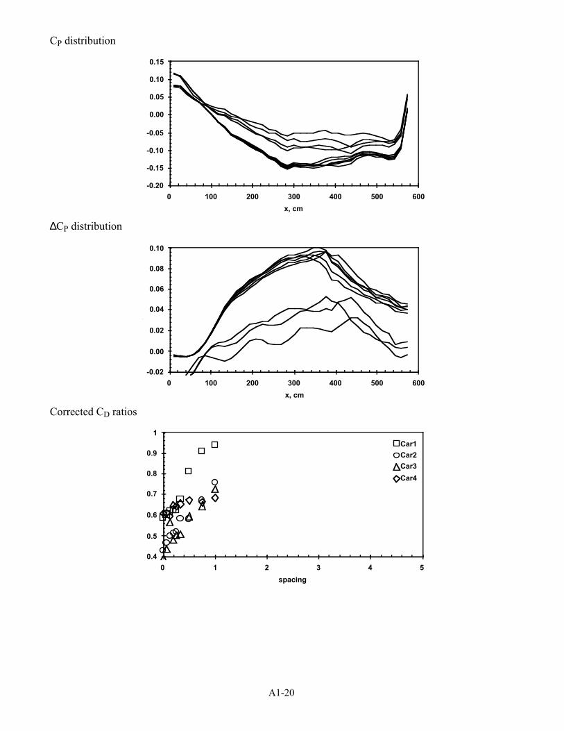
A1-20

CP distribution

x, cm

-0.20

-0.15

-0.10

-0.05

0.00

0.05

0.10

0.15

0 100 200 300 400 500 600

∆CP distribution

x, cm

DC

-0.02

0.00

0.02

0.04

0.06

0.08

0.10

0 100 200 300 400 500 600

Corrected CD ratios

spacing

CD

0.4

0.5

0.6

0.7

0.8

0.9

1

0 1 2 3 4 5

Car1

Car2

Car3

Car4

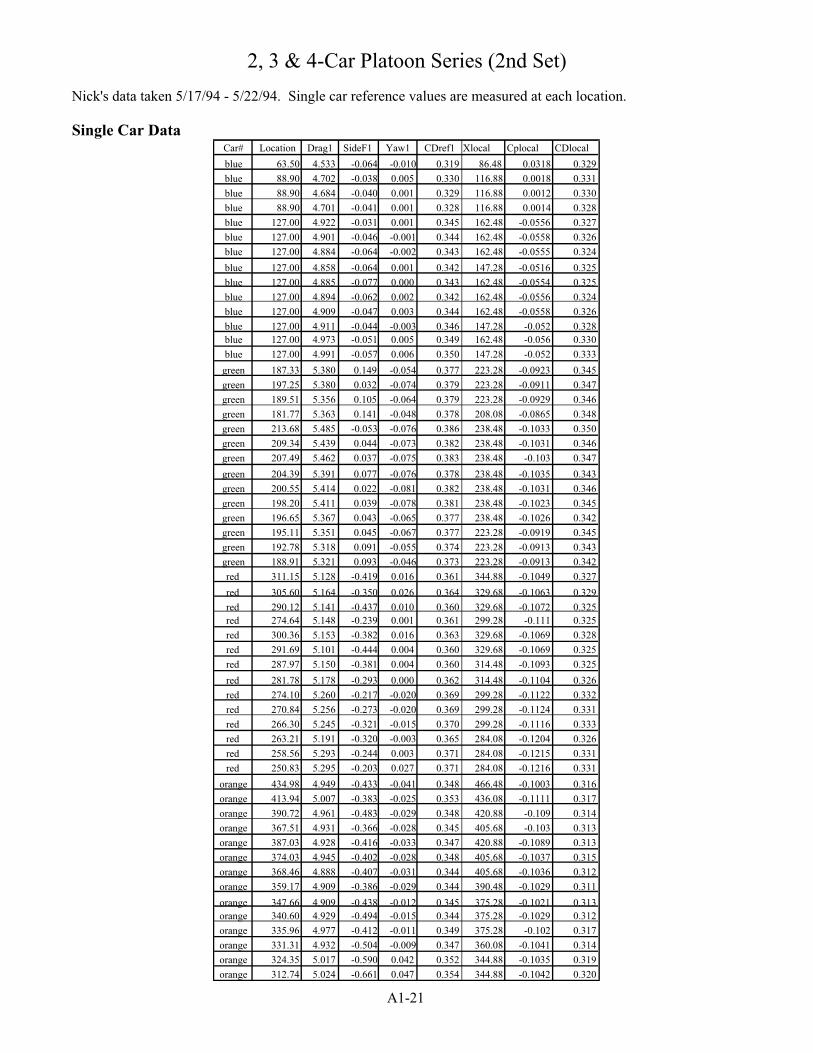
A1-21

2, 3 & 4-Car Platoon Series (2nd Set)

Nick's data taken 5/17/94 - 5/22/94. Single car reference values are measured at each location.

Single Car DataCar# Location Drag1 SideF1 Yaw1 CDref1 Xlocal Cplocal CDlocal

blue 63.50 4.533 -0.064 -0.010 0.319 86.48 0.0318 0.329

blue 88.90 4.702 -0.038 0.005 0.330 116.88 0.0018 0.331

blue 88.90 4.684 -0.040 0.001 0.329 116.88 0.0012 0.330

blue 88.90 4.701 -0.041 0.001 0.328 116.88 0.0014 0.328

blue 127.00 4.922 -0.031 0.001 0.345 162.48 -0.0556 0.327

blue 127.00 4.901 -0.046 -0.001 0.344 162.48 -0.0558 0.326

blue 127.00 4.884 -0.064 -0.002 0.343 162.48 -0.0555 0.324

blue 127.00 4.858 -0.064 0.001 0.342 147.28 -0.0516 0.325

blue 127.00 4.885 -0.077 0.000 0.343 162.48 -0.0554 0.325

blue 127.00 4.894 -0.062 0.002 0.342 162.48 -0.0556 0.324

blue 127.00 4.909 -0.047 0.003 0.344 162.48 -0.0558 0.326

blue 127.00 4.911 -0.044 -0.003 0.346 147.28 -0.052 0.328blue 127.00 4.973 -0.051 0.005 0.349 162.48 -0.056 0.330

blue 127.00 4.991 -0.057 0.006 0.350 147.28 -0.052 0.333

green 187.33 5.380 0.149 -0.054 0.377 223.28 -0.0923 0.345

green 197.25 5.380 0.032 -0.074 0.379 223.28 -0.0911 0.347

green 189.51 5.356 0.105 -0.064 0.379 223.28 -0.0929 0.346

green 181.77 5.363 0.141 -0.048 0.378 208.08 -0.0865 0.348

green 213.68 5.485 -0.053 -0.076 0.386 238.48 -0.1033 0.350

green 209.34 5.439 0.044 -0.073 0.382 238.48 -0.1031 0.346

green 207.49 5.462 0.037 -0.075 0.383 238.48 -0.103 0.347

green 204.39 5.391 0.077 -0.076 0.378 238.48 -0.1035 0.343

green 200.55 5.414 0.022 -0.081 0.382 238.48 -0.1031 0.346

green 198.20 5.411 0.039 -0.078 0.381 238.48 -0.1023 0.345

green 196.65 5.367 0.043 -0.065 0.377 238.48 -0.1026 0.342

green 195.11 5.351 0.045 -0.067 0.377 223.28 -0.0919 0.345

green 192.78 5.318 0.091 -0.055 0.374 223.28 -0.0913 0.343

green 188.91 5.321 0.093 -0.046 0.373 223.28 -0.0913 0.342

red 311.15 5.128 -0.419 0.016 0.361 344.88 -0.1049 0.327

red 305.60 5.164 -0.350 0.026 0.364 329.68 -0.1063 0.329

red 290.12 5.141 -0.437 0.010 0.360 329.68 -0.1072 0.325red 274.64 5.148 -0.239 0.001 0.361 299.28 -0.111 0.325

red 300.36 5.153 -0.382 0.016 0.363 329.68 -0.1069 0.328

red 291.69 5.101 -0.444 0.004 0.360 329.68 -0.1069 0.325

red 287.97 5.150 -0.381 0.004 0.360 314.48 -0.1093 0.325

red 281.78 5.178 -0.293 0.000 0.362 314.48 -0.1104 0.326

red 274.10 5.260 -0.217 -0.020 0.369 299.28 -0.1122 0.332

red 270.84 5.256 -0.273 -0.020 0.369 299.28 -0.1124 0.331

red 266.30 5.245 -0.321 -0.015 0.370 299.28 -0.1116 0.333

red 263.21 5.191 -0.320 -0.003 0.365 284.08 -0.1204 0.326

red 258.56 5.293 -0.244 0.003 0.371 284.08 -0.1215 0.331

red 250.83 5.295 -0.203 0.027 0.371 284.08 -0.1216 0.331

orange 434.98 4.949 -0.433 -0.041 0.348 466.48 -0.1003 0.316

orange 413.94 5.007 -0.383 -0.025 0.353 436.08 -0.1111 0.317

orange 390.72 4.961 -0.483 -0.029 0.348 420.88 -0.109 0.314

orange 367.51 4.931 -0.366 -0.028 0.345 405.68 -0.103 0.313

orange 387.03 4.928 -0.416 -0.033 0.347 420.88 -0.1089 0.313

orange 374.03 4.945 -0.402 -0.028 0.348 405.68 -0.1037 0.315

orange 368.46 4.888 -0.407 -0.031 0.344 405.68 -0.1036 0.312

orange 359.17 4.909 -0.386 -0.029 0.344 390.48 -0.1029 0.311

orange 347.66 4.909 -0.438 -0.012 0.345 375.28 -0.1021 0.313orange 340.60 4.929 -0.494 -0.015 0.344 375.28 -0.1029 0.312

orange 335.96 4.977 -0.412 -0.011 0.349 375.28 -0.102 0.317

orange 331.31 4.932 -0.504 -0.009 0.347 360.08 -0.1041 0.314

orange 324.35 5.017 -0.590 0.042 0.352 344.88 -0.1035 0.319

orange 312.74 5.024 -0.661 0.047 0.354 344.88 -0.1042 0.320

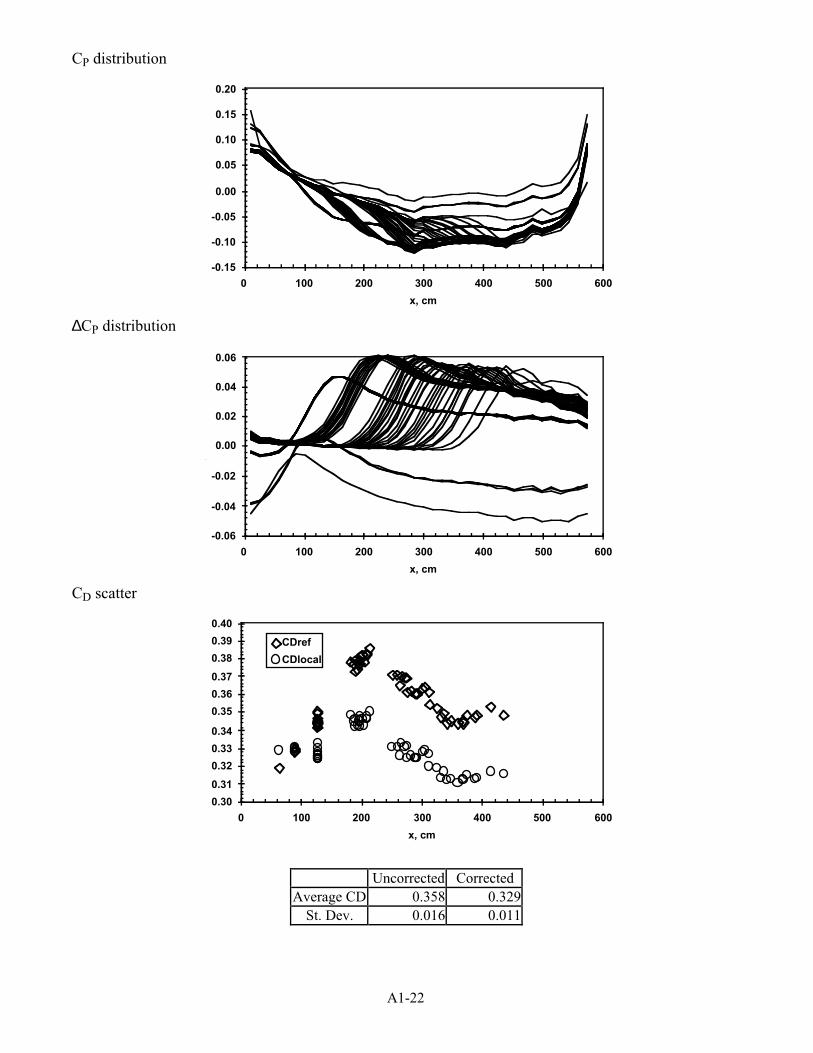
A1-22

CP distribution

x, cm

-0.15

-0.10

-0.05

0.00

0.05

0.10

0.15

0.20

0 100 200 300 400 500 600

∆CP distribution

x, cm

DC

-0.06

-0.04

-0.02

0.00

0.02

0.04

0.06

0 100 200 300 400 500 600

CD scatter

x, cm

0.30

0.31

0.32

0.33

0.34

0.35

0.36

0.37

0.38

0.39

0.40

0 100 200 300 400 500 600

CDref

CDlocal

Uncorrected CorrectedAverage CD 0.358 0.329

St. Dev. 0.016 0.011

A1-23

2-Car Platoon Data

Spacing Car1 Location1 Drag1 SideF1 Yaw1 CDref1 CD/CDref1 Xlocal1 Cplocal1 CDloc1 CD/CDloc11.00 green 187.33 5.168 0.142 -0.053 0.364 0.966 223.28 -0.0909 0.334 0.9670.75 green 197.25 4.996 0.060 -0.069 0.352 0.930 223.28 -0.0904 0.323 0.9300.63 green 189.51 4.828 0.149 -0.057 0.340 0.897 223.28 -0.0947 0.310 0.8960.50 green 181.77 4.577 0.186 -0.042 0.321 0.851 208.08 -0.0883 0.295 0.8490.40 green 213.68 4.284 0.027 -0.066 0.302 0.782 238.48 -0.1053 0.273 0.7800.33 green 209.34 3.869 0.047 -0.075 0.273 0.714 238.48 -0.1081 0.246 0.7110.30 green 207.94 3.663 0.150 -0.063 0.258 0.673 238.48 -0.1096 0.232 0.6690.25 green 204.39 3.678 -0.155 -0.114 0.257 0.679 238.48 -0.112 0.231 0.6730.19 green 200.55 3.532 -0.331 -0.130 0.248 0.651 238.48 -0.1142 0.223 0.6440.15 green 198.20 3.464 -0.337 -0.131 0.243 0.637 238.48 -0.1157 0.218 0.6300.13 green 196.65 3.403 -0.421 -0.130 0.240 0.636 238.48 -0.1172 0.215 0.6280.10 green 195.11 3.426 -0.477 -0.145 0.242 0.641 223.28 -0.1006 0.219 0.6360.06 green 192.78 3.382 -0.515 -0.145 0.237 0.634 223.28 -0.1015 0.216 0.6280.00 green 188.91 3.329 -0.845 -0.173 0.234 0.627 223.28 -0.1037 0.212 0.620

Spacing Car2 Location2 Drag2 SideF2 Yaw2 CDref2 CD/CDref2 Xlocal2 Cplocal2 CDloc2 CD/Cdloc21.00 red 311.15 4.126 -0.352 0.005 0.291 0.806 344.88 -0.1351 0.256 0.7850.75 red 305.60 3.885 -0.279 -0.001 0.274 0.752 329.68 -0.1370 0.241 0.7320.63 red 290.12 3.736 -0.251 0.010 0.263 0.730 314.48 -0.1399 0.231 0.7090.50 red 274.64 3.723 -0.120 0.009 0.261 0.724 299.28 -0.1400 0.229 0.7060.40 red 300.36 3.733 -0.095 0.012 0.263 0.725 329.68 -0.1369 0.231 0.7050.33 red 291.69 3.865 -0.101 0.009 0.273 0.758 314.48 -0.1392 0.239 0.7360.30 red 287.97 3.981 -0.117 0.016 0.280 0.778 299.28 -0.1381 0.246 0.7580.25 red 281.78 4.092 0.021 -0.007 0.286 0.789 299.28 -0.1392 0.251 0.7690.19 red 274.10 4.098 0.082 -0.024 0.288 0.781 284.08 -0.1485 0.251 0.7560.15 red 270.84 4.108 0.108 -0.020 0.288 0.781 284.08 -0.1480 0.251 0.7570.13 red 266.30 4.007 0.121 -0.029 0.283 0.764 284.08 -0.1480 0.246 0.7400.10 red 263.21 3.924 0.138 -0.042 0.277 0.758 284.08 -0.1479 0.241 0.7400.06 red 258.56 3.853 0.268 -0.038 0.271 0.729 268.88 -0.1425 0.237 0.7150.00 red 250.83 3.832 0.582 -0.058 0.269 0.726 268.88 -0.1423 0.236 0.713

Uncorrected CD ratios

spacing

CD

0.5

0.6

0.7

0.8

0.9

1.0

1.1

0 1 2 3 4 5

Car1

Car2

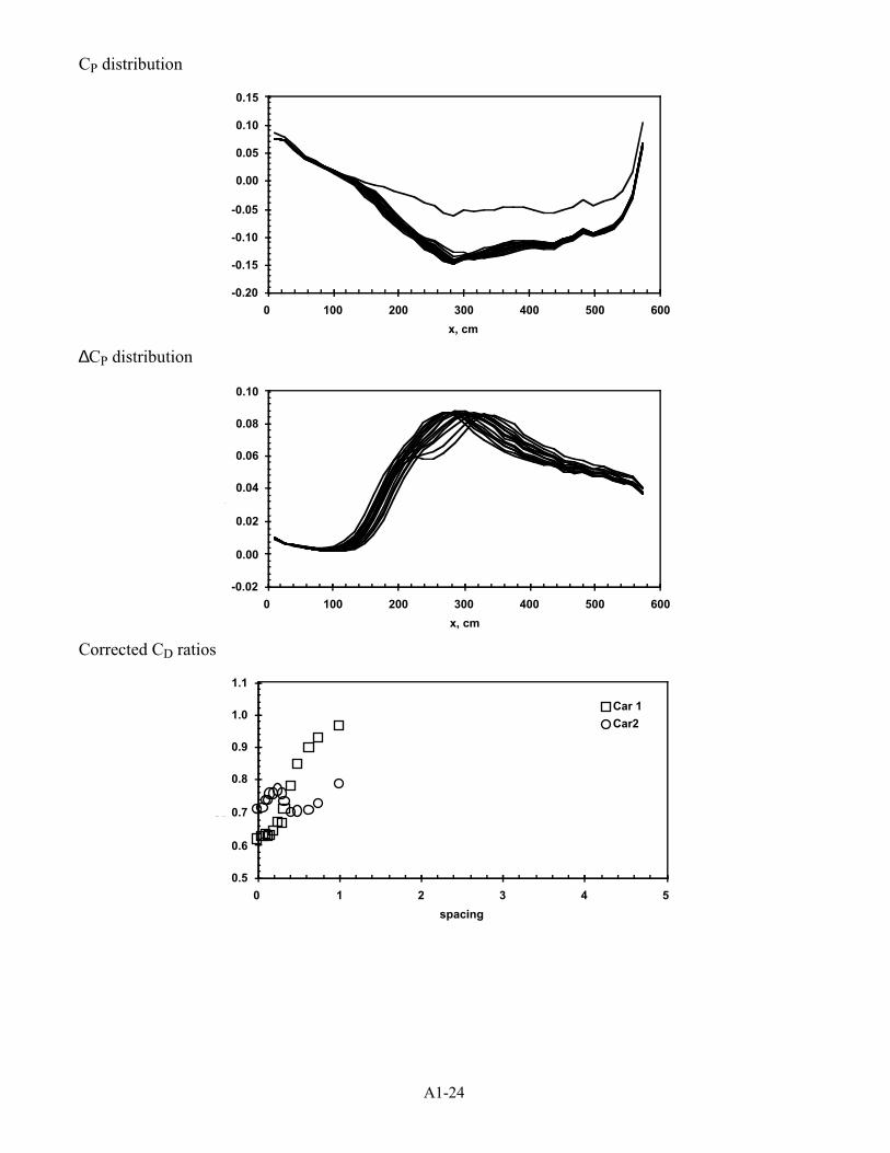
A1-24

CP distribution

x, cm

-0.20

-0.15

-0.10

-0.05

0.00

0.05

0.10

0.15

0 100 200 300 400 500 600

∆CP distribution

x, cm

DC

-0.02

0.00

0.02

0.04

0.06

0.08

0.10

0 100 200 300 400 500 600

Corrected CD ratios

spacing

CDl

0.5

0.6

0.7

0.8

0.9

1.0

1.1

0 1 2 3 4 5

Car 1

Car2

A1-25

3-Car Platoon Data

Spacing Car# Location Drag1 SideF1 Yaw1 CDref1 CD/CDref1 Xlocal1 Cplocal1 CDloc1 CDloc_inf1 CD/CDloc11.00 blue 63.50 4.283 -0.079 -0.016 0.301 0.944 86.48 0.0293 0.310 0.329 0.941

0.75 blue 88.90 4.277 -0.036 -0.005 0.300 0.907 116.88 0.0028 0.300 0.331 0.9080.63 blue 88.90 4.103 -0.048 -0.010 0.288 0.876 116.88 0.0008 0.289 0.330 0.8750.50 blue 88.90 3.867 -0.061 -0.006 0.270 0.823 116.88 -0.0007 0.270 0.328 0.8220.40 blue 127.00 3.716 -0.077 -0.010 0.261 0.757 162.48 -0.0605 0.246 0.327 0.7530.33 blue 127.00 3.359 -0.100 -0.017 0.237 0.689 162.48 -0.0623 0.223 0.326 0.6840.30 blue 127.00 3.193 -0.167 -0.021 0.224 0.655 162.48 -0.0632 0.211 0.324 0.6500.25 blue 127.00 3.025 -0.071 -0.008 0.212 0.620 147.28 -0.0549 0.201 0.325 0.6180.19 blue 127.00 3.053 -0.433 -0.055 0.215 0.626 162.48 -0.0654 0.202 0.325 0.620

0.15 blue 127.00 3.119 -0.656 -0.086 0.217 0.635 162.48 -0.0660 0.204 0.324 0.6290.13 blue 127.00 3.086 -0.685 -0.090 0.217 0.629 162.48 -0.0671 0.203 0.326 0.6230.10 blue 127.00 3.080 -0.735 -0.101 0.217 0.627 147.28 -0.0570 0.205 0.328 0.6240.06 blue 127.00 3.092 -0.846 -0.118 0.217 0.621 162.48 -0.0676 0.203 0.330 0.6150.00 blue 127.00 3.035 -1.002 -0.132 0.212 0.605 147.28 -0.0586 0.200 0.333 0.601

Spacing Car# Location Drag2 SideF2 Yaw2 CDref2 CD/CDref2 Xlocal2 Cplocal2 CDloc2 CDloc_inf2 CD/CDloc21.00 green 187.33 4.014 0.014 -0.091 0.282 0.747 223.28 -0.0436 0.270 0.345 0.782

0.75 green 197.25 3.681 -0.088 -0.103 0.258 0.681 223.28 -0.0583 0.244 0.347 0.7020.63 green 189.51 3.319 0.045 -0.079 0.233 0.616 223.28 -0.0612 0.220 0.346 0.6350.50 green 181.77 3.107 0.106 -0.065 0.217 0.575 208.08 -0.0561 0.205 0.348 0.5910.40 green 213.68 3.209 0.035 -0.067 0.226 0.585 238.48 -0.1165 0.202 0.350 0.5780.33 green 209.34 3.202 0.058 -0.066 0.226 0.591 238.48 -0.1185 0.202 0.346 0.5830.30 green 207.94 3.158 0.080 -0.068 0.222 0.579 238.48 -0.1196 0.198 0.347 0.5710.25 green 204.39 2.909 0.090 -0.065 0.204 0.539 238.48 -0.1203 0.182 0.343 0.5310.19 green 200.55 2.861 0.111 -0.105 0.201 0.528 238.48 -0.1220 0.179 0.346 0.519

0.15 green 198.20 2.923 0.004 -0.148 0.204 0.535 238.48 -0.1238 0.181 0.345 0.5250.13 green 196.65 2.912 -0.221 -0.177 0.204 0.542 238.48 -0.1245 0.182 0.342 0.5320.10 green 195.11 2.855 -0.341 -0.205 0.201 0.533 223.28 -0.1101 0.181 0.345 0.5240.06 green 192.78 2.610 -0.283 -0.218 0.183 0.489 223.28 -0.1100 0.165 0.343 0.4800.00 green 188.91 2.380 -0.231 -0.231 0.166 0.445 223.28 -0.1100 0.150 0.342 0.437

Spacing Car# Location Drag3 SideF3 Yaw3 CDref3 CD/CDref3 Xlocal3 Cplocal3 CDloc3 CDloc_inf3 CD/CDloc31.00 red 311.15 3.870 -0.328 0.001 0.272 0.753 329.68 -0.0790 0.252 0.327 0.7710.75 red 305.60 3.707 -0.215 0.003 0.260 0.713 329.68 -0.0919 0.238 0.329 0.7220.63 red 290.12 3.610 -0.208 0.020 0.254 0.704 299.28 -0.0945 0.232 0.325 0.7120.50 red 274.64 3.662 -0.160 0.014 0.256 0.709 284.08 -0.1050 0.231 0.325 0.7130.40 red 300.36 3.621 -0.130 0.024 0.255 0.702 314.48 -0.1401 0.223 0.328 0.6820.33 red 291.69 3.531 -0.131 0.019 0.249 0.692 299.28 -0.1399 0.218 0.325 0.6720.30 red 287.97 3.561 -0.100 0.014 0.250 0.695 299.28 -0.1406 0.219 0.325 0.6760.25 red 281.78 3.614 -0.089 0.018 0.253 0.699 284.08 -0.1489 0.220 0.326 0.675

0.19 red 274.10 3.506 -0.140 -0.014 0.247 0.668 284.08 -0.1499 0.215 0.332 0.6460.15 red 270.84 3.697 0.146 -0.032 0.258 0.699 284.08 -0.1517 0.224 0.331 0.6750.13 red 266.30 3.640 0.251 -0.049 0.255 0.691 268.88 -0.1456 0.223 0.333 0.6700.10 red 263.21 3.591 0.334 -0.060 0.253 0.692 268.88 -0.1458 0.221 0.326 0.6770.06 red 258.56 3.531 0.350 -0.066 0.247 0.666 268.88 -0.1446 0.216 0.331 0.6530.00 red 250.83 3.547 0.459 -0.078 0.247 0.667 268.88 -0.1432 0.216 0.331 0.654

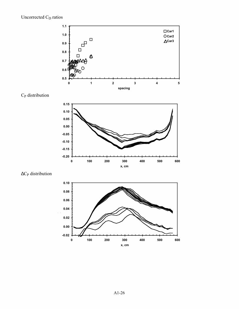
A1-26

Uncorrected CD ratios

spacing

CD

0.5

0.6

0.7

0.8

0.9

1.0

1.1

0 1 2 3 4 5

Car1

Car2

Car3

CP distribution

x, cm

-0.20

-0.15

-0.10

-0.05

0.00

0.05

0.10

0.15

0 100 200 300 400 500 600

∆CP distribution

x, cm

DC

-0.02

0.00

0.02

0.04

0.06

0.08

0.10

0 100 200 300 400 500 600

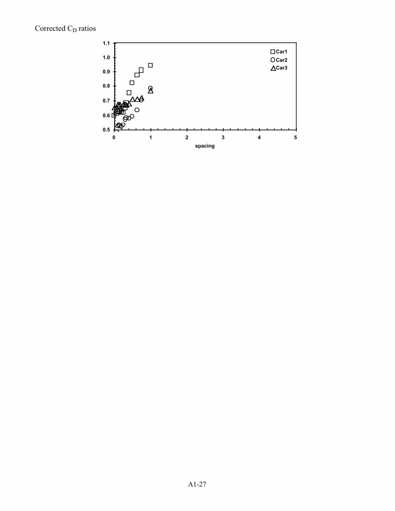
A1-27

Corrected CD ratios

spacing

CD

0.5

0.6

0.7

0.8

0.9

1.0

1.1

0 1 2 3 4 5

Car1

Car2

Car3

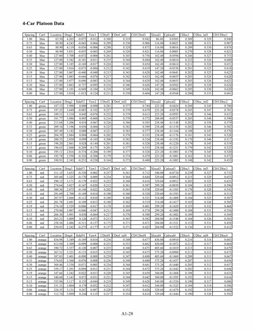
A1-28

4-Car Platoon Data

Spacing Car# Location Drag1 SideF1 Yaw1 CDref1 CDref_inf1 CD/CDref1 Xlocal1 Cplocal1 CDloc1 CDloc_inf1 CD/CDloc11.00 blue 63.50 4.265 -0.075 -0.012 0.300 0.319 0.942 86.48 0.0305 0.309 0.329 0.9400.75 blue 88.90 4.243 -0.043 0.004 0.299 0.330 0.906 116.88 0.0025 0.300 0.331 0.9070.63 blue 88.90 4.119 -0.036 -0.006 0.288 0.329 0.875 116.88 0.0016 0.289 0.330 0.8760.50 blue 88.90 3.851 -0.055 -0.003 0.269 0.328 0.821 116.88 0.0005 0.270 0.328 0.8210.40 blue 127.00 3.708 -0.072 -0.006 0.261 0.345 0.756 162.48 -0.0594 0.246 0.327 0.7530.33 blue 127.00 3.342 -0.101 -0.011 0.235 0.344 0.684 162.48 -0.0614 0.222 0.326 0.6800.30 blue 127.00 3.185 -0.169 -0.017 0.224 0.343 0.654 162.48 -0.0614 0.211 0.324 0.6510.25 blue 127.00 3.016 -0.075 -0.004 0.212 0.342 0.619 147.28 -0.0538 0.201 0.325 0.6180.19 blue 127.00 3.067 -0.440 -0.048 0.215 0.343 0.628 162.48 -0.0641 0.202 0.325 0.6230.15 blue 127.00 3.083 -0.666 -0.076 0.217 0.342 0.633 162.48 -0.0655 0.203 0.324 0.6280.13 blue 127.00 3.077 -0.696 -0.083 0.216 0.344 0.629 162.48 -0.0655 0.203 0.326 0.6230.10 blue 127.00 3.063 -0.737 -0.095 0.216 0.346 0.626 147.28 -0.0562 0.205 0.328 0.6240.06 blue 127.00 3.101 -0.849 -0.104 0.218 0.349 0.626 162.48 -0.0662 0.205 0.330 0.6200.00 blue 127.00 3.018 -1.013 -0.124 0.211 0.350 0.604 147.28 -0.0568 0.200 0.333 0.601

Spacing Car# Location Drag2 SideF2 Yaw2 CDref2 CDref_inf2 CD/CDref2 Xlocal2 Cplocal2 CDloc2 CDloc_inf2 CD/CDloc21.00 green 187.33 3.990 0.000 -0.090 0.281 0.377 0.744 223.28 -0.0424 0.269 0.345 0.7800.75 green 197.25 3.649 -0.083 -0.102 0.257 0.379 0.679 223.28 -0.0578 0.243 0.347 0.7010.63 green 189.51 3.318 0.045 -0.076 0.232 0.379 0.613 223.28 -0.0593 0.219 0.346 0.6330.50 green 181.77 3.086 0.095 -0.068 0.216 0.378 0.572 208.08 -0.0537 0.205 0.348 0.5900.40 green 213.68 3.206 0.034 -0.067 0.226 0.386 0.585 238.48 -0.1148 0.202 0.350 0.5790.33 green 209.34 3.196 0.056 -0.066 0.225 0.382 0.589 238.48 -0.1158 0.202 0.346 0.5820.30 green 207.49 3.142 0.080 -0.067 0.221 0.383 0.577 238.48 -0.1164 0.198 0.347 0.5700.25 green 204.39 2.884 0.094 -0.064 0.202 0.378 0.535 238.48 -0.1176 0.181 0.343 0.5280.19 green 200.55 2.850 0.099 -0.105 0.200 0.382 0.524 238.48 -0.1192 0.179 0.346 0.5170.15 green 198.20 2.861 0.028 -0.144 0.201 0.381 0.528 238.48 -0.1220 0.179 0.345 0.5190.13 green 196.65 2.860 -0.209 -0.175 0.201 0.377 0.533 238.48 -0.1231 0.179 0.342 0.5230.10 green 195.11 2.816 -0.374 -0.206 0.199 0.377 0.528 223.28 -0.1083 0.179 0.345 0.5200.06 green 192.78 2.550 -0.326 -0.206 0.179 0.374 0.479 223.28 -0.1081 0.162 0.343 0.4720.00 green 188.91 2.345 -0.251 -0.230 0.164 0.373 0.440 223.28 -0.1085 0.148 0.342 0.433

Spacing Car# Location Drag3 SideF3 Yaw3 CDref3 CDref_inf3 CD/CDref3 Xlocal3 Cplocal3 CDloc3 CDloc_inf3 CD/CDloc31.00 red 311.15 3.653 -0.330 0.002 0.257 0.361 0.712 344.88 -0.0734 0.239 0.327 0.7330.75 red 305.60 3.325 -0.170 0.009 0.234 0.364 0.644 329.68 -0.0912 0.215 0.329 0.6530.63 red 290.12 3.171 -0.179 0.022 0.222 0.360 0.616 329.68 -0.0912 0.203 0.325 0.6250.50 red 274.64 3.027 -0.147 0.020 0.212 0.361 0.587 299.28 -0.0939 0.194 0.325 0.5960.40 red 300.36 2.875 -0.148 0.022 0.202 0.363 0.558 329.68 -0.1385 0.178 0.328 0.5430.33 red 291.69 2.700 -0.149 0.014 0.190 0.360 0.528 329.68 -0.1393 0.167 0.325 0.5130.30 red 287.97 2.666 -0.112 0.010 0.188 0.360 0.521 314.48 -0.1408 0.164 0.325 0.5070.25 red 281.78 2.681 -0.109 0.013 0.188 0.362 0.519 314.48 -0.1417 0.165 0.326 0.5050.19 red 274.10 2.529 -0.086 -0.017 0.178 0.369 0.481 299.28 -0.1429 0.155 0.332 0.4680.15 red 270.84 3.007 -0.046 -0.047 0.211 0.369 0.574 299.28 -0.1480 0.184 0.331 0.5560.13 red 266.30 3.091 0.030 -0.064 0.217 0.370 0.588 299.28 -0.1482 0.189 0.333 0.5690.10 red 263.21 3.009 0.126 -0.073 0.213 0.365 0.582 284.08 -0.1548 0.184 0.326 0.5650.06 red 258.56 2.486 -0.311 -0.157 0.175 0.371 0.471 284.08 -0.1521 0.152 0.331 0.4580.00 red 250.83 2.242 -0.275 -0.177 0.157 0.371 0.423 284.08 -0.1522 0.136 0.331 0.412

Spacing Car# Location Drag4 SideF4 Yaw4 CDref4 CDref_inf4 CD/CDref4 Xlocal4 Cplocal4 CDloc4 CDloc_inf4 CD/CDloc41.00 orange 434.98 3.349 -0.169 -0.016 0.236 0.348 0.677 436.08 -0.0910 0.216 0.316 0.6830.75 orange 413.94 3.309 -0.099 -0.006 0.233 0.353 0.662 420.88 -0.1072 0.211 0.317 0.6640.63 orange 390.72 3.357 -0.120 0.007 0.235 0.348 0.675 405.68 -0.1019 0.213 0.314 0.6790.50 orange 367.51 3.321 -0.133 0.015 0.232 0.345 0.673 375.28 -0.0988 0.211 0.313 0.6750.40 orange 387.03 3.401 -0.090 0.009 0.239 0.347 0.690 405.68 -0.1469 0.209 0.313 0.6670.33 orange 374.03 3.360 -0.076 0.008 0.236 0.348 0.680 375.28 -0.1437 0.207 0.315 0.6560.30 orange 368.46 3.330 -0.071 0.005 0.234 0.344 0.681 375.28 -0.1440 0.205 0.312 0.6570.25 orange 359.17 3.291 -0.094 0.011 0.231 0.344 0.672 375.28 -0.1442 0.202 0.311 0.6480.19 orange 347.66 3.242 -0.022 -0.013 0.228 0.345 0.659 360.08 -0.1468 0.198 0.313 0.6330.15 orange 340.60 3.143 0.072 -0.031 0.221 0.344 0.642 360.08 -0.1505 0.192 0.312 0.6160.13 orange 335.96 3.117 0.155 -0.044 0.219 0.349 0.628 344.88 -0.1524 0.190 0.317 0.6000.10 orange 331.31 3.004 0.179 -0.052 0.212 0.347 0.612 344.88 -0.1525 0.184 0.314 0.5860.06 orange 324.35 3.131 0.267 0.097 0.220 0.352 0.626 329.68 -0.1479 0.192 0.319 0.6020.00 orange 312.74 3.099 0.244 0.115 0.217 0.354 0.614 329.68 -0.1444 0.190 0.320 0.592

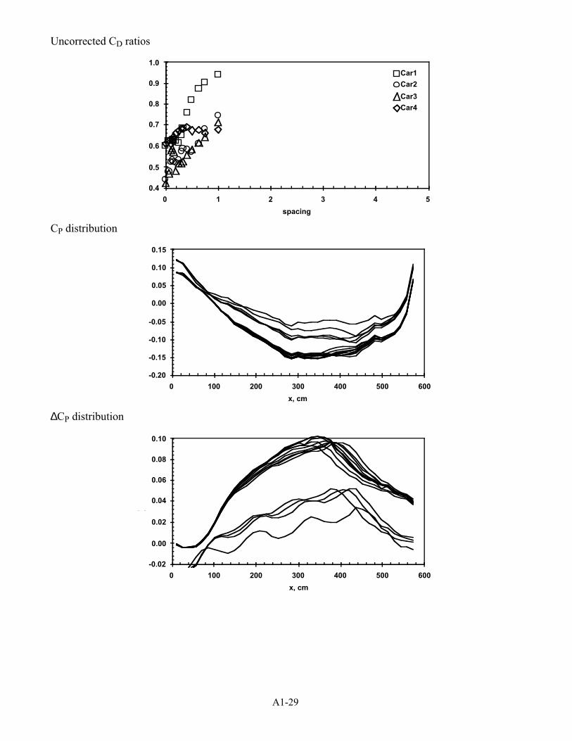
A1-29

Uncorrected CD ratios

spacing

CD

0.4

0.5

0.6

0.7

0.8

0.9

1.0

0 1 2 3 4 5

Car1

Car2

Car3

Car4

CP distribution

x, cm

-0.20

-0.15

-0.10

-0.05

0.00

0.05

0.10

0.15

0 100 200 300 400 500 600

∆CP distribution

x, cm

DC

-0.02

0.00

0.02

0.04

0.06

0.08

0.10

0 100 200 300 400 500 600

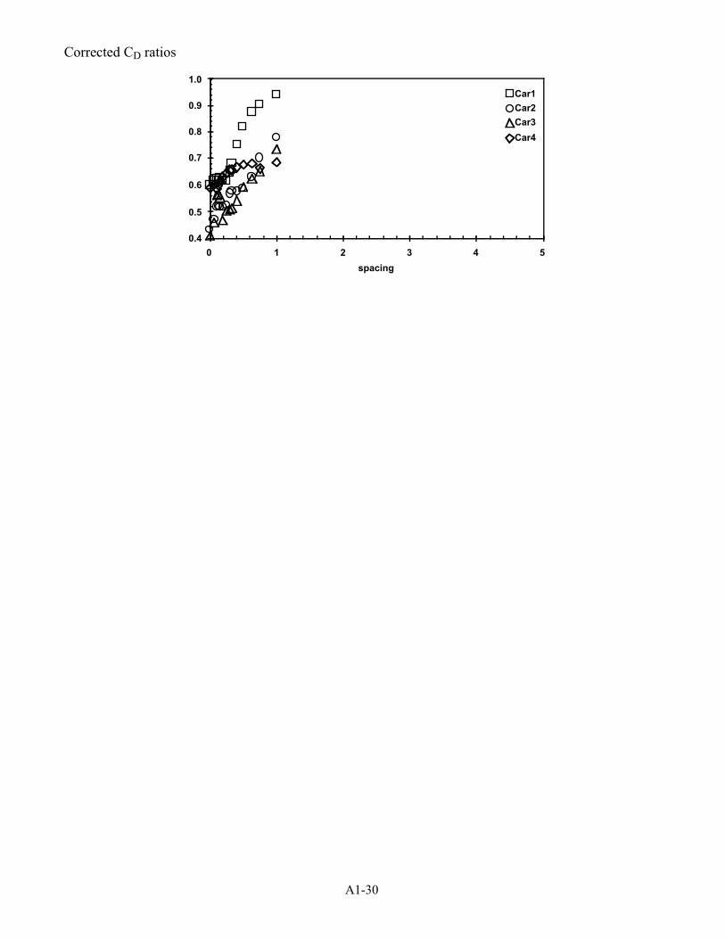
A1-30

Corrected CD ratios

spacing

CD

0.4

0.5

0.6

0.7

0.8

0.9

1.0

0 1 2 3 4 5

Car1

Car2

Car3

Car4

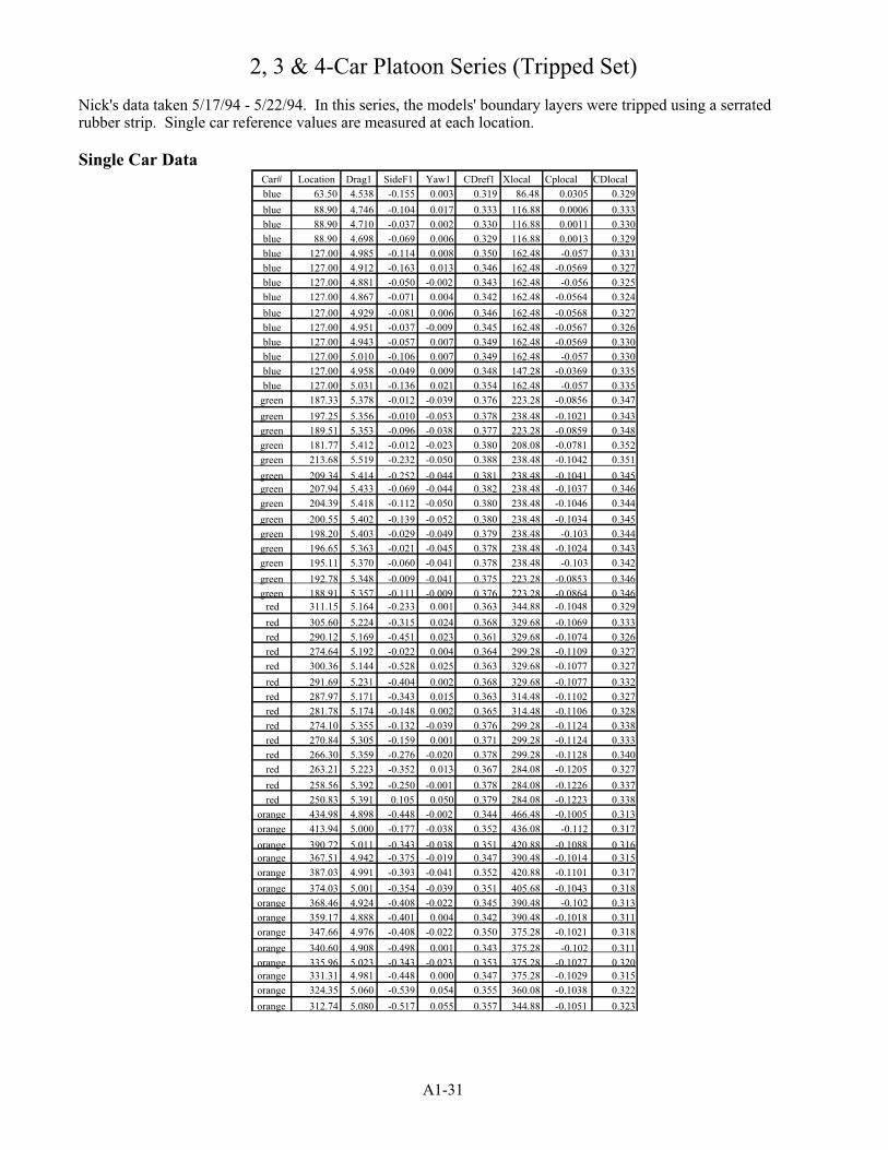
A1-31

2, 3 & 4-Car Platoon Series (Tripped Set)

Nick's data taken 5/17/94 - 5/22/94. In this series, the models' boundary layers were tripped using a serratedrubber strip. Single car reference values are measured at each location.

Single Car DataCar# Location Drag1 SideF1 Yaw1 CDref1 Xlocal Cplocal CDlocalblue 63.50 4.538 -0.155 0.003 0.319 86.48 0.0305 0.329

blue 88.90 4.746 -0.104 0.017 0.333 116.88 0.0006 0.333blue 88.90 4.710 -0.037 0.002 0.330 116.88 0.0011 0.330blue 88.90 4.698 -0.069 0.006 0.329 116.88 0.0013 0.329blue 127.00 4.985 -0.114 0.008 0.350 162.48 -0.057 0.331blue 127.00 4.912 -0.163 0.013 0.346 162.48 -0.0569 0.327blue 127.00 4.881 -0.050 -0.002 0.343 162.48 -0.056 0.325blue 127.00 4.867 -0.071 0.004 0.342 162.48 -0.0564 0.324

blue 127.00 4.929 -0.081 0.006 0.346 162.48 -0.0568 0.327blue 127.00 4.951 -0.037 -0.009 0.345 162.48 -0.0567 0.326blue 127.00 4.943 -0.057 0.007 0.349 162.48 -0.0569 0.330blue 127.00 5.010 -0.106 0.007 0.349 162.48 -0.057 0.330blue 127.00 4.958 -0.049 0.009 0.348 147.28 -0.0369 0.335blue 127.00 5.031 -0.136 0.021 0.354 162.48 -0.057 0.335

green 187.33 5.378 -0.012 -0.039 0.376 223.28 -0.0856 0.347

green 197.25 5.356 -0.010 -0.053 0.378 238.48 -0.1021 0.343green 189.51 5.353 -0.096 -0.038 0.377 223.28 -0.0859 0.348green 181.77 5.412 -0.012 -0.023 0.380 208.08 -0.0781 0.352green 213.68 5.519 -0.232 -0.050 0.388 238.48 -0.1042 0.351

green 209.34 5.414 -0.252 -0.044 0.381 238.48 -0.1041 0.345green 207.94 5.433 -0.069 -0.044 0.382 238.48 -0.1037 0.346green 204.39 5.418 -0.112 -0.050 0.380 238.48 -0.1046 0.344

green 200.55 5.402 -0.139 -0.052 0.380 238.48 -0.1034 0.345green 198.20 5.403 -0.029 -0.049 0.379 238.48 -0.103 0.344green 196.65 5.363 -0.021 -0.045 0.378 238.48 -0.1024 0.343green 195.11 5.370 -0.060 -0.041 0.378 238.48 -0.103 0.342

green 192.78 5.348 -0.009 -0.041 0.375 223.28 -0.0853 0.346green 188.91 5.357 -0.111 -0.009 0.376 223.28 -0.0864 0.346

red 311.15 5.164 -0.233 0.001 0.363 344.88 -0.1048 0.329

red 305.60 5.224 -0.315 0.024 0.368 329.68 -0.1069 0.333red 290.12 5.169 -0.451 0.023 0.361 329.68 -0.1074 0.326red 274.64 5.192 -0.022 0.004 0.364 299.28 -0.1109 0.327red 300.36 5.144 -0.528 0.025 0.363 329.68 -0.1077 0.327

red 291.69 5.231 -0.404 0.002 0.368 329.68 -0.1077 0.332red 287.97 5.171 -0.343 0.015 0.363 314.48 -0.1102 0.327red 281.78 5.174 -0.148 0.002 0.365 314.48 -0.1106 0.328red 274.10 5.355 -0.132 -0.039 0.376 299.28 -0.1124 0.338red 270.84 5.305 -0.159 0.001 0.371 299.28 -0.1124 0.333red 266.30 5.359 -0.276 -0.020 0.378 299.28 -0.1128 0.340red 263.21 5.223 -0.352 0.013 0.367 284.08 -0.1205 0.327

red 258.56 5.392 -0.250 -0.001 0.378 284.08 -0.1226 0.337red 250.83 5.391 0.105 0.050 0.379 284.08 -0.1223 0.338

orange 434.98 4.898 -0.448 -0.002 0.344 466.48 -0.1005 0.313orange 413.94 5.000 -0.177 -0.038 0.352 436.08 -0.112 0.317

orange 390.72 5.011 -0.343 -0.038 0.351 420.88 -0.1088 0.316orange 367.51 4.942 -0.375 -0.019 0.347 390.48 -0.1014 0.315orange 387.03 4.991 -0.393 -0.041 0.352 420.88 -0.1101 0.317

orange 374.03 5.001 -0.354 -0.039 0.351 405.68 -0.1043 0.318orange 368.46 4.924 -0.408 -0.022 0.345 390.48 -0.102 0.313orange 359.17 4.888 -0.401 0.004 0.342 390.48 -0.1018 0.311orange 347.66 4.976 -0.408 -0.022 0.350 375.28 -0.1021 0.318

orange 340.60 4.908 -0.498 0.001 0.343 375.28 -0.102 0.311orange 335.96 5.023 -0.343 -0.023 0.353 375.28 -0.1027 0.320orange 331.31 4.981 -0.448 0.000 0.347 375.28 -0.1029 0.315orange 324.35 5.060 -0.539 0.054 0.355 360.08 -0.1038 0.322

orange 312.74 5.080 -0.517 0.055 0.357 344.88 -0.1051 0.323

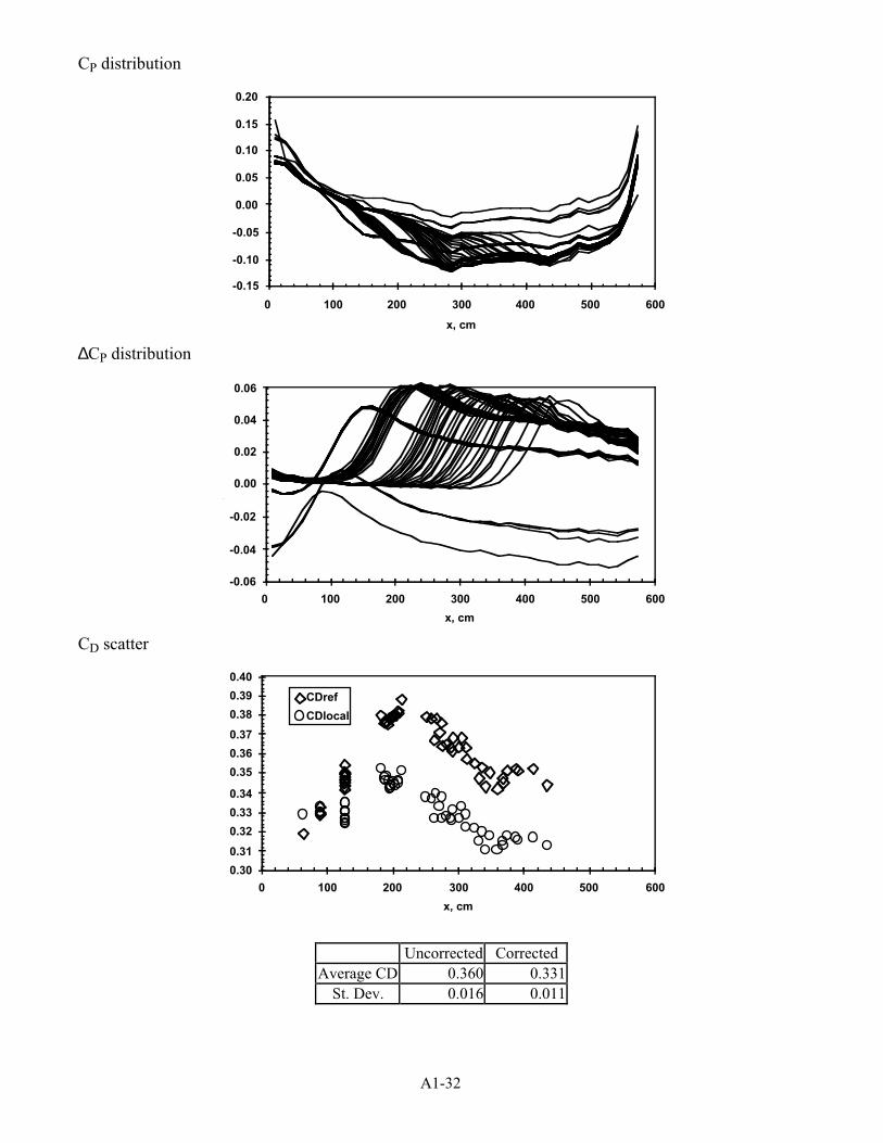
A1-32

CP distribution

x, cm

-0.15

-0.10

-0.05

0.00

0.05

0.10

0.15

0.20

0 100 200 300 400 500 600

∆CP distribution

x, cm

DC

-0.06

-0.04

-0.02

0.00

0.02

0.04

0.06

0 100 200 300 400 500 600

CD scatter

x, cm

0.30

0.31

0.32

0.33

0.34

0.35

0.36

0.37

0.38

0.39

0.40

0 100 200 300 400 500 600

CDref

CDlocal

Uncorrected CorrectedAverage CD 0.360 0.331

St. Dev. 0.016 0.011

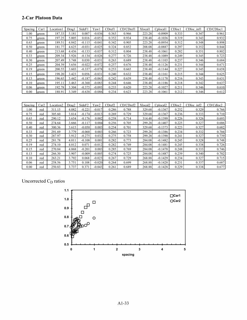
A1-33

2-Car Platoon Data

Spacing Car1 Location1 Drag1 SideF1 Yaw1 CDref1 CD/CDref1 Xlocal1 Cplocal1 CDloc1 CDloc_inf1 CD/CDloc11.00 green 187.33 5.181 0.007 -0.036 0.363 0.966 223.28 -0.0909 0.333 0.347 0.9610.75 green 197.25 5.005 0.016 -0.051 0.352 0.934 238.48 -0.1036 0.319 0.343 0.9320.63 green 189.51 4.842 -0.115 -0.041 0.342 0.905 223.28 -0.0954 0.312 0.348 0.8980.50 green 181.77 4.625 -0.031 -0.025 0.324 0.852 208.08 -0.0887 0.297 0.352 0.8440.40 green 213.68 4.436 -0.133 -0.037 0.312 0.804 238.48 -0.1061 0.282 0.351 0.8020.33 green 209.34 3.926 -0.134 -0.026 0.277 0.726 238.48 -0.1089 0.249 0.345 0.7230.30 green 207.49 3.748 0.030 -0.031 0.263 0.689 238.48 -0.1103 0.237 0.346 0.6840.25 green 204.39 3.656 -0.022 -0.072 0.257 0.676 238.48 -0.1126 0.231 0.344 0.6710.19 green 200.55 3.603 -0.337 -0.078 0.253 0.665 238.48 -0.1144 0.227 0.345 0.658

0.15 green 198.20 3.423 0.056 -0.031 0.240 0.632 238.48 -0.1161 0.215 0.344 0.6250.13 green 196.65 3.442 -0.187 -0.065 0.242 0.639 238.48 -0.1178 0.216 0.343 0.6310.10 green 195.11 3.463 -0.368 -0.083 0.244 0.646 238.48 -0.1186 0.218 0.342 0.6370.06 green 192.78 3.304 -0.375 -0.093 0.233 0.620 223.28 -0.1027 0.211 0.346 0.6100.00 green 188.91 3.349 -0.638 -0.086 0.234 0.623 223.28 -0.1061 0.212 0.346 0.612

Spacing Car2 Location2 Drag2 SideF2 Yaw2 CDref2 CD/CDref2 Xlocal2 Cplocal2 CDloc2 CDloc_inf2 CD/Cdloc21.00 red 311.15 4.082 -0.221 -0.017 0.286 0.788 329.68 -0.1367 0.252 0.329 0.7660.75 red 305.60 3.814 -0.174 -0.013 0.269 0.729 329.68 -0.1367 0.236 0.333 0.7100.63 red 290.12 3.654 -0.176 0.002 0.258 0.714 314.48 -0.1399 0.226 0.326 0.6930.50 red 274.64 3.666 -0.117 0.004 0.256 0.705 299.28 -0.1407 0.225 0.327 0.6860.40 red 300.36 3.615 -0.050 0.003 0.254 0.701 329.68 -0.1373 0.223 0.327 0.6820.33 red 291.69 3.779 -0.068 0.003 0.266 0.723 299.28 -0.1386 0.234 0.332 0.7040.30 red 287.97 3.912 -0.275 0.032 0.275 0.758 299.28 -0.1390 0.241 0.327 0.7390.25 red 281.78 4.011 -0.108 0.001 0.282 0.773 284.08 -0.1482 0.245 0.328 0.7480.19 red 274.10 4.012 0.071 -0.012 0.282 0.749 284.08 -0.1481 0.245 0.338 0.7260.15 red 270.84 4.068 -0.201 0.003 0.285 0.769 284.08 -0.1478 0.248 0.333 0.7460.13 red 266.30 3.907 -0.009 -0.005 0.274 0.725 284.08 -0.1487 0.239 0.340 0.7020.10 red 263.21 3.792 0.068 -0.023 0.267 0.729 268.88 -0.1429 0.234 0.327 0.7150.06 red 258.56 3.751 0.108 -0.020 0.264 0.699 268.88 -0.1428 0.231 0.337 0.6870.00 red 250.83 3.737 0.371 -0.043 0.261 0.689 268.88 -0.1428 0.229 0.338 0.677

Uncorrected CD ratios

spacing

CD

0.5

0.6

0.7

0.8

0.9

1.0

1.1

0 1 2 3 4 5

Car1

Car2

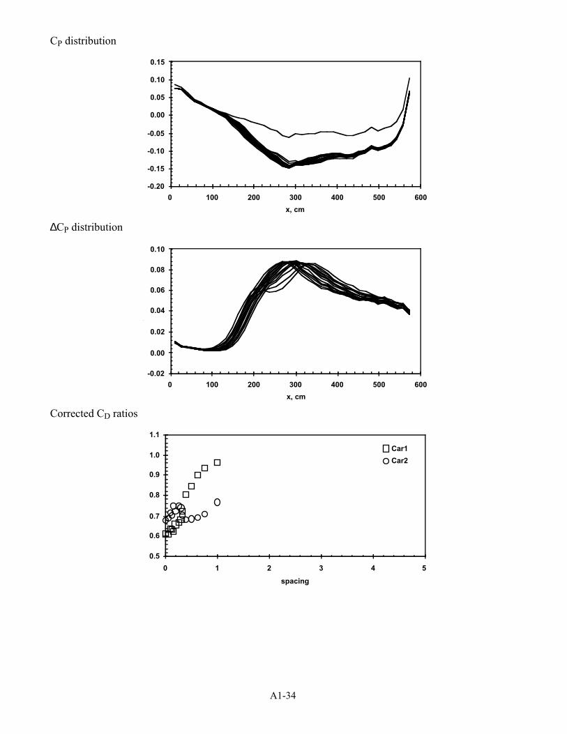
A1-34

CP distribution

x, cm

-0.20

-0.15

-0.10

-0.05

0.00

0.05

0.10

0.15

0 100 200 300 400 500 600

∆CP distribution

x, cm

DC

-0.02

0.00

0.02

0.04

0.06

0.08

0.10

0 100 200 300 400 500 600

Corrected CD ratios

spacing

CDl

0.5

0.6

0.7

0.8

0.9

1.0

1.1

0 1 2 3 4 5

Car1

Car2

A1-35

3-Car Platoon Data

Spacing Car# Location Drag1 SideF1 Yaw1 CDref1 CD/CDref1 Xlocal1 Cplocal1 CDloc1 CDloc_inf1 CD/CDloc11.00 blue 63.50 4.273 -0.014 -0.019 0.301 0.943 86.48 0.0294 0.310 0.329 0.942

0.75 blue 88.90 4.333 -0.096 0.016 0.305 0.916 116.88 0.0017 0.306 0.333 0.9170.63 blue 88.90 4.117 -0.046 -0.002 0.289 0.877 116.88 0.0003 0.289 0.330 0.8770.50 blue 88.90 3.854 -0.058 0.000 0.270 0.822 116.88 -0.001 0.270 0.329 0.8200.40 blue 127.00 3.835 -0.040 -0.010 0.270 0.772 162.48 -0.0616 0.255 0.331 0.7690.33 blue 127.00 3.433 -0.133 -0.004 0.242 0.701 162.48 -0.0635 0.228 0.327 0.6960.30 blue 127.00 3.208 -0.089 -0.019 0.226 0.658 162.48 -0.0635 0.212 0.325 0.6530.25 blue 127.00 3.075 -0.006 -0.001 0.215 0.628 162.48 -0.0643 0.202 0.324 0.6230.19 blue 127.00 3.256 -0.520 -0.044 0.229 0.663 162.48 -0.0661 0.215 0.327 0.657

0.15 blue 127.00 3.129 -0.636 -0.072 0.219 0.635 162.48 -0.0668 0.205 0.326 0.6290.13 blue 127.00 3.202 -0.595 -0.074 0.225 0.646 162.48 -0.0678 0.211 0.330 0.6400.10 blue 127.00 3.187 -0.618 -0.086 0.224 0.642 162.48 -0.068 0.210 0.330 0.6360.06 blue 127.00 3.019 -0.659 -0.087 0.213 0.612 147.28 -0.0586 0.201 0.335 0.5990.00 blue 127.00 3.038 -0.751 -0.080 0.213 0.602 162.48 -0.0688 0.199 0.335 0.595

Spacing Car# Location Drag2 SideF2 Yaw2 CDref2 CD/CDref2 Xlocal2 Cplocal2 CDloc2 CDloc_inf2 CD/CDloc21.00 green 187.33 3.982 0.005 -0.086 0.280 0.744 223.28 -0.0437 0.268 0.347 0.774

0.75 green 197.25 3.634 -0.004 -0.108 0.256 0.678 238.48 -0.0688 0.239 0.343 0.6990.63 green 189.51 3.286 -0.034 -0.066 0.231 0.612 223.28 -0.0616 0.217 0.348 0.6260.50 green 181.77 3.081 0.105 -0.063 0.216 0.569 208.08 -0.0564 0.204 0.352 0.5800.40 green 213.68 3.127 0.029 -0.062 0.221 0.568 238.48 -0.1176 0.197 0.351 0.5620.33 green 209.34 3.136 0.041 -0.058 0.221 0.581 238.48 -0.1193 0.198 0.345 0.5730.30 green 207.94 3.161 0.058 -0.057 0.222 0.581 238.48 -0.1194 0.198 0.346 0.5730.25 green 204.39 2.878 0.066 -0.057 0.201 0.530 238.48 -0.1204 0.180 0.344 0.5220.19 green 200.55 2.843 0.029 -0.110 0.200 0.526 238.48 -0.1231 0.178 0.345 0.517

0.15 green 198.20 2.845 -0.033 -0.151 0.199 0.525 238.48 -0.1245 0.177 0.344 0.5150.13 green 196.65 2.869 -0.327 -0.166 0.202 0.534 238.48 -0.125 0.180 0.343 0.5240.10 green 195.11 2.823 -0.491 -0.195 0.199 0.526 238.48 -0.1254 0.176 0.342 0.5150.06 green 192.78 2.341 1.061 0.406 0.165 0.439 223.28 -0.111 0.148 0.346 0.4290.00 green 188.91 2.347 -0.480 -0.213 0.165 0.438 223.28 -0.1109 0.148 0.346 0.429

Spacing Car# Location Drag3 SideF3 Yaw3 CDref3 CD/CDref3 Xlocal3 Cplocal3 CDloc3 CDloc_inf3 CD/CDloc31.00 red 311.15 3.848 -0.336 0.003 0.271 0.745 329.68 -0.0783 0.251 0.329 0.7630.75 red 305.60 3.701 -0.233 0.006 0.261 0.708 329.68 -0.0931 0.238 0.333 0.7170.63 red 290.12 3.626 -0.212 0.018 0.255 0.705 299.28 -0.0951 0.233 0.326 0.7130.50 red 274.64 3.668 -0.171 0.013 0.257 0.706 284.08 -0.1046 0.233 0.327 0.7100.40 red 300.36 3.649 -0.143 0.027 0.257 0.709 314.48 -0.1410 0.226 0.327 0.6890.33 red 291.69 3.550 -0.126 0.019 0.250 0.680 299.28 -0.1405 0.220 0.332 0.6610.30 red 287.97 3.525 -0.095 0.015 0.248 0.683 299.28 -0.1404 0.217 0.327 0.6650.25 red 281.78 3.628 -0.107 0.021 0.254 0.696 284.08 -0.1492 0.221 0.328 0.673

0.19 red 274.10 3.327 -0.090 -0.017 0.234 0.623 284.08 -0.1508 0.204 0.338 0.6030.15 red 270.84 3.696 0.153 -0.034 0.259 0.698 284.08 -0.1510 0.225 0.333 0.6740.13 red 266.30 3.600 0.260 -0.050 0.253 0.670 268.88 -0.1464 0.221 0.340 0.6500.10 red 263.21 3.543 0.338 -0.063 0.249 0.680 268.88 -0.1461 0.217 0.327 0.6650.06 red 258.56 3.490 0.346 -0.067 0.246 0.650 268.88 -0.1444 0.215 0.337 0.6370.00 red 250.83 3.486 0.506 -0.090 0.244 0.645 268.88 -0.1429 0.214 0.338 0.633

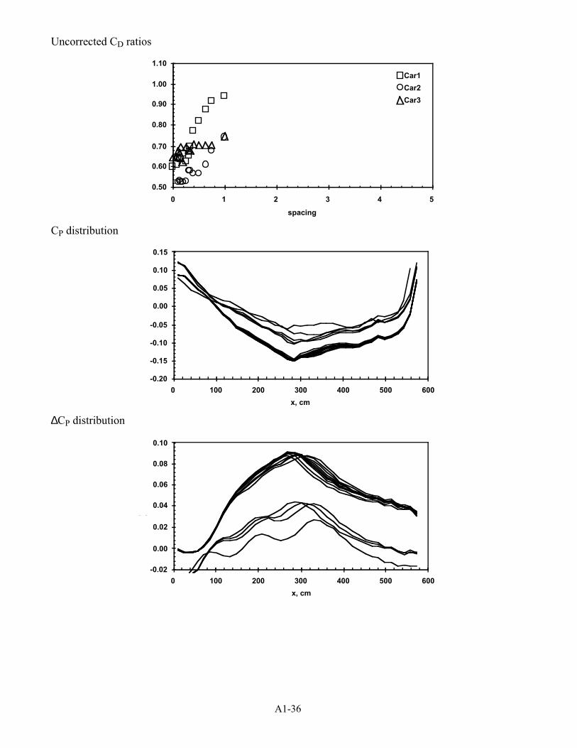
A1-36

Uncorrected CD ratios

spacing

CD

0.50

0.60

0.70

0.80

0.90

1.00

1.10

0 1 2 3 4 5

Car1

Car2

Car3

CP distribution

x, cm

-0.20

-0.15

-0.10

-0.05

0.00

0.05

0.10

0.15

0 100 200 300 400 500 600

∆CP distribution

x, cm

DC

-0.02

0.00

0.02

0.04

0.06

0.08

0.10

0 100 200 300 400 500 600

A1-37

Corrected CD ratios

spacing

CD

0.50

0.60

0.70

0.80

0.90

1.00

1.10

0 1 2 3 4 5

Car1

Car2

Car3

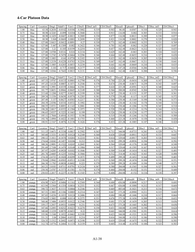
A1-38

4-Car Platoon Data

Spacing Car# Location Drag1 SideF1 Yaw1 CDref1 CDref_inf1 CD/CDref1 Xlocal1 Cplocal1 CDloc1 CDloc_inf1 CD/CDloc11.00 blue 63.50 4.2636 -0.0142 -0.0186 0.3002 0.319 0.943 86.48 0.0307 0.310 0.329 0.9430.75 blue 88.90 4.3245 -0.099 0.0184 0.3048 0.333 0.915 116.88 0.002 0.305 0.333 0.9160.63 blue 88.90 4.1429 -0.0447 -0.0013 0.2889 0.330 0.877 116.88 0.0013 0.289 0.330 0.8770.50 blue 88.90 3.848 -0.0669 0.0001 0.2698 0.329 0.821 116.88 0.0002 0.270 0.329 0.8200.40 blue 127.00 3.8415 -0.0412 -0.0091 0.27 0.350 0.771 162.48 -0.0602 0.255 0.331 0.7690.33 blue 127.00 3.447 -0.1309 -0.002 0.2422 0.346 0.701 162.48 -0.062 0.228 0.327 0.6970.30 blue 127.00 3.21 -0.105 -0.0199 0.2254 0.343 0.657 162.48 -0.0623 0.212 0.325 0.6530.25 blue 127.00 3.0708 0.0316 0.018 0.2154 0.342 0.629 162.48 -0.063 0.203 0.324 0.6250.19 blue 127.00 3.2742 -0.5478 -0.0464 0.2296 0.346 0.664 162.48 -0.0652 0.216 0.327 0.6580.15 blue 127.00 3.1003 -0.64 -0.0738 0.2183 0.345 0.633 162.48 -0.0656 0.205 0.326 0.6280.13 blue 127.00 3.2158 -0.6228 -0.0763 0.2256 0.349 0.647 162.48 -0.0667 0.211 0.330 0.6410.10 blue 127.00 3.1805 -0.6203 -0.0853 0.2238 0.349 0.641 162.48 -0.0669 0.210 0.330 0.6350.06 blue 127.00 3.101 -0.717 -0.0684 0.2177 0.348 0.626 147.28 -0.0566 0.206 0.335 0.6150.00 blue 127.00 3.0366 -0.7643 -0.0815 0.2131 0.354 0.602 162.48 -0.0672 0.200 0.335 0.596

Spacing Car# Location Drag2 SideF2 Yaw2 CDref2 CDref_inf2 CD/CDref2 Xlocal2 Cplocal2 CDloc2 CDloc_inf2 CD/CDloc21.00 green 187.33 3.9747 -0.0133 -0.0881 0.2798 0.376 0.744 223.28 -0.0416 0.269 0.347 0.7750.75 green 197.25 3.6128 -0.0007 -0.1071 0.2546 0.378 0.674 238.48 -0.0671 0.239 0.343 0.6970.63 green 189.51 3.2991 -0.0339 -0.0664 0.2301 0.377 0.610 223.28 -0.0591 0.217 0.348 0.6250.50 green 181.77 3.0651 0.0966 -0.0645 0.2149 0.380 0.566 208.08 -0.0542 0.204 0.352 0.5790.40 green 213.68 3.1288 0.0277 -0.0633 0.2199 0.388 0.567 238.48 -0.1151 0.197 0.351 0.5610.33 green 209.34 3.1356 0.0438 -0.0576 0.2203 0.381 0.579 238.48 -0.117 0.197 0.345 0.5720.30 green 207.49 3.157 0.0627 -0.0583 0.2217 0.382 0.580 238.48 -0.1169 0.198 0.346 0.5730.25 green 204.39 2.8396 0.0334 -0.0532 0.1992 0.380 0.524 238.48 -0.1182 0.178 0.344 0.5180.19 green 200.55 2.8531 0.0093 -0.1143 0.2001 0.380 0.526 238.48 -0.1206 0.179 0.345 0.5180.15 green 198.20 2.8017 -0.0352 -0.1504 0.1973 0.379 0.520 238.48 -0.1214 0.176 0.344 0.5120.13 green 196.65 2.8357 -0.3225 -0.1663 0.199 0.378 0.526 238.48 -0.1238 0.177 0.343 0.5160.10 green 195.11 2.7844 -0.4916 -0.1933 0.196 0.378 0.519 238.48 -0.1246 0.174 0.342 0.5090.06 green 192.78 2.4994 -0.4422 -0.1881 0.1755 0.375 0.468 223.28 -0.1078 0.158 0.346 0.4580.00 green 188.91 2.3167 -0.4876 -0.2138 0.1626 0.376 0.433 223.28 -0.1085 0.147 0.346 0.424

Spacing Car# Location Drag3 SideF3 Yaw3 CDref3 CDref_inf3 CD/CDref3 Xlocal3 Cplocal3 CDloc3 CDloc_inf3 CD/CDloc31.00 red 311.15 3.6671 -0.3338 0.0017 0.2582 0.363 0.711 344.88 -0.0733 0.241 0.329 0.7310.75 red 305.60 3.3331 -0.1851 0.0124 0.2349 0.368 0.638 329.68 -0.0911 0.215 0.333 0.6470.63 red 290.12 3.1811 -0.1878 0.0201 0.2218 0.361 0.614 329.68 -0.0917 0.203 0.326 0.6230.50 red 274.64 3.0242 -0.1457 0.0186 0.212 0.364 0.583 299.28 -0.0936 0.194 0.327 0.5920.40 red 300.36 2.9091 -0.1522 0.0245 0.2045 0.363 0.564 329.68 -0.1376 0.180 0.327 0.5490.33 red 291.69 2.7108 -0.1479 0.0149 0.1904 0.368 0.517 329.68 -0.1395 0.167 0.332 0.5030.30 red 287.97 2.6285 -0.0928 0.0102 0.1846 0.363 0.509 314.48 -0.1414 0.162 0.327 0.4950.25 red 281.78 2.6605 -0.1235 0.0162 0.1866 0.365 0.512 314.48 -0.1423 0.163 0.328 0.4980.19 red 274.10 2.6735 -0.1028 -0.0299 0.1875 0.376 0.499 299.28 -0.1452 0.164 0.338 0.4850.15 red 270.84 2.9942 -0.0503 -0.0513 0.2108 0.371 0.569 299.28 -0.1474 0.184 0.333 0.5510.13 red 266.30 3.1785 -0.0038 -0.0692 0.223 0.378 0.589 299.28 -0.1494 0.194 0.340 0.5710.10 red 263.21 3.0183 0.0711 -0.0791 0.2124 0.367 0.580 284.08 -0.1565 0.184 0.327 0.5610.06 red 258.56 2.4787 -0.3373 -0.1581 0.174 0.378 0.460 284.08 -0.152 0.151 0.337 0.4490.00 red 250.83 2.2017 -0.2237 -0.1867 0.1545 0.379 0.408 284.08 -0.152 0.134 0.338 0.397

Spacing Car# Location Drag4 SideF4 Yaw4 CDref4 CDref_inf4 CD/CDref4 Xlocal4 Cplocal4 CDloc4 CDloc_inf4 CD/CDloc41.00 orange 434.98 3.3655 -0.0486 0.1161 0.2369 0.344 0.688 436.08 -0.0898 0.217 0.313 0.6950.75 orange 413.94 3.3364 -0.1354 0.0016 0.2351 0.352 0.667 436.08 -0.1088 0.212 0.317 0.6690.63 orange 390.72 3.3637 -0.1111 0.0066 0.2346 0.351 0.669 405.68 -0.1021 0.213 0.316 0.6730.50 orange 367.51 3.3003 -0.1186 0.0085 0.2314 0.347 0.667 375.28 -0.0988 0.211 0.315 0.6690.40 orange 387.03 3.4236 -0.1033 0.0124 0.2406 0.352 0.684 390.48 -0.1446 0.210 0.317 0.6640.33 orange 374.03 3.3805 -0.098 0.0114 0.2375 0.351 0.676 375.28 -0.1436 0.208 0.318 0.6530.30 orange 368.46 3.3406 -0.0935 0.0122 0.2346 0.345 0.681 375.28 -0.1439 0.205 0.313 0.6560.25 orange 359.17 3.2937 -0.0931 0.0098 0.231 0.342 0.675 375.28 -0.1445 0.202 0.311 0.6500.19 orange 347.66 3.2493 0.0252 -0.0223 0.2278 0.350 0.651 344.88 -0.1490 0.198 0.318 0.6240.15 orange 340.60 3.1239 0.0879 -0.0433 0.22 0.343 0.641 344.88 -0.1501 0.191 0.311 0.6140.13 orange 335.96 3.1348 0.1852 -0.0463 0.2199 0.353 0.623 344.88 -0.1521 0.191 0.320 0.5960.10 orange 331.31 3.04 0.2004 -0.0533 0.214 0.347 0.616 344.88 -0.1521 0.186 0.315 0.5900.06 orange 324.35 3.1312 0.2692 0.0971 0.2198 0.355 0.619 329.68 -0.1475 0.192 0.322 0.5950.00 orange 312.74 3.0776 0.2484 0.1135 0.2159 0.357 0.605 314.48 -0.1470 0.188 0.323 0.583

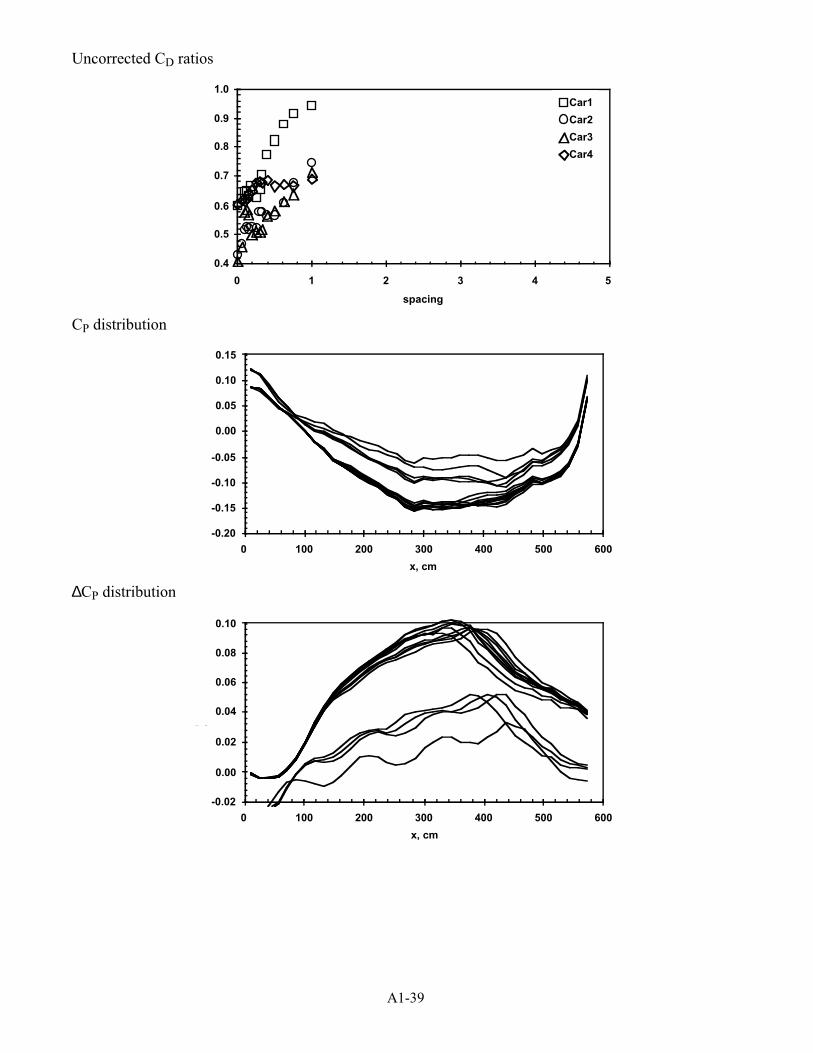
A1-39

Uncorrected CD ratios

spacing

CD

0.4

0.5

0.6

0.7

0.8

0.9

1.0

0 1 2 3 4 5

Car1

Car2

Car3

Car4

CP distribution

x, cm

-0.20

-0.15

-0.10

-0.05

0.00

0.05

0.10

0.15

0 100 200 300 400 500 600

∆CP distribution

x, cm

DC

-0.02

0.00

0.02

0.04

0.06

0.08

0.10

0 100 200 300 400 500 600

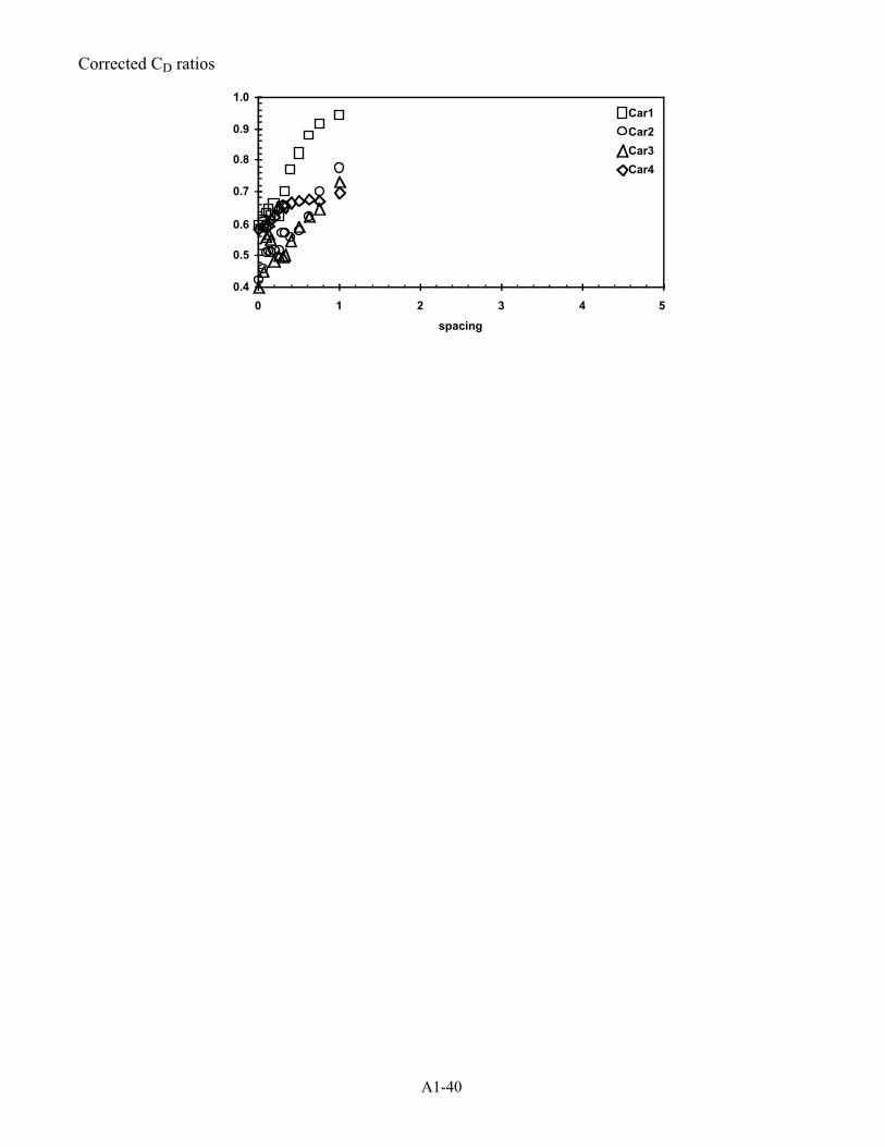
A1-40

Corrected CD ratios

spacing

CD

0.4

0.5

0.6

0.7

0.8

0.9

1.0

0 1 2 3 4 5

Car1

Car2

Car3

Car4

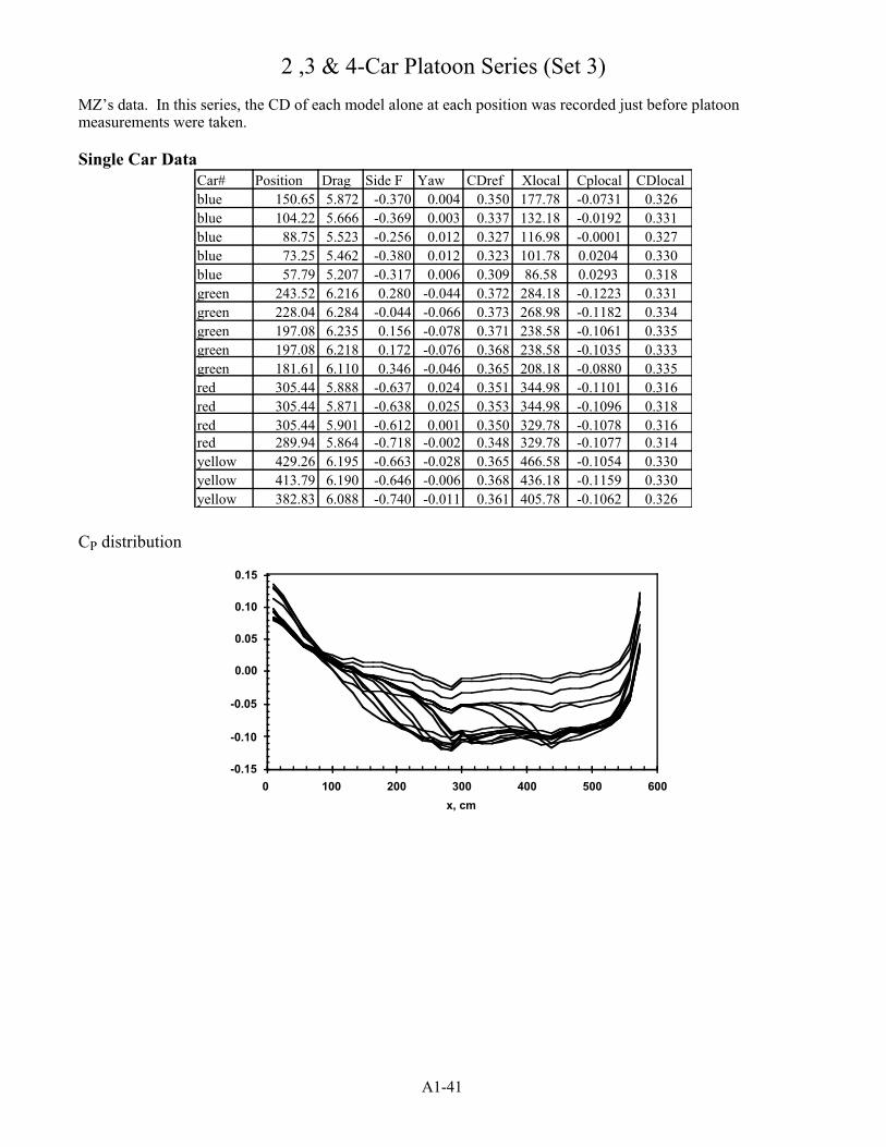
A1-41

2 ,3 & 4-Car Platoon Series (Set 3)

MZ’s data. In this series, the CD of each model alone at each position was recorded just before platoonmeasurements were taken.

Single Car DataCar# Position Drag Side F Yaw CDref Xlocal Cplocal CDlocalblue 150.65 5.872 -0.370 0.004 0.350 177.78 -0.0731 0.326blue 104.22 5.666 -0.369 0.003 0.337 132.18 -0.0192 0.331blue 88.75 5.523 -0.256 0.012 0.327 116.98 -0.0001 0.327blue 73.25 5.462 -0.380 0.012 0.323 101.78 0.0204 0.330blue 57.79 5.207 -0.317 0.006 0.309 86.58 0.0293 0.318green 243.52 6.216 0.280 -0.044 0.372 284.18 -0.1223 0.331green 228.04 6.284 -0.044 -0.066 0.373 268.98 -0.1182 0.334green 197.08 6.235 0.156 -0.078 0.371 238.58 -0.1061 0.335green 197.08 6.218 0.172 -0.076 0.368 238.58 -0.1035 0.333green 181.61 6.110 0.346 -0.046 0.365 208.18 -0.0880 0.335red 305.44 5.888 -0.637 0.024 0.351 344.98 -0.1101 0.316red 305.44 5.871 -0.638 0.025 0.353 344.98 -0.1096 0.318red 305.44 5.901 -0.612 0.001 0.350 329.78 -0.1078 0.316red 289.94 5.864 -0.718 -0.002 0.348 329.78 -0.1077 0.314yellow 429.26 6.195 -0.663 -0.028 0.365 466.58 -0.1054 0.330yellow 413.79 6.190 -0.646 -0.006 0.368 436.18 -0.1159 0.330yellow 382.83 6.088 -0.740 -0.011 0.361 405.78 -0.1062 0.326

CP distribution

x, cm

C

-0.15

-0.10

-0.05

0.00

0.05

0.10

0.15

0 100 200 300 400 500 600

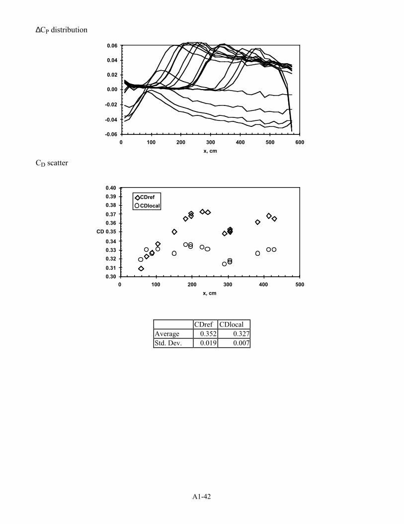
A1-42

∆CP distribution

x, cm

DC

-0.06

-0.04

-0.02

0.00

0.02

0.04

0.06

0 100 200 300 400 500 600

CD scatter

x, cm

CD

0.30

0.31

0.32

0.33

0.34

0.35

0.36

0.37

0.38

0.39

0.40

0 100 200 300 400 500

CDref

CDlocal

CDref CDlocalAverage 0.352 0.327Std. Dev. 0.019 0.007

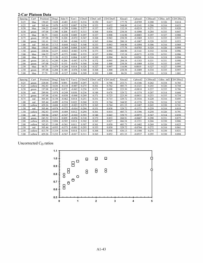
A1-43

2-Car Platoon DataSpacing Car# Position1 Drag1 Side F1 Yaw1 CDref1 CDref_inf1 CD/CDref1 Xlocal1 Cplocal1 CDlocal1 CDloc_inf1 CD/CDloc1

0.25 blue 150.65 3.628 -0.401 -0.013 0.216 0.350 0.617 177.78 -0.0789 0.200 0.326 0.6140.25 red 305.44 3.870 -0.555 0.007 0.230 0.353 0.652 344.98 -0.1141 0.206 0.316 0.6530.50 blue 104.22 4.663 -0.298 0.006 0.277 0.337 0.822 132.18 -0.0219 0.271 0.331 0.8200.50 green 197.08 5.300 0.208 -0.073 0.315 0.368 0.856 238.58 -0.1090 0.284 0.335 0.8470.75 blue 88.75 5.022 -0.230 0.009 0.297 0.327 0.908 116.98 -0.0003 0.297 0.327 0.9080.75 green 197.08 5.759 0.220 -0.072 0.347 0.368 0.943 238.58 -0.1069 0.313 0.335 0.9351.00 green 181.61 5.912 0.360 -0.046 0.352 0.365 0.964 208.18 -0.1007 0.320 0.335 0.9531.00 red 305.44 5.713 -0.644 0.023 0.340 0.353 0.963 344.98 -0.1094 0.306 0.316 0.9691.50 blue 150.65 5.862 -0.369 0.004 0.347 0.350 0.991 177.78 -0.0703 0.324 0.326 0.9941.50 green 228.04 6.227 -0.022 -0.063 0.370 0.373 0.992 268.98 -0.1141 0.332 0.334 0.9962.00 blue 104.22 5.677 -0.371 0.001 0.335 0.337 0.994 132.18 -0.0171 0.329 0.331 0.9962.00 blue 57.79 5.150 -0.323 0.004 0.307 0.309 0.994 86.58 0.0298 0.316 0.318 0.9942.00 green 243.52 6.240 0.266 -0.047 0.370 0.372 0.995 284.18 -0.1183 0.331 0.331 0.9982.00 green 197.08 6.227 0.155 -0.078 0.368 0.368 1.000 238.58 -0.1009 0.334 0.335 0.9972.50 blue 88.75 5.479 -0.244 0.014 0.326 0.327 0.997 116.98 0.0019 0.327 0.327 0.9992.50 green 197.08 6.204 0.189 -0.076 0.368 0.368 1.000 238.58 -0.1009 0.334 0.335 0.9975.00 blue 57.79 5.199 -0.327 0.004 0.309 0.309 1.000 86.58 0.0298 0.318 0.318 1.001

Spacing Car# Position2 Drag2 Side F2 Yaw2 CDref2 CDref_inf2 CD/Cdref2 Xlocal2 Cplocal2 CDlocal2 Cdloc_inf2 CD/CDloc20.25 green 228.04 4.983 0.091 -0.050 0.297 0.373 0.796 253.71 -0.1346 0.262 0.334 0.7850.25 yellow 382.83 4.636 -0.118 -0.007 0.275 0.361 0.762 405.73 -0.1321 0.243 0.326 0.7440.50 green 197.08 4.302 0.072 -0.065 0.256 0.371 0.690 223.30 -0.0810 0.237 0.335 0.7060.50 red 289.94 3.974 -0.249 0.030 0.236 0.348 0.678 329.72 -0.1374 0.207 0.314 0.6600.75 green 197.08 4.541 -0.030 -0.068 0.269 0.371 0.725 223.30 -0.0631 0.253 0.335 0.7540.75 red 305.44 4.158 -0.462 0.014 0.251 0.351 0.715 329.72 -0.1416 0.220 0.316 0.6951.00 red 305.44 4.499 -0.554 0.022 0.268 0.351 0.764 344.92 -0.1376 0.236 0.316 0.7451.00 yellow 429.26 4.684 -0.225 -0.023 0.279 0.365 0.764 451.33 -0.1407 0.245 0.330 0.7411.50 red 305.44 4.974 -0.372 -0.014 0.294 0.351 0.838 329.72 -0.1371 0.259 0.316 0.8181.50 yellow 382.83 4.959 -0.489 0.012 0.294 0.361 0.814 405.73 -0.1396 0.258 0.326 0.7912.00 red 289.94 4.967 -0.547 -0.010 0.293 0.348 0.842 329.72 -0.0972 0.267 0.314 0.8502.00 green 243.52 5.211 0.029 -0.056 0.310 0.372 0.833 268.91 -0.0687 0.290 0.331 0.8752.00 yellow 429.26 5.094 -0.505 0.014 0.302 0.365 0.827 466.54 -0.1351 0.266 0.330 0.8062.00 yellow 382.83 5.188 -0.561 0.011 0.307 0.361 0.850 405.73 -0.1402 0.269 0.326 0.8252.50 red 305.44 4.935 -0.573 -0.001 0.293 0.353 0.830 329.72 -0.0764 0.272 0.316 0.8612.50 yellow 413.79 5.319 -0.556 0.014 0.315 0.368 0.856 436.13 -0.1500 0.274 0.330 0.8315.00 yellow 429.26 5.232 -0.567 -0.017 0.311 0.365 0.852 451.33 -0.0537 0.295 0.330 0.894

Uncorrected CD ratios

0.5

0.6

0.7

0.8

0.9

1.0

1.1

0 1 2 3 4 5

A1-44

CP distribution

x, cm

-0.20

-0.15

-0.10

-0.05

0.00

0.05

0.10

0.15

0 100 200 300 400 500 600

∆CP distribution

x, cm

DC

-0.03

-0.01

0.01

0.03

0.05

0.07

0.09

0 100 200 300 400 500 600

Corrected CD ratios

spacing

CDl

0.5

0.6

0.7

0.8

0.9

1.0

1.1

0 1 2 3 4 5

Car 1

Car2

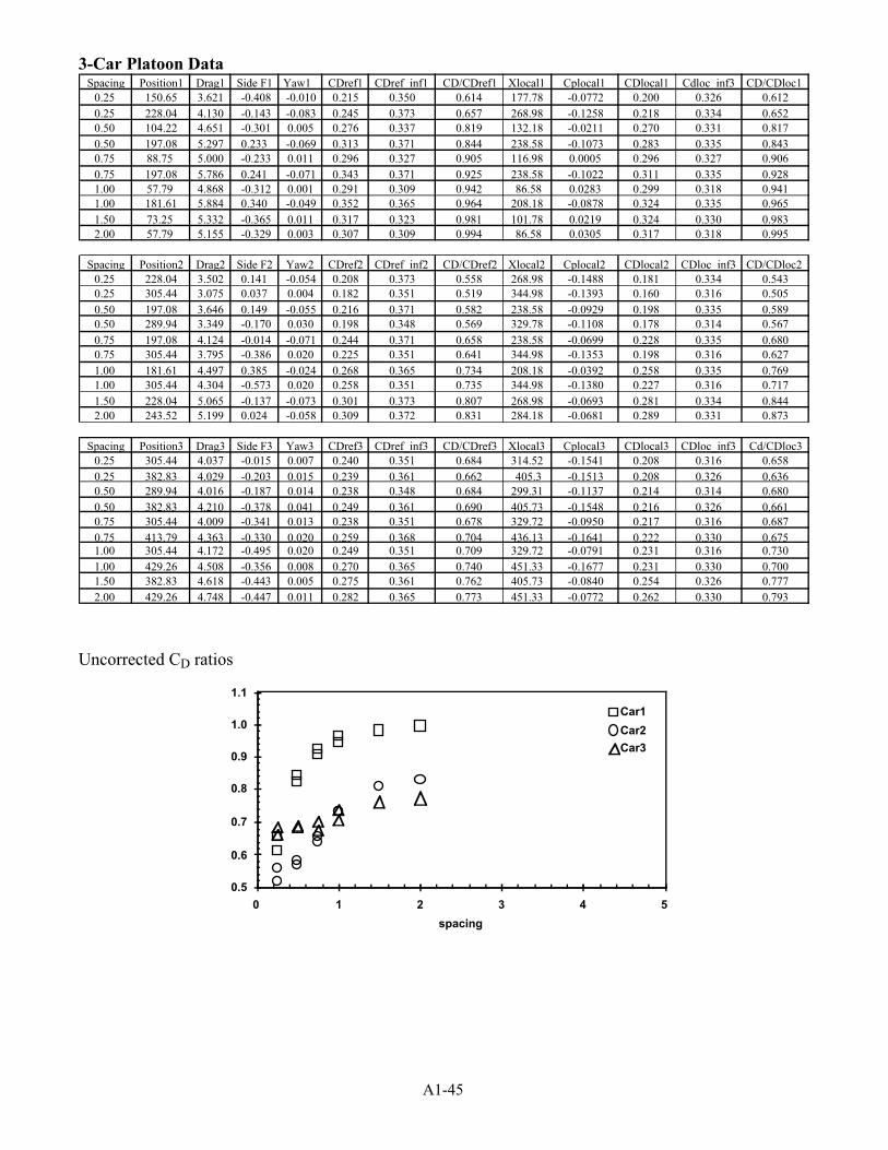
A1-45

3-Car Platoon DataSpacing Position1 Drag1 Side F1 Yaw1 CDref1 CDref_inf1 CD/CDref1 Xlocal1 Cplocal1 CDlocal1 Cdloc_inf3 CD/CDloc1

0.25 150.65 3.621 -0.408 -0.010 0.215 0.350 0.614 177.78 -0.0772 0.200 0.326 0.6120.25 228.04 4.130 -0.143 -0.083 0.245 0.373 0.657 268.98 -0.1258 0.218 0.334 0.6520.50 104.22 4.651 -0.301 0.005 0.276 0.337 0.819 132.18 -0.0211 0.270 0.331 0.8170.50 197.08 5.297 0.233 -0.069 0.313 0.371 0.844 238.58 -0.1073 0.283 0.335 0.8430.75 88.75 5.000 -0.233 0.011 0.296 0.327 0.905 116.98 0.0005 0.296 0.327 0.9060.75 197.08 5.786 0.241 -0.071 0.343 0.371 0.925 238.58 -0.1022 0.311 0.335 0.9281.00 57.79 4.868 -0.312 0.001 0.291 0.309 0.942 86.58 0.0283 0.299 0.318 0.9411.00 181.61 5.884 0.340 -0.049 0.352 0.365 0.964 208.18 -0.0878 0.324 0.335 0.9651.50 73.25 5.332 -0.365 0.011 0.317 0.323 0.981 101.78 0.0219 0.324 0.330 0.9832.00 57.79 5.155 -0.329 0.003 0.307 0.309 0.994 86.58 0.0305 0.317 0.318 0.995

Spacing Position2 Drag2 Side F2 Yaw2 CDref2 CDref_inf2 CD/CDref2 Xlocal2 Cplocal2 CDlocal2 CDloc_inf3 CD/CDloc20.25 228.04 3.502 0.141 -0.054 0.208 0.373 0.558 268.98 -0.1488 0.181 0.334 0.5430.25 305.44 3.075 0.037 0.004 0.182 0.351 0.519 344.98 -0.1393 0.160 0.316 0.5050.50 197.08 3.646 0.149 -0.055 0.216 0.371 0.582 238.58 -0.0929 0.198 0.335 0.5890.50 289.94 3.349 -0.170 0.030 0.198 0.348 0.569 329.78 -0.1108 0.178 0.314 0.5670.75 197.08 4.124 -0.014 -0.071 0.244 0.371 0.658 238.58 -0.0699 0.228 0.335 0.6800.75 305.44 3.795 -0.386 0.020 0.225 0.351 0.641 344.98 -0.1353 0.198 0.316 0.6271.00 181.61 4.497 0.385 -0.024 0.268 0.365 0.734 208.18 -0.0392 0.258 0.335 0.7691.00 305.44 4.304 -0.573 0.020 0.258 0.351 0.735 344.98 -0.1380 0.227 0.316 0.7171.50 228.04 5.065 -0.137 -0.073 0.301 0.373 0.807 268.98 -0.0693 0.281 0.334 0.8442.00 243.52 5.199 0.024 -0.058 0.309 0.372 0.831 284.18 -0.0681 0.289 0.331 0.873

Spacing Position3 Drag3 Side F3 Yaw3 CDref3 CDref_inf3 CD/CDref3 Xlocal3 Cplocal3 CDlocal3 CDloc_inf3 Cd/CDloc30.25 305.44 4.037 -0.015 0.007 0.240 0.351 0.684 314.52 -0.1541 0.208 0.316 0.6580.25 382.83 4.029 -0.203 0.015 0.239 0.361 0.662 405.3 -0.1513 0.208 0.326 0.6360.50 289.94 4.016 -0.187 0.014 0.238 0.348 0.684 299.31 -0.1137 0.214 0.314 0.6800.50 382.83 4.210 -0.378 0.041 0.249 0.361 0.690 405.73 -0.1548 0.216 0.326 0.6610.75 305.44 4.009 -0.341 0.013 0.238 0.351 0.678 329.72 -0.0950 0.217 0.316 0.6870.75 413.79 4.363 -0.330 0.020 0.259 0.368 0.704 436.13 -0.1641 0.222 0.330 0.6751.00 305.44 4.172 -0.495 0.020 0.249 0.351 0.709 329.72 -0.0791 0.231 0.316 0.7301.00 429.26 4.508 -0.356 0.008 0.270 0.365 0.740 451.33 -0.1677 0.231 0.330 0.7001.50 382.83 4.618 -0.443 0.005 0.275 0.361 0.762 405.73 -0.0840 0.254 0.326 0.7772.00 429.26 4.748 -0.447 0.011 0.282 0.365 0.773 451.33 -0.0772 0.262 0.330 0.793

Uncorrected CD ratios

spacing

CD

0.5

0.6

0.7

0.8

0.9

1.0

1.1

0 1 2 3 4 5

Car1

Car2

Car3

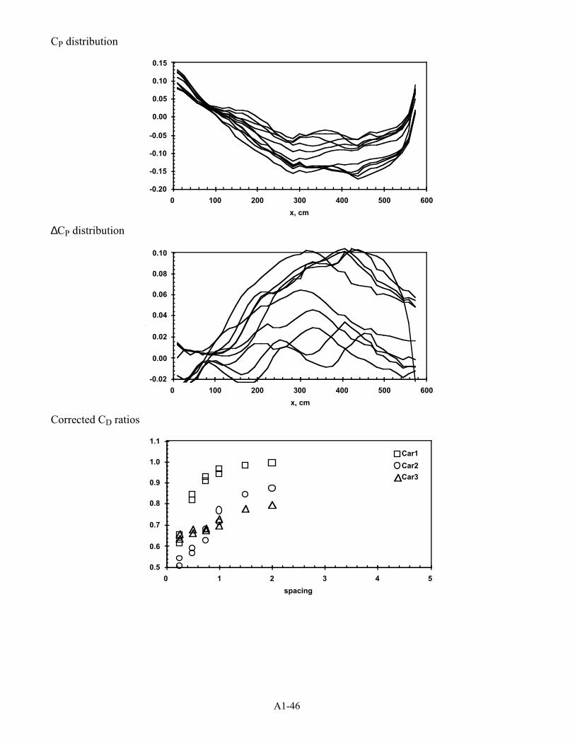
A1-46

CP distribution

x, cm

-0.20

-0.15

-0.10

-0.05

0.00

0.05

0.10

0.15

0 100 200 300 400 500 600

∆CP distribution

x, cm

DC

-0.02

0.00

0.02

0.04

0.06

0.08

0.10

0 100 200 300 400 500 600

Corrected CD ratios

spacing

CD

0.5

0.6

0.7

0.8

0.9

1.0

1.1

0 1 2 3 4 5

Car1

Car2

Car3

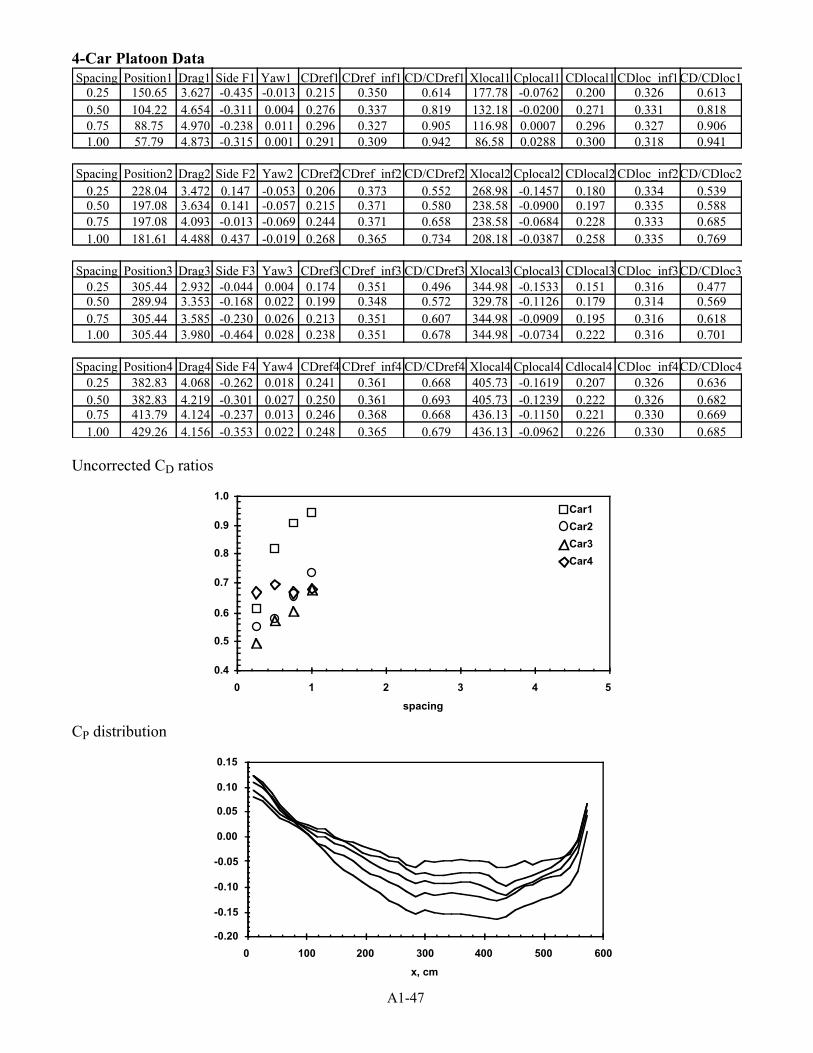
A1-47

4-Car Platoon DataSpacing Position1 Drag1 Side F1 Yaw1 CDref1 CDref_inf1 CD/CDref1 Xlocal1 Cplocal1 CDlocal1 CDloc_inf1CD/CDloc1

0.25 150.65 3.627 -0.435 -0.013 0.215 0.350 0.614 177.78 -0.0762 0.200 0.326 0.6130.50 104.22 4.654 -0.311 0.004 0.276 0.337 0.819 132.18 -0.0200 0.271 0.331 0.8180.75 88.75 4.970 -0.238 0.011 0.296 0.327 0.905 116.98 0.0007 0.296 0.327 0.9061.00 57.79 4.873 -0.315 0.001 0.291 0.309 0.942 86.58 0.0288 0.300 0.318 0.941

Spacing Position2 Drag2 Side F2 Yaw2 CDref2 CDref_inf2 CD/CDref2 Xlocal2 Cplocal2 CDlocal2 CDloc_inf2CD/CDloc20.25 228.04 3.472 0.147 -0.053 0.206 0.373 0.552 268.98 -0.1457 0.180 0.334 0.5390.50 197.08 3.634 0.141 -0.057 0.215 0.371 0.580 238.58 -0.0900 0.197 0.335 0.5880.75 197.08 4.093 -0.013 -0.069 0.244 0.371 0.658 238.58 -0.0684 0.228 0.333 0.6851.00 181.61 4.488 0.437 -0.019 0.268 0.365 0.734 208.18 -0.0387 0.258 0.335 0.769

Spacing Position3 Drag3 Side F3 Yaw3 CDref3 CDref_inf3 CD/CDref3 Xlocal3 Cplocal3 CDlocal3 CDloc_inf3CD/CDloc30.25 305.44 2.932 -0.044 0.004 0.174 0.351 0.496 344.98 -0.1533 0.151 0.316 0.4770.50 289.94 3.353 -0.168 0.022 0.199 0.348 0.572 329.78 -0.1126 0.179 0.314 0.5690.75 305.44 3.585 -0.230 0.026 0.213 0.351 0.607 344.98 -0.0909 0.195 0.316 0.6181.00 305.44 3.980 -0.464 0.028 0.238 0.351 0.678 344.98 -0.0734 0.222 0.316 0.701

Spacing Position4 Drag4 Side F4 Yaw4 CDref4 CDref_inf4 CD/CDref4 Xlocal4 Cplocal4 Cdlocal4 CDloc_inf4CD/CDloc40.25 382.83 4.068 -0.262 0.018 0.241 0.361 0.668 405.73 -0.1619 0.207 0.326 0.6360.50 382.83 4.219 -0.301 0.027 0.250 0.361 0.693 405.73 -0.1239 0.222 0.326 0.6820.75 413.79 4.124 -0.237 0.013 0.246 0.368 0.668 436.13 -0.1150 0.221 0.330 0.6691.00 429.26 4.156 -0.353 0.022 0.248 0.365 0.679 436.13 -0.0962 0.226 0.330 0.685

Uncorrected CD ratios

spacing

CD

0.4

0.5

0.6

0.7

0.8

0.9

1.0

0 1 2 3 4 5

Car1

Car2

Car3

Car4

CP distribution

x, cm

C

-0.20

-0.15

-0.10

-0.05

0.00

0.05

0.10

0.15

0 100 200 300 400 500 600

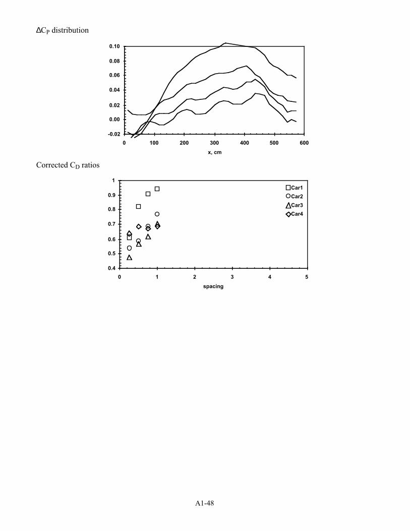
A1-48

∆CP distribution

x, cm

-0.02

0.00

0.02

0.04

0.06

0.08

0.10

0 100 200 300 400 500 600

Corrected CD ratios

spacing

CD

0.4

0.5

0.6

0.7

0.8

0.9

1

0 1 2 3 4 5

Car1

Car2

Car3

Car4

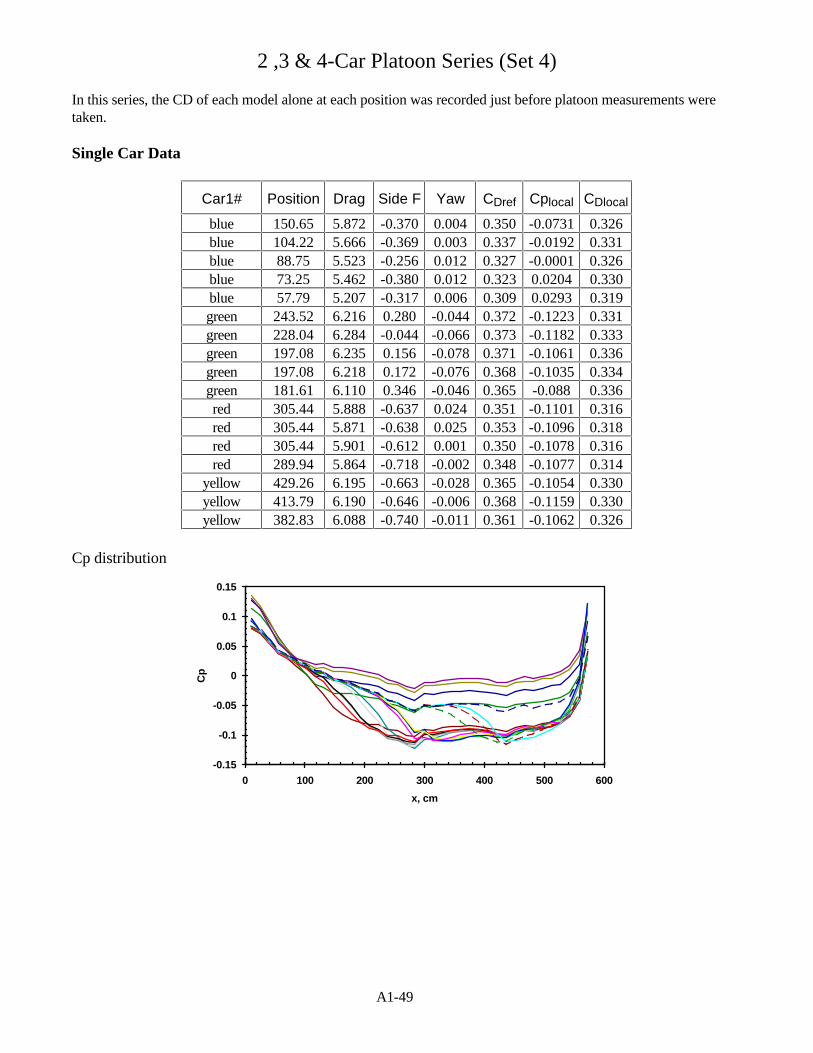
A1-49

2 ,3 & 4-Car Platoon Series (Set 4)

In this series, the CD of each model alone at each position was recorded just before platoon measurements weretaken.

Single Car Data

Car1# Position Drag Side F Yaw CDref Cplocal CDlocal

blue 150.65 5.872 -0.370 0.004 0.350 -0.0731 0.326blue 104.22 5.666 -0.369 0.003 0.337 -0.0192 0.331blue 88.75 5.523 -0.256 0.012 0.327 -0.0001 0.326blue 73.25 5.462 -0.380 0.012 0.323 0.0204 0.330blue 57.79 5.207 -0.317 0.006 0.309 0.0293 0.319green 243.52 6.216 0.280 -0.044 0.372 -0.1223 0.331green 228.04 6.284 -0.044 -0.066 0.373 -0.1182 0.333green 197.08 6.235 0.156 -0.078 0.371 -0.1061 0.336green 197.08 6.218 0.172 -0.076 0.368 -0.1035 0.334green 181.61 6.110 0.346 -0.046 0.365 -0.088 0.336red 305.44 5.888 -0.637 0.024 0.351 -0.1101 0.316red 305.44 5.871 -0.638 0.025 0.353 -0.1096 0.318red 305.44 5.901 -0.612 0.001 0.350 -0.1078 0.316red 289.94 5.864 -0.718 -0.002 0.348 -0.1077 0.314

yellow 429.26 6.195 -0.663 -0.028 0.365 -0.1054 0.330yellow 413.79 6.190 -0.646 -0.006 0.368 -0.1159 0.330yellow 382.83 6.088 -0.740 -0.011 0.361 -0.1062 0.326

Cp distribution

x, cm

Cp

-0.15

-0.1

-0.05

0

0.05

0.1

0.15

0 100 200 300 400 500 600

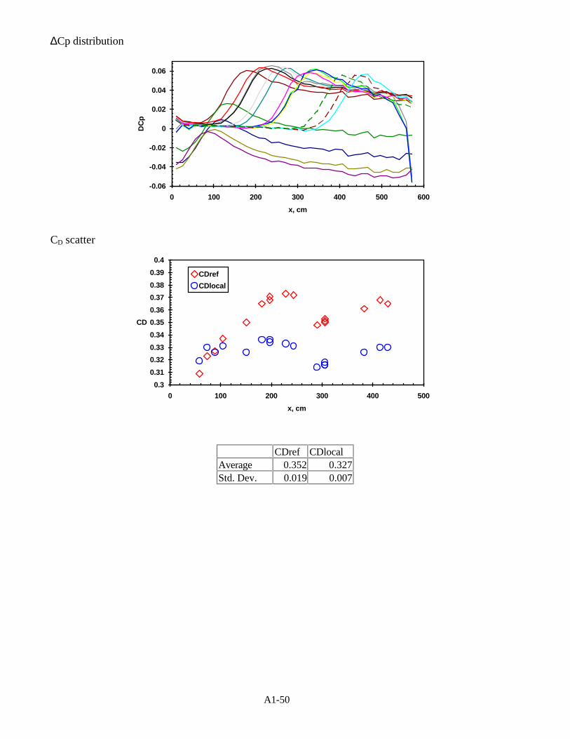
A1-50

∆Cp distribution

x, cm

DC

p

-0.06

-0.04

-0.02

0

0.02

0.04

0.06

0 100 200 300 400 500 600

CD scatter

x, cm

CD

0.3

0.31

0.32

0.33

0.34

0.35

0.36

0.37

0.38

0.39

0.4

0 100 200 300 400 500

CDref

CDlocal

CDref CDlocalAverage 0.352 0.327Std. Dev. 0.019 0.007

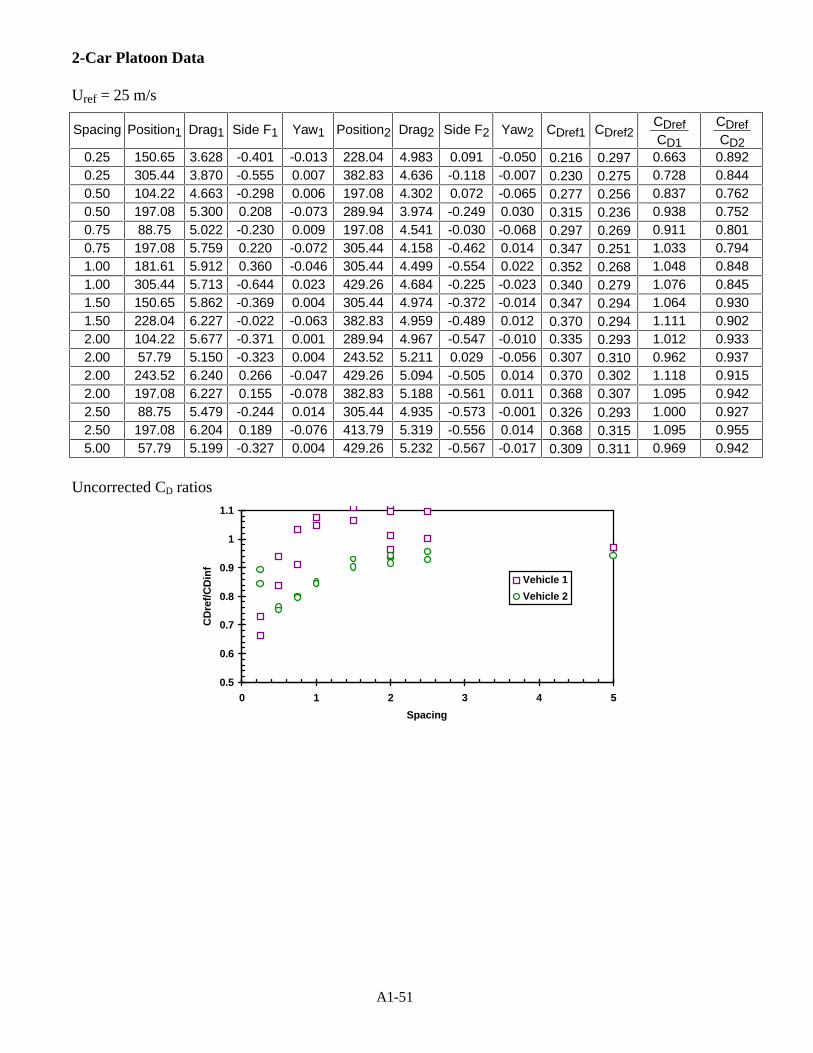
A1-51

2-Car Platoon Data

Uref = 25 m/s

Spacing Position1 Drag1 Side F1 Yaw1 Position2 Drag2 Side F2 Yaw2 CDref1 CDref2CDrefCD1

CDrefCD2

0.25 150.65 3.628 -0.401 -0.013 228.04 4.983 0.091 -0.050 0.216 0.297 0.663 0.8920.25 305.44 3.870 -0.555 0.007 382.83 4.636 -0.118 -0.007 0.230 0.275 0.728 0.8440.50 104.22 4.663 -0.298 0.006 197.08 4.302 0.072 -0.065 0.277 0.256 0.837 0.7620.50 197.08 5.300 0.208 -0.073 289.94 3.974 -0.249 0.030 0.315 0.236 0.938 0.7520.75 88.75 5.022 -0.230 0.009 197.08 4.541 -0.030 -0.068 0.297 0.269 0.911 0.8010.75 197.08 5.759 0.220 -0.072 305.44 4.158 -0.462 0.014 0.347 0.251 1.033 0.7941.00 181.61 5.912 0.360 -0.046 305.44 4.499 -0.554 0.022 0.352 0.268 1.048 0.8481.00 305.44 5.713 -0.644 0.023 429.26 4.684 -0.225 -0.023 0.340 0.279 1.076 0.8451.50 150.65 5.862 -0.369 0.004 305.44 4.974 -0.372 -0.014 0.347 0.294 1.064 0.9301.50 228.04 6.227 -0.022 -0.063 382.83 4.959 -0.489 0.012 0.370 0.294 1.111 0.9022.00 104.22 5.677 -0.371 0.001 289.94 4.967 -0.547 -0.010 0.335 0.293 1.012 0.9332.00 57.79 5.150 -0.323 0.004 243.52 5.211 0.029 -0.056 0.307 0.310 0.962 0.9372.00 243.52 6.240 0.266 -0.047 429.26 5.094 -0.505 0.014 0.370 0.302 1.118 0.9152.00 197.08 6.227 0.155 -0.078 382.83 5.188 -0.561 0.011 0.368 0.307 1.095 0.9422.50 88.75 5.479 -0.244 0.014 305.44 4.935 -0.573 -0.001 0.326 0.293 1.000 0.9272.50 197.08 6.204 0.189 -0.076 413.79 5.319 -0.556 0.014 0.368 0.315 1.095 0.9555.00 57.79 5.199 -0.327 0.004 429.26 5.232 -0.567 -0.017 0.309 0.311 0.969 0.942

Uncorrected CD ratios

0.5

0.6

0.7

0.8

0.9

1

1.1

0 1 2 3 4 5

Spacing

CD

ref/C

Din

f

Vehicle 1

Vehicle 2

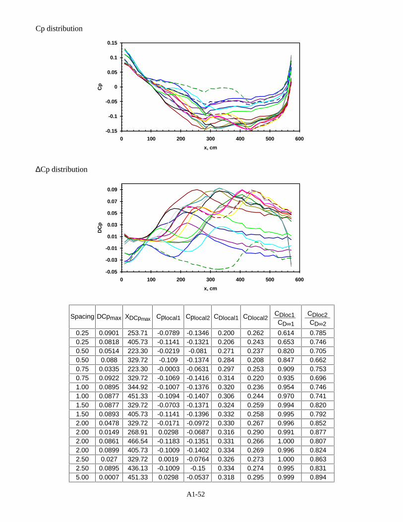
A1-52

Cp distribution

x, cm

Cp

-0.15

-0.1

-0.05

0

0.05

0.1

0.15

0 100 200 300 400 500 600

∆Cp distribution

x, cm

DC

p

-0.05

-0.03

-0.01

0.01

0.03

0.05

0.07

0.09

0 100 200 300 400 500 600

Spacing DCpmax XDCpmax Cplocal1 Cplocal2 CDlocal1 CDlocal2CDloc1CD∞1

CDloc2CD∞2

0.25 0.0901 253.71 -0.0789 -0.1346 0.200 0.262 0.614 0.7850.25 0.0818 405.73 -0.1141 -0.1321 0.206 0.243 0.653 0.7460.50 0.0514 223.30 -0.0219 -0.081 0.271 0.237 0.820 0.7050.50 0.088 329.72 -0.109 -0.1374 0.284 0.208 0.847 0.6620.75 0.0335 223.30 -0.0003 -0.0631 0.297 0.253 0.909 0.7530.75 0.0922 329.72 -0.1069 -0.1416 0.314 0.220 0.935 0.6961.00 0.0895 344.92 -0.1007 -0.1376 0.320 0.236 0.954 0.7461.00 0.0877 451.33 -0.1094 -0.1407 0.306 0.244 0.970 0.7411.50 0.0877 329.72 -0.0703 -0.1371 0.324 0.259 0.994 0.8201.50 0.0893 405.73 -0.1141 -0.1396 0.332 0.258 0.995 0.7922.00 0.0478 329.72 -0.0171 -0.0972 0.330 0.267 0.996 0.8522.00 0.0149 268.91 0.0298 -0.0687 0.316 0.290 0.991 0.8772.00 0.0861 466.54 -0.1183 -0.1351 0.331 0.266 1.000 0.8072.00 0.0899 405.73 -0.1009 -0.1402 0.334 0.269 0.996 0.8242.50 0.027 329.72 0.0019 -0.0764 0.326 0.273 1.000 0.8632.50 0.0895 436.13 -0.1009 -0.15 0.334 0.274 0.995 0.8315.00 0.0007 451.33 0.0298 -0.0537 0.318 0.295 0.999 0.894

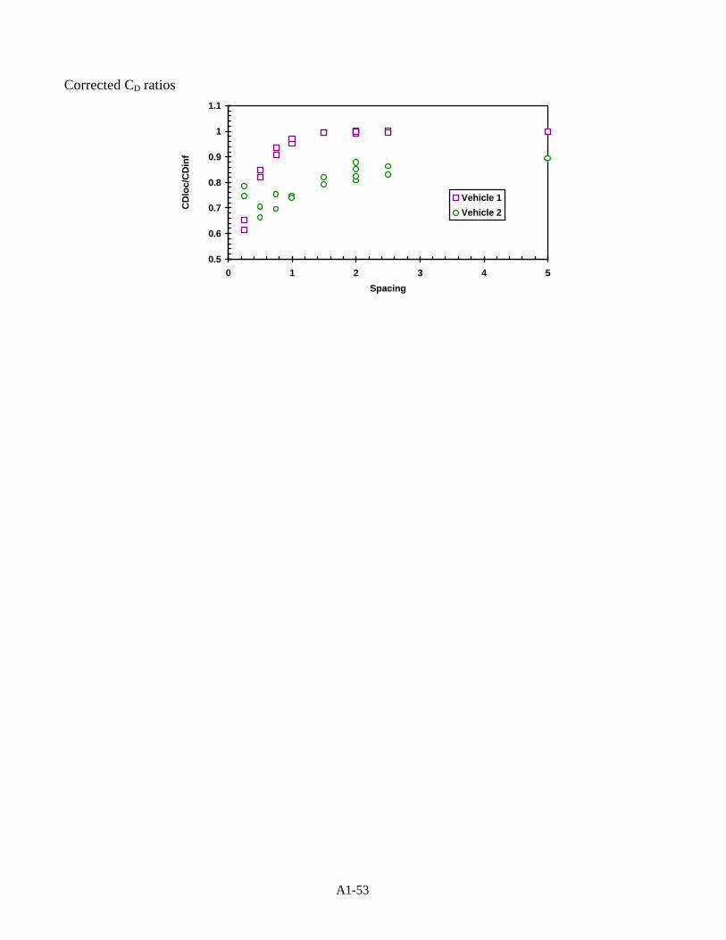
A1-53

Corrected CD ratios

0.5

0.6

0.7

0.8

0.9

1

1.1

0 1 2 3 4 5

Spacing

CD

loc/

CD

inf

Vehicle 1

Vehicle 2

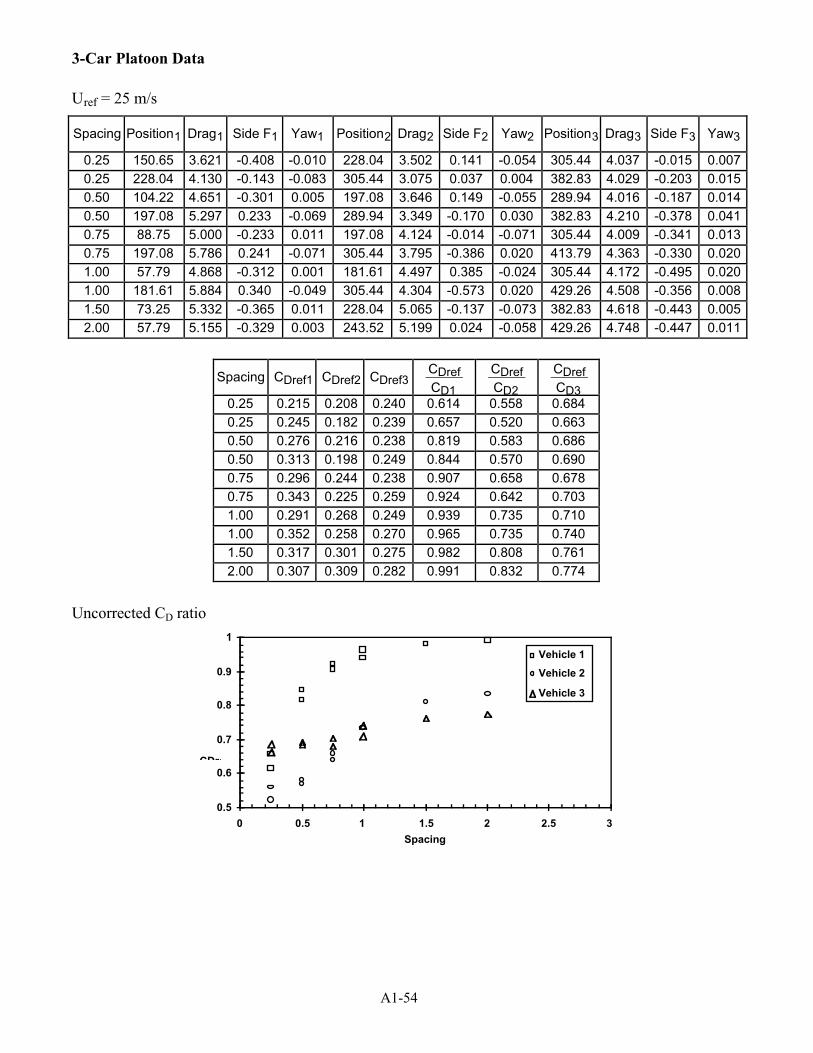
A1-54

3-Car Platoon Data

Uref = 25 m/s

Spacing Position1 Drag1 Side F1 Yaw1 Position2 Drag2 Side F2 Yaw2 Position3 Drag3 Side F3 Yaw3

0.25 150.65 3.621 -0.408 -0.010 228.04 3.502 0.141 -0.054 305.44 4.037 -0.015 0.0070.25 228.04 4.130 -0.143 -0.083 305.44 3.075 0.037 0.004 382.83 4.029 -0.203 0.0150.50 104.22 4.651 -0.301 0.005 197.08 3.646 0.149 -0.055 289.94 4.016 -0.187 0.0140.50 197.08 5.297 0.233 -0.069 289.94 3.349 -0.170 0.030 382.83 4.210 -0.378 0.0410.75 88.75 5.000 -0.233 0.011 197.08 4.124 -0.014 -0.071 305.44 4.009 -0.341 0.0130.75 197.08 5.786 0.241 -0.071 305.44 3.795 -0.386 0.020 413.79 4.363 -0.330 0.0201.00 57.79 4.868 -0.312 0.001 181.61 4.497 0.385 -0.024 305.44 4.172 -0.495 0.0201.00 181.61 5.884 0.340 -0.049 305.44 4.304 -0.573 0.020 429.26 4.508 -0.356 0.0081.50 73.25 5.332 -0.365 0.011 228.04 5.065 -0.137 -0.073 382.83 4.618 -0.443 0.0052.00 57.79 5.155 -0.329 0.003 243.52 5.199 0.024 -0.058 429.26 4.748 -0.447 0.011

Spacing CDref1 CDref2 CDref3CDrefCD1

CDrefCD2

CDrefCD3

0.25 0.215 0.208 0.240 0.614 0.558 0.6840.25 0.245 0.182 0.239 0.657 0.520 0.6630.50 0.276 0.216 0.238 0.819 0.583 0.6860.50 0.313 0.198 0.249 0.844 0.570 0.6900.75 0.296 0.244 0.238 0.907 0.658 0.6780.75 0.343 0.225 0.259 0.924 0.642 0.7031.00 0.291 0.268 0.249 0.939 0.735 0.7101.00 0.352 0.258 0.270 0.965 0.735 0.7401.50 0.317 0.301 0.275 0.982 0.808 0.7612.00 0.307 0.309 0.282 0.991 0.832 0.774

Uncorrected CD ratio

0.5

0.6

0.7

0.8

0.9

1

0 0.5 1 1.5 2 2.5 3

Spacing

CDre

Vehicle 1

Vehicle 2

Vehicle 3

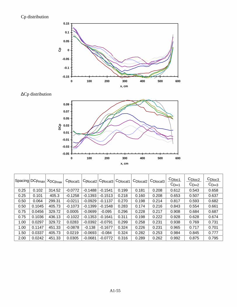
A1-55

Cp distribution

-0.15

-0.1

-0.05

0

0.05

0.1

0.15

0 100 200 300 400 500 600

x, cm

Cp

∆Cp distribution

-0.05

-0.03

-0.01

0.01

0.03

0.05

0.07

0.09

0 100 200 300 400 500 600

x, cm

DC

p

Spacing DCpmax XDCpmax Cplocal1 Cplocal2 Cplocal3 CDlocal1 CDlocal2 CDlocal3CDloc1CD∞1

CDloc2CD∞2

CDloc3CD∞3

0.25 0.102 314.52 -0.0772 -0.1488 -0.1541 0.199 0.181 0.208 0.612 0.543 0.6580.25 0.101 405.3 -0.1258 -0.1393 -0.1513 0.218 0.160 0.208 0.653 0.507 0.6370.50 0.064 299.31 -0.0211 -0.0929 -0.1137 0.270 0.198 0.214 0.817 0.593 0.6820.50 0.1045 405.73 -0.1073 -0.1399 -0.1548 0.283 0.174 0.216 0.843 0.554 0.6610.75 0.0456 329.72 0.0005 -0.0699 -0.095 0.296 0.228 0.217 0.908 0.684 0.6870.75 0.1036 436.13 -0.1022 -0.1353 -0.1641 0.311 0.198 0.222 0.928 0.628 0.6741.00 0.0297 329.72 0.0283 -0.0392 -0.0791 0.299 0.258 0.231 0.938 0.769 0.7311.00 0.1147 451.33 -0.0878 -0.138 -0.1677 0.324 0.226 0.231 0.965 0.717 0.7011.50 0.0337 405.73 0.0219 -0.0693 -0.084 0.324 0.282 0.253 0.984 0.845 0.7772.00 0.0242 451.33 0.0305 -0.0681 -0.0772 0.316 0.289 0.262 0.992 0.875 0.795

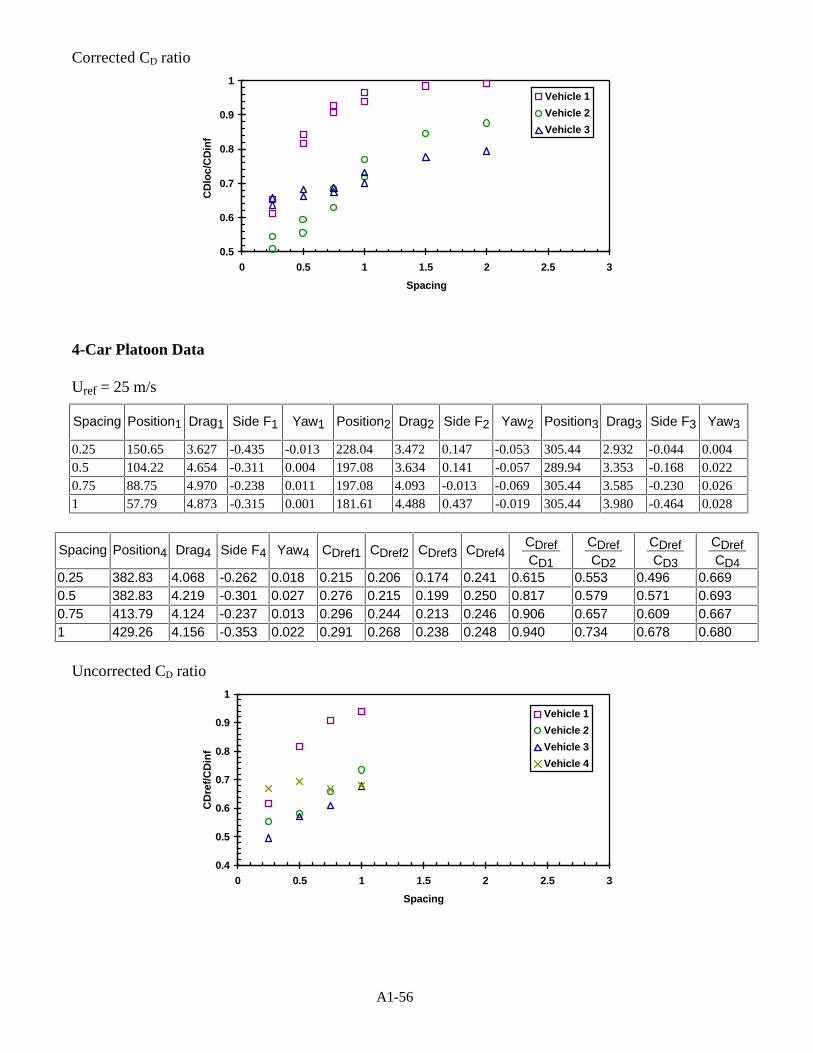
A1-56

Corrected CD ratio

0.5

0.6

0.7

0.8

0.9

1

0 0.5 1 1.5 2 2.5 3

Spacing

CD

loc/

CD

inf

Vehicle 1

Vehicle 2

Vehicle 3

4-Car Platoon Data

Uref = 25 m/s

Spacing Position1 Drag1 Side F1 Yaw1 Position2 Drag2 Side F2 Yaw2 Position3 Drag3 Side F3 Yaw3

0.25 150.65 3.627 -0.435 -0.013 228.04 3.472 0.147 -0.053305.44 2.932 -0.044 0.0040.5 104.22 4.654 -0.311 0.004 197.08 3.634 0.141 -0.057289.94 3.353 -0.168 0.0220.75 88.75 4.970 -0.238 0.011 197.08 4.093 -0.013 -0.069305.44 3.585 -0.230 0.0261 57.79 4.873 -0.315 0.001 181.61 4.488 0.437 -0.019305.44 3.980 -0.464 0.028

Spacing Position4 Drag4 Side F4 Yaw4 CDref1 CDref2 CDref3 CDref4CDrefCD1

CDrefCD2

CDrefCD3

CDrefCD4

0.25 382.83 4.068 -0.262 0.018 0.215 0.206 0.174 0.241 0.615 0.553 0.496 0.6690.5 382.83 4.219 -0.301 0.027 0.276 0.215 0.199 0.250 0.817 0.579 0.571 0.6930.75 413.79 4.124 -0.237 0.013 0.296 0.244 0.213 0.246 0.906 0.657 0.609 0.6671 429.26 4.156 -0.353 0.022 0.291 0.268 0.238 0.248 0.940 0.734 0.678 0.680

Uncorrected CD ratio

0.4

0.5

0.6

0.7

0.8

0.9

1

0 0.5 1 1.5 2 2.5 3

Spacing

CD

ref/C

Din

f

Vehicle 1

Vehicle 2

Vehicle 3

Vehicle 4

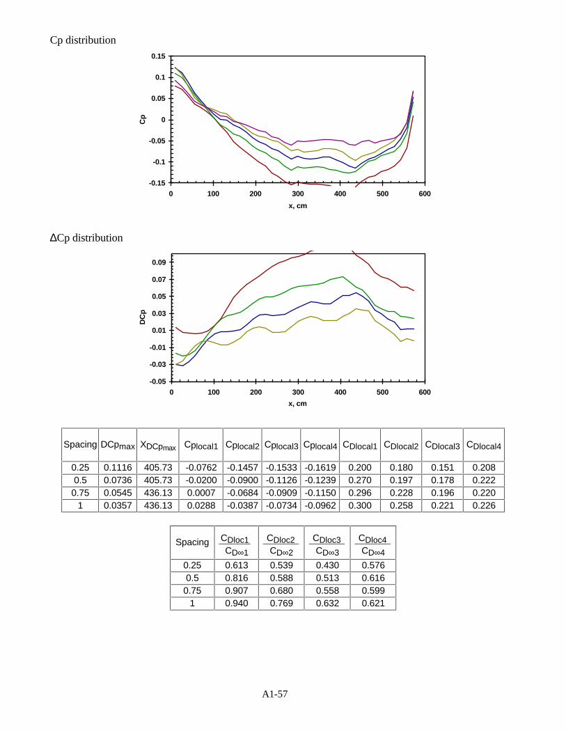
A1-57

Cp distribution

-0.15

-0.1

-0.05

0

0.05

0.1

0.15

0 100 200 300 400 500 600

x, cm

Cp

∆Cp distribution

-0.05

-0.03

-0.01

0.01

0.03

0.05

0.07

0.09

0 100 200 300 400 500 600

x, cm

DC

p

Spacing DCpmax XDCpmax Cplocal1 Cplocal2 Cplocal3 Cplocal4 CDlocal1 CDlocal2 CDlocal3 CDlocal4

0.25 0.1116 405.73 -0.0762 -0.1457 -0.1533 -0.1619 0.200 0.180 0.151 0.2080.5 0.0736 405.73 -0.0200 -0.0900 -0.1126 -0.1239 0.270 0.197 0.178 0.222

0.75 0.0545 436.13 0.0007 -0.0684 -0.0909 -0.1150 0.296 0.228 0.196 0.2201 0.0357 436.13 0.0288 -0.0387 -0.0734 -0.0962 0.300 0.258 0.221 0.226

Spacing CDloc1CD∞1

CDloc2CD∞2

CDloc3CD∞3

CDloc4CD∞4

0.25 0.613 0.539 0.430 0.5760.5 0.816 0.588 0.513 0.616

0.75 0.907 0.680 0.558 0.5991 0.940 0.769 0.632 0.621

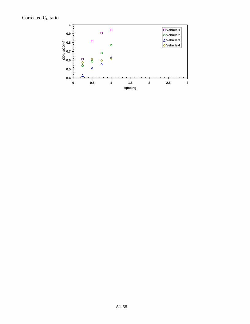
A1-58

Corrected CD ratio

0.4

0.5

0.6

0.7

0.8

0.9

1

0 0.5 1 1.5 2 2.5 3

spacing

CD

loc/

CD

inf

Vehicle 1

Vehicle 2

Vehicle 3

Vehicle 4

Appendix 2:

2-Vehicle Platoon Data with Varying Geometries

A2-1

Geometry Variation Series (porous plate with suction)

Front-to-Front Platoon Set A

Single Car Data

Car# Location Drag1 SideF1 Yaw1 CDref1 Cp_max_dC Xlocal1 CDloc1green 127.00 5.306 -0.153 -0.009 0.374 -0.042 147.28 0.359green 127.00 5.311 -0.154 -0.010 0.373 -0.042 147.28 0.358green 127.00 5.321 -0.163 -0.003 0.373 -0.042 147.28 0.358green 127.00 5.319 -0.159 -0.004 0.373 -0.041 147.28 0.359green 127.00 5.276 -0.160 -0.005 0.373 -0.042 147.28 0.358green 127.00 5.291 -0.156 -0.009 0.372 -0.042 147.28 0.357green 127.00 5.287 -0.163 -0.005 0.372 -0.041 147.28 0.357green 127.00 5.309 -0.156 -0.008 0.373 -0.041 147.28 0.358green 127.00 5.302 -0.148 -0.009 0.372 -0.042 147.28 0.357green 127.00 5.299 -0.153 -0.011 0.372 -0.042 147.28 0.358green 127.00 5.303 -0.164 -0.006 0.372 -0.042 147.28 0.357green 127.00 5.299 -0.157 -0.009 0.372 -0.042 147.28 0.357green 127.00 5.293 -0.164 -0.005 0.372 -0.042 147.28 0.357blue 374.65 5.221 -0.300 -0.034 0.366 -0.097 405.68 0.333blue 343.70 5.175 -0.360 -0.018 0.364 -0.099 375.28 0.331blue 312.74 5.210 -0.439 -0.014 0.367 -0.102 329.68 0.333blue 281.78 5.263 -0.361 -0.022 0.369 -0.110 299.28 0.333blue 250.83 5.309 -0.219 0.004 0.374 -0.117 284.08 0.334blue 235.35 5.370 -0.334 0.002 0.378 -0.113 268.88 0.339blue 219.87 5.370 -0.493 -0.029 0.378 -0.105 253.68 0.342blue 209.34 5.386 -0.404 -0.026 0.379 -0.101 238.48 0.344blue 204.39 5.361 -0.410 -0.033 0.377 -0.101 238.48 0.342blue 200.55 5.332 -0.409 -0.033 0.375 -0.100 238.48 0.340blue 196.65 5.317 -0.415 -0.023 0.373 -0.100 238.48 0.339blue 192.78 5.278 -0.392 -0.023 0.372 -0.089 223.28 0.341blue 188.91 5.299 -0.389 -0.020 0.374 -0.083 208.08 0.345

Cp distribution

-0.15

-0.10

-0.05

0.00

0.05

0.10

0.15

0 100 200 300 400 500 600x. cm

Cp

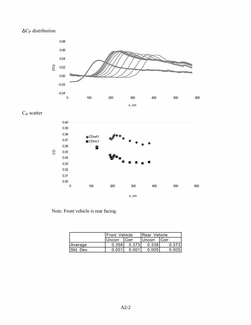
A2-2

∆CP distribution

-0.04

-0.02

0.00

0.02

0.04

0.06

0.08

0 100 200 300 400 500 600

x, cm

DC

p

CD scatter

0.30

0.31

0.32

0.33

0.34

0.35

0.36

0.37

0.38

0.39

0.40

0 100 200 300 400 500 600

x, cm

CD

CDref1CDloc1

Note: Front vehicle is rear facing.

Front Vehicle Rear VehicleUncorr Corr Uncorr Corr

Average 0.358 0.373 0.338 0.373Std. Dev. 0.001 0.001 0.005 0.005

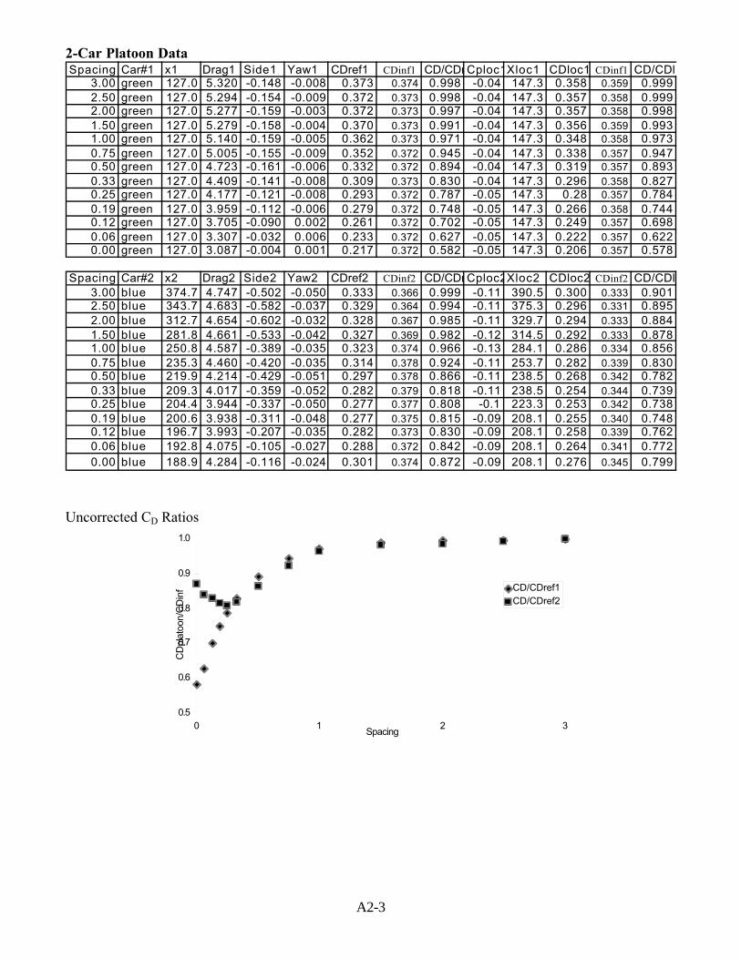
A2-3

2-Car Platoon DataSpacing Car#1 x1 Drag1 Side1 Yaw1 CDref1 CDinf1 CD/CDrCploc1Xloc1 CDloc1 CDinf1 CD/CDlo

3.00 green 127.0 5.320 -0.148 -0.008 0.373 0.374 0.998 -0.04 147.3 0.358 0.359 0.9992.50 green 127.0 5.294 -0.154 -0.009 0.372 0.373 0.998 -0.04 147.3 0.357 0.358 0.9992.00 green 127.0 5.277 -0.159 -0.003 0.372 0.373 0.997 -0.04 147.3 0.357 0.358 0.9981.50 green 127.0 5.279 -0.158 -0.004 0.370 0.373 0.991 -0.04 147.3 0.356 0.359 0.9931.00 green 127.0 5.140 -0.159 -0.005 0.362 0.373 0.971 -0.04 147.3 0.348 0.358 0.9730.75 green 127.0 5.005 -0.155 -0.009 0.352 0.372 0.945 -0.04 147.3 0.338 0.357 0.9470.50 green 127.0 4.723 -0.161 -0.006 0.332 0.372 0.894 -0.04 147.3 0.319 0.357 0.8930.33 green 127.0 4.409 -0.141 -0.008 0.309 0.373 0.830 -0.04 147.3 0.296 0.358 0.8270.25 green 127.0 4.177 -0.121 -0.008 0.293 0.372 0.787 -0.05 147.3 0.28 0.357 0.7840.19 green 127.0 3.959 -0.112 -0.006 0.279 0.372 0.748 -0.05 147.3 0.266 0.358 0.7440.12 green 127.0 3.705 -0.090 0.002 0.261 0.372 0.702 -0.05 147.3 0.249 0.357 0.6980.06 green 127.0 3.307 -0.032 0.006 0.233 0.372 0.627 -0.05 147.3 0.222 0.357 0.6220.00 green 127.0 3.087 -0.004 0.001 0.217 0.372 0.582 -0.05 147.3 0.206 0.357 0.578

Spacing Car#2 x2 Drag2 Side2 Yaw2 CDref2 CDinf2 CD/CDrCploc2Xloc2 CDloc2 CDinf2 CD/CDlo3.00 blue 374.7 4.747 -0.502 -0.050 0.333 0.366 0.999 -0.11 390.5 0.300 0.333 0.9012.50 blue 343.7 4.683 -0.582 -0.037 0.329 0.364 0.994 -0.11 375.3 0.296 0.331 0.8952.00 blue 312.7 4.654 -0.602 -0.032 0.328 0.367 0.985 -0.11 329.7 0.294 0.333 0.8841.50 blue 281.8 4.661 -0.533 -0.042 0.327 0.369 0.982 -0.12 314.5 0.292 0.333 0.8781.00 blue 250.8 4.587 -0.389 -0.035 0.323 0.374 0.966 -0.13 284.1 0.286 0.334 0.8560.75 blue 235.3 4.460 -0.420 -0.035 0.314 0.378 0.924 -0.11 253.7 0.282 0.339 0.8300.50 blue 219.9 4.214 -0.429 -0.051 0.297 0.378 0.866 -0.11 238.5 0.268 0.342 0.7820.33 blue 209.3 4.017 -0.359 -0.052 0.282 0.379 0.818 -0.11 238.5 0.254 0.344 0.7390.25 blue 204.4 3.944 -0.337 -0.050 0.277 0.377 0.808 -0.1 223.3 0.253 0.342 0.7380.19 blue 200.6 3.938 -0.311 -0.048 0.277 0.375 0.815 -0.09 208.1 0.255 0.340 0.7480.12 blue 196.7 3.993 -0.207 -0.035 0.282 0.373 0.830 -0.09 208.1 0.258 0.339 0.7620.06 blue 192.8 4.075 -0.105 -0.027 0.288 0.372 0.842 -0.09 208.1 0.264 0.341 0.7720.00 blue 188.9 4.284 -0.116 -0.024 0.301 0.374 0.872 -0.09 208.1 0.276 0.345 0.799

Uncorrected CD Ratios

0.5

0.6

0.7

0.8

0.9

1.0

0 1 2 3Spacing

CD

plat

oon/

CD

inf CD/CDref1

CD/CDref2

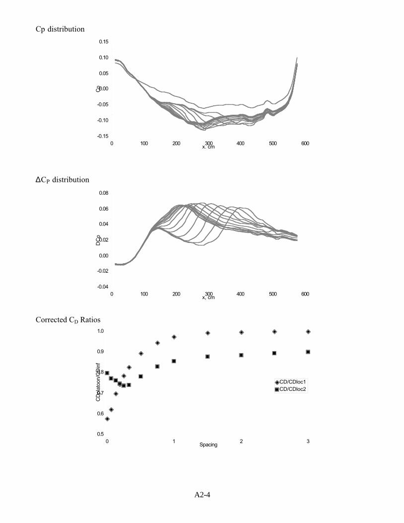
A2-4

Cp distribution

-0.15

-0.10

-0.05

0.00

0.05

0.10

0.15

0 100 200 300 400 500 600x. cm

Cp

∆CP distribution

-0.04

-0.02

0.00

0.02

0.04

0.06

0.08

0 100 200 300 400 500 600x, cm

DC

p

Corrected CD Ratios

0.5

0.6

0.7

0.8

0.9

1.0

0 1 2 3Spacing

CD

plat

oon/

CD

inf

CD/CDloc1CD/CDloc2

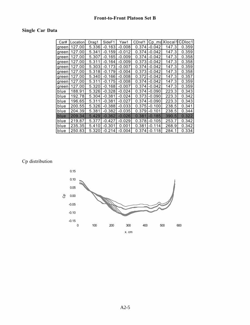
A2-5

Front-to-Front Platoon Set B

Single Car Data

Car# Location Drag1 SideF1 Yaw1 CDref1 Cp_ma Xlocal1 CDloc1green 127.00 5.336 -0.163 -0.008 0.374 -0.042 147.3 0.359green 127.00 5.341 -0.159 -0.012 0.374 -0.042 147.3 0.359green 127.00 5.307 -0.165 -0.009 0.374 -0.042 147.3 0.358green 127.00 5.311 -0.164 -0.009 0.373 -0.042 147.3 0.358green 127.00 5.303 -0.173 -0.007 0.374 -0.042 147.3 0.359green 127.00 5.318 -0.179 -0.004 0.373 -0.042 147.3 0.358green 127.00 5.340 -0.166 -0.008 0.372 -0.042 147.3 0.357green 127.00 5.311 -0.175 -0.008 0.374 -0.042 147.3 0.359green 127.00 5.320 -0.168 -0.007 0.374 -0.042 147.3 0.359blue 188.91 5.326 -0.328 -0.024 0.374 -0.090 223.3 0.343blue 192.78 5.304 -0.381 -0.024 0.373 -0.090 223.3 0.342blue 196.65 5.311 -0.381 -0.027 0.374 -0.090 223.3 0.343blue 200.55 5.326 -0.388 -0.033 0.375 -0.100 238.5 0.341blue 204.39 5.381 -0.382 -0.035 0.379 -0.101 238.5 0.344blue 209.34 5.429 -0.362 -0.026 0.381 -0.185 390.5 0.322blue 219.87 5.377 -0.427 -0.029 0.378 -0.105 253.7 0.342blue 235.35 5.410 -0.301 0.001 0.381 -0.114 268.9 0.342blue 250.83 5.320 -0.214 -0.004 0.374 -0.118 284.1 0.334

Cp distribution

-0.15

-0.10

-0.05

0.00

0.05

0.10

0.15

0 100 200 300 400 500 600

x. cm

Cp

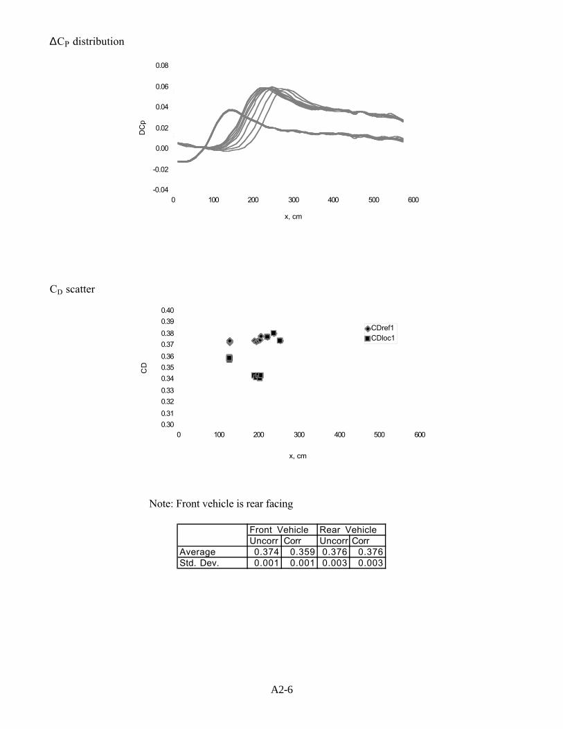
A2-6

∆CP distribution

-0.04

-0.02

0.00

0.02

0.04

0.06

0.08

0 100 200 300 400 500 600

x, cm

DC

p

CD scatter

0.30

0.31

0.32

0.33

0.34

0.35

0.36

0.37

0.38

0.39

0.40

0 100 200 300 400 500 600

x, cm

CD

CDref1CDloc1

Note: Front vehicle is rear facing

Front Vehicle Rear VehicleUncorr Corr Uncorr Corr

Average 0.374 0.359 0.376 0.376Std. Dev. 0.001 0.001 0.003 0.003

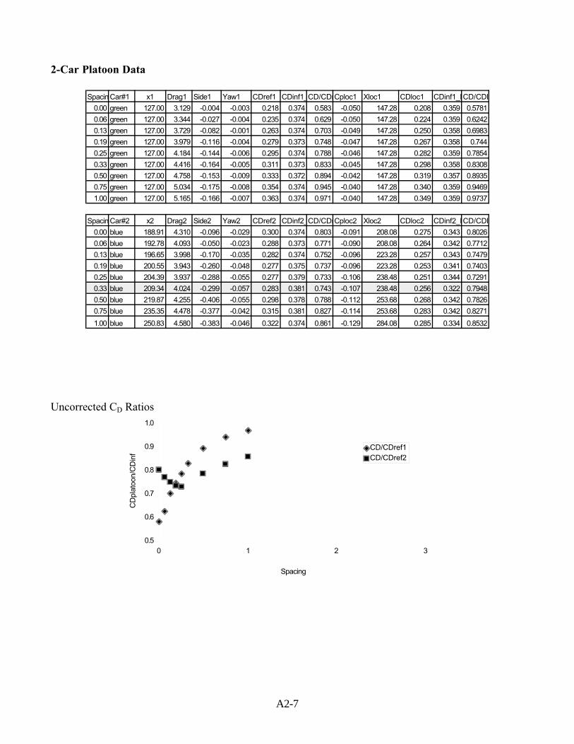
A2-7

2-Car Platoon Data

SpacingCar#1 x1 Drag1 Side1 Yaw1 CDref1 CDinf1_CD/CDrCploc1 Xloc1 CDloc1 CDinf1_loCD/CDlo

0.00 green 127.00 3.129 -0.004 -0.003 0.218 0.374 0.583 -0.050 147.28 0.208 0.359 0.5781

0.06 green 127.00 3.344 -0.027 -0.004 0.235 0.374 0.629 -0.050 147.28 0.224 0.359 0.6242

0.13 green 127.00 3.729 -0.082 -0.001 0.263 0.374 0.703 -0.049 147.28 0.250 0.358 0.6983

0.19 green 127.00 3.979 -0.116 -0.004 0.279 0.373 0.748 -0.047 147.28 0.267 0.358 0.744

0.25 green 127.00 4.184 -0.144 -0.006 0.295 0.374 0.788 -0.046 147.28 0.282 0.359 0.7854

0.33 green 127.00 4.416 -0.164 -0.005 0.311 0.373 0.833 -0.045 147.28 0.298 0.358 0.8308

0.50 green 127.00 4.758 -0.153 -0.009 0.333 0.372 0.894 -0.042 147.28 0.319 0.357 0.8935

0.75 green 127.00 5.034 -0.175 -0.008 0.354 0.374 0.945 -0.040 147.28 0.340 0.359 0.9469

1.00 green 127.00 5.165 -0.166 -0.007 0.363 0.374 0.971 -0.040 147.28 0.349 0.359 0.9737

SpacingCar#2 x2 Drag2 Side2 Yaw2 CDref2 CDinf2_CD/CDrCploc2 Xloc2 CDloc2 CDinf2_loCD/CDlo

0.00 blue 188.91 4.310 -0.096 -0.029 0.300 0.374 0.803 -0.091 208.08 0.275 0.343 0.8026

0.06 blue 192.78 4.093 -0.050 -0.023 0.288 0.373 0.771 -0.090 208.08 0.264 0.342 0.7712

0.13 blue 196.65 3.998 -0.170 -0.035 0.282 0.374 0.752 -0.096 223.28 0.257 0.343 0.7479

0.19 blue 200.55 3.943 -0.260 -0.048 0.277 0.375 0.737 -0.096 223.28 0.253 0.341 0.7403

0.25 blue 204.39 3.937 -0.288 -0.055 0.277 0.379 0.733 -0.106 238.48 0.251 0.344 0.7291

0.33 blue 209.34 4.024 -0.299 -0.057 0.283 0.381 0.743 -0.107 238.48 0.256 0.322 0.7948

0.50 blue 219.87 4.255 -0.406 -0.055 0.298 0.378 0.788 -0.112 253.68 0.268 0.342 0.7826

0.75 blue 235.35 4.478 -0.377 -0.042 0.315 0.381 0.827 -0.114 253.68 0.283 0.342 0.8271

1.00 blue 250.83 4.580 -0.383 -0.046 0.322 0.374 0.861 -0.129 284.08 0.285 0.334 0.8532

Uncorrected CD Ratios

0.5

0.6

0.7

0.8

0.9

1.0

0 1 2 3

Spacing

CD

plat

oon/

CD

inf

CD/CDref1CD/CDref2

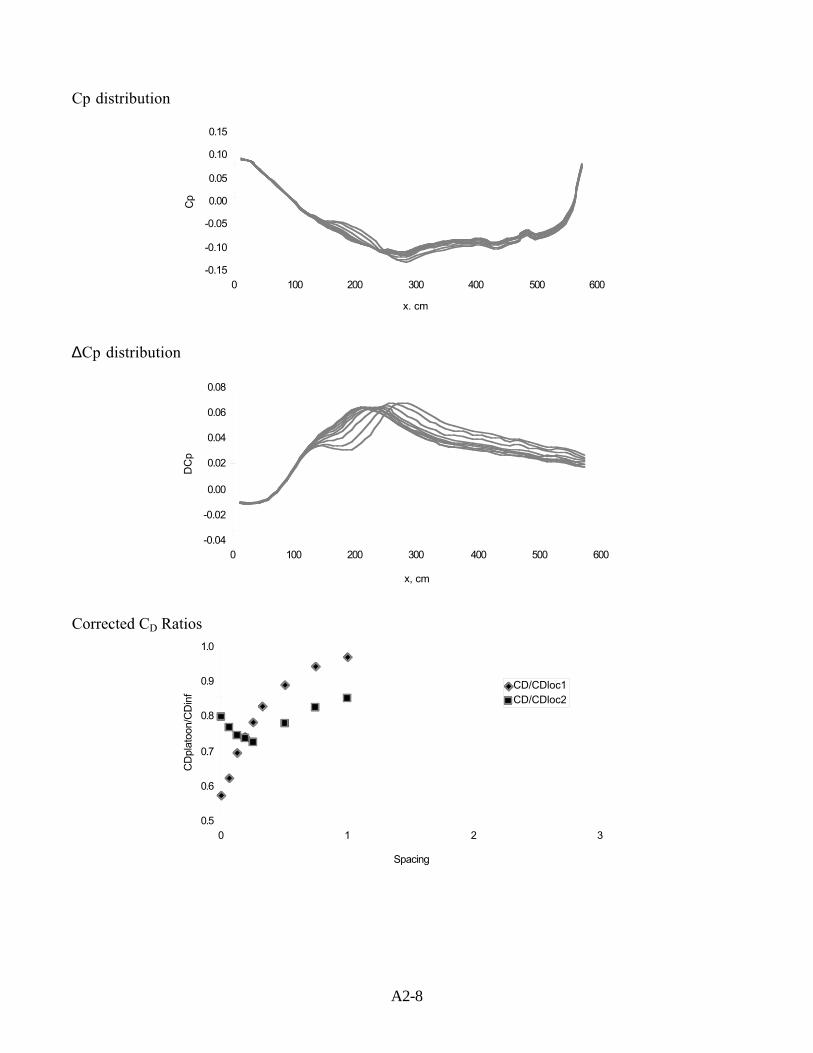
A2-8

Cp distribution

-0.15

-0.10

-0.05

0.00

0.05

0.10

0.15

0 100 200 300 400 500 600

x. cm

Cp

∆Cp distribution

-0.04

-0.02

0.00

0.02

0.04

0.06

0.08

0 100 200 300 400 500 600

x, cm

DC

p

Corrected CD Ratios

0.5

0.6

0.7

0.8

0.9

1.0

0 1 2 3

Spacing

CD

plat

oon/

CD

inf

CD/CDloc1CD/CDloc2

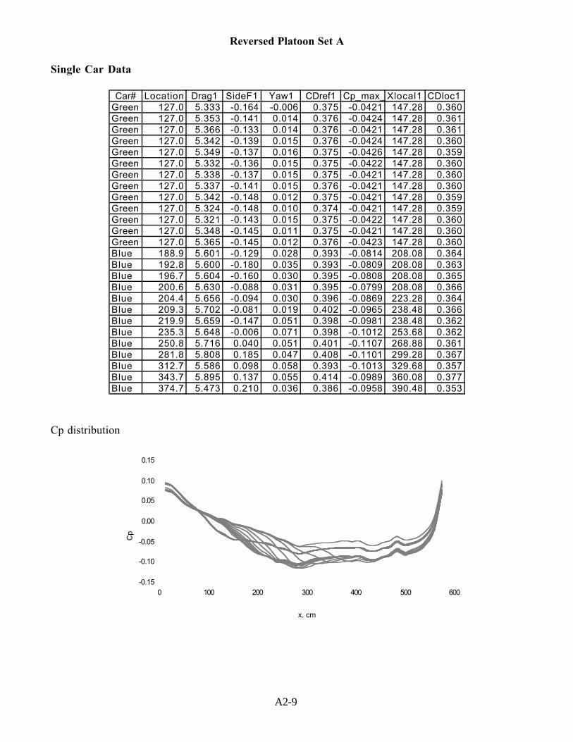
A2-9

Reversed Platoon Set A

Single Car Data

Car# Location Drag1 SideF1 Yaw1 CDref1 Cp_max_ Xlocal1 CDloc1Green 127.0 5.333 -0.164 -0.006 0.375 -0.0421 147.28 0.360Green 127.0 5.353 -0.141 0.014 0.376 -0.0424 147.28 0.361Green 127.0 5.366 -0.133 0.014 0.376 -0.0421 147.28 0.361Green 127.0 5.342 -0.139 0.015 0.376 -0.0424 147.28 0.360Green 127.0 5.349 -0.137 0.016 0.375 -0.0426 147.28 0.359Green 127.0 5.332 -0.136 0.015 0.375 -0.0422 147.28 0.360Green 127.0 5.338 -0.137 0.015 0.375 -0.0421 147.28 0.360Green 127.0 5.337 -0.141 0.015 0.376 -0.0421 147.28 0.360Green 127.0 5.342 -0.148 0.012 0.375 -0.0421 147.28 0.359Green 127.0 5.324 -0.148 0.010 0.374 -0.0421 147.28 0.359Green 127.0 5.321 -0.143 0.015 0.375 -0.0422 147.28 0.360Green 127.0 5.348 -0.145 0.011 0.375 -0.0421 147.28 0.360Green 127.0 5.365 -0.145 0.012 0.376 -0.0423 147.28 0.360Blue 188.9 5.601 -0.129 0.028 0.393 -0.0814 208.08 0.364Blue 192.8 5.600 -0.180 0.035 0.393 -0.0809 208.08 0.363Blue 196.7 5.604 -0.160 0.030 0.395 -0.0808 208.08 0.365Blue 200.6 5.630 -0.088 0.031 0.395 -0.0799 208.08 0.366Blue 204.4 5.656 -0.094 0.030 0.396 -0.0869 223.28 0.364Blue 209.3 5.702 -0.081 0.019 0.402 -0.0965 238.48 0.366Blue 219.9 5.659 -0.147 0.051 0.398 -0.0981 238.48 0.362Blue 235.3 5.648 -0.006 0.071 0.398 -0.1012 253.68 0.362Blue 250.8 5.716 0.040 0.051 0.401 -0.1107 268.88 0.361Blue 281.8 5.808 0.185 0.047 0.408 -0.1101 299.28 0.367Blue 312.7 5.586 0.098 0.058 0.393 -0.1013 329.68 0.357Blue 343.7 5.895 0.137 0.055 0.414 -0.0989 360.08 0.377Blue 374.7 5.473 0.210 0.036 0.386 -0.0958 390.48 0.353

Cp distribution

-0.15

-0.10

-0.05

0.00

0.05

0.10

0.15

0 100 200 300 400 500 600

x. cm

Cp

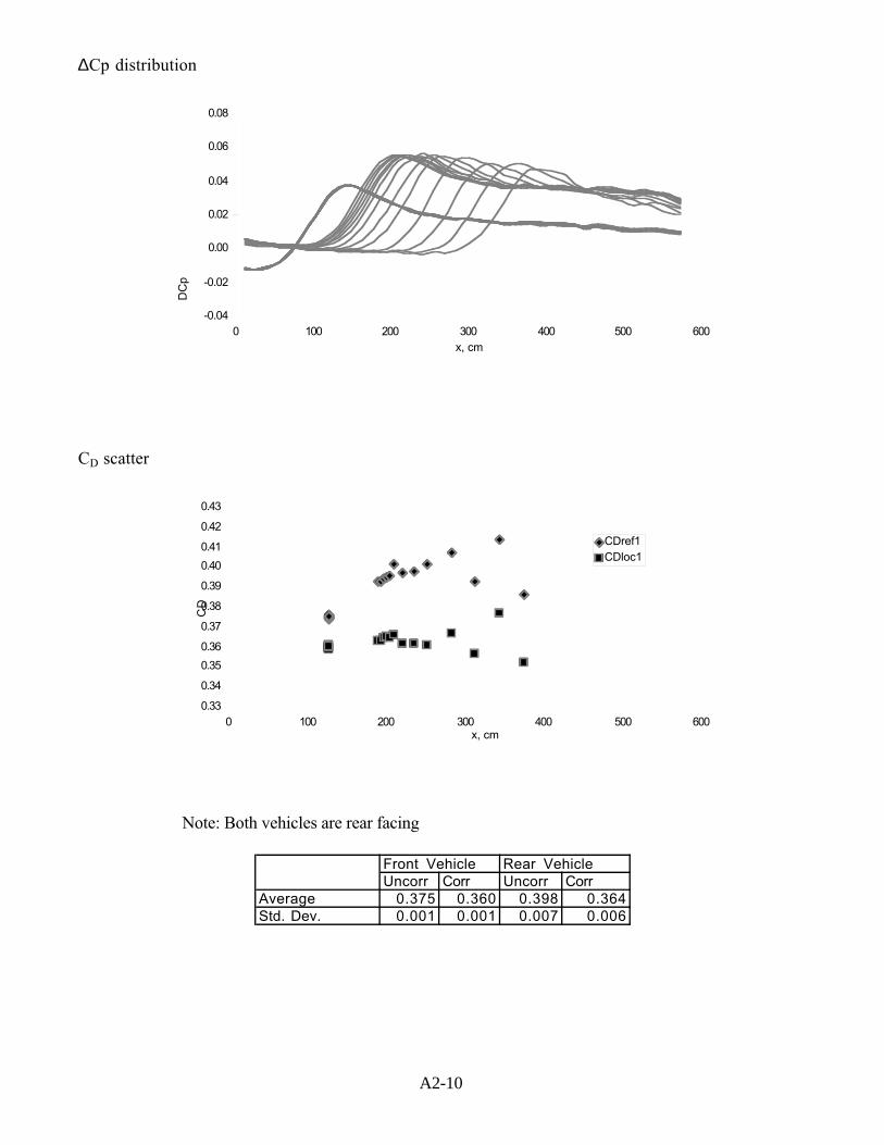
A2-10

∆Cp distribution

-0.04

-0.02

0.00

0.02

0.04

0.06

0.08

0 100 200 300 400 500 600x, cm

DC

p

CD scatter

0.33

0.34

0.35

0.36

0.37

0.38

0.39

0.40

0.41

0.42

0.43

0 100 200 300 400 500 600x, cm

CD

CDref1CDloc1

Note: Both vehicles are rear facing

Front Vehicle Rear VehicleUncorr Corr Uncorr Corr

Average 0.375 0.360 0.398 0.364Std. Dev. 0.001 0.001 0.007 0.006

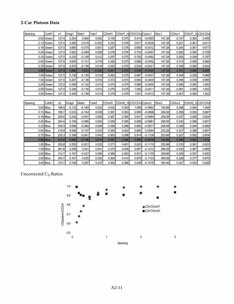
A2-11

2-Car Platoon Data

Spacing Car#1 x1 Drag1 Side1 Yaw1 CDref1 CDinf1_refCD/CDreCploc1 Xloc1 CDloc1 CDinf1_loCD/CDloc

0.00 Green 127.0 2.204 0.084 0.002 0.155 0.375 0.415 -0.0565 147.28 0.147 0.360 0.409

0.13 Green 127.0 3.290 -0.018 -0.002 0.232 0.376 0.617 -0.0528 147.28 0.221 0.361 0.611

0.19 Green 127.0 3.660 -0.070 0.001 0.257 0.376 0.683 -0.0512 147.28 0.244 0.361 0.677

0.25 Green 127.0 3.923 -0.099 0.009 0.276 0.376 0.733 -0.0497 147.28 0.262 0.360 0.728

0.33 Green 127.0 4.220 -0.108 0.012 0.297 0.375 0.792 -0.0482 147.28 0.283 0.359 0.787

0.50 Green 127.0 4.645 -0.131 0.016 0.326 0.375 0.869 -0.0452 147.28 0.312 0.360 0.866

0.75 Green 127.0 4.979 -0.136 0.016 0.350 0.375 0.934 -0.0421 147.28 0.336 0.360 0.934

0.88 Green 127.0 2.869 0.023 -0.008 0.201 0.376 0.535 -0.0540 147.28 0.191 0.360 0.529

1.00 Green 127.0 5.136 -0.135 0.016 0.362 0.375 0.967 -0.0407 147.28 0.348 0.359 0.968

1.50 Green 127.0 5.287 -0.136 0.014 0.372 0.374 0.993 -0.0400 147.28 0.358 0.359 0.995

2.00 Green 127.0 5.308 -0.132 0.013 0.374 0.375 0.999 -0.0405 147.28 0.360 0.360 1.000

2.50 Green 127.0 5.326 -0.135 0.013 0.376 0.375 1.002 -0.0411 147.28 0.361 0.360 1.003

3.00 Green 127.0 5.349 -0.136 0.014 0.376 0.376 1.001 -0.0412 147.28 0.361 0.360 1.002

Spacing Car#2 x2 Drag2 Side2 Yaw2 CDref2 CDinf2_refCD/CDreCploc2 Xloc2 CDloc2 CDinf2_loCD/CDloc

0.00 Blue 188.9 6.133 -0.160 0.032 0.432 0.393 1.099 -0.0862 192.88 0.398 0.364 1.094

0.13 Blue 196.7 5.533 -0.154 0.008 0.391 0.393 0.995 -0.0896 208.08 0.359 0.363 0.987

0.19 Blue 200.6 5.234 -0.091 0.006 0.367 0.395 0.931 -0.0884 208.08 0.337 0.365 0.924

0.25 Blue 204.4 5.108 -0.066 0.004 0.359 0.395 0.908 -0.0881 208.08 0.330 0.366 0.901

0.33 Blue 209.3 5.068 -0.080 0.008 0.356 0.396 0.900 -0.0877 208.08 0.328 0.364 0.899

0.50 Blue 219.9 5.098 -0.107 0.023 0.358 0.402 0.890 -0.0944 223.28 0.327 0.366 0.891

0.75 Blue 235.3 5.166 -0.041 0.043 0.363 0.398 0.914 -0.1108 253.68 0.327 0.362 0.904

0.88 Blue 243.6 5.665 -0.186 0.015 0.397 0.398 0.996 -0.0838 192.88 0.366 0.362 1.012

1.00 Blue 250.8 5.255 -0.001 0.035 0.371 0.401 0.923 -0.1110 253.68 0.333 0.361 0.923

1.50 Blue 281.8 5.258 0.021 0.041 0.370 0.408 0.907 -0.1212 299.28 0.330 0.367 0.898

2.00 Blue 312.7 5.187 -0.027 0.056 0.366 0.393 0.931 -0.1135 329.68 0.329 0.357 0.920

2.50 Blue 343.7 5.161 0.025 0.052 0.364 0.414 0.879 -0.1103 360.08 0.328 0.377 0.870

3.00 Blue 374.7 5.156 0.097 0.037 0.362 0.386 0.938 -0.1078 390.48 0.327 0.353 0.928

Uncorrected CD Ratios

0.5

0.6

0.7

0.8

0.9

1.0

0 1 2 3

Spacing

CD

plat

oon/

CD

inf

CD/CDref1CD/CDref2

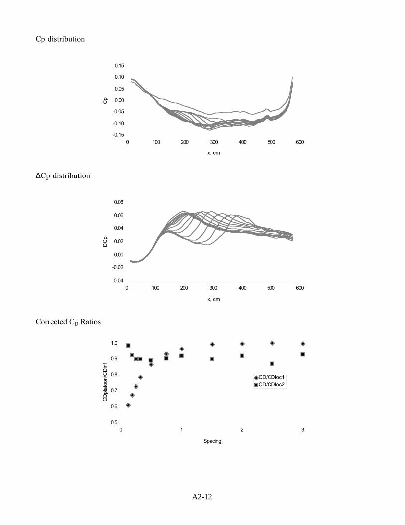
A2-12

Cp distribution

-0.15

-0.10

-0.05

0.00

0.05

0.10

0.15

0 100 200 300 400 500 600

x. cm

Cp

∆Cp distribution

-0.04

-0.02

0.00

0.02

0.04

0.06

0.08

0 100 200 300 400 500 600

x, cm

DC

p

Corrected CD Ratios

0.5

0.6

0.7

0.8

0.9

1.0

0 1 2 3

Spacing

CD

plat

oon/

CD

inf

CD/CDloc1CD/CDloc2

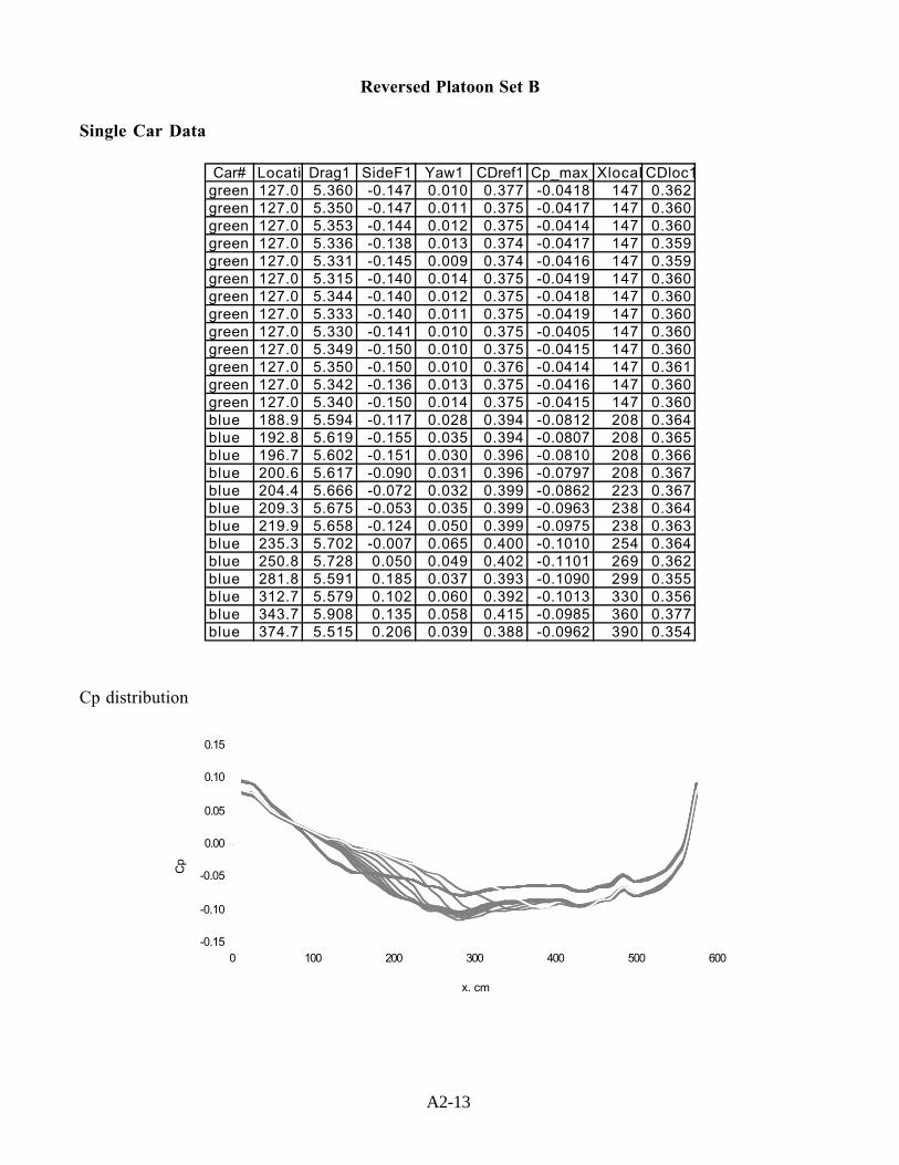
A2-13

Reversed Platoon Set B

Single Car Data

Car# LocatioDrag1 SideF1 Yaw1 CDref1 Cp_max_Xlocal CDloc1green 127.0 5.360 -0.147 0.010 0.377 -0.0418 147 0.362green 127.0 5.350 -0.147 0.011 0.375 -0.0417 147 0.360green 127.0 5.353 -0.144 0.012 0.375 -0.0414 147 0.360green 127.0 5.336 -0.138 0.013 0.374 -0.0417 147 0.359green 127.0 5.331 -0.145 0.009 0.374 -0.0416 147 0.359green 127.0 5.315 -0.140 0.014 0.375 -0.0419 147 0.360green 127.0 5.344 -0.140 0.012 0.375 -0.0418 147 0.360green 127.0 5.333 -0.140 0.011 0.375 -0.0419 147 0.360green 127.0 5.330 -0.141 0.010 0.375 -0.0405 147 0.360green 127.0 5.349 -0.150 0.010 0.375 -0.0415 147 0.360green 127.0 5.350 -0.150 0.010 0.376 -0.0414 147 0.361green 127.0 5.342 -0.136 0.013 0.375 -0.0416 147 0.360green 127.0 5.340 -0.150 0.014 0.375 -0.0415 147 0.360blue 188.9 5.594 -0.117 0.028 0.394 -0.0812 208 0.364blue 192.8 5.619 -0.155 0.035 0.394 -0.0807 208 0.365blue 196.7 5.602 -0.151 0.030 0.396 -0.0810 208 0.366blue 200.6 5.617 -0.090 0.031 0.396 -0.0797 208 0.367blue 204.4 5.666 -0.072 0.032 0.399 -0.0862 223 0.367blue 209.3 5.675 -0.053 0.035 0.399 -0.0963 238 0.364blue 219.9 5.658 -0.124 0.050 0.399 -0.0975 238 0.363blue 235.3 5.702 -0.007 0.065 0.400 -0.1010 254 0.364blue 250.8 5.728 0.050 0.049 0.402 -0.1101 269 0.362blue 281.8 5.591 0.185 0.037 0.393 -0.1090 299 0.355blue 312.7 5.579 0.102 0.060 0.392 -0.1013 330 0.356blue 343.7 5.908 0.135 0.058 0.415 -0.0985 360 0.377blue 374.7 5.515 0.206 0.039 0.388 -0.0962 390 0.354

Cp distribution

-0.15

-0.10

-0.05

0.00

0.05

0.10

0.15

0 100 200 300 400 500 600

x. cm

Cp

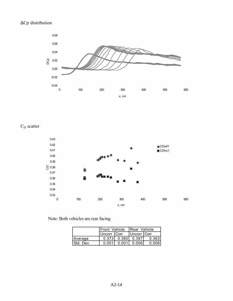
A2-14

∆Cp distribution

-0.04

-0.02

0.00

0.02

0.04

0.06

0.08

0 100 200 300 400 500 600

x, cm

DC

p

CD scatter

0.33

0.34

0.35

0.36

0.37

0.38

0.39

0.40

0.41

0.42

0.43

0 100 200 300 400 500 600

x, cm

CD

CDref1CDloc1

Note: Both vehicles are rear facing

Front Vehicle Rear VehicleUncorr Corr Uncorr Corr

Average 0.373 0.360 0.397 0.363Std. Dev. 0.001 0.001 0.006 0.006

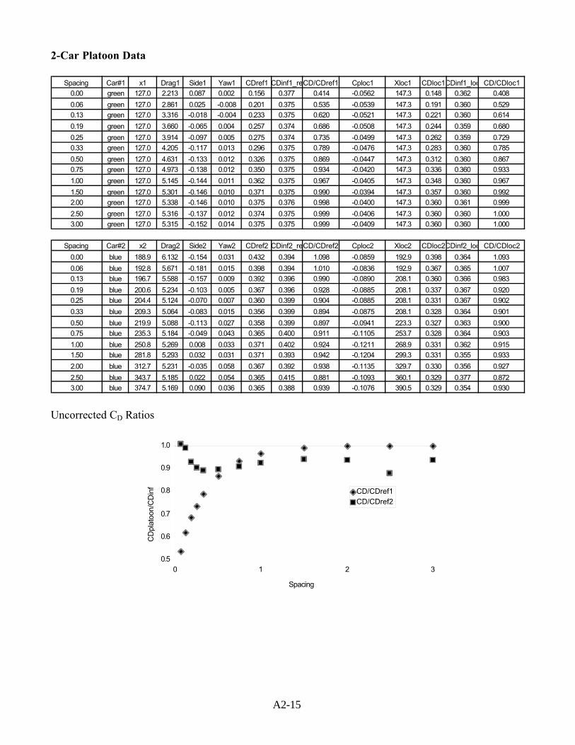
A2-15

2-Car Platoon Data

Spacing Car#1 x1 Drag1 Side1 Yaw1 CDref1 CDinf1_refCD/CDref1 Cploc1 Xloc1 CDloc1CDinf1_loc CD/CDloc1

0.00 green 127.0 2.213 0.087 0.002 0.156 0.377 0.414 -0.0562 147.3 0.148 0.362 0.408

0.06 green 127.0 2.861 0.025 -0.008 0.201 0.375 0.535 -0.0539 147.3 0.191 0.360 0.529

0.13 green 127.0 3.316 -0.018 -0.004 0.233 0.375 0.620 -0.0521 147.3 0.221 0.360 0.614

0.19 green 127.0 3.660 -0.065 0.004 0.257 0.374 0.686 -0.0508 147.3 0.244 0.359 0.680

0.25 green 127.0 3.914 -0.097 0.005 0.275 0.374 0.735 -0.0499 147.3 0.262 0.359 0.729

0.33 green 127.0 4.205 -0.117 0.013 0.296 0.375 0.789 -0.0476 147.3 0.283 0.360 0.785

0.50 green 127.0 4.631 -0.133 0.012 0.326 0.375 0.869 -0.0447 147.3 0.312 0.360 0.867

0.75 green 127.0 4.973 -0.138 0.012 0.350 0.375 0.934 -0.0420 147.3 0.336 0.360 0.933

1.00 green 127.0 5.145 -0.144 0.011 0.362 0.375 0.967 -0.0405 147.3 0.348 0.360 0.967

1.50 green 127.0 5.301 -0.146 0.010 0.371 0.375 0.990 -0.0394 147.3 0.357 0.360 0.992

2.00 green 127.0 5.338 -0.146 0.010 0.375 0.376 0.998 -0.0400 147.3 0.360 0.361 0.999

2.50 green 127.0 5.316 -0.137 0.012 0.374 0.375 0.999 -0.0406 147.3 0.360 0.360 1.000

3.00 green 127.0 5.315 -0.152 0.014 0.375 0.375 0.999 -0.0409 147.3 0.360 0.360 1.000

Spacing Car#2 x2 Drag2 Side2 Yaw2 CDref2 CDinf2_refCD/CDref2 Cploc2 Xloc2 CDloc2CDinf2_loc CD/CDloc2

0.00 blue 188.9 6.132 -0.154 0.031 0.432 0.394 1.098 -0.0859 192.9 0.398 0.364 1.093

0.06 blue 192.8 5.671 -0.181 0.015 0.398 0.394 1.010 -0.0836 192.9 0.367 0.365 1.007

0.13 blue 196.7 5.588 -0.157 0.009 0.392 0.396 0.990 -0.0890 208.1 0.360 0.366 0.983

0.19 blue 200.6 5.234 -0.103 0.005 0.367 0.396 0.928 -0.0885 208.1 0.337 0.367 0.920

0.25 blue 204.4 5.124 -0.070 0.007 0.360 0.399 0.904 -0.0885 208.1 0.331 0.367 0.902

0.33 blue 209.3 5.064 -0.083 0.015 0.356 0.399 0.894 -0.0875 208.1 0.328 0.364 0.901

0.50 blue 219.9 5.088 -0.113 0.027 0.358 0.399 0.897 -0.0941 223.3 0.327 0.363 0.900

0.75 blue 235.3 5.184 -0.049 0.043 0.365 0.400 0.911 -0.1105 253.7 0.328 0.364 0.903

1.00 blue 250.8 5.269 0.008 0.033 0.371 0.402 0.924 -0.1211 268.9 0.331 0.362 0.915

1.50 blue 281.8 5.293 0.032 0.031 0.371 0.393 0.942 -0.1204 299.3 0.331 0.355 0.933

2.00 blue 312.7 5.231 -0.035 0.058 0.367 0.392 0.938 -0.1135 329.7 0.330 0.356 0.927

2.50 blue 343.7 5.185 0.022 0.054 0.365 0.415 0.881 -0.1093 360.1 0.329 0.377 0.872

3.00 blue 374.7 5.169 0.090 0.036 0.365 0.388 0.939 -0.1076 390.5 0.329 0.354 0.930

Uncorrected CD Ratios

0.5

0.6

0.7

0.8

0.9

1.0

0 1 2 3

Spacing

CD

plat

oon/

CD

inf

CD/CDref1CD/CDref2

A2-16

Cp distribution

-0.15

-0.10

-0.05

0.00

0.05

0.10

0.15

0 100 200 300 400 500 600

x. cm

Cp

∆Cp distribution

-0.04

-0.02

0.00

0.02

0.04

0.06

0.08

0 100 200 300 400 500 600

x, cm

DC

p

Corrected CD Ratios

0.5

0.6

0.7

0.8

0.9

1.0

0 1 2 3

Spacing

CD

plat

oon/

CD

inf

CD/CDloc1CD/CDloc2

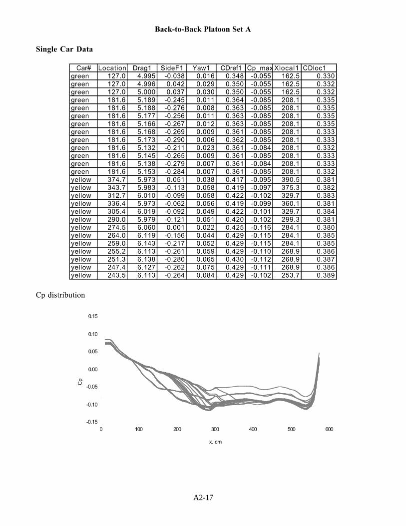
A2-17

Back-to-Back Platoon Set A

Single Car Data

Car# Location Drag1 SideF1 Yaw1 CDref1 Cp_max Xlocal1 CDloc1green 127.0 4.995 -0.038 0.016 0.348 -0.055 162.5 0.330green 127.0 4.996 0.042 0.029 0.350 -0.055 162.5 0.332green 127.0 5.000 0.037 0.030 0.350 -0.055 162.5 0.332green 181.6 5.189 -0.245 0.011 0.364 -0.085 208.1 0.335green 181.6 5.188 -0.276 0.008 0.363 -0.085 208.1 0.335green 181.6 5.177 -0.256 0.011 0.363 -0.085 208.1 0.335green 181.6 5.166 -0.267 0.012 0.363 -0.085 208.1 0.335green 181.6 5.168 -0.269 0.009 0.361 -0.085 208.1 0.333green 181.6 5.173 -0.290 0.006 0.362 -0.085 208.1 0.333green 181.6 5.132 -0.211 0.023 0.361 -0.084 208.1 0.332green 181.6 5.145 -0.265 0.009 0.361 -0.085 208.1 0.333green 181.6 5.138 -0.279 0.007 0.361 -0.084 208.1 0.333green 181.6 5.153 -0.284 0.007 0.361 -0.085 208.1 0.332yellow 374.7 5.973 0.051 0.038 0.417 -0.095 390.5 0.381yellow 343.7 5.983 -0.113 0.058 0.419 -0.097 375.3 0.382yellow 312.7 6.010 -0.099 0.058 0.422 -0.102 329.7 0.383yellow 336.4 5.973 -0.062 0.056 0.419 -0.099 360.1 0.381yellow 305.4 6.019 -0.092 0.049 0.422 -0.101 329.7 0.384yellow 290.0 5.979 -0.121 0.051 0.420 -0.102 299.3 0.381yellow 274.5 6.060 0.001 0.022 0.425 -0.116 284.1 0.380yellow 264.0 6.119 -0.156 0.044 0.429 -0.115 284.1 0.385yellow 259.0 6.143 -0.217 0.052 0.429 -0.115 284.1 0.385yellow 255.2 6.113 -0.261 0.059 0.429 -0.110 268.9 0.386yellow 251.3 6.138 -0.280 0.065 0.430 -0.112 268.9 0.387yellow 247.4 6.127 -0.262 0.075 0.429 -0.111 268.9 0.386yellow 243.5 6.113 -0.264 0.084 0.429 -0.102 253.7 0.389

Cp distribution

-0.15

-0.10

-0.05

0.00

0.05

0.10

0.15

0 100 200 300 400 500 600

x. cm

Cp

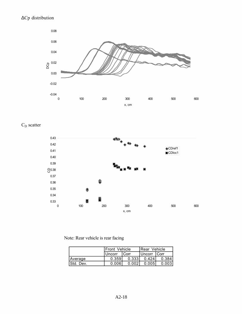
A2-18

∆Cp distribution

-0.04

-0.02

0.00

0.02

0.04

0.06

0.08

0 100 200 300 400 500 600

x, cm

DC

p

CD scatter

0.33

0.34

0.35

0.36

0.37

0.38

0.39

0.40

0.41

0.42

0.43

0 100 200 300 400 500 600

x, cm

CD

CDref1CDloc1

Note: Rear vehicle is rear facing

Front Vehicle Rear VehicleUncorr Corr Uncorr Corr

Average 0.359 0.333 0.424 0.384Std. Dev. 0.006 0.002 0.005 0.003

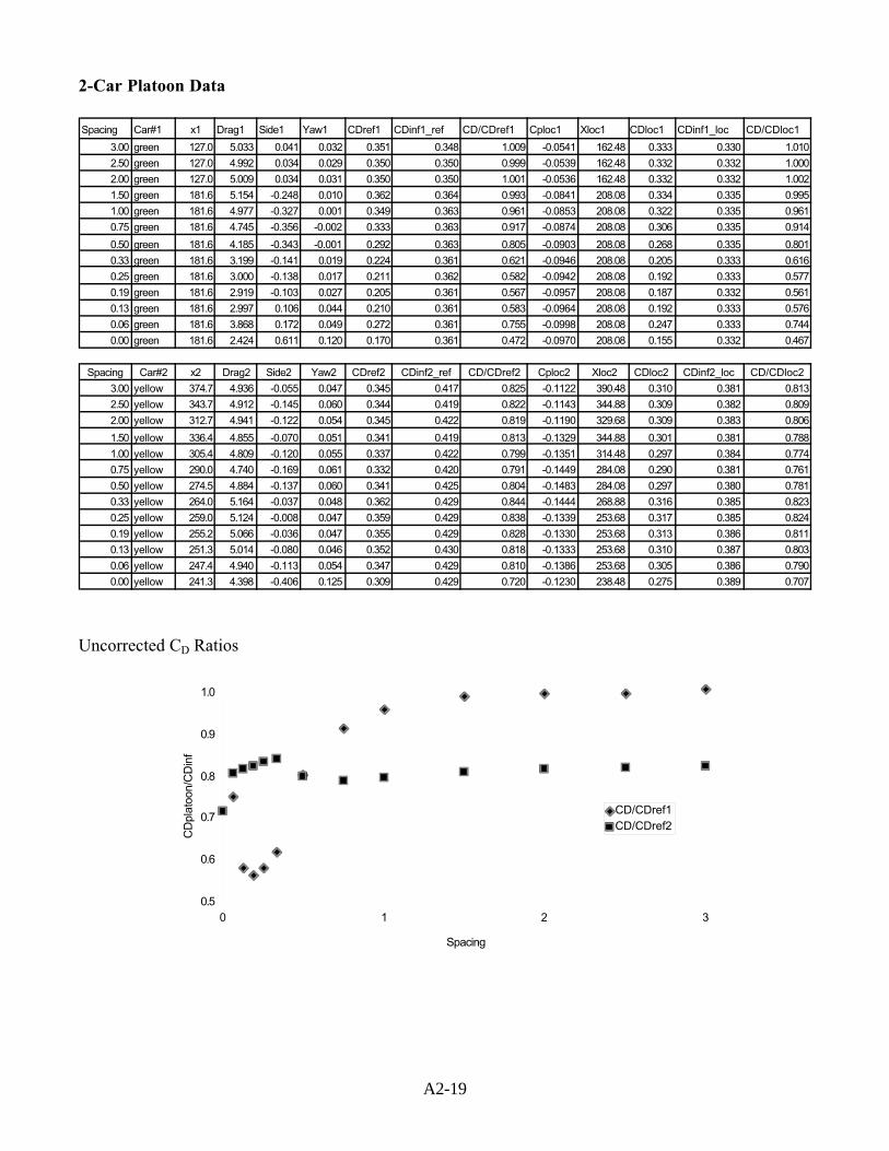
A2-19

2-Car Platoon Data

Spacing Car#1 x1 Drag1 Side1 Yaw1 CDref1 CDinf1_ref CD/CDref1 Cploc1 Xloc1 CDloc1 CDinf1_loc CD/CDloc1

3.00 green 127.0 5.033 0.041 0.032 0.351 0.348 1.009 -0.0541 162.48 0.333 0.330 1.010

2.50 green 127.0 4.992 0.034 0.029 0.350 0.350 0.999 -0.0539 162.48 0.332 0.332 1.000

2.00 green 127.0 5.009 0.034 0.031 0.350 0.350 1.001 -0.0536 162.48 0.332 0.332 1.002

1.50 green 181.6 5.154 -0.248 0.010 0.362 0.364 0.993 -0.0841 208.08 0.334 0.335 0.995

1.00 green 181.6 4.977 -0.327 0.001 0.349 0.363 0.961 -0.0853 208.08 0.322 0.335 0.961

0.75 green 181.6 4.745 -0.356 -0.002 0.333 0.363 0.917 -0.0874 208.08 0.306 0.335 0.914

0.50 green 181.6 4.185 -0.343 -0.001 0.292 0.363 0.805 -0.0903 208.08 0.268 0.335 0.801

0.33 green 181.6 3.199 -0.141 0.019 0.224 0.361 0.621 -0.0946 208.08 0.205 0.333 0.616

0.25 green 181.6 3.000 -0.138 0.017 0.211 0.362 0.582 -0.0942 208.08 0.192 0.333 0.577

0.19 green 181.6 2.919 -0.103 0.027 0.205 0.361 0.567 -0.0957 208.08 0.187 0.332 0.561

0.13 green 181.6 2.997 0.106 0.044 0.210 0.361 0.583 -0.0964 208.08 0.192 0.333 0.576

0.06 green 181.6 3.868 0.172 0.049 0.272 0.361 0.755 -0.0998 208.08 0.247 0.333 0.744

0.00 green 181.6 2.424 0.611 0.120 0.170 0.361 0.472 -0.0970 208.08 0.155 0.332 0.467

Spacing Car#2 x2 Drag2 Side2 Yaw2 CDref2 CDinf2_ref CD/CDref2 Cploc2 Xloc2 CDloc2 CDinf2_loc CD/CDloc2

3.00 yellow 374.7 4.936 -0.055 0.047 0.345 0.417 0.825 -0.1122 390.48 0.310 0.381 0.813

2.50 yellow 343.7 4.912 -0.145 0.060 0.344 0.419 0.822 -0.1143 344.88 0.309 0.382 0.809

2.00 yellow 312.7 4.941 -0.122 0.054 0.345 0.422 0.819 -0.1190 329.68 0.309 0.383 0.806

1.50 yellow 336.4 4.855 -0.070 0.051 0.341 0.419 0.813 -0.1329 344.88 0.301 0.381 0.788

1.00 yellow 305.4 4.809 -0.120 0.055 0.337 0.422 0.799 -0.1351 314.48 0.297 0.384 0.774

0.75 yellow 290.0 4.740 -0.169 0.061 0.332 0.420 0.791 -0.1449 284.08 0.290 0.381 0.761

0.50 yellow 274.5 4.884 -0.137 0.060 0.341 0.425 0.804 -0.1483 284.08 0.297 0.380 0.781

0.33 yellow 264.0 5.164 -0.037 0.048 0.362 0.429 0.844 -0.1444 268.88 0.316 0.385 0.823

0.25 yellow 259.0 5.124 -0.008 0.047 0.359 0.429 0.838 -0.1339 253.68 0.317 0.385 0.824

0.19 yellow 255.2 5.066 -0.036 0.047 0.355 0.429 0.828 -0.1330 253.68 0.313 0.386 0.811

0.13 yellow 251.3 5.014 -0.080 0.046 0.352 0.430 0.818 -0.1333 253.68 0.310 0.387 0.803

0.06 yellow 247.4 4.940 -0.113 0.054 0.347 0.429 0.810 -0.1386 253.68 0.305 0.386 0.790

0.00 yellow 241.3 4.398 -0.406 0.125 0.309 0.429 0.720 -0.1230 238.48 0.275 0.389 0.707

Uncorrected CD Ratios

0.5

0.6

0.7

0.8

0.9

1.0

0 1 2 3

Spacing

CD

plat

oon/

CD

inf

CD/CDref1CD/CDref2

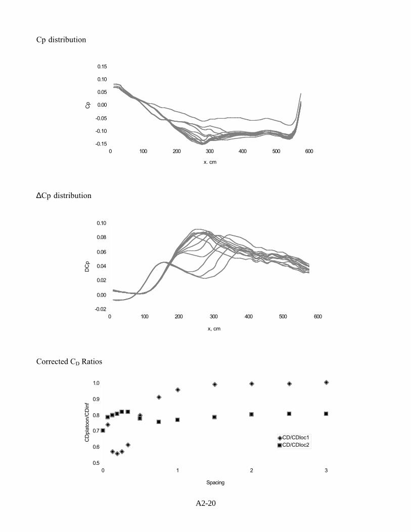
A2-20

Cp distribution

-0.15

-0.10

-0.05

0.00

0.05

0.10

0.15

0 100 200 300 400 500 600

x. cm

Cp

∆Cp distribution

-0.02

0.00

0.02

0.04

0.06

0.08

0.10

0 100 200 300 400 500 600

x, cm

DC

p

Corrected CD Ratios

0.5

0.6

0.7

0.8

0.9

1.0

0 1 2 3

Spacing

CD

plat

oon/

CD

inf

CD/CDloc1CD/CDloc2

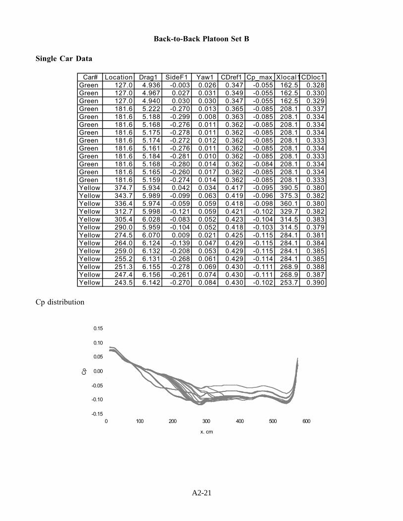
A2-21

Back-to-Back Platoon Set B

Single Car Data

Car# Location Drag1 SideF1 Yaw1 CDref1 Cp_max_Xlocal1CDloc1Green 127.0 4.936 -0.003 0.026 0.347 -0.055 162.5 0.328Green 127.0 4.967 0.027 0.031 0.349 -0.055 162.5 0.330Green 127.0 4.940 0.030 0.030 0.347 -0.055 162.5 0.329Green 181.6 5.222 -0.270 0.013 0.365 -0.085 208.1 0.337Green 181.6 5.188 -0.299 0.008 0.363 -0.085 208.1 0.334Green 181.6 5.168 -0.276 0.011 0.362 -0.085 208.1 0.334Green 181.6 5.175 -0.278 0.011 0.362 -0.085 208.1 0.334Green 181.6 5.174 -0.272 0.012 0.362 -0.085 208.1 0.333Green 181.6 5.161 -0.276 0.011 0.362 -0.085 208.1 0.334Green 181.6 5.184 -0.281 0.010 0.362 -0.085 208.1 0.333Green 181.6 5.168 -0.280 0.014 0.362 -0.084 208.1 0.334Green 181.6 5.165 -0.260 0.017 0.362 -0.085 208.1 0.334Green 181.6 5.159 -0.274 0.014 0.362 -0.085 208.1 0.333Yellow 374.7 5.934 0.042 0.034 0.417 -0.095 390.5 0.380Yellow 343.7 5.989 -0.099 0.063 0.419 -0.096 375.3 0.382Yellow 336.4 5.974 -0.059 0.059 0.418 -0.098 360.1 0.380Yellow 312.7 5.998 -0.121 0.059 0.421 -0.102 329.7 0.382Yellow 305.4 6.028 -0.083 0.052 0.423 -0.104 314.5 0.383Yellow 290.0 5.959 -0.104 0.052 0.418 -0.103 314.5 0.379Yellow 274.5 6.070 0.009 0.021 0.425 -0.115 284.1 0.381Yellow 264.0 6.124 -0.139 0.047 0.429 -0.115 284.1 0.384Yellow 259.0 6.132 -0.208 0.053 0.429 -0.115 284.1 0.385Yellow 255.2 6.131 -0.268 0.061 0.429 -0.114 284.1 0.385Yellow 251.3 6.155 -0.278 0.069 0.430 -0.111 268.9 0.388Yellow 247.4 6.156 -0.261 0.074 0.430 -0.111 268.9 0.387Yellow 243.5 6.142 -0.270 0.084 0.430 -0.102 253.7 0.390

Cp distribution

-0.15

-0.10

-0.05

0.00

0.05

0.10

0.15

0 100 200 300 400 500 600

x. cm

Cp

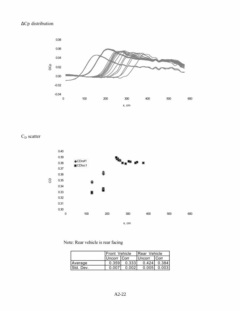
A2-22

∆Cp distribution

-0.04

-0.02

0.00

0.02

0.04

0.06

0.08

0 100 200 300 400 500 600

x, cm

DC

p

CD scatter

0.30

0.31

0.32

0.33

0.34

0.35

0.36

0.37

0.38

0.39

0.40

0 100 200 300 400 500 600

x, cm

CD

CDref1CDloc1

Note: Rear vehicle is rear facing

Front Vehicle Rear VehicleUncorr Corr Uncorr Corr

Average 0.359 0.333 0.424 0.384Std. Dev. 0.007 0.002 0.005 0.003

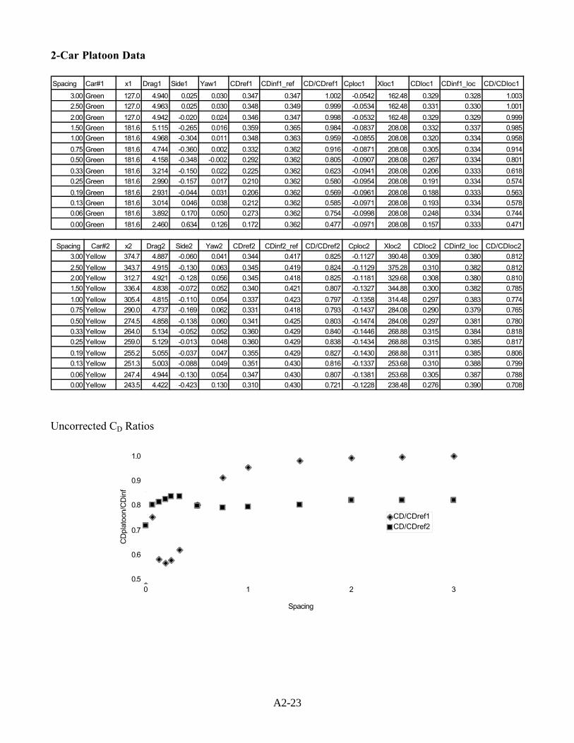
A2-23

2-Car Platoon Data

Spacing Car#1 x1 Drag1 Side1 Yaw1 CDref1 CDinf1_ref CD/CDref1 Cploc1 Xloc1 CDloc1 CDinf1_loc CD/CDloc1

3.00 Green 127.0 4.940 0.025 0.030 0.347 0.347 1.002 -0.0542 162.48 0.329 0.328 1.003

2.50 Green 127.0 4.963 0.025 0.030 0.348 0.349 0.999 -0.0534 162.48 0.331 0.330 1.001

2.00 Green 127.0 4.942 -0.020 0.024 0.346 0.347 0.998 -0.0532 162.48 0.329 0.329 0.999

1.50 Green 181.6 5.115 -0.265 0.016 0.359 0.365 0.984 -0.0837 208.08 0.332 0.337 0.985

1.00 Green 181.6 4.968 -0.304 0.011 0.348 0.363 0.959 -0.0855 208.08 0.320 0.334 0.958

0.75 Green 181.6 4.744 -0.360 0.002 0.332 0.362 0.916 -0.0871 208.08 0.305 0.334 0.914

0.50 Green 181.6 4.158 -0.348 -0.002 0.292 0.362 0.805 -0.0907 208.08 0.267 0.334 0.801

0.33 Green 181.6 3.214 -0.150 0.022 0.225 0.362 0.623 -0.0941 208.08 0.206 0.333 0.618

0.25 Green 181.6 2.990 -0.157 0.017 0.210 0.362 0.580 -0.0954 208.08 0.191 0.334 0.574

0.19 Green 181.6 2.931 -0.044 0.031 0.206 0.362 0.569 -0.0961 208.08 0.188 0.333 0.563

0.13 Green 181.6 3.014 0.046 0.038 0.212 0.362 0.585 -0.0971 208.08 0.193 0.334 0.578

0.06 Green 181.6 3.892 0.170 0.050 0.273 0.362 0.754 -0.0998 208.08 0.248 0.334 0.744

0.00 Green 181.6 2.460 0.634 0.126 0.172 0.362 0.477 -0.0971 208.08 0.157 0.333 0.471

Spacing Car#2 x2 Drag2 Side2 Yaw2 CDref2 CDinf2_ref CD/CDref2 Cploc2 Xloc2 CDloc2 CDinf2_loc CD/CDloc2

3.00 Yellow 374.7 4.887 -0.060 0.041 0.344 0.417 0.825 -0.1127 390.48 0.309 0.380 0.812

2.50 Yellow 343.7 4.915 -0.130 0.063 0.345 0.419 0.824 -0.1129 375.28 0.310 0.382 0.812

2.00 Yellow 312.7 4.921 -0.128 0.056 0.345 0.418 0.825 -0.1181 329.68 0.308 0.380 0.810

1.50 Yellow 336.4 4.838 -0.072 0.052 0.340 0.421 0.807 -0.1327 344.88 0.300 0.382 0.785

1.00 Yellow 305.4 4.815 -0.110 0.054 0.337 0.423 0.797 -0.1358 314.48 0.297 0.383 0.774

0.75 Yellow 290.0 4.737 -0.169 0.062 0.331 0.418 0.793 -0.1437 284.08 0.290 0.379 0.765

0.50 Yellow 274.5 4.858 -0.138 0.060 0.341 0.425 0.803 -0.1474 284.08 0.297 0.381 0.780

0.33 Yellow 264.0 5.134 -0.052 0.052 0.360 0.429 0.840 -0.1446 268.88 0.315 0.384 0.818

0.25 Yellow 259.0 5.129 -0.013 0.048 0.360 0.429 0.838 -0.1434 268.88 0.315 0.385 0.817

0.19 Yellow 255.2 5.055 -0.037 0.047 0.355 0.429 0.827 -0.1430 268.88 0.311 0.385 0.806

0.13 Yellow 251.3 5.003 -0.088 0.049 0.351 0.430 0.816 -0.1337 253.68 0.310 0.388 0.799

0.06 Yellow 247.4 4.944 -0.130 0.054 0.347 0.430 0.807 -0.1381 253.68 0.305 0.387 0.788

0.00 Yellow 243.5 4.422 -0.423 0.130 0.310 0.430 0.721 -0.1228 238.48 0.276 0.390 0.708

Uncorrected CD Ratios

0.5

0.6

0.7

0.8

0.9

1.0

0 1 2 3

Spacing

CD

plat

oon/

CD

inf

CD/CDref1CD/CDref2

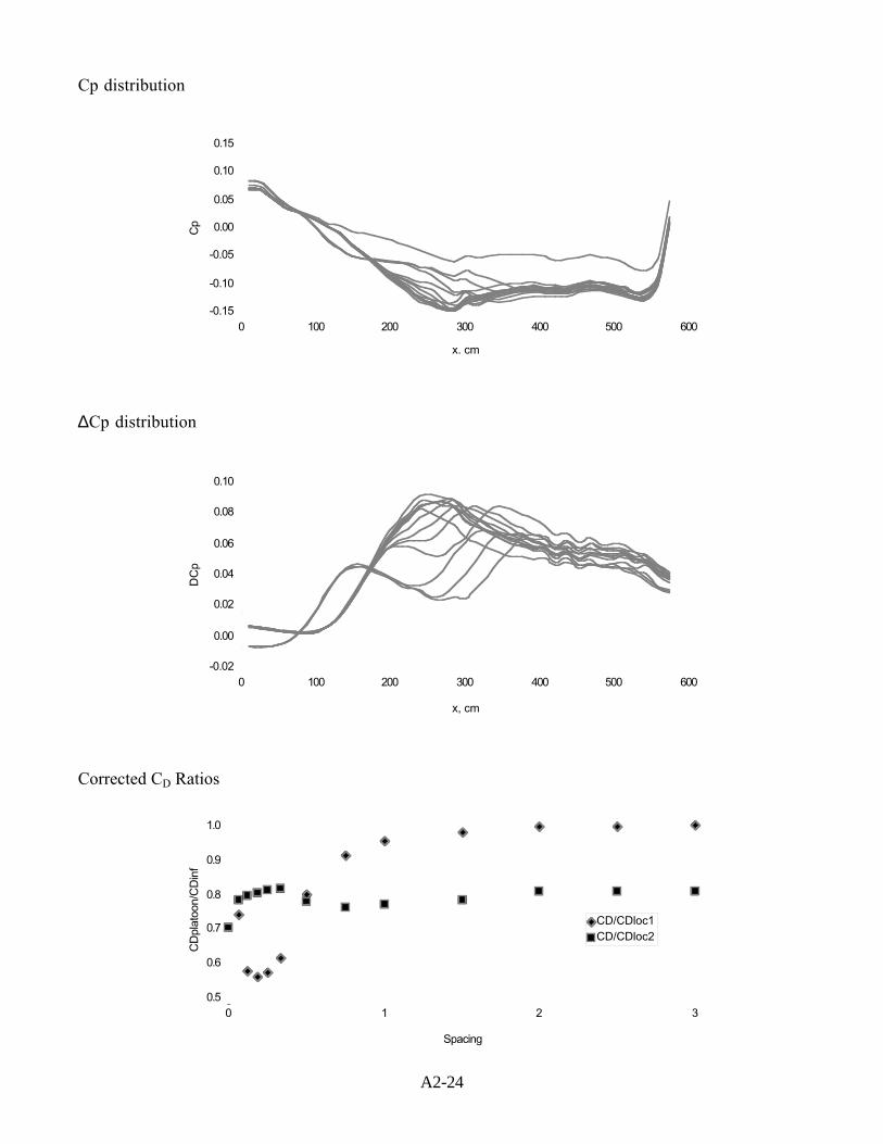
A2-24

Cp distribution

-0.15

-0.10

-0.05

0.00

0.05

0.10

0.15

0 100 200 300 400 500 600

x. cm

Cp

∆Cp distribution

-0.02

0.00

0.02

0.04

0.06

0.08

0.10

0 100 200 300 400 500 600

x, cm

DC

p

Corrected CD Ratios

0.5

0.6

0.7

0.8

0.9

1.0

0 1 2 3

Spacing

CD

plat

oon/

CD

inf

CD/CDloc1CD/CDloc2

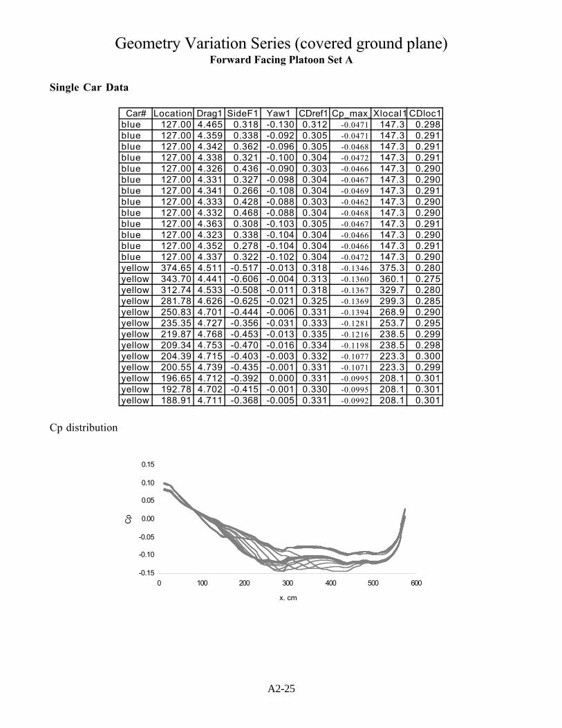
A2-25

Geometry Variation Series (covered ground plane)Forward Facing Platoon Set A

Single Car Data

Car# Location Drag1 SideF1 Yaw1 CDref1 Cp_max_Xlocal1 CDloc1blue 127.00 4.465 0.318 -0.130 0.312 -0.0471 147.3 0.298blue 127.00 4.359 0.338 -0.092 0.305 -0.0471 147.3 0.291blue 127.00 4.342 0.362 -0.096 0.305 -0.0468 147.3 0.291blue 127.00 4.338 0.321 -0.100 0.304 -0.0472 147.3 0.291blue 127.00 4.326 0.436 -0.090 0.303 -0.0466 147.3 0.290blue 127.00 4.331 0.327 -0.098 0.304 -0.0467 147.3 0.290blue 127.00 4.341 0.266 -0.108 0.304 -0.0469 147.3 0.291blue 127.00 4.333 0.428 -0.088 0.303 -0.0462 147.3 0.290blue 127.00 4.332 0.468 -0.088 0.304 -0.0468 147.3 0.290blue 127.00 4.363 0.308 -0.103 0.305 -0.0467 147.3 0.291blue 127.00 4.323 0.338 -0.104 0.304 -0.0466 147.3 0.290blue 127.00 4.352 0.278 -0.104 0.304 -0.0466 147.3 0.291blue 127.00 4.337 0.322 -0.102 0.304 -0.0472 147.3 0.290yellow 374.65 4.511 -0.517 -0.013 0.318 -0.1346 375.3 0.280yellow 343.70 4.441 -0.606 -0.004 0.313 -0.1360 360.1 0.275yellow 312.74 4.533 -0.508 -0.011 0.318 -0.1367 329.7 0.280yellow 281.78 4.626 -0.625 -0.021 0.325 -0.1369 299.3 0.285yellow 250.83 4.701 -0.444 -0.006 0.331 -0.1394 268.9 0.290yellow 235.35 4.727 -0.356 -0.031 0.333 -0.1281 253.7 0.295yellow 219.87 4.768 -0.453 -0.013 0.335 -0.1216 238.5 0.299yellow 209.34 4.753 -0.470 -0.016 0.334 -0.1198 238.5 0.298yellow 204.39 4.715 -0.403 -0.003 0.332 -0.1077 223.3 0.300yellow 200.55 4.739 -0.435 -0.001 0.331 -0.1071 223.3 0.299yellow 196.65 4.712 -0.392 0.000 0.331 -0.0995 208.1 0.301yellow 192.78 4.702 -0.415 -0.001 0.330 -0.0995 208.1 0.301yellow 188.91 4.711 -0.368 -0.005 0.331 -0.0992 208.1 0.301

Cp distribution

-0.15

-0.10

-0.05

0.00

0.05

0.10

0.15

0 100 200 300 400 500 600

x. cm

Cp

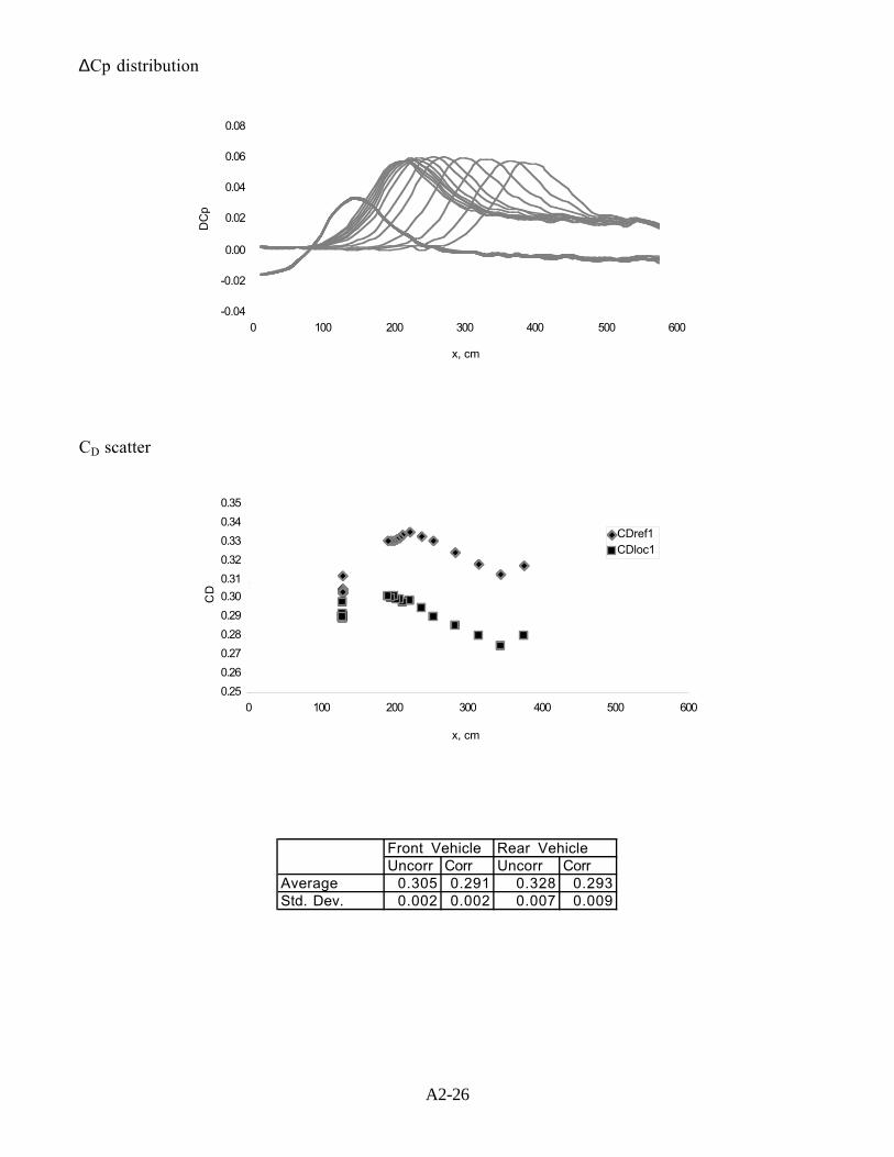
A2-26

∆Cp distribution

-0.04

-0.02

0.00

0.02

0.04

0.06

0.08

0 100 200 300 400 500 600

x, cm

DC

p

CD scatter

0.25

0.26

0.27

0.28

0.29

0.30

0.31

0.32

0.33

0.34

0.35

0 100 200 300 400 500 600

x, cm

CD

CDref1CDloc1

Front Vehicle Rear VehicleUncorr Corr Uncorr Corr

Average 0.305 0.291 0.328 0.293Std. Dev. 0.002 0.002 0.007 0.009

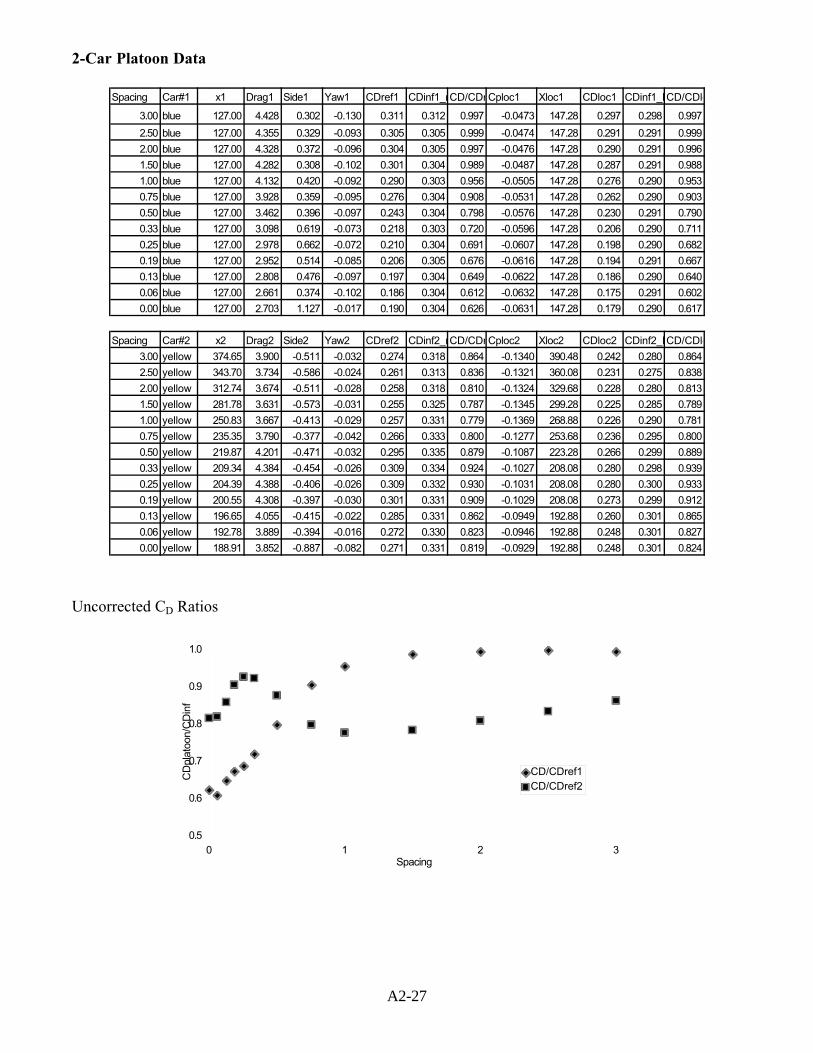
A2-27

2-Car Platoon Data

Spacing Car#1 x1 Drag1 Side1 Yaw1 CDref1 CDinf1_rCD/CDreCploc1 Xloc1 CDloc1 CDinf1_loCD/CDlo

3.00 blue 127.00 4.428 0.302 -0.130 0.311 0.312 0.997 -0.0473 147.28 0.297 0.298 0.997

2.50 blue 127.00 4.355 0.329 -0.093 0.305 0.305 0.999 -0.0474 147.28 0.291 0.291 0.999

2.00 blue 127.00 4.328 0.372 -0.096 0.304 0.305 0.997 -0.0476 147.28 0.290 0.291 0.996

1.50 blue 127.00 4.282 0.308 -0.102 0.301 0.304 0.989 -0.0487 147.28 0.287 0.291 0.988

1.00 blue 127.00 4.132 0.420 -0.092 0.290 0.303 0.956 -0.0505 147.28 0.276 0.290 0.953

0.75 blue 127.00 3.928 0.359 -0.095 0.276 0.304 0.908 -0.0531 147.28 0.262 0.290 0.903

0.50 blue 127.00 3.462 0.396 -0.097 0.243 0.304 0.798 -0.0576 147.28 0.230 0.291 0.790

0.33 blue 127.00 3.098 0.619 -0.073 0.218 0.303 0.720 -0.0596 147.28 0.206 0.290 0.711

0.25 blue 127.00 2.978 0.662 -0.072 0.210 0.304 0.691 -0.0607 147.28 0.198 0.290 0.682

0.19 blue 127.00 2.952 0.514 -0.085 0.206 0.305 0.676 -0.0616 147.28 0.194 0.291 0.667

0.13 blue 127.00 2.808 0.476 -0.097 0.197 0.304 0.649 -0.0622 147.28 0.186 0.290 0.640

0.06 blue 127.00 2.661 0.374 -0.102 0.186 0.304 0.612 -0.0632 147.28 0.175 0.291 0.602

0.00 blue 127.00 2.703 1.127 -0.017 0.190 0.304 0.626 -0.0631 147.28 0.179 0.290 0.617

Spacing Car#2 x2 Drag2 Side2 Yaw2 CDref2 CDinf2_rCD/CDreCploc2 Xloc2 CDloc2 CDinf2_loCD/CDlo

3.00 yellow 374.65 3.900 -0.511 -0.032 0.274 0.318 0.864 -0.1340 390.48 0.242 0.280 0.864

2.50 yellow 343.70 3.734 -0.586 -0.024 0.261 0.313 0.836 -0.1321 360.08 0.231 0.275 0.838

2.00 yellow 312.74 3.674 -0.511 -0.028 0.258 0.318 0.810 -0.1324 329.68 0.228 0.280 0.813

1.50 yellow 281.78 3.631 -0.573 -0.031 0.255 0.325 0.787 -0.1345 299.28 0.225 0.285 0.789

1.00 yellow 250.83 3.667 -0.413 -0.029 0.257 0.331 0.779 -0.1369 268.88 0.226 0.290 0.781

0.75 yellow 235.35 3.790 -0.377 -0.042 0.266 0.333 0.800 -0.1277 253.68 0.236 0.295 0.800

0.50 yellow 219.87 4.201 -0.471 -0.032 0.295 0.335 0.879 -0.1087 223.28 0.266 0.299 0.889

0.33 yellow 209.34 4.384 -0.454 -0.026 0.309 0.334 0.924 -0.1027 208.08 0.280 0.298 0.939

0.25 yellow 204.39 4.388 -0.406 -0.026 0.309 0.332 0.930 -0.1031 208.08 0.280 0.300 0.933

0.19 yellow 200.55 4.308 -0.397 -0.030 0.301 0.331 0.909 -0.1029 208.08 0.273 0.299 0.912

0.13 yellow 196.65 4.055 -0.415 -0.022 0.285 0.331 0.862 -0.0949 192.88 0.260 0.301 0.865

0.06 yellow 192.78 3.889 -0.394 -0.016 0.272 0.330 0.823 -0.0946 192.88 0.248 0.301 0.827

0.00 yellow 188.91 3.852 -0.887 -0.082 0.271 0.331 0.819 -0.0929 192.88 0.248 0.301 0.824

Uncorrected CD Ratios

0.5

0.6

0.7

0.8

0.9

1.0

0 1 2 3Spacing

CD

plat

oon/

CD

inf

CD/CDref1CD/CDref2

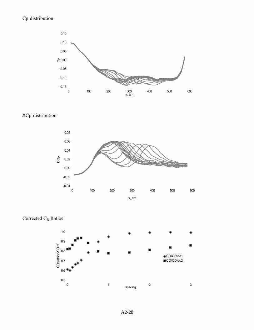
A2-28

Cp distribution

-0.15

-0.10

-0.05

0.00

0.05

0.10

0.15

0 100 200 300 400 500 600x. cm

Cp

∆Cp distribution

-0.04

-0.02

0.00

0.02

0.04

0.06

0.08

0 100 200 300 400 500 600

x, cm

DC

p

Corrected CD Ratios

0.5

0.6

0.7

0.8

0.9

1.0

0 1 2 3Spacing

CD

plat

oon/

CD

inf

CD/CDloc1CD/CDloc2

A2-29

Forward Facing Platoon Set B

Single Car Data

Car# Location Drag1 SideF1 Yaw1 CDref1 Cp_max_Xlocal1CDloc1blue 127.0 4.378 0.200 -0.137 0.307 -0.0471 147.3 0.293blue 127.0 4.377 0.293 -0.124 0.307 -0.0474 147.3 0.293blue 127.0 4.386 0.318 -0.127 0.307 -0.0471 147.3 0.293blue 127.0 4.400 0.274 -0.127 0.308 -0.0471 147.3 0.294blue 127.0 4.405 0.314 -0.126 0.309 -0.0468 147.3 0.295blue 127.0 4.386 0.326 -0.121 0.308 -0.0473 147.3 0.294blue 127.0 4.417 0.343 -0.131 0.310 -0.0470 147.3 0.296blue 127.0 4.417 0.376 -0.127 0.311 -0.0470 147.3 0.297blue 127.0 4.447 0.264 -0.139 0.313 -0.0472 147.3 0.298blue 127.0 4.456 0.276 -0.137 0.312 -0.0467 147.3 0.298yellow 281.8 4.636 -0.544 0.001 0.325 -0.1369 299.3 0.286yellow 250.8 4.720 -0.474 0.001 0.331 -0.1384 268.9 0.291yellow 235.3 4.765 -0.418 -0.014 0.336 -0.1282 253.7 0.298yellow 219.9 4.791 -0.461 -0.011 0.336 -0.1218 238.5 0.300yellow 209.3 4.771 -0.447 -0.008 0.334 -0.1079 223.3 0.302yellow 204.4 4.735 -0.401 -0.002 0.333 -0.1076 223.3 0.300yellow 200.6 4.713 -0.431 -0.002 0.332 -0.1069 223.3 0.300yellow 196.7 4.712 -0.410 0.002 0.331 -0.1065 223.3 0.299yellow 192.8 4.731 -0.400 -0.034 0.332 -0.0994 208.1 0.302yellow 188.9 4.728 -0.346 -0.016 0.331 -0.0991 208.1 0.301

Cp distribution

-0.15

-0.10

-0.05

0.00

0.05

0.10

0.15

0 100 200 300 400 500 600

x. cm

Cp

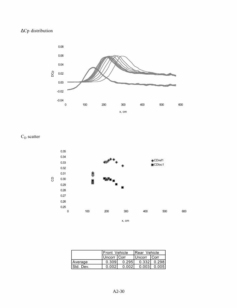
A2-30

∆Cp distribution

-0.04

-0.02

0.00

0.02

0.04

0.06

0.08

0 100 200 300 400 500 600

x, cm

DC

p

CD scatter

0.25

0.26

0.27

0.28

0.29

0.30

0.31

0.32

0.33

0.34

0.35

0 100 200 300 400 500 600

x, cm

CD

CDref1CDloc1

Front Vehicle Rear VehicleUncorr Corr Uncorr Corr

Average 0.309 0.295 0.332 0.298Std. Dev. 0.002 0.002 0.003 0.005

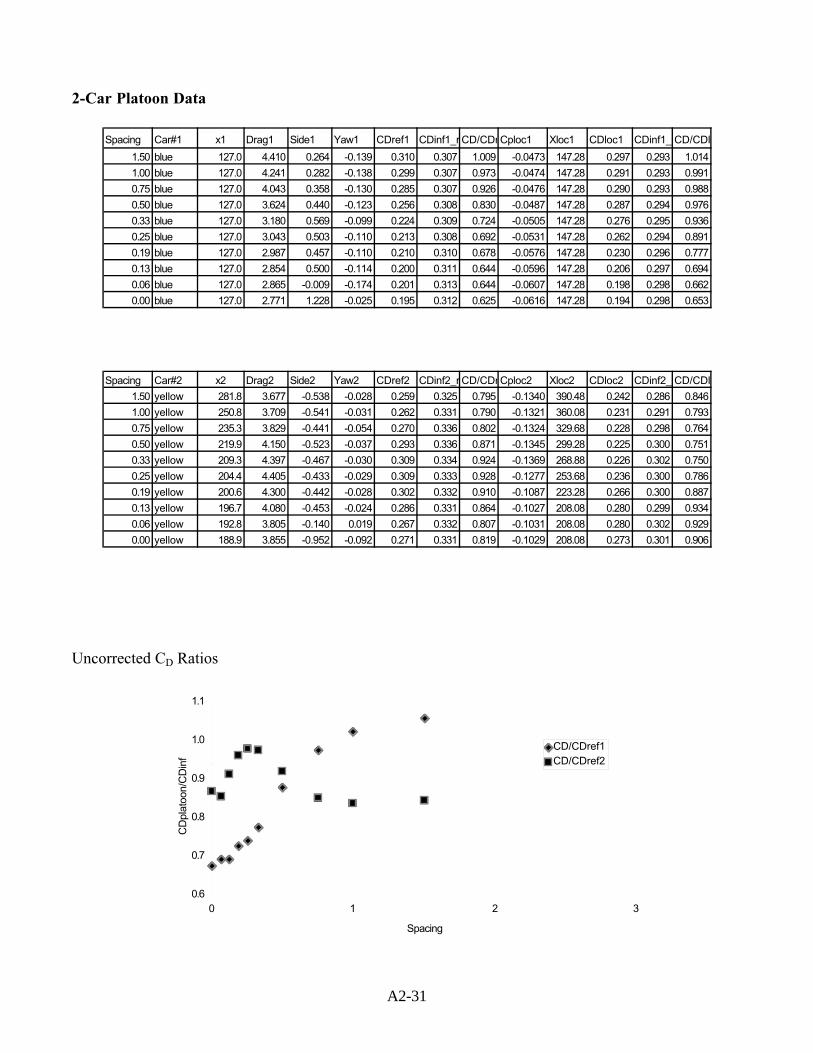
A2-31

2-Car Platoon Data

Spacing Car#1 x1 Drag1 Side1 Yaw1 CDref1 CDinf1_reCD/CDreCploc1 Xloc1 CDloc1 CDinf1_lCD/CDlo

1.50 blue 127.0 4.410 0.264 -0.139 0.310 0.307 1.009 -0.0473 147.28 0.297 0.293 1.014

1.00 blue 127.0 4.241 0.282 -0.138 0.299 0.307 0.973 -0.0474 147.28 0.291 0.293 0.991

0.75 blue 127.0 4.043 0.358 -0.130 0.285 0.307 0.926 -0.0476 147.28 0.290 0.293 0.988

0.50 blue 127.0 3.624 0.440 -0.123 0.256 0.308 0.830 -0.0487 147.28 0.287 0.294 0.976

0.33 blue 127.0 3.180 0.569 -0.099 0.224 0.309 0.724 -0.0505 147.28 0.276 0.295 0.936

0.25 blue 127.0 3.043 0.503 -0.110 0.213 0.308 0.692 -0.0531 147.28 0.262 0.294 0.891

0.19 blue 127.0 2.987 0.457 -0.110 0.210 0.310 0.678 -0.0576 147.28 0.230 0.296 0.777

0.13 blue 127.0 2.854 0.500 -0.114 0.200 0.311 0.644 -0.0596 147.28 0.206 0.297 0.694

0.06 blue 127.0 2.865 -0.009 -0.174 0.201 0.313 0.644 -0.0607 147.28 0.198 0.298 0.662

0.00 blue 127.0 2.771 1.228 -0.025 0.195 0.312 0.625 -0.0616 147.28 0.194 0.298 0.653

Spacing Car#2 x2 Drag2 Side2 Yaw2 CDref2 CDinf2_reCD/CDreCploc2 Xloc2 CDloc2 CDinf2_lCD/CDlo

1.50 yellow 281.8 3.677 -0.538 -0.028 0.259 0.325 0.795 -0.1340 390.48 0.242 0.286 0.846

1.00 yellow 250.8 3.709 -0.541 -0.031 0.262 0.331 0.790 -0.1321 360.08 0.231 0.291 0.793

0.75 yellow 235.3 3.829 -0.441 -0.054 0.270 0.336 0.802 -0.1324 329.68 0.228 0.298 0.764

0.50 yellow 219.9 4.150 -0.523 -0.037 0.293 0.336 0.871 -0.1345 299.28 0.225 0.300 0.751

0.33 yellow 209.3 4.397 -0.467 -0.030 0.309 0.334 0.924 -0.1369 268.88 0.226 0.302 0.750

0.25 yellow 204.4 4.405 -0.433 -0.029 0.309 0.333 0.928 -0.1277 253.68 0.236 0.300 0.786

0.19 yellow 200.6 4.300 -0.442 -0.028 0.302 0.332 0.910 -0.1087 223.28 0.266 0.300 0.887

0.13 yellow 196.7 4.080 -0.453 -0.024 0.286 0.331 0.864 -0.1027 208.08 0.280 0.299 0.934

0.06 yellow 192.8 3.805 -0.140 0.019 0.267 0.332 0.807 -0.1031 208.08 0.280 0.302 0.929

0.00 yellow 188.9 3.855 -0.952 -0.092 0.271 0.331 0.819 -0.1029 208.08 0.273 0.301 0.906

Uncorrected CD Ratios

0.6

0.7

0.8

0.9

1.0

1.1

0 1 2 3

Spacing

CD

plat

oon/

CD

inf

CD/CDref1CD/CDref2

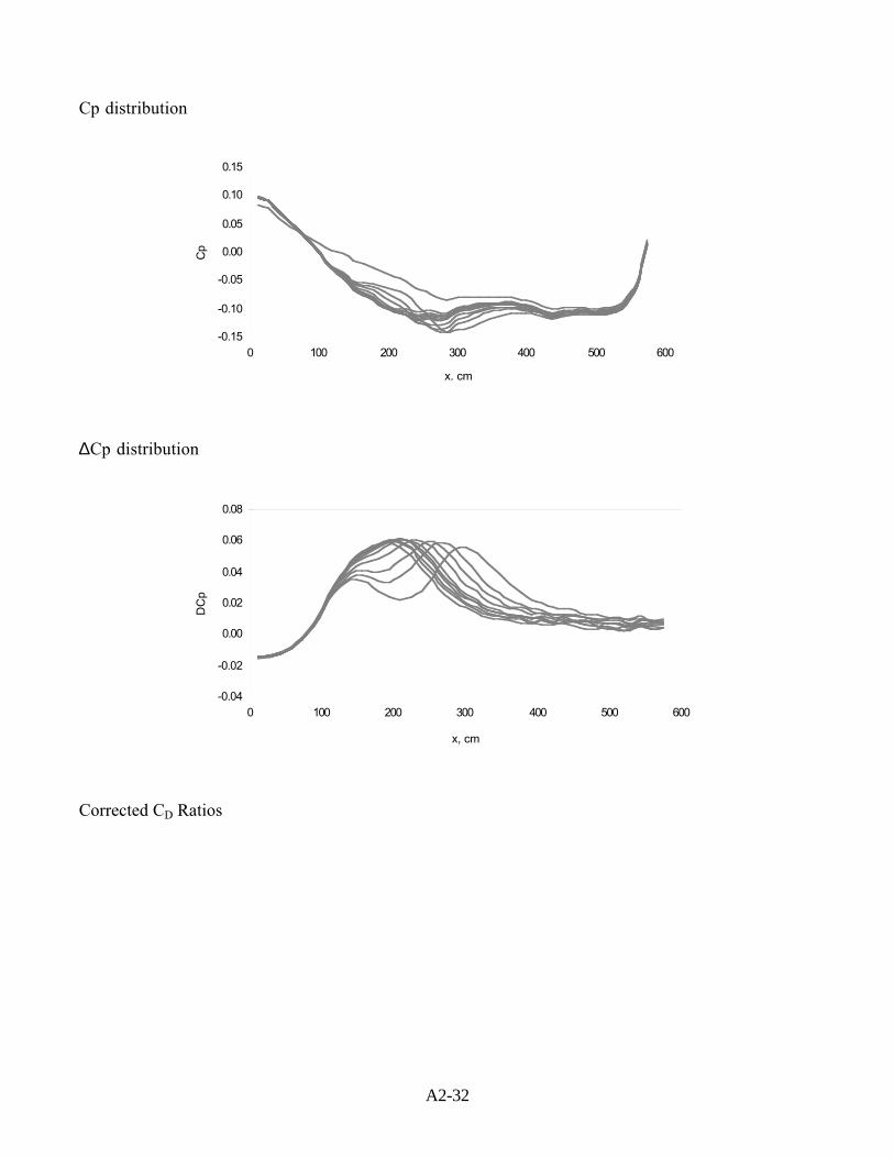
A2-32

Cp distribution

-0.15

-0.10

-0.05

0.00

0.05

0.10

0.15

0 100 200 300 400 500 600

x. cm

Cp

∆Cp distribution

-0.04

-0.02

0.00

0.02

0.04

0.06

0.08

0 100 200 300 400 500 600

x, cm

DC

p

Corrected CD Ratios

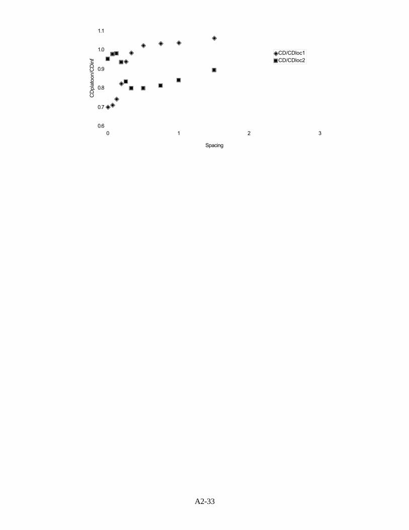
A2-33

0.6

0.7

0.8

0.9

1.0

1.1

0 1 2 3

Spacing

CD

plat

oon/

CD

inf

CD/CDloc1CD/CDloc2

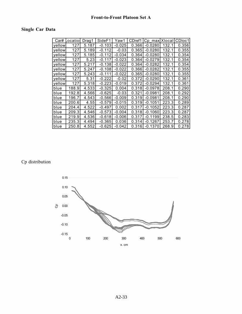
A2-33

Front-to-Front Platoon Set A

Single Car Data

Car# Location Drag1 SideF1 Yaw1 CDref1 Cp_max_Xlocal1CDloc1yellow 127 5.187 -0.103 -0.025 0.366 -0.0280 132.1 0.356yellow 127 5.189 -0.112 -0.03 0.365 -0.0280 132.1 0.355yellow 127 5.185 -0.112 -0.034 0.364 -0.0280 132.1 0.354yellow 127 5.23 -0.117 -0.023 0.364 -0.0279 132.1 0.354yellow 127 5.217 -0.138 -0.022 0.364 -0.0282 132.1 0.354yellow 127 5.247 -0.108 -0.022 0.366 -0.0282 132.1 0.355yellow 127 5.243 -0.111 -0.022 0.365 -0.0280 132.1 0.355yellow 127 5.31 -0.222 -0.02 0.372 -0.0290 132.1 0.361yellow 127 5.318 -0.223 -0.019 0.372 -0.0294 132.1 0.361blue 188.9 4.533 -0.325 0.004 0.318 -0.0978 208.1 0.290blue 192.8 4.566 -0.625 -0.03 0.321 -0.0981 208.1 0.292blue 196.7 4.543 -0.566 -0.009 0.319 -0.0981 208.1 0.290blue 200.6 4.55 -0.579 -0.015 0.319 -0.1051 223.3 0.289blue 204.4 4.522 -0.497 0.002 0.317 -0.1052 223.3 0.287blue 209.3 4.546 -0.573 -0.004 0.318 -0.1060 223.3 0.287blue 219.9 4.536 -0.618 -0.006 0.317 -0.1199 238.5 0.283blue 235.3 4.494 -0.365 0.036 0.314 -0.1267 253.7 0.278blue 250.8 4.552 -0.625 -0.042 0.316 -0.1370 268.9 0.278

Cp distribution

-0.15

-0.10

-0.05

0.00

0.05

0.10

0.15

0 100 200 300 400 500 600

x. cm

Cp

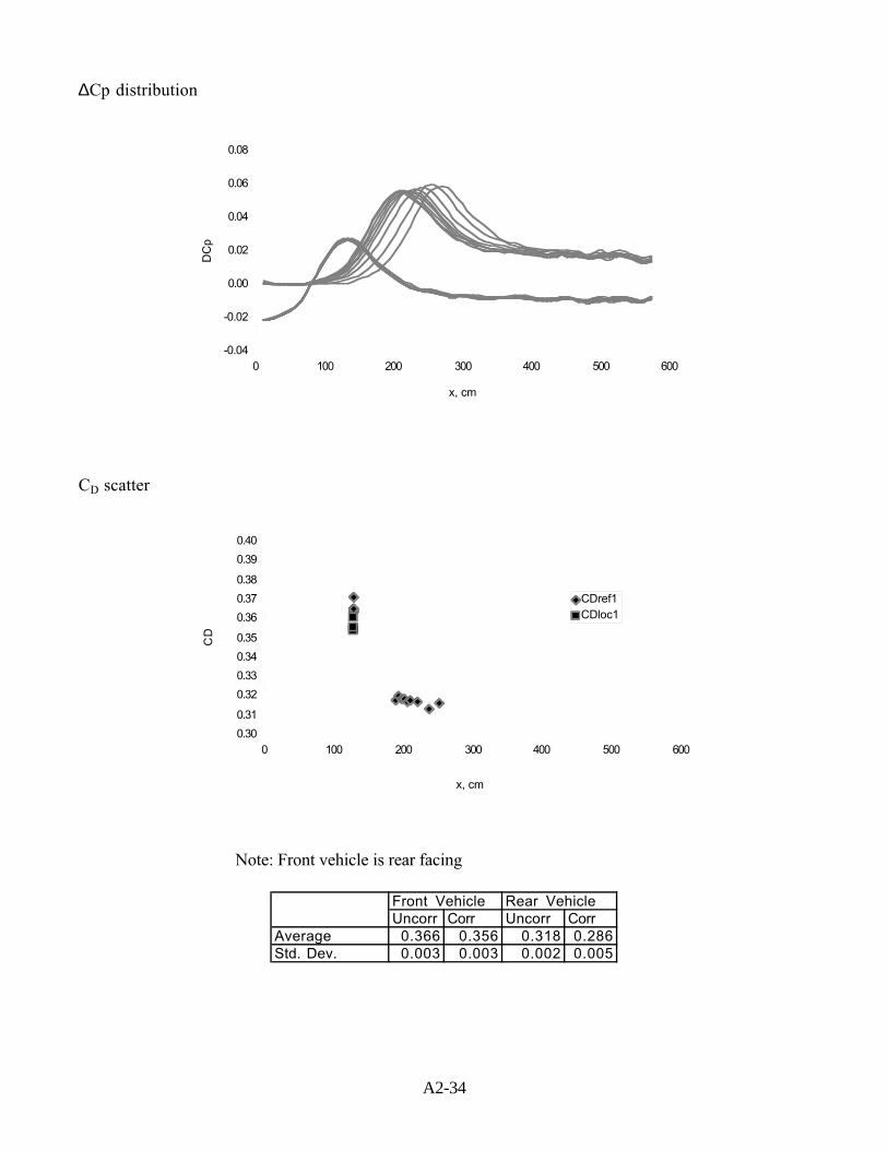
A2-34

∆Cp distribution

-0.04

-0.02

0.00

0.02

0.04

0.06

0.08

0 100 200 300 400 500 600

x, cm

DC

p

CD scatter

0.30

0.31

0.32

0.33

0.34

0.35

0.36

0.37

0.38

0.39

0.40

0 100 200 300 400 500 600

x, cm

CD

CDref1CDloc1

Note: Front vehicle is rear facing

Front Vehicle Rear VehicleUncorr Corr Uncorr Corr

Average 0.366 0.356 0.318 0.286Std. Dev. 0.003 0.003 0.002 0.005

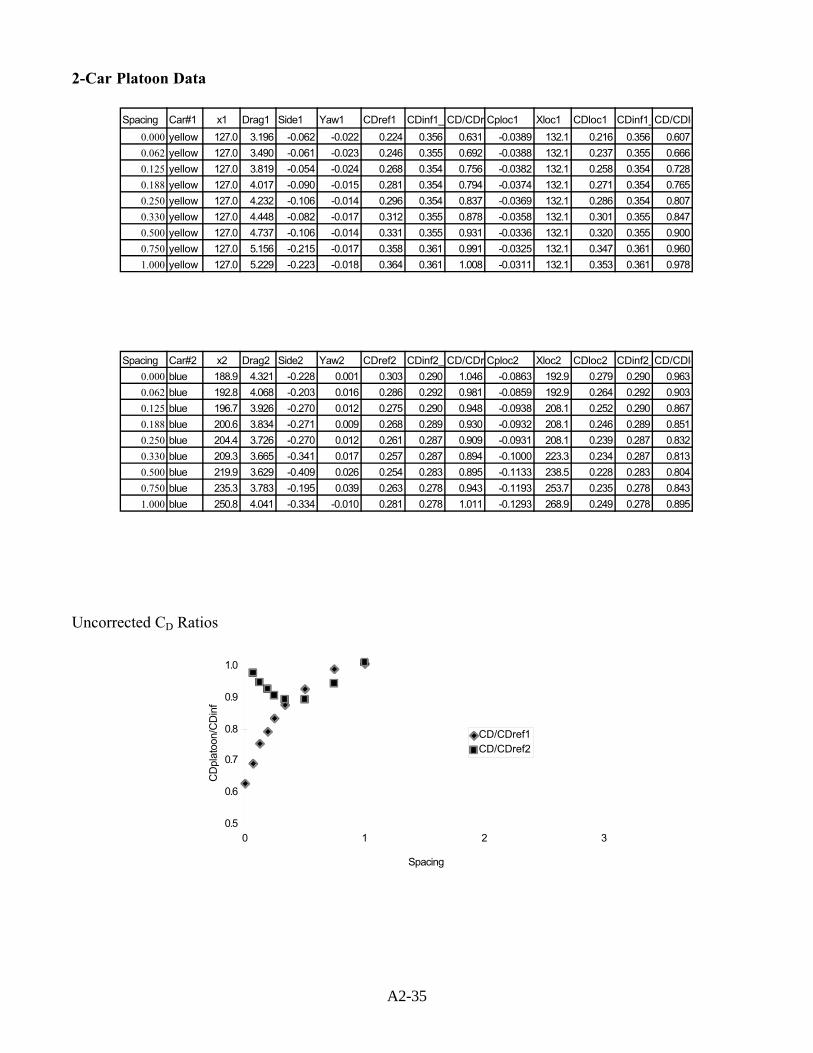
A2-35

2-Car Platoon Data

Spacing Car#1 x1 Drag1 Side1 Yaw1 CDref1 CDinf1_rCD/CDreCploc1 Xloc1 CDloc1 CDinf1_CD/CDlo

0.000 yellow 127.0 3.196 -0.062 -0.022 0.224 0.356 0.631 -0.0389 132.1 0.216 0.356 0.607

0.062 yellow 127.0 3.490 -0.061 -0.023 0.246 0.355 0.692 -0.0388 132.1 0.237 0.355 0.666

0.125 yellow 127.0 3.819 -0.054 -0.024 0.268 0.354 0.756 -0.0382 132.1 0.258 0.354 0.728

0.188 yellow 127.0 4.017 -0.090 -0.015 0.281 0.354 0.794 -0.0374 132.1 0.271 0.354 0.765

0.250 yellow 127.0 4.232 -0.106 -0.014 0.296 0.354 0.837 -0.0369 132.1 0.286 0.354 0.807

0.330 yellow 127.0 4.448 -0.082 -0.017 0.312 0.355 0.878 -0.0358 132.1 0.301 0.355 0.847

0.500 yellow 127.0 4.737 -0.106 -0.014 0.331 0.355 0.931 -0.0336 132.1 0.320 0.355 0.900

0.750 yellow 127.0 5.156 -0.215 -0.017 0.358 0.361 0.991 -0.0325 132.1 0.347 0.361 0.960

1.000 yellow 127.0 5.229 -0.223 -0.018 0.364 0.361 1.008 -0.0311 132.1 0.353 0.361 0.978

Spacing Car#2 x2 Drag2 Side2 Yaw2 CDref2 CDinf2_rCD/CDreCploc2 Xloc2 CDloc2 CDinf2_CD/CDlo

0.000 blue 188.9 4.321 -0.228 0.001 0.303 0.290 1.046 -0.0863 192.9 0.279 0.290 0.963

0.062 blue 192.8 4.068 -0.203 0.016 0.286 0.292 0.981 -0.0859 192.9 0.264 0.292 0.903

0.125 blue 196.7 3.926 -0.270 0.012 0.275 0.290 0.948 -0.0938 208.1 0.252 0.290 0.867

0.188 blue 200.6 3.834 -0.271 0.009 0.268 0.289 0.930 -0.0932 208.1 0.246 0.289 0.851

0.250 blue 204.4 3.726 -0.270 0.012 0.261 0.287 0.909 -0.0931 208.1 0.239 0.287 0.832

0.330 blue 209.3 3.665 -0.341 0.017 0.257 0.287 0.894 -0.1000 223.3 0.234 0.287 0.813

0.500 blue 219.9 3.629 -0.409 0.026 0.254 0.283 0.895 -0.1133 238.5 0.228 0.283 0.804

0.750 blue 235.3 3.783 -0.195 0.039 0.263 0.278 0.943 -0.1193 253.7 0.235 0.278 0.843

1.000 blue 250.8 4.041 -0.334 -0.010 0.281 0.278 1.011 -0.1293 268.9 0.249 0.278 0.895

Uncorrected CD Ratios

0.5

0.6

0.7

0.8

0.9

1.0

0 1 2 3

Spacing

CD

plat

oon/

CD

inf

CD/CDref1CD/CDref2

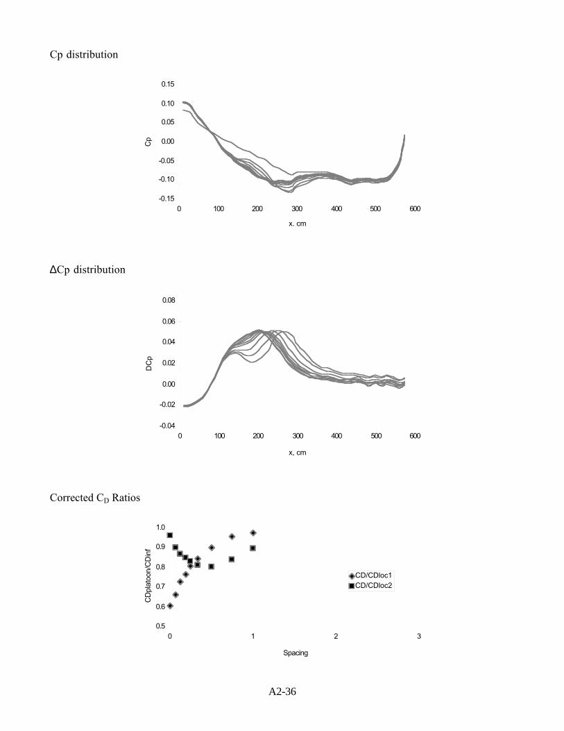
A2-36

Cp distribution

-0.15

-0.10

-0.05

0.00

0.05

0.10

0.15

0 100 200 300 400 500 600

x. cm

Cp

∆Cp distribution

-0.04

-0.02

0.00

0.02

0.04

0.06

0.08

0 100 200 300 400 500 600

x, cm

DC

p

Corrected CD Ratios

0.5

0.6

0.7

0.8

0.9

1.0

0 1 2 3

Spacing

CD

plat

oon/

CD

inf

CD/CDloc1CD/CDloc2

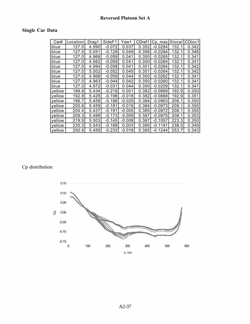
A2-37

Reversed Platoon Set A

Single Car Data

Car# Location Drag1 SideF1 Yaw1 CDref1 Cp_max_Xlocal1CDloc1blue 127.0 4.990 -0.072 0.037 0.352 -0.0284 132.1 0.342blue 127.0 5.051 -0.129 0.049 0.356 -0.0284 132.1 0.346blue 127.0 4.968 -0.059 0.041 0.350 -0.0265 132.1 0.341blue 127.0 4.982 -0.059 0.041 0.350 -0.0264 132.1 0.341blue 127.0 4.994 -0.058 0.041 0.351 -0.0264 132.1 0.342blue 127.0 5.002 -0.052 0.045 0.351 -0.0264 132.1 0.342blue 127.0 4.968 -0.059 0.044 0.350 -0.0262 132.1 0.341blue 127.0 4.963 -0.044 0.042 0.350 -0.0260 132.1 0.341blue 127.0 4.972 -0.031 0.044 0.350 -0.0259 132.1 0.341yellow 188.9 5.434 -0.218 0.001 0.382 -0.0889 192.9 0.350yellow 192.8 5.428 -0.198 -0.018 0.382 -0.0888 192.9 0.351yellow 196.7 5.458 -0.186 -0.025 0.384 -0.0963 208.1 0.350yellow 200.6 5.459 -0.181 -0.018 0.384 -0.0973 208.1 0.350yellow 204.4 5.437 -0.191 -0.005 0.385 -0.0972 208.1 0.350yellow 209.3 5.488 -0.173 -0.009 0.387 -0.0970 208.1 0.353yellow 219.9 5.503 -0.145 -0.008 0.387 -0.1057 223.3 0.350yellow 235.3 5.543 -0.169 0.003 0.390 -0.1191 238.5 0.349yellow 250.8 5.459 -0.233 -0.018 0.385 -0.1244 253.7 0.343

Cp distribution

-0.15

-0.10

-0.05

0.00

0.05

0.10

0.15

0 100 200 300 400 500 600

x. cm

Cp

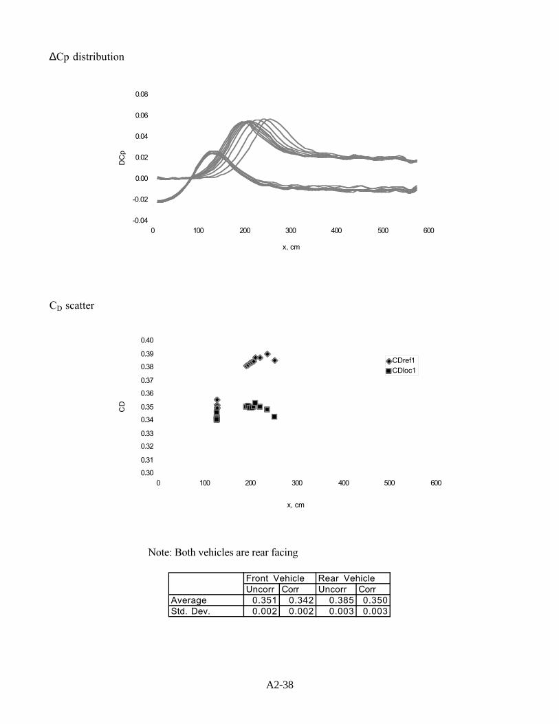
A2-38

∆Cp distribution

-0.04

-0.02

0.00

0.02

0.04

0.06

0.08

0 100 200 300 400 500 600

x, cm

DC

p

CD scatter

0.30

0.31

0.32

0.33

0.34

0.35

0.36

0.37

0.38

0.39

0.40

0 100 200 300 400 500 600

x, cm

CD

CDref1CDloc1

Note: Both vehicles are rear facing

Front Vehicle Rear VehicleUncorr Corr Uncorr Corr

Average 0.351 0.342 0.385 0.350Std. Dev. 0.002 0.002 0.003 0.003

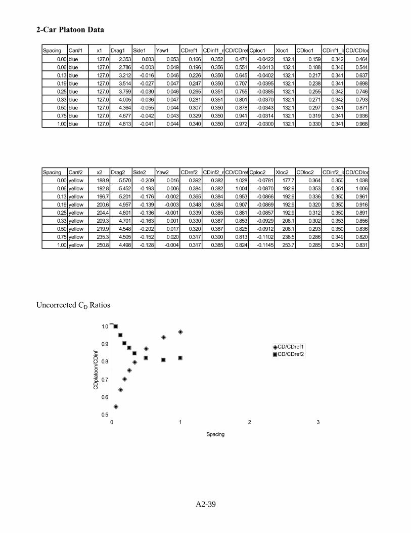
A2-39

2-Car Platoon Data

Spacing Car#1 x1 Drag1 Side1 Yaw1 CDref1 CDinf1_reCD/CDref Cploc1 Xloc1 CDloc1 CDinf1_loCD/CDloc

0.00 blue 127.0 2.353 0.033 0.053 0.166 0.352 0.471 -0.0422 132.1 0.159 0.342 0.464

0.06 blue 127.0 2.786 -0.003 0.049 0.196 0.356 0.551 -0.0413 132.1 0.188 0.346 0.544

0.13 blue 127.0 3.212 -0.016 0.046 0.226 0.350 0.645 -0.0402 132.1 0.217 0.341 0.637

0.19 blue 127.0 3.514 -0.027 0.047 0.247 0.350 0.707 -0.0395 132.1 0.238 0.341 0.698

0.25 blue 127.0 3.759 -0.030 0.046 0.265 0.351 0.755 -0.0385 132.1 0.255 0.342 0.746

0.33 blue 127.0 4.005 -0.036 0.047 0.281 0.351 0.801 -0.0370 132.1 0.271 0.342 0.793

0.50 blue 127.0 4.364 -0.055 0.044 0.307 0.350 0.878 -0.0343 132.1 0.297 0.341 0.871

0.75 blue 127.0 4.677 -0.042 0.043 0.329 0.350 0.941 -0.0314 132.1 0.319 0.341 0.936

1.00 blue 127.0 4.813 -0.041 0.044 0.340 0.350 0.972 -0.0300 132.1 0.330 0.341 0.968

Spacing Car#2 x2 Drag2 Side2 Yaw2 CDref2 CDinf2_reCD/CDref2Cploc2 Xloc2 CDloc2 CDinf2_loCD/CDloc

0.00 yellow 188.9 5.570 -0.209 0.016 0.392 0.382 1.028 -0.0781 177.7 0.364 0.350 1.038

0.06 yellow 192.8 5.452 -0.193 0.006 0.384 0.382 1.004 -0.0870 192.9 0.353 0.351 1.006

0.13 yellow 196.7 5.201 -0.176 -0.002 0.365 0.384 0.953 -0.0866 192.9 0.336 0.350 0.961

0.19 yellow 200.6 4.957 -0.139 -0.003 0.348 0.384 0.907 -0.0869 192.9 0.320 0.350 0.916

0.25 yellow 204.4 4.801 -0.136 -0.001 0.339 0.385 0.881 -0.0857 192.9 0.312 0.350 0.891

0.33 yellow 209.3 4.701 -0.163 0.001 0.330 0.387 0.853 -0.0929 208.1 0.302 0.353 0.856

0.50 yellow 219.9 4.548 -0.202 0.017 0.320 0.387 0.825 -0.0912 208.1 0.293 0.350 0.836

0.75 yellow 235.3 4.505 -0.152 0.020 0.317 0.390 0.813 -0.1102 238.5 0.286 0.349 0.820

1.00 yellow 250.8 4.498 -0.128 -0.004 0.317 0.385 0.824 -0.1145 253.7 0.285 0.343 0.831

Uncorrected CD Ratios

0.5

0.6

0.7

0.8

0.9

1.0

0 1 2 3

Spacing

CD

plat

oon/

CD

inf

CD/CDref1CD/CDref2

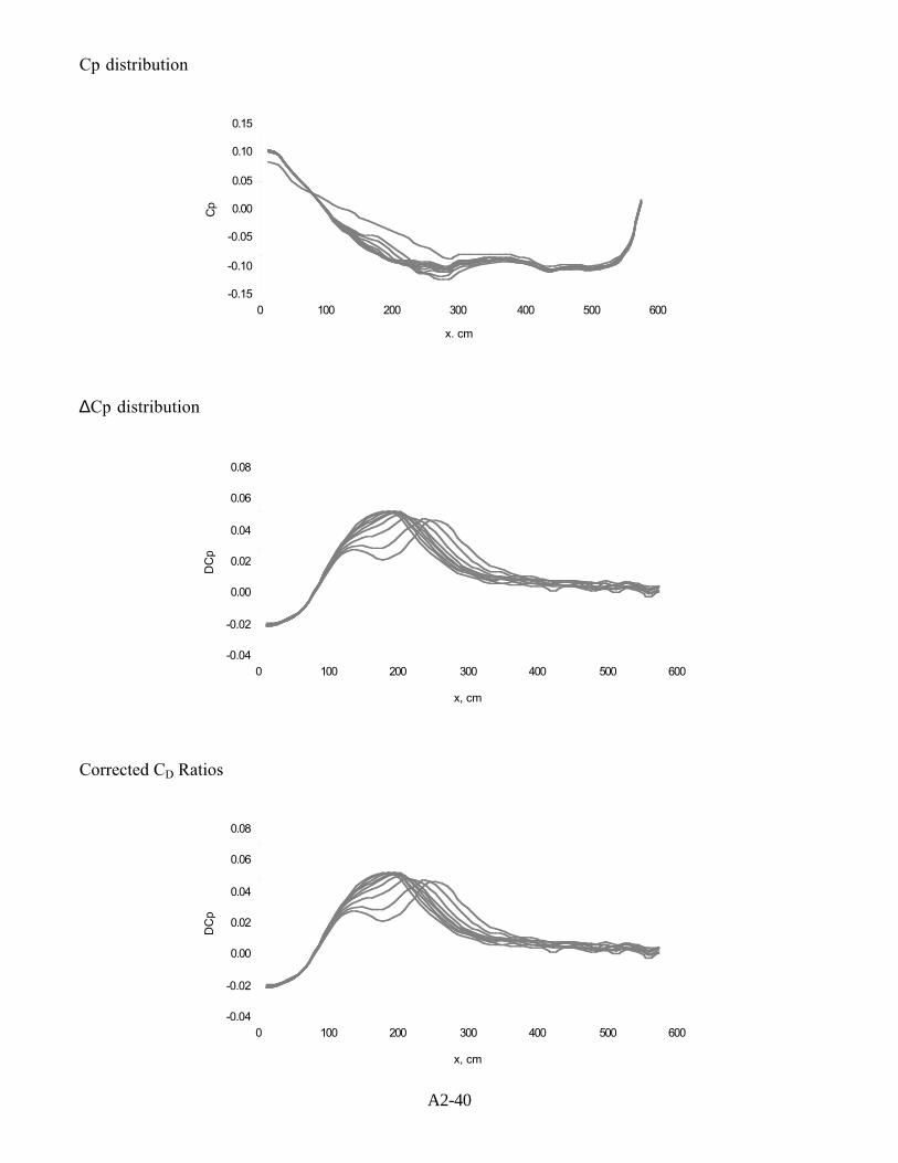
A2-40

Cp distribution

-0.15

-0.10

-0.05

0.00

0.05

0.10

0.15

0 100 200 300 400 500 600

x. cm

Cp

∆Cp distribution

-0.04

-0.02

0.00

0.02

0.04

0.06

0.08

0 100 200 300 400 500 600

x, cm

DC

p

Corrected CD Ratios

-0.04

-0.02

0.00

0.02

0.04

0.06

0.08

0 100 200 300 400 500 600

x, cm

DC

p

A2-41

Back-to-Back Platoon Set A

Single Car Data

Car# Location Drag1 SideF1 Yaw1 CDref1 Cp_max_dXlocal1 CDloc1blue 127.0 4.485 -0.255 -0.005 0.310 -0.1255 253.7 0.276blue 127.0 4.439 -0.263 -0.005 0.310 -0.1238 253.7 0.276blue 127.0 4.343 -0.322 -0.025 0.302 -0.1217 253.7 0.269blue 127.0 4.337 -0.318 -0.024 0.302 -0.0470 147.3 0.289blue 127.0 4.383 -0.365 -0.035 0.304 -0.0468 147.3 0.290blue 127.0 4.362 -0.369 -0.035 0.304 -0.1069 223.3 0.274blue 127.0 4.360 -0.312 -0.031 0.303 -0.1191 238.5 0.271blue 127.0 4.318 -0.312 -0.028 0.304 -0.1049 223.3 0.275blue 127.0 4.347 -0.412 -0.043 0.305 -0.1035 208.1 0.276yellow 188.9 5.429 -0.211 -0.013 0.382 -0.0468 147.3 0.365yellow 192.8 5.434 -0.222 -0.004 0.381 -0.0468 147.3 0.364yellow 196.7 5.449 -0.235 -0.006 0.381 -0.0978 192.9 0.347yellow 200.6 5.504 -0.220 0.012 0.384 -0.0960 192.9 0.351yellow 204.4 5.542 -0.243 0.008 0.387 -0.1057 223.3 0.350yellow 209.3 5.529 -0.196 0.020 0.387 -0.0990 208.1 0.352yellow 219.9 5.528 -0.204 0.008 0.385 -0.0979 192.9 0.350yellow 235.3 5.563 -0.203 0.022 0.387 -0.0473 147.3 0.369yellow 250.8 5.413 -0.467 0.013 0.377 -0.0470 147.3 0.360

Cp distribution

-0.15

-0.10

-0.05

0.00

0.05

0.10

0.15

0 100 200 300 400 500 600

x. cm

Cp

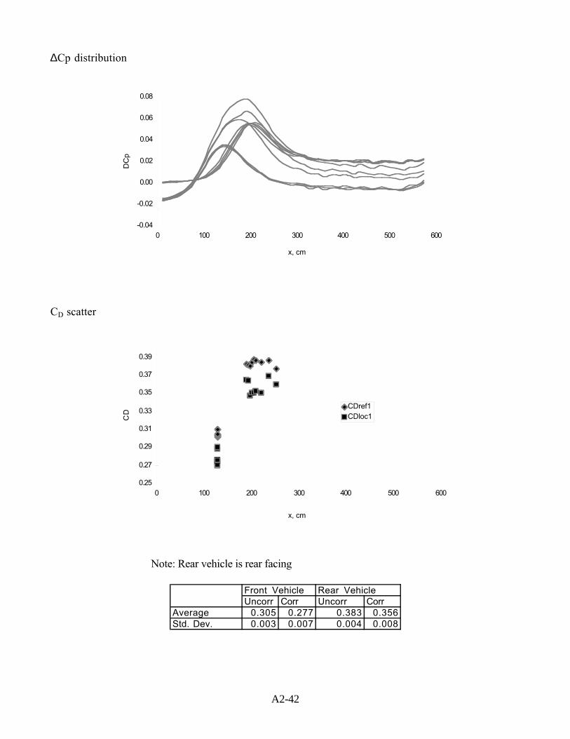
A2-42

∆Cp distribution

-0.04

-0.02

0.00

0.02

0.04

0.06

0.08

0 100 200 300 400 500 600

x, cm

DC

p

CD scatter

0.25

0.27

0.29

0.31

0.33

0.35

0.37

0.39

0 100 200 300 400 500 600

x, cm

CD

CDref1CDloc1

Note: Rear vehicle is rear facing

Front Vehicle Rear VehicleUncorr Corr Uncorr Corr

Average 0.305 0.277 0.383 0.356Std. Dev. 0.003 0.007 0.004 0.008

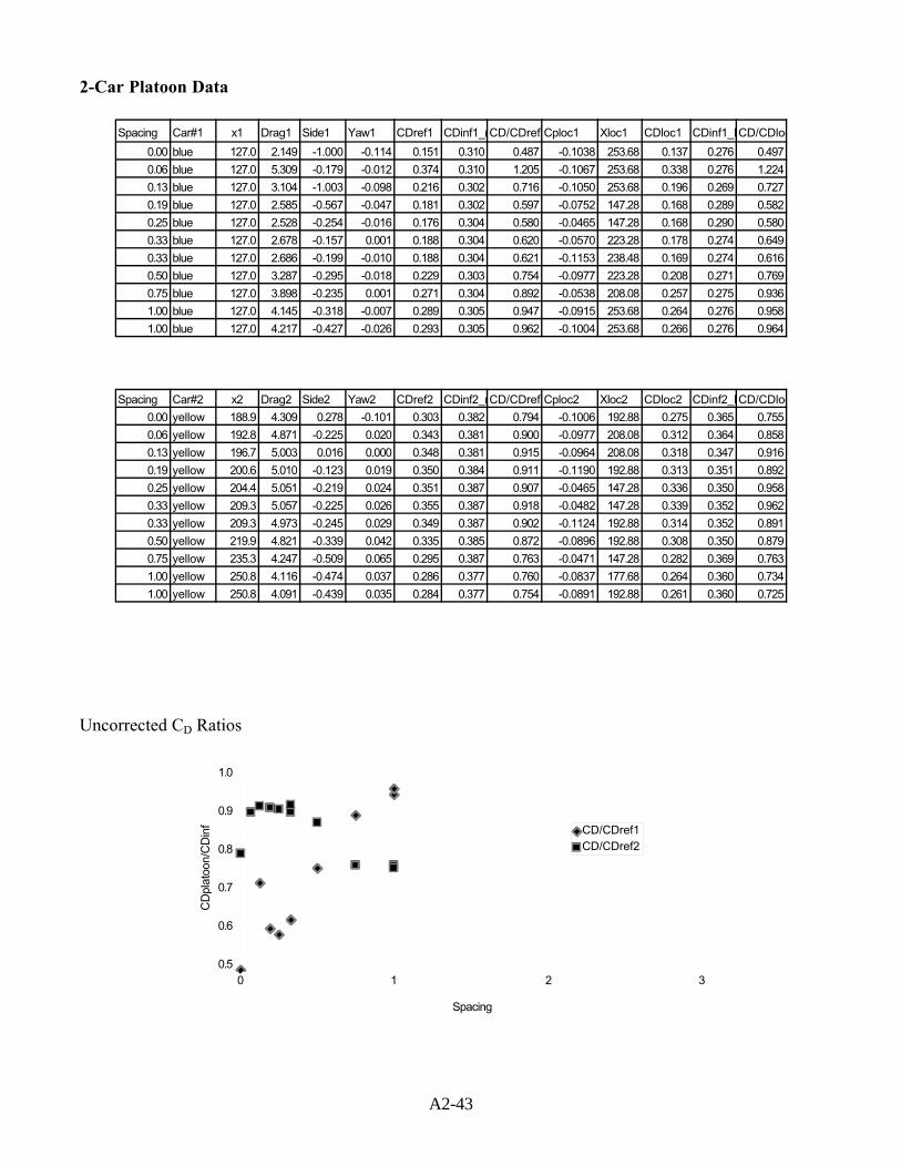
A2-43

2-Car Platoon Data

Spacing Car#1 x1 Drag1 Side1 Yaw1 CDref1 CDinf1_rCD/CDref1Cploc1 Xloc1 CDloc1 CDinf1_loCD/CDloc

0.00 blue 127.0 2.149 -1.000 -0.114 0.151 0.310 0.487 -0.1038 253.68 0.137 0.276 0.497

0.06 blue 127.0 5.309 -0.179 -0.012 0.374 0.310 1.205 -0.1067 253.68 0.338 0.276 1.224

0.13 blue 127.0 3.104 -1.003 -0.098 0.216 0.302 0.716 -0.1050 253.68 0.196 0.269 0.727

0.19 blue 127.0 2.585 -0.567 -0.047 0.181 0.302 0.597 -0.0752 147.28 0.168 0.289 0.582

0.25 blue 127.0 2.528 -0.254 -0.016 0.176 0.304 0.580 -0.0465 147.28 0.168 0.290 0.580

0.33 blue 127.0 2.678 -0.157 0.001 0.188 0.304 0.620 -0.0570 223.28 0.178 0.274 0.649

0.33 blue 127.0 2.686 -0.199 -0.010 0.188 0.304 0.621 -0.1153 238.48 0.169 0.274 0.616

0.50 blue 127.0 3.287 -0.295 -0.018 0.229 0.303 0.754 -0.0977 223.28 0.208 0.271 0.769

0.75 blue 127.0 3.898 -0.235 0.001 0.271 0.304 0.892 -0.0538 208.08 0.257 0.275 0.936

1.00 blue 127.0 4.145 -0.318 -0.007 0.289 0.305 0.947 -0.0915 253.68 0.264 0.276 0.958

1.00 blue 127.0 4.217 -0.427 -0.026 0.293 0.305 0.962 -0.1004 253.68 0.266 0.276 0.964

Spacing Car#2 x2 Drag2 Side2 Yaw2 CDref2 CDinf2_rCD/CDref2Cploc2 Xloc2 CDloc2 CDinf2_loCD/CDloc

0.00 yellow 188.9 4.309 0.278 -0.101 0.303 0.382 0.794 -0.1006 192.88 0.275 0.365 0.755

0.06 yellow 192.8 4.871 -0.225 0.020 0.343 0.381 0.900 -0.0977 208.08 0.312 0.364 0.858

0.13 yellow 196.7 5.003 0.016 0.000 0.348 0.381 0.915 -0.0964 208.08 0.318 0.347 0.916

0.19 yellow 200.6 5.010 -0.123 0.019 0.350 0.384 0.911 -0.1190 192.88 0.313 0.351 0.892

0.25 yellow 204.4 5.051 -0.219 0.024 0.351 0.387 0.907 -0.0465 147.28 0.336 0.350 0.958

0.33 yellow 209.3 5.057 -0.225 0.026 0.355 0.387 0.918 -0.0482 147.28 0.339 0.352 0.962

0.33 yellow 209.3 4.973 -0.245 0.029 0.349 0.387 0.902 -0.1124 192.88 0.314 0.352 0.891

0.50 yellow 219.9 4.821 -0.339 0.042 0.335 0.385 0.872 -0.0896 192.88 0.308 0.350 0.879

0.75 yellow 235.3 4.247 -0.509 0.065 0.295 0.387 0.763 -0.0471 147.28 0.282 0.369 0.763

1.00 yellow 250.8 4.116 -0.474 0.037 0.286 0.377 0.760 -0.0837 177.68 0.264 0.360 0.734

1.00 yellow 250.8 4.091 -0.439 0.035 0.284 0.377 0.754 -0.0891 192.88 0.261 0.360 0.725

Uncorrected CD Ratios

0.5

0.6

0.7

0.8

0.9

1.0

0 1 2 3

Spacing

CD

plat

oon/

CD

inf CD/CDref1

CD/CDref2

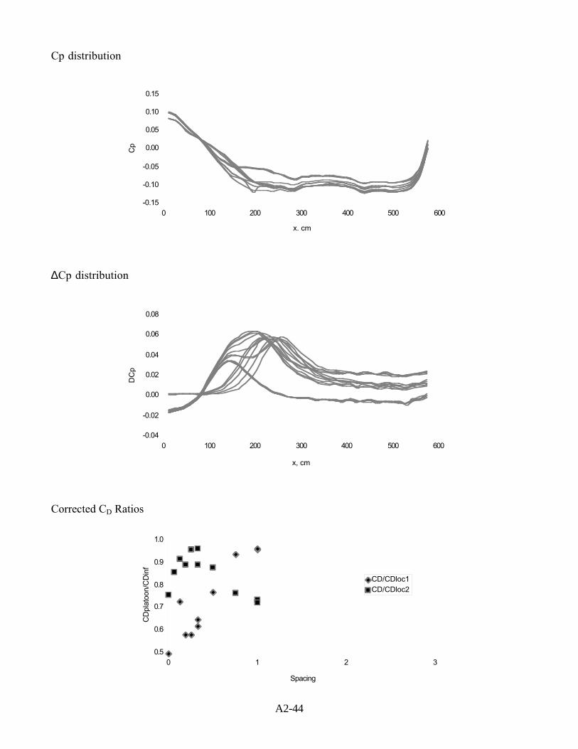
A2-44

Cp distribution

-0.15

-0.10

-0.05

0.00

0.05

0.10

0.15

0 100 200 300 400 500 600

x. cm

Cp

∆Cp distribution

-0.04

-0.02

0.00

0.02

0.04

0.06

0.08

0 100 200 300 400 500 600

x, cm

DC

p

Corrected CD Ratios

0.5

0.6

0.7

0.8

0.9

1.0

0 1 2 3

Spacing

CD

plat

oon/

CD

inf

CD/CDloc1CD/CDloc2

Appendix 3:

Flow Visualization

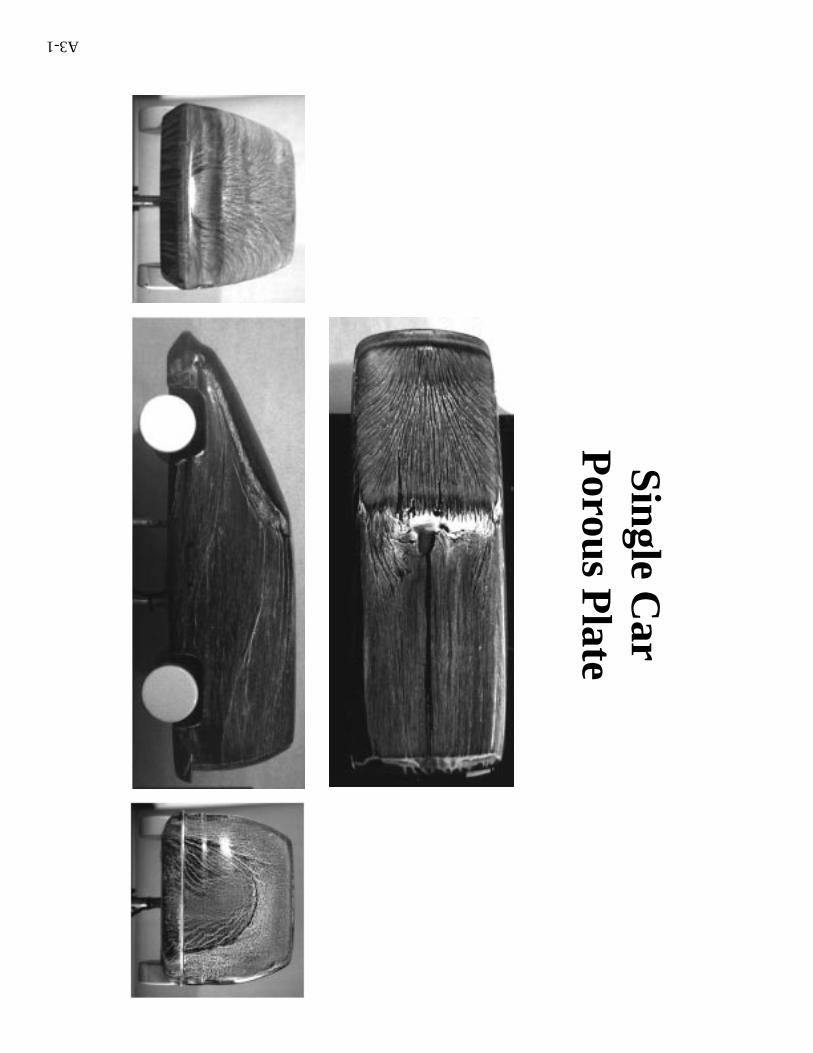
Single C

arP

orous Plate

A3-1

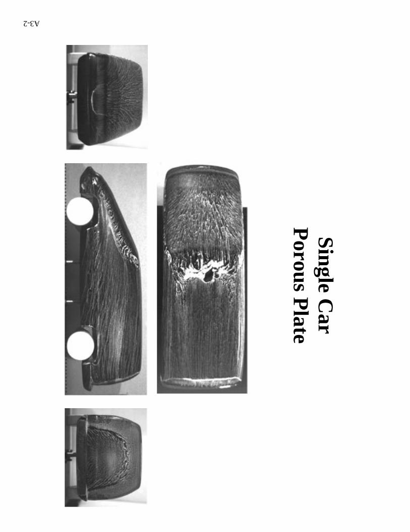
Single C

arP

orous Plate

A3-2

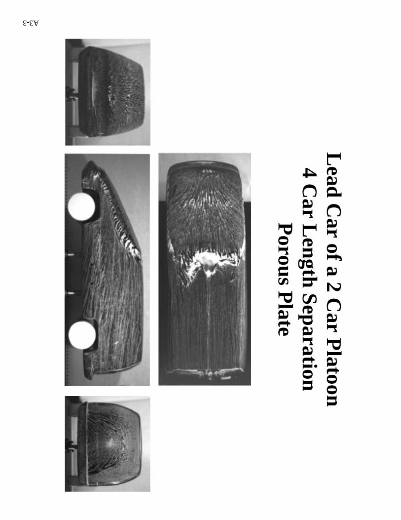
Lead Car of a 2 C

ar Platoon

4 Car Length S

eparationP

orous Plate

A3-3

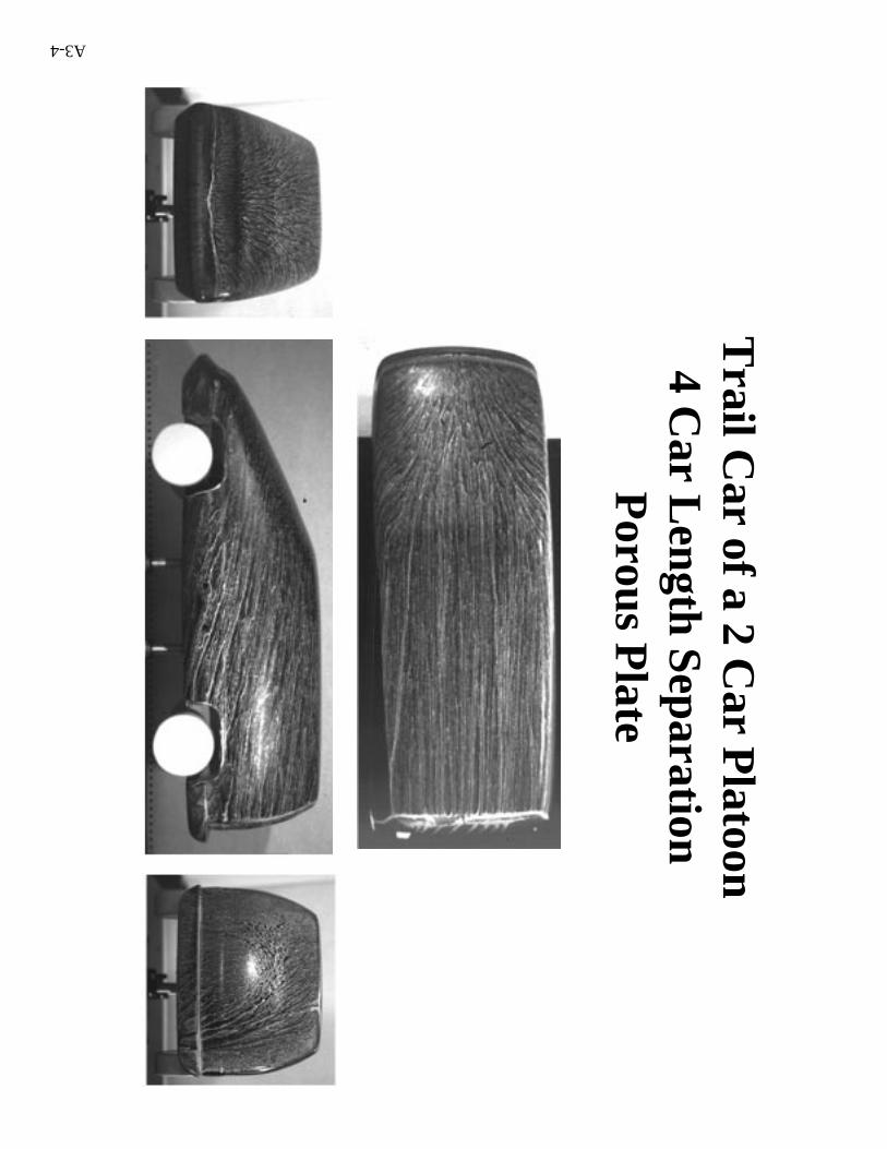
Trail C

ar of a 2 Car P

latoon4 C

ar Length Separation

Porous P

late

A3-4

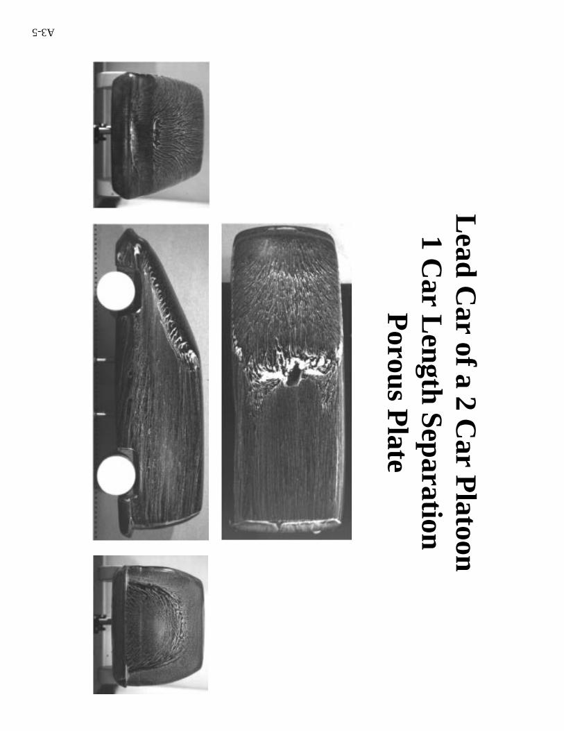
Lead Car of a 2 C

ar Platoon

1 Car Length S

eparationP

orous Plate

A3-5

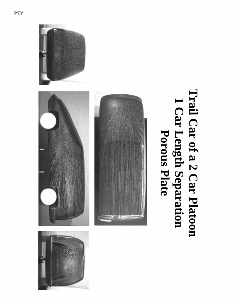
Trail C

ar of a 2 Car P

latoon1 C

ar Length Separation

Porous P

late

A3-6

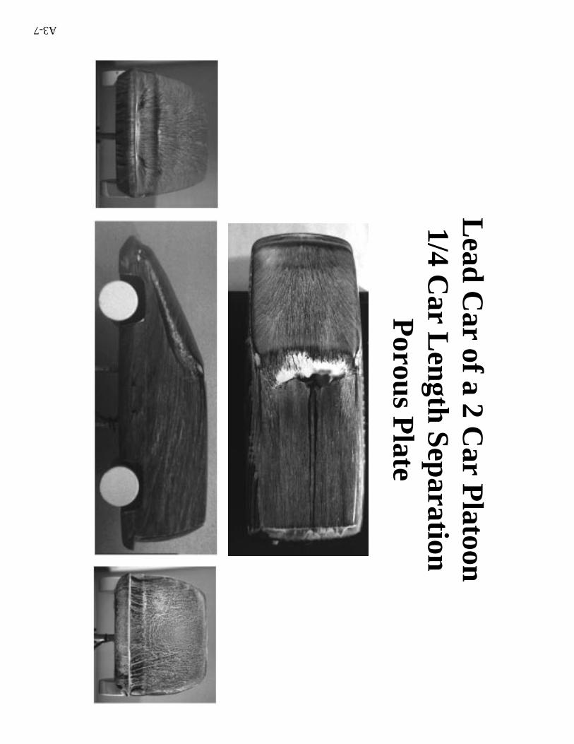
Lead Car of a 2 C

ar Platoon

1/4 Car Length S

eparationP

orous Plate

A3-7

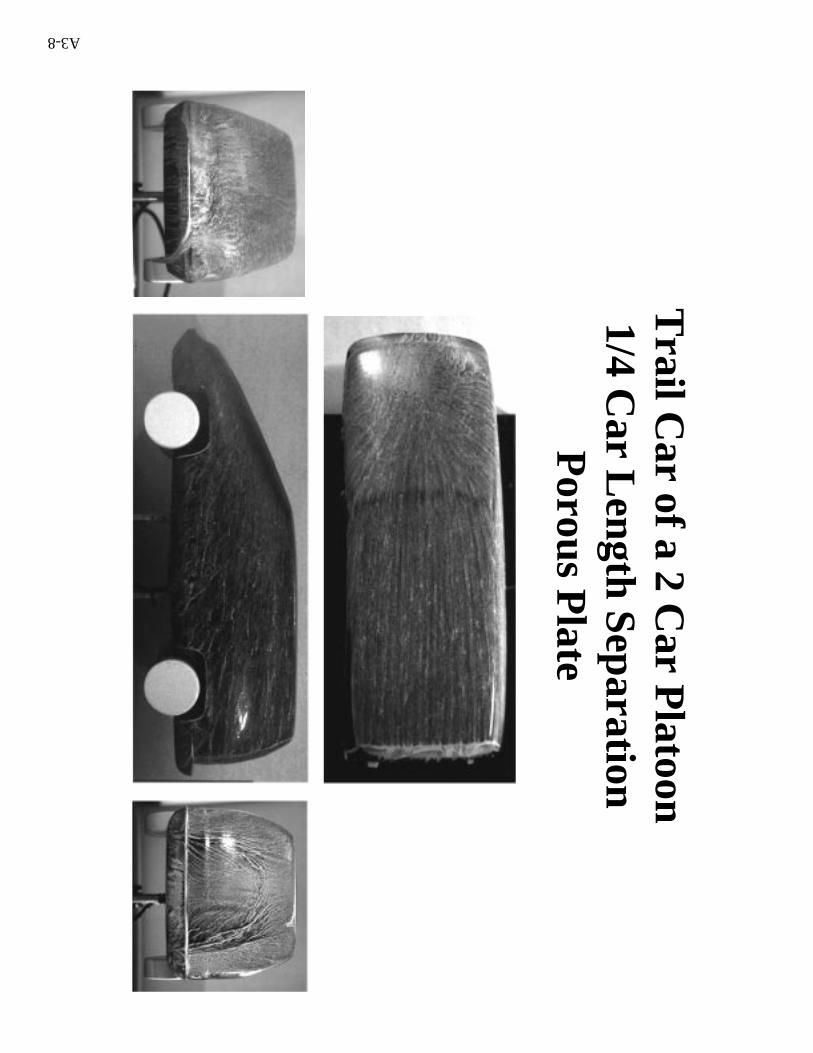
Trail C

ar of a 2 Car P

latoon1/4 C

ar Length Separation

Porous P

late

A3-8

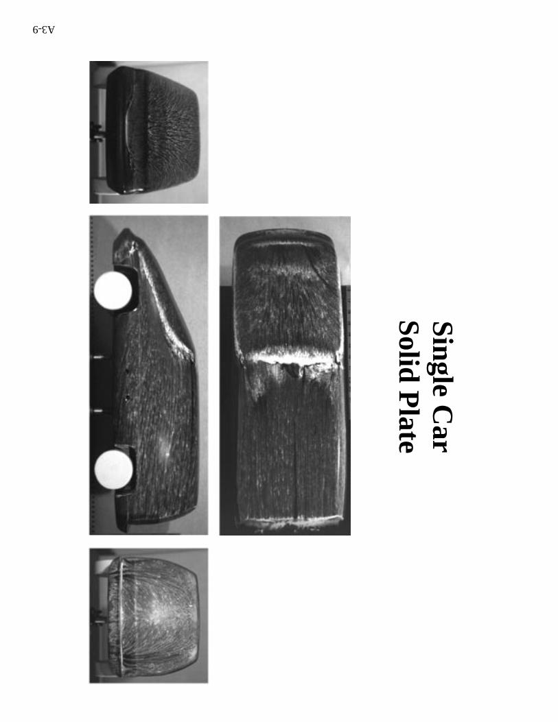
Single C

arS

olid Plate

A3-9

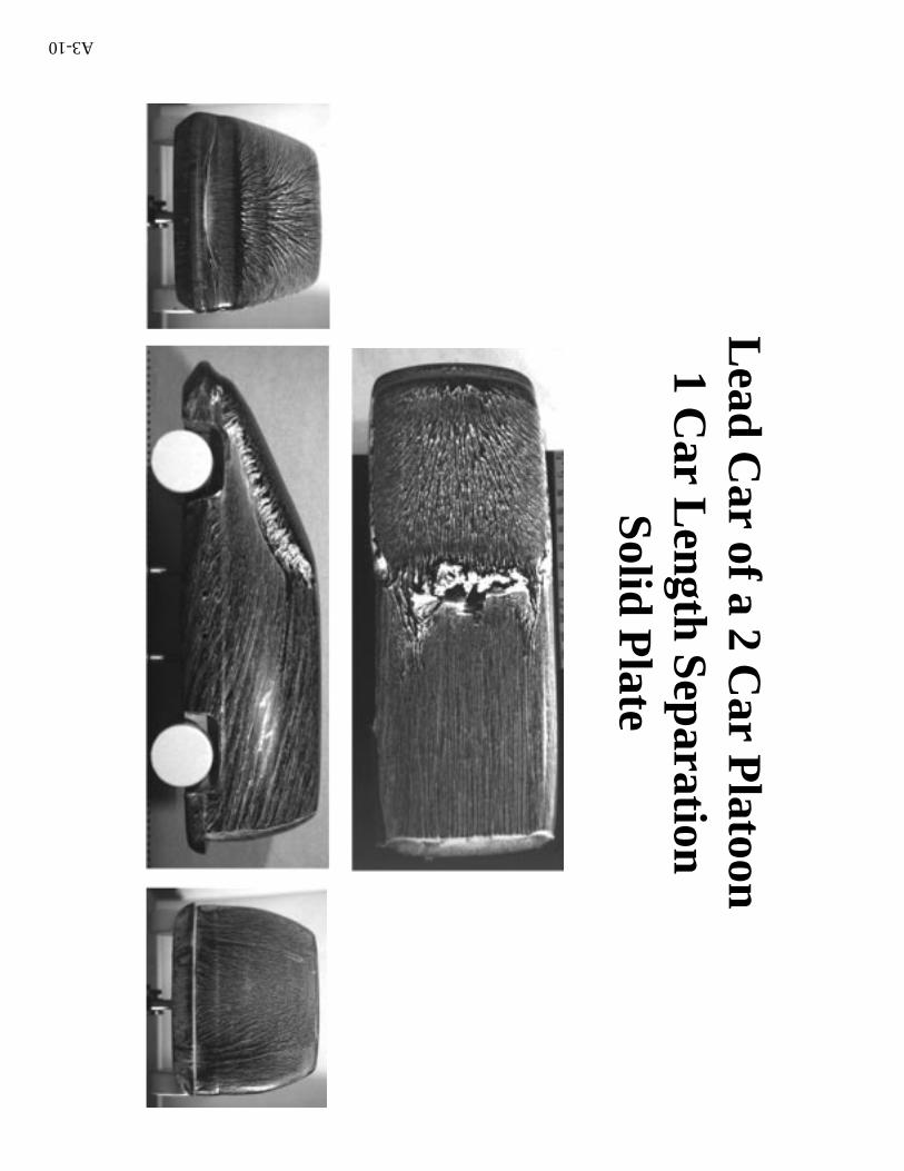
Lead Car of a 2 C

ar Platoon

1 Car Length S

eparationS

olid Plate

A3-10

Trail C

ar of a 2 Car P

latoon1 C

ar Length Separation

Solid P

late

A3-11

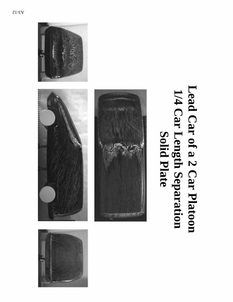
Lead Car of a 2 C

ar Platoon

1/4 Car Length S

eparationS

olid Plate

A3-12

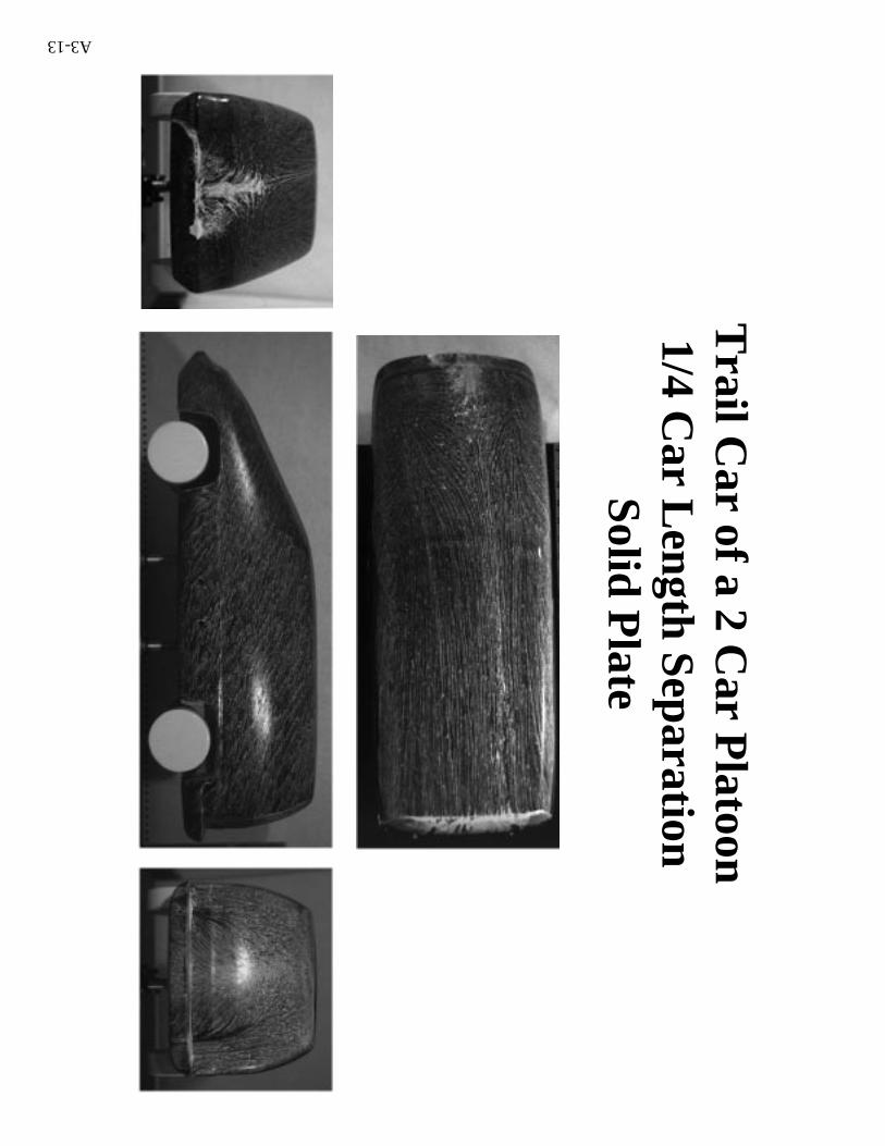
Trail C

ar of a 2 Car P

latoon1/4 C

ar Length Separation

Solid P

late

A3-13