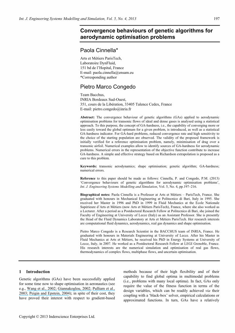
Int. J. Engineering Systems Modelling and Simulation, Vol. 5, No. 4, 2013 197

Copyright © 2013 Inderscience Enterprises Ltd.

Convergence behaviours of genetic algorithms for aerodynamic optimisation problems

Paola Cinnella* Arts et Métiers ParisTech, Laboratoire DynFluid, 151 bd de l’Hopital, France E-mail: paola.cinnella@ensam.eu *Corresponding author

Pietro Marco Congedo Team Bacchus, INRIA Bordeaux Sud-Ouest, 351, cours de la Libération, 33405 Talence Cedex, France E-mail: pietro.congedo@inria.fr

Abstract: The convergence behaviour of genetic algorithms (GAs) applied to aerodynamic optimisation problems for transonic flows of ideal and dense gases is analysed using a statistical approach. To this purpose, the concept of GA-hardness, i.e., the capability of converging more or less easily toward the global optimum for a given problem, is introduced, as well as a statistical GA-hardness indicator. For GA-hard problems, reduced convergence rate and high sensitivity to the choice of the starting population are observed. The validity of the proposed framework is initially verified for a reference optimisation problem, namely, minimisation of drag over a transonic airfoil. Numerical examples allow to identify sources of GA-hardness for aerodynamic problems. Numerical errors in the representation of the objective function contribute to increase GA-hardness. A simple and effective strategy based on Richardson extrapolation is proposed as a cure to this problem.

Keywords: transonic aerodynamics; shape optimisation; genetic algorithm; GA-hardness; numerical errors.

Reference to this paper should be made as follows: Cinnella, P. and Congedo, P.M. (2013) ‘Convergence behaviours of genetic algorithms for aerodynamic optimisation problems’, Int. J. Engineering Systems Modelling and Simulation, Vol. 5, No. 4, pp.197–216.

Biographical notes: Paola Cinnella is a Professor at Arts et Métiers – ParisTech, France. She graduated with honours in Mechanical Engineering at Politecnico di Bari, Italy in 1995. She received her Master in 1996 and PhD in 1999 in Fluid Mechanics at the Ecole Nationale Supérieure d’Arts et Métiers (now Arts et Métiers ParisTech), France, where she also worked as a Lecturer. After a period as a Postdoctoral Research Fellow at Politecnico di Bari, she joined the Faculty of Engineering at University of Lecce (Italy) as an Assistant Professor. She is presently the Head of the Fluid Dynamics Laboratory at Arts et Métiers ParisTech. Her research interests are computational fluid dynamics, aerodynamics, real gas dynamics and shape optimisation.

Pietro Marco Congedo is a Research Scientist in the BACCHUS team of INRIA, France. He graduated with honours in Materials Engineering at University of Lecce. After his Master in Fluid Mechanics at Arts et Métiers, he received his PhD in Energy Systems at University of Lecce, Italy, in 2007. He worked as a Postdoctoral Research Fellow at LEGI Grenoble, France. His research interests are the numerical simulation and optimisation of real gas flows, thermodynamics of complex flows, multiphase flows, and uncertain optimisation.

1 Introduction

Genetic algorithms (GAs) have been successfully applied for some time now to shape optimisation in aeronautics (see e.g., Wang et al., 2002; Giannakoglou, 2002; Pulliam et al., 2003; Peigin and Epstein, 2004); in spite of their cost, they have proved their interest with respect to gradient-based

methods because of their high flexibility and of their capability to find global optima in multimodal problems (i.e., problems with many local optima). In fact, GAs only require the value of the fitness function in terms of the design variables, which can be readily achieved via their coupling with a ‘black-box’ solver, empirical calculations or approximated functions. In turn, GAs have a relatively

198 P. Cinnella and P.M. Congedo

high computational cost, since they require a large number of evaluations of the fitness function; moreover, it is frequently observed that convergence tends to slow down as the algorithm approaches the optimum, and that the convergence rate is strongly problem-dependent. Demonstrations of the convergence of GAs to global optima for general problems are scarce and difficult. Some results about limit states and steady distributions of GAs and some conditions for GAs to converge to these limit states, in terms of control parameters such as the population size, encoding length and mutation probability, have been obtained by Rudolph (1994) and Leung et al. (1997) using Markov chain theory. Specifically, Markov chain analysis is used to predict the dynamics of a GA, i.e., how it evolves through generations. The approach leads to the definition of ‘transition matrices’, whose elements are transition probabilities between populations. Unfortunately, since GAs work with a population instead of a single individual and with several search operators, transition formulas are complicated and transition matrices are huge. Moreover, though interesting from a theoretical viewpoint, these results on the limit behaviour (or long-term behaviour) of GAs are of little use, since in practical problems GAs will invariably terminate within finite generations due to the limited computational resources. From a practical point of view, results concerning the short-term are more pertinent, since they provide information about how close to the global optimum the GA will get within a prescribed number of generations. For instance, Gao (1998) provides some estimates of the convergence rates of GAs, showing that the larger the mutation probability and the smaller the population size and encoding length, the higher the GA short-term convergence rate. Unfortunately, such a choice of the GA control parameters has almost the contrary effects on GA long-term performance. There are in fact results showing that when the population size is large and the mutation probability tends to zero the GA converges in probability to the global optimum (Peck and Dhawan, 1995). In practice, there is a trade-off between the short-term convergence rate and the long-term behaviour of the algorithm. An additional difficulty is related to the fact that the short-term convergence properties of GAs are always problem-dependent. It is then important to provide some measure of how a given GA will perform for a given problem.

The aim and the originality of this work is to transpose some concepts previously introduced in GA-theory to study the convergence properties of GAs applied to the engineering field of aerodynamic design. Precisely, we investigate a class of optimisation landscapes often encountered in transonic Aerodynamics and their impact on GA convergence. In GA-theory, the term landscape analysis is used to indicate attempts at predicting the convergence behaviour of the GA on a fitness function by looking at a number of detectable properties of this function. Contrarily to the above-mentioned studies, these attempts have no intention at describing the exact dynamics of the convergence process. Rather, and that is what we will

use the term convergence behaviour for, they aim at predicting what kind of problems the GA will encounter when it is run on a given fitness function. The notion of fitness landscape was introduced in theoretical genetics (Davidor, 1991) as a way to visualise evolution dynamics. The intuition behind it is that fitness can be thought of as a ‘height function’, orthogonal to the genome space and hence high fitness points are located in ‘peaks’ and low fitness points in ‘valleys’. Properties of the landscapes are expected to affect the performance of the search algorithm, so that in theory one could infer GA convergence behaviour from these properties. An optimisation problem for which a GA readily converges to the global optimum will be said to be GA-easy. On the contrary, a problem is informally defined to be GA-hard when a GA cannot detect a global optimum within a ‘reasonable’ number of generations. Of course, the notion of a ‘GA-hard problem’ depends on the characteristics of the particular GA being used (generational, elitist, etc.), the internal search space representation (binary, real, etc.), the operators used (form and rate of crossover, etc.), the non-linear dynamics of the search process, in addition to the characteristics of the function to be optimised.

The present paper attempts to characterise landscapes associated to a class of optimisation problem in transonic aerodynamics and to find a reliable measure for their GA-hardness. It is the first time, to the authors’ knowledge, that this kind of analysis is applied to GA-optimisation of aerodynamic problems. In fact, in spite of the ever increasing number of applications of GAs to aerodynamic design, little or no studies of their convergence properties has been made available in the literature. Specifically, quantitative information lacks about how the flow-physics of a given problem and the errors introduced by its numerical approximation affect the GA fitness landscape, and hence, GA convergence. Moreover, most theoretical studies about GA convergence behaviour concern binary-coded algorithms. Now, for aerodynamic optimisation applications, real encoding is best suited since it provides a representation of individuals conceptually closer to the real design space and reduces computational costs for optimisation problems characterised by many genes (see e.g., Michalewicz, 1996; Zhang et al., 2004), for which binary GAs lead to large string lengths. For instance, a problem with 100 design variables with a precision of six digits results in a binary string length of about 2,000. GA would perform poorly for such design problems. Another drawback comes from the discrepancy between the binary space representation and the actual problem space. Two optimisation points, even close to each other in the actual space, may be far from each other in the representation space.

A review of past attempts to define GA-hardness measures in GA theory shows that it is not feasible to give a general predictive measure of problem difficulty (Borenstein and Poli, 2005). From a theoretical perspective, such a measure should assess hardness irrespective of the search algorithm. However, different search operators

Convergence behaviours of genetic algorithms for aerodynamic optimisation problems 199

induce different landscapes (Borenstein and Poli, 2005) and, even when restricting the study to GAs, the variety of operators and parameters available makes it very difficult to encompass all of them with a single measure of difficulty. This is why in the present paper we mainly investigate GA-hardness for a specific search algorithm (i.e., specific operators, parameters and neighbourhood structure) and a specific family of optimisation problems, even if the proposed analysis can be applied to different contexts. The GA selected for present investigations is the non-dominated sorting genetic algorithm (NSGA) proposed by Srinivas and Deb (1995), widely used for several applications in engineering, because of its good convergence properties, robustness, and capability of treating multi-objective problems. We focus here on the real-coded formulation of the NSGA. Comparisons with a commercially available binary-coded GA are also carried out to investigate to what degree the results depend on algorithmic details. Precisely, we investigate the convergence behaviour of the real-coded GA applied to a class of flow problems in transonic aerodynamics, involving both perfect and real gases, with the objective of minimising wave drag. Elliott and Peraire (1997) stated that almost any drag minimisation exercise based on the Euler equations and applied to modern supercritical wings in cruise conditions is doomed to failure; however, they also concluded that Euler-based optimisation can be useful as a first step in the design process (Elliott and Peraire, 1998). Thus, since we are mainly interested here in developing and validating mathematical tools to analyse GA convergence behaviour, more than in finding accurate solutions to practical optimisation problems, we restrict our analysis to the inviscid flow model.

In Section 2, we first review the GA-hardness concept and some of its most commonly used measures, with focus on the so-called fitness distance correlation (FDC) measure, and discuss their validity. Then, in Section 3, we introduce a class of optimisation problems in transonic aerodynamics, describe the computational fluid dynamics solver used to compute the fitness function and provide some information about the optimisation algorithm. In Section 4, the FDC measure is applied to study the GA convergence behaviour for the class of aerodynamic problems of interest and the results predicted from this measure are compared with the observed behaviours for several optimisation runs at different conditions. Particular interest is developed into how physical parameters governing the problem (e.g., the working fluid properties and the operating conditions) and numerical parameters used in the flow solver (e.g., the discretisation scheme accuracy and the computational grid) affect GA convergence. Some conclusions are driven about the validity of the FDC measure as an indicator of the difficulty of the aerodynamic problems under investigation. Finally, in Section 5, we propose some possible cures to GA hardness and verify their effectiveness by means of FDC measures and numerical experiments.

Since the mathematical concepts and properties of GAs reviewed in the first part of the paper are of general interest for the whole community of GA users, they could

found application to many other optimisation problem in engineering (e.g., thermal problems or structure design).

2 GA-hardness: definitions and measures

The standard measures of performance for optimisation algorithms involve convergence properties (i.e., the ability to find an optimum) as well as convergence rates (how quickly the optimum is found). For parallel, population-based stochastic search procedures like GAs, there are a number of possible definitions of convergence. The simplest notion is that ultimately a GA population converges to a uniform population consisting of n copies of a single individual (which may or may not correspond to a global optimum). On the other hand, many other questions related to GA performance arise. For instance, we wish to know how likely is it that a given generation contains a copy of the optimum, what is the expected waiting time until a global optimum is encountered for the first time, what is the waiting time until the solution gets within some error tolerance of the optimum, and how much variance is there in such measures from run to run.

Situations which exhibit shorter mean waiting times and smaller variances will be referred-to as GA-easy situations, whereas those with longer mean waiting times and higher variances are viewed as harder. Consequently, these statistics (mean waiting time and variance) appear to be natural quantitative measures of the difficulty of a particular GA situation.

Naudts and Kallel (2000) propose a rough classification of types of convergence behaviour (in the fitness-landscape context), based on a hierarchy of what they call the convergence quality of the GA subject to some fitness function:

1 The GA detects the optimum of the fitness function independently on the choice of the (randomly sampled) initial population. The variance on the number of iterations needed to detect the optimum given an initial population is comparatively small. This behaviour is called stable convergence.

2 Each run of the GA still detects the optimum of the fitness function, but now the variance on the number of iterations needed for detection is comparatively large. The GA exhibits unstable convergence.

3 The GA sometimes detects the optimum of the fitness function after a reasonable number of iterations, but it takes a number of runs because the problem is sensitive to the choice of initial population and the choices made by the algorithm. This behaviour can be seen as follows: there are a number of easy paths to the global optimum, but if the GA is not in one of them then it gets trapped in a local optimum from which it cannot escape.

4 The GA performs no better than random search. It cannot detect the optimum of the fitness function in a

200 P. Cinnella and P.M. Congedo

reasonable length of time, no matter how often it is run and how its parameters are tuned.

Figure 1 Examples of GA-easy and GA-hard fitness landscapes, (a) maximally multimodal problem (b) ‘needle in a haystack’ problem (see online version for colours)

(a)

(b)

Functions for which the GA shows class 1 behaviour are those functions for which the GA is a good optimisation algorithm (but not necessarily the best algorithm). An example of this kind of functions is given by the maximally multimodal problem (Horn and Goldberg, 1995), for which half of the points in the search space are local optima, yet the problem is easy for a GA to solve [see Figure 1(a)], contrarily to what would happen for a gradient-based algorithm. At the opposite, the function for which the GA shows class 4 convergence are the hardest to be optimised. An extreme example is the classical ‘needle-in-a-haystack problem’ [Figure 2(b)], which is simply unsolvable through a GA.

One of the major causes of GA-hardness is strong coupling in the objective function among different components of the chosen encoding of the search space. For example, the success of GAs using binary encoding lies on the verification of the hypothesis (H) ‘a bit string with high fitness must contain high-fitness lower structures that can be combined with other good ones to form better solutions’. These high-fitness structures are usually called ‘building blocks’ and were extensively studied for instance by Holland (1975). Holland showed that, in a classical GA,

good building blocks receive an exponential descent. This result, called ‘the fundamental theorem’, proves the efficiency of a GA when hypothesis (H) is verified.

In practice, however, it is not easy to cast hypothesis (H) into mathematical terms. Instead, some different ‘measures’ have been proposed to determine how far (H) is verified. Given the connection between GAs and theoretical genetics, some attempts to explain the behaviour of GAs were inspired by biology. Indeed, gene interaction is a central issue in natural genetics, where genes not only are dependent on each other in order to jointly express phenotypical characteristics, but also suppress and activate the expression of other genes. In analogy to gene interaction dynamics, Davidor (1991) introduced the notion of epistasis, a term used to denote that the expression of a chromosome is not merely a linear function of the effects of its individual alleles, i.e., a measure of the degree of the interdependence among genes with respect to their contribution to the phenotype (fitness). The higher epistasis is, the more genes will depend on other genes for expression. From an algorithmic viewpoint, as epistasis increases the advantage of crossover over mutation becomes smaller, and in the end a GA will perform no better than random search.

It is beyond the scope of this paper to go into details of function optimisation and GA theory and notations. However, to define hardness from a bit more quantitative point of view, let us consider the following simplified framework (inspired by Naudts and Kallel, 2000): let Σ be an alphabet, and Ω = ΣN be the universe, i.e., the space of all possible N-ples of elements chosen in Σ. In particular, if Σ is the binary alphabet (Σ = 0, 1), Ω is the set of the binary strings

( )1 2... , 0, 1N is s s s i= = ∀s

of length equal to N (which is the case of binary-coded GAs); otherwise, if Σ is the set of floating-point numbers Float ,∈ℜ then Ω = FloatN is the set of composed by the real n-ples 1 2( , , ..., ), Float .N is s s s i= ∈ ∀s The first choice of the alphabet represents binary-coded GAs, the second one real-coded GA. For binary GAs, the integer N is the encoding length and the components si, considered with their order, are called the sites of s. For real-coded ones, N is the number of design variables.

We now consider any function f defined over a subset S ⊆ Ω. The subset S will be called the search space, while f is said the fitness function. The evaluation of f in s ∈ S, denoted f(s) is the fitness value of s. The properties of f referred to a given structure of the search space S will define a particular fitness landscape.

Let us introduce a suitable distance measure between elements of S:

( ): , ,d S d′ ′∈ →s s s s

For instance, d may be the Hamming distance if S is composed of binary strings (i.e., the number of positions in the strings s and s’ for which the corresponding symbols are

Convergence behaviours of genetic algorithms for aerodynamic optimisation problems 201

different) or a floating-point approximation of the Euclidean distance if S ⊂ FloatN.

Definition 2.1: A fitness function f is first-order if it can be written as a linear combination of independent functions of the components of s:

( ): ( ) i ii

f f c g s→ = +∑s s (1)

with c a constant. The set of all 1st-order functions is noted 1ORD.

For a first-order function, there is no interaction between the effects of different design variables si, i.e., the optimum can be found by optimising each function gi separately.

Definition 2.2: A function f is linear if it is of the form:

( )1 2: ( ) , *f f C C d→ = −s s s s (2)

where C1 and C2 are constants and s* is the optimum in S with respect to f.

For this kind of function, the fitness varies linearly with the distance from the global optimum, so that all elements lying at the same distance from the optimum exhibit the same fitness level. In statistical terms, there is a full correlation between the fitness of an individual and its distance to the global optimum.

Definition 2.3: A function f is monotone if:

( ) ( ) ( ) ( )( ) ( )( )

(1) (2) (1) (2)

(1) (1)

, * , *

resp.,

d d f f

f f

< ⇒ <

>

s s s s s s

s s (3)

i.e., if the fitness strictly increases (resp., decreases), with the distance to the global optimum.

Of course if f is linear, it is necessarily monotone. It has been shown (Naudts and Kallel, 2000) that a GA displays class 1 convergence when applied to monotone fitness functions, i.e., problems with monotone fitness functions are GA-easy.

Definition 2.4: A fitness function f is unimodal if it has no local optima, apart from the global optimum.

According to the previous discussion, epistasis is the degree of interaction between the genes (sites or design variables, resp. for binary and real GAs) in the expression of a fitness function f. Now, any fitness function may be expressed according to the order of interaction of its alleles (Reeves and Wright, 1995):

( )

( )

( )

, ... random error

i ii

ij i ji j

f c g s

g s s

= +

+ + +

∑∑∑

s

(4)

where higher-order terms introduce more and more correlation between genes. Equation (4) is referred-to as the full epistatic model. Epistasis expresses the extent to which a fitness function can be decomposed into

lower-dimensional functions. In fitness landscapes with high epistasis, there is high interaction between the sites; epistatically free functions are a combination of one-dimensional sub-functions.

Epistasis variance (Davidor, 1991) and epistasis correlation (Rochet, 1997) are measures for the GA-hardness of a function, which have been used to predict the performances of GA using binary encoding. The underlying assumption is that a low-epistatic function is easier for a GA to optimise than a high-epistatic one. Precisely, Davidor (1991) measures the epistasis ε of a binary string s with respect to a fitness function :f S →ℜ and a sample P ⊂ S as:

( ) ( ) ( )P Pε f ξ= −s s s (5)

with ξP a first-order approximation to f over P (see Davidor, 1991, for details), i.e., the first-order function closest to f in Euclidean distance (Van Hove and Verschoren, 1994; Rochet et al., 1996). The definition of ξ depends on the particular encoding chosen for the elements of S, so that a given fitness function may be more or less epistatic according to the chosen encoding structure, encoding length, etc.

Definition 2.5: Epistasis variance is defined as:

2

2

( )epiv ( )

( )

PPP

P

εf

f∈

∈

=∑∑

s

s

s

s (6)

It is equal to 0 for a fully non-epistatic function, and tends to the unity for highly epistatic ones.

On the other hand, Rochet et al. (1996) introduce the alternative measure of Def. 2.6.

Definition 2.6: Epistasis correlation is defined as:

( )( )( ) ( )2 2

epic ( )

( ) ( )

( ) ( )

P

P P PP

P P PP P

f

f f ξ ξ

f f ξ ξ

∈

∈ ∈

=

− −

− −

∑∑ ∑

s

s s

s s

s s

(7)

1 1( ) and ( )| | | |P P P

P P

f f ξ ξP P∈ ∈

= =∑ ∑s s

s s

being the mean values of f and ξP over P, respectively.

Epistasis correlation measures the correlation between f and its first order approximation in P. It is equal to 1 for non-epistatic functions and tends to 0 for highly epistatic ones. For first-order functions, the exact value of epistasis correlation over the whole search space (instead of a sample), epic(f) = 1.

In general, both epistasis variance and epistasis correlation measure how close a fitness function is to the class of first order functions, which are fully decomposable into one-dimensional functions and, by their very definition, are epistasis-free. As a quantification of epistasis, these measures assume that only the first order functions have no

202 P. Cinnella and P.M. Congedo

epistasis, while there are many others: if we replace the summation sign in equation (1) by a product sign we still have epistatically free functions according to the intuitive definition of epistasis. Actually, it has been pointed-out (Van Hove and Verschoren, 1994) that, seen over all possible fitness functions, the only characteristic which epistasis variance and epistasis correlation can reliably detect is the absence of epistasis. Moreover, both measures cannot distinguish between first-order functions and constant functions, which are fully non-epistatic according to these measures. However, GAs deal very differently with the two types of functions: the former are easily optimised, while constant areas in the fitness landscape decrease the search efficiency of the GA. Finally, note that the above measures have been primarily defined for binary-coded GAs. An extension of the epistasis concept to real encoding has been proposed by Rochet et al. (1998), but it has not found application in practice.

An alternative measure of GA-hardness well suited for GA using real encoding is the FDC, introduced by Jones and Forrest (1995). FDC is a statistical correlation between the fitness of strings encoding a given individual and the distance of these strings to the nearest global optimum; the underlying hypothesis is that good correlation between fitness of individuals and their distance to global optimum means that the fitness function is almost linear, and as such is easily optimisable using a GA. FDC tries to measure the intrinsic hardness of a landscape, independently of the search algorithm. From this point of view, FDC is more a general hardness measure than a specific GA-hardness measure. Another advantage of FDC is that it uses standard statistical tools, and as such it can be easily applied both to binary- and real-coded GAs. Because of its generality, FDC avoids difficulties related to the coupling, in the fitness landscape, between the definition of the search space, the fitness function defined over it, and the algorithm used to optimise it. Let us consider a fitness function f:

: ( )f S f∈ → ∈ℜs s

characterised, without loss of generality, by a unique global optimum s*.

Definition 2.7: The FDC of f with respect to the fitness information in a discrete sample of the search space P ⊂ S is:

( )( )

( ) ( )1 12 22 2

( ) ( , *)fdc ( )

( ) ( , *)

P PP

P

P PP P

f f d df

f f d d

∈

∈ ∈

⎡ ⎤− −⎣ ⎦=⎛ ⎞ ⎛ ⎞

− −⎜ ⎟ ⎜ ⎟⎜ ⎟ ⎜ ⎟⎝ ⎠ ⎝ ⎠

∑

∑ ∑

s

s s

s s s

s s s

(8)

with 1 ( )| |P

P

f fP ∈

= ∑s

s and 1 ( , *)| |P

s P

d dP ∈

= ∑ s s the mean

fitness and the mean distance of the sample individuals from the global optimum, respectively.

In Jones and Forrest (1995), d is the Hamming distance. In the present work, however, the following distance definition

(a normalised Euclidean distance) is applied, best suited for a real-coded GA:

( )2*

21

( , *)N

i i

ii

s sd

=

−=

Δ∑s s (9)

with si the ith input variable of the N-ple and Δi its range of variation (difference between the maximum and minimum value that si can take in S). The distance (9) measures how different two individuals are compared to the range of variation of each variable.

If a maximisation (respectively, minimisation) problem is considered, the FDC returns a value of –1 (resp., +1) for a linear fitness function of the form

( )( )( )

1 2

1 2

, *

resp., , * ,

f C C d

f C C d

= −

= +

s s

s s (10)

With 1 2 2, , 0.C C C∈ℜ > FDC measures the deviation of a fitness function from the class of linear fitness functions. Note however that, working with real encoding, an individual s is a point of ,Nℜ and the reference class of functions is represented by strictly concave (resp., strictly convex) functions of the form of (10), which are easily optimisable by a GA: if the FDC of a given fitness function is close to –1 (resp., +1), this one can be easily optimised by a GA, whereas if FDC ≈ 0 [no correlation with function (8)], the function is expected to be GA-hard.

Besides its generality and easy extension to real encoding, FDC is also able to detect constant functions: for these functions, FDC is equal to 0, which is coherent with their intractability. For these reasons, in the present work we adopt FDC as a GA-hardness measure for a class of optimisation problems in aerodynamics.

A first and obvious drawback of FDC is that one of the global optima has to be known. This can be overcome by approximating the global optimum by the best-fit individuals found so far (Naudts and Kallel, 2000) up to the current generation. At the beginning of the computation, in the present work we initialise s* with the best-fit individual selected through a preliminary design of experiments (DOEs). Another inconvenient is, as for most GA-hardness measures, that FDC computation is restricted to a random sample. GAs, however, process samples (populations) that might be random to begin with, but quickly become decidedly non-random. In the present work, successive GA populations are used to compute FDC, which allows a progressive refinement of the GA-hardness measure as the GA evolves.

As a final comment, we recall that in Naudts and Kallel (2000) a thorough investigation of the properties and predictive qualities of different GA-hardness measures is carried out and a GA-hardness measure, called the site-wise optimisation measure, is introduced in order to overcome some of the shortcomings of the epistasis variance and FDC measures. However, it is found that for some classes of functions all of the above-mentioned GA-Hardness measures can provide misleading results and the use of

Convergence behaviours of genetic algorithms for aerodynamic optimisation problems 203

experimental design techniques is recommended in order to achieve a better knowledge of the fitness landscape. In general, it is now largely accepted that no generally valid GA-hardness measure may be defined (Borenstein and Poli, 2005). For each measure, it is always possible to find a class of fitness functions, or special encoding, or particular algorithm for which the measure provides misleading results about the problem hardness. However, it is possible to introduce measures that work well for a given class of problems, solved by using a given encoding and a given GA.

Because of its simplicity and generality, in the present work the FDC measure is adopted to evaluate the GA-hardness of a class of optimisation problems in aerodynamics solved using a real-coded GA described in the next section. To check the generality of the FDC measure, comparisons with a commercially available, binary coded GA, implemented within the ModeFrontier Software package (http://www.esteco.com) are also presented, the use of a different encoding affecting, in principle, the fitness landscape representation.

3 Problem definition

We consider a classical optimisation problem in transonic aerodynamics, i.e., the minimisation of the drag coefficient for a given lift level. The objective is to generate an aerodynamic shape that, at design conditions, provides the required lift with the highest possible aerodynamic efficiency. Since we are interested into studying the effects of the flow physics and of the numerical errors associated to fitness evaluations more than into solving an optimisation problem of practical interest, we restrict most of our analyses to the following simplified problem: minimise the drag coefficient for a symmetric airfoil at zero angle of attack; for this airfoil the lift level is automatically set to zero, since the forces on both airfoil surfaces cancel. Because of the of the problem symmetry, flow analyses can be restricted to a half domain, which reduces computational costs.

Let s ∈ S be an airfoil shape and S the search space. The structure of s and S depends:

1 on the particular parameterisation used to represent s (which also determines the encoding length)

2 on the encoding rules (e.g., binary or real) used by the optimisation algorithm.

In the present work, two parameterisations, both largely used in aerodynamic optimisation, are considered. The first one uses a reconstruction of the airfoil surface by means of Bézier curves and spans a large variety of shapes, whereas the second one uses Hicks-Hennes perturbation of a baseline profile (Hicks and Hennes, 1978), which restricts the search space to a neighbourhood of the baseline individual. In both cases, the airfoil is constrained to satisfy the following conditions:

1 the coordinates of the leading edge and trailing edge normalised by the airfoil chord are respectively (0, 0) and (1, 0)

2 the relative thickness is fixed and equal to 12%.

In the first parameterisation the airfoil (upper) surface is approximated by means of a Bézier curve, using 8 Bézier control points: the fixed leading edge P0 and trailing edge P7, 5 control points Pk=2,6(xk, yk), regularly spaced along the chord, with the xk coordinates varying in distinct sub-intervals of ]0, 1[ and a control point P1(0, y1), which ensures the upper surface of the profile is tangent to the y-axis at the leading edge. A fixed 12% thickness-to-chord ratio is ensured through ad-hoc normalisation of the airfoil coordinates. The preceding parameterisation of the airfoil geometry generates a family of airfoil shapes depending on 11 design parameters, which are varied continuously between prescribed limiting values. This family of airfoils includes the classical NACA0012 airfoil. An individual s is then defined by the following real n-ple:

( ) ( )1 11 1 2 2 6 6, ..., , , , ..., , , ,k k

s s y x y x yx y k

= =

∈ℜ ∀

s

The Bézier coefficients corresponding to the baseline individual sNACA approximating the NACA0012 airfoil are computed by means of a regression algorithm. This individual is used to set the intervals of variation for the design variables si, which lie in the range [0.7( ) , 1.3( ) ], .i NACA i NACAs s i∀ The airfoils generated by this parameterisation are then normalised to obtain a relative thickness of 12%.

When the Hicks-Hennes parameterisation is adopted, a baseline profile (in our case, the NACA0012 airfoil) is perturbed by means of functions of the form:

( )3ln 5( ) sin with

lnim

i ii

η x πx mt

⎛ ⎞= = ⎜ ⎟⎝ ⎠

where x is the chord wise coordinate (normalised with the chord length) and ti is the chord wise location of the maximum thickness of the shape function fi. Here, we choose uniformly distributed shape functions, i.e.,

.1i

itn

=+

The geometry of a perturbed profile is finally

defined by:

00121

( ) ( ) ( )n

NACA i ii

y x y x a η x=

= +∑

In this work, we choose n = 10, to ensure a good diversity of the perturbed shapes. The design parameters are the coefficients ai, which can vary in the interval [–0.002; +0.002].

The drag reduction of an airfoil at given lift can be expressed as the constrained minimisation problem:

204 P. Cinnella and P.M. Congedo

,0find: min ( ), with ( )

d l lS

c c c

S∈

=

∀ ∈s

s s

s (11)

where cd and cl denote the airfoil drag and lift coefficients, respectively. In the present simplified framework, the search space S is restricted to symmetric airfoils with zero angle of attack. Consequently, cl(s) ≡ cl,0 = 0 ∀s ∈ S by construction. The fitness value (drag coefficient) associated to any single individual s is computed by solving numerically the flow field around the airfoil. The optimisation algorithm is then coupled to a numerical flow solver. Details of the governing equations, the flow solver and the optimiser are provided in the following sections.

3.1 Governing equations

In the present study, we consider two-dimensional transonic flows of gases governed by an arbitrary equation of state. As frequently done in aerodynamic optimisation procedures, we restrict our attention to inviscid flows, in order to reduce computational costs. The governing equations, written in integral form for a control volume Ω with boundary ∂Ω are:

0d w d dSdt Ω ∂Ω

Ω+ ⋅ =∫ ∫ F n (12)

In equation (12), w is the conservative variable vector,

( ), , ,Tw ρ ρ ρE= v

n is the outer normal to ∂Ω, and f is the flux density:

( ), ,T

ρ pI ρ ρ H= +F v vv v

where ρ is the fluid density, v is the velocity vector, E the specific total energy, H = E + p / ρ the specific total enthalpy, and I the unit tensor. The preceding equations are completed by a thermal and a caloric equation of state:

( )( ), ( ) ,p p ρ w T w= (13)

( )( ), ( ) ,e e ρ w T w= (14)

where e is the specific internal energy, and T the absolute temperature.

In the present work, both dilute and dense gases (DGs) are considered. For dilute gases, the standard model for perfect polytropic gases is adopted. The thermodynamic response of DGs is modelled through the van der Waals equation of state for polytropic gases.

The interest in DGs is due to their applications as working fluids in energy-conversion cycles and many industrial processes (see e.g., Brown and Argrow, 2000; Zamfirescu and Dincer, 2009; Kirillov, 2004). DGs are single-phase vapours whose thermodynamic behaviour deviates significantly from that of a perfect gas. The most striking differences are encountered for the so-called Bethe-Zel’dovich-Thompson (BZT) fluids, for which compression shocks are predicted to violate the entropy

inequality over a certain range of temperatures and pressures and are therefore inadmissible (Thompson, 1971; Cramer and Kluwick, 1984; Cramer, 1989). This phenomenon is referred-to as reversed or non-classical non-linearity. More generally, for transonic and supersonic flows of many DGs and for a suitable choice of the thermodynamic conditions, entropy changes across shock waves may be up to one order of magnitude lower compared with shocks of the same intensity (e.g., pressure jump) in perfect gases; consequently, losses related to wave drag are strongly reduced (Cramer and Kluwick, 1984). The key thermodynamic parameter governing DG flows is the so-called fundamental derivative of gas dynamics:

: 1σ

ρ aa ρ⎛ ⎞∂

Γ = + ⎜ ⎟∂⎝ ⎠

with a the speed of sound and σ the entropy. Γ measures the rate of change of a in isentropic perturbations. Γ is greater than 1 for perfect gases and for most light gases. For molecularly complex fluids, Γ may be lower than 1 for some ranges of thermodynamic conditions in the vapour phase, or even less than 0 (this is the case for BZT fluids). In the thermodynamic region where Γ < 1 the speed of sound decreases in isentropic compressions, which may lead to a non-classical variation of the Mach number with pressure. Details about the complex dynamics of DGs can be found in Cramer (1991) and references cited therein. The van der Waals model is the simplest one which allows taking into account BZT effects. It is possible to show that, taking the specific heat ratio γ in the range 1 < γ ≤ 1.06, a region of reversed non-linearity appears. In the subsequent computations of DG problems, we consider a polytropic van der Waals gas with γ = 1.02.

In previous works (Congedo et al., 2007; Cinnella and Congedo, 2008), the present authors have applied GAs to shape optimisation of transonic flows of DGs past an airfoil. For dense-gas-flow optimisation problems, high sensitivity of GA convergence behaviour to flow conditions (e.g., flow Mach number or thermodynamic operation point) as well as to numerical approximations used to evaluate the fitness function have been observed (Cinnella and Congedo, 2006, 2008). Similar difficulties can also arise for weakly transonic flows of dilute (perfect) gases (Cinnella and Congedo, 2006). For all of these flows, a behaviour similar to what has been defined as ‘class 2’ or even ‘class 3’ convergence (see Section 2) is observed. Note that for steady inviscid flows past an airfoil at subcritical conditions (i.e., conditions such that the Mach number is below 1 throughout the flow) cd ≡ 0 for any airfoil shape and the problem is thus unoptimisable.

3.2 Flow solver

A major drawback of GA optimisation strategies is that they require a large number of evaluations of the fitness function. The computations are expensive for aerodynamic optimisation problems, for which GAs are typically coupled with a numerical flow solver. Because of the high

Convergence behaviours of genetic algorithms for aerodynamic optimisation problems 205

computational cost, fitness function evaluations are often performed by using relatively coarse meshes and simple, low-order accurate, numerical schemes. This reduces the CPU time necessary for a single fitness evaluation but introduces more or less significant numerical errors on the computed fitness value and thus influences the shape of the response surface.

In the present work, the governing equations are approximated by means of a finite volume method on structured grids. Two spatial approximations are considered:

1 the popular second-order-accurate centred Jameson’s scheme (Jameson et al., 1981)

2 a third-order accurate extension of Jameson’s scheme (Cinnella and Congedo, 2005b) generalised to multi-dimensional flows in complex geometries by means of weighted discretisation formulas, which ensures a truly third-order accuracy on moderately deformed non-Cartesian meshes and at least second-order accuracy on highly distorted meshes.

The equations are then integrated in time using a four-stage Runge-Kutta scheme (Jameson et al., 1981). Local time stepping, implicit residual smoothing and multigrid are used to efficiently drive the solution to the steady state. Non-reflecting boundary conditions based on a multidimensional method of characteristic are applied at the far-field boundaries and a slip condition based on a multidimensional linear extrapolation of the wall pressure is imposed at solid boundaries. The accuracy properties of the numerical solver just described have been demonstrated elsewhere (see Cinnella and Congedo, 2005a, 2005b, and references cited therein), and will not be discussed further.

In Section 4, the effects of the accuracy order of the numerical approximation as well as of grid density on GA convergence behaviour are investigated in detail.

3.3 Genetic algorithm

The flow solver described in the previous section has been coupled with the non-dominated sorting algorithm (NDSA) proposed by Srinivas and Deb (1995). Precisely, we adopt here a real-coded version of the NDSA. The main parameters of the algorithm are the population size, the number of generations, the crossover and mutation probabilities πc, πm and the so-called sharing parameter s used to take into account the relative isolation of an individual along a dominance front. Typical values for πc, πm are respectively 0.9 and 0.1; values of s are retained following a formula given in Pulliam et al., 2003, which takes into account the population size and the number of objectives. Theoretically, the population size and the number of generations used by the algorithm should be chosen according to the number of parameters and objectives of the optimisation problem under study; in practice however, the population size and number of generations are fixed by the global amount of CPU time devoted to the computation : taking too small a population may rapidly lead to a local optimum and make useless the

iteration process on the generation number; reversely, a large population will impose a limited number of generations which could not allow the population to evolve sufficiently towards the optimum. A typical choice made in the present work is to retain 36 individuals in the population and to let this population evolve for 24 generations.

4 GA-hardness of optimisation problems: application to transonic aerodynamics

The convergence behaviour of the NSDA coupled with the previously described flow solver is now investigated for a class of optimisation problems in transonic aerodynamics. Optimisation runs are performed for a perfect diatomic gas (specific heat ratio γ = 1.4) and for a BZT van der Waals gas at two different free-stream conditions. If not specified otherwise, the airfoil is parameterised by means of Bézier curves. Sensitivity of GA convergence to different choices of the starting population, parameterisation, flow conditions, computational grid, and discretisation scheme is carefully analysed by means of the FDC concept.

4.1 Drag minimisation for transonic flows over an airfoil – perfect gas flow case

To check preliminarily the sensitivity of the FDC measure to errors introduced in the fitness estimate by the numerical flow solver, a subcritical inviscid steady perfect gas (PFG) flow at M∞ = 0.6 and α = 0° with M∞ the free-stream Mach number and α the angle of attack is considered first. For this flow, the drag is theoretically predicted to be zero, so that the corresponding fitness function is constant and equal to zero for all individuals in the search space S. In other terms, the problem is unoptimisable unless viscous effects are taken into account. Even if viscous effects would be taken into account, differences in friction drag would be small since, for airfoils close to the global optimum, only friction drag would play a role (no flow separation), and this would be nearly the same for all designs and roughly close to that of the flow over a flat plate with the same angle of attack (see for instance, Anderson, 2000), provided the considered airfoils are thin and the angle of attack is small enough. In other terms, the optimisation problem is expected to be GA-hard, the exact FDC value associated to it being equal to 0 in the inviscid flow case. In practice, however, even when an inviscid flow model is adopted, the computed drag coefficient is not zero, but takes some small positive value because of numerical errors introduced by the approximation scheme and boundary conditions. Such a value, which varies from one individual to another, implies that the numerical approximation of the fitness function is not constant. Moreover, since the numerical drag will tend to be larger for lower-order numerical schemes and coarser grids, the shape of approximated fitness response will vary according to the discretisation adopted to compute it. This will also reflect on the computed FDC value. For the exact fitness function FDC exactly equals zero; for numerical ones, FDC will be more or less close to zero according to

206 P. Cinnella and P.M. Congedo

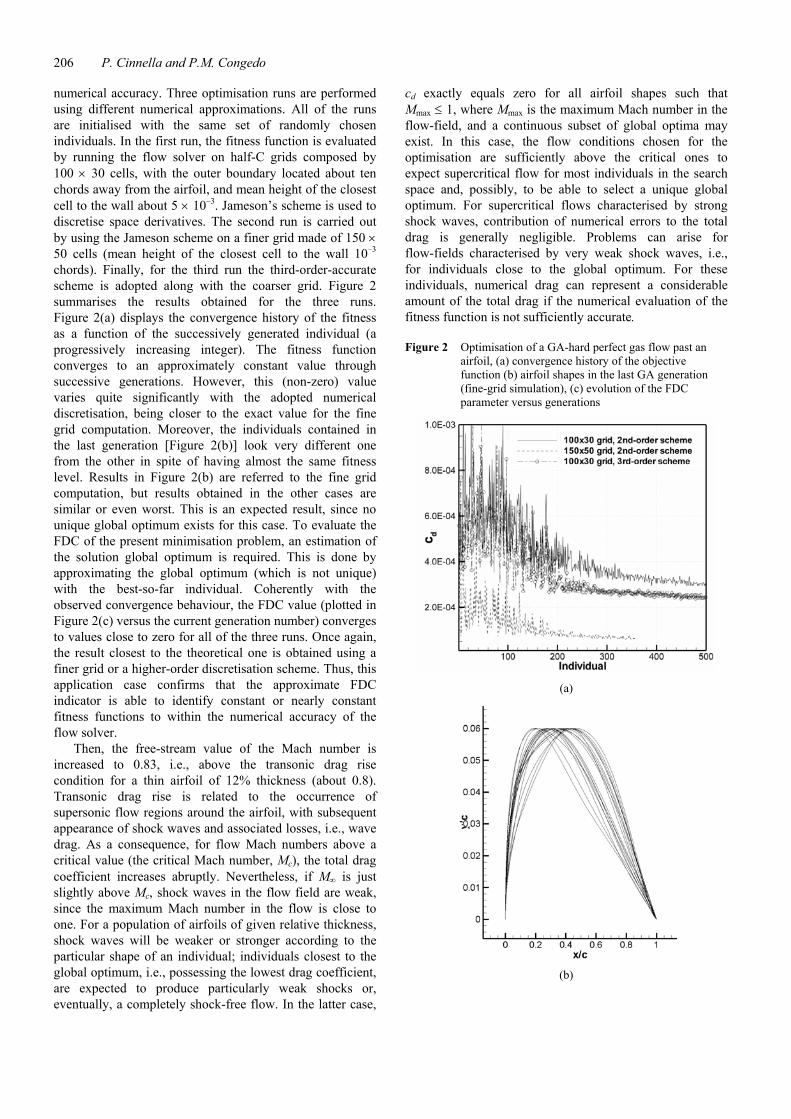
numerical accuracy. Three optimisation runs are performed using different numerical approximations. All of the runs are initialised with the same set of randomly chosen individuals. In the first run, the fitness function is evaluated by running the flow solver on half-C grids composed by 100 × 30 cells, with the outer boundary located about ten chords away from the airfoil, and mean height of the closest cell to the wall about 5 × 10–3. Jameson’s scheme is used to discretise space derivatives. The second run is carried out by using the Jameson scheme on a finer grid made of 150 × 50 cells (mean height of the closest cell to the wall 10–3 chords). Finally, for the third run the third-order-accurate scheme is adopted along with the coarser grid. Figure 2 summarises the results obtained for the three runs. Figure 2(a) displays the convergence history of the fitness as a function of the successively generated individual (a progressively increasing integer). The fitness function converges to an approximately constant value through successive generations. However, this (non-zero) value varies quite significantly with the adopted numerical discretisation, being closer to the exact value for the fine grid computation. Moreover, the individuals contained in the last generation [Figure 2(b)] look very different one from the other in spite of having almost the same fitness level. Results in Figure 2(b) are referred to the fine grid computation, but results obtained in the other cases are similar or even worst. This is an expected result, since no unique global optimum exists for this case. To evaluate the FDC of the present minimisation problem, an estimation of the solution global optimum is required. This is done by approximating the global optimum (which is not unique) with the best-so-far individual. Coherently with the observed convergence behaviour, the FDC value (plotted in Figure 2(c) versus the current generation number) converges to values close to zero for all of the three runs. Once again, the result closest to the theoretical one is obtained using a finer grid or a higher-order discretisation scheme. Thus, this application case confirms that the approximate FDC indicator is able to identify constant or nearly constant fitness functions to within the numerical accuracy of the flow solver.

Then, the free-stream value of the Mach number is increased to 0.83, i.e., above the transonic drag rise condition for a thin airfoil of 12% thickness (about 0.8). Transonic drag rise is related to the occurrence of supersonic flow regions around the airfoil, with subsequent appearance of shock waves and associated losses, i.e., wave drag. As a consequence, for flow Mach numbers above a critical value (the critical Mach number, Mc), the total drag coefficient increases abruptly. Nevertheless, if M∞ is just slightly above Mc, shock waves in the flow field are weak, since the maximum Mach number in the flow is close to one. For a population of airfoils of given relative thickness, shock waves will be weaker or stronger according to the particular shape of an individual; individuals closest to the global optimum, i.e., possessing the lowest drag coefficient, are expected to produce particularly weak shocks or, eventually, a completely shock-free flow. In the latter case,

cd exactly equals zero for all airfoil shapes such that Mmax ≤ 1, where Mmax is the maximum Mach number in the flow-field, and a continuous subset of global optima may exist. In this case, the flow conditions chosen for the optimisation are sufficiently above the critical ones to expect supercritical flow for most individuals in the search space and, possibly, to be able to select a unique global optimum. For supercritical flows characterised by strong shock waves, contribution of numerical errors to the total drag is generally negligible. Problems can arise for flow-fields characterised by very weak shock waves, i.e., for individuals close to the global optimum. For these individuals, numerical drag can represent a considerable amount of the total drag if the numerical evaluation of the fitness function is not sufficiently accurate.

Figure 2 Optimisation of a GA-hard perfect gas flow past an airfoil, (a) convergence history of the objective function (b) airfoil shapes in the last GA generation (fine-grid simulation), (c) evolution of the FDC parameter versus generations

(a)

(b)

Convergence behaviours of genetic algorithms for aerodynamic optimisation problems 207

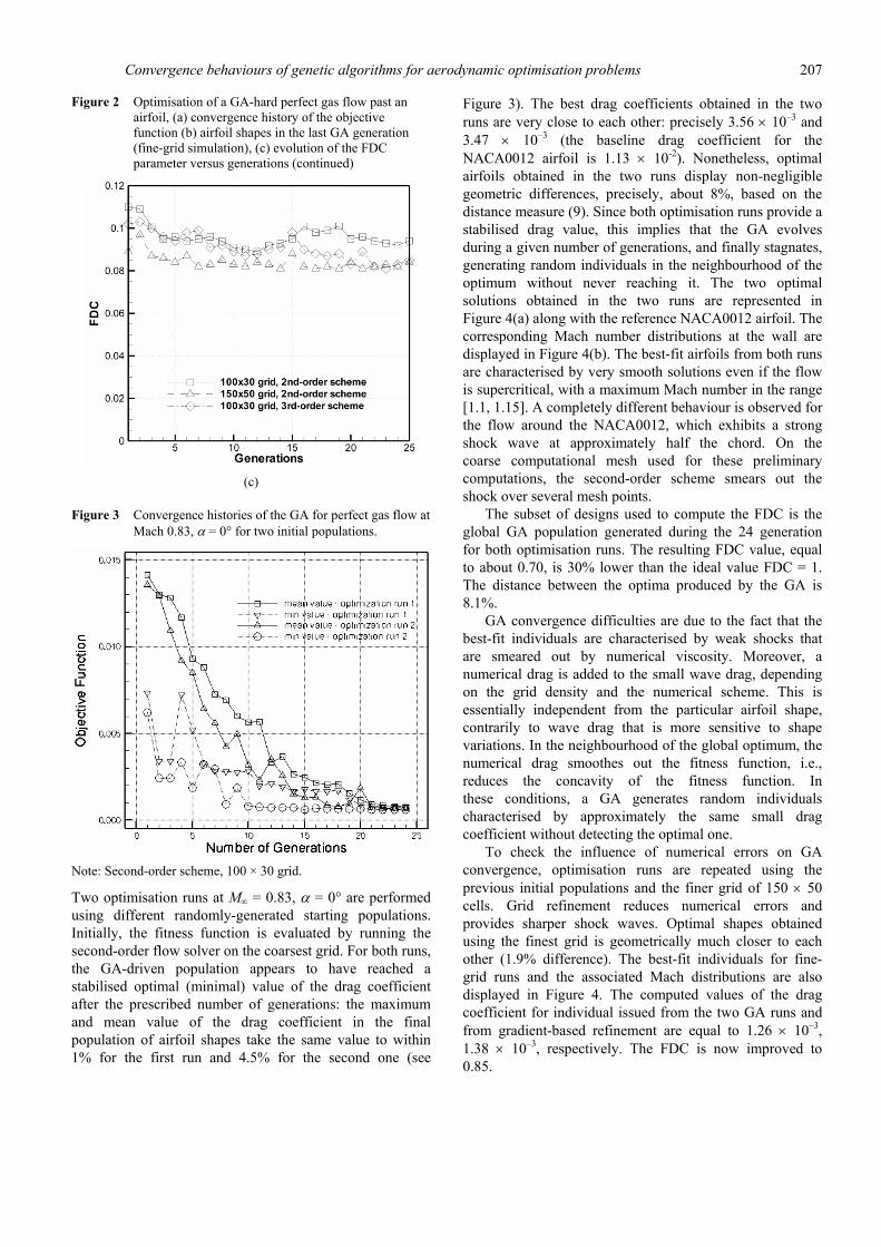
Figure 2 Optimisation of a GA-hard perfect gas flow past an airfoil, (a) convergence history of the objective function (b) airfoil shapes in the last GA generation (fine-grid simulation), (c) evolution of the FDC parameter versus generations (continued)

(c)

Figure 3 Convergence histories of the GA for perfect gas flow at Mach 0.83, α = 0° for two initial populations.

Note: Second-order scheme, 100 × 30 grid.

Two optimisation runs at M∞ = 0.83, α = 0° are performed using different randomly-generated starting populations. Initially, the fitness function is evaluated by running the second-order flow solver on the coarsest grid. For both runs, the GA-driven population appears to have reached a stabilised optimal (minimal) value of the drag coefficient after the prescribed number of generations: the maximum and mean value of the drag coefficient in the final population of airfoil shapes take the same value to within 1% for the first run and 4.5% for the second one (see

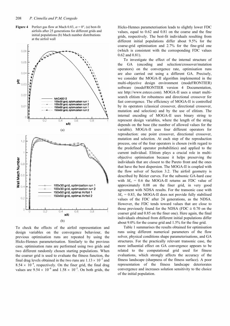
Figure 3). The best drag coefficients obtained in the two runs are very close to each other: precisely 3.56 × 10–3 and 3.47 × 10–3 (the baseline drag coefficient for the NACA0012 airfoil is 1.13 × 10-2). Nonetheless, optimal airfoils obtained in the two runs display non-negligible geometric differences, precisely, about 8%, based on the distance measure (9). Since both optimisation runs provide a stabilised drag value, this implies that the GA evolves during a given number of generations, and finally stagnates, generating random individuals in the neighbourhood of the optimum without never reaching it. The two optimal solutions obtained in the two runs are represented in Figure 4(a) along with the reference NACA0012 airfoil. The corresponding Mach number distributions at the wall are displayed in Figure 4(b). The best-fit airfoils from both runs are characterised by very smooth solutions even if the flow is supercritical, with a maximum Mach number in the range [1.1, 1.15]. A completely different behaviour is observed for the flow around the NACA0012, which exhibits a strong shock wave at approximately half the chord. On the coarse computational mesh used for these preliminary computations, the second-order scheme smears out the shock over several mesh points.

The subset of designs used to compute the FDC is the global GA population generated during the 24 generation for both optimisation runs. The resulting FDC value, equal to about 0.70, is 30% lower than the ideal value FDC = 1. The distance between the optima produced by the GA is 8.1%.

GA convergence difficulties are due to the fact that the best-fit individuals are characterised by weak shocks that are smeared out by numerical viscosity. Moreover, a numerical drag is added to the small wave drag, depending on the grid density and the numerical scheme. This is essentially independent from the particular airfoil shape, contrarily to wave drag that is more sensitive to shape variations. In the neighbourhood of the global optimum, the numerical drag smoothes out the fitness function, i.e., reduces the concavity of the fitness function. In these conditions, a GA generates random individuals characterised by approximately the same small drag coefficient without detecting the optimal one.

To check the influence of numerical errors on GA convergence, optimisation runs are repeated using the previous initial populations and the finer grid of 150 × 50 cells. Grid refinement reduces numerical errors and provides sharper shock waves. Optimal shapes obtained using the finest grid is geometrically much closer to each other (1.9% difference). The best-fit individuals for fine-grid runs and the associated Mach distributions are also displayed in Figure 4. The computed values of the drag coefficient for individual issued from the two GA runs and from gradient-based refinement are equal to 1.26 × 10–3, 1.38 × 10–3, respectively. The FDC is now improved to 0.85.

208 P. Cinnella and P.M. Congedo

Figure 4 Perfect gas flow at Mach 0.83, α = 0°, (a) best-fit airfoils after 25 generations for different grids and initial populations (b) Mach number distributions at the airfoil wall

(a)

(b)

To check the effects of the airfoil representation and design variables on the convergence behaviour, the previous optimisation runs are repeated by using the Hicks-Hennes parameterisation. Similarly to the previous case, optimisation runs are performed using two grids and two different randomly chosen starting populations. When the coarser grid is used to evaluate the fitness function, the final drag levels obtained in the two runs are 1.13 × 10–3 and 8.54 × 10–4, respectively. On the finer grid, the final drag values are 9.54 × 10–4 and 1.58 × 10–3. On both grids, the

Hicks-Hennes parameterisation leads to slightly lower FDC values, equal to 0.62 and 0.81 on the coarse and the fine grids, respectively. The best-fit individuals resulting from different initial populations differ about 9.5% for the coarse-grid optimisation and 2.7% for the fine-grid one (which is consistent with the corresponding FDC values 0.62 and 0.81).

To investigate the effect of the internal structure of the GA (encoding and selection/crossover/mutation operators) on the convergence rate, optimisation runs are also carried out using a different GA. Precisely, we consider the MOGA-II algorithm implemented in the multi-objective design environment (modeFRONTIER) software (modeFRONTIER version 4 Documentation, see http://www.esteco.com). MOGA-II uses a smart multi-search elitism for robustness and directional crossover for fast convergence. The efficiency of MOGA-II is controlled by its operators (classical crossover, directional crossover, mutation and selection) and by the use of elitism. The internal encoding of MOGA-II uses binary string to represent design variables, where the length of the string depends on the base (the number of allowed values for the variable). MOGA-II uses four different operators for reproduction: one point crossover, directional crossover, mutation and selection. At each step of the reproduction process, one of the four operators is chosen (with regard to the predefined operator probabilities) and applied to the current individual. Elitism plays a crucial role in multi-objective optimisation because it helps preserving the individuals that are closest to the Pareto front and the ones that have the best dispersion. The MOGA-II is coupled with the flow solver of Section 3.2. The airfoil geometry is described by Bézier curves. For the subsonic GA-hard case with M∞ = 0.6 the MOGA-II returns an FDC value of approximately 0.08 on the finer grid, in very good agreement with NDSA results. For the transonic case with M∞ = 0.83, the MOGA-II does not provide fully stabilised values of the FDC after 24 generations, as the NDSA. However, the FDC tends toward values that are close to those previously found for the NDSA (FDC ≅ 0.70 on the coarser grid and 0.85 on the finer one). Here again, the final individuals obtained from different initial populations differ about 9.0% for the coarse grid and 1.5% for the fine grid.

Table 1 summarises the results obtained for optimisation runs using different numerical parameters of the flow solver, physical conditions shape parameterisations, and GA structures. For the practically relevant transonic case, the more influential effect on GA convergence appears to be related to the computational grid used for fitness evaluations, which strongly affects the accuracy of the fitness landscape (sharpness of the fitness surface). A poor representation of the fitness landscape deteriorates convergence and increases solution sensitivity to the choice of the initial population.

Convergence behaviours of genetic algorithms for aerodynamic optimisation problems 209

Table 1 Summary of the main results obtained for perfect gas flow optimisation problems

Run description Results

M∞ GA Param. Grid Scheme Cd,seed1 Cd,seed2

( )

( )1 2

21, 2,

21

,

Ni i

ii

d

s s

=

=

−

Δ∑

s s

FDC

0.6 NDSA Bézier 100 × 30 2nd-order 2.86-04 5.25E-04 150.1% 0.095 0.6 NDSA Bézier 150 × 50 2nd-order 6.5E-05 1.09E-04 120.3% 0.084 0.6 NDSA Bézier 100 × 30 3rd-order 2.42E-04 3.30E-04 89.3% 0.083 0.6 MOGA-II Bézier 100 × 30 2nd-order 1.89E-04 2.0E-04 87.7% 0.12 0.6 MOGA-II Bézier 150 × 50 2nd-order 6.7E-05 8.80E-05 65.9% 0.08 0.83 NDSA Bézier 100 × 30 2nd-order 3.51E-03 2.47E-03 8.1% 0.70 0.83 NDSA Bézier 150 × 50 2nd-order 1.26E-03 1.38E-03 1.9% 0.85 0.83 NDSA H-H 100 × 30 2nd-order 1.13E-03 8.5E-04 9.5% 0.62 0.83 NDSA H-H 150 × 50 2nd-order 9.54E-04 1.58E-03 2.7% 0.81 0.83 MOGA-II Bézier 100 × 30 2nd-order 1.59E-03 1.14E-03 9.0% 0.70 0.83 MOGA-II Bézier 150 × 50 2nd-order 1.43E-03 9.36E-04 1.5% 0.82

Figure 5 BZT flow problem

Note: Frequency histogram for DOE data.

4.2 Drag minimisation for transonic flows over an

airfoil – DG flow case

Next, transonic DG flows are considered. The working fluid is supposed to be a BZT polytropic van der Waals gas with a specific heat ratio equal to 1.02. When DG flows are considered, the free-stream Mach number and the angle of attack are no longer sufficient to completely determine the flow field, but information about free-stream

thermodynamic conditions has to be added: for the computations presented in the following, the operating pressure and density, normalised with their critical-point values, are taken equal to p∞/pc = 1.0696, p∞/pc = 0.735. With this choice, the free-stream value of the fundamental derivative is Γ∞ = 1.95 × 10–4, and the flow exhibits very weak shock waves. The computations are initially carried out using a coarse grid composed by 100 × 30 cells.

210 P. Cinnella and P.M. Congedo

The peculiar behaviour of the sound speed in BZT flows (see for example, Cinnella and Congedo, 2005a) delays the transonic drag rise considerably with respect to a perfect gas flow over an airfoil of the same thickness: for the BZT gas at the thermodynamic conditions considered in this study, the critical Mach number Mc is found to be about 0.94 for an airfoil of 12% thickness. On the other hand, even for supercritical free-stream Mach numbers (M∞ > Mc), shock waves characterising the flow-field are much weaker than in PFG flows at similar conditions. For a shock wave of given intensity/pressure jump, the entropy gradients generated in a BZT flow are about one order of magnitude lower than those generated in a PFG flow, if their jump conditions are located in a properly chosen thermodynamic region (Cramer and Kluwick, 1984).

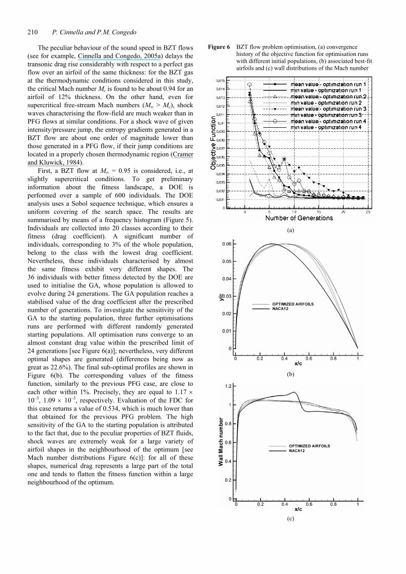
First, a BZT flow at M∞ = 0.95 is considered, i.e., at slightly supercritical conditions. To get preliminary information about the fitness landscape, a DOE is performed over a sample of 600 individuals. The DOE analysis uses a Sobol sequence technique, which ensures a uniform covering of the search space. The results are summarised by means of a frequency histogram (Figure 5). Individuals are collected into 20 classes according to their fitness (drag coefficient). A significant number of individuals, corresponding to 3% of the whole population, belong to the class with the lowest drag coefficient. Nevertheless, these individuals characterised by almost the same fitness exhibit very different shapes. The 36 individuals with better fitness detected by the DOE are used to initialise the GA, whose population is allowed to evolve during 24 generations. The GA population reaches a stabilised value of the drag coefficient after the prescribed number of generations. To investigate the sensitivity of the GA to the starting population, three further optimisations runs are performed with different randomly generated starting populations. All optimisation runs converge to an almost constant drag value within the prescribed limit of 24 generations [see Figure 6(a)]; nevertheless, very different optimal shapes are generated (differences being now as great as 22.6%). The final sub-optimal profiles are shown in Figure 6(b). The corresponding values of the fitness function, similarly to the previous PFG case, are close to each other within 1%. Precisely, they are equal to 1.17 × 10–3, 1.09 × 10–3, respectively. Evaluation of the FDC for this case returns a value of 0.534, which is much lower than that obtained for the previous PFG problem. The high sensitivity of the GA to the starting population is attributed to the fact that, due to the peculiar properties of BZT fluids, shock waves are extremely weak for a large variety of airfoil shapes in the neighbourhood of the optimum [see Mach number distributions Figure 6(c)]: for all of these shapes, numerical drag represents a large part of the total one and tends to flatten the fitness function within a large neighbourhood of the optimum.

Figure 6 BZT flow problem optimisation, (a) convergence history of the objective function for optimisation runs with different initial populations, (b) associated best-fit airfoils and (c) wall distributions of the Mach number

(a)

(b)

(c)

Convergence behaviours of genetic algorithms for aerodynamic optimisation problems 211

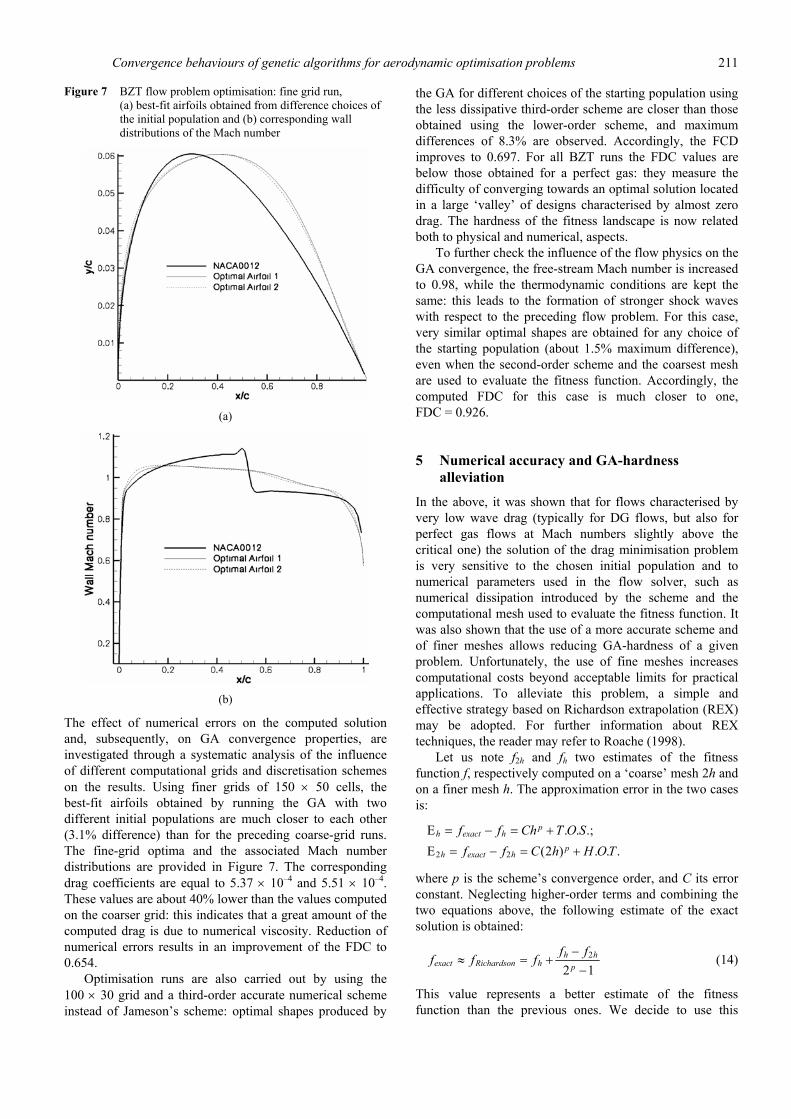
Figure 7 BZT flow problem optimisation: fine grid run, (a) best-fit airfoils obtained from difference choices of the initial population and (b) corresponding wall distributions of the Mach number

(a)

(b)

The effect of numerical errors on the computed solution and, subsequently, on GA convergence properties, are investigated through a systematic analysis of the influence of different computational grids and discretisation schemes on the results. Using finer grids of 150 × 50 cells, the best-fit airfoils obtained by running the GA with two different initial populations are much closer to each other (3.1% difference) than for the preceding coarse-grid runs. The fine-grid optima and the associated Mach number distributions are provided in Figure 7. The corresponding drag coefficients are equal to 5.37 × 10–4 and 5.51 × 10–4. These values are about 40% lower than the values computed on the coarser grid: this indicates that a great amount of the computed drag is due to numerical viscosity. Reduction of numerical errors results in an improvement of the FDC to 0.654.

Optimisation runs are also carried out by using the 100 × 30 grid and a third-order accurate numerical scheme instead of Jameson’s scheme: optimal shapes produced by

the GA for different choices of the starting population using the less dissipative third-order scheme are closer than those obtained using the lower-order scheme, and maximum differences of 8.3% are observed. Accordingly, the FCD improves to 0.697. For all BZT runs the FDC values are below those obtained for a perfect gas: they measure the difficulty of converging towards an optimal solution located in a large ‘valley’ of designs characterised by almost zero drag. The hardness of the fitness landscape is now related both to physical and numerical, aspects.

To further check the influence of the flow physics on the GA convergence, the free-stream Mach number is increased to 0.98, while the thermodynamic conditions are kept the same: this leads to the formation of stronger shock waves with respect to the preceding flow problem. For this case, very similar optimal shapes are obtained for any choice of the starting population (about 1.5% maximum difference), even when the second-order scheme and the coarsest mesh are used to evaluate the fitness function. Accordingly, the computed FDC for this case is much closer to one, FDC = 0.926.

5 Numerical accuracy and GA-hardness alleviation

In the above, it was shown that for flows characterised by very low wave drag (typically for DG flows, but also for perfect gas flows at Mach numbers slightly above the critical one) the solution of the drag minimisation problem is very sensitive to the chosen initial population and to numerical parameters used in the flow solver, such as numerical dissipation introduced by the scheme and the computational mesh used to evaluate the fitness function. It was also shown that the use of a more accurate scheme and of finer meshes allows reducing GA-hardness of a given problem. Unfortunately, the use of fine meshes increases computational costs beyond acceptable limits for practical applications. To alleviate this problem, a simple and effective strategy based on Richardson extrapolation (REX) may be adopted. For further information about REX techniques, the reader may refer to Roache (1998).

Let us note f2h and fh two estimates of the fitness function f, respectively computed on a ‘coarse’ mesh 2h and on a finer mesh h. The approximation error in the two cases is:

2 2

. . .;(2 ) . . .

ph exact h

ph exact h

f f Ch T O Sf f C h H O T

Ε = − = +

Ε = − = +

where p is the scheme’s convergence order, and C its error constant. Neglecting higher-order terms and combining the two equations above, the following estimate of the exact solution is obtained:

2

2 1h h

exact Richardson h p

f ff f f −≈ = +

− (14)

This value represents a better estimate of the fitness function than the previous ones. We decide to use this

212 P. Cinnella and P.M. Congedo

extrapolated value as an approximation of the fitness of a given individual in the GA. Precisely, the algorithm is as follows:

1 for each individual, a coarse and a finer mesh are generated, the coarser mesh being obtained from the finer one by halving the number of points in each direction

2 a coarse-grid estimate of the fitness function is computed

3 the coarse grid solution is used to initialise a finer-grid computation; a finer-grid estimate of the fitness function is obtained

4 the values obtained at steps (2) and (3) are used to compute a more accurate estimate of the fitness function via formula (14)

5 this value is compared with fitness values obtained for the other individuals in the population in order to perform standard operations of selection, crossover and elitism in the GA.

The above strategy is now applied to the test cases of Sections 4.1 and 4.2. Preliminary mesh studies returned a convergence order p of about 1.9 for the second-order solver used in this study.

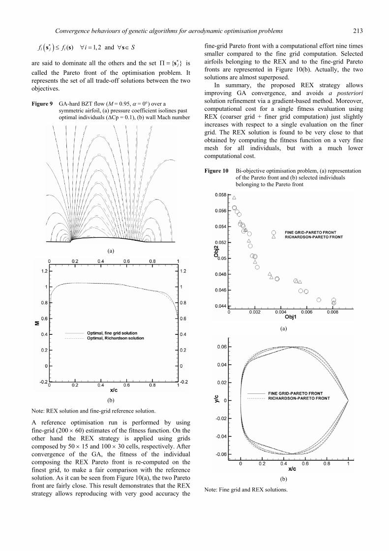
Specifically, we consider the GA-hard drag minimisation problem for a BZT van der Waals gas flow over a symmetric airfoil, with free-stream conditions M∞ = 0.95, α = 00, p∞/pc = 1.0696, and p∞/pc = 0.735. A reference optimal solution is computed by using a very fine mesh composed by 200×64 cells. CPU time required for a single fitness evaluation on this grid is about 40 minutes on a Pentium V processor. The whole optimisation process requires about 800 fitness evaluations.

Then, the same optimisation run is performed by applying the extrapolation strategy described above: for each individual, the fitness function is first computed using a coarse grid of 50 × 16 cells, then using a finer grid of 100 × 32 cells, finally a refined value is extrapolated via Richardson’s formula. The total CPU time required to obtain the final estimate of the fitness function for a single individual is about 5 minutes, i.e., 1/8 of the fine-grid computation. The reduction in computational time is due, on the one hand to the lower number of operations required to compute solutions on the coarser grids and, on the other hand to higher convergence rates of the flow solver. An important role is also played by initialisation of the medium grid computation with the coarse grid solution.

The computed FDC parameter of the GA for this problem was 0.534 using a grid composed by 100 × 30 cells (close to the present medium mesh). For the optimisation run using the 200 × 64 grid FDC grows to 0.676. For the REX optimisation run, FDC is even better and equals 0.691. These results demonstrate once more the tight connection between the fitness function evaluation accuracy and the convergence rate of the GA. Figure 8 displays the optimal individuals obtained, respectively, by using the finest grid

and the REX strategy to evaluate the fitness function. The two geometries are very close to each other, their distance based on equation (9) being 1.8%. The greatest differences are encountered at the rear part of the airfoil. Differences between the two individuals are related to the different representations of the fitness function provided by the fine grid computations and by the REX method. The corresponding values of the drag coefficient are also very similar: cd = 7.32 × 10–4 for the REX optimal individual (a posteriori evaluated on the finest mesh) and cd = 7.64 × 10–4 for the fine grid one. Figure 9 shows the iso-lines of the pressure coefficient and the wall Mach number distribution for the two solutions: once again, they are almost superposed. To check the sensitivity to the choice of the initial population, the REX optimisation is also run with a different starting population. The REX strategy provides airfoils with geometrical differences to within 0.3% (solution labelled as ‘Richardson 2’ in Figure 8). This represent a striking difference with respect to the results of Section 4 (Figure 6), where differences up to 22% where observed. Similar results (not shown for brevity) where found applying the REX strategy to the drag minimisation problem for an inviscid perfect gas flow with M∞ = 0.83, α = 00.

Figure 8 BZT van der Waals gas flow over a symmetric non-lifting airfoil

Note: Optimal geometries obtained using a fine-grid

estimate and Richardson extrapolation (REX) estimate of the fitness function

As a final application, the REX approach is applied to a bi-objective optimisation. The drag coefficient is simultaneously minimised for two different operating conditions. A BZT van der Waals gas flow over a symmetric airfoil with α = 00, p∞/pc = 1.0696, and p∞/pc = 0.735 is optimised for M∞ = 0.95 and M∞ = 0.98. The fitness function is now a vector defined as f = (f1, f2), with f1 = cd(M∞ = 0.95) and f2 = cd(M∞ = 0.98). Individuals are ranked according to their fitness with respect to the two components of f. In particular, individuals such that

Convergence behaviours of genetic algorithms for aerodynamic optimisation problems 213

( )* ( ) 1,2 and i j if f i S≤ ∀ = ∀ ∈s s s

are said to dominate all the others and the set * jΠ = s is called the Pareto front of the optimisation problem. It represents the set of all trade-off solutions between the two objectives.

Figure 9 GA-hard BZT flow (M = 0.95, α = 0°) over a symmetric airfoil, (a) pressure coefficient isolines past optimal individuals (ΔCp = 0.1), (b) wall Mach number

(a)

(b)

Note: REX solution and fine-grid reference solution.

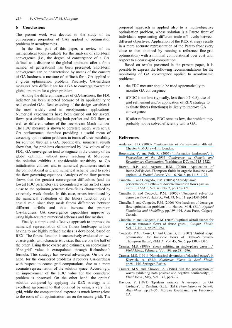
A reference optimisation run is performed by using fine-grid (200 × 60) estimates of the fitness function. On the other hand the REX strategy is applied using grids composed by 50 × 15 and 100 × 30 cells, respectively. After convergence of the GA, the fitness of the individual composing the REX Pareto front is re-computed on the finest grid, to make a fair comparison with the reference solution. As it can be seen from Figure 10(a), the two Pareto front are fairly close. This result demonstrates that the REX strategy allows reproducing with very good accuracy the

fine-grid Pareto front with a computational effort nine times smaller compared to the fine grid computation. Selected airfoils belonging to the REX and to the fine-grid Pareto fronts are represented in Figure 10(b). Actually, the two solutions are almost superposed.

In summary, the proposed REX strategy allows improving GA convergence, and avoids a posteriori solution refinement via a gradient-based method. Moreover, computational cost for a single fitness evaluation using REX (coarser grid + finer grid computation) just slightly increases with respect to a single evaluation on the finer grid. The REX solution is found to be very close to that obtained by computing the fitness function on a very fine mesh for all individuals, but with a much lower computational cost.

Figure 10 Bi-objective optimisation problem, (a) representation of the Pareto front and (b) selected individuals belonging to the Pareto front

(a)

(b)

Note: Fine grid and REX solutions.

214 P. Cinnella and P.M. Congedo

6 Conclusions

The present work was devoted to the study of the convergence properties of GAs applied to optimisation problems in aerodynamics.

In the first part of this paper, a review of the mathematical tools available for the analysis of short-term convergence (i.e., the degree of convergence of a GA, defined as a distance to the global optimum, after a finite number of generations) has been presented. Short-term convergence can be characterised by means of the concept of GA-hardness, a measure of stiffness for a GA applied to a given optimisation problem. Precisely, GA-hardness measures how difficult are for a GA to converge toward the global optimum for a given problem.

Among the different measures of GA-hardness, the FDC indicator has been selected because of its applicability to real-encoded GAs. Real encoding of the design variables is the most widely used in aerodynamics applications. Numerical experiments have been carried out for several flows past airfoils, including both perfect and DG flow, as well as different values of the free-stream Mach number. The FDC measure is shown to correlate nicely with actual GA performance, therefore providing a useful mean of assessing optimisation problems in terms of their suitability for solution through a GA. Specifically, numerical results show that, for problems characterised by low values of the FDC, GA-convergence tend to stagnate in the vicinity of the global optimum without never reaching it. Moreover, the solution exhibits a considerable sensitivity to GA initialisation choices, and to numerical parameters such as the computational grid and numerical scheme used to solve the flow governing equations. Analysis of the flow patterns shows that the greatest convergence difficulties (and the lowest FDC parameter) are encountered when airfoil shapes close to the optimum generate flow-fields characterised by extremely weak shocks. In this case, errors introduced by the numerical evaluation of the fitness function play a crucial role, since they mask fitness differences between different airfoils and thus increase the problem GA-hardness. GA convergence capabilities improve by using high-accurate numerical schemes and fine meshes.

Finally, a simple and effective approach to improve the numerical representation of the fitness landscape without having to use highly refined meshes is developed, based on REX. The fitness function is successively evaluated on two coarse grids, with characteristic sizes that are one the half of the other. Using these coarse grid estimates, an approximate ‘fine-grid’ value is extrapolated through Richardson’s formula. This strategy has several advantages. On the one hand, for the considered problems it reduces GA-hardness with respect to coarse grid computations, due to a more accurate representation of the solution space. Accordingly, an improvement of the FDC value for the considered problem is observed. On the other hand, the optimal solution computed by applying the REX strategy is in excellent agreement to that obtained by using a very fine grid, while the computational expense is much lower (close to the costs of an optimisation run on the coarse grid). The

proposed approach is applied also to a multi-objective optimisation problem, whose solution is a Pareto front of individuals representing different trade-off levels between different objectives. Application of the REX strategy results in a more accurate representation of the Pareto front (very close to that obtained by running a reference fine-grid optimisation) with a minimal computational over cost with respect to a coarse-grid computation.

Based on results presented in the present paper, it is possible to express the following recommendations for the monitoring of GA convergence applied to aerodynamic problems:

• the FDC measure should be used systematically to monitor GA convergence

• if FDC is too low (typically, less than 0.7–0.8), use of grid refinement and/or application of REX strategy to evaluate fitness function(s) is likely to improve GA convergence

• if, after refinement, FDC remains low, the problem may probably not be solved efficiently with a GA.

References Anderson, J.D. (2000) Fundamentals of Aerodynamics, 4th ed.,

Chapter 4, McGraw-Hill, London. Borenstein, Y. and Poli, R. (2005) ‘Information landscapes’, in

Proceeding of the 2005 Conference on Genetic and Evolutionary Computation, Washington DC, pp.1515–1522.

Brown, B.P. and Argrow, B.M. (2000) ‘Application of Bethe-Zel’dovich-Thompson fluids in organic Rankine cycle engines’, J. Propul. Power, Vol. 16, No. 6, pp.1118–1123.

Cinnella, P. and Congedo, P.M. (2005a) ‘Aerodynamic performance of Bethe-Zel’dovich-Thompson flows past an airfoil’, AIAA J., Vol. 43, No. 2, pp.370–378.

Cinnella, P. and Congedo, P.M. (2005b) ‘Numerical solver for dense gas flows’, AIAA J., Vol. 43, No. 11, pp.2458–2461.

Cinnella, P. and Congedo, P.M. (2006) ‘GA-hardness of dense-gas flow optimisation problems’, in Hamza, M.H. (Ed.): Applied Simulation and Modelling, pp.489–494, Acta Press, Calgary, Canada.

Cinnella, P. and Congedo, P.M. (2008) ‘Optimal airfoil shapes for viscous transonic flows of dense gases’, Comput. Fluids, Vol. 37, No. 3, pp.250–264.

Congedo, P.M., Corre, C. and Cinnella, P. (2007) ‘Airfoil shape optimisation for transonic flows of Bethe-Zel’dovich-Thompson fluids’, AIAA J., Vol. 45, No. 6, pp.1303–1316.

Cramer, M.S. (1989) ‘Shock splitting in single-phase gases’, J. Fluid Mech., February, Vol. 199, pp.281–296.

Cramer, M.S. (1991) ‘Nonclassical dynamics of classical gases’, in Kluwick, A. (Ed.): Nonlinear Waves in Real Fluids, pp.91–145, Springer, Berlin.

Cramer, M.S. and Kluwick, A. (1984) ‘On the propagation of waves exhibiting both positive and negative nonlinearity’, J. Fluid Mech., May, Vol. 142, pp.9–37.

Davidor, Y. (1991) ‘Epistasis variance. A viewpoint on GA hardness’, in Rawlins, G.J.E. (Ed.): Foundations of Genetic Algorithms, pp.23–35, Morgan Kaufmann, San Francisco, CA.

Convergence behaviours of genetic algorithms for aerodynamic optimisation problems 215

Elliott, J. and Peraire, J. (1997) ‘Aerodynamic optimisation on unstructured meshes with visous effects’, AIAA Paper 97-1849.

Elliott, J. and Peraire, J. (1998) ‘Constrained, multipoint shape optimisation for complex 3-D configurations’, Aeronautical Journal, August/September, Vol. 102, pp.365–376.

Gao, Y. (1998) ‘An upper bound on the convergence rates of canonical genetic algorithms’, Complexity International, p.5 [online] http://www.complexity.org.au/ci/vol05/gao/grateGao.html (accessed 20 December 2012).

Giannakoglou, K.C. (2002) ‘Design of optimal aerodynamic shapes using stochastic optimisation methods and computational intelligence’, Prog. Aerosp. Sci., Vol. 38, No. 1, pp.43–76.

Hicks, R. and Hennes, P. (1978) ‘Wing design by numerical optimisation’, J. Aircraft, Vol. 15, No. 7, pp.407–413.

Holland, J.H. (1975) Adaptation in Natural and Artificial Systems, Univ. Michigan Press, Ann Arbour.

Horn, J. and Goldberg, D.E. (1995) ‘Genetic algorithm difficulty and the modality of fitness landscapes’, in Whiley, L.D. and Vose, M.D. (Eds.): Foundations of Genetic Algorithms, Vol. 3, pp.243–269, Morgan Kauffman, San Mateo, CA.

Jameson, A., Schmidt, W. and Turkel, E. (1981) ‘Solutions of the euler equations by finite volume methods using Runge-Kutta time-stepping schemes’, AIAA, Fluid and Plasma Dynamics Conference, 14th, Palo Alto, CA, 23–25 June, AIAA Paper 8l-l259.

Jones, T. and Forrest, S. (1995) ‘Fitness distance correlation as a measure of problem difficulty for genetic algorithms’, Proc. 6th International Conference on Genetic Algorithms, pp.184–192, San Francisco, CA.

Kirillov, N.G. (2004) ‘Analysis of modern natural gas liquefaction technologies’, Chem. Petrol. Eng., Vol. 40, Nos. 7–8, pp.401–406.

Leung, Y., Gao, Y. and Xu, Z.B. (1997) ‘Degree of population diversity: a perspective on premature convergence in genetic algorithms and its Markov chain analysis’, IEEE T Neural Networ., Vol. 8, No. 5, pp.1165–1176.

Michalewicz, Z. (1996) Genetic Algorithms + Data Structures = Evolution Programs, Springer, Berlin.

Naudts, B. and Kallel, L. (2000) ‘A comparison of predictive measures of problem difficulty in evolutionary algorithms’, IEEE T. Evolut. Comput., Vol. 4, No. 1, pp.1–15.

Peck, C.C. and Dhawan, A.P. (1995) ‘Genetic algorithms as global random search methods: an alternative perspective’, Evol. Comput., Vol. 3, No. 1, pp.39–80.

Peigin, S. and Epstein, B. (2004) ‘Robust optimisation of 2D airfoils driven by full Navier-Stokes computations’, Comput. Fluids, Vol. 33, No. 9, pp.175–1200.

Pulliam, T.H., Nemec, N., Holst, T. and Zingg, D.W. (2003) ‘Comparison of evolutionary (genetic) algorithm and adjoint methods for multi-objective viscous airfoil optimisation’, 41st Aerospace Sciences Meeting, Reno, NV, AIAA Paper 2003-0298.

Reeves, C. and Wright, C. (1995) ‘An experimental design perspective on genetic algorithms’, in Whiley, L.D. and Vose, M.D. (Eds.): Foundations of Genetic Algorithms, Vol. 3, pp.7–22, Morgan Kauffman, San Mateo, CA.

Roache, P.J. (1998) Verification and Validation in Computational Science and Engineering, Hermosa Publishers, Albuquerque, New Mexico.

Rochet, S. (1997) ‘Epistasis in genetic algorithms revisited’, Inform. Sciences, Vol. 102, No. 1, pp.133–155.

Rochet, S., Slimane, M. and Venturini, G. (1996) ‘Epistasis for encoding in genetic algorithms’, Proc. Australian and New Zeland Conference on Intelligent Information Systems, IEEE ANZIIS’96, Adelaide, Australia, pp.268–271.

Rochet, S., Venturini, G., Slimane, M. and El Kharoubi, F.M. (1998) ‘A critical and empirical study of epistasis measures for predicting GA performances: a summary’, in Artificial Evolution, Lecture Notes in Computer Science, Springer, Berlin, Vol. 1363, p.275.

Rudolph, G. (1994) ‘Convergence analysis of canonical genetic algorithms’, IEEE T Neural Networ., Vol. 5, No. 1, pp.96–101.

Srinivas, N. and Deb, K. (1995) ‘Multiobjective function optimisation using nondominated sorting genetic algorithms’, Evol. Comput., Vol. 2, No. 3, pp.221–248.

Thompson, P.A. (1971) ‘A fundamental derivative in gas dynamics’. Phys Fluids, Vol. 14, No. 9, pp.1843–1849.

Van Hove, H. and Verschoren, A. (1994) ‘On epistasis’, Comput. Artif. Intell., Vol. 14, No. 3, pp.271–277.

Wang, J.F., Periaux, J. and Sefrioui, M. (2002) ‘Parallel evolutionary algorithms for optimisation problems in aerospace engineering’, J. Comput. Appl. Math., Vol. 149, No. 1, pp.155–169.

Zamfirescu, C. and Dincer, I. (2009) ‘Performance investigation of high-temperature heat pumps with various BZT working fluids’, Thermochim. Acta, Vol. 488, No. 1, pp.66–77.

Zhang, F., Chen, S. and Khalid, M. (2004) ‘Optimisation of transonic wings with fuselage by real-coded genetic algorithms’, 10th AIAA/ISSMO Multidisciplinary Analysis and Optimisation Conference, Albany, New York, 30 August–1 September, AIAA Paper 2004-4540.

Nomenclature

a Speed of sound

α Airfoil angle of attack

cd Drag coefficient of an airfoil γ Ratio of the specific heats for a gas Γ Fundamental derivative of gas dynamics (Duhem

parameter) d = d(s, s′). Distance between two elements of s. Its

precise definition depends on the nature of its arguments (binary or floating point)

e Specific internal energy ε Epistasis function. Measures the degree of interaction

between different design variables with respect to their influence on the fitness function.

E Numerical truncation error f Fitness function (cost function) F Physical flux density of the governing conservation

laws FDC Fitness distance correlation (GA-hardness measure) η Hicks-Hennes perturbation function M Mach number P Fluid pressure

216 P. Cinnella and P.M. Congedo

Nomenclature (continued)

πc, πm Crossover and mutation probabilities used in the genetic algorithm

ρ Fluid density s String encoding the design variables associated to a

point in the design space si I = 1, 2, …, N. Components of s. May be binary or

floating-point. S Search space s* Global optimum in S σ Specific entropy Σ Alphabet (set of symbols used to encode the design

variables) T Fluid temperature x Chordwise coordinate y Airfoil profile coordinate Ω = Σn, Univers (space of all possible N-uples of

elements of Σ) (.)∞ Free-stream property (.)c Critical-point property (referred to liquid-vapour

critical point)