Regression analysis

In statistics, regression analysis is a statistical process for estimating the relationships among

variables. It includes many techniques for modeling and analyzing several variables, when the

focus is on the relationship between a dependent variable and one or more independent variables.

More specifically, regression analysis helps one understand how the typical value of the

dependent variable changes when any one of the independent variables is varied, while the other

independent variables are held fixed.

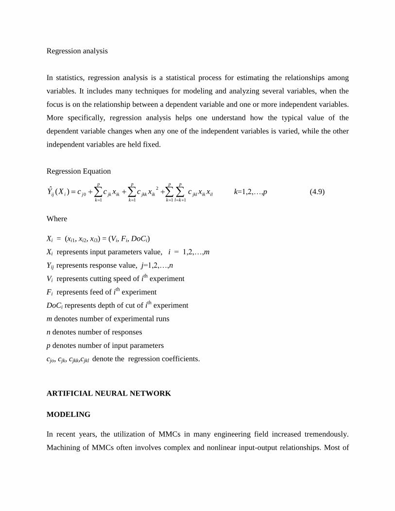
Regression Equation

p

k

ilikjkl

p

kl

p

k

ikjkk

p

k

ikjkjiij xxcxcxccXY1 11

2

1

0)(ˆ

k=1,2,…,p (4.9)

Where

Xi = (xi1, xi2, xi3) = (Vi, Fi, DoCi)

Xi represents input parameters value, i = 1,2,…,m

Yij represents response value, j=1,2,…,n

Vi represents cutting speed of ith

experiment

Fi represents feed of ith

experiment

DoCi represents depth of cut of ith

experiment

m denotes number of experimental runs

n denotes number of responses

p denotes number of input parameters

cjo, cjk, cjkk,cjkl denote the regression coefficients.

ARTIFICIAL NEURAL NETWORK

MODELING

In recent years, the utilization of MMCs in many engineering field increased tremendously.

Machining of MMCs often involves complex and nonlinear input-output relationships. Most of

the research articles presented the modeling of manufacturing process with regression, fuzzy

logic and ANN model. Among these models, ANN plays a very important role in the area of

modeling manufacturing processes where analytical models cannot give the best accurate results.

ANN becomes increasingly popular in predicting complicated experimental trends in the

manufacturing processes and also it performs much faster than other prediction techniques with

good accuracy.

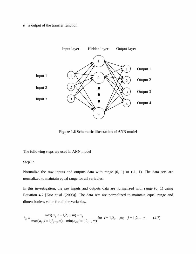
ANN consists of an interconnected group of neurons, and the learning processes are performed

in parallel by the neurons as biological neural network systems. In general, neural network

consists of three layers namely input layer, hidden layer and output layer. In each neuron, the

sum of product of input of all variables and corresponding weight, and bias is calculated which is

supplied as input to transfer function. The transfer function is identified based on the method of

normalization of input and output raw parameters. The transfer function predicts the output for

the given input parameters. The information flow and Schematic illustration of ANN is shown in

Figure 1.6.

Figure 4.1 General neuron architecture

Figure 4.1 General neuron architecture

where

k is number of elements in input parameters

d is sum of weighted input parameters and bias

w1

w2

wk

ck

bk

wd

f (d)

b1

bk

b2

Bias

Bias

c

e

Inputs Weights

Transfer function

Output

e is output of the transfer function

Figure 1.6 Schematic illustration of ANN model

The following steps are used in ANN model

Step 1:

Normalize the raw inputs and outputs data with range (0, 1) or (-1, 1). The data sets are

normalized to maintain equal range for all variables.

In this investigation, the raw inputs and outputs data are normalized with range (0, 1) using

Equation 4.7 [Kuo et al. (2008)]. The data sets are normalized to maintain equal range and

dimensionless value for all the variables.

),...,2,1,min(),...,2,1,max(

),...,2,1,max(

miamia

amiab

ijij

ijij

ij

for i = 1,2,…,m; j = 1,2,…,n (4.7)

1

2

3

1

2

3

4

n

2

1

Output 1

Input 3

Input 2

Output 2

rate Material removal rate

Output 3

Output 4

Input 1

Input layer Hidden layer Output layer

where

aij is raw(inputs and outputs) data

bij is normalized or predicted data

m is number of experimental runs

n is total number of input and output parameters

Step 2:

Select approximately 2/3 of experimental data for training the ANN model. The ANN model

with maximum trained data is expected to give better solution accuracy. The untrained data sets

are used for testing the developed ANN model.

Step 3:

Assign the normalized input and output parameters as the input and target values for ANN

model.

Step 4:

Create the network by choosing proper network type, training function, performance function,

number of layers and properties of each layer, which includes the number of neurons and transfer

function for the model.

Step 5:

Choose the training parameters such as number of epochs, goal, learning rate, learning rate

increment, etc. and then train the network.

Step 6:

Find the error of model by comparing normalized untrained data with predicted data and

correlation between data sets. If the calculated error is within the tolerance then save the network

otherwise repeat the process from step 4 till to get sufficient number of optimum solutions.

Step 7:

Select the optimum ANN model by comparing mean absolute prediction error and correlation

coefficient. Finally, denormalize the predicted data for practical usage.

),...,2,1,min()1)(,...,2,1,max( miabbmiaa ijijijijij fori=1,2,…,m;j=1,2,…,n (4.8)

The third objective of this research work is to develop an expert system for turning parameters of

Al-Cu/TiB2 in-situ MMCs using ANN. The ANN model is developed using experimental data

collected during turning of MMCs which was subjected to SE condition. The material removal

rate is calculated using Equation (3.6). The experimental results obtained are shown in Table

4.14.

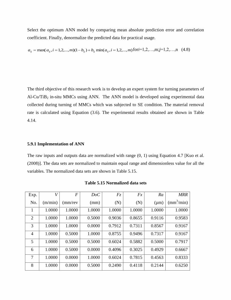
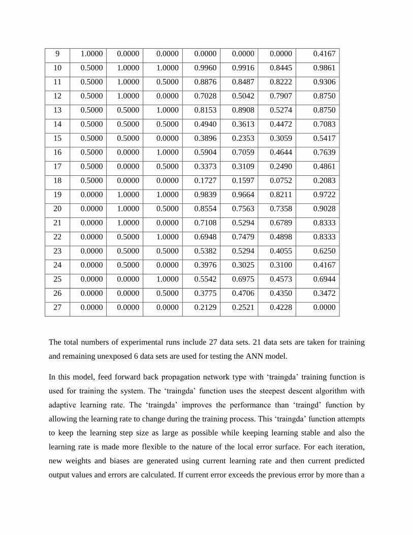
5.9.1 Implementation of ANN

The raw inputs and outputs data are normalized with range (0, 1) using Equation 4.7 [Kuo et al.

(2008)]. The data sets are normalized to maintain equal range and dimensionless value for all the

variables. The normalized data sets are shown in Table 5.15.

Table 5.15 Normalized data sets

Exp.

No.

V

(m/min)

F

(mm/rev

)

DoC

(mm)

Fz

(N)

Fx

(N)

Ra

(µm)

MRR

(mm3/min)

1 1.0000 1.0000 1.0000 1.0000 1.0000 1.0000 1.0000

2 1.0000 1.0000 0.5000 0.9036 0.8655 0.9116 0.9583

3 1.0000 1.0000 0.0000 0.7912 0.7311 0.8567 0.9167

4 1.0000 0.5000 1.0000 0.8755 0.9496 0.7317 0.9167

5 1.0000 0.5000 0.5000 0.6024 0.5882 0.5000 0.7917

6 1.0000 0.5000 0.0000 0.4096 0.3025 0.4929 0.6667

7 1.0000 0.0000 1.0000 0.6024 0.7815 0.4563 0.8333

8 1.0000 0.0000 0.5000 0.2490 0.4118 0.2144 0.6250

9 1.0000 0.0000 0.0000 0.0000 0.0000 0.0000 0.4167

10 0.5000 1.0000 1.0000 0.9960 0.9916 0.8445 0.9861

11 0.5000 1.0000 0.5000 0.8876 0.8487 0.8222 0.9306

12 0.5000 1.0000 0.0000 0.7028 0.5042 0.7907 0.8750

13 0.5000 0.5000 1.0000 0.8153 0.8908 0.5274 0.8750

14 0.5000 0.5000 0.5000 0.4940 0.3613 0.4472 0.7083

15 0.5000 0.5000 0.0000 0.3896 0.2353 0.3059 0.5417

16 0.5000 0.0000 1.0000 0.5904 0.7059 0.4644 0.7639

17 0.5000 0.0000 0.5000 0.3373 0.3109 0.2490 0.4861

18 0.5000 0.0000 0.0000 0.1727 0.1597 0.0752 0.2083

19 0.0000 1.0000 1.0000 0.9839 0.9664 0.8211 0.9722

20 0.0000 1.0000 0.5000 0.8554 0.7563 0.7358 0.9028

21 0.0000 1.0000 0.0000 0.7108 0.5294 0.6789 0.8333

22 0.0000 0.5000 1.0000 0.6948 0.7479 0.4898 0.8333

23 0.0000 0.5000 0.5000 0.5382 0.5294 0.4055 0.6250

24 0.0000 0.5000 0.0000 0.3976 0.3025 0.3100 0.4167

25 0.0000 0.0000 1.0000 0.5542 0.6975 0.4573 0.6944

26 0.0000 0.0000 0.5000 0.3775 0.4706 0.4350 0.3472

27 0.0000 0.0000 0.0000 0.2129 0.2521 0.4228 0.0000

The total numbers of experimental runs include 27 data sets. 21 data sets are taken for training

and remaining unexposed 6 data sets are used for testing the ANN model.

In this model, feed forward back propagation network type with „traingda‟ training function is

used for training the system. The „traingda‟ function uses the steepest descent algorithm with

adaptive learning rate. The „traingda‟ improves the performance than „traingd‟ function by

allowing the learning rate to change during the training process. This „traingda‟ function attempts

to keep the learning step size as large as possible while keeping learning stable and also the

learning rate is made more flexible to the nature of the local error surface. For each iteration,

new weights and biases are generated using current learning rate and then current predicted

output values and errors are calculated. If current error exceeds the previous error by more than a

predefined ratio then the current weights and biases are discarded and learning rate is decreased,

otherwise the weights and biases are retained and learning rate is increased. Finally optimal

learning rate is obtained. In our case, there is no much variation in the processing time on

normalizing the data set in the ranges (-1, 1) and (0, 1). Hence, the log-sigmoid transfer function

is used for normalizing the data in the range (0, 1). The log-sigmoid function is expressed as

f (d) = 1 / (1 + exp(-d)), range (0, 1) (5.1)

Initially, the ANN model is developed with three neurons in input layer, two neurons in one

hidden layer and four neurons in output layer. The model is trained with maximum epochs of

2000 and other default training parameters available in MATLAB software. After training the

model, the prediction data set are collected for the unexposed data set. The prediction error is

calculated using Equation 5.2 and correlation is also identified between unexposed and

prediction data sets. The model with less prediction errors and better correlation is stored. This

process is repeated by changing number of neurons in each hidden layer for better results. The

performance of the ANN model is evaluated by comparing prediction values with unexposed

experimental values.

valuealexperiment Normalised

valuepredicted ANN - valuealexperiment Normalised %error Prediction

(5.2)

The final ANN model architecture is shown in Figure 5.47. The comparison between ANN

predicted values and unexposed normalized experimental values for tangential force, axial force,

surface roughness and material removal rate are shown in Figures 5.48 - 5.51 respectively.

Figure 5.47 Schematic illustration of artificial neural network model

Figure 5.48 Comparison between ANN predicted value and unexposed

normalized experimental value for tangential force

1

2

3

1

2

3

4

28

2

1

Tangential force

Depth of cut

Feed

Axial force

rate Material removal rate

Surface roughness

Material removal rate

Mrate

Cutting speed

Input layer Hidden layer Output layer

Figure 5.49 Comparison between ANN predicted value and unexposed

normalized experimental value for axial force

Figure 5.50 Comparison between ANN predicted value and unexposed

normalized experimental value for surface roughness

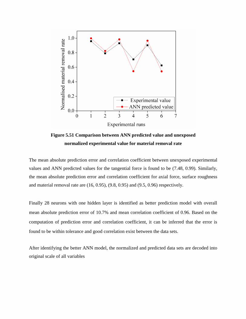
Figure 5.51 Comparison between ANN predicted value and unexposed

normalized experimental value for material removal rate

The mean absolute prediction error and correlation coefficient between unexposed experimental

values and ANN predicted values for the tangential force is found to be (7.48, 0.99). Similarly,

the mean absolute prediction error and correlation coefficient for axial force, surface roughness

and material removal rate are (16, 0.95), (9.8, 0.95) and (9.5, 0.96) respectively.

Finally 28 neurons with one hidden layer is identified as better prediction model with overall

mean absolute prediction error of 10.7% and mean correlation coefficient of 0.96. Based on the

computation of prediction error and correlation coefficient, it can be inferred that the error is

found to be within tolerance and good correlation exist between the data sets.

After identifying the better ANN model, the normalized and predicted data sets are decoded into

original scale of all variables

OPTIMIZATION USING DESIRABILITY FUNCTION

Practically, optimization of multiple performance characteristics is more complex. The

desirability function can be used for optimizing the multiple performance characteristics with

complicated interrelationships. In desirability function, multiple performance characteristics are

converted into a single overall desirability and then optimum condition can be identified based

on maximum value of overall desirability [Harrington (1965), Derringer and Suich (1980), Jeong

and Kim (2009), Aggarwal et al. (2008) and Malenović et al. (2011)]. The multiple response

optimizations is performed using the following steps

Step 1: Create the fitted response models for all the responses using regression Equation 4.9.

p

k

ilikjkl

p

kl

p

k

ikjkk

p

k

ikjkjiij xxcxcxccXY1 11

2

1

0)(ˆ

k=1,2,…,p (4.9)

Where

Xi = (xi1, xi2, xi3) = (Vi, Fi, DoCi)

Xi represents input parameters value, i = 1,2,…,m

Yij represents response value, j=1,2,…,n

Vi represents cutting speed of ith

experiment

Fi represents feed of ith

experiment

DoCi represents depth of cut of ith

experiment

m denotes number of experimental runs

n denotes number of responses

p denotes number of input parameters

cjo, cjk, cjkk,cjkl denote the regression coefficients.

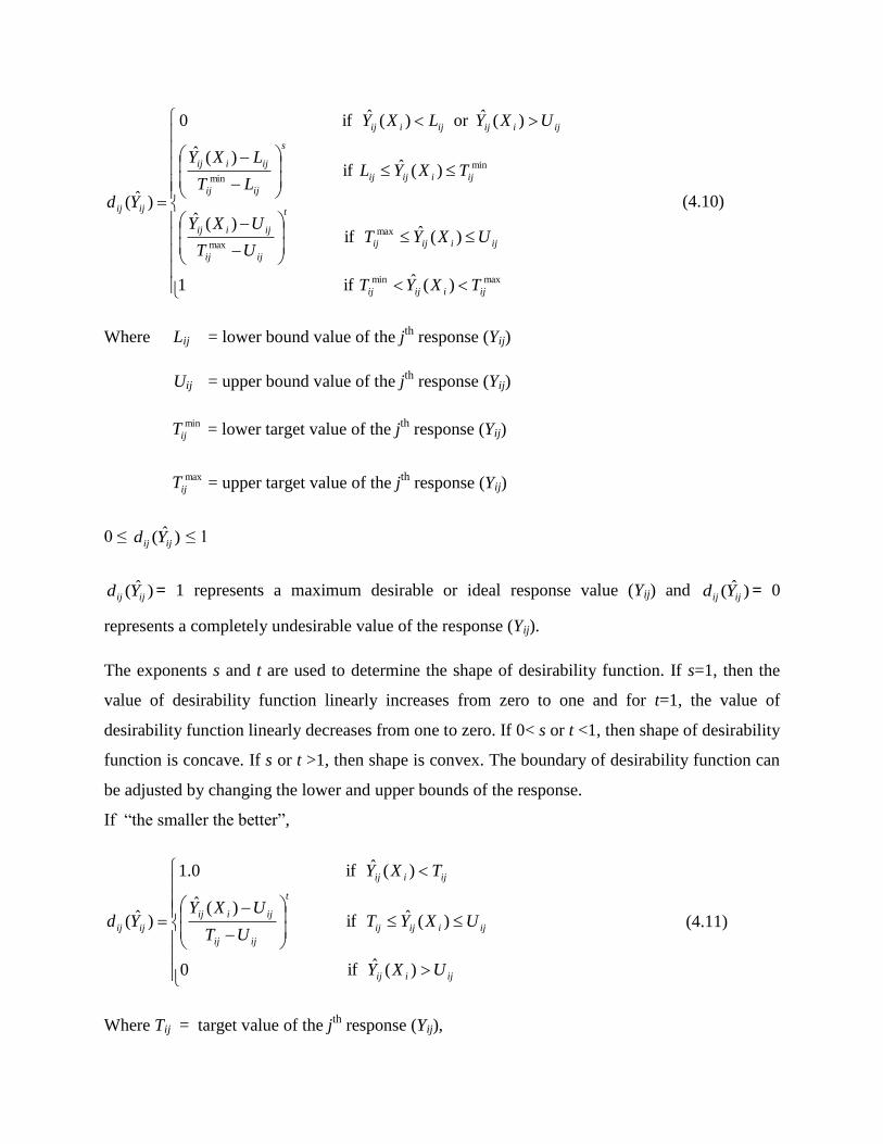
Step 2: If the expected performance characteristic is of the form “the-target-the-better”, then the

individual desirability function is defined as

maxmin

max

max

min

min

)(ˆ if 1

)(ˆ if )(ˆ

)(ˆ if )(ˆ

)(ˆor )(ˆ if 0

)ˆ(

ijiijij

ijiijij

t

ijij

ijiij

ijiijij

s

ijij

ijiij

ijiijijiij

ijij

TXYT

UXYTUT

UXY

TXYLLT

LXY

UXYLXY

Yd (4.10)

Where Lij = lower bound value of the jth

response (Yij)

Uij = upper bound value of the jth

response (Yij)

min

ijT = lower target value of the jth

response (Yij)

max

ijT = upper target value of the jth

response (Yij)

0 ≤ )ˆ( ijij Yd ≤ 1

)ˆ( ijij Yd = 1 represents a maximum desirable or ideal response value (Yij) and )ˆ( ijij Yd = 0

represents a completely undesirable value of the response (Yij).

The exponents s and t are used to determine the shape of desirability function. If s=1, then the

value of desirability function linearly increases from zero to one and for t=1, the value of

desirability function linearly decreases from one to zero. If 0< s or t <1, then shape of desirability

function is concave. If s or t >1, then shape is convex. The boundary of desirability function can

be adjusted by changing the lower and upper bounds of the response.

If “the smaller the better”,

ijiij

ijiijij

t

ijij

ijiij

ijiij

ijij

UXY

UXYTUT

UXY

TXY

Yd

)(ˆ if 0

)(ˆ if )(ˆ

)(ˆ if 0.1

)ˆ( (4.11)

Where Tij = target value of the jth

response (Yij),

The target value is lower bound value of the response ( Tij = Lij )

If “the-larger-the-better”,

ijiij

ijiijij

s

ijij

ijiij

ijiij

ijij

TXY

TXYLLT

LXY

LXY

Yd

)(ˆ if 0.1

)(ˆ if )(ˆ

)(ˆ if 0

)ˆ( (4.12)

The target value is upper bound value of the response ( Tij = Uij )

Step 3: Find overall desirability by combining the individual desirability using the geometric

mean

nn

j

ijij

n

ininiiiii YdYdYdYdD

/1

1

/1

2211 )ˆ( )}ˆ(*...*)ˆ(*)ˆ({

(4.13)

Where Di is overall desirability, 0≤ Di ≤1

Identify the optimal conditions for overall responses by maximizing the overall desirability Di.

Step 4: Confirm the optimum parameters using experimental results.

Step 5: Develop the overall desirability response surface using response surface methodology.

Identify the effect of parameters on overall desirability and obtain the optimum region using

contour plot.

5.10 DESIRABILITY FUNCTION

The final objective of the present research is to optimize the turning operation parameters on Al-

Cu/TiB2 in-situ MMCs subjected to SE condition using desirability function.

5.10.1 Implementation of desirability function and response surface methodology

Step 1: The regression models are developed for all the responses (Table 5.14), which include

the linear, quadratic, and cross terms of input variables. In the present study, the adjusted R2

values are greater than 92%, which revealed that the experimental data show a good fit with the

second order polynomial equations. The developed regression models using Equation (4.9) are

given below

)(ˆ1 ii XY = Fz = - 175 + 1.45 xi1 + 980 xi2 + 269 xi3 + 0.0004 xi1

2 - 683 xi2

2 - 63.0 xi3

2- 4.54 xi1xi2

- 1.26 xi1xi3 + 406 xi2xi3 (R2 = 97.8% R

2 (adj) = 96.6%) (5.3)

)(ˆ2 ii XY = Fx = - 204 + 3.21 xi1 + 568 xi2 + 165 xi3 - 0.0143 xi1

2 - 772 xi2

2 - 34.0 xi3

2- 2.83 xi1xi2 -

0.611 xi1xi3 + 192 xi2xi3 (R2 = 95.2% R

2 (adj) = 92.6%) (5.4)

)(ˆ3 ii XY = Ra = - 17.9 + 0.313 xi1 + 85.1 xi2 + 8.51 xi3 - 0.00118 xi1

2 - 99.2 xi2

2- 1.73 xi3

2

- 0.482 xi1xi2 - 0.0658 xi1xi3 + 14.8 xi2xi3 (R2 = 95.2% R

2 (adj) = 92.6%) (5.5)

)(ˆ4 ii XY = MRR = 7200 - 90.0 xi1 - 48000 xi2 - 12000 xi3 + 600 xi1xi2 + 150 xi1xi3 + 80000 xi2xi3

(R2 = 99.6% R

2 (adj) = 99.5%) (5.6)

Step 2: The minimum value of tangential force, axial force and surface roughness, and maximum

value of material removal rate are considered as better performance measures. Hence, Equation

(4.11) is used to calculate the individual desirability values for cutting force components and

surface roughness. The optimization criteria for input parameters and responses are presented in

Tables 5.16 and 5.17 respectively. The exponent „t‟ is set to one. The corresponding desirability

function value decreases linearly from maximum value (1) to minimum value (0). The target

value is set to lower bound value of the respective response since the individual responses are to

be minimized. Similarly the Equation (4.12) is used to calculate desirability value for material

removal rate. The exponent „s‟ is set to one. The corresponding desirability function value

increases linearly from minimum value (0) to maximum value (1). The target value is set to

upper bound value of the response due to maximization of material removal rate. Using

Equations (4.10-4.12), the corresponding desirability function values are calculated and

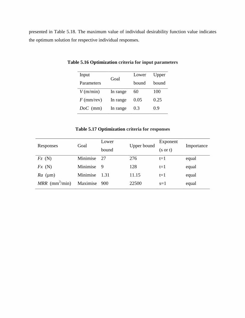
presented in Table 5.18. The maximum value of individual desirability function value indicates

the optimum solution for respective individual responses.

Table 5.16 Optimization criteria for input parameters

Input

Parameters Goal

Lower

bound

Upper

bound

V (m/min) In range 60 100

F (mm/rev) In range 0.05 0.25

DoC (mm) In range 0.3 0.9

Table 5.17 Optimization criteria for responses

Responses Goal Lower

bound Upper bound

Exponent

(s or t) Importance

Fz (N) Minimise 27 276 t=1 equal

Fx (N) Minimise 9 128 t=1 equal

Ra (µm) Minimise 1.31 11.15 t=1 equal

MRR (mm3/min) Maximise 900 22500 s=1 equal

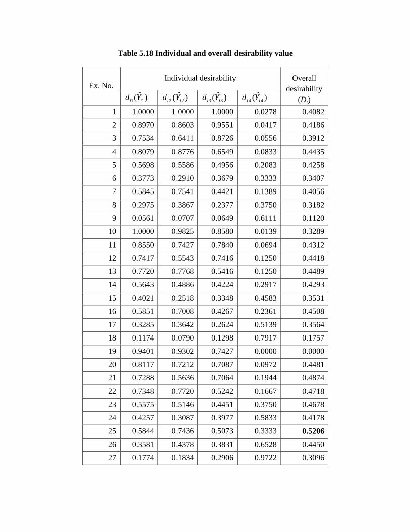
Table 5.18 Individual and overall desirability value

Ex. No. Individual desirability Overall

desirability

(Di) )ˆ( 11 ii Yd )ˆ( 22 ii Yd )ˆ( 33 ii Yd )ˆ( 44 ii Yd

1 1.0000 1.0000 1.0000 0.0278 0.4082

2 0.8970 0.8603 0.9551 0.0417 0.4186

3 0.7534 0.6411 0.8726 0.0556 0.3912

4 0.8079 0.8776 0.6549 0.0833 0.4435

5 0.5698 0.5586 0.4956 0.2083 0.4258

6 0.3773 0.2910 0.3679 0.3333 0.3407

7 0.5845 0.7541 0.4421 0.1389 0.4056

8 0.2975 0.3867 0.2377 0.3750 0.3182

9 0.0561 0.0707 0.0649 0.6111 0.1120

10 1.0000 0.9825 0.8580 0.0139 0.3289

11 0.8550 0.7427 0.7840 0.0694 0.4312

12 0.7417 0.5543 0.7416 0.1250 0.4418

13 0.7720 0.7768 0.5416 0.1250 0.4489

14 0.5643 0.4886 0.4224 0.2917 0.4293

15 0.4021 0.2518 0.3348 0.4583 0.3531

16 0.5851 0.7008 0.4267 0.2361 0.4508

17 0.3285 0.3642 0.2624 0.5139 0.3564

18 0.1174 0.0790 0.1298 0.7917 0.1757

19 0.9401 0.9302 0.7427 0.0000 0.0000

20 0.8117 0.7212 0.7087 0.0972 0.4481

21 0.7288 0.5636 0.7064 0.1944 0.4874

22 0.7348 0.7720 0.5242 0.1667 0.4718

23 0.5575 0.5146 0.4451 0.3750 0.4678

24 0.4257 0.3087 0.3977 0.5833 0.4178

25 0.5844 0.7436 0.5073 0.3333 0.5206

26 0.3581 0.4378 0.3831 0.6528 0.4450

27 0.1774 0.1834 0.2906 0.9722 0.3096

Step 3: The overall desirability values are calculated based on individual desirability function

values, which are combined using geometrical mean (Equation 4.13). The calculated overall

desirability values are presented in Table 5.18. The maximum value (0.5206) of overall

desirability indicates the optimum condition for the combined responses. Based on overall

desirability, the third level (100 m/min) of cutting speed, third level (0.25 mm/rev) of feed and

first level (0.3 mm) of depth of cut are found to possess the maximum value of desirability. The

optimum value of individual responses are Fz = 138 N, Fx = 45 N, Ra = 6.65 µm and MRR =

7500 mm3/min and their contributions of individual desirability are shown in Figure 5.52.

Figure 5.52 Individual and overall desirability value at optimum level

0.5844

0.7436

0.5073

0.3333

0.5206

0.0 0.1 0.2 0.3 0.4 0.5 0.6 0.7 0.8 0.9 1.0

Fz

Fx

Ra

MRR

Overall desirability

Desirability value