Power System Repair and Restoration Optimisation - The ...
156
THE UNIVERSITY OF SYDNEY Faculty of Engineering School of Electrical and Information Engineering Power System Repair and Restoration Optimisation by Theyab R. Alsenani (BSc, 2MSc, PE, CEM, CEA, PMP, PgMP, PMI-ACP) Supervisors: Dr. Jing Qiu and Prof. Zhao Yang Dong A thesis submitted in partial fulfillment for the degree of Doctor of Philosophy May 2020
-
Upload
khangminh22 -
Category
Documents
-
view
1 -
download
0
Transcript of Power System Repair and Restoration Optimisation - The ...

THE UNIVERSITY OF SYDNEY
Faculty of Engineering
School of Electrical and Information Engineering
Power System Repair and
Restoration Optimisation
by
Theyab R. Alsenani
(BSc, 2MSc, PE, CEM, CEA, PMP, PgMP, PMI-ACP)
Supervisors:
Dr. Jing Qiu and Prof. Zhao Yang Dong
A thesis submitted in partial fulfillment for the
degree of Doctor of Philosophy
May 2020
DECLARATION OF AUTHORSHIP
I, Theyab R. Alsenani, declare that this thesis entitled ”Power System Repair and
Restoration Optimisation” and the work presented in it are my own. I confirm
that: this work is original and was done wholly while in candidature for a research
degree at this University; this work has not been submitted in whole or in part for a
degree or any other qualification at this University or any other institution; where
I have consulted the published work of others, this is always clearly attributed;
all the assistance received in preparing this work and main sources have been
acknowledged; I designed the study and wrote the drafts of the papers of parts of
this work that have been published as:
Theyab R. Alsenani, Jing Qiu, “Mathematical Approach for Solving Power Sys-
tems Repair and Restoration Problem,” Saudi Arabia Smart Grid Conference
(SASG), Jeddah, November 2019.
Theyab R. Alsenani, Archie C. Chapman, Zhao Yang Dong, “Power System Re-
pair and Restoration — A Literature Review,” IET Journal of Engineering, 2020.
(Accepted).
Theyab R. Alsenani, Kui Zhang, Jing Qiu, “Studying Power Outages Trends and
the Smart Grid Technologies Investments.” IET Journal of Engineering, 2020.(Ac-
cepted).
Theyab R. Alsenani, Jing Qiu, “Reliability Assessment of Power Distribution Sys-
tem Considering Cold Load Pickups” IEEE Access, 2020. (Submitted).
Theyab R. Alsenani, Jing Qiu, “Advanced Approach for Solving Power Transmis-
sion System Repair and Restoration” IEEE Access, 2020. (Submitted).
Signature:
Date:
i
[REDACTION]

ABSTRACT
This thesis contributes to the power system restoration (PSR) field by studying (in
the aim of improving) the power system repair and restoration (PSRR) which is a
novel problem in PSR. The optimisation concept was our approach and mechanism
in tackling this topic. The thesis provides a basic contribution to the PSRR field
by studying some of its main subjects and presenting improvements to the best
practices in the field. This thesis is built on five research papers related to the
thesis title.
The thesis investigated a large number of high-quality published research papers,
and presented a novel, precise, and comprehensive overview of the topic that could
be considered a good introduction for anyone who would like to learn the topic.
This was presented in chapter two. We have presented a well developed and easy
to understand structure that starts from the basics of PSR and PSRR to their
details and relevant subjects.
Also, in this thesis we provided application-based studies using mathematical opti-
misation techniques, where we model a specific power system then solve the PSRR
problem aiming optimality. Different optimisation techniques were applied, anal-
ysed,and compared for both sides of the problem (i.e. the restoration problem,
and the repair problem) as well as different modelling for power systems. Our
findings in this chapter were interesting and align with other high-quality studies
in the literature. This was presented in details in chapter three.
This thesis also tackled a very important relevant subject which is the system
reliability under certain restoration scenarios. Where we studied the effects of
restoration actions under certain conditions such as cold load pickup events to the
reliability indices of the system. A novel Nature-inspired optimisation technique
was developed and compared to an old technique that was presented in a high-
quality study in the literature. This was presented in chapter four.
ii

iii
We concluded this thesis research by developing a statistical analysis for power
system outages for a decade period of time in the Australian industry as well as
investigating the potential benefits of smart grid technologies and their investments
to the power grid. Many statistical methods were applied and investigated using
state-of-the-art programming tools. This was presented in chapter five. We have
presented very interesting results and findings in this chapter.
KEYWORDS: Power System Restoration, Power System Repair and Restoration,
Mathematical Applications, Power-flow Models, Reliability Analysis, Cold Load
Pickup, Statistical Analysis, Smart Grid Technologies.

Contents
Abstract ii
Contents iv
List of Figures x
List of Tables xiii
Acronyms xv
List of Research Outcomes xvii
Acknowledgements 1
1 Introduction 1
1.1 Thesis Topic Overview . . . . . . . . . . . . . . . . . . . . . . . . . 1
1.2 Thesis Topic Motivation . . . . . . . . . . . . . . . . . . . . . . . . 3
1.3 Thesis Contributions . . . . . . . . . . . . . . . . . . . . . . . . . . 6
1.4 Thesis Organisation . . . . . . . . . . . . . . . . . . . . . . . . . . . 7
2 Literature Review 8
2.1 Introduction . . . . . . . . . . . . . . . . . . . . . . . . . . . . . . . 8
2.1.1 Power System Repair and Restoration . . . . . . . . . . . . 9
iv

CONTENTS v
2.1.2 The Decomposition Technique . . . . . . . . . . . . . . . . . 10
2.1.3 AC Load Pickup Problem AC-LPP . . . . . . . . . . . . . . 10
2.1.4 The Restoration Order problem . . . . . . . . . . . . . . . . 11
2.1.5 The Restoration Problem . . . . . . . . . . . . . . . . . . . 11
2.1.6 Routing Repair Crews Problem . . . . . . . . . . . . . . . . 12
2.2 Power System Modeling for Restoration Study . . . . . . . . . . . . 13
2.2.1 Power Flow Tool in Restoration Study . . . . . . . . . . . . 14
2.3 The Restoration Problem . . . . . . . . . . . . . . . . . . . . . . . . 15
2.3.1 Goals and Steps in Power System Restoration . . . . . . . . 16
2.3.2 Bulk Power System Restoration Issues . . . . . . . . . . . . 17
2.3.3 Restoration Problem in Transmission Systems . . . . . . . . 19
2.3.4 Restoration Problem in Distribution Systems . . . . . . . . . 21
2.3.5 Restoration Optimisation Problem Formulation . . . . . . . 22
2.3.6 Methodologies and Analysis in Restoration . . . . . . . . . . 24
2.3.7 Technical Issues in Restoration Problem . . . . . . . . . . . 25
2.3.7.1 Generators Start-up Sequence Problem . . . . . . 25
2.3.7.2 Cold Load Pickup . . . . . . . . . . . . . . . . . . 26
2.3.7.3 Parallel Restoration . . . . . . . . . . . . . . . . . 26
2.4 The Routing Repair Crews Problem . . . . . . . . . . . . . . . . . . 27
2.4.1 The Routing Repair Crews Problem Formulation . . . . . . 27
2.4.2 RRCP Computational Considerations . . . . . . . . . . . . . 29
2.4.3 Technical Issues in Routing Repair Crews Problem . . . . . 29
2.4.3.1 Stockpile of Resources . . . . . . . . . . . . . . . . 30
2.5 Conclusion . . . . . . . . . . . . . . . . . . . . . . . . . . . . . . . . 31

CONTENTS vi
3 Mathematical Applications on Power System Repair and Restora-
tion 32
3.1 Mathematical Approach for Solving Power Transmission System
Repair and Restoration Problem . . . . . . . . . . . . . . . . . . . . 32
3.1.1 Introduction . . . . . . . . . . . . . . . . . . . . . . . . . . . 32
3.1.2 Proposed Approach . . . . . . . . . . . . . . . . . . . . . . . 33
3.1.3 Mathematical Formulation . . . . . . . . . . . . . . . . . . . 34
3.1.3.1 Power System Operation . . . . . . . . . . . . . . . 36
3.1.3.2 Routing Repair Crews . . . . . . . . . . . . . . . . 36
3.1.3.3 Availability of Resources . . . . . . . . . . . . . . . 37
3.1.3.4 Evaluating Damages . . . . . . . . . . . . . . . . . 37
3.1.3.5 Decoupling Approach . . . . . . . . . . . . . . . . 37
3.1.4 Results and discussion . . . . . . . . . . . . . . . . . . . . . 38
3.1.4.1 Depots Distributing . . . . . . . . . . . . . . . . . 39
3.1.4.2 Results using TSRRP Approach . . . . . . . . . . . 39
3.1.4.3 Results using Decoupling Approach . . . . . . . . . 42
3.1.5 Conclusion and future work . . . . . . . . . . . . . . . . . . 43
3.2 Advanced Approach for Solving Power Transmission System Repair
and Restoration . . . . . . . . . . . . . . . . . . . . . . . . . . . . . 44
3.2.1 Introduction . . . . . . . . . . . . . . . . . . . . . . . . . . . 44
3.2.2 Proposed Method . . . . . . . . . . . . . . . . . . . . . . . . 45
3.2.3 Problem Formulation . . . . . . . . . . . . . . . . . . . . . . 46
3.2.3.1 Operation of Power Transmission System . . . . . . 48
3.2.3.2 Repair Crews Routing . . . . . . . . . . . . . . . . 48
3.2.3.3 Resources Availability . . . . . . . . . . . . . . . . 49
3.2.3.4 Damages Evaluation . . . . . . . . . . . . . . . . . 49
CONTENTS vii
3.2.3.5 Decoupling Methodology . . . . . . . . . . . . . . . 50
3.2.4 Results and discussion . . . . . . . . . . . . . . . . . . . . . 51
3.2.4.1 Depots Allocation . . . . . . . . . . . . . . . . . . 52
3.2.4.2 TSRR Methodology Results . . . . . . . . . . . . . 52
3.2.4.3 Decoupling (Route First) Methodology Results . . 55
3.2.5 Conclusion . . . . . . . . . . . . . . . . . . . . . . . . . . . . 56
4 Reliability Analysis in Power System Restoration 57
4.1 Introduction . . . . . . . . . . . . . . . . . . . . . . . . . . . . . . . 57
4.2 Load Modelling . . . . . . . . . . . . . . . . . . . . . . . . . . . . . 59
4.3 Problem Formulation . . . . . . . . . . . . . . . . . . . . . . . . . . 61
4.3.1 Mathematical Formulation . . . . . . . . . . . . . . . . . . . 61
4.3.2 Selected Test System . . . . . . . . . . . . . . . . . . . . . . 63
4.4 Proposed Methodology . . . . . . . . . . . . . . . . . . . . . . . . . 64
4.4.1 Monte Carlo Platform . . . . . . . . . . . . . . . . . . . . . 64
4.4.2 LSA and A-LSA Optimisation Platform . . . . . . . . . . . 64
4.5 Results and Analysis . . . . . . . . . . . . . . . . . . . . . . . . . . 67
4.5.1 Load Model Results . . . . . . . . . . . . . . . . . . . . . . . 67
4.5.2 Optimal Restoration of One Outage Resulting in CLPU . . . 68
4.5.3 Reliability Assessment Results . . . . . . . . . . . . . . . . . 70
4.6 Discussion . . . . . . . . . . . . . . . . . . . . . . . . . . . . . . . . 72
4.7 Conclusion . . . . . . . . . . . . . . . . . . . . . . . . . . . . . . . . 73
5 Statistical Analysis for Power System Outages 75
5.1 Introduction . . . . . . . . . . . . . . . . . . . . . . . . . . . . . . . 75
5.2 Background . . . . . . . . . . . . . . . . . . . . . . . . . . . . . . . 79

CONTENTS viii
5.2.1 Smart Grid . . . . . . . . . . . . . . . . . . . . . . . . . . . 79
5.2.2 Smart Grid Investments in Australia . . . . . . . . . . . . . 79
5.2.3 Environmental Reasons . . . . . . . . . . . . . . . . . . . . . 80
5.2.4 Weather Trends in Australia . . . . . . . . . . . . . . . . . . 81
5.2.5 The Australian Electricity Infrastructure . . . . . . . . . . . 82
5.2.5.1 National Power Generation Data: . . . . . . . . . . 83
5.2.6 Australian Electric Infrastructure Security: . . . . . . . . . 84
5.2.7 Cascading Outages . . . . . . . . . . . . . . . . . . . . . . . 86
5.3 Study Questions . . . . . . . . . . . . . . . . . . . . . . . . . . . . . 87
5.3.1 Power Disturbances Hypotheses: . . . . . . . . . . . . . . . . 87
5.3.2 Reliability Hypotheses: . . . . . . . . . . . . . . . . . . . . . 87
5.3.3 Used Statistical Methods: . . . . . . . . . . . . . . . . . . . 88
5.4 Research Hypotheses Analysis . . . . . . . . . . . . . . . . . . . . . 88
5.5 Discussion . . . . . . . . . . . . . . . . . . . . . . . . . . . . . . . . 109
5.5.1 Power Disturbances Hypotheses: . . . . . . . . . . . . . . . . 109
5.5.2 Reliability Hypotheses: . . . . . . . . . . . . . . . . . . . . . 110
5.6 Conclusion and Recommendations . . . . . . . . . . . . . . . . . . . 111
6 Conclusions and Future Work 114
6.1 Conclusions . . . . . . . . . . . . . . . . . . . . . . . . . . . . . . . 114
6.2 Future Work . . . . . . . . . . . . . . . . . . . . . . . . . . . . . . . 115
Bibliography 117
7 Appendix 135
7.1 Tools used in this Thesis . . . . . . . . . . . . . . . . . . . . . . . . 135
7.2 Awards and Achievements . . . . . . . . . . . . . . . . . . . . . . . 136

List of Figures
1.1 Illustration of a Restoration Process [21] . . . . . . . . . . . . . . . 5
2.1 A sequence of restoration order problem. . . . . . . . . . . . . . . . 11
2.2 A general framework for the PSRRP. . . . . . . . . . . . . . . . . . 13
2.3 Power system operating states. . . . . . . . . . . . . . . . . . . . . 16
2.4 Power system restoration steps and areas. . . . . . . . . . . . . . . 16
2.5 An example of power system restoration strategy. . . . . . . . . . . 17
2.6 Example of cold load pick-up transient over time. . . . . . . . . . . 19
2.7 A general framework for routing repair crews problem. . . . . . . . 28
2.8 A representation for the impact of routing repair crews performance
on power system. . . . . . . . . . . . . . . . . . . . . . . . . . . . . 28
3.1 K-Means Clustering Algorithm Procedure. . . . . . . . . . . . . . . 34
3.2 Example of repair crews routing and service restoration. . . . . . . 34
3.3 IEEE 30-bus transmission system. . . . . . . . . . . . . . . . . . . . 39
3.4 Cluster assignments and depots. . . . . . . . . . . . . . . . . . . . . 40
3.5 Total restored loads for TSRRP and Decoupling Approach. . . . . . 43
3.6 K-Means Clustering Algorithm Procedure. . . . . . . . . . . . . . . 45
3.7 Example of TSRR operation. . . . . . . . . . . . . . . . . . . . . . 46
3.8 IEEE 30-bus transmission system. . . . . . . . . . . . . . . . . . . . 51
ix

LIST OF FIGURES x
3.9 Cluster assignments and depots. . . . . . . . . . . . . . . . . . . . . 52
3.10 Total restored loads for TSRR and Decoupling Methodologies. . . . 56
4.1 A general figure for delayed exponential model with CLPU. . . . . . 60
4.2 Radial power distribution system. . . . . . . . . . . . . . . . . . . . 63
4.3 General flowchart represents the fundamental mechanisms for the
Advanced LSA Algorithm. . . . . . . . . . . . . . . . . . . . . . . . 66
4.4 Time to Use (TOU) curves of different customers. . . . . . . . . . . 67
4.5 Model for Summer day and Winter day. . . . . . . . . . . . . . . . 68
4.6 CLPU curves of the distribution system. . . . . . . . . . . . . . . . 68
4.7 Low TCL demand and restoration after extended outage. . . . . . . 69
4.8 Low bus voltage restoration without planning. . . . . . . . . . . . . 69
4.9 Optimal load restoration with A-LSA algorithm. . . . . . . . . . . . 70
4.10 Comparison of converging between the Advanced LSA and previous
LSA algorithm. . . . . . . . . . . . . . . . . . . . . . . . . . . . . . 71
4.11 For sample duration, status of sections 9 and 10, and LP10. . . . . 72
5.1 Figure showing the increase of customers number in millions by year. 77
5.2 The Australian total electricity generation by year in GWh. . . . . 77
5.3 The relationship between the number of costumers and the electric-
ity generation. . . . . . . . . . . . . . . . . . . . . . . . . . . . . . . 78
5.4 The average household electricity bills annually and the average
commercial and industrial prices from 2007-17 by ACCC. . . . . . . 78
5.5 Annual average temperature change in the world over 167 years
period. . . . . . . . . . . . . . . . . . . . . . . . . . . . . . . . . . . 81
5.6 Annual sea surface temperature change in Australia over 118 years
period . . . . . . . . . . . . . . . . . . . . . . . . . . . . . . . . . . 82
5.7 A map of electricity transmission lines in Australia. . . . . . . . . . 82

LIST OF FIGURES xi
5.8 Australia total generation by source, 27 July to16 August, 2017. . . 83
5.9 Worldwide Cyber-Attacks events on critical infrastructure and in-
dustrial control systems (ICS). . . . . . . . . . . . . . . . . . . . . . 84
5.10 The administrative principles for the development of the AESCSF. . 85
5.11 Criticality scale and bands by energy market sub-sectors [160]. . . . 85
5.12 SAIFI index for each utility in NEM region . . . . . . . . . . . . . . 102
5.13 Q-Q Plot for SAIFI index in each state. . . . . . . . . . . . . . . . . 103
5.14 CAIDI index for each utility in NEM region. . . . . . . . . . . . . . 104
5.15 Q-Q Plot for CAIDI index in each state. . . . . . . . . . . . . . . . 104

List of Tables
2.1 Power system models and evaluation algorithms for operation stud-
ies including Restoration [119]. . . . . . . . . . . . . . . . . . . . . . 13
2.2 Power system operations planning timeframe [8]. . . . . . . . . . . . 13
3.1 Locations and capacity of the generators. . . . . . . . . . . . . . . . 40
3.2 Summary of damaged components. . . . . . . . . . . . . . . . . . . 40
3.3 Repair crews path for TSRRP. . . . . . . . . . . . . . . . . . . . . . 41
3.4 Times when each component is available for TSRRP (variable zi,t). 41
3.5 Repair crews path for decoupling approach. . . . . . . . . . . . . . 42
3.6 Times when each component is available for decoupling approach
(variable zi,t). . . . . . . . . . . . . . . . . . . . . . . . . . . . . . 42
3.7 Location and capacity of system generators. . . . . . . . . . . . . . 52
3.8 Damages numbers and damaged elements. . . . . . . . . . . . . . . 53
3.9 Repair crews paths for TSRR. . . . . . . . . . . . . . . . . . . . . . 54
3.10 The time when each element is available for TSRR (variable zi,t). . 54
3.11 Repair crews paths for Decoupling Methodology. . . . . . . . . . . 55
3.12 The time when each component is available for Decoupling Method-
ology (variable zi,t). . . . . . . . . . . . . . . . . . . . . . . . . . . . 55
4.1 Results for A-LSA and LSA optimisation algorithms. . . . . . . . . 70
4.2 Results for A-LSA and LSA optimisation algorithms. . . . . . . . . 71
xii

LIST OF TABLES xiii
4.3 Reliability indices values for A-LSA and LSA optimisation algorithms. 71
4.4 Reliability indices values for A-LSA and LSA optimisation algo-
rithms for different procedures. . . . . . . . . . . . . . . . . . . . . 73
5.1 Smart grid applications deployed in the SGSC project [1]. . . . . . . 80
5.2 Australia electricity generation data for the period of 27 July to 16
August 2017. . . . . . . . . . . . . . . . . . . . . . . . . . . . . . . 83
5.3 Descriptive Analysis Table For the USA Department of Energy out-
ages data from 2002 to 2019. . . . . . . . . . . . . . . . . . . . . . . 92
5.4 Descriptive Analysis Table for SAIFI and CAIDI indices statistics
for Australian power system data from 2006-2017. . . . . . . . . . . 102

Acronyms
AC Alternative Current
AMPL Algebric Modeling Programming Language
BSGU Black Start Generating Units
CLPU Cold load Pickup
CP Constrained Programming
DC Direct Current
DER Distributed Energy Resources
DSRRP Distribution System Repair and Restoration Problem
EHV Extra High Voltage
ES Expert System
HV High Voltage
KB Knowledge-Based
LNS Large Neighborhood Search
LP Linear Programming
LPAC Linear Aproximation of Alternative Current
LPP Load Pickup Problem
MIP Mixed Integer Programming
MIQCP Mixed-integer Quadratically-constrained Program
xiv

Acronyms xv
NBSGU None-Black Start Generation Units
NISAC The National Infrastructure Simulation and Analysis Center
PSRP Power System Restoration Problem
PSRRP Power System Repair and Restoration Problem
PSSSP Power System Stochastic Storage Problem
RAD Randomized Adaptive Decomposition
ROP Restoration Ordering Problem
RRCP Rputing Repair Crews Problem
SDP Semidefinite Programming
SOCP Second-order Cone Programming
TSRRP Transmission System Repair and Restoration Problem
UCP Unit Commitement Problem

List of Research Outcomes
The research outcomes during my research candidature are listed as follows:
1. Theyab R. Alsenani, Jing Qiu, “Mathematical Approach for Solving Power
Systems Repair and Restoration Problem,” Saudi Arabia Smart Grid Conference
(SASG), Jeddah, November 2019.
2. Theyab R. Alsenani, Archie C. Chapman, Zhao Yang Dong, “Power System
Repair and Restoration — A Literature Review,” IET Journal of Engineering,
2020. (Accepted).
3. Theyab R. Alsenani, Kui Zhang, Jing Qiu, “Studying Power Outages Trends
and the Smart Grid Technologies Investments.” IET Journal of Engineering, 2020.
(Accepted).
4. Theyab R. Alsenani, Jing Qiu, “Reliability Assessment of Power Distribution
System Considering Cold Load Pickups” IEEE Access, 2020. (Submitted).
5. Theyab R. Alsenani, Jing Qiu, “Advanced Approach for Solving Power Trans-
mission System Repair and Restoration” IEEE Access, 2020. (Submitted).
xvi

Acknowledgements
First of all I would like to thank Allah for his guidance through life storms, for
easing the hard days, and giving me the strength to deal with the ups and downs.
Secondly, I must thank myself to make it to this point despite the unbearable
obstacles that I have faced during this journey. Also, I would like to express
my deepest and heartfelt gratitude and appreciation to my supervisors, Dr. Jing
Qiu, and Prof. Zhao Yang Dong, for all the kindness, guidance, encouragement,
inspiration, assistance, direction, and advice they have given me. Special thanks
and appreciation to Prof. Zhao Yang Dong for his sincere and constant support
and kindness from the beginning of my journey. He was a wise man with a great
character and professional skills, I was lucky meeting him and starting with him in
my journey. You all have been exceptional for me and provided what I needed most
and what I see is the main criteria for students when choosing their supervisors,
kindness and mutual respect. Thank you immensely for your efforts and support.
I also own a special gratitude and appreciation to my previous and first super-
visor in my postgraduate studies Dr. Sumit Paudyal (at Florida International
University, USA) and Prof. Kui Zhang (at Michigan Technological University,
USA), for their immense support in my work. You have all taught and inspired
me in different ways. I gratefully acknowledge the financial support provided by
Prince Sattam Bin Abdulaziz University (PSAU) − Saudi Arabia, and the Saudi
Arabian Cultural Mission in Australia (SACM), for my PhD studies. Thank you
immensely for your support.
Furthermore, I would like to thank all members of the Centre for Future Energy
Networks at the school of Electrical and Information Engineering, the University of
Sydney, for being such a dynamic team and for being supportive and encouraging.
To my friends and colleagues, thank you immensely for your kind support and
efforts.
xvii

Acknowledgements xviii
Finally, to my supportive grandmother, my dear mother, my father, my sisters, my
brother, my uncles, my aunties, thank you sincerely and wholeheartedly for your
relentless support, efforts, prayers, and sacrifices − I could not have completed
this without you.

To . . .my Mom, my fututre wife and children
xix
Chapter 1
Introduction
In this chapter, an introduction for the thesis topic, its motivation and the contri-
butions made to the topic by this thesis will be presented.
1.1 Thesis Topic Overview
The bulk power system currently provides a highly reliable supply of electric power.
Nevertheless, due to growing demand, increasing in size and complexity, deregula-
tion, and economic competition the power system tends to work to its maximum
design limits. In combination with this and due to unpredictable circumstances,
such as natural disasters (e.g. hurricanes, heavy ice, or floods), there is always a
possibility of a system-wide outage. Therefore, it is wise to be ready for such situ-
ation by having an up-to-date, simply understood, and readily accessible restora-
tion plan that allows a fast and arranged recovery from the outage, with resulting
minimum impact on human and economic welfare.
Although blackouts are rare events, they can happen. And when they happen, the
impacts on the industry, commerce, and daily life of people could be quite severe.
The subject of critical importance after a blackout is how to restore the power
system as fast as possible in order to minimise the cost of the outage economically
and socially. As mentioned in the previous paragraph, the electric utilities have
pre-established restoration plans to restore the power system to its normal condi-
tions. However, it must be mentioned that these restoration plans and procedures
are made under specific assumptions of system conditions after the blackout, this
together with the highly stressed conditions encountered after the blackout could
1

Chapter 1. Introduction 2
make these pre-established restoration plans and procedures not valid. In other
words, it reduces the success rate of this practice. The main reason behind the low
success level is that the assumed situations of the power system when the restora-
tion plan was established might vary completely from the system conditions after
the blackout.
As an effort to improve the power system restoration process, too much effort has
been put on computational tools and other methods of system automation. Re-
cently, many power restoration approaches are proposed to provide new techniques
to tackle the problem as a substitute for the older commonly used techniques and
procedures.
The restoration process involves many generation, transmission and distribution,
and load constraints [2],[3]. The Power System Repair and Restoration Problem
PSRRP after a brownout/partial or a blackout/complete is as old as the electric
industry itself. Most electric utilities have developed restoration plans that meet
the requirement of their specific systems. These plans and schemes give a good
deal of awareness into how the restoration procedures are seen by the operators and
planners and what constraints and conditions any scheme should operate under.
Power system repair and restoration after a blackout or brownout is one of the
most important missions for power system operators in a control centre [4]. The
task arises after a system disturbance or a disaster and it is an essential part of
disaster recovery. Specifically, the power system repair and restoration problem
PSRRP is a complex process that aims to (i) repair damaged power system com-
ponents or reactivate disconnected ones in order to (ii) restore the system back to
normal operating conditions after a wide outage. It has been observed that most
power system restoration studies assume that all power system components are op-
erational and only need to be reactivated [5] and this is what differs the restoration
problem from the repair and restoration problem. The PSRRP is tremendously
difficult from a computational angle. It comprises of two challenging subproblems:
(i) the restoration problem and (ii) the routing repair crews problem.
As mentioned in previously, power system operators rely on pre-established restora-
tion schemes to restore a power system to its steady-state operation. This involves
the following steps: (i) evaluate system conditions, (ii) restart the black start
generators, (iii) create transmission path to power other non-black-start NBSGU
generating units, (iv) pick up the critical loads to soothe the power system and (v)
coordinate the islands created by the outage. A typical method to simplify this job
is to split the power system restoration process into steps (e.g. assessment, system

Chapter 1. Introduction 3
restoration and load restoration steps) [6]. However, one common measurement
connecting each of these steps is the generation capability at each restoration step
for soothing the system, creating the transmission skeleton/path and restoring the
load. Succeeding a system blackout, other conventional units might need a crank-
ing power from an external source to be able to start. While other generation units
might have time-constraints so it can be restarted successfully or else they have to
be off-line for a long time, so-called minimum down times previously, they could
be resumed and re-synchronized to the power grid. Consequently, it is vital that,
through power system restoration, to maximise the capability of the generation
units available in the system.
Assuming that there are a limited number of black-start generating units BSGU
and many system constraints on different units, by finding the optimal start-up
sequence of all generating units available in the system, we can reach the maximum
accessible generation.
The power system repair and restoration problem PSRRP consists of dispatch-
ing crews to repair damaged electrical components in order to minimise the size
of the blackout [4]. The PSRRP can be modeled as a multi-objective, multi-
stage large-scale combinatorial mixed nonconvex, nonlinear constrained optimisa-
tion problem, including both routing components and the nonlinear steady-state
power flow equations [4].
The main aim of this thesis research is to optimise/improve the process of PSRRP.
This goal was the main goal tackled in this thesis and covers the main idea behind
the thesis topic. However, there were side studies tied to this topic as well and they
were presented and covered in this thesis chapters. The main relevant subjects
studied were system reliability in restoration process and statistical analysis for
power system outages in the Australian power industry.
The optimisation concept is widely used in scientific research recently. It aims
to enhance the current practices in any scientific field. Thus, the optimisation
component in the thesis topic was our mechanism in dealing with the thesis topic
and its chosen relevant subjects presented in this thesis.
1.2 Thesis Topic Motivation
The restoration of power system after a large disturbance like a natural disaster
is an important process with large consequences on human and economic welfare.

Chapter 1. Introduction 4
Especially with the noticeable climate change in the world and the increase in bad
weather induced disasters. An example for the economic side, the economic loss
from San Diego 24-hour blackout in 2011 that was estimated by 100 million dollars
[4]. Also, large natural disasters such as the hurricane Sandy and Irene usually
cause a blackout that lasts up to a week leaving a huge portion of the population
without heating, air conditioning, lighting, refrigeration, telecommunication use,
etc. Hence, it is sensible that power system restoration is a main mission in
natural disaster recovery. The common used method in power system restoration
is called the “best practice’ in the field, which uses simple optimisation methods by
applying a power system restoration order devoted by governmental related sector
that is based on network utilization heuristic and then uses a greedy agent-based
routing algorithm that implement the restoration order [4].
Thus, the main motivation of this study is to tackle the probable benefits of math-
ematical programming for the repair and restoration of power system after a large
disruption. The objective of the mathematical applications on power system re-
pair and restoration studies represented in this thesis is to dispatch crews to repair
the power system affected elements in the system as quickly as possible objecting
minimising the size of the outage over time. It is known now that the large outages
last many days as the case of hurricane Irene in 2011. The power system repair
and restoration problem PSRRP is a very complex problem even when ignoring
all transient aspects and considering the steady-state behaviour of the power grid.
The problem is a large scale mixed nonlinear, nonconvex optimisation problem
when modeled globally. Additionally, the two subproblems of the PSRRP which
are the sequence of restoration and the repairs job scheduling are complex from
a computational point of view. Where the repair work scheduling is equivalent
to a pickup and delivery vehicle-routing problem minimising the sum of delivery
completing time periods [4].
In this thesis research we focus on how to use mathematical programming methods
to improve the “best practice” in the this field. This paper [4] which inspired
the thesis topic idea, proposes a scalable algorithm to the TSRRP based on two
stages approach that decouples the restoration order and the routing aspects of
the problem. The first stage is a restoration order problem ROP that finds the
restoration sequence that minimises the power outage size, ignoring the logistics
of scheduling repairs works. The second stage is a large-scale pickup and repair
routing problem that applies the restoration orders computed in the first stage.
Both stages are found to be computationally complex as mentioned in [4].

Chapter 1. Introduction 5
Figure 1.1: Illustration of a Restoration Process [21]
The restoration order problem ROP is a mixed nonlinear, nonconvex optimisation
problem as it considers the power flow equations for active and reactive powers.
Additionally, the power restoration process is applied when the power system is
damaged and when the objective is to restore and serve as much load as possible,
which is different from the traditional optimal power flow problems [4]. Thus,
solving the power flow equations is challenging in such conditions [7].
The second stage is the routing problem which is modeled mathematically in this
thesis. Our main reference [4] findings shows that a constrained program in ad-
dition to a large neighborhood search and a randomised adaptive decomposition
provide a scalable approach to scheduling the repairs. Their approach was not
investigated in this thesis, however, a similar mathematical approaches was devel-
oped and studied on specific benchmarks.
Additional motivation for studying this topic is the importance and criticality
of power system reliability especially in outages management. Costumers need
a reliable power supply and consider the power supply reliability an important
criteria when choosing their power provider.
Another motivation is that the high importance of having statistical analysis stud-
ies that rank the power utilities and represent the performance of these utilities to
the public, as well as providing a detailed answers to the utilities for where their
vulnerabilities are in order to enhance their services.
Chapter 1. Introduction 6
1.3 Thesis Contributions
The contributions of this thesis research are performed on many aspects of its topic.
We tried to cover the thesis topic fully. At first, we did an extensive literature
review for the topic. The literature review was done on hundreds of high quality
peer-reviewed references that tackle all possible sides of the problem and present
them to the readers in a clear an systematic way.
As recent research in power system repair and restoration is pushed toward a more
efficient restoration strategies, to save costs for both utilities and costumers. We
have developed mathematical programming methods for the problem to rise the
efficiency of power restoration process (i.e minimising the time of outage duration),
thus minimising the duration time of outage by improving the techniques of tack-
ling the whole restoration problem; then we applied them on different standard
IEEE systems. The mathematical representation used a common model (DCOPF)
for one of the studies, then we extended and enhanced the mathematical represen-
tation of the power system with an advance and more accurate model that takes
voltages magnitudes, line losses and reactive power (which are critical for contin-
gencies studies) into account called (LPAC-OPF) [8] in another study. We have
shown in these studies that used model that represents the operational/physical
aspects of the power system is a major variable in the results accuracy and relia-
bility. A major contribution of these two studies is showing that the restoration
problem can be approximated by a mixed integer program MIP which linearises
the power flow equations and represent the operational/physical aspects of the
power system in two different linear models.
Another important contribution of this thesis research was developing and imple-
menting an advanced heuristic method to assess the reliability of power distribu-
tion system under abnormal power restoration conditions such as cold load pickup
events (CLPU).
An additional contribution of this thesis research was studying the power system
outages using statistical methods which provides guidance to the power utilities in
Australia in terms of decision-making regarding the optimality of their networks
operations. Final contribution was assessing the probable benefits of smart grid
technologies in power outages prevention.

Chapter 1. Introduction 7
1.4 Thesis Organisation
The thesis content is systematically organised and presented as follows. Chap-
ter 2 presents the related works, Literature review of the thesis topic which gives
a comprehensive information about this thesis topic and all its related subjects.
Chapter 3 presents the related works, Mathematical Applications on Power Sys-
tem Repair and Restoration. In this chapter we present two application-based
studies on the problem, where one is a basic study and the next one is an im-
proved application of the same study. Chapter 4 presents the related works,
Reliability Analysis on Power System Restoration. In this chapter we present a
detailed reliability analysis for the system in restorative state under special con-
dition (CLPU). Chapter 5 presents the Statistical Analysis for Power System
Outages. In this chapter we investigate the Australian gird outages data and
present useful recommendations for the industry. Chapter 6 summarises our
findings and gives directions for future work.
In the next chapter, the related literature will be reviewed.
Chapter 2
Literature Review
With the rapid pace developments and improvements in the power industry tech-
nologies, new technical articles and research efforts addressing the raising power
system repair and restoration issues is brought out to the industry. Given the
recent focus of research activity on the Power System Restoration Problem PSRP
and the Power System Repair and Restoration Problem PSRRP, and the prolif-
eration of approaches adopted by them, a comprehensive review of methods and
techniques is needed. This chapter systematically and comprehensively reviews
work on the power system restoration problem and the power system repair and
restoration problem. The chapter covers almost all aspects of these two subjects.
The goal of this chapter is to clarify the problem nature and considerations, formu-
lation, and technical issues. The hope of the is chapter is to give new researchers
on the restoration and repair field a good understanding of the problem in order
to improve the current practice in the field.
2.1 Introduction
As stated in the first chapter, power system operators rely on pre-established
restoration schemes to restore/recover the network to its steady-state operation.
This involves the following steps: (i) evaluate system conditions, (ii) restart the
black start generators BSGU, (iii) create transmission path to power different non-
black-start generation units NBSGU, (iv) pick up the critical loads to soothe the
power network and (v) coordinate the islands formed by the outage. A typical
method to make this job simple is to split the power system restoration course
into steps (e.g. groundwork, system restoration and load restoration steps) [6].
8

Chapter 2. Literature Review 9
However, one mutual measurement connecting every one of these steps is the gen-
eration capability at every restoration step for soothing the network, creating the
transmission skeleton/path and recovering the load. Following a network black-
out, some conventional units will need a cranking/starting power from an external
source in order to be able to start. Other generation units might have time-
constraints so it can be restarted successfully or else they have to be off-line for
a long time, so-called minimum down times before they can be restarted and re-
synchronized to the power network. Consequently, it is vital that, through power
network restoration, to maximize the capability of the generation units available
in the system. Assuming that there are a limited number of black-start generating
units BSGU and many system constraints on different units, by finding the best
start-up sequence of all generating units available in the network, we can reach
the maximum accessible generation.
The power system repair and restoration problem PSRRP consist of sending off
crews/teams to fix damaged network elements to minimize the magnitude of the
blackout [4]. The PSRRP can be expressed as a multi-objective, multi-stage large-
scale combinatorial mixed nonconvex, nonlinear constrained optimisation problem,
which includes the routing elements and the nonlinear steady-state power flow
equations [4].
2.1.1 Power System Repair and Restoration
The first step in solving the PSRRP is to define the power system. In general, let
P be the power system comprising a set of B buses and L lines, P = (B,L), and
a graph G = (S,W ) where S are the locations of interest for restoration, and W
are the set of switches among these locations [4]. Each bus is categorized by its
real and reactive power desired. The line between every two buses is characterized
by its electrical admittance and line thermal capacity. A detailed, concrete model
is instantiated by defining the constraints that apply for a particular setting or
network. Specifically, all or some of the operational and engineering constraints
stated in Section 2.3.5 are applied to this optimisation problem based on the
system’s nature (transmission or distribution).

Chapter 2. Literature Review 10
2.1.2 The Decomposition Technique
The PSRRP is best to be approached as a multi-stage problem for scalability
benefits, decomposing the power system restoration/operation and the routing
repair crews problem RRCP. The first stage comprises a set of load pickup problems
LPP named restoration order problem ROP which is independent of the second
problem the routing repair crews problem RRCP [9]. The second stage of the
PSRRP is an RRCP which receives a group of precedence constraints that deliver
a partial order from the ROP resultant repairs. The computational benefits of
decomposing the PSRRP in this way arises because the LPP/ROP can be treated
independently of the routing repair crews problem RRCP [4].
2.1.3 AC Load Pickup Problem AC-LPP
The optimisation problem could be formulated as follows:
max∑n∈N
plnln (2.1)
s.t. pgn − plnln =∑
(n,m)∈L
pnm ∀(n ∈ N) (2.2)
qgn − qlnln =∑
(n,m)∈L
qnm ∀(n ∈ N) (2.3)
pnm = v2ngnm − vnvmgnm cos(θn − θm)
− vnvmbnm sin(θn − θm) ∀(n,m ∈ L) (2.4)
qnm = v2nbnm − vnvmbnm cos(θn − θm)
− vnvmgnm sin(θn − θm) ∀(n,m ∈ L) (2.5)
p2nm + q2
nm ≤ S2nm ∀(n,m ∈ L) (2.6)
The optimisation objective fucnction (2.1) maximizes the active load served.
Constraints (2.2–2.3) represent Kirchhoff’s Current Law, the flow conservation.
Constraints (2.4–2.5) capture the active and reactive power flow on lines and
constraint (2.6) applies lines thermal limits.
The optimisation inputs are as follows: The power network P = (N,L), the
admittance between buses n and m, gnm and bnm, the required active and reactive
loads at bus n, pln qln, and the loading limit on line (n,m) Snm.

Chapter 2. Literature Review 11
The optimisation variables are as follows: The phase angle of bus n, θn ∈(−∞,∞), the voltage magnitude of bus n, vn ∈ (vminn , vmaxn ), active power gen-
erated at bus n, pgn ∈ (pg(min)n , p
g(max)n ), and the reactive power generated at bus
n, qgn ∈ (qg(min)n , q
g(max)n ), percentage of active load served at bus n, ln ∈ [0, 100],
active and reactive power on line (n,m) , pnm qnm ∈(-Snm,Snm).
2.1.4 The Restoration Order problem
The first phase of the PSRRP is comprised of modeling an LPP as power system
restoration/operation problem. Where the objective is to obtain a steady state
solution for the system that pushes the system to accept as much load as feasible.
This operation is repeated R times where R is the set of damaged components
in the system. A precedence constraint M is injected from each previous LPP
solution to the follows LPP problem after repairing one system’s component each
time. This process is repeated until reaching the final steady state of the system
that comes after repairing the R set of damaged components. This process is also
called a restoration order problem ROP [4].
Figure 2.1: A sequence of restoration order problem.
2.1.5 The Restoration Problem
The power system main troubles are mainly triggered by transient faults and
natural disasters such as Hurricanes and primary happen in power transmission
systems. Many of these sources of supply interruption are because of temporary
faults like lightening, which is cleared instantly by the system protective relays.
However, in other cases, these short-term sources lead to cascading effects which
could be lasting and that may include the loss of generation units, loads and
interconnections. These following impacts may result in partial or complete failure
of the unfaulted sides of the power system. Consequently, assessing the system
status after fault may help to enhance restoration.
At the early phases of the restoration course, the system operator’s main objective
is to steady the network’s constraints and recover the key transmission system.
When the goal moves from sustaining proper situations for load recovering to

Chapter 2. Literature Review 12
minimising the blackout effect, then the planned restoration technique might be
implemented. The main part in initial efforts to restoring power system is in
restart and rebuilding plans for generating units and transmission corridors in
conjunction to load pickup in these initial phases. Because that could help in
getting generators to their steady generation points and upholding the voltage
profile. To minimise the probability and period of major failures in bulk power
systems, initial preparation, remedial and restorative arrangements are essential.
In the past decades, the industry has commenced considerable efforts in these
areas. However, there is still need for additional efforts in the path of decreasing
the period of an outage.
2.1.6 Routing Repair Crews Problem
The second phase of the PSRRP decomposition approach is the routing repair
crews problem RRCP, which is approached as a vehicle routing problem (VRP).
The RRCP is also known as the pickup and delivery vehicle-routing optimisation
problem. This problem was studied for long-term in operations research [4]. Al-
though, for practical system sizes, it is hard to obtain an optimal solution for it,
especially when the objective function is to minimise the nominal transport time,
which is linked to the PSRRP objective function [4]. It was shown in [9] that mixed
integer programming MIP methods face major scalability issues. In addition, the
restoration objective, which is maximising the served load or minimising the black-
out size generalizes the optimal transmission switching problem, which was shown
to be difficult for MIP solvers [10]. Moreover, it was shown to be difficult even
with the use of linear approximations for the power-flow equations [4].
The RRCP receives two inputs from the ROP. The restoration sites graph rep-
resentation G and the group of precedence constraints obtained M . The RRCP
calculates a routing scheme for the repair crews that satisfies the stated problem
constraints and the precedence constraints received from the ROP. The objective
of the RRCP is to minimise the overall time of repair visits. Fig. 2.2 gives an
illustration for the PSRRP general framework.

Chapter 2. Literature Review 13
Figure 2.2: A general framework for the PSRRP.
2.2 Power System Modeling for Restoration Study
Fundamentally, restoring or restarting a power system relies heavily on tools and
methods for modelling network transients and power-flows. These tools are essen-
tial to forming any restoration plan. Modeling the power system is the process
of forming an approximation of a real-world system. Modeling the power system
infrastructure is the first part of doing any study on the system such as planning,
operation, restoration etc. An accurate model results in more accurate results, al-
though it may lead to the need for more computational time. Consequently, there
is a trade-off between the results accuracy and the computational time required
[11]. These trade-offs are summarised in Tables 2.1 and 2.2. Thus, the power
system restoration results are only as accurate as the physical assumptions that
are made.
Table 2.1: Power system models and evaluation algorithms for operation stud-ies including Restoration [119].
Table 2.2: Power system operations planning timeframe [8].

Chapter 2. Literature Review 14
2.2.1 Power Flow Tool in Restoration Study
The AC power flow equations of real and reactive power provide the main op-
erational constraints in restoration studies, as they are nonlinear and nonconvex
(see, for example, [Mhanna, PSCC, 2016]). Which even when given to a nonlinear
solver like IPOPT [12], it is not assured that it will converge to feasible results
or it may produce low-voltage results that are not practical in reality [13]. Thus,
linear approximations to the AC Power-flow equations have been introduced.
The AC power flow equations:
pnm = v2ngnm − vnvmgnmcos(θn − θm)
−vnvmbnmsin(θn − θm) ∀(n,m ∈ L) (AC1)
qnm = v2nbnm − vnvmbnmcos(θn − θm)
−vnvmgnmsin(θn − θm) ∀(n,m ∈ L) (AC2)
The most common approximation used in power system applications is the DC
Power flow model [14]. This model was derived through assumptions and simpli-
fications such as assuming the voltage magnitudes of two connected buses is 1.0
per unit, the conductance of the physical network is very small comparing to the
susceptance, and the reactive power is small and could be neglected comparing
to the real power. Additionally, the phase angle difference is assumed to be very
small. Consequently, The DC model can not measure reactive power, voltage mag-
nitudes, and system losses, which are very important aspects of the restoration
study.
That led the research community to try to introduce better linear approximations
such as the approximation called LPAC [9]. The LPAC model is derived through a
set of mathematical approximations and relaxation steps. This model successfully
considers the reactive power, line losses, and voltage magnitudes. Thus, it is
obviously performing better than the DC model in the case where the system is
weak and stressed as the situation in the restoration study. For more details on
the LPAC model refer to [9].
Another approximation approach is to develop efficient convex relaxations, with
the second-order cone programming (SOCP) and the semidefinite programming
(SDP) relaxations recieving much attention. The SDP relaxation is proven to be
exact or tight on a variety of case studies [15], [16]. However, in many practical

Chapter 2. Literature Review 15
OPF instances, the SDP relaxation yields inexact solutions [17], [18], and more-
over, an AC feasible solution cannot be recovered from the SDP relaxed solution.
The main drawback of the SDP relaxation is that it cannot be readily embedded
in MIP models as easily as LP models. Similarly, much attention has recently been
given to the SOCP relaxation [19], [20], [21], [22]. One advantage of the SOCP
relaxation of the AC optimal power flow problem is that it is straightforward to
extend it to a mixed-integer quadratically-constrained program (MIQCP), to suit
applications with discrete variables, such as the PSRRP. More efforts have been
made to linearise the power-flow equations such as in [23].
All power-flow models such as DC model and LPAC model and other richer models
exhibit Braess’s paradox in RRCP.
Braess’s Paradox definition: Adding additional capacity to a system when the
moving objects selfishly [least resistance] choose their own route, can in some
cases reduce the over-all performance [24].
2.3 The Restoration Problem
Generally, many problems in power system restoration contain several actions
such as reactive power balance, load-generation balance, control, monitoring, pro-
tective system structures, energy storage systems, distributed energy resources,
planning, and training. To analyse the power system restoration problem, it is
good to mention the four different states of the power system as illustrated in Fig.
2.3 [25]. In the normal state, system reconfiguration could be done to minimise
losses, balance loads and advance operation efficiency. When the system operating
constraints are placed in jeopardy, the system will enter the pre-outage state, for
example, when an element is being overloaded such that protection devices may
disconnect it. Preventive actions in this state could take the network back to its
normal operational conditions. Some activities in the pre-outage state have the
same features of restorative state action. The power system will enter the outage
state when a component in the system is out of service, either because of a failure
or overloading. In this case, the component cannot go back to normal operation
conditions before the source of its outage is cleared. If the outage cause is cleared
it is likely for the network to go back to its normal operational condition. Other-
wise, the system will enter the restorative state which will deliver the best possible
service with the left system components. In case another outage occurs during the
restorative state that will move the system to the outage state again.

Chapter 2. Literature Review 16
Figure 2.3: Power system operating states.
2.3.1 Goals and Steps in Power System Restoration
An illustration for the power system restoration steps and aimed goals are given in
Fig. 2.4 below [26]. Before going into details, we give an overview of the objectives
and strategies employed in the restoration problem.
Figure 2.4: Power system restoration steps and areas.
The restoration objective is to recover as much load as conceivable as fast as
possible starting from critical loads at the early stage of restoration in order to
steady the power network and coordinate the formed islands if there is any, which
is very different from the routing repair crews objective which is the minimum
travel distance between sites, that will be discussed in the routing repair crews
problem RRCP in later sections.
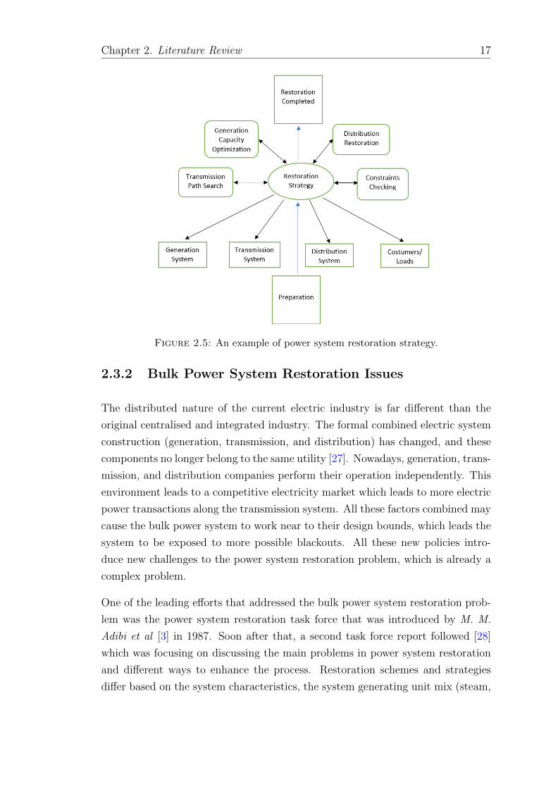
An applied strategy to simplify automatic power system restoration is to create
separate modules for generation, transmission, and distribution systems. These
parts are connected and synchronised over the strategy module for the recovering
of power networks [25]; see Fig. 2.5.
After a major disturbance in a power system, the generation capability must be
maximised in order to rapidly restore the whole power system. Though, it is a
complex combinatorial problem to optimise the utilization of available BSGU [25]
as we describe in later sections.
Chapter 2. Literature Review 17
Figure 2.5: An example of power system restoration strategy.
2.3.2 Bulk Power System Restoration Issues
The distributed nature of the current electric industry is far different than the
original centralised and integrated industry. The formal combined electric system
construction (generation, transmission, and distribution) has changed, and these
components no longer belong to the same utility [27]. Nowadays, generation, trans-
mission, and distribution companies perform their operation independently. This
environment leads to a competitive electricity market which leads to more electric
power transactions along the transmission system. All these factors combined may
cause the bulk power system to work near to their design bounds, which leads the
system to be exposed to more possible blackouts. All these new policies intro-
duce new challenges to the power system restoration problem, which is already a
complex problem.
One of the leading efforts that addressed the bulk power system restoration prob-
lem was the power system restoration task force that was introduced by M. M.
Adibi et al [3] in 1987. Soon after that, a second task force report followed [28]
which was focusing on discussing the main problems in power system restoration
and different ways to enhance the process. Restoration schemes and strategies
differ based on the system characteristics, the system generating unit mix (steam,

Chapter 2. Literature Review 18
hydro, gas turbines and combined cycles units), and the extent of the system’s
interconnection.
When designing a practical restoration plan, the initial settings of the network as
well as the issues that arise during the restoration process are of big importance.
One of the main measures of system stability is the network’s frequency. The
network’s frequency indicates the balancing state between the power supplied and
the loads.
The acceptable operation for the system is found by maintaining the frequency
nominal value during operation and make it limited to specific limits. Nevertheless,
because of the abnormal nature of the system during system restoration, it is
difficult to maintain a perfect balance between the supplied and the consumed
real power at all time stages. Also, due to the present network configuration and
the turbine-governor characteristics of the power plants, the load pickup amount
at any time point is limited.
From practice, it is being noted that when a load raise of 5 percent from the
synchronised system’s generation that leads to a 0.5 Hz decrease in the system’s
current frequency [3]. More discussion on the frequency-real power response is
introduced in [25].
Another major issue that arises during restoration is the voltage-reactive power
relationship. The voltage profile during restoration is of an important considera-
tion. In order to keep the system within normal operating conditions, the voltages
must be maintained between certain minimum and maximum values. Generally, a
good voltage profile is obtained by having enough reactive power sources that are
able to satisfy the systems requirements. The reactive power is usually provided
and/or adjusted by generating units, synchronous condensers, shunt capacitors
and other power system electronics. However, due to the nonlinear behaviour
of reactive power and the need to be sent on long distances, fulfilling the reac-
tive power balance is not easy. Furthermore, other phenomena’s in power system
restoration such as energising high voltage transmission lines results in charging
currents which cause an unexpected change in the system’s reactive power. The
mentioned unexpected changes are recognised as switching operations transient
voltages, which rise the voltage magnitudes to unsafe points subject to the trans-
mission line features. These issues along with others arise the importance of proper
allocation of reactive power sources and their control capabilities in order to ap-
ply a good restoration plan. More discussion on transmission corridors energising
could be found in [29].
Chapter 2. Literature Review 19
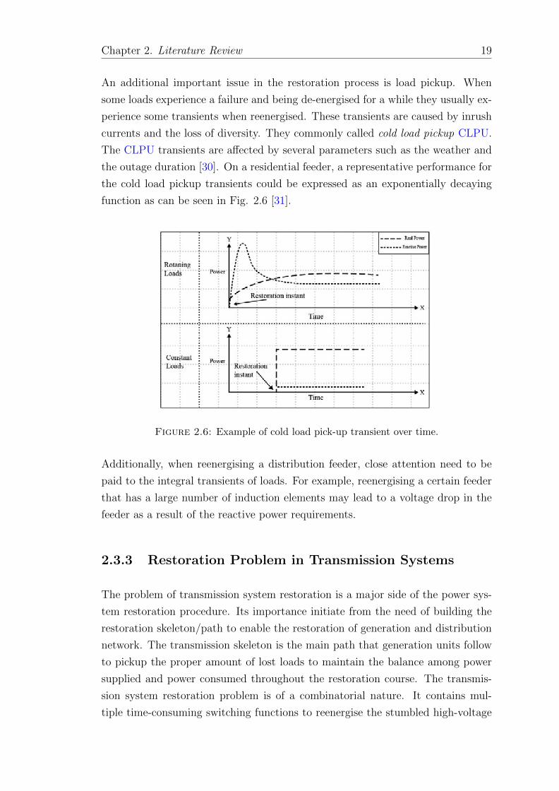
An additional important issue in the restoration process is load pickup. When
some loads experience a failure and being de-energised for a while they usually ex-
perience some transients when reenergised. These transients are caused by inrush
currents and the loss of diversity. They commonly called cold load pickup CLPU.
The CLPU transients are affected by several parameters such as the weather and
the outage duration [30]. On a residential feeder, a representative performance for
the cold load pickup transients could be expressed as an exponentially decaying
function as can be seen in Fig. 2.6 [31].
Figure 2.6: Example of cold load pick-up transient over time.
Additionally, when reenergising a distribution feeder, close attention need to be
paid to the integral transients of loads. For example, reenergising a certain feeder
that has a large number of induction elements may lead to a voltage drop in the
feeder as a result of the reactive power requirements.
2.3.3 Restoration Problem in Transmission Systems
The problem of transmission system restoration is a major side of the power sys-
tem restoration procedure. Its importance initiate from the need of building the
restoration skeleton/path to enable the restoration of generation and distribution
network. The transmission skeleton is the main path that generation units follow
to pickup the proper amount of lost loads to maintain the balance among power
supplied and power consumed throughout the restoration course. The transmis-
sion system restoration problem is of a combinatorial nature. It contains mul-
tiple time-consuming switching functions to reenergise the stumbled high-voltage

Chapter 2. Literature Review 20
transmission corridors. In general, the transmission network restoration is a mixed
variable problem, the transmission line status (i.e. connected or disconnected) is
binary and the other constraints are real numbers. Thus, the restoration problem
of the transmission network is formed as an optimisation problem that has multi-
ple objectives and subjected to operational and engineering constraints. Problems
faced in transmission system restoration include:
Energising high or extra-high voltage EHV transmission corridors lead to
over-voltages transients [32].
Energising unloaded or softly loaded EHV transmission corridors, or under-
ground cables will lead to constant frequency over-voltages [25].
Constant over-voltages could overexcite transformers, which may lead to
overheating or harmonic distortions, and may lead to generator self-excitation,
and instability [25].
Reenergising transmission lines can lead to a harmonic-resonance. The har-
monic resonance on long softly loaded transmission lines can lead to an
extremely high-voltage which could also be enlarged by transformer over-
excitation [33].
The switching operation of circuit breakers will lead to high transients.
Switching operation transients on lengthy HV transmission corridors, even
of a small period of time, can incur arrestor failures, especially if joined with
sustained over-voltages situations [25].
For the duration of the transmission system restoration, at any time, the
reactive absorption or the under-excitation capability of the generation units
in the power system is important to keep a good and steady transmission
line re-energisation [25].
For the period of the transmission restoration course, the issue of lag and
lead reactive power ability bounds of synchronous machineries in the re-
established network needs appropriate consideration. The mentioned limits
are significant to keep voltages under the acceptable limits for high charging-
current necessities of unloaded and softly loaded transmission lines, or for
the large reactive-currents drained by the start-up of the power system plant
ancillary engines [25], [34], [35], [36].

Chapter 2. Literature Review 21
Most of these transient issues are addressed by manipulating the following control
variables:
Assuring adequate under-excitation capability on the generators.
Adjusting transformer taps.
Switching on shunt-reactors.
Considering loads with low power-factor.
Controlled islanding.
Since modifications to these control variables are influenced by the constraints
forced by plants and system operational requirements, the entire outcome of the
control variables would govern the decision if the transmission line could be reen-
ergised effectively or not [37], It is this coupling between the control elements that
makes the RP such a difficult problem to solve. Nevertheless, the transmission
lines considered for recovering might not be energised instantaneously, and for
every transmission switching process we must consider it solely based on many
factors such as Braess’s Paradox [24] and other network effects.
Many procedures that are dealing with the transmission system restoration differ-
ent issues discussed above can be found in the following references [38],[39],[40],[41],
[42], [43],[44],[45],[46], [5], [32],[47],[30],[48],[49],[50].
2.3.4 Restoration Problem in Distribution Systems
Distribution network restoration or typically named load restoration is the field
of interest in recent years. This increased interest is a normal outcome of new
practices related to deregulation, marketing and the technical advances used in
the distribution network. The restoration problem in general aims to minimise
the impact and duration of the outage by discovering the best sequence of healthy
distribution feeders that should be recovered. This problem is similar to the unit
commitment problem UCP [51]. The distribution network restoration problem
with the UCP exhibit similarities in nature and structure which might advise that
the two problems are duals of each other [25].
Some issues in distribution system restoration problem might be because of these
parameters [25]:

Chapter 2. Literature Review 22
Combinatorial nature of the problem.
Bulky network dimensions and a large number of integrated devices.
Distributed generation units.
Several operational objectives that might be opposite to each other.
The need for fast network restoration.
The likability of suboptimal solutions.
The problem of distribution network restoration aims to re-establish the service
after the outage and minimise its impacts on economic and human welfare. This
mission is started once a significant portion of the transmission system has been
recovered to a sable state. In this process, the fluctuations in the system’s fre-
quency and voltage control are not the main concern for the system’s operator
since some generation and loads have been connected. However, there are several
challenges facing the operator due to the different decision variables in the opti-
misation formulation, the large dimension of the network and the combinatorial
nature of the problem. More discussion on issues in distribution system restora-
tion could be found in the following references, load estimation [52], loss reduction
[53], distribution network reconfiguration [54], among others.
2.3.5 Restoration Optimisation Problem Formulation
The main goal of service restoration/recovering is to restore/recover as much dis-
tribution network loads as we can considering the critical loads first by minimising
the out-of-service load zones. This could be done by shifting the de-energised loads
through system reconfiguration to different healthy feeders in the system with no
violations to the operational and physical constraints of the system.
As mentioned in previous sections, the power system restoration optimisation
problem could be expressed as a mixed nonlinear, nonconvex, combinatorial, con-
strained problem with the following possible objectives [55]:
Maximising the summation of power transfer capability.
Maximising the restored power to the unfaulted areas.
Minimising the switching operations.

Chapter 2. Literature Review 23
Minimising the losses in the created network.
Minimising the total time of the restoration process.
These possible objective functions are subjected to a whole or a partial set of the
following constraints based on the restoration system:
Voltage limits.
Frequency limits.
Power balance constraints for both real and reactive power.
Power-flow equations.
line thermal limits.
Current limits.
Load constraints.
Switching time.
Loads priority.
Time of finding restoration solution.
Reliability.
Feasibility.
Man-machine interface.
Radiality (specific for distribution networks restoration problems).
Transient Stability.
Generators ramp rates.
Feasibility of islanding.
A major task in finding a restoration plan is formulating these constraints in
a tractable mathematical representation. This consideration was touched on in
Section 2.2, with respect to power-flow tools. More generally, in the past, the
more common methods used were knowledge-based (KB) and expert system (ES),
Chapter 2. Literature Review 24
and they were deployed and used for specific systems. After 1993 power system
restoration studies started using and applying other non-traditional techniques
[55] including heuristic, optimisation-based and automated restoration planning
methods, as discussed next. After this, we discuss some of the many technical
issues that arise in restoration problems.
2.3.6 Methodologies and Analysis in Restoration
Given to the operational problems identified in power system restoration, studying
the problem for off-line planning or on-line/near on-line operations is significant.
Studying the power system restoration problem needs an accurate model for the
system as mentioned in previous sections, and the use of many analytical tech-
niques. These techniques must consider the static, transient and dynamics of the
network to be able to yield a suitable restoration plan. Thus, to provide restora-
tion plans that can support the operator in decision-making through power system
restoration, many methods and techniques were applied in the bulk power system,
transmission system, and distribution system as follows:
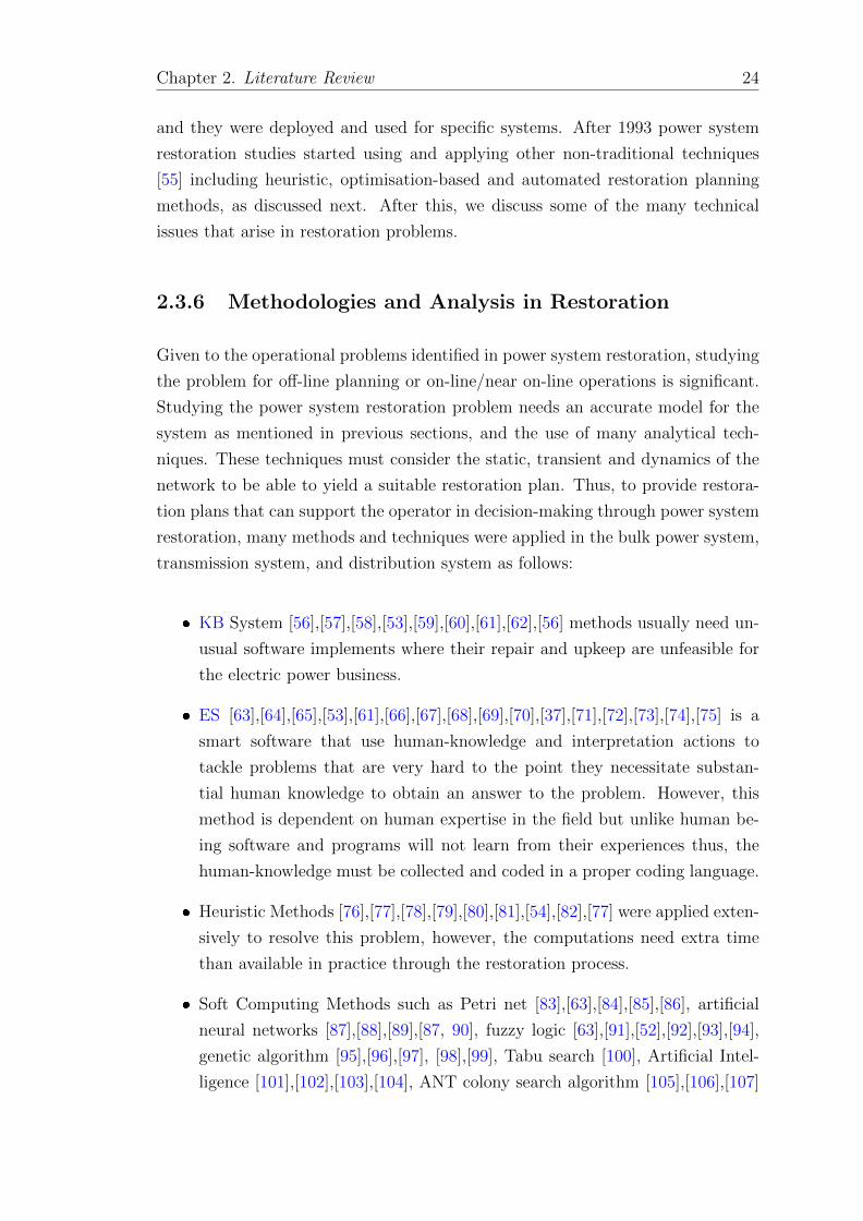
KB System [56],[57],[58],[53],[59],[60],[61],[62],[56] methods usually need un-
usual software implements where their repair and upkeep are unfeasible for
the electric power business.
ES [63],[64],[65],[53],[61],[66],[67],[68],[69],[70],[37],[71],[72],[73],[74],[75] is a
smart software that use human-knowledge and interpretation actions to
tackle problems that are very hard to the point they necessitate substan-
tial human knowledge to obtain an answer to the problem. However, this
method is dependent on human expertise in the field but unlike human be-
ing software and programs will not learn from their experiences thus, the
human-knowledge must be collected and coded in a proper coding language.
Heuristic Methods [76],[77],[78],[79],[80],[81],[54],[82],[77] were applied exten-
sively to resolve this problem, however, the computations need extra time
than available in practice through the restoration process.
Soft Computing Methods such as Petri net [83],[63],[84],[85],[86], artificial
neural networks [87],[88],[89],[87, 90], fuzzy logic [63],[91],[52],[92],[93],[94],
genetic algorithm [95],[96],[97], [98],[99], Tabu search [100], Artificial Intel-
ligence [101],[102],[103],[104], ANT colony search algorithm [105],[106],[107]

Chapter 2. Literature Review 25
are original methods that impersonate the system operator movements. Nev-
ertheless, the lack of accuracy may not lead to an accurate solution at a
critical time such as in the restoration study.
Some common optimisation techniques have been used to deliver more pre-
cise solutions. Most of them rely on: mathematical programming [108],
dynamic programming [109], mixed-integer programming method [110],a
restoration index [111], Benders decomposition [112], and Lagrangian re-
laxation [113]. These optimisation methods need a suitable and accurate
model to reach global optimality.
Hybrid Models [114],[115],[116],[117],[118], [119],[120],[121] it was observed
from the literature that there is a necessity for development to the current
restoration methods. As some algorithms are simple but provide a subopti-
mal solution other give accurate solutions but they are complex. To reach an
improvement in the current techniques, one algorithm should complement
the other. Thus, many algorithms have been merged together in order to
reach an improved performance and meet the industry needs.
2.3.7 Technical Issues in Restoration Problem
There are many issues arise during the system restoration. They include all
restoration areas; generation, transmission, distribution, operations, and compu-
tation. In this section, we will cover some of the main problems and issues during
system restoration.
2.3.7.1 Generators Start-up Sequence Problem
Generation units are categorised into two types, the Black Start Units BSGU and
the Non-Black Start Units NBSGU. The BSGU has the ability to start by itself,
examples for this type are combustion turbine units and Hydro units. On the other
hand, the NBSGU does not have this ability and needs a starting power to be pro-
vided from an external source to be able to start, an example of this type is steam
turbine units. As mentioned in previous sections, a main objective of the restora-
tion problem is to maximise the network’s generation capability so that it could
be utilised to crank the NBSGU in the system during the restoration/recovering
process.

Chapter 2. Literature Review 26
The network’s total generation capacity is the sum of the MW capacity left after
subtracting the total start-up needs. The NBSGU have many physical require-
ments and characteristics such as the critical maximum and minimum time inter-
vals constraints. An NBSGU with critical minimum time interval constraint will
not be able to restart till the time interval finishes. Also, if it cannot start in the
critical maximum time interval constraint, it may not be accessible till after some
time delay. In addition, all NBSGU have a start-up power prerequisite constraint,
that means they could be restarted only when the system has enough cranking/s-
tarting power. The generators start-up sequence problem could be expressed as
an optimisation problem with an objective function of maximising the total gen-
eration capability which is subjected to the previously mentioned constraints. For
more see reference [25].
2.3.7.2 Cold Load Pickup
The cold load pickup has a main concern, which is the uncertainty of the load fore-
casting because of the unidentified configuration of loads at the time of restora-
tion. Reference by Adibi in [30] gives a general framework for modeling and
classifying the loads during restoration. Many studies were done to explain the
cold load pickup problem in system recovering/restoration [122], [123]. There are
many other issues that require the attention of the system operator during sys-
tem restoration, in addition to the main issues, voltage, frequency, load pickup
coordination. Some of these issues are, standing phase angle reduction [124],
protection schemes [125], overvoltage control [33], reactive power limitation in
synchronous machines [35], intentional islanding, local load shedding, switching,
generating units sequencing, remote cranking power, and excessive alarms during
system restoration [30], [126]. Many of these problems are due to the system’s
characteristics, whereas others are due to the interface between different variables
during system restoration.
2.3.7.3 Parallel Restoration
It was shown that parallel restoration method is a good way of speeding the system
restoration process. Parallel restoration consists of the following three steps:
Sectionalising the power system to subsystems (Microgrids).
Restoring the formed islands separately.

Chapter 2. Literature Review 27
Synchronisation of the formed islands throw tie-lines.
The parallel restoration method is commonly used in power system utilities. And
it faces the same issues mentioned in previous sections. The main criteria to decide
whether the parallel restoration method can be implemented and feasible is that
the availability of BSGU and their geographical locations in the system. When
the feasibility criteria of parallel restoration are found then it is time to define the
boundaries of the created islands in a systematic way, which can efficiently speed
up the restoration process [25]. When a decision has been made to use the parallel
restoration method, splitting the system needs to satisfy the following conditions:
Each island must have at least one BSGU, where they must be coordinated
based on each unit sequence and the starting power capability.
In every formed island, the generation-load balance should be maintained as
much as possible.
No transmission capacity limits should be violated [25].
2.4 The Routing Repair Crews Problem
As stated in Section 2.1, the RRCP is the second stage of the PSRRP decomposi-
tion approach, which is approached as a vehicle routing problem. In this part we
will illustrate the RRCP formulation and its computational considerations.
2.4.1 The Routing Repair Crews Problem Formulation
The main goal in the routing repair crews process is to rout the repair teams
efficiently in order to repair the damaged components as fast as possible. The
routing repair crews problem could be expressed as a combinatorial optimisation
problem with an objective function of minimising the nominal delivery time.
These objective function is subjected to a whole or a partial set of the following
constraints based on the system needs:
available resources;

Chapter 2. Literature Review 28
travelling time;
repair time;
damage type;
routing crew skills; and
vehicle capacity.
Figure 2.7: A general framework for routing repair crews problem.
Figure 2.8: A representation for the impact of routing repair crews perfor-mance on power system.
Fig. 2.7 shows a general framework for the routing repair crews problem. This
figure illustrates an instance of the problem with two repair crews. Where each
crew is assigned to visit specific resources pickup sites and repair sites with specific
time frame. For example, crew 1 starts at the start point in the depot and visits

Chapter 2. Literature Review 29
the resources pickup sites A+ and B+ and carry a specified resource based on the
vehicle’s capacity, then reaches site C− at Time = 25 and repair it, then reaches
the next site D− at Time = 35 and repair it. The same process happens for crew
2.
It can be seen from Fig. 2.8 that the power restored to the system is 50 percent
at Time = 25 (where C− site is repaired). Also, it can be noted that repairing
site F− does not contribute positively to the power restored to the system, that
can highlight the Braess Paradox phenomenon. This phenomenon is addressed
well in the model presented in reference [4]. We can observe that the full power
restoration could not be reached before repairing site D− at Time = 35.
2.4.2 RRCP Computational Considerations
The RRCP is computationally difficult as mentioned in previous sections. Mixed
liner Programming MIP with the Constrained Programming CP approaches have
difficulty in finding optimal solutions, even for small systems. However, it was
shown in [4] that a combination of CP along with Large Neighborhood Search
LNS are proved to be effective and scalable in finding optimal solution even for
complex large-scale routing problems [127], [128]. There are four types of the LNS:
Random, Spatial, Temporal and Vehicle neighborhood. The random neighborhood
search was proved to be the best strategy in selecting the routing sites [129].
However, it was shown that a combination of LNS with the Randomized Adaptive
Decomposition RAD can improve the RRCP solution significantly [130].
The key difference between LNS and RAD is that the routing problem using RAD
is compeletly broke down, consequently the search space is smaller [4]. More
advanced spatial and temporal decouplings were investigated in [130]. As a result,
RAD was recommended to solve the RRCP in [4].
2.4.3 Technical Issues in Routing Repair Crews Problem
There are problems and issues realted to the routing repair crews problem, in this
section we will cover the main one.

Chapter 2. Literature Review 30
2.4.3.1 Stockpile of Resources
The National Infrastructure Simulation and Analysis Center NISAC in Los Alamos
national laboratory in the USA has delivered a procedure in dealing with natural
disasters impacts on electric infrastructure. They use Hurricane Katrina as a
general example. The procedure has two steps:
Pre-Disaster: NISAC aim is to focus on providing situational awareness.
Post-Disaster: Highlights the need for a decision support tool that helps
in mitigating negative impacts and guides to use the available resources
efficiently.
Thus, NISAC was required to provide a ”fast response” analysis and decision
support tool when a disaster has occurred or is pending. In the fast response
procedure on how to stockpile power network elements through a state to minimise
the restoration time following a natural disaster [131], many issues have risen:
The stochasticity of the disasters.
The optimum locating of the capacitated warehouse.
The routing repair crews problem.
The modeling of the nonlinear power system.
The fast solution requirement (minutes/hours, not days) [131].
The main task is how to stockpile power system elements through a state to
minimise the restoration time after a natural disaster. Because of the problem
difficulty, stochasticity, and runtime constraints, obtaining an optimal solution
is very hard. The key goals of their effort are to overcome the quality of the
current best practices and bound the quality of the solution using mathematical
relaxations [131].
Given the disaster recovery equipment such as warehouses with fixed storage ca-
pacity, a fixed-size vehicle fleet, and a stochastic set of disaster scenarios, each with,
destroyed power system elements (which need repair times), location-to-location
travel times. The disaster recovery objectives are: preparation costs (money),
minimising the blackout size (welfare), the restoration time (distance) [131].
Therefore, the disaster recovery main questions are:

Chapter 2. Literature Review 31
Where to optimally locate the recovery supplies?
How much of each elements to stockpile?
In a specific disaster, how to deliver a fast recovery plan? [131]
A research effort has been made to address these questions. Carleton Coffrin et
al [131] have made a good job on that. They named the problem, Power System
Stochastic Storage Problem PSSSP. Their paper introduced an original application
in determining how to store power system elements through an occupied area
where the objective is to maximise the total power restored following an outage.
Their applied approaches reached a better solution comparing to the common best
practice in the field.
2.5 Conclusion
This chapter provides an in-depth review and investigations for a large number of
published articles in the field of PSRRP. An overview of the concepts of the PSRRP
has been provided. This chapter studies the power system repair and restoration
problem PSRRP, which is a generalisation of the transmission system repair and
restoration problem TSRRP and the distribution system repair and restoration
problem DSRRP. It covers almost all aspects of the system restoration problem
and system repair problem. All issues in the PSRRP have been investigated.
PSRRP historical development, formulation, objectives, and main concerns.
In addition, it addresses the literature developed over the years in dealing with
the problem issues and aspects. All operational characteristics and computational
tools have been analysed and categorised based on the recent advancements and
achievements in the field. A major application of this chapter is to illustrate the
problem for new power engineers and researchers, as they will lead the future work
in the industry.

Chapter 3
Mathematical Applications on
Power System Repair and
Restoration
In this chapter, the application-based studies of this thesis research will be pre-
sented and discussed fully.
3.1 Mathematical Approach for Solving Power
Transmission System Repair and Restora-
tion Problem
3.1.1 Introduction
Severe weather conditions and natural disasters increase highlights the need of im-
proved restoration methods of power systems. The literature has several research
efforts that tackles the power system restoration [132], however, more high-level
research on new restoration schemes is needed.
The focus of this study is optimising the power-flow in transmission system, and
routing repair crews (RRC) optimally. The problem was first examined in [133],
the study suggested a multi-stage style that decouples the power-flow and RRC
problems. The paper proposed two sub-problems to find a minimised set of ele-
ments that could lead in recovering the system to its full capacity, and discover an
32

Chapter 3. Mathematical Applications on Power System Repair andRestoration 33
optimised restoration order that could help to minimise the outage duration. Ref-
erence [134] has provided an extension for this study, by proposing a randomised
adjustable vehicle decomposition method in order to solve large-scale problems.
In this study, we present a mathematical approach for solving the transmission
system repair and restoration problem (TSRRP) with no decomposition. A mixed
integer linear program (MILP) is modelled to pickup as much loads as possible.
In this study we have modelled the operational constraints of the system using
the linearised (DCOPF). The RRC to damages problem was modelled as a vehicle
routing problem (VRP). Where the VRP is modelled as a combinatorial optimi-
sation and integer programming approach that seeks finding the a fleet of vehicles
best route [135], [136], [137].
Repair teams start their jobs from central bases called depots, then, they visit the
damaged elements to perform repairs and after finishing their jobs they travel back
to their central stations where they started. The travelling and repair times have
been considered in the model. The rapier teams can carry a certain amount of re-
sources to perform their jobs. The State-of-the-Art k-means clustering algorithm
was used to help finding the optimal locations of each depot in the system among
clusters.Using this algorithm can assure that the repair teams are strategically lo-
cated which will enhance the recovery rate of the system. When a system element
get damaged, the TSRRP algorithm can find the repair teams and system gener-
ators scheduling. It is important to mention that generators damages are ignored
in this study, as it is sensible to presume that on-site repair teams will handle their
damages. A similar study [138] tried to implement the same approach. We found
out that the paper has major errors and mistakes in formulating the problem and
presenting results. Thus, in our study, we tried to enhance and verify the approach
by testing it on a different transmission system and justify the obtained results
well.
The developed approach is assessed using the standard IEEE 30-bus power trans-
mission system. We have compared the TSRRP results with a standard method
where the RRC and power-flow optimisation are decoupled.
3.1.2 Proposed Approach
The developed approach consists of two stages: distributing central stations (de-
pots) by elements clustering, and TSRRP. Every central station (depot) has a

Chapter 3. Mathematical Applications on Power System Repair andRestoration 34
number of repair crews/teams available along with needed resources such as man-
power, equipment, vehicles, etc. to manage the damages to the system. Every
depot is positioned by the k-means clustering method, where depots locations are
the midpoints of each cluster. A State-of-the-Art k-means clustering algorithm was
developed in such it considers the number of depots and the locations of power
system elements.
Figure 3.1: K-Means Clustering Algorithm Procedure.
When a power outage happen, a damage assessment study is to be done to specify
the damaged elements state and predict the time needed for repairs. Afterwards,
it is time to send the repair teams to the sites of damages to repair and restore/re-
cover damaged system elements. Every repair team travels through an optimised
route to reach the damaged elements. Fig. 3.2 gives an example of the TSRRP.
Figure 3.2: Example of repair crews routing and service restoration.
3.1.3 Mathematical Formulation
A co-optimisation frame for the TSRRP is implemented and a MILP problem.
Where it couples the power transmission system operational aspects and RRC
problem. Maximising the loads pickup subject to sizes and importance was our

Chapter 3. Mathematical Applications on Power System Repair andRestoration 35
objective function as shown in (3.1). The optimisation problem can be formulated
as follows:
max∑∀t
∑∀i∈ΩB
ωDi ρi,tPDi,t (3.1)
0 ≤ PGi,t ≤ Pmax
i , ∀i ∈ ΩB, t (3.2)
− uLkPmaxk ≤ Pk,t ≤ uLkP
maxk , ∀k, t (3.3)
Bk (θi,t − θj,t)− PLk,t ≥ −
(1− uLk,t
)M, ∀k, t (3.4)
Bk (θi,t − θj,t)− PLk,t ≤
(1− uLk,t
)M, ∀k, t (3.5)∑
k∈K(i,.)
Pk,t + PGi,t =
∑k∈K(.,i)
Pk,t + ρi,tPDi,t ,
∀i ∈ ΩB, t
(3.6)
ρi,t+1 ≥ ρi,t , ∀i ∈ ΩB, t (3.7)∑j∈N\i
xi,j,c −∑
j∈N\i
xj,i,c = 0 , ∀c ∈ RC, i ∈ N (3.8)
∑j∈N\0
x0,j,c −∑
j∈N\0
xj,0,c = 1 , ∀c ∈ RC (3.9)
∑j∈N\dp,c∈RC
xj,dp,c = nc (3.10)
∑c∈RC
yi,c = 1 , ∀i ∈ N (3.11)
yi,c =∑
j∈N\0,i
xi,j,c , ∀c ∈ RC, i ∈ N (3.12)
ResCc ≥∑∀i∈N
ResNi yi,c , ∀c (3.13)
ATi,c + ri,c + tri,j,c − ATj,c ≤ (1− xi,j,c)M ,
∀i ∈ N\ dp , j ∈ N, c ∈ RC(3.14)
∑∀t
fi,t = 1 , ∀i ∈ N (3.15)
∑∀t
tfi,t ≥∑c∈RC
(ATi,c + ri,cyi,c) , ∀i ∈ N (3.16)
∑∀t
tfi,t ≤∑c∈RC
(ATi,c + ri,cyic) + 1− ε, ∀i ∈ N (3.17)
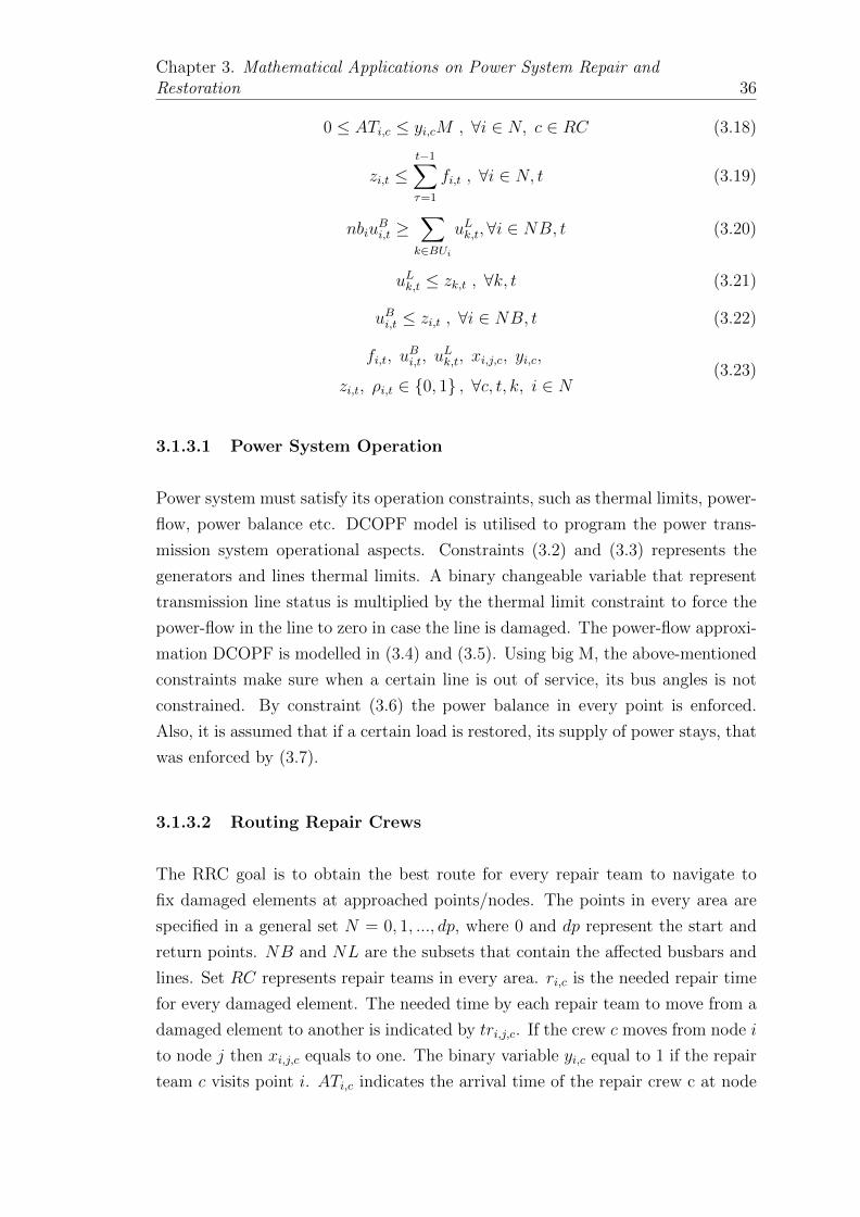
Chapter 3. Mathematical Applications on Power System Repair andRestoration 36
0 ≤ ATi,c ≤ yi,cM , ∀i ∈ N, c ∈ RC (3.18)
zi,t ≤t−1∑τ=1
fi,t , ∀i ∈ N, t (3.19)
nbiuBi,t ≥
∑k∈BUi
uLk,t,∀i ∈ NB, t (3.20)
uLk,t ≤ zk,t , ∀k, t (3.21)
uBi,t ≤ zi,t , ∀i ∈ NB, t (3.22)
fi,t, uBi,t, u
Lk,t, xi,j,c, yi,c,
zi,t, ρi,t ∈ 0, 1 , ∀c, t, k, i ∈ N(3.23)
3.1.3.1 Power System Operation
Power system must satisfy its operation constraints, such as thermal limits, power-
flow, power balance etc. DCOPF model is utilised to program the power trans-
mission system operational aspects. Constraints (3.2) and (3.3) represents the
generators and lines thermal limits. A binary changeable variable that represent
transmission line status is multiplied by the thermal limit constraint to force the
power-flow in the line to zero in case the line is damaged. The power-flow approxi-
mation DCOPF is modelled in (3.4) and (3.5). Using big M, the above-mentioned
constraints make sure when a certain line is out of service, its bus angles is not
constrained. By constraint (3.6) the power balance in every point is enforced.
Also, it is assumed that if a certain load is restored, its supply of power stays, that
was enforced by (3.7).
3.1.3.2 Routing Repair Crews
The RRC goal is to obtain the best route for every repair team to navigate to
fix damaged elements at approached points/nodes. The points in every area are
specified in a general set N = 0, 1, ..., dp, where 0 and dp represent the start and
return points. NB and NL are the subsets that contain the affected busbars and
lines. Set RC represents repair teams in every area. ri,c is the needed repair time
for every damaged element. The needed time by each repair team to move from a
damaged element to another is indicated by tri,j,c. If the crew c moves from node i
to node j then xi,j,c equals to one. The binary variable yi,c equal to 1 if the repair
team c visits point i. ATi,c indicates the arrival time of the repair crew c at node
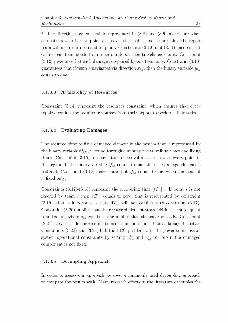
Chapter 3. Mathematical Applications on Power System Repair andRestoration 37
i. The direction-flow constraints represented in (3.8) and (3.9) make sure when
a repair crew arrives to point i it leaves that point, and assures that the repair
team will not return to its start point. Constraints (3.10) and (3.11) ensures that
each repair team starts from a certain depot then travels back to it. Constraint
(3.12) presumes that each damage is repaired by one team only. Constraint (3.13)
guarantees that if team c navigates via direction xi,j, then the binary variable yi,j
equals to one.
3.1.3.3 Availability of Resources
Constraint (3.14) represent the resources constraint, which ensures that every
repair crew has the required resources from their depots to perform their tasks.
3.1.3.4 Evaluating Damages
The required time to fix a damaged element in the system that is represented by
the binary variable tfi,t , is found through summing the travelling times and fixing
times. Constraint (3.15) represent time of arrival of each crew at every point in
the region. If the binary variable tfi,t equals to one, then the damage element is
restored. Constraint (3.16) makes sure that tfi,t equals to one when the element
is fixed only.
Constraints (3.17)-(3.18) represent the recovering time [tfi,t] . If point i is not
reached by team c then ATi,c equals to zero, that is represented by constraint
(3.19), that is important as that ATi,c will not conflict with constraint (3.17).
Constraint (3.20) implies that the recovered element stays ON for the subsequent
time frames, where zi,t equals to one implies that element i is ready. Constraint
(3.21) serves to de-energise all transmission lines linked to a damaged busbar.
Constraints (3.22) and (3.23) link the RRC problem with the power transmission
system operational constraints by setting uLk,t and uBi,t to zero if the damaged
component is not fixed.
3.1.3.5 Decoupling Approach
In order to assess our approach we used a commonly used decoupling approach
to compare the results with. Many research efforts in the literature decouples the

Chapter 3. Mathematical Applications on Power System Repair andRestoration 38
TSRRP into two subproblems, optimising the RRC first then optimising the power
flow in the system. The RRC is formulated as follows:
min∑∀t
∑i∈N
t fi,t (3.24)
Subject to
Constraints (3.8)− (3.20)
fi,t, xi,j,c, yi,c, zi,t ∈ 0, 1 , ∀c, t, i ∈ N (3.25)
Where the objective function is to minimise the time of restoration as presented in
(3.24). And when finding and completing the predicted times of restoration and
the schedules of routes for repair crews, the results of the binary variable zi,t are
to be utilised in optimising the power-flow of the system, that was modelled as
follows:
max Equation (3.1)
Subject to
Constraints (3.2)− (3.7)
Constraints (3.21)− (3.23)
uBi,t, uLk,t,∈ 0, 1 , ∀t, k, i ∈ NB (3.26)
The Decoupling Approach splits the RRC and power flow optimisation problems,
which in many cases cannot assure the optimality of solutions.
3.1.4 Results and discussion
The developed model is assessed on the standard IEEE 30-bus power transmission
system [139] as shown in Fig. 3.3. The k-means algorithm is programmed in
MATLAB and the MILP model is formulated in AMPL and resolved by CPLEX
12.9.0.0 on a PC with Intel® Core i7-8650U 1.90GHz 2.11GHz CPU and 8 GB
RAM. The time needed to repair a damaged element depends on the repair crew
skills. The travelling time, as the travelled distance dependant, varies from few
minutes to a number of hours. The time scale is 30hours with a 1-hour time-step.

Chapter 3. Mathematical Applications on Power System Repair andRestoration 39
Figure 3.3: IEEE 30-bus transmission system.
3.1.4.1 Depots Distributing
Step one is to assign the locations of depots using the k-means clustering algorithm.
It was assumed that the positions of buses and line are given. Also, it was supposed
that the X and Y coordination of several locations are given and select to place
two depots for repair crew. The clustering process is completed and its findings
are presented in Fig. 3.4. Depot number one is placed in the midst of buses 22
and 24, and depot two is placed in the midst of buses 4 and 6.
3.1.4.2 Results using TSRRP Approach
To make it easy to understand, we have randomly picked 5 buses and 5 lines to
be considered damaged components. Seventeen transmission lines linked to five
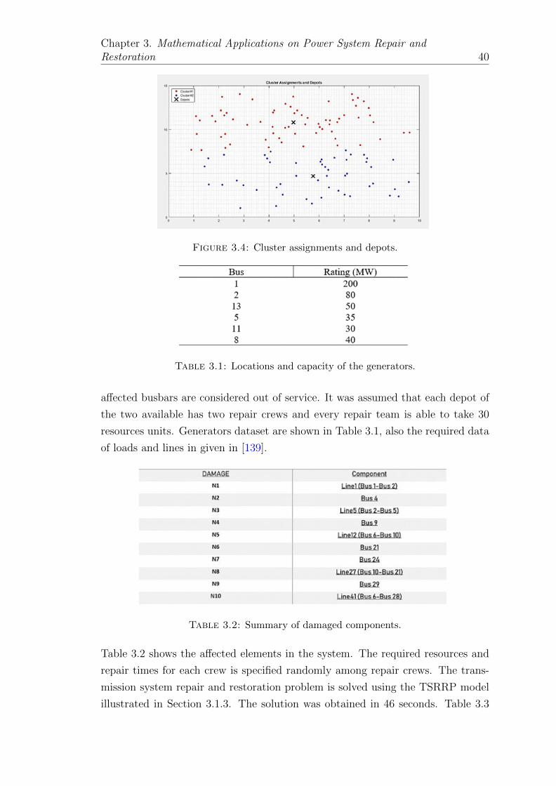
Chapter 3. Mathematical Applications on Power System Repair andRestoration 40
Figure 3.4: Cluster assignments and depots.
Table 3.1: Locations and capacity of the generators.
affected busbars are considered out of service. It was assumed that each depot of
the two available has two repair crews and every repair team is able to take 30
resources units. Generators dataset are shown in Table 3.1, also the required data
of loads and lines in given in [139].
Table 3.2: Summary of damaged components.
Table 3.2 shows the affected elements in the system. The required resources and
repair times for each crew is specified randomly among repair crews. The trans-
mission system repair and restoration problem is solved using the TSRRP model
illustrated in Section 3.1.3. The solution was obtained in 46 seconds. Table 3.3

Chapter 3. Mathematical Applications on Power System Repair andRestoration 41
reveals the found route for every repair team. Repair team 1 fixes the damaged
transmission line between buses 6 and 28 after 8 hours. This damage is prioritised
as the generator at bus 11 is out of service till this damage is repaired. Afterwards,
the same repair team moves to line 27 and fix it, that is finished after 14 hours.
Crew 2 goes the path N2 → N7 → N4 → N5 and finishes fixing jobs after 29
hours. The damage N5 is fixed at another time due to the fact that total it does
not affect the amount of restored loads. Repair crew 3 is assigned to fix N9 and
N3 , and Crew 4 is scheduled to fix N6 and N1. Whole loads are supplied after
16hours, that is accomplished by fixing N2, N3, N6 to N10. The other elements
are fixed in the sake of restoring the full system. Table 3.3 presents a time-frame
of the availability of all restored elements. All damages are fixed after 29 hours.
Table 3.3: Repair crews path for TSRRP.
Table 3.4: Times when each component is available for TSRRP (variable zi,t).

Chapter 3. Mathematical Applications on Power System Repair andRestoration 42
3.1.4.3 Results using Decoupling Approach
To prove the good performance of the developed TSRRP model. We have com-
pared the solution with the Decoupling Approach method presented in Section
3.1.3.5. The repair crews routing sequence is shown in Table 3.5.
Table 3.5: Repair crews path for decoupling approach.
Table 3.6: Times when each component is available for decoupling approach(variable zi,t).

Chapter 3. Mathematical Applications on Power System Repair andRestoration 43
Figure 3.5: Total restored loads for TSRRP and Decoupling Approach.
3.1.5 Conclusion and future work
This section presented a co-optimisation approach for transmission system repair
and restoration problem. The study proposed a MILP formulation to coordinate
repair crews and system generators to pick-up the maximum possible loads after a
damage. The developed model was implemented on an IEEE 30-bus power trans-
mission system. The findings are compared to a different optimisation method.
The results prove the advantages of the developed approach (TSRRP) in restoring
all loads in 16 hours comparing to 20 hours in Decoupling Approach.
Currently, the industry depends on power system operators and power engineers
experience in case of a power outage to optimise the power-flow for the system
and the repair crews dispatching process. A co-optimised approach such as the
proposed TSRRP can enhance the process of power system repair and restoration
after damages as shown in this study.
Possible future work includes using new and more accurate approximation of the
AC optimal power flow such as linear-programming models (LPAC) [140], and
many others [141] that incorporate reactive power and voltage magnitudes in a
linear power-flow approximation. Also, implementing the developed approach in
electrical distribution systems with the presence of distributed generators. As well
as, implementing the proposed approach on larger systems that simulates real life
scenarios.

Chapter 3. Mathematical Applications on Power System Repair andRestoration 44
3.2 Advanced Approach for Solving Power Trans-
mission System Repair and Restoration
3.2.1 Introduction
Climate change and the increase in natural disasters induced by bad weather
illustrates the need of new and more accurate methods to restore electric power
systems. The literature has several research efforts that tackles the power system
restoration [132], however, more high-level research on new restoration schemes is
needed.
The focus of this study is optimising the power-flow in transmission system, and
routing repair crews (RRC) optimally. The problem was first examined in [133],
the study suggested a multi-stage style that decouples the power-flow and RRC
problems. The paper proposed two sub-problems to find a minimised set of ele-
ments that could lead in recovering the system to its full capacity, and discover an
optimised restoration order that could help to minimise the outage duration. Ref-
erence [134] has provided an extension for this study, by proposing a randomised
adjustable vehicle decomposition method in order to solve large-scale problems.
In this study, we present an advanced and more accurate method for solving the
power transmission system repair and restoration (TSRR) with no decomposition.
A mixed integer linear program (MILP) is modelled to pickup as much loads
as possible. The more accurate and advanced linear approximation of power-
flow LPAC optimal power-flow (LPAC-OPF) is used to represent the operation
constraints of the power transmission system. The RRC to damages problem was
modelled as a vehicle routing problem (VRP). Where the VRP is modelled as a
combinatorial optimisation and integer programming approach that seeks finding
the a fleet of vehicles best route [135], [136], [137].
Repair teams start their jobs from central bases called depots, then, they visit the
damaged elements to perform repairs and after finishing their jobs they travel back
to their central stations where they started. The travelling and repair times have
been considered in the model. The rapier teams can carry a certain amount of re-
sources to perform their jobs. The State-of-the-Art k-means clustering algorithm
was used to help finding the optimal locations of each depot in the system among
clusters.Using this algorithm can assure that the repair teams are strategically lo-
cated which will enhance the recovery rate of the system. When a system element

Chapter 3. Mathematical Applications on Power System Repair andRestoration 45
get damaged, the TSRRP algorithm can find the repair teams and system gener-
ators scheduling. It is important to mention that generators damages are ignored
in this study, as it is sensible to presume that on-site repair teams will handle their
damages. A similar study [138] tried to implement the same approach. We found
out that the paper has major errors and mistakes in formulating the problem and
presenting results. Thus, in our study, we tried to enhance and verify the approach
by testing it on a different transmission system and justify the obtained results
well.
The developed approach is assessed using the standard IEEE 30-bus power trans-
mission system. We have compared the TSRRP results with a standard method
where the RRC and power-flow optimisation are decoupled.
3.2.2 Proposed Method
The proposed method comprises of two phases: distributing depots by clustering
repair crews, and TSRR. Every crew depot has its assets such as manpower, gear,
repair vehicles, etc. and a number of repair teams offered to handle the damages
to the network. The repair crews depots are distributed using state-of-art k-means
algorithm, where the spots of depots are the centres of the clusters. The k-means
clustering procedure was created in such it takes into account the number of depots
and the positions of power system parts.
Figure 3.6: K-Means Clustering Algorithm Procedure.
Once a power outage happens in the system, a damage assessment study is to be
done. The aim of this analysis is to investigate and determine the damaged parts
state and forecast the required repair times.

Chapter 3. Mathematical Applications on Power System Repair andRestoration 46
Afterwards, the accessible repair teams are to be sent to the damaged elements
locations to repair and restore the power network. Each repair team has an op-
timised direction to go to the damaged parts. Fig. 3.7 gives an example of the
TSRR.
Figure 3.7: Example of TSRR operation.
3.2.3 Problem Formulation
A co-optimisation frame for the TSRRP is implemented and a MILP problem.
Where it couples the power transmission system operational aspects and RRC
problem. Maximising the loads pickup subject to sizes and importance was our
objective function as shown in (3.27). The optimisation problem can be formulated
as follows:
max∑∀t
∑∀i∈ΩB
ωDi ρi,tpDi,t (3.27)
0 ≤ pGi,t ≤ pmaxi , ∀i ∈ G, t (3.28)
− uLk pmaxk ≤ pk,t ≤ uLk pmaxk , ∀k, t (3.29)
− uLk qmaxk ≤ qk,t ≤ uLk qmaxk , ∀k, t (3.30)
qgn = 0 , ∀n ∈ N\G (3.31)
qn =
n6=m∑m∈N
−qTnm + qδnm , ∀n ∈ G (3.32)
θ0s = 0 , φs = 0 (3.33)
pn =
n6=m∑m∈N
pTnm , ∀n ∈ N , n 6= s (3.34)

Chapter 3. Mathematical Applications on Power System Repair andRestoration 47
qn =
n6=m∑m∈N
qTnm + qδnm , ∀n ∈ N , n 6= s , n /∈ G , ∀(n,m), (m,n) ∈ L (3.35)
[pTnm](k,t) = |V Tn |2gnm − |V T
n ||V Tm |(gnmcosnm + bnm(θ0
n − θ0m)) ≥
−(1− uLk,t
)M, ∀k, t
(3.36)
[pTnm](k,t) = |V Tn |2gnm − |V T
n ||V Tm |(gnmcosnm + bnm(θ0
n − θ0m)) ≤(
1− uLk,t)M, ∀k, t
(3.37)
[qTnm](k,t) = −|V Tn |2bnm − |V T
n ||V Tm |(gnm(θ0
n − θ0m)− bnmcosnm) ≥
−(1− uLk,t
)M, ∀k, t
(3.38)
[qTnm](k,t) = −|V Tn |2bnm − |V T
n ||V Tm |(gnm(θ0
n − θ0m)− bnmcosnm) ≤(
1− uLk,t)M, ∀k, t
(3.39)
qδnm = −|V tn |bnm(φn − φm)− (|V t
n | − |V tm|)bnmφn (3.40)
cosnm = PWLA((cos(θ0n − θ0
m),−π/3 , π/3)) (3.41)∑k∈K(i,.)
pk,t + pGi,t =∑
k∈K(.,i)
pk,t + ρi,tpDi,t ,
∀i ∈ G, t(3.42)
ρi,t+1 ≥ ρi,t , ∀i ∈ G, t (3.43)∑j∈N\i
xi,j,c −∑
j∈N\i
xj,i,c = 0 , ∀c ∈ RC, i ∈ N (3.44)
∑j∈N\0
x0,j,c −∑
j∈N\0
xj,0,c = 1 , ∀c ∈ RC (3.45)
∑j∈N\dp,c∈RC
xj,dp,c = nc (3.46)
∑c∈RC
yi,c = 1 , ∀i ∈ N (3.47)
yi,c =∑
j∈N\0,i
xi,j,c , ∀c ∈ RC, i ∈ N (3.48)
ResCc ≥∑∀i∈N
ResNi yi,c , ∀c (3.49)
ATi,c + ri,c + tri,j,c − ATj,c ≤ (1− xi,j,c)M ,
∀i ∈ N\ dp , j ∈ N, c ∈ RC(3.50)
∑∀t
fi,t = 1 , ∀i ∈ N (3.51)

Chapter 3. Mathematical Applications on Power System Repair andRestoration 48∑
∀t
tfi,t ≥∑c∈RC
(ATi,c + ri,cyi,c) , ∀i ∈ N (3.52)
∑∀t
tfi,t ≤∑c∈RC
(ATi,c + ri,cyic) + 1− ε, ∀i ∈ N (3.53)
0 ≤ ATi,c ≤ yi,cM , ∀i ∈ N, c ∈ RC (3.54)
zi,t ≤t−1∑τ=1
fi,t , ∀i ∈ N, t (3.55)
nbiuBi,t ≥
∑k∈BUi
uLk,t,∀i ∈ NB, t (3.56)
uLk,t ≤ zk,t , ∀k, t (3.57)
uBi,t ≤ zi,t , ∀i ∈ NB, t (3.58)
fi,t, uBi,t, u
Lk,t, xi,j,c, yi,c,
zi,t, ρi,t ∈ 0, 1 , ∀c, t, k, i ∈ N(3.59)
3.2.3.1 Operation of Power Transmission System
Power transmission system must has its operation/processing constraints met, such
as system thermal limits, power-flow, power-balance etc. The LPAC-OPF model
is applied to program the power transmission system operation. Constraints (3.28)
and (3.29) characterizes the output restrictions of generators and transmission lines
respectively. A binary adjustable variable that symbolise the status of the trans-
mission line is multiplied by the thermal limit constraint to drive the power-flow in
the line to zero in case the line is damaged. The power-flow linear approximation
LPAC is modelled in LPAC Constraints presented in Section 3.2.3. Using big M,
the above-mentioned constraints make sure when a certain line is out of service,
its bus angles is not constrained. By constraint (3.42) the power balance in every
point is enforced. Also, it is assumed that if a certain load is restored, its supply
of power stays, that was enforced by (3.43).
3.2.3.2 Repair Crews Routing
The RRC purpose is to obtain the best route for every repair team to navigate to
fix damaged elements at approached points/nodes. The points in every area are
specified in a general set N = 0, 1, ..., dp, where 0 and dp represent the start and
return points. NB and NL are the subsets that contain the affected busbars and

Chapter 3. Mathematical Applications on Power System Repair andRestoration 49
lines. Set RC represents repair teams in every area. ri,c is the needed repair time
for every damaged element. The needed time by each repair team to move from
a damaged element to another is indicated by tri,j,c. If the crew c moves from
node i to node j then xi,j,c equals to one. The binary variable yi,c equal to 1 if
the repair team c visits point i. ATi,c indicates the arrival time of the repair crew
c at node i. The direction-flow constraints represented in (3.44) and (3.45) make
sure when a repair crew arrives to point i it leaves that point, and assures that
the repair team will not return to its start point. Constraint (3.46) ensures that
each repair team starts from a certain depot then travels back to it. Constraint
(3.48) presumes that each damage is repaired by one team only. Constraint (3.47)
guarantees that if team c navigates via direction xi,j, then the binary variable yi,j
equals to one.
3.2.3.3 Resources Availability
Constraint (3.49) represent the resources constraint, which ensures that every
repair crew has the required resources from their depots to perform their tasks.
3.2.3.4 Damages Evaluation
The required time to fix a damaged element in the system that is represented by
the binary variable tfi,t , is found through summing the travelling times and fixing
times. Constraint (3.50) represent time of arrival of each crew at every point in
the region. If the binary variable tfi,t equals to one, then the damage element is
restored. Constraint (3.51) makes sure that tfi,t equals to one when the element
is fixed only.
Constraints (3.52)-(3.53) represent the recovering time [tfi,t] . If point i is not
reached by team c then ATi,c equals to zero, that is represented by constraint
(3.54), that is important as that ATi,c will not conflict with constraint (3.51).
Constraint (3.55) implies that the recovered element stays ON for the subsequent
time frames, where zi,t equals to one implies that element i is ready. Constraint
(3.56) serves to de-energise all transmission lines linked to a damaged busbar.
Constraints (3.57) and (3.58) link the RRC problem with the power transmission
system operational constraints by setting uLk,t and uBi,t to zero if the damaged
component is not fixed.

Chapter 3. Mathematical Applications on Power System Repair andRestoration 50
3.2.3.5 Decoupling Methodology
To test our proposed method we used a known approach that is commonly used to
compare our results with. Lots of studies in the literature decouples the TSRR into
two subproblems, optimising the RRC problem first then optimising the power-
flow in the network. The RRC is prepared as follows:
min∑∀t
∑i∈N
t fi,t (3.60)
Subject to
Constraints (3.44)− (3.55)
fi,t, xi,j,c, yi,c, zi,t ∈ 0, 1 , ∀c, t, i ∈ N (3.61)
Where the objective function is to minimise the time of restoration as presented in
(3.60). And when finding and completing the predicted times of restoration and
the schedules of routes for repair crews, the results of the binary variable zi,t are
to be utilised in optimising the power-flow of the system, that was modelled as
follows:
max Equation (3.27)
Subject to
Constraints (3.28)− (3.43)
Constraints (3.56)− (3.58)
uBi,t, uLk,t,∈ 0, 1 , ∀t, k, i ∈ NB (3.62)
This Decoupling Style divides the RRC and power-flow optimisation processes.
That is usually found to be less accurate and cannot guarantee the optimality of
results.

Chapter 3. Mathematical Applications on Power System Repair andRestoration 51
3.2.4 Results and discussion
The developed model is assessed on the standard IEEE 30-bus power transmission
system [139] as shown in Fig. 3.8. The k-means algorithm is programmed in
MATLAB and the MILP model is formulated in AMPL and resolved by CPLEX
12.9.0.0 on a PC with Intel® Core i7-8650U 1.90GHz 2.11GHz CPU and 8 GB
RAM. The time needed to repair a damaged element depends on the repair team
abilities. The travelling time, as the travelled distance dependant, varies from few
minutes to a number of hours. The time limit is chosen to be 30 hours with a
one-hour step.
Figure 3.8: IEEE 30-bus transmission system.

Chapter 3. Mathematical Applications on Power System Repair andRestoration 52
Figure 3.9: Cluster assignments and depots.
3.2.4.1 Depots Allocation
Step one is to assign the locations of depots using the k-means clustering algorithm.
It was assumed that the positions of buses and line are given. Also, it was supposed
that the X and Y coordination of several locations are given and select to place
two depots for repair crew. The clustering process is completed and its findings
are presented in Fig. 3.9. Depot number one is placed in the midst of buses 22
and 24, and depot two is placed in the midst of buses 4 and 6.
The results for depots allocation is persistent with the first study presented in
Section 3.1, which is sensible because we used the same state-of-the-art clustering
algorithm on the same system.
Table 3.7: Location and capacity of system generators.
3.2.4.2 TSRR Methodology Results
To make it easy to illustrate our study, we have arbitrarily picked 5 buses and
5 transmission lines to be deemed damaged parts. 17 lines linked to 5 damaged
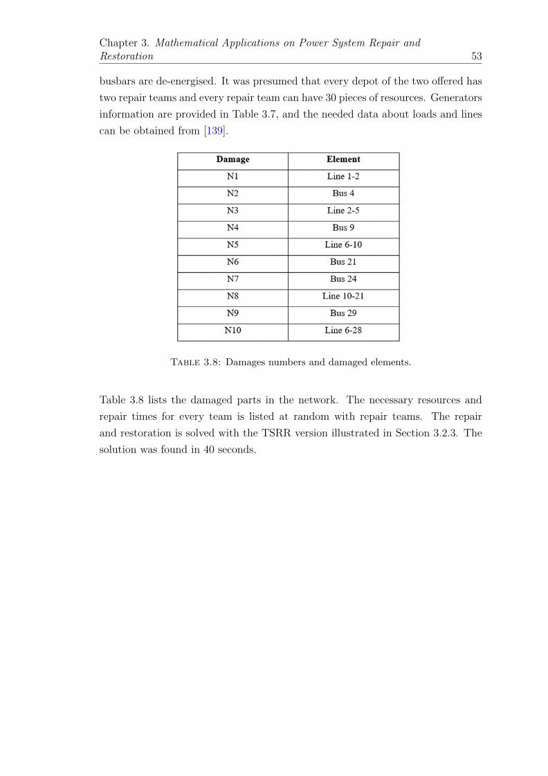
Chapter 3. Mathematical Applications on Power System Repair andRestoration 53
busbars are de-energised. It was presumed that every depot of the two offered has
two repair teams and every repair team can have 30 pieces of resources. Generators
information are provided in Table 3.7, and the needed data about loads and lines
can be obtained from [139].
Table 3.8: Damages numbers and damaged elements.
Table 3.8 lists the damaged parts in the network. The necessary resources and
repair times for every team is listed at random with repair teams. The repair
and restoration is solved with the TSRR version illustrated in Section 3.2.3. The
solution was found in 40 seconds.

Chapter 3. Mathematical Applications on Power System Repair andRestoration 54
Table 3.9 introduce the observed route for every repair team. Table 3.10 displays
the time when every element is accessible. All damages are fixed after 22 hours.
Table 3.9: Repair crews paths for TSRR.
Table 3.10: The time when each element is available for TSRR (variable zi,t).

Chapter 3. Mathematical Applications on Power System Repair andRestoration 55
3.2.4.3 Decoupling (Route First) Methodology Results
To validate the good implementation of the created TSRR version. We have
compared the solution with the Decoupling Approach method AKA (Route First)
introduced in Section 3.2.3.5. The repair crews routing directions of the Route
First method is displayed in Table 3.11.
Table 3.11: Repair crews paths for Decoupling Methodology.
Table 3.12: The time when each component is available for DecouplingMethodology (variable zi,t).

Chapter 3. Mathematical Applications on Power System Repair andRestoration 56
Figure 3.10: Total restored loads for TSRR and Decoupling Methodologies.
3.2.5 Conclusion
This study introduced a co-optimisation style for power transmission system repair
and restoration using an advanced and more accurate model for the power-flow.
The study suggested a MILP template to manage repair teams and network gen-
erators to pick-up the maximum feasible loads after a damage. The template
was applied using a more accurate and advanced linear approximation of optimal
power flow (LPAC-OPF) compared to the commonly used model DCOPF that was
published in [142] and presented in Section 3.2 of this thesis. The created model
was applied on a modified IEEE 30-bus power transmission system. The findings
is compared with a different commonly used optimisation method (Route First).
The outcomes prove the improvements and accuracy of the created methodology
(TSRR) in re-establishing all loads in 22 hours comparing to 23 hours in the
Decoupling Approach.
The reader can observe that using the more accurate and advanced linear model
of power-flow (LPAC-OPF) has enhanced the TSRRP results in both of the opti-
misation methods and helped to restore the system in shorter time comparing to
the DCOPF model.
At Present, the industry hinges on power system operators and power engineers
experiences when a power outage happens, in order to optimise the repair and
restoration of the power network. A co-optimised approach such as the proposed
TSRR combined with more accurate and advanced model for the power-flow can
enhance the practice of power system repair and restoration after damages as
demonstrated in this chapter’s sections.

Chapter 4
Reliability Analysis in Power
System Restoration
In this chapter, a very important aspect of PSR will be presented and discussed
(Reliability Analysis).
4.1 Introduction
The power distribution system is considered the main important part of power
system as it has to fed the load directly. These loads are the residential, com-
mercial and industrial. In these loads-based distribution systems, the reliability
of the residential distribution system is lesser as compared to the commercial and
industrial. The quality of power feeding to these loads has gained importance due
to the introduction of deregulated electricity to these loads. The cost of operation
of these systems also includes the reliability cost nowadays. The cost is paid by
the utility companies if the grid is less reliable. This cost is yielded by the utilities
directly in the form of compensation paid to customers or indirectly by some other
means [143]. There are certain parameters regarded as the reliability indices that
are adopted for the reliability assessment of power distribution system. These are
system average interruption frequency index (SAIFI), system average interrup-
tion duration index (SAIDI) and energy not supplied (ENS). These reliability
indices are accessed with different techniques presented in the literature. The
techniques involve both simulation and analytical methods. The most commonly
used simulation technique is the Monte Carlo Simulations and these determine
the system reliability on the basis of system failures history and maintenance data
57

Chapter 4. Reliability Analysis in Power System Restoration 58
[144]. Contrarily, these reliability indices do not include the non-component-based
failures such as cold load pickups or embedded failures of the system. Thus, from
this fact it is clear that these reliability indices do not completely represent the
reliability of the distribution system.
The thermostatic controlled loads are responsible for the occurrence of cold load
events and these require a high sudden load demand. It will result in single step
restoration of the system and in many cases of the restoration it is impossible.
These high stresses on the system will lead to a violated operation of the system
and will not follow the required protection limits. In the absence of proper planning
for the cold load pickups, the equipment associated with this operation will be
damaged. In addition to these damages, it also causes unnecessary restoration
that are not acceptable for the proper operation of system within its stability
limits. However, the system restoration is possible only with the help of the low
concentration of total connected load (TCL) and low power demands for the TCL.
The other procedure for the restoration of the system dynamics is the sectionalising
of the system [145].
The CLPU phenomenon in power distribution systems was first time presented in
1979. The physical model of the load facing CLPU was developed and is presented
in [122]. The factors affecting the CLPU in power distribution system are presented
in [146]. The factors that causes the occurrence of these events involve the system
outage duration, ambient temperature, thermostat setting, thermal insulation of
house and the customer behaviour. The CLPU studies on the main distribution
transformer of the system are presented in [147]. From these studies it is found
that voltage limits following CLPU are violated but no other protection limits are
affected. In [148] the exponential decay studies are performed on the distribution
transformer facing CLPU and it is suggested to enhance the transformer size after
restoration because of thermal stresses faced by transformer during the process
of restoration. Thus, with these outcomes and several damages and effects faced
due to CLPU an optimal research technique was introduced that addressed these
transformer constraints. It resulted in the formation of artificial neural network-
based algorithms that addressed these problems. Firstly, Genetic Algorithm (GA)
was opted in order to solve these problems [145]. The other scheme introduced was
the adjacent pairwise interchange for optimal restoration when subjected to these
cold load pickup events [31]. The GA is also capable for optimal restoration of the
system when it is also using distributed generation and the thermal stresses it has
to face with cold load pickups. The Monte Carlo simulations for the determination
of the stochastic behaviour of loads and its impacts on the optimal restoration of
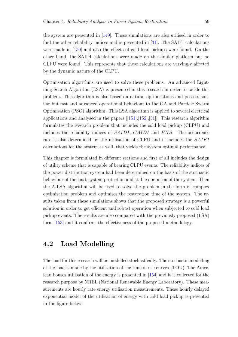
Chapter 4. Reliability Analysis in Power System Restoration 59
the system are presented in [149]. These simulations are also utilised in order to
find the other reliability indices and is presented in [31]. The SAIFI calculations
were made in [150] and also the effects of cold load pickups were found. On the
other hand, the SAIDI calculations were made on the similar platform but no
CLPU were found. This represents that these calculations are varyingly affected
by the dynamic nature of the CLPU.
Optimisation algorithms are used to solve these problems. An advanced Light-
ning Search Algorithm (LSA) is presented in this research in order to tackle this
problem. This algorithm is also based on natural optimisations and possess sim-
ilar but fast and advanced operational behaviour to the GA and Particle Swarm
Optimisation (PSO) algorithm. This LSA algorithm is applied to several electrical
applications and analysed in the papers [[151],[152],[31]]. This research algorithm
formulates the research problem that includes the cold load pickup (CLPU) and
includes the reliability indices of SAIDI, CAIDI and ENS. The occurrence
rate is also determined by the utilisation of CLPU and it includes the SAIFI
calculations for the system as well, that yields the system optimal performance.
This chapter is formulated in different sections and first of all includes the design
of utility scheme that is capable of bearing CLPU events. The reliability indices of
the power distribution system had been determined on the basis of the stochastic
behaviour of the load, system protection and stable operation of the system. Then
the A-LSA algorithm will be used to solve the problem in the form of complex
optimisation problem and optimises the restoration time of the system. The re-
sults taken from these simulations shows that the proposed strategy is a powerful
solution in order to get efficient and robust operation when subjected to cold load
pickup events. The results are also compared with the previously proposed (LSA)
form [153] and it confirms the effectiveness of the proposed methodology.
4.2 Load Modelling
The load for this research will be modelled stochastically. The stochastic modelling
of the load is made by the utilisation of the time of use curves (TOU). The Amer-
ican houses utilisation of the energy is presented in [154] and it is collected for the
research purpose by NREL (National Renewable Energy Laboratory). These mea-
surements are hourly rate energy utilisation measurements. These hourly delayed
exponential model of the utilisation of energy with cold load pickup is presented
in the figure below:

Chapter 4. Reliability Analysis in Power System Restoration 60
Figure 4.1: A general figure for delayed exponential model with CLPU.
The AC load of the residential distribution system depends on the ambient tem-
perature, the probability of the use of curves are formulated and are presented
below:
AC Load Status =
Prob > 0 if T > TU or T < TD
Prob = 0 otherwise
As the AC load modelled above is dependent on the lower and higher values of
the temperature, the TU is presenting the upper limit of the temperature while
the TD is representing the lower limit of the temperature. The probability of the
utilisation of AC loads increases as the dead environmental time increases. The
dead ambient time is the difference of the high ambient time and lower ambient
time. Initially, the TOU curves are developed for all the electric appliances and
these curves are adjusted for the two commonly used multipliers. The multipliers
for which the power distribution system is modelled are the demand factor and load
factor. After this, the number of units are found for each load of the residential
distribution system. The number of AC loads utilised in this study are the 70
percent of the load point divided by the power rating of the power device. Thus,
for 1MW load 580 loads are used with 1.2kW each of the AC load point. The
reactive power compensation of the system is also of the importance as the power
factor for the system load usage is almost about 0.8 to 0.9 and the fall in the power
factor of the system requires the reactive power compensation so that the system
may operate within its stable operating limits. The exponential model of the load
is shown in Fig. 4.1 and the mathematical modelling of the load with the CLPU
points is presented below:
S(t) = SD + (SU −SD)e−α(t−t1)u(t− t1) +SD([1−u(t− t1)]u(t− (Ri− ti))) (4.1)

Chapter 4. Reliability Analysis in Power System Restoration 61
In the equation above the α represents the decay factor and state as the rate
of decay. The diversified demand before the outages of the equipment from the
power distribution system is represented as SD. The undiversified demand after
the restoration of the system from the outages faced due to the CLPU is states
the power SU . Thus, the total SU power can be represented in the form of below:
SU = kSDTCL + SDNTCL (4.2)
The factor ‘k′ in the above equation is presented in the form below:
k =ln( toutage
0.107)
1.101(4.3)
It states the empirical relation when the CLPU events has been occurred in the
system and the relation exist between the outage duration and demand taken
by the load. The factor ‘k′ is representing the increase in the demand. This
increase in the demand is only affected by the load variation possessed by the
TCL. This demand variation is also shown in the Figure 4.1 presented above. The
other important parameters variation caused by the customer behaviour, thermal
variation due to variation in the ambient temperature are presented in the research
paper [122].
4.3 Problem Formulation
4.3.1 Mathematical Formulation
The optimal restoration plan is considered during the mathematical formulation
for the reliability indices measurements with the inclusion of the CLPU events.
The failure is faced in the system and after elapsing this failure time, the program
is modelled to run for a suitable time for restoring the load affected by such events.
The mathematical problem formulated for this purpose is presented below:
min
(k∑1
TTRl −k∑1
TTRi
)(4.4)

Chapter 4. Reliability Analysis in Power System Restoration 62
In this statement the TTR represents the time to restore the ith load point when
the ‘k′ number of load points are out of service. The adjusted TTR is the sum of
the total TTR considering them without CLPU and the additional time that is
to be waived by the system for the restoration. Thus, we can say that this is sum
of multiple at the different load points and can be written in the form presented
below.
k∑1
TTRl =k∑1
TTRi + tr1 + tr2 + tr3 · · ·+ trn (4.5)
Thus, our objective function can be rewritten in the form presented below:
min (tr1 + tr1 + tr1 + . . . trn) (4.6)
All the reliability indices SAIDI, CAIDI and ENS are minimised with the min-
imisation of the restoration time followed by the technique presented in this re-
search. However, the SAIFI is not affected if the number of failures is not affected.
The above research problem is subjected to following constraints:
The maximum loading on the transformer should not exceed the 125 percent
of the provided rating. This is regarded as the protection system constraint:
ST ≤ 1.25pu (4.7)
The voltage of the system should not vary above and below the 5 percent
of the rated voltage value. This is regarded as the operational constraint of
the system:
0.95 ≤ Vi ≤ 1.05 ,∀i ∈ [1, N ] (4.8)
The reliability indices of the power distribution system for the complete time
assessment with the cold load pickup points of the different load points are stated
in the statements given below:
SAIFI =Total number of all interruptions
Total number of customers connected=
∑Ni
NT
(4.9)

Chapter 4. Reliability Analysis in Power System Restoration 63
SAIDI =Total duration of all interruptions
Total number of customers connected=
∑OiNi
NT
(4.10)
CAIDI =SAIDI
SAIFI(4.11)
Thus, the ENS reliability index of the system can be stated as shown in (4.12).
ENS =∑
PiOi (4.12)
In the above equations the NT is the total number of customers at each load point
and Ni is stating the total number of the interruptions and the average power that
would be supplied during interruption is presented as Pi. When CLPU events are
faced by the system then duration of restoration of the system is changed and it
is represented as Oi.
4.3.2 Selected Test System
In this study the radial power distribution system is presented and this system is
shown in the figure presented below. The feeders presented in this distribution
system has the property that it can restore all the feeders at once. The main
transformer of the feeder is of main importance and its total size is determined by
the running the load model. The maximum duration for this is presented for the
time period of 20 years.
Figure 4.2: Radial power distribution system.
The power demand of this system is 6.74MVA and this is 60 minutes power de-
mand, thus, it utilises the standard size transformer of 5MVA. If the protection
constraints of the system are considered then the required power for the system
will be 8.125MVA at the required full load current value of 125 percent.

Chapter 4. Reliability Analysis in Power System Restoration 64
The power required in the distribution system will be 8MVA for the load flow
analysis of the system. The length of the main feeder in this system is 600m. This
complete feeder length is further divided into four sections. The other sections of
the distribution system are of 200m and these sections include 1,2,3,8,9 and 10
load points. All other remaining sections of the distribution system are taken as
300m and these are underground cables.
4.4 Proposed Methodology
4.4.1 Monte Carlo Platform
The methodology in order to perform these simulations is presented in the chart
given below. The reliability indices are found by the usage of the MC platform.
The simulation is carried for the period of 200 years. The up status for the
electrical appliances is considered at the beginning of the simulations (T = 0),
The uniformly distributed generated unit is utilised to find the time to repair and
time to fail.
TTR =−1
rln(U) (4.13)
TTF =−1
γln(U) (4.14)
Initially, the simulations are carried out for the period of 200 years without con-
sidering the CLPU and the system analysis is performed and then the TTR is
found with inclusion of the CLPU events. This includes the optimal restoration
plan that is capable to reduce the restoration time such that it does not violates
the opted constraints. The A-LSA algorithm is utilised to calculate these TTR
and TTF . These time to restore and time to fail modified values with the help of
the A-LSA algorithm will be injected back to the power distribution system and
it enhances the operation capability of the system.
4.4.2 LSA and A-LSA Optimisation Platform
The optimal restoration of each outage at any load point in the power distribution
system is done by the utilisation of the Lightening Search Algorithm (LSA) and

Chapter 4. Reliability Analysis in Power System Restoration 65
the advanced A-LSA. They both works with uniform initialisation with random
population. This uniformly initialised population is regarded as the transition
projectiles. The A-LSA algorithm is capable to produce the results in a step wise
sequence and the nth step of the A-LSA algorithm for the presented system is
given as:
ESLn = [tr1, tr2, tr3 + . . . trn] (4.15)
This is representing the system of ‘k′ load points (LP) and the outage is faced
radially in this system. This can be elaborated in such a way that LP8, LP9 and
LP10 will be simultaneously affected with the outage faced at the load point 8.
The transition periods of the projectiles in the A-LSA algorithm will be tr8tr9 and
tr10. As the outage is occurred at the load point 8, the tr8 will be in the duration
from 0 to tr. Then further tr9 will lie in the duration from tr8 and TM . On the
other hand, the tr10 will occupy the duration from tr9 and TM . These transitions
are followed in the form of step ladder. The ‘n′ multiple step ladders adopted by
the A-LSA algorithm are presented in the equation below:
ESLs = [esl1, esl2, esl3 + . . . esln] (4.16)
Thus, the exponentially distribution of the objective function can be presented as:
rn+1ri = rnri ± exprand(u) (4.17)
In the best step ladder, the difference between the reference projectile and depen-
dent projectile is represented as ‘u′ and is utilised in the equation above. The
best projectile ladder regarded as the lead projectile is in the form of the normal
distribution function is presented in the equation below:
rn+1ri = rnri ± normrand(u, σ) (4.18)
The α is the scaling parameters in the equation above. This utilises the forking
process of lightning search algorithm. The forking is the secondary process of the
A-LSA algorithm, it redirects to search and yields different solutions within the
prescribed space of the system. There are two ways to perform forking within the
A-LSA algorithm.

Chapter 4. Reliability Analysis in Power System Restoration 66
A general flow chart of the developed advanced lighting algorithm is presented in
the figure below [155]. This algorithm contains some additional steps as compared
to the previously proposed LSA algorithm used in our main comparative reference
[153] in order to enhance the efficiency of the solution of the investigated problem.
Figure 4.3: General flowchart represents the fundamental mechanisms for theAdvanced LSA Algorithm.

Chapter 4. Reliability Analysis in Power System Restoration 67
4.5 Results and Analysis
4.5.1 Load Model Results
The load model results of the power distribution system are taken on the basis of
the time to use (TOU) curves of the electrical appliances. These TOU curves are
yielded from the multiplication of load factor with the demand factor. This value
is measured to have a value of 0.285 in Saudi Arabia. The thermostat settings
possess the upper and lower values of temperature. The upper temperature of
TU = 22o and the lower values of the temperature is TD = 20o. The measured
TOU curves for the different electric appliances are presented in the figure below.
Figure 4.4: Time to Use (TOU) curves of different customers.
The results of stochastic model of residential distribution system based on the
above presented (TOU) curves are presented in the figure below. These stochastic
curves are taken for two different load picks on the different time durations, i.e.
for Summer and Winter days. For the Winter day it is taken for January 1 and
for Summer day it is taken for August 1. This is incorporating human behaviour
that is directly incorporated with the ambient temperature effect of the system
TOU curves that caused by the heating and cooling phenomenon of the system.
The simulation is carried for 200 years and load demand for every minute over
this duration is produced at each load point. The cold load pickup model of the
test system is presented in the figure below. This modelling is done with the
time deviation of δt = 30min with the α parameter variation of 0.5hr−1. From
the curves, it can be concluded that, at the restored points, the power demand is

Chapter 4. Reliability Analysis in Power System Restoration 68
Figure 4.5: Model for Summer day and Winter day.
enhanced two times than the normal power demand. Thus, it results in the increase
of power demand on the main distribution transformer of the power system.
Figure 4.6: CLPU curves of the distribution system.
4.5.2 Optimal Restoration of One Outage Resulting in CLPU
The peak demand that occurs due to the outages in the system results in violation
of protection and operational limits of the system. But this does not happen with
all the outages that causes the peak rise in the system peak power limits that
violates the prescribed system limits. The 3485879-minute event in the system
duration is the point at which the failure faced and it tripped the load points LP1,
LP2 and LP3. In this case the power was supposed to restored after 482 minutes.
This was actually the outage faced due to outage of section 1. The low TCL
concentration was main responsible for this outage. From Fig. 4.7 it is observed
that with this outage no violation limit is made and no CLPU event is happened
and it takes just a single step to restore to original point. This phenomenon of
restoration is presented in the figure:
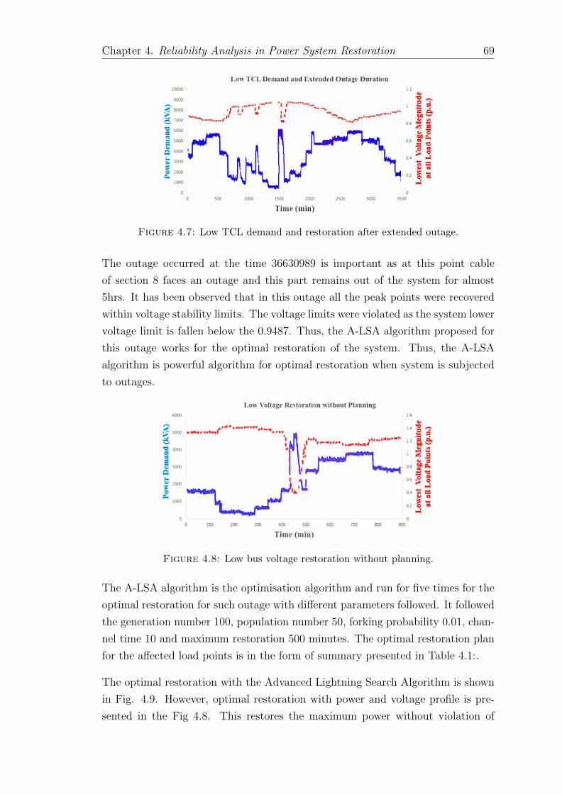
Chapter 4. Reliability Analysis in Power System Restoration 69
Figure 4.7: Low TCL demand and restoration after extended outage.
The outage occurred at the time 36630989 is important as at this point cable
of section 8 faces an outage and this part remains out of the system for almost
5hrs. It has been observed that in this outage all the peak points were recovered
within voltage stability limits. The voltage limits were violated as the system lower
voltage limit is fallen below the 0.9487. Thus, the A-LSA algorithm proposed for
this outage works for the optimal restoration of the system. Thus, the A-LSA
algorithm is powerful algorithm for optimal restoration when system is subjected
to outages.
Figure 4.8: Low bus voltage restoration without planning.
The A-LSA algorithm is the optimisation algorithm and run for five times for the
optimal restoration for such outage with different parameters followed. It followed
the generation number 100, population number 50, forking probability 0.01, chan-
nel time 10 and maximum restoration 500 minutes. The optimal restoration plan
for the affected load points is in the form of summary presented in Table 4.1:.
The optimal restoration with the Advanced Lightning Search Algorithm is shown
in Fig. 4.9. However, optimal restoration with power and voltage profile is pre-
sented in the Fig 4.8. This restores the maximum power without violation of

Chapter 4. Reliability Analysis in Power System Restoration 70
Table 4.1: Results for A-LSA and LSA optimisation algorithms.
voltage and power constraints and limits of the system.
Figure 4.9: Optimal load restoration with A-LSA algorithm.
The comparison of the advanced lightning search algorithm and conventional light-
ening search algorithm is presented in Fig. 4.10. The convergence rate of the
advanced lightening search algorithm is faster than the previous presented algo-
rithm. Thus, this algorithm is capable to restore the outage values at a faster rate
as compared to the previous algorithm.
4.5.3 Reliability Assessment Results
In order to assess the reliability of the system, different analysis are performed.
This includes the inclusion of system failures and unavailability at different load
points. The 10 different load points are included for this simulation study. This
simulation is carried in the duration from 15684183 to 15685455 minutes. In this
duration, the affected elements of the system are main transformer, feeder circuit

Chapter 4. Reliability Analysis in Power System Restoration 71
Figure 4.10: Comparison of converging between the Advanced LSA and pre-vious LSA algorithm.
Table 4.2: Results for A-LSA and LSA optimisation algorithms.
breaker, main circuit breaker, section 8, 9 and 10 of the system. It is observed
that the outage faced at section 8 of system caused the load outage of the section
10 of the system due to radial nature of the system. The reliability indices are
calculated.
The reliability indices determined and the calculated values for these indices are
presented in the table below:
Table 4.3: Reliability indices values for A-LSA and LSA optimisation algo-rithms.
In Table 4.3, the reliability indices i.e. SAIDI, SAIFI, CAIDI and ENS are
increasing and this verifies that these are real time values and present the real time

Chapter 4. Reliability Analysis in Power System Restoration 72
Figure 4.11: For sample duration, status of sections 9 and 10, and LP10.
simulations. And this is summarised in the table presented above. The reliability
indices are also calculated for the time variation of different values, i.e. for the
time 20 minutes, 30 minutes and 60 minutes for restoring the equipment without
violating the system operating and protection limits as presented in Table 4.4.
4.6 Discussion
In this chapter the reliability indices are calculated for a typical power distribution
system with cold load pickup points. The 200 years simulation is carried out
in order to find the reliability indices for the system. The A-LSA algorithm is
used for the optimal restoration of the system after it has subjected to outages
or contingencies. These reliability indices parameters of the system include the
SAIFI, CAIDI, SAIDI, and ENS measurements.
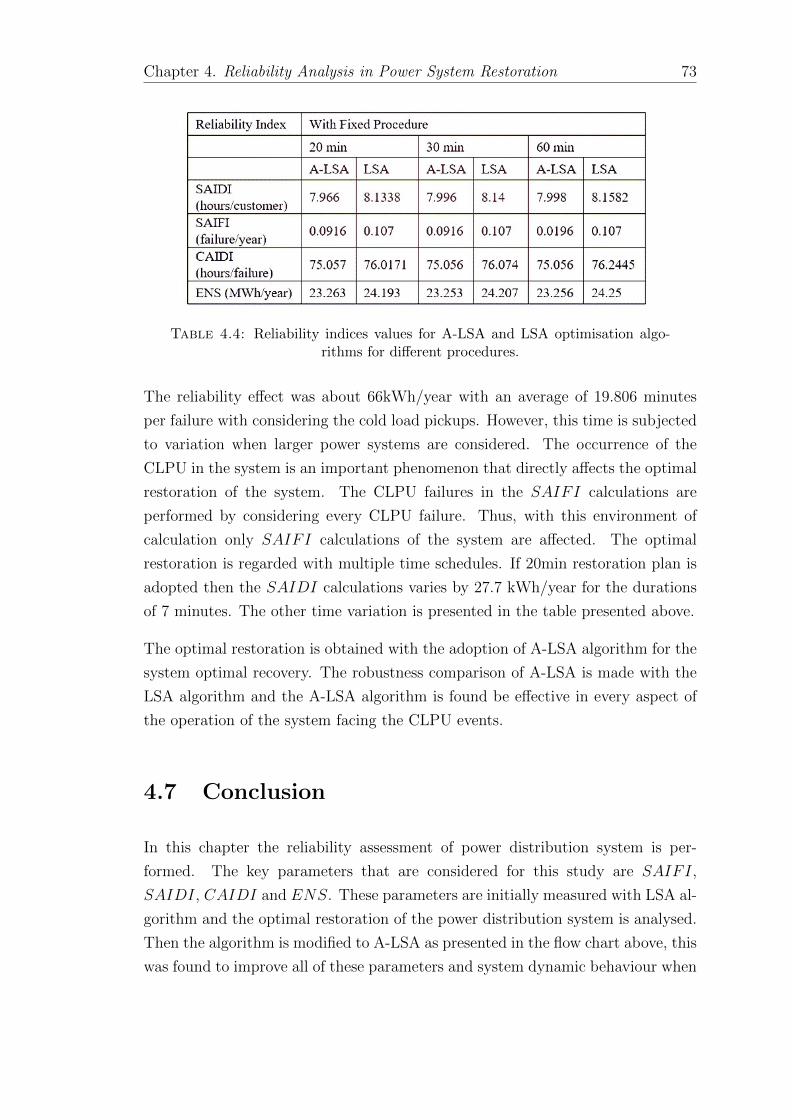
Chapter 4. Reliability Analysis in Power System Restoration 73
Table 4.4: Reliability indices values for A-LSA and LSA optimisation algo-rithms for different procedures.
The reliability effect was about 66kWh/year with an average of 19.806 minutes
per failure with considering the cold load pickups. However, this time is subjected
to variation when larger power systems are considered. The occurrence of the
CLPU in the system is an important phenomenon that directly affects the optimal
restoration of the system. The CLPU failures in the SAIFI calculations are
performed by considering every CLPU failure. Thus, with this environment of
calculation only SAIFI calculations of the system are affected. The optimal
restoration is regarded with multiple time schedules. If 20min restoration plan is
adopted then the SAIDI calculations varies by 27.7 kWh/year for the durations
of 7 minutes. The other time variation is presented in the table presented above.
The optimal restoration is obtained with the adoption of A-LSA algorithm for the
system optimal recovery. The robustness comparison of A-LSA is made with the
LSA algorithm and the A-LSA algorithm is found be effective in every aspect of
the operation of the system facing the CLPU events.
4.7 Conclusion
In this chapter the reliability assessment of power distribution system is per-
formed. The key parameters that are considered for this study are SAIFI,
SAIDI, CAIDI and ENS. These parameters are initially measured with LSA al-
gorithm and the optimal restoration of the power distribution system is analysed.
Then the algorithm is modified to A-LSA as presented in the flow chart above, this
was found to improve all of these parameters and system dynamic behaviour when

Chapter 4. Reliability Analysis in Power System Restoration 74
the system is subjected to cold load pickups. All of these dynamic operational pro-
cedures are verified by implementing this algorithm on the power distribution in
MATLAB. Thus, this modified advanced lighting search algorithm is found to be
effective in restoring the power distribution system when it is subjected to cold
load pickups.

Chapter 5
Statistical Analysis for Power
System Outages
In this chapter, a related subject to PSR will be presented and discussed. (Outages
Analysis).
5.1 Introduction
There is a big debate around the world among policy makers for the benefits
of smart grid technologies to the power grid. Thus, as a result, it is our rule as
researchers to study and analyse the problem in a scientific and data-driven way in
order to guide the policy makers to make the right and optimal decisions towards
the power grid future. This study is aimed to be directed to the Australian power
grid, but the results could be generalised to any power grid around the world.
Studying power outages events can enable us to investigate important queries such
as if the power outages are decreasing with the increasing deployment of smart grid
technologies. There has been a large amount of money deployed by governments
to fund smart grid assets around the world. The goal of these investments is
to increase the reliability of electric systems. Many studies on power outages
usually focus on large individual events because of the discomfort they cause to
the public and the large media attention for such events. This attention may
help in discovering the root-causes in specific events, however, it may not show
other hidden issues that affects the power grid. A potion of these underlying
75

Chapter 5. Statistical Analysis for Power System Outages 76
issues comprise of weather vulnerabilities, human error, equipment failure, and
infrastructure failure.
Analysing power outages trends through time will give us the opportunity to ex-
plore important trends like the frequency/magnitude of power outages, time of a
year, time of a day and the geographical positions of these events. All of these
rising queries and more can be investigated using the appropriate dataset from
official references, in our case, the Australian Energy Market Operator (AEMO)
and electricity service providers over Australia.
In this chapter, we will examine power outages data in Australia, and investi-
gate trends of magnitude, frequency, duration, and geographic positions. We will
also study states and utilities reliability data trends in an attempt to find a cor-
relation between states, utilities, reliability indices and smart grid technologies
investments. After that, recommendations will be provided to regulators, utilities
and official references to use resources more efficiently and enable new researchers
in this field to analyse smart grid investments data more efficiently in future.
In this introductory Section, we will study the power industry facts, which gives
an idea about where the power industry in Australia headed. We will start by the
following four points.
The number of customers is increasing over time.
The total electricity generated annually has increased over time.
A relationship between the number of customers and electricity generation
annually exists.
The price of electricity of cents/kWh is increasing over time.
The following graphs answer these points.

Chapter 5. Statistical Analysis for Power System Outages 77
Figure 5.1: Figure showing the increase of customers number in millions byyear.
Figure 5.2: The Australian total electricity generation by year in GWh.

Chapter 5. Statistical Analysis for Power System Outages 78
Figure 5.3: The relationship between the number of costumers and the elec-tricity generation.
Figure 5.4: The average household electricity bills annually and the averagecommercial and industrial prices from 2007-17 by ACCC.

Chapter 5. Statistical Analysis for Power System Outages 79
5.2 Background
5.2.1 Smart Grid
Smart grid is a future goal for almost all traditional power grid utilities in the
world. It is a broad concept, which means generally making the power grid smarter
and dynamic by making it easy to monitor and control through adding smart grid
technologies such as Advanced Metering Infrastructure (AMI), grid-scale energy
storage systems such as large-scale batteries, and renewable energy sources (RES)
such as solar panels and wind turbines.
5.2.2 Smart Grid Investments in Australia
As an extreme continent, with unpredictable weather, aged power grids infras-
tructure and constantly changing electricity market, and with the fact that robust
supply of electricity is essential for Australia’s economic growth, it made it an
urgent task for Australia to have a long-term power grid strategy. Thus, it started
investing its smart grid technologies and investigating their benefits to the current
aged power grid.
Australia has made a first step into this concept by accomplishing the Smart Grid
Smart City (SGSC) project which started in 2010 and finished at 2014 and cost
about AU(Dollars)100m government funds. The SGSC project analysis indicated
that adding smart grid technologies to the power grid will improve the grid re-
liability and the utilities operations. And the project’s cost-benefits assessments
predicted more than AU(Dollars)27bn economic benefits over the next twenty
years and lower network charges if smart grid technologies and improved tariffs
were rolled out [1] .
The study also examined and recommended technologies such as fault detection,
isolation and restoration (FDIR), which allows operators to rapidly recognise any
fault in the grid by their exact source and location. This technology allows grid
operators to isolate the faulted section of the grid and restore power to costumers
in healthy sections, which can be done remotely in some cases [1].
The SGSC project included deployment of other smart grid technologies and ap-
plications such as in Table 5.1.

Chapter 5. Statistical Analysis for Power System Outages 80
Table 5.1: Smart grid applications deployed in the SGSC project [1].
As per the current dynamics between the decreased forecasted electricity demand
and the growing number of customers in Australia, the network service providers
were able to delay some capital investment. Yet, maintaining and replacing aged
elements in the network is becoming more of a serious matter. The state-wide
blackout in South Australia on 28 September 2016 due to a storm damaging the
transmission infrastructure is one example [156].
At the same time, costumers are becoming more sensitive to electricity prices, and
aware of the competitive alternatives that are becoming more affordable such as,
residential solar PV installations, using more energy efficient appliances, thus, a
descending pressure on utilities energy demand is expected. All these elements
together, make the energy storage systems important in the transformation of the
Australian electricity industry. Australia was a world leader in the deployment of
the largest residential battery storage system in terms of power capacity in 2017
[157].
5.2.3 Environmental Reasons
Weather is an important factor in smart grid tendency around the world as the
climate change issue is becoming a world-wide issue. There is a big number if major
blackouts around the world that was caused mainly by severe weather conditions.
In Fig.5.5 below an average annual temperature change in the world for the past

Chapter 5. Statistical Analysis for Power System Outages 81
167 years from 1850 to 2017. The figure indicates a change in the annual average
temperature in the world. Which supports the claims of climate change by many
organisations around the world [158].
Figure 5.5: Annual average temperature change in the world over 167 yearsperiod.
5.2.4 Weather Trends in Australia
As the world is trying to deal with the climate change issue, mitigate its reasons
and consequences, there become a noticeable political pressure in Australia to close
coal fired power plants and minimise the use of fusel fuels in electricity production.
It can be seen from Fig.5.6 that the climate change is real as the rise in sea surface
temperature in Australia started spiking from 1975 and kept rising in general
afterwards.

Chapter 5. Statistical Analysis for Power System Outages 82
Figure 5.6: Annual sea surface temperature change in Australia over 118 yearsperiod .
5.2.5 The Australian Electricity Infrastructure
Figure 5.7: A map of electricity transmission lines in Australia.
The map in Fig. 5.7 shows the locations of Australia’s electricity transmission
lines. NSW, Queensland, Victoria, South Australia and Tasmania (via the under-
sea Basslink) are interconnected and make up the National Electricity Market

Chapter 5. Statistical Analysis for Power System Outages 83
(NEM). Northern Territory has no available data, and the Western Australia is
considered an electricity island.
5.2.5.1 National Power Generation Data:
There was an opportunity to evaluate the performance of the Australian grid
when an Energy Matters contributor recorded the electricity generation data from
a published Australian reference [159]. The data were limited to 19.5 days starting
from Thursday 27 July 2017 at 19:30 to Wednesday 16 August 2017 at 07:45 (NEM
Time). The data shows the following generation resources table:
Table 5.2: Australia electricity generation data for the period of 27 July to 16August 2017.
The data shows large differences in generation mixes between different states. The
data also propose that Gas-Fired power plants are having difficulties balancing
irregular wind generation against demand in South Australia [159].
Figure 5.8: Australia total generation by source, 27 July to16 August, 2017.
The data are 5-minutes interval. They comprise generation differentiated by state
and source. The peak generation of (34,246MW) happened at 6:20pm NEM time
on 3 August 2017 [159]. Because Australia is an electricity island, the peak gen-
eration will be equal to the peak demand.

Chapter 5. Statistical Analysis for Power System Outages 84
5.2.6 Australian Electric Infrastructure Security:
The important dual of reliability and security was getting an increasing attention
over the past few years because of the advanced cyber-attacks against important
infrastructure in different domains. These cyber-attacks may not only impact the
energy sector in Australia but have broader impacts on the nation’s economy,
public health and society [160].
Figure 5.9: Worldwide Cyber-Attacks events on critical infrastructure andindustrial control systems (ICS).
In response to the increasing threat landscape, AEMO has specially made a sector
wide Cyber Security project. Key considerations underneath its establishment
included [161]:
AEMO’s responsibility for maintaining the security of the grid means cyber
considerations are a material concern.
Finkel Recommendation 2.10 requires an annual report into the cyber secu-
rity preparedness of the National Electricity Market.
Increasing level of concern and urgency from Australian government agencies
(ASD, Critical Infrastructure Centre) in relation to cyber threats.
International events and incidents related to Energy Critical Infrastructure
that have been attributed to cyber threat actors such as those on the previous
slide.
The trend of increasing digitisation and automation of critical energy system
has increased the risk of disruption through cyber-attacks.

Chapter 5. Statistical Analysis for Power System Outages 85
The project has mainly been started to deliver a tailored cyber security frame-
work, the Australian Energy Sector Cyber Security Framework (AESCSF), and
supporting tools to set the foundation for the future of energy cyber security in
Australia [161].
The administrative principles for the development of the AESCSF include:
Figure 5.10: The administrative principles for the development of theAESCSF.
The project has started with a Critical Assessment Tool (CAT), the purpose of
CAT is to determine the criticality of the entity, to rank entities within their
industry sub sector, and to assist in the determination of the target maturity
state for the entity [161].
Figure 5.11: Criticality scale and bands by energy market sub-sectors [160].

Chapter 5. Statistical Analysis for Power System Outages 86
5.2.7 Cascading Outages
The definition of cascading outages by IEEE is: it is a sequence of events in which
an initial disturbance, or set of disturbances, triggers a sequence of one or more
dependent component outages [162].
The major cascading blackout happened in the NEM region was the state-wide
blackout in South Australia that occurred as a result of storm damage to electricity
transmission infrastructure on 28 September 2016.
Lessons learnt from cascading blackouts in South Australia and around the world:
Fault ride-through capability of renewable energy sources
Extreme weather
Incompatibility of UFLS with high RoCoF
Local voltage / reactive power support
Frequency support from renewable sources
Robustness of cyber security system
Hidden problems in protection schemes
Emergency load shedding
It is been noticed in many studies that the developing speed of cascading outages
are different in different stages, and that is due to protection scheme characteris-
tics and properties.
Important question: Is the reliability of the power system increasing
with the combined high penetration of renewable energy sources and
energy storage systems?
We could not find data to test this question as a hypothesis, however we found
many strong studies that indicate the benefit to system reliability when using
Battery-based energy storage systems, especially when the system has high pene-
tration of RES. Refer to [163] for more.

Chapter 5. Statistical Analysis for Power System Outages 87
5.3 Study Questions
The National Electricity Market (NEM) covers the main 6 states where the ma-
jority of population lives. It interconnects the 6 eastern and southern states and
territories and delivers around 80 percent of all electricity consumption in Aus-
tralia [1]. In this research paper we will investigate the following hypotheses in
the NEM region majorly with the deployment of smart grid technologies.
5.3.1 Power Disturbances Hypotheses:
H1: The frequency of power outages is decreasing over time.
H2: The duration of power outages is decreasing over time.
H3: Weather is one of the main causes of outages in Australian power systems.
H4: The loss in MW by year is decreasing over time.
H5: There is a relationship between the number of customers and the magnitude
of the outage.
H6: There is a relationship between power outage duration and the magnitude of
the outage.
H7: The magnitude of power outages fits a power-law model.
H8: Outages greater than 5 GW are uncommon.
H9: The number of power outages is greater during specific times of a day.
H10: The number of power outages is greater during specific seasons of the year.
H11: The market impact of outages is increasing over time.
5.3.2 Reliability Hypotheses:
H12: SAIFI (frequency of outages reliability index) values vary from
state-to-state, utility-to-utility, and year from year.
H13: CAIDI (duration of outages reliability index) values vary from
state-to-state, utility-to-utility, and year from year.
H14: The frequency of power outages is decreasing with the deployment of smart
grid technologies.
H15: The duration of power outages is decreasing with the deployment of smart
grid technologies.
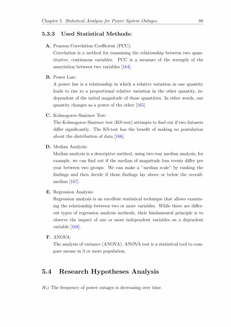
Chapter 5. Statistical Analysis for Power System Outages 88
5.3.3 Used Statistical Methods:
A. Pearson Correlation Coefficient (PCC):
Correlation is a method for examining the relationship between two quan-
titative, continuous variables. PCC is a measure of the strength of the
association between two variables [164].
B. Power Law:
A power law is a relationship in which a relative variation in one quantity
leads to rise to a proportional relative variation in the other quantity, in-
dependent of the initial magnitude of those quantities. In other words, one
quantity changes as a power of the other [165].
C. Kolmogorov-Smirnov Test:
The Kolmogorov-Smirnov test (KS-test) attempts to find out if two datasets
differ significantly. The KS-test has the benefit of making no postulation
about the distribution of data [166].
D. Median Analysis:
Median analysis is a descriptive method, using two-way median analysis, for
example, we can find out if the median of magnitude loss events differ per
year between two groups. We can make a ”median scale” by ranking the
findings and then decide if those findings lay above or below the overall-
median [167].
E. Regression Analysis:
Regression analysis is an excellent statistical technique that allows examin-
ing the relationship between two or more variables. While there are differ-
ent types of regression analysis methods, their fundamental principle is to
observe the impact of one or more independent variables on a dependent
variable [168].
F. ANOVA:
The analysis of variance (ANOVA). ANOVA test is a statistical tool to com-
pare means in 3 or more population.
5.4 Research Hypotheses Analysis
H1: The frequency of power outages is decreasing over time.

Chapter 5. Statistical Analysis for Power System Outages 89
From graph above we can see that the peak of frequency of power outages is in
2005. The lower frequency of power outages is in 2017. The graph show that the
frequency of power outages has negative trend, which indicates that the frequency
of power outages is decreasing over time. A formal analysis is conducted based on
the linear regression.
From output of linear regression above we can see that the coefficient yearly vari-
able is negative, which means if the year variable increases a year then the fre-
quency of power outages will be decreasing by -0.054. From the p-value of coef-
ficient yearly (6.9*10-7) and 95 percent confidence interval ((-0.065, -0.043)), we
can conclude that the frequency of power outages is significantly decreasing over
the time .
From the graph below we can see that the frequency of power outages is above
median on 2006 until 2011, and below median on 2012-2017. From the median
analysis, frequency of power outages indicates decreasing over the year. The result
is consistent with regression analysis above.

Chapter 5. Statistical Analysis for Power System Outages 90
H2: The duration of power outages is decreasing over time.
From graph above we can see that the peak of duration of power outages is in
2005. The lower duration of power outages is in 2017. The graph shows that the
duration of power outages has negative trend, which indicates that the duration
of power outages is decreasing over time. A formal analysis is conducted based on
the linear regression.

Chapter 5. Statistical Analysis for Power System Outages 91
From output of linear regression above we can see that the coefficient yearly vari-
able is negative, which means if the year variable increases a year then the duration
of power outages will be decreasing by -2.62. From the p-value of coefficient yearly
(0.0003) and 95 percent confidence interval ((-3.712, -1.528)), we can conclude that
the duration of power outages is significantly decreasing over time.
From the graph of median analysis we know that the duration of power outages
is above median on 2006 until 2011, and below median on 2012-2017. From the
median analysis, the duration of power outages is decreasing over time. The result
is consistent with regression analysis above.
H3: Weather is one of the main causes of outages in Australian power systems.
From the available data for AusGrid distribution network outages for the year
2016. We analysed the data and the conclusions are shown in the graph above.
The data indicates that faults are the major cause for outages in the Australian
distribution sector which resulted in about 53 percent of total outages while the
weather is the second major cause which resulted in about 38 percent of total

Chapter 5. Statistical Analysis for Power System Outages 92
outages. The faults and weather together caused more than 90 percent of total
outrages.
Table 5.3: Descriptive Analysis Table For the USA Department of Energyoutages data from 2002 to 2019.
From table above we can observe that the mean is greater than the median, so the
distribution from variables magnitude, duration and customer is positive skewness.
The mode of three variables varies.
H4: The loss in MW by year is decreasing over time.
From the graph below we can see that the peak of magnitude is in 2002. The lower
magnitude is in 2019. But in 2011 the magnitude increases. The graph shows that
the magnitude of power outages is fluctuating and have negative trend, which
indicates that the magnitude is decreasing over time. To know if the decreasing is
significant or not, a formal analysis is conducted based on the linear regression.

Chapter 5. Statistical Analysis for Power System Outages 93
From output of linear regression below we can see that the coefficient yearly vari-
able is negative, which means if the year variable increases a year then the duration
of power outages will be decreasing by -2206.2. From the p-value from coefficient
yearly (0.015) and 95 percent confidence interval ((-3901.38, -510.9)), We can con-
clude that the magnitude of power outages loss in MW is significantly decreasing
over time .
From the graph of median analysis we can observe that the magnitude value be-
low the median is increasing over the years. Then for the value below median it
is higher than values above the median, which means most of magnitude value is
below the median. The magnitude value below median in 2002-2008 is less than
in 2009-2019. It indicates that the magnitude is decreasing over the years. The
result is consistent with regression analysis above.

Chapter 5. Statistical Analysis for Power System Outages 94
H5: There is a relationship between the number of customers and the magnitude
of the outage.
From graph above we can see that customers and magnitude have positive rela-
tionship if the value of log10(customers) above than 3. Then if we see the scatter
plot for log10(customers) below than 3, the points spread out, that indicates no
relationship for those data. So we exclude them for the next analysis.

Chapter 5. Statistical Analysis for Power System Outages 95
From the graph above we get an indication that the magnitude has a relationship
with customers, to test if the relationship is significant or not, a formal analysis is
conducted based on the linear regression.
From output of linear regression above we can see that the coefficient log10(customer)
variable is positive, which means if the customers variable increases by 1 then the
magnitude will be increasing too. From the p-value from coefficient yearly (¡0.000)
and 95 percent confidence interval ((0.598, 0.726)), We can conclude that the mag-
nitude has a positive relationship with customers.
H6: There is a relationship between power outage duration and the magnitude of
the outage.
We want to know if there is a relationship between duration and magnitude of
outages, to do that we can use correlation analysis. To test if the correlation is
significant we can use Pearson correlation. The result from Pearson is p = 0.23

Chapter 5. Statistical Analysis for Power System Outages 96
and p-value is < 0.000. which means p 6= 0 because the p-value < 0.05, so we have
evidence that magnitude has a relationship with duration.

Chapter 5. Statistical Analysis for Power System Outages 97
H7: The magnitude of power outages fits a power-law model.
From the graph we can see that the distribution of outages magnitudes is highly
positive skewness. The graph shows the shape is likely to power law distribution.
To test our hypothesis that the magnitude fits a power law distribution, we used
Kolmogorov-Smirnov test. The Kolmogorov-Smirnov test was also used to test if
the magnitude fits with several other distributions such as Normal, Exponential,
LogNormal etc. Form the p-values in the table below, we can see only the p-value
from the power law is 0.96 while other p-values are much less than 0.05, indicating
that the magnitude does fit with power law distribution.

Chapter 5. Statistical Analysis for Power System Outages 98
H8: Outages greater than 5 GW are uncommon.
From the table above, we can see that outages greater than 5 GW are uncommon
because they account only for 1.68 percent of total outages.
H9: The number of power outages is greater during specific times of a day.
We were able to get data for outages in AusGrid distribution network from 2012
to 2018. We divided the day to 4 periods as shown above. As can be seen in
the figure above, the number of outages is greater during specific times of a day.
Period 3 which is the peak hours was having the majority of power outages (about
34 percent) comparing to other periods. Then we compare period 3 with others
period to see if there is a significant difference of outages between period 3 and
any other period with the linear regression.

Chapter 5. Statistical Analysis for Power System Outages 99
From results above we can see that the p-value for period 1, 2, and 4 is less than 5
percent, so we have evidence to say that the number of power outages in period 3
is significantly different form others periods. Thus, our finding indicates that the
number of power outages is greater during specific times of a day.
H10: The number of power outages is greater during specific seasons of the year.
We were able to get data for outages in AusGrid distribution network from 2012
to 2018. We divided the year to 4 seasons as shown above. As can be seen in
the figure above, the number of outages is greater during specific seasons of the
year. Summer season was having the majority of power outages (about 34 percent)
comparing to other seasons. Then we compare summer season with others seasons
to see if there is significant difference of outages between summer season and any
other seasons with the linear regression.

Chapter 5. Statistical Analysis for Power System Outages 100
From results in the table above we can see that the p-value for Spring and Autumn
is lower than 5 percent, so we have evidence to say that the number of power out-
ages in summer season is significantly different from spring and autumn seasons,
but not with winter season.
H11: The market impact of power outages is increasing over time.
From graph above we can see that the peak of market impact is in 2006. The
lower market impact is in 2011.Then on 2016 the market impact is high again.
The graph shows that the market impact has negative trend starting from 2006
until 2011, then starting from 2012 the market impact is having a positive trend.
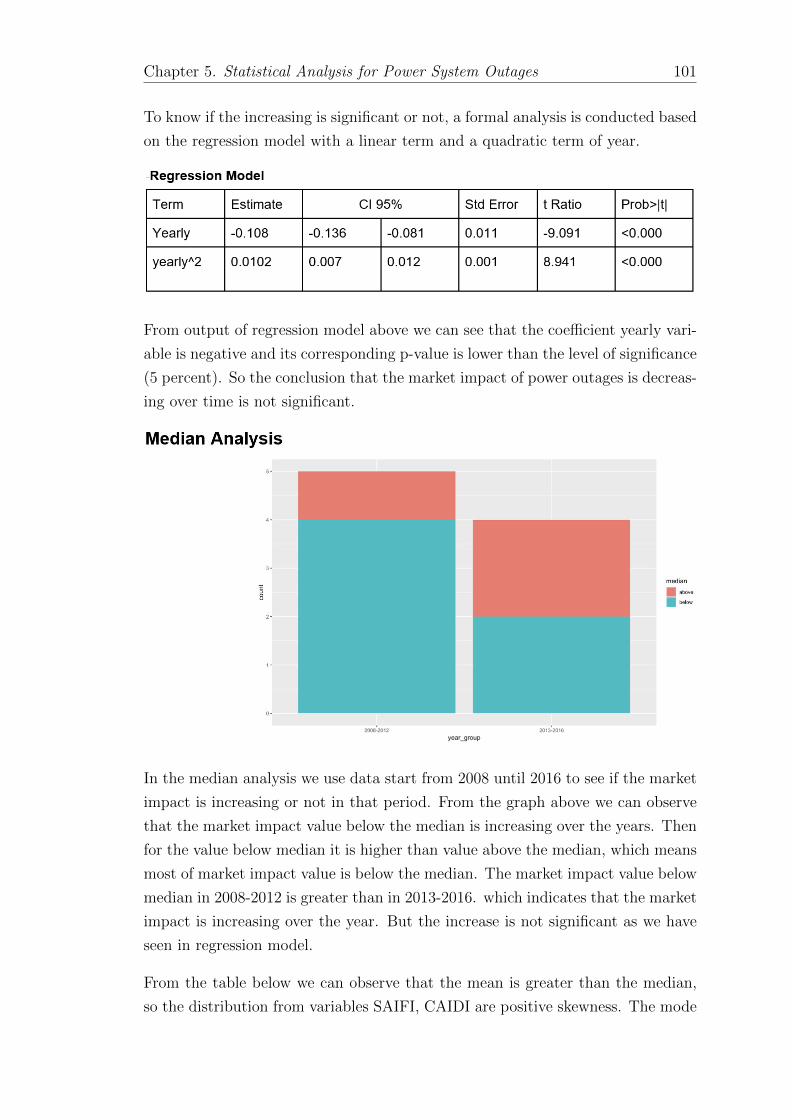
Chapter 5. Statistical Analysis for Power System Outages 101
To know if the increasing is significant or not, a formal analysis is conducted based
on the regression model with a linear term and a quadratic term of year.
From output of regression model above we can see that the coefficient yearly vari-
able is negative and its corresponding p-value is lower than the level of significance
(5 percent). So the conclusion that the market impact of power outages is decreas-
ing over time is not significant.
In the median analysis we use data start from 2008 until 2016 to see if the market
impact is increasing or not in that period. From the graph above we can observe
that the market impact value below the median is increasing over the years. Then
for the value below median it is higher than value above the median, which means
most of market impact value is below the median. The market impact value below
median in 2008-2012 is greater than in 2013-2016. which indicates that the market
impact is increasing over the year. But the increase is not significant as we have
seen in regression model.
From the table below we can observe that the mean is greater than the median,
so the distribution from variables SAIFI, CAIDI are positive skewness. The mode

Chapter 5. Statistical Analysis for Power System Outages 102
Table 5.4: Descriptive Analysis Table for SAIFI and CAIDI indices statisticsfor Australian power system data from 2006-2017.
of three variables varies. Also we can see that the median and mean values are
close in proximity suggesting that the data is fairly normally distributed.
SAIFI (frequency of outages reliability index.)
Figure 5.12: SAIFI index for each utility in NEM region

Chapter 5. Statistical Analysis for Power System Outages 103
From our analysis we found that there is a variability from utility-to-utility, year-
to-year, and state-to-state.
Figure 5.13: Q-Q Plot for SAIFI index in each state.
Also, we can see from the Q-Q Plot that the SAIFI approximately follows a normal
distribution in each state.
CAIDI (duration of outages reliability index)
From our analysis we found that there is variability from utility-to-utility, year-
to-year, and state-to-state.

Chapter 5. Statistical Analysis for Power System Outages 104
Figure 5.14: CAIDI index for each utility in NEM region.
Figure 5.15: Q-Q Plot for CAIDI index in each state.
Also, we can see from the Q-Q Plot that CAIDI approximately follows normal
distribution in each state.
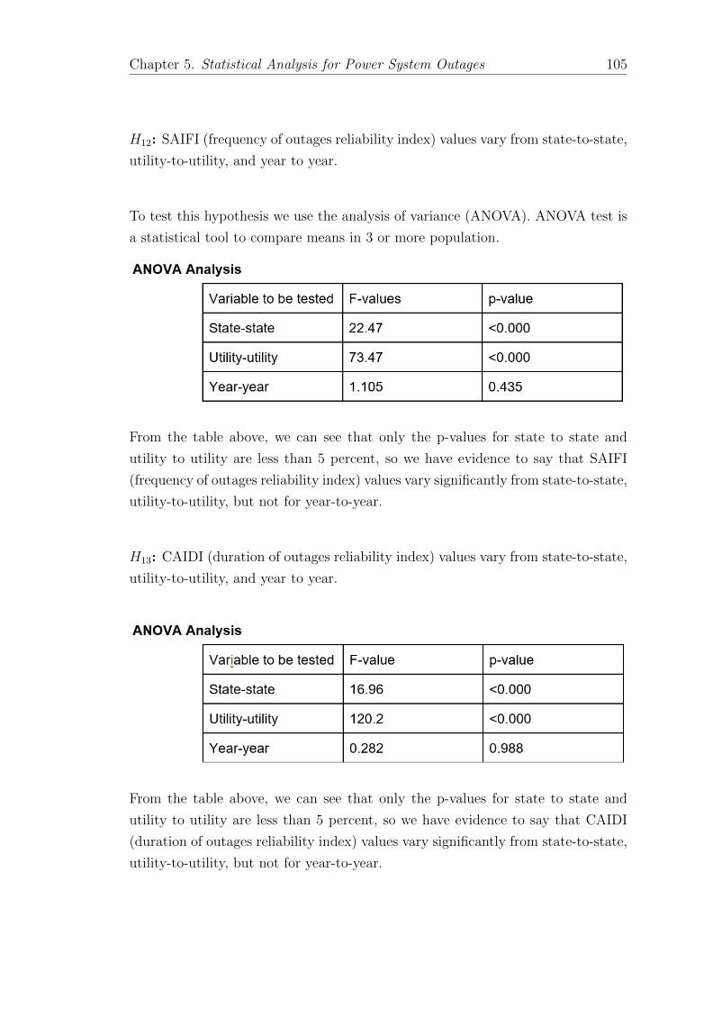
Chapter 5. Statistical Analysis for Power System Outages 105
H12: SAIFI (frequency of outages reliability index) values vary from state-to-state,
utility-to-utility, and year to year.
To test this hypothesis we use the analysis of variance (ANOVA). ANOVA test is
a statistical tool to compare means in 3 or more population.
From the table above, we can see that only the p-values for state to state and
utility to utility are less than 5 percent, so we have evidence to say that SAIFI
(frequency of outages reliability index) values vary significantly from state-to-state,
utility-to-utility, but not for year-to-year.
H13: CAIDI (duration of outages reliability index) values vary from state-to-state,
utility-to-utility, and year to year.
From the table above, we can see that only the p-values for state to state and
utility to utility are less than 5 percent, so we have evidence to say that CAIDI
(duration of outages reliability index) values vary significantly from state-to-state,
utility-to-utility, but not for year-to-year.

Chapter 5. Statistical Analysis for Power System Outages 106
H14: The frequency of power outages is decreasing with the deployment of smart
grid technologies.
From graph above we can see that the peak of frequency of power outages is in
2010. The lower frequency of power outages is in 2017. The graph show that the
frequency of power outages has negative trend, which indicates that the frequency
of power outages is decreasing over time. To know if the decreasing is significant
or not, a formal analysis is conducted based on linear regression.
From output of linear regression we can see that the coefficient yearly variable is
negative, which means if the year variable increases a year then the frequency of
power outages will be decreasing by -0.054. To know if the decreasing is significant
or not, we can see the p-value from coefficient yearly (0.002). The p-value is lower
than level of significance (5 percent). So the conclusion is that the frequency of
power outages is significantly decreasing over time.
From the graph below we can observe that the frequency of power outages value
below the median is increasing over the years. Then for the value below median it
is higher than value above the median, which means most of frequency of power
outages value is below the median. The frequency of power outages value below

Chapter 5. Statistical Analysis for Power System Outages 107
median in 2010-2014 is less than in 2015-2017. Which indicates that the frequency
of power outages is decreasing over the years. The result is consistent with regres-
sion analysis above. Thus we have an evidence to say that the frequency of power
outages is decreasing over time with the deployment of smart grid technologies
which started from 2010 to 2014.
H15: The duration of power outages is decreasing with the deployment of smart
grid technologies.

Chapter 5. Statistical Analysis for Power System Outages 108
From graph above we can see that the peak of frequency of power outages is in
2011. The lower duration power outages is in 2013. The graph shows that the
duration of power outages has no clear trend, but we can notice that the duration
of power outages is slightly decreasing over time. To know if the decreasing is
significant or not, a formal analysis is conducted based on linear regression.
From output of linear regression above we can see that the coefficient yearly vari-
able is negative, which means if the year variable increases a year then the duration
of power outages will be decreasing by -0.95. To know if the decreasing is signifi-
cant or not, we can see the p-value from coefficient yearly (0.362). The p-value is
greater than level of significance (5 percent). So the conclusion is that the duration
of power outages is not significantly decreasing over time.
From the graph above we can observe that the duration of power outages value
above the median is decreasing over the years. The duration of power outages
value above median in 2015-2017 is less than in 2010-2014. It indicates that the
duration of power outages is decreasing over the years. The result is not consistent
with regression analysis above. Thus we don’t have an evidence to say that the
duration of power outages is significantly decreasing over time with the deployment
of smart grid technologies that started from 2010 to 2014.

Chapter 5. Statistical Analysis for Power System Outages 109
5.5 Discussion
This study has been done on the limited data available for power outages and
power system’s reliability indices. The hypotheses that are constructed to test
the Australian power system (mostly distribution networks), we were able to find
limited-but-enough data from 2006-2017 to test them. Other general hypotheses
we had to use the USA, Department of Energy (DOE) power outages data form
2002-2019 to test them, as they are considered confidential in the Australian power
system market. The analysis was done using R statistics software [169].
5.5.1 Power Disturbances Hypotheses:
Our analysis showed that the frequency of power outages is decreasing over time.
That could be explained by the effects of the significant network investment cycle,
smart grid technology deployment and changes to regulations. There is an evidence
that the duration of power outages is decreasing over time as well. Many potential
explanations of this finding include: adding more resources to reduce the power
restoration time, and using FDIR and AMI technologies to report power outages
faster so they can be fixed earlier.
When looking at the major causes of power outages in the Australian power sys-
tem, our findings indicate that the most common cause was equipment failure not
weather. It is important to mention that our analysis for this hypothesis were
made on data for the distribution system not the transmission system. It is to
our believe that the most common cause of power outages could be weather if
the analysis were done on transmission system data, as many good studies and
technical reports indicate. To test if the loss in MW by year is decreasing over
time we had to use the USA, DOE 2002-2019 data. Our finding was that the loss
in MW by year is significantly decreasing over time. The potential explanations
for these findings could be the same for previous ones.
When testing the relationship between the number of costumers and the magnitude
of a power outage, a reasonable correlation was found. Instinctively, it makes
sense that a larger power outage magnitude would impact a larger number of
customers. The outliers in the XY plot of log(magnitude) and log(costumers) could
be interpreted as large scale customers (industrial, commercial) that have large
loss but considered as only one costumer. We also tested if there is a relationship
between the power outage duration and the magnitude of the outage. Our finding

Chapter 5. Statistical Analysis for Power System Outages 110
indicates that there was a significant correlation between the restoration time and
the size of the outage. That could be explained by the fact that a larger loss
indicates a probable larger damage to the network, and a larger damage would
intuitively need a larger restoration time and that’s a whole new problem (sending
repair crews, carrying resources, repair crew skills etc.).
We tested if the distribution of power outages magnitude data fits a power-law
model. Our finding indicates that the sizes of power outages fits a power-law
distribution model and does not fit other four distributions considered in this
paper. This test was made to verify previous research findings but on a new set
of data. Outages larger than 5 GW were found to be uncommon, and that could
be due to the large investments and modernisation on power system, mainly the
power system protection schemes, which would prevent/isolate cascading outages.
We tested if the frequency of power outages is greater during specific times of
the day and specific seasons of the year. Our findings indicate that the frequency
of power outages is time-of-a-day dependent and season-of-a-year dependent. It
seems that certain types of power outages are more likely to occur in certain times
of the day. The frequency of power outages was larger during peak hours (1pm-
6pm). This time slot is the one with the maximum expected electricity usage by
costumers. Thus, it is expected that the highest number of outages happen in
this time period. The number of power outages during summer (which is the peak
season followed by winter) is significantly higher than other seasons. This could
be driven by severe weather combined with a large demand on the network. It
has been suggested in many scientific articles and researches that climate change
is real and is causing severe weather situations, which has a large impact on our
power system. Last thing we tested that is related to power system disturbances
was the power outages market impact, which is a very important indicator for
power utilities that basically means the cost of a power outage to utilities and
costumers. Our analysis has shown that the market impact of power outages is
increasing over time, but the increase is not significant based on the limited data
we analysed.
5.5.2 Reliability Hypotheses:
In this part of the research we have analysed the power system reliability indices,
mainly SAIFI (frequency of outages reliability index) and CAIDI (duration of out-
ages reliability index). It must be mentioned that there are many other reliability
Chapter 5. Statistical Analysis for Power System Outages 111
indices used in the power industry, but these two are the main ones and the ones
that we were able to find data to test.
There was enough data to test hypotheses 12 and 13, that SAIFI and CAIDI
vary from state-to-state, utility-to-utility and year-to-year. Our findings are that
SAIFI and CAIDI are significantly different from state-to-state and utility-to-
utility but not year-to-year. An explanation for these finding could be that each
state has different electricity providers and each electricity provider has different
set of equipment installed, age of equipment, number of costumers and network
topology.
We tested the impact of smart grid technologies deployment on power outages
frequency and duration. For this test we used data of the SGSC project that
was done on AusGrid network in NSW from 2010-2014. The initial analysis on
the limited available data showed that there was a reduction on the frequency of
power outages in AusGrid network with the deployment of smart grid technologies.
However, we found no significant reduction on the duration of power outages with
the deployment of smart grid technologies.
We must mention that there were many different approaches to tackle these hy-
potheses, but none of them would give us an affirm answer or a clear correlation
between the reduction in frequency and duration of power outages and the smart
grid technologies deployment. That is due to the mix of variables and factors
involved in SAIF and CAIDI behaviours in power system, which were mentioned
earlier in this discussion. However, the results are inspiring and these hypotheses
may be proved with more and detailed data in the future. Looking at the whole
dynamics of power systems and of SAIFI and CAIDI indices in power systems,
suggests that other factors could participate in their reduction and not only the
smart grid technologies deployments.
5.6 Conclusion and Recommendations
This chapter provided a detailed statistical analysis of power outages trends and
power system reliability metrics. We have stated the conclusions of each hypothesis
analysis we tested. Also, we illustrated and explained the scientific reasons that
support our findings in the discussion section. In this conclusion we will address
the variables that affected our analysis, such as the limited amount of detailed data
and the lack of cooperation form utilities in Australia. There were many factors

Chapter 5. Statistical Analysis for Power System Outages 112
affected our ability to get solid conclusions about specific research hypothesis. We
have tried to correlate smart grid technologies deployments to the improvements
in power system reliability indices. That was a hard task given that many other
variables and factors could participate in the result we find. Utilities do not
provide detailed data for their smart grid technologies funding, or investments in
modernising their aged infrastructure broken down year by year. This led us to
use the SGSC project with its small scale and data availability limitations as an
indirect measure in our try to answer these questions.
We also wanted to study the impact of large-scale battery-based energy storage
systems to the power system’s reliability indices, but we found no sufficient data
to do such analysis. However, we found strong studies indicate its positive impact
and we mentioned them in previous sections of this paper. We were able to get
enough data to analyse the correlation of SAIFI and CAIDI by state, utility and
year and analyse them fully in their designated section.
Additionally, we have faced many difficulty variables in doing this study, as many
important information were not readily available, such as age of equipment, types
of smart grid technologies, type of transmission lines (overhead, underground),
type of area (rural or urban). Thus, it was hard to take these factors in con-
sideration as we perform our study. However, it is understandable that some of
these data were not made available publicly for security reasons, as they could be
misused by someone looking for a weakness in the power network.
Based on the available data, we were able to get to certain conclusions and rec-
ommendations for specific points. Equipment failure and severe weather were the
main causes of outages in Australian power system. Thus, it is important to rec-
ommend that along with the deployment of smart grid technologies, it is important
to reinforce and modernise the power system infrastructure to be more resilient
against severe weather. This could ease the repair problem aspects in a case of
power system restoration. Aging equipment need to be replaced. Power utilities
need to perform risk-analysis and cost-benefit analysis in order to decide which
equipment should be replaced first.
From time-of-a-day and season-of-a-year perspective, it is recommended to have
more repair crews ready in peak period of the day and in certain seasons that
have severe weather usually such as summer and winter based on the predictable
weather forecasting. Also, it makes sense to locate the repair depots and resources
optimally among the covered network especially near important and large loads
such as commercial and industrial costumers to insure they are better protected.

Chapter 5. Statistical Analysis for Power System Outages 113
An agreement between large and important loads owners and power utilities could
be reached, for example the owners could install backup systems to protect them-
selves in return of discounted rates from utilities. Time-of-Use (TOU) pricing
scheme could be implemented to encourage costumers to use electricity more in
off-peak times, which may result in lower outages that are caused by large de-
mand on power. On the other hand, utilities are encouraged to increase supply
capacity in time windows that are likely to be impacted by power outages due to
high power demand. Intuitively, shorter power outages are preferred over longer
outages, thus, utilities are recommended to look for a good trade-off that come up
with a substantial reduction in longer power outages at a cost of frequent shorter
power outages.
Most power system regulators and utilities provide data in a research unfriendly
formats that need a lot of data management in order to make it suitable to be
imported to a software program to analyse the data. The data management must
be done manually which is a big waste of the researcher time. Many important
information and items are missed from the available data which highlights the
importance of data classification techniques and machine learning in order to cor-
rectly classify items. Dealing with such data needs a lot of work to manage them,
which may cause errors in analysing the data and wrong results in conclusion.
Governments, Academics, and power utilities are going to continue in their re-
search efforts that aim to find correlations between smart grid technologies de-
ployments, and power system reliability indices, which requires the availability of
detailed and readily accessible data from power system regulators and power utili-
ties, with the security concerns of making data publicly available, it is an essential
step to help researchers draw solid conclusions in this field.
Chapter 6
Conclusions and Future Work
In this chapter, the thesis research conclusions and findings will be presented
alongside with probable future work.
6.1 Conclusions
This thesis has developed and presented many important contributions to the PSR
field. Our findings were interesting and very useful to the PSR community and
their efforts to enhance the current practices in the field. We have developed and
presented a high-quality review to the best research efforts made to date in the
aim of easing and well illustrating the problem to new researchers. A systematic
and comprehensive literature review was presented in chapter two.
A major finding in this thesis is showing and proving that mathematical pro-
gramming is outperforming technique in solving PSRR and handling its daunting
computational complexity. A detailed studies and analysis are presented in chap-
ter three providing basic and advanced mathematical applications for the PSRR.
The chapter also provides readers with the ability to compare between different
power systems models in terms of performance with the trade-off factor between
computational easiness and accuracy in mind.
Another major finding was that the suitability and usefulness of Nature-inspired
optimisation techniques in power system reliability studies. Chapter four presents
a promising study for power system reliability in the restorative state under certain
conditions such as CLPU.
114

Chapter 6. Conclusions and Future Work 115
Another important findings in this thesis that were presented in chapter five for
power systems outages and smart grid investments in Australia. We have shown
the potential benefits of statistical analysis in power system studies. We have
developed and investigated many research hypotheses on power outages and sys-
tem reliability, and shown the potential benefits for smart grid technologies to the
power grid.
A complete and detailed list of findings are presented in each chapter’s conclusion.
6.2 Future Work
Based on our research efforts in this thesis, many questions arose and many in-
teresting research ideas have sparked. We have spotted several weak areas in the
PSR field. Thus, in terms of future work, we plan to extend our studies to all
aspects of the PSRRP and all areas of PSR. The following research subjects will
be investigated:
A historical review for major power system blackouts around the world.
Developing a more sophisticated optimisation method for a large-scale PSRRP.
Optimal allocation for black-start generators in power grid.
Investigating advanced optimisation techniques for restoration of large-scale
systems.
Transient stability in system restoration.
Protection schemes control in system restoration.
Vehicle routing strategies for large-scale systems.
Generation, transmission, distribution restoration strategies.
Investigating the optimal sequence to black-start a power system.
Developing a more accurate linear approximation of AC power-flow for sys-
tem restoration studies.
Developing a system operator training software for power system restoration.

Bibliography 116
Developing a more reliable communication scheme for power system opera-
tors that could make the disaster recovery operations optimal.
Investigating the physics of the power system and the logistics of the problem
in a more novel, advanced and applicable way, in the aim of producing a real
applicable research that could enhance disaster recovery approaches in power
systems and enhance people’s life.
Power system islanding coordination and synchronisation.
Rebuilding power system after a disaster.
Optimal sequential operation of switching devices.
Developing a machine learning framework for logistics operations time esti-
mation.
Efficient utilisation of mobile energy sources in power grid.
Studying the restoration problem with the existence of renewable energy
sources.
Power system stochastic storage problem optimisation.
We aim to collaborate with researchers and research centres interested in PSR
around the world in order to make novel and major contributions in this field in
future.

Bibliography
[1] Australian Government. Department of th Environment and En-
ergy, 2000. URL https://www.energy.gov.au/government-priorities/
energy-programs.
[2] C. Liu, K. Liou, R. F. Chu, and A. T. Holen. Generation capability dis-
patch for bulk power system restoration: a knowledge-based approach. IEEE
Transactions on Power Systems, 8(1):316–325, Feb 1993. ISSN 0885-8950.
doi: 10.1109/59.221225.
[3] M. Adibi, P. Clelland, L. Fink, H. Happ, R. Kafka, J. Raine, D. Scheurer, and
F. Trefny. Power system restoration - a task force report. IEEE Transactions
on Power Systems, 2(2):271–277, May 1987. ISSN 0885-8950. doi: 10.1109/
TPWRS.1987.4335118.
[4] Pascal Van Hentenryck and C. Coffrin. Transmission system repair and
restoration. Mathematical Programming, Series B, 151:347–373, 2015. doi:
10.1007/s10107-015-0887-0.
[5] M. M. Adibi and L. H. Fink. Power system restoration planning. IEEE
Transactions on Power Systems, 9(1):22–28, Feb 1994. ISSN 0885-8950.
doi: 10.1109/59.317561.
[6] North American Electric Reliability Council. System restoration from black
start resources. Technical report, (NERC Standard EOP-005-2), 2009.
[7] T. J. Overbye, Xu Cheng, and Yan Sun. A comparison of the ac and dc
power flow models for lmp calculations. In 37th Annual Hawaii International
Conference on System Sciences, 2004. Proceedings of the, pages 9 pp.–, Jan
2004. doi: 10.1109/HICSS.2004.1265164.
[8] Coffrin Carleton and Van Hentenryck Pascal. A linear-programming approx-
imation of ac power flows. 26, 06 2012.
117

Bibliography 118
[9] Ann Melissa Campbell, Dieter Vandenbussche, and William Hermann. Rout-
ing for relief efforts. Transportation Science, 2008.
[10] E. B. Fisher, R. P. O’Neill, and M. C. Ferris. Optimal transmission switching.
IEEE Transactions on Power Systems, 23(3):1346–1355, Aug 2008. ISSN
0885-8950. doi: 10.1109/TPWRS.2008.922256.
[11] Theyab R. Alsenani and Sumit Paudyal. Distributed approach for solving
optimal power flow in three phase unbalanced distribution network. Master’s
thesis, Michigan Technological University, 2014.
[12] Wachtar A. and Biegler LT. On the implementation of a primal dual interior
point filter line search algorithm for large scale nonlinear programming. Math
Program, 2006.
[13] Y. Tamura, H. Mori, and S. Iwamoto. Relationship between voltage in-
stability and multiple load flow solutions in electric power systems. IEEE
Power Engineering Review, PER-3(5):30–31, May 1983. ISSN 0272-1724.
doi: 10.1109/MPER.1983.5519145.
[14] U. G. Knight. Power systems engineering and mathematics. International
Series of Monographs in Electrical Engineering, 1972.
[15] J. Lavaei and S. H. Low. Zero duality gap in optimal power flow problem.
IEEE Transactions on Power Systems, 27(1):92–107, Feb 2012. ISSN 0885-
8950. doi: 10.1109/TPWRS.2011.2160974.
[16] H. Hijazi, C. Coffrin, and P. Van Hentenryck. Polynomial SDP cuts for opti-
mal power flow. In 2016 Power Systems Computation Conference (PSCC),
pages 1–7, June 2016. doi: 10.1109/PSCC.2016.7540908.
[17] D. K. Molzahn, B. C. Lesieutre, and C. L. DeMarco. Investigation of non-
zero duality gap solutions to a semidefinite relaxation of the optimal power
flow problem. In 2014 47th Hawaii International Conference on System
Sciences, pages 2325–2334, Jan 2014. doi: 10.1109/HICSS.2014.293.
[18] B. Kocuk, S. S. Dey, and X. A. Sun. Inexactness of sdp relaxation and
valid inequalities for optimal power flow. IEEE Transactions on Power Sys-
tems, 31(1):642–651, Jan 2016. ISSN 0885-8950. doi: 10.1109/TPWRS.
2015.2402640.

Bibliography 119
[19] R. A. Jabr. Radial distribution load flow using conic programming. IEEE
Transactions on Power Systems, 21(3):1458–1459, Aug 2006. ISSN 0885-
8950. doi: 10.1109/TPWRS.2006.879234.
[20] C. Coffrin, H. Hijazi, and P. Van Hentenryck. The QC relaxation: A
theoretical and computational study on optimal power flow. In 2017
IEEE Power Energy Society General Meeting, pages 1–1, July 2017. doi:
10.1109/PESGM.2017.8274004.
[21] S. S. Dey B. Kocuk and X. A. Sun. Strong SOCP relaxations for the optimal
power flow problem. Operations Research, 2016.
[22] Carleton Coffrin, Hassan L. Hijazi, and Pascal Van Hentenryck. Strengthen-
ing convex relaxations with bound tightening for power network optimiza-
tion. In Gilles Pesant, editor, Principles and Practice of Constraint Program-
ming, pages 39–57, Cham, 2015. Springer International Publishing. ISBN
978-3-319-23219-5.
[23] S. Mhanna, G. Verbic, and A. C. Chapman. Tight LP approximations for
the optimal power flow problem. In 2016 Power Systems Computation Con-
ference (PSCC), pages 1–7, June 2016. doi: 10.1109/PSCC.2016.7540937.
[24] Eric I.PasShari L.Principio. Braess’ paradox: Some new insights. Trans-
portation Research Part B: Methodological, Volume 31(Issue 3):Pages 265–
276, 1997.
[25] Chen ching Liu, Vijay Vittal, and Gerald T. Development and evaluation of
system restoration strategies from a blackout. Power Systems Engineering
Research Center, 2009.
[26] Daniel Lindenmeyer. A framework for power system restoration. PhD thesis,
The University of British Colombia, 2000.
[27] Paul L. Joskow. Restructuring competition and regulatory reform in the
USA electricity sector. The Journal of Economic Perspectives, 1997.
[28] M. M. Adibi, J. N. Borkoski, and R. J. Kafka. Power system restoration -
the second task force report. IEEE Transactions on Power Systems, 2(4):
927–932, Nov 1987. ISSN 0885-8950. doi: 10.1109/TPWRS.1987.4335278.
[29] M. M. Adibi, R. W. Alexander, and D. P. Milanicz. Energizing high and
extra-high voltage lines during restoration. IEEE Transactions on Power

Bibliography 120
Systems, 14(3):1121–1126, Aug 1999. ISSN 0885-8950. doi: 10.1109/59.
780939.
[30] M. M. Adibi, L. H. Fink, C. J. Andrews, F. Arsanjani, M. W. Lanier, J. M.
Miller, T. A. Volkmann, and J. Wrubel. Special considerations in power
system restoration. IEEE Power Engineering Review, 12(11):43–, November
1992. ISSN 0272-1724. doi: 10.1109/MPER.1992.161433.
[31] Kirby Brendan and HIRST ERIC. Maintaining system blackstart in com-
petitive bulk-power markets. 61, 01 1999.
[32] M. M. Adibi and R. J. Kafka. Power system restoration issues. IEEE
Computer Applications and Power; (United States), 4:2, 4 1991. doi:
10.1109/67.75871.
[33] M. M. Adibi, W. Alexander, and B. Avramovic. Overvoltage control during
restoration. IEEE Power Engineering Review, 12(11):43–, November 1992.
ISSN 0272-1724. doi: 10.1109/MPER.1992.161434.
[34] M. M. Adibi, D. P. Milanicz, and T. L. Volkmann. Remote cranking of
steam electric stations. IEEE Transactions on Power Systems, 11(3):1613–
1618, Aug 1996. ISSN 0885-8950. doi: 10.1109/59.535705.
[35] M. M. Adibi and D. P. Milanicz. Reactive capability limitation of syn-
chronous machines. IEEE Transactions on Power Systems, 9(1):29–40, Feb
1994. ISSN 0885-8950. doi: 10.1109/59.317560.
[36] D. Lindenmeyera H., W. Dommela, and M. M. Adibi. Power system restora-
tion a bibliographical survey. International Journal of Electrical Power and
Energy Systems, 2001.
[37] M. M. Adibi, L. R. J. Kafka, and D. P. Milanicz. Expert system requirements
for power system restoration. IEEE Transactions on Power Systems, 9(3):
1592–1600, Aug 1994. ISSN 0885-8950. doi: 10.1109/59.336099.
[38] J. A. Huang, F. D. Galiana, and G. T. Vuong. Power system restoration
incorporating interactive graphics and optimization. In [Proceedings] Confer-
ence Papers 1991 Power Industry Computer Application Conference, pages
216–222, May 1991. doi: 10.1109/PICA.1991.160633.
[39] J. A. Huang, L. Audette, and S. Harrison. A systematic method for power
system restoration planning. IEEE Transactions on Power Systems, 10(2):
869–875, May 1995. ISSN 0885-8950. doi: 10.1109/59.387928.

Bibliography 121
[40] Naoto kakimoto, Bunpin Lin, and Hiroaki Sugihara. Expert system for volt-
age control in restoration of ehv power system following complete blackout.
Wiley online library, 1995.
[41] G. Morin. Service restoration following a major failure on the Hydro-Quebec
power system. IEEE Transactions on Power Delivery, 2(2):454–463, April
1987. ISSN 0885-8977. doi: 10.1109/TPWRD.1987.4308129.
[42] G. H. Cheng and Z. Xu. Analysis and control of harmonic overvoltages
during power system restoration. In 2005 IEEE/PES Transmission Distri-
bution Conference Exposition: Asia and Pacific, pages 1–7, Aug 2005. doi:
10.1109/TDC.2005.1546935.
[43] Lindenmeyer D., Dommel HW, Moshref A., and Kundur P. Prony analysis
of electromagnetic transients for automated system restoration planning. In
Proceedings of the International Power Engineering Conference, 1999.
[44] S. Nishida, H. Suzuki, and S. Takeda. Analysis of overvoltages caused by
self-excitation in a separated power system with heavy load and large shunt
capacitance. IEEE Power Engineering Review, PER-3(7):24–24, July 1983.
ISSN 0272-1724. doi: 10.1109/MPER.1983.5518932.
[45] M. M. Adibi. Energizing High and ExtraHigh Voltage Lines During Restora-
tion. IEEE, 2000. doi: 10.1109/9780470545607.ch26. URL https://
ieeexplore.ieee.org/xpl/articleDetails.jsp?arnumber=5273414.
[46] M. M. Adibi, D. P. Milanicz, and T. L. Volkmann. Asymmetry issues in
power system restoration. IEEE Transactions on Power Systems, 14(3):
1085–1091, Aug 1999. ISSN 0885-8950. doi: 10.1109/59.780930.
[47] Hayden MC and Kennedy JG. Use of soft energization in power system
restoration. In Proceedings of the Universities Power Engineering Confer-
ence, London, UK, 1995.
[48] Agneholm E. The restoration process following a major breakdown in a
power system technical report. Master’s thesis, Chalmers University of Tech-
nology, 1996.
[49] Agneholm E. Cold load pickup. PhD thesis, Chalmers University of Tech-
nology, 1999.

Bibliography 122
[50] Agneholm E. and Daalder JE. Shunt reactor behavior during power system
restoration. In International Symposium on Modern Electric Power Systems,
1996.
[51] R. E. Perez-Guerrero and G. T. Heydt. Viewing the distribution restoration
problem as the dual of the unit commitment problem. IEEE Transactions
on Power Systems, 23(2):807–808, May 2008. ISSN 0885-8950. doi: 10.1109/
TPWRS.2008.919134.
[52] Han-Ching Kuo and Yuan-Yih Hsu. Distribution system load estimation
and service restoration using a fuzzy set approach. IEEE Transactions on
Power Delivery, 8(4):1950–1957, Oct 1993. ISSN 0885-8977. doi: 10.1109/
61.248307.
[53] C. Liu, S. J. Lee, and S. S. Venkata. An expert system operational aid for
restoration and loss reduction of distribution systems. IEEE Transactions
on Power Systems, 3(2):619–626, May 1988. ISSN 0885-8950. doi: 10.1109/
59.192914.
[54] D. Shirmohammadi. Service restoration in distribution networks via network
reconfiguration. In Proceedings of the 1991 IEEE Power Engineering Society
Transmission and Distribution Conference, pages 626–632, Sept 1991. doi:
10.1109/TDC.1991.169571.
[55] T. D. Sudhakar K. and N. Srinivas. Restoration of power network a biblio-
graphic survey. Wiley online library, 2010.
[56] K. Matsumoto, T. Sakaguchi, R. J. Kafka, and M. M. Adibi. Knowledge-
based systems as operational aids in power system restoration. Proceedings of
the IEEE, 80(5):689–697, May 1992. ISSN 0018-9219. doi: 10.1109/5.137224.
[57] Y. Kojima, S. Warashina, M. Kato, and H. Watanabe. The development
of power system restoration method for a bulk power system by applying
knowledge engineering techniques. IEEE Transactions on Power Systems, 4
(3):1228–1235, Aug 1989. ISSN 0885-8950. doi: 10.1109/59.32621.
[58] K. Shimakura, J. Inagaki, Y. Matsunoki, M. Ito, S. Fukui, and S. . Hori. A
knowledge-based method for making restoration plan of bulk power system.
IEEE Transactions on Power Systems, 7(2):914–920, May 1992. ISSN 0885-
8950. doi: 10.1109/59.141804.

Bibliography 123
[59] T. Ma, C. Liu, M. Tsai, R. Rogers, S. L. Muchlinski, and J. Dodge. Opera-
tional experience and maintenance of an on-line expert system for customer
restoration and fault testing. In [Proceedings] Conference Papers 1991 Power
Industry Computer Application Conference, pages 350–357, May 1991. doi:
10.1109/PICA.1991.160600.
[60] Kan-Lee Lieu, Chen-Ching Liu, and R. F. Chu. Tie line utilization during
power system restoration. IEEE Transactions on Power Systems, 10(1):
192–199, Feb 1995. ISSN 0885-8950. doi: 10.1109/59.373942.
[61] K. Hotta, H. Nomura, H. Takemoto, K. Suzuki, S. Nakamura, and S. Fukui.
Implementation of a real-time expert system for a restoration guide in a dis-
patching center. In Conference Papers Power Industry Computer Application
Conference, pages 172–178, May 1989. doi: 10.1109/PICA.1989.38992.
[62] D. S. Kirschen and T. L. Volkmann. Guiding a power system restoration
with an expert system. IEEE Transactions on Power Systems, 6(2):558–566,
May 1991. ISSN 0885-8950. doi: 10.1109/59.76698.
[63] Chao-Shun Chen, Chia-Hung Lin, and Hung-Ying Tsai. A rule-based ex-
pert system with colored petri net models for distribution system service
restoration. IEEE Transactions on Power Systems, 17(4):1073–1080, Nov
2002. ISSN 0885-8950. doi: 10.1109/TPWRS.2002.804947.
[64] K. Aoki, K. Nara, M. Itoh, T. Satoh, and H. Kuwabara. A new algorithm
for service restoration in distribution systems. IEEE Transactions on Power
Delivery, 4(3):1832–1839, July 1989. ISSN 0885-8977. doi: 10.1109/61.
32679.
[65] K. Komai, K. Matsumoto, and T. Sakaguchi. Analysis and evaluation of
expert’s knowledge for power system restoration by mathematical program-
ming method. In 1988., IEEE International Symposium on Circuits and
Systems, pages 1895–1898 vol.2, June 1988. doi: 10.1109/ISCAS.1988.15307.
[66] H. Y. Marathe, C. Liu, M. Tsai, R. G. Roger, and J. M. Maurer. An online
operational expert system with data validation capabilities. In Conference
Papers Power Industry Computer Application Conference, pages 56–63, May
1989. doi: 10.1109/PICA.1989.38974.
[67] E. Mondon, B. Heilbronn, Y. Harmand, O. Paillet, and H. Fargier. Mars:
an aid for network restoration after a local disturbance. IEEE Transactions

Bibliography 124
on Power Systems, 7(2):850–855, May 1992. ISSN 0885-8950. doi: 10.1109/
59.141795.
[68] Yasuo Fujii, Akihiro Miura, Junichiro Tsukamoto, Michel G., and
Youssef Yoshiro Noguchi. On-line expert system for power distribution sys-
tem control. International Journal of Electrical Power & Energy Systems,
1992.
[69] T. Brunner, W. Nejdl, H. Schwarzjirg, and M. Sturm. On-line expert system
for power system diagnosis and restoration. Intelligent Systems Engineering,
2(1):15–24, Spring 1993. ISSN 0963-9640. doi: 10.1049/ise.1993.0003.
[70] J. Bernard and D. Durocher. An expert system for fault diagnosis integrated
in existing scada system. IEEE Transactions on Power Systems, 9(1):548–
554, Feb 1994. ISSN 0885-8950. doi: 10.1109/59.317567.
[71] Heung-Jae Lee and Young-Moon Park. A restoration aid expert system
for distribution substations. IEEE Transactions on Power Delivery, 11(4):
1765–1770, Oct 1996. ISSN 0885-8977. doi: 10.1109/61.544255.
[72] B. Zhou, N. A. Chowdhury, and D. Slade. A case-based intelligent agent for
power system restoration. In Proceedings of 1996 Canadian Conference on
Electrical and Computer Engineering, volume 1, pages 369–372 vol.1, May
1996. doi: 10.1109/CCECE.1996.548114.
[73] S. Islam and N. Chowdhury. A case-based expert system for power
system restoration. In Engineering Solutions for the Next Millennium.
1999 IEEE Canadian Conference on Electrical and Computer Engineering
(Cat. No.99TH8411), volume 2, pages 1159–1163 vol.2, May 1999. doi:
10.1109/CCECE.1999.808222.
[74] C. Y. Teo and Wei Shen. Development of an interactive rule-based system for
bulk power system restoration. In 2000 Power Engineering Society Summer
Meeting (Cat. No.00CH37134), volume 1, pages 267 vol. 1–, July 2000. doi:
10.1109/PESS.2000.867539.
[75] T. Nagata and H. Sasaki. An efficient algorithm for distribution network
restoration. In 2001 Power Engineering Society Summer Meeting. Confer-
ence Proceedings (Cat. No.01CH37262), volume 1, pages 54–59 vol.1, July
2001. doi: 10.1109/PESS.2001.969982.

Bibliography 125
[76] T. D. Sudhakar N., S. Vadivoo, and S. M. Slochanal. Heuristic based strategy
for the restoration problem in electric power distribution systems. In Proc.
Power Systems Technology, 2004.
[77] S. Toune, H. Fudo, T. Genji, Y. Fukuyama, and Y. Nakanishi. Comparative
study of modern heuristic algorithms to service restoration in distribution
systems. In 2002 IEEE Power Engineering Society Winter Meeting. Con-
ference Proceedings (Cat. No.02CH37309), volume 2, pages 787 vol.2–, Jan
2002. doi: 10.1109/PESW.2002.985113.
[78] Hsu YY, Huang MM, Kuo HC, Peng SK, Chang CW, Chang KJ, Yu HS,
Chow CE, and Kuo RT. Distribution system service restoration using a
heuristic search approach. In Transmission and Distribution Conference,
1991.
[79] Morelato Al and montecilli A. Huristic search approach to distribution sys-
tem restoration. In IEEE Transactions on Power Delivery, 1989.
[80] J. S. Wu, K. L. Tomsovic, and C. S. Chen. A heuristic search approach to
feeder switching operations for overload, faults, unbalanced flow and main-
tenance. IEEE Transactions on Power Delivery, 6(4):1579–1586, Oct 1991.
ISSN 0885-8977. doi: 10.1109/61.97695.
[81] C. Y. Teo. A computer aided system to automate the restoration of electrical
power supply. Electric Power Systems Research, 1992.
[82] G. Peponis and M. Papadopoulos. Reconfiguration of radial distribution
networks: application of heuristic methods on large-scale networks. IEE
Proceedings - Generation, Transmission and Distribution, 142(6):631–638,
Nov 1995. ISSN 1350-2360. doi: 10.1049/ip-gtd:19952155.
[83] Jaw-Shyang Wu, Chen-Ching Liu, Kan-Lee Liou, and R. F. Chu. A petri net
algorithm for scheduling of generic restoration actions. IEEE Transactions
on Power Systems, 12(1):69–76, Feb 1997. ISSN 0885-8950. doi: 10.1109/
59.574925.
[84] N. A. Fountas, N. D. Hatziargyriou, and K. P. Valavanis. Hierarchical time-
extended petri nets as a generic tool for power system restoration. IEEE
Transactions on Power Systems, 12(2):837–843, May 1997. ISSN 0885-8950.
doi: 10.1109/59.589712.

Bibliography 126
[85] C. M. Huang, H. L. Jiang, H. T. Yang, W. Y. Chang, and C. L. Huang.
A petri nets model for fast substation service restoration. In Proceedings
of EMPD ’98. 1998 International Conference on Energy Management and
Power Delivery (Cat. No.98EX137), volume 2, pages 473–478 vol.2, March
1998. doi: 10.1109/EMPD.1998.702707.
[86] Hong TzerYanga and Chao-MingHuangb. Distribution system service
restoration using fuzzy petri net models. International Journal of Electrical
Power & Energy Systems, 2002.
[87] A. S. Bretas and A. G. Phadke. Artificial neural networks in power system
restoration. IEEE Transactions on Power Delivery, 18(4):1181–1186, Oct
2003. ISSN 0885-8977. doi: 10.1109/TPWRD.2003.817500.
[88] H. Kim, Y. Ko, and K. Jung. Artificial neural-network based feeder re-
configuration for loss reduction in distribution systems. IEEE Transac-
tions on Power Delivery, 8(3):1356–1366, July 1993. ISSN 0885-8977. doi:
10.1109/61.252662.
[89] Y. Hsu and H. Huang. Distribution system service restoration using the
artificial neural network approach and pattern recognition method. IEE
Proceedings - Generation, Transmission and Distribution, 142(3):251–256,
May 1995. ISSN 1350-2360. doi: 10.1049/ip-gtd:19951713.
[90] L. Xu, M. Chow, J. Timmis, and L. S. Taylor. Power distribution outage
cause identification with imbalanced data using artificial immune recognition
system (airs) algorithm. IEEE Transactions on Power Systems, 22(1):198–
204, Feb 2007. ISSN 0885-8950. doi: 10.1109/TPWRS.2006.889040.
[91] K. Prasad, R. Ranjan, N. C. Sahoo, and A. Chaturvedi. Optimal reconfigura-
tion of radial distribution systems using a fuzzy mutated genetic algorithm.
IEEE Transactions on Power Delivery, 20(2):1211–1213, April 2005. ISSN
0885-8977. doi: 10.1109/TPWRD.2005.844245.
[92] S. K. Starrett, W. R. Anis Ibrahim, B. P. Rust, and A. L. Turner. An on-line
fuzzy logic system for voltage/var control and alarm processing. In IEEE
Power Engineering Society. 1999 Winter Meeting (Cat. No.99CH36233),
volume 1, pages 766–771 vol.1, Jan 1999. doi: 10.1109/PESW.1999.747553.
[93] Chao-Ming Huang. Multiobjective service restoration of distribution systems
using fuzzy cause-effect networks. IEEE Transactions on Power Systems, 18
(2):867–874, May 2003. ISSN 0885-8950. doi: 10.1109/TPWRS.2003.811003.

Bibliography 127
[94] J. R. A. Rodriguez and A. Vargas. Fuzzy-heuristic methodology to es-
timate the load restoration time in mv networks. IEEE Transactions
on Power Systems, 20(2):1095–1102, May 2005. ISSN 0885-8950. doi:
10.1109/TPWRS.2005.846095.
[95] Y. Hsiao and C. Chien. Enhancement of restoration service in distribu-
tion systems using a combination fuzzy-GA method. IEEE Transactions
on Power Systems, 15(4):1394–1400, Nov 2000. ISSN 0885-8950. doi:
10.1109/59.898118.
[96] W. P. Luan, M. R. Irving, and J. S. Daniel. Genetic algorithm for supply
restoration and optimal load shedding in power system distribution net-
works. IEE Proceedings - Generation, Transmission and Distribution, 149
(2):145–151, March 2002. ISSN 1350-2360. doi: 10.1049/ip-gtd:20020095.
[97] M. R. Irving, W. P. Luan, and J. S. Daniel. Supply restoration in distribu-
tion networks using a genetic algorithm. International Journal of Electrical
Power & Energy Systems, 2002.
[98] Y. Fukuyama and Hsaio-Dong Chiang. A parallel genetic algorithm for
service restoration in electric power distribution systems. In Proceedings of
1995 IEEE International Conference on Fuzzy Systems., volume 1, pages
275–282 vol.1, March 1995. doi: 10.1109/FUZZY.1995.409692.
[99] Gregory Levitin, Shmuel Mazal-Tov, and David Elmakis. Genetic algorithm
for optimal sectionalizing in radial distribution systems with alternative sup-
ply. Electric Power Systems Research, 1995.
[100] S. Toune, H. Fudo, T. Genji, Y. Fukuyama, and Y. Nakanishi. A reac-
tive tabu search for service restoration in electric power distribution sys-
tems. In 1998 IEEE International Conference on Evolutionary Computa-
tion Proceedings. IEEE World Congress on Computational Intelligence (Cat.
No.98TH8360), pages 763–768, May 1998. doi: 10.1109/ICEC.1998.700148.
[101] S. Rahman. Artificial intelligence in electric power systems: a survey of the
japanese industry. IEEE Transactions on Power Systems, 8(3):1211–1218,
Aug 1993. ISSN 0885-8950. doi: 10.1109/59.260875.
[102] Y. Tamura, Y. Huang, and S. Tsukao. Monitoring and control strategy of
power system stability based on the restoration characteristics index. In
[1993] Proceedings of the Second International Forum on Applications of
Bibliography 128
Neural Networks to Power Systems, pages 118–123, April 1993. doi: 10.
1109/ANN.1993.264339.
[103] G. Georgescu, M. Gavrilas, and G. Cartina. Aspects concerning power distri-
bution networks planning using artificial intelligence. In 14th International
Conference and Exhibition on Electricity Distribution. Part 1. Contributions
(IEE Conf. Publ. No. 438), volume 6, pages 7/1–7/5 vol.6, June 1997. doi:
10.1049/cp:19970621.
[104] C. Y. Teo and H. B. Gooi. Artificial intelligence in diagnosis and supply
restoration for a distribution network. IEE Proceedings - Generation, Trans-
mission and Distribution, 145(4):444–450, July 1998. ISSN 1350-2360. doi:
10.1049/ip-gtd:19982091.
[105] I. Watanabe. An aco algorithm for service restoration in power distribution
systems. In 2005 IEEE Congress on Evolutionary Computation, volume 3,
pages 2864–2871 Vol. 3, Sept 2005. doi: 10.1109/CEC.2005.1555054.
[106] I. Mohanty, J. Kalita, S. Das, A. Pahwa, and E. Buehler. Ant algorithms for
the optimal restoration of distribution feeders during cold load pickup. In
Proceedings of the 2003 IEEE Swarm Intelligence Symposium. SIS’03 (Cat.
No.03EX706), pages 132–137, April 2003. doi: 10.1109/SIS.2003.1202258.
[107] Li Ling, Liao Zhiwei, Huang Shaoxian, and Wang Gang. A distributed model
for power system restoration based on ant colony optimization algorithm.
In 2005 IEEE/PES Transmission Distribution Conference Exposition: Asia
and Pacific, pages 1–5, Aug 2005. doi: 10.1109/TDC.2005.1547092.
[108] T. Nagata, H. Sasaki, and R. Yokoyama. Power system restoration by joint
usage of expert system and mathematical programming approach. IEEE
Transactions on Power Systems, 10(3):1473–1479, Aug 1995. ISSN 0885-
8950. doi: 10.1109/59.466501.
[109] R. Perez-Guerrero, G. T. Heydt, N. J. Jack, B. K. Keel, and A. R. Castel-
hano. Optimal restoration of distribution systems using dynamic program-
ming. IEEE Transactions on Power Delivery, 23(3):1589–1596, July 2008.
ISSN 0885-8977. doi: 10.1109/TPWRD.2007.916112.
[110] Ching-Tzong Su and Chu-Sheng Lee. Network reconfiguration of distribution
systems using improved mixed-integer hybrid differential evolution. IEEE
Transactions on Power Delivery, 18(3):1022–1027, July 2003. ISSN 0885-
8977. doi: 10.1109/TPWRD.2003.813641.

Bibliography 129
[111] S. Lim, S. Lee, M. Choi, D. Lim, and D. Park. Restoration index in dis-
tribution systems and its application to system operation. IEEE Transac-
tions on Power Systems, 21(4):1966–1971, Nov 2006. ISSN 0885-8950. doi:
10.1109/TPWRS.2006.882468.
[112] S. Binato, M. V. F. Pereira, and S. Granville. A new Benders decomposi-
tion approach to solve power transmission network design problems. IEEE
Transactions on Power Systems, 16(2):235–240, May 2001. ISSN 0885-8950.
doi: 10.1109/59.918292.
[113] R. E. Perez-Guerrero and G. T. Heydt. Distribution system restoration via
subgradient-based Lagrangian relaxation. IEEE Transactions on Power Sys-
tems, 23(3):1162–1169, Aug 2008. ISSN 0885-8950. doi: 10.1109/TPWRS.
2008.926471.
[114] N. G. Bretas, A. C. B. Delbem, and A. de Carvalho. Optimal energy
restoration for general distribution systems by genetic algorithms. In POW-
ERCON ’98. 1998 International Conference on Power System Technology.
Proceedings (Cat. No.98EX151), volume 1, pages 43–47 vol.1, Aug 1998. doi:
10.1109/ICPST.1998.728705.
[115] Yuan-Yih Hsu and Han-Ching Kuo. A heuristic based fuzzy reason-
ing approach for distribution system service restoration. IEEE Transac-
tions on Power Delivery, 9(2):948–953, April 1994. ISSN 0885-8977. doi:
10.1109/61.296277.
[116] Y. Fukuyama, H. Endo, and Y. Nakanishi. A hybrid system for service
restoration using expert system and genetic algorithm. In Proceedings of In-
ternational Conference on Intelligent System Application to Power Systems,
pages 394–398, Jan 1996. doi: 10.1109/ISAP.1996.501105.
[117] Sheng Siqing, Sun Youjiang, Liu Yan, Zhang Wenqin, and Yang Yihan.
Integrating genetic algorithm with expert system for service restoration in
distribution system. In POWERCON ’98. 1998 International Conference on
Power System Technology. Proceedings (Cat. No.98EX151), volume 1, pages
265–269 vol.1, Aug 1998. doi: 10.1109/ICPST.1998.728967.
[118] Dong-Joon, Shina Jin, OKima Tae, Kyun Kimb Jin, and Boo Choob C
Singhc. Optimal service restoration and reconfiguration of network using
genetic tabu algorithm. Electric Power Systems Research, 2004.

Bibliography 130
[119] Dong Liu, Rongxiang Yuan, Yunping Chen, Guang Shen, and Ying Li. The
application of backtracking search algorithm in hierarchical time-extended
petri net model for power system restoration. In 2004 International Confer-
ence on Power System Technology, 2004. PowerCon 2004., volume 1, pages
912–917 Vol.1, Nov 2004. doi: 10.1109/ICPST.2004.1460124.
[120] Wen-Hui Chen, Men-Shen Tsai, and Hsi-Lin Kuo. Distribution system
restoration using the hybrid fuzzy-grey method. IEEE Transactions on
Power Systems, 20(1):199–205, Feb 2005. ISSN 0885-8950. doi: 10.1109/
TPWRS.2004.841234.
[121] H. Ma and D. J. Hill. A fast local search scheme for adaptive coordinated
voltage control. IEEE Transactions on Power Systems, 33(3):2321–2330,
May 2018. ISSN 0885-8950. doi: 10.1109/TPWRS.2017.2748149.
[122] S. Ihara and F. C. Schweppe. Physically based modeling of cold load pickup.
IEEE Transactions on Power Apparatus and Systems, PAS-100(9):4142–
4150, Sept 1981. ISSN 0018-9510. doi: 10.1109/TPAS.1981.316965.
[123] J. E. McDonald and A. M. Bruning. Cold load pickup. IEEE Transactions
on Power Apparatus and Systems, PAS-98(4):1384–1386, July 1979. ISSN
0018-9510. doi: 10.1109/TPAS.1979.319340.
[124] M. M. Adibi. An Approach to Standing Phase Angle Reduction. IEEE,
2000. doi: 10.1109/9780470545607.ch19. URL https://ieeexplore.ieee.
org/xpl/articleDetails.jsp?arnumber=5273428.
[125] M. M. Adibi and D. P. Milanicz. Protective system issues during restoration.
IEEE Transactions on Power Systems, 10(3):1492–1497, Aug 1995. ISSN
0885-8950. doi: 10.1109/59.466498.
[126] E. K. Nielson, M. M. Adibi, O. Barrie, M. E. Cooper, K. W. Heussner, M. E.
Robertson, J. L. Scheidt, and D. Scheurer. System operations challenges.
IEEE Transactions on Power Systems, 3(1):118–126, Feb 1988. ISSN 0885-
8950. doi: 10.1109/59.43189.
[127] R. Bent and Van Hentenryck P. A two-stage hybrid local search for the
vehicle routing problem with time windows. Transp. Sci., 2004.
[128] Shaw P. Using constraint programming and local search methods to solve
vehicle routing problems. In: Proceedings of Fourth International Conference
on the Principiles and Practices of Constraint Programming (CP98), 1998.

Bibliography 131
[129] Simon B., Coffrin C., and Van Hentenryck P. Randomized adaptive vehicle
decomposition for large-scale power restoration. In: Beldiceanu, N., Jussien,
N., Pinson, E. (eds.) CPAIOR, 2012.
[130] R. Bent and Hentenryck P. Randomized adaptive spatial decoupling for
large-scale vehicle routing with time windows. In: Cohen, D. (ed.) CP,
2010.
[131] Carleton Coffrin, Pascal Van Hentenryck, and Russell Bent. Strategic plan-
ning for power system restoration. Department of Computer Science Opti-
mization Lab, Los Alamos national laboratory, 2012.
[132] M. M. Adibi. Power System Restoration: Methodologies and Implementation
Strategies. IEEEE Press, 2000.
[133] Russell W Bent, Carleton Coffrin, and Pascal Van Hentenryck. Vehicle
routing for the last mile of power system restoration. 11 2010.
[134] Ben Simon, Carleton Coffrin, and Pascal Van Hentenryck. Randomized
adaptive vehicle decomposition for large-scale power restoration. In Nico-
las Beldiceanu, Narendra Jussien, and Eric Pinson, editors, Integration of
AI and OR Techniques in Contraint Programming for Combinatorial Opti-
mzation Problems, pages 379–394, Berlin, Heidelberg, 2012. Springer Berlin
Heidelberg. ISBN 978-3-642-29828-8.
[135] Seongmoon Kim, M. E. Lewis, and C. C. White. Optimal vehicle routing
with real-time traffic information. IEEE Transactions on Intelligent Trans-
portation Systems, 6(2):178–188, 2005.
[136] John Willmer Escobar, Rodrigo Linfati, and Paolo Toth. A two-phase hybrid
heuristic algorithm for the capacitated location-routing problem. Computers
& Operations Research, 40(1):70 – 79, 2013. ISSN 0305-0548. doi: https://
doi.org/10.1016/j.cor.2012.05.008. URL http://www.sciencedirect.com/
science/article/pii/S0305054812001116.
[137] A. Lim and Fan Wang. Multi-depot vehicle routing problem: a one-stage
approach. IEEE Transactions on Automation Science and Engineering, 2
(4):397–402, 2005.
[138] A. Arif, S. Ma, and Z. Wang. Optimization of transmission system repair and
restoration with crew routing. In 2016 North American Power Symposium
(NAPS), pages 1–6, 2016.

Bibliography 132
[139] Dept. of Electrical Engineering University of Washington. Power system test
case archive, May 2010. URL http://www.ee.washington.edu/research/
pstca/index.html.
[140] Carleton Coffrin and Pascal Van Hentenryck. A linear-programming approx-
imation of ac power flows. INFORMS Journal on Computing, 26(4):718–734,
2014. doi: 10.1287/ijoc.2014.0594. URL https://doi.org/10.1287/ijoc.
2014.0594.
[141] C. Bingane, M. F. Anjos, and S. Le Digabel. Tight-and-cheap conic relax-
ation for the ac optimal power flow problem. In 2019 IEEE Power Energy
Society General Meeting (PESGM), pages 1–1, 2019.
[142] Theyab R Alsenani and Jing Qiu. Mathematical approach for solving power
sytem repair and restoration problem”. In IEEE Saudi Arabia Smart Grid
Conference, SASG, 2019.
[143] Abdullah Al-Shaalan. Reliability Evaluation of Power Systems. 05 2019.
doi: 10.5772/intechopen.85571.
[144] R. Karki, Po Hu, and R. Billinton. A simplified wind power generation
model for reliability evaluation. IEEE Transactions on Energy Conversion,
21(2):533–540, 2006.
[145] Mukesh Nagpal, Gilles Delmee, Ahmad El-Khatib, Kelly Stich, Devinder
Ghangass, Amit Bimbhra, Bc Hydro, and Canada Bc. A practical and cost
effective cold load pickup management using remote control. 10 2014.
[146] C. Chong and R. P. Malhami. Statistical synthesis of physically based load
models with applications to cold load pickup. IEEE Transactions on Power
Apparatus and Systems, PAS-103(7):1621–1628, 1984.
[147] R. L. Wilde. Effects of cold load pickup at the distribution substation trans-
former. IEEE Transactions on Power Apparatus and Systems, PAS-104(3):
704–710, 1985.
[148] F. Edstrom, J. Rosenlind, P. Hilber, and L. Soder. Modeling impact of cold
load pickup on transformer aging using ornstein-uhlenbeck process. IEEE
Transactions on Power Delivery, 27(2):590–595, 2012.
[149] E. Agneholm and J. Daalder. Cold load pick-up of residential load. IEE Pro-
ceedings - Generation, Transmission and Distribution, 147(1):44–50, 2000.

Bibliography 133
[150] M. Gilvanejad, H. Askarian Abyaneh, and K. Mazlumi. Estimation of cold-
load pickup occurrence rate in distribution systems. IEEE Transactions on
Power Delivery, 28(2):1138–1147, 2013.
[151] Luis Santiago Azuara Grande, Imene Yahyaoui, and Santiago Arnaltes
Gomez. Energetic, economic and environmental viability of off-grid pv-
bess for charging electric vehicles: Case study of spain. Sustainable Cities
and Society, 37:519 – 529, 2018. ISSN 2210-6707. doi: https://doi.org/10.
1016/j.scs.2017.12.009. URL http://www.sciencedirect.com/science/
article/pii/S2210670717309058.
[152] Swapnil Dubey, Jatin Narotam Sarvaiya, and Bharath Seshadri. Tem-
perature dependent photovoltaic (pv) efficiency and its effect on pv
production in the world - a review. Energy Procedia, 33:311 – 321,
2013. ISSN 1876-6102. doi: https://doi.org/10.1016/j.egypro.2013.
05.072. URL http://www.sciencedirect.com/science/article/pii/
S1876610213000829. PV Asia Pacific Conference 2012.
[153] A. Al-Nujaimi, M. A. Abido, and M. Al-Muhaini. Distribution power system
reliability assessment considering cold load pickup events. IEEE Transac-
tions on Power Systems, 33(4):4197–4206, 2018.
[154] Hendron R and C Ngebrecht. Building america research benchmark defini-
tion. Technical report, National Renewable Energy Laboratory, 2005.
[155] Hussain Shareef, Ahmad Asrul Ibrahim, and Ammar Hussein Mutlag. Light-
ning search algorithm. Applied Soft Computing, 36:315 – 333, 2015. ISSN
1568-4946. doi: https://doi.org/10.1016/j.asoc.2015.07.028. URL http:
//www.sciencedirect.com/science/article/pii/S1568494615004688.
[156] Australian Energy Regulator. Australian Energy Regulator.
https://www.aer.gov.au/news-release/aer-releases-investigation-report-
into-south-australias-2016-state-wide-blackout., 2000.
[157] Export.gov, 2000. URL https://www.export.gov/article?id=
Australia-smart-grid.
[158] Bureau of Meteorology, Australian Government. www.bom.gov.au/cgi-
bin/climate/change, 2000.
[159] Australian Government, Geoscience Australia.
https://www.ga.gov.au/scientific-topics/energy/basics, 2000.

Bibliography 134
[160] Department of Homeland Security. CISA, 2000. URL https://www.
us-cert.gov/ncas/alerts/TA18-074A.
[161] Australian Energy Sector Cyber Security Framework, 2000. URL
https://www.aemo.com.au/-/media/Files/Cyber-Security/2018/
AESCSF--Education-Workshop-Pack-v10.pdf.
[162] Vaiman, Bell, Chen, Chowdhury, Dobson, Hines, Papic, Miller, and Zhang.
Risk assessment of cascading outages: Methodologies and challenges. IEEE
Transactions on Power Systems, 27(2):631–641, May 2012. doi: 10.1109/
TPWRS.2011.2177868.
[163] P. V. Brogan, R. J. Best, D. J. Morrow, K. McKinley, and M. L. Kubik.
Effect of bess response on frequency and rocof during underfrequency tran-
sients. IEEE Transactions on Power Systems, 34(1):575–583, Jan 2019. doi:
10.1109/TPWRS.2018.2862147.
[164] University of West England, 2000. URL ,http://learntech.uwe.ac.uk/
da/Default.aspx?pageid=1442.
[165] A. Clauset, C. Shalizi, and M. Newman. Power-law distributions in empirical
data. SIAM Review, 51(4):661–703, 2009. doi: 10.1137/070710111. URL
https://doi.org/10.1137/070710111.
[166] Tools for science. http://www.physics.csbsju.edu/stats/KS-test.html, 2000.
[167] Shawn Adderly. Reviewing power outage trends, electric reliability indices
and smart grid funding. Master’s thesis, .Graduate College Dissertations
and Theses. 531., 2016.
[168] Harvard Business Review. A refresher of regression analysis.
https://hbr.org/2015/11/a-refresher-on-regression-analysis, 2000.
[169] R Core Team (2013). R: A language and environment for statistical com-
puting. R Foundation for Statistical Computing,, Vienna, Austri.

Chapter 7
Appendix
7.1 Tools used in this Thesis
The following tools were used for the completion of this thesis research:
Python programming language.
Pyomo library in Python with appropriate solvers such as GLPK and IPOPT.
AMPL optimisation software with appropriate solvers.
MATLAB programming software.
A Power-Flow simulation software to adequately model the effects of each
restoration action on the system.
Microsoft Visio, Word, Excel and Power Point.
LaTex editing platform.
The General Algebraic Modeling System (GAMS).
R Programming language.
Relevant peer-reviewed journal and conference papers.
135

Appendix 136
7.2 Awards and Achievements
We have received the best paper and presentation award for our confer-
ence paper “Mathematical Approach for Solving Power Systems Repair and
Restoration Problem” from the Saudi Arabia Smart Grid conference in 2019.
In the making of this thesis research, we have studied and analysed about
300 relevant peer-reviewed journal and conference papers.
All research papers produced by this thesis were accepted and submitted at
prestigious conference and highly ranked journals.
In the making of this thesis research, we have collaborated with many experts
from the Australian industry along with experts from around the world, in
addition to a big benefit that we have studied, learned, and explored many
technical tools and programming languages.