Multiobjective Optimisation of Heat Exchangers Using ...

Multiobjective Optimisation of

Heat Exchangers Using

Evolutionary Algorithms

by

Rihanna Khosravi

Supervisors:

Prof Saeid Nahavandi

Dr Abbas Khosravi

Dr Shady Mohamed

Submitted in fulfilment of the requirements for the degree of

Doctor of Philosophy

Deakin University

May 2017

lswan

Redacted stamp

To my family

Abstract

A heat exchanger is an equipment in which two cold and hot fluid streams arebrought into thermal contact, and heat transfers from hot fluid stream to the cold.Temperature difference between two fluids is the driving force for the operation ofa heat exchanger. Shell and tube heat exchangers (STHXs) are the most versatileand widely used type of heat exchangers. They are used in process industries,conventional and nuclear power stations, steam generators, and refineries. STHXsprovide relatively large ratios of heat transfer to volume.

Optimal design of STHX is a challenging engineering task. Several criteria suchas efficiency and capital, operating, and energy costs can be considered in the design.The design process has an iterative nature and includes several trials for obtaining areasonable configuration that fulfils the design specifications and satisfies the trade-off between pressure drops and thermal exchange transfers. No doubt, this processis highly time-consuming and expert expensive. Furthermore, there is no guaranteethat the final design is optimal in terms of considered criteria. This is due tothe limited capability of the design engineers in consideration and evaluation of alladmissible designs. Budget constraints during the design phase even worsen this.So it is not surprising to see real world STHXs that their designs are far away frombeing optimal.

In literature, evolutionary algorithms have been used for optimal selection ofdesign parameters of STHXs. These algorithms often try to solve a constrainedmulti-objective optimisation problem where efficiency and total cost are its keycomponents. These are thermodynamic and economic design objectives respectively.Despite recent progress and promising results, there are many gaps and defects inthe literature regarding how STHX parameters can be globally optimised and hownew objective functions can be formulated to improve the quality of final solution.

The first subject investigated in this thesis is how advanced evolutionary op-timisation algorithms can be adopted and applied for optimal design of STHXs.Traditionally, techniques such as genetic algorithm have been mainly used for min-imisation of a constrained objective function. Two advanced evolutionary optimi-sation algorithms, called firefly algorithm and cuckoo search method, are studiedand applied here to optimally determine all parameters of a typical STHX. Thethesis presents a comprehensive review and comparative analysis of performance ofthese evolutionary optimisation algorithms. This review and comparison identifiesthe most suitable evolutionary algorithms for design optimisation of STHXs. For afair and biased free comparison, simulations are repeated several times for differentconstrained objective functions.

iii

The existing literature on STHX design optimisation mainly uses a constrainedmultiobjective function. Researchers often try to minimise the total cost, includinginvestment and operation components, subject to an efficiency constraint. Thesecond subject investigated in this thesis is how this constrained multiobjectivefunction can be converted into a non-constrained single objective function. It isexpected that optimisation of this new objective function will lead to better qualityand more diverse design solutions. Flexibility is the key feature of the new objectivefunctions as they allow the designers to directly apply their preferences into theoptimisation formulation. The thesis presents a few of these new objective functions.

Acknowledgments

There are many people who have kindly helped me during the long and windingjourney that is now about to end. My sincere gratitude extends to all of those whohave been with me, although I cannot make a full list here.

I am deeply grateful to my principal supervisor, Professor Saeid Nahavandi. Theresearch would not have happened without his great support and patience. He gaveme plenty of scope to use my own imagination which also trained me to be anindependent researcher. I deeply appreciate his effort in providing me the uniqueopportunity to pursue my PhD study which is a remarkable personal achievementin my life.

My gratitude also goes to my associate supervisors Dr. Shady Mohamed andDr. Abbas Khosravi for their continuous support and encouragement during myresearch. The project would not be completed in its current form without theirconstructive comments and feedbacks.

Besides my advisors, I would like to thank Dr H. Hajabdollahi. I am grateful forhis constructive and generous advice during my early phases of research.

I am also very grateful for the assistance given to me by my colleagues at theInstitute for Intelligent Systems Research and Innovation (IISRI). A special note ofgratitude to Ms Trish O’Toole for assisting and supporting me during my research.I would also like to thank the entire academic and support staff of Deakin Universityfor their help.

I gratefully acknowledge the financial support from Deakin University to makemy study possible.

I am also grateful to my parents and parents-in-law for their continuous encour-agement and assistance.

Lastly and most importantly, I am feeling everlasting gratitude to my husband,Abbas Khosravi, for his tremendous support to my pursuit of the PhD. My researchwould not have been possible without his strong back-up and sacrifice. I also thankhim for him quiet patience through the many lonely hours during the last threeyears.

Abbreviations

AI Artificial intelligence

ANSI American National Standards Institute

API American Petroleum Institute

ASME American Society of Mechanical Engineering

CI Computational intelligence

CS Cuckoo search

EA Evolutionary algorithm

FA Firefly algorithm

GA Genetic algorithm

HX Heat exchanger

PSO Particle swarm optimization

SA Simulated Annealing

STHX Shell and tube heat exchanger

TEMA Tubular Exchanger Manufacturers Association

Nomenculature

Ao,t Tube side flow cross section area per pass (m2)

At Total tube outside heat transfer area (m2)

As Cross flow area at or near the shell centerline (m2)

BC Baffle cut

cp Specific heat in constant pressure (W/K)

cmin Minimum of Ch and Cc (W/K)

cmax Maximum of Ch and Cc (W/K)

C∗ heat capacity rate ratio Cmin/Cmax

Cinv Total investment cost ($)

Copr Total operating cost ($)

Co Annual operating cost ($/yr)

Ctotal Total cost ($)

CL Tube layout constant

CTP Tube count calculation constant

di Tubeside inside diameter (m)

do Tubeside outside diameter (m)

Ds Shell diameter (m)

f Friction factor

ht Tube side heat transfer coefficient (W/m2K)

hs Shellside heat transfer coefficient (W/m2K)

hopt Annual operating hours

hk Heat transfer coefficient for an ideal tube bank

i Annual discount rate (%)

j Culburn number

vii

Kc Entrance pressure loss coefficient

Ke Exit pressure loss coefficient

kt Tubeside fluid thermal conductivity

Jc Correction factors for baffle configuration (cut and spacing)

Jl Correction factors for baffle leakage

Jb Correction factors for bundle and pass partition bypass streams

Js Correction factors for bigger baffle spacing at the shell inlet and outletsections

Jr Correction factors for adverse temperature gradient in laminar flows

κe Price of electrical energy ($/kWh)

k Thermal conductivity (W/mk)

L Tube length (m)

Lbc Baffle spacing (m)

ms Shellside mass flow rate (kg/s)

mt Tubeside mass flow rate (kg/s)

Nb Number of baffles in the heat exchanger

ny Equipment life (yr)

np Number of tube pass

Nt Number of tube

NTU Number of transfer units

pt Tube pitch (m)

P Pumping power (W)

Pr Prandtl number

Re Reynolds number

T Temperature (oC)

U Overall heat transfer coefficient (W/m2K)

Nr,cc Number of effective tube rows crossed during flow through one crossflow section (between baffle tips)

viii

Nr,cw Number of effective tube rows crossed during flow through one windowzone in a segmental baffled shell-and-tube heat exchanger

Rs Correction factor for the entrance and exit sections

Rs,f Shellside fouling resistances (m2K/W )

Rt,f Tubeside fouling resistances (m2K/W )

∆pw,id Equivalent pressure drop in the window section

∆pb,i Fluid static pressure drop associated with an ideal cross flow sectionbetween two baffles

∆pc Pressure drop in cross-flow zone

∆pw Pressure drop in window zone

∆pe Pressure drop in end zone

Rb Correction factor for bypass flow

Rl Correction factor for baffle leakage effects

ε Thermal efficiency of a HX

ρs Shellside fluid density

ρt Tubeside fluid density

Contents

Contents ix

List of Figures xi

List of Tables 1

1 Introduction 21.1 Preliminary Remarks . . . . . . . . . . . . . . . . . . . . . . . . . . . 2

1.1.1 Why Shell and Tube Heat Exchanger . . . . . . . . . . . . . . 21.2 STHX Design . . . . . . . . . . . . . . . . . . . . . . . . . . . . . . . 41.3 Optimal Design of STHX . . . . . . . . . . . . . . . . . . . . . . . . . 61.4 Research Objectives and Scope . . . . . . . . . . . . . . . . . . . . . 10

1.4.1 Research Objectives . . . . . . . . . . . . . . . . . . . . . . . 101.4.2 Research Scope . . . . . . . . . . . . . . . . . . . . . . . . . . 11

1.5 Outline of Thesis . . . . . . . . . . . . . . . . . . . . . . . . . . . . . 121.6 Publications . . . . . . . . . . . . . . . . . . . . . . . . . . . . . . . . 13

2 Literature Review 162.1 Introduction . . . . . . . . . . . . . . . . . . . . . . . . . . . . . . . . 162.2 Design Optimisation of STHX . . . . . . . . . . . . . . . . . . . . . . 162.3 Discussion about STHX Optimisation using Evolutionary Algorithms 262.4 Conclusion . . . . . . . . . . . . . . . . . . . . . . . . . . . . . . . . . 27

3 Shell and Tube Heat Exchanger 283.1 Introduction . . . . . . . . . . . . . . . . . . . . . . . . . . . . . . . . 283.2 STHX Nomenclature . . . . . . . . . . . . . . . . . . . . . . . . . . . 31

3.2.1 Baffles . . . . . . . . . . . . . . . . . . . . . . . . . . . . . . . 323.2.2 Tube Bundle . . . . . . . . . . . . . . . . . . . . . . . . . . . 323.2.3 Tube Arrangement . . . . . . . . . . . . . . . . . . . . . . . . 333.2.4 Tube Passes . . . . . . . . . . . . . . . . . . . . . . . . . . . . 34

3.3 Modelling of STHX . . . . . . . . . . . . . . . . . . . . . . . . . . . . 343.3.1 Modelling Standard . . . . . . . . . . . . . . . . . . . . . . . . 343.3.2 Thermodynamic Modelling . . . . . . . . . . . . . . . . . . . . 35

ix

CONTENTS x

3.3.3 Economic Modeling . . . . . . . . . . . . . . . . . . . . . . . . 423.3.4 Model Verification . . . . . . . . . . . . . . . . . . . . . . . . 43

3.4 Conclusion . . . . . . . . . . . . . . . . . . . . . . . . . . . . . . . . . 44

4 Evolutionary Optimisation Algorithms 454.1 Introduction . . . . . . . . . . . . . . . . . . . . . . . . . . . . . . . . 454.2 Genetic Algorithm . . . . . . . . . . . . . . . . . . . . . . . . . . . . 454.3 Firefly Algorithm . . . . . . . . . . . . . . . . . . . . . . . . . . . . . 484.4 Cuckoo Search . . . . . . . . . . . . . . . . . . . . . . . . . . . . . . . 524.5 Conclusion . . . . . . . . . . . . . . . . . . . . . . . . . . . . . . . . . 54

5 STHX Design Optimisation and Comparison 575.1 Introduction . . . . . . . . . . . . . . . . . . . . . . . . . . . . . . . . 575.2 Optimisation Results and Discussions . . . . . . . . . . . . . . . . . . 575.3 Conclusion . . . . . . . . . . . . . . . . . . . . . . . . . . . . . . . . . 71

6 Hybrid Objective Function 736.1 Introduction . . . . . . . . . . . . . . . . . . . . . . . . . . . . . . . . 736.2 Issues with Traditional Objective Function . . . . . . . . . . . . . . . 736.3 Proposed Optimisation Objective Function . . . . . . . . . . . . . . . 746.4 Optimisation Results for Hybrid Objective Function . . . . . . . . . . 766.5 Flexibility of Hybrid Objective Function . . . . . . . . . . . . . . . . 80

6.5.1 Optimisation Results . . . . . . . . . . . . . . . . . . . . . . . 816.6 Conclusion . . . . . . . . . . . . . . . . . . . . . . . . . . . . . . . . . 82

7 Conclusion and Future Work 847.1 Research Contribution . . . . . . . . . . . . . . . . . . . . . . . . . . 84

7.1.1 Application of Advanced Evolutionary Algorithms for STHXOptimisation . . . . . . . . . . . . . . . . . . . . . . . . . . . 85

7.1.2 Comprehensive Comparison of Evolutionary Algorithms forSTHX Optimisation . . . . . . . . . . . . . . . . . . . . . . . 86

7.1.3 Development of Hybrid Objective Function . . . . . . . . . . . 877.2 Future Work . . . . . . . . . . . . . . . . . . . . . . . . . . . . . . . . 88

7.2.1 Application of New Evolutionary Algorithms . . . . . . . . . . 887.2.2 Application of Hybrid Evolutionary Algorithms . . . . . . . . 897.2.3 Developing Novel Hybrid Objective Function . . . . . . . . . . 907.2.4 Optimisation of Heat Exchanger Network . . . . . . . . . . . . 92

Appendices 95

A Modelling, Simulation, and Optimisation Code 95

References 118

List of Figures

1.1 The layout of a STHX with shell and tube fluid flows [1]. . . . . . . . 31.2 The general assembly view of a STHX. . . . . . . . . . . . . . . . . . 41.3 STHX applications in different industries. . . . . . . . . . . . . . . . 51.4 The design process of STHX. . . . . . . . . . . . . . . . . . . . . . . 71.5 The scatter plot of efficiency (effectiveness) vs. the total cost for a

STHX [2]. . . . . . . . . . . . . . . . . . . . . . . . . . . . . . . . . . 10

3.1 Classification of HX by construction. . . . . . . . . . . . . . . . . . . 293.2 Classification of tubular HXs. . . . . . . . . . . . . . . . . . . . . . . 303.3 Counter-current and co-current type heat exchangers. . . . . . . . . . 313.4 Tube bundle for straight-tube STHX. . . . . . . . . . . . . . . . . . . 333.5 Tube pitch patterns for a STHX. . . . . . . . . . . . . . . . . . . . . 343.6 Two and four pass tube side flow for a STHX. . . . . . . . . . . . . . 353.7 Pressure drop regions in shellside flow. . . . . . . . . . . . . . . . . . 40

4.1 Single and two point crossover operation of GA. . . . . . . . . . . . . 474.2 Point and swap mutation operation of GA. . . . . . . . . . . . . . . . 474.3 Pseudo code describing the algorithmic steps of GA. . . . . . . . . . . 484.4 Flow chart indicating the algorithmic steps of the firefly algorithm. . 554.5 Flowchart of cuckoo search optimisation algorithm including Levy

flights. . . . . . . . . . . . . . . . . . . . . . . . . . . . . . . . . . . . 56

5.1 Tube pitch and ligament width (p-d) of a heat exchanger [3]. . . . . . 595.2 STHX efficiency optimisation using GA, FA, and CS method for 50

runs. . . . . . . . . . . . . . . . . . . . . . . . . . . . . . . . . . . . . 615.3 The convergence behaviour of FA for maximising efficiency. . . . . . . 625.4 The convergence behaviour of CS method for maximising efficiency. . 625.5 Tube arrangement values for best solution during the optimisation

process. . . . . . . . . . . . . . . . . . . . . . . . . . . . . . . . . . . 635.6 Tube diameter values for best solution during the optimisation process. 645.7 Pitch Ratio values for best solution during the optimisation process. . 645.8 Tube length values for best solution during the optimisation process. 655.9 Tube number values for best solution during the optimisation process. 66

xi

LIST OF FIGURES xii

5.10 Spacing ratio values for best solution during the optimisation process. 665.11 Cut ratio values for best solution during the optimisation process. . . 675.12 The scatter plot of efficiency and dollar cost for solutions found by

FA (left) and CS (right). . . . . . . . . . . . . . . . . . . . . . . . . . 685.13 Optimal values of STHX design parameters in 50 runs of FA optimi-

sation. . . . . . . . . . . . . . . . . . . . . . . . . . . . . . . . . . . . 705.14 Optimal values of STHX design parameters in 50 runs of CS optimi-

sation. . . . . . . . . . . . . . . . . . . . . . . . . . . . . . . . . . . . 71

6.1 The profile of new cost function for different values of η and δε. . . . 766.2 Optimisation results for 100 runs of CS method for εd = 83% and

η = 50. . . . . . . . . . . . . . . . . . . . . . . . . . . . . . . . . . . . 786.3 Optimisation results for 100 runs of CS method for εd = 83.8% and

η = 50. . . . . . . . . . . . . . . . . . . . . . . . . . . . . . . . . . . . 796.4 Optimal values of seven design variables found in 100 runs of CS

method for εd = 83.8% and η = 1000. . . . . . . . . . . . . . . . . . . 806.5 CS optimisation results for 100 runs for Cd

total = $20, 000 and η = 10. 826.6 CS optimisation results for 20 runs for Cd

total = $15, 800 and η = 0.05. 83

7.1 Radar chart for comparing GA, CS, and FA for design optimisationof STHX. . . . . . . . . . . . . . . . . . . . . . . . . . . . . . . . . . 87

7.2 Fuzzy membership function for efficiency. . . . . . . . . . . . . . . . . 917.3 Fuzzy membership function for total cost. . . . . . . . . . . . . . . . 91

List of Tables

2.1 Evolutionary algorithms used for design optimisation of STHXs . . . 22

3.1 Geometrical properties of tube banks common in shell and tube ex-changers . . . . . . . . . . . . . . . . . . . . . . . . . . . . . . . . . . 38

3.2 The operating conditions of the SHTX. . . . . . . . . . . . . . . . . . 433.3 Accuracy of the developed model compared to the corresponding re-

sults from [4] . . . . . . . . . . . . . . . . . . . . . . . . . . . . . . . 44

5.1 The list of design variables (STHX parameters) and their range. . . . 585.2 The inner (di) and outer (do) diameter of 20 standard tubes. . . . . . 585.3 The mean of computation time for GA, FA, and CS methods (50 runs) 67

6.1 Number of cases with satisfying efficiency out of 100 runs for η = 50and η = 100 . . . . . . . . . . . . . . . . . . . . . . . . . . . . . . . . 79

1

Chapter 1

Introduction

1.1 Preliminary Remarks

A shell and tube heat exchanger (STHX) consists of a number of tubes mounted

inside a cylindrical shell. As the tubeside flow enters the exchanger, flow is directed

into tubes that run parallel to each other. These tubes run through a shell that has

a fluid passing through it. Heat energy is transferred through the tube wall into

the cooler fluid. Heat transfer occurs primarily through conduction and convection.

Two fluids can exchange heat, one fluid flows over the outside of the tubes while

the second fluid flows through the tubes. The fluids can be single or two phases and

can flow in a parallel or a cross/counter flow arrangement. Figure 1.1 illustrates a

typical unit that may be found in a petrochemical plant. The general assembly view

of STHX is also demonstrated in Fig. 1.2. Tubes act as the mean for transferring

heat energy from the hot fluid into the cold fluid. The passing direction of shellside

and tubeside fluids can be parallel or cross/counter.

1.1.1 Why Shell and Tube Heat Exchanger

STHXs are one of the most widely used thermal equipment in the world. They

account for more than 85% of new HXs delivered to different industries including

2

1.1. Preliminary Remarks 3

Figure 1.1: The layout of a STHX with shell and tube fluid flows [1].

but not limited to food and beverages, petroleum, hydro carbon processing, polymer,

pharmaceutical, automotive, power, and marine (Fig. 1.3).

There are several reasons for the popularity of STHXs in different industries:

• They can be designed and engineered for a wide range of operating temper-

atures and pressures. These features provide engineer with a great deal of

flexibility to design and manufacture them as per specific requirements of a

project.

• They can be built in many materials. This allows engineers to easily accom-

modate corrosions and other concerns. More importantly, different parts, e.g.,

shell and tube, can be made of different materials.

• Thermal stresses can be accommodated inexpensively by their proper design.

• As there is no mechanical movement, they remain operational for several years.

• They have low maintenance costs. Cleanings, repairs, and regular checks are

straightforward. All these can be handled by technicians (non-specialists).

1.2. STHX Design 4

Figure 1.2: The general assembly view of a STHX.

• Design standards, codes, and techniques have been established from decades

of experience. These are widely accepted and applied by manufacturers.

• There are numerous suppliers.

Usually, STHXs are used for high pressure applications, where operating pressure

and temperature are greater than 20 bars and 200◦C, respectively. This is because

they are robust in design and construction. However, they can be built for any

design and operating conditions.

1.2 STHX Design

In engineering world, sizing and designing a STHX is based on (i) a set of condi-

tions related to fluid flow rates, inlet and outlet temperatures, and thermo-physical

properties of fluids, (ii) assumptions related to surface area, overall heat transfer

coefficient, and size, length, and number of tubes and their arrangement, and (iii)

acceptable pressure drops across the HX. Usually design conditions and require-

1.2. STHX Design 5

Figure 1.3: STHX applications in different industries.

ments are advised by overall plant designer and detailed in the scope of project.

Trial and error calculations are then performed to optimally determine design pa-

rameters and to check validity of assumptions. Finally pressure drops are calculated

and examined to ensure they are within allowable limits. This process is repeated

until reliable assumptions are discovered and all required conditions are satisfied.

Fig. 1.4 shows the design process of STHX.

Several interacting design parameters and operating conditions influence the op-

timal performance of a STHXs. These have to be carefully selected and determined

for the optimum thermal design of STHXs. Some of these are listed below in two

general categories [5]:

• Process

1.3. Optimal Design of STHX 6

1. Assigning process fluid to shellside and tubeside.

2. Specifying inlet and outlet temperatures.

3. Determining design limits (acceptable ranges) for shellside and tubeside

pressure drop and velocity.

4. Selecting heat transfer models and fouling coefficients for shellside and

tubeside.

• Mechanical

1. Deciding about HX layout and number of passes.

2. Specifying HX tubeside parameters, e.g., size, layout, length, pitch1 and

material.

3. Specifying HX shellside parameters, e.g., materials, baffle cut, baffle spac-

ing and clearances.

1.3 Optimal Design of STHX

As per design variables and objectives listed above, it is easy to observe that there

are too many geometrical and operating variables and parameters associated with

sizing and designing STHXs. The question to answer is how someone can find the

best possible design solution amongst all feasible solutions that meets the perfor-

mance, addresses conflicting objectives, and satisfies imposed implicit and explicit

constraints. The design of a STHX is usually a constrained multiobjective optimi-

sation problem.

Due to their wide applications in different industries, STHX design may require

addressing specific optimisation criteria. These objectives are evaluated during the

design process as shown in Fig. 1.4. Examples of these objectives are:

• maximising thermal efficiency;

1The distance between the centres of the tube holes on the tube sheet is called the tube pitch.


Figure 1.4: The design process of STHX.

• minimising operational cost;

• minimising capital cost;

• minimising pressure drop;

• minimising weight or material;

• minimising volume or heat transfer surface area;

• minimising frontal area; and

• optimising a combination of these objectives.


As discussed in Chapter 2, most designs are based on optimisation of a com-

bination of multiple objectives (solving a constrained multi-objective optimisation

problem).

Economic and thermodynamic objectives are often formulated and covered for

optimal design of STHXs. The optimisation process usually aims at minimising the

total cost while maximising the thermal efficiency. The total cost consists of operat-

ing (mainly due to pumping power) and capital (investment) cost. Minimising cost

and maximising efficiency are two conflicting objectives (Fig. 1.5) [2]. STHXs with

a higher thermal efficiency require more capital and operating costs. The optimal

design of a STHX is always required to resolve the optimal conflict between the

thermal efficiency and total cost. The common practice in industry is to consider

the total cost as the primary optimisation objective and treat the efficiency require-

ments as a hard constraint [6] [7]. Of course there are several other design process

constraints that have to be considered and addressed. Examples of these are the

maximum fluid velocity in tubes, maximum pressure drop for shellside and tubeside,

and limits on the surface area and volume.

All design variables are mathematically bounded and their lower and upper

bounds are set by the engineering team. In many cases, these limits are due to

installation area restricting the tube length and shell diameter. According to all

these, the design of STHXs is a constrained multi-objective optimisation problem

[2] [7] [8].

The engineering teams consider a set of trials and errors to design STHXs [1]

[9]. They first make an intelligent guess about the design variables considering the

project requirements and specifications. The heat transfer area is calculated for

this initial guess and then another set of variables (another combination) is tried to

check if there is any possibility of improving objectives. Designers essentially need a

proper strategy to quickly yet efficiently locate the design configurations satisfying

all requirements and improving objectives [1]. There is no doubt that the manual

design of STHXs is far away from being optimal. As the search space is often too

big and design resources are limited, it is not possible to comprehensively examine

different design configurations. Therefore, found solutions are often sub-optimal and

can be improved if the trial and error process is continued for a prolonged period.


Of course, this is not possible in real world due to limits on engineering design

resources. So, the industry is in a dire desire to automate the whole process of

design optimisation of STHXs.

Gradient descent optimisation methods cannot be applied for automatic optimal

design of STHXs. This is due to a high level of nonlinearity and discrete nature

of decision variables making the objective function nondifferentiable. Examples of

discontinuous variables are tube and baffle quantities (they take integer values).

Also gradient descent algorithms are highly likely to be trapped in local optima due

to the massiveness of variable search space [1] [7]. These techniques do not ensure

global optimum and therefore have limited applications.

Evolutionary algorithms, in contrast, are able to efficiently explore the search

space and find approximate optimal solutions in a short time. These algorithms

have been inspired by natural mechanisms of evolution where the exploration and

the exploitation of the search space are done through selection and reproduction

operators. They are global optimisation methods and can avoid local optima using

different mechanisms and operations. Also, they have shown promising performance

in handling and solving non-linearity, nonconvexity (concavity), discontinuity, non-

differentiability and multi-modality in optimisation problems. Their flexibility al-

lows them to easily manage mixed integer programming 2 optimisation problems as

well. Therefore, using evolutionary algorithms has become a standard practice for

design of STHXs in the recent years [6] [7].

Next chapter provides a comprehensive review of application of evolutionary

algorithms for design optimisation of STHXs.

2A mixed-integer programming problem is one where some of the decision variables are con-strained to be integer values.

1.4. Research Objectives and Scope 10

Figure 1.5: The scatter plot of efficiency (effectiveness) vs. the total cost for aSTHX [2].

1.4 Research Objectives and Scope

1.4.1 Research Objectives

Although several studies have investigated the problem of optimal design of STHXs,

there are many gaps and defects in the way this is performed. Specifically, this re-

search study aims at filling the following gaps in the scientific and practical literature:

• to adopt and implement advanced evolutionary optimisation algorithm for

optimal design of STHXs. The majority of existing literature focuses on using

traditional evolutionary algorithms for STHX design optimisation. As part of

this research, advanced evolutionary algorithms will be adopted and applied

to optimally determine multiple design parameters of STHXs. These will

include tube (arrangement, diameter, pitch ratio, length, number) and baffle

(spacing and cut ratio) related parameters which are key variables for design of

1.4. Research Objectives and Scope 11

STHXs. It is expected that application of advanced evolutionary optimisation

algorithms will lead to better results in terms of thermodynamic performance

and economic cost.

• to comprehensively examine and compare performance of different evolution-

ary algorithms. Comparisons made between different evolutionary algorithms

in the existing literature are not comprehensive. Often conclusions are made

based on a single run of optimisation algorithms which can be misleading.

This is due to the fact that there is a random component used in all evolution-

ary algorithms. Accordingly, their performance may change between different

runs depending on generated initial solutions and the status of used random

number generators. As part of this research, algorithms will be executed mul-

tiple times for optimal design of STHXs and then conclusions will be driven.

This is to avoid any bias in judgement about performance of algorithms.

• to propose and solve new formulation for conversion of constrained multiob-

jective function of STHXs into a constraint-free single objective optimisation

problem. By making more design solutions feasible, the formulation will boost

the searchability of evolutionary algorithms for better and quicker finding of

the optimal design parameters of STHXs. The efficiency and effectiveness

of evolutionary algorithms (convergence and quality) by removing constraints

and integrating them into the objective function is investigated. Flexibility in

terms of design preferences will be another key benefit of this integration too.

1.4.2 Research Scope

To achieve the research objective mentioned in section 1.4.1, the research scope

covers the followings:

• Conducting a comprehensive literature review for modelling and optimisation

of STHX;

• Implementing available STHX models in literature;

1.5. Outline of Thesis 12

• Formulating a constrained multiobjective optimisation problem considering

both thermodynamic and economic aspects of STHXs;

• Solving the constrained multiobjective optimisation problem using traditional

and advanced evolutionary algorithms;

• Analysing optimisation results for finding and quantifying effects of different

design variables on thermodynamic efficiency and economic cost of STHXs;

• Proposing a novel approach for formulating novel constraint-free hybrid ob-

jective functions for optimal design of STHXs; and

• Optimising the novel hybrid objective functions using advanced evolutionary

algorithms.

1.5 Outline of Thesis

This reports continues in Chapter 2 with a comprehensive review of STHX design

optimisation using evolutionary algorithms. This review covers different types of

optimisation techniques in particular traditional and advanced evolutionary algo-

rithms. Pros and cons of each method are precisely investigated, as their proper

understanding is essential for better planning and completion of this research work.

The fundamental and supporting thermodynamic concepts required for develop-

ing the model and calculation of its efficiency and cost are investigated in Chapter

3. The Chapter provides some high level background information about heat ex-

changers and then focuses on STHXs. It introduces different components of STHXs

which are directly related to design parameters. It then discusses the thermody-

namic modelling of STHX using Bell-Dellware technique. This is then followed by

economic modelling which completes the modelling of STHXs used in this research

work.

Chapter 4 introduces three evolutionary algorithms used for optimal design of

STHXs. These are genetic algorithm, firefly algorithm, and cuckoo search technique.

Details of different operations and mechanisms in each algorithm are discussed.

1.6. Publications 13

Some diagrams are also provided to better demonstrate how these algorithms gen-

erate new solutions and explore the search space to find better solutions.

Simulation results for different optimisation scenarios are demonstrated and com-

pared for three evolutionary optimisation algorithms in Chapter 5. Performance of

these algorithms for finding the optimal configurations and parameters of STHX are

comprehensively investigated and compared. These algorithms are implemented to

optimally tune seven design variables for the STHX model introduced in Chapter 3.

Simulations and optimisation scenarios are repeated multiple times before making

conclusions about their efficiency and effectiveness. Also some engineering insights

related to design of STHX considering different objectives are demonstrated and

discussed.

Chapter 6 introduces a framework for development of novel hybrid objective

functions. The key motivation is to develop constraint-free objective functions.

Elimination of constraints on objectives and their integration into the objective

function improve the flexibility and quality of optimisation process. Multiple ver-

sions of these new objective functions are defined to cover different preferences of

the designer. These hybrid objective functions are then optimised using advanced

evolutionary algorithms.

Finally, Chapter 7 summarises the work presented in this report and presents

the conclusions that have been drawn from this research. It also provides some

guidelines for further research in the area of STHX design optimisation.

1.6 Publications

The list of publications made out of this research is as follows:

Journal Papers

1. Rihanna Khosravi, Abbas Khosravi, and Saeid Nahavandi, Effectiveness of

Evolutionary Algorithms for Optimisation of Heat Exchangers, Energy Con-

version and Management, Vol. 89, pp. 281–288, 2015.


2. Rihanna Khosravi, Abbas Khosravi, and Saeid Nahavandi, Evolutionary-based

Optimisation of Heat Exchangers: Current and Future Trends, (under prepa-

ration for submission to Applied Energy).

3. Rihanna Khosravi, Abbas Khosravi, and Saeid Nahavandi, New Hybrid Ob-

jective Functions for Optimal Design of Heat Exchangers, (under preparation

for submission to Energy Conversion and Management).

Conference Papers

4. Rihanna Khosravi, Abbas Khosravi, and Saeid Nahavandi, A novel objec-

tive function for design optimisation of shell and tube heat exchangers, IEEE

10th Conference on Industrial Electronics and Applications, Auckland, New

Zealand, 2015.

5. Rihanna Khosravi, Abbas Khosravi, and Saeid Nahavandi, Assessing Perfor-

mance of Genetic and Firefly Algorithms for Optimal Design of Heat Exchang-

ers, IEEE International Conference on Systems, Man, and Cybernetics, USA,

2014.

6. Rihanna Khosravi, Abbas Khosravi, and Saeid Nahavandi, Application of

Cuckoo Search for Design Optimisation of Heat Exchangers, The 21st Inter-

national Conference on Neural Information Processing, Malaysia, 2014.

Contributions have also been made in the following papers where evolutionary

algorithms have been researched and applied for optimisation of model parameters:

i. Abbas Khosravi, Saeid Nahavandi, Dipti Srinivasan, Rihanna Khosravi, Con-

structing Optimal Prediction Intervals by Using Neural Networks and Boot-

strap Method, IEEE Transactions on Neural Networks and Learning Systems,

Vol. 26, No. 8, pp. 1810-1815, 2015.

ii. Abbas Khosravi, Saeid Nahavandi, Dipti Srinivasan, Rihanna Khosravi, Eval-

uation and comparison of type reduction algorithms from a forecast accuracy

perspective, IEEE International Conference on Fuzzy Systems, Hyderabad,

India, 2013.


iii. Abbas Khosravi, Saeid Nahavandi, Dipti Srinivasan, Rihanna Khosravi, A new

neural network-based type reduction algorithm for interval type-2 fuzzy logic

systems, IEEE International Conference on Fuzzy Systems, Hyderabad, India,

2013.

Chapter 2

Literature Review

2.1 Introduction

This chapter first describes a STHX model widely used in literatures. Then it reviews

existing literature works related to optimal design of STHXs using evolutionary

algorithms. As part of review, it is discussed what and how optimisation techniques

are implemented and what the decision variables and objective functions are.

2.2 Design Optimisation of STHX

A variety of design optimisation methods have been proposed and applied in liter-

ature for optimally designing and configuring STHXs. In this section the existing

literature is reviewed and discussed. The key focus is on (i) what optimisation

techniques have been used, (ii) what the decision variables (STHX parameters) are,

and (iii) what cost functions (also called objective or fitness functions) have been

considered in the process.

Table 2.1 provides a summary of existing literature where evolutionary algo-

rithms have been used for optimally designing STHXs. These papers are briefly

discussed and reviewed in the following sections.

16

2.2. Design Optimisation of STHX 17

In [10], STHX design is performed using multi-objective particle swarm optimisa-

tion (MOPSO) algorithm. It is shown that MOPSO algorithm is an efficient method

for finding optimal values for seven design variables. These are tube arrangement,

tube diameter, tube pitch ratio, tube length, tube number, baffle spacing ratio as

well as baffle cut ratio. The results are compared with those reported in [2]. Ob-

tained results for two different objective functions indicate that MOPSO is better

and more effective than nondominated sorting GA II (NSGA-II) algorithm.

Authors in [11] use imperialist competitive algorithm (ICA) technique for op-

timising STHXs. The purpose of optimisation is to minimise the total cost of the

equipment including capital investment and the sum of discounted annual energy ex-

penditures related to pumping of a STHX. Tube length, tube outer diameter, pitch

size, and baffle spacing are four parameters optimally tunned using ICA technique.

A biogeography-based optimisation (BBO) algorithm is applied in [12] for op-

timal design of STHXs. Three design parameters are optimally found to minimise

the total cost. It is demonstrated that application of BBO algorithm reduces the

capital investment by up to 14% and saves operating costs by up to 96%. In over-

all it decreases the total cost by up to 56.1%. Also, these results demonstrate its

superiority over traditional optimisation techniques such as GA.

Authors in [8] optimise STHXs for two objectives using GA. The optimisation

objectives are increment in heat transfer rate and a decrement in the total cost.

Eleven decision variables are considered as part of the optimisation process. Authors

do a kind of sensitivity analysis for different variables to demonstrate that it is

impossible to find their optimal values using trial and error method.

Multiple pareto-optimal solutions which capture the trade-off between the heat

transfer area (capital cost) and pumping power (operating cost) are found in [13]

using non-dominated sorting GA II (NSGA-II). Two case studies from literature

are investigated to demonstrate the efficiency of NSGA-II in finding pareto-optimal

solutions. Direct comparisons show that the costs for optimal design using NSGA-II

are lower than those reported in the literature.

A fast elitist NSGA-II is used in [14] for optimising STHXs. Tube arrangement,

tube diameters, tube pitch ratio, tube length, tube number, baffle spacing ratio,


and baffle cut ratio are seven decision variables used during the optimisation. The

results of optimisation are presented in the form of multiple optimum solutions called

pareto optimal solutions. It is demonstrated that GA is capable of finding pareto

optimal solutions considering a fairly large population size.

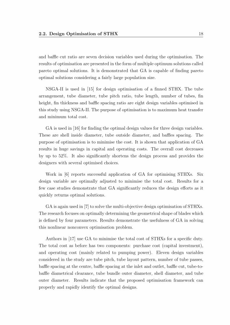
NSGA-II is used in [15] for design optimisation of a finned STHX. The tube

arrangement, tube diameter, tube pitch ratio, tube length, number of tubes, fin

height, fin thickness and baffle spacing ratio are eight design variables optimised in

this study using NSGA-II. The purpose of optimisation is to maximum heat transfer

and minimum total cost.

GA is used in [16] for finding the optimal design values for three design variables.

These are shell inside diameter, tube outside diameter, and baffles spacing. The

purpose of optimisation is to minimise the cost. It is shown that application of GA

results in huge savings in capital and operating costs. The overall cost decreases

by up to 52%. It also significantly shortens the design process and provides the

designers with several optimised choices.

Work in [6] reports successful application of GA for optimising STHXs. Six

design variable are optimally adjusted to minimise the total cost. Results for a

few case studies demonstrate that GA significantly reduces the design efforts as it

quickly returns optimal solutions.

GA is again used in [7] to solve the multi-objective design optimisation of STHXs.

The research focuses on optimally determining the geometrical shape of blades which

is defined by four parameters. Results demonstrate the usefulness of GA in solving

this nonlinear nonconvex optimisation problem.

Authors in [17] use GA to minimise the total cost of STHXs for a specific duty.

The total cost as before has two components: purchase cost (capital investment),

and operating cost (mainly related to pumping power). Eleven design variables

considered in the study are tube pitch, tube layout pattern, number of tube passes,

baffle spacing at the centre, baffle spacing at the inlet and outlet, baffle cut, tube-to-

baffle diametrical clearance, tube bundle outer diameter, shell diameter, and tube

outer diameter. Results indicate that the proposed optimisation framework can

properly and rapidly identify the optimal designs.


Artificial bee colony (ABC) is applied in [18] to minimise the total cost of STHXs.

Four decision variables are shell inside diameter, tube outside diameter, the num-

ber of passes, and baffle spacing. The optimisation results are compared to those

obtained and reported in literature. This comparison indicates that ABC algorithm

can achieve promising results even better than traditional design techniques [16].

The study in [19] reports successful application of particle swarm optimisation

(PSO) technique for the optimal design of a STHX from an economic view point.

Shell internal diameter, outer tube diameter, and baffle spacing are the three design

variables in this work. It is shown that PSO finds the optimum value of the objective

function in a few iterations. It is then argued that PSO is a powerful tool for design

optimisation of HXs.

Authors in [20] report design formulation and optimisation of STHXs using PSO.

The optimisation objective is to minimise the total cost. The optimisation process

deals with eleven design parameters, so the search space is quite big. It is demon-

strated that PSO can avoid local minima in the search space and always finds the

globally optimal solution. It is also shown that PSO outperforms traditional design

techniques including GA.

Harmony search algorithm (HSA) is successfully deployed in [21] for the optimal

design of STHXs. It is claimed that the HSA is a proper option for optimisation

due to its simplicity and ease of implementation. Results demonstrate that HSA can

converge to optimum solutions with a higher accuracy in comparison with traditional

GA.

Authors in [1] demonstrate the first successful application of differential evolution

(DE) [22] [23] for the optimal design of STHXs. Optimisation results indicate that

DE algorithm is significantly faster compared to GA and yields the global optimum

for a wide range of the key parameters.

Authors in [24] introduce a new quantum particle swarm optimisation approach

combined with Zaslavskii chaotic map sequences and apply to optimise STHXs. The

purpose of optimisation is to minimise the total cost of STHX. Simulation results

demonstrate that savings more than 30% are obtained for different case studies when

quantum particle swarm optimisation approach used instead of GA and traditional


PSO.

Authors in [25] use GA and alumina nanofluid for optimal design of STHXs.

Application of alumina nanofluid and GA greatly increases the Nusselt number

which boosts the heat transfer coefficient of STHXs. The increase of heat transfer

rate reduces the required tube length leading to reduced pressure drop in the heat

exchanger. The optimal geometry of heat exchanger is determined using GA by

minimising the total cost. The design variables are the volume ratio of nanoparticles,

tube diameter, baffle spacing and the number of tubes.

GA and PSO are both implemented and compared in [26] for optimal design of

STHXs. Optimisation of the total cost is done through fine-tuning of three design

variables: tube diameter, central baffles spacing, and shell diameter. A comparison

of the results obtained by GA and PSO reveals that PSO-based results are superior

to GA-based results.

Economic optimisation design of STHXs using Tsallis differential evolution is

proposed in [27]. Tsallis differential evolution is an improved version of differential

evolution. The decision variables are the shell internal diameter, the outside tube

diameter, and the baffles spacing. Optimisation results demonstrate that a reduction

on the total annual cost up to 26.99% and 54.60% in comparison to the original

case studies can be achieved through application of the proposed Tsallis differential

evolution.

Multiobjective design optimisation of STHXs using bat algorithm is proposed

and implanted in [28]. The bat algorithm is based on echolocation features of micro-

bats and frequency tuning technique to further diversify the candidate solutions.

The design variables are limited to the baffle spacing, baffle cut, tube pitch and

tube length. It is demonstrated that the proposed bath algorithm outperforms GA

in terms of finding superior solutions.

Electromagnetism-like algorithm is employed in [29] for optimal design of a

STHX. It is applied to save on the STHX capital cost and designing a compact,

high performance heat exchanger with the effective use of the allowable pressure

drop. The proposed approach in the paper is compared with four other evolutionary

algorithms to check its plausibility. Comparisons demonstrate that its application


greatly improves the resulting designs.

Design and economic optimisation of STHX using cohort intelligence algorithm

is presented in [30]. The tube outside diameter, baffle spacing, pitch size, shell

inside diameter and number of tube passes are design parameters optimised in three

case studies of this paper. The performance of the cohort intelligence method is

compared with existing algorithms and it is shown it outperform them.

Design optimisation of STHXs is performed using gravitational search algorithm

in [31]. Three design variables are the shell internal diameter, tube outside diameter,

and baffle spacing. Modelling and total cost optimisation results for two case studies

demonstrate the effectiveness of the proposed gravitational search algorithm for

optimal design of STHXs. In particular, it is shown that the operating cost can be

reduced by 61.5% while the total cost can be reduced by 22.3% as compared to the

original design for a STHX of heat duty 4.34 MW.

Multi-objective design optimisation of STHXs using elitist-Jaya algorithm is pre-

sented in [32]. One of the key advantages of elitist-Jaya algorithm is that it has no

algorithmic–specific parameters to be set except the common control parameters of

number of iterations and population size [33]. The total cost is considered as the

fitness function for optimisation. The results of computational experiments demon-

strate the superiority of the proposed algorithm over the latest reported approaches

for STHX design optimisation.

2.2

.D

esig

nO

ptim

isatio

nof

ST

HX

22

Table 2.1: Evolutionary algorithms used for design optimisation of

STHXs

Reference Optimisation

Technique

Objectives Variable Number Design Variables

[10] Particle

swarm op-

timisation

maximum effective-

ness (heat recovery)

and the minimum

total cost

7 Tube arrangement, tube diameter, tube pitch ratio, tube length, tube

number, baffle spacing ratio as well as baffle cut ratio

[11] Imperialist

competitive

algorithm

cost minimisation 4 Tube length, tube outer diameter, pitch size and baffle spacing

[12] Biogeography-

based optimi-

sation

Cost minimisation 3 Shell internal diameter Ds, tubes outside diameter do, baffles spacing

B

[8] Genetic algo-

rithm

Heat transfer rate

and total cost

11 Fluid allocation, do and di from TEMA tubes bigger than 3/4 inches,

number of tube passes, number of tubes,tube pitch ratio, tube lay-

out, tube length, inlet and outlet baffle, spacing ratio, middle baffle

spacing ratio, baffle cut ratio and number of sealing strips

[14] Nondominated

sorting GA II

(NSGA-II)

Efficiency, exergy

destruction, and

total cost

7 Tube arrangement, tube diameters, tube pitch ratio, tube length,

tube number, baffle spacing ratio, and baffle cut ratio

Continued on next page

2.2

.D

esig

nO

ptim

isatio

nof

ST

HX

23

Table 2.1 – continued from previous page


Technique


[18] Artificial bee

colony

Cost minimisation 4 Shell inside diameter, tube outside diameter, the number of tube side

passages, and baffle spacing

[2] Genetic algo-

rithm

Efficiency and cost

(pareto optimal)

7 Tube, arrangement, tube diameter, tube pitch ratio, tube length,

tube number, baffle spacing ratio, and baffle cut ratio

[19] particle swarm

optimisation

Cost minimisation 3 Shell internal diameter, outer tube diameter, and baffle spacing

[20] Particle

swarm op-

timisation

Total cost 12 Tube inside diameter, tube outside diameter, tube arrangement, tube

pitch, tube length, number of tube passes, number of tubes, the exter-

nal shell diameter, the tube bundle diameter, the number of baffles,

the baffles cut, and the baffle spacing

[21] Harmony

search algo-

rithm

Total cost 10 Inside shell diameter, baffle cut, tube arrangement, number of passes,

number of sealing strips, baffle spacing ratio, length ratio, tube out-

side diameter, pitch ratio, and material type

[16] Genetic algo-

rithm

Total cost 3 Shell inside diameter, tube outside diameter, and baffles spacing

[1] Differential

evolution

Total cost 7 Tube outer diameter, tube pitch , shell head type, tube passes, tube

length, baffle spacing, and baffle cut


2.2

.D

esig

nO

ptim

isatio

nof

ST

HX

24



Technique


[6] Genetic algo-

rithm

Cost minimisation 6 Outer tube diameter, tube layout, number of tube passes, outer shell

diameter, baffle spacing, and baffle cut

[7] Genetic Algo-

rithms

Efficiency and pres-

sure drops

4 Geometrical shape of blades

[24] Quantum PSO Total cost 3 Tube outside diameter, shell internal diameter, and baffles spacing

[13] Non-

dominated

sorting GA

(NSGA-II)

Total cost 9 tube layout pattern, number of tube passes, baffle spacing, baffle

cut, tube-to-baffle diametrical clearance, shell-to-baffle diametrical

clearance, tube length, tube outer diameter, and tube wall thickness

[17] Genetic algo-

rithm

Total cost 11 Tube pitch, tube layout pattern, number of tube passes, baffle spacing

at the center, baffle spacing at the inlet and outlet, baffle cut, tube-

to-baffle diametrical clearance, tube bundle outer diameter, shell di-

ameter, and tube outer diameter

[25] Genetic algo-

rithm

Total cost 4 The volume ratio of nanoparticles, tube diameter, baffle spacing and

the number of tubes

[26] Genetic al-

gorithm and

PSO

Total cost 3 Tube diameter, central baffles spacing and shell diameter


2.2

.D

esig

nO

ptim

isatio

nof

ST

HX

25



Technique


[15] NSGA-II Total cost 8 The tube arrangement, tube diameter, tube pitch ratio, tube length,

numbers of tube, fin height, fin thickness and baffle spacing ratio

[27] Tsallis dif-

ferential

evolution

Total cost 3 The shell internal diameter, the outside tube diameter, and the baffles

spacing

[28] Bat algorithm Effectiveness and

total cost

4 The baffle spacing, baffle cut, tube pitch and tube length

[29] Electromagnetism-

like algorithm

Total cost 3 The inner diameter of the shell, The outer diameter of the tube, and

the baffle spacing

[30] Cohort in-

telligence

algorithm

Total cost 5 The tube outside diameter, baffle spacing, pitch size, shell inside

diameter, and number of tube passes

[31] Gravitational

search algo-

rithm

Total cost 3 The shell internal diameter, tube outside diameter, and baffle spacing

[32] Elitist-Jaya al-

gorithm

Total cost 3 The number of tube passes, tube arrangements, and outer diameter

of tube

2.3. Discussion about STHX Optimisation using EvolutionaryAlgorithms 26

2.3 Discussion about STHX Optimisation using

Evolutionary Algorithms

Despite many breakthroughs in the field of evolutionary optimisation (mainly re-

ported in publications handled by IEEE Computational Intelligence Society), GA is

the most used method by process engineering researchers for design optimisation of

HXs [6] [7] [8] [34] [35] [36]. A comprehensive review of GA application for this spe-

cific field can be found in [37]. Several optimisation methods have been introduced

in recent years that outperform genetic algorithm in term of optimisation results.

Also some of these methods are even computationally less demanding. Examples

of these methods are particle swarm optimisation [38] [39], cuckoo search [40], bee

colony optimisation [41], and firefly algorithm [42]. These methods show different

performances in different engineering applications. A comparison of these methods

for several case studies can be found in [43].

As showed in Table 2.1 and discussed in section 2.2, a few of more advanced

evolutionary algorithms have been recently employed for design and optimisation of

HXs [9] [10] [12] [18] [19] [24] [44]. However, some strongly efficient algorithms such

as firefly or cuckoo search have never been applied and explored for optimal design

of STHXs.

Another important issue is how different evolutionary algorithms have been com-

pared in literature. There is no doubt that performance of optimisation algorithms

closely depends on (i) how their key parameters are set (mainly the population size

and the number of generations/iterations), and (ii) how the initial set of decision

variables (initial population) is valued. It is of paramount importance to examine

effects of these factors by repeating optimisation experiments several times before

making conclusions about a method performance for solving the STHX optimisation

problem. While the pure evolutionary algorithm optimisation literature is quite rich

in this respect [45] [42] [46] [47], this critical point is simply missed in the literature

relevant to the scope of this research project.

In theory, all evolutionary algorithms can be applied for optimal design of STHXs.

However, one should note the followings when implementing these:

2.4. Conclusion 27

• Some optimisation algorithms require several parameters [48]. Fine-tuning of

these parameters is quite challenging and time consuming. Improper settings

of a promising evolutionary algorithms may simply lead to inferior results.

• Obtained improvements by implementing a new algorithm can be little and

often statistically insignificant. Thus, it is of paramount importance to conduct

comprehensive analyses and simulations before concluding about an algorithm

performance.

Rush into the use of evolutionary algorithm has resulted in some mistakes in

terms of used algorithms as picked by some other researchers [49].

The existing literature often treats the total cost as the main objective function.

This is then minimised subject to efficiency requirement and process constraints.

This is valid for all papers cited in Table 2.1. From an optimisation perspective, it is

much more appropriate to convert these constrained optimisation problems into non-

constrained optimisation problems. Removing constraints through reformulation

of the optimisation problem allows evolutionary algorithms to better explore the

decision variable space. It greatly improves the chance of finding the global solutions

as different corners of the search space can be easily explored.

2.4 Conclusion

The literature review in this chapter shows that the interest to application of evolu-

tionary algorithms for optimisation of STHXs has increased in recent years. These

have been applied to minimise both economic and thermodynamic aspects of STHXs.

The design variables used for optimisation are not the same in different studies which

makes the direct comparison between different papers not possible. They vary from

a few to more than ten variables. Scientifically, the greater the number of variables,

the larger the search space, and the more difficult the optimisation process. The

performance of these algorithms will be checked in the upcoming chapters for opti-

mal design of STHXs. Comprehensive simulations will be conducted before making

a judgement about the performance of each method.

Chapter 3

Shell and Tube Heat Exchanger

3.1 Introduction

A HX can be defined as any device that transfers heat (thermal energy) from one

fluid (liquid or gas) to another fluid or the environment. There is no direct contact

between two fluids in a HX. Heat is transmitted from hot fluid to the metal isolating

the two fluids and then to the cold fluid. It is also always assumed that there is no

external heat and work interactions.

HXs are normally well-insulated devices that allow energy exchange between hot

and cold fluids. Pumps, fans, and blowers causing the fluids to move across the

control surface are usually located outside the control surface (not part of HX).

Regardless of the function the HX fulfils, the two fluids must be at different tem-

peratures and they must come into thermal contact in order to transfer heat.

Different heat exchangers are named according to their applications. For exam-

ple, heat exchangers being used to condense are known as condensers, similarly heat

exchangers for boiling purposes are called boilers.

Heat exchangers can be classified from different perspectives. Some are according

to:

28

3.1. Introduction 29

Heat Exchangers

Recuperative

Indirect

Tubular

Plate

Direct

Cooling Towers

Direct Contact Condensers

Steam Injectors

Direct Heaters

Specials

Scared Surface

Wet surface Air Coolers

Regenerative

Static Dynamic

Reciprocating

Rotary

Figure 3.1: Classification of HX by construction.

• transfer process: direct and indirect type;

• construction: tubular type, plate type, etc;

• flow arrangement: co-current and counter current;

• heat transfer mechanism: single phase convection on both sides, two phase

convection on both sides; and

• process function: condenser, evaporator, heaters, coolers, chillers, etc.

HX types can be broadly classified into recuperative and regenerative. Fig. 3.1

demonstrates this classification and lists different types within each class. Power

stations and other energy demanding industries usually use regenerators in particular

for gas/gas heat recovery. Indirect contact, direct contact, and specials are three

groups of recuperative HXs. Within these groups, indirect is the most important

one, where tubes and plates are used to separate hot and cold fluids.

3.1. Introduction 30

Tubular

Shell & Tube

TEMA Types

Graphite

Glass

Plastic

Double Pipe

Helical Coil

Furnaces

Fired

Electrical

Tube in Plate Elec. Heated Air Cooled Special

Heat Pipes

Agitated Vessels

Graphite Block

Bayonet

Figure 3.2: Classification of tubular HXs.

STHXs can be also classified in terms shellside and tubeside flow arrangement,

as demonstrated in Fig. 3.3. When the two fluids are flowing in opposite direction

through the heat exchanger, the type is counter-current. This leads to most efficient

heat transfer design. However, engineers may consider co-current type (both fluids

moving in one direction) due to specific requirements of a project.

Tubular and plate types are within the family of indirect HXs. Tubular HXs can

operate in a very wide range of pressures and temperatures. They can be further

subdivided into a number of classes as demonstrated in Fig. 3.2. The shell and tube

HX (STHX) is the most common one within the indirect tubular HXs. It consists

of a bundle of tubes installed in a cylindrical shell. The tube and shell axes are

parallel. The fluid flowing inside the tubes is called tubeside fluid and the fluid

flowing on the outside of the tubes is called shellside fluid.

3.2. STHX Nomenclature 31

Figure 3.3: Counter-current and co-current type heat exchangers.

3.2 STHX Nomenclature

There are several local and international codes and standards that have to be con-

sidered for design and construction of STHXs. Examples are:

• American Society of Mechanical Engineering (ASME) Section VIII Division.

• Tubular Exchanger Manufacturers Association (TEMA) Type C, B, R.

• British Standard BS-3274.

• American National Standards Institute (ANSI) and American Petroleum In-

stitute (API) Standard 660.

TEMA consists of companies manufacturing STHXs. Engineering standards

developed by TEMA are widely used in industry to design and build STHXs. TEMA


[50] provides the common terminology for different components of STHXs. As this

nomenclature is used in this report, we discuss some of STHX parts in this section.

3.2.1 Baffles

A baffle is a metal plate usually in the form of a circle segment. Baffles are used

to support the structural rigidity of tubes and to prevent vibration. Also they

effectively divert the flow across the bundle to help achieve a better heat transfer

rate. The modified flow by baffles improves the heat transfer between the shellside

and tubeside fluids. Baffles can be broadly classified into transverse (perpendicular

to the axis of the heat exchanger) and longitudinal (parallel to the axis of the heat

exchanger). Transverse baffles direct the shellside fluid into the tube bundle at

approximately right angles to the tubes. This significantly increases the turbulence

of the shellside fluid. The longitudinal baffles are used for controlling the direction

of shellside fluid. Transverse baffles are of two types named plate and grid. Plate

baffles are also three types: segmental, disk and doughnut, and orifice [3]. The

segmental transverse baffles can be single or multi segmental [4].

Usually baffles are spaced evenly throughout the shell to aid in reducing pressure

drop and fluid velocity. The distance between adjacent baffles is called baffle-spacing.

They have a diameter slightly smaller than the shell. This is to ensure their proper

fitting in to the shell. Large space between shell and baffle edge allows fluid bypass

and consequently reduces the thermal efficiency.

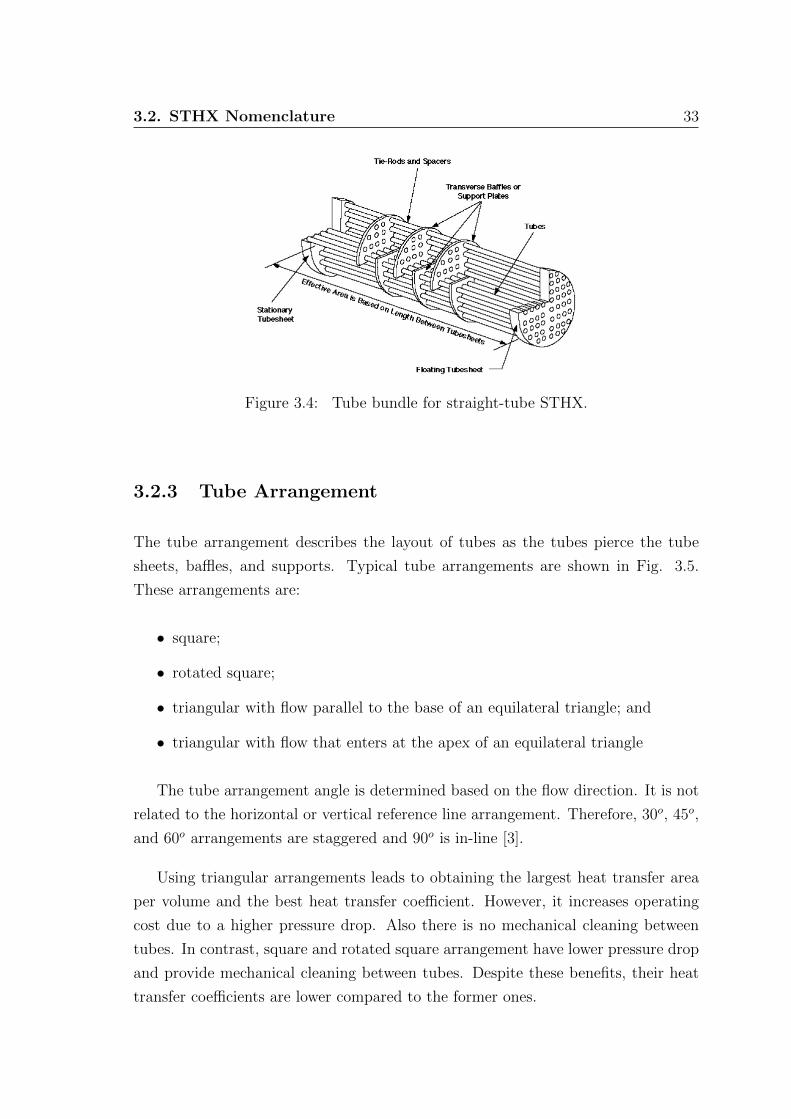
3.2.2 Tube Bundle

As per [51], a tube bundle is an assembly of tubes, baffles, tube sheets and tie rods,

and support plates. The bundle of a straight-tube, split-ring, floating-head-type

heat exchanger is pictured in Fig. 3.4. This figure also shows the baffles and how

they support the tubes.


Figure 3.4: Tube bundle for straight-tube STHX.

3.2.3 Tube Arrangement

The tube arrangement describes the layout of tubes as the tubes pierce the tube

sheets, baffles, and supports. Typical tube arrangements are shown in Fig. 3.5.

These arrangements are:

• square;

• rotated square;

• triangular with flow parallel to the base of an equilateral triangle; and

• triangular with flow that enters at the apex of an equilateral triangle

The tube arrangement angle is determined based on the flow direction. It is not

related to the horizontal or vertical reference line arrangement. Therefore, 30o, 45o,

and 60o arrangements are staggered and 90o is in-line [3].

Using triangular arrangements leads to obtaining the largest heat transfer area

per volume and the best heat transfer coefficient. However, it increases operating

cost due to a higher pressure drop. Also there is no mechanical cleaning between

tubes. In contrast, square and rotated square arrangement have lower pressure drop

and provide mechanical cleaning between tubes. Despite these benefits, their heat

transfer coefficients are lower compared to the former ones.

3.3. Modelling of STHX 34

Figure 3.5: Tube pitch patterns for a STHX.

3.2.4 Tube Passes

Tube passes refer to the number of times the tubeside fluid travels across the bun-

dle. There are practical limits to the number of passes in a heat exchanger. The

maximum practical number of passes is usually eight. Fig. 3.6 illustrates two-pass

and four-pass tubeside heat exchanger designs.

3.3 Modelling of STHX

3.3.1 Modelling Standard

There are a couple of standard ways for the design of STHXs. There are:

• Kern method: it is simple to implement and often used for preliminary design

calculations. It does not take into account bypass and leakage streams. Also,

it is only restricted to a fixed baffle cut (25%).

• Bell-Delware method: it is the most complete STHX design method. It is


Figure 3.6: Two and four pass tube side flow for a STHX.

based on mechanical shellside details and provides more precise results for the

overall heat transfer coefficient and shellside and tubeside pressure drops.

The phrase TEMA-type refers to STHX designed to comply with TEMA re-

quirements [50]. A thermodynamic and economic model for a TEMA-type STHX

is described in the following section. This model will be later used in Chapter 4 for

examining performance of different optimisation algorithms.

3.3.2 Thermodynamic Modelling

Effectiveness ε is a measure of HX thermal performance. It is mathematically defined

as a ratio of the actual heat transfer rate from the hot fluid to the cold fluid to the

maximum possible heat transfer rate [4]. This definition is applicable to all types of

HXs regardless of their fluids and tube configurations. The efficiency of an TEMA

E-type STHX is calculated as,

ε = 2

(1 + C∗ +

√1 + C∗2

1− e−NTU√

1+C∗2)

1 + e−NTU√

1+C∗2

)−1

(3.1)


where the heat capacity ratio (C∗) is calculated as,

C∗ =CminCmax

=min(Cs, Ct)

max(Cs, Ct)=min ((mcp)s, (mcp)t)

max ((mcp)s, (mcp)t)(3.2)

where subscripts s and t stand for shell and tube respectively. The number of

transfer units is defined as,

NTU =Uo AtCmin

(3.3)

where Cmin is,

Cmin = min(Ch, Cc) = min(Cs, Ct) (3.4)

where Ch and Cc are the hot and cold fluid heat capacity rates, i.e., Ch = (mcp)h

and Cc = (mcp)c. m is the fluid mass flow rate. Specific heats cp are assumed to be

constant.

The overall heat transfer coefficient (Uo) in (3.3) is then computed as,

Uo =

(1

hs+Rs,f +

do ln(do/di)

2kw+Rt,f

dodi

+dohtdi

)−1

(3.5)

where L, Nt, di, do, Rt,f , Rs,f , and kw are the tube length, number, inside and

outside diameter, tube and shell side fouling resistances and thermal conductivity of

tube wall, respectively. ht and hs are heat transfer coefficients for inside and outside

flows, respectively.

Fouling is the buildup and deposition of sediments and debris (any undesired

material) on the HX surface area that inhibits heat transfer. The heat transfer re-

sistance caused by the deposit is called the fouling factor or dirt factor. Different

types of fouling observed in different STHXs are crystallisation, sedimentation, bi-

ological organic, chemical reaction coking, corrosion, and freezing fouling. Fouling


increases the thermal resistance and lowers the HX heat transfer coefficient. This

leads to inferior performance of the HX and often an increase in the pressure drop

and pumping power [51]. Consequently, fouling and accumulation of undesired ma-

terials cause a big economic loss as they massively impact capital cost, operating

cost, and HX performance. The fouling factor for a new HX is zero as there is no

deposition on heat transfer surface in the beginning. It is not possible to directly

determine the fouling factor to use for a fluid in a particular application. Fouling

factor can be only determined from experimental data on heat transfer coefficient

of two identical intact and fouled HXs. Fouling factors, as considered in the STHX

modelling, are accounted for maximisation of lifespan, runtime, and efficiency of a

HX. Their inclusion results in increasing the HX surface area, so that fouling effects

will be minimised

The total tube outside heat transfer area is calculated as,

At = π L do Nt (3.6)

where L and do are the tube length and outside diameter.

The tube side heat transfer coefficient (ht) is calculated as,

ht = 0.024ktdiRe0.8

t Pr0.4t (3.7)

for 2500 < Ret < 124000. kt and Prt are tubeside fluid thermal conductivity and

Prandtl number respectively. The tube flow Reynold number (Ret) is also defined

as,

Ret =mt diµtAo,t

(3.8)

where mt is the tube mass flow rate and Ao,t is the tube side flow cross section area


Table 3.1: Geometrical properties of tube banks common in shell and tube exchang-ers

Triangle Arrangement (30◦) Rotated Square Arrangement (45◦) Square Arrangement (90◦)

pt√

2pt ptsqrt3

2 ptpt

sqrt2 pt

per pass,

Ao,t = 0.25πd2i

Nt

np(3.9)

where np is the number of passes.

The average shell side heat transfer coefficient is calculated using the Bell-

Delaware method correlation,

hs = hk Jc Jl Jb Js Jr (3.10)

where hk is the heat transfer coefficient for an ideal tube bank,

hk = ji cp,s

(ms

As

)(ks

cp,sµs

) 23(µsµs,w

)0.14

(3.11)

where ji is the Colburn j-factor for an ideal tube bank. As is also the cross flow area

at the centreline of the shell for one cross flow between two baffles. Its relationship

with pt is demonstrated in Table 3.1. µsµs,w

is the viscosity ratio at bulk to wall

temperature in the shell side. Jc, Jl, Jb, Js, and Jr in (3.10) are the correction

factors for baffle configuration (cut and spacing), baffle leakage, bundle and pass

partition bypass streams, bigger baffle spacing at the shell inlet and outlet sections,

and the adverse temperature gradient in laminar flows.

Graphs are available for Colburn j-factor as a function of shell-side Reynolds

number, tube layout, and pitch size. However, a set of curve-fit equations are better

for the purpose of computer simulation and analysis. As per this, an approximation


of ji is given below,

Ji = a1

(1.33

pt/do

)aRea2 (3.12)

where

a =a3

1 + 0.14Rea4(3.13)

Values for a1, a2, a3, and a4 are listed in Chapter 8 of [51].

Determining the pressure drop in a STHX is essential for many applications.

Both shellside and tubeside fluids need to be pumped through the HX. This requires

fluid pumping power which is proportional to the HX pressure drop. Shellside

pressure drop involves three components (Fig. 3.7 shows flows causing these pressure

drops [52]):

• pressure drop in cross-flow zone (∆pc).

• pressure drop in window zone (∆pw).

• pressure drop in end zone (∆pe).

So, the total shellside pressure drop is [52],

∆ps = ∆pc + ∆pw + ∆pe (3.14)

The cross flow pressure drop and the entrance and exist region pressure drops

depend on the ideal tube bank pressure drop [3]. The pressure drop in the interior

cross flow sections is affected by both bypass and leakage. So, ∆pc of all the interior

cross flow section is given by,

∆pc = (Nb − 1)(∆pb,i Rb Rl) (3.15)


Figure 3.7: Pressure drop regions in shellside flow.

where ∆pb,i is the fluid static pressure drop associated with an ideal cross flow section

between two baffles. Nb is the number of baffles in the HX. Rb and Rl are correction

factor for bypass flow and correction factor for baffle leakage effects, respectively.

The pressure drop in the entrance and exist section is only affected by bypass

but not by leakage and variable baffle spacing. Therefore, ∆pe is calculated as,

∆pe = 2 ∆pb,i

(1 +

Nr,cw

Nr,cc

)Rb Rs (3.16)

where Nr,cc is the number of effective tube rows crossed during flow through one

cross flow section (between baffle tips). Nr,cw is also the number of effective tube

rows crossed during flow through one window zone in a segmental baffled STHX. Rs

is also the correction factor for the entrance and exit sections.


The pressure drop in the windows is affected by leakage but not by pass. There-

fore, the combined pressure drop of all the window section is given by,

∆pw = Nb Rl ∆pw,id (3.17)

where ∆pw,id is the equivalent pressure drop in the window section.

Summing individual pressure drops, the total nozzle to nozzle shellside pressure

drop is calculated as,

∆ps = [(Nb − 1)(∆pb,i Rb) +Nb∆pw,id)]Rl + 2∆pb,i

(1 +

Nr,cw

Nrcc

)Rb Rs (3.18)

It is known that the total shellside pressure drop is of the order 20-30% of the

pressure drop that would be calculated for the flow through the corresponding HX

without baffle leakage and without tube bundle bypass effects [3].

The tubeside pressure drop is mainly due to friction along the length of the tube

and also to the sudden contraction and expansion at the tube inlet and outlet.

∆pt =m2t

2 ρtA2o,t

[(4 f

di

)+(1− σ2 +Kc

)−(1− σ2 −Ke

)]× np (3.19)

where Kc is the contraction loss coefficient at the tube entrance. Ke is also the

expansion loss coefficient at the tube outlet. σ is the ratio of minimum free flow

area to frontal area. Ao,t and np are the tube side cross flow area per pass and

number of passes respectively.

More details about the STHX model used in this study can be found in [2].

Calculations of shell and tube side heat transfer coefficients as well as pressure

drops can be found in basic HX design books [4] [51].


3.3.3 Economic Modeling

The STHX total cost is made up of capital investment (Cinv) and operating (Copr)

costs [16],

Ctotal = Cinv + Copr (3.20)

There are several methods for determining the price of STHX. Here we use the

Halls method for estimation of the investment cost as detailed in [53] (alternative

cost estimation methods can be found in [54]).

Cinv as a function of the total tube outside heat transfer surface area (At) is

defined as,

Cinv = 8500 + 409 A0.85t (3.21)

where the construction materials are carbon and stainless steel. This cost function

has been widely used in literature for optimal design of STHXs [2] [8].

The total discounted operating cost associated to pumping power is computed

as follows [16],

Copr =

Ny∑k=1

C0

(1 + i)k(3.22)

where i and Ny are the annual discount rate (%) and the STHX life time in year.

C0 is the annual operating cost and is calculated as follows,

C0 = κe P hopt (3.23)

where κe and hopt are the price of electricity ($/kWh) and annual operating hours.


Table 3.2: The operating conditions of the SHTX.

Thermophysical and process data Shell side Tube side

Density (kg/m3) 860 995

Specific hear (j/kgK) 2115 4120

Viscosity 0.0643 0.000695

Fouling factor m2W/K 0.00015 0.00074

The pumping power (P ) is also calculated in watts (W),

P =1

η

(mt

ρt∆pt +

ms

ρs∆ps

)(3.24)

where η is pump efficiency. ρs and ρt are the fluid densities for shell and tube sides

respectively.

3.3.4 Model Verification

The mathematical model described in Section 3.3.2 is implemented in Matlab and

used for the purpose of simulation in this thesis. The operating conditions of STHX

including characteristics of shell and tube streams are shown in Table 3.2. The shell

side has oil as the hot stream. The cold stream is waster in the tube side.

Implemented model is used for simulation and generation of results which are

compared with the corresponding results reported in [4]. The comparison results

are demonstrated in Table 3.3. These results indicate that the effectiveness and

total cost of the developed model are in good match with benchmark results. The

differences between calculated and actual values are 2.83% and 0.65% respectively.

The same thing holds for ∆pt and ∆ps. Accordingly, the developed model is reliable

and can be confidently used for optimisation purposes.

3.4. Conclusion 44

Table 3.3: Accuracy of the developed model compared to the corresponding resultsfrom [4]

Variables Unit Reference [4] Developed model Difference (%)

ε – 0.1555 0.1599 2.83

Ctotal $ 74,598 74,112 0.65

∆pt kPa 17.58 17.660 0.45

∆ps kPa 112 111.02 -0.875

q kW 393.6 404.63 2.78

ht W/m2 k 7837 7838.2 0.0153

hs W/m2 k 698.8 730.226 4.497

3.4 Conclusion

This chapter described the modelling of STHX which will be used in the next chap-

ters for testing performance of evolutionary algorithms and developing new objective

functions for design optimisation. The introduced model includes seven parameters

which make the search space big. There will be thousands of design candidate

configurations to be examined by the evolutionary algorithms in the search for the

optimal configuration.

Chapter 4

Evolutionary Optimisation

Algorithms

4.1 Introduction

In this chapter, three evolutionary algorithms are briefly introduced. In the family of

evolutionary algorithms, also called approximate methods, the guarantee of finding

optimal and perfect solutions is compromised for the sake of obtaining reasonably

good solutions in a fraction of time and effort required by complete algorithms

[55]. The introduction in this chapter describes components and operators of three

optimisation algorithms and how the candidate solutions are evolving during the

optimisation process.

4.2 Genetic Algorithm

Genetic algorithm (GA) is highly likely the most widely used and researched evolu-

tionary optimisation method in the scientific world. It is a guided stochastic search

technique inspired from the principles of natural fittest selection and population ge-

netics. In general terms, it is based on the parent and offspring iterations and their

45

4.2. Genetic Algorithm 46

evolution through generations. GA generates candidate solutions from the space of

all possible solutions and examines their performance as per the considered objective

function. It has been proven that GA performs strongly well in both constrained and

unconstrained search problems where the number of good solutions is very limited

compared to the size of the search space.

GA converges towards more competitive solutions by applying elitism, crossover,

and mutation mechanisms. It first creates a population (often randomly) of potential

solutions (also called chromosomes) for the optimisation problem. This population

is then assessed using the objective function of the interest. Then GA uses its three

operators to create the new population for the next generation.

• The best performing chromosome(s) is copied to the next generation un-

changed. This process is called elitism and makes sure that the best solution(s)

is not lost as the optimisation proceeds.

• Crossover operator is used for combining good parents and generating off-

spring. This operator is applied with the hope of retaining the spirit of good

chromosomes. In its simplest form, i.e., single point as shown in Fig. 4.1, a

crossover point is randomly selected. Then the operator swaps portions of a

pair chromosomes at the crossover point. Alternative crossover methods are

multi-points, uniform, and arithmetic.

• Regardless of the type of applied crossover operator, its generated offspring

only include information held by the current population. A new operator is

required to introduce and bring new information (solutions) to the population.

Mutation operator creates a new offspring by randomly changing the values of

genes at one or more positions of a selected chromosome. Fig. 4.2 demonstrates

point and swap mutation operations for binary solutions.

• Performance of GA closely depends on these three operators. Therefore,

the proper selection of parameters and algorithms for these operators is of

paramount importance.

In literature, several versions for crossover and mutation operators have been

4.2. Genetic Algorithm 47

1 1 1 1 0 0 0 0

1 1 0 0 1 1 0 0

Parent 1

Parent 2

Single point crossover

1 1 1 1 1 1 0 0

1 1 0 0 0 0 0 0

Child 1

Child 2

1 1 1 1 0 0 0 0

1 1 0 0 1 1 0 0

Parent 1

Parent 2

Two point crossover

1 1 1 0 1 0 0 0

1 1 0 1 0 1 0 0

Child 1

Child 2

Figure 4.1: Single and two point crossover operation of GA.

1 1 0 0 1 1 0 0

1 1 0 1 1 1 0 0

Parent

Child

Point Mutation

1 1 0 0 1 1 0 0

1 1 1 0 1 0 0 0

Parent

Child

Swap Mutation

Figure 4.2: Point and swap mutation operation of GA.

proposed [56] [57] [58] [59] [60] [61] [62] [63]. The pseudo code for GA including

three genetic operators is displayed in Fig. 4.3.

GA is stochastic and gradient-free, so it can be easily applied for minimisation

or maximisation of discontinuous and nondifferentiable objective functions. Theo-

retical literature of GA is quite rich and numerous applications of GA for real world

optimisation problems have been reported in the recent decades. Detailed discussion

about GA and its operators can be found in basic reading sources such as [64], [65],

and [66].

4.3. Firefly Algorithm 48

Begin

Generate initial population of individuals

Evaluate the fitness of the individuals

while (termination criteria)

Select the best individuals to be used by GA operators

Generate new individuals using crossover and mutation operators

Evaluate the fitness of new individuals

Replace the worst individuals by the best new individuals

end while

Postprocess results and visualization

end

begin

Objective function f(x), x = (x1, ..., xd)T

Generate initial population of n host nests xi (i = 1, 2, ..., n)


Get a cuckoo randomly by Levy flights

Evaluate its quality/fitness fi

Choose a nest among n (say, j) randomly

if (fi > fj ),

replace solution j by the new solution;

end A fraction (pa) of worse nests are abandoned and new ones are built

Keep the best solutions (or nests with quality solutions)

Rank the solutions and find the current best

end while Postprocess results and visualization

end

begin

Objective function f(x), x = (x1, ..., xd)T

Generate initial population of n host nests xi (i = 1, 2, ..., n)


Get a cuckoo randomly by Levy flights

Evaluate its quality/fitness fi

Choose a nest among n (say, j) randomly

if (fi > fj ),

replace solution j by the new solution;

end

A fraction (pa) of worse nests are abandoned and new ones are built

Keep the best solutions (or nests with quality solutions)

Rank the solutions and find the current best

end while

Postprocess results and visualization

end

Figure 4.3: Pseudo code describing the algorithmic steps of GA.

4.3 Firefly Algorithm

Similar to other evolutionary optimisation methods, firefly algorithm (FA) is an

approximate rather than complete optimisation algorithm. FA was originally devel-

oped and engineered by Prof Yang in late 2007 and 2008 at Cambridge University

[42] as a swarm intelligence method. The algorithm is inspired by the flashing be-

haviour and movement of fireflies. The method assumes that the attractiveness

between two fireflies is proportional to their brightness and the less brighter one will

move towards the brighter one. Movement will be random if there is no brighter

adjacent firefly. Fig. 4.4 shows the diagram of the FA.

Firefly, also called a lightning bug, is a little tropical insect that can conspicuously

emit short and rhythmic light flashes. These cold lights are produced by a process

of bioluminescence during twilight. Fireflies use these lights to send warning signals

to predators or attract partners and preys. Accordingly, this intensity of light is the

factor of the other fireflies to move toward the other firefly.

In the FA, the following assumptions are made about flashing characteristics of

fireflies:

• All fireflies are unisex. Accordingly, they are attracted to each other regardless

of their sex.


• Attractiveness of a firefly is proportional to its light intensity. Accordingly, for

any two flashing fireflies, the less bright one will fly towards the brighter one.

• Brightness of fireflies is proportional to their distance. This means that in-

creasing the distance between two fireflies will decrease their brightness which

lead to less attractiveness. Two fireflies having the same brightness will troll

randomly.

• The light intensity of a firefly is determined by the objective function to be

optimised

As attractiveness is proportional to the light intensity, the variation of attrac-

tiveness β with the distance r can be defined as,

β = β0 e−γ r2 (4.1)

where β0 is attractiveness at r = 0. γ is also the medium light absorption coefficient.

The distance between any two fireflies i and j at spatial coordinates xi and xj is

the Cartesian distance calculated as,

r =‖ xi − xj ‖=

√√√√ d∑k=1

(xi,k − xj,k)2 (4.2)

where xi,k is the kth component of the coordinate xi of ith firefly. In normal 2D

space, (4.2) is as follows,

r =√

(xi − xj)2 + (yi − yj)2 (4.3)

Assuming the jth firefly is brighter than the ith firefly, the movement of xi

towards xj is defined as,

xi = xi + β0 e−γ r2i,j (xi − xj) + α εi (4.4)


where the second and the third term in right are due to the attraction and randomi-

sation. α is a parameter multiplied in the vector of random numbers εi. This vector

is generated through drawing numbers from a normal or uniform distribution. As

mentioned in [42], often β0 = 1 and α ∈ [0, 1] satisfy most of FA implementations.

Note that (4.4) is a pure random walk search if β = 0. Also other distributions such

as Levy flights can be considered for the the randomisation terms (ε) in (4.4).

γ is the key parameter of FA. It characterises the variation of the attractiveness

between different fireflies. Its value has a direct impact on the convergence speed of

the algorithm and how the spatial coordinates of fireflies change. If γ approaches

infinity (γ → ∞) and β0 is a constant value, the sky is fully clear and the light

intensity does not decrease. Thus, a flashing firefly can be always seen by others.

On the other hand, if γ approaches zero (γ → 0), there is no light (attractiveness)

and a firefly cannot see other fireflies. Accordingly, movements will be completely

random. While in theory γ can take any value in [0,∞), it is usually set to a value

in (0, 10].

FA has been widely used in several engineering and optimisation problems in

literature. Examples are model development [67], control [68] [69] [70], unit com-

mitment and economic dispatch [45] [71] [72]. The key advantage of the FA is its

ability to divide into subgroups. It boosts its searchability and increases the prob-

ability of finding the best global solution [73]. Also it can well handle multimodal

problem as long as the population size is big enough [74].

In this work, we use a modified version of FA introduced and presented math-

ematically in [75]. Two proposed modifications aim to minimise the chance of al-

gorithm being trapped in local optima and to eliminate the effects of initialisation

process on the algorithm performance. The modification process is based on the fol-

lowing two ideas: (a) applying a mutation operator to further diversify the current

population and (b) moving the average of the population towards the best global

optimal solution in the entire search space.

In the modified FA, three fireflies called h1, h2, and h3 are randomly selected

and hi is the ith firefly in the swarm. Then a new improved solution, Ximproved is


generated,

Ximproved = Xh1 + γ × (Xh2 −Xh3) (4.5)

where γ is a random value in the range of (0,1). Then, three new fireflies are

generated using Ximproved and Xbest (best solution in the swarm),

xfirefly1,j =

ximproved,j k1 ≤ k2

xbest,j otherwise(4.6)

xfirefly2,j =

ximproved,j k3 ≤ k2

xj otherwise(4.7)

Xfirefly,3 = ϕXbest + ζ (Xbest −XIrand) (4.8)

where XIrand is a random firefly selected from the swarm. After these modifications,

the three modified fireflies replace the three original fireflies if their positions in the

swarm is better.

Also for each firefly, a new position is generated,

XNewi = XOld

i + χ(Xbest − FF ×MD) (4.9)

where TF is a random number and MD is the mean value of the swarm calculated

column-wise. If XOldi has a better position that XNew

i , it is kept. Otherwise, it is

replaced by XNewi .

4.4. Cuckoo Search 52

4.4 Cuckoo Search

The CS method is a nature-inspired metaheuristic optimisation method which was

proposed by Yand and Deb in 2009 [76]. The reproduction strategy of cuckoos is

the core idea behind the CS method. The CS method has been developed based on

three idealised assumptions:

• Each cuckoo lays one egg at a time and deposits it at a random chosen nest.

• The best nests with the highest quality eggs are carried to the next generations.

• The number of host nests for depositing eggs are fixed.

Eggs laid by a cuckoo are discovered by the host bird with a pre-set fraction

probability, pa ∈ [0, 1]. In case of discovering alien eggs, the host bird may simply

throw them away or abandon the nest and build a completely new one.

In terms of optimisation implementation, eggs in nests represent solutions. The

idea is to replace not-so-good solutions in the nests with new and potentially bet-

ter solutions. Fig. 4.5 presents the flowchart for CS method including Levy flights.

Based on the three idealised assumptions, the method applies two exploration mech-

anism. Some solutions are generated in the neighbourhood of the current best so-

lution (a Levy walk). This speeds up the local search. At the same time, a major

fraction of new solutions are generated by far field randomisation and whose loca-

tions are far away from the current best solution location. This is done to make

sure the method is not trapped in a local optimum. The CS method is in general

population-based, elitist, and single objective.

A Levy flight is considered when generating new solutions xt+1 for the ith cuckoo,

xt+1i = xti + α⊕ Levy (4.10)

where α is the step size which depends on the scales of the problem of interest. Often,

α = O(L/100) satisfies the search requirements for most optimisation problems. L

4.4. Cuckoo Search 53

represents the difference between the maximum and minimum valid value of the

problem of interest. The product ⊕ means entry-wise multiplication.

The Levy flight provides a random walk where its step is drawn from a Levy

distribution. There are several ways to generate this random step [42]. The Man-

tegna’s algorithm is one of the most efficient algorithms for generating symmetric

(positive or negative) Levy distributed steps. In this method, the step length in

(4.10) is calculated as

s =u

|v|1/β(4.11)

where u and v are drawn from normal distributions,

u ∼ N(0, σu), v ∼ N(0, σv) (4.12)

where σv = 1 and,

σu =

{Γ(1 + β) sin(πβ/2)

Γ(1 + β)/2) β 2(β−1)/2

} 1β

(4.13)

where Γ(z) is the gamma function,

Γ(z) =

∫ ∞0

tz−1 e−t dt (4.14)

Two normal distributions are used by Mantegna’s algorithm to generate a third

random variable which has the same behaviour of a Levy distribution. In the CS

method proposed by Yang and Deb [42], the entry-wise multiplication of the random

number and distance between the current and best solution is applied as a transition

probability to move from the current location to the next location. Accordingly,

4.5. Conclusion 54

(4.10) can be rewritten as,

xt+1i = xti + α s (xti − xbesti ) r (4.15)

where xbesti is the current best solution and r is a random number drawn from a

normal distribution with zero mean and unit variance. The step length s is also

calculated using (4.11).

CS method has also been widely used in many optimisation problems including

but not limited to job scheduling [77] [78], distributed generation allocation [79],

milling operations [80], and structural optimisation [81].

Further discussion about CS method and its details can be found in [40] and

[42].

4.5 Conclusion

The three evolutionary optimisation algorithms were introduced in this chapter.

Their components, operations, and mechanisms were briefly discussed. These meth-

ods differ in how they evolutionarily change candidate solutions with the purpose of

minimising/maximising the objective functions. These impact their efficiency, opti-

mality and computational burden. Their applications for optimal design of STHX

are discussed in the next chapter.

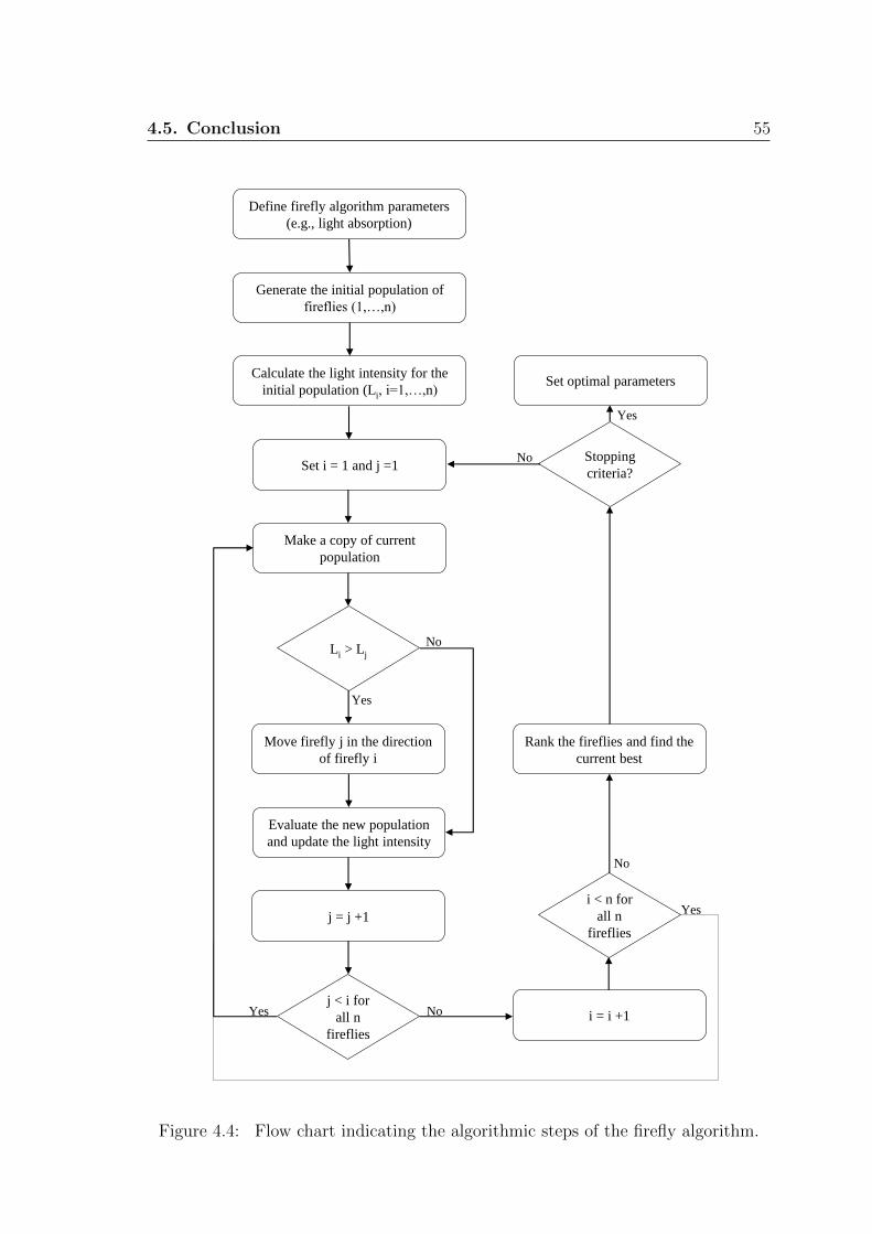
4.5. Conclusion 55

Generate the initial population of

fireflies (1,…,n)

Calculate the light intensity for the

initial population (Li, i=1,…,n)

Define firefly algorithm parameters

(e.g., light absorption)

Stopping

criteria?Set i = 1 and j =1

Make a copy of current

population

Li > Lj

Move firefly j in the direction

of firefly i

Evaluate the new population

and update the light intensity

j = j +1

j < i for

all n

fireflies

i = i +1

i < n for

all n

fireflies

Rank the fireflies and find the

current best

Set optimal parameters

Yes No

Yes

No

No

Yes

No

Yes

Figure 4.4: Flow chart indicating the algorithmic steps of the firefly algorithm.

4.5. Conclusion 56

Randomly choose a cuckoo (e.g., i)

by Levy flights and evaluate its

fitness function Fi

Randomly choose a nest from n nests

(e.g., j) with fitness Fj

Randomly generate an initial

population of n host nests (xi,

i=1,…,n)

Fi ≤ Fj

Yes

No

Consider j as the solution

Replace j by the new solution

Abandon a fraction (pa) of worse

nests

Generate new nests using Levy

flights

Keep the best solutions (nests)

Stopping

criteria?

Yes

Select optimal solution

No

Figure 4.5: Flowchart of cuckoo search optimisation algorithm including Levyflights.

Chapter 5

STHX Design Optimisation and

Comparison

5.1 Introduction

This chapter describes the simulation results for optimising the design of STHX

using GA, FA, and CS methods.

5.2 Optimisation Results and Discussions

The STHX model used in simulations is identical to one described and analysed in

[2]. Table 5.1 summarises the list of decision variables (STHX parameters) and their

ranges. These variables have a huge impact on the total cost and efficiency of the

STHX. Besides, all their combinations are not feasible due to practical constrains.

It is important to note that all these seven variables are discontinuous due to prac-

tical construction constraints. For instance, tube internal diameter is determined

according to relevant standards and suppliers’ catalogues The inner (di) and outer

(do) diameters of twenty standard tubes used in this study are listed in Table 5.2.

57

5.2. Optimisation Results and Discussions 58

Table 5.1: The list of design variables (STHX parameters) and their range.Variable Minimum Maximum Increment Number of solutions

Tube arrangement (30°, 45°, 90°) - - 3

Tube inside diameter (m) 0.0112 0.0153 - 20 (as per standard tubes)

pt/do 1.25 3 0.001 1750

Tube length (m) 3 8 0.001 5000

Tube number 100 600 1 500

Baffle cut ratio 0.19 0.32 0.001 130

Baffle spacing ratio 0.2 1.4 0.001 1200

Table 5.2: The inner (di) and outer (do) diameter of 20 standard tubes.

Item di (inch) do (inch) Item di (inch) do (inch)

1 0.444 1/2 11 0.435 5/8

2 0.495 5/8 12 0.527 5/8

3 0.555 5/8 13 0.510 3/4

4 0.560 3/4 14 0.606 3/4

5 0.634 3/4 15 0.680 3/4

6 0.407 5/8 16 0.481 5/8

7 0.509 5/8 17 0.541 5/8

8 0.482 3/4 18 0.532 3/4

9 0.584 3/4 19 0.620 3/4

10 0.352 3/4 20 0.607 7/8

Before going further, it is important to note the followings regarding the optimal

values for design parameters:

• The thickness of the wall of the tubes is usually determined to ensure that

(i) corrosion will not be an issue during lifetime of the heat exchanger, (ii)

flow induced vibrations have resistance, (iii) axial strength, (iv) hoop strength

to withstand internal tube pressure, and (v) bulking strength to withstand

overpressure in the shell.

• Heat exchangers are usually cheaper when they have a small shell diameter and

a long tube length. Design engineers usually aim to make the heat exchanger

as long as practically possible while not exceeding production capabilities. At

the same time, several requirements and design limitations have to be care-

fully considered to ensure heat exchangers are built to a project specifications.

Examples are available installation space and ease of future maintenances and

repairs (long thin tubes are difficult to be taken out and replaced).

• The tube pitch is the centre-to-centre distance of adjoining tubes. Its selection


Figure 5.1: Tube pitch and ligament width (p-d) of a heat exchanger [3].

is a compromise between a smaller pitch for increased shellside heat transfer

and surface compactness, and a larger pitch for decreased shellside pressure

drop and fouling and cleaning ease [3]. As a rule of thumb, the minimum

tube pitch ratio is set to 1.25. For smaller values, the ligament may become

very weak for rolling of the tubes into the tube sheet. The ligament width, as

visualised in Fig. 5.1, is the tube pitch minus the tube hole diameter. When

tubes are too close, the tube sheet becomes structurally weak (too many tubes

to be supported by it).

• For obtaining the maximum heat transfer area, tube arrangements are designed

so as to include as many tubes as possible within the shell. Four common types

of tube arrangements are triangular (30o), rotated triangular (60o), square

(90o), and rotated square (45o). Considering other variables are fixed, a layout

of 30o results in the greatest tube density and is therefore used as the best

(initial) choice. For a given tube pitch/outside diameter ratio, about 15%

more tube can be accommodated within a given diameter using triangular and

rotated triangular layouts. Mechanical cleaning is more problematic for these

pattern as it is difficult to insert a rigid tool between tubes. For this case, only

chemical or water jet cleaning is possible. The square pitch generally offers

lower pressure drops and lower heat transfer coefficients than the triangular

pitch. The 45o layout is preferred for single-phase laminar flow or fouling

service. Such an arraignment is more suitable for clean service. 45o and 90o

layouts must be used when mechanical cleaning is necessary. The minimum

gap between tubes must be 6.35mm (1/4 inch) for ease of cleaning [3].

For the three optimisation methods, we set the number of iterations (generations)

to 30 and 60. The population size is also set to 10, 20, 30, and 50. Accordingly,


8 different sets of experiments are performed for each optimisation method (combi-

nation of different population sizes and iteration numbers). Each experiment (e.g.,

GA with 30 iterations and 10 populations) is repeated 50 times and then statistics

of experiments are reported. In total, 400 runs are simulated and completed for

each optimisation method. This is done to make sure conclusions are made based

on general and extensive optimisation scenarios rather than a few tailored ones.

Therefore, obtained results and driven conclusions are statistically meaningful and

believable. Simulations are performed using a Lenovo Thinkpad T420s laptop com-

puter with Intel Core i7-2640M CPU @2.8G Hz and 8GB memory, running Windows

7 Professional.

The purpose of optimisation is to maximise the efficiency through finding the

best values for seven design parameters listed in Table 5.1. For each run, the seven

decision variables are randomly initialised within their range (see Table 5.1).

Fig. 5.2 shows the efficiency of the optimised STHX using GA, FA and CS

method for 50 runs. According to these results, FA and CS show a much more

consistent behaviour in terms of maximising the STHX efficiency. The maximum

efficiency (ε) is 83.80%. The efficiency of CS optimised heat exchanger (εCS) is

equal to this value almost in all 400 simulations. There is only one case (#iter=30,

#pop=10) where εCS is less than 80%. FA also shows a similar performance although

there are 5 out of 400 cases where FA cannot find an admissible solution.

The efficiency of GA-optimised heat exchangers (εGA) is equal to 83.80% in only

a few cases out of 400 simulations. More interestingly, εGA is less than 80% in

more than 75% of simulations. GA cannot find admissible solutions in 284 out of

400 simulations (71%). This indicates the inability of the GA operators in find-

ing permissible solutions within the search space. As per demonstrated results in

Fig. 5.2, this is not something to be easily solved by simply increasing the number

of iterations or the population size. GA performance is highly dependent on the

initialisation process for STHX design optimisation. It can find globally optimal

solutions if the initial values selected for seven design parameters are proper (at

least being admissible). Otherwise it fails to find generate optimal solutions using

its two operators (crossover and mutation). In contrast, both FA and CS method

always find permissible solutions and maximise the efficiency through appropriate


0 5 10 15 20 25 30 35 40 45 50

0

50

100

Effi

cien

cy (

%)

#iter=30, #pop=10

0 5 10 15 20 25 30 35 40 45 50

0

50

100

Effi

cien

cy (

%)

#iter=30, #pop=20

GAFACS

0 5 10 15 20 25 30 35 40 45 50

0

50

100

Effi

cien

cy (

%)

#iter=30, #pop=30

0 5 10 15 20 25 30 35 40 45 50

0

50

100

Effi

cien

cy (

%)

#iter=30, #pop=50

0 5 10 15 20 25 30 35 40 45 50

0

50

100

Effi

cien

cy (

%)

#iter=60, #pop=10

0 5 10 15 20 25 30 35 40 45 50

0

50

100

Effi

cien

cy (

%)

#iter=60, #pop=20

0 5 10 15 20 25 30 35 40 45 50

0

50

100

Replicate

Effi

cien

cy (

%)

#iter=60, #pop=30

0 5 10 15 20 25 30 35 40 45 50

0

50

100

Replicate

Effi

cien

cy (

%)

#iter=60, #pop=50

Figure 5.2: STHX efficiency optimisation using GA, FA, and CS method for 50runs.

exploration of the search space. They both generate best results even with a small

number of iterations and populations (top plots in Fig. 5.2). The optimisation re-

sults illustrated in Fig 5.2 clearly show that GA fails to achieve good results, and

consequently no numerical comparison to FA and CS methods is required.

Fig. 5.3 displays the profile of efficiency as the objective function along optimi-

sation iterations. Here the optimal solution is found in the eighth generation. There

is no need to continue optimisation after this. Similar patterns are also observed

in other runs of FA. Therefore, the effective and efficient required time for FA is

around 2.6sec. Also note that all these computations and optimisations are done

offline. Therefore, computational burden is the least important thing for the optimal

design of STHX.

The convergence profile of the CS optimisation method is displayed in Fig. 5.4 for


Figure 5.3: The convergence behaviour of FA for maximising efficiency.

Figure 5.4: The convergence behaviour of CS method for maximising efficiency.

an experiment. According to this, only a few iterations are required for the method

to find the optimal solution. Note that the initial efficiency is zero which means that

all initial solutions are inadmissible. This clearly demonstrate the effectiveness of

the Levy flight search method in CS optimisation for exploring the search space. For

this specific experiment, CS finds the optimal solution in 10 generations. Similar

results are obtained in other experiments as well.

How seven decision variables for the best candidate solution are changing during


Figure 5.5: Tube arrangement values for best solution during the optimisationprocess.

the CS optimisation process is demonstrated in Fig. 5.5–5.11. The number of

generation is set to 50 for the sake of this visualisation. 5 out of 7 STHX design

variables are changed in these 50 generations.

The tube arrangement takes three values during the optimisation process. It

is first set to triangle arrangement (30◦). In generation four, it becomes rotated

square arrangement (45◦). It then further changes to square arrangement (90◦) in

generation sixteen and remains unchanged to end of optimisation process.

The tube diameter values in Fig. 5.6 are changed three time during the optimi-

sation. The last one occurs in generation twenty one which is halfway through the


The pitch ratio takes five different values during the optimisation process as

shown in Fig. 5.7. According to this figure, all these five values are close to the

lower bound of this variable. This indicates that the optimisation process has been

in favour of smaller pitch ratios.

As shown in Fig. 5.8, the tube length only changes once in the fourth generation

and then remains unchanged in the other forty six generations. Such a pattern

indicates that the found value in iteration four has had a key impact on the fitness

function. Further variation from this value would be resulting in an increased fitness


Figure 5.6: Tube diameter values for best solution during the optimisation process.

Figure 5.7: Pitch Ratio values for best solution during the optimisation process.


Figure 5.8: Tube length values for best solution during the optimisation process.

function. So, the CS algorithm has kept it unchanged during the optimisation

process.

The tube number changes three times during the optimisation process. Interest-

ingly, it only takes values greater than the mean value. The optimal value for the

tube number is very close to the upper limit which means that the optimisation has

gone in favour larger values for this variable.

The spacing ratio as shown in Fig. 5.10 takes different values during the optimi-

sation. Its four taken values cover the whole range of admissible values which means

CS method has well explored this variable. Optimal value is obtained in generation

twenty and remains unchanged after that point.

As per results shown in Fig. 5.11, the cut ration does not change during the

optimisation process. Similar to tube length, it has had a major impact on the

fitness function and its initial solution found has been treated as an optimal one.

As demonstrated and discussed below, its optimal value is close to its lower bound.

The computational cost of GA, FA, and CS method are also compared in this

section. Comparison is made based on the time required to finalise one optimisation

run and return the optimised design parameters. The mean values of elapsed time

for running GA, FA, and CS method are shown in Table 5.3 for 8 experiments.


Figure 5.9: Tube number values for best solution during the optimisation process.

Figure 5.10: Spacing ratio values for best solution during the optimisation process.


Figure 5.11: Cut ratio values for best solution during the optimisation process.

Table 5.3: The mean of computation time for GA, FA, and CS methods (50 runs)

Simulation GA FA CS

#iter=30, #pop=10 0.90 3.77 0.97

#iter=30, #pop=20 1.03 9.79 1.01

#iter=30, #pop=30 1.53 21.39 1.49

#iter=30, #pop=50 2.53 61.39 2.53

#iter=60, #pop=10 0.55 4.97 1.01

#iter=60, #pop=20 1.01 19.15 1.97

#iter=60, #pop=30 1.56 43.73 2.97

#iter=60, #pop=50 2.54 122.94 5.02

Optimisation time increase as the number of iterations and population size increase.

GA and CS have almost the same computational burden. However, FA is much more

demanding in this respect. This is in particular more evident for simulations with a

larger population size (e.g., 30 and 50). For these cases, tFA � tGA and tFA � tCS.

However, we should note that GA is not able to find admissible solutions in the

majority of simulations. According to all these, CS is the best in terms of global

and fast optimisation of STHX considering random initialisation.

As the performance of GA for optimal design of STHX is inferior, we hereafter

just report the optimisation results for the FA and CS methods. It is important to


82 82.5 83 83.5 8415,000

20,000

25,000

30,000

35,000

40,000

45,000

50,000

Efficiency (%)

Tot

al C

ost (

$)

82 82.5 83 83.5 8415,000

20,000

25,000

30,000

35,000

40,000

45,000

50,000

Efficiency (%)

Tot

al C

ost (

$)

Figure 5.12: The scatter plot of efficiency and dollar cost for solutions found byFA (left) and CS (right).

note that the week performance of the GA is not something to be rectified purely by

increasing the number of optimisation generations or the population size. Even if

the performance is improved, the computational burden for finding globally optimal

solutions will be massive 1.

Fig. 5.12 displays the scatter plot of efficiency and dollar cost for STHX opti-

mised using FA (left) and CS (right) methods. These results are from the eighth

experiment (#iter=60, #pop=50 ). It is easy to see that while efficiency is almost

the same for in the majority of experiments (83.80%), there is a huge difference in

terms of the dollar cost. The total cost for the majority of solutions found by FA

and CS methods is around $45,000. Also the plot clearly shows that the total cost

increases as the efficiency increases. This is consistent with findings in [2]. As per

results in this figure, designs identical in terms of efficiency can have completely

different total costs.

The optimal values for seven design variables obtained using FA optimisation are

shown in Fig. 5.13. These are plotted for fifty runs of FA simulation (#8) to see how

their values change from one simulation to another. The followings are observed:

1Note that this does not mean that GA is not a suitable tool for STHX design optimisation.GA can generate optimal results if initialisation is performed properly (admissible values are firstpicked and assigned to design parameters).


• The optimal values for tube arrangement are 30o and 90o. The interesting

point is that 45o arrangement is not returned as a solution for maximising the

efficiency.

• Tube diameter and pitch ratio often take a value between there minimum and

median in 50 runs. This tendency is in particular more obvious for the pitch

ratio.

• Tube lengths between 3m to 8m are returned in different optimisation runs.

However, there is a tendency towards smaller values.

• In contrast to the tube length, the number of tube is often returned close to

the upper bound (600). From a practical point of view this makes sense. The

effect of short tube length is compensated by increasing the number of tubes.

• There is no obvious pattern in the baffle spacing ratio in the 50 runs of the


• Baffle cut ratio is set to its minimum value in 42 out of 50 optimisation runs.

This is a strong indication of the optimality of the minimum values of baffle

cut ratios for optimal design of heat exchangers.

Now, we look at the same experiment and results obtained using CS method:

• The optimal values for tube arrangement are 45o and 90o. In contrast to FA

method, 30o arrangement is not selected by CS method.

• Often middle values are returned for the tube diameter. The pitch ratio has

lower value tendency. These patterns are similar to those found by FA method.

• There is no clear preference for the tube length.

• CS method always picks the maximum tube number as the optimal value.

• Similar to FA method, there is no consistent pattern for the baffle spacing

ratio in the 50 runs of the CS method.

• Baffle cut ratio is always set to its minimum value (similar to FA results).


0 10 20 30 40 5020

40

60

80

100

Tub

e A

rran

gem

ent

0 10 20 30 40 50

0

10

20

Tub

e D

iam

eter

0 10 20 30 40 50

0

1000

2000

Pitc

h R

atio

0 10 20 30 40 50

0

2000

4000

Leng

th

0 10 20 30 40 50

0

200

400

600

Tub

e N

umbe

r

Replicate0 10 20 30 40 50

0

50

100

150

Spa

cing

Rat

io

Replicate

0 10 20 30 40 50

0

500

1000

1500

Cut

Rat

io

Replicate

Figure 5.13: Optimal values of STHX design parameters in 50 runs of FA optimi-sation.

According to these findings, we may conclude that the tube number is positively

correlated with the STHX efficiency. The greater the number of tubes, the greater

the efficiency. Also, the correlation coefficient between the baffle cut ratio and

efficiency is negative. So, it is reasonable to select the smallest allowable baffle cut

ratio to obtain maximum efficiency. Selection of middle values for tube diameter

is the best in terms of efficiency. The pitch ratio also should be set to values less

than the median value. These findings can be smartly used by engineers as rules of

thumb for optimal design of STHXs. The design can then be revised as per project

requirements.

5.3. Conclusion 71

0 10 20 30 40 5020

40

60

80

100

Tub

e A

rran

gem

ent

0 10 20 30 40 50

0

10

20

Tub

e D

iam

eter

0 10 20 30 40 50

0

1000

2000

Pitc

h R

atio

0 10 20 30 40 50

0

2000

4000

Leng

th

0 10 20 30 40 50

0

200

400

600

Tub

e N

umbe

r

Replicate0 10 20 30 40 50

0

50

100

150

Spa

cing

Rat

io

Replicate

0 10 20 30 40 50

0

500

1000

1500

Cut

Rat

io

Replicate

Figure 5.14: Optimal values of STHX design parameters in 50 runs of CS optimi-sation.

5.3 Conclusion

The results of three evolutionary algorithms applied for optimal design of a STHX

were presented in this chapter. Simulations were repeated several times with differ-

ent parameters to ensure conclusions and made decisions are unbiased. It was found

the CS method demonstrates a better performance in terms of locating optimal so-

lutions in a short period of time. In contrast, GA was not able to find a feasible

solution in most cases. Its application leaded to poor convergence pattern. FA also

demonstrates a good performance; however it was found that it is computation-

5.3. Conclusion 72

ally much more demanding than CS method. According to these findings, the CS

method will be used in the next chapter for optimising hybrid objective functions.

Chapter 6

Hybrid Objective Function

6.1 Introduction

This chapter introduces a new approach for integrating design efficiency constraint

into the optimisation cost-based objective function. This approach enables the evo-

lutionary algorithms to better evaluate inferior and even unacceptable solutions and

appropriately use them in the search for superior solutions. Adjustable parameters

of the new objective function allow the engineers to effectively apply their design

preferences.

6.2 Issues with Traditional Objective Function

The traditional STHX design optimisation is formulated as follows,

θopt = min∀θ∈Θ

Ctotal (6.1)

s.t. ε ≥ εd (6.2)

73

6.3. Proposed Optimisation Objective Function 74

where θ is the set of STHX design parameters, e.g., tube length and number. Ctotal

is the total cost defined in (3.20) which includes investment and operating costs. εd

is the target design efficiency set by STHX designers. Optimisation algorithms such

as genetic algorithm are used to find best values of design variables (θ) within the

their admissible ranges (Θ). (6.1) and (6.2) simply form a constrained optimisation

problem. So, θopt first satisfies efficiency requirement, ε ≥ εd, and then globally

minimises (6.1).

The issue with this approach is that it immediately and imprudently rejects

solutions not satisfying the efficiency constraint. For instance, consider the case

that ε(θ) = εd − ξ. Even if ξ → 0, θ is rejected by the optimisation algorithm due

to not satisfying performance requirement. Usually for these solutions, an infinite

value is assigned to Ctotal. This is a disadvantage for evolutionary algorithms as

they always combine potential solutions and search their neighbourhood with the

purpose of finding superior solutions. The fact that the globally optimal solution can

be in the vicinity of a discarded inferior solution renders this approach for solution

evaluation potentially inefficient.

6.3 Proposed Optimisation Objective Function

The new optimisation objective is described in this section. The key idea here is to

not discard unsatisfactory solutions. Instead, they are treated as inferior solutions

and are given the chance to contribute to the optimisation search. These solutions

are penalised depending on their level of efficiency constrain violation. Accordingly,

the following hybrid cost function is defined to implement this strategy:

CF = Ctotal + 1{∆ε > 0}eη∆ε (6.3)

where

∆ε = εd − ε (6.4)

6.3. Proposed Optimisation Objective Function 75

where εd and ε are the design and actual efficiencies, respectively. 1{· } is also a step

function which its value becomes one when its argument holds; otherwise, it is zero.

η is a boosting parameter used to enlarges small deviation from the design efficiency.

The exponential term becomes quite large in (6.3) even for a small ∆ε. The objective

function is called hybrid because it covers both total cost and efficiency at the same

time.

Note that if ∆ε ≤ 0, we have CF = Ctotal. This means if the obtained efficiency

is greater than the design efficiency, the new cost function converts to the traditional

cost function. Therefore, the proposed approach covers the traditional approach.

Fig. 6.1 displays the profile of the new cost function for different values of η. It

is assumed that Ctotal = 0 for the sake of better visualisation. As per this figure,

CF is zero when ∆ε < 0. When ∆ε > 0, CF exponentially grows depending on η

values. The greater the η value, the greater the increase rate. A small value for

η can be chosen for those cases where small deviation from the design efficiency

can be tolerated. Otherwise, it can be set to a large value massively penalising

unsatisfactory solutions. Through this approach, hard conditions and constraints

related to the STHX are integrated into the cost function.

Considering the new formulation, the optimisation process using the new cost

function defined in (6.3) will be as follows,

θopt = min∀θ∈Θ

CF (6.5)

Compared to (6.1) and (6.2), there is no constraint required.

It is important to note the proposed hybrid objective function is different from

hybrid optimisation algorithms [82]. The proposed hybrid objective function simul-

taneously covers both efficiency and cost of STHXs. In contrast, hybrid optimi-

sation algorithms aim at boosting the efficiency of optimisation process by apply-

ing/modifying different operators such as multiple crossover, propagating mecha-

nism, and the maintenance of the best achieve of an individual [82]. It is important

to note that these two (objective function and optimisation algorithm) are two dif-

ferent things and cannot be compared.

6.4. Optimisation Results for Hybrid Objective Function 76

Figure 6.1: The profile of new cost function for different values of η and δε.

6.4 Optimisation Results for Hybrid Objective Func-

tion

This section describes the simulation results for optimising the design of STHX.

STHX model described in chapter 3 is used for simulation and analysis. Table 5.1

summarises the list of decision variables (STHX parameters) and their range. It is

important to note that all these seven variables are discontinuous due to practical

construction constraints.

As discussed in previous section, two cost functions are considered for optimisa-

tion:

• Traditional approach: minimising the total cost subject to efficiency require-

ments. This is defined in (6.1) and (6.2).

• New approach: minimising proposed objective function in (6.3).

In both approaches, the optimisation algorithm aims at finding the best values


for seven design parameters to minimise the objective functions. For each run, the

seven decision variables are randomly initialised within their range (see Table 5.1).

Two sets of experiments are performed here. In the first one, required efficiency

is set to 83%. In the second one, it is set to 83.8% which is the maximum achievable

efficiency for this system [83]. As there are numerous design solutions for the op-

timisation problem, each experiment is repeated 100 times. This is done to ensure

obtained conclusions and insights are well evidenced and are not affected by ran-

dom number generators used by optimisation algorithm. Simulations are performed

using a Lenovo Thinkpad T420s laptop computer with Intel Core i7-2640M CPU

@2.8G Hz and 8 GB memory, running Windows 7 Professional.

The CS evolutionary optimisation method is applied here for minimising objec-

tive functions. The number of population and iteration in CS method is set to 50

and 50 respectively. According to this, the method has enough capacity to search

the space for finding the globally optimal solution.

Optimisation results for 100 runs for εd = 83% and η = 50 are plotted in Fig.

6.2. The blue dashed line shows the design efficiency. There are three clusters of

solutions found by CS methods for two traditional and new cost functions. Solutions

to the right have a higher cost compared to solutions in other two clusters. So, they

are not quality solutions. Solutions in the top of the figure have a lower cost and

higher efficiency compared to solutions in the right of the figure. However, their

costs are higher than solutions in the bottom of the figure with the same efficiency.

So, here we just focus on the latter ones. Both approaches find several solutions

with a cost around $18,500. For the case of traditional approach, all found solutions

have a cost greater than $18,500 and satisfy the 83% efficiency constraint. For the

case of new approach, some solutions fail to satisfy the efficiency requirement (less

than 0.1% deviation). However, their corresponding cost is around 3% lower than

the best solutions. This is up to design engineers and project owners to see whether

they can accept less than 0.1% efficiency deviation to achieve 3% saving in costs.

Note that for both traditional and new approach, the minimum cost satisfying 83%

efficiency requirement is $18,450. So, the new approach still finds the best possible

solution returned by traditional approach. Furthermore, it provides extra solutions

that can be quite useful for selecting the final STHX configuration.


Figure 6.2: Optimisation results for 100 runs of CS method for εd = 83% andη = 50.

Fig. 6.3 demonstrates optimisation results for 100 runs using εd = 83.8% and

η = 50. 83.8% is the maximum possible efficiency for this STHX [83]. No doubt,

achieving this efficiency is challenging for both optimisation approaches. Design

found based on the traditional approach again achieve the targeted design efficiency.

Efficiencies returned by optimisation algorithm are exactly 83.8%. However, they

are bearing different costs. The minimum cost found by optimisation of constrained

traditional cost function is $27,632 which is slightly smaller than the minimum value

found by the proposed approach ($27,951). However, if a drop of 0.01% or 0.02% in

efficiency are acceptable, costs returned by the proposed approach will be $25,335

and $23,981. These are 8.3% and 13.2% smaller than the minimum value found by

the traditional approach, respectively. These values highlight the real benefit and

capability of the proposed approach in finding optimal solutions.

It is also important to examine effects of η on the quality of found solutions. In

two other sets of experiments, we set η value to 50, 100, and 1000 and repeat the

previous simulations. Table 6.1 shows the summary of results compared to those

demonstrated in Fig. 6.3. As per listed values, setting η to 100 highly penalises

solutions with unsatisfactory efficiency. This is why the number of solutions with


Figure 6.3: Optimisation results for 100 runs of CS method for εd = 83.8% andη = 50.

Table 6.1: Number of cases with satisfying efficiency out of 100 runs for η = 50 andη = 100

Case Study η = 50 η = 100 η = 1000

ε ≥ 83.60 100 100 100

ε ≥ 83.70 55 100 100

ε ≥ 83.75 45 94 100

ε ≥ 83.78 41 89 100

ε ≥ 83.80 37 79 86

an efficiency greater than 83.80 has increased from 37 (η = 50) to 79 (η = 100). It

is 86 for the case of η = 1000. Technically, the proposed approach converges to the

traditional approach (hard constraint) by increasing the η values. This best shows

the flexibility of the proposed objective function for design optimisation of STHXs.

Finally, Fig. 6.4 demonstrates the optimal values for seven design variables

found by CS method in 100 runs. As per these plots, 45◦ and 90◦ are the preferred

arrangement in 84 out of 100 runs.

6.5. Flexibility of Hybrid Objective Function 80

Figure 6.4: Optimal values of seven design variables found in 100 runs of CS methodfor εd = 83.8% and η = 1000.

6.5 Flexibility of Hybrid Objective Function

The beauty of the proposal hybrid cost function in (6.3) is that it can take different

formats depending on designer objectives. To maximise efficiency while keeping cost

bounded, it can be simply rewritten as follows:

CF = ε+ 1{∆Ctotal > 0}eη∆Ctotal (6.6)

where

∆Ctotal = Cdtotal − Ctotal (6.7)

Cdtotal and Ctotal in (6.6) are the desired and actual total costs, respectively.

1{· } is also a step function which its value becomes one when its argument holds;

otherwise, it is zero. This is similar to (6.3) except that total cost and efficiency

6.5. Flexibility of Hybrid Objective Function 81

components have been swapped. Minimisation of this cost function could lead to

significantly different design parameters.

This aspect of proposed hybrid objective function makes it unique compared to

traditional constrained-based objective functions. It can take any format and accept

parameters to address process designers preferences.

6.5.1 Optimisation Results

Here, simulations done in Section (6.5) are rerun to minimise (6.6) using the cuckoo

search algorithm. Everything remains the same except the hybrid cost function.

Cdtotal in (6.7) is set to $20,000 for the purpose of this study (this is a value to be set

by designer as per the project budget). Putting a cap on the total cost limits the

STHX efficiency.

Fig. 6.5 shows the scatter plot of total cost and efficiency values of STHX

optimised based on (6.6). Simulation results indicate that minimisation of both

traditional and hybrid objective functions leads to similar results in this case. The

maximum efficiency achieved by both methods is 83.54%. The majority of found

solutions have an efficiency greater than 83.4%. Interestingly, found solutions using

(6.6) never have a total cost greater than $20,000. This is because η has been set

to a large value which leads to a major jump in the objective function value if the

total cost is bigger than the desired cost.

The real benefit of proposed hybrid cost function can be well demonstrated

by setting a very tight constrain on budget. Let’s assume that Cdtotal in (6.7) is

set to $15,800. This is quite challenging as it greatly limits the scope of feasible

solutions. The same experiments are repeated to minimise (6.7) using cuckoo search

algorithm. Optimisation results for eta set to 0.05 are shown in Fig. 6.6. According

to these results, the majority of solutions found by minimisation of both objective

functions have a small efficiency (between 20%-30%). The other group of found

solutions have an efficiency 80% and a total cost less than $15,800. Interestingly,

some solutions found by minimisation of proposed hybrid objective function have

the highest efficiency and the lowest total cost. Achieving this optimal solution

6.6. Conclusion 82

Figure 6.5: CS optimisation results for 100 runs for Cdtotal = $20, 000 and η = 10.

is purely due to the flexibility of the proposed hybrid function allowing to accept

inferior and infeasible solutions with the purpose of achieving better results during

the optimisation process.

6.6 Conclusion

New hybrid objective functions were introduced and optimised using CS method in

this chapter. The flexibility and usefulness of these objective functions compared

to traditional objective functions were demonstrated through comprehensive sim-

ulations. Treating infeasible solutions as inferior solutions is the key advantage of

proposed hybrid objective functions. This allows evolutionary algorithms to find new

optimal configurations that could not be found by optimising traditional objective

functions.

6.6. Conclusion 83

Figure 6.6: CS optimisation results for 20 runs for Cdtotal = $15, 800 and η = 0.05.

Chapter 7

Conclusion and Future Work

7.1 Research Contribution

This thesis is about advancing the research in the area of design optimisation of

chemical and process equipment. The contribution of this thesis for design and

optimisation of STHX is multifold. Overall, it can be divided in three categories:

i how advanced evolutionary optimisation techniques can be applied for optimal

design of STHXs considering different design criteria, constrains, and require-

ments;

ii what the comparative performance of evolutionary algorithms is for maximisa-

tion of efficiency and minimisation of the total cost of STHXs; and

iii how the constrained objective function can be formulated and optimised as a

continuous flexible objective function.

84

7.1. Research Contribution 85

7.1.1 Application of Advanced Evolutionary Algorithms for

STHX Optimisation

In the course of this thesis, three evolutionary optimisation algorithms were stud-

ied and implemented for optimal design of STHXs. These are genetic algorithm,

butterfly algorithm, and cuckoo search. Seven design variables (tube arrangement,

tube diameters, tube pitch ratio, tube length, tube number, baffle spacing ratio,

and baffle cut ratio) are a mix of continuous and discontinuous variables. So, these

algorithms and their operators (e.g., mutation, crossover, etc.) were modified to

correctly generate new solutions in each iteration. Ample care was exercised to

properly tune parameters of firefly and cuckoo search algorithms to ensure their

global convergence and best performance. This tuning was backed by knowledge

gained from the comprehensive literature review as well as some trial and errors.

For the case of firefly algorithm, an enhanced version was applied which improves

the searchability power and the convergence speed of the method.

Regardless of the optimisation algorithm, the search space is massive considering

the quantity and range of design variables. Different combinations of design variables

may be rendered as infeasible due to STHX process and physical limitations. Fur-

thermore, the search space is quite bumpy which increases the risk of being trapped

in a local minima. Accordingly, the quality of final solution may depend on initial

candidates. All these were considered in the design of experiments and implementa-

tion of simulations to ensure obtained results and made conclusions are statistically

sound and unbiased. These considerations and comprehensive simulations make this

piece of work unique compared to existing literature.

Detailed modelling and simulation of STHX was a prerequisite for optimisation.

A thermodynamic model of STHX was developed and validated against existing

literature. Its thermal efficiency and capital and running costs were also formulated

to be used as objective functions. This model and developed objective functions

were then used to optimally fine tune seven design variables.


7.1.2 Comprehensive Comparison of Evolutionary Algorithms

for STHX Optimisation

Performances of three evolutionary algorithms were comprehensively analysed and

compared through extensive simulations. Optimisation process was run 50 times

for each algorithm before making a conclusion about the algorithm performance in

finding the globally optimal design for STHXs. The evolution and behaviour of

optimal seven variables were visualised and analysed to identify optimal patterns.

Simulation and optimisation results indicate that the CS method is the best in

terms of performance and convergence speed. Leveraging its promising search and

reproduction capability, it can efficiently generate feasible candidate solutions and

optimally evolve them with the purpose of minimising (maximising) the objective

function.

Another key advantage of the CS method is its ease of implementation. It has

only a few parameters to be tuned. Its mechanisms and operations are simple to

be understood, implemented, and even improved. Besides, its performance is less

sensitive to its key parameters compared to GA and FA. All these introduce it as

the best algorithm for design optimisation of STHXs.

GA is the least performing one among investigated algorithms. It is observed

that in most cases it can not find a feasible solution which results in poor design.

So, its performance greatly depends on initial values of decision variables. If one

or a few of initial candidate solutions are feasible, it can evolve them and find the

globally optimal solution. Otherwise, it fails to escape the infeasible region and

does not converge to an optimal solution. That is a key weakness which has been

overlooked in previous studies in this field.

FA can also find globally optimal solutions even if it starts its search in an

infeasible region. However, its convergence speed is not as promising as the CS

method. It is computationally much more demanding than CS method. It compares

and combines all candidate solutions in each generation which is an extremely time

consuming process.


Figure 7.1: Radar chart for comparing GA, CS, and FA for design optimisation ofSTHX.

Fig. 7.1 visualises the score of evolutionary algorithms investigated in this re-

search work for optimal design of STHXs. It summarises all findings regarding the

comprehensive and fair comparison of performance of optimisation algorithms. Both

CS and FA are doing better than GA considering different factors. CS becomes the

best considering the ease of implementation and computational efficiency.

7.1.3 Development of Hybrid Objective Function

One of the key contributions of this thesis is proposing a novel approach for trans-

forming a constrained objective function into a non-constrained multi-objective func-

tion. In traditional approach, constraints are treated as hard constraints. If unsat-

isfied, the objective function (thermal efficiency, running cost, or a mix of both)

takes an extreme value. In the proposed new approach, an exponential penalty

term is added to the objective function for each constraint. Some coefficients are

also introduced to determine the importance of each constraint. These increase the

design flexibility and allow the designer to apply some preferences. The penalty

term value demonstrates the severity of unsatisfied constraint. For instance, if the

7.2. Future Work 88

minimum efficiency has been set to εd, the difference between obtained efficiency

(ε) and desired efficiency (ε) determines the severity of unsatisfied condition. Tra-

ditional approaches fully ignore this closeness and consider the current candidate

solution as infeasible even if the difference between ε and εd is very little.

This approach allows evolutionary algorithms to treat infeasible candidate solu-

tions as inferior solutions. This is one step ahead of the existing literature related

to STHX optimisation. It improves the flexibility of the optimisation algorithms as

new globally optimal solutions could be found in the close vicinity of these infeasible

solutions. Besides, it leads to finding new optimal designs which may not be found

when optimisation is done based on traditional objective functions.

7.2 Future Work

Considering the work done in this thesis, further research is envisaged and outlined

as the following.

7.2.1 Application of New Evolutionary Algorithms

Several novel evolutionary optimisation algorithms have been proposed in recent

years. Examples of these new algorithms are:

• ant lion optimiser [84] [85] and its multi-objective version [86];

• the whale optimisation algorithm [87];

• multi-objective grey wolf optimiser [88] [89];

• multi-verse optimiser [90] [91];

• the sine cosine algorithm [92]; and

• the moth-flame optimisation algorithm [93]

7.2. Future Work 89

It has been demonstrated that some of these are performing better than tradi-

tional evolutionary algorithms such as genetic algorithm. No doubt, their applica-

tion for engineering problems such as STHX design can improve the overall efficiency

and reduce the total cost. Some modifications will be required to ensure these al-

gorithms can generate promising results for a mix of continuous and discontinuous

parameters. Also operators of these algorithms can be modified to maximise their

usefulness for STHX design optimisation.

7.2.2 Application of Hybrid Evolutionary Algorithms

In the course of this research work, it was shown that both cuckoo search and firefly

algorithms outperform genetic algorithm for optimal design of STHXs in different

runs. Accordingly, it was concluded that they are better choices to determine op-

timal values of several design parameters. However, this does not imply that they

are the best optimisation algorithms for optimal design of heat exchangers with

different types, parameters, and ranges. This is in accordance with no free lunch

theorem which explains there is no (optimisation) algorithm that works best for all

case studies [94] [95]. According to this theorem, there is little reason to expect that

one can find a uniformly optimal algorithm for solving all optimisation problems.

There are some types of specific problems where a direct evolutionary optimisation

algorithm fails to obtain a globally optimal solution [95] [96] [97].

In some papers, the final solution found by the first optimisation algorithm is

used for generating the initial population of the second optimisation algorithm [98].

In this sequential set up, one algorithm is used as a pre-optimiser of the other

algorithm. Another effective approach is to apply a hybridisation mechanism to

address inherent shortcomings and limitations of individual algorithms. Through

this, at least two evolutionary algorithms are combined with the purpose of achieving

better results. Hybridisation improves the quality of solutions found for real world

optimisation problems that involve complexity, noisy environments, imprecision,

uncertainty, and vagueness. The key idea to is combine the searching ability of

different algorithms to minimise the risk of premature convergence, to maximise

diversity within population, to speed up convergence, and to improve the quality

of final solution. It is expected that fusion of these algorithms will lead to superior

7.2. Future Work 90

performances over employing them individually.

A variety of hybrid optimisation algorithms have been introduced in recent years

[82] [99] [100] [101] [102] [103] [104]. In the majority of these papers, the key

idea is to improve the local searchability of one algorithm by applying some oper-

ations/mechanisms borrowed from the other algorithm. These hybrid optimisation

algorithms with some modifications can be applied to improve the optimal design of

STHXs. Also, their solution generation mechanisms can be also modified considering

specific requirements of STHXs to further improve the quality of final solution.

A recent work [105] reports the use of hybrid particle swarm optimisation and

ant colony optimisation for design of STHXs from an economic point of view. While

the particle swarm optimisation applies for the global optimisation, the ant colony

approach does the local search. It updates positions of particles for rapid and better

exploration of the feasible solution space. It is demonstrated that the proposed

hybrid optimisation process is able to efficiently and effectively reduce the total cost

of heat exchanger. Obtained results outperforms those obtained using traditional

optimisation algorithms such as genetic algorithm.

7.2.3 Developing Novel Hybrid Objective Function

Two novel hybrid objection functions were introduced and optimised in this research

work. However, there are many other design goals and preferences that can be sim-

ilarly integrated into the hybrid objective function. Similar to objective functions

defined in (6.3) and (6.6), one may decide to consider both total cost (Ctotal) and

efficiency (ε) at the same time in the objective function. Other mathematical func-

tions can be used instead of exponential component to better capture the designer’s

preferences and to achieve more quality results.

In particular, application of fuzzy logic-based objective functions can be quite

promising. Similar to the ideas mentioned in [106] [107] [83] [108], membership

functions can be defined for efficiency (Fig. 7.2) and total cost (Fig. 7.3). An

interactive fuzzy logic-based mechanism can be then developed to generate and

obtain the best possible solutions out of inferior solutions. The new multi-objective

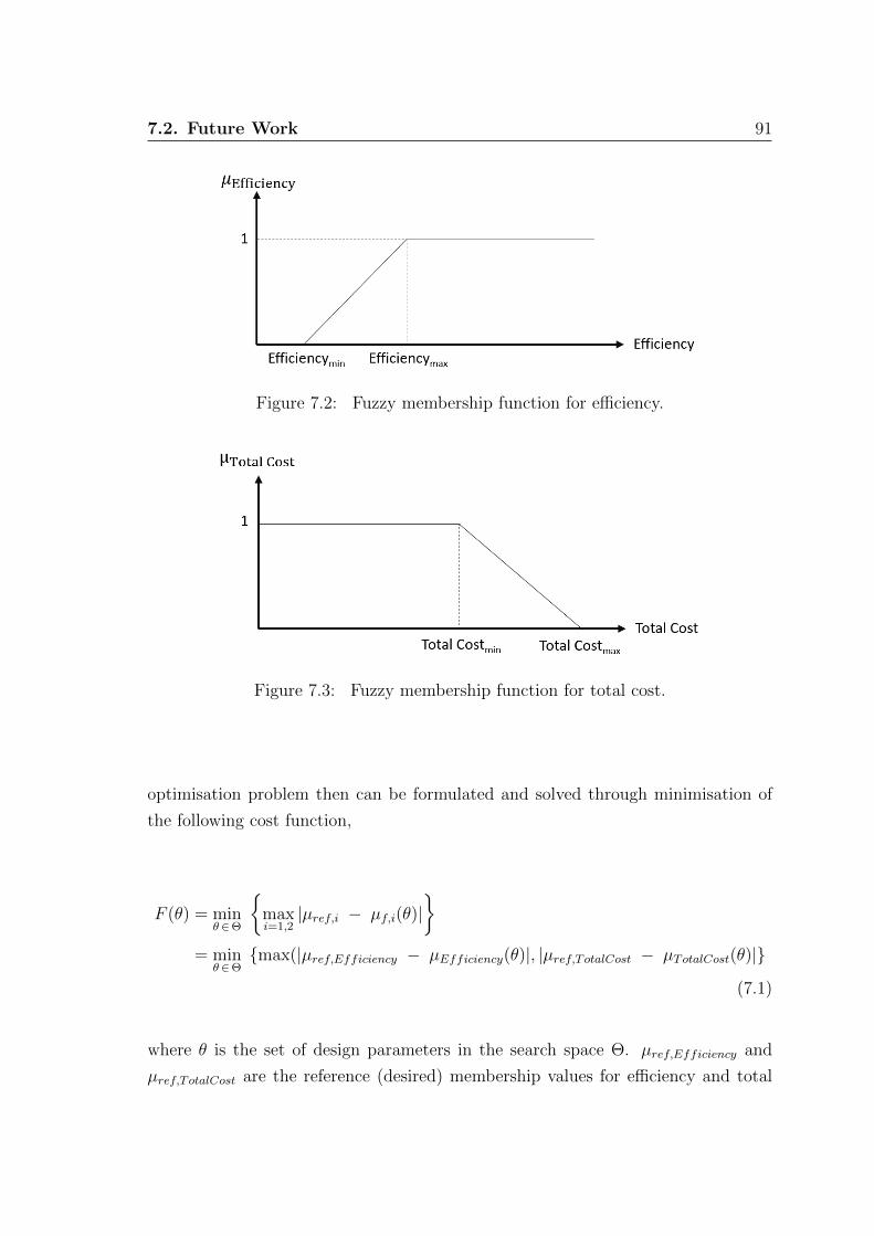
7.2. Future Work 91

Figure 7.2: Fuzzy membership function for efficiency.

Figure 7.3: Fuzzy membership function for total cost.

optimisation problem then can be formulated and solved through minimisation of

the following cost function,

F (θ) = minθ∈Θ

{maxi=1,2|µref,i − µf,i(θ)|

}= min

θ∈Θ{max(|µref,Efficiency − µEfficiency(θ)|, |µref,TotalCost − µTotalCost(θ)|}

(7.1)

where θ is the set of design parameters in the search space Θ. µref,Efficiency and

µref,TotalCost are the reference (desired) membership values for efficiency and total

7.2. Future Work 92

cost objectives respectively. The designer first sets values in the range of [0, 1] for

µref,Efficiency and µref,TotalCost. Efficiencymin, Efficiencymax, TotalCostmin, and

TotalCostmax are set by the designer in Fig. 7.2 and Fig. 7.3. Extreme values for

Efficiencymin and Efficiencymax are 0% and 100%.

According to this approach, the multi-objective design optimisation of STHXs is

transformed into a constrained free single objective optimisation problem. During

minimisation of (7.1), the cost function will be increased if the efficiency and total

cost objectives are not satisfied as per set values in Fig. 7.2 and Fig. 7.3.

Other types of membership functions can be used for transformation and evalu-

ation of fuzzy-based cost function. Trapezoidal type shown in Fig. 7.2 and Fig. 7.3

has a simple form and makes calculations fast and simple. Alternatives are complex

exponential ones and even type-2 membership functions.

7.2.4 Optimisation of Heat Exchanger Network

Methods for the optimal design of heat exchanger networks can be broadly cate-

gorised into three classes: (i) pinch analysis [109] [110] [111], (ii) mathematical pro-

gramming method [112], and (iii) meta-heuristic optimisation method [113]. The

latest set of approaches has become popular in recent years for solving the prob-

lem of optimisation of heat exchanger networks. Suggestions mentioned in sections

7.2.1, 7.2.2, and 7.2.3 can be easily extended and applied for optimal design of heat

exchanger networks [114] [115] [116] [117].

More specifically, the followings can be further investigated and applied:

• Novel evolutionary optimisation algorithms such as those listed in section 7.2.1

can be applied for optimal design of heat exchanger networks.

• The objectives for optimal design of a heat exchanger network could be: (i)

minimisation of utilities, (ii) reducing the number of exchangers, or (iii) min-

imising the total annual costs including the initial investment and the util-

isation cost [113]. This multi-objective optimisation problem can then be

7.2. Future Work 93

formulated as a single objective hybrid optimisation problem similar to ideas

mentioned in section 7.2.3.

• Once formulated, it can be effectively and efficiently solved using individual

or hybrid evolutionary optimisation algorithms (using algorithms mentioned

in section 7.2.2).

Appendices

94

Appendix A

Modelling, Simulation, and

Optimisation Code

Matlab code developed for modelling, simulation, and optimisation of STHXs is

provided in this section.

95

hx_optimisation.m

% Inputs (7 variables): % - Tube arrangement % - Tube diameter % - Tube pitch ratio % - Tube length % - Tube number % - Baffle spacing ratio % - Baffle cut ratio % Order of variables % [Arrangement di_do pt/do L Nt Lbc/Di baffle_cut/Di];

clc, clear all, close all; global LB UB xGAall = []; cfGAall = []; xFAall = []; cfFAall = []; xCSall = []; cfCSall = []; tGA = []; tFA = []; tCS = [];

[LB, UB] = hxparambounds; %LB = [0.50 0.500 1.25 3.00 100 0.20 0.19]; % Lower

bounds for parameters %UB = [3.49 64.49 2.00 8.00 600 1.40 0.32]; % Upper

bounds for parameters

popsize = 50; % Population

size in genetic algorithm iternum = 100; % Number of

iterations (GA/FA/CS)

for iRep = 1:50 sprintf('Optimisation Loop: %g. \n',iRep) initparam = [0 0 0 0 0 0 0]; % Initial

parameters (single solution) for i = 1:length(initparam) rng('shuffle'); xinit(:,i) = initparam(1,i) + randi(UB(i),popsize,1); % Initial

solutions for genetic algorithm end %xinit(1,:) = [1 10 10 10 10 10 10]; GAoptions =

gaoptimset('PopulationSize',popsize,'Generations',iternum,'InitialPopulation',xinit); GAoptions = gaoptimset(GAoptions,'Display','off'); %GAoptions = gaoptimset(GAoptions,'PlotFcns',@gaplotbestf); tic; [xGA, cfGA] = ga(@hxcostfunc,7,[],[],[],[],LB,UB,[],[1:7],GAoptions); tGA = [tGA; toc];

%FAxinit = repmat(xGA,popsize,1); FAoptions.NoIter = iternum; % number of

iterations FAoptions.NoFF = popsize; % population

size (number of fireflies) FAoptions.Beta0 = 0.0001; % adjusting

parameters FAoptions.gama = 0.05; % adjusting

parameters FAoptions.alpha = 100; % adjusting

parameters FAoptions.Beta2 = 0.5; FAoptions.LB = LB; FAoptions.UB = UB;

tic; [xFA, cfFA] = famopt(@hxcostfunc,xinit,FAoptions); % firefly

optimisation tFA = [tFA; toc];

rng('shuffle'); % Cuckoo Search CSoptions.NoIter = iternum; % number of

iterations CSoptions.NoNest = popsize; % population

size (number of nests) CSoptions.pa = 0.25; % discovery

rate of alien eggs/solutions CSoptions.LB = LB; CSoptions.UB = UB; tic; [xCS, cfCS, X] = csopt(@hxcostfunc,xinit,CSoptions); % cuckoo

search optimisation tCS = [tCS; toc];

xGAall = [xGAall; xGA]; cfGAall = [cfGAall; cfGA]; xFAall = [xFAall; xFA]; cfFAall = [cfFAall; cfFA]; xCSall = [xCSall; xCS]; cfCSall = [cfCSall; cfCS];

close all; clear xGA xFA cfGA cfFA xCS cfCS xinit end %close all; plot(1:10,-cfGAall,1:10,-cfFAall); AAAcf = [cfGAall cfFAall cfCSall] AAAvar = [xGAall; xFAall; xCSall] AAAt = [tGA tFA tCS] cd('C:\Users\CISR-KHOSRAVI-ABBAS\Desktop\General\Papers for Shell and Tube\RK - 2st

Paper\Matlab Codes\Results'); save(['Res_Efficiency_','IterNo_',num2str(iternum),'_Popsize_',num2str(popsize),'.mat']); %save('Res_DollarCost.mat');

hxcostfunc.m

% Inputs (7 variables): % - Tube arrangement % - Tube diameter % - Tube pitch ratio % - Tube length % - Tube number % - Baffle spacing ratio % - Baffle cut ratio % Outputs: % - Heat exchanger effectiveness % - Heat exchanger total annual cost % - Heat exchanger length (L) % - Heat exchanger diameter (D) %==========================================================================

function out = hxcostfunc(x) namber_of_population = size(x,1);

% mapping parameters to Min:step:Max % for z = 1:namber_of_population % params = sthx_mapparams(x(z,:)); % converting

parameters % x(z,:) = params([1 3:8]); % di is not

an optimization parameter. It depends on do. % end

for z = 1:namber_of_population label = 0; %-------------dicision variables---------------------- % [Arrangement di_do pt/do L Nt Lbc/Di baffle_cut/Di]; params = sthx_mapparams(x(z,:)); % converting

parameters % assiging parameters Arrangement = params(1); di = params(2); do = params(3); pt = params(4); L = params(5); Nt = params(6); Lbc_ratio = params(7); baffle_cut_ratio = params(8);

%TubeArang = [30 45 90]; %Arrangement = TubeArang((round(x(z,1)))); %[di do] = di_do((round(x(z,2)))); %pt = x(z,3)*do; %L = x(z,4); %Nt = round(x(z,5)); %Lbc_ratio = x(z,6); % Baffle

spacing ratio %baffle_cut_ratio = x(z,7); %----------------------------------------------------- np = 2; if (Arrangement == 30) Xt = pt; Xl = (sqrt(3)/2)*pt; sigma = (pt-do)/pt; elseif (Arrangement == 45) Xt = sqrt(2)*pt; Xl = pt/sqrt(2);

if ((pt/do) >= 1.707) sigma = (sqrt(2)*pt-do)/(sqrt(2)*pt); else sigma = 2*(pt-do)/(sqrt(2)*pt); end elseif (Arrangement == 90) Xt = pt; Xl = pt; sigma = (pt-do)/pt; end %----------------------------------------------------------- Nss = 1; wp = 19e-3; Np = 2; delta_tb = 0.794e-3; delta_sb = 2.946e-3; kw = 109; %----------------initial condition-------------------------- % Sanaye2010 - Section 5 (Case Study) ms = 8.1; % Shell mass

flow rate mt = 12.5; % Tube mass

flow rate Tsi = 78.3; % Shell inlet

temperature Tti = 30; % Tube inlet

temperature %-------thermophisical propertice of two sides-------------- ros = 860; rot = 995; cps = 2115; % Shell

specific heat in constant pressure cpt = 4120; % Tube

specific heat in constant pressure meus = 64.3e-3; % Shell

viscosity meut = 0.695e-3; % Tube

viscosity prs = 968; % Prandtl

number - shell prt = 4.89; % Prandtl

number - tube Rof = 0.00015; % Fouling

resistance shell side (m2 K/W) Rif = 0.000074; % Fouling

resistance tube side (m2 K/W) ks = 0.16; kt = 0.6; %---------------shell diameter-------------------- if(Arrangement == 45 || Arrangement == 90) CL = 1; else CL = 0.87; end if(np == 1) CTP = 0.93; elseif(np == 2) CTP = 0.9; elseif(np == 3) CTP = 0.85; end PR = pt/do; Ao = pi*do*Nt*L;

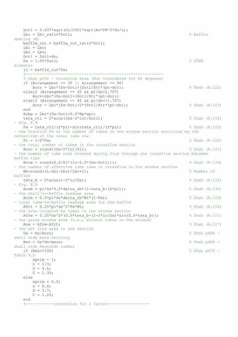
Dctl = 0.637*sqrt(CL/CTP)*sqrt(Ao*PR^2*do/L); Lbc = Lbc_ratio*Dctl; % Baffle

spacing (m) baffle_cut = baffle_cut_ratio*Dctl; Lbi = Lbc; Lbo = Lbc; Dotl = Dctl+do; Ds = 1.05*Dotl; % STHE

diameter lc = baffle_cut*Ds; %----------------------------------------------------------- % Shah p592 - Crossflow Area (Not Considered for 60 degrees) if (Arrangement == 30 || Arrangement == 90) Aocr = Lbc*(Ds-Dotl+(Dctl/Xt)*(pt-do)); % Shah (8.122) elseif (Arrangement == 45 && pt/do>1.707) Aocr=Lbc*(Ds-Dotl+(Dctl/Xt)*(pt-do)); elseif (Arrangement == 45 && pt/do<=1.707) Aocr = Lbc*(Ds-Dotl+2*(Dctl/Xt)*(pt-do)); % Shah (8.123) end Aobp = Lbc*(Ds-Dotl+0.5*Np*wp); teta_ctl = 2*acos((Ds-2*lc)/Dctl); % Shah (8.114)

- Fig. 8.9 Fw = teta_ctl/(2*pi)-sin(teta_ctl)/(2*pi); % Shah (8.113)

- the fraction Fw of the number of tubes in one window section encircled by the

centerline of the outer tube row Fc = 1-2*Fw; % Shah (8.120)

- the total number of tubes in the crossflow section Nrcc = round((Ds-2*lc)/Xl); % Shah (8.121)

- the number of tube rows crossed during flow through one crossflow section between

baffle tips Nrcw = round(0.8/Xl*(lc-0.5*(Ds-Dctl))); % Shah (8.119)

- the number of effective tube rows in crossflow in the window section Nb=round((L-Lbi-Lbo)/Lbc+1); % Number of

baffles teta_b = 2*acos(1-2*lc/Ds); % Shah (8.112)

- Fig. 8.9 Aosb = pi*Ds*0.5*delta_sb*(1-teta_b/(2*pi)); % Shah (8.130)

- the shell-to-baffle leakage area Aotb = 0.5*pi*do*delta_tb*Nt*(1-Fw); % Shah (8.129)

- total tube-to-baffle leakage area for one baffle Afrt = 0.25*pi*do^2*Fw*Nt; % Shah (8.116)

- the area occupied by tubes in the window section Afrw = 0.25*Ds^2*(0.5*teta_b-(1-2*lc/Ds)*sin(0.5*teta_b)); % Shah (8.111)

- the gross window area (i.e., without tubes in the window) Aow = Afrw-Afrt; % Shah (8.117)

- the net flow area in one section Gs = ms/Aocr; % Shah p684 -

shell side mass velocity Res = Gs*do/meus; % Shah p684 -

shall side Reynolds number if (Res<=100) % Shah p679 -

Table 9.2 nprim = 1; n = 1/3; D = 4.5; C = 1.35; else nprim = 0.2; n = 0.6; D = 3.7; C = 1.25; end %------------correction for J factor------------------

% Shah p679 - Table 9.2 Jc = 0.55+0.72*Fc; rs = Aosb/(Aosb+Aotb); rlm = (Aosb+Aotb)/Aocr; Jl = 0.44*(1-rs)+(1-0.44*(1-rs))*exp((-2.2*rlm)); rb = Aobp/Aocr; Nssplus = Nss/Nrcc; if (Nssplus <= 0.5) %Jb = exp(-C*rb*(1-(2*Nssplus)^(1/3))); Jb = exp(-C*rb*(1-abs((2*Nssplus)^(1/3)))); else Jb = 1; end Liplus = Lbi/Lbc; Loplus = Liplus; Js = (Nb-1+Liplus^(1-n)+Loplus^(1-n))/(Nb-1+Liplus+Loplus); Nrc = Nrcc+Nrcw; if(Res >= 100) Jr = 1; elseif(Res <= 20) Jr = (10/Nrc)^0.18; else Jr = 0.5*(1+(10/Nrc)^0.18); end %---------heat transfer coefficient in shell side---------- % Sadick p336 - (8.25) (8.26) Table 8.6 [colburn fid] = jf(Res,pt,do,Arrangement); hid = colburn*cps*(Gs)*(prs)^(-2/3); % Sadick

(8.24) - ideal heat transfer coefficient for pure}rJssflow in an ideal tube bank hs = hid*Jc*Jl*Jb*Js*Jr; % Sadick

(8.23) - heat transfer coef in shell sdie %---------heat transfer coefficient in tube side---------- Ntp = 0.5*Nt; % number of

tube per pass Aot = 0.25*pi*di^2*Ntp; % tube side

flow cross section Ret = (mt*di)/(Aot*meut); % tube side

Reynolds number if (Ret > 2500 && Ret < 1.24e5) % Shah (7.80)

- Table 7.6 p513 Nut = 0.024*Ret^0.8*prt^0.4; % Nusselt

number - Shah p655 (Example) else Nut = 0.001; label = 1; end ht = Nut*kt/di; % tube side

heat transfer coefficient %----------- effectiveness--------------------- % Sanaye2010 - Section 2 (Thermal Modeling) Uo = 1/(1/hs+Rof+do*log(do/di)/(2*kw)+Rif*do/di+(do/di)/ht); % Eq. (5) Ato = pi*L*do*Nt; % Eq. (4) Ct = mt*cpt; % Eq. (3) last

part Cs = ms*cps; % Eq. (3) last

part Cmax = max(Ct,Cs); % Eq. (3)

first part Cmin = min(Ct,Cs); % Eq. (3)

first part Cstar = Cmin/Cmax; % Eq. (3) the

capacity rate ratio

Ntu = Uo*Ato/Cmin; % Eq. (2)

number of transfer units e = 2/((1+Cstar)+sqrt(1+Cstar^2)*coth(0.5*Ntu*sqrt(1+Cstar^2))); % Shah p159 -

Table 3.3 q = e*Cmin*(Tsi-Tti); % NOT USED Tso = Tsi-e*(Tsi-Tti); % Eq. (26)

Shell Outlet Temperature Tto = Tti+e*(Tsi-Tti); % Eq. (27)

Tube Outlet Temperature Tsm = 0.5*(Tsi+Tso); % NOT USED Ttm = 0.5*(Tti+Tto); % NOT USED %------------pressure drop in two sides---------------------- % Section 6.5, page 216 of Ref [17] %6.5 % Kuppan Thulukkanam, "Heat Exchanger Design Handbook", Second Edition, %

deltap_bid = 4*fid*Gs^2*Nrcc/(2*ros); if (Nssplus < 0.5) % Nss: Number

of sealing strip pairs zetab = exp(-D*rb*(1-abs((2*Nssplus)^(1/3)))); else zetab = 1; end p = -0.15*(1+rs)+0.8; zetal = exp(-1.33*(1+rs)*rlm^p); deltap_cr = deltap_bid*(Nb-1)*zetab*zetal; % Crossflow

pressure drop Gw = ms/sqrt(Aocr*Aow); % Gw: window

mass velocity deltap_w = Nb*(2+0.6*Nrcw)*Gw^2*zetal/(2*ros); % Window

section pressure drop

zetas = (Lbc/Lbo)^(2-nprim)+(Lbc/Lbi)^(2-nprim); deltap_io = 2*deltap_bid*(1+Nrcw/Nrcc)*zetab*zetas; % Inlet and

outlet pressure drop deltap_s = deltap_cr + deltap_w + deltap_io; % Eq. (14) if(Ret > 4000 && Ret < 1e7) frictiont = 0.00128+0.1143*Ret^-0.311; else frictiont = 100; label = 1; end [Kc Ke] = KcKe(Ret,sigma); deltap_t = mt^2/(2*rot*Aot^2)*(4*frictiont*L/di+(1-sigma^2+Kc)-(1-sigma^2-Ke))*np; %----------Cost function------------------------------------ CE = 0.15; ny = 10; i = 0.1; H = 7500; eta = 0.6; Co = (1/eta)*(mt/rot*deltap_t+ms/ros*deltap_s)*CE*H/1000; % Eq. (23) CoD = 0; for k = 1:ny CoD = Co/((1+i)^k)+CoD; % Eq. (21) -

operating cost for ny years (here 10 years) end Ci = 8500+409*(Ato)^0.85; % Eq. (20) -

investment cost (sst made) Ctotal = (Ci+CoD); % Eq. (19) -

operating cost + investment cost %----------------------------------------------------------- % Exergy Cost (NOT USED in Sanaye2010)

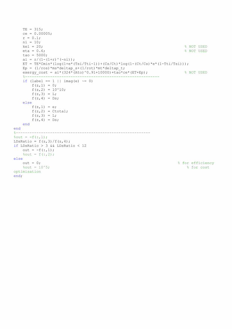
TE = 315; ce = 0.00005; r = 0.1; ni = 10; kel = 20; % NOT USED eta = 0.6; % NOT USED tao = 5000; ai = r/(1-(1+r)^(-ni)); ET = TE*Cmin*(log(1+e*(Tsi/Tti-1))+(Cs/Ct)*log(1-(Ct/Cs)*e*(1-Tti/Tsi))); Ep = (1/ros)*ms*deltap_s+(1/rot)*mt*deltap_t; exergy_cost = ai*(324*(Ato)^0.91+10000)+tao*ce*(ET+Ep); % NOT USED %----------------------------------------------------------- if (label == 1 || imag(e) ~= 0) f(z,1) = 0; f(z,2) = 10^10; f(z,3) = L; f(z,4) = Ds; else f(z,1) = e; f(z,2) = Ctotal; f(z,3) = L; f(z,4) = Ds; end end %----------------------------------------------------------- %out = -f(:,1); LDsRatio = f(z,3)/f(z,4); if LDsRatio > 3 && LDsRatio < 12 out = -f(:,1); %out = f(:,2); else out = 0; % for efficiency %out = 10^5; % for cost

optimisation end;

csopt.m

function [bestnest,fmin, X] = csopt(CostFun,ipop,options)

NoIter = options.NoIter; % number of

iterations NoNest = options.NoNest; % population

size (number of fireflies) Nd = size(ipop,2); % number of

decision variables pa = options.pa; % Discovery

rate of alien eggs/solutions Xmin = options.LB; % lower bound Xmax = options.UB; % upper bound

nest = ipop; % initial

solutions (nests)

% Get the current best fitness = 10^10*ones(NoNest,1); [fmin,bestnest,nest,fitness] = get_best_nest(nest,nest,fitness,CostFun); % find the

current best nest

N_iter = 0; % number of

iterations %% Starting iterations for iter = 1:NoIter % Generate new solutions (but keep the current best) new_nest = get_cuckoos(nest,bestnest,Xmin,Xmax); [fnew,best,nest,fitness] = get_best_nest(nest,new_nest,fitness,CostFun); % Update the counter N_iter = N_iter + NoNest; % Discovery and randomization new_nest = empty_nests(nest,Xmin,Xmax,pa) ;

% Evaluate this set of solutions [fnew,best,nest,fitness] = get_best_nest(nest,new_nest,fitness,CostFun); % Update the counter again N_iter = N_iter + NoNest; % Find the best objective so far if fnew < fmin, fmin = fnew; bestnest = best; end fprintf('Cukoo Search Iteration is %g/%g - Best CF %g. \n', iter,NoIter,fmin); X(iter,:) = bestnest; end %% End of iterations

%% Post-optimization processing %% Display all the nests disp(strcat('Total number of calculations = ',num2str(N_iter))); %$$$$$$$$$$$$$$$$$$$$$$$$$$$$$$$$$$$$$$$$$$$$$$$$$$$$$$$$$$$$$$$$$$$$$$$$$$ %$$$$$$$$$$$$$$$$$$$$$$$$$$$$$$$$$$$$$$$$$$$$$$$$$$$$$$$$$$$$$$$$$$$$$$$$$$

%% --------------- All subfunctions are list below ------------------ %% Get cuckoos by ramdom walk function nest = get_cuckoos(nest,best,Xmin,Xmax) % Levy flights NoNest = size(nest,1); % Levy exponent and coefficient % For details, see equation (2.21), Page 16 (chapter 2) of the book

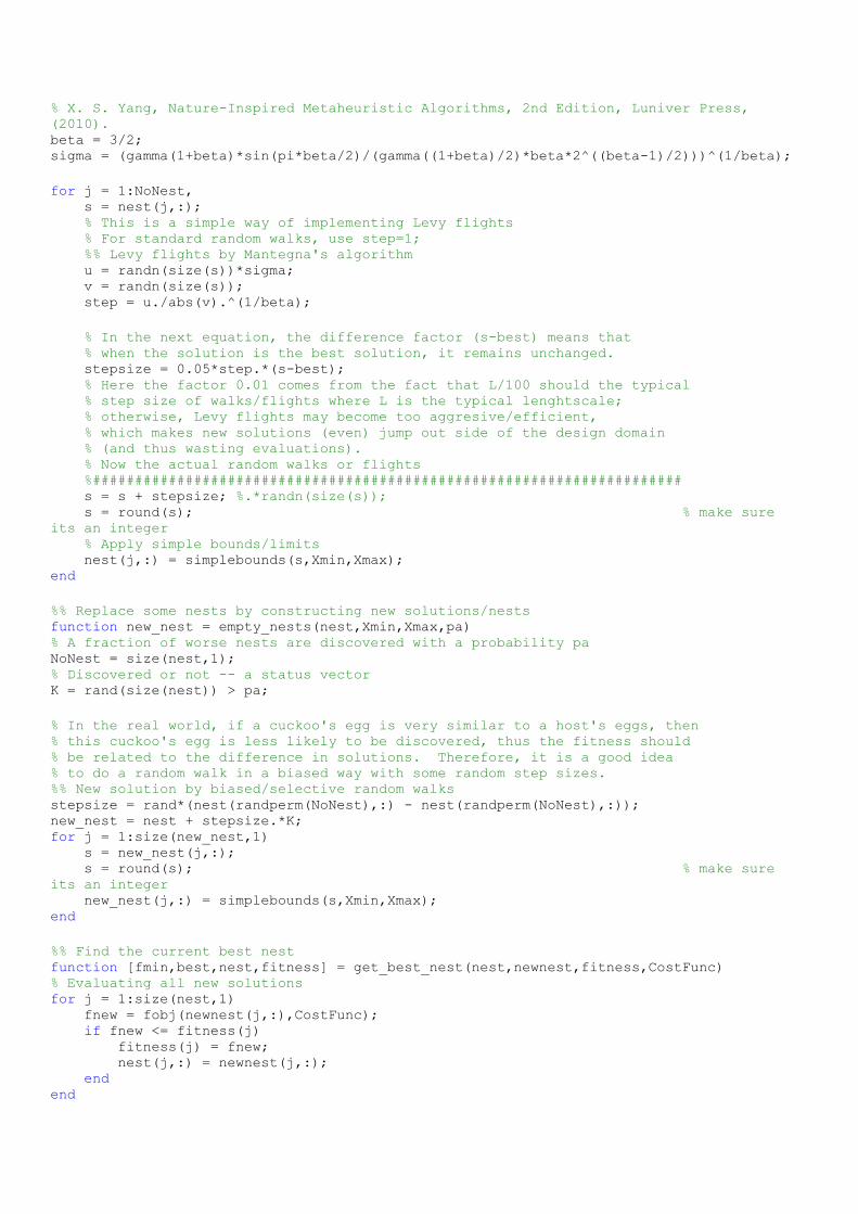
% X. S. Yang, Nature-Inspired Metaheuristic Algorithms, 2nd Edition, Luniver Press,

(2010). beta = 3/2; sigma = (gamma(1+beta)*sin(pi*beta/2)/(gamma((1+beta)/2)*beta*2^((beta-1)/2)))^(1/beta);

for j = 1:NoNest, s = nest(j,:); % This is a simple way of implementing Levy flights % For standard random walks, use step=1; %% Levy flights by Mantegna's algorithm u = randn(size(s))*sigma; v = randn(size(s)); step = u./abs(v).^(1/beta);

% In the next equation, the difference factor (s-best) means that % when the solution is the best solution, it remains unchanged. stepsize = 0.05*step.*(s-best); % Here the factor 0.01 comes from the fact that L/100 should the typical % step size of walks/flights where L is the typical lenghtscale; % otherwise, Levy flights may become too aggresive/efficient, % which makes new solutions (even) jump out side of the design domain % (and thus wasting evaluations). % Now the actual random walks or flights %###################################################################### s = s + stepsize; %.*randn(size(s)); s = round(s); % make sure

its an integer % Apply simple bounds/limits nest(j,:) = simplebounds(s,Xmin,Xmax); end

%% Replace some nests by constructing new solutions/nests function new_nest = empty_nests(nest,Xmin,Xmax,pa) % A fraction of worse nests are discovered with a probability pa NoNest = size(nest,1); % Discovered or not -- a status vector K = rand(size(nest)) > pa;

% In the real world, if a cuckoo's egg is very similar to a host's eggs, then % this cuckoo's egg is less likely to be discovered, thus the fitness should % be related to the difference in solutions. Therefore, it is a good idea % to do a random walk in a biased way with some random step sizes. %% New solution by biased/selective random walks stepsize = rand*(nest(randperm(NoNest),:) - nest(randperm(NoNest),:)); new_nest = nest + stepsize.*K; for j = 1:size(new_nest,1) s = new_nest(j,:); s = round(s); % make sure

its an integer new_nest(j,:) = simplebounds(s,Xmin,Xmax); end

%% Find the current best nest function [fmin,best,nest,fitness] = get_best_nest(nest,newnest,fitness,CostFunc) % Evaluating all new solutions for j = 1:size(nest,1) fnew = fobj(newnest(j,:),CostFunc); if fnew <= fitness(j) fitness(j) = fnew; nest(j,:) = newnest(j,:); end end

% Find the current best [fmin, K] = min(fitness); best = nest(K,:);

%% Application of simple constraints function s = simplebounds(s,Xmin,Xmax) % Apply the lower bound ns_tmp = s; I = ns_tmp < Xmin; ns_tmp(I) = Xmin(I);

% Apply the upper bounds J = ns_tmp > Xmax; ns_tmp(J) = Xmax(J); % Update this new move s = ns_tmp;

%% Cost Function Calculation function z = fobj(x,CostFun) z = CostFun(x);

famopt.m

function [xMin,CostFinal] = famopt(CostFun,ipop,options) %##########################################################################

format long NoIter = options.NoIter; % number of

iterations NoFF = options.NoFF; % population

size (number of fireflies) Nd = size(ipop,2); % number of

decision variables Beta0 = options.Beta0; % adjusting

parameters Beta2 = options.Beta2; % adjusting

parameters gama = options.gama; % adjusting

parameters alpha = options.alpha; % adjusting

parameters Xmin = options.LB; Xmax = options.UB;

for icf = 1:NoFF cost(icf,1) = CostFun(ipop(icf,:)); % Calculate

cost fucntion for initial end ipop_cost = [ipop,cost]; ipop_sort = sortrows(ipop_cost,Nd+1); % Sort based

on cost function values best = ipop_sort(1,:); % Best initial

solution and min cost function for Iter = 1:NoIter mD = mean(ipop_cost(:,[1:Nd])); differ = 1*rand*(best([1:Nd])-round(1+rand)*mD); % ##### for i = 1:NoFF for j = 1:NoFF if cost(j,1) < cost(i,1) dist = (sum((ipop(j,:)-ipop(i,:)).^2))^0.5; % distance

between x(i) and x(j) Beta = Beta0*exp(-gama*dist); Ipop_new = (1-Beta)*ipop(i,:) + Beta*ipop(j,:) + alpha*(rand(1,Nd)-0.5); else Ipop_new = ipop(i,:) + alpha*(rand(1,Nd)-0.5); end %-------------------------------- Ipop_new = round(Ipop_new); % all

variables are INTIGER Ipop_new = limitfunc(Ipop_new,Xmax,Xmin); cost_new = CostFun(Ipop_new); if cost_new < cost(i,1) ipop_cost(i,:) = [Ipop_new,cost_new]; ipop(i,:) = Ipop_new; cost(i,1) = cost_new; end end end % Modification 1 Ipop_new = ipop(i,:) + differ; %-------------------------------- Ipop_new = round(Ipop_new); % all

variables are INTIGER Ipop_new = limitfunc(Ipop_new,Xmax,Xmin);

cost_new = CostFun(Ipop_new); if cost_new < cost(i,1) ipop_cost(i,:) = [Ipop_new,cost_new]; ipop(i,:) = Ipop_new; cost(i,1) = cost_new; end % Modification 2 ZZ = randperm(NoFF); ZZZ = find(ZZ~=j); nn = ZZ(ZZZ); X_mut = round(ipop(nn(1),[1:Nd])+rand*(ipop(nn(2),[1:Nd])-ipop(nn(3),[1:Nd]))); rand_sp = round(rand(1,1)*NoFF); if rand_sp==0 rand_sp=1; end for h = 1:Nd cros = rand(1,1); if cros < Beta2 broode(1,h) = X_mut(1,h); else broode(1,h) = best(1,h); end

cros = rand(1,1); if cros < Beta2 broode(2,h) = X_mut(1,h); else broode(2,h) = ipop(i,h); end

cros = rand(1,1); if cros < Beta2 broode(3,h) = X_mut(1,h); else broode(3,h) = round(rand*best(1,h)+rand*(best(1,h)-ipop(rand_sp,h))); end end cost_b = zeros(3,1); for ii=1:3 %-------------------------------- Ipop_new = round(broode(ii,:)); % all

variables are INTIGER broode(ii,:)= limitfunc(broode(ii,:),Xmax,Xmin); cost_b(ii,:) = CostFun(broode(ii,:)); if cost(i) > cost_b(ii,1) ipop(i,:) = broode(ii,:); cost(i,1) = cost_b(ii,1); end end ipop_cost = [ipop,cost]; ipop_sort = sortrows(ipop_cost,Nd+1); if ipop_sort(1,Nd+1) < best(Nd+1) best = ipop_sort(1,:); end fprintf('Firefly Iteration is %g/%g - Best CF %g. \n', Iter,NoIter,best(1,Nd+1)); end xMin = best(1,1:Nd); CostFinal = best(1,Nd+1);

Utility Functions

function X = limitfunc(X,xmax,xmin) n = size(xmax,2); for k = 1:n if X(1,k)>xmax(1,k) X(1,k)=xmax(1,k); end if X(1,k)<xmin(1,k) X(1,k)=xmin(1,k); end end

function Population = pop_creation(GenomeLength,FitnessFcn,options) %range = [1 5; 1 20; 1 100; 1 10; 1 100]; %options.step = [0.1 0.2 0.3 0.4 0.8]';

totalpopulation = sum(options.PopulationSize); range = options.PopInitRange;

Population = zeros(totalpopulation,GenomeLength); for ivar = 1:GenomeLength Population(:,ivar) = randi([range(ivar,1) range(ivar,2)],1,totalpopulation); end Population = pop_map(Population); % End of creation function

function out = roundtoclosest(x,Min,Max,stepsize)

vec = Min:stepsize:Max; [c index] = min(abs(vec-x)); % finding the

index of closest value to x out = vec(index); % returning

the closest value to x from vec

function [LB UB] = hxparambounds;

% This function calculates the number of elements for each variable within % its min and max values considering the step size. Then these lower and % upper bounds are used by the optimization algorithm to generate % solutoins. %-------------------------------------------------------------------------- TubeArang = [30 45 90]; TubeInteDia = 1:20; min_TubePitchRatio = 1.25; max_TubePitchRatio = 2; step_TubePitchRatio = 0.001; min_TubeLength = 3; max_TubeLength = 8; step_TubeLength = 0.001; min_TubeNumber = 100; max_TubeNumber = 600; step_TubeNumber = 1; min_BaffleSpacingRatio = 0.19; max_BaffleSpacingRatio = 0.32; step_BaffleSpacingRatio =

0.001; min_BaffleCutRatio = 0.2; max_BaffleCutRatio = 1.4; step_BaffleCutRatio = 0.001;

size_TubeArang = length(TubeArang); size_TubeInteDia = length(TubeInteDia); size_TubePitchRatio = length(min_TubePitchRatio:step_TubePitchRatio:max_TubePitchRatio); size_TubeLength = length(min_TubeLength:step_TubeLength:max_TubeLength); size_TubeNumber = length(min_TubeNumber:step_TubeNumber:max_TubeNumber); size_BaffleSpacingRatio =

length(min_BaffleSpacingRatio:step_BaffleSpacingRatio:max_BaffleSpacingRatio); size_BaffleCutRatio = length(min_BaffleCutRatio:step_BaffleCutRatio:max_BaffleCutRatio);

LB = [1 1 1 1 1 1 1]; UB = [size_TubeArang, size_TubeInteDia, size_TubePitchRatio, size_TubeLength,

size_TubeNumber, size_BaffleSpacingRatio, size_BaffleCutRatio];

function[ddi ddo]=di_do(k) %di=[0.194 0.206 0.214 0.277 0.305 0.319 0.331 0.37 0.402 0.43 0.444 0.407 0.435 0.481

0.495 0.509 0.527 0.541 0.555 0.482 0.51 0.532 0.56 0.584 0.606 0.62 0.634 0.352 0.68

0.607 0.635 0.657 0.685 0.709 0.745 0.777 0.805 0.67 0.732 0.76 0.782 0.81 0.834 0.856

0.87 0.902 0.93 0.89 0.92 0.982 1.01 1.032 1.06 1.084 1.12 1.152 1.18 1.232 1.282 1.334

1.37 1.76 1.81 2.204]; %do=[0.25 0.25 0.25 3/8 3/8 3/8 3/8 0.5 0.5 0.5 0.5 5/8 5/8 5/8 5/8 5/8 5/8 5/8 5/8 0.75

0.75 0.75 0.75 0.75 0.75 0.75 0.75 0.75 0.75 7/8 7/8 7/8 7/8 7/8 7/8 7/8 7/8 1 1 1 1 1 1

1 1 1 1 11/4 11/4 11/4 11/4 11/4 11/4 11/4 11/4 11/4 11/4 11/2 11/2 11/2 11/2 2 2 2.5 ];

di = [0.444 0.495 0.555 0.560 0.634 0.407 0.509 0.482 0.584 0.352 0.435 0.527 0.510 0.606

0.680 0.481 0.541 0.532 0.620 0.607]; do = [1/2 5/8 5/8 3/4 3/4 5/8 5/8 3/4 3/4 3/4 5/8 5/8 3/4 3/4

3/4 5/8 5/8 3/4 3/4 7/8 ];

ddi = di(k)/39.7; ddo = do(k)/39.7;

function[Kc Ke]=KcKe(Re,sigma) %--------Ke turbulent------------- %----------Re=inf----------------- Ket_inf=[0.0973056 0.812641 0.135869 0.750936 0.172776 0.686743 0.209682 0.62255 0.24656 0.565789 0.286781 0.50657 0.326984 0.452305 0.378899 0.385723 0.429119 0.326562 0.467609 0.284673 0.506089 0.245262 0.551255 0.200935 0.609762 0.154208 0.658214 0.122286 0.706657 0.0928416 0.740064 0.0732182 0.770118 0.0585297 0.803497 0.0463377 0.840218 0.031688 0.880263 0.0195348 0.916956 0.0123165 0.961983 0.00514671 0.993658 0.00285366]; %----------Re=10000-------------- Ket_10000=[0.0973149 0.810164 0.134249 0.73854 0.164452 0.684217 0.194664 0.627417 0.224857 0.575572 0.253356 0.531148 0.286883 0.479322 0.327104 0.420103 0.360612 0.373231 0.400815 0.318966

0.440989 0.272133 0.487877 0.212952 0.53807 0.161223 0.596605 0.107065 0.646761 0.0652441 0.698565 0.0283873 0.748674 -0.00104777 0.813811 -0.0378271 0.863884 -0.0573536 0.910614 -0.0744223 0.957325 -0.0865368 0.992352 -0.0937647]; %----------Re=5000-------------- Ket_5000=[0.0973149 0.810164 0.129221 0.745943 0.157757 0.69161 0.191312 0.632352 0.226561 0.565673 0.260106 0.508892 0.296985 0.452131 0.33215 0.407746 0.367344 0.355929 0.400843 0.311534 0.434332 0.269617 0.471164 0.225241 0.509663 0.180876 0.548153 0.138987 0.591624 0.102082 0.633419 0.0676438 0.668529 0.0381215 0.708629 0.0111054 0.758748 -0.0208068 0.805506 -0.045307 0.855597 -0.0697878 0.902327 -0.0868565 0.947372 -0.0989806 0.990741 -0.108637]; %----------Re=3000-------------- Ket_3000=[0.0973519 0.800256 0.132601 0.733576 0.159452 0.684188 0.181266 0.64468 0.206441 0.597759 0.231598 0.555793 0.263458 0.503957 0.296985 0.452131 0.325465 0.412661 0.365677 0.35592 0.397509 0.311515 0.431008 0.26712 0.464489 0.22768 0.501302 0.188259 0.536449 0.148828 0.5833 0.099556 0.626771 0.0626507 0.670223 0.0306997 0.708676 -0.0012803 0.752119 -0.0307541 0.792201 -0.0528159 0.830607 -0.0724102 0.889031 -0.0968426 0.942418 -0.111395 0.990787 -0.121023];

%------------------------------ %--------Ke laminar------------- %----------4L/dRe=0.05--------- Kel_5=[0.0975001 0.760621 0.137804 0.679108 0.164702 0.617334 0.188238 0.562973 0.225181 0.488872 0.2638 0.412303 0.29904 0.348101 0.342668 0.269084 0.394676 0.17773 0.443286 0.103696 0.476812 0.0518701 0.512006 5.35443e-005 0.545514 -0.0468184 0.580698 -0.0961579 0.620873 -0.142991 0.664399 -0.194759 0.702889 -0.236648 0.736351 -0.271134 0.769803 -0.303143 0.804913 -0.332666 0.840023 -0.362188 0.878467 -0.391691 0.918577 -0.421184 0.958686 -0.450677 0.993759 -0.470291]; %----------4L/dRe=0.1---------- Kel_10=[0.0975464 0.748236 0.119407 0.696341 0.141267 0.644447 0.159785 0.595011 0.184997 0.538182 0.206839 0.491242 0.2287 0.439348 0.262273 0.375136 0.292503 0.313382 0.322697 0.261536 0.356261 0.199801 0.383093 0.155368 0.411611 0.105989 0.436786 0.059069 0.472007 -0.000178991 0.500506 -0.0446029 0.532348 -0.0914846 0.565884 -0.145788 0.601049 -0.190173 0.634548 -0.234568 0.669714 -0.278953 0.706546 -0.323329 0.741702 -0.365237 0.783534 -0.409583 0.828728 -0.461342 0.868865 -0.498266 0.903984 -0.530266 0.944094 -0.559759 0.979186 -0.584327 0.994232 -0.596625]; %----------4L/dRe=0.2---------- Kel_20=[0.0975464 0.748236 0.124462 0.681508 0.154721 0.612322

0.181618 0.550548 0.208524 0.486298 0.233737 0.429469 0.267328 0.360302 0.297568 0.296071 0.32278 0.239242 0.351316 0.184909 0.383204 0.125642 0.413388 0.0762734 0.446952 0.0145386 0.482173 -0.0447095 0.527431 -0.113808 0.56431 -0.170569 0.599503 -0.222386 0.632993 -0.264303 0.673177 -0.313614 0.70837 -0.36543 0.746869 -0.409796 0.795423 -0.468967 0.840616 -0.520725 0.889105 -0.562556 0.940946 -0.609321 0.994426 -0.648645]; %----------4L/dRe=inf--------- Kel_inf=[0.0975279 0.75319 0.124453 0.683985 0.15473 0.609845 0.184988 0.540659 0.216922 0.469006 0.253893 0.387473 0.287503 0.313353 0.324447 0.239252 0.353011 0.177488 0.386574 0.115753 0.413407 0.0713191 0.443601 0.0194735 0.475479 -0.0373168 0.505654 -0.0842082 0.542551 -0.145924 0.577735 -0.195263 0.616299 -0.256969 0.656492 -0.308756 0.698343 -0.358057 0.74186 -0.407348 0.768683 -0.449305 0.807163 -0.488716 0.835644 -0.528186 0.8808 -0.570036 0.927623 -0.611876 0.962742 -0.643875 0.994482 -0.663508]; %---------------------------- %--------Kc turbulent------------- %----------Re=inf----------------- Kct_inf=[0.100639 0.366765 0.195784 0.327683 0.297605 0.286162 0.396093 0.244622 0.49959 0.200635 0.599716 0.166536 0.701518 0.12997 0.805015 0.0859818 0.901846 0.0419551

0.991982 0.00532111]; %----------Re=10000-------------- Kct_10000=[0.10362 0.460916 0.165378 0.436503 0.223802 0.41207 0.333974 0.365644 0.399056 0.343728 0.459156 0.316828 0.540931 0.287577 0.611021 0.263212 0.667779 0.23877 0.744573 0.204536 0.801321 0.182571 0.874763 0.153272 0.944881 0.121476 0.99163 0.0994527]; %----------Re=5000-------------- Kct_5000=[0.100231 0.475759 0.197043 0.436687 0.297198 0.395157 0.395667 0.358571 0.495812 0.319518 0.600966 0.278017 0.669408 0.248689 0.741175 0.221857 0.811284 0.192538 0.87805 0.165677 0.953168 0.13391 0.994898 0.116812]; %----------Re=3000-------------- Kct_3000=[0.100167 0.493099 0.196988 0.45155 0.297142 0.41002 0.395621 0.370957 0.49908 0.336878 0.597568 0.295338 0.684362 0.261162 0.779507 0.222079 0.872995 0.180511 0.953122 0.146296 0.993176 0.131665]; %--------Kc laminar------------- %----------4l/dRe=0.05--------- Kcl_5=[0.0988611 0.842377 0.295846 0.75682 0.496136 0.678714 0.698102 0.598141 0.898411 0.51508 0.993556 0.475998]; %----------4l/dRe=0.1--------- Kcl_10=[0.0967316 0.966224 0.206904 0.919798 0.327067 0.875907 0.482303 0.812402 0.605827 0.761099 0.737693 0.707368 0.87792 0.646253 0.99475 0.602342]; %----------4l/dRe=0.2--------- Kcl_20=[0.0981852 1.02321 0.220043 0.971896 0.348576 0.918145 0.483775 0.864432

0.610632 0.813148 0.747499 0.759446 0.879374 0.703237 0.994546 0.65684]; %----------4l/dRe=inf--------- Kcl_inf=[0.0981667 1.02816 0.194969 0.991568 0.305133 0.947618 0.428647 0.898792 0.573856 0.842661 0.700704 0.793854 0.814219 0.74497 0.94777 0.686294 0.996176 0.666758]; %---------------------------- %---------------------------- if(sigma<0.105) Kc=inf; Ke=inf; else if(Re>50000) Kc=interp1(Kct_inf(:,1),Kct_inf(:,2),sigma); Ke=interp1(Ket_inf(:,1),Ket_inf(:,2),sigma); elseif(Re>=10000&&Re<=50000) Kc=interp1([10000 50000],[interp1(Kct_10000(:,1),Kct_10000(:,2),sigma)

interp1(Kct_inf(:,1),Kct_inf(:,2),sigma)],Re); Ke=interp1([10000 50000],[interp1(Ket_10000(:,1),Ket_10000(:,2),sigma)

interp1(Ket_inf(:,1),Ket_inf(:,2),sigma)],Re); elseif(Re>=5000&&Re<10000) Kc=interp1([5000 10000],[interp1(Kct_5000(:,1),Kct_5000(:,2),sigma)

interp1(Kct_10000(:,1),Kct_10000(:,2),sigma)],Re); Ke=interp1([5000 10000],[interp1(Ket_5000(:,1),Ket_5000(:,2),sigma)

interp1(Ket_10000(:,1),Ket_10000(:,2),sigma)],Re); elseif(Re>=3000&&Re<5000) Kc=interp1([3000 5000],[interp1(Kct_3000(:,1),Kct_3000(:,2),sigma)

interp1(Kct_5000(:,1),Kct_5000(:,2),sigma)],Re); Ke=interp1([3000 5000],[interp1(Ket_3000(:,1),Ket_3000(:,2),sigma)

interp1(Ket_5000(:,1),Ket_5000(:,2),sigma)],Re); else Kc=1e15; Ke=1e15; end if(isnan(Kc)||isnan(Ke)) Kc=1e15; Ke=1e15; end end

% heat transfer coefficient in shell side function[colburn friction]=jf(Re,pt,do,arayesh); label=0; if(arayesh==30) if(Re<=1e5 && Re>=1e4) a1=0.321; a2=-0.388; a3=1.45; a4=0.519; b1=0.372; b2=-0.123; b3=7; b4=0.5; elseif(Re<1e4 && Re>=1e3)

a1=0.321; a2=-0.388; a3=1.45; a4=0.519; b1=0.486; b2=-0.152; b3=7; b4=0.5; elseif(Re<1e3 && Re>=1e2) a1=0.593; a2=-0.477; a3=1.45; a4=0.519; b1=4.57; b2=-0.476; b3=7; b4=0.5; elseif(Re<1e2 && Re>=1e1) a1=1.36; a2=-0.657; a3=1.45; a4=0.519; b1=45.1; b2=-0.973; b3=7; b4=0.5; elseif(Re<10) a1=1.4; a2=-0.667; a3=1.45; a4=0.519; b1=48; b2=-1; b3=7; b4=0.5; else label=1; end elseif(arayesh==45) if(Re<=1e5 && Re>=1e4) a1=0.37; a2=-0.396; a3=1.93; a4=0.5; b1=0.303; b2=-0.126; b3=6.59; b4=0.52; elseif(Re<1e4 && Re>=1e3) a1=0.37; a2=-0.396; a3=1.93; a4=0.5; b1=0.333; b2=-0.136; b3=6.59; b4=0.52; elseif(Re<1e3 && Re>=1e2) a1=0.73; a2=-0.5; a3=1.93; a4=0.5; b1=3.5;

b2=-0.476; b3=6.59; b4=0.52; elseif(Re<1e2 && Re>=1e1) a1=0.498; a2=-0.656; a3=1.93; a4=0.5; b1=26.2; b2=-0.913; b3=6.59; b4=0.52; elseif(Re<10) a1=1.55; a2=-0.667; a3=1.93; a4=0.5; b1=32; b2=-1; b3=6.59; b4=0.52; else label=1; end elseif(arayesh == 90) if(Re<=1e5 && Re>=1e4) a1=0.37; a2=-0.395; a3=1.187; a4=0.37; b1=0.391; b2=-0.148; b3=0.63; b4=0.378; elseif(Re<1e4 && Re>=1e3) a1=0.107; a2=-0.266; a3=1.187; a4=0.37; b1=0.0815; b2=0.022; b3=6.3; b4=0.378; elseif(Re<1e3 && Re>=1e2) a1=0.408; a2=-0.46; a3=1.187; a4=0.37; b1=6.09; b2=-0.602; b3=6.3; b4=0.378; elseif(Re<1e2 && Re>=1e1) a1=0.9; a2=-0.631; a3=1.187; a4=0.37; b1=32.1; b2=-0.963; b3=6.3; b4=0.378; elseif(Re<10) a1=0.97;

References

[1] B. Babu and S. Munawar, “Differential evolution strategies for optimal design

of shell-and-tube heat exchangers,” Chemical Engineering Science, vol. 62,

no. 14, pp. 3720–3739, 2007.

[2] S. Sanaye and H. Hajabdollahi, “Multi-objective optimization of shell and

tube heat exchangers,” Applied Thermal Engineering, vol. 30, pp. 1937–1945,

2010.

[3] K. Thulukkanam, Heat Exchanger Design Handbook. CRC Press Inc, 2013.

[4] R. K. Shah and D. P. Sekulik, Fundamentals of Heat Exchanger Design. John

Wiley & Sons, 2003.

[5] J. E. Edwards, “Design and rating shell and tube heat exchanger,” P&I Design

Ltd, Teesside, UK, 2008.

[6] R. Selbas, O. Kizilkan, and M. Reppich, “A new design approach for shell-and-

tube heat exchangers using genetic algorithms from economic point of view,”

Chemical Engineering and Processing: Process Intensification, vol. 45, no. 4,

pp. 268–275, 2006.

[7] R. Hilbert, G. Janiga, R. Baron, and D. Thvenin, “Multi-objective shape opti-

mization of a heat exchanger using parallel genetic algorithms,” International

Journal of Heat and Mass Transfer, vol. 49, no. 15-16, pp. 2567–2577, 2006.

[8] M. Amini and M. Bazargan, “Two objective optimization in shell-and-tube

heat exchangers using genetic algorithm,” Applied Thermal Engineering, Ar-

ticle in Press.

118

REFERENCES 119

[9] S. Banooni, H. Zarea, and M. Molana, “Thermodynamic and economic opti-

mization of plate fin heat exchangers using the bees algorithm,” Heat Transfer

Asian Research, 2013.

[10] A. Ghanei, E. Assareh, M. Biglari, A. Ghanbarzadeh, and A. R. Noghrehabadi,

“Thermal-economic multi-objective optimization of shell and tube heat ex-

changer using particle swarm optimization (pso),” Heat Mass Transfer, Article

in Press, 2014.

[11] A. Hadidi, M. Hadidi, and A. Nazari, “A new design approach for shell-and-

tube heat exchangers using imperialist competitive algorithm (ica) from eco-

nomic point of view,” Energy Conversion and Management, vol. 67, pp. 66–74,

2013.

[12] A. Hadidi and A. Nazari, “Design and economic optimization of shell-and-tube

heat exchangers using biogeography-based (bbo) algorithm,” Applied Thermal

Engineering, vol. 51, no. 1–2, pp. 1263–1272, 2013.

[13] S. Fettaka, J. Thibault, and Y. Gupta, “Design of shell-and-tube heat ex-

changers using multiobjective optimization,” International Journal of Heat

and Mass Transfer, vol. 60, no. 0, pp. 343–354, 2013.

[14] H. Hajabdollahi, P. Ahmadi, and I. Dincer, “Exergetic optimization of shell-

and-tube heat exchangers using nsga-ii,” Heat Transfer Engineering, vol. 33,

no. 7, pp. 618–628, 2011.

[15] H. Sadeghzadeh, M. Aliehyaei, and M. A. Rosen, “Optimization of a finned

shell and tube heat exchanger using a multi-objective optimization genetic

algorithm,” Sustainability (Switzerland), vol. 7, no. 9, pp. 11 679–11 695, 2015.

[16] A. C. Caputo, P. M. Pelagagge, and P. Salini, “Heat exchanger design based

on economic optimisation,” Applied Thermal Engineering, vol. 28, no. 10, pp.

1151–1159, 2008.

[17] P. Wildi-Tremblay and L. Gosselin, “Minimizing shell-and-tube heat ex-

changer cost with genetic algorithms and considering maintenance,” Int. J.

Energy Res., vol. 31, no. 9, pp. 867–885, 2007.

REFERENCES 120

[18] A. S. Sahin, B. Kilic, and U. Kilic, “Design and economic optimization of shell

and tube heat exchangers using artificial bee colony (abc) algorithm,” Energy

Conversion and Management, vol. 52, no. 11, pp. 3356–3362, 2011.

[19] V. Patel and R. Rao, “Design optimization of shell-and-tube heat exchanger

using particle swarm optimization technique,” Applied Thermal Engineering,

vol. 30, no. 11-12, pp. 1417–1425, 2010.

[20] M. A. S. S. Ravagnani, A. P. Silva, E. C. Biscaia, and J. A. Caballero, “Optimal

design of shell-and-tube heat exchangers using particle swarm optimization,”

Ind. Eng. Chem. Res., vol. 48, no. 6, pp. 2927–2935, 2009.

[21] M. Fesanghary, E. Damangir, and I. Soleimani, “Design optimization of shell

and tube heat exchangers using global sensitivity analysis and harmony search

algorithm,” Applied Thermal Engineering, vol. 29, no. 5-6, pp. 1026–1031,

2009.

[22] R. Storn and K. Price, “Differential evolution a simple and efficient heuristic

for global optimization over continuous spaces,” Journal of Global Optimiza-

tion, vol. 11, no. 4, pp. 341–359, 1997.

[23] R. Storn, “System design by constraint adaptation and differential evolution,”

IEEE Transactions on Evolutionary Computation, vol. 3, no. 1, pp. 22–34,

1999.

[24] V. C. Mariani, A. R. K. Duck, F. A. Guerra, L. d. S. Coelho, and R. V. Rao,

“A chaotic quantum-behaved particle swarm approach applied to optimization

of heat exchangers,” Applied Thermal Engineering, vol. 42, no. 0, pp. 119–128,

2012.

[25] A. Vahdat Azad and N. Vahdat Azad, “Application of nanofluids for the op-

timal design of shell and tube heat exchangers using genetic algorithm,” Case

Studies in Thermal Engineering, vol. 8, pp. 198–206, 2016.

[26] H. Sadeghzadeh, M. A. Ehyaei, and M. A. Rosen, “Techno-economic opti-

mization of a shell and tube heat exchanger by genetic and particle swarm

algorithms,” Energy Conversion and Management, vol. 93, pp. 84–91, 2015.

REFERENCES 121

[27] E. H. D. Vasconcelos Segundo, A. L. Amoroso, V. C. Mariani, and L. D. S.

Coelho, “Economic optimization design for shell-and-tube heat exchangers by

a tsallis differential evolution,” Applied Thermal Engineering, vol. 111, pp.

143–151, 2017.

[28] T. K. Tharakeshwar, K. N. Seetharamu, and B. Durga Prasad, “Multi-

objective optimization using bat algorithm for shell and tube heat exchangers,”

Applied Thermal Engineering, vol. 110, pp. 1029–1038, 2017.

[29] A. M. Abed, I. A. Abed, H. S. Majdi, A. N. Al-Shamani, and K. Sopian,

“A new optimization approach for shell and tube heat exchangers by us-

ing electromagnetism-like algorithm (em),” Heat and Mass Transfer/Waerme-

und Stoffuebertragung, vol. 52, no. 12, pp. 2621–2634, 2016.

[30] S. V. Dhavle, A. J. Kulkarni, A. Shastri, and I. R. Kale, “Design and eco-

nomic optimization of shell-and-tube heat exchanger using cohort intelligence

algorithm,” pp. 1–15, 2016.

[31] D. K. Mohanty, “Gravitational search algorithm for economic optimization

design of a shell and tube heat exchanger,” vol. 107, pp. 184–193, Aug. 2016.

[32] R. V. Rao and A. Saroj, “Multi-objective design optimization of heat exchang-

ers using elitist-jaya algorithm,” Energy Systems, pp. 1–37, 2016.

[33] R. Venkata Rao, “Jaya: A simple and new optimization algorithm for solving

constrained and unconstrained optimization problems,” International Journal

of Industrial Engineering Computations, vol. 7, no. 1, pp. 19–34, 2016.

[34] J. M. Ponce-Ortega, M. Serna-Gonzalez, and A. Jimenez-Gutierrez, “Use of

genetic algorithms for the optimal design of shell-and-tube heat exchangers,”

Applied Thermal Engineering, vol. 29, no. 2–3, pp. 203–209, 2009.

[35] J. Guo, L. Cheng, and M. Xu, “Optimization design of shell-and-tube heat

exchanger by entropy generation minimization and genetic algorithm,” Applied

Thermal Engineering, vol. 29, no. 14-15, pp. 2954–2960, 2009.

[36] F. Hajabdollahi, Z. Hajabdollahi, and H. Hajabdollahi, “Optimum design of

gasket plate heat exchanger using multimodal genetic algorithm,” vol. 44,

no. 8, pp. 761–789, 2013.

REFERENCES 122

[37] L. Gosselin, M. Tye-Gingras, and F. Mathieu-Potvin, “Review of utilization of

genetic algorithms in heat transfer problems,” International Journal of Heat

and Mass Transfer, vol. 52, no. 9-10, pp. 2169–2188, 2009.

[38] R. Eberhart and Y. Shi, “Particle swarm optimization: developments, applica-

tions and resources,” in Proceedings of Congress on Evolutionary Computation,

vol. 1, 2001, pp. 81–86.

[39] I. C. Trelea, “The particle swarm optimization algorithm: convergence analysis

and parameter selection,” Information Processing Letters, vol. 85, no. 6, pp.

317–325, 2003.

[40] X.-S. Yang and S. Deb, “Cuckoo search via levy flights,” in World Congress

on Nature and Biologically Inspired Computing, 2009, pp. 210–214.

[41] D. Karaboga and B. Akay, “A modified artificial bee colony (abc) algorithm for

constrained optimization problems,” Applied Soft Computing, vol. 11, no. 3,

pp. 3021–3031, 2011.

[42] X. Yang, Nature-inspired metaheuristic algorithms. Luniver Press, 2008.

[43] P. Civicioglu and E. Besdok, “A conceptual comparison of the cuckoo-search,

particle swarm optimization, differential evolution and artificial bee colony

algorithms,” Artificial Intelligence Review, vol. 39, pp. 315–346, 2013.

[44] H. Zarea, F. Moradi Kashkooli, A. Mansuri Mehryan, M. R. Saffarian, and

E. Namvar Beherghani, “Optimal design of plate-fin heat exchangers by a bees

algorithm,” Applied Thermal Engineering, Article in Press, 2014.

[45] X.-S. Yang, S. S. Sadat Hosseini, and A. H. Gandomi, “Firefly algorithm for

solving non-convex economic dispatch problems with valve loading effect,”

Applied Soft Computing, vol. 12, no. 3, pp. 1180–1186, 2012.

[46] R. Brits, A. Engelbrecht, and F. van den Bergh, “Locating multiple optima

using particle swarm optimization,” Applied Mathematics and Computation,

vol. 189, no. 2, pp. 1859–1883, 2007.

[47] Y. Jiang, T. Hu, C. Huang, and X. Wu, “An improved particle swarm opti-

mization algorithm,” Applied Mathematics and Computation, vol. 193, no. 1,

pp. 231–239, 2007.

REFERENCES 123

[48] M. K. Naik and R. Panda, “A novel adaptive cuckoo search algorithm for

intrinsic discriminant analysis based face recognition,” vol. 38, pp. 661–675,

Jan. 2016.

[49] I. Fister Jr., I. Fister, and X.-S. Yang, “A short discussion about economic

optimization design of shell-and-tube heat exchangers by a cuckoo-search-

algorithm,” vol. 76, pp. 535–537, Feb. 2015.

[50] Standards of the Tubular Exchanger Manufactures Association, Seventh ed.,

TEMA, Tarrytown, NY, 1998 Std.

[51] S. Kakac and H. Liu, Heat Exchangers Selection Rating, and Thermal Design.

CRC Press, New York, 2000.

[52] J. R. Thome, Engineering Data Book III. Wolverine Tube, Inc, 2004.

[53] S. Hall, S. Ahmad, and R. Smith, “Capital cost targets for heat exchanger

networks comprising mixed materials of construction, pressure ratings and

exchanger types,” Computers & Chemical Engineering, vol. 14, no. 3, pp.

319–335, 1990.

[54] M. Taal, I. Bulatov, J. Klemes, and P. Stehlik, “Cost estimation and energy

price forecasts for economic evaluation of retrofit projects,” Applied Thermal

Engineering, vol. 23, no. 14, pp. 1819–1835, 2003.

[55] S. K. Pal, C. Rai, and A. P. Singh, “Comparative study of firefly algorithm

and particle swarm optimization for noisy non-linear optimization problems,”

International Journal of Intelligent Systems and Applications, vol. 4, no. 10,

pp. 50–57, 2012.

[56] K. A. D. Jong and W. M. Spears, “A formal analysis of the role of multi-

point crossover in genetic algorithms,” Annals of Mathematics and Artificial

Intelligence, vol. 5, no. 1, pp. 1–26, 1992.

[57] M. Srinivas and L. Patnaik, “Adaptive probabilities of crossover and mutation

in genetic algorithms,” IEEE Transactions on Systems, Man and Cybernetics,

vol. 24, no. 4, pp. 656–667, 1994.

REFERENCES 124

[58] I. De Falco, A. Della Cioppa, and E. Tarantino, “Mutation-based genetic

algorithm: performance evaluation,” Applied Soft Computing, vol. 1, no. 4,

pp. 285–299, 2002.

[59] F. Herrera, M. Lozano, and A. M. Sanchez, “A taxonomy for the crossover

operator for real-coded genetic algorithms: An experimental study,” Int. J.

Intell. Syst., vol. 18, no. 3, pp. 309–338, 2003.

[60] K. Deep and M. Thakur, “A new crossover operator for real coded genetic

algorithms,” Applied Mathematics and Computation, vol. 188, no. 1, pp. 895–

911, 2007.

[61] C. Garcia-Martinez, M. Lozano, F. Herrera, D. Molina, and A. Sanchez,

“Global and local real-coded genetic algorithms based on parent-centric

crossover operators,” European Journal of Operational Research, vol. 185,

no. 3, pp. 1088–1113, 2008.

[62] X.-B. Hu and E. Di Paolo, “An efficient genetic algorithm with uniform

crossover for air traffic control,” Computers & Operations Research, vol. 36,

no. 1, pp. 245–259, 2009.

[63] M. Albayrak and N. Allahverdi, “Development a new mutation operator to

solve the traveling salesman problem by aid of genetic algorithms,” Expert

Systems with Applications, vol. 38, no. 3, pp. 1313–1320, 2011.

[64] J. H. Holland, Adaptation in Natural and Artificial Systems. Michigan Press,

1975.

[65] D. E. Goldberg, Genetic Algorithm in Search, Optimization, and Machine

Learning. Reading, MA:Addision-Wesley, 1989.

[66] M. Mitchell, An Introduction to Genetic Algorithms. MIT Press, 1998.

[67] A. Kazem, E. Sharifi, F. K. Hussain, M. Saberi, and O. K. Hussain, “Support

vector regression with chaos-based firefly algorithm for stock market price

forecasting,” Applied Soft Computing, vol. 13, no. 2, pp. 947–958, 2013.

[68] S.-E. K. Fateen, A. Bonilla-Petriciolet, and G. P. Rangaiah, “Evaluation of co-

variance matrix adaptation evolution strategy, shuffled complex evolution and

REFERENCES 125

firefly algorithms for phase stability, phase equilibrium and chemical equilib-

rium problems,” Chemical Engineering Research and Design, vol. 90, no. 12,

pp. 2051–2071, 2012.

[69] L. d. S. Coelho and V. C. Mariani, “Firefly algorithm approach based on

chaotic tinkerbell map applied to multivariable pid controller tuning,” Com-

puters & Mathematics with Applications, vol. 64, no. 8, pp. 2371–2382, 2012.

[70] L. C. Saikia and S. K. Sahu, “Automatic generation control of a combined

cycle gas turbine plant with classical controllers using firefly algorithm,” In-

ternational Journal of Electrical Power & Energy Systems, vol. 53, pp. 27–33,

2013.

[71] T. Niknam, R. Azizipanah-Abarghooee, and A. Roosta, “Reserve constrained

dynamic economic dispatch: A new fast self-adaptive modified firefly algo-

rithm,” IEEE Systems Journal, vol. 6, no. 4, pp. 635–646, 2012.

[72] K. Chandrasekaran and S. P. Simon, “Network and reliability constrained unit

commitment problem using binary real coded firefly algorithm,” International

Journal of Electrical Power & Energy Systems, vol. 43, no. 1, pp. 921–932,

2012.

[73] M. H. A. C. Adaniya, L. F. Carvalho, B. B. Zarpelao, L. D. H. Sampaio,

T. Abrao, P. J. E. Jeszensky, and M. L. Proenca Jr., “Chapter 3 - firefly

algorithm in telecommunications,” in Bio-Inspired Computation in Telecom-

munications. Boston: Morgan Kaufmann, 2015, pp. 43–72.

[74] X.-S. Yang and X. He, “Firefly algorithm: recent advances and applications,”

Int. J. Swarm Intell., vol. 1, no. 1, p. 3650, 2013.

[75] T. Niknam and A. Kavousifard, “Impact of thermal recovery and hydrogen

production of fuel cell power plants on distribution feeder reconfiguration,”

IET Generation, Transmission & Distribution, vol. 6, no. 9, pp. 831–843,

2012.

[76] X.-S. Yang and S. Deb, “Cuckoo search via levy flights,” in World Congress

on Nature & Biologically Inspired Computing, 2009, pp. 210–214.

REFERENCES 126

[77] K. Chandrasekaran and S. P. Simon, “Multi-objective scheduling problem:

Hybrid approach using fuzzy assisted cuckoo search algorithm,” Swarm and

Evolutionary Computation, vol. 5, pp. 1–16, 2012.

[78] S. Burnwal and S. Deb, “Scheduling optimization of flexible manufacturing

system using cuckoo search-based approach,” The International Journal of

Advanced Manufacturing Technology, vol. 64, no. 5-8, pp. 951–959, 2013.

[79] Z. Moravej and A. Akhlaghi, “A novel approach based on cuckoo search for dg

allocation in distribution network,” International Journal of Electrical Power

and Energy Systems, vol. 44, no. 1, pp. 672–679, 2013.

[80] A. R. Yildiz, “Cuckoo search algorithm for the selection of optimal machin-

ing parameters in milling operations,” The International Journal of Advanced

Manufacturing Technology, vol. 64, no. 1–4, pp. 55–61, 2013.

[81] A. H. Gandomi, X. S. Yang, and A. H. Alavi, “Cuckoo search algorithm: a

metaheuristic approach to solve structural optimization problems,” Engineer-

ing with Computers, vol. 29, no. 1, pp. 17–35, 2013.

[82] L. Tang and X. Wang, “A hybrid multiobjective evolutionary algorithm for

multiobjective optimization problems,” IEEE Transactions on Evolutionary

Computation, vol. 17, no. 1, pp. 20–45, 2013.

[83] A. Khosravi, S. Nahavandi, D. Srinivasan, and R. Khosravi, “Constructing

optimal prediction intervals by using neural networks and bootstrap method,”

IEEE Transactions on Neural Networks and Learning Systems, vol. 26, no. 8,

pp. 1810–1815, 2015.

[84] S. Mirjalili, “The ant lion optimizer,” vol. 83, pp. 80–98, May 2015.

[85] E. Emary, H. M. Zawbaa, and A. E. Hassanien, “Binary ant lion approaches

for feature selection,” Neurocomputing, vol. 213, pp. 54–65, 2016.

[86] S. Mirjalili, P. Jangir, and S. Saremi, “Multi-objective ant lion optimizer:

a multi-objective optimization algorithm for solving engineering problems,”

Applied Intelligence, pp. 1–17, 2016.

REFERENCES 127

[87] S. Mirjalili and A. Lewis, “The whale optimization algorithm,” vol. 95, pp.

51–67, May 2016.

[88] S. Mirjalili, “How effective is the grey wolf optimizer in training multi-layer

perceptrons,” Applied Intelligence, vol. 43, no. 1, pp. 150–161, 2015.

[89] S. Mirjalili, S. Saremi, S. M. Mirjalili, and L. d. S. Coelho, “Multi-objective

grey wolf optimizer: A novel algorithm for multi-criterion optimization,”

vol. 47, pp. 106–119, Apr. 2016.

[90] S. Mirjalili, S. M. Mirjalili, and A. Hatamlou, “Multi-verse optimizer: a

nature-inspired algorithm for global optimization,” Neural Computing and Ap-

plications, vol. 27, no. 2, pp. 495–513, 2016.

[91] E. E. Ali, M. A. El-Hameed, A. A. El-Fergany, and M. M. El-Arini, “Param-

eter extraction of photovoltaic generating units using multi-verse optimizer,”

Sustainable Energy Technologies and Assessments, vol. 17, pp. 68–76, 2016.

[92] S. Mirjalili, “Sca: A sine cosine algorithm for solving optimization problems,”

vol. 96, pp. 120–133, Mar. 2016.

[93] ——, “Moth-flame optimization algorithm: A novel nature-inspired heuristic

paradigm,” vol. 89, pp. 228–249, Nov. 2015.

[94] D. H. Wolpert and W. G. Macready, “No free lunch theorems for optimiza-

tion,” IEEE Transactions on Evolutionary Computation, vol. 1, no. 1, pp.

67–82, 1997.

[95] C. Grosan and A. Abraham, “Hybrid evolutionary algorithms: Methodologies,

architectures, and reviews,” pp. 1–17, 2007.

[96] Y. Wang, Z. Cai, G. Guo, and Y. Zhou, “Multiobjective optimization and

hybrid evolutionary algorithm to solve constrained optimization problems,”

IEEE Transactions on Systems, Man, and Cybernetics, Part B: Cybernetics,

vol. 37, no. 3, pp. 560–575, 2007.

[97] T. Niknam, “An efficient hybrid evolutionary algorithm based on pso and

hbmo algorithms for multi-objective distribution feeder reconfiguration,” En-

ergy Conversion and Management, vol. 50, no. 8, pp. 2074–2082, 2009.

REFERENCES 128

[98] L. Idoumghar, M. Melkemi, and R. Schott, “A novel hybrid evolutionary al-

gorithm for multi-modal function optimization and engineering applications,”

in 13th IASTED International Conference on Artificial Intelligence and Soft

Computing, 2009.

[99] D. S. Lee, L. F. Gonzalez, J. Priaux, and K. Srinivas, “Efficient hybrid-game

strategies coupled to evolutionary algorithms for robust multidisciplinary de-

sign optimization in aerospace engineering,” IEEE Transactions on Evolution-

ary Computation, vol. 15, no. 2, pp. 133–150, 2011.

[100] W.-Y. Lin, “A ga-de hybrid evolutionary algorithm for path synthesis of four-

bar linkage,” Mechanism and Machine Theory, vol. 45, no. 8, pp. 1096–1107,

2010.

[101] M. Lozano and C. Garca-Martnez, “Hybrid metaheuristics with evolutionary

algorithms specializing in intensification and diversification: Overview and

progress report,” Computers and Operations Research, vol. 37, no. 3, pp. 481–

497, 2010.

[102] L. Wang and L.-p. Li, “An effective hybrid quantum-inspired evolutionary

algorithm for parameter estimation of chaotic systems,” Expert Systems with

Applications, vol. 37, no. 2, pp. 1279–1285, 2010.

[103] J. Xiao, J. Xu, Z. Chen, K. Zhang, and L. Pan, “A hybrid quantum chaotic

swarm evolutionary algorithm for dna encoding,” Computers and Mathematics

with Applications, vol. 57, no. 11-12, pp. 1949–1958, 2009.

[104] C. Liang, Y. Huang, and Y. Yang, “A quay crane dynamic scheduling problem

by hybrid evolutionary algorithm for berth allocation planning,” Computers

and Industrial Engineering, vol. 56, no. 3, pp. 1021–1028, 2009.

[105] S. K. Lahiri and N. M. Khalfe, “Hybrid particle swarm optimization and ant

colony optimization technique for the optimal design of shell and tube heat

exchangers,” Chemical Product and Process Modeling, vol. 10, no. 2, pp. 81–96,

2015.

[106] A. Kavousi-Fard, A. Khosravi, and S. Nahavandi, “A new fuzzy-based com-

bined prediction interval for wind power forecasting,” IEEE Transactions on

Power Systems, vol. 31, no. 1, pp. 18–26, 2016.

REFERENCES 129

[107] A. Khosravi and S. Nahavandi, “An interval type-2 fuzzy logic system-based

method for prediction interval construction,” Applied Soft Computing Journal,

vol. 24, pp. 222–231, 2014.

[108] H. Quan, D. Srinivasan, A. M. Khambadkone, and A. Khosravi, “A compu-

tational framework for uncertainty integration in stochastic unit commitment

with intermittent renewable energy sources,” Applied Energy, vol. 152, pp.

71–82, 2015.

[109] B. Linnhoff and E. Hindmarsh, “The pinch design method for heat exchanger

networks,” Chemical and Engineering Science, vol. 38, no. 5, pp. 745–763,

1983.

[110] B. Linnhoff and S. Ahmad, “Cost optimum heat exchanger networks- 1. mini-

mum energy and capital using simple models for capital cost,” Computers and

Chemical Engineering, vol. 14, no. 7, pp. 729–750, 1990.

[111] B. Linnhoff, G. T. Polley, and V. Sahdev, “General process improvements

through pinch technology.” Chemical Engineering Progress, vol. 84, no. 6, pp.

51–58, 1988.

[112] K.-M. Bjork and R. Nordman, “Solving large-scale retrofit heat exchanger net-

work synthesis problems with mathematical optimization methods,” vol. 44,

no. 8, pp. 869–876, Aug. 2005.

[113] M. Gorji-Bandpy, H. Yahyazadeh-Jelodar, and M. Khalili, “Optimization of

heat exchanger network,” Applied Thermal Engineering, vol. 31, no. 5, pp.

779–784, 2011.

[114] T. R. Biyanto, E. K. Gonawan, G. Nugroho, R. Hantoro, H. Cordova, and

K. Indrawati, “Heat exchanger network retrofit throughout overall heat trans-

fer coefficient by using genetic algorithm,” Applied Thermal Engineering,

vol. 94, pp. 274–281, 2016.

[115] X. Luo, Q.-Y. Wen, and G. Fieg, “A hybrid genetic algorithm for synthesis

of heat exchanger networks,” Computers and Chemical Engineering, vol. 33,

no. 6, pp. 1169–1181, 2009.

REFERENCES 130

[116] M. A. S. S. Ravagnani, A. P. Silva, P. A. Arroyo, and A. A. Constantino,

“Heat exchanger network synthesis and optimisation using genetic algorithm,”

Applied Thermal Engineering, vol. 25, no. 7 SPEC. ISS., pp. 1003–1017, 2005.

[117] H. Soltani and S. Shafiei, “Heat exchanger networks retrofit with considering

pressure drop by coupling genetic algorithm with lp (linear programming) and

ilp (integer linear programming) methods,” Energy, vol. 36, no. 5, pp. 2381–

2391, 2011.

Multiobjective Optimisation of Heat Exchangers Using ...

Documents

Transcript of Multiobjective Optimisation of Heat Exchangers Using ...