OR Spectrum (2011) 33:27–48DOI 10.1007/s00291-008-0154-3

REGULAR ARTICLE

Global formulation for interactive multiobjectiveoptimization

Mariano Luque · Francisco Ruiz ·Kaisa Miettinen

Published online: 20 December 2008© Springer-Verlag 2008

Abstract Interactive methods are useful and realistic multiobjective optimizationtechniques and, thus, many such methods exist. However, they have two importantdrawbacks when using them in real applications. Firstly, the question of which methodshould be chosen is not trivial. Secondly, there are rather few practical implementa-tions of the methods. We introduce a general formulation that can accommodate sev-eral interactive methods. This provides a comfortable implementation framework fora general interactive system. Besides, this implementation allows the decision makerto choose how to give preference information to the system, and enables changing itanytime during the solution process. This change-of-method option provides a veryflexible framework for the decision maker.

Keywords Multiple criteria decision making · Multiple objectives · Interactivemethods · Preference information

1 Introduction

During the years, many methods have been suggested for solving multiobjective opti-mization problems (see, e.g., Hwang and Masud 1979; Miettinen 1999; Sawaragi et al.

M. Luque (B) · F. RuizUniversity of Málaga, Calle Ejido 6, 29071 Málaga, Spaine-mail: mluque@uma.es

F. Ruize-mail: rua@uma.es

K. MiettinenDepartment of Mathematical Information Technology, University of Jyväskylä,P.O. Box 35 (Agora), 40014 Jyväskylä, Finlande-mail: kaisa.miettinen@jyu.fi

123

28 M. Luque et al.

1985) where the aim is to find the most preferred solution in the presence of severalconflicting objectives. The task of multiobjective optimization methods is to supporta decision maker (DM) in formulating one’s preferences and identifying the best ofmany Pareto optimal solutions. Different multiobjective optimization methods usea variety of forms of preference information and versatile techniques in generatingPareto optimal solutions. Because the task is to support a DM, so-called interactiveapproaches have turned out to be very useful and applicable. For this reason, manyinteractive methods, based on different solution philosophies, have been developed.

In interactive multiobjective optimization methods, a solution pattern is formed andrepeated several times and at each iteration the DM can direct the search towards suchPareto optimal solutions that are interesting. The DM gets to see some informationabout the feasible Pareto optimal solutions available (and maybe some other informa-tion describing the trade-offs in the problem) and can specify preference informationin order to find more preferable solutions. The benefit of using an interactive method isthat the DM has a chance to learn about the interrelationships between the objectivesand what kind of solutions are feasible for the problem. This helps in having morerealistic expectations about the solutions. On the other hand, the DM can concentrateon such solutions that seem interesting and, thus, it typically is sufficient to produce arelatively small amount of Pareto optimal solutions, which means low computationalcosts.

Because there are many interactive methods available, it is not always easy to selectthe method to be used. As pointed out by Kaliszewski (2004), it would be good tocreate environments (with a common interface) where different methods were presentand the DM could freely select the method (and the way of specifying preferenceinformation) as well as switch between methods. There have been some attempts offormulating this kind of an environment. For example, Gardiner and Steuer (1994a,b)suggested a unified algorithm which incorporates nine to thirteen different meth-ods. However, the implementation of this unified algorithm is not a straightforwardtask. This conclusion is supported by Kaliszewski (2004) with the statement thateven though the idea was appealing, it has remained too complex for DMs. Romero(2001) presented another attempt to prepare a general optimization structure whereseveral variants of goal programming as well as some other methods can be cov-ered. However, the usefulness and benefits of this approach have not been demon-strated or discussed from the implementation point of view. One more generalizedformulation is given in Vassileva et al. (2005) incorporating thirteen different sub-problems used in different methods but the formulation is rather complex. As faras implementations are concerned, PROMOIN (Caballero et al. 2002) is an exam-ple of an environment where several interactive methods are included but there isno general problem formulation and each method must be implemented separately.Furthermore, the synchronous NIMBUS method (Miettinen and Mäkelä 2006) andits implementations WWW-NIMBUS® (http://nimbus.it.jyu.fi/) and IND-NIMBUS®

(Miettinen 2006) contain scalarizing functions of different methods but the way tospecify preferences is the same for all of them.

In this paper, we introduce a general formulation that covers eight interactive multi-objective optimization methods representing three (or actually four) different methodtypes. Namely, the reference point (Wierzbicki 1980), GUESS (Buchanan 1997),

123

Global formulation for interactive multiobjective optimization 29

NIMBUS (Miettinen and Mäkelä 1995, 2006), STEM (Benayoun et al. 1971), STOM(Nakayama and Sawaragi 1984), Chebyshev (Steuer and Choo 1983), SPOT (Sakawa1982) and PROJECT (Luque et al. 2008) methods are covered. The advantage of thisformulation is its simple and compact structure which enables easy implementation.Furthermore, the framework presented allows the DM to conveniently change thestyle of expressing preference information, that is, changing the method used. How-ever, the DM is not supposed to know different multiobjective optimization methodsand their specificities but can concentrate on the actual problem to be solved and mustonly decide which kinds of preferences one could provide in order to direct the solu-tion process to a desired direction so that the most preferred solution can be identified.Based on the preference type used, the general interactive solution scheme will choosethe most appropriate method(s) for each case. The flexible possibility of changing themethod means that the DM is not restricted to one way of specifying preferences. Indifferent phases of the solution process the DM may wish to approach the problemin different ways and this is now possible. For example, at the early stages, in theso-called learning phase, the DM may wish to get a general overview of the solutionsavailable and later on, once an interesting region of solutions has been identified, theDM may wish to fine-tune one’s preferences in a smaller neighborhood. Our frame-work supports the DM in this and the DM has easy access to methods representingdifferent solution philosophies.

It has often been wondered in the literature why relatively few real life applicationsof multiobjective optimization have been reported. One possible explanation is thatcomputer implementations of the plethora of methods developed are not always easilyaccessible. Another explanation could be that they and their user interfaces are toocomplex for real DMs (as mentioned, e.g., in Kaliszewski 2004). The benefit of ourframework is that it is easy to implement. Thus, we can say that one of our motiva-tions in this paper is to bridge the gap between methods developed and their real-worldapplicability.

In practice, our interactive solution scheme is used so that at each iteration of thesolution process, the DM can decide the type of preferences one wishes to specify:a reference point (or a classification of objective functions), selecting from a set ofPareto optimal solutions or marginal rates of substitution (MRSs). Our formulationcontains several methods in each method type and problems corresponding to the typeselected are formed (by setting appropriate variable values in the general problemformulation) and solved and the DM can decide whether to consider one such solu-tion or more solutions based on the same preference information. Then, the DM canfine-tune one’s preferences and get new solutions or continue by changing the type ofpreference information specified.

Let us point out that if the DM so desires, after having specified preferences in someform and obtained solution(s), it is possible to deduce what preferences of some othertype could have produced the same solution, see Luque et al. (2007). This propertycan easily be included in our solution framework.

The rest of this paper is organized as follows. We discuss some concepts andnotations in Sect. 2 and introduce our general problem framework, that is, GLIDE,the global formulation for interactive multiobjective optimization and the interac-tive solution scheme based on GLIDE in Sect. 3. Section 4 is devoted to an example

123

30 M. Luque et al.

demonstrating how our formulation can be applied and, finally, we conclude inSect. 5.

2 Concepts and notations

We consider multiobjective optimization problems of the form

minimize { f1(x), f2(x), . . . , fk(x)}subject to x ∈ S

(1)

involving k (≥ 2) conflicting objective functions fi : S → R that we want to minimizesimultaneously. The decision variables x = (x1, . . . , xn)T belong to the nonemptycompact feasible region S ⊂ R

n . Objective vectors in objective space Rk consist of

objective values f(x) = ( f1(x), . . . , fk(x))T and the image of the feasible region iscalled the feasible objective region Z = f(S).

In multiobjective optimization, objective vectors are optimal if none of their compo-nents can be improved without deteriorating at least one of the others. More precisely,a decision vector x′ ∈ S is said to be efficient if there does not exist another x ∈ S suchthat fi (x) ≤ fi (x′) for all i = 1, . . . , k and f j (x) < f j (x′) for at least one index j . Onthe other hand, a decision vector x′ ∈ S is said to be weakly efficient for problem (1)if there does not exist another x ∈ S such that fi (x) < fi (x′) for all i = 1, . . . , k andx′ is said to be properly efficient if unbounded trade-offs are not allowed. The corre-sponding objective vectors f(x′) are called (weakly/properly) nondominated objectivevectors. Note that the set of properly nondominated solutions is a subset of nondomi-nated solutions which is a subset of weakly nondominated solutions. In what follows,we denote the current nondominated solution by fh .

Let us assume that for problem (1) the set of nondominated objective vectors con-tains more than one vector. Because it is often useful to know the ranges of objec-tive vectors in the nondominated set, we calculate the ideal objective vector z� =(z�

1, . . . , z�k)

T ∈ Rk by minimizing each objective function individually in the feasi-

ble region, that is, z�i = minx∈S fi (x) = minx∈E fi (x) for all i = 1, . . . , k, where E

is the set of efficient solutions. This gives lower bounds for the objectives. The upperbounds, that is, the nadir objective vector znad = (znad

1 , . . . , znadk )T , can be defined as

znadi = maxx∈E fi (x) for all i = 1, . . . , k. In practice, the nadir objective vector is

usually difficult to obtain. Its components can be approximated using a pay-off tablebut in general this kind of an estimate is not necessarily too good (see, e.g., Miettinen1999, Section 2.4, and references therein). As an alternative, we can ask from the DMthe worst possible objective values one could consider and use them as componentsof the nadir objective vector. In this way, the solution process is not disturbed by thepossibly weak approximation obtained from the pay-off table.

Furthermore, sometimes (as proposed in Steuer 1986, 473–474) a utopian objec-tive vector z�� = (z��

1 , . . . , z��k )T is defined as a vector strictly better than the ideal

objective vector. Then we set z��i = z�

i − ε (i = 1, . . . , k), where ε > 0 is a small realnumber. This vector can be considered instead of an ideal objective vector in order toavoid the case where ideal and nadir values are equal or very close to each other. In

123

Global formulation for interactive multiobjective optimization 31

what follows, we assume that the set of nondominated objective vectors is boundedand that we have global estimates of the ranges of nondominated solutions available.

All nondominated solutions can be regarded as equally desirable in the mathemati-cal sense and we need a DM to identify the most preferred one among them. A DM isa person who can express preference information related to the conflicting objectives.In this paper, it will be assumed that the solution process is carried out using someinteractive method (the general features of this class of methods have been describedin Sect. 1). Among other issues, these methods differ from each other in the kind ofinformation asked from the DM at each iteration.

In this paper, we consider different styles of specifying preference information:reference levels (that is, levels that are regarded as desirable for the DM for eachobjective function; or classification, that is, a division of the objectives into classesdepending on whether the DM wishes to improve, impair or maintain the currentvalue), just choosing one solution among several ones, or MRSs, that is, the amountof decrement in the value of one objective function that compensates an infinitesimalincrement in the value of another one, while the values of all the other objectivesremain unaltered. In this paper we introduce a global formulation which can be trans-formed, by changing some parameters, into interactive methods belonging to all thesethree classes.

3 GLIDE: a global formulation for interactive multiobjective optimization

We want to define a global formulation for interactive multiobjective optimizationtechniques. For this purpose, we define a general scalarized formulation called theGLobal Interactive Decision Environment (GLIDE), which has been designed so thatit can generate different interactive techniques by changing the values of its param-eters. Although eight different methods obtained from GLIDE are reported in thispaper, the global formulation can accommodate other interactive procedures as well.For the multiobjective optimization problem (1), the GLIDE problem is defined asfollows

(GLIDE)

⎧⎪⎪⎪⎪⎨

⎪⎪⎪⎪⎩

minimize α + ρ∑k

i=1 ωhi ( fi (x) − qh

i )

subject to μhi ( fi (x) − qh

i ) ≤ α (i = 1, . . . , k)

fi (x) ≤ εhi + sε · �εh

i (i = 1, . . . , k)

x ∈ S,

(2)

where x ∈ Rn is a vector of decision variables, and α ∈ R is an auxiliary variable

(not a parameter), introduced to make the problem differentiable. In addition, we haveseveral parameters (α, ρ, ωh

i , qhi , μh

i , εhi , sε and �εh

i ) which are to be set depend-ing on the kind of information the DM is willing to provide, and consequently, onthe corresponding interactive method used. That is, by changing the values of theseparameters (as described in Tables 1, 2, 3, 4, 5, 6, 7, 8, 9), the GLIDE problem istransformed into the (intermediate) single objective problems employed by the eightdifferent interactive methods covered by the general formulation.

123

32 M. Luque et al.

Table 1 REF: parameters forthe reference point method (herei = 1, . . . , k)

Weights ωhi = 1 μh

i = 1znadi −z��

iρ > 0

Reference levels qhi = qh

i

Objective bounds εhi = znad

i �εhi = 0 sε = 0

Table 2 REF: parameters forthe GUESS method (herei = 1, . . . , k)

Weights ωhi = 0 μh

i = 1znadi −qh

iρ = 0

Reference levels qhi = qh

i

Objective bounds εhi = znad

i �εhi = 0 sε = 0

Table 3 CLASS: parameters for the NIMBUS method

Weights ωhi = 1

znadi −z��

iμh

i = 1znadi −z��

ifor i ∈ I≤

h ρ > 0

(i = 1, . . . , k) μhi = 1 for i ∈ I=

h ∪ I≥h

Reference levels qhi = qh

i for i ∈ I≤h qh

i = znadi + 1 for i ∈ I=

h ∪ I≥h

Objective εhi = qh

i for i ∈ I≥h �εh

i = 0 (i = 1, . . . , k) sε = 0

Bounds εhi = f h

i for i ∈ I≤h ∪ I=

h

Table 4 CLASS: parameters for the STEP method

Weights ωhi = 0 (i = 1, . . . , k) μh

i = znadi −z��

imax{|znad

i |,|z��i |} for i ∈ I≤

h ρ = 0

μhi = 1 for i ∈ I=

h ∪ I≥h

Reference levels qhi = z��

i for i ∈ I≤h qh

i = znadi for i ∈ I=

h ∪ I≥h

Objective εhi = qh

i for i ∈ I≥h �εh

i = 0 (i = 1, . . . , k) sε = 0

Bounds εhi = f h

i for i ∈ I≤h ∪ I=

h

Therefore, if the optimal solution obtained is denoted by xh+1 and the correspondingobjective vector by fh+1 = f(xh+1), the (weak, proper) efficiency is guaranteed just asin the corresponding methods. Anyway, the following theorem collects general resultsabout the efficiency of the optimal solutions of problem (2), depending on the valuesof some parameters.

Theorem 1 Let xh+1 be an optimal solution of problem (2). Then, the following state-ments hold:

(i) If ρ > 0, ωhi > 0 and μh

i > 0 (i = 1, . . . , k), then xh+1 is an efficient solutionof problem (1).

Table 5 SAMPLE: parameters for the Chebyshev method (here i = 1, . . . , k)

Weights ωhi = 1 μh

i (random) ρ > 0

Reference levels qhi = z��

i

Objective bounds εhi = znad

i �εhi = 0 sε = 0

123

Global formulation for interactive multiobjective optimization 33

Table 6 MRS: parameters forthe calculation of the optimalKKT multipliers, option 1 (herei = 1, . . . , k)

Weights ωhi = 0 (i = r) μh

i = 0 ρ = 1

ωhr = 1

Reference levels qhi = 0

Objective εhi = f h

i (i = r) �εhi = 0 sε = 0

Bounds εhr = znad

r

Table 7 MRS: parameters forthe calculation of the optimalKKT multipliers, option 2 (herei = 1, . . . , k)

Weights ωhi = 0 μh

i = 1f hi −z��

iρ = 0

Reference levels qhi = z��

i

Objective bounds εhi = znad

i �εhi = 0 sε = 0

Table 8 MRS: parameters for the SPOT method (here i = 1, . . . , k)

Weights ωhi = 0 (i = r) μh

i = 0 ρ = 1

ωhr = 1

Reference levels qhi = 0

Objective εhi = f h

i (i = r) �εhi = λh

ri − mhri (i = r) sε (varied)

Bounds εhr = znad

r �εhr = 0

Table 9 MRS: parameters forthe PROJECT method (herei = 1, . . . , k)

Weights ωhi = 0 μh

i = 1∣∣∣qh

i − f hi

∣∣∣

ρ = 0

Reference levels qhi = qh

i

Objective bounds εhi = znad

i �εhi = 0 sε = 0

(ii) If ρ = 0 or all ωhi = 0, and μh

i > 0 (i = 1, . . . , k), then xh+1 is a weaklyefficient solution of problem (1). Moreover, if xh+1 is a unique solution, then itis efficient.

(iiii) If ρ > 0, ωhi > 0 and μh

i = 0 (i = 1, . . . , k), then xh+1 is efficient. If for anyj we have ωh

j = 0, then xh+1 is a weakly efficient solution of problem (1).

Proof

(i) Let us suppose that ρ > 0, ωhi > 0 and μh

i > 0 for all i and that xh+1 is notefficient. Then, there exists a feasible solution x∗ ∈ S such that fi (x∗) = f ∗

i ≤f h+1i (i = 1, . . . , k) with some j such that f ∗

j < f h+1j . Therefore, we have for

all i = 1, . . . , k

f ∗i ≤ f h+1

i ≤ εhi + sε · �εh

i ,

μhi ( f ∗

i − qhi ) ≤ μh

i ( f h+1i − qh

i ) ≤ α and

ρ

k∑

i=1

ωhi ( f ∗

i − qhi ) < ρ

k∑

i=1

ωhi ( f h+1

i − qhi ),

123

34 M. Luque et al.

which implies that x∗ is feasible for problem (2), and the corresponding valueof the objective function is better than the objective value of xh+1, which con-tradicts the fact that xh+1 is an optimal solution of (2). Thus, xh+1 must beefficient.

(ii) If ρ = 0 or all ωhi = 0, and μh

i > 0 (i = 1, . . . , k), then problem (2) is equiv-alent to solving a minmax problem with a restricted feasible region. If xh+1

is not weakly efficient, then there exists a feasible solution x∗ ∈ S, such thatfi (x∗) < fi (xh+1) (i = 1, . . . , k).

Therefore, for each i = 1, . . . , k, we have:

f ∗i < f h+1

i ≤ εhi + sε · �εh

i ,

μhi ( f ∗

i − qhi ) < μh

i ( f h+1i − qh

i ) ≤ α.

Thus, x∗ is feasible for problem (2), and the corresponding value of the objec-tive function is strictly better than the objective value of xh+1 (as in case (i)).Because of this contradiction, xh+1 must be weakly efficient. Using the samereasoning it follows that if xh+1 is a unique optimal solution of (2), then it isefficient.

(iii) If ρ > 0, ωhi > 0 and μh

i = 0 (i = 1, . . . , k), the first block of constraintsof problem (2) is actually a non-negativity condition on α. Therefore, at theoptimal solution α must be zero, and thus, problem (2) is equivalent to solving

minimizek∑

i=1ωh

i fi (x)

subject to fi (x) ≤ εhi + sε · �εh

i (i = 1, . . . , k)

x ∈ S,

which is equivalent to a weighted sum problem with a restricted feasible region,whose additional constraints are the same as in the previous case. Therefore,any feasible solution with better or at least the same objective values as in xh+1

(with at least one strictly better value) would be feasible for (2), and it wouldhave a better objective function value. Here we again have a contradiction and,thus, xh+1 must be efficient. Analogously, if for some j we have ωh

j = 0, then

xh+1 is weakly efficient.

It is important to point out that all the efficient (or properly efficient) solutions ofproblem (1) can be obtained using this global scalarized formulation with adequatevalues for the parameters. For example, if we set μh

i > 0 and εhi + sε · �εh

i ≥ znadi

(i = 1, . . . , k), we get the achievement scalarizing function defined by Wierzbicki(1980).

Besides giving a general problem formulation, we also want to design a flexibleglobal interactive solution scheme which allows the DM to choose the kind of informa-tion one wants to provide at each iteration. This will make the decision process easierfor the DM, who does not have to follow the same preference elicitation pattern duringthe whole solution process. Rather than that, the scheme is adapted to the way the DM

123

Global formulation for interactive multiobjective optimization 35

NO

YES

NO

Just choose one among several solutions

START

Reference levels

Marginal rates of substitution

SAMPLE REF CLASS MRS

Solve GLIDE

Only a single solution obtained.

If several solutions obtained, let DM choose one of them.

END

YES

Which information

would DM like to provide?

All reference values improve corresponding

objective value

Some reference value is worse than corresponding

objective value

Obtain more solutions without

specifying additional information?

Is DM satisfied with

the solution?

IF POSSIBLE

Fig. 1 Flowchart of the global interactive solution scheme for multiobjective optimization

prefers to provide preference information in, by changing the interactive method. Tothis end, based on the GLIDE formulation, we propose the global interactive solutionscheme described in Fig. 1. Given the current solution, the DM can choose what kindof information (s)he wants to provide: just choose a solution among several ones,reference levels or marginal rates of substitution. The discontinuous line leading to

123

36 M. Luque et al.

the MRS option means that this case cannot be applied to all kinds of problems, aswill be specified later in Sect. 3.3. Then the DM is asked to provide the correspondingpreference information, and the parameters for GLIDE are set accordingly. Namely,if the reference point option is chosen, the reference point based methods (REF) orthe classification methods (CLASS) can be used, as will be described in Sect. 3.1; ifthe DM wants to choose a solution among several ones, the corresponding methods(SAMPLE) are used as will be described in Sect. 3.2; and if the MRS option is chosen,then some methods of this type can be used, as will be described in Sect. 3.3.

Once the parameters have been set, problem (2) must be solved. If several solutionsare generated, the DM has to choose one of them. The next step is to ask whetherthe DM is satisfied with this solution. If so, the solution process finishes. Otherwise,the DM can decide whether it is desirable to obtain more solutions without having toprovide extra information. If the answer is positive, problem (2) is solved again withinternally updated parameters values. To this end, several methods of the selected typeare used. Finally, if the DM wishes to provide new kind of information, a new iterationis carried out.

In the implementation of this global formulation, it can be useful to allow the DMto save interesting solutions found during the solution process in a database (see, e.g.,Jaszkiewicz and Slowinski 1999; Miettinen and Mäkelä 2006). In other words, theDM can save solutions that are potential candidates as a final solution although theydo not seem quite satisfactory yet. In addition, given two already saved solutions,it may be interesting for the DM to generate intermediate solutions between them.This can be done by considering as reference points several points belonging to thesegment which joins both the solutions, and adjusting the parameters as described inSect. 3.1.

In what follows, we describe the different ways of specifying preference informa-tion that we consider and the corresponding interactive methods in more detail.

3.1 Reference levels

If the DM wishes to specify reference levels (also known as aspiration levels), giventhe current nondominated objective vector fh , the DM must provide such objectivefunction values that should be reached. The point consisting of these reference levelsis referred to as a reference point qh = (qh

1 , . . . , qhk ).

Because the current solution is nondominated, it is not possible to improve allobjective function values simultaneously. However, the DM can specify a referencepoint without taking this specifically into account. Then, once a new solution is gen-erated with a reference point based method, the DM can see which objective valuesdid actually impair in order to let the others improve. However, if the DM wants tocontrol the search more by specifying which objective functions are allowed to impair,we can utilize this information by using a classification based method. Thus, based onwhat kind of values the DM specifies, we differentiate two separate cases:

1. If each reference level improves the corresponding objective value, that is, qhi ≤

f hi (i = 1, . . . , k), then a reference point based method (REF) will be used.

123

Global formulation for interactive multiobjective optimization 37

2. Otherwise, that is, if there exists j such that qhj > f h

j , then a classification basedmethod (CLASS) is chosen.

Note that based on the reasoning above, if classification based methods can be used,then also reference point based methods can be used but not vice versa (Miettinen andMäkelä 2002).

3.1.1 REF: generate first solution

If the DM has specified reference levels such that a reference point based method isto be used, we use the reference point method (Wierzbicki 1980) to generate the firstnew nondominated solution to be shown to the DM. To this end, let us set the param-eters for problem (2) as shown in Table 1.1 Parameter ρ is the so-called augmentationcoefficient.2

Using these parameters, problem (2) is equivalent to solving the following problem:

minimize α + ρ

k∑

i=1

( fi (x) − qhi )

subject tofi (x) − qh

i

znadi − z��

i

≤ α (i = 1, . . . , k)

x ∈ S.

(3)

It must be pointed out that the weights μhi in Table 1 have a pure normalizing role.

It is also possible for the DM to use these coefficients in order to express preferencesregarding the achievement of the reference levels. This possibility, which can acceler-ate in many cases the convergence of the method, is described in full detail in Luqueet al. (2009), and from the implementation point of view, it only involves assigningdifferent values to the weights μh

i in Table 1.

3.1.2 REF: generate more solutions

If the DM wants to generate more solutions with the same preference information (thatis, the same reference levels), we can consider a perturbation of the reference point,

1 Let us note that the nadir value will be used in some parameters of this and other tables. If the nadirvalue appears in the parameter denoted by ε in the general formulation, the aim is just to eliminate thecorresponding constraint. Therefore, in this case, any big enough number can be used to approximate thenadir value. If, on the other hand, the nadir value appears in a weighting parameter (denoted by μ or ω),then the final solution does depend on the approximated nadir value used. Nevertheless, the properties ofthe solution (regarding efficiency) hold anyway, and if the same approximation of the nadir value is usedthroughout the whole procedure, the solutions will be equally significant.2 These augmented achievement scalarizing functions produce properly efficient solutions (see, e.g.,Miettinen 1999, Sect. 3.4 and 3.5, and Wierzbicki 1986, for more details). It has also been shown thatthe augmentation terms may improve computational efficiency (Miettinen et al. 2006).

123

38 M. Luque et al.

as suggested by Wierzbicki (1980), for each j ∈ {1, . . . , k} as follows

�qh, jj =

∥∥∥qh − fh,0

∥∥∥

2,

�qh, ji = 0 (i = 1, . . . , k, i = j),

where fh,0 is the objective vector corresponding to the solution generated by (3).In this way, up to k new solutions can be generated by solving problem (2) withqh = qh + �qh, j ( j = 1, . . . , k) and keeping the other parameters as in Table 1.

If the DM still wants to see one more solution, the GUESS method (Buchanan 1997)can be used by setting the parameters for problem (2) as shown in Table 2.

In this case, problem (2) is equivalent to solving the problem

minimize α

subject tofi (x) − qh

i

znadi − qh

i

≤ α (i = 1, . . . , k)

x ∈ S.

Note that there is no augmentation term in the original method but in our formu-lation we can easily generate properly efficient solutions (instead of weakly efficientones) by setting ρ > 0 and ωh

i = μhi (i = 1, . . . , k).

3.1.3 CLASS: generate first solution

If the DM specifies a reference point such that a classification based method canbe used, we use the NIMBUS method (Miettinen and Mäkelä 1995, 2006) to gen-erate the first solution. Let us define three classes of indices: I ≤

h = {i | qhi < f h

i },I =h = {i | qh

i = f hi }, and I ≥

h = {i | qhi > f h

i }, and let us set the parameters forproblem (2) as shown in Table 3.

Given the parameter values of Table 3, problem (2) can be expressed as

minimize α + ρ

k∑

i=1

fi (x)

znadi − z��

i

subject tofi (x) − qh

i

znadi − z��

i

≤ α (i ∈ I ≤h )

fi (x) ≤ f hi (i ∈ I ≤

h ∪ I =h )

fi (x) ≤ qhi (i ∈ I ≥

h )

x ∈ S.

(4)

However, it may be necessary to clarify the reasoning behind the equivalence withproblem (2) by showing an intermediate phase. Given that

123

Global formulation for interactive multiobjective optimization 39

μhi ( fi (x) − qh

i ) = 1 · ( fi (x) − (znadi + 1)) ≤ −1 for i ∈ I =

h ∪ I ≥h and

μhj ( f j (x) − qh

j ) = f j (x) − qhj

znadj − z��

j

≥ −1 for j ∈ I ≤h ,

then it follows that:

for any i ∈ I =h ∪ I ≥

h and j ∈ I ≤h we have μh

i ( fi (x) − qhi ) ≤ μh

j ( f j (x) − qhj ) ≤ α

and, therefore, the optimal value for α is achieved at some constraint belonging to I ≤h .

Therefore, the constraints regarding I =h ∪ I ≥

h can be eliminated from problem (2), andthus, we have the equivalent problem (4).

Note that in the original NIMBUS method, there are two more classes: I <h and I �

h forfunctions to be improved as much as possible and functions that are allowed to changefreely for a while, respectively. Anyway, if a reference level qh

i is set equal to the cor-responding ideal objective value z�

i , then this index could be considered as belongingto I <

h . In the same way, if any reference level qhj is set equal to the corresponding

nadir objective value znadi , then this index could be considered as belonging to I �

h . Forfurther details, see Miettinen (1999, Section 5.12), and Miettinen and Mäkelä (1995,1999, 2000, 2006).

3.1.4 CLASS: generate more solutions

The GLIDE formulation can accommodate two other classification based methods:STEM and STOM. In order to obtain the STEP method (STEM) (Benayoun et al.1971), let us define classes I ≤

h , I =h , and I ≥

h as in the NIMBUS method, and let us setthe parameters for problem (2) as shown in Table 4.

Using a similar reasoning as in the previous method, problem (2) takes the followingequivalent form:

minimize α

subject toznad

i − z��i

max{|znadi |, |z��

i |} ( fi (x) − z��i ) ≤ α (i ∈ I ≤

h )

fi (x) ≤ f hi (i ∈ I ≤

h ∪ I =h )

fi (x) ≤ qhi (i ∈ I ≥

h )

x ∈ S,

which corresponds to STEM modified for nonlinear problems (Eschenauer et al. 1990).(Note that the original method was for linear problems only.)

Finally, the satisficing trade-off method (STOM) by Nakayama and Sawaragi (1984)can also be obtained from the GLIDE formulation by setting qh

i = z��i and μh

i =1

qhi −z��

i(i = 1, . . . , k). All the other parameter values are the same as in the

GUESS method in Table 2. (Under certain assumptions, the original STOM offers a

123

40 M. Luque et al.

possibility to calculate reference levels for objectives in I ≥h using sensitivity analysis,

see Nakayama and Sawaragi (1984). However, we do not utilize it here because in ourformulation we assume that the DM specifies all reference levels.)

Let us point out that if the DM wants to see more nondominated solutions afterthe solutions of NIMBUS, STEM and STOM have been generated, we can use thereference point based methods described earlier.

3.2 SAMPLE: several solutions

3.2.1 SAMPLE: generate first solution

If the DM wants only to compare a set of nondominated solutions, we use theChebyshev method by Steuer and Choo (1983) (also known as the interactive weightedTchebycheff method). To this end, the DM is asked to decide the number of solutions,NS, to be shown. Then, a sample of weight vectors (with all coordinates rangingbetween 0 and 1) will be randomly generated. For each vector of weights μμμh , let usset the parameters for problem (2) as shown in Table 5.

This problem is equivalent to solving:

minimize α + ρk∑

i=1( fi (x) − z��

i )

subject to μhi ( fi (x) − z��

i ) ≤ α (i = 1, . . . , k)

x ∈ S,

and a corresponding objective vector is obtained. (Actually, more than NS solutionscan be generated and then filtered in order to obtain the NS most different objectivevectors to be shown to the DM; see Steuer and Choo (1983) for further details aboutthe random generation of weights and the filtering process).

If the DM wants to generate more concentrated solutions (for example solutionsfocused on an area around a given previously saved solution), the Chebyshev methodoffers the possibility to reduce the weights space using a reduction factor. Again, seeSteuer and Choo (1983) for further details on this option. Finally, if the DM wants togenerate another set of solutions, a new random generation process can be carried outusing the same method (and therefore, the same parameters but new random weights).3

3.3 MRS: marginal rates of substitution

If the DM desires to specify marginal rates of substitution, then, given the currentobjective vector fh , the DM must choose a reference objective function fr , and thenprovide MRSs mh

ri comparing each objective function to fr (i = 1, . . . , k, i = r ).This information can be approximated in the following way. Starting from fh , the DM

3 If the random process is well designed and there are enough different solutions, the new solutions obtainedare expected to be different from the previous ones.

123

Global formulation for interactive multiobjective optimization 41

is required to provide the amount � f hi to be improved on the value of objective func-

tion fi that can exactly offset the given amount � f hr to be worsened of the reference

objective fr . Then, these amounts allow us to approximate the MRSs as

mhri = � f h

r

� f hi

(i = 1, . . . , k).

As previously mentioned, MRS methods cannot be applied to any kind of problem.In what follows, we will state the conditions under which the different methods areassured to work properly. It is strongly recommended not to use this kind of methodsunless one can somehow be sure that the corresponding conditions are fulfilled. Tobegin with, optimal Karush–Kuhn–Tucker (KKT) multipliers have to be calculated atthe current solution. To this end, some regularity condition (constraint qualification)has to be satisfied at every iteration.

The optimal KKT multipliers can be calculated in two different ways. In option 1,it is also necessary that second order optimality conditions (Chankong and Haimes1983, Chapter 4) are satisfied at the current solution. If this holds, the followingproblem is solved:

minimize fr (x)

subject to fi (x) ≤ f hi (i = 1, . . . , k, i = r)

x ∈ S,

(5)

which is obtained from problem (2) by setting the parameters as shown in Table 6.Let us denote by λh

ri the optimal KKT multipliers corresponding to the constraintsset on objective functions (i.e., fi (x) ≤ f h

i , i = r ). Furthermore, we set λhrr := 1.

Option 2 to obtain the optimal KKT multipliers, which does not assume secondorder optimality conditions (Yang 1999), is by solving the following minmax problem

minimize α

subject to1

f hi − z��

i

( fi (x) − z��i ) ≤ α (i = 1, . . . , k)

x ∈ S,

(6)

which can also be obtained from problem (2) by considering the parameter valuesgiven in Table 7. Again, we denote by λh

ri the optimal KKT multipliers correspondingto the constraints (1/( f h

i − z��i ))( fi (x) − z��

i ) ≤ α (i = 1, . . . , k).

3.3.1 MRS: generate first solution

The first solution based on MRSs is an adaptation of the SPOT method (Sakawa1982). This adaptation does not make use of the proxy function (whose estimationgoes beyond the reach of the GLIDE formulation). This method is applicable if theobjective functions are twice continuously differentiable and convex, and the feasibleset is convex. Besides, the existence of a continuously differentiable implicit value

123

42 M. Luque et al.

function of the DM, which is strictly decreasing and concave, is also assumed. Let usset the parameters for problem (2) as shown in Table 8.

Then, problem (2) is equivalent to solving the following problem:

minimize fr (x)

subject to fi (x) ≤ f hi + sε · (λh

ri − mhri ) (i = 1, . . . , k, i = r)

x ∈ S.

(7)

Several values for sε are set and, in this way, different solutions are obtained bysolving problem (7). The DM is then asked to choose one of them. The variation inter-val for sε must be chosen in such a way that problem (7) is assured to have feasiblesolutions. To this end, it is necessary to calculate an upper bound for sε, denoted by sε.Let sε be the smallest value of sε such that some coordinate of εh

i + sε · �εhi reaches

its corresponding ideal value. If problem (7), for sε = sε, has feasible solutions, thensε is an appropriate upper bound. If not, we reduce sε, multiplying it by a numberbetween 0 and 1 (usually, this number is chosen between 0.5 and 1), and we checkthe feasibility again. The process continues until a valid value for sε is found. Then,several values between 0 and sε are selected and the corresponding problem (7) issolved.

3.3.2 MRS: generate more solutions

Finally, the algorithm used to generate alternative solutions under the MRS option is amodification of the GRIST method (Yang 1999), called PROJECT (Luque et al. 2008).In this method, the objective functions are assumed to be continuously differentiable,and the efficient set is assumed to be connected. Given the current objective vector andthe MRSs between the objective functions, an approximation of the normalized valuefunction gradient is calculated and a normal vector to the current objective vector isgiven by the optimal KKT multipliers mentioned above. The projection of this vectoronto the tangent plane of the efficient set can provide an ascending direction in theDM’s value function that better approximates the feasible region. Starting from fh andin the direction of this projection vector, several points are generated and shown theDM. To generate these points, we calculate the last point whose coordinates are equalto or smaller than the corresponding ideal objective values (i.e., the first point with atleast one coordinate being equal to the corresponding ideal objective value). Then wecalculate several points between this point and the current objective vector and showthem to the DM who is supposed to choose one. Let us denote it by qh . This pointchosen by the DM, which is infeasible in the majority of cases, is used to generate asolution which obeys the MRSs by solving the following problem:

minimize α

subject tofi (x) − qh

i∣∣qh

i − f hi

∣∣

≤ α (i = 1, . . . , k)

x ∈ S,

(8)

123

Global formulation for interactive multiobjective optimization 43

which can be obtained from the GLIDE formulation by setting the parameters as shownin Table 9. For further details about the determination of the normal vector and otherfeatures of the algorithm, see Yang (1999), Yang and Li (2002).

4 Example

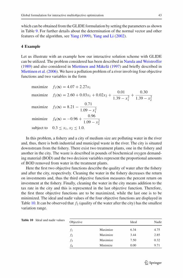
Let us illustrate with an example how our interactive solution scheme with GLIDEcan be utilized. The problem considered has been described in Narula and Weistroffer(1989) and also considered in Miettinen and Mäkelä (1997) and briefly described inMiettinen et al. (2006). We have a pollution problem of a river involving four objectivefunctions and two variables in the form

maximize f1(x) = 4.07 + 2.27x1

maximize f2(x) = 2.60 + 0.03x1 + 0.02x2 + 0.01

1.39 − x21

+ 0.30

1.39 − x22

maximize f3(x) = 8.21 − 0.71

1.09 − x21

minimize f4(x) = −0.96 + 0.96

1.09 − x22

subject to 0.3 ≤ x1, x2 ≤ 1.0.

In this problem, a fishery and a city of medium size are polluting water in the riverand, thus, there is both industrial and municipal waste in the river. The city is situateddownstream from the fishery. There exist two treatment plants, one in the fishery andanother in the city. The waste is described in pounds of biochemical oxygen demand-ing material (BOD) and the two decision variables represent the proportional amountsof BOD removed from water in the treatment plants.

Here the first two objective functions describe the quality of water after the fisheryand after the city, respectively. Cleaning the water in the fishery decreases the returnon investments and, thus the third objective function measures the percent return oninvestment at the fishery. Finally, cleaning the water in the city means addition to thetax rate in the city and this is represented in the last objective function. Therefore,the first three objective functions are to be maximized, while the last one is to beminimized. The ideal and nadir values of the four objective functions are displayed inTable 10. It can be observed that f2 (quality of the water after the city) has the smallestvariation range.

Table 10 Ideal and nadir valuesObjective Ideal Nadir

f1 Maximize 6.34 4.75

f2 Maximize 3.44 2.85

f3 Maximize 7.50 0.32

f4 Minimize 0.00 9.71

123

44 M. Luque et al.

Iteration 1. When we start solving the problem, let us assume that the DM wishesto get an overall picture of the problem with four different nondominated solutions.Therefore, the option ’just choose one among several solutions’ is used, and the fol-lowing nondominated solutions are obtained by solving the GLIDE problem (2) withthe parameters given in Table 5 (with four sets of random weights):

(5.56, 2.87, 7.13, 0.00), (6.00, 2.88, 6.27, 0.00),

(5.80, 3.02, 6.82, 0.95), (6.21, 3.15, 4.75, 2.00).

Among these solutions, the DM chooses the last one: (6.21, 3.15, 4.75, 2.00). Inrelative terms, here the value of f1 (water quality after the fishery) is the closest oneto its ideal value.

Iteration 2. Next, the DM wishes to give MRSs,4 taking f1 as the reference objec-tive. If this objective is relaxed by 0.1 units, the DM says that this is compensatedby an improvement of 0.3 units in f2, or an improvement of 0.1 units in f3, or animprovement of 0.05 units in f4. This implies that we can roughly speaking say thatthe DM regards f2 as (locally) less important than objective 1, objective 3 as (locally)equally important than objective 1, and f4 as (locally) more important than objectiveone. Therefore, problem (2) is solved using the parameters shown in Table 8 for fourstep sizes, and the following solutions are shown to the DM:

(6.21, 3.15, 4.75, 2.00), (6.18, 3.09, 5.05, 1.38)

(6.15, 3.03, 5.35, 0.87), (6.12, 2.95, 5.65, 0.39),

who chooses the second one: (6.18, 3.09, 5.05, 1.38).

As it can be seen, the environmental objectives f1 and f2 have experimented a lightdecrease, while the economical ones ( f3 and f4) have been improved.

Iteration 3. Let us now assume that the DM wishes to set very optimistic referencelevels for every objective, as follows:

qh1 = 6.2, qh

2 = 3.2, qh3 = 6.0, qh

4 = 1.0.

Therefore, the reference point option is selected, and the parameters for problem(2) are set as shown in Table 1. As a consequence, the following solution is obtained:(6.16, 3.14, 5.29, 1.97).

In this iteration, the quality of the water after the fishery ( f1) has slightly decreasedand the addition to the tax rate ( f4) has increased significantly. On the other hand,both the quality of the water after the city ( f2) and the return on investments ( f3) haveincreased.

Iteration 4. Now the DM wishes to improve the economical objectives at the price ofrelaxing a little bit in the environmental ones. Therefore, the DM sets the followingreference levels:

4 Note that for illustrative purposes we here use this option even though the problem does not satisfy theassumptions specified in Sect. 3.3.1.

123

Global formulation for interactive multiobjective optimization 45

Iteration 1

2,00

4,75

3,15

6,21

Objective 4

Objective 3

Objective 2

Objective 1

Iteration 2

6,18

3,09

5,05

1,38Objective 4

Objective 3

Objective 2

Objective 1

Iteration 3

6,16

3,14

5,29

1,97Objective 4

Objective 3

Objective 2

Objective 1

Iteration 4

1,10

6,28

3,05

6,00

Objective 4

Objective 3

Objective 2

Objective 1

Fig. 2 Graphical display of the four iterations

qh1 = 6.0, qh

2 = 3.0, qh3 = 6.0, qh

4 = 1.5.

In this case, the classification based option is chosen and problem (2) is solvedusing the parameters shown in Table 3. The solution obtained is the following one:(6.00, 3.05, 6.28, 1.10).

As it can be seen, the quality of the water after the fishery is at its reference leveland the quality of water after the city is slightly better than the reference level. Onthe other hand, the economical objectives have been improved beyond their referencelevels. Let us assume that the DM decides to stop with this solution, which implies toremove the 85.02% of the BOD at the treatment plant of the fishery, and the 79.01%of the BOD at the treatment plant of the city. A graphical representation of the fouriterations (with the solutions selected) can be seen in Fig. 2, where the bigger thehorizontal bars are, the better the value of the corresponding objective is.

Finally, it must be pointed out that the purpose of this example is to illustrate theperformance and flexibility of the global interactive solution scheme, and that is whyfour iterations have been carried out, all of them with different preference elicitationstyles. Obviously, the DM does not have to change the type of preference informationso often, but it is possible to ask for several solutions based on the information alreadyspecified and continue the solution process as long as desired.

5 Conclusions

In this paper, a global formulation which can accommodate several interactive mul-tiobjective optimization methods has been introduced. The compact structure of this

123

46 M. Luque et al.

formulation takes the form of a general optimization problem with a set of parametersthat have to be changed in order to obtain the different interactive methods supported.To be more specific, in this paper we show how the Reference Point, GUESS, NIM-BUS, STEM, STOM, Chebyshev, SPOT and PROJECT methods can be derived fromthis general formulation (besides, other interactive methods like Klamroth and Miet-tinen 2008 could also be considered by choosing the corresponding parameters).

It is clear that one of the main features that an interactive decision aid tool must havein order to successfully tackle real problems is flexibility. This flexibility is understoodas the ability of the system to adapt the solution process to the DM’s wishes allowingone to choose the most appropriate way of providing information any time duringthe process. To this end, it is necessary to implement different interactive techniqueswhich utilize different kinds of preference information. On the other hand, one ofthe weak points of the interactive multiobjective optimization field is the very limitednumber of practical and easy-to-use implementation.

We would like to emphasize the compactness of the formulation proposed, whichmakes it different from the other general counterparts previously published. TheGLIDE formulation has been designed with two main aims. First, providing a comfort-able decision aid environment for the DM, and second, aiding potential programmersto implement the interactive system.

From the point of view of the user, a general algorithm has been built where the DMonly has to decide what type of preference information (reference levels, choosing asolution among some efficient solutions or MRSs) to provide at each iteration. Thealgorithm chooses the corresponding method and produces the solution(s). Given thatmore than one interactive method of each class is supported by the global formulation,it is also possible to generate several different solutions with the same information ifthe DM so wishes.

From the point of view of the programmer, the global formulation is complementedwith tables with the values of the parameters of GLIDE for each of the methods consid-ered. This provides a simple implementation framework that makes it easier to createan interactive system based on the GLIDE formulation.

Finally, a simple hypothetical illustrative example has been used to show the per-formance of the global formulation and of the interactive solution scheme proposed.Although a preliminary implementation has been developed in order to test the algo-rithm and to solve the example, our future research trends include a more versatileimplementation of an interactive system based on GLIDE with a flexible and graphicaluser interface, and its application to real life problems.

Acknowledgments This research was partly supported by the Andalusian Regional Ministry of Inno-vation, Science and Enterprises (PAI group SEJ-445), the Spanish Ministry of Education and Science(MTM2006-01921) as well as Tekes, the Finnish Funding Agency for Technology and Innovation (theTechnology Programme for Modelling and Simulation).

References

Benayoun R, de Montgolfier J, Tergny J, Laritchev O (1971) Programming with multiple objective func-tions: step method (STEM). Math Program 1(3):366–375

123

Global formulation for interactive multiobjective optimization 47

Buchanan JT (1997) A naïve approach for solving MCDM problems: the GUESS method. J Oper Res Soc48(2):202–206

Caballero R, Luque M, Molina J, Ruiz F (2002) PROMOIN: an interactive system for multiobjective pro-gramming. Int J Inform Technol Decis Making 1:635–656

Chankong V, Haimes YY (1983) Multiobjective decision making: theory and methodology. North-Holland,New York

Eschenauer HA, Osyczka A, Schäfer E (1990) Interactive multicriteria optimization in design process. In:Eschenauer H, Koski J, Osyczka A (eds) Multicriteria design optimization procedures and applications.Springer, Berlin, pp 71–114

Gardiner L, Steuer RE (1994a) Unified interactive multiple objective programming. Eur J Oper Res74(3):391–406

Gardiner L, Steuer RE (1994b) Unified interactive multiple objective programming: an open architecturefor accommodating new procedures. J Oper Res Soc 45(12):1456–1466

Hwang CL, Masud ASM (1979) Multiple objective decision making—methods and applications: a state-of-the-art survey. Springer, Berlin

Jaszkiewicz A, Slowinski R (1999) The ‘light beam search’ approach—an overview of methodology andapplications. Eur J Oper Res 113:300–314

Kaliszewski I (2004) Out of the mist—towards decision-maker-friendly multiple criteria decision makingsupport. Eur J Oper Res 158:293–307

Klamroth K, Miettinen K (2008) Integrating approximation and interactive decision making in multicriteriaoptimization. Oper Res 56(1):222–234

Luque M, Caballero R, Molina J, Ruiz F (2007) Equivalent information for multiobjective interactive pro-cedures. Manage Sci 53(1):125–134

Luque M, Yang JB, Wong BYH (2008) PROJECT method for multiobjective optimisation based on gradientprojection and reference point. IEEE Trans Syst Man Cybern—Part A (to appear)

Luque M, Miettinen K, Eskelinen P, Ruiz F (2009) Incorporating preference information in interactivereference point methods for multiobjective optimization. Omega 37(2):450–462

Miettinen K (1999) Nonlinear multiobjective optimization. Kluwer, BostonMiettinen K (2006) IND-NIMBUS for demanding interactive multiobjective optimization. In: Trzaskalik

T (ed) Multiple Criteria Decision Making ’05. The Karol Adamiecki University of Economics inKatowice, Katowice, pp 137–150

Miettinen K, Mäkelä MM (1995) Interactive bundle-based method for nondifferentiable multiobjectiveoptimization: NIMBUS. Optimization 34(3):231–246

Miettinen K, Mäkelä MM (1997) Interactive method NIMBUS for nondifferentiable multiobjective opti-mization problems. In: Climaco J (ed) Multicriteria analysis. Springer, Berlin, pp 310–319

Miettinen K, Mäkelä MM (1999) Comparative evaluation of some interactive reference point-based meth-ods for multi-objective optimisation. J Oper Res Soc 50(9):949–959

Miettinen K, Mäkelä MM (2000) Interactive multiobjective optimization system WWW-NIMBUS on theInternet. Comput Oper Res 27(7–8):709–723

Miettinen K, Mäkelä MM (2002) On scalarizing functions in multiobjective optimization. OR Spectr24(2):193–213

Miettinen K, Mäkelä MM (2006) Synchronous approach in interactive multiobjective optimization. EurJ Oper Res 170(3):909–922

Miettinen K, Mäkelä MM, Kaario K (2006) Experiments with classification-based scalarizing functions ininteractive multiobjective optimization. Eur J Oper Res 175(2):931–947

Nakayama H, Sawaragi Y (1984) Satisficing trade-off method for multiobjective programming. In:Grauer M, Wierzbicki AP (eds) Interactive decision analysis. Springer, Berlin, pp 113–122

Narula SC, Weistroffer HR (1989) A flexible method for nonlinear multicriteria decisionmaking problems.IEEE Trans Syst Man Cybern 19(4):883–887

Romero C (2001) Extended lexicographic goal programming: a unified approach. Omega 29:63–71Sakawa M (1982) Interactive multiobjective decision making by the sequential proxy optimization tech-

nique: SPOT. Eur J Oper Res 9(4):386–396Sawaragi Y, Nakayama H, Tanino T (1985) Theory of multiobjective optimization. Academic Press,

OrlandoSteuer RE (1986) Multiple criteria optimization: theory, computation and applicationSteuer RE, Choo EU (1983) An interactive weighted Tchebycheff procedure for multiple objective pro-

gramming. Math Program 26:326–344

123

48 M. Luque et al.

Vassileva M, Miettinen K, Vassilev V (2005) Generalized scalarizing problem for multicriteria optimization.IIT Working Papers IIT/WP-205, Institute of Information Technologies, Bulgaria

Wierzbicki AP (1980) The use of reference objectives in multiobjective optimization. In: Fandel G, Gal T(eds) Multiple criteria decision making, theory and applications. Springer, Berlin, pp 468–486

Wierzbicki AP (1986) On the completeness and constructiveness of parametric characterizations to vectoroptimization problems. OR Spectr 8(2):73–87

Yang JB (1999) Gradient projection and local region search for multiobjective optimization. Eur J OperRes 112:432–459

Yang JB, Li D (2002) Normal vector identification and interactive tradeoff analysis using minimax formu-lation in multiobjective optimisation. IEEE Trans Syst Man Cybern A Syst Humans 32(3):305–319

123