SOFTWARE TESTING, VERIFICATION AND RELIABILITYSoftw. Test. Verif. Reliab. 0000; 00:1–34Published online in Wiley InterScience (www.interscience.wiley.com). DOI: 10.1002/stvr

Defect Prediction as a Multi-Objective Optimization Problem

Gerardo Canfora1, Andrea De Lucia2, Massimiliano Di Penta1, Rocco Oliveto3,Annibale Panichella∗4, Sebastiano Panichella5

1University of Sannio, Benevento, Italy2University of Salerno, Fisciano, Italy3University of Molise, Pesche (IS), Italy4Delft University of Technology, Delft, Netherlands5University of Zurich, Zurich, Switzerland

SUMMARY

In this paper we formalize the defect prediction problem as a multi-objective optimization problem.Specifically, we propose an approach, coined as MODEP (Multi-Objective DEfect Predictor), based onmulti-objective forms of machine learning techniques—logistic regression and decision trees specifically—trained using a genetic algorithm. The multi-objective approach allows software engineers to choosepredictors achieving a specific compromise between the number of likely defect-prone classes, or thenumber of defects that the analysis would likely discover (effectiveness), and LOC to be analyzed/tested(which can be considered as a proxy of the cost of code inspection). Results of an empirical evaluationon 10 datasets from the PROMISE repository indicate the quantitative superiority of MODEP with respectto single-objective predictors, and with respect to trivial baseline ranking classes by size in ascending ordescending order. Also, MODEP outperforms an alternative approach for cross-project prediction, based onlocal prediction upon clusters of similar classes.Copyright c© 0000 John Wiley & Sons, Ltd.

Received . . .

KEY WORDS: Defect prediction; multi-objective optimization; cost-effectiveness; cross-project defectprediction.

1. INTRODUCTION

Defect prediction models aim at identifying likely defect-prone software components to prioritize

Quality Assurance (QA) activities. The main reason why such models are required can be found in

the limited time or resources available that required QA teams to focus on subsets of software

entities only, trying to maximize the number of discovered defects. Existing defect prediction

models try to identify defect-prone artifacts based on product or process metrics. For example, Basili

et al. [1] and Gyimothy et al. [2] use Chidamber and Kemerer (CK) metrics [3] while Moser et al.

[4] use process metrics, e.g., number and kinds of changes occurred on software artifacts. Ostrand

et al. [5] and Kim et al. [6] perform prediction based on knowledge about previously occurred

faults. Also, Kim et al. [7] used their SZZ algorithm [8, 9] to identify fix-inducing changes and

characterized them aiming at using change-related features—e.g., change size, delta of cyclomatic

complexity—to predict whether a change induces or not a fault.

All these approaches, as pointed out by Nagappan et al. [10] and as it is true for any supervised

prediction approach, require the availability of enough data about defects occurred in the history of

a project. For this reason, such models are difficult to be applied on new projects for which limited

or no historical defect data is available. In order to overcome this limitation, several authors [11],

[12], [13], [14] have argued about the possibility of performing cross-project defect prediction, i.e.,

Copyright c© 0000 John Wiley & Sons, Ltd.

Prepared using stvrauth.cls [Version: 2010/05/13 v2.00]

using data from other projects to train machine learning models, and then perform a prediction on a

new project. However, Turhan et al. [11] and Zimmermann et al. [12] found that cross-project defect

prediction does not always work well. The reasons are mainly due to the projects’ heterogeneity,

in terms of domain, source code characteristics (e.g., classes of a project can be intrinsically larger

or more complex than those of another project), and process organization (e.g., one project exhibits

more frequent changes than another). Sometimes, such a heterogeneity can also be found within a

single, large project consisting of several, pretty different subsystems. A practical approach to deal

with heterogeneity—either for within-project prediction, or above all, for cross project prediction—

is to perform local prediction [13, 14] by (i) grouping together similar artifacts possibly belonging to

different projects according to a given similarity criteria, e.g., artifacts having a similar size, similar

metric profiles, or similar change frequency, and (ii) performing prediction within these groups.

In summary, traditional prediction models cannot be applied out-of-the-box for cross-project

prediction. However, a recent study by Rahman et al. [15] pointed out that cross-project defect

predictors do not necessarily work worse than within-project predictors. Instead, such models are

often quite good in terms of the cost-effectiveness. Specifically, they achieve a good compromise

between the number of defect-prone artifacts that the model predicts, and the amount of code—i.e.,

LOC of the artifact predicted as defect-prone—that a developer has to analyze/test to discover such

defects. Also, Harman [16] pointed out that when performing prediction models there are different,

potentially conflicting objectives to be pursued (e.g., prediction quality and cost).

Stemming from the considerations by Rahman et al. [15], who analyzed the cost-effectiveness

of a single objective prediction model, and from the seminal idea by Harman [16], we propose

to shift from the single-objective defect prediction model—which recommends a set or a ranked

list of likely defect-prone artifacts and tries to achieve an implicit compromise between cost and

effectiveness—towards multi-objective defect prediction models. We use a multi-objective Genetic

Algorithm (GA), and specifically the NSGA-II algorithm [17] to train machine learning predictors.

The GA evolves the coefficients of the predictor algorithm (in our case a logistic regression or a

decision tree, but the approach can be applied to other machine learning techniques) to build a set of

models (with different coefficients) each of which provide a specific (near) optimum compromise

between the two conflicting objectives of cost and effectiveness. In such a context, the cost is

represented by the cumulative LOC of the entities (classes in our study) that the approach predicts

as likely defect-prone. Such a size indicator (LOC) provides a proxy measure of the inspection

cost; however, without loss of generality, one can also model the testing cost considering other

aspects (such as cyclomatic complexity, number of method parameters, etc) instead of LOC. As

effectiveness measure, we use either (a) the proportion of actual defect-prone classes among the

predicted ones, or (b) the proportion of defects contained in the classes predicted as defect-prone

out of the total number of defects. In essence, instead of training a single model achieving an implicit

compromise between cost and effectiveness, we obtain a set of predictors, providing (near) optimum

performance in terms of cost-effectiveness. Therefore, for a given budget (i.e., LOC that can be

reviewed or tested with the available time/resources) the software engineer can choose a predictor

that (a) maximizes the number of defect-prone classes tested (which might be useful if one wants

to ensure that an adequate proportion of defect-prone classes has been tested), or (b) maximizes

the number of defects that can be discovered by the analysis/testing. Note that the latter objective is

different from the former because most of the defects can be in few classes. Also, we choose to adopt

a cost-effectiveness multi-objective predictor rather than a precision-recall multi-objective predictor

because—and in agreement with Rahman et al. [15]—we believe that cost is a more meaningful

(and of practical use) information to software engineers than precision.

The proposed approach, called MODEP (Multi-Objective DEfect Predictor), has been applied

on 10 projects from the PROMISE dataset∗. The results achieved show that (i) MODEP is more

effective than single-objective predictors in the context of a cross-project defect prediction, i.e., it

identifies a higher number of defects at the same level of inspection cost; (ii) MODEP provides

∗https://code.google.com/p/promisedata/

2

software engineers the ability to balance between different objectives; and (iii) finally, MODEP

outperforms a local prediction approach based on clustering proposed by Menzies et al. [13].

Structure of the paper. The rest of the paper is organized as follows. Section 2 discusses the

related literature, while Section 3 describes the multi-objective defect-prediction approach proposed

in this paper, detailing its implementation using both logistic regression and decision trees. Section 4

describes the empirical study we carried out to evaluate the proposed approach. Results are reported

and discussed in Section 5, while Section 6 discusses the threats to validity. Section 7 concludes the

paper and outlines directions for future work.

2. RELATED WORK

In the last decade, a substantial effort has been devoted to define approaches for defect prediction

that train the model using a within project training strategy. A complete survey on all these

approaches can be found in the paper by D’Ambros et al. [18], while in this section we focus

on approaches that predict defect prone classes using a cross-project training strategy.

The earliest works on such a topic provided empirical evidence that simply using projects in

the same domain does not help to build accurate prediction models [12, 19]. For this reason,

Zimmermann et al. [12] identified a series of factors that should be evaluated before selecting the

projects to be used for building cross-project predictors. However, even when using such guidelines,

the choice of the training set is not trivial, and there might be cases where projects from the same

domain are not available.

The main problem for performing cross-project defect prediction is in the heterogeneity of

data. Several approaches have been proposed in the literature to mitigate such a problem. Turhan

et al. [11] used nearest-neighbor filtering to fine tune cross-project defect prediction models.

Unfortunately, such a filtering only reduces the gap between the accuracy of within- and cross-

project defect prediction models. Cruz et al. [20] studied the application of data transformation for

building and using logistic regression models. They showed that simple log transformations can

be useful when measures are not as spread as those measures used in the construction. Nam et al.

[21] applied a data normalization (z-score normalization) for cross-project prediction in order to

reduce data coming from different projects to the same interval. This data pre-processing is also

used in this paper to reduce the heterogeneity of data. Turhan et al. [22] analyzed the effectiveness

of prediction models built on mixed data, i.e., within- and cross-project. Their results indicated

that there are some benefits when considering mixed data. Nevertheless, the accuracy achieved

considering project-specific data is greater than the accuracy obtained for cross-project prediction.

Menzies et al. [13] observed that prediction accuracy may not be generalizable within a project

itself. Specifically, data from a project may be crowded in local regions which, when considered at a

global level, may lead to different conclusions in terms of both quality control and effort estimation.

For this reason, they proposed a “local prediction” that could be applied to perform cross-project or

within-project defect prediction. In the cross-project defect prediction scenario, let us suppose we

have two projects, A and B, and suppose one wants to perform defect prediction in B based on data

available for A. First, the approach proposed by Menzies et al. [13] clusters together similar classes

(according to the set of identified predictors) into n clusters. Each cluster contains classes belonging

to A and classes belonging to B. Then, for each cluster, classes belonging to A are used to train the

prediction model, which is then used to predict defect-proneness of classes belonging to B. This

means that n different prediction models are built. The results of an empirical evaluation indicated

that conclusions derived from local models are typically superior and more insightful than those

derived from global models. The approach proposed by Menzies et al. [13] is used in our paper as

one of the experimental baselines.

A wider comparison of global and local models has been performed by Bettenburg et al. [14], who

compared (i) local models, (ii) global models, and (iii) global models accounting for data specificity.

Results of their study suggest that local models are valid only for specific subsets of data, whereas

global models provide trends that are too general to be used in the practice.

3

All these studies suggested that cross-project prediction is particularly challenging and, due to

the heterogeneity of projects, prediction accuracy might be poor in terms of precision, recall and F-

score. Rahman et al. [15] argued that while broadly applicable, such measures are not well-suited for

the quality-control settings in which defect prediction models are used. They showed that, instead,

the choice of prediction models should be based on both effectiveness (e.g., precision and recall)

and inspection cost, which they approximate in terms of number of source code lines that need to be

inspected to detect a given number/percentage of defects. By considering such factors, they found

that the accuracy of cross-project defect prediction are adequate, and comparable to within-project

prediction from a practical point of view.

Arisholm et al. [23] also suggested to measure the performance of prediction models in terms of

cost and effectiveness for within-project prediction. A good model is the one that identifies defect-

prone files with the best ratio between (i) effort spent to inspect such files, and (ii) number of

defects identified. Once again, the cost was approximated by the percentage of lines of code to

be inspected, while the effectiveness was measured as the percentage of defects found within the

inspected code. However, they used classical predicting models (classification tree, PART, Logistic

Regression, Back-propagation neural networks) to identify the defect-prone classes. Arisholm and

Briand [24] used traditional logistic regression with a variety of metrics (history data, structural

measures, etc.) to predict the defect-proneness of classes between subsequent versions of a Java

legacy system, and used the cost-effectiveness to measure the performance of the obtained logistic

models.

Our work is also inspired by previous work that use cost-effectiveness when performing a

prediction [15, 24, 23]. However, cost-effectiveness has been, so far, only used to assess the quality

of a predictor, and previous work still relies on single-objective predictors (such as the logistic

regression) which, by definition, find a model that minimizes the fitting error of precision and

recall, thus achieving a compromise between them. In this paper we introduce, for the first time, an

explicit multi-objective definition of the defect prediction problem, which produces a Pareto front

of (near) optimal prediction models—instead of a single model as done in the past—with different

effectiveness and cost values.

Harman [16] was the first to argue that search-based optimization techniques, and in particular

multi-objective optimization, can be potentially used to build predictive models where the user can

balance across multiple objectives, such as predictive quality, cost, privacy, readability, coverage

and weighting. At that time, Harman pointed out that the way how such multi-objective predictors

could be built remained an open problem. Our work specifically addresses this open problem, by

specifying a multi-objective prediction model based on logistic regression, and by using a GA to

train it.

Finally, this paper represents an extension of our previous conference paper [25], where we

introduced the multi-objective defect-prediction approach. The specific contributions of this paper as

compared to the conference paper can be summarized as follows: (i) we instanced MODEP by using

two different machine learning techniques, namely logistic regression and decision trees, while in

the conference paper, we only used logistic regression. In addition, we measure the effectiveness

through the proportion of (i) correctly predicted defect-prone classes and (ii) of defects in classes

predicted as defect-prone. In the conference paper, we only used as effectiveness measure the

proportion of correctly predicted defect-prone classes. The new measure was introduced to provide a

more accurate measure of effectiveness but also to provide evidence that the approach can be easily

extended by adding other goals; (ii) we evaluated MODEP on 10 projects from the PROMISE

dataset as done in the conference paper. However, we extended the quantitative analysis and we

also performed a qualitative analysis to better highlight the advantages of the multi-objective defect

prediction, i.e., its ability to show how different values of predictor variables lead towards a high

cost and effectiveness, and the capability the software engineer has to choose, from the provided

prediction models, the model that better suits her needs.

4

PastFaults

Bug Tracking System

Sourcecode

Versioning System

Compute Predictors (e.g., CK metrics)

Raw Data

Predict Fault Prone Components

Data Pre-processing

DataFault ProneComponents

Figure 1. The generic process for building defect prediction models.

3. MODEP: MULTI-OBJECTIVE DEFECT PREDICTOR

MODEP builds defect prediction models following the process described in Figure 1. First, a set

of predictors (e.g., product [1, 2] or process metrics [4]) is computed for each class of a software

project. The computed data is then preprocessed or normalized to reduce data heterogeneity. Such

preprocessing step is particularly useful when performing cross-project defect prediction, as data

from different projects—and in some cases in the same project—have different properties [13].

Once the data have been preprocessed, a machine learning technique is used to build a prediction

model. In this paper, we focus on logistic regression or decision trees. However, other techniques

can be applied without loss of generality.

3.1. Data Preprocessing

From a defect prediction point-of-view, software projects are often heterogeneous because they

exhibit different software metric distributions. For example, the average number of lines of code

(LOC) of classes, which is a widely used (and obvious) defect predictor variable, can be quite

different from a project to another. Hence, when evaluating prediction models on a software project

with a software metric distribution that is different with respect to the data distribution used to build

the models themselves, the prediction accuracy can be compromised [13].

In MODEP we perform a data standardization, i.e., we convert metrics into a z distribution aiming

at reducing the effect of heterogeneity between different projects. Specifically, given the value of

the metric mi computed on class cj of project P , denoted as mi(cj , P ), we convert it into:

mi(cj , P ) =mi(cj , P )− µ(mi, P )

σ(mi, P )(1)

In other words, we subtract from the value of the metric mi the mean value µ(mi, P ) obtained

across all classes of project P , and divide by the standard deviation σ(mi, S). Such a normalization

transforms the data belonging to different projects to fall within the same range, by measuring

the distance of a data point from the mean in terms of the standard deviation. The standardized

dataset has mean 0 and standard deviation 1, and it preserves the shape properties of the original

dataset (i.e., same skewness and kurtosis). Note that the application of data standardization is a

quite common practice when performing defect prediction [2, 21]. Specifically, Gyimothy et al. [2]

used such preprocessing to reduce CK metrics to the same interval before combining them (using

5

logistic regression) for within-project prediction, while Nam et al. [21] recently demonstrated that

the cross-project prediction accuracy can be better when the model is trained on normalized data.

Note that in the study described Section 4 we always apply data normalization, on both MODEP

and the alternative approaches, so that the normalization equally influences both approaches.

3.2. Multi-Objective Defect Prediction Models

Without loss of generality, a defect prediction model is a mathematical function/model F : Rn → R,

which takes as input a set of predictors and returns a scalar value that measures the likelihood that a

specific software entity is defect-prone. Specifically, a model F combines the predictors into some

classification/prediction rules through a set of scalar values A = a1, a2, . . . , ak. The number of

scalar values and the type of classification/prediction rules depend on the model/function F itself.

During the training process of the model F , an optimization algorithm is used to find the set of

values A = a1, a2, . . . , ak that provides the best prediction of the outcome. For example, when

using a linear regression technique, the predictors are combined through a linear combination, where

the scalar values A = a1, a2, . . . , ak are the linear combination coefficients.

Formally, given a set of classes C = c1, c2, . . . , cn and a specific machine learning model Fbased on a set of combination coefficients A = a1, a2, . . . , ak, the traditional defect prediction

problem consists of finding the set of coefficients A, within the space of all possible coefficients,

that minimizes the root-mean-square error (RMSE) [26]:

minRMSE =

√√√√n∑

i=1

(FA(ci)−DefectProne(ci))2 (2)

where FA(ci) and DefectProne(ci) range in 0; 1 and represent the predicted defect-proneness

and the actual defect-proneness of ci.In other words, such a problem corresponds to minimizing the number of defect-prone classes

erroneously classified as defect-free (false negatives), and minimizing the number of defect-free

classes classified as defect-prone ones (false positives) within the training set. Thus, optimizing

this objective function means maximizing both precision (no false positives) and recall (no false

negatives) of the prediction. Since the two contrasting goals (precision and recall) are treated using

only one function, an optimal solution for a given dataset represents an optimal compromise between

precision and recall.

However, focusing on precision and recall might be not enough for building an effective and

efficient prediction model. In fact, for the software engineer—who has to test/inspect the classes

classified as defect-prone—the prediction error does not provide any insights on the effort required

to analyze the identified defect-prone classes (that is a crucial aspect when prioritizing QA

activities). Indeed, larger classes might require more effort to detect defects than smaller ones,

because in the worst case the software engineer has to inspect the whole source code. Furthermore,

it would be more useful to analyze early classes having a high likelihood to be affected by more

defects. Unfortunately, all these aspects are not explicitly captured by traditional single-objective

formulation of the defect prediction problem.

For this reason, we suggest to shift from the single-objective formulation of defect prediction

towards a multi-objective one. The idea is to measure the goodness of a defect prediction model in

terms of cost and effectiveness, that, by definition, are two contrasting goals. More precisely, we

provide a new (multi-objective) formulation of the problem of creating defect prediction models.

Given a set of classes C = c1, c2, . . . , cn and given a specific machine learning model F based on

a set of combination coefficients A = a1, a2, . . . , ak, solving the defect prediction problem means

finding a set of values A = a1, a2, . . . , ak that (near) optimize the following objective functions:

max effectiveness(A) =

n∑

i=1

FA(ci) · DefectProne(ci)

min cost(A) =

n∑

i=1

FA(ci) · LOC(ci)

(3)

6

where FA(ci) and DefectProne(ci) range in 0; 1 and represent the predicted defect-proneness and

the actual defect-proneness of ci, respectively, while LOC(ci) measures the number of lines of code

of ci.In this formulation of the problem, we measure the effectiveness in terms of the number of actual

defect-prone classes predicted as such. However, defect-prone classes could have different density

of defects. In other words, there could be classes with only one defect and other classes with several

defects. Thus, could be worthwhile—at the same cost—to focus the attention on classes having

a high defect density. For this reason, we propose a second multi-objective formulation of the

problem. Given a set of classes C = c1, c2, . . . , cn and given a specific machine learning model

F based on a set of combination coefficients A = a1, a2, . . . , ak, solving the defect prediction

problem means finding a set of values A = a1, a2, . . . , ak that (near) optimizes the following

objective functions:

max effectiveness(A) =

n∑

i=1

FA(ci) · DefectNumber(ci)

min cost(A) =

n∑

i=1

FA(ci) · LOC(ci)

(4)

where DefectNumber(ci) denotes the actual number of defects in the class ci.In both formulations, cost and effectiveness are two conflicting objectives, because one cannot

increase the effectiveness (e.g., number of defect-prone classes correctly classified) without

increasing (worsening) the inspection cost†. As said in the introduction, we choose not to consider

precision and recall as the two contrasting objectives, because precision is less relevant than

inspection cost when choosing the most suitable predictor. Similarly, it does not make sense to build

models using cost and precision as objectives, because precision is related to the inspection cost,

i.e., a low precision would imply a high code inspection cost. However, as pointed out by Rahman

et al. [15], the size (LOC) of the software components to be inspected provides a better measure of

the cost required by the software engineer to inspect them with respect the simple number of classes

to be inspected (using the precision all classes have an inspection cost equals to 1).

Differently from single-objective problems, finding optimal solutions for problems with multiple

criteria requires trade-off analysis. Given the set of all possible coefficients, generally referred to as

feasible region, for a given prediction model FA, we are interested in finding the solutions that allows

to optimize the two objectives. Therefore, solving the multi-objective defect prediction problems

defined above requires to find the set of solutions which represent optimal compromises between

cost and effectiveness [27]. Hence, the goal becomes to find a multitude of optimal sets of decision

coefficients A, i.e., a set of optimal prediction models. For multi-objective problems, the concept

of optimality is based on two widely used notions of Pareto dominance and Pareto optimality (or

Pareto efficiency), coming from economics and having also a wide range of applications in game

theory and engineering [27]. Without loss of generality, the definition of Pareto dominance for

multi-objective defect prediction is the following:

Definition 1

A solution x dominates another solution y (also written x <p y) if and only if the values of the

objective functions satisfy the following conditions:

cost(x) ≤ cost(y) and effectiveness(x) > effectiveness(y)orcost(x) < cost(y) and effectiveness(x) ≥ effectiveness(y)

(5)

Conceptually, the definition above indicates that x is preferred to (dominates) y if and only if, at

the same level of effectiveness, x has a lower inspection cost than y. Alternatively, x is preferred

to (dominates) y if and only if, at the same level of inspection cost, x has a greater effectiveness

†In the ideal case the inspection cost is increased by the cost required to analyze the new classes classified as defect-prone.

7

0 50 100 150 200 2500

20

40

60

80

100

B

A

C

DE

Cost

Eff

ecti

ven

ess

(N.D

efec

ts)

Figure 2. Graphical interpretation of Pareto dominance.

than y. Figure 2 provides a graphical interpretation of Pareto dominance in terms of effectiveness

and inspection cost in the context of defect prediction. All solutions in the line-pattern rectangle (C,

D, E) are dominated by B, because B has both a lower inspection cost and a greater effectiveness,

i.e., it is better on both dimensions. All solutions in the gray rectangle (A and B) dominate solution

C. The solution A does not dominate the solution B because it allows to improve the effectiveness

(with respect to B) but at the same time it increases the inspection cost. Vice versa, the solution Bdoes not dominate the solution A because B is better in terms of inspection cost but it is also worsen

in terms of effectiveness. Thus, the solutions A and B are non-dominated by any other solution,

while the solutions C, D, and E are dominated by either A or B.

Among all possible solutions (coefficients A for defect prediction model FA) we are interested

in finding all the solutions that are not dominated by any other possible solution. This properties

corresponds to the concept of Pareto Optimality:

Definition 2

A solution x∗ is Pareto optimal (or Pareto efficient) if and only if it is not dominated by any other

solution in the space of all possible solutions Ω (feasible region), i.e., if and only if

∄ x 6= x∗ ∈ Ω : f(x) <p f(x∗) (6)

In others words, a solution x∗ is Pareto optimal if and only if no other solution x exists which

would improve effectiveness, without worsening the inspection cost, and vice versa. While single-

objective optimization problems have one solution only, solving a multi-objective problem may

lead to find a set of Pareto-optimal solutions which, when evaluated, correspond to trade-offs in

the objective space. All the solutions (i.e., decision vectors) that are not dominated by any other

decision vector are said to form a Pareto optimal set, while the corresponding objective vectors

(containing the values of two objective functions effectiveness and cost) are said to form a Pareto

front. Identifying a Pareto front is particularly useful because the software engineer can use the

front to make a well-informed decision that balances the trade-offs between the two objectives.

In other words, the software engineer can choose the solution with lower inspection cost or higher

effectiveness on the basis of the resources available for inspecting the predicted defect-prone classes.

The two multi-objective formulations of the defect prediction problem can be applied to any

machine learning technique, by identifying the Pareto optimal decision vectors that can be used to

combine the predictors in classification/prediction rules. In this paper we provide a multi-objective

formulation of logistic regression and decision trees. The details of both multi-objective logistic

regression and multi-objective decision tree are reported in Sections 3.2.1 and 3.2.2 respectively.

8

Once the two prediction models are reformulated as multi-objective problems, we use search-based

optimization techniques to solve them, i.e., to efficiently find Pareto Optimal solutions (coefficients).

Specifically, in this paper we use multi-objective GAs. Further details on multi-objective GAs and

how they are used to solve the multi-objective defect prediction problems are reported in section 3.3.

3.2.1. Multi-Objective Logistic Regression One of the widely used machine learning techniques

is the multivariate logistic regression [28]. In general, multivariate logistic regression is used for

modeling the relationship between a dichotomous predicted variable and one or more predictors

p1, p2, . . . , pm. Thus, it is suitable for defect-proneness prediction, because there are only two

possible outcomes: either the software entity is defect-prone or it is non defect-prone. In the context

of defect prediction, logistic regression has been applied by Gyimothy et al. [2] and by Nagappan et

al. [10], which related product metrics to class defect-proneness. It was also used by Zimmermann

et al. [12] in the first work on cross-project defect prediction.

Let C = c1, c2, . . . , cn be the set of classes in the training set and let P be the corresponding

class-by-predictor matrix, i.e., a m× n matrix, where m is the number of predictors and n is the

number of classes in the training set, while its generic entry pi,j denotes the value of the ith predictor

for the jth class. The mathematical function used for regression is called logit:

logit(cj) =eα+β1 pj,1+···+βm pj,m

1 + eα+β1 pj,1+···+βm pj,m(7)

where logit(cj) is the estimated probability that the jth class is defect-prone, while the scalars

(α, β1, . . . , βm) represent the linear combination coefficients for the predictors pj,1, . . . , pj,m. Using

the logit function, it is possible to define a defect prediction model as follows:

F (cj) =

1 if logit(cj) > 0.5;0 otherwise.

(8)

In the traditional single-objective formulation of the defect prediction problem, the predicted values

F (cj) are compared against the actual defect-proneness of the classes in the training set, in order to

find the set of decision scalars (α, β1, . . . , βn) minimizing the RMSE. The procedure used to find

such a set of decision scalars is the maximum likelihood [26] search algorithm, which estimates

the coefficients that maximize the likelihood of obtaining the observed outcome values, i.e., actual

defect-prone classes or number of defects. Once obtained the model, it can be used to predict the

defect-proneness of other classes.

The multi-objective logistic regression model can be obtained from the single-objective model,

by using the same logit function, but evaluating the quality of the obtained model by using (i) the

inspection cost, and (ii) the effectiveness of the prediction, that can be the number of defective

classes or defect density. In this way, given a solution A = (α, β1, . . . , βm) and the corresponding

prediction values F (cj) computed applying the equation 7, we can evaluate the Pareto optimality

of A using the cost and effectiveness functions (according to the equations 3 or the equations 4).

Finally, given this multi-objective formulation, it is possible to apply multi-objective GAs to find the

set of Pareto optimal defect prediction models which represents optimal compromises (trade-offs)

between the two objective functions. Once this set of solutions is available, the software engineer

can select the one that she considers the most appropriate and uses it to predict the defect-proneness

of other classes.

3.2.2. Multi-Objective Decision Trees Decision trees are also widely used for defect prediction and

they are generated according to a specific set of classification rules [12, 29]. A decision tree has,

clearly, a tree structure where the leaf nodes are the prediction outcomes (class defect-proneness in

our case), while the other nodes, often called as decision nodes, contain the decision rules. Each

decision rule is based on a predictor pi, and it partitions the decision in two branches according to

a specific decision coefficient ai. In other words, a decision tree can be viewed as a sequence of

questions, where each question depends on the previous questions. Hence, a decision corresponds

to a specific path on the tree. Figure 3 shows a typical example of decision tree used for defect

9

p1 < a1

yes no

1 p2 < a2

yes no

p1 < a3

yes no

0 1

p3 < a4

yes no

0 1

Figure 3. Decision tree for defect prediction.

prediction. Each decision node has the form if pi < ai, while each leaf node contains 1 (defective

class) or 0 (non defective class).

The process of building a decision tree consists of two main steps: (i) generating the structure

of the tree, and (ii) generating the decision rules for each decision node according to a given set

of decision coefficients A = a1, a2, . . . , ak. Several algorithms can be used to build the structure

of a decision tree [30] that can use a bottom-up or top-down approach. In this paper we use the

ID3 algorithm developed by Quinlan [31], which applies a top-down strategy with a greedy search

through the search space to derive the best structure of the tree. In particular, starting from the root

node, the ID3 algorithm uses the concepts of Information Entropy and Information Gain to assign

a given predictor pi to the current node‡, and then to split each node in two children, partitioning

the data in two subsets containing instances with similar predictors values. The process continues

iteratively until no further split affects the Information Entropy.

Once the structure of the tree is built, the problem of finding the best decision tree in the traditional

single-objective paradigm consists of finding for the all decision nodes the set of coefficients

A = a1, a2, . . . , ak which minimizes the root square prediction error. Similarly to the logistic

regression, we can shift from the single objective formulation towards a multi-objective one by

using the two-objective functions reported in equations 3 or 4. We propose to find a multiple sets

of decision coefficients A = a1, a2, . . . , an that (near) represent optimal compromises between

(i) the inspection cost, and (ii) the prediction effectiveness. Note that MODEP only acts on the

decision coefficients, while it uses a well-known algorithm, i.e., the ID3 algorithm, for building the

tree structure. This means that the set of decision trees on the Pareto front have all the same structure

but different decision coefficients.

3.3. Training the Multi-Objective Predictor using Genetic Algorithms

The problem of determining the coefficients for the logistic model or for the decision tree can be

seen as an optimization problem with two conflicting goals (i.e., fitness functions). In MODEP we

decided to solve such a problem using a multi-objective GA. The first step for the definition of a

GA is the solution representation. In MODEP, a solution (chromosome) is represented by a vector

of values. For the logistic regression, the chromosome contains the coefficients of the logit function.

Instead, the decision coefficients of the decision nodes are encoded in the chromosome in the case of

‡A predictor pi is assigned to a given node nj if and only if the predictor pi is the larger informational gain with respectto the other predictors.

10

Algorithm 1: NSGA-II

Input:Number of coefficients N for defect prediction modelPopulation size M

Result: A set of Pareto efficient solutions (coefficients for defect prediction model)1 begin2 t←− 0 // current generation3 Pt ←− RANDOM-POPULATION(N ,M )4 while not (end condition) do5 Qt ←−MAKE-NEW-POP(Pt)6 Rt ←− Pt

⋃Qt

7 F←− FAST-NONDOMINATED-SORT(Rt)8 Pt+1 ←− ∅9 i←− 1

10 while | Pt+1 | + | Fi |6 M do11 CROWDING-DISTANCE-ASSIGNMENT(Fi)12 Pt+1 ←− Pt+1

⋃Fi

13 i←− i+ 1

14 Sort(Fi) //according to the crowding distance15 Pt+1 ←− Pt+1

⋃Fi[1 : (M− | Pt+1 |)]

16 t←− t+ 1

17 S ←− Pt

decision trees. For example, a chromosome for the decision tree is A = a1, a2, a3, a4 (see Figure

3) which is the set of decision coefficients used to make a decision on each decision node.

Once the model coefficients are encoded as chromosomes, multi-objective GAs are used to

determine them. Several variants of multi-objective GA have been proposed, each of which differs

from the others on the basis of how the contrasting objective goals are combined for building the

selection algorithm. In this work we used NSGA-II, a popular multi-objective GA proposed by

Deb et al. [17]. As shown in Algorithm 1, NSGA-II starts with an initial set of random solutions

(random vectors of coefficients in our case) called population, obtained by randomly sampling the

search space (line 3 of Algorithm 1). Each individual (i.e., chromosome) of the population represents

a potential solution to the optimization problem. Then, the population is evolved towards better

solutions through subsequent iterations, called generations, to form new individuals by using genetic

operators. Specifically, to produce the next generation, NSGA-II first creates new individuals, called

offsprings, by merging the genes of two individuals in the current generation using a crossover

operator or modifying a solution using a mutation operator (function MAKE-NEW-POP [17], line

5 of Algorithm 1). A new population is generated using a selection operator, to select parents and

offspring according to the values of the objective functions. The process of selection is performed

using the fast non-dominated sorting algorithm and the concept of crowding distance. In line 7 of

Algorithm 1, the function FAST-NON-DOMINATED-SORT [17] assigns the non-dominated ranks

to individuals parents and offsprings. The loop between lines 10 and 14 adds as many individuals

as possible to the next generation, according to their non-dominance ranks. Specifically, at each

generation such an algorithm identifies all non-dominated solutions within the current population

and assigns to them the first non-dominance rank (rank = 1). Once this step is terminated, the

solutions with assigned ranks are removed from the assignment process. Then, the algorithm assigns

rank = 2 to all non-dominated solutions remaining in the pool. Subsequently, the process is iterated

until the pool of remaining solutions is empty, or equivalently until each solutions have an own non-

dominance rank. If the number of individuals in the next generation is smaller than the population

size M , then further individuals are selected according to the descending order of crowding distance

in lines 15–16. The crowding distance to each individual is computed as the sum of the distances

between such an individual and all the other individuals having the same Pareto dominance rank.

Hence, individuals having higher crowding distance are stated in less densely populated regions of

the search space. This mechanism is used to avoid the selection of individuals that are too similar to

each other.

11

The population evolves under specific selection rules by adapting itself to the objective functions

to be optimized. In general, after some generations the algorithm converges to the set of best

individuals, which hopefully represents an approximation of the Pareto front [27].

It is important to clarify that we apply NSGA-II to define decision/coefficient values based on data

belonging to the training set. After that, each Pareto-optimal solution can be used to build a model

(based on logistic regression or decision tree) for performing the prediction outside the training set.

4. DESIGN OF THE EMPIRICAL STUDY

This section describes the study we conducted to evaluate the proposed multi-objective formulation

of the defect prediction problem. The description follows a template originating from the Goal-

Question-Metric paradigm [32].

4.1. Definition and Context

The goal of the study is to evaluate MODEP, with the purpose of investigating the benefits

introduced by the proposed multi-objective model in a cross-project defect prediction context. The

reason why we focus on cross-project prediction is because (i) this is very useful when project

history data is missing and challenging at the same time [12]; and (ii) as pointed out by Rahman et

al. [15], cross-project prediction may turn out to be cost-effective while not exhibiting high precision

values.

The quality focus of the study is the capability of MODEP to highlight likely defect-prone classes

in a cost-effective way, i.e., recommending the QA team to perform a cost-effective inspection of

classes giving higher priority to classes that have a higher defect density and in general maximizing

the number of defects identified at a given cost. The perspective is of researchers aiming at

developing a better, cost-effective defect prediction model, also able to work well for cross-project

prediction, where the availability of project data does not allow a reliable within-project defect

prediction.

The context of our study consists of 10 Java projects having the availability of information about

defects. All of them come from the Promise repository§. A summary of the project characteristics

is reported in Table II. All the datasets report the actual defect-proneness of classes, plus a pool of

metrics used as predictors, i.e., LOC and the Chidamber & Kemerer metric suite [3]. Table I reports

the metrics (predictors) used in our study.

It is worth noting that, while in this paper we used only LOC and the CK metric suite, other

software metrics have been used in literature as predictors for building defect prediction models.

The choice of the CK suite is not random but it is guided by the wide use of such metrics to measure

the quality of Object-Oriented (OO) software systems. However, the purpose of this paper is not

to evaluate which is the best suite of predictors for defect prediction, but to show the benefits of

multi-objective approaches independently of the specific model the software engineer can adopt .

An extensive analysis of the different software metrics used as predictors can be found in the survey

by D’Ambros et al. [33].

4.2. Research Questions

In order to evaluate the benefits of MODEP we preliminarily formulate the following research

questions:

• RQ1: How does MODEP perform, compared to trivial prediction models and to an ideal

prediction model? This research question aims at evaluating the performances of MODEP

with respect to an ideal model that selects all faulty classes first (to maximize effectiveness)

and in increasing order of LOC (to minimize the cost). While we do not expect that MODEP

§https://code.google.com/p/promisedata/

12

Table I. Metrics used as predictors in our study.

Name Description

Lines of Code (LOC) Number of non-commented lines of code for

each software component (e.g., in a class)

Weighted Methods per Class (WMC) Number of methods contained in a class

including public, private and protected methods

Coupling Between Objects (CBO) Number of classes coupled to a given class

Depth of Inheritance (DIT) Maximum class inheritance depth for a given

class

Number Of Children (NOC) Number of classes inheriting from a given parent

class

Response For a Class (RFC) Number of methods that can be invoked for an

object of given class

Lack of Cohesion Among Methods (LCOM) Number of methods in a class that are not related

through the sharing of some of the class fields

Table II. Characteristics of the Java projects used in the study.

CharacteristicsSystem

Ant Camel Ivy jEdit Log4j Lucene Poi Prop Tomcat Xalan

Release 1.7 1.6 2.0 4.0 1.2 2.4 3.0 6.0 6.0 2.7Classes 745 965 352 306 205 340 442 661 858 910N. Defect. classes 166 188 40 75 189 203 281 66 77 898% Defect. classes 22% 19% 11% 25% 92% 60% 64% 10% 9% 99%

WMCmin 4 4 5 4 4 5 4 5 4 4mean 11 9 11 13 8 10 14 9 13 11max 120 166 157 407 105 166 134 40 252 138

DITmin 1 0 1 1 1 1 1 1 1 1mean 3 2 2 3 2 2 2 1 2 3max 7 6 8 7 5 6 5 6 3 8

NOCmin 0 0 0 0 0 0 0 0 0 0mean 1 1 0 0 0 1 1 0 0 1max 102 39 17 35 12 17 134 20 31 29

CBOmin 0 0 1 1 0 0 0 0 0 0mean 11 11 13 12 8 11 10 10 8 12max 499 448 150 184 65 128 214 76 109 172

RFCmin 0 0 1 1 0 1 0 1 0 0mean 34 21 34 38 25 25 30 24 33 29max 288 322 312 494 392 390 154 511 428 511

LCOMmin 0 0 0 0 0 0 0 0 0 0mean 89 79 132 197 54 69 100 42 176 126max 6,692 13,617 11,749 16,6336 4,900 6,747 7,059 492 29,258 8,413

LOCmin 4 4 5 5 5 5 4 5 4 4mean 280 117 249 473 186 303 293 148 350 471max 4,571 2,077 2,894 23,683 2,443 8,474 9,886 1,051 7,956 4,489

performs better than the ideal model, we want to know how much our approach is close

to it. In addition, as larger classes are more likely defect-prone, we compare MODEP with

a trivial model, ranking classes in decreasing order of LOC. Finally, we consider a further

trivial model ranking classes in increasing order of LOC, mimicking how developers could

(trivially) optimized their effort by testing/analyzing smaller classes first, in absence of any

other information obtained by means of predictor models. The comparison of MODEP with

13

these three models is useful to (ii) understand to what extent is MODEP able to approximate

an optimal model; and (i) investigate whether we really need a multi-objective predictor or

whether, instead, a simple ranking based on LOC would be enough to achieve the cost-benefit

tradeoff outlined by Rahman at al. [15].

After this preliminary investigation, we analyze the actual benefits of MODEP as compared

to other defect prediction approaches proposed in the literature. Specifically, we formulate the

following research questions:

• RQ2: How does MODEP perform compared to single-objective prediction? This research

question aims at evaluating, from a quantitative point of view, the benefits introduced by the

multi-objective definition of a cross-project defect prediction problem. We evaluate multi-

objective predictors based on logistic regression and decision trees. Also, we consider models

producing Pareto fronts of predictors (i) between LOC and number of predicted defect-prone

classes, and (ii) between LOC and number of predicted defects.

• RQ3: How does MODEP perform compared to the local prediction approach? This research

question aims at comparing the cross-project prediction capabilities of MODEP with those

of the approach—proposed by Menzies et al. [13]—that uses local prediction to mitigate the

heterogeneity of projects in the context of cross-project defect prediction. We consider such

an approach as a baseline for comparison because it is considered as the state-of-the-art for

cross-project defect prediction.

In addition, we provide qualitative insights about the practical usefulness of having Pareto fronts

of defect predictors instead of a single predictor. Also, we highlight how, for a given machine

learning model (e.g., logistic regression or decision trees) one can choose the appropriate rules

(on the various metrics) that leads towards a prediction achieving a given level of cost-effectiveness.

Finally, we report the time performance of MODEP, to provide figures about the time needed to

train predictors.

4.3. Variable Selection

Our evaluation studied the effect of the following independent variables:

• Machine learning algorithm: both single and multi-objective prediction are implemented

using logistic regression and decision trees. We used the logistic regression and the decision

tree implementations available in MATLAB [34]. The glmfit routine was used to train

the logistic regression model with binomial distribution and using the logit function as

generalized linear model, while for the decision tree model we used the classregtree class

to built decision trees.

• Objectives (MODEP vs. other predictors): the main goal of RQ2 is to compare single-

objective models with multi-objective predictors. The former are a traditional machine

learning models in which the model is built by fitting data in the training set. As explained

in Section 3.2, the latter are a set of Pareto-optimal predictors built by a multi-objective GA,

achieving different cost-effectiveness tradeoffs. In addition to that, we preliminarily (RQ1)

compare MODEP with two simple heuristics, i.e., ideal model and trivial model, aiming at

investigating whether we really need a multi-objective predictor.

• Training (within-project vs. cross-project prediction): we compare the prediction capability in

the context of within-project prediction with those of cross-project prediction. The conjecture

we want to test is wether the cross-project strategy is comparable/better than the within-project

strategy in terms of cost-effectiveness when using MODEP.

• Prediction (local vs. global): we consider—within RQ3–both local prediction (using the

clustering approach by Menzies et al. [13]) and global prediction.

In terms of dependent variables, we evaluated our models using (i) code inspection cost, measured

as the KLOC of the of classes predicted as defect-prone (as done by Rahman at al. [15]), and

(ii) recall, which provides a measure of the model effectiveness. In particular, we considered two

14

granularity levels for recall, by counting (i) the number of defect-prone classes correctly classified;

and (ii) the number of defects:

recallclass =

n∑

i=1

F (ci) · DefectProne(ci)

n∑

i=1

DefectProne(ci)

recalldefect =

n∑

i=1

F (ci) · DefectNumber(ci)

n∑

i=1

DefectNumber(ci)

where F (ci) denotes the predicted defect proneness of the class ci, DefectProne(ci) measures its

actual defect proneness and DefectNumber(ci) is the number of defects in ci. Hence, the recall

metric computed at class granularity level corresponds to the traditional recall metric which

measures the percentage of defect prone classes that are correctly classified as defect-prone or

defect-free. The recall metric computed at defect granularity level provides a weighted version

of recall where the weights are represented by the number of defects in the classes. That is, at the

same level of inspection cost, it would be more effective to inspect early classes having a higher

defect density, i.e., classes, that are affected by a higher number of defects.

During the analysis of the results, we also report precision to facilitate the comparison with other

models:

precision =

n∑

i=1

F (ci) · DefectProne(ci)

n∑

i=1

F (ci)

It is important to note that precision, recall and cost refer to defect-prone classes only. It is

advisable not to aggregate such values with those of defect-free classes and hence show overall

precision and recall values. This is because a model with a high overall precision (say 90%) when the

number of defect-prone classes is very limited (say 5%), performs worse than a constant classifier

(95% overall precision). Similar considerations apply when considering the cost instead of the

precision: a model with lower cost (lower number of KLOC to analyze), but with a limited number

of defect-prone classes might not be effective.

We use a cross-validation procedure [35] to compute precision, recall and inspection cost.

Specifically, for the within-project prediction, we used a 10-fold cross validation implemented in

MATLAB by the crossvalind routine, which randomly partitions a software project into 10 equal

size folds; we used 9 folds as training set and the 10th as test set. This procedure was performed 10

times, with each fold used exactly once as the test set. For the cross-project prediction, we applied a

similar procedure, removing each time a project from the set, training on 9 projects and predicting

on the 10th one.

4.4. Analysis Method

To address RQ1 we compare MODEL with an ideal model and two trivial models. For MODEP,

we report the performance of logistic regression and decision trees. Also, we analyze the two

multi-objective models separately, i.e., the one that considers as objectives cost and defect-prone

classes, and the one that consider cost and number of defect. In order to compare the experimented

predictors, we visually compare the Pareto fronts obtained with MODEP (more specifically, the line

obtained by computing the median over the Pareto fronts of 30 GA runs), and the cost-effectiveness

curve of the ideal and the two trivial models. The latter have been obtained by plotting n points in

the cost-effectiveness plane, where the generic ith point represents the cost-effectiveness obtained

considering the first i classes ranked by the model (ideal or trivial). In order to facilitate the

comparison across models, we report the Area Under the Curve (AUC) obtained by MODEP and the

two trivial models. An area of 1 represents a perfect cost-effective classifier, whereas for a random

classifier an area of 0.5 would be expected.

As for RQ2, we compare the performance of MODEP with those of the single objective (i) within

project (ii) and cross-project predictors. For both MODEP and the single objective predictors, we

15

report the performance of logistic regression and decision trees. Also, in this case we analyze the

two multi-objective models separately, i.e., the one that considers as objectives cost and defect-

prone classes, and the one that consider cost and number of defect. To compare the experimented

predictors, we first visually compare the Pareto fronts (more specifically, the line obtained by

computing the median over the Pareto fronts of 30 GA runs) and the performance (a single dot

in the cost-effectiveness plane) of the single-objective predictors. Then, we compare the recall and

precision of MODEP and single-objective predictors at the same level of inspection cost. Finally,

by using the precision and recall values over the 10 projects, we also statistically compare MODEP

with the single objective models using the two-tailed Wilcoxon paired test [36] to determine whether

the following null hypotheses could be rejected:

• H0R : there is no significant difference between the recall of MODEP and the recall of the

single-objective predictor.

• H0P : there is no significant difference between the precision of MODEP and the precision of

the single-objective predictor.

Note that the comparison is made by considering both MODEP and the single-objective predictor

implemented with logistic regression and decision tree, and with the two different kinds of recall

measures (based on the proportion of defect-prone classes and of defects). In addition, we use

the Wilcoxon test, because it is non-parametric and does not require any assumption upon the

underlying data distribution; also, we perform a two-tailed test because we do not know a priori

whether the difference is in favor of MODEP or of the single-objective models. For all tests we

assume a significance level α = 0.05, i.e., 5% of probability of rejecting the null hypothesis when it

should not be rejected.

Turning to RQ3, we compare MODEP with the local prediction approach proposed by Menzies

et al. [13]. In the following, we briefly explain our re-implementation of the local prediction

approach using the MATLAB environment [34] and, specifically, the RWeka and cluster packages.

The prediction process consists of three steps:

1. Data preprocessing: we preprocess the data set as described in Section 3.1.

2. Data clustering: we cluster together classes having similar characteristics (corresponding

to the WHERE heuristic by Menzies et al. [13]). We use a traditional multidimensional

scaling algorithm (MDS)¶ to cluster the data based on the Euclidean distance to compute

the dissimilarities between classes. We use its implementation available in MATLAB with the

mdscale routine and setting as number of iterations it =√n, where n is the number of classes

in the training set (such a parameter is the same used by Menzies et al. [13]). As demonstrated

by Yang et al. [37] such an algorithm is exactly equivalent to the FASTMAP algorithm

used by Menzies et al. [13], except for the computation cost. FASTMAP approximates the

classical MDS by solving the problem for a subset of the data set, and by fitting the remainder

solutions [37]. A critical factor in the local prediction approach is represented by the number

of clusters k to be considered. To determine the number of clusters, we used an approach

based on the Silhouette coefficient [38]. The Silhouette coefficient ranges between -1 and 1,

and measures the quality of a clustering. A high Silhouette coefficient means that the average

cluster cohesion is high, and that clusters are well separated. Clearly, if we vary the number

of considered clusters (k) for the same clustering algorithm, we obtain different Silhouette

Coefficient values, since this leads to a different assignment of classes to the extracted clusters.

Thus, in order to determine the number of clusters, we computed the Silhouette coefficients

for all the different clusterings obtained by FASTMAP when varying the number of clusters kfrom 1 to the number of classes contained in each dataset, and we considered the k value that

resulted in the maximum for the Silhouette coefficient value. In our study we found a number

of clusters k =10 to be optimal.

¶Specifically we used a metric-based multidimensional scaling algorithm, where the metric used is the Euclidean distancein the space of predictors.

16

3. Local prediction: finally, we perform a local prediction within each cluster identified using

MDS. Basically, for each cluster obtained in the previous step, we use classes from n− 1projects to train the model, and then we predict defects for classes of the remaining project. We

use an association rule learner to generate a predicting model according to the cluster-based

cross-project strategy (WHICH heuristic by Menzies et al. [13]). We used a MATLAB’s tool,

called ARMADA‖, which provides a set of routines for generating and managing association

rule discovery.

4.5. Implementation and Settings of the Genetic Algorithm

MODEP has been implemented using MATLAB Global Optimization Toolbox (release R2011b).

In particular, the gamultiobj routine was used to run the NSGA-II algorithm, while the routine

gaoptimset was used to set the GA parameters. We used the GA configuration typically used for

numerical problems [27]:

• Population size: we choose a moderate population size with p = 200.

• Initial population: for each software system the initial population is uniformly and randomly

generated within the solutions space. Since such a problem in unconstrained, i.e., there are

no upper and lower bounds for the values that the coefficients can assume, we consider as

feasible solutions all the solutions ranging within the interval [−10,000; 10,000], while the

initial population was randomly and uniformly generated in the interval [−10; 10].• Number of generations: we set the maximum number of generation equal to 400.

• Crossover function: we use arithmetic crossover with probability pc = 0.60. This operator

combines two selected parent chromosomes to produce two new offsprings by linear

combination. Formally, given two parents x = (x1, . . . , xn) and y = (y1, . . . , yn), the

arithmetic crossover generates two offsprings z and w as follows: zi = xi · p+ yi · (1− p)and wi = xi · (1− p) + yi · p, where p is a random number generated within the interval [0; 1].Graphically, the two generated offsprings lie on the line segment connecting the two parents.

• Mutation function: we use a uniform mutation function with probability pm = 1/n where

n is the size of the chromosomes (solutions representation). The uniform mutation randomly

changes the values of each individual with small probability pm, replacing an element (real

value) of the chromosome with another real value of the feasible region, i.e. within the

interval [−10,000; 10,000]. Formally, given a solution x = (x1, . . . , xn) with lower bound

xmin = −10,000 and upper bound xmax =10,000. The uniform mutation will change with

small probability pm a generic element xi of x as follows: xi = ximin+ p · (ximax

− ximin),

where p is a random number generated within the interval [0; 1].• Stopping criterion: if the average Pareto spread is lower than 10−8 in the subsequent 50

generations, then the execution of the GA is stopped. The average Pareto spread measures

the average distance between individuals of two subsequent Pareto fronts, i.e., obtained from

two subsequent generations. Thus, the average Pareto spread is used to measure whether the

obtained Pareto front does not change across generations (i.e., whether NSGA-II converged).

The algorithm has been executed 30 times on each object program to account the inherent

randomness of GAs [39]. Then, we select a Pareto front composed of points achieving the median

performance across the 30 runs.

4.6. Replication Package

The replication package of our study is publicly available∗∗. In the replication package we provide:

• the script for running MODEP on a specific dataset;

• the datasets used in our experimentation; and

• the raw data for all the experimented predictors.

‖http://www.mathworks.com/matlabcentral/fileexchange/3016-armada-data-mining-tool-version-1-4∗∗http://distat.unimol.it/reports/MODEP

17

5. STUDY RESULTS

This section discusses the results of our study aimed at answering the research questions formulated

in Section 4.2.

5.1. RQ1: How does MODEP perform, compared to trivial prediction models and to an ideal

prediction model?

As planned, we preliminarily compare MODEP with an ideal model and two trivial models that

select the classes in increasing and decreasing order of LOC respectively. This analysis is required

(i) to understand whether we really need a multi-objective predictor or, to achieve the cost-benefit

tradeoff outlined by Rahman at al. [15], a simple ranking would be enough; and (ii) to analyze to

what extent MODEP is able to approximate the optimal cost-effectiveness predictor.

Figure 4 compares MODEP with the ideal model and the two trivial models when optimizing

inspection cost and number of defect-prone classes. TrivialInc. and TrivialDec. denote the trivial

models ranking classes in increasing and decreasing order of LOC, respectively. As we can see, in

5 cases (JEdit, Log4j, Lucene, Xalan, Poi) out of 10, MODEP reaches a cost-effectiveness that is

very close to the cost-effectiveness of the ideal model, confirming the usefulness of the proposed

approach. Also, as expected, in all cases MODEP outperforms the trivial model TrivialDec.. This

result is particular evident for Tomcat, Xalan, Lucene and Log4j. MODEP solutions also generally

dominate the solutions provided by the trivial model TrivialInc.. However, MODEP is not able to

overcome TrivialInc. on Xalan and Log4j, where the results obtained by MODEP and the trivial

model are substantially the same. This means that for projects like Log4j and Xalan where the

majority of classes are defect-prone (92% and 99% respectively) the trivial model TrivialInc.provides results that are very close to those achieved by MODEP and by the ideal model. These

findings are also confirmed by the quantitative analysis reported in Tables III and IV. Indeed, on 8

out of 10 projects, the AUC values achieved by MODEP are better (higher) than the AUC values

of the trivial models. In such cases the improvement achieved by MODEP with respect to the two

trivial models varies between 10% and 36%. This result suggests that the use of trivial models based

only on LOC is not sufficient to build a cost-effectiveness prediction model.

Similar results are also obtained when comparing MODEP with the ideal and trivial models when

optimizing inspection cost and number of defects. Specifically, MODEP always outperforms the

trivial models and, in some cases (on three projects, Log4j, Lucene, Xalan), it is able to reach a

cost-effectiveness very close to the cost-effectiveness of the ideal model.

In conclusion, we can claim that MODEP can be particularly suited for cross-project defect

prediction, since it is able to achieve in several cases a cost-effectiveness very close to the optimum.

As expected, MODEP also outperforms two trivial models that just rank classes in decreasing or

increasing order of LOC. Finally, the results are pretty consistent across most of the studied projects

(except Log4j and Xalan). This means that a developer can rely in MODEP since it seems to be

independent of the specific characteristics of a given project (in terms of predictors and number of

defects).

5.2. RQ2: How does MODEP perform compared to single-objective prediction?

In this section we compare MODEP with a single-objective defect predictor. We first discuss the

results achieved when using as objective functions inspection cost and number of defect-prone

classes classified as such. Then, we discuss the results achieved when considering as objective

functions inspection cost and number of defects (over the total number of defects) contained in the

defect-prone classes classified as such.

5.2.1. MODEP based on inspection cost and defect-prone classes. Figure 6 shows the Pareto fronts

achieved by MODEP (using logistic regression and decision trees), when predicting defect-prone

classes—and optimizing the inspection cost and the number of defect-prone classes identified—

on each of the 10 projects after training the model on the remaining 9. The plots also show, as

single points: (i) the single-objective cross-project logistic regression and decision tree predictors

18

0 50 100 150 200

0

20

40

60

80

100

KLOC

%D

efec

t-p

ron

eC

lass

es

(a) Ant

0 50 100

0

20

40

60

80

100

KLOC

%D

efec

t-p

ron

eC

lass

es

(b) Camel

0 20 40 60 80

0

20

40

60

80

100

KLOC

%D

efec

t-p

ron

eC

lass

es

(c) Ivy

0 50 100

0

20

40

60

80

100

KLOC

%D

efec

t-p

ron

eC

lass

es

(d) JEdit

0 10 20 30 40

0

20

40

60

80

100

KLOC

%D

efec

t-p

ron

eC

lass

es

(e) Log4j

0 50 100

0

20

40

60

80

100

KLOC

%D

efec

t-p

ron

eC

lass

es

(f) Lucene

0 50 100

0

20

40

60

80

100

KLOC

%D

efec

t-p

ron

eC

lass

es

(g) Poi

0 20 40 60 80 100

0

20

40

60

80

100

KLOC

%D

efec

t-p

ron

eC

lass

es

(h) Prop

0 100 200 300

0

20

40

60

80

100

KLOC

%D

efec

t-p

ron

eC

lass

es

(i) Tomcat

0 200 400

0

20

40

60

80

100

KLOC

%D

efec

t-p

ron

eC

lass

es Multi-Objective Logistic

Trivial Inc.

Multi-Objective DTree

Trivial Dec.

Ideal

(j) Xalan

Figure 4. Comparison of MODEP with an ideal and trivial models when optimizing inspection cost andnumber of defect-prone classes.

19

0 50 100 150 200

0

20

40

60

80

100

KLOC

%D

efec

ts

(a) Ant

0 50 1000

20

40

60

80

100

KLOC

%D

efec

ts

(b) Camel

0 20 40 60 800

20

40

60

80

100

KLOC

%D

efec

ts

(c) Ivy

0 50 1000

20

40

60

80

100

KLOC

%D

efec

tsC

lass

es

(d) JEdit

0 10 20 30 400

20

40

60

80

100

KLOC

%D

efec

ts

(e) Log4j

0 50 1000

20

40

60

80

100

KLOC

%D

efec

ts(f) Lucene

0 50 1000

20

40

60

80

100

KLOC

%D

efec

ts

(g) Poi

0 20 40 60 80 1000

20

40

60

80

100

KLOC

%D

efec

ts

(h) Prop

0 100 200 3000

20

40

60

80

100

KLOC

%D

efec

ts

(i) Tomcat

0 200 4000

20

40

60

80

100

KLOC

%D

efec

ts

Multi-Objective Logistic

Trivial Inc.

Multi-Objective DTree

Trivial Dec.

Ideal

(j) Xalan

Figure 5. Comparison with trivial models when optimizing inspection cost and number of defects.

20

Table III. AUC values achieved when comparing MODEP (using logistic regression and decision trees) andTrivial models when considering as objective functions inspection cost and number of defect-prone classes.

System MODEP-Logistic MODEP-DTree TrivialInc. TrivialDec.

Ant 0.71 0.71 0.64 0.54Camel 0.85 0.85 0.74 0.35Ivy 0.70 0.70 0.60 0.49jEdit 0.87 0.86 0.76 0.38Log4j 0.97 0.97 0.97 0.27Lucene 0.93 0.93 0.85 0.29Poi 0.97 0.96 0.88 0.40Prop 0.69 0.68 0.56 0.50Tomcat 0.68 0.68 0.60 0.47Xalan 0.99 0.99 0.99 0.19

Table IV. AUC values achieved when comparing MODEP (using logistic regression and decision trees) andTrivial models when considering as objective functions inspection cost and number of defects.

System MODEP-Logistic MODEP-DTree TrivialInc. TrivialDec.

Ant 0.78 0.79 0.65 0.68Camel 0.69 0.70 0.61 0.49Ivy 0.70 0.72 0.57 0.59jEdit 0.83 0.79 0.53 0.58Log4j 0.95 0.95 0.94 0.30Lucene 0.88 0.86 0.78 0.41Poi 0.84 0.83 0.74 0.49Prop 0.68 0.68 0.58 0.48Tomcat 0.67 0.67 0.57 0.56Xalan 0.99 0.99 0.99 0.26

(as a black triangle for logistic regression, and gray triangle for decision trees); and (ii) the single-

objective within-project for logistic and decision tree predictors (a black square for the logistic and

a gray square for the decision tree), where the prediction has been performed using 10-fold cross-

validation within the same project.

A preliminary analysis indicates that, generally, the solutions (sets of predictors) provided by

MODEP (based on logistic regression or decision tree) dominate the solutions provided by both

cross- and within-project single objective models. This means that the Pareto-optimal predictors

provided by MODEP are able to predict a larger number of defect-prone classes with a lower

inspection cost. Only in one case MODEP is not able to overcome the single-objective predictors.

Specifically, for Tomcat the single-objective solutions (both cross- and within- project) are quite

close to the Pareto fronts provided by MODEP based on decision trees.

In order to provide a deeper comparison of the different prediction models, Table V compares the

performances of MODEP with those of the cross project single-objective predictors (both logistic

and decision tree predictors) in terms of precision and recallclass. Specifically, the table reports

the recallclass and the precision of the two models for the same level of inspection cost. Results

indicate that the logistic model MODEP always achieves better recallclass levels. In particular, for

6 systems (Ant, Camel, Log4j, Lucene, Poi, and Prop) the recallclass is greater (of at least 10%) than

the recallclass of the single-objective predictors. However, the precision generally decreases, even

if in several cases the decrement is negligible. The same considerations also apply when MODEP

uses decision trees.

We also compare MODEP with the single-objective predictors trained using a within-project

strategy. This analysis is necessary to analyze to what extent MODEP trained with a cross-

project strategy is comparable/better than single-objective predictors trained with a within-project

strategy in terms of cost-effectiveness. Table V reports the achieved results in terms of precisionand recallclass for the same level of inspection cost. Not surprisingly, the within-project logistic

predictor achieves a better precision, for 8 out of 10 projects (Ant, Camel, Ivy, jEdit, Lucene, Poi,

Prop, and Tomcat). Instead, the precision is the same for both logistic-based models for Log4j, and

21

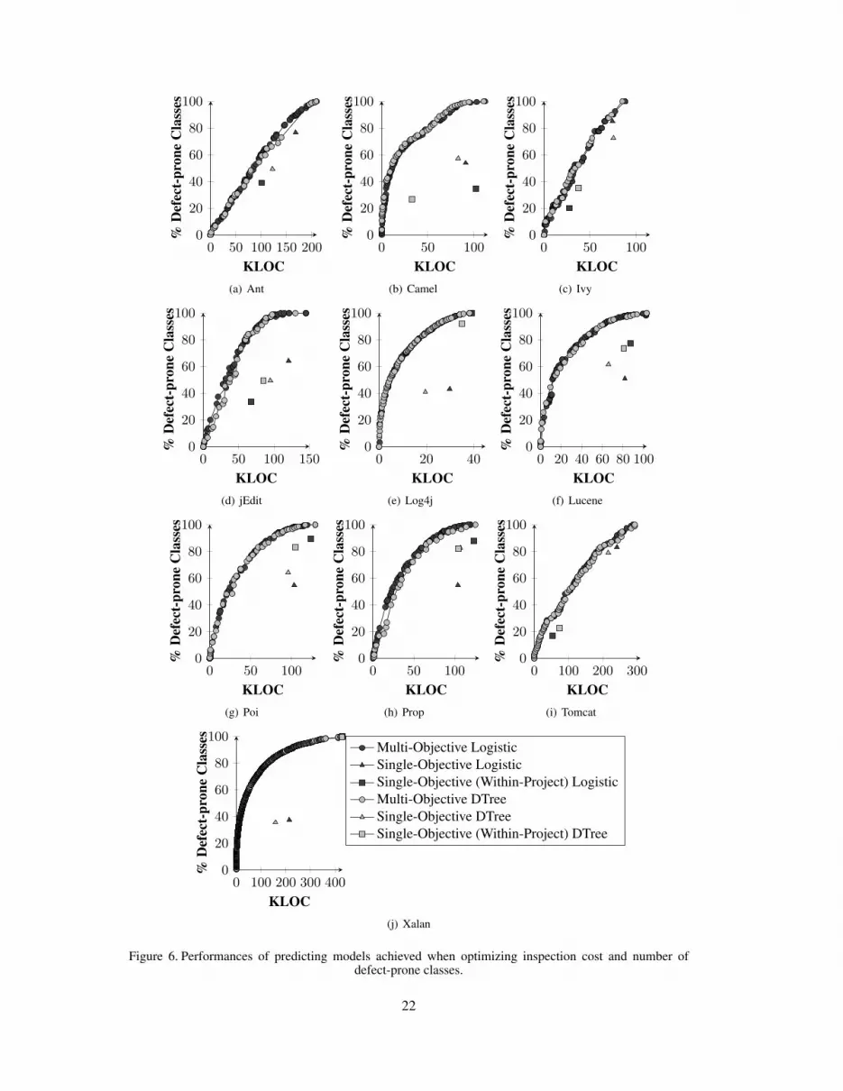
0 50 100 150 2000

20

40

60

80

100

KLOC

%D

efec

t-p

ron

eC

lass

es

(a) Ant

0 50 1000

20

40

60

80

100

KLOC

%D

efec

t-p

ron

eC

lass

es

(b) Camel

0 50 1000

20

40

60

80

100

KLOC

%D

efec

t-p

ron

eC

lass

es

(c) Ivy

0 50 100 1500

20

40

60

80

100

KLOC

%D

efec

t-p

ron

eC

lass

es

(d) jEdit

0 20 400

20

40

60

80

100

KLOC

%D

efec

t-p

ron

eC

lass

es

(e) Log4j

0 20 40 60 80 1000

20

40

60

80

100

KLOC

%D

efec

t-p

ron

eC

lass

es(f) Lucene

0 50 1000

20

40

60

80

100

KLOC

%D

efec

t-p

ron

eC

lass

es

(g) Poi

0 50 1000

20

40

60

80

100

KLOC

%D

efec

t-p

ron

eC

lass

es

(h) Prop

0 100 200 3000

20

40

60

80

100

KLOC

%D

efec

t-p

ron

eC

lass

es

(i) Tomcat

0 100 200 300 4000

20

40

60

80

100

KLOC

%D

efec

t-p

ron

eC

lass

es

Multi-Objective Logistic

Single-Objective Logistic

Single-Objective (Within-Project) Logistic

Multi-Objective DTree

Single-Objective DTree

Single-Objective (Within-Project) DTree

(j) Xalan

Figure 6. Performances of predicting models achieved when optimizing inspection cost and number ofdefect-prone classes.

22

Table V. MODEP vs. single-objective predictors when optimizing inspection cost and number of defect-prone classes identified. Single-objective predictors are also applied using a within-project training strategy.

System MetricLogistic Dtree Logistic Dtree

SO-C MO Diff SO-C MO Diff SO-W MO Diff SO-W MO Diff

Ant

Cost 167 167 - 121 121 - 101 101 - 104 104 -

Recallclass 0.77 0.90 +0.13 0.49 0.68 +0.19 0.39 0.60 +0.21 0.43 0.60 +0.17

precision 0.43 0.21 -0.22 0.50 0.17 -0.33 0.68 0.52 -0.16 0.35 0.15 -0.20

Camel

Cost 93 93 - 83 83 - 13 13 - 33 33 -

Recallclass 0.54 0.94 +0.40 0.57 0.90 +0.33 0.09 0.36 +0.25 0.25 0.59 +0.24

precision 0.26 0.19 -0.07 0.37 0.19 -0.18 0.54 0.14 -0.30 0.33 0.16 - 0.17

Ivy

Cost 74 74 - 75 75 - 28 28 - 38 38 -

Recallclass 0.83 0.90 +0.07 0.72 0.90 +0.18 0.25 0.40 +0.15 0.35 0.52 +0.17

precision 0.27 0.11 -0.16 0.22 0.21 -0.01 0.50 0.06 -0.44 0.37 0.07 -0.30

jEdit

Cost 121 121 - 95 95 - 66 66 - 85 85 -

Recallclass 0.64 1.00 - 0.49 0.97 +0.38 0.33 0.84 +0.51 0.49 0.91 +0.42

precision 0.42 0.25 -0.19 0.66 0.24 -0.42 0.66 0.22 -0.44 0.50 0.23 -0.27

Log4j

Cost 30 30 - 20 20 - 38 38 - 35 35 -

Recallclass 0.42 0.96 +0.54 0.41 0.85 +0.44 0.99 0.99 - 0.92 0.99 +0.07

precision 0.94 0.92 -0.02 0.93 0.92 -0.01 0.92 0.92 - 0.93 0.92 -0.01

Lucene

Cost 83 83 - 66 66 - 86 86 - 81 81 -

Recallclass 0.53 0.97 +0.44 0.62 0.94 32 0.77 0.99 +0.22 0.73 0.95 +0.13

precision 0.80 0.59 -0.21 0.63 0.59 -0.04 0.74 0.60 -0.14 0.74 0.59 -0.15

Poi

Cost 102 102 - 96 96 - 120 120 - 104 104 -

Recallclass 0.53 0.98 +0.45 0.64 0.96 +0.32 0.90 1.00 +0.10 0.83 0.96 +0.13

precision 0.87 0.63 -0.24 0.73 0.63 -0.10 0.79 0.64 -0.15 0.81 0.64 -0.23

Prop

Cost 76 76 - 107 107 - 74 74 - 104 104 -

Recallclass 0.69 0.91 +0.22 0.83 0.97 +0.14 0.87 0.90 +0.03 0.82 0.95 +0.13

precision 0.67 0.62 -0.05 0.81 0.63 -0.18 0.77 0.61 -0.16 0.83 0.63 -0.20

Tomcat

Cost 214 214 - 241 241 - 64 64 - 54 54 -

Recallclass 0.82 0.86 +0.04 0.84 0.87 +0.03 0.18 0.33 +0.15 0.18 0.32 +0.14

precision 0.21 0.08 -0.13 0.22 0.08 -0.14 0.58 0.04 -0.53 0.59 0.59 -

Xalan

Cost 285 285 - 158 158 - 429 429 - 428 428 -

Recallclass 0.38 0.95 - 0.36 0.81 +0.45 6 1.00 1.00 - 0.99 1.00 +0.01

precision 1 0.99 -0.01 0.99 0.98 -0.01 0.99 0.99 - 0.99 0.99 -

SO-C: Single-Objective Cross-project; SO-W: Single-Objective Within-project; MO: Multi-Objective

Xalan. Similarly, the within-project decision tree predictor achieves a better precision, for 8 out of

10 projects. However, the difference between the precision values achieved by MODEP and the

single-objective predictor are lower then 5% on 3 projects. Thus, the within-project single-project

predictors achieve—for both logistic and decision tree—better precision than MODEP trained with

a cross-project strategy. These results are consistent with those of a previous study [12], and show

that, in general, within-project prediction outperforms cross-project prediction (and when this does

not happen, performances are very similar). However, although the precision decreases, MODEP is

able to generally achieve higher recallclass values using both the machine learning algorithms. This

means that—for the same cost (KLOC)—the software engineer has to analyze more false positives,

but she is also able to identify more defect-prone classes.

Let us now deeply discuss some specific cases among the projects we studied. For some of them—

such as Ivy or Tomcat—a cross-project single-objective logistic regression reaches a high recall and

a low precision, whereas for others—such as Log4j or Xalan—it yields a relatively low recall and a

high precision. Instead, MODEP allows the software engineer to understand, based on the amount

of code she can analyze, what would be the estimated level of recall—i.e., the percentage of defect-

prone classes identified—that can be achieved, and therefore to select the most suitable predictors.

For example, for Xalan, achieving an (estimated) recall of 80% instead of 38% would require the

analysis of about 132 KLOC instead of 13 KLOC (see Figure 6-j). In this case, the higher additional

cost can be explained because most of the Xalan classes are defect-prone; therefore achieving a

good recall means analyzing most of the system, if not the entire system. Let us suppose, instead,

to have only a limited time available to perform code inspection. For Ivy, as indicated by the multi-

objective decision tree predictor, we could choose to decrease the inspection cost from 32 KLOC to

15 KLOC if we accept a recall of 50% instead of 83% (see Figure 6-c). It is important to point out

that the recall value provided by the multi-objective model is an estimated one (based on the training

set) rather than an actual one, because the recall cannot be known a priori when the prediction is

23

Table VI. MODEP vs. single-objective predictors when optimizing inspection cost and number of defectsidentified. Single-objective predictors are also applied using a within-project training strategy.

System MetricLogistic Dtree Logistic Dtree

SO-C MO Diff SO-C MO Diff SO-W MO Diff SO-W MO Diff

Ant

Cost 167 168 - 121 121 - 101 101 - 104 104 -

recalldefects 0.85 0.85 - 0.64 0.64 - 0.57 0.48 -0.09 0.51 0.49 -0.03

precision 0.43 0.43 - 0.50 0.56 +0.06 0.68 0.25 -0.43 0.35 0.30 -0.05

Camel

Cost 93 92 -1 83 83 - 13 13 - 33 33 -

recalldefects 0.74 0.90 +0.16 0.67 0.90 +0.023 0.15 0.20 +0.05 0.30 0.36 +0.06

precision 0.26 0.18 -0.08 0.37 0.18 -0.19 0.54 0.14 -0.40 0.33 0.16 -0.17

Ivy

Cost 74 74 - 75 75 - 28 28 - 38 38 -

recalldefects 0.89 0.93 +0.04 0.79 0.80 +0.01 0.29 0.30 +0.01 0.39 0.45 +0.06

precision 0.27 0.11 -0.16 0.22 0.16 -0.06 0.71 0.45 -0.26 0.37 0.35 -0.02

jEdit

Cost 121 121 - 95 95 - 66 66 - 85 85 -

recalldefects 0.64 1.00 +0.36 0.49 0.97 +0.48 0.33 0.84 +0.51 0.49 0.93 +0.44

precision 0.42 0.24 -0.20 0.66 0.24 -0.42 0.66 0.22 -0.44 0.50 0.23 -0.27

Log4j

Cost 30 30 - 20 20 - 38 38 - 35 35 -

recalldefects 0.51 0.90 +0.39 0.42 0.79 +0.37 0.98 1.00 +0.02 0.92 0.98 +0.06

precision 0.94 0.93 -0.01 0.93 0.92 -0.01 0.92 0.92 - 0.93 0.92 -0.01

Lucene

Cost 83 83 - 66 66 - 86 86 - 81 81 -

recalldefects 0.67 0.94 +0.27 0.56 0.79 +0.23 0.84 0.95 +0.11 0.24 0.87 +0.63

precision 0.80 0.59 -0.21 0.63 0.58 -0.05 0.74 0.55 -0.19 0.74 0.57 -0.17

Poi

Cost 102 102 - 96 96 - 120 120 - 104 104 -

recalldefects 0.67 0.89 +0.22 0.64 0.90 +0.26 0.92 1.00 +0.08 0.58 0.92 +0.34

precision 0.87 0.63 -0.16 0.73 0.63 -0.10 0.77 0.63 -0.14 0.81 0.64 -0.17

Prop

Cost 76 76 - 107 107 - 112 112 - 104 104 -

recalldefects 0.67 0.92 +0.25 0.67 1.00 +0.33 0.91 1.00 +0.09 0.84 1.00 +0.16

precision 0.67 0.62 -0.05 0.81 0.63 -0.19 0.77 0.61 -0.16 0.83 0.59 -0.24

Tomcat

Cost 214 214 - 241 241 - 64 64 - 54 54 -

recalldefects 0.86 0.83 -0.03 0.56 0.83 +0.27 0.28 0.28 - 0.11 0.22 +0.11

precision 0.22 0.08 -0.14 0.22 0.09 -0.13 0.58 0.04 -0.54 0.59 0.04 -0.55

Xalan

Cost 285 285 - 158 158 - 429 429 - 428 428 -

recalldefects 0.38 0.70 +0.32 0.37 0.78 +0.41 1.00 1.00 - 0.99 1.00 +0.01

precision 1 0.99 -0.01 0.99 0.99 - 0.99 0.99 - 0.99 0.99 -

SO-C: Single-Objective Cross-project; SO-W: Single-Objective Within-project; MO: Multi-Objective

made. Nevertheless, even such an estimated recall provides the software engineering with a rough

idea that high inspection cost would be paid back by more defects detected.

All these findings are also confirmed by our statistical analysis. As for the logistic regression,

the Wilcoxon test indicate that the precision of MODEP is significantly lower (p-value = 0.02)

than for the single-objective, but at the same time the recallclass is also significantly greater (p-

value < 0.01) than for the single-objective. Similarly, for the decision tree we also obtained a

significant difference in terms of both precision (it is significantly lower using MODEP, with p-value

< 0.01) and recallclass (it is significantly higher using MODEP with p-value < 0.01). Thus, we can

reject both the null hypotheses, H0R in favor of MODEP and H0P in favor of the single-objective

predictors. This means that, for the same inspection cost, MODEP achieves a lower prediction

precision, but it increases the number of defect-prone classes identified, with respect to the single-

objective predictors.

5.2.2. MODEP based on inspection cost and number of defects. Figure 7 shows the Pareto fronts

produced by MODEP when optimizing inspection cost and number of defects. Also in this case, the

models were evaluated on each of the 10 projects after training the model on the remaining 9.

A preliminary analysis shows that, also when considering the number of defects as effectiveness

measure, MODEP dominates the solutions provided by both cross- and within-project single

objective models, using either logistic regression or decision trees. This means that the Pareto-

optimal predictors provided by MODEP are able to predict classes having more defects with a

lower inspection cost. Only in few cases, i.e., for Tomcat and Ivy, the single-objective solutions

(both cross- and within-project) are quite close to the Pareto fronts provided by MODEP while only

in one case, i.e., for Ant, the within-project logistic regression dominates the solutions achieved by

MODEP.

24

0 50 100 150 2000

20

40

60

80

100

KLOC

%D

efec

ts

(a) Ant

0 50 1000

20

40

60

80

100

KLOC

%D

efec

ts

(b) Camel

0 20 40 60 800

20

40

60

80

100

KLOC

%D

efec

ts

(c) Ivy

0 50 100 1500

20

40

60

80

100

KLOC

%D

efec

ts

(d) jEdit

0 20 400

20

40

60

80

100

KLOC

%D

efec

ts

(e) Log4j

0 20 40 60 80 1000

20

40

60

80

100

KLOC

%D

efec

ts(f) Lucene

0 50 1000

20

40

60

80

100

KLOC

%D

efec

ts

(g) Poi

0 50 1000

20

40

60

80

100

KLOC

%D

efec

ts

(h) Prop

0 100 200 3000

20

40

60

80

100

KLOC

%D

efec

ts

(i) Tomcat

0 100 200 300 4000

20

40

60

80

100

KLOC

%D

efec

ts

Multi-Objective Logistic

Single-Objective Logistic

Single-Objective (Within-Project) Logistic

Multi-Objective DTree

Single-Objective DTree

Single-Objective (Within-Project) DTree

(j) Xalan

Figure 7. Performances of predicting models achieved when optimizing inspection cost and number ofdefects.

25

As done for the previous two-objective formulation of the defect prediction problem, Table VI

reports the performances, in terms of precision and recalldefect, achieved by the experimented

defect prediction models for the same inspection costs. Results indicate that MODEP is able to

provide better results than the corresponding single-objective predictors in terms of number of

predicted defects—i.e., contained in the classes identified as defect-prone—at the same cost. Indeed,

on 8 out of 10 projects, and for both logistic regression and decision trees, the number of defects

contained in the classes predicted by MODEP as defect-prone is greater than the number of defects

contained in the classes predicted as defect-prone by the single-objective predictors. Specifically,

MODEP allows the software engineer to analyze the trade-off between cost and percentage of

defects contained in the classes identified as defect-prone, and then to select the predictors that best

fit the practical constraints (e.g., limited time for analyzing the predicted classes). For example, let

us assume to have enough time/resources to inspect the Xalan source code. In this case, by selecting

a predictor that favors recall over precision, we can achieve a recall (percentage of defects) of 80%

instead of 40% by analyzing about 200 KLOC instead of 50 KLOC (see Figure 7-j). Let us suppose,

instead, to have only a limited time available to perform code inspection. For Ivy, as indicated by

the multi-objective decision tree predictor, we could choose to decrease the inspection cost from 80

KLOC to 40 KLOC if we accept to identify defect-prone classes containing 50% of the total amount

of defects instead of 83% (see Figure 7-c). The only exceptions is represented by Tomcat for the

logistic regression, where the number of defects is the same for both MODEP and single-objective

cross-project predictors.

In summary, also when formulating the multi-objective problem in terms of cost and number of

defects, MODEP is able to increase the number of defects in the predicted classes. However, the

prediction achieved with single-objective predictors provides a higher precision.

We also compare MODEP with single-objective defect predictors trained using a within-project

strategy (see Table VI). Results indicate that MODEP is able to better prioritize classes with more

defects than the single-objective models. Indeed, for the logistic model, at same level of cost

MODEP classifies as defect-prone classes having more defects than the classes classified as defect-

prone by the within-project single objective logistic regression. For 3 out of 10 projects (Ant, Ivy,

and Tomcat), the recalldefects is (about) the same, while for the other projects the difference in favor

of MODEP ranges between +1% and +48% in terms of recalldefects for the same amount of source

code to analyze (KLOC), mirroring an increase of the number of defects contained in the classes

identified as defect-prone ranging between +11 and +121 defects. The only exception to the rule is

represented by Ant where the within-project single-objective predictor identifies a higher number

of defects as compared to MODEP. Once again, MODEP provides an improvement in number of

defects but also a general decrement of precision. For what concerns the decision trees, we can

observe that the results achieved are even better. MODEP predicts classes having more defects than

those predicted by the single-objective within project prediction for 8 out of 10 projects. In this case,

the difference in terms recalldefects ranges between +1% and +63% with a corresponding increase

of number of defects ranging between +3 and +401. Also for the decision tree predictor, there is a

decrement of the precision for all the projects (lower than 6% in 50% of cases).

Also in this case, the statistical analysis confirmed our initial findings. Considering the logistic

regression, the precision is significantly lower (p-value = 0.02) while, at the same cost, the

recalldefects significantly increases (p-value = 0.02). Similarly, for the decision tree we also

obtained a significant decrement in terms of precision using MODEP (p-value = 0.03) but at the

same inspection cost value we also achieved a statistically significant increase of recalldefects (p-

value < 0.01). Thus, we can reject both the null hypotheses, H0R in favor of MODEP and H0P in

favor of the single-objective predictors.

In summary, besides the quantitative advantages highlighted above, a multi-objective model (like

MODEP, as well as, the two trivial models presented above) has also the advantage of providing the

software engineer with the possibility to make choices to balance between prediction effectiveness

and inspection cost. Certainly, on the one hand this does not necessarily mean that the use of

MODEP would necessarily help the software engineer to reduce the inspection cost, or to increase

the number of detected defects. On the other hand, it provides to the software engineer with different

26

Table VII. MODEP vs. local predictors when optimizing inspection cost and number of predicted defect-prone classes.

System Metric Local MO-Logistic MO-DTree

Ant

Cost 132 132 - 132 -

RecallClasses 0.62 0.74 +0.12 0.66 +0.04

Precision 0.32 0.28 -0.04 0.17 -0.15

Camel

Cost 68 68 - 68 -

RecallClasses 0.34 0.82 +0.48 0.86 +0.52

Precision 0.26 0.18 -0.08 0.17 -0.15

Ivy

Cost 59 59 - 59 -

RecallClasses 0.68 0.78 +0.10 0.78 +0.10

Precision 0.25 0.20 -0.05 0.10 -0.15

jEdit

Cost 104 104 - 104 -

RecallClasses 0.56 0.97 +0.41 0.85 +0.44

Precision 0.46 0.24 -0.22 0.22 -

Log4j

Cost 28 28 - 28 -

RecallClasses 0.52 0.94 +0.42 0.94 +0.42

Precision 0.94 0.92 -0.02 0.92 -0.02

Lucene

Cost 73 73 - 73 -

RecallClasses 0.42 0.95 +0.43 0.95 +0.43

Precision 0.80 0.58 -0.22 0.59 -0.21

Poi

Cost 85 85 - 85 -

RecallClasses 0.62 0.66 +0.64 0.93 +0.43

Precision 0.88 0.62 -0.26 0.59 -0.21

Prop

Cost 91 91 - 91 -

RecallClasses 0.66 0.96 +0.30 0.94 +0.28

Precision 0.85 0.63 -0.21 0.62 -0.23

Tomcat

Cost 201 201 - 201 -

RecallClasses 0.68 0.83 +0.15 0.83 +0.15

Precision 0.22 0.08 -0.14 0.08 -0.14

Xalan

Cost 201 201 - 201 -

RecallClasses 0.68 0.81 +0.13 0.73 +0.05

Precision 0.22 0.08 -0.14 0.08 -0.14

Local: Local Prediction; MO: Multi-Objective

possible choices, instead of only one as single-objective models do. Indeed, a single-objective

predictor (either logistic regression or decision trees) provides a single model that classifies a given

set of classes as defect-prone or not. This means that, given the results of the prediction, the software

engineer should inspect all classes classified as defect-prone. Depending on whether the model

favors a high recall or a high precision, the software engineer could be asked to inspect a too high

number of classes (hence, an excessive inspection cost), or the model may fail to identify some

defect-prone classes.

5.3. RQ3: How does MODEP perform compared to the local prediction approach?

In this section we compare the performance of MODEP with an alternative method for cross-project

predictor, i.e., the “local” predictor based on clustering proposed by Menzies et al. [13]. Table VII

shows recallclass and precision—for both approaches—at the same level of inspection cost. Results

indicate that, at the same level of cost, MODEP is able to identify a larger number of defect-prone

classes (higher recallclass values). Specifically, the difference in terms of recallclass ranges between

+13% and +64%. We can also note that in the majority of cases MODEP achieves a lower precision,

ranging between 2% and 22% except for Jedit where it increases of 1%.

27

Table VIII. MODEP vs. local predictors when optimizing inspection cost and number of predicted defects.

System Metric Local MO-Logistic MO-DTree

Ant

Cost 132 132 - 132 -

RecallDefects 0.66 0.63 -0.03 0.58 -0.08

Precision 0.32 0.18 -0.13 0.64 +0.32

Camel

Cost 68 68 - 68 -

RecallDefects 0.46 0.62 +0.16 0.62 +0.16

Precision 0.26 0.18 -0.08 0.18 -0.08

Ivy

Cost 59 59 - 59 -

RecallDefects 0.48 0.66 +0.18 0.66 +0.18

Precision 0.25 0.09 -0.16 0.14 -0.11

jEdit

Cost 104 104 - 104 -

RecallDefects 0.56 0.97 +0.39 0.97 +0.39

Precision 0.46 0.24 -0.22 0.24 -0.22

Log4j

Cost 28 28 - 28 -

RecallDefects 0.56 0.90 +0.34 0.91 +0.35

Precision 0.94 0.92 -0.02 0.92 -0.02

Lucene

Cost 73 73 - 73 -

RecallDefects 0.57 0.99 +0.42 0.87 +0.44

Precision 0.80 0.59 -0.21 0.56 -0.24

Poi

Cost 85 85 - 85 -

RecallDefects 0.65 0.85 +0.20 0.87 +0.22

Precision 0.88 0.63 -0.25 0.59 -0.21

Prop

Cost 91 91 - 91 -

RecallDefects 0.70 0.89 +0.19 0.87 +0.17

Precision 0.85 0.63 -0.22 0.69 -0.16

Tomcat

Cost 201 201 - 201 -

RecallDefects 0.71 0.75 +0.04 0.78 +0.07

Precision 0.22 0.08 -0.14 0.13 -0.09

Xalan

Cost 201 201 - 201 -

RecallDefects 0.73 0.75 +0.03 0.73 +0.05

Precision 0.22 0.08 -0.14 0.08 -0.14

Local: Local Prediction; MO: Multi-Objective

These findings are supported by our statistical analysis. Specifically, the Wilcoxon test indicates

that the differences are statistically significant (p-value < 0.01) for both recallclass and precision.

Such results are not surprising since the local prediction model where designed to increase the

prediction accuracy over the traditional (global) model in the context of cross-project prediction.

Table VII shows recalldefect and precision—for both MODEP and the local prediction

approach—at the same level of cost. We can observe that MODEP is able to identify a larger number

of defects (higher recalldefect values), mirroring a better ability to identify classes having a higher

density of defects. The difference, in terms of number of defects, ranges between +3% and +44%.

There is only one exception, represented by Ant, for which the recalldefect value is lower (-3%). At

the same time, the results reported in Table VII also show that, in the majority of cases, MODEP

achieves a lower precision, raging between -3% and -25%, with the only exception of Camel where

it increases by 3%. Also in this case, the Wilcoxon test highlight that the differences in terms of

recalldefect and precision are statistically significant (p-value < 0.01).

28

Table IX. The first 10 Pareto optimal models obtained by MODEP (using logistic regression) on Log4j.

Training Set Test Set Logistic Coefficients

Cost Recallclasses Cost Recallclasses Scalar WMC DIT NOC CBO RFC LCOM LOC0 0% 0 0% -0.91 0.26 -0.03 -0.55 -0.08 -0.06 -0.11 -0.65

0 0% 0 0% -0.84 0.04 -0.02 -0.14 -0.01 -0.02 0.05 -0.40

2,330 1% 0 0% -0.52 0.05 -0.01 -0.29 -0.11 -0.09 -0.01 -0.45

8,663 3% 46 6% -0.47 -0.30 -0.02 -0.10 0.03 0.04 -0.03 -0.39

10,033 3% 133 6% -0.42 0.10 -0.02 -0.25 -0.03 -0.04 -0.06 -0.73

18,089 6% 401 18% -0.41 0.13 -0.01 -0.34 -0.03 -0.05 -0.08 -0.50

25,873 8% 512 20% -0.36 -0.03 -0.02 0.00 0.04 -0.02 0.13 -0.56

33,282 8% 608 22% -0.32 -0.06 -0.02 -0.06 0.04 -0.03 0.11 -0.49

43,161 10% 837 26% -0.32 -0.03 -0.02 0.01 0.04 -0.02 0.12 -0.55

57,441 13% 1384 31% -0.32 -0.05 -0.01 0.00 0.03 -0.01 0.02 -0.54

Table X. Average execution time in seconds.

System MO Logistic SO Logistic MO Decision Tree SO Decision tree

Ant 136.27s 0.31s 155.30s 0.63s

Camel 167.14s 0.54s 130.47s 1.04s

Ivy 74.55s 0.56s 141.39s 2.23s

jEdit 163.66s 0.43s 120.95s 2.21s

Log4j 176.70s 0.45s 134.48s 2.07s

Lucene 164.64s 0.50s 171.39s 1.63s

Poi 162.20s 0.61s 157.81s 1.35s

Prop 155.88s 0.45s 207.95s 1.39s

Tomcat 123.80s 0.39s 203.75s 1.38s

Xalan 148.83s 0.39s 294.17s 1.31s

SO: Single-Objective Cross-project; MO: Multi-Objective Cross-project

5.4. Further analyses

In this section we report further analyses related to the evaluation of MODEP. Specifically, we

analyzed the execution time of MODEP as compared to traditional single-objective prediction

models and the benefits provided by the data standardization.

5.4.1. Execution time.

Table X reports the average execution time required by MODEP and traditional single objective

algorithm to build prediction models when using cross-project strategy. For MODEP, the table

reports the average execution time required over 30 independent runs for each system considered

in our empirical study. The execution time was measured using a machine with an Intel Core i7

processor running at 2.6GHz with 12GB RAM and using the MATLAB’s cputime routine, which

returns the total CPU time (in seconds) used by a MATLAB script.

Measurement results reported in Table X show how MODEP requires more time than the

traditional single objective models. Specifically, executing MODEP requires, on average, 2 minutes

and 27 seconds when using Logistic Regression, and 2 minutes and 52 seconds when using Decision

Trees. This is an expected result since MODEP has to find a set of multiple solutions instead of

only one. However, the running time required by MODEP is always lower than 3 minutes. In our

understanding, such an increase of execution time can be considered as acceptable if compared with

the improvement in terms of inspection cost (measures as number of LOC to be analyzed) obtained

by MODEP. For example, on Ant the single objective logistic regression is built in 0.31 seconds

while MODEP requires 136 seconds to find multiple trade-offs between recall and LOC. Despite

this increase of running time, MODEP allows to reduce by thousands the number of LOC to analyze.

Specifically, the single-objective logistic regression requires the analysis of 167,334 LOC to cover

77% of defect-prone classes, while MODEP is able to reach the same percentage of defect-prone

classes with 125,242 LOC.

29

Table XI. MODEP vs. single-objective predictors when optimizing inspection cost and number of defect-prone classes identified. Data are not normalized. Single-objective predictors are also applied using a within-

project training strategy.

System MetricLogistic Dtree Logistic Dtree

SO-C MO Diff SO-C MO Diff SO-W MO Diff SO-W MO Diff

Ant

Cost 38 38 - 141 141 - 101 101 - 104 104 -

Recallclass 0.23 0.41 +0.18 1.00 1.00 - 0.39 0.71 +0.32 0.43 0.78 +0.35

precision 0.15 0.14 -0.01 0.22 0.22 - 0.68 18 -0.50 0.35 0.19 -0.16

Camel

Cost 41 41 - 110 110 - 13 13 - 33 -

Recallclass 0.69 0.72 +0.04 1.00 1.00 - 0.09 0.46 +0.35 0.25 0.64 +0.39

precision 0.17 0.17 - 0.19 0.19 - 0.54 0.17 -0.27 0.33 0.17 -0.16

Ivy

Cost 13 13 - 83 81 -2 28 28 - 38 38 -

Recallclass 0.15 0.25 +0.10 1.00 1.00 - 0.25 0.63 +0.38 0.35 0.63 +0.28

precision 0.06 0.04 -0.02 0.11 0.12 +0.01 0.50 0.08 -0.42 0.37 0.09 -0.28

jEdit

Cost 15 15 - 83 82 -1 66 66 - 85 85 -

Recallclass 0.20 0.37 +0.17 1.00 1.00 - 0.33 1.00 +0.67 1.00 1.00 -

precision 0.15 0.16 +0.01 0.24 0.25 +0.01 0.66 0.25 -0.41 0.50 0.24 -0.26

Log4j

Cost 13 13 - 38 35 -3 38 35 -3 35 35 -

Recallclass 0.70 0.75 +0.05 1.00 1.00 - 0.99 1.00 +0.01 0.92 0.93 +0.01

precision 0.92 0.93 +0.01 0.92 0.93 +0.01 0.92 0.93 +0.01 0.93 0.93 -

Lucene

Cost 19 19 - 61 61 - 86 61 -25 81 61 -20

Recallclass 0.58 0.70 +0.12 1.00 1.00 - 0.77 1.00 +0.23 0.73 1.00 +0.27

precision 0.54 0.57 +0.03 0.60 0.60 - 0.74 0.60 -0.14 0.74 0.60 -0.14

Poi

Cost 26 26 - 92 90 -2 120 92 -28 104 104 -14

Recallclass 0.52 0.61 +0.09 1.00 1.00 - 0.90 1.00 +0.10 0.83 1.00 +0.17

precision 0.57 0.57 - 0.64 0.64 - 0.79 0.64 -0.15 0.81 0.64 -0.17

Prop

Cost 32 32 - 94 97 -3 74 74 - 104 97 -7

Recallclass 0.41 0.49 +0.08 1.00 1.00 - 0.70 0.80 +0.10 0.82 1.00 +0.18

precision 0.08 0.07 -0.01 0.10 0.10 - 0.77 0.09 -0.69 0.83 0.10 -0.73

Tomcat

Cost 37 37 - 144 129 -15 64 64 - 54 54 -

Recallclass 0.18 0.59 +0.41 1.00 1.00 - 0.18 0.70 +0.52 0.18 0.68 +0.50

precision 0.05 0.07 +0.02 0.09 0.09 - 0.58 0.08 -0.50 0.59 0.08 -0.51

Xalan

Cost 62 62 - 197 194 -3 197 194 -3 197 194 -3

Recallclass 0.68 0.75 +0.07 1.00 1.00 - 1.00 1.00 - 0.99 1.00 +0.01

precision 0.98 0.99 +0.01 0.98 0.99 +0.01 0.99 0.99 - 0.99 0.99 -

SO-C: Single-Objective Cross-project; SO-W: Single-Objective Within-project; MO: Multi-Objective

5.4.2. Effect of data standardization.

In the previous sections we reported the results obtained by the different defect prediction

techniques when applying a data standardization. Such a pre-processing has been performed in

order to mitigate the effect of project heterogeneity in cross-project prediction. Even if data

standardization is a quite common practice in defect prediction, we are still interested in analyzing

to what extent such a pre-processing affected the achieved results. Thus, we compared MODEP

with traditional single-objective defect prediction models, without performing data standardization.

The comparison was based on precision and recallclass.

Table XI compares the performances of MODEP with those of the cross project single-objective

predictors (both logistic and decision tree predictors) when optimizing inspection cost and number

of defect-prone classes identified. Specifically, the table reports the recallclass and the precision of

the different models for the same level of inspection cost. Results indicate that MODEP (based on

the logistic regression) always achieves better recallclass levels. In particular, for 5 systems (Ant,

Ivy, jEdit, Lucene, and Tomcat) the recallclass is greater (of at least 10%) than the recallclass of the

single-objective predictors. Moreover, the precision generally increases, even if the improvement is

negligible (less than 4% in all the cases). As for the decision tree, we observe an interesting behavior

of the prediction models. The traditional single-objective cross-project approach always (i.e., for all

the systems) produces a constant classifier which classifies all the classes as defect-prone ones,

hence, reaching the maximum recallclass and also the maximum (worst) inspection cost. This is

due to the data heterogeneity and such a result emphasizes the need of data standardization when

performing cross-project defect prediction. Instead, the decision tree MODEP does not produce

constant classifier and then it reaches the same maximum recallclass but with a lower inspection

cost (cost decrease raging between 2% and 21%).

30

Table XII. MODEP vs. single-objective predictors when optimizing inspection cost and number of defectsidentified. Data are not normalized. Single-objective predictors are also applied using a within-project

training strategy.

System MetricLogistic Dtree Logistic Dtree

SO-C MO Diff SO-C MO Diff SO-W MO Diff SO-W MO Diff

Ant

Cost 38 38 - 141 141 - 101 101 - 104 104 -

recalldefects 0.14 0.47 +0.33 1.00 1.00 - 0.57 0.75 +0.18 0.51 0.79 +0.28

precision 0.15 0.14 -0.01 0.22 0.22 - 0.68 0.20 -0.48 0.35 0.20 -0.15

Camel

Cost 41 41 - 110 110 - 13 13 - 33 33 -

recalldefects 0.44 0.55 +0.11 1.00 1.00 - 0.15 0.35 +0.20 0.30 0.48 +0.18

precision 0.17 0.17 - 0.19 0.19 - 0.54 0.17 -0.37 0.33 0.17 -0.16

Ivy

Cost 13 13 - 83 77 -6 28 28 - 38 38 -

recalldefects 0.11 0.21 +10 1.00 1.00 - 0.29 0.39 +0.10 0.39 0.55 +0.14

precision 0.06 0.04 -0.02 0.11 0.12 +0.01 0.71 0.07 -0.64 0.37 0.08 -0.29

jEdit

Cost 15 15 - 82 82 - 66 66 - 85 81 -4

recalldefects 0.09 0.48 +0.39 1.00 1.00 - 0.33 0.90 +0.57 0.49 1.00 +0.51

precision 0.15 0.17 +0.02 0.24 0.25 +0.01 0.66 0.23 -0.43 0.50 0.25 -0.25

Log4j

Cost 13 13 - 38 35 -3 38 35 -3 35 35 -

recalldefects 0.63 0.68 +0.05 1.00 1.00 - 0.98 1.00 +0.02 0.92 1.00 +0.08

precision 0.92 0.93 +0.01 0.92 0.93 +0.01 0.92 0.93 +0.01 0.93 0.93 -

Lucene

Cost 19 19 - 61 60 -1 86 60 -26 81 60 -21

recalldefects 0.41 0.70 +0.29 1.00 1.00 - 0.84 1.00 +0.16 0.24 1.00 +0.86

precision 0.54 0.57 +0.03 0.60 0.60 - 0.74 0.60 -0.14 0.74 0.60 -0.14

Poi

Cost 26 26 - 92 90 -2 120 90 -30 104 90 -14

recalldefects 0.40 0.56 +0.16 1.00 1.00 - 0.92 1.00 +0.08 0.58 1.00 +0.42

precision 0.58 0.56 -0.02 0.64 0.64 - 0.77 0.64 -0.13 0.81 0.64 -0.17

Prop

Cost 32 32 - 97 93 -4 112 93 - 104 93 -11

recalldefects 0.42 0.47 +0.05 1.00 1.00 - 0.91 1.00 +0.09 0.84 1.00 +0.16

precision 0.08 0.07 -0.01 0.10 0.10 - 0.77 0.10 -0.67 0.83 0.10 -0.73

Tomcat

Cost 37 37 - 144 128 -16 64 64 - 54 54 -

recalldefects 0.13 0.64 +0.51 1.00 1.00 - 0.28 0.75 +0.47 0.11 0.72 +0.61

precision 0.09 0.07 -0.02 0.05 0.09 +0.04 0.58 0.08 -0.50 0.59 0.07 -0.52

Xalan

Cost 62 62 - 197 195 -2 197 194 -3 197 194 -3

recalldefects 0.62 0.68 +0.07 1.00 1.00 - 1.00 1.00 - 0.99 1.00 -

precision 0.98 0.99 +0.01 0.99 0.99 - 0.99 0.99 - 0.99 0.99 -

SO-C: Single-Objective Cross-project; SO-W: Single-Objective Within-project; MO: Multi-Objective

We also compare MODEP with the single-objective predictors trained using a within-project

strategy without data standardization (see Table V). Not surprisingly, in this case the single-objective

predictors achieve a better precision, for 8 out of 10 projects. These results are consistent with those

achieved with data standardization and of a previous study [12]. However, although the precisiondecreases, MODEP is able to generally achieve higher recallclass values using both the machine

learning algorithms. This means that—for the same or lower cost (KLOC)—the software engineer

has to analyze more false positives, but she is also able to identify more defect-prone classes. Indeed,

the improvements in terms of recallclass range between +1% and +67%, with the only exception of

jEdit when using the decision tree and jEdit when using the logistic regression.

Table XII reports the results of the comparison of MODEP with the other predictors when

optimizing inspection cost and number of defects identified (problem formulation in Equation

3). Considering the logistic regression as machine learning technique used to build the prediction

models, the results are consistent with those achieved with data standardization: MODEP is able to

provide better performance than the corresponding single-objective predictors in terms of number

of predicted defects—i.e., contained in the classes identified as defect-prone—at the same cost.

When using the decision tree, we observe the same behavior observed with the first two-objective

formulation, i.e., the model works as a constant classifier. Once again, this behavior is due to the

data heterogeneity problem.

Also for the second two-objective formulation of the defect-prediction problem (Equation 4),

we compare MODEP with single-objective defect predictors trained using a within-project strategy

(see Table XII). Results indicate that MODEP is able to better prioritize classes with more defects

than the single-objective models, similarly to the results obtained using the data standardization

process. Indeed, for both logistic regression and decision tree in 9 out of 10 projects the difference

in favor of MODEP ranges between +1% and +61% in terms of recalldefects for the same amount

31

of source code to analyze (KLOC). Also for this two-objective formulation, there is a decrement of

the precision for all the projects and for both logistic regression and decision tree.

6. THREATS TO VALIDITY

This section discusses the threats that could affect the validity of MODEP evaluation and

of the reported study. Threats to construct validity concern the relation between theory and

experimentation. Some of the measures we used to assess the models (precision and recall) are

widely adopted in the context of defect prediction. We computed recall in two different ways, i.e.,

(i) as percentage of defect-prone classes identified as such by the approach, and (ii) as percentage

of defects the approach is able to highlight. In addition, we use the LOC to be analyzed as a proxy

indicator of the analysis/testing cost, as also done by Rahman et al. [15]. We are aware that such

a measure is not necessarily representative of the testing cost especially when black-box testing

techniques or object-oriented (e.g., state-based) testing techniques are used. Also, another threat

to construct validity can be related to the used metrics and defect data sets. Although we have

performed our study on widely used data sets from the PROMISE repository, we cannot exclude

that they can be subject to imprecision and incompleteness. Threats to internal validity concern

factors that could influence our results. We mitigated the influence of the GA randomness when

building the model by repeating the process 30 times and reporting the median values achieved.

Also, it might be possible that the performances of the proposed approach and of the approaches

being compared depend on the particular choice of the machine learning technique. In this paper,

we evaluated the proposed approach using two machine learning techniques—logistic regression

and decision trees—that have been extensively used in previous research on defect prediction (e.g.,

Basili et al. [1] and Gyimothy et al. [2] for the logistic, Zimmermann et al. [12] for the decision

tree). We cannot exclude that specific variants of such techniques would produce different results,

although the aim of this paper is to show the advantages of the proposed multi-objective approach,

rather than comparing different machine learning techniques. Threats to conclusion validity concern

the relationship between the treatment and the outcome. In addition to showing values of cost,

precision and recall, we have also statistically compared the various model using the Wilcoxon,

non-parametric test, indicating whether differences in terms of cost and precision are statistically

significant. Threats to external validity concern the generalization of our findings. Although we

considered data from 10 projects, the study deserves to be replicated on further projects. Also, it is

worthwhile to use the same approach with different kinds of predictor metrics, e.g., process metrics

or other product metrics.

7. CONCLUSION AND FUTURE WORK

In this paper we proposed a novel formulation of the defect prediction problem. Specifically, we

proposed to shift from the single-objective defect prediction model—which recommends a set or

a ranked list of likely defect-prone artifacts and tries to achieve an implicit compromise between

cost and effectiveness—towards multi-objective defect prediction models. The proposed approach,

named MODEP (Multi-Objective DEfect Predictor), produces a Pareto front of predictors (in our

work a logistic regression or a decision tree, but the approach can be applied to other machine

learning techniques) that allow to achieve different trade-off between the cost of code inspection—

measured in this paper in terms of KLOC of the source code artifacts (class)—and the amount of

defect-prone classes or number of defects that the model can predict (i.e., recall). In this way, for

a given budget—i.e., LOC that can be reviewed or tested with the available time/resources—the

software engineer can choose a predictor that (a) maximizes the number of defect-prone classes

to be tested (which might be useful if one wants to ensure that an adequate proportion of defect-

prone classes has been tested), or (b) maximizes the number of defects that can be discovered by

the analysis/testing.

32

MODEP has been applied on 10 datasets from the PROMISE repository. Our results indicated

that:

1. while cross-project prediction is worse than within-project prediction in terms of precision

and recall (as also found by Zimmermann et al. [12]), MODEP allows to achieve a better

cost-effectiveness than single-objective predictors trained with both a within- or cross-project

strategy.

2. MODEP outperforms a state-of-the-art approach for cross-project defect prediction [13],

based on local prediction among classes having similar characteristics. Specifically, MODEP

achieves, at the same level of cost, a significantly higher recall (based on both the number of

defect-prone classes and the number of defects).

3. Instead of producing a single predictor MODEP, allows the software engineer to choose the

configuration that better fits her needs, in terms of recall and of amount of code she can

inspect. In other words, the multi-objective model is able to tell the software engineer how

much code one needs to analyze to achieve a given level of recall. Also, the software engineer

can easily inspect the different models aiming at understanding what predictor variables lead

towards a higher cost and/or a higher recall. Although in principle (and in absence of any

prediction model) a software engineer could simply test larger or smaller classes first, hence

optimizing the likelihood of finding bugs or the testing effort, our results indicate that, with

the exception of two projects where over 90% of the classes are fault-prone, MODEP achieves

significantly better results than when using such trivial heuristics.

In summary, MODEP seems to be particularly suited for cross-project defect prediction, although

the advantages of such a multi-objective approach can also be exploited in within-project

predictions.

Future work aims at replicating the experiment on other datasets (considering software projects

written in other programming languages) and considering different kinds of cost-effectiveness

models. As said, we considered LOC as a proxy for code inspection cost, but certainly it is not a

perfect indicator of the cost of analysis and testing. It would therefore be worthwhile to also consider

alternative cost models, e.g., those better reflecting the cost of some testing strategies, such as code

cyclomatic complexity for white box testing, or input characteristics for black box testing. Last,

but not least, we plan to investigate whether the proposed approach could be used in combination

with—rather than as an alternative to—the local prediction approach [13].

REFERENCES

1. Basili VR, Briand LC, Melo WL. A validation of object-oriented design metrics as quality indicators. IEEE Trans.Software Eng. 1996; 22(10):751–761.

2. Gyimothy T, Ferenc R, Siket I. Empirical validation of object-oriented metrics on open source software for faultprediction. IEEE Trans. Software Eng. 2005; 31(10):897–910.

3. Chidamber SR, Kemerer CF. A metrics suite for object oriented design. IEEE Trans. Software Eng. 1994;20(6):476–493.

4. Moser R, Pedrycz W, Succi G. A comparative analysis of the efficiency of change metrics and static codeattributes for defect prediction. 30th International Conference on Software Engineering (ICSE 2008), ACM:Leipzig, Germany, May, 2008; 181–190.

5. Ostrand TJ, Weyuker EJ, Bell RM. Predicting the location and number of faults in large software systems. IEEETrans. Software Eng. 2005; 31(4):340–355.

6. Kim S, Zimmermann T, Whitehead JE, Zeller A. Predicting faults from cached history. 29th InternationalConference on Software Engineering (ICSE 2007), IEEE Computer Society: Minneapolis, MN, USA, May 20-26,2007, 2007; 489–498.

7. Kim S, Jr EJW, Zhang Y. Classifying software changes: Clean or buggy? IEEE Trans. Software Eng. 2008;34(2):181–196.

8. Sliwerski J, Zimmermann T, Zeller A. When do changes induce fixes? Proceedings of the 2005 InternationalWorkshop on Mining Software Repositories, MSR 2005, Saint Louis, Missouri, USA, May 17, 2005, ACM, 2005.

9. Kim S, Zimmermann T, Pan K, Jr EJW. Automatic identification of bug-introducing changes. 21st IEEE/ACMInternational Conference on Automated Software Engineering (ASE 2006), 18-22 September 2006, Tokyo, Japan,IEEE Computer Society, 2006; 81–90.

10. Nagappan N, Ball T, Zeller A. Mining metrics to predict component failures. 28th International Conference onSoftware Engineering (ICSE 2006), ACM: Shanghai, China, May 20-28, 2006, 2006; 452–461.

33

11. Turhan B, Menzies T, Bener AB, Di Stefano JS. On the relative value of cross-company and within-company datafor defect prediction. Empirical Software Engineering 2009; 14(5):540–578.

12. Zimmermann T, Nagappan N, Gall H, Giger E, Murphy B. Cross-project defect prediction: a large scale experimenton data vs. domain vs. process. Proceedings of the 7th joint meeting of the European Software EngineeringConference and the ACM SIGSOFT International Symposium on Foundations of Software Engineering, ACM,2009; 91–100.

13. Menzies T, Butcher A, Marcus A, Zimmermann T, Cok DR. Local vs. global models for effort estimation anddefect prediction. 26th IEEE/ACM International Conference on Automated Software Engineering (ASE 2011),2011, IEEE, 2011; 343–351.

14. Bettenburg N, Nagappan M, Hassan AE. Think locally, act globally: Improving defect and effort prediction models.9th IEEE Working Conference o Mining Software Repositories, MSR 2012, June 2-3, 2012, Zurich, Switzerland,IEEE, 2012; 60–69.

15. Rahman F, Posnett D, Devanbu P. Recalling the ”imprecision” of cross-project defect prediction. Proceedings of theACM-Sigsoft 20th International Symposium on the Foundations of Software Engineering (FSE-20), ACM: ResearchTriangle Park, NC, USA, 2012; 61.

16. Harman M. The relationship between search based software engineering and predictive modeling. Proceedingsof the 6th International Conference on Predictive Models in Software Engineering, PROMISE 2010, Timisoara,Romania, September 12-13, 2010, ACM, 2010; 1.

17. Deb K, Pratap A, Agarwal S, Meyarivan T. A fast elitist multi-objective genetic algorithm: NSGA-II. IEEETransactions on Evolutionary Computation 2000; 6:182–197.

18. D’Ambros M, Lanza M, Robbes R. Evaluating defect prediction approaches: a benchmark and an extensivecomparison. Empirical Software Engineering 2012; 17(4-5):531–577.

19. Briand LC, Melo WL, Wurst J. Assessing the applicability of fault-proneness models across object-orientedsoftware projects. IEEE Transactions on Software Engineering 2002; 28:706–720.

20. Camargo Cruz AE, Ochimizu K. Towards logistic regression models for predicting fault-prone code across softwareprojects. Proceedings of the Third International Symposium on Empirical Software Engineering and Measurement(ESEM 2009), Lake Buena Vista, Florida, USA, 2009; 460–463.

21. Nam J, Pan SJ, Kim S. Transfer defect learning. Proceedings of the 2013 International Conference on SoftwareEngineering, ICSE ’13, IEEE Press: Piscataway, NJ, USA, 2013; 382–391.

22. Turhan B, Misirli AT, Bener AB. Empirical evaluation of mixed-project defect prediction models. Proceedings ofthe 37th EUROMICRO Conference on Software Engineering and Advanced Applications, IEEE: Oulu, Finland,2011; 396–403.

23. Arisholm E, Briand LC, Johannessen EB. A systematic and comprehensive investigation of methods to build andevaluate fault prediction models. J. Syst. Softw. January 2010; 83(1):2–17.

24. Arisholm E, Briand LC. Predicting fault-prone components in a java legacy system. Proceedings of the 2006ACM/IEEE international symposium on Empirical software engineering, ISESE ’06, ACM, 2006; 8–17.

25. Canfora G, De Lucia A, Di Penta M, Oliveto R, Panichella A, Panichella S. Multi-objective cross-project defectprediction. Proceedings of the International Conference on Software Testing, Verification and Validation, ICST2013, Luxemburg, March 18-22, 2013, IEEE, 2013.

26. Devore JL, Farnum N. Applied Statistics for Engineers and Scientists. Duxbury, 1999.27. Coello Coello CA, Lamont GB, Veldhuizen DAV. Evolutionary Algorithms for Solving Multi-Objective Problems

(Genetic and Evolutionary Computation). Springer-Verlag New York, Inc.: Secaucus, NJ, USA, 2006.28. Marsland S. Machine Learning: An Algorithmic Perspective. 1st edn., Chapman & Hall/CRC, 2009.29. Knab P, Pinzger M, Bernstein A. Predicting defect densities in source code files with decision tree learners.

Proceedings of the 2006 international workshop on Mining software repositories, MSR ’06, ACM, 2006; 119–125.

30. Rokach L, Maimon O. Decision trees. The Data Mining and Knowledge Discovery Handbook. 2005; 165–192.31. Quinlan JR. Induction of decision trees. Mach. Learn. 1986; 1(1):81–106.32. Basili V, Caldiera G, Rombach DH. The Goal Question Metric Paradigm, Encyclopedia of Software Engineering.

John Wiley and Sons, 1994.33. DAmbros M, Lanza M, Robbes R. Evaluating defect prediction approaches: a benchmark and an extensive

comparison. Empirical Software Engineering 2012; 17(4-5):531–577.34. MATLAB. version 7.10.0 (R2010b). The MathWorks Inc.: Natick, Massachusetts, 2010.35. Stone M. Cross-validatory choice and assesment of statistical predictions (with discussion). Journal of the Royal

Statistical Society B 1974; 36:111–147.36. Sheskin DJ. Handbook of Parametric and Nonparametric Statistical Procedures (fourth edition). Chapman & All,

2007.37. Yang T, Liu J, Mcmillan L, Wang W. A fast approximation to multidimensional scaling, by. Proceedings of the

ECCV Workshop on Computation Intensive Methods for Computer Vision (CIMCV, 2006.38. Kogan J. Introduction to Clustering Large and High-Dimensional Data. Cambridge University Press: New York,

NY, USA, 2007.39. Arcuri A, Briand LC. A practical guide for using statistical tests to assess randomized algorithms in software

engineering. Proceedings of the 33rd International Conference on Software Engineering, ICSE 2011, Waikiki,Honolulu , HI, USA, May 21-28, 2011, ACM, 2011; 1–10.

34