4.5. Multiobjective programming

Energ? Vol. IS. No. 718, pp. 583605, 1990 Printed in Great Britain

036M442/90 E3.00 + 0.00 Pergamon Press plc

4.5. MULTIOBJECTIVE PROGRAMMING

J. PSARRAS’, P. CAPROS , and J.-E. SAMOUILIDIS

National Technical University of Athens, Department of Electrical Engineering 42, 28is Octovriou Street, 106 82 Athens,

GREECE

Abstract - The work presented in this paper focuses on the introduction of multiobjective programming methods into a large-scale energy systems planning model. We first review several multiobjective techniques, ranging from simple methods aiming at exploring the set of efficient solutions, to complex interactive algorithms providing best compromise solutions. We also review and apply an algorithm which implements a decentralized hierarchical decision process with multiple objectives. All methods are applied to versions of an existing large-scale linear programming model of the energy system. We evaluate these methods on a practical basis, concerning mainly the computational effort needed to implement the algorithms and the quality of the interaction with a decision-maker.

1. INTRODUCTION2

In this paper, we intend to review multiobjective programming methods in the context of energy modeling and, in particular, their application to linear programming models of the energy system.

Multiobjective programming represents a very useful generalization of traditional, single-objective approaches to energy-planning problems. The consideration of many objectives accomplishes at least three major improvements in planning: (i) a better understanding of the inherent features of the decision problem (e.g. trade-offs, points of view, etc.) is achieved; (ii) appropriate roles for the participants involved in the decision process are defined; hence, compromises and collective decisions are facilitated, (iii) both the models and the analysts’ perception of a problem become more realistic and are viewed less critically.

Conflicting objectives are present in most energy-planning problems and, generally, in most decision problems of the public sector. Moreover, several decision actors3 are explicitly or implicitly involved in energy-planning problems. Thus, in the context of energy modeling, we should generally deal with a problem of ootimization in the presence of multiple obiectives and multiole actors.

Multiobjective programming is now considered as a separate speciality within Operations Research. A more general term is used, namely MCDM, Multiple Criteria Decision Making, involving discrete choice multicriteria techniques, multiobjective programming techniques, decision

‘To whom all correspondence should be addressed.

2This work has been partly financed by General Secretariat for Research and Technology of Greece. We are indebted to John Stone for very helpful comments.

3Decisionmakers, participants, pressure groups; they may or may not organized within an institutional frame.

583

584 J. F%ARRAS et al

process analysis, etc.; for a review of this field see R. Keeney and H. Raiffa (1976), J.L Cohon (1978), M. Zcleny (1982) and B. Roy (1985).

Energy system optimization models have been extensively used for long range energy planning. These models represent the present and future states of production, conversion and final use of energy. They are traditionally solved as linear programming problems using the total discounted cost of the energy system as an objective function; for the most known examples of such models, see A. Kydes (1978), G. Egberts (1980) and Van der Voort (1982).

Concerning the application of multiobjective programming techniques to energy system planning, we should mention the work of the Brookhaven National Laboratory (BNL) with the BESOM model (Chemiavsky, 1974). It seems to be the only work of this nature reported in the literature. The work of BNL includes multiobjective analysis with trade-off curves, (Hoffman et al., 1976; Chemiavsky, Kydes and Davidoff 1977), the use of utility functions instead of the original objective function, (see J. Schank (1978)), and the implementation of the Zionts-Wallenius interactive multiobjective algorithm, (see Zionts and Desphande (1978)).

In this paper, we present the methodology and applications dealing with the implementation of multiobjective programming techniques to versions of the GRESOM/EFOM energy system model, which is a version of the EFOM-12C model applied to Greece, (see CEC (1984) and J.-E. Samouilidis and A. Arambatzi-Ladia (1982)). We applied techniques for both single and multiple decision makers, namely a version of the constraint method, the STEP method and a goal programming method for a single decision maker, as well as a decentralized hierarchical decision process method for multiple decision makers organized in a hierarchical frame.

2. METHODOLOGY

Any energy systems linear programming model is formulated in mathematical terms as the problem of finding x - (x1,..+.,), a N-dimensional vector of unknown variables, such that an objective is optimized (for instance minimized), in condition that the solution x is feasrble. This problem can be written as follows:

minimize c =A

subject to XeF,,

The N-dimensional vector of unknown variables x represents energy flows (i.e. production, conversion and final use of energy), as well as new energy capacities (i.e. investment). The parameters c, correspond to energy cost elements including fuel and variable and fixed energy costs. The domain of feasible solutions F,, is determined from linear equalities and inequalities. Constraints such as Fd may represent equilibrium between input and output of each energy activity, restrictions on production and conversion capacities, limitations of natural resources and various technological possibilities.

Variables may refer to several time periods, in which case, discounted factors should be introduced in the cost parameters. Final or useful energy demand figures, unit cost elements, energy prices, upper limits of natural resources and technical progress factors are considered exogenous to such a model.

The model’s outcome is a complete energy plan (activities and investments) consistent with the objective function. Notice that a single objective is optimized, namely the total discounted cost of the energy system.

Supply optimization methodologies 585

Basic Concerns

For introducing other objectives into such a model, we must provide the rules and the data for evaluating the consequences of energy actions (i.e. of x representing flows and investment). These rules should be linear and provide the values of p sets of parameters corresponding to the p objectives. The multiobjective problem which is a modified version of (1) is to search for the value of x which minimizes simultaneously all the p objectives. This is written:

minimize T C; X,, k-l ,...., p (2)

subject to x e Fd

This is called a vector minimization problem. Each set of the ck parameters represent the unit (negative) effects of energy flows and investment on the kth decision criterion.

For the whole set of feasible solutions (i.e. x e... Fd) we must focus the analysis on the set of efficient solutions (E,) defined as follows:

x is an efficient solution if it is feasible (xa in F,,) and if there exists no other feasible solution y performing equally or better on all the criteria, i.e. such that:

c c;y, s c c:x, VK - 1 ,.-.., p A3j : Cc! Y, ( C C,‘x, i i I f

The best we could do would be to find a vector x which minimizes simultaneously all objectives. This is called the ideal solution. We assume that it is standing outside the feasible domain. In Figure 1, the set F, of feasible solutions and the set AB of efficient solutions are represented in the space of two objectives. Obviously I corresponds to the ideal solution. We should define a way to find the most “satisfactory solution” in the feasible domain. It is obvious that this “satisfactory” solution should belong to the set of efficient solutions. It is also clear that the term “satisfactory” solution refers to the preference system of the decision maker. In any case, this “satisfactory’ solution will be a sort of compromise between the conflicting objectives. For that reason, this particular point is called “the best compromise solution”; the term “best” expresses the degree of accuracy with respect to the decision-maker’s system of preferences.

However, it is sometimes interesting for the decision-maker to obtain information on several solutions entering the efficient set. This is conceived either as a preliminary step towards the search for a best compromise solution or generally as a descriptive procedure. We should be able, in this case, to explore the set of efficient solutions in a comprehensive and structured manner.

It can be assumed, without important loss of generality, that the decision-maker’s system of preferences can be represented by a function called the utility function:

c c;Xi, K- 1 ,...., p i

If we do not impose restrictions on the functional form of U, this representation is very general. Generality IS drastically reduced if we accept some common assumptions imposing rationality to the system of preferences. Such assumptions concern, mainly, preference independence and utility independence, (see Keeney and Raiffa (1976)). These assumptions lead to additive or multiplicative utility functions. In any case, decision criteria are aggregated into a single criterion. In our case, where objectives are linear, this approach leads to a single objective function having the form of a weighted sum of individual objectives:

FAk (Tc;x,), ;Ak - 1, 1’ r 0, VK

J. Psruuus et al 586

cz X

A

%

_-_ I

Fd

‘. ‘.

Space of objectives

Fd : Set of feasible solutions

AB : Set of efficient solutions

I : Ideal point

U=u* : Iso-utility curve

S1,S2 : Best compromise solutions

Figure 1. Basic Concepts

It is generally admitted that this is an oversimplified approach being inexact with respect to the representation of preferences.

Thus, it is preferable to perform successive approximations of the underlying utility function (or generally to the decision-maker’s system of preferences) without violating the linearity restrictions in the form of the objective functions. Such an approximation is based on the concept


of the “marginal rate of substitution” between objectives, or in other terms, the trade-offs between objectives. This is defined as the “amount” of satisfaction that the decision-maker accepts to concede on the objective k in order to improve his satisfaction by 1% on the objective j. This is written:

We can distinguish between two strategies for obtaining successive approximations to the underlying decision-maker’s system of preferences. The first one is based on the concept of ideal solution. The problem of finding the best compromise solution can be reduced in the definition of the distance between the ideal point (I) and the set of efficient solutions (AB), (see Figure 1). The slope of the line IS, connecting I with AB represents the relative importance that the decision-maker gives to the criteria. In other terms it approximates the trade-offs between the objectives. All techniques that search for a best compromise solution and are based on the concept of the ideal point use a procedure for deducing the slope of the IS, line from the decision-maker’s preferences.

The second approach is based on the concept of utility function. The utility function can be viewed on the space of objectives by means of the so-called iso-utility curves U = u*, (see Figure 1). Such a curve corresponds to the set of values of the objectives implying equal utility. The best compromise solution can be obtained at the intersection between the iso-utility curve and the set of efficient solutions. The strategy is then to approximate with linear segments the underlying iso-utility curve. It is obvious that the values of trade-offs between objectives represent the slopes of such linear segments.

In the case of linear utility functions represented in Figure 1, the best compromise solution is determined at point Sa by moving the iso-utility curve U = U* parallely while u* varies.

Thus, both approaches searching for a best compromise solution should deal with the problem of determining the relative importance accorded to the criteria by the decision-maker. Some approaches establish a procedure of dialogue with the decision-maker in order to obtain trade-off ratios from successive approximations (or iterations). They are called interactive techniques. The algorithmic problem is then to obtain accurate information from the decision-maker by means of pertinent questions and to prove that this information leads to a best compromise solution. In other approaches, such an interactive process is not established. The decision-maker should provide, information on his preference system. Afterwards, the multiobjective technique directly fin& the best compromise solution.

In summary, a first classification is based on the nature of the information provided to the decision-maker. We distinguish between two approaches: (a) those generating and exploring the set of efficient solutions; (b) those providing the best compromise solution.

The approaches entering the second category (b) can be cross-classified. Depending on the way the best compromise solution is defined, we distinguish between those ($1) based on the concept of the ideal solution and those (b.2) based on the concept of the utility function.

Depending on the involvement of the decision-maker within the procedure of determining the best compromise solution, the methods can be further classified in those (b.i) using an interactive solution procedure, and those @ii) providing directly the final result (non interactive). See Figure 2 for a schematic representation of this classification.

J.-et al

Multiobjective programming

techniques for a single

decision maker

Generating

Techniques

- Weighting

- Constraint Interactive Non Interactive

b-i b-ii

+ STEP .g CPSTEM

Goal

CL b-l

2 IMCP Programming

P P.O.P.

5 3 Zionts-Wallenius

Weighting sum

z nz b-2 C.D.F. >,

Maximin pro-

.z t 3 I.S.W.T. gramming

Figure 2. A General Classification Scheme for a Single Decision Maker

of Multiobjective Programming Techniques

There is only one method, namely the weighted sum method, which can be interpreted both as a generating technique and a best compromise solution technique. Moreover, this method can be considered as being based both on the concept of the ideal point and on the concept of the utility function. The weighting sum method converts problem (2) into a single-objective linear programming problem, as follows:

(3) minimize

subject to x u Fd, Jpk - 1, Ak 2 0, v K


wi * k e’ ’ . By varying the weights Ak and solving (3), the set of efficient solutions can be explored. For a given system of weights, the resolution of (3) provides a best compromise solution. The ratio Ak /Al is a measure of the relative importance of the k and j objectives and is equal to the marginal rate of substitution. Moreover, the slopes of both the distance line IS, and of the iso-utility curve (see Figure l), are determined from the Ak/Al ratio. Although the weighting sum method is often used in practice, because of its simplicity, it is generally admitted that it does a very bad approximation of the decision-maker’s preferences.

The Constraint Method

Instead of providing the weighting coefficients, it is much easier for the decision-maker to provide a level, called tolerance level, for each objective function. This level has the sense of a veto: all solutions for which at least one objective function has a value superior to its tolerance level should be rejected. Thus, the set of alternative solutions which interests the decision-maker can be drastically reduced. The introduction of tolerance levels into the problem (2) leads to the following one, called the constraint method:

minimize c’ ci 3 f

(4

subject to x s F,, , cc/X, s L, , j - 1 ,...., t-l, k+l ,... , P I

The kth objective is arbitrarily chosen for optimization and all other objectives are introduced as constraints, with Ll denoting the tolerance levels. Notice first that it seems easier for the decision-maker to provide values for corresponding objectives and because ‘3,

because these are measured in terms of the units of the ere is no need for inter-criteria comparisons. Notice, also,

that problem (4) is closely related to (3) provided that the two problems generate the same solution.

In fact, the dual price of a constraint (i.e. the relative change of the value of the objective function for 1% relaxation of the constraint) of (4) corresponding to the j objective, is equal to the corresponding relative weight Al of problem (3), provided that this constraint is binding (i.e. an equality holds for the optimum value of x.

By varying the levels I.,, efficient solutions of problem (2) can be generated from (4) under the condition that there is a feasible solution and that all constraints on objectives are binding at the optimum solution. Note that a binding constraint on an objective of (4) corresponds to a non zero weighting coefficient of (3). Also a non binding constraint on an objective means that the corresponding objective is ignored since its corresponding weighting coefficient is zero. The concept of quasi-efficient solution’ can characterize the solution of (4), (see Lowe and Thisse (1984)).

The problem of using either the weighting sum or the constraint method for generating efficient solutions is how to exploit the abundant information obtained from the method in order to provide well-structured results to the decision maker.

We proposed, (see Psarras, Capros and Samouilidis (1986)), a method for presenting structured information to the decision-maker based on the resolution of problem (4). First, a payoff table is constructed in the following manner: p minimization problems are solved to find the optimal solution for each objective; the values of the objective functions at each of the previous p optimal solutions are organized in a pxp table.

‘x E F, is quasi-efficient if there exists no y c Fd such that I: C: y, < c c,k x , Y k, which means that there is no other solution performing strictly better than x in all the objectives.

590 J. Psuuus et al

The minimum and the maximum values in each column indicate the range of possible variations of the value of the corresponding objective.

The second source of information is provided by performing trade-off analyses between pairs of objective functions. This is performed by minimizing one objective function while requiring that the other does not exceed a specified level, the latter being set within the range of the corresponding minimum and maximum levels obtained from the payoff table. The values obtained by the other objective functions are also reported. This information is very important for a good understanding of the decision problem.

By exploring qualitatively the results of the trade-off analyses, it is possible to further structure the information by organizing it in the form of decision trees. These depend on the particularities of the decision problem and will be illustrated with an application presented in the next section.

Normally, the decision-maker will at this point get a good understanding of the inherent features of the problem. He will probably be able to provide a final set of tolerance levels for obtaining a compromise solution from (4).

The constraint method, enriched with the information structuring elements we proposed, is directly applicable to an existing linear programming model and does not require any special computing effort.

The Zionts-Wallenius and the STEP Methods

On the contrary, all best compromise solution techniques require important computing efforts for implementing their complex algorithms. We tested three such algorithms, namely the Zion&Wallenius, the STEP method and a goal programming method. The first method is based on the concept of the utility function, while the two others are based on that of the ideal point. The Zion&Wallenius and the STEP methods are interactive while the goal programming one is non interactive, (see S. Zionts and J. Wallenius (1976), R. Benayoun et al. (1971) and Lee (1972)).

The Zion&Wallenius method follows an iterative process for approximating locally the underlying utility function. Given an arbitrary vector of criteria weights, the method first solves the following problem:

minimize

subject to xeF,, xi’- 1, X,kO,VK k

(5)

The solution of this problem is presented to the decision-maker together with some alternative directions of improvement having the form of trade-offs. The decision-maker is asked to answer positively or negatively to each trade-off presented. These answers are subsequently taken into account as constraints in a new linear program whose solution is a new set of weights Ak’ The process is terminated either if there are no more trade-offs to be proposed or if the decision-maker is satisfied, (see Figure 3 for a schematic representation of the algorithm).

The STEP method follows an iterative process that should converge to the best compromise solution in p steps, with p as the number of objectives. STEP defines the minimum distance from an ideal solution and measures this distance on a direction preferred by the decision-maker. The distance is defined by weighiing its components, (i.e. the values of the objective functions).

The method begins with the construction of a payoff table obtained by optimizing separately each of the p objectives. This table is used to determine a first approximation to the weights that will be used for the distance.

If M, denotes the best value of the kth objective found in the payoff table, the value of this objective taken as a solution to a problem involving all the objectives will be inferior to M,. Thus, each component k of the distance (6) for x, being an efficient solution, will be positive.


Choice of initial

arbitrary weights

Find x from:

Max SUM[wU(x)] s.t. Ax< b

x20

Find efficient non basic variables from

a L.P. formulated from tradeoffs,

weights and previous answers of the DM

NO

I Interaction with the DM I

NO

-4 Determination of new

weights consistent with

all answers of the DM (LP)

t

END

Figure 3. A Flow Fiagram for the Zion&Wallenius Method

592 J. PSARRAS et al

In an iteration, a solution minimidng the weighting sum of the distance’s components, such as (6), is proposed to the decision-maker. If he is not satisfied, an objective j is chosen and an amount AM,, is specified by which the value of j is reduced in order to improve the values of the other objectives. This amount is used for recalculating the weights. A new restricted domain of feasible solutions is defined and, thus the search for the best compromise solution becomes more narrow, (see Figure 4).

Construction of

a payoff table

Calculation of

initial weights

I

Minimum distance

LP problem

I Interaction

The DM chooses an objective

k and a % decrease dZk

Calculation of new feasible

set and new weights

any feasible solution NO There is

or the number of no

solution

END d

Figure 4. Flow Diagram for the STEP Method


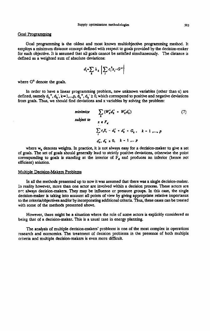
Goal Prom

Goal programming is the oldest and most known multiobjective programming method. It employs a minimum distance concept defined with respect to goals provided by the decision-maker for each objective. It is assumed that all goals cannot be satisfied simultaneously. The distance is defined as a weighted sum of absolute deviations:

where Gk denote the goals.

In order to have a linear programming problem, new unknown variables (other than 1) are defined, namely d,+, d,‘, k-l ,..., p, d, , + d k _ 2 0, which correspond to positive and negative deviations from goals. Thus, we should find deviations and x variables by solving the problem:

minimize c (w;d; + J$d;) (‘1 t

subject to x e F,,

pt5 - d; + d; + G, , k - 1 ,...., p

d;, d; L 0. k - 1 ..- P

where wk denotes weights. In practice, it is not always easy for a decision-maker to give a set of goals. The set of goals should generally lead to strictly positive deviations, otherwise the point corresponding to goals is standing at the interior of Fd and produces an inferior (hence not efficient) solution.

MultiDIe Decision-Makers Problems

In all the methods presented up to now it was assumed that there was a single decision-maker. In reality however, more than one actor are involved within a decision process. These actors are n-t always decision-makers. They may be influence or pressure groups. In this case, the single decision-maker is taking into account all points of view by giving appropriate relative importance to the criteria/objectives and/or by incorporating additional criteria. Thus, these cases can be treated with some of the methods presented above.

However, there might be a situation where the role of some actors is explicitly considered as being that of a decision-maker. This is a usual case in energy planning.

The analysis of multiple decision-makers’ problems is one of the most complex in operations research and economics. The treatment of decision problems in the presence of both multiple criteria and multiple decision-makers is even more difficult.

594 J. Psmw et al

In the context of mathematical programming, the multiobjective and multiple decision-makers’ problem can be viewed as a two-level vector optimization problem in which the two levels should be solved simultaneously. Thus, problem (2) is extended as followss*6:

minimize C ’ ci XP J ’ - 1 ,...., p, K-l ,...., m (8) 1

subject to x e Fd

where k denotes the decision-makers and j the objectives-criteria. We have p x m objective functions that should be optimized simultaneously.

In the context of multiple decision-makers, the concept of Pareto optimal solutions is analogous to that of efficient solutions. A solution is Pareto optimal when the satisfaction or utility of a decision-maker cannot be improved without a reduction of the satisfaction of some other decision-maker. By assuming the existence of a utility function for each decision-maker and by considering a weighting sum aggregation over decision makers,_problem (8) can be written:

subject to x e F,

where wk is the relative weight of the kth decision-maker. This is a measure of a decision-maker’s bargaining power, political influence or voting quota. This problem obviously has a single objective function.

It is desired to have a solution of problem (9) which is efficient with respect to objectives and is simultaneously Pareto optimal in terms of the decision-makers’ utilities.

. . . Decraons m a Decent-d Hierarchical m

The formulation of problems (8) and (9) illustrates some basic concepts, but it is especially inefficient when dealing with a practical case in the public policy domain. In public as in corporate policy, the decision actors involved are neither standing at the same hierarchical level nor are they making decisions on the same variables.

Thus, it is preferable to retain thr following decision process structure: (i) the decision actors are organized in a hierarchical frame, consisting of a central unit and several sub-units; a single decision actor is representative of a unit; (ii) decisions are decentralized, this means that each sub-unit has its own specific decision domain which is different from that of the others; the decision domains of the sub-units are disjoint but their union coincides with the decision domain of the whole system in the case that there is no decentralization; (iii) the role of the central unit is threefold: (1) ensure coordination of the whole system in order to obtain an overall consistent solution; (2) impose its own general objectives; and (3) distriiute common resources to the sub-units; (iv) each sub-unit (as well as the central unit) has its own specific set of objectives, which differs from that of the others and its own system of preferences; (v) each sub-unit is not free to formulate simply its own decision problem; it is obliged to take into account the objectives of the central unit, (i.e. the general objectives of the system), the resources allocated by the central unit and, eventually, restrictions of its set of feasible solutions that the central unit has imposed; (vi) each sub-unit transmits to the central unit the degree of dissatisfaction provoked by the constraints or objectives imposed; (vii) a solution to the system’s decision problem is defined as being the best compromise solution (in the sense of objectives) to the decision problem of each unit constrained by its inclusion in a collective decision process and at the same time being consistent with respect to the system’s global constraints, goals and resources; let us call this solution a global compromise solution.

‘It is assumed that for each decision-maker some coefficients cy may be equal to zero in order to reflect differences in the choice of the set of objectives.

‘It is not assumed that all decision-makers decide about all components of x.


The objective of the analysis is to simulate the decision process of the whole system by iterating towards a global compromise solution. This will provide insight into the following issues: (a) feasibility of a global compromise solution; (b) antagonisms between decision actors; (c) resource allocation problems; (d) necessary shifts of the multiobjective set of preferences of an actor in order to be consistent with the whole system; (e) efficiency of the organizational structure.

The energy systems planning problem is an excellent example of the decentralized procedure defined above. In fact, if we consider the energy sub-systems as sub-units (for instance the electricity, oil, coal and gas sub-systems) and the government as the central unit, all specifications of the decision process described above apply. For example, the electricity sub-unit has its own objectives which may not include environmental impacts. However, this objective is imposed by the government. A global solution to the decision process should satisfy the objectives of each sub-unit but also it should be consistent with the objectives and the equilibrium of the whole energy system. Notice that, conceptually, the distinction between sub-systems is made in all energy supply optimization models. It is thus easy to isolate the constraints (equalities and inequalities) belonging to each sub-system and the constraints for the whole energy system.

A systems approach to the formulation of decentrahzed hierarchical processes is proposed as a theory of multi-level systems by Mesarovic, Macko and Takahara (1970). Concerning mathematical programmin g techniques major contriiutions have been provided by Dantzig and Wolfe (1963) with the decomposition principle and by Komai and Iiptak (1965). The decomposition approach breaks up the program of the whole system into a set of sub-programs corresponding to the sub-units.

The central unit has exclusively a coordination role which is ensured either via prices (price-directive) or via resources (resource-directive). Because of this particular role devoted to the central unit and the somewhat artificial method used for the coordination, the decomposition approach is not considered that it represents realistically a decentralized decision process. However, it guarantees the convergence of the iterative process.

For these reasons several attempts have been made to reformulate this approach in order to improve its simulation capabilities. This effort has been termed by DJ. Sweeney et al. (1978) “composition” approach. In this direction we should also mention T. Ruefli (1971), J. Freeland and N. Baker (1975), as well as D.T. Whitford and W.J. Davis (1983). All these authors have formulated the sub-units’ decision problems as goal programs (see Section 2.5); thus, the inclusion of multiple objectives has been possible. Each subunit has to choose its own actions (i.e. its own variables x) by minimizing the deviations from its own goals, but also the deviations from the goals of the organization. In both Ruefli’s and Freeland and Baker’s contributions, the central unit is playing only a coordination role for resource allocation and receives dual prices from the sub-units as measures of their dissatisfaction. Especially in the Freeland and Baker algorithm, this is formulated in a way that convergence is guaranteed. This is achieved by the fact that this algorithm is in reality a Bender-type decomposition, which in the linear case is dual to the Dantzig-Wolfe one. In brief, these two approaches fail to overcome the drawbacks of using decomposition techniques for simulating decentralized decision processes.

On the contrary, the Whitford and Davis approach seems more promising, since it formulates a real goal programming decision problem for the central unit. We have used a mod&d version of this approach for modeling decentralized hierarchical decision processes (DHDP) in the energy sector.

For simplicity, let us consider the case of two sub-units, as in Figure 5. Decentralization is expressed by the fact that only the sub-units are to decide about their actions, i.e. decision variables. Hierarchy is expressed by the fact that the sub-units are constrained to satisfy some goals imposed by the central unit and are also constrained by the amounts of some resources allocated to them by the central unit. The central unit itself has to decide about the allocation of goals and resources in order to achieve its own goals. In addition, it takes into consideration the deviation from previously allocated resources and goals which occurred in the sub-units’ decisions. Limits are also imposed at the level of the central unit concerning the total amounts of goals and resources.

596 J.-et al

Global programming

problem of

central unit

Goals

and

limits

constraints

Goal programming

problem of

sub-unit 1

Goal programming

problem of

sub-unit m

Figure 5. Schematic Representation of the Decentralized Hierarchical Decision Process

Thus, the central unit transmits goals and resources to the sub-units and receives deviations from the sub-units. The iterative process terminates when there is no change in the values of the central unit’s objectives. The mathematical form of the algorithm (for two sub-units) is presented in Figure 6. Notice that the multiobjective optimization problem of a sub-unit is the same to that of Section 2.5 (goal programming) except the part concerning goals and resources that are transmitted by the central unit. Global organizational constraints which imrolye simuhaneously decision variables from several sub-units, can he considered as resources (i.e. as part of Q). This is necessary especially for energy systems applications. For example, energy production of the sub-systems (assimilated to sub-units) should sum to energy demand, which may be exogenous to the system. Energy demand may be represented by some components of the central unit’s resources Qo. The allocation of Q. to the sub-units, (in other terms the substitutions between energy forms), are decided by the central unit according to the procedure descriid above.

Supply optjmixgtion methodologies 597

CENTRAL UNIT

Minimize 5 ( IJ; E;(iter l 1) l II; E;(itcr l 1) 1

j= 1

Subject to : Q j(iter l 1) + Ef(iter + 1) - Ei(iter l 1) = Q j (iter) + e ; (itcr) - e; (iter)

5 [ ljQj(iter+l) I \< Q,

j= 1

Q ja E J+ E ; non negative

Qj(iter + 1)

V

A

e ;(iter)

e ;(iter)

SUB-UNIT No j

Minimize w;d;(iter) + w;d;(iter) l u;e;(iter) l u-je-j(iter)

Subject to : dcr,’

2 c (I xi + d;(iter) - d;(iter) = C ’

t a jj xi l e i(iter) - e ;(iter) = Q I (iter)

i

d;, d;, e-j. e;, xj are non negative

where :

u-. d+. w-. w+

E-,E’,e-,e*.d-,d+

x 1. j- 1.2

Td. j- 1.2

Q jt j- 1.2

Cj, j = 1.2

QO

jj . j-1,2

cj, aj i i

are vectors of coefficients weighting the deviations from goals

(u for the central unit and w for the sub-unit)

are unknown vectors denoting deviations from goals

are unknown vectors of decision variables

are the feasible domains corresponding to the sub-units

are vectors of resources and/or goals ellocated/imposed by the central unit

to the the sub-units; these are unknown variables only for the central unit

are known vectors of resources and/or goals specific to each sub-unit

is a known vtctor of total resources/goals disposed by the central unit

are predetermined parameters, expressing weighting of the sub-units

as viewed by the central unit

are coefficients expressing the decision variable xj in terms of

resources/goals (i.e. they are evaluation coefficients)

iter is the iteration number

Figure 6. Mathematical Form of the Decentralized Hierarchical Decision Process (DHPP)

598 J. PSARMS et d

3. APPLICATIONS

All methods presented in the previous section were applied to the GRESOMEFOM model. This is a large-scale linear programming model and represents dynamically all energy activities and investments of the Greek energy system. The model has about 3005 constraints and 4000 variables for several 5-year periods. A sophisticated software (in FORTRAN) performs database management and matrix generation for the LP problem. The whole system is installed in an IBM13083 mainframe computer and uses the MPSX linear progrrg package.

Initially the model was minimizing total discounted cost of the energy system and, hence, it was a single objective program. The 5rst task for transforming this model into a multiobjective one was to define alternative decision criteria (objectives) and to extend the data base of the model in order to be able to evaluate the performances of energy scenarios (generated by the model) on these new criteria. The evaluations of performances were formulated as linear functions of energy variables (5ows and investments), which are unknown to the program. In other terms, the functions evaluating the performance of actions should have a mathematical form similar to that of the original objective function. This restriction is imposed for the preservation of the linearity of the model but also for minimizing the computational work in adapting the matrix generation program. Finally, after this preliminary step, the model was able to evaluate performances on all objectives-criteria as functions of energy flows and investments.

The objectives-criteria that we retained are the following:

Total discounted cost, that is the old objective function corresponding to the present value of total cost for construction, operation and maintenance of all actual and future energy activities, including costs at the level of the end-consumer; performances are measured in monetary units.

Total discounted cost in foreign exchange, called briefly the exchange bill. It includes all charges in foreign currency evaluated as a part of the cost of fuel and investment for all energy activities. The evaluation coefficients re5ect assumptions about the future technological development of the country and represent the imported part of each cost; it is also measured in monetary units.

Environmental consequences, measured in an aggregate form by means of an environmental index. This index is a weighting sum of various emissions, such as SO, GO, NO, particulates, etc. The evaluation coefficients correspond to emission factors associated with energy flows, including energy consumption. Weights reflect the estimated damage caused by each pollutant to health.

Use of Depletable National Resources’ measured in ktoe. This criterion reflects the will for preserving depletable indigenous resources for future generations. It is connected to the rational use of depletable resources.

Total discounted investment cost, measured in monetary units. This includes all energy capacity expansion costs and it reflects the need for the minimization of financial charges.

All objectives are to be minimized. The choice of these particular objectives is adapted to the case of energy planning problems for Greece.

‘In some cases there is a confusion about this objective. In some countries the government promotes actually the use of depletable national resources in order to reduce energy imports. This should considered as an outcome of multicriteria evaluation and not an objective. This may result from the fact that the government accords more importance to criteria, such as the exchange bill, instead of the preservation of indigenous resources.


Most energy system optimization models are large-scale linear programs (i.e. more than 2000 variables) and use a complex matrix generation software. The main practical problems in introducing multiple objectives in such models deal with: (i) computer programming efforts needed for the modification of the matrix generation sofhvare and the application of the multiobjective algorithm, (ii) computer resources (mainly CPU time) needed for running the complex multiobjective programming algorithm with such a large-scale modeL In order to appreciate the computational burden, notice that in all multiobjective algorithms the model, that is the linear program, must run several times, at least as many as the objectives. In addition, the linear program is modified in each step (by adding constraints, for example) and this of course should be done automatically. In the case of application of an interactive multiobjective technique to a large-scale model, computer response time is crucial since the decision-maker may not want to wait.

Because of these computational problems we gave priority to the application of the modiiied constraint method (see Section 23) to GRESOMEFOM.

The application with the constraint method modified for information structuring (see Section 2.3) requires minimum programming efforts and does not need any modification of the matrix generation software. The method is directly applicable to an existing energy system LP model. We applied this method to the entire GRESOM/EFOM model. All other applications require important computational work. For this reason we applied them only to a simplified version of GRESOM/EFOM. Furthermore, the Zion&Wallenius, the STEP and the goal programming methods were applied only to a simplified version of the electricity generation sub-system of GRESOM/EFOM (about 100 variables). The decentrahzed hierarchical decision process was applied to a version having about 250 variables but including all sub-systems. In all these cases, except the application of the constraint method, the computer code was completely rewritten. The code corresponding to the implementation of the multiobjective algorithm was also rewritten in order to be integrable with the code corresponding to the model. For the goal programming method (Section 2.5), and at a lower degree for the STEP method (Section 2.4), the programming effort was considerably less important than for the Zionts-Wallenius method (Section 24) and the decentralized hierarchical decision process (Section 2.7).

Because of the computer time, the Zion&Wallenius method is practically inapplicable to large-scale models. This is due to the big number of linear programs which must be solved during the iterations (see Figure 3). Remember that in order to find all efficient and non basic variables, a linear program must be solved for each non basic variable. All the other methods presented are more practical with respect to their application to a large-scale model.

Since the constraint method is an exploratory one, with respect to the set of efficient solutions, it provides an important amount of information about the features of the decision problem. Trade-offs, extreme possibilities and crucial decision choices are presented to the decision-maker (see Table 1, Figure 7, 8 and 9, which present a sample output). Our extension which concerned the structuring of output information, is applicable when one of the objectives is considered as being more important than others. In energy models this is the old objective function, that is total discounted cost. In this case, all results, namely the payoff matrix and the decision trees, are presented relatively to the values of this objective. For example, it is important for the decision-maker to be informed about the alternative decision choices when he accepts to make some concession on total cost.

600 J. F’SMMS et al

Table 1. The Payoff Matrix

value of

Minimization of

TOTAL COST 9.774 I 8.385

EXCHANGE BILL

ENVIRONM. INDEX

NAT. RESOURCES

INVESTMENT COST

TOTAL EXCHANGE

COST BILL

x 1012 x 1012

d&83 drs’83

10.100 1 7.602

13.200 I 12.080

11.500 I 9.628

10.800 I 8.746

ENVIRONM. NATIONAL INVESTMENT

INDEX RESOURCES COST

x106 KTOE x 1012

drs’83

7.595 I 53120 I 5.284 I

6.768 I 55390 I 4.802 I 4.787 I 7913 I 7.937 I 7.655 I 6119 I 4.874 I 9.388 I 38400 I 3.804 I

cost - Exchange Bill Trade - off

Other Criteria

1 .05 i”. . ..., /.. . . . . . . ..“..-.‘.‘.“.‘....... . . . . .._..._.._........... __._.- ._....... ,: * Exchange

--- Environment

.......... Nat. Resources

----‘Investment

‘. ‘\

,-

OS85 ‘L_ _ _ ___“.““_____/~’ I . I 1 . I

1 1.005 1.01 1.015 1.02 1.025 1.03

cost -.-.

cost - Environment Trade - off

Other Criteria

- Exchange

-* Environment

....--- Net. Resources

.---- Investment

‘.-.. 0.4 -

_‘. . . . .._._ ‘.._ Y.,

.‘... “..,, 0.2-, ( ~ ( , , , , _,_ A . . . . .,,,_.

1 1.05 1.1 1.15 1.2 1.25 1.3 1.35

cost

Figure 7. Values of the Objectives in the Trade-Off Analyses


-2% of the total Cost

---I- wlthout 8ddltional

llnancl~l charges

Figure 8. Alternative Choices

Other Criteria

” \/ \/ A /\ i-1

1 -1 2 3

/A

! ______----- ____---

---

0.95 -__ : : : :

0.9 - :

0.85

0.8

0.75

0.88 0.9 0.92 0.94 0.96 0.98 I

Investment

* cost

---- Exchange

. . . . . . . E”“*ro”.

.----- Nat. rcs.

1

Figure 9. Four Global Runs for +2% of Total Cost

602 J. F’SNUUS et al

The payoff matrix is presented in Table 1. Notice that the ranges between the maximum and the minimum values of each column are important for all objectives. Thus, the domain to explore is big. Figure 7 presents the trade-off analyses between pairs of objectives (the trade-off curves are those having numbered points). The values of the non interning objectives are also reported on the drawings. In order to appreciate the type of information provided to the decision-maker, see solution No 9 of the cost-environment trade-off. At only 3.5% additional total energy cost, this solution achieves 25% improvement of the environmental index, while there are no significant consequences for the other objectives. By combining the information obtained from these trade-off curves, decision trees can be proposed to the decision-maker. An example is presented in Figure 8. It corresponds to four global multiobjective runs reported also in Figure 9. Notice in these figures that if the decision-maker accepts 2% additional energy systems cost, he must choose between improving the environmental index or diminishing the use of depletable national resources. A further dilemma arises concerning financial (i.e. total investment and foreign exchange) charges.

In summary, the constraint method provides good insight into the nature of the problem, it is very comprehensive for the decision-maker and well accepted. However, it is not very efficient in acquiring and then representing the decision-maker’s preferences. By considering also its computational facility, we conclude that the constraint method, as extended with information structuring process, is very efficient in practice for energy systems planning.

The Zion&Wallenius and the STEP methods are the only truly interactive multiobjective techniques. With respect to the interaction with the decision-maker the Zion&Wallenius method had the best performance. Questions addressed to the decision-maker were well accepted and easy to answer. They provided also a good insight into trade-offs and alternative decision paths of the problem. This method is, however, inefficient for large-scale energy models, as mentioned. The STEP method is simpler to implement but it is less efficient concerning the interaction with the decision-maker. In each iteration, although it was easy to choose the objective function to reduce, it was difficult to decide about the amount of the reduction. Moreover, the method does not provide information about trade-offs.

Goal programming was the less efficient method concerning the interaction with the decision-maker. Results were sensitive to the levels of goals, which are defined by the decision-maker who had also significant difficulty in providing them. It seems that this is a general drawback of goal programming especially when applied to public decision-making; see Cohon (1978).

The decentralized hierarchical decision process (DHDP) provides insight mainly into organizational issues related to energy planning. In order to implement this method, it is necessary, first, to define an organizational structure. Then the original model is broken down in sub-systems corresponding to this structure. It is necessary then to reformulate the model and to write a code for m+l linear programs, with m the number of sub-systems. A code corresponding to the coordination mechanism is also needed.

The DHDP method provides important information on antagonisms between decision-makers at two levels, namely between the decision-makers corresponding to the sub-units and between the central unit and the subunits. Because of its realistic approach in representing information flows between the units, this method is appropriate for simulating the collective decision process in energy (or other non energy) planning. Our research work with DHDP is under progress.

Table 2 provides a comparative evaluation of the applications carried out.

Supply optimization methodologies

Table 2. Comparative Evaluation of Applications

603

1. Modification of the matrix generation software

Constraint method with information structuring

NO

Zionts- Wallenius

YES

STEP

YES

Goal Program- Decentralized ming Hierarchical

Decision Pro-

cess

YES YES

2. Computer programming effort

3. Computer time for

large-scale models

4. Interaction eith a decision-maker

minimal high

low prohibitive

limited YES

medium

medium

low

low

limited

high

high

limited

5. Acceptance and comprehension by a decision maker

high medium low low ?

6. Insight into the multicriteria na-

ture of the problem

medium high medium 1oW low/medium

7. Organizational im- NO NO NO NO YES plications

B. Insight into relations NO NO NO NO between decision makers I

9. Efficiency for energy high low medium 1oW high

planning

4. CONCLUSIONS

Our analysis has been successful in providing information on the following: (i) what are the practical problems of introducing multiobjective programmin g techniques into a large-scale energy systems LP model; (ii) what are the advantages and the disadvantages of the most well known multiobjective methods with respect to feasrbility, interactions with the decision-maker and accuracy of output information; (iii) which methods are overall efficient in energy planning.

We conclude, first, that there is effectively a need for introducing multiple objectives or criteria in energy systems planning. In fact, the trade-offs between the objectives, the decision dilemmas and the additional information provided to the decision-maker were significant. Secondly, we conclude that two particular methods are most applicable to energy systems planning with a large-scale energy model, namely (i) the constraint method as extended with an information structuring process, which provides a good understanding of trade-offs between the objectives, and (ii) the decentralized hierarchical decision process which appears to be a powerful simulation tool for studying the energy planning decision process and for analyzing antagonisms and compromises between the energy sub-units.

We believe that the introduction of multiple objectives into an energy system programming model represents a net gain in all respects.

604 J. PSARRAS et al

REFERENCES

Benayoun, R., J. de Montgolfier, J. Tergny and 0. Laritchev (1971). “Linear Programming with Multiple Objective Functions: STEP Method”, v .

CEC (1984). “Energy Supply Modeling Package EFOM-12C’, Commission of the European Communities, DG-XII, Brussels.

Chemiavsky, E (1974). “Brookhaven Energy System Optimization Model, Brookhaven National Laboratory”, Report B&19569, Upton, New York

CherniavsQ, E., A Kydes and J. Davidoff (1977). “Multi-objective Function Analysis of ERDA Forecasts-2”, Year-2000 Scenario, Brookhaven National Laboratory, Report B&50685, Upton, New York.

Cohon, J.L (1978). “Multiobiective Prm and Pw, New York: Academic Press.

Dantzig, G.B. and P. Wolfe (1963). ‘Decomposition Principle for Linear Programs”, Operations Research Vol. 8, pp. 101-111.

Egberts, G. (1980). “MARKALA Multi-Period Linear Optimization Model of the Energy Supply System”, STE-KFA, Report, Julich, West Germany, April.

Freeiand, J. and N. Baker (1975). “Goal Partitioning in a Hierarchical Organization”, OMEGA, 3(6), pp. 673688.

Hoffman, KC., M. Belier, E. Chemiavsky and MFisher (1976). “Multi-objective Analysis of ERDA Combined Technology Scenarios”, Brookhaven National Laboratory, Report B&21091, Upton, New York.

Keeney, R and H. Raiffa (1976). “Decisions with Multirile Obiectives: Preferences and Value Tradeoffs”, New York: John Wiley & Sons.

Komai, J. and T. Liptak (1965). “Two-Level Planning”, Economctrica 3.1, pp. 141-169.

Kydes, A (1978). ‘The Brookhaven Energy System Optimization Model”, Brookhaven National Laboratory, Report B&50373 and B&50873, Upton, New York.

. . ’ Lee, S. (1972). “Goal m for Decrsim “, Philadelphia: Auerbach Publ. Inc.

Lowe and Thisse (1984). “On Efficient Solutions to Multiple Objective Mathematical Programs”, went Sciem 30(11), pp. 1346-9.

Mesarovic, M.D., D. Macko and Y. Takahara (1970). ‘ThcoIy Hierarchical Multilevel Svstems”, New York: Academic Press.

Psarras, J., P. Capros and J.-E. Samouilidis (1986). “Multicriteria Analysis with a Large-Scale Energy Supply LP Model”, Proceedings of the 25th IEEE Conference on Decision and Control, Athens, Greece, December 10-12.

Roy, B. (1985). “Methodoloeie Multicritere d’ Aide a la Decision”, Paris: Editions ECONOMICA

Ruefli, T. (1971). “A Generalized Goal Decomposition Model”, Manaeement Science, 17(8), pp. 505-518.

Samouilidis, J.-E. and A Arabatzi-Ladia (1982). “A Model for the Greek Energy System”, Euroaean Journal of Operations Research, 9, pp. 144-160.


Schank, J. (1978). “An Alternative, Semi-Automated Method for Performing Multi-Objective Analysis”, Brookhaven National Laboratory, Report B&50892, Upton, New York.

Sweeney, D.S., E.P. Winkofsky, P. Roy and N. Baker (1978). “Composition vs. Decomposition: Two Approaches to Modeling Organizational Decision Process”, &lanaeement Science, 24, pp. 1491-1499.

Van der Voort (1982). “The EFOM-12C Energy Supply Model Within the EC Modeling System”, OMEGA, 10(S), pp. 507-523.

Whitford, D.T. and W.J. Davis (1983). “A Generalized Hierarchical Model of Resource Allocation”, ll(3). OMRGA

Zeleny, M. (1982). “JhltiDle Criteria DecisiQn MaId&‘, New York: McGraw Hill Co.

Zionts, S. and P. Desphande (1978). “An Application of Multiple Criteria Problem Solving to Energy Planning”, 8th Conference of IFORS, Toronto, Canada.

Zionts, S. and J. Wallenius (1976). “An Interactive Programming Method for Solving the Multiple Criteria Problem”, Management Science, 22(6).

4.5. Multiobjective programming

Documents

Transcript of 4.5. Multiobjective programming