SFB

823

Benchmarking evolutionary Benchmarking evolutionary Benchmarking evolutionary Benchmarking evolutionary

multiobjective optimization multiobjective optimization multiobjective optimization multiobjective optimization

algorithmsalgorithmsalgorithmsalgorithms

Discussion Paper

Olaf Mersmann, Heike Trautmann,

Boris Naujoks, Claus Weihs

Nr. 3/2010

Benchmarking Evolutionary Multiobjective Optimization Algorithms

Olaf Mersmann1, Heike Trautmann1, Boris Naujoks2 and Claus Weihs1

1 Statistics Faculty, TU Dortmund2 Log!in GmbH, Schwelm

e-mail: {mersmann;trautmann;weihs}@statistik.tu-dortmund.de,

boris.naujoks@login-online.de

February 2010

Abstract:Choosing and tuning an optimization procedure for a given class of nonlinear optimization

problems is not an easy task. One way to proceed is to consider this as a tournament, where

each procedure will compete in different ‘disciplines’. Here, disciplines could either be different

functions, which we want to optimize, or specific performance measures of the optimization

procedure. We would then be interested in the algorithm that performs best in a majority of

cases or whose average performance is maximal.

We will focus on evolutionary multiobjective optimization algorithms (EMOA), and will present

a novel approach to the design and analysis of evolutionary multiobjective benchmark exper-

iments based on similar work from the context of machine learning. We focus on deriving a

consensus among several benchmarks over different test problems and illustrate the methodol-

ogy by reanalyzing the results of the CEC 2007 EMOA competition.

1 Introduction

Comparing the outcome of competitors in multiple disciplines is a complex task. It always de-

pends on the considered ranking and consensus methods applied. The task to judge the outcome

of evolutionary algorithms on different test problems considering multiple runs falls into this

area. It becomes even harder if one wants to compare evolutionary multiobjective optimization

algorithms as different performance measures have to be taken into account as well.

The development of such algorithms has evolved into a large research field during the last 20

years. Recently there has been work on the systematic evaluation and benchmarking of the

rapidly increasing number of EMOA [1]. This focuses on the systematic comparison of pairs

and groups of algorithms using statistical tests and graphical representations of the algorithms’

performance. Furthermore, there have been several competitions for EMOA where the resulting

rankings were analyzed using an ad hoc approach.

Motivated by the work of Hornik and Meyer [2] on the systematic benchmarking of classifi-

cation algorithms, we will derive a suitable benchmarking framework to statistically compare

EMOA. All necessary functions are implemented in an R package named emoa [3]. The rank-

ing and consensus methods stem from the R package relations [4].

In Section 2 we will review relations, rankings and orders. Then we will introduce benchmark

scenarios in Section 3, define ranking operators for these scenarios and then derive a consensus

ranking from these individual benchmark scenario rankings. In Section 6 we apply the methods

previously proposed to a dataset from the CEC 2007 EMOA competition. Since there cannot be

a universal best consensus [5], we find different outcomes for the competition depending on the

quality indicator, the ranking method and the consensus method applied. We close by giving a

short summary and suggestions for future research in section 7.

2 Relations, orders and rankings

We successively refine the general term relation ([6]) until we arrive at a formal definition for a

ranking.

Definition 1 A binary relation R is given by the pair 〈D(R), G(R)〉 where D(R) = (X1, X2)

is the domain of the relation R and G(R) the graph of R. A tuple x ∈ D(R) is said to be

contained in the relation R if and only if (iff) it is an element of the graph G(R). Let si be the

cardinality of Xi. Then s = (s1, s2) is called the size of R. A binary relation R is called an

endorelation iff X1 = X2. If all the si are finite, the graph G(R) can be represented by a matrix~I(R) with size s. It is called the incidence matrix of the relation R and for any x ∈ D(R)

~Ix = 1 iff x is contained in G(R).

We will assume that all elements of our domain D are finite sets. A relation R can therefore

always be uniquely represented by its incidence array ~I(R).

Definition 2 Let R be an endorelation with domain D(R) = (X,X). Then it is called

• reflexive if for all x ∈ X , xRx.

• transitive if for x, y, z ∈ X , xR y ∧ y R z ⇒ xR z.

2

• antisymmetric if for x, y ∈ X , xR y ∧ y Rx⇒ x = y.

• complete if for all distinct x, y ∈ X , xR y ∨ y Rx.

Definition 3 A weak order is a complete, reflexive and transitive endorelation. A partial order

is a reflexive, antisymmetric and transitive endorelation. A linear (or total) order is a antisym-

metric weak order.

All orders have the important property of being transitive.

Definition 4 A ranking R of a set of items A = {a1, a2, . . . , ak} is a weak order over the set

A. For x, y ∈ A we say x is better than y and denote this by x � y iff y Rx and not xR y. If

xR y and y Rx, then we say x and y are tied and denote this by x ∼ y.

A strict ranking R of a set A = {a1, a2, . . . , ak} is a linear order over the set A. For x, y ∈ Awe say x is preferred over y (x � y) iff y Rx.

In the following we will denote the ranking, as well as the relation by R and use � for the

corresponding binary operator between elements from the domain of R. If applicable, we will

use the shorthand form of writing x � y � z.

3 Benchmark Scenarios

Informally, we are interested in the best algorithm from a set of EMOA. At first we need to

limit ourselves to a domain of optimization problems. A crucial and very important task is the

definition of better.

Definition 5 Given a set of possible parameters X and d functions f1, . . . , fd with fi : X → R

for i ∈ {1, . . . , d}, a multiobjective optimization problem is given by

arg min~x∈X

fi(~x) i = 1, . . . , d (1)

where fi = fi if fi should be minimized and fi = −fi if fi should be maximized.

For a performance analysis of EMOA [7] we need to pick a fixed quality indicator I (e.g.

Dominated Hypervolume, see [1] for an overview) which has to be maximized by assumption.

If I is a binary quality indicator we assume that we use a given common reference set. So we

can always take I to be a unary quality indicator for which greater values mean higher worth.

3

So given a quality indicator I , a multiobjective optimization problem f and two EMOA a1 and

a2 we wish to define a comparison operator � which tells us if a1 is as good as or better than a2

where, by definition, a � a for any algorithm a.

Definition 6 Given two algorithms a1 and a2, a fixed optimization problem f , quality indicator

I and a pairwise comparison operator �, we say a1 is best iff a1 � a2 and not a2 � a1.

Conversely, we say a2 is best iff a2 � a1 and not a1 � a2. If both a1 � a2 and a2 � a1, we say

a1 and a2 are tied.

This definition is similar to the definition of Pareto dominance.

Definition 7 Given two parameter settings ~x and ~x′, ~x dominates ~x′ (~x � ~x′) iff ∀i ∈ {1, . . . , d}:

fi(~x) ≤ fi(~x′) ∧ ∃i ∈ {1, . . . , d} : fi(~x) < fi(~x

′) (2)

The problem with this definition is that it cannot be generalized to three or more algorithms. To

see this, let us look at the set of possible results from all pairwise comparisons between three

algorithms a1, a2 and a3.

A = {a1 � a2, a1 � a3, a2 � a1, a2 � a3, a3 � a1, a3 � a2}.

The implied ai � ai entries have been ommited and we will assume that we have no tied entries

for the moment.

The subset A′ = {a1 � a2, a1 � a3, a2 � a3} could be shortened to a1 � a2 � a3. So we have

deduced a ranking of the three algorithms. In fact, we can say with some confidence, that a1 is

the best algorithm since it is better than any algorithm in a pairwise comparison.

However, we could just as well have gotten the result A′′ = {a1 � a2, a2 � a3, a3 � a1},which does not induce an order on the algorithms since it contains a cycle. The only possible

conclusion is that a1 is equal to a2 is equal to a3. But this would mean that we should have also

observed a2 � a1, a3 � a2 and a1 � a3. In this case we have no real interpretation for the result

set.

Generally, any subset of A defines a graph over {a1, a2, a3}. We can therefore interpret our

pairwise comparison operator as an endorelation over {a1, a2, a3}. Knowing this, we can now

use the definitions from Section 2 to derive desirable properties for our comparison operator, so

that the corresponding endorelation is some type of order.

We know that the comparison operator is by definition reflexive and needs to be transitive. In

the following sections we will develop several different comparison operators and show which

properties they meet. In all cases, we will assume that there is some true underlying order of

the algorithms.

4

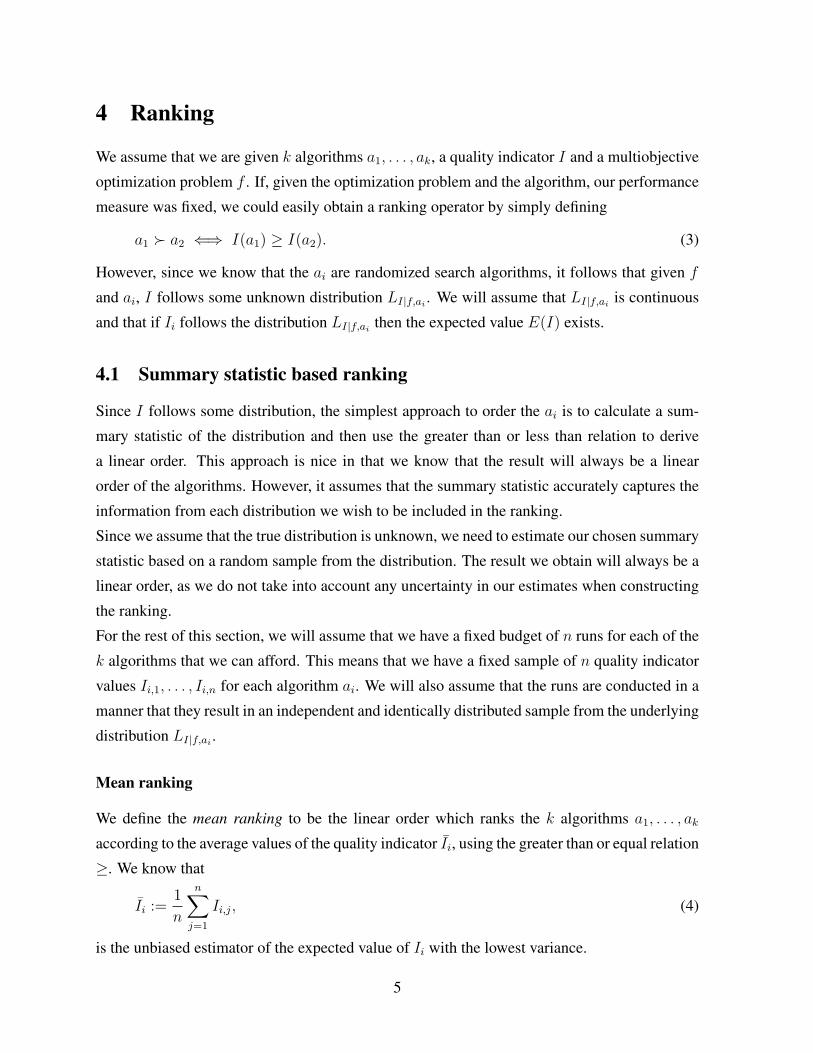
4 Ranking

We assume that we are given k algorithms a1, . . . , ak, a quality indicator I and a multiobjective

optimization problem f . If, given the optimization problem and the algorithm, our performance

measure was fixed, we could easily obtain a ranking operator by simply defining

a1 � a2 ⇐⇒ I(a1) ≥ I(a2). (3)

However, since we know that the ai are randomized search algorithms, it follows that given f

and ai, I follows some unknown distribution LI|f,ai. We will assume that LI|f,ai

is continuous

and that if Ii follows the distribution LI|f,aithen the expected value E(I) exists.

4.1 Summary statistic based ranking

Since I follows some distribution, the simplest approach to order the ai is to calculate a sum-

mary statistic of the distribution and then use the greater than or less than relation to derive

a linear order. This approach is nice in that we know that the result will always be a linear

order of the algorithms. However, it assumes that the summary statistic accurately captures the

information from each distribution we wish to be included in the ranking.

Since we assume that the true distribution is unknown, we need to estimate our chosen summary

statistic based on a random sample from the distribution. The result we obtain will always be a

linear order, as we do not take into account any uncertainty in our estimates when constructing

the ranking.

For the rest of this section, we will assume that we have a fixed budget of n runs for each of the

k algorithms that we can afford. This means that we have a fixed sample of n quality indicator

values Ii,1, . . . , Ii,n for each algorithm ai. We will also assume that the runs are conducted in a

manner that they result in an independent and identically distributed sample from the underlying

distribution LI|f,ai.

Mean ranking

We define the mean ranking to be the linear order which ranks the k algorithms a1, . . . , ak

according to the average values of the quality indicator Ii, using the greater than or equal relation

≥. We know that

Ii :=1

n

n∑j=1

Ii,j, (4)

is the unbiased estimator of the expected value of Ii with the lowest variance.

5

Median ranking

The median ranking is defined to be the linear order of the empirical medians of the quality

indicator values. We can interpret the median as a compromise between average case quality

and likely quality. We again use the≥ relation to induce a linear order on the observed medians

since, by definition, we want to maximize the value of the quality indicator.

Maxi-Min ranking

If we wanted to choose our algorithm to maximize the worst case quality, we would use the

empirical minimum of our quality indicator values as the statistic to order. Similarly if we

wanted to maximize the best case quality we would order the empirical maximum of the quality

indicator values.

Variance ranking

The unbiased estimator with the lowest variance for the variance of LI|f,aiis

Ivari :=

1

n− 1

n∑j=1

(Ii,j − Ii)2. (5)

A low variance implies that we get consistent quality, thus now we want to minimize the sum-

mary statistic. So the variance ranking of our algorithms is given by the linear order of the Isdi

using the less than or equal relation ≤.

The proposed summary statistics are summarized in Table 1. The corresponding comparison

operator can be constructed from the table by the following rule:

ai � aj ⇐⇒ siRsj (6)

The list of summary statistics and benchmarking scenarios is certainly not complete. Other

comparison operators can be constructed based on the same principles.

4.2 Relevance ranking

All summary statistics based comparison operators do not take into account the variability of

the underlying data. They do not consider how sure we can be that the difference between two

summary statistics si and sj is relevant and that their relation to each other is not reversed. In

this section we will discuss two approaches to deal with this. The first one is based on expert

6

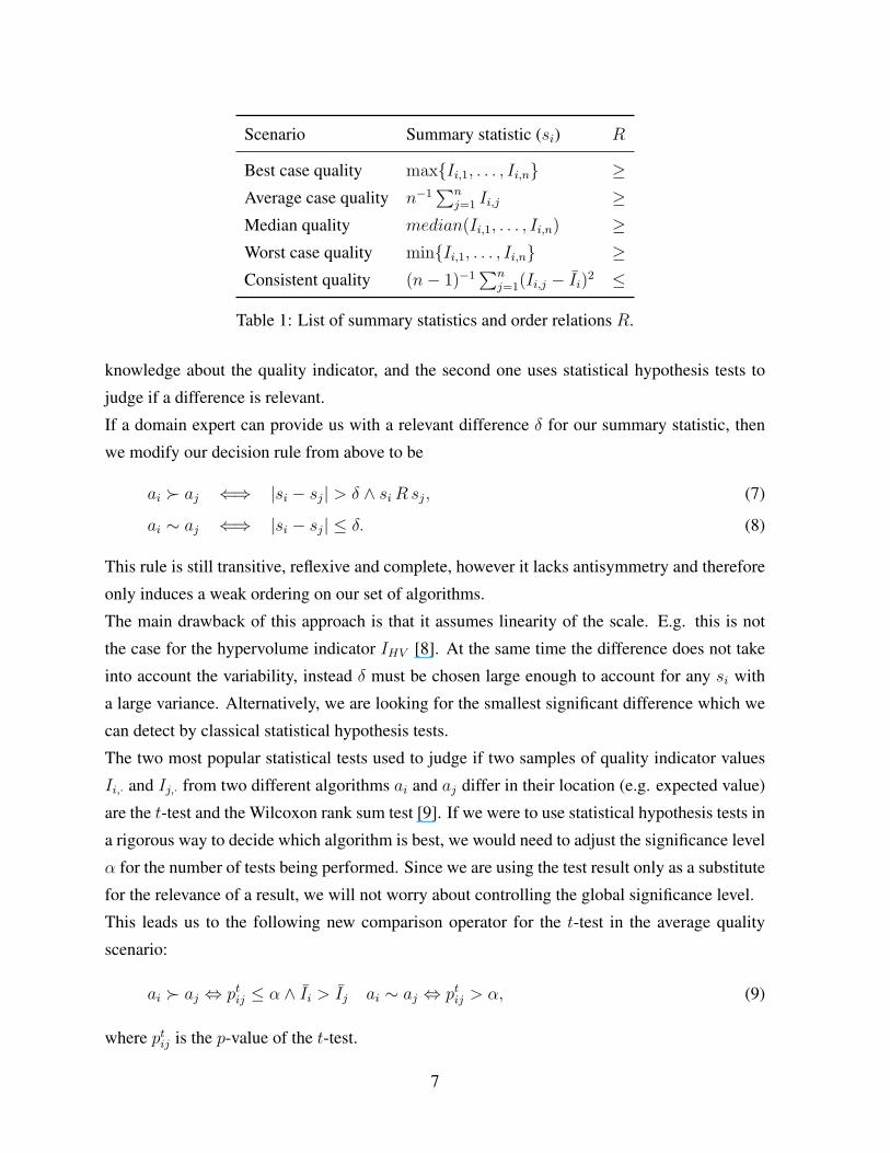
Scenario Summary statistic (si) R

Best case quality max{Ii,1, . . . , Ii,n} ≥Average case quality n−1

∑nj=1 Ii,j ≥

Median quality median(Ii,1, . . . , Ii,n) ≥Worst case quality min{Ii,1, . . . , Ii,n} ≥Consistent quality (n− 1)−1

∑nj=1(Ii,j − Ii)2 ≤

Table 1: List of summary statistics and order relations R.

knowledge about the quality indicator, and the second one uses statistical hypothesis tests to

judge if a difference is relevant.

If a domain expert can provide us with a relevant difference δ for our summary statistic, then

we modify our decision rule from above to be

ai � aj ⇐⇒ |si − sj| > δ ∧ siRsj, (7)

ai ∼ aj ⇐⇒ |si − sj| ≤ δ. (8)

This rule is still transitive, reflexive and complete, however it lacks antisymmetry and therefore

only induces a weak ordering on our set of algorithms.

The main drawback of this approach is that it assumes linearity of the scale. E.g. this is not

the case for the hypervolume indicator IHV [8]. At the same time the difference does not take

into account the variability, instead δ must be chosen large enough to account for any si with

a large variance. Alternatively, we are looking for the smallest significant difference which we

can detect by classical statistical hypothesis tests.

The two most popular statistical tests used to judge if two samples of quality indicator values

Ii,· and Ij,· from two different algorithms ai and aj differ in their location (e.g. expected value)

are the t-test and the Wilcoxon rank sum test [9]. If we were to use statistical hypothesis tests in

a rigorous way to decide which algorithm is best, we would need to adjust the significance level

α for the number of tests being performed. Since we are using the test result only as a substitute

for the relevance of a result, we will not worry about controlling the global significance level.

This leads us to the following new comparison operator for the t-test in the average quality

scenario:

ai � aj ⇔ ptij ≤ α ∧ Ii > Ij ai ∼ aj ⇔ pt

ij > α, (9)

where ptij is the p-value of the t-test.

7

The Wilcoxon rank sum test is based on the operator

ai � aj ⇔ pUij ≤ α ∧ U > 0.5 ai ∼ aj ⇔ pU

ij > α, (10)

where U is the test statistic and pUij the corresponding p-value.

Both rules are reflexive, complete but not antisymmetric. In the t-test case, we would need to

assume equal variances. This seems highly unrealistic and might suggest that the procedure is

not useful for any real world problems, but in practice the procedure is usually transitive which

justifies its application.

For the Wilcoxon rank sum test there are several conditions under which it is transitive. For

continuous distributions they usually reduce to the assumption that the density function is sym-

metric. Again, this is not necessarily realistic since we may assume that the distribution of our

quality indicator has an upper bound.

There exists a wealth of literature on deriving transitive relations from intransitive relations in

the context of social choice theory ([10]). The resulting transitive relation would then be a

partial ordering of the algorithms.

5 Consensus ranking

If we have a single function f and a single quality indicator I we can use one of the comparison

operators from the previous section, depending on our scenario, to derive a (partial) order of the

algorithms. Sadly, most real world situations are not that easy. Often we will have numerous,

if not an infinite number of functions, representing our problem domain. At the same time,

we may be interested in more than one quality indicator. If we want to find the best algorithm

in such a situation, we need to first reduce it into a set of benchmark scenarios for which we

already know how to infer a ranking.

First, we need to choose a fixed set of test problems F = {f1, . . . , fb} which represents our

problem domain. In choosing the fi, it is crucial that we uniformly sample from the set of

all possible functions. Then we need to define one or more suitable quality indicators and

corresponding comparison operators for each test problem. Denote these by V = {V1, . . . , Vq}.Combining these will give us a set of benchmark scenarios we are interested in. We will denote

the bq rankings resulting from the analysis of these benchmark scenarios by ri,j for the ranking

induced by the i-th function and the j-th comparison operator. Let us call the resulting set of

rankingsR.

8

What we now have are bq different opinions on which algorithm is best. What we need is a

consensus among these opinions. We have seen in the previous section that depending on our

benchmarking scenario we need different comparison operators which may lead to different

rankings of the algorithms. This is to be expected since we are ranking them based on different

definitions on what we consider to be a better algorithm. In this section, we will see that there

are different methods for deriving a consensus from our set of rankings R. These methods

do not coincide with a benchmarking scenario. Instead, they offer different tradeoffs between

properties that the consensus fulfills. So, before we have seen the first consensus method we

need to accept the fact that from this point forward, we cannot objectively define the best algo-

rithm. Instead, our statement of which algorithm is best depends on our subjective choice of a

consensus method.

5.1 Consensus Criteria

In order to ease the choice of a consensus method, let us begin by defining some criteria that a

consensus method should meet [5]:

Criterion 1 A consensus method cm that takes into account all rankings instead of mimicking

one predetermined ranking is said to be non-dictatorial.

Criterion 2 A cm that, given a fixed set of rankings, deterministically returns a complete rank-

ing is called a universal consensus method or is said to have a universal domain.

Criterion 3 A cm fulfills the independence of irrelevant alternatives criterion, short IIA crite-

rion, if given two sets of rankings R = {r1, . . . , rn} and S = {s1, . . . , sn} in which for every

i ∈ {1, . . . , n} the order of two algorithms a1 and a2 in ri and si is the same, the resulting

consensus rankings rank a1 and a2 in the same order.

IIA means that introducing a further algorithm does not lead to a rank reversal between any of

the already ranked algorithms which is a very strict requirement. In fact the next criterion is

incompatible with IIA

Criterion 4 A cmwhich ranks an algorithm higher than another algorithm if it is ranked higher

in a majority of the individual rankings, fulfills the majority criterion.

Criterion 5 A cm is called Pareto efficient if given a set of rankings in which for every ranking

an algorithm ai is ranked higher than an algorithm aj , the consensus also ranks ai higher than

aj .

9

No consensus method can meet all of these criteria because the IIA criterion and the majority

criterion are incompatible. But even if we ignore the majority criterion, there is no consensus

method which fulfills the remaining criteria [5]. So if we choose different criteria that our

consensus method should meet, we may get very different consensus rankings.

5.2 Positional methods

In a positional consensus method we need a function swhich, given a ranking r and an algorithm

ai, returns the score of ai under ranking r. We can then calculate the sum of the scores for each

algorithm as follows

si =b∑

k=1

p∑l=1

s(ai, rk,l). (11)

We then derive the consensus ranking by ordering the algorithms according to their scores

ai � aj ⇐⇒ si > sj ai ∼ aj ⇐⇒ si = sj. (12)

This leaves us with the choice of a suitable score function. The simplest possible choice would

be

s(ai, r) =

1 if in r ai � aj for all j

0 otherwise. (13)

With this score function the best algorithm in each scenario gets one vote and all other algo-

rithms do not. However, this introduces bias into the consensus.

Instead we will consider the following function

sBC(ai, r) =∑i 6=j

I(ai � aj) (14)

It counts the number of algorithms that are not better than the algorithm whos score we are

calculating. So an algorithm gets one point for each algorithm that it weakly dominates.

The function sBC leads to one one of the oldest consensus methods [11] namely the Borda count

method. This is the optimal consensus method under all positional consensus methods [12].

While optimal in some sense, the Borda method lacks mathematical rigor. It seems like an ad

hoc definition without any theoretical justification. The next approach to consensus ranking is

exactly the opposite.

10

5.3 Optimization based methods

Assume we have a set of candidate consensus rankings C. This could be the set of all linear,

partial or weak orders of our k algorithms or some reasonable subset of these. Further assume

we have a function

d : T × T → R+, (15)

where T := R∪ C, with the following properties

• Non-negativity: For any t1, t2 ∈ T , d(t1, t2) ≥ 0 and d(t1, t2) = 0 iff t1 = t2.

• Symmetry: For any t1, t2 ∈ T , d(t1, t2) = d(t2, t1).

• Triangle inequality: For any t1, t2, t3 ∈ T , d(t1, t2) + d(t2, t3) ≥ d(t1, t3) and equality

only holds iff t2 lies between t1 and t3.

Then d is a measure for how far apart two rankings are. What is missing is a notion of between-

ness. We will define this in terms of pairwise comparisons. We will say t2 lies between t1 and

t3 if for all pairs of algorithms either t2 agrees with t1 or t3 on the relative order of the pair, or

t1 and t3 have conflicting orderings for the pair and t2 declares the pair to be tied.

Using this distance measure, we could transform our consensus ranking problem into an opti-

mization problem

arg minc∈C

b∑i=1

q∑j=1

d(ri,j, c)l l ≥ 1. (16)

The consensus ranking is then given by the ranking whose median (for l = 1) or mean (for

l = 2) distance to all benchmark scenario rankings is minimal.

We will only review one distance function (see [10] for an overview) and motivate it by postulat-

ing a set of axioms which it should satisfy [13]. The first axiom simply states that a permutation

of the labels should not change the distance between two rankings. The second axiom states

that if the two rankings differ only on a subset of all algorithms that form a segment of the

rankings, then the distance between the two rankings should be equal to the distance between

the two differing segments. And finally we need one axiom to fix the scale. It simply states that

the minimum distance between two different rankings is 1.

Kemeny and Snell [13] showed that these three axioms and the metric properties uniquely de-

scribe a single distance function, the symmetric difference or short SD. It is defined as

dSD(t1, t2) := ~1′|~I t1 − ~I t2|~1 (17)

11

where ~1 is the k dimensional one vector, ~I ti the incidence matrix belonging to the relation that

corresponds to the ranking ti and |·| denotes the element wise absolute value. It counts how

many cases there are where ai � aj is contained in one of the relations but not the other. Thus,

the optimization problem from above tries to minimize the average number of rank reversals in

the consenus ranking.

When we talk about a symmetric difference consensus we will denote it by SD/C where we

replace C with L for the set of all linear orders and O for the set of all partial orders.

5.4 Comparison

So far we have introduced two consensus methods. The SD/L and SD/O methods meet the

majority criterion, the Border count (BC) method does not.

SD/L and SD/O fulfill the majority criterion, therefore they cannot fulfill the IIA criterion.

However, on real data they seldom show rank reversals if algorithms are added or dropped from

the rankings [14]. Sadly, the Borda count method also fails the IIA. A thorough investigation

and comparison of the Borda method and the SD method is given in [14]. Two remarkable

results proven there are that the SD method always ranks the Borda winner above the Borda

loser and that the Borda method always ranks the SD winner above the SD loser.

To summarize, if we want to find a best algorithm for a problem domain, we need to uniformally

pick a set of test functions from the problem domain. These combined with a quality indicator

and corresponding comparisons operator define our benchmark scenarios and induce a set of

partial or linear orders of our algorithms. Using consensus methods, we can combine these

rankings into a final order. The choice of consensus method is crucial and at the same time

highly subjective. There is no right way to choose and therefore no one best algorithm. Our

choice of algorithm will always depend on our choice of consensus method.

6 Experimental Results

This section will illustrate two possible benchmarking scenarios using a publicly available

dataset from the CEC 2007 competition [15]. We will see that there is no such thing as the

‘best’ algorithm. Instead, we can only gain insight into the relative strengths and weaknesses of

the different procedures.

The stated goal of the competition was to evaluate how well the entries meet the following three

objectives

12

Function Objectives Separable Unimodal Geometry

oka2 2 partial partial concave

sympart 2 no no concave

s zdt1 2 yes yes convex

s zdt2 2 yes yes concave

s zdt4 2 yes partial convex

r zdt4 2 no no convex

s zdt6 2 yes no concave

s dtlz2 3; 5 yes yes concave

r dtlz2 3; 5 no no concave

s dtlz3 3; 5 yes no concave

wfg1 3; 5 yes yes mixed

wfg8 3; 5 no yes concave

wfg9 3; 5 no no concave

Table 2: Properties and number of objectives used of the 13 test functions chosen for the

CEC2007 EMOA competition.

• maximize well defined performance measures,

• scale with the number of objectives,

• scale with the number of parameters.

In order to assess the quality of each algorithm, a set of test functions over which to formulate

the optimization problems was chosen (Table 2).

The domain of problems that these test functions try to cover is not stated. Judging by their

diversity, an attempt was made to cover all possible aspects of multiobjective optimization.

While the choices are fairly balanced when it comes to being separable (yes: 7, no: 5, mixed:

1) and unimodal (yes: 5, no: 6, partial: 2) some combinations are nevertheless missing, e.g. a

nonseperable multimodal function with a convex Pareto front. If there are interactions between

the different characterizations, then it would be desirable to extend the set of test functions to

include examples from all possible characterizations. This would in fact be equivalent to a full

factorial experimental design. Using these 13 test functions, given objective dimensions and

budgets of 5 000, 50 000, and 500 000 function evaluations, 57 unique multiobjective optimiza-

tion problems were constructed.

13

Algorithm Description

demowsa Differential Evolution with Self Adaption

gde3 Generalized Differential Evolution 3

mo de MO Differential Evolution

mo pso MO Particle Swarm Optimization

mosade Self adapting Differential Evolution

nsga2 pcx NSGA-II variant using PCX variation

nsga2 sbx NSGA-II variant using SBX variation

mts Multiple Trajectory Search

Table 3: Contestants in the CEC2007 EMOA competition.

The last ingredient for the competition are criteria by which to measure how well each algorithm

approximated the Pareto front. Here, the dominated hypervolume difference indicator (IHV ) and

theR2 indicator (IR2) were used. For the hypervolume indicator a reference point was provided

for each problem definition. A reference set was also provided for each test problem. In the

results section we will see that some hypervolume indicator values are negative. This leads us

to believe that a better reference set could have been provided.

Eight contestants took part in the competition (see http://www3.ntu.edu.sg/home/

EPNSugan/ for details), which are given in Table 3.

6.1 Results

Each contestant was asked to perform 25 independent runs on each problem and report mini-

mum, median, maximum, mean and variance of each performance measure over the 25 runs.

They where also asked to report how they tuned the algorithms and how many function evalu-

ations were necessary for this step. We will only consider the raw data and will not take into

account how much effort each team spent tuning the hyperparameters of their algorithm.

Many algorithms nearly have no variation in quality for some test problems while others have

consistently high variation. For some test problems and quality indicator combinations, it is

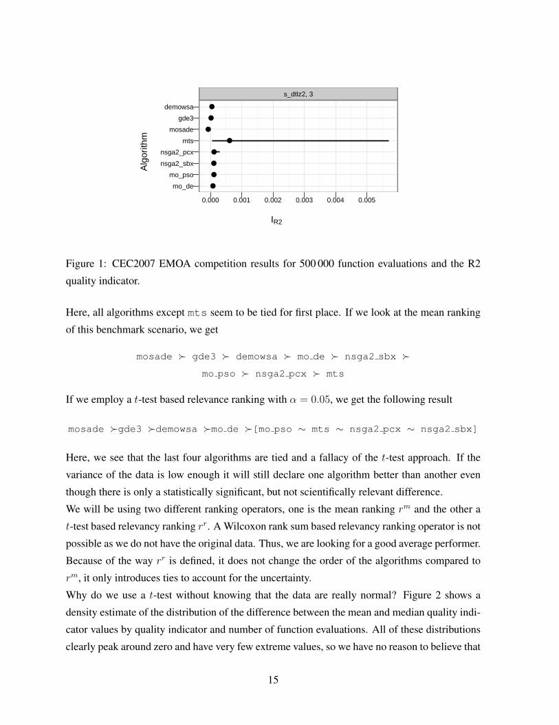
hard to see if there truly is a best algorithm. An example is s dtlz2 with a 3 dimensional

objective space, 500 000 function evaluations and the R2 quality indicator, which is visualized

in Figure 1. The dot represents the mean performance of the algorithm on the optimization

problem and the line marks the range of the quality indicator values.

14

IR2

Alg

orith

m

mo_de

mo_pso

nsga2_sbx

nsga2_pcx

mts

mosade

gde3

demowsa

s_dtlz2, 3

●

●

●

●

●

●

●

●

0.000 0.001 0.002 0.003 0.004 0.005

Figure 1: CEC2007 EMOA competition results for 500 000 function evaluations and the R2

quality indicator.

Here, all algorithms except mts seem to be tied for first place. If we look at the mean ranking

of this benchmark scenario, we get

mosade � gde3 � demowsa � mo de � nsga2 sbx �

mo pso � nsga2 pcx � mts

If we employ a t-test based relevance ranking with α = 0.05, we get the following result

mosade �gde3 �demowsa �mo de �[mo pso ∼ mts ∼ nsga2 pcx ∼ nsga2 sbx]

Here, we see that the last four algorithms are tied and a fallacy of the t-test approach. If the

variance of the data is low enough it will still declare one algorithm better than another even

though there is only a statistically significant, but not scientifically relevant difference.

We will be using two different ranking operators, one is the mean ranking rm and the other a

t-test based relevancy ranking rr. A Wilcoxon rank sum based relevancy ranking operator is not

possible as we do not have the original data. Thus, we are looking for a good average performer.

Because of the way rr is defined, it does not change the order of the algorithms compared to

rm, it only introduces ties to account for the uncertainty.

Why do we use a t-test without knowing that the data are really normal? Figure 2 shows a

density estimate of the distribution of the difference between the mean and median quality indi-

cator values by quality indicator and number of function evaluations. All of these distributions

clearly peak around zero and have very few extreme values, so we have no reason to believe that

15

100(Imed − I)

dens

ity

0

1

2

3

4

0

5

10

15

20

25

hv, 5000

0 2 4 6 8 10 12

r2, 5000

−0.4 −0.2 0.0 0.2

0

2

4

6

8

10

0

20

40

60

80

hv, 50000

0 2 4 6

r2, 50000

−1.0 −0.5 0.0

0

5

10

15

0

10

20

30

40

50

60

70

hv, 500000

−2 −1 0 1 2 3 4

r2, 500000

−1.5 −1.0 −0.5 0.0 0.5

Figure 2: Density estimates of the difference between the median and mean quality indicator

by metric and number of function evaluations. Note the change in scale to increase readability.

the distributions of the quality indicators’ means are not symmetric. Furthermore, we have 25

observations, so that the central limit theorem tells us that we are well on our way to normality.

One thing we need to check before we can use the rankings produced by rr is if they are all

transitive. This is the case, so all of the rankings are weak orderings of the algorithms. Of the

114 rankings 32 are strict rankings, meaning they are a linear order of the algorithms, which

means that rr introduces ties into 82 of the rankings. This may lead us to believe that the mean

rankings are not very accurate. As we will later see, this does not seem to be the case because

most of the consensus rankings over the two sets of rankings are in agreement.

We will use both consensus methods introduced to compare and contrast some of the results.

They will be indicated by cmBC for the Borda count consensus and cmSD/L for the SD/L con-

sensus. The original analysis of the competition used a mean ranking operator and a consensus

method that is equivalent to the Borda count method. The overall ranking that results under this

analysis regime is

nsga2 sbx � gde3 � demowsa � nsga2 pcx � mts � mo de � mosade �

mo pso.

16

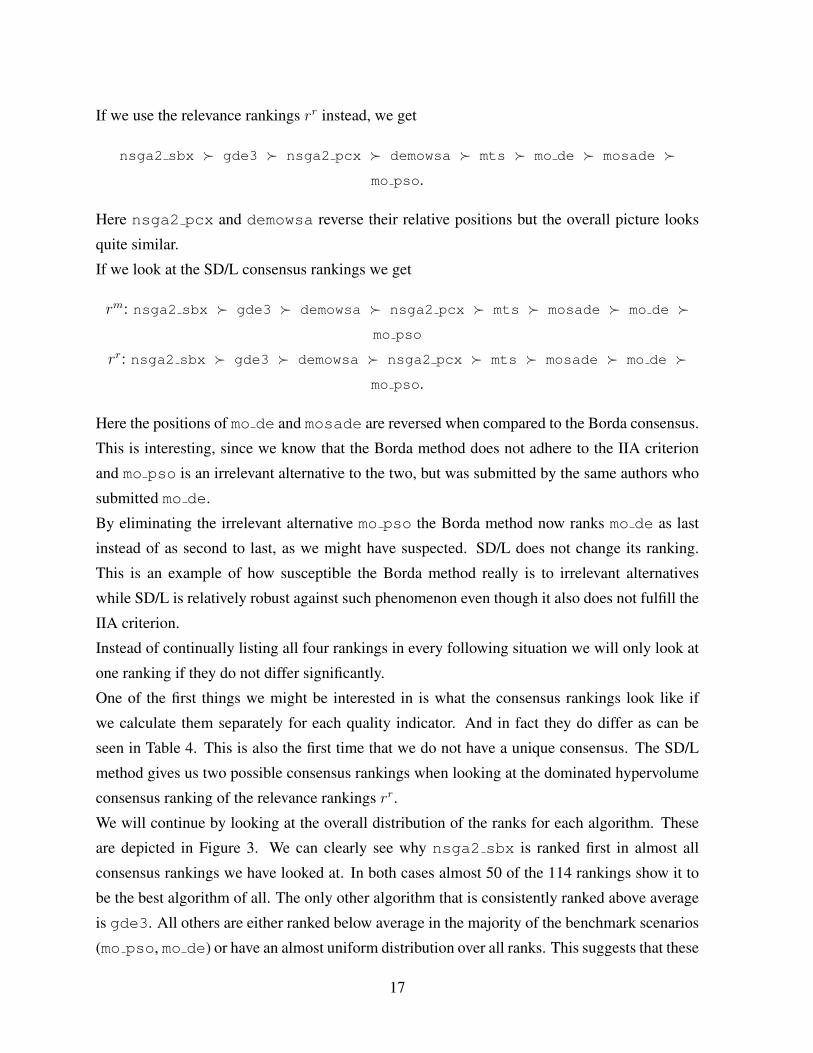
If we use the relevance rankings rr instead, we get

nsga2 sbx � gde3 � nsga2 pcx � demowsa � mts � mo de � mosade �

mo pso.

Here nsga2 pcx and demowsa reverse their relative positions but the overall picture looks

quite similar.

If we look at the SD/L consensus rankings we get

rm: nsga2 sbx � gde3 � demowsa � nsga2 pcx � mts � mosade � mo de �

mo pso

rr: nsga2 sbx � gde3 � demowsa � nsga2 pcx � mts � mosade � mo de �

mo pso.

Here the positions of mo de and mosade are reversed when compared to the Borda consensus.

This is interesting, since we know that the Borda method does not adhere to the IIA criterion

and mo pso is an irrelevant alternative to the two, but was submitted by the same authors who

submitted mo de.

By eliminating the irrelevant alternative mo pso the Borda method now ranks mo de as last

instead of as second to last, as we might have suspected. SD/L does not change its ranking.

This is an example of how susceptible the Borda method really is to irrelevant alternatives

while SD/L is relatively robust against such phenomenon even though it also does not fulfill the

IIA criterion.

Instead of continually listing all four rankings in every following situation we will only look at

one ranking if they do not differ significantly.

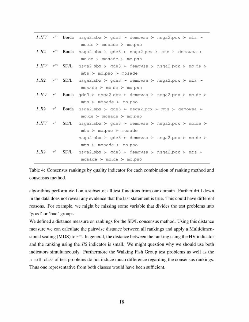
One of the first things we might be interested in is what the consensus rankings look like if

we calculate them separately for each quality indicator. And in fact they do differ as can be

seen in Table 4. This is also the first time that we do not have a unique consensus. The SD/L

method gives us two possible consensus rankings when looking at the dominated hypervolume

consensus ranking of the relevance rankings rr.

We will continue by looking at the overall distribution of the ranks for each algorithm. These

are depicted in Figure 3. We can clearly see why nsga2 sbx is ranked first in almost all

consensus rankings we have looked at. In both cases almost 50 of the 114 rankings show it to

be the best algorithm of all. The only other algorithm that is consistently ranked above average

is gde3. All others are either ranked below average in the majority of the benchmark scenarios

(mo pso, mo de) or have an almost uniform distribution over all ranks. This suggests that these

17

I HV rm Borda nsga2 sbx � gde3 � demowsa � nsga2 pcx � mts �mo de � mosade � mo pso

I R2 rm Borda nsga2 sbx � gde3 � nsga2 pcx � mts � demowsa �mo de � mosade � mo pso

I HV rm SD/L nsga2 sbx � gde3 � demowsa � nsga2 pcx � mo de �mts � mo pso � mosade

I R2 rm SD/L nsga2 sbx � gde3 � demowsa � nsga2 pcx � mts �mosade � mo de � mo pso

I HV rr Borda gde3 � nsga2 sbx � demowsa � nsga2 pcx � mo de �mts � mosade � mo pso

I R2 rr Borda nsga2 sbx � gde3 � nsga2 pcx � mts � demowsa �mo de � mosade � mo pso

I HV rr SD/L nsga2 sbx � gde3 � demowsa � nsga2 pcx � mo de �mts � mo pso � mosade

nsga2 sbx � gde3 � demowsa � nsga2 pcx � mo de �mts � mosade � mo pso

I R2 rr SD/L nsga2 sbx � gde3 � demowsa � nsga2 pcx � mts �mosade � mo de � mo pso

Table 4: Consensus rankings by quality indicator for each combination of ranking method and

consensus method.

algorithms perform well on a subset of all test functions from our domain. Further drill down

in the data does not reveal any evidence that the last statement is true. This could have different

reasons. For example, we might be missing some variable that divides the test problems into

‘good’ or ‘bad’ groups.

We defined a distance measure on rankings for the SD/L consensus method. Using this distance

measure we can calculate the pairwise distance between all rankings and apply a Multidimen-

sional scaling (MDS) to rm. In general, the distance between the ranking using the HV indicator

and the ranking using the R2 indicator is small. We might question why we should use both

indicators simultaneously. Furthermore the Walking Fish Group test problems as well as the

s zdt class of test problems do not induce much difference regarding the consensus rankings.

Thus one representative from both classes would have been sufficient.

18

rank

coun

t

02040

02040

02040

02040

02040

02040

02040

02040

rm

1 2 3 4 5 6 7 8

rr

1 2 3 4 5 6 7 8

mo_de

mo_pso

nsga2_sbx

nsga2_pcx

mts

mosade

gde3

demowsa

Figure 3: Distribution of the ranks for all rankings using the mean ranking operator and the

relevance ranking operator.

7 Conclusion and Outlook

We have developed a framework to systematically compare evolutionary multiobjective opti-

mization algorithms under different settings. We then introduced methods to combine these

rankings from different benchmark scenarios into a consensus ranking to choose the ‘best’ al-

gorithm. Here, we saw that there is no such thing as a universally best consensus and therefore

there can be no best algorithm for everyone. To illustrate this we analyzed a competition dataset

from the CEC 2007 EMOA competition.

All of the methods shown are either implemented in the R-package emoa or can easily be

constructed from the functions contained in the emoa and relations packages. In the future,

we would like to study other ranking operators as well based on parametric models of the data.

Examples would include the Bradley-Terry model also used by [2] to estimate the abilities of

machine learning algorithms. Furthermore, a comprehensive survey of voting literature could

reveal more criteria which might ease the choice of a consensus method.

In addition, benchmarking is a very important issue for single-objective evolutionary optimiza-

tion as well. Modifications of the proposed methodology itself are not required. It will be

investigated which performance indicators are suited best for deriving consensus rankings for

single-objective evolutionary algorithms and which kind of test functions form a representative

19

testset in order to perform benchmarking studies in a systematic and statistically sound way.

Lastly a research group in Munich has started working on new graphical representations of

rankings [16].

Acknowledgment

This work was supported by the Collaborative Research Center SFB 823 of the German Re-

search Foundation. Special thanks to Prof. Dr. Gunter Rudolph for his constructive comments.

References

[1] J. Knowles, L. Thiele, and E. Zitzler, “A Tutorial on the Performance Assessment of

Stochastic Multiobjective Optimizers,” Computer Engineering and Networks Laboratory,

ETH Zurich, TIK Report 214, 2006.

[2] K. Hornik and D. Meyer, “Deriving consensus rankings from benchmarking experiments,”

in Advances in Data Analysis (Proc. of the 30th Ann. Conf. of the Gesellschaft fur Klassi-

fikation, R. Decker and H.-J. Lenz, Eds. Springer, Berlin, 2007, pp. 163–170.

[3] O. Mersmann, emoa: Evolutionary Multiobjective Optimization Algorithms, 2009, R

package version 0.1-0. [Online]. Available: http://www.statistik.tu-dortmund.de/∼olafm/

emoa/

[4] K. Hornik and D. Meyer, “Relations: Data structures and algorithms for relations,” 2009,

R package version 0.5-4 + modifications.

[5] K. J. Arrow, “A difficulty in the concept of social welfare,” Journal of Political Economy,

vol. 58, p. 328, 1950.

[6] D. J. Hunter, Essentials of Discrete Mathematics. Jones and Bartlett Publishers, Boston,

MA, 2008.

[7] C. A. Coello Coello, D. A. V. Veldhuizen, and G. B. Lamont, Evolutionary Algorithms for

Solving Multi-Objective Problems. Kluwer Academic Publishers, New York, 2002.

[8] E. Zitzler and L. Thiele, “Multiobjective optimization using evolutionary algorithms — A

comparative case study,” in Parallel Problem Solving from Nature V, E. A. Eiben et al.,

Eds., Springer, Berlin, 1998, pp. 292–301.

20

[9] A. Mood, F. Graybill, and D. Boes, Introduction to the Theory of Statistics. McGraw-Hill,

New York, 1974.

[10] W. D. Cook and M. Kress, Ordianl Information & Preference Structures. Prentice Hall,

Upper Saddle River, NJ, 1992.

[11] J. C. de Borda, “Memoire sur les Elections au scrutin,” Historie de l’Academie Royale des

Sciences, 1781.

[12] D. G. Saari, “The optimal ranking method is the borda count,” Northwestern University,

Center for Mathematical Studies in Economics and Management Science, Discussion

Papers 638, 1985. [Online]. Available: http://ideas.repec.org/p/nwu/cmsems/638.html

[13] J. G. Kemeny and J. L. Snell, Mathematical Models in the Social Siences. MIT Press,

Cambridge, MA, 1972.

[14] D. G. Saari and V. R. Merlin, “A geometric examination of kemeny’s rule,” Social Choice

and Welfare, vol. 17, p. 2000, 1997.

[15] V. L. Huang, A. K. Qin, K. Deb, E. Zitzler, P. N. Suganthan, J. J. Liang, M. Preuss, and

S. Huband, “Problem definitions for performance assessment on multi-objective optimiza-

tion algorithms,” Nanyang Technological University, Tech. Rep., January 2007.

[16] M. J. A. Eugster, T. Hothorn, and F. Leisch, “Exploratory and inferential analysis of bench-

mark experiments,” Ludwigs-Maximilians-Universitat Munchen, Department of Statis-

tics, Tech. Rep. 30, 2008.

21