PDMC 2003

Benchmarking Explicit State Parallel ModelCheckers

Mike Jones and Eric G. Mercer 1,2

Tonglaga Bao and Rahul Kumar and Peter Lamborn 3,4,5

Verification and Validation LaboratoryDepartment of Computer Science

Brigham Young UniversityProvo, USA

Abstract

This paper presents a set of benchmarks and metrics for performance reporting inexplicit state parallel model checking algorithms. The benchmarks are selected forcontrollability, and the metrics are chosen to measure speedup and communicationoverhead. The benchmarks and metrics are used to compare two parallel modelchecking algorithms: partition and random walk. Implementations of the partitionalgorithm using synchronous and asynchronous communication are used. Metricsare reported for each benchmark and algorithm for up to 128 workstations usinga network of dynamically loaded workstations. Empirical results show that loadbalancing becomes an issue for more than 32 workstations in the partition algorithmand that random walk is a reasonable, low overhead, approach for finding errorsin large models. The synchronous implementation is consistently faster than theasynchronous. The benchmarks, metrics and results given here are intended to bea starting point for a larger discussion of performance reporting in parallel explicitstate model checking.

1 Introduction

The usefulness of explicit state model checking is limited by the capacity ofavailable computational resources. Parallel explicit state model checking ad-dresses capacity limitations by aggregating the memory and processing powerof several computational nodes. The first parallel explicit state model checking

1 Email: jones@cs.byu.edu2 Email: egm@cs.byu.edu3 Email: tonglaga@hotmail.com4 Email: rahul@cs.byu.edu5 Email: pcl@email.byu.edu

This is a preliminary version. The final version will be published inElectronic Notes in Theoretical Computer Science

URL: www.elsevier.nl/locate/entcs

Jones et al.

algorithm was given by Stern and Dill in [8]. Recently, several other parallelexplicit state model checkers have been successfully implemented [3,5,7]. Ineach case, new algorithms use the same basic architecture as the original algo-rithm: the table of visited states is partitioned and distributed across availablenodes and successors are computed by the node that owns a state.

The primary obstacle to designing and comparing novel parallel or dis-tributed model checking algorithms is a lack of performance data. Perfor-mance data from existing algorithms can be used to identify and eliminatebottlenecks while performance data from a new algorithm can be used tomore precisely demonstrate improvement.

In the longer term, a standardized set of benchmarks and metrics mayyield performance data that can be used to compare the relative strengthsof different algorithms and implementations. Correlating the relative meritsof the various extant approaches, however, is difficult due to the diversity ofbenchmarks and metrics used in various publications. Each paper describingeach algorithm presents results for a different model checking problem, andoften reports a unique set of metrics, aside from speedup. Although someapproaches provide a parameterized equation to predict performance, there isoften not enough empirical results to give confidence in the predictor. Thelack of consensus in benchmark characterization and reporting obscures themerits of new approaches to parallel model checking.

We do not intend for this paper to solve the problem of standardizingbenchmarks and metrics for parallel model checking algorithms. Instead, weintend to bring attention to the issue and open a dialog on a sufficient and com-plete set of benchmarks and metrics for parallel model checking algorithms.

In addition to giving a preliminary set of benchmarks and metrics, we usethe benchmarks and metrics to analyze the performance of two parallel modelchecking algorithms. We give results for the original partitioned hashtablealgorithm due to Stern and Dill [8] and parallel random walk. We give resultsfor two implementations of the partition algorithm: one using synchronouscommunication and the other asynchronous.

The random state generation starts at an initial state and randomly chooseseither to visit a successor from the enabled transitions or to backtrack to aprevious state in the current path. Random walk was used as a baselinecomparison. Uncoordinated, parallel random walks are perhaps the simplestway to find errors and prove correctness. Non-trivial parallel model checkingalgorithms, such as the partitioning algorithm , should show measurable im-provements over parallel random walks. As will be seen in the results thatfollow, random walk is at least competitive and perhaps superior to otherexplicit model checking algorithms when searching for errors in large mod-els. The partition algorithm with synchronous communication consistentlyoutperformed the partition algorithm with asynchronous communication.

Results are given on a network of workstations (NOWs) consisting of up to128 dynamically loaded processors. The analysis revealed that load balancing

2

Jones et al.

can be a problem for the partition algorithm on more than 32 nodes and thatrandom walk can be a reasonable strategy for finding errors.

The next section surveys the benchmarks and metrics reported in variousparallel explicit state model checking publications. Section 3 gives four modelsfor use as benchmarks. Section 4 proposes a set of metrics for reportingparallel model checking results. Section 5 describes the two algorithms whichwe analyze using the proposed metrics and benchmarks. Section 6 containsexperimental results and includes an analysis of the significant issues raisedby the results. Section 7 gives our conclusions about the proposed metrics andbenchmarks and points out inadequacies that should be addressed in futurework.

2 Survey of Published Benchmarks and Metrics

A survey of the literature shows no intersection in benchmark models used todescribe parallel model checking algorithms and little overlap in measures usedto describe benchmark problems. In one case, a set of error-free benchmarksconsisting of Lamport’s bakery algorithm, the leader selection algorithm fromthe SPIN distribution, and the dining philosophers problem was considered in[7]. In another paper, an alternating bit protocol and simple elevator modelwith errors and sizes ranging from 20 to 218k states are reported in [3]. Severalerror-free protocol problems are benchmarked in [5] and in [8]. ranging from40k to 20M states. Stern and Dill do include the bytes per state and thediameter of the reachable state space in their protocols in [8].

There is some consensus in the metrics reported among published results,but results are uniformly limited to a relatively small number of nodes. Aver-age running time and average peak memory usage over the number of partic-ipating processors is consistently reported in most publications. However, itis not clear if the running time is real time or CPU time. Not all publicationsreport a speedup metric, and the algorithm used as a basis for the speedupis not clear from those that do publish speedup. Some publications reportvisited states and transitions to characterize algorithm behavior. [7,3]. Ofparticular interest, however, is the number of nodes considered. Experimentson NOWs do not exceed 32 participating nodes.

3 Models

There are no obvious well defined criteria for selecting models for benchmark-ing model checking algorithms, so we suggest several models and explain ourselection process. Our models and criteria open a dialog to begin building aset of generally accepted publicly available models for reporting and relativecomparison. The suggested models are neither complete nor sufficient andthe selection criteria cannot be directly mapped to real designs. This type of

3

Jones et al.

critical analysis still remains to be completed. 6

A necessary component in the selection criteria is that the models existin as many input formats as possible and generate nearly identical state andtransition counts in a variety of tools. This criteria helps give a referencepoint for as large an audience as possible. The three benchmarks proposedin this work are written for either Murϕ or SPIN, since these tools are astarting point for much research in parallel model checking algorithms (exceptthe work in real time parallel model checking in UPPAAL [5], but we do notconsider timed benchmarks in this paper). As new input languages emerge, itwill be important to migrate benchmark models to those new languages.

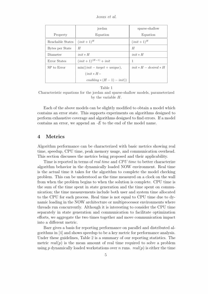
Another important component in the selection criteria is the ability tocontrol the model characteristics. The jordan and ss7-E models in our bench-mark set are included because the size and shape of their state space, as wellas the location and frequency of their errors, are controlled by relatively fewparameters. Although the jordan and ss7-E models do not reflect any realphysical system or protocol, the model parameters can be manipulated toresemble characteristics observed in real systems Both models consist of anarray of counters that are incremented, decremented, or reset according toa few simple rules. Table 1 gives parameterized equations that describe themodel characteristics. The variable init is a value between 0 and 256 used toinitialize all of the counters in the array. The variable H is the size of the array(e.g., the number of counters in the model). The size of the reachable statespace, bytes per state, diameter, and number of error states can be completelycontrolled with these 2 parameters.

The final characteristic equation relates to the shortest path to error (SPto Error) in the reachable state space and requires additional parameters tobe computed. In the jordan model, target is the error state and unique is thelength of the sequence of unique transitions to the error. The enabled variabledescribes the state in which the unique transitions begin.

The third model in the benchmark set is atomix and is included for itsirregular state structure. Atomix is a single-player game where the goal isto form a specified molecule from atoms that are randomly distributed in agrid. The simulation picks an atom and a direction (up, down, left or right)and moves the atom in the chosen direction until it hits either an obstacle oranother atom and then repeats the move process until it creates the specifiedmolecule—the error state. The characteristics of the reachable state space areaffected by the size of the grid, as well as the number of obstacles inserted intothe grid—adding obstacles reduces the size of the state space. The difficultyof locating the error is affected by the complexity of the specified molecule.There are never more atoms in the grid than are necessary to construct themolecule. The error can be strategically placed to expose various propertiesof the model checking algorithm.

6 All of the models used in the paper are be available at vv.cs.byu.edu

4

Jones et al.

jordan sparse-shallow

Property Equation Equation

Reachable States (init + 1)H (init + 1)H

Bytes per State H H

Diameter init ∗H init ∗H

Error States (init + 1)(H−1) + init 1

SP to Error min((init − target + unique), init ∗H − desired ∗H

(init ∗H−enabling ∗ (H − 1)− init))

Table 1Characteristic equations for the jordan and sparse-shallow models, parameterized

by the variable H.

Each of the above models can be slightly modified to obtain a model whichcontains an error state. This supports experiments on algorithms designed toperform exhaustive coverage and algorithms designed to find errors. If a modelcontains an error, we append an -E to the end of the model name.

4 Metrics

Algorithm performance can be characterized with basic metrics showing realtime, speedup, CPU time, peak memory usage, and communication overhead.This section discusses the metrics being proposed and their applicability.

Time is reported in terms of real time and CPU time to better characterizealgorithm behavior in the dynamically loaded NOW environment. Real timeis the actual time it takes for the algorithm to complete the model checkingproblem. This can be understood as the time measured on a clock on the wallfrom when the problem begins to when the solution is complete. CPU time isthe sum of the time spent in state generation and the time spent on commu-nication; the time measurements include both user and system time allocatedto the CPU for each process. Real time is not equal to CPU time due to dy-namic loading in the NOW architecture or multiprocessor environments wherethreads run concurrently. Although it is interesting to consider the CPU timeseparately in state generation and communication to facilitate optimizationefforts, we aggregate the two times together and move communication impactinto a different metric.

Barr gives a basis for reporting performance on parallel and distributed al-gorithms in [4] and shows speedup to be a key metric for performance analysis.Under these guidelines, Table 2 is a summary of our reporting statistics. Themetric real(p) is the mean amount of real time required to solve a problemusing p dynamically loaded workstations over n runs. real(p) is either the time

5

Jones et al.

to completely enumerate the reachable state space or reach an occurrence ofan error in the problem. S (p) is the classical definition of speedup relative tothe fastest known serial algorithm running on a dynamically loaded worksta-tion in the NOW architecture [4]. The fastest serial code for model checking isnot well defined. As such, it is tempting to revert to a relative speedup givenby:

RS(p) =Time to solve with parallel code on a single processor

Time to solve with parallel code on p processors

There is danger in relative speedup, however, because it is a self comparison;thus, we propose the computation of S (p) relative to either sequential SPIN orMurϕ –whichever is faster. Although real(p) and S (p) give a good indicationof performance, the do not fully describe algorithm behavior.

An algorithm and its implementation can be more effectively described bya brief summary of CPU time, memory behavior, and communication profiles.The CPU (p) and MEM (p) metrics in Table 2 return the mean amount ofCPU time and peak memory used by workstation p in the NOW architectureto solve a model checking problem. Although the individual statistics areinteresting, they are not easily reported; thus, we use the summary statistics ofthe minimum, maximum, and aggregate metrics instead. This brief summarygive insight without overwhelming the reader with data.

The COM (p) statistic describes the message passing behavior of the al-gorithm to show a more complete picture of communication. Specifically,C = COM (p) is a p × p matrix where each entry Cij is the mean number ofstates sent from workstation i to workstation j in solving the model checkingproblem. Although this matrix can be reported in raw form, it can also bevisualized as a surface or a stacked bar chart.

The proposed metrics are designed for describing the behavior of explicitstate enumeration model checkers on a cluster of workstations. Different setsof metrics would be needed for symbolic model checkers or any model checkeron a distributed shared memory architecture. While metrics for these settingsare of interest, they are beyond the scope of this paper.

5 Algorithms

The following sections give a high level description of the behavior and imple-mentation of each algorithm.

5.1 Random Walk

The parallel random walk consists of each node randomly generating statesin isolation. Each random walk process stores the path to the current activestate. The random state generation starts at an initial state and randomlychooses either to visit a successor from the enabled transitions or to backtrackto a previous state in the current path. It is possible that the successor is a

6

Jones et al.

Metric Definition

real(p) mean real time to complete using p processors

S (p) fastest serial code on workstationreal(p)

CPU (p) mean CPU time for processor p

CPU min(n) mini∈n(CPU (i))

CPU max(n) maxi∈n(CPU (i))

CPU agg(n)∑

i∈n(CPU (i))

MEM (p) mean peak memory usage for processor p

MEM min(n) mini∈n(MEM (i))

MEM max(n) maxi∈n(MEM (i))

MEM agg(n)∑

i∈n(MEM (i))

COM (p) p x p communication matrix

Table 2A table describing proposed metrics for standardized reporting.

previously visited state. The probability of backtracking is a function of thecurrent walk depth. As the depth increases, the probability of backtrackingincreases. The maximum probability of backtracking, the depth at which theprobability reaches half of maximum and the rate of increase can be set bythe user.

Parallel random walk requires communication only to initiate and ter-minate the search. The search is initiated by a request from a controllingprocess. Upon receiving a initiation request, a participating node begins gen-erating random walks until either finding and error or receiving a terminationrequest. When a node finds an error, that node sends the path to the errorto the controlling node. The controlling node can be configured to stop onthe first error or stop on a user request. In either case, the controlling nodeterminates the search by sending a termination request to every participatingnode.

5.2 Partitioned Hash Table

The partitioned hash table (PHT) algorithm is a reimplementation of the al-gorithm presented by Stern in [8], only it uses MPI instead of sockets. A nodewaits for incoming states on the network and inserts them into the wait andpassed queues if they are new states. The node removes states from the waitqueue, generates all successor states, and then sends them to owning nodesaccording to a global hash function. PHT buffers states in packets being sent

7

Jones et al.

Table 3Standardized performance report for the atomix model.

2 4 8 16 32 64 96 128

real(n)

PHTA 25:40 20:42 15:09 9:27 7:32 6:35 5:19 3:59

PHTS 32:28 17:31 18:26 2:51 3:36 2:46 2:15 3:31

RW* 39:42:17 19:51:08 9:55:34 4:57:47 2:28:54 1:14:27 49:37 37:13

CPU min(n)

PHTA 21:08 9:32 5:41 2:48 2:40 50 25 23

PHTS 31:40 16:49 7:16 2:30 1:31 1:47 26 12

CPU max(n)

PHTA 21:23 16:17 11:47 7:23 5:36 4:51 3:50 1:40

PHTS 32:04 17:20 15:34 2:34 3:13 1:04 52 1:51

CPU agg(n)

PHTA 42:31 53:56 1:14:39 1:32:49 2:09:07 3:18:51 3:32:24 2:01:53

PHTS 1:08:04 1:08:35 1:15:48 41:06 1:07:22 7:38:06 1:01:53 3:20:24

across the network to improve communication performance. Termination ishandled with Dijkstra’s token termination algorithm [6].

The PHT algorithm is implemented using an asynchronous (PHTA) andsynchronous (PHTS) state passing communication architecture in MPICH1.2.5. MPICH 1.2.5 is an open source implementation of the Message PassingInterface (MPI) standard that provides portability between various computerarchitectures and communication fabrics [2,1]. The asynchronous communi-cation architecture has 2 threads that communicate through shared memory,to separately handle the communication and state generation parts of thePHT algorithm. The synchronous architecture is not multithreaded and in-terleaves communication with state generation using non-blocking send andreceive calls. The purpose of the asynchronous and synchronous architecturesis comparison to see which scheme gives better performance.

6 Results

Tables 3 through 7 contain the results of running the algorithms in Section 5 onthe problems described in Section 3 using the applicable metrics of Section 4.For all testing purposes the following machine configurations and hardwarewas used:

• 40 Single Processor Pentium 3 1 GHz with 380 MB RAM

• 100 Single Processor Pentium 4 2.5 GHz with 750 MB RAM

8

Jones et al.

Table 4Standardized performance report for the jordan model.

2 4 8 16 32 64 96 128

real(n)

PHTA 25:44 23:39 11:36 9:03 3:53 4:08 4:26 3:47

PHTS 25:27 22:06 7:13 3:19 2:23 1:34 1:25 1:50

CPU min(n)

PHTA 14:26 8:42 4:19 3:29 1:18 57 15 24

PHTS 22:56 15:37 4:41 2:11 1:27 24 31 23

CPU max(n)

PHTA 17:32 10:48 5:34 4:32 1:51 1:44 2:31 1:31

PHTS 23:14 19:37 6:43 3:07 2:01 41 40 42

CPU agg(n)

PHTA 31:59 39:01 39:38 1:04:45 51:06 1:23:06 2:07:57 1:56:19

PHTS 46:10 1:08:13 46:18 39:50 1:03:12 23:24 37:46 48:01

Table 5Standardized performance report for the Atomix-E model.

2 4 8 16 32 64 96 128

real(n)

PHTA 20:33 12:31 6:55 3:00 2:13 1:14 2:33 1:53

PHTS 24:43 6:06 1:29 51 45 1:01 1:56 2:22

RW dnf dnf dnf 7:06 8:40 3:54 6:57 2:59

CPU min(n)

PHTA 8:06 2:18 2:15 10 13 0 1 0

PHTS 5:13 3:01 30 37 17 3 4 3

RW 0 5:41 2:29 3:25 36

CPU max(n)

PHTA 8:19 3:09 3:11 1:03 27 18 23 11

PHTS 6:52 5:48 55 38 23 11 19 22

RW 15:18 16:48 5:50 29:01 6:37

CPU agg(n)

PHTA 7:20 15:32 21:36 10:53 10:39 6:35 12:19 10:21

PHTS 12:06 18:17 12:51 10:09 11:49 8:10 12:59 19:04

RW 27:57 56:06 1:57:01 2:40:47 4:35:11 5:27:18 10:06:07 6:10:32

9

Jones et al.

Table 6Standardized performance report for the ss7-E model.

2 4 8 16 32 64 96 128

real(n)

PHTA dnf dnf dnf dnf dnf dnf dnf dnf

PHTS dnf dnf dnf dnf dnf dnf dnf dnf

RW dnf 8:09 3:32 1:27 2:52 32 30 44

CPU min(n)

RW 9:13 5:03 2:39 57 1:23 9 2 9

CPU max(n)

RW 14:47 8:05 5:27 1:29 3:46 40 29:01 29:13

CPU agg(n)

RW 24.15 23:20 31:18 20:06 1:12:42 32:11 43:31 1:51:38

Table 7Memory allocated for all models, measured in megabytes.

2 4 8 16 32 64 96 128

MEM min(n)

PHTA 200 100 50 25 25 20 15 15

PHTS 200 100 50 25 25 20 15 15

RW 1 1 1 1 1 1 1 1

MEM max(n)

PHTA 200 100 50 25 25 20 15 15

PHTS 200 100 50 25 25 20 15 15

RW 1 1 1 1 1 1 1 1

MEM agg(n)

PHTA 400 400 400 400 800 1280 1440 1920

PHTS 400 400 400 400 800 1280 1440 1920

RW 2 4 8 16 32 64 96 128

• Every workstation is connected to a 100 Mbits/second Ethernet connection

Tables 3 through 5 report real and CPU time use. The times for randomwalk (RW) are extrapolated from a polynomial approximation of the covertimes for a subset of each model. Table 7 gives aggregate and individual nodememory use. In each table, times are given in the form hours:minutes:secondsand memory is reported in Megabytes.

10

Jones et al.

In the tables, “dnf” means the algorithm did not finish on the given model.For the partition algorithm, this means the states to be stored exceeded theavailable memory on at least one node. For the random walk algorithm, thismeans no node found the error after 15 minutes of search time.

The difference between CPU min(p) and CPU max(p) for p = 64 in Ta-ble 3 would seem to indicate load balancing problems for the partition algo-rithm on the atomix model. Consider, however, the corresponding numbersfor the random walk algorithm in Table 5 and Table 6. It appears that bothapproaches report the same variation in minimum and maximum CPU time.Associating the variance with load balancing in the algorithm is inconsistentsince each node in the random walk has an equal load. The variance in therandom walk may be a measure of the dynamic load on the individual work-stations; thus, the CPU min(p) and CPU max(p) should be considered inthat light in conjunction with the results from COM (p).

The expected cover time for random walk grows exponentially in the num-ber of reachable states. The expected cover time for the atomix model, with2.97 M states, is 37:13 on 128 nodes while the expected cover time on thejordan model, with 7.53 M states, is 11,638 hours. The cover time growsquickly because the number of new unique states generated is logarithmic inthe number of states visited by a random walk. In other words, exponentiallymore states must be generated to find each new unvisited state.

As can be noticed from Tables 3 and 4 the speedup when using a syn-chronous model of communication (PHTS) is greater than the speedup achievedwhen using an asynchronous model of communication (PHTA). In general thereal time taken by PHTS is less than the time taken by PHTA even though thecumulative time can be greater. This observation would suggest that PHTAactually spends more time waiting for communication to complete completelyrather than performing the operation of verification and PHTS spends lesstime waiting for communication and more time on verification.

Generalizing real(p) for locating invariant violations is difficult becausereal(p) depends entirely on the search order and error location. However,claims can be made for individual problems and algorithms. For the atomix-Eproblem, the partition algorithm finds errors 2-3 times faster than randomwalk on the same number of nodes. But for the ss7-E problem, random walkfinds an invariant violation rather quickly while partition never finds an in-variant violation before exhausting the memory available on at least one ofthe nodes.

Aggregate memory use in Table 7 varies only with p due to the staticallocation of hashtables in the Murϕ implementation. This means each node’shashtable must be large enough to contain the maximum number of statesthat must be stored by any single node participating in the search. Thisproblem is exacerbated when the states are not evenly distributed betweenthe participating nodes.

11

Jones et al.

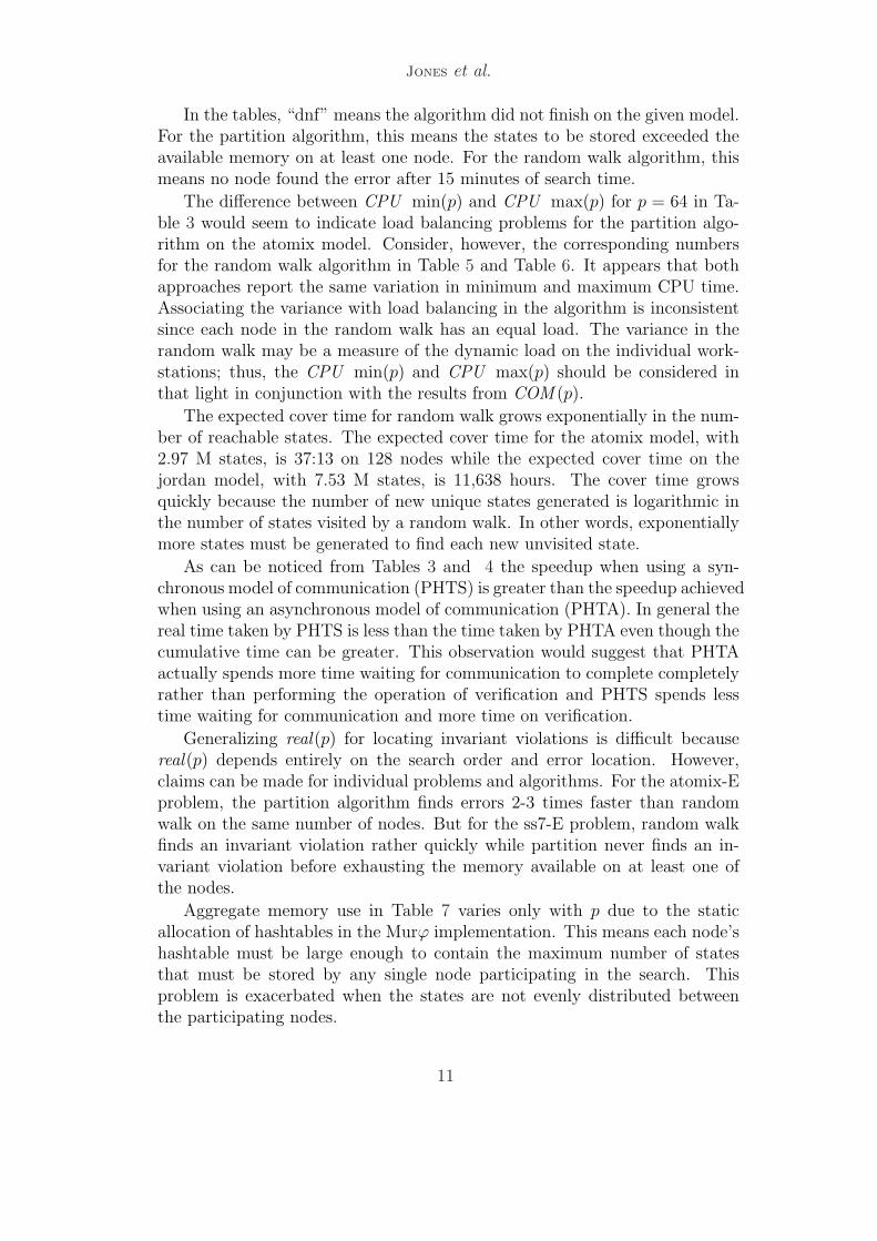
Figures 1(a), 1(b), and 2(a) show the speedup obtained by each algorithmfor the atomix, atomix-E and jordan models. Speedups are relative to se-quential Murϕ running times. No speedup results are given for ss7-E becausess7-E is not tractable for sequential Murϕ. No algorithm achieved linear, ornear-linear speedup, on any problem. The partition algorithm achieved goodspeedup for less than 32 processors on exhaustive analysis of the jordan andatomix models. While the speedup curve climbs between p = 64 and p = 128for the atomix problem, we note that partition on 128 processors achieved aspeedup of 12.1. We do not expect the curve to continue at the same slopefor p > 128. The lack of speedup for more than 32 processors could be dueto either the small problem size or the poor load balancing indicated by theCPU time metrics for p > 32 in Tables 3 and 4.

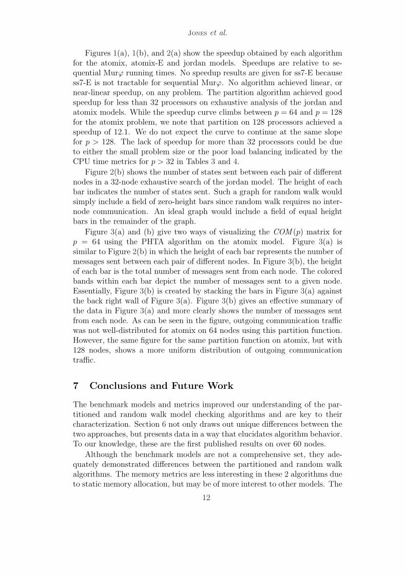
Figure 2(b) shows the number of states sent between each pair of differentnodes in a 32-node exhaustive search of the jordan model. The height of eachbar indicates the number of states sent. Such a graph for random walk wouldsimply include a field of zero-height bars since random walk requires no inter-node communication. An ideal graph would include a field of equal heightbars in the remainder of the graph.

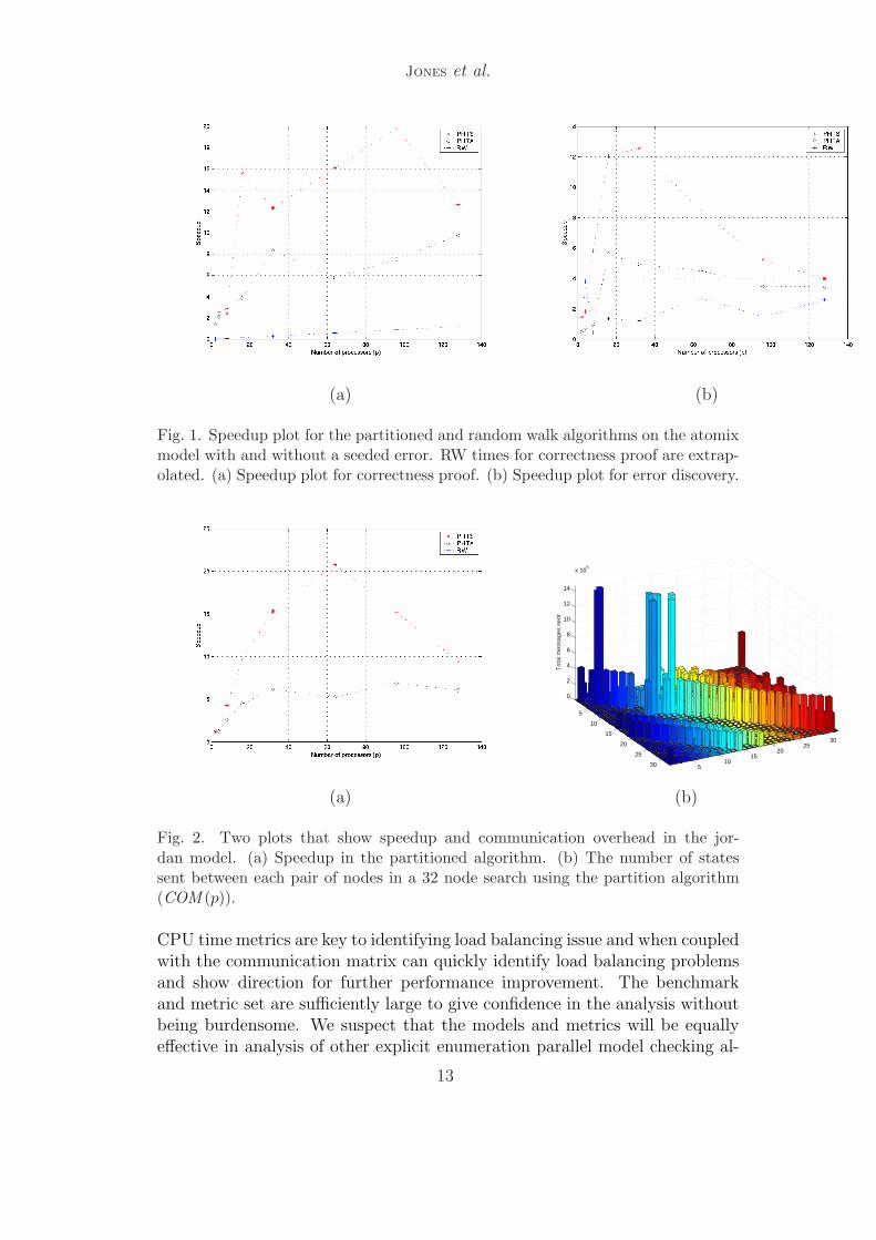
Figure 3(a) and (b) give two ways of visualizing the COM (p) matrix forp = 64 using the PHTA algorithm on the atomix model. Figure 3(a) issimilar to Figure 2(b) in which the height of each bar represents the number ofmessages sent between each pair of different nodes. In Figure 3(b), the heightof each bar is the total number of messages sent from each node. The coloredbands within each bar depict the number of messages sent to a given node.Essentially, Figure 3(b) is created by stacking the bars in Figure 3(a) againstthe back right wall of Figure 3(a). Figure 3(b) gives an effective summary ofthe data in Figure 3(a) and more clearly shows the number of messages sentfrom each node. As can be seen in the figure, outgoing communication trafficwas not well-distributed for atomix on 64 nodes using this partition function.However, the same figure for the same partition function on atomix, but with128 nodes, shows a more uniform distribution of outgoing communicationtraffic.

7 Conclusions and Future Work

The benchmark models and metrics improved our understanding of the par-titioned and random walk model checking algorithms and are key to theircharacterization. Section 6 not only draws out unique differences between thetwo approaches, but presents data in a way that elucidates algorithm behavior.To our knowledge, these are the first published results on over 60 nodes.

Although the benchmark models are not a comprehensive set, they ade-quately demonstrated differences between the partitioned and random walkalgorithms. The memory metrics are less interesting in these 2 algorithms dueto static memory allocation, but may be of more interest to other models. The

12

Jones et al.

(a) (b)

Fig. 1. Speedup plot for the partitioned and random walk algorithms on the atomixmodel with and without a seeded error. RW times for correctness proof are extrap-olated. (a) Speedup plot for correctness proof. (b) Speedup plot for error discovery.

510

1520

2530

5

10

15

20

25

30

0

2

4

6

8

10

12

14

x 105

Tot

al m

essa

ges

sent

(a) (b)

Fig. 2. Two plots that show speedup and communication overhead in the jor-dan model. (a) Speedup in the partitioned algorithm. (b) The number of statessent between each pair of nodes in a 32 node search using the partition algorithm(COM (p)).

CPU time metrics are key to identifying load balancing issue and when coupledwith the communication matrix can quickly identify load balancing problemsand show direction for further performance improvement. The benchmarkand metric set are sufficiently large to give confidence in the analysis withoutbeing burdensome. We suspect that the models and metrics will be equallyeffective in analysis of other explicit enumeration parallel model checking al-

13

Jones et al.

(a) (b)

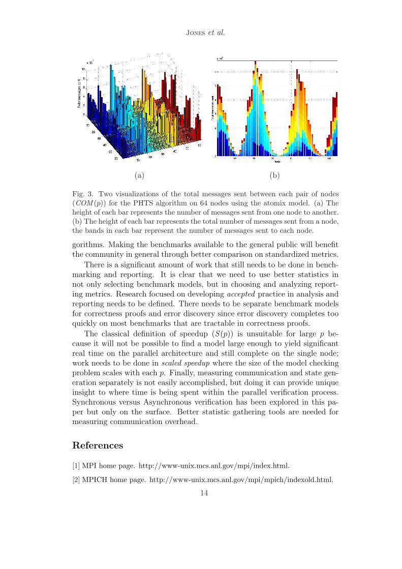
Fig. 3. Two visualizations of the total messages sent between each pair of nodes(COM (p)) for the PHTS algorithm on 64 nodes using the atomix model. (a) Theheight of each bar represents the number of messages sent from one node to another.(b) The height of each bar represents the total number of messages sent from a node,the bands in each bar represent the number of messages sent to each node.

gorithms. Making the benchmarks available to the general public will benefitthe community in general through better comparison on standardized metrics.

There is a significant amount of work that still needs to be done in bench-marking and reporting. It is clear that we need to use better statistics innot only selecting benchmark models, but in choosing and analyzing report-ing metrics. Research focused on developing accepted practice in analysis andreporting needs to be defined. There needs to be separate benchmark modelsfor correctness proofs and error discovery since error discovery completes tooquickly on most benchmarks that are tractable in correctness proofs.

The classical definition of speedup (S (p)) is unsuitable for large p be-cause it will not be possible to find a model large enough to yield significantreal time on the parallel architecture and still complete on the single node;work needs to be done in scaled speedup where the size of the model checkingproblem scales with each p. Finally, measuring communication and state gen-eration separately is not easily accomplished, but doing it can provide uniqueinsight to where time is being spent within the parallel verification process.Synchronous versus Asynchronous verification has been explored in this pa-per but only on the surface. Better statistic gathering tools are needed formeasuring communication overhead.

References

[1] MPI home page. http://www-unix.mcs.anl.gov/mpi/index.html.

[2] MPICH home page. http://www-unix.mcs.anl.gov/mpi/mpich/indexold.html.

14

Jones et al.

[3] J. Barnat, L. Brim, and I. Cerna. Property driven distribution of nested DFS.Technical Report VCL-2002, Faculty of Informatics, Masaryk University, 2002.

[4] R. Barr and B. Hickman. Reporting computational experiments with parallelalgorithms: Issues, measures, and experts. INFORMS Journal on Computing,5(1):2–18, 1993.

[5] G. Behrmann. A performance study of distributed timed automata reachabilityanalysis. In Michael Mislove, editor, Workshop on Parrallel and DistributedModel Checking 2002, volume 68 of Electronic Notes in Theorical ComputerScience, pages 7–23, Brno, Czech Republic, August 2002. Springer-Verlag.

[6] Vipin Kumar, Ananth Grama, Anshul Gupta, and Geroge Karypis. Introductionto Parallel Computing: Deisgn and Analysis of Algorithms. Benjamin/CummingsPublishing Company, 1993.

[7] F. Lerda and R. Sisto. Distributed-memory model checking in SPIN. In TheSPIN Workshop, volume 1680 of Lecture Notes in Computer Science. Springer,1999.

[8] Ulrich Stern and David L. Dill. Parallelizing the Murϕ verifier. In OrnaGrumburg, editor, Computer-Aided Verification, CAV ’97, volume 1254 ofLecture Notes in Computer Science, pages 256–267, Haifa, Israel, June 1997.Springer-Verlag.

15