Multiobjective Evolutionary Algorithm With Controllable Focus on the Knees of the Pareto Front

810 IEEE TRANSACTIONS ON EVOLUTIONARY COMPUTATION, VOL. 13, NO. 4, AUGUST 2009

Multiobjective Evolutionary Algorithm withControllable Focus on the Knees of the Pareto Front

Lily Rachmawati, and Dipti Srinivasan, Senior Member, IEEE

Abstract— The optimal solutions of a multiobjectiveoptimization problem correspond to a nondominated frontthat is characterized by a tradeoff between objectives. A kneeregion in this Pareto-optimal front, which is visually a convexbulge in the front, is important to decision makers in practicalcontexts, as it often constitutes the optimum in tradeoff, i.e.substitution of a given Pareto-optimal solution with anothersolution on the knee region yields the largest improvementper unit degradation. This paper presents a selection schemethat enables a multiobjective evolutionary algorithm (MOEA)to obtain a nondominated set with controllable concentrationaround existing knee regions of the Pareto front. The preference-based focus is achieved by optimizing a set of linear weightedsums of the original objectives, and control of the extent of thefocus is attained by careful selection of the weight set basedon a user-specified parameter. The fitness scheme could beeasily adopted in any Pareto-based MOEA with little additionalcomputational cost. Simulations on various two- and three-objective test problems demonstrate the ability of the proposedmethod to guide the population toward existing knee regionson the Pareto front. Comparison with general-purpose Paretobased MOEA demonstrates that convergence on the Paretofront is not compromised by imposing the preference-basedbias. The performance of the method in terms of an additionalperformance metric introduced to measure the accuracy ofresulting convergence on the desired regions validates theefficacy of the method.

Index Terms— Genetic algorithms, multiobjective evolutionaryalgorithm (MOEA), multiobjective optimization, preference.

I. INTRODUCTION

MANY real-world engineering problems involve theoptimization of multiple conflicting objectives. The

conflict inherent in these multiobjective optimization problems(MOPs) implies that a tradeoff in the attainment level ofvarious objectives is an inherent feature of optimal solutions.Improvement to an optimal solution in one or more objectivesnecessarily entails degradation in other objectives such that,given the incomparability and noncommensurability of theobjectives, the optimization of an MOP results in a set ofsolutions characterized by tradeoffs in their objectives. Suchsolutions are said to be Pareto-optimal and their corresponding

Manuscript received January 4, 2008; revised April 24, 2008 and August19, 2008; accepted February 18, 2009. Current version published August 14,2009. This research work was supported by National University of Singapore,Research Grant WBS: R-263-000-425-112.

The authors are with the Department of Electrical and Computer En-gineering, National University of Singapore, Singapore 117576 (e-mail:[email protected]; [email protected]).

Digital Object Identifier 10.1109/TEVC.2009.2017515

objective vectors comprise a Pareto front characterized byvarying tradeoffs.

Without a clearly articulated decision-maker preference,the entire Pareto front is relevant in solving any MOP. Thissituation constitutes the norm in evolutionary multiobjectiveoptimization (EMOO), where research is focused largely ontechniques to discover an evenly distributed set of solutionsapproximating the Pareto-optimal front, e.g., [1]–[4]. Recentadaptations of other well-known stochastic meta-heuristics tosolve multiobjective problems, e.g., scatter search [5] andsimulated annealing [6], [7], are also geared toward attaining auniform sampling of the Pareto front. Equipped with the well-distributed Pareto-front approximation, the decision makerexercises his/her preference to select a final solution from thenondominated set.

In [8], Das noted that “from practical experience . . . theuser or designer usually picks a point in the middle of thesurface . . .where the Pareto surface bulges out the most’.”Interest in such solutions, also designated “knee” solutionsto signify the location of the corresponding objective vectorson the Pareto front, is also documented in [9]–[12]. Kneesolutions are attractive, as they constitute the optima in objec-tive tradeoff. A solution on the knee region of a Pareto frontexhibits significant improvement in some objectives at the costof a small deterioration of other objectives relative to otherPareto-optimal solutions located away from the knee region.The optimality in terms of tradeoff potentially translates intosignificant cost saving in practical applications.

Knee solutions can in practice be obtained a posteriori tothe generic multiobjective optimization with software toolsthat assist decision makers in analyzing the tradeoff char-acteristics of the obtained Pareto-front approximation, e.g.,the Pareto filter proposed in [9]. The availability of theapproximation of the entire Pareto front and the facility for in-teraction with a human decision maker allow a more effectivepreference-based selection in a posteriori approaches. As thenumber of objectives increases, however, post-optimal analysisbecomes prohibitively complex. A further disadvantage is thatthe uniform spread of solutions over the nondominated front,which are desirable in generic multiobjective solvers and nec-essary to accomplish effective a posteriori selection, results infew relevant solutions being available to the decision maker. Apriori formulation and incorporation of preference criteria intothe optimization as performed in [13]–[18] allow the searcheffort to be concentrated on the desired subset of the objectivespace. Algorithms such as the normal boundary intersection(NBI) technique [8] and the multiobjective evolutionary algo-

1089-778X/$26.00 © 2009 IEEE

RACHMAWATI AND SRINIVASAN: MULTIOBJECTIVE EVOLUTIONARY ALGORITHM 811

rithm (MOEA) proposed by Branke et al. [11] accomplishthe a priori preference based optimization to obtain kneesolutions. Interactive or progressive techniques can alsoachieve a selective approximation of the Pareto optima, withthe added facility of user intervention to refine the formu-lation of preference, e.g., in [19]–[22]. While advantageousin contexts where preference is changeable and/or unclear,an interactive approach is not necessary for finding kneesolutions.

The NBI technique proposed by Das is simple, although un-fortunately it requires good a priori knowledge of the extremepoints in the Pareto front to accurately find the knee solutions.Extensions to cater to problems with multiple knee regionswith nonuniform geometry were not provided either in [8].The MOEA proposed by Branke [11] does not require such apriori knowledge and could easily find solutions on multipleknee regions. However, its reliance on a global niching criteriabased on the weighted sums of objectives precludes solutionson nonconvex regions of the Pareto front and leads to possibleloss of less pronounced knee regions. The selection schemeproposed in this paper attempts to address these problems aswell as provide an additional facility of controlling the concen-tration on the knee regions. The observation that knee solutionsare local optimizers of linear aggregation with suitable weightcoefficients motivates the design of the scheme. By identifyingthese suitable weights and pursuing the local Pareto optimaof the weighted sums derived therefrom, selection pressurefavoring a controllable extent of the knee regions can beeffectively exerted.

Unlike the preceding work of the authors presented in[23], the approach presented here possesses a hybrid of thefeatures of a posteriori and a priori approaches. In [23],the identification of appropriate weighted sums is achievedimplicitly by employing evenly distributed sets of weightsand allowing solutions to compete based on the weighted sumthey rank highest in. The algorithm in [23] essentially seeksthe global Pareto optima of the identified weighted sums,and applies selective pressure favoring knee regions fromthe onset. Consequently, the success in retaining solutionsin all the knee regions and the efficacy of control overthe focus highly depend upon the geometrical properties ofthe Pareto front in question. These weaknesses are rectifiedin the new approach by performing an explicit identificationof the proper weight coefficients, thereby allowing the localoptima of the weighted sums to be pursued. The approachincludes an information-gathering first stage, where a roughapproximation of the Pareto front is sought; an identificationof potential knee regions, for each of which an analysisof the best weight coefficients is conducted; and a secondoptimization stage where the local Pareto optima of theselected weighted sums are pursued. Benefits accrued by thenew approach include improved ability of discovering kneesolutions in nonconvex parts of the Pareto front, better controlover the extent of the preference-based focus, and fewerrequired weighted sums in comparison to the earlier weighted-sum niching in [23].

As in a posteriori approaches, the ability of the proposedscheme to find desired solutions in difficult problems isenhanced by problem-specific information. At the same time,

the algorithm also affords the decision maker with a highlyrelevant solution set. Most importantly, no additional objectivefunction evaluations are needed for the entire algorithm tobe competitive with a baseline-generic MOEA in terms ofconvergence, as will be demonstrated in the empirical study.This is possible since both stages contribute directly towardpromoting proximity to the true Pareto front. Since the firstand the second stage involve the optimization of M functions(where M is the number of the original objective functions),adoption into any general-purpose population-based multiob-jective optimization algorithm that employs Pareto-dominance-based fitness to guide the search is also straightforward, andthe increase in computational cost is minimal.

The paper is organized as follows. In Section II salientconcepts are reprised and related work in the area is brieflyreviewed. In Section III the algorithm is described. In SectionIV empirical validation of the algorithm with a set of difficulttwo- and three-objective problems is presented. Two metrics toevaluate the performance of the preference-based search algo-rithm are also introduced. The paper is concluded in Section V.

II. FITNESS FUNCTION IN MULTIOBJECTIVE

OPTIMIZATION

Important concepts in EMOO are reprised and the notion oftradeoff is discussed in Section II-A. Multiobjective optimizerswith focus on the knee solutions are briefly surveyed inSection II-B.

A. Multiobjective Optimization

The MOP may be defined as follows [24]:

Find the vectors of decision variables X∗ = [x1, x2, . . . , xn]that satisfy:

p inequality constraints: gi X∗ ≥ 0, i = 1, 2, . . . , pq equality constraints: hi X∗ ≥ 0, i = 1, 2, . . . , qAnd minimize M conflicting objective functions:

F = [ f1(X∗), f2(X∗), . . . , fM (X∗)]where fm : Rn → R

The incomparability and noncommensurability betweenthe conflicting multiple objectives underlie the definitionof Pareto-optimality. A solution X is Pareto-optimal ifimprovement in any objective necessarily entails degradationin at least another objective. For any particular MOP, a set ofsolutions X are Pareto-optimal. The set of solutions constitutea Pareto-optimal set, which maps to the Pareto front in theobjective space.

Central to the Pareto-optimality criterion is the nonre-flexive, transitive, and antisymmetric binary relation, i.e.,Pareto dominance. Pareto dominance is described in thefollowing for a minimization of the set of objectivesF = [ f1, f2, . . . , fm, . . . , fM ]. For any two solution vectorsXi , X j ∈ S, solution vector Xi dominates the vector X j if andonly if Xi performs at least as well as X j in all objectives andstrictly better than X j in at least one objective, i.e.,

Xi ≺ X j ⇔ ∀m ∈ [1 . . . M],

fm(Xi ) ≤ fm(X j ) ∧ ∃l ∈ [1 . . . M], fl(Xi ) < fl(X j ). (1)


A pair of solutions for which Pareto-dominance relationdoes not apply is nondominated. The Pareto optima of anMOP comprise a nondominated solution set which correspondto the Pareto front in the objective space. The conflict betweenobjectives in an MOP implies that performance tradeoffscharacterize the Pareto-optimal front—i.e., any pair of Pareto-optimal solutions represents improvement in some objectiveand degradation in at least another objective. The magnitudeof performance tradeoffs usually varies across the Pareto front.

Tradeoff characterizes a pair of nondominated objectivevectors and may be defined as the net gain of improvement insome objectives offset by the accompanying deterioration inother objectives as a result of substituting one objective vectorwith another nondominated objective vector. Mathematicaldefinition of tradeoff is commonly given for every pair of ob-jective functions. In (2) we offer a different working definitionof tradeoff that is highly intuitive and directly employed laterin the proposed scheme

T(Xi , X j

) =∑

1≤m≤M max[0, fm(X j − fm(Xi )

]∑

1≤m≤M max[0, fm(Xi − fm(X j )

] . (2)

As the notion of tradeoff encapsulates exchange of per-formance between objectives, comparability and commensu-rability between objectives are assumed in the quantificationof tradeoff. To prevent one objective being predominant overothers, normalization is performed before T () is computed fora pair of objective vectors.

In the definition of (2) the numerator evaluates the aggre-gated improvement gained by exchanging X j with Xi whilethe denominator evaluates the deterioration effected by theexchange. The objective vector F may be of any cardinality.The definition is given in terms of objective vectors sinceobjective vectors of Pareto-optimal solutions, and not thesolutions themselves, are of central importance in the conceptof tradeoff. Without loss of generality, later discussions assumethat each solution corresponds uniquely to an objective vector.

A more concise metric to evaluate the worth of a solutionXi in terms of performance tradeoff, relative to the set ofnondominated solutions it belongs to, S, is given in thefollowing equation:

μ(Xi , S) = minj,X j ∈S,Xi ⊀X j ,X j ⊀Xi

T (Xi , X j ). (3)

In (3) X j denotes members of the set of nondominatedsolutions S and is nondominated with respect to Xi . μ(Xi , S)reflects the least amount of improvement per unit deteriorationobtained by exchanging any alternative solutions X j in thenondominated set S with Xi . A knee solution Xi correspondsto a local maximum in μ(Xi , S) computed over the Paretofront S, implying that objective vectors on and around the kneeregions are efficient in terms of tradeoff. This property rendersknee solutions of particular interest in practical contexts.

B. Related Work

Das characterized the knee solution in terms of the convexhull of individual minima (CHIM), which was defined in [8]as the set of points in Rn that are convex combinations ofF∗ − F(X∗), where F∗ is the utopia vector of the global

minima of objectives F = [ f1, f2, . . . , fm, . . . , fM ] andF(X∗

m) the objective vector of the global minimizer of fm , X∗m

[8]. Knee solutions correspond to the local maxima in terms ofthe distance from the CHIM measured along the normal to theCHIM. The nonlinear programming in [8] finds knee solutionby maximization of the distance to the CHIM. The techniquerequires an a priori estimate of F(X∗

m) for each objective m,of which accuracy is directly related to the accuracy of theobtained solution, as shown in [8].

In general, it is difficult to furnish an accurate a prioriestimate of the CHIM. It is even more so when multiple kneeregions are present in the Pareto front. As each knee regionis associated with its unique local CHIM, finding all kneesolutions requires the estimation of multiple CHIMs and thediscovery of each local maxima in terms of distance to theCHIMs. No facility to address this was provided or suggestedin Das’s work to enable discovery of multiple knee regions inthe Pareto front.

The guided MOEA proposed by Branke et al. [11] doesnot have the same shortcoming. The algorithm utilizes a localgeometrical property of knee regions, i.e., that the externalangle formed by an objective vector and its neighboringnondominated solutions is larger for objective vectors lying onthe knee region than for those otherwise situated. Maximiza-tion of the external angle subject to ties in Pareto rank canbe implemented to introduce a bias favoring knee solutions.Although effective, it is not amenable to generalization tohigher dimensional problems. An approximation of the an-gle by expected marginal utility, as measured by the linearweighted sums of objectives, was also proposed to address theissue. The larger the external angle between a solution and itsneighbors, the larger the gain in linear utility obtained fromsubstituting the neighbors with the solution of interest. Thereliance on aggregated weighted sums in the method precludesconvergence to the nonconvex parts of the Pareto front andmay result in the loss of less pronounced knee regions. Theseweaknesses are not present in the approach proposed in thispaper although it also relies on linear weighted sums. Facilityfor user control over the extent of the focus on the kneeregions, which is not available in [11], is also incorporatedin the proposed scheme.

The scheme is motivated by fact that knee solutions consti-tute local minima in terms of linear aggregation with weightcoefficients describing the CHIM, as shown in [8]. Note thatthis implies Das’s characterization of the knee solution isequivalent to the one given in (3). Given normalization of ob-jectives, the CHIM may be described by the equally weightedlinear aggregation. The minimum in this weighted sum cor-responds to the maximum in improvement–deterioration ra-tio computed over all the Pareto-front approximation. Dasfurnished a proof of the relationship between the weighted-sum minimization and the nonlinear programming he proposedbased on multiplier theory in an earlier paper [25]. One mayalternatively arrive at the conclusion that the minimum ofparticular weighted sums corresponds to the knee solution byobservation of Pareto fronts with knee, as illustrated in Fig. 1.

From an inspection of Fig. 1 it is obvious that minimizationof the weighted sum described by W1 leads to a knee solution.


f1

f2

W1

W2

W3

Knee

Fig. 1. Weighted-sum minimization in an MOP with a knee region.

While weight sets close to W1 also exhibit this property,those sufficiently different, like W2 and W3, give nonkneesolutions when minimized. Thus, it is important to identifythe appropriate weight sets, especially where multiple kneeregions are present in the Pareto front, as illustrated in Fig. 2.The required weights constitute good approximations of theindividual CHIMs.

Provided that the appropriate sets of weights are known,knee solutions can be obtained by finding the local minimato these weighted sums. Estimation of the suitable weightsets is carried out implicitly in the algorithm proposed in[23]. Q-weighted sums of of objectives are computed witha set of Q uniformly distributed weight sets. These weightedsums are then sorted according to magnitude to yield Q rankfigures for each candidate solutions. The best P rank figuresconstitute objective values to be optimized for a candidatesolution. P and Q are user-defined positive integer parameters,where P < Q. A biasing selection criterion formulated onthis strategy favors the global optima of P subsets of the Qweighted sums.

The strategy is susceptible to the loss of less pronouncedknee regions, which constitute local Pareto optima in theaggregation computed with the sets of weights describing theirrespective CHIMs but are not part of the global optima inthe very same weighted sums. While a judicious choice ofthe parameter P and a large Q minimize the loss of lesspronounced knee regions, there are extreme cases where someknee solutions cannot be obtained. An extreme example of thesituation is given in Fig. 3. No weighted sum could be found inthe case shown, in which knee solutions in region B constitutethe global minima. In comparison to these solutions, nonkneesolutions around A and C will be favored by the weighted-sum niching in [23] and the marginal utility-based approachin [11].

Another disadvantage of the weighted-sum niching in [23]is that the efficacy of control over the extent of convergenceby means of the setting of P and Q depends heavily on thecontour of the nondominated front. The issues are addressed inthe scheme proposed here, which seeks the local Pareto optima

f1

f2

Fig. 2. Multiple knee regions with differing geometrical property.

of linear aggregation with explicitly identified weight sets. Byfocusing on the local optima, the extent of convergence on theknee regions can also be easily controlled. Lower numbers ofweighted sums to be optimized and the ease of controlling theextent of convergence are further additional advantages offeredby the approach proposed in this paper. The following sectionpresents this approach in greater detail.

III. PREFERENCE-BASED SELECTION TO ATTAIN

FOCUSED CONVERGENCE ON KNEE REGIONS

This section presents a preference-based selection thatenables an MOEA to obtain a set of solutions with user-controllable concentration around the knee regions of thePareto-optimal front. The proposed fitness scheme involvesthe optimization of transformed objective functions and hencemay easily be adopted into various frameworks of an MOEAwith different population initialization, crossover and mutationtechniques (e.g., [26], [27]), and Pareto-ranking methods. Theproposed approach can also be easily incorporated into otherpopulation-based multiobjective optimization algorithms thatrely on Pareto-dominance criterion.

Two optimization stages are required. The first stage islargely similar to the generic MOEA in that the purpose isto discover a rough approximation of the Pareto front. Ananalysis performed on the obtained approximation identifiesthe local maxima in terms of tradeoff and selects the bestcorresponding weight sets. In the second stage, the sets ofweight coefficients are employed in the linear aggregations ofobjectives in lieu of the original objective functions to exertselective pressure favoring knee solutions.

The success of the scheme in finding solutions in all knee re-gions depends on the quality of the approximation obtained atthe end of stage 1. Premature termination of stage 1 may resultin the loss of knee regions. In general, the higher the amount ofcomputing resources dedicated to stage 1 of the optimization,the better the accuracy of the tradeoff analysis. However,computational resources are finite and a limit must be set forthe scheme to have practical appeal. A recommended stopping


f1

f2

C

B

A

Fig. 3. Knee region (B): local minima but not global optima of weightedsums.

criterion for stage 1 includes the requirement that at least 50%of the population of candidate solutions comprise the bestnondominated front and/or a prespecified number of objectivefunction evaluations. Further investigation into the effect ofchanging the stopping criteria will be furnished in Section IV.

The block diagram of Fig. 4 summarizes the overall se-lection strategy. Within each of stage 1 and stage 2, Pareto-based optimization of M functions is performed. Thus theapproach can be easily adapted into any MOEA with Pareto-dominance-based selection criterion. Sections III-A–E discussfurther details of stages 1 and 2 as well as the tradeoffanalysis performed to identify potential knee solutions and theestimation of the best weight coefficients.

A. Optimization Stage 1

The goal of this stage is to gain a rough approximationof the Pareto front. This can be accomplished without anymodification to any general purpose Pareto-dominance-basedMOEA.

MOEAs usually achieve the optimization goal of a well-spread nondominated front close to the true optima witha fitness function built upon Pareto-ranking and diversity-promoting criterion computed in lexicographic order. Paretoranking derives a total order from the Pareto-dominance rela-tions between candidate solutions in the population, where forevery solution pair Xi and X j , solution Xi is ranked higherthan X j if Xi dominates X j . Ties in the Pareto rank areresolved by a niching criterion, where solutions lying in lesscrowded area of the objective space are favored. The effectof such a fitness function is to promote the convergenceof a uniformly distributed nondominated front on the truePareto front. Alternatives to Pareto ranking do exist, e.g.,the maxi–min function [28], but selection criterion in most

state-of-the art MOEAs results in fitness that preserves thePareto-dominance relation, i.e., the fitness functions satisfy thefollowing:

Xi ≺ X j ⇒ Fit≺(Xi ) < Fit≺(X j ). (4)

The first stage of the algorithm is performed until adequateinformation for the tradeoff analysis has been garnered. Al-though the number of generations is the usual terminationcriterion for MOEA, it is recommended here that the per-centage of the population included in the best nondominatedset discovered thus far is employed. Once this criterion issatisfied, tradeoff analysis is conducted to identify potentialknee solutions and the associated weight sets.

B. Identification of Potential Knee Solutions

Potential knee solutions Xi in the obtained nondominatedfront S have the property of being the local minima inweighted-sum aggregations with particular weight sets asmentioned earlier. Detection of potential knee solutions usingthis property is difficult to perform when no knowledge of theappropriate weights is available. Hence detection of possibleknee solutions is carried out by indentifying the local maximain μ(Xi , S).

Let S be the subset of the population at the end of stage1 that contains the best nondominated front. μ(Xi , S) iscomputed for each Xi in S. Once this is accomplished, existinglocal maxima of the numerical data must be identified.

A number of heuristic algorithms have been proposed tofind local maxima from data, with most requiring at leastone user-supplied parameter. Here we present a very simpleheuristic that performs well. First, the difference between theof a solution Xi and that of its k nearest neighbors in theobjective space is computed, with parameter k set at 0.2N2(where N2 is the number of solutions in the best nondominatedset S). If the differences associated with the solution have apositive value of above the sum of the mean and 0.5 of thestandard deviation, the corresponding solution is designated asa potential knee solution.

C. Estimation of Appropriate Weight Coefficients

Appropriate weight coefficients must be estimated for eachpotential knee solution discovered. A set of Q evenly distrib-uted sets of weights are defined and employed in weighted-sum aggregations of the objective vectors of S, which arethe best nondominated solutions available at the end of thefirst optimization stage. The resulting aggregations for eachweight set are sorted and the rank of each solution withinthis sorted list is recorded. Hence, each solution in the bestnondominated set is associated with Q ordinal figures, eachreflecting the relative performance in terms of the linearaggregation corresponding to a specific set of weights.

Estimation of the set of weights best describing the CHIMassociated with each knee solution Xk is performed as follows.The sets of weights corresponding to which Xk is ranked in thefirst percentile are noted. That is, the weight sets correspondingto the aggregations in which the knee solution is ranked 1to 0.1N2 (where N2 is the number of solutions in the best


nondominated set) are noted and the median is taken as theestimate of the CHIM. At the conclusion of this step, eachpotential knee region is associated with a unique weight setthat estimates the corresponding CHIM.

The accuracy of the estimation depends on two factors: theability to detect potential knee solutions and the resolution ofthe Q set of weight sets. While the former depends on howwell the nondominated front approximates the shape of thetrue Pareto front and the ability of the heuristics to identifylocal maxima in the tradeoff curve, the latter depends on themagnitude of Q. It is important to note here that in the eventthat the potential knee solution identified does not in factconstitute a knee, the approach will still converge to solutionson a real knee or close to it as only the weighted sum favorssolutions near knee regions.

Once the CHIM weight-set estimate is obtained, M weightsets, where M is the number of original objective functions,are computed based on the user input parameter to controlthe extent of the focus on the knee region. Suppose theweight-set estimate for potential knee solution Xk is Wk =[wk1, . . . , wk M ], then the weight sets to be employed in theweighted-sum niching are determined by adding δe f f to oneof M weights and subtracting δe f f from another such that Mweight sets are generated where

δe f f = min [δ,wk1, . . . , wk M ] (5)

so that the weights equal to unity is not violated. That is, ifW = [w1, . . . , wM ], then the weight sets for a bi-objectiveproblem are

W′k1 =

(wk1 + δe f f

wk2 − δe f f

)(6)

and

W′k2 =

(wk1 − δe f f

wk2 + δe f f

)(7)

whereas for a tri-objective problem the weight sets are

W′k1 =

⎛⎝ wk1 + δe f f

wk2 − δe f f

wk3

⎞⎠ (8)

W′k2 =

⎛⎝ wk1

wk2 + δe f f

wk3 − δe f f

⎞⎠ (9)

W′k3 =

⎛⎝ wk1 − δe f f

wk2wk3 + δe f f

⎞⎠ . (10)

The maximum δe f f results in the set of M weight sets whichconstitute an M×M unity matrix. Thus, the original objectivesare optimized and the entire Pareto front becomes the targetof the optimization. The same set of weights is employed forMOPs containing no knee region in the nondominated front,which constitutes the special case where the tradeoff analysiscarried out yields no local maxima.

D. Optimization Stage 2

In the preceding stages, identification of potential kneesolutions Xk and derivation of their associated M weight-sets Wk1 from the respective estimated CHIMs have been

Stage 1: MOEAOptimizing F = {f}

Stage 2: MOEAOptimizing W = {w f}

Computetradeoff

Find localmaxima

Find suitablesets of weights

Fig. 4. Block diagram.

performed. The local Pareto optima to these M weight setsare pursued in this stage to obtain knee solutions that con-verge on the true Pareto front. That is, instead of F =[ f1, f2, . . . , fm, . . . , fM ], P = [p1, p2, . . . , pr , . . . , pR] areemployed in the computation of the fitness, where pr denotesthe weighted-sum aggregation of the original objective func-tions F and R is equal to R as follows:

pr =M∑

m=1

wkm fm(Xi ), wkm ∈ Wkr . (11)

The set of weight sets Wkr employed in the computation of thefunctions pr (Xi ) for each candidate solution Xi correspondsto the knee region k, whose representative is closest to Xi

in the objective space. Note that the P(Xi ) and P(X j ) arecomputed with different weight sets if they belong to differentknee regions. Population-wide Pareto ranking is conductedwith M ordinal rank figures ζ(Xi ) and ζ(X j ), obtained byranking the cardinal values of P within each knee region.Weak potential knee region, therefore, is not overshadowed bystronger ones, as the best nondominated solutions associatedwith each potential knee are included. The use of the rankfigures also leads to an even distribution of the numberof solutions across multiple potential knees. A secondaryniching criterion resolves ties in Pareto rank with an estima-tion of crowding as is usually practiced in general-purposeMOEAs.

In summary, P(Xi ) is computed and the values rankedamong solutions belonging to the same knee region to obtainζ(Xi ), which is a vector of M ordinal rank figures which areemployed in Pareto-dominance-based comparison underlyingthe fitness of (Xi ).

A fitness function designed with the above principles appliesselective pressure favoring knee solutions as well as promotesproximity to the true Pareto front. The latter is due to thefact that Pareto-dominance relation in terms of the originalobjective functions F is preserved in P for any pair of solutionsbelonging to the same knee region

F(Xi ) ≺ F(X j )

⇒∑

wkm[ fm(Xi ) − fm(X j )] < 0

⇒∑

wkm fm(Xi ) <∑

wkm fm(X j )]

⇒ P(Xi ) ≺ P(X j )

⇒ ζ(Xi ) ≺ ζ(X j ).

Effectively, the Pareto optima in the locality of each kneeregion are pursued, as the best nondominated front in termsof ζ(Xi ) is also the best nondominated front in F(Xi ) in the


vicinity of the knee. Further, the following also applies:

(ζ(Xi ) ⊀ ζ(X j )) ∧ (ζ(X j ) ⊀ ζ(Xi ))

⇒ (F(Xi ) ⊀ F(X j )) ∧ (F(X j ) ⊀ F(Xi )). (12)

The use of multiple weighted sums with distinct weight setsin the formulation of ζ(Xi ) introduces a partial order amongcandidate solutions. The partial order implies that the optimumin terms of ζ(Xi ) constitutes a set of solutions that is also asubset of the Pareto-optimal in the original objective functions.The nondominated set obtained by optimization of ζ(Xi ) is asubset of the nondominated set in F(Xi ). In particular, theseare solutions near the knees of the front, including those onnonconvex parts. Thus solutions with objective vectors lyingon nonconvex parts of the Pareto front can be retained as willbe demonstrated in the simulations.

Integration of preference information into a MOEA is thusperformed by transformation of the objective functions Finto ζ(Xi ). Adaptation of the approach into any MOEAwith dominance-based ranking, e.g., NSGA-II [3], SPEA2 [4],PESA2 [2], PAES [1], or even in multiobjective versions ofsimulated annealing [6], [7] and scatter search [5], can beperformed by simply replacing the original objective functions,irrespective of the manner in which dominance-based rankingis performed.

E. Computational Cost

Both the weighted-sum niching and the parallel localweighted-sum optimization can be easily adopted into theframework of current MOEAs. While the former approach isdesigned to be incorporated in the secondary niching criterionof MOEAs with dominance ranking, it may be incorporatedinto MOEAs with aggregative fitness functions by simpleobjective transformation. In particular, the P best rank figuresconstitute the values to be optimized instead of the originalobjective functions.

In this section, the additional computational complexity in-curred by inclusion of the preference information is analyzed.Within each of stage 1 and 2 of the second approach, Pareto-based optimization of M functions is performed. Thus theapproach can be easily adapted into any MOEA with Pareto-dominance-based selection criterion. The first optimizationstage can be performed with any algorithm that promote awell-diversified approximation of the Pareto front. The secondstage optimization is the one in which preference informationis involved in the formulation of the fitness. The local Paretooptima in terms of the appointed M weighted sum sets aresought. The weighted sums replace the original objectivefunctions in the optimization.

The parallel local weighted-sum optimization combinesproperties of a posteriori and a priori preference incorpora-tion. Problem-specific information, which is a feature of aposteriori approaches, is gained in the first optimization stagewhile focus on solutions highly likely to be relevant to thedecision maker, which is a feature of a priori approaches, isattained in the second optimization stage. Additional computa-tion cost is incurred, particularly in the one-time identification

TABLE I

ADDITIONAL COMPUTATIONAL COST INCURRED

Category Marginalutility

Weighted-sumniching

Parallel localweighted-sumoptimization

Worst case O(N 3) O(N 3) O(M N 2)

Average case O(M N 2) O(N 2 log N ) O(M N log N )

Best case O(M N 2) O(N 2) O(M N )

of potential knee regions, the computation of correspond-ing weight sets, and the modification introduced to fitnesscomputation in the second optimization stage. The additionalcost, however, is shown in this section to be insignificant andless than that associated with the marginal utility approachpresented in [11] and the weighted-sum niching in [23].

Let M be the number of objective functions, N the size ofthe population, Q the number of uniformly distributed weightsets employed in the estimation, and K the number of potentialknee regions discovered. The estimation of the weight sets in-cludes extraction of the best nondominated front, computationof tradeoff (μ(Xi , S)) and Q weighted sums, the sorting ofweighted sums, and the selection of the weight sets. The one-time estimation may be accomplished with O(M N 2) computa-tions in the worst case. During the second stage, additional costis incurred in identifying the knee region a candidate solutionbelongs to and in computing as well as sorting the M Nweighted sums. The former can be achieved with M K com-putations in the worst case, M in the best case, and 0.5M Kon average, while the latter can be easily accomplished withM N 2+M N , 2M N , and M N log N +M N computations usingquick sort in the worst, best, and average cases, respectively.

In contrast, the approach in [23] requires the computationand ranking of Q weighted sums, and extraction of the P bestranking figures each time the fitness of candidate solutionsin the population is to be evaluated throughout the entireoptimization. Achieving the same accuracy afforded by the useof a large Q implies that the additional QN 2 + QN , 2QN ,and QN log N + QN computations in the worst, best, andaverage cases, respectively, are larger. To obtain the P bestrank figures, further sorting is required, with complexity ofN Q2 + N Q, 2N Q, and N Q log Q + N Q in the worst, best,and average cases, respectively.

The utility-based approach in [11] requires the computationof utility in terms of Q randomly selected weighted sums andthe marginal utility for each candidate solution in additionto the usual Pareto ranking to obtain the fitness. Utility isdetermined with QM N computations. Marginal utility of asolution Xi evaluates the minimum utility gained by thepresence of the associated solution in the population, if Xi

constitutes the minima of the corresponding weighted sumand zero otherwise. Identification of the two solutions with thesmallest aggregations in each of the Q weighted sums as wellas computations of the difference between pairs are required toobtain the marginal utility. As the authors recommend Q to beset equal to the population size (N ), the additional computationcost is M N 2 + N 3, M N 2 + N log N and (M + 1)N 2 in theworst, best, and average cases, respectively.


TABLE II

TEST PROBLEMS

Problem Function

DO2DK f1(X) = g(X)r(X)[sin

(πx12s+1

)+ π

(1 + 2s−1

2s+2

)]; f2(X) = g(X)r(X)

[cos

(πx12 + π

) + 1]

g(X) = 1 + 9n−1

∑ni=2 xi ; r(X) = 5 + 10 (x1 − 0.5)2 + 2s/2

K cos (2Kπx1)

0 ≤ xi ≤ 1, i = 1, . . . , 30

DO2DK-1 f1(X) = g(X)r(X)[sin

(πx12s+1

)+ π

(1 + 2s−1

2s+2

)]; f2(X) = g(X)r(X)

[cos

(πx12 + π

) + 1]

g(X) = 1 + ∑ni=2 x0.1

i ; r(X) = 5 + 10 (x1 − 0.5)2 + 2s/2

K cos (2Kπx1)

0 ≤ xi ≤ 1, i = 1, . . . , 30

DEB2DK f1(X) = g(X)r(X) sin( x1π

2

); f2(X) = g(X)r(X) cos

( x1π2

)g(X) = 1 + 9

n−1∑n

i=2 xi ; r(X) = 5 + 10 (x1 − 0.5)2 + 2s/2

K cos (2Kπx1)

0 ≤ xi ≤ 1, i = 1, . . . , 30

DEB2DK1 f1(X) = g(X)r(X) sin( x1π

2

); f2(X) = g(X)r(X) cos

( x1π2

)g(X) = 1 + ∑n

i=2 x0.1i ; r(X) = 5 + 10 (x1 − 0.5)2 + 2s/2

K cos (2Kπx1)

0 ≤ xi ≤ 1, i = 1, . . . , 30

DEB2DK2 f1(X) = g(X)r(X) sin3 ( x1π2

); f2(X) = g(X)r(X) cos

( x1π2

)g(X) = 1 + 9

n−1∑n

i=2 xi ; r(X) = 2.5 + 10 (x1 − 0.5)2 + 2s/2

K cos (2Kπx1)

0 ≤ xi ≤ 1, i = 1, . . . , 30

DEB2DK3 f1(X) = g(X)r(X) sin(

π2

∑10i=1 xi 2i−10( j−1)+1

); f2(X) = g(X)r(X) cos

(π2

∑10i=1 xi 2i−10( j−1)+1

)g(X) = 1 + ∑10

j=2∑10 j

i=10( j−1)+1 xi 2i−10( j−1)+1;

r(X) = 5 + 10(

xi 2i−10( j−1)+1 − 0.5)2 + 1

K cos(

d Kπxi 2i−10( j−1)+1)

xi ∈ {0, 1}, i = 1, . . . , 100

DEB3DK f1(X) = g(X)r(X) sin( x1π

2

)sin

( x2π2

); f2(X) = g(X)r(X) sin

( x1π2

)cos

( x2π2

)f3(X) = g(X)r(X) cos

( x2π2

); g(X) = 1 + 9

n−1∑n

i=2 xi

r(X) = r1(x1)+r2(x2)2 ; ri (xi ) = 5 + 10 (xi − 0.5)2 + 2

K cos (2Kπxi )

0 ≤ xi ≤ 1, i = 1, . . . , 12

DEB3DK1 f1(X) = g(X)r(X) sin( x1π

2

)sin

( x2π2

); f2(X) = g(X)r(X) sin

( x1π2

)cos

( x2π2

)f3(X) = g(X)r(X) cos

( x2π2

); g(X) = 1 + ∑n

i=2 x0.1i

r(X) = r1(x1)+r2(x2)2 ; ri (xi ) = 5 + 10 (xi − 0.5)2 + 2

K cos (2Kπxi )

0 ≤ xi ≤ 1, i = 1, . . . , 12

The additional costs of the methods are rendered in Table Iwith Q set to N to facilitate easier comparison. It is clearthat the parallel local optimization approach incurs the leastadditional computation cost per iteration of a MOEA.

IV. EMPIRICAL STUDY

The objective of this section is to investigate the abilityof the proposed scheme to discover a nondominated frontwith controllable focused convergence at the knee regionsof the Pareto front. The strategy described in the precedingsection is adopted into the MOEA framework presented in [29]and applied to various difficult test functions in an empiricalstudy. In particular, the empirical study aims to investigate theproperties of convergence, solution distribution, and efficacyof control over the preference-based focus obtainable by the

modified MOEA. A comparison is also performed againstthe nondominated sets obtained with the baseline MOEA in[29] and other strategies, namely the marginal utility-basedstrategy [11] and weighted-sum niching [23], implementedwithin the framework of the same baseline ([29]) with thediversity preservation introduced in [30].

Metrics to evaluate performance in terms of proximity tothe Pareto front and accuracy in discovering knee regionsare introduced in Section IV-A. Test functions and simulationparameters are given in Section IV-B. Discussion of resultsfollow in Section IV-C and IV-D.

A. Performance Metric

The primary attribute of a nondominated set of solutions toa MOP concerns its proximity to the Pareto optima. Various


f2

f1

K = 1

Fig. 5. Pareto front of problem DEB2DK2 with K = 1.

f2

f1

K = 2

f2

f1

K = 3


metrics have been proposed as indicators of the convergence ofnondominated solution sets to the Pareto optima. In particular,the S metric [31], which measures the hypervolume of objec-tive space covered by the nondominated set being evaluated,has enjoyed wide popularity in EMOO. Unfortunately, themetric is unsuitable for performance comparison betweennondominated sets obtained by a general-purpose MOEA anda preference-based one, as the hypervolume of objective spacecovered depends also on the distribution of solutions. Theformer, with solutions well spread across the nondominatedfront, will almost always outperform a front that is focusedaround the knee regions, irrespective of which one is actuallycloser to the true Pareto front.

Another well-known metric, the generational distance, isemployed to measure the proximity of the obtained solutionsets to the true optima. Generational distance is given bythe average of the Euclidean distance between the obtainedsolutions and the nearest member of a uniformly distributedreference set taken from the Pareto front. In this paper thegenerational distance metric is employed with a referencePareto front of size 500 for the two-objective problems and900 for the three-objective problems. An additional metric,the nondominance ratio [33], is also employed to complement

f2

f1

K = 3


f1

K = 4

f2


the unary generational distance. The n-ary nondominance ratiowas proposed by Goh and Tan to address the weaknesses ofunary performance metrics as studied in [34]. Nondominanceratio for the set S1 computes the proportion of solutions inset S1 that are nondominated in the superset composed of allsolution sets obtained from the MOEAs being compared.

The secondary attribute to be considered for a solution setto an MOP concerns its distribution in the objective space.In the absence of specific decision maker preference, a setof uniformly distributed solutions is desirable to optimallyequip the decision maker with tradeoff information. Wherepreference is specified, however, solution sets must be eval-uated on the compatibility of the obtained solutions with theexplicated preference. The performance metric σ1 is proposedto indicate the compatibility of obtained solution set S with thedecision maker’s preference for the knee regions. The metricmeasures the proportion of knee regions not represented in theobtained nondominated set S. In the ideal situation the metricσ1 evaluates to zero.

B. Simulation Details

The empirical study is performed in MATLAB. Theweighted-sum niching was implemented with P = 20 andQ = 100 unless otherwise specified in particular cases.Simulated binary crossover and mutation [35] were employedin all the MOEAs with Px = 0.9 and Pm = 1/n (with n


signifying the number of decision variables), respectively. Thetest problems in this paper present various difficulties to theMOEA. A summary is provided in Table II.

Test problems DO2DK, DEB2DK, and DEB3DK, proposedin [11], embody problem difficulties pertinent for the val-idation of a preference-based MOEA and the facility forintroducing variable number of knees (K ). In DO2DK, theparameter s introduces a skew to the Pareto front whileproblems DEB2DK and DEB3DK contains nonconvex regionsin the Pareto front.

The test problem DO2DK1 is designed based on DO2DKwith a modification introduced in the g(X) function to imposea greater density of solutions away from the true Pareto frontand thereby challenge the MOEA to progress toward theoptima [36]. Problems DEB2DK1 and DEB3DK1 are similarlyconstructed from DEB2DK and DEB3DK, respectively. Thetest problem DEB2DK2 contains a bias in the distribution ofsolution, discontinuity, as well as knee in concave parts inthe Pareto optimal front. Illustration of the Pareto front of theDEB2DK2 problem with K set at 1 to 4 is given in Figs. 5–8.The discrete version of the problem DEB2DK (DEB2DK3) isalso included in the empirical study.

Test problems DO2DK and DO2DK1 are implemented withK = 1 to 4. The parameter s was set to 0 for K = 1 and 1 forhigher number of knees. Test problems DEB2DK, DEB2DK1,DEB2DK2, and DEB2DK3 likewise are implemented with Kof 1 to 4 while test problems DEB3DK and DEB3DK1 areimplemented with 1 and 2 knees. In total, 28 problem instancesare involved in the study.

A set of 10 simulations was performed for each MOEAand problem instance pair on a Pentium IV 3.00 GHz CPUin MATLAB. Each of the four algorithms was run forthe same overall number of objective function evaluations(EvalT ), i.e., 20 000 function evaluations for test problemsDO2DK and DO2DK1, 25 000 function evaluations for testproblems DEB2DK, DEB2DK1, DEB2DK2, DEB2DK3, and30 000 function evaluations for test problems DEB3DK andDEB3DK1.

The two optimization stages in the MOEA modified withthe proposed selection scheme are accommodated within thisoverall number of objective function evaluations. Variousstopping criteria were applied for the first optimization stageto investigate the effect of delimiting the amount of problem-specific information used in the estimation of the appropriateweight sets. These include the condition that the best nondom-inated front in the current population comprises more than 50,80, and 100% of the population, each applied in disjunctionwith the condition that half of the number of objective functionevaluations has been exceeded. The termination criteria aresummarized in Table III. In practice, for most test problems thecondition involving the proportion of nondominated solutionsis satisfied before half of the total function evaluations allowedare performed. The second condition is invoked only whentermination criterion #3 is applied with some of the testproblems.

The study likewise investigates the effect of varying thevalue of δ on the quality of the obtained solutions. Theproposed approach is implemented with three different values

3

2

1

00.5 1 1.5 2

2

1

0

3

2

1

0

3

2.5

0.5 1 1.5 2 2.5

0.5 1 1.5 2 2.5

9

8

7

6

5

4

3

2

1

00.5 1 1.5 2 2.5 3 3.5 4 4.5 5 5.5

Fig. 9. Pareto front of problem DEB2DK-2 with K = 4.

TABLE III

VARIOUS TERMINATION CRITERION FOR STAGE 1

Index Termination criterion

1 50% of the population belongs to thebest nondominated front



of δ, namely 0.1, 0.2, and 0.5, for each test problem. Ineach instance, the population was initialized randomly with100 candidate solutions (N = 100). The number of weightedsums (Q) is also set at 100. Results in terms of convergence,accuracy, and pertinent features of the proposed approach arepresented in the following sections.

C. Simulation Results

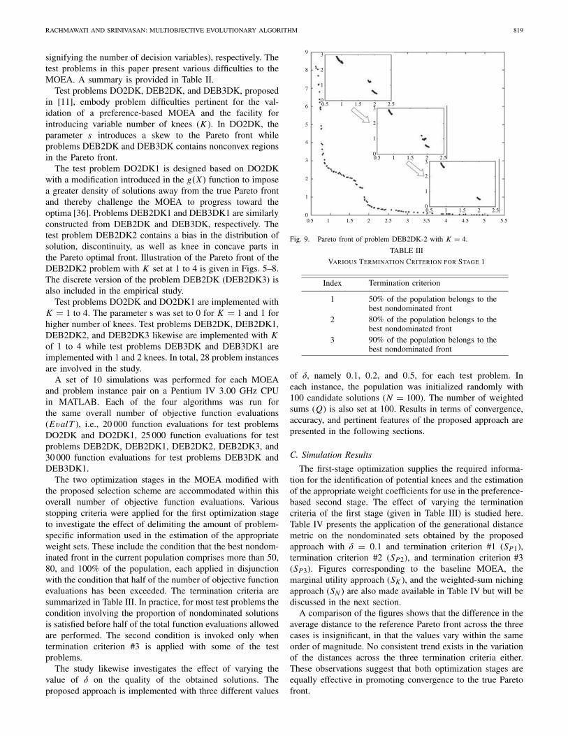
The first-stage optimization supplies the required informa-tion for the identification of potential knees and the estimationof the appropriate weight coefficients for use in the preference-based second stage. The effect of varying the terminationcriteria of the first stage (given in Table III) is studied here.Table IV presents the application of the generational distancemetric on the nondominated sets obtained by the proposedapproach with δ = 0.1 and termination criterion #1 (SP1),termination criterion #2 (SP2), and termination criterion #3(SP3). Figures corresponding to the baseline MOEA, themarginal utility approach (SK ), and the weighted-sum nichingapproach (SN ) are also made available in Table IV but will bediscussed in the next section.

A comparison of the figures shows that the difference in theaverage distance to the reference Pareto front across the threecases is insignificant, in that the values vary within the sameorder of magnitude. No consistent trend exists in the variationof the distances across the three termination criteria either.These observations suggest that both optimization stages areequally effective in promoting convergence to the true Paretofront.


TABLE IV

GENERATIONAL DISTANCE

Problem Baseline SP1 SP2 SP3 SK SN

Mean S.D. Mean S.D. Mean S.D. Mean S.D. Mean S.D. Mean S.D.

DO2DK (K = 1) 0.032 0.02555 0.00347 0.00064 0.00329 0.00024 0.00316 0.00013 0.03505 0.01858 0.00437 0.00003

DO2DK (K = 2) 0.0077 0.00052 0.00325 0.00026 0.0029 0.00066 0.00274 0.00017 0.02497 0.00628 0.00396 0.00043

DO2DK (K = 3) 0.00741 0.00091 0.00449 0.00035 0.00365 0.00029 0.00367 0.00023 0.02511 0.0036 0.00463 0.00038

DO2DK (K = 4) 0.00712 0.00072 0.00435 0.00073 0.00437 0.00036 0.00421 0.00035 0.02305 0.00305 0.00483 0.00073

DO2DK1 (K = 1) 0.12341 0.02159 0.00328 0.00032 0.00339 0.00018 0.00339 0.00017 0.24272 0.60024 0.00442 0.00023

DO2DK1 (K = 2) 0.04398 0.00694 0.0032 0.00094 0.00287 0.00018 0.0028 0.00022 0.0142 0.01566 0.00361 0.00017

DO2DK1 (K = 3) 0.00452 0.00364 0.00457 0.00127 0.00445 0.00092 0.00374 0.00027 0.06192 0.10532 0.00348 0.00026

DO2DK1 (K = 4) 0.04883 0.00958 0.00356 0.00066 0.00457 0.00168 0.00387 0.00065 0.00696 0.00781 0.00363 0.00025

DEB2DK (K = 1) 0.08354 0.07323 0.01444 0.00223 0.01624 0.00125 0.01842 0.00054 0.0406 0.00708 0.42352 0.39414

DEB2DK (K = 2) 0.0077 0.00052 0.00325 0.00026 0.0029 0.00066 0.00274 0.00017 0.02497 0.00628 0.00396 0.00043

DEB2DK (K = 3) 0.00741 0.00091 0.00449 0.00035 0.00365 0.00029 0.00367 0.00023 0.02511 0.0036 0.00463 0.00038

DEB2DK (K = 4) 0.05608 0.02921 0.00618 0.00083 0.00674 0.00114 0.00611 0.00107 0.01368 0.00139 0.31743 0.47184

DEB2DK1 (K = 1) 0.12341 0.02159 0.00328 0.00032 0.00339 0.00018 0.00339 0.00017 0.24272 0.60024 0.54071 0.74018

DEB2DK1 (K = 2) 0.04398 0.00694 0.0032 0.00094 0.00287 0.00018 0.0028 0.00022 0.0142 0.01566 0.00361 0.00017

DEB2DK1 (K = 3) 0.04522 0.00364 0.00457 0.00127 0.00445 0.00092 0.00374 0.00027 0.06192 0.10532 0.00348 0.00026

DEB2DK1 (K = 4) 0.09952 0.08489 589 0.00088 0.00666 0.00129 0.00606 0.0003 0.03299 0.00573 2.7844 3.662

DEB2DK2 (K = 1) 0.01867 0.00155 0.02388 0.00156 0.02538 0.00143 0.02528 0.0015 0.03446 0.00295 0.03669 0.00491

DEB2DK2 (K = 2) 0.01997 0.00255 0.01954 0.00242 0.01883 0.00096 0.02116 0.00134 0.03393 0.00351 0.0415 0.00532

DEB2DK2 (K = 3) 0.01949 0.00155 0.01762 0.00203 0.01439 0.00216 0.01673 0.00199 0.03262 0.00293 0.04632 0.00368

DEB2DK2 (K = 4) 0.01861 0.00123 0.01538 0.00333 0.01279 0.00187 0.01283 0.00134 0.03367 0.0028 0.04783 0.00388

DEB2DK3 (K = 1) 0.01669 0.00156 0.01508 0.0016 0.0165 0.0016 0.01693 0.0016 0.03294 0.00306 0.02879 0.00462

DEB2DK3 (K = 2) 0.01831 0.00266 0.01319 0.00172 0.01238 0.00109 0.01498 0.0144 0.03265 0.00352 0.0328 0.00558

DEB2DK3 (K = 3) 0.01781 0.00162 0.01216 0.00138 0.01044 0.00154 0.01246 0.00212 0.03128 0.00297 0.0361 0.0036

DEB2DK3 (K = 4) 0.01669 0.00134 0.01079 0.00234 0.00944 0.00112 0.00992 0.00138 0.03246 0.00295 0.03644 0.00379

DEB3DK (K = 1) 0.11469 0.00522 0.11131 0.01531 0.11368 0.01958 0.10937 0.01450 0.17511 0.117187 0.13382 0.02361

DEB3DK (K = 2) 0.87549 0.28445 0.32241 0.136 0.3293 0.1569 0.22568 0.14581 0.7632 0.25049 0.29348 0.07652

DEB3DK1 (K = 1) 0.11089 0.00505 0.09254 0.02267 0.11282 0.04535 0.1064 0.01458 0.13239 0.1011 2.3128 0.35338

DEB3DK1 (K = 2) 1.63909 0.6325 0.47793 0.28742 0.27393 0.16129 0.51246 0.32057 2.18844 0.60789 12.1006 1.04223

Results from applying the nondominance ratio to the ob-tained solution sets are summarized in Table VI. These alsoconfirm the observation that the termination criterion of thefirst stage does not affect convergence to the true Pareto frontsignificantly.

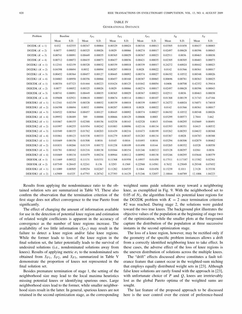
The effect of changing the amount of information availablefor use in the detection of potential knee region and estimationof related weight coefficients is apparent in the accuracy ofconvergence as the number of knee regions increase. Theavailability of too little information (SP1) may result in thefailure to detect a knee region and/or false knee regions.While the former leads to loss of the knee region in thefinal solution set, the latter potentially leads to the survival ofundesired solutions (i.e., nondominated solutions away fromknees). Results of applying metric σ1 to the nondominated setsobtained from SP1, SP2, and SP3, summarized in Table Vdemonstrate the proportion of knees not represented in thefinal solution set.

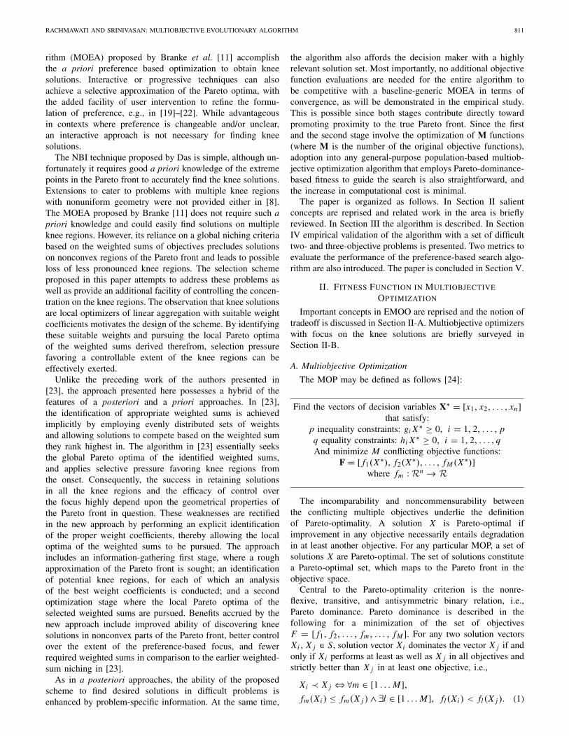
Besides premature termination of stage 1, the setting of theneighborhood size may lead to the local maxima heuristicsmissing potential knees or identifying spurious ones. Largeneighborhood sizes lead to the former, while smaller neighbor-hood sizes result in the latter. In general, spurious knees are notretained in the second optimization stage, as the corresponding

weighted sums guide solutions away toward a neighboringknee, as exemplified in Fig. 9. With the neighborhood set to0.05 of N2, the algorithm found six potential knee regions forthe DO2DK problem with K = 2 once termination criterion#2 was reached. During stage 2, the solutions were guidedtoward the two true knees. The background plot illustrates theobjective values of the population at the beginning of stage twoof the optimization, while the smaller plots at the foregroundcapture the distribution of the population at three successiveinstants in the second optimization stage.

The loss of a knee region, however, may be rectified only ifthe geometry of the specific problem instances allows a driftfrom a correctly identified neighboring knee to take effect. Inthese cases, the adverse effect of the loss of knee regions isthe uneven distribution of solutions across the multiple knees.

The “drift” effects discussed above constitutes a fault tol-erance feature that cannot occur in the weighted-sum nichingthat employs equally distributed weight sets in [23]. Althoughfalse knee solutions are rarely found with the approach in [23],with unfortunate choice of P and Q, knees are irretrievablylost as the global Pareto optima of the weighted sums aresought.

The last feature of the proposed approach to be discussedhere is the user control over the extent of preference-based


TABLE V

PROPORTION OF LOST KNEE REGIONS

Problem S P1 S P2 S P3

Mean S.D. Mean S.D. Mean S.D.

DO2DK (K = 1) 0 0 0 0 0 0

DO2DK (K = 2) 0 0 0 0 0 0

DO2DK (K = 3) 0 0 0 0 0 0

DO2DK (K = 4) 0 0 0 0 0 0

DO2DK1 (K = 1) 0 0 0 0 0 0

DO2DK1 (K = 2) 0 0 0 0 0 0

DO2DK1 (K = 3) 0.1 0.161 0 0 0 0

DO2DK1 (K = 4) 0.2 0.158 0 0 0 0

DEB2DK (K = 1) 0 0 0 0 0 0

DEB2DK (K = 2) 0 0 0 0 0 0

DEB2DK (K = 3) 0 0 0 0 0 0

DEB2DK (K = 4) 0.05 0.105 0 0 0 0

DEB2DK1 (K = 1) 0 0 0 0 0 0

DEB2DK1 (K = 2) 0 0 0 0 0 0

DEB2DK1 (K = 3) 0 0 0 0 0 0

DEB2DK1 (K = 4) 0.05 0.105 0 0 0 0

DEB2DK2 (K = 1) 0 0 0 0 0 0

DEB2DK2 (K = 2) 0 0 0 0 0 0

DEB2DK2 (K = 3) 0.167 0.176 0.0333 0.1054 0 0

DEB2DK2 (K = 4) 0.125 0.132 0.1 0.129 0.025 0.079

DEB2DK3 (K = 1) 0 0 0 0 0 0

DEB2DK3 (K = 2) 0 0 0 0 0 0

DEB2DK3 (K = 3) 0 0 0 0 0 0

DEB2DK3 (K = 4) 0.025 0.079 0 0 0 0

DEB3DK (K = 1) 0 0 0 0 0 0

DEB3DK (K = 2) 0.55 0.105 0.175 0.1208 0.05 0.105

DEB3DK1 (K = 1) 0 0 0 0 0 0

DEB3DK1 (K = 2) 0.4 0.129 0.225 0.142 0.075 0.121

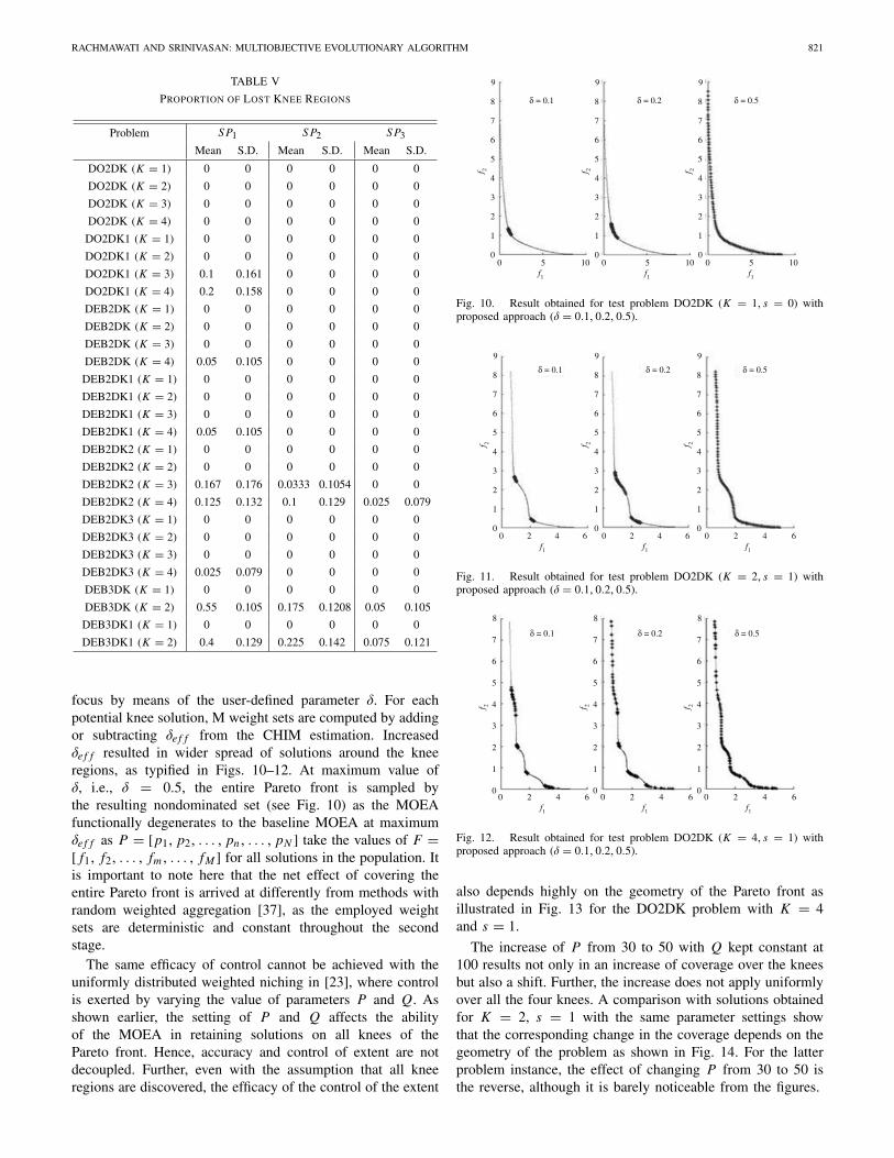
focus by means of the user-defined parameter δ. For eachpotential knee solution, M weight sets are computed by addingor subtracting δe f f from the CHIM estimation. Increasedδe f f resulted in wider spread of solutions around the kneeregions, as typified in Figs. 10–12. At maximum value ofδ, i.e., δ = 0.5, the entire Pareto front is sampled bythe resulting nondominated set (see Fig. 10) as the MOEAfunctionally degenerates to the baseline MOEA at maximumδe f f as P = [p1, p2, . . . , pn, . . . , pN ] take the values of F =[ f1, f2, . . . , fm, . . . , fM ] for all solutions in the population. Itis important to note here that the net effect of covering theentire Pareto front is arrived at differently from methods withrandom weighted aggregation [37], as the employed weightsets are deterministic and constant throughout the secondstage.

The same efficacy of control cannot be achieved with theuniformly distributed weighted niching in [23], where controlis exerted by varying the value of parameters P and Q. Asshown earlier, the setting of P and Q affects the abilityof the MOEA in retaining solutions on all knees of thePareto front. Hence, accuracy and control of extent are notdecoupled. Further, even with the assumption that all kneeregions are discovered, the efficacy of the control of the extent

f 2

9

8

7

6

5

4

3

2

1

0

f 2

9

8

7

6

5

4

3

2

1

0

f 2

9

8

7

6

5

4

3

2

1

0

f1

0 5 10f1

0 5 10f1

0 5 10

δ = 0.1 δ = 0.2 δ = 0.5

Fig. 10. Result obtained for test problem DO2DK (K = 1, s = 0) withproposed approach (δ = 0.1, 0.2, 0.5).

δ = 0.1 δ = 0.2 δ = 0.5

f 2

9

8

7

6

5

4

3

2

1

0

9

8

7

6

5

4

3

2

1

f 2

9

8

7

6

5

4

3

2

1

f1

0 2 4 6f1

0 2 4 6f1

0 2 4 60

f 2

0


δ = 0.1 δ = 0.2 δ = 0.5

f 2

8

7

6

5

4

3

2

1

0

f 2

8

7

6

5

4

3

2

1

f 2

8

7

6

5

4

3

2

1

f1

0 2 4 6f1

0 2 4 6f1

0 2 4 60 0


also depends highly on the geometry of the Pareto front asillustrated in Fig. 13 for the DO2DK problem with K = 4and s = 1.

The increase of P from 30 to 50 with Q kept constant at100 results not only in an increase of coverage over the kneesbut also a shift. Further, the increase does not apply uniformlyover all the four knees. A comparison with solutions obtainedfor K = 2, s = 1 with the same parameter settings showthat the corresponding change in the coverage depends on thegeometry of the problem as shown in Fig. 14. For the latterproblem instance, the effect of changing P from 30 to 50 isthe reverse, although it is barely noticeable from the figures.


TABLE VI

NONDOMINANCE RATIO

Problem Baseline SP1 SP2 SP3 SK SN

Mean S.D. Mean S.D. Mean S.D. Mean S.D. Mean S.D. Mean S.D.

DO2DK (K = 1) 0.844 0.046 0.997 0.00949 1 0 1 0 0.272 0.08417 0.999 0.00316

DO2DK (K = 2) 0.851 0.04864 0.988 0.023 1 0 1 0 0.159 0.0796 0.636 0.07412

DO2DK (K = 3) 0.863 0.03802 0.914 0.0988 0.951 0.07475 0.958 0.0663 0.188 0.06303 0.457 0.11295

DO2DK (K = 4) 0.825 0.04301 0.961 0.0619 0.888 0.09998 0.982 0.01874 0.214 0.06467 0.38 0.08819

DO2DK1 (K = 1) 0.96 0 1 0 1 0 0.999 0.00316 0.941 0.1517 1 0

DO2DK1 (K = 2) 0.98 0 1 0 1 0 1 0 0.996 0.00699 1 0

DO2DK1 (K = 3) 0.98 0 1 0 1 0 1 0 0.996 0.00699 1 0

DO2DK1 (K = 4) 0.978 0.00422 1 0 1 0 0.989 0.03479 0.999 0.0316 1 0

DEB2DK (K = 1) 0.857 0.0335 0.834 0.15457 0.887 0.18619 0.991 0.00994 0.436 0.09935 0.621 0.2158

DEB2DK (K = 2) 0.766 0.03596 0.874 0.14623 0.952 0.0646 0.884 0.13327 0.99 0 0.783 0.12885

DEB2DK (K = 3) 0.796 0.05125 0.898 0.10152 0.832 0.09716 0.841 0.10115 0.346 0.13335 0.609 0.24786

DEB2DK (K = 4) 0.75 0.04163 0.998 0.00632 0.992 0.0253 0.968 0.023 0.419 0.35967 0.705 0.19979

DEB2DK1 (K = 1) 0.96 0 0.98 0.01944 0.963 0.03234 0.996 0.00843 0.99 0 0.659 0.19846

DEB2DK1 (K = 2) 0.96 0 0.992 0.02201 0.937 0.08744 0.98 0.00471 0.99 0 0.698 0.15498

DEB2DK1 (K = 3) 0.75 0.04163 0.998 0.00632 0.992 0.0253 0.968 0.023 0.419 0.35967 0.705 0.19979

DEB2DK1 (K = 4) 0.676 0.0918 0.99 0.00316 1 0 1 0 0.99 0 0.78 0.15122

DEB2DK2 (K = 1) 0.888 0.02781 0.229 0.05953 0.169 0.0628 0.161 0.05216 0.55 0.06 0.078 0.03553

DEB2DK2 (K = 2) 0.835 0.04378 0.271 0.10619 0.263 0.08179 0.213 0.05056 0.554 0.06132 0.052 0.04517

DEB2DK2 (K = 3) 0.788 0.04104 0.496 0.12686 0.563 0.06832 0.451 0.07156 0.47 0.06532 0.339 0.09098

DEB2DK2 (K = 4) 0.757 0.04668 0.419 0.1121 0.448 0.0839 0.443 0.06961 0.446 0.06979 0.033 0.01767

DEB2DK3 (K = 1) 0.892 0.02098 0.999 0.00316 1 0 1 0 0.303 0.04473 0.186 0.0782

DEB2DK3 (K = 2) 0.833 0.03802 0.803 0.05851 0.816 0.06867 0.795 0.07352 0.326 0.04993 0.269 0.08034

DEB2DK3 (K = 3) 0.767 0.1303 0.918 0.06215 0.912 0.05514 0.851 0.08185 0.384 0.21874 0.226 0.27702

DEB2DK3 (K = 4) 0.805 0.06151 0.834 0.09834 0.88 0.08692 0.827 0.09262 0.273 0.03433 0.109 0.04581

DEB3DK (K = 1) 0.96 0.06766 0.797 0.0822 0.832 0.07052 0.817 0.07917 0.819 0.2019 0.434 0.09709

DEB3DK (K = 2) 0.695 0.04859 0.872 0.12839 0.818 0.07997 0.71 0.07803 0.237 0.10253 0.107 0.0587

DEB3DK1 (K = 1) 0.981 0.00738 0.876 0.12851 0.859 0.11377 0.94 0.06566 0.94 0.09384 0 0

DEB3DK1 (K = 2) 0.695 0.09277 0.409 0.16435 0.842 0.12778 0.827 0.05187 0.223 0.18786 0 0

f 2

f1

7

6

5

4

3

2

1

8

021 3 40 5

f 2

P = 50, Q = 100P = 30, Q = 100

f1

8

7

6

5

4

3

2

1

02 31 40 5

Fig. 13. Result obtained for test problem DO2DK (K = 4, s = 1) withweighted sum niching in [23].

D. Discussion

This section presents comparison of the solution sets ob-tained with the proposed approach with those obtained withthe other three MOEAs. Tables IV and VI summarize therelevant results from the application of performance metrics

f 2

f1

9

8

7

6

5

4

3

2

1

00 2 4 6

f 2

P = 50, Q = 100P = 30, Q = 100

f1

9

8

7

6

5

4

3

2

1

00 2 4 6

Fig. 14. Result obtained for test problem DO2DK (K = 2, s = 1) withweighted sum niching in [23].

to the obtained solutions.The figures in Table IV demonstrate that the focus on a

subset of the Pareto front improved proximity to the referencePareto front in most problems except DEB2DK-2, which arediscrete in nature. Examination of the results in Table VIconfirms this observation. Delimitation of the search direction


imposed by the modified fitness function in the case ofthe discrete problems adversely affected the convergence. Asimilar observation can be made of the marginal utility-basedapproach [11] and the weighted-sum niching [23]. Resultsfrom both approaches consistently performed worse than thesolutions from the baseline algorithm.

In comparison to the marginal utility approach implementedon the same baseline MOEA, the proposed approach has adecided advantage in terms of convergence. The former out-performed the latter in nearly all test problems as measured bythe generational distance metric as well as the nondominanceratio. In terms of the accuracy with which desired solutionsare discovered, the marginal utility-based method fared well,except for problem DEB2DK-2, where the method cannotretain the knees in nonconvex region of the Pareto front, andthe 3-D problem with K greater than 1, where the methodconsistently found only one of the prominent knees in thePareto front. A comparison of the figures with those in tablesuggests that, overall, the proposed method performed betterin terms of accuracy.

In comparison to the weighted-sum niching implementedon the same baseline MOEA, the proposed approach alsoperformed better. The weighted-sum niching produced inferiorsolutions even compared to the baseline MOEA in some of themore difficult test problems. In terms of accuracy with whichknee regions are retained, the weighted-sum niching performedreasonably well with the selected values for parameters P andQ (20 and 100, respectively). In the case of 3-D problems withK greater than 1, the weighted-sum niching also managed tofind only one prominent knee.

The results of the comparative study argue for the superi-ority of the proposed approach, with the exception of thoserelated to the discrete problem, where applying the proposedapproach resulted in worse convergence in comparison to thebaseline MOEA. With improvement to the search operator,e.g., by means of the jumping gene mechanism [26] or withmodel-based generation of new solutions [27], the discrepancymay be reduced. Still, among the methods designed for fo-cused convergence on the knee regions, the proposed approachfared considerably better than all the others.

V. CONCLUSION

The desirability of knee solutions is widely acknowledgedin the practice of multiobjective optimization. This paper pre-sented a fitness scheme that applies preference-based selectionpressure in a MOEA to obtain solutions in the vicinity of theknee regions. The strategy may be easily incorporated in anyMOEA framework with Pareto-based ranking in the selectionof solutions. In the first stage, the MOEA seeks a roughapproximation to the Pareto front, and in the second stage,the linear weighted-sums of the original objective functionsare optimized to guide solutions toward the knee regions. Aheuristic was introduced to compute the appropriate weightsfor each potential knee region in the front approximation.A mechanism to control the extent of focus on the kneeregion was also provided via the user-defined parameter δ.Although the approach relies on weighted sums, solutions

on the nonconvex region of the Pareto front can also beretained once discovered given large enough δ. The preference-based fitness introduces little added computational cost, as thenumber of functions to be Pareto-optimized in the second stageis the same as the number of original objective functions.

The approach has been successfully applied on several2- and 3-D test cases with various numbers of knee regions.The adoption of the proposed method does not compromise theproximity of obtained nondominated set to the true Pareto frontin comparison to the baseline MOEA. Further, the approacheffectively identified solutions in the vicinity of the kneeregions.

REFERENCES

[1] J. Knowles and D. Corne, “The pareto archived evolution strategy:A new baseline algorithm for multiobjective optimization,” in Proc.Congr. Evol. Comput. 1999, Piscataway, NJ: IEEE Press, pp. 98–105.

[2] D. W. Corne, N. R. Jerram, J. D. Knowles, and M. J. Oates, “PESA-II: Region-based selection in evolutionary multiobjective optimization,”in Proc. Genetic Evol. Comput. Conf. (GECCO ’01), San Mateo, CA:Morgan Kaufmann, pp. 283–290.

[3] K. Deb, A. Pratap, S. Agarwal, and T. Meyarivan, “A fast andelititst multiobjective genetic algorithm: NSGA-II,” IEEE Trans. Evol.Comput., vol. 6, no. 2, pp. 182–197, Apr. 2002.

[4] E. Zitzler, M. Laumanns, and L. Thiele. “SPEA2: Improving thestrength Pareto evolutionary algorithm for multiobjective optimization,”in Evolutionary Methods for Design, Optimisation and Control withApplication to Industrial Problems (EUROGEN 2001), Int. CenterNumerical Methods Eng. (CIMNE), pp. 95–100, 2002.

[5] A. J. Nebro, F. Luna, E. Alba, B. Dorronsoro, J. J. Durillo, andA. Beham, “AbYSS: Adapting scatter search to multiobjective opti-mization,” IEEE Trans. Evol. Comput., vol. 12, no. 4, pp. 439–457,Aug. 2008.

[6] S. Bandyopadhyay, S. Saha, U. Maulik, and K. Deb, “A simulatedannealing-based multiobjective optimization algorithm: AMOSA,”IEEE Trans. Evol. Comput., vol. 12, no. 3, pp. 269–283, Jun. 2008.

[7] K. I. Smith, R. M. Everson, J. E. Fieldsend, C. Murphy, and R. Misra,“Dominance-based multiobjective simulated annealing,” IEEE Trans.Evol. Comput., vol. 12, no. 3, pp. 323–342, Jun. 2008.

[8] I. Das, “On characterizing the knee of the pareto curve based onnormal-boundary intersection,” Structural Optimization, vol. 18, no.2–3, pp. 107–115, Oct. 1999.

[9] C. A. Mattson, A. A. Mullur, and A. Messac, “Smart pareto filter:Obtaining a minimal representation of multiobjective design space,”Eng. Optimization, vol. 36, no. 6, pp. 271–740, 2004.

[10] K. Deb, “Multiobjective evolutionary algorithms: Introducing biasamong Pareto-optimal solutions,” in Proc. Advances Evol. Computing:Theory Applicat., London, U.K.: Springer-Verlag, 2003, pp. 263–292.

[11] J. Branke, K. Deb, H. Dierolf, and M. Osswald, “Finding kneesin multiobjective optimization,” in Proc. 8th Conf. Parallel ProblemSolving from Nature (PPSN VIII), 2004, pp. 722–731.

[12] O. L. De Weck, “Multiobjective optimization: History and promise,”in Proc. 3rd China-Japan-Korea Joint Symp. Optimization StructuralMech. Syst. Invited Keynote Paper GL2-2, Kanazawa, Japan, Oct.–Nov.,2004.

[13] J. Branke, J. Kaußler, and H. Schmeck, “Guidance in evolution-ary multiobjective optimization,” Advances Eng. Software, vol. 32,pp. 499–507, 2001.

[14] D. Cvetkovic and I. C. Parmee, “Preferences and their application inevolutionary multiobjective optimization,” IEEE Trans. Evol. Comput.,vol. 6, no. 1, pp. 42–57, Feb. 2002.

[15] J. Branke and K. Deb, “Integrating user preferences into evo-lutionarymultiobjective optimization,” Kanpur Genetic Algorithm Laboratory,Indian Inst. Technol., KanGAL Rep. No. 2004004, May 2004.

[16] G. W. Greenwood, X. Hu, and J. G. D’Ambrosio, “Fitness functionsfor multiple objective optimization problems: Combining preferenceswith pareto rankings,” in Proc. Found. Genetic Algorithms, 1996,pp. 437–455.

[17] Y. Jin and B. Sendhoff, “Incorporation of fuzzy preferences intoevolutionary multiobjective optimization,” in Proc. 4th Asia PacificConf. Simulated Evolution Learning, vol. 1. Singapore, Nov. 2002,pp. 26–30.


[18] K. C. Tan, E. F. Khor, T. H. Lee, and R. Sathikannan, “An evolutionaryalgorithm with advanced goal and priority specification for multiobjec-tive optimization,” J. Artificial Intell. Res., vol. 18, pp. 183–215, 2003.

[19] C. M. Fonseca and P. J. Fleming, “Genetic algorithms for multiobjec-tive optimization: Formulation, discussion and generalization,” in Proc.5th Int. Conf. Genetic Algorithms, San Mateo, CA, 1993, pp. 416–423.

[20] S. F. Adra, I. Griffin, and P. J. Fleming, “A comparative studyof progressive preference articulation techniques for multiobjectiveoptimization,” in Proc. 4th Int. Conf. Evol. Multicriterion Optimization,LNCS vol. 4403, 2007, pp. 908–921.

[21] M. J. Geiger, “The interactive pareto iterated local search meta-heuristicand its application to the biobjective portfolio optimization problem,”in Proc. IEEE Symp. Comput. Intell. Multicriteria Decision Making2007, pp. 193–199.

[22] M. J. Geiger, W. Wenger, and W. Habenicht, “Interactive utilitymaximization in multiobjective vechicle routing problems: A decisionmaker in the loop approach,” in Proc. IEEE Symp. Comput. Intell.Multicriteria Decision Making 2007, pp. 178–184.

[23] L. Rachmawati and D. Srinivasan, “A multiobjective evolutionary al-gorithm with weighted-sum niching for convergence on knee regions,”in Proc. IEEE Congr. Evol. Comput., 2006, pp. 1916–1923.

[24] K. Deb. Multiobjective Evolutionary Algorithm. Chichester, U.K.:Wiley, 2001.

[25] I. Das and J. E. Dennis, “Normal-boundary intersection: A newmethod for generating the pareto surface in multicriteria optimizationproblems,” SIAM J. Optimization, vol. 8, pp. 631–657, 1998.

[26] T. M. Chan, K. F. Man, K. S. Tang, and S. Kwong, “A jumping geneparadigm for evolutionary multiobjective optimization,” IEEE Trans.Evol. Comput., vol. 12, no. 2, pp. 143–159, Apr. 2008.

[27] Q. Zhang, A. Zhou, and Y. Jin, “RM-MEDA: A regularity model-basedmultiobjective estimation of distribution algorithm,” IEEE Trans. Evol.Comput., vol. 12, no. 1, pp. 41–63, Feb. 2008.

[28] X. Li, “Better spread and convergence: Particle swarm multiobjectiveoptimization using the maxi-min fitness function,” in Proc. GECCO’04, Berlin, Germany: Springer-Verlag, pp. 117–128.

[29] D. Srinivasan and L. Rachmawati, “An efficient multiobjective evo-lutionary algorithm with steady-state replacement model,” in Proc.GECCO ’06, pp. 715–722.

[30] L. Rachmawati and D. Srinivasan, “Dynamic resizing for grid-basedarchiving in evolutionary multiobjective optimization,” in Proc. IEEECongr. Evol. Comput., Singapore, 2006, pp. 3975–3982.

[31] E. Zitzler and L. Thiele, “Multiobjective optimization using evolu-tionary algorithms - A comparative case study,” in Proc. 5th ParallelProblem Solving from Nature (PPSN), Sep. 1998, pp. 292–301.

[32] E. Zitzler, “Evolutionary algorithms for multiobjective optimiza-tion: Methods and applications,” Ph.D. dissertation, Springer-Verlag,Aachen, Germany, 1999.

[33] C. K. Goh and K. C. Tan, “A Competitive-cooperative coevolutionaryparadigm for dynamic multiobjective optimization,” IEEE Trans. Evol.Comput., vol. 13, no. 1, pp. 103–127, Feb. 2009.

[34] E. Zitzler, L. Thiele, M. Laumanns, C. M. Fonseca, andV. G. da Fonseca, “Performance assessment of multiobjective optimiz-ers: An analysis and review,” IEEE Trans. Evol. Comput., vol. 7, no. 2,pp. 117–131, Apr. 2003.

[35] K. Deb and S. Agrawal, “Simulated binary crossover for continuoussearch space,” Complex Syst., vol. 9, pp. 115–148, Apr. 1995.

[36] K. Deb, L. Thiele, M. Laumanns, and E. Zitzler, “Scalable testproblems for evolutionary multiobjective optimization,” in Proc. Evol.Comput. Based Multicriteria Optimization: Theoretical Advances Ap-plicat., London, U.K.: Springer-Verlag, 2005, pp. 105–145.

[37] Y. Jin, T. Okabe, and B. Sendhoff, “Adapting weighted aggregationfor multiobjective evolution strategies,” in Proc. 1st Int. Conf. Evol.Multicriterion Optimization, 2001, pp. 96–110.

Lily Rachmawati received the Bachelor’s degreein electrical and computer engineering from theNational University of Singapore (NUS) in 2004.

She is currently a Research Fellow at the NUS.Her research interests include multiobjective opti-mization and evolutionary computation.

Dipti Srinivasan (SM’02) obtained the M.Eng. andPh.D. degrees in electrical engineering from theNational University of Singapore (NUS) in 1991 and1994, respectively.

She was with the Computer Science Division,University of California, Berkeley as a PostdoctoralResearcher from 1994 to 1995. In June 1995, shejoined the faculty of the Electrical and ComputerEngineering Department, NUS, where she is cur-rently an Associate Professor. From 1998 to 1999,she was a Visiting Faculty Member with the De-

partment of Electrical and Computer Engineering, the Indian Institute ofScience, Bangalore, India. Her main areas of interest are neural networks,evolutionary computation, intelligent multiagent systems, and application ofcomputational intelligence techniques to engineering optimization, planning,and control problems in intelligent transportation systems and power systems.She has published/presented over 170 technical papers in international refereedjournals and conferences.

Dr. Srinivasan is a member of IES, Singapore.

Multiobjective Evolutionary Algorithm With Controllable Focus on the Knees of the Pareto Front

Documents

Transcript of Multiobjective Evolutionary Algorithm With Controllable Focus on the Knees of the Pareto Front