�����������������

Citation: Gambier, A. Multiobjective

Optimal Control of Wind Turbines: A

Survey on Methods and

Recommendations for the

Implementation. Energies 2022, 15,

567. https://doi.org/10.3390/

en15020567

Academic Editor: Davide Astolfi

Received: 29 September 2021

Accepted: 1 January 2022

Published: 13 January 2022

Publisher’s Note: MDPI stays neutral

with regard to jurisdictional claims in

published maps and institutional affil-

iations.

Copyright: © 2022 by the author.

Licensee MDPI, Basel, Switzerland.

This article is an open access article

distributed under the terms and

conditions of the Creative Commons

Attribution (CC BY) license (https://

creativecommons.org/licenses/by/

4.0/).

energies

Review

Multiobjective Optimal Control of Wind Turbines: A Survey onMethods and Recommendations for the ImplementationAdrian Gambier

Fraunhofer Institute for Wind Energy Systems, IWES, Am Seedeich 45, 27572 Bremerhaven, Germany;adrian.gambier@iwes.fraunhofer.de or agambier@ieee.org; Tel.: +49-471-14290-375

Abstract: Advanced control system design for large wind turbines is becoming increasingly complex,and high-level optimization techniques are receiving particular attention as an instrument to fulfilthis significant degree of design requirements. Multiobjective optimal (MOO) control, in particular, istoday a popular methodology for achieving a control system that conciliates multiple design objectivesthat may typically be incompatible. Multiobjective optimization was a matter of theoretical studyfor a long time, particularly in the areas of game theory and operations research. Nevertheless, thediscipline experienced remarkable progress and multiple advances over the last two decades. Thus,many high-complexity optimization algorithms are currently accessible to address current controlproblems in systems engineering. On the other hand, utilizing such methods is not straightforwardand requires a long period of trying and searching for, among other aspects, start parameters,adequate objective functions, and the best optimization algorithm for the problem. Hence, theprimary intention of this work is to investigate old and new MOO methods from the applicationperspective for the purpose of control system design, offering practical experience, some open topics,and design hints. A very challenging problem in the system engineering application of power systemsis to dominate the dynamic behavior of very large wind turbines. For this reason, it is used as anumeric case study to complete the presentation of the paper.

Keywords: multiobjective optimization; multiobjective optimal control; controller tuning; objectivefunctions; multiobjective optimization algorithms; wind turbines control

1. Introduction

Control engineering is obligated to evolve in line with world progress, where themastery of engineering systems is becoming more and more difficult. One characteristicproblem is that advanced systems need to fulfill optimality in several ways, where thestated objectives could simultaneously be opposing, conflicting, or complementary. Hence,Multiobjective Optimal Control (MOOC, see e.g., [1–4] and their references) arose primarilyin the last two decades as a helpful instrument to handle these types of control cases.Ongoing survey works about the subject are, for instance, [5,6].

A significant expectation at that point was the thought of finding a general-purposeoptimizer able to manage several objectives, with the capacity to address a wide range ofcontrol configurations and control operation problems. Nowadays, it is realized that suchideal MOO tools are very difficult to create and that MOO techniques can only undertake aminor number of problems and, in addition, under concrete situations. Furthermore, somealgorithms that work correctly in the case of a concrete set of optimization problems arenot able to provide acceptable solutions in other cases, where other algorithms performbetter [7]. Moreover, experience shows that earlier information about the control problem,the tuning parameters, the numerical behavior of the optimization approach, as well asthe objective functions supplemented by much working time is essential before a MOOoptimizer yields satisfactory outcomes. This point can be especially frustrating if thesought-after Pareto front is unknown a priori.

Energies 2022, 15, 567. https://doi.org/10.3390/en15020567 https://www.mdpi.com/journal/energies

Energies 2022, 15, 567 2 of 18

While the research in the field of MOO is focused on the obtention of new algorithms,whose aim is to find more complex Pareto frontiers or more accurate solutions by utilizingspecially constructed test objective functions, MOO users, for example, control engineers,work with realistic cost functions. In such circumstances, the forms of Pareto fronts areunknown in advance, and consequently, adjusting and tuning of optimization methodsis not straightforward. Despite MOO being an extremely effective instrument for solvingvery complex problems in control system design, its application is not simple.

Furthermore, current design issues appear to be fast gaining in complexity, where theinclusion of several systems with subsystem levels and additional objective functions mustalso be considered in the optimization procedure. Thus, Pareto methods cannot providesatisfactory results, and bilevel multiobjective optimization can facilitate the possibility ofobtaining the desired outcome (see, for instance, [8]). An application of bilevel MOO to acontrol problem is given in [9].

Hence, the aim of this work, following the previous study [10], is to depict MOOcontrol from a practitioner’s perspective. The remainder of the work will be presented inthe following form: The next section, Section 2, is devoted to introducing the concept ofmultiobjective optimization for the sake of completeness and describing the most importantalgorithms. Typical objective functions for control are the subject of Section 3, as well asthe evaluation procedures analyzed in Section 4. In Section 5, aspects related to decision-making are shown, followed by the application example and the corresponding results inSections 6 and 7, respectively. Finally, conclusions are portrayed in Section 8.

2. Some Fundamentals on Multiobjective Optimization

Multiobjective optimization can be found in the literature under several differentnames, such as, for instance, multiperformance, multicriteria, or vector optimization. Itcan be described as the activity of obtaining a vector of parameters or decision variables asthe outcome of an optimization process carried out on a vector field of objective functionswith constraints that have to be satisfied during the operation. These objective functionsnormally correspond to mathematical descriptions of design specifications that are often inconflict with each other.

2.1. Definitions

The multiobjective optimization problem can be formally stated as

to find α = [α1 . . . α np]T or u = [u1 . . . ul]T,optimizing J(u,α) = [J1(u,α) . . . Jnf(u,α)]T

with respect to α or to usubject to gi(u,α) ≤ 0 and hj(u,α) = 0,for i = 1, . . . , ng, j = 1, . . . , nh,

where J∈ϑ ⊂ Rnf is a vector of objective functions, u∈U ⊂ Rl is a vector of decisionvariables, α∈A ⊂ Rnp is a vector of parameters, nf is the number of objective functions, ngis the number of inequalities constraints and nh is the number of equality constraints. Byoptimization, it means either minimization or maximization, depending on the problem tobe addressed.

Contrarily to single-objective optimization (SOO), where only a unique global optimalsolution exists, there are many optimal equivalent solutions for a MOO problem. There-fore, a definition of the optimum has to be defined in advance. In the present work, themultiobjective Pareto optimality formulated in [11] is assumed.

Definition 1: A point, α◦∈A ⊂ Rl, is said to be Pareto optimal with respect to A iff no otherpoint, α∈A, satisfies the conditions J(u,α) ≤ J(u,α◦) and Ji(u,α) < Ji(u,α◦) for at least one i.This means that it is impossible to enhance a Pareto optimal point without worsening thevalue of at least one of the other objective functions.

Energies 2022, 15, 567 3 of 18

In some cases, it is helpful to reckon with a definition for a suboptimal point that canbe reached more easily by the algorithm, and, at the same time, it is an acceptable solutionfrom the practical point of view. This is provided, e.g., by the definition of weakly Paretooptimality.

Definition 2: A point, α◦∈ A ⊂ Rl, is said to be weakly Pareto optimal if no other point α∈A,satisfies J(u,α) < J(u,α◦).

In other words, a point is weakly Pareto optimal if no other point can improve allobjective functions at the same time. Thus, Pareto optimal points are always weakly Paretooptimal, but not the contrary case. All Pareto optimal points constitute the Pareto optimal setdefined as

℘ ,{α◦ ∈ A ⊆ Rl

∣∣∣¬∃ α ∈ A, ∀ i Ji(u,α) ≤ Ji(u,α◦) ∧ ∃ i : Ji(u,α) < Ji(u,α◦)}

. (1)

The image ℘f of the Pareto optimal set ℘ ⊂ U is called Pareto front and is defined in theobjective space ϑ.

Definition 3: Given a vector objective function J(u,α) and the corresponding Pareto optimalset ℘, the Pareto front is defined by

℘ f ,{

J(u,αi) ∈ ϑ ⊆ Rn f∣∣∣αi ∈ ℘, ∀ i

}. (2)

Three points in the objective space are very important. The former is the utopia point,also known as ideal point, the second one is the threat point (disagreement point or nadir point),and the latter is the worst point, which is described in the following definition.

Definition 4: A point, J◦ is a utopia point iff J◦i = minJi(u, α) with respect to α for ∀ i = 1,

. . . , nf. A point, J* is a threat point iff J∗i = maxJi(u, α) with respect to α for ∀ i = 1, . . . , nf.A point, Jw is the worst point iff Jw

i = maxJi(u, α) with respect to α for ∀ i = 1, . . . , nf.

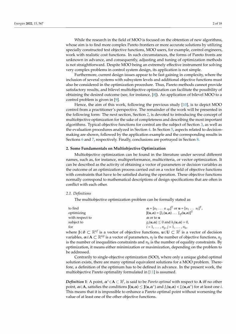
Normally, the utopia point does not belong to ℘f. All definitions are formulated,including the threat point and the worst point, which are defined using the max function,in the sense of minimization. However, they can be modified accordingly to express themaximization case. Moreover, all definitions can be stated in the sense of the vector ofdecision variables u instead of the parameter vector α. All definitions are geometricallyexplained in Figure 1 for a two-dimensional Pareto front.

Energies 2022, 14, x FOR PEER REVIEW 3 of 18

In some cases, it is helpful to reckon with a definition for a suboptimal point that can be reached more easily by the algorithm, and, at the same time, it is an acceptable solution from the practical point of view. This is provided, e.g., by the definition of weakly Pareto optimality. Definition 2: A point, α°∈ A ⊂ ℝl, is said to be weakly Pareto optimal if no other point α∈A, satisfies J(u,α) < J(u,α°).

In other words, a point is weakly Pareto optimal if no other point can improve all objective functions at the same time. Thus, Pareto optimal points are always weakly Pareto optimal, but not the contrary case. All Pareto optimal points constitute the Pareto optimal set defined as

{ }| , ( , ) ( , ) : ( , ) ( , )li i i ii J J i J J℘ °∈ ⊆ ¬ ∃ ∈ ∀ ≤ ° ∧ ∃ < °α Α α Α u α u α u α u α

. (1)

The image ℘f of the Pareto optimal set ℘ ⊂ U is called Pareto front and is defined in the objective space ϑ. Definition 3: given a vector objective function J(u,α) and the corresponding Pareto opti-mal set℘, the Pareto front is defined by

{ }( , ) | ,nff i i i℘ ∈ ⊆ ∈℘ ∀J u α α ϑ . (2)

Three points in the objective space are very important. The former is the utopia point, also known as ideal point, the second one is the threat point (disagreement point or nadir point), and the latter is the worst point, which is described in the following definition. Definition 4: A point, J° is a utopia point iff with respect to α for ∀ i = 1,…,

nf . A point, J* is a threat point iff * = max ( , )i iJ J u α with respect to α for ∀ i = 1,…, nf . A point,

Jw is the worst point iff = max ( , )wi iJ J u α with respect to α for ∀ i = 1,…, nf .

Normally, the utopia point does not belong to ℘f. All definitions are formulated, in-cluding the threat point and the worst point, which are defined using the max function, in the sense of minimization. However, they can be modified accordingly to express the maximization case. Moreover, all definitions can be stated in the sense of the vector of decision variables u instead of the parameter vector α. All definitions are geometrically explained in Figure 1 for a two-dimensional Pareto front.

J1

J2

Pareto front

Utopia point

Objective space ϑ ⊂ 2

J2° J1°

J:Α→ϑ Threat point c

α3

α2

a1

Solution space

Α ⊂ 3

Worst point w

Figure 1. Schematic description of the multiobjective optimization problem.

Nowadays, numerical implementations of the multiobjective optimization theory became a well-known design instrument, where a significant number of different methods is available. A priori, two groups must be distinguished: algorithms for discrete, binary, or combinatorial optimization problems and methods for continuous optimization prob-lems. The attention in the present research is limited to the latter category.

? min ( , )i iJ J u α

Figure 1. Schematic description of the multiobjective optimization problem.

Nowadays, numerical implementations of the multiobjective optimization theorybecame a well-known design instrument, where a significant number of different methodsis available. A priori, two groups must be distinguished: algorithms for discrete, binary, or

Energies 2022, 15, 567 4 of 18

combinatorial optimization problems and methods for continuous optimization problems.The attention in the present research is limited to the latter category.

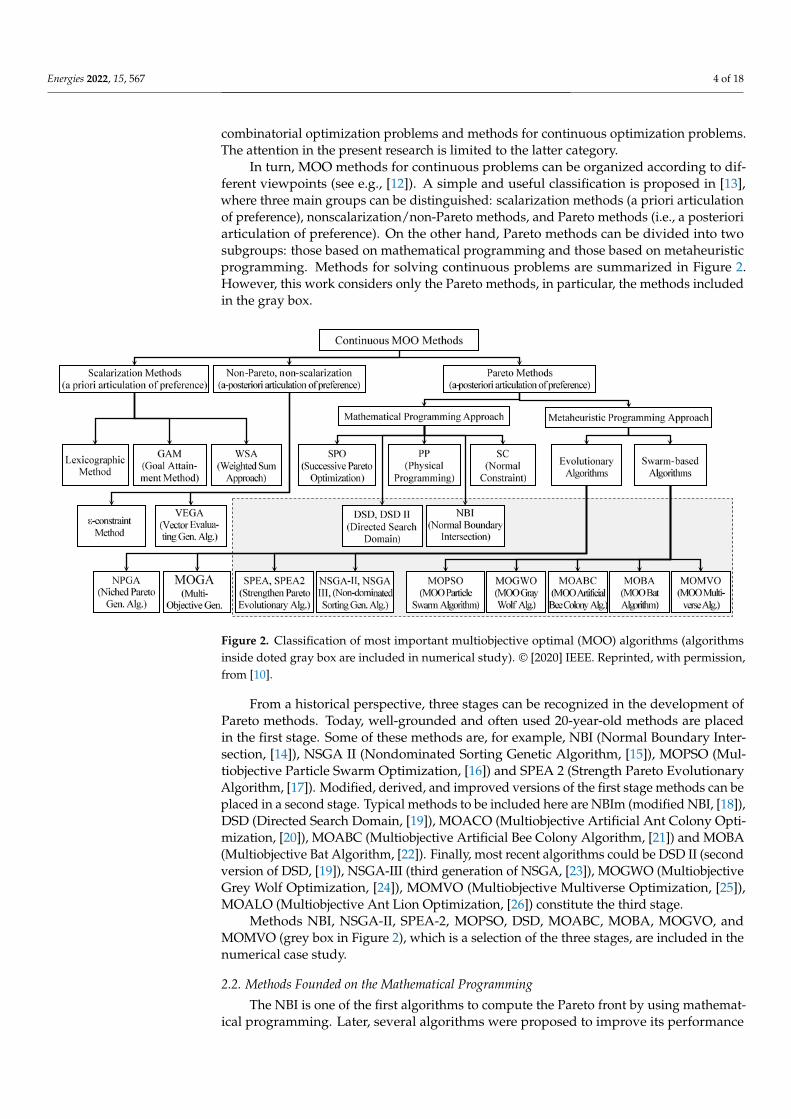
In turn, MOO methods for continuous problems can be organized according to dif-ferent viewpoints (see e.g., [12]). A simple and useful classification is proposed in [13],where three main groups can be distinguished: scalarization methods (a priori articulationof preference), nonscalarization/non-Pareto methods, and Pareto methods (i.e., a posterioriarticulation of preference). On the other hand, Pareto methods can be divided into twosubgroups: those based on mathematical programming and those based on metaheuristicprogramming. Methods for solving continuous problems are summarized in Figure 2.However, this work considers only the Pareto methods, in particular, the methods includedin the gray box.

Energies 2022, 14, x FOR PEER REVIEW 4 of 18

In turn, MOO methods for continuous problems can be organized according to dif-ferent viewpoints (see e.g., [12]). A simple and useful classification is proposed in [13], where three main groups can be distinguished: scalarization methods (a priori articulation of preference), nonscalarization/non-Pareto methods, and Pareto methods (i.e., a posteri-ori articulation of preference). On the other hand, Pareto methods can be divided into two subgroups: those based on mathematical programming and those based on metaheuristic programming. Methods for solving continuous problems are summarized in Figure 2. However, this work considers only the Pareto methods, in particular, the methods in-cluded in the gray box.

Figure 2. Classification of most important multiobjective optimal (MOO) algorithms (algorithms inside doted gray box are included in numerical study). © [2020] IEEE. Reprinted, with permission, from [10].

From a historical perspective, three stages can be recognized in the development of Pareto methods. Today, well-grounded and often used 20-year-old methods are placed in the first stage. Some of these methods are, for example, NBI (Normal Boundary Intersec-tion, [14]), NSGA II (Nondominated Sorting Genetic Algorithm, [15]), MOPSO (Multi-objective Particle Swarm Optimization, [16]) and SPEA 2 (Strength Pareto Evolutionary Algorithm, [17]). Modified, derived, and improved versions of the first stage methods can be placed in a second stage. Typical methods to be included here are NBIm (modified NBI, [18]), DSD (Directed Search Domain, [19]), MOACO (Multiobjective Artificial Ant Colony Optimization, [20]), MOABC (Multiobjective Artificial Bee Colony Algorithm, [21]) and MOBA (Multiobjective Bat Algorithm, [22]). Finally, most recent algorithms could be DSD II (second version of DSD, [19]), NSGA-III (third generation of NSGA, [23]), MOGWO (Multiobjective Grey Wolf Optimization, [24]), MOMVO (Multiobjective Multiverse Op-timization, [25]), MOALO (Multiobjective Ant Lion Optimization, [26]) constitute the third stage.

Methods NBI, NSGA-II, SPEA-2, MOPSO, DSD, MOABC, MOBA, MOGVO, and MOMVO (grey box in Figure 2), which is a selection of the three stages, are included in the numerical case study.

Figure 2. Classification of most important multiobjective optimal (MOO) algorithms (algorithmsinside doted gray box are included in numerical study). © [2020] IEEE. Reprinted, with permission,from [10].

From a historical perspective, three stages can be recognized in the development ofPareto methods. Today, well-grounded and often used 20-year-old methods are placedin the first stage. Some of these methods are, for example, NBI (Normal Boundary Inter-section, [14]), NSGA II (Nondominated Sorting Genetic Algorithm, [15]), MOPSO (Mul-tiobjective Particle Swarm Optimization, [16]) and SPEA 2 (Strength Pareto EvolutionaryAlgorithm, [17]). Modified, derived, and improved versions of the first stage methods can beplaced in a second stage. Typical methods to be included here are NBIm (modified NBI, [18]),DSD (Directed Search Domain, [19]), MOACO (Multiobjective Artificial Ant Colony Opti-mization, [20]), MOABC (Multiobjective Artificial Bee Colony Algorithm, [21]) and MOBA(Multiobjective Bat Algorithm, [22]). Finally, most recent algorithms could be DSD II (secondversion of DSD, [19]), NSGA-III (third generation of NSGA, [23]), MOGWO (MultiobjectiveGrey Wolf Optimization, [24]), MOMVO (Multiobjective Multiverse Optimization, [25]),MOALO (Multiobjective Ant Lion Optimization, [26]) constitute the third stage.

Methods NBI, NSGA-II, SPEA-2, MOPSO, DSD, MOABC, MOBA, MOGVO, andMOMVO (grey box in Figure 2), which is a selection of the three stages, are included in thenumerical case study.

2.2. Methods Founded on the Mathematical Programming

The NBI is one of the first algorithms to compute the Pareto front by using mathemat-ical programming. Later, several algorithms were proposed to improve its performance

Energies 2022, 15, 567 5 of 18

and to overcome its drawbacks. In such a sense, the Normal Constraint (NC) [27], PhysicalProgramming (PP) [28], Successive Pareto Optimization (SPO) [29], and the Directed SearchDomain (DSD) [19] can be cited.

The above-mentioned methods transform the multiobjective problem into many single-objective constrained subproblems. Thus, the optimization is carried out by using a single-objective solver subjected to imposed restrictions. The standard solver is the active-setalgorithm, which works reasonably well if the objective functions are smooth and wellscaled. These approaches produce a Pareto front with equally spaced points within theframework of a fast convergence, which are important properties for control applications.

2.3. Methods Founded on the Metaheuristic Programming

The methods based on metaheuristic programming can be grouped into evolution-ary algorithms and particle swarm intelligence. Multiobjective evolutionary algorithms(MOEA) define first an initial set of solutions (initial population) and then attempt to refinethe set of solutions by means of a random selection from the solution space until the optimalPareto set is obtained.

The population is renewed by the action of several genetic operators, which areknown as recombination (a new point is generated from the other point of the population,e.g., averaging), mutation (a recently created point is randomly chosen and replaced withanother obtained via the realization of a random variable) and selection (newly createdpoints are taken from the new population considering the best fitness and used to replacepoints from the old population). These three operations are implemented by many differentevolutionary algorithms (for a comparative study, see [30]).

Particle swarm optimization is another stochastic optimization method. It startswith an initial population of particles, which evolve and survive until the last generation.This characteristic distinguishes particle swarm intelligence from evolutionary algorithms,where the population changes.

Particle swarm algorithms search the space of variables by using knowledge from oldgenerations and going at a specifically determined speed within the direction of the globalbest particle. Many other algorithms were created following this principle. The commonidea is to imitate the behavior of various swarms or colonies of animals, such as bats, bees,or ants. However, it should be distinguished from algorithms like MOALO and MOGWO,which emulate the hunting activities of antlions and grey wolves and their interaction withprays. These are based on the Predator-Prey formalism [31].

2.4. Methods for Bilevel Multiobjective Optimization Problems

Bilevel multiobjective optimization consists of two multiobjective optimization algo-rithms running at two different levels, where one algorithm runs inside the other one. Theinternal algorithm solves the low-level optimization problem while the external algorithmprocesses the upper-level problem. This is a nested operation, where the outer algorithmcalls the inner one at every upper-level point. Hence, the computational burden of thebilevel optimization algorithm is very high and, therefore, it can only be used by appli-cations that require optimization of low complexity. It is common to find metaheuristicprogramming at the external level and mathematical programming at the internal one.Nonetheless, both levels can be satisfied for the same class of algorithms. This optimizationconcept is not considered in the current study, but it is an ongoing research topic.

2.5. Selecting Methods for the Application

Optimization algorithms for MOO problems work properly for a limited numberof applications [7] and, therefore, it is difficult to suggest one. Thus, recommendationsare exceptionally formulated in the literature. As an indication of general purposes, it ispointed out in [32] that methods that guarantee necessary and sufficient conditions forPareto optimality should be tested first. In the second term, methods with only guaranteedsufficient conditions may be studied, followed at the end by other methods.

Energies 2022, 15, 567 6 of 18

From a practical standpoint, having numerous algorithms may be beneficial in termsof being able to select the most appropriate one according to the application. Hence, thedesigner can prioritize the choice where accuracy of the solution, computational load,regular distribution of Pareto points on the front, and speed of convergence are just afew examples.

3. Objective Functions for MOO Control Problems

Using advanced optimization techniques, the appropriate choice of the objectivefunctions is crucial for an effective control system design. This is particularly relevant in thecase of MOO, since several objectives must be compromised at the same time. Moreover,the objective functions must not only be a useful indicator for the operation of the controlsystem, but they also have to fulfill the corresponding mathematical properties imposed bythe optimizer.

3.1. Typical Performance Indices

Performance indices are widely used as objective functions in the classic optimizationproblem of control systems. They are normally expressed in the form of a function of thecontrol error in the form of

J =∫ ∞

0f [e(t)] dt and J =

∞

∑k=0

f [e(k)] (3)

for the continuous and discrete time cases, respectively. Function f can be, for instance, |e(t)|(Integrated Absolute value of Error, AIE), e(t)2 (Integral Squared Error, ISE), t e (t)2 (IntegralTime-weighted Squared Error, ITSE) and t2 e (t)2 (Integral Squared Time-weighted SquaredError, ISTSE). Function f can also include an argument for the control error derivative,which acts as a soft constraint for the control error rate, i.e.,

J =∫ ∞

0f [e(t),

.e(t)] dt and J =

∞

∑k=0

f [e(k), ∆e(k)]. (4)

In general, several other variables and their derivatives can be added as soft constraintsfor control signals to obtain more complex objective functions of the form

J =∫ ∞

0f [e(t),

.e(t), u(t),

.u(t)] dt and J =

∞

∑k=0

f [e(k), ∆e(k), u(k), ∆u(k)]. (5)

3.2. Performance Indices for Time-Limited Problems

The performance indices of the previous subsection consider infinite time. However,these indices can be solved only in a few cases, where the Laplace transform is used to leavethe time domain. However, this is not possible in the case of nonlinear systems. Anotherprocedure is the evaluation of performance indices by using simulation data. In such acase, the time series are truncated and, as a consequence, the integrals must be averaged intime, as for instance,

J =1

tmax − tmin

∫ tmax

tmin

f [e(t)] dt and J =1

(N − k0)Ts

N

∑k=k0

f [e(k)]. (6)

Ts is the sampling time. Time-averaged integral can be used for all performanceindices proposed in Section 3.1.

3.3. Performance Indices Formulated Using Fractional Order Calculus

Fractional-order analysis was developed in the 19th century as a generalization ofinteger-order integral-differential calculus to the real-order case. This work was undertaken

Energies 2022, 15, 567 7 of 18

by several well-known mathematicians, for example, Cauchy, Euler, Grünwald, Letnikov,Liouville, and Riemann [33].

Another application field for the fractional-order calculus is the system theory andcontrol, where many new developments were carried out in the past 15 years (see, amongothers, [34]). Integral performance indices as described in 3.1 can also be formulated inthe framework of the fractional calculus. Thus, it is pointed out in [35] that a controlapplication presents a better response in the case of oscillatory signals when it is designedusing a fractional order cost function. An application of MOO control using fractional orderperformance indices is reported in [36].

Moreover, the classic performance indices presented at the beginning of this sectionwere generalized in [37] for fractional-order integrals. The continuous time performanceindex (4) is expressed in the sense of the fractional integral by

J =1

tmax − tmin

∫ tmax

tmin

D(1−k) f [e(t)] dt, (7)

where D(1−k) is the fractional derivative and k the fractional order.The fractional definite integral of Equation (7) can be solved by means of the fractional

Barrow formula if an admissible fractional derivative such as the Grünwald–Letnikov orLiouville formula is used [38]. The implementation of the fractional integral can be doneby using, for instance, N-Integer [39] or FOTF [40].

3.4. Objective Functions for Specific Applications

In the case of control system design, time domain specifications like maximum risetime, minimum settling time, and minimum overshoot or frequency domain specificationslike bandwidth, gain margin, phase margin, and resonant peak can be used as metricsfor MOO control. However, since such measures are not convex, MOO algorithms canfail during the optimization process. The construction of solid and mathematically soundobjective functions based on the above-mentioned metrics for MOO control is still anopen subject.

Following this idea, a convex objective function including fatigue damage was pro-posed in [41] for the particular cases of wind turbine control. The metric is designed toformulate a compromise between the pitch actuation and the reduction of blade fatigueproduced by the individual pitch control.

Wind turbine systems are also characterized by periodic signals as a consequenceof the permanent rotation. Hence, the use of such variables in the objective functions isdifficult because integrals do not converge. A possible way to overcome the limitation is toevaluate the functions in a finite period or to construct a piecewise signal for the objectivefunction that considers only some periods of the original signal and zero for the rest. Thisprocedure is often used to build an objective function including three 120-degree shiftedcoupled moments (M1, M2, M3). The cost function is then defined as

J = (1/3)√

M21 + M2

2 + M23. (8)

4. Evaluation of Objective Functions

The evaluation of the objective functions is carried out by the solver several times periteration during the numerical optimization process. This evaluation means, for example,the calculation of the definite integrals (3–5). The values of the objective functions can becomputed in two different ways: the evaluation based on models and the evaluation basedon simulation data. Both are explained in the following.

4.1. Evaluation of Objective Functions Based on Dynamic Models

Objective functions are normally related to output variables of a system, whose behav-ior is represented by a dynamic model. If the model is linear and the objective function is

Energies 2022, 15, 567 8 of 18

simple, it is possible to find a closed formula to compute the objective function. In the caseof [42], models are given in the form of transfer functions, and the infinite integrals (3)–(5)are computed using the Parseval formula

J =∫ ∞

0f (t)g(t)dt =

12π j

∫ j∞

−j∞F(s)G(−s)ds, (9)

(or its discrete-time counterparts) combined with the Åström–Jury–Agniel algorithms [43].This approach is also used here in the numerical study. The study case in Section 6demonstrates how to use this formula from a practical point of view.

4.2. Evaluation Based on Simulation Data

As previously seen, the evaluation based on models is restricted to linear systems withspecific objective functions. However, the approach cannot be used in the case of highlycomplex objective functions. Fractional order objective functions present a similar difficultybecause an extension of the Parseval formula for fractional integrals and a numericalprocedure to compute them are still unavailable at present. An alternative methodology isto compute the objective functions numerically as part of the simulation.

The benefit of this approach is that almost every type of objective function can becomputed. The disadvantage is that simulations must be ended at a finite point in time,and consequently, steady-state values can only be obtained by approximation. In such asituation, time-averaged objective functions (see Section 3.2) should be applied.

Another weakness of the simulation-based approach is the need for long simulationtimes. It is remarked in [44] that the numerical evaluation of objective functions by usingsimulation data may take from minutes to days. Practical experience shows that a fastMOPSO algorithm requires about 45 days to generate a three-dimensional Pareto surfacein a control design problem, including three objective functions and a simulation time of60 s. The simulation-based approach is schematized in Figure 3.

Energies 2022, 14, x FOR PEER REVIEW 8 of 18

4.1. Evaluation of Objective Functions Based on Dynamic Models Objective functions are normally related to output variables of a system, whose be-

havior is represented by a dynamic model. If the model is linear and the objective function is simple, it is possible to find a closed formula to compute the objective function. In the case of [42], models are given in the form of transfer functions, and the infinite integrals (3)–(5) are computed using the Parseval formula

0

1( ) ( ) ( ) ( )2

j

jJ f t g t dt F s G s ds

jπ∞ ∞

− ∞= = −∫ ∫ , (9)

(or its discrete-time counterparts) combined with the Åström–Jury–Agniel algorithms [43]. This approach is also used here in the numerical study. The study case in Section 6 demonstrates how to use this formula from a practical point of view.

4.2. Evaluation Based on Simulation Data As previously seen, the evaluation based on models is restricted to linear systems

with specific objective functions. However, the approach cannot be used in the case of highly complex objective functions. Fractional order objective functions present a similar difficulty because an extension of the Parseval formula for fractional integrals and a nu-merical procedure to compute them are still unavailable at present. An alternative meth-odology is to compute the objective functions numerically as part of the simulation.

The benefit of this approach is that almost every type of objective function can be computed. The disadvantage is that simulations must be ended at a finite point in time, and consequently, steady-state values can only be obtained by approximation. In such a situation, time-averaged objective functions (see Section 3.2) should be applied.

Another weakness of the simulation-based approach is the need for long simulation times. It is remarked in [44] that the numerical evaluation of objective functions by using simulation data may take from minutes to days. Practical experience shows that a fast MOPSO algorithm requires about 45 days to generate a three-dimensional Pareto surface in a control design problem, including three objective functions and a simulation time of 60 s. The simulation-based approach is schematized in Figure 3.

MOO Optimizer

Initialization

Call the optimizer

Simulation based calculation of

objective functions

Pareto Front

Decision Maker

Figure 3. Scheme for optimization process with simulation-based evaluation of objective functions.

5. Decision-Making All points of the Pareto front are equally optimal and valid solutions to the vector

optimization problem. Although all points can be selected for final control implementa-tion, not all points provide the same performance. Hence, the final solution is carried out by a decision maker. Two main concepts can be applied to decision-making. The first one is to introduce additional criteria, as, for example, particular specifications for the closed loop control system design, and the other one is to establish a point in the Pareto front that represents a good balance for all objective functions.

Figure 3. Scheme for optimization process with simulation-based evaluation of objective functions.

5. Decision-Making

All points of the Pareto front are equally optimal and valid solutions to the vectoroptimization problem. Although all points can be selected for final control implementation,not all points provide the same performance. Hence, the final solution is carried out bya decision maker. Two main concepts can be applied to decision-making. The first oneis to introduce additional criteria, as, for example, particular specifications for the closedloop control system design, and the other one is to establish a point in the Pareto front thatrepresents a good balance for all objective functions.

5.1. Approach Using Additional Control Criteria

The idea here is to introduce a second optimization round with search space in theoptimal Pareto set and a particular control system specification that has to be satisfied as

Energies 2022, 15, 567 9 of 18

an objective function (for instance, minimum overshoot, minimum settling time, maximumbandwidth, etc.). For example, the minimum structured singular value is used in [45] toselect the controller with the best robustness contained within the Pareto set.

This second round only selects the best possibility as an additional feature for the ana-lyzed property inside the finite Pareto set. Therefore, the solution is normally suboptimalwith regard to an optimal solution obtained for this property as a direct optimization in thefirst round.

5.2. Approach Using a Compromise between the Criteria

This approach does not require evaluation of supplementary objective functions toselect the solution. This technique can be implemented by means of cooperative negoti-ation [46] or bargaining games [47]. The latter is a helpful and simple mechanism that isexplained in the following.

Beginning with the shortest distance between the utopia point and the Pareto front,which is known as the compromise solution (CS), bargaining games offer various possiblesolutions. The shortest distance is computed from

JCS = argmini

√√√√ n

∑j=1

(Jji − J◦j )2

. (10)

The Nash bargaining game provides the solution (NS) as the point on the Pareto frontthat maximizes the n-volume

JNS = argmaxi

[n

∏j=1

(Jji − J◦j )

]. (11)

In the case of a two-dimensional problem, it is the area of the rectangle (c, B, NS, A) inFigure 4. The Kalai–Smorodinsky solution (KS) to the game is formally expressed as

JKS = maximal point of J on the segment connecting (J∗1 , J∗2 , · · · , J∗n) to (J◦1 , J

◦2 , · · · , J

◦n

). (12)

Energies 2022, 14, x FOR PEER REVIEW 9 of 18

5.1. Approach Using Additional Control Criteria The idea here is to introduce a second optimization round with search space in the

optimal Pareto set and a particular control system specification that has to be satisfied as an objective function (for instance, minimum overshoot, minimum settling time, maximum bandwidth, etc.). For example, the minimum structured singular value is used in [45] to select the controller with the best robustness contained within the Pareto set.

This second round only selects the best possibility as an additional feature for the analyzed property inside the finite Pareto set. Therefore, the solution is normally subop-timal with regard to an optimal solution obtained for this property as a direct optimization in the first round.

5.2. Approach Using a Compromise between the Criteria This approach does not require evaluation of supplementary objective functions to

select the solution. This technique can be implemented by means of cooperative negotia-tion [46] or bargaining games [47]. The latter is a helpful and simple mechanism that is explained in the following.

Beginning with the shortest distance between the utopia point and the Pareto front, which is known as the compromise solution (CS), bargaining games offer various possible solutions. The shortest distance is computed from

21

arg min ( )nCS ji jji

J J °=

= − ∑J . (10)

The Nash bargaining game provides the solution (NS) as the point on the Pareto front that maximizes the n-volume

1arg max ( )n

NS ji jjiJ J °

= = − ∏J . (11)

In the case of a two-dimensional problem, it is the area of the rectangle (c, B, NS, A) in Figure 4. The Kalai–Smorodinsky solution (KS) to the game is formally expressed as

* * *1 2 1 2maximal point of on the segment connecting ( , , , ) to ( , , , )KS n nJ J J J J J° ° °=J J . (12)

The Kalai–Smorodinsky solution is defined geometrically as the intersection point between the straight line connecting the threat point to the utopia point and the Pareto front for two-dimensional problems. Finally, the Egalitarian solution is defined by

* *maximal point in for which , , 1, ,ES i i j jJ J J J i j n= − = − =J J , (13)

which becomes the intersection point between the Pareto front and a 45°-ray passing through the threat point if the problem includes only two dimensions. All cases of two objective functions are illustrated in Figure 4.

J1

J2

Pareto front

Utopia point J2°

J1°

45° J2*

J1*

CS

ES

KS

Threat point c

NS A

B

Objective space ϑ ⊂ 2

Figure 4. Description of a two-decisional decision maker according to bargaining games. Figure 4. Description of a two-decisional decision maker according to bargaining games.

The Kalai–Smorodinsky solution is defined geometrically as the intersection pointbetween the straight line connecting the threat point to the utopia point and the Paretofront for two-dimensional problems. Finally, the Egalitarian solution is defined by

JES = maximal point in J for which Ji − J∗i = Jj − J∗j , i, j = 1, · · · , n, (13)

which becomes the intersection point between the Pareto front and a 45◦-ray passingthrough the threat point if the problem includes only two dimensions. All cases of twoobjective functions are illustrated in Figure 4.

Energies 2022, 15, 567 10 of 18

6. Application Study6.1. Description of the Application and the Control Problem

A numerical example of the wind turbine control systems is introduced in the follow-ing to study the behavior of the multiobjective optimization algorithms. The application isthe generator speed control of a wind turbine operated in the case of overrated wind speed.The control variable is the blade pitch angle acting through the pitch actuator. A character-istic of this control system is the fact that the pitching activity introduces disturbances tothe tower and, consequently, the fatigue increases.

Thus, the control objective is to maintain a constant rotational speed independently ofvariations in the overrated wind speed and, at the same time, to increase the tower dampingto reduce the amplitude of oscillations. The control system, as presented in [48,49], includestwo control loops, namely the collective pitch control and the active tower damping control.The control system configuration is presented in Figure 5, where y1, y2 and w are therotational speed of the generator, the fore-aft tower-top acceleration and the rated rotationalspeed of the generator, respectively.

Energies 2022, 14, x FOR PEER REVIEW 10 of 18

6. Application Study 6.1. Description of the Application and the Control Problem

A numerical example of the wind turbine control systems is introduced in the fol-lowing to study the behavior of the multiobjective optimization algorithms. The applica-tion is the generator speed control of a wind turbine operated in the case of overrated wind speed. The control variable is the blade pitch angle acting through the pitch actuator. A characteristic of this control system is the fact that the pitching activity introduces dis-turbances to the tower and, consequently, the fatigue increases.

Thus, the control objective is to maintain a constant rotational speed independently of variations in the overrated wind speed and, at the same time, to increase the tower damping to reduce the amplitude of oscillations. The control system, as presented in [48,49], includes two control loops, namely the collective pitch control and the active tower damping control. The control system configuration is presented in Figure 5, where y1, y2 and w are the rotational speed of the generator, the fore-aft tower-top acceleration and the rated rotational speed of the generator, respectively.

w (s) u(s) – +

y1(s) e1(s)

y2(s) –

+ +

e2(s) 0

Figure 5. Generalized representation of closed-loop control system for study case.

Both control loops have the same control variable, and therefore, the coupling be-tween control loops is evident. Transfer functions from control errors to the references are described by

1 1 11 21 2 21 2 1 11 21 2 21

1 11 1 11 1 21 2 21 2 11 21 1 2

( ) [ ( ) ]( )( ) ( )( )

N s P A A P B Q r B A Q re sD s A P B Q A P B Q B B Q Q

+ −= =

+ + − and (14)

2 2 21 11 1 1 21 11 1 11 1 22

2 11 1 11 1 21 2 21 2 11 21 1 2

( ) [ ( ) ]( )( ) ( )( )

N s P B A Q r A A P B Q re sD s A P B Q A P B Q B B Q Q

− + += =

+ + −, (15)

respectively, where the Laplace variable s is removed for simplicity. The interdependence between both control loops is also observable from (14) and (15), where both controllers appear in the transfer functions. An important problem at the beginning of the controller tuning occurs when there is no information available to start the search for parameters and there is no reference to the interdependence between them. Hence, an automatic search to find an adequate starting reference is useful. Consequently, a combined search for the optimal parameters of both controllers is an illustrative application to assess Pareto optimization algorithms.

6.2. Simplified Model of the System The model-based approach is used in the study for the evaluation of the objective

functions. Hence, a dynamic model of the wind turbine is necessary. However, the wind turbine is a very complex system, and therefore a simplified model including the rota-tional dynamics of the powertrain and the fore-aft dynamics of the tower is considered. The state-space equations are given by

Figure 5. Generalized representation of closed-loop control system for study case.

Both control loops have the same control variable, and therefore, the coupling be-tween control loops is evident. Transfer functions from control errors to the references aredescribed by

e1(s) =N1(s)D1(s)

=P1[A11(A21P2 + B21Q2)r1 − B11 A21Q2r2]

(A11P1 + B11Q1)(A21P2 + B21Q2)− B11B21Q1Q2and (14)

e2(s) =N2(s)D2(s)

=P2[−B21 A11 Q1 r1 + A21(A11P1 + B11Q1)r2]

(A11P1 + B11Q1)(A21P2 + B21Q2)− B11B21Q1Q2, (15)

respectively, where the Laplace variable s is removed for simplicity. The interdependencebetween both control loops is also observable from (14) and (15), where both controllersappear in the transfer functions. An important problem at the beginning of the controllertuning occurs when there is no information available to start the search for parametersand there is no reference to the interdependence between them. Hence, an automaticsearch to find an adequate starting reference is useful. Consequently, a combined searchfor the optimal parameters of both controllers is an illustrative application to assess Paretooptimization algorithms.

6.2. Simplified Model of the System

The model-based approach is used in the study for the evaluation of the objectivefunctions. Hence, a dynamic model of the wind turbine is necessary. However, the windturbine is a very complex system, and therefore a simplified model including the rotationaldynamics of the powertrain and the fore-aft dynamics of the tower is considered. Thestate-space equations are given by

.x1 = −Ddt

Jrx1 +

DdtJr

x2 − KdtJr

x3 +1Jr

Ta(β),.x2 = Ddt

nx Jgx1 − Ddt

n2x Jg

x2 +Kdt

nx Jgx3 − 1

JgTg(x2),

.x3 = x1 − 1

nxx2,

.x4 = x5, and

.x5 = − Kt

mtx4 − Dt

mtx3 +

1mt

Ft(β),

(16)

Energies 2022, 15, 567 11 of 18

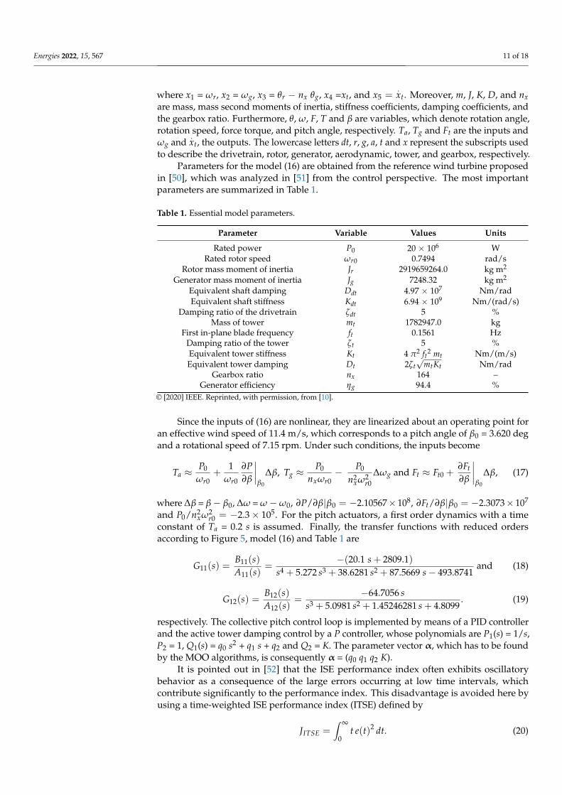
where x1 = ωr, x2 = ωg, x3 = θr − nx θg, x4 =xt, and x5 =.xt. Moreover, m, J, K, D, and nx

are mass, mass second moments of inertia, stiffness coefficients, damping coefficients, andthe gearbox ratio. Furthermore, θ, ω, F, T and β are variables, which denote rotation angle,rotation speed, force torque, and pitch angle, respectively. Ta, Tg and Ft are the inputs andωg and

.xt, the outputs. The lowercase letters dt, r, g, a, t and x represent the subscripts used

to describe the drivetrain, rotor, generator, aerodynamic, tower, and gearbox, respectively.Parameters for the model (16) are obtained from the reference wind turbine proposed

in [50], which was analyzed in [51] from the control perspective. The most importantparameters are summarized in Table 1.

Table 1. Essential model parameters.

Parameter Variable Values Units

Rated power P0 20 × 106 WRated rotor speed ωr0 0.7494 rad/s

Rotor mass moment of inertia Jr 2919659264.0 kg m2

Generator mass moment of inertia Jg 7248.32 kg m2

Equivalent shaft damping Ddt 4.97 × 107 Nm/radEquivalent shaft stiffness Kdt 6.94 × 109 Nm/(rad/s)

Damping ratio of the drivetrain ζdt 5 %Mass of tower mt 1782947.0 kg

First in-plane blade frequency ft 0.1561 HzDamping ratio of the tower ζt 5 %Equivalent tower stiffness Kt 4 π2 ft2 mt Nm/(m/s)Equivalent tower damping Dt 2ζt

√mtKt Nm/rad

Gearbox ratio nx 164 –Generator efficiency ηg 94.4 %

© [2020] IEEE. Reprinted, with permission, from [10].

Since the inputs of (16) are nonlinear, they are linearized about an operating point foran effective wind speed of 11.4 m/s, which corresponds to a pitch angle of β0 = 3.620 degand a rotational speed of 7.15 rpm. Under such conditions, the inputs become

Ta ≈P0

ωr0+

1ωr0

∂P∂β

∣∣∣∣β0

∆β, Tg ≈P0

nxωr0− P0

n2xω2

r0∆ωg and Ft ≈ Ft0 +

∂Ft

∂β

∣∣∣∣β0

∆β, (17)

where ∆β = β− β0, ∆ω = ω − ω0, ∂P/∂β|β0 = −2.10567× 108, ∂Ft/∂β|β0 = −2.3073× 107

and P0/n2xω2

r0 = −2.3× 105. For the pitch actuators, a first order dynamics with a timeconstant of Ta = 0.2 s is assumed. Finally, the transfer functions with reduced ordersaccording to Figure 5, model (16) and Table 1 are

G11(s) =B11(s)A11(s)

=−(20.1 s + 2809.1)

s4 + 5.272 s3 + 38.6281 s2 + 87.5669 s− 493.8741and (18)

G12(s) =B12(s)A12(s)

=−64.7056 s

s3 + 5.0981 s2 + 1.45246281 s + 4.8099. (19)

respectively. The collective pitch control loop is implemented by means of a PID controllerand the active tower damping control by a P controller, whose polynomials are P1(s) = 1/s,P2 = 1, Q1(s) = q0 s2 + q1 s + q2 and Q2 = K. The parameter vector α, which has to be foundby the MOO algorithms, is consequently α = (q0 q1 q2 K).

It is pointed out in [52] that the ISE performance index often exhibits oscillatorybehavior as a consequence of the large errors occurring at low time intervals, whichcontribute significantly to the performance index. This disadvantage is avoided here byusing a time-weighted ISE performance index (ITSE) defined by

JITSE =∫ ∞

0t e(t)2 dt. (20)

Energies 2022, 15, 567 12 of 18

6.3. Mechanization of the Optimization Procedure

The first step is to generate an objective function that can be evaluated by the MOOalgorithms. From the general Parseval Formula (9) and the ITSE index (20), functions f (t)and g(t) can be defined as

f (t) = e(t) and g(t) = t e(t), (21)

respectively. According to (14) and (15), the Laplace transform of f (t) can be described by apolynomial rational function, i.e.,

F(s) = e(s) =N(s)D(s)

(22)

and the Laplace transform of g(t) is

G(s) = −de(s)ds

= −dF(s)ds

, (23)

which can also be expressed as the polynomial rational function

G(s) = − (dN/ds)D− N(dD/ds)

D(s)2 . (24)

The derivatives are then obtained by polynomial differentiation, that is,

dD(s)/ds = nd d0snd−1 + (nd − 1) d1snd−2 + · · ·+ 2 dnd−2s + dnd−1 and (25)

dN(s)/ds = nn n0snn−1 + (nn − 1) n1snn−2 + · · ·+ 2 nnn−2s + nnn−1. (26)

If the functions F and G are rational, i.e.,

J =1

2π j

∫ j∞

−j∞

B1(s)A1(s)

C1(−s)A1(−s)

ds. (27)

the complex integral of Equation (16) can be solved using the Åström–Jury–Agniel algo-rithm [43] modified by [53]. Hence, the evaluation of the objective functions is completed,defining

A1(s) = D(s)2, B1(s) = D(s)N(s) and (28)

C1(s) = N(s)[dD(s)/ds]− D(s)[dN(s)/ds], (29)

where N and D are either N1 and D1 from (14) for the first control loop or N2 and D2 from(15) for the second control loop. A Matlab implementation of the generalized algorithm tocompute (27) can be found in [42].

It is important to remark that the condition for the existence of the solution is thatpolynomials D1 and D2 are stable, which is satisfied by the controller design. Thus, closed-loop stability is checked for every choice of controller parameters in the search space duringthe optimization process.

7. Optimization Results

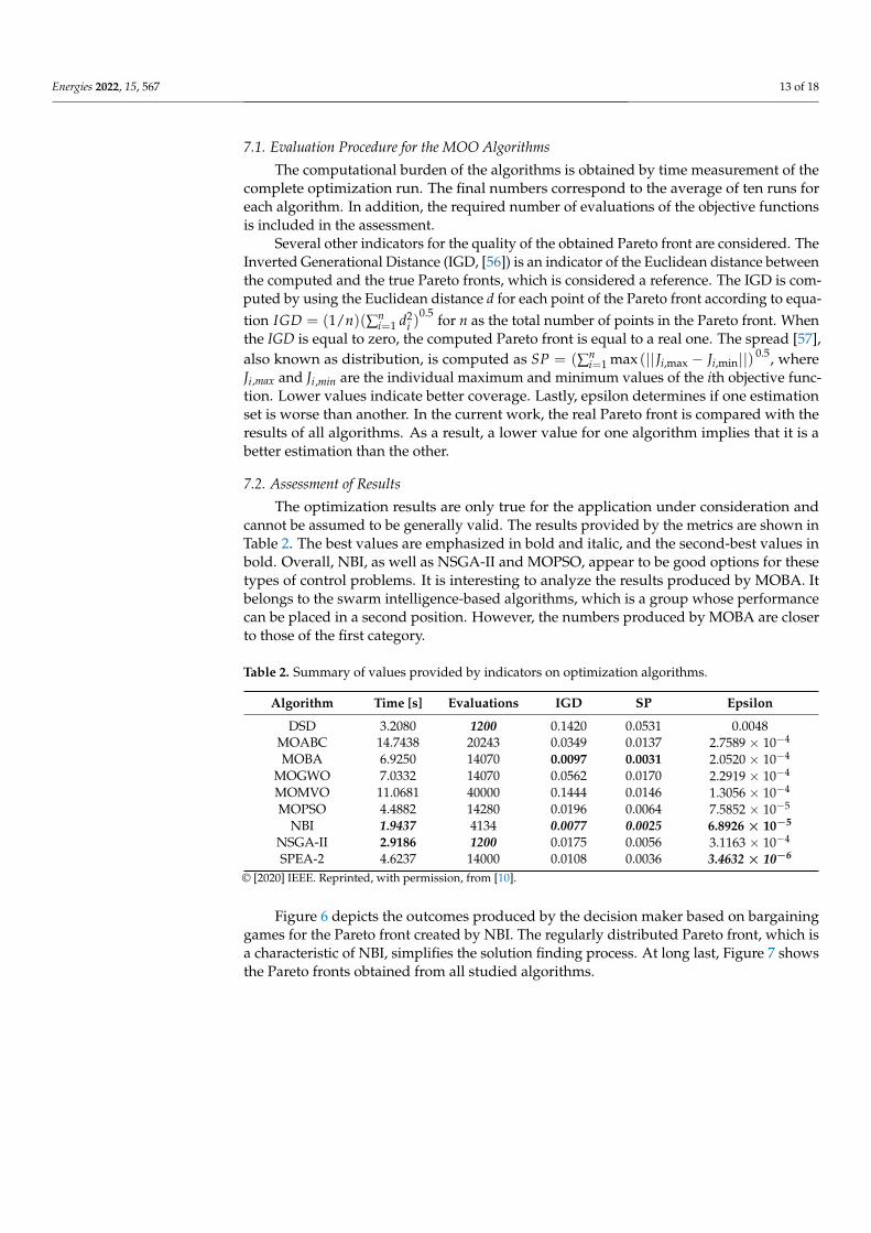
To carry out a quantitative assessment of the optimization outcomes, the effectivecomputation time for a whole Pareto front of 70 points, the number of evaluations of theobjective functions during the optimization process, the inverted generational distance(IGD), the spread (SP), and epsilon ε (see [54,55]) are considered.

Energies 2022, 15, 567 13 of 18

7.1. Evaluation Procedure for the MOO Algorithms

The computational burden of the algorithms is obtained by time measurement of thecomplete optimization run. The final numbers correspond to the average of ten runs foreach algorithm. In addition, the required number of evaluations of the objective functionsis included in the assessment.

Several other indicators for the quality of the obtained Pareto front are considered. TheInverted Generational Distance (IGD, [56]) is an indicator of the Euclidean distance betweenthe computed and the true Pareto fronts, which is considered a reference. The IGD is com-puted by using the Euclidean distance d for each point of the Pareto front according to equa-tion IGD = (1/n)(∑n

i=1 d2i )

0.5 for n as the total number of points in the Pareto front. Whenthe IGD is equal to zero, the computed Pareto front is equal to a real one. The spread [57],also known as distribution, is computed as SP = (∑n

i=1 max (||Ji,max − Ji,min||) 0.5, whereJi,max and Ji,min are the individual maximum and minimum values of the ith objective func-tion. Lower values indicate better coverage. Lastly, epsilon determines if one estimationset is worse than another. In the current work, the real Pareto front is compared with theresults of all algorithms. As a result, a lower value for one algorithm implies that it is abetter estimation than the other.

7.2. Assessment of Results

The optimization results are only true for the application under consideration andcannot be assumed to be generally valid. The results provided by the metrics are shown inTable 2. The best values are emphasized in bold and italic, and the second-best values inbold. Overall, NBI, as well as NSGA-II and MOPSO, appear to be good options for thesetypes of control problems. It is interesting to analyze the results produced by MOBA. Itbelongs to the swarm intelligence-based algorithms, which is a group whose performancecan be placed in a second position. However, the numbers produced by MOBA are closerto those of the first category.

Table 2. Summary of values provided by indicators on optimization algorithms.

Algorithm Time [s] Evaluations IGD SP Epsilon

DSD 3.2080 1200 0.1420 0.0531 0.0048MOABC 14.7438 20243 0.0349 0.0137 2.7589 × 10−4

MOBA 6.9250 14070 0.0097 0.0031 2.0520 × 10−4

MOGWO 7.0332 14070 0.0562 0.0170 2.2919 × 10−4

MOMVO 11.0681 40000 0.1444 0.0146 1.3056 × 10−4

MOPSO 4.4882 14280 0.0196 0.0064 7.5852 × 10−5

NBI 1.9437 4134 0.0077 0.0025 6.8926 × 10−5

NSGA-II 2.9186 1200 0.0175 0.0056 3.1163 × 10−4

SPEA-2 4.6237 14000 0.0108 0.0036 3.4632 × 10−6

© [2020] IEEE. Reprinted, with permission, from [10].

Figure 6 depicts the outcomes produced by the decision maker based on bargaininggames for the Pareto front created by NBI. The regularly distributed Pareto front, which isa characteristic of NBI, simplifies the solution finding process. At long last, Figure 7 showsthe Pareto fronts obtained from all studied algorithms.

Energies 2022, 15, 567 14 of 18

Energies 2022, 14, x FOR PEER REVIEW 14 of 18

Table 2. Summary of values provided by indicators on optimization algorithms.

Algorithm Time [s] Evaluations IGD SP Epsilon DSD 3.2080 1200 0.1420 0.0531 0.0048

MOABC 14.7438 20243 0.0349 0.0137 2.7589 × 10−4 MOBA 6.9250 14070 0.0097 0.0031 2.0520 × 10−4

MOGWO 7.0332 14070 0.0562 0.0170 2.2919 × 10−4 MOMVO 11.0681 40000 0.1444 0.0146 1.3056 × 10−4 MOPSO 4.4882 14280 0.0196 0.0064 7.5852 × 10−5

NBI 1.9437 4134 0.0077 0.0025 6.8926 × 10−5 NSGA-II 2.9186 1200 0.0175 0.0056 3.1163 × 10−4 SPEA-2 4.6237 14000 0.0108 0.0036 3.4632 × 10−6

© [2020] IEEE. Reprinted, with permission, from [10].

Figure 6 depicts the outcomes produced by the decision maker based on bargaining games for the Pareto front created by NBI. The regularly distributed Pareto front, which is a characteristic of NBI, simplifies the solution finding process. At long last, Figure 7 shows the Pareto fronts obtained from all studied algorithms.

Figure 6. Decision-making based on bargaining games for the NBI Pareto front. © [2020] IEEE. Re-printed, with permission, from [10].

Figure 7. Pareto fronts of all algorithms. (a) NBI, DSD, MOPSO, NSGA-II, and SPEA-2. (b) MO-ABC, MOBA, MOGWO, and MOMVO, where NBI is included as a reference. © [2020] IEEE. Re-printed, with permission, from [10].

Figure 6. Decision-making based on bargaining games for the NBI Pareto front. © [2020] IEEE.Reprinted, with permission, from [10].

Energies 2022, 14, x FOR PEER REVIEW 14 of 18

Table 2. Summary of values provided by indicators on optimization algorithms.

Algorithm Time [s] Evaluations IGD SP Epsilon DSD 3.2080 1200 0.1420 0.0531 0.0048

MOABC 14.7438 20243 0.0349 0.0137 2.7589 × 10−4 MOBA 6.9250 14070 0.0097 0.0031 2.0520 × 10−4

MOGWO 7.0332 14070 0.0562 0.0170 2.2919 × 10−4 MOMVO 11.0681 40000 0.1444 0.0146 1.3056 × 10−4 MOPSO 4.4882 14280 0.0196 0.0064 7.5852 × 10−5

NBI 1.9437 4134 0.0077 0.0025 6.8926 × 10−5 NSGA-II 2.9186 1200 0.0175 0.0056 3.1163 × 10−4 SPEA-2 4.6237 14000 0.0108 0.0036 3.4632 × 10−6

© [2020] IEEE. Reprinted, with permission, from [10].

Figure 6 depicts the outcomes produced by the decision maker based on bargaining games for the Pareto front created by NBI. The regularly distributed Pareto front, which is a characteristic of NBI, simplifies the solution finding process. At long last, Figure 7 shows the Pareto fronts obtained from all studied algorithms.

Figure 6. Decision-making based on bargaining games for the NBI Pareto front. © [2020] IEEE. Re-printed, with permission, from [10].

Figure 7. Pareto fronts of all algorithms. (a) NBI, DSD, MOPSO, NSGA-II, and SPEA-2. (b) MO-ABC, MOBA, MOGWO, and MOMVO, where NBI is included as a reference. © [2020] IEEE. Re-printed, with permission, from [10].

Figure 7. Pareto fronts of all algorithms. (a) NBI, DSD, MOPSO, NSGA-II, and SPEA-2. (b) MOABC,MOBA, MOGWO, and MOMVO, where NBI is included as a reference. © [2020] IEEE. Reprinted,with permission, from [10].

7.3. Important Issues Emerging from Practical Experience

Several issues associated with MOO control have come to light during the implemen-tation process that ought to be addressed. For example, there is today a tendency towardusing a large number of basic objective functions. Despite evidence that the performanceof MOO algorithms for more than two objective functions has improved significantly inrecent years, optimization times for problems with three objective functions in the order ofhours or days suggest that the effort is still insufficient. Furthermore, decisions-making insuch situations becomes a difficult task.

Thus, it is still preferable from the practical point of view to scale down the problem totwo complex objective functions, clustering multiple basic objectives into two classes. Thisidea can be realized by using the concept of cooperative and non-cooperative team gamescombined with a weighted sum objective function per team, where each summed objectivefunction includes a collection of noncontradictory characteristics. As a result, conflictingcriteria are assigned to different teams.

Another open aspect is the initialization of the algorithms by setting start values.Depending on these values, convergence usually takes more or less time. At present,there are no optimal and automatic procedures to initiate the algorithms, and therefore,experience is necessary to minimize the time for trial and error. In particular, algorithms

Energies 2022, 15, 567 15 of 18

need a search space at the start, which is typically not free in numerous control problems.For instance, if the stability region for the controller parameters is unknown a priori andthe search ranges for the parameters are chosen incorrectly, the closed-loop system maybecome unstable at start, and the algorithm will take a long time to converge to a stabilityregion. It is also possible that the whole optimization takes places outside the parameterstabilizing region and the optimization becomes infeasible. Thus, previous work should beto determine first the stabilizing parameter region to define the start search range inside it.

Related to the previously described issue is the fact that there are often several uncon-nected stabilizing search spaces. Since MOO algorithms are restricted to work within afixed search space, the global optimum could never be reached because the correspondingparameters are in a different search space. Furthermore, the value of one parameter oftenextends or contracts the stability range of other parameters, causing the effect that the searchspaces of other parameters change all the time. This effect is illustrated in Figure 8, whereit can be observed that the search space for (q0 q1 q2) depends on the value of parameter p1.

Energies 2022, 14, x FOR PEER REVIEW 15 of 18

7.3. Important Issues Emerging from Practical Experience Several issues associated with MOO control have come to light during the implementation

process that ought to be addressed. For example, there is today a tendency toward using a large number of basic objective functions. Despite evidence that the performance of MOO algorithms for more than two objective functions has improved significantly in recent years, optimization times for problems with three objective functions in the order of hours or days suggest that the effort is still insufficient. Furthermore, decisions-making in such situations becomes a difficult task.

Thus, it is still preferable from the practical point of view to scale down the problem to two complex objective functions, clustering multiple basic objectives into two classes. This idea can be realized by using the concept of cooperative and non-cooperative team games combined with a weighted sum objective function per team, where each summed objective function includes a collection of noncontradictory characteristics. As a result, conflicting criteria are assigned to different teams.

Another open aspect is the initialization of the algorithms by setting start values. De-pending on these values, convergence usually takes more or less time. At present, there are no optimal and automatic procedures to initiate the algorithms, and therefore, experi-ence is necessary to minimize the time for trial and error. In particular, algorithms need a search space at the start, which is typically not free in numerous control problems. For instance, if the stability region for the controller parameters is unknown a priori and the search ranges for the parameters are chosen incorrectly, the closed-loop system may be-come unstable at start, and the algorithm will take a long time to converge to a stability region. It is also possible that the whole optimization takes places outside the parameter stabilizing region and the optimization becomes infeasible. Thus, previous work should be to determine first the stabilizing parameter region to define the start search range inside it.

Related to the previously described issue is the fact that there are often several un-connected stabilizing search spaces. Since MOO algorithms are restricted to work within a fixed search space, the global optimum could never be reached because the correspond-ing parameters are in a different search space. Furthermore, the value of one parameter often extends or contracts the stability range of other parameters, causing the effect that the search spaces of other parameters change all the time. This effect is illustrated in Figure 8, where it can be observed that the search space for (q0 q1 q2) depends on the value of parameter p1.

-100 -0.5

0.5

q2

q1p1 = 0.5 p1 = 1.0

q0

-4.0 -3.5 -3.0 -2.0 -1.5 -1.0 -0.5 0 -2.5

-200 -1.0

-1.5

-2.0

0

-2.5

-3.0

Figure 8. Stabilizing subspaces for (q0 q1 q2) in dependence of parameter p1. Figure 8. Stabilizing subspaces for (q0 q1 q2) in dependence of parameter p1.

All these cases are not considered in the existing MOO algorithms. Thus, algorithmswith variable, conditioned, and discontinuous search ranges are needed, but they arecurrently unavailable.

Finally, current MOO algorithms are not deterministic in the computer science sense.Therefore, there is no guarantee that MOO control approaches can work in a real-timeenvironment where the optimization must be finished inside a sampling period to meetthe deadlines.

8. Conclusions

In this paper, multiobjective optimal (MOO) control is investigated from the userperspective. Multiobjective optimization is introduced shortly. In particular, aspectsrelated to the control application, such as, for example, the selection and evaluation ofobjective functions as well as the decision-making process, are examined. Several oldand relatively new MOO algorithms are studied from the control viewpoint by usingan example from wind energy control systems. The performances of the algorithms arecompared quantitatively by using standard indicators for MOO algorithms.

Results show that old-stablished algorithms like NBI, NSGA-II, and MOPSO aresolid and still maintain the state of the art, at least for control applications. From thelatest algorithms, MOBA stands out, but in general, they all need to be improved forreal-life control applications. In addition, several aspects arising from user experience werereported and limitations regarding the stability of the closed loop system and search spacesare highlighted.

Energies 2022, 15, 567 16 of 18

In general, multiobjective optimization is a sophisticated tool that greatly aids in theeffort to master the control system design of very complex applications. On the other hand,the current state of the art of MOO algorithms only allows a limited use.

Finally, the work is focused on the comparison of MOO methods for solving multiplecontrol loops with multiple controllers and the associated problems. Since all methodssolve the same objective functions with the same parameters, it is also expected that theyprovide the same results for the same decision-making. Thus, a study of the parametricsensibility and robustness of results is necessary before concluding whether the methodscan be thrust for application with real wind turbines in real-time operation. Such aspectsare currently being analyzed and will be reported in a future work.

Funding: This work is financed by the Federal Ministry of Economic Affairs and Energy (BMWi).

Institutional Review Board Statement: Not applicable.

Informed Consent Statement: Not applicable.

Data Availability Statement: Not applicable.

Conflicts of Interest: The authors declare no conflict of interest.

References1. Liu, G.P.; Yang, J.B.; Whidborne, J.F. Multiobjective Optimisation and Control; Research Studies Press Ltd.: Exeter, UK, 2003.2. Gambier, A.; Badreddin, E. Multi-objective optimal control: An overview. In Proceedings of the IEEE Conference on Control

Applications, Singapore, 1–3 October 2007; pp. 170–175.3. Gambier, A. MPC and PID control based on multi-objective optimization. In Proceedings of the 2008 American Control Conference,

Seattle, WA, USA, 11–13 June 2008; pp. 2886–2891.4. Gambier, A.; Jipp, M. Multi-objective optimal control: An introduction. In Proceedings of the Asian Control Conference,

Kaohsiung, Taiwan, 15–18 May 2011; pp. 1084–1089.5. Reynoso-Meza, G.; Ferragud, X.B.; Saez, J.S.; Durá, J.M.H. Controller Tuning with Evolutionary Multiobjective Optimization: A Holistic

Multiobjective Optimization Design Procedure, 1st ed.; Springer: Cham, Switzerland, 2017.6. Peitz, S.; Dellnitz, M. A survey of recent trends in multiobjective optimal control—Surrogate models, feedback control and

objective reduction. Math. Comput. Appl. 2018, 23, 30. [CrossRef]7. Wolpert, D.H.; Macready, W.G. No free lunch theorems for optimization. IEEE Trans. Evol. Comput. 1997, 1, 67–82. [CrossRef]8. Eichfelder, G. Multiobjective bilevel optimization. Math. Program. 2010, 123, 419–449. [CrossRef]9. Liang, J.Z.; Miikkulainen, R. Evolutionary bilevel optimization for complex control tasks. In Proceedings of the 2015 Annual

Conference on Genetic and Evolutionary Computation, Madrid, Spain, 11–15 July 2015; pp. 871–878.10. Gambier, A. Multiobjective Optimal Control: Algorithms, Approaches and Advice for the Application. In Proceedings of the 2020

International Automatic Control Conference, Hsinchu, Taiwan, 4–7 November 2020; pp. 1–7.11. Pareto, V. Manuale di Economia Politica; Societa Editrice Libraria: Milan, Italy, 1906; (Translated into English by A. S. Schwier as

Manual of Political Economy, Macmillan, New York, 1971).12. Miettinen, K.M. Nonlinear Multiobjective Optimization, 4th ed.; Kluwer Academic Publishers: New York, NY, USA, 2004.13. de Weck, O.L. Multiobjective optimization: History and promise. In Proceedings of the 3rd China-Japan-Korea Joint Symposium

on Optimization of Structural and Mechanical Systems, Kanazawa, Japan, 30 October–2 November 2004; pp. 1–14.14. Das, I.; Dennis, J.E. Normal-Boundary Intersection: A new method for generating the Pareto surface in nonlinear multicriteria

optimization problems. SIAM J. Optim. 1998, 8, 631–657. [CrossRef]15. Deb, K.; Pratap, A.; Agarwal, S.; Meyarivan, T. A fast and elitist multiobjective genetic algorithm: NSGA-II. IEEE Trans. Evol.

Comput. 2002, 6, 182–197. [CrossRef]16. Coello, C.A.; Lechuga, M.S. MOPSO: A proposal for multiple objective particle swarm optimization. In Proceedings of the 2002

Congress on the Evolutionary Computation, Honolulu, HI, USA, 12–17 May 2002; pp. 1051–1056.17. Zitzler, E.; Laumanns, M.; Thiele, L. SPEA2: Improving the Strength Pareto Evolutionary Algorithm; Research Report; Swiss Federal

Institute of Technology (ETH): Zurich, Switzerland, 2001.18. Motta, R.S.; Afonso, S.M.; Lyra, P.R. A modified NBI and NC method for the solution of N-multiobjective optimization problems.

Struct. Multidiscip. Optim. 2012, 46, 239–259. [CrossRef]19. Erfani, T.; Utyuzhnikov, S.V. Directed Search Domain: A Method for even generation of Pareto frontier in multiobjective

optimization. J. Eng. Optim. 2010, 43, 1–17. [CrossRef]20. Angus, D.; Woodward, C. Multiple objective ant colony optimisation. Swarm Intell. 2009, 3, 69–85. [CrossRef]21. Akbari, R.; Hedayatzadeh, R.; Ziarati, K.; Hassanizadeh, B. A multi-objective artificial bee colony algorithm. Swarm Evol. Comput.

2012, 2, 39–52. [CrossRef]22. Yang, X.S. Bat algorithm for multi-objective optimisation. Int. J. Bio-Inspired Comput. 2011, 3, 267–274. [CrossRef]

Energies 2022, 15, 567 17 of 18

23. Deb, K.; Jain, H. An evolutionary many-objective optimization algorithm using reference-point-based nondominated sortingapproach, Part I: Solving problems with Box constraints. IEEE Trans. Evol. Comput. 2014, 18, 577–601. [CrossRef]

24. Mirjalili, S.; Saremi, S.; Mirjalili, S.M.; Coelho, L.d.S. Multi-objective grey wolf optimizer: A novel algorithm for multicriterionoptimization. Expert Syst. Appl. 2016, 47, 106–119. [CrossRef]

25. Mirjalili, S.; Jangir, P.; Mirjalili, S.Z.; Saremi, S.; Trivedi, I.N. Optimization of problems with multiple objectives using themulti-verse optimization algorithm. Knowl.-Based Syst. 2017, 134, 50–71. [CrossRef]

26. Mirjalili, S.; Jangir, P.; Saremi, S. Multi-objective ant lion optimizer: A multi-objective optimization algorithm for solvingengineering problems. Appl. Intell. 2017, 46, 79–95. [CrossRef]

27. Messac, A.; Mattson, C. Normal constraint method with guarantee of even representation of complete Pareto frontier. AIAA J.2004, 42, 2101–2111. [CrossRef]

28. Messac, A. Physical programming: Effective optimization for computational de sign. AIAA J. 1996, 34, 149–158. [CrossRef]29. Mueller-Gritschneder, D.; Graeb, H.; Schlichtmann, U. A successive approach to compute the bounded Pareto front of practical

multiobjective optimization problems. SIAM J. Optim. 2009, 20, 915–934. [CrossRef]30. Kunkle, D. A Summary and Comparison of MOEA Algorithms; Research Report; College of Computer and Information Science

Northeastern University: Boston, MA, USA, 2005.31. Grimme, C.; Schmitt, K. Inside a predator-prey model for multiobjective optimization: A second study. In Proceedings of the

Genetic and Evolutionary Computation Conference, Seattle, WA, USA, 8–12 July 2006; pp. 707–714.32. Marler, R.T.; Arora, J.S. Survey of multi-objective optimization methods for engineering. Struct. Multidiscip. Optim. 2004, 26,

369–395. [CrossRef]33. Miller, K.S.; Ross, B. An Introduction to the Fractional Calculus and Fractional Differential Equations; John Wiley & Sons: New York,

NY, USA, 1993.34. Monje, C.A.; Chen, Y.; Vinagre, B.M.; Xue, D.; Feliu-Batlle, V. Fractional-Order Systems and Controls, 1st ed.; Springer: London, UK,

2010.35. Das, S.; Pan, I.; Halder, K.; Das, S.; Gupta, A. LQR based improved discrete PID controller design via optimum selection of

weighting matrices using fractional order integral performance index. Appl. Math. Model. 2013, 37, 4253–4268. [CrossRef]36. Gambier, A. Evolutionary multiobjective optimization with fractional order integral objectives for the pitch control system design

of wind turbines. IFAC-PapersOnLine 2019, 52, 274–279. [CrossRef]37. Romero, M.; de Madrid, A.P.; Vinagre, B.M. Arbitrary real-order cost functions for signals and systems. Signal Process. 2011, 91,

372–378. [CrossRef]38. Ortigueira, M.; Machado, J. Fractional definite integral. Fractal Fract. 2017, 1, 2. [CrossRef]39. Valério, D.; Sá da Costa, J. Ninteger: A non-integer control toolbox for MatLab. In Proceedings of the First IFAC Workshop on

Fractional Differentiation and Applications, Bordeaux, France, 19–21 July 2004; pp. 208–213.40. Xue, D. FOTF toolbox for fractional-order control systems. In Volume 6 Applications in Control; Petráš, I., Ed.; De Gruyter: Berlin,

Germany, 2019; Volume 6, pp. 237–266.41. Alamir, M.; Collet, D.; Di Domenico, D.; Sabiron, G. A fatigue-oriented cost function for optimal individual pitch control of wind

turbines. IFAC-PapersOnLine 2020, 52, 12632–12637.42. Gambier, A. Optimal PID controller design using multiobjective normal boundary intersection technique. In Proceedings of the

7th Asian Control Conference, Hong Kong, China, 27–29 August 2009; pp. 1369–1374.43. Åström, K. Introduction to Stochastic Control Theory; Academic Press: London, UK, 1970.44. Akhtar, T.; Shoemaker, C.A. Efficient Multi-Objective Optimization through Population-Based Parallel Surrogate Search; Research

Report; National University of Singapore: Singapore, 2019.45. Wellenreuther, A.; Gambier, A.; Badreddin, E. Application of a game-theoretic multi-loop control system design with robust

performance. IFAC Proc. Vol. 2008, 41, 10039–10044. [CrossRef]46. Gatti, N.; Amigoni, F. An approximate Pareto optimal cooperative negotiation model for multiple continuous dependent issues.

In Proceedings of the 2005 IEEE/WIC/ACM International Conference on Intelligent Agent Technology, Compiègne, France,19–22 October 2005; pp. 565–571.

47. Thomson, W. Cooperative models of bargaining. In Handbook of Game Theory with Economic 2; Aumann, R.J., Hart, S., Eds.; Elsevier:Oxford, UK, 1994; pp. 1237–1284.

48. Gambier, A. Simultaneous design of pitch control and active tower damping of a wind turbine by using multi-objectiveoptimization. In Proceedings of the 1st IEEE Conference on Control Technology and Applications, Kohala Coast, HI, USA, 27–30August 2017; pp. 1679–1684.

49. Gambier, A.; Nazaruddin, Y. Collective pitch control with active tower damping of a wind turbine by using a nonlinear PIDapproach. IFAC–PapersOnLine 2018, 51, 238–243. [CrossRef]

50. Ashuri, T.; Martins, J.R.R.; Zaaijer, M.B.; van Kuik, G.A.M.; van Bussel, G.J.W. Aeroservoelastic design definition of a 20 MWcommon research wind turbine model. Wind Energy 2016, 19, 2071–2087. [CrossRef]

51. Gambier, A.; Meng, F. Control system design for a 20 MW reference wind turbine. In Proceedings of the 3rd. IEEE Conference onControl Technology and Application, Hong Kong, China, 19–21 August 2019; pp. 258–263.

52. Zhuang, M.; Atherton, D.P. Tuning PID controllers with integral performance criteria. In Proceedings of the IEE Conference onControl 91, Edinburgh, UK, 25–28 March 1991; pp. 481–486.

Energies 2022, 15, 567 18 of 18

53. Wan, K.C.; Sreeram, V. Solution of bilinear matrix equation using Astrom-Jury-Agniel algorithm. IEE Proc. Part-D Control TheoryAppl. 1995, 142, 603–610. [CrossRef]

54. Riquelme, N.; von Lücken, C.; Baran, B. Performance metrics in multi-objective optimization. In Proceedings of the 2015 LatinAmerican Computing Conference, Arequipa, Peru, 19–23 October 2015; pp. 1–11.

55. Zitzler, E.; Thiele, L.; Laumanns, M.; Fonseca, C.M.; Grunert da Fonseca, V. Performance assessment of multiobjective optimizers:An analysis and review. IEEE Trans. Evol. Comput. 2003, 7, 117–132. [CrossRef]

56. Coello Coello, C.A.; Cortés, N. Solving multiobjective optimization problems using an artificial immune system. Genet. Program.Evol. Mach. 2005, 6, 163–190. [CrossRef]

57. Zitzler, E.; Deb, K.; Thiele, L. Comparison of multiobjective evolutionary algorithms: Empirical results. Evol. Comput. J. 2000, 8,125–148. [CrossRef] [PubMed]