SEA formulation and modeling issues

SEAmodeling

E. Savin

SEAformulation

Basichypotheses

Two coupledsub-systems

N coupledsub-systems

Modelingissues

Definingsub-systems

Modaldensity

Loss factor

Couplingloss factor

Powerinputs

Bibliography

SEA formulation and modeling issuesMG3409 - Lecture #5

E. Savin1,2

1Computational Fluid Dynamics Dept.Onera, France

2Mechanical and Civil Engineering Dept.Ecole Centrale Paris, France

February 2, 2015

SEAmodeling

E. Savin

SEAformulation

Basichypotheses



Modelingissues

Definingsub-systems

Modaldensity

Loss factor

Couplingloss factor

Powerinputs

Bibliography

Outline

1 SEA formulationBasic hypothesesTwo coupled sub-systemsN coupled sub-systems

2 Modeling issuesDefining sub-systemsInput parameters: modal densitiesInput parameters: loss factorsInput parameters: coupling loss factorsPower inputs

SEAmodeling

E. Savin

SEAformulation

Basichypotheses



Modelingissues

Definingsub-systems

Modaldensity

Loss factor

Couplingloss factor

Powerinputs

Bibliography

Basic SEA hypotheses

SEA aims at describing the energy transfers betweenN continuous sub-systems.

It is based on two groups of hypotheses:

1 The ones introduced in the previous lectures;2 The ones necessary to extend the results of the previous

lectures to the coupling of several (N ą 2) sub-systems.

Remark: SEA describes the flow of vibrational energy between

sub-systems, hence ”energy fluxes”, though the terminology ”power

flow” is mainly used in SEA literature.

SEAmodeling

E. Savin

SEAformulation

Basichypotheses



Modelingissues

Definingsub-systems

Modaldensity

Loss factor

Couplingloss factor

Powerinputs

Bibliography


Hypotheses introduced in the previous lectures:

1 The analysis is done in bands I0 “ rω0 ´∆ω2 , ω0 `

∆ω2 s.

2 The loads are:

wideband noises with bandwidth ∆ω;uncorrelated between sub-systems.

3 Each sub-system is weakly dissipative and characterizedby its own vibrational modes. Consequently:

∆ω " πζαωα, where 0 ă ζα ! 1;an unbounded domain cannot be an SEA sub-system.

4 The coupling is conservative: mass, stiffness, andgyroscopic couplings.

5 The vibrational modes of which eigenfrequencies lie inthe frequency band I0 are the only ones whichcontribute to the mechanical energy of each sub-systemin that band.

SEAmodeling

E. Savin

SEAformulation

Basichypotheses



Modelingissues

Definingsub-systems

Modaldensity

Loss factor

Couplingloss factor

Powerinputs

Bibliography


Additional hypotheses:6 Each sub-system r P t1, 2, . . .N u has a large numberNr of vibrational modes in the band I0.

Remark #1: Therefore the method is adapted to thehigh-frequency range of vibrations.Remark #2: Practically a mode count Nr Á 6, 7 isenough.

7 The average modal energies of each sub-system are close.8 Each vibrational mode of each sub-system has roughly

the same contribution to the power flows with the othersub-systems.

Remark #3: This hypothesis allows to extend thefundamental relationship Π129E1 ´ E2 for coupledoscillators to several coupled sub-systems.Remark #4: The last two hypotheses are reasonablefor high-frequency bands.

SEAmodeling

E. Savin

SEAformulation

Basichypotheses



Modelingissues

Definingsub-systems

Modaldensity

Loss factor

Couplingloss factor

Powerinputs

Bibliography

SEA formulationTwo coupled sub-systems

Notations: For the rth sub-system, r P t1, 2u, the”blocked” (angular) eigenfrequencies are tωrαuαPIr andthe associated loss factors are tηrαuαPIr . The modescontributing to the response are Ir “ tα; ωrα P I0u.Then the mode count Nr “ #Ir " 1.

The average modal density in the frequency band I0:

nrpω0q “Nr

∆ω.

From the hypothesis [3]: ηrα ! 1, α P Ir.From the hypothesis [6]: Nr " 1.

SEAmodeling

E. Savin

SEAformulation

Basichypotheses



Modelingissues

Definingsub-systems

Modaldensity

Loss factor

Couplingloss factor

Powerinputs

Bibliography


From the hypothesis [7]: ωrαηrα » ωrα1ηrα1 , α, α1 P Ir.

We then introduce an average loss factor ηrpω0q in thefrequency band I0 s.t.:

ω0ηrpω0q “1

Nr

ÿ

αPIr

ωrαηrα .

From the hypothesis [7]: EtErmα,tu “ πSrαDrα

» Er, whereEr is the average modal energy in the frequency bandI0:

Erpω0q “1

Nr

ÿ

αPIr

EtErmα,tu .

Consequently, the average mechanical energy of the rth

sub-system is EtEmr,tu » NrErpω0q.

SEAmodeling

E. Savin

SEAformulation

Basichypotheses



Modelingissues

Definingsub-systems

Modaldensity

Loss factor

Couplingloss factor

Powerinputs

Bibliography


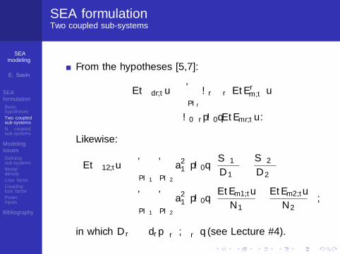
From the hypotheses [5,7]:

EtΠdr,tu »ÿ

αPIr

ωrαηrαEtErmα,tu

» ω0ηrpω0qEtEmr,tu .

Likewise:

EtΠ12,tu »ÿ

αPI1

ÿ

βPI2

a2β1αpω0q

„

πS1α

D1α´πS2β

D2β

“ÿ

αPI1

ÿ

βPI2

a2β1αpω0q

„

EtEm1,tu

N1´

EtEm2,tu

N2

,

in which Drα “ drpφrα,φrαq (see Lecture #4).

SEAmodeling

E. Savin

SEAformulation

Basichypotheses



Modelingissues

Definingsub-systems

Modaldensity

Loss factor

Couplingloss factor

Powerinputs

Bibliography


From the hypothesis [8]: a2β1αpω0q » a2β1

1α1pω0q, α, α1 P I1,

β, β1 P I2. Consequently:

EtΠ12,tu » N1N2a2β1αpω0q

„

EtEm1,tu

N1´

EtEm2,tu

N2

.

We then introduce the average coupling loss factor η12

in the frequency band I0 s.t.

ω0η12pω0q “ N2a2β1αpω0q .

Then reciprocity holds (from EtΠ12,tu “ ´EtΠ21,tu):N1η12pω0q “ N2η21pω0q, and

EtΠ12,tu “ ω0 pη12pω0qEtEm1,tu ´ η21pω0qEtEm2,tuq .

SEAmodeling

E. Savin

SEAformulation

Basichypotheses



Modelingissues

Definingsub-systems

Modaldensity

Loss factor

Couplingloss factor

Powerinputs

Bibliography


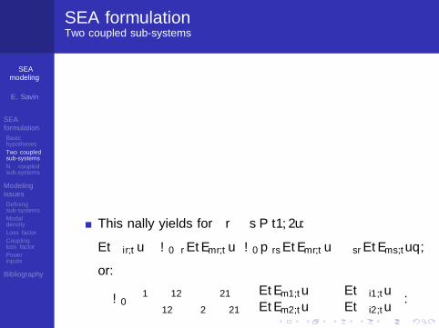
i2Πi1Π

Πd1 Πd2

Π

Π

12

21

E E1 21 2,n n ,

This finally yields for r ‰ s P t1, 2u:

EtΠir,tu “ ω0ηrEtEmr,tu`ω0 pηrsEtEmr,tu ´ ηsrEtEms,tuq ,

or:

ω0

„

η1 ` η12 ´η21

´η12 η2 ` η21

ˆ

EtEm1,tu

EtEm2,tu

˙

“

ˆ

EtΠi1,tu

EtΠi2,tu

˙

.

SEAmodeling

E. Savin

SEAformulation

Basichypotheses



Modelingissues

Definingsub-systems

Modaldensity

Loss factor

Couplingloss factor

Powerinputs

Bibliography

SEA formulationN coupled sub-systems

The relationships obtained for the power flows betweentwo sub-systems are extended to an arbitrary numberN of coupled sub-systems (r ‰ s P t1, 2, . . .N u):

EtΠdr,tu “ ω0ηrpω0qEtEmr,tu ,

EtΠrs,tu “ ω0 pηrspω0qEtEmr,tu ´ ηsrpω0qEtEms,tuq ,

EtΠir,tu “ EtΠdr,tu `

s“Nÿ

s “ 1s ‰ r

EtΠrs,tu .

SEAmodeling

E. Savin

SEAformulation

Basichypotheses



Modelingissues

Definingsub-systems

Modaldensity

Loss factor

Couplingloss factor

Powerinputs

Bibliography


In matrix form:

ω0

»

—

—

—

—

—

–

η1,tot ´η21 ´η31 ¨ ¨ ¨ ´ηN 1

´η12 η2,tot ´η32 ¨ ¨ ¨ ´ηN 2

´η13 ´η23 η3,tot ¨ ¨ ¨ ´ηN 3

......

.... . .

...´η1N ´η2N ´η3N ¨ ¨ ¨ ηN ,tot

fi

ffi

ffi

ffi

ffi

ffi

fl

¨

˚

˚

˚

˚

˚

˝

EtEm1,tu

EtEm2,tu

EtEm3,tu

...EtEmN ,tu

˛

‹

‹

‹

‹

‹

‚

“

¨

˚

˚

˚

˚

˚

˝

EtΠi1,tu

EtΠi2,tu

EtΠi3,tu

...EtΠiN ,tu

˛

‹

‹

‹

‹

‹

‚

where:ηr,totpω0q “ ηrpω0q `

s“Nÿ

s “ 1s ‰ r

ηrspω0q .

SEAmodeling

E. Savin

SEAformulation

Basichypotheses



Modelingissues

Definingsub-systems

Modaldensity

Loss factor

Couplingloss factor

Powerinputs

Bibliography


If the rth sub-system is coupled to an external acousticfluid, this apparent loss factor is modified to:

ηr,totpω0q “ ηr,radpω0q`ηr

c

%r%r ` %r,radpω0q

`

s“Nÿ

s “ 1s ‰ r

ηrspω0q .

Practically ηr,rad ă ηrs.

Reciprocity is enforced: Nrηrspω0q “ Nsηsrpω0q.

SEAmodeling

E. Savin

SEAformulation

Basichypotheses



Modelingissues

Definingsub-systems

Modaldensity

Loss factor

Couplingloss factor

Powerinputs

Bibliography

Outline

1 SEA formulationBasic hypothesesTwo coupled sub-systemsN coupled sub-systems

2 Modeling issuesDefining sub-systemsInput parameters: modal densitiesInput parameters: loss factorsInput parameters: coupling loss factorsPower inputs

SEAmodeling

E. Savin

SEAformulation

Basichypotheses



Modelingissues

Definingsub-systems

Modaldensity

Loss factor

Couplingloss factor

Powerinputs

Bibliography

SEA sub-systemsOverview

An SEA sub-system is a group of eigenmodes havingsimilar characteristics: energies (i.e. H7), couplingstrength with the other groups (i.e. H8).

The parameters describing the groups are:

the modal density,the loss factor,the coupling loss factor,and the input power,

averaged over the frequency band of analysis.

The proportionality relationship between the powerflows and the difference of the mechanical energies isrigorously wrong for more than two dofs; it holdsapproximatively for weak coupling.

SEAmodeling

E. Savin

SEAformulation

Basichypotheses



Modelingissues

Definingsub-systems

Modaldensity

Loss factor

Couplingloss factor

Powerinputs

Bibliography

SEA sub-systemsCoupling strength

Let µ “ M12?M1M2

, κ “ K12?K1K2

, γ “ Ω?D1D2

.

Then if µ “ κ “ γ “ Opεq, η12 “ Opε2q.

In case of weak coupling, the mechanical energy of asub-system in the actual configuration is close to itsmechanical energy in the decoupled, or ”blocked”configuration.

Likewise, the eigenfrequencies of a sub-system in the”blocked” and actual configurations are close.

SEAmodeling

E. Savin

SEAformulation

Basichypotheses



Modelingissues

Definingsub-systems

Modaldensity

Loss factor

Couplingloss factor

Powerinputs

Bibliography


D D1

1

1 2

2

2

uu 21

f2f1 Ωm m

k kk

m

Example #1: two-dofs system. The ”blocked”eigenfrequencies and half-power bandwidths are

ωα “

c

Mα

Kα, ∆α “ ηαωα “

DαMα

,

respectively, with Mα “ mα `m4 and Kα “ kα ` k.

If ω1 » ω2: then EtΠ12,tu 9 p∆1`∆2q´1. This is strong

coupling.

If |ω1 ´ ω2| ą ∆1 `∆2: then EtΠ12,tu 9 ∆1 `∆2. Thisis weak coupling.

SEAmodeling

E. Savin

SEAformulation

Basichypotheses



Modelingissues

Definingsub-systems

Modaldensity

Loss factor

Couplingloss factor

Powerinputs

Bibliography


0

D D

uu 21

f1m m

k k

k

0

0

0

0

0

Example #2: two-dofs system with stiffness couplingand no load on the second mass,

„

m0 00 m0

ˆ

:u1

:u2

˙

`

„

D0 00 D0

ˆ

9u1

9u2

˙

`

„

k0 ` k ´k´k k0 ` k

ˆ

u1

u2

˙

“

ˆ

f1

0

˙

.

The actual eigenfrequencies are:

ω1 “ ω0 “

c

k0

m0, ω2 “ ω0

c

1` 2k

k0,

whereas the ”blocked” ones are:

ω1 “ ω2 “

c

k0 ` k

m0.

SEAmodeling

E. Savin

SEAformulation

Basichypotheses



Modelingissues

Definingsub-systems

Modaldensity

Loss factor

Couplingloss factor

Powerinputs

Bibliography


One can compute exactly:

EtEm2,tu

EtEm1,tu“

η21

η0 ` η21,

with η0 “D0?

m0pk0`kqand η12 “ η21 “

12η0p kk0`k

q2.

If k0k Ñ 0 (strong coupling): then η21 Ñ

12η0

;

If kk0Ñ 0 (weak coupling): then η21 “ Op kk0

q2.

SEAmodeling

E. Savin

SEAformulation

Basichypotheses



Modelingissues

Definingsub-systems

Modaldensity

Loss factor

Couplingloss factor

Powerinputs

Bibliography

SEA sub-systemsGroups of modes

Sub-systems should be identified in order to satisfy theSEA hypotheses, and more particularly:

The modes in a sub-system should have similar dynamiccharacteristics;Those sub-systems should be considered as groups ofweakly coupled modes.

A group of modes is carried on by a physicalsub-system, which in turn can support different groups.

They are coupled as soon as they are constrained tohave the same motion at a given point, line, or surfaceof the overall physical system.

SEAmodeling

E. Savin

SEAformulation

Basichypotheses



Modelingissues

Definingsub-systems

Modaldensity

Loss factor

Couplingloss factor

Powerinputs

Bibliography


Example #3: beam junction. The longitudinalmotion of the vertical beam is coupled to the bendingmotion of the horizontal beams. The latter are coupledto the bending motion of the vertical beam, thus thelongitudinal and bending motions of the vertical beamare coupled.

SEAmodeling

E. Savin

SEAformulation

Basichypotheses



Modelingissues

Definingsub-systems

Modaldensity

Loss factor

Couplingloss factor

Powerinputs

Bibliography


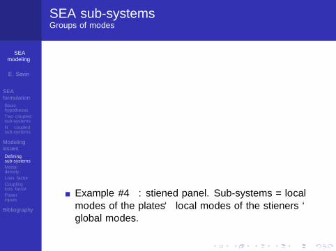
Example #4: stiffened panel. Sub-systems = localmodes of the plates ‘ local modes of the stiffeners ‘global modes.

SEAmodeling

E. Savin

SEAformulation

Basichypotheses



Modelingissues

Definingsub-systems

Modaldensity

Loss factor

Couplingloss factor

Powerinputs

Bibliography

SEA sub-systemsEnergy sinks

The SEA framework can be used to model a limitedpart of a complex system, considering the remainingparts as ”energy sinks”.

Example #5: noise induced by an electromechanicaldevice in a building.

f

bâtiment

équipement

1

SEAmodeling

E. Savin

SEAformulation

Basichypotheses



Modelingissues

Definingsub-systems

Modaldensity

Loss factor

Couplingloss factor

Powerinputs

Bibliography

SEA sub-systemsEnergy sinks

Example #6: two coupled sub-systems without loadon the second one,

ω0

„

η1 ` η12 ´η21

´η12 η2 ` η21

ˆ

EtEm1,tu

EtEm2,tu

˙

“

ˆ

EtΠi1,tu

0

˙

.

ThenEtEm2,tu

EtEm1,tu“ n2

n1

η21

η2`η21and:

EtΠi1,tu “ ω0η1EtEm1,tu ` ω0 pη12EtEm1,tu ´ η21EtEm2,tuq

“ ω0η1,netEtEm1,tu ,

where η1,net “ η1 `n2n1pη2η21

η2`η21q: the net loss factor.

SEAmodeling

E. Savin

SEAformulation

Basichypotheses



Modelingissues

Definingsub-systems

Modaldensity

Loss factor

Couplingloss factor

Powerinputs

Bibliography

Modal densityOne-dimensional system

In a bounded one-dimensional system of length L,λ2 “

Lα , α P N˚. Therefore the wave numbers and

eigenfrequencies have the form:

kα “ pα` δBCqπ

L, ωα “ pα` δBCq

πc

L,

where δBC ď 1 depends on the boundary conditions,and c (in m.s´1) may be a function of the frequency.

The modal density:

n1Dpωq “dα

dω“

dα

dkˆ

dk

dω“

L

πcgpωq,

where cg “dωdk is the group velocity.

SEAmodeling

E. Savin

SEAformulation

Basichypotheses



Modelingissues

Definingsub-systems

Modaldensity

Loss factor

Couplingloss factor

Powerinputs

Bibliography


Remark (group velocity): Consider the wave trainscospωt´ kxq and cos rpω ` dωqt´ pk ` dkqs, their sumis:

2 cos

ˆ

dω

2t´

dk

2x

˙

cos

„ˆ

ω `dω

2

˙

t´

ˆ

k `dk

2

˙

x

.

The average wave front is located at the position x andtime t s.t. tdω ´ xdk “ 0, thus it travels at the groupvelocity:

cg “dω

dk.

The group velocity is the speed of transport of theenergy.

SEAmodeling

E. Savin

SEAformulation

Basichypotheses



Modelingissues

Definingsub-systems

Modaldensity

Loss factor

Couplingloss factor

Powerinputs

Bibliography


Example: bending of a simply-supported beam(considering Euler-Bernoulli kinematics),

ω “pπαq2

L2

c

D

%A“πα

Lcbpωq ,

where cbpωq “?ω 4

b

D%A

is the bending phase velocity, Dis the bending stiffness, % is the density.

Other modes:

c (m.s´1) cg (m.s´1)

tractionb

E%

c

pure shearb

κG%

c

torsionb

GJ%I

c

bending?ω 4

b

D%A

2c

SEAmodeling

E. Savin

SEAformulation

Basichypotheses



Modelingissues

Definingsub-systems

Modaldensity

Loss factor

Couplingloss factor

Powerinputs

Bibliography

Modal densityTwo-dimensional system

The wave numbers of a square two-dimensional systemof size L1 ˆ L2 have the form:

kα “

d

„

pα1 ` δ1qπ

L1

2

`

„

pα2 ` δ2qπ

L2

2

,

where δ1 and δ2 depend on the boundary conditions.

The number of modes α “ pα1, α2q s.t. kα ď k:

α1pkq “L1

π

αmaxÿ

α2“1

d

k2 ´

„

pα2 ` δ2qπ

L2

2

´ δ1

“A

4πk2` γBCPk ,

where αmax is s.t. the square-rooted terms remainpositive, A “ L1L2, P “ 2pL1 ` L2q, and γBC dependson the boundary conditions.

SEAmodeling

E. Savin

SEAformulation

Basichypotheses



Modelingissues

Definingsub-systems

Modaldensity

Loss factor

Couplingloss factor

Powerinputs

Bibliography


The modal density:

n2Dpωq “dα

dω“

dα

dkˆ

dk

dω“

1

cgpωq

ˆ

Ak

2π` γBCP

˙

.

But k “ ωc where c is the phase velocity, thus:

n2Dpωq “Aω

2πcgc` ΓBCpωqP ,

where ΓBCpωq Ñ 0 as ω Ñ `8.

The modal density is less and less sensitive to theboundary conditions and the shape as the frequencyincreases. This formula is then used in SEA forarbitrary boundary conditions and shapes.

SEAmodeling

E. Savin

SEAformulation

Basichypotheses



Modelingissues

Definingsub-systems

Modaldensity

Loss factor

Couplingloss factor

Powerinputs

Bibliography


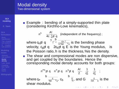
Example: bending of a simply-supported thin plate(considering Kirchhoff-Love kinematics),

nb“

Aω

4πc2bpωq(independent of the frequency) ,

where cbpωq “?ω 4

b

Eh2

12%p1´ν2qis the bending phase

velocity, cgpωq “ 2cbpωq, E is the Young modulus, ν isthe Poisson ratio, h is the thickness, % is the density.

The shear and compressional modes are non dispersive,and get coupled by the boundaries. Hence thecorresponding modal density accounts for both groups:

nPSpωq “ nP

pωq ` nSpωq “

Aω

2π

ˆ

1

c2P`

1

c2S

˙

,

where cP “b

E%p1´ν2q

, cS “b

G%, and G “ E

2p1`νqis the

shear modulus.

SEAmodeling

E. Savin

SEAformulation

Basichypotheses



Modelingissues

Definingsub-systems

Modaldensity

Loss factor

Couplingloss factor

Powerinputs

Bibliography

Modal densityThree-dimensional system

Modal density of a three-dimensional system of sizeL1 ˆ L2 ˆ L3 (e.g. an acoustic cavity):

n3Dpωq “V ω2

2π2cgc2`

Aω

2πcgcΓ1pωq ` PΓ2pωq ,

where Γjpωq Ñ 0 as ω Ñ 0, j “ 1, 2, depend on theboundary conditions, and V “ L1L2L3 (volume),A “ 2pL1L2 ` L1L3 ` L2L3q (area),P “ 4pL1 ` L2 ` L3q (total length of the edges).

SEAmodeling

E. Savin

SEAformulation

Basichypotheses



Modelingissues

Definingsub-systems

Modaldensity

Loss factor

Couplingloss factor

Powerinputs

Bibliography

Modal densityExperimental determination

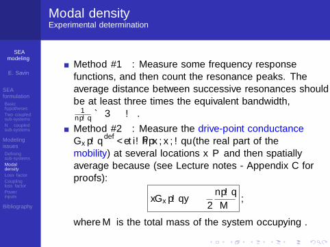
Method #1: Measure some frequency responsefunctions, and then count the resonance peaks. Theaverage distance between successive resonances shouldbe at least three times the equivalent bandwidth,

1npωq Á 3πζαωα.

Method #2: Measure the drive-point conductanceGxpωq

def“ <etiωphpx,x, ωqu (the real part of the

mobility) at several locations x P Ω and then spatiallyaverage because (see Lecture notes - Appendix C forproofs):

xGxpωqyΩ “π

2

npωq

M,

where M is the total mass of the system occupying Ω.

SEAmodeling

E. Savin

SEAformulation

Basichypotheses



Modelingissues

Definingsub-systems

Modaldensity

Loss factor

Couplingloss factor

Powerinputs

Bibliography

Modal densityNumerical determination

Compute the frequency response functions by a finiteelement model, or any other numerical technique (finitedifferences, particle-based and Monte-Carlo methods...).

Four elements/wavelength are usually enough to get agood estimate with an error lower than 10%.

SEAmodeling

E. Savin

SEAformulation

Basichypotheses



Modelingissues

Definingsub-systems

Modaldensity

Loss factor

Couplingloss factor

Powerinputs

Bibliography

Loss factorLoss factor of an elastic system

The loss factor ηs of an elastic structure is obtained byfitting some experimental data with the equivalentresult of a mathematical model, hence it has notheoretical ground. The fitting depends in addition onthe frequency/frequency band of analysis I0.

Reverberation time: the time of persistence of sound orvibration after a sound or vibration is produced. It istypically measured as the time TR it takes for a signal(vibrational energy) to drop by 60 dB.

Practically, one measures the mechanical energy of thefree response to some impulse loads:

E`mpTRq » Em0 e´ηsω0TR “ 10´6Em0 ,

so that:

TR “13.8

ηsω0.

SEAmodeling

E. Savin

SEAformulation

Basichypotheses



Modelingissues

Definingsub-systems

Modaldensity

Loss factor

Couplingloss factor

Powerinputs

Bibliography

Loss factorLoss factor of an acoustic cavity

Both (i) the fluid viscosity and (ii) the boundaryabsorption on the walls by multiple reflections of thewaves contribute to the loss factor of an acoustic cavity.Therefore:

ηf “cf

ω0

ˆ

αA

4V` νf

˙

,

where α is Sabine’s absorption coefficient of the walls(α » 0.1 in the air), and νf is the attenuation coefficientdue to the fluid viscosity (it depends on its density anddynamic viscosity).

The contribution (ii) of νf is usually negligible (e.g. air).

SEAmodeling

E. Savin

SEAformulation

Basichypotheses



Modelingissues

Definingsub-systems

Modaldensity

Loss factor

Couplingloss factor

Powerinputs

Bibliography

Equivalent loss factorRadiation efficiency

The average power radiated by a structure:

EtΠrad,tu “ σradpω0q%fcf |Γ|Et 9U2t u ,

where %fcfAV2

is the power radiated by a plate of areaA with uniform celerity V .

The radiation efficiency σrad is used to evaluated theequivalent loss factor ηrad:

ω0ηradpω0q “%fcf

%effpω0qσradpω0q ,

where %effpω0q “|Ωs|

|Γ| p%s ` %radpω0qq is the effectivesurface density of the structure.

SEAmodeling

E. Savin

SEAformulation

Basichypotheses



Modelingissues

Definingsub-systems

Modaldensity

Loss factor

Couplingloss factor

Powerinputs

Bibliography

Coupling loss factorPoint junction

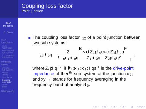
The coupling loss factor η12 of a point junction betweentwo sub-systems:

η12pω0q »2

πω0n1pω0q

B

<etZ1pω0u<etZ1pω0u

|Z1pω0q ` Z2pω0q|2

F

∆ω

,

where Zrpωq “ riωphrpxJ ,xJ , ωqs´1 is the drive-point

impedance of the rth sub-system at the junction xJ ;and x¨y∆ω stands for frequency averaging in thefrequency band of analysis I0.

SEAmodeling

E. Savin

SEAformulation

Basichypotheses



Modelingissues

Definingsub-systems

Modaldensity

Loss factor

Couplingloss factor

Powerinputs

Bibliography

Coupling loss factorDiffuse field approach

τ

τ

σ

σ

joint Σ

12

21

E1 , n1

, nE1

2

2 2

Consider two sub-systems coupled through a thirdsub-system (a joint Σ) characterized by some energyfluxes transmission and reflection coefficients τrs and σrrespectively, r ‰ s P t1, 2u.

SEAmodeling

E. Savin

SEAformulation

Basichypotheses



Modelingissues

Definingsub-systems

Modaldensity

Loss factor

Couplingloss factor

Powerinputs

Bibliography


Diffuse field approximation: the vibrational fieldwithin the rth sub-system is diffuse if it is thesuperposition of uncorrelated wave trains traveling inall directions, the latter being uniformly random.

The average mechanical energy EtEmr,tu is in additionuniformly distributed over the frequency band ofanalysis.

SEAmodeling

E. Savin

SEAformulation

Basichypotheses



Modelingissues

Definingsub-systems

Modaldensity

Loss factor

Couplingloss factor

Powerinputs

Bibliography


In the diffuse field approximation, the energy fluxdensity impinging the area dσ of the joint Σ within thesolid angle dΩ centered on the incident direction k is:

dπirpkq “ cgrEtEmr,tukdσ

|Ωr|

dΩpkq

|Ωd|,

where |Ω2| “ 2π (d “ 2 in 2D) or |Ω3| “ 4π (d “ 3 in3D) is the total solid angle, and cgr is the group velocity.

The energy flux density transmitted through the jointfrom the sub-system #1 to the sub-system #2:

dπ1Ñ2 “ τ12pkq ˆ dπi1pkq .

SEAmodeling

E. Savin

SEAformulation

Basichypotheses



Modelingissues

Definingsub-systems

Modaldensity

Loss factor

Couplingloss factor

Powerinputs

Bibliography


Then the average power transmitted from thesub-system #1 to the sub-system #2 is:

EtΠ1Ñ2,tu »

ż

k

dΩpkq

|Ωd|

ż

Σ

dσ

|Ω1|cg1EtEm1,tupk ¨ nqτ12pkq

“π

|Ωd|

|Σ|

|Ω1|xτ12ycg1EtEm1,tu ,

where xτ12y “1π

ş

k¨ną0pk ¨ nqτ12pkqdΩpkq.

The power balance for the 1st sub-system reads:

EtΠi1,tu ` EtΠ2Ñ1,tu “ EtΠd1,tu ` EtΠ1Ñ2,tu ,

where equivalently:

EtΠ2Ñ1,tu “π

|Ωd|

|Σ|

|Ω2|xτ21ycg2EtEm2,tu ,

SEAmodeling

E. Savin

SEAformulation

Basichypotheses



Modelingissues

Definingsub-systems

Modaldensity

Loss factor

Couplingloss factor

Powerinputs

Bibliography


Therefore:

EtΠi1,tu “ EtΠd1,tu `

˜

π

|Ωd|

|Σ|

|Ω1|xτ12ycg1EtEm1,tu

´π

|Ωd|

|Σ|

|Ω2|xτ21ycg2EtEm2,tu

¸

.

Coupling loss factor in the diffuse field approximation:

ω0ηrspω0q “π|Σ|

|Ωd|

cgrxτrsy

|Ωr|,

where reciprocity nrηrs “ nsηsr stems from the factthat c1´d

r τrs “ c1´ds τsr in that approximation, and

nr 9|Ωr|

cgrcd´1r

.

SEAmodeling

E. Savin

SEAformulation

Basichypotheses



Modelingissues

Definingsub-systems

Modaldensity

Loss factor

Couplingloss factor

Powerinputs

Bibliography

Coupling loss factorExperimental determination

Method #1: Power injection method (PIM). Theinput power Πi is imposed to each sub-systemsuccessively, and the mechanical energies are measuredfor all sub-systems. Then one solves for rηs:

ω0rηsEr “ Πir ,

where Πir “ p0, . . . , 0,Πi, 0, ...0qT is the vector of input

powers when only the rth sub-system is loaded, and Er

is the vector of mechanical energies.

Constraints on rηs: symmetry, negative off-diagonalterms.

However rηs is ill-conditioned.

SEAmodeling

E. Savin

SEAformulation

Basichypotheses



Modelingissues

Definingsub-systems

Modaldensity

Loss factor

Couplingloss factor

Powerinputs

Bibliography


i2Πi1Π

Πd1 Πd2

Π

Π

12

21

E E1 21 2,n n ,

Method #2: To single out a junction at a time. IfΠi2 “ 0 then:

E2

E1“n2

n1

η21

η2 ` η21ñ η12 “

η2E2

E1 ´n1n2E2

.

One measures the loss factor η2 of the receiving system(possibly adding some damping in order to haveE2 ! E1) and E1, E2.

SEAmodeling

E. Savin

SEAformulation

Basichypotheses



Modelingissues

Definingsub-systems

Modaldensity

Loss factor

Couplingloss factor

Powerinputs

Bibliography


Remark #1: The mechanical energy of an elasticsub-system:

Er “Mrxv2yΩr .

The mechanical energy of an acoustic cavity:

Er “V

%cxp2yΩr .

Remark #2: In room and building acoustics thetransmissivity xτsry is given in the form of thetransmission loss factor TL:

TL “ ´10 logxτsry .

SEAmodeling

E. Savin

SEAformulation

Basichypotheses



Modelingissues

Definingsub-systems

Modaldensity

Loss factor

Couplingloss factor

Powerinputs

Bibliography

Power inputs

The input power for the rth sub-system:

Πirptq “

ż

Ωr

frptq ¨ 9ufr ptq dx .

The loads t ÞÑ f rptq are known, but the forced responset ÞÑ ufr ptq of the rth sub-system coupled to all the othersub-systems and considering all applied loads isunknown.

The input power for the rth sub-system considered inisolation, when the other sub-systems are ”blocked”:

Πbirptq “

ż

Ωr

frptq ¨ 9ubrptq dx .

Considering weakly coupled sub-systems, SEA assumes:

EtΠir,tu » EtΠbir,tu .

SEAmodeling

E. Savin

SEAformulation

Basichypotheses



Modelingissues

Definingsub-systems

Modaldensity

Loss factor

Couplingloss factor

Powerinputs

Bibliography

Power inputs

”Equivalence” between:

The overall input powerş

R Πbirptqdt for wideband loads

with deterministic amplitudes and point supports;The average overall input power

ş

R EtΠbir,tudt for

wideband loads with deterministic amplitudes anduniformly random point supports within Ωr;The average input power EtΠb

ir,tu for widebandstationary random loads with deterministic or uniformlyrandom supports within Ωr;The average input power EtxΠb

ir,tyΩru for harmonicloads with deterministic or uniformly random pointsupports, and Ωr s.t. its ”blocked” eigenfrequencies areuniformly random and independent in the frequencyband of analysis I0.

SEAmodeling

E. Savin

SEAformulation

Basichypotheses



Modelingissues

Definingsub-systems

Modaldensity

Loss factor

Couplingloss factor

Powerinputs

Bibliography

Power inputs

These averages then read:

EtΠbir,tu »

π

2

nrpω0q

MrxEt|F r,t|

2uy∆ω ,

where xEt|F r,t|2uy∆ω stands for the total power of the

loads within I0, and xGxpωqyΩr “π2nrpω0q

Mrstands for the

average drive-point conductance of the rth sub-system.

Example: pF r,t, t P Rq is a m.s. stationary point force,of which spectral density function reads

SF rpωq “ Sr b 1I0YI0pωq .

Then xEt|F r,t|2uy∆ω ” 2∆ωTrSr.

SEAmodeling

E. Savin

SEAformulation

Basichypotheses



Modelingissues

Definingsub-systems

Modaldensity

Loss factor

Couplingloss factor

Powerinputs

Bibliography

Power inputsExperimental determination

Step #1: consider the rth sub-system and measure itsreverberant response to some known impulse loads:xv2yΩr (structure) or xp2yΩr (cavity) is deduced, thenEtEmr,tu.

Step #2: turn-off the loads, and deduce the total or netloss factor ηr,net from the reverberation time. Then:

EtΠir,tu » ω0ηr,netpω0qEtEmr,tu .

Remark: Power inputs are the most difficult toestimate, and the most critical to the overall response.

SEAmodeling

E. Savin

SEAformulation

Basichypotheses



Modelingissues

Definingsub-systems

Modaldensity

Loss factor

Couplingloss factor

Powerinputs

Bibliography

Bibliography

D.A. Bies, S. Hamid, ”In situ determination of loss and couplingloss factors by the power injection method”, J. Sound Vib. 70(2),187-204 (1980).

C.B. Burrough, R.W. Fisher, F.R. Kern, ”An introduction tostatistical energy analysis”, J. Acoust. Soc. Am. 101(4),1779-1789 (1997).

G. Borello, ”Analyse statistique energetique (SEA) del’environnement vibroacoustique - SEA (Statistical EnergyAnalysis)”, Techniques de l’Ingenieur R6-215v2 (2012).

G. Borello, ”Applications industrielles de la SEA”, Techniques del’Ingenieur R6-216 (2007).

F.J. Fahy, W.G. Price (Eds.): IUTAM Symposium on StatisticalEnergy Analysis. Springer, Dordrecht (1999).

T. Lafont, N. Totaro, A. Le Bot, ”Review of statistical energyanalysis hypotheses in vibroacoustics”, Proc. R. Soc. A470(2162), 20130515 (2014).

http://dx.doi.org/10.1016/0022-460X(80)90595-7

http://dx.doi.org/10.1016/0022-460X(80)90595-7

http://dx.doi.org/10.1016/0022-460X(80)90595-7

http://dx.doi.org/10.1121/1.418074

http://dx.doi.org/10.1121/1.418074

http://dx.doi.org/10.1121/1.418074

http://www.techniques-ingenieur.fr/base-documentaire/mesures-analyses-th1/mesures-acoustiques-et-vibratoires-42420210/analyse-statistique-energetique-sea-de-l-environnement-vibroacoustique-r6215/



http://www.techniques-ingenieur.fr/base-documentaire/transports-th14/technologies-avancees-et-systemes-de-transport-42575210/applications-industrielles-de-la-sea-r6216/

http://www.techniques-ingenieur.fr/base-documentaire/transports-th14/technologies-avancees-et-systemes-de-transport-42575210/applications-industrielles-de-la-sea-r6216/

http://dx.doi.org/10.1007/978-94-015-9173-7

http://dx.doi.org/10.1007/978-94-015-9173-7

http://dx.doi.org/10.1098/rspa.2013.0515



SEAmodeling

E. Savin

SEAformulation

Basichypotheses



Modelingissues

Definingsub-systems

Modaldensity

Loss factor

Couplingloss factor

Powerinputs

Bibliography

Bibliography

R.S. Langley, F.J. Fahy, ”High-frequency structural vibration”, inAdvanced Applications in Acoustics, Noise and Vibration (F.J.Fahy, J. Walker Eds.), pp. 490-529. Spon Press, London (2004).

C. Lesueur: Rayonnement Acoustique des Structures, Chap. 7.Eyrolles, Paris (1988).

R.H. Lyon, R.G. DeJong: Theory and Applications of StatisticalEnergy Analysis, 2nd Ed. Butterworth-Heinemann, Boston MA(1995).

W.G. Price, A.J. Keane (Eds.), ”Statistical energy analysis”, Phil.Trans. R. Soc. Lond. A 346(1681), 429-552 (1994).

P.W. Smith Jr., R.H. Lyon: Sound and Structural Vibration.NASA CR-160, March 1965.

http://www.crcpress.com/product/isbn/9780415237291



http://www.eyrolles.com/Sciences/Livre/rayonnement-acoustique-des-structures-0000000057035

http://www.eyrolles.com/Sciences/Livre/rayonnement-acoustique-des-structures-0000000057035

http://dx.doi.org/10.1098/rsta.1994.0027

http://dx.doi.org/10.1098/rsta.1994.0027

SEA formulation and modeling issues

Documents

Transcript of SEA formulation and modeling issues