ANKARA YILDIRIM BEYAZIT UNIVERSITY

GRADUATE SCHOOL OF NATURAL AND APPLIED SCIENCES

FIRST AND SECOND LAW ANALYSIS OF COMPACT HEAT

EXCHANGERS USED FOR INTERCOOLING PURPOSES

M.Sc. Thesis by

Ahmet Yasin SEDEF

Department of Mechanical Engineering

January, 2017

ANKARA

FIRST AND SECOND LAW ANALYSIS OF COMPACT

HEAT EXCHANGERS USED FOR INTERCOOLING

PURPOSES

A Thesis Submitted to

The Graduate School of Natural and Applied Sciences of

Ankara Yıldırım Beyazıt University

In Partial Fulfillment of the Requirements for the Degree of Master of Science

in Mechanical Engineering, Department of Mechanical Engineering

by

Ahmet Yasin SEDEF

January, 2017

ANKARA

ii

M.Sc. THESIS EXAMINATION RESULT FORM

We have read the thesis entitled “FIRST AND SECOND LAW ANALYSIS OF

COMPACT HEAT EXCHANGERS USED FOR INTERCOOLING

PURPOSES” completed by AHMET YASİN SEDEF under the supervision of

ASSIST. PROF. DR. KEMAL BİLEN and we certify that in our opinion it is fully

adequate, in scope and in quality, as a thesis for the degree of Master of Science.

Assist. Prof. Dr. Kemal BİLEN

Supervisor

Assoc. Prof. Dr. Malik M. NAUMAN Prof. Dr. Atilla BIYIKOĞLU

Jury Member Jury Member

Prof. Dr. Fatih V. ÇELEBİ

Director

Graduate School of Natural and Applied Sciences

iii

ETHICAL DECLARATION

I hereby declare that, in this thesis which has been prepared in accordance with the

Thesis Writing Manual of Graduate School of Natural and Applied Sciences,

All data, information and documents are obtained in the framework of

academic and ethical rules,

All information, documents and assessments are presented in accordance with

scientific ethics and morals,

All the materials that have been utilized are fully cited and referenced,

No change has been made on the utilized materials,

All the works presented are original,

and in any contrary case of above statements, I accept to renounce all my legal rights.

iv

ACKNOWLEDGMENTS

Firstly, I would like to express my sincere gratitude to my supervisor, Assist. Prof.

Dr. Kemal BİLEN for his tremendous support and motivation during my study. His

immense knowledge and precious recommendations constituted the milestones of

this study. His guidance assisted me all the time of my research and while writing

this thesis.

I would like to thank Prof. Dr. Veli ÇELİK for his understanding and endless

support. He always motivated me during my hard times and his advices helped me a

lot to overcome problems.

I also would like thank Assoc. Prof. Dr. Malik Muhammed NAUMAN and Prof. Dr.

Atilla BIYIKOĞLU for their valuable contributions and constructive criticisms

during my thesis defense examination.

I am grateful to my friend Ömer YILDIRIM for his superior contribution and great

effort while preparing the computer program for my thesis. Also my dearest friends

Hasan Ersel GÜREL and Meltem YAKTUBAY provided me enormous support

during my study and always trusted me. I am very fortunate to have such friends.

Finally, I must express my profound appreciations to my family for providing me

emotional support, loving care and continuous encouragement throughout my years

of study and through the period of writing this thesis. This accomplishment would

not have been possible without them. Thank You.

2017, 12 January Ahmet Yasin SEDEF

v

FIRST AND SECOND LAW ANALYSIS OF COMPACT HEAT

EXCHANGERS USED FOR INTERCOOLING PURPOSES

ABSTRACT

Intercooling is a process that is employed in turbocharged engines to cool the charge

air. This cooling enables to feed more air into the cylinders and decreases the

operating temperatures of the engine. Intercoolers -kind of compact heat exchangers-

are used to carry out this process. Depending on the required thermal-hydraulic

performance, intercoolers can be designed using different fin types.

In this study, the fin types that are utilized in the design of intercoolers are

theoretically examined using the first and second law of thermodynamics. For this

purpose, various intercooler configurations are established with five different fin

geometries, namely plain fins, louvered fins, offset strip fins, wavy fins and

perforated fins. Then, sizing and rating procedures are applied on these

configurations. In sizing procedure, the dimensions of the intercooler configurations

are determined. In rating procedure, heat transfer, pressure drop and second law

performances of the configurations are computed. The obtained results are tabulated

and compared with each other.

It is found that offset strip fins provide very good heat transfer performances whereas

plain fins enable least pressure drops in the fluid pressures. In second law analysis

the following outcome is attained; since the configurations in this study have

unbalanced flow, eliminating entropy generation or exergy destruction is not possible

even with an infinite surface area and zero pressure drops.

Keywords: Turbocharging, intercooling, intercoolers, compact heat exchangers,

plate-fin heat exchangers, heat transfer, pressure drop, second law analysis.

vi

ARA SOĞUTMA AMAÇLI KULLANILAN KOMPAKT ISI

DEĞİŞTİRİCİLERİNİN BİRİNCİ VE İKİNCİ YASA

ANALİZLERİ

ÖZ

Aşırı doldurmalı motorlarda, dolgu havasının sıcaklığını düşürmek amacıyla ara

soğutma işlemi uygulanır. Yapılan soğutma ile motora beslenen hava miktarında

artış, motordaki genel sıcaklık seviyesinde ise azalma sağlanır. Bu soğutma işlemi,

bir kompakt ısı değiştiricisi olan ara soğutucu ile gerçekleştirilir. İhtiyaç duyulan

termal-hidrolik performansa bağlı olarak ara soğutucular, farklı kanatçık tipleri

kullanılarak tasarlanabilir.

Yapılan bu çalışmada; ara soğutucu tasarımında kullanılan kanatçık tipleri, birinci ve

ikinci yasa analizleri vasıtasıyla teorik olarak incelenmiştir. Bu kapsamda; düz

kanatçık, panjurlu kanatçık, kaydırılmış şerit kanatçık, dalgalı kanatçık ve delikli

kanatçık olmak üzere beş kanatçık tipi kullanılarak farklı ara soğutucu yapıları

kurgulanmıştır. Daha sonra bu yapılara boyutlandırma ve performans değerlendirme

işlemleri uygulanmıştır. Boyutlandırma işlemi ile ara soğutucu yapılarının ebatları

bulunurken, performans değerlendirme işlemi ile yapıların ısı geçişi, basınç düşümü

ve ikinci yasa performansı hesaplanmıştır. Elde edilen sonuçlar tablolar halinde

verilmiş ve birbirleriyle kıyaslanmıştır.

Sonuçlar, kaydırılmış şerit kanatçık tipinin kullanılması ile ısıl açıdan iyi bir

performans elde edilebileceğini, düz kanatçık tipinin kullanılması ile de akışkanların

en az miktarda basınç düşüşüne maruz kalacağını göstermiştir. İkinci yasa analizleri

ise; bu çalışmadaki ara soğutucuların dengeli akışa sahip olmaması nedeniyle, sonsuz

büyüklükteki bir yüzey alanı ve sıfır basınç kaybıyla bile ara soğutucuda entropi

üretiminin ya da ekserji yıkımının tamamen yok edilemeyeceğini göstermiştir.

Anahtar Kelimeler: Aşırı doldurma, ara soğutma, ara soğutucular, kompakt ısı

değiştiricileri, plakalı-kanatlı ısı değiştiricileri, ısı geçişi, basınç düşümü, ikinci yasa

analizi.

vii

CONTENTS

M.Sc. THESIS EXAMINATION RESULT FORM ................................................ ii

ETHICAL DECLARATION .................................................................................. iii

ACKNOWLEDGMENTS ...................................................................................... iv

ABSTRACT ............................................................................................................ v

ÖZ ........................................................................................................................... vi

NOMENCLATURE ............................................................................................... ix

LIST OF TABLES ................................................................................................. xii

LIST OF FIGURES .............................................................................................. xiii

CHAPTER 1 - INTRODUCTION ............................................................................ 1

1.1 A General View of Internal Combustion Engines ............................................. 2

1.1.1 Engine Classifications ............................................................................... 2

1.1.2 Engine Operating Cycles ........................................................................... 3

1.2 Supercharging of Internal Combustion Engines................................................ 5

1.2.1 Mechanical Supercharging ........................................................................ 8

1.2.2 Turbocharging ............................................................................................ 8

1.2.3 Pressure Wave Supercharging.................................................................... 9

1.3 Intercooling in Internal Combustion Engines ................................................... 9

1.4 A General View of Heat Exchangers ............................................................... 11

1.4.1 Heat Exchanger Classifications ............................................................... 12

1.4.2 Compact Heat Exchangers ....................................................................... 14

1.5 Aim of the Study .............................................................................................. 16

1.6 Review of Related Works ................................................................................ 17

CHAPTER 2 - BASICS OF INTERCOOLERS .................................................... 21

2.1 General Design Considerations of Intercoolers ............................................... 21

2.2 Theory of Intercoolers ..................................................................................... 22

2.2.1 Thermal Design ....................................................................................... 22

2.2.2 Pressure Drop Analysis ............................................................................ 27

2.2.3 Second Law Analysis ............................................................................... 30

2.3 Some Additional Considerations for Thermal Design..................................... 35

2.3.1 Influence of Temperature-Dependent Fluid Properties ........................... 35

2.3.2 Longitudinal Heat Conduction Effects .................................................... 36

viii

2.3.3 Determination of Plate-fin Efficiency ..................................................... 38

CHAPTER 3 - DESIGN PROCEDURES OF INTERCOOLERS ...................... 42

3.1 Some Selected Surface Types and Their Characteristics ................................. 42

3.1.1 Colburn Factor and Fanning Friction Factor ........................................... 43

3.2 Operating Conditions of Intercooler ................................................................ 44

3.3. Rating Problem ............................................................................................... 47

3.4 Sizing Problem ................................................................................................ 51

CHAPTER 4 - RESULTS ........................................................................................ 55

4.1 Sizing Results .................................................................................................. 56

4.2 Rating Results .................................................................................................. 59

4.2.1 Comparison in terms of Heat Transfer and Pressure Drop Performance. 59

4.2.2 Comparison in terms of Second Law of Thermodynamics ..................... 62

4.2.3 Variation of Performance Parameters with Mass Flow Rate ................... 66

4.3 Intercooler and Engine Performance Results .................................................. 71

CHAPTER 5 - DISCUSSION AND CONCLUSION ............................................ 76

REFERENCES ......................................................................................................... 80

APPENDICES .......................................................................................................... 84

Appendix A – Surface Characteristics of Fins ....................................................... 85

Appendix B – j and f Factor Equations and Reynolds Number Ranges ............... 86

Appendix C – Thermophysical Properties of Air .................................................. 89

Appendix D – Kc and Ke Coefficients .................................................................. 90

CURRICULUM VITAE .......................................................................................... 91

ix

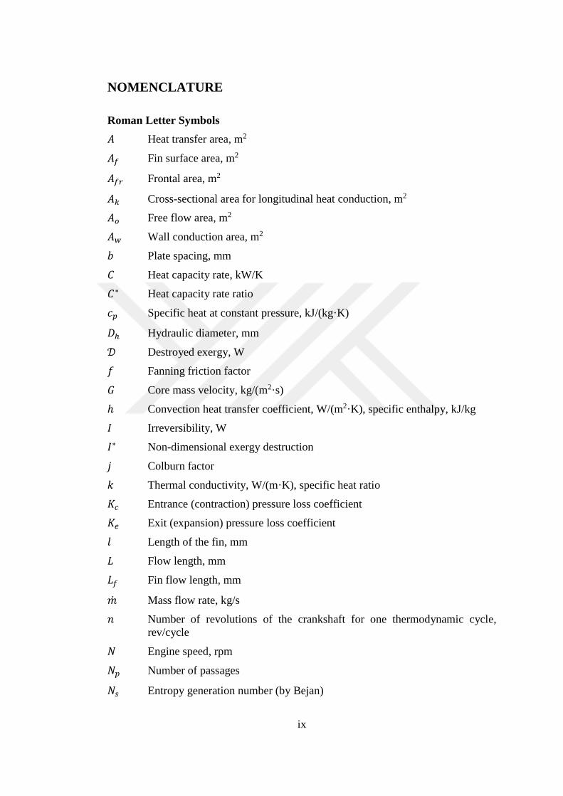
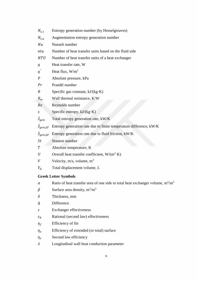
NOMENCLATURE

Roman Letter Symbols

𝐴 Heat transfer area, m2

𝐴𝑓 Fin surface area, m2

𝐴𝑓𝑟 Frontal area, m2

𝐴𝑘 Cross-sectional area for longitudinal heat conduction, m2

𝐴𝑜 Free flow area, m2

𝐴𝑤 Wall conduction area, m2

𝑏 Plate spacing, mm

𝐶 Heat capacity rate, kW/K

𝐶∗ Heat capacity rate ratio

𝑐𝑝 Specific heat at constant pressure, kJ/(kg·K)

𝐷ℎ Hydraulic diameter, mm

𝒟 Destroyed exergy, W

𝑓 Fanning friction factor

𝐺 Core mass velocity, kg/(m2·s)

ℎ Convection heat transfer coefficient, W/(m2·K), specific enthalpy, kJ/kg

𝐼 Irreversibility, W

𝐼∗ Non-dimensional exergy destruction

𝑗 Colburn factor

𝑘 Thermal conductivity, W/(m·K), specific heat ratio

𝐾𝑐 Entrance (contraction) pressure loss coefficient

𝐾𝑒 Exit (expansion) pressure loss coefficient

𝑙 Length of the fin, mm

𝐿 Flow length, mm

𝐿𝑓 Fin flow length, mm

�̇� Mass flow rate, kg/s

𝑛 Number of revolutions of the crankshaft for one thermodynamic cycle,

rev/cycle

𝑁 Engine speed, rpm

𝑁𝑝 Number of passages

𝑁𝑠 Entropy generation number (by Bejan)

x

𝑁𝑠,1 Entropy generation number (by Hesselgreaves)

𝑁𝑠,𝑎 Augmentation entropy generation number

𝑁𝑢 Nusselt number

𝑛𝑡𝑢 Number of heat transfer units based on the fluid side

𝑁𝑇𝑈 Number of heat transfer units of a heat exchanger

𝑞 Heat transfer rate, W

𝑞" Heat flux, W/m2

𝑃 Absolute pressure, kPa

𝑃𝑟 Prandtl number

𝑅 Specific gas constant, kJ/(kg·K)

𝑅𝑤 Wall thermal resistance, K/W

𝑅𝑒 Reynolds number

𝑠 Specific entropy, kJ/(kg·K)

�̇�𝑔𝑒𝑛 Total entropy generation rate, kW/K

�̇�𝑔𝑒𝑛,∆𝑇 Entropy generation rate due to finite temperature difference, kW/K

�̇�𝑔𝑒𝑛,∆𝑃 Entropy generation rate due to fluid friction, kW/K

𝑆𝑡 Stanton number

𝑇 Absolute temperature, K

𝑈 Overall heat transfer coefficient, W/(m2·K)

𝑉 Velocity, m/s, volume, m3

𝑉𝑑 Total displacement volume, L

Greek Letter Symbols

𝛼 Ratio of heat transfer area of one side to total heat exchanger volume, m2/m3

𝛽 Surface area density, m2/m3

𝛿 Thickness, mm

Δ Difference

휀 Exchanger effectiveness

휀𝑅 Rational (second law) effectiveness

𝜂𝑓 Efficiency of fin

𝜂𝑜 Efficiency of extended (or total) surface

𝜂𝑠 Second law efficiency

𝜆 Longitudinal wall heat conduction parameter

xi

𝜇 Dynamic viscosity of fluid, N·s/m2

𝜈 Specific volume of fluid, m3/kg

𝜌 Density of fluid, kg/m3

𝜎 Ratio of free-flow area to frontal area

𝜏𝑤 Surface (wall) shear stress, kg/(m·s2)

𝜓 Flow exergy, kJ/kg

Subscripts

𝑐 Cold fluid

𝑓 Fin

ℎ Hot fluid

𝑖 Inlet

𝑚 Mean

𝑚𝑎𝑥 Maximum

𝑚𝑖𝑛 Minimum

𝑜 Outlet

𝑠𝑡 Stack

𝑤 Wall

0 Reference (temperature or pressure)

1, 2 Any flow side of the heat exchanger (hot or cold side)

Acronyms

BDC Bottom Dead Center

CI Compression-ignition

ICE Internal Combustion Engine

LHC Longitudinal Heat Conduction

LMTD Logarithmic Mean Temperature Difference

SI Spark-ignition

TDC Top Dead Center

xii

LIST OF TABLES

Table 2.1 Exponents of (Tw/Tm) ............................................................................... 36

Table 3.1 Technical specifications of Ford Cargo TCI engine ................................. 46

Table 4.1 Sizing results of intercooler configurations............................................... 57

Table 4.2 Thermal-hydraulic performance results of intercooler configurations. ..... 60

Table 4.3 Second law performance results of intercooler configurations. ................ 63

Table 4.4 Charge air density and temperatures in the cycle for different engine

operation types. .......................................................................................................... 72

Table A.1 Surface characteristics of fins ................................................................... 85

Table B.1 j factor equations for fin types. ................................................................. 86

Table B.2 f factor equations for fin types. ................................................................. 87

Table B.3 Reynolds number ranges for j and f factor equations ............................... 88

Table C.1 Thermophysical properties of air at one atmospheric pressure ................ 89

xiii

LIST OF FIGURES

Figure 1.1 Four-stroke SI engine cycle ....................................................................... 4

Figure 1.2 A two-stroke SI engine .............................................................................. 5

Figure 1.3 Supercharging and turbocharging configurations ...................................... 7

Figure 1.4 Types of charge air cooling systems ........................................................ 11

Figure 1.5 Schematic diagram of a plate-fin heat exchanger .................................... 15

Figure 1.6 Various fin geometries for plate-fin heat exchangers .............................. 16

Figure 2.1 Depiction of heat transfer in a counterflow heat exchanger .................... 24

Figure 2.2 Pressure drop components in a plate-fin exchanger flow passage ........... 28

Figure 2.3 Straight, thin fin with uniform rectangular cross-section ........................ 40

Figure 2.4 (a) Plain rectangular fin and (b) plain triangular fin ................................ 41

Figure 3.1 Charge air flow in a turbocharged and intercooled engine ...................... 45

Figure 4.1 The change of effectiveness with respect to hot side mass flow rate. ..... 67

Figure 4.2 The change of hot side pressure drop with respect to hot side mass flow

rate. ............................................................................................................................. 68

Figure 4.3 The change of hot side outlet density with respect to hot side mass flow

rate .............................................................................................................................. 69

Figure 4.4 The change of total entropy generation rate with respect to hot side mass

flow rate ..................................................................................................................... 69

Figure 4.5 The change of normalized entropy generation rate with respect to hot side

mass flow rate ............................................................................................................ 70

Figure 4.6 The change of second law efficiency with respect to hot side mass flow

rate. ............................................................................................................................. 71

Figure 4.7 P-ν diagram of an air-standard dual cycle ............................................... 72

Figure 4.8 Effect of charge cooling on inlet air density. ........................................... 74

Figure 4.9 Effect of pressure drop on inlet air density. ............................................. 75

Figure D.1 Entrance and exit pressure loss coefficients ........................................... 90

1

CHAPTER 1

INTRODUCTION

Internal combustion engines (ICE) have found wide application in today’s world,

especially in the land, sea, and air transportation sectors and power generation fields.

ICEs are highly preferred because of their simplicity, durability and high power to

weight ratios. On the other hand, their most critical and vital problem is the

emissions generated by the engine. These emissions pollute the environment and

threat the human health. Therefore the allowable emission levels for the engines are

decreased day by day. More efficient and low emissions power generation has

become very crucial.

Supercharging the ICEs, that is providing compressed air to the engine cylinders, is

one way of increasing the engine efficiency and decreasing the emissions. It is a

process of pressurizing the air (so increasing density of the air) before entry to

cylinders. Therefore more fuel can be fed and more power can be generated

efficiently without changing the engine size. Supercharging process has many

advantages but it generally requires some additional modifications to the engine.

Increasing the pressure also increases the temperature of intake air by compressive

heating which in turn elevates the temperatures throughout the entire engine

operating cycle. This condition overshadows the positive effect of supercharging. In

order to eliminate it, a process often called intercooling (or aftercooling, charge air

cooling) is performed in supercharged engines by means of intercoolers -kind of

compact heat exchangers. This intercooling process also further increases the density

of charge air which is very desirable.

When intercoolers are utilized, the compressed air leaving the supercharger is

directed to the intercooler and cooled using a fluid. Here the important point is that;

intercooler must provide necessary amount of cooling to the charge air without

dropping its pressure much. If not so, the advantages gained by supercharging are

diminished and practicality of intercooling process becomes questionable.

2

In this chapter, firstly a brief explanation of internal combustion engines is

introduced. Then, supercharging and intercooling applications employed in internal

combustion engines are described in details. Since intercoolers are essentially heat

exchangers, heat exchanger classifications, and the position of intercoolers in given

classifications are mentioned. Last, the aim of this study and related works in the

literature are presented.

1.1 A General View of Internal Combustion Engines

Internal combustion engines date back to 1876 when Otto first created the spark-

ignition engine and 1892 when Diesel developed the compression-ignition engine.

Since then, these engines have been continuously improved as new technologies or

advancements have become available. The demand for new types of engines and

environmental constraints are the main causes of that ongoing development. Today

these engines play a dominant role in fields of power, propulsion and energy [1].

The purpose of internal combustion engines is the production of mechanical power

from the chemical energy of the fuel. This energy is released by burning or oxidizing

the fuel inside the engine. Because this energy supplied to the engine parts is created

inside the engine, it is called internal combustion engine (ICE).

ICEs which are the subjects of this study are spark-ignition (SI) or gasoline engines

(although other fuels can be used) and compression-ignition (CI) or diesel engines.

Gas turbines are also internal combustion engines by this definition, yet, customarily;

the term is only used for SI and CI engines.

Because of their simplicity, durability and high power to weight ratio, SI and CI

engines have found wide application in transportation sectors (land, sea and air) and

power generation fields [1].

1.1.1 Engine Classifications

There are many different types of internal combustion engines. They can be

classified by [1]:

3

1. Application. Automobile, truck, locomotive, light aircraft, marine, portable

power system, power generation.

2. Basic engine design. Reciprocating engines, rotary engines.

3. Working cycle. Four-stroke cycle, two-stroke cycle.

4. Valve or port design and location. Overhead (or I-head) valves, underhead (or

L-head) valves, rotary valves, cross-scavenged porting, loop-scavenged

porting, through- or uniflow-scavenged.

5. Fuel. Gasoline (or petrol), fuel oil (or diesel fuel), natural gas, liquid

petroleum gas, alcohols (methanol, ethanol), hydrogen, dual fuel.

6. Method of mixture preparation. Carburetion, fuel injection into the intake

ports or intake manifold, fuel injection into the engine cylinder.

7. Method of ignition. Spark ignition, compression ignition.

8. Method of air intake process. Naturally aspirated, supercharged, turbocharged

[2].

9. Combustion chamber design. Open chamber, divided chamber.

10. Method of load control. Throttling of fuel and air flow together so mixture

composition is essentially unchanged, control of fuel alone, a combination of

these.

11. Method of cooling. Water cooled, air cooled, uncooled (other than by

natural convection and radiation)

12. Position and number of cylinders of reciprocating engines. Single cylinder

engine, in-line engine, V engine, opposed cylinder engine, W engine, opposed

piston engine, radial engine [2].

1.1.2 Engine Operating Cycles

Most internal combustion engines, both SI and CI, operate on either a four-stroke

cycle or a two-stroke cycle. These cycles are quite standard for all engines. Only

slight variations may be found in separate designs [2].

In a four-stroke engine, piston in each cylinder has four strokes; intake, compression,

power and exhaust strokes, to complete its cycle. This corresponds to two revolutions

of the crankshaft.

4

For an SI engine, in intake stroke, the piston moves from top-dead-center (TDC) to

bottom-dead-center (BDC) and draws fresh air-fuel mixture through the open intake

valve into the cylinder. In compression stroke, the piston moves from BDC to TDC

to compress that mixture. The temperature and pressure inside the cylinder is

increased to a certain value and the mixture is ignited by a spark plug to initiate

combustion toward the end of the stroke. The combustion ideally occurs at constant

volume. In power stroke, the high temperature and pressure gas expands and moves

the piston to the BDC position. As the piston approaches BDC, the exhaust valve

opens to initiate exhaust process. Finally, in exhaust stroke the piston moves from

BDC to TDC to sweep out the burned gases. A schematic diagram explaining the

entire cycle is given in Figure 1.1.

Figure 1.1 Four-stroke SI engine cycle [Modified from 3].

The four-stroke CI or diesel engine goes through the almost same steps with SI

engine. Slight differences occur in the cycle. The most important difference is that in

CI engine only air is inducted into the cylinder during the intake stroke and

combustion is initiated not by a spark plug but injection of fuel over the air. Self-

ignition occurs when the fuel meets the air in the cylinder. Combustion proceeds

ideally at constant pressure. The remaining steps are identical to the SI engine.

To obtain a higher power output from a given engine size and a simpler valve design,

the two-stroke cycle was developed. In two-stroke SI and CI engines, the processes

occur with similar manner. However, in these engines one cycle corresponds to one

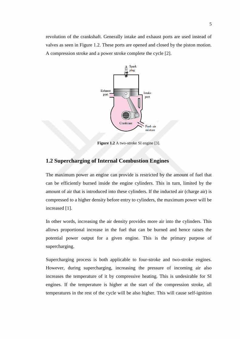
5

revolution of the crankshaft. Generally intake and exhaust ports are used instead of

valves as seen in Figure 1.2. These ports are opened and closed by the piston motion.

A compression stroke and a power stroke complete the cycle [2].

Figure 1.2 A two-stroke SI engine [3].

1.2 Supercharging of Internal Combustion Engines

The maximum power an engine can provide is restricted by the amount of fuel that

can be efficiently burned inside the engine cylinders. This in turn, limited by the

amount of air that is introduced into these cylinders. If the inducted air (charge air) is

compressed to a higher density before entry to cylinders, the maximum power will be

increased [1].

In other words, increasing the air density provides more air into the cylinders. This

allows proportional increase in the fuel that can be burned and hence raises the

potential power output for a given engine. This is the primary purpose of

supercharging.

Supercharging process is both applicable to four-stroke and two-stroke engines.

However, during supercharging, increasing the pressure of incoming air also

increases the temperature of it by compressive heating. This is undesirable for SI

engines. If the temperature is higher at the start of the compression stroke, all

temperatures in the rest of the cycle will be also higher. This will cause self-ignition

6

and knocking problems in SI engines [2]. Several parameters can be adjusted to

avoid knocking in these engines, yet generally they are not supercharged because of

the application difficulties [4]. In CI engines, on the other hand, there is no concern

about knocking problems. Supercharged diesel engine output is usually limited by

stress levels in critical components. The maximum stress level constrains the

maximum cylinder pressure. As charge air pressure is raised, the maximum pressures

and thermal loadings will increase nearly in proportion. Therefore, in practice the

compression ratio is often reduced in these engines relative to naturally aspirated

ones [2]. Supercharging the diesel engines provides high performance and smooth

operation.

In two-stroke engines, supercharging is inevitable. Ports are used instead of valves

for intake and exhaust processes. These ports are opened and closed with the motion

of piston (not by a camshaft). Therefore, in order to clear the cylinder from burned

gases and charge it with the fresh air or air-fuel mixture -scavenging process- there

should be high-enough pressure of intake. The necessary pressure boost to displace

the burned gases can be accomplished by supercharging.

Supercharging which is mainly pressurizing the charge air can be applied to engines

in three fundamental methods; Mechanical supercharging, turbocharging and

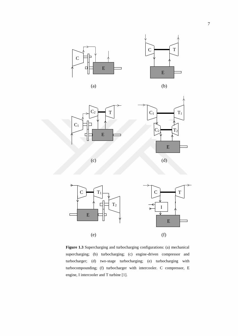
pressure wave supercharging. Figure 1.3 shows typical arrangements of the different

supercharging and turbocharging systems.

Most commonly, mechanical supercharger (Fig. 1.3a) or turbocharger (Fig. 1.3b)

arrangements are preferred. Combinations of an engine driven compressor and a

turbocharger can also be used as in large marine engines (Fig. 1.3c). Two-stage

turbocharger is another available method to engines to provide very high pressures

(Fig. 1.3d). Turbocompounding which operates with two turbines, one is coupled to

compressor and other is directly geared to engine crankshaft, is an alternative method

of increasing engine power (Fig. 1.3e). Cooling the compressed air before entry to

the cylinders (intercooling) is used to further increase air or mixture density as shown

in Fig. 1.3f [1].

7

C

C T

C2 T C1 T1

C2 T2

C T1

T2

C T

I

C1

(a) (b)

(c) (d)

(e) (f)

Figure 1.3 Supercharging and turbocharging configurations: (a) mechanical

supercharging; (b) turbocharging; (c) engine-driven compressor and

turbocharger; (d) two-stage turbocharging; (e) turbocharging with

turbocompounding; (f) turbocharger with intercooler. C compressor, E

engine, I intercooler and T turbine [1].

T

T-1

E E

E

E

E

E

8

1.2.1 Mechanical Supercharging

In this system, a separate compressor usually driven by the engine crankshaft is used

to increase the incoming air density. Compressors running at speeds about the same

as engine speed are used. A major advantage of this type of supercharging is having

very quick response to throttle changes. Being mechanically linked to the crankshaft,

any alteration in engine speed is instantly transferred to the compressor [2].

On the other hand, the power to run the compressor is a parasitic (undesired) load on

the engine and this creates a drawback for this method. Other disadvantages include

higher cost, greater weight and noise [2].

1.2.2 Turbocharging

The second method is combining a compressor with a turbine on a single shaft and

using the energy of exhaust gases leaving the cylinders. The exhaust gases passing

through turbine rotate its blades and this rotation is transferred to compressor via the

common shaft. The compressor then increases the pressure of intake air.

The advantage of this system is none of the engine shaft power output is used to run

the compressor and only the waste thermal energy in the exhaust is used. However

the existence of the turbine in the exhaust system slightly increases the pressure of

exhaust flow and causing a more restricted flow in the ports. This reduces the power

output of the engine very slightly but it is compensated and amount of power

production can be improved by turbocharging the engine. Also turbocharged engines

have lower fuel consumption than the naturally aspirated ones [2].

Turbo lag is a shortcoming of turbochargers and it occurs when there is an abrupt

change in throttle position. When the throttle is quickly opened to speed up an

automobile, the turbocharger will not react to it as fast as a supercharger will. It takes

several engine revolutions to alter exhaust flow rate and to accelerate the turbine

rotor. This problem can be solved to high extent by using light ceramic rotors that

can both withstand high temperatures and has less inertia of mass. Using smaller

intake manifolds also reduce the turbo lag [2].

9

1.2.3 Pressure Wave Supercharging

It is a type of supercharger technology that harnesses the pressure waves produced by

the engine exhaust gas pulses to compress intake mixture. Comprex is an example of

a pressure wave supercharging device which utilizes the pressure available in the

exhaust gas to compress the inlet mixture by directly contacting the streams in the

narrow channels [1].

Energy exchange in this device occurs at the local sound speed which is equal to

speed of pressure waves. Therefore the response of the system is fairly quick even at

low engine rpms.

Besides these pros, Comprex has several shortcomings. One is that, during the direct

contact of intake and exhaust streams there occurs mixing and heat transfer which

will lead to increased intake stream temperatures. Mechanical drive complexity and

higher cost are other disadvantages of this device [5].

1.3 Intercooling in Internal Combustion Engines

The fundamental reason for supercharging is to increase the power output of an

engine without changing its size. This is accomplished by raising the charge air

pressure, hence increasing the amount of air inducted into the cylinder and allowing

more fuel to be burnt. However, it is not possible to compress air without increasing

the temperature of it. This condition downgrades the positive effect of supercharging

and partly offsets the benefit of it. The temperature rise decreases the density of air

and limits the amount of mass inducted. Therefore while increasing the pressure of

the charge air, the temperature rise must be minimized or eliminated. In order to

accomplish this and take the full advantage of supercharging, the compressed air is

cooled before entry to the cylinders -a process often called intercooling (also called

aftercooling or charge air cooling) [6].

In supercharged/turbocharged engines, intercooling is performed by using a heat

exchanger named intercooler (also called aftercooler or charge air cooler) and

positioned between the compressor and the cylinders. Pressurized air leaving the

10

compressor is first directed to the intercooler and heat exchange occurs here between

air and a cooling fluid. Later, it is fed to the engine cylinders. In this way, the charge

air temperature is brought down to a certain value and density of it is further

increased just before the intake process. This cooling also decreases the temperature

throughout the entire cycle and thus reduces thermal loadings in the engine [6].

Higher compression ratios become available which provides a favorable impact on

engine efficiency. In SI engines intercooling also prevents knocking problems [1].

The advantages of charge air cooling are pretty obvious and the technique is

commonly used, but it has also some drawbacks. From the fluid dynamics point of

view, one problem is that air flow through the intercooler results in a pressure loss.

This will deteriorate the density increase obtained by cooling [6]. Weight and size is

another issue. The intercooler should be lightweight and as compact as possible. Also

the benefits of charge cooling should outweigh the additional cost.

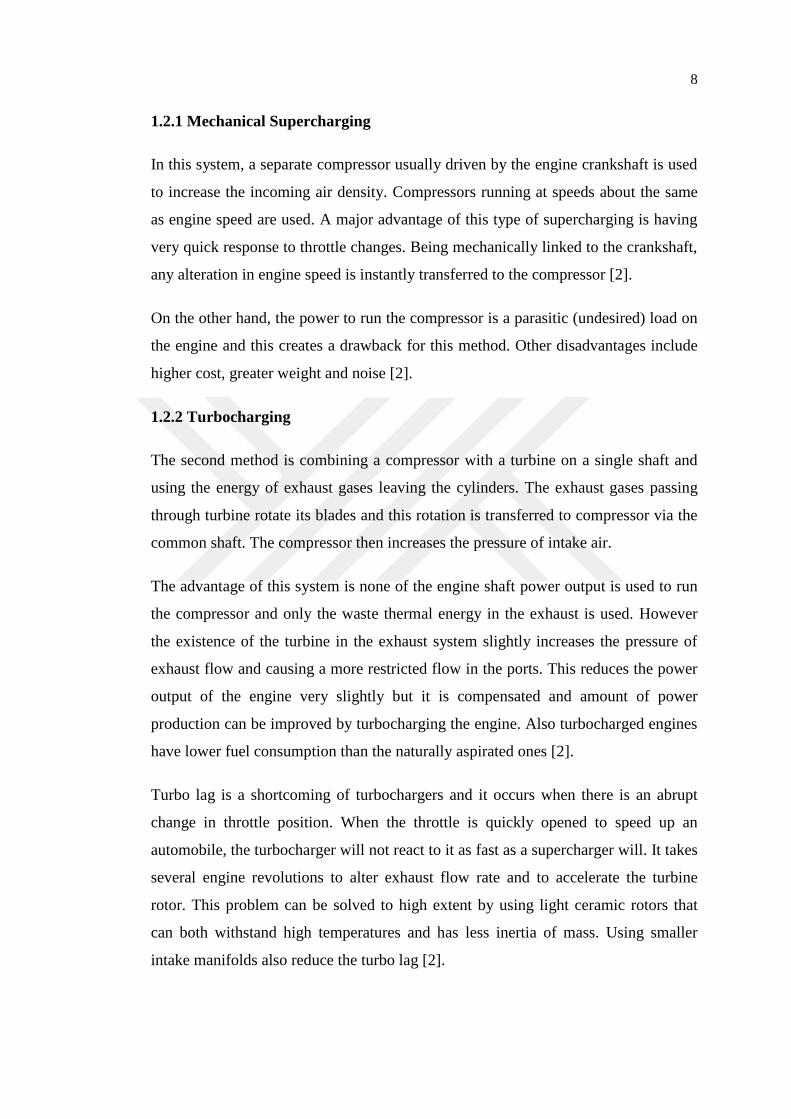
Depending on the application or availability air-to-air or air-to-water cooling systems

are used in intercoolers. Various configurations of these systems are given in Figure

1.4.

Air-to-air cooling system (Fig. 1.4a) might be utilized in cases when a source of

cooling water is not readily available, and high ambient temperatures restricts the use

of local closed cooling system. In this type, the air-to-air intercooler is usually placed

in front of the engine coolant radiator. An alternative way of this cooling system

(Fig. 1.4b) uses bleed air from the turbocharging system to run the cooling air supply

fan. This provides more coolant air flow to the intercooler. Air-to-water cooling

systems can use the normal water cooling system of the engine (Fig. 1.4c) or a

separate closed water cooling system having its own water-to-air radiator (Fig. 1.4d).

The advantage of the first type is the simplicity of installation but the cooling

capacity is restricted by the water temperature of the engine cooling system. The

latter type does not have such a problem and has a greater potential for cooling [6].

Air-to-water intercooling systems are preferred for marine applications [4].

11

Figure 1.4 Types of charge air cooling systems [6].

1.4 A General View of Heat Exchangers

A heat exchanger is a device that is used to transfer thermal energy between two or

more fluids at different temperatures and in thermal contact. Typical applications

involve heating or cooling of a fluid stream and evaporation or condensation (phase

change) of fluid streams. They have variety of application areas in industry such as

process, power, heat recovery, transportation, air-conditioning, refrigeration, and

cryogenic industries [7].

12

1.4.1 Heat Exchanger Classifications

The classification of heat exchangers can be done with many different ways. Main

classification types are summarized below.

1.4.1.1 Classification According to Transfer Process

A. Indirect Contact Type Heat Exchangers: In this type of heat exchangers the

fluids streams are held apart and heat is transferred via a separating wall.

1. Direct-Transfer Type Exchangers (Recuperators)

2. Storage Type Exchangers (Regenerators)

3. Fluidized-Bed Exchangers

B. Direct Contact Type Heat Exchangers: Two fluid streams are brought into

direct contact. Heat exchange occurs between the fluids and then they are

separated.

1. Immiscible Fluid Exchangers

2. Gas-Liquid Exchangers

3. Liquid-Vapor Exchangers

1.4.1.2 Classification According to Construction Features

A. Tubular Heat Exchangers

1. Shell-and-Tube Exchangers

2. Double Pipe Exchangers

3. Spiral Tube Exchangers

B. Plate Heat Exchangers

C. Extended Surface Heat Exchangers

1. Plate-Fin Exchangers

2. Tube-Fin Exchangers

D. Regenerative Heat Exchangers

1. Rotary Regenerators

2. Stationary Regenerators

13

1.4.1.3 Classification According to Flow Arrangements

A. Single-Pass Heat Exchangers

1. Counterflow Exchangers

2. Parallelflow Exchangers

3. Crossflow Exchangers

a) Both fluids unmixed

b) One fluid mixed, the other unmixed

c) Both fluids mixed

B. Multipass Heat Exchangers

1.4.1.4 Classification According to Heat Transfer Mechanisms

A. Single-Phase Convection on Both Sides

B. Single-Phase Convection on One Side, Two-Phase Convection on Other Side

C. Two-Phase Convection on Both Sides

D. Combined Convection and Radiation

1.4.1.5 Classification According to Number of Fluids

A. Two-Fluid Heat Exchangers

B. Three-Fluid Heat Exchangers

C. N-Fluid Heat Exchangers (N>3)

1.4.1.6 Classification According to Fluid Type

A. Gas-Gas Heat Exchangers

B. Gas-Liquid Heat Exchangers

C. Liquid-Liquid Heat Exchangers

D. Gas-Two Phase Heat Exchangers

E. Liquid-Two Phase Heat Exchangers

1.4.1.7 Classification According to Surface Compactness

Surface compactness of a heat exchanger is characterized by a parameter called

surface area density and denoted by 𝛽. It is defined as the ratio of heat transfer

14

surface area of the given fluid stream side to volume of that side. Sometimes it may

be defined with the total volume of the heat exchanger instead of volume of one side

as in the case of shell-and-tube exchangers [7].

A. Gas-to-Fluid Heat Exchangers

1. Compact (𝛽≥700 m2/m3)

2. Non-compact (𝛽<700 m2/m3)

B. Liquid-to-Liquid and Phase-Change Heat Exchangers

1. Compact (𝛽≥400 m2/m3)

2. Non-compact (𝛽<400 m2/m3)

1.4.2 Compact Heat Exchangers

Compact heat exchangers are heat exchangers that have high surface area density to

enhance heat transfer effectively. Increasing the heat transfer surface area provides a

better heat transfer characteristics and hence improves heat transfer. This enables

reduced space, weight and cost [7].

The simplest way to obtain a compact surface is to use small diameter tubes that are

closely packed constructing a tube bundle. When the fluid flows over this bundle, it

experiences high heat transfer surface per unit volume [8].

Another way is to use secondary surfaces, or fins, on one or both fluid sides.

Attaching fins to the outside of circular tubes is an example of this method. It is

generally used in gas-to-liquid heat exchangers where fins provide an extended

surface on the gas side to compensate relatively low heat transfer coefficient of the

gas. Tube-fin heat exchanger has this type of arrangement. Fins placed on both fluid

sides are preferred in gas-to-gas applications. In this case the heat exchanger is built

up as a sandwich of flat plates bonded each other with fins. The fluids flow through

the narrow gaps formed by the consecutive pairs of plates. A heat exchanger with

such an arrangement is called plate-fin heat exchanger [8]. Figure 1.5 shows an

example of this type of exchanger.

15

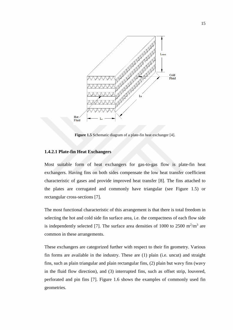
Figure 1.5 Schematic diagram of a plate-fin heat exchanger [4].

1.4.2.1 Plate-fin Heat Exchangers

Most suitable form of heat exchangers for gas-to-gas flow is plate-fin heat

exchangers. Having fins on both sides compensate the low heat transfer coefficient

characteristic of gases and provide improved heat transfer [8]. The fins attached to

the plates are corrugated and commonly have triangular (see Figure 1.5) or

rectangular cross-sections [7].

The most functional characteristic of this arrangement is that there is total freedom in

selecting the hot and cold side fin surface area, i.e. the compactness of each flow side

is independently selected [7]. The surface area densities of 1000 to 2500 m2/m3 are

common in these arrangements.

These exchangers are categorized further with respect to their fin geometry. Various

fin forms are available in the industry. These are (1) plain (i.e. uncut) and straight

fins, such as plain triangular and plain rectangular fins, (2) plain but wavy fins (wavy

in the fluid flow direction), and (3) interrupted fins, such as offset strip, louvered,

perforated and pin fins [7]. Figure 1.6 shows the examples of commonly used fin

geometries.

16

Figure 1.6 Various fin geometries for plate-fin heat exchangers: (a) plain triangular fin; (b) plain

rectangular fin; (c) wavy fin; (d) offset strip fin; (e) multi-louvered fin; (f) perforated fin [7].

1.5 Aim of the Study

Intercoolers especially used in land vehicles are air-to-air crossflow compact heat

exchangers. Because of having air on both flow sides, the suitable construction type

for these intercoolers becomes plate-fin arrangement. With such a construction, the

fin geometry of each flow side of the intercooler can be freely chosen depending on

the requirements or limitations.

In this study, the main purpose is to theoretically examine the plate-fin geometries

applicable to intercoolers. Each fin type shows different characteristic and thus leads

to different intercooler performances. Evaluating these performance data enables

comparison of fin geometries and determination of the most suitable ones for a given

cooling duty.

A computer program is written for the theoretical calculations. All necessary

parameters related with the fin geometries are embedded in this program. This speeds

17

up the laborious solution procedure of the performance data and provides extensive

choice to the user in terms of fin variety.

Another purpose of this study is to illustrate the benefits of intercooling on engine

performance; therefore the alteration of engine performance with the utilization of

intercooler is established. Under some conditions intercooling becomes an

impractical application and does not affect the engine operating parameters much.

These conditions are demonstrated.

1.6 Review of Related Works

The performance characteristics of various fin geometries have been extensively

investigated in terms of both first law and second law of thermodynamics. Heat

transfer, pressure drop and second law performances (i.e. entropy generation, exergy

destruction and second law efficiency) of them have been studied by researchers

analytically, numerically and experimentally.

The most comprehensive experimental study has been established by Kays and

London [8] with 132 compact heat exchanger surfaces. In the study, surfaces have

been tested at certain Reynolds number ranges and their dimensionless heat transfer

and friction factor parameters are determined. Results are given in graphical forms as

a function of Reynolds number. Also, in this study the entrance and exit loss

coefficients for different flow passage geometries are presented as a function of

Reynolds number and contraction ratio.

In another study, London and Shah [9] have tested eight offset rectangular plate fin

surfaces and presented basic heat transfer and flow friction characteristics of them.

They also investigated nondimensional parameters characterizing the geometry of the

fins and concluded that small offset spacing, small fin thickness and large aspect

ratios are advantageous from heat transfer power versus flow friction power point of

view. They also reported some important points related with application and

fabrication of this type of surfaces.

18

Ismail et al. [10] have investigated flow patterns of compact plate-fin exchangers.

The influence of flow maldistribution in the headers is examined numerically in the

study. In order to improve the flow distribution, authors suggested to place punched

baffles (plates) with different sized holes inside the header. They also generated

dimensionless heat transfer and fluid friction data, for some offset and wavy fins,

applicable for turbulent flow region.

Manglik and Bergles [11] have studied various offset strip fin surfaces and proposed

new correlations for dimensionless heat transfer and fluid friction data that is both

valid in laminar and turbulent region. They also compared these values with the

existing experimental results in the literature and obtained agreement within ±20%.

Another study related to offset strip fin correlations has been established by Kim et

al. [12]. They have generated new sets of dimensionless heat transfer and fluid

friction data that is also applicable to some fluids other than air. Also the geometries

of offset strip fins in a fuel cooler were optimized with proposed correlations.

In another study, Li and Yang [13] have numerically investigated 3D models of

offset strip fins and presented the effect of geometrical three-dimensionality on

thermal-hydraulic performances. New correlations are proposed accounting the effect

of third dimension and compared them with the existing experimental data. It is

claimed that the proposed correlations are well adapted for offset strip fins with

different fin thicknesses.

Cowell et al. [14] investigated performance characteristics of louvered fin surfaces

and explained that; louvers do not generate turbulence and at high Reynolds numbers

the flow has almost complete alignment with louvers. Also they compared louvered

fins with offset strip fins and claimed that louvered fins are capable of outperforming

offset strip fins.

Ryu and Lee [15] examined louvered fins both numerically and experimentally and

suggested new correlations in terms of Reynolds number and ratio of fin pitch to

louver pitch. They reported that these correlations are applicable to the surfaces

having fin pitch to louver pitch ratios larger than 1.

19

Li and Wang [16] conducted an experimental study with new type of louver fins

called multi-region louver fins and compared them with conventional ones. They

suggested a new factor for comparison. It is claimed that some of the new louver fin

types shows better performance than conventional ones. They also concluded that

heat transfer coefficients and fluid friction factor tend to decrease with increased

number of louver regions.

Vaisi et al. [17] have studied the effect of louver configuration on the heat transfer

and pressure drop characteristics. They have carried out experiments by using

symmetrical and asymmetrical arrangements of louver fins. It is reported that

louvered fins with symmetrical arrangement provide 9.3% increment in heat transfer

performance and 18.2% decrement in pressure drop. Also for a given heat transfer

and pressure drop, the symmetrical arrangement ensures a 17.6% decrease in fin

weight.

Ranganayakulu et al. [18] have investigated the effects of longitudinal heat

conduction (LHC) on thermal performance in compact crossflow plate-fin,

counterflow plate-fin, parallelflow plate-fin and crossflow tube-fin heat exchangers

using a finite element method. They claimed that LHC is not always negligible in

crossflow and counterflow compact heat exchangers especially when there is

balanced flow and LHC parameter is larger than 0.005. Also it is reported that the

performance deterioration in crossflow heat exchangers are higher than counterflow

and parallelflow in all cases due to two dimensional wall temperature distribution in

crossflow heat exchangers.

Ranganayakulu and Seetharamu [19] have conducted a finite element analysis on

crossflow tube-fin heat exchangers and included the combined effects of LHC, inlet

flow non-uniformity and temperature non-uniformity in their analysis. They have

illustrated that, this combined effect is not always negligible especially when the

capacity rates are equal and LHC parameter is larger than 0.05.

Shah and Skiepko [20] have conducted second law analysis on heat exchangers and

illustrated the irreversibilities in terms of entropy generation. It is reported that

effectiveness can be maximum, minimum or can have an intermediate value at the

20

maximum irreversibility point or effectiveness can be minimum or maximum at the

minimum irreversibility point depending on the flow arrangement of two fluids.

They have investigated the existence of entropy generation extrema and a

relationship between extrema and the heat exchanger effectiveness for 18 different

flow arrangements.

Gheorghian et al. [21] have proposed an entropy generation assessment criterion for

compact heat exchangers and applied this criterion to totally 30 different heat

transfer surfaces. They have investigated entropy generation rate caused exclusively

due to change in heat transfer surface types and this made it possible to classify the

surfaces in terms of entropy generation criterion. A comparison has been also made

between proposed assessment criterion and augmentation entropy generation number

criterion.

Canlı et al. [22] have compared three different compact heat exchangers in terms of

second law of thermodynamics. They have experimentally evaluated heat transfer

and pressure drop performance of the heat exchangers, and calculated the

irreversibility and exergy efficiency of them using these data. The exergy efficiencies

of the heat exchangers have been found between 15-40%. In the study, it is also

concluded that increase in temperature difference results in larger entropy generation

rate due to finite temperature difference, and by decreasing cooling fluid velocity,

pressure drop and hence entropy generation rate due to fluid friction can be

decreased.

21

CHAPTER 2

BASICS OF INTERCOOLERS

2.1 General Design Considerations of Intercoolers

The design of an intercooler mainly requires consideration of two parameters. These

are heat transfer rate and pressure drop due to fluid friction. For effective cooling of

intake air, intercoolers must be designed with a high surface area density. In fact this

is a must for any gas-flow heat exchanger to compensate relatively low heat transfer

coefficient of gases (low relative to most liquids). On the other hand, pressure drop

of intake air due to fluid friction must be minimized. It adversely affects the charge

air density and diminishes the benefits of supercharging.

To enhance heat transfer rate of an intercooler, surface area can be increased.

However, this leads to larger size and higher cost. Another way of enhancing heat

transfer rate is to increase the fluid flow velocity. In this case the increment rate will

be something less than the first power of velocity but the increase in the fluid friction

will be not less than the square of the velocity. This illustrates that there is a

compromise between heat transfer rate and the fluid friction. Intercoolers should

have a high frontal area and a short flow length to reduce pressure losses. A well-

designed intercooler is the one that performs high heat transfer rate with a minimum

pressure drop.

In intercoolers two different options are available in terms of cooling fluid type.

Coolant can be liquid (water) or gas (air). Air-to-air cooling is preferred in most

applications because it has some advantages over air-to-water cooling systems.

Firstly, air is free and can be given back to atmosphere after passing through the

intercooler whereas water must be cooled in a separate unit and requires a circulation

pump for operation. Also fouling and corrosion can occur in water channels and this

makes water treatment a necessity. Air-cooled systems mostly do not have fouling

problems and corrosion is rarely seen [4].

22

Intercoolers are mounted on the engine and designed as an integral part of it. They

should be as compact as possible not to hold much space in engine compartment.

They are generally made of aluminum which is a lightweight material and has a good

thermal conductivity. It has also good corrosion resistance [4]. The service life and

maintenance periods of intercoolers must not be less than those of the basic engine

[6].

2.2 Theory of Intercoolers

2.2.1 Thermal Design

In this section, beginning with the assumptions employed in the theory of heat

exchanger design, the basic relations for the heat transfer analysis will be formulated.

2.2.1.1 Assumptions for Heat Transfer Analysis

Introducing a group of assumptions in heat transfer analysis provides to construct

theoretical models that are easy enough to handle. For the analysis, the following

assumptions and/or idealizations are proposed.

1. The heat exchanger operates under steady-state conditions, i.e. all the

variables are independent of time.

2. Heat transfer only takes place between the fluids. The exchanger walls are

insulated, i.e. no heat losses to or from the surroundings.

3. There is no generation or dissipation of thermal energy in the exchanger walls

or fluids.

4. Wall thermal resistance is distributed uniformly in the entire exchanger.

5. Longitudinal heat conduction effects in the fluids and in the wall are

negligible.

6. The individual or overall heat transfer coefficients are constant throughout the

exchanger.

7. The velocity and temperature distribution over the flow cross-section is

uniform.

8. Kinetic and potential energy of fluids are negligible.

23

2.2.1.2 Problem Formulation

In thermal analysis of heat exchangers two main approaches are possible. Theoretical

models are built up using either the first law of thermodynamics (energy based

analysis) or second law of thermodynamics (entropy/exergy based analysis). In

energy based analysis, the effectiveness-number of transfer units (ε-NTU) or

logarithmic mean temperature difference (LMTD) methods are commonly used to

evaluate exchanger performance. On the other hand, in entropy/exergy based

analysis various dimensionless parameters (see section 2.2.3) are derived to assess

the quality of heat transfer and associated phenomena.

In this section thermal analysis of heat exchangers based on the first law of

thermodynamics will be introduced. Later, the definition of effectiveness and ε-NTU

relation for an air-to-air intercooler will be presented.

Consider a two-fluid counterflow heat exchanger shown in Figure 2.1. Two

differential energy conservation equations for the control volume can be combined as

follows:

𝑑𝑞 = 𝑞"𝑑𝐴 = −𝐶ℎ𝑑𝑇ℎ = −𝐶𝑐𝑑𝑇𝑐 (2.1)

Here 𝑑𝑞 represents the differential amount of heat transfer rate from hot fluid to cold

fluid through the differential wall surface area 𝑑𝐴. The hot and cold fluids are

denoted by subscripts ℎ and 𝑐, respectively. The negative signs in the equation are a

result of decreasing fluid temperatures in the direction of positive x. Heat capacity

rate of the fluid is denoted by 𝐶 and equal to the product of mass flow rate of fluid,

�̇� and fluid specific heat at constant pressure, 𝑐𝑝.

𝐶 = �̇�𝑐𝑝 (2.2)

The heat transfer rate equation (Eq. 2.1) can also be written in the form of:

𝑑𝑞 = 𝑈(𝑇ℎ − 𝑇𝑐)𝑑𝐴 = 𝑈∆𝑇𝑑𝐴 (2.3)

24

where 𝑈 is the overall heat transfer coefficient. For this differential area, 𝑑𝐴, the

driving force for heat transfer is the local temperature difference 𝑇ℎ − 𝑇𝑐 = ∆𝑇, and

the overall thermal conductance is 𝑈𝑑𝐴.

Figure 2.1 Depiction of heat transfer in a counterflow heat exchanger [7].

Integration of Eq. 2.1 and Eq. 2.3 over the entire heat exchanger surface for the

specified inlet and outlet temperatures will give the expressions:

𝑞 = ∫ 𝐶𝑑𝑇 = 𝐶ℎ(𝑇ℎ,𝑖 − 𝑇ℎ,𝑜) = 𝐶𝑐(𝑇𝑐,𝑜 − 𝑇𝑐,𝑖) (2.4)

𝑞 = ∫ 𝑈∆𝑇𝑑𝐴 = 𝑈𝐴∆𝑇𝑚 (2.5)

The subscripts 𝑖 and 𝑜 in Eq. 2.4 represents the inlet and outlet, respectively. In Eq.

2.5, ∆𝑇𝑚 is the true (or effective) mean temperature difference between the fluids. 𝑈

is considered as constant over the entire surface.

25

To evaluate overall thermal conductance, a thermal circuit is constructed. This yields

to an expression in the form of:

1

𝑈𝐴=

1

(𝜂𝑜ℎ𝐴)ℎ+

𝛿𝑤

𝑘𝑤𝐴𝑤+

1

(𝜂𝑜ℎ𝐴)𝑐 (2.6)

In the equation, ℎ is the convection heat transfer coefficient, 𝑘𝑤 is the thermal

conductivity of the wall, 𝐴𝑤 is the wall conduction area and 𝛿𝑤 is the thickness of

the wall. 𝜂𝑜 represents the efficiency of extended (or total) surface and equal to unity

when only primary surfaces (i.e. having no fins) are used. In this equation the fouling

resistances are neglected on both sides of the flow.

ε-NTU Method

In an adiabatic heat exchanger, the thermal energy removed from the hot fluid is

totally transferred to cold fluid. This provides a first law efficiency of 100% in such a

system regardless of the amount of heat transferred. However, while designing a heat

exchanger the main purpose is to transfer as much amount of heat as possible from

hot fluid to cold one. Since the first law efficiency is insufficient to rate the heat

transfer process in this manner, a new parameter called effectiveness is used. This

parameter can take the maximum theoretical value of 1 and the larger the

effectiveness, the greater amount of heat is transferred between the fluids.

In order to demonstrate effectiveness of a heat exchanger, firstly the maximum

possible heat transfer should be evaluated. This limit could be achieved with a

perfect counterflow heat exchanger that has an infinite surface area [4].

Consider that two fluid streams are flowing through a conventional direct-transfer

type heat exchanger in opposite directions as in Figure 2.1. The maximum

temperature difference in the exchanger is Δ𝑇𝑚𝑎𝑥 = 𝑇ℎ,𝑖 − 𝑇𝑐,𝑖. The heat transfer will

reach to its maximum value when the cold fluid is heated to the inlet temperature of

hot fluid or the hot fluid is cooled to the inlet temperature of cold fluid. Both cases

cannot be reached simultaneously unless the heat capacity rates are equal. When

𝐶ℎ ≠ 𝐶𝑐, which is usually the case, the fluid with the smaller heat capacity rate will

26

undergo a larger temperature change and hence it will be the first to experience the

maximum temperature difference. At that instant heat transfer will stop. Therefore

the maximum possible heat transfer becomes equal to:

𝑞𝑚𝑎𝑥 = 𝐶𝑚𝑖𝑛(𝑇ℎ,𝑖 − 𝑇𝑐,𝑖) (2.7)

where 𝐶𝑚𝑖𝑛 is the smaller of 𝐶ℎ and 𝐶𝑐 [23]. It is deduced from the equation that the

fluid having larger heat capacity rate will experience smaller temperature difference.

Effectiveness which is defined as the ratio of actual heat transfer rate to the

maximum possible heat transfer rate can now be clarified.

휀 =𝑞𝑎𝑐𝑡.

𝑞𝑚𝑎𝑥.=

𝐶𝑐(𝑇𝑐,𝑜 − 𝑇𝑐,𝑖)

𝐶𝑚𝑖𝑛(𝑇ℎ,𝑖 − 𝑇𝑐,𝑖)=

𝐶ℎ(𝑇ℎ,𝑖 − 𝑇ℎ,𝑜)

𝐶𝑚𝑖𝑛(𝑇ℎ,𝑖 − 𝑇𝑐,𝑖) (2.8)

Effectiveness can also be expressed in terms of nondimensional groups.

휀 = 𝜙 (𝑈𝐴

𝐶𝑚𝑖𝑛,

𝐶𝑚𝑖𝑛

𝐶𝑚𝑎𝑥, 𝑓𝑙𝑜𝑤 𝑎𝑟𝑟𝑎𝑛𝑔𝑒𝑚𝑒𝑛𝑡) (2.9)

Here the first dimensionless group is named as number of (heat) transfer units and

second is heat capacity rate ratio.

𝑁𝑇𝑈 =𝑈𝐴

𝐶𝑚𝑖𝑛 (2.10)

𝐶∗ =𝐶𝑚𝑖𝑛

𝐶𝑚𝑎𝑥 (2.11)

𝑁𝑇𝑈 designates the nondimensional heat transfer size or thermal size of the heat

exchanger and thus it is a design parameter. Heat capacity rate ratio, 𝐶∗ is an

operating parameter since it is dependent on mass flow rate and temperatures of the

fluids.

Effectiveness expressions in terms of 𝑁𝑇𝑈 and 𝐶∗for different flow arrangements

can be found in references [24, 25]. The expression that will be used in this study is

given below. It is the one for unmixed-unmixed type crossflow heat exchangers.

27

휀 = 1 − exp {𝑁𝑇𝑈0.22

𝐶∗[𝑒𝑥𝑝(−𝐶∗𝑁𝑇𝑈0.78) − 1]} (2.12)

Note that for a given effectiveness and heat capacity rate ratio, the value of 𝑁𝑇𝑈 in

Eq. 2.12 cannot be determined without performing iterations.

2.2.2 Pressure Drop Analysis

In most applications fluids need to be pumped to move through the heat exchanger. It

is therefore necessary to evaluate fluid pumping power expenditure as a part of the

system design and operating cost analysis. Pumping power is proportional to the

fluid pressure drop (or fluid friction) which in turn has a direct relationship with

exchanger heat transfer, operation, size, mechanical characteristics and some other

factors [7].

In the design of liquid-to-liquid heat exchangers, friction characteristics of the heat

transfer surface is relatively unimportant because of the lower power requirement for

pumping high density fluids. However, for gases, because of their low density,

friction power greatly increases. It is important to have an accurate knowledge of

friction characteristics of heat exchangers in gas-to-gas applications.

In intercoolers which are the subject of this study, the fluid pressure drop is an

important design parameter and should be minimized. This minimization may be

important in terms of operating cost but mainly it is essential to prevent decrement in

air density. While evaluating the pressure drop in the intercoolers, the method

available for the compact heat exchangers is adopted.

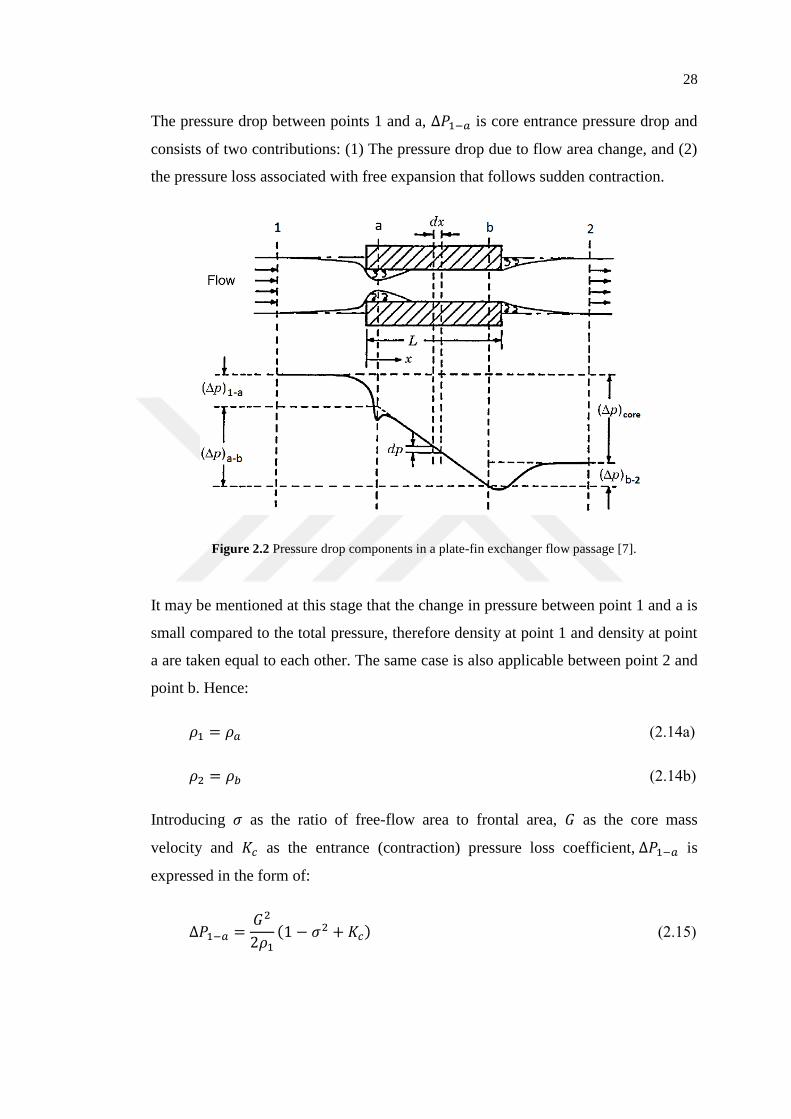
Total core pressure drop in compact heat exchangers can be examined in three main

parts. These are core entrance pressure drop, core pressure drop and core exit

pressure rise. To delineate better, a flow passage in a plate-fin heat exchanger is

shown in Figure 2.2 along with the static pressure distribution. Here, the total core

pressure drop between points 1 and 2 is given with the following expression.

∆𝑃 = ∆𝑃1−𝑎 + ∆𝑃𝑎−𝑏 − ∆𝑃𝑏−2 (2.13)

28

The pressure drop between points 1 and a, ∆𝑃1−𝑎 is core entrance pressure drop and

consists of two contributions: (1) The pressure drop due to flow area change, and (2)

the pressure loss associated with free expansion that follows sudden contraction.

Figure 2.2 Pressure drop components in a plate-fin exchanger flow passage [7].

It may be mentioned at this stage that the change in pressure between point 1 and a is

small compared to the total pressure, therefore density at point 1 and density at point

a are taken equal to each other. The same case is also applicable between point 2 and

point b. Hence:

𝜌1 = 𝜌𝑎 (2.14a)

𝜌2 = 𝜌𝑏 (2.14b)

Introducing 𝜎 as the ratio of free-flow area to frontal area, 𝐺 as the core mass

velocity and 𝐾𝑐 as the entrance (contraction) pressure loss coefficient, ∆𝑃1−𝑎 is

expressed in the form of:

∆𝑃1−𝑎 =𝐺2

2𝜌1

(1 − 𝜎2 + 𝐾𝑐) (2.15)

29

where:

𝐺 = �̇�

𝐴𝑜= 𝜌𝑎𝑉𝑎 = 𝜌𝑏𝑉𝑏 (2.16)

𝜎 =𝐴𝑜

𝐴𝑓𝑟 (2.17)

The core pressure drop, ∆𝑃𝑎−𝑏 consists of two contributions that are (1) the pressure

loss caused by fluid friction, and (2) the pressure change due to momentum rate

change in the core. The expression for core pressure drop is:

∆𝑃𝑎−𝑏 =𝐺2

2𝜌1[𝑓

𝐴

𝐴𝑜𝜌1 (

1

𝜌)

𝑚

+ 2 (𝜌1

𝜌2− 1)] (2.18)

Here 𝑓 is Fanning friction factor and 𝐴 is heat transfer surface area. Also the fluid

mean specific volume, 𝜈𝑚 is determined using the relation:

(1

𝜌)

𝑚

= 𝜈𝑚 =𝜈𝑎 + 𝜈𝑏

2=

1

2(

1

𝜌𝑎+

1

𝜌𝑏) (2.19)

The core exit pressure rise, ∆𝑃𝑏−2 is also divided into two contributions: (1) pressure

rise due to deceleration with an area increase, and (2) pressure loss associated with

the irreversible free expansion and momentum rate changes following an abrupt

expansion. It is similar to Eq. 2.15:

∆𝑃𝑏−2 =𝐺2

2𝜌2

(1 − 𝜎2 − 𝐾𝑒) (2.20)

In the equation, 𝐾𝑒 is exit (expansion) pressure loss coefficient that is analogous

to 𝐾𝑐. The values of both coefficients for different flow passage geometries are given

in Figure D.1, in appendices.

Finally, by doing some manipulations, the total core pressure drop equation (Eq.

2.13) can be rearranged as:

30

∆𝑃

𝑃1=

𝐺2

2𝜌1𝑃1[(1 − 𝜎2 + 𝐾𝑐) + 𝑓

𝐴

𝐴𝑜𝜌1 (

1

𝜌)

𝑚

+ 2 (𝜌1

𝜌2− 1)

− (1 − 𝜎2 − 𝐾𝑒)𝜌1

𝜌2] (2.21)

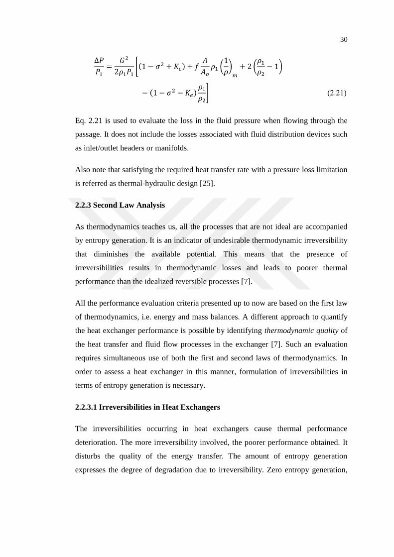
Eq. 2.21 is used to evaluate the loss in the fluid pressure when flowing through the

passage. It does not include the losses associated with fluid distribution devices such

as inlet/outlet headers or manifolds.

Also note that satisfying the required heat transfer rate with a pressure loss limitation

is referred as thermal-hydraulic design [25].

2.2.3 Second Law Analysis

As thermodynamics teaches us, all the processes that are not ideal are accompanied

by entropy generation. It is an indicator of undesirable thermodynamic irreversibility

that diminishes the available potential. This means that the presence of

irreversibilities results in thermodynamic losses and leads to poorer thermal

performance than the idealized reversible processes [7].

All the performance evaluation criteria presented up to now are based on the first law

of thermodynamics, i.e. energy and mass balances. A different approach to quantify

the heat exchanger performance is possible by identifying thermodynamic quality of

the heat transfer and fluid flow processes in the exchanger [7]. Such an evaluation

requires simultaneous use of both the first and second laws of thermodynamics. In

order to assess a heat exchanger in this manner, formulation of irreversibilities in

terms of entropy generation is necessary.

2.2.3.1 Irreversibilities in Heat Exchangers

The irreversibilities occurring in heat exchangers cause thermal performance

deterioration. The more irreversibility involved, the poorer performance obtained. It

disturbs the quality of the energy transfer. The amount of entropy generation

expresses the degree of degradation due to irreversibility. Zero entropy generation,

31

which is the case for ideal processes, corresponds to the highest quality of energy

transfer, and entropy generation greater than zero represents poorer quality [7].

There are two main important phenomena that shape the extent of generated entropy

within a heat exchanger: (1) heat transfer through finite temperature difference and

(2) fluid friction.

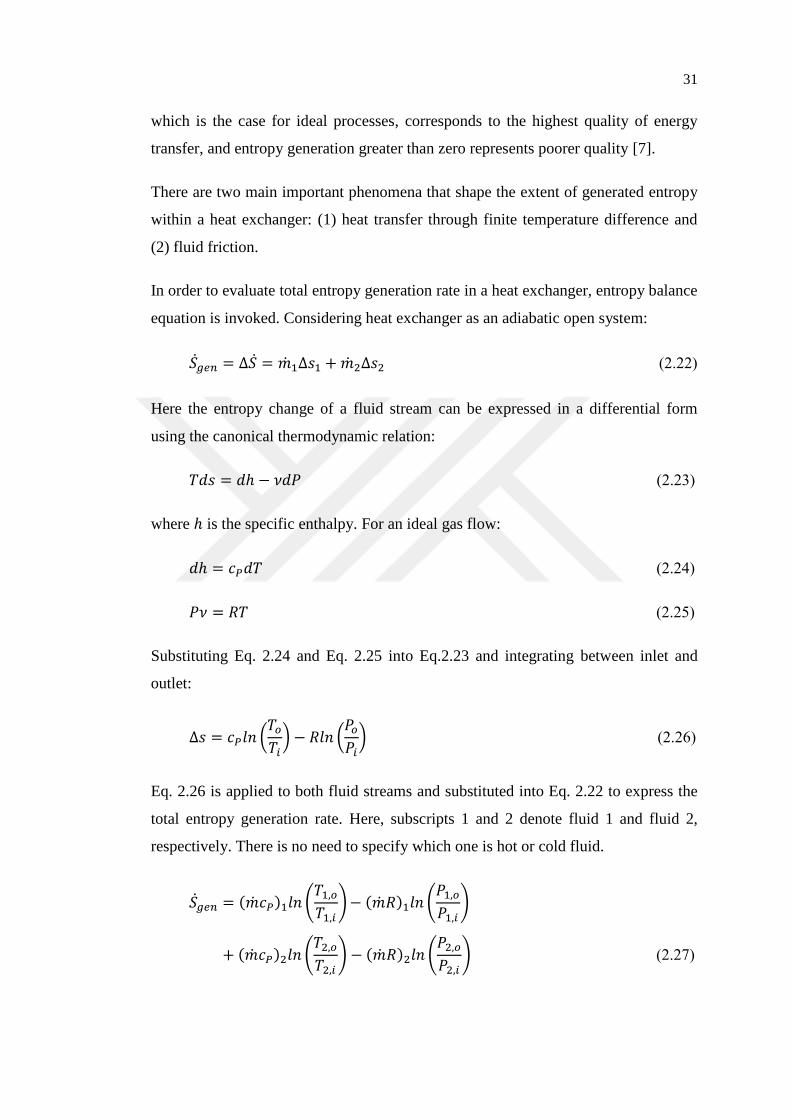
In order to evaluate total entropy generation rate in a heat exchanger, entropy balance

equation is invoked. Considering heat exchanger as an adiabatic open system:

�̇�𝑔𝑒𝑛 = ∆�̇� = �̇�1∆𝑠1 + �̇�2∆𝑠2 (2.22)

Here the entropy change of a fluid stream can be expressed in a differential form

using the canonical thermodynamic relation:

𝑇𝑑𝑠 = 𝑑ℎ − 𝜈𝑑𝑃 (2.23)

where ℎ is the specific enthalpy. For an ideal gas flow:

𝑑ℎ = 𝑐𝑃𝑑𝑇 (2.24)

𝑃𝜈 = 𝑅𝑇 (2.25)

Substituting Eq. 2.24 and Eq. 2.25 into Eq.2.23 and integrating between inlet and

outlet:

∆𝑠 = 𝑐𝑃𝑙𝑛 (𝑇𝑜

𝑇𝑖) − 𝑅𝑙𝑛 (

𝑃𝑜

𝑃𝑖) (2.26)

Eq. 2.26 is applied to both fluid streams and substituted into Eq. 2.22 to express the

total entropy generation rate. Here, subscripts 1 and 2 denote fluid 1 and fluid 2,

respectively. There is no need to specify which one is hot or cold fluid.

�̇�𝑔𝑒𝑛 = (�̇�𝑐𝑃)1𝑙𝑛 (𝑇1,𝑜

𝑇1,𝑖) − (�̇�𝑅)1𝑙𝑛 (

𝑃1,𝑜

𝑃1,𝑖)

+ (�̇�𝑐𝑃)2𝑙𝑛 (𝑇2,𝑜

𝑇2,𝑖) − (�̇�𝑅)2𝑙𝑛 (

𝑃2,𝑜

𝑃2,𝑖) (2.27)

32

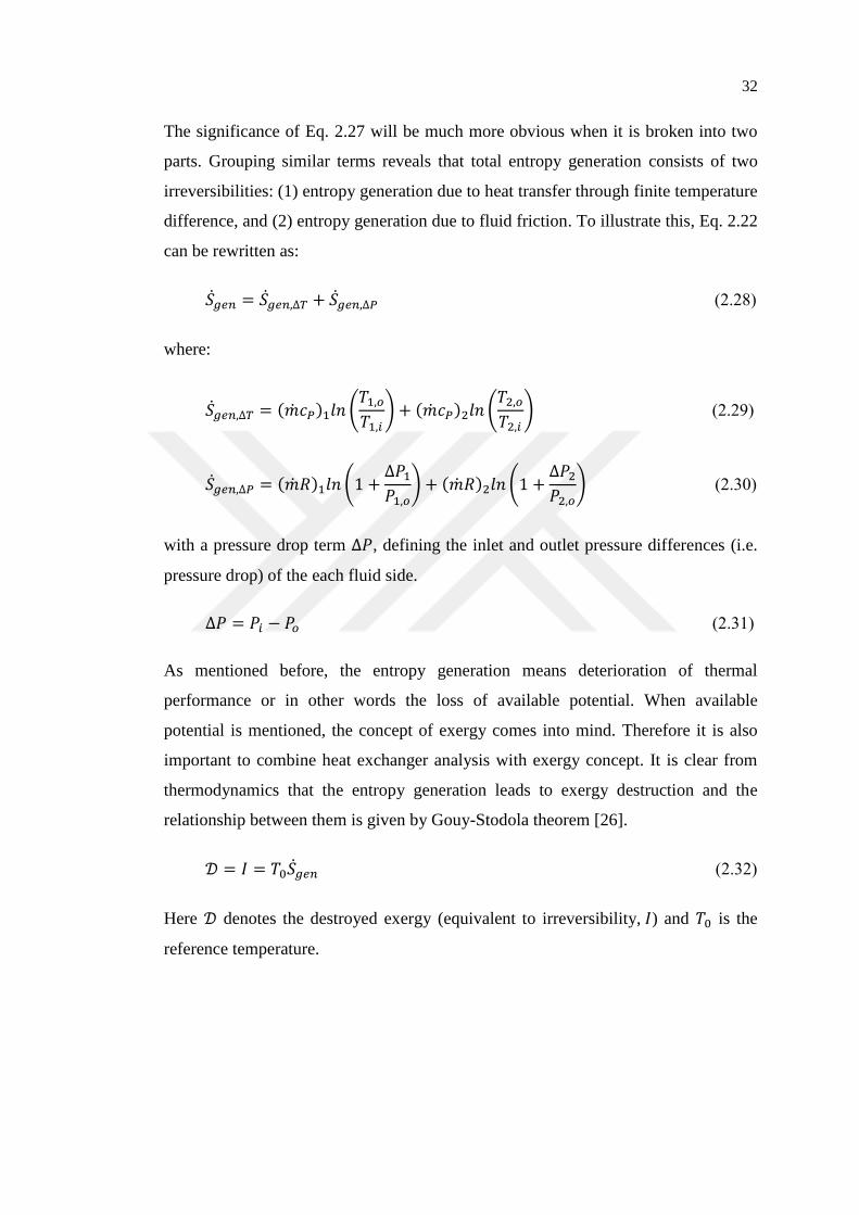
The significance of Eq. 2.27 will be much more obvious when it is broken into two

parts. Grouping similar terms reveals that total entropy generation consists of two

irreversibilities: (1) entropy generation due to heat transfer through finite temperature

difference, and (2) entropy generation due to fluid friction. To illustrate this, Eq. 2.22

can be rewritten as:

�̇�𝑔𝑒𝑛 = �̇�𝑔𝑒𝑛,∆𝑇 + �̇�𝑔𝑒𝑛,∆𝑃 (2.28)

where:

�̇�𝑔𝑒𝑛,∆𝑇 = (�̇�𝑐𝑃)1𝑙𝑛 (𝑇1,𝑜

𝑇1,𝑖) + (�̇�𝑐𝑃)2𝑙𝑛 (

𝑇2,𝑜

𝑇2,𝑖) (2.29)

�̇�𝑔𝑒𝑛,∆𝑃 = (�̇�𝑅)1𝑙𝑛 (1 +∆𝑃1

𝑃1,𝑜) + (�̇�𝑅)2𝑙𝑛 (1 +

∆𝑃2

𝑃2,𝑜) (2.30)

with a pressure drop term ∆𝑃, defining the inlet and outlet pressure differences (i.e.

pressure drop) of the each fluid side.

∆𝑃 = 𝑃𝑖 − 𝑃𝑜 (2.31)

As mentioned before, the entropy generation means deterioration of thermal

performance or in other words the loss of available potential. When available

potential is mentioned, the concept of exergy comes into mind. Therefore it is also

important to combine heat exchanger analysis with exergy concept. It is clear from

thermodynamics that the entropy generation leads to exergy destruction and the

relationship between them is given by Gouy-Stodola theorem [26].

𝒟 = 𝐼 = 𝑇0�̇�𝑔𝑒𝑛 (2.32)

Here 𝒟 denotes the destroyed exergy (equivalent to irreversibility, 𝐼) and 𝑇0 is the

reference temperature.

33

2.2.3.2 Dimensionless Parameters

While evaluating the heat exchanger performance in terms of second law, two

different evaluation techniques are offered: (1) evaluation technique using entropy as

evaluation parameter, and (2) evaluation technique using exergy as evaluation

parameter. Each technique has its own dimensionless parameters in different forms

proposed by different investigators. In this section, some of these dimensionless

parameters will be discussed.

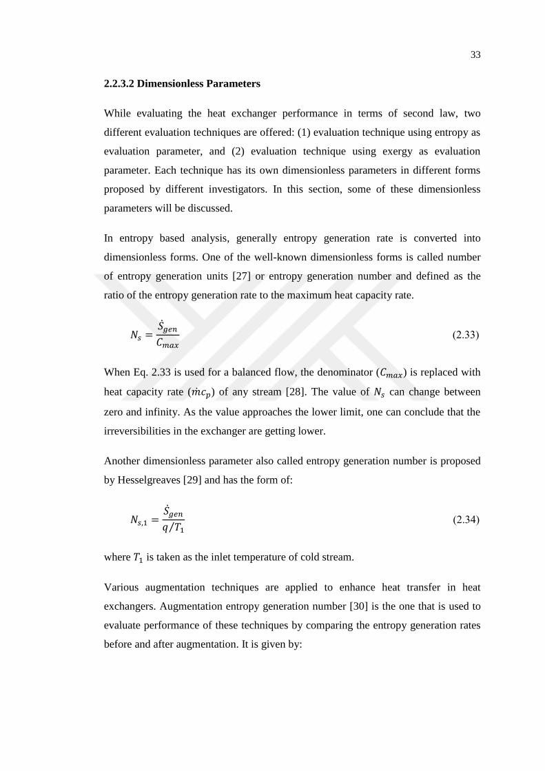
In entropy based analysis, generally entropy generation rate is converted into

dimensionless forms. One of the well-known dimensionless forms is called number

of entropy generation units [27] or entropy generation number and defined as the

ratio of the entropy generation rate to the maximum heat capacity rate.

𝑁𝑠 =�̇�𝑔𝑒𝑛

𝐶𝑚𝑎𝑥 (2.33)

When Eq. 2.33 is used for a balanced flow, the denominator (𝐶𝑚𝑎𝑥) is replaced with

heat capacity rate (�̇�𝑐𝑝) of any stream [28]. The value of 𝑁𝑠 can change between

zero and infinity. As the value approaches the lower limit, one can conclude that the

irreversibilities in the exchanger are getting lower.

Another dimensionless parameter also called entropy generation number is proposed

by Hesselgreaves [29] and has the form of:

𝑁𝑠,1 =�̇�𝑔𝑒𝑛

𝑞 𝑇1⁄ (2.34)

where 𝑇1 is taken as the inlet temperature of cold stream.

Various augmentation techniques are applied to enhance heat transfer in heat

exchangers. Augmentation entropy generation number [30] is the one that is used to

evaluate performance of these techniques by comparing the entropy generation rates

before and after augmentation. It is given by:

34

𝑁𝑠,𝑎 =�̇�𝑔𝑒𝑛,𝑎

�̇�𝑔𝑒𝑛,0

(2.35)

Augmentation techniques with 𝑁𝑠,𝑎 < 1 are thermodynamically advantageous since

it both increases heat transfer and reduces the degree of irreversibility.

Similar to foregoing analysis, in exergy based evaluation technique, various

nondimensional irreversibility parameters are used. A parameter called non-

dimensional exergy destruction [31] is defined as:

𝐼∗ =𝐼

�̇�𝑇0𝑐𝑝 (2.36)

Another dimensionless measure of heat exchanger irreversibility can be calculated

using the following equation:

휀𝑅 =�̇�𝑐(𝜓𝑜𝑢𝑡 − 𝜓𝑖𝑛)𝑐

�̇�ℎ(𝜓𝑖𝑛 − 𝜓𝑜𝑢𝑡)ℎ (2.37a)

Here 휀𝑅 is called rational (second law) effectiveness [32]. It has the maximum value

of one when exergy gained by cold stream is equal to exergy donated by the hot

stream, and this condition corresponds to the operation of the heat exchanger in a

pure reversible manner. Note that when the temperature (or pressure) of the cold

stream remains below the temperature (or pressure) of the surrounding during

operation, it is better to use a more general definition instead of Eq. 2.37a. In such

cases, Çengel [3] proposes to use:

𝜂𝑠 =(�̇�𝜓𝑜𝑢𝑡)𝑐 + (�̇�𝜓𝑜𝑢𝑡)ℎ

(�̇�𝜓𝑖𝑛)𝑐 + (�̇�𝜓𝑖𝑛)ℎ (2.37b)

In this equation 𝜂𝑠 is referred as second law efficiency. It is also known as rational

efficiency or exergetic efficiency [33].

All these dimensionless parameters are commonly used in the literature by different

investigators. More detailed review can be found in reference [33].

35

2.3 Some Additional Considerations for Thermal Design

2.3.1 Influence of Temperature-Dependent Fluid Properties

During the operation of heat exchangers, the temperatures of streams vary both over

the flow cross section and in the flow direction. The change in the temperature

affects the fluid properties (density, viscosity, specific heat etc.) and therefore the

accuracy of thermal analysis. Some kind of correction is generally applied to recover

the effect of temperature-dependent fluid properties.

The influence of temperature variation along the flow direction is compensated by

evaluating the fluid properties at a mean temperature with respect to flow length.

This is a typical case applied in the heat exchanger analysis. The arithmetic average

of terminal temperatures is given by:

𝑇𝑚 =𝑇𝑖 + 𝑇𝑜

2 (2.38)

Eq. 2.38 is applied to hot and cold streams individually and fluid properties of each

side are evaluated with respect to these mean temperatures.

To take into account the change in the temperature over the flow cross section, more

elaborate correction scheme is presented. When the temperature difference between

the fluid and heat transfer surface is large, fluid properties in the transverse direction

to the flow vary considerably. This change in fluid properties may lead to significant

variation in two important dimensionless parameters that are used in the assessment

of heat exchanger performance: Nusselt number, 𝑁𝑢 and friction factor, 𝑓 [7].

To compensate it, the values of Nusselt number and friction factor evaluated at

appropriate mean temperatures (𝑁𝑢𝑚 and 𝑓𝑚) are modified with the following

expressions [8].

𝑁𝑢

𝑁𝑢𝑚= (

𝑇𝑤

𝑇𝑚)

𝑛

(2.39)

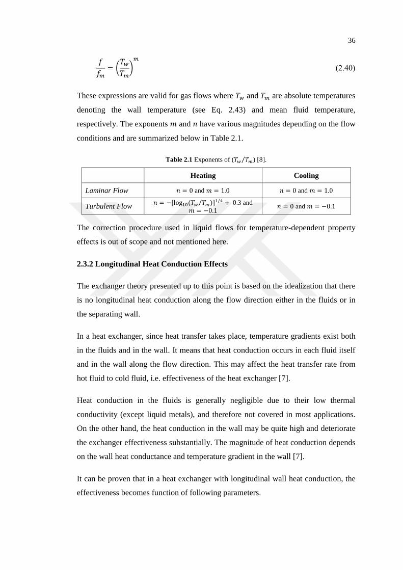
36

𝑓

𝑓𝑚= (

𝑇𝑤

𝑇𝑚)

𝑚

(2.40)

These expressions are valid for gas flows where 𝑇𝑤 and 𝑇𝑚 are absolute temperatures

denoting the wall temperature (see Eq. 2.43) and mean fluid temperature,

respectively. The exponents 𝑚 and 𝑛 have various magnitudes depending on the flow

conditions and are summarized below in Table 2.1.

Table 2.1 Exponents of (𝑇𝑤 𝑇𝑚⁄ ) [8].

Heating Cooling

Laminar Flow 𝑛 = 0 and 𝑚 = 1.0 𝑛 = 0 and 𝑚 = 1.0

Turbulent Flow 𝑛 = −[log 10(𝑇𝑤 𝑇𝑚⁄ )]1/4 + 0.3 and

𝑚 = −0.1 𝑛 = 0 and 𝑚 = −0.1

The correction procedure used in liquid flows for temperature-dependent property

effects is out of scope and not mentioned here.

2.3.2 Longitudinal Heat Conduction Effects

The exchanger theory presented up to this point is based on the idealization that there

is no longitudinal heat conduction along the flow direction either in the fluids or in

the separating wall.

In a heat exchanger, since heat transfer takes place, temperature gradients exist both

in the fluids and in the wall. It means that heat conduction occurs in each fluid itself

and in the wall along the flow direction. This may affect the heat transfer rate from

hot fluid to cold fluid, i.e. effectiveness of the heat exchanger [7].

Heat conduction in the fluids is generally negligible due to their low thermal

conductivity (except liquid metals), and therefore not covered in most applications.

On the other hand, the heat conduction in the wall may be quite high and deteriorate

the exchanger effectiveness substantially. The magnitude of heat conduction depends

on the wall heat conductance and temperature gradient in the wall [7].

It can be proven that in a heat exchanger with longitudinal wall heat conduction, the

effectiveness becomes function of following parameters.

37

휀 = 𝜙[𝑁𝑇𝑈, 𝐶∗, 𝜆ℎ, 𝜆𝑐, (𝜂𝑜ℎ𝐴)∗, 𝑓𝑙𝑜𝑤 𝑎𝑟𝑟𝑎𝑛𝑔𝑒𝑚𝑒𝑛𝑡] (2.41)

Here 𝜆ℎ and 𝜆𝑐 are referred as the longitudinal wall heat conduction parameters for

hot and cold fluid sides, respectively. They are defined in the form of:

𝜆ℎ = (𝑘𝑤𝐴𝑘

𝐿𝐶)

ℎ (2.42a)

𝜆𝑐 = (𝑘𝑤𝐴𝑘

𝐿𝐶)

𝑐 (2.42b)

Higher values of 𝜆 indicate greater rate of heat conduction in the wall.

The parameter (𝜂𝑜ℎ𝐴)∗ denotes the ratio of cold side conductance to hot side

conductance and used to evaluate wall temperature in the heat exchanger. Neglecting

wall resistance and fouling, the wall temperature at any location can be written as:

𝑇𝑤 =𝑇ℎ + (𝜂𝑜ℎ𝐴)∗𝑇𝑐

1 + (𝜂𝑜ℎ𝐴)∗ (2.43)

where:

(𝜂𝑜ℎ𝐴)∗ =(𝜂𝑜ℎ𝐴)𝑐

(𝜂𝑜ℎ𝐴)ℎ (2.44)

If (𝜂𝑜ℎ𝐴)∗ is zero (as in a condenser) or infinity (as in an evaporator) the

longitudinal heat conduction is zero even the value of 𝜆 is finite. Because in these

cases, temperature of the wall becomes equal to phase-changing side temperature and

it is constant. Longitudinal conduction effects are greatest when (𝜂𝑜ℎ𝐴)∗ equal to

unity [7].

Note that for a counterflow heat exchanger, the flow length and wall cross-sectional

area of both sides are the same, therefore a unique longitudinal wall heat conduction

parameter can be defined and Eq.2.41 can be simplified. Then, for a counterflow heat

exchanger:

38

𝜆 =𝑘𝑤𝐴𝑘

𝐿𝐶𝑚𝑖𝑛 (2.45)

휀 = 𝜙[𝑁𝑇𝑈, 𝐶∗, 𝜆, (𝜂𝑜ℎ𝐴)∗] (2.46)

For unmixed-unmixed type crossflow heat exchangers, the temperature gradients in

the wall in x and y directions of two fluid flows are different. Also hot side flow

length is generally different than cold side flow length (𝐿ℎ ≠ 𝐿𝑐). In this case,

effectiveness is a function of five independent parameters as given in Eq. 2.41 [7].

This makes the problem more complicated and yields evaluation in terms of

numerical methods.

In the analysis of intercoolers as crossflow heat exchangers, tabulated numerical

results given by Shah and Sekulic [7] can be used to take into account the effects of

longitudinal wall heat conduction.

The effect of heat conduction in the wall is generally expressed in terms of reduction

in the exchanger effectiveness (∆휀/휀) and defined as:

∆휀

휀=

휀𝜆=0 − 휀𝜆≠0

휀𝜆=0 (2.47)

2.3.3 Determination of Plate-fin Efficiency

In the analysis of intercoolers (or in any other extended surface heat exchangers), one

of the important consideration is to evaluate the performance of fins that are used to

increase surface area and hence the rate of heat transfer. Ideally, if fins are

considered to have infinite thermal conductivity, the unfinned surface (also called

primary surface or base surface) and finned surface temperatures will be equal.

However, this is not the case in practice. Because of the finite value of thermal

conductivity of the fins, the average temperature difference between fin and fluid is

smaller when compared with the difference between base and fluid. This in turn

leads to less heat transfer through fins than through primary surface. In order to take

into account that effect, concept of fin efficiency, 𝜂𝑓 and extended (or total) surface

efficiency, 𝜂𝑜 is introduced [7].

39

The efficiency of the fin is defined as the ratio of actual heat transfer to the

maximum possible heat transfer through the fin. Such that:

𝜂𝑓 =𝑞𝑓

𝑞𝑓,𝑚𝑎𝑥 (2.48)

Here the maximum possible heat transfer through fin, 𝑞𝑓,𝑚𝑎𝑥. can be calculated

considering base and fin temperatures as equal.

The total (finned and unfinned) surface performance is measured by the introduction

of extended surface efficiency.

𝜂𝑜 =𝑞𝑡𝑜𝑡𝑎𝑙

𝑞𝑚𝑎𝑥. (2.49)

where 𝑞𝑡𝑜𝑡𝑎𝑙 includes both the heat transfer rate through the fin and the primary area.

Maximum possible heat transfer rate again calculated presuming equal surface

temperature for the fin and the base.

These two equations can be interrelated with the following form.

𝜂𝑜 = 1 −𝐴𝑓

𝐴(1 − 𝜂𝑓) (2.50)

Here 𝐴𝑓 is the fin surface area whereas 𝐴 is the total surface area including fin and

primary surface areas. Eq. 2.50 reveals that the determination of fin efficiency

directly provides the value of surface efficiency.

Assessment of fin efficiency depends on the geometry of the fin and fin tip boundary

condition [7]. Considering a thin, straight fin of uniform rectangular cross-section as

in Figure 2.3 with adiabatic fin tip, the fin efficiency takes the form of:

𝜂𝑓 =tanh 𝑚𝑙

𝑚𝑙 (2.51)

where 𝑙 is the length of the fin and:

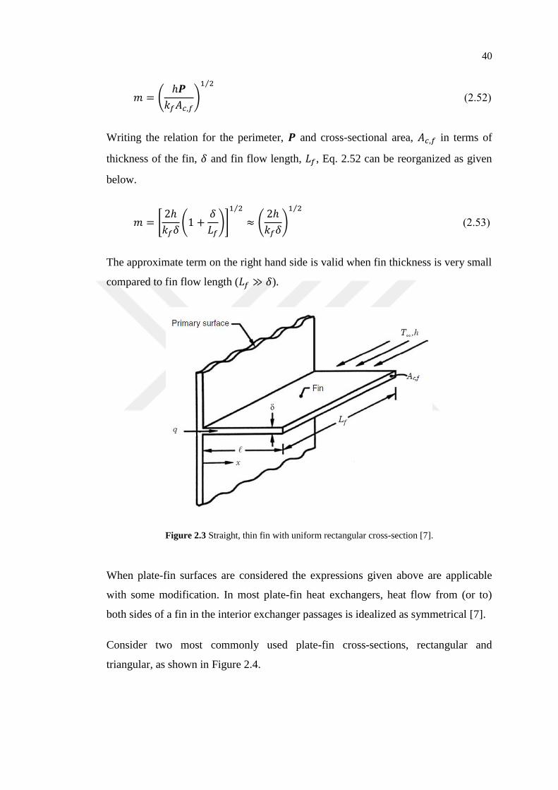
40

𝑚 = (ℎ𝑷

𝑘𝑓𝐴𝑐,𝑓)

1 2⁄

(2.52)

Writing the relation for the perimeter, 𝑷 and cross-sectional area, 𝐴𝑐,𝑓 in terms of

thickness of the fin, 𝛿 and fin flow length, 𝐿𝑓, Eq. 2.52 can be reorganized as given

below.

𝑚 = [2ℎ

𝑘𝑓𝛿(1 +

𝛿

𝐿𝑓)]

1 2⁄

≈ (2ℎ

𝑘𝑓𝛿)

1 2⁄

(2.53)

The approximate term on the right hand side is valid when fin thickness is very small

compared to fin flow length (𝐿𝑓 ≫ 𝛿).

Figure 2.3 Straight, thin fin with uniform rectangular cross-section [7].

When plate-fin surfaces are considered the expressions given above are applicable

with some modification. In most plate-fin heat exchangers, heat flow from (or to)

both sides of a fin in the interior exchanger passages is idealized as symmetrical [7].

Consider two most commonly used plate-fin cross-sections, rectangular and

triangular, as shown in Figure 2.4.

41

Figure 2.4 (a) Plain rectangular fin and (b) plain triangular fin [7].

For such passages, the fin efficiency is generally evaluated using Eq. 2.51. However,

it is assumed that there is no heat transfer through the center of the fin (treated as

adiabatic) and hence fin length is approximately taken equal to half of the plate

spacing, 𝑏.

𝑙 =𝑏 − 𝛿

2≈

𝑏

2 𝑜𝑟 𝑙 =

𝑏 − 2𝛿

2≈

𝑏

2 (2.54)

Here the approximate term in each formula is valid for 𝑏 (or 𝑙) ≫ 𝛿.

42

CHAPTER 3

DESIGN PROCEDURES OF INTERCOOLERS

From the quantitative analysis point of view, two important cases are encountered in

thermal design of intercoolers (or any heat exchangers). These are rating and sizing

problems [7]. In a rating problem the main purpose is to find the performance of an

intercooler of given size under predetermined input conditions. This will tell us how

effective the intercooler can operate (i.e. the extent of ability of it) under given

conditions. This is why rating problem is also called performance problem. When the

dimensions of an intercooler is not known but both input and required output

conditions are known, this time the procedure yields a broad sense design and called

sizing problem. The suitable dimensions (size) of the intercooler that satisfy the

desired performance are determined at the end of the analysis. Both rating and sizing

problems require an iterative solution procedure.

In this section, the stepwise solution procedures of these problems will be given.

However, before explaining them, it is convenient to establish some specifications

and operating conditions of the intercooler.

The construction type and flow arrangement is already known. Intercooler under

discussion is unmixed-unmixed type crossflow heat exchanger having fins on both

flow sides. On the other hand, there are numerous fin types (hence surface types)

each having different geometry and performance characteristics in terms of heat

transfer and fluid friction. Therefore the surface types for the intercooler must be

elaborated first and then the operating conditions should be set up. The following

two titles cover these topics. Later, rating and sizing procedures will be elucidated

step by step.

3.1 Some Selected Surface Types and Their Characteristics

The plate-fin surfaces have various forms as mentioned in Chapter 1. The surfaces

can be built with plain (triangular or rectangular), louvered, offset strip, wavy,

43

perforated and pin fins. Each of them has different geometry and exhibits different

performance characteristics.

In this study, some (fin) surfaces investigated by Kays and London [8] will be used

to construct the intercooler geometry. The effect of surface types on performance (in

a rating problem) or dimensions (in a sizing problem) of the intercooler will be

examined.

The selected surface types and their characteristics are given in Table A.1 in

appendices. In order to denote each surface the notation given by reference [8] is

used. Notations consist of numbers (sometimes numbers with letters) and have been

created in such a way that, they give information about the dimensional

characteristics of the fins in terms of inches. For example: Plain 12.00T denotes that

this surface has fin density of 12 per inch and fins are triangular in shape. Some

surfaces are designated with two separate numbers. The first refers to length of fin in

flow direction; the second gives the fin density. This kind of notation is used in

louvered and offset strip fins. For wavy fins, the first number is fin density and the

second is the wavelength of the fin. Perforated fins are like plain fins and designated

with a single number only.

3.1.1 Colburn Factor and Fanning Friction Factor

The basic data for heat transfer and pressure drop characteristics of compact heat

exchanger surfaces are mostly obtained experimentally and hence introduced in

terms of dimensionless parameters that are functions of Reynolds number. These

parameters are Colburn factor (𝑗 factor) and Fanning friction factor (𝑓 factor), and

denoted as:

𝑗 = 𝑆𝑡 ∙ 𝑃𝑟2 3⁄ = 𝜙1(𝑅𝑒) (3.1)

𝑓 =𝜌𝜏𝑤

𝐺2/2= 𝜙2(𝑅𝑒) (3.2)

Each surface type has different geometry, therefore exhibits a unique heat transfer

and pressure drop performance. This reveals that each surface has its own value of 𝑗

44

and 𝑓 factor and these values must be known to perform the analysis of the

intercooler. For this reason, the experimental values of 𝑗 and 𝑓 factors tabulated by

Kays and London [8] are gathered together for each selected surface. To minimize

reading error and reduce the time of calculations, these tabulated data are curve-fitted

as a function of 𝑅𝑒 and suitable equation models are extracted. For curve-fitting,

least squares method is used and it is ensured that proposed equations gives

coefficient of determination (R2) value of at least 0.999 in all fittings. These

equations are given in Table B.1 and Table B.2, in appendices. Reynolds number

ranges at which the equations are valid are also given in Table B.3.

3.2 Operating Conditions of Intercooler

Identifying the operating conditions is an essential step before starting the intercooler

analysis. In a rating problem in which the size of the intercooler is already known,

determination of operating conditions requires knowing only the input conditions of

each fluid side (hot and cold) in advance. Output conditions are evaluated at the end

of the solution. However, in a sizing problem, both input and output conditions of

each fluid side must be specified at the beginning of the analysis. The solution of the

sizing problem gives the size of the intercooler.

It is already known that, the hot fluid is the charge air directed from the compressor

of the turbocharger and the cold fluid is the ambient air. It is easy to specify the inlet

properties of the ambient air which is considered to be at room temperature and one

atmospheric pressure. Therefore cold side inlet temperature and pressure of the

intercooler is 298.15 K and 101.325 kPa, respectively. Also the mass flow rate of

cold fluid can be calculated considering the velocity of air (equal to vehicle speed)

90 km/h and cold side frontal area of the intercooler roughly 500x500 mm2. This

yields a mass flow rate of 3 kg/s for cold side. When it comes to hot side flow

properties, more elaborated computation is required. The hot fluid passes through the

compressor of the turbocharger and its pressure and temperature increases. Besides,

the mass flow rate of it is arranged with respect to engine parameters. To go further

some information related with the compressor and engine should be given. In this

study, inlet conditions to the compressor are considered to be 298.15 K and 101.325

45

kPa and the pressure ratio (compression ratio of the compressor) is taken as 2.5. The

air leaving the compressor is the hot side inlet of the intercooler. Figure 3.1 shows

the air flow through the turbocharger, intercooler and the engine.

Figure 3.1 Charge air flow in a turbocharged and intercooled engine [4].

Assuming isentropic compression in the compressor, following expression can be

written to find the exit temperature of air.

𝑇2 = 𝑇1 (𝑃2

𝑃1)

𝑘−1𝑘

(3.3)

Here 𝑘 is the specific heat ratio and equal to 1.4. Using this relation the exit

temperature of the air from the compressor is found to be 387.38 K where the exit

pressure of it is easily calculated from pressure ratio information and equal to

253.313 kPa.

In order to evaluate the mass flow rate of charge air, engine specifications that

belong to Ford Cargo TCI (TCI: turbocharged and intercooled) engine is used. Its

technical details are given in Table 3.1. In addition to this, the hot fluid outlet

conditions of the intercooler should be stated. It is supposed that there occurs 60 K of

temperature drop and 1.5% pressure loss in the fluid during cooling. This yields

327.38 K exit temperature and 249.513 kPa exit pressure for the charge air leaving

the intercooler.

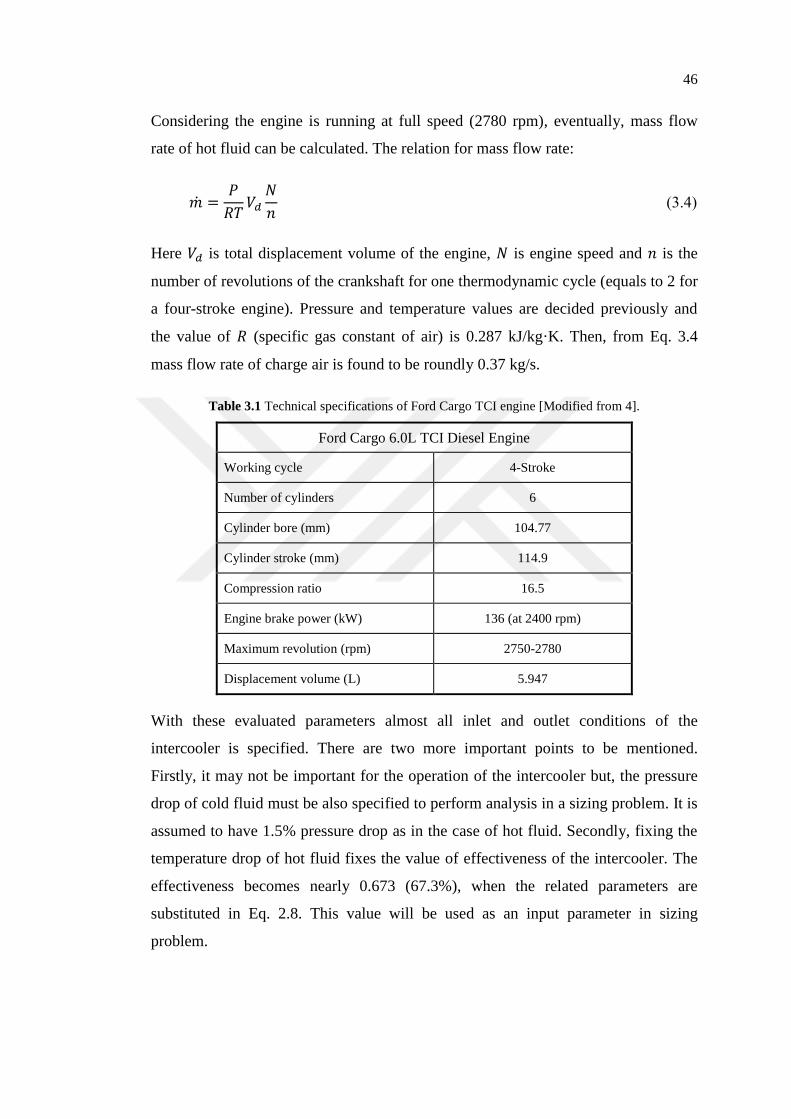
46

Considering the engine is running at full speed (2780 rpm), eventually, mass flow

rate of hot fluid can be calculated. The relation for mass flow rate:

�̇� =𝑃

𝑅𝑇𝑉𝑑

𝑁

𝑛 (3.4)

Here 𝑉𝑑 is total displacement volume of the engine, 𝑁 is engine speed and 𝑛 is the

number of revolutions of the crankshaft for one thermodynamic cycle (equals to 2 for

a four-stroke engine). Pressure and temperature values are decided previously and

the value of 𝑅 (specific gas constant of air) is 0.287 kJ/kg·K. Then, from Eq. 3.4

mass flow rate of charge air is found to be roundly 0.37 kg/s.

Table 3.1 Technical specifications of Ford Cargo TCI engine [Modified from 4].

Ford Cargo 6.0L TCI Diesel Engine

Working cycle 4-Stroke

Number of cylinders 6

Cylinder bore (mm) 104.77

Cylinder stroke (mm) 114.9

Compression ratio 16.5

Engine brake power (kW) 136 (at 2400 rpm)

Maximum revolution (rpm) 2750-2780

Displacement volume (L) 5.947

With these evaluated parameters almost all inlet and outlet conditions of the

intercooler is specified. There are two more important points to be mentioned.

Firstly, it may not be important for the operation of the intercooler but, the pressure

drop of cold fluid must be also specified to perform analysis in a sizing problem. It is

assumed to have 1.5% pressure drop as in the case of hot fluid. Secondly, fixing the

temperature drop of hot fluid fixes the value of effectiveness of the intercooler. The

effectiveness becomes nearly 0.673 (67.3%), when the related parameters are

substituted in Eq. 2.8. This value will be used as an input parameter in sizing

problem.

47

3.3. Rating Problem

In a rating problem of an intercooler, the parameters to start the solution procedure

are: surface type of each flow side, dimensions and input conditions of the hot and

cold fluids. At the end of the solution, the output conditions and the effectiveness of

the intercooler is obtained. The solution steps [7] are given below in details.

1. The surface geometry properties on each fluid side are determined using the

characteristic information (see Table A.1) of the selected surface types and

dimensions of the intercooler. Firstly, frontal area of both sides and total volume of

the intercooler is determined with the following expressions.

𝐴𝑓𝑟,ℎ = 𝐿𝑐𝐿𝑠𝑡 (3.5a)

𝐴𝑓𝑟,𝑐 = 𝐿ℎ𝐿𝑠𝑡 (3.5b)

𝑉 = 𝐿ℎ𝐿𝑐𝐿𝑠𝑡 (3.6)

Here 𝐿ℎ and 𝐿𝑐 are hot and cold fluid flow lengths, respectively. 𝐿𝑠𝑡 is the length

called stack height (noflow height) as given in Fig. 1.5.

The ratio of heat transfer area of one side to total heat exchanger volume, 𝛼 and ratio

of free flow area to frontal area, 𝜎 of both sides can be calculated using the term after

the second equality sign of the expressions:

𝛼1 =𝐴1

𝑉=

𝑏1𝛽1

𝑏1 + 𝑏2 + 2𝛿𝑤 (3.7)

𝜎1 = (𝐴𝑜

𝐴𝑓𝑟)

1

=𝑏1𝛽1(𝐷ℎ/4)

𝑏1 + 𝑏2 + 2𝛿𝑤 (3.8)

Here 𝑏 is plate spacing, 𝛽 is surface area density, 𝐷ℎ is hydraulic diameter and 𝛿𝑤 is

plate thickness. The values of first three terms are fixed when the surface type is

chosen but the last term 𝛿𝑤 can be freely altered which is taken as 0.3 mm in this

study.

48

Knowing the value of 𝛼 and volume of the intercooler, the heat transfer surface area

can be evaluated using Eq. 3.7. Same is valid for free flow area that can be found by

putting the values of 𝜎 and frontal area into Eq. 3.8.

2. In this step, the fluid mean temperatures and thermophysical properties of each

flow side is computed. Since the outlet temperatures are not known in a rating

problem, initially an assumption for the exchanger effectiveness is necessary. It is

generally taken between 50 and 75% for most single-pass crossflow exchangers [7].

Then outlet temperatures can be calculated such that:

𝑇ℎ,𝑜 = 𝑇ℎ,𝑖 − 휀𝐶𝑚𝑖𝑛

𝐶ℎ(𝑇ℎ,𝑖 − 𝑇𝑐,𝑖) (3.9)

𝑇𝑐,𝑜 = 𝑇𝑐,𝑖 + 휀𝐶𝑚𝑖𝑛

𝐶𝑐(𝑇ℎ,𝑖 − 𝑇𝑐,𝑖) (3.10)

While calculating heat capacity rate in foregoing equations, the specific heat values

of fluids are taken equal to each other as a first approximation. Once the outlet

temperatures are calculated in this way, specific heat values are updated with respect

to mean temperatures and Eq. 3.9 and 3.10 is reevaluated. This procedure is repeated

until the evaluated outlet temperatures have the same value with the ones that are

used to calculate specific heat of fluids at mean temperature. After determining the

true outlet temperatures, the thermophysical properties (𝑐𝑝, 𝜇, 𝑘 and 𝑃𝑟) of both

fluids are evaluated at the corresponding mean temperatures by using Table C.1 in

appendices.

3. Next, the core mass velocity and Reynolds number of both fluid sides are

evaluated by means of following equations.

𝐺 =�̇�

𝐴𝑜 (3.11)

𝑅𝑒 =𝐺𝐷ℎ

𝜇 (3.12)

49

Reynolds number is used to determine the nondimensional heat transfer and flow

friction characteristics (𝑗 and 𝑓 factors) of selected surfaces. From equations given in

Table B.1 and Table B.2, 𝑗 and 𝑓 factors of both sides are calculated. Then, to correct

these two parameters for variable fluid property effects, Eq. 2.39 and Eq. 2.40 can be

used. Conversion of 𝑗 factor to 𝑁𝑢 (Nusselt number) or vice-versa is done by the

following expression.

𝑗 =𝑁𝑢 ∙ 𝑃𝑟−1/3

𝑅𝑒 (3.13)

Note that in the first iteration of the solution since the wall temperature is not known

and cannot be calculated without finding the heat transfer coefficient of both sides, it

is not possible to correct 𝑗 and 𝑓 factors for variable fluid property effects. However,

for the second and subsequent iterations the correction can be performed by using the

values of the previous iteration.

4. From 𝑗 and 𝑓 factors, the heat transfer coefficients of both sides are computed by:

ℎ =𝑗𝐺𝑐𝑝

𝑃𝑟2/3 (3.14)

Later, the fin efficiency and extended surface efficiency of both sides are evaluated

using Eq. 2.50, Eq. 2.51 and Eq. 2.53. At this point, material of the fins must be

known to appoint their thermal conductivities. In this study, the aluminum fins

having thermal conductivity of 238 W/m·K are used.

In order to find overall thermal conductance, the wall thermal resistance (𝑅𝑤) must

be evaluated using the following equation:

𝑅𝑤 =𝛿𝑤

𝑘𝑤𝐴𝑤 (3.15)

The plate material is considered to be the same as fin material and hence 𝑘𝑤 is

known. However, to evaluate 𝐴𝑤, number of passages of both flow sides should be

known.

50

Assuming 𝑁𝑝 passages for the hot fluid and (𝑁𝑝 + 1) passages for the cold fluid,

stack height can be written as:

𝐿𝑠𝑡 = 𝑁𝑝𝑏ℎ + (𝑁𝑝 + 1)𝑏𝑐 + (2𝑁𝑝 + 2)𝛿𝑤 (3.16a)

In a rating problem 𝐿𝑠𝑡 is known and hence the value of 𝑁𝑝 can be found by writing

Eq. 3.16a in the form of:

𝑁𝑝 =𝐿𝑠𝑡 − 𝑏𝑐 − 2𝛿𝑤

𝑏ℎ + 𝑏𝑐 + 2𝛿𝑤 (3.16b)

Then the wall conduction area, 𝐴𝑤 is calculated using the relation:

𝐴𝑤 = 𝐿ℎ𝐿𝑐(2𝑁𝑝 + 2) (3.17)

Finally, all necessary parameters are substituted into Eq. 2.6 to compute overall

thermal conductance.

5. From the known heat capacity of each fluid side 𝐶∗ is calculated using Eq. 2.11.

Then the value of 𝑈𝐴 and 𝐶𝑚𝑖𝑛 is substituted into Eq. 2.10 to find 𝑁𝑇𝑈. Lastly, the

effectiveness of the heat exchanger is determined using Eq. 2.12.

6. In order to calculate the reduction in effectiveness due to the longitudinal wall heat

conduction, two more parameters should be evaluated: 𝜆 and (𝜂𝑜ℎ𝐴)∗.

To find 𝜆ℎ and 𝜆𝑐 from Eq. 2.42a and Eq. 2.42b, respectively, the unknown term in

these equations denoting the cross-sectional area for longitudinal heat conduction

(𝐴𝑘) must be evaluated. To compute 𝐴𝑘 for hot and cold sides, following expressions

are used, and then 𝜆 value of both sides is calculated.

𝐴𝑘,ℎ = 2𝑁𝑝𝐿𝑐𝛿𝑤 (3.18a)

𝐴𝑘,𝑐 = (2𝑁𝑝 + 2)𝐿ℎ𝛿𝑤 (3.18b)

The parameter (𝜂𝑜ℎ𝐴)∗ is evaluated using Eq. 2.44. With the determined values of

𝑁𝑇𝑈, 𝐶∗, 𝜆ℎ, 𝜆𝑐 and (𝜂𝑜ℎ𝐴)∗, the reduction in effectiveness is found from the

51

tabulated data presented by Shah and Sekulic [7]. Finally the true effectiveness is

computed from Eq. 2.47 and outlet temperatures are reevaluated using this value.

If new outlet temperatures are significantly different from those assumed at step 2,

iteration is continued throughout the steps 2 to 6 until the assumed and computed

outlet temperatures converge within the desired degree of accuracy.

7. With the ultimate value of the effectiveness obtained at the end of the iteration, the

heat transfer rate can be calculated using the following expression.

𝑞 = 휀𝐶𝑚𝑖𝑛(𝑇ℎ,𝑖 − 𝑇𝑐,𝑖) (3.19)

8. After evaluating all the correct values of previous steps, the pressure drop

calculations are performed by using Eq. 2.21.

Firstly, fluid densities (reciprocal of specific volume) at the exchanger inlet and

outlet are determined using ideal gas equation, Eq. 2.25. Since the outlet pressures

are not known at this point, fluid outlet densities are calculated using the inlet

pressures. The mean specific volume is the harmonic mean of inlet and outlet

densities and evaluated from Eq. 2.19.

Then, 𝑓 is corrected for variable fluid property effects by using Eq. 2.40 and 𝐾𝑐 and

𝐾𝑒 values are determined from Figure D.1.

Last, pressure drop of both sides are evaluated by using Eq. 2.21 and the outlet

pressures are found. With these outlet pressures, the outlet densities are reevaluated

and the pressure drop calculations are repeated until the outlet pressures used to find

outlet densities converge within the certain degree of accuracy with the evaluated

outlet pressures.

3.4 Sizing Problem

In a sizing problem of an intercooler, the surface type of each flow side, input

conditions and also output conditions are known. The aim is to determine the

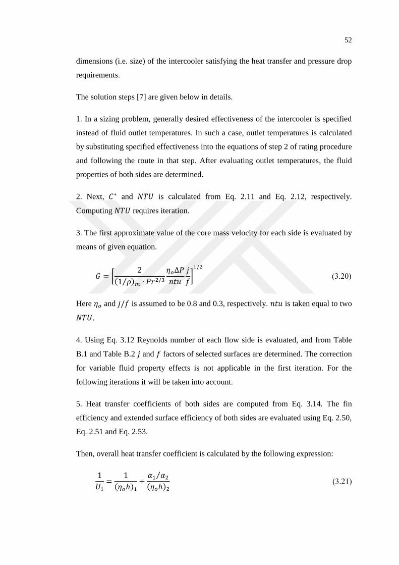
52

dimensions (i.e. size) of the intercooler satisfying the heat transfer and pressure drop

requirements.

The solution steps [7] are given below in details.

1. In a sizing problem, generally desired effectiveness of the intercooler is specified

instead of fluid outlet temperatures. In such a case, outlet temperatures is calculated

by substituting specified effectiveness into the equations of step 2 of rating procedure

and following the route in that step. After evaluating outlet temperatures, the fluid

properties of both sides are determined.

2. Next, 𝐶∗ and 𝑁𝑇𝑈 is calculated from Eq. 2.11 and Eq. 2.12, respectively.

Computing 𝑁𝑇𝑈 requires iteration.

3. The first approximate value of the core mass velocity for each side is evaluated by

means of given equation.

𝐺 = [2

(1 𝜌⁄ )𝑚 ∙ 𝑃𝑟2/3

𝜂𝑜∆𝑃

𝑛𝑡𝑢

𝑗

𝑓]

1/2

(3.20)

Here 𝜂𝑜 and 𝑗/𝑓 is assumed to be 0.8 and 0.3, respectively. 𝑛𝑡𝑢 is taken equal to two

𝑁𝑇𝑈.

4. Using Eq. 3.12 Reynolds number of each flow side is evaluated, and from Table

B.1 and Table B.2 𝑗 and 𝑓 factors of selected surfaces are determined. The correction

for variable fluid property effects is not applicable in the first iteration. For the

following iterations it will be taken into account.

5. Heat transfer coefficients of both sides are computed from Eq. 3.14. The fin

efficiency and extended surface efficiency of both sides are evaluated using Eq. 2.50,

Eq. 2.51 and Eq. 2.53.

Then, overall heat transfer coefficient is calculated by the following expression:

1

𝑈1=

1

(𝜂𝑜ℎ)1+

𝛼1 𝛼2⁄

(𝜂𝑜ℎ)2 (3.21)

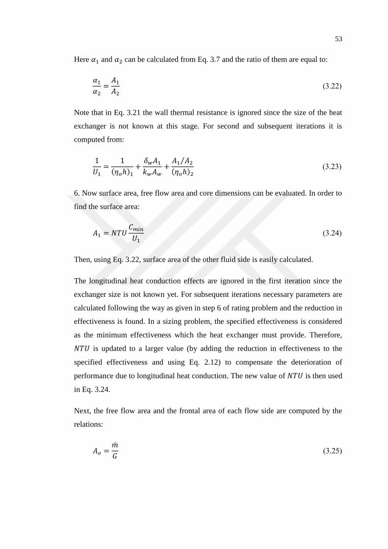
53

Here 𝛼1 and 𝛼2 can be calculated from Eq. 3.7 and the ratio of them are equal to:

𝛼1

𝛼2=

𝐴1

𝐴2 (3.22)

Note that in Eq. 3.21 the wall thermal resistance is ignored since the size of the heat

exchanger is not known at this stage. For second and subsequent iterations it is

computed from:

1

𝑈1=

1

(𝜂𝑜ℎ)1+

𝛿𝑤𝐴1

𝑘𝑤𝐴𝑤+

𝐴1 𝐴2⁄

(𝜂𝑜ℎ)2 (3.23)

6. Now surface area, free flow area and core dimensions can be evaluated. In order to

find the surface area:

𝐴1 = 𝑁𝑇𝑈𝐶𝑚𝑖𝑛

𝑈1 (3.24)

Then, using Eq. 3.22, surface area of the other fluid side is easily calculated.

The longitudinal heat conduction effects are ignored in the first iteration since the

exchanger size is not known yet. For subsequent iterations necessary parameters are

calculated following the way as given in step 6 of rating problem and the reduction in

effectiveness is found. In a sizing problem, the specified effectiveness is considered

as the minimum effectiveness which the heat exchanger must provide. Therefore,

𝑁𝑇𝑈 is updated to a larger value (by adding the reduction in effectiveness to the

specified effectiveness and using Eq. 2.12) to compensate the deterioration of

performance due to longitudinal heat conduction. The new value of 𝑁𝑇𝑈 is then used

in Eq. 3.24.

Next, the free flow area and the frontal area of each flow side are computed by the

relations:

𝐴𝑜 =�̇�

𝐺 (3.25)

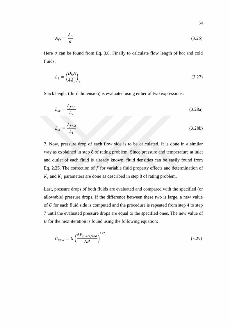
54

𝐴𝑓𝑟 =𝐴𝑜

𝜎 (3.26)

Here 𝜎 can be found from Eq. 3.8. Finally to calculate flow length of hot and cold

fluids:

𝐿1 = (𝐷ℎ𝐴

4𝐴𝑜)

1

(3.27)

Stack height (third dimension) is evaluated using either of two expressions:

𝐿𝑠𝑡 =𝐴𝑓𝑟,1

𝐿2 (3.28a)

𝐿𝑠𝑡 =𝐴𝑓𝑟,2

𝐿1 (3.28b)

7. Now, pressure drop of each flow side is to be calculated. It is done in a similar

way as explained in step 8 of rating problem. Since pressure and temperature at inlet

and outlet of each fluid is already known, fluid densities can be easily found from

Eq. 2.25. The correction of 𝑓 for variable fluid property effects and determination of

𝐾𝑐 and 𝐾𝑒 parameters are done as described in step 8 of rating problem.

Last, pressure drops of both fluids are evaluated and compared with the specified (or

allowable) pressure drops. If the difference between these two is large, a new value

of 𝐺 for each fluid side is computed and the procedure is repeated from step 4 to step

7 until the evaluated pressure drops are equal to the specified ones. The new value of

𝐺 for the next iteration is found using the following equation:

𝐺𝑛𝑒𝑤 = 𝐺 (∆𝑃𝑠𝑝𝑒𝑐𝑖𝑓𝑖𝑒𝑑

∆𝑃)

1/2

(3.29)

55

CHAPTER 4

RESULTS

This section is to be presented in three parts. In the first part, sizing procedure is

performed on 20 different intercooler configurations. The characteristics of surface

types given in Table A.1 and operating conditions explained in Chapter 3 have been

utilized in this procedure. 15 number of intercooler configurations are built using

same surface type (same fin geometry) on both flow sides and remaining 5 are set up

such that, the surface type on one side is different than the surface type on the other

side. Distinct configurations yield different dimensions as expected. Therefore, in

this part it is possible to observe and compare these configurations in terms of

dimensions when they have same operating conditions. Also the resulting

configurations are examined to see whether or not they can satisfy the space

requirements when installed into the engine compartment of a vehicle.

In the second part, a suitable reference size (hot flow length, cold flow length and

stack height) for an intercooler is decided considering the size and weight limitations

during installation. It is clear that a perfect intercooler with implausible dimensions is

useless since its mounting on an engine compartment will not be possible. Therefore,

in this part the reference size is set and all 20 configurations are considered to be at

this size. The aim is to see their performance (in terms of first and second law of

thermodynamics) when the same input conditions are applied to them. Later four of

these configurations are chosen and the effect of mass flow rate on their performance

is examined. Miscellaneous charts have been created for this purpose.

In the last part, intercooler is coupled to an engine and its effect on engine

performance is explained. Here the purpose is to show the extent of improvements an

intercooler (or a turbocharger intercooler combination) can provide to an engine.

Also a discussion has been made to clarify whether or not intercoolers are always

feasible to be utilized.

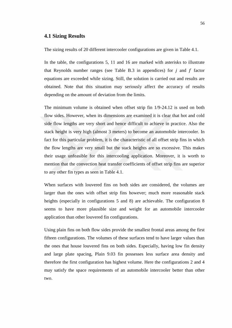
56

4.1 Sizing Results

The sizing results of 20 different intercooler configurations are given in Table 4.1.

In the table, the configurations 5, 11 and 16 are marked with asterisks to illustrate

that Reynolds number ranges (see Table B.3 in appendices) for 𝑗 and 𝑓 factor

equations are exceeded while sizing. Still, the solution is carried out and results are

obtained. Note that this situation may seriously affect the accuracy of results

depending on the amount of deviation from the limits.

The minimum volume is obtained when offset strip fin 1/9-24.12 is used on both

flow sides. However, when its dimensions are examined it is clear that hot and cold

side flow lengths are very short and hence difficult to achieve in practice. Also the

stack height is very high (almost 3 meters) to become an automobile intercooler. In

fact for this particular problem, it is the characteristic of all offset strip fins in which

the flow lengths are very small but the stack heights are so excessive. This makes

their usage unfeasible for this intercooling application. Moreover, it is worth to

mention that the convection heat transfer coefficients of offset strip fins are superior

to any other fin types as seen in Table 4.1.

When surfaces with louvered fins on both sides are considered, the volumes are

larger than the ones with offset strip fins however; much more reasonable stack

heights (especially in configurations 5 and 8) are achievable. The configuration 8

seems to have more plausible size and weight for an automobile intercooler

application than other louvered fin configurations.

Using plain fins on both flow sides provide the smallest frontal areas among the first

fifteen configurations. The volumes of these surfaces tend to have larger values than

the ones that house louvered fins on both sides. Especially, having low fin density

and large plate spacing, Plain 9.03 fin possesses less surface area density and

therefore the first configuration has highest volume. Here the configurations 2 and 4

may satisfy the space requirements of an automobile intercooler better than other

two.

57

Table 4.1 Sizing results of intercooler configurations.

Config.

# Fin type

𝑳𝒉 mm

𝑳𝒄 mm

𝑳𝒔𝒕 mm

𝑽 m3

𝒉𝒉 W/(m2‧ K)

𝒉𝒄 W/(m2‧ K)

1 Plain 9.03

on both fluid sides 1021.5 122 129 0.01611 176.13 163.82

2 Plain 11.11

on both fluid sides 474.3 53.73 283.4 0.00722 233.89 210.39

3 Plain 19.86

on both fluid sides 277.1 30.85 527.14 0.00451 248.03 220.39

4 Plain 12.00T

on both fluid sides 474.5 54 286.2 0.00733 214.86 193.6

5 Louvered 1/2-6.06

on both fluid sides* 374.8 47.46 420.86 0.00749 313.7 301.78

6 Louvered 3/8(a)-8.7

on both fluid sides 274 34.67 620 0.00589 334.57 321.5

7 Louvered 1/4-11.1

on both fluid sides 218.2 26.9 713.6 0.00419 399.45 380.17

8 Louvered 3/4-11.1

on both fluid sides 330.16 38.74 430.4 0.00551 306.32 281.07

9 Offset strip 1/8-15.61

on both fluid sides 156.53 19.35 980.6 0.00297 456.76 436.61

10 Offset strip 1/8-19.86

on both fluid sides 95.7 11.32 1730.2 0.00187 502.52 462.16

11 Offset strip 1/9-24.12

on both fluid sides* 66 7.9 2747.3 0.00143 533.13 499.26

12 Offset strip 1/10-

19.74

on both fluid sides

75.23 9.08 2413.2 0.00165 456.13 432.1

13 Wavy 11.5-3/8W

on both fluid sides 189.5 23.5 897.7 0.00400 449.46 423.7

14 Wavy 17.8-3/8W

on both fluid sides 165.42 20.53 972.4 0.00330 393.9 370.48

15 Perforated 13.95P

on both fluid sides 227.2 24.26 711.1 0.00392 423.74 364.44

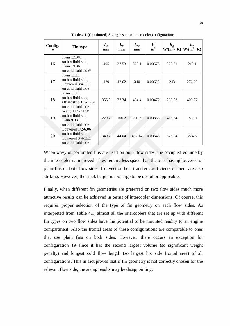
58

Table 4.1 (Continued) Sizing results of intercooler configurations.

Config.

# Fin type

𝑳𝒉 mm

𝑳𝒄 mm

𝑳𝒔𝒕 mm

𝑽 m3

𝒉𝒉 W/(m2‧ K)

𝒉𝒄 W/(m2‧ K)

16

Plain 12.00T

on hot fluid side,

Plain 19.86

on cold fluid side*

405 37.53 378.1 0.00575 228.71 212.1

17

Plain 11.11

on hot fluid side,

Louvered 3/4-11.1

on cold fluid side

429 42.62 340 0.00622 243 276.06

18

Plain 11.11

on hot fluid side,

Offset strip 1/8-15.61

on cold fluid side

356.5 27.34 484.4 0.00472 260.53 400.72

19

Wavy 11.5-3/8W

on hot fluid side,

Plain 9.03

on cold fluid side

229.7 106.2 361.89 0.00883 416.84 183.11

20

Louvered 1/2-6.06

on hot fluid side,

Louvered 3/4-11.1

on cold fluid side

340.7 44.04 432.14 0.00648 325.04 274.3

When wavy or perforated fins are used on both flow sides, the occupied volume by

the intercooler is improved. They require less space than the ones having louvered or

plain fins on both flow sides. Convection heat transfer coefficients of them are also

striking. However, the stack height is too large to be useful or applicable.

Finally, when different fin geometries are preferred on two flow sides much more

attractive results can be achieved in terms of intercooler dimensions. Of course, this

requires proper selection of the type of fin geometry on each flow sides. As

interpreted from Table 4.1, almost all the intercoolers that are set up with different

fin types on two flow sides have the potential to be mounted readily to an engine

compartment. Also the frontal areas of these configurations are comparable to ones

that use plain fins on both sides. However, there occurs an exception for

configuration 19 since it has the second largest volume (so significant weight

penalty) and longest cold flow length (so largest hot side frontal area) of all

configurations. This in fact proves that if fin geometry is not correctly chosen for the

relevant flow side, the sizing results may be disappointing.

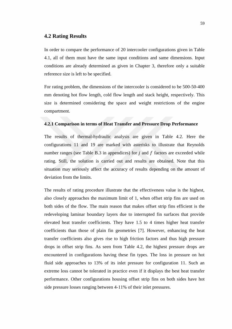
59

4.2 Rating Results

In order to compare the performance of 20 intercooler configurations given in Table

4.1, all of them must have the same input conditions and same dimensions. Input

conditions are already determined as given in Chapter 3, therefore only a suitable

reference size is left to be specified.

For rating problem, the dimensions of the intercooler is considered to be 500-50-400

mm denoting hot flow length, cold flow length and stack height, respectively. This

size is determined considering the space and weight restrictions of the engine

compartment.

4.2.1 Comparison in terms of Heat Transfer and Pressure Drop Performance

The results of thermal-hydraulic analysis are given in Table 4.2. Here the

configurations 11 and 19 are marked with asterisks to illustrate that Reynolds

number ranges (see Table B.3 in appendices) for 𝑗 and 𝑓 factors are exceeded while

rating. Still, the solution is carried out and results are obtained. Note that this

situation may seriously affect the accuracy of results depending on the amount of

deviation from the limits.

The results of rating procedure illustrate that the effectiveness value is the highest,

also closely approaches the maximum limit of 1, when offset strip fins are used on

both sides of the flow. The main reason that makes offset strip fins efficient is the

redeveloping laminar boundary layers due to interrupted fin surfaces that provide

elevated heat transfer coefficients. They have 1.5 to 4 times higher heat transfer

coefficients than those of plain fin geometries [7]. However, enhancing the heat

transfer coefficients also gives rise to high friction factors and thus high pressure

drops in offset strip fins. As seen from Table 4.2, the highest pressure drops are

encountered in configurations having these fin types. The loss in pressure on hot

fluid side approaches to 13% of its inlet pressure for configuration 11. Such an

extreme loss cannot be tolerated in practice even if it displays the best heat transfer

performance. Other configurations housing offset strip fins on both sides have hot

side pressure losses ranging between 4-11% of their inlet pressures.

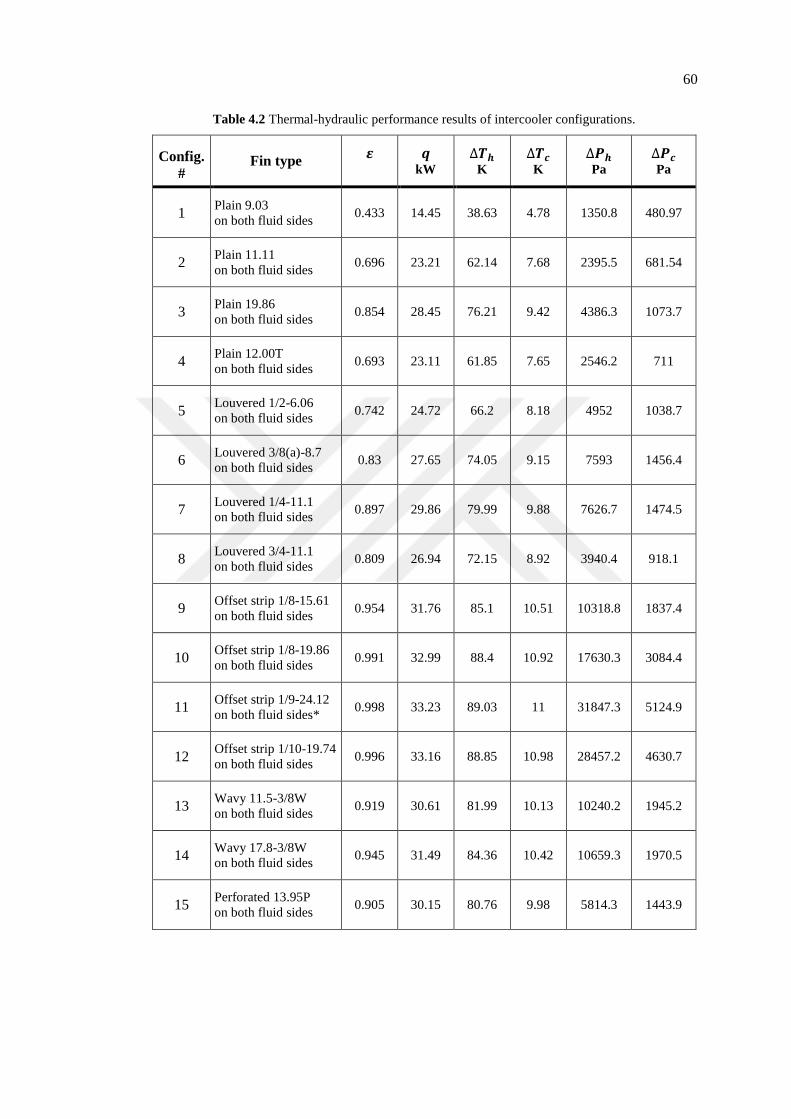
60

Table 4.2 Thermal-hydraulic performance results of intercooler configurations.

Config.

# Fin type

𝜺

𝒒 kW

∆𝑻𝒉 K

∆𝑻𝒄 K

∆𝑷𝒉 Pa

∆𝑷𝒄 Pa

1 Plain 9.03

on both fluid sides 0.433 14.45 38.63 4.78 1350.8 480.97

2 Plain 11.11

on both fluid sides 0.696 23.21 62.14 7.68 2395.5 681.54

3 Plain 19.86

on both fluid sides 0.854 28.45 76.21 9.42 4386.3 1073.7

4 Plain 12.00T

on both fluid sides 0.693 23.11 61.85 7.65 2546.2 711

5 Louvered 1/2-6.06

on both fluid sides 0.742 24.72 66.2 8.18 4952 1038.7

6 Louvered 3/8(a)-8.7

on both fluid sides 0.83 27.65 74.05 9.15 7593 1456.4

7 Louvered 1/4-11.1

on both fluid sides 0.897 29.86 79.99 9.88 7626.7 1474.5

8 Louvered 3/4-11.1

on both fluid sides 0.809 26.94 72.15 8.92 3940.4 918.1

9 Offset strip 1/8-15.61

on both fluid sides 0.954 31.76 85.1 10.51 10318.8 1837.4

10 Offset strip 1/8-19.86

on both fluid sides 0.991 32.99 88.4 10.92 17630.3 3084.4

11 Offset strip 1/9-24.12

on both fluid sides* 0.998 33.23 89.03 11 31847.3 5124.9

12 Offset strip 1/10-19.74

on both fluid sides 0.996 33.16 88.85 10.98 28457.2 4630.7

13 Wavy 11.5-3/8W

on both fluid sides 0.919 30.61 81.99 10.13 10240.2 1945.2

14 Wavy 17.8-3/8W

on both fluid sides 0.945 31.49 84.36 10.42 10659.3 1970.5

15 Perforated 13.95P

on both fluid sides 0.905 30.15 80.76 9.98 5814.3 1443.9

61

Table 4.2 (Continued) Thermal-hydraulic performance results of intercooler configurations.

Config.

# Fin type

𝜺

𝒒 kW

∆𝑻𝒉 K

∆𝑻𝒄 K

∆𝑷𝒉 Pa

∆𝑷𝒄 Pa

16

Plain 12.00T

on hot fluid side,

Plain 19.86

on cold fluid side

0.777 25.88 69.31 8.57 2505 1070.3

17

Plain 11.11

on hot fluid side,

Louvered 3/4-11.1

on cold fluid side

0.756 25.19 67.44 8.34 2369 916.1

18

Plain 11.11

on hot fluid side,

Offset strip 1/8-15.61

on cold fluid side

0.834 27.77 74.39 9.19 2334.2 1830.3

19

Wavy 11.5-3/8W

on hot fluid side,

Plain 9.03

on cold fluid side*

0.593 19.79 52.95 6.55 25229.7 199.44

20

Louvered 1/2-6.06

on hot fluid side,

Louvered 3/4-11.1

on cold fluid side

0.778 25.92 69.41 8.58 4923 916.9

Another interrupted fin type, louvered fins provide good heat transfer and pressure

drop characteristics when used on both sides of the flow. The effectiveness of them

ranges between 0.74-0.90. The highest pressure drop on hot flow side is around 3%

which is much more less than most of the offset strip fins. If combination of high

heat transfer rate and low pressure drop is mandated, choosing configuration 8 seems

to be more reasonable than the other ones. It can maintain nearly 1.5% pressure drop

on hot fluid side with a substantial effectiveness value of 0.809. Configurations 6 and

7 have higher effectiveness values but pressure losses are also higher.

Configurations with wavy and perforated fins show even better heat transfer rates

than the ones having louvered fins on both sides. However, the pressure loss of fluids

inside the core is again large, especially for the intercoolers housing wavy fins.

Plain fins exhibit different performance features when used on both sides of the flow.

Configuration 1 has the lowest effectiveness among all configurations whereas

configuration 3 has comparable heat transfer performance. This condition is in fact

due to discrete characteristics of their fin geometries. Plain 9.03 has large plate

spacing and low fin density therefore provides less surface area density. This results

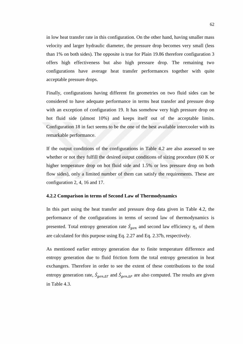
62

in low heat transfer rate in this configuration. On the other hand, having smaller mass

velocity and larger hydraulic diameter, the pressure drop becomes very small (less

than 1% on both sides). The opposite is true for Plain 19.86 therefore configuration 3

offers high effectiveness but also high pressure drop. The remaining two

configurations have average heat transfer performances together with quite

acceptable pressure drops.

Finally, configurations having different fin geometries on two fluid sides can be

considered to have adequate performance in terms heat transfer and pressure drop

with an exception of configuration 19. It has somehow very high pressure drop on

hot fluid side (almost 10%) and keeps itself out of the acceptable limits.

Configuration 18 in fact seems to be the one of the best available intercooler with its

remarkable performance.

If the output conditions of the configurations in Table 4.2 are also assessed to see

whether or not they fulfill the desired output conditions of sizing procedure (60 K or

higher temperature drop on hot fluid side and 1.5% or less pressure drop on both

flow sides), only a limited number of them can satisfy the requirements. These are

configuration 2, 4, 16 and 17.

4.2.2 Comparison in terms of Second Law of Thermodynamics

In this part using the heat transfer and pressure drop data given in Table 4.2, the

performance of the configurations in terms of second law of thermodynamics is

presented. Total entropy generation rate �̇�𝑔𝑒𝑛 and second law efficiency 𝜂𝑠 of them

are calculated for this purpose using Eq. 2.27 and Eq. 2.37b, respectively.

As mentioned earlier entropy generation due to finite temperature difference and

entropy generation due to fluid friction form the total entropy generation in heat

exchangers. Therefore in order to see the extent of these contributions to the total

entropy generation rate, �̇�𝑔𝑒𝑛,∆𝑇 and �̇�𝑔𝑒𝑛,∆𝑃 are also computed. The results are given

in Table 4.3.

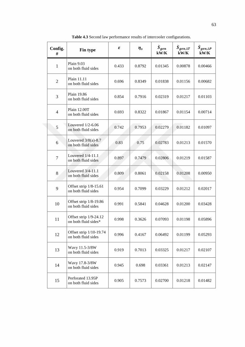
63

Table 4.3 Second law performance results of intercooler configurations.

Config.

# Fin type

𝜺

𝜼𝒔

�̇�𝒈𝒆𝒏

kW/K

�̇�𝒈𝒆𝒏,∆𝑻

kW/K

�̇�𝒈𝒆𝒏,∆𝑷

kW/K

1 Plain 9.03

on both fluid sides 0.433 0.8792 0.01345 0.00878 0.00466

2 Plain 11.11

on both fluid sides 0.696 0.8349 0.01838 0.01156 0.00682

3 Plain 19.86

on both fluid sides 0.854 0.7916 0.02319 0.01217 0.01103

4 Plain 12.00T

on both fluid sides 0.693 0.8322 0.01867 0.01154 0.00714

5 Louvered 1/2-6.06

on both fluid sides 0.742 0.7953 0.02279 0.01182 0.01097

6 Louvered 3/8(a)-8.7

on both fluid sides 0.83 0.75 0.02783 0.01213 0.01570

7 Louvered 1/4-11.1

on both fluid sides 0.897 0.7479 0.02806 0.01219 0.01587

8 Louvered 3/4-11.1

on both fluid sides 0.809 0.8061 0.02158 0.01208 0.00950

9 Offset strip 1/8-15.61

on both fluid sides 0.954 0.7099 0.03229 0.01212 0.02017

10 Offset strip 1/8-19.86

on both fluid sides 0.991 0.5841 0.04628 0.01200 0.03428

11 Offset strip 1/9-24.12

on both fluid sides* 0.998 0.3626 0.07093 0.01198 0.05896

12 Offset strip 1/10-19.74

on both fluid sides 0.996 0.4167 0.06492 0.01199 0.05293

13 Wavy 11.5-3/8W

on both fluid sides 0.919 0.7013 0.03325 0.01217 0.02107

14 Wavy 17.8-3/8W

on both fluid sides 0.945 0.698 0.03361 0.01213 0.02147

15 Perforated 13.95P

on both fluid sides 0.905 0.7573 0.02700 0.01218 0.01482

64

Table 4.3 (Continued) Second law performance results of intercooler configurations.

Config.

# Fin type

𝜺

𝜼𝒔

�̇�𝒈𝒆𝒏

kW/K

�̇�𝒈𝒆𝒏,∆𝑻

kW/K

�̇�𝒈𝒆𝒏,∆𝑷

kW/K

16

Plain 12.00T

on hot fluid side,

Plain 19.86

on cold fluid side

0.777 0.8001 0.02217 0.01197 0.01020

17

Plain 11.11

on hot fluid side,

Louvered 3/4-11.1

on cold fluid side

0.756 0.814 0.02070 0.01188 0.00882

18

Plain 11.11

on hot fluid side,

Offset strip 1/8-15.61

on cold fluid side

0.834 0.7411 0.02881 0.01213 0.01668

19

Wavy 11.5-3/8W

on hot fluid side,

Plain 9.03

on cold fluid side*

0.593 0.7883 0.02356 0.01072 0.01284

20

Louvered 1/2-6.06

on hot fluid side,

Louvered 3/4-11.1

on cold fluid side

0.778 0.8034 0.02189 0.01198 0.00991

Since the accuracy of the results in this part is dependent on the accuracy of the heat

transfer and pressure drop values given in Table 4.2, the configurations 11 and 19 are

also marked with asterisks in Table 4.3.

The evaluation in terms of second law reveals some interesting outcomes when the

table is carefully examined. First of all, it is clear that the configuration 11 which has

highest effectiveness value among all configurations in fact gets the worst ranking

when assessed in terms of second law efficiency. �̇�𝑔𝑒𝑛 value of this configuration is

the largest which holds it in the worst place since entropy production is directly

proportional to exergy destruction. The leading contribution to entropy generation

comes from the excessive pressure loss of fluids or in other words the generated

entropy due to fluid friction. This situation is actually characteristics of the

configurations having offset strip fins on both flow sides. Therefore most of them

have lower second law efficiency values when compared to other configurations.

Having lower pressure drop values the configurations with louvered fins on both

flow sides display better second law performances than the ones with offset strip

fins. The contributions of �̇�𝑔𝑒𝑛,∆𝑇 and �̇�𝑔𝑒𝑛,∆𝑃 to total entropy generation rate are

65

pretty much same in these configurations. Also, an interesting situation arises in

configuration 7. It has the largest finite temperature difference entropy generation

among all configurations although the largest temperature changes in hot and cold

fluids are not reached in this configuration.

Wavy and perforated fins leads to high pressure drops, therefore �̇�𝑔𝑒𝑛,∆𝑃 provides

larger contribution to the total entropy generation in configurations having these fins

on both flow sides. The configuration housing perforated fins have lower entropy

generation and hence higher 𝜂𝑠 value than other two.

Intercoolers with different fin types on hot and cold flow sides exhibit similar second

law characteristics. Here remarkable point to mention is that, configuration 19 has

very large pressure drop on hot fluid side (see Table 4.2) but due to low mass flow

rate of hot fluid, it has less entropy generation rate than configuration 18.

When configurations having plain fins on both flow sides are investigated, attention

should be given to configuration 1. It exhibits the best performance when assessed in

terms of second law efficiency and provides the lowest entropy generation rate

within 20 configurations. However, in terms of thermal performance it has the lowest

effectiveness value and therefore poorest heat transfer. By looking at these results

someone could have a misleading perception such that; using a configuration with

low effectiveness maintains high second law efficiency and vice versa. This

statement is of course incorrect and true outcome is reached with the detailed

examination of the second law efficiency expression. In order to attain the maximum

value of 𝜂𝑠 from Eq. 2.37b there are two ways. First, if there is no heat transfer and

pressure drop in the heat exchanger the second law efficiency becomes maximum, 1.

The sum of output exergies will be equal to sum of input exergies since there is no

change in the fluid exergies. This situation in fact creates a contradiction to the heat

exchanger’s raison d’être. The other way is the reasonable one; transferring exergy of

hot fluid to cold fluid in a reversible manner and hence accomplishing the process

with the maximum possible second law efficiency. It is actually what a heat

exchanger must try to do.

66

Consequently, two important conclusions can be attained with these explanations.

First, since fluids passing through configuration 1 experience the least amount of

heat transfer and pressure drop (therefore produces small amount of irreversibility),

the second law efficiency of this process appears to be very high. But in fact it

operates with a low effectiveness and hence shows poor performance in terms of heat

transfer. Second, in order to avoid such contradictory results while analyzing the

second law characteristics of heat exchangers in terms of second law efficiency, it

could be better to use Eq. 2.37a instead of Eq. 2.37b.

As final words of this part; it is clear that if there is no entropy generation and hence

exergy destruction (ideally achievable with infinite surface area and zero pressure

drop), a heat exchanger will be performing its duty perfectly. However, the entropy

generation cannot be eliminated in these configurations even if they have infinite

heat transfer area and zero core pressure drop. It is due to the fact that, the

configurations do not have equal heat capacity rates and thus, at the end of the heat

exchange process, the cold fluid outlet temperature cannot be equal to hot fluid inlet

temperature. This will create an inevitable irreversibility called remanent or flow

imbalance irreversibility. In other words, the high quality fluid (hot fluid) will be

transformed to a low quality one during heat transfer and the cold fluid cannot be

raised to the same high quality at the exit of the intercooler because of its higher heat

capacity rate. Therefore the exergy destruction becomes unavoidable during the

process. To sum up, the second law efficiency of these configurations could attain its

maximum theoretical value only if the intercooler is ideal and hot and cold fluids

have equal heat capacity rates (i.e. balanced flow).

4.2.3 Variation of Performance Parameters with Mass Flow Rate

Four configurations, namely configuration 1, 8, 9 and 16 having reference size are to

be examined in this part. All the input parameters explained before are held constant

except mass flow rate of hot fluid which is altered from 0.1 to 0.5 kg/m3. The

purpose is to investigate the influence of mass flow rate on their effectiveness, hot

side pressure drop, hot side outlet density and second law characteristics by means of

charts.

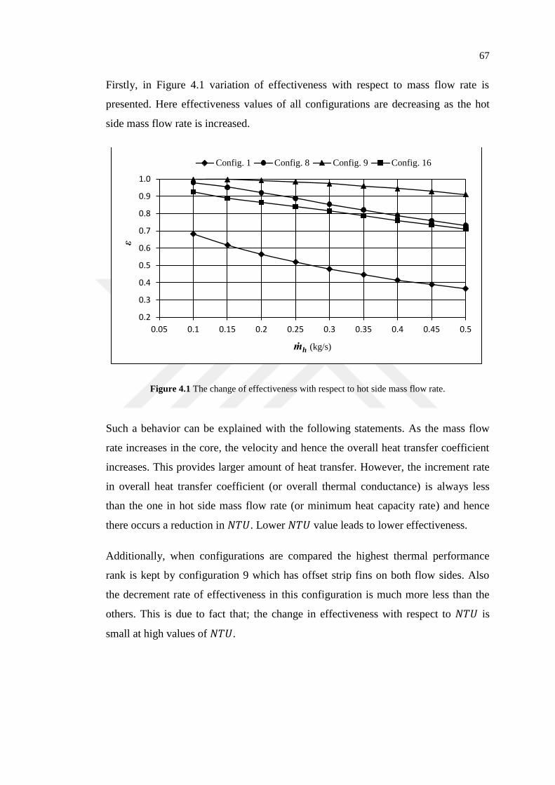
67

Firstly, in Figure 4.1 variation of effectiveness with respect to mass flow rate is

presented. Here effectiveness values of all configurations are decreasing as the hot

side mass flow rate is increased.

Figure 4.1 The change of effectiveness with respect to hot side mass flow rate.

Such a behavior can be explained with the following statements. As the mass flow

rate increases in the core, the velocity and hence the overall heat transfer coefficient

increases. This provides larger amount of heat transfer. However, the increment rate

in overall heat transfer coefficient (or overall thermal conductance) is always less

than the one in hot side mass flow rate (or minimum heat capacity rate) and hence

there occurs a reduction in 𝑁𝑇𝑈. Lower 𝑁𝑇𝑈 value leads to lower effectiveness.

Additionally, when configurations are compared the highest thermal performance

rank is kept by configuration 9 which has offset strip fins on both flow sides. Also

the decrement rate of effectiveness in this configuration is much more less than the

others. This is due to fact that; the change in effectiveness with respect to 𝑁𝑇𝑈 is

small at high values of 𝑁𝑇𝑈.

0.2

0.3

0.4

0.5

0.6

0.7

0.8

0.9

1.0

0.05 0.1 0.15 0.2 0.25 0.3 0.35 0.4 0.45 0.5

ε

ṁh (kg/s)

Config. 1 Config. 8 Config. 9 Config. 16

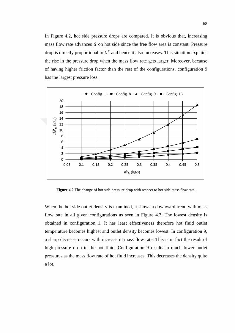
68

In Figure 4.2, hot side pressure drops are compared. It is obvious that, increasing

mass flow rate advances 𝐺 on hot side since the free flow area is constant. Pressure

drop is directly proportional to 𝐺2 and hence it also increases. This situation explains

the rise in the pressure drop when the mass flow rate gets larger. Moreover, because

of having higher friction factor than the rest of the configurations, configuration 9

has the largest pressure loss.

Figure 4.2 The change of hot side pressure drop with respect to hot side mass flow rate.

When the hot side outlet density is examined, it shows a downward trend with mass

flow rate in all given configurations as seen in Figure 4.3. The lowest density is

obtained in configuration 1. It has least effectiveness therefore hot fluid outlet

temperature becomes highest and outlet density becomes lowest. In configuration 9,

a sharp decrease occurs with increase in mass flow rate. This is in fact the result of

high pressure drop in the hot fluid. Configuration 9 results in much lower outlet

pressures as the mass flow rate of hot fluid increases. This decreases the density quite

a lot.

0

2

4

6

8

10

12

14

16

18

20

0.05 0.1 0.15 0.2 0.25 0.3 0.35 0.4 0.45 0.5

ΔP

h(k

Pa)

ṁh (kg/s)

Config. 1 Config. 8 Config. 9 Config. 16

69

Figure 4.3 The change of hot side outlet density with respect to hot side mass flow rate.

Figure 4.4 The change of total entropy generation rate with respect to hot side mass flow rate.

Delivering larger flow rate to the intercoolers increases total entropy generation rate

as shown in Figure 4.4. It is an expected outcome since mass flow rate and total

entropy generation rate is directly proportional. The highest entropy production rate

2.4

2.5

2.6

2.7

2.8

2.9

3.0

0.05 0.1 0.15 0.2 0.25 0.3 0.35 0.4 0.45 0.5

ρh

,o(k

g/m

3)

ṁh (kg/s)

Config. 1 Config. 8 Config. 9 Config. 16

0.000

0.005

0.010

0.015

0.020

0.025

0.030

0.035

0.040

0.045

0.05 0.1 0.15 0.2 0.25 0.3 0.35 0.4 0.45 0.5

Ṡg

en

(kW

/K)

ṁh (kg/s)

Config. 1 Config. 8 Config. 9 Config. 16

70

is observed in configuration 9. In this configuration, offset strip fins lead to high

pressure losses (see Fig. 4.2) and hence largest contribution to total entropy

generation rate is provided by the fluid friction. Configurations 8 and 16 have close

�̇�𝑔𝑒𝑛 values as seen in the figure, but the increment rate of configuration 8 is slightly

higher.

In Figure 4.5 the change of normalized (or nondimensional) entropy generation rate

with respect to mass flow rate is given. To obtain the normalized form, entropy

generation rate is divided by minimum heat capacity rate (hot side heat capacity

rate). Neglecting slight variation in the specific heat of hot fluid, actually this graph

illustrates that the entropy generation per unit mass flow rate decreases as �̇�ℎ

increases.

Figure 4.5 The change of normalized entropy generation rate with respect to hot side mass flow rate.

Presenting the second law efficiency characteristics of configurations in Figure 4.6,

the previous two charts draw more attention. It is plausible to interpret all of them

together. Someone looking at Figure 4.4 can reach a conclusion that the second law

efficiency decreases as the mass flow rate increases, however this is not the case as

0.00

0.02

0.04

0.06

0.08

0.10

0.12

0.14

0.16

0.18

0.20

0.05 0.1 0.15 0.2 0.25 0.3 0.35 0.4 0.45 0.5

Ṡg

en

/ C

min

ṁh (kg/s)

Config. 1 Config. 8 Config. 9 Config. 16

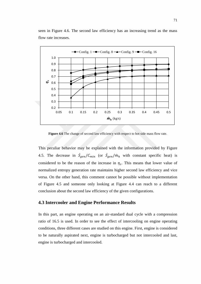
71

seen in Figure 4.6. The second law efficiency has an increasing trend as the mass

flow rate increases.

Figure 4.6 The change of second law efficiency with respect to hot side mass flow rate.

This peculiar behavior may be explained with the information provided by Figure

4.5. The decrease in �̇�𝑔𝑒𝑛/𝐶𝑚𝑖𝑛 (or �̇�𝑔𝑒𝑛/�̇�ℎ with constant specific heat) is

considered to be the reason of the increase in 𝜂𝑠. This means that lower value of

normalized entropy generation rate maintains higher second law efficiency and vice

versa. On the other hand, this comment cannot be possible without implementation

of Figure 4.5 and someone only looking at Figure 4.4 can reach to a different

conclusion about the second law efficiency of the given configurations.

4.3 Intercooler and Engine Performance Results

In this part, an engine operating on an air-standard dual cycle with a compression

ratio of 16.5 is used. In order to see the effect of intercooling on engine operating

conditions, three different cases are studied on this engine. First, engine is considered

to be naturally aspirated next, engine is turbocharged but not intercooled and last,

engine is turbocharged and intercooled.

0.2

0.3

0.4

0.5

0.6

0.7

0.8

0.9

1.0

0.05 0.1 0.15 0.2 0.25 0.3 0.35 0.4 0.45 0.5

ηs

ṁh (kg/s)

Config. 1 Config. 8 Config. 9 Config. 16

72

For the engine, pressure ratio and cut-off ratio is taken as 1.6 and 1.9, respectively.

Also to provide a clear understanding, 𝑃 − 𝜈 diagram of the cycle is given in Figure

4.7. Here the aim is to find the temperatures of each thermodynamic state (state 1 to

5) for aforementioned three cases and compare them with each other. Whenever

necessary, pressure ratio of the turbocharger compressor is taken as 2.5 and

intercooler is considered to provide 60 K temperature drop with 1.5% pressure loss.

Figure 4.7 𝑃 − 𝜈 diagram of an air-standard dual cycle [Modified from 2].

For three cases, temperatures of all states in the cycle and also the density of the

charge air at the inlet to the cylinders are given in Table 4.4.

Table 4.4 Charge air density and temperatures in the cycle for different engine operation types.

Engine

operation type

𝝆𝒊,𝒂𝒊𝒓

kg/m3

𝑻𝟏 K

𝑻𝟐 K

𝑻𝟑 K

𝑻𝟒 K

𝑻𝟓 K

1. Naturally aspirated. 1.184 298.15 915.02 1464.03 2781.65 1171.68

2. Turbocharged and

non-intercooled. 2.279 387.38 1188.85 1902.15 3614.09 1522.32

3. Turbocharged and

intercooled. 2.656 327.38 1004.71 1607.53 3054.31 1286.53

73

As it is seen in the table, when the engine is turbocharged the charge air density

increases more than 1.9 times compared to naturally aspirated one. However in this

case the temperature throughout the entire cycle is also increased. The peak

temperature at the end of the combustion reaches more than 3600 K. This creates

high thermal loadings on the engine during operation and also increases heat transfer

losses. Such a problem can be diminished by cooling the charge air before entry to

the cylinders as in the case of turbocharged and intercooled engines. Also this

cooling further increases the density of charge air. As deduced from table, the

turbocharged and intercooled engine has nearly 16.6% higher inlet air density when

compared with the uncooled one. The peak temperature in the cycle is reduced

substantially. Also enhancement in density of air with intercooling provides better

volumetric efficiency for the engine and raises the mean effective pressure in the

cylinders. These improvements in the engine operating conditions in fact reveal the

importance of the intercooling applications in internal combustion engines.

By the way, increasing density allows burning higher amount of fuel, thus more

power can be produced in the same engine provided that it mechanically withstands

the high pressure and temperature during operation.

At this point it is appropriate to clarify whether utilizing an intercooler in a

turbocharged engine is always feasible or not. This statement can be explained by

establishing Figure 4.8 in which the effect of intercooling on inlet air density is given

for different compressor pressure ratios.

In Figure 4.8 the notation given in Figure 3.1 is used and compression process is

considered to be isentropic. The pressure drop in the intercooler is neglected and

cooling fluid (ambient air) temperature and pressure are taken as 298.15 K and

101.325 kPa, respectively.

74

Figure 4.8 Effect of charge cooling on inlet air density.

As seen in Figure 4.8, no cooling and full cooling lines (휀 = 1) are approaching to

each other as the compressor pressure ratio is decreased. It means that at low

compression ratios the charge air cooling process does not provide significant density

rise, and thus becomes impractical. This is valid especially for compression ratios

less than 1.5. On the other hand, for 2.0 and higher compression ratios charge air

cooling seems to be inevitable and provides high inlet air density.

Finally, if the effect of pressure drop on the charge air cooling process is

investigated, it is understood that loosing high amount of pressure during cooling

deteriorates the advantages of the process. This effect can better clarified by looking

at Figure 4.9 which shows the effect of pressure drop on inlet air density in an

intercooler having 80% effectiveness. As the pressure drop increases the benefit of

charge air cooling diminishes. It becomes significant especially at high compression

ratios and with pressure losses more than 5%.

1.0

1.5

2.0

2.5

3.0

1.0 1.5 2.0 2.5 3.0

Den

sity

ra

tio

(𝜌

3/𝜌

1)

Compressor pressure ratio (P2/P1)

ε=1

ε=0.8

ε=0.7

ε=0.6

No cooling

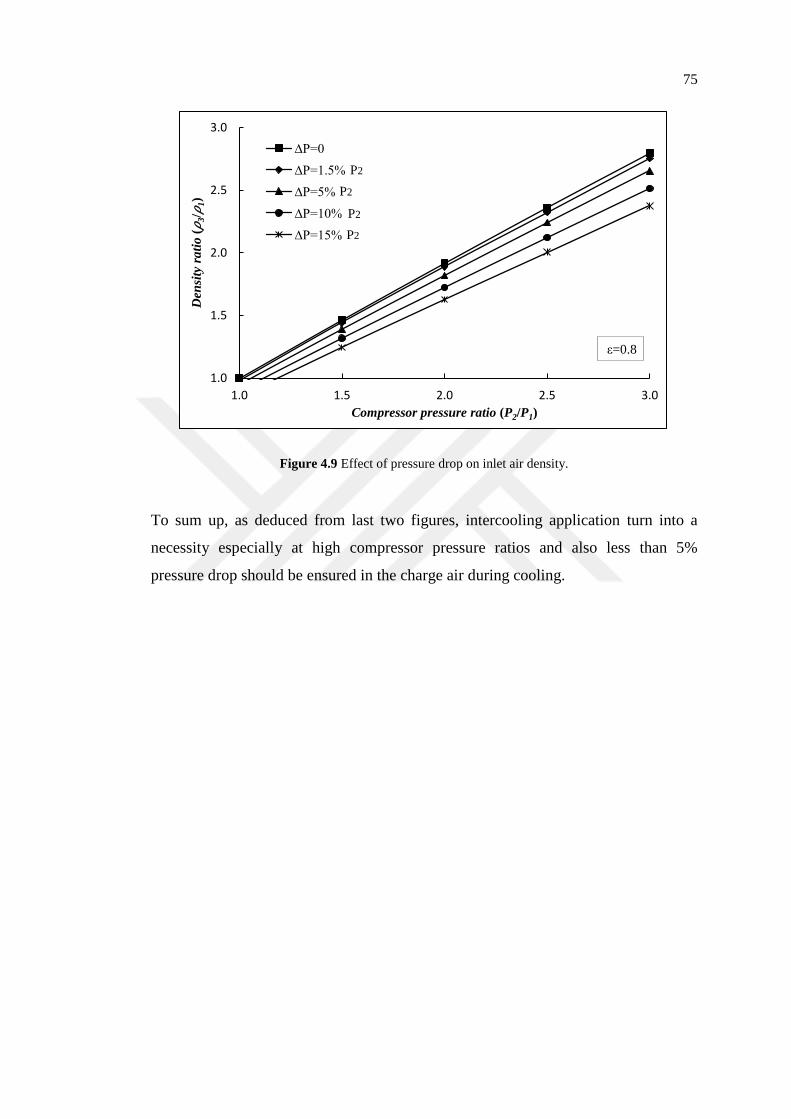
75

Figure 4.9 Effect of pressure drop on inlet air density.

To sum up, as deduced from last two figures, intercooling application turn into a

necessity especially at high compressor pressure ratios and also less than 5%

pressure drop should be ensured in the charge air during cooling.

1.0

1.5

2.0

2.5

3.0

1.0 1.5 2.0 2.5 3.0

Den

sity

ra

tio

(𝜌

3/𝜌

1)

Compressor pressure ratio (P2/P1)

∆P=0

∆P=1.5%

∆P=5%

∆P=10%

∆P=15%

ε=0.8

P2

P2

P2

P2

76

CHAPTER 5

DISCUSSION AND CONCLUSION

In this study, compact plate-fin heat exchangers more specifically intercoolers used

in turbocharged engines are theoretically examined. 20 different intercooler

configurations housing various fin geometries are established. Sizing and rating

procedures are performed on these configurations.

While sizing, operating conditions are taken as the same for all configurations and

resulting dimensions of them are compared with each other. While rating, input

conditions and dimensions are taken as the same and the resulting performance data

is compared with each other in terms of first and second law of thermodynamics.

Moreover, the influence of charge air flow rate (hot side mass flow rate) on the

performance of the configurations is presented. Effect of intercooling on the engine

operating conditions and the feasibility of the intercooling process are discussed.

A computer program is written to handle the iterative solution steps and thus speed

up the calculations. During the analysis, the longitudinal heat conduction effects are

examined and found to be negligible due to low effectiveness of the intercooler

(while sizing) and highly unbalanced flow characteristics of the process.

Longitudinal heat conduction effects are not quite serious in heat exchangers having

effectiveness values less than 0.9 [8] and also there is no available data for

longitudinal heat conduction in the literature for an intercooler application having

such an unbalanced flow. This further supports the claim about the negligible effect

of it for this study. Furthermore, the pressure drops in the fluids are evaluated such

that they only include core pressure drop. The losses in fluid distribution elements

are not considered. It is obvious that the overall pressure drop will be higher in the

process when losses in inlet and outlet headers are included.

Basically 5 different fin types, namely plain (triangular and rectangular) fin, louvered

fin, offset strip fin, wavy fin and perforated fin are proposed for 20 intercooler

configurations.

77

Among these types, offset strip fins provide smaller intercooler volumes than the

others for given input and output conditions but their excessive stack heights make

their placement on the engine compartment impossible. On the other hand, when the

size is preset and thermal-hydraulic performances are investigated, offset strip fins

show very good heat transfer performance but also lead to unacceptable amount of

pressure drops. Therefore, using offset strip fins, especially on both flow sides, for

this particular intercooling application seems to be unreasonable.

Louvered fins do not show as good heat transfer performance as offset strip fins.

However they provide more suitable intercooler dimensions and fewer losses in the

fluid pressures. This makes their usage more plausible when compared to offset strip

fins. Also it should be mentioned that the manufacturing cost of louvered fins are

lower than offset strip fins when produced in very large quantities and they allow

flexibility in fin spacing due to their triangular cross-sections.

Plain fins are straight fins (i.e. uncut in the flow direction) and thus differ from

interrupted fins such as offset strip fins and louvered fins. They generally provide

poorer heat transfer performance but better pressure drop characteristics as seen in

the results. It is convenient to use these fin types where the allowed pressure drop is

low for a fixed frontal area. For an intercooler application mostly their heat transfer

performances are adequate and pressure drops are satisfactorily low. Since being less

expensive, plain surfaces are more preferable than interrupted ones provided that it

can fulfill the given duty. Furthermore, using triangular or rectangular plain fins

depends on the requirements. Triangular plain fins are less expensive, can be

produced at a faster rate and have improved flexibility of adjustable fin density,

however not structurally strong as rectangular ones for the same passage size and fin

thickness.

Being uncut but wavy in the flow direction, wavy fins enable better heat transfer

coefficients however lead to higher friction factors when compared to plain fins. This

situation can be clearly seen from Table 4.2. Both the heat transfer and pressure drop

values are larger for wavy fins. In addition to that, because of having high friction

factor, limiting pressure drop to low values results in high stack heights in the

78

intercooler. Wavy fins may not be preferred for such an intercooler application

because of these performance characteristics.

Perforated fin surfaces have either round or rectangular perforations. The holes

interrupt the flow and may increase heat transfer coefficient. However, considerable

amount of heat transfer surface is lost to form these holes. Their heat transfer

performances are comparable to wavy fins as seen in the results. Amount of pressure

drop is less than wavy fins but again high for an intercooler application.

When it comes to the second law analysis of the surfaces, their second law

performances vary depending on the heat transfer and pressure drop characteristics of

them. Here the important point is that, it is not possible to eliminate entropy

generation or exergy destruction in the intercoolers even with an infinite surface area

and zero pressure drops. The reason is the unbalanced flow and it is unavoidable in

these configurations. High quality fluid (hot fluid) is transformed into a low quality

one during heat transfer, but other fluid (cold fluid) cannot be raised to the same high

quality due to its larger mass flow rate. The best way to minimize entropy generation

and correspondingly exergy destruction is to decrease pressure losses on both flow

sides as much as possible. By doing so, second law efficiency of the process is

increased.

Mass flow rate of hot fluid affects the performance and this effect is also investigated

for some configurations. Low flow rates correspond to the low speed engine

operations and at these speeds intercooler provides better effectiveness and less

pressure drops. Increase in mass flow rate however, leads to reduction in

effectiveness even if the heat transfer rate is increased. Pressure drop performance is

also influenced unfavorably. Next, in terms of second law: nondimensional entropy

generation rate decreases and second law efficiency increases with an increase in

mass flow rate.

Last, the effect of intercooler on an engine performance is examined and the decrease

in engine operating temperatures with the utilization of the intercooler is established.

The importance of intercooling process especially at high compressor pressure ratios

79

(2 or more), are explained with charts. It is also shown that not to diminish benefits

of intercooling, the charge air pressure drop should be maintained below 5%.

Finally, it could be convenient to touch on some important considerations related to

intercooler surface specifications. While selecting the material for the surface,

density and thermal conductivity of it should be taken into consideration. Having low

density and high thermal conductivity maintains less weight and good conduction

characteristics, respectively. Aluminum is one of the best available material types

that can satisfy aforementioned properties and thus mostly preferred in intercooler

applications. Despite having remarkable thermal properties, copper may not be

preferred due to its high density. On the other hand, a potential fouling or clogging

problem due to particulates and moisture can be faced during operation thus; such

cases should also be accounted while selecting the fin type.

80

REFERENCES

[1] Heywood, J. B., “Internal Combustion Engine Fundamentals”, McGraw-Hill,

New York, 1988.

[2] Pulkrabek, W. W., “Engineering Fundamentals of the Internal Combustion

Engines”, Prentice Hall, Upper Saddle River, N. J., 1997.

[3] Çengel, Y. A. & Boles, M. A., “Thermodynamics: An Engineering Approach”,

(5th Ed.), McGraw-Hill, Boston, 2006.

[4] Bilen, K., “Turbo Doldurmalı Bir Dizel Motoru İçin Ara Soğutucu Dizaynı”

M.Sc. Thesis, Kırıkkale University, Graduate School of Natural and Applied

Sciences, Kırıkkale-Turkey, 1998.

[5] Arcoumanis, C., “Internal Combustion Engines”, Academic Press, London,

1988.

[6] Watson, N. & Janota, M. S., “Turbocharging the Internal Combustion Engine”,

Macmillan Press, London, 1982.

[7] Shah, R. K. & Sekulic, D. P., “Fundamentals of Heat Exchanger Design”, John

Wiley and & Sons Inc., New Jersey, 2003.

[8] Kays, W. M. & London, A. L., “Compact Heat Exchangers” (3rd Reprint Ed.),

Krieger Publishing Company, Florida, 1988.

[9] London, A. L. & Shah, R. K., “Offset Rectangular Plate-fin Surfaces-Heat

Transfer and Flow Friction Characteristics” ASME J. Eng. Power, 90(3), 218-

228, 1968.

[10] Ismail, L. S. & Ranganayakulu, C. & Shah, R. K., “Numerical Study of Flow

Patterns of Compact Plate-fin Heat Exchangers and Generation of Design Data

for Offset and Wavy Fins” Int. J. Heat and Mass Transfer, 52(17-18), 3972-

3983, 2009.

81

[11] Manglik, R. M. & Bergles, A. E., “Heat Transfer and Pressure Drop

Correlations for the Rectangular Offset Strip Fin Compact Heat Exchanger”

Experimental Thermal and Fluid Science, 10(2), 171-180, 1995.

[12] Kim, M. S. & Lee, J. & Yook, S. J. & Lee, K. S., “Correlations and

Optimization of a Heat Exchanger with Offset Strip Fins” Int. J. Heat and Mass

Transfer, 54(9-10), 2073-2079, 2011.

[13] Yang, Y. & Li, Y., “General Prediction of the Thermal Hydraulic Performance

for Plate-fin Heat Exchanger with Offset Strip Fins” Int. J. Heat and Mass

Transfer, 78, 860-870, 2014.

[14] Cowell, T. A. & Heikal, M. R. & Achaichia, A., “Flow and Heat Transfer in

Compact Louvered Fin Surfaces” Experimental Thermal and Fluid Science,

10(2), 192-199, 1995.

[15] Ryu, K. & Lee, K. S., “Generalized Heat-Transfer and Fluid-Flow Correlations

for Corrugated Louvered Fins” Int. J. Heat and Mass Transfer, 83, 604-612,

2015.

[16] Li, W. & Wang, X., “Heat Transfer and Pressure Drop Correlations for

Compact Heat Exchangers with Multi-Region Louver Fins” Int. J. Heat and

Mass Transfer, 53(15-16), 2955-2962, 2010.

[17] Vaisi, A. & Esmaeilpour, M. & Taherian, H., “Experimental Investigation of

Geometry Effects on the Performance of A Compact Louvered Heat

Exchanger” Applied Thermal Engineering, 31(16), 3337-3346, 2011.

[18] Ranganayakulu, C. & Seetharamu, K. N. & Sreevatsan, K. V., “The Effect of

Longitudinal Heat Conduction in Compact Plate-fin and Tube-fin Heat

Exchangers Using a Finite Element Method” Int. J. Heat and Mass Transfer,

40(6), 1261-1277, 1997.

82

[19] Ranganayakulu, C. & Seetharamu, K. N., “The Combined Effects of Wall

Longitudinal Heat Conduction, Inlet Fluid Flow Nonuniformity and

Temperature Nonuniformity in Compact Tube-fin Heat Exchangers: a Finite

Element Method” Int. J. Heat and Mass Transfer, 42(2), 263-273, 1999.

[20] Shah, R. K. & Skiepko, T., “Entropy Generation Extrema and Their

Relationship with Heat Exchanger Effectiveness-Number of Transfer Unit

Behavior for Complex Flow Arrangements” ASME J. Heat Transfer, 126(6),

994-1002, 2005.

[21] Gheorghian, A. T. & Dobrovicescu, A. & Popescu, L. G. & Cruceru, M. &

Diaconu, B. M., “Entropy Generation Assessment Criterion for Compact Heat

Transfer Surfaces” Applied Thermal Engineering, 87, 137-149, 2015.

[22] Canlı, E. & Darıcı, S. & Doğan, S. & Özgören, M., “Kompakt Isı

Değiştiricilerinde Kararlı Çalışma Halindeki Ekserji Yıkımının Deneysel

Olarak Tespiti ve Aynı Isıl Kapasite Oranı için Üç Farklı Isi Değiştiricisinin

Ekserji Yıkımlarının Karşılaştırılması” 11. Ulusal Tesisat Mühendisliği

Kongresi, 17-20 Nisan 2013, MMO Tepekule Kongre ve Sergi Merkezi-İzmir:

TMMOB Makina Mühendisleri Odası, 1149-1175, 2013.

[23] Çengel, Y. A. & Ghajar, A. J., “Heat and Mass Transfer: Fundamentals and

Applications” (4th Ed.), McGraw-Hill, New York, 2011, p. 652.

[24] Incropera, F. P. & Dewitt, D. P. & Bergman, T. L. & Lavine, A. S.,

“Fundamentals of Heat and Mass Transfer” (6th Ed.), John Wiley & Sons Inc.,

New Jersey, 2007.

[25] Mills, A. F., “Heat Transfer” (2nd Ed.), Prentice Hall, Upper Saddle River, N.

J., 1999.

[26] Bejan, A., “Entropy Generation Minimization”, CRC Press LLC, Florida,

1995, p. 23.

83

[27] Bejan, A., “The Concept of Irreversibility in Heat Exchanger Design:

Counterflow Heat Exchangers for Gas-to-Gas Applications” ASME J. Heat

Transfer, 99(3), 374-380, 1977.

[28] Bejan, A., “Advanced Engineering Thermodynamics”, John Wiley and & Sons

Inc., New Jersey, 2006, p. 589.

[29] Hesselgreaves, J. E., “Rationalisation of Second Law Analysis of Heat

Exchangers” Int. J. Heat and Mass Transfer, 43(22), 4189-4204, 2000.

[30] Zimparov V. & Vulchanov, N. L., “Performance Evaluation Criteria for

Enhanced Heat Transfer Surfaces” Int. J. Heat and Mass Transfer, 37(12)

1807-1816, 1994.

[31] Prasad, R. C. & Shen, J., “Performance Evaluation of Convective Heat

Transfer Enhancement Devices Using Exergy Analysis” Int. J. Heat and Mass

Transfer, 36(17), 4193-4197, 1993.

[32] Bruges, E. A., “Available Energy and the Second Law Analysis”, Academic

Press Inc., London, 1959.

[33] Yılmaz, M. & Sara, O. N. & Karslı, S., “Performance Evaluation Criteria for

Heat Exchangers Based on Second Law Analysis” Exergy Int. J., 1(4), 278-

294, 2001.

84

APPENDICES

Appendix A: Surface Characteristics of Fins.

Appendix B: 𝑗 and 𝑓 Factor Equations and Reynolds Number Ranges.

Appendix C: Thermophysical Properties of Air.

Appendix D: 𝐾𝑐 and 𝐾𝑒 Coefficients.

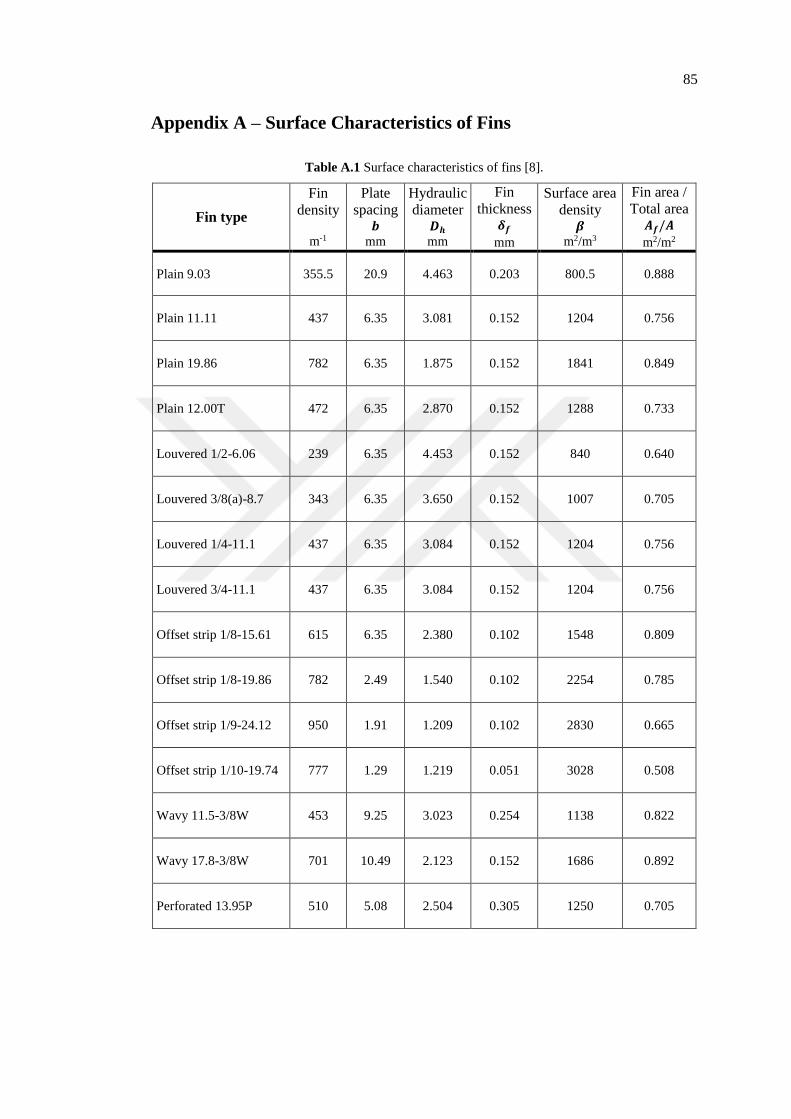
85

Appendix A – Surface Characteristics of Fins

Table A.1 Surface characteristics of fins [8].

Fin type

Fin

density

m-1

Plate

spacing 𝒃

mm

Hydraulic

diameter 𝑫𝒉

mm

Fin

thickness 𝜹𝒇

mm

Surface area

density 𝜷

m2/m3

Fin area /

Total area 𝑨𝒇/𝑨

m2/m2

Plain 9.03 355.5 20.9 4.463 0.203 800.5 0.888

Plain 11.11 437 6.35 3.081 0.152 1204 0.756

Plain 19.86 782 6.35 1.875 0.152 1841 0.849

Plain 12.00T 472 6.35 2.870 0.152 1288 0.733

Louvered 1/2-6.06 239 6.35 4.453 0.152 840 0.640

Louvered 3/8(a)-8.7 343 6.35 3.650 0.152 1007 0.705

Louvered 1/4-11.1 437 6.35 3.084 0.152 1204 0.756

Louvered 3/4-11.1 437 6.35 3.084 0.152 1204 0.756

Offset strip 1/8-15.61 615 6.35 2.380 0.102 1548 0.809

Offset strip 1/8-19.86 782 2.49 1.540 0.102 2254 0.785

Offset strip 1/9-24.12 950 1.91 1.209 0.102 2830 0.665

Offset strip 1/10-19.74 777 1.29 1.219 0.051 3028 0.508

Wavy 11.5-3/8W 453 9.25 3.023 0.254 1138 0.822

Wavy 17.8-3/8W 701 10.49 2.123 0.152 1686 0.892

Perforated 13.95P 510 5.08 2.504 0.305 1250 0.705

86

Appendix B – 𝒋 and 𝒇 Factor Equations and Reynolds Number

Ranges

Table B.1 𝑗 factor equations for fin types.

Fin type

Equation type

𝑗1 = 𝑎𝑗 +𝑏𝑗

ln 𝑅𝑒+

𝑐𝑗

(ln 𝑅𝑒)2+

𝑑𝑗

(ln 𝑅𝑒)3

𝑗2 =𝑎𝑗 +

𝑐𝑗

ln 𝑅𝑒+

𝑒𝑗

(ln 𝑅𝑒)2 +𝑔𝑗

(ln 𝑅𝑒)3

1 +𝑏𝑗

ln 𝑅𝑒+

𝑑𝑗

(ln 𝑅𝑒)2 +𝑓𝑗

(ln 𝑅𝑒)3

𝑎𝑗 𝑏𝑗 𝑐𝑗 𝑑𝑗 𝑒𝑗 𝑓𝑗 𝑔𝑗

Plain 9.03

𝑗2 -76·10-5 -0.4364 77·10-6 0.06265 18·10-6 -0.00297 2·10-6

Plain 11.11

𝑗2 -34·10-4 -0.4894 97·10-5 0.07797 -75·10-6 -0.0041 69·10-8

Plain 19.86

𝑗2 -33·10-4 -0.4955 93·10-5 0.08017 -67·10-6 -0.0043 11·10-8

Plain 12.00T

𝑗2 -0.0149 -0.5373 0.00505 0.08904 -0.00056 -0.00476 2·10-5

Louvered 1/2-6.06

𝑗2 -0.0117 -0.5071 0.00332 0.07946 -0.00029 -0.00399 66·10-7

Louvered 3/8(a)-8.7

𝑗1 -0.0494 1.0440 -6.9121 18.199 - - -

Louvered 1/4-11.1

𝑗2 -0.0268 -0.6097 0.00927 0.11338 -0.0010 -0.00668 33·10-6

Louvered 3/4-11.1

𝑗2 -0.0077 -0.4720 0.00219 0.07045 -0.00019 -0.0034 48·10-7

Offset strip 1/8-15.61

𝑗1 -0.0192 0.56408 -5.2580 20.6722 - - -

Offset strip 1/8-19.86

𝑗1 -0.0505 1.13017 -8.2922 24.2204 - - -

Offset strip 1/9-24.12

𝑗1 -0.1099 2.49627 -18.266 47.1236 - - -

Offset strip 1/10-19.74

𝑗1 0.02304 -0.2802 0.77926 3.82960 - - -

Wavy 11.5-3/8W

𝑗1 0.04332 -1.2929 12.3976 -33.041 - - -

Wavy 17.8-3/8W

𝑗1 -33·10-5 -0.1300 2.00937 -3.3043 - - -

Perforated 13.95P

𝑗2 -0.0051 -0.4705 0.00134 0.07123 94·10-6 -0.0035 70·10-8

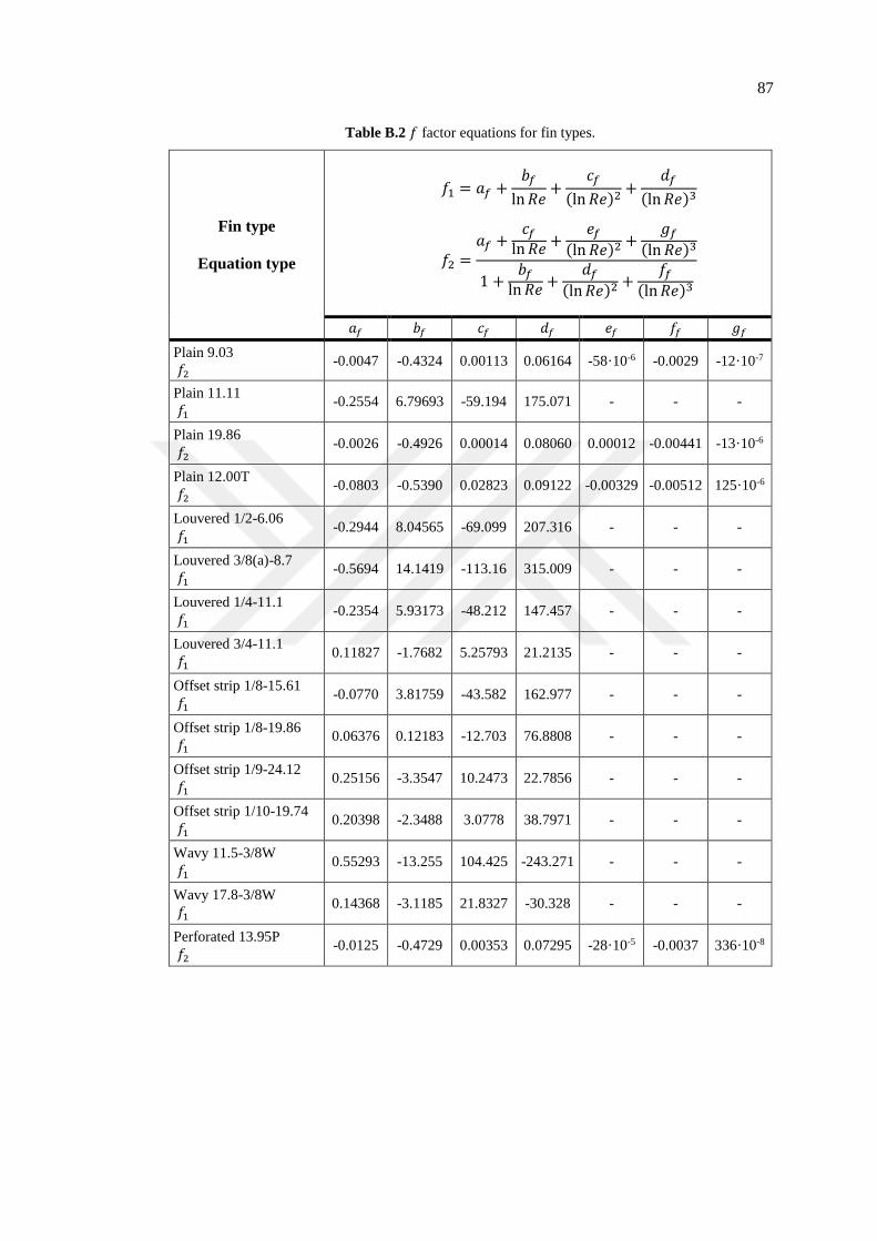
87

Table B.2 𝑓 factor equations for fin types.

Fin type

Equation type

𝑓1 = 𝑎𝑓 +𝑏𝑓

ln 𝑅𝑒+

𝑐𝑓

(ln 𝑅𝑒)2+

𝑑𝑓

(ln 𝑅𝑒)3

𝑓2 =𝑎𝑓 +

𝑐𝑓

ln 𝑅𝑒+

𝑒𝑓

(ln 𝑅𝑒)2 +𝑔𝑓

(ln 𝑅𝑒)3

1 +𝑏𝑓

ln 𝑅𝑒+

𝑑𝑓

(ln 𝑅𝑒)2 +𝑓𝑓

(ln 𝑅𝑒)3

𝑎𝑓 𝑏𝑓 𝑐𝑓 𝑑𝑓 𝑒𝑓 𝑓𝑓 𝑔𝑓

Plain 9.03

𝑓2 -0.0047 -0.4324 0.00113 0.06164 -58·10-6 -0.0029 -12·10-7

Plain 11.11

𝑓1 -0.2554 6.79693 -59.194 175.071 - - -

Plain 19.86

𝑓2 -0.0026 -0.4926 0.00014 0.08060 0.00012 -0.00441 -13·10-6

Plain 12.00T

𝑓2 -0.0803 -0.5390 0.02823 0.09122 -0.00329 -0.00512 125·10-6

Louvered 1/2-6.06

𝑓1 -0.2944 8.04565 -69.099 207.316 - - -

Louvered 3/8(a)-8.7

𝑓1 -0.5694 14.1419 -113.16 315.009 - - -

Louvered 1/4-11.1

𝑓1 -0.2354 5.93173 -48.212 147.457 - - -

Louvered 3/4-11.1

𝑓1 0.11827 -1.7682 5.25793 21.2135 - - -

Offset strip 1/8-15.61

𝑓1 -0.0770 3.81759 -43.582 162.977 - - -

Offset strip 1/8-19.86

𝑓1 0.06376 0.12183 -12.703 76.8808 - - -

Offset strip 1/9-24.12

𝑓1 0.25156 -3.3547 10.2473 22.7856 - - -

Offset strip 1/10-19.74

𝑓1 0.20398 -2.3488 3.0778 38.7971 - - -

Wavy 11.5-3/8W

𝑓1 0.55293 -13.255 104.425 -243.271 - - -

Wavy 17.8-3/8W

𝑓1 0.14368 -3.1185 21.8327 -30.328 - - -

Perforated 13.95P

𝑓2 -0.0125 -0.4729 0.00353 0.07295 -28·10-5 -0.0037 336·10-8

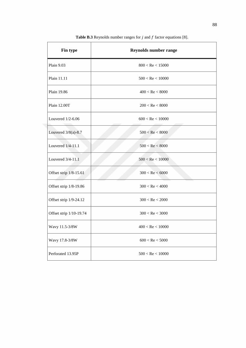
88

Table B.3 Reynolds number ranges for 𝑗 and 𝑓 factor equations [8].

Fin type Reynolds number range

Plain 9.03 800 < Re < 15000

Plain 11.11 500 < Re < 10000

Plain 19.86 400 < Re < 8000

Plain 12.00T 200 < Re < 8000

Louvered 1/2-6.06 600 < Re < 10000

Louvered 3/8(a)-8.7 500 < Re < 8000

Louvered 1/4-11.1 500 < Re < 8000

Louvered 3/4-11.1 500 < Re < 10000

Offset strip 1/8-15.61 300 < Re < 6000

Offset strip 1/8-19.86 300 < Re < 4000

Offset strip 1/9-24.12 300 < Re < 2000

Offset strip 1/10-19.74 300 < Re < 3000

Wavy 11.5-3/8W 400 < Re < 10000

Wavy 17.8-3/8W 600 < Re < 5000

Perforated 13.95P 500 < Re < 10000

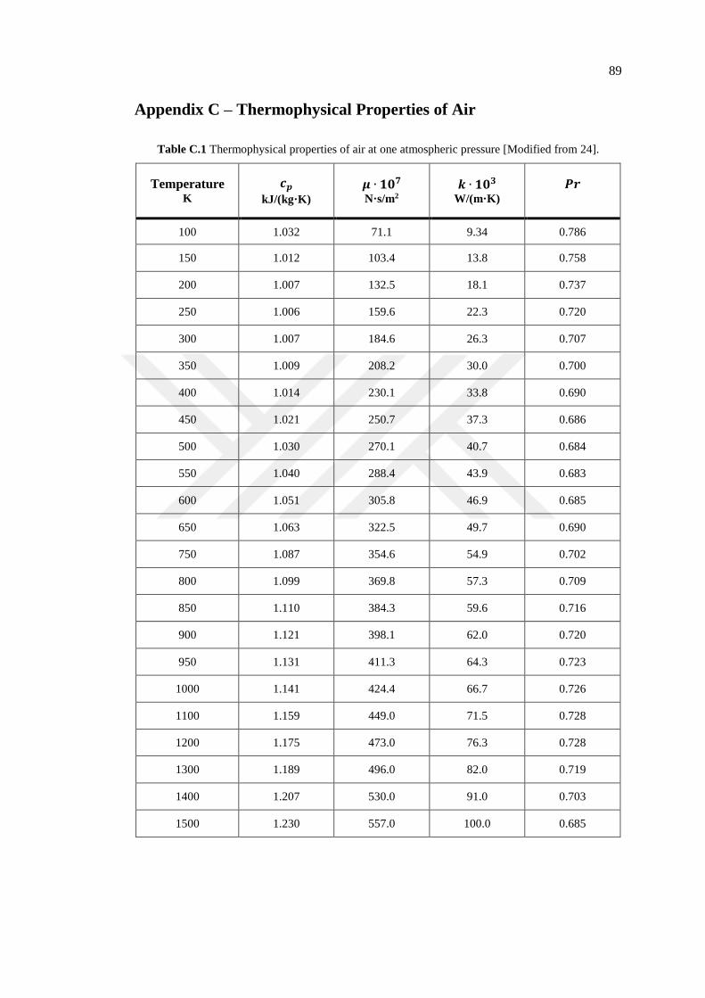
89

Appendix C – Thermophysical Properties of Air

Table C.1 Thermophysical properties of air at one atmospheric pressure [Modified from 24].

Temperature K

𝒄𝒑

kJ/(kg·K)

𝝁 ∙ 𝟏𝟎𝟕 N·s/m2

𝒌 ∙ 𝟏𝟎𝟑 W/(m·K)

𝑷𝒓

100 1.032 71.1 9.34 0.786

150 1.012 103.4 13.8 0.758

200 1.007 132.5 18.1 0.737

250 1.006 159.6 22.3 0.720

300 1.007 184.6 26.3 0.707

350 1.009 208.2 30.0 0.700

400 1.014 230.1 33.8 0.690

450 1.021 250.7 37.3 0.686

500 1.030 270.1 40.7 0.684

550 1.040 288.4 43.9 0.683

600 1.051 305.8 46.9 0.685

650 1.063 322.5 49.7 0.690

750 1.087 354.6 54.9 0.702

800 1.099 369.8 57.3 0.709

850 1.110 384.3 59.6 0.716

900 1.121 398.1 62.0 0.720

950 1.131 411.3 64.3 0.723

1000 1.141 424.4 66.7 0.726

1100 1.159 449.0 71.5 0.728

1200 1.175 473.0 76.3 0.728

1300 1.189 496.0 82.0 0.719

1400 1.207 530.0 91.0 0.703

1500 1.230 557.0 100.0 0.685

90

Appendix D – 𝑲𝒄 and 𝑲𝒆 Coefficients

Figure D.1 Entrance and exit pressure loss coefficients for (a) a multiple circular

tube core, (b) multiple-tube flat-tube core, (c) multiple square tube core, and (d)

multiple triangular tube core with abrupt contraction (entrance) and abrupt

expansion (exit) [7].

91

CURRICULUM VITAE

PERSONAL INFORMATION

Name Surname : Ahmet Yasin SEDEF

Date of Birth : 1989

Phone : +90 506 5717438

E-mail : aysedef@ybu.edu.tr

EDUCATION

High School : Ümitkoy Anatolian High School / ANKARA (2003-2007)

(82.75/100)

Bachelor : University of Gaziantep / GAZİANTEP (2008-2013)

(3.61/4.0)

Master Degree : Ankara Yıldırım Beyazıt University / (2014-continued)

WORK EXPERIENCE

Research Assist. : Ankara Yıldırım Beyazıt University / (2014-continued)

TOPICS OF INTEREST

- Thermodynamics - Fluid Mechanics

- Heat Transfer - Internal Combustion Engines