i

STRATEGIC MARINE ECOSYSTEM RESTORATION IN NORTHERN BRITISH COLUMBIA

by

CAMERON H. AINSWORTH

B. Sc., The University of British Columbia, 1997

A THESIS SUBMITTED IN PARTIAL FULFILLMENT OF

THE REQUIREMENTS FOR THE DEGREE OF

DOCTOR OF PHILOSOPHY

in

THE FACULTY OF GRADUATE STUDIES

(Resource Management and Environmental Studies)

THE UNIVERSITY OF BRITISH COLUMBIA

May 2006

© Cameron H. Ainsworth, 2006

ii

ABSTRACT

Innovative methodology is developed for Back to the Future (BTF) restoration policy analysis to

aid long-term strategic planning of ecosystem-based restoration in marine ecosystems. Mass-

balance and dynamic ecosystem simulation models (Ecopath with Ecosim: EwE) are developed

to represent the marine system of northern British Columbia as it appeared in 1750, 1900, 1950

and 2000 AD. Time series statistics are assembled for biomass and catch, incorporating local

ecological knowledge (LEK) from community interviews and new estimates of illegal,

unreported and unregulated (IUU) fishery catch. The dynamic behaviour of the historic models

is fitted to agree with this time series information, when driven by historic catch rates and

climate anomalies. Each historic period is evaluated in an optimal policy analysis for its

potential to supply sustainable harvest benefits. Harvest benefits are quantified using

socioeconomic and ecological indicators, including novel measures such as the Q-90 biodiversity

statistic. Candidate goals for restoration are drafted based on these historic ecosystems. A new

conceptual goal for ecosystem-based restoration is introduced, the optimal restorable biomass

(ORB) that represents an optimized form of the historic ecosystems. It is structured to maximize

sustainable harvest benefits, and to achieve a compromise between exploitation and the

maintenance of historic abundance and biodiversity. Finally, restoration plans are drafted using

a novel addition to Ecosim’s policy search routine, the specific biomass objective function,

which determines the pattern of fishing effort required to restore the depleted present-day

ecosystem into one resembling a more productive ORB state. Cost-benefit analysis indicates that

northern BC ecosystem restoration to an ORB state based on the 1950 ecosystem can deliver a

rate of economic return, in terms of increased fisheries yields, that is superior to bank interest.

The effect of fleet structure is paramount; reducing bycatch will greatly enhance the

effectiveness of the fleet as a restoration tool. Restoration plans that sacrifice immediate

fisheries profits tend to restore more biodiversity in a given amount of time, but a convex

relationship between profit and biodiversity suggests there is an optimal rate of restoration.

iii

TABLE OF CONTENTS

Abstract ....................................................................................................................................................................... ii Table of Contents....................................................................................................................................................... iii List of Tables................................................................................................................................................................v List of Figures ........................................................................................................................................................... vii List of Equations..........................................................................................................................................................x Acknowledgements .....................................................................................................................................................xi 1 Back to the Future ...................................................................................................................................................1

1.1 Introduction.........................................................................................................................................................1 1.2 Ecopath with Ecosim ..........................................................................................................................................7 1.3 Northern British Columbia ...............................................................................................................................10 1.4 Structure of thesis .............................................................................................................................................14

2 Harvest Policy Evaluation Techniques ................................................................................................................19 2.1 Introduction.......................................................................................................................................................19 2.2 Economic index: Net present value (NPV).......................................................................................................19 2.3 Social utility index: Employment diversity ......................................................................................................22 2.4 Ecological indices .............................................................................................................................................23 2.5 Q-90 case study: NE Pacific ecosystems ..........................................................................................................26

3 Community Interviews..........................................................................................................................................35 3.1 Introduction.......................................................................................................................................................35 3.2 Methods ............................................................................................................................................................36 3.3 Results ..............................................................................................................................................................42 3.4 Discussion.........................................................................................................................................................55

4 Estimating Illegal, Unreported and Unregulated Catch ....................................................................................59 4.1 Introduction.......................................................................................................................................................59 4.2 Methods ............................................................................................................................................................61 4.3 Results ..............................................................................................................................................................71 4.4 Discussion.........................................................................................................................................................76

5 Modeling the Past and Present .............................................................................................................................82 5.1 Introduction.......................................................................................................................................................82 5.2 Fisheries..........................................................................................................................................................121 5.3 Ecosim parameterization.................................................................................................................................122 5.4 Assembling time series data............................................................................................................................132 5.5 Analysis of fitted vulnerabilities .....................................................................................................................134 5.6 Validation of dynamic function ......................................................................................................................138 5.7 Discussion.......................................................................................................................................................142

iv

6 Evaluating Restoration Goals .............................................................................................................................146 6.1 Introduction.....................................................................................................................................................146 6.2 Methods ..........................................................................................................................................................154 6.3 Results ............................................................................................................................................................165 6.4 Discussion.......................................................................................................................................................188

7 Achieving Restoration .........................................................................................................................................197 7.1 Introduction.....................................................................................................................................................197 7.2 Methods ..........................................................................................................................................................199 7.3 Results ............................................................................................................................................................215 7.4 Discussion.......................................................................................................................................................244

8 Conclusions ..........................................................................................................................................................250 8.1 Summary.........................................................................................................................................................250 8.2 An ecosystem approach to management.........................................................................................................251 8.3 The developing role of ecosystem models ......................................................................................................264 8.4 Policy recommendations.................................................................................................................................265 8.5 Concluding remarks........................................................................................................................................266

References ................................................................................................................................................................268 Appendices ...............................................................................................................................................................298

Appendix 2.1 The Effect of Discounting on Fisheries..........................................................................................298 Appendix 2.2 Cost-benefit Analysis of Education...............................................................................................310 Appendix 3.1 LEK Trends of Relative Abundance .............................................................................................313 Appendix 4.1 BC Fisheries Timeline...................................................................................................................314 Appendix 4.2 IUU Influences Table ....................................................................................................................322 Appendix 4.3 BC Reported Landings ..................................................................................................................330 Appendix 4.4 Average Species Weight ...............................................................................................................331 Appendix 5.1 Ecopath Parameters.......................................................................................................................332 Appendix 5.2 Ecosim Parameters ........................................................................................................................346 Appendix 5.3 Time Series ...................................................................................................................................351 Appendix 5.4 Dynamic Fit to Data: 1950-2000...................................................................................................357 Appendix 5.5 Equilibrium Analysis of 2000 Model............................................................................................361 Appendix 5.6 Comparison of Derived 2000 Model with Proper 2000 Model.....................................................363 Appendix 6.1 Policy Search Parameters ..............................................................................................................365 Appendix 6.2 Evaluation of ORB Ecosystems ....................................................................................................367 Appendix 7.1 Input for Restoration Scenarios.....................................................................................................372 Appendix 7.2 Candidate Restoration Trajectories ...............................................................................................373 Appendix 8.1 Gwaii Haanas Spatial Investigations.............................................................................................376 Appendix 8.2 Ecospace Parameters .....................................................................................................................402 Appendix 9.1 References cited in the Appendices...............................................................................................407

v

LIST OF TABLES

Table 1.1 Published materials appearing in this thesis. ..............................................................................................18 Table 2.1 Eight EwE models of the NE Pacific. .........................................................................................................28 Table 3.1 Percentage of interviewee comments that agree with stock assessment records. .......................................43 Table 3.2 Biomass estimates (t·km-2) used in Ecopath models compared to LEK trend. ...........................................50 Table 3.3 Place names mentioned during interviews..................................................................................................53 Table 4.1 Incentive ratings. ........................................................................................................................................67 Table 4.2 Anchor point range. ....................................................................................................................................67 Table 4.3 Mean reported catch. ..................................................................................................................................67 Table 4.4 Absolute ranges of IUU catch rate for each incentive rating. .....................................................................72 Table 4.5 Monte Carlo input: IUU catch range. .........................................................................................................74 Table 4.6 Monte Carlo output: Mean IUU catch with 95% confidence intervals.......................................................74 Table 5.1 Data sources for NE Pacific environmental indices..................................................................................128 Table 6.1 List of nine criteria for sustainable and responsible ‘lost valley’ fisheries. ..............................................153 Table 6.2 Lost valley fleet catch. ..............................................................................................................................156 Table 6.3 Lost valley fleet discards...........................................................................................................................157 Table 6.4 Rank order of ORB ecosystem performance in various evaluation fields. ...............................................177 Table 6.5 Fishing rates of ORB solutions, analysis of response surface geometry and ecosystem stability. ...........184 Table 7.1 Available settings for the specific biomass rebuilding objective function. ...............................................203 Table 8.1 Criticisms of MSY and their applicability to the ORB concept................................................................255 Table A2.1.1 CBA of education. ..............................................................................................................................312 Table A4.1.1 BC fisheries timeline ..........................................................................................................................314 Table A4.2.1 IUU influences table ...........................................................................................................................322 Table A4.3.1 BC reported landings ...........................................................................................................................330 Table A4.4.1 Average species weight ......................................................................................................................331 Table A5.1.1 Species aggregation by functional group. ...........................................................................................332 Table A5.1.2 Basic parameters for all periods..........................................................................................................336 Table A5.1.3 Diet composition.................................................................................................................................338 Table A5.1.4 Landings data for all time periods (t·km-2)..........................................................................................342 Table A5.1.5 Discard data for 1950 and 2000 (t·km-2) .............................................................................................344 Table A5.1.6 Market prices ($·kg-1) for 2000 BC fleet.............................................................................................345 Table A5.2.1 Juvenile/adult stage transition parameters for all models ...................................................................346 Table A5.2.2 Feeding parameters for 1950 ..............................................................................................................347 Table A5.2.3 Trophic flow parameters for 1950 ......................................................................................................348 Table A5.3.1 Biomass time series data (t·km-2): 1900-1950.....................................................................................351 Table A5.3.2 Biomass time series data (t·km-2): 1950-2000.....................................................................................352

vi

Table A5.3.3 Catch time series data (t·km-2): 1900-1950.........................................................................................353 Table A5.3.4 Catch time series data (t·km-2): 1950-2000.........................................................................................354 Table A5.3.5 Fishing mortality time series data (yr-1): 1900-1950...........................................................................355 Table A5.3.6 Fishing mortality time series data (yr-1): 1950-2000...........................................................................356 Table A5.6.1 Comparison of derived 2000 model with proper 2000 model ............................................................363 Table A6.1.1 Market prices ($·kg-1) for lost valley fleet...........................................................................................365 Table A6.1.2 Biomass/production (B/P) ratios by functional group. .......................................................................366 Table A6.2.1 Functional group biomass (t·km2) for selected ORB ecosystems. ......................................................369 Table A6.2.2 Fisheries landings by gear type (t·km2) for selected ORB ecosystems. ..............................................371 Table A7.1.1 Catch profile for maxdex fleet.............................................................................................................372 Table A8.1.1 Ecospace habitat definitions. ..............................................................................................................383 Table A8.1.2 Group behaviour guidelines used to standardize Ecospace functional groups....................................390 Table A8.2.1 Habitat occupancy ..............................................................................................................................402 Table A8.2.2 Fishery activity by habitat...................................................................................................................403 Table A8.2.3 Salmon straying rates..........................................................................................................................403 Table A8.2.4 Dispersal parameters...........................................................................................................................404 Table A8.2.5 Ecospace output region definitions .....................................................................................................405 Table A9.2.1 IG discounting case study references cited in Appendix 2.1. .............................................................407 Table A9.2.2 Cost-benefit analysis of education references cited in Appendix 2.2. ................................................408 Table A9.4.1 BC fisheries timeline references cited in Appendix 4.1......................................................................409 Table A9.4.2 Average species weight references cited in Appendix 4.4..................................................................414 Table A9.4.3 Illegal catch anchor point references cited in Appendix 4.2 ...............................................................415 Table A9.4.4 Discard anchor point references cited in Appendix 4.2 ......................................................................416 Table A9.4.5 Unreported catch anchor point references cited in Appendix 4.2 .......................................................417 Table A9.5.3 Biomass, catch and effort time series data references cited in Appendix 5.3. ....................................418 Table A9.8.1 Spatial investigations for Gwaii Haanas references cited in Appendix 8.1. .......................................421

vii

LIST OF FIGURES

Figure 1.1 Biodiversity and species abundance decline caused by fisheries. ...............................................................2 Figure 1.2 The Back to the Future approach to marine ecosystem restoration. ............................................................4 Figure 1.3 Northern BC study area.............................................................................................................................12 Figure 2.1 Q-90 statistic definition. ............................................................................................................................25 Figure 2.2 Dynamic ecosystem biodiversity (Q-90) of three example Ecopath with Ecosim simulations. ................29 Figure 2.3 Absolute Q-90 value at baseline (year zero) for eight northeastern Pacific Ecopath models. ...................30 Figure 2.4 Change in Q-90 index after 30 years of fishing for eight EwE models of the NE Pacific. .......................30 Figure 2.5 Q-90 sensitivity to changes in system biomass structure. .........................................................................31 Figure 2.6 Q-90 sensitivity to changes in ecosystem structure using three depletion filter thresholds.......................32 Figure 3.1 Fraction of comments that agree with DFO records by functional group. ................................................44 Figure 3.2 Interviewee agreement with stock assessment data by career length. .......................................................45 Figure 3.3 LEK abundance trend versus stock assessment.........................................................................................48 Figure 3.4 Rank correlation of LEK abundance trend versus stock assessment. ........................................................49 Figure 3.5 Correlation of LEK relative abundance trend and stock assessment with model ouputs. .........................52 Figure 3.6 A map of the study area showing the number of LEK comments indicating species presence.................54 Figure 4.1 A time series of numerical influence factors assigned semi-quantitative ‘incentive’ ratings. ...................64 Figure 4.2 Salmon recreational catch estimates..........................................................................................................66 Figure 4.3 Cumulative probability distribution of missing catch. ..............................................................................70 Figure 4.4 Likely range of groundfish discards ..........................................................................................................70 Figure 4.5 Estimates of missing catch for salmon and groundfish fisheries. ..............................................................75 Figure 4.6 Total estimated extractions in BC salmon and groundfish fisheries..........................................................76 Figure 5.1 EwE’s predicted climate anomalies versus their strongest correlating environmental indices................128 Figure 5.2 Correlation of primary production and herring recruitment anomalies with environmental indices. ......129 Figure 5.3 Predicted and observed herring trend (1950-2000) under three conditions of climate forcing. ..............130 Figure 5.4 Predicted and observed variance of group biomass trajectories (1950-2000). ........................................131 Figure 5.5 Rank order of vulnerabilities in the fitted 1950 model versus predator and prey trophic level...............135 Figure 5.6 Log vulnerabilities in fitted 1950 model versus predator and prey trophic level. ...................................135 Figure 5.7 Evaluation of short-cut methods used to parameterize Ecosim vulnerabilities. ......................................137 Figure 5.8 Group biomass predicted in 2050 by derived and proper 2000 models after fishing release. .................140 Figure 5.9 Biomass change predicted by the derived and proper 2000 models after fishing release........................141 Figure 5.10 Direction of biomass change predicted by proper and derived 2000 models after fishing release. .......142 Figure 6.1 Optimal Restorable Biomass (ORB) concept.. ........................................................................................148 Figure 6.2 Cluster analysis of group biomass configurations for two example ORB ecosystems............................166 Figure 6.3 Value equilibriums for ORB ecosystems based on various historical periods. .......................................167 Figure 6.4 ORB equilibrium catch value per gear type. ...........................................................................................170

viii

Figure 6.5 ORB equilibrium value by group under various harvest objectives. .......................................................171 Figure 6.6 Social utility provided by ORB ecosystems based on various historical periods. ...................................173 Figure 6.7 Biodiversity of ORB ecosystems based on various historical periods. ...................................................175 Figure 6.8 Biodiversity of historic ecosystems under optimal fishing policies using lost valley fleet structure.......176 Figure 6.9 Profit and biodiversity of ORB equilibriums based on 1750, 1900, 1950 and 2000 periods. .................179 Figure 6.10 Social utility provided by ORB ecosystems based on 1750, 1900, 1950 and 2000 periods..................181 Figure 6.11 Response surface geometries.................................................................................................................183 Figure 6.12 Biomass depletion risk of ORB solutions, considering Ecopath parameter uncertainty. ......................186 Figure 6.13 The effects of data uncertainty on ORB equilibrium values determined by Monte Carlo. ...................187 Figure 7.1 Controls added to Ecosim’s policy search interface for SB algorithm. ...................................................203 Figure 7.2 Three models describing marginal improvement in SB function as group biomass approaches goal. ....206 Figure 7.3 Constrained marginal improvement model (MIM). ................................................................................208 Figure 7.4 Dynamic progress display form to monitor rebuilding success of the SB algorithm. .............................211 Figure 7.5 Conceptual diagram showing cost-benefit analysis.................................................................................214 Figure 7.6 Performance of SB algorithm towards achieving historic 1950 ecosystem structure..............................217 Figure 7.7 Commercial biomass increase under various restoration plans. ..............................................................218 Figure 7.8 Principle components analysis showing ecosystem configurations after restoration. .............................219 Figure 7.9 Average improvement in functional group biomass towards target level after restoration. ....................221 Figure 7.10 End-state group biomass after rebuilding relative to target 1950 goal biomass. ...................................222 Figure 7.11 End-state group biomass after rebuilding relative to target 1900 goal biomass. ...................................223 Figure 7.12 End-state profit and biodiversity of restoration plans targeting the historic 1950 ecosystem. ..............225 Figure 7.13 Progress towards goal ecosystems 1950 and 1900 for all diagnostic optimizations. ............................226 Figure 7.14 End-state ecosystem condition of nine restoration plans targeting the biodiversity ORB.....................228 Figure 7.15 End-state profit after 50 years of restoration versus sum of squares against goal ecosystem................229 Figure 7.16 Change in average system trophic level and biodiversity following restoration. ..................................231 Figure 7.17 Best reduction in sum of squares versus target system achieved by SB algorithm. ..............................232 Figure 7.18 End-state profit and biodiversity after restoration for all 50-year restoration plans tested....................233 Figure 7.19 Worked example of a 30 year ecosystem restoration plan. ...................................................................234 Figure 7.20 Net present value of restoration plans achieving a minimum reduction in residuals versus goal..........237 Figure 7.21 Equilibrium level profit and biodiversity achieved by restoration scenarios.........................................241 Figure 7.22 Net present value of restoration scenarios. ............................................................................................242 Figure 7.23 Internal rate of return (IRR) making restoration/harvest scenarios economically worthwhile..............243 Figure A2.1.1 Stability analysis of dynamic ecosystem model. ...............................................................................302 Figure A2.1.2 Real price of cod based on harvest from Atlantic Canada.................................................................304 Figure A2.1.3 Historic cod biomass trajectory estimated from VPA versus EwE optimal trajectories....................305 Figure A2.1.4 Optimal end-state biomasses after 16 years of harvest under various discounting methods. ............306 Figure A2.1.5 Optimal end-state catches after 16 years of harvest under various discounting methods..................307

ix

Figure A2.1.6 Net present value of 40-year harvest profile based on real-world data and optimum solutions. .......308 Figure A2.1.7 Generational share of catch after 40 years for three harvest profiles.................................................308 Figure A2.1.8 Sensitivity analysis showing the effect of discount rate on the optimal end-state biomass. ..............309 Figure A2.2.1 Costs and benefits of education in BC discounted from a 1981 time perspective .............................311 Figure A3.1.1 LEK trends of relative abundance .....................................................................................................313 Figure A5.4.1 Biomass fit to data (t·km-2). ...............................................................................................................357 Figure A5.4.2 Catch fit to data (t·km-2) ....................................................................................................................360 Figure A5.5.1 Equilibrium analysis of 2000 model..................................................................................................361 Figure A6.2.1 Equilibrium harvest benefits from ORB ecosystems derived from 1750, 1900, 1950 and 2000.......367 Figure A7.2.1 Restoration scenarios using the BC fishing fleet. ..............................................................................373 Figure A7.2.2 Restoration scenarios using the lost valley fishing fleet. ...................................................................374 Figure A7.2.3 Restoration scenarios using the maxdex fishing fleet. ......................................................................375 Figure A8.1.1 Ecospace habitats...............................................................................................................................382 Figure A8.1.2 Bathymetry. .......................................................................................................................................382 Figure A8.1.3 Tidal speed. .......................................................................................................................................382 Figure A8.1.4 Primary production forcing pattern used in Ecospace .......................................................................385 Figure A8.1.5 Modeled current circulation...............................................................................................................387 Figure A8.1.6 Ecospace output regions used to summarize results by area. ............................................................391 Figure A8.1.7 Catch by output region. .....................................................................................................................393 Figure A8.1.8 Regional effects of NMCA area closures on landings.......................................................................394 Figure A8.1.9 Equilibrium trophic level of catch in regions adjacent to MPA. .......................................................395 Figure A8.1.10 Group biomass change within MPA resulting from area closures...................................................397 Figure A8.1.11 Equilibrium biodiversity in MPA and adjacent regions following fishery closure..........................398 Figure A8.1.12 Equilibrium state changes within the MPA under zero to twelve month area closures. ..................399 Figure A8.2.1 Value of catch per gear type ..............................................................................................................406

x

LIST OF EQUATIONS

Equation 1.1 Ecopath production equation...................................................................................................................8 Equation 1.2 Ecopath consumption equation................................................................................................................8 Equation 1.3 Ecosim biomass dynamics.......................................................................................................................9 Equation 2.1 Conventional discounting model ...........................................................................................................20 Equation 2.2 Discount factor ......................................................................................................................................20 Equation 2.3 Intergenerational discounting model .....................................................................................................21 Equation 2.4 Intergenerational discount factor ...........................................................................................................21 Equation 2.5 Shannon entropy function .....................................................................................................................22 Equation 2.6 Shannon-Weaver biodiversity model ....................................................................................................22 Equation 2.7 Q-90 statistic definition .........................................................................................................................25 Equation 2.8 Q-90 10th percentile ..............................................................................................................................26 Equation 2.9 Q-90 90th percentile ..............................................................................................................................26 Equation 4.1 Likely error range used for IUU Monte Carlo analysis .........................................................................68 Equation 4.2 Probability density function of triangular IUU catch error distribution ................................................68 Equation 6.1 Policy search routine objective function .............................................................................................159 Equation 7.1 SB algorithm summation term.............................................................................................................200 Equation 7.2 Proximity to goal index (�) used by SB algorithm ..............................................................................201 Equation 7.3 Proximity to goal index (�) modified for biomass unit of improvement .............................................202 Equation 7.4 Proximity to goal index (�) modified for combined unit of improvement ..........................................202 Equation 7.5 Linear marginal improvement valuation model ..................................................................................204 Equation 7.6 Quadratic marginal improvement valuation model .............................................................................204 Equation 7.7 Gamma marginal improvement valuation model ................................................................................205 Equation 7.8 Biomass term substitution for functional groups already close to target in SB algorithm ..................207 Equation 7.9 Fast-track modification to SB algorithm summation term ..................................................................210 Equation A2.1 Cost-abundance relationship of fishing ............................................................................................303

xi

ACKNOWLEDGEMENTS

I extend deep gratitude to my supervisor, Tony Pitcher, for his advice and assistance, and the

many opportunities he gave me. This project could not have been done without the support of

the Fisheries Centre. I thank Daniel Pauly, Villy Christensen, Rashid Sumaila, Carl Walters,

Nigel Haggan, Sheila Heymans, Sylvie Guénette and many other friends and colleagues who

supported my work. Many thanks go to Alan Sinclair and my research committee. I especially

want to express my most sincere gratitude to Les Lavkulich, who went beyond his obligation to

help me. Interviews were conducted under the guidelines and approval of the UBC Ethical

Review Committee. On behalf of myself, Coasts Under Stress and the UBC Fisheries Centre, I

would very much like to thank all our interviewees for lending their time and expertise to this

project. I also thank the following organizations for project funding: the University of British

Columbia Graduate Fellowship; Natural Sciences and Engineering Research Council; Coasts

Under Stress, World Wildlife Fund Canada and the BC Ministry of Water, Land and Air

Protection. I offer thanks and love to Erin Foulkes for her support, her patience and

encouragement. To my dear parents, Herb and Vi Ainsworth, who did everything to help me, I

dedicate this report.

1

1 BACK TO THE FUTURE

The significant problems we face cannot be solved at the same level of thinking we were at when

we created them.

Albert Einstein

Qu. Dukas and Hoffman (1979)

1.1 Introduction

For thousands of years, humans have been exploiting the seas for food. Paleoecological and

archaeological evidence records the significant impacts that we have caused (Jackson et al.

2001). Fishing is thought to have become important to humans during the Upper Paleolithic

period, 10 to 30 thousand years ago (Bar-Yosef, 2004), although fish may have contributed to

our diet much earlier than that (Yellen et al., 1995; Fiore et al., 2004). From the earliest

harpoons, nets and bone hooks, each advancement made in capturing fish must have opened up

new habitats and new species to exploitation. But it was not until the development of industrial

fisheries, less than 200 years ago, that the major depletion of marine systems began (e.g., Myers

and Worm, 2003; Pauly et al., 2005). With the advent of sail, steam and diesel powered boats,

areas became accessible that were once out of reach. The end of the Second World War saw the

modernization of fleets, including the addition of at-sea freezers, radar navigation, acoustic fish

finders and other conveniences that increase catching power (Pauly et al., 2002). The trend

continues today with satellite navigation systems and communication networks that make fishing

easier, safer and more efficient than ever before. Unfortunately, a step up in technology has

proven to be a step down in the biodiversity and abundance of marine ecosystems (Pitcher and

Pauly, 1998) (Fig. 1.1). The effect is cumulative. Globally, fisheries are in crisis (Pauly et al.,

1998; Myers and Worm, 2003).

Many factors can potentially contribute to the decline of fish stocks and the failure of fisheries.

Climate is known to influence productivity of fish populations (e.g. Beamish et al., 1995;

2

Polovina, 2005), and changes in climate may be related to long-duration environmental cycles

that are poorly understood (Finney et al., 2002). Other culprits like coastal development, land-

based pollution and marine industries are also identified. In some cases, scientific error may

contribute to fishery declines (e.g., Hutchings, 1996). However, it is overfishing that many

scientists now believe has been the primary driver of fisheries collapse world-wide.

Pleistocene Recordedhistory

Presentday

Near future

Bio

dive

rsity

or a

bund

ance

Sustainable trajectories

Deplete

Sustain

Rebuild

Time

Figure 1.1 Biodiversity and species abundance decline caused by fisheries. The stepped downward line represents the serial depletion of marine ecosystems. Each fishing innovation, from simple harpoons to factory trawlers, opens up new species and habitats to exploitation. Horizontal arrows show sustainable use, which could have been achieved, in theory, at any level of ecosystem abundance. The three-way arrow shows policy options currently open to us. Modified from Pitcher and Pauly (1998).

Fishing overcapacity is viewed by some as the single greatest threat to sustainable fisheries

(Mace, 1997; Gréboval and Munro, 1999; Ward et al., 2001). Ludwig (1993) suggested that

overcapitalization in the fishing fleet is driven by a dangerous bioeconomic ratcheting effect,

where good fishing years encourage over-investment and bad fishing years demand government

subsides to keep the industry afloat. Compounding the problem, investors in the fishing industry

may also expect a rate of return that is comparable to other types of enterprises, but cannot be

supported sustainably by the natural growth rate of fish populations (Clark, 1973). Therefore,

3

overfishing is driven by complex social, economic and political factors. Any lasting solution

will require cooperation across disciplines, and the commitment of many stakeholders groups.

To form this alliance we will need tools that can weigh the interests of all resource users, we will

need to improve our understanding of human impacts on marine systems, and we will need to

agree on a proper goal for fisheries management. Although sustainability is usually pursued as an

explicit objective in regulated fisheries, repeated failures indicate that it is rarely achieved in

practice (Ludwig et al., 1993; Botsford et al., 1997). When environmental conditions are

favorable, sustainable fisheries may be achieved without careful restraints on human activities.

But when climate turns against the interests of people, which may be increasingly of our own

causing, our management systems need to operate according to strict precautionary principles.

Sustainability is now too low of standard to aim for; we realize this when we look to the past as a

reference point and understand the enormous benefits that a healthy ecosystem is capable of

providing.

A new perspective on fisheries management

Many traditional target species have declined to only a fraction of their abundance prior to the

industrialization of fisheries (Christensen et al., 2003; Worm and Myers, 2003; Reid et al., 2005;

Rosenberg et al., 2005; Ward and Myers, 2005). The public, and scientists as well, are generally

unaware of the magnitude of the historic decline. It is perhaps because of Pauly’s (1995) shifting

baseline syndrome. He suggested that one’s concept or perception of ecosystem abundance is

based on a mental benchmark set at the beginning of the career. As the ecosystem is slowly

degraded, each generation accepts a lower standard as the rule. This can apply to fisheries

scientists as well as the general public. Considering the poor state of the oceans, it has been

argued that the proper goal for fisheries management should not be to sustain current fish

populations, but rather to restore them to historic levels (Pitcher et al. 1998; Pitcher and Pauly,

1998; Pitcher, 2001).

The Back to the Future (BTF) approach to restorative marine ecology offers a new perspective

on what management objectives should be (see Pitcher, 2001a, 2004, 2005; Pitcher et al., 1999,

4

2004, 2005; Ainsworth and Pitcher, 2005b). Under the BTF approach, an initial objective for

any ecosystem-based restoration initiative should be to establish long-term goals for restoration.

Candidate goals should be quantitatively evaluated for their potential to provide benefits to

stakeholders and maintain ecological health.

Using ecosystem models, BTF simulates fishing of historic ecosystems to determine their long-

term sustainable production potential. From this we can estimate what resource value has been

lost due to human influences, and what a restored ecosystem might be worth to society. Fig. 1.2.

shows a schematic illustration of the BTF concept. The symbols in Fig. 1.2 document many new

and unconventional sources of information that must be relied upon to create whole ecosystem

models of the past. Although there will be some aspects of historical ecosystems that are

unknowable, multidisciplinary data on fish stocks and the environment can be used to form a

picture of what the ecosystem looked like before heavy exploitation.

Figure 1.2 The Back to the Future approach to marine ecosystem restoration. Triangles represent trophic pyramids; height is directly related to biomass and internal connectance. Internal boxes show biomasses of representative species through time, with closed circles indicating extirpations. Ecosystems of the past contained longer trophic chains than they do now, greater biodiversity and predator biomass. The BTF approach advocates setting restoration goals based on historic ecosystems (right). Ecosystem models are constructed to evaluate various periods using historical documents (paper sheet symbol), data archives (tall data table symbol), archaeological data (trowel), the traditional environmental knowledge of indigenous Peoples (open balloons) and local environmental knowledge (solid balloons). Reproduced from Pitcher et al. (2004).

5

Historic ecosystems may hold special resonance with stakeholders as restoration goals if people

can appreciate the long-term impacts that fisheries have had (Pitcher, 2000; Pitcher and Haggan,

2003). There may also be a scientific rationale for selecting restoration goals based on historic

ecosystems. Because they existed, their relative species compositions may represent workable

ecosystem goals, more so than an arbitrary design. If we can allow for environmental changes

that have occurred since their time, then historic ecosystems can serve as an analogue for the

future. The study of historic ecosystems can inform us as to what level of abundance and

productivity can be expected from a natural system, given any constraints that regional

oceanographic conditions impose.

Pitcher et al. (2004) imagined a bright future for marine fisheries, where the ecosystem is

restored to something resembling a historic condition. They likened the reconstituted ecosystem

to a lost valley1, an untouched area as discovered in Sir Arthur Conan Doyle’s “The Lost World”.

This lost valley offers humans a second chance to responsibly use the marine ecosystem. BTF

asks the following questions: what might this lost valley look like, how might we sustainably

harvest it, and what would be the costs and benefits of rebuilding to this goal? To answer these

questions, a new methodology has been developed that makes use of the ecosystem simulator,

Ecopath with Ecosim (EwE: Christensen and Pauly, 1992; Walters et al., 1997; Christensen and

Walters, 2004a).

A quantitative goal for ecosystem based approaches

Quantitative techniques are often called upon to help set safe removal rates. Numerical targets

and reference points have been established to guide fisheries management and allow the

responsible use of living marine resources. Historically, a widely used paradigm has been the

maintenance of maximum sustainable yield (MSY) from fisheries. For a given stock size, it is

the theoretical amount of catch that can be taken each year, under average environmental

conditions, without influencing the abundance of the stock. The “puritanical philosophy”

identified by Larkin (1977), to take only surplus stock production and forever maintain MSY 1 The term lost valley was suggested by Prof. Daniel Pauly (Pitcher et al., 2004).

6

once promised to solve all fisheries issues. Now people question whether MSY has ever been

achieved in practice and whether it is achievable in theory (Larkin, 1977; Sissenwine, 1978; Punt

and Smith, 2001). Amendments have been proposed to address the well-known inadequacies of

MSY; for example, optimum sustainable yield (OSY: Roedel, 1975), maximum economic yield

(MEY) and F0.1 (see Hilborn and Walters, 1992). However, some question whether proper

fisheries management is at all possible through a reductionist approach (Ludwig et al. 1993),

which is the traditional mechanism of single species science. More and more, scientists are

turning towards ecosystem based approaches in the hopes that a holistic view of ecosystem

functioning will provide a better foundation for fisheries management.

Ecosystem based management (EBM) could benefit from a new objective reference point; one

that considers the health and productivity of the ecosystem as a whole. Such a standard could do

for EBM what indices like MSY, OSY, MEY and F0.1 did for single species management –

provide a quantitative policy goal that can potentially set the benchmark for sustainable use.

This volume presents a new conceptual target for ecosystem based approaches. It is the optimal

restorable biomass (ORB), an equilibrium biomass configuration for the ecosystem that

maximizes sustainable harvest benefits, and is designed to meet specific criteria for ecosystem

health.

ORB is calculated based on historic ecosystems. It is the species biomass vector, defining the

relative abundance of each ecosystem component, that would naturally result after the long-term

responsible use of historic ecosystems. Sidestepping the serial depletion of stocks witnessed in

reality, it takes into account the activities of fisheries and determines the best compromise

between maintaining historic abundance and diversity, while still providing for the needs of

humans.

Mace (2001) pointed out that even if we could establish suitable goals for whole-ecosystem

restoration, it is doubtful whether we would have the capability to manipulate the ecosystem into

the desired state. The work presented in this volume offers a first step towards developing an

integrated approach to management that can accomplish just that. Tools and techniques

developed here for use with EwE models provide a strategic aid to help draft restoration plans

7

that would use selective fishing as a tool to manipulate the marine ecosystem, and ultimately

restore it to some former level of abundance and productivity.

1.2 Ecopath with Ecosim

EwE provides a fresh tool to explore the complex interactions of marine organisms. To enable

multi-sector fishery policy analysis, the competing effects of fisheries must be considered, as

well as trophic interactions throughout the food web. Single species models, versatile and

informative, are completely indispensable to whole ecosystem work, as they form the basis of

our understanding for key ecosystem components. Nevertheless, they are limited in scope. Even

traditional multi-species models can isolate and examine only a small number of interactions,

and strict data requirements limit these analyses to well understood ecosystem components.

Although ecosystem models offer no panacea, they can provide a new perspective on population

dynamics and help us understand unintuitive processes. They can complement well-established

analysis methods and provide an integrated overview of ecosystem functioning and the impact of

fisheries. The mass-balance approach, in particular, makes it possible to construct a virtual

ecosystem without the need for exhaustive supporting science.

Invented by Polovina (1984) and advanced by Christensen and Pauly (1992, 1993), Walters et al.

(1997, 1998) and Christensen and Walters (2004a) among others, EwE is a mass-balance trophic

simulator that acts as a thermodynamic accounting system. Summarizing all ecosystem

components into a small number of functional groups (i.e., species aggregated by trophic

similarity), the box model describes the flux of matter and energy in and out of each group, and

can represent human influence through removals and other ways. There are now dozens of

published articles that use EwE to describe ecosystems, qualify data, test hypotheses and

demonstrate other applications (see review in Christensen and Walters, in press). EwE has been

used in actual fisheries management, but to a limited extent. Reviews and criticisms of the EwE

approach are provided by Fulton et al. (2003), Christensen and Walters (2004a), and Plagányi

and Butterworth (2004).

8

Ecopath

The static model Ecopath (Polovina, 1984; Christensen and Pauly, 1992) implicitly represents all

biotic components of the ecosystem. The model operates under two main assumptions. The first

assumption is that biological production within a functional group equals the sum of mortality

caused by fisheries and predators, net migration, biomass accumulation and other unexplained

mortality. Eq. 1.1 expresses this relationship:

( ) ( ) ( ) ( )�=

−⋅+++⋅⋅+=⋅n

jiiiiiijjjiii EEBPBBAEDCBQBYBPB

1

1 Equation 1.1

Where Bi and Bj are biomasses of prey (i) and predator (j), respectively;

P/Bi is the production/biomass ratio;

Yi is the total fishery catch rate of group (i);

Q/Bj is the consumption/biomass ratio;

DCij is the fraction of prey (i) in the average diet of predator (j);

Ei is the net migration rate (emigration – immigration); and

BAi is the biomass accumulation rate for group (i).

EEi is the ecotrophic efficiency; the fraction of group mortality explained in the model;

The second assumption is that consumption within a group equals the sum of production,

respiration and unassimilated food, as in eq. 1.2.

( ) ( ) ( ) ( ) ( ) GSBQBPTMQGSBPBBQB ⋅+⋅−−⋅−+⋅=⋅ 11/ Equation 1.2

Where GS is the proportion of food unassimilated; and TM is the trophic mode expressing the

degree of heterotrophy; 0 and 1 represent autotrophs and heterotrophs, respectively.

Intermediate values represent facultative consumers.

Ecopath uses a set of algorithms (Mackay, 1981) to simultaneously solve n linear equations of

the form in eq. 1.1, where n is the number of functional groups. Under the assumption of mass-

balance, Ecopath can estimate missing parameters. This allows modelers to select their inputs.

9

Ecopath uses the constraint of mass-balance to infer qualities of unsure ecosystem components

based on our knowledge of well-understood groups. It places piecemeal information on a

framework that allows us to analyze the compatibility of data, and it offers heuristic value by

providing scientists a forum to summarize what is known about the ecosystem and to identify

gaps in knowledge.

Ecosim

Ecosim (Walters et al., 1997) adds temporal dynamics to turn the mass-balance model into a

simulation. It describes biomass flux between groups through coupled differential equations

derived from the first Ecopath master equation. The set of differential equations is solved using

the Adams-Bashford integration method by default. Biomass dynamics are described by eq. 1.3.

( ) ( ) ( ) iiiii

n

jji

n

jiji

i BeFMIBBfBBfgdt

dB⋅++−+−= ��

== 11

,, Equation 1.3

Where dBi/dt represents biomass growth rate of group (i) during the interval dt;

gi represents the net growth efficiency (production/consumption ratio);

Ii is the immigration rate;

Mi and Fi are natural and fishing mortality rates of group (i), respectively;

ei is emigration rate; and

ƒ(Bj,Bi) is a function used to predict consumption rates of predator (j) on prey (i) according to the

assumptions of foraging arena theory (Walters and Juanes 1993; Walters and Korman, 1999;

Walters and Martell, 2004).

The principle innovation in Ecosim considers risk-dependant growth by attributing a specific

vulnerability term for each predator-prey interaction. The vulnerability parameter is directly

related to the carrying capacity of the system, and it describes the maximum increase in the rate

of predation mortality on a given prey. A high value represents a top-down (Lotka-Volterra)

interaction, a low value represents a bottom-up (donor-driven) interaction, and an intermediate

value indicates mixed trophic control. Variable speed splitting enables Ecosim to simulate the

10

trophic dynamics of both slow and fast growing groups (e.g., whales/plankton), while

juvenile/adult split pools allow us to represent life histories and model ontogenetic dynamics. A

new multi-stanza routine in Ecopath (Christensen and Walters, 2004a) back-calculates juvenile

cohorts based on the adult pool biomass and on life history parameters. The multi-stanza routine

has replaced former the split-pool method; however, it was not available at the time of this work.

As such, recruitment to juvenile stanzas in this model are determined by Ecosim using a Deriso-

Schnute delay difference model (Walters et al., 2000).

Ecospace

Ecospace (Walters et al. 1998) models the feeding interactions of functional groups in a spatially

explicit way. A simple grid represents the study area, and it is divided into a number of habitat

types. Each functional group is allocated to its appropriate habitat(s), where it must find enough

food to eat, grow and reproduce - while providing energy to its predators and to fisheries. Each

cell hosts its own Ecosim simulation and cells are linked through symmetrical biomass flux in

four directions; the rate of transfer is affected by habitat quality. Optimal and sub-optimal

habitat can be distinguished using various parameters such as the availability of food,

vulnerability to predation and immigration/emigration rate. By delimiting an area as a protected

zone, and by defining which gear types are allowed to fish there and when, we can explore the

effects of marine protected areas (MPAs) and test hypotheses regarding ecological function and

the effect of fisheries. Many authors have used Ecospace in this capacity (e.g., Walters et al.,

1998; Beattie, 2001; Pitcher and Buchary, 2002a/b; Pitcher et al., 2001; Salomon et al., 2002;

Sayer et al., 2005).

1.3 Northern British Columbia

Whenever viable fisheries are lost, communities and cultures that have traditionally relied on the

sea can be impacted in deep and lasting ways. This is especially true when social and cultural

values are tied closely to the sea. That is the case in northern British Columbia (BC). Fishery

failures, such as the herring collapse of early 1960s, the Northern abalone collapse of the 1980s,

11

and the present decline of the salmon fisheries displaces workers, disrupts communities and

sabotages a sustainable source of revenue.

This volume evaluates restoration scenarios for northern BC that would return the ecosystem to

historic conditions of biodiversity and abundance. For this, I create ecosystem models of

northern BC at various points in history: 1750, 1900, 1950 and 2000 AD. The models are

described in Chapter 5. The 1750 model represents the marine ecosystem prior to contact by

Europeans. It contains the most abundant array of marine fish and animals, although it does not

represent an unexploited system since indigenous coastal human populations are thought to have

relied on the sea to a great extent (Haggan et al., in press; Turner et al., in press). A model of

1900 represents the ecosystem as it appeared prior to the industrialization of fisheries, and before

the advent of major advances in fishing technology such as steam trawlers. The 1950 model

demonstrates what the ecosystem looked like during the heyday of the Pacific salmon fisheries,

and before most major depletions of commercial fish populations. Finally, the present-day

model, 2000, provides a contemporary representation of the ecosystem. It is from this vantage

point that restoration plans are drafted.

12

Physical area

This study models the marine

environment of northern BC, from the

northern tip of Vancouver Island to the

southern tip of the Alaskan panhandle,

including the waters of Dixon Entrance

(DE), Hecate Strait (HS) and Queen

Charlotte Sound (QCS) (Fig. 1.3). It

covers the shelf and continental slope,

about 70,000 km2 of ocean, using the

same delineation as in Beattie (2001),

including Department of Fisheries and

Oceans (DFO) statistical areas 1-10.

Oceanography of the region was

described by Crean (1967), Thomson

(1981), Ware and McFarlane (1989) and

Crawford (1997).

The area roughly corresponds to the

eastern region of the Coastal

Downwelling Domain identified by Ware

and McFarlane (1989). Water movement

is influenced by the counterclockwise flow of the Alaska gyre, which creates a northeastern

flowing Alaskan current year round. The Alaskan current enters QCS and extends northward

along the coast into HS. In the south of the study region there is a transitional zone, where the

clockwise flowing California Current diverges from the Alaska current and flows south. Coastal

convergence occurs mainly on the west coast of Haida Gwaii and along the mainland shoreline

of QCS and HS.

The shelf area is relatively shallow, more than two thirds of the total area is less than 200 m in

depth. Three major gullies transect the continental shelf from east to west. Crossing HS and

Dixon Entrance

Hecate Strait

Queen Charlo tte Sound

Graham Is.

Moresby Is.

Figure 1.3 Northern BC study area. The study area

includes the shelf waters of Queen Charlotte Sound, Hecate

Strait and Dixon Entrance (DFO statistical areas 1-10).

13

terminating south of Moresby Island (S. Haida Gwaii) is the Moresby Trough. QCS is divided

twice, by Mitchell’s Trough in the north and Goose Island Trough in the south. The mainland

coastline is rugged, with many islands and inlets.

Biological system

The waters of northern BC host a diverse marine biota. With the greatest human populations

concentrated in the south of the province, the marine ecosystem of northern BC remains

relatively intact compared to the Strait of Georgia and Southern BC. The complex coastline

provides a range of habitats including rock, sand and mud flats, with various degrees of wave

exposure. With its large expanse open to the Pacific Ocean, QCS offers an ‘oceanic’ habitat

which is subject to oceanographic intrusions. HS and DE provide a more shallow and protected

zone. Deep troughs and productive banks in QCS support large populations of rockfish, flatfish

and demersal fish species. The coastal corridor is migrated annually by five salmon species,

each an important commercial asset. Important nesting areas for seabirds, like cormorants

(Phalacrocoracidae), gulls (Laridae) and auklets (Alcidae), are located along the coastal islands

and on the mainland. Large kelp beds covering much of the coast provide habitat for juvenile

fish, and support a large population of benthic invertebrates. Echinoderms like urchins, sea stars

and sea cucumbers are common. Also occurring in the tidal and subtidal zones are massive beds

of bivalves and barnacles. Seals and seal lions occur throughout northern BC. There are five

species of pinnepeds: two Phocidae (true seals) and three Otariidae (eared seals). Cetacean

species like killer whale (Orcinus orca), minke whales (Balaenoptera acutorostrata) and

dolphins can occur throughout the year, and there are seasonal populations of migratory gray

(Eschrichtius robustus) and humpback whales (Megaptera novaeangliae). Four hexactinellid

sponge reefs in central QCS and HS are noted for their uniqueness and conservation utility

(Conway, 1999; Sloan et al. 2001; Ardron, 2005).

14

Fisheries

Commercial fisheries in northern BC are conducted by seine boats, gillnetters, trawlers (or

draggers), trollers, demersal traps, hook and line, scuba diving and other gear types. Commercial

capture fisheries yielded a value of $359 million in 2004 (DFO, 2004d), contributing a meagre

0.1% to the provincial gross domestic product. By comparison, recreational fisheries and their

supporting industries contributed an estimated $675 million in the same period, while

aquaculture, mainly for Atlantic salmon (Salmo salar), contributed another $287 million. Pacific

salmon constitutes the most valuable component of the commercial catch. Salmon species

include sockeye (Oncorhynchus nerka), pink (O. gorbuscha), chum (O. keta), chinook (O.

tshawytscha) and coho (O. kisutch). The large majority of salmon captures is achieved by the

seine net fishery, followed by gillnets and trollers. The halibut (Hippoglossus stenolepis) fishery

is second in importance after the salmon species. It mainly uses longline gear and trolling

methods. Herring roe purse seine fisheries and shrimp trawl and trap fisheries follow. Fisheries

for rockfish, sablefish (traps), crabs, lingcod and other invertebrates also contribute to the coastal

economy.

1.4 Structure of thesis

Chapter 1 summarizes the Back to the Future approach to restorative marine ecology. It

describes the EwE ecosystem modeling software and provides background on the study area of

northern BC. A new conceptual and quantitative target for ecosystem restoration is introduced:

optimal restorable biomass (ORB).

Chapter 2 introduces quantitative indices used throughout this volume to evaluate harvest

benefits in economic, social and ecological terms. Case studies are provided to demonstrate the

use of these indices within the EwE framework and their application to restoration ecology.

Economic valuation indices include net present value (NPV), calculated using conventional and

intergenerational discounting approaches. A case study examines the Newfoundland cod

collapse, and demonstrates that intergenerational valuation of fisheries resources advocates better

maintenance of fish stocks than conventional valuation. An employment diversity index is

15

developed to help quantify social benefits of fishing, and a new ecological index is introduced to

describe species biodiversity, the Q-90 biodiversity statistic. A case study compares biodiversity

impacts of fishing policies using the Q-90 index across eight EwE models of the NE Pacific, and

demonstrates that the index is invariant to model structure.

In Chapter 3, I describe the BTF community interviews conducted in northern BC, and explain

the methodology used to turn the subjective comments of interviewees into a relative abundance

trend for EwE functional groups. These trends help set the dynamics for data-poor functional

groups in the northern BC models. The perceived changes in biomass are compared with stock

assessment information and with preliminary model outputs as a diagnostic tool used to identify

problem dynamics.

Chapter 4 quantifies illegal, unreported and unregulated (IUU) catch in BC for salmon and

groundfish fleets using a new subjective methodology. It is part of a larger effort to establish

reliable estimates of extractions, which can be used to tune the dynamic models. A timeline of

BC fisheries is compiled that includes regulatory, technological and political changes likely to

have affected the quantity of unreported catch. From this, a semi-quantitative Monte Carlo

procedure provides estimates of IUU catch for each 5 year period between 1950 and 2000 based

on qualified anchor points (i.e., real-world estimates of misreporting from the literature and

expert opinion).

Chapter 5 explains the northern BC models in detail, including basic parameterization and all

fitting procedures used to improve dynamic predictions. Climate factors are addressed that may

have influenced observed ecosystem dynamics, and some generalizations are drawn concerning

predator-prey trophic vulnerabilities: Ecosim’s chief dynamic parameters. A novel procedure is

introduced whereby the dynamics of ancient EwE models are tuned based on the fitted dynamics

of more recent models. This assumes stationarity in density-dependent foraging tactics. It is

demonstrated that this method improves predictions by the 1900 northern BC model over other

common parameterization methods.

In Chapter 6, I demonstrate ORB as a new ecosystem-based goal for restoration. Various ORB

restoration targets are determined from historic ecosystems. ORB equilibriums are structured to

16

maximize socioeconomic or ecological benefits in varying degrees, and a trade-off spectrum of

available benefits is presented for each historical period. This analysis demonstrates what wealth

we have sacrificed over the last 250 years through our unsustainable fishing practices, and it also

demonstrates what restoration could be worth to stakeholders in monetary and non-monetary

terms. New techniques are used to relate the geometry of the optimization response surface to

various policy considerations. Uncertainties surrounding historic model parameter estimates are

also considered in the ORB solutions through use of a Monte Carlo routine.

Chapter 7 describes a new procedure integrated into Ecosim that can be used to determine

optimal restoration plans to transform the current ecosystem into a desired configuration. A new

objective function called specific biomass is created for EwE’s policy search routine, and

possible restoration policies are evaluated that would turn the present-day depleted system into

one resembling a more productive ORB state. Plans are tested that provide various degrees of

continued harvest benefits during the restoration period. A cost-benefit analysis tests the

economic feasibility of ecosystem restoration. A conservative approach to restoration is

demonstrated to provide a better economic return than bank interest.

Chapter 8 offers conclusions on the strengths and weaknesses of this restoration approach, and

suggests new avenues of research that could take this integrated methodology from theory into

practice. A comparison is made between ORB as an ecosystem management target and

Maximum Sustainable Yield (MSY), an analogous single species index. Criticisms of the BTF

approach are addressed, and comment is made on the usefulness of EwE as a policy aid for

restoration ecology. Finally, policy recommendations are provided based on the general

conclusions of this study.

The appendices provide results and supporting information for each chapter. Appendix 2

includes a cost-benefit analysis of education, as an existing example of a multigenerational

enterprise, that can be used to set the intergenerational discount rate for valuation of fisheries

resources. Appendix 3 presents qualitative trends of relative abundance for EwE functional

groups based on LEK information. Appendix 4 provides supporting materials for the IUU

analysis, including a timeline of BC fisheries, a table summarizing influences in the rate of

misreporting, as well as reported landings and species weights used to estimate the IUU trend.

17

Appendix 5 presents parameters used in the Ecopath and Ecosim models of northern BC for all

time periods. Time series data for biomass and catch are presented; other information includes

model outputs such as dynamic biomass and catch, and an equilibrium analysis of the present-

day (2000) model. Appendix 5 also compares the present-day 2000 model with the one derived

from the 1950 model (following a 50 year simulation). Appendix 6 first presents the parameters

used in the policy optimization routine in Chapter 6, and then presents the results of the

optimizations, listing harvest benefits of ORB ecosystems measured using various indices of

harvest utility. Appendix 7 provides supporting information used to parameterize the policy

search in Chapter 7, and biomass trajectories are presented for restoration plans that vary the

speed of restoration and the level of sustained harvest benefits. Appendix 8 provides a spatial

analysis of the consequences of marine protected area (MPA) zonation in northern BC. Various

harvest strategies are analyzed for the National Marine Conservation Area (NMCA) surrounding

Moresby Island in southern Haida Gwaii. Appendix 9 lists references cited in the appendices.

The published materials appearing in this thesis are presented in Table 1.1.

18

Table 1.1 Published materials appearing in this thesis. Articles in review or in preparation are available from this author (contact:

c.ainsworth@fisheries.ubc.ca) Thesis section Subject Reference Journal or publisher Description

Chapter 1 Back to the Future policy approach. Pitcher et al. (2004) American Fisheries Society Symposium * Conference procedings

Chapter 2 Application of Q-90 biodiversity statistic to EwE models of NE Pacific.

Ainsworth and Pitcher (in press ) Ecological Indicators * Primary literature

As above. Ainsworth and Pitcher (2004b) Fisheries Centre Research Reports Grey literature

Economic valuation technqiues. Ainsworth and Sumaila (2004a) Fisheries Centre Research Reports Grey literature

Employment diversity index. Ainsworth and Sumaila (2004b) Fisheries Centre Research Reports Grey literature

Chapter 3 Use of local ecological knowledge in ecosystem models.

Ainsworth and Pitcher (2005a) Alaska Sea Grant * Conference procedings

Interview methodology. Ainsworth (2004) Fisheries Centre Research Reports Grey literature

Chapter 4 Estimation of IUU catch in BC Ainsworth and Pitcher (2005c) Fisheries Research * Primary literatureAs above. Ainsworth and Pitcher (2005d) State of the Environment Reporting (MWLAP) Internal government report

Chapter 5 Preliminary Northern BC models for 1750, 1900, 1950 and 2000 AD.

Ainsworth et al. (2002) Fisheries Centre Research Reports Grey literature

As above. Alcock et al. (in prep. ) McGill-Queens University Press * Book

Analysis of predator-prey vulnerabilities for northern BC models

Ainsworth and Pitcher (2004a) Fisheries Centre Research Reports Grey literature

Chapter 6 Evaluation of restoration goals based on ORB concept.

Ainsworth and Pitcher (2005b) Alaska Sea Grant * Conference procedings

As above. Pitcher et al. (2005) NATO Science Series IV: Earth and Env. Sciences. Book

Introduction of ORB concept. Baker et al. (in prep .) McGill-Queens University Press * Book

Trade-off analysis of ORB benefits. Pitcher and Ainsworth (in review ) Procedings of the 4th World Fisheries Congress * Conference procedings

Policy search methods. Ainsworth et al. (2004) Fisheries Centre Research Reports Grey literature

Chapter 7 Restoration policy optimization; introduction of specific biomass algorithm.

Ainsworth and Pitcher (in review ) Procedings of the 4th World Fisheries Congress * Conference procedings

Cost benefit analysis of ecosystem restoration to various ORB states.

Ainsworth and Pitcher (in review ) ICES Annual Science Conference Proceedings (2005) * Conference procedings

Demonstration of ecosystem-based population viability analysis.

Pitcher et al. (in review ) ICES Annual Science Conference Proceedings (2005) * Conference procedings

Appendix 2 Intergenerational discounting case study: Newfoundland Northern cod collapse.

Ainsworth and Sumaila, (2005) Canadian Journal of Fisheries and Aquatic Sciences * Primary literature

As above. Ainsworth and Sumaila (2003) Fisheries Centre Research Reports Grey literature

Appendix 8 Spatial analysis of Gwaii Haanas NMCA zonation options.

Ainsworth (2004) (Available from author) Workshop proceedings

* Peer reviewed contribution 18

19

2 HARVEST POLICY EVALUATION TECHNIQUES

The prudent heir takes careful inventory of his legacies and gives a faithful accounting to those

whom he owes an obligation of trust.

John F. Kennedy

State of the Union Address, 1961

2.1 Introduction

To evaluate economic, social and ecological benefits of harvest policies for the BTF procedure, I

have adapted standard evaluation techniques and developed new ones for use with EwE models.

The indices described in this chapter include an economic index, net present value (NPV)

calculated under conventional and intergenerational discounting equations (Ainsworth and

Sumaila, 2004a; Sumaila, 2004; Sumaila and Walters, 2005), a social utility index based on

employment diversity (Ainsworth and Sumaila, 2004b) and an ecological index used to represent

biodiversity (Q-90 statistic) (Ainsworth and Pitcher, 2004b; in press). Chapters 6 and 7 use

these indices along with standard EwE outputs to compare candidate ecosystem goals for

restoration, and evaluate the success of fishing plans to achieve those goals.

2.2 Economic index: Net present value (NPV)

Although benefits of marine ecosystem restoration may be measured in ecological and social

terms, economic considerations will likely weigh heavily in determining the practicability of any

long-term restoration agenda. The NPV term is used to summarize the economic success of

harvest plans because it condenses the flow of future benefits into a single expression, while

introducing a time component through discounting that reflects the preference of an investor for

immediate benefit and delayed payment. The conventional discounting NPV term weights

immediate harvest benefits heavily, but the present value of benefits to be received far in the

future is reduced exponentially with time. Under the intergenerational discounting approach

20

(Sumaila, 2004; Sumaila and Walters, 2005), future benefits are discounted less, and the welfare

of future generations is considered explicitly in the present value term.

Conventional discounting

Under the conventional model discounting, the flow of fishery benefits is summarized in the

NPV term using the expression in eq. 2.1.

( )�=

×=T

tt

t NBdNPV0

Equation 2.1

Where NB is net benefit accruing in year t; d is the discount factor defined in eq. 2.2,

( )δ+=

11

d Equation 2.2

Where δ is the discount rate.

Intergenerational discounting

The intergenerational discounting equation considers a continuous interlacing of generations,

where the discounting of future benefit is countered each year by the addition of 1/G

stakeholders (G is generation time). These new entrants bring with them a renewed perspective

on future earnings, partially resetting the discounting clock. The equation requires a standard

annual discount factor (d) and a discount factor to evaluate benefits destined for future

generations (dfg). NPV is represented as in eq. 2.3.

21

���

�

���

�

�

��

�

� +⋅+

≠��

�

�

��

���

�

∆−∆−⋅

⋅+

=

�

�

=

=

−

otherwise 1)1(

if 11

0

fg0

1

GtNB

G

dddNB

NPVT

tt

t

T

t

ttfgt

t

δ

δδ

Equation 2.3

G is assumed to be 20 years, the average age at which a Canadian woman has her first child, and

d

d fg=∆ Equation 2.4

The conventional approach to discounting will favour fishing policies that provide immediate

benefits to stakeholders, while the intergenerational approach will assign a higher NPV to

policies that spread out benefits over several decades.

The need for a new resource valuation method

In cost-benefit analysis (CBA), standard discounting is often unable to sanction long-term

environmental policies that fulfill the frequently stated mandate to provide for the needs of future

generations (e.g., DFO, 2001; EC, 2002). Scaling down the value of future benefits

exponentially through time ensures that immediate costs will outweigh far-off benefits at any

practicable level of discounting, so that only myopic policies can result (Clark, 1973; Sumaila,

2001; 2004). In valuing the stream of benefits from a fisheries resource, use of conventional

discounting may lead to early profit taking at the expense of sustained productive potential.

Evidence of this type of ‘front-loading’ of fisheries benefits is clear in the harvest record of

Northern cod (Gadus morhua) in the years before the 1992 collapse.

Appendix 2.1 presents a case study on the Newfoundland cod fishery that suggests conventional

valuation of fishery resources may have contributed to the decline and collapse of the Atlantic

cod fishery. The case study also demonstrates that intergenerational valuation of fisheries

resources could make long-term conservation an affordable prospect. The discount rates I use to

22

evaluate fishery benefits are based on a CBA of education (Appendix 2.2). Schooling of

children serves as an example of an existing multigenerational investment. By applying the

apparent discount rate that people use to value the education of their children, I implicitly

account for a variety of non-monetary benefits which could also apply to resource conservation.

2.3 Social utility index: Employment diversity

Ainsworth and Sumaila (2004b) used an employment diversity index to evaluate harvest plans

after the methodology of Attaran (1986). Based on the Shannon’s entropy function (Shannon

and Weaver, 1949), this measure describes the diversity of employment across fishing sectors.

The entropy function is defined as in eq. 2.5:

�=

−=n

iiiN EEEEED

1221 log),...,( Equation 2.5

Where n is the number of (possible) fishing sectors active in the ecosystem, and E is the

proportion of total employment that is located in the ith fishing sector.

The measure is normalized across sectors with respect to their maximum possible diversity so

that D(E1, E2,… En) ranges from 0 to 1, as in eq. 2.6.

( )),...,(log)...,( 211

221 n

n

iiin EEEDMAXEEEEED ��

�

� ⋅−= �=

Equation 2.6

When D = 0, this indicates that all fishing activity is concentrated in a single sector; D = 1

indicates the maximum possible employment diversity with all sectors contributing equally to

employment (all Ei are equal).

23

Application to Ecosim

A VB algorithm uses this descriptor to assess the annual employment diversity of the dynamic

50-year harvest schedule for each optimal policy suggested by the EWE policy search routine.

Beginning with Ecosim’s output CSV file, total value per gear type is calculated as the sum of all

functional group landings, multiplied by gear-specific prices (Chapter 5; Appendix Table

A5.1.6). Total value per gear type is converted to relative number of jobs using an estimated

“jobs per catch value”. It is considered equal for all fleets, so employment is proportional to

landed value. Employment per sector (Ei) is then calculated as a fraction of total employment.

2.4 Ecological indices

Although the commercial value of fishing a restored ecosystem may offset the costs of rebuilding

(Chapter 7), any practical restoration agenda will need to include ecological criteria for

ecosystem improvement. A range of ecological indicators is useful for forecasting non-monetary

benefits in fishing scenarios, and many have been developed or adapted for use with EwE

models.

It can be difficult to define appropriate indices to summarize ecosystem model outputs (Fulton et

al., 2003), but considering the generic nature of EwE, its wide availability and comparatively

simple implementation, there is a need to develop standardized outputs that can help users

interpret ecosystem effects of experimental harvest scenarios. Ecosystem modelers have begun

to realize that functional group aggregation styles and other nuances of model structure can have

significant impacts on the dynamic predictions (Fulton et al., 2003; Pinnegar et al., 2005).

Output indices therefore need to be robust and deliver consistent results despite subjective

variations in model structure.

Ecosystem modelers must often make judgments on the applicability of imperfect data, but there

are also fundamentally subjective components in EwE. 1) Functional groups of species are

aggregated depending on the objectives of modeling, fishery and policy targets and availability

of data. 2) When time-series data are unavailable for fitting, flow parameters may be set

according to rules of convention. 3) The model diet matrix is usually based on incomplete and

24

imprecise data, and arbitrary manipulation of the matrix may be required to achieve mass-

balance. Some attempts have been made to standardize the EwE model construction process

(e.g., automatic mass-balance: Kavanagh et al., 2004; semi-automated data retrieval from

Fishbase: Froese and Pauly, 2005).

Existing EwE outputs

Ecological indicators automated in EwE include the Finn cycling index (Finn, 1976), indices

relating to emergy and primary production required (Odum, 1988; Christensen and Pauly, 1993),

trophic flow indices (Ulanowicz, 1986), resource niche overlap (based on Pianka, 1973), system

omnivory index (Pauly et al., 1993), fishing-in-balance index (Pauly et al., 2000), mixed trophic

impacts (Ulanowicz and Puccia, 1990), among other system state and trophodynamic indictors.

Indicators developed for the BTF approach include an ecosystem resiliency index based on

information theory (Heymans, 2004), a fuzzy logic algorithm to estimate local extinction risk

based on fish life history parameters (Cheung and Pitcher, 2004; Cheung et al. 2005) and a

biodiversity statistic, Q-90, which is described here (also see Ainsworth and Pitcher, in press).

Q-90 biodiversity statistic

The Q-90 biodiversity statistic is a variant on Kempton’s Q index (Kempton and Taylor, 1976)

that has been adapted for use with EwE, where taxonomic species are grouped into aggregate

biomass pools of functionally similar organisms. When used in conjunction with other

indicators, the Q-90 index offers a useful method to evaluate consequences of alternative fishing

plans, track the effect of climate fluctuations and changes on biodiversity, estimate the non-

consumptive value of ecosystems, and generally inform the ecosystem-based approach to marine

science. Although ecological indicators of all varieties are of scientific interest, biodiversity

holds special appeal to the public and is often addressed directly by policy - even though the

appropriate scientific definition may not be made explicit (Harper and Hawksworth, 1994;

Hamilton, 2005). In this section, I refer to biodiversity as organismal diversity at the level of

species functional groups.

25

Definition

Kempton’s Q index describes the slope

of the cumulative species abundance

curve (Fig. 2.1). As applied here, each

functional group in the EwE model

represents one ‘species’, and the

biomasses of these groups, sorted into

bins, serves as a proxy for the number of

individuals in that species. Kempton

and Taylor (1976) suggested using the

inter-quartile slope of the species

abundance curve in order to avoid

problems arising from the inclusion of

tails, which, in field sampling, may be

long and include a high number of low-

abundance species. In applying this

methodology to Ecosim, tails are less of

a problem since modelers do not

normally represent a large number of low abundance functional groups. I therefore used the

slope between the upper and lower 10-percentiles rather than quartiles.

The Q-90 statistic is defined as in eq. 2.7.

( )[ ]12log8.090 RRSQ = Equation 2.7

Where S is the total number of functional groups in the model; R1 and R2 are the representative

biomass values of the 10th and 90th percentiles in the cumulative abundance distribution.

0.1S

0.9S

Cum

ulat

ive

spec

ies

log-abundance

log R1 log R2

Q-900.1S

0.9S

Cum

ulat

ive

spec

ies

log-abundance

log R1 log R2

Q-90

Figure 2.1 Q-90 statistic definition. S is number of

functional groups in reference model; R1 and R2 are lower

and upper 10-percentiles of the species abundance

distribution. Modified from Kempton and Taylor (1976).

26

The 10th and 90th percentiles are determined by eq. 2.8 and eq. 2.9, respectively,

��−

≤⋅<11

1

1

1

1.0R

R

R

R nSn Equation 2.8

��−

≤⋅<22

1

1

1

9.0R

R

R

R nSn Equation 2.9

Where nR is the total number of functional groups with abundance R.

Magurran (1988) describes the qualities of Kempton’s index that make it well suited to this

application. Kempton’s index is not dependent on the assumption of a particular species

abundance model, which makes it generically applicable to a wide variety of ecosystem types. It

is not biased by very abundant or very rare species, and this can be advantageous if there are

highly aggregated functional groups, as is sometimes the case with data-poor models. It

expresses both species richness and evenness, which allows it to discriminate ecosystem effects

among harvest plans (since exploitative fishing strategies can result in depletions or

extirpations), while also capturing changes in the ecosystem that occur outside of harvested

functional groups. In field studies, Kempton’s index is robust against changes in sample size if

very small samples are avoided, but this is not critical with EwE models since the entire

ecosystem is represented explicitly or implicitly.

The following case study evaluates the effect of fisheries on ecosystem biodiversity, and

demonstrates that the Q-90 statistic delivers consistent results regardless of model structure.

2.5 Q-90 case study: NE Pacific ecosystems

I use the Q-90 statistic to evaluate biodiversity after 25 years of fishing for eight ecosystem

models of the northeastern Pacific under a variety of fishing plans. I test the ability of Q-90 to

respond to fishing influence on the ecosystem, and compare predictions made using simple and

complex ecosystem models. By choosing similar shelf ecosystems, biodiversity predictions

27

should be comparable across models. Any real differences in biodiversity among the ecosystems

should be minimized so that we can examine the effects of model structure on the index.

Applying index to Ecosim output

Using a Visual Basic algorithm, a user-defined number of bins is established that represents the

complete range of functional group biomasses. The biomass of each functional group is then

sorted into its appropriate bin as a count; this serves as a proxy for the number of individuals in

that group. Bins may be linear or logarithmic. The Q-90 index is the slope of the cumulative

species abundance curve is determined between the 10- and 90-percentiles; the Q-90 value may

be plotted for each year in the simulation.

At present, EwE does not permit absolute extinctions; it returns a low but non-zero biomass

value for critically depleted groups. Therefore, every fishing scenario at its conclusion will

contain the same number of functional groups as the base model. To increase the sensitivity of

the index to group depletions, a filter is passed over group biomasses for each year of the

simulation. If the biomass of a given functional group falls below a reference value, that group

is omitted from the Q-90 calculation, reducing the overall biodiversity score.

In previous applications of this index, the depletion filter threshold has been set as an arbitrary

60% of the unfished biomass (B0) and pristine biomasses represented in models of ancient

ecosystems have been used as a proxy for B0 (e.g., Ainsworth and Pitcher, 2005b; also see

Chapter 6). Setting a high threshold makes the index more sensitive to group depletions; the Q-

90 value therefore drops off quickly as fishing plans tend towards heavy exploitation and the

index provides greater discrimination between conservative and exploitative fishing plans. The

filter threshold may be reduced when evaluating severely depleted ecosystems; alternatively, one

may set the threshold at a fraction of the baseline biomass.

28

Methods

Using eight EwE models of present-day ecosystems in the northeastern Pacific (Table 2.1), I

compare the effects of three simple fishing policies on biodiversity: a reduction in fishing

mortality to one-half the model baseline (0.5 F), baseline fishing mortality (1 F) and a five-times

increase in fishing mortality (5 F). Baseline represents an estimate of current real-world fishing

mortality. In lieu of biomass estimates for unfished populations (i.e., that correspond to the

species group aggregation style used by the original modelers), the depletion filter is set here as a

proportion of baseline group population size for all simulations. If groups fall below 80% of

their initial biomass, they are removed from the Q-90 calculation.

Table 2.1 Eight EwE models of the NE Pacific.

Abbreviation Model area # of groups Reference

WCVI West Coast Vancouver Is. 15 Pauly et al. (1996)

SNBC Northern BC – small model 26 Ainsworth, C. (unpublished manuscript)1

SOG Strait of Georgia 27 Dalsgaard et al. (1998)

ALU Aleutians 40 Heymans (2005)

HEC Hecate Strait 50 Beattie (2001)

PWS Prince William Sound 51 Okey and Pauly (1999); Okey and Wright (2004)

LNBC Northern BC – large model 53 Ainsworth et al. (2002)

NCC Northern California Current 65 Field (2004)

1. Contact: c.ainsworth@fisheries.ubc.ca

Results

Long-term fishing simulations show a relationship between biodiversity maintenance and the

overall level of fishing mortality applied. Fig. 2.2 shows Q-90 biodiversity predictions from the

Ecosim model of the Northern California Current (Field 2004). As we increase extractions from

the ecosystem, biodiversity is sacrificed. Under the exploitative fishing policy described by the

(5 F) scenario, there is an initial 50% drop in ecosystem biodiversity.

29

0

2

4

6

8

10

0 10 20 30

Years

Q-9

0

80

100

120

140

0.5 F 1 F 5 F

Fishing mortality

Tota

l cat

ch (t

·km

-2)

Figure 2.2 Dynamic ecosystem biodiversity (Q-90) of three example Ecopath with Ecosim simulations. A.) White circles show reduced fishing mortality from model baseline (0.5 F); grey

circles show baseline fishing mortality (1 F); black circles show increased fishing mortality (5 F).

B.) Bar graph shows total catch for these policies. Model of Northern California Current ecosystem

(Field, 2004).

Fig. 2.3 compares baseline biodiversity among Ecopath models of the NE Pacific constructed by

various authors using independent group aggregation criteria. The absolute value of the Q-90

statistic increases in direct relation with the total number of functional groups. The scatter

around the trendline represents differences in functional group aggregation style and real

ecological differences, although I have tried to minimize this factor by using models of similar

ecosystems. Fig. 2.4 suggests that the relative change in the Q-90 statistic is not dependant on

model complexity. However, model complexity itself can affect dynamic function if functional

groups are over- or under- aggregated and a key ecological interaction is misrepresented (Fulton

et al., 2003). In that case, the Q-90 index will report the errant model behaviour. Because of

this, we may expect a small degree of variation around the trend line in Fig 2.3, owing to

inherent behavioural differences between models of varying complexity. However, Q-90

measurements for complex models (containing many functional groups and interactions) should

be resistant to the compounded data uncertainty (see Håkanson, 1995) if errors surrounding the

slope line in Fig 2.3 tend to cancel.

30

0

2

4

6

8

10

0 20 40 60 80

Number of functional groups

Q-9

0 ab

solu

te v

alue

Figure 2.3 Absolute Q-90 value at baseline (year zero) for eight northeastern Pacific Ecopath models. The simplest Ecopath model represents the ecosystem using only 15 functional groups, while the most complex model uses 65 functional groups.

-60

-40

-20

0

20

WCVI SNBC SOG ALU HEC PWS LNBC NCC

∆Q

-90

(%)

15 26 27 40 50 51 53 65# groups

Figure 2.4 Change in Q-90 index after 30 years of fishing for eight EwE models of the NE Pacific. From left to right, models increase in number of functional groups. White bars show reduced fishing mortality from model baseline (0.5 F); grey bars show baseline fishing mortality (1 F); black bars show increased fishing mortality (5 F). West Coast Vancouver Is. (WCVI); small-Northern British Columbia (SNBC); Straight of Georgia (SOG); Aleutian Islands (ALU); Hecate Strait (HEC); Prince William Sound (PWS); large-Northern British Columbia (LNBC); Northern California Current (NCC).

31

Fig. 2.4 also shows the effects of fishing on the biodiversity of the ecosystem. At five times

model baseline fishing mortality, every EwE model predicts a drop in biodiversity over 30 years.

Except for SNBC, LNBC and PWS, which were designed to be steady state under baseline

fishing mortality, all models predict a biodiversity decline under baseline fishing mortality.

Several models suggest that even halving the exploitation rate will not prevent biodiversity from

declining over the long-term. However, the fishing scenarios tested are simplistic because all

assume a constant level of fishing mortality without regard to changing stock size and the fishing

rates tested also assume a uniform change in fishing mortality across all gear sectors.

Index resolution

The Q-90 statistic tends to

change in a step-wise fashion

with dynamic biomass

predictions. Models

containing many functional

groups allow the index to

resolve more precise changes

in species composition, but

models containing fewer

functional groups tend to

produce coarse changes in the

biodiversity index over time

reflecting only large-scale

changes in species

composition. Resolving

power of the index is

therefore reduced in models

containing fewer functional

groups (Fig. 2.5). A one tailed Student’s t test indicates that resolving power is significantly less

for small models (< 40 functional groups) than large models (> 50 groups) (p < 0.05). Linear

0

5

10

15

20

# functional groups

Ste

p-w

ise

chan

ges

in Q

-90

15 - 40 50 - 65

Figure 2.5 Q-90 sensitivity to changes in system biomass structure. Q-90 sensitivity is compared in small (< 40 functional groups) and large

models (> 50 groups). Y-axis shows mean number of step-wise changes

in Q-90 value (i.e., resolving power) for a standard set of harvest

simulations (30 year simulations at 0, 0.5, 1 and 5 times baseline fishing

mortality). Closed circles show logarithmic bins, open circles show

linear bins (error bars; 1 SD).

32

bins provide better resolution for small models than logarithmic bins (t test; p < 0.01), but

logarithmic bins produce less variable results overall (F test; p < 0.05).

Fig. 2.6 shows application of the depletion filter at 30%, 50% and 80% of baseline functional

group biomass. A high filter threshold causes functional groups to fall out of the Q-90

calculation, and increases the sensitivity of the index to ecosystem changes. Under high

depletion filter thresholds, linear bins may be slightly better at resolving biodiversity changes

than logarithmic bins (t test; p = 0.104).

Discussion

This application of Kempton and

Taylor’s (1976) index to ecosystem

models considers both evenness

and richness in the biodiversity

score. Although most ecological

studies determine biodiversity

based on occurrence and

abundance of taxonomic species

(‘speciosity’), the number of

functional groups in a EwE model

is fixed and species-level

population changes are not

considered in the dynamics unless

those species are explicitly

represented. The method

introduced here therefore provides

an approximation to the original

Kempton index, which was

developed for field studies.

0

5

10

15

20

Depletion filter threshold (%)

Ste

p-w

ise

chan

ges

in Q

-90

30 50 80

Figure 2.6 Q-90 sensitivity to changes in ecosystem structure using three depletion filter thresholds. Thresholds are set at

30%, 50% and 80% of baseline functional group biomass. Y-axis

shows mean number of step-wise changes in Q-90 value (i.e.,

resolving power) for a standard set of harvest simulations (30-year

simulations at 0, 0.5, 1 and 5 times baseline fishing mortality).

Closed circles show logarithmic bins, open circles show linear bins

(error bars; 1 SD).

33

Evenness can be represented in the ecosystem models, with biomass serving as a proxy for the

number of individuals in each functional group. Under some circumstances this proxy could

produce a bias; for example, if the average weight of animals changes suddenly as a result of

fishing, as new technologies are introduced or in response to market influences. When

comparing ecosystem models of different time periods, evolutionary changes in response to

fishing could also cause a bias. Calculating richness is less straightforward. Since the number of

model functional groups is fixed, the depletion filter is used to drop groups from the calculation

and the total number of functional groups active in the calculation is therefore analogous to

species richness. By setting a high depletion filter threshold we increase the contribution of

species richness to the overall biodiversity score, but without the filter the index solely represents

evenness.

Eliminating groups from the computation with the filter increases the sensitivity of the index to

depletion events or effects and reduces the overall Q-90 value. However, as functional groups

are removed, the remaining biodiversity calculation is based on fewer groups and the ability of

the index to recognize small changes in biodiversity is compromised. I suggest using a high

threshold to increase sensitivity of the index for models containing many functional groups,

which can stand to loose a few from the calculation, or to exaggerate small differences in

ecosystem biodiversity when comparing similar models or fishing plans.

The algorithm could be adapted to work with any static or dynamic multispecies or ecosystem

model that represents species biomass in aggregated functional groups; see Fulton et al. (2003),

Hollowed et al. (2000) and Whipple et al. (2000) for reviews of multispecies and ecosystem

models. Model dynamics do not need to be based on trophic flows, but the biomass of functional

groups must be accessible. Models which are primarily oceanographic or biogeochemical likely

could not benefit; nor could EwE models that use nutrients as the currency of group exchange

instead of biomass (e.g., Watkinson, 2001).

The Kempton Q index is now automated in EwE V5.1 and is available as a dynamic output for

simulations (Christensen and Walters, 2004b). However, the integrated version is not exactly as

described here. It considers only high trophic level functional groups (> TL 3), it uses the inter-

quartile slope of the cumulative abundance curve rather than 90-percentiles. It can also

34

accommodate only linear species biomass bins, and as it does not employ a depletion filter it

mainly serves as an indicator of biodiversity evenness.

Contribution to ecosystem studies

The use of ecological indicators is recognized as a critical component of EBM (e.g., FAO, 2003;

Cury et al., 2005; Garcia and Cochrane, 2005), although firm ecological theory is needed to

relate changes in ecological indices to proper remedial management actions (Hall and Mainprize,

2004). As the relatively new field of ecosystem modeling continues to advance, facilitated by an

increase in inexpensive computing power and the current drive towards ecosystem-based

approaches in marine systems (Link, 2002), standardized indices will make ecosystem models

tools that are more effective toward understanding fisheries and climate effects on marine

communities.

Not only can ecosystem models be used to evaluate potential repercussions of fishing on non-

target organisms, broad indicators which describe the state of the natural environment may hold

special resonance with the general public (Rogers and Greenway, 2005); and public buy-in is

critical since fishery stakeholders become a far more encompassing group once the entire marine

ecosystem is factored in to management decisions.

The next chapter will summarize work done with communities in northern BC. Community

members helped evaluate candidate restoration goals and suggested fisheries that could be used

to harvest a restored ecosystem. Through interviews, they provided local ecological knowledge

to supplement scientific information and help satisfy the vast data requirements of the ecosystem

models used in BTF research.

35

3 COMMUNITY INTERVIEWS

All our knowledge has its origins in our perceptions.

Leonardo de Vinci

Qu. E. MacCurdy (1954)

3.1 Introduction

In modeling whole marine ecosystems, data deficiencies become especially apparent among

species that hold no commercial appeal. Stock assessment records exist for only a small

minority of species so modelers must borrow parameters from other ecosystems, or rely on

guesswork. Although EWE grants modelers some reprieve by automatically estimating

biomasses of data-poor groups based on the assumption of mass-balance, there is a clear need to

reduce uncertainty in our estimates by incorporating supplemental information, particularly for

historic ecosystems. Local ecological knowledge (LEK) held by fishing community members is

one such resource.

LEK can be used to fine-tune static Ecopath models, to confirm dynamic Ecosim function, or to

inform us how the ecosystem might have been structured decades ago - before time-series data

began for most species. LEK therefore holds obvious application for BTF, which seeks to

quantify ecosystem changes over time. The key step in adapting LEK to our modeling needs

comes in producing a quantitative data series from qualitative accounts. This section describes

how that was done for the northern BC models, and how the LEK trends are used to improve

dynamics in the northern BC models. I also compare LEK trends with stock assessment in the

hope that fishers’ perceptions can help establish criteria by which we can assess the quality of

scientific data - by challenging it with an independent authority and identifying where fishers’

perceptions depart from the scientific understanding. Interview methods used in this chapter are

published in Ainsworth (2004); results are in Ainsworth and Pitcher (2005a).

36

3.2 Methods

Interviews

Under approval of the University of British Columbia Ethical Review Committee, workers from

the Fisheries Centre2 interviewed forty-eight community members from the Prince Rupert region

and Haida Gwaii, BC in two community workshops in 2002 (Pitcher et al., 2002b; Pitcher,

2004). The processed anonymous data is searchable online at

[www.fisheries.ubc.ca/projects/btf/]. Interviewees represented a broad cross-section of

commercial, recreational and aboriginal fishers as well as processors and others who are familiar

with the marine system in Hecate Strait, Dixon Entrance and Queen Charlotte Sound. As the aim

was to improve the northern BC models, participants were not selected randomly; snowball

sampling was used to find the most knowledgeable contributors as recommended by partners and

participants.

One hundred and eighteen flashcards of marine mammals, birds, fish and invertebrates were

shown to each interviewee. LEK information recorded included species population changes,

fisheries interactions and spatial information - such as animal aggregations and seasonal

movements. These data along with career and demographic information were processed to

ensure anonymity, and entered into the BTF Historical and Interview Database (Erfan,. in press).

Creating a time-series of relative abundance

Respondents were asked whether the abundance of marine creatures had increased, remained the

same or decreased during their careers. This method assumes that respondents made implicit

allowance in their answers for any changes in catchability arising from new methods or fishing

technology. To create a numerical trend, an interviewee’s comment of increase, stable or

decrease is assigned the numerical value of +1, 0 or -1, respectively. Every year that the

respondent fished receives one numerical ‘vote’ for that organism. Summing votes from all

2 Dr. Tony Pitcher (P.I.), Dr. Ussif Rashid Sumaila, Dr. Sheila Heymans, Dr. Melanie Powers, Nigel Haggan, Russ

Jones (Haida Fisheries Council), Eny Buchary, Cameron Ainsworth, Pablo Trujillo, Louisa Wood, Richard Stanford,

Erin Foulkes and Aftab Erfan.

37

respondents, the annual total is assumed to indicate the average perception for that year. A value

greater than zero therefore indicates that the fishers perceived an increase in biomass during that

period, while a value less than zero indicates a perceived decline. The resulting time-series

provides an index of the rate of change for each organism, which is converted into a running total

to serve as a proxy for relative abundance.

Data trends for organisms are compiled into Ecopath functional groups (see Chapter 5 for group

descriptions). Some functional groups include multiple species, so I assume that the abundance

trend of the group closely follows the species mentioned most often by respondents. For

example, only eight comments out of 59 concerning the functional group Odontocetae mentioned

the Northern right whale dolphin, while 36 comments were made for orca. The abundance trend

of Odontocetae therefore more closely reflects the trend for orca; it is a weighted average of the

relative number of comments. Ideally, one would weigh the contribution of each species to the

overall functional group abundance trend using some independent estimate of relative

abundance. However, in the base Ecopath model, important and commercial species (i.e.,

species for which independent abundance data are available), are typically assigned their own

dedicated functional group.

38

Weighting by expertise

The interview data captures a diverse sample of local knowledge. Many fisheries (and

industries) were represented at the interviews, and each sector is expected to carry its own

special expertise in species of particular importance to the specialization. I therefore applied

weighting to the votes offered by each participant according to their expertise. ‘Expert’ opinions

were taken to be worth twice as much towards calculating the average (i.e., +2 and –2 for

increasing and decreasing votes), ‘Novice’ opinions were taken to be worth half as much (i.e.,

+0.5 and –0.5).

The following criteria are used to define ‘expert’ and ‘novice’ comments:

1. Fishers are considered expert in their target functional groups;

2. Group interviews are novice in all functional groups;

3. First Nation group interviews remain unchanged in First Nation specialties;

4. Non-fishers are novice in all functional groups;

5. Recreational fishers are novice on all functional groups except their specialty, in

which they are expert;

6. Interviewee #20 was judged expert in all functional groups;

7. Interviewee #21 was judged expert in all rockfish functional groups.

Group interviews operated on consensus; their vote is reduced in importance to limit the effect of

influence between respondents in the analysis. However, one exception is made. Since the

majority of First Nations respondents participated in group interviews, I do not want to reduce

the impact of their comments on the LEK abundance trends. Comments made during First

Nations group interviews therefore remain ‘unchanged’ in importance regarding the abundance

of traditionally harvested species. I assume that non-fishers and recreational fishers spend less

time at sea than commercial harvesters, so their contribution to the overall trend is weighted half

as much. In addition to years of fishing experience, interviewees 20 and 21 had formal

ecological training.

39

Alternatively, a weighting scheme based on years of experience could be used, although some

degree of ranking by gear specialization should still be included. Information from experienced

fishers does actually influence the LEK abundance trend more than information from less

experienced fishers under the current methodology, since their comments apply to more years in

the analysis.

Qualitative agreement of LEK versus stock assessment

To determine how often comments agreed with stock assessment records, I compare the

qualitative change in abundance offered by each interviewee with time series biomass data

assembled from stock assessment. For the period in which a respondent fished, an Excel macro

consults time series stock assessment records assembled from various DFO publications3. The

algorithm determines whether the abundance of the subject functional group had increased,

stayed the same or decreased in the stock assessment record. It compares this result against the

suggested population change provided by the interviewee to determine agreement. This

procedure is conducted for functional groups that have continuous stock assessment information.

Comments are used from only the respondents whose career spanned a period covered by stock

assessment data.

For each comment made concerning a particular functional group, the span of the interviewee’s

career at sea is divided into two halves. The average abundance of that functional group in the

first and second halves of the fisher’s career is determined from stock assessment records. If the

average abundance was greater in the second half than in the first, the functional group is said to

have increased. If the fisher had indicated an increase in abundance, then their comment is

considered ‘true’ (indicating only agreement between datasets). Similarly, if the stock had

declined according to stock assessment, then comments that indicate a decrease in abundance are

considered ‘true’.

3 Vasconcellos, M. (2001. Unpublished manuscript. Marine Resources Service. Food and Agriculture

Organization, Viale delle Terme di Caracalla, 00100 Rome, Italy. Contact Marcelo.Vasconcellos@fao.org).

40

An arbitrary threshold is assigned so that if only a slight increases or decreases in abundance had

occurred during the fisher’s career according to stock assessment records, the functional group

could be considered ‘stable’. Then comments providing that response would be considered

‘true’. By decreasing the threshold required for a change in biomass to be considered significant,

fewer comments indicating ‘stable’ become true. The threshold used for the analysis is set as a

fraction of the total amplitude of change seen in that group’s abundance since stock assessment

began (see Table 3.1).

It was found that when considering all functional groups together, a threshold of 15% change in

absolute biomass yielded agreement equally often between increasing, stable and decreasing

votes (σ2 = 0.0018). This approach assumes that fishers are equally likely to agree with stock

assessment data regardless of the direction of abundance change. That threshold is used for all

calculations. For fishers whose careers were shorter than the 61 year maximum (the most

experienced interviewee), the required threshold was decreased proportionately. For example,

the biomass would need to have increased or decreased by only 7% of its maximum amplitude

over the course of a 30-year career to be considered significant.

Correlation of LEK time series versus stock assessment

I compare the LEK relative abundance trend of commercial groups with stock assessment

records. Time series are available for the following Ecopath functional groups: chinook, coho,

transient salmon , flatfish, halibut, herring, lingcod, Pacific cod, sablefish and seals and sea lions.

In order to compare the LEK information with stock assessment, I convert the relative abundance

time series suggested by the interviews into absolute abundance by assuming the same mean and

amplitude of change as in stock assessment data. The correlation of the LEK information to the

assessment records was then measured using a non-parametric Spearman’s rank sum test for the

weighted and unweighted interview information. I also tried dividing the time series into two

periods, before and after 1965, and repeated the correlation analysis.

41

Challenging the model

The models are challenged with the LEK data to verify their structure and dynamic functioning.

LEK information is used here in two ways: first, as a test of the relative (static) structure of the

1950 and 2000 Ecopath models, and second, as a test of the dynamic function of a 50-year

Ecosim simulation beginning in 1950.

Static structure

LEK information can serve as an independent check to compare Ecopath models of different

periods. Here I attempt to verify that the relative abundance has increased, remained the same,

or decreased between the 1950 and 2000 models in accordance with the fishers’ average

perception. By weighing the credibility of our model data source against the magnitude of the

disparity with the LEK information, a judgment can be reached whether or not to accept an

alternate value, if one is available, or allow Ecopath to estimate that parameter. Table 3.2

compares model biomass parameters with the LEK trend, and includes Ecopath’s data ranking

pedigree as a measure of data quality (see Christensen et al., 2004a). The pedigree describes the

following ranking of data quality, where 1 indicates the lowest quality data and 6 indicates the

highest:

1. Estimated by Ecopath;

2. From other model;

3. Guesstimate;

4. Approximate or indirect method;

5. Sampling based, low precision;

6. Sampling based, high precision.

Ecopath’s pedigree considers any user input to be more reliable than an internally generated

value. However, the six criteria listed above are only established by convention – if the user has

reason to believe that a value estimated by Ecopath is reliable, a higher data quality ranking can

be entered manually. Similarly, if a ‘guesstimate’ is made by expert opinion, it may warrant a

better ranking than 3.

42

Dynamic function

LEK data is used to verify dynamic group interactions occurring in a 50-year harvest simulation

from 1950 to 2000. The simulations are driven by historic production and fishing mortality

trends (see Chapter 5) to reconstruct real-world population dynamics observed since 1950 (for

groups where stock assessment records exist). For all functional groups, Ecosim’s predicted

abundance trend is compared with the suggested biomass trend from the LEK interviews, and

stock assessment information assembled in Chapter 5 (for commercial groups only). A

Spearman’s rank correlation test determines whether abundance trends are in concordance with

the two datasets.

3.3 Results

Qualitative agreement of LEK versus stock assessment

Appendix Fig. A3.1.1 shows the LEK trends for functional groups that had adequate coverage in

the interview materials; the trends are standardized to a mean of zero. Table 3.1 records the

fraction of instances where the interviewee comments qualitatively agree with stock assessment

records, varying the threshold of abundance change required to be considered significant. As

that threshold is decreased, fewer ‘stable’ comments become true.

43

Table 3.1 Percentage of interviewee comments that agree with stock assessment records. Shown at left is the threshold of abundance change required for ‘increase’ or ‘decrease’ votes to be considered true, as a fraction of the total amplitude of abundance change seen in stock assessment. If the abundance change is less than this amount, then ‘stable’ votes are considered true. This threshold is proportionately reduced for fishers whose career is shorter than the maximum (61 years). Fisher’s exact test shows that ‘increase’ votes agree more often with stock assessment at low threshold values. Based on (n = 234) comments.

Threshold Increase Stable Decrease Total Variance Exact p

(% values)

0 58 0 36 34 0.086 0.002

0.05 58 22 32 37 0.035 0.0004

0.10 49 31 30 36 0.012 0.005

0.15 37 38 30 34 0.002 0.082

0.20 37 40 29 34 0.004 0.063

0.25 28 42 26 30 0.007 0.129

0.30 19 56 23 30 0.041 0.126

0.35 15 66 17 28 0.082 0.158

0.40 15 73 14 28 0.113 0.171

0.45 15 78 13 29 0.139 0.159

0.50 12 80 9 27 0.162 0.161

Overall, agreement between LEK and stock assessment datasets is poor, with a maximum of only

37% of comments agreeing with official records. This highest level of agreement occurs when

the abundance change threshold is set to 5% of the total amplitude of change observed in stock

assessment records. Votes that indicate increase, stable and decrease are true equally often when

the threshold is set at 15% (σ2 = 0.002). At most threshold levels, the ‘increase’ votes show

agreement with stock assessment more often than ‘decrease’ votes. The discrepancy is

significant (α = 0.05) at all levels of threshold below 15%, according to Fisher’s exact test.

Fig. 3.1 shows the fraction of comments that agree with stock assessment records per functional

group at a biomass threshold level of 15%. Not shown, flatfish comments (n = 16) were never in

agreement with stock assessment. Transient salmon is a composite functional group; the

44

comments (n = 90) refer to sockeye (Oncorhynchus nerka), chum (O. keta) and pink salmon (O.

gorbuscha).

A binomial test shows that comments provided for three functional groups disagree with stock

assessment more often than could be expected by chance at α = 0.05. By experts, the interview

trend for chinook contradicts stock assessment (p = 0.004; Spearman’s rank correlation); by non-

experts, the interview trend for transient salmon and Pacific cod contradicts stock assessment (p

= 0.002 and 0.011 respectively). Non-expert comments agree with stock assessment more often

than expert comments for all groups except transient salmon, herring and sablefish. Although

non-experts are in agreement with stock assessment more often than experts, they are not as

consistent across functional groups (σ2 = 0.010 for experts; σ2 = 0.046 for non-experts). Still,

there is little evidence to support the division between expert and non-expert (non-expert

including both unchanged and novice votes).

0

0.1

0.2

0.3

0.4

0.5

0.6

0.7

0.8

TransientSalmon

Halibut Cohosalmon

Herring Chinooksalmon

Lingcod PacificCod

Sablefish All groups

Frac

tion

of c

omm

ents

th

at a

gree

with

sto

ck a

sses

smen

t

0

10

20

30

40

50

60

70

80

90

100

Num

ber of comm

ents (n)

n=202

Figure 3.1 Fraction of comments that agree with DFO records by functional group. Dark bars represent expert comments; light bars represent non-expert comments. Broken

line at 50% indicates proportion of correct responses expected by chance. Crossbars

show the number of comments received for each functional group. Biomass threshold

level is 15%.

45

Fig. 3.2 tests whether experienced interviewees are in agreement with stock assessment more

often than less experienced ones. There is a trend suggesting that agreement between datasets

improves as fishers’ experience increases. Fisher’s exact test reveals that interviewees with 40

or more years of experience provide a significantly (p = 0.045) higher fraction of comments that

agree with stock assessment (41%, n = 74) than less experienced interviewees (31%, n = 148).

0.0

0.2

0.4

0.6

0.8

1.0

0 20 40 60 80

Experience (years)

Agr

eem

ent w

ith

stoc

k as

sess

men

t

Figure 3.2 Interviewee agreement with stock assessment data by career length. Y-axis shows the fraction of comments that agree with the qualitative stock

assessment trend (increase, stable or decrease); trend line is shown (solid). Dotted

line shows 40-year division for Fisher’s exact test.

Correlation of LEK time series versus stock assessment

Fig. 3.3 presents the absolute abundance for ten functional groups estimated from the interview

materials, and from DFO stock assessment information. The average and amplitude have been

scaled to match the stock assessment record. Unweighted abundance trends are shown. Fig. 3.4

summarizes correlation of weighted and unweighted LEK trends with stock assessment.

There is a significant positive correlation between the interview trends and stock assessment for

four groups using the unweighted LEK trend, and only three groups using the trend weighted for

46

expertise. In fact, there are significant negative correlations for several groups, indicating that

the average fisher perception is in contradiction to the scientific dataset. The abundance trend

weighted by respondents’ expertise outperforms the unweighted trend only for chinook salmon.

With functional groups that display a large degree of inter-annual variability, the correlation of

the LEK trend versus stock assessment can be expected to suffer, since the abundance trend from

the interview data is not suited to detect fine-scale (e.g., annual) changes in abundance. The

LEK trend may be better suited to detect decadal changes. In fact, the best correlation occurs in

lingcod and sablefish, two long-lived species whose abundances even under long-term trends do

not fluctuate greatly from year to year.

Since fewer interviewees could contribute to the early years of the analysis, I tried dividing the

abundance datasets into 2 series (1933-1965 and 1965-2000). The expectation was that the LEK

trend would match stock assessment information better, and for more functional groups, in the

latter time series than in the former. However, not only did the LEK trend from the 1965-2001

data series achieve agreement with stock assessment less often than the 1933-1964 series,

significant negative correlations were found for six functional groups, as opposed to three for the

combined data set in Fig. 3.4. Even when there were a maximum number of respondents

contributing to the LEK trend, their perceptions of change in abundance still disagreed, and more

frequently, with stock assessment information.

The failure of these experts to perfectly recreate the scientifically assessed population trends is

not necessarily an indication that the information is generally untrue or unhelpful. The

discrepancy with data may partly be due to animal biology, observational bias or psychological

factors, and some of these effects could be mediated by a more refined analysis (see discussion).

It is worth noting that the judgments of ‘experts’ can also contradict analytical information in

other fields of human endeavor, yet the judgments of experts are nonetheless accorded their

appropriate respect. For example, the skilled predictions made by economists appear subject to

bias when compared to time series data (Brown 2001, Richardson et al. 2004), and can

sometimes be less accurate than ‘naïve’ forecast models that use simple prediction rules (e.g.,

Ciccone, 2004). In no way does this diminish the employability of financial analysts. Similarly,

researchers studying the accuracy of weather predictions found that, on average, meteorologists

47

tended to outperform a simple persistent temperature model (which assumes that tomorrow’s

temperature will be the same as today’s) in only ~60% of U.S. cities (Anon. 2005). Even

fishery scientists, with their qualifications and expertise, frequently disagree on the interpretation

of stock status based on immediate indicators. Moxnes (1998) confirmed that fishers, fishery

bureaucrats and scientists judged stock status equally well in simulated stock management. I

take this as evidence that the interpretation of the interviewees is a viable source of information,

and that their opinions are as reliable as the anecdotal judgments of other, more formally

recognized marine experts.

48

Transient salmon Chinook Coho

0

25000

50000

75000

100000

1933 1953 1973 1993

Tonn

es

0

1000

2000

3000

4000

1933 1953 1973 1993

Tonn

es

0

4000

8000

12000

16000

1933 1953 1973 1993

Tonn

es

Seals and sea lions Flatfish Halibut

0

4000

8000

12000

16000

1933 1953 1973 1993

Tonn

es

0

3000

6000

9000

12000

1933 1953 1973 1993

Tonn

es

0

10000

20000

30000

40000

1933 1953 1973 1993

Tonn

es

Herring Pacific cod Lingcod

0

30000

60000

90000

120000

1933 1953 1973 1993

Tonn

es

0

10000

20000

30000

1933 1953 1973 1993

Tonn

es

0

2000

4000

6000

8000

1933 1953 1973 1993

Tonn

es

Sablefish

0

25000

50000

75000

100000

1933 1953 1973 1993

Tonn

es

Figure 3.3 LEK abundance trend versus stock assessment. Open circles show stock assessment; solid line shows

unweighted LEK trend. Absolute LEK trend is scaled using the same mean and amplitude as stock assessment.

49

-1.0

-0.5

0.0

0.5

1.0

Sablefish Lingcod Halibut CohoSalmon

Seals/sealions

PacificCod

Transientsalmon

Chinook PacificHerring

Flatfish

Spe

arm

ans

Ran

k C

orre

latio

n

Figure 3.4 Rank correlation of LEK abundance trend versus stock assessment. Dark bars show

unweighted LEK trend; light bars show weighted LEK trend; crossbars indicate correlation required for

significance at α = 0.05.

Challenging the model

Static structure

Table 3.2 shows biomass estimates used in the 1950 and 2000 Ecopath models. Biomass change

between these periods is compared to the trend suggested by LEK materials. The LEK column

indicates the net change in fisher’s perception of abundance since 1950 according to the trends

determined in Appendix Fig. A3.1.1. The data pedigree in the right column indicates the quality

of data used in the 2000 model. Data quality in the 1950 model is generally poor for non-

commercial groups. Not shown are the functional groups whose biomass remains constant

between modelled periods.

50

Table 3.2 Biomass estimates (t·km-2) used in Ecopath models compared to LEK trend. LEK

column indicates if interviewees perceived a positive or negative change in species group biomass

from 1950 to 2000; the LEK trend is averaged across respondents without weighting; the LEK trend

for composite functional groups is weighted toward species most often mentioned in interviews.

1950 2000 Change LEK Agree? Data

pedigree1

Seals and sea lions 0.130 0.256 0.126 + Y 6

Transient salmon 0.500 0.208 -0.292 - Y 5

Coho salmon 0.100 0.024 -0.076 + N 6

Chinook salmon 0.090 0.036 -0.054 + N 6

Dogfish 0.417 0.909 0.492 + Y 2

Forage fish 7.600 8.478 0.878 - N 1

Eulachon 1.893 1.660 -0.233 - Y 1

Herring 1.001 0.658 -0.343 - Y 6

Piscivorous rockfish 0.541 0.654 0.113 - N 1

Flatfish 0.535 0.236 -0.299 - Y 5

Halibut 0.429 0.628 0.199 - N 6

Pacific cod 0.348 0.163 -0.185 - Y 4

Sablefish 0.600 0.269 -0.331 - Y 4

Lingcod 0.104 0.039 -0.065 - Y 2

Large crabs 0.506 0.456 -0.050 - Y 2

Epifaunal invertebrates 11.191 13.448 2.257 - N 1 1Data pedigree column indicates the quality of data. This scale measures from 1, the lowest quality (data point

estimated by Ecopath) to 6 (high precision sample based measures).

For 10 of the functional groups analyzed (63%), the qualitative LEK trend agrees with the

biomass data used to construct the 1950 and 2000 models, which is a marked improvement over

the findings of Ainsworth and Pitcher (2005a); they found agreement in only 31% of functional

groups. This indicates that recent revisions to the 1950 and 2000 models have reduced

discrepancies with the LEK information. However, a one-tailed Fisher’s exact test shows that

agreement between LEK and the models’ change in biomass is independent of the data pedigree

51

(p = 0.549), when data quality is divided into two categories, high and low. LEK information is

no more likely to contradict low quality data than high quality data.

However, agreement between the LEK trend and model data is apparently related to the direction

of biomass change, in contrast to the findings of Ainsworth and Pitcher (2005a) who detected no

bias4. Of the 16 functional groups in Table 3.2, respondents consistently guessed the direction of

biomass change correctly for groups that had experienced a stock decline between 1950 and

2000; (the change in 8 out of 10 functional groups was represented accurately by the LEK

information). However, fewer interviewees answered in accordance with the models if the

biomass had increased during that period (4 out of 6 functional groups are contradicted by LEK).

A one-tailed Fisher’s exact test indicates a weak bias (p = 0.092).

Dynamic function

A 50-year Ecosim simulation was run using the 1950 model as the starting point. Fig. 3.5 shows

how well LEK and stock assessment correlate with the Ecosim model’s predicted biomass trend

using a non-parametric Spearman’s rank sums test.

4 The analysis of Ainsworth and Pitcher (2005a) is based on older versions of the 1950 and 2000 Ecopath models of

northern BC from Ainsworth et al. (2002).

52

-1.0

-0.5

0.0

0.5

1.0

Sea

Otte

rs

Sea

l/Sea

Lio

n

Ling

cod

Sab

lefis

h

Dog

fish

Odo

ntoc

etae

Bird

s

Fla

tfish

Cra

bs

Eul

acho

n

Epi

. Inv

erts

For

age

Fis

h

Pac

ific

Cod

Ska

tes

Tra

nsie

nt S

alm

on

Inf.

Inve

rts

Chi

nook

Hal

ibut

Insh

ore

Roc

kfis

h

Pis

c. R

ockf

ish

Her

ring

Coh

o

Cor

rela

tion

coef

ficie

nt (

Rs)

Figure 3.5 Correlation of LEK relative abundance trend and stock assessment with model ouputs. Dark bars show correlation of LEK relative abundance trend versus Ecosim

predictions; light bars show correlation of stock assessment versus Ecosim predictions. The

50-year biomass trajectories predicted by the 1950 model are driven by historical fishing

mortalities and production modifiers. Crossbars show significant correlation at α = 0.05.

Spatial analysis of LEK information

Many of the comments received in interviews included a spatial reference. Although modeling

efforts using Ecospace (Appendix 8) do not use this information in any quantitative way, the data

has been summarized in maps showing the location of areas often cited. If, for any functional

group, one assumes that an area mentioned often in interviews is likely to contain a higher

abundance of animals than an area mentioned less frequently, then the number of comments

concerning a particular region can be viewed as an indicator of relative abundance in that group.

Certainly, the spatial distribution of comments is biased to include common fishing areas and

travel routes. The study area was divided into cells, and comments mentioning species presence

in specific areas were tallied in the corresponding grid square (Table 3.3). Fig. 3.6 provides an

example for Odontocetae and seabirds. Charismatic and commercial functional groups tended to

receive the most comments overall, but similar maps have been constructed for a number of

functional groups.

53

Table 3.3 Place names mentioned during interviews. Each area was assigned a corresponding set of grid cells on the map of the study area for a spatial representation of relative abundance.

2 peaks Finlayson Arm Metlakatla S. Dixon Entrance Alice arm Flamingo Inlet Milbanke Sound S. QCI Aristazabal Island Freeman's Pass Mill rocks Sandspit Banks Island Gardner Channel Moresby Island SE. Dundas Bella Bella Gilttoyees Inlet N. Danger rocks SE. QCI Birnie Island Goose Island N. Dixon Entrance Skedans Point Bonilla Island Grenville Channel Nass River Skeena River Browning Entrance Grenville rocks NE. Graham Island Skidegate Burke Channel Hartely Bay NE. Moresby Island Smith Island Burnt cliff The ‘horseshoe’ N. QCI Spiller Channel Butterworth rocks Hudson Bay Pass Ogden Channel Saint Johns Caamano Sound Hunts Inlet Oval Bay Sue Channel Cape Calvert Kennedy Canal Porcher Island SW. Moresby Centre Hecate St. Kennedy Island Port Dundas Thurston Harbour Chatham Sound Kildala Port Edward Triple Island Chief Matthews Bay Kitasu Bay Port Hardy Ursula Channel Collins Bay Kitimat Port Simpson W. Banks Island Devestation Channel Kitkatla Portland Inlet W. Dixon Entrance Digby Island Klemtu Princess Royal Island W. Dundas Dixon Entrance Langara Island Principe Channel W. Gill Island Dogfish Banks Laredo Sound Promise Island W. Graham Island Douglas Channel Lema Pass Queen Charlotte Islands W. Moresby Island Dundas Island Louise Island Roland rocks Whales Island E. Dixon entrance Lucy Island Rose Inlet Work Channel Eddy Pass Macintyre Bay Rose Spit W. QCI E. QCI McNichol Creek Rupert Harbour Wright Sound Estevan Island Melville S. Chatham Sound

54

Odontocetae Seabirds 1 1 1

1 1 1 2 1 1 1 1 1 3 41 1 1 1 1 1 1 1 1 1 1 1 3 4 43 3 3 2 3 4 3 3 1 1 1 1 5 4 3

1 4 4 3 3 3 3 3 5 5 1 3 46 4 2 25 2 2 15 2 2 1 15 1 2 2 2 4 6 3 35 5 2 4 2 1 1 4

9 5 2 2 1 1 15 5 5 5 3 2 1

5 5 3 2 2 2 25 5 2 2 2 2 2

6 6 6 2 2 1 12 6 5 2 1 1 2 2

2 3 3 3 3 32 2 2 3 2 2

1 1

1 1 11 1 1 2 1 1 1 1 1 2 2 21 1 1 1 1 1 1 1 1 1 1 1 36 6 6 5 6 7 6 6 1 1 106 6 6 6 6 6 6 6 6 1 1 5

10 5 5 1 3 3 310 5 5 110 5 510 4 5 5 5 1 110 10 5 10 5 1

16 10 6 611 11 11 11 6 6

11 10 7 7 7 7 711 12 6 7 8 7 7

11 11 11 7 75 11 11 7 1

6 6 6 7 7 66 7 6 7 7 7

1 11

Figure 3.6 A map of the study area showing the number of LEK comments indicating species presence. Place

names mentioned in interviews were assigned to a corresponding set of grid cells; the frequency that an area was

mentioned may indicate relative abundance, although distribution is likely biased to include fishing locations. Examples

for Odontocetae and seabirds are provided; detailed spatial information was recorded mainly for charismatic and

commercial functional groups.

The collated spatial information may be used as an independent data source regarding

distribution of species to complement existing spatial information. For example, DFO has

spatial information regarding groundfish distribution from Hecate Strait trawl survey records

(e.g., Schnute and Haigh, 2000), and there are upcoming Dixon Entrance and Queen Charlotte

Sound surveys (Sinclair et al., in press). Relative abundance indices from catch per unit effort

(CPUE) estimates are also available from observer records (NWFSC, 2004) (i.e., GF TRAWL

and PAC HARV datasets).

As this chapter compares temporal species abundance information between two data sources, the

LEK responses and official statistics, so too may an analogous spatial analysis allow us to

identify areas where fishers perceptions differ from the scientific understanding concerning

aggregations and community structure. Eventually, spatial information from these sources,

particularly spatial information forming a time series, could be used to parameterize Ecospace in

the same way that abundance time series are used to parameterize Ecosim models. Such an

analysis should be carefully considered as far as the application of LEK data is concerned. It

would be prudent to restrict the analysis only to popular fishing areas to reduce any bias in

55

spatial reporting – and only functional groups that received wide mention in the interviews

should be considered quantitatively. However, there is an immense volume of spatial

information contained in the BTF Historical and Interview Database, and only a fraction of it has

been utilized in the present investigation. Future efforts to model northern BC fisheries using

spatial techniques would be well advised to consider this resource.

3.4 Discussion

Validating LEK

In comparing the LEK trend with stock assessment, agreement is poor, only 37% of comments

agree with the qualitative trend (increase or decrease) as indicated by stock assessment, although

agreement does increase with years of experience. There are a number of possible explanations.

For example, retired fishers may be inclined to answer differently that those who continue to rely

on the resource. As one reviewer of Ainsworth and Pitcher (2005a) pointed out, abundance

trends suggested by local ecological knowledge may also partly reflect changes in the spatial

distribution of species – particularly if LEK is more spatially restricted than broad-scale survey

data. However, there are enough site-specific references in the interview materials that we could

compare abundance trends with stock assessment by area to estimate this potential bias.

It is clear that LEK information is better suited to detect long-scale trends in population

abundance. The best correlation with stock assessment occurs in slow growing species, whose

abundance does not fluctuate greatly from year to year. However, considering that LEK

comments indicate a decrease in abundance for the majority of functional groups, regardless of

fishing experience, it is likely that fishers’ perceptions comes to resemble the scientific

understanding only when considering the long-term trend. Presumably, a steady depletion

(particularly among commercial species) becomes obvious over the course of several decades,

where a short-term trend can be mired in fluctuations, and is open to interpretation.

Interestingly, I found that interviewees were more likely to contradict stock assessment if they

were reporting a decrease in abundance. This suggests that respondents are more likely to err on

the side of pessimism and/or stock assessment is more likely to err on the side of optimism. That

is not to not suggest that one dataset is more accurate than the other, only that there is persistent

56

bias in that direction. At any rate, discrepancies show where stock assessment records are in

contradiction with fishers’ perceptions.

Challenging the models

I tested the relative biomass values used in the static 1950 and 2000 Ecopath models against the

LEK trend. The LEK trend verifies the change in biomass for 9 out of 16 functional groups. Of

those that disagree with LEK, we can remain confident in the data sources concerning well-

studied groups such as coho, chinook and halibut. However, the LEK trend also disagrees with

data-poor groups like forage fish, piscivorous rockfish and epifaunal invertebrates. However, as

will be demonstrated in Chapter 5 (see Appendix Fig. A5.4.1), the relative abundance trend

predicted by the LEK information does fall within the confidence limits assigned to these data-

poor groups.

I next compared the LEK and stock assessment datasets with the output of a 50-year simulation.

Four functional groups show a significant negative correlation with the LEK trend: inshore

rockfish, piscivorous rockfish, herring and coho salmon. Of these, the herring group is

vindicated by a strong positive correlation with stock assessment data. Suspect groups are

therefore coho salmon, inshore rockfish and piscivorous rockfish. For coho, as with all salmon

groups, the problems involved in modeling a highly migratory stock make it difficult to recreate

observed dynamics in Ecosim when the model is driven by only local mortality and production

series. For that reason, salmon biomass was forced in all fitting procedures (Chapter 5).

Predictive forecasts concerning salmon may suffer from inaccuracies however, and LEK

information calls rockfish dynamics into question as well. The uncertainty regarding these

groups can be addressed using broad confidence intervals in Monte Carlo procedures used to

verify dynamic output (vis. Pitcher et al., in press).

Future work

The analysis presented in this chapter represents a rough, first attempt to quantify abundance

information provided by LEK interviews. Poor agreement between stock assessment time series

57

information and the LEK abundance trends estimated here raises questions. It is possible that

disagreement between the community members and scientific data sources reflect legitimate

discrepancies between the scientific understanding and the perceptions of resources users.

Before we make that conclusion, the methodology should be reconsidered.

Future revisions to this work should consider several elements. First, the methodology should

account for the location of fishery activities, as the interview information probably contains a

strong bias towards these areas relative to stock assessment data. Considering stock assessment

information from only the most popular fishing areas may be one way to resolve the

disagreement. Alternatively, a more thorough analysis of the interview responses may be

required. One suggestion would be to apply a fuzzy logic approach to estimate the relative

abundance trend from qualitative remarks. Another meeting with community members and

presentation of the current results would also help us decide whether or not stock assessment

information is in conflict with local knowledge, or whether the current methodology is too basic

to accurately reflect fishers’ perceptions.

If after additional analysis and consultations, there still exists a strong discrepancy between LEK

trends and stock assessment information, several factors could be at work. Observational

selection effects may bias the trend from interviews when compared to stock assessment unless

the scientific data refers to a similar area, season and environment in which the experts are

familiar. Perhaps the perceptions of resource users differ from the conclusions of formal science,

or perhaps there are other psychological factors at work that limit the usefulness of the LEK

information to a detailed quantitative analysis of ecosystem structure. In any case, the

application of this information is of limited value from the prospect of strict biological modeling.

The data may still be useful from a sociological perspective but since the scope of the present

investigation is not able to satisfactorily resolve the discrepancy between the two data sources,

the LEK data is used sparingly throughout this volume to guide the modeling.

Scientific abundance information from surveys, models and other sources were always

considered more reliable that the LEK information. Specific instances are mentioned throughout

Chapter 5 where interview information was used to guide construction of the static Ecopath

models, and Appendix Fig. A5.4.1 demonstrates a limited use of LEK information in

58

parameterizing ecosystem dynamics for data-poor functional groups. Specifically, the start and

end points of model predictions were tied to our best biomass estimates from scientific sources,

while system dynamics during the interceding years were guided by LEK trends.

Where this chapter contributes biomass trends to help guide the modeling process, the next

chapter will improve estimates of removals through time by quantifying illegal, unreported and

unregulated catches in the BC marine ecosystem.

59

4 ESTIMATING ILLEGAL, UNREPORTED AND UNREGULATED CATCH

When it was full, the fishermen pulled it up on the shore. Then they sat down and collected the

good fish in baskets, but threw the bad away.

Matthew 13: 48

4.1 Introduction

To fully understand the ecological impact of fishing on the marine environment, it is necessary

for biologists to have an estimate of total extractions from the ecosystem. In addition to nominal

fisheries landings and reported discards, which are regulated and monitored, removals will

include a certain amount of IUU catch. Quantifying these removals can present a significant

technical challenge if, for certain fisheries and species, regulatory agencies hold no mandate to

record catch statistics. The difficulty is compounded by the politically sensitive nature of the

question. Sometimes governments are reluctant to reveal the scope of catch that escapes their

notice, or to embarrass particular sectors engaged in ‘dirty’ or illegal activities, and fisheries

agencies may have few incentives to attempt to estimate the quantity of unreported catch.

In the absence of reliable estimates, some assume an implicit ‘zero’ quantity for these elements

(Pitcher et al., 2002d). It is a potentially dangerous assumption. If considered, the missing catch

could profoundly affect estimates of stock abundance and safe removal rates. When managers

are forced to set harvest goals without knowing at least the magnitude of catch left unaccounted

for, we put fisheries and ecosystem services at risk. If the missing quantities are significant, then

not only can ‘blind’ management jeopardize ecosystem structure, but fisheries benefits could

also be compromised, since a precautionary and ecosystem-based approach to management

demands conservative harvest regulations (Evans, 2000). Moreover, the presence of IUU fishing

distorts and devalues information obtained from compliant sectors, often at their own expense.

60

Here I present a methodology to estimate the quantity of IUU catches over time, based on

influences in the history of the fishery, and on independent estimates of misreporting. I use a

Monte Carlo routine to determine missing catch with an associated error range for British

Columbia salmon and groundfish fisheries. Although any reasonable estimate of IUU would be

better than a zero-rate assumption, the values calculated here, using this subjective but

transparent methodology, are intended to provide a starting point for further discussion and

amendment. This chapter is published in Ainsworth and Pitcher (2005c; 2005d).

What is IUU?

For many fisheries, the largest component of IUU will be discarded bycatch, which may or may

not be illegal, but is generally not recorded by fishery observers. Illegal catch refers to catch

deliberately concealed, or misreported as other species to contravene regulatory limitations (such

as time or area closures, species quotas, gear restrictions and so on). Illegal catch may also

include unreported harvests landed in foreign ports or trans-shipped to foreign vessels at sea.

Illegal catch is the most difficult component of IUU to quantify as an accurate record may be

hard to obtain, even from surveys, if fishers are reluctant to contribute for fear of incriminating

the industry – while the presence of onboard observers is likely to curb such activities altogether.

Finally, IUU will include unregulated catches of species which authorities are not mandated to

monitor, or harvests originating from certain vessels or gear types that are not subject to strict

accounting.

BC Case study

In west coast Canadian fisheries, the only IUU component regularly assessed is discards for the

groundfish trawl and hook and line fleets. Efforts to quantify discarding through use of on-board

observers have been limited to large vessels. Although observer coverage is now very high

(100% of vessels are covered, but not for 100% of the time) for groundfish trawl, coverage is not

adequate in the hook and line fleet (Haigh et al., 2002). Where it is assessed, time-series discard

information extends back barely a decade. Although attempts have sometimes been made to

quantify missing catch through statistical techniques (e.g., Patterson 1998), no reliable estimates

61

are published for BC (A. Sinclair, Department of Fisheries and Oceans. Pacific Biological

Station. Nanaimo. pers. comm.).

Here I examine discards and illegal catch present in the major fishing sectors for salmon (gillnet,

troll, seine and recreational) and groundfish (bottom trawl, hook and line and recreational).

Discards in the salmon and groundfish fleets are assumed to contain both ‘unreported’ and

‘unregulated’ catch, but I do not try to distinguish them. A separate analysis of the salmon

recreational fleet provided estimates of missing catch, which I call ‘unreported’.

4.2 Methods

The estimation procedure

To estimate missing catch I use a technique similar to Pitcher et al. (2002d). For example,

Pitcher and Watson (2000) estimated IUU for Atlantic Canada, Pitcher et al. (2002d) looked at

Iceland and Morocco (also Forrest et al., 2001), and Kalikoski et al. (in press) considered Chile.

The methodology can be broken down into seven steps.

1. Create a timeline of the fishery - taking note of regulatory, technological and

political changes that are likely to have affected the quantity of fishery discards,

illegal, unreported and misreported catch.

2. Assign ‘influence factors’ to each event (usually increase or decrease), to

describe the effect on IUU rates.

3. Based on the frequency and severity of influences, assign an ‘incentive’ rating

(e.g., low, medium or high) to describe the overall incentive to misreport for

each five or ten year period in the timeline.

4. Establish an absolute range of values for each ‘incentive’ rating (e.g., in percent

IUU catch per target species catch) – these are based on fixed ‘anchor points’,

quantitative estimates of IUU available from the literature or expert opinion.

5. Scale absolute IUU estimates for missing periods, based on relative ‘incentive’

rating.

62

6. Using the range established in step 4, provide an estimate of total extractions

for each fishery (reported plus missing catch), weighing the contribution of

each gear type to IUU by its mean reported catch. For each period, estimates

will contain an upper and lower bound. If possible, determine a ‘best guess’

estimate within the total range.

7. Use Monte Carlo resampling to determine the mean weight of missing catch

with associated confidence intervals for each period, based on the likely error

range established in step 6. Previous authors have assumed an asymmetric

triangular distribution around a specified mode (the ‘best guess’).

Revisions to the methodology

The method used in this article has been modified from previous case studies. Other authors

combined fishery discards, illegal catch, and other unreported or unregulated sources of catch

into a single quantity, IUU, assuming that influence factors affect each component equally.

However, it is likely that certain regulatory, technological and political changes will affect the

categories of IUU differently. For example, an area closure for the trawl fleet meant to protect

sensitive benthic habitat may reduce discarding of non-target benthic organisms, but at the same

time will introduce an opportunity for poaching groundfish. So, in this paper I expand the

methodology to consider these IUU categories separately. I develop an independent history of

influences for each type of IUU based on a literature review (Appendix Table A4.1.1).

Categories of IUU examined are discards (including both unreported and unregulated catch),

illegal catch,2 and unreported catch. I construct three absolute trends using independent anchor

points for discards, illegal, and unreported catch. Parallel analyses are conducted and then

combined to provide an estimated sum of IUU. By keeping these IUU components separate in

the analysis, I hope that the technique will be more flexible and adaptable to any fishery. The

relative quantities of missing catch in each category will also signal to managers what actions are

required to reduce misreporting.

63

Influence factors

I also try to introduce a more precise methodology to assign influence factors. Where other

authors allocated to each historical event a simple influence factor indicating an ‘increase’ or

‘decrease’ in the rate of IUU catch, I refine the ranking here into minor and major influences.

This system can be used to discriminate significant from routine changes in the fishery, or it can

be used to restrict the influence of certain events if they affect only a portion of the fleet or study

area. The assumption introduced is that minor influences have half the effect of major influences

in determining the rate of misreporting.

I then create a numerical running total throughout the time series, where major positive

influences add 1.0 to the cumulative score, and minor positive influences add 0.5; negative

influences subtract the same. In this way, events that have duration will contribute, and then

withdraw from the ranking; multiple events will be additive, and so on. The influence table

(Appendix Table A4.2.1) considers 154 events in the history of BC fisheries since 1950 which

are likely to have affected IUU rates, including changes in management and politics, as well as

technological and market developments.

Quantifying incentive

Previous authors used a subjective and arbitrary technique to assign each historical period a

‘low’, ‘medium’ or ‘high’ incentive rating based on their general impression of the severity and

frequency of influences within that period. To standardize the process of quantifying incentives,

I divide the total amplitude of the numerical influence trend into five categories: low,

low/medium, medium, medium/high and high. Fig. 4.1 shows an example. Total influences

affecting unreported catch for groundfish trawl begin with a ‘medium’ incentive score in the

1950s, indicating median levels of missing catch. Changes in the fishery increase unreported

catch throughout the 1970s and 1980s to ‘high’, but by the 1990s the trend has reversed and

incentives quickly fall to ‘low’.

64

-5

-4

-3

-2

-1

0

1

2

3

4

5

6

1950 1960 1970 1980 1990 2000

Year

Ove

rall

influ

ence

H

L

L/M

M

M/H

Figure 4.1 A time series of numerical influence factors assigned semi-quantitative ‘incentive’ ratings. Ratings are high (H), medium-high (M/H),

medium (M), low-medium (L/M) or low (L). Example shows unreported catch for

groundfish trawl.

As here, all previous IUU studies under this methodology used five categories to describe the

magnitude of the incentive factor – most authors have labeled these categories low, low/med,

med, med/high and high. Table 4.1 shows the predicted incentives for each period and gear

sector used in the analysis. Grey cells indicate periods where anchor points exist.

Anchor points

To turn the incentive ratings into a series of absolute catch, it is necessary to ground the relative

trend using anchor points – examples of known discards, illegal and unreported catch taken from

the literature and other sources. Table 4.2 indicates the range of estimates available in the

literature for each of these IUU categories, shown as a percentage of reported catch for each gear

type. Absolute quantities for the lower and upper bounds were calculated based on official catch

statistics summarized in Table 4.3. Data is averaged over five year periods. Assembled catch

statistics are presented in Appendix 4.3; Table 4.3.1.

65

Discards

Information regarding discards for the salmon and groundfish fisheries includes data from

experimental fisheries, onboard observer programs and predictive models. In some cases, data

from outside BC is used. In the case of groundfish trawl, I often assumed that proportional

discard data from the halibut fishery (which has the most information) can be applied without

modification to other groundfish target species as well. See Table 4.2 for additional caveats.

Illegal catch

With regard to illegal catches, the anchor points provided in Table 4.2 represent a very rough

first attempt at this quantity. Each year, DFO news releases record, for only a small proportion

of incidents, the confiscated weight of illegally caught salmon, groundfish and other species

taken by fishery officers during vessel inspections, road blocks, and other enforcement

operations. No compendium exists, however, of total confiscated weight for any year, as the

DFO Protection and Conservation Branch is not mandated to record that information along with

the legal record of charges laid. In addition to the large number of incidents that presumably go

unnoticed, the specific record of confiscated weights available in the news releases refers to only

exceptional cases that are deemed newsworthy by the press (Anon., DFO. Victoria. pers. comm.).

To accurately estimate the total weight of illegal catches occurring in the salmon and groundfish

fisheries, rigorous surveys would be required. Under the scope of the present investigation, I

therefore make a critical assumption: that DFO news releases account for 10% of the total weight

of fish taken illegally (including weight confiscated but not reported, and including illegal catch

that goes unnoticed by authorities). In reality, DFO news releases probably account for a much

smaller percentage of the total illegal catch, so the final estimate is bound to be conservative.

Unreported catch

Anchor points for unreported catches of the salmon recreational fleet are based on the

discrepancy between the two available datasets regarding sport catches in BC (Fig. 4.2). DFO

Pacific Region conducts annual creel and logbook surveys (supplemented by aerial observations)

to calculate recreational catch. These estimates can represent as little as one third of the total

66

amount estimated by mail-out surveys, conducted every five years by the DFO Statistical

Services Branch. The disagreement is likely due to differences in methodology, as the Pacific

Region’s creel estimates do not account for landings in many ports and do not capture activity on

the shore or at private docks.

The rigor with which creel surveys are conducted has declined in recent years as fewer financial

and human resources are being dedicated to the process. Moreover, the actual coverage for all

creels is unknown, and is only assumed to be complete (K. Brickley, DFO Statistical Services

Branch. Ottawa pers. comm.). Forrest (2002) discusses the discrepancy further. I therefore

assume that the Pacific Region sport catch estimates represent the lower bound of the possible

catch range, while the Statistical Services Branch estimates represent the upper bound – the

difference being called ‘unreported’. Both datasets refer to pieces retained, so I converted to wet

weight using ratios reported in Appendix 4.4; Table A4.4.1.

0

5

10

15

20

25

1980 1984 1988 1992 1996 2000

Year

Cat

ch (t

onne

s · 1

03)

Figure 4.2 Salmon recreational catch estimates. Solid line shows DFO Pacific

Region estimates from creel surveys and logbooks, dotted line shows DFO Statistical

Services Branch estimates from mail-out surveys.

67

Table 4.1 Incentive ratings. Grey cells indicate periods for which anchor points exist. H = high; M = medium; L = low.

Discards Salmon GillnetTrollerSeineRecreational

Groundfish TrawlHook and lineRecreational

Illegal Salmon AllGroundfish All

Unreported Salmon Recreational

1975-1979Period

1950-1954 1955-1959 1960-1964 1965-1969 1970-1974 1980-1984 1985-1989 1990-1994 1995-1999 2000-2003

L/ML/ML/ML/M

L/MM

FleetIUU Category Target Sp.

MM/H

M/HL/M

LLL/M

L

L/MM/HL/M

L

LLLLH

HHH

HM/HMM

M/HHH

H

M/HM/H

HM/H

M/HM/HM/H

HHH

HHH

M/H M/HHHH

HH

M/HM

HH H

HHH

HH

HHHMM

M/HH

M/H

M/HM/HHH

HHH

M/HL/ML/M

HH

HHH

M/H M/HHHH

HH

M/HL/M

HH H

HHH

LL

M/HH

HHH

L/M

Table 4.2 Anchor point range. Values show percentage (%) of catch per gear type.

Discards Salmon Gillnet 190,193,203 0.0 – 10.0

Troller 190

Seine 190

Recreational 194

Groundfish Trawlb c d 182-190,203 4.3 – 25.0 7.7 – 25.0 12.0 – 26.1 8.3 – 26.8 6.8 – 25.0 5.9 – 22.2 6.6 – 21.5 3.2 – 17.5Hook and linee 190-192 16.1 – 27.4 26.0 – 50.0 15.7 – 75.3 46.4 – 75.3

Recreationalf 203

Illegal Salmon All 140-164,193 0.1 – 0.15 0.1 – 0.15 0.1 – 0.15

Groundfish All 165-181

Unreported Salmon Recreational 195-201

a References listed in Appendix Tables 8.1.3-5b Low estimate from 1962-1986 includes information from shrimp trawl fishery; we therefore assume GF trawl has similar discard/target ratio as shrimp trawl.c Low estimate from 1974-1990 based on halibut bycatch and halibut landings; we therefore assume other groundfish have similar discard/landing ratio as halibutd High estimate from 1960 to 1969 based on subsequent decadee Low estimate from 1992-1994 Includes information from Bering Sea; 1988-1989 based on halibut hook and line; f Datum from Oregon coast

2000-2003Period

Refa1980-1984 1985-1989 1990-1994 1995-19991955-1959 1960-1964 1965-1969 1970-1974 1975-1979

IUU Category Target Sp. Fleet1950-1954

7.6 7.6

10.3

0.04 0.04 0.04

21.0

5.0 6.0

5.0

5.05.0

5.0

332415246120169

Table 4.3 Mean reported catch. Values reported in tones (t).

Discards Salmon Gillnet 0.0 – 2.7TrollerSeineRecreational

Groundfish Trawl 3.8 – 22.1 6.8 – 22.1 10.6 – 23.0 7.7 – 24.8 6.3 – 23.2 4.7 – 17.7 5.9 – 19.0 2.8 – 15.5Hook and line 1.1 – 1.8 2.8 – 5.5 1.7 – 8.2 5.1 – 8.2Recreational

Illegal Salmon All 0.1 – 0.15 0.1 – 0.15 0.1 – 0.15Groundfish All

Unreported Salmon Recreational

2000-2003Period

1950-1954 1955-1959 1960-1964 1965-1969 1970-1974 1975-1979IUU Category Target Sp. Fleet

1995-1999

1.0

169 120 2460.04

4150.04

2.5

1.1

3320.04

2.3

9.11.71.71.01.5

1990-1994

2.1

1980-1984 1985-1989

67

68

Addressing uncertainty

Once I identify a likely range for the quantity of IUU using the subjective procedure (i.e., a lower

and upper bound), I employ a Monte Carlo technique to estimate the mean of missing catch with

error for each time period. The true amount of missing catch (X) will fall somewhere in the

estimated range between the lower bound (A) and the upper bound (C) in eq. 4.1,

[ ] � ==≤≤c

adXXfCXAP 1)( Equation 4.1

For values of X between A and C, the probability density function ƒ(X) of the triangular

distribution is given by eq. 4.2,

���

�

���

�

�

≤≤−−

−

≤≤−−

−

=

if ))((

)(2

if ))((

)(2

)(

CXBBCAC

XC

BXAABAC

AX

Xf Equation 4.2

B is the ‘best guess’; the mode of the distribution. Sampling 5000 times, the Monte Carlo

empirically determines the mean and 95% confidence intervals (Fig. 4.3).

Best guess

A ‘best guess’ estimate could be found only for groundfish trawl (Fig. 4.4), as there were several

independent time series of discards available for that fishery. The lower and upper bounds and

the best guess do not represent contiguous data series; they are each composites of three or more

data series. The lower and upper bounds are set respectively by the largest and smallest estimate

of discards found in the literature for a given year. The ‘best guess’ is based on an intermediate

estimate, if available.

69

In my calculations, the ‘best guess’ estimate for groundfish trawl was extended to other

groundfish fleets in proportion to their respective (independently scored) absolute ranges. I

therefore assumed that the annual discard trend for trawl could be applied to other groundfish

fleets, and that years of high discarding in trawl would correspond to years of high discarding in

hook and line and the recreational fishery.

Sufficient data is not available to provide a ‘best guess’ estimate for salmon discards, salmon

illegal catch, or groundfish illegal catch. Therefore, the ‘best guess’ for these IUU elements is

said to be 20% of the total range offered by their lower and upper bounds (i.e., the Monte Carlo

draws from an error distribution skewed to the right; 20% of the error falls to the left of the

mode, see Fig. 4.3). I therefore assume that if the true quantity of missing catch is less than the

best guess, then the amount will not be too far off, but if the true value is greater than the best

guess, it is liable to be much greater. In other words, I am certain that there is at least an

appreciable amount of missing catch. For unreported catch in the salmon recreational fleet, the

‘best guess’ is assumed to fall in the middle of the possible range, so that the Monte Carlo draws

from a symmetrical distribution. Considering the potential magnitude of missing catch, I did not

feel that the ‘best guess’ ought to be conservative.

70

0

25

50

75

100

Missing catch

Pro

babi

lity

(%)

A B C

Figure 4.3 Cumulative probability distribution of missing catch. Line shows probability distribution. A) Lower bound; B) ‘Best guess’; C) Upper bound. Triangle distribution provided for comparison (shaded area); the height of the triangle is 2/(C-A). Monte Carlo empirically estimates the mean (open arrow) and 95% confidence limits (closed arrows). The example distribution shows the error assumption used for most fisheries, where 20% of the error falls to the left of the mode.

0

5

10

15

20

25

30

35

40

1962 1972 1982 1992 2002

Year

% o

f gro

un

dfis

h c

atch

Figure 4.4 Likely range of groundfish discards. Shaded area shows full range of estimates available in the literature; black line shows ‘best guess’.

71

4.3 Results

Determining absolute quantities of missing catch

Assigning absolute quantities to the incentive ratings is the most subjective component in this

methodology - and one that will require additional refinement and review by experts if such an

analysis is to contribute to management. Based on the range of discarding, illegal and

unreported catch rates described by the anchor points, Table 4.4 defines the absolute quantity of

missing catch for each incentive rating. The three IUU categories, discard, illegal and

unreported catch, are treated independently.

Numbers listed in bold are anchor points based on one or more sources from the literature

(values are taken from representative periods in Table 4.2). Numbers listed in italics are scaled

based on these available estimates, such that the influence ‘medium-high’ represents 80% of the

upper bound, ‘medium’ is 60%, ‘low-medium’ is 40 %, and ‘low’ is 20%.

Treating all salmon gear types the same, I assume that each sector will conform to this range,

defined by an upper bound of 2.7% discards per weight of total catch, and 0.19% illegal catches

per weight of total catch. Similarly, I assume that the unknown catch occurring in the groundfish

fishery is comparable among sectors, and contained within an upper bound of 24.8% for

discards, and 0.19% for illegal catch. The unreported catch range (upper bound 246%) refers to

the recreational salmon sector only. However, the majority of ‘unreported’ catch for commercial

salmon and groundfish fleets is probably considered within the calculation of discards. There

will be some degree of overlap between categories.

Table 4.5 shows the product of the subjective portion of the methodology, a minimum and

maximum estimate of missing catch for each period and gear type. Missing catch is presented as

a percentage of known catch for each fleet. These values are converted into absolute quantities

using catch statistics in Table 4.3 for input into the Monte Carlo.

72

Table 4.4 Absolute ranges of IUU catch rate for each incentive rating. Values show percentage

(%) IUU per weight of target catch. Bold numbers are from literature (rated low to high based on

time series), numbers in italics are scaled based on bold number.

IUU Category Influences Scaling factor Salmon Groundfish

Discard H 1.0 2.7% 24.8%

M/H 0.8 2.2% 19.8%

M 0.6 1.6% 14.9%

L/M 0.4 1.1% 9.9%

L 0.2 0.5% 5.0%

Illegal H 1.0 0.19% 0.19%

M/H 0.8 0.15% 0.15%

M 0.6 0.11% 0.11%

L/M 0.4 0.08% 0.08%

L 0.2 0.04% 0.04%

Unreported H 1.0 246% –

M/H 0.8 197% –

M 0.6 148% –

L/M 0.4 98% –

L 0.2 49% –

73

Table 4.6 shows the output of the Monte Carlo, the mean estimate of missing catch with 95%

confidence limits in each category of IUU, by period and gear type.

Fig. 4.5 shows the estimated catch missing from official statistics for all BC salmon and

groundfish fisheries. Discards are low in the pelagic salmon fishery compared to the demersal

fleet, but discards for both salmon and groundfish are currently on the decline. Illegal catch is

small in both fisheries compared to total IUU extractions, although the estimate is conservative.

Missing catch from the salmon recreational fishery (called ‘unreported’) is not shown, but it

comprises the large majority of total salmon IUU (lower-left graph).

Fig. 4.6 shows total estimated extractions from BC salmon and groundfish fisheries. The black

area shows the official reported catch and the grey area shows the upper limit of missing catch at

95% confidence. IUU catch is currently on the decline for both salmon and groundfish sectors in

proportion to recorded weight and in absolute terms. In 2000, catch missing from official

salmon statistics appears negligible overall, but catch missing from groundfish records may be a

concern.

74

Table 4.5 Monte Carlo input: IUU catch range. Values show percentage (%) of fleet catch by weight.

�������� ���� ���� ��� � ��� ��� � ��� ��� � ��� ��� � ��� ��� � ��� ��� � ��� ��� � ��� ��� � ��� ��� � ��� ��� � ��� ��� � ���

����� ��� � ��� ��� � ��� ��� � ��� ��� � ��� ��� � ��� ��� � ��� ��� � ��� ��� � ��� ��� � ��� ��� � ��� ��� � ���

����� ��� � ��� ��� � ��� ��� � ��� ��� � ��� ��� � ��� ��� � ��� ��� � ��� ��� � ��� ��� � ��� ��� � ��� ��� � ���

����������� ��� � ��� ��� � ��� ��� � ��� ��� � ��� ��� � ��� ��� � ��� ��� � ��� ��� � ��� ��� � ��� ��� � ��� ��� � ���

��������� ���� � � ��� ��� � ��� ���� � ���� ���� � ���� ���� � ���� ���� � ���� ���� � ���� ��� � ���� ���� � ���� ��� � ��� ��� � ���

��!"���"��� � � ��� ��� � ��� ��� � ��� ���� � ���� ��� � ���� ��� � ���� ��� � ���� ��� � ���� ���� � ���� ���� � ���� ���� � ����

����������� ��� � ��� ���� � ���� ���� � ���� ���� � ���� ��� � ���� ���� � ���� ���� � ���� ���� � ���� ���� � ���� ��� � ���� ��� � ���

#�$� ���� % ���� � ���� ���� � ���� ���� � ���� ���� � ���� ���� � ���� ���� � ���� ���� � ���� ���� � ���� ���� � ���� ���� � ���� � � ����

��������� % ���� � ���� ���� � ���� ���� � ���� ���� � ���� ���� � ���� ���� � ���� ���� � ���� ���� � ���� ���� � ���� � � ���� � � ����

&���'����� ���� ����������� ��� � ��� ��� � ��� ��� � ��� ��� � ��� ��� � ��� ��� � ��� ��� � ��� ��� � ��� ��� � ��� �� � �� � � ��

����(���)����(���� ����(���� ����(���� ����(����#&&"*���$��+ ���$��"�'� ,���

-�����

����(���� ����(���� ����(���� ����(���� ����(���� ����(����

Table 4.6 Monte Carlo output: Mean IUU catch with 95% confidence intervals. Values in tonnes (t).

�������� ���� ���� &''��

.���

/����

����� &''��

.���

/����

����� &''��

.���

/����

����������� &''��

.���

/����

��������� ���� &''��

.���

/����

��!"���"��� &''��

.���

/����

����������� &''��

.���

/����

#�$� ���� % &''��

.���

/����

��������� % &''��

.���

/����

&���'����� ���� ����������� &''��

.���

/����

��� ��� ��� �)�

��� ���� ���� ���� ���) ���� ���� ���� �)��� ���� ����

�� ��� )�)� )��� �)�) )��� ���� ���� ����� ���� �)��

��� ��� ��� ��) ��� ��� ��� ��� ��� )� ��

��) ��� ��) ��� �)� ��� ��� ��) ��� �� �

�)� �� �� ��� ��� �� ��� ��� �� �� �

)� )� �) �) )� �� �� �� ��� )� )�

)) )� )� )� �� �� �� �� ��� �� ��

)� )� )� )� �� )� �� �) �� ) )

���� ��)� �)��� ����� ���)� ����� ��)�� ����� ����) ���� ���

���� ���� ����� �)�)� ����� ����� ��))� ����� ����� ���� ��)

�)�� ���� ����� ����� ����� ����� ��)�� ���)� �)��� ���� ���

��� ��� )�) ��� ��� ��� ���

��� ��� ��� ��) ��� ��� )�� ��� ��� ��� ��

��) ��� �)� ��� �)� )�� ))� ��� )�� �)� ��

)�� ��� )�� �)� ��) ��) ��� ��� ��� ��� ��

��� ��� ��� )�� ��) ��) ��) ��� )�� �� ��

��� ��� ��� )��

���� ���)) ���� ��)))�� ���� )��) )�)� ���� )��� �)��

)�� )�� ���

��� �)� ��)

���

��� )�� �� ��

��� ��� ��� ��� ��)� ��� ��� ��)

��� ��� ��� ��� ��� ��� ���� ��� ��� ���

��� ��� ��) ��� �)� ��� ��� ���� ��� ��� ��

�� �� ��� ��� ��� ��) �)� ��� ��� �� ��

�� �� �)� ��� ��� ��� ��) ��� ��� )� ��

�� �� ��� �)� ��� �)� ��� ��� ��� )� ��

�� ��� ��� ��� ��� ��) )�� ��� ���� ���� ����

�� ��� ��� ��� ��� ��� ��� ��� ���� ���� ����

� ��� ��� ��� ��� ��) �)� ��� �)�� ���� ���)

( ( ( ( ( ( ��� ��� ��� ��� ��

( ( ( ( ��� ��

( ( ( (

( ( ��� �)�

����(���� ����(���)

( ( ��� ��) �)� �� ��

���

-�����

����(���� ����(���� ����(���� ����(���� ����(���� ����(���� ����(���� ����(���� ����(����#&&"*���$��+ ���$��"�'� ,��� ��0"*#

74

75

Salmon Groundfish

A)

0.0

0.5

1.0

1.5

2.0

2.5

3.0

1950 1960 1970 1980 1990 2000

Year

Cat

ch (t

onne

s · 1

03)

0

2

4

6

8

10

12

14

16

1950 1960 1970 1980 1990 2000

Year

Cat

ch (

tonn

es ·

103)

B)

0.00

0.04

0.08

0.12

0.16

0.20

1950 1960 1970 1980 1990 2000

Year

Cat

ch (

tonn

es ·

103)

0.00

0.02

0.04

0.06

0.08

0.10

0.12

1950 1960 1970 1980 1990 2000

Year

Cat

ch (t

onne

s · 1

03)

C)

0

5

10

15

20

25

1950 1960 1970 1980 1990 2000

Year

Cat

ch (t

onne

s · 1

03)

0

2

4

6

8

10

12

14

16

1950 1960 1970 1980 1990 2000

Year

Cat

ch (

tonn

es ·

103)

Figure 4.5 Estimates of missing catch for salmon and groundfish fisheries. Line shows the mean of 5000 Monte

Carlo samples with 95% confidence intervals. A.) Discards; B.) Illegal catch; C.) Total IUU catch. Salmon (C) also

includes unreported recreational catch.

76

Salmon Groundfish

0

20

40

60

80

100

120

1950 1960 1970 1980 1990 2000

Year

Cat

ch (t

onne

s · 1

03)

0

20

40

60

80

100

120

1950 1960 1970 1980 1990 2000

Year

Cat

ch (t

onne

s · 1

03)

Figure 4.6 Total estimated extractions in BC salmon and groundfish fisheries. Black area shows official

reported catch; grey area shows upper estimate of IUU catch at the 95% confidence limit.

4.4 Discussion

Discards

Discards in the salmon fleet appear small in comparison to the reported catch. The highest

values in the literature suggest they are around 5% to 6% of total landings. This analysis

suggests that discards hovered around 2.2% until the mid eighties, when they began to drop to

current levels of less than 1%. Major political changes in the fishing industry would have

contributed to this reduction, but the 1980s also saw technical changes in the way people fish for

salmon. Gear modifications were introduced, like weedlines in gillnets and brailing boards in the

seine fishery, and used in conjunction with new techniques to improve selectivity and reduce

interception of non-target species. Ongoing experiments to improve gear selectivity, and the

revival of effective traditional techniques in terminal fisheries (e.g., weirs, fish wheels) may be

expected to reduce discarding even further in the future. Generally, the nature of pelagic salmon

fisheries allows fishers to avoid bycatch more easily than the demersal fleet.

After shrimp trawl, the most unselective fisheries in BC are for groundfish. At its worst (from

1980-1985), I estimate that the hook and line fleet discarded a weight of fish equivalent to 22.6%

of its recorded catch, and the trawl fleet (at its worst between 1975 and 1980) discarded about

17.8%. Unlike the fisheries for Pacific salmon, groundfish operations have seen a steady

77

increase in landings since the 1950s. As effort increases, so does incidental catch. However, in

recent years, bycatch reduction initiatives have seen some success. Mesh size regulations,

exclusion panels, grates, unhooking techniques and species-selective baits have been used to

reduce incidental capture. Thanks to these modifications, I estimate that discards are now at

their lowest levels in 20 years, despite a three-fold increase in groundfish landings.

Illegal catch

Illegal catch probably constitutes a very small portion of IUU in BC fisheries. The incentives

and opportunities to poach in both salmon and groundfish fleets remained stable, according to

this review, until about the 1990s. Observer programs began in this period for several fisheries,

but more importantly, the significant quantity of illegal catch that had been occurring in an

unofficial commercial aboriginal fishery was made legitimate by political changes (e.g., Sparrow

decision, pilot sales program) (Wappel, 2003). BC salmon stocks are not what they once were

however, and we may expect to see an increase in illegal catch in the coming years as restoration

efforts restrict lawful fishing opportunities. This is certainly the case with northern abalone

(Haliotis kamtschatkana), in fact rampant poaching has been blamed for preventing its recovery

in BC (DCI, 1999).

Unreported catch

In recent decades, the recreational sector accounted for only 8 percent of salmon landings

throughout the province (Table 4.3). Although the gross quantity of unreported salmon catch in

the sport fishery may be small compared to commercial extractions, there exists a wide-spread

(and probably well-founded) perception among commercial fishers that the recreational sector is

not subject to the same strict accounting as the rest of the fleet (C. Ainsworth. pers. obs.). Data

entry is not standardized, reporting is often voluntary, and large data gaps exist in the catch

record – these factors combined make the estimate of unreported catch significant. The results

here suggest that unreported sport salmon catches may have exceeded 220% of the official

statistics until the mid 1990s. I estimate that since that time unreported catch has been reduced

by almost an order of magnitude relative to recorded landings. As salmon stocks continue to

78

decline, particularly troubled chinook populations that have been the mainstay of anglers, the

absolute quantity of missing catch may be expected to fall.

This analysis of unreported catch could be extended to include commercial salmon fisheries

using a back-calculation technique employed by other authors. Patterson et al. (1990) estimated

the unreported catch of the Ecuadorian tropical chub mackerel (Scomber japonicus) based on the

output of fishmeal factories, and Castillo and Mendo (1987) estimated catch for Peruvian

anchovy (Engraulis ringens) using the same method. In BC, packing records extending back to

the 1950s are available from industry (BCSMC, 2004), and could be compared with official

catch statistics to provide an estimate of unreported catch throughout the years.

Although this study has not attempted to quantify unreported recreational catch in the groundfish

sector, it is worth noting that there is a discrepancy of almost 20-fold between the DFO Pacific

Region creel estimates of recreational rockfish landings (22 tonnes in 2000), and the DFO

Statistical Services Branch estimate (400 tonnes) (K. Brickley, DFO Statistical Services Branch.

Ottawa. pers. comm.). Although the gross amount is small compared to commercial rockfish

landings, unreported catch could be an important factor in this fishery considering the

vulnerability of rockfish stocks to overexploitation, and the current drive to reduce landings. On

the other hand, recreational catch of halibut seems to be well recorded. Catch records between

Washington State (USA) data and DFO national survey results agree within 3% for the number

of fish landed in Canadian waters.

Limitations to this methodology

The nature of IUU catch demands a subjective method for quantification. The most approximate

step in this methodology, and the one most likely to arouse scrutiny, comes when I assign an

absolute range of missing catch for each low, medium or high rank in the relative incentives

table. Certainly, the approximation could benefit from further discussion with experts in BC

fisheries, particularly with experts involved in each gear class. With their contribution, the

general trend suggested by the influence table could be applied more relevantly to each gear

type.

79

Also, it is difficult under this methodology to estimate the species-specific composition of IUU

catch. In this chapter, I have aggregated all species together by weight to produce an estimate of

IUU catch per tonne of fish landed. In fact, anchor points recorded cannot distinguish even

target species discards (e.g., juveniles) from non-target fish or invertebrates. It would be

possible to refine the estimate into species-specific categories of discards and illegal catch, but

each series would require its own anchor points.

The estimation procedure presented here can be easily updated as more and better information

becomes available. The analysis could be expanded to include additional anchor points, and

improved ‘best guess’ estimates to define the distribution of likely error. There is still unused

potential in the influences table; however, the availability of anchor points is limiting.

IUU in British Columbia

As fishing power increased from the 1950s to 1970s, IUU catch increased in proportion to

recorded landings for the major fisheries in BC. During the 1970s, operational changes began to

take effect that would begin to counteract the improved catching ability of fishers, and regulate

fisheries that were previously open access. Exploitation increased throughout the 1980s, and the

largest quantities of missing catch probably occurred in the early 1990s for most fleets. It was

not until the mid 1990s when IUU catch began to fall in proportion to landings, but these days

enforcement and monitoring are strict, and new regulations have likely reduced the amount of

catch missing from official statistics.

From about the 1950s to the 1980s, I estimate that between 10 and 20 thousand tonnes of catch

went unrecorded every year in the BC salmon and groundfish fisheries. IUU catch increased

throughout the 1980s, and by 1990, the amount was probably closer to 30 thousand tonnes per

year. That is equivalent to 18% of recorded landings. By 2000, IUU catch appears to have

fallen to about 8 thousand tonnes per year, or 6.6% of landings. The influences table suggests

that the downward trend has continued to the present for salmon fleets, due to better enforcement

and data collection, but may have leveled off for the groundfish fleets. Continued fishery

80

closures and routine reductions in the legal capture size restrict the amount of catch that can be

landed - encouraging discards. Despite compulsory observer programs, I suggest that wide scale

implementation of the quota system in groundfish fisheries has also increased the motivation to

high grade.

Global IUU issues

This method provides a simple and quick way to quantify IUU catch, and it can be done under

data-limited conditions. It may therefore prove to be a useful tool for addressing the IUU

problem on a global scale. So far, the methodology has been applied to ten countries or

jurisdictions worldwide, and the estimates of missing catch are being integrated into the Sea

Around Us Project (SAUP) Global IUU Database (R. Watson and T.J. Pitcher, UBC Fisheries

Centre. Vancouver. pers. comm.). The database also currently contains 21591 individual entries;

quantitative and semi-quantitative reports of missing catch indexed by year, country, gear type,

taxon and other fields. The collected information should make it easier for future authors to

apply this methodology to other parts of the world, while the new technique will offer a rigorous

way to incorporate subjective information and expert knowledge into the database.

Future work

A significant ecological concern in BC is the effect that incidental catch and discarding is having

on inshore rockfish populations (Sebastes spp.). Slow-growing and sensitive to the effects of

overfishing, their numbers are in decline (Yamanaka and Lacko, 2001). In addition to directed

harvests, mortality is kept high by incidental capture in both salmon and groundfish fisheries.

Due to their anatomy, bycatch mortality can be a significant problem (Yamanaka and Lacko,

2001), and needs to be considered in setting the total allowable catch for directed fisheries.

However, the quantity of discards is not well known. As with most groundfish, discards have

only been recorded in logbooks since 2001; and compliance is poor (Haigh et al., 2002). An

emerging fishery for premium live rockfish (active in BC since the 1970s, but now gaining

momentum; Love et al., 2002), has been very poorly recorded because of the fragmentary nature

of the fishery, and a drive for fishers to deliver the product quickly to market (Stevens, 2003).

81

This species group could benefit from a dedicated IUU analysis, although qualified anchor points

may be difficult to find.

Northern abalone (Haliotis kamtschatkana) is important to First Nations culture, and was once a

significant economic resource in northern BC. They have been listed by the Committee on the

Status of Endangered Wildlife in Canada (COSEWIC) as ‘threatened’, and despite a coast-wide

fishery closure since 1990, populations have shown no hint of recovery (Campbell, 2000;

Lessard et al., 2002). They are subject to a widespread black market fishery, and poaching has

been blamed for the failure of the stock to recover (DCI, 1999). An IUU analysis using the

present methodology would provide a rough estimate of illegal removals, and help us to

understand whether poaching has sabotaged rebuilding efforts. Records of abalone confiscated

in enforcement operations litter the DFO news releases. They could be used to produce an

absolute series of estimates for anchor points, following the technique used here for illegal

salmon and groundfish captures.

82

5 MODELING THE PAST AND PRESENT

We believe the food web modeling approach is hopeless as an aid to formulating management

advice; the number of parameters and assumptions required are enormous.

Hilborn and Walters (1992) p 448.

5.1 Introduction

Four EwE models are developed to represent the marine ecosystem of northern BC at different

periods in the past. The models represent a ‘best guess’ of what the historic ecosystems may

have looked like. The historic periods were chosen to represent distinct eras in the development

of west coast fisheries. These periods are prior to European contact (c. 1750), before the

introduction of steam trawlers (c. 1900), during the peak of the Pacific salmon fishery (1950),

and in the present day (2000). This chapter describes Ecopath functional groups for northern

BC, and provides rationale and data sources for parameterization. Species that compose each

group are listed in Appendix Table A5.1.1. Basic parameters for all groups are listed in

Appendix Table A5.1.2, and diet composition is provided in Appendix Table A5.1.3.

History of northern BC models

The northern BC EwE models have had a long lineage, and this volume represents the fifth

major revision. A present day model representing the marine system of Hecate Strait was

developed by Beattie (1999) following a BTF workshop that assembled expert knowledge on the

ecosystem and tried to quantify historical changes since the pre-contact period. The Hecate

Strait model of Beattie (1999) was largely based on a southern BC shelf model (Pauly and

Christensen, 1996). Major revisions were made by Beattie (2001), who increased the study area

from 46,000 km2 to 70,000 km2, and included the waters of Dixon Entrance and Queen Charlotte

sound. That area delineation has been preserved to the current version. Beattie (2001) also

increased the number of functional groups from 25 to 49, including split-pool juvenile groups.

83

He expanded the salmon group to consider resident and transient populations separately, and he

diversified rockfish and invertebrate groups. He also added a group for fishery discards. The

next revision came from Vasconcellos and Pitcher (2002i) based on proceedings of a second

BTF workshop. They increased the number of functional groups to 53, the current number.

They also created preliminary models of 1750 and 1900 based on expert opinion. Ainsworth et

al. (2002) revised the northern BC models again, particularly the fisheries, adding bycatch and

including a new recreational fishing fleet, new costs and market prices. They also developed a

preliminary 1950 model. In the current volume, basic model structure is maintained from

Ainsworth et al. (2002), but parameters are revised and dynamics are greatly improved. A

preliminary Ecospace model was created for demonstration at a Haida Gwaii workshop,

organized by the Fisheries Centre and World Wildlife Fund. The spatial model was used to

perform predictions regarding fishery closures in the proposed Gwaii Haanas National Marine

Conservation Area (NMCA), and is included here as a demonstration of Ecospace in northern

BC (Appendix 8).

EwE Model groups

Sea Otters

The pre-contact sea otter (Enhydra lutris) population is estimated to have been between 100,000

and 150,000 animals (Kenyon, 1975) before they were decimated by the fur trade (Nichol et al.

2003). Vasconcellos and Pitcher (2002a) estimated that there are 5,000 animals in northern BC

by assuming that area covers 1/20th of the sea otter range. With an average weight of 22.4 kg

(Bodkin et al., 1998) the density of sea otters in the pre-contact period may have been about 1.6

kg·km-2; this value was used for the 1750 model. Remnants of the population were represented

in the 1900 model with a biomass of 0.1 kg·km-2. Although sea otters were extirpated by the

1950s, a small biomass value of 0.05 kg·km-2 was given to that functional group to maintain a

common model structure among periods. By 2000, the population is assumed to be back to the

1900 level of abundance, 0.1 kg·km-2. This value agrees with a recent estimate by Nichol et al.

(2003) if we can assume that one eighth of the BC population occurs in central and northern BC.

Biomass accumulations were taken as zero for the 1750 and 1900 models, and a small (2%)

increase per year was assumed in the 1950 model. With this base rate of population growth,

84

dynamic simulations beginning in 1950 can forecast the population increase mentioned by

Riedman and Estes (1998). They suggested that sea otter populations grew at a rate of about

15% per year during the early phase of their reintroductions (late 1960s); dynamic predictions

are also consistent with the biomass trend suggested by LEK interviews (Ainsworth and Pitcher,

2005a)5.

Bodkin et al. (1998) estimated an instantaneous mortality rate of 0.13 yr-1, based on an average

age of 7 years in the Prince William Sound (PWS) area; Okey and Pauly (1999) used this value

for PWS. Vaconcellos and Pitcher (2002a) assumed that the mortality was representative of the

production rate, P/B, and I extended that estimate to all periods. Consumption rate is based on

Riedman and Estes (1998); it is assumed to be between 23 and 33% of body mass per day for

adults. I used the average value, adjusted to an annual rate for Q/B in all periods (101.5 yr-1).

Sea otter diet was based on Riedman and Estes (1998), who suggested that it consists of 50%

epifaunal invertebrates; also crabs, shallow water benthic fish, juvenile pollock and squid.

Pre-contact fishing mortality is based on Irwin (1984), who reported that First Nations hunted

sea otters with harpoons and clubs. I assume that sustainable harvest rates were used in 1750, and

so matching the population growth rate of 2.5% per year from Kenyon (1975). This equates to

0.2 kg·km-2. Sea otter kills in the other time periods are assumed to be negligible.

To represent sea otter dynamics accurately throughout recent decades it would be necessary to

apply a time forcing pattern to represent the critical influence of reintroductions, or drive

dynamics of the group using a biomass time series. This is not attempted. Neither were

mediating functions applied that could capture keystone dynamics, such as sea otter interactions

with kelp and urchins (vis. Steneck et al., 2002).

5 BTF Interview and historical archive database. Searchable online: [www.fisheries.ubc.ca/projects/btf/]. Contact:

C. Ainsworth, UBC Fisheries Centre, Vancouver, BC.

85

Mysticetae

The baleen whales include the blue whale (Balaenoptera musculus), fin whale (B. physalus), sei

whale (B. borealis), humpback whale (Megaptera novaeangliae), right whale (Eubalaena

australis), and gray whale (Eschrichtius robustus). Gregr (2002) gives historic population

estimates for baleen whales and sperm whales. Using the mean weight per species from Trites

and Pauly (1998), the biomass of the Mysticetae was calculated in 1750, 1900 and 2000 as 2.67

t·km-2, 1.54 t·km-2 and 1.34 t·km-2, respectively. The value for 1950 calculated by this method

was too low. Although in preliminary simulations of the 1950 model the collapse of baleen

whales did follow expectations under historic fishing mortalities (such that whale biomass had

been seriously depleted by 1967 when whaling was banned), the slow rate of production for this

group would not thereafter permit the pace of recovery needed to rebuild biomass to 2000 levels

and agree with time series. I therefore assume that baleen whale biomass had been higher in the

1950s than originally estimated, and has not yet recovered to that level in the present. A new

value is adopted for 1950: 120% of the present-day estimate or 1.60 t·km-2. I accept a small

negative biomass accumulation rate in the 1950 model (-0.014 t·km-2) to influence Ecosim

dynamics, and a small positive value in 2000 (0.004 t·km-2) based on the results of dynamic

simulations using the 1950 model driven by historic production and mortality rates.

Trites and Heise (1996) suggested that the P/B ratio should be half of the 4% maximum rate of

population increase, thus I use a P/B ratio of 0.02 yr-1 in the 2000 model after Beattie (2001).

That value is increased in the 1900 and 1950 models to 0.06 yr-1 and 0.04 yr-1 respectively to

improve model fit to data. Trites and Heise (1996) suggested a Q/B ratio of 13 yr-1 in summer

and 5.1 yr-1 in winter. For the 2000 and 1950 models I use the average (9.1 yr-1), while for the

1900 and 1750 models, I use a value of 8 yr-1 to represent an older population and one composed

of larger blue and humpback whales present at that time. The diet of Mysticetae is adapted from

Trites and Heise (1996).

First Nations people harpooned Gray whales according to Irwin (1984), and if one assumes that

they caught about two per year then the calculation gives an annual pre-contact catch of 0.5

kg·km-2. During the period 1908 to 1967, at least 18,643 baleen whales were caught and

86

processed at BC whaling stations at Sechart, Kyuquot and Coal Harbour in Vancouver Island,

and Rose and Naden Harbours in the Queen Charlotte Islands (Gregr, 2002). Annual landings for

1900 are based on the records of Nichol and Heise (1992) for fin and humpback whales (61

kg·km-2), and landings for 1950 are based on Gregr (2002) (69 kg·km-2). I assume zero catch in

the present-day. To incorporate the sizable amount of catch in 1950 stated by Gregr (2002),

Ecosim dynamics demanded a small negative biomass accumulation (<1% per year). The result

maintains an EE of 0.6, a reasonable figure for a highly migratory group.

Odontocetae

The toothed whales include the sperm whale (Physeter macrocephalus), Baird’s beaked whale

(Berardius bairdii), northern right whale dolphin (Lissodelphis borealis), Pacific white-sided

dolphin (Lagenorhynchus obliquidens), Dall’s porpoise (Phocoenoides dalli), harbour porpoise

(Phocoena phocoena) and killer whale (Orcinus orca). Trites and Heise (1996) gave the number

of toothed whales (excluding sperm whales) and average weight of each species in northern BC.

The average sperm whale biomass is approximately 19 tonnes, and there are about 150 sperm

whales according to Gregr (2002) giving a total biomass of 0.061 t·km-2. This value is used for

present day and 1950. As in Beattie et al. (1999), I assume that the biomass of killer whales,

dolphins and porpoises was about 20% larger during the early 1900s than at present time, and

that the number of sperm whales was similar compared to today. Thus, the biomass in 1900 is

estimated to be 0.066 t·km-2; I apply this value to 1750 as well.

The P/B of toothed whales is assumed higher than that of baleen whales, but lower than seals and

sea lions. A P/B of 0.04 yr-1 is adopted for 1750, 1900 and 2000. P/B is lowered in 1950 to 0.02

yr-1 to fit population dynamics described in Preikshot (2005). Trites and Heise (1996) suggested

a Q/B of 15.6 yr-1 for toothed whales in the summer and 15.3 yr-1 in the winter. The average is

used for all periods (15.5 yr-1).

For all periods, the diet of toothed whales is based on Beattie (2001). The Odontocetae group

has a major influence on the system in this model and some changes were made in the diet

composition to balance and fit dynamics, particularly with the 1900 model.

87

Seals and Sea lions

This group includes Steller sea lions (Eumetopias jubatus), harbour seals (Phoca vitulina),

northern fur seals (Callorhinus ursinus) and northern elephant seals (Mirounga angustirostris).

Biomass values for 1750 and 1900 are taken as 0.08 t·km-2, 0.069 t·km-2, respectively based on

the suggestions of Vasconcellos and Pitcher (2002b). They used expert opinion to modify the

present-day biomass estimate of Beattie (2001) for an estimate of historic abundance Biomass

estimates in the 1950 model (0.13 t·km-2) and 2000 model (0.27 t·km-2) are based on Preikshot

(2005), who used BC sea lion data from Bigg (1985), Straight of Georgia seal data from Olesiuk

(1999) and expert opinion. In all cases, abundance data is converted to wet weight using body

mass figures supplied by Trites and Heise (1996). I assume that the BC and Straight of Georgia

biomass density estimates can be applied to the study area without change.

Trites and Heise (1996) suggested that the maximum rate of population growth for pinnipeds is

about 12%, and they assumed P/B was half that, 0.06 yr-1. I use that value for all models except

1900, in which I increased P/B to 0.1 yr-1 to maintain the population under historic kill rates

(Bigg, 1985). Trites and Heise (1996) estimated a Q/B for seals and sea lions of 15.3 yr-1 in

summer and 14.8 yr-1 in winter, and I use the average in all models (15.1 yr-1).

Seals and sea lions were hunted by First Nations people (Vasconcellos and Pitcher, 2002b), so I

assume a catch of 0.1 kg·km-2 in the 1750 model. The 1900 catch value, 5 kg·km-2, is based on

the average figure from 1912-1915 as supplied by Bigg (1985), with numbers killed converted

into wet weight using data from Trites and Heise (1996). The same sources are used for catch in

the 1950 model, although the year 1950 saw anomalously high landings compared to adjacent

years. Rather than accept a spurious biomass accumulation in the 1950 base model, which

would be required to reconcile that anomalous year, I instead assign catch as the average of

surrounding years (1945-1955). This permits a more conservative biomass accumulation rate

representing the long-term, -0.009 t·km-2. The biomass accumulation rate is set to improve

Ecosim’s fit to time series.

The diet of seals and sea lions is adapted from Trites and Heise (1996) by assuming that 1/6th of

the predation on forage fish is directed towards eulachon (Vasconcellos and Pitcher, 2002c);

88

other minor corrections were made to represent the assemblage in northern BC more accurately.

However, seals and sea lions proved to be a controlling group in the ecosystem through

simulation work, and so the diet composition is modified to adjust dynamics.

Seabirds

Seabirds present in northern BC include gulls (Laridae), grebes (Podicipedidae), Cassin’s auklet

(Ptychoramphus aleuticus), tufted puffin (Fratercula cirrhata), common murre (Uria aalge),

rhinoceros auklet (Cerorhinca monocerata), marbled murrelet (Brachyramphus marmoratus),

pigeon guillemot (Cephus columba), mergansers (Mergus spp.), pelagic cormorant

(Phalacrocorax pelagicus), sooty shearwater (Puffinus griseus), northern fulmar (Fulmarus

glacialis), double-crested cormorant (Phalacrocorax auritus) and the common loon (Gavia

immer) (Kaiser, 2002). Kaiser (2002) suggested that until 1900, the effect of contact between

native people and Europeans may have been of benefit to seabirds; their range expanded as

epidemic and cultural disaster overtook the native people. Many parts of the coast became

uninhabited by humans, and European foods became commonplace which may have relieved

hunting pressure on birds and their eggs. However, in the twentieth century, human activity often

had a negative impact on the marine birds of British Columbia (Kaiser 2002). Thus, it is assumed

that the biomass of seabirds would be higher in 1900 than in 1750, or any subsequent years.

Kaiser (2002) gives the biomass of seabirds that are currently feeding in the study area as 516

tonnes (0.007 t·km-2), which is used for the 1750 model. As in Haggan et al. (1999), I double the

1750 biomass for the 1900 model (0.015 t·km-2). Biomass for the 1950 model was taken as an

intermediate value, the average of 1900 and present day to assume a gradual transition.

Wada and Kelson (1996) suggested a P/B of 0.1 yr-1 for seabirds and I use this ratio for all

periods. They suggested a Q/B for seabirds of 112 yr-1 in summer and 98.4 yr-1 in winter. I use

the average (105.2 yr-1) in all models.

The diet of seabirds in all models was adapted from Beattie (2001). The amount of forage fish

consumed was divided into the forage fish and eulachon groups in the northern BC models,

based on Vasconcellos and Pitcher (2002c). Consumption of benthos from Wada and Kelson

(1996) was divided into epifaunal invertebrates and small crabs. Minor changes were made to

89

the diet matrix in the 1750 and 1900 models to balance and fit dynamics. Also, fishery discards

were removed from the diet.

Transient salmon

The transient salmon group includes sockeye (Oncorhynchus nerka), chum (O. keta) and pink

salmon (O. gorbuscha), which migrate through the system on their way to spawning areas.

Biomass for 1750 and 1900 (1.0 t·km-2 and 0.84 t·km-2) is taken from Vasconcellos and Pitcher

(2002d). They used the ratio between catch and exploitation rate to calculate biomass for 1900

(assuming an exploitation rate of 15%); then they assumed that biomass in 1750 was 20% higher

than in 1900. Biomass for 1950 and 2000 (0.5 t·km-2 and 0.208 t·km-2) is based on catch and

escapement data (C.J. Walters, UBC Fisheries Centre, pers. comm.). Escapement data is from

Wood et al. (1999) and Rutherford and Wood (2000). It is converted to wet weight using ratios

in Groot and Margolis (1991). A negative biomass accumulation rate of -0.025 t·km-2 (or -5%) is

used in the 1950 model to improve fit to data. In the 2000 model, a negative biomass

accumulation rate of -0.028 t·km-2 was estimated through simulations of the 1950 model driven

by historic mortality and production rates.

Newlands (1998) calculated a P/B value of 2.48 yr-1 for transient salmon. That is used for all

periods except 1750, which uses a smaller value to represent an older population (0.517 yr-1). It

is based on the sum of fishing and natural mortality calculated by Ainsworth et al. (2002;

Appendix B Table B1) using the empirical formula of Pauly (1980), and supplied with growth

data from FishBase (Froese and Pauly, 2005). The Q/B estimates for 1750 and 1900 were

calculated by Ainsworth et al. (2002; Appendix B Table B2) as 3.72 yr-1 using an empirical

formula from Palomares and Pauly (1989) modified by Christensen et al. (2004a)6. Christensen

(1996) gave annual Q/B ratios for pink, sockeye and chum of 12.2, 4.6 and 8.2 yr-1 respectively;

an average value of 8.33 yr-1 was used in the 1950 and 2000 models.

Chum and humpback salmon were fished by First Nations people with hook and line, harpoon,

spear, traps (weir, stone weir) dip nets, basket traps, or fall traps, and eaten fresh and smoked, or

6 The empirical formula for Q/B by Palomares and Pauly (1989) is modified by Christensen et al. (2004a).

90

dried (Irwin, 1984). Hewes (1973) estimated that First Nations caught approximately 6,400

tonnes of salmon in pre-contact times, and I split this catch equally between transient (0.046

t·km-2) and resident salmon (i.e., coho and chinook groups). Vasconcellos and Pitcher (2002d)

estimated the catch of transient salmon in 1900-1905 to be 0.126 t·km-2 and this value is used in

the 1900 model. Landings for 1950 and 2000 models are based on official commercial statistics

(DFO 2004a and b), Pacific region DFO creel surveys for sport catches (DFO 2004c) and

estimates of IUU fishing made by Ainsworth and Pitcher (2005c). It was assumed that 30% of

the sports catch reported as ‘salmon’ could be apportioned to the transient salmon group. Catch

in numbers is converted into wet weight using ratios from Groot and Margolis (1991). 1950 and

2000 catches represent statistical areas 1-10, including Hecate Strait, Dixon Entrance and Queen

Charlotte Sound. The historical record for transient salmon tends to apportion catch into gillnets,

seine and troll. The latter was split evenly in the models between salmon troll and salmon freezer

troll. Total catch for 1950 is 0.598 t·km-2 and total catch for 2000 is 0.230 t·km-2.

Transient salmon feed mostly on zooplankton, but outside of the ecosystem. Migratory species

such as these are problematic during dynamic simulations since the abundance of their food is

independent of system fluctuations. A large amount of diet import was found to cause serious

dynamic instabilities in the group, and so import was limited to 60% for all periods. This could

be an underestimate considering that Vasconcellos and Pitcher (2002d) used 100% diet import

for the static model; however such values provide nonsense results in Ecosim. The diet of

transient salmon remained the same for all four models.

Coho salmon

The 1750 biomass value for coho salmon (Oncorhynchus kisutch) is taken from Vasconcellos

and Pitcher (2002d) (0.096 t·km-2). Those authors estimated biomass of coho salmon in 1900 to

be 0.08 t·km-2 based on the assumption that there has been a 75% decrease in the standing stock

over the last century. However, this value may be low considering the more reliable 1950

estimate of 0.1 t·km-2, especially in light of the fact that exploitation rates had increased

considerably in years following World War II. Moreover, time series estimates of biomass

beginning in 1925, though uncertain, indicate a higher level of stock abundance throughout the

1920s and 1930s (ranging from 0.15-0.19 t·km-2) than could be accounted for under the assumed

91

levels of fishing mortality. As further evidence of a discrepancy, the observed catches from the

1920s and 1930s result in stock collapse when entered as a forced catch in the 1900 model. The

1900 estimate for coho salmon was therefore increased two-fold over the estimate of

Vasconcellos and Pitcher (2002d) to 0.16 t·km-2. The 1950 biomass value (0.1 t·km-2) is based

on catch and escapement data (C.J. Walters, UBC Fisheries Centre, pers. comm.). Escapement

data is from PSC (2002) and Holtby et al. (1999), converted to wet weight using ratios in Groot

and Margolis (1991). The 2000 biomass value is retained from Beattie (2001) at 0.024 t·km-2

since it agrees closely with time series. A negative biomass accumulation rate (-0.01 t·km-2) is

entered into the 1950 model to improve dynamic fit to data.

Beattie (2001) uses monthly estimates of 23% for the increase in body size of coho (obtained

from Newlands, 1998). This gives a P/B ratio of 2.76 yr-1 for coho which I use in the 1900, 1950

and 2000 models. The 1750 model received a lower value to account for an older population

(1.16 yr-1); this value was calculated by Ainsworth et al. (2002) as the sum of fishing and natural

mortality, using the empirical formula of Pauly (1980) to determine the latter. This production

value results in an EE of 0.95, which is appropriate for a resident population. Q/B was estimated

for the 1950 and 2000 models as 13.8 yr-1; this value originates from Beattie (2001). He used

Ecopath to estimate the figure assuming a P/Q ratio of 0.2. The Q/B value for 1750 (4 yr-1) was

taken from Ainsworth et al. (2002) who also assumed a P/Q ratio of 0.2. The value for 1900 (10

yr-1) was chosen to fall between the 1750 and 1950 values.

Catches in 1750 are based on Hewes (1973), who estimated that First Nations caught about 6400

tonnes of salmon in pre-contact times. Of that, one half was assumed to be directed to transient

salmon, and the remainder was divided among coho and chinook, producing an estimate of 0.023

t·km-2 catch for each. Catches in 1900 were calculated by Vasconcellos and Pitcher (2002d) as

0.012 t·km-2; they assumed that catches were directly proportional to fishing mortality, and that

fishing mortality, arrived at through expert consensus, was close to 0.15 yr-1 at the turn of the

century. Catches for 1950 and 2000 models are based on official commercial statistics (DFO,

2004a; 2004b), Pacific region DFO creel surveys for sport catches (DFO, 2004c) and estimates

of IUU fishing made by Ainsworth and Pitcher (2005c). It was assumed that 30% of the sports

catch reported as ‘salmon’ could be apportioned to the coho salmon group. Catch in numbers is

92

converted into wet weight using ratios from Groot and Margolis (1991). 1950 and 2000 catches

represent statistical areas 1-10, including Hecate Strait, Dixon Entrance and Queen Charlotte

Sound. Catch estimates for coho are 0.14 t·km-2 in 1950, and 0.05 t·km-2 in 2000. Discards in

1750 and 1900 and 1950 are assumed to be negligible; discards in 2000 is taken from Beattie

(2001) (0.001 t·km-2), and this value originates from Pacific region DFO’s observer database

1997.

The diet matrix for all periods is adapted from Beattie (2001), with some changes made,

particularly to the 1750 and 1900 models, to achieve mass balance and fit dynamics to data. It is

assumed that 1/6th of the predation on forage fish in Beattie (2001) is directed at eulachon

(Vasconcellos and Pitcher, 2002c).

Chinook salmon

Chinook (Oncorhynchus tshawytscha) biomass in 1750 comes from Vasconcellos and Pitcher

(2002d) (0.144 t·km-2). Biomass in the 1900 model is assumed to be 0.16 t·km-2, higher than the

estimate of Vasconcellos and Pitcher (2002d) (0.12 t·km-2). The value was chosen so that the

dynamics would reconcile with the available time series (Eggers et al. 2003), which begins in

1925 at 0.19 t·km-2 when corrected for model area. The 1950 biomass value (0.09 t·km-2) is

calculated from catches, assuming an exploitation rate of 10%. The 2000 biomass value (0.036

t·km-2) is based on catch and escapement data (C.J. Walters, UBC Fisheries Centre, pers.

comm.). The escapement data is from PSC (2003), and numbers of fish are converted to wet

weight using ratios in Groot and Margolis (1991).

For all models except 1750, I use the P/B estimate of Beattie (2001) (2.16 yr-1), which he

calculated from growth rates in Newlands (1998). The 1750 model uses a smaller value (0.366

yr-1), as calculated by Ainsworth et al. (2002; Appendix B Table B1) using the empirical formula

of Pauly (1980) and supplied with growth data from FishBase (Froese and Pauly 2005). The

Q/B ratio of chinook used here for 1750 (2.82 yr-1) was calculated by Ainsworth et al. (2002)

based on the empirical relationship in Palomares and Pauly (1989). The value for 1900 (10 yr-1)

is set slightly lower than 1950 to represent an older population, while the 1950 and 2000 models

(10.8 yr-1) are based on Beattie (2001).

93

Catches in 1750 are based on Hewes (1973) (0.023 t·km-2); chinook catch is assumed to

constitute 25% of pre-contact salmon catch. Catches in 1900 (0.018 t·km-2) are taken from

Vasconcellos and Pitcher (2002d). Catches for the 1950 and 2000 models are based on official

commercial statistics (DFO 2004a and b), Pacific region DFO creel surveys for sport catches

(DFO, 2004c) and estimates of IUU fishing made by Ainsworth and Pitcher (2005c). It was

assumed that chinook catch in the salmon recreational fishery accounted for 40% of total number

of fish. Numbers of fish are converted to wet weight using ratios from Groot and Margolis

(1991). Discards in the 2000 model (0.01 kg·km-2) are based on Beatie (2001), who used data

from the DFO observer program.

For all models, the diet of chinook was adapted from Beattie (2001), eulachon having been

extracted from the forage fish compartment. It was assumed that 1/6th of the predation on forage

fish in Beattie (2001) was directed at eulachon (Vasconcellos and Pitcher, 2002c).

Small and large squid

Squid are split into two functional groups, small and large, to alleviate cannibalism in the models

but the groups are not ontogenically linked in Ecosim. The small squid group includes opal squid

(Loligo opalescens); the large squid group includes flying squid (Ommastrephes bartramii), red

squid (Berryteuthis magister), Nail squid (Onychoteuthis borealijaponica) and eight-armed squid

(Gonatopsis borealis). In experimentation, rigorous manipulation of diet, feeding and

vulnerability parameters was not able to reproduce the downward trend for squid and small squid

from 1950 to 2000 reported by Ainsworth et al. (2002). Moreover, LEK Information obtained

from community interviews did not support a downward trend. The biomass estimate in the

1950 model made by Ainsworth et al. (2002) was abandoned and replaced with the 2000

quantity to produce a stable trend; this 1950 biomass value maintained the EEs of small and large

squid between 90-95%, which is appropriate for forage species. A negative biomass

accumulation is used for both groups in 1950 to improve dynamics (small: -0.109 t·km-2; large: -

0.038 t·km-2). Biomass accumulation in 2000 is based on simulations driving the 1950 with

historic mortality and production rates (small: -0.006 t·km-2; large: 0.027 t·km-2).

94

I use Beattie’s (2001) estimate of P/B (6.023 yr-1) for the flying squid (Onychoteuthis

borealijaponica) for both squid groups. The same author calculates a Q/B ratio of 34.68 yr-1 for

two other Loligo species (L. peale and, L. vulgaris) and I use this ratio for both groups in all

models.

No squid were caught in the 1750s, 1900s or 1950s. In 2000, opal squid (Loligo opalescens) are

fished primarily as bait for sablefish, crabs and halibut using seine nets (DFO, 1999a) while a

new fishery for the neon flying squid Ommastrephes bartrami is currently being promoted

(DFO, 1999b). Based on DFO observer data, the groundfish trawl fishery is known to discard a

small amount of squid (0.002 kg·km-2) Beattie (2001).

The diet of squid is adapted from Beattie (2001) assuming that 1/6th of the predation on forage

fish was directed at eulachon (Vasconcellos and Pitcher 2002c). The diet of adult squid remained

the same for all four models, although significant changes were made in this group for balancing

and fitting.

Ratfish

Ratfish (Hydrolagus colliei) biomass for 1750 and 1900 (0.262 and 0.183 t·km-2 respectively) is

based on Ainsworth et al. (2002), who used Ecopath to estimate the figures. Values for 1950 and

2000 were taken from Beattie (2001) (0.517 t·km-2) who based his estimate on central coast

survey data in Fargo et al. (1990) using average values from 1984, 1986 and 1987. I therefore

assume that ratfish biomass has remained quite stable over the last 50 years.

For the 1750 and 1900 models, P/B is based on natural mortality calculated in Ainsworth et al.

(2002; Appendix Table B1) using the empirical formula of Pauly (1980) (0.199 yr-1). Beattie

(2001) suggests that the P/B of ratfish should be similar to dogfish and his figure is used here

(0.099 yr-1) for the 1950 and 2000 models. Beattie (2001) calculates a Q/B ratio for ratfish of 1.4

yr-1 using an empirical formula (Palomares and Pauly, 1989), and this figure is used in all models

Landings of ratfish are assumed negligible in all periods except the present day. It is now caught

by the groundfish fishery in small amounts (Beattie, 2001); 0.052 kg·km-2 was recorded by the

95

DFO observer program database for 1997. Beattie (2001) obtained values on discards of ratfish

by the groundfish trawl fisheries of about 0.01 t·km-2, and this value is used in the 1950 and 2000

models. Hay et al. (1999) suggest that ratfish are caught as bycatch to the shrimp trawl fishery. I

use the estimate obtained by Hay et al. (1999) for ratfish bycatch (1.25 kg·km-2) as a discard

from the ratfish compartment in the 2000 and 1950 models.

Diet composition for ratfish is taken from Beattie (2001) for all periods. Benthic invertebrates

consumed by ratfish were divided equally between carnivorous and detritivorous groups in the

northern BC models. It is assumed that 1/6th of the predation on forage fish is directed towards

eulachon (after Vasconcellos and Pitcher, 2002c).

Dogfish

The 1750 biomass of dogfish (Squalus acanthias) was assumed to be 50% higher than the

biomass in the present day based on Vasconcellos and Pitcher (2002e) (1.36 t·km-2). I assume

that the 1900 biomass (0.6 t·km-2) is 40% greater than in 1950 due to a revived fishery for liver

oil following World War II (Anon, 1958). The 1950 figure (0.427 t·km-2) is estimated by

Ecopath so that EE equals 0.94; the biomass value agrees with the qualitative LEK information

that suggests a clear increase in dogfish biomass over the last 50 years (Ainsworth and Pitcher,

2005a). Dogfish biomass from Beattie (2001) (0.909 t·km-2) is used for the 2000 model. A

small biomass accumulation rate (5% yr-1) is set in the 1900 model, which works together with

trophic effects to achieve suitable agreement with the 1950 biomass estimate upon simulation.

The 1950 biomass accumulation rate (4 kg·km-2) is in place to improve dogfish fit to data, and

the 2000 biomass accumulation rate (-0.06 t·km-2) is estimated through simulations of the 1950

model, driven by historic mortality and production.

For the 1750 model, P/B is represented by the natural mortality rate (0.11 yr-1) calculated in

Ainsworth et al. (2002; Appendix B Table B1) using an empirical relationship (Pauly, 1980).

Their estimate for 1900, calculated in the same way, is revised upwards here to 0.2 yr-1 in fitting

the 1900 model to data in order to avoid stock collapse in simulations that use the historical catch

rate. The estimate for 1950 made by Ainsworth et al (2002) is similarly revised upwards to 0.15

yr-1; this provides enough net production in the baseline model to accommodate the considerable

96

catch rate seen in the late 1950s and early 1960s and permit biomass growth in the 1960s and

1970s as suggested by LEK data (Ainsworth and Pitcher, 2005a). For 2000, I apply the P/B

estimate of Beattie (2001) (0.099 yr-1); he used the sum of natural mortality obtained from Wood

et al. (1979) and fishing mortality of 0.005 yr-1 obtained from the DFO Fishery Observer

Database. The production rate in 2000 should be lower than 1950 considering the assumed

increase in stock size. For the 1900 and 1750 models, the Q/B calculated by Ainsworth et al.

(2002; Appendix B Table B2) using an empirical relationship was used (3.33 yr-1) (Palomares

and Pauly, 1989). The Q/B ratio in the 2000 and 1950 models is based on Beattie (2001) (2.72

yr-1).

Catch of dogfish is assumed negligible in the 1750 model, since the dogfish fishery (for liver oil)

started around 1872 (Vasconcellos and Pitcher, 2002e). Longline catch in 1900 (0.039 t·km-2)

and 1950 (0.032 t·km-2) is based on Ketchen (1986). Beattie (2001) obtained values on discards

of dogfish by the groundfish trawl fisheries from DFO’s observer program database for 1997,

and I applied this value in the 1950 and 2000 models. Based on personal observation, I include a

discard rate for the salmon gillnet fleet roughly equivalent to the rates from the groundfish trawl

fleet, and I apply that to 1950 and 2000 models producing a total annual discard estimate of

0.019 t·km-2 and 0.018 t·km-2, respectively. The discard estimate for the present day model also

includes a small amount from the shrimp trawl fishery (Hay et al., 1999)

.

The diet obtained from Beattie (2001) was adapted for the 2000 and 1950 models by assuming

that 1/6th of the predation on forage fish was directed to eulachon (Vasconcellos and Pitcher,

2002c) and the proportion of the diet attributed to benthic invertebrates was divided into infaunal

carnivorous invertebrates and infaunal invertebrate detritivores. Transient salmon was also

included in the diet of dogfish for these models, and the percentage of coho and chinook was

reduced to balance those compartments. Dogfish are a controlling group in dynamic simulations,

and so their diet was modified extensively to achieve mass-balance and improve fit to time series

data (1900 and 1950 models).

97

Juvenile and adult pollock

Walleye pollock (Theragra chalcogramma) is split into adult and juveniles to reduce

cannibalism in the model. Biomass values for juvenile and adult pollock are retained from

Ainsworth et al. (2002) for the 1750 (juveniles 1.318 t·km-2; adults: 0.622 t·km-2) and 1900

models (juveniles: 0.926 t·km-2; adults: 0.479 t·km-2). Ecopath calculated the values. Beattie

(2001) used the figure 11-22 thousand tonnes of pollock in Hecate Strait from Saunders and

Andrews (1996), under the assumption that 37% of the pollock stock are juveniles (Niggol,

1982), to calculate both juvenile and adult walleye pollock biomasses (0.132 t·km-2 and 0.359

t·km-2). The 1950 and 2000 models use these values.

Natural mortalities calculated by Ainsworth et al. (2002; Appendix B Table B1), based on the

empirical relationship of Pauly (1980), are used as P/B estimates for the 1750 and 1900 models

(juveniles: 0.23 yr-1; adults: 0.15 yr-1). The P/B estimates of 1.061 yr-1 (for juveniles) and 0.263

yr-1 (for adults) are obtained from Beattie (2001), and used in the 1950 and 2000 models. The

1750 and 1900 Q/B estimates for juvenile pollock remain unchanged from Ainsworth et al.

(2002; Appendix B Table B2) at 5.05 yr-1 for juveniles and 3.36 yr-1 for adults; both values come

from the empirical formula of Palomares and Pauly (1989). The rates for 1950 and 2000 are

based on Beattie (2001) (5.31 and 1.17 yr-1 for juveniles and adults, respectively), who assumed

a P/Q ratio of 0.2 for juveniles, and used laboratory results to parameterize the adult group

(Livingston et al., 1986).

Catches of pollock are assumed negligible in the 1750 and 1900 models. Groundfish trawl catch

in the 1950 and 2000 models (0.007 t·km-2) is taken from Beattie (2001), who based his

information on the DFO’s observer program database for 1997. Likewise, I use his discard rate

from groundfish trawl (0.002 t·km-2) and include a small bycatch for the shrimp trawl fishery in

the 2000 model (based on Hay et al., 1999).

Diet estimates are obtained from Beattie (2001). Decapods, euphausiids and mysids are assumed

to be euphausiids, while larvaceans, amphipods and gastropods are assumed to be epifaunal

invertebrates. Fish are considered to be forage fish and are split into 1/6th eulachon and 5/6th

98

forage fish groups based on Vasconcellos and Pitcher (2002c). The 1750 and 1900 models

required moderate alteration to balance this group.

Forage fish and eulachon

Forage fish consist mainly of sandlance (Ammodytes hexapterus), although pilchard (Sardinops

sagax), anchovy (Engraulis mordax), capelin (Mallotus villosus), chub mackerel (Scomber

japonicus), shad (Alosa sapidissima) and smelts (Osmeridae) are also present (Beattie 2001).

Eulachon (Thaleichthys pacificus) receives its own functional group due to its cultural

importance among First Nations. All diet references to forage fish were split into 1/6th eulachon

and 5/6th forage fish as per Vasconcellos and Pitcher (2002c). The biomass of forage fish and

eulachon in all four time periods was estimated by Ecopath in Ainsworth et al. (2002), and those

values are used here.

The P/B ratios for forage fish in 1750 and 1900 (0.595 and 0.588 yr-1) are based on calculations

in Ainsworth et al. (2002; Appendix B Table B1). Those authors used the empirical relationship

of Pauly (1980) to estimate natural mortality. The P/B ratio for eulachon is based on these

values, but is increased to 0.6 yr-1 in the 1750 model and 0.7 yr-1 in the 1900 model to account

for additional mortality caused by traditional native fisheries. Ecopath calculated production rate

of forage fish in 1950 as 1.17 yr-1 by assuming an EE of 0.95,. Beattie (2001) used the average

of adult and juvenile herring P/B ratios for forage fish (1.43 yr-1), and that value is applied here

to forage fish and eulachon groups in the 2000 model, and to eulachon in the 1950 model. The

Q/B rate of 6.61 yr-1 calculated by Ainsworth et al. (2002; Appendix B Table B2) using the

empirical formula of Palomares and Pauly (1989) for both forage fish and eulachon is employed

in the 1750 and 1900 models. Beattie (2001) uses the average of adult and juvenile herring Q/B

ratios for forage fish (8.4 yr-1), and I use that value for both forage fish and eulachon groups in

the 1950 and 2000 models.

There was a small recreational fishery for capelin in the past in the Georgia Strait area and this is

probably also true for northern BC (Vasconcellos and Pitcher, 2002f). A seine net reduction

fishery for sardine began in 1917, and catch increased to 80,558 tonnes by 1943. In 1947 that

amount was down to 444 tonnes (Schweigert, 1987). The 1943 value was used for the 1950

99

forage fish group (6 kg·km-2). However, at present no forage fish are caught except for eulachon,

for which the total catch in BC is approximately 366 tonnes, and I assume that 3/5ths of that is

taken from northern British Columbia (3 kg·km-2). First Nations people harvest eulachon with

rakes, seine, dip and bag nets after which they are dried or smoked and oil is extracted (Irwin

1984). Vasconcellos and Pitcher (2002c) estimate a catch of 3,000 tonnes per year for the early

1900s by assuming that catches were one order of magnitude higher than at the present time.

Those authors also suggested that pre-contact (1750) catch was probably similar (0.043 t·km-2),

and their estimate is used here. Beattie (2001) obtained values on discards of forage fish by the

groundfish trawl fisheries from DFO’s observer program database for 1997, and I split the

discards into forage fish (0.04 kg·km-2) and eulachon (0.007 kg·km-2) assuming that 1/6th of the

discards can be attributed to eulachon groups after Vasconcellos and Pitcher (2002c). Eulachon

is also discarded by the shrimp trawl fishery, and Hay et al. (1999) calculated that shrimp

trawlers on the central coast discard approximately 90 tonnes (1 kg·km-2) annually.

The diet of forage fish was obtained from Beattie (2001), and was used in all four models. This

value was adapted for eulachon, reducing the proportion of euphausiids in their diet in order to

balance the model. I also assume that they do not feed on detritus and that copepods are more

important in their diet.

Juvenile and adult herring

Herring (Clupea pallasi) was split into adult and juvenile compartments to reduce the effects of

cannibalism in the model. Biomass of juvenile and adult herring in 1750 (5.45 and 7.50 t·km-2)

was taken from Ainsworth et al. (2002), who used Ecopath to estimate the figures, as were the

1900 biomass estimates (3.73 and 2.48 t·km-2). The 1950 biomass estimate for the juvenile

group (1.32 t·km-2) was estimated assuming a similar proportion of juveniles to adults as in the

present day. The 1950 estimate of adult herring biomass (1 t·km-2) is based on Schweigert

(2004). The 2000 biomass of juvenile herring was obtained from Beattie (2001) at 2.265 t·km-2,

and the adult biomass (0.658 t·km-2) comes from Schweigert (2004). A biomass accumulation

rate of -5% is applied to the adult group in 1950 to represent the damaging reduction fishery that

continued until the late 1960s. In 2000, a small negative biomass accumulation (-0.5%) was

100

estimated for the adult group through simulations with the 1950 model under historical mortality

rates.

For 1750, natural mortality is used to represent P/B for juvenile and adult groups, as calculated in

Ainsworth et al. (2002; Appendix B Table B1) based on the empirical relationship of Pauly

(1980) (juveniles: 1.173 yr-1; adults: 0.792 yr-1). The P/B ratio for 1900 had to be increased over

this estimate in both juvenile and adult groups to satisfy the feeding demands of higher predators

and achieve mass-balance (juveniles: 2 yr-1; adults: 0.9 yr-1). Juvenile production rates for the

1950 and 2000 models were taken from Beattie (2001), who based his estimate for the present

day on calculations done by Robinson and Ware (1994). Adult production rates are taken for the

1950 model as 1.54 yr-1 from Prince William Sound (Okey and Pauly, 1999) because the

(present-day) value used by Beattie (2001) (0.683 yr-1) was found to be irreconcilable with the

reported catch series and resulted in stock collapse under historic fishing pressure. The adult

production rate for the 2000 model (0.683 yr-1) is from Beattie (2001). It results in an EE of

0.95, which is appropriate for herring. The Q/B ratios for 1750 and 1900 were calculated in

Ainsworth et al. (2002; Appendix B Table B2) based on the empirical relationship of Palomares

and Pauly (1989) as 11.3 yr-1 for the juvenile group and 7.5 yr-1 for the adult group.

Consumption rates for 1950 and 2000 are taken from Beattie (2001), who cited Robinson and

Ware (1994) (juveniles: 5.84 yr-1; adults: 3.21 yr-1).

BC First Nations caught a quarter million pounds of herring annually in pre-contact times

(Carrothers 1941), which equals 2 kg·km-2. By the turn of the century, there was less aboriginal

fishing and the commercial herring fishery in Prince Rupert (DFO, 2001a) and on the Central

Coast (DFO, 2001b) was only getting started; total catch in northern BC was 0.65 kg·km-2 at that

time (Daniel et al., 2001). Catch increased during the 1930s with the start of the dry salt fishery

(DFO, 2001c; Jones, 2000). By 1950 annual landings topped 0.922 t·km-2 and remained at high

levels throughout the reduction fishery until it ended in 1967. A more conservative fishery for

roe now exists, that captures 0.241 t·km-2 (Daniel et al., 2001). Beattie (2001) reports that

herring is now caught and discarded by the groundfish trawl fishery at a rate of 0.003 t·km-2,

based on DFO observer data.

101

It is assumed that juvenile herring eat 90% copepods and 10% euphausiids, and that adult herring

eat 10% copepods and 90% euphausiids, as in Beattie (2001).

Juvenile and adult Pacific ocean perch

For 1750, 1900 and 1950, biomass for juvenile and adult Pacific ocean perch (POP) (Sebastes

alutus) are taken from Ainsworth et al. (2002) who used Ecopath to estimate values for 1750

(juveniles: 0.213 t·km-2; adults: 1.404 t·km-2), for 1900 (juveniles: 0.153 t·km-2; adults: 1.011

t·km-2) and 1950 (juveniles: 0.036 t·km-2; adults: 1.019 t·km-2). These values yield reasonable

EEs for an unexploited and long-lived group in 1750 and 1900 (adult EE ~0.4-0.5); EE is also

acceptable for 1950, by which time exploitation had increased (adult EE ~0.8). The 2000

biomass (juveniles: .062 t·km-2; adults: 0.561 t·km-2) is based on a catch-age model of Goose

Island gully fishery data (Schnute et al., 2001). The downward trend throughout periods agrees

with scientific consensus (Beattie, 1999). Biomass for the juvenile group represents invulnerable

biomass reported in Schnute et al. (2001), and the adult group represents vulnerable biomass.

For 1750 and 1900, natural mortality is used to represent P/B, as calculated by Ainsworth et al.

(2002; Appendix B Table B1) based on the empirical formula of Pauly (1980). For adults, it is

0.227 yr-1 and for juveniles it is 0.338 yr-1. I assume that a lower P/B is justified for juvenile

groups in the ancient models as compared with the present day, since many are now killed as

bycatch in fishing activities. The 1950 and 2000 P/B ratios for juveniles (0.672 yr-1) and adults

(0.144 yr-1) are based on Beattie (2001), except the juvenile P/B for 1950 has been adjusted (0.5

yr-1) to facilitate dynamic fitting; the directional change is logical considering that populations

are now depleted over 1950 levels. Q/B estimates for 1750 and 1900 are based on the empirical

formula of Palomares and Pauly (1989); the calculations are presented in Ainsworth et al. (2002;

Appendix B Table B2) (juveniles: 6.12 yr-1; adults: 4.08 yr-1). As recommended in Ainsworth et

al. (2002), P/Q ratios for the pre-contact and 1900 models are maintained for both juvenile and

adult groups at around 0.05, which is appropriate for a long-lived and unexploited species. Q/B

rates for 1950 and 2000 models are borrowed from Beattie (2001), who also used the empirical

formula.

102

There was no fishery for Pacific ocean perch during 1750 or 1900, but 1950 catches (2.6 kg·km-

2) are based on red and rock cod landings from historical DFO catch statistics from 1951 (DFO

1995). Landings in 2000 (0.06 t·km-2) are based on the catch-age model of Schnute et al. (2001),

but also include data from the sport fishery (DFO, 2004c) and IUU catch (Ainsworth and Pitcher,

2005c). Pacific Ocean perch was caught and discarded in the 1950 and 2000 model by the

groundfish trawl fishery (0.002 t·km-2 – obtained from Beattie (2001) from observer data).

Diet is taken from Beatie (2001), and includes primarily euphausiids (90%); the remainder is

divided among copepods and squid groups.

Inshore rockfish

Inshore rockfish include copper (Sebastes caurinus), quillback (S. maliger), tiger (S.

nigrocinctus), China (S. nebulosus) and yelloweye rockfish (S. ruberrimus). Biomass in 1750

and 1900 (0.096 and 0.081 t·km-2) is based on Ainsworth et al. (2002), who used Ecopath to

estimate the figures. Biomass in 2000 is based on Beattie (2001) (0.1 t·km-2), which produces a

reasonable EE of 0.96. The 1950 value is also based on Beattie (2001), but was modified to

0.095 t·km-2 to increase EE to 0.85. A small negative biomass accumulation is set in the 1950

model (-0.002 t·km-2) to improve dynamic fit to data, and a small positive biomass accumulation

is estimated for the 2000 model (0.001 t·km-2), based on the end-state of a 50-year simulation

with the 1950 model (using historical mortality and production drivers).

The P/B ratio used in 1750 and 1900 is assumed to be represented by natural mortality, and is

based on calculations made by Ainsworth et al. (2002; Appendix B Table B1) using the

empirical formula of Pauly (1980). In 1950 and 2000, the P/B ratio (0.19 yr-1) is based on the

value suggested by Beattie (2001), who used data from Oregon in Rogers et al. (1996). The Q/B

ratio in 1750 (3.7 yr-1) is based on the empirical formula of Palomares and Pauly (1989) as

calculated in Ainsworth et al. (2002); it is an average value for copper, yelloweye and quillback.

The Q/B value for 1900 (5.54 yr-1) is reduced slightly from Beattie’s (2001) present-day estimate

to represent an older population, while the 1950 and 2000 values are taken directly (5.69 yr-1)

(represents copper and quillback populations described by Murie et al. (1994).

103

Catches of inshore rockfish are assumed to be negligible in the 1750 and 1900 models. Catch for

1950 (3.7 kg·km-2) was assumed to represent one half of the amount landed by the commercial

fleet in 2000 (from Kronlund and Yamanaka, 1999), while landings in the 2000 model (10.3

kg·km-2) also includes IUU catch from Ainsworth and Pitcher (2005c), and sports catch reported

in Forrest (2002) based on a personal communication. The total recreational catch for rockfish in

Forrest (2002) was divided evenly among inshore rockfish and planktivorous rockfish.

Diet composition is based on Beattie (2001), who cited Murie et al. (1994). Beattie’s (2001)

forage fish diet item is divided into forage fish and eulachon groups in the northern BC models,

and other changes were made for balancing, especially in the 1750 and 1900 models.

Juvenile and adult piscivorous rockfish

Piscivorous rockfish include species that feed mainly on fish and large invertebrates: rougheye

(Sebastes aleutianus), shortraker (S. borealis), black (S. melanops), blue (S. mystinus),

chillipepper (S. goodei) and dusky rockfish (S. ciliatus); also shortspine thornyhead

(Sebastolobus alascanus) and longspine thornyheads (S. altivelis). Biomasses in 1750

(juveniles: 0.02 t·km-2; adults: 0.137 t·km-2) and in 1900 (juveniles: 0.016 t·km-2; adults: 0.119

t·km-2) were estimated by Ecopath in Ainsworth et al. (2002). Biomass in the 2000 model

(juveniles: 0.007 t·km-2; adults: 0.654 t·km-2) was estimated by Ecopath in Ainsworth et al.

(2004), as was adult biomass in the 1950 model, but juvenile biomass in the 1950 model was

calculated assuming the same ratio of juveniles to adults as seen in 2000 (juveniles: 0.008 t·km-2;

adults: 0.541 t·km-2). A small biomass accumulation was accepted in the 1950 to improve

dynamic fit to data (0.004 t·km-2), and a small negative biomass accumulation was used in 2000

(-0.006 t·km-2), as estimated through simulations of the 1950 model under historic mortality and

production drivers.

The P/B ratio for all time periods is taken from Beattie (2001) (juveniles: 0.261 yr-1; adults:

0.037 yr-1), who based his estimate on total mortality (Z) for rougheye and shortraker from

Leaman (1986). The Q/B value used for the adult group in all models (1.26 yr-1) was calculated

by Beattie (2001) using the empirical relationship of Palomares and Pauly (1989). He assumed

104

that the consumption rate of juveniles was 50% higher than adults (1.89 yr-1), and I use this

estimate in all models.

I assume that no fishery existed for piscivorous rockfish in 1750 or 1900. Landings in 1950 are

based on Ainsworth et al. (2002) (0.011 t·km-2). Those authors assumed that commercial

landings were 50% of the present day amount, and that recreational catch was 9% (based on

Forrest, 2002). Landings in 2000 (0.027 t·km-2) are based on DFO observer data reported in

Beattie (2001), plus rougheye catch from Kronlund et al. (1999) and recreational catch from an

unpublished DFO survey reported in Forrest (2002).

Diet is based on Beattie (2001). The prey item squid was divided in the northern BC models into

small and large squid, and forage fish were divided into forage fish and eulachon. Further

changes were made, particularly to the 2000 model, to balance.

Juvenile and adult planktivorous rockfish

Planktivorous rockfish include yellowmouth (Sebastes reedi), redstripe (S. proriger), widow (S.

entomelas), yellowtail (S. flavidus), darkblotch (S. crameri), canary (S. pinniger), splitnose (S.

diploproa), sharpchin (S. zacentrus), Puget sound (S. emphaeus), bocaccio (S. paucispinis) and

shortbelly rockfish (S. jordani). Biomass in the 1750 model (juveniles: 0.207 t·km-2; adults:

2.086 t·km-2) was estimated by Ecopath in Ainsworth et al. (2002), as was biomass in the 1900

model (juveniles: 0.134 t·km-2; adults: 1.286 t·km-2). Juvenile biomass in 1950 (0.189 t·km-2) is

based on Ainsworth et al. (2002), who assumed that there were a similar proportion of juveniles

to adults as in the present day. Adult biomass in 1950 (1.213 t·km-2) is estimated by Ecopath

assuming an EE of 0.9. Biomass values in 2000 (juveniles: 0.136 t·km-2; adults: 1.207 t·km-2) are

based on Beattie (2001) who found yellowmouth and redstripe data in Schnute et al. (1999).

There is a positive biomass accumulation in 1950 (0.006 t·km-2) and a negative biomass

accumulation in 2000 (-0.027 t·km-2), which was reduced slightly for balancing from the

estimates of Walters and Bonfil (1999) for yellowmouth, yellowtail and canary rockfish (1994-

1996 data).

105

The P/B values for all time periods are from Beattie (2001) (juveniles: 0.261 yr-1; adults: 0.068

yr-1). He based his estimate on total mortality data derived from otoliths (Leaman, 1986). The

estimate for Q/B is based on the empirical formula of Palomares and Pauly (1998) and is

calculated in Beattie (2001) (juveniles: 3.21 yr-1; adults: 2.14 yr-1).

I assume there is no catch for planktivorous rockfish in 1750 or 1900. In 1950, landings are

assumed to equal one half of the present day commercial landings, or 0.036 t·km-2. The 2000

figure (0.077 t·km-2) includes groundfish trawl data from the DFO observer database reported in

Beattie (2001), and recreational data from Forrest (2002). Total recreational catch for rockfish in

Forrest (2002) was divided evenly among inshore rockfish and planktivorous rockfish. There are

also discards in the 1950 and 2000 models (0.06 t·km-2), which are caught by groundfish trawl

(Beattie, 2001) and salmon gillnet (C. Ainsworth, pers. obs.).

Diet is adapted from Beattie (2001), and he based his estimate on splitnose, darkblotch,

yellowtail and canary rockfishes (Brodeur and Pearcy, 1992). Forage fish prey items were

divided in the northern BC models into forage fish and eulachon. Minor changes were made to

the 1900 model for balancing.

Juvenile and adult turbot

Turbot, also called arrowtooth flounder (Atheresthes stomias), is abundant in northern BC.

Biomass in 1750 was calculated by Ecopath in Ainsworth et al. (2002) (juveniles: 0.248 t·km-2;

adults: 2.196 t·km-2). Vasconcellos and Fargo (2002) warn that the unfished equilibrium biomass

of turbot is only 56,000 tonnes, or 0.8 t·km-2 – far lower than the 1750 estimate. However,

equilibrium analysis using the 2000 model suggests a B0 of at least 2.4 t·km-2, so I accept the

larger pre-contact estimate. Adult biomass in 1900 is assumed to be the same as in the present

day (1.53 t·km-2), and juvenile biomass (0.17 t·km-2) is held over from Ainsworth et al. (2002),

who used Ecopath to estimate. Turbot biomass is assumed to have remained constant over the

last fifty years based on qualitative accounts from LEK interviews (Ainsworth and Pitcher,

2005a). Biomass in 1950 and 2000 is 0.218 t·km-2 for juveniles and 1.53 t·km-2 for adults based

on Beattie (2001). A small negative biomass accumulation for turbot in 2000 (-5 kg·km-2) is

used to increase EE to a preferred level (0.8).

106

The P/B ratio for all time periods is based on Beattie (2001) (juveniles: 0.33 yr-1; adults 0.22 yr-

1), except for adults in 1900 and juveniles in 1950. Beattie’s (2001) adult value was from Prince

William Sound (Willette, 1999), and his juvenile value assumes 150% of the adult production

rate. The 1900 adult value (0.3 yr-1) was increased over this estimate to facilitate historic catch

rates in simulations, and the 1950 juvenile value (0.56 yr-1) was estimated by Ecopath assuming

an EE of 0.95 to balance the model. The Q/B ratio for all periods is based on Beattie (2001)

(juveniles: 2.17 yr-1; adults 1.98 yr-1) which he takes from the eastern Bering Sea (Livingston et

al., 1986).

I assume that there was no catch for turbot in 1750 or 1900. DFO commercial catch statistics

from 1951 (DFO, 2004e) are used in the 1950 model (3.8 kg·km-2); all fishing was done by

groundfish trawlers, primarily for mink feed (Beattie, 1999). Catch in 2000 are from commercial

statistics (DFO, 2004b) and IUU estimates from Ainsworth and Pitcher (2005c). In the 2000

model, turbot bycatch is 0.028 t·km-2. The figure is based on DFO observer data for groundfish

trawl (Beattie, 2001), also bycatch in the shrimp trawl fishery (Hay et al., 1999). A small

amount of bycatch is assumed in the halibut hook and line fishery.

Turbot diet is based on Beattie (2001), who used stomach content analysis from the Gulf of

Alaska (Yang, 1995). Minor modifications were made in all models for balancing.

Juvenile and adult flatfish

The flatfish group includes flounders and soles (Pleuronectidae, except arrowtooth), and

sanddabs (Citharichthys spp.). Few species are pursued in northern BC, mainly rock sole

(Pleuronectes bilineatus), English sole (Pleuronectes vetulus), Petrale sole (Eopsetta jordani),

dover sole (Microstomas pacificus) and butter sole (Isopsetta isolepis). Biomass of flatfish for

1750 (juveniles: 2.583 t·km-2; adults: 1.765 t·km-2) and 1900 (juveniles: 1.606 t·km-2; adults:

1.014 t·km-2) was estimated by Ecopath in Ainsworth et al. (2002). Adult biomass in 1950 is

based on catch-age analysis by Fargo (1999), and includes information on English sole, dover

sole and rock sole. Juvenile biomass in 1950 is assumed to be the same as the present day, and

juvenile biomass in the 2000 model is taken from Beattie (2001) (0.259 t·km-2). Biomass for the

107

adult pool in 2000 is taken from Fargo (1999) (0.236 t·km-2). There is a small negative biomass

accumulation for the adult group in the 1950 model to improve fit to data (-0.08 t·km-2), and

there is a small positive biomass accumulation in the 2000 model as estimated in simulations of

the 1950 model (juveniles: 0.007 t·km-2; adults: 0.006 t·km-2).

The P/B values for flatfish used for 1750 and 1900 (juveniles: 0.382 yr-1; adults: 0.257 yr-1) are

based on natural mortality rates calculated by Ainsworth et al. (2002) using the empirical

formula of Pauly (1980). The 1950 P/B ratios (juveniles: 1.0 yr-1; adults: 0.45 yr-1) are set

approximately midway between 1900 and 2000 values. After Beattie (2001), the 2000 P/B ratio

for juvenile flatfish (1.935 yr-1) is based on a reported daily growth rate of 0.53%, while adult

flatfish is based 0.026% per day (0.949 yr-1) (Smith et al. 1995). Q/B rates for the 1750 and

1900 models were estimated by Ainsworth et al. (2002) using the empirical formula of

Palomares and Pauly (1989) (juveniles: 6.31 yr-1; adults: 4.21 yr-1). Adult Q/B rates for 1950

and 2000 are based on estimates from the Bering Sea (Wakabayashi, 1986), while the juvenile

consumption rate is based on laboratory work (Smith et al., 1995), as cited in Beattie (2001).

Catch of flatfish is assumed negligible in the 1750 and 1900 models. Landings in 1950 (0.073

t·km-2) are based on commercial data for dover, petrale, English and rock sole from Fargo

(1999), and on flounder catch from DFO (2004e). The value was increased by 10% to cover

remaining flatfish species. Catch in 2000 (0.058 t·km-2) is based on official commercial catch

statistics (DFO, 2004b) for sole and flounders, and also includes IUU from Ainsworth and

Pitcher (2005c).

Diet is based on Beattie (2001) for all periods. The forage fish prey item was divided between

forage fish and eulachon in the northern BC models.

Juvenile and adult halibut

Halibut (Hippoglossus stenolepis) have been hunted for a long time on the Pacific coast. It was

an important food fish for First Nations in pre-contact times (Carrothers, 1941); especially in

Haida Gwaii where salmon were less available (Swan, 1884). Although no quantitative

estimates were found, I assume that adult biomass in 1750 was the highest of all periods

108

modelled (1.0 t·km-2), about 60% higher than at present. Ainsworth et al. (2002) estimated pre-

contact juvenile biomass as 0.445 t·km-2 and that value is used here. Schreiber (2002) suggested

that the biomass during pre-contact times was higher than at the turn of the century, so for 1900 I

use a lower estimate, approximately equal to the present-day (Beattie 2001) (juveniles: 0.296

t·km-2; adults: 0.608 t·km-2). Adult biomass in the 1950 model is based on cohort analysis

(Quinn et al., 1985) (0.429 t·km-2); and I assume that the study area comprises 30% of

International Pacific Halibut Commission regulatory area 2B. Juvenile biomass for 1950 is taken

from Ainsworth et al. (2002) (0.406 t·km-2), who assumed a similar biomass to the adult pool.

Adult biomass in the 2000 model is based on values in Clark and Hare (2001) corrected for area

(0.608 t·km-2), and juvenile biomass is assumed to equal adult. A small negative biomass

accumulation in was set in 2000 for juveniles (-0.011 t·km-2), based on the simulation results

with the 1950 model under historic drivers.

Production rates in 1750 (juveniles: 0.099 yr-1; adults: 0.067 yr-1) and 1900 (juveniles: 0.116 yr-1;

adults 0.084 yr-1) are assumed equal to fishing mortality plus natural mortality. Ainsworth et al.

(2002; Appendix B Table B1) calculated fishing mortality as catch divided by biomass, and they

estimated natural mortality from the empirical relationship of Pauly (1980). The P/B ratios for

adults in 1950 and 2000 (0.4 yr-1) are based on Beattie (2001) who cited Clark and Parma (2000).

As in Beattie (2001), I assume that the juvenile production rate 50% higher than adult (0.6 yr-1).

The Q/B rate for 1750 and 1900 models is based on the empirical formula of Palomares and

Pauly (1989), as estimated by Ainsworth et al. (2002: Appendix B Table B2) (juveniles: 2.556

yr-1; adults: 1.704 yr-1). The consumption rate for adults in 1950 and 2000 (1.10 yr-1) is taken

from Beattie (2001), who assumed a daily ration that is 0.3% of body mass, while juveniles are

assumed to be one third more productive than adults: 1.46 yr-1.

In pre-contact times halibut were baited with cuttlefish, and caught by wooden hooks attached to

lines of plaited cedar-bark or kelp, which had been treated to make it tough and pliable. (Anon,

1952). It is estimated that First Nations caught as much as 1.4 thousand tonnes of halibut per

year prior to the commercial fisheries (Carrothers, 1941). This figure is used in 1750 assuming

an even split between juveniles and adults (juveniles/adults: 0.01 t·km-2). Commercial fishing

for Pacific halibut began in the 1880s and by 1909 fishermen already noticed that most of the

109

formerly productive inshore areas had been depleted, and they began actively searching for

previously unfished offshore grounds (Schreiber 2002). Catch in 1900 is based on Bell (1981); it

has been standardized to the model area (adults: 0.018 t·km-2). Catch in 1950 (juveniles: 0.7

kg·km-2; adult: 0.072 t·km-2) is also based on Bell (1981), but includes IUU catch from

Ainsworth and Pitcher (2005c) and recreational catch, which is assumed to be 9% of the present

day recreational catch (Forrest, 2002). Commercial catch in 1950 is divided by gear type

according to ratios found in DFO (2004e) for the year 1951. Catch in 2000 (juveniles: 0.029

t·km-2; adult: 0.046 t·km-2) is based on IPHC (2003), and include IUU catch from Ainsworth and

Pitcher (2005c), as well as recreational catch from Forrest (2002); it is assumed that juveniles

constitute 5% of the total recreational catch in 2000.

Diet for halibut is based on Beattie’s (2001) estimate from Yang (1995). The prey item forage

fish is divided into forage fish and eulachon groups. Changes have been made in all models for

balancing and/or fitting dynamics to data.

Juvenile and adult Pacific cod

For 1750 and 1900, biomass values for Pacific cod (Gadus macrocephalus) is taken from

Ainsworth et al. (2002), who used Ecopath to estimate the figures: (juveniles: 0.464 t·km-2;

adults: 2.039 t·km-2) in 1750, and (juveniles: 0.307 t·km-2; adults: 1.219 t·km-2) in 1900. Adult

biomass in 1950 (0.348 t·km-2) is taken from a delay-difference stock production model

described by Sinclair et al. (2001). The data refers to Hecate Strait, so I assume it can be applied

to the whole study area. The first data point given by those authors refers to 1956, so I assume

that the value in 1950 is similar. The biomass of juveniles in 1950 (0.185 t·km-2) was decided

based on the assumption that there were, at that time, a similar proportion of juveniles to adults

as in the present day - and that they constitute approximately 35% of total biomass. That

proportion originates from the Gulf of Alaska (Niggol, 1982), as cited in Beattie (2001); it

assumes that juveniles consist of ages 0-3 years. Adult biomass in 2000 is 0.163 t·km-2 (Sinclair

et al., 2001), and juvenile biomass is assumed to account for 35% of the total cod biomass (0.089

t·km-2). A small negative biomass accumulation (-9 kg·km-2) was accepted for juveniles in the

1950 model to improve dynamic fit of the adult group, and a small biomass accumulation was

110

accepted for 2000 based on simulations using the 1950 model under historic mortality and

production drivers (juveniles: 5 kg·km-2; adults: -2 kg·km-2).

The production rate in 1750 and 1900 (juveniles: 0.258 yr-1; adults: 0.174 yr-1) is assumed to

equal natural mortality, and is based on calculations done by Ainsworth et al. (2002; Appendix B

Table B1) using the empirical formula of Pauly (1980). The P/B ratio in 1950 and 2000 is from

Beattie (2001) (juveniles: 1.98 yr-1; adults: 1.32 yr-1). The adult rate is based on total mortality

estimated by Westrheim (1997); as in Beattie (2001), I assume that juveniles have a production

rate 50% larger than adults. For 1750 and 1900, the consumption rate is based on calculations by

Ainsworth et al. (2001; Appendix B Table B2), who used the empirical formula of Palomares

and Pauly (1989) (juveniles: 3.43 yr-1; adults: 2.29 yr-1). The Q/B ratio in 1950 and 2000

(juveniles: 7.50 yr-1; adults: 4.00 yr-1) is based on Beattie (2001), who for adults used a daily

ration rate of 1.1% (from Paul et al., 1990), and for juveniles assumed a similar juvenile/adult

consumption ratio as seen in sablefish.

Irwin (1984) reports that First Nations caught Pacific cod using lures and spears. Although no

quantitative estimates for pre-contact catch were found, I assume there is a small annual

aboriginal catch in the 1750 and 1900 models of 1 kg·km-2 (70 tonnes per year for the study

area). Catches for 1950 (0.056 t·km-2) and 2000 (0.054 t·km-2) are based on the delay-difference

model of Sinclair et al. (2001), and include IUU estimates from Ainsworth and Pitcher (2005c).

Catch is apportioned across gear types according to the ratio found in catch records (DFO,

2004e).

For all models, the diets of juvenile and adult Pacific cod were obtained from Beattie (2001) and

adapted for new model groupings by assuming that 1/6th of the proportion of forage fish in their

diet is obtained from eulachon. His estimates were based on Bering Sea stomach content

analysis in Yang (1995). Diet for adults in all periods is modified to balance the model. Data

presented by Sinclair et al. (2001) suggested that Pacific cod went through several large spikes in

abundance between 1950 and 2000, but the present day abundance is purported to have returned

to the levels of 50 years ago or even lower. The model was not able to recreate this trend until

the contribution of Pacific cod to the diet of seals and sea lions was increased

111

Juvenile and adult sablefish

Sablefish (Anoplopoma fimbria) biomass in 1750 (juveniles: 0.180 t·km-2; adults: 0.191 t·km-2) is

estimated by Ecopath in Ainsworth et al. (2002), as was juvenile biomass in 1900 (0.108 t·km-2).

Adult biomass in 1900 was assumed to be 0.6 t·km-2, which is twice the present-day estimate of

Walters and Bonfil (1999). I assume that adult biomass in 1950 was similar to 1900, (0.6 t·km-2),

while juvenile biomass in 1950 (0.238 t·km-2) is from Ainsworth et al. (2002), who assumed that

was a similar ratio of juveniles to adults as in the present day. Juvenile biomass in 2000 (0.119

t·km-2) is from Beattie (2001), who assumed that 30% of the stock consists of juveniles by

weight based on a qualitative account by Haist et al. (1999), while the estimate of adult biomass

(0.269 t·km-2) is revised from Haist et al. (2001).

The P/B estimate for 1750 and 1900 (juveniles: 0.273 yr-1; adults: 0.174 yr-1) is based on natural

mortality calculated in Ainsworth et al. (2004) using the empirical relationship of Pauly (1980).

The adult P/B estimate for 1950 and 2000 (0.276 yr-1) was taken from Beattie (2001), and is

based on total mortality: the sum of fishing mortality (Haist et al., 1999) and natural mortality

(assumed 0.08 yr-1). Juvenile P/B in 1950 and 2000 (0.6 yr-1) is based on Beatie (2001), and

represents the value reported in McFarlane and Beamish (1983). Consumption rates are from

Beattie (2001). For all periods, juvenile Q/B (3.73 yr-1) is from McFarlane and Beamish (1983);

for all periods, adult Q/B (7 yr-1) is from Livingston (1996).

I assume that there is no catch for sablefish in 1750 or 1900. Landings in 1950 (0.006 t·km-2) are

taken from DFO (2004e) for the year 1951; the total value is partitioned across gear types

according to the historical record, and it also includes a small amount of IUU catch from

Ainsworth and Pitcher (2005c). I assume a similar amount of discards in 1950 as in the present

day, about 3 kg·km-2 as estimated from unpublished DFO observer data reported in Beattie

(2001). Catch in 2000 (0.041 t·km-2) is taken from DFO (1999c), and similarly includes IUU

estimates and discards (same data sources as 1950).

Diet for all periods is taken from Beattie (2001), which he based on stomach content analysis

from the west coast of Vancouver Island (Tanisichuk, 1997). Diet remains unchanged from

112

Beattie’s (2001) estimate, except for minor modifications to the adult matrix in 1750, which were

made for the purpose of balancing.

Juvenile and adult lingcod

Lingcod populations in Hecate Strait have been reduced greatly by fishing over the last 50 years

(Martell, 1999; Beattie 1999), although the depletion is far worse in southern BC (Martell et al.,

2000). Pre-contact biomass is taken from Ainsworth et al. (2002), who used Ecopath to estimate

the values (juveniles: 0.006 t·km-2; adults: 0.148 t·km-2), as were 1900 biomass values (juveniles:

0.005 t·km-2; adults: 0.119 t·km-2). Juvenile biomass in 1950 (0.078 t·km-2) is based on

Ainsworth et al. (2002), who assumed a similar proportion to adults as in the present day. Adult

biomass in 1950 (0.104 t·km-2) is based on the stock reduction analysis in Martell (1999); it is

assumed that his value for 1955 can be applied to 1950. Biomass in 2000 (juveniles: 0.031 t·km-

2; adults: 0.039 t·km-2) is also based on Martell (1999). A small biomass accumulation was

accepted for 1950 to assist dynamic fitting (juveniles: -0.016 t·km-2; adults: 0.001 t·km-2), while

2000 biomass accumulation is based on the results of forward simulations using the 1950 model

with historic mortality and production drivers (juveniles: 0.002 t·km-2; adults: -0.001 t·km-2).

The P/B ratios in 1750 (juveniles: 0.389 yr-1; adults: 0.262 yr-1) are based on total mortality as

calculated in Ainsworth et al. (2002; Appendix B Table B1). Juvenile P/B in 1900 is assumed to

equal the pre-contact rate, but adult P/B was increased to 0.3 yr-1 to facilitate catch and biomass

dynamics similar to the historical record (catch: Cass et al., 1990; biomass: Martell, 1999)). For

adults in 1950 and 2000, I use the P/B value of Beattie (2001) (0.8 yr-1), who consulted a tagging

study based in the Strait of Georgia (Smith et al., 1990). The production rate of juveniles in

1950 is set high (1.4 yr-1) to achieve a better dynamic fit to data in the adult group, while

juveniles in 2000 are assumed to be 50% more productive than adults (1.2 yr-1). The Q/B rate in

1750 and 1900 (juveniles: 3.94 yr-1; adults: 2.80 yr-1) is based on Ainsworth et al. (2002;

Appendix B Table B2), who used the empirical formula of Palomares and Pauly (1989). The Q/B

rates in 1950 for juveniles and adults were increased and decreased respectively from the

present-day estimate of Beattie (2001) to help fit the model to data (juveniles: 3.5 yr-1; adults: 3.0

yr-1). For 2000, I use the estimate of Beattie (2001) for juveniles and adults (3.3 yr-1).

113

First Nations people caught lingcod with wooden gorges in pre-contact times, but the species

was of minor importance (Vasconcellos and Pitcher, 2002h). I assume a small catch of 0.5

kg·km-2 for the 1750 model. Cass et al. (1990) provide a catch estimate for 1900 for the whole

BC coast. I scaled their time series to agree with the one provided by King and Surry (2001),

who gave data for the correct area (but began in 1927). Using the scaled estimate, catch in 1900

is 5 kg·km-2. In the 1950 model, groundfish trawl, groundfish hook and line and recreational

fisheries together catch 6 kg·km-2 of adult lingcod based on King and Surry (2001). Catch is

apportioned across gear types according to the ratios found in Cass et al. (1990), and includes a

small recreational catch (5%) for juveniles and adults. Lingcod catch in 2000 (0.02 t·km-2) is

based on King and Surry (2001) and includes a small recreational catch for both juveniles and

adults from Cass et al. (2001). Adult lingcod is discarded by groundfish trawl in the 1950 and

2000 models (Beattie 2001) (1 kg·km-2).

The diet of juvenile lingcod was adapted from the text of Cass et al. (1990), who suggested that

juvenile lingcod feed on herring, forage fish, juvenile flatfish, Pacific cod, shrimp and

invertebrates. I assume that each prey item constitutes 20% of the diet as in Beattie (2001), and

divide among appropriate functional groups for the northern BC models. Diet for adults is based

on Cass et al. (1986) as cited in Beattie (2001).

Shallow water benthic fish

This group includes sculpins (Cottidae), blennies (Bleniidae), poachers (Agonidae), gobies

(Gobieiedae), greenlings (Hexagrammidae, except lingcod), eelpouts (Zoarcidae), northern

clingfish (Gobiesox maeandricus), red Irish lord (Hemilepidotus hemilepidotus), cabezon

(Scorpaenichthys marmoratus), snowy snailfish (Liparis pulchrettus), cutthroat trout

(Oncorhynchus clarki clarki) and white sturgeon (Acipenser transmontanus). Biomass for 1750

and 1900 was estimated by Ecopath in Ainsworth et al. (2002) (7.506 t·km-2 and 4.465 t·km-2,

respectively). Biomass for 1950 and 2000 is based on Beattie’s (2001) present-day estimate of

0.509 t·km-2, which he obtained from an eastern Bering Sea survey (Wakabayashi, 1986).

Ecopath is used to estimate the P/B rate of shallow water benthic fish in 1750 and 1900 (0.266

yr-1) in Ainsworth et al. (2002). The production rate for 1950 and 2000 is assumed equal to the

114

natural rate of mortality (1.5 yr-1) based on Beattie’s (2001) estimate that used the empirical

relationship of Pauly (1980). The Q/B rate for 1750 and 1900 (2.1 yr-1) is based on the empirical

formula of Palomares and Pauly (1989), and is calculated in Ainsworth et al. (2002; Appendix B

Table B2). The Q/B rate for 1950 and 2000 (5.26 yr-1) is based on the mean consumption rate of

poachers, eelpouts and sculpins given in Wakabayashi (1986) and cited by Beattie (2001).

In the 2000 model, a small amount of shallow water benthic fish is caught and discarded by

groundfish trawlers (Beattie, 2001) and shrimp trawlers (Hay et al., 1999) totaling 1.24 kg·km-2.

Diet for this group is modified from Beattie (2001), to accommodate the northern BC functional

groups and to permit balancing (especially for 1900). The source information is from stomach

content analysis in the eastern Bering Sea (Wakabayashi, 1986).

Skates

This compartment consists mostly of skates, although the few stingrays and sharks that are

present in the system are also included. The skates include the big skate (Raja binoculata),

longnose skate (R. rhina), starry skate (R. stellulata), black skate (Bathyraja interrupta) and the

deep-sea skate (B. abyssicola) (Beattie 2001), while sharks include the tope shark (Galeorhinus

galeus), great white shark (Carcharodon carcharias), broadnose sevengill shark (Notorynchus

cepedianus), bluntnose sixgill shark (Hexanchus griseus), blue shark (Prionace glauca) and

basking shark (Cetorhinus maximus). Stingrays include the diamond stingray (Dasyatis

dipterura) and pelagic stingray (Pteroplatytrygon violacea). Biomass for 1750 and 1900 is

estimated by Ecopath in Ainsworth et al. (2002) as 0.239 t·km-2 and 0.167 t·km-2, respectively.

Biomass in 2000 (0.335 t·km-2) is taken from Beattie (1999), who cites Fargo et al. (1990).

Biomass in 1950 was reduced from this estimate to 0.3 t·km-2 because the LEK trend suggested

that biomass has increased over the last 50 years (Ainsworth and Pitcher, 2005a).

The P/B ratio used in the 1750 and 1900 models is based on natural mortality (0.15 yr-1) as

estimated by Ainsworth et al. (2002; Appendix B Table B1) using the empirical formula of Pauly

(1980). The P/B ratio used in the 1950 and 2000 models (0.31 yr-1) is taken from Beattie (1999).

115

The Q/B rate used in the 1750 and 1900 models (1.2 yr-1) is reduced slightly from the estimate of

Beattie (1999). The 1950 and 2000 models use his value directly (1.24 yr-1).

I assume there is no catch for skates in 1750 or 1900. A very small catch of skate was included

in the 1950 model, 0.09 kg·km-2 (DFO, 2004e). Only half this amount was indicated by the DFO

catch records for groundfish trawl in 1951, but an equal value was arbitrarily assigned to longline

in order to account for some level of bycatch. Catch in 2000 (0.029 t·km-2) is based on observer

data for groundfish trawl (Beattie, 2001).

The diet of skates is represented by the Atlantic species thorny skate (Amblyraja radiata) from

Robichaud et al. (1991) as cited in Beattie (2001). Diet is adapted for the northern BC model

groupings: forage fish are divided into forage fish and eulachon, and the proportion of the diet

attributed to benthic invertebrates is divided into infaunal carnivorous invertebrates and infaunal

invertebrate detritivores.

Small and large crabs

Crabs are divided into large crabs with a carapace length of more than 120 mm, and small crabs

with carapace length less than 120 mm. The large crabs include mostly dungeness crab (Cancer

magister), but also the red rock crab (C. productus), tanner crab (Chionoecetes bairdi) and king

crab (Paralithodes spp.), while the small crabs include the juveniles (< 120 mm carapace length)

and other small crabs like kelp crab (Pugettia producta) (Beattie 2001). Biomass of small and

large crabs in 1750 (small: 2.407 t·km-2; large: 0.652 t·km-2) is estimated by Ecopath in

Ainsworth et al. (2002), as was biomass in 1900 (small: 1.458 t·km-2; large: 0.388 t·km-2), 1950

(large: 0.506 t·km-2) and 2000 (small: 0.650 t·km-2; large: 0.456 t·km-2). Ecopath estimated the

biomass of small crabs in 1950 as 0.599 t·km-2 by assuming an EE of 0.95. A small biomass

accumulation is used in the 1950 model (large: -0.05 t·km-2) to balance the model, and a small

biomass accumulation is used in 2000 (small: -0.01 t·km-2; large: 0.002 t·km-2) based on dynamic

simulations of the 1950 model, driven by historic mortality and production rates.

The P/B used for small crabs in all models (3.5 yr-1) is based on Beattie (2001); he assumed a

production rate three times greater than large crabs. Beattie (2001) approximated the P/B for

116

large crabs as 1.5 yr-1 based on total mortality rates from Clayoquat Sound (Smith and Jamieson,

1991). For all periods, the Q/B for small and large crabs is from Beattie (2001) (small: 14 yr-1;

large: 5 yr-1). He estimated the value for small crabs by assuming a P/Q ratio of 0.2, and he

based the value for large crabs on red king and tanner crab data from Alaskan waters

(Wakabayashi, 1986).

Catch of large crabs by traps and trawls in 1950 (0.005 t·km-2) is based on historical records from

1951 (DFO 1995), and includes a recreational estimate from Forrest (2002), who assumed 9% of

the current sports catch. Catch in 2000 (0.027 t·km-2) is based on DFO 2004b, and includes a

recreational estimate from Forrest (2002). In the 2000 model groundfish trawl is said to discard

0.037 kg·km-2 of small crabs and 0.225 kg·km-2 of large crabs based on observer data (Beattie,

2001).

Diet of small crabs is based on juvenile dungeness crab, and the diet of large crabs is based on

dungeness crab (Bernard 1981); the 1750 and 2000 models have been modified for balancing.

Commercial shrimp

This group includes prawn and shrimp (Pandalidae): smooth shrimp (Pandalus jordani), spiny

shrimp (P. borealis), pink shrimp (P. montagui), coonstripe (P. danae), humpback shrimp (P.

hypsinotus), sidestripe (Pandalopsis disbar) and prawn (P. platycerus) (Beattie, 2001). The

biomass of shrimp in 1750 and 1900 (0.07 t·km-2 and 0.047 t·km-2, respectively) was taken from

Ainsworth et al. (2001); they used Ecopath to estimate the values. The 2000 value (0.2 t·km-2) is

based on pink shrimp and sidestripe shrimp biomass estimates given by Rutherford et al. (2004),

which have been scaled for area. Since the revised 2000 value is much larger than the estimate

made by Ainsworth et al. (2001), I also increased the 1950 estimate to 0.15 t·km-2. I therefore

assume a 33% increase over the last 50 years, which is commensurate with the trend suggested in

Ainsworth et al. (2002). The 2000 model uses a small biomass accumulation (2 kg·km-2) based

on simulations using the 1950 model, driven by historic production and mortality rates.

Beattie (2001) calculated the production rate of shrimp as 11.48 yr-1 based on data collected of

southwestern Vancouver Island by Jarre-Teichmann and Guénette (1996). This value was used

117

in 1950 and 2000, while the 1750 and 1900 production rate was assumed to be 50% less (5.7 yr-

1) to represent an unexploited population. Consumption rates for 1750 and 1900 (22.8 yr-1) and

1950 and 2000 (45.9 yr-1) are taken from Ainsworth et al. (2002); they assumed a P/Q ratio of

0.25.

I assume there was no catch for shrimp in 1750 or 1900. Catch in 1950 is based on shrimp trawl

landings in DFO (2004e), and includes a small recreational catch from Forrest (2002) equal to

9% of the 2000 sport estimate. I have also assumed a small catch using traps to provide a total

catch of 1.65 kg·km-2 in 1950. Catch in 2000 is based on Beattie (2001), who used 1996-1998

values from the shrimp trawl fishery (DFO 1999d) and prawn trap fishery (DFO 1999e). I also

use recreational catch from Forrest (2002) to provide a total present-day catch estimate of 3.67

kg·km-2.

Beattie (2001) cites qualitative diet information in Bundy et al. (2000); I use a variant of his data

matrix. I have assumed that zooplankton includes copepods as well as euphausiids, and I also

assume a small (10%) invertebrate diet component (i.e., infaunal detritivorous invertebrates).

Epifaunal and infaunal invertebrates

Epifaunal invertebrates include Echinodermata, Mollusca, Cnidaria and Amphipoda, while

infaunal carnivorous invertebrates include mostly Annelida (polychaetes). Infaunal detritivorous

invertebrates include Nemertea, Gastropoda, Pelecypoda, Scaphopoda, Ostracoda, Cumacea,

Isopoda, Amphipoda, Decapoda, Sipunculida, Ophiuroidea, Echinoidea, and Holothuroidea that

feed on detritus. Biomass of epifaunal invertebrates for all periods was estimated by Ecopath in

Ainsworth et al. (2002) (1750: 42.8 t·km-2; 1900: 28.6 t·km-2; 1950: 11.2 t·km-2; 2000: 13.4 t·km-

2). Biomass estimates for carnivorous and detritivorous infaunal invertebrates for 1750

(carnivorous: 8.2 t·km-2; detritivorous: 39.3 t·km-2) were estimated by Ecopath in Ainsworth et

al. (2002), while biomass in both groups is assumed to have remained constant since 1900.

Biomass of these groups in 1900, 1950 and 2000 is based on the functional group ‘benthic

infauna’ used in Beattie (2001). The biomass of polychaetes was extracted from his group and is

used to represent carnivorous infauna in the northern BC model (13.2 t·km-2); the remainder

represents detritivorous infauna (34.3 t·km-2). A large negative biomass accumulation is

118

accepted in the 1950 model for epifaunal invertebrates (-0.224 t·km-2). This value in the base

year allows the population density to remain stable under historic mortality and production

drivers; otherwise, an erroneous population increase is seen (Ainsworth and Pitcher, 2005a). A

large negative biomass accumulation is accepted for epifaunal invertebrates in the 2000 model (-

0.194), based on simulations of the 1950 model under historic mortality and production drivers.

Carnivorous and detritivorous infaunal invertebrates also receive biomass accumulations in the

2000 model based on simulations (0.270 t·km-2 and -0.377 t·km-2, respectively).

For all periods, the P/B rate for epifaunal invertebrates (1.448 yr-1) and detritivorous infaunal

invertebrates (1.349 yr-1) is based on Beattie (2001); he used an empirical formula from Anon

(1993) to estimate the figures. The P/B rate for carnivorous infaunal invertebrates (2 yr-1) is

based on Jarre-Teichmann and Guénette (1996). As in Beattie (2001), the Q/B ratio for all

invertebrate groups was based on the assumption that P/Q equals 0.09.

Vasconcellos and Pitcher (2002h) suggest that aboriginal fisheries for invertebrates have always

existed, but with no estimate of catch I assume 0.5 kg·km-2 each for epifaunal invertebrates and

infaunal detritivores in the 1750 model. I assume a smaller catch of 0.1 kg·km-2 each in the 1900

model, as there was a large reduction in First Nations people from the pre-contact period.

Historic catch records (DFO, 2004e) reveal that the commercial harvest of epifaunal

invertebrates in 1950 was approximately 37.7% of the present day; this guideline is used to

calculate the 1950 catch estimate, 0.0294 t·km-2. That amount accounts for butter clams

primarily and includes some recreational catch (assumed 9% of the present-day based on Forrest,

2002). In the 2000 model, a small amount of epifaunal invertebrates are caught by groundfish

trawlers (0.08 kg·km-2) from observer records in Beattie (2001). The largest directed fishery for

epifaunal invertebrates (0.078 t·km-2) is for sea urchins, Stronglyocentrotus spp., and sea

cucumbers, primarily Parastichopus californicus (Beattie 2001). Forrest (2002) cites an

unpublished DFO survey that identifies a small recreational catch composed of clams, oysters

and other shellfish. Epifaunal invertebrates (0.002 t·km-2) and detritivorous infaunal invertebrates

(0.003 kg·km-2) are caught and discarded by the groundfish trawl fishery in the 1950 and 2000

models based on observer records in Beattie (2001).

119

Carnivorous infaunal invertebrates are said to consume detritus and other invertebrates. I assume

that epifaunal invertebrates consume mainly detritus, and some amount of infaunal invertebrates.

Epifaunal invertebrates are a populous and controlling group in the northern BC models; their

diet was modified to balance the Ecopath models, and to adjust dynamic Ecosim behaviour in the

1950 model.

Carnivorous jellyfish

The biomass of jellyfish in 1750 (4.625 t·km-2) and 1900 (3.363 t·km-2) was estimated by

Ecopath in Ainsworth et al. (2002). The 1950 and 2000 biomass estimate (3.0 t·km-2) was

obtained from Beattie (2001), who halved the value of Mackas (1992) to account for seasonal

presence. The P/B ratio for jellyfish (18 yr-1) was obtained from Beattie (2001); it represents an

average value from Larson (1986). The Q/B for jellyfish (60 yr-1) is set by assuming a P/Q ratio

of 0.3.

I assume there is no directed catch for jellyfish in any period. However, jellyfish are caught as

bycatch and discarded (0.134 kg·km-2) by the groundfish trawl fishery (Beattie 2001) and by

salmon gillnets (C. Ainsworth, pers. obs.). For the 1950 model, I assume a bycatch from only

salmon gillnets (0.1 kg·km-2). I assume that jellyfish consume mainly suspended detritus,

zooplankton and other jellies.

Euphausiids and copepods

Ninety percent of euphausiid biomass consists of three species: Thysanoessa spinifera, T.

longipes and Euphausia pacifica (Beattie, 2001). Copepods include Pseudocalanus spp., Oithona

spp. and Acartia spp. (Beattie 2001). Biomass of euphausiids in 1750 and 1900 was estimated

by Ecopath in Ainsworth et al. (2002) as 22.7 t·km-2 and 12.6 t·km-2, respectively; biomass of

copepods was similarly estimated as 13.1 t·km-2 in 1750 and 8.7 t·km-2 in 1900. The biomass

estimates of euphausiids (8.70 t·km-2) and copepods (4.7 t·km-2) in the 1950 and 2000 models

were obtained from Beattie (2001). The P/B ratio for euphausiids (6 yr-1) is based on E. pacifica

(Iguchi and Ikeda, 1999) as cited in Beattie (2001); he found an estimate for the copepod

production rate (27 yr-1) in Robinson and Ware (1994). Consumption rate for euphausiids and

120

copepods is based on the assumption that P/Q equals 0.3. Euphausiids are assumed to eat

copepods and phytoplankton; copepods are assumed to eat phytoplankton.

Corals and sponges

Coral and sponge biomass is calculated based on data in Conway (2002). Areas that have not

been affected by trawl damage or other stressors are thought to have approximately 300 t·km-2 of

sponge reef biomass, and there are approximately 700 km2 of sponge reef in the study area. This

provides a pristine estimate of 3.2 t·km-2 for the 1750 and 1900 models. Assuming that 30-50%

of coral and sponge biomass has been removed by fishing effects and anthropogenic damage, the

resulting biomass for 1950 and 2000 is 1.9 t·km-2. Conway (2002) suggested a P/B ratio of 0.01

yr-1, which I used for all models. I assume a Q/B rate of 2.0 yr-1. Corals and sponges filter

detritus from the water column in all models.

Phytoplankton and macrophytes

Beattie (2001) calculates phytoplankton biomass (15.4 t·km-2) based on the mean annual density

from Robinson et al. (1999). All models use this value. Macrophyte biomass is assumed to be

5.3 t·km-2 in 1900, 1950 and 2000 based on Beattie (2001). Pre-contact macrophyte biomass was

assumed to be two times higher (10.6 t·km-2), since there were more sea otters to keep grazing

populations of urchins suppressed (see Steneck et al., 2002). Beattie’s (2001) P/B rate for

phytoplankton (178.5 yr-1) was calculated using information in Ware and McFarlane (1989),

while the P/B rate for macrophytes (5.26 yr-1) was based on data for Macrocystis pyrifera from

Lobban and Harrison (1994).

Discards

This functional group represents fishery discards, which are fed upon by birds and other

scavengers. The discard pool is assumed to be zero in the 1750 model. The discard pool in 1900

is assumed to small (0.001 t·km-2), while the pool for 1950 and 2000 (0.072 t·km-2) is based on

evidence from groundfish trawl observer data (Beattie, 2001).

121

5.2 Fisheries

Present-day

The fleet structure in the 2000 model contains 17 gear types: groundfish trawl, groundfish hook

and line, halibut hook and line, sablefish trap, salmon gillnet, salmon seine, salmon troll, salmon

troll freezer, longline, herring gillnet, herring seine, crab trap, shrimp/prawn trap, shrimp trawl,

eulachon, other invertebrates, and recreational. The gear structure is based on Beattie (2001),

which was later modified by Pitcher et al. (2002c) using expert opinion. Appendix Table A5.1.4

gives landings data for all models; Appendix Table A5.1.5 gives discards data, which is based on

observer records in Beattie (2001) and estimates of IUU made in Chapter 4 (see functional group

descriptions for landings and discard data sources).

Market prices for the present-day model, reported in Appendix Table A5.1.6, were assembled by

Beattie (2001) based on various governmental reports and subsequently adjusted by this author

and by S. Heymans to reflect gear-specific prices (Unpublished manuscript. UBC Fisheries

Centre. Contact: c.ainsworth@fisheries.ubc.ca). For example, troll-caught salmon were

assigned a higher value than salmon caught with gillnets or seine nets; groundfish and rockfish

caught with hook and line were assigned a higher value than groundfish and rockfish caught

using trawl; and trap-caught shrimp were assigned a higher value than trawl-caught shrimp.

These gear-specific adjustments were made approximately; they were not based rigorously on

data and could be improved upon. Note that the prices for the lost valley fleet version of the

northern BC models, upon which the forecasts made in this volume rely, are improved upon and

reported in Chapter 6 (see section 6.2: The lost valley fleet). Operating costs for all gear types

was assumed to equal 60% of catch value based on Anon. (1994), and an additional 20% sailing

cost was included to bring net profit to 20%, as in Beattie (2001). For trap fisheries, sailing-

related costs are reduced by 10% and effort costs are increased by 10%.

122

Historical

The fleet structure in the 1750 model includes fisheries for sea otters, halibut hook and line,

salmon seine, eulachon, herring, whaling, other demersals (cod, etc.) and invertebrates. The

1900 model omits the fishery for sea otter, and adds a setline fishery for demersals. Both 1750

and 1900 fleet structures are based on expert opinion summarized in Pitcher et al. (2002c). The

1950 model contains the same fleet structure as the present-day model, with the addition of sea

lion shooting, and another seine fishery for miscellaneous catches of forage fish and squid

(Pitcher et al., 2002c). Landings data appear in Appendix Table A5.1.4.

5.3 Ecosim parameterization

Stage linking

Trophic ontogeny is represented using 11 juvenile/adult split-pool functional groups (Appendix

Table A5.2.1). All values are taken from Fishbase (Froese and Pauly, 2005) or left at Ecosim

defaults. A recent addition to Ecosim has succeeded the juvenile/adult group linking routine; the

new multi-stanza routine (Christensen and Walters, 2004a) considers a more detailed age

structure based on life-stage transition parameters, and state parameters of a ‘leading’ stanza

group. However, the routine was not available at the time of this study.

Feeding parameters

Appendix Table A5.2.2 provides feeding parameters used in the 1950 model. These were altered

from default values to improve biomass fit to data. Most assignments are made arbitrarily to

affect the generated time series of predation mortality rates. Feeding time adjustment rates for

juveniles are set equal to or greater than the adult rates; feeding time adjustment rates are set to

zero for some invertebrate groups, which are assumed not vary their feeding time in relation to

predator abundance (e.g., sessile filter feeders). All feeding parameters in the 1750, 1900 and

2000 models remain as default.

123

Trophic flow parameters

The main parameters governing ecosystem behaviour in temporal simulations are the predator-

prey vulnerability settings, entered as a matrix in Ecosim. Each predator-prey trophic interaction

is assigned a vulnerability coefficient, from one to infinity. The figure is unitless and it describes

the maximum increase in predation mortality allowable on that feeding interaction. By assigning

a low value, we imply a donor driven density-dependant interaction. In foraging arena theory

(Walters and Juanes, 1993; Walters and Korman, 1999; Walters and Martell 2004), the prey can

remain hidden or defended during periods of high predator abundance. Predators are never

satiated, and handling time or physiological constraints do not limit predation mortality

(Essington et al., 2000). By assigning a high value, we imply a predator driven density-

independent interaction, in which predation mortality is proportional to the product of prey and

predator abundance (i.e., Lotka-Volterra). This implies a high flux rate for prey species in and

out of vulnerable biomass pools.

Strict bottom-up control in Ecosim tends to produce unrealistically smooth changes in prey and

predator biomass that fail to propagate through the food web (Christensen et al., 2004aa), and

can impart an unrealistic degree of resilience to the effects of fishing (Martell et al. 2002). Strict

top-down control may cause rapid oscillations in biomass and unpredictable simulation

behaviour (Christensen et al., 2004a; Mackinson, 2002), and will often produce a complex

response surface that is difficult to work with under policy optimizations (Cheung et al., 2002;

Ainsworth, C. Unpublished manuscript). Mid-range vulnerabilities may offer an adequate

solution to temper the dynamics (Okey and Wright, 2004; Ainsworth and Pitcher, in press) and

most users do assume mixed trophic control in the absence of better information (e.g., default

EwE setting = 2). Ideally, parameters should be set independently for each trophic interaction

(C. Walters, UBC Fisheries Centre, pers. comm.), because the specific vulnerabilities will

depend on the particular mode of attack and defense, which is determined by evolutionary

ecology.

Although empirical evidence is not usually available to help parameterize vulnerabilities, we can

use the dynamic behaviour of Ecosim to determine reasonable settings. By comparing dynamic

output of the simulator with observed time series for catch, fishing mortality, biomass and

124

relative biomass, the user can adjust vulnerabilities to minimize residuals between predicted

dynamics and observed time series. A routine for optimizing vulnerability parameters is

automated in Ecosim. Manual adjustment of key values can also bring results, especially if the

improved dynamics are not earmarked by a reduction in residuals, but by a subjective

improvement in catch or biomass forecasts.

Vulnerability parameterization

The automated procedure to fit vulnerability parameters in Ecosim was used initially to establish

vulnerability settings for all group interactions in the model. Subsequently, a smaller set of

vulnerabilities was optimized, between 10 and 15 key interactions, with manual adjustments

being made to achieve specific effects (see next section: Tuning the model). With each revision

to Ecopath and Ecosim parameters, further improvements were made to the vulnerability matrix

to approach the final solution iteratively.

The fitted vulnerabilities for 1950 were next extended to the other time periods to reflect relative

differences in predation mortality during those periods (C. Walters. University of British

Columbia, pers. comm.). For example, if the predation mortality rate was higher in the past, then

the vulnerability parameter, which represents the maximum increase in predation mortality as

compared to model baseline, should be proportionately reduced. Therefore, for each trophic

interaction, the product of the vulnerability rate and the predation mortality rate is conserved

between periods. This approach assumes stationarity in the density-dependant foraging tactics of

species.

Where the calculated vulnerability parameters for the 1750, 1900 and 2000 models are less than

1, the value 1.001 is used (a value >1 must be entered). Predator-prey vulnerabilities determined

for the 1950 model are listed in Appendix Table A5.2.3.

125

Tuning the model

Time series patterns of historical fishing mortalities were used to drive fisheries in the model.

Coarse corrections were first made to basic Ecopath parameters, primarily the diet matrix.

Biomass accumulations were used widely to balance baseline production versus mortality. The

relationship of these two variables at time zero is critical in determining a functional group’s

response to fishing and predation. In the absence of biomass time series with which to tune the

model, many EwE modelers assign zero biomass accumulations under baseline conditions.

However, this involves a weighty and often overlooked assumption - that baseline exploitation

rates are sustainable over the long term, and catch rates perfectly balance with surplus production

in all groups. I suggest that a steady-state condition is not a good default assumption. It will

usually be incorrect for all ecosystems except unexploited systems near virgin biomass and

systems that are nearly collapsed from overfishing. Moreover, assuming that baseline fisheries

are sustainable, when they are not, will cause the model to overestimate safe yields under policy

forecasts.

Certain commercial groups, which are greatly influenced by fishing, could be fitted to data quite

well using only historic fishing mortalities in the 1950 northern BC model. Other groups were

coerced to follow time series by finessing predation mortality trends through the diet matrix and

vulnerability parameters. The greatest improvement in model fits to data was achieved though a

process of ‘trading off’ predation mortalities among prey items. Any predator group that sees an

increase in biomass over the simulated period exerts an increasing amount of predation mortality

on its prey. Such a group can be used as a tool to reduce the biomass of a prey group towards the

end of a simulation in order to achieve better agreement with time series data. Similarly, a

predator that undergoes a reduction in biomass throughout the simulation exerts a diminishing

level of predation mortality. By increasing the relative proportion of predation mortality due to

that predator under baseline conditions, a prey group can be made to increase in biomass towards

the end of the simulation. Through the diet matrix, the relative proportion of mortality suffered

by a given predator can be adjusted.

The available array of predators for any given prey group offers a palette of mortality trends that

can be applied in varying degrees and overlapped to produce specific temporal changes in prey

126

abundance. That palette can be extended somewhat through manual adjustment of trophic flow

parameters. When vulnerabilities are set high, the predation mortality trends very closely reflect

predator biomass. By lowering the vulnerability for a particular interaction, the shape of the

predation mortality trend can be altered to reflect the feeding time of the prey, giving the

modeler a wider range of options when deliberately imposing mortality trends. Further, the

feeding time of the prey can be adjusted through Ecosim feeding parameters. There is far more

potential to affect precise changes in ecosystem dynamics through the diet matrix than by

altering vulnerabilities, and the technique is more defensible than arbitrary production forcing.

The diet composition for predators needs only to remain reasonable for this to be a powerful

fitting technique.

Using these general procedures, redistribution of mortality sources, and reshaping of mortality

trends, fair improvement can be made to system dynamics. However, the procedure works best

for prey groups that are not heavily fished and have no other major sources of mortality, and for

groups that have high ecotrophic efficiency (i.e., dynamics are dictated by local mortality

sources). This kind of manipulation should be reserved for high trophic level prey groups that

are expected to be subject to top-down controlling factors. However, functional group structure

in EwE models is often heavily aggregated at the lower end of the food web, (this is true of

ecosystem models in general; Hall and Raffaelli, 1993), and so the majority of functional groups

can benefit from this kind of adjustment.

Forced catch routine

A recent development in Ecosim (V5.1) allows the user to force model dynamics using a catch

series. The simulator removes the expected catch at each time step directly, rather than to infer

the amount of catch based on biomass and fishing mortality. The forced catch routine is a useful

technique where fishing mortality trends are uncertain, and it can be a valuable diagnostic tool

for evaluating historic models because it quickly reveals whether functional groups are capable

of sustaining required levels of production. However, it does not use a back-calculation method

like stock reduction analysis (an initial confusion); it is mechanistically similar to a previous

routine used to force biomass trends.

127

Unfortunately, few complete time series of commercial fishing mortalities were available for

northern BC stocks. As a default, fishing mortality was assumed to equal catch divided by

biomass (Appendix Tables A5.3.5 and A5.3.6). Where this assumption is in place, there is little

advantage to apply the forced catch routine over the previously available method to drive

dynamics by fishing mortality, since our estimates of fishing mortality are exactly proportional to

catch when corrected for biomass. In effect, the models are being driven by catch already under

the assumed Fs. Under the new forced-catch option, any failure to recreate observed system

dynamics will reveal itself in a poor fit to expected catch values, while under the forced-F option,

failure to recreate observed dynamics will reveal itself in a poor fit to both biomass and catch

time series.

Incorporating the effects of climate

Primary production anomaly

An automated procedure in Ecosim was used to create a forcing pattern to represent primary

production anomalies, predicted by the model to minimize discrepancies between model

dynamics and biomass time series across all functional groups (EwE production forcing: Walters

et al. 2004). This assumes that a spike in primary production will cascade up the food web,

increasing the average abundance of high order species (Beamish, 1995; McFarlane et al., 2000).

A forcing factor was introduced for each year between 1950 and 2000. The sum of squares

versus biomass time series (Appendix Table A5.3.2) for all functional groups was reduced 2% by

applying the primary production anomaly pattern after initial fitting through diet matrix and

vulnerability adjustments. A two-tailed Spearman’s rank sums test suggests significant negative

correlation with sea surface temperature (rs = -0.57; α < 0.001) (Fig. 5.1). Generally, there is

less primary production than expected in the second half of the simulation ~1975-2000; this

period corresponds to a warming trend, and possibly a regime shift around 1977 (Lluch-Belda et

al., 2001; Parrish et al. 2000; Hare and Mantua, 2000; Steele, 1998; Francis and Hare , 1994).

The apparent negative correlation with temperature then may be more closely connected to

changes in the nutrient supply and other factors associated with the regime shift, for example - as

may be related to disruptions in the thermocline or upwelling patterns (Wong et al., 2004).

128

Table 5.1 describes data

sources for NE Pacific

environmental indices

tested in this chapter.

Fig. 5.2 demonstrates

that the predicted

production anomaly

pattern also correlates

with northern

oscillation index (NOI)

and the Pacific decadal

oscillation (PDO) index

(although Guénette,

2005 established no

such link to PDO in

southeast Alaska).

A.)

-3

-2

-1

0

1

2

3

1950 1960 1970 1980 1990 2000

Simulation year

Prim

ary

prod

uctio

n an

omal

y (%

)

B.)

-200

-100

0

100

200

300

400

1950 1960 1970 1980 1990 2000

Simulation year

Her

ring

recr

uitm

ent a

nom

aly

(%)

Figure 5.1 EwE’s predicted climate anomalies versus their strongest correlating environmental indices. Anomaly (shaded area); environmental index (line). A.) Primary production anomaly versus sea surface temperature (inverted). B.) Herring recruitment anomaly versus PDO. Environmental indices are scaled to minimize discrepancies with predicted anomaly patterns. All series show 5-year running means (annual anomalies in Appendix 5.4).

Table 5.1 Data sources for NE Pacific environmental indices.

Index Abbreviation Reference

Sea surface temperature1 SST DFO (2005a)

Pacific decadal oscillation index PDO Mantua et al. (1997)

Upwelling index (Hecate St.) UI NOAA (2005)2

Northern Pacific index NPI Trenberth and Hurrell (1994)

Southern oscillation index SOI IOS (2005)

Northern oscillation index NOI Schwing et al. (2002)

1 Includes observations from six BC lighthouses (Preikshot, 2005).

2 Average values for central and northern BC with smoothing factor (Preikshot, 2005).

129

Herring recruitment anomaly

As herring are suspected of being a controlling factor in the ecosystem, I have introduced a

forcing pattern to account for anomalies in their recruitment, or egg production. Forcing patterns

for egg production are used less frequently in EwE than primary production; other examples

include Baltic Sea cod (Harvey et al., 2003) and E. Pacific oviparous piscivores (Watters et al.

2003). The forcing pattern determined by Ecosim is designed to reduce residuals versus herring

biomass in Appendix Table A5.3.2. Fig. 5.2 compares the recruitment anomaly with the

strongest correlating environmental index, Pacific Decadal Oscillation (PDO). Fig. 5.3

demonstrates the effect of climate forcing patterns on herring recruitment in the model.

-0.6

-0.4

-0.2

0

0.2

0.4

0.6

0.8

SST PDO UI NPI SOI NOI

Environmental index

Cor

rela

tion

coef

ficie

nt (

Rs)

Figure 5.2 Correlation of primary production and herring recruitment anomalies with environmental indices. Open circles show

time series correlation of the predicted primary production anomaly

versus known environmental indices, closed circles show correlation of

the predicted herring recruitment anomaly. Dotted line indicates

significant correlations at α = 0.05. SST = Sea surface temperature; PDO

= Pacific decadal oscillation index; UI = Upwelling index (Hecate St.);

NPI = North Pacific index; SOI = Southern oscillation index; NOI =

Northern oscillation index.

130

A) No climate forcing

(SS = 33.8)

B) Primary production only

(SS = 33.5)

C) PP and herring recruitment

(SS = 22)

0.0

0.5

1.0

1.5

2.0

2.5

1950 1975 2000

Year

Bio

mas

s (t•

km-2

)

0.0

0.5

1.0

1.5

2.0

2.5

1950 1975 2000

YearB

iom

ass

(t•k

m-2

)

0.0

0.5

1.0

1.5

2.0

2.5

1950 1975 2000

Year

Bio

mas

s (t•

km-2

)

Figure 5.3 Predicted and observed herring trend (1950-2000) under three conditions of climate forcing. Open

circles show observed biomass trend from stock assessment, line shows biomass trend predicted by EwE model.

All simulations are driven by historic fishing mortalities. A) Predicted biomass dynamics without climate forcing;

B) with primary production forcing only; C) with primary production and herring recruitment forcing. Addition of

climate forcing patterns reduces sum of squares (SS) between the observed and predicted biomass series.

Although numerous studies have examined the relationship of herring recruitment with

environmental proxies e.g., salinity, river discharge, wind transport, upwelling (Beamish et al.,

1994; Schweigert, 1995; Williams and Quinn, 2000; Zebdi and Collie, 1995), Williams and

Quinn (2000) point out that the only impacting index people tend to agree on is sea surface

temperature. The herring recruitment anomaly defined here does correlate strongly with

temperature (rs = 0.566; α < 0.001) (Fig. 5.2). However, it is a positive correlation, which

contradicts Williams and Quinn (2000). They suggested that variations in herring recruitment

tend to correlate negatively with SST in BC waters, even though it is a positive correlation

elsewhere in the north Pacific.

Matching system variability to data

Initial tests of the model using the primary production and herring recruitment forcing patterns

achieved a good fit to data. However, for most functional groups the biomass trajectory

predicted by the model was less variable than the time series information, when driven by

historical mortalities and climate forcing. This was particularly noticeable for planktonic groups

that show a high inter-annual degree of variability. In order to account for stochastic processes

131

and increase the overall variability of functional group biomass, the forcing pattern for primary

production was scaled to match the observed annual variance of phytoplankton abundance (from

Gulf of Alaska; Preikshot, 2005). To do this, the initial primary production anomaly was used to

generate a time series of predicted biomass for the phytoplankton group between 1950 and 2000.

The biomass was scaled and reentered as a direct driver of phytoplankton biomass in the CSV

input file (i.e., using data code -1; see Walters et al., 2004).

Scaling phytoplankton variance to data allows Ecosim to predict the correct variability of

functional groups biomass within an order of magnitude throughout all levels of the food web

(Fig. 5.4). The automated routine in Ecosim used to generate a primary production anomaly

pattern cannot be trusted to produce accurate variability in biomass predictions, even for low

trophic levels, if the least squares criterion is better satisfied using flat biomass trajectories. For

most EwE models there will likely be a cost associated with scaling the variability of biomass

predictions; for the 1950

northern BC model, the sum

of squares was increased by

about 9% in order to

accommodate the scaling

factor. However, the fit to

data was good to begin with,

and this procedure should

further improve predictions

under policy scenarios that

estimate extinction risk based

on historical climate

variability (T.J. Pitcher, in

review. Conference

proceedings: 2005 ICES

Annual Science Conference,

Aberdeen, UK). The

vulnerability of the

1.E-05

1.E-04

1.E-03

1.E-02

1.E-01

1.E+00

1.E+01

1.E+02

Odo

ntoc

etae

Chi

nook

sal

mon

Adu

lt lin

gcod

Coh

o sa

lmon

Sea

ls, s

ea li

ons

Flat

fish

Hal

ibut

Tran

sien

t sal

mon

Adu

lt P

ac. c

od

Adu

lt sa

blef

ish

Ad.

PO

P

Adu

lt he

rrin

g

Eup

haus

iids

Phy

topl

ankt

on

Functional group

Var

ianc

e ( σ

2 )

Figure 5.4 Predicted and observed variance of group biomass trajectories (1950-2000). Black bars show annual biomass variance

predicted by EwE; white bars show variance observed in stock

assessment records. Variability of phytoplankton biomass has been

fixed at the observed level and re-entered into Ecosim as a biomass

driver. The realistic level of phytoplankton variability is propagated

throughout the food web so that predicted variances of other groups are

within an order of magnitude of observed trends.

132

phytoplankton group to euphausiid predation was increased ad hoc to help propagate production

variability throughout the food web.

5.4 Assembling time series data

Time series for biomass trends, catch and fishing mortality were developed for Northern British

Columbia by several previous authors: M. Vasconcellos (Unpublished manuscript.

Departamento de Oceanografia, Universidade do Rio Grande, Caixa Postal 474, 96201-900, Rio

Grande, RS, Brazil), Preikshot (2005) and S. Heymans (Unpublished manuscript. UBC

Fisheries Centre. Contact: s.heymans@fisheries.ubc.ca). The data time series compiled here

utilize some of their sources, add newer information, and include biomass trends based on LEK

information (Chapter 3; Ainsworth and Pitcher, 2005a). Also included in the assembled time

series are estimates for illegal, unreported and unregulated catch (Chapter 4; Ainsworth and

Pitcher, 2005c) for salmon and groundfish functional groups.

Appendix 5.3 summarizes time series data for the period 1900 to 2000. Appendix Tables A5.3.1

and A5.3.2 show 50-year biomass series beginning in 1900 and 1950, respectively, Appendix

Tables A5.3.3 and A5.3.4 show catch, and Appendix Tables A5.3.5 and A5.3.6 show fishing

mortality. All tables in Appendix 5.3 provide an approximate ranking of data quality. A dark

cell colour indicates high quality data and a light cell colour indicates poor quality data.

References are listed in Appendix 9.5.3. All estimates of catch and biomass are presented in

t·km2, and are calculated assuming the whole shelf area of BC is 113,000 km2 (D. Preikshot,

unpublished manuscript. Contact: d.preikshot@fisheries.ubc.ca) and the whole area of northern

BC is 70,000 km2 (Chapter 1).

133

Local environmental knowledge

For data-poor functional groups, I use time series estimates of relative abundance determined

from LEK information in Chapter 3. For certain functional groups, Ainsworth and Pitcher

(2005a) discovered discrepancies in the period 1950-2000, between biomass trends suggested by

stock assessment and biomass trends suggested by interviews (Chapter 3). Therefore, in order to

use the LEK information to validate model dynamics, several key assumptions are made.

Scientific information is always considered preferable to interview information. LEK data is

never used for groups where stock assessment is available, and so primarily non-commercial

groups are guided by LEK. The relative LEK abundance trends, which are categorized in yearly

time steps between 1950 and 2000, are assumed proportional to functional group biomass; and

the start and end points are fixed to equal the biomass estimates of the 1950 and 2000 models,

respectively. As the LEK data cannot be used to infer an absolute quantity of biomass, this

method allows me to verify at least the relative trends. In the absence of better information, I

believe the assumption is reasonable, although there is a drawback. For completely data-

deficient groups, the assumption made most often in creating the models is that the biomass level

has not changed between 1950 and 2000, or has changed very little. Therefore, start and end

points for these groups were similar, resulting in a flat line estimate of biomass change for all but

the most variable LEK trends. Groups prone to this were forage fish, eulachon, infaunal

detritivorous invertebrates and epifaunal invertebrates. Having scaled the information to agree at

its endpoints with model estimates, I enter the LEK time series as an absolute trend of abundance

in the EwE input file (data type 1), for all Ecosim simulations.

Unfortunately, LEK cannot help validate predicted variability of biomass fluctuations; instead it

provides relative estimates that should be viewed as decadal averages of biomass change. I

therefore disregarded all LEK trends from the quantitative fitting procedure, but I have included

the information for the purpose of comparison in Appendix Fig. A5.4.1. Some of the LEK trends

extend back in time beyond 1950, but they are available for only a small number of functional

groups and are based on information from only a few respondents. LEK data prior to 1950 was

therefore omitted.

134

Appendix 5.4 shows the model’s dynamic fit to data. Appendix Fig. A5.4.1 shows predicted and

observed biomass trajectories when driving the 1950 model forward fifty years under historical

trends of fishing mortality and climate forcing. Climate forcing factors are presented for primary

production and herring recruitment. Biomass error bars reflect the quality of data used in the

2000 models; they show default confidence intervals employed by the data pedigree routine

(Christensen and Walters, 2004a). Appendix Fig. A5.4.2 shows predicted and observed catch

series (1950-2000).

5.5 Analysis of fitted vulnerabilities

I found a positive, significant correlation of the fitted vulnerabilities with predator trophic level

(p < 0.01; Spearman’s rank correlation test), as did Lozano, H. (in prep. Ph.D. thesis.

Department of Zoology. University of British Columbia) for the northern Gulf of California.

This finding (Fig. 5.5a) indicates that top predators like salmon exert the most control over prey

populations (e.g., forage fish), while mid-range predators like herring are subject to more bottom

up control from their prey (e.g., zooplankton), likely because of climate effects. It is difficult to

generalize any further because there is so much variability in the mode of attack and defense.

Although the correlation is weak (p = 0.16), average prey vulnerability also tends to increase

with prey trophic level (Fig. 5.5b), which supports a similar conclusion. Predators of low trophic

level creatures are more often subject to environmental control than are apex predators. This was

confirmed also by Ainsworth and Pitcher (2004a). Variability of the fitted vulnerability

parameters increases with TL of both prey and predator (by prey: p < 0.01; by predator: p <

0.01). This is a consequence of the fact that high TL predators feed on a greater variety of

species than low TL predators, although the result is also determined by model structure. Fig.

5.6 shows the log-scale relationship between vulnerability parameters and the trophic level of

predator and prey.

135

A.) Rank vulnerability compared with predator TL.

(p < 0.01)

B.) Rank vulnerability compared with prey TL.

(p = 0.16)

0

10

20

30

40

1 2 3 4 5

Trophic level of predator

Mea

n vu

ln. o

f pre

y (r

ank)

0

10

20

30

40

50

1 2 3 4 5

Trophic level of prey

Mea

n vu

ln. o

f pre

y (r

ank)

Figure 5.5 Rank order of vulnerabilities in the fitted 1950 model versus predator and prey trophic level. Trophic level of predator (A); prey (B). Fitted vulnerability parameters are positively correlated with trophic level of predator and prey; Spearman’s rank correlation test finds the former significant. Trend line is shown.

Figure 5.6 Log vulnerabilities in fitted 1950 model versus predator and prey trophic level. Vulnerability is positively correlated with trophic level for both predator and prey. A high vulnerability indicates top-down control of trophic interaction.

136

Testing vulnerability shortcuts

Until recently, Ecosim has allowed users to search for only up to 15 predator-prey vulnerability

interactions. As a result, most authors have assumed that the same vulnerability setting can be

applied to each prey sought by a predator, and optimized vulnerability parameters uniformly by

columns. Another approach used is to search by rows, so that a particular prey is assumed

equally vulnerable to all its predators. Newer versions of Ecosim (beginning V.5.1 Oct, 2004)

have allowed users to search for additional vulnerability parameters, including every predator-

prey interaction in the model.

It is important to consider the policy impacts of various assumptions on trophic flow. Ainsworth

and Pitcher (2004a) examined several assumptions on vulnerabilities, and determined which

‘short-cuts’ allow the best predictions of ecosystem dynamics. They tested historic models of

northern BC (1950 model; Ainsworth et al., 2002), Bay of Biscay (1970 model; Ainsworth et al.,

2001), Strait of Georgia (1950 model; Dalsgaard et al., 1998) and the English Channel (1973

model; Stanford, 2002). Ainsworth and Pitcher (2004a) suggested scaling vulnerabilities

proportionately to prey trophic level (prey-control), as this provided a better fit to data for three

out of four models tested. The exception, northern BC, showed a better fit to data under the

assumption of predator-control. However, after revisions made to the 1950 northern BC model

for the current volume, results now agree with the other tested systems: scaling vulnerabilities

proportionately to prey trophic level provides a better fit to data than scaling by predator trophic

level (Fig. 5.7). Results from 1900 northern BC model also confirm that this is a suitable

assumption (analysis for both models is based on minimizing residuals versus time series data in

Appendix Table A5.3.1).

Results for 1900 and 1950 models in Fig. 5.7 show remarkable consistency, demonstrating that

individual parameterization using search methods provides the best fit to data. However, short-

cut methods can provide a reasonable representation of system dynamics. Global vulnerabilities

provide a good fit to data in both the 1900 and 1950 models, particularly when using low

vulnerability settings. However, low vulnerabilities are expected to provide a good fit to data

137

only in lightly exploited systems like the ones represented by the 1900 and 1950 models (W.

Cheung, UBC Fisheries Centre, pers. comm.), but when dynamics are changing fast, low

vulnerabilities will under estimate ecosystem response (Martell et al., 2002).

1950

model

0

500

1000

1500

2000

Individual By prey(row)

By pred(column)

Flat vulns(0.1)

Flat vulns(0.3)

Flat vulns(0.5)

Prop.Prey TL

Prop.Pred TL

Vulnerability parameterization method

Sum

of s

quar

es

1900

model

0

1000

2000

3000

Individual(inferred)

By prey(inferred)

By pred(inferred)

Flat vulns(0.1)

Flat vulns(0.3)

Flat vulns(0.5)

Prop.Prey TL

Prop.Pred TL

Vulnerability parameterization method

Sum

of s

quar

es

Figure 5.7 Evaluation of short-cut methods used to parameterize Ecosim vulnerabilities. Common parameterization methods are compared in their ability to recreate observed time series (1950 model and 1900 model; 50 year simulations). A low sum of squares indicates the model’s predictions agree closely with observed biomass trends. Black bars use customized vulnerabilities fitted with a non-linear search routine; white bars show generic parameterizations using short-cut methods. Fitted vulnerabilities outperform short-cut methods; short-cut methods that employ low global vulnerabilities create conservative dynamics, and can outperform vulnerability values assigned proportionately to trophic level (TL), at least for un-degraded ecosystems.

138

5.6 Validation of dynamic function

Equilibrium analysis

As a test of ecosystem predictions of the 2000 model, the analysis presented in Appendix Fig.

A5.5.1 reduces EwE to a single species model. Increasing fishing mortality stepwise from zero

to several times the baseline value, the automated equilibrium routine in Ecosim calculates the

equilibrium biomass established for the subject functional group under that level of fishing

mortality (Equilibrium routine: Christensen et al. 2004). For this example, the biomass of other

functional groups is held constant to remove confounding effects from trophic interactions. At

their left-most extent, the biomass equilibrium curves tell us what biomass level the group

assumes under zero fishing mortality (B0). The catch equilibrium curves are essentially single-

species surplus production curves; the maximum height of the curve shows the maximum

sustainable yield (MSY) of the stock and the fishing mortality at which that occurs, the FMSY.

The dotted vertical line shows the baseline (current) level of fishing mortality. In a properly

parameterized model, the baseline fishing mortality of underexploited groups should generally

fall to the left of FMSY, and to the right for overexploited stocks. How a functional group behaves

under dynamic simulation will be greatly influenced by the initial relative level of exploitation

represented in the basic Ecopath model.

Recreating the present-day system from 1950 model

Driving the 1950 model forward 50 years should produce a new ecosystem structure that is very

similar to the 2000 model, when dynamics are driven by historical fishing mortalities and climate

forcing. Dynamic predictions of the 1950 model under these conditions are shown in Appendix

5.4. For most functional groups, the end-state biomass (in year 2000) falls within the confidence

interval suggested by the Ecopath pedigree ranking of data quality (Walters et al., 2004) for the

2000 model. Confidence intervals associated with each degree of data quality are based on the

default settings used by Ecosim’s Monte Carlo routine.

139

Appendix Table A5.6.1 compares the end-state of the 1950 model simulation (called the

‘derived’ 2000 model), versus the 2000 model that is based on current scientific data (called the

‘proper’ 2000 model). Biomass trends for seven functional groups out of 51 fall outside of the

confidence intervals set for the year 2000 data points. The biomass of flatfish, herring and

Pacific cod (juv/adult) is overestimated in the dynamics, and the biomass of seals and sea lions

and halibut (juv/adult) falls short of observed levels. The time series fit to data is actually quite

good for flatfish, halibut, herring and Pacific cod (see Appendix Fig. A5.4.1), but the confidence

intervals used are extremely narrow due to high data quality. Only one group, seals and sea

lions, is of concern. The predicted biomass trend could not be made to recreate observed

dynamics despite all efforts to tune the model. Preikshot (2005) encountered a similar result

using the same data series for observed biomass in BC, which suggests this may be data problem.

The data represents an average of biomass change throughout the whole BC coast (harbour seals:

Olesiuk, 1999; Sea lions: Bigg, 1985), so one likely explanation is that the population increase in

northern BC has been more modest than in southern BC (vis. Strait of Georgia: Olesiuk, 1999).

Otherwise, there may still be population dynamics concerning pinnepeds that are poorly

represented. For a discussion regarding the difficulties of modeling marine mammal populations

in Ecosim, see Guénette (2005).

140

Dynamic tests of the derived 2000 model

A new 2000 Ecopath model was created based on the end-state of the 1950 dynamic simulation,

using the EII export/import procedure described in Walters et al. (2004). The derived 2000

model was subjected to tests to determine dynamic responses of the ecosystem, and to compare

responses with predictions made using the proper 2000 model. Figs. 5.8 shows the equilibrium

ecosystem condition in 2050 predicted by both versions of the 2000 model, after shutting off

fishing for 50 years. The long simulation length allows the system to reach equilibrium. The

behaviour of functional groups is largely consistent between the two models except for infaunal

invertebrates. Figs. 5.9 and 5.10 compare the resulting ecosystem structure for commercial

functional groups in both the derived and proper 2000 models, after 50 years without fishing.

Predictions are similar between the models in relative change of functional groups.

0

10

20

30

40

Sal

mon

Fla

tfish

Hal

ibut

Her

ring

Dem

ersa

ls

Com

m. I

nver

ts

Mam

mal

s

Cho

ndric

hthy

es

Juv.

Fis

h

Roc

kfis

h

Zoo

plan

kton

Non

com

m. f

ish

Non

com

m. i

nv.

Inf.

detri

tivor

es

Oth

er

Functional groups (combined)

Bio

mas

s (t·

km-2

)

Figure 5.8 Group biomass predicted in 2050 by derived and proper 2000 models after fishing release. Black bars are based on the derived 2000 model (end state of a 50-year

forward simulation using the 1950 model); white bars are based on the proper 2000 model

(constructed using current scientific data). X-axis combines functional groups.

141

A.)

0

2

4

6

8

10

12

1950 2000(derived)

2050

Ecosystem model

Bio

mas

s (t

•km

-2)

SalmonHerringRockfishHalibutDemersalsFlatfish

B.)

0

2

4

6

8

10

12

1950 2000(proper)

2050

Ecosystem model

Bio

mas

s (t•

km-2

)

Figure 5.9 Biomass change predicted by the derived and proper 2000 models after fishing release. Biomass of commercial groups shown. (A) Biomass predictions of the

derived 2000 model (end state of a 50-year forward simulation using the 1950 model).

(B) Biomass predictions of the proper 2000 model (constructed using current scientific

data). 1950 model is provided for comparison. The proper and derived 2000 models

predict a similar ecosystem response when fishing pressure is removed.

142

-100

-50

0

50

100

150

200

Sal

mon

Her

ring

Roc

kfis

h

Hal

ibut

Dem

ersa

ls

Fla

tfish

Tot

alco

mm

erci

al

Tot

albi

omas

s

Functional group

Cha

nge

in b

iom

ass

(%)

Figure 5.10 Direction of biomass change predicted by proper and derived 2000 models after fishing release. Black bars show group biomass predictions

in 2050 after 50 years of fishing release based on the derived 2000 model;

white bars show biomass predictions of the proper 2000 model.

5.7 Discussion

EwE models

This chapter introduced the revised northern BC Ecopath and Ecosim models, and established

that dynamics of the 1950 model are functioning well enough to predict observed trends in the

ecosystem over the last 50 years, providing one plausible explanation for observations.

Predicting the abundances of commercial groups is relatively easy, since a large part of their

mortality is caused by the direct impacts of fisheries. The observed mortality rate can be

approached closely using only catch or fishing mortality drivers. Predicting abundances in non-

commercial groups presents more of a challenge since their population dynamics are determined

by the sum action of many semi-independent mortality sources and generally, there is no single

overwhelming influence. The modeler must determine a combination of diets and mortalities

that permits the observed dynamics, while staying within the realm of what is ecologically

reasonable. Although data on non-commercial groups is scarce, the model shows agreement

with proxy abundance information provided by LEK interviews.

143

There are many ways to recreate observed dynamics to any given level of precision, and so there

are unavoidably subjective parts to the modeling process. Chapter 8 will address this.

Nevertheless, it is an achievable goal to represent broad ecosystem responses, and this chapter

offers several hints that real ecological processes are being reflected in the population dynamics.

The models for northern BC await their next revision. Thanks to the efforts of previous authors,

and the contributions in this volume, the 1950 and 2000 models especially represent useful

potential tools for Canadian fishery policy analysis. Only one application of the models is

presented in this report, under the auspice of the BTF project - the development of whole

ecosystem restoration strategies. However, the flexibility of EwE encourages diverse uses, and

the northern BC models are unique in that so many individual authors have contribute to them. I

invite future researchers to carry on the lineage.

Climate factors

The primary production and herring recruitment anomalies both correlate with environmental

time series in a consistent way. Both series concur that SST, PDO and NOI are closely linked to

system productivity. However, the reciprocal relationship in Fig. 5.2 seems unlikely to have

emerged by chance. It may be only an artifact of the modeling. Primary production forcing was

added first, and so the herring recruitment trend could be correcting for damages done to the

herring fit. However, Fig. 5.3 indicates that is not the case, the sum of squares was reduced in

herring by primary production forcing. At any rate, the recruitment anomaly has an

overwhelming effect on herring productivity, so it cannot simply be reacting to the primary

production trend. Another possibility is that the series are revealing actual ecology. An apparent

shift in productivity is predicted by both series to have occurred around the mid 1970s. The

hypothesized regime shift in that period (Ebbesmeyer et al. 1991) lends credence to the

suggestion that the anomaly patterns are meaningful, and have independently arrived at the same

conclusions regarding mesoscale climate variation. In this case, the primary production anomaly

reads evidence of climate variation hidden in system-scale dynamics, while the herring

recruitment trend sees the effect of the same climate factors on herring alone. Although, the

144

correlation could break down at longer timescales if the environmental proxies themselves only

indirectly relate to the real causes of environmental change (Holm et al., 2001).

Fitting procedure

The fitted vulnerabilities may also reveal real ecosystem dynamics. There is a correlation with

trophic level: low trophic level dynamics are dominated by bottom-up controls, while high

trophic level dynamics also include top-town interactions. This indicates a wasp-waist

ecosystem (Cury et al., 2000). Strong predator control does not cascade down to phytoplankton,

possibly due to compensatory mechanisms operating in the ecosystem and revealed in the time

series data (Vander Zanden et al., 2005; McQueen et al., 1989). Certainly, this can be one

hypothesis to explain the observed dynamics, but it is difficult to rule out the possibility that the

relationship is spurious or only a modeling effect. Since trophic dynamics of ecosystems are not

well understood, and since any result can be particular to the ecosystem in question, there is

currently no way to validate the result. Ongoing attempts to fit historical models to data in other

ecosystems may demonstrate a link to trophic level or some other measurable quantity, and

ground the vulnerability parameter more firmly to empirical evidence. Considering the results in

Fig 5.5 are noisy, and considering prior EwE investigations have sometimes failed to detect a

relationship with trophic level, it may take much work before we can draw generalizations

between trophic flow dynamics and the inherent oceanographic or biological properties of

ecosystems.

Only the 1900 and 1950 models can be fitted to data. Precise biomass dynamics in pre-contact

times can never be known, and we will have to wait some time before the 2000 model can be

validated with data. Since the current ecosystem will be the starting point for any future

restoration policies, it is critical that the dynamics are well represented in the 2000 model. The

key assumption I have made, that the fitted vulnerabilities in the 1950 model can be applied to

other time periods, must be supported if predictions of the 2000 model are to be trusted. Of

course, an assumption must be made in any case regarding vulnerabilities for a present-day

model that cannot be fitted to data. However, Fig. 5.7 demonstrates that transferring

vulnerabilities to other time periods from a fitted model is a sound approach, and is better than

145

other typical short-cuts used to parameterize present-day models. Although the method assumes

stationarity in the vulnerability parameters, the fact that the 1900 model performs well under the

1950 vulnerability scheme indicates that the modelled vulnerabilities are appropriate for the

system and that the true vulnerabilities governing trophic interactions have not changed much in

the last century. The decision was made to use the ‘proper’ 2000 model for policy explorations

(Chapter 7) rather than the ‘derived’ 2000 model to avoid any errors accumulated in forward

simulations of the 1950 model. The proper 2000 model represents the best guess of current

ecosystem structure; and with the vulnerability matrix based on fitted parameters, the dynamics

should perform adequately.

Having designed and tested suitable models for 1750, 1900, 1950 and 2000, the next chapter will

introduce a new conceptual goal for ecosystem restoration based on the historic systems. It will

evaluate the potential harvest benefits from the restored historic states, and make trade-offs

explicit that are inherent in the choice of restoration goal.

146

6 EVALUATING RESTORATION GOALS

A goal is not always meant to be reached, it often serves simply as something to aim at.

Bruce Lee

Tao of Jeet Kune Do (1975)

6.1 Introduction

In this chapter, I design whole-ecosystem restoration goals for northern BC. The goals are based

on descriptions of four historic ecosystems developed in Chapter 5; 1750, 1900, 1950 and 2000

AD, but the goals represent modified forms of these systems. Using patterns of fishing mortality

determined by a policy optimization routine, the historic ecosystems are fished under dynamic

simulation. This restructures them over time into more productive forms, tailored to deliver

harvest benefits specified by imaginary resource users. The exercise is analogous to the changes

caused by the uncontrolled experiment witnessed in the real-world history of exploitation.

Except, the fishing rates used to harvest the ecosystem are optimal for the specified goal, the

fishing fleet is designed to minimize environmental impact, and the selective pattern of

exploitation leaves the ecosystem not degraded and devalued, but in a healthy and maximally

productive state. I put forward these idealized ecosystems as potential goals for restoration.

Candidate restoration goals based on the four historical periods are compared, and a variety of

optimization objective functions are used to reveal the full range of sustainable (i.e., equilibrium-

level) benefits available from each historic system. Five optimization objective functions are

tested that, together, span the spectrum of human use versus conservation. A continuum of

possible restoration targets is identified from each historic system. At one extreme, the historic

ecosystem is manipulated to support maximum catch rates or fishery’s economic value. At the

other, biodiversity or ecosystem maturity is preserved or augmented using a harvest agenda

orientated towards conservation. Between these extremes, potential harvest benefits trade-off

147

between socioeconomic and ecological returns. The trade-off range inherent to each period is

made explicit using existing ecosystem indicators and new ones developed in Chapter 2.

Comparing sustainable benefits predicted from several historic ecosystems allows us to estimate

the relative worth of these periods in both monetary and non-monetary terms. This serves two

purposes. First, it demonstrates what potential harvest benefits have been lost through

shortsighted fishing practices in northern BC. It is an admonishment, but it should also help

combat the shifting baseline syndrome (Pauly, 1995) in a site-specific and historical context.

Second, evaluating fishery benefits of these periods also demonstrates what a restored ecosystem

may be worth to stakeholders. Knowing this could help us justify the initial economic and social

costs of ecosystem restoration.

The expected economic, social and ecological benefits from each historical period are quantified

in this chapter under a range of policy objectives, and a few candidate goals for ecosystem

restoration are considered in detail: Chapter 7 will look at ways of approaching these restoration

goals through restorative fishing policies. The precise choice of ecosystem structure that we

might adopt for a restoration goal is left open to policy makers, to the public, and to the reader -

but characterization of benefits here, and further cost-benefit analysis of restoration strategies in

Chapter 7 should help to inform the choice. This chapter builds on the work of Ainsworth and

Pitcher (2005b) and Pitcher et al. (2005), but all models have been improved and further

validated against data since those preliminary efforts.

Optimal restorable biomass

Any amount of fishing will disturb the biomass configuration of a pristine ecosystem. Pursuing a

pristine historic state as a restoration goal, such as the pre-European contact period in northern

BC, could only be done at a huge expense to industrial fishing. Moreover, single species science

has long understood that the most productive state of a stock is not in its unfished condition, but

when older, less productive individuals have been removed from the population. No rational

restoration policy would therefore seek to restore the pristine state, just to allow fisheries to

reduce stock populations to more productive levels. Instead, we should restore that maximally

148

productive state directly. In other words, the goal for ecosystem restoration should be the

biomass equilibrium that naturally results from the historic ecosystem, once subjected to a

responsible fishing regime and optimized in biomass structure to deliver maximum equilibrium-

level benefits. Fig. 6.1 illustrates this conceptual goal for restoration, which is called the optimal

restorable biomass, or ORB.

The ORB ecosystem configuration I advocate as a restoration goal is a theoretical one. It does

not represent a particular period in the real-world evolution of the northern BC ecosystem. It

represents how the ecosystem might have looked today if past generations had preserved and

cultivated the productive potential. However, there is no ideal solution. The specific ORB

configuration that we prefer to restore will depend on what harvest benefits we wish to

maximize.

Figure 6.1 Optimal Restorable Biomass (ORB) concept.. ORB is the theoretical ecosystem

biomass equilibrium that would result after long-term optimal harvesting of the historic ecosystem

(downward arrows). A possible restoration trajectory is shown (broken line) that would see the

present ecosystem changed to resemble the ORB state. Simultaneity is not implied between the

ORB determination, which is theoretical, and restoration, which is practical.

149

Where stocks interact through predation or competition, it may be impossible to achieve the

biomass that permits the single species maximum sustainable yield (BMSY) simultaneously for

multiple stocks (Larkin, 1977; 1996; Walters et al. 2005). From a whole-ecosystem perspective,

it becomes necessary to choose between stocks, holding the biomass of some close to their

optimal levels while sacrificing the productivity of others. According to our choice, total catch

from the ecosystem can be maximized; the desired modality may be profit, or biodiversity, or

any other practical measure of socioeconomic or ecological utility. If our management goal is

simply to maximize catch, for example, BMSY should be sought only for the most productive and

massive stocks, while maximum productivity of low-volume fisheries may need to be sacrificed.

Similarly, a plan to maximize total profit would see biomass of the most profitable stocks held

close to the level permitting maximum economic yield (BMEY), while the biomass of less

profitable stocks may need to lie further away from their BMEY. An alternative goal may

maximize system biodiversity, in which case the biomass of ecosystem components would be

altered from the historic state to maximize species evenness or richness as required. In most

cases, a practical policy goal for restoration will contain a balance between socioeconomic and

ecological priorities.

By use of ecosystem models, we can calculate the specific biomass configuration that will yield

maximum harvest benefits, though the optimal design may be constrained by additional caveats

(e.g., a minimum species biomass threshold). If we structure the ecosystem to deliver maximum

catch, then ORB becomes a whole-ecosystem analogy to BMSY; if we structure the ecosystem to

provide maximum profit, then ORB becomes an analogy to BMEY. ORB calculation based on

historic systems therefore satisfies two requirements: it increases the production rate or harvest

utility of key groups by changing their equilibrium biomass level and the biomass of

supporting/detracting groups, and it trades off optimality between groups in order to provide

maximum net benefit from the ecosystem as a whole.

Response surface analysis

In this work, the ORB system configuration is calculated by the policy search routine in Ecosim

(Christensen and Walters, 2004b) through iterative harvest simulations of the historic models.

150

An optimal fleet-effort solution is determined (i.e., a set of equilibrium fishing mortalities per

gear type) that will manipulate the historic ecosystem into a maximally beneficial form. The

policy search routine probes an n-dimensional parameter space (a response surface) for zones

that yield increased fishery benefits, where n is equal to the number of gear types or fishery

sectors in the model. However, the response surface may be non-linear, and the starting point of

the optimization procedure can have a large impact on the recommended solution. If the initial

fleet-effort configuration used by the policy search routine is far from the optimal solution, then

a sub-optimal peak on the response surface may be identified by the search algorithm (Ainsworth

and Pitcher, 2005b). Note that this problem is exacerbated in models that apply high trophic

flow vulnerabilities (Cheung et al., 2002). In these models, the response surface is typically

convoluted and this leads to inconsistent optimization results that are highly dependant on the

initializing parameters. Because of this danger, many optimizations are conducted in this chapter

for each candidate restoration goal. Each optimization begins from a random location on the

response surface (i.e., the fishing mortality exerted by each gear type is set randomly in year

zero) so we can be sure to have located the best peak on the response surface. The

macrostructure (geometry) of the response surface is also revealed by repeated optimizations,

and policy implications can be considered in addition to the rank benefit of the harvest plan.

Often, optimal policies will cluster around the same peak indicating one indisputable fleet-effort

configuration that maximizes fishery benefit over the simulation time horizon. If a

recommended harvest policy resides on a narrow peak (i.e., a global maximum), than any

variation from the optimal fishing pattern may result in sub-optimal harvests. However, if

multiple local maxima are present then random-F initializations will indicate two or more

discrete, tight clusters of solutions. For example, multiple policy avenues may exist if the

structure of the ecosystem can be manipulated to permit great landings on target group A or B,

but not both. If these target groups are associated with a contradictory set of supporters (e.g.,

prey) and detractors (e.g., predators, competitors), then the policy search must decide between

mutually incompatible solutions that yield comparable benefits.

If the identified maximum resides on a broad peak (i.e., a plateau), then the solutions will form a

continuous loose cluster where minor variations in the fleet-effort configuration will not

151

significantly affect the net harvest benefits received. In this case, the precise structure of the

ORB ecosystem is less important; near maximum benefits can be obtained even without precise

application of fishing effort. A restoration policy seeking this goal will be forgiving of

management and implementation errors. Response surface geometries are illustrated in this

chapter for candidate restoration goals based on objective criteria.

Addressing parameter uncertainty

Ecosystem models always have data deficiencies, and the problem is amplified when we try to

quantify historic systems. Models of the distant past must rely on anecdotal information and use

unconventional data sources (Chapter 3; Ainsworth and Pitcher, 2005a). EwE has several

capacities to deal with data limitation (Ainsworth and Pitcher, 2005a); nevertheless, data points

used to construct historic models typically have wide confidence intervals. Unfortunately,

multispecies models can be sensitive to initializing parameters (Hollowed et al. 2000; Fulton et

al. 2003), and even broad policy outcomes in EwE are highly dependant on the underlying

Ecopath model. Uncertainty surrounding input data can carry major implications for our harvest

policy recommendations, and so in this chapter I predict a range of possible outcomes from

harvest simulations of the historic ecosystems using an automated Monte Carlo procedure in

Ecosim.

Biomass and production rates contained in the baseline model are randomly varied under a static

fishing plan to address the economic and ecological consequences of the optimal fishing vector

in the face of parameter uncertainty. From this, we can evaluate the optimality of the ORB

ecosystem configuration under different assumptions of historical ecosystem structure, and we

can set confidence limits on the estimates of harvest benefits from the optimized systems. Model

specification uncertainty is not covered by this procedure.

The lost valley fleet

It may be unwise to restore the marine ecosystem through a long and costly process of

conservation and rehabilitation, only to unleash the current fleet upon it (Pitcher et al., 2004).

152

Fishing has been linked to some troubling changes in the ecology of marine systems (Pauly et

al., 1998; Jackson et al., 2001; Myers and Worm, 2003), and many of the criticisms of fisheries

are related to issues of overcapacity (Mace, 1997; Gréboval and Munro, 1999; Ward et al.,

2001). Pitcher (2001a) realized that overcapacity would work against the aims of ecosystem

restoration. The issue of fleet overcapacity is assumed to be resolved under the current

methodology, since optimal fishing effort will be decided by the policy search routine in

calculating ORB ecosystems. Also, I have assumed completely malleable fishing capital, in that

there is no cost or penalty associated with reducing or increasing fishing effort in any gear type7.

Some suggest that the fishing methods themselves may be partly to blame for current troubles.

That is, the gear types and fishing techniques currently in use may be the product of a ‘bad

evolution’ of management decisions that placed politics ahead of efficiency or stewardship

(Haggan et al. in press). Pitcher et al. (2001; 2004) designed a responsible fishing fleet that

could be used to sustainably fish a restored historic system, and preserve much of the health and

biodiversity while providing a reasonable source of jobs and income to resource users. In their

interpretation, the pristine ecosystem represents a blank slate; a newly discovered ‘lost valley’

awaiting responsible, sustainable use by humans. Those authors envisaged a fleet designed to

minimize collateral damage to the ecosystem. A similar lost valley fleet was created for northern

BC based on community input in Pitcher et al. (2002b). The lost valley fleet is used in this

chapter to harvest the historic ecosystems and to determine various ORB ecosystem

configurations. The hypothetical fleet structure is not based on past or present fisheries. It is

designed according to responsible criteria (Table 6.1); discards and habitat damage are

minimized within achievable technological limits. The criteria also satisfy the FAO Code of

Conduct for Responsible Fisheries (FAO, 1995).

7 Modifications are currently being made to EwE optimization source code to allow consideration of fleet buyback

schemes (W. Cheung, pers. comm. UBC Fisheries Centre).

153

Table 6.1 List of nine criteria for sustainable and responsible ‘lost valley’ fisheries. Reproduced

from Pitcher et al. (2004).

Criteria for sustainable fisheries Notes

1 Minimal by-catch and discards Technological modifications to gear

2 No damage to habitat by gear Technological modifications to gear

3 Includes aboriginal fisheries Customary rights recognized

4 Includes traditional target species Except where #1 and #2 would bar

5 Minimizes risk to charismatic species Except as under #3 and #7

6 Excludes fisheries on juveniles Except where minimal impact is proven

7 Participatory vetting of fisheries By management agency, local community and public

8 Simulations show fishery sustainable 100-year simulations are satisfactory

9 Adaptive management plan in place Adaptive changes to the unexpected (e.g., climate change)

The procedure introduced in this chapter uses the fishing fleet as a tool to modify the historic

ecosystems, so the gear structure affects the optimal ecosystem design. The degree of precision

to which the fleet can simultaneously affect the biomass of functional groups will put strict limits

on the sustainable harvest benefits delivered by ORB ecosystems. The issue of fleet

performance in manipulating the ecosystem will be revisited in Chapter 7, when we develop

fishing strategies to achieve restoration and compare the effectiveness of the lost valley fleet with

other fleet structures.

154

6.2 Methods

EwE models

Ecopath and Ecosim models of northern BC for four historical time periods are described in

Chapter 5 (1750, 1900, 1950 and 2000). The only modification made for Chapter 6 was to

remove the historical fishing fleets characteristic to each real-world period, and replace them

with the hypothetical lost valley fishing fleet.

None of the historical models were assumed in Chapter 5 to be steady-state. Instead, each model

was parameterized so that the instantaneous biomass flux of every functional group matched

reality, or the best guess in lieu of an estimate. The biomass accumulation rates used in the

historic Ecopath models are indeed representative of real-world dynamics during the baseline

year, but they are only appropriate to use in the model if the historical rates of fishing mortalities

are also in place. If we remove sources of mortality from the baseline model caused by fishing,

and we do not permit a corresponding increase in the biomass accumulation rate, then we have

disturbed the initial balance of production and mortality in the model. This will lead us to

overestimate biological production rates. Conversely, if fishing mortalities are increased by the

fleet substitution, a corresponding reduction in the biomass accumulation rates is required to

preserve the initial production-mortality ratio.

Therefore, in substituting the lost valley fleet for the historic fleet I did not preserve the historic

biomass accumulation rates, and I did not adjust the diet matrix to rebalance the models. Instead,

I carried over the EEs of the historic models into the lost valley versions, and adjusted the

biomass accumulation rates to preserve mass-balance. The baseline lost valley models therefore

do not represent any real-world condition. However, model dynamics should faithfully recreate

actual ecosystem performance under the imposed fleet structure.

The lost valley fleet

The lost valley fleet for northern BC was designed by Ainsworth et al. (2004), and used in policy

explorations by Ainsworth and Pitcher (2005b) and Pitcher et al. (2005). The same fleet design

155

is applied here. It includes groundfish trawl, shrimp trawl, shrimp trap, herring seine, halibut

longline, salmon freezer troll, salmon wheel, live rockfish, crab trap, clam dredge, aboriginal and

recreational fisheries. Directed catch and retained bycatch is shown in Table 6.2 (reproduced

from Ainsworth et al., 2004); retained bycatch occurs in all fleets except salmon wheel, live

rockfish, clam dredge and aboriginal fisheries. Discards were assumed minimal, only groundfish

trawl, shrimp trawl, salmon freezer troll and clam dredge produce discards (Table 6.3;

reproduced from Ainsworth et al., 2004). Directed fisheries were set to catch 2.5% of the total

biomass of their target groups annually under baseline conditions, and 0.5% or 0.25% of retained

bycatch groups. Major discards were set at 1.25% of group biomass, while minor discards were

set to 0.25% or 0.025% of group biomass. The catch / bycatch ratios chosen for this hypothetical

fleet represent what may be an achievable reduction in non-targeted interceptions based on

expert opinion (T. Pitcher, UBC Fisheries Centre. Pers. comm.). Catches and discards vary

between time periods in proportion to functional group biomass. The fishing policy

optimizations used in this chapter are free to vary catch in year zero8, so absolute catches

represented under baseline conditions are not important. Only the relative proportions of

directed catch, bycatch and discards are important.

The northern BC models do not consider the problems of trawl damage, ghost fishing, or any

other deleterious (non-trophic) gear effect. In simulations, there is no ecological or economic

benefit associated with preserving habitat, and nothing is to be gained by restricting damaging

fisheries, except perhaps a coincidental reduction in discards. Similarly, ecologically responsible

fleets that omit damaging gear types will not be credited with their full ecological benefit in the

simulations. I will address the prospect of modeling non-trophic gear effects in the discussion.

8 This represents a special modification to the policy search routine made by this author. The default setting in EwE

uses baseline Fs in the first year of the simulation as a numerical convenience for calculating the proportional

increase in harvest benefits. However, this would not be appropriate for the present application because the initial

exploitation rate of the lost valley fleet does not relate to any real-world condition, and so a relative increase over the

baseline value is meaningless. Modified EwE executable file is available from author

(c.ainsworth@fisheries.ubc.ca).

156

Table 6.2 Lost valley fleet catch. Values in percentage (%) of target group biomass per year. Directed catch under

model baseline conditions represent 2.5% of target species biomass; retained bycatch is 0.5% or 0.25%. The ratios

between catch and retained bycatch used for this hypothetical fleet are meant to represent a realistic reduction in non-

targeted interceptions that is achievable through modifications to fishing gear and techniques.

Target group Gro

undf

ish

traw

l

Shr

imp

traw

l

Shr

imp

trap

Her

ring

sei

ne

Hal

ibut

long

line

Sal

mon

free

zer t

roll

Sal

mon

whe

el

Roc

kfis

h liv

e

Cra

b tra

p

Cla

m d

redg

e

Abo

rigi

nal

Rec

reat

iona

l

Transient salmon 2.5 2.5 2.5

Coho salmon 2.5 2.5 2.5

Chinook salmon 2.5 2.5 2.5

Ratfish 0.25 0.25

Dogfish 0.25 0.25 0.25

Pollock 0.25

Eulachon 2.5 2.5

J. herring 2.5

A. herring 2.5

A. POP 2.5

Inshore rockfish 2.5 0.25 0.25 2.5 0.25

A. pisc. rockfish 2.5 0.25 0.25

A. plank. rockfish 2.5 0.25

J. turbot 0.25

A. turbot 0.25 0.25 2.5

J. flatfish 0.25

A. flatfish 2.5 0.5 0.25

J. halibut 2.5 0.25

A. halibut 2.5 2.5 0.25

A. Pacific cod 2.5 0.25

A. sablefish 0.25 0.25

A. lingcod 0.25 0.25 2.5 2.5

S. benthic fish 0.25 0.25 0.25

Skates 0.25 0.25 2.5

Large crabs 0.25 2.5

Small crabs 0.25

Comm. shrimp 2.5 2.5

Epifaunal inv. 2.5

Gear type

157

Table 6.3 Lost valley fleet discards. Values are in percentage

(%) of target group biomass per year. The discard rates employed

are meant to represent a reduction over current levels that is

realistically achievable through modifications to fishing gear and

techniques.

Group Name Gro

undf

ish

traw

l

Shr

imp

traw

l

Sal

mon

free

zer t

roll

Cla

m d

redg

e

Seabirds - - 0.025 -Small crabs 1.25 1.25 - 0.25Epifaunal inv. 1.25 1.25 - 0.25Inf. carn. inv. 1.25 1.25 - 0.25Inf. det. inv. 1.25 1.25 - 0.25Corals and sponges 1.25 1.25 - 0.25

Gear type

Market prices for the lost valley fleet are improved over the northern BC historical estimates for

the 2000 model (see section 5.2: Fisheries). The prices used are important because they

determine which species and gear types are favoured in economic and social optimizations. The

lost valley prices were assembled by Buchary and Sumaila (2002) based on DFO records for

landed value available online [www.dfo-mpo.gc.ca/communic/statistics/commercial/landings

/sum_e.htm]. The lost valley fleet prices are similar overall to the historical estimates for 2000.

The only major modification to the historical price estimates was made for the recreational

sector; salmon, halibut, lingcod and rockfish were assumed to be worth 20 times more when

landed by the recreational fleet than the commercial fleet. The prices are meant to reflect

additional revenues enjoyed by supporting industries, such as hotels and fishing charter

companies. A proper calculation of recreational value would require study across multiple

service industries. This approximation therefore represents a speculative estimate, however

since the lost valley fleet is hypothetical, I am assuming in effect that a well-marketed and well-

158

attended recreational industry could add value to choice stocks pursued by anglers. There is also

a new specialty gear-type added for the lost valley fleet, live rockfish capture; the value of

rockfish caught with this gear type is assumed to be worth 10 times more than other commercial

gear types. Market prices for the lost valley fleet are reported in Appendix Table A6.1.1.

As with the historical 2000 fleet, operating costs for all gear types was assumed to equal 60% of

catch value based on Anon. (1994), and an additional 20% sailing cost was included to bring net

profit to 20%, as in Beattie (2001). For trap fisheries, sailing-related costs are reduced by 10%

and effort costs increased by 10%.

Policy search routine

The policy search routine in Ecosim is used to identify the optimal fleet-effort configuration that

maximizes harvest benefits from the historic systems over a given time horizon. The simulation

length used to calculate ORBs is not critical provided that it is long enough to allow the

ecosystem to adjust to its new long-term equilibrium. All simulations tested in this chapter apply

a 50-year time horizon. In most cases, this is a long enough simulation time to result in steady-

state dynamics, or at least eliminate non-repetitive dynamics. To verify that each ORB solution

represents a stable system, I quantify in this chapter the residual biomass dynamics present at the

simulation end-state. The stability of the ecosystem is judged based on biomass fluctuations in

the last 5 years of the simulation, and is reported as an average coefficient of variance across

functional groups. An ORB restoration goal should only be considered if it can be demonstrated

as a stable equilibrium. Any severe biomass fluctuations present will invalidate the ORB

solution as a policy goal. I did not encounter chaotic behaviour in any of the simulations.

159

Using a nonlinear optimization procedure called the Fletcher-Powell (FP) method9, the search

routine iteratively adjusts fishing mortality on each gear type in the model. It runs the harvest

simulation and evaluates socio-economic and ecological success measures until the optimal

vector of fishing mortalities is discovered that maximizes harvest benefit. As programmed by

Christensen et al. (2004a), harvest benefit is defined by a multi-criterion objective function

(OBJ) that can accommodate economic, social or ecological harvest priorities (eq. 6.1).

OBJ = WECON · Σ NPVij + WSOC · Σ Jobsjt + WECOL · Σ B/Pit + WMR · Σ MRit Equation 6.1

WECON, WSOC, WECOL and WMR are, respectively, relative weighting factors applied for

economic, social, ecological and mandated ecosystem rebuilding criteria. The summed terms

evaluate socio-economic and ecological benefits of the harvest plan across each functional group

(i), gear type (j) and simulation time step (t), the latter is set by default at monthly intervals. I

have modified the ecological and MR criteria as described below.

In this chapter, each of the four historical periods is optimized under five harvest objectives,

creating 20 ORBs for review as candidate restoration goals. The five harvest objectives tested

are: an economic objective maximizing fishery profit; one maximizing social utility in the form

of direct employment in the fisheries; two ecological objectives (ecosystem maturity and

biodiversity); and a mixed objective function that balances economic and ecological (maturity)

objectives. The policy objectives are explained in detail below.

9 The Fletcher-Powell (Fletcher and Powell, 1963) algorithm uses a conjugate gradient search method. Like steepest

descent (SD) methods, the gradient vector along the response surface (approximated locally as a quadratic function)

is taken as the direction of the maximum rate of change of the function; this vector provides the starting direction for

the iteration. Unlike SD, conjugate methods also consider the history of gradients to move more efficiently towards

the optimum. NB: An alternate optimization procedure is available in Ecosim based on the Davidon-Fletcher-

Powell method (Davidon, 1959).

160

Economic criterion

By default in Ecosim, the NPV is the metric for assessing economic benefits of a harvest plan.

NPV condenses the expected economic benefit of all forecasted years into a sin,gle term. In

calculations, the discount rate used represents an assumed human preference for early benefits.

The form of the discounting equation can be made to represent either conventional discounting

or the intergenerational form introduced by Sumaila (2001) (also see Sumaila, 2004; Sumaila and

Walters, 2005). Intergenerational discounting is used by default in Ecosim10, where the standard

discount rate (δ) is 4% and the rate for future generations (δfg) is 10%. The properties and

applications of intergenerational discounting are discussed in Chapter 2 and elsewhere (e.g.,

Sumaila, 2001, 2004; Sumaila and Walters, 2005; Ainsworth and Sumaila, 2003; 2005). In

short, bequest value is included in the present value term. Optimizing for intergenerational NPV

will return more conservative harvest policies than conventional NPV.

However, for the current exercise, we are interested only in maximizing the equilibrium-level

profit of the ORB system – that is, the end year of the theoretical 50-year simulation. The NPV

of the policy is not relevant because the “fishing down” of the historic system is done only in

simulation to determine the ORB configuration; it is never meant to be recreated in reality by the

BTF approach. (NB: The practical harvest plan will come when we rebuild the current

ecosystem to the ORB condition in Chapter 7). To have the economic objective maximize end-

state profit a very low discount rate, approaching zero, is used in the analysis11. Ecosim

calculates catch value in each simulation year based on market prices for the lost valley fleet

(Appendix Table A6.1.1); costs of fishing are assumed to be 60% of landed value based on

Anon. (1994).

10 The conventional form of the discounting equation can be accessed by setting the intergenerational discount rate =

20 (C. Walters, pers. comm. UBC Fisheries Centre). This number is not arbitrary; only a rate of 20 (i.e., dfg =

2000%) will deactivate intergenerational discounting due to the specific code structure used in Ecosim. The

generation length is assumed to be 20 years in the intergenerational form. 11 A non-zero value is required because of the specific coding used in the economic evaluation routine (C. Walters,

pers. comm.).

161

Social criterion

Under the social criterion, harvest benefits are assessed as the total number of jobs directly

produced by the harvest plan, summed across each gear type and simulation year. The number

of jobs is calculated as the sum product of catch value (calculated internally in Ecosim) and jobs-

per-unit-catch-value, as input on the policy search form. Jobs-per-unit-catch-value for all gear

types in the lost valley fleet was assumed to equal 1, so that total employment is proportional to

catch value. Future efforts should use better estimates of employment rates per gear type,

although to determine appropriate values would be a substantial task and would likely require

interviews to consider fisheries and supporting industries. For now, a simple weighting scheme

may be appropriate, since EwE handles the employment estimates in a coarse way and provides

only a rough estimate of employment figures. In Chapter 8 (section 8.2: Social values

reconsidered), I comment on the limitations of the current EwE code for determining social

harvest benefits, and suggest alternate employment models that would improve estimates of

employment rates.

Ecological criterion

For the ecological criterion, Christensen et al. (2004a) expressed harvest benefit according to a

proxy for ecosystem maturity, after Christensen (1995). Biomass over production (B/P) is

summed across functional groups and simulation years. B/P ratios for functional groups

calculated from the northern BC models are in Appendix Table A6.1.2. Use of the index was

inspired by E.P. Odum’s description of mature ecosystems (Odum, 1969). The optimization

criterion is used in practice to reduce and reverse simplification of ecosystems attributable to

fishing.

A recent addition by this author allows an alternate function to be used for the ecological

criterion - biodiversity based on the Q-90 index. But in this chapter, the biodiversity objective

function utilizes the existing Q-75 code in EwE (Christensen et al., 2004a), changing only the

quartile boundaries to 10-percentiles. As explained in Chapter 2, this is not precisely the same

form of Kempton’s index as was used by Ainsworth and Pitcher (in press). However, the two

correlate adequately well under most circumstances.

162

Balanced multi-criterion objective function

Combining economic and ecological criteria in the objective function causes the search routine

to maximize the weighted sum of fisheries profit (dollars) and B/P per functional group.

Optimizations performed using the multi-criterion objective function may represent more a likely

management approach to ecosystem restoration than purely economic, social or ecological

approaches.

Balancing the two criteria for a combination run is not straightforward. Placing equal weightings

on both criteria rarely results in an equal improvement in each field. This is entirely due to a

mismatch in the units measuring economic and ecological utility. Since there is no intrinsic

comparability between the objective function units (dollars and B/P), then the relative weightings

used to parameterize the policy search are meaningless - only the relative improvement in each

field over baseline is significant. In particular, the ecological return from the system (average

system B/P) remains virtually unchanged unless it receives a heavy weighting in the policy

search relative to the economic criterion.

Mackinson (2002) tried a multi-criterion objective function on a model of the North Sea. He

found that the relative improvement in ecosystem maturity (B/P) consistently failed to match the

relative improvement of social and economic criteria, and the ratio barely improved using a

higher relative weight for ecology in the objective function. However, he used a relatively small

weighting for ecology; the largest weighting he applied was 1:1:10 for economic, social and

ecological criteria. Zeller and Freire (2002) likewise found that the relative improvement in

ecology was insensitive to the ecological weighting factor, and Buchary et al. (2002) found that a

1:1:1 mixed search for economics, social and ecological benefit results in an optimal policy that

was very similar to their social optimization. However Ainsworth et al. (2004) found that a ratio

of 1:1:100 for economic, social and ecological criteria provided equal increase in harvest benefits

versus the model baseline for northern BC models (Ainsworth et al., 2002) and Newfoundland

models (Pitcher et al., 2002a). As there is no comparability between harvest benefits, there is no

right or wrong weighting to use. But to see an effective increase in average system B/P over the

course of a 50 year restoration plan, a high ratio is needed in the ecological objective. A ratio of

163

1:100 for economics and ecology is therefore used for all ‘mixed’ objective optimizations in this

chapter.

Where I have standardized the input to the multi-criterion objective function at a 1:1:100 ratio,

other authors have standardized the output so that the proportional increase in all fields is equal

(e.g. Pitcher et al., 2004). However, I maintain that neither method is more appropriate since

there is no inherent comparability between the economic, social and ecological harvest benefits.

An equivalent increase in each criterion (e.g. economics, social and ecology) is a meaningless

artifact of the units used to express benefits. For example, a harvest plan that increases the B/P

of the system by a given amount, say 10%, may produce a very different result if we measure

ecosystem maturity instead in terms of trophic connectivity, prevalence of specialists, or average

food chain length. Equating a dollar value to any of these ecological changes is arbitrary. It is

only the pattern of trade offs that is interesting, and several ecological factors should be

considered simultaneously.

Preventing depletions

In preliminary work determining ORB restoration goals from historic systems, Ainsworth and

Pitcher (2005b) used Ecosim’s ‘mandated rebuilding’ option ad hoc to prevent functional group

depletions beyond a certain biomass threshold. By iteratively increasing the weighting of MR in

the overall objective function, those authors were able to preserve the biomass of species that

would have otherwise been depleted, especially by the exploitative economic and social

optimizations. However, the method was subjective. A relative weighting for the MR function

was required that was large enough to prevent depletions, but small enough so that the principle

policy objective (e.g., economic return) was not impaired.

With the addition of a new check box in the policy search form by this author (see Fig. 7.1), the

ad hoc technique is obsolete. When the ‘No Extinctions’ box is marked, the routine will return

only fishing policies that maintain functional group biomass above the selected threshold. The

default threshold value is used for all simulations in this chapter, so that no functional group

biomass in the ORB configuration is allowed to fall below 5% of the historic level. This

procedure has the effect that the ORB goals for restoration must somewhat resemble the parent

164

historical period and the policy search routine is not completely free to restructure the historic

ecosystem - extirpations are prohibited.

Response surface analysis

This chapter introduces a new objective methodology to classify the response surface into one of

three categories: a global maximum, multiple local maxima or a plateau surface. Two statistical

techniques formalize the classification. A two-way analysis of variance test (ANOVA) measures

how disperse the optimal solutions are in absolute terms (with a tight clustering, p < 0.05,

indicating a global maximum). Hierarchical cluster analysis differentiates whether multiple local

maxima are present, or whether a plateau surface is present based on the pattern of clustering. If

there is a small number of clusters, then multiple local maxima are said to be present, but if there

is a large number of clusters (indicating a continuous spread of points on the response surface) a

plateau surface is said to be present. An arbitrary number of clusters is set as a threshold, below

which the former condition applies and above which the latter condition applies. The threshold

was chosen to produce an equal number of cases among the two possibilities (threshold is 10

clusters, based on the squared Euclidian distance separating optimal F vectors).

Multidimensional scaling (MDS) is also used in this chapter to illustrate the response surface in

two dimensions for visualization purposes, although the technique did not contribute to any

quantitative statistical application. Multivariate statistical analyses were performed using SPSS

v.10.0 software package.

Addressing parameter uncertainty

An automated Monte Carlo routine in Ecosim is used to test the consequences of uncertain

parameters on the fisheries optimization procedure, and quantify uncertainty surrounding the

optimized ORB biomass goals for functional groups. Input Ecopath biomass and production rate

(P/B) values are varied for all functional groups assuming a uniform probability distribution.

The routine re-samples the Ecopath model using randomly generated data until it finds a

combination of new data points that produces a balanced model. The coefficient of variation

165

(c.v.) for biomass is taken as 10%; c.v. for production rate is 5%. A recent contribution by this

author provides an output form for the Monte Carlo routine to summarize variance in key

parameters (biomass, catch, P/B, Q/B, M) and estimate depletion risk.

At present, the Monte Carlo routine has a limit of 2000 iterations. After that point, it uses the

final iteration whether the solution produced a balanced model or not. I therefore used low c.v.’s

to ensure that the large majority of samples resulted in balanced models. The variations

surrounding ORB value and biomass structure estimated in this chapter may therefore be a

minimum estimate. Ideally, we should use a wide confidence interval for unsure data points,

such as biomass and production variables used in models of the ancient past.

However, this would require substantial modifications to the existing Monte Carlo routine.

Simply increasing the maximum number of iterations is not a sufficient remedy. Although it

would ensure that all iterations result in balanced solutions, it would still exclude extreme

combinations of initial data values because they tend to result in unbalanced models. Ideally, the

automatic mass-balance routine of Kavanagh et al. (2004) should be used at each iteration so that

any reasonable combination of Ecopath data values could be considered. There is an option in

the Monte Carlo routine to use coefficients of variation based on the data pedigree from Ecopath,

but experience suggests that the option is not generally usable: confidence intervals provided by

default are typically too large for a balanced solution to be located in only 2000 iterations. Since

the proportion of unbalanced runs is not reported (presently) to the user, the procedure could

provide misleading results.

6.3 Results

Appendix Fig. A6.2.1 shows the results of all random-F initializations (n = 25) for each of the 20

ORB ecosystems investigated (i.e., four historical periods optimized under five harvest

objectives). The total observed range of values is presented, along with the mean and standard

deviation of the random-F solutions. Equilibrium harvest benefits are shown for each ORB in a

variety of terms: catch, trophic level of catch, standing commercial biomass, catch value and

biodiversity using Q-90 and the Shannon-Weaver index (see Chapter 2 for methods). Table 6.4

166

evaluates the rank order of harvest benefits for each period and objective function. Table 6.5

describes the average fleet-effort configuration associated with each ORB and reports whether

residual biomass dynamics confound a clear equilibrium solution. From among the random-F

repeats, an ORB should be accepted for a policy goal only if a steady-state solution is available.

Table 6.5 also categorizes the shape of the response surface using objective criteria.

For each ORB, an example ecosystem is selected from among the 25 random-F repeats, and the

optimal biomass values are presented in Appendix Table A6.2.1 with measurements of

uncertainty determined through Monte Carlo resampling of Ecopath input data. Appendix Table

A6.2.2 presents the landings by gear type for each of these example ORB solutions, with

Economic ORB Ecological Q-90 ORB

Figure 6.2 Cluster analysis of group biomass configurations for two example ORB ecosystems. ORB ecosystems are based on the 1950 period. Left figure shows economic optimum maximizing profit; right figure shows ecological optimum maximizing Q-90 biodiversity. 25 solutions are presented for each ORB based on random-F initializations of the policy search routine. Optimal solutions marked with an asterix represent recovery targets pursued in Chapter 7. Similarity is based on squared Euclidean distance between functional group biomass vectors.

167

confidence intervals. The example ORB ecosystems were selected objectively to represent the

peak on the response surface that was identified most often. The ‘peak’ is a clustering of similar

ORB solutions identified using hierarchical analysis of the type presented in Fig. 6.2. Shown in

Fig. 6.2 are ORB solutions derived from the 1950 model (economic and Q-90 biodiversity

harvest objectives). I will present these two ORB solutions several times throughout this results

section and analyze them special detail because draft restoration scenarios (Chapter 7) will

attempt to restore the present-day ecosystem into these particular forms.

Economic benefits of ORB ecosystems

Fig. 6.3 shows the fishery value of 20 ORB ecosystems. The data in Fig. 6.3 show the means of

25 random-F initializations (NB: the complete range of observations is presented in Appendix

Fig. A6.2.1).

The greatest end-state value is

offered by ORB ecosystems based on

1750 and optimized for social and

economic benefits. BC fisheries had

approximately a $360 million value

in 2004, (this figure includes revenue

from the Straight of Georgia; DFO,

2004d). By comparison, the 1750

ecosystem of northern BC could

sustainably deliver about $1073

million annually. The 1750 system

produces the most valuable harvest

profiles under all harvest objectives,

owing to its large abundance of

valuable commercial species. The

1950 system offers the second best

alternative followed by 1900 and

SocialEcon

MixEcol BP Ecol

Q-90

2000

1950

1900

17500

200

400

600

800

1000

1200

Value($106)

Harvest objective

Period

Figure 6.3 Value equilibriums for ORB ecosystems based on various historical periods. ORB ecosystems optimized to deliver social and economic harvest objectives generate the greatest harvest value. The pre-contact 1750 system shows the greatest potential for sustainable harvest value, and the 1950 system provides a much higher value than 2000. Values represent mean of 25 optimizations using random-F initializations.

168

2000. Kendall’s concordance indicates that the rank order is on the margin of significance (χ2 =

7.80; χ2(0.05,3) = 7.82) (Table 6.4). One might expect that 1900 would outperform 1950, since it

possesses a greater resource density. The 1900 model can probably be blamed for this

discrepancy, and it may reflect an incomplete knowledge of system dynamics occurring during

that period (see discussion).

Overall, ORBs based on the 1750 system could provide about 5.5 times the value of current

northern BC fisheries (social objective). This is a downgraded estimate from Ainsworth and

Pitcher (2005b), who projected the potential value of the 1750 ecosystem at around 10 times the

current value, based on the social optimum. The present Monte Carlo analysis establishes a 95%

confidence interval between 3.5 - 8.0 times the real-world fishery value in 2000, and so the high

estimate of Ainsworth and Pitcher (2005b) clearly falls outside of the likely range identified here

(see Appendix Table A6.2.2 for range and standard deviation of Monte Carlo solutions). The

difference is attributable to improved dynamic predictions resulting from the fitting procedure

used in Chapter 5. In any case, such large economic benefits of the exploitative plans would

only come at the expense of system health (see tradeoffs below), as social and economic

optimizations tend to sacrifice a large amount of biodiversity from the historic system.

Fig. 6.3 also demonstrates the effect of the harvest objective. The greatest catch value is

delivered by the social and economic objectives, the least value is delivered by the ecological

objectives, and the mixed objective provides intermediate value (Table 6.4). The rank order is

highly significant (χ2 = 13.80; χ2

(0.05,3) = 7.82).

To maximize total employment, the social objective increases effort by fishing uneconomically,

disregarding the costs of fishing. The smallest exploitation rates are advocated by the ecological

objective function for system maturity. The biodiversity objective, Q-90, tends to employ higher

fishing mortalities than expected and creates a substantial catch value. This results stems from

the fact that the index is based on the existing Q-75 code in EwE, which does not include

reference to species richness, only species evenness (see Chapter 2). As a result, biodiversity can

be increased by reducing population size. Under the social optimization, the policy search tends

to identify fleet configurations that support a large harvest of invertebrates, and also a large

169

recreational sector (see Fig. 6.4). This amounts to reducing fishing in commercial gear types that

compete with these sectors. Examining mixed trophic impacts for the lost valley fleet12, the

invertebrate fisheries operate largely independently of other sectors. In the case of ORB systems

based on the ancient models, 1750 and 1900, it is primarily halibut longline and aboriginal

terminal fisheries that compete with sport fisheries. With ORB models based on the recent past,

1950 and 2000, all fleets conflict with recreational fisheries to some degree because the baseline

abundance of target species is lower.

Value per gear type

Fig. 6.4 shows the catch value per gear type at ORB equilibrium associated with each harvest

objective (Y-axis) and period (X-axis). The economic potential of the 1750 system, as discerned

by the social and economic objectives, lies in its large harvestable biomass of epifaunal

invertebrates. The invertebrate fisheries are responsible for more than 75% of the revenue made

available by this restoration goal. This may even be an underestimate, since the pre-contact

ecosystem contains a higher relative proportion of valuable Northern abalone (Haliotis

kamtschatkana) than the recent past models, although the species is not explicitly represented in

the model. The ecological solutions for system maturity and biodiversity advocate a

proportionately larger recreational sector than do the other objectives. The optimizations

presented in Fig. 6.4 are key examples selected from among random-F initializations,

representing the most common peaks located by the policy search routine. Details on these

solutions are provided in Appendix Tables A6.2.1 and A6.2.2 (biomass and landings,

respectively).

12 Mixed trophic impacts is a form of sensitivity analysis that summarizes the net impact of functional groups and

fisheries on each other, considering direct and indirect trophic interactions caused by predation and competition.

The routine is based on the Leontief matrix (Leontief, 1951), and was applied to Ecosim by Ulanowicz and Puccia

(1990). Christensen et al. (2004a) provide more detail.

170

Social Economic Mixed Ecology (B/P) Ecology (Q-90)

1750

1900

1950

2000

Figure 6.4 ORB equilibrium catch value per gear type. X-axis compares harvest objective; Y-axis compares restoration period. The solutions presented represent the response surface peaks most commonly located by the policy search routine. Black shows invertebrate fisheries, grey shows demersal fisheries, white shows pelagic fisheries, and horizontal bands show recreational fisheries. The pre-contact system provides its greatest social and economic benefit through invertebrate fisheries. The recent past models (1950 and 2000) rely on the recreational sector to generate wealth and jobs, and tend to spread fishing pressure out evenly among gear sectors in solutions maintaining ecological health.

Value per functional group

Fig. 6.5 shows equilibrium profits per functional group made available by the 1750 ORB system

and the 2000 ORB system under the economic harvest objective, the mixed objective, and the

ecosystem maturity objective. Fishery value is presented for highly commercial groups as a

fraction of the current real-world profit from northern BC. The profits detailed in Fig. 6.5

represent the optimum profits per functional group necessary to maximize benefit from the

171

system as a whole, and not the maximum profit available from each individual group. The

absolute levels of harvest, therefore, do not necessarily reflect the available production per

group, but the optimum combination of harvests that will maximize system benefit.

Under the most exploitative solution, the ORB ecosystem of 1750 is able to provide more than

35 times the current value of today’s epifaunal invertebrate fisheries (shellfish), and it is

sustainable. The ORB lingcod fishery also sustains about 30 times the value of the contemporary

1750 0.001

0.010

0.100

1.000

10.000

100.000

Epi

faun

al in

v.

Rat

fish

A. l

ingc

od

Larg

e cr

abs

Chi

nook

sal

mon

A. h

alib

ut

Coh

o sa

lmon

J. h

alib

ut

A. P

acifi

c co

d

A. p

isc.

Roc

kfis

h

A. f

latfi

sh

A. t

urbo

t

A. p

lank

. roc

kfis

h

Dog

fish

A. P

OP

Insh

ore

rock

fish

Pol

lock

Com

m. s

hrim

p

Tra

nsie

nt s

alm

on

Ska

tes

A. h

errin

g

A. s

able

fish

2000

0.001

0.010

0.100

1.000

10.000

100.000

A. p

isc.

Roc

kfis

h

Rat

fish

A. h

alib

ut

A. l

ingc

od

J. h

alib

ut

Epi

faun

al in

v.

Larg

e cr

abs

Chi

nook

sal

mon

Insh

ore

rock

fish

Coh

o sa

lmon

Ska

tes

Com

m. s

hrim

p

Tra

nsie

nt s

alm

on

A. p

lank

. roc

kfis

h

A. t

urbo

t

Dog

fish

A. P

acifi

c co

d

A. h

errin

g

A. f

latfi

sh

Pol

lock

A. P

OP

A. s

able

fish

Figure 6.5 ORB equilibrium value by group under various harvest objectives. Black bars show economic

objective, grey bars show mixed objective, white bars show ecological objective. ORB ecosystems are derived from

1750 and 2000 periods. Catch value of these optimal solutions is presented as a fraction of today’s real value.

172

lingcod fishery. Mostly, this is a sad comment on the state of the stocks in northern BC. There

are ratfish to spare, and crab fisheries also do well thanks to the pre-contact abundance.

However, even if we were to restore northern BC’s marine ecosystem to the abundance and

diversity of the ORB goal based on the pre-contact period, current real-world harvests would still

exceed the optimal rate for many functional groups. This suggests that present real-world profits

for these groups may be unsustainable, or conflict with the optimal harvest profile through higher

order interactions.

Even the 2000 ecosystem, after 50 years of restructuring into an ORB configuration, is able to

deliver greater value in several fisheries – at least under the economic and social harvest

objectives. The current pittance we receive for lingcod is easily improved upon by the optimal

solution by a factor of 3.5 times the current value. The value for piscivorous rockfish increases

greatly (5.3X, social objective) as does halibut (3.7X, economic objective). The improved catch

rate is a product of 50 years of growth; the ORB solution based on the 2000 model increases the

biomass of these groups by 90% and 15%, respectively. It is interesting that neither period, 1750

or 2000, maintains the current real value of the sablefish industry. The 1750 biomass estimate

for adult sablefish (0.191 t·km-2) was made by mass-balance in Ecopath, and it is uncertain

(Appendix Table A5.1.2). If it were underestimated, then the restored value of the fishery could

also be underestimated. However, the pre-contact biomass assumed for 1750 is already larger

than the unfished vulnerable biomass used by Haist et al. (2004) (0.168 t·km-2; assumes BC area

is 113,000 km2; Chapter 5) so this is probably not the case. Current catch rates for sablefish

appear to be unsustainable or at least suboptimal under a variety of whole-ecosystem objectives.

Generally, ORB goals based on the 1750 ecosystem use higher fishing mortalities than goals

based on the 2000 system. The optimal harvest strategies advocated by the policy search routine

tend to deplete the system to a more productive level, but harvest strategies based on the 2000

system use lower harvest rates and allow the ecosystem to build up to ORB biomass levels. That

is why there is a profit to be made from the 2000 ecosystem on currently depleted groups;

equilibrium profits are higher than current levels because some rebuilding has occurred up to

ORB biomass levels. Fifty years is enough time to thoroughly restructure the 2000 ecosystem,

but the decision on what groups to restore depends largely on the price matrix in use.

173

Social benefits of ORB ecosystems

Jobs created

Fig. 6.6 (left) demonstrates the level of employment supported by ORB ecosystems. The social

harvest objective generates the most jobs annually followed by the economic, mixed and

ecological objectives. The rank order is almost significant (χ2 = 7.80; χ2

(0.05,3) = 7.82) (Table

6.4). As with the economic valuation, the 1750 system offers the best potential for employment

followed by 1950 then 1900 and 2000.

Total employment Employment diversity

SocialEcon

MixEcol BP

Ecol Q-90

2000

1950

1900

17500

1

2

3

4

5

6

Rel. jobs

Harvest objective

Period

SocialEcon

MixEcol BP Ecol

Q-90

2000

1950

1900

17500

0.1

0.2

0.3

0.4

0.5

0.6

0.7

Empl. Div.

(S•W)

Harvest objective

Period

Figure 6.6 Social utility provided by ORB ecosystems based on various historical periods. Total employment

(left) shows the relative number of jobs sustained at ORB equilibrium; employment diversity (right) reveals the

concentration of fishing effort among lost valley gear types based on the Shannon-Weaver entropy function

(Shannon and Weaver, 1949). ORB ecosystems optimized to deliver social and economic benefits tend to

concentrate fishing in a few profitable gear types, while ecological runs spread effort across more sectors. Values

represent the mean of 25 optimizations using random-F initializations.

174

Employment diversity

As a second social indicator, we have used the methodology of Attaran (1986) to measure the

employment diversity (D) of the optimal harvest simulations, based on Shannon’s entropy

function (Shannon and Weaver, 1946) (Fig. 6.6; right). Chapter 2 describes how this function

was applied to evaluate BTF restoration scenarios (also see Ainsworth and Sumaila, 2004b).

ORB solutions optimized for ecological harvest objectives tend to use lower exploitation rates

than economic and social objectives, and spread out fishing more evenly across sectors. The

rank order between harvest objectives is highly significant (χ2 = 13.00; χ2

(0.05,3) = 7.82) (Table

6.4); the ecological objectives provide a much more even distribution of fishing effort than the

more exploitative harvest plans. The rank order between periods is not significant. However,

the results suggest that 1750, at least, can maintain high catch rates simultaneously among

several gear types, whereas the recent past must concentrate fishing in fewer sectors (i.e.,

exploiting the strongest stocks) in order to maintain high levels of employment.

Ecological benefits of ORB ecosystems

Biodiversity

Fig. 6.7 shows the biodiversity of ORB ecosystems. 1750 always outperforms the more depleted

systems, maintaining a higher biodiversity equilibrium under harvests. 1900, 1950 and 2000

follow. It is predictable that the exploitative social and economic optimizations result in poor

biodiversity, since the Q-90 measure considers group biomass. The ecosystem maturity (B/P)

objective function settles on a higher optimum biodiversity than the Q-90 objective function.

This is due to the fact that the policy search routine has maximized for a different version of the

Q-90 index than the one used to compute results in Fig. 6.7. The optimization maximizes the Q-

75 index of Christensen et al. (2004a) (modified to 10-percentiles rather than quartiles; see

Chapter 2), while the analysis in Fig. 6.7 uses the method of Ainsworth and Pitcher (in press.).

175

SocialEcon

MixEcol BP Ecol

Q-90

2000

1950

1900

17500

2

4

6

8

Biodiv.(Q-90)

Harvest objective

Period

Figure 6.7 Biodiversity of ORB ecosystems based on various historical periods. ORB ecosystems optimized under social and economic criteria for

harvest benefits tend to have a lower equilibrium-level biodiversity than

systems optimized for ecosystem maturity. The biodiversity equilibrium is

highest for ORBs based on ancient periods. Values represent the mean of 25

optimizations using random-F initializations.

Fig. 6.8 shows dynamic biodiversity trajectories for some example ORB simulations. These

scenarios represent the most commonly identified fleet-effort pattern among the random-F

initializations. There is a fair bit of variation in the specific biodiversity trajectories, but some

generalizations can be made. ORBs calculated based on 1750 always lose biodiversity from the

pre-contact level, which implies that there would be a heavy cost to maintain that high degree of

biodiversity. All other periods exhibit optimal fishing solutions that increase or decrease the

initial level of biodiversity (depending on the harvest objective). For all periods, the highest

level of biodiversity is maintained by one of the ecological objectives, either ecosystem maturity

(B/P) or Q-90 biodiversity. The 1950 system is especially responsive in simulations (see

discussion). It can assume a wide variety of equilibrium positions, and optimal fishing plans are

able to increase biodiversity from the depauparate state, even while satisfying social and

176

economic demands. The 1950 ORB system, optimized for ecosystem maturity, achieves a

particularly favorable increase in biodiversity compared to the initial system configuration.

Effect of period and objective function on harvest benefits

Table 6.4 shows the rank order of each period and objective function in its ability to produce

ORB solutions that maximize economic, social and ecological gains. Kendall’s concordance

coefficient (W) shows when the rank order is significant (Kendall, 1962) and is calculated to

compare benefits based on period and harvest objective. A variety of evaluation measures is

1750

2

4

6

8

0 10 20 30 40 50

Simulation year

Bio

dive

rsity

(Q-9

0)

1950

2

4

6

8

0 10 20 30 40 50

Simulation year

Bio

dive

rsity

(Q-9

0)

1900

2

4

6

8

0 10 20 30 40 50

Simulation year

Bio

dive

rsity

(Q-9

0)

2000

2

4

6

8

0 10 20 30 40 50

Simulation year

Bio

dive

rsity

(Q-9

0)

Figure 6.8 Biodiversity of historic ecosystems under optimal fishing policies using lost valley fleet structure.

Simulation end-states represent ORB ecosystem configurations. The system is assumed to be at equilibrium after 50

years of optimal fishing. Closed circles show economic objective, open circles show social objective, closed squares

show mixed objective, open squares show ecological objective (ecosystem maturity) and triangles show an alternate

ecological objective (biodiversity).

177

considered: dollar value, relative number of jobs created, employment diversity, etc.. To assess

the significance of the association represented by the Kendall coefficient, an equivalent chi-

square value χ2 was determined based on Zar (1996).

The 1750 period produces the most attractive ORB solutions from the perspective of gross

equilibrium benefits. ORBs based on the pre-contact ecosystem are able to sustain large catch

rates, generating wealth and jobs, while preserving the biodiversity of the system at a higher

level than the other periods (Fig. 6.8).

Social and economic optimizations tend to concentrate fishing effort in fewer gear types than the

ecological objectives. The option to ‘specialize’ fisheries on fewer target species is supported by

all ecosystems as a means of generating wealth. In the case of the ancient system (1750), effort

tends to focus on the invertebrate fisheries; with the more recent systems (1900, 1950 and 2000),

Table 6.4 Rank order of ORB ecosystem performance in various evaluation fields. A high value indicates that

the period or harvest objective supports increased utility. Kendall concordance coefficient (W) determines if rank

order is significant (corresponding chi-squared value is presented based on Zar, 1996); bold values show significant

effects of period or harvest objective. Employment diversity is based on the Shannon-Weaver entropy function

(after Attaran, 1986). Biodiversity is based on the Q-90 statistic and Shannon-Weaver function (see Chapter 2).

Value Catch Jobs Employment

diversity Biodiversity

(Q-90) Biodiversity

(S-W)

Period 1750 1 1 1 4 1 1

1900 3 3 3 2 2 2

1950 2 2 2 1 3 4

2000 4 4 4 3 4 3

W 0.52 0.65 0.52 0.49 0.94 0.94

χ2 7.80 9.72 7.80 7.32 14.04 14.04 χ2

(0.05,3) 7.82

Objective Social 1 1 1 5 3 2

Economic 1 2 1 3 4 5

Mix 2 4 2 4 2 4

Ecology (B/P) 4 5 4 2 1 3

Ecology (Q-90) 3 3 3 1 5 1

W 0.86 0.79 0.86 0.81 0.46 0.19

χ2 13.80 12.60 13.80 13.00 7.40 3.00

χ2(0.05,4) 9.49

178

effort concentrates in the recreational sector (Fig. 6.4). The effect of period on employment

diversity is not significant, but 1950 shows the greatest tendency to support diverse fisheries.

This may be due to the fact that 1950 is generally depleted, and no single commercial group (or

set of groups) can support intensive harvesting. 2000 is also depleted, but it has a prodigious

biomass of halibut (Appendix Table A5.1.2) which enables a greater proportional take by the

recreational sector. For example, when optimized for social utility, 90% of the catch supplied by

the 2000 ecosystem comes from the recreational sector (79% of that amount is halibut). In the

case of 1950, the recreational sector contributes less to overall landings (85%), and no single

functional group is responsible for more than 35% of recreational catch (the main contributors

are salmon groups).

The resulting ORB biodiversity is more dependent on the historical period used than the harvest

objective. The Shannon-Weaver index considers species evenness alone, and so exploitative

harvest plans do not necessarily result in reduced biodiversity. They can maintain the relative

proportion of group biomass despite allowing serious depletions from the historic level.

Examining trade-offs

Fig. 6.9 shows the inherent trade off between exploitation and conservation contained in the

ORB solution for each historical period. Along the X-axis are various ORB solutions

determined by the policy search routine, varying the harvest objective and the fishing mortality

vector used to initialize the search. At the left extreme of the X-axis are harvest plans that

generate large revenues from the restored system at the expense of biodiversity (typically social

and economic optimizations), while on the right are plans that preserve biodiversity but return

only modest harvest value (ecological objectives). Between these extremes lie mixed objective

runs, which provide an intermediate trade-off. All systems except 2000 exhibit a clear decline in

ORB system biodiversity with increasing profits: there is little variation in the 2000 output,

regardless of the objective function in place. This may indicate that there is little scope to

increase profits sustainably beyond the 2000 baseline, and that biodiversity cannot be reduced

any further from the baseline level without impacting socioeconomic benefits. In other words,

179

ORBs geared for socioeconomic and ecological returns converge on the same optimal policy

solution for this depleted system.

The absolute level of profit and biodiversity achieved by ORB solutions is less for models

representing more recent ecosystems. For its most lucrative ORB solution (determined under the

1750 1900

0

10

20

30

40

Random F initializations

Val

ue ($

106 •y

r-1)

2

3

4

5

6

7

8

Bio

dive

rsity

(Q-9

0)

0

10

20

30

40

Random F initializations

Val

ue ($

106 •y

r-1)

2

3

4

5

6

7

8

Bio

dive

rsity

(Q-9

0)

1950 2000

0

10

20

30

40

Random F initializations

Val

ue ($

106 •y

r-1)

2

3

4

5

6

7

8B

iodi

vers

ity (Q

-90)

0

10

20

30

40

Random F initializations

Val

ue ($

106 •y

r-1)

2

3

4

5

6

7

8

Bio

dive

rsity

(Q-9

0)

Figure 6.9 Profit and biodiversity of ORB equilibriums based on 1750, 1900, 1950 and 2000 periods. Closed circles show biodiversity (Q-90) and shaded area shows harvest value. X-axis shows various ORB

ecosystems determined using random-F initializations of the policy search routine, and increasing (from left

to right) the weighting of socioeconomic benefits in the objective function relative to ecological benefits. A

continuous trade-off between socioeconomic and ecological utility is presented for each period; ORB

ecosystems optimized to deliver economic benefits tend to sacrifice system biodiversity, and vice versa. A

candidate ORB goal for restoration should be selected from some region along the X-axis according to

contemporary social priorities.

180

economic harvest objective), the 1750 period generates a greater profit than the other historical

periods, about $22,500 per km2, almost $1.6 billion per year for the study area. This enormous

value was located only once by random-F solutions, but the mean value of 1750 economic runs

is still $15,400 per km2; this is significant when compared to the current real-world value of

$2,790 per km2. For that level of performance, biodiversity of the 1750 state is sacrificed. On

average, the Q-90 value of the resulting ORB is reduced from 7.4 (the historic value) to 6.3.

The maximum profit available from ORBs based on the 1900 period is about $8,200 per square

kilometer, or about $574 million for the entire area. That amount corresponds to a smaller loss

of biodiversity, from 5.5 (historic Q-90) to 5.2 (average ORB for economic objective). The 1950

period can produce $9,380 per square kilometer, or $656 million for the total area under the

economic objective. That corresponds to a still smaller proportional loss of biodiversity - from

4.4 to 4.2. ORBs based on the 2000 system could produce $4,400 per square kilometer, almost

$308 million annually. That represents a 57% increase over the current real-world fishery value.

Importantly, this economic optimization actually results in a slight increase in biodiversity (3.53

to 3.55). With depleted systems then, we risk far less to maximize the value of the fishing

industry. In fact, given the currently depleted state of fisheries in northern BC, an economic

solution demands that we protect system biodiversity and even increase it.

Fig. 6.10 evaluates the social utility of ORB solutions for each period. The figure compares total

employment, considered proportional to catch, with employment diversity. A similar trade-off

emerges as in Fig. 6.9. The 1750 ecosystem promises a greater number of jobs than the more

recent periods. The great abundance of commercial species in 1750 permits ‘specialized’ harvest

policies that concentrate fishing effort on a relatively small proportion of species in order to

provide more jobs overall. These solutions correspond to the right side of the graphs in Fig.

6.10. Effectively, the 1750 ecosystem is restructured by the ORB solution to augment

production in the invertebrate groups. This ancient system exhibits the clearest tradeoff between

total employment and employment diversity, because many harvesting options exist due to the

ample biomass of target species. With the more recent ecosystems, 1900, 1950 and 2000, there

are less available jobs. Highly exploitative strategies are rarely optimal, and even scenarios

designed to maximize fishery production (and therefore jobs) tend to use conservative

181

exploitation rates spread out evenly among target species. Fishing options have been foreclosed

with the more recent ecosystems due to less available commercial biomass, and only a

diminished level of employment can be sustained compared to the ancient system.

1750 1900

0

2

4

6

8

10

12

14

Random F initializations

Rel

ativ

e #

of jo

bs

0.0

0.2

0.4

0.6

0.8

Em

ploy

. Div

. (S

-W)

0

2

4

6

8

10

12

14

Random F initializations

Rel

ativ

e #

of jo

bs

0.0

0.2

0.4

0.6

0.8

Em

ploy

. Div

. (S

-W)

1950 2000

0

2

4

6

8

10

12

14

Random F initializations

Rel

ativ

e #

of jo

bs

0.0

0.2

0.4

0.6

0.8

Em

ploy

. Div

. (S

-W)

0

2

4

6

8

10

12

14

Random F initializations

Rel

ativ

e #

of jo

bs

0.0

0.2

0.4

0.6

0.8

Em

ploy

. Div

. (S

-W)

Figure 6.10 Social utility provided by ORB ecosystems based on 1750, 1900, 1950 and 2000 periods. Closed circles show employment diversity (based on Shannon-Weaver entropy function) and shaded area

shows the relative number of jobs sustained at equilibrium (where 1 corresponds to the total employment

offered by northern BC fisheries in 2000). X-axis shows various ORB ecosystems determined using random-

F initializations of the policy search routine, and increasing (from left to right) the weighting of ecological

benefits in the objective function relative to socioeconomic benefits. There is a continuous trade-off between

total employment and employment diversity. Optimal solutions favouring the ecology of the system (left most

solutions along X-axis) tend to have light exploitation rates, employ fewer people, and spread out exploitation

across gear types. Solutions favouring socioeconomic returns tend to concentrate fishing effort in a few

number of profitable sectors, most notably in the ancient systems. A candidate ORB goal for restoration

should be selected from some region along the X-axis according to contemporary social priorities.

182

Response surface analysis

Fig. 6.11 examines the response surface geometry of three example ORB scenario categories: a

global maximum, multiple local maxima, and a plateau surface. MDS reduces the 12-

dimensional gear-space to two dimensions (i.e., 12 gear types of independently varying effort are

used in the lost valley fleet). A two-way ANOVA tests the similarity of the resulting optimal

fleet-effort configurations. A global maximum occurs when there is a low absolute diversity

between solutions (high p value); the presence of multiple local maxima will generate two or

more tight clusters that are dissimilar to each other (low p value; few clusters); a plateau will

generate a loose cluster containing dissimilar solutions (low p value; many clusters). Only

scenarios that most clearly demonstrate these surface geometries are presented. Table 6.5

presents the full results for ANOVA and cluster analyses, and reports on the stability of the ORB

solution by quantifying residual biomass dynamics at simulation end-state.

183

Response surface geometry (conceptual) Example

ORB 2-dimension MDS

ANOVA (2) p-value1

Global maximum

1750 Ecology (B/P)2

2.8x10-7

Multiple local

maxima

1950 Social

0.87

Plateau

1900 Ecology

(B/P)

0.99

Figure 6.11 Response surface geometries. Conceptual illustrations of three geometries are presented, along with

examples from the ORB targets calculated in this chapter. Multi-dimensional scaling (MDS) reveals the degree of

clustering among optimal fleet-effort solutions determined using 25 random-F initializations. A two-way ANOVA test

analyzes variance surrounding optimal fishing mortalities; a tight clustering of points is revealed by a low p value (i.e.,

global maximum); a high p value indicates a broad peak (with multiple local maxima or a plateau surface). The area of

the circle is scaled to represent relative fishery value (dollars); white circles denote the representative optimizations

presented in Appendix Tables A.6.2.1 and A.6.2.2. Geometry of the response surface holds implications for

management. Pursuing a global maximum as a policy goal will require precise maintenance of fleet-effort to ensure

maximum fishery benefits are realized. Multiple local maxima may yield similar net benefits overall, but provide very

different allocations among fishing sectors. A plateau surface indicates that variations in the fishing pattern, as may be

encountered in a practical input control management policy, will still result in near-maximum benefits.

1 Full results presented in Table 6.5.

2 An outlier was removed.

184

Table 6.5 Fishing rates of ORB solutions, analysis of response surface geometry and ecosystem stability. Hierarchical cluster analysis indicates relatedness

of 25 ORB fleet-effort structures determined using random-F initializations. MDS clustering is based on similarity of optimal fishing mortality vectors measured

using squared Euclidean distance; a high number of clusters indicates that dissimilar solutions are present. Two-way ANOVA shows the overall diversity of

solutions. A low ANOVA p value indicates that all ORB solutions form a common peak on the response surface (global maximum). A high p value indicates a

loose cluster of points, either multiple local maxima or a plateau. Local maxima are considered present when solutions form a small number of clusters (<10); a

plateau is considered present when solutions form a large number (i.e., continuous solutions). The optimal fishing rates presented here produce ORB

configurations represented in Appendix Fig. A6.2.1. A fraction of random-F repeats result in residual (generally cyclic) biomass dynamics; these solutions are

less appropriate as policy targets than steady-state equilibrium solutions.

Period Objective Salmon Halibut Demersals Inverts. Rockfish Juv. fish Herring Other Cluster analysis1

(# of peaks)ANOVA (2) (p - value) Geometry2 Mean biomass

C.V. (last 5 years)

Fraction of solutions unstable

at endstate3

1750 Social 0.142 0.114 0.044 0.072 0.046 0.025 0.026 0.006 17 0.98 Plateau 1.8E-03 80%Economic 0.103 0.118 0.048 0.113 0.039 0.032 0.018 0.003 10 0.49 Local maxima 7.9E-04 56%Mixed 0.069 0.170 0.058 0.059 0.013 0.051 0.013 0.001 8 0.57 Local maxima 1.2E-04 8%Ecology (B/P) 0.037 0.118 0.037 0.010 0.011 0.036 0.016 0.001 17 < 0.05 Global maximum 5.9E-05 0%Ecology (Q-90) 0.071 0.123 0.036 0.036 0.021 0.031 0.026 0.005 9 0.42 Local maxima 2.8E-04 24%

1900 Social 0.707 0.321 0.117 0.076 0.065 0.050 0.022 0.006 5 < 0.05 Global maximum 1.7E-04 44%Economic 0.447 0.272 0.075 0.077 0.046 0.042 0.011 0.003 9 < 0.05 Global maximum 1.7E-04 24%Mixed 0.396 0.223 0.066 0.058 0.027 0.041 0.017 0.002 10 < 0.05 Global maximum 1.5E-04 0%Ecology (B/P) 0.112 0.152 0.027 0.011 0.010 0.027 0.020 0.001 15 0.99 Plateau 1.5E-04 4%Ecology (Q-90) 0.123 0.121 0.027 0.036 0.023 0.019 0.021 0.005 15 0.89 Plateau 9.1E-05 4%

1950 Social 0.782 0.355 0.131 0.053 0.081 0.044 0.026 0.008 8 0.87 Local maxima 1.2E-03 92%Economic 0.552 0.337 0.076 0.037 0.052 0.035 0.027 0.005 5 0.23 Local maxima 8.1E-04 100%Mixed 0.674 0.312 0.117 0.033 0.050 0.047 0.025 0.003 5 0.36 Local maxima 6.3E-04 92%Ecology (B/P) 0.205 0.289 0.042 0.015 0.012 0.042 0.027 0.002 7 1.00 Local maxima 8.3E-04 88%Ecology (Q-90) 0.081 0.046 0.036 0.043 0.083 0.013 0.026 0.007 18 0.35 Plateau 2.0E-04 72%

2000 Social 0.755 0.294 0.145 0.068 0.078 0.059 0.051 0.005 13 0.68 Plateau 9.5E-04 36%Economic 0.732 0.317 0.144 0.047 0.064 0.056 0.025 0.002 4 0.89 Local maxima 3.1E-04 4%Mixed 0.525 0.272 0.104 0.016 0.040 0.050 0.025 0.001 4 0.79 Local maxima 1.8E-04 24%Ecology (B/P) 0.089 0.201 0.050 0.010 0.012 0.050 0.025 0.001 13 0.46 Plateau 2.3E-04 92%Ecology (Q-90) 0.060 0.088 0.058 0.052 0.113 0.023 0.020 0.008 20 1.00 Plateau 1.7E-04 20%

1 Between-group linkage based on optimal fishing mortality per gear type (Euclidean2 distance)2 Criteria: Global maximum (p < 0.05); Local maxima (p > 0.05; # peaks < 10); Plateau (p > 0.05; # peaks > 10)3 C.V. of unstable runs > 2.1•10-4 (i.e. median value of all optimzations - based on variations in total system biomass during last 5 years)

Response surface geometry Residual biomass dynamicsAverage fishing rate (y-1)

184

185

Addressing parameter uncertainty

In setting the ORB goals for ecosystem rebuilding, we should consider the inherent uncertainty

of the models, and especially the uncertainty surrounding historical parameter estimates. If our

baseline assessment of the ancient ecosystems is incorrect, in structure or function, then the final

ORB configuration that we should pursue by use of the optimal F vector may also vary.

In this chapter, I introduced an arbitrary caveat for ORB ecosystems that no functional group

should deplete below 5% of the historic biomass, in order to prohibit extirpations. This simple

qualification is just one example of the kind of provision that policy makers may wish to impose

on the ecosystem goal for rebuilding. For example, regulators may demand that charismatic or

culturally important species remain abundant despite other considerations. Restoring historical

production potential may not be sufficient for political reasons; some degree of aesthetic

resemblance to the historical period may be required in order to enlist public support for a

restoration goal based on the past ecosystem.

Drawing again on the two key example ORB ecosystems from 1950, economic and biodiversity

maxima (these will be revisited in Chapter 7), Fig. 6.12 shows that the optimal F vector, as

calculated by the policy search routine, may drive some functional groups below an acceptable

level of depletion when compared to the historic system. The optimal fishing solution

maximized for economics should, by design, only deplete 3 groups below 40% of the historic

1950 biomass level and no groups should be depleted below 5% (Fig 6.12). Both of those

expected outcomes are violated in Monte Carlo retrials. For example, 4% of simulations contain

extirpations of infaunal carnivorous invertebrates below the 5% historical biomass threshold. In

addition, adult lingcod is depleted below the target ORB biomass in 8% of runs and juvenile

lingcod is depleted below the target in 6% of runs (Fig 6.12; left). This can happen because the

policy search routine (at present) does not run forecasts using a Monte Carlo technique to

consider the implications of parameter uncertainty. As a result, the ORB systems are optimal

only under mean parameter values. This shortcoming needs to be addressed in upcoming EwE

revisions. It would also be wise to include a subroutine that considers stochastic variations in

system productivity.

186

For the biodiversity optimum, at least three model groups are prone to deplete beyond the level

predicted by the ORB solution. The consequences of uncertain input data will be more critical if

these unexpected casualties include charismatic or otherwise valuable species groups. The

prescribed equilibrium level of fishing effort may need to be constrained under a precautionary

approach to ensure that that the ecosystem goal for rebuilding is acceptable to all stakeholders.

Economic ORB Ecology (Q-90) ORB

Biomass depletion

50% 40% 30% 20% 15% 10% 5% 50% 40% Risk (%)

Sea otters Sea otters • • 1-10 •

A. herring • A. herring 11-20 •J. pisc. rockfish • J. pisc. rockfish • 21-40 •A. pisc. rockfish • • • A. pisc. rockfish • • 41-60 •J. halibut J. halibut • 61-80 •A. halibut • • A. halibut 81-100 •J. lingcod • • • J. lingcod

A. lingcod • • • • • A. lingcod

Small crabs Small crabs • •Epifaunal inv. Epifaunal inv. •Inf. carn. inv. • • • • • • • Inf. carn. inv.

Biomass depletion

Figure 6.12 Biomass depletion risk of ORB solutions, considering Ecopath parameter uncertainty. Two

ORB solutions are presented, the economic optimum and the biodiversity optimum, both based on the 1950

ecosystem. A Monte Carlo procedure draws random Ecopath parameter values for biomass (c.v. 10%) and

production rate (c.v. 5%) from a uniform distribution. Grey cells indicate the level of depletion mandated by the

ORB solution, compared to the historic 1950 system. Data uncertainty tends to result in the depletion of some

functional groups by more than is expected under the optimal fleet-effort solution. Depletion risk is defined as the

number of simulations (out of 100) that contain biomass depletions to any given level. Both objectives are prone to

deplete groups beyond the level expected by the ORB solution. NB: The degree of parameter variation used is

probably inadequate to assess the potential consequences of data uncertainty in the modeling historic systems (see

discussion).

187

Fig. 6.13 assesses the economic consequences of uncertain data input on our optimal solutions.

By varying the initial model structure through Monte Carlo resampling, deviations in fishery

value per functional group are revealed. The economic solution tends to show a wider variation

in ORB fishery values because the absolute catch rate is higher than under the biodiversity

optimum. With some functional groups, the error range fails to intersect with the expected

harvest value (centre line), indicating that data uncertainty is likely to have significant impact on

Economic ORB

70%

100%

130%

Tra

nsie

nt s

alm

on

Coh

o sa

lmon

Chi

nook

sal

mon

Rat

fish

Dog

fish

Pol

lock

Eul

acho

n

A. h

errin

g

A. P

OP

Insh

ore

rock

fish

A. p

isc.

Roc

kfis

h

A. p

lank

. roc

kfis

h

A. t

urbo

t

A. f

latfi

sh

A. h

alib

ut

A. P

acifi

c co

d

A. s

able

fish

A. l

ingc

od

S. b

enth

ic fi

sh

Ska

tes

Larg

e cr

abs

Sm

all c

rabs

Com

m. s

hrim

p

Epi

faun

al in

v.

Rel

ativ

e va

lue

Ecological (Q-90) ORB

70%

100%

130%

Tran

sien

t sal

mon

Coh

o sa

lmon

Chi

nook

sal

mon

Rat

fish

Dog

fish

Pol

lock

Eul

acho

n

A. h

errin

g

A. P

OP

Insh

ore

rock

fish

A. p

isc.

Roc

kfis

h

A. p

lank

. roc

kfis

h

A. t

urbo

t

A. f

latfi

sh

A. h

alib

ut

A. P

acifi

c co

d

A. s

able

fish

A. l

ingc

od

S. b

enth

ic fi

sh

Ska

tes

Larg

e cr

abs

Sm

all c

rabs

Com

m. s

hrim

p

Epi

faun

al in

v.

Rel

ativ

e va

lue

Figure 6.13 The effects of data uncertainty on ORB equilibrium values determined by Monte Carlo. Monte Carlo trials (n = 100) vary Ecopath biomass (c.v. 10%) and production rate (c.v. 5%).

The centre line, at 100%, indicates the fishery value expected from example ORB solutions (see

Appendix Table A.6.2.2). For most functional groups, the range of likely fishery value falls below the

centre line, indicating that data uncertainty has the potential to compromise the projected ORB value.

Less often, is the fishery value greater than we expected. The ecological solutions (bottom) tend to

employ less fishing effort than the economic solutions (top), and so the range of possible fishery values

varies less in the face of uncertainty. Error bars show mean ±1 SD.

188

the profitability of fishing sectors exploiting those groups. When the error range falls below the

centre line, as it does for the majority of groups, then the expected ORB fishery value will not be

realized unless the models turn out to be very accurate. In other words, the F vector

recommended by the policy search routine turns out to be suboptimal, because the baseline

model was a poor representation of the ecosystem. The fishery value of other functional groups

seems assured, regardless of data inaccuracies, because the error range falls above the centre

line. For piscivorous rockfish, halibut, and in the case of the biodiversity optimum, some

invertebrate groups, the fishery value predicted by the ORB solution is usually achieved or even

improved upon by Monte Carlo retrials.

6.4 Discussion

The ORB concept

The policy search routine determines an optimal vector of fishing mortalities that generates the

greatest sustainable wealth or harvest benefits when applied to historic systems. That optimal

harvest plan will be realized, in practice, only following restoration efforts that have transformed

the current ecosystem into the ORB configuration. Subsequently, the ORB system should be

capable of sustaining those optimal catch rates. However, ORB, like MSY, relies on an

equilibrium assumption, and the prediction of catch constancy comes with important caveats.

Chapter 8 will more fully address the significance of the equilibrium assumption.

The actual fishing plan we use to approach the ORB ecosystem during restoration may or may

not resemble the long-term harvest equilibrium determined in this chapter. It also depends where

the actual biomasses are in relation to the ORB goal when the restoration starts. If a linear

transformation of the ecosystem is required, then the very fishing mortalities determined here by

the policy search routine should, over time, drive the present-day ecosystem directly towards the

ORB goal. More complex restoration solutions, such as those requiring a non-linear or hysteretic

state change, will probably not be accessible using simple equilibrium rate harvest strategies (see

Chapter 7 section 7.4: Complex optimizations).

189

Comparison of ORB goals

In many respects, ORBs based on 1750 in northern BC emerge as the most desirable restoration

goals. They promise the greatest financial and social rewards, and are able to maintain a level of

biodiversity under any tested harvest objective that is superior to the base-state of the more

recent ecosystems such as 1950 or 2000. However, since the pre-contact ecosystem is the least

similar to the present day in overall terms of biomass, ORBs derived from this period represent

more ambitious restoration targets. Commercially important functional groups must increase in

biomass substantially; as such, these restoration targets would likely require painful conservation

measures to achieve in practice.

The greatest economic incentive for restoring the pre-contact ecosystem lies in the re-

establishment of abundant invertebrate populations. The profit potential offered by invertebrates

in this ancient system may even be underestimated, since the ‘epifaunal invertebrate’ group is

highly aggregated. Separating high value stocks such as Northern abalone (Haliotis

kamtschatkana) would open additional avenues for the policy search routine, and may improve

the profit potential for economic and social ORBs based on this most abundant system.

Traditional commercial species also promise a sustainable fishery value that we are not

accustomed to in modern times (Fig. 6.5; top). Chinook salmon, coho salmon and halibut stocks

could sustain between 3 and 4 times the current annual value of landings. At the same time,

current catch rates for some species in northern BC appear unsustainable (or at least sub-optimal)

even for the immense resource base of this ancient ecosystem. This applies to several long-lived

species such as inshore rockfish, Pacific ocean perch and sablefish. Any concern that this may

raise regarding the current rate of exploitation is confirmed by Fig 6.5 (bottom). The current

landed value of these species is much greater than the optimal value from the 2000 ecosystem,

especially for Pacific ocean perch and sablefish (current annual landed value is between 50 and

100 times the long-term optimal rate).

For ORBs that focus on ecological maintenance, such as those determined under the ecological

policy objectives, excessive depletion of the ancient system is undesirable. The policy search

routine therefore manipulates the 1750 ecosystem to sustain a large recreational sector and

190

permits only a fraction of the overall fishing mortality used by the more exploitative optimums.

In contrast, ORBs based on models of the more recent past (1950 and 2000) have only the

recreational sector to rely upon for generating wealth and employment, even under the social and

economic objectives, since further depletion of these systems will hurt economic performance in

the long-run. This conclusion is evident from Fig. 6.8; the optimal fishing policy, even when

directed by a social or economic objective, generally involves rebuilding biodiversity (the Q-90

term includes biomass) for the 1950 and 2000 ecosystems. Fig. 6.9 leads us to a similar

conclusion; the 2000 ecosystem, especially, does not loose biodiversity under an economic

optimization. The optimal policy therefore uses the recreational sector as a means to maintain an

inflow of benefits at a minimum of disturbance to the ecosystem. It is used as the primary

fishing instrument if depletion of the system is unacceptable, either because an ecological

objective is in place, or because rebuilding biomass and diversity is prerequisite to satisfying an

economic harvest objective.

This result is highly dependant on the price and jobs per unit catch value used for the recreational

sector. Admittedly, the values in place are only rough estimates. They were not arrived at by

any rigorous analysis, only expert opinion, and could definitely be improved upon. These

parameters are difficult to set however, especially for the recreational sector where there can be

much debate over appropriate figures. In this chapter, I have given sports fisheries catch a much

higher value than the commercial fisheries for the same species, in order to take account of

hotels and other service industries.

For ecological objectives using the more recent ecosystems, the recreational sector is still key.

However, demersal fisheries, primarily for halibut, take on an increasingly important role.

Halibut is relatively plentiful in the 1950 and 2000 models. Fisheries for this group, conducted

by halibut longline and to a lesser extent, groundfish trawl, remain significant under any policy

objective, but they become a proportionately greater fraction of the total take under the

ecological objectives. One key observation is that the more recent ecosystems require that

fishing effort is spread out evenly across fishing sectors for efficient management.

191

The ancient ecosystems, 1750 and 1900, tend to be depleted down to a more productive level by

the social and economic objectives. However, ORBs based on the 1950 and 2000 ecosystems

tend to bear smaller exploitation rates under the social and economic objectives, and the

ecosystem typically builds biomass up to an optimally productive level. From the vantage point

of 1950 or 2000 then, some degree of rebuilding is advocated by the optimization even from a

purely economic perspective. In modern times, the ecosystem is depleted enough that the long-

term goals of fisheries and conservation have converged, at least in regard to traditional target

species. It should not come as a surprise. These findings indicate that this impoverished state

has persisted for at least 50 years. Which parts of the ecosystem to rebuild, and which fisheries

need to be maintained, are still matters of social priority.

In simulations, the 1950 model seems generally more responsive to changes in fishing mortality

than the 1900 model. Commercial groups display a wider range of possible end-state biomass

values following the optimal fishing programs. Because of this greater scope for growth, ORB

fishing solutions based on 1950 tend to show greater potential for social and economic value

than solutions based on 1900, despite a lower resource density. The fitting procedure used on the

1950 model was rigorous, however, and I suspect the discrepancy lies more with the 1900 model.

If it is underestimating system responsiveness, it may be because baseline sources of fishing and

predation mortality were under-represented in Ecopath. As those sources of mortality are

removed through direct or indirect action of the optimal fishing policy, depressed groups could

be expected to achieve a greater degree of biomass increase. Benefits expected from the 1900

system may therefore prove to be underestimated by future revisions to this work.

Response surface analysis

The geometry of the response surface will hold implications for management, and it should be

considered when selecting restoration goals. The safest policy goal will lie in the centre of a

plateau surface, where minor variations in fleet-effort will yield similar harvest benefits. A

global maximum represents a more risky policy goal, because effort must be maintained close to

optimal levels in order for maximum benefits to occur.

192

If multiple local maxima are present, then dissimilar fleet-effort configurations may yield similar

harvest benefits. Distributional equity could vary greatly from peak to peak, however, as

different fishing strategies are employed. One peak may hold a slight advantage over the rest,

but a slim increase in Pareto efficiency is not a sufficient basis for a policy goal, unless the

specific pattern of allocation is also considered. Each solution will favour different stakeholder

groups and achieve different secondary management objectives. Multiple local maxima may

therefore afford managers a choice. However, if two or more peaks are shown to provide similar

benefits, then we can expand the evaluation criteria to include additional measures of utility, and

reveal further distinctions between the optimal solutions.

One other possible response surface geometry overlooked by Fig. 6.11 is a mountain or valley

chain. Under this form, certain core fisheries dominate the policy outcome. They need to be

maintained close to their optimal effort levels in order for maximum benefits to occur, while less

critical fisheries can vary from their optimal levels without impacting overall benefits. The

prescribed fishing effort for these core fisheries is inflexible. Any deviation from the optimal

solution, as may caused by shortcomings in management, technology or enforcement, will result

in a major loss of benefits overall. For this reason, sectors with a poor track record of meeting

management objectives should not form the ‘core’ fisheries. Instead, fisheries that are subject to

a high degree of accountability and have a low degree of inter-annual variation should occupy

the position central to the harvest policy.

Fleet structure

All the optimizations conducted in this chapter used the lost valley fishing fleet, a hypothetical

set of contemporary and traditional gear types that minimize bycatch and habitat damage within

technologically achievable limits. However, Ainsworth and Pitcher (2005b) tested the efficacy

of various fleet designs in creating optimized ORB ecosystems, using preliminary versions of the

northern BC models. They tested variations on the lost valley fleet, including one version

without shrimp and groundfish trawlers, and one without a recreational sector in response to

queries made by workshop participants as reported in Pitcher et al. (2002b).

193

They showed that ORB ecosystems can be structured to deliver similar harvest benefits, in dollar

terms, regardless of the fleet design in use. Their findings contradicted earlier predictions made

by Ainsworth et al. (2004). Since the policy search routine is at liberty to reduce or eliminate

fishing effort on any gear type, it was expected that including additional gear types could only

improve the dexterity of the policy search routine to manipulate the ecosystem, and increase the

maximum fishery value. In fact, the rank order of value was consistent with the original

hypothesis, although the results were not significant. The potential to supply jobs, however, did

hinge critically on the fleet structure in use. The lost valley fleet consistently provided the most

jobs. When trawlers were excluded from the optimal fishing plan, the ORB ecosystems provided

fewer jobs regardless of the harvest objective or parent historical period. Without the

recreational sector, employment potential was reduced even more.

The analysis conducted in this chapter did not factor in benthic habitat damage, which could

impact juvenile fish survival and therefore the profitability of fisheries as well as ecosystem

health. The economic and ecological consequences of excluding trawlers from the ORB

solutions could be addressed with revisions to the current methodology. Revisions should begin

with the use of mediating functions, to represent juvenile fish habitat contained in benthic

structure13. Until the potentially major effects of benthic habitat damage can be properly

assessed, there is little point in conducting a dedicated analysis to estimate strict trophodynamic

effects associated with demersal and epibenthic gear activity. For this reason, the effects of fleet

structure have not been closely considered so far, but I will revisit the issue of fleet design in

Chapter 7 in application to rebuilding strategies.

System network indicators

Information theory (Ulanowicz, 1986; 1997) allows us to measure the level of organization

present in an ecosystem. In a relatively disorganized system there is a prevalence of generalist

feeders; this leads to a redundant trophic structure - energy may pass from one trophic level to

13 Some applications of mediation functions in EwE are described by Okey et al. 2004 (sea floor shading by

plankton blooms), and Cox et al. 2002 (tunas mediating forage fish mortality caused by birds).

194

the next through multiple pathways. Such a system carries with it great ‘strength in reserve’

(Ulanowicz, 1986). That is, the system can fend off perturbations by rerouting trophic flow

around a depleted hub. As the system becomes more complex, specialists come to fill every

niche. The highly organized system makes more efficient use of available energy, supports a

broader biota with longer trophic chains, but has lost trophic redundancy and therefore resilience

to perturbation. Under cataclysm, the organized system may be reduced to a disorganized state.

Likewise, chronic damage in a marine system caused from over-harvesting may be detected by

observing the system’s progression towards a less organized state. The disorder, or ‘freedom’ of

the system is measured in terms of overhead (Φ), where an increase in Φ denotes simplification

of the ecosystem.

Following the methodology suggested by Heymans (2004), Ainsworth et al. (unpublished

manuscript14) analyzed various ORB ecosystems of northern BC using information theory. They

found that ORBs based on the 1750 ecosystem tended to preserve a greater amount of the initial

system order than the other periods (i.e., change in Φ was lower under fishing), but ORBs based

on the other periods lost a proportionately greater amount of order. The pre-contact ecosystem

therefore seemed able to support large harvests without losing trophic complexity, and it was

expected that 1900 would show a similar quality. Instead, the second lowest change in Φ was

seen in the 2000 system, followed by 1950 and then 1900. An examination of historical

Newfoundland models showed a different result (Heymans et al., unpublished manuscript15). In

that case, the pre-contact ecosystem (c. 1450 AD) displayed the greatest change in system order

upon harvesting, not the least. Again, there was no clear trend to link the historical periods.

Overhead (Φ) is dependant on total system throughput (the sum of trophic flows). Since

throughput is heavily influenced by primary production and other climate factors (J.J. Heymans,

UBC Fisheries Centre, pers. comm.), it may be difficult to apply this measure to evaluate the

14 Ainsworth, C., J.J. Heymans, W. Cheung and T.J. Pitcher. 2003. Evaluating Ecosystem Restoration Goals and

Sustainable Harvest Strategies in Northern BC. Unpublished manuscript. Available from author:

[c.ainsworth@fisheries.ubc.ca]. 15 J.J. Heymans, C. Ainsworth, W. Cheung and T.J. Pitcher. 2003. Newfoundland BTF Results. Available:

[s.heymans@fisheries.ubc.ca].

195

response of ancient ecosystems to fishing unless the productivity regime can be more carefully

accounted for.

Metrics of system information have therefore shown inconclusive results so far in BTF

applications, although the treatment has been simplistic. However, additional work by Heymans

(2003) has applied information theory to interpret ecosystem changes described by EwE models;

they met with more sensible answers. Also, recent additions to EwE software now allow

dynamic monitoring of system information content (Christensen and Walters, 2004a), which

could facilitate a more thorough analysis of this type. The approach is still under development,

but work is underway to use indices of information theory to interpret dynamic responses in EwE

models (e.g., Pinnegar et al., 2005).

What is an appropriate restoration target?

This chapter demonstrates a new method to estimate the value of historic ecosystems as

restoration targets, and it offers a new quantitative ecosystem-based goal for marine restoration,

the ORB ecosystem. Although the benefits of restoration can be presented to policy makers

using helpful indices, the decision on what ecosystem to restore will ultimately require a value

judgment. A trade-off between socioeconomic and ecological priorities is inevitable regardless

of the historical period chosen.

A restoration goal based on the pre-contact ecosystem could sustain a fishing industry worth 5.5

times its current value (social objective: Appendix Table A.6.2.2) while maintaining a higher

level of biodiversity than we are currently familiar with (Fig. 6.8). This conclusion should make

the point clearly that myopic exploitation of resources has hurt the fishing industry and degraded

the ecology of northern BC over the last 250 years. It should also inspire us, because the

ecosystem seems able to provide enormous sustainable harvest benefits when fisheries are

designed optimally, and make use of responsible gear types. Climate, biology, technology and

economics will primarily determine whether a goal such as the pre-contact ecosystem is realistic,

and whether anthropogenic damage is reversible over the course of decades or centuries. For our

196

part, as custodians of the marine system, we may need to settle realistically for a more modest

restoration goal. Yet even plans based on 1950 improve greatly over the present-day situation.

As the next chapter (7) will demonstrate, restoration plans to that goal may be possible, even

practical. Chapter 7 will investigate strategies to achieve restoration to some example ORB

ecosystems based on 1950, and it will estimate costs and benefits associated with ecosystem

restoration while identifying potential barriers.

197

7 ACHIEVING RESTORATION

To keep every cog and wheel is the first rule of intelligent tinkering

Aldo Leopold

Sand County Almanac (1953)

7.1 Introduction

Having established whole ecosystem goals for restoration in Chapter 6, I now introduce a

procedure to calculate optimal fishing strategies that would restore an ecosystem to a specific

configuration of biomass per functional group. Beginning with the present-day ecosystem,

optimal equilibrium-level fishing mortalities are applied to each gear type that will manipulate

the biomasses of functional groups over time, through direct and indirect influences of fishing, to

resemble the goal ecosystem. Optimal fishing mortalities are determined using a new algorithm

developed for Ecosim’s policy search routine.

A new objective function called “specific biomass” (SB) is described here for use with Ecosim’s

policy search routine (Christensen and Walters, 2004b); the algorithm has been incorporated into

V5.1 Ecosim software, along with additional refinements made for the BTF approach (available

from author). Two key parameters, the unit of improvement and the marginal improvement

valuation model, are used to guide the optimization and establish criteria for ecosystem

improvement towards the goal ecosystem. A new output form allows the user to monitor the

progress of the optimization towards achieving the goal ecosystem, and displays ecological

consequences of the rebuilding plan. After demonstrating the functionality of the new SB

routine and verifying its policy outcomes, I draft restoration scenarios that would transform the

present-day ecosystem into an ORB-structured ecosystem.

198

The ORB ecosystem (optimal restorable biomass; Chapter 6) is a practical target for restoration

based on historic ecosystems, where group biomass is tailored to support maximum sustainable

harvest benefits from the ecosystem overall. Restoration plans targeting the economic ORB

(based on 1950, and optimized to deliver maximum fisheries profit) are compared with plans

targeting the 1950 historic ecosystem, to demonstrate ORB’s superior ability to support

profitable fisheries. Restoration plans targeting the 1950 ORB ecosystem optimized for

biodiversity are also presented, and the properties of the SB algorithm are evaluated with respect

to the restoration of species biodiversity. These example ORB ecosystems were developed in

Chapter 6. Finally, a cost-benefit analysis evaluates the economic pay-offs from particular

whole-ecosystem restoration trajectories, where the intensity and duration of the restoration

program is varied. The internal rate of return of restoration plans is calculated and compared

with bank interest. Although motivation to restore an ecosystem will likely include non-

monetary considerations, a conservation agenda may be easier to implement if some potential for

economic return can be demonstrated.

The need for a new rebuilding algorithm

Chapter 6 describes the policy search routine from Christensen et al. (2004a), and the economic,

social and ecological criteria that compose the objective function for the numerical optimization.

The fourth criterion listed in eq. 6.1, mandated rebuilding, was originally designed to help the

user determine what management action leads to the quickest recovery of depleted groups. That

information could be useful to policy makers in the case of threatened species, for example.

I used the existing EwE mandated rebuilding routine in preliminary work to generate an ORB-

structured ecosystem, but found that it was not adequate to achieve restoration when multiple

groups were mandated for recovery. Nor was there adequate control over the policy outcome.

There were two main problems. First, the algorithm recognized improvement only in the

positive direction, as groups increased in biomass towards their target levels. There was no

benefit tendered to the objective function if a group decreased in size in order to approach its

target. However, in all historical and ORB ecosystems evaluated here, there are at least some

ecosystem components below the present-day level of abundance. Moreover, selective biomass

199

declines may be desirable in restoration scenarios to facilitate growth in other functional groups

through direct or indirect trophic interactions. Secondly, the routine assumed that restoration

was equally desirable in all functional groups. This does not pose a problem if one is concerned

about restoring only a small number of groups. However, for whole ecosystem restoration this

severely restricts the types of policy outcomes.

I found that results were always conservative using the existing mandated rebuilding objective

function - meaning that the optimal fishing mortalities were never far from the gear type’s

baseline level. The policy search routine tried to improve a maximum number of functional

groups. Consequently, it would not allow large reductions in fishing mortality to rebuild

depleted groups, if the restoration plan upset an equal or greater number of groups that would

otherwise have been easy to restore (e.g., groups under high levels of baseline fishing mortality,

highly volatile groups or groups already close to the biomass target). Unfortunately, in order to

restore large and severely depleted groups, as commercial groups often are, it may be necessary

to ignore other ecosystem components and permit their biomass to increase or decrease far from

the target level. A more sophisticated definition for the rebuilding objective function is therefore

introduced here that can determine the fishing pattern needed to manipulate the ecosystem into a

precise configuration and execute judgments, according to user-defined criteria, as to what

functional groups deserve overriding attention.

7.2 Methods

Specific biomass objective function

The SB objective function is designed to make any prioritization between groups explicit, and to

give the user more control over the trade-offs inherent in whole ecosystem restoration. The new

function is used to estimate optimal fishing mortalities that will adjust group biomasses to

specific levels. The SB objective function is summed for each mandated functional group (i) and

time step (t), so that the term maximized by the policy search routine, SB , is represented in eq.

7.1.

200

��= =

=T

t

n

iitSBSB

1 1 Equation 7.1

Here, n is equal to the total number of mandated functional groups and T is the total number of

time steps (by default in Ecosim, the number of simulation years times twelve to represent

monthly time steps). The algorithm used to compute the new SB function essentially governs the

trade-off between restoring biomass of a large number of easily recoverable groups, versus a

smaller number of critical ‘problem’ groups. Those are, groups that resist biomass change in

either the positive direction (as with slow growing, or heavily depleted groups) or the negative

direction (as with groups not subject to direct harvests). Based on Ainsworth and Pitcher (in

review), the SB function uses two main parameters to define the desired trade-off: the measure of

ecosystem ‘improvement’ towards goal biomass, and the choice of model used to calculate the

value of marginal improvement.

At each time step of a draft harvest policy, the SB algorithm evaluates the biomass of every

functional group that has been flagged by the user for rebuilding. The difference between

starting biomass, when t = 1, and the goal biomass for restoration defines the potential scope for

improvement. At each time step, an internal term (�) is calculated based on group biomass. It

represents the proximity of the group’s biomass to the rebuilding goal, where � is a unitless

multiple of the initial start-goal biomass difference. Initially, � = 0 if starting biomass is less

than goal and � = 2 if starting biomass is greater than goal. If group biomass in time step (t) has

moved closer to goal than the starting position, � will approach 1. This happens through

population growth if �start = 0, or through attenuation if �start = 2. When � = 1, the group biomass

has been exactly restored to the goal level, and the functional group contributes it’s maximum to

the SB term.

201

Proximity to goal (�) is calculated as in eq. 7.2,

���

�

���

�

�

>��

�

���

�

−−

−

<−−

=

goalstartstartgoal

startcurrent

goalstartstartgoal

startcurrent

BBBBBB

BBBBBB

if

2

if

θ Equation 7.2

Bcurrent is the functional group’s biomass in time step t, Bgoal is the goal biomass and Bstart is

baseline biomass when t = 0.

Each group’s contribution to the SB function is calculated based on �. Groups will contribute

their maximum to the objective function when � = 1. The more groups that approach their goal

biomass, the larger the overall objective function will become. The contribution of each group

can be weighed as a function of the group’s absolute or relative biomass change towards target

using the ‘unit of improvement’ setting, or as a function of its current distance to target using one

of three marginal improvement valuation models.

Unit of improvement

If we define the unit of ecosystem ‘improvement’ towards the target configuration strictly as a

change in group biomass (hereafter called the biomass criterion), then in depleted ecosystems the

policy search routine will tend to advocate fishing strategies that greatly reduce fishing mortality

from baseline levels. The optimization will try to rebuild severely depleted groups, especially

groups that exhibit a large potential scope for growth (i.e., where scope for growth is related to

the absolute start-goal biomass difference and the amount of production available for growth).

Groups with a large potential scope for growth will include massive commercial groups that are

subject to a high level of baseline fishing mortality. Removing fishing mortality will help satisfy

the biomass criterion for severely depressed groups. Small biomass groups may be neglected

under the biomass criterion, however, and drift further away from their target biomass.

202

If we define the unit of ecosystem ‘improvement’ in terms of a percent change towards target

(hereafter called the percent criterion), then the optimization procedure will be able to affect

recovery for the greatest number of groups by applying only minor changes to the existing fleet-

effort structure. Every ecosystem evaluated here as a candidate restoration target contains at

least some functional groups which are similar in abundance to their present-day counterparts

(this is true of historical ecosystems, ORB ecosystems and probably most potential ecosystem

goals). With these functional groups, 100% improvement is easily achieved by increasing or

decreasing biomass by only a slight amount (or none at all). If these groups constitute a major

portion of the ecosystem, then drastic changes in the fleet-effort structure, as would be required

to rebuild commercial productivity for example, would introduce unwanted secondary trophic

effects and perhaps incidental captures. If these effects disturb groups that were already close to

their target biomass, then the overall objective function SB could suffer. Fishing strategies

designed to restore ecosystem productivity will be conservative under the percent criterion,

optimal fishing mortalities will remain close to baseline levels and most of the restoration

improvement will be realized in groups that were already close to their target in absolute terms.

When the unit of improvement is taken as percent progress towards target, proximity to target (�)

is passed directly to the marginal improvement model as �percent for each functional group. If the

unit of improvement is biomass, then �biomass is first calculated as in eq. 7.3,

startgoalbiomass BB −⋅= θθ Equation 7.3

Between these extremes, the new algorithm can also quantify the SB objective function based on

a combination of the biomass and percent criteria, weighted in relative proportion so that the

combined term (�combined) is determined by eq. 7.4,

percentbiomasscombined XX θθθ ⋅−+⋅= )1( Equation 7.4

203

X is a weighting factor between 0 and 1,

accessed by a slider bar on the policy search

input form [frmOptF.frm] (Fig. 7.1). There are

eleven positions on the slider bar (left to right, X

= 0, 0.1, 0.2 … 1), where 0.5 assigns equal

weighting to the biomass and percent criteria. If

the unit of ecosystem improvement is biomass,

then the maximum value achievable by the

objective function will be equal to the sum of all

mandated (goal) biomass values. If the unit of

improvement is percent, then the most each

group can contribute is 1, and the maximum

value achievable by the objective function is n,

the total number of mandated functional groups.

Table 7.1 details the new policy search controls.

Table 7.1 Available settings for the specific biomass rebuilding objective function. EwE: [frmOptF.frm].

Control Usage

Restore ORB Activates new restoration objective function.

No Extinctions Prohibits extinctions below threshold biomass (default 5% of initial biomass. Activates frame “Extinction threshold”)

Ecol is Q90 Q90 biodiversity index replaces ecosystem maturity (B/P) as ecological optimization criterion.

ORB results Enables dynamic progress display form (see Fig. 7.4) [frmORBresults.frm]

SByear Rebuilding function is summed over last x years (counted from end). Default x = total simulation years, all years included.

Marginal improvement value Selects valuation model for marginal improvement: linear, quadratic or gamma.

Unit of improvement Slider bar sets relative weightings of ‘percent’ and ‘biomass’ restoration criteria in combined objective function. Left (%); centre (equal weighting); right (biomass).

Time preference Introduces discounting term into the objective function making immediate improvement more valuable; it produces ‘fast-track’ restoration plans. Fixed discount rate is 10%. This feature is not related to the economic evaluation.

Figure 7.1 Controls added to Ecosim’s policy search interface for SB algorithm. EwE form is [frmOptF.frm]; see Table 7.1 for description of

controls.

204

Marginal improvement valuation model

The marginal improvement valuation model allows the user to weigh the relative contribution of

a functional group to the objective function SB according to the group’s current distance from

the goal biomass. Under the linear valuation model (Fig. 7.2a), all functional groups are

weighted equally in the calculation regardless of their distance to target. For each mandated

group and time step, the SB function is represented by eq. 7.5,

��

��

�

>+−

<

=

goalstart

goalstart

lin

BB

BB

SB

if 2

if

θ

θ

Equation 7.5

The linear model will make whatever trade-offs are necessary between groups to achieve the

greatest overall reduction in biomass residuals versus the desired ecosystem configuration (i.e.,

minimizing� −it it 1θ for each functional group i and time step t).

Under the quadratic model (Fig. 7.2b), the greatest marginal increase in the objective function

occurs when groups first begin to move towards their goal biomass. More groups will improve

in the optimal fishing policies than under the linear model, but the average improvement in the

proximity function � will be lower. The quadratic model is somewhat precautionary because the

objective function decreases rapidly as group biomasses drift away from their goals in either

positive or negative direction. There will be a strong incentive, therefore, for the policy search to

include as many groups as possible in the rebuilding plan. The quadratic model is given by eq.

7.6,

θθ 22 +−=quadSB Equation 7.6

205

The gamma valuation model (Fig. 7.2c) is the most precautionary. It is asymmetric, so

improvement from functional group biomass growth contributes more to the objective function

than improvement from group biomass decline. Optimal policies will more often overshoot

target biomasses than fall short. The gamma model is represented by eq. 7.7,

( )γββθ

φ

βθγ

Γ

⋅���

�

�

⋅=

���

�

�−−

eSBgam

1

where: �

∞ −−=Γ0

1)( dtet tγγ

Equation 7.7

Phi (φ) is a scaling term for the Y-axis, γ is the shape parameter and β �is a scaling term for the

gamma function (Γ). In pilot work, I tested a simpler asymmetric relationship, lognormal, but

the complex gamma model provided more flexibility to define the shape of the valuation curve.

It allowed me to standardize the model response into something arbitrary but interpretable.

Parameters are set so that the gamma objective function is worth 0.5 when proximity to goal (�)

is equal to 0.5 or 2.0. In other words, a functional group will contribute the same to the SB

objective function when it is 50% short of its goal biomass as when it is 100% in excess of its

goal biomass – and that value corresponds to 50% of the maximum possible contribution for that

group towards the objective function. Parameters used to set this relationship were φ = 1.74, γ =

3.21 and β = 0.45.

206

A.)

0

0.5

1

0 1 2Proximity to goal (�)

SB

B.)

0

0.5

1

0 1 2Proximity to goal (�)

SB

C.)

0

0.5

1

0 1 2 3 4 5Proximity to goal (�)

SB

Figure 7.2 Three models describing marginal improvement in SB function as group biomass approaches goal. The initial ecosystem condition is taken as � = 0

if start biomass is less than goal, or � = 2 if start biomass is greater than goal. As

the functional group approaches its goal biomass, � approaches 1. A.) Linear model

weighs a unit of improvement the same, regardless of the current distance from

goal; B.) Quadratic model gives the greatest improvement to objective function

when groups first begin to move towards target; C.) Asymmetric gamma model is

precautionary; biomass increase towards target is more valuable to the objective

function than biomass decrease.

207

Caveats

For groups already close to target

With either unit of improvement, biomass or percent, � is measured with regards to the initial

biomass differential between start and goal. When the start and goal biomasses are quite similar,

then the absolute biomass differential represented by the multiple (�) will be small. In that case,

even minor unfavorable changes in group biomass could constitute many multiples of the initial

biomass difference between start and goal, leading to large negative values of �. This would be

avoided by the policy search routine unless favorable changes in other functional groups could

make up the difference. Moreover, � will be undefined when Bstart = Bgoal. I therefore introduced

a caveat. The absolute reference frame that defines � cannot be smaller than 10% of the goal

biomass. In cases where Bstart is already within 10% Bgoal, the initial value of � in time step t = 1

will be greater than zero (if Bstart < Bgoal) or less than 2 (if Bstart > Bgoal). The value Bstart� then

substitutes for Bstart in equation 7.3, where Bstart� is defined as in eq. 7.8,

���

���

� ⋅<−⋅

=otherwise,

1.0 if .90

'

start

goalstartgoalgoal

start

B

BBBB

B Equation 7.8

Under this caveat, groups that begin exactly at their goal biomass will have an initial proximity

of � = 1, and in the first time step of the simulation they will contribute their maximum value to

the objective function. The shape of the marginal improvement model will therefore be

constrained as in Fig. 7.3.

208

0

0.5

1

0

0.5

1

S 2G-S

Biomass

G-10% G+10%

SB

G

Figure 7.3 Constrained marginal improvement model (MIM). Quadratic form is presented. Solid curve shows the MIM when

starting biomass (S) is less than 10% of goal biomass (G). The

dotted curve shows the most leptokurtic form of the MIM allowable,

when the absolute start-goal biomass differential is less than 10% of

goal biomass. The shaded area shows the total range that the MIM

curve can occupy. The subject functional group will contribute a

negative value to the SB term when current biomass is less than S or

greater than (2G-S).

Negative values of specific biomass term

Throughout a harvest simulation, if the biomass of any particular functional group moves further

away from its target than the baseline condition, then � becomes less than 0 or greater than 2;

and the objective function SB becomes negative. For the linear and quadratic valuation models,

this can happen in either the negative or positive direction (i.e., when current biomass falls

further from goal than the baseline condition (if Bstart < Bgoal), or when current biomass

overshoots the goal beyond the baseline condition (if Bstart > Bgoal). The gamma model will only

produce a negative SB when biomass falls further away from the goal than the baseline condition

in the negative direction (i.e., through group depletions). Of course, the cumulative SB term

(summed over all functional groups) can only increase as the target ecosystem is approached.

An EwE model that is constructed to be steady state (i.e., where all group biomass trajectories

are a flat-line under baseline fishing mortalities) will necessarily have a SB value of zero on the

209

first iteration. It is possible, however, that the first iteration will carry a negative value of SB if

baseline fishing mortalities drive the system away from the goal configuration; this can only

happen if biomass accumulations are included in Ecopath. If that is the case, then longer

simulations (i.e., including more simulation years) will assume a greater negative value of SB

than short simulations - the system having had more time to be disturbed by baseline fishing

levels. To accommodate negative numbers in the optimization a minor change had to be made to

the existing Ecosim code in module [Fletch.bas]. Originally, the term maximized by the

optimization was equivalent to baselinecurrent SBSB ; but increasing this quotient represents

improvement only if baselineSB is positive. In the new revision, the term remains unchanged if

baselineSB is positive, but if baselineSB is negative then the term becomes 2+baselinecurrent SBSB . In this way,

the SB term maximized by the policy search routine has been standardized so that it will always

equal 1 upon the baseline iteration, and improvement towards the target ecosystem configuration

will correspond to an increase in the term.

Additional parameters for specific biomass function

Summation year

The new objective function can use several auxiliary parameters. The parameter “SByear”

shown in Fig. 7.1 allows the user to specify the number of years over which SB is summed. By

default, SB is summed over every year in the simulation. The default value appearing in the text

box is equal to the total number of simulation years. The user can specify that fewer years be

considered in the calculation of SB (eq. 7.1). The value in the text box is counted backwards

from the final simulation year, so that entering 5 in the “SByear” text box will sum SB over the

last five simulation years only. An optimal fishing plan identified under this setting will have no

incentive to achieve restoration quickly, but the final agreement with target may be slightly

better than under default settings. Moreover, unstable and cyclic dynamics will not be penalized

as long as the end-state ecosystem resembles the target biomass configuration. Under this

setting, the optimization will register great improvements in the objective function even if the

end-state ecosystem structure is unstable, and agreement with the goal biomass vector is

210

momentary. I recommend keeping the default value. This will effect a quicker restoration, and

the policy search will have incentive to produce stable biomass trajectories.

Fast track

An option is included in the SB interface to permit a faster recovery towards target. By checking

“Done fast” under time preference, near-term restoration benefits are weighed more heavily than

distant future benefits in calculation of the term SB . Under this ‘fast-track’ option, eq. 7.1 is

modified to include a standard discounting model, as shown in eq. 7.9:

��= =

�

���

�+=

T

t

n

it

itSBSB1 1 )1( δ Equation 7.9

The discount rate δ represents our preference for early restoration benefits. It is fixed at 10%.

This modification can be used to determine what management actions are needed to approach the

target ecosystem quickly. As such, much of the benefit to the objective function will result in the

fishing down of groups to target levels, rather than through cultivation and re-growth. Note that

the “Done right” option is selected by default.

Extinction threshold

The text input box under “Extinction threshold” allows the user to specify a minimum level of

functional group biomass (as a percent of baseline biomass) below which it is considered

managerially unacceptable for the optimal harvest plan. At each time step of the simulation, the

corresponding code evaluates whether the biomass of any functional group has fallen below this

relative threshold. If so, the value of the objective function is set to zero for all simulation years,

and the harvest plan is discarded from consideration. This feature is functional with the SB

objective function as well as all previous objective functions (i.e., economic, social, ecological,

mandated rebuilding and portfolio-log utility). This feature may be most useful for constraining

exploitative harvest plans optimized, for example, under the economic and social criteria for

harvest benefits. However, it is also useful for constraining rebuilding plans that do not

211

explicitly include all functional groups (e.g., rebuilding plans concerned only with commercial

groups). All harvest plans evaluated in this chapter employ a 5% extinction cut-off threshold,

the default in the new interface.

Dynamic progress display form

Checking the “ORB Results” check box on the input form (Fig. 7.1) enables the dynamic

progress display form during optimizations (Fig. 7.4). Readouts appear that allow the user to

monitor the progress of the objective function throughout the optimization, and the ecological

Figure 7.4 Dynamic progress display form to monitor rebuilding success of the SB algorithm. Form is

enabled by ‘ORB Results’ check box. Figures under column heading ‘SB functions’ show the values of the SB term

for each simulation year using biomass and percent unit of improvement; ‘Combined objective function’ combines

these terms using weightings specified by the user. The green lines show the result of the first iteration (i.e.,

baseline fishing mortalities) and the blue lines show the best solution discovered by the optimization. Graphs under

“Policy results” display the effects on the ecosystem in terms of total ecosystem biomass, catch and biodiversity (Q-

90). ‘SB progress’ shows SB , the cumulative objective function summed over all years and functional groups. The

value of SB is plotted against the iteration number; it corresponds to the area under the blue curve in the combined

function graph (top left). The spreadsheet in the lower right provides the end-state ecosystem structure (biomass,

t·km-2); it is updated every ten iterations.

212

consequences of the optimal policy in terms of system biomass, catch and biodiversity. The SB

objective function is displayed for each simulation year, and the cumulative term SB (summed

over all simulation years and functional groups) is displayed each iteration. A spreadsheet is

accessible in the lower-right that updates every 10 iterations to provide the end-state ecosystem

biomass configuration. Dynamic progress display form is [frmORBresults.frm].

Maximum dexterity fleet

Larkin (1996) said, “Existing fleets are a blunt instrument for fine tuning the relative abundance

of species”. Where gear types catch multiple species, this limits our ability to manipulate the

ecosystem. We cannot easily choose to rebuild one weak species, while increasing catch on a

sympatric species using unselective gear. If, however, each gear type were to catch one and only

one target species (through application of bycatch reducing devices and techniques, for

example), this would increase our ability to selectively fish the ecosystem and approach the

configuration that permits maximum sustainable benefits. Any limitation imposed by the

unselective nature of gear can only cause the restoration policy to fall short of the ideal

ecosystem configuration.

Achieving perfect gear selectivity would be impossible in practice, but it is possible to simulate

and there is heuristic benefit in testing this unrealistic gear structure. If under these ideal fishing

conditions we can reshape the ecosystem into the desired configuration, then we can be confident

first, that the restoration algorithm is operating correctly, and second, we can determine the

extent to which ecosystem reconstruction is ecological feasible. Because this special fleet

configuration eliminates limitations imposed by the technology of fishing, the restoration

policies represent ‘best case’ scenarios limited only by the ecology of the ecosystem. This

allows us to set the benchmark for restoration and evaluate the effectiveness of candidate fleets

to be used for the task of rebuilding.

All diagnostic procedures in this chapter used to verify behaviour of the SB algorithm apply this

idealized fleet structure, called the ‘maximum dexterity’ fleet, or maxdex. The maxdex fleet uses

27 gear types to capture 29 functional groups; fisheries for halibut and lingcod were said to catch

213

juveniles and adults. Catch per gear type is provided in Appendix Table A7.1.1. Total catch for

each group remains unchanged from the 2000 northern BC model (including both directed catch

and discards; see Appendix Tables A5.1.4 and A5.1.5). A new fishery, seal cull, is added to give

the policy search routine maximum capability to manipulate the ecosystem. A small catch for

seals and sea lions was set (5% of biomass); only a non-zero number for seal and sea lion catch

is required to open up this avenue for manipulation to the policy search routine. Year zero was

included in all rebuilding optimizations, so the actual amount of seal and sea lion catch set in the

base model is irrelevant. Provided, that is, that the addition of the new fishery did not cause the

EE of the group to exceed 1, which would have then require additional balancing to correct.

Cost-benefit analysis of restoration

Following the methodology of Ainsworth and Pitcher (in review), an economic analysis of

restoration evaluates the potential value of rebuilding. I restricted the analysis to restoration

plans targeting the economic ORB, since it proved to be a competitive economic goal when

compared to the historical 1950 ecosystem (see Fig. 7.15). Fig. 7.5 shows the basis of the cost-

benefit analysis.

The stream of benefits from the restoration plan can be divided into three stages. In the

rebuilding phase (α), optimal fishing mortalities reduce harvests and allow the system to rebuild.

The profit sacrificed from baseline is considered the ‘cost’ of restoration. As the ecosystem

rebuilds, the small ‘medicinal’ harvest rate is rewarded with a slight increase in catch as

commercial groups grow in abundance. The second phase is transitional (β); fishing effort is

adjusted to cancel biomass accumulations and establish new group-biomass equilibriums. In the

third phase (γ), final equilibrium harvests are maintained until the end year. Since the standing

level of commercial biomass has increased, fisheries can draw more yield and/or profit

sustainably from the restored system than from the original system. The difference is the

‘benefit’ of restoration. Note that I have assumed completely malleable capital in that there is no

penalty associated with fleet restructuring or decommissioning of fishing effort.

214

Baseline(2000 system)

ORB

Profits

Simulation time

Cost

Benefit

Αα Ββ Γγ

Figure 7.5 Conceptual diagram showing cost-benefit analysis. Restoration

plan consists of three phases: Optimal fishing for ecosystem rebuilding

(rebuilding phase) (α); readjustment of fishing effort to establish new profit

equilibrium and cancel biomass accumulations (settling phase) (β); sustainable

fishing at new profit equilibrium (equilibrium harvest phase) (γ) �. Costs and

benefits of restoration are taken in relation to forecasted profits from the 2000

system (baseline) assuming a status quo level of profit.

Applying optimal fishing mortalities during the rebuilding phase generates a stream of profits,

biodiversity and other indices analyzed in this chapter. They are obtained through the standard

Ecosim CSV output and program interface (Christensen et al., 2004a). In order to get dynamic

information regarding the settling phase, the EII export/import procedure was used to generate a

new equilibrium model at the termination year of the rebuilding phase. In rare cases, minor

changes were made to the imported models to recreate mass-balance, but any effect on the

equilibrium position was minimal. All indices measuring harvest benefit were assumed to be at

steady-state for the equilibrium harvest phase following the termination year of the settling

phase.

In the economic analysis of restoration, costs and benefits in each year are considered in relation

to the status quo profit (i.e., current profit from fisheries). The profit, I assume, will remain

constant over the next 50 years, and therefore that the current levels of fishing mortality in

215

northern BC are sustainable. There may be reason to doubt this where declining species are

concerned, notably rockfish and other valuable demersal fish. I am therefore using a generous

estimate of baseline profit, at least towards the end of the simulation. In reality, the current real-

world level of profit may be expected to decline over the next 50 years. In that case, the benefits

of restoration would be underestimated, and consequently, the NPV of the restoration plan.

7.3 Results

Algorithm diagnostics

This section evaluates the behaviour and success of the new SB objective function in obtaining a

desired ecosystem configuration. Starting with the present-day 2000 ecosystem, I draft

restoration scenarios to reconstruct the historic ecosystems of 1950 and 1900. I first tested the

parameters that set functional group priorities for rebuilding: the unit of improvement and the

marginal improvement model. Next, I evaluate how closely the ecosystem can be manipulated to

resemble the target. All restoration scenarios in the diagnostics section use the maxdex fleet, so

that the full ecological potential for restoration can be represented without the impediment of

unselective fishing gear.

Unit of improvement

Fig. 7.6 shows the performance of the SB algorithm towards achieving an ecosystem target, the

historic 1950 ecosystem. The algorithm operates as expected. Using ‘biomass’ as the unit of

improvement allows a greater overall change in functional group biomass towards the target

configuration, than either the ‘mixed’ or ‘percent’ unit of improvement. This is revealed by the

sum of squares of the functional group biomass values in the restored ecosystem versus the goal

ecosystem (Fig. 7.6a). Selecting ‘biomass’ as the relative unit of improvement will result in the

rebuilding of mainly large and depleted functional groups. The percent criteria for ecosystem

improvement results in the greatest average percent improvement across functional groups;

where 100% improvement corresponds to perfect restoration in all groups (Fig. 7.6b). The

percent and mixed unit of improvement affects a greater number of functional groups than the

216

biomass unit of improvement, although the total change in system biomass is not as drastic,

indicating that low-biomass functional groups most often restored under these settings (Fig.

7.6c). In all cases, restoration plans concerning only commercial functional groups are able to

achieve a closer match to the target ecosystem, then when all functional groups are considered.

There are two reasons for this. First, fewer conflicting dynamics need to be resolved in an

optimization of narrow purpose, and second, commercial groups can be neatly restored through

the direct action of fisheries (more precisely the inaction of fisheries), rather than through

indirect trophic effects.

Marginal improvement valuation model

Fig. 7.6 also shows what effect the marginal improvement valuation model has on the policy

outcome. As expected, the linear model produces the greatest overall change in the ecosystem

(Fig. 7.6a); this is revealed in a low sum of squares versus the target configuration. The

quadratic and gamma valuation models are not able to restructure the ecosystem to match the

target configuration as precisely. The average percent improvement across functional groups is

approximately the same for the linear and quadratic valuation models; however, the gamma

model sacrifices precision by allowing more groups to exceed their target biomasses (Fig. 7.6b,

also see Fig. 7.7). The number of functional groups that see improvement is not dependant on

the valuation model selected (Fig. 7.6c). In all cases, restoration plans concerning only

commercial functional groups are able to achieve a closer match to the target ecosystem then

when all functional groups are considered.

217

Unit of improvement1 Marginal improvement model2

A)

0

10

20

30

40

50

% M B

SS

vs.

all

0.0

0.2

0.4

0.6

0.8

1.0

1.2

SS

vs. comm

.

0

20

40

60

80

Lin Quad Gam

SS

vs.

all

0.65

0.70

0.75

0.80

SS

vs. comm

.

B)

0%

20%

40%

60%

80%

100%

% M B

Ave

. im

prov

emen

t of m

anda

ted

grou

ps

-20%

0%

20%

40%

60%

80%

100%

Lin Quad Gam

Ave

. im

prov

emen

t of m

anda

ted

grou

ps

Success measure

C)

0%

20%

40%

60%

80%

100%

% M B

Gro

ups

impr

oved

/ gr

oups

man

date

d

0%

20%

40%

60%

80%

100%

Lin Quad Gam

Gro

ups

impr

oved

/ gr

oups

man

date

d

Figure 7.6 Performance of SB algorithm towards achieving historic 1950 ecosystem structure. Shown are 50-year forecasts beginning from the present-day, applying optimal fleet fishing mortalities with the maxdex fleet. Closed circles show optimizations where all groups are mandated for rebuilding; open circles show commercial groups mandated only. Optimizing for biomass change as the unit of improvement (B) concentrates rebuilding efforts on fewer, large functional groups and sum of squares, which is based on biomass, improves; percent (%) improvement affects a greater number of groups, and the groups tend to be smaller. Mixed (M) runs show intermediate solutions. The linear marginal improvement model achieves a greater overall change in biomass than the more precautionary quadratic and gamma models. The optimization can approach its goal more closely when fewer groups are mandated (e.g., commercial groups only).

1 Uses linear marginal improvement model. Initial (2000) SS is 7.9 versus all groups; 1.58 versus commercial. 2 Uses mixed unit of improvement. Initial (2000) improvement is ~ 0%.

218

8

9

10

11

0 10 20 30 40 50

Simulation year

Com

mer

cial

bio

mas

s (t

•km-2

)

Figure 7.7 Commercial biomass increase under various restoration plans. Target ecosystem is 1950 (dotted line). The results of nine optimizations are shown, each varying the unit of improvement (percent, mixed, biomass) and marginal improvement model (linear, quadratic, gamma). Black lines are ‘gamma’ model optimums, grey lines are ‘quadratic’ and ‘linear’ optimums. The precautionary gamma model overshoots the target biomass; the greatest biomass (top line) is achieved by the gamma model using “biomass” unit of improvement. All solutions are optimized for a 50-year harvest using the maxdex fleet.

Achieving a specific biomass structure

Fig. 7.8 demonstrates the success of the SB algorithm in reconfiguring the ecosystem to resemble

a specific goal configuration. The target for restoration in this case is the 1950 ecosystem.

Principle components analysis (PCA) summarizes the similarity of the end-state functional group

biomass vector with the target ecosystem configuration after a 50-year restoration plan. Fig. 7.8a

shows that effective ecosystem reconfiguration is possible when the biomass of all functional

groups is mandated for adjustment. Since the PCA recognizes changes in biomass, only plans

optimized under the biomass unit of improvement can be expected to achieve results. However,

when fewer groups are mandated for restoration (Fig. 7.8b), the distinction between biomass and

percent unit of improvement becomes less important (i.e., the solutions converge). In that case,

all optimizations achieve success regardless of parameter settings.

219

A.)

B.)

Figure 7.8 Principle components analysis showing ecosystem configurations after restoration. Large square represents the initial ecosystem configuration (2000); large circle represents the goal configuration (historic 1950 ecosystem); small closed circles show harvest simulations optimized for biomass recovery (unit of improvement is biomass); small open circles show additional simulations (percent and mixed unit of improvement). Fishing plan uses maxdex fleet. A.) All groups mandated for restoration. B.) Commercial groups mandated only. Simulations optimized for biomass recovery (unit of improvement is biomass) tend to cluster around the goal ecosystem, indicating restoration success. When fewer functional groups are mandated for restoration the goal is more easily approached, and the distinction between percent improvement and absolute improvement in biomass disappears (simulations converge on the same solution). Plots have been rotated to reveal restoration success along the X-axis.

Fig. 7.9 shows the average improvement in functional group biomass for all restoration plans

tested that target the historic 1950 ecosystem. All scenarios represent 50-year restoration plans

to allow the ecosystem to settle on a new group-biomass equilibrium, and variations on all key

parameters are tested (unit of improvement and marginal improvement valuation model). When

100% agreement is achieved, functional group biomass exactly resembles the target. The range

of end-state biomass is broad for most functional groups, indicating that there is a good deal of

variation in policy outcomes depending on the algorithm settings. For many functional groups,

end-state biomass regularly exceeds B0 (unfished biomass: calculated by equilibrium routine in

Appendix Fig. A5.5.1). This is the result of ecosystem restructuring; functional group biomass is

driven above the unfished level through the manipulation of predator, competitor and prey

biomasses. The carrying capacity of these groups has been changed in the ecosystem to meet our

requirements. Most functional groups demonstrate the potential to grow (or decline) to the

biomass level prescribed by the target 1950 historical ecosystem. Use of the key parameters will

determine which groups achieve the greatest restoration improvement, and which ‘supporting’

220

groups must remain far off their target biomass. When fewer groups are mandated for

restoration the goal is more closely approached (Fig. 7.9b).

Fig. 7.10 shows the end-state functional group biomass in relation to the target ecosystem

(historical 1950) as determined by the most successful optimizations (judged visually). Key

parameters varied include the unit of improvement and the marginal improvement valuation

model. As demonstrated earlier, average improvement is less when all groups are included in the

restoration objective (Fig. 7.10a). However, the axes in Fig. 7.10a are heavily aggregated across

functional groups, and the aggregation belies the true improvement on a group-by-group basis.

Fig. 7.10b more clearly demonstrates the ability of the SB algorithm to restructure the

ecosystem; it shows the results of a simpler restoration objective that considers commercial

groups only.

Fig. 7.11 shows the rebuilding success to the 1900 ecosystem target. Although there is

improvement, the rebuilding plan tested is not sufficient to restore the ecosystem to this ancient

condition. Likely, complex optimizations would be required to approach the target more closely,

that is, using dynamic optimal fishing mortalities as opposed to constant equilibrium-level

mortalities (see discussion).

221

A.)

Impr

ovem

ent t

owar

ds ta

rget

-40%

-20%

0%

20%

40%

60%

80%

100%

Epi

faun

al in

vert

ebra

tes

Adu

lt lin

gcod

Chi

nook

sal

mon

Coh

o sa

lmon

Eul

acho

n

For

age

fish

Larg

e cr

abs

Adu

lt P

acifi

c co

d

Adu

lt fla

tfis

h

Com

mer

cial

shr

imp

Adu

lt ha

libut

Adu

lt he

rrin

g

Ska

tes

Mys

ticet

ae

Adu

lt sa

blef

ish

Dog

fish

Adu

lt P

OP

Sea

ls, s

ea li

ons

Adu

lt pi

civo

rous

rock

fish

Tran

sien

t sa

lmon

B.)

Impr

ovem

ent t

owar

ds ta

rget

-40%

-20%

0%

20%

40%

60%

80%

100%

Com

mer

cial

shr

imp

Chi

nook

sal

mon

Coh

o sa

lmon

Adu

lt fla

tfis

h

Adu

lt P

acifi

c co

d

Adu

lt sa

blef

ish

Larg

e cr

abs

Adu

lt lin

gcod

Adu

lt pi

civo

rous

roc

kfis

h

Adu

lt ha

libut

Adu

lt P

OP

Adu

lt he

rrin

g

Tra

nsie

nt s

alm

on

Ska

tes

Epi

faun

al in

verte

brat

es

For

age

fish

Dog

fish

Eul

acho

n

Sea

ls,

sea

lions

Mys

ticet

ae

Mandated groups

Figure 7.9 Average improvement in functional group biomass towards target level after restoration. Fifty year restoration plans use varied settings for unit of improvement and marginal improvement valuation model. For all restoration scenarios, the maxdex fishing fleet is used to manipulate the ecosystem into a form resembling the historic 1950 condition. Y-axis indicates percent improvement towards the target biomass level by simulation end-state. At the first iteration of the policy search, functional groups begin at ~0%. At 100%, functional group biomass equals its target exactly. ‘Improvement’ may describe population growth or decline. Cross bars show unfished biomass B0 estimated by the 2000 model under baseline conditions (equilibrium analysis; Appendix Fig. A5.5.1). The B0 value is off the scale for most groups, indicating that the optimal biomass is below B0. Error bars show total range of output observed from the optimizations. A) All groups mandated for restoration; B) commercial groups mandated only. Groups are not shown whose start biomasses are within 10% of goal. In many cases, the biomass of functional groups is driven above B0 in pursuit of target biomass levels. Carrying capacity has been increased by the restoration policy.

222

Before restoration (2000 ecosystem) After restoration (2050 ecosystem)

A.)

Mammals

Pelagics

DemersalsComm. Inv.

Other Inv.

Mammals

Pelagics

DemersalsComm. Inv.

Other Inv.

B.)

Rockfish

Salmon

Demersals

Flatfish

Halibut

Herring

Rockfish

Salmon

Demersals

Flatfish

Halibut

Herring

Figure 7.10 End-state group biomass after rebuilding relative to target 1950 goal biomass. Results

shown for best optimizations1 using the maxdex fleet. Thin line shows 1950 goal biomass (set at 1); thick

line shows initial 2000 biomass (left) and restoration end-state biomass (right). A.) All functional groups

mandated for restoration. B.) Commercial functional groups mandated only. Species groups shown

represent aggregate biomass values for several functional groups.

1 A.) Unit %, marginal model gamma; B.) Unit biomass; marginal model linear.

223

Before restoration (2000 ecosystem) After restoration (2050 ecosystem)

A.)

Mammals

Pelagics

DemersalsComm. Inv.

Other Inv.

Mammals

Pelagics

DemersalsComm. Inv.

Other Inv.

B.)

Rockfish

Salmon

Demersals

Flatfish

Halibut

Herring

Rockfish

Salmon

Demersals

Flatfish

Halibut

Herring

Figure 7.11 End-state group biomass after rebuilding relative to target 1900 goal biomass. Results shown

for best optimizations1 using the maxdex fleet Thin line shows 1900 goal biomass (defined as 1); thick line

shows initial 2000 state (left) and restoration end-state (right). A.) All functional groups mandated for

restoration. B.) Commercial functional groups mandated only. Species groups shown represent aggregate

biomass values for several functional groups.

1 A.) Unit %; marginal model gamma. B.) Unit mixed; marginal model gamma.

224

Quantifying tradeoffs

Restoration plans featured in Fig. 7.12 attempt to restore the historic 1950 ecosystem.

Restoration plans are tested that incrementally increase the relative weighting of the economic

criterion in the objective function versus the SB rebuilding criterion. Policies that increase

biodiversity tend to generate less end-state profit, and plans that generate more profit tend to

sacrifice any potential gain in biodiversity. Considering only runs that successfully reduced the

sum of squares versus the target ecosystem by more than 50%, a convex relationship illustrates

potential benefits of a restoration policy directed towards this ecosystem target. Because the

relationship is convex, restoration scenarios that leave the ecosystem in the middle of this range

achieve an advantageous compromise between profit and biodiversity.

Fig. 7.13 shows end-state results after restoration for all optimizations tested in the diagnostics

section varying key parameters (unit of improvement and marginal improvement valuation

model). In these optimal harvest scenarios, the 2000 ecosystem is manipulated under a fifty year

restoration plan, and the closed circles represent the end-state ecosystem condition, tailored to

resemble either the 1950 or the 1900 target ecosystem. Commercial biomass is contrasted

against biodiversity (represented by Q-90 and the Shannon-Weaver entropy function) (Shannon

and Weaver, 1949). The 1950 ecosystem appears to be more achievable than the 1900

ecosystem, as its biomass configuration lies closer to the initial 2000 condition, the starting point

for the optimization (initial sum of squares versus 1950 goal = 7.9; sum of squares versus 1900

goal = 861.6). The biodiversity indices give qualitatively similar results, although the

optimization routine is unable to affect an adequate increase in the Q-90 index to match either

the 1950 or the 1900 level.

225

0

1

2

3

4

5

6 7 8 9

Pro

fit (

$'00

0•km

-2yr

-1)

Biodiversity (Q-90)

6 7 8 9

Biodiversity (Q-90)

1

2

3

4

5

Pro

fit ($

'000

*km

^-2*

yr^-

1)P

rofit

($'

000•

km-2

yr-1

)

Biodiversity (Q-90)

Figure 7.12 End-state profit and biodiversity of restoration plans targeting the historic 1950 ecosystem. Maxdex fleet is used. The optimal equilibriums were calculated using various weightings in

the objective function for ecosystem restoration and economic performance. All functional groups were

considered in the restoration objective; plans used biomass as the unit of improvement and employed a

linear marginal improvement valuation model. All solutions were optimized using random-F starting

points. Left: Open circles represent restoration plans that successfully reduced the sum of squares by �

50% versus target ecosystem group biomasses; closed circles represent less successful runs. Right:

contours show reduction in sum of squares; peak represents 65% reduction. Initial ecosystem values:

profit $480·km-2·yr-1; biodiversity 7.4.

In order for the initial 2000 ecosystem to resemble its target (1950 or 1900), the restoration

scenario must permit an increase of both (net) commercial biomass and biodiversity. However,

the SB objective function does not include explicit reference to either of these requirements.

Any increase in the biodiversity, for example, comes incidentally from the reconstruction of

individual functional groups under the SB algorithm. Testing confirms that the 2000 model is

capable of matching the goal ecosystem (1950 or 1900) in either of these broad terms,

biodiversity or commercial biomass (i.e., in an optimization devoted to those criteria). However,

226

in that case, the net biomass or biodiversity gain would be achieved through manipulation of

different functional groups than the ones required to match the target ecosystem under the SB

objective function.

Biodiversity index

Q90 Shannon-Weaver

1950

7

8

9

10

11

3 4 5Biodiversity (Q90)

Com

m. b

iom

.(T

•km

2 )

7

8

9

10

11

1.12 1.14 1.16 1.18Biodiversity (S•W)

Com

m. b

iom

.(T

•km

2 )

1900

7

9

11

13

3 4 5 6 7Biodiversity (Q90)

Com

m. b

iom

.(T

•km

2 )

7

8

9

10

11

12

1.08 1.12 1.16 1.2Biodiversity (S•W)

Com

m. b

iom

.(T

•km

2 )

Figure 7.13 Progress towards goal ecosystems 1950 and 1900 for all diagnostic optimizations. Maxdex fleet is

used. Open squares show initial ecosystem configuration (2000); open circles show goal ecosystem (1950 or 1900);

closed circles show end state ecosystem configuration for all optimized fishing solutions. Optimizations vary in

complexity, simulation length and other variables. X-axis shows biodiversity; Y-axis shows commercial biomass.

227

Evaluating restoration policies

The remainder of this results section will evaluate restoration trajectories to two ORB targets

based on 1950 and a restoration target based on the historical 1950 ecosystem for comparison.

The ORB targets are optimized using the biodiversity (Q-90) and the economic objective

functions. The derivation of these ORB targets was presented earlier in Chapter 6. Details on

the ORB targets are provided in Appendix Table A6.2.1 (biomass, biodiversity) and A6.2.2

(landings, value).

Restoring biodiversity ORB

Fig. 7.14 demonstrates the end-result of restoration plans targeting the biodiversity ORB using

the maxdex fleet. These results represent the best improvement in biodiversity that can be

achieved through equilibrium-level optimal fishing mortalities under the new rebuilding

algorithm. Key parameters varied include the unit of improvement and marginal improvement

valuation model. Biodiversity, as measured using the Q-90 index, is improved the most when

using a mixed unit of improvement, but Shannon-Weaver biodiversity is better achieved through

the percent unit of improvement. This result highlights functional differences between the

biodiversity measures. Where Shannon-Weaver measures species evenness alone, the Q-90

index also considers species richness. Therefore, the Q-90 index responds better to restoration

plans that value an increase in biomass, like the mixed plans. The level of commercial biomass

required by the biodiversity ORB is 7.32 t·km-2, less than the initial 2000 state (8.52 t·km-2). A

close match is achieved by the linear model using biomass as the measure of improvement. The

gamma model tends to overshoot the target biomass compared to the linear and quadratic

models.

228

Linear Quadratic Gamma

Q-90

biodiversity

6

7

8

9

% M BUnit of improvement

Q-9

0 B

iodi

vers

ity

6

7

8

9

% M BUnit of improvement

Q-9

0 B

iodi

vers

ity

6

7

8

9

% M BUnit of improvement

Q-9

0 B

iodi

vers

ity

Shannon-Weaver biodiversity

2.60

2.63

2.66

2.69

2.72

% M B

Unit of improvement

S-W

Bio

dive

rsity

2.60

2.63

2.66

2.69

2.72

% M B

Unit of improvement

S-W

Bio

dive

rsity

2.60

2.63

2.66

2.69

2.72

% M B

Unit of improvement

S-W

Bio

dive

rsity

Commercial biomass

6

7

8

9

% M B

Unit of improvement

Com

m. b

iom

. (t•

km-2

)

6

7

8

9

% M B

Unit of improvement

Com

m. b

iom

. (t•

km-2

)

6

7

8

9

% M B

Unit of improvement

Com

m. b

iom

. (t•

km-2

)

Figure 7.14 End-state ecosystem condition of nine restoration plans targeting the biodiversity ORB. Maxdex fleet is used. Optimizations vary the marginal improvement valuation model (linear, quadratic and

gamma) and the unit of improvement (percent (%), mixed (M) and biomass (B)). Shown are end-state biodiversity

(Q-90 and Shannon-Weaver) and commercial biomass. The target commercial biomass is 7.32 t·km-2; it is best

achieved by the biomass criterion unit of improvement under the linear marginal valuation model. Plans use a 50-

year simulation length; restoration of all functional groups is considered in the objective function.

Comparison of restoration goals: historic system versus economic ORB

Comparisons of candidate restoration strategies targeting the historic 1950 system and the

economic ORB using the BC fleet are presented in Appendix Fig. A7.2.1; restoration plans using

the lost valley fleet are in Appendix Fig. A7.2.2 and plans using the maxdex fleet are presented in

Appendix Fig. A7.2.3. Simulations plotted in the Appendix vary the relative contribution of SB

229

and economic criteria to the overall objective function, in order to produce a spread of restoration

trajectories. However, all restoration plans presented achieve at least some degree of

improvement in the sum of squares criterion.

Fig. 7.15 shows the end-state ecosystem condition after 50 years of restoration using the SB

algorithm. Each point represents a different candidate restoration plan, optimized using various

SB parameter settings. The restoration simulations begin from the present-day (2000)

ecosystem. The target for restoration is the 1950 historical ecosystem or the economic ORB

ecosystem. This example demonstrates that for any equivalent reduction in the sum of squares

versus the two target ecosystem configurations, the economic ORB produces more profit than the

(unmodified) historical ecosystem. This is evidence of the fact that the economic ORB

ecosystem has been retooled to support higher populations of valuable species. The closer that

the optimization was able to approach its target, the more profit was made at end-state. The

opposite is true for runs considering commercial groups only for restoration – in that case, profit

is reduced to allow rebuilding of commercial groups; and the most successful harvest plans (i.e.,

those that reduce SS discrepancies versus target) make less profit.

0.3

0.4

0.5

0.6

1 2 3 4

Profit ($'000s•km-2•yr-1)

SS

EN

D/S

SS

TA

RT

Figure 7.15 End-state profit after 50 years of restoration versus sum of squares against goal ecosystem. Goal ecosystem: 1950 historical ecosystem (open circles); economic ORB ecosystem (closed circles). All functional groups were considered in the restoration objective; plans used biomass as the unit of improvement and employed a linear marginal improvement valuation model. The optimal equilibriums were calculated using the maxdex fleet by applying various weightings in the objective function for ecosystem restoration and economic performance.

230

Fig. 7.16 shows that biodiversity and average trophic level of functional groups tends to increase

from model baseline (present-day 2000) under optimizations targeting the 1950 economic ORB

ecosystem, but optimizations targeting the 1950 historic ecosystem do not see as consistent of

increase in either factor. The biodiversity of the economic ORB lies above the baseline

condition, despite the fact that biodiversity was not a criterion for developing the ORB. The

increase in trophic level stimulated by the ORB goal is expected, since the ORB represents an

economically optimized target - and since predator fish tend to be worth more than low trophic

level fish (market prices: Appendix Table A5.1.6). The 1950 target has a lower average

functional group trophic level than the baseline condition, so it is not surprising that the

simulations targeting this ecosystem configuration, in many cases, reduce the average trophic

level of the system. However, biodiversity of the 1950 ecosystem lies above the baseline

condition and this is not reflected in the results. In fact, the 1950 historic ecosystem has a higher

biodiversity than the economic ORB (4.35 versus 3.36; compare Appendix Tables A5.1.2 and

A6.2.1), yet optimizations targeting the ORB perform better in this respect. This may suggest

that high biodiversity is in some way linked to the optimal economic performance of the

ecosystem. For example, if valuable predators consume a wide range of diet items, then the

supporting prey base would tend to be diverse. Further research may substantiate this.

231

-0.02

-0.01

0.00

0.01

0.02

0.03

-1.5 -1 -0.5 0 0.5 1

∆ Q-90

TL

Figure 7.16 Change in average system trophic level and biodiversity

following restoration. Y-axis shows change in trophic level (∆TL); X-axis

shows change in biodiversity (∆Q-90) after 50 years of restoration to the 1950

historical ecosystem (open circles) and the economic ORB ecosystem (closed

circles). The origin represents the present day (2000) ecosystem. Goal values for

the economic ORB are +0.074 (∆TL) and +0.30 (∆Q-90); goal values for the

1950 historical system are -0.043 (∆TL) and+0.43 (∆Q-90). Plans used biomass

as the unit of improvement and employed a linear marginal improvement

valuation model; all functional groups were considered in the restoration

objective. The optimal equilibriums were calculated using the maxdex fleet by

applying various weightings in the objective function for ecosystem restoration

and economic performance.

Effect of fleet structure

Three fleets are compared in Fig. 7.17 in their ability to restore target ecosystems (economic

ORB derived from 1950, and historical 1950). Consistently, the maxdex fleet achieves a better

match to the target ecosystem as measured by the sum of squares, followed by the BC fleet and

the lost valley fleet. The maxdex fleet has 27 gear types, the BC fleet has 17 gear types and the

LV fleet has 12 gear types. Additional gear types generally provide the optimization routine

with improved ability to manipulate the ecosystem, but there is an exception. When all groups

232

are mandated for rebuilding under the ORB goal the lost valley fleet out-performs the more

intricate fleet structures. Since the lost valley fleet was itself used to determine the ORB

structure, it may have an inherent advantage over the BC and maxdex fleets (see discussion). A

similar result is found when attempting to restore the ORB structure optimized for biodiversity.

In that case, the lost valley fleet again achieves a closer match to the target ecosystem (84%

reduction in sum of squares) than the BC fleet (80%) or maxdex fleet (80%).

Economic ORB Historical 1950

All groups

0

500

1000

1500

2000

2500

2000 2025 2050

Simulation year

SS

0

2

4

6

8

10

12

2000 2025 2050

Simulation yearS

S

Commercial

groups

0

2

4

6

8

10

12

2000 2025 2050

Simulation year

SS

0.0

0.2

0.4

0.6

0.8

1.0

2000 2025 2050

Simulation year

SS

Figure 7.17 Best reduction in sum of squares versus target system achieved by SB algorithm. Target

ecosystems are 1950 economic ORB (left) and historic 1950 ecosystem (right). Fleets used are: British Columbia

fleet (closed circles), lost valley fleet (open circles) and the maxdex fleet (line).

233

Ecological limits on restoration

Fig. 7.18 shows the full range of possible restoration outcomes tested in this report. All

parameters are varied, including restoration goal, fleet structure, objective function and search

variables. The broken horizontal and vertical lines mark the current ecosystem condition (2000).

In the upper-right quadrant, all restoration plans achieve an improvement in profit and

biodiversity. The boundary established by the outermost range of points defines the ecological

limit to restoration achievable using simple (i.e., equilibrium level) optimal fishing mortalities

like the ones tested in this report. There is the potential to increase overall gains in profit and

biodiversity beyond this level using complex multi-stage restoration strategies, but this was not

done due to software limitations (see discussion).

Each point displayed in Fig. 7.18 achieves an improvement in the sum of squares versus its target

ecosystem configuration, although only a subset of those optimizations reveal an increase in both

profit and biodiversity. Any improvement in profit or biodiversity above baseline levels has

resulted indirectly by restructuring ecosystem components towards the restoration goal.

However, by including an optimization criterion for profit or biodiversity, in addition to the

rebuilding criterion, we could direct the policy search to uncover only those desirable optima.

-2

0

2

4

6

8

5.5 6.5 7.5 8.5

Biodiversity (Q-90)

Pro

fits

($'0

00•k

m-2

•y-1

)

Figure 7.18 End-state profit and biodiversity after restoration for all 50-year restoration plans tested. Scenarios vary restoration goal, fleet

structure, objective function and search variables. Horizontal and vertical

broken lines indicate the baseline (2000) ecosystem condition.

234

Cost-benefit analysis of restoration

Fig. 7.19 provides a worked

example of restoration that

could be done immediately

using the BC fleet. It targets the

economic ORB developed from

1950. Profits are reduced from

baseline levels for 30 years,

following the restoration plan

advocated by the SB algorithm

using biomass as the unit of

improvement and using the

linear marginal improvement

valuation model. As with all

economic restoration plans

targeting commercial species,

profit is reduced during the

rebuilding phase. This plan

causes an overall increase in

catch to trim down functional

group biomass to economically

optimal levels. Commercial

group biomass levels in the

economic ORB ecosystem are

typically greater than the

present-day 2000 ecosystem

(Appendix Table A.7.1.1), requiring population growth throughout the rebuilding phase to

achieve the target. However, the biomass of some functional groups must be decreased from

A.)

0.0

0.2

0.4

0.6

0.8

1.0

0 20 40 60 80 100Year

Pro

fit ($

'000

s•km

-2•y

r-1)

α β γ

B.)

1.5

1.53

1.56

1.59

1.62

0 20 40 60 80 100Year

Cat

ch (t

•km

-2)

α β γ

Figure 7.19 Worked example of a 30 year ecosystem restoration

plan. Restoration plan includes rebuilding phase (α), settling phase (β)

and equilibrium harvest (γ). A.) Profit (baseline is

0.48 $‘000s·km-2·yr-1); B.) Catch (baseline is 1.53 t·km-2). Example

shows rebuilding towards economic ORB biomass levels (commercial

groups only); unit of improvement is biomass, marginal improvement

valuation model is linear.

235

present levels to achieve the economic ORB (e.g., herring, halibut and rockfish (except inshore

rockfish)).

Varying speed of restoration

Fig. 7.20 evaluates the NPV of restoration to the economic ORB ecosystem using the lost valley

fleet and the BC fleet. These scenarios apply optimal fishing mortalities to rebuild the system

until an arbitrary restoration target is achieved. For policies that target commercial groups only,

restoration is considered ‘complete’ when the sum of squares has been reduced by 20% against

the goal configuration. For policies that target all functional groups, sum of squares must be

reduced by 45%. These values were chosen to provide the widest spread of points along the X-

axis in Fig. 7.20. A variety of restoration plans are tested that incrementally increase the

weighting of the economic benefit criterion versus the SB rebuilding criterion in the policy

search objective function. By adding an economic component in the optimization, we slow

down restoration. The rebuilding phase takes longer to achieve the specified reduction in the

sum of squares but a greater annual share of profits is enjoyed by resource users.

The rebuilding plans shown in Fig. 7.20 allow some level of fishing to occur throughout the

rebuilding process. This important attribute could make restoration more socially responsible

and acceptable to stakeholders than a bang-bang approach to rebuilding, like the one presented

by Clark and Munro (1975). Fundamentally, a bang-bang approach would not help this kind of

precise ecosystem manipulation since we are not strictly eliminating fishing effort in these

rebuilding plans. We are instead using selective fishing as a tool to manipulate the ecosystem,

and careful application of fishing effort (e.g., to remove competitors of depressed species) should

out-perform a blanket policy of fishing cessation. Moreover, non-malleability of fishing capital

and other economic externalities should slow down the optimal rate of rebuilding in real

applications compared to the idealized bang-bang solution, as would encumbering species

interactions that can now be explicitly managed with this ecosystem-based approach.

236

NPV is calculated in Fig. 7.20 assuming a standard discount rate of δ = 5%, similar to long-term

bank interest16. Restoration plans are devised using various weightings on economic and SB

rebuilding criteria in the policy search to produce a spread of points. At one extreme, the plans

achieve restoration quickly at the expense of profits. At the other extreme, restoration proceeds

slowly and costs are spread out over a longer period. The lost valley fleet is able to achieve

restoration more quickly than the BC fleet when all functional groups are considered and more

cost-effectively than the BC fleet when commercial groups are considered. Results indicate that

slow restoration scenarios using the lost valley fleet can outperform bank interest when restoring

commercial groups (lost valley fleet scenarios that take 25+ years to achieve the rebuilding

benchmark have a positive NPV). Restoration using the BC fleet is never quite as profitable as

bank interest. The relationship between the speed and profitability of restoration is clear when

commercial groups are considered alone, since to rebuild commercial groups the policy search

has only one option, to reduce fishing.

However, when all groups are considered the success of restoration does not closely relate to the

annual share of profits. There may be several avenues open to the policy search routine that can

achieve a similar reduction in the sum of squares, and only a fraction of those policies will

involve restoring commercial species to a higher sustainable level of profitability. When

restoring all groups to the economic ORB, the BC fleet can achieve some profitable scenarios.

In this case, fishing levels on commercial groups are never reduced far from baseline, and the

greatest improvement in the sum of squares is seen in non-commercial groups. Of the five

restoration plans tested in Fig. 7.20 (BC fleet; all functional groups), sum of squares for the

entire system is reduced an average of 47% versus the target ecosystem, but the sum of squares

regarding commercial groups nearly doubles due to depletions, contrary to the requirements of

the ORB target (commercial group biomass depleted ~23%).

16 Government of Canada marketable bonds, average yield (10+ years) was 4.29% as of Aug., 2005 [www.bankofcanada.ca]

237

Commercial groups only

-15

-12

-9

-6

-3

0

3

6

0 10 20 30 40 50

Duration of restoration phase (years)

NP

V ($

'000

s•km

-2)

All groups

-20

-15

-10

-5

0

5

10

0 10 20 30 40 50

Duration of restoration phase (years)

NP

V ($

'000

s•km

-2)

Figure 7.20 Net present value of restoration plans achieving a minimum reduction in residuals versus goal. Each scenario includes a restoration and harvest

phase. Discount rate (δ) = 5%. Target ecosystem is the 1950 economic ORB. Fleets

used are: BC fleet (closed circles) and the lost valley fleet (open circles). Criterion for

successful restoration is a 20% reduction in the sum of squares versus commercial

groups, when commercial groups are considered alone, and a 45% reduction when all

groups are considered. These criteria were chosen to provide a maximum spread in

points along the X-axis. Plans optimized for restoration achieve the SS reduction

criterion quickly, but plans that include an economic objective achieve restoration

more slowly and maintain higher annual profit during the rebuilding phase.

238

Varying restoration time

Where the previous section assigned an arbitrary criterion to determine when restoration is

complete, this section will draft plans that last a fixed amount of time. Plans optimized to

facilitate rebuilding tend to achieve a greater degree of restoration during the fixed period, while

plans that include an economic optimization criterion tend to achieve less restoration but

maintain higher annual profits.

Fig. 7.21 shows the results of restoration plans that target the economic ORB ecosystem based

on 1950. Policies were determined by the optimization routine by including various weightings

on the economic benefit criterion and the SB rebuilding criterion. The upper limit to profit (and

the lower limit to biodiversity) represents restoration plans that achieve only a slight

improvement towards the target ecosystem, measured using a least squares criterion versus the

target ecosystem. The resulting spread of points in Fig. 7.21 therefore represents the full range

of possible scenarios that can be used to transform the current ecosystem into one resembling the

economic ORB. Prioritizing economic benefit any higher in the optimizations will prevent any

improvement from being made towards the target ecosystem. Runs that are purely optimized for

rebuilding are shown, and these represent the upper limit to restoration achievable using simple

equilibrium-level optimal fishing mortalities.

The duration of the rebuilding phase is varied: 5, 7.5, 10, 15, 20 or 30 years. Presented in Fig.

7.21 is the new end-state profit equilibrium available from the system after restoration is

completed (i.e., equilibrium harvest phase profit). Generally, longer restorations plans are able

to achieve a closer match to the target ORB system, and so can deliver a greater sustained profit

once the new equilibrium is reached. The restoration plans tested here use equilibrium-level

optimal fishing mortalities, one for each gear type, which are applied to every year in the

rebuilding phase. Most of the restoration benefit occurs within the first 15-20 years. It takes that

long for the system to equilibrate to a new biomass configuration according to the imposed fleet-

effort pattern.

239

Both the BC fleet and the lost valley fleet can be used to draft restoration plans that lead to an

increase in annual profit. The profit is realized during the equilibrium harvest phase, while

biodiversity increases throughout the rebuilding phase and the sum of squares is reduced versus

the target ecosystem. The lost valley fleet has an advantage over the BC fleet for restoring profit

but the BC fleet is better able to improve biodiversity. This is likely a modeling effect that has to

do with the functional group aggregation style used for the fisheries (see Discussion).

Fig. 7.22 represents the NPV of restoration/harvest plans targeting the 1950 economic ORB

ecosystem using the BC fleet and lost valley fleet. The economic evaluations assume a

rebuilding phase of 5, 7.5, 10, 15, 20 or 30 years, a setting phase of 20 years, and continued

harvesting at the restored profit equilibrium until year 100. Using either the BC or lost valley

fleet, restoration scenarios are able to deliver a greater NPV than status-quo exploitation, which

is assumed constant at the year 2000 profit level. As an investment in natural capital, restoration

plans involving both fleets are able to outperform bank interest, and restoration plans using the

lost valley fleet remain profitable even after 30 years of reduced fishing. The conventional NPV

and the intergenerational NPV are not directly comparable since the intergenerational model

includes bequest value in addition to monetary value (Sumaila and Walters, 2005). However,

even restoration plans drafted using a strong ecological optimization criterion (i.e., lower points

along the Y-axis spread) appear worthwhile under the intergenerational model of discounting,

but only plans containing a strict economic optimization criterion (i.e., higher points along the Y-

axis spread) are advisable under the conventional model. Gear structure is demonstrated to have

a critical effect on the economics of ecosystem restoration.

Fig. 7.23 shows the internal rate of return (IRR) needed to make restoration/harvest plans

economically worthwhile under conventional and intergenerational discounting approaches.

Results from lost valley fleet reflect the potential economic advantage of this efficient fleet

structure, but even the BC fleet is able to facilitate restoration scenarios that outperform bank

interest. Using the BC fleet, plans that extend the rebuilding phase to 15 or more years are still

able to provide attractive returns, albeit this mainly includes plans heavily weighted for

economic performance (i.e., higher points along Y-axis spread). The lost valley fleet is able to

proffer lucrative restoration plans that out-perform bank interest even after 30+ years of

240

restoration. In fact, the IRR of the lost valley fleet appears to asymptote at a level above the

alternate rate of return. This indicates that profit taken during the rebuilding phase is greater

than the status quo model baseline (and profits taken at the readjusted level during the

equilibrium harvest phase are greater still). In other words, even the ‘medicinal’ fisheries

designed to rebuild the system generate a greater profit using the lost valley fleet than current

real-world fisheries do today.

241

" BC fleet LV fleet

A.)

0.0

0.2

0.4

0.6

0.8

1.0

5 10 15 20 25 30Years of restoration

Pro

fit (

$'00

0s•k

m-2

)

0.0

0.5

1.0

1.5

2.0

2.5

3.0

5 10 15 20 25 30

Years of restoration

Pro

fit ($

'000

s•km

-2)

B.)

6

7

8

9

5 10 15 20 25 30

Years of restoration

Bio

dive

rsity

(Q

-90)

5

6

7

8

5 10 15 20 25 30

Years of restoration

Bio

dive

rsity

(Q

-90)

Figure 7.21 Equilibrium level profit and biodiversity achieved by restoration scenarios. A vertical spread of

points is produced by varying the relative weightings on the economic and SB rebuilding optimization criteria. (A)

shows profit achieved by various restoration scenarios; (B) shows biodiversity. The rebuilding phase, which

followed previously, lasted for 5, 7.5, 10, 15, 20 or 30 years (X-axis). When recuperative fishing mortalities are

applied for a longer period in the rebuilding phase, the ecosystem tends to enter the equilibrium harvest phase

equipped with greater biodiversity and a higher profit equilibrium. The broken line indicates baseline (2000) profit

and biodiversity, or the status quo; solid lines indicate maximum and minimum values obtained by any restoration

plan. The target ecosystem for these rebuilding plans is the economic ORB ecosystem based on 1950 (commercial

groups only). All optimizations consider biomass as the unit of improvement, and employ a linear marginal

improvement valuation model. All restoration scenarios presented achieve a reduction in the sum of squares to

some degree versus the target ecosystem. For the analysis of profit, the vertical spread of points along the Y-axis

indicates runs optimized for economic returns at top, and runs optimized for strict rebuilding at bottom. The pattern

is reversed for the analysis of biodiversity.

242

" BC fleet LV fleet

A.)

-20

-15

-10

-5

0

5

5 10 15 20 25 30

Years of restoration

NP

V (

$'00

0s•k

m-2

)

-20

-15

-10

-5

0

5

10

5 10 15 20 25 30

Years of restoration

NP

V (

$'00

0s•k

m-2

)

B.)

-30

-20

-10

0

10

5 10 15 20 25 30

Years of restoration

NP

V (

$'00

0s•k

m-2

)

-20

-10

0

10

20

30

40

50

60

5 10 15 20 25 30

Years of restoration

NP

V ($

'000

s•km

-2)

Figure 7.22 Net present value of restoration scenarios. Fleet used for restoration is BC fleet (left) and lost valley

fleet (right). Restoration scenarios last 100 years, and include a rebuilding phase and an equilibrium harvest phase.

Costs associated with rebuilding are incurred during the rebuilding phase, and benefits of rebuilding are

accumulated throughout the equilibrium harvest phase. Rebuilding phase lasts 5, 7.5, 10, 15, 20 or 30 years (X-

axis); equilibrium harvest phase continues until year 100. The profit stream predicted by each restoration scenario

is evaluated under two discounting models, conventional and intergenerational. A.) Conventional discounting

model uses a discount rate similar to long-term bank interest (δ = 5%). B.) Intergenerational discounting model uses

the same standard discount rate (δ = 5%) and an equal intergenerational rate (δfg = 5%). Broken line indicates status

quo NPV (assumed constant harvest benefits at year 2000 level). All optimizations use biomass as the unit of

improvement, and employ a linear marginal improvement valuation model. Target ecosystem is ORB optimized for

economics (commercial groups only) and based on 1950. Various weightings on economic and SB rebuilding

optimization criteria provide a spread of possible restoration plans, yet all achieve a reduction in the sum of squares

to some degree versus the target ecosystem. The vertical spread of points along the Y-axis indicates runs optimized

for economic returns at top, and runs optimized for strict rebuilding at bottom.

243

BC fleet LV fleet

A.)

-20

0

20

40

60

80

100

5 10 15 20 25 30

Years of restoration

IRR

(%)

-20

0

20

40

60

80

100

5 10 15 20 25 30

Years of restoration

IRR

(%)

B.)

-20

0

20

40

60

80

100

5 10 15 20 25 30

Years of restoration

IRR

(%

)

-20

0

20

40

60

80

100

5 10 15 20 25 30

Years of restoration

IRR

(%)

Figure 7.23 Internal rate of return (IRR) making restoration/harvest scenarios economically worthwhile. Fleets used are BC fleet (left) and lost valley fleet (right). Costs associated with rebuilding are incurred during the

rebuilding phase, and benefits of rebuilding are accumulated throughout the equilibrium harvest phase. Rebuilding

phase lasts 5, 7.5, 10, 15, 20 or 30 years (X-axis); equilibrium harvest phase continues until year 100. The profit

stream predicted by each restoration scenario is evaluated under two discounting models, conventional and

intergenerational. A.) Conventional discounting model. Broken line represents alternate rate of return from bank

interest (δ = 5%). B.) Intergenerational discounting model. Broken line represents alternate rate of return from bank

interest, which has been converted to the equivalent intergenerational rate (δ and δfg = 8.3%). All optimizations use

biomass as the unit of improvement, and employ a linear marginal improvement valuation model. Target ecosystem

is ORB optimized for economics (commercial groups only) and based on 1950. Various weightings on economic

and SB rebuilding optimization criteria provide a spread of possible restoration plans, yet all achieve a reduction in

the sum of squares to some degree versus the target ecosystem. The vertical spread of points along the Y-axis

indicates runs optimized for economic returns at top, and runs optimized for strict rebuilding at bottom.

244

7.4 Discussion

SB algorithm

To effect restoration in commercial functional groups, as is required for the economic ORB

solutions and for profitable solutions in general, the SB algorithm must achieve a gross increase

in commercial biomass. Therefore, using biomass as the unit of improvement offers the most

potential from an economic perspective. Likewise, the most accurate manipulation of biomass

towards target levels occurs using the linear marginal improvement valuation model.

Rebuilding heavily depleted populations becomes less of a concern when the restoration policy

focuses on improving biodiversity, as with the biodiversity ORB. In this case, the mixed unit of

improvement allows improvement in both species evenness and richness. This is evident by the

fact that the Q-90 index (which contains reference to both biodiversity qualities) is satisfied best

under this setting, while the Shannon-Weaver index (which considers evenness alone) is satisfied

best using percent change as the unit of improvement. In that case, the policy affects a

maximum number of functional groups (Fig. 7.6). Fig. 7.13 confirms that Shannon-Weaver

biodiversity can be improved more easily by the new algorithm than Q-90 biodiversity. This is

probably due to the fact that species evenness can be improved by the intentional depletion or re-

growth of group biomasses, while species richness can only be improved through biomass

growth.

Complex optimizations

Edits were made to the Fletcher optimization routine in EwE to increase the maximum number

of gear-year blocks searchable by the policy search routine. I hoped that complex optimizations

using decadal or yearly time blocks would reveal multi-stage restoration scenarios, where

distinct fishing regimes could be seen preparing the ecosystem for succession by an artificially

increased table fish population. However, complex optimizations were abandoned for this work

as a bug in the policy search routine became evident. Since this work, an error has been

identified in the way that parameters are scaled when estimating the numerical derivatives in the

245

Fletcher-Powell optimization routine (C. Walters, UBC Fisheries Centre, pers. comm.). The bug

has now been fixed (August, 2005) and a corrected version of the policy search routine will soon

be available in an upcoming EwE release.

All the optimizations conducted in Chapters 6 and 7 therefore use a ‘single block’ optimization –

a single fishing mortality assigned to each gear type and held constant throughout all simulation

years. Revisions to this work could explore the use of complex, multi-staged restorations plans,

which would likely be able to provide more effective restoration than has been presented here

using equilibrium-level fishing mortalities. If we can achieve a more effective restoration, it will

become possible to compare restoration ORBs based on the 1900 and 1750 ecosystems in

addition to the 1950 solutions tested here. Unfortunately, equilibrium-level fishing mortalities

can only propel the 2000 system a short way towards these lofty restoration goals.

A multi-staged optimal fishing solution that could potentially be identified by complex

optimizations is a cyclical plan that alternates between pulse fishing events and re-growth of

target fish populations. It has long been known that periodic pulses of harvest may be an

effective strategy under certain circumstances to maximize yield, as was shown for terrestrial

systems (Walters and Bandy, 1972). This may apply to fisheries as well (Clark et al., 1973,

Hannesson, 1975). It has been demonstrated that pulse fishing can increase yields in simplified

ecosystem models based on lake-locked salmon populations (C. Walters, UBC Fisheries Centre,

pers. comm.). As in agriculture, when fields are left fallow between harvests, it is hypothesized

periodic fishing can increase yields if the target species has, first, the potential to over-eat its

food supply, and second, the potential to stimulate growth of predator populations. Complex

calculated fishing patterns may hold the potential to improve the profitability of rebuilding

schemes through strategies not yet described, and make restoration more attractive economically.

Complex restoration schemes may be identified using the SB algorithm that would advance the

ecosystem into an alternative stable state desirable from a policy perspective. It is theorized that

non-linear and hysteretic change may prevent a complex marine system from reverting to its

wilderness state, once fishing pressure is removed (Scheffer et al., 2001; Hughes et al., 2005).

However, such a recovery may be possible through intentional, directed manipulation of the food

246

web. The obvious Canadian application would be to examine Northern cod recovery strategies.

Through that work it would be possible to test regime-shift hypotheses that explain the recovery

failure (e.g., environment, mammal predation, poaching/bycatch; Rice and Rivard, 2003,

compensation/depensation; Walters and Kitchell, 2001). If trophodynamics, rather than the

environment, is responsible for the persistent alternative state, then we could draft ecological

recovery plans that use direct and indirect trophic effects as tools for ecosystem restoration. In

the case of northern BC, a pre-industrial assemblage may only be achieved through careful

manipulation of keystone groups and maintenance of key trophic interactions (e.g., sea otter-

kelp-urchin triad; Estes and Duggins, 1995; Steneck et al., 2002). We now have a method to

evaluate these ambitious policy objectives in a quantitative and predictive way.

However, using the policy optimization routine to locate complex solutions would present new

challenges. For example, the optimization may be unable to find a radical solution as may be

required to reverse a severe change in community state, if it requires a pointed readjustment of

fishing activity too extreme for algorithm to locate. Firm knowledge of ecosystem behaviour

would be required only to guide the optimization to a plausible solution. A deep understanding of

ecosystem functioning would clearly be necessary to implement such a policy. If the optimal

solution required substantial modification of current fishing practices, then social and political

resolve may be a greater barrier to implementation.

Restoration time

The limitation in the policy search routine described above prevented any detailed analysis of the

effects of restoration time. Most of the benefits of restoration are achieved quickly in these

rebuilding plans, first from an initial redistribution of fishing effort that reduces group biomasses

towards their targets, and then from subsequent growth in the remaining groups. Generalizing,

most restoration scenarios achieve maximum success within 20 years, and then the new biomass

equilibrium is reached. Longer restoration periods do not confer any additional advantage when

using these equilibrium-level solutions. By increasing the complexity of the optimizations,

longer restoration periods would have the potential to achieve a greater increase in harvest

benefits and/or agreement with the target ecosystem. Due to this limitation, all plans tested in

247

this chapter involve fifty-year optimizations, which were assumed long enough to achieve an

equilibrium level fleet-effort configuration.

Fleet structure

It is demonstrated that the lost valley fleet is able to achieve better restoration to the economic

ORB and biodiversity ORB than either the BC fleet or the maxdex fleet, despite having fewer

gear types and therefore less precision in ecosystem restructuring (see Fig. 7.17). This is

probably related to the fact that the lost valley fleet was itself used to determine the ORB

configurations (Chapter 6). That assertion is supported by the fact that the maxdex fleet achieves

a far better restoration solution than the lost valley fleet when restoring the historical system

(which was not derived from a previous optimization), or when restoring ORB biomasses for

commercial groups only (in which case the specific catch composition offered by the lost valley

fleet imparts no particular advantage).

Any biases in the ORB structure that reflect innate properties of the host fleet will be most easily

replicated by the policy search routine if it uses a similar fleet for restoration. It is therefore

important to tailor the ecosystem goal with practical limitations of the proposed fleet structure in

mind. It is otherwise difficult to imagine what benefit the lost valley fleet can offer in principle

over the maxdex fleet, since the maxdex fleet can achieve any degree of species selectivity (even

to the point of matching the lost valley catch composition exactly). I conclude that there are

computational limitations in the Fletcher optimization routine that prevent it from finding the

maxdex fleet-effort configuration that approximates lost valley fleet behaviour.

The species selectivity of the gear structure has a large impact on the effectiveness and

profitability of the of restoration plan. As Larkin (1996) observed, the existing fleets are a blunt

instrument for fine tuning the relative abundance of species, and bycatch is a confusing influence

on the species mix. However, the work in this volume suggests that immediate costs to improve

the selectivity of fishing gear may be worthwhile in the long-term, if the upper-bound to

ecosystem profitability is increased.

248

Quantifying trade offs

The analysis in this chapter supports the finding of Ainsworth and Pitcher (in review.

Conference proceedings: 4th World Fisheries Congress, Vancouver, BC.)17. There exists a

convex trade off between end-state profit and biodiversity inherent in some rebuilding plans.

Although relative benefits received depend greatly on the fleet structure and the goal used for

restoration, there appears to be an optimal rate of restoration that corresponds to mid-range

scenarios, which include some economic priority for harvest benefits. Restoration plans in this

region will generate the greatest restoration benefits at the least cost to resource users.

Economic analysis

This chapter demonstrates that marine ecosystem restoration can pay for itself in northern BC,

and can even outperform bank interest when viewed as an investment in natural capital.

Restoration proceeds slowly under the most economically attractive scenarios, but continued

benefits to resource users may make these solutions appealing as potential restoration plans. It

should be noted that fishing the system optimally, alone, could offer a great improvement over

current real-world profit levels since fisheries in BC are not currently optimal, nor directed by

any overarching ecosystem-based strategy. Also, it is possible to achieve an improvement in

profit, biodiversity, and any other desirable ecosystem value without adopting a plan to explicitly

restore historic systems, or their ORB derivatives.

Fleet structure has a critical effect on the profitability of restoration, and the results from Fig.

7.21, 7.22 and 7.23 demonstrate that the lost valley fleet has a clear advantage over the BC fleet

where economics is concerned. Switching the current fleet into a more responsible form like the

lost valley fleet will entail certain economic and social costs not considered in this report, but

these hereto unknown costs cannot be used as an excuse to defer restoration, since it is shown to

be affordable even under the existing fleet structure.

17 Ainsworth and Pitcher (in review) used a preliminary form of the northern BC models based on Ainsworth et al.

(2002), and a more primitive rebuilding algorithm.

249

A greater improvement in biodiversity can be achieved using the BC fleet than the lost valley

fleet (Fig. 7.21). The BC fleet has more gear types than the lost valley fleet (17 versus 12), and

so can produce a more even manipulation of ecosystem components as required by the

biodiversity criterion. Equilibrium profits, in contrast, are determined through the action of

fewer functional groups and so advantage tendered by the lost valley fleet becomes clear. Future

revisions to the lost valley fleet should include a more detailed gear structure for accurate

comparisons with the BC fleet, including at least an equal number of gear types. The reduced

level of bycatch occurring in the lost valley fleet may then be expected to provide a clearer

advantage in ecosystem manipulation.

Restoration policies containing an economic optimization criterion are shown to be affordable

under conventional discounting, yielding a positive NPV that is greater than status quo

exploitation (Fig. 7.22), and yielding an internal rate of return that is at least comparable to bank

interest (Fig. 7.23). This applies even for scenarios budgeting for 15 and 20 years of restoration

using the present BC fleet structure. Under intergenerational discounting the evaluated

restoration/harvest scenarios are even more attractive since we consider bequest value in the

calculation of the present value term, and since restoration plans leave a higher profit equilibrium

than the status quo alternative.

250

8 CONCLUSIONS

He will win whose army is animated by the same spirit throughout all its ranks.

Sun Tzu.

Art of War. c.500BC Tr. Giles (1910)

8.1 Summary

In this thesis, mass-balance simulation models (EwE) were developed for the marine ecosystem

of northern British Columbia (BC) for the historical periods 1750, 1900, 1950 and 2000 AD

(Chapter 5). Time series data were compiled for catch, fishing mortality and biomass using

fisheries statistics and literature values; additional analyses were conducted to improve estimates

of biomass (Chapter 3) and catch (Chapter 4). Using the assembled dataset, dynamics of the

1950-based simulations were fitted to agree with observations over 50 years to 2000 through the

manipulation of predator-prey vulnerability parameters and the addition of climate factors. The

fitted vulnerabilities showed a positive correlation with predator trophic level, indicating wasp-

waist trophic control. The climate factors reflected documented environmental series, most

strongly sea surface temperature and the Pacific Decadal Oscillation index. Dynamic

parameterization of the other historical periods was achieved by transferring the vulnerabilities

from this 1950 fitted model, and assuming stationarity in density-dependant foraging tactics.

The 1900 model exhibited an improved fit to data using this approach.

The historical models were next used to develop potential goals for ecosystem restoration based

on the Optimal Restorable Biomass concept (ORB: Chapter 6). ORB ecosystems are designed to

preserve the diversity and relative abundance of the original historical period, while providing

sustainable benefits to resource users. New indicators were developed for use with EwE to

explain the potential value of ecosystem restoration (Chapter 2). Using the new specific biomass

algorithm designed for EwE’s policy search routine, restoration plans were drafted that would

251

use selective harvesting as a tool to manipulate a depleted, present-day ecosystem into one

resembling a more productive ORB state (Chapter 7). Various simulated ORB ecosystems based

on 1950 were restored and compared to the historical ecosystem. Plans that restore biomass

quickly tend to produce less profit and vice versa. However, I found a convex relationship

between the amount of profit that can be sustained by the fishery and the biodiversity that can be

restored in a given time, suggesting that there may be an optimal rate of restoration which

corresponds to mid-range policies lending priority to both rebuilding and maintenance of

socioeconomic benefits. With the historical 1950 period as our goal, that rate roughly equates to

an average 30-50% reduction in current fishing effort for commercial fish groups, except halibut.

It was demonstrated in Chapter 7 that the current BC fleet, with existing gear-types, can be used

effectively for ecosystem rebuilding, increasing species biodiversity and profitability of fisheries

simultaneously. Reducing bycatch by use of a more responsible fleet structure greatly increases

the benefits of restoration. Nevertheless, a cost-benefit analysis using the present-day BC fleet

demonstrated that conservative restoration plans, lasting 10 to 20 years, and including some

priority for continued harvest benefits, could offer a rate of return superior to bank interest when

viewed as an investment in natural capital.

8.2 An ecosystem approach to management

In 1977, Peter Larkin made a prediction, “In another 20 years, the understanding of community

dynamics may have proceeded to the point that we could be rather cute at manipulating species

compositions while preserving the stability and qualitative integrity of aquatic communities.”

(Larkin, 1977). By his own review in 1996, he acknowledged that purposeful ecosystem

manipulation was still beyond reach saying, “There may come a day when it is possible to create

upwelling wherever and whenever desired, and to control which species will constitute a food

web, but for the foreseeable future those choices are only available to the fish culturist” (Larkin,

1996).

As with terrestrial systems, human managers have limited control over climate and the

environment, but there can be no argument that human beings strongly influence the composition

252

of marine food webs. We would be remiss as managers unless we strived to predict and mediate

human impacts using the latest ecosystem tools. Moreover, a formalized and comprehensive

strategy to ensure the best possible long-term use of ecosystem resources is overdue. The first

aim of this strategy should be to introduce an overarching goal for management so that the

livelihoods of people are not reliant on the dividends of a directionless regulation policy. Larkin

(1996) agreed that the biological objective of ecosystem management should be to specify the

species mix that is desired in the yield, albeit with wide variation related to year-class strength,

and to optimize that mix for overall ecosystem benefit.

Now in 2006, many challenges remain before we can claim the ability to safely manipulate

ecosystem structure to meet the needs of people. However, ecosystem-based approaches

continue to develop rapidly, and we can expect quick advancement as they become more widely

used. I hope that the contributions of this volume are a step in the right direction, and that they

can provide a theoretical foundation for optimal system use.

This chapter will discuss the strengths of the Back to the Future approach, address

methodological challenges, and suggest future lines of research. Some policy recommendations

will be provided based on the general conclusions of this study.

Engaging stakeholders

Under this methodology, the expected socioeconomic and ecological qualities of an ecosystem

restoration goal can be demonstrated during the policy planning phase. This should engage

stakeholders, and allow allocation issues to be addressed before managers commit to a policy

action. In fact, the technique introduced here for setting restoration goals is greatly strengthened

by stakeholder participation. First, in modeling the ecosystem, since there are many unknowns

that the experience of mariners can help us with. Second, in designing the fishing fleet that is to

be used as a restoration tool. Third, through the vetting of optimal fishing strategies to determine

which elements are socially acceptable.

253

To manipulate stock biomasses effectively and achieve higher sustainable catch rates, problems

of gear selectivity need to be addressed (Chapter 7). Much of the improvement we have seen in

recent decades in the reduction of bycatch is thanks to changes undertaken by fishers, in where

and how they fish (Chapter 4); an effective restoration plan will require the continued

contribution and innovation of fishers. Much more so will the process of achieving restoration

require stakeholder consent, since an ecosystem approach demands the coordination of many

industries and user groups. The BTF project has so far attempted to integrate community

knowledge into the modeling (Chapter 3) and stimulate participation among stakeholders.

Perhaps this will foster a sense of ownership in the process of setting restoration goals.

The methodology needs only to be scaled up to be a significant new policy aid. Fortunately,

interaction with communities is increasingly common in western fisheries management, and we

may expect local ecological knowledge to become a more important resource for scientists and

managers as regulatory budgets are cut in response to declining stock value.

Optimal restorable biomass (ORB)

It is a reasonable biological objective for EBM to specify the desired species mix in the

ecosystem, since fishing commonly changes the relative abundance of species from the natural

state (Larkin, 1996). The candidate goals presented here as ORB targets take this important step

in a quantitative way. The species mix designated by the ORB ecosystem can be used to gauge

progress towards a specific restoration goal, which sets tangible benchmarks for management.

The optimization procedure also ensures that the needs of resource users and the environment

will be explicitly considered in the policy decision.

A whole-ecosystem analogy to BMSY

MSY (and its associated biomass, BMSY) is used world-wide as a management goal for single

species fisheries management, despite well understood shortcomings. By capturing only the

quantity of fish allowed by MSY, it was once believed by many that the sustainable take could

be maintained year after year. Like spending only the interest on an investment, the principle, in

254

this case a living resource left in the water, would never diminish. However, MSY has been

applied in management beyond the intentions of its creators. Related indices, for example

maximum economic yield (MEY) and optimal sustainable yield (OSY; Roedel, 1975), address

some of its deficiencies. But it was not until the development of ecosystem models that an

optimal quantitative solution could be proposed that adequately takes into account trophic

interactions and other technicalities missing from the MSY concept.

The origin of the MSY concept, beginning in the 1930s especially with papers by Russell (1931)

and Graham (1935), is reviewed by Larkin (1977) and Punt and Smith (2001). It was developed

during a period when management for single species was appropriate, since a small number of

species were exploited, and since the exploitation levels were usually low enough so that

interacting species were unaffected (Sissenwine, 1978). That is no longer the case, and attitudes

are shifting to favour ecosystem-based approaches (Browman and Stergiou, 2004).

255

Table 8.1 Criticisms of MSY and their applicability to the ORB concept. An ORB ‘report card’ (right column) shows how well these criticisms are addressed by the ORB concept. From best to worst: A(+/-), B(+/-), C(+/-).

MSY criticism ORB response ORB

‘report card’

1. Does not reduce the risk of

catastrophe from depensatory mortality.

ORB solutions can be designed to prohibit biomass

depletions. Risk of depletion can be assessed based on data uncertainty and climate variation using Ecosim’s

Monte Carlo routine. However, the Monte Carlo routine cannot yet accommodate wide confidence

intervals for input data.

B-

2. Ignores changes in

catchability resulting from

biology or technology.

Optimal ORB fishing mortalities may be inflexible,

and managers will need to regulate fishing effort with

the tools already available. Although, the EwE models are flexible enough to be used in adaptive

management, and ORB solutions can be selected to be robust against unintended increases in fishing

mortality.

C

3. Ignores multispecies

interactions like predation

and competition.

Multispecies effects are considered explicitly by ORB

solutions. Non-trophic effects can also be represented.

A+

4. Is not economically

optimal.

ORB solutions explicitly consider value and fishing

costs. However, fleet decommissioning costs need to be accounted for more carefully.

B

5. Ignores social values. ORB solution can explicitly consider social harvest values, however the social objective currently in use is

quite simple (assumed proportional to catch value).

B

6. Overestimates average yield under stochastic

uncertainty.

Restoration simulations can be subjected to variable climate regimes, similar to population viability analysis

(e.g. Pitcher et al., in press). This was not done here. See text, section 8.2: Equilibrium assumption.

C+

7. Eliminates less productive sub-stocks and genetics.

Ecopath functional groups can be designed to consider subpopulations explicitly. Depletion risk can be

determined in Ecosim, and mediated by the ORB

configuration.

A-

256

Despite early warnings that MSY was no silver bullet for achieving the sustainable exploitation

of stocks, fisheries management bodies throughout the world have adopted the concept. It first

gained acceptance as a management goal in the late 1950s; it was widely used, but fell under

intense criticism in the 1970s. The 1982 United Nations agreement, the Convention on the Law

of the Sea (UNCLOS, 2005) endorsed MSY as a management objective, and this encouraged its

use by member countries. The success of MSY in establishing itself into the bureaucracy of

world fisheries management probably has less to do with its biological merits, and more to do

with its ease of interpretation, the (false) promise of catch constancy, its accessibility under data-

limited conditions, and the fact that total allowable catch limits (TAC) are set by the biology of

the stock, resolving conflict between regulators and industry.

Major criticisms levied against MSY are listed in Table 8.1, and comment is provided on how

well the new ORB goal addresses these concerns. The methodology presented in this paper,

including ecosystem modeling, multi-criterion optimization and evaluation of uncertainty helps

to resolve some of the problems associated with MSY. More discussion regarding MSY and its

shortcomings can be found in Larkin (1977; 1996), Sissenwine (1978), Punt and Smith (2001),

Mace (2001) and Walters et al. (2005).

Equilibrium assumption

It should be noted that ORB as a management goal is an equilibrium concept, and therefore

subject to some of the same criticisms as MSY. The fishing policies developed in this volume

assume deterministic fish growth and mortality. However, natural fluctuations in fish stocks will

necessitate that the optimal fleet-effort vectors presented here represent only an average long-

term fishing solution. Natural variations in population production and biomass will cause the

equilibrium-level fishing mortalities to be sub-optimal in any given year. However, EwE has

some capacity to assess the implications of environmental stochasticity, and new techniques are

in development that may soon allow us to consider it in the optimal ORB solution.

257

EwE can represent annual climactic forcing factors on primary production, stock recruitment and

other parameters. Previous authors have modeled the effects of variable ocean regimes and

stochastic environmental factors. Pitcher and Forrest (2004) challenged the northern BC 1750

model of Ainsworth et al. (2002) using transformed annual temperature data from tree rings

(Gedalof and Smith, 2001). Two other studies tested predictive forecasts, like those prepared for

Chapter 7, using annual climate drivers based on real environmental data. The effects of future

climate variability were estimated through an ecosystem based population viability analysis for

fish populations in Lake Malawi (T.J. Pitcher and E. Nsiku, UBC Fisheries Centre, pers. comm.).

In that work, primary productivity was driven by randomized data obtained from biogenic silica

deposits (Johnson et al., 2001). More recently, Pitcher et al. (in press) examined the effect of

potential climate fluctuations on harvest policies, where variability in climate is based on

randomized dendroclimatic records. Those authors examined several ecosystems, including

northern BC based on the EwE models developed in this volume. Micropaleological evidence of

fish abundance from scales (e.g., Walker and Pellatt, 2003) could similarly be used to validate

predictions made by historic models of northern BC.

Criticisms of the EwE approach

Review papers by Christensen and Walters (2004a) and Plagányi and Butterworth (2004)

describe shortcomings of the EwE approach. This section reviews only fundamental issues that

affect BTF modeling.

Representing abiotic influences

EwE primarily models trophic interactions. Some facilities exist to represent non-trophic effects,

such as facilitation and protection. Predator and prey behaviour are also modeled through the

vulnerability matrix to some extent. Ecospace adds more realism by representing current

movements and habitat quality. Most other abiotic influences are difficult to represent in EwE

without resorting to a black-box production modifier.

258

The effects of salinity, temperature, nutrient and oxygen concentrations can be represented

explicitly in an ecosystem model, as well as the microbial loop and more detailed transport

processes (e.g. Atlantis: Fulton et al., 2003; LakeWeb: Håkanson and Gyllenhammar, 2005).

However, it is not clear how well trophodynamic modeling alone can be made to reproduce

system-wide dynamics, especially over time scales important to BTF modeling. Therefore, I

restricted the detailed analysis of restoration to 1950 and its ORB derivatives. Restoration plans

targeting 1750 and 1900 are more likely to be compromised due to a poor representation of

environmental and abiotic conditions during those periods.

Subjectivity in modeling

The behaviour of EwE models is certainly influenced by the bias and prejudices of the modeler.

An EwE model is largely founded on empirical data, but it is relatively easy to manipulate

dynamics by altering parameters that have no empirical support. Model structure also affects the

dynamic output (Fulton et al., 2003; Pinnegar et al., 2005), and it represents a subjective

interpretation of the ecosystem. However, an impressive collection of theoretical studies now

uses EwE to explain real biomass observations. Christensen and Walters (in press) list 28

models that have been fitted to time series data. Neither the present analysis or similar studies

have necessarily explained any real ecosystem dynamics, but they are able to put forward

plausible explanations to relate mortality and production trends seen in recent decades.

For any given ecosystem model, a similar fit to data, in terms of a least square criterion, could be

achieved by several different means. For example, the data fitting procedure outlined in Chapter

5, from an objective standpoint, utilized predation mortality to a great extent to fit model

predictions to data. As a result, little additional improvement in the sum of squares was obtained

through application of climate forcing patterns (e.g., Fig. 5.3). Any further attempt to attach

mediating functions to improve the dynamic fit or to add additional climate forcing patterns

would likely achieve only a small reduction in residuals, since model behaviour is now mainly

resolved through ‘hard-wired’ predator and fishery dynamics. However, a similar fit to data

could have been achieved in other ways. For example, applying forcing patterns earlier in the

259

process would ensure that more of the model’s discrepancy with reality is explained through

climate factors.

There are almost an infinite number of ways to fit a model to data. Few solutions, if any, may

accurately reflect what happened in the past. However, I argue that broad-scale trophic impacts

can usually be forecast, and there are several indications that real ecosystem dynamics have been

revealed in this work. However, even if the models can be trusted to recreate past events, the

past may be a poor predictor for the future.

The assumption of stationarity

Constructing Ecopath models of historic ecosystems presents some difficulties. These problems

are not intractable, but simplifying assumptions must be made (see reviews by Pitcher, 2004;

Pitcher and Heymans, 2004). When we move into dynamic simulations, additional challenges

arise, such as choosing an appropriate trophic flow model (i.e., consumer versus nutrient/donor

driven). With models of the recent past, time series catch, abundance and biomass data can be

used to tune dynamic behaviour (e.g., this volume; Cox et al., 2002; Stanford, 2004; Christensen

and Walters in press.). However, predictions made into the future using EwE have always relied

on the assumption that certain parameters will remain unchanged and applicable throughout the

simulation time horizon. In the case of BTF, the behaviour of ancient ecosystems is also subject

to this assumption.

However, there is some evidence that the ecosystem of northern BC behaves differently now

from the ecosystem of the 18th and 19th century. For example, tree ring data suggests that strong

oscillations in the PDO seem to be a 20th century phenomenon (Francis et al., 2001). However,

Chapter 7 did test the 1900 system behaviour using available time series, and found encouraging

results. The assumption of parameter stationarity, at least with regards to the critical

vulnerability matrix, seems to be a reasonable one because dynamics are predicted accurately by

the 1900 model using trophic flow parameters adopted from the 1950 model. Nevertheless,

uncertainty regarding past ecosystem behaviour should be considered when setting restoration

benchmarks. This was attempted here through use of Monte Carlo simulations (Chapter 6), but

260

more could be done to improve the prediction of policy consequences given uncertain and

variable climate factors.

Economic assumptions reconsidered

If the biology represented in the northern BC models is credible, then this report has

demonstrated that ecosystem restoration is possible from an ecological point of view. However,

economics may prove to be a greater adversary to the restoration agenda. Chapter 7 contains

hints that restoration becomes surprisingly affordable under intergenerational valuation of living

resources, but to evaluate the feasibility of an ecosystem restoration project on a scale as large as

northern BC, a more thorough economic analysis is warranted.

The effect of changing prices on fisheries rent will have an impact on ORB solutions, and much

more could be done to improve the bioeconomic model used by the policy search routine.

Especially, the malleability of fishing capital should be considered more carefully. Some

fisheries scientists and managers view overcapacity and overcapitalization as the single greatest

threat to the long-term viability of fish stocks (Mace, 1997; Gréboval and Munro, 1999; Ward et

al., 2001). However, in this work I assumed there was no cost or penalty associated with fleet

restructuring or decommissioning. The impact of this economic consideration must be carefully

featured in any practical application of this methodology. Work is presently underway to

incorporate a fleet buy-back scheme into the optimization procedure (W. Cheung and R.

Sumaila, UBC Fisheries Centre, pers. comm.). The ORB calculations in this report could benefit

from such an analysis.

Social values reconsidered

The social value of fishing should be defined more completely in the simulation models.

Optimal fishing rates for rebuilding stocks are determined using the present methodology, but

restructuring the fishing fleet holds great implications for resource users, stakeholders and people

whose social and cultural values depends on a healthy and viable marine environment. The

261

social impact of shutting down fisheries to allow rebuilding may be more disruptive to society

than the economic loss suffered by the fishing industry. A restoration policy, like the ones

presented in this volume, could only be implemented in practice if we had a clear idea of the

likely social impacts. Unfortunately, EwE quantifies social benefits of fisheries in a very basic

way, by considering only direct employment in the fishery.

Instead of the simple assumption made by EwE, that employment in the fishing industry is

directly proportional to the catch value, one could easily argue that the number of jobs supplied

by fisheries can follow a step function, where the employment level remains constant over a

wide range of catch and value. There may also be an upper limit to the number of jobs set by the

physical space on the boats, total capacity of the fleet, space limitation in fishing areas, etc. The

existing EwE code also predicts an instantaneous and linear change in employment with fishery

revenues. For many fisheries, these may not be valid assumptions. In some cases, there may be

a lag in the industry’s response to changing conditions of profitability. If economic and

sociopolitical factors restrict entry of participants or create a gold rush mentality, then the

assumption of a linear change in employment with revenue will also be invalid. The

optimization procedure to maximize fishery jobs could be improved by making the social

objective function more flexible, and introducing gear-specific employment models. This would

be a relatively simple addition to EwE code.

However, there is no easy way to represent complex social values beyond sheer employment

numbers. Future work could perhaps consider the issue in more detail by using economic

proxies for social benefits. Coastal real estate values are an example of one such proxy that

could be used to judge the social value of the marine system (R. Ommer, University of Victoria,

pers. comm.). A detailed spatial analysis may also contribute useful information; for example,

knowing where fishing occurs would allow us to consider issues of safety and convenience.

However, to quantify something as subjective as social and culture values of fisheries and a

healthy ecosystem, an encompassing approach would be required; the analysis would need to

expand beyond the simple bioeconomic approach used here. It may include surveys, interviews

and sociological studies. The methods of integrative research initiatives like Coast Under Stress

262

[www.coastsunderstess.org] and existing government-stakeholder consultations, could be

utilized to make the optimal harvest plans more beneficial and acceptable to the public.

Ecological limits to restoration

An objection made of the BTF approach is that marine ecosystems may not easily ‘rewind’ to

historic states under time scales relevant to fisheries management. The main criticisms relate to

issues of climate change and regime shifts. For example, if trophic energy flows up the food

web have become more linear and simplified, then the energy budget of coastal marine

ecosystems may no longer support a broad diversity of specialized predators. If directional

climate change has occurred since historic times, then restoration policies directed towards

historic states will be fighting a natural shift in the assemblage. Concerns have also been raised

regarding the reduced fitness of populations due to founder effects, evolutionary change in

response to fishing, and irreversible species introductions. The problem of extinctions is also

recognized (Pitcher, 2004), and the loss of locally adapted populations and keystone species

(Pitcher, 2005).

These are ecological limits to restoration, and some of them will never be overcome. Others will

require the use of new and existing techniques that were not described in this volume. However,

new ecosystem tools are providing us with our first opportunity to consider some of these

obstacles and to learn from them. For example, I suggested in Chapter 7 that non-linear and

hysteretic changes in ecosystem structure may be reversible if the persistent stable state is held in

place by trophodynamic relationships, and not environmental factors. Such a plan could use

staged depletion and succession events to force the ecosystem into an alternative stable state

beneficial to stakeholders.

Considering climate change

In the North Pacific and elsewhere, climate shifts affect the biomass and composition of

harvested species (e.g., Ware, 1995; Barenge, 2002; Chavez et al., 2003). Changing temperature

regimes can alter the species assemblage (McFarlane and Beamish, 2001; Benson and Trites,

263

2002) because temperature influences the distribution of species (DeYoung and Rose, 1993).

For example, temperature variations have been linked with groundfish distributions (Perry et al.

1994), and it is warned that a modest rise in temperature could drive sockeye salmon from BC

waters (Welch et al. 1998).

Although global warming may ultimately change and degrade the coastal marine ecosystem at its

foundation, we also must consider in our ecosystem management plan the more immediate

potential for ocean-basin-scale regime shifts. These shifts tend to cause extreme temperature

changes that can persist for decades (Steneck et al., 2002). Unfortunately, the full extent to

which climate affects marine populations is not yet understood (Parsons and Lear, 2001), and if

the effects of climate change on marine populations are non-linear (e.g., Hare and Mantua 2000)

than the policy implications may be difficult to predict.

However, problems associated with interpreting the variable effects of climate challenges

conventional stock assessment (Hofmann and Powell 1998) as well as ecosystem science. Yet

ecosystem models can offer a useful tool to predict the consequences of climate change beyond

traditional approaches. For example, trophic impacts of a temperature-induced influx of warm

water species have been modeled in Ecosim (the “Russell cycle” in the English Channel: Russell,

1935; Southward et al., 1995; Stanford and Pitcher, 2004). A similar approach could be used to

predict the future of fisheries that rely on periodic, temperature-driven movements of fish (e.g.

hake in southern BC). A northward distribution shift of warm water species may be foretold by

seasonal movement patterns during brief warming interludes caused by El Niño (McFarlane and

Beamish, 2001).

If species distribution changes because of global warming, then Pacific ecosystems southward of

northern BC may serve as a spatial analogue to what the future holds. Like using the past as an

analogue for the future in the BTF approach, we may account for broad changes in the species

assemblage and forecast succession caused by climate change. See Pitcher and Forrest (2004)

for a suggested method. The analysis needs to carefully consider possible interactions and

nonlinearities. For example, if predators lag behind their prey in the succession, then the species

complex may not be comparable across latitudes until equilibrium is reestablished, if at all.

264

8.3 The developing role of ecosystem models

Traditional stock assessment models may never be surpassed in their ability to help set harvest

regulations. Ecosystem models are in their infancy, and there are certainly few examples, if any,

where they are actively used in fishery management. Issues arise due to the complexity of

ecosystem models (Fulton et al. 2003), but this is not necessarily a barrier to their

implementation considering the vast data requirements of single species stock assessment models

typically used in management (Aydin and Friday, 2001). Nevertheless, multiplying those data

requirements up to the ecosystem level is not feasible, and simplifying assumptions need to be

made when considering the entire ecosystem (Christensen and Walters, in press). Choosing

what variables to omit is critical if we wish to capture only the processes most relevant to

ecosystem function (Monte et al., 1996).

Larkin (1996) postulated that the next generation of ecosystem modelers may be “armed to the

teeth with computing savoir faire”, enabling them apply known aspects of ecosystem ecology

more effectively in fisheries management. Ecosystem models have seen much development in

the last two decades. If we can trust their output, then they will allow us to see a broader picture

of ecosystem functioning. They provide a new capacity to account for species interactions in a

way that was impossible 20 years ago and they allow us to analyze changes in trophic structure

holistically, in a way that single species models cannot (Trites et al., 1999).

As the ecosystem based approach becomes more widely implemented, driven by shifting

attitudes towards conservation and facilitated by advances in computing technologies, ecosystem

science will require a better understanding of fisheries and climate effects on marine

communities (FAO, 2004). Scientists from diverse disciplines will need to work together in

order to breakdown walls that have so far divided marine science into disjointed sectors

(Rosenberg and McLeod, 2005). In many cases, the legislation to monitor fisheries impacts on

the ecosystem has developed ahead of the science (Fulton et al., 2005), but new approaches like

the one introduced in this volume may eventually go some ways towards satisfying the technical

requirements of EBM.

265

8.4 Policy recommendations

The methodology introduced here best serves as a strategic guide to coordinate restoration efforts

among interrelated stocks and fisheries. Simulations using EwE cannot provide sufficient advice

on ‘tactical’ management actions by itself, and must be used in conjunction with traditional stock

assessment methods (Christensen et al., 2004b). If an ORB restoration policy drafted using the

present method requires us to reduce the impact of a particular fishery, there is no practical guide

provided here that would help managers decide the best way to do that. Whether through

protected areas, time closures, modification of fishing gear, or through application of effort

controls or property rights, the options for management are wide open. The specific methods we

use to reduce fishing mortality will need to be considered on a case-by-case basis, and will need

to be informed by experience gained with the particular stock. These are technical challenges

that can be solved using existing tools and techniques.

General policy recommendations can be made regarding current fisheries management in

northern BC based on the findings in this study.

1. Enact policies that curtail further loss of biodiversity.

With the 1750 and 1900 models, maintenance of biodiversity opposes high economic

returns from fisheries. However, with the more depleted models, 1950 and 2000, the

aims of conservation and management have converged. Results in Chapter 6 suggest that

an economically optimal fishing plan will need to recover biodiversity for the

maintenance of healthy predator populations.

2. Spread out fishing pressure across the ecosystem.

Whenever the ecology of the ecosystem is taken into account, optimal fishing policies

tend to spread out fishing pressure among functional groups. In as much as this can be

266

done under the present market conditions, this will allow greater fisheries take with less

impact on sustainability.

3. Reduce fishing on low-production functional groups.

Functional groups with low production rates, particularly inshore rockfish and sablefish,

have exploitation rates today that are well above optimal limits - even for the pre-

industrial models. Equilibrium analysis of the 2000 model indicates that rockfish

exploitation in all groups is currently above safe limits.

4. Reduce bycatch.

The profit potential of the marine ecosystem increases dramatically when more selective

fishing practices are employed. Reducing discarded and retained bycatch will increase

the sustainable take from the ecosystem under an optimal harvest plan, and improve the

economic outlook regarding restoration.

5. Allow recreational fisheries to take a prominent role in conservation.

Optimal fishing plans tend to rely mainly on recreational fisheries to generate wealth

whenever depletion is undesirable. This occurs under ecological optimizations using

1750 and 1900 models, and under economic optimizations using the recent past models,

1950 and 2000. However, the sport sector needs to be better regulated and documented

(Chapter 4; community interviews: Erfan, in press.). The cultural value of commercial

fisheries must also be respected.

8.5 Concluding remarks

Regulation of anthropogenic influences, habitat restoration and species reintroductions: there are

many paths that we might take back to the future. It is too late for Steller’s Sea Cow

(Hydrodamalis gigas), a large sirenian mammal of the NE Pacific driven to global extinction in

267

1768 (Domning, 1976). But it is not too late for sea otters, whose reintroductions on the west

coast of Vancouver Island and on the central coast have seen impressive success (Riedman and

Estes, 1998). It is not too late for humpback whales, whose resident population once numbering

over 200 was extirpated by commercial whaling in the 1920s (Gregr, 2002). Although the

resident population is lost, the species is making a slow, natural return to northern British

Columbia (Gregr, 2002); anecdotal accounts place the wintering number at around 30 (Erfan, in

press). It is not too late for Northern abalone, inshore rockfish, eulachon and other depressed

stocks that were once significant commercial and cultural assets in northern BC.

If reversing the damage done by people holds any appeal to the public, then presenting the

historic ecosystem as a restoration goal may provide us with a policy agenda that most

stakeholders can accept. It may also satisfy the stated interests of First Nations groups to restore

the natural ecosystem (Pitcher et al., 2002b). Lucas (2004) and Jones and Williams-Davidson

(2000) describe how the cultural and spiritual health of coastal First Nations is closely linked to

the marine environment. Ecosystem restoration then could potentially have positive social

effects for these communities that extend well beyond fishery employment numbers or dollar

value. Choosing the past to inform our restoration goal may also combat the shifting baselines

syndrome (Pauly, 1995) and help people understand that that marine ecosystem once supported

an incredible diversity and abundance of animals. It can again.

Before capture fisheries become an icon of the past, and before we squander our childrens’

inheritance, we will have the opportunity to correct some past mistakes. Depletion on the west

coast of Canada is less severe than in many places of the world. If our privileged society cannot

free up the resources needed to restore the natural environment, it is difficult to imagine where

that plan stands a better chance of success.

268

REFERENCES

Anonymous, 1952. British Columbia Heritage Series, Series 1: Our Native Peoples, Vol. 4: Haida.

Provincial Archives. Victoria, B.C. Article 472 in: BTF Interview and Historical Archive Database.

Available through UBC Fisheries Centre. c.ainsworth@fisheries.ubc.ca.

Anonymous, 1958. British Columbia History Supplement for Special Centennial Newspaper Editions.

Provincial Archives. Victoria, B.C. Article 73 in: BTF Interview and Historical Archive Database.

Available through UBC Fisheries Centre. c.ainsworth@fisheries.ubc.ca.

Anonymous, 1993. Appendix I. Proximate analysis of selected organisms important for constructing

trophic models of ecosystems. Pages 353-355 in: Christensen, V. and Pauly, D. (Eds.) Trophic

models of aquatic ecosystems. ICLARM Conference Proceedings, 26: 390 pp.

Anonymous, 1994. Report of fishing vessel performance Scotia-Fundy Fisheries. Economic and

Commercial Analysis Report No. 152.

Anonymous, 2005. Best places to live or work if you need to know what the weather will be like

tomorrow. Intellovations, LLC. Available: [http://www.forecastwatch.com/premium/bestplaces

2005/].

Ainsworth, C., 2004. How we carried out the Back-to-the-future interviews. Pages 117-125 in: Pitcher,

T.J. (Ed.) Back to the Future: Advances in Methodology for Modeling and Evaluating Past

Ecosystems as Future Policy Goals. Fisheries Centre Research Reports, 12(1): 158 pp.

Ainsworth, C. and T.J. Pitcher, 2004a. Estimating the effects of predator-prey vulnerability settings on

Ecosim’s dynamic function. Pages 45-47 in: Pitcher, T.J. (Ed.) Back to the Future: Advances in

Methodology for Modeling and Evaluating Past Ecosystems as Future Policy Goals. Fisheries

Centre Research Reports, 12(1), 158 pp.

Ainsworth, C. and T.J. Pitcher, 2004b. Modifying Kempton’s biodiversity index for use with dynamic

ecosystem simulation models. Pages 91-93 in: Pitcher, T.J. (Ed.) Back to the Future: Advances in

Methodology for Modeling and Evaluating Past Ecosystems as Future Policy Goals. Fisheries

Centre Research Reports, 12(1), 158 pp.

Ainsworth, C. and T.J. Pitcher, 2005a. Using Local Ecological Knowledge in Ecosystem Models. Pages

289-304 in: G.H. Kruse, V.F. Gallucci, D.E. Hay, R.I. Perry, R.M. Peterman, T.C. Shirley, P.D.

Spencer, B. Wilson, and D. Woodby (Eds.) Fisheries assessment and management in data-limited

situations. Alaska Sea Grant College Program, University of Alaska Fairbanks.

Ainsworth, C. and T.J. Pitcher, 2005b. Evaluating Marine Ecosystem Restoration Goals for Northern

British Columbia. Pages 419-438 in: G.H. Kruse, V.F. Gallucci, D.E. Hay, R.I. Perry, R.M.

269

Peterman, T.C. Shirley, P.D. Spencer, B. Wilson, and D. Woodby (Eds.) Fisheries assessment and

management in data-limited situations. Alaska Sea Grant College Program, University of Alaska

Fairbanks.

Ainsworth, C. and T.J. Pitcher, 2005c. Estimating Illegal, Unreported and Unregulated catch in British

Columbia’s Marine Fisheries. Fisheries Research, 75: 40-55.

Ainsworth, C. and T.J. Pitcher, 2005d. The Dark Side of BC Marine Fisheries: Estimating Illegal,

Unreported and Unregulated Catch. State of Environment Reporting, Internal Report. Ministry of

Water, Land and Air Protection. 44 pp.

Ainsworth, C. and T.J. Pitcher, in press. Modifying Kempton’s Species Diversity Index for use with

Ecosystem Simulation Models. Ecological Indicators.

Ainsworth, C. and T.J. Pitcher, in review. Back-to-the-Future in Northern British Columbia: Evaluating

Historic Marine Ecosystems and Optimal Restorable Biomass as Restoration Goals for the Future.

Proceedings of the 4th World Fisheries Congress. Vancouver, Canada. May 2-6, 2004.

Ainsworth, C. and U.R. Sumaila, 2003. Intergenerational discounting and the conservation of fisheries

resources: A case study in Canadian Atlantic cod. Pages 26-32 in: Sumaila, U.R. (Ed.) Three Essays

on the Economics of Fishing. Fisheries Centre Research Reports, 11(3): 33 pp.

Ainsworth, C. and U.R. Sumaila, 2004a. Economic valuation techniques for Back-to-the-Future optimal

policy searches. Pages 104-107 in: Pitcher, T.J. (Ed.) Back to the Future: Advances in methodology

for modeling and evaluating past ecosystems as future policy goals. Fisheries Centre Research

Reports, 12(1): 158 pp.

Ainsworth, C. and U.R. Sumaila, 2004b. An employment diversity index used to evaluate ecosystem

restoration strategies. Page 108 in: Pitcher, T.J. (Ed.) Back to the Future: Advances in methodology

for modeling and evaluating past ecosystems as future policy goals. Fisheries Centre Research

Reports, 12(1): 158 pp.

Ainsworth, C. and U.R. Sumaila, 2005. Intergenerational valuation of fisheries resources can justify

long-term conservation: a case study in Atlantic cod (Gadus morhua). Canadian Journal of Fisheries

and Aquatic Sciences, 62: 1104-1110.

Ainsworth, C., J.J. Heymans and T.J. Pitcher, 2004. Policy Search Methods for Back to the Future.

Pages 48-63 in: Pitcher, T.J. (Ed.) Back to the Future: Advances in Methodology for Modeling and

Evaluating Past Ecosystems. Fisheries Centre Research Reports, 12(1): 158 pp.

Ainsworth, C., J.J. Heymans, T.J. Pitcher and M. Vasconcellos, 2002. Ecosystem Models of Northern

British Columbia for the Time Periods 2000, 1950, 1900 and 1750. Fisheries Centre Research

Reports, 10(4), 41 pp.

270

Ainsworth, C., B. Ferris, E. Leblond and S. Guenette, 2001. The Bay of Biscay, France; 1998 and 1970

models. Pages 271-313 in: Fisheries Impacts on North Atlantic Ecosystems: Models and Analyses.

Fisheries Centre Research Reports, 9(4): 344 pp.

Alcock, E., D. Harris, D. Ings, J. Kennedy, Q. Mackie, G. Murray, B. Neis, T. Pitcher, N. Haggan, C.

Ainsworth, R. Sumaila, K. Rogers, D. Ryan, K. Vodden and J. Whelan, (in prep.). A Social-

Ecological History of Canada’s Fisheries. Chapter 2 in: Ommer, R. (Ed.) Coasts Under Stress:

Understanding Restructuring and the Social-Ecological Health of Coastal Communities. McGill-

Queens University Press. Montreal.

Attaran, M., 1986. Industrial Diversity and Economic Performance in U.S. Areas. Annals of Regional

Science, 20(2): 44-55.

Ardron, J.A., 2005. Protecting British Columbia’s Coral and Sponges from Bottom Trawling. A report

by Living Oceans Society (v. 1.0). Available: [http://www.livingoceans.org].

Aydin, K. and N. Friday, 2001. The Early Development of Ecosim as a Predictive Multi-Species

Fisheries Management Tool. Document SC/53/E3 presented to the IWC Scientific Committee July

2001 (unpublished). 8 pp. Available: [www.afsc.noaa.gov/refm/stocks/classes/ecosim/Default.htm].

Baker, K., R. Davis, D. Haedrich, L. Hamilton, T. Pitcher, S. Heymans, R. Sumaila, C. Ainsworth, K.

Vodden and J. Wroblewski, (in prep.) New Options for Governance I: Marine and Coastal Waters.

Chapter 14 in: Ommer, R. (Ed.) Coasts Under Stress: Understanding Restructuring and the Social-

Ecological Health of Coastal Communities. McGill-Queens University Press. Montreal.

Bar-Yosef, O., 2004. Eat what is there: Hunting and gathering in the world of Neanderthals and their

neighbours. International Journal of Osteoarchaeology, 14(3-4): 333-342.

Barenge, M., 2002. Influence of Climate Variability and Change on the Structure, Dynamics and

Exploitation of Marine Ecosystems. In: R.E. Hester, and R.M. Harrison (Eds.) Global Environment

Change. Royal Society of Chemistry, Cambridge, UK, pp. 57-82.

Beamish, R.J. 1995. Climate change and northern fish populations. National Research Council, Ottawa.

739 pp.

Beamish, R.J., C. Neville, B.L. Thomson, P.J. Harrison and M. St. John, 1994. A relationship between

Fraser River discharge and interannual production of Pacific salmon (Oncorynchus spp.) and Pacific

herring (Clupea pallasi) in the Strait of Georgia. Canadian Journal of Fisheries and Aquatic

Sciences, 51: 28-43.

Beamish, R.J., B.E. Riddell, C. Neville, B.L. Thomson and Z.Y. Zhang, 1995. Declines in Chinook

salmon catches in the Strait of Georgia in relations to shifts in the marine environment. Fisheries

Oceanography, 4(3): 243-256.

271

Beattie, A., 1999. The Hecate Strait: a preliminary model. Pages 13-27 in: Haggan, N. and.Beattie, A.

(Eds.) Back to the Future: reconstructing the Hecate Strait ecosystem. Fisheries Center Research

Reports, 7(3): 65 pp.

Beattie, A., 2001. A New Model for Evaluating the Optimal Size, Placement and Configuration of Marine

Protected Areas. Unpublished Masters Thesis. Department of Resource Management and

Environmental Science, University of British Columbia, 158 pp.

Beattie, A., S. Wallace and N. Haggan, 1999. Report of the BTF workshop on reconstruction of the

Hecate Strait Ecosystem. Pages 1-12 in: Haggan, N. and Beattie, A. (Eds.) Back to the Future:

Reconstructing the Hecate Strait Ecosystem. Fisheries Centre Research Reports, 7(3): 65 pp.

Bell, F., 1981. The Pacific Halibut. Alaska Northwest Publishing Company, Anchorage, Alaska.

Benson, A.J. and A.W. Trites, 2002. Ecological Effects of Regime Shifts in the Bering Sea and Eastern

North Pacific Ocean. Fish and Fisheries, 3(2): 95-113.

Bigg, M.A., 1985. Status of the Steller Sea Lion (Eumentopias jubatus) and California Sea Lion

(Zalophus californianus) in British Columbia. Canadian Special Publication of Fisheries and

Aquatic Science, 77:1-20.

Bodkin, J. L., D.H. Monson and G.E. Esslinger, 1998. Mammals: Sea otter. Pages 56-61 in: Okey, T. and

Pauly, D. (Eds.). Trophic Mass-Balance Model of Alaska's Prince William Sound Ecosystem, for the

Post-Spill Period 1994-1996. Fisheries Centre Research Reports, 6(4): 144 pp.

Botsford, L.W., J.C. Castilla and C.H. Peterson, 1997. The management of fisheries and marine

ecosystems. Science, 277: 509-515.

BCSTATS, 2002. British Columbia’s Fisheries and Aquaculture Sector. September 2002. Government

of British Columbia. Ministry of Agriculture and Lands. Available:

[www.agf.gov.bc.ca/fish_stats/statistics.htm]

British Columbia Salmon Marketing Council, 2004. Salmon Market Database. Available:

[www.bcsalmon.ca].

Brodeur, R.D. and W.G. Pearcy, 1992. Effects of environmental variability on trophic interactions and

food web structure in a pelagic upwelling system. Marine Ecology Progress Series, 84: 101-119.

Browman, H.I. and K.I. Stergiou, 2004. Perspectives on ecosystem-based approaches to the management

of marine resources. Marine Ecology Progress Series, 274: 269-303.

Brown, L.D., 2001. A Temporal Analysis of Earnings Surprises: Profits versus Losses. Journal of

Accounting Research, 39(2): 221-241.

Buchary, E.A. and U.R. Sumaila, 2002. Which restoration goal is best? Pages 25-27 in: Pitcher, T.J.,

Power, M. and Wood, L. (Eds.) Restoring the past to salvage the future: report on a community

participation workshop in Prince Rupert, BC. Fisheries Centre Research Reports, 10(7): 55 pp.

272

Buchary, E., J. Alder, S. Nurhakim and T. Wagey, 2002. The Use of Ecosystem-based Modeling to

Investigate Multi-species Management Stategies for Capture Fisheries in the Bali Strait, Indonesia.

Pages 25-32 in: Pitcher. T. and K. Cochrane (Eds.) The Use of Ecosystem Models to Investigate

Multispecies Management Strategies for Capture Fisheries. Fisheries Centre Research Reports,

10(2): 156 pp.

Campbell, A., 2000. Review of Northern Abalone, Haliotis kamtschatkana, stock status in British

Columbia. Canadian Special Publication of Fisheries and Aquatic Sciences, 130: 41-50.

Carrothers, W.A., 1941. The British Columbia Fisheries. Toronto, University of Toronto Press.

Cass, A.J., R.J. Beamish and G.A. McFarlane, 1990. Lingcod (Ophiodon elongatus). Canadian Special

Publication of Fisheries and Aquatic Sciences, 109: 1-40.

Cass, A.J., J.R. Selsby and L.J. Richards, 1986. Lingcod maturity cruise off southwest Vancouver Island

and in Queen Charlotte Sound, R/V G.B. Reed, August 20 - September 5, 1985. Canadian Data

Report of Fisheries and Aquatic Sciences 594: 78 pp.

Castillo, S. and J. Mendo, 1987. Estimation of unregistered Peruvian anchoveta (Engraulis ringens) in

official catch statistics, 1951-1982. Pages 109-116 in: Pauly, D. and Tsukayama, I. (Eds.) The

Peruvian Anchoveta and its Upwelling Ecosystem: Three Decades of Change. ICLARM Studies and

Reviews no. 15.

Chavez, F.P., J. Ryan, S.E. Lluch-Cota, and M.C. Ñiquen, 2003. From Anchovies to Sardines and Back:

Multidecadal Change in the Pacific Ocean. Science, 299: 217-221.

Cheung, W.L. and T.J. Pitcher, 2004. An index expressing risk of local extinction for use with dynamic

ecosystem simulation models. Pages 94-102 in: Pitcher, T.J. (Ed.) Back to the Future: Advances in

Methodology for Modeling and Evaluating Past Ecosystems as Future Policy Goals. Fisheries

Centre Research Reports, 12(1), 157 pp.

Cheung, W.W.L., T.J. Pitcher and D. Pauly, 2005. A Fuzzy Logic Expert System to Estimate Intrinsic

Extinction Vulnerabilities of Marine Fishes to Fishing. Biological Conservation, 124: 97-111.

Cheung, W., R. Watson and T.J. Pitcher, 2002. Policy Simulation of Fisheries in the Hong Kong Marine

Ecosystem. Pages 46-53 in: Pitcher, T. and K. Cochrane (Eds.) The Use of Ecosystem Models to

Investigate Multispecies Management Strategies for Capture Fisheries. Fisheries Centre Research

Reports, 10(2):156 pp.

Christensen, V., 1995. Ecosystem maturity - towards quantification. Ecological Modeling, 77: 3-32.

Christensen, V., 1996. Balancing the Alaska Gyre model. Pages 32-35 in: Pauly, D., Christensen, V. and

Haggan, N. (Eds.) Mass-Balance Models of North-eastern Pacific Ecosystems. Fisheries Centre

Research Reports 4(1): 131 pp.

273

Christensen, V. and D. Pauly, 1992. ECOPATH II - A software for balancing steady-state models and

calculating network characteristics. Ecological Modeling, 61: 169-185.

Christensen, V. and D. Pauly (Eds.), 1993. Flow characteristics of aquatic ecosystems. In: Trophic

models of aquatic ecosystems. ICLARM Conference Proceedings, 26: Manila, 390 pp.

Christensen, V. and C.J. Walters, 2004a. Ecopath with Ecosim: methods, capabilities and limitations.

Ecological Modeling, 172: 109-139.

Christensen, V. and C.J. Walters, 2004b. Trade-offs in ecosystem-scale optimization of fisheries

management policies. Bulletin of Marine Science, 74(3): 549-562.

Christensen, V. and C.J. Walters, in press. Using ecosystem modeling for fisheries management: Where

are we? ICES CM. 2005/M:19. ICES Annual Science Conference Proceedings. Aberdeen,

Scotland, UK. Sept 20-24, 2005.

Christensen, V., C.J. Walters and D. Pauly, 2004a. Ecopath with Ecosim: A User’s Guide. May 2004

Edition. Fisheries Centre, University of British Columbia, Vancouver, Canada. Available:

[www.ecopath.org].

Christensen, V.S., J.L. Maclean and T.A. Okey (Eds.), 2004b. Placing fisheries in their ecosystem

context, an introduction. Ecological Modelling, 172: 103-107.

Christensen, V., S. Guénette, J.J. Heymans, C.J. Walters, R. Watson, D. Zeller, and D. Pauly, 2003.

Hundred-Year Decline of North Atlantic Predatory Fishes. Fish and Fisheries, 4: 1-24.

Ciccone, S. 2004. Analysts’ Annual Forecasts and Quarterly Earnings Releases. ACFI Seminar.

Whittemore School of Business and Economics. University of New Hampshire. Available:

[http://www.unh.edu/acfi/dynamic-forecasts.pdf].

Clark, C.W., 1973. The economics of overexploitation. Science, 181: 630-634.

Clark, W.G. and S.R. Hare, 2003. Assessment of the Pacific halibut stock at the end of 2003.

International Pacific Halibut Commission. 30 pp. Available: http://www.iphc.washington.edu/.

Clark, W.G. and G.R. Munro, 1975. Economics of Fishing and Modern Capital Theory: A Simplified

Approach. Journal of Environmental Economics and Management, 2: 92-106.

Clark, W.G. and A.M. Parma, 2000. Stock Assessment. Pages 33-46 in: International Pacific Halibut

Commission Report of the 76th Annual Meeting, 52 pp. Available:

http://www.iphc.washington.edu/.

Clark, C.W., G. Edwards and M. Friedlaender, 1973. Beverton-Holt model of commercial fisheries:

optimal dynamics. Journal of the Fisheries Research Baord of Canada, 30: 1629-1640.

Conway, K.W., 2002. Hexactinellid sponge reefs on the British Columbia shelf. Pages 108-109 in:

Pitcher, T.J., Heymans, J.J. and Vasconcellos, M. (Eds.) Information Supporting Past and Present

274

Ecosystem Models of Northern British Columbia and the Newfoundland Shelf. Fisheries Centre

Research Reports, 10(1): 116 pp.

Cox, S.P., T.E. Essington, J.F. Kitchell, S.J. Martell, C.J. Walters, C. Boggs, and I. Kaplan, 2002.

Reconstructing Ecosystem Dynamics in the Central Pacific Ocean, 1952-1998 II. The Trophic

Impacts of Fishing and Effects on Tuna Dynamics. Canadian Journal of Fisheries and Aquatic

Sciences, 59: 1736-1747.

Crawford, W.R., 1997. Physical Oceanography of the Waters around the Queen Charlotte Islands. Pages

8-17 in: Vermeer, K. and Morgan, K.H. (Eds.) The Ecology, Status and Conservation of Marine and

Shoreline Birds of the Queen Charlotte Islands. Canadian Wildlife Service Occasional Paper 93.

Crean, P.B., 1967. Physical Oceanography of Dixon Entrance, British Columbia. Fisheries Research

Board Bulletin, 156: 66p.

Cury, P.M., A. Bakun, R.J.M. Crawford, A. Jarre-Teichmann, R.A. Quiñones, L.J. Shannon, H.M.

Verheye, 2000. Small pelagics in upwelling systems: Patterns of interaction and structural changes

in ‘wasp-waist’ ecosystems. Academic Press, ICES Journal of Marine Science, Symposium Edition,

57(3): 603-618.

Cury, P.M., L.J. Shannon, J-P. Roux, G.M. Daskalov, A. Jarre, C.L. Moloney and D. Pauly, 2005.

Trophodynamic indicators for an ecosystem approach to fisheries. ICES Journal of Marine Science,

62: 430-442.

Dalsgaard, J., S. Wallace, S. Salas, D. Preikshot, 1998. Mass-balance model reconstructions of the Strait

of Georgia: the present, one hundred, and five hundred years ago. Pages 72-86 in: Pauly, D., Pitcher,

T., Preikshot, D. and Hearne, J. (Eds.) Fisheries Centre Research Reports, 6(5): 99 pp.

Daniel, K.S., P.B. McCarter and D.E. Hay, 2001. The construction of a database of Pacific herring

catches recorded in British Columbia from 1888 to 1950. Canadian Technical Report of Fisheries

and Aquatic Sciences, 2368: 108

Davidon, W.C., 1959. Variable metric method for minimization. AEC Research and Development

Report, ANL-5990. Argonne National Laboratory, Argonne, Illinois.

Department of Fisheries and Oceans, 1994. Report on fishing vessel performance Scotia-Fundy fisheries

– Maritimes region. Economic and Commercial Analysis Report No. 152.

Department of Fisheries and Oceans, 1999a. Opal squid. DFO Stock Status Report C6-04 (1999), 3 pp.

Department of Fisheries and Oceans, 1999b. Neon flying squid. DFO Stock Status Report C6-12 (1999),

4 pp.

Department of Fisheries and Oceans, 1999c. Sablefish. DFO Stock Status Report A6-02 (1999), 3 pp.

Department of Fisheries and Oceans, 1999d. Shrimp survey bulletin 99-03. 5 pp.

275

Department of Fisheries and Oceans, 1999e. Prawn, Pandalus platyceros, off the west coast of Canada.

DFO Stock Status Report C6-07 (1999), 4 pp.

Department of Fisheries and Oceans, 2001a. Prince Rupert Herring. DFO Stock Status Report B6-01

(2001), 3 pp.

Department of Fisheries and Oceans, 2001b. Central Coast Herring. DFO Stock Status Report B6-02

(2001), 3 pp.

Department of Fisheries and Oceans, 2001c. Queen Charlotte Islands Herring. DFO Stock Status Report

B6-03 (2001), 3 pp.

Department of Fisheries and Oceans, 2001d. Sustainable Development Strategy 2001-2003. Cat. No.

Fs23-329/2001E-IN. [http://www.dfo-mpo.gc.ca/sds-sdd/toc_e.htm]

Department of Fisheries and Oceans, 2004a. Historic Catch Statistics. Pacific Regional Data Unit.

Available: [www-sci.pac.dfo-mpo.gc.ca/sa/Commercial/HistoricStats_e.htm]

Department of Fisheries and Oceans, 2004b. Official Commercial Catch Statistics. Pacific Regional Data

Unit. Available: [www-sci.pac.dfo-mpo.gc.ca/sa/Commercial/AnnSumm_e.htm]

Department of Fisheries and Oceans, 2004c. Recreational Catch Statistics. Pacific Regional Data Unit.

Available: [www-sci.pac.dfo-mpo.gc.ca/sa/Recreational/default_e.htm]

Department of Fisheries and Oceans, 2004d. Commercial landings by Province (thousands of dollars).

Seafisheries. Statistical Services. Available: [www.dfo-mpo.gc.ca/

communic/statistics/commercial/landings/seafisheries/s2004pv_e.htm]

Department of Fisheries and Oceans, 2004e. British Columbia Commercial Catch Statistics 1951-1995.

Department of Fisheries and Oceans Historical Archives. CD-ROM. Available:

c.ainsworth@fisheries.ubc.ca.

Department of Fisheries and Oceans, 2005a. Data from BC Lighthouses. Ocean Sciences. Available:

[http://www-sci.pac.dfo-mpo.gc.ca/osap/data/SearchTools/Searchlighthouse_e.htm]. Accessed May,

2005.

DeYoung, B. and G.A. Rose, 1993. On recruitment and distribution of Atlantic cod (Gadus morhua) off

Newfoundland. Canadian Journal of Fisheries and Aquatic Sciences, 50(12): 2729-2740.

Dukas, H. and B. Hoffman (Eds.), 1979. Albert Einstein – The Human Side. Princeton University Press.

167 pp.

Domning, D.P., 1978. An ecological model for late Tertiary sirenian evolution in the North Pacific

Ocean. Systematic Zoology, 25: 353-362.

Dovetail Consulting Inc., 1999. A Strategy for Rebuilding Abalone Stocks in British Columbia. Report

on the Workshop on Rebuilding Abalone Stocks in British Columbia. Nanaimo, BC. Feb 23-26,

1999.

276

Ebbesmeyer, C.C., D.R. Cayan, D.R. McLain, E.H. Nichols, D.H. Peterson and K.T. Redmond, 1991.

1976 step in the Pacific climate: forty environmental changes between 1968 and 1975 and 1977-84.

Interagency Ecological Study Program Technical Report 26. In: Proceedings of the Seventh Annual

Pacific Climate (PACLIM) Workshop. Asilomar, California. April, 1990. California Department of

Water Resources, pp. 115-126.

Eggers, D.M., J. Irvine, M. Fukuwaka and V. Karpenko, 2003. Catch Trends and Status of North Pacific

Salmon. North Pacific Anadromous Fish Commission. Doc. 723, 34 pp.

Environment Canada, 2002. Report on plans and priorities of Environment Canada. Cat. No. Bt31-

2/2003-III-16.[http://collection.nlc-bnc.ca/100/201/301/tbs-sct/estimates_report_plans/

environment_can/02-03/rec____e.pdf]

Erfan, A. in press. The Database of Historical and Interview Material for the Back to the Future Project

in Northern British Columbia. In: T.J. Pitcher (Ed.) Fisheries Centre Research Reports.

Essington, T.E., J.R. Hodgson and J.F. Kitchell, 2000. Role of satiation in the functional response of a

piscivore, largemouth bass (Micropterus salmoides). Canadian Journal of Fisheries and Aquatic

Sciences, 57: 548-556.

Estes, J.A. and D.O. Duggins, 1995. Sea Otters and Kelp Forests in Alaska: Generality and Variation in a

community Ecological Pardigm. Ecological Monographs, 65(1): 75-100.

Evans, D., 2000. The consequences of illegal, unreported and unregulated fishing for fishery data and

management. Expert consultation on illegal, unreported and unregulated fishing. FAO:

IUU/2000/12, 9 pp.

FAO, 1995. The Code of Conduct for Responsible Fisheries. Food and Agriculture Organization of the

United Nations. Adopted by the Twenty-eighth session of the FAO Conference in October 1995.

Available: [www.fao.org]. 41 pp.

Fargo, J., 1999. Flatfish Stock Assessments for the West Coast of Canada for 1998 and Recommended

Yield Options for 1999. Canadian Stock Assessment Secretariat Research Document, 99/17: 51 pp.

Fargo, J., A.V. Tyler and R.P. Foucher, 1990. Distribution of demersal fishes in Hecate Strait, British

Columbia, based on systematic trawl surveys conducted from 1984-1987. Canadian Journal of

Fisheries and Aquatic Sciences, 1745: 115 pp.

Field, J.C., 2004. Application of ecosystem-based fishery management approaches in the northern

California current. Ph.D. Thesis. School of Aquatic and Fishery Sciences, University of

Washington, 408 pp.

Finn, J.T., 1976. Measures of ecosystem structure and function derived from analysis of flows. Journal

of Theoretical Biology, 56: 363-380.

277

Finney, B,P., I. Gregory-Eaves, M.S.V. Douglas and J.P. Smol, 2002. Fisheries productivity in the

northeastern Pacific Ocean over the past 2200 years. Nature, 416: 729-733.

Fiore, I., M. Gala and A. Tagliacozzo, 2004. Ecology and subsistence strategies in the eastern Italian

Alps during the Middle Palaeolithic. International Journal of Osteoarchaeology, 14(3-4): 273-286.

Fletcher, R. and M.J.D. Powell, 1963. A Rapidly Convergent Descent Method for Minimization. The

Computer Journal, 6: 163-168.

Food and Agriculture Organization of the United Nations, 2003. Fisheries management. The ecosystem

approach to fisheries. FAO Technical Guidelines for Responsible Fisheries, 4 (Suppl. 2): 112 pp.

Food and Agriculture Organization of the United Nations, 2004. State of world fisheries and aquaculture.

FAO Fisheries Department, Rome, 153 pp. Available: [www.fao.org/documents/].

Forrest, R., 2002. Estimating the sports catch in northern BC. Pages 38-40 in: Pitcher, T.J., Power, M.D.

and Wood, L. (Eds.) Restoring the past to salvage the future: report on a community participation

workshop in Prince Rupert, BC. Fisheries Centre Research Reports, 10(7): 56 pp.

Forrest, R., T.J. Pitcher, R. Watson, H. Valtýsson and S. Guénette, 2001. Estimating illegal and

unreported catches from marine ecosystems: two case studies. Pages 81-93 in: Pitcher, T.J., Sumaila,

U.R., Pauly, D. (Eds.) Fisheries Impacts on North Atlantic Ecosystems: Evaluations and Policy

Explorations. Fisheries Centre Research Reports, 9(5): 94 pp.

Francis, R.C. and S.R. Hare, 1994. Decadal-scale regime shifts in the large marine ecosystems of the

North-east Pacific: a case for historical science. Fisheries Oceanography, 3(4): 279-291.

Francis, R.C., J. Field, D. Holmgren and A. Strom, 2001. Historical approaches to the Northern

California Current Ecosystem. Pages 123-139 in: Holm, P., T.D. Smith and D.J. Starkey (Eds.) The

exploited seas: new directions for marine environmental history. International Maritime Economic

History Association/Census of Marine Life. Memorial University of Newfoundland.

Froese, R. and D. Pauly (Eds.), 2005. FishBase. World Wide Web electronic publication.

www.fishbase.org, version (05/2005).

Fulton, E.A., D.M. Smith and C.R. Johnson, 2003. Effect of complexity on marine ecosystem models.

Marine Ecology Progress Series, 253: 1-16.

Fulton, E.A., D.M. Smith, A.E. Punt, 2005. Which ecological indicators can robustly detect effects of

fishing? ICES Journal of Marine Science, 62(3): 540-551.

Garcia, S.M. and K.L. Cochrane, 2005. Ecosystem approach to fisheries: a review of implementation

guidelines. ICES Journal of Marine Science, 62(3), 311-318.

Gedalof, Z. and D.J. Smith, 2001. Interdecadal climate variability and regime-scale shifts in Pacific

North America. Geophysical Research Letters, 28(8): 1515-1518.

278

Giles, L., 1910. Sun Tzu on the art of war, the oldest military treatise in the world, tr. From the Chinese

with introduction and critical notes, by Lionel Giles. Taipei, Literature House, 1964. 204 pp.

Graham, M., 1935. Modern theory of exploiting a fishery and application to North Sea trawling. Journal

du Conseil International pour l’Exploration de la Mer, 10(3): 264-274.

Gréboval, D. and G.R. Munro, 1999. Overcapitalization and Excess Capacity in World Fisheries.:

Underlying Economics and Methods of Control. In: Managing Fishing Capacity: Selected papers on

Underlying Concepts and Issues, Food and Agriculture Organization of the U.N. FAO Fisheries

Technical Paper No. 286, Rome, 1-48 pp.

Gregr, E.J., 2002. Whales in Northern BC, Past and Present. In: Pitcher, T., Heymans, J. J., and

Vasconcellos, M. (Eds.) Information Supporting Past And Present Ecosystem Models of Northern

British Columbia and the Newfoundland Shelf. Fisheries Centre Research Reports, 10(1): 116 pp.

Groot, C. and L. Margolis (Eds.), 1991. Pacific salmon life histories. University of British Columbia

Press, Vancouver, BC, Canada.

Guénette, S. 2005. Models of Southeast Alaska. Pages 106-178 in: Guenette, S. and Christensen, V.

(Eds.) Food Web Models and Data for Studying Fisheries and Environmental Impacts on Eastern

Pacific Ecosystems. Fisheries Centre Research Reports, 13(1): 237 pp.

Haggan, N., 2004. Evaluating Future Ecosystems: A Great Step Backward? Pages 109-111 in: Pitcher,

T.J. (Ed.) Back to the Future: Advances in Methodology for Modeling and Evaluating Past

Ecosystems as Future Policy Goals. Fisheries Centre Research Reports, 12(1): 158 pp.

Haggan, N., A. Beattie and D. Pauly (Eds.), 1999. Back to the Future: Reconstructing the Hecate Strait

Ecosystem. Fisheries Centre Research Reports, 7(3): 65 pp.

Haggan, N., C. Ainsworth, T.J. Pitcher and J.J. Heymans, in press. Chapter 4 in: Parrish, C.C., Turner, N.

and Solberg, S. (Eds.) Resetting the Kitchen Table: Food Security, Culture, Health and Resilience in

Coastal Communities. Nova Science Publishers, Inc., New York.

Haigh, R., J. Schnute, L. Lacko, C. Eros, G. Korkman and B. Ackerman, 2002. At-sea observer coverage

for catch monitoring of the British Columbia hook and line fisheries. Canadian Science Advisory

Secretariat. Research Document 2002/108, 61 pp.

Haist, V., D. Fournier and M.W. Saunders, 1999. Reconstruction of B.C. sablefish stocks, 1966-1998,

and catch projections for 1999, using an integrated catch-age and mark-recapture model with area

and depth movement. Canadian Stock Assessment Secretariat Research Document 1999/79: 48 pp.

Haist, V., R. Hilborn, M.R. Wyeth, 2001. Sablefish Stock Assessment for 2001 and advice to managers

for 2002. Canadian Stock Assessment Secretariat Research Document 2001/135: 53 pp.

279

Haist, V., A.R. Kronlund and M.R. Wyeth, 2004. Sablefish (Anoplopoma fimbria) in British Columbia,

Canada: Stock Assessment for 2003 and Advice to Managers for 2004. Candaian Science Advsory

Secretariat Research Document 2004/005: 259 pp.

Håkanson, L. and A. Gyllenhammar, 2005. Setting fish quotas based on holistic ecosystem modeling

including environmental factors and foodweb interactions – a new approach. Aquatic Ecology, 39:

325-351.

Hall, S.J. and B. Mainprize, 2004. Towards ecosystem-based fisheries management. Fish and Fisheries

5: 1-20.

Hall, S.J. and D.G. Raffaelli, 1993. Food-webs: theory and reality. Advances in Ecological Research, 24:

187-239.

Hamilton, A.J., 2005. Species diversity or biodiversity? Journal of Environmental Management, 75(1):

89-92.

Hannesson, R., 1975. Fishery dynamics: a North Atlantic cod fishery, Canadian Journal of Economics, 8:

151-173.

Hare, S.R. and N.J. Mantua, 2000. Empirical evidence for North Pacific regime shifts in 1977 and 1989.

Progress in Oceanography, 47: 103-145.

Harper, J.L and D.L. Hawksworth, 1994. Biodiversity: measurement and estimation. Philosophical

Transactions of the Royal Society of London, Series B, 345: 5-12.

Harvey, C.J., S.P. Cox, T.E. Essington, S. Hansson and J.F. Kitchell, 2003. An Ecosystem Model of

Food Web and Fisheries Interactions in the Baltic Sea. ICES Journal of Marine Science 60: 939-

950.

Hay, D. E., R. Harbo, C.E. Southey, J.R. Clarke, G. Parker and P.B. McCarter. 1999. Catch composition

of BC shrimp trawls and preliminary estimation of bycatch with emphasis on eulachons. Canadian

Stock Assessment Secretariat, PSARC 199: 1-45.

Hewes, G.W., 1973. Indian Fisheries Productivity in Pre-Contact Times in the Pacific Salmon Area.

Northwest Anthropological Research Notes, 7(2):133-155.

Heymans, J.J. 2002. Simulations requested by Group 2. Pages 21-23 in: Pitcher, T., Power, M. and

Wood, L. (Eds.) Restoring the Past to Salvage the Future: Report on a Community Participation

Workshop in Prince Rupert, BC. Fisheries Centre Research Reports, 10(7): 55 pp.

Heymans, J.J., 2004. Evaluating the ecological effects on exploited ecosystems using information theory.

Pages 87-90 in: Pitcher, T.J. (Ed.) Back to the Future: Advances in Methodology for Modeling and

Evaluating Past Ecosystems as Future Policy Goals. Fisheries Centre Research Reports No. 12(1):

158 pp.

280

Heymans, J.J., 2005. Ecosystem models of the Western and Central Aleutian Islands in 1963, 1979 and

1991. Pages 8-82 in Guénette, S. and Christensen, V. (Eds.) Food web models and data for studying

fisheries and environmental impacts on Eastern Pacific ecosystems. Fisheries Centre Research

Reports, 13(1): 178 pp.

Hilborn, R. and C.J. Walters, 1992. Quantitative fisheries stock assessment: choice, dynamics and

uncertainty. Chapman and Hall, New York.

Hofmann, E.E. and T.M. Powell, 1998. Environmental Variability Effects on Marine Fisheries: Four

Case Histories. Ecological Applications, 8(1): S23-S32.

Hollowed, A.B., N. Bax, R. Beamish, J. Collie, M. Fogarty, P. Livingston, J. Pope, and J. Rice, 2000.

Are multispecies models an improvement on single-species models for measuring fishing impacts on

marine ecosystems? ICES Journal of Marine Science, 57: 707-719.

Holm, P., T. Smith and D.J. Starkey (Eds.), 2001. The exploited seas: new directions for marine

environmental history. International Maritime Economic History Association/Census of Marine

Life. Memorial University of Newfoundland.

Holtby, B., B. Finnegan and B. Spilsted, 1999. Forecast for northern British Columbia coho salmon in

1999. Canadian Stock Assessment Secretariat Research Document 1999/186: 47 pp.

Hughes, T.P., D.R. Bellwood, C. Folke, R. Steneck and J. Wilson, 2005. New paradigms for supporting

the resilience of marine ecosystems. Trends in Ecology and Evolution, 20(7): 380-386.

Hutchings, J.A., 1996. Spatial and temporal variation in the density of northern cod and review of

hypotheses for the stock collapse. Canadian Journal of Fisheries and Aquatic Sciences, 53: 943-962.

Iguchi, N. and T. Ikeda, 1999. Production, metabolism and P:B ratio of Euphausia pacifica (Crustacea:

Euphausiacea) in Toyama Bay, southern Japan Sea. Plankton Biology and Ecology, 46(1): 68-74.

Institute of Ocean Sciences, 2005. Southern Oscillation Index (1951-2005). Department of Fisheries and

Oceans. Available: http://www-sci.pac.dfo-mpo.gc.ca/osap/projects/elnino/s_osc.txt

International Pacific Halibut Commission, 1998. The Pacific Halibut: Biology, Fishery, and

Management.Technical Report No. 40. Seattle, Washington.

International Pacific Halibut Commission, 2003. Commercial Halibut Catch and Effort for IPHC

Statistical Areas on the BC Coast (Regulatory Area 2B). Available:

[www.iphc.washington.edu/halcom/commerc/2bcpue2002.pdf]

Irwin, S.D., 1984. Hunters of the Sea. The providers: Hunting and fishing methods of the North American

Natives. Surrey, B.C., Hancock House: 209-253.

Jackson, J.B.C., M.X. Kirby, W.H. Berger, K.A. Bjorndal, L.W. Botsford, B.J. Bourque, R.H. Bradbury,

R. Cooke, J. Erlandson, J.A. Estes, T.P. Hughes, S. Kidwell, C.B. Lange, H.S. Lenihan, J.M.

281

Pandolfi, C.H. Peterson, R.S. Steneck, M.J. Tegner and R. Warner, 2001. Historical Overfishing and

Recent Collapse of Coastal Systems. Science, 293: 629-638.

Jarre-Teichmann, A. and S. Guénette, 1996. Invertebrate benthos. Pages 38-39 in: Pauly, D. and

Christensen, V. (Eds.) Mass-balance models of North-eastern Pacific ecosystems. Fisheries Centre

Research Reports, 4(1): 131 pp.

Johnson, T.C., S.L. Barry, Y. Chan and P. Wilkinson, 2001. Decadal Record of Climate Variability

Spanning the Last 700 Years in the Southern Tropics of East Africa. Geology, 29(1): 83-86.

Jones, R.R., 2000. The Herring Fisheries of Haida Gwaii. Pages 201-224 in: Coward, H., Ommer, R. and

Pitcher, T. (Eds.) Just Fish: Ethics and Canadian Marine Fisheries. ISER Books, St. Johns,

Newfoundland, 304 pp.

Jones, R.R. and Williams-Davidson, T-L., 2000. Applying Haida ethics in today’s fisheries. Pages 100-

115 in: Coward, H., Ommer, R. and Pitcher, T. (Eds.) Just Fish: Ethics and Canadian Marine

Fisheries. ISER Books, St. Johns, Newfoundland, 304 pp.

Kaiser, G.W., 2002. Seabirds in Northern British Columbia. Pages 85-87 in: Pitcher, T., Heymans, J.J.,

and Vasconcellos, M. (Eds.) Information Supporting Past and Present Ecosystem Models of

Northern British Columbia and the Newfoundland Shelf. Fisheries Centre Research Reports, 10(1):

116 pp.

Kalikoski, D., M. Aguero, W. Stotz and T.J. Pitcher, in press. Estimating illegal and unreported catches

from Chile. Fisheries Centre Research Reports.

Kavanagh, P., N. Newlands, V. Christensen and D. Pauly, 2004. Automated parameter optimization for

Ecopath ecosystem models. Ecological Modeling, 172: 141-149.

Kempton, R.A. and L.R. Taylor, 1976. Models and statistics for species diversity. Nature, 262: 818-820.

Kenyon, K.W., 1975. The sea otter in the eastern Pacific Ocean. Dover Publications. 352 pp.

Ketchen, K.S., 1986. The spiny dogfish (Squalus acanthias) in the Northeast Pacific and a history of its

utilization. Canadian Journal of Fisheries and Aquatic Sciences, 88: 1-78.

King, J.R. and A.M. Surry, 2001. Lingcod Stock Assessment and Recommended Yield Options for 2001.

Canadian Science Advisory Secretariat Research Document 2000/164: 50 pp.

Kronlund, A.R. and K.L. Yamanaka, 1999. Inshore rockfish stock assessments for the west coast of

Canada in 1998 and recommendations for 1999/2000. Canadian Stock Assessment Secretariat

Research Document 1999/58: 54 pp.

Larkin, P.A., 1977. An Epitaph for the Concept of Maximum Sustained Yield. Transactions of the

American Fisheries Society, 106(1): 1-11.

Larkin, P.A., 1996. Concepts and issues in marine ecosystem management. Rev. Fish Biol. Fish., 6: 139-

164.

282

Leaman, B.M., 1986. Incorporating reproductive value into Pacific Ocean perch management. Alaska

Sea Grant Report, No. 87-2: 355-368.

Lee, B., 1975. Tao of Jeet Kune Do. Ohara Publications. 212 pp.

Leontief, W.W., 1951. The structure of the U.S. economy, 2nd Ed. Oxford University Press, New York.

Leopold, A., 1989. A Sand County almanac, and sketches here and there. New York, Oxford University

Press. 228 pp.

Lessard, J., A. Campbell and W. Hajas, 2002. Survey protocol for the removal of allowable numbers of

northern abalone, Haliotis kamtschatkana, for use as a broodstock in aquaculture in British

Columbia. Canadian Science Advisory Secretariat, Research Document 2002/126.

Link, J., 2002. Does food-web theory work for marine ecosystems? Marine Ecology Progress Series,

230: 1-9.

Livingston, P., 1996. Pacific cod and sablefish. Pages 41-43 in: Pauly, D. and Christensen V. (Eds.)

Mass-balance models of northeastern Pacific ecosystems. Fisheries Centre Research Reports, 4(1):

131 pp.

Livingston, P.A., D.A. Dwyer, D.L. Wencker, M.S. Yang and G.M. Lang, 1986. Trophic interactions of

key fish species in the eastern Bering Sea. INPFC Bulletin, No. 47: 49-65.

Lluch-Belda, D., R.M. Laurs, D.B. Lluch-Cota and S.E. Lluch-Cota, 2001. Long-term trends of

interannual variability in the California Current system. CalCOFI Report, 42: 129-144.

Lobban, C.S. and P.J. Harrison, 1994. Seaweed Ecology and Physiology. Press Syndicate of the

University of Cambridge, Cambridge. 366 pp.

Love, M.S., M. Yoklavich and L. Thorsteinson, 2002. The Rockfishes of the Northeast Pacific.

Berkeley, California, University of California Press, Ltd. 404 pp.

Lucas, S., 2004. Aboriginal values. Pages 114-116 in: Pitcher, T. (Ed.) Back to the Future: Advances in

Methodology for Modelling and Evaluating Past Ecosystems as Future Policy Goals. Fisheries

Centre Research Reports 12(1): 157 pp.

Ludwig, D., R. Hilborn and C. Walters, 1993. Uncertainty, resource exploitation, and conservation:

lessons from history. Science, 260(5104): 17-18.

Mace, P.M., 1997. Developing and sustaining world fisheries resources: the state of science and

management (Keynote presentation) In: Hancock, D.A., Smith, D.C., Grant, A. and Beumer, J.P.

(Eds.) Developing and Sustaining World Fisheries Resources: the State of Science and Management.

Proceedings of the Second World Fisheries Congress. CSIRO Publishing. Australia.

Mace, P.M., 2001. A new role for MSY in single-species and ecosystem approaches to fisheries stock

assessment and management. Fish and Fisheries, 2: 2-32.

283

Mackas, D.L., 1992. Seasonal cycle of zooplankton off Southwestern British Columbia, 1979-1980.

Canadian Journal of Fisheries and Aquatic Sciences, 49: 903-921.

Mackay, A. 1981. The Generalized Inverse. Practical Computing (September): 108-110.

Mackinson, S. 2002. Simulating Management Options for the North Sea in the 1880s. Pages 73-82 in:

Pitcher, T. and Cochrane, K. (Eds.) The Use of Ecosystem Models to Investigate Multispecies

Management Strategies for Capture Fisheries. Fisheries Centre Research Reports, 10(2): 156 pp.

Mantua, N.J., S.R. Hare, Y. Zhang, J.M. Wallace and R.C. Francis, 1997. A Pacific Interdecadal Climate

Oscillation with Impacts on Salmon Production. Bulletin of the American Meteorological Society,

78(6): 1069-1079.

Martell, S., 1999. Estimating lingcod biomass in Hecate Strait using stock reduction analysis. Pages 49-

55 in: Haggan, N. and Beattie, A.I. (Eds.) Back to the Future: reconstructing the Hecate Strait

ecosystem. Fisheries Centre Research Reports, 7(3): 65 pp.

Martell, S., C.J. Walters and S.S. Wallace, 2000. The use of marine protected areas for conservation of

lingcod (Ophiodon elongatus). Bulletin of Marine Science, 66(3): 729-743.

Martell, S., A. Beattie, C. Walters, T. Nayar and R. Briese, 2002. Simulating Fisheries Management

Strategies in the Strait of Georgia Ecosystem using Ecopath and Ecosim. Pages 16-23 In: Pitcher, T.

and Cochrane, K. (Eds.) The Use of Ecosystem Models to Investigate Multispecies Management

Strategies for Capture Fisheries. Fisheries Centre Research Reports, 10(2): 156 pp.

MacCurdy, E., 1954 (Ed.). The notebooks of Leonardo da Vinci. New York, G Brazziller. 1247 pp.

McFarlane, G.A. and R.J. Beamish, 1983. Preliminary observations on the juvenile biology of sablefish

(Anoplopoma fimbria) in waters off the west coast of Canada. Alaska Sea Grant Report, No. 87-2:

119-136.

McFarlane, G.A., and R.J. Beamish, 2001. The Re-occurrence of Sardines off British Columbia

Characterizes the Dynamic Nature of Regimes. Progress in Oceanography, 49: 151-165.

McFarlane, G.A., J.P. King and R.J. Beamish, 2000. Have there been recent changes to climate? Ask the

fish. Progress in Oceanography, 47: 147-169.

McQueen, D.J., M.R.S. Johannes and J.R. Post, 1989. Bottom-up and top-down impacts on freshwater

pelagic community structure. Ecological Monographs, 59(3): 289-309.

Monte, L., 1996. Collective models in environmental science. Science of the Total Environment, 192:

41-47

Moxnes, E., 1998. Not Only the Tragedy of the Commons: Misperceptions of Bioeconomics.

Management Science, 44(9): 1234-1248.

284

Murie, D.J., D.C. Parkin, B.G. Clapp and G.G. Krause, 1994. Observations on the distribution and

activities of rockfish, Sebastes spp., in Saanich Inlet, British Columbia, from the Pisces IV

submersible. Fisheries Bulletin, 92(2): 313-323.

Myers, R.A. and B. Worm, 2003. Rapid Worldwide Depletion of Predatory Fish Communities. Nature,

423: 280-283.

National Oceanic and Atmospheric Administration. 2005. PFEL Upwelling and Environmental Index

Products. Pacific Fisheries Environmental Laboratory. US Dept. of Commerce. Available :

[http://www.pfeg.noaa.gov/products/PFEL/modeled/indices/PFELindices.html].

Newlands, N., 1998. Box 3: Salmon Population Parameters. Page 77 in: Pauly, D., Pitcher, T. and

Preikshot, D. (Eds.) Back to the Future: Reconstructing the Strait of Georgia Ecosystem. Fisheries

Centre Research Reports, 6(5): 99 pp.

Nichol, L. and K. Heise, 1992. The Historical Occurrence of Large Whales off the Queen Charlotte

Islands. Report Prepared for South Moresby/Gwaii Haanas National Park Reserve. 67 pp.

Nichol, L.M., M. Badry, J. Broadhead, L. Convey, C. Cote, C. Eros, J. Ford, R. Frank, F. Gillette, M.

James, R.J. Jameson, S. Jeffries, M. Joyce, D. Lawseth, D. Lynch, M. Patterson, P. Shepherd, J.

Watson, 2003. National Recovery Strategy for the Sea Otter (Enhydra lutris) in British Columbia.

Draft Sept. 30, 2003. National Recovery Strategy. Recovery of Nationally Endangered Wildlife

(RENEW). Ottawa, Ontario. 59 pp.

Niggol, K. 1982. Data on fish species from Bering Sea and Gulf of Alaska. NOAA Tech. Mem. NMFS

F/NWC-29.

Northwest Fisheries Science Center, 2004. West Coast Groundfish Observer Program data report and

summary analyses.

Odum, E.P. 1969. The strategy of ecosystem development. Science, 104: 262-270.

Odum, H.T., 1988. Self-organization, transformity and information. Science, 242: 1132-1139.

Okey, T. and D. Pauly (Eds.), 1999. A Trophic Mass-Balance Model of Alaska's Prince William Sound

Ecosystem for the Post-Spill Period 1994-1996, 2nd Edition. Fisheries Centre Research Reports,

7(4): 136 pp.

Okey, T.A. and B.A. Wright, 2004. Toward ecosystem-based extraction policies for Prince William

Sound, Alaska: integrating conflicting objectives and rebuilding pinnipeds. Bulletin of Marine

Science, 74(3): 727-747.

Okey, T., G.A. Vargo, S. Mackinson, M. Vasconcellos, B. Mahmoudi and C.A. Meyer, 2004. Simulating

community effects of sea floor shading by plankton blooms over the West Florida Shelf. Ecological

Modeling 172: 339-359.

285

Olesiuk, P.F., 1999. An Assessment of the Status of Harbour Seals (Phoca vitulina) in British Columbia.

Canadian Science Advisory Secretariat Research Document 1999/33: 130 pp.

Pacific Salmon Commission, 2002. Status of Coho Salmon Stocks and Fisheries in the Northern

Boundary Area. Northern Boundary Technical Committee Report. TCNB (02)-3.

Pacific Salmon Commission, 2003. Catch and Escapement of Chinook Salmon Under Pacific Salmon

Commission Jurisdiction 2003. Report TCCHINOOK (04)-2. June 22, 2004.

Palomares, M.L.D. and D. Pauly, 1989. A multiple regression model for predicting the food consumption

of marine fish populations. Australian Journal of Marine and Freshwater Research, 40: 259-273.

Parrish, R.H., F.B. Schwing and R. Mendelssohn, 2000. Mid-latitude wind stress: the energy source for

climate shifts in the North Pacific Ocean. Fisheries Oceanography, 9(3): 224-238.

Parsons, L.S. and W.H. Lear, 2001. Climate Variability and Marine Ecosystem Impacts: a North Atlantic

Perspective. Progress Oceanography, 49: 167-188.

Patterson, K.R., 1998. Assessing fish stocks when catches are misreported: model simulation test, and

application to cod, haddock and whiting in the ICES area. ICES Journal of Marine Science, 55: 878-

891.

Patterson, K.R., M. Castello, M. Santos and M. Barcia, 1990. Validation and Recomputation of Catch

and Effort Data in the Nearshore Fleet of Ecuador for the Period 1981-1989. Report to INP.

Guayaquil, Ecuador, 47 pp. [in Spanish].

Paul, A.J., J.M. Paul and R.L. Smith, 1990. Consumption, growth, and evacuation in the Pacific cod,

Gadus macrocephalus. Journal of Fish Biology, 37: 117-124.

Pauly, D., 1980. On the interrelationships between natural mortality, growth parameters, and mean

environmental temperature in 175 fish stocks. Journal du Conceil International pour l'Exploration de

la Mer, 39: 175-192.

Pauly, D., 1995. Anecdotes and the shifting baseline syndrome of fisheries. Trends in Ecology and

Evolution, 10: 430.

Pauly, D., and V. Christensen (Eds.), 1996. Southern BC Shelf Model. Pages 37-61 in: Mass-Balance

Models of the north-eastern Pacific. Fisheries Centre Research Reports, 4(1): 131 pp.

Pauly, D., V. Christensen and J. Dalsgaard, 1998. Fishing down marine food webs. Science, 279(5352):

860-863.

Pauly, D., V. Christensen and C.J. Walters, 2000. Ecopath, Ecosim and Ecospace as tools for evaluating

ecosystem impact of fisheries. ICES Journal of Marine Science, 57 : 697-706.

Pauly, D., R. Watson and J. Alder, 2005. Global trends in world fisheries: impacts on marine ecosystems

and food security. Philosophical Transactions of the Royal Society, 360: 5-12.

286

Pauly, D., M. Soriano-Bartz and M.L. Palomares, 1993. Improved construction, parameterization and

interpretation of stead-state ecosystem models. In: Christensen, V., Pauly, D. (Eds.), Trophic models

of aquatic ecosystems. ICLARM Conference Proceedings No. 26.

Pauly, D., V. Christensen, T.J. Pitcher, U.R. Sumaila, C.J. Walters, R. Watson and D. Zeller, 2002.

Diagnosing and overcoming fisheries’ lack of sustainability. Nature, 418(6898): 689-695.

Pauly, D., M. Arai, E.A. Buchary, R. Bucksworth, S. Guénette, K. Heise, A. Jarre-Teichmann, J. Kelson,

P. Livingston, T. Pitcher, J. Polvina, J. Purcell, A. Trites, J. Venier and Y. Wada, 1996. Southern

BC shelf model. Pages 37-62 in: Pauly, D., Christensen, V., Haggan, N. (Eds.) Mass-Balance

Models of North-eastern Pacific Ecosystems. Fisheries Centre Research Reports, 4(1): 131 pp.

Perry, R.I, M. Stocker and J. Fargo, 1994. Environmental effects on the distributions of groundfish in

Hecate Strait, British Columbia. Canadian Journal of Fisheries and Aquatic Sciences, 51: 1401-

1409.

Pianka, E.R., 1973. The structure of lizard communities. Annual Review of Ecology and Systematics, 4:

53-74.

Pinnegar, J.K., J.L., Blanchard, S. Mackinson, R.D. Scott and D.E. Duplisea. 2005. Aggregation and

removal of weak-links in food-web models: system stability and recovery from disturbance.

Ecological Modeling, 184: 229-248.

Pitcher, T.J., 2000. Fisheries management that aims to rebuild resources can help resolve disputes,

reinvigorate fisheries science and encourage public support. Fish and Fisheries, 1(1): 99-103.

Pitcher, T.J., 2001a. Fisheries Managed to Rebuild Ecosystems: Reconstructing the Past to Salvage The

Future. Ecological Applications, 11(2): 601-617.

Pitcher, T.J. (Ed.), 2004. Back to the Future: Advances in Methodology for Modeling and Evaluating

Past Ecosystems as Future Policy Goals. Fisheries Centre Research Reports, 12(1), 157 pp.

Pitcher, T.J., 2004b. Why we have to “open the lost valley”: Criteria and Simulations for Sustainable

Fisheries. Pages 78-86 in: Pitcher, T.J. (Ed.) Back to the Future: Advances in Methodology for

Modeling and Evaluating Past Ecosystems as Future Policy Goals. Fisheries Centre Research

Reports, 12(1), 157 pp.

Pitcher, T.J., 2005. “Back to the Future”: A Fresh Policy Initiative for Fisheries and a Restoration

Ecology for Ocean Ecosystems. Philosophical Transactions of the Royal Society. Series B.

Biological Sciences, 360(1453): 107-121.

Pitcher, T.J. and E.A. Buchary, 2002a. Ecospace simulations for Hong Kong Waters. Pages27-35 in:

Pitcher, T.J., Buchary, E. and Trujillo, P. (Eds.) Spatial Simulations of Hong Kong’s Marine

Ecosystem: Forecasting with MPAs and Human-Made Reefs. Fisheries Centre Research Reports,

10(3): 170 pp.

287

Pitcher, T.J. and E.A. Buchary, 2002b. Ecospace Simulations for the People’s Republic of China (PRC)

Inshore Waters. Pages 36-44 in: Pitcher, T., Buchary, E. and Trujillo, P. (Eds.) Spatial Simulations

of Hong Kong’s Marine Ecosystem: Forecasting with MPAs and Human-Made Reefs. Fisheries

Centre Research Reports, 10(3): 170 pp.

Pitcher, T.J. and J.J. Heymans, 2004. Synoptic methods for constructing ecosystem models of the past.

Pages 11-17 in: Pitcher, T.J. (Ed.) Back to the Future: Advances in Methodology for Modeling and

Evaluating Past Ecosystems as Future Policy Goals. Fisheries Centre Research Reports, 12(1), 157

pp.

Pitcher, T.J. and R. Forrest, 2004. Challenging Ecosystem Simulation Models with Climate Change: the

‘Perfect Storm’. Pages 29-38 in: Pitcher, T.J. (Ed.) Back to the Future: Advances in Methodology

for Modeling and Evaluating Past Ecosystems as Future Policy Goals. Fisheries Centre Research

Reports, 12(1): 29-38.

Pitcher, T.J. and N. Haggan, 2003. Cognitive maps: cartography and concepts for ecosystem-based

fisheries policy. Pages 456-463 in: Haggan, N. Brignall, C. and Wood, L. (Eds.) Putting Fisher’s

Knowledge to Work. Fisheries Centre Research Reports, 11(1): 540 pp.

Pitcher, T.J. and D. Pauly, 1998. Rebuilding ecosystems, non sustainability, as the proper goal of

fisheries management. In: Pitcher, T.J., Hart, P.J.B. and Pauly, D. (Eds.) Reinventing Fisheries

Management. Chapman & Hall, London, pp. 311-329.

Pitcher, T.J. and R. Watson, 2000. The Basis for Change 2: Estimating Total Fishery Extractions from

Marine Ecosystems of the North Atlantic. Pages 40-43 in: Pauly, D., Pitcher, T.J. (Eds.), Methods

for assessing the impact of fisheries on marine ecosystem of the North Atlantic. Fisheries Centre

Research Reports, 8(2): 195 pp.

Pitcher, T.J., E.A. Buchary and T. Hutton, 2001. Forecasting the Benefits of No-take Artificial Reefs

Using Spatial Ecosystems Simulations. ICES Journal of Marine Science, 59: S17-S26.

Pitcher, T.J., J.J. Heymans and M. Vasconcellos, 2002a. Ecosystem models of Newfoundland for the

time periods 1995, 1985, 1900 and 1450. Fisheries Centre Research Report 10(5), 74 pp.

Pitcher, T.J., M. Power and L. Wood (Eds.), 2002b. Restoring the past to salvage the future: report on a

community participation workshop in Prince Rupert, BC. Fisheries Centre Research Reports, 10(7):

56 pp.

Pitcher, T.J., N. Haggan, D. Preikshot and D. Pauly, 1999. “Back to the Future”: a method employing

ecosystem modeling to maximize the sustainable benefits from fisheries. In: Ecosystem Approaches

for Fisheries Management. Proceedings of the 16th Lowell Wakefield Fisheries Symposium AK-SG-

99-01. University of Alaska. Sea Grant Fairbanks, Alaska, pp. 447-466.

288

Pitcher, T.J., M. Vasconcellos, J.J. Heymans, C. Brignal and N. Haggan (Eds.), 2002c. Information

supporting past and present ecosystem models of northern British Columbia and the Newfoundland

Shelf. Fisheries Centre Research Reports, 10(1): 116 pp.

Pitcher, T.J., R. Watson, R. Forrest, H. Valtýsson and S. Guénette, 2002d. Estimating Illegal and

Unreported Catches from Marine Ecosystems: A Basis for Change. Fish and Fisheries 3: 317-339.

Pitcher, T.J., C. Ainsworth, H. Lozano, W. Cheung and G. Skaret, in press. ICES CM. 2005/M:24. ICES

Annual Science Conference Proceedings. Aberdeen, Scotland, UK. Sept 20-24, 2005.

Pitcher, T.J., J.J. Heymans, C. Ainsworth, E.A. Buchary, U.R. Sumaila and V. Christensen, 2004.

Opening the Lost Valley: Implementing a “Back to the Future” Restoration Policy for Marine

Ecosystems and their Fisheries. Pages 173-201 in: Knudsen, E.E., MacDonald, D.D. and Muirhead,

J.K. (Eds.) Sustainable Management of North American Fisheries. American Fisheries Society

Symposium 43.

Pitcher, T.J., C. Ainsworth, E.A. Buchary, W. Cheung, R. Forrest, N. Haggan, H. Lozano, T. Morato and

L. Morissette. 2005. Strategic Management of Marine Ecosystems using Whole-Ecosystem

simulation Modeling: The “Back to the Future” Policy Approach. Pages 199-258 in: Levner, E.,

Linkov, I. and Proth, J.M. (Eds.) Strategic Management of Marine Ecosystems. NATO Science

Series IV. Earth and Environmental Sciences, 50: 313 pp.

Plagányi, E.E. and D.S. Butterworth, 2004. A critical look at what Ecopath with Ecosim can and cannot

achieve in practical fisheries management. African Journal of Marine Science, 26: 261-287.

Polovina, J.J., 1984. Model of a Coral Reef Ecosystem I. The Ecopath Model and its Application to

French Frigate Shoals. Coral reefs, 3(1): 1-11.

Polovina, J.J., 2005. Climate variation, regime shifts, and implications for sustainable fisheries. Bulletin

of Marine Science, 76(2): 233-244.

Preikshot, D. 2005. Data Sources and Derivations of Parameters for Generalized Northeast Pacific Ocean

Ecopath with Ecosim Models. Pages 179-206 in: Guénette, S. and Christensen, V. (Eds.) The Stellar

Sea Lion Decline: Models and Data of the Northeast Pacific. Fisheries Centre Research Reports,

13(1): 237 pp.

Punt, A.E. and A.D.M. Smith, 2001. The gospel of maximum sustainable yield in fisheries management:

birth, crucifixion and reincarnation. Pages 41-66 in: J.D. Reynolds, G.M. Mace, K.R. Redford and

J.R. Robinson (Eds.) Conservation of Exploited Species. Cambridge University Press, UK.

Quinn, T., R. Deriso and S. Hoag, 1985. Methods of Population Assessment of Pacific Halibut.

International Pacific Halibut Commission. Seattle, Washington. 18 pp.

Reid, W.V., H.A. Mooney, A. Cropper, D. Capistrano, S.R. Carpenter, K. Chopra, P. Dasgupta, T. Dietz,

A.K. Duraiappah, R. Hassan, R. Kasperson, R. Leemans, R.M. May, T.A.J. McMichael, P. Pingali,

289

C. Samper, R. Scholes, R.T. Watson, A.H. Zakri, Z Shidong, N.J. Ash, E. Bennett, P. Kumar, M.J.

Lee, C. Raudsepp-Hearne, H. Simons, J. Thonell and M.B. Zurek, 2005. Ecosystems and Human

Well-Being: Synthesis. Millennium Ecosystem Assessment. ISBN: 1-59726-040-1. 155 pp.

Rice, J. and D. Rivard, 2003. Proceedings of the Zonal assessment Meeting – Atlantic Cod. Halifax,

Nova Scotia. Feb. 17-26, 2003. Available: [http://www.dfo-

mpo.gc.ca/csas/Csas/proceedings/2003/PRO2003_021_E.pdf]

Richardson, S., S.H. Teoh and P.D. Wysocki, 2004. The Walk-down to Beatable Analyst Forecasts: The

Role of Equity Issuance and Insider Trading Incentives. Contemporary Accounting Research, 21(4):

885-924.

Riedman, M. L. and J.A. Estes, 1998. A review of the history, distribution and foraging ecology of sea

otters. In: G. R. Van Blarian and J. A. Estes (Eds.) The community ecology of sea otters. Springer

Verlag: 4-21.

Roedel, P. (Ed.), 1975. Optimum Sustainable Yield as a Concept in Fisheries Management. American

Fisheries Society, Special publication, 9: 89 pp.

Robichaud, D.A, R.W. Elner and R.F.J Bailey, 1991. Differential selection of crab Chionoecetes opilio

and Hyas spp. as prey by sympatric cod Gadus morhua and thorny skate Raja radiata. Fishery

Bulletin, 89(4): 669-680.

Robinson, C.L.K. and D.M. Ware, 1994. Modeling pelagic fish and plankton trophodynamics off

southwestern Vancouver Island, British Columbia. Canadian Journal of Fisheries and Aquatic

Sciences, 51(8): 1737-1751.

Robinson, C.L.K., R. Douglas and D.M. Ware, 1999. A synthesis of oceanographic and biological

information for Gwaii Haanas NMCA continental shelf systems. Northwest Ecosystems Institute

Report, prepared for Parks Canada. 118 pp.

Rogers, S.I. and B. Greenway, 2005. A UK perspective on the development of marine ecosystem

indicators. Marine Pollution Bulletin, 50: 9-19.

Rogers, J.B., M. Wilkins, D. Kamikawa, F. Wallace, T. Builder, M. Zimmerman, M. Kander and B.

Culver, 1996. Status of the remaining rockfish in the Sebastes complex in 1996 and

recommendations for management in 1997. Pages E1 - E59 in: PFMC. Appendix Volume II. Status

of the Pacific coast groundfish fishery through 1996 and recommended biological catches for 1997:

Stock assessment and fishery evaluation. PFMC, Portland, Oregon.

Rosenberg, A., W.J. Bolster, K.E. Alexander, W.B. Leavenworth, A.B. Cooper, M.G. McKenzie, 2005.

The history of ocean resources: modeling cod biomass using historical records. Frontiers in Ecology

and the Environment, 2(3): 83-90.

290

Rosenberg, A. and K.O. Macleod, 2005. Implementing Ecosystem-Based Approaches to Management for

the Conservation of Ecosystem Services. Marine Ecology Progress Series, 300: 270-274.

Russell, E.S., 1931. Some theoretical considerations of the overfishing problem. ICES Journal of Marine

Science, 6: 3-20.

Russell, F.S., 1935. On the Value of Certain Plankton Animals as Indicators of Water Movements in the

English Channel and North Sea. Journal of the Marine Biological Association of the United

Kingdom, 20: 309-322.

Rutherford, D. and C. Wood, 2000. Trends in Abundance and Pre-season 2000 Stock Size Forecasts for

Major Sockeye, Pink and Chum Salmon Stocks in the Central Coast and Selected Salmon Stocks in

Northern British Columbia. Canadian Stock Assessment Secretariat Research Document 2000/114:

58 pp.

Saunders, M. and W. Andrews, 1996. Walleye pollock stock assessment for 1996 and recommended

yield options for 1997. PSARC Working Paper G96-8, 19 pp.

Salomon, A.K., N. Waller, C. McIlhagga, R. Yung, and C. Walters, 2002. Modeling the trophic effects of

marine protected area zoning policies; a case study. Aquatic Ecology, 36: 85-95.

Sayer, M.D.J., S.H. Magill, T.J. Pitcher, L. Morissette and C.H. Ainsworth, 2005. Simulation-based

investigations of fishery changes as influenced by the scale and design of artificial habitats. Journal

of Fish Biology, 67(Suppl B): 1–26.

Scheffer, M., S. Carpenter, J.A. Foley, C. Folke and B. Walker, 2001. Catastrophic shifts in ecosystems.

Nature, 413: 591-596.

Schnute, J. and R. Haigh. 2000. Estimating stock biomass from tow-by-tow data for Pacific Groundfish.

Canadian Science Advisory Secretariat Research Document 2000/155: 35 pp.

Schnute, J., R. Haigh, B. Krishka and P. Starr, 2001. Pacific Ocean perch assessment for the West Coast

of Canada in 2001. Canadian Science Advisory Secretariat Research Document 2001/138: 95 pp.

Schnute, J., N. Olsen and R. Haigh. 1999. Slope rockfish assessment for the west coast of Canada in

1999. Canadian Stock. Assessment Secretariat Research Document 1999/184: 104 pp.

Schreiber, D., 2002. Halibut. Pages 89-90 in: Pitcher, T., Heymans, J. J., and Vasconcellos, M. (Eds.)

Information Supporting Past and Present Ecosystem Models of Northern British Columbia and the

Newfoundland Shelf. Fisheries Centre Research Reports, 10(1): 116 pp.

Schweigert, J.F. 1987. Status of the Pacific Sardine, Sardinops sagax, in Canada. Canadian Field-

Naturalist, 102(2): 296-303.

Schweigert, J.F., 1995. Environmental effects on long-term population dynamics and recruitment of

Pacific herring (Clupea pallasi) populations in British Columbia. In: Beamish, R.J. (Ed.) Climate

291

change and northern fish populations. Canadian Special Publication of Fisheries and Aquatic

Sciences, 121: 569-583.

Schweigert, J.F., 2004. Stock Assessment for British Columbia Herring in 2003 and Forecasts of the

Potential Catch in 2004. Canadian Science Advisory Secretariat Research Document 2004/005: 95

pp.

Schwing, F.B., T. Murphee and P.M. Green, 2002. The northern oscillation index (NOI): a new climate

index for the northeast Pacific. Progress in Oceanography, 53: 115-139.

Shannon, C.E. and W. Weaver, 1949. The Mathematical Theory of Communication. University of

Illinois Press, Urbana, IL.

Sinclair, A.F., S. Martell and J. Boutillier, 2001. Assessment of Pacific Cod off the West Coast of

Vancouver Island and in Hecate Strait, Nov. 2001. Canadian Science Advisory Secretariat Research

Document 2001/159: 61 pp.

Sinclair, A., K. Conway and W. Crawford, in press. Associations between bathymetric, geologic and

oceanographic features and the distribution of the British Columbia groundfish trawl survey. ICES

CM. 2005/M:19. ICES Annual Science Conference Proceedings. Aberdeen, Scotland, UK. Sept

20-24, 2005.

Sissenwine, M.P., 1978. Is MSY an adequate foundation for optimum yield? Fisheries, 3(6): 22-42.

Smith, B.D. and G.S Jamieson, 1991. Movement, spatial distribution, and mortality of male and female

Dungeness crab Cancer magister near Tofino, British Columbia. Fishery Bulletin, 89(1): 137-148.

Smith, B.D., G.A. McFarlane and A.J. Cass, 1990. Movements and mortality of tagged male and female

lingcod in the strait of Georgia, British Columiba. Transactions of the American Fisheries Society,

119(5): 813-824.

Smith, R.L., A.J. Paul and J.M. Paul, 1995. Minimal food requirements for yellowfin sole in Alaska:

estimates from laboratory bioenergetics. Alaska Sea Grant College Program Report, No. 95-04: 285-

296.

Southward, A.J., S.J. Hawkins and M.T. Burrows, 1995. Seventy Years' Observations of Changes in

Distribution and Abundance of Zooplankton and Intertidal Organisms in the Western English

Channel in Relation to Rising Sea Temperature. Journal of Thermal Biology, 20: 127-155.

Stanford, R., 2002. The English Channel: A mixed fishery, but which mix is best? M.Sc. Thesis.

Resource Management and Environmental Studies. University of British Columbia.

Stanford, R., 2004. Tuning Ecosim Models to Past Data. Pages 39-40 in: T.J. Pitcher (Ed.), Back to the

Future: Advances in Methodology for Modeling and Evaluating Past Ecosystems as Future Policy

Goals. Fisheries Centre Research Reports, 12(1): 158pp.

292

Stanford, R. and T.J. Pitcher, 2004. Ecosystem Simulations of the English Channel: Climate and Trade-

offs. Fisheries Centre Research Reports, 12(3): 103 pp.

Steele, J.H., 1998. Regime shifts in marine ecosystems. Ecological Applications, 8: S33-S36.

Stejneger, L., 1889. Contribution to the history of the Pallas’ cormorant. Proceedings of the United

States National Museum, 12: 83-88.

Steneck, R.S., M.H. Graham, B.J. Bourque, D. Corbette, J.M. Erlandson, J.A. Estes and M.J. Tegner,

2002. Kelp forest ecosystems: biodiversity, stability, resilience and future. Environmental

Conservation, 29(4): 436-489.

Stevens, M., 2003. Rockfishes of the genera Sebastes and Sebastolobus. Seafood Watch Seafood Report.

Monterey Bay Aquarium.

Sumaila, U.R., 2001. Generational cost benefit analysis for the evaluation of marine ecosystem

restoration. Pages 3-9 in: Pitcher, T.J. and Sumaila, U.R. (Eds.) Fisheries Impacts on North Atlantic

Ecosystems: Evaluations and Policy Exploration. Fisheries Centre Research Reports, 9(5): 94 pp

Sumaila, U.R., 2004. Intergenerational Cost Benefit Analysis and Marine Ecosystem Restoration. Fish

and Fisheries, 5(4): 329-343.

Sumaila, U.R. and C.J. Walters, 2005. Intergenerational discounting. Ecological Economics, 52: 135-

142.

Swan, J.G., 1884. Report on Explorations & Collections in the Queen Charlotte Islands, British

Columbia. Provincial Archives. Victoria, B.C. Article 35 in: BTF Interview and Historical Archive

Database. Available: c.ainsworth@fisheries.ubc.ca.

Thomson, R.E., 1981. Oceanography of the British Columbia Coast. Canadian Special Publication of

Fisheries and Aquatic Sciences, 56. Canada Department of Fisheries and Oceans, Ottawa On. 291

pp.

Trenberth, K.E. and J.W. Hurrell, 1994. Decadal atmosphere-ocean variations in the Pacific. Climate

Dynamics, 9: 303-319.

Trites, A. and K. Heise, 1996. Marine mammals. Pages 51-55 in: Pauly, D., Christensen, V. and Haggan,

N. (Eds.) Mass-Balance Models of North-eastern Pacific Ecosystems. Fisheries Centre Research

Reports, 4(1): 131 pp.

Trites, A. and D. Pauly, 1998. Estimating mean body masses of marine mammals from maximum body

lengths. Canadian Journal of Zoology, 76(5): 886-896.

Trites, A., P.A. Livingston, M. Vasconcellos, S. Mackinson, A.M. Springe and D. Pauly, 1999.

Ecosystem considerations and the limitations of ecosystem models in fisheries management: insights

from the Bering Sea. Pages 609-620 in: Ecosystem approaches for fisheries management.

293

Proceedings of the 16th Lowell Wakefield Fisheries Symposium. AK-SG-99-01. Alaska Sea Grant

College Program, University of Alaska Fairbanks.

Turner, N.J., C.C. Parrish and S.M. Solberg, in press. Chapter 1 in: Parrish, C.C., Turner, N. and Solberg,

S. (Eds.). Resetting the Kitchen Table: Food Security, Culture, Health and Resilience in Coastal

Communities. Nova Science Publishers, Inc., New York.

Ulanowicz, R.E., 1986. Growth and development: ecosystem phenomenology. Springer Verlag, New

York.

Ulanowicz, R.E. and C.J. Puccia, 1990. Mixed trophic impacts in ecosystems. Coenoses, 5: 7-16.

UNCLOS, 2005. 1982 United Nations Convention on the Law of the Sea. Available:

[www.un.org/Depts/los/convention_agreements/convention_overview_convention.htm].

Vander Zanden, J., T.E. Essington and Y. Vadeboncoeur, 2005. Is pelagic top-down control in lakes

augmented by benthic energy pathways? Canadian Journal of Fisheries and Aquatic Sciences, 62:

1422-1431.

Vasconcellos, M. and J. Fargo, 2002. A historical perspective for flatfish species in Hecate Strait. Pages

94-96 in: Pitcher, T., Heymans, J.J., and Vasconcellos, M. (Eds.) Information Supporting Past and

Present Ecosystem Models of Northern British Columbia and the Newfoundland Shelf. Fisheries

Centre Research Reports, 10(1): 116 pp.

Vasconcellos, M. and T.J. Pitcher, 2002a. Workshop notes on Sea Otters. Pages 80-81 in: Pitcher, T.,

Heymans, J. J., and Vasconcellos, M. (Eds.) Information Supporting Past and Present Ecosystem

Models of Northern British Columbia and the Newfoundland Shelf. Fisheries Centre Research

Reports, 10(1): 116 pp.

Vasconcellos, M. and T.J. Pitcher, 2002b. Workshop notes on Seals and sea lions. Pages 83-85 in:

Pitcher, T., Heymans, J. J., and Vasconcellos, M. (Eds.) Information Supporting Past and Present

Ecosystem Models of Northern British Columbia and the Newfoundland Shelf. Fisheries Centre

Research Reports, 10(1): 116 pp.

Vasconcellos, M. and T.J. Pitcher, 2002c. Workshop notes on eulachon. Pages 106-107 in: Pitcher, T.,

Heymans, J. J., and Vasconcellos, M. (Eds.) Information Supporting Past and Present Ecosystem

Models of Northern British Columbia and the Newfoundland Shelf. Fisheries Centre Research

Reports, 10(1): 116 pp.

Vasconcellos, M. and T.J. Pitcher, 2002d. Workshop notes on Pacific salmon. Pages 87-89 in: Pitcher,

T., Heymans, J. J., and Vasconcellos, M. (Eds.) Information Supporting Past and Present Ecosystem

Models of Northern British Columbia and the Newfoundland Shelf. Fisheries Centre Research

Reports, 10(1): 116 pp.

294

Vasconcellos, M. and T.J. Pitcher, 2002e. Workshop notes on dogfish. Page 87 in: Pitcher, T., Heymans,

J. J., and Vasconcellos, M. (Eds.) Information Supporting Past and Present Ecosystem Models of

Northern British Columbia and the Newfoundland Shelf. Fisheries Centre Research Reports, 10(1):

116 pp.

Vasconcellos, M. and T.J. Pitcher, 2002f. Workshop notes on forage fish. Pages 97-98 in: Pitcher, T.,

Heymans, J. J., and Vasconcellos, M. (Eds.) Information Supporting Past and Present Ecosystem

Models of Northern British Columbia and the Newfoundland Shelf. Fisheries Centre Research

Reports, 10(1): 116 pp.

Vasconcellos, M. and T.J. Pitcher, 2002g. Historic reference points for models of past ecosystems in

northern British Columbia. Pages 60-67 in: Pitcher, T.J., Heymans, J.J., and Vasconcellos, M. (Eds.)

Information Supporting Past and Present Ecosystem Models of Northern British Columbia and the

Newfoundland Shelf. Fisheries Centre Research Reports, 10(1): 116 pp.

Vasconcellos, M. and T.J. Pitcher, 2002h. Workshop notes on Invertebrates. Pages 107-108 in: Pitcher,

T., Heymans, J.J., and Vasconcellos, M. (Eds.) Information Supporting Past and Present Ecosystem

Models of Northern British Columbia and the Newfoundland Shelf. Fisheries Centre Research

Reports, 10(1): 116 pp.

Vasconcellos, M. and T.J. Pitcher, 2002i. Preliminary mass-balance models of past ecosystems. Pages

114-115 in: Pitcher, T., Heymans, J.J., and Vasconcellos, M. (Eds.) Information Supporting Past and

Present Ecosystem Models of Northern British Columbia and the Newfoundland Shelf. Fisheries

Centre Research Reports, 10(1): 116 pp.

Wada, Y. and J. Kelson, 1996. Seabirds of the southern B.C. shelf. Pages 55-56 in: Christensen, V. and

Haggan, N. (Eds.) Mass-Balance Models of North-eastern Pacific Ecosystems. Fisheries Centre

Research Reports, 4(1): 131 pp.

Wakabayashi, K., 1986. Interspecific feeding relationships on the continental shelf of the eastern Bering

Sea, with special reference to Yellowfin sole. Pages 3-30 in: Symposium on biological interactions

in the North Pacific region and on factors affecting recruitment, distribution, and abundance of non-

anadromous species. International North Pacific Fisheries Commission Bulletin, 47: 279 pp.

Walker, I.R. and M.G. Pellatt, 2003. Climate Change in Coastal British Columbia – A

Paleoenvironmental Perspective. Canadian Water Resources Journal, 28(4): 531-566.

Walters, C.J. and P.J. Bandy, 1972. Periodic harvest as a method of increasing big game yields. Journal

of Wildlife Management, 36(1): 128-134.

Walters, C.J. and R. Bonfil, 1999. Multispecies spatial assessment models for the British Columbia

groundfish trawl fishery. Canadian Journal of Fisheries and Aquatic Sciences, 56: 601-628.

295

Walters, C.J. and F. Juanes, 1993. Recruitment Limitation as a Consequence of Natural Selection for use

of Restricted Feeding Habitats and Predation Risk Taking by Juvenile Fishes. Canadian Journal of

Fisheries and Aquatic Sciences, 50: 2058-2070.

Walters, C.J. and J.F. Kitchell. 2001. Cultivation/depensation effects on juvenile survival and

recruitment: implications for the theory of fishing. Canadian Journal of Fisheries and Aquatic

Sciences, 58(1): 39-50.

Walters, C.J. and J. Korman. 1999. Linking recruitment to trophic factors: revisiting the Beverton-Holt

recruitment model from a life history and multispecies perspective. Reviews in Fish Biology and

Fisheries, 9: 187-202.

Walters, C.J. and S.J. Martell, 2004. Harvest Management for Aquatic Ecosystems. Princeton University

Press.

Walters, C., V. Christensen and D. Pauly, 1997. Structuring Dynamic Models of Exploited Ecosystems

from Trophic Mass-balance Assessments. Reviews in Fish Biology and Fisheries, 7: 139-172.

Walters, C., D. Pauly and V. Christensen, 1998. Ecospace: Prediction of Mesoscale Spatial Patterns in

Trophic Relationships of Exploited Ecosystems, with Emphasis on the Impacts of Marine Protected

Areas. Ecosystems, 2(6): 539-554.

Walters, C.J., V. Christensen, S.J. Martell and J.F. Kitchell, 2005. Possible ecosystem impacts of

applying MSY policies from single-species assessment. ICES Journal of Marine Science, 62: 558-

568.

Walters, C.J., D. Pauly, V. Christensen and J.F. Kitchell, 2000. Prpresenting density dependent

consequences of life history strategies in aquatic ecosystems: Ecosim II. Ecosystems, 3: 70-83.

Ward, J.M., T. Brainerd, S. Freese, P. Mace, M. Milazzo, D. Squires, J. Terry, E. Thunberd, M. Travis

and J. Walden, 2001. Report of the National Task Force for Measuring Fishing Capacity. NOAA

Technical Memorandum.

Watters, G.M., R.J. Olsen, R.C. Francis, P.C. Fielder, J.J. Polovina, S.B. Reilly, K.Y. Aydin, C.H. Boggs,

T.E. Essington, C.J. Walters and J.F. Kitchell, 2003. Physical forcing and the dynamics of the

pelagic ecosystem in the eastern tropical Pacific: simulations with ENSO-scale and global-warming

climate drivers. Canadian Journal of Fisheries and Aquatic Sciences, 60(9): 1161-1175.

Wappel, T., 2003. The 2001 Fraser River Salmon Fishery. Sixth Report of the Standing Committee on

Fisheries and Oceans. House of Commons Canada.

Ward, P. and R.A. Myers, 2005. Shifts in open-ocean fish communities coincideing with the

commencement of commercial fishing. Ecology, 86(4): 835-847.

Ware, D.M., 1995. A Century and a Half of Change in the Climate of the Northeast Pacific. Fisheries

Oceanography, 4(4): 267-277.

296

Ware, D.M. and G.A. McFarlane, 1989. Fisheries production domains in the Northeast Pacific Ocean.

In: R.J. Beamish and G.A. McFarlane (Eds.) Effects of ocean variability on recruitment and an

evaluation of parameters used in stock assessment models. Canadian Special Publications of

Fisheries and Aquatic Sciences, 108: 359-379.

Watkinson, S., 2001. Salmon Carcasses, Nature’s Nitrogen Pill. M.Sc. Thesis. Department of Resource

Management and Environmental Science, University of British Columbia.

Welch, D.W, Y. Ishida and K. Nagasawa, 1998. Thermal limits and ocean migrations of sockeye salmon

(Oncorhynchus nerka): long-term consequences of global warming. Canadian Journa of Fisheries

and Aquatic Sciences, 55: 937-948.

Western, D., 2001. Human-modified ecosystems and future evolution. Proceedings of the National

Academy of Sciences of the United States of America, 98(10): 5458-5465.

Westrheim, S.J., 1997. On the Pacific cod (Gadus macrocephalus) in British Columbia waters, and a

comparison with Pacific cod elsewhere, and Atlantic cod (Gadus morhua). Canadian Technical

Report of Fisheries and Aquatic Sciences, 2092: 390 pp.

Whipple, S.J., J.S. Link, L.P. Garrison and M.J. Fogarty, 2000. Models of predation and fishing mortality

in aquatic ecosystems. Fish and Fisheries, 1(1): 22-40.

Willette, M. 1999. Arrowtooth flounder. Pages 41-42 in: Okey, T.A. and Pauly D. (Eds.) Trophic mass-

balance model of Alaska's Prince William Sound ecosystem for the post-spill period 1994-1996.

Fisheries Centre Research Reports, 7(4): 137 pp.

Williams, E.H. and T.J. Quinn, 2000. Pacific herring, Clupea pallasi, recruitment in the Bering Sea and

north-east Pacific Ocean, II: relationships to environmental variables and implications for

forecasting. Fisheries Oceanography, 9(4): 300-315.

Wong, C.S., L. Xie and W. Hsieh, 2004. Variation of nutrients and carbon caused by regime shift in

subarctic Northeast Pacific. Conference Proceedings: Understanding North Pacific Carbon-cycle

Changes: A data synthesis and modeling workshop. Seattle, WA. June, 2004. Available:

[http://www.pmel.noaa.gov/co2/NP/JGR/wong_jgr_05b_subm.pdf].

Wood, C., D. Rutherford and L. Jantz, 1999. Trends in Abundance and Pre-season 1999 Stock Size

Forecasts for Major Sockeye, Pink and Chum Salmon Stocks in Northern British Columbia.

Canadian Science Advisory Secretariat Research Document 99/126: 52 pp.

Yamanaka, K.L. and L.C. Lacko, 2001. Inshore Rockfish (Sebastes ruberrimus, S. maliger, S. caurinus,

S. melanops, S. nigrocinctus and S. nebulosus) Stock Assessment for the West Coast of Canada and

Recommendations for Management. Canadian Science Advisory Secretariat, Research Document

2001/139. 101 pp.

297

Yang, M. 1995. Food habits and diet overlap of Arrowtooth flounder (Aresthes stomias) and Pacific

halibut (Hippoglossus stenolepsis) in the Gulf of Alaska. Pages 205-223 in: Proceedings of the

International Symposium on North Pacific Flatfish. Alaska Sea Grant Program. AK-SG-95-04.

Yellen, J.E., A.A. Brooks, E. Cornelissen, M.J. Mehlman and K. Steward, 1995. A middle stone-age

worked bone industry from Katanda, Upper Semliki Valley, Zaire. Science, 268: 553-556.

Zar, J.H., 1996. Biostatistical Analysis, 3rd Edition, Prentice-Hall, Inc., Englewood Cliffs, NJ.

Zebdi, A. and J.S. Collie, 1995. Effect of climate on herring (Clupea pallasi) population dynamics in the

northeast Pacific Ocean. Canadian Special Publication of Fisheries and Aquatic Sciences, 121: 277-

290.

Zeller, D. and K.M.F. Freire, 2002. A preliminary North-East Atlantic Marine Ecosystem Model: Faroe

Islands and ICES Area Vb. Pages 39-45 in: Pitcher, T. and Cochrane, K. (Eds.) The Use of

Ecosystem Models to Investigate Multispecies Management Strategies for Capture Fisheries.

Fisheries Centre Research Reports, 10(2): 156 pp.

298

APPENDICES

Appendix 2.1 The Effect of Discounting on Fisheries

Intergenerational valuation of fisheries resources can justify long-term conservation:

A case study in Atlantic Northern cod (Gadus morhua)

Introduction

In a departure from what he called the ‘standard economic argument for overexploitation’, Clark

(1973) proposed that depletion of the Grand Banks demersal fisheries may not be entirely due to

problems of open access, or open competition among impoverished fishermen. It may be partly

the result of discounting practices applied by fishing companies. For economic reasons, Clark

suggests, a corporate owner of property rights might prefer extermination to conservation. If

true, then a cost-benefit analysis of the harvest record may find depletion justified over a more

conservative harvest strategy at a discount rate equal to the market interest rate.

Among other factors, the discount rate used in CBA reflects investors’ time-preference for early

consumption and delayed payment, and reflects uncertainties associated with the investment

(Brennan, 1997). The human tendency to prefer early benefits can be called impatience, a trait

possibly stemming from our own mortality (Fearnside, 2002). The time preference people

choose to discount the flow of future benefits may act as a function of some distance measure

that relates the investor to the recipient (Schelling, 1995; Azar and Sterner, 1996). Whether we

are speaking of geographic, ethnic, cultural or temporal distance, investors would prefer to

bestow benefits to those whom they consider more closely related, than to strangers. In this

respect, discounting emulates human behavior, providing investors with an analytical means to

make a value-based decision.

Yet, a CBA of education in Appendix 2.2 demonstrates that conventional discounting does not

wholly capture human tendency. If an alternate investment were to promise a greater return than

299

a person’s increased earning potential through education, we would expect children to be rarely

educated to the highest levels. However, parents and society chose to do so. People, perhaps

unwittingly, apply some form of intergenerational valuation – where assured benefit to one’s

children carries significant value in the present. For long-term environmental conservation to

work economically, similar intergenerational consideration may be required.

A very low discount rate has been suggested as a means to protect the environment (Hasselmann

et al., 1997; UN-FCCC, 1997), though others have cautioned against this on the grounds that it

may result in wasteful use of resources if the social rate of discounting is set arbitrarily (Fisher

and Krutilla, 2002). Moreover, using a low social discount rate may blur the distinction between

potential Pareto improvement, a measure of policy efficiency, and other legitimate policy-

evaluation criteria such as distribution equity (Goulder and Stavins, 2002). Recently,

alternatives to standard discounting have been proposed that limit discounting of future benefits

(e.g., Heal, 1998; Weitzman, 2001; Nielsen, 2001). A method by Sumaila and Walters (2005)

allows us to separate the discount rates we use to value benefits to ourselves (i.e., standard

discount rate - δ) and benefits destined for future generations (δfg). Their approach is applied

here.

The current study tests the ability of three intergenerational discount rates to preserve the cod

resource from a pre-collapse perspective: one that is less than, equal to, and greater than the

standard discount rate. The standard discount rate used here is equivalent to the market interest

rate. A CBA of education informs us as to what may be considered an upper and lower estimate

of δfg that society may be willing to apply in order to value benefits destined for future

generations. The education of children is therefore taken as an example of a well-established

multigenerational investment that people often make. By finding the apparent discount rate that

parents and society use to value a child’s education, I account for a variety of non-monetary

benefits that may be considered by those investors. Similar benefits, I argue, could also apply to

resource conservation where future generations are the recipients of today’s investment.

Comparing conventional and intergenerational discounting approaches, I perform cost benefit

analyses on five cod harvest profiles: the actual historic trend since 1985 followed by projected

300

post-collapse earnings, the conventional optimum estimated using an ecosystem model, and three

intergenerational optima - maximizing net present value (NPV) when δ �> δfg, δ �= δfg and δ �< δfg.

Although optimal scenarios generate less immediate benefit than the historic fishing pattern, they

maintain higher resource abundance at equilibrium and so permit greater sustained yields over

time. This case study is published in Ainsworth and Sumaila (2003; 2005).

Methods

Selecting the conventional discount rate

The conventional discount rate used to represent the rate of return for an alternate investment (�

= 10%) approximately corresponds to the average annual rate of return for Bank of Canada long-

term (10+ years) marketable bonds from 1981 to 2001, which was 9.3% (Bank of Canada,

Department of Monetary and Financial Analysis). Since the early 1980s saw anomalously high

interest rates (e.g., 15.2% in 1981) I have instead used the average rate during this 20 year

period.

Selecting the intergenerational discount rate

The intergenerational rates chosen for this evaluation were 5%, 10% and 15% (for cases δ > δfg,

δ = δfg and δ < δfg respectively). These represent discount rates that society may be willing to

apply in order to value benefits received by future generations. They are based on a CBA of

education in BC (Appendix 2.2). The low value (5%) approximately corresponds to the IRR

needed to make a PhD education worthwhile, and the high value (15%) approximately equals the

IRR needed to make a grade 10 education worthwhile. Although the CBA of education in

Appendix 2.2 ignores non-monetary benefits, I ignore other non-monetary benefits in the

following analysis of the Atlantic cod fishery (e.g., ecosystem health, aesthetics). Ultimately, I

argue that commercial considerations center foremost when deciding fishing policy.

301

Model parameterization

The EwE model used for this evaluation is based on Heymans (2003). It represents the

ecosystem of the Grand Banks off Newfoundland as it appeared in 1985, prior to the 1992

Northern cod collapse (Canadian Department of Fisheries and Oceans (DFO) statistical areas

2J3KLNO). Minor modifications to the diet matrix and basic parameters were made in the static

Ecopath base model to improve dynamic predictions, particularly concerning cod. When driven

by historic fishing mortalities, the sum of squares between the predicted and observed biomass

trends were reduced slightly for the ecosystem overall (~2%; based on residuals from 17 species

groups), and much more for cod alone (~50%). See Heymans (2003) for data sources regarding

fishing mortality and biomass time series.

In the dynamic model Ecosim, a global setting of 0.3 for the vulnerability parameters is used to

emulate mixed trophic control18. This intermediate value is default in Ecosim, and it has been

used often where better estimates are lacking. Following the methodology of Okey and Wright

(2004), a stability analysis confirms that this value results in reasonably stable and conservative

ecosystem dynamics (Fig. A2.1.1).

Determining optimal harvest patterns

The optimal fishing mortalities (F) per gear type that would maximize cod value over a 16-year

harvest simulation are determined using the policy search routine in Ecosim (Christensen and

Walters, 2004b).

To have the fisheries optimization routine return a harvest strategy geared for maximum cod

catch, the search criterion is restricted to an economic optimization and cod are assigned a high

price compared to other target groups in the model. This configuration causes the search routine

to increase the cod fishery at the expense of other sectors. The procedure does not merely 18 The Ecosim model used in this section is based on EwE V5.0, which defines the vulnerability parameter as a flux

rate linking vulnerable and invulnerable biomass pools. The global value used, 0.3, is roughly equivalent to 2 under

a revised definition of the vulnerability parameter incorporated in EwE V5.1. The vulnerability parameter now

indicates the maximum increase in predation mortality (Christensen and Walters, 2004).

302

regulate cod biomass to achieve maximum sustainable yield (MSY), it tailors the entire

ecosystem to augment cod production, redefining MSY at an increased level. Through selective

fishing, predators and competitors of cod are eliminated, while other species groups are

preserved only in so much as they may support a large cod population.

The fishing mortalities per gear type maximizing NPV under conventional and intergenerational

discounting approaches are identified by the optimization and applied to a 16-year dynamic

simulation, using the 1985 model as a starting point. End-state catch equilibrium was maintained

for another 24 years, totaling 40 years (consisting of two generations of an assumed 20 years

each).

0

50

100

150

0.1 0.3 0.5 0.7

Predator-prey vulnerability

Var

ianc

e ar

ound

in

itial

bio

mas

s

Figure A2.1.1 Stability analysis of dynamic ecosystem model. Mean

variance of biomass change per species group is shown for a 16-year simulation.

There is a non-linear increase in the directional responsiveness of biomass

change with increasing predator-prey vulnerabilities. Black bars show

simulations optimized for intergenerational benefit (� = �fg); white bars show

conventional discounting optima (δ = 10%). A global vulnerability setting of

0.3 for all species groups should provide a stable and conservative dynamic

response; model dynamics become unstable when vulnerabilities exceed 0.5.

Model adapted from Heymans (2003). Stability analysis after Okey and Wright

(2004).

303

Calculating fisheries profits

The policy search routine maximizes the NPV of future earnings. If one applies a large discount

rate, the optimal fishing mortalities are high, the population is aggressively harvested and

landings increase to the point where future productivity is finally compromised. However, since

greater harvests leave less standing stock biomass, which in turn increases harvesting cost, I

introduce the following linear cost-abundance relationship to capture this effect (eq. A2.1).

��

���

��

���

��

�

�

�

��

�

���

� −+⋅−⋅=

>

>

fg

fg

B

BBCGBNB

ttt

δδ

δδ11 Equation A2.1

Where GB is gross benefit (i.e., landed value) in year t; C is base cost of fishing (assumed 60%

of landed value based on Anon., 1994); B�>�fg is equilibrium biomass resulting from the

optimum solution when � > �fg (δfg = 5%) and B is biomass in year t. Net benefit is therefore

standardized so that costs equal 60% of gross benefit at the stock density left by the most

conservative strategy, with cost of fishing increasing linearly as standing biomass is reduced

from that level.

For all projections I assume a steadily increasing price for cod that reflects the trend from 1972-

1992 (Fig. A2.1.2), based on historical value and landings data obtained from the DFO

Department of Statistical Services, Ottawa (available online at http://www.dfo-

mpo.gc.ca/communic/statistics/commercial/landings/historical). The trend is adjusted for

inflation using the Bank of Canada consumer price index. I did not consider prices after 1992 in

calculating the trend since the collapse of the cod fishery may have contributed to the jump in

price after that year, whereas optimal solutions would have averted the collapse. I think this

assumption is reasonable for the purpose at hand, even though it is worth noting that price

formation and determination is a broad area of research activity, and that prices are determined

by various variables. For instance, the price of whitefish is determined by variables such as the

304

income level of consumers, the availability of substitutes, the specific market in which the fish is

sold, etc.

300

500

700

900

1100

1970 1980 1990 2000Year

Pric

e (1

985

dolla

rs•t

-1)

Figure A2.1.2 Real price of cod based on harvest from Atlantic Canada. Trend line (broken) shows linear price projection used in

the analysis based on data from 1972 – 1992. The price increase

after 1992 may have been influenced by the cod collapse, whereas

optimal solutions would have averted the collapse. Source:

Fisheries and Oceans Department of Statistical Services, Ottawa.

Results

Optimal policies

Harvest profiles optimized under intergenerational valuation return more conservative

exploitation rates than those optimized under conventional valuation (F = 0.172 y-1 [� > �fg]; F =

0.202 y-1 [� = �fg]; F = 0.229 yr-1 [� < �fg]; F = 0.415 yr-1 [conv.]), so, as might be expected,

intergenerational policies maintain a greater standing stock abundance. Fig. A2.1.3 compares the

stock biomass profiles optimized under these valuation schemes with the real-world trend. A

Monte Carlo procedure was used to vary basic Ecopath parameters for biomass, consumption

and production (n = 20; c.v. = 0.2); error bars show the effect of parameter uncertainty on the

305

model’s biomass estimates. The real-world time series data is taken from VPA stock assessment

(Ahrens 1999); 1985 (baseline) model estimate is based on Heymans (2003). The difference in

end-state biomass between the conventional optimum and the intergenerational optimum may be

blamed on the application of conventional discounting (A in Fig. A2.1.3). If we can assume that

fishing consortiums operate at a discount rate equal to the market interest rate, then the

difference in end-state biomass between the real-world profile and the conventional optimum

may be blamed on ineffective management and/or environmental factors (B in Fig. A2.1.3).

0.0

0.5

1.0

1.5

2.0

2.5

1985 1990 1995 2000Year

Cod

bio

mas

s (t

•km-2

)

B

A

Figure A2.1.3 Historic cod biomass trajectory estimated from VPA versus EwE optimal trajectories. Solid line shows VPA biomass, open

circles show intergenerational optimum (� = �fg) and closed circles show

conventional optimum (� = 10%). Difference between end biomasses:

(A) represents depletion that may be blamed on the application of

conventional discounting, (B) represents depletion that may be blamed

on environment factors or ineffective management. Error bars show one

SD around the mean from a Monte Carlo procedure varying basic

Ecopath parameters (biomass, production and consumption) for all

species groups (n = 20; c.v. = 0.2). Model adapted from Heymans et al.

(2003), VPA from Ahrens (1999).

306

I then show end-state biomass (year 16)

of all harvest simulations (Fig. A2.1.4).

Intergenerational solutions preserve the

resource better than the conventional

solution, and far better than the real-

world harvest profile. Not shown, real-

world biomass estimate in 2000 is 0.116

t·km-2 based on Ahrens (1999).

Comparing end-state catch rates between

optimal solutions (Fig. A2.1.5), we see a

curve analogous to a surplus production

plot. At the lowest intergenerational

discount rate (� > �fg; �fg = 5%), the

conservative optimal harvest plan does

not fully take advantage of available

production. The maximum long-term

harvest rate is reached by the

intermediate intergenerational solution (�

= �fg; �fg = 10%). At greater exploitation rates, such as those advocated by the most aggressive

intergenerational solution (� < �fg; �fg = 15%) and the conventional solution (� = 10%), the

standing stock is depleted to the point where productivity is compromised. Not shown, the

actual end-state cod catch (0.013 t·km-2) is based on year 2000 landings and estimated unreported

discards from unpublished DFO and Northwest Atlantic Fisheries Organization (NAFO) records

(Watson et al., 2000).

0.0

0.2

0.4

0.6

0.8

1.0

1.2

1.4

Discounting method

End

-sta

te b

iom

ass

(t•k

m-2)

δ > δfg δ = δfg δ < δfg conv.

Figure A2.1.4 Optimal end-state biomasses after 16 years of harvest under various discounting methods. Under harvest profiles optimized for net present value, the

conventional discounting method (conv.) leaves a small

standing biomass at δ = 10% (right). Intergenerational

optima (δ > δfg, δ = δfg and δ < δfg) leave larger standing

biomasses, especially at low intergenerational discount

rates (left) (δfg = 5%, 10% and 15% respectively). Real-

world biomass in 2001 is 0.116 t·km-2 (not shown).

307

Economic results

The NPV of harvest profiles based on the

real-world cod dataset and optimal

solutions is shown under conventional and

intergenerational valuation (Fig. A2.1.6).

Under intergenerational valuation the

conservative strategies are worth more

than the depletory real-world harvest

profile. However, under conventional

valuation, the real-world pillage

outperforms the more conservative optimal

plan. NB: All optimizations use a fixed

exploitation rate throughout the 16 year

harvest simulation, providing a long-term

(equilibrium level) optimal solution.

The share of catch enjoyed by the first and

second generations under intergenerational

and conventional discounting models

(generation time = 20 years) is compared

with the real-world harvest profile, including projected catches until 2025 at current levels (Fig.

A2.1.7). Benefit to the second generation carries considerable weight under intergenerational

valuation, so a higher catch rate is maintained into the future.

Sensitivity analysis

The relationship between the discount rate and the equilibrium biomass for conventional and

intergenerational valuation (� = �fg) is shown (Fig. A2.1.8). At all levels of discounting,

intergenerational optima leave a larger biomass at end-state than conventional optima.

0.0

0.1

0.2

0.3

Discounting method

End

-sta

te c

atch

(t•

km-2

)

δ > δfg δ = δfg δ < δfg conv.

Figure A2.1.5 Optimal end-state catches after 16 years of harvest under various discounting methods. Under harvest profiles optimized for net present value,

the conventional discounting method (conv.) depletes the

system early, leaving only small catches by end-time

(right), while intergenerational optima (δ > δfg, δ = δfg

and δ < δfg) maintain larger harvests to simulation’s end

(δfg = 5%, 10% and 15% respectively). Real-world catch

in 2001 is 0.013 t·km-2 (not shown).

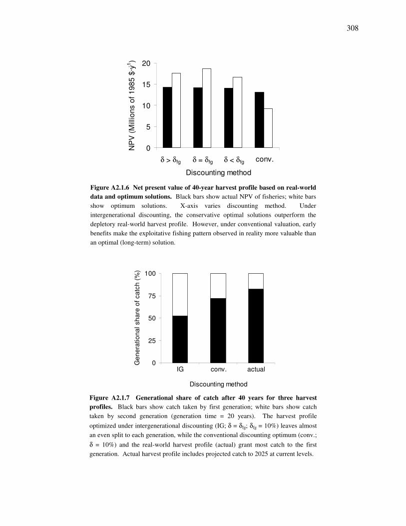
308

0

5

10

15

20

Discounting method

NP

V (M

illio

ns o

f 198

5 $·

y-1)

δ > δfg δ = δfg δ < δfg conv.

Figure A2.1.6 Net present value of 40-year harvest profile based on real-world data and optimum solutions. Black bars show actual NPV of fisheries; white bars show optimum solutions. X-axis varies discounting method. Under intergenerational discounting, the conservative optimal solutions outperform the depletory real-world harvest profile. However, under conventional valuation, early benefits make the exploitative fishing pattern observed in reality more valuable than an optimal (long-term) solution.

0

25

50

75

100

Discounting method

Gen

erat

iona

l sha

re o

f cat

ch (

%)

IG conv. actual

Figure A2.1.7 Generational share of catch after 40 years for three harvest profiles. Black bars show catch taken by first generation; white bars show catch taken by second generation (generation time = 20 years). The harvest profile optimized under intergenerational discounting (IG; δ = δfg; δfg = 10%) leaves almost an even split to each generation, while the conventional discounting optimum (conv.; δ = 10%) and the real-world harvest profile (actual) grant most catch to the first generation. Actual harvest profile includes projected catch to 2025 at current levels.

309

Discussion

Impatience of the individual is

fundamental to cost-benefit decisions at

all levels. It is an ingrained human

attribute that allows us to instinctively

account for uncertainty, lost opportunity

costs, and other considerations relevant

in resource acquisition. The economist’s

practice of discounting emulates this

tendency; providing an analytical and

quantitative guide for us to make value-

based judgments. Yet under the

conventional model of discounting it

may be impossible to conserve a

fisheries resource like Atlantic cod, or

implement an environmental recovery

strategy whose benefits may be years or

decades in the coming.

Using education as an example of an existing and well-established multigenerational investment,

parents and society seemingly disregard conventional financial wisdom and educate their

children with little promise of return - except the confidence that they have equipped them with

the tools needed to prosper. If that confidence carries value in the present, then this new form of

intergenerational discounting provides a more accurate model of human valuation. It can be

used to justify long-term environmental protection when investors are separated in time from

recipients. As management agendas turn toward long-term environmental conservation,

proactively or in response to fishery failures, we will need to change the way we value the stream

of benefits derived from our living resources. As conventional discounting emulates an

instinctive human behaviour, so too may intergenerational discounting emulate our willingness

to support future generations.

0.0

0.4

0.8

1.2

1.6

0 5 10 15 20

Discount rate (%)

Equ

ilibr

ium

bio

mas

s (t•

km-2

)

Figure A2.1.8 Sensitivity analysis showing the effect of discount rate on the optimal end-state biomass. Closed

circles show optimal biomass under conventional. valuation;

open circles show optimal biomass under IG valuation (δ =

δfg). Large discount rates leave less standing biomass in the

ecosystem, but the intergenerational solution maintains the

stock at higher levels than the conventional solution. The

conventional solution advocates stock collapse at discount

rates greater than δ � 15%.

310

Appendix 2.2 Cost-benefit Analysis of Education

As an estimate of the highest and lowest discount rate the public may be prepared to accept in

valuing the benefits bestowed on future generations (δfg), I have chosen to use the internal rates

of return needed to make a grade 10, and a PhD education economically worthwhile. Therefore,

the following cost-benefit analysis may be what a taxpayer in 1981 would have used to compare

the expected benefits from a child’s education with that of an alternative investment. The value

used to represent the rate of return for an alternate investment (� = 9.3%) corresponds to the

average annual rate of return for Bank of Canada long-term (10+ years) marketable bonds

between 1981-2001 (GOC, 2002).

A child enters grade 1 at a BC public school in 1981. He or she graduates high school in 1992 at

a total cost of $54,307 paid for by the provincial government (BC, 1989; BC, 1990). The four-

year arts or science undergraduate degree at the University of British Columbia costs $50,192

(PAIR, 2002; UBC, 2002), which is paid for by tuition and government grants. Masters and PhD

take six more years and costs $80,430 (PAIR, 2002; UBC, 2002). After 22 years he/she has

completed his education at a total cost of $184,931 and begins earning income. As a national

average, someone with a PhD level of training may expect to make $59,000 per year (HRDC,

2002a), while a high-school dropout earns only $21,000 (HRDC, 2002b).

Fig. A2.2.1 compares the costs and benefits of education to PhD and grade 10 levels. Each

year’s cost and benefit has been adjusted to 1981-dollar equivalents, and discounted to reveal the

time preference for payment made far from the 1981 perspective. A grade 10 education

outperforms the alternate investment, bank interest at � = 9.3% (NPV = 19.9 $·103), but a PhD

education is not worthwhile (NPV = -17.3 $·103).

Table A2.1.1 shows discount rates where varying levels of education become worthwhile. A

PhD becomes uneconomic at all discount rates greater than � = 6.3%, but an incomplete high

school education (grade 10) is worthwhile at � = 15.0%. Although average annual income of the

high school drop-out is only 36% that of the PhD, the lower level of education is more advisable

311

from a conventional cost-benefit perspective at the discount rate set by an alternative rate of

return from bank interest. Total career length is also longer for a high school drop-out (the

individual retires in 2032 in both cases).

This example represents a conservative estimate of the costs of education. Were this analysis

repeated for private grade school the increased cost would weigh heavily in the evaluation

because of its immediacy from the 1981 vantage point. Also, the early eighties saw very high

yields in long-term marketable bonds (15.2% in 1981). If we had used this rate to represent an

alternative investment rather than 9.3%, the average rate between 1981-2001, the returns from

even the most modest education level would become less attractive than returns from the

alternative investment rate.

This analysis disregards non-monetary benefits to education. However, even if the benefits to

education are increased by 50% to approximate these considerations the discount rate required to

make a PhD worthwhile is still 8.6% - less than the alternate rate of return.

Ph.D. Grade 10

0

1

2

3

4

5

1981 1991 2001 2011 2021 2031Year

1981

dol

lars

•103

0

1

2

3

4

5

1981 1991 2001 2011 2021 2031

Year

1981

dol

lars

•103

Figure A2.2.1 Costs and benefits of education in BC discounted from a 1981 time perspective. Education to a

Ph.D. level takes 22 years, education to grade 10 takes 10 years; total career length is 50 years including education

(black area) and employment (grey area). The Ph.D. makes more money once employed, but earlier benefits make

grade 10 education a better investment at a discount rate that represents an alternate rate of return (bank interest � =

9.3%). Dollar values are adjusted to 1981-dollar equivalents using the consumer price index.

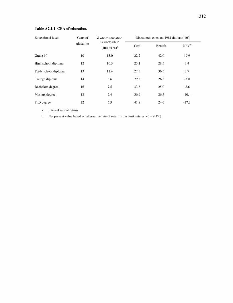
312

Table A2.1.1 CBA of education.

Discounted constant 1981 dollars (·103) Educational level Years of

education

δ where education is worthwhile

(IRR in %)a Cost Benefit NPVb

Grade 10 10 15.0 22.2 42.0 19.9

High school diploma 12 10.3 25.1 28.5 3.4

Trade school diploma 13 11.4 27.5 36.3 8.7

College diploma 14 8.6 29.8 26.8 -3.0

Bachelors degree 16 7.5 33.6 25.0 -8.6

Masters degree 18 7.4 36.9 26.5 -10.4

PhD degree 22 6.3 41.8 24.6 -17.3

a. Internal rate of return

b. Net present value based on alternative rate of return from bank interest (δ = 9.3%)

313

Appendix 3.1 Local Ecological Knowledge (LEK): Trends of Relative Abundance

Figure A3.1.1 LEK trends of relative abundance

Sea otters Odontocetae Seals and sea lions Seabirds

-1

0

1

1950 1975 2000 -1

0

1

1950 1975 2000 -1

0

1

1950 1975 2000 -1

0

1

1950 1975 2000 Transient salmon Coho salmon Chinook salmon Dogfish

-1

0

1

1950 1975 2000 -1

0

1

1950 1975 2000 -1

0

1

1950 1975 2000 -1

0

1

1950 1975 2000 Forage fish Eulachon Herring Inshore rockfish

-1

0

1

1950 1975 2000 -1

0

1

1950 1975 2000 -1

0

1

1950 1975 2000 -1

0

1

1950 1975 2000 Piscivorous rockfish Flatfish Halibut Pacific cod

-1

0

1

1950 1975 2000 -1

0

1

1950 1975 2000 -1

0

1

1950 1975 2000 -1

0

1

1950 1975 2000 Sablefish Lingcod Skates Crabs

-1

0

1

1950 1975 2000 -1

0

1

1950 1975 2000 -1

0

1

1950 1975 2000 -1

0

1

1950 1975 2000 Epifaunal invertebrates Inf. carn. invertebrates

-1

0

1

1950 1975 2000 -1

0

1

1950 1975 2000

314

Appendix 4.1 BC Fisheries Timeline

Table A4.1.1 BC fisheries timeline

References listed in Appendix 9.4.1

Period Event

1950-1954

Otter trawls introduced in BC (c. 1950), previously most vessels were side trawlers [105]. Drum seiners

introduced (c. 1950) [126]. Purse seining mechanized using hydraulic systems (e.g., “puretic block”) [115,

126]. American fleet enters BC waters in numbers (c. 1950) [127, 5], although US had been operating near

S. Vancouver Island previously [82]. International North Pacific Fisheries Commission established19

(1952) [119]. Canada/US treaty signed, “Convention for the Preservation of the Halibut Fishery of the

Northern Pacific Ocean and Bering Sea” (1953) [32]. Collection of catch statistics improves for Pacific

Ocean perch and other rockfish under voluntary trawl logbook program (1954) [82, 57].

1955-1959

Synthetic fibres (nylon, polyester) used in net construction (c. 1955) [15]. Echo-sounders integrated into

fleet following World War II. Western Canadian Whaling Ltd. close operations (1959), limited foreign

whale harvest continues until late 1960s [126].

1960-1964

Larger trawl vessels in use (c. 1960). Spawning channel construction, flow control projects and hatchery

programs initiated to improve salmon production (c. 1960) [126]. Foreign catch now includes sablefish

(1961) [82]. Foreign vessels required to carry license (1961) [105]. USSR fleet enters BC waters (c. 1965)

[127]. Canadians begin groundfish trawl in earnest [82]. Rockfish fishery begins (c. 1960), but accurate

records not kept until 1967 [82].

1965-1969

Japanese fleet enters BC waters (c. 1966) [127]. Rockfish records begin (1967) [82], but with a large

degree of aggregation in early years [35]. Final whaling season (1968) [107]. Improved technology to

preserve fish at sea (e.g., quick freezing) [12]. Long-range navigation systems (LORAN) in use.

1970-1974

Fishermen begin reporting an increasing variety of rockfish species, misreporting may have occurred to

avoid restrictive regulations (c. 1970) [82]. Freezers and ‘cold chains’ open a market for less valuable

species to make processed foods (e.g., Kamaboko, imitation crab meat, faux scallops) (c. 1970) [128].

Large area fishery closure in Queen Charlotte Sound to reduce foreign fishing for Pacific Ocean perch

(POP) (1971) [57].

19 INPFC was responsible for numerous projects from 1952 to 1993 to protect stocks and habitats of anadromous species, to

control harvesting and improve productivity.

315

Table A4.1.1 BC fisheries timeline (cont.)

1975-1979

Polish fleet enters BC waters (c. 1975) [127]. Average vessel size has doubled since 1940 up to 60 tonnes

(c. 1975) [105]. Trawl fishery shifts away from POP and towards other rockfish and flatfish species [122].

Limited entry to groundfish trawl established using trip limits (1976) [128]. Canada unilaterally extends

its fisheries jurisdiction to 200 nautical miles - Economic Exclusive Zone (EEZ) formed20 (1977) [8, 31].

Other countries follow, and UNCLOS III will eventually formalize EEZ concept in 1982 [125]. Soviet and

Japanese rockfish catches cease (1977) [127]. Salmonid Enhancement Program21 (SEP) begins (1977)

[51]. A change in British Columbia Fishing Regulations of 1888 explicitly prohibits natives from selling

their catch commercially (1977) [118]. Aquaculture begins in BC in the late 1970s: first farms were on the

sunshine coast and northeast coast of Vancouver Is. raising Pacific species chinook, coho and sockeye (c.

1977) [1]. Annual quotas applied to groundfish fishery (1978) [82]. Department of Fisheries and Oceans

(DFO) established (1979) [19]. DFO implements measures to control harvest of groundfish stocks (1979) -

license limitations, total allowable catches (TACs), species/area/time closures and trip limits [82].

1980-1984

Global Positioning System (GPS) in use by fishing vessels (1980) [64] – not widespread. Rock-

hoppers/tickle chains reduce habitat damage and bycatch in trawl fleet (c. 1980). Most foreign fishing

ends in EEZ (c. 1980) [5]. Increasing engine power and the availability of fiberglass hull designs

facilitates more “bow pickers” in the salmon gillnet fleet (c. 1980) [9], which use shorter ‘soak’ times,

reducing bycatch [3]. BC recognizes Race Rocks as an ecological reserve (1980) [104]. Groundfish trawl

advisory committee formed (GTAC) (1980). Trip limits and area quotas imposed on yellowtail rockfish

fisheries (1980) [71]; quota applied on rock sole (1980) [68]. Increased misreporting, discards in rockfish

fishery in response to new regulations (c. 1980) [122]. Amendment to 1888 BC Fishing Regulations

restricts the number and species that may be caught by aboriginals for food, social and ceremonial

purposes (1981) [118]. New techniques improve aging of major groundfish species (1981) [114]. US

rockfish catch ceases (1982) [127, 57]. Widow rockfish quota implemented (1983) [70].

20 EEZ formed under authority of Territorial Sea and Fishing Act of 1964. 21 SEP increases salmon production through hatchery programs, spawning channel improvement and lake fertilization; also

assists in Community Economic Development Program (CEDP).

316

Table A4.1.1 BC fisheries timeline (cont.)

1985-1989

SEP integrated into Pacific Region Salmon Resource Management Plan22 (SRMP) (1985) [126]. Fisheries

Act23 introduced (1985) [20]. Canada/US Pacific Salmon Treaty24 (PST) of 1984 is ratified by Canada

(1985) [33]. Commercial fishery for widow rockfish begins (1986) [70]. First quota for lingcod

introduced (area 3b, W. Vancouver Is.; 1987) [91]. Pacific Regions Fisheries Observer Program25 initiated

by DFO, Archipelago Marine Research Ltd. contracted to provide observer coverage for foreign and

domestic vessels operating within EEZ (1987) [10]. General Agreement on Tariffs and Trade (1988).

Observer coverage extended offshore to seamount fisheries (1989) [10]. With salmon aquaculture on the

rise, and Alaskan salmon fisheries producing unprecedented yields, salmon prices fall throughout late

1980s and 1990s [106]. Commercial size limit for lingcod increased from 58 cm to 65 cm in Strait of

Georgia (area 4b; 1989) (original coast-wide limit of 58 cm was established in 1940s) [91].

1990

Sparrow decision (1990) affirms aboriginal right to fish under Sec. 35(1) of 1982 Constitution Act [21].

Individual transferable quota (ITQ) established for sablefish fishery (1990) [93]. Annual quotas for

English sole applied (1990) [63]. Vessel trip quotas for petrale sole applied (1990) [66]. Commercial

lingcod fishery closed in area Strait of Georgia (area 4b; 1990) - still open for recreational fleet, but 65 cm

size limit imposed in 1991 [91]. Dockside monitoring initiated for ITQ sablefish fishery, 100% coverage

of landings (1990) [10]. Weedlines used in gillnet fishery to reduce steelhead bycatch (c. 1990). Sorting

grids (c. 1990).

1991

Canada-US Free Trade Agreement (FTA) (1991) [34]. Joint Canada/US commitment to reduce halibut

bycatch through International Pacific Halibut Commission (IPHC) (1991) [108]. Halibut individual vessel

quota system initiated in British Columbia, beginning with a 2 year trial (1991) [108, 10]. Voluntary 140

mm cod-end mesh size suggested by 1991 Pacific groundfish trawl management plan for Pacific cod

fishery (78 mm was already legislated) (1991) [65]. Dockside monitoring initiated for halibut IVQ fishery

(1991) [10].

22 SRMP includes fleet management, habitat restoration, natural stock rebuilding and salmonid enhancement. 23 Main provisions of the Fisheries Act deal with habitat protection, pollution prevention, licensing, powers of fishery officers

and marine safety; authorizes DFO to implement fishery closures for conservation purposes. 24 Pacific Salmon Commission established by PST; it has power to enact time/area closures, gear restrictions and harvest

limitations. 25 Observer program includes several objectives: to monitor trawl offloading events, to collect data on experimental fisheries

(e.g. tanner crab traps, squid fishing, seamount fishing), to collect information for research programs (e.g. halibut bycatch), and to

monitor for enforcement purposes.

317

Table A4.1.1 BC fisheries timeline (cont.)

1992

TAC and trip limits imposed on Hecate Strait Pacific cod fishery (1992), previously open access [65].

DFO cooperates with Department of National Defense to conduct air surveillance patrols of North Pacific

(primarily looking for high seas drift netting) (1992) [72]. Salmon agreements made by Canada and US

under the 1984 Pacific Salmon Treaty expire, competitive harvesting commences under the political limbo

(1992) [82]. Aboriginal Fishing Strategy (AFS) established in response to Sparrow decision (1992) [94].

Pilot Sales Program permits limited commercial catch for natives (1992) [118], intended to reduce wide-

scale poaching. DFO issues permits for commercial aboriginal salmon fisheries in Port Alberni and Lower

Fraser R. (1992) and later, Skeena R. under the Aboriginal Fishing Strategy - controversial fisheries called

“race-based” by critics [124, 13]. 1992 Fraser R. sockeye fishery an “environmental disaster”, while

opponents to Sparrow decision claim link to AFS [4]; Pearse-Larkin report commissioned in response

[120]. Pacific license retirement plan initiated (1992) [118].

1993

North Pacific Fisheries Commission dissolved (1992), replaced by Convention for the Conservation of

Anadromous Stocks in the North Pacific Ocean (1993) [119]. Sustainable Fisheries Program launched by

DFO to conserve Skeena R. salmonids (1993) – includes steelhead observer program and selective fishing

experiments [38]. Widow and canary rockfish receive coast-wide quotas and trip limits (1993), both

fisheries previously unrestricted [70, 60]. Quota for lingcod introduced (area 5c/d; 1993) [91]. Aboriginal

Communal Fishing Licenses Regulations approved (1993) [106, 2].

1994

User-pay mandatory dock-side monitoring program put in place for majority of groundfish trawl fisheries

(1994) [45, 10] – misreporting reduced. United Nations Law of the Sea26 (UNCLOS) enters into force

(ratified by Canada 2003) [28].

26 UNCLOS III sets out general rules to govern oceans: defines territorial sea, contiguous zones and establishes Exclusive

Economic Zones (EEZ).

318

Table A4.1.1 BC fisheries timeline (cont.)

1995

Directed fishery for Petrale sole discontinued coast-wide (1995) [66]. IPHC regulation: halibut must be

dressed before offloading (1995) [109]. IPHC regulation: halibut caught as bycatch in Pacific cod and

sablefish fisheries can now be kept (1995) [109]. Staged reduction of halibut trawl bycatch mortality

(1995) [130]. Mesh size regulation introduced for rock sole fishery to minimize juvenile mortality (1995)

[82]. 140 mm mesh size for Pacific cod trawl fishery is legislated (1995), was previously voluntary [65].

Under 1992 Pilot Sales Program, commercial licenses granted to three lower mainland First Nations bands

on lower Fraser River. Jack, John and John case27 (1995) [16]. United Nations Food and Agriculture

Organization (FAO) draft ‘Code of Conduct for Responsible Fisheries’, adopted by Canada (1995) [103].

Groundfish trawl fishery suspended mid-season (TAC exceeded), hook and line limited (1995) [39].

Mifflin Plan announced, for voluntary buy-back of commercial fishing licenses (1995) [106]. BC Sport

Fishing Regulations now prohibit on-sea canning to improve data collection (1995) [37]. Restrictions

introduced on west coast Vancouver Island and Strait of Georgia coho stocks due to conservation concerns

(1995) [121]. 1995 – 2000 see budget cuts for DFO.

1996

Van der Peet case28 [23]. New sport fishery limits introduced for many species not previously regulated,

including sablefish and yelloweye rockfish; also higher fines for offences under BC Sport Fishing

Regulations (1996) [41]. Canada Oceans Act passed29 (1996) [22, 99]. Coastal fisheries protection

regulations amended; it is now mandatory for foreign fishing vessels to notify DFO on passage through BC

waters (1996) [42]. New aerial surveillance pilot project augments DFO’s enforcement capabilities,

improves data collection for commercial fisheries effort statistics 1996 [40]. Public consultation begins for

upcoming groundfish IVQ allocations (1996) [44]. IPHC increases recreational halibut limit in Strait of

Georgia (area 2b), halibut fletching (filleting) prohibited at sea (1996) [110]. Lingcod size limit increased

from 58 cm – 65cm near Queen Charlotte Is. (area 5e) and west coast Vancouver Is. (area 3c/d) (1996)

[91]. Trawl catch for Pacific cod in Hecate Strait limited to bycatch only, IVQs implemented (1996) [65].

IVQs implemented for dover sole (area quotas previously), and English sole (1996) [82, 62]. New

Groundfish Management Plan (1996) includes: mandatory on-board observer program for groundfish trawl

(replaces limited observer program in place since 1987), and bycatch caps for trawlers (1996) [82, 43, 46].

Despite additional costs of observer program, IVQ scheme stimulates a large increase in the number of

active trawlers; probably increased the occurrence of illegal sales and high grading (1996) [12]. British

Columbia Liberal government places 6 year moratorium on new Salmon aquaculture (netpen) operations

(1996).

27 Jack, John and John case affirms DFO fiduciary obligation to manage stocks specific fish to a tribal group’s traditional area

(1995) [123] 28 Van der Peet (1996) conviction was eventually upheld by the Supreme Court of Canada, affirming that aboriginal commercial

rights to the resource exist only if sale is a continuation of traditional tribal practices. 29 Major provisions of the Oceans Act (1996) include recognition of Canada’s ocean jurisdiction, guidelines for sustainable

development, integrated management and precautionary approach, and consolidation of federal fisheries/environmental

responsibilities [77].

319

Table A4.1.1 BC fisheries timeline (cont.)

1997

Major groundfish trawl regulation change: comprehensive IVQ scheme set for 25 groundfish species

(1997), IVQ holders allocated 80% of TAC [50] - formalized in 1998 [54]. Pacific halibut management

plan reallocates halibut IVQ; bycatch objectives set under 1991 IPHC agreement have been well exceeded

(1997) [49]. Kwakiutl Aboriginal Fisheries Guardians join DFO on enforcement patrols on Vancouver Is.

and central BC (1997) [48]. Following major regulatory changes in groundfish trawl industry, Groundfish

Development Authority (GDA) formed to protect non-quota shareholders (1997) [77]. Limited entry

established for groundfish hook and line (1997) [46]. Delgamuukw decision30 (1997) [24]. Quota for

lingcod introduced (area 5e; 1997) [91]. Steady decline in world salmon prices due to continued

development of aquaculture, particularly in Norway and Chile [96]; in 1997, prices are approximately 1/3

of ten years ago [7]. Retention/possession of coho, chinook and steelhead for all seine fisheries disallowed

(1997) [46, 47].

1998

Canadian Code of Conduct for Responsible Fisheries developed through grassroots industry initiative

(1998) [30, 95]. Under new Pacific Fisheries Adjustment and Restructuring Program (PFAR) (1998) [79],

the Selective Fishing Program (SFP) is initiated by DFO; 5% of salmon TAC allocated to improve

fisheries selectivity [69, 76, 80]; experimental fisheries authorized for data collection and aboriginal

fisheries: includes fish wheels, weirs, beach seine, live fish traps and Norwegian fish herders [13, 14, 79,

73, 58] NB: widespread use has not materialized as of 2004 [14]. Under Selective Fishing Program, gear

modifications31 are mandated between 1998 and 2002 through licensing conditions to reduce coho bycatch

mortality [14, 81, 56, 75, 78], however time/area closures still principle methods [14]. Selective fishing

initiative successfully reduces coho bycatch mortality from 60% to 5% [14, 69]. New Coho Response

Team evaluates coho conservation in BC, seeks new methods to reduce bycatch among other projects

(1998) [92]. Fisheries Renewal BC established, coordinates resources for habitat enhancement made

available under Pacific Salmon Endowment Fund and Pacific Salmon Treaty (1998) – Fisheries Renewal

operates until 2002 [89, 83]. IPHC issues new halibut logbooks to improve in-season data collection

(1998) [111]. DFO and BC Wildlife Federation (BCWF) create first fishery officer-dog team trained for

fisheries enforcement (1998) [55]. Commercial troll fleet in lower Strait of Georgia (area H) gets 10%

observer coverage (1998) [10]. DFO releases PFAR report, “A new direction for Pacific Salmon

Fisheries” – reiterates commitment to develop selective fishing practices, among other priorities (1998)

[52].

30 Delgamuukw decision recognizes aboriginal title to land and resources, affirms aboriginal right to fish commercially [29]. 31 Revival tanks are made mandatory throughout BC salmon fleet; gillnetters employ shorter-than-regulation nets and shorter

soak times; seiners use brailing with dip nets, knot-less mesh to reduce abrasion, and plastic escape holes to release undersized

fish; trollers use large and barbless hooks [14].

320

Table A4.1.1 BC fisheries timeline (cont.)

1999

DFO begins pilot project using satellite technology and psion units to collect real-time catch information,

as well as biological and oceanographic data (1999) [84]. BC Fisheries Survival Coalition organizes a

large-scale protest fishery in 1998 on the Fraser River following smaller actions in 1996 and 1997, to

protest native-only fisheries set under DFO’s 1992 Pilot Sales Program. Thomas case affirms that “race-

based” fisheries are discriminatory and illegal, stays charges against 24 non-aboriginal protesters from

1996/1997 Fraser River protest fisheries (1998) [6]; an appeal is made to BC supreme court, but rejected in

1999. The 1999 groundfish trawl fleet was composed of 142 licensed vessels, of which approximately 88

recorded landings (1999) [82]. DFO observer program extended to include halibut fisheries (hook and line

now, in addition to trawl) (1999) [82]. Observer coverage extended to include rockfish fisheries and

Rockfish Protected Areas (RPAs) implemented under recommendation of Groundfish Hook and Line

Advisory Committee [87]; rockfish discarding now prohibited (1999) [82, 61]. Size limit for recreational

lingcod increased to 65 cm off West Vancouver Island (areas 3c/d) (1999) [91]. BC recreational fishers

required to supply catch records (1999) [67]. Formal joint commitment by Canada and US to restore

salmon habitat, improve management under 1985 Pacific Salmon Treaty, two endowment funds

established totaling $200 million CDN (1999) [59]. Additional selective fishing experiments in Juan de

Fuca Strait (1999) [36]. Supreme Court of Canada Marshall decision affirms the rights of two Maritime

aboriginal groups to fish, hunt and gather in pursuit of “moderate livelihood” (1999) [26]. Canadian

Environmental Protection Act32 (CEPA) passed (1999) [25].

2000

Nis’ga treaty becomes law, first modern-day land claim - includes exclusive aboriginal fishing rights

(2000) [11]. Groundfish trawlers accept voluntary area closures to protect Hexactinellida sponge reefs

(2000) [116, 113]. Environment Canada announces National Programme of Action33 (NPA) (2000) in

response to Global Plan of Action initiated by United Nations Environment Programme (UNEP) in 1995.

Additional DFO funding strengthens fishery enforcement (2000) [74].

32 CEPA includes marine protection provisions to complement existing measures, gives Minister of the Environment additional

powers to enact environmental guidelines. Particularly addresses land-based marine pollution concerns. 33 NPA highlights conservation, sustainable use and economic diversification to reduce land-based marine pollution [101].

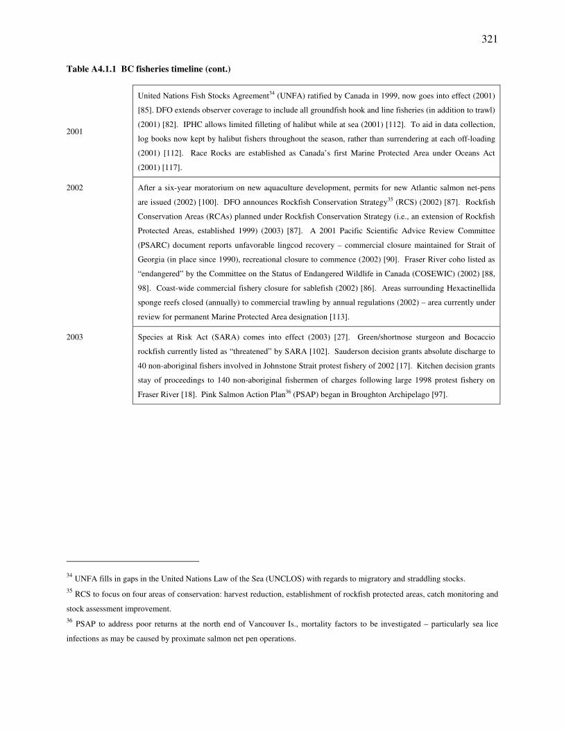
321

Table A4.1.1 BC fisheries timeline (cont.)

2001

United Nations Fish Stocks Agreement34 (UNFA) ratified by Canada in 1999, now goes into effect (2001)

[85]. DFO extends observer coverage to include all groundfish hook and line fisheries (in addition to trawl)

(2001) [82]. IPHC allows limited filleting of halibut while at sea (2001) [112]. To aid in data collection,

log books now kept by halibut fishers throughout the season, rather than surrendering at each off-loading

(2001) [112]. Race Rocks are established as Canada’s first Marine Protected Area under Oceans Act

(2001) [117].

2002 After a six-year moratorium on new aquaculture development, permits for new Atlantic salmon net-pens

are issued (2002) [100]. DFO announces Rockfish Conservation Strategy35 (RCS) (2002) [87]. Rockfish

Conservation Areas (RCAs) planned under Rockfish Conservation Strategy (i.e., an extension of Rockfish

Protected Areas, established 1999) (2003) [87]. A 2001 Pacific Scientific Advice Review Committee

(PSARC) document reports unfavorable lingcod recovery – commercial closure maintained for Strait of

Georgia (in place since 1990), recreational closure to commence (2002) [90]. Fraser River coho listed as

“endangered” by the Committee on the Status of Endangered Wildlife in Canada (COSEWIC) (2002) [88,

98]. Coast-wide commercial fishery closure for sablefish (2002) [86]. Areas surrounding Hexactinellida

sponge reefs closed (annually) to commercial trawling by annual regulations (2002) – area currently under

review for permanent Marine Protected Area designation [113].

2003 Species at Risk Act (SARA) comes into effect (2003) [27]. Green/shortnose sturgeon and Bocaccio

rockfish currently listed as “threatened” by SARA [102]. Sauderson decision grants absolute discharge to

40 non-aboriginal fishers involved in Johnstone Strait protest fishery of 2002 [17]. Kitchen decision grants

stay of proceedings to 140 non-aboriginal fishermen of charges following large 1998 protest fishery on

Fraser River [18]. Pink Salmon Action Plan36 (PSAP) began in Broughton Archipelago [97].

34 UNFA fills in gaps in the United Nations Law of the Sea (UNCLOS) with regards to migratory and straddling stocks. 35 RCS to focus on four areas of conservation: harvest reduction, establishment of rockfish protected areas, catch monitoring and

stock assessment improvement. 36 PSAP to address poor returns at the north end of Vancouver Is., mortality factors to be investigated – particularly sea lice

infections as may be caused by proximate salmon net pen operations.

322

Appendix 4.2 IUU Influences Table

Table A4.2.1 IUU influences table

Gillnet Troll Seine Rec Trawl H&L Rec1950 - 1954

otter trawls 105

�

����

Increased catching power 1950 2003

drum seiners 126

�

����

Increased catching power 1950 2003

hydraulics 115, 126 �

���� ���� ���� ���� ����

Increased catching power 1950 2003

US fleet enters127, 5

� ���� ���� ���� ���� ���� Increased catching power, heavy American presence 1950 1982 EEZ Formed

INPFC established119

� ���� ���� ���� ���� ���� Functions include harvest controls 1952 1992 CCASNPO established

Can/US halibut treaty32

� � ���� ����Co-management commitment, power of seizure for illegal activity 1953 2003

trawl logbook programme

82, 57� ���� Logbooks only voluntary 1954 1960 Mandatory recording

1955-1959synthetic fibres

15� ���� ���� ���� ���� ���� ���� ���� Increased catching power 1955 2003

echo sounders � ���� ���� ���� ���� ���� Increased catching power 1955 2003

1960-1964 unrecorded rockfish landings begin

82� ���� 1960 1967

larger trawl vessels � Increased catching power 1960 2003

foreign sablefish fishery begins

82� ���� ����

Increased catching power; foreign fleet less accountable than domestic 1961 1977 EEZ Formed

foreign vessles licenced105

� ���� ���� ���� ���� ���� Improved data collection 1961 2003

USSR fleet enters127

� ���� ����Increased catching power, heavy Soviet presence; rockfish targeted 1965 1977 EEZ Formed

domestic trawling begins

82� ���� ���� Increased catching power 1967 2003

foreign / domestic rockfish fishery begins

82� � ���� ����

Increased catching power; no rockfish records are kept initially 1967 2003

1965-1969Japan fleet enters

127� ���� ����

Increased catching power, light Japanese presence; rockfish targeted 1966 1977

rockfish records begin82, 35

� ���� ���� Records are highly aggregated in early years 1968 2003

freezing/preservation12

� ���� ���� ���� ���� ���� Fishing vessels have access to ice 1968 2003

ground-based navigation systems � ���� ���� ���� ���� ���� Fisheries become more selective 1969 2003

� 12����"�����"��"�������$���"������""�����"��"��3�"�"���"������'����"��"�2����

3 %33��2�������"����4"������"��" ���$��"5�6 78" �����"������"5 �78"9���"*����":�����2��"#��"59*:#78";����"*�������"#��"5;*#78";����"*�������"�����"5;*�7�

� ����������"�����"��"��3�"��

� *����"�����"<"�=��"��������8"�'��"�����"<"����"��������"5���"��������7�

� ����"���"�������"�"�������"���!"���"���"�������

� ���"��>�"���"���2�������"�����

$ �?�"<"����������"�2���"���"'��2����"��������

Rationalef Termination eventStart

Event summarya b Influenced

Period SalmonAffected fleete

GroundfishPolicy Technology Supply/marketPolitical

Refsc

Discard Ende

Duration

Illegal Unreport.

322

323

Table A4.2.1 IUU influences table (cont.)

Gillnet Troll Seine Rec Trawl H&L Rec1970-1974

new rockfish regulations82

� � ���� ����Rockfish misreporting increases to contravene restrictions 1970 1980 DFO regulations

"cold chains" introduced128

� ���� ���� ���� ���� ����Cold chains open a market for less valuable species previously discarded 1970 2003

POP closure (QCS)57

� � ���� ���� ����Affects only a portion of study area (QCS); opportunity for poaching 1971 1974

1975-1979Poland fleet enters

127� ���� ����

Increased catching power; rockfish targeted; light Polish presence 1975 1977 EEZ Formed

larger fishing vessels105

� ���� ���� ���� ���� ���� Increased catching power, longer trips 1975 2003

additional rockfish/flatfish spp. targeted

122� � ���� ����

Bycatch retained and sold; data collection inadequate for rockfish 1975 2003

trip limits GF trawl128

� � ����Fishers can no longer land everything they catch; incentive to high grade, misreporting as other species 1976 2003

EEZ formed8, 31

� � � ���� ���� ���� ���� ����

Reduced catching power (foreign restricted); opportunity for poaching; better monitoring of domestic fleet than foreign fleet

n/a n/a

USSR / Japan rockfish fishery ends

127� � � ���� ����

Reduced catching power (foreign restricted); opportunity for poaching; better monitoring of domestic fleet than foreign fleet

n/a n/a

SEP begins51

� ���� ���� ����CEDP assists fishers (subsidy); increased catching power 1977 2003

legislation ends native commercial fishery

118� � ���� ���� ���� ���� ���� Opportunity for poaching; catch not reported 1977 1992 Pilot sales program

annual quotas set for GF

82� � ���� ����

Fishers can no longer land everything they catch; incentive to high-grade, misreporting as other species 1978 2003

DFO established19

� � ���� ���� ���� ���� ���� Enforcement improved; data collection improved 1979 2003

GF TAC, trip limits, closures, license limitations 82

� � ���� ����Fishers can no longer land everything they catch; incentive to high-grade, misreporting as other species 1979 2003

1980-1984GPS

42� ���� ���� ���� ���� ���� Fisheries become more selective 1980 2003

rockhoppers � ���� Increased catching power 1980 2003

tickle chains, cod-end sensors � ���� Bycatch reduction devices 1980 2003

foreign fishing ends in EEZ

5� � � ���� ���� ���� ���� ����

Better monitoring of domestic fleet than of foreign fleet; opportunity for poaching n/a n/a

more bowpickers in salmon fleet

9, 3� ���� Bowpickers use shorter soak times, reduce bycatch 1980 2003

Race Rocks ecological reserve

104� � ���� ����

Minor: affects only a portion of study area; increased opportunity for poaching 1980 2003

GTAC formed � ����Helps establish GF regulations; management-industry liason 1980 2003

Policy Technology Political Supply/market Discard Illegal Unreport.Salmon

Affected fleetRationale

DurationTermination eventGroundfish

Start EndPeriod

Event summaryRefs

Influence

323

324

Table A4.2.1 IUU influences table (cont.)

Gillnet Troll Seine Rec Trawl H&L Rec

1980-1984

trip limits, area quotas for yellowtail rockfish

71� � ���� ����

Fishers can no longer land everything they catch; incentive to high-grade, misreporting as other species 1980 2003

(continued)rock sole quota

68� � ���� ����

Fishers can no longer land everything they catch; incentive to high-grade, misreporting as other species 1980 2003

new rockfish regulations122

� � ���� ����Tighter regulations on rockfish retention; increased misreporting to conceal catch [122] 1980 2003

restrictions on aboriginal food fish

118� ���� ���� ���� ���� ���� Opportunity for poaching 1981 1990 Sparrow case

US rockfish fishery ends127, 57

� � ���� ���� Less foreign fishing, fewer unreported catches n/a n/a

widow rockfish quota70

� � ���� ����Fishers can no longer land everything they catch; incentive to high-grade, misreporting as other species 1983 2003

1985-1989SRMP drafted

126� ���� ���� ���� Assists salmon fishers, catching power increased 1985 2003

Fisheries Act passed20

� � � ���� ���� ���� ���� ����Provisions allow fisheries closures, grants powers to DFO officers 1985 2003

Pacific Salmon Treaty ratified

33� ���� ���� ���� Tighter regulations on salmon retention 1985 1992 Expires

commercial widow rockfish fishery begins

70� ���� ���� Increased catching power 1986 2003

lingcod quota91

� ���� ����Fishers can no longer land everything they catch; incentive to high-grade, misreporting as other species 1987 2003

GF at-sea observer program begins

10� � � ���� ���� Partial coverage only 1987 1996 Trial program ends

GATT treaty � ���� ���� ���� ���� ���� Market is less restrictive, new markets open. 1988 2003

GF observer coverage extended offshore

10� � � ���� ���� Partial coverage only 1989 2003

salmon prices fall throughout 80s/90s

106� � ���� ���� ���� Incentive to sell privately, incentive to highgrade 1985 2003

lingcod size limit increased (SOG)

91�

More discarding of undersized individuals. Only a portion of study area. 1989 1990 Commercial retention

banned (SOG)

1990-1994Sparrow decision

21� ���� ���� ���� ���� ���� Aboriginal subsistance fishery is now legal 1990 2003

sablefish ITQ93

� ���� ����Fishers can no longer land everything they catch; incentive to high-grade 1990 2001 Closure

English sole quota63

� � ���� ����Fishers can no longer land everything they catch; incentive to high-grade, misreporting as other species 1990 2003

petrale sole trip limits66

� � ���� ����Fishers can no longer land everything they catch; incentive to high-grade, misreporting as other species 1990 2003

SOG closed to commercial lingcod

91� � ���� ����

Affects only a portion of study area (SOG); opportunity for poaching 1991 2003

sport size limit for lingcod introduced

91� ���� More discarding of undersized individuals 1990 2001 Closure

GroundfishStart EndPolicy Technology Political Supply/market Discard Illegal Unreport.

SalmonPeriodEvent summary

RefsInfluence Affected fleet

RationaleDuration

Termination event

324

325

Table A4.2.1 IUU influences table (cont.)

Gillnet Troll Seine Rec Trawl H&L Rec

1990-1994

dockside monitoring for sablefish (100%)

10� � ���� ���� Data collection improved; improved enforcement 1990 2003

(continued)gillnet weedlines � ���� Bycatch reduction device 1990 2003

sorting grids � ���� Bycatch reduction device 1990 2003

Free Trade Agreement34

� ���� ���� ���� ���� ���� Market is less restrictive, new markets open. 1991 2003

IPHC bycatch reduction agreement

108� ���� ����

Agreement's stated purpose is to reduce halibut bycatch 1991 2003

Halibut IVQ108, 10

� ���� ����Fishers can no longer land everything they catch; incentive to high-grade 1991 1993 Trial program ends

voluntary mesh size increase for Pacific cod

65� ���� ����

Fewer discards of undersized fish; voluntary (limited effect) 1991 2003

dockside monitoring for halibut

10� � ���� ���� Data collection improved; improved enforcement 1993 2003

TAC/trip limits Pacific cod

65� ���� ����

Fishers can no longer land everything they catch; incentive to high-grade 1992 2003

high seas aerial surveillance

72� ���� ����

Minor improvement to enforcement (adjacent to study area) 1992 2003

Pacific Salmon Treaty expires

82� � � ���� ���� ���� Widely publicized "fish wars" begin - grab for fish n/a n/a

INPFC dissolved 129 � Founded in 1953. n/a n/a

CCASNPO founded 129 � Replaces INPFC. 1992 2003

Aboriginal Fishing Strategy

94� � ���� ���� ���� ���� ����

First Nations contribute to management. FN harvest allocations. Gov't must consult FN before restrictions. 1992 2003

Pilot sales program118

� ���� ���� ���� Intended to reduce poaching - salmon openings only 1992 2002 Kitchen ruling

Pacific license retirement plan

118� ���� ���� ����

reallocation to FN under AFS; subsistence needs satisfied 1992 2003

Sustainable Fisheries Program

38� � � ���� ���� ����

SFP includes steelhead observer program, selective fishing experiments. Only affects part of study area (Skeena)

1993 2003

widow rockfish quota70

� � ���� ����Fishers can no longer land everything they catch; incentive to high-grade, misreporting as other species 1993 2003

canary rockfish quota60

� � ���� ����Fishers can no longer land everything they catch; incentive to high-grade, misreporting as other species 1993 2003

lingcod quota91

� � ���� ����Fishers can no longer land everything they catch; incentive to high-grade, misreporting as other species 1993 2003

Policy Technology Political Supply/market Discard Illegal Unreport.Salmon

Affected fleetRationale

DurationTermination eventGroundfish

Start EndPeriod

Event summaryRefs

Influence

325

326

Table A4.2.1 IUU influences table (cont.)

Gillnet Troll Seine Rec Trawl H&L Rec

1990-1994

Aboriginal communal licenses

106, 2� � ���� ���� ���� Allows sale of product. Aids data collection. 1993 2003

(continued) dockside monitoring for all GF

45, 10� � ���� ����

Mandatory user-pay system, improves data collection. 1993 2003

UNCLOS ratified28

� � � ���� ���� ���� ���� ���� ���� ���� Formalizes EEZ by international law. 1994 2003

1995-1999

Petrale sole fishery ends

66� ���� ����

Directed fishery ends, petrale bycatch in other sectors is less likely to be discarded. 1995 1995 Closure

several IPHC regulations reduce bycatch 109

� ���� ���� Certain bycatch must now be landed 1995 2003

rock sole mesh size regulation

82� ���� Reduced capture of undersized individuals. 1995 2003

Pacific cod mesh size regulation now mandatory 65

� ���� Trawl only 1995 2003

Jack, John and John case

16� ���� ���� ���� ���� ����

DFO under obligation to manage traditional tribal areas. Improved enforcement, monitoring. 1995 2003

UN FAO Code of Conduct adopted

103� � � ���� ���� ���� ���� ���� ���� ���� Contains numerous guidelines for responsible fishing. 1995 2003

GF trawl suspended temporarily

39� � � ���� Remainder of season closed to GF trawl. 1995 1996

vessel buy-back (Mifflin plan)

106� ���� ���� ���� ���� ����

Reallocation to FN under AFS; subsistence needs satisfied 1995 2003

Salmon sport fishery bans on-sea canning

37� ���� Regulation meant to improve data collection 1995 2003

Coho restrictions (SOG, WCVI)

121� � ���� ���� ����

Selective fishing measures to protect coho (localized); commercial catch is now illegal 1995 2003

DFO funding cuts begin � ���� ���� ���� ���� ���� ���� ����Gradual decline in funding, beginning in mid 1990s. Until 2000 when enforcment is strengthened. 1995 2000 Additional enforcement

funding

Van der Peet case23

� � ���� ���� ����

Sale is illegal unless a continuation of traditional tribal practices. Illegal catch goes unreported. Most often refers to salmon.

1996 2003

new sport regulations41

� � � ����

Sablefish, yelloweye sport now regulated, fishers can no longer land everything they catch. Higher fines reduce illegal.

1996 2003

Oceans Act20, 99

� � � ���� ���� ���� ���� ���� ���� ����Improved federal/provincial management, improved monitoring and data collection. 1996 2003

Foreign vessels must report to DFO

42� ���� ���� ���� ���� ����

Greater accountability to foreign vessels within EEZ. Less opportunity for illegal practices. 1996 2003

coastal aerial surveillance

40� � ���� ���� ���� ���� ���� ���� ���� Reduces illegal activity, improves data collection. 1996 2003

Policy Technology Political Supply/market Discard Illegal Unreport.Salmon

Affected fleetRationale

DurationTermination eventGroundfish

Start EndPeriod

Event summaryRefs

Influence

326

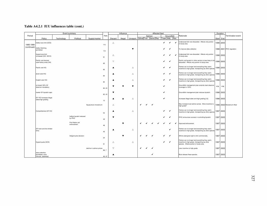
327

Table A4.2.1 IUU influences table (cont.)

Gillnet Troll Seine Rec Trawl H&L Rec

1995-1999halibut size limit (SOG)

110� ���� ���� ����

Undersized fish now discarded. Affects only portion of study area. 1996 2003

(continued) halibut fletching prohibited

110� ���� ���� To improve data collection 1996 2001 IPHC regulation

lingcod size limit increased (QCI, WCVI)

91� ���� ���� ����

Undersized fish now discarded. Affects only portion of study area. 1996 2003

Pacific cod directed trawl fishery ends (HS)

65� ���� ����

Pacific cod bycatch in other sectors is less likely to be discarded. Affects only portion of study area. 1996 2003

Pacific cod IVQ65

� � ���� ����Fishers can no longer land everything they catch; incentive to high grade, misreporting as other species 1996 2003

dover sole IVQ62

� � ���� ����Fishers can no longer land everything they catch; incentive to high grade, misreporting as other species 1996 2003

English sole IVQ82

� � ���� ����Fishers can no longer land everything they catch; incentive to high grade, misreporting as other species 1996 2003

on-board !00% GF observer mandatory

82, 43� � � ����

Groundfish management plan extends trawl observer coverage to 100%. n/a n/a

trawler GF bycatch caps82, 43

� ���� Groundfish management plan reduces bycatch. 1996 2003

GF IVQ increases illegal sales/high grading

12� � � ���� Increases illegal sales and high grading [12] 1996 2003

Aquaculture moratorium � ���� ���� ����May increase local salmon prices. More incentive to high grade? 1996 2002 Moratorium lifted

Comprehensive GF IVQ54

� � ���� ����Fishers can no longer land everything they catch; incentive to high grade, misreporting as other species 1997 2003

halibut bycatch reduced by IPHC

49� ���� ���� IPHC announces success in controlling bycatch. 1997 2003

First Nation aid enforcement

48� ���� ���� ���� ���� ���� ���� ���� Improved enforcement. 1997 2003

GF hook and line limited entry

46� � ����

Fishers can no longer land everything they catch; incentive to high grade, misreporting as other species 1997 2003

Delgamuukw decision24

� ���� ���� ���� ���� ���� Affirms aboriginal right to fish commercially. 1997 2003

lingcod quota (QCS)91

� � ���� ����

Fishers can no longer land everything they catch; incentive to high grade, misreporting as other species. Affects portion of study area

1997 2003

decline in salmon prices96, 7

� ���� ���� ���� Less incentive to high grade 1997 2003

seine retention prohibited: coho, chinook, steelhead 46, 47

� ���� Must release these species. 1997 2003

Policy Technology Political Supply/market Discard Illegal Unreport.Salmon

Affected fleetRationale

DurationTermination eventGroundfish

Start EndPeriod

Event summaryRefs

Influence

327

328

Table A4.2.1 IUU influences table (cont.)

Gillnet Troll Seine Rec Trawl H&L Rec

1995-1999

Canadian Code of Conduct

30, 95� � � ���� ���� ���� ���� ���� ���� ���� Contains numerous guidelines for responsible fishing. 1998 2003

(continued) Selective Fishing Program

69, 76, 80

� ���� ���� ����

SFP under Pacifc Fisheries Adjustment and Restructuring. Designed to reduce bycatch. Salmon only.

1998 2003

experimental fisheries 13, 14, 19, 73, 58

� � ���� ���� ����Selective methods under SFP not widespread. Mainly used to aid data collection. 1998 2003

gear modification to reduce coho mortality

14, 81, 56, 75, 78

� ���� ���� ����Less coho bycatch in salmon fisheries, greater release survival. 1998 2003

Coho Response Team92

� ���� ���� ����Active monitoring and response to incidental coho mortality. 1998 2003

IPHC logbook regulation111

� ���� ���� To improve in-season data collection 1998 2001 IPHC regulation

dog team for enforcement

55� ���� ���� ���� ���� ���� Dog program not widely used. 1998 2003

10% troll observer coverage (SOG)

10� � � ���� Limited coverage, limited portion of study area. 1998 2003

Psion/satellite pilot project

84� ���� ���� ����

Real time catch information recorded. Pilot project only. 1999 2001 Trial program ends

Protest fishery (Fraser R.)

6� ����

Largest of four protest fisheries, over 100 boats (smaller protests 96, 97, 02 not included). Limited duration/area.

1999 1999 Single opening

halibut hook and line observers

82� � � ����

GF observer program extended to include hook and line. 1999 2000 Becomes mandatory

rockfish observers87

� � � ���� ���� GF observer program extended to include rockfish. 1999 2000 Becomes mandatory

Rockfish Protected Areas

87� ���� ���� ���� Opportunity for poaching. Permanent area closure. 1999 2003

rockfish discards prohibited

87� ���� ���� Discarding is illegal 1999 2003

sport lingcod size limit increased (WCVI)

91� ����

More discarding of undersized individuals. Only a portion of study area. 1999 2003

sport salmon catch records begin

67� ���� Improved data collection. 1999 2003

Can/US commitment to improve salmon management 36

� ���� ���� ���� Improved cross-border enforcment 1999 2003

Marshall decision26

� ���� ���� ���� Permits limited commercial aboriginal fishery. 1999 2003

PeriodEvent summary

RefsInfluence

Policy Technology Political Supply/market Discard Illegal

Affected fleetRationale

DurationTermination eventSalmon Groundfish

Start EndUnreport.

328

329

Table A4.2.1 IUU influences table (cont.)

Gillnet Troll Seine Rec Trawl H&L Rec

2000-2004Nis'ga treaty

11� ���� ���� ���� Establishes exclusive aboriginal fishing rights. 2000 2003

GF trawl voluntary area closure

116, 113

� ����To protect sponge reefs (limited effect on discards, small area), only voluntary (illegal catch not affected). 2000 2002 Becomes mandatory

DFO enforcement gets more funding

74� ���� ���� ���� ���� ���� ���� ���� Improved enforcement. n/a n/a

UNFA in effect85

� ���� ���� ���� ���� ���� ���� ����Migrating stocks (salmon) management improves. Improved data collection. 2001 2003

GF hook and line observer mandatory

82� � � ����

Mandatory observer coverage extended to include hook and line. n/a n/a

IPHC allows at-sea limited filleting of halibut

112� ���� ����

Regulation in response to industry petition, data collection compromised. 2001 2003

IPHC logbook regulations changed

112� ���� ���� Data collection improved 2001 2003

Race Rocks MPA established

117� ���� ���� ���� ���� ���� ���� ���� Opportunity for poaching. Permanent area closure. 2002 2003

aquaculture moratorium lifted

100� ���� ���� ����

Continued decline in salmon prices as farmed product finds market. Less incentive to high grade? 2002 2003

Rockfish Conservation Strategy

87� �

Improved data collection, harvests reductions increase incentive to high grade. 2002 2003

recreational lingcod closure (SOG)

90� � ���� Only portion of study area, opportunity for poaching. 2002 2003

commercial sablefish fishery closed coast-wide 86

� ���� ���� Landings decrease, all catch is discarded. 2002 2003

GF trawl closure around sponge reefs

113� � ����

To protect sponge reefs (limited effect on discards, small area), mandatory (opportunity for poaching). 2002 2003

PeriodEvent summary

RefsInfluence Affected fleet

RationaleDuration

Termination eventPolicy Technology Political Supply/market Discard Illegal Unreport.

Salmon GroundfishStart End

329

330

Appendix 4.3 BC Reported Landings

Table A4.3.1 BC reported landings

Chinook Sockeye Coho Pink Chum Total Salmon Halibut Other GF Total GF Gillnet Seine Troll Sport1 aTrawl Hook & Line Sport7 c

1951 5851 13517 15967 27307 28799 91522 9052 19873 28926 1951 37043 41237 13236 4576 17545 2328 –1952 6536 14003 10065 23261 14456 68552 10655 22447 33101 1952 29570 26381 12601 3428 19817 2630 –1953 7108 16029 10505 28005 24687 86551 11286 17785 29072 1953 34765 39726 11766 4328 15702 2083 –1954 6119 21328 9385 11685 33748 82518 11431 18847 30277 1954 34953 38335 9226 4126 16639 2208 –1955 5684 7552 10682 28713 8246 60986 8926 16242 25168 1955 23687 26882 10424 3049 14339 1903 –1956 6214 9751 11408 13141 12442 53062 10576 18863 29439 1956 23800 18838 10424 2653 16654 2210 –1957 5738 7135 10333 25987 12355 61621 10225 20072 30297 1957 26212 23463 11939 3081 17721 2351 –1958 6446 33621 11204 15382 17287 84052 13087 21584 34671 1958 34869 37148 12039 4203 19055 2528 –1959 6128 8192 8877 15894 10483 49633 13969 20817 34786 1959 20825 17488 11322 2482 18379 2439 –1960 4681 7022 6455 7707 9217 35195 15362 23760 39122 1960 16910 10918 7366 3519 20977 2783 –1961 4125 12075 11217 22707 6627 56845 13373 21931 35304 1961 25415 20289 11140 5684 19362 2569 –1962 4112 9120 12070 42453 8189 76053 15683 22339 38022 1962 30500 34184 11369 7605 19722 2617 –1963 4611 5386 11558 27478 6997 56095 16907 21475 38382 1963 20754 22195 13147 5610 18959 2516 –1964 6064 10411 14359 16677 10856 58472 15101 28644 43746 1964 25952 18283 14237 5847 25289 3356 –1965 5747 7358 16638 10402 3019 43225 14957 32769 47726 1965 16975 10814 15436 4323 28930 3839 –1966 6951 11660 17546 33325 6968 76589 14515 40364 54879 1966 29451 29007 18131 7659 35636 4728 –1967 6965 16816 10214 23425 5508 63043 11894 11111 23005 1967 23588 21887 17568 6304 9809 1302 –1968 6911 18774 15142 25220 16561 82709 13331 16582 29913 1968 33554 31058 18097 8271 14639 1942 –1969 6452 10949 7991 6272 6077 37806 15332 17079 32411 1969 17800 6969 13037 3781 15078 2001 –1970 6565 11424 13649 24022 16770 72489 13381 14421 27802 1970 30856 25498 16135 7249 12732 1689 –1971 8702 17329 14092 17630 5419 63252 11476 15001 26477 1971 22138 19658 21456 6325 13244 1757 –1972 8352 9517 10533 18141 30192 76832 10025 19103 29128 1972 28633 33053 15146 7683 16865 2238 –1973 7556 21526 11250 13306 32762 86458 6577 20251 26828 1973 36751 33339 16368 8646 17879 2372 –1974 7637 21694 10378 11207 12479 63444 3402 17569 20971 1974 24367 22034 17044 6344 15511 2058 –1975 7289 5681 7737 10239 5389 36384 5126 20272 25398 1975 12014 12128 12241 3638 17897 2375 –1976 7776 12339 9322 17056 10922 57462 5444 22854 28298 1976 17746 24925 14790 5746 20177 2677 –1977 7522 17388 9857 24723 6032 65582 3951 19453 23403 1977 22028 24661 18893 6558 18467 985 –1978 7887 22321 9152 15331 15855 70604 3864 25310 29174 1978 19102 34337 17165 7060 24028 1282 –1979 6845 14532 10342 24696 4751 61214 2935 31402 34337 1979 13430 24717 23067 6121 29812 1590 –1980 6540 7727 9025 13718 16809 53871 3305 32966 36271 1980 14084 24796 14991 5387 31296 1670 –1981 5916 21000 7514 38253 6157 78921 2456 58735 61191 1981 18153 40994 19774 2537 55760 2975 5521982 7092 30143 9297 3977 15091 65704 2382 31635 34017 1982 17742 26952 21010 4095 30032 1602 12181983 5378 14326 10461 39539 4899 74659 2398 72047 74445 1983 12100 43225 19334 5150 68398 3649 16351984 6254 12877 10089 12058 9003 50431 4033 33357 37390 1984 12761 20514 17156 8457 31668 1690 19761985 5470 31568 8977 37701 23646 107565 4704 56508 61212 1985 25219 58676 23669 7947 53646 2862 13601986 5007 30833 13238 29505 25197 103936 5390 48483 53873 1986 26130 53156 24652 6360 46027 2456 13941987 5249 15035 8415 26921 11000 66695 5444 43895 49339 1987 16026 29465 21203 6240 41671 2223 13741988 5922 11943 7077 32217 30297 87548 5866 62656 68522 1988 19281 50401 17866 7940 55751 6905 15231989 5235 34383 8752 31004 9322 88728 4659 57977 62636 1989 20616 42936 25174 7264 51588 6389 13331990 5228 37134 10569 26240 17181 96396 3783 62118 65901 1990 23257 47338 25801 7133 55272 6846 7261991 5058 25211 10053 35096 10236 85680 3241 81405 84646 1991 19410 42543 23725 5638 72434 8971 5671992 5336 20938 7328 14913 17964 66497 3441 86646 90087 1992 23183 28641 14674 7508 77097 9549 6611993 4817 42529 4316 16046 17274 84989 4796 79735 84531 1993 28549 38566 17874 8182 70948 8787 6771994 3574 30828 7713 3383 20323 65827 4498 85704 90202 1994 21186 27427 17214 5151 76259 9445 7721995 3574 10533 4866 19767 12115 48794 4320 79057 83377 1995 15081 21339 17214 3557 70345 8712 8601996 456 15647 3869 8620 6555 35147 5453 81304 86757 1996 15922 14129 5131 3208 72344 8960 10041997 1658 25305 750 12217 8676 48606 6901 95708 102608 1997 14339 25567 8700 3855 85160 10547 10411998 1401 5170 25 3921 19913 30429 7573 93986 101560 1998 7820 19657 2952 1959 83629 10358 10791999 768 1811 28 9515 4991 17112 7106 121594 128700 1999 4945 11465 702 2328 108194 13400 5042000 521 8860 34 7219 2843 19476 6213 56822 63035 2000 8180 10556 740 2259 50560 6262 10002001 666 7184 53 10970 5850 24724 4937 88985 93923 2001 9568 14142 1014 2438 79179 9807 11962002 1675 10065 460 8609 12341 33151 6495 106836 113331 2002 12356 17761 3033 2722 95062 11774 6062003 2099 6181 753 15321 13430 37785 5370 110054 115424 2003 12417 21872 3496 949 97926 12128 364

Caveatsa Salmon sport landings assumed 5% of total catch prior to 1960, 10% of total catch prior to 1981 when data series begins.b Trawl/hook and line data estimated from total groundfish landings; relative landings per gear type estimated from example years in data series.c Groundfish sport catch assumed negligable prior to beginning of time series.

References1 1951-1995 Salmon: DFO. 2004. Historic Catch Statistics. Pacific Regional Data Unit. Department of Fisheries and Oceans. Available at [www-sci.pac.dfo-mpo.gc.ca/sa/Commercial/HistoricStats_e.htm]2 1996-2000 Salmon: DFO. 2004. Official Commercial Catch Statistics. Pacific Regional Data Unit. Department of Fisheries and Oceans. Available at [www-sci.pac.dfo-mpo.gc.ca/sa/Commercial/AnnSumm_e.htm]3 1951-1995 Halibut: DFO. 2004. Commercial Halibut Landings in BC. Pacific Regional Data Unit. Department of Fisheries and Oceans. Available at [www-sci.pac.dfo-mpo.gc.ca/sa/Commercial/Summaries/Halibut/comhal_e.htm]4 1996-2002 Halibut: IPHC. 2003. Commercial halibut catch and effort for IPHC statistical areas on the BC coast (Regulatory Area 2B). International Pacific Halibut Commission. Available at [www.iphc.washington.edu] 2bcpue2002.pdf5 2003 Halibut: IPHC. 2003. Halibut Landing Report No.14. November 20, 2003. Available at [www.iphc.washington.edu/halcom/newsrel/2003/nr20031120.htm]6 1951-1995 Groundfish: DFO 2002. British Columbia Commercial Catch Statistics 1951-1995. CD Rom. Department of Fisheries and Oceans. Available: c.ainsworth@fisheries.ubc.ca. UBC Fisheries Centre. Vancouver.

7 1981-2003 Sport Statistics: DFO. 2004. Recreational Catch Statistics. Pacific Regional Data Unit. Department of Fisheries and Oceans. Available at [www-sci.pac.dfo-mpo.gc.ca/sa/Recreational/default_e.htm]

Groundfish6 bSalmon1, 2

YearGroundfish3,4,5 Salmon

Year

241 330

331

Appendix 4.4 Average Species Weight

Table A4.4.1 Average species weight

References listed in Appendix Table A9.1.2

Species Weight (kg) Ref #

Sockeye 2 131

Coho 4 132

Pink 1.85 133

Chum 4.5 134

Chinook 14 135

Halibut 10 136

Lingcod 5.4 137

Rockfish1 1.5 138

Reproduced from [139]

1Average of rougheye (Sebastes aleutianus)

and yellowmouth rockfish (S. reedi).

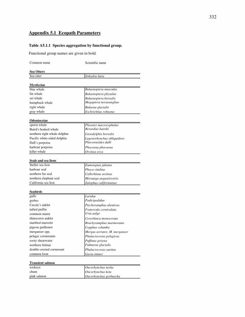
332

Appendix 5.1 Ecopath Parameters

Table A5.1.1 Species aggregation by functional group.

Functional group names are given in bold.

Common name Scientific name

Sea OttersSea otter Enhydra lutra

Mysticetae blue whale Balaenoptera musculusfin whale Balaenoptera physalussei whale Balaenoptera borealishumpback whale Megaptera novaeangliaeright whale Balaena glacialisgray whale Eschrichtius robustus

Odontocetaesperm whale Physeter macrocephalusBaird's beaked whale Berardius bairdiinorthern right whale dolphin Lissodelphis borealisPacific white-sided dolphin Lagenorhynchus obliquidensDall’s porpoise Phocoenoides dalliharbour porpoise Phocoena phocoenakiller whale Orcinus orca

Seals and sea lionsSteller sea lion Eumetopias jubatusharbour seal Phoca vitulinanorthern fur seal Callorhinus ursinusnorthern elephant seal Mirounga angustirostrisCalifornia sea lion Zalophus californianus

Seabirds gulls Laridaegrebes PodicipedidaeCassin’s auklet Ptychoramphus aleuticustufted puffin Fratercula corniculatacommon murre Uria aalgerhinoceros auklet Cerorhinca monoceratamarbled murrelet Brachyramphus marmoratuspigeon guillemot Cepphus columbamerganser spp. Mergus serrator, M. merganserpelagic cormorants Phalacrocorax pelagicussooty shearwater Puffinus griseusnorthern fulmar Fulmarus glacialisdouble-crested cormorant Phalacrocorax aurituscommon loon Gavia immer

Transient salmonsockeye Oncorhynchus nerkachum Oncorhynchus ketapink salmon Oncorhynchus gorbuscha

333

Table A5.1.1 Species aggregation by functional group (cont.)

Common name Scientific name

Coho and chinook salmoncoho salmon Oncorhynchus kisutchchinook salmon Oncorhynchus tshawytscha

Large and small squidcommon squid Loligo opalescens

Ratfish ratfish Hydrolagus collei

Dogfishdogfish Squalus acanthias

Juvenile and adult pollock walleye pollock Theragra chalcogramma

Forage fish and eulachonsandlance Ammodytes hexapteruspilchards Sardinops sagax anchovy Engraulis mordax capelin Mallotus villosus chub mackerel Scomber japonicus shad Alosa sapidissima smelts Osmeridaeeulachon Thaleichthys pacificus

Juvenile and adult herringPacific herring Clupea pallasi

Juvenile and adult Pacific ocean perchPacific Ocean perch Sebastes alutus

Inshore rockfishcopper rockfish Sebastes caurinusquillback rockfish Sebastes maligertiger rockfish Sebastes nigrocinctusChina rockfish Sebastes nebulosusyelloweye rockfish Sebastes rubberrimus

Juvenile and adult piscivorous rockfishrougheye rockfish Sebastes aleutioanusshortraker rockfish Sebastes borealisshortspine thornyhead Sebastolobus altivelis longspine thornyhead Sebastolobus alascanusblack rockfish Sebastes melanopsblue rockfish Sebastes mystinuschillipepper Sebastes goodeidusky rockfish Sebastes ciliatus

334

Table A5.1.1 Species aggregation by functional group (cont.)

Common name Scientific name

Juvenile and adult planktivorous rockfishyellowmouth rockfish Sebastes reedired-stripe rockfish Sebastes prorigerwidow rockfish Sebastes entomelasyellowtail rockfish Sebastes flavidusdarkblotch rockfish Sebastes cremericanary rockfish Sebastes pinnigersplitnose rockfish Sebastes diploproasharpchin rockfish Sebastes zacentrusPuget sound rockfish Sebastes emphaeusbocaccio Sebastes paucispinisshortbelly rockfish Sebastes jordani

Juvenile and adult turbotarrowtooth flounder Atheresthes stomias

Juvenile and adult flatfishrock sole Lepidosetta bilineataEnglish sole Parophyrys vetulusdover sole Microstomas pacificus

Juvenile and adult halibuthalibut Hippoglossus stenolepsis

Juvenile and adult Pacific codPacific cod Gadus macrocephalus

Juvenile and adult sablefish Sablefish Anoplopoma fimbria

Juvenile and adult lingcodlingcod Ophiodon elongatus

Shallow water benthic fishsculpins Cottidaeblennies Blennidaepoachers Agonidaegobies Gobiedaegreenlings Hexagramidaerock greenling Hexagrammos lagocephaluseelpouts Zoarcidaenorthern clingfish Gobiesox maeandricus red irish lords Hemilepidotus hemilepidotus cabezon Scorpaenichthys marmoratus cutthroat trout Oncorhynchus clarki clarki white sturgeon Acipenser transmontanus

335

Table A5.1.1 Species aggregation by functional group (cont.)

Common name Scientific name

Skatesbig skate Raja binoculatalongnose skate Raja rhinastarry skate Raja stellulatablack skate Raja kincaidideep-sea skate Raja abyssicolatope shark Galeorhinus galeus great white shark Carcharodon carcharias broadnose sevengill shark Notorynchus cepedianus bluntnose sixgill shark Hexanchus griseus blue shark Prionace glauca basking shark Cetorhinus maximus diamond stingray Dasyatis dipterura Pelagic stingray Pteroplatytrygon violacea

Large and small crabsDungeness crab Cancer magisterred rock crab Cancer productustanner crab Chionecetes sp.king crab Paralithodes sp.kelp crab Pugettia producta

Commercial shrimp smooth shrimp Pandalus jordanispiny shrimp Pandalus borealis eouspink shrimp Pandalus goniuruscoonstripe shrimp Pandalus danaehumpback shrimp Pandalus hypsinotussidestripe shrimp Pandalopsis disbarprawn Pandalus platycterus

Macrophytesbull kelp Nereocystis leutkeanagiant kelp Macrocystis integrifolia

336

Table A5.1.2 Basic parameters for all periods

# Groups 1750 1900 1950 2000 1750 1900 1950 2000 1750 1900 1950 2000 1750 1900 1950 2000

1 Sea otters 0.0016 0.0001 0.00005 0.0001 0.000 0.000 1.E-06 0.000 0.130 0.130 0.130 0.130 101.50 101.50 101.50 101.50

2 Mysticetae 2.672 1.541 1.607 1.339 0.000 0.028 -0.014 0.004 0.020 0.060 0.040 0.020 8.00 8.00 9.10 9.10

3 Odontocetae 0.066 0.066 0.061 0.061 0.000 0.000 0.001 0.000 0.040 0.040 0.020 0.040 15.50 15.50 15.50 15.50

4 Seals, sea lions 0.080 0.069 0.130 0.258 0.000 0.001 -0.001 0.000 0.060 0.100 0.060 0.060 15.10 15.10 15.10 15.10

5 Seabirds 0.007 0.015 0.007 0.007 0.000 0.000 0.000 0.0000 0.100 0.100 0.100 0.100 105.20 105.20 105.20 105.20

6 Transient salmon 1.008 0.840 0.500 0.208 0.000 0.000 -0.025 -0.028 0.517 2.480 2.480 2.480 3.72 3.72 8.33 8.33

7 Coho salmon 0.096 0.160 0.100 0.024 0.000 0.000 -0.010 0.000 1.157 2.760 2.760 2.760 4.00 10.00 13.80 13.80

8 Chinook salmon 0.144 0.160 0.090 0.036 0.000 0.000 0.000 0.000 0.366 2.160 2.160 2.160 2.82 10.00 10.80 10.80

9 Small squid 1.207 0.795 1.090 1.090 0.000 0.000 -0.109 -0.006 6.023 6.023 6.023 6.023 34.68 34.68 34.67 34.68

10 Squid 0.399 0.259 0.765 0.765 0.000 0.026 -0.038 0.027 6.023 6.023 6.023 6.023 34.68 34.68 34.67 34.68

11 Ratfish 0.262 0.183 0.517 0.517 0.000 0.000 0.003 -0.011 0.199 0.199 0.099 0.099 1.40 1.40 1.40 1.40

12 Dogfish 1.364 0.600 0.417 0.909 0.000 0.030 0.004 -0.060 0.110 0.200 0.150 0.099 3.33 3.33 2.72 2.72

13 Juvenile pollock 1.318 0.926 0.132 0.132 0.000 0.000 0.000 0.002 0.230 0.230 1.060 1.061 5.05 5.05 5.31 5.31

14 Pollock 0.622 0.479 0.359 0.359 0.000 0.000 0.022 0.011 0.153 0.154 0.450 0.263 3.36 3.36 1.17 1.17

15 Forage fish 32.499 24.603 7.600 8.478 0.000 0.000 -0.076 0.130 0.595 0.588 1.743 1.432 6.61 6.61 8.40 8.40

16 Eulachon 7.315 5.033 1.893 1.660 0.000 0.000 0.000 0.049 0.600 0.700 1.432 1.432 6.61 6.61 8.40 8.40

17 Juvenile herring 5.446 3.729 1.317 2.265 0.000 0.000 0.000 0.061 1.173 2.000 2.190 2.190 11.26 11.26 10.95 10.95

18 Adult herring 7.503 2.480 1.001 0.658 0.000 0.000 -0.050 -0.003 0.792 0.900 1.540 0.683 7.51 7.51 5.84 5.84

19 Juvenile POP 0.213 0.153 0.036 0.062 0.000 0.000 -0.004 0.001 0.338 0.338 0.500 0.672 6.12 6.12 3.21 3.21

20 Adult POP 1.404 1.011 1.019 0.561 0.000 0.000 0.000 0.000 0.227 0.227 0.144 0.144 4.08 4.08 2.14 2.14

21 Inshore rockfish 0.096 0.081 0.095 0.100 0.000 0.000 -0.002 0.001 0.182 0.182 0.190 0.190 3.70 5.54 5.69 5.69

22 Juvenile piscivorous rockfish 0.020 0.016 0.008 0.007 0.000 0.000 0.000 0.000 0.261 0.261 0.261 0.261 1.89 1.89 1.89 1.89

23 Adult piscivorous rockfish 0.137 0.119 0.541 0.654 0.000 0.000 0.004 -0.006 0.037 0.037 0.037 0.037 1.26 1.26 1.26 1.26

24 Juvenile planktivorous rockfish 0.207 0.134 0.189 0.136 0.000 0.000 -0.009 0.005 0.261 0.261 0.261 0.261 3.21 3.21 3.21 3.21

25 Adult planktivorous rockfish 2.086 1.286 1.213 1.207 0.000 0.000 0.006 -0.027 0.068 0.068 0.068 0.068 2.14 2.14 2.14 2.14

Biomass accumulation (t•km-2•yr-1)Biomass (t•km-2) Production/Biomass ratio (yr-1) Consumption/Biomass ratio (yr-1)

336

337

Table A5.1.2 Basic parameters for all periods (cont.)

# Groups 1750 1900 1950 2000 1750 1900 1950 2000 1750 1900 1950 2000 1750 1900 1950 2000

26 Juvenile turbot 0.248 0.170 0.218 0.218 0.000 0.000 -0.013 -0.003 0.330 0.330 0.559 0.330 2.17 2.17 2.17 2.17

27 Adult turbot 2.196 1.530 1.530 1.530 0.000 0.000 0.000 -0.050 0.220 0.300 0.220 0.220 1.98 1.98 1.98 1.98

28 Juvenile flatfish 2.583 1.606 0.259 0.259 0.000 0.000 0.000 0.007 0.382 0.382 1.000 1.935 6.31 6.31 6.02 6.02

29 Adult flatfish 1.765 1.014 0.535 0.236 0.000 0.000 -0.080 0.006 0.257 0.257 0.450 0.949 4.21 4.21 4.27 4.27

30 Juvenile halibut 0.445 0.296 0.406 0.628 0.000 0.000 0.000 -0.011 0.099 0.450 0.550 0.600 2.56 2.56 1.46 1.46

31 Adult halibut 1.000 0.608 0.429 0.628 0.000 0.000 0.000 0.000 0.067 0.220 0.450 0.400 1.70 1.70 1.10 1.10

32 Juvenile Pacific cod 0.464 0.307 0.185 0.089 0.000 0.000 -0.009 0.005 0.258 0.258 1.980 1.980 3.43 3.43 7.50 7.50

33 Adult Pacific cod 2.039 1.219 0.348 0.163 0.000 0.000 0.000 -0.020 0.174 0.174 1.320 1.320 2.29 2.29 4.00 4.00

34 Juvenile sablefish 0.180 0.108 0.238 0.119 0.000 0.000 -0.002 0.002 0.273 0.273 0.600 0.600 7.00 7.00 7.00 7.00

35 Adult sablefish 0.191 0.602 0.600 0.269 0.000 0.000 -0.030 0.000 0.183 0.184 0.276 0.276 3.73 3.73 3.73 3.73

36 Juvenile lingcod 0.006 0.005 0.078 0.031 0.000 0.000 -0.016 0.002 0.389 0.389 1.400 1.200 3.94 3.94 3.50 3.30

37 Adult lingcod 0.148 0.119 0.104 0.039 0.000 0.000 0.001 -0.001 0.262 0.300 0.800 0.800 2.80 2.80 3.00 3.30

38 Shallow-water benthic fish 7.506 4.464 0.509 0.509 0.000 0.000 0.025 0.006 0.266 0.266 1.500 1.500 2.10 2.10 5.26 5.26

39 Skates 0.239 0.167 0.300 0.335 0.000 0.000 0.006 -0.003 0.150 0.150 0.310 0.310 1.20 1.20 1.24 1.24

40 Large crabs 0.652 0.388 0.506 0.456 0.000 0.000 -0.051 -0.002 1.500 1.500 1.500 1.500 5.00 5.00 5.00 5.00

41 Small crabs 2.407 1.458 0.599 0.650 0.000 0.000 0.000 -0.010 3.500 3.500 3.500 3.500 14.00 14.00 8.75 14.00

42 Commercial shrimp 0.070 0.047 0.150 0.200 0.000 0.000 0.000 0.002 5.700 5.700 11.480 11.475 22.80 22.80 45.90 45.90

43 Epifaunal invertebrates 42.833 28.604 11.191 13.448 0.000 0.000 -0.224 -0.194 1.448 1.448 1.448 1.448 16.09 16.09 4.05 16.09

44 Infaunal carnivorous invertebrates 8.205 13.245 13.245 13.245 0.000 0.000 0.000 0.270 2.000 2.000 2.000 2.000 22.22 22.22 22.22 22.22

45 Infaunal invertebrate detritivores 39.279 34.305 34.305 34.305 0.000 0.000 0.000 -0.377 1.296 1.300 2.848 1.349 14.40 14.44 14.99 14.99

46 Carnivorous jellyfish 4.625 3.363 3.000 3.000 0.000 0.000 0.000 -0.008 18.00 18.00 18.00 18.00 60.00 60.00 60.00 60.00

47 Euphausiids 22.660 12.606 8.700 8.700 0.000 0.000 0.000 -0.042 6.00 6.00 6.00 6.10 24.82 24.82 24.82 24.82

48 Copepods 13.127 8.671 4.667 4.667 0.000 0.000 0.000 -0.018 27.000 27.000 27.000 27.000 99.00 99.00 90.00 90.00

49 Corals and sponges 1.929 1.929 1.929 1.929 0.000 0.000 0.000 0.000 0.010 0.010 0.010 0.010 2.00 2.00 2.00 2.00

50 Macrophytes 10.560 5.280 5.280 5.280 0.000 0.000 0.000 0.000 5.256 5.256 5.256 5.256 - - - -

51 Phytoplankton 15.406 15.406 15.406 15.406 0.000 0.000 0.000 26.118 178.5 178.5 178.5 178.5 - - - -

52 Discards 0.000 0.001 0.072 0.072 - - - - - - - - - - - -

Production/Biomass ratio (yr-1)Biomass (t•km-2) Biomass accumulation (t•km-2•yr-1) Consumption/Biomass ratio (yr-1)

Biodiversity (Q-90) 7.44 5.84 4.35 3.54

337

338

Table A5.1.3 Diet composition

# Group # Group1 Sea Otters 5 Seabirds

1750 1900 1950 2000 1750 1900 1950 2000Small squid 0.045 0.045 0.045 0.045 Transient salmon 0.054 0.054 0.054 0.054Squid 0.045 0.045 0.045 0.045 Small squid 0.035 0.035 0.035 0.035J. pollock 0.100 0.100 0.100 0.100 Squid 0.055 0.055 0.055 0.055S. benthic fish 0.100 0.100 0.100 0.100 Forage fish 0.243 0.243 0.243 0.243Large crabs 0.010 0.010 0.010 0.010 Eulachon 0.079 0.005 0.079 0.079Small crabs 0.200 0.200 0.200 0.200 J. herring 0.105 0.025 0.105 0.105Epifaunal inv. 0.500 0.500 0.500 0.500 A. herring 0.113 0.083 0.003 0.003

Small crabs 0.041 0.041 0.041 0.0412 Mysticetae Mysticetae Epifaunal inv. 0.041 0.115 0.041 0.041

1750 1900 1950 2000 Carn. jellyfish 0.036 0.036 0.036 0.036Forage fish 0.014 0.372 0.014 0.014 Euphausiids 0.112 0.112 0.112 0.112A. herring 0.101 0.001 0.001 0.001 Copepods 0.046 0.156 0.156 0.156Epifaunal inv. 0.035 0.035 0.035 0.035 Import 0.041 0.041 0.041 0.041Inf. carn. inv. 0.045 0.045 0.045 0.045Inf. det. inv. 0.258 0.300 0.658 0.658 6 Transient salmonEuphausiids 0.420 0.226 0.226 0.226 1750 1900 1950 2000Copepods 0.127 0.021 0.021 0.021 Carn. jellyfish 0.100 0.100 0.100 0.100

Euphausiids 0.150 0.150 0.150 0.1503 Odontocetae Copepods 0.150 0.150 0.150 0.150

1750 1900 1950 2000 Import 0.600 0.600 0.600 0.600Sea otters <0.001 <0.001 <0.001 <0.001Seals, sea lions <0.001 <0.001 <0.001 <0.001 7 Coho salmonTransient salmon 0.041 0.046 0.041 0.041 1750 1900 1950 2000Coho salmon 0.011 0.031 0.011 0.004 Small squid 0.200 0.200 0.200 0.200Chinook salmon 0.005 0.050 0.005 0.004 Squid 0.190 0.175 0.190 0.190Small squid 0.213 0.283 0.213 0.213 Forage fish 0.167 0.167 0.167 0.167Squid 0.213 0.094 0.213 0.213 Eulachon 0.033 0.063 0.033 0.033Ratfish 0.016 0.001 0.026 0.026 A. herring 0.200 0.040 0.040 0.040Forage fish 0.162 0.162 0.162 0.162 J. Pacific cod 0.010 0.005 0.010 0.010Eulachon 0.032 0.032 0.032 0.032 Euphausiids 0.200 0.350 0.360 0.360J. herring 0.026 0.026 0.026 0.056A. herring 0.140 0.065 0.040 0.010 8 Chinook salmonJ. POP 0.005 <0.001 0.005 0.005 1750 1900 1950 2000J. plank. rockfish 0.008 0.008 0.008 0.002 Forage fish 0.353 0.353 0.353 0.433A. plank. rockfish 0.011 0.011 0.011 0.011 Eulachon 0.067 0.067 0.067 0.067J. turbot 0.015 0.015 0.015 0.015 A. herring 0.180 0.180 0.180 0.050A. halibut <0.001 0.015 0.011 0.028 Euphausiids 0.400 0.400 0.400 0.450Large crabs 0.042 0.021 0.021 0.028Euphausiids 0.052 0.132 0.152 0.142 9 Small squidImport 0.008 0.008 0.008 0.008 1750 1900 1950 2000

Forage fish 0.131 0.011 0.081 0.0814 Seals, sea lions Eulachon 0.014 0.001 0.014 0.014

1750 1900 1950 2000 J. herring 0.035 0.001 0.030 0.050Transient salmon 0.100 0.110 0.100 0.010 Carn. jellyfish 0.085 0.142 0.060 0.060Coho salmon 0.002 0.002 0.002 0.001 Euphausiids 0.350 0.430 0.430 0.380Chinook salmon 0.015 0.005 0.015 0.004 Copepods 0.099 0.129 0.099 0.099Small squid 0.045 0.059 0.045 0.045 Detritus 0.286 0.286 0.286 0.316Squid 0.045 0.045 0.045 0.052Dogfish 0.002 0.002 0.002 0.021 10 SquidPollock 0.040 0.040 0.040 0.001 1750 1900 1950 2000Forage fish 0.070 0.070 0.070 0.100 Small squid 0.174 0.174 0.174 0.174J. herring 0.200 0.100 0.200 0.210 Squid 0.001 0.010 0.100 0.100A. herring 0.127 0.179 0.027 0.010 Forage fish 0.187 0.151 0.187 0.187A. POP 0.031 0.021 0.031 0.001 Eulachon 0.025 0.001 0.025 0.025Inshore rockfish 0.002 0.002 0.002 <0.001 Carn. jellyfish 0.060 0.210 0.060 0.060J. pisc. rockfish <0.001 <0.001 <0.001 <0.001 Euphausiids 0.187 0.107 0.107 0.107A. pisc. rockfish 0.001 0.004 0.001 <0.001 Copepods 0.060 0.041 0.041 0.041J. plank. rockfish 0.004 0.001 0.004 <0.001 Detritus 0.307 0.307 0.307 0.307A. plank. rockfish 0.005 0.001 0.005 0.002A. turbot 0.062 0.062 0.062 0.022 11 RatfishA. flatfish 0.049 0.049 0.049 0.004 1750 1900 1950 2000J. halibut 0.010 0.010 0.010 0.061 Forage fish 0.278 0.278 0.278 0.278A. halibut 0.005 0.009 0.005 0.014 Eulachon 0.056 0.056 0.056 0.056A. Pacific cod 0.091 0.061 0.121 0.007 Epifaunal inv. 0.183 0.183 0.183 0.183J. sablefish 0.005 0.005 0.005 0.005 Inf. carn. inv. 0.070 0.070 0.070 0.200A. sablefish 0.001 <0.001 0.052 0.003 Inf. det. inv. 0.080 0.080 0.080 0.080A. lingcod 0.010 0.010 0.010 <0.001 Euphausiids 0.333 0.333 0.333 0.203S. benthic fish 0.010 0.010 0.010 0.036Epifaunal inv. 0.041 0.116 0.060 0.194Inf. carn. inv. 0.028 0.028 0.028 0.195

Period Period

339

Table A5.1.3 Diet composition (cont.)

# Group # Group12 Dogfish 17 J. herring

1750 1900 1950 2000 1750 1900 1950 2000Transient salmon 0.054 0.024 0.054 0.014 Euphausiids 0.100 0.100 0.100 0.100Coho salmon 0.015 0.050 0.015 0.003 Copepods 0.900 0.900 0.900 0.900Chinook salmon 0.001 0.020 0.010 0.004Small squid 0.077 0.125 0.064 0.065 18 A. herringSquid 0.102 0.032 0.102 0.117 1750 1900 1950 2000Ratfish 0.006 0.004 0.006 0.006 Euphausiids 0.900 0.900 0.900 0.900Forage fish 0.072 0.072 0.072 0.072 Copepods 0.100 0.100 0.100 0.100Eulachon 0.015 0.015 0.015 0.015J. herring 0.023 0.023 0.023 0.023 19 J. POPA. herring 0.249 0.010 0.010 0.010 1750 1900 1950 2000J. POP 0.001 0.001 0.001 0.001 Euphausiids 0.200 0.200 0.200 0.200A. POP 0.003 0.003 0.003 0.003 Copepods 0.800 0.800 0.800 0.800J. plank. rockfish <0.001 <0.001 0.003 0.003A. plank. rockfish 0.005 0.012 0.005 0.002 20 A. POPJ. turbot 0.005 0.001 0.005 0.005 1750 1900 1950 2000A. turbot 0.020 0.020 0.020 0.020 Small squid 0.012 0.012 0.012 0.012J. flatfish 0.010 0.010 0.010 0.020 Squid 0.012 0.012 0.012 0.012A. flatfish 0.020 0.020 0.020 0.020 Euphausiids 0.893 0.893 0.893 0.893A. Pacific cod 0.001 0.010 0.010 0.010 Copepods 0.083 0.083 0.083 0.083J. sablefish 0.001 0.001 0.014 0.005A. sablefish 0.001 0.005 0.020 0.004 21 Inshore rockfishS. benthic fish 0.017 0.017 0.017 0.062 1750 1900 1950 2000Large crabs 0.037 0.017 0.037 0.037 Forage fish 0.150 0.060 0.060 0.060Small crabs 0.026 0.026 0.026 0.026 Eulachon 0.012 0.012 0.012 0.012Epifaunal inv. 0.092 0.062 0.052 0.052 J. herring 0.300 0.100 0.300 0.330Inf. carn. inv. 0.019 0.024 0.019 0.019 A. herring 0.050 0.250 0.050 0.020Inf. det. inv. 0.008 0.008 0.008 0.008 S. benthic fish 0.045 0.065 0.045 0.045Carn. jellyfish 0.029 0.029 0.029 0.029 Large crabs 0.005 0.005 0.005 0.005Euphausiids 0.020 0.160 0.149 0.139 Small crabs 0.107 0.107 0.107 0.107Copepods 0.020 0.070 0.130 0.126 Comm. shrimp 0.005 0.075 0.095 0.095Detritus 0.051 0.129 0.051 0.080 Epifaunal inv. 0.050 0.050 0.050 0.050

Inf. carn. inv. 0.124 0.124 0.124 0.12413 J. pollock Euphausiids 0.152 0.152 0.152 0.152

1750 1900 1950 2000J. pollock 0.015 0.001 0.025 0.025 22 J. pisc. rockfishForage fish 0.072 0.096 0.072 0.072 1750 1900 1950 2000Eulachon 0.014 0.014 0.014 0.014 Small crabs 0.100 0.100 0.100 0.100Epifaunal inv. 0.081 0.071 0.071 0.071 Comm. shrimp 0.100 0.100 0.100 0.100Inf. carn. inv. 0.020 0.020 0.020 0.020 Epifaunal inv. 0.100 0.100 0.100 0.100Euphausiids 0.369 0.369 0.369 0.300 Euphausiids 0.400 0.400 0.400 0.400Copepods 0.429 0.429 0.429 0.498 Copepods 0.300 0.300 0.300 0.300

14 Pollock 23 A. pisc. rockfish1750 1900 1950 2000 1750 1900 1950 2000

Small squid 0.016 0.016 0.016 0.016 Small squid 0.070 0.070 0.070 0.070Squid 0.016 0.016 0.016 0.016 Squid 0.070 0.070 0.070 0.080J. pollock 0.050 0.001 0.100 0.100 Forage fish 0.027 0.027 0.027 0.027Forage fish 0.198 0.288 0.198 0.198 Eulachon 0.005 0.005 0.005 0.005Eulachon 0.028 0.037 0.028 0.028 J. POP 0.005 0.005 0.005 0.020Epifaunal inv. 0.072 0.022 0.022 0.022 J. pisc. rockfish 0.002 0.002 0.002 <0.001Euphausiids 0.461 0.461 0.461 0.461 Skates 0.068 0.068 0.068 0.028Copepods 0.160 0.160 0.160 0.160 Small crabs 0.130 0.130 0.130 0.130

Epifaunal inv. 0.254 0.254 0.254 0.25415 Forage fish Inf. det. inv. 0.040 0.040 0.040 0.150

1750 1900 1950 2000 Carn. jellyfish 0.038 0.038 0.038 0.038Epifaunal inv. 0.100 0.100 0.100 0.100 Euphausiids 0.196 0.196 0.196 0.086Carn. jellyfish 0.270 0.205 0.270 0.270 Detritus 0.096 0.096 0.096 0.112Euphausiids 0.080 0.115 0.080 0.200Copepods 0.500 0.520 0.500 0.380 24 J. plank. rockfishDetritus 0.050 0.060 0.050 0.050 1750 1900 1950 2000

Euphausiids 0.500 0.500 0.500 0.50016 Eulachon Copepods 0.500 0.500 0.500 0.500

1750 1900 1950 2000Epifaunal inv. 0.100 0.100 0.100 0.100Carn. jellyfish 0.200 0.200 0.200 0.200Euphausiids 0.100 0.100 0.100 0.100Copepods 0.600 0.600 0.600 0.600

Period Period

340

Table A5.1.3 Diet composition (cont.)

# Group # Group25 A. plank. rockfish 30 J. halibut

1750 1900 1950 2000 1750 1900 1950 2000Small squid 0.101 0.101 0.101 0.101 Small squid 0.032 0.032 0.032 0.032Squid 0.101 0.061 0.101 0.101 Squid 0.032 0.032 0.032 0.032Forage fish 0.028 0.028 0.028 0.028 Forage fish 0.055 0.055 0.055 0.055Eulachon 0.006 0.006 0.006 0.006 Eulachon 0.011 0.011 0.011 0.011J. herring 0.109 0.109 0.109 0.109 J. herring 0.050 0.050 0.050 0.050Carn. jellyfish 0.006 0.006 0.006 0.006 J. POP 0.003 0.003 0.003 0.003Euphausiids 0.574 0.574 0.574 0.574 J. turbot 0.001 <0.001 0.100 0.010Copepods 0.075 0.115 0.075 0.075 J. flatfish 0.020 0.020 0.020 0.020

J. Pacific cod 0.008 0.008 0.008 0.00826 J. turbot S. benthic fish 0.105 0.055 0.055 0.055

1750 1900 1950 2000 Large crabs 0.200 0.280 0.200 0.240Small squid 0.087 0.087 0.087 0.087 Small crabs 0.309 0.300 0.300 0.300Squid 0.087 0.087 0.087 0.087 Comm. shrimp 0.001 0.060 0.060 0.060J. pollock 0.030 0.030 0.030 0.030 Epifaunal inv. 0.050 0.070 0.050 0.050Pollock 0.070 0.070 0.070 0.070 Detritus 0.124 0.025 0.025 0.075Forage fish 0.111 0.111 0.111 0.111Eulachon 0.022 0.022 0.022 0.022 31 A. halibutJ. herring 0.150 0.150 0.150 0.180 1750 1900 1950 2000A. herring 0.067 0.048 0.048 0.018 Small squid 0.064 0.064 0.064 0.064Inshore rockfish 0.007 0.007 0.007 0.007 Squid 0.064 0.064 0.064 0.064J. pisc. rockfish 0.001 <0.001 0.001 0.001 Forage fish 0.014 0.014 0.014 0.014J. plank. rockfish 0.017 0.007 0.017 0.017 Eulachon 0.003 0.003 0.003 0.003J. flatfish 0.033 0.044 0.033 0.033 A. herring 0.072 0.020 0.020 0.020Small crabs 0.100 0.100 0.100 0.100 A. POP 0.020 0.020 0.020 0.005Comm. shrimp 0.001 0.100 0.100 0.100 J. plank. rockfish 0.005 0.005 0.005 0.005Epifaunal inv. 0.113 0.033 0.033 0.033 A. plank. rockfish 0.001 0.001 0.001 0.001Euphausiids 0.074 0.074 0.074 0.074 A. turbot 0.074 0.074 0.074 0.090Detritus 0.030 0.030 0.030 0.030 A. flatfish 0.123 0.053 0.123 0.100

J. halibut 0.001 0.001 0.080 0.08027 A. turbot A. Pacific cod 0.005 0.055 0.100 0.050

1750 1900 1950 2000 A. lingcod <0.001 0.005 0.040 0.005Small squid 0.161 0.221 0.161 0.161 S. benthic fish 0.095 - - -Squid 0.161 0.101 0.161 0.161 Skates 0.001 0.003 0.053 0.053J. pollock 0.009 0.009 0.009 0.009 Large crabs 0.155 0.155 0.155 0.155Pollock 0.001 0.001 0.001 0.001 Small crabs 0.110 0.189 0.110 0.125Forage fish 0.107 0.107 0.107 0.107 Epifaunal inv. 0.159 0.110 0.040 0.090Eulachon 0.051 0.051 0.051 0.051 Detritus 0.035 0.165 0.035 0.077J. herring 0.099 0.001 0.099 0.099A. herring 0.050 0.010 0.010 <0.001 32 J. Pacific codJ. POP 0.001 0.001 0.001 0.001 1750 1900 1950 2000A. POP 0.015 0.015 0.015 0.001 Small crabs 0.027 0.027 0.027 0.027J. turbot 0.001 0.001 0.001 0.001 Epifaunal inv. 0.210 0.210 0.210 0.210J. flatfish 0.005 0.005 0.005 0.005 Inf. carn. inv. 0.079 0.079 0.079 0.079A. flatfish 0.005 0.005 0.005 0.005 Inf. det. inv. 0.363 0.363 0.363 0.363A. Pacific cod 0.003 0.003 0.003 0.003 Euphausiids 0.115 0.115 0.115 0.115J. lingcod <0.001 <0.001 0.020 0.002 Copepods 0.057 0.057 0.057 0.057S. benthic fish 0.079 0.079 0.078 0.088 Detritus 0.149 0.149 0.149 0.149Large crabs 0.034 0.015 0.015 0.015Comm. shrimp 0.050 0.001 0.050 0.050 33 A. Pacific codEpifaunal inv. 0.024 0.024 0.024 0.028 1750 1900 1950 2000Euphausiids 0.050 0.118 0.050 0.050 Forage fish 0.393 0.393 0.393 0.393Detritus 0.095 0.233 0.135 0.163 Eulachon 0.079 0.009 0.079 0.079

J. herring 0.009 0.009 0.009 0.03028 J. flatfish A. herring 0.112 0.100 0.103 0.023

1750 1900 1950 2000 J. turbot 0.001 0.001 0.001 0.001Forage fish 0.050 0.050 0.050 0.050 A. turbot 0.009 0.001 0.059 0.059Eulachon 0.010 0.010 0.010 0.010 J. halibut <0.001 0.020 0.020 0.020Small crabs 0.068 0.068 0.068 0.068 J. Pacific cod 0.001 0.010 0.001 0.001Epifaunal inv. 0.046 0.046 0.046 0.046 A. Pacific cod 0.020 0.001 0.020 0.020Inf. carn. inv. 0.373 0.373 0.373 0.373 J. sablefish 0.005 0.001 0.005 0.005Inf. det. inv. 0.453 0.453 0.453 0.453 J. lingcod <0.001 <0.001 0.023 0.013

A. lingcod 0.005 0.001 0.005 0.00129 A. flatfish S. benthic fish 0.175 0.082 0.122 0.122

1750 1900 1950 2000 Skates 0.001 0.003 0.010 0.010Forage fish 0.154 0.154 0.154 0.154 Epifaunal inv. 0.064 0.053 0.024 0.074Eulachon 0.031 0.031 0.031 0.031 Inf. carn. inv. 0.070 0.079 0.070 0.070J. lingcod <0.001 <0.001 0.005 0.005 Detritus 0.056 0.237 0.056 0.079Small crabs 0.038 0.039 0.038 0.038Epifaunal inv. 0.052 0.051 0.051 0.051Inf. carn. inv. 0.272 0.272 0.272 0.272Inf. det. inv. 0.445 0.445 0.445 0.445Euphausiids 0.008 0.008 0.004 0.004

Period Period

341

Table A5.1.3 Diet composition (cont.)

# Group # Group34 J. sablefish 38 Shallowwater benthic fish

1750 1900 1950 2000 1750 1900 1950 2000Small squid 0.009 0.009 0.009 0.009 Small squid <0.001 <0.001 <0.001 <0.001Squid 0.009 0.009 0.009 0.009 Squid <0.001 <0.001 <0.001 <0.001Forage fish 0.025 <0.001 0.025 0.025 Forage fish 0.198 0.198 0.198 0.198Eulachon 0.005 0.005 0.005 0.005 Eulachon 0.053 0.001 0.040 0.040J. herring 0.020 0.020 0.020 - A. lingcod <0.001 <0.001 0.010 <0.001A. herring 0.010 0.035 0.010 0.010 S. benthic fish 0.010 0.010 0.010 0.010A. POP 0.001 0.001 0.001 0.001 Small crabs 0.333 0.283 0.333 0.333J. plank. rockfish 0.001 0.001 0.001 0.001 Comm. shrimp 0.001 0.004 0.004 0.004J. turbot 0.010 <0.001 0.010 0.010 Epifaunal inv. 0.037 0.037 0.037 0.037S. benthic fish 0.049 - - - Inf. carn. inv. 0.181 0.181 0.181 0.181Comm. shrimp 0.001 0.001 0.050 0.050 Inf. det. inv. 0.096 0.096 0.096 0.096Epifaunal inv. 0.020 0.079 0.020 0.020 Euphausiids 0.025 0.073 0.025 0.025Carn. jellyfish 0.010 0.010 0.010 0.010 Copepods 0.048 0.048 0.048 0.048Euphausiids 0.830 0.830 0.830 0.850 Detritus 0.017 0.068 0.017 0.027

35 A. sablefish 39 Skates1750 1900 1950 2000 1750 1900 1950 2000

Small squid 0.025 0.025 0.025 0.025 Dogfish 0.030 0.001 0.001 0.001Squid 0.025 0.025 0.025 0.025 Forage fish 0.238 0.238 0.238 0.238J. pollock 0.010 0.010 0.010 0.010 Eulachon 0.048 0.048 0.048 0.048Forage fish 0.313 0.313 0.313 0.313 A. halibut 0.060 0.060 0.060 0.060Eulachon 0.067 0.067 0.067 0.067 S. benthic fish 0.019 0.019 0.019 0.019A. herring 0.250 0.010 0.010 0.010 Large crabs 0.154 0.140 0.140 0.140J. plank. rockfish 0.004 0.004 0.004 0.004 Small crabs 0.259 0.180 0.180 0.080J. turbot 0.010 0.010 0.010 0.010 Comm. shrimp 0.001 0.100 0.100 0.100J. flatfish 0.010 0.010 0.010 0.010 Epifaunal inv. 0.090 0.090 0.090 0.090J. halibut 0.005 0.005 0.005 0.005 Inf. carn. inv. 0.050 0.050 0.050 0.150J. Pacific cod 0.005 0.005 0.005 0.005 Inf. det. inv. 0.050 0.050 0.050 0.050J. sablefish 0.001 0.001 0.030 0.030 Detritus 0.001 0.024 0.024 0.024Small crabs 0.040 0.011 0.011 0.011Comm. shrimp 0.105 0.015 0.105 0.105 40 Large crabsEpifaunal inv. 0.010 0.100 0.010 0.010 1750 1900 1950 2000Carn. jellyfish 0.100 0.340 0.340 0.340 J. flatfish 0.024 0.010 0.010 0.010Detritus 0.020 0.049 0.020 0.020 Small crabs 0.100 0.100 0.100 0.100

Comm. shrimp 0.001 0.015 0.015 0.01536 J. lingcod Epifaunal inv. 0.435 0.435 0.435 0.395

1750 1900 1950 2000 Inf. carn. inv. 0.065 0.065 0.065 0.105Forage fish 0.227 0.227 0.227 0.227 Inf. det. inv. 0.075 0.075 0.075 0.075Eulachon 0.063 0.063 0.063 0.063 Detritus 0.300 0.300 0.300 0.300J. herring 0.170 0.120 0.170 0.170J. flatfish 0.070 0.120 0.070 0.070 41 Small crabsJ. halibut 0.160 0.080 0.160 0.160 1750 1900 1950 2000J. Pacific cod 0.100 0.100 0.100 0.100 Epifaunal inv. 0.800 0.800 0.800 0.600Small crabs 0.150 0.150 0.150 0.150 Inf. carn. inv. 0.100 0.100 0.100 0.300Comm. shrimp 0.050 0.050 0.050 0.050 Inf. det. inv. 0.100 0.100 0.100 0.100Detritus 0.010 0.090 0.010 0.010

42 Comm. shrimp37 A. lingcod 1750 1900 1950 2000

1750 1900 1950 2000 Inf. det. inv. 0.100 0.100 0.100 0.100J. pollock 0.020 0.020 0.020 0.020 Euphausiids 0.300 0.300 0.300 0.300Forage fish 0.117 0.143 0.117 0.117 Copepods 0.200 0.200 0.200 0.200Eulachon 0.063 0.063 0.063 0.063 Detritus 0.400 0.400 0.400 0.400J. herring 0.050 0.050 0.050 0.099A. herring 0.309 0.069 0.069 0.020 43 Epifaunal inv.J. POP 0.021 <0.001 0.021 0.021 1750 1900 1950 2000Inshore rockfish 0.010 0.010 0.010 0.010 Inf. det. inv. 0.010 0.005 0.200 0.060J. pisc. rockfish 0.001 <0.001 0.001 0.001 Macrophytes 0.041 0.010 0.001 0.001J. plank. rockfish 0.020 <0.001 0.020 0.020 Detritus 0.949 0.985 0.799 0.939J. turbot 0.020 0.001 0.020 0.020J. flatfish 0.011 0.032 0.011 0.111 44 Inf. carn. inv.J. halibut 0.001 0.050 0.050 0.050 1750 1900 1950 2000A. halibut 0.005 0.150 0.150 0.050 Inf. det. inv. 0.100 0.075 0.250 0.060J. Pacific cod 0.109 0.050 0.011 0.011 Detritus 0.900 0.925 0.750 0.940A. Pacific cod 0.070 0.020 0.070 0.070J. lingcod <0.001 0.001 0.050 0.050 46 Carn. jellyfishA. lingcod <0.001 0.010 0.010 0.010 1750 1900 1950 2000Comm. shrimp 0.001 0.060 0.100 0.100 J. herring 0.011 0.001 0.001 0.001Epifaunal inv. 0.115 0.141 0.100 0.100 Carn. jellyfish 0.010 0.060 0.060 0.060Detritus 0.057 0.130 0.057 0.057 Euphausiids 0.050 0.010 0.010 0.010

Copepods 0.080 0.080 0.080 0.080Detritus 0.849 0.849 0.849 0.849

Period Period

342

Table A5.1.4 Landings data for all time periods (t·km-2)

1750 landings# Group

Sea otters Halibut H+L Salmon seine Eulachon Herring Whaling Cod, etc. Invertebrates Total1 Sea otters <0.001 <0.0012 Mysticetae <0.001 <0.0014 Seals, sea lions <0.001 <0.0016 Transient salmon 0.046 0.0467 Coho salmon 0.023 0.0238 Chinook salmon 0.023 0.023

16 Eulachon 0.043 0.04318 A. herring 0.002 0.00230 J. halibut 0.010 0.01031 A. halibut 0.010 0.01033 A. Pacific cod 0.001 0.00137 A. lingcod <0.001 <0.00143 Epifaunal inv. <0.001 <0.00145 Inf. det. inv. <0.001 <0.001

Sum <0.001 0.01944 0.09149 0.04286 0.00162 <0.001 0.0015 0.001 0.15871

1900 landings# Group

Herring Hook + Line Salmon seine Eulachon Whaling Longline FN - Halibut FN Inverts. Total2 Mysticetae 0.061 0.0613 Odontocetae 0.002 0.0024 Seals, sea lions 0.005 0.0056 Transient salmon 0.126 0.1267 Coho salmon 0.012 0.0128 Chinook salmon 0.020 0.020

12 Dogfish 0.040 0.04016 Eulachon 0.043 0.04318 A. herring <0.001 0.00131 A. halibut 0.014 0.005 0.01833 A. Pacific cod 0.001 0.00137 A. lingcod 0.005 0.00543 Epifaunal inv. <0.001 <0.00145 Inf. det. inv. <0.001 <0.001

Sum 0.001 0.019 0.186 0.043 0.069 0.040 0.006 <0.001 0.336

Fleet

Fleet

342

343

Table A5.1.4 Landings data for all time periods (cont.)

1950 landings# Group

GF trawl Sablefish Herr. gillnet GF H+L Salm. gillnet Crab trap Prawn trap Other Inv. Halibut H+L Salm. troll Salm. seine Salm. Freezer Herr. seine Shrimp trawl Eulachon Longline Seine nets Rec. Sea lion cull Total2 Mysticetae 0.069 0.0694 Seals, sea lions 0.004 0.0046 Transient salmon 0.271 0.007 0.312 0.007 <0.001 0.5987 Coho salmon 0.046 0.033 0.027 0.033 0.001 0.1408 Chinook salmon 0.014 0.016 0.003 0.016 0.005 0.054

12 Dogfish 0.032 0.03214 Pollock 0.007 0.00715 Forage fish 0.006 0.00616 Eulachon <0.001 <0.00118 A. herring <0.001 0.461 0.461 0.92220 A. POP 0.002 <0.001 <0.001 0.00321 Inshore rockfish 0.002 0.002 <0.001 0.00423 A. pisc. Rockfish 0.010 0.001 <0.001 0.01125 A. plank. rockfish 0.036 <0.001 0.03627 A. turbot 0.004 0.00429 A. flatfish 0.073 0.07330 J. halibut <0.001 <0.00131 A. halibut 0.071 <0.001 0.001 0.07233 A. Pacific cod 0.019 <0.001 0.033 0.05235 A. sablefish 0.002 0.004 0.00636 J. lingcod 0.003 0.00337 A. lingcod 0.004 0.001 <0.001 0.00639 Skates <0.001 <0.001 <0.00140 Large crabs <0.001 0.005 <0.001 0.00542 Comm. shrimp 0.001 <0.001 <0.001 0.00243 Epifaunal inv. 0.029 <0.001 0.029

Sum 0.227 0.004 <0.001 0.004 0.332 0.005 0.001 0.029 0.003 0.056 0.342 0.056 0.461 <0.001 <0.001 0.033 0.500 0.012 0.073 2.138

2000 landings# Group

GF trawl Sablefish Herr. gillnet GF H+L Salm. gillnet Crab trap Prawn trap Other Inv. Halibut H+L Salm. troll Salm. seine Salm. Freezer Herr. seine Shrimp trawl Eulachon Longline Rec. Total6 Transient salmon 0.150 0.003 0.067 0.010 <0.001 0.2307 Coho salmon 0.045 <0.001 <0.001 0.001 0.002 0.0508 Chinook salmon 0.036 <0.001 <0.001 0.009 0.046

11 Ratfish <0.001 <0.00112 Dogfish <0.001 0.030 0.03114 Pollock 0.007 0.00716 Eulachon 0.003 0.00318 A. herring 0.155 0.087 0.24120 A. POP 0.060 0.06021 Inshore rockfish <0.001 0.003 0.004 0.003 0.01023 A. pisc. Rockfish 0.023 0.002 0.002 0.02725 A. plank. rockfish 0.077 0.07727 A. turbot 0.067 0.06729 A. flatfish 0.058 0.05830 J. halibut <0.001 0.028 0.001 0.02931 A. halibut <0.001 0.031 0.016 0.04632 J. Pacific cod <0.00133 A. Pacific cod 0.051 0.003 0.05435 A. sablefish <0.001 0.038 0.002 0.04136 J. lingcod 0.002 0.00237 A. lingcod 0.019 0.001 0.02039 Skates 0.029 0.02940 Large crabs 0.026 0.001 0.02742 Comm. shrimp 0.004 0.033 <0.001 0.03743 Epifaunal inv. <0.001 0.078 <0.001 0.078

Sum 0.391 0.038 0.155 0.005 0.231 0.026 0.004 0.078 0.067 0.004 0.067 0.012 0.087 0.033 0.003 0.030 0.038 1.267

Fleet

Fleet

343

344

Table A5.1.5 Discard data for 1950 and 2000 (t·km-2)

1950 discards# Group

GF trawl Salm. gillnet Salm. seine Shrimp trawl Total4 Seals, sea lions <0.001 <0.001

11 Ratfish 0.010 0.01012 Dogfish 0.009 0.010 0.01914 Pollock 0.002 0.002 0.00420 A. POP 0.002 0.00225 A. plank. rockfish 0.005 0.001 0.00631 A. halibut 0.003 0.00333 A. Pacific cod 0.002 0.00235 A. sablefish 0.003 0.00337 A. lingcod 0.001 0.00139 Skates <0.001 <0.00143 Epifaunal inv. 0.002 0.00246 Carn. jellyfish <0.001 <0.001

Sum 0.039 0.011 <0.001 0.002 0.052

2000 discards# Group

GF trawl Salm. gillnet Halibut H+L Shrimp trawl Total4 Seals, sea lions <0.001 <0.0017 Coho salmon <0.001 <0.0018 Chinook salmon <0.001 <0.001

10 Squid <0.001 <0.00111 Ratfish 0.010 0.001 0.01112 Dogfish 0.009 0.008 <0.001 0.01814 Pollock 0.002 <0.001 0.00315 Forage fish <0.001 <0.00116 Eulachon <0.001 0.001 0.00118 A. herring <0.001 <0.00120 A. POP 0.002 0.00221 Inshore rockfish <0.001 <0.00123 A. pisc. Rockfish <0.001 <0.00125 A. plank. rockfish 0.005 0.001 0.00627 A. turbot 0.026 0.002 <0.001 0.02829 A. flatfish 0.002 0.00230 J. halibut 0.003 0.00331 A. halibut 0.003 0.00333 A. Pacific cod 0.002 0.00235 A. sablefish 0.003 0.00337 A. lingcod 0.001 0.00138 S. benthic fish <0.001 0.001 0.00139 Skates 0.007 <0.001 0.00740 Large crabs <0.001 <0.00141 Small crabs <0.001 <0.00142 Comm. shrimp <0.001 <0.00143 Epifaunal inv. 0.002 0.00245 Inf. det. inv. <0.001 <0.00146 Carn. jellyfish <0.001 <0.001 <0.00149 Corals and sponges 0.001 0.001 0.002

Sum 0.078 0.010 0.002 0.009 0.098

Fleet

Fleet

345

Table A5.1.6 Market prices ($·kg-1) for 2000 BC fleet

Groundfish trawl Salmon trollRatfish 3.32 Transient salmon 8Dogfish 0.55 Coho salmon 2Pollock 0.49 Chinook salmon 4.5A. POP 1.28Inshore rockfish 0.95 Salmon seineA. pisc. rockfish 0.95 Transient salmon 2.62A. plank. rockfish 0.95 Coho salmon 1.52A. turbot 1.28A. flatfish 1.16 Salmon troll freezerA. Pacific cod 1.07 Transient salmon 6A. lingcod 0.95 Coho salmon 1.75Skates 0.8 Chinook salmon 4Epifaunal inv. 2.26

Herring seineSablefish A. herring 0.46A. sablefish 6.17

Shrimp trawlHerring gillnet Comm. shrimp 4.88A. herring 0.46

EulachonHalibut hook & line Eulachon 3.33Inshore rockfish 13A. pisc. rockfish 13 Recreational

Transient salmon 2.62Salmon gillnet Coho salmon 1.52Transient salmon 2.62 Chinook salmon 3.92Coho salmon 1.52 Inshore rockfish 1.28Chinook salmon 3.92 A. pisc. rockfish 1.28

J. halibut 0Crab traps A. halibut 4.06Large crabs 7.21 J. lingcod 1.69

A. lingcod 1.69Shrimp & prawn traps Large crabs 7.21Commercial shrimp 9.05 Comm. shrimp 4.88

Epifaunal inv. 2.26Other invertebratesEpifaunal inv. 2.26

Halibut hook & lineInshore rockfish 13J. halibut 6A. halibut 6A. Pacific cod 1.07A. sablefish 6.17

346

Appendix 5.2 Ecosim Parameters

Table A5.2.1 Juvenile/adult stage transition parameters for all models

HerringPisc.

RockfishPlank.

RockfishT urbot Flatfish Halibut Sablefish Lingcod Pollock POP

Pacific cod

Min. time as juv. (rel. to orig. setting)

1 1 1 1 1 1 1 1 1 1 1

Max. time as juv. (rel. to orig. setting)

1.0001 1.0001 1.0001 1.0001 1.0001 1.0001 1.0001 1.0001 1.0001 1.0001 1.0001

Recruitment power parameter

1 1 1 1 1 1 1 1 1 1 1

Age (year) at transition to adult group (tk)

2.1 16.0 11.0 4.5 4.5 10.0 4.5 4.0 2.3 16.0 2.3

Wavg / Wk (Av. adult weight / weight at transition)

2.00 2.70 1.92 2.00 2.00 1.36 1.88 3.68 3.60 2.70 1.73

K of the VBGF (•yr-1) 0.470 0.050 0.125 0.243 0.243 0.080 0.300 0.263 0.373 0.880 0.270

Base fraction of food intake used for reproduct ion

0.3 0.3 0.3 0.3 0.3 0.3 0.3 0.3 0.3 0.3 0.3

Fraction of increase in food intake used for growth

0.8 0.8 0.8 0.8 0.8 0.8 0.8 0.8 0.8 0.8 0.8

347

Table A5.2.2 Feeding parameters for 1950

Max. rel. feeding time

Feeding time adjust rate [0,1]

Fraction of 'other' mortality sens. to

changes in feeding time

Predator effect on feeding time

[0,1]

Density-dependent

catchability: Qmax/Q0 Qbmax/QB0

Sea otters 2 0.5 0 0 1 1000Mysticetae 1 0.2 1 0 1 1000Odontocetae 2 0.5 1 0 1 1000Seals, sea lions 2 1 1 0 1 1000Seabirds 2 0.5 1 0 1 1000Transient salmon 2 0.5 1 0 1 1000Coho salmon 2 0.5 1 0 1 1000Chinook salmon 2 0.5 1 0 1 1000Small squid 2 0.5 1 0 1 1000Squid 2 0.5 1 0 1 1000Ratfish 2 0.5 1 0 1 1000Dogfish 1.4 0.5 1 0 1 1000J. pollock 2 0.5 1 0 1 1000Pollock 2 0.5 1 0 1 1000Forage fish 2 0.5 1 0 1 1000Eulachon 2 0.5 1 0 1 1000J. herring 2 0.9 0 0 1 1000A. herring 2 0.5 1 0 1 1000J. POP 2 0.5 1 0 1 1000A. POP 2 0.5 1 0 1 1000Inshore rockfish 2 0.5 1 0 1 1000J. pisc. rockfish 2 0.5 1 0 1 1000A. pisc. rockfish 2 0.5 1 0 1 1000J. plank. rockfish 2 0.5 1 0 1 1000A. plank. rockfish 2 0.5 1 0 1 1000J. turbot 2 0.5 1 0 1 1000A. turbot 2 0.5 1 0 1 1000J. flatfish 2 0.3 1 0 1 1000A. flatfish 2 0.1 1 0 1 1000J. halibut 2 0.1 1 0 1 1000A. halibut 2 0.1 1 0 1 1000J. Pacific cod 2 0.6 1 0 1 1000A. Pacific cod 1.1 0.1 1 0 1 1000J. sablefish 2 0.05 1 0 1 1000A. sablefish 2 0.05 1 0 1 1000J. lingcod 2 0 1 0 1 1000A. lingcod 2 0.5 1 0 1 1000S. benthic fish 1 0.5 1 0 1 1000Skates 2 0.5 1 0 1 1000Large crabs 2 0 1 0 1 1000Small crabs 2 0 1 0 1 1000Comm. shrimp 2 0 1 0 1 1000Epifaunal inv. 2 0 1 0 1 1000Inf. carn. inv. 2 0 1 0 1 1000Inf. det. inv. 2 0 1 0 1 1000Carn. jellyfish 2 0 1 0 1 1000Euphausiids 2 0 1 0 1 1000Copepods 2 0 1 0 1 1000Corals and sponges 2 0 1 0 1 1000

348

Table A5.2.3 Trophic flow parameters for 1950

Prey 1 2 3 4 5 6 7 8 9 10 11 12 13 14 15 16 171 Sea otters 1

2 Mysticetae

3 Odontocetae

4 Seals, sea lions 1

5 Seabirds

6 Transient salmon 1 1 1 1

7 Coho salmon 1 1021 1

8 Chinook salmon 1 1021 1

9 Small squid 1014 1 109 365 1 106 1 1

10 Squid 1014 1 1012 1 1 108 1 1019

11 Ratfish 1 1

12 Dogfish 1021

13 J. pollock 108 483 32068

14 Pollock 1

15 Forage fish 719 1 1014 15300 1 1 109 105 1021 1 1 50.9

16 Eulachon 1 1 1 1 38158 105 1021 1 1 14260

17 J. herring 1 1 813 29521 1

18 A. herring 8902 1 1 1 1 1 1

19 J. POP 1 1

20 A. POP 1 1

21 Inshore rockfish 1

22 J. pisc. Rockfish 418

23 A. pisc. Rockfish 1

24 J. plank. rockfish 1 47 1

25 A. plank. rockfish 1 1012 1

26 J. turbot 1 1

27 A. turbot 1021 1

28 J. flatfish 1

29 A. flatfish 1 1

30 J. halibut 1

31 A. halibut 1 1

32 J. Pacific cod 1

33 A. Pacific cod 1021 1

34 J. sablefish 1305 1

35 A. sablefish 3.18 1

36 J. lingcod

37 A. lingcod 1015

38 S. benthic fish 1011 30 1

39 Skates

40 Large crabs 106 1 1

41 Small crabs 106 85.2 1

42 Comm. shrimp

43 Epifaunal inv. 1 3737 1 1266 1 1 20429 1014 1 1873

44 Inf. carn. inv. 28457 1 1 1 1.03

45 Inf. det. inv. 31930 1 1

46 Carn. jellyfish 1 1 501 106 1 1 2.7

47 Euphausiids 1249 1 105 1 1 1 106 6857 1 1 1 1 1 1 1.91

48 Copepods 9053 277 1 1 105 1 1 1 1 1 2.98

49 Corals and sponges

50 Macrophytes

51 Phytoplankton

52 Discards 1 3354

53 Detritus 1 107 1 1

Predator

349

Table A5.2.3 Trophic flow parameters for 1950 (cont.)

Prey 18 19 20 21 22 23 24 25 26 27 28 29 30 31 32 33 341 Sea otters

2 Mysticetae

3 Odontocetae

4 Seals, sea lions

5 Seabirds

6 Transient salmon

7 Coho salmon

8 Chinook salmon

9 Small squid 1 1 1021 1012 1021 1 1 1

10 Squid 1 1021 1021 1021 1021 1 1 1

11 Ratfish

12 Dogfish

13 J. pollock 1013 1.01

14 Pollock 1012 1021

15 Forage fish 3292 1021 1021 1014 1021 1 1 1 1 1 1

16 Eulachon 1021 1021 1021 1012 1021 249 1 1 1 1 1

17 J. herring 1 1021 1012 1021 1 1 1

18 A. herring 1 1012 1021 1 1 1

19 J. POP 1 1021 1

20 A. POP 1021 1 1

21 Inshore rockfish 16.2

22 J. pisc. Rockfish 1092 1012

23 A. pisc. Rockfish

24 J. plank. rockfish 1012 1 1

25 A. plank. rockfish 1

26 J. turbot 1021 1 1 1

27 A. turbot 1 1

28 J. flatfish 1012 1021 1

29 A. flatfish 1021 1

30 J. halibut 1 1021

31 A. halibut

32 J. Pacific cod 1 1

33 A. Pacific cod 1021 1021 1

34 J. sablefish 1

35 A. sablefish

36 J. lingcod 2 1 1

37 A. lingcod 1 1

38 S. benthic fish 1 1021 1 1

39 Skates 1021 1 1

40 Large crabs 1.01 1021 1 1

41 Small crabs 6545 105 1021 1012 1.1 1 1 1 1

42 Comm. shrimp 438 965 1012 1021 1 46.8

43 Epifaunal inv. 1 105 1021 1012 1021 1 1010 22686 1 76.3 1 1

44 Inf. carn. inv. 1 1021 1018 1 1

45 Inf. det. inv. 1021 457 1 1

46 Carn. jellyfish 1021 1021 1

47 Euphausiids 1.29 1 1 1.08 1021 1021 107 1021 1012 1021 1 1 1

48 Copepods 1 1 1 1021 1 1021 1

49 Corals and sponges

50 Macrophytes

51 Phytoplankton

52 Discards

53 Detritus 1021 >105 >105 1 1 1 1

Predator

350

Table A5.2.3 Trophic flow parameters for 1950 (cont.)

Prey 35 36 37 38 39 40 41 42 43 44 45 46 47 48 49 501 Sea otters

2 Mysticetae

3 Odontocetae

4 Seals, sea lions

5 Seabirds

6 Transient salmon

7 Coho salmon

8 Chinook salmon

9 Small squid 1021 23.3

10 Squid 1 1

11 Ratfish

12 Dogfish 1

13 J. pollock 1021 1

14 Pollock

15 Forage fish 1021 1 1 1 1

16 Eulachon 1021 1 1 1020 1

17 J. herring 1 1 1131

18 A. herring 1021 1

19 J. POP 1

20 A. POP

21 Inshore rockfish 1

22 J. pisc. Rockfish 1

23 A. pisc. Rockfish

24 J. plank. rockfish 1021 1

25 A. plank. rockfish

26 J. turbot 1021 1

27 A. turbot

28 J. flatfish 1021 1 1 1.02

29 A. flatfish

30 J. halibut 1021 1 1.01

31 A. halibut 1021 1

32 J. Pacific cod 1021 1 1

33 A. Pacific cod 1

34 J. sablefish 1021

35 A. sablefish

36 J. lingcod 1

37 A. lingcod 1 1021

38 S. benthic fish 1 25.3

39 Skates

40 Large crabs 1

41 Small crabs 1021 1 1 1 1

42 Comm. shrimp 1021 1 1.01 1021 1 1010

43 Epifaunal inv. 1021 1 1 1 1 1

44 Inf. carn. inv. 1021 1 1 1021

45 Inf. det. inv. 1021 1 1019 1 1012 105 9.26

46 Carn. jellyfish 1021 106

47 Euphausiids 10043 1 1

48 Copepods 22489 1 264 1

49 Corals and sponges

50 Macrophytes 853 2

51 Phytoplankton 18 1

52 Discards

53 Detritus 1.28 1 1 109 1 1 1 919 1021 1 2.36 1021

Predator

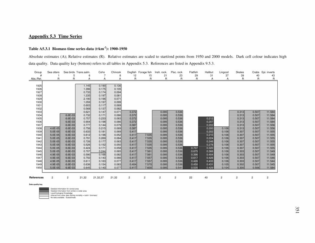
351

Appendix 5.3 Time Series

Table A5.3.1 Biomass time series data (t·km-2): 1900-1950

Absolute estimates (A); Relative estimates (R). Relative estimates are scaled to start/end points from 1950 and 2000 models. Dark cell colour indicates high

data quality. Data quality key (bottom) refers to all tables in Appendix 5.3. References are listed in Appendix 9.5.3.

Group Sea otters Sea birds Trans.salm. Coho Chinook Dogfish Forage fish Insh. rock. Pisc. rock Flatfish Halibut Lingcod Skates Crabs Epi. inverts# 1 5 6 7 8 12 15 21 23 29 31 37 39 40 43

Abs./Rel. R R A A A R R R R R A A R R R

1925 1.145 0.190 0.1361926 1.396 0.175 0.1051927 0.733 0.174 0.0941928 1.235 0.197 0.0811929 2.190 0.196 0.0711930 1.059 0.197 0.0991931 0.603 0.117 0.0691932 0.568 0.137 0.0821933 0.621 0.147 0.071 0.372 0.095 0.536 0.313 0.507 11.5841934 6.6E-03 0.732 0.171 0.086 0.372 0.095 0.536 0.313 0.507 11.5841935 6.6E-03 0.757 0.233 0.083 0.372 0.095 0.536 0.212 0.313 0.507 11.5841936 6.6E-03 0.904 0.198 0.086 0.372 0.095 0.536 0.207 0.313 0.507 11.5841937 6.6E-03 0.777 0.144 0.079 0.387 0.095 0.536 0.202 0.313 0.507 11.5561938 4.6E-05 6.6E-03 0.756 0.215 0.069 0.387 0.095 0.536 0.200 0.106 0.313 0.507 11.5561939 5.0E-05 6.6E-03 0.633 0.181 0.069 0.417 0.095 0.536 0.202 0.106 0.307 0.507 11.5551940 5.0E-05 6.6E-03 0.612 0.196 0.052 0.417 7.535 0.095 0.536 0.210 0.106 0.307 0.507 11.5551941 5.0E-05 6.6E-03 0.791 0.269 0.084 0.417 7.535 0.095 0.536 0.224 0.106 0.307 0.507 11.5551942 5.0E-05 6.6E-03 0.726 0.177 0.063 0.417 7.535 0.095 0.536 0.246 0.106 0.307 0.507 11.5551943 5.0E-05 6.6E-03 0.526 0.152 0.050 0.417 7.535 0.095 0.536 0.278 0.106 0.307 0.507 11.5551944 5.0E-05 6.6E-03 0.424 0.171 0.058 0.417 7.535 0.095 0.536 0.707 0.320 0.106 0.307 0.507 11.5551945 5.0E-05 6.6E-03 0.707 0.244 0.065 0.417 7.561 0.095 0.536 0.675 0.366 0.106 0.303 0.507 11.5491946 4.9E-05 6.6E-03 0.590 0.168 0.082 0.417 7.561 0.095 0.536 0.396 0.404 0.106 0.303 0.507 11.5491947 4.9E-05 6.6E-03 0.750 0.143 0.066 0.417 7.557 0.095 0.536 0.617 0.426 0.106 0.303 0.507 11.5461948 4.9E-05 6.6E-03 0.611 0.163 0.077 0.417 7.557 0.095 0.536 0.426 0.433 0.106 0.303 0.507 11.5441949 4.9E-05 6.6E-03 0.636 0.154 0.083 0.404 7.570 0.095 0.536 0.450 0.431 0.105 0.302 0.507 11.5451950 5.0E-05 6.6E-03 0.645 0.140 0.077 0.417 7.600 0.095 0.541 0.535 0.429 0.104 0.300 0.506 11.584

References 2 2 21,32 21,32,37 21,32 2 2 2 2 22 40 2 2 2 2 Data quality key

Detailed information for correct area Detailed information from similar or wider area Local Ecological Knowledge Inferred from other data (fishing mortality = catch / biomass) No data available. Guesstimate.

351

352

Table A5.3.2 Biomass time series data (t·km-2): 1950-2000

Values given in t·km2. Absolute estimates (A); Relative estimates (R). Relative estimates are scaled to start/end points from 1950 and 2000 models. References

are listed in Appendix 9.5.3.

Group Sea otters Odont. Seals & SL Sea birds Trans.salm. Coho Chinook Dogfish Forage fish Eulachon Herring J. POP Ad. POP Insh. rock. Pisc. rock Turbot1 Flatfish Halibut Pac. cod Sablefish Lingcod Skates Crabs Shrimp Epi. inverts Inf. inverts Euphasiid Phytoplank.# 1 3 4 5 6 7 8 12 15 16 18 19 20 21 23 27 29 31 33 35 37 39 40 42 43 45 47 51

Abs./Rel. R R A R A A A R R R A R R R R R R A A A A R R R R R R R

1950 5.0E-05 6.6E-03 0.645 0.140 0.077 0.417 7.600 1.893 1.001 0.095 0.541 0.535 0.429 0.348 0.104 0.300 0.506 11.584 34.3051951 5.1E-05 6.6E-03 0.540 0.092 0.086 0.430 7.630 1.886 1.001 0.095 0.546 0.782 0.433 0.348 0.104 0.298 0.505 11.623 34.3051952 5.1E-05 6.6E-03 0.620 0.096 0.092 0.453 7.659 1.879 0.585 0.095 0.551 0.868 0.450 0.348 0.104 0.295 0.504 11.660 34.3051953 5.2E-05 6.6E-03 0.451 0.086 0.100 0.475 7.689 1.872 0.796 0.096 0.557 0.520 0.478 0.348 0.104 0.291 0.503 11.696 34.3051954 5.3E-05 6.7E-03 0.384 0.095 0.088 0.498 7.719 1.867 0.705 0.096 0.560 0.675 0.502 0.348 0.104 0.288 0.501 11.735 34.3051955 5.4E-05 6.7E-03 0.342 0.102 0.079 0.521 7.748 1.863 0.875 0.096 0.564 0.536 0.509 0.348 0.104 0.285 0.500 11.774 34.305 6.4161956 5.4E-05 86 0.108 6.7E-03 0.484 0.092 0.084 0.543 7.778 1.858 0.825 0.096 0.567 0.436 0.505 0.348 0.103 0.281 0.499 11.813 34.305 5.988 0.3811957 5.5E-05 86 6.7E-03 0.356 0.098 0.079 0.566 7.808 1.854 0.340 0.096 0.571 0.330 0.493 0.370 0.103 0.278 0.498 11.852 34.305 8.447 0.3561958 5.6E-05 90 6.7E-03 0.478 0.081 0.090 0.589 7.837 1.849 0.644 0.096 0.574 0.431 0.482 0.490 0.103 0.275 0.497 11.891 34.305 5.560 0.3911959 5.7E-05 90 6.7E-03 0.304 0.074 0.083 0.612 7.867 1.845 0.796 0.096 0.578 0.299 0.479 0.548 0.103 0.271 0.495 11.930 34.305 3.742 0.4081960 5.8E-05 92 6.7E-03 0.356 0.113 0.071 0.642 7.896 1.841 1.058 0.096 0.581 0.412 0.480 0.594 0.102 0.268 0.494 11.969 34.305 7.913 0.3641961 5.9E-05 94 0.052 6.7E-03 0.519 0.121 0.066 0.672 7.926 1.836 0.843 0.097 0.585 0.076 0.467 0.482 0.559 0.102 0.265 0.494 12.009 34.305 4.277 0.3711962 6.0E-05 97 6.8E-03 1.113 0.117 0.071 0.702 7.956 1.832 1.051 0.097 0.588 0.079 0.430 0.479 0.582 0.101 0.261 0.493 12.048 34.305 4.598 0.2801963 6.1E-05 98 6.8E-03 0.585 0.141 0.072 0.733 7.985 1.827 0.869 0.234 1.002 0.097 0.592 0.080 0.446 0.463 0.685 0.100 0.258 0.492 12.087 34.305 2.352 0.5311964 6.2E-05 91 6.8E-03 0.609 0.172 0.088 0.763 8.015 1.823 0.722 0.192 1.040 0.097 0.595 0.080 0.350 0.432 1.084 0.099 0.255 0.491 12.126 34.305 3.742 0.4611965 6.3E-05 94 6.8E-03 0.324 0.170 0.085 0.781 8.037 1.818 0.343 0.155 1.059 0.097 0.598 0.080 0.382 0.390 1.346 0.708 0.097 0.253 0.489 12.165 34.305 7.057 0.3771966 6.4E-05 84 6.8E-03 0.653 0.106 0.102 0.799 8.059 1.814 0.182 0.122 1.009 0.097 0.602 0.080 0.479 0.344 1.166 0.752 0.095 0.252 0.488 12.204 34.305 9.517 0.3561967 6.5E-05 76 6.9E-03 0.375 0.147 0.100 0.817 8.080 1.810 0.160 0.097 0.771 0.097 0.605 0.080 0.431 0.303 0.939 0.796 0.093 0.250 0.487 12.243 34.305 8.982 0.4971968 6.6E-05 71 6.9E-03 0.947 0.090 0.103 0.835 8.106 1.804 0.179 0.108 0.646 0.097 0.609 0.079 0.340 0.272 0.797 0.796 0.090 0.249 0.486 12.281 34.305 16.574 0.3831969 6.7E-05 73 6.9E-03 0.261 0.138 0.094 0.854 8.132 1.799 0.114 0.124 0.556 0.097 0.612 0.079 0.269 0.252 0.588 0.796 0.090 0.247 0.485 12.319 34.305 2.780 0.4271970 6.8E-05 72 0.046 6.9E-03 0.501 0.144 0.088 0.870 8.159 1.794 0.528 0.123 0.517 0.097 0.616 0.079 0.374 0.242 0.451 0.752 0.089 0.246 0.484 12.355 34.305 11.441 0.3431971 7.0E-05 72 0.049 6.9E-03 0.266 0.111 0.109 0.891 8.182 1.789 0.725 0.116 0.483 0.097 0.618 0.080 0.317 0.235 0.429 0.752 0.088 0.246 0.483 12.390 34.305 7.592 0.3161972 7.1E-05 73 0.050 7.0E-03 0.516 0.117 0.106 0.912 8.205 1.783 0.529 0.113 0.485 0.098 0.620 0.084 0.382 0.229 0.530 0.717 0.088 0.246 0.482 12.426 34.305 11.762 0.5641973 7.2E-05 79 0.052 7.0E-03 0.365 0.110 0.100 0.936 8.214 1.778 0.832 0.103 0.457 0.098 0.622 0.090 0.479 0.221 0.779 0.699 0.089 0.249 0.481 12.457 34.305 5.133 0.5311974 7.4E-05 81 0.056 7.0E-03 0.407 0.087 0.096 0.953 8.223 1.772 1.129 0.089 0.447 0.098 0.624 0.101 0.512 0.221 0.963 0.646 0.090 0.251 0.480 12.488 34.305 6.309 0.4061975 7.5E-05 80 0.062 7.0E-03 0.161 0.097 0.089 0.965 8.236 1.766 1.300 0.076 0.386 0.098 0.626 0.118 0.430 0.234 0.986 0.584 0.090 0.254 0.479 12.525 34.305 5.133 0.5711976 7.6E-05 84 0.067 7.0E-03 0.363 0.102 0.096 0.977 8.249 1.760 1.043 0.075 0.362 0.098 0.629 0.132 0.351 0.235 0.860 0.531 0.091 0.256 0.478 12.561 34.305 9.623 0.3981977 7.7E-05 82 0.072 7.0E-03 0.385 0.095 0.094 0.990 8.262 1.754 0.923 0.073 0.359 0.098 0.631 0.148 0.293 0.239 0.711 0.487 0.091 0.259 0.477 12.598 34.305 8.447 0.3701978 7.8E-05 79 0.077 7.1E-03 0.449 0.106 0.096 0.995 8.278 1.749 0.613 0.064 0.364 0.098 0.633 0.161 0.327 0.258 0.651 0.442 0.093 0.262 0.476 12.634 34.305 9.837 0.3401979 7.9E-05 77 0.082 7.1E-03 0.457 0.093 0.087 1.000 8.293 1.745 0.472 0.053 0.373 0.098 0.635 0.172 0.318 0.286 0.688 0.425 0.093 0.264 0.476 12.670 34.305 13.901 0.3001980 8.0E-05 75 0.087 7.1E-03 0.361 0.069 0.083 1.006 8.309 1.741 1.536 0.043 0.375 0.098 0.638 0.183 0.311 0.307 0.581 0.398 0.093 0.267 0.475 12.706 34.305 8.768 0.2761981 8.1E-05 76 0.093 7.1E-03 0.450 0.089 0.063 1.006 8.317 1.737 1.620 0.033 0.368 0.098 0.639 0.198 0.300 0.329 0.556 0.398 0.092 0.270 0.474 12.742 34.305 10.051 0.5591982 8.2E-05 87 0.095 7.1E-03 0.323 0.100 0.082 1.006 8.326 1.732 1.472 0.033 0.362 0.098 0.640 0.213 0.298 0.351 0.546 0.407 0.091 0.272 0.473 0.090 12.778 34.305 10.051 0.4431983 8.3E-05 85 0.104 7.1E-03 0.502 0.110 0.074 1.006 8.335 1.728 1.250 0.081 0.372 0.098 0.641 0.225 0.383 0.387 0.536 0.425 0.091 0.275 0.472 0.050 12.815 34.305 21.492 0.4351984 8.4E-05 85 0.115 7.1E-03 0.393 0.093 0.097 1.006 8.343 1.724 1.056 0.101 0.388 0.099 0.642 0.236 0.347 0.409 0.581 0.442 0.091 0.278 0.471 0.060 12.852 34.305 11.655 0.3541985 8.5E-05 86 0.125 7.2E-03 0.647 0.126 0.090 1.006 8.352 1.720 1.065 0.101 0.416 0.099 0.643 0.252 0.352 0.420 0.556 0.442 0.089 0.281 0.470 0.110 12.889 34.305 8.233 0.3071986 8.6E-05 85 0.136 7.2E-03 0.813 0.091 0.075 1.006 8.360 1.716 0.907 0.095 0.443 0.099 0.644 0.272 0.461 0.452 0.559 0.442 0.087 0.283 0.470 0.140 12.926 34.305 11.958 0.3611987 8.7E-05 91 0.158 7.2E-03 0.609 0.079 0.085 1.006 8.369 1.713 0.764 0.108 0.473 0.099 0.646 0.295 0.401 0.486 0.970 0.434 0.081 0.286 0.469 0.290 12.963 34.305 10.800 0.4151988 8.8E-05 92 0.180 7.2E-03 0.952 0.092 0.093 1.006 8.377 1.709 1.059 0.108 0.495 0.099 0.647 0.310 0.450 0.512 1.073 0.425 0.077 0.289 0.468 0.380 13.000 34.305 10.693 0.3241989 8.9E-05 97 0.192 7.2E-03 0.449 0.105 0.084 1.000 8.386 1.705 1.213 0.108 0.523 0.099 0.647 0.325 0.363 0.515 0.897 0.398 0.074 0.292 0.467 0.330 13.037 34.305 8.875 0.3791990 9.0E-05 95 0.217 7.2E-03 0.608 0.099 0.079 0.994 8.394 1.701 0.936 0.098 0.549 0.099 0.648 0.341 0.360 0.556 0.750 0.372 0.069 0.296 0.466 0.300 13.074 34.305 9.303 0.3141991 9.1E-05 97 0.230 7.2E-03 0.661 0.082 0.078 0.989 8.403 1.697 0.739 0.106 0.572 0.099 0.649 0.352 0.309 0.584 0.800 0.354 0.062 0.300 0.465 0.430 13.111 34.305 6.736 0.7141992 9.2E-05 98 0.216 7.3E-03 0.636 0.055 0.090 0.983 8.411 1.693 1.008 0.100 0.599 0.099 0.649 0.364 0.301 0.617 0.601 0.414 0.058 0.304 0.464 0.440 13.148 34.305 11.014 0.3351993 9.3E-05 92 0.266 7.3E-03 0.403 0.081 0.081 0.977 8.420 1.689 0.921 0.089 0.619 0.099 0.650 0.383 0.316 0.668 0.440 0.596 0.053 0.308 0.464 0.530 13.185 34.305 8.768 0.3001994 9.4E-05 90 0.300 7.3E-03 0.246 0.045 0.057 0.972 8.428 1.685 0.670 0.074 0.633 0.100 0.651 0.399 0.308 0.729 0.251 0.458 0.048 0.311 0.463 0.440 13.221 34.305 8.839 0.4831995 9.5E-05 85 0.283 7.3E-03 0.626 0.037 0.058 0.966 8.437 1.681 0.474 0.064 0.623 0.100 0.651 0.408 0.303 0.790 0.178 0.357 0.043 0.315 0.462 0.470 13.258 34.3051996 9.6E-05 0.305 7.3E-03 0.518 0.015 0.027 0.954 8.445 1.678 0.602 0.058 0.603 0.100 0.652 0.420 0.263 0.811 0.161 0.299 0.042 0.319 0.461 0.450 13.295 34.3051997 9.7E-05 0.288 7.3E-03 0.310 0.005 0.040 0.942 8.453 1.673 0.703 0.058 0.598 0.100 0.653 0.433 0.236 0.794 0.193 0.357 0.035 0.323 0.460 13.333 34.3051998 9.8E-05 0.255 7.3E-03 0.344 0.006 0.030 0.930 8.461 1.668 0.844 0.060 0.585 0.100 0.653 0.451 0.738 0.189 0.269 0.028 0.327 0.459 13.371 34.3051999 9.9E-05 0.256 7.4E-03 0.193 0.024 0.030 0.917 8.470 1.664 0.796 0.061 0.573 0.100 0.654 0.468 0.676 0.185 0.376 0.039 0.331 0.458 0.200 13.409 34.3052000 1.0E-04 0.258 7.4E-03 0.208 0.024 0.036 0.909 8.478 1.660 0.658 0.062 0.561 0.100 0.654 0.481 0.628 0.163 0.269 0.039 0.335 0.456 0.200 13.448 34.3052001 1.0E-04 7.4E-03 0.260 0.026 0.901 8.486 1.656 0.646 0.100 0.654 0.499 0.596 0.155 0.381 0.339 0.455 13.487 34.3052002 0.332 0.039 0.579 0.533 0.4752003 0.367 0.948 0.557 0.4442004

Reference 2 36 7,35,36 2 23,41,49 27,37 39 2 2 2 44 43 43 2 2 36,48 22 9,10,11,40 45 25,26 31,33 2 2 42 2 2 36,46 36,46

1 Not used for fitting

352

353

Table A5.3.3 Catch time series data (t·km-2): 1900-1950

Values given in t·km-2. Composite functional groups (Y/N) combine catch records for multiple species. References listed in Appendix 9.5.3.

Group Mysticetae Seals & SL Trans.salm. Coho Chinook Dogfish Herring Flatfish Halibut Sablefish Lingcod# 2 4 6 7 8 12 18 29 31 35 37

Composite? Y Y Y N N N N Y N N N

1900 0.061 0.005 0.126 0.012 0.018 0.039 0.001 0 0.018 0 4.94E-031901 0.061 0.005 0.126 0.012 0.018 0.038 0.000 0 0.024 0 3.52E-051902 0.061 0.005 0.126 0.012 0.018 0.046 0.001 0 0.034 0 3.16E-051903 0.061 0.005 0.126 0.012 0.018 0.062 0.001 0 0.040 0 3.46E-051904 0.061 0.005 0.126 0.012 0.018 0.053 0.001 0 0.050 0 3.93E-051905 0.061 0.005 0.126 0.012 0.018 0.054 0.001 0 0.033 0 4.67E-051906 0.061 0.005 0.190 0.025 0.025 0.055 0.001 0 0.043 0 4.29E-051907 0.061 0.005 0.190 0.025 0.025 0.051 0.001 0 0.053 0 4.56E-051908 0.061 0.005 0.190 0.025 0.025 0.060 0.009 0 0.065 0 4.78E-051909 0.061 0.005 0.254 0.038 0.032 0.072 0.002 0 0.081 0 4.04E-051910 0.063 0.005 0.254 0.038 0.032 0.030 0.008 0 0.082 0 3.19E-051911 0.381 0.005 0.254 0.038 0.032 0.025 0.017 0 0.073 0 3.80E-051912 0.288 0.018 0.317 0.051 0.039 0.028 0.108 0 0.095 0 8.63E-051913 0.125 0.006 0.317 0.051 0.039 0.018 0.040 0 0.083 0.018 8.99E-051914 0.130 0.007 0.317 0.051 0.039 0.000 0.044 0 0.080 0.028 9.33E-051915 0.061 0.036 0.381 0.065 0.047 0.004 0.019 0 0.073 0.022 1.37E-041916 0.154 0.008 0.381 0.065 0.047 0.015 0.020 0 0.046 0.038 1.39E-041917 0.037 0.008 0.381 0.065 0.047 0.009 0.019 0 0.042 0.053 1.30E-041918 0.121 0.008 0.445 0.078 0.054 0.038 0.016 0 0.070 0.018 1.40E-041919 0.109 0.008 0.445 0.078 0.054 0.033 0.015 0 0.079 0.006 3.05E-041920 0.128 0.008 0.445 0.078 0.054 0.013 0.019 0 0.089 0.016 3.26E-041921 0.093 0.008 0.509 0.091 0.061 0.034 0.027 0 0.122 0.012 2.35E-041922 0.057 0.002 0.509 0.091 0.061 0.026 0.026 0 0.109 0.011 2.01E-041923 0.109 0.017 0.509 0.091 0.061 0.042 0.038 0 0.125 0.010 1.94E-041924 0.081 0.024 0.573 0.104 0.068 0.066 0.029 0 0.124 0.011 2.01E-041925 0.080 0.025 0.573 0.104 0.068 0.084 0.028 0 0.119 0.009 2.84E-041926 0.109 0.017 0.698 0.096 0.052 0.065 0.027 0 0.118 0.006 2.22E-041927 0.119 0.015 0.440 0.095 0.056 0.093 0.057 0 0.101 0.010 1.86E-041928 0.110 0.010 0.741 0.108 0.049 0.174 0.089 0 0.113 0.008 3.71E-041929 0.137 0.012 1.314 0.107 0.043 0.208 0.082 0 0.114 0.009 5.00E-041930 0.054 0.009 0.742 0.108 0.070 0.077 0.103 0 0.095 0.010 2.57E-041931 0.032 0.012 0.422 0.064 0.049 0.103 0.112 0 0.068 0.004 1.43E-051932 0.032 0.010 0.397 0.075 0.057 0.023 0.039 0 0.063 0.004 4.29E-051933 0.010 0.008 0.435 0.081 0.050 0.072 0.035 0 0.064 0.004 5.71E-051934 0.061 0.007 0.512 0.094 0.060 0.117 0.070 0 0.066 0.004 1.43E-051935 0.025 0.006 0.530 0.127 0.058 0.073 0.058 0 0.064 0.006 1.29E-041936 0.044 0.034 0.633 0.108 0.060 0.102 0.393 0 0.063 0.004 1.00E-041937 0.038 0.023 0.544 0.078 0.055 0.090 0.552 0 0.070 0.008 1.00E-041938 0.041 0.029 0.529 0.118 0.048 0.143 0.854 0 0.072 0.005 1.14E-041939 0.057 0.011 0.443 0.099 0.048 0.122 1.120 0 0.085 0.005 1.57E-041940 0.073 0.001 0.428 0.107 0.037 0.125 0.293 0 0.089 0.008 2.00E-041941 0.071 0.001 0.554 0.147 0.059 0.199 0.443 0 0.048 0.011 6.71E-041942 0.020 0.002 0.508 0.097 0.044 0.243 0.064 0 0.041 0.007 1.09E-031943 0.016 0.000 0.368 0.083 0.035 0.293 0.495 0 0.047 0.013 2.26E-031944 0.020 0.001 0.296 0.094 0.041 0.445 0.527 0.007 0.049 0.013 3.86E-031945 0.024 0.003 0.495 0.134 0.046 0.334 0.189 0.034 0.056 0.013 6.21E-031946 0.028 0.003 0.413 0.092 0.057 0.163 0.170 0.041 0.067 0.014 1.03E-021947 0.032 0.002 0.525 0.078 0.046 0.215 0.875 0.052 0.090 0.008 9.17E-031948 0.036 0.001 0.427 0.089 0.054 0.174 1.043 0.091 0.070 0.013 8.01E-031949 0.057 0.003 0.445 0.084 0.058 0.228 1.060 0.055 0.067 0.017 6.86E-031950 0.069 0.019 0.598 0.083 0.054 0.032 0.922 0.074 0.071 0.006 5.70E-03

References 24,34,47 7 21 21 21 30 12 22 5 26 8,31

• Unshaded entries (guesses) are based on trend or average of adjacent values.

262 353

354

Table A5.3.4 Catch time series data (t·km-2): 1950-2000

Values given in t·km2. Composite functional groups (Y/N) combine catch records for multiple species. References listed in Appendix 9.5.3.

Group Mysticetae Seals & SL Trans.salm. Coho Chinook Squid Dogfish Herring Ad. POP Turbot Flatfish Halibut Pac. cod Sablefish Lingcod Skates Crabs Shrimp Epi. inverts# 2 4 6 7 8 10 12 18 20 27 29 31 33 35 37 39 40 42 43

Composite? Y Y Y N N Y N N N N Y N N N N N Y Y Y

1950 0.069 0.019 0.598 0.083 0.054 0.032 0.922 0.003 0.004 0.074 0.071 0.052 0.006 0.006 2.4E-031951 0.106 0.002 0.569 0.138 0.060 0.057 1.337 0.003 0.004 0.048 0.065 0.052 0.008 0.005 2.4E-031952 0.114 0.002 0.438 0.091 0.064 0.044 0.805 0.003 0.004 0.071 0.076 0.052 0.005 0.003 2.3E-031953 0.123 0.003 0.565 0.094 0.070 0.045 0.573 0.003 0.004 0.034 0.081 0.052 0.004 0.001 1.2E-031954 0.127 0.002 0.551 0.085 0.062 0.036 1.008 0.018 0.006 0.035 0.082 0.052 0.005 0.005 2.3E-031955 0.129 0.002 0.369 0.094 0.055 0.037 0.886 0.003 0.014 0.054 0.064 0.052 0.005 0.007 2.3E-031956 0.090 0.003 0.299 0.100 0.059 0.016 1.841 0.012 0.022 0.057 0.076 0.055 0.004 0.010 2.3E-031957 0.146 0.005 0.377 0.091 0.055 0.035 1.295 0.008 0.006 0.048 0.073 0.046 0.006 0.011 2.4E-031958 0.198 0.010 0.531 0.097 0.063 0.023 0.577 0.027 0.004 0.052 0.093 0.162 0.004 0.009 2.3E-031959 0.199 0.030 0.295 0.080 0.058 0.091 0.768 0.027 0.008 0.039 0.100 0.108 0.006 0.011 2.4E-031960 0.201 0.018 0.248 0.072 0.057 0.062 0.543 0.025 0.012 0.058 0.110 0.132 0.008 0.012 4.6E-031961 0.203 0.007 0.382 0.112 0.053 0.085 1.149 0.016 0.023 0.043 0.096 0.091 0.008 0.013 4.3E-031962 0.205 0.012 0.523 0.119 0.057 0.006 1.106 0.026 0.016 0.042 0.112 0.095 0.007 0.017 4.3E-031963 0.131 0.009 0.369 0.115 0.057 0.003 1.808 0.053 0.009 0.043 0.121 0.164 0.009 0.013 4.1E-031964 0.139 0.009 0.349 0.140 0.071 0.014 1.691 0.050 0.011 0.041 0.108 0.292 0.009 0.014 4.2E-031965 0.130 0.004 0.210 0.170 0.068 0.004 1.602 0.114 0.010 0.044 0.107 0.509 0.013 0.018 4.4E-031966 0.126 0.002 0.461 0.167 0.081 0.015 0.865 0.318 0.010 0.077 0.104 0.532 0.019 0.027 4.2E-031967 0.103 0.001 0.419 0.104 0.080 0.022 0.401 0.249 0.019 0.071 0.085 0.287 0.031 0.030 4.1E-031968 0 0.000 0.530 0.146 0.082 0.017 0.034 0.183 0.012 0.070 0.095 0.290 0.050 0.039 4.1E-031969 0 0 0.241 0.088 0.075 0.011 0.000 0.141 0.022 0.055 0.110 0.169 0.054 0.022 5.2E-031970 0 0 0.481 0.137 0.079 0.007 0.022 0.111 0.005 0.063 0.096 0.076 0.035 0.020 4.1E-031971 0 0 0.384 0.143 0.098 0.006 0.115 0.061 0.002 0.058 0.082 0.085 0.056 0.017 3.6E-031972 0 0 0.527 0.109 0.096 0.006 0.283 0.094 0.003 0.035 0.072 0.153 0.039 0.015 3.9E-031973 0 0 0.602 0.116 0.090 0.005 0.291 0.086 0.008 0.046 0.047 0.225 0.046 0.012 3.9E-031974 0 0 0.430 0.109 0.088 0.005 0.301 0.131 0.006 0.044 0.024 0.268 0.069 0.017 3.7E-031975 0 0 0.221 0.085 0.083 0.005 0.297 0.078 0.011 0.060 0.037 0.282 0.067 0.013 6.8E-031976 0 0 0.373 0.096 0.086 0.004 0.462 0.043 0.017 0.071 0.039 0.280 0.047 0.013 7.0E-031977 0 0 0.434 0.100 0.084 0.003 0.533 0.028 0.017 0.050 0.029 0.197 0.039 0.009 8.6E-031978 0 0 0.476 0.094 0.088 0.015 0.510 0.018 0.026 0.039 0.028 0.119 0.044 0.006 7.7E-031979 0 0 0.402 0.105 0.078 0.023 0.204 0.041 0.025 0.059 0.022 0.263 0.044 0.009 8.2E-031980 0 0 0.352 0.092 0.074 0.107 0.161 0.072 0.023 0.061 0.024 0.255 0.043 0.011 1.4E-021981 0 0 0.551 0.068 0.057 0.033 0.212 0.065 0.015 0.056 0.018 0.180 0.045 0.016 1.2E-021982 0 0 0.431 0.089 0.073 0.002 0.199 0.079 0.010 0.032 0.020 0.118 0.049 0.020 9.3E-03 0.0061983 0 0 0.505 0.099 0.060 0.001 0.230 0.070 0.009 0.036 0.022 0.154 0.044 0.024 1.0E-02 0.0071984 0 0 0.324 0.109 0.081 1.5E-04 0.001 0.259 0.086 0.010 0.038 0.034 0.100 0.047 0.016 9.7E-03 0.0081985 0 0 0.794 0.092 0.068 1.2E-04 0.003 0.294 0.079 0.013 0.034 0.062 0.065 0.048 0.019 8.8E-03 0.003 0.0111986 0 0 0.733 0.125 0.060 8.4E-04 0.004 0.254 0.067 0.011 0.035 0.065 0.122 0.048 0.030 9.8E-03 0.004 0.0121987 0 0 0.496 0.090 0.066 9.1E-04 0.009 0.201 0.077 0.021 0.040 0.071 0.499 0.055 0.033 1.2E-02 0.005 0.0291988 0 0 0.661 0.078 0.074 9.4E-04 0.013 0.215 0.088 0.008 0.059 0.067 0.350 0.056 0.031 1.1E-02 0.008 0.0291989 0 0 0.660 0.091 0.066 7.4E-04 0.003 0.305 0.069 0.011 0.069 0.064 0.272 0.052 0.035 9.1E-03 0.007 0.0281990 0 0 0.690 0.104 0.064 7.7E-04 0.018 0.345 0.066 0.029 0.076 0.065 0.205 0.062 0.044 1.3E-02 0.016 0.0241991 0 0 0.614 0.098 0.059 1.2E-03 0.016 0.314 0.051 0.026 0.090 0.055 0.430 0.062 0.044 1.6E-02 0.009 0.0371992 0 0 0.497 0.082 0.069 9.8E-04 0.015 0.282 0.044 0.029 0.088 0.025 0.289 0.061 0.034 1.5E-02 0.032 0.0341993 0 0 0.666 0.054 0.065 1.4E-04 0.002 0.332 0.043 0.030 0.104 0.036 0.225 0.061 0.035 1.5E-02 0.096 0.0401994 0 0 0.499 0.080 0.047 1.9E-03 0.002 0.279 0.060 0.033 0.079 0.034 0.092 0.052 0.034 1.8E-02 0.085 0.0401995 0 0 0.327 0.044 0.037 8.1E-04 0.005 0.195 0.077 0.020 0.083 0.034 0.084 0.039 0.033 1.6E-02 0.055 0.0761996 0 0 0.244 0.037 0.013 9.0E-04 0.040 0.139 0.061 0.072 0.052 0.042 0.032 0.047 0.017 2.2E-02 0.066 0.083 0.0871997 0 0 0.357 0.014 0.024 7.6E-05 0.023 0.168 0.057 0.047 0.045 0.051 0.079 0.049 0.011 2.8E-02 0.031 0.045 0.0801998 0 0 0.230 0.004 0.017 9.0E-04 0.027 0.239 0.060 0.061 0.051 0.056 0.071 0.051 0.013 1.5E-02 0.022 0.046 0.0891999 0 0 0.140 0.005 0.013 4.2E-04 0.034 0.227 0.057 0.057 0.056 0.053 0.045 0.043 0.017 2.5E-02 0.027 0.036 0.0802000 0 0 0.145 0.005 0.010 4.2E-04 0.072 0.241 0.060 0.067 0.058 0.046 0.034 0.041 0.026 2.9E-02 0.027 0.037 0.0782001 0 0 0.182 0.006 0.012 0.071 0.165 0.057 0.123 0.054 0.040 0.017 0.035 0.021 2.8E-02 0.051 0.039 0.0722002 0 0 0.233 0.009 0.020 0.046 0.165 0.057 0.079 0.065 0.049 0.012 0.029 0.024 2.8E-02 0.037 0.017 0.0742003 0 0 0.257 0.008 0.018 0.054 0.139 0.060 0.067 0.054 0.041 0.013 0.028 0.024 3.8E-02 0.063 0.011 0.0772004 0 0 0.102 0.007 0.018 0.077 0.146 0.031 0.047 0.031 0.063 0.013 0.024 0.023 1.8E-02 0.019 0.004 0.030

Reference 24 7 1,16,19,20,21 1,16,19,20,21 1,16,19,20,21 14,15 18,19,30 12 1,15,43 1,3,16,19,36 1,16,19 1,5,17,28,29 3,19,45 1,19,26 1,19,31 1,6,16,19 13,19 19,42 19

354

355

Table A5.3.5 Fishing mortality time series data (yr-1): 1900-1950

References listed in Appendix 9.5.3.

Group Mysticetae Seals & SL Trans.salm. Coho Chinook Dogfish Herring Halibut Sablefish Lingcod# 2 4 6 7 8 12 18 31 35 37

1900 0.040 0.072 0.150 0.150 0.2 0.095 0.000 0.030 0 0.0481901 0.040 0.072 0.150 0.150 0.2 0.090 0.000 0.040 0 0.0001902 0.040 0.072 0.150 0.150 0.2 0.109 0.000 0.058 0 0.0001903 0.040 0.072 0.150 0.150 0.2 0.149 0.000 0.071 0 0.0001904 0.040 0.072 0.150 0.150 0.2 0.127 0.000 0.090 0 0.0001905 0.040 0.072 0.150 0.150 0.2 0.129 0.000 0.061 0 0.0001906 0.040 0.072 0.200 0.200 0.2 0.132 0.000 0.080 0 0.0001907 0.040 0.072 0.200 0.200 0.2 0.123 0.001 0.103 0 0.0001908 0.040 0.072 0.200 0.200 0.2 0.144 0.004 0.129 0 0.0001909 0.040 0.072 0.250 0.250 0.3 0.173 0.001 0.163 0 0.0001910 0.041 0.072 0.250 0.250 0.3 0.071 0.003 0.168 0 0.0001911 0.247 0.072 0.250 0.250 0.3 0.059 0.007 0.155 0 0.0001912 0.187 0.142 0.300 0.300 0.3 0.066 0.044 0.204 0 0.0011913 0.081 0.044 0.300 0.300 0.3 0.043 0.016 0.185 0.029 0.0011914 0.084 0.053 0.300 0.300 0.3 0.000 0.018 0.182 0.047 0.0011915 0.039 0.289 0.350 0.350 0.4 0.010 0.008 0.170 0.036 0.0011916 0.100 0.067 0.350 0.350 0.4 0.035 0.008 0.110 0.063 0.0011917 0.024 0.067 0.350 0.350 0.4 0.023 0.007 0.104 0.088 0.0011918 0.078 0.067 0.400 0.400 0.4 0.092 0.006 0.176 0.030 0.0011919 0.071 0.067 0.400 0.400 0.4 0.079 0.006 0.205 0.011 0.0031920 0.083 0.067 0.400 0.400 0.4 0.032 0.007 0.240 0.026 0.0031921 0.060 0.067 0.450 0.450 0.5 0.082 0.011 0.337 0.020 0.0021922 0.037 0.015 0.450 0.450 0.5 0.062 0.011 0.313 0.019 0.0021923 0.071 0.132 0.450 0.450 0.5 0.101 0.015 0.370 0.017 0.0021924 0.053 0.190 0.500 0.500 0.5 0.159 0.012 0.379 0.018 0.0021925 0.052 0.199 0.500 0.547 0.5 0.202 0.011 0.377 0.015 0.0031926 0.071 0.137 0.500 0.547 0.5 0.155 0.011 0.387 0.010 0.0021927 0.077 0.117 0.600 0.547 0.6 0.223 0.023 0.346 0.016 0.0021928 0.072 0.080 0.600 0.547 0.6 0.417 0.036 0.402 0.013 0.0041929 0.089 0.095 0.600 0.547 0.6 0.499 0.033 0.420 0.015 0.0051930 0.035 0.075 0.700 0.547 0.7 0.184 0.041 0.368 0.017 0.0021931 0.021 0.095 0.700 0.547 0.7 0.246 0.045 0.275 0.006 0.0001932 0.021 0.072 0.700 0.547 0.7 0.055 0.016 0.267 0.006 0.0001933 0.006 0.059 0.700 0.547 0.7 0.172 0.014 0.284 0.006 0.0011934 0.040 0.050 0.700 0.547 0.7 0.282 0.028 0.308 0.006 0.0001935 0.016 0.040 0.700 0.547 0.7 0.174 0.024 0.301 0.010 0.0011936 0.029 0.248 0.700 0.547 0.7 0.244 0.158 0.303 0.007 0.0011937 0.025 0.166 0.700 0.547 0.7 0.215 0.223 0.347 0.013 0.0011938 0.027 0.208 0.700 0.547 0.7 0.343 0.344 0.362 0.008 0.0011939 0.037 0.080 0.700 0.547 0.7 0.292 0.452 0.421 0.009 0.0021940 0.048 0.009 0.700 0.547 0.7 0.301 0.118 0.426 0.014 0.0021941 0.046 0.007 0.700 0.547 0.7 0.478 0.179 0.215 0.017 0.0061942 0.013 0.013 0.700 0.547 0.7 0.583 0.026 0.167 0.012 0.0101943 0.010 0.003 0.700 0.547 0.7 0.704 0.200 0.171 0.021 0.0221944 0.013 0.006 0.700 0.547 0.7 1.067 0.213 0.154 0.022 0.0371945 0.016 0.019 0.700 0.547 0.7 0.800 0.076 0.152 0.021 0.0601946 0.018 0.019 0.700 0.547 0.7 0.391 0.068 0.165 0.024 0.0991947 0.021 0.023 0.700 0.547 0.7 0.516 0.353 0.211 0.013 0.0881948 0.028 0.009 0.700 0.547 0.7 0.417 0.421 0.162 0.022 0.0771949 0.043 0.030 0.700 0.547 0.7 0.548 0.427 0.156 0.028 0.0661950 0.053 0.173 0.927 0.596 0.7 0.076 0.921 0.164 0.018 0.055

References 4

• All light grey entries are estimated based on catch and biomass, except lingcod.• Unshaded entries (guesses) are based on trend or average of adjacent values.• Groups not displayed use baseline fishing mortality (assumed constant). 355

356

Table A5.3.6 Fishing mortality time series data (yr-1): 1950-2000

References listed in Appendix 9.5.3.

Group Mysticetae Seals & SL Trans.salm. Coho Chinook Dogfish Herring Ad. POP Turbot Halibut Pac. cod Sablefish Lingcod Skates Crabs Shrimp# 2 4 6 7 8 12 18 20 27 31 33 35 37 39 40 42

1950 0.053 0.173 0.927 0.596 0.7 0.076 0.921 0.050 0.002 0.164 0.159 0.018 0.055 0.008 0.005 0.11951 0.082 0.019 1.053 1.495 0.7 0.137 1.336 0.050 0.007 0.149 0.159 0.018 0.044 0.008 0.005 0.11952 0.088 0.021 0.707 0.953 0.7 0.105 1.377 0.050 0.007 0.169 0.159 0.018 0.029 0.008 0.005 0.11953 0.095 0.025 1.253 1.092 0.7 0.107 0.720 0.050 0.007 0.169 0.159 0.018 0.007 0.004 0.005 0.11954 0.097 0.015 1.436 0.898 0.7 0.086 1.429 0.050 0.004 0.163 0.159 0.018 0.046 0.008 0.005 0.11955 0.099 0.014 1.080 0.919 0.7 0.090 1.013 0.050 0.009 0.125 0.159 0.018 0.069 0.008 0.005 0.11956 0.069 0.024 0.618 1.090 0.7 0.039 2.231 0.050 0.014 0.150 0.159 0.018 0.100 0.008 0.005 0.11957 0.112 0.043 1.058 0.922 0.7 0.085 3.806 0.050 0.004 0.148 0.124 0.018 0.104 0.008 0.005 0.11958 0.152 0.090 1.109 1.200 0.7 0.055 0.896 0.050 0.003 0.194 0.330 0.018 0.090 0.008 0.005 0.11959 0.153 0.572 0.971 1.076 0.7 0.219 0.965 0.050 0.005 0.208 0.198 0.018 0.105 0.008 0.005 0.11960 0.154 0.347 0.695 0.637 0.8 0.150 0.513 0.050 0.008 0.229 0.222 0.018 0.115 0.015 0.005 0.11961 0.156 0.138 0.735 0.931 0.8 0.203 1.362 0.050 0.015 0.198 0.162 0.018 0.125 0.014 0.005 0.11962 0.157 0.234 0.470 1.010 0.8 0.014 1.051 0.050 0.010 0.234 0.163 0.018 0.167 0.014 0.005 0.11963 0.100 0.175 0.631 0.817 0.8 0.008 2.081 0.053 0.006 0.261 0.239 0.018 0.131 0.014 0.005 0.11964 0.107 0.165 0.574 0.815 0.8 0.034 2.344 0.049 0.007 0.250 0.269 0.018 0.142 0.014 0.005 0.11965 0.100 0.081 0.648 1.002 0.8 0.009 4.672 0.108 0.006 0.274 0.379 0.018 0.184 0.015 0.005 0.11966 0.096 0.041 0.706 1.573 0.8 0.035 4.765 0.315 0.006 0.301 0.456 0.026 0.287 0.014 0.005 0.11967 0.079 0.013 1.117 0.707 0.8 0.053 2.514 0.323 0.012 0.280 0.305 0.038 0.321 0.014 0.005 0.11968 0 0.003 0.559 1.621 0.8 0.041 0.191 0.283 0.008 0.350 0.363 0.062 0.436 0.014 0.005 0.11969 0 0 0.927 0.637 0.8 0.026 0.000 0.253 0.014 0.434 0.287 0.067 0.246 0.017 0.005 0.11970 0 0 0.961 0.950 0.9 0.016 0.042 0.215 0.003 0.395 0.169 0.046 0.224 0.014 0.005 0.11971 0 0 1.445 1.292 0.9 0.015 0.158 0.127 0.002 0.348 0.198 0.074 0.193 0.012 0.005 0.11972 0 0 1.020 0.937 0.9 0.014 0.535 0.194 0.002 0.313 0.288 0.054 0.168 0.013 0.005 0.11973 0 0 1.648 1.049 0.9 0.013 0.350 0.188 0.005 0.213 0.289 0.065 0.140 0.013 0.005 0.11974 0 0 1.056 1.251 0.915 0.012 0.267 0.294 0.004 0.110 0.278 0.107 0.192 0.012 0.005 0.11975 0 0 1.374 0.879 0.932 0.011 0.228 0.201 0.007 0.157 0.286 0.115 0.142 0.023 0.005 0.11976 0 0 1.029 0.944 0.901 0.010 0.443 0.119 0.011 0.165 0.325 0.089 0.138 0.023 0.005 0.11977 0 0 1.129 1.050 0.897 0.008 0.578 0.078 0.011 0.122 0.277 0.080 0.101 0.029 0.005 0.11978 0 0 1.062 0.886 0.920 0.037 0.833 0.049 0.017 0.109 0.183 0.099 0.068 0.026 0.005 0.11979 0 0 0.880 1.129 0.828 0.056 0.433 0.110 0.017 0.077 0.383 0.103 0.093 0.027 0.005 0.11980 0 0 0.975 1.334 0.966 0.257 0.105 0.192 0.015 0.078 0.440 0.109 0.116 0.047 0.005 0.11981 0 0 1.223 0.763 1.313 0.079 0.131 0.177 0.010 0.056 0.324 0.114 0.174 0.039 0.005 0.11982 0 0 1.335 0.888 0.808 0.004 0.135 0.218 0.007 0.057 0.216 0.119 0.221 0.031 0.005 0.2221983 0 0 1.005 0.901 0.873 0.002 0.184 0.187 0.006 0.056 0.287 0.103 0.262 0.034 0.005 0.4311984 0 0 0.825 1.172 1.183 0.003 0.245 0.222 0.006 0.084 0.172 0.107 0.175 0.032 0.005 0.4421985 0 0 1.228 0.733 1.262 0.006 0.276 0.191 0.009 0.148 0.117 0.107 0.212 0.029 0.007 0.3141986 0 0 0.901 1.373 0.781 0.009 0.280 0.150 0.007 0.143 0.219 0.110 0.343 0.033 0.009 0.2731987 0 0 0.814 1.141 1.026 0.021 0.264 0.162 0.014 0.145 0.514 0.128 0.409 0.040 0.010 0.3271988 0 0 0.694 0.853 0.687 0.032 0.203 0.178 0.005 0.131 0.326 0.131 0.398 0.038 0.015 0.2501989 0 0 1.471 0.871 0.950 0.006 0.251 0.132 0.007 0.124 0.303 0.132 0.469 0.030 0.014 0.2741990 0 0 1.135 1.051 0.804 0.043 0.368 0.120 0.019 0.117 0.274 0.166 0.637 0.044 0.031 0.2611991 0 0 0.928 1.189 0.748 0.038 0.424 0.089 0.017 0.095 0.538 0.174 0.703 0.053 0.018 0.2851992 0 0 0.782 1.486 0.589 0.037 0.280 0.073 0.019 0.041 0.480 0.148 0.588 0.050 0.064 0.2541993 0 0 1.652 0.673 0.798 0.005 0.361 0.069 0.020 0.054 0.513 0.103 0.660 0.048 0.192 0.2461994 0 0 2.033 1.773 0.889 0.006 0.417 0.094 0.021 0.047 0.365 0.113 0.697 0.058 0.171 0.2971995 0 0 0.522 1.187 0.324 0.011 0.410 0.124 0.013 0.043 0.469 0.110 0.774 0.053 0.109 0.5281996 0 0 0.472 2.515 0.033 0.096 0.231 0.102 0.018 0.052 0.199 0.156 0.404 0.072 0.133 0.6051997 0 0 1.152 2.831 0.296 0.054 0.239 0.095 0.018 0.064 0.410 0.138 0.317 0.093 0.063 0.4571998 0 0 0.668 0.717 0.531 0.064 0.283 0.102 0.018 0.076 0.376 0.191 0.446 0.050 0.044 0.3091999 0 0 0.727 1.805 0.195 0.082 0.286 0.099 0.018 0.078 0.243 0.115 0.434 0.084 0.054 0.2392000 0 0 0.700 1.805 0.095 0.172 0.367 0.107 0.018 0.074 0.207 0.152 0.658 0.096 0.053 0.2712001 0 0 0.700 1.805 0.123 0.170 0.256 0.100 0.018 0.067 0.110 0.093 0.685 0.094 0.102 0.1222002 0 0 0.700 1.805 0.248 0.110 0.284 0.100 0.018 0.103 0.269 0.138 0.685 0.092 0.074 0.1222003 0 0 0.700 1.805 0.248 0.129 0.146 0.100 0.018 0.093 0.269 0.138 0.685 0.125 0.125 0.1222004 0 0 0.700 1.805 0.248 0.184 0.146 0.100 0.018 0.138 0.269 0.138 0.685 0.059 0.039 0.122

Reference 38 33 42

• All light grey entries are estimated based on catch and biomass, except lingcod.• Unshaded entries (guesses) are based on trend or average of adjacent values.• Groups not displayed use baseline fishing mortality (assumed constant). 356

357

Appendix 5.4 Dynamic Fit to Data: 1950-2000

Figure A5.4.1 Biomass fit to data (t·km-2).

Predicted from model (line) versus observed trend (circles). Large circles at beginning and end of series show 1950

and 2000 model values. Error bars in year 2000 show confidence interval of data point based on data pedigree in

2000 model. Observed trend is from A) stock assessment; B.) local environmental knowledge; C.) model start/end

points. The anomaly trends for phytoplankton production and herring recruitment that best reduce the sum of

squares between predicted and observed time series are provided in section C (lower right); the forcing patterns are

used in all simulations.

A.) Stock assessment

6����������" ����@"���"����" ���������"����" *���"����" *�����!"����"

0.00

0.02

0.04

0.06

0.08

0.10

1950 1975 20000.0

0.1

0.2

0.3

0.4

1950 1975 20000.0

0.3

0.6

0.9

1.2

1950 1975 20000.00

0.05

0.10

0.15

0.20

1950 1975 20000.00

0.03

0.06

0.09

0.12

1950 1975 2000

�����$" A�"-6-" -6-" ,������" ��3��"

0.0

0.5

1.0

1.5

2.0

2.5

1950 1975 20000.00

0.05

0.10

0.15

0.20

0.25

1950 1975 20000.0

0.4

0.8

1.2

1.6

1950 1975 2000

0.0

0.2

0.4

0.6

0.8

1.0

1950 1975 20000.0

0.2

0.4

0.6

0.8

1.0

1950 1975 2000

-������"���" ��3�����" /��$���" 1�'��������" -�+��'��!���"

0.0

0.4

0.8

1.2

1.6

1950 1975 20000.0

0.2

0.4

0.6

0.8

1.0

1950 1975 2000

0.00

0.04

0.08

0.12

0.16

1950 1975 2000

0

5

10

15

20

25

1950 1975 2000

0

8

16

24

32

1950 1975 2000

358

Figure A5.4.1 Biomass fit to data (cont.)

B.) Local Environmental Knowledge

���"������" ���3����" ��$����" ,���$�"����" 1������"

0.0E+00

5.0E-05

1.0E-04

1.5E-04

1950 1975 2000 0.000

0.003

0.006

0.009

0.012

1950 1975 2000 0.0

0.4

0.8

1.2

1.6

1950 1975 2000 0

4

8

12

16

1950 1975 2000

0.0

0.8

1.6

2.4

3.2

1950 1975 2000

#������"���!����" -����2�����"���!����" �!����" *��3�" 1'������"��2�����"

0.00

0.05

0.10

0.15

0.20

1950 1975 2000

0.0

0.4

0.8

1.2

1950 1975 2000

0.0

0.2

0.4

0.6

1950 1975 2000 0.0

0.2

0.4

0.6

0.8

1950 1975 2000 0

10

20

30

1950 1975 2000

#���"�������2���"��2�����" " " " "

0

20

40

60

1950 1975 2000

359

Figure A5.4.1 Biomass fit to data (cont.)

C.) Model start/end points

Mysticetae Small squid Squid Ratfish J. Pollock

0.0

0.5

1.0

1.5

2.0

1950 1975 2000 0.0

0.8

1.6

2.4

3.2

1950 1975 2000 0.0

0.6

1.2

1.8

1950 1975 2000 0.0

0.4

0.8

1.2

1950 1975 2000

0.00

0.08

0.16

0.24

0.32

1950 1975 2000

Pollock J. herring J. piscivorous rockfish J. planktivorous rockfish Planktivorous rockfish

0.0

0.2

0.4

0.6

0.8

1950 1975 2000

0

2

4

6

8

10

1950 1975 2000 0.000

0.005

0.010

0.015

1950 1975 2000

0.0

0.1

0.2

0.3

1950 1975 2000

0.0

0.5

1.0

1.5

2.0

1950 1975 2000

J. turbot Turbot J. flatfish J. halibut J. Pacific cod

0.0

0.1

0.2

0.3

0.4

0.5

1950 1975 2000 0.0

0.8

1.6

2.4

3.2

1950 1975 2000 0.0

0.1

0.2

0.3

0.4

0.5

1950 1975 2000 0.0

0.2

0.4

0.6

0.8

1.0

1950 1975 2000 0.0

0.1

0.2

0.3

1950 1975 2000

J. sablefish J. lingcod Shallow benthic fish S. crabs Commercial shrimp

0.0

0.1

0.2

0.3

0.4

1950 1975 2000 0.00

0.05

0.10

0.15

1950 1975 2000 0.0

0.2

0.4

0.6

0.8

1.0

1950 1975 2000 0.0

0.5

1.0

1.5

1950 1975 2000 0.0

0.1

0.2

0.3

0.4

1950 1975 2000

Infaunal carn. inverts. Carnivorous jellyfish Copepods Primary production Herring recruitment

0

8

16

24

32

1950 1975 2000 0

2

4

6

1950 1975 2000 0

2

4

6

8

1950 1975 2000 -10%

-5%

0%

5%

10%

1950 1975 2000 -250%

0%

250%

500%

1950 1975 2000

360

Figure A5.4.2 Catch fit to data (t·km-2)

Predicted from model (line) versus observed trend (circles). Large circles at beginning and end of series show 1950

and 2000 model values.

Mysticetae Seals, sea lions Transient salmon Coho salmon Chinook salmon

0.00

0.05

0.10

0.15

0.20

0.25

1950 1975 2000 0.00

0.02

0.04

0.06

0.08

1950 1975 2000 0.0

0.2

0.4

0.6

0.8

1.0

1950 1975 2000 0.00

0.04

0.08

0.12

0.16

0.20

1950 1975 2000 0.00

0.03

0.06

0.09

0.12

1950 1975 2000 Squid Ratfish Dogfish Pollock Eulachon

0.000

0.001

0.002

0.003

1950 1975 2000 0.00

0.01

0.02

0.03

1950 1975 2000 0.0

0.1

0.2

0.3

0.4

1950 1975 2000 0.000

0.005

0.010

0.015

0.020

1950 1975 2000 0.000

0.001

0.002

0.003

0.004

0.005

1950 1975 2000 Herring POP Inshore rockfish Piscivorous rockfish Planktivorous rockfish

0.0

0.8

1.6

2.4

3.2

1950 1975 2000 0.0

0.1

0.2

0.3

0.4

1950 1975 2000 0.000

0.003

0.006

0.009

0.012

1950 1975 2000 0.00

0.01

0.02

0.03

1950 1975 2000 0.00

0.02

0.04

0.06

0.08

0.10

1950 1975 2000 Turbot Flatfish Halibut Pacific cod Sablefish

0.00

0.02

0.04

0.06

0.08

0.10

1950 1975 2000 0.00

0.02

0.04

0.06

0.08

0.10

1950 1975 2000 0.00

0.04

0.08

0.12

0.16

1950 1975 2000 0.0

0.2

0.4

0.6

1950 1975 2000 0.00

0.02

0.04

0.06

0.08

0.10

1950 1975 2000 J. lingcod Lingcod Skates Crabs Shrimp

0.000

0.001

0.002

0.003

0.004

0.005

1950 1975 2000 0.00

0.02

0.04

0.06

1950 1975 2000 0.00

0.01

0.02

0.03

0.04

1950 1975 2000 0.00

0.03

0.06

0.09

0.12

1950 1975 2000 0.00

0.03

0.06

0.09

0.12

1950 1975 2000 Epifaunal inverts. Jellyfish

0.00

0.03

0.06

0.09

0.12

1950 1975 2000 0.E+00

1.E-04

2.E-04

1950 1975 2000

361

Appendix 5.5 Equilibrium Analysis of 2000 Model

Figure A5.5.1 Equilibrium analysis of 2000 model

Solid curve shows biomass; broken curve shows catch. Vertical broken line shows baseline fishing mortality.

Seals, sea lions Transient salmon Coho salmon

0.00

0.05

0.10

0.15

0.20

0.25

0.30

0 100 200 300

F/ Fbaseline

Bio

mas

s (T

•km

2 )

0.000

0.002

0.004

0.006

0.008

0.010

0.012

Catch (T

•km2)

0.0

0.1

0.2

0.3

0.4

0.5

0.6

0.7

0.8

0.9

0 1 2

F/ Fbaseline

Bio

mas

s (T

•km

2 )

0.00

0.05

0.10

0.15

0.20

0.25

Catch (T

•km2)

0

0.01

0.02

0.03

0.04

0.05

0 1 2 3 4 5 6 7 8

F/ Fbaseline

Bio

mas

s (T

•km

2 )

0

0.004

0.008

0.012

0.016

Catch (T•km

2)

Chinook salmon Ratfish Dogfish

0

0.01

0.02

0.03

0.04

0.05

0.06

0 1 2 3 4 5 6 7 8

F/ Fbaseline

Bio

mas

s (T

•km

2 )

0.000

0.005

0.010

0.015

0.020

0.025

Catch (T

•km2)

0.0

0.1

0.2

0.3

0.4

0.5

0.6

0 1 2 3 4 5 6 7 8

F/ Fbaseline

Bio

mas

s (T

•km

2 )

0.000

0.005

0.010

0.015

0.020

Catch (T•km

2)

0.4

0.5

0.6

0.7

0.8

0.9

1.0

0 1 2 3

F/ Fbaseline

Bio

mas

s (T

•km

2 )

0.00

0.01

0.02

0.03

0.04

0.05

0.06

0.07

0.08

Catch (T

•km2)

Pollock Eulachon Herring

0.00

0.10

0.20

0.30

0.40

0.50

0.60

0 5 10 15

F/ Fbaseline

Bio

mas

s (T

•km

2 )

0.00

0.02

0.04

0.06

0.08

0.10

Catch (T

•km2)

0.0

0.5

1.0

1.5

2.0

0 200 400 600 800

F/ Fbaseline

Bio

mas

s (T

•km

2 )

0

0.2

0.4

0.6

0.8

1

Catch (T

•km2)

0.0

0.2

0.4

0.6

0.8

1.0

1.2

1.4

1.6

0 1 2 3

F/ Fbaseline

Bio

mas

s (T

•km

2 )

0.00

0.05

0.10

0.15

0.20

0.25

0.30

0.35

0.40

Catch (T•km

2)

POP Inshore rockfish Piscivorous rockfish

0.0

0.2

0.4

0.6

0.8

1.0

1.2

1.4

0 1 2 3

F/ Fbaseline

Bio

mas

s (T

•km

2 )

0.00

0.02

0.04

0.06

0.08

0.10

0.12

0.14

Catch (T

•km2)

0.0

0.2

0.4

0.6

0.8

1.0

1.2

0 1 2 3

F/ Fbaseline

Bio

mas

s (T

•km

2 )

0.000

0.004

0.008

0.012

0.016

0.020

Catch (T•km

2)

0.0

0.2

0.4

0.6

0.8

1.0

1.2

1.4

1.6

0 1 2 3

F/ Fbaseline

Bio

mas

s (T

•km

2 )

0.000

0.004

0.008

0.012

0.016

Catch (T•km

2)

362

Figure A5.5.1 Equilibrium analysis of 2000 model (cont.)

Planktivorous rockfish Turbot Flatfish

0

1

2

3

4

5

0 1 2 3

F/ Fbaseline

Bio

mas

s (T

•km

2 )

0.00

0.02

0.04

0.06

0.08

0.10

Catch (T

•km2)

0

1

2

3

0 1 2 3

F/ FbaselineB

iom

ass

(T•k

m2 )

0.00

0.01

0.02

0.03

0.04

0.05

0.06

Catch (T•km

2)

0

0.1

0.2

0.3

0.4

0 1 2 3 4 5 6

F/ Fbaseline

Bio

mas

s (T

•km

2 )

0.00

0.05

0.10

0.15

0.20

0.25

Catch (T

•km2)

Halibut Pacific cod Sablefish

0

0.2

0.4

0.6

0.8

0 3 6 9 12 15

F/ Fbaseline

Bio

mas

s (T

•km

2 )

0

0.1

0.2

0.3

0.4

0.5

Catch (T

•km2)

0.00

0.04

0.08

0.12

0.16

0.20

0 1 2 3 4 5 6 7 8

F/ Fbaseline

Bio

mas

s (T

•km

2)

0.00

0.02

0.04

0.06

0.08

0.10

0.12

Catch (T

•km2)

0.0

0.1

0.2

0.3

0.4

0.5

0.6

0.7

0 1 2 3

F/ FbaselineB

iom

ass

(T•k

m2 )

0.00

0.01

0.02

0.03

0.04

0.05

0.06

Catch (T

•km2)

Lingcod Shallow water benthic fish Skates

0.00

0.02

0.04

0.06

0.08

0.10

0.12

0 1 2 3

F/ Fbaseline

Bio

mas

s (T

•km

2 )

0.000

0.005

0.010

0.015

0.020

0.025

0.030

Catch (T

•km2)

0.0

0.1

0.2

0.3

0.4

0.5

0.6

0.7

0.8

0 400 800 1200

F/ Fbaseline

Bio

mas

s (T

•km

2 )

0.0

0.1

0.2

0.3

Catch (T

•km2)

0.0

0.1

0.2

0.3

0.4

0.5

0 1 2 3 4

F/ Fbaseline

Bio

mas

s (T

•km

2 )

0.00

0.02

0.04

0.06

0.08

0.10

Catch (T

•km2)

Crabs Shrimp

0.0

0.1

0.2

0.3

0.4

0.5

0.6

0 10 20 30 40 50

F/ Fbaseline

Bio

mas

s (T

•km

2 )

0.0

0.1

0.2

0.3

0.4

0.5

Catch (T

•km2)

0.00

0.05

0.10

0.15

0.20

0.25

0 40 80 120

F/ Fbaseline

Bio

mas

s (T

•km

2 )

0.0

0.2

0.4

0.6

0.8

1.0

1.2

Catch (T

•km2)c

363

Appendix 5.6 Comparison of Derived 2000 Model with Proper 2000 Model

Table A5.6.1 Comparison of derived 2000 model with proper 2000 model

Proper 2000 model is determined using current scientific data; derived 2000 model represents the ecosystem

condition predicted by the 1950 model driven forward 50 years under historic fishing drivers and climate forcing.

Biomass in t·km-2; Ecopath pedigree describes data quality of proper 2000 model; confidence intervals (CI) shown

in Fig. A5.4.1. Predictions of the 1950 model agree with the 2000 model for most functional groups.

Group

1950 biomass

(proper) 2000

biomass

(derived) 2000

biomass

derived /proper

2000 pedigree ranking

2000 pedigree

CI

2000 biomass

error (-/+)

Within CI?

1 Sea otters 5E-5 1E-4 1E-4 98% 5 0.3 3E-5 Y

2 Mysticetae 1.593 1.339 1.260 94% 5 0.3 0.402 Y

3 Odontocetae 0.062 0.061 0.074 120% 5 0.3 0.018 Y

4 Seals sea lion 0.122 0.258 0.173 67% 5 0.3 0.078 low

5 Sea birds 0.007 0.007 0.008 103% 4 0.5 0.004 Y

6 Trans. Salm. 0.633 0.208 0.206 99% 5 0.3 0.062 Y

7 Coho 0.136 0.024 0.022 90% 5 0.3 0.007 Y

8 Chinook 0.078 0.036 0.035 98% 5 0.3 0.011 Y

9 S. Squid 1.078 1.090 1.134 104% 1 0.8 0.872 Y

10 Squid 0.757 0.765 0.659 86% 1 0.8 0.612 Y

11 Ratfish 0.518 0.517 0.501 97% 1 0.8 0.414 Y

12 Dogfish 0.428 0.909 0.881 97% 1 0.8 0.727 Y

13 J. Pollock 0.132 0.132 0.111 84% 4 0.5 0.066 Y

14 Pollock 0.368 0.359 0.304 85% 5 0.3 0.108 Y

15 Forage fish 7.618 8.478 7.248 85% 1 0.8 6.782 Y

16 Eulachon 1.899 1.660 1.755 106% 1 0.8 1.328 Y

17 J. Herring 1.151 2.265 1.905 84% 4 0.5 1.133 Y

18 Herring 0.991 0.658 0.757 115% 6 0.1 0.066 high

19 J. POP 0.035 0.062 0.032 52% 4 0.5 0.031 Y

20 POP 1.006 0.561 0.494 88% 5 0.3 0.168 Y

21 Insh. Rock. 0.094 0.100 0.114 114% 4 0.5 0.050 Y

22 J. Pisc. Rock 0.008 0.007 0.005 76% 1 0.8 0.006 Y

23 Pisc. Rock. 0.543 0.654 0.579 89% 4 0.5 0.327 Y

24 J. Plank. Rock. 0.185 0.136 0.139 102% 1 0.8 0.109 Y

25 Plank. Rock. 1.220 1.207 1.157 96% 4 0.5 0.604 Y

26 J. Turbot 0.212 0.218 0.245 112% 4 0.5 0.109 Y

27 Turbot 1.532 1.530 1.480 97% 5 0.3 0.459 Y

28 J. Flatfish 0.259 0.259 0.252 97% 4 0.5 0.130 Y

29 Flatfish 0.504 0.236 0.342 145% 5 0.3 0.071 high

30 J. Halibut 0.404 0.628 0.233 37% 4 0.5 0.314 low

31 Halibut 0.442 0.628 0.529 84% 6 0.1 0.063 low

32 J. Pac. Cod 0.183 0.089 0.151 170% 4 0.5 0.045 high

364

Table A5.6 Comparison of derived 2000 model with proper 2000 model (cont.)

Group

1950 biomass

(proper) 2000

biomass

(derived) 2000

biomass

derived /proper

2000 pedigree ranking

2000 pedigree

CI

2000 biomass

error (-/+)

Within CI?

33 Pac. Cod 0.354 0.163 0.230 141% 5 0.3 0.049 high

34 J. Sablefish 0.238 0.119 0.108 91% 4 0.5 0.060 Y

35 Sablefish 0.589 0.269 0.181 67% 4 0.5 0.135 Y

36 J. Lingcod 0.072 0.031 0.054 174% 1 0.8 0.025 Y

37 Lingcod 0.104 0.039 0.035 90% 4 0.5 0.020 Y

38 SWB fish 0.518 0.509 0.412 81% 1 0.8 0.407 Y

39 Skates 0.301 0.335 0.270 80% 5 0.3 0.101 Y

40 L. Crabs 0.491 0.456 0.401 88% 4 0.5 0.228 Y

41 S. Crabs 0.596 0.650 0.496 76% 1 0.8 0.520 Y

42 Shrimp 0.150 0.200 0.164 82% 4 0.5 0.100 Y

43 Epi. Inv. 11.094 13.448 9.155 68% 1 0.8 10.758 Y

44 Inf. Carn. Inv. 13.256 13.245 12.059 91% 4 0.5 6.623 Y

45 Inf. Det. Inv. 34.324 34.305 38.848 113% 4 0.5 17.153 Y

46 Jellyfish 3.006 3.000 3.109 104% 1 0.8 2.400 Y

47 Euphasiids 8.815 8.700 7.930 91% 4 0.5 4.350 Y

48 Copepods 4.683 4.667 4.551 98% 4 0.5 2.334 Y

49 Coral, sponge 1.929 1.929 1.914 99% 4 0.5 0.964 Y

50 Macrophytes 5.280 5.280 5.283 100% 1 0.8 4.224 Y

51 Phytoplankton 15.416 15.406 15.803 103% 4 0.5 7.703 Y

365

Appendix 6.1 Policy Search Parameters

Table A6.1.1 Market prices ($·kg-1) for lost valley fleet.

Groundfish trawl Salmon freezer trollRatfish 2.09 Transient salmon 2.48Dogfish 0.35 Coho salmon 1.44Pollock 0.31 Chinook salmon 3.70A. POP 0.81 Dogfish 0.35Inshore rockfish 0.81 Inshore rockfish 0.81A. pisc. rockfish 0.81 A. pisc. rockfish 0.81A. plank. rockfish 0.81 A. plank. rockfish 0.81A. turbot 0.20A. flatfish 0.73 Salmon wheelA. Pacific cod 0.67 Transient salmon 2.48A. sablefish 0.63A. lingcod 1.06 Rockfish liveSkates 0.14 Inshore rockfish 8.06Large crabs 4.54 A. lingcod 1.06

Shrimp trawl Crab trapRatfish 2.09 Large crabs 4.54Dogfish 0.35 Small crabs 3.64Eulachon 1.26A. turbot 0.20 Clam dredgeA. flatfish 0.73 Epifaunal inv. 1.42S. benthic fish 0.52Skates 0.14 AboriginalComm. shrimp 3.07 Transient salmon 1.65

Coho salmon 0.96Shrimp trap Chinook salmon 2.47S. benthic fish 0.52 Eulachon 1.26Comm. shrimp 3.07 A. halibut 2.56

Herring seine RecreationalA. herring 0.29 Coho salmon 19.15S. benthic fish 0.52 Chinook salmon 49.39

Inshore rockfish 16.13Halibut longline A. pisc. rockfish 16.13Inshore rockfish 0.81 J. halibut 51.16J. turbot 0.20 A. halibut 51.16A. turbot 0.20 A. lingcod 21.29J. flatfish 0.73A. flatfish 0.73J. halibut 2.56A. halibut 2.56A. Pacific cod 0.67A. sablefish 0.63A. lingcod 1.06Skates 0.14

366

Table A6.1.2 Biomass/production (B/P) ratios by functional group.

B/P is an index for species longevity used to assign relative weightings of groups in ecology (B/P) objective

function.

1750 1900 1950 2000Sea otters 7.6 7.6 7.6 7.6Mysticetae 50.0 50.0 50.0 50.0Odontocetae 25.0 25.0 25.0 25.0Seals, sea lions 16.6 16.6 16.6 16.6Seabirds 10.0 10.0 10.0 10.0Transient salmon 2.0 2.0 2.0 0.4Coho salmon 0.8 0.8 0.8 0.4Chinook salmon 1.4 1.4 1.4 0.4Small squid 0.2 0.2 0.2 0.2Squid 0.2 0.2 0.2 0.2Ratfish 5.0 5.0 5.0 10.2Dogfish 9.0 9.0 9.0 10.2J. pollock 4.4 4.4 4.4 1.0Pollock 6.6 6.6 6.6 3.8Forage fish 1.6 1.6 1.6 0.6Eulachon 1.6 1.6 1.6 0.6J. herring 0.8 0.8 0.8 0.4A. herring 1.2 1.2 1.2 1.4J. POP 3.0 3.0 3.0 1.4A. POP 4.4 4.4 4.4 7.0Inshore rockfish 5.4 5.4 5.4 5.2J. pisc. Rockfish 3.8 3.8 3.8 3.8A. pisc. Rockfish 27.0 27.0 27.0 27.0J. plank. rockfish 3.8 3.8 3.8 3.8A. plank. rockfish 14.8 14.8 14.8 14.8J. turbot 3.0 3.0 3.0 3.0A. turbot 4.6 4.6 4.6 4.6J. flatfish 2.6 2.6 2.6 0.6A. flatfish 3.8 3.8 3.8 1.0J. halibut 10.2 10.2 10.2 1.6A. halibut 15.0 15.0 15.0 2.4J. Pacific cod 3.8 3.8 3.8 0.6A. Pacific cod 5.8 5.8 5.8 0.8J. sablefish 3.6 3.6 3.6 1.6A. sablefish 5.4 5.4 5.4 3.6J. lingcod 2.6 2.6 2.6 0.8A. lingcod 3.8 3.8 3.8 1.2S. benthic fish 3.8 3.8 3.8 0.6Skates 6.6 6.6 6.6 3.2Large crabs 0.6 0.6 0.6 0.6Small crabs 0.2 0.2 0.2 0.2Comm. shrimp 0.2 0.2 0.2 0.0Epifaunal inv. 0.6 0.6 0.6 0.6Inf. carn. inv. 0.4 0.4 0.4 0.4Inf. det. inv. 0.8 0.8 0.7 0.7

Carn. jellyfish 0.1 0.1 0.1 0.1

Euphausiids 0.2 0.2 0.2 0.2

Copepods 0.04 0.04 0.04 0.04

Corals and sponges 100 100 100 100

Macrophytes 0.2 0.2 0.2 0.2

Phytoplankton 0.01 0.01 0.01 0.01

367

Appendix 6.2 Evaluation of ORB Ecosystems

Figure A6.2.1 Equilibrium harvest benefits from ORB ecosystems derived from 1750, 1900, 1950 and 2000.

Box and whisker plot shows variation in ORB solutions from n = 25 random-F initializations. Whiskers show total

range, boxes show mean ± 1 SD. Harvest objectives: economic objective (profit), social utility (jobs), mixed objective (profit and B/P), ecological objectives ecosystem maturity (B/P) and biodiversity (Q-90).

Harvest

objective Catch TL catch Commercial biomass

Economic

(profit)

0

4

8

12

16

20

1750 1900 1950 2000

Historical period

Cat

ch (t

•km

-2)

2

3

4

1750 1900 1950 2000

Historical period

TL

catc

h

0

5

10

15

20

25

1750 1900 1950 2000

Historical period

Com

mer

cial

bio

mas

s (t•

km-2

)

Social

(jobs)

0

4

8

12

16

20

1750 1900 1950 2000

Historical period

Cat

ch (t

•km

-2)

2

3

4

1750 1900 1950 2000

Historical period

TL c

atch

0

5

10

15

20

25

1750 1900 1950 2000

Historical period

Com

mer

cial

bio

mas

s (t•

km-2

)

Mixed

0

4

8

12

1750 1900 1950 2000

Historical period

Cat

ch (t

•km

-2)

2

3

4

1750 1900 1950 2000

Historical period

TL

catc

h

0

5

10

15

20

25

1750 1900 1950 2000

Historical period

Com

mer

cial

bio

mas

s (t•

km-2

)

Ecol

(B/P)

0

4

8

1750 1900 1950 2000

Historical period

Cat

ch (t

•km

-2)

2

3

4

1750 1900 1950 2000

Historical period

TL

catc

h

0

5

10

15

20

25

1750 1900 1950 2000

Historical period

Com

mer

cial

bio

mas

s (t•

km-2

)

Ecol

(Q-90)

0

4

8

12

16

20

24

1750 1900 1950 2000

Historical period

Cat

ch (t

•km

-2)

2

3

4

1750 1900 1950 2000

Historical period

TL

catc

h

0

5

10

15

20

25

1750 1900 1950 2000

Historical period

Com

mer

cial

bio

mas

s (t•

km-2

)

368

Figure A6.2.1 Equilibrium harvest benefits of ORB ecosystems (cont.)

Harvest

objective Value Biodiversity (Q-90) Biodiversity (S-W)

Economic

(profit)

0

5

10

15

20

25

30

35

1750 1900 1950 2000

Historical period

Val

ue ($

'000

s•km

-2)

2

4

6

8

1750 1900 1950 2000

Historical period

Bio

dive

rsity

(Q-9

0)

0.8

0.9

1.0

1.1

1.2

1.3

1750 1900 1950 2000

Historical period

Bio

dive

rsity

(S-W

)

Social

(jobs)

0

5

10

15

20

25

30

35

1750 1900 1950 2000

Historical period

Val

ue ($

'000

s•km

-2)

2

4

6

8

1750 1900 1950 2000

Historical period

Bio

dive

rsity

(Q-9

0)

0.8

0.9

1.0

1.1

1.2

1.3

1750 1900 1950 2000

Historical period

Bio

dive

rsity

(S-W

)

Mixed

0

5

10

15

20

25

30

35

1750 1900 1950 2000

Historical period

Val

ue ($

'000

s•km

-2)

2

4

6

8

1750 1900 1950 2000

Historical period

Bio

dive

rsity

(Q-9

0)

0.8

0.9

1.0

1.1

1.2

1.3

1750 1900 1950 2000

Historical periodB

iodi

vers

ity (S

-W)

Ecol

(B/P)

0

5

10

15

1750 1900 1950 2000

Historical period

Val

ue ($

'000

s•km

-2)

2

4

6

8

1750 1900 1950 2000

Historical period

Bio

dive

rsity

(Q-9

0)

0.8

0.9

1.0

1.1

1.2

1.3

1750 1900 1950 2000

Historical period

Bio

dive

rsity

(S-W

)

Ecol

(Q-90)

0

5

10

15

20

25

30

35

1750 1900 1950 2000

Historical period

Val

ue ($

'000

s•km

-2)

2

4

6

8

1750 1900 1950 2000

Historical period

Bio

dive

rsity

(Q-9

0)

0.8

0.9

1.0

1.1

1.2

1.3

1750 1900 1950 2000

Historical period

Bio

dive

rsity

(S-W

)

369

Table A6.2.1 Functional group biomass (t·km2) for selected ORB ecosystems.

One example ORB configuration is shown for each period and harvest objective; the example is selected from a series of random-F initializations, and represents

the response surface peak most commonly located by the optimization routine. Mean c.v. is based on Monte Carlo runs (n = 100) varying biomass and

production rate of the historic model (c.v. 10% and 5% respectively).

# Groups 1750 1900 1950 2000 1750 1900 1950 2000 1750 1900 1950 2000 1750 1900 1950 2000 1750 1900 1950 2000

1 Sea otters 0.001 0.000 0.001 0.000 0.001 0.000 0.001 0.000 0.002 0.000 0.001 0.000 0.002 0.000 0.002 0.000 0.002 0.000 0.000 0.000

2 Mysticetae 2.905 1.666 2.099 1.460 2.867 1.723 2.067 1.474 2.878 1.710 2.064 1.310 2.804 1.637 2.074 1.425 2.972 1.740 1.669 1.585

3 Odontocetae 0.089 0.140 0.077 0.065 0.118 0.142 0.076 0.065 0.132 0.141 0.078 0.066 0.090 0.143 0.078 0.064 0.100 0.142 0.068 0.068

4 Seals, sea lions 0.082 0.074 0.217 0.276 0.094 0.070 0.210 0.257 0.092 0.072 0.231 0.299 0.094 0.070 0.258 0.261 0.082 0.070 0.106 0.266

5 Seabirds 0.008 0.021 0.014 0.009 0.009 0.019 0.014 0.009 0.009 0.018 0.014 0.009 0.011 0.018 0.017 0.008 0.008 0.019 0.006 0.010

6 Transient salmon 0.989 0.883 0.493 0.137 1.081 0.880 0.494 0.144 0.905 0.864 0.481 0.104 0.945 0.876 0.463 0.169 0.648 0.877 0.501 0.184

7 Coho salmon 0.122 0.193 0.092 0.004 0.289 0.203 0.093 0.024 0.315 0.205 0.105 0.018 0.261 0.221 0.097 0.025 0.244 0.194 0.103 0.032

8 Chinook salmon 0.036 0.033 0.087 0.011 0.085 0.153 0.087 0.039 0.090 0.147 0.105 0.034 0.288 0.169 0.089 0.040 0.185 0.156 0.100 0.043

9 Small squid 1.351 0.371 1.088 0.983 0.362 0.470 1.174 0.976 0.338 0.452 1.121 1.036 0.425 0.445 1.499 0.989 0.424 0.494 1.092 0.966

10 Squid 0.499 0.851 0.879 0.833 1.850 0.620 0.761 0.810 1.866 0.648 0.813 0.781 1.118 0.666 0.331 0.791 1.332 0.574 0.821 0.931

11 Ratfish 0.160 0.180 1.357 0.527 0.123 0.190 1.294 0.496 0.145 0.213 1.459 0.572 0.228 0.196 1.842 0.508 0.222 0.192 0.474 0.430

12 Dogfish 1.067 0.710 0.649 0.820 1.370 0.745 0.617 0.835 1.627 0.717 0.650 0.817 1.745 0.759 0.666 0.833 1.405 0.748 0.387 0.817

13 J. pollock 1.283 1.048 0.213 0.158 1.348 1.012 0.194 0.161 1.380 1.025 0.213 0.158 1.345 1.031 0.160 0.159 1.448 1.013 0.138 0.157

14 Pollock 0.501 0.710 0.594 0.506 0.582 0.652 0.493 0.601 0.738 0.678 0.592 0.478 0.726 0.713 0.330 0.587 0.733 0.648 0.411 0.555

15 Forage fish 31.753 23.676 11.068 9.883 29.731 24.594 10.905 9.630 30.610 24.251 11.405 10.212 32.021 24.067 12.503 9.466 31.927 24.701 7.002 9.154

16 Eulachon 7.290 4.407 3.260 2.061 6.275 3.868 3.161 2.088 6.699 4.669 3.168 1.895 6.836 4.982 2.886 2.076 6.701 3.996 1.754 1.872

17 J. herring 5.694 4.468 1.453 2.297 5.841 4.367 1.404 2.059 5.660 4.344 1.380 2.221 6.147 4.286 0.615 2.031 5.915 4.317 1.418 2.498

18 A. herring 6.943 3.014 1.039 0.773 7.391 2.853 0.928 0.804 6.653 2.833 0.949 0.669 8.179 2.760 0.319 0.753 7.197 2.796 1.076 0.839

19 J. POP 0.231 0.170 0.040 0.057 0.234 0.167 0.040 0.059 0.221 0.166 0.037 0.060 0.223 0.165 0.036 0.057 0.227 0.167 0.042 0.057

20 A. POP 1.301 1.132 1.038 0.764 1.509 1.152 0.952 0.781 1.485 1.189 1.087 0.727 1.414 1.188 0.747 0.785 1.544 1.160 0.855 0.778

21 Inshore rockfish 0.019 0.057 0.072 0.041 0.034 0.067 0.079 0.064 0.033 0.074 0.182 0.180 0.067 0.082 0.153 0.222 0.057 0.082 0.080 0.070

22 J. pisc. Rockfish 0.003 0.001 0.005 0.001 0.008 0.017 0.005 0.014 0.054 0.016 0.034 0.012 0.053 0.021 0.027 0.014 0.032 0.020 0.004 0.003

23 A. pisc. Rockfish 0.018 0.007 0.138 0.062 0.046 0.108 0.172 1.256 0.308 0.102 1.975 1.110 0.236 0.142 2.453 1.503 0.200 0.136 0.221 0.213

24 J. plank. rockfish 0.075 0.117 0.179 0.238 0.148 0.147 0.160 0.284 0.346 0.154 0.215 0.217 0.273 0.182 0.160 0.291 0.273 0.165 0.124 0.121

25 A. plank. rockfish 0.652 0.970 1.325 1.923 1.285 1.337 1.215 2.391 3.396 1.390 1.916 1.843 2.847 1.721 1.664 2.501 2.636 1.558 0.693 0.729

Ecology (Q-90)Social Economic Mix Ecology (B/P)

369

370

Table A6.2.1 Functional group biomass (t·km2) for selected ORB ecosystems (cont.)

# Groups 1750 1900 1950 2000 1750 1900 1950 2000 1750 1900 1950 2000 1750 1900 1950 2000 1750 1900 1950 2000

26 J. turbot 0.320 0.013 0.397 0.140 0.249 0.059 0.582 0.013 0.076 0.039 0.410 0.186 0.080 0.010 1.226 0.013 0.148 0.058 0.136 0.039

27 A. turbot 3.016 0.095 2.125 0.823 2.037 0.492 3.313 0.071 0.541 0.313 2.181 1.120 0.524 0.078 7.200 0.071 1.184 0.492 0.977 0.217

28 J. flatfish 2.462 1.655 0.357 0.128 2.357 1.673 0.331 0.142 2.141 1.723 0.362 0.102 2.294 1.698 0.292 0.149 2.140 1.691 0.223 0.168

29 A. flatfish 1.488 1.140 0.643 0.115 1.435 1.155 0.561 0.127 1.567 1.214 0.653 0.092 1.553 1.205 0.422 0.133 1.618 1.176 0.386 0.147

30 J. halibut 0.435 0.240 0.407 0.698 0.391 0.323 0.595 0.589 0.168 0.329 0.747 0.673 0.386 0.304 0.947 0.567 0.318 0.321 0.242 0.490

31 A. halibut 0.812 0.260 0.143 0.756 0.495 0.532 0.281 0.689 0.117 0.542 0.425 0.813 0.445 0.433 0.725 0.665 0.262 0.526 0.426 0.705

32 J. Pacific cod 0.373 0.301 0.180 0.120 0.372 0.299 0.167 0.112 0.393 0.301 0.181 0.109 0.465 0.297 0.174 0.107 0.420 0.299 0.180 0.094

33 A. Pacific cod 1.592 1.082 0.885 0.219 1.689 1.098 0.814 0.200 1.789 1.111 0.847 0.190 1.775 1.110 0.729 0.188 1.961 1.122 0.276 0.162

34 J. sablefish 0.152 0.127 0.285 0.139 0.189 0.127 0.276 0.125 0.276 0.125 0.269 0.133 0.227 0.121 0.243 0.120 0.250 0.125 0.209 0.138

35 A. sablefish 0.170 0.671 0.575 0.311 0.204 0.692 0.563 0.279 0.325 0.682 0.546 0.297 0.355 0.644 0.497 0.266 0.287 0.681 0.502 0.301

36 J. lingcod 0.002 0.003 0.036 0.017 0.003 0.004 0.033 0.038 0.004 0.004 0.129 0.041 0.006 0.004 0.133 0.040 0.005 0.004 0.073 0.038

37 A. lingcod 0.050 0.032 0.020 0.013 0.068 0.106 0.020 0.044 0.096 0.107 0.123 0.050 0.121 0.111 0.132 0.051 0.128 0.113 0.100 0.046

38 S. benthic fish 6.461 4.826 1.596 0.682 8.312 4.452 1.282 0.778 8.114 4.546 1.546 0.634 7.157 4.647 1.063 0.793 7.410 4.436 0.488 0.739

39 Skates 0.240 0.135 0.864 0.424 0.055 0.170 0.819 0.309 0.010 0.163 0.737 0.420 0.024 0.124 0.833 0.300 0.032 0.166 0.275 0.359

40 Large crabs 0.550 0.444 1.852 0.818 0.358 0.507 1.669 0.747 0.796 0.514 1.889 0.882 0.949 0.494 1.868 0.714 0.824 0.506 0.357 0.624

41 Small crabs 2.245 1.831 3.193 1.047 2.043 1.909 2.981 0.966 2.593 1.910 3.035 1.157 2.977 1.837 3.413 0.942 2.916 1.920 0.362 0.820

42 Comm. shrimp 0.058 0.083 0.146 0.205 0.123 0.066 0.135 0.207 0.366 0.065 0.137 0.193 0.209 0.064 0.101 0.197 0.190 0.060 0.167 0.219

43 Epifaunal inv. 37.155 40.185 72.356 33.131 34.791 41.312 67.875 30.200 47.029 41.883 75.860 37.704 50.964 40.032 90.920 27.942 52.508 41.532 5.962 23.092

44 Inf. carn. inv. 13.347 1.942 1.071 0.921 10.207 2.171 2.009 1.878 1.908 1.745 0.931 0.938 0.011 2.646 0.827 5.079 0.459 2.062 14.286 4.054

45 Inf. det. inv. 39.779 37.878 40.467 32.475 41.581 37.812 40.007 35.025 45.609 37.935 40.065 26.798 42.518 37.889 35.508 32.514 43.344 37.618 33.427 38.065

46 Carn. jellyfish 5.185 3.326 2.996 2.987 5.510 3.470 3.000 3.024 5.529 3.391 3.025 3.034 4.871 3.422 3.106 3.033 5.024 3.508 3.051 2.963

47 Euphausiids 21.859 15.230 9.729 9.074 22.307 14.849 9.521 8.577 21.548 14.837 9.268 8.955 25.724 14.634 7.928 8.508 22.655 14.646 9.714 9.654

48 Copepods 13.839 8.625 4.885 4.924 13.185 8.785 4.968 5.027 13.510 8.736 4.981 5.017 14.363 8.761 5.439 5.087 13.305 8.833 4.899 4.829

49 Corals and sponges 1.144 2.234 1.959 2.874 0.852 2.315 1.958 2.867 1.646 2.750 1.956 3.071 2.776 2.735 1.951 3.203 2.335 2.396 1.939 1.762

50 Macrophytes 12.489 4.808 5.191 5.060 13.217 4.719 5.200 5.088 10.756 4.703 5.170 5.062 8.536 4.777 5.179 5.102 9.565 4.702 5.288 5.117

51 Phytoplankton 16.641 14.822 15.164 16.044 16.311 14.945 15.247 16.204 16.672 15.090 15.291 16.050 15.600 15.099 15.484 16.177 16.274 14.939 15.191 15.903

Social Economic Mix Ecology (B/P) Ecology (Q-90)

Mean biomass c.v. 11.0% 5.7% 3.6% 1.4% 23.8% 6.9% 4.0% 1.6% 6.8% 4.7% 3.4% 2.4% 0.0% 4.8% 3.9% 2.1% 1.5% 6.1% 1.9% 1.5%

Biodiversity (Q-90) 6.05 4.75 4.46 3.29 6.07 5.93 3.36 3.50 6.20 6.07 6.92 3.83 6.57 5.98 5.30 3.56 6.75 5.96 3.16 4.62

370

371

Table A6.2.2 Fisheries landings by gear type (t·km2) for selected ORB ecosystems.

Annual landings for some example ORB ecosystems; one example is provided for each period and harvest objective; the example is selected from a series of

random-F initializations, and represents the response surface peak most commonly located by the optimization routine. Uncertainty surrounding the equilibrium

catch rate is determined through Monte Carlo analysis (n = 100), where basic Ecopath parameters for biomass and production are varied (c.v. 10% and 5%,

respectively).

Landings

1750 1900 1950 2000 1750 1900 1950 2000 1750 1900 1950 2000 1750 1900 1950 2000 1750 1900 1950 2000

Groundfish trawl 0.224 0.189 0.169 0.045 0.257 0.078 0.050 0.224 0.073 0.046 0.103 0.027 0.049 0.052 0.044 0.023 0.076 0.042 0.167 0.167

Shrimp trawl 0.258 0.233 0.259 0.140 0.414 0.303 0.074 0.258 0.118 0.167 0.341 0.268 0.066 0.081 0.495 0.040 0.381 0.286 0.054 0.057

Shrimp trap 0.017 0.006 0.005 0.007 0.041 0.015 0.006 0.017 0.014 0.007 0.007 0.008 0.011 0.007 0.004 0.005 0.026 0.012 0.005 0.003

Herring Seine 0.171 0.110 0.037 0.049 0.058 0.248 0.051 0.171 0.176 0.133 0.070 0.079 0.221 0.158 0.022 0.045 0.411 0.168 0.051 0.053

Halibut longline 0.090 0.164 0.352 0.263 0.221 0.116 0.200 0.090 0.173 0.122 0.356 0.166 0.140 0.136 0.446 0.180 0.167 0.106 0.036 0.142

Salmon freezer troll 0.029 0.109 0.139 0.021 0.033 0.073 0.014 0.029 0.028 0.087 0.060 0.020 0.020 0.031 0.074 0.006 0.043 0.059 0.023 0.015

Salmon wheel 0.014 0.037 0.034 0.009 0.009 0.051 0.007 0.014 0.014 0.056 0.038 0.011 0.011 0.023 0.053 0.003 0.023 0.040 0.012 0.004

Rockfish live 0.005 0.015 0.021 0.011 0.005 0.007 0.009 0.005 0.005 0.006 0.012 0.004 0.003 0.004 0.004 0.004 0.003 0.003 0.006 0.007

Crab trap 0.132 0.207 0.115 0.018 0.558 0.043 0.080 0.132 0.057 0.015 0.132 0.040 0.027 0.029 0.044 0.025 0.089 0.040 0.018 0.061

Clam dredge 5.663 1.041 2.012 0.447 6.368 0.897 0.299 5.663 5.816 0.134 1.388 0.348 0.318 0.200 0.434 0.091 1.284 0.757 0.211 0.996

Aboriginal 0.260 0.357 0.381 0.245 0.381 0.396 0.137 0.260 0.127 0.274 0.416 0.389 0.089 0.134 0.656 0.089 0.397 0.366 0.063 0.093

Recreational 0.017 0.088 0.126 0.037 0.023 0.031 0.024 0.017 0.021 0.038 0.037 0.023 0.015 0.017 0.039 0.016 0.024 0.025 0.009 0.014

Total value ($106) 1074 565 835 326 1079 574 657 307 881 393 501 169 130 150 323 100 511 184 83 191

ORB value vs. today 549% 289% 427% 167% 552% 293% 336% 157% 450% 201% 256% 87% 67% 77% 165% 51% 261% 94% 42% 98%

Landings coefficient of variation (%)

1750 1900 1950 2000 1750 1900 1950 2000 1750 1900 1950 2000 1750 1900 1950 2000 1750 1900 1950 2000

Groundfish trawl 0.090 0.056 0.034 0.015 0.083 0.025 0.007 0.090 0.063 0.012 0.046 0.003 0.000 0.019 0.044 0.003 0.030 0.016 0.013 0.036

Shrimp trawl 0.059 0.147 0.235 0.073 0.090 0.216 0.032 0.059 0.041 0.117 0.233 0.206 0.000 0.046 0.260 0.015 0.060 0.207 0.014 0.022

Shrimp trap 0.006 0.003 0.002 0.004 0.216 0.009 0.003 0.006 0.004 0.004 0.003 0.004 0.000 0.004 0.002 0.003 0.001 0.007 0.001 0.002

Herring Seine 0.274 0.044 0.009 0.019 0.109 0.103 0.022 0.274 0.013 0.051 0.021 0.035 0.000 0.056 0.290 0.019 0.043 0.057 0.011 0.016

Halibut longline 0.035 0.103 1.039 0.079 0.046 0.079 0.053 0.035 1.532 0.073 0.847 0.052 0.001 0.077 0.662 0.044 0.359 0.067 0.011 0.038

Salmon freezer troll 0.031 0.059 0.038 0.005 0.011 0.028 0.004 0.031 0.009 0.032 0.018 0.009 0.000 0.013 0.031 0.001 0.007 0.025 0.006 0.005

Salmon wheel 0.003 0.028 0.025 0.009 0.001 0.037 0.007 0.003 0.004 0.044 0.029 0.015 0.000 0.017 0.042 0.003 0.008 0.032 0.009 0.003

Rockfish live 0.005 0.008 0.042 0.011 0.005 0.002 0.003 0.005 0.001 0.002 0.006 0.001 0.000 0.001 0.002 0.003 0.000 0.001 0.001 0.002

Crab trap 0.099 0.187 0.096 0.009 0.523 0.054 0.043 0.099 0.018 0.012 0.100 0.029 0.000 0.024 0.028 0.015 0.004 0.038 0.048 0.033

Clam dredge 15.619 0.652 0.987 0.124 49.601 0.650 0.143 15.619 3.329 0.070 0.578 0.099 0.000 0.112 0.158 0.054 0.199 0.500 1.355 0.347

Aboriginal 0.070 0.121 0.124 0.057 0.152 0.188 0.029 0.070 0.019 0.084 0.172 0.155 0.002 0.039 0.280 0.022 0.057 0.181 0.018 0.070

Recreational 0.040 0.065 0.062 0.014 0.012 0.009 0.006 0.040 0.009 0.012 0.016 0.006 0.000 0.005 0.026 0.005 0.003 0.008 0.001 0.004

Ecology (Q-90)Social Economic Mix Ecology (B/P)

Ecology (Q-90)Social Economic Mix Ecology (B/P)

371

372

Appendix 7.1 Input for Restoration Scenarios

Table A7.1.1 Catch profile for maxdex fleet.

Catch in t·km-2. Fleet consists of 27 gear types, each catching one or two functional groups.

Gear# Gear name Catch Functional group#

1 Seals 0.013 4 2 Seabirds 0.001 5

3 Trans. salm. 0.223 6

4 Coho salm. 0.013 7

5 Chinook salm. 0.015 8

6 Ratfish 0.012 11

7 Dogfish 0.049 12

8 Pollock 0.009 14

9 Forage fish 0.848 15

10 Eulachon 0.004 16

11 Adult herring 0.242 18

12 Adult POP 0.062 20

13 Inshore rock. 0.011 21

14 Pisc. Rock. 0.027 23

15 Plank. Rock 0.083 25

16 Turbot 0.095 27

17 Flatfish 0.060 29

18 Halibut 0.081 30,31

19 Pac. cod 0.055 33

20 Sablefish 0.044 35

21 Lingcod 0.023 36,37

22 SWB fish 0.001 38

23 Skates 0.036 39

24 Large crabs 0.027 40

25 Shrimp 0.037 42

26 Epi. Inverts. 0.080 43

27 Carn. jellyfish <0.001 46

Sum 2.151

373

Appendix 7.2 Candidate Restoration Trajectories

Figure A7.2.1 Restoration scenarios using the BC fishing fleet.

Unit of improvement is biomass; marginal improvement valuation model is linear. Optimization criterion varies economic benefit versus restoration success.

Groups

mandated for

rebuilding

Goal

ecosystem Commercial biomass Biodiversity Profit Sum of squares versus goal

All groups Economic

ORB

5

6

7

8

9

10

11

2000 2025 2050

Year

T•k

m-2

4

5

6

7

8

9

10

2000 2025 2050

Year

Q-9

0

0.0

0.2

0.4

0.6

0.8

1.0

1.2

1.4

2000 2025 2050

Year

$'00

0•km

-2

0

500

1000

1500

2000

2500

2000 2025 2050

Year

SS

Commercial

groups

Economic

ORB

5

6

7

8

9

10

11

2000 2025 2050

Year

T•km

-2

4

5

6

7

8

9

10

2000 2025 2050

Year

Q-9

0

-1.5

-1

-0.5

0

0.5

1

2000 2025 2050Year

$'00

0•km

-2

0

2

4

6

8

10

12

2000 2025 2050Year

SS

All groups Historical

1950

5

6

7

8

9

10

11

2000 2025 2050

Year

T•km

-2

4

5

6

7

8

9

10

2000 2025 2050

Year

Q-9

0

-2

-1

0

1

2

2000 2025 2050

Year

$'00

0•km

-2

0

5

10

15

20

25

30

2000 2025 2050Year

SS

Commercial

groups

Historical

1950

5

6

7

8

9

10

11

2000 2025 2050

Year

T•k

m-2

4

5

6

7

8

9

10

2000 2025 2050

Year

Q-9

0

-1.5

-1.0

-0.5

0.0

0.5

1.0

2000 2025 2050

Year

$'00

0•km

-2

0.0

0.2

0.4

0.6

0.8

1.0

2000 2025 2050

Year

SS

373

374

Figure A7.2.2 Restoration scenarios using the lost valley fishing fleet.

Unit of improvement is biomass; marginal improvement valuation model is linear. Optimization criterion varies economic benefit versus restoration success.

Groups

mandated for

rebuilding

Goal

ecosystem Commercial biomass Biodiversity Profit Sum of squares versus goal

All groups Economic

ORB

5

6

7

8

9

10

11

2000 2025 2050

Year

T•k

m-2

4

5

6

7

8

9

10

1 26 51

Year

Q-9

0

-4

0

4

2000 2025 2050

Year

$'00

0s•k

m-2

0

500

1000

1500

2000

2500

2000 2025 2050

Year

ss

Commercial

groups

Economic

ORB

5

6

7

8

9

10

11

2000 2025 2050Year

T•k

m-2

4

5

6

7

8

9

10

2000 2025 2050

Year

Q-9

0

-1.5

-1.0

-0.5

0.0

0.5

1.0

1.5

2000 2025 2050Year

$'00

0s•k

m-2

0

2

4

6

8

10

12

2000 2025 2050

Year

SS

All groups Historical

1950

5

6

7

8

9

10

11

2000 2025 2050Year

T•km

-2

4

5

6

7

8

9

10

1 26 51

Year

Q-9

0

-3

-2

-1

0

1

2

2000 2025 2050

Year

$'00

0s•k

m-2

0

2

4

6

8

10

12

14

2000 2025 2050

Year

SS

Commercial

groups

Historical

1950

5

6

7

8

9

10

11

2000 2025 2050Year

T•km

-2

4

5

6

7

8

9

10

2000 2025 2050

Year

Q-9

0

-2

-1

0

1

2

2000 2025 2050

Year

$'00

0s•k

m-2

0.0

0.2

0.4

0.6

0.8

1.0

2000 2025 2050

Year

ss

374

375

Figure A7.2.3 Restoration scenarios using the maxdex fishing fleet.

Unit of improvement is biomass; marginal improvement valuation model is linear. Optimization criterion varies economic benefit versus restoration success.

Groups

mandated for

rebuilding

Goal

ecosystem Commercial biomass Biodiversity Profit Sum of squares versus goal

All groups Economic

ORB

5

6

7

8

9

10

11

2000 2025 2050

Year

T•km

-2

4

5

6

7

8

9

10

2000 2025 2050

Year

Q-9

0

0

1

2

3

4

5

2000 2025 2050

Year

$'00

0•km

-2

0

500

1000

1500

2000

2500

2000 2025 2050

Year

SS

Commercial

groups

Economic

ORB

5

6

7

8

9

10

11

2000 2025 2050Year

T•km

-2

4

5

6

7

8

9

10

2000 2025 2050

YearQ

-90

0

2

4

6

8

2000 2025 2050

Year

$'00

0•km

-2

0

2

4

6

8

10

12

2000 2025 2050

Year

SS

All groups Historical

1950

5

6

7

8

9

10

11

2000 2025 2050Year

T•km

-2

4

5

6

7

8

9

10

2000 2025 2050

Year

Q-9

0

0

1

2

3

4

5

2000 2025 2050

Year

$'00

0•km

-2

0

2

4

6

8

10

2000 2025 2050

Year

SS

Commercial

groups

Historical

1950

5

6

7

8

9

10

11

2000 2025 2050

Year

T•km

-2

5

6

7

8

9

10

11

2000 2025 2050

Year

Q-9

0

0

2

4

6

8

2000 2025 2050

Year

$'00

0s•k

m-2

0.0

0.2

0.4

0.6

0.8

1.0

2000 2025 2050

Year

SS

375

376

Appendix 8.1 Gwaii Haanas Spatial Investigations

Abstract

A preliminary spatial food web model is constructed for central and northern British Columbia

using Ecospace. Various fishery closure schemes are simulated for the proposed Gwaii Haanas

National Marine Conservation Area, on Moresby Island. Time closures (0, 2, 4, 6, 8, 10 and 12

months per year) test the effect of strict effort reduction in the MPA, and specific gear

restrictions (no groundfish, no commercial) tests benefits of effort redistribution. Local and

regional MPA effects are examined in terms of fisheries benefits and ecological impact. Coast-

wide catch is improved over baseline under any MPA configuration, with greatest benefits

occurring under a total closure to fishing. The model suggests that the recreational fleet and the

commercial salmon fleet stand the most to gain from a partial or complete closure because of

spillover effects. Although many groundfish and rockfish species benefit from MPA protection,

cross-boundary groundfish catch does not improve because of lower fish dispersal rates. The

herring fleet suffers reduced harvests under MPA protection schemes because of inflated

piscivore populations. Although protection results in an overall loss of biomass within the MPA,

the species assemblage changes to include proportionately more long-lived species and longer

trophic chains compared to baseline (no area protection).

Introduction

This appendix summarizes the findings of a preliminary exploration into the economic, social

and ecological benefits that could be provided by the proposed Gwaii Haanas National Marine

Conservation Area (NMCA) on the southern end of Gwaii Haanas. Using EwE and Ecospace, I

represent the marine ecosystem of northern BC and examine the effects of various area closure

schemes for the proposed Gwaii Haanas National Marine Conservation Area (NMCA) in Haida

Gwaii.

377

Benefit of marine reserves

As fishing technology improved, particularly over the last few centuries, humans became able to

exploit areas of the world’s oceans that were previously out of reach. When deep seas, offshore

areas and areas with obstructive terrain were once safe from exploitation, they functioned as

massive natural marine reserves that buffered fisheries impacts (Pauly 2003; Pauly et al., 2005).

However, today there are few areas left untouched by exploitation – and virtually none on the

continental shelves. Combined with high exploitation rates, this has permitted depletion and

stock collapse in many of the worlds most valuable fisheries (Christensen et al., 2003; Myers and

Worm, 2003).

In the face of declining marine resources, MPAs may offer an important tool to reduce fishing

mortality, mediate habitat damage, increase stock biomass, and preserve ecosystem biodiversity

in the face of environmental variability (Pitcher, 1997; Gell and Roberts, 2003). The spatial

nature of the protection scheme may offer unique advantages over other strategies of

conservation in terms of effectiveness and implementation. MPAs can be used to preserve

sedentary benthic fauna and habitat from damaging gear, but mobile and migratory species can

benefit as well if critical spawning and nursing habitats are protected. ‘Source’ populations, in a

metapopulation context, can also be protected to ensure sustenance of sink populations.

The benefits of marine reserves as conservation tools extend beyond ecology. Compared to

other conservation measures, this form of fishing control can be inexpensive to implement, easy

to enforce and may encourage communities to take an active role in management. The wider

public may support the establishment of marine reserves too for aesthetic purposes, and an area

restricted to fishing may encourage and facilitate development of non-consumptive industries.

Reserves that prohibit fishing activity also provide scientists with a baseline to evaluate the true

impacts of human disturbance on marine populations elsewhere.

However, the ‘spillover’ effect may engage fishers’ support where preservation of reproductive

stocks leads to a net outflow of living resources to areas outside the marine reserve through

random diffusion and/or density dependant emigration. Although the ecological benefits of

MPAs are well established, direct experimental evidence for spillover remains scarce and

378

scientists are divided in the debate whether these fisheries benefits occur (e.g., Sladek-Nowlis

and Yoklavich, 1999; Crowder et al., 2000; Roberts et al., 2001), and especially whether MPAs

can be used to protect migratory stocks (Willis et al., 2003). This report therefore considers the

question; the simulations presented here give us an idea of the quantity and composition of

spillover, and estimates how far from the reserve those benefits extend.

Importance of scale

In developing an ecosystem model, it is necessary to consider what questions will be asked of it.

Its ability to predict dynamics, test hypotheses and deliver pertinent outputs will be wholly

dependent on the model’s structure and scale. Like the current effort, the two previous attempts

to model the BC coast using Ecospace (Beattie, 2001; Salomon et al., 2002) investigated benefits

of marine protected areas (MPAs), but used very different scales in time, space and model

complexity to answer their research questions.

Beattie’s (2001) main objective was to determine the optimal size and placement of an MPA in

order to maximize market and non-market benefits derived from living resources. For this, he

developed a recursive algorithm, Ecoseed, which increases the size of the MPA based on an

initial ‘seed’ location – a single Ecospace cell that is at least partly closed to fishing. As the

calculation progresses, fisheries benefits from the entire system are maximized through

incremental increases in the area protected. The MPA grows in a regular fashion until optimality

is reached. At each step, the routine calculates which adjacent grid cell will contribute most to

the objective function. Optimal placement of the MPA can be determined by varying seed

location. As in the present work, he used a large spatial scale (70,000 km2) to explore regional

effects, and a long time simulation (50 years) to allow the ecosystem to reach equilibrium under

simulations.

Salomon et al. (2002) used a smaller Ecospace map (1600 km2) and a short 10-year time horizon

to resolve questions of fine scale edge effects and multi-zoning issues in an MPA surrounding

Burnaby Narrows (SE Moresby Is.). Their analysis tested the ability of an MPA buffer zone (an

area of restricted human use surrounding a no-take core) to protect system biomass, varying the

relative size of the buffer and no-take zones, and testing different gear restriction schemes. Also

379

investigated, was the predator-prey biomass gradient established under various MPA designs,

and indirect trophic effects caused by shifts in ecosystem structure under protection (i.e., cascade

effects).

A small map size is particularly useful for (and practically restricted to) an examination of

organisms with low dispersal rates and heterogeneous distributions, such as demersal fish and

benthic invertebrates. This is no hindrance if small MPAs are best suited to protect the same.

However, the problem that EwE and Ecospace have with migration (Martel, 2004) becomes

acute at small spatial scales since many functional groups roam beyond the boundaries of the

study area (see ‘disadvantages’ below). Because of this limitation, Salomon et al. (2002) made

the simplifying assumption to exclude salmon from the model, though some other migratory

groups were included.

Benefits of a large scale spatial model

At the large spatial scale adopted for this report, fishery activity represents an average of what is

occurring in the reserve. Considering the whole NMCA as a uniform protected area type in

Ecospace does not imply that the only testable management strategy is one of a single, sweeping

area protection scheme that treats the entire reserve as a homogeneous unit. Actually, any

number of zoning strategies can be modeled so long as the broad scale model adequately

represents net effects inside the MPA. For instance, the effort reduction schemes tested in this

paper may result, in practice, from any combination of time or area closures that affect gear types

evenly. Effort redistribution schemes could be achieved through a number of strategies that

differentially favour fishing sectors. The reason to use a broad scale model then, is to estimate

regional consequences of the MPA zoning policy; fisheries and ecological effects that extend

beyond the boundaries of the reserve, in this case affecting the ecosystem of northern BC. Use

of a broad scale model for policy analysis would allow us to select an overarching management

objective for the NMCA that is relevant at the regional scale (e.g., improved resilience of weak

stocks, increased catch). Subsequently, we can choose an appropriate multi-zone configuration

to achieve this effect while minimizing user conflict.

380

Benefits of a small scale spatial model

The main advantage of modeling a small geographic area at high resolution is that one can

incorporate a detailed description of the study area. We can make use of available site-specific

information as may be collected on a local scale. Small spatial models are especially well suited

to represent animals of low dispersal rate, like sedentary and sessile invertebrates, and demersal

fish. As such, the benthic environment becomes a critical and controlling factor in the

simulation. The composition and distribution of the assemblage is highly influenced by sediment

type, bottom structural complexity, relief and other physical determinants; these data can be used

to develop a habitat map and determine species presence or optimality of habitat. Considering

this information will lend reality to the predicted dynamics, and make a small spatial scale model

more pertinent to the area studied.

Where predator and prey occupy overlapping habitats, it is only in the area of co-occupation

where direct trophic interactions may occur. This constraint will considerably influence the

Ecospace simulation, although spatial information is actually implicit in Ecopath and Ecosim as

well. It is established through the diet matrix and flow control parameters (Walters et al., 1997),

which manage feeding interactions between functional groups. For instance, if in Ecopath we

include juvenile herring as part of a piscivore’s diet, we imply that the piscivore must spend at

least part of its time feeding inshore. Accordingly, it is up to the modeler to make that piscivore

available to any appropriate inshore predators. However, Ecospace makes our assumptions on

group habitation explicit.

Disadvantages of a small scale model

As we reduce the geographic area represented by an Ecospace model, we increase the number of

functional groups that tend to stray beyond the borders of the study area. Whether due to

seasonal, periodic or ontogenic migrations, groups that move outside of the study area cause

problems within the trophic simulation for a number of reasons.

Where feeding occurs outside the modeled system, a diet import term must be used in Ecopath to

maintain the mass-balance assumption. The import term, however, is not subject to the same

381

systemic fluctuations in productivity that affect local diet components. In the case of the model

presented here, Pacific salmon are doubly troubled by this. Juvenile phases consume in the

adjacent freshwater systems, and adult phases consume throughout their oceanic migration.

During periods of low productivity in the simulation, migratory Pacific salmon have an

advantage over resident functional groups. Their diet import is steady and continuous, and it

becomes a greater fraction of their total consumption when prey becomes scarce in the modeled

region. The opposite is also true. During periods of increased productivity, salmon are not able

to capitalize on available resources, and their biomass may fall in relation to other groups.

When translated into Ecospace, the fraction of total diet occupied by an external import is not

subject to the same adjustment in feeding rate that distinguishes optimal from suboptimal habitat.

In other words, where the division between optimal and suboptimal habitat is usually defined by

adjustments in availability of prey and vulnerability to predators, Ecospace can use only the

latter variable to define the distinction for a migratory species group that has diet import, since

their feeding is largely unaffected by trophic dynamics in the model.

In the case of functional groups that undergo range expansion into the modeled area as may be

due to temperature induced regime shifts, or range collapse out of the modeled area as may be

due to over-harvesting, other variables than diet composition will fail. In this case, range

inhabited is a function of stock size. Where only a fraction of the contiguous population is

represented in the system, the recruitment ability of the adult stock may be underestimated,

particularly at low stock size. If a supporting biomass of adult animals in the adjacent system is,

in actuality, available to sustain the fraction of the stock considered by the model, then depletion

of the functional group within the modeled system will not be accompanied by the expected

reduction in recruitment, and the safe level of harvest may be underestimated. This is also true

in the case of metapopulations, where an external adult pool may fortify the modeled stock.

382

Methods

The EwE models used for this

analysis are based on Ainsworth et al.

(2002). Costs of fishing and market

prices for species are based on this

volume (Appendix Table A5.1.6).

Habitat type

The Ecospace base map divides

northern BC into 26 x 38 grid cells

(Fig. A8.1.1). Nine Ecospace habitat

types are identified by depth and tidal

speed (Table A8.1.1). Most of the

habitat types describe areas less than

500 m depth on the continental shelf.

‘Shallow’ refers to areas less than 20

m in depth, and is further divided into

areas of high and low tidal speed

(greater than or less than 30 cm·s-1).

‘Continental slope’ (501 m – 1000 m)

describes the transition to the bathyal

zone, or ‘offshore’ area, which

constitutes the remainder of the map

and extends from 1001 m to 4032 m

(maximum depth). NB: I include a

special habitat for sponge biohermes

in central Hecate Strait and Queen

Charlotte Sound (Conway, 1999;

Sloan et al. 2001). Hexactinellid

sponges are not explicitly modeled,

Figure A8.1.1 Ecospace habitats. Nine habitat types are described, demarked by depth and tidal speed.

Figure A8.1.2 Bathymetry. Contours show depth classification used to assign habitats. Overlaid is Ecospace grid showing land cells (shaded).

Figure A8.1.3 Tidal speed. Areas of high tidal speed (> 30 cm·s−1 dark areas) were used to classify ‘exposed shallow’ habitat (in ‘shallow’ habitat only < 20 m). Overlaid is Ecospace grid showing land cells (shaded).

383

the aggregate Ecopath group ‘corals and sponges’ currently represents them. Figs. A8.1.2 and

A8.1.3 show depth and tidal speed in the study area, supporting information used to classify

habitat types.

Table A8.1.1 Ecospace habitat definitions.

Habitat Name of habitat Depth range % Area

0 All habitats 10-4032.2 m 100%

1 Sheltered shallow 10-20 m 1%

2 Exposed shallow1 10-20 m 2%

3 21-100 m 21-100 m 17%

4 101-200 m 101-200 m 19%

5 201-300 m 201-300 m 9%

6 301-500 m 301-500 m 8%

7 Continental slope 501-1000 m 5%

8 Off shelf 1001-4032.2 m 37%

9 Reefs ~160-230 m < 1%

1 Includes tidal speeds >30 cm·s-1

Occurrence in habitat

In order to represent the spatial distribution of all functional groups in an ecosystem, it would be

necessary to model a large number of habitat types in Ecospace, enough to cover all observed

combinations of species occurrence. To simplify the spatial representation, it is necessary to

describe habitats in broad terms. Depth has been used (Beattie 2001), or used in combination

with a physical description of the substrate (e.g., Okey and Pauly 1998; Pitcher and Buchary

2002a/b) to classify areas. Since Ecospace offers a two-dimensional representation of the

environment, each habitat type must implicitly describe both benthic and pelagic zones. For this

reason, pelagic near-shore species as herring are also present in deep habitats despite being

confined to the upper water column.

Occurrence by habitat, as entered into Ecospace, only describes the preferred habitat of the

functional group. By altering dispersal parameters, the distinction between optimal and

384

suboptimal habitat types can be blurred or removed. Appendix Table A8.2.1 summarizes habitat

occupancy. Fishery presence by habitat types is shown in Appendix Table A8.2.2.

Base dispersal rate

Dispersal rate, measured in kilometers per year, represents the average distance traveled in a

single year by individuals within the study area (e.g., between mark and recapture locations).

The value will affect how quickly a functional group spreads to occupy adjacent regions. Direct

quantitative estimates from tagging studies were available for only two groups, herring and

sablefish. The parameter is not related to migration or motility but reflects the tendency to roam

as a result of random movements (V. Christensen, UBC Fisheries Centre, pers. comm.).

Failure to home was taken as an index of dispersal rate for migratory salmon functional groups,

for which tagging data were available. The relative base dispersal rate of salmon groups was set

to agree with the rank order of straying rates suggested from tagging studies. The group

‘transient salmon’ was assumed to stray the most, containing pink salmon, which are notorious

strayers (Mortensen et al. 2000), and chum salmon, which stray the most of all species (Tallman

and Healy 1994). Following transient salmon are coho and chinook (Appendix Table A8.2.3).

For other functional groups, a number of guidelines were used to parameterize dispersal rates.

Territorial groups, rockfish and lingcod, were assigned a low rate. Their juveniles received a

higher dispersal rate relative to the adults. A common value was assigned to all groups whose

primary means of dispersal is through planktonic drift (i.e., jellyfish, zooplankton and

phytoplankton; or through propagules, as in the case of sessile invertebrates). The absolute

dispersal rate in this case was set lower (200 km·yr-1) than most actively swimming groups.

The precise value used to describe the base dispersal rate becomes less important as the spatial-

temporal model approaches equilibrium (D. Pauly, UBC Fisheries Centre. pers. comm.).

Therefore, under long time horizons as the one applied in this report, the resulting end-state

ecosystem configuration should be invariant to the initial dispersal rates modeled (supported by

testing). Only the speed of the corrective reaction after a system perturbance should be affected

by this rate in most cases. However, in specific cases, the end-state ecosystem configuration

385

may be affected by the dispersal rates (C. Walters, UBC Fisheries Centre pers. comm.). For

instance, if a juvenile group recruits in an inshore spawning area, and must then travel to join the

offshore adult pool, their dispersal rate must be fast enough to transverse the sub-optimal habitat

(where they are vulnerable) before they are completely consumed by predators. In cases like

this, dispersal rates should be set high for juvenile groups, or their vulnerability to predation in

sub-optimal habitat kept low.

A.)

B.)

Figure A8.1.4 Primary production forcing pattern used in Ecospace. A.) Ecospace

base map; B.) Primary production. Source: Global Monitoring of Oceanic Resources.

SAI, Italy.

Primary production

A value representing primary production is associated with each marine grid cell in the basemap

(Fig. A8.1.5). Ecospace scales the input values (entered here in gC·m-2·y-1) into a relative index

of primary production, and distributes phytoplankton biomass proportionately. As available

386

production trickles up the food web, secondary and tertiary production is also affected, leading to

spatial concentration of predator and prey species.

Primary production data used to parameterize this model were taken from the Global Monitoring

of Oceanic Resources (GoMOR) database provided by the Joint Research Centre of Space

Applications Institute, Italy. Data represent depth integrated aerial primary production

(integration at depth is to the -0.1% light level) at 18 km2 cell resolution, and is averaged for all

of 1998 based on monthly information. Each grid cell in the GoMOR dataset contains a primary

production value measured in gC·m-2·y-1. If the grid cell contains land, or if there were no

available production data for that area, the dataset included a value of zero. When the available

dataset was applied to this model, several marine cells were discovered to lack associated values

for primary production. In this case production was taken as the average value of adjacent cells.

387

Advection

Ecospace allows the user to sketch in circulation or wind as a forcing pattern that will affect

surface currents. The advection routine solves linearized pressure field and velocity equations

for each grid cell to estimate horizontal and vertical flow rates at equilibrium (maintaining mass-

balance of water movement). It considers upwelling/downwelling rate, water acceleration due to

bottom slope, bottom friction and the Coriolis Effect in order to generate an advection pattern

that is sensitive to the base map design. The modeled flow represents net water movement, or

residual current, and is irrespective of bi-directional tidal motion (though not asymmetric tidal

motion). Any functional group may be associated with the resulting pattern, so that its

A) B)

C) D)

Figure A8.1.5 Modeled current circulation. A.) Conceptual diagram showing modeled residual currents.

Numbers correspond to oceanographic features mentioned in text; B.) Advection field sketched as Ecospace input.

Arrows show direction of residual current; C.) Resultant transport velocities calculated by Ecospace; D.) Resultant

upwelling and downwelling zones calculated by Ecospace. Down arrows show downwelling zones (mainly W.

coast of Haida Gwaii and Mainland Coast of Queen Charlotte Sound and Hecate Strait); up arrows show

upwelling zones.

388

movement is influenced by advective drift in addition to swimming and random movement.

With this, we can model oceanographic features; for example, a convergence zone with

concentrating effects on pelagic components, or an upwelling zone’s effect on primary

productivity. When applied to primary and secondary producers, the advection field has the

effect of smearing the underlying map of productivity in the direction of the net current. The

advection model created for this exercise was based on the descriptions of physical

oceanography provided by Thompson (1981), Ware and McFarlane (1989) and Hunt (1995).

The advection field modeled in this exercise (Fig. A8.1.5) contains the oceanographic features

listed below. Functional groups that were associated with the advection pattern include

carnivorous jellyfish, euphausiids, copepods and phytoplankton.

1. Divergence of North Pacific Current into the northeastern flowing Alaska Current and

southeastern flowing California Current near the northwest tip of Vancouver Island.

Although the centre of the divergence actually occurs at latitudes south of the study area

(approximately southern BC or Washington), transition is confused between 45-50o N

(Thomson, 1981). It is modeled in this exercise as a region (surrounding the seaward

face of Vancouver Is.), where north-south flow is minimal, currents run almost

perpendicular to the coast.

2. The North Pacific Current enters Hecate Strait in a northeasterly direction via Queen

Charlotte Sound, and on the continental slope, flows northeast along the western shore of

Haida Gwaii.

3. There is a downwelling zone along the northwest extent of the study area, where the

Alaska Coastal Current (reinforced by northeasterly winds in fall/winter) skirts north

along the panhandle, causing coastal convergence.

4. Freshwater outflow (current is modeled, not salinity) from Chatham Sound, along the

north shore of Dixon Entrance, into the open sea and north towards the Gulf of Alaska.

Also modeled, is the saline counter flow along the south side of Dixon Entrance. This

exchange is most significant in the spring during peak run-off. It occurs year-round and

is reinforced by a counter-clockwise vortex in the centre of Dixon Entrance, which is

389

caused by asymmetric tidal action (Thompson 1981). However, cell size is too coarse to

incorporate this effect.

5. Coastal convergence occurs mainly on the west coast of Haida Gwaii and along the

mainland shoreline of Queen Charlotte Sound and Hecate Strait.

Tuning the spatial model

The initial Ecospace model was well behaved. No runaway or oscillating dynamics were

present, and only slight changes to dispersal patterns were required to cause the dynamic

behaviour of most functional groups to conform to guidelines in Table A8.1.2. Note that some

early changes in group abundances are expected under baseline simulation, as groups settle to

their equilibrium level (biomass accumulations are present). The model takes between 15 and 20

years to stabilize under baseline fishing mortalities. The equilibrium condition arrived at by the

dynamic model depends on the base level of exploitation inherited from Ecopath, in addition to

other parameter specifics. However, no functional group was allowed to decrease in biomass by

more than 50% of its baseline abundance. Problems encountered with group behaviour involved

depletions in biomass and unrealistic or patchy distributions.

390

Table A8.1.2 Group behaviour guidelines used to standardize Ecospace

functional groups.

Effect on functional group biomass

Optimal habitat Sub-optimal habitat

No fishing Increase Increase

Baseline F No change No change

Increased F Depletion Depletion/Extinction

Much increased F Depletion/extinction Extinction

Since most functional groups are restricted to shelf habitat, there is a high concentration of

predators in those regions. As a result, prey species which also inhabit oceanic waters as prime

habitat (i.e., ‘offshore’ areas), tended to increase in biomass offshore (where they were relatively

free from predators), while becoming depleted on the shelf. Groups most prone to this error

were large and small squid. In order to distribute their biomass more evenly, offshore areas were

removed as prime habitat, and then dispersal parameters were adjusted to allow them to occupy

off shore areas. Vulnerability to predation in bad habitat was reduced, and relative feeding time

in bad habitat was increased (Appendix Table A8.2.4). This distributed their biomass more

evenly over the whole study area, with a slim line of concentration appearing over the

continental slope in the case of large squid. A similar procedure was used to correct the

distribution of small squid. A less severe distribution problem in forage fish, pollock and skates

was managed by increasing their dispersal rate. Their populations became more continuous, and

predation effects more evenly distributed.

In preliminary tests of the spatial model, chinook salmon became depleted to less than one third

of their initial biomass under a 50-year baseline simulation, and went practically extinct under

increased fishing pressure. The negative biomass accumulation originally described in

Ainsworth et al. (2002) contributed to the effect. Although negative accumulation was retained,

dispersal parameters were edited to slow the decline after about 15 years of simulation.

391

Vulnerability to predators in bad habitat was reduced, and feeding rate in bad habitat was

increased. Modifications to dispersal parameters restricted their baseline depletion to about 40%

by the time equilibrium was established. A gradual decline was allowed to persist in order to

reflect recent real-world evidence.

Results Regions

Ecospace can summarize spatial results according to output regions, which are set by the user.

Fig. A8.1.6 shows the 19 output regions used and Appendix Table A8.2.5 provides a description

of each. The output regions were designed to correspond roughly to DFO management areas to

facilitate easy comparison of model output with DFO data. Regions 1 and 2 represent the east

and west coasts of the proposed NMCA. Regions 3 and 8 are adjacent to the protected zone.

These were included to examine local ‘spillover’ effects.

MPA Investigations

Ecological effects of five effort

reduction schemes are tested for the

proposed NMCA (2, 4, 6, 8, 10 and

12 month closures) and compared to

the status quo, 0 month closure (i.e.,

“full exploitation”). Fishing rates

during open seasons remain at

baseline levels for all sectors and

closures affect all sectors evenly.

Additionally, two special effort

redistribution schemes are tested,

which include gear restrictions “no

trawl” and “no commercial”.

Figure A8.1.6 Ecospace output regions used to summarize

results by area.

392

Results

Fisheries Impacts

Change in total catch

In Fig. A8.1.7, catch is shown as a percentage of baseline catch. Warm regions indicate an

improved catch in the presence of gear restrictions and cool regions indicate a sacrifice in catch

compared to full exploitation. The chasm around Moresby Island shows reduced catch occurring

within the NMCA because of fishery closures. Results are presented by output regions. Regions

adjacent to the marine reserve (areas 3 and 8) show an improved catch under all gear restriction

models.

Catch per gear type

Fig. A8.1.8 shows the regional effects of fishery closures in the NMCA as percent change in

landings from baseline. Fleet-wide effort reduction programs (i.e., 12 and 6 month fishing

closures) are compared with specific gear restrictions (2 scenarios: no groundfish and no

commercial fisheries). Protection increases the abundance of piscivorous fish (Fig. A8.1.12);

this causes a decline in forage fish species.

Under monthly closures, gear types that pursue high trophic level fish do well (recreational

sector, salmon fleet, groundfish fleet), but herring gillnet and herring seine suffer. The

recreational fleet reaches a maximum increase in landings under the 12 month MPA closure,

29% over baseline. The rest of the salmon fleet sees an increase between 5-10% (Fig. A8.1.10).

Benefits are reduced considerably from this level under the 6 month closure.

Under the 12 month closure, the significant size of the MPA permits total coast-wide landings to

increase by as much as 4.4%; under 6 month closure, total landings increase by 1.3%. When

groundfish catch is removed from the MPA, biomass increases for several groundfish species

(Fig. A8.1.10). However, groundfish have a low dispersal rate and production is not transferred

393

Monthly closures

2

4

6

8

10

12

Gear restrictions

No

GF

No

com.

Figure A8.1.7 Catch by output region. Change in catch over baseline (full exploitation) under monthly

closures and gear restrictions. Results presented by output region. Shown are 2-12 month closures and

gear restrictions (No GF = no groundfish; No com. = no commercial). Red and yellow show an increase

in catch; blue and cyan show a decrease. The pit around Moresby Island results from NMCA fishing

closures.

394

outside the protected area. There is little net change for any fishery, and excluding groundfish

fisheries from the MPA has a barely noticeable effect on coastal landings. NB: secondary gear

effects are not considered in this model, so the ecological benefits of a demersal fishery

exclusion policy may not be fully expressed. Closure to all but the recreational fleet results in a

substantial increase in salmon availability outside the MPA, except for the prime target species

of the recreational fleet, chinook. Appendix Fig. A8.2.1 shows the value of catch per gear type.

A.)

-5

0

5

10

15

Rec

reat

iona

l

Sal

mon

sei

ne

Sal

mon

gilln

et

Sal

mon

trol

l

Sal

mon

trol

lfr

eeze

r

Gro

und

H&

L

Oth

er in

v.

Shr

imp/

praw

ntr

ap

Cra

b tr

ap

Shr

imp

traw

l

Eul

acho

n

Her

ring

gilln

et

Her

ring

sein

e

Tot

al

Cha

nge

in la

ndin

gs (%

)

29%

B.)

-5

0

5

10

Rec

reat

iona

l

Sal

mon

sei

ne

Sal

mon

gilln

et

Sal

mon

trol

l

Sal

mon

trol

lfr

eeze

r

Gro

und

H&

L

Oth

er in

v.

Shr

imp/

praw

ntr

ap

Cra

b tr

ap

Shr

imp

traw

l

Eul

acho

n

Her

ring

gilln

et

Her

ring

sein

e

Tot

al

Cha

nge

in la

ndin

gs (%

)

Figure A8.1.8 Regional effects of NMCA area closures on landings. Percent change over

baseline (full exploitation). A.) Effect of time closure, 12 months (solid bars) and 6 months (open

bars). B. Effect of gear restrictions, no groundfish fisheries (solid bars) and no commercial

fisheries (open bars). Not shown: groundfish trawl, halibut hook and line, sablefish and longline.

These show less than 1% change from baseline under time closures.

395

Local effects on trophic level of catch

Fig. A8.1.9 shows the mean trophic level

of fish harvested in areas adjacent to the

MPA at equilibrium (assumed after 50

years). The simulation predicts that on the

oceanic side of the reserve, the mean

trophic level of catch will decline under

any MPA protection scheme, but the

decline is mediated most by a total closure.

Towards the shelf, mean TL is predicted to

decrease under long-term harvests for all

protection plans except a total closure. The

‘no groundfish’ gear exclusion scheme (not

shown) manages to protect the mean

trophic level of catch (equilibrium TL

3.319 in area 3; 3.357 in area 8). The ‘no

commercial’ scheme does nothing to halt

the decline in average trophic level of

landings.

Overall, the seaward side of the MPA (area 8) sees the mean trophic level of catch vary by an

order of magnitude compared to the side adjacent to Hecate Strait (area 3) under area closure

schemes. This suggests that the species composition of the catch in area 8 may be more robust to

management decisions regarding the MPA. From a modeling standpoint, one possible

explanation is that for many of the predatory fish (e.g., salmon, halibut and rockfish) offshore

areas are not described as a prime habitat (Appendix Table A8.2.1). Area 8 contains offshore

cells. Since the relative dispersal rate increases in bad habitat, the model may be predicting

greater circulation of these species in and out of area 8, and so changes in the species

composition of the MPA are revealed in the catch of this adjacent zone.

Area 3

3.310

3.315

3.320

0 2 4 6 8 10 12

Monthly closures

TL

of c

atch

baseline = 3.36

Area 8

3.34

3.36

3.38

3.4

0 2 4 6 8 10 12

Monthly closuresT

L of

cat

ch

Figure A8.1.9 Equilibrium trophic level of catch in regions adjacent to MPA. Closure is maintained from 0

to 12 months per year. Broken line shows baseline

trophic level. Area 3, E. Moresby; area 8, W. Moresby.

396

Ecosystem impacts

Local changes in biomass

Fig. A8.1.10 shows the change in functional group abundance within the MPA under 12 and 6

month closures, and under gear closure schemes ‘no groundfish’ and ‘no commercial’.

Qualitatively, 12 and 6 month closures are similar, the greatest increase occurs in salmon groups,

especially chinook (see discussion). Species that benefit the most from area closures are those

that normally suffer the greatest fishing mortality. When pressure is removed, their populations

bounce back and their new equilibrium biomass can thereafter sustain higher catches than are

presently realized. Herring are the only species whose equilibrium abundance is expected to

drop seriously with MPA protection due to additional mortality from piscivores.

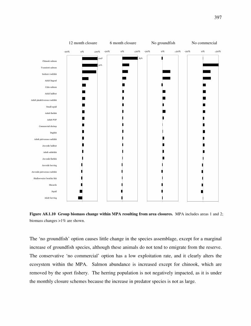
397

12 month closure 6 month closure No groundfish No commercial

(��0

%���"������$

�B���

��������

����������"3������"����

A�2����"'���2�����"���!����

A�2����"������$

A�2����"�������

%���"��3�����

A�2����"���3��

%���"'���2�����"���!����

��$����

*������"����'

%���"-6-

%���"�������

��"�B���

%���"'��!��2�����"���!����

%���"���3��

*���"����

%���"��$���

#������"���!����

���������"����

*�����!"����

(��0 �0 ��0

���0

)�0

C (��0 �0 ��0

�)0

C (��0 �0 ��0C (��0 �0 ��0C

Figure A8.1.10 Group biomass change within MPA resulting from area closures. MPA includes areas 1 and 2;

biomass changes >1% are shown.

The ‘no groundfish’ option causes little change in the species assemblage, except for a marginal

increase of groundfish species, although these animals do not tend to emigrate from the reserve.

The conservative ‘no commercial’ option has a low exploitation rate, and it clearly alters the

ecosystem within the MPA. Salmon abundance is increased except for chinook, which are

removed by the sport fishery. The herring population is not negatively impacted, as it is under

the monthly closure schemes because the increase in predator species is not as large.

398

Local effects on biodiversity

Fig. A8.1.11 shows the

equilibrium level of biodiversity

under 0 to 12 month time

closures for the MPA and

adjacent regions. Biodiversity is

measured using the Q-90

statistic (Chapter 2; Ainsworth

and Pitcher, in press). Areas 3

and 8 adjacent to the reserve

show a slight increase in

biodiversity with area

protection. The effect is more

pronounced within the MPA.

Area 2 sees the expected

increase in biodiversity with

monthly closures. Area 1 shows

a drop in biodiversity under 10

and 12 month fishery closures.

Salomon et al. (2003)

speculated that an increase in top predators might result in the local depletion of particular prey

species, lowering the overall biodiversity within the protected zone.

Ecosystem changes in the MPA

Fig. A8.1.12 shows the effects of area protection inside the reserve. Indicated are equilibrium

levels of total biomass, trophic level of the assemblage and average biomass over production

(B/P) ratio, a proxy for system longevity. As longer and longer time closures are applied, we see

less total biomass at equilibrium, but an increase in the average trophic level. Under protection,

trophic chains become longer; more production is shunted to high trophic levels and the

abundance of low trophic level animals is kept in check by top-down effects.

Figure A8.1.11 Equilibrium biodiversity in MPA and adjacent regions following fishery closure. Y-axes show ecosystem

biodiversity (Q-90); X-axes present zero to twelve month time

closures.

399

Discussion

Improving the models

Minor modifications to the base Ecopath model may be required in order to make the results

from the present investigation worthwhile as an aid to management. The Ecopath base model

used for this report describes the study area as waters of the continental shelf, roughly 70,000

km2 (see Chapter 1). This value was used directly in parameter calculations for group biomass

densities. Water temperature, which is

used for empirical calculation of basic

parameters (Chapter 5), also refers to shelf

waters. As long as the Northern BC model

was restricted to Ecopath and Ecosim, we

could describe the shelf waters implicitly,

in effect accommodating an irregular

shape for the study area (e.g., the western

boundary following the shelf break).

However, the Ecospace map used here is

square, and must cover a larger area than is

represented by the base EwE models,

approximately 140,000 km2 including

offshore waters. Although inshore groups

are restricted to shelf waters by habitat

type, functional groups that also occur in

deep water may be under-represented by

EwE biomass densities. The simulations

presented in this Appendix are based on

EwE models done by Ainsworth et al.

(2002). Following data fitting done in

Chapter 5 of this volume, the spatial work

should be repeated to verify results.

A.)

209.8

209.9

210.0

210.1

0 2 4 6 8 10 12Monthly closures

Bio

mas

s (t

•km-2

)

B.)

1.874

1.876

1.878

1.880

1.882

0 2 4 6 8 10 12

Monthly closures

Ave

. TL

C.)

2.872

2.874

2.876

2.878

0 2 4 6 8 10 12

Monthly closures

Ave

. B/P

Figure A8.1.12 Equilibrium state changes within the MPA under zero to twelve month area closures. A.)

Assemblage biomass. B.) Average trophic level of

assemblage. C.) Average biomass/production.

400

Ecosim has an automated routine to tune model predictions to known time-series. However,

there is no analogous procedure in Ecospace, and no previous exercise has attempted to verify

spatial output. It would be possible to develop a routine that adjusts Ecospace input (most

importantly the dispersal parameters), until maximum agreement is reached between model

output and observed spatial data. DFO has georeferenced catch per unit effort data (CPUE) for

British Columbia that could be applied as a proxy for biomass (e.g., PacHarv dataset; K.

Rutherford, Fisheries and Oceans Canada, Nanaimo, pers. comm.). Similarly, predicted fishing

effort could be compared with georeferenced effort data. In order to improve the spatial

dynamics of non-commercial groups, LEK information compiled from Prince Rupert community

interviews (Chapter 3; Ainsworth and Pitcher, 2005) could also be used to verify model

dynamics if it were converted into a spatial index (see Fig. 3.6).

Chinook salmon

The predicted increase in chinook abundance and catch under time and gear closures may be a

modeling effect. Ecotrophic efficiency tells us how much mortality in a functional group is

explained by the model. Beattie (2001) accepted an EE for chinook of 0.26, indicating that 74%

of chinook mortality remains unexplained in the model. However, Ainsworth et al. (2002)

entered a negative biomass accumulation of 10% per year, to reflect real-world evidence of

decline. Since Ainsworth et al. (2002) did not modify any other input parameters, EE increased

to 0.995, which is inappropriate for chinook. To accept such a high EE implies that virtually all

of the mortality of chinook salmon occurs within the study area, when in fact chinook suffer

losses throughout their Pacific migration. Chinook and any migratory species may be better

represented by a low EE to account for losses suffered outside the system, and so that favorable

or unfavorable conditions in the study area do not have disproportionate effects on group

abundance.

Spillover

Beattie (2001) found little evidence of market benefits offered by marine reserves in northern BC

in terms of salmon production outside of the reserve. As the size of the MPA increased in his

gaming scenarios, the system became less profitable as more area was closed to the industrial

401

salmon fleet. This is in contradiction with current findings, which indicate that under any level

of protection there are gains to be made by the salmon fleet. Some of the discrepancy may be

because Beattie assumed a more homogeneous distribution of primary productivity then was

suggested by the GoMOR dataset (used here). Productivity in coastal regions, like the area

covered by the MPA in this report, would be underrepresented in his calculations.

The inconsistency is also related to the trophic flow parameters. Beattie (2001) used default

Ecosim flow-control vulnerabilities, which impart on the salmon populations greater resistance

to fisheries impacts than were assumed in the present model. Under the comparatively top-down

settings for salmon used in this report (vulnerabilities set proportional to predator trophic level,

as in Ainsworth (2003), the populations are more heavily influenced by the activities of the fleet

and so clearly show the benefit of effort reduction. Combined with higher dispersal rates, this

makes the present model predict greater fisheries benefits outside the MPA.

402

Appendix 8.2 Ecospace Parameters

Table A8.2.1 Habitat occupancy

Functional Group Habitat

0 1 2 3 4 5 6 7 8 9

Ecospace

area

occupied

Sea otters + + + 21% Mysticetae + 100% Odontocetae + 100% Seals, sea lions + + + + 40% Seabirds + 100% Transient salmon + + + + + + + + 63% Coho salmon + + + + + + + + 63% Chinook salmon + + + + + + + + 63% Small squid + + + + + + 96% Squid + + + + + + 96% Ratfish + + + + + + + + 63% Dogfish + + + + + + + + 63% J. pollock + + + + + + + 95% Pollock + + + + + + + 96% Forage fish + 100% Eulachon + + + + + + + + 63% J. herring + + + 21% A. herring + + + + + + + + 100% J. POP + + + + + + + + 63% A. POP + + + + + + + + 63% Inshore rockfish + + + + + 41% J. pisc. Rockfish + + + 21% A. pisc. Rockfish + + + + + + + + 63% J. plank. rockfish + + + 21% A. plank. rockfish + + + + + + + + 63% J. turbot + + + + 40% A. turbot + + + + + + + + 63% J. flatfish + + 4% A. flatfish + + + + + + + 58% J. halibut + + + + 41% A. halibut + + + + + + + + 63% J. Pacific cod + + + + 40% A. Pacific cod + + + + + + 50% J. sablefish + + + + + 41% A. sablefish + 100% J. lingcod + + 4% A. lingcod + + + + + + + 58% S. benthic fish + + + 21% Skates + 100% Large crabs + + + 21% Small crabs + + 4% Comm. shrimp + + + + + + + 58% Epifaunal inv. + 100% Inf. carn. inv. + 100% Inf. det. inv. + 100% Carn. jellyfish + 100% Euphausiids + 100% Copepods + 100% Corals and sponges + + + + 40% Macrophytes + 100% Phytoplankton + 100% Habitat area 100% 1% 2% 17% 19% 9% 8% 5% 37% 1%

403

Table A8.2.2 Fishery activity by habitat

Fleet Habitat

0 1 2 3 4 5 6 7 8 9

Groundfish trawl + + + + + +

Sable + + + + +

Herring gillnet + + + + + +

Ground H+L + + + + + + +

Salmon gillnet + + + + + +

Crab trap + + +

Shrimp / prawn trap + + + +

Other Inv. + + +

Halibut H+L + + + + + + +

Salmon troll + + + + + +

Salmon seine + + + + + +

Salmon troll freezer + + + + + + +

Herring seine + + + + + + +

Shrimp trawl + + + + +

Eulachon + + + +

Longline +

Recreational + + + + + + + +

Table A8.2.3 Salmon straying rates

Functional

Group Species

Straying

rates Reference*

Transient salmon Sockeye 0.6-1.5% Foerster 1936, 1968

Pink 0.4-2.2% Boyd 1964; Blair 1968

Chum 2.0-46.0% Sakano 1960, cited in Sano 1966; Harding 1981, cited in Lister et al. 1981

Chinook Chinook 1.4-13% Snyder 1931; Sholes and Hallock 1979; Quinn and Fresh 1984

Coho Coho 0.5-27.0% Shapovalov and Taft 1954; Donaldson and Allen 1958

*Cited in Tallman and Healey (1994)

404

Table A8.2.4 Dispersal parameters

Group

Base dispersal

rate (km·yr-1)

Rel. dispersal

in bad habitat

Rel. vuln. to

predation in

bad habitat

Rel. feeding

rate in bad

habitat Advected?

Sea otters 300 10 2 0.01 Mysticetae 300 5 2 0.01 Odontocetae 300 5 2 0.01 Seals, sea lions 300 5 2 0.01 Seabirds 300 5 2 0.01 Transient salmon 1000 5 4 0.05 Coho salmon 300 5 1 0.05 Chinook salmon 250 5 0.5 0.5 Small squid 300 1 1 0.01 Squid 300 1 0.5 0.05 Ratfish 300 5 2 0.01 Dogfish 300 5 2 0.01 J. pollock 1000 5 5 0.01 Pollock 1500 5 2 0.01 Forage fish 1500 5 2 0.01 Eulachon 300 5 2 0.01 J. herring 300 5 5 0.01 A. herring 300 1 1 0.01 J. POP 300 5 5 0.01 A. POP 200 5 2 0.01 Inshore rockfish 200 5 2 0.01 J. pisc. Rockfish 300 5 5 0.01 A. pisc. Rockfish 200 5 2 0.01 J. plank. rockfish 300 5 5 0.01 A. plank. rockfish 200 5 2 0.01 J. turbot 300 5 5 0.01 A. turbot 300 5 2 0.01 J. flatfish 300 5 0.5 0.05 A. flatfish 300 5 2 0.01 J. halibut 300 5 5 0.01 A. halibut 300 5 2 0.01 J. Pacific cod 300 5 5 0.01 A. Pacific cod 300 5 2 0.01 J. sablefish 460 5 5 0.01 A. sablefish 200 5 2 0.01 J. lingcod 1000 5 0.4 0.5 A. lingcod 200 5 2 0.1 S. benthic fish 300 5 2 0.01 Skates 1500 5 2 0.01 Large crabs 300 1 1 0.05 Small crabs 300 5 0.5 0.02 Comm. shrimp 300 5 2 0.01 Epifaunal inv. 200 5 2 0.01 Inf. carn. inv. 200 5 2 0.01 Inf. det. inv. 200 5 2 0.01 Carn. jellyfish 200 5 2 0.01 Y Euphausiids 200 5 2 0.01 Y Copepods 200 5 2 0.01 Y Corals and sponges 200 5 50 0.01 Macrophytes 200 5 2 0.01 Phytoplankton 200 5 2 0.01 Y

405

Table A8.2.5 Ecospace output region definitions

Area1 Name DFO management area

Haida Gwaii

1 E. Gwaii Haanas NMCA 2-6 to 2-19

2 W. Gwaii Haanas NMCA 2-20 to 2-47

3 E. Moresby Island 2-2 to 2-6, 102-2, 102-3

4 E. Graham Island 2-1, 102-1

5 E. Dixon Entrance 101-4 to 101-9

6 W. Dixon Entrance 101-1 to 101-3

7 W. Graham Island 2-48 to 2-99

8 W. Moresby Island E142*

Mainland coast

9 N. Vancouver Island 9 to 12

10 Bella Bella 7,8

11 Douglas Channel 6

12 Banks Island 5

13 Chatham Sound 3,4,103

Shelf waters

14 N. Hecate Strait 104, 105

15 S. Hecate Strait 106

16 N. Queen Charlotte Sound 107 to 109

17 S. Queen Charlotte Sound 110, 111

Off-shelf waters

18 Offshore Haida Gwaii W1422

19 Offshore Central BC 130+127 1 Area numbers correspond to Fig.A8.1.6. 2 Regions 7 and 17 share statistical area 142 equally

406

Figure A8.2.1 Value of catch per gear type

���������"����

�����

�����

�����

�����

� � � � � �� ��

:���"��"�����"5D?!�?+7

��3�����

�����

�����

�����

�����

� � � � � �� ��

�����$"$����

����

����

�)��

����

� � � � � �� ��

���������"���!"���"���

����

����

�)��

����

� � � � � �� ��

:���"��"�����"5D?!�?+7

����"$����

�����

�����

�����

�����

� � � � � �� ��

*��3"���'

)����

)����

)����

)����

� � � � � �� ��

����'?'����"���'

����

����

�)��

����

� � � � � �� ��

:���"��"�����"5D?!�?+7

6����"��2����3�����

����

����

����

����

����

� � � � � �� ��

��3��"���!"���"���

)����

)����

)����

)����

� � � � � �� ��

����"���

����

����

����

����

����

� � � � � �� ��

:���"��"�����"5D?!�?+7

����"�����

�����

�����

�����

�����

� � � � � �� ��

����"���"����E��

�����

�����

�����

)����

)����

� � � � � �� ��

�����$"�����

����

����

�)��

����

� � � � � �� ��

:���"��"�����"5D?!�?+7

����'"����

�����

�����

�����

�����

� � � � � �� ��

1������

���

���

���

���

���

� � � � � �� �� /��$���

�)���

�)���

�)���

�)���

�)���

� � � � � �� ��

.����+"�������

:���"��"�����"5D?!�?+7

�����������

�����

�����

�����

�����

� � � � � �� ��

.����+"�������

����

�����

�����

�����

�����

� � � � � �� ��

.����+"�������

407

Appendix 9.1 References cited in the Appendices

Table A9.2.1 IG discounting case study references cited in Appendix 2.1.

1. Ahrens, R. 1999. Heritable risk sensitive foraging in juvenile fish: potential implications for the dynamics of harvested

populations. Unpublished Masters Thesis, Department of Zoology, University of British Columbia, 75 pp.

2. Ainsworth, C. and U.R. Sumaila, 2003. Intergenerational discounting and the conservation of fisheries resources: A

case study in Canadian Atlantic cod. Pages 26-32 in: Three Essays on the Economics of Fishing. Edited by U.R.

Sumaila. Fish. Cent. Res. Rep., 11(3): 33 pp.

3. Ainsworth, C. and U.R. Sumaila, 2005. Intergenerational valuation of fisheries resources can justify long-term

conservation: a case study in Atlantic cod (Gadus morhua). Can. J. of Fish. Aquat.Sci. 62: 1104-1110.

4. Azar, C. and T. Sterner, 1996. Discounting and Distributional Considerations in the Context of climate Change. Ecol.

Econ. 19: 169-185.

5. Brennan, T.J., 1997. Discounting the future: economics and ethics. In: The RFF Reader In Environmental and

Resource Management. Edited by W.E. Oates. Resources for the Future. Washington, D.C.

6. Christensen, V. and C.J. Walters, 2004. Trade-offs in ecosystem-scale optimization of fisheries management policies.

Bull. Mar. Sci. 74(3): 549-562.

7. Clark, C.W., 1973. The economics of overexploitation. Science. 181: 630-634.

8. Department of Fisheries and Oceans, 1994. Report on fishing vessel performance Scotia-Fundy fisheries – Maritimes

region. Economic and Commercial Analysis Report No. 152.

9. Fearnside, P.M, 2002. Greenhouse Gas Emissions from a Hydroelectric Reservoir (Brazil’s Tucurui Dam) and the

Energy Policy Implications. Water Air Soil Poll. 133: 69-96.

10. Fisher, A.C., and J.V. Krutilla, 2002. Resource conservation, environmental preservation, and the rate of discount. Q.

J. Econ., 89(3): 358-370.

11. Goulder, L.H. and R.N. Stavins, 2002. Discounting: an eye on the future. How economists’ controversial practice of

discounting really affects the evaluation of environmental policies. Nature. 419: 673-674.

12. Hasselmann, K., S. Hasselmann, R. Giering, V. Ocana and H.V. Sorch, 1997. Sensitivity study of optimal CO2

emission paths using a simplified structural integrated assessment model (SIAM). Clim. Chan. 37: 335-343

13. Heal, G.M., 1998. Valuing the future: economic theory and sustainability. Columbia University Press, New York.

14. Heymans, J.J., 2003. A revised model for Newfoundland and southern Labrador (2J3KLNO) for the time period 1985-

1987. Pages 40-60 in: Heymans, J.J. (Ed.) Ecosystem Models of Newfoundland and Southeastern Labrador.

Additional information and Analyses for ‘Back to the Future’. Fish. Cent. Res. Rep. 11(5): 79 pp

15. Nielsen, U., 2001. Hyperbolic discounting and sustainable development. Department of Economics and Natural

Resources. Royal Veterinary and Agricultural University. Denmark. [http://www.flec.kvl.dk/kok/ore-

seminar/hyperbsustdev.pdf]

16. Okey, T.A. and B.A. Wright, 2004. Toward ecosystem-based extraction policies for Prince William Sound, Alaska:

integrating conflicting objectives and rebuilding pinnipeds. Bull. Mar. Sci. 74(3): 727-747.

17. Schelling, T.C. 1995. Intergenerational discounting. Energy Policy, 23: 395-401.

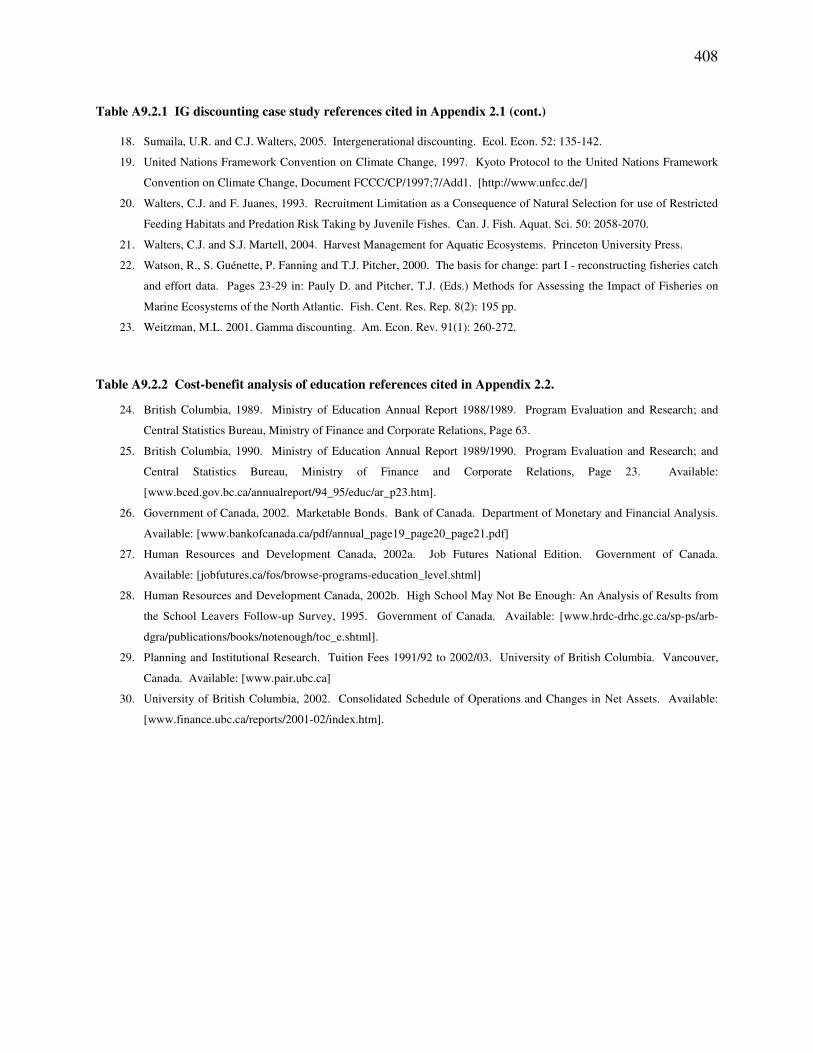
408

Table A9.2.1 IG discounting case study references cited in Appendix 2.1 (cont.)

18. Sumaila, U.R. and C.J. Walters, 2005. Intergenerational discounting. Ecol. Econ. 52: 135-142.

19. United Nations Framework Convention on Climate Change, 1997. Kyoto Protocol to the United Nations Framework

Convention on Climate Change, Document FCCC/CP/1997;7/Add1. [http://www.unfcc.de/]

20. Walters, C.J. and F. Juanes, 1993. Recruitment Limitation as a Consequence of Natural Selection for use of Restricted

Feeding Habitats and Predation Risk Taking by Juvenile Fishes. Can. J. Fish. Aquat. Sci. 50: 2058-2070.

21. Walters, C.J. and S.J. Martell, 2004. Harvest Management for Aquatic Ecosystems. Princeton University Press.

22. Watson, R., S. Guénette, P. Fanning and T.J. Pitcher, 2000. The basis for change: part I - reconstructing fisheries catch

and effort data. Pages 23-29 in: Pauly D. and Pitcher, T.J. (Eds.) Methods for Assessing the Impact of Fisheries on

Marine Ecosystems of the North Atlantic. Fish. Cent. Res. Rep. 8(2): 195 pp.

23. Weitzman, M.L. 2001. Gamma discounting. Am. Econ. Rev. 91(1): 260-272.

Table A9.2.2 Cost-benefit analysis of education references cited in Appendix 2.2.

24. British Columbia, 1989. Ministry of Education Annual Report 1988/1989. Program Evaluation and Research; and

Central Statistics Bureau, Ministry of Finance and Corporate Relations, Page 63.

25. British Columbia, 1990. Ministry of Education Annual Report 1989/1990. Program Evaluation and Research; and

Central Statistics Bureau, Ministry of Finance and Corporate Relations, Page 23. Available:

[www.bced.gov.bc.ca/annualreport/94_95/educ/ar_p23.htm].

26. Government of Canada, 2002. Marketable Bonds. Bank of Canada. Department of Monetary and Financial Analysis.

Available: [www.bankofcanada.ca/pdf/annual_page19_page20_page21.pdf]

27. Human Resources and Development Canada, 2002a. Job Futures National Edition. Government of Canada.

Available: [jobfutures.ca/fos/browse-programs-education_level.shtml]

28. Human Resources and Development Canada, 2002b. High School May Not Be Enough: An Analysis of Results from

the School Leavers Follow-up Survey, 1995. Government of Canada. Available: [www.hrdc-drhc.gc.ca/sp-ps/arb-

dgra/publications/books/notenough/toc_e.shtml].

29. Planning and Institutional Research. Tuition Fees 1991/92 to 2002/03. University of British Columbia. Vancouver,

Canada. Available: [www.pair.ubc.ca]

30. University of British Columbia, 2002. Consolidated Schedule of Operations and Changes in Net Assets. Available:

[www.finance.ubc.ca/reports/2001-02/index.htm].

409

Table A9.4.1 BC fisheries timeline references cited in Appendix 4.1.

1. AAFC. 2004. Fish and Seafood Online. Agriculture and Agri-Food Canada. Webpage [atn-riae.agr.ca]

2. Aboriginal Communal Fishing Licenses Regulations, SOR/93-332, s.4

3. Ainsworth, C. Personal observation. UBC Fisheries Centre, 2202 Main Mall, Vancouver, BC. V6T 1Z4.

4. Allain, J and J. Fréchette. 1993. The aboriginal fisheries and the sparrow decision. Parliamentary Research

Branch. BP-341E. Available: [www.parl.gc.ca]

5. Alverson, D.L., A.T. Pruter and L.L. Ronholt. 1964. A study of demersal fishes and fisheries of the

Northeastern Pacific Ocean. H.R. MacMillan Lectures in Fisheries, University of British Columbia, 190 p.

6. Anderson, D. 1998. Aboriginal Fisheries Strategy. Statement by David Anderson Minister of Fisheries and

Oceans Canada and Member of Parliament for Victoria. Available: [www.dfo-mpo.gc.ca/media]

7. Anderson, D. 1998. Speaking notes for the Honourable David Anderson, P.C., M.P. Minister of Fisheries and

Oceans. House of Commons Standing Committee on Fisheries and Oceans. Vancouver, B.C. Jan 20, 1998.

8. Anon. 1971. Exclusive fisheries zones proclaimed by Canada. Fish. of Can. 23:10-12

9. Anon. 2004. Personal communication (commercial harvester).

10. Archipelago. 2004. Archipelago Marine Research Ltd. Webpage [www.archipelago.bc.ca] Accessed Feb,

2004.

11. BC. 2000. Nis'ga Final Agreement. Treaty Negotiations Office. Available:

[www.gov.bc.ca/tno/negotiation/nisgaa]

12. Beattie, A. 2002. A history of the British Columbia trawl fishery. Fish. Centre Res. Rep. 10(1): 67-74

13. Beattie, J. 2003. Treaty will give natives fishing rights. Liberals opposed to separate fisheries, but have no

choice in matter. Vancouver Sun. Newspaper editorial. January 9, 2003.

14. Bert Ionson, Personal communication. A/Resource Management Coordinator; Fisheries and Oceans Canada.

Vancouver, BC.

15. Billig, P. 2000. Reef Wrap: A recent expedition to the Northwest Hawaiian Islands netted 25 tons of derelict

fishing gear and marine debris. There's still choke left. Honolulu Weekly. 10(50). Dec 13-19, 2000

16. British Columbia. 1995. R. v. Jack, John and John, 1995. BCJ 2632

17. British Columbia. 2003. R. v. Anderson et al. 2003. BCPC 0217.

18. British Columbia. 2003. R. v. Kapp et al. 2003. BCPC 0279.

19. Canada. 1979. Department of Fisheries and Oceans Act, 1978-79, c.13, s.2

20. Canada. 1985. Fisheries Act, R.S.C. 1985, c.F-14

21. Canada. 1990. R. v. Sparrow, 1990. 1 S.C.R. 1075

22. Canada. 1996. Oceans Act. S.C. c.31

23. Canada. 1996. R. v. Van der Peet, 1996. 2 S.C.R. 507

24. Canada. 1997. Delgamuukw v. British Columbia, 1997. 3 S.C.R. 1010

25. Canada. 1999. Canadian Environmental Protection Act. , 1999, c.33

26. Canada. 1999. R. v. Marshall. 1999. 3 S.C.R. 26014

27. Canada. 2003. Species at Risk Act. Available: [www.sararegistry.gc.ca]

28. Canada. 2003. Canada Ratified United Nations Convention on the Law of the Sea. Speech from the Throne.

Nov 6, 2003. No. 171

410

Table A9.4.1 BC fisheries timeline references cited in Appendix 4.1 (cont.)

29. CNLR. 1998. Delgamuukw vs. British Columbia. Canadian Native Law Reporter. Pp 14-97.

30. CRFB. 1998. Canadian Code of Conduct for Responsible Fisheries. Canadian Responsible Fisheries Board.

Available: [www.responsiblefisheries.com]

31. Crowley, W. Ronald and R. Bourgeois. 1988. The Development of Canada's Ocean Policy. Ottawa:

Department of Fisheries and Oceans. 171 pp.

32. CTS. 1953. Convention between Canada and the United States of America for the preservation of the halibut

fishery of the Northern Pacific Ocean and Bering Sea. Canada Treaty Series 1953/14.

33. CTS. 1985. Pacific Salmon Treaty. Canada Treaty Series 1985/7.

34. CTS. 1991. Canada-US Free Trade Agreement. Canada Treaty Series 1991/53.

35. DFO 1999. Silvergrey rockfish. DFO Science Stock Status Report A6-09 (1999). Canadian Science Advisory

Secretariat

36. DFO 1999. Three selective fishing experimental pilots are scheduled for Juan de Fuca Strait. Aug 24, 1999 NR-

PR-99-82E

37. DFO. 1995. News release. Dec 20, 1995.

38. DFO. 1995. Progress report on the Skeena and Kitimat Rivers released. News Release. Dec 4, 1995. NR-PR-

95-60E

39. DFO. 1995. Trawl quotas caught, fishery closes for season. Sept. 29, 1995. NR-PR-95-53E

40. DFO. 1996. New air surveillance patrol for fisheries. Aug 9, 1996. NR-PR-96-38E

41. DFO. 1996. New BC sport fishing regulations announced. April 4, 1996. NR-PR-96-16E

42. DFO. 1996. New regulations governing foreign commercial fishing vessels now in effect. July 23, 1996. NR-

PR-96-31E

43. DFO. 1996. News release. Feb 16, 1996. NR-PR-96-10E

44. DFO. 1996. News release. Nov 13, 1996

45. DFO. 1997. New Groundfish Management Plan. Backgrounder. Media release. March 19, 1997

46. DFO. 1997. Coho Conservation Measures. Backgrounder. Media release. June 27, 1997 NR-HQ-97-25/B

47. DFO. 1997. Details of the 1997 Pacific commercial salmon plans. Backgrounder. NR-HQ-97-24/B

48. DFO. 1997. DFO and KTFC combine efforts in enforcement patrols. Aug 6, 1997. NR-PR-97-37E

49. DFO. 1997. DFO announces 1997 Pacific halibut management plan. March 14, 1997. NR-PR-97-05E

50. DFO. 1997. Federal, provincial fisheries ministers cooperate on new groundfish management plan. March 19,

1997.

51. DFO. 1997. Salmonid Enhancement Program (SEP) marks 20 years of salmon production, partnerships with

public. Sept 30, 1997. NR-PR-97-49E

52. DFO. 1998. A new direction for Canada's Pacific Salmon Fisheries. Backgrounder. Oct. 1998. Available:

[www-comm.pac.dfo-mpo.gc.ca]

53. DFO. 1998. A policy for selective fishing in Canada's Pacific Fisheries. Available [www-comm.pac.dfo-

mpo.gc.ca/english/selective/default.htm]

54. DFO. 1998. Canada and BC sign groundfish trawl fishery agreement. May 13, 1998. NR-PR-98-27E

55. DFO. 1998. Dog team joins DFO enforcement. Sept 17, 1998. NR-PR-98-81E

56. DFO. 1998. Selective harvesting in commercial salmon fisheries moves ahead. April 24, 1998. NR-PR-98-23E

411

Table A9.4.1 BC fisheries timeline references cited in Appendix 4.1 (cont.)

57. DFO. 1999. Pacific Ocean Perch British Columbia Coast. DFO Science Stock Status Report A6-11 (1999).

Canadian Science Advisory Secretariat.

58. DFO. 1999. A guide to selective salmon fishing in British Columbia. Backgrounder. June 26, 1999. BC-PR-99-

83E

59. DFO. 1999. Canada and US reach a comprehensive agreement under the Pacific Salmon Treaty. June 3, 1999.

NR-HQ-99-29E

60. DFO. 1999. Canary Rockfish. DFO Science Stock Status Report A6-08 (1999). Canadian Science Advisory

Secretariat.

61. DFO. 1999. Conservation concerns lead to cross-sector strategy for rockfish. May 6, 1999. NR-PR-99-40e

62. DFO. 1999. Dover Sole West Coast Vancouver Island (Areas 3C, D) to Queen Charlotte Lslands (Areas 5A-E).

DFO Stock Status Report A6-04 (1999). Canadian Science Advisory Secretariat.

63. DFO. 1999. English Sole Hecate Strait (Areas 5C/D) DFO Science Stock Status Report A6-05 (1999).

Canadian Science Advisory Secretariat.

64. DFO. 1999. Global positioning system (GPS) end of week rollover. News Release. Aug 19, 1999. NR-HQ-99-

50E

65. DFO. 1999. Pacific Cod. DFO Science Stock Status Report A6-01 (1999). Canadian Science Advisory

Secretariat.

66. DFO. 1999. Petrale Sole British Columbia (Areas 3C-5D) Stock Status Report A6-06 (1999). Canadian Science

Advisory Secretariat.

67. DFO. 1999. Recreational fishing operators required to supply catch records. May 7, 1999. NR-PR-99-41e

68. DFO. 1999. Rock Sole Queen Charlotte Sound (Areas 5A/B) and Hecate Strait (Areas 5C/D). DFO Science

Stock Status Report A6-03 (1999) Canadian Science Advisory Secretariat.

69. DFO. 1999. Selective fishing. Backgrounder. June 18, 1999. BG-PR-99-60(d)

70. DFO. 1999. Widow Rockfish. DFO Science Stock Status Report A6-10 (1999). Canadian Science Advisory

Secretariat.

71. DFO. 1999. Yellowtail Rockfish. DFO Science Stock Status Report A6-07 (1999). Canadian Science Advisory

Secretariat.

72. DFO. 2000. Canada begins high seas driftnet operation in the North Pacific. May 15, 2000. NR-PR-00-47E

73. DFO. 2000. Dhaliwal announces funding for 31 projects under the First Nations Selective Fisheries Gear

Purchase Program. July 11, 2000. NR-PR-00-76E

74. DFO. 2000. Dhaliwal announces new funding to strengthen fisheries enforcement. News Release. Mar 24,

2000. NR-HQ-00-09E

75. DFO. 2000. Experimental selective fishing project will test innovative gear to release coho unharmed. June 23,

2000 NR-PR-00-63E

76. DFO. 2000. Fisheries and Oceans Canada invests in selective fishing projects for 2000. June 16, 2000 NR-PR-

00-61E

77. DFO. 2000. Groundfish trawl fishery opens. April 28, 2000. NR-PR-00-36E

78. DFO. 2000. New gillnet technology advances sustainable and selective salmon fishing. Sept. 8, 2000. NR-PR-

00-118E

412

Table A9.4.1 BC fisheries timeline references cited in Appendix 4.1 (cont.)

79. DFO. 2000. Pacific Fisheries Adjustment and Restructuring Program. Backgrounder. March 15, 2000. BG-PR-

00-09E

80. DFO. 2000. Recreational selective fishing projects focus on coho avoidance education and awareness. July 7,

2000. NR-PR-00-75E

81. DFO. 2000. Salmon Update July 31, 2000. NR-PR-00-93E

82. DFO. 2001. Fish Stocks of the Pacific Coast. Online Book. Department of Fisheries and Oceans, Canada.

Catalogue no. Fs23-397-2001e. Available: [www-comm.pac.dfo-

mpo.gc.ca/publications/speciesbook/Introduction/default.html]

83. DFO. 2001. Minister winds up fisheries renewal BC. Ministry of Agriculture Food and Fisheries. News Release

#01-37. Oct. 18, 2001.

84. DFO. 2001. Satellite technology increases catch data efficiency. Oct 12, 2001. NR-PR-01-095E

85. DFO. 2002. Performance Report for the period ending March 31, 2002. Fisheries and Oceans Canada. DPR

2001-2002

86. DFO. 2002. Closure of west coast sablefish fishery. News Release. Jan 17, 2002. NR-PR-02-002E

87. DFO. 2002. DFO protects inshore rockfish by restricting fishing activity. News Release. Aug 1, 2002. NR-PR-

02-050E

88. DFO. 2002. DFO's coho conservation measures reinforced by COSEWIC decision. News Release. May 3,

2002.

89. DFO. 2002. Fisheries Policy Development. Fisheries and Oceans Canada Program Records. Office of the

Associate Deputy Minister. DFO MAN 335

90. DFO. 2002. Lingcod conservation measures strengthened. News Release. July 26, 2002. NR-PR-02-047E

91. DFO. 2002. Lingcod. Stock Status Report A6-18 (2002).

92. DFO. 2002. Responsible fisheries summary: Code of Conduct for Responsible Fishing Operations - A Review

(1998-2001). January 2002.

93. DFO. 2002. Sablefish. DFO Science Stock Status Report A6-02 (2002). Canadian Science Advisory

Secretariat.

94. DFO. 2003. Aboriginal Fisheries Strategy. Fisheries Management Reports and Publications. Webpage

[www.dfo-mpo.gc.ca] Accessed Feb, 2004.

95. DFO. 2003. Canadian code of conduct for responsible fishing operations. Backgrounder. April 2003. B-HQ-03-

26E(b)

96. DFO. 2003. State of Canada's Fishery -2002. Fact Sheet. Aquaculture Production. Available: [www.dfo-

mpo.gc.ca]

97. DFO. 2003. Thibault announces pink salmon action plan for the Broughton Archipelago. News Release. Feb

20, 2003. NR-PR-03-011e

98. DFO. 2004. Three BC salmon species targeted by DFO for recovery. News Release. Jan. 7, 2004. NR-PR-04-

004e

99. DOJ. 1996. An act respecting the Oceans of Canada. Department of Justice. 1996, c.31. Available:

[laws.justice.gc.ca/en/O-2.4/88102.html]

413

Table A9.4.1 BC fisheries timeline references cited in Appendix 4.1 (cont.)

100. ENS. 2002. Fish Farming Moratorium Lifted in British Columbia. Environmental News Service. News Release

Jan 31, 2002.

101. Environment Canada. 2000. National Programme of Action in Place to Protect Canada's Oceans. News Release

Archive. June 8, 2000.

102. Environment Canada. 2004. Species at Risk. Webpage [www.speciesatrisk.gc.ca] Accessed Mar, 2004

103. FAO. 1995. The Code of Conduct for Responsible Fisheries. Food and Agriculture Organization of the United

Nations. Adopted by the Twenty-eighth session of the FAO Conference in October 1995. 41 pp. Available:

[www.fao.org]

104. Fletcher, G. 1996. The history of the Race Rocks marine ecological reserve. Available: [www.racerocks.com]

105. Forrester, C.R., A. J. Beardsley, and Y. Takahashi. 1978. Groundfish, shrimp and herring fisheries in the

Bering Sea and Northeast Pacific - historical catch statistics through 1970. Int. North Pac. Fish. Comm. Bull.

37:147 p

106. Gislason, G., E. Lam and K. Knowles. 2002. Western Economic Diversification and Pacific Fisheries

Adjustment. Western Economic Diversification. Ottawa, Ontario. Available: [www.wd.gc.ca]

107. Gregr, E.J. 1999. An analysis of historic (1908-1967) whaling records from British Columbia, Canada. M.Sc.

Thesis, University of British Columbia. 101 pp.

108. IPHC. 1995. Halibut commission completes annual meeting. News Release. January 27, 1995.

109. IPHC. 1995. Halibut commission completes annual meeting. News Release. January 27, 1995.

110. IPHC. 1996. Halibut commission completes 1996 annual meeting. News release. January 26, 1996.

111. IPHC. 1997. Halibut commission completes 1997 annual meeting. News release. January 31, 1997.

112. IPHC. 2001. Halibut commission completes 2001 annual meeting. News release. January 26, 2001.

113. Jamieson, G. and L. Chew. 2002. Hexactinellid sponge reefs: areas of interest as Marine Protected Areas in the

north and central coast areas. Canadian Science Advisory Secretariat. Research Document 2002/122.

114. Leaman, B.M. 1987. Incorporating reproductive value into Pacific Ocean perch management. Proc. Int.

Rockfish Symposium. p. 355-368. October, 1986, Anchorage, Alaska.

115. MARCO. 2004. Marco announces new 56G power block design. Marco marine news. Webpage

[www.marcoseattle.com] Accessed Feb, 2004

116. MARE. 2002. Canada designates trawl closures to protect unique sponge reefs. MPA News 4(3) Sept. 2002.

117. MELP. 2002. Race Rocks Ecological Reserve Management Plan. Environmental Stewardship Division.

Ministry of Water, Land and Air Protection. C2002-960086-3

118. Mills, D. 1997. The west coast aboriginal fishery. Aboriginal Rights Coalition of BC. Available:

[arcbc.tripod.com]

119. NPAFC. 2004. North Pacific Anadromous Fish Commission. Webpage [www.npafc.org] Accessed Feb, 2004

120. Pearse, P. and P. Larkin. 1992. Managing salmon in the Fraser: report to the Minister of Fisheries and Oceans

on the Fraser River Salmon Investigation. 36p

121. PFRCC 1999. Coast-Wide Coho. Pacific Fisheries Resource Conservation Council. Background Paper No.

1999/1d.

122. Richards, L.J. 1994. Trip limits, catch, and effort in the British Columbia rockfish trawl fishery. N. Am. J. Fish.

Mgmt. 14:742-750

414

Table A9.4.2 Average species weight references cited in Appendix 4.4.

123. Rush, S. 1998. The Fiduciary obligation in Delgamuukw. Assembly of First Nations. Available:

[www.delgamuukw.org]

124. TV Times. 2003. Race-Based Fisheries Wrong Legally and Morally. Magazine article. August 29, 2003.

125. UNCLOS. 1982. United Nations Convention on the Law of the Sea. Available:

[www.un.org/Depts/los/convention_agreements/convention_overview_convention.htm].

126. Vasconcellos, M. and T.J. Pitcher. 2002. Historical reference points for models of past ecosystems in northern

British Columbia. Fish. Centre Res. Rep. 10(1): 60-67

127. Westrheim, S.J. 1986. The rockfish fisheries off western Canada, 1860 - 1985. Proc. Int. Rockfish Symposium,

p. 43-49. October, 1986, Anchorage, Alaska.

128. Zugarramurdi, A. and M.A. Parin. 1995. Economic engineering applied to the fishery industry. FAO Fisheries

Technical Paper - 351. Food and Agriculture Organization of the United Nations.

129. NPFC. 2004. International North Pacific Fisheries Commission. North Pacific Anadromous Fish Commission

Webpage [www.npfc.org]

130. IPHC 1998. The Pacific Halibut: Biology, Fishery and Management. International Pacific Halibut

Commission. Technical Report No. 40. (Revision of Nos. 6, 16 and 22). Seattle, Washington.

131. Burgner, R.L. 1991. Life history of sockeye salmon. In: C. Groot and L. Margolis (eds.) Pacific Salmon Life

Histories. UBC Press, Vancouver, pp2-117.

132. Sandercock, F.K. 1991. Life history of coho salmon. In: C. Groot and L. Margolis (eds.) Pacific Salmon Life

Histories. UBC Press, Vancouver, pp395-445.

133. Heard, W.R. 1991. Life history of pink salmon. In: C. Groot and L. Margolis (eds.) Pacific Salmon Life

Histories. UBC Press, Vancouver, pp119-230.

134. Burgner, R.L. 1991. Life history of sockeye salmon. In: C. Groot and L. Margolis (eds.) Pacific Salmon Life

Histories. UBC Press, Vancouver, pp2-117.

135. Salo E.O. 1991. Life history of chum salmon. In: C. Groot and L. Margolis (eds.) Pacific Salmon Life

Histories. UBC Press, Vancouver, pp231-309.

136. King, J.R. and Gjernes, T.W. 1999. Estimate of the 1998 recreational halibut catch in British Columbia waters.

CSAS Research Document 99/121, 25pp.

137. King, J.R. and Surry, A.M. 2000. Lingcod assessment and recommended yield options for 2001. CSAS

Research Documents 2000/164.

138. DFO. 1999. Rougheye Rockfish British Columbia Coast. DFO Science Stock Status Report A6-15.

139. Forrest, R. 2004. Northern British Columbia: Adding Recreational Catches to the Ecosystem Simulation

Model. Fish. Centre Res. Rep. (in press.)

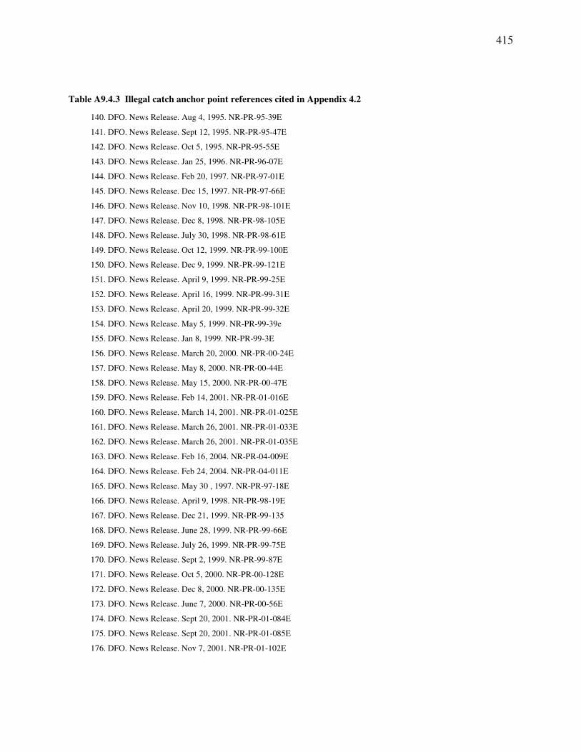
415

Table A9.4.3 Illegal catch anchor point references cited in Appendix 4.2

140. DFO. News Release. Aug 4, 1995. NR-PR-95-39E

141. DFO. News Release. Sept 12, 1995. NR-PR-95-47E

142. DFO. News Release. Oct 5, 1995. NR-PR-95-55E

143. DFO. News Release. Jan 25, 1996. NR-PR-96-07E

144. DFO. News Release. Feb 20, 1997. NR-PR-97-01E

145. DFO. News Release. Dec 15, 1997. NR-PR-97-66E

146. DFO. News Release. Nov 10, 1998. NR-PR-98-101E

147. DFO. News Release. Dec 8, 1998. NR-PR-98-105E

148. DFO. News Release. July 30, 1998. NR-PR-98-61E

149. DFO. News Release. Oct 12, 1999. NR-PR-99-100E

150. DFO. News Release. Dec 9, 1999. NR-PR-99-121E

151. DFO. News Release. April 9, 1999. NR-PR-99-25E

152. DFO. News Release. April 16, 1999. NR-PR-99-31E

153. DFO. News Release. April 20, 1999. NR-PR-99-32E

154. DFO. News Release. May 5, 1999. NR-PR-99-39e

155. DFO. News Release. Jan 8, 1999. NR-PR-99-3E

156. DFO. News Release. March 20, 2000. NR-PR-00-24E

157. DFO. News Release. May 8, 2000. NR-PR-00-44E

158. DFO. News Release. May 15, 2000. NR-PR-00-47E

159. DFO. News Release. Feb 14, 2001. NR-PR-01-016E

160. DFO. News Release. March 14, 2001. NR-PR-01-025E

161. DFO. News Release. March 26, 2001. NR-PR-01-033E

162. DFO. News Release. March 26, 2001. NR-PR-01-035E

163. DFO. News Release. Feb 16, 2004. NR-PR-04-009E

164. DFO. News Release. Feb 24, 2004. NR-PR-04-011E

165. DFO. News Release. May 30 , 1997. NR-PR-97-18E

166. DFO. News Release. April 9, 1998. NR-PR-98-19E

167. DFO. News Release. Dec 21, 1999. NR-PR-99-135

168. DFO. News Release. June 28, 1999. NR-PR-99-66E

169. DFO. News Release. July 26, 1999. NR-PR-99-75E

170. DFO. News Release. Sept 2, 1999. NR-PR-99-87E

171. DFO. News Release. Oct 5, 2000. NR-PR-00-128E

172. DFO. News Release. Dec 8, 2000. NR-PR-00-135E

173. DFO. News Release. June 7, 2000. NR-PR-00-56E

174. DFO. News Release. Sept 20, 2001. NR-PR-01-084E

175. DFO. News Release. Sept 20, 2001. NR-PR-01-085E

176. DFO. News Release. Nov 7, 2001. NR-PR-01-102E

416

Table A9.4.3 Illegal catch anchor point references cited in Appendix 4.2 (cont.)

177. DFO. News Release. April 15, 2002. NR-PR-02-022E

178. DFO. News Release. May 14, 2001. NR-PR-02-026E

179. DFO. News Release. Jan 16, 2003. NR-PR-03-007E

180. DFO. News Release. June 11, 2003. NR-PR-03-034E

181. DFO. News Release. July 7, 2003. NR-PR-03-036E

Table A9.4.4 Discard anchor point references cited in Appendix 4.2

182. Williams, G. 1999. Incidental Catch and Mortality of Pacific Halibut, 1962-1999. IPHC Report of Assessment

and Research Activities. Avaliable at [www.iphc.washington.edu]

183. Hare, S. and G. Williams. Halibut bycatch mortality and length composition: 1974-1999. International Pacific

Halibut Commission. Available: [www.iphc.washington.edu/Staff/hare/html/bycatch/Bycatch.html]

184. Stanley, R.D., D. Davenport. 1982. A study of Trawl Mesh Selectivity for English Sole and Rock Sole in

Hecate Strait, August 1-5, 1980. Department of Fisheries and Oceans. Nanaimo, British Columbia.

185. Sullivan, P.J., R.J. Trumble and S.A. Adlerstein. 1994. Pacific Halibut bycatch in the groundfish fisheries:

effects on and management implications for the Halibut Fishery. International Pacific Halibut Commission

Scientific Report 78:4-9.

186. DFO. 2004. Trawl Observer Database. Department of Fisheries and Oceans. Pacific Biological Station.

Nanaimo, BC.

187. Fargo, J. 1992. A summary of data collected for a study of the bycatch of Pacific halibut (Hippoglossus

stenolepis) in the winter trawl fishery in Hecate Strait 1991-1992. International Pacific Halibut Commission.

(cit. Alverson, 1994)

188. Williams, G.H., C.C. Schmitt, S.H. Hoag, J.D. Berger. 1989. Incidental Catch and Mortality of Pacific halibut,

1962-1986. International Pacific Halibut Commission. Seattle, Washington. (cit. Alverson 1994)

189. Williams, G.H. 1987. Stock Assessment Document II, Section 6. Results of the 1987 IPHC Observer Trips.

International Pacific Halibut Commission (cit. Alverson, 1994)

190. Alverson, D.L. and M.H. Freeberg. 1994. A global assessment of fisheries bycatch and discards. FAO Fisheries

Technical Paper 339: 233pp.

191. FIS. 2002. Discards in the Groundfish Fisheries of the Bering Sea/Aleutian Islands and the Gulf of Alaska,

1998-2000. State of Alaska Department of Fish and Game. Fisheries Information Services. Juneau, Alaska.

192. Haigh, R., J. Schnute, L. Lacko, C. Eros, G. Korkman, B. Ackerman. 2002. At-sea observer coverage for catch

monitoring of the British Columbia hook and line fisheries. Canadian Science Advisory Secretariat. Research

Document 2002/108.

193. C. Ainsworth. Personal observation. UBC Fisheries Centre. Vancouver, Canada.

194. Okey, T. and D. Pauly (eds.) 1999. A Trophic Mass-Balance Model of Alaska's Prince William Sound

Ecosystem, for the Post-Spill Period 1994-1996 2nd Edition. Fisheries Centre Research Reports 7(4): 136pp.

417

Table A9.4.5 Unreported catch anchor point references cited in Appendix 4.2

195. DFO. 2004. Creel/Logbook Official Recreational Statistics. Pacific Regional Data Unit. Department of

Fisheries and Oceans. Available: [www-sci.pac.dfo-mpo.gc.ca/sa/Recreational/default_e.htm]

196. DFO. 1975. Survey of Recreational Fishing in Canada. Department of Fisheries and Oceans. Ottawa.

Available: [www.dfo-mpo.gc.ca/communic/statistics/recreational/historical/index_e.htm]

197. DFO. 1980. Survey of Recreational Fishing in Canada. Department of Fisheries and Oceans. Ottawa.

Available: [www.dfo-mpo.gc.ca/communic/statistics/recreational/historical/index_e.htm]

198. DFO. 1985. Survey of Recreational Fishing in Canada. Department of Fisheries and Oceans. Ottawa.

Available: [www.dfo-mpo.gc.ca/communic/statistics/recreational/historical/index_e.htm]

199. DFO. 1990. Survey of Recreational Fishing in Canada. Department of Fisheries and Oceans. Ottawa.

Available: [www.dfo-mpo.gc.ca/communic/statistics/recreational/canada/index_e.htm]

200. DFO. 1995. Survey of Recreational Fishing in Canada. Department of Fisheries and Oceans. Ottawa.

Available: [www.dfo-mpo.gc.ca/communic/statistics/recreational/canada/index_e.htm]

201. DFO. 2000. Survey of Recreational Fishing in Canada. Department of Fisheries and Oceans. Ottawa.

Available: [www.dfo-mpo.gc.ca/communic/statistics/recreational/canada/index_e.htm]

202. ODFW. 2001. Marine Recreational Fishery Observers/Samplers. Project completion report. Project #01-006.

Fish Restoration and Enhancement Program. Oregon Department of Fish and Wildlife. Available:

[hmsc.oregonstate.edu/odfw/reports/mar_rec_obs_program2001.pdf].

203. Ainsworth, C. 2002. RAPFISH. Fisher interviews for northern British Columbia. (Unpublished data).

418

Table A9.5.3 Biomass, catch and effort time series data references cited in Appendix 5.3.

1. Ainsworth, C. and T.J. Pitcher. 2005. The Dark side of BC's Marine Fisheries: Estimating Illegal, Unreported

and Unregulated Catch. Internal Report. British Columbia Ministry of Water, Land and Air Protection.

2. Ainsworth, C. and T.J. Pitcher, 2005. Using Local Ecological Knowledge in Ecosystem Models. In: G.H.

Kruse, V.F. Gallucci, D.E. Hay, R.I. Perry, R.M. Peterman, T.C. Shirley, P.D. Spencer, B. Wilson, and D.

Woodby (Eds.) Fisheries assessment and management in data-limited situations. Alaska Sea Grant College

Program, University of Alaska Fairbanks.

3. Ainsworth, C., J.J. Heymans and T.J. Pitcher. 2002. Ecosystem Models of Northern British Columbia for the

Time Periods 2000, 1950, 1900 and 1750. Fish. Cent. Res. Rep. 10(4): 41 pp.

4. Beattie, A. 2001. A New Model for Evaluating the Optimal Size, Placement and Configuration of Marine

Protected Areas. M.Sc. Thesis. Resource Management and Environmental Studies. University of British

Columbia. 159 pp.

5. Bell, F. 1981. The Pacific Halibut. Alaska Northwest Publ. Co. Anchorage, Alaska.

6. Benson, A.J., G.A. McFarlane and J.R. King. 2001. A Phase "0" Review of Elasmobranch Biology, Fisheries,

Assessment and Management. Can. Sci. Adv. Sec. Res. Doc. 2001/129.

7. Bigg, M.A. 1985. Status of the Steller Sea Lion (Eumentopias jubatus) and California Sea Lion (Zalophus

californianus) in British Columbia Can. Spec. Pub. Fish. Aquat. Sci. 77: 1-20.

8. Cass, A.J., R.J. Beamish and G.A. McFarlane. 1990. Lingcod (Ophiodon elongatus). Can. Spec. Pub. Fish.

Aquat. Sci. 109:1-40.

9. Clark, W.G. and S.R. Hare. 2001. Assessment of the Pacific Halibut Stock at the End of 2001. International

Pacific Halibut Commission.

10. Clark, W.G. and S.R. Hare. 2002. Assessment of the Pacific Halibut Stock at the End of 2002. International

Pacific Halibut Commission.

11. Clark, W.G. and S.R. Hare. 2003. Assessment of the Pacific Halibut Stock at the End of 2003. International

Pacific Halibut Commission.

12. Daniel, K.S., P.B. McCarter and D.E. Hay. 2001. The Construction of a Database of Pacific Herring Catches

Recorded in British Columbia From 1888 to 1950. Can. Tech. Rep. Fish. Aquat. Sci. 2368:108.

13. DFO 1999. Dungeness Crab North Coast License Area A. Department of Fisheries and Oceans Canada.

Science Stock Status Report C6-01 (1999).

14. DFO 1999. Neon flying squid. Department of Fisheries and Oceans Canada. Science Stock Status Report C6-

12 (1999).

15. DFO 1999. Opal Squid. Department of Fisheries and Oceans Canada. Science Stock Status Report C6-04

(1999).

16. DFO 2004. British Columbia Commercial Catch Statistics 1951-1995. CD-Rom. Department of Fisheries and

Oceans Canada. Available: [C.Ainsworth, University of British Columbia Fisheries Centre. 2202 Main Mall,

Vancouver, BC. V6T 1Z4. Email: c.ainsworth@fisheries.ubc.ca).

17. DFO 2004. Commercial Halibut Landings in BC. Pacific Regional Data Unit. Department of Fisheries and

Oceans. Available: [www-sci.pac.dfo-mpo.gc.ca/sa/Commercial/Summaries/Halibut/comhal_e.htm].

18. DFO 2004. Groundfish Catch and Effort Database (GFCATCH). Pacific Biological Station, Nanaimo, BC.

Department of Fisheries and Oceans Canada.

419

Table A9.5.3 Biomass, catch and effort time series data references cited in Appendix 5.3 (cont.).

19. DFO 2004. Official Commercial Catch Statistics. Pacific Regional Data Unit. Department of Fisheries and

Oceans. Available: [www-sci.pac.dfo-mpo.gc.ca/sa/Commercial/AnnSumm_e.htm].

20. DFO 2004. Recreational Catch Statistics. Pacific Regional Data Unit. Department of Fisheries and Oceans.

Available: [www-sci.pac.dfo-mpo.gc.ca/sa/Recreational/default_e.htm].

21. Eggers, D.M., J. Irvine, M. Fukuwaka and V. Karpenko. 2003. Catch Trends and Status of North Pacific

Salmon. North Pacific Anadromous Fish Commission. Doc. 723. 34 pp.

22. Fargo, J. 1999. Flatfish Stock Assessments for the West Coast of Canada for 1998 and Recommended Yield

Options for 1999. Can. Sci. Adv. Sec. Res. Doc. 1999/17.

23. Forrest, R. (in press). Northern British Columbia: Adding Recreational Catches to the Ecosystem Simulation

Model. Fish. Centre Res. Rep.

24. Gregr, E. J. 2000. An Analysis of Historic (1908-1967) Whaling Records from British Columbia, Canada.

M.Sc. Thesis. Department of Zoology. University of British Columbia. 101 pp.

25. Haist, V., D. Fournier and M.W. Saunders. 1999. Reconstruction of BC Sablefish Stocks, 1966-1998, and

Catch Projections for 1999, Using an Integrated Catch-Age Mark-Recapture Model with Area and Depth

Movement. Can. Sci. Adv. Sec. Res. Doc. 1999/79.

26. Haist, V., R. Hilborn and M. Wyeth. 2001. Sablefish Stock Assessment for 2001 and Advice to Managers for

2002. Can. Sci. Adv. Sec. Res. Doc. 2001/135.

27. Holtby, B., B. Finnegan and B. Spilsted. 1999. Forecast for Northern British Columbia Coho Salmon in 1999.

Can. Sci. Adv. Sec. Res. Doc. 1999/186.

28. IPHC 2003. Commercial Halibut Catch and Effort for IPHC Statistical Areas on the BC Coast (Regulatory

Area 2B). International Pacific Halibut Commission. Available:

[www.iphc.washington.edu/halcom/commerc/2bcpue2002.pdf].

29. IPHC 2003. Halibut Landing Report No.14. November 20, 2003. Available:

[www.iphc.washington.edu/halcom/newsrel/2003/nr20031120.htm].

30. Ketchen, K.S. 1986. The Spiny Dogfish (Squalus acanthias) in the Northeast Pacific and a History of its

Utilization. Can. J. Fish. Aquat. Sci. 88: 1-78.

31. King, J.R. and A.M. Surry. 2000. Lingcod Stock Assessment and Recommended Yield Options for 2001. Can.

Sci. Adv. Sec. Res. Doc. 2000/164.

32. M. Vasconcellos. 2001. Unpublished Manuscript. Departamento de Oceanografia, Universidade do Rio

Grande, Caixa Postal 474, 96201-900, Rio Grande, RS, Brazil.

33. Martell, S. 1999. Estimating Lingcod Biomass in Hecate Strait Using Stock Reduction Analysis. In: Haggan,

N. and A. Beattie (Eds). Back to the Future: Reconstructing the Hecate Strait Ecosystem. Fish. Cent. Res. Rep.

7(3): 49-55.

34. Nichol, L. and K. Heise. 1992. The Historical Occurrence of Large Whales off the Queen Charlotte Islands.

Report Prepared for South Moresby/Gwaii Haanas National Park Reserve. 67 pp.

35. Olesiuk, P.F. 1999. An Assessment of the Status of Harbour Seals (Phoca vitulina) in British Columbia. Can.

Sci. Adv. Sec. Res. Doc. 1999/33.

420

Table A9.5.3 Biomass, catch and effort time series data references cited in Appendix 5.3 (cont.).

36. Preikshot, D. 2005. Data Sources and Derivations of Parameters for Generalised Northeast Pacific Ocean

Ecopath with Ecosim Models. In: Guénette, S. and V. Christensen (Eds.). The Stellar Sea Lion Decline: Models

and Data of the Northeast Pacific. Fish. Cent. Res. Rep. 13(1) (in press).

37. PSC 2002. Status of Coho Salmon Stocks and Fisheries in the Northern Boundary Area. Northern Boundary

Technical Committee Report. TCNB (02)-3. Pacific Salmon Commission.

38. PSC 2003. Annual Exploitation Rate Analysis and Model Calibration. Report TCCHINOOK (03)-2. November

28, 2003. Pacific Salmon Commission Joint Chinook Technical Committee Report.

39. PSC 2003. Catch and Escapement of Chinook Salmon Under Pacific Salmon Commission Jurisdiction.

TCCHINOOK (04)-2. Pacific Salmon Commission.

40. Quinn, T.J., R.B. Deriso and S.H. Hoag. 1985. Methods of Population Assessment of Pacific Halibut.

International Pacific Halibut Commission. Seattle, Washington. Scientific Report 72: 1-18.

41. Rutherford, D. and C. Wood. 2000. Trends in Abundance and Pre-season 2000 Stock Size Forecasts for Major

Sockeye, Pink and Chum Salmon Stocks in the Central Coast and Selected Salmon Stocks in Northern British

Columbia. Can. Sci. Adv. Sec. Res. Doc. 2000/114.

42. Rutherford, D.T., L.L. Barton, G.E. Gillespie and J.A. Boutillier. 2004. Utility of Historical Catch Data in

Setting Reference Points for the British Columbia Shrimp by Trawl Fishery. Can. Sci. Adv. Sec. Res. Doc.

2004/026.

43. Schnute, J., R. Haigh, B. Krishka and P. Starr. 2001. Pacific Ocean Perch Assessment for the West Coast of

Canada in 2001. Can. Sci. Adv. Sec. Res. Doc. 2001/138.

44. Schweigert, J. 2004. Stock Assessment for British Columbia Herring in 2003 and Forecasts of the Potential

Catch in 2004. Can. Sci. Adv. Sec. Res. Doc. 2004/005.

45. Sinclair, A.F., S. Martell and J. Boutillier. 2001. Assessment of Pacific Cod off the West Coast of Vancouver

Island and in Hecate Strait. November 2001. Can. Sci. Adv. Sec. Res. Doc. 2001/159.

46. Tadokor, K. 2001. Long-Term Variations of Plankton Biomass in the North Pacific. Proceedings of the

PICES/CoML/IPRC Workshop on Impact of Climate Variability on Observation and Prediction of Ecosystem

and Biodiversity Changes in the North Pacific. Report 18. September 2001. pp. 132-136.

47. Trites, A.W. and D. Pauly. 1998. Estimating Mean Body Masses of Marine Mammals from Maximum Body

Lengths. Can. J. Zool. 76: 886-896.

48. Turnock, B.J., T.K. Wilderbuer and E.S. Brown. 2003. Arrowtooth flounder. pp. 369-406. In: Anonymous

(Ed.) Appendix B: Stock Assessment and Fishery Evaluation Report for the Grounfish Resources of the Gulf of

Alaska. North Pacific Fishery Management Council, Anchorage.

49. Wood, C., D. Rutherford and L. Jantz. 1999. Trends in Abundance and Pre-Season 1999 Stock Size Forecasts

for Major Sockeye, Pink and Chum Salmon Stocks in Northern British Columbia. Can. Sci. Adv. Sec. Res.

Doc. 1999/126.

421

Table A9.8.1 Spatial investigations for Gwaii Haanas references cited in Appendix 8.1.

1. Ainsworth, C. 2004. Estimating the Effects of Prey-predator Vulnerability Settings on Ecosim’s Dynamic

Function. In T.J. Pitcher (ed.). Back to the Future: Advances in Methodology for Modeling and Evaluating

Past Ecosystems. Fish. Centre Res. Rep. 12(1): 158pp.

2. Ainsworth, C. and T.J. Pitcher, in press. Modifying Kempton's Biodiversity Index for use with Dynamic

Ecosystem Models. Back to the Future: Advances in Methodology for Modeling and Evaluating Past

Ecosystems. Ecological Indicators.

3. Ainsworth, C. and T.J. Pitcher, 2005. Using Local Ecological Knowledge in Ecosystem Models. In: G.H.

Kruse, V.F. Gallucci, D.E. Hay, R.I. Perry, R.M. Peterman, T.C. Shirley, P.D. Spencer, B. Wilson, and D.

Woodby (Eds.) Fisheries assessment and management in data-limited situations. Alaska Sea Grant College

Program, University of Alaska Fairbanks.

4. Ainsworth, C., J.J. Heymans, T.J. Pitcher and M. Vasconcellos, 2002. Ecosystem Models of Northern British

Columbia for the Time Periods 2000, 1950, 1900 and 1750. Fisheries Centre Research Reports, 10(4), 41 pp.

5. Beattie, A. I. 2001. A New Model for Evaluating the Optimal Size, Placement and Configuration of Marine

Protected Areas. Unpublished Masters thesis. Department of Resource Management and Environmental

Science, University of British Columbia, 58pp.

6. Christensen, V., Guénette, S., J.J. Heymans, C.J. Walters, R. Watson, D. Zeller and D. Pauly. 2003. Hundred-

year decline of North Atlantic predatory fishes. Fish and Fisheries 4:1-24.

7. Conway, K.W. 1999. Hexactinellid sponge reefs on the British Columbia continental shelf: geological and

biological structure with a perspective on their role in the shelf ecosystem. Can. Stock Ass. Sec. Res. Doc.

99/192.

8. Crowder, L.B., S.L. Lyman, W.F. Figueira and J. Priddy. 2000. Source-sink Population Dynamics and the

Problem of Siting Marine Reserves. Bull. Mar. Sci. 66(3): 799-820.

9. Gell, F.R. and C.M. Roberts. 2003. Benefits Beyond Boundaries: the Fishery Effects of Marine Reserves.

Trends in Ecol. Evol. 18(9): 448-455

10. GOMER Database. Global Monitoring of Oceanic Resources. Space Applications Institute, Italy.

11. Hunt, G.L. 1995. Oceanographic Processes and Marine Productivity in Waters Offshore of Marbled Murrelet

Breeding Habitat. In Ecology and Conservation of Marbled Murrelet. Ralph, C.J., Hunt, G.L., Raphael, M.G.

and Piatt, J.F. (eds.) USDA Forest Service Gen. Tech Rep. PSW-152.

12. Mortensen, D., A. Wertheimer, J. Maselko, and S. Taylor. 2000. Survival and Straying of Pink Salmon

Using Recoveries of Coded-Wire Tags and Thermally-Induced Otolith Marks. Quarterly Report for July-

Aug-Sept 2000. National Marine Fisheries Service.

http://www.afsc.noaa.gov/Quarterly/jas2000/feature.htm#body

13. Myers, R.A. and Worm, B. 2003. Rapid Worldwide Depletion of Predatory Fish Communities. Nature 423:

280-283.

14. Okey, T.A. and D. Pauly. 1998. Trophic Mass-Balance Model of Alaska's Prince William Sound Ecosystem,

for the Post-Spill Period 1994-1996. 2nd Edition. Fish. Centre Res. Rep. 7(4): 137p

15. Pauly, D. 2003. On the Need for a Global Network of Large Marine Reserves. Oral presentation. 133rd

Annual Meeting of the American Fisheries Society. August 10-14. Québec City, Canada.

16. Pitcher, T.J. 1997. The Design and Monitoring of Marine Reserves - Introduction to the Issues. In Pitcher,

T.J. (ed.) The Design and Monitoring of Marine Reserves. Fish. Centre Res. Rep. 5(1): 1-3

422

Table A9.8.1 Spatial investigations for Gwaii Haanas references cited in Appendix 8.1 (cont.).

17. Pitcher, T.J. and E.A. Buchary. 2002a. Ecospace simulations for Hong Kong Waters. In Pitcher, T. Buchary,

E. and Trujillo, P. (eds.). Spatial Simulations of Hong Kong's Marine Ecosystem: Forecasting with MPAs

and Human-Made Reefs. Fish. Centre Res. Rep. 10(3): 30-35

18. Pitcher, T.J. and E.A. Buchary. 2002b. Ecospace Simulations for the People's Republic of China (PRC)

Inshore Waters. In Pitcher, T. Buchary, E. and Trujillo, P. (eds.). Spatial Simulations of Hong Kong's Marine

Ecosystem: Forecasting with MPAs and Human-Made Reefs. Fish. Centre Res. Rep. 10(3): 30-35

19. Roberts, C.M., J.A. Bohnsack, F. Gell, J.P. Hawkins, R. Goodridge. 2001. Effects of Marine Reserves on

Adjacent Fisheries. Science. 294: 1920-1923.

20. Sladek Nowlis, J. and M. Yoklavich. 1999. Fisheries Benefits and Optimal Design of Marine Reserves.

Fish. Bull. 97: 604-616.

21. Salomon, A.K., N. Waller, C. McIlhagga, R. Yung, and C. Walters. 2002. Modeling the trophic effects of

marine protected area zoning policies: a case study. Aquatic Ecology 36: 85-95.

22. Sloan, N.A., P.M. Bartier and W.C. Austin. 2001. Living Marine Legacy of Gwaii Haanas. II: marine

invertebrate baseline to 2000 and invertebrate-related management issues. Parks Canada – Technical Reports

in Ecosystem Science #035.

23. Tallman, R.F. and M.C. Healey. 1994. Homing, Straying, and Gene Flow among Seasonally Separated

Populations of Chum Salmon (Oncorhynchus keta). Can. J. Fish. Aquat. Sci. 51:577-588

24. Thompson, R.E. 1981. Oceanography of the British Columbia Coast. Can. Spec. Publ. Fish. Aquat. Sci. 56:

291 pp.

25. Walters, C. V. Christensen and D. Pauly. 1997. Structuring Dynamic Models of Exploited Ecosystems from

Trophic Mass-balance Assessments. Rev. Fish Biol. Fish. 7:139-172.

26. Ware, D.M. and G.A. McFarlane. 1989. Fisheries Production Domains in the Northeast Pacific Ocean. P.

359-379. In R.J. Beamish and G.A. McFarlane (eds.). Effects of Ocean Variability on Recruitment and an

Evaluation of Parameters used in Stock Assessment Models. Can. Spec. Publ. Fish. Aquat. Sci. 108: 359-

379.

27. Willis, T.J., R.B. Millar, R.C. Babcock and N. Tolimieri. 2003. Burdens of Evidence and the Benefits of

Marine Reserves: Putting Descartes Before des Horse? Env. Cons. 30(2): 97-103.