Lecture 4 Image Restoration
75
Lecture 4 Image Restoration
Transcript of Lecture 4 Image Restoration

Lecture 4
Image Restoration

2
Image Restoration
• Image restoration: recover an image that has been
degraded by using a prior knowledge of the degradation
phenomenon.
• Model the degradation and applying the inverse process in
order to recover the original image.

3
A Model of Image Degradation/Restoration
Process
• Degradation
– Degradation function H
– Additive noise ),( yx

4
A Model of Image Degradation/Restoration
Process
If is a process, then
the degraded image is given in the spatial domain by
( , ) ( , ) ( , ) ( , )
H linear, position-invariant
g x y h x y f x y x y

5
A Model of Image Degradation/Restoration
Process
The model of the degraded image is given in
the frequency domain by
( , ) ( , ) ( , ) ( , )G u v H u v F u v N u v

6
Noise Sources
• The principal sources of noise in digital images arise during
image acquisition and/or transmission
Image acquisition
e.g., light levels, sensor temperature, etc.
Transmission
e.g., lightning or other atmospheric disturbance in wireless
network
7
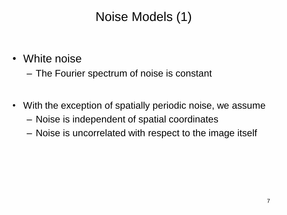
Noise Models (1)
• White noise
– The Fourier spectrum of noise is constant
• With the exception of spatially periodic noise, we assume
– Noise is independent of spatial coordinates
– Noise is uncorrelated with respect to the image itself

8
Noise Models (2)
Gaussian noiseElectronic circuit noise, sensor noise due to poor illumination and/or high temperature
Rayleigh noiseRange imaging

9
Range Imaging (1)
Short for High Dynamic Range Imaging. HDRI is an imaging technique that allows for a greater dynamic range of exposure than would be obtained through any normal imaging process.
It is now popularly used to refer to the process of tone mapping* together with bracketed** exposures of normal digital images, giving the end result a high, often exaggerated dynamic range
* Tone mapping is a technique used in image processing and computer graphics to map a set of colours to another; often to approximate the appearance of HDRI in media with a more limited dynamic range
** bracketing is the general technique of taking several shots of the same subject using different or the same camera settings

10
Range Imaging (2)
The intention of HDRI is to accurately represent the wide range of intensity levels found in real scenes ranging from direct sunlight to shadows
HDRI, also called HDR (High Dynamic Range) is a feature commonly found in high-end graphics and imaging software

11
Range Imaging: Examples (1)
Tower Bridge in Sacramento,
CA

12
Range Imaging: Examples (2)
http://en.wikipedia.org/wiki/High_dynamic_range_imaging
Sydney Harbour Bridge HDRi produces greater detail and fewer shadows

13Old Saint Paul’s Wellinton, New Zealand

14
Noise Models (3)
Erlang (gamma) noise: Laser imaging
Exponential noise: Laser imaging
Uniform noise: Least descriptive; Basis for numerous random number generators
Impulse noise: quick transients,
such as faulty switching

15
Gaussian Noise (1)
2 2( ) /2
The PDF of Gaussian random variable, z, is given by
1 ( )
2
z zp z e
where, represents intensity
is the mean (average) value of z
is the standard deviation
z
z

16
Gaussian Noise (2)
2 2( ) /2
The PDF of Gaussian random variable, z, is given by
1 ( )
2
z zp z e
– 70% of its values will be in the range
– 95% of its values will be in the range
)(),(
)2(),2(

17
Rayleigh Noise
2( ) /
The PDF of Rayleigh noise is given by
2( ) for
( )
0 for
z a bz a e z ap z b
z a
2
The mean and variance of this density are given by
/ 4
(4 )
4
z a b
b

18
Erlang (Gamma) Noise
1
The PDF of Erlang noise is given by
for 0 ( ) ( 1)!
0 for
b baza z
e zp z b
z a
2 2
The mean and variance of this density are given by
/
/
z b a
b a

19
Exponential Noise
The PDF of exponential noise is given by
for 0 ( )
0 for
azae zp z
z a
2 2
The mean and variance of this density are given by
1/
1/
z a
a

20
Uniform Noise
The PDF of uniform noise is given by
1 for a
( )
0 otherwise
z bp z b a
2 2
The mean and variance of this density are given by
( ) / 2
( ) /12
z a b
b a

21
Impulse (Salt-and-Pepper) Noise
The PDF of (bipolar) impulse noise is given by
for
( ) for
0 otherwise
a
b
P z a
p z P z b
If either or is zero, the impulse noise is calleda bP P
unipolar
if , gray-level will appear as a light dot,
while level will appear like a dark dot.
b a b
a

22

23
Examples of Noise: Original Image

24
Examples of Noise: Noisy Images(1)

25
Examples of Noise: Noisy Images(2)

26
Periodic Noise
• Periodic noise in an image arises typically from electrical or
electromechanical interference during image acquisition.
• It is a type of spatially dependent noise
• Periodic noise can be reduced significantly via frequency
domain filtering

27
An Example of Periodic Noise

28
Estimation of Noise Parameters (1)
The shape of the histogram identifies the closest PDF match

29
Estimation of Noise Parameters (2)
Consider a subimage denoted by , and let ( ), 0, 1, ..., -1,
denote the probability estimates of the intensities of the pixels in .
The mean and variance of the pixels in :
s iS p z i L
S
S
1
0
12 2
0
( )
and ( ) ( )
L
i s i
i
L
i s i
i
z z p z
z z p z
30
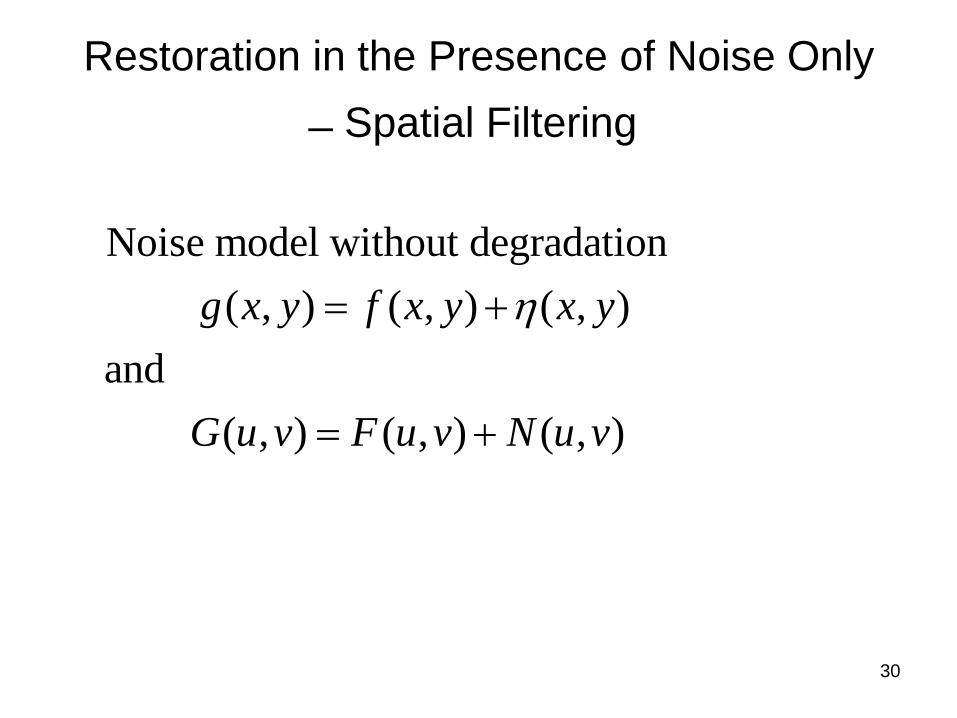
Restoration in the Presence of Noise Only
Spatial Filtering
Noise model without degradation
( , ) ( , ) ( , )
and
( , ) ( , ) ( , )
g x y f x y x y
G u v F u v N u v

31
Spatial Filtering: Mean Filters (1)
Let represent the set of coordinates in a rectangle
subimage window of size , centered at ( , ).
xyS
m n x y
Arithmetic mean filter
xySts
tsgnm
yxf
),(
),(.
1),(ˆ

32
Spatial Filtering: Mean Filters (2)
Generally, a geometric mean filter achieves smoothing comparable to the arithmetic mean filter, but it tends to lose less image detail in the process
mn
Sts xy
tsgyxf
1
),(
),(),(ˆ
Geometric mean filter:

33
Spatial Filtering: Example

34
Spatial Filtering: Order-Statistic Filters (1)
),(max),(ˆ),(
tsgyxfxySts
),(),(ˆ),(
tsgmedianyxfxySts
Median filter:
),(min),(ˆ),(
tsgyxfxySts
Max filter:
Min filter:

35
Spatial Filtering: Order-Statistic Filters (2)
),(min),(max
2
1),(ˆ
),(),(tsgtsgyxf
xyxy StsSts
Mid-point filter:

36
Spatial Filtering: Order-Statistic Filters (3)
We delete the / 2 lowest and the / 2 highest intensity values of
( , ) in the neighborhood . Let ( , ) represent the remaining
- pixels.
xy r
d d
g s t S g s t
mn d
xySts
r tsgdmn
yxf
),(
),(1
),(ˆ
Alpha-trim mean filter:

37

38
39
Spatial Filtering: Adaptive Filters
Adaptive filters
The behavior changes based on statistical characteristics of the image inside the filter region defined by the mхn rectangular window.
The performance is superior to that of the filters discussed

40
Adaptive Filters:
Adaptive, Local Noise Reduction Filters (1)
2
: local region
The response of the filter at the center point (x,y) of
is based on four quantities:
(a) ( , ), the value of the noisy image at ( , );
(b) , the variance of the noise corrupti
xy
xy
S
S
g x y x y
2
ng ( , )
to form ( , );
(c) , the local mean of the pixels in ;
(d) , the local variance of the pixels in .
L xy
L xy
f x y
g x y
m S
S

41
Adaptive Filters:
Adaptive, Local Noise Reduction Filters (2)
2
2
The behavior of the filter:
(a) if is zero, the filter should return simply the value
of ( , ).
(b) if the local variance is high relative to , the filter
should return a value cl
g x y
ose to ( , );
(c) if the two variances are equal, the filter returns the
arithmetic mean value of the pixels in .xy
g x y
S

42
Adaptive Filters:
Adaptive, Local Noise Reduction Filters (3)
L
L
myxgyxgyxf ),(),(),(ˆ2
2
An adaptive expression for obtaining a filtered image based on the assumptions:

43

44
Adaptive Filters:
Adaptive Median Filters (1)
min
max
med
max
The notation:
minimum intensity value in
maximum intensity value in
median intensity value in
intensity value at coordinates ( , )
maximum all
xy
xy
xy
xy
z S
z S
z S
z x y
S
owed size of xyS

45
Adaptive Filters:
Adaptive Median Filters (2)
med min med max
max
The adaptive median-filtering works in two stages:
Stage A:
A1 = ; A2 =
if A1>0 and A2<0, go to stage B
Else increase the window size
if window size , re
z z z z
S
med
min max
med
peat stage A; Else output
Stage B:
B1 = ; B2 =
if B1>0 and B2<0, output ; Else output
xy xy
xy
z
z z z z
z z

46
Adaptive Filters:
Adaptive Median Filters (2)
med min med max
max
The adaptive median-filtering works in two stages:
Stage A:
A1 = ; A2 =
if A1>0 and A2<0, go to stage B
Else increase the window size
if window size , re
z z z z
S
med
min max
med
peat stage A; Else output
Stage B:
B1 = ; B2 =
if B1>0 and B2<0, output ; Else output
xy xy
xy
z
z z z z
z z
The median filter output is an impulse
or not
The processed point is an impulse or not

47
Example:
Adaptive Median Filters

48
Periodic Noise Reduction by Frequency
Domain Filtering
The basic idea
Periodic noise appears as concentrated bursts of energy in the Fourier transform, at locations corresponding to the frequencies of the periodic interference
Approach
A selective filter is used to isolate the noise

49
Perspective Plots of Bandreject Filters

50

51
Perspective Plots of Notch Filters

52

53
Several interference components are present, the methods discussed in the preceding sections are not always acceptable because they remove much image information The components tend to have broad skirts that carry information about the interference pattern and the skirts are not always easily detectable.

54
Linear, Position-Invariant Degradations
( , ) ( , ) ( , )g x y H f x y x y

55
Linear, Position-Invariant Degradations
An operator having the input-output relationship
( , ) ( , ) is said to be position invariant
if
( , ) ( , )
for any ( , ) and any and .
g x y H f x y
H f x y g x y
f x y
1 2 1 2
1 2
is linear
( , ) ( , ) ( , ) ( , )
and are any two input images.
H
H af x y bf x y aH f x y bH f x y
f f

56
Linear, Position-Invariant Degradations
In the presence of additive noise,
if is a linear operator and position invariant,
( , ) ( , ) ( , ) ( , )
( , ) ( , ) ( , )
( , ) ( , ) ( , ) ( , )
H
g x y f h x y d d x y
h x y f x y x y
G u v H u v F u v N u v

57
Estimating the Degradation Function
• Three principal ways to estimate the degradation function
1. Observation
2. Experimentation
3. Mathematical Modeling

58
Mathematical Modeling (1)
• Environmental conditions cause degradation
A model about atmospheric turbulence
2 2 5/6( ) ( , )
: a constant that depends on
the nature of the turbulence
k u vH u v e
k

59

60
Mathematical Modeling (2)
• Derive a mathematical model from basic principles
E.g., An image blurred by uniform linear motion between the
image and the sensor during image acquisition
61
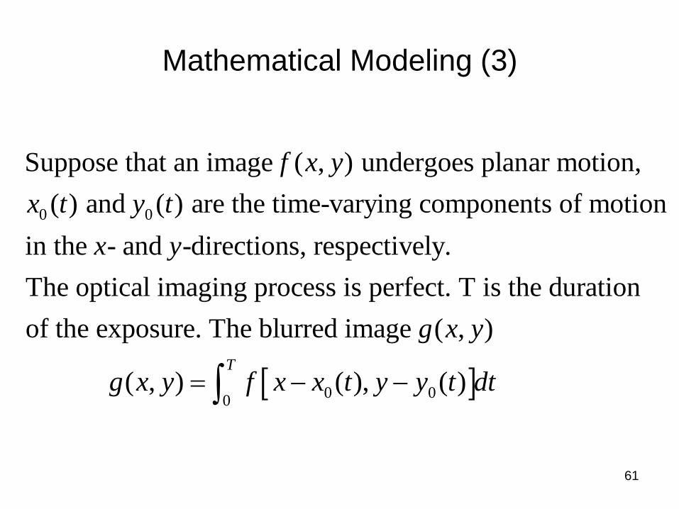
Mathematical Modeling (3)
0 0
Suppose that an image ( , ) undergoes planar motion,
( ) and ( ) are the time-varying components of motion
in the - and -directions, respectively.
The optical imaging process is perfect. T is th
f x y
x t y t
x y
0 00
e duration
of the exposure. The blurred image ( , )
( , ) ( ), ( )T
g x y
g x y f x x t y y t dt

62
Mathematical Modeling (4)
0 0
0 0
2 ( ) ( )
0
Suppose that the image undergoes uniform linear motion
in the -direction and -direction, at a rate given by
( ) / and ( ) /
( , )
T j ux t vy t
x y
x t at T y t bt T
H u v e dt
e
2 [ ] /
0
( ) sin ( )( )
Tj ua vb t T
j ua vb
dt
Tua vb e
ua vb
(Consider g(x,y) as f(x,y) convolves with an array of Dirac pulses at different (x0,y0))
T « time of integration »

63

64
Inverse Filtering
),(/),(),(
),(
),(),(*),(),(ˆ
),(
),(),(ˆ
vuHvuNvuF
vuH
vuNvuHvuFvuF
vuH
vuGvuF
An estimate of the original image:
Problem : noise is at high frequencies, H(u,v) is very small at high frequencies => amplify noise !!!

65
Inverse Filtering
1. We can't exactly recover the undegraded image
because ( , ) is not known.
2. If the degradation function has zero or very
small values, then the ratio ( , ) / ( , ) could
easily dominate th
N u v
N u v H u v
e estimate ( , ).F u v

66
Inverse Filtering
2
/2 (
EXAMPLE
The image in Fig. 5.25(b) was inverse filtered using the
exact inverse of the degradation function that generated
that image. That is, the degradation function is
( , )k u M v
H u v e
5/62/2)
, 0.0025N
k

67
A Butterworth
lowpass
function of
order 10
The poor performance of direct inverse
filtering in general
68
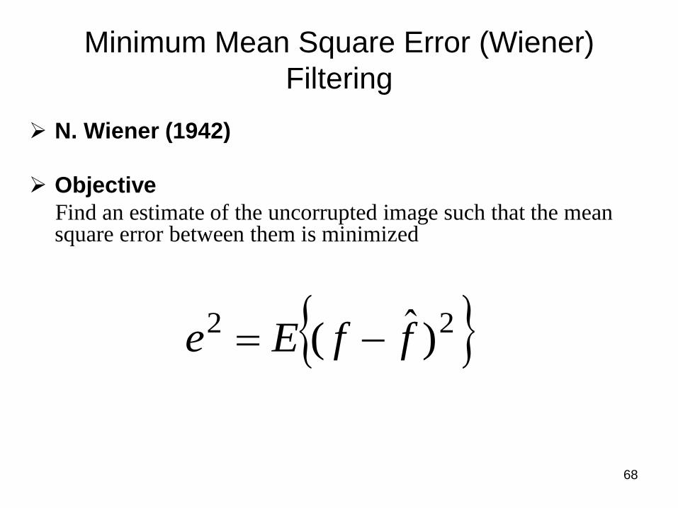
Minimum Mean Square Error (Wiener)
Filtering
N. Wiener (1942)
Objective
Find an estimate of the uncorrupted image such that the mean square error between them is minimized
22 )ˆ( ffEe

69
Minimum Mean Square Error (Wiener)
Filtering
),(),(/),(),(
),(
),(
1),(ˆ
2
2
vuGvuSvuSvuH
vuH
vuHvuF
f
H(u,v): degradation function
H*(u,v): complex conjugate of H(u,v)
|H(u,v)|2 = H(u,v)H*(u,v)
Sn(u,v)= |N(u,v)|2: power spectrum of the noise
Sf(u,v)= |F(u,v)|2 : power spectrum of the undegraded image

70
Minimum Mean Square Error (Wiener)
Filtering
),(),(
),(
),(
1),(ˆ
2
2
vuGKvuH
vuH
vuHvuF
K is a specified constant. Generally, the value of K is chosen interactively to yield the best visual results.
71
Minimum Mean Square Error (Wiener)
Filtering

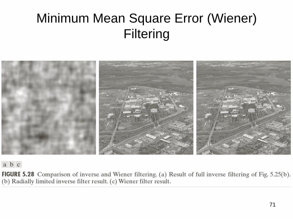
72
Left: degradated image
Middle: inverse filtering
Right: Wiener filtering

73
Constrained Least Squares Filtering
• In Wiener filter, the power spectra of the undegraded
image and noise must be known. Although a constant
estimate is sometimes useful, it is not always suitable.
• Constrained least squares filtering just requires the mean
and variance of the noise.

74
Constrained Least Squares Filtering
2 2
*( , )( , ) ( , )
| ( , ) | | ( , ) |
( , ) is the Fourier transform of the function
0 1 0
( , ) 1 4 1
0 1 0
is a parameter
H u vF u v G u v
H u v P u v
P u v
p x y
(Regualarization term: ensure « smoothness » at high frequencies-Tikhonov regularization - minimize the output of the Laplacian operator ! )

75
Examples


![“Le Monde à son image: le cinéma et le mythe d’Icare [Guest Lecture].”](https://static.fdokumen.com/doc/165x107/633d5f5ad0a2f101870ab50b/le-monde-a-son-image-le-cinema-et-le-mythe-dicare-guest-lecture.jpg)