Lecture 22:

Erkut Erdem // Hacettepe University // Fall 2021

Lecture 22:K-Means Example Applications

Spectral clustering Hierarchical clustering

What is a good clustering?

AIN311Fundamentals of

Machine Learning

Photo by Unsplash user @foodiesfeed

Last time… K-Means• An iterative

clustering algorithm- Initialize: Pick K

random points as cluster centers (means)

- Alternate:• Assign data instances

to closest mean • Assign each mean to

the average of its assigned points

- Stop when no points’ assignments change

2

slide by David Sontag

Today• K-Means Example Applications• Spectral clustering • Hierarchical clustering• What is a good clustering?

3

K-Means Example Applications

4

Example: K-Means for Segmentation

5


K = 2 K = 3 K = 10 Original imageK=2 Original Goal of Segmentation is to partition an image into regions each of which has reasonably homogenous visual appearance.




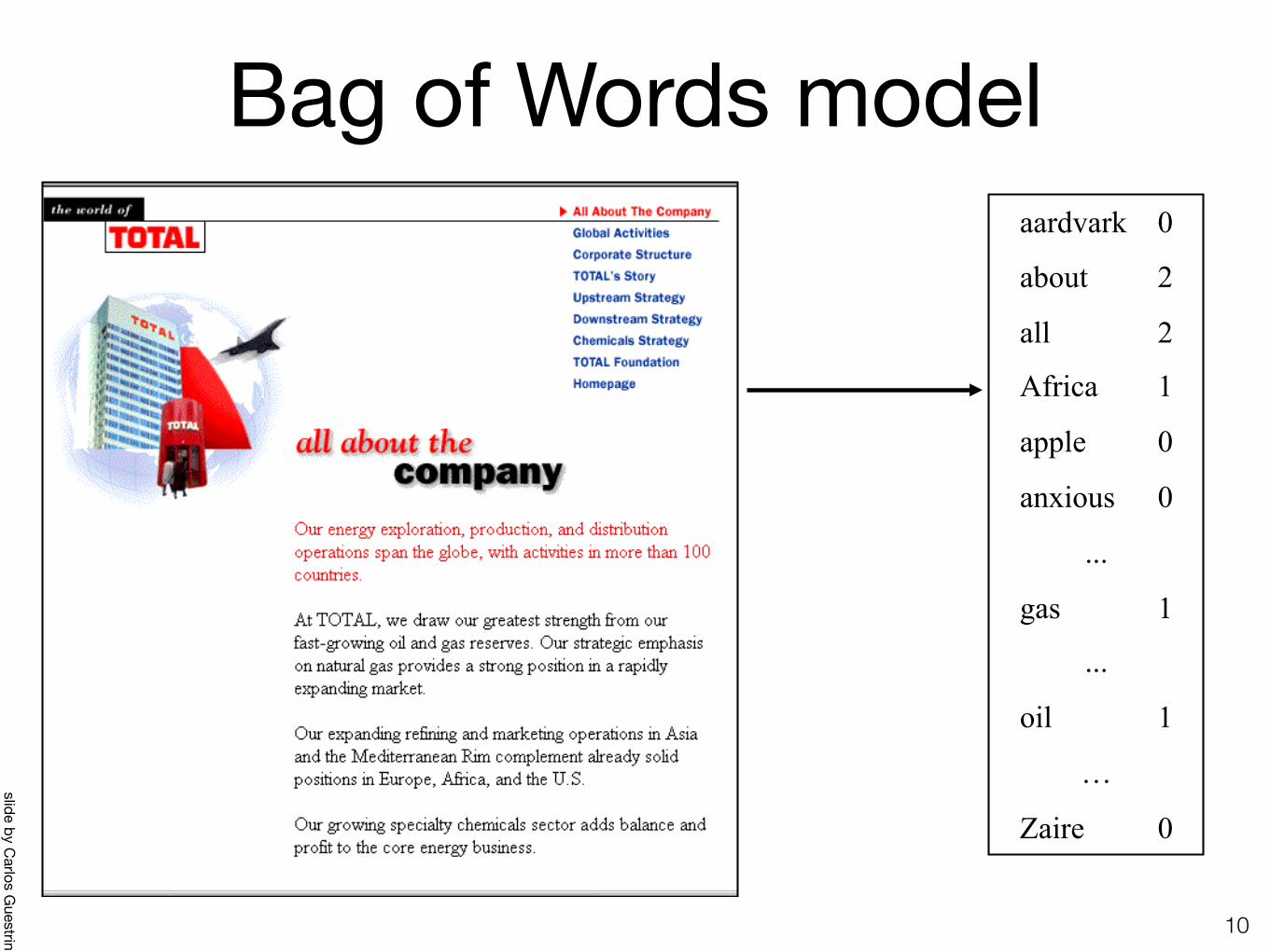
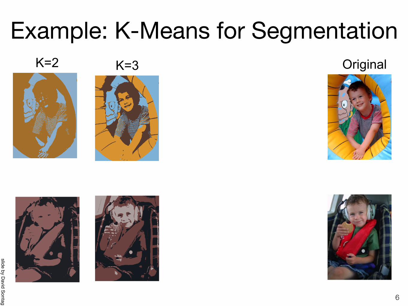
K = 2 K = 3 K = 10 Original imageK=2 K=3 K=10 Original



4% 8% 17%

Goal of Segmentation is to partition an image into regions each of which has reasonably homogenous visual appearance.



6









4% 8% 17%



7









4% 8% 17%


Example: Vector quantization

8

Example: Vector quantization 514 14. Unsupervised Learning

FIGURE 14.9. Sir Ronald A. Fisher (1890 ! 1962) was one of the foundersof modern day statistics, to whom we owe maximum-likelihood, su!ciency, andmany other fundamental concepts. The image on the left is a 1024"1024 grayscaleimage at 8 bits per pixel. The center image is the result of 2" 2 block VQ, using200 code vectors, with a compression rate of 1.9 bits/pixel. The right image usesonly four code vectors, with a compression rate of 0.50 bits/pixel

We see that the procedure is successful at grouping together samples ofthe same cancer. In fact, the two breast cancers in the second cluster werelater found to be misdiagnosed and were melanomas that had metastasized.However, K-means clustering has shortcomings in this application. For one,it does not give a linear ordering of objects within a cluster: we have simplylisted them in alphabetic order above. Secondly, as the number of clustersK is changed, the cluster memberships can change in arbitrary ways. Thatis, with say four clusters, the clusters need not be nested within the threeclusters above. For these reasons, hierarchical clustering (described later),is probably preferable for this application.

14.3.9 Vector Quantization

The K-means clustering algorithm represents a key tool in the apparentlyunrelated area of image and signal compression, particularly in vector quan-tization or VQ (Gersho and Gray, 1992). The left image in Figure 14.92 is adigitized photograph of a famous statistician, Sir Ronald Fisher. It consistsof 1024! 1024 pixels, where each pixel is a grayscale value ranging from 0to 255, and hence requires 8 bits of storage per pixel. The entire image oc-cupies 1 megabyte of storage. The center image is a VQ-compressed versionof the left panel, and requires 0.239 of the storage (at some loss in quality).The right image is compressed even more, and requires only 0.0625 of thestorage (at a considerable loss in quality).

The version of VQ implemented here first breaks the image into smallblocks, in this case 2!2 blocks of pixels. Each of the 512!512 blocks of four

2This example was prepared by Maya Gupta.

[Figure from Hastie et al. book]


Example: Simple Linear Iterative Clustering (SLIC) superpixels

9

R. Achanta, A. Shaji, K. Smith, A. Lucchi, P. Fua, and S. Susstrunk SLIC Superpixels Compared to State-of-the-art Superpixel Methods, IEEE T-PAMI, 2012

λ: spatial regularization parameter

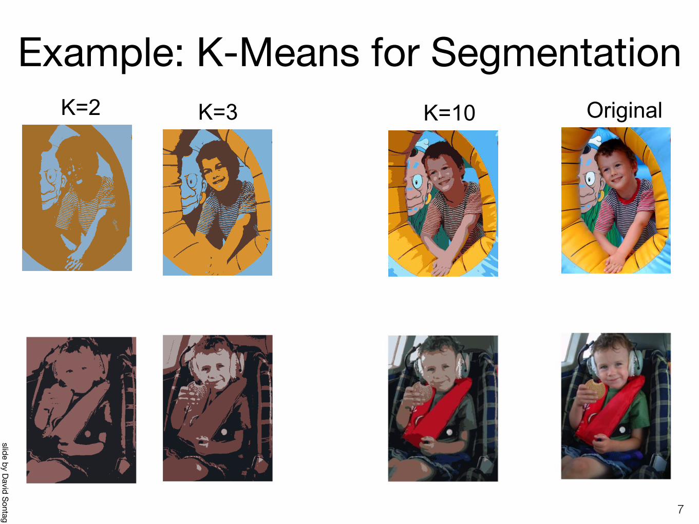
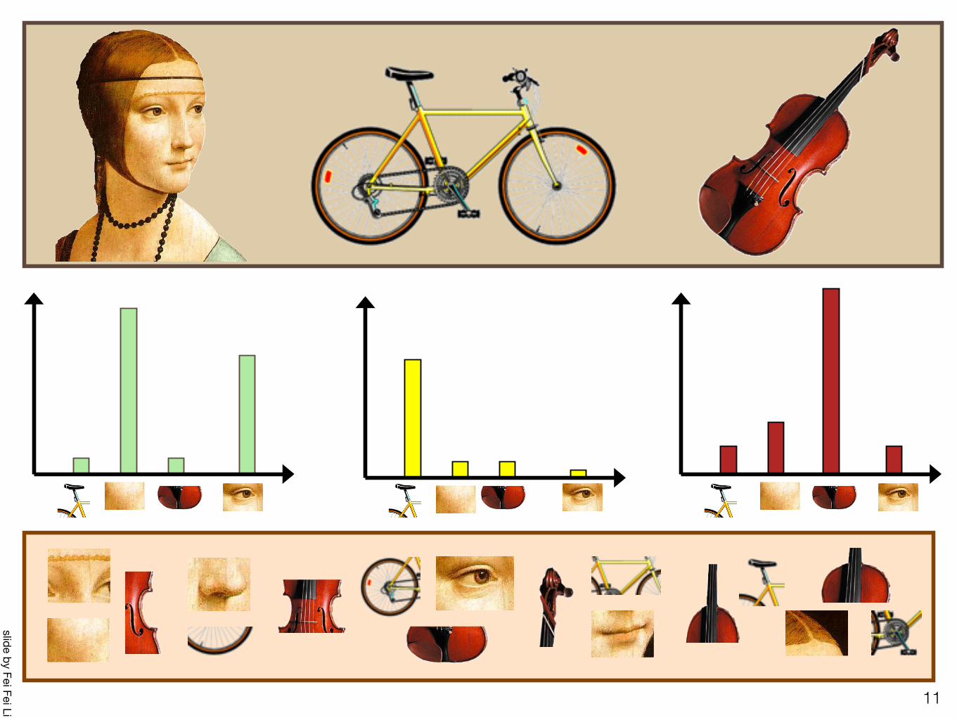
Bag of Words model

10

aardvark 0

about 2

all 2

Africa 1

apple 0

anxious 0

...

gas 1

...

oil 1

…

Zaire 0

slide by Carlos G

uestrin

11

slide by Fei Fei Li

12

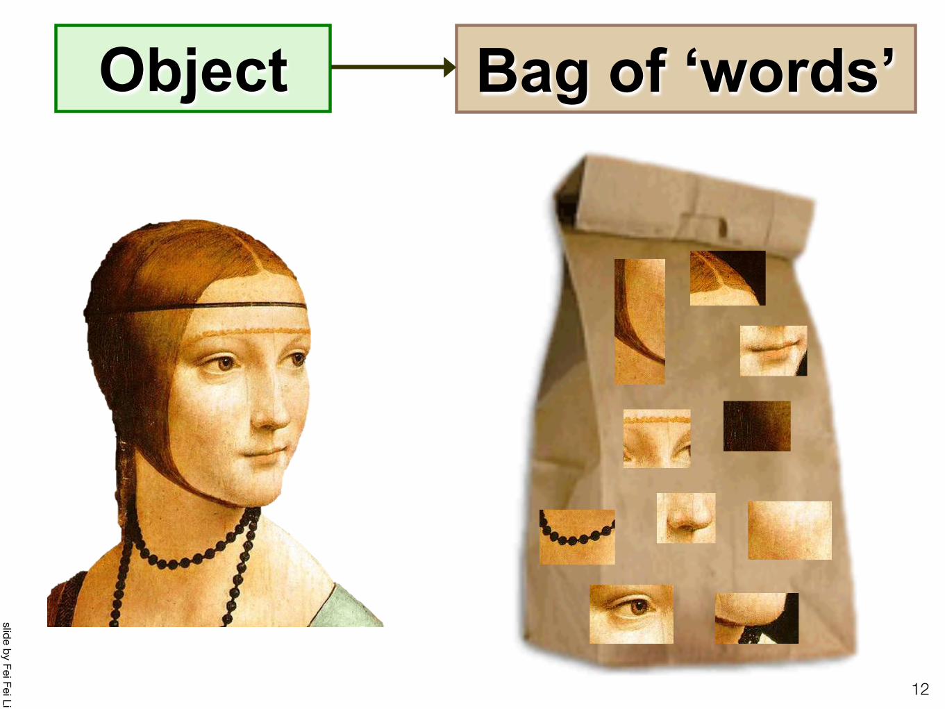
Object Bag of ‘words’

slide by Fei Fei Li

Interest Point Features

13

Normalize patch

Detect patches [Mikojaczyk and Schmid ’02]

[Matas et al. ’02]

[Sivic et al. ’03]

Compute SIFT

descriptor [Lowe’99]

slide by Josef Sivic

Patch Features

14

…


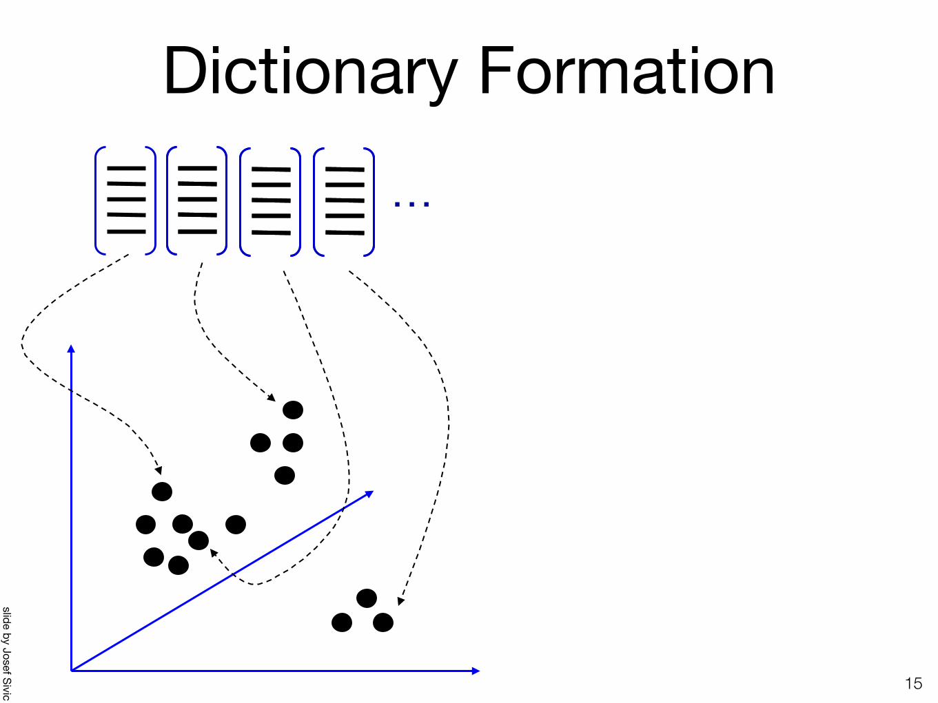
Dictionary Formation

15

…


Clustering (usually K-means)

16

Vector quantization

…


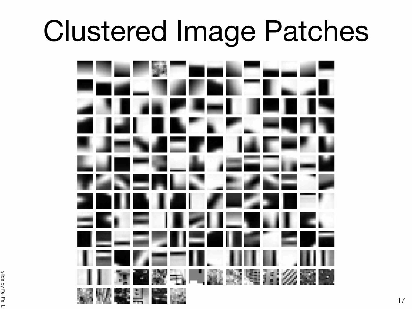
Clustered Image Patches

17

slide by Fei Fei Li

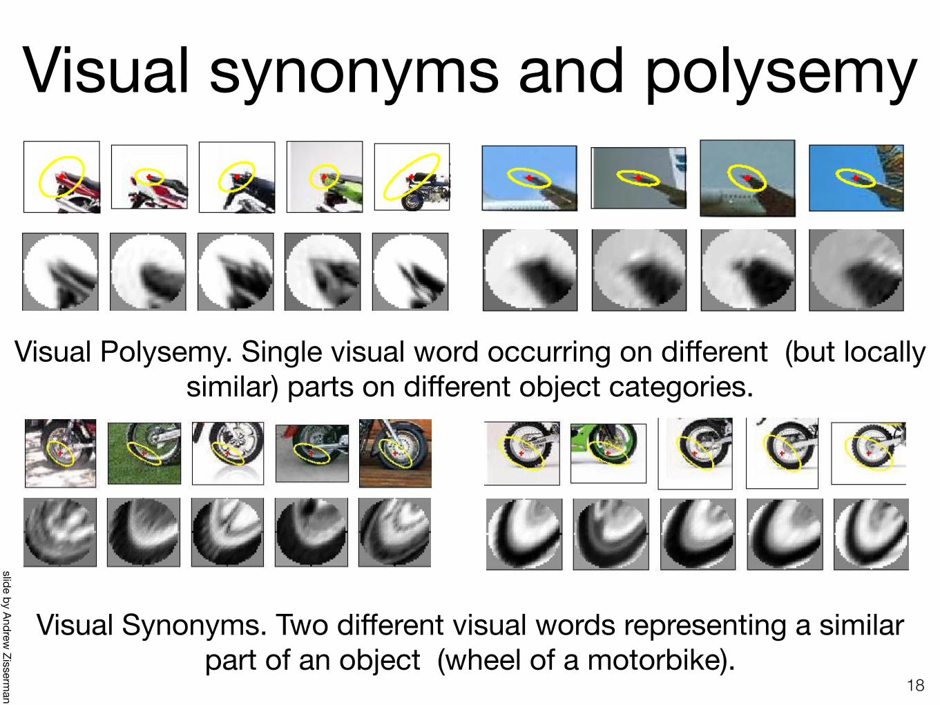
Visual synonyms and polysemy

18

Visual Polysemy. Single visual word occurring on different (but locally similar) parts on different object categories.

Visual Synonyms. Two different visual words representing a similar part of an object (wheel of a motorbike).

slide by Andrew Zisserm

an

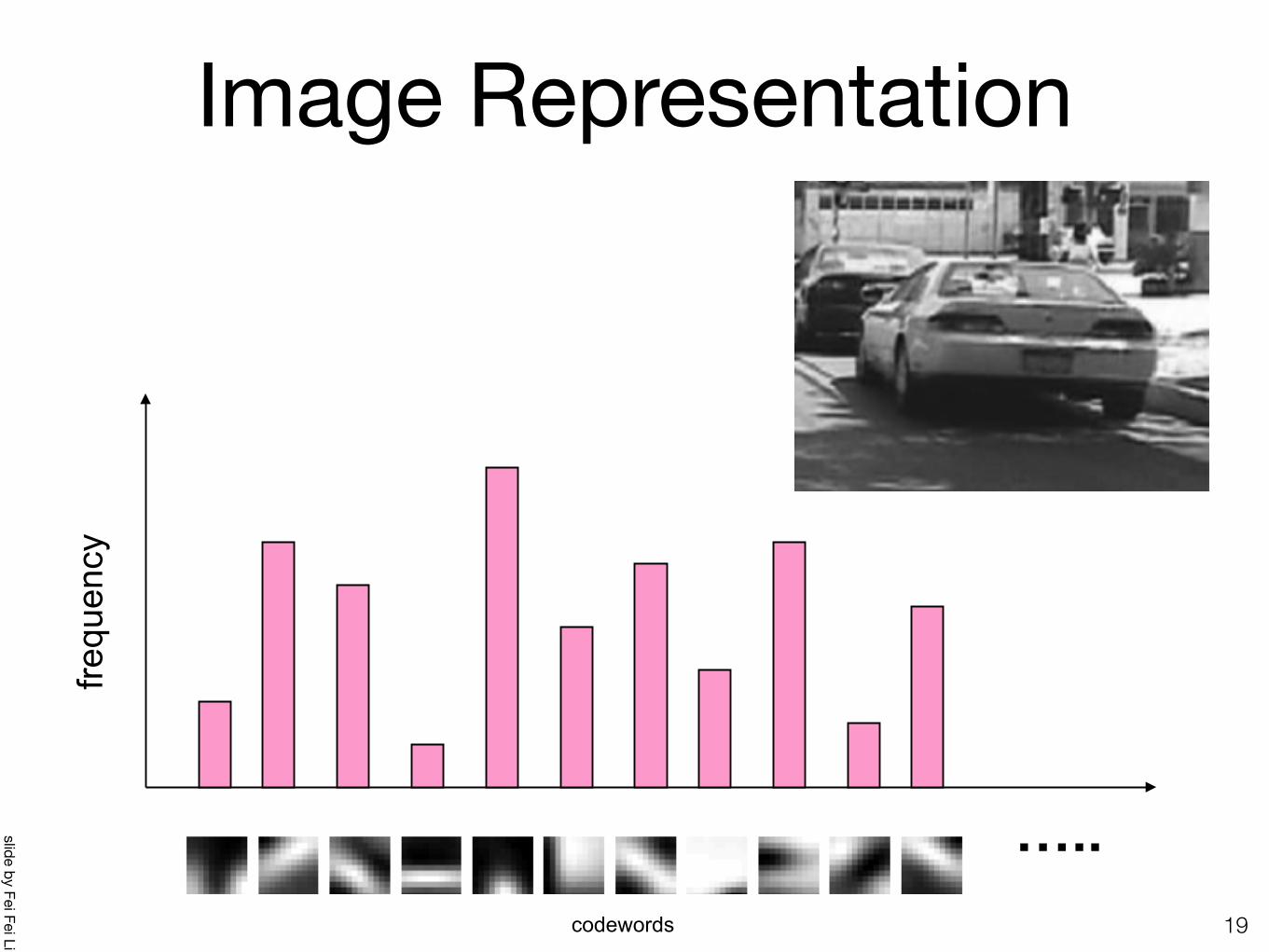
Image Representation

19

…..

frequ

ency

codewords

slide by Fei Fei Li

Spectral clustering

20

Graph-Theoretic ClusteringGoal: Given data points X1, ..., Xn and similarities W(Xi ,Xj), partition the data into groups so that points in a group are similar and points in different groups are dissimilar.

21

Similarity Graph: G(V,E,W) V – Vertices (Data points) E – Edge if similarity > 0 W - Edge weights (similarities)

Partition the graph so that edges within a group have large weights and edges across groups have small weights.

Graph)Clustering)Goal: Given data points X1, …, Xn and similarities W(Xi,Xj), partition the data into groups so that points in a group are similar and points in different groups are dissimilar. Similarity Graph: G(V,E,W) V – Vertices (Data points)

E – Edge if similarity > 0 W - Edge weights (similarities)

Similarity graph


Graph)Clustering)Goal: Given data points X1, …, Xn and similarities W(Xi,Xj), partition the data into groups so that points in a group are similar and points in different groups are dissimilar. Similarity Graph: G(V,E,W) V – Vertices (Data points)

E – Edge if similarity > 0 W - Edge weights (similarities)

Similarity graph


slide by Aarti Singh

Graphs Representations

a

e

d

c

b

!!!!!!

"

#

$$$$$$

%

&

0110110000100000000110010

Adjacency Matrix

a b c d eab

c

d

e

22

slide by Bill Freeman and Antonio Torralba

A Weighted Graph and its Representation

!!!!!!

"

#

$$$$$$

%

&

117.2.0116.007.6.14.3.2.04.11.003.1.1

Affinity Matrixa

e

d

c

b

6

W =

region same the tobelong

j& iy that probabilit :ijW

cluster23


Similarity)graph)construc6on)Similarity Graphs: Model local neighborhood relations between data points

E.g. epsilon-NN

or mutual k-NN graph (Wij = 1 if xi or xj is k nearest neighbor of the other)

Controls size of neighborhood

Data clustering

Wij

Wij =

⇢1 kxi � xjk ✏0 otherwise

Similarity graph construction• Similarity Graphs: Model local neighborhood relations

between data points• E.g. epsilon-NN


24



E.g. epsilon-NN



Data clustering

Wij

Wij =



E.g. epsilon-NN



Data clustering

Wij

Wij =



Similarity graph construction• Similarity Graphs: Model local neighborhood relations

between data points• E.g. Gaussian kernel similarity function

25



E.g. epsilon-NN



Data clustering

Wij

Wij =



E.g. epsilon-NN



Data clustering

Wij

Wij =



E.g. Gaussian kernel similarity function


Data clustering

Wij


-

Scale affects affinity

26

• Small σ: group only nearby points• Large σ: group far-away points

slide by Svetlana Lazebnik

Three points in feature space

Wij = exp(-|| zi – zj ||2 / s2)With an appropriate s

W=

The eigenvectors of W are:

The first 2 eigenvectors group the pointsas desired…

British Machine Vision Conference, pp. 103-108, 1990


Example eigenvector

points

Affinity matrix

eigenvector

28


Example eigenvector

points

eigenvector

Affinity matrix

29


Graph cut

• Set of edges whose removal makes a graph disconnected

• Cost of a cut: sum of weights of cut edges• A graph cut gives us a partition (clustering)

- What is a “good” graph cut and how do we find one?

AB

30

slide by Steven Seitz

Minimum cut

€

cut(A,B) = W(u,v),u∈A,v∈B∑

with A ∩ B = ∅

Cut: sum of the weight of the cut edges:

• A cut of a graph G is the set of edges S such that removal of S from G disconnects G.

31


Minimum cut• We can do clustering by finding the

minimum cut in a graph- Efficient algorithms exist for doing this

Minimum cut example

32


Minimum cut• We can do segmentation by finding the

minimum cut in a graph- Efficient algorithms exist for doing this

33

Minimum cut example


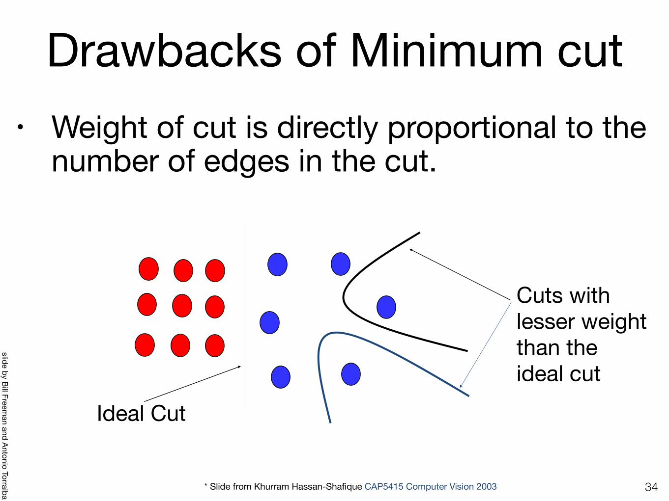
Drawbacks of Minimum cut• Weight of cut is directly proportional to the

number of edges in the cut.

Ideal Cut

Cuts with lesser weightthan the ideal cut

* Slide from Khurram Hassan-Shafique CAP5415 Computer Vision 2003 34


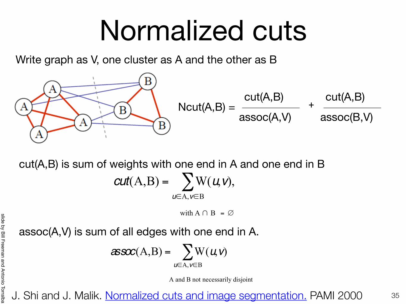
Normalized cuts

assoc(A,V) is sum of all edges with one end in A.

cut(A,B) is sum of weights with one end in A and one end in B

Write graph as V, one cluster as A and the other as B

cut(A,B)

assoc(A,V)

cut(A,B)

assoc(B,V)+Ncut(A,B) =

€

cut(A,B) = W(u,v),u∈A,v∈B∑

with A ∩ B = ∅

€

assoc(A,B) = W(u,v)u∈A,v∈B

∑

A and B not necessarily disjoint

35

slide by Bill Freeman and Antonio Torralba J. Shi and J. Malik. Normalized cuts and image segmentation. PAMI 2000

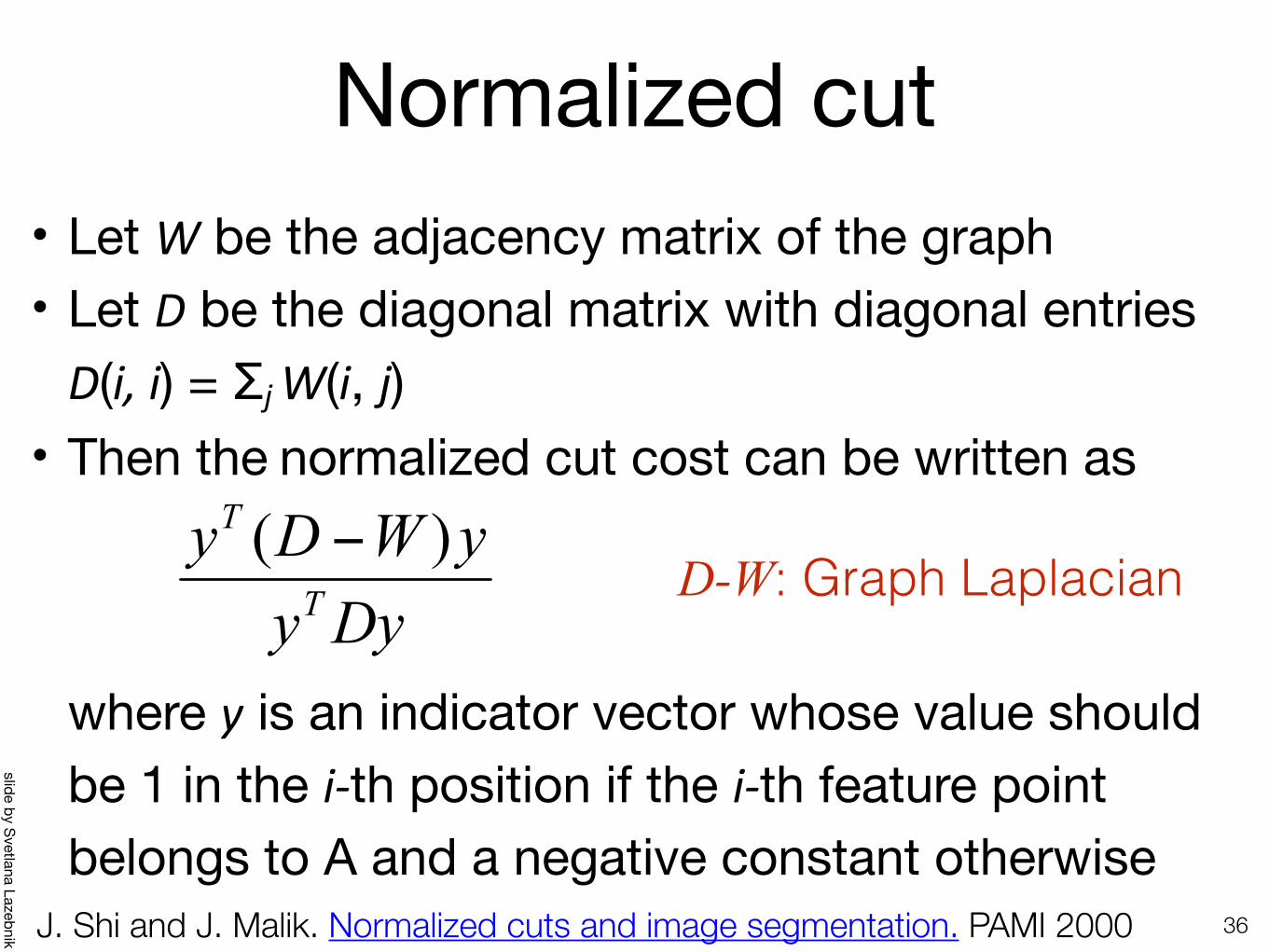
http://www.cs.berkeley.edu/~malik/papers/SM-ncut.pdf

Normalized cut• Let W be the adjacency matrix of the graph• Let D be the diagonal matrix with diagonal entries

D(i, i) = Σj W(i, j) • Then the normalized cut cost can be written aswhere y is an indicator vector whose value should be 1 in the i-th position if the i-th feature point belongs to A and a negative constant otherwise

DyyyWDy

T

T )( −

36

slide by Svetlana Lazebnik J. Shi and J. Malik. Normalized cuts and image segmentation. PAMI 2000

D-W: Graph Laplacian


Normalized cut• Finding the exact minimum of the normalized cut cost is

NP-complete, but if we relax y to take on arbitrary values, then we can minimize the relaxed cost by solving the generalized eigenvalue problem (D − W)y = λDy

• The solution y is given by the generalized eigenvector corresponding to the second smallest eigenvalue, aka the Fiedler vector

• Intuitively, the i-th entry of y can be viewed as a “soft” indication of the component membership of the i-th feature- Can use 0 or median value of the entries as the splitting point

(threshold), or find threshold that minimizes the Ncut cost

37

slide by Svetlana Lazebnik J. Shi and J. Malik. Normalized cuts and image segmentation. PAMI 2000


Normalized cut algorithm

38

slide by Bill Freeman and Antonio Torralba J. Shi and J. Malik. Normalized cuts and image segmentation. PAMI 2000


K-Means vs. Spectral Clustering• Applying k-means to Laplacian

eigenvectors allows us to find cluster with non-convex boundaries.

39

k=means)vs)Spectral)clustering)Applying k-means to laplacian eigenvectors allows us to find cluster with non-convex boundaries.

Both perform same Spectral clustering is superior


Both perform same Spectral clustering is superior




40


Spectral clustering output k-means output


Spectral clustering output k-means output




41


Similarity matrix

Second eigenvector of graph Laplacian


Similarity matrix

Second eigenvector of graph Laplacian


Examples

42[Ng et al., 2001]

Examples)Ng et al 2001


Some Issues• Choice of number of clusters k

- Most stable clustering is usually given by the value of k that maximizes the eigengap (difference between consecutive eigenvalues)

43

Some)Issues)!  Choice of number of clusters k

Most stable clustering is usually given by the value of k that maximizes the eigengap (difference between consecutive eigenvalues)

1k k kλ λ −Δ = −


Most stable clustering is usually given by the value of k that maximizes the eigengap (difference between consecutive eigenvalues)

1k k kλ λ −Δ = −


Some Issues• Choice of number of clusters k• Choice of similarity

- Choice of kernel for Gaussian kernels, choice of σ

44


!  Choice of similarity choice of kernel for Gaussian kernels, choice of σ

Good similarity measure Poor similarity measure


!  Choice of similarity choice of kernel for Gaussian kernels, choice of σ

Good similarity measure Poor similarity measure


Some Issues• Choice of number of clusters k

• Choice of similarity - Choice of kernel for Gaussian kernels, choice of σ

• Choice of clustering method- k-way vs. recursive 2-way

45


Hierarchical clustering

46

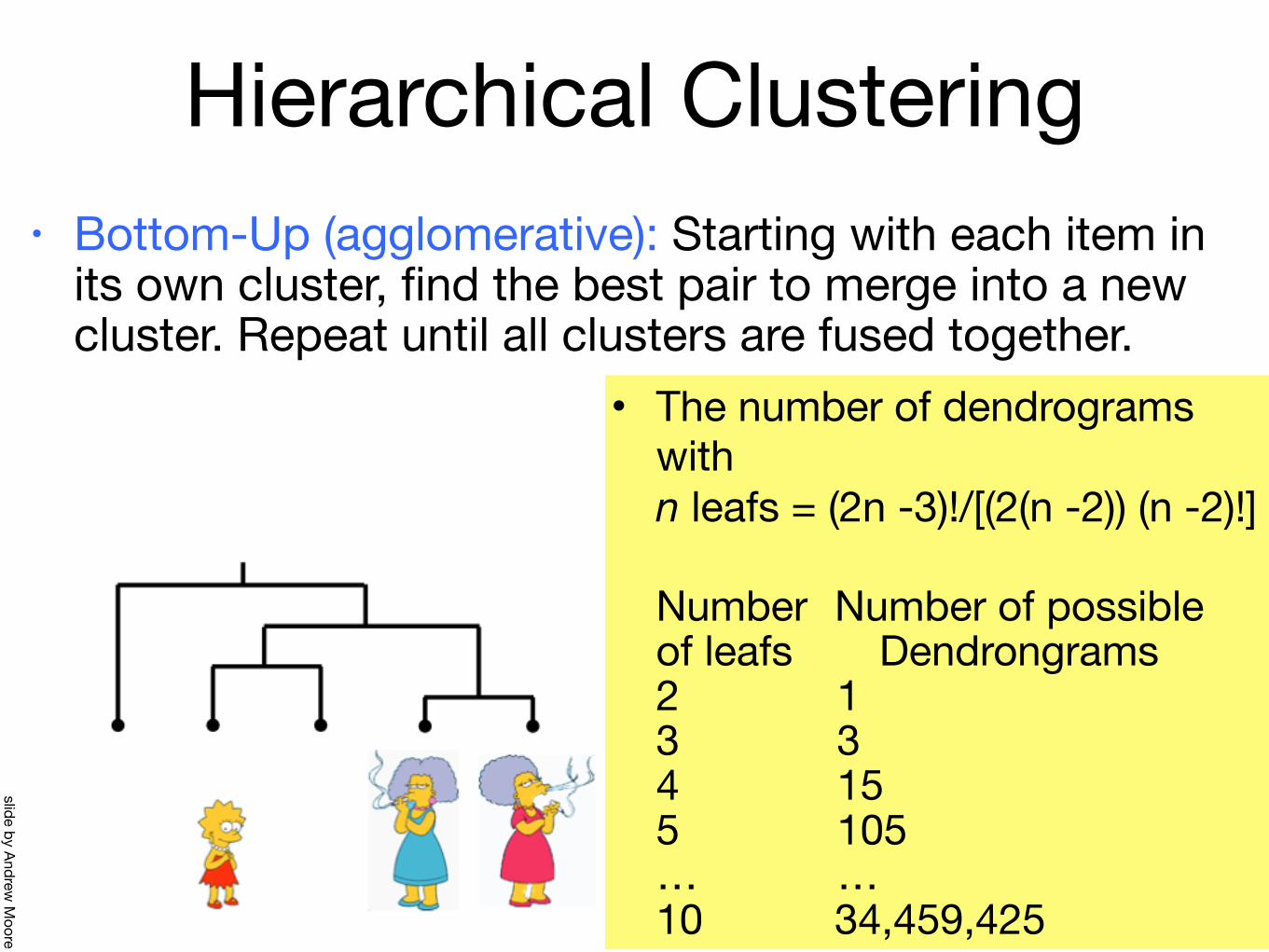
Hierarchical Clustering• Bottom-Up (agglomerative): Starting with each item in

its own cluster, find the best pair to merge into a new cluster. Repeat until all clusters are fused together.

47

• The number of dendrograms with n leafs = (2n -3)!/[(2(n -2)) (n -2)!]

Number Number of possible of leafs Dendrongrams 2 1 3 3 4 15 5 105 … … 10 34,459,425

slide by Andrew M

oore

We begin with a distancematrix which contains thedistances between every pair of objects in our dataset

48

slide by Andrew M

oore

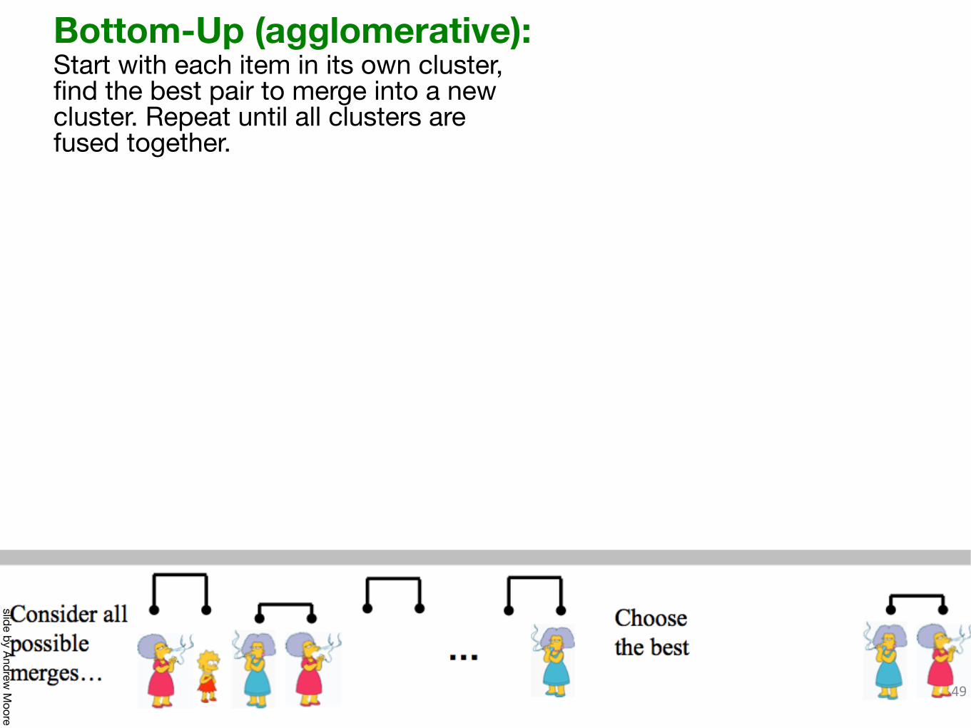
49

Bottom-Up (agglomerative):Start with each item in its own cluster, find the best pair to merge into a new cluster. Repeat until all clusters are fused together.

slide by Andrew M

oore

50


slide by Andrew M

oore

51


slide by Andrew M

oore

52


But how do we compute distances between clusters rather than objects?

slide by Andrew M

oore

Computing distance between clusters: Single Link

• Cluster distance = distance of two closest members in each class

53

Computing distance between clusters: Single Link

• cluster distance = distance of two closest members in each class

- Potentially long and skinny clusters

• Potentially long and skinny clusters

slide by Andrew M

oore

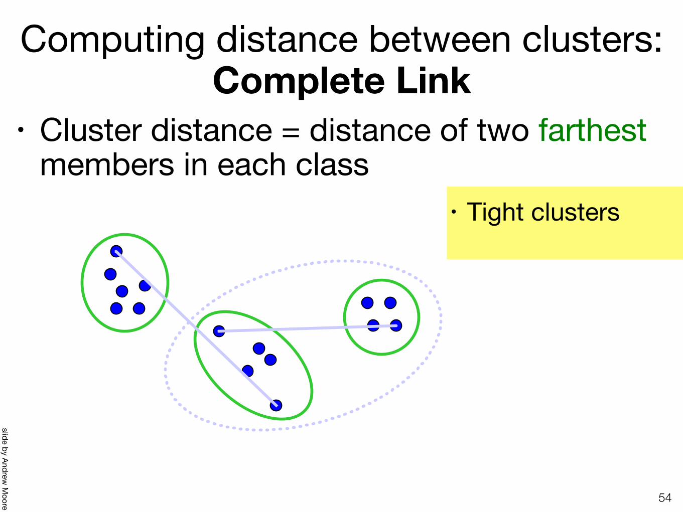
Computing distance between clusters: Complete Link

• Cluster distance = distance of two farthest members in each class

54

• Tight clusters

Computing distance between clusters: : Complete Link

• cluster distance = distance of two farthest members

+ tight clusters

slide by Andrew M

oore

Computing distance between clusters: Average Link

• Cluster distance = average distance of all pairs

55

• The most widely used measure

• Robust against noise

slide by Andrew M

oore

Agglomerative ClusteringGood• Simple to implement, widespread application• Clusters have adaptive shapes• Provides a hierarchy of clusters

Bad• May have imbalanced clusters• Still have to choose number of clusters or threshold

• Need to use an “ultrametric” to get a meaningful hierarchy

56

slide by Derek Hoiem

— silhouette coefficient

What is a good clustering?

57

What is a good clustering?• Internal criterion: A good clustering will produce high

quality clusters in which: - the intra-class (that is, intra-cluster) similarity is high - the inter-class similarity is low - The measured quality of a clustering depends on both the

obj. representation and the similarity measure used

• External criteria for clustering quality- Quality measured by its ability to discover some or all of the

hidden patterns or latent classes in gold standard data- Assesses a clustering with respect to ground truth- Example:

• Purity• Entropy of classes in clusters (or Mutual Information between

classes and clusters) 58

slide by Eric P. Xing

External Evaluation of Cluster Quality• Simple measure: purity, the ratio between the dominant

class in the cluster and the size of cluster- Assume documents with C gold standard classes, while

our clustering algorithms produce K clusters, ω1, ω2, ..., ωK with ni members.

- Example:

purity = 1/17* (max(5, 1, 0)+max(1, 4, 1)+max(2, 0, 3)) = 1/17*(5+4+3) ≈ 0.71 59

External Evaluation of Cluster QualityQuality

z Simple measure: purity, the ratio between the dominant class p p yin the cluster and the size of clusterz Assume documents with C gold standard classes, while our clustering algorithms

produce K clusters, Ȧ1, Ȧ2, …, ȦK with ni members.

Examplez Example

Cluster I: Purity = 1/6 (max(5, 1, 0)) = 5/6Cluster II: Purity = 1/6 (max(1 4 1)) = 4/6Cluster II: Purity = 1/6 (max(1, 4, 1)) = 4/6Cluster III: Purity = 1/5 (max(2, 0, 3)) = 3/5

38© Eric Xing @ CMU, 2006-2012

slide by Eric P. Xing

purity(⌦, C) =1

N

X

k

maxj

|!k \ cj |

External Evaluation of Cluster Quality• Let: TC = TC1 ∪ TC2 ∪...∪ TCn CC = CC1 ∪ CC2 ∪...∪ CCm

be the target and computed clusterings, respectively.

• TC = CC = original set of data• Define the following:

- a: number of pairs of items that belong to the same cluster in both CC and TC

- b: number of pairs of items that belong to different clusters in both CC and TC

- c: number of pairs of items that belong to the same cluster in CC but different clusters in TC

- d: number of pairs of items that belong to the same cluster in TC but different clusters in CC

60

slide by Christophe G

iraud-Carrier

External Evaluation of Cluster Quality

F-measure

61

Measure of clustering agreement: how similar are these two ways of partitioning the data?

Rand Index

DMLBYU DATA MINING LAB

FOmeasure#

€

P =a

a + cR =

aa + d

F =2 × P × RP + R


Rand#Index#

a+ba+b+c+d



iraud-Carrier


62

Rand Index Adjusted Rand Index

Extension of the Rand index that attempts to account for items that may have been clustered by chance


Rand#Index#

a+ba+b+c+d



Adjusted#Rand#Index#

€

2(ab − cd)(a + c)(c + b) + (a + d)(d + b)

Extension of the Rand index that attempts to account for items that may have been clustered by chance


iraud-Carrier


63


Average#Entropy#

€

Entropy(CCi) = −p(TC j |CCi)log p(TC j |CCi)TC j ∈ TC∑

AvgEntropy(CC) =CCi

CCEntropy(CCi)

i=1

m

∑

Measure of purity with respect to the target clustering


iraud-Carrier

Measure of purity wrtthe target clustering

Entropy(CC1) = (5/6)log(5/6) + (1/6)log(1/6) + (0/6)log(0/6) = -.650 Entropy(CC2) = (1/6)log(1/6) + (4/6)log(4/6) + (1/6)log(1/6) = -1.252 Entropy(CC3) = (2/5)log(2/5) + (0/5)log(0/5) + (3/5)log(3/5) = -.971

External Evaluation of Cluster QualityQuality

z Simple measure: purity, the ratio between the dominant class p p yin the cluster and the size of clusterz Assume documents with C gold standard classes, while our clustering algorithms

produce K clusters, Ȧ1, Ȧ2, …, ȦK with ni members.

Examplez Example

Cluster I: Purity = 1/6 (max(5, 1, 0)) = 5/6Cluster II: Purity = 1/6 (max(1 4 1)) = 4/6Cluster II: Purity = 1/6 (max(1, 4, 1)) = 4/6Cluster III: Purity = 1/5 (max(2, 0, 3)) = 3/5

38© Eric Xing @ CMU, 2006-2012

- Example:

AvgEntropy(CC) = (-.650 * 6/17) + (-1.252 * 6/17) + (-.971 * 5/17) AvgEntropy(CC) = -.956

Next Lecture: Dimensionality Reduction

64

Lecture 22:

Documents

Transcript of Lecture 22: