
Availability Evaluation and Optimisation of Grid Connection ...
211
Availability Evaluation and Optimisation of Grid Connection Concepts for Wind Farms Diploma Thesis Institute for Electrical Power Systems Graz University of Technology Submitted by Jörg Schweighart Supervisor Univ.-Prof. DI Dr.techn. Lothar Fickert External Supervisor M.Sc. Steven Coppens Head of Institute: Univ.-Prof. DI Dr.techn. Lothar Fickert A - 8010 Graz, Inffeldgasse 18-I Telefon: (+43 316) 873 – 7551 Telefax: (+43 316) 873 – 7553 http://www.ifea.tugraz.at http://www.tugraz.at Graz / 22-02-2013
-
Upload
khangminh22 -
Category
Documents
-
view
1 -
download
0
Transcript of Availability Evaluation and Optimisation of Grid Connection ...

AAvvaaiillaabbiilliittyy EEvvaalluuaattiioonn aanndd OOppttiimmiissaattiioonn ooff GGrriidd CCoonnnneeccttiioonn CCoonncceeppttss ffoorr WWiinndd FFaarrmmss
DDiipplloommaa TThheessiiss
IInnssttiittuuttee ffoorr EElleeccttrriiccaall PPoowweerr SSyysstteemmss
GGrraazz UUnniivveerrssiittyy ooff TTeecchhnnoollooggyy
SSuubbmmiitttteedd bbyy
JJöörrgg SScchhwweeiigghhaarrtt
SSuuppeerrvviissoorr
UUnniivv..--PPrrooff.. DDII DDrr..tteecchhnn.. LLootthhaarr FFiicckkeerrtt
EExxtteerrnnaall SSuuppeerrvviissoorr
MM..SScc.. SStteevveenn CCooppppeennss
HHeeaadd ooff IInnssttiittuuttee:: UUnniivv..--PPrrooff.. DDII DDrr..tteecchhnn.. LLootthhaarr FFiicckkeerrtt
AA -- 88001100 GGrraazz,, IInnffffeellddggaassssee 1188--II TTeelleeffoonn:: ((++4433 331166)) 887733 –– 77555511 TTeelleeffaaxx:: ((++4433 331166)) 887733 –– 77555533
hhttttpp::////wwwwww..iiffeeaa..ttuuggrraazz..aatt hhttttpp::////wwwwww..ttuuggrraazz..aatt
GGrraazz // 2222--0022--22001133


iii
Acknowledgement
This thesis was written as part of my work at the project support department at REpower
Systems AG. Many people supported me during my internship and in writing this thesis. I
would like to thank the following persons in particular:
My external supervisor, Mr. Steven Coppens who always encouraged me in my work. He
always took his time to discuss with me various aspects of my thesis and brought new ap-
proaches and concepts to my attention.
Mr. R. Schendel, the team leader of the electrical engineering group who gave me the oppor-
tunity to write this thesis and who always had a sympathetic ear for my problems.
My supervisor, Prof. Dr. Lothar Fickert, who gave me basic ideas about this topic and pro-
vided great academic support during this period.
All the employees in the project support department who supported me during my work.
Above all, however, I would like to thank my parents who gave me the opportunity for an
academic education.
REpower Systems AG
Überseering 10
22297-Hamburg
www.repower.de

iv

v
EIDESSTATTLICHE ERKLÄRUNG
Ich erkläre an Eides statt, dass ich die vorliegende Arbeit selbstständig verfasst, andere als
die angegebenen Quellen/Hilfsmittel nicht benutzt, und die den benutzten Quellen wörtlich
und inhaltlich entnommenen Stellen als solche kenntlich gemacht habe.
Graz, am 22.02.2013
Jörg Schweighart

vi

vii
Abstract
Over the past years, the wind power market has changed from a sellers to a buyers market,
thus the customer requirements regarding performance capabilities of wind farms and their
technical availability became tougher. The subject of this thesis is the availability evaluation
of grid connection concepts for large wind farms, with approaches to determine the level of
availability of wind farms and approaches for improvement measures. Reliability calculation
methods and their applicability to wind power systems will be discussed as well as certain
cost-benefit methods in order to quantify the impact of different levels of reliability. Where is
the optimal point between technological possibilities and economic design of electrical grid
connection systems. What are the best network configurations and the most efficient mainte-
nance strategies for wind farms according to their installed capacity. These questions to-
gether with questions concerning insurance possibilities and contractual aspects will be
elaborated. Although whole wind farms will be taken into account the main focus will be on
the electrical grid connection system.
Keywords: Reliability, Availability, Maintenance, Wind Farm, Grid Connection, Risk Assess-
ment, Insurance, Layout Optimisation
Kurzfassung
Die Windkraft Branche hat sich innerhalb der letzten Jahre von einem Verkäufermarkt zu
einem Käufermarkt entwickelt. Die Anforderungen der Kunden an die Leistungsfähigkeit von
Windparks und deren technische Verfügbarkeit sind dadurch zusehends gestiegen. Diese
Arbeit beschäftigt sich mit der Verfügbarkeit von Netzanbindungssystemen großer Wind-
parks. Wie hoch ist die technische Verfügbarkeit bestimmter elektrischer Komponenten und
Systeme und wo sind Verbesserungsmöglichkeiten. Welches ist die effektivste Netzstruktur
sowie die effizienteste Wartungsstrategie von Windparks und welchen Einfluss darauf hat die
installierte Leistung. Eine Risikobewertung von Netzanbindungssystemen sowie Versiche-
rungs- und vertragliche Möglichkeiten werden diskutiert, um das Risiko zu minimieren. Der
Schwerpunkt dieser Diplomarbeit liegt in der Bewertung von Windpark-Netzanbindungs-
systemen und nicht einzelner Windkraftanlagen.
Schlüsselwörter: Zuverlässigkeit, Verfügbarkeit, Wartung, Windpark, Netzanbindung, Risi-
komanagement, Versicherung, Optimierung

viii

ix
Table of Contents
Symbols and Abbreviations .............................................................. xii
Executive Summary ........................................................................... xv
Goal ................................................................................................................................. xv
Methods ........................................................................................................................... xv
Results ............................................................................................................................. xv
Conclusion and Outlook ................................................................................................... xv
List of Tables .................................................................................... xvii
List of Figures .................................................................................... xix
1 Introduction ..................................................................................... 1
1.1 Investigation of the Problem .................................................................................... 1
1.2 Investigation Questions and Goals .......................................................................... 3
1.4 Structure of the Thesis ............................................................................................. 5
2 General ............................................................................................ 6
2.1 Terms and Definitions .............................................................................................. 6
2.2 Stochastics .............................................................................................................. 7
2.2.1 Probability Theory ............................................................................................. 7
2.2.2 Probability Functions ...................................................................................... 12
2.3 Reliability Theory ................................................................................................... 17
2.3.1 Reliability and Availability................................................................................ 17
2.3.2 Reliability of Components ............................................................................... 20
2.3.3 Reliability of Systems ...................................................................................... 28
2.3.4 Summary of Definitions and Equations ........................................................... 32
2.4 Cost-Benefit Analysis ............................................................................................. 33
2.4.1 Net Present Value and Internal Rate of Return ............................................... 33
2.4.2 Application to Reliability Engineering .............................................................. 37
2.4.3 Application to Wind Energy Systems .............................................................. 41
2.5 Failure, Fault and Error .......................................................................................... 47
2.5.1 Common Cause Failures ................................................................................ 48
2.5.2 Single and Multiple Faults ............................................................................... 49
2.5.3 Types of faults and their Frequency of Occurrence ......................................... 49
2.6 Restrictions and Assumptions ................................................................................ 51
3 Reliability Data .............................................................................. 52
3.1 Data Preparation ................................................................................................... 52

x
3.1.1 Method of Moments ........................................................................................ 52
3.1.2 Maximum Likelihood ....................................................................................... 53
3.1.3 Chi-Square Test (Goodness-of-Fit Test) ......................................................... 54
3.1.4 Confidence Limits ........................................................................................... 54
3.2 Reliability Statistics ................................................................................................ 58
3.2.1 Historical Data from Utilities ............................................................................ 58
3.2.2 Reliability Statistics from Subcontractors ........................................................ 58
4 Reliability Modelling ..................................................................... 59
4.1 Lifetime of Electrical Components .......................................................................... 59
4.1.1 The Bathtub Curve .......................................................................................... 59
4.1.2 The Ageing Concept ....................................................................................... 62
4.2 Grid Connection Components ................................................................................ 66
4.2.1 The Wind Energy Converter ........................................................................... 66
4.2.2 Medium Voltage Equipment ............................................................................ 70
4.2.3 High Voltage Equipment ................................................................................. 81
4.2.4 UPS and Protection Systems .......................................................................... 81
4.3 Subsystems ........................................................................................................... 90
4.3.1 The Wind Energy Converter ........................................................................... 91
4.3.2 MV Collector System ...................................................................................... 92
4.3.3 Substation ....................................................................................................... 93
4.3.4 Protection System ........................................................................................... 94
4.3.5 Availability and Expected Energy Not Supplied ............................................... 99
4.4 Human- and Environmental-Factors .................................................................... 102
4.4.1 Weather Effects ............................................................................................ 102
4.4.2 Human factors .............................................................................................. 104
5 Availability Optimisation ............................................................ 108
5.1 Optimisation Methods .......................................................................................... 108
5.2 Grid Architecture .................................................................................................. 110
5.2.1 MV Collector System .................................................................................... 111
5.2.2 Substation ..................................................................................................... 114
5.2.3 Summary of Layout Alternatives ................................................................... 118
5.2.4 Sensitivity Analysis ....................................................................................... 120
5.3 Active Power Losses............................................................................................ 121
5.4 Neutral-Point Treatment ....................................................................................... 127
5.5 Maintenance ........................................................................................................ 130
5.7 Alternative Electrical Parameters ......................................................................... 136
5.7.1 Voltage Level Variation of the MV-Collector System ..................................... 136

xi
5.7.2 Variation of the Rated Power of Transformers .............................................. 136
6 Contract and Insurance Possibilities ........................................ 137
6.1 REpower Standard Contract ................................................................................ 138
6.2 Warranty and Guarantee ..................................................................................... 140
6.3 Risk Assessment and Mitigation .......................................................................... 142
6.4 Insurance Possibilities ......................................................................................... 148
7 Results and Increase of Knowledge .......................................... 152
8 Conclusion and Outlook ............................................................. 156
Bibliography ..................................................................................... 157
Appendix ........................................................................................... 163

xii
Symbols and Abbreviations
Acronyms and Abbreviations
AP …….… Actual Production
BIP ……… Burn-In Period (Teething Period)
CB ……… Circuit Breaker
CCF ….…… Common cause failure
CDF ……… Cumulated distribution function
CEA ……… Canadian Electricity Association
CMF ….…… Common mode failure
COI ……… Continuous operating Item
DC ……… Disconnector
EENS …….… Expected Energy not supplied
ETS ……… External Transformer Station
HV ……… High Voltage (72,5kV<UN<125kV)
IEC ……… International Electrotechnical Comission
IEEE ……… Institute of Electrical and Electronics Engineers
IOI ……… Intermittent operating Item
IRR ……… Internal Rate of Return
ISP ……… Integrated Service Package (incl. availability guarantee)
ITS ……… Internal Transformer Station
LBS ……… Load Break Switch
LCC ……… Life-cycle Costs
LCLR ……… Life Cycle Lost Revenue
LCMC ……… Life Cycle Maintenance Cost
LD …….… Liquid Damage
LP …….… Lost Production
LV ……… Low Voltage (UN<1kV)
MAD ……… Mean Administrative Delay
MFT ……… Mean Time of a Fault
MLD ……… Mean Logistic Delay
MRT ……… Mean Restoration Time
MTBF ……… Mean Time between Failure
MTBM ……… Mean Time between Maintenance
MTD ……… Mean Technical Delay
MTTF ……… Mean Time to Failure
MTTM ……… Mean Time to Maintain

xiii
MTTR ……… Mean Time to Repair
MV ……… Medium Voltage (1kV<UN<72,5kV)
NPV ……… Net Present Value
O&M …….… Operations and Maintenance
PDF ……… Probability density function
RBD ……… Reliability Block Diagram
REAG ……… REpower Systems AG
TP …….… Theoretical Production
ULP ……… Useful life period
VDN ……… Verband deutscher Netzbetreiber (neu BDEW)
WEC ……… Wind Energy Converter
WP ……… Wear out period
WSV ……… Wartungs- und Servicevertrag
Symbols
A ……… Availability [p.u.]
C0 ……… Investment cost [€]
m ……… MTTM [h]
PL ……… Power Loss [kW]
Pr ……… Rated Power [kW]
Q ……… Unreliability [p.u.]
r ……… MTTR [h]
R ……… Reliability [p.u.]
scl ……… System Cable Length [km per 3~]
TD ……… Down Time [h]
TU ……… Up Time [h]
U ……… Unavailability [p.u.]
x ……… Mean Value (Expected Value)
α ……… Weibull-Distribution Shape Parameter
γ ……… Confidence Level
η ……… Efficiency [%]
λF ……… Failure Rate (frequency) [1/yr]
λM ……… Maintenance Rate [1/yr]
σ ……… Standard Deviation
σ2 ……… Variance
……… Repair Rate [1/yr]

xiv

xv
Executive Summary
Goal In order to ensure a certain level of availability of whole wind farms, a thorough understand-
ing of how the system can fail is needed. Thus the objective of this investigation is the
evaluation of wind farms regarding their failure mechanisms and their level of availability;
furthermore an optimisation of grid connection concepts with respect to their configuration,
their maintenance strategy and their support structure will be carried out. In addition specific
insurance possibilities and contractual settings will be elaborated as well, in order to mitigate
the inherent risk of certain layouts.
Methods The first part of this investigation deals with quantitative and qualitative methods to evaluate
the reliability of electrical components and whole systems. Mathematical models are derived
using reliability block diagrams and fault tree methods. The second part basically consists of
the application of these mathematical models to wind farm layout alternatives. Cost-benefit
analysis methods are used to optimise the layout with respect to its level of availability and
maintainability.
Results The wind energy converter itself is the major cause of reduced power output at the point of
common coupling. The level of availability of the grid connection is beyond the target value of
97% and can be assumed to be not less than 99%. The bottleneck of the grid connection is
still the high voltage part, not because of the high failure rate but because of the high impact
of failure and maintenance related energy not supplied. Thus a thorough design and mainte-
nance strategy is essential for this part of the wind farm in order to mitigate the corporate
risk. The investigation shows, that a redundant layout of the HV connection is reasonable for
wind farms with an installed capacity larger than 100MW and a capacity factor above 40%.
Conclusion and Outlook
Over the next years the market requirements will certainly get even tougher for availability
and performance guarantees for wind farms. Therefore it is necessary for companies to pay
more attention to disturbance mechanisms. Furthermore a specific quality management
process to improve the long term performance is recommended with the special focus on
failure data acquisition and evaluation as well as maintenance strategies and support. The
results of this investigation are based on analytical evaluation methods, for further calcula-
tions simulation approaches should be considered. (E.g. Monte Carlo Method)

xvi

xvii
List of Tables Table 2.1 Boolean Operators ................................................................................................................................... 8
Table 2.2 Relationships between reliability indices ................................................................................................ 22
Table 2.3 Minimal cut sets of figure 4.4-3 .............................................................................................................. 30
Table 2.4 Summary of definitions ........................................................................................................................... 32
Table 2.5 Useful lifetime according to BMF-AfA..................................................................................................... 36
Table 2.6 Capacity factors ..................................................................................................................................... 42
Table 4.1 Set points for Figure 4.1 ......................................................................................................................... 60
Table 4.2 WEC MTBF rates ................................................................................................................................... 66
Table 4.3 WEC MTTR rates ................................................................................................................................... 67
Table 4.4 WEC availability ..................................................................................................................................... 67
Table 4.5 MM failure causes and mean down time [68] ......................................................................................... 68
Table 4.6 MV-cable reliability figures ..................................................................................................................... 70
Table 4.7 MV-cable availability .............................................................................................................................. 70
Table 4.8 Properties of insulation systems [53]...................................................................................................... 71
Table 4.9 Influences on loading capability of cables[46] ........................................................................................ 72
Table 4.10 MTTR of MV-cables ............................................................................................................................. 72
Table 4.11 MV transformer reliability figures [29][53] ............................................................................................. 75
Table 4.12 MV transformer availability ................................................................................................................... 75
Table 4.13 MV-switchgear reliability figures [53] .................................................................................................... 79
Table 4.14 MV switchgear availability .................................................................................................................... 79
Table 4.15 HV-cable reliability figures .................................................................................................................... 81
Table 4.16 HV cable availability ............................................................................................................................. 81
Table 4.17 HV transformer reliability figures [53] ................................................................................................... 82
Table 4.18 HV transformer availability ................................................................................................................... 82
Table 4.19 MTBFs of OLTC types ......................................................................................................................... 83
Table 4.20 MTTR of different failure causes .......................................................................................................... 84
Table 4.21 HVswitchgear reliability figures ............................................................................................................ 86
Table 4.22 HV switchgear availability .................................................................................................................... 86
Table 4.23 Protection settings................................................................................................................................ 95
Table 4.24 Reliability figures of protection devices ................................................................................................ 96
Table 4.25 Zone branches and their unavailability ................................................................................................. 98
Table 4.26 Protection system availability ............................................................................................................... 98
Table 4.27 Availability of the grid connection ....................................................................................................... 100
Table 4.28 Availability of the grid connection ....................................................................................................... 100
Table 4.29 Human behaviours and their corresponding considerations [14] ....................................................... 105
Table 5.1 Radial collector system ........................................................................................................................ 111
Table 5.2 Redundant collector system ................................................................................................................. 112
Table 5.3 Redundant collector system, main and transfer substation .................................................................. 113
Table 5.4 MV collector system with interconnections (feeder ties)....................................................................... 114
Table 5.5 Single power transformer ..................................................................................................................... 115
Table 5.6 Redundant power transformers ............................................................................................................ 116

xviii
Table 5.7 MV Substation, single busbar ............................................................................................................... 116
Table 5.8 MV Substation, double busbar, double disconnectors .......................................................................... 117
Table 5.9 Layout alternatives of the grid connection, availability .......................................................................... 118
Table 5.10 Layout alternatives of the grid connection, lost revenue ..................................................................... 118
Table 5.11 MTTR and MTTM ............................................................................................................................... 119
Table 5.12 Active power loss of components ....................................................................................................... 122
Table 5.13 Active power loss of components ....................................................................................................... 125
Table 5.14 Technical cable data [21] ................................................................................................................... 128
Table 5.15 EENS and NPV of compensated collector system ............................................................................. 128
Table 5.16 Equipment failure rate multipliers vs. maintenance quality [29] .......................................................... 133
Table 5.17 Maintenance of HV switchgear ........................................................................................................... 134
Table 5.18 Maintenance of power transformers (ABB) ........................................................................................ 134
Table 5.19 Maintenance of ITS/ETS .................................................................................................................... 134
Table 5.20 Maintenance of MV cable systems ..................................................................................................... 135
Table 5.21 Maintenance of MV switchgear primary ............................................................................................. 135
Table 6.1 Risk evaluation of HV components ....................................................................................................... 145
Table 6.2 Risk evaluation of power transformers ................................................................................................. 145
Table 6.3 Risk evaluation of MV substation ......................................................................................................... 146
Table 6.4 Risk evaluation of MV collector systems .............................................................................................. 146
Table 7.1 Increase of availability .......................................................................................................................... 154

xix
List of Figures Figure 1.1 Single line diagram of an internal connection system ............................................................................. 1
Figure 1.2 Evaluation criteria for technical equipment ............................................................................................. 2
Figure 1.3 Dependability management [25] ............................................................................................................. 2
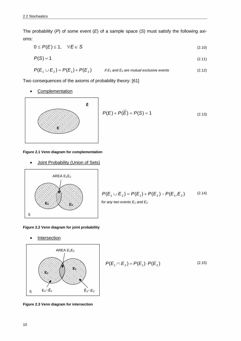
Figure 2.1 Venn diagram for complementation ...................................................................................................... 10
Figure 2.2 Venn diagram for joint probability ......................................................................................................... 10
Figure 2.3 Venn diagram for intersection ............................................................................................................... 10
Figure 2.4 The concept of random variables .......................................................................................................... 12
Figure 2.5 Probability density function (PDF) and cumulative distribution function (CDF) ..................................... 13
Figure 2.6 CDF and PDF of a discrete random variable ........................................................................................ 13
Figure 2.7 State, state duration and state transition of a two-stage process .......................................................... 14
Figure 2.8 A two state Markov model ..................................................................................................................... 14
Figure 2.9 Operation modes of items and their states ........................................................................................... 15
Figure 2.10 Not Repairable item ............................................................................................................................ 15
Figure 2.11 Repairable item, TR=0 ......................................................................................................................... 15
Figure 2.12 Alternating renewal process (Stochastic point process), TR>0 ............................................................ 16
Figure 2.13 Frequency of failures in the time interval (0, t) .................................................................................... 16
Figure 2.14 Concept of availability and reliability ................................................................................................... 17
Figure 2.15 Mean residual life of an item ............................................................................................................... 21
Figure 2.16 Relation between failure probability F(t), failure density f(t), ............................................................... 22
Figure 2.17 Exponential distribution (=0,5) .......................................................................................................... 23
Figure 2.18 Weibull distribution (=1, a=3) ............................................................................................................ 24
Figure 2.19 Behaviour of the Weibull distribution at different shape parameter settings ( and ) ........................ 25
Figure 2.20 Availability of an item with exponential life and repair time (=0,3, µ=10) ........................................... 27
Figure 2.21 RBD series system ............................................................................................................................. 28
Figure 2.22 RBD parallel system ........................................................................................................................... 29
Figure 2.23 Minimal cut sets .................................................................................................................................. 30
Figure 2.24 Fault tree for a series structure ........................................................................................................... 31
Figure 2.25 Fault tree for a parallel structure ......................................................................................................... 31
Figure 2.26 Fault tree for a combined structure ..................................................................................................... 31
Figure 2.27 Basic fault tree (metric) shapes .......................................................................................................... 31
Figure 2.28 Calculation example ............................................................................................................................ 33
Figure 2.29 PVF at different interest rates ............................................................................................................. 34
Figure 2.30 Incremental reliability (R) with respect to investment costs (C0) ....................................................... 37
Figure 2.31. Relation of investment and interruption costs .................................................................................... 37
Figure 2.32 Life cycle costs in terms of availability [25] ......................................................................................... 38
Figure 2.33 Generation duration curve .................................................................................................................. 41
Figure 2.34 Generation modes, shore side ............................................................................................................ 42
Figure 2.35 Approach for generation modes of different locations ......................................................................... 43
Figure 2.36 Seasonal energy output variation of WF Lübke Koog 06-10 ............................................................... 44
Figure 2.37 Seasonal energy output variation of WF Lübke Koog 06-09 ............................................................... 44
Figure 2.38 Seasonal wind speed and energy output variations ............................................................................ 45

xx
Figure 2.39 Failure, fault and error ......................................................................................................................... 47
Figure 2.40 Common cause failures ...................................................................................................................... 48
Figure 2.41 Types of faults and their frequency [54] .............................................................................................. 49
Figure 2.42 Multiple phase faults [54] .................................................................................................................... 49
Figure 2.43 Outage causes w/o short circuits [54] ................................................................................................. 50
Figure 3.1 Failure rate confidence limits ................................................................................................................ 56
Figure 3.2 XLPE Cable failure rate ......................................................................................................................... 57
Figure 4.1 Typical failure rate function ................................................................................................................... 59
Figure 4.2 WEC, Availability over its expected lifetime .......................................................................................... 60
Figure 4.3 WEC, Availability over one year ............................................................................................................ 60
Figure 4.4 The ageing concept according to IEC 60505 [26] ................................................................................. 62
Figure 4.5 The concept of cross-bonding ............................................................................................................... 71
Figure 4.6 Water tree in an PE isolated MV cable [63] ........................................................................................... 73
Figure 4.7 Sketch of a cable trench (excavation and laying) .................................................................................. 74
Figure 4.8 Failure causes of power transformers ................................................................................................... 83
Figure 4.9 MTBM of different OLTC types[80] ........................................................................................................ 83
Figure 4.10 Concept of an online monitoring system for power transformers ........................................................ 84
Figure 4.11 Transformer bath tub curve [5] ............................................................................................................ 85
Figure 4.12 Static UPS ........................................................................................................................................... 87
Figure 4.13 Emergency power generator ............................................................................................................... 88
Figure 4.14 Protection System ............................................................................................................................... 89
Figure 4.15 Fault tree of a protection system ......................................................................................................... 89
Figure 4.16 Wind farm SLD (Pr=102MW) ............................................................................................................... 90
Figure 4.17 Capacity outage probability ................................................................................................................. 91
Figure 4.18 Single line diagram of one feeder (#1) ................................................................................................ 92
Figure 4.19 Feeder-reliability block diagram .......................................................................................................... 92
Figure 4.20 ITS-reliability block diagram ................................................................................................................ 93
Figure 4.21 Windfarm substation SLD.................................................................................................................... 93
Figure 4.22 RBD of the substations power trafo connection .................................................................................. 93
Figure 4.23 RBD of the MV part of the substation .................................................................................................. 94
Figure 4.24 Substation protection concept ............................................................................................................. 95
Figure 4.25 ITS/ETS Protection concept (alternative 1) ......................................................................................... 95
Figure 4.26 Wind farm zone branches ................................................................................................................... 96
Figure 4.27 Lumped failure rate of components ..................................................................................................... 99
Figure 4.28 Wind farm failure causes ..................................................................................................................... 99
Figure 4.29 EENS of components ........................................................................................................................ 101
Figure 4.30 lost revenue caused by MV components .......................................................................................... 101
Figure 4.31 lost revenue caused by HV components ........................................................................................... 101
Figure 4.32 Human performance vs. stress level ................................................................................................. 105
Figure 4.33 System state space diagram incl. human errors ............................................................................... 106
Figure 5.1 Marginal costs vs. marginal benefits ................................................................................................... 109
Figure 5.2 Radial MV collector system ................................................................................................................. 111
Figure 5.3 Looped MV collector system with single substation (open loop) ......................................................... 112
Figure 5.4 Redundant collector system with main and transfer substation .......................................................... 113

xxi
Figure 5.5 MV collector system with interconnections (feeder-ties) ..................................................................... 114
Figure 5.6 Single power transformer .................................................................................................................... 115
Figure 5.7 Redundant power transformers .......................................................................................................... 115
Figure 5.8 MV part of the substation, single busbar ............................................................................................. 116
Figure 5.9 MV part of the substation, double busbar, single breakers ................................................................. 117
Figure 5.10 Lost revenue, investment costs and NPV of layout alternatives w/o maintenance ........................... 119
Figure 5.11 Lost revenue, investment costs and NPV of layout alternatives w. maintenance ............................. 119
Figure 5.12 NPV* for MTTM variations ................................................................................................................ 120
Figure 5.13 NPV for MTTR variations .................................................................................................................. 121
Figure 5.14 Generation modes, shore site ........................................................................................................... 122
Figure 5.15 Generation-duration curve vs. loss duration curve ............................................................................ 123
Figure 5.16 Sankey Diagram ............................................................................................................................... 124
Figure 5.17 Causes of active power losses, generation mode A ......................................................................... 125
Figure 5.18 Neutral point arrangements .............................................................................................................. 127
Figure 5.19 The concept of maintenance ............................................................................................................. 130
Figure 5.20 Failure rate function with preventive maintenance ............................................................................ 131
Figure 5.21 Availability with respect to MTTR and number of failures ................................................................. 133
Figure 6.1 Decision process for risk and insurance possibilities .......................................................................... 137
Figure 6.2 Definition of risk [18] ........................................................................................................................... 142
Figure 6.3 Reliability and related risk for the burn-in period ................................................................................. 143
Figure 6.4 Reliability and related risk for the wear-out period .............................................................................. 143
Figure 6.5 Risk of component damage ................................................................................................................ 144
Figure 6.6 Risk matrix of grid connection components ........................................................................................ 147
Figure 6.7 Insurances over the life cycle of electrical components [75] ............................................................... 148
Figure 7.1 Additional investment, lost revenue and NPV of layout alternatives ................................................... 154


1 Introduction
1
1 Introduction
1.1 Investigation of the Problem
Over the last decades the wind energy market developed from a research field to an
important factor in electrical power generation. Due to the increasing amount of installed
wind power generation, network companies established some rules for connections to the
grid, also known as grid codes. The goal of these grid codes is to ensure system stability and
reliability and therefore treating wind turbines as distributed active generators, which remain
connected to the grid during disturbances and are able to contribute to the restoration of the
system. However, a large wind farm may have hundreds of generators, which are distributed
in the range of several kilometres, so that, at a certain level of reliability, there are various
solutions for the electric connection system of wind farms. (Figure 1.1) The engineer has to
search for an optimal solution, usually with the criterion of lowest cost. Such an optimization
is of much significance [25].
Figure 1.1 Single line diagram of an internal connection system
In fact, the internal electric connection system, which comprises numerous devices, also has
a major influence on the availability of wind farms, thus economy and reliability has to be
considered as one problem [62]. There are many requirements concerning the design and

1.1 Investigation of the Problem
2
operation of electrical power systems. These requirements may be grouped into five
classifications as shown in Figure 1.2.
The safety requirements include prefentive of
damage to equipment and humans. The
availability requirements include increasing the
amount of time the system can operate. The
performance requirements include the intended
function of an item or a system. Finally the
usability requirements include the applicability and
the system’s handling. Therefore the main
objective is to optimise the design and operation
of complex systems within these five evaluation
criteria.
The focus of this thesis is the definition of availability measures and the design of reliability
models considering economical aspects.
According to IEC 60300 (Dependability Management) the term availability is subdivided into
reliability, maintainability and support. (Figure 1.3) The particular subdivisions and their
interaction will be explained and discussed in detail in subchapter 2.3 (Reliability Theory)
Figure 1.3 Dependability management [25]
To improve the availability of an item or system the four basic parameters are: quality (
manufacturing, testing, human factors), redundancy (active, standby), diversity (software,
hardware) and maintenance (stocking spares etc.). Quality and redundancy solutions are
always related to additional investments.When it comes to maintainabillity and support the
reliability centered maintenance (RCM) is the state-of-the-art strategy. This is a method for
developing and selecting maintenance design alternatives, based on safety, operational and
economic criteria. RCM analysis system functions, failures of functions, and prevention of
these failures.
The scope of reliability engineering can be described by the following tasks [16]:
Figure 1.2 Evaluation criteria for technical equipment
Safety Availability
Economy
Performance
Usability

1 Introduction
3
The collection and evaluation of component failure data
The definition of reliability measures and the determination of reliability requirements
or standards for the various applications
The development of mathematical models for system reliability, and the solution of
these models
The verification of the results
The evaluation of results, conclusions and recommendations
During tendering phase future wind farm operators are most concerned about the
performance curve of the wind energy converter and the time-dependent availability of the
whole system. That means; wind farm operators are most interested in the energy yield of
the farm and thus maximising the revenue. It is common practise to guarantee a certain level
of availability of the wind farm (at the point of common coupling) which is contractually
stated. It is obvious that if the availability doesn’t meet the guaranteed value, a contractual
penalty has to be paid in order to compensate for the customer’s damage. For this reason, a
good understanding and thorough consideration of the systems behaviour and its reliability is
needed.
In this case the point of interest is the point of common coupling and the improvement of the
wind farms ability to stay connected.
1.2 Investigation Questions and Goals
As penetration levels of wind power increase, the contribution of wind generators to the
system adequacy is becoming an important reliability issue. Therefore large wind farms are
requested to stay in operation and connected to the grid, during disturbances, in order to
ensure power system stability and reliability. In other words, to ensure system adequacy,
large wind farms have to be available at a very high level. Out of these considerations the
following questions arise: Where is the optimal point between technological possibilities and
economic design of power systems? What is the best network configuration and the most
efficient maintenance strategy for wind farms according to their installed capacity.
These questions together with questions concerning insurance possibilities and contract
standards will be elaborated in the described work.
1. What is the level of availability of grid connection systems used by REpower Systems
AG?
2. Are there any significant influences to the systems availability? How can these
parameters be optimised to achieve a higher availability and what is the optimum -
relationship between technological and economical design?

1.2 Investigation Questions and Goals
4
3. What recommendations for contractual aspects can be derived from case studies by
the use of reliability models?
The scope of this master’s thesis is to determine the availability of different grid connection
concepts for onshore wind farms as well as their optimisation. By use of analytical and
simulative approaches single components as well as whole grid connection systems will be
evaluated and improved. The availability of the wind energy converter system shall not be
taken into account. Hence the main focus lies on the grid connection system that connects
each wind turbine to the transmission system, including all significant components.
A special challenge is the goal of contract causes and insurance possibilities. Therefore, the
impact of the availability evaluation on contract settings and insurance possibilities and how
they have to be adopted to meet the specified requirements shall be investigated.

1 Introduction
5
1.3 Structure of the Thesis
In chapter 2 (General) probability theory, reliability theory and cost-benefit analysis will be
presented and different evaluation methods and there applicability will be discussed.
In chapter 3 (Reliability Data) the necessary basis for reliability evaluations i.e. reliability fig-
ures will be presented. Furthermore different data preparation methods as well as the con-
cept of confidence limits for failure rates will be explained.
In chapter 4 (Reliability Modelling) reliability models of primary grid connection components
as well as for entire subsystems will be established, based on reliability figures presented in
chapter 3. In addition a wind farm example will be evaluated regarding its availability, active
power losses and its expected energy not supplied, the results of this chapter serve as refer-
ence for chapter 5.
In chapter 5 (Availability Optimisation) referring to the results of chapter 4, concepts are pro-
posed to optimise the availability of whole wind farms. According to the classification made in
the previous chapter, each subsystem will be optimised regarding its availability, maintain-
ability, active power losses and investment costs. The Life cycle costs will be elaborated and
serve as basis for the optimisation and the decision process.
Chapter 6 (Contract and Insurance Policies) is intended to give an overview about current
contractual settings, risk assessment concepts and different insurance possibilities. The first
section of this chapter deals with contractual settings (e.g. guarantee, warranty...etc.) and the
risk assessment of the wind farms grid connection. The second part of this chapter focuses
on risk mitigation possibilities in general and on insurance policies in particular.
In chapter 7 (Results and Increase of Knowledge) the final results from the availability and
investment analysis, which was carried out in chapter 5, are presented.
In chapter 9 (Conclusion and Outlook) further investigation problems shall be discussed, as
well as a short outlook on market requirements and their influences on availability guaran-
tees are provided.
The appendix serves as reference for reliability figures, statistical tables and theoretical
background of different fault types.

2.1 Terms and Definitions
6
2 General
This chapter is intended to provide a short overview of significant terms and definitions which
will be used in this investigation. A basic understanding of different reliability evaluation
methods and their applicability in electrical power system design shall be provided. Further-
more the life cycle cost management according to IEC 60300-3-3 as well as basic cost bene-
fit analysis methods will be introduced to estimate the economic output of different levels of
reliability.
2.1 Terms and Definitions
To evaluate the reliability and availability of engineering systems, many terms and definitions
have to be taken into account. The international electrotechnical vocabulary (Electropedia1)
published by the International Electrotechnical Commission (IEC) contains all electrical engi-
neering definitions and shall serve as a basis for this work. Especially the publication IEC
60050-191 ‘Dependability and quality of service’ is used for reliability and availability defini-
tions in this thesis. Some basic terms and definitions are listed below.
Item: Any part, component, device, subsystem, functional unit, equipment or system that can be individually considered
Dependability: The collective term used to describe the availability performance and its in-fluencing factors: reliability performance, maintainability performance and maintenance sup-port performance.
Availability: The ability of an item to be in a state to perform a required function under given conditions at a given instant of time or over a given time interval, assuming that the external resources are provided
Reliability: The ability of an item to perform a required function under given conditions for a given time interval (t1-t2)
Maintenance: The combination of all technical and administrative actions, including supervi-sion actions, intended to retain an item in, or restore it to, a state in which it can perform a required function.
Failure: The termination of the ability of an item to perform a required function
Common Mode Failures: Failures if items characterized by the same fault mode
Fault: The state of an item characterized by inability to perform a required function, exclud-ing the inability during preventive maintenance or other planned actions, or due to lack of external resources
1 Electropedia contains all the terms and definitions in the International Electrotechnical Vocabulary or IEV which
is published also as a set of publications in the IEC 60050 series that can be ordered separately from the IEC.
http://www.electropedia.org/

2 General
7
(Instantaneous) Failure Rate: the limit, if it exists, of the quotient of the conditional probabil-ity that the instant of a failure of a non-repaired item falls within a given time interval (t, t + Δt) and the duration of this time interval, Δt, when Δt tends to zero, given that the item has not failed up to the beginning of the time interval
(Instantaneous) Failure Intensity: the limit, if this exists, of the ratio of the mean number of failures of a repaired item in a time interval (t, t + Δt), and the length of this interval, Δt, when the length of the time interval tends to zero
Error: a discrepancy between a computed, observed or measured value or condition and the true, specified or theoretically correct value or condition
Force Majeure Event: means an exceptional event or circumstance which is beyond the reasonable control of the seller or the client and which could not reasonably have been pro-vided against and which makes it impossible or unlawful for a Party to perform its obligations under this Contract.
Most of the terms and definitions above will be explained in more detail in the relevant sub-
chapters. In particular, the equations used for calculating the different reliability parameters
will be derived in subchapter 2.3.2.
In order to develop reliability models of single electrical components and furthermore of en-
tire electrical systems a thorough understanding of basic probability theory and its application
to electrical power systems is needed. Therefore, the basic theoretical background of reliabil-
ity engineering will be introduced within the next few subchapters. For further information
regarding probabilistic methods for electrical power systems see [5],[8],[9],[10] and [44].
2.2 Stochastics
Stochastics is a mathematical sub discipline and combines probability theory and statistics.
Mathematical stochastics focus on random processes, also known as stochastic processes
which are the counterpart of deterministic processes. Instead of dealing with only one way of
how the process might evolve under time, in a random process there is some statistical inde-
terminacy in its future evolution described by probability distributions. (See random proc-
esses p.11) [44] Since the mean time to failure (MTTF) of electrical components is of sto-
chastic nature only random processes will be taken into account.
2.2.1 Probability Theory
Set Theory (Sample Space and Events)
The sample space of an experiment is the set of all possible outcomes of that experiment.
Mathematically the sample space is denoted by the symbol S. An event is any collection
(subset) of outcomes contained in the sample space S. To illustrate this concept Venn dia-
grams can be used, which are a useful way to graphically illustrate sets and their relation-
ships.

2.2 Stochastics
8
Venn Diagrams
A Venn diagram is a representation of a Boolean operation using shaded overlapping re-
gions. There is one region for each variable, all circular in the examples below (figure 2.1 –
2.3). The interior and exterior of region x corresponds respectively to the values 1 (true) and
0 (false) for variable x. The shading indicates the value of the operation for each combination
of regions; with dark denoting 1 and light 0 (some authors use the opposite convention).
The Venn diagrams in Figure 2.1,Figure 2.2 and Figure 2.3 represent respectively conjunc-tion xy, disjunction xy, and complement x
Boolean Algebra
Boolean algebra provides a mean for evaluating sets. The rules are fairly simple and the ba-
sic axioms can be seen in Table 2.1 .
Operator Logic theory Set theory
OR Disjunction Union
AND Conjunction Intersection
NOT Complement X Complement X
Table 2.1 Boolean Operators
In this thesis the set theoretical interpretation and notation will be used.
Axioms [5]
ABBA Commutative Law (2.1)
CBACBA )()( Associative Law (2.2)
)()()( CABACBA Distributive Law (2.3)
ABAA )( Absorption Law (2.4)
1 AA Complementation Law (2.5)
BABA )( deMorgans’s Theorem (2.6)
Basic Laws of Probability
Probability theory has a long history in science, but yet there is no consistent definition for
the word probability itself. The three major conceptual interpretations of probability are the
classical interpretation also known as the equally likely concept, the frequency interpretation
(empirical Concept) and the subjective interpretation of probability [38]. The classical inter-
pretation supposes that all possible outcomes of an event are different and equally likely.
The subjective interpretation assumes that the probability is a measure of degree of belief
one holds in a specified event. Both concepts are rather inadequate for engineering applica-
tions.

2 General
9
The most widely used definition in engineering applications today is the frequency interpreta-
tion. It defines the probability of an event as the limit of its relative frequency in a large num-
ber of trials. This concept is based on the central limit theorem equation (2.8)
Frequentists talk about probabilities only when dealing with well-defined random experi-
ments, also known as stochastic processes. The set of all possible outcomes of a random
experiment is called the sample space of the experiment. An event is defined as a particular
subset of the sample space that you want to consider. For any event only one of two possi-
bilities can happen; it occurs or it does not occur. The relative frequency of occurrence of an
event, in a number of repetitions of the experiment, is a measure of the probability of that
event.
The relative frequency of an event (E) can be obtained from the following equation:
nEnEf )()( (2.7)
If an experiment with n trials the event E (outcome E) occurs n(E) times the relative fre-
quency of E can be calculated with the above equation. Where E is a special event, n(E) is
the number of elements in the set E or in other words how often the event occurs during the
experiment and n denotes the number of trials, hence the possible outcomes.
With the increasing number of trials the ratio n(E)/n, called the relative frequency of the event
E, would tend to a finite limit. This value is called the probability of the event.
nEnEP
n
)(lim)( (2.8)
The limit cannot be calculated exactly from a sample, because of the lack of knowledge, but
one can estimate the limit in an accurate way for n>>1.
)()( EfEP 1n (2.9)
A problem associated with the relative frequency concept is that some events occur only
once or rarely, yet the uncertainty associated with these rare events has to be measurable.
In cases like this another probability interpretation such as the subjective probability that
would measure a degree of belief that the event will occur may be used. Furthermore f(E) of
a random experiment, if repeated, would change, because the event itself occurs at random.
Despite this, the relative frequency concept is still the tool that engineers apply the most to
estimate the probability of repeated events.
The first one who described the probability concept in an axiomatic way and therefore can be
seen as the founder of the modern probability concept was Andrei Kolmogorow in 1933. Ac-
cording to Kolmogorow a probability quantity has to fulfil the following three axioms [60].
2.2 Stochastics
10
The probability (P) of some event (E) of a sample space (S) must satisfy the following axi-
oms:
1)(0 EP , SE (2.10)
1)( SP (2.11)
)()()( 2121 EPEPEEP if E1 and E2 are mutual exclusive events (2.12)
Two consequences of the axioms of probability theory: [61]
Complementation
Figure 2.1 Venn diagram for complementation
Joint Probability (Union of Sets)
Figure 2.2 Venn diagram for joint probability
Intersection
Figure 2.3 Venn diagram for intersection
1)()()( SPEPEP (2.13)
),()()()( 212121 EEPEPEPEEP (2.14)
for any two events E1 and E2
)()()( 2121 EPEPEEP (2.15)
S
E2 E1
AREA E1E2
Ē1E2 E1Ē2
S
E2 E2
AREA E1E2
Ē
E

2 General
11
Properties of Events
Independency: Events E1 and E2 are independent if:
)()|( 121 EPEEP , or equivalent if:
)()|( 212 EPEEP , or more general if
)()()( 2121 EPEPEEP
(2.16)
(2.17)
(2.18)
Real-life events are independent if the occurrence of one has no effect on the occurrence of
another.
Mutual Exclusiveness: In probability theory events are mutual exclusive if they cannot occur
at the same time, e.g. tossing a coin. In other words the intersection of events is the null set.
0)( 21 EEP (2.19)
Conditional Probability
When calculating probabilities sometimes the likelihood of an event E1 occurring whether
another event E2 has occurred (or not) is of interest. The conditional probability of E1, given
E2 (P(E1|E2) can be obtained by the following equation.
)(
)()|(2
2121 EP
EEPEEP (2.20)
Therefore,
)( 21 EEP can also be obtained by )|()()|()()( 12121221 EEPEPEEPEPEEP
Bayes’Theorem
An important law known as Bayes’theorem follows directly from the concept of conditional
probability and it shows the relation between conditional probability and its inverse.
)|()()|()(
)|()()|(121121
12121 EEPEPEEPEP
EEPEPEEP
(2.21)
Equation 2.21 can easily be simplified to the following equation:
)(
)|()()|(2
12121 EP
EEPEPEEP (2.22)
The Bayes‘theorem enables calculations with conditional probabilities and particularly the
calculations with their reverse. Furthermore it provides a mean of changing the knowledge
about an event because of new evidence related to the event. Because of the updating ca-
pability, Bayes’theorem is useful for failure data analysis [38].

2.2 Stochastics
12
2.2.2 Probability Functions
Random Variables
A random event can be represented by a random variable. A random variable (X) is a func-
tion that defines a real number (X(s)) to each element (s) of a sample space (S). The function
has to be one to one and mutually exclusive events are mapped into disjoint intervals on the
real line, see Figure 2.4 P(X≥x) is then the probability that the random variable X is not
smaller than a real number (x) [5]. In other words, a random variable transforms an outcome
of an event into a real number.
Figure 2.4 The concept of random variables
The parameter of the measured event (e.g. the failure rate of a component) is a variable that
randomly varies in time and/or space. It may be defined as discrete or continuous random
variable [8].
Probability Distribution- and Density-Function
Given a continuous random variable X, the probability of X being not larger than a real num-
ber x is a function of x. This function is defined as the cumulative distribution function F(x) of
random variable X
)()( xXPxF )( x (2.23)
The cumulative distribution function (CDF) contains the probabilities of all possible values of
X. Where f(x) is the probability density function (PDF).
x
dxxfxF )()( (2.24)
dx
xdFxf )()( (2.25)
According to equation 2.24, the probability of a continuous random variable at a single point
is zero. If the random variable takes values in the set of real numbers, the probability distribu-
SAMPLE SPACE S
a b
c
E2 E1
REAL NUMBERS

2 General
13
tion is completely described by the cumulative distribution function, whose value at each real
x is the probability that the random variable is smaller than or equal to x.
Figure 2.5 Probability density function (PDF) and cumulative distribution function (CDF)
Properties of the CDF and PDF:
1)(lim
0)(lim
xF
xF
x
x (2.26)
0)( xf
(2.27)
The CDF is a monotone increasing function, according to equation 2.26. Furthermore the
CDF of a continuous random variable cannot be calculated at a single point; as shown in
equation 2.24.Unlike the CDF of a discrete random variable which is exactly defined for each
x, the CDF of a continuous random variable can only be evaluated for a defined interval.
Figure 2.6 CDF and PDF of a discrete random variable
Figure 2.6 shows the CDF and the PDF of a discrete random variable, it is obvious that the
integral in equation 2.24 can be replaced by a simple summation. Please note, that F(x) has
actually a quadratic shape for small values of x, according to equation 2.24.
00,10,20,30,40,50,60,70,80,9
11,1
0 0,5 1 1,5 2 2,5 3
f(x),
F(x)
xf(x) F(x)
0
0,2
0,4
0,6
0,8
1
1,2
00,05
0,10,15
0,20,25
0,30,35
0,40,45
0,5
0 0,1 0,2 0,3 0,4 0,5 0,6 0,7 0,8 0,9
F(x)f(x
)
xf(x) F(x)

2.2 Stochastics
14
Random Processes
A stochastic process (X(t),t E Q) is a collection of random variables, also known as random
process. Q is called the index set of the process and for each index t in Q, X(t) is a random
variable. The index t is often interpreted as time, and X(t) is called the state of the process as
time t. Discrete and Continuous processes according to the properties of the index set Q.
Figure 2.7 State, state duration and state transition of a two-stage process
State transition rates will be neglected - t=0.
Figure 2.8 A two state Markov model
The probability that the component is in state i is equal to the transition rate (µ,) times the
state duration (TSi). Hence the proportion of time the component is in state i is:
ii µ
P T
(2.28)
The frequency of encountering the up state (equation 2.28) is therefore the probability of be-
ing in the up state times the rate of departure from the up state.
µPPf o 1 frequency of encountering the up state (2.29)
Continuous Markov Process
Counting Process, particular stochastic process [N(t), t>0], where N(t) denote the number of
events (failures). The state of the system at time t is denoted X(t), a special class of stochas-
tic processes which are following the property [X(t), t>0] are called a Markov process [44].
One of the major properties of Markov models are their lack of memory, or in other words the
system’s ability to work accurately at an arbitrary time in the future does not depend on pre-
vious states and conditions of the system. Hence Markov chains do not take the systems
history into account, the future function only depends on the current state.
By use of Markov models entire complex systems can be modelled and evaluated in a very
accurate way. Nevertheless the high calculation effort of this particular method has to be
taken into account.
S1
S0 t
TS1
TS0
Ψ
Si……state i TSi…...state duration (Si) Ψ…….state transition

2 General
15
Electrical Components and their Operation Modes
Electrical components can be categorised according to their repairability and their operation
mode. Figure 2.9 displays the two operation modes of electrical components and the related
states.
Figure 2.9 Operation modes of items and their states
It can be distinguished between continuous operating item and intermittent operating item.
Most of the grid connection components are continuously operating; therefore the main focus
will be on this type.
Concerning the repairability of electrical components it can be distinguished between not
repairable items and repairable items with zero or non-zero time to restoration. The figure
above shows the particular state diagram for a not repairable item. It is obvious that in case a
failure occurs the component stays out of service.
Figure 2.10 Not Repairable item
This concept is applicable for most of the
electronic components where the repair of
the component is technically possible but
economically not reasonable.
The state space diagram of repairable items with zero time to restoration is shown in the fol-
lowing figure.
Figure 2.11 Repairable item, TR=0
Software and most of the redundant
systems can be assigned to this par-
ticular type of components.
Continuous Operating Item (COI)
2.2 Stochastics
16
Almost all primary components of electrical power systems are repairable items with non
zero time to restoration (MTTR>0). Since most of the grid connection components are as-
sumed to be repair- or replaceable, the following state space diagrams are valid.
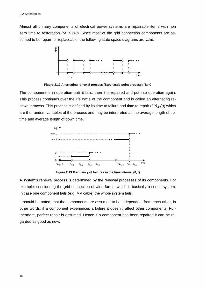
Figure 2.12 Alternating renewal process (Stochastic point process), TR>0
The component is in operation until it fails, then it is repaired and put into operation again.
This process continues over the life cycle of the component and is called an alternating re-
newal process. This process is defined by its time to failure and time to repair ((t),µ(t)) which
are the random variables of the process and may be interpreted as the average length of up-
time and average length of down time.
Figure 2.13 Frequency of failures in the time interval (0, t)
A system's renewal process is determined by the renewal processes of its components. For
example, considering the grid connection of wind farms, which is basically a series system.
In case one component fails (e.g. MV cable) the whole system fails.
It should be noted, that the components are assumed to be independent from each other, in
other words: if a component experiences a failure it doesn’t’ affect other components. Fur-
thermore, perfect repair is assumed. Hence if a component has been repaired it can be re-
garded as good as new.
1
2
m - 1
m + 1
SF,0=0 SF,1 SF,2 SR,m-1 SF,mtime
SR,mSR,2SR,1
0
N(t)

2 General
17
2.3 Reliability Theory
2.3.1 Reliability and Availability
From the previous reliability and availability definition in subchapter 1.1, there are some im-
portant differences between these two concepts. The term reliability refers to the notion that
the system performs its specified task correctly for certain time duration (t1,t2). Hence the
reliability of an item is time dependent that means the longer the time the lower the reliability,
regardless of the system design. The term availability refers to the readiness of a system to
immediately perform its task, at a particular time. When calculating the availability of a sys-
tem its maintainability and repairability is taken into account. In Figure 2.14 the concept of
reliability and availability and their influences are graphically illustrated.
Figure 2.14 Concept of availability and reliability
Note, that the availability of a non-repairable item or an item with zero time to restoration is
equal to the reliability of that particular item.
First of all it can be distinguished between non-repairable items, repaired items with zero
time to restoration and repairable items with non-zero time to restoration. This concept was
discussed in more detail in the previous chapter. The transition between a repairable and a
not repairable item is continuous [8]. Since almost all primary electrical components are re-
pairable items with non-zero time to restoration (mean time to repair MTTR > 0) only this type
shall be taken into account. However, for more information see [5] and [65].
Within the next few subchapters each subsection of Figure 2.14 will be described in detail
and furthermore different evaluation methods of significant reliability parameters will be intro-
duced.
Availability
System
Reliability
Component Reliability
Failure Rate
Redundancy
Topology
(Software&Hardware)
Maintainability
Repairability
(Support&Service)
Considered Aspects
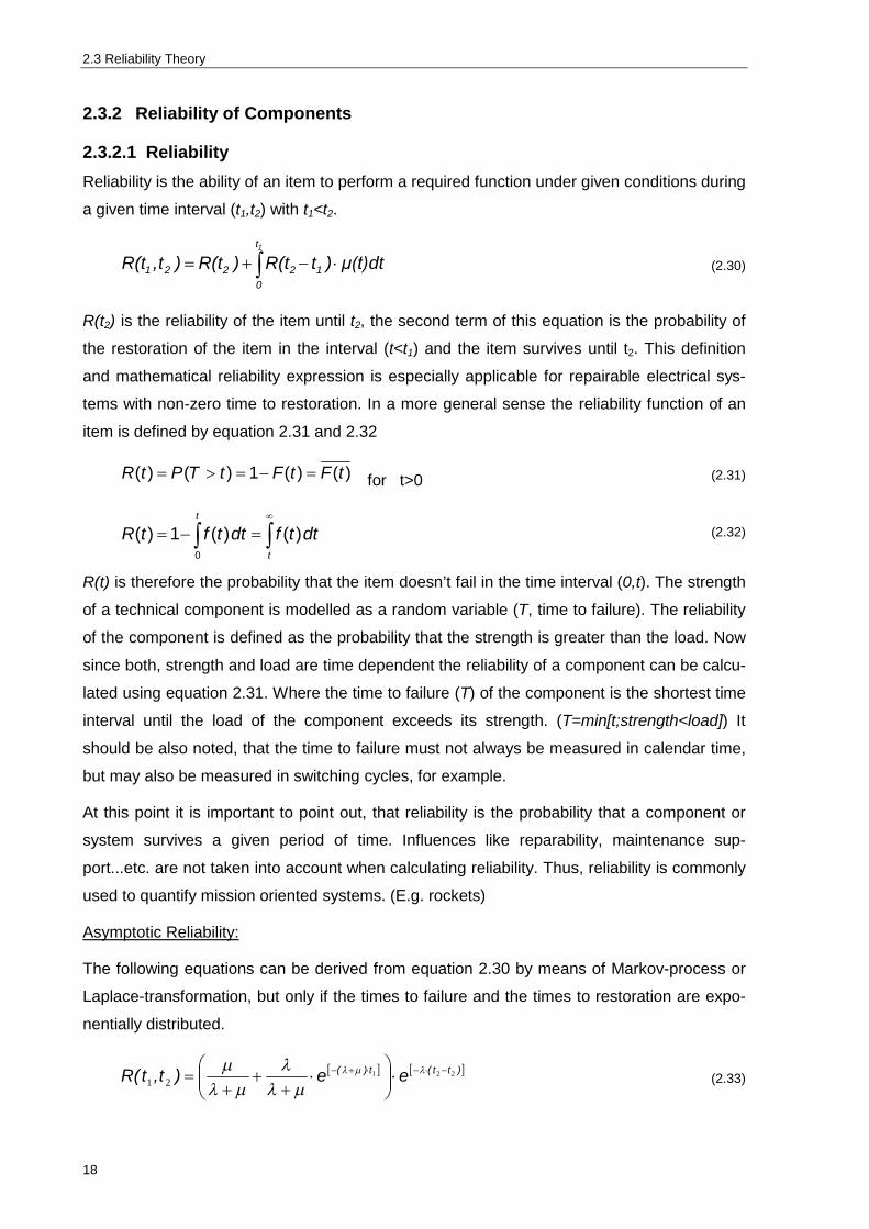
2.3 Reliability Theory
18
2.3.2 Reliability of Components
2.3.2.1 Reliability Reliability is the ability of an item to perform a required function under given conditions during
a given time interval (t1,t2) with t1<t2.
1t
012221 dtμ(t))tR(t)R(t)t,R(t (2.30)
R(t2) is the reliability of the item until t2, the second term of this equation is the probability of
the restoration of the item in the interval (t<t1) and the item survives until t2. This definition
and mathematical reliability expression is especially applicable for repairable electrical sys-
tems with non-zero time to restoration. In a more general sense the reliability function of an
item is defined by equation 2.31 and 2.32
)()(1)()( tFtFtTPtR for t>0 (2.31)
t
t
dttfdttftR )()(1)(0
(2.32)
R(t) is therefore the probability that the item doesn’t fail in the time interval (0,t). The strength
of a technical component is modelled as a random variable (T, time to failure). The reliability
of the component is defined as the probability that the strength is greater than the load. Now
since both, strength and load are time dependent the reliability of a component can be calcu-
lated using equation 2.31. Where the time to failure (T) of the component is the shortest time
interval until the load of the component exceeds its strength. (T=min[t;strength<load]) It
should be also noted, that the time to failure must not always be measured in calendar time,
but may also be measured in switching cycles, for example.
At this point it is important to point out, that reliability is the probability that a component or
system survives a given period of time. Influences like reparability, maintenance sup-
port...etc. are not taken into account when calculating reliability. Thus, reliability is commonly
used to quantify mission oriented systems. (E.g. rockets)
Asymptotic Reliability:
The following equations can be derived from equation 2.30 by means of Markov-process or
Laplace-transformation, but only if the times to failure and the times to restoration are expo-
nentially distributed.
)tt(t)( ee)t,t(R 22121
(2.33)

2 General
19
t
te)tt,t(Rlim
asymptotic reliability (2.34)
The reliability of electric systems can be classified into to functional aspects. Adequacy,
which is the ability of the electric system to supply the energy requirements of customers at
all times, taking into account scheduled and unscheduled disturbances. And Security, which
can be described as the ability of the electric system to withstand sudden disturbances, like
short circuits etc.
2.3.2.2 Failure Rate The probability that an item will fail in the time interval (t,t+Δt) is given by equation 2.35, as-
suming that the item is functioning at time t.
)(
)()()(
)()|(tR
tFttFtTP
ttTtPtTttTtP
(2.35)
Now the failure rate function can be obtained by dividing the probability by the time interval
(Δt) and calculate the right-hand limit for Δt→0. The received equation (2.36) is also known
as the instantaneous failure rate function (λ(t)).
(Instantaneous) Failure Rate: the limit, if it exists, of the quotient of the conditional probabil-
ity that the instant of a failure of a non-repaired item falls within a given time interval (t, t + Δt)
and the duration of this time interval, Δt, when Δt tends to zero, given that the item has not
failed up to the beginning of the time interval
)()(
)()()(1lim)(
0 tRtf
tRtFttF
tt
t
(2.36)
(Instantaneous) Failure Intensity: the limit, if this exists, of the ratio of the mean number of
failures of a repaired item in a time interval (t, t + Δt), and the length of this interval, Δt, when
the length of the time interval tends to zero.
dt
tdZt
tNttNEtzt
)()]()([lim)(0
(2.37)
)]([)( tNEtZ
Where N(t) is the number of failures that occur in the time interval (0, t) and E denotes the
expectation. If the item is continuously operating and its up-time is exponentially distributed
the following simplifications are valid (A(t) denotes the availability of the item).
)()()( ttAtz (2.38)
MTTF
tzz 1)(lim)( asymptotic failure intensity (2.39)

2.3 Reliability Theory
20
Equation 2.40 can be obtained by means of Markov-process or Laplace-transformation, but
only if the times to failure and the times to restoration are exponentially distributed.
t)(e)t(A)t(z
2
(2.40)
111
)t(zlim)(z
t (2.41)
It should be stated, that the difference between the failure rate of components and the failure
intensity lies only in the operation mode. The instantaneous failure rate function is normally
restricted to not-repairable items, or repairable items with zero time to restoration (MTTR=0).
On the other hand the instantaneous failure intensity function is also valid for repairable, in-
termittent operating items with non-zero time to restoration (MTTR>0). However, since both
terms (z(t), λ(t)) become identical for long observation times (equations 2.38-2.40), in this
thesis only the term failure rate (λ(t)) will be used for further calculations.
2.3.2.3 Lifetime Indices (MTTF, MTBF, MTTR) There are different possibilities to determine the lifetime of components or a systems. The
mean lifetime of an item, (mean time to failure MTTF), is the expected value E(T) of the life-
time T that can be calculated by using equation (2.42).
Mean Time To Failure (MTTF): The expectation of the time to failure.
00
)()()( dttRdttftTEMTTF (2.42)
n
operationoftimeMTTF
i
n
i)(
1 n…number of failures in the time interval
(2.43)
If the time to repair or replace a failed item is very short, compared to the MTTF, or in other
words if the repair rate (µ) is significantly less than the failure rate (λ), the MTTF also repre-
sents the MTBF (mean time between failure). On the other hand, if the time to repair cannot
be neglected, the MTBF also includes the MTTR. This concept is mathematical described by
equation 2.44 and 2.45.
Mean Time Between Failures (MTBF): The Mean operation time between failures.
MTTRMUTMTBF for intermittent operating items (IOI)
MTTRMTTFMTBF for continuously operating items (COI)
(2.44)
(2.45)
MUT….mean up time
MDT….mean down time for IOI

2 General
21
n
timetotalMTBF
i
n
i)(
1
(2.46)
Since the restriction <<µ is applicable for electrical components, the term MTBF will be
used throughout the ongoing chapters. (Assumed MTTF=MTBF)
Mean Time to Repair or Restoration (MTTR): The expectation of the time to restoration.
The mean time to repair of a failed item can be described as the sum of the expected times
of the included actions.
MRTMTDMLDMADMUFTMTTR (2.47)
If repair figures of different items are available (e.g. from experience) the following equation
provides a good estimate for the MTTR.
R
n
ii
k
nrestoratiototimeMTTR
1
)( kR….cumulated time to restoration
(2.48)
Assuming that the repair times follow an exponential distribution, with a constant repair rate
(µ), the equation for MTTR can be written as follows
µ
MTTR 1 (2.49)
Mean Residual or Remaining Life (MRL)
The probability that an item in operation at time t, survives an additional time interval (x) is
called the mean residual life (MRL)
t
dxxRtR
tgtMRL )()(
1)()( (2.50)
At time t=0 the item is new and
therefore g(0) is equal to the
MTTF.
The relationship between stress
level and mean residual lifetime
is displayed in Figure 2.15 Mean
residual life of an item Figure 2.15 Mean residual life of an item
MUFT meantime of a fault MAD mean administrative delay MLD mean logistic delay MTD mean technical delay MRT mean restoration time

2.3 Reliability Theory
22
2.3.2.4 Reliability Indices and their Interaction
The relationships between f(t), F(t), R(t) and λ(t) are presented in Table 2.2 below.
given )(tf )(tF )(tR )(t
)(tf dt
tdF )(
dttdR )(
t
dttet 0
)()(
)(tF t
dttf0
)( )(1 tR
t
dtte 0
)(1
)(tR
t
dttf )( )(1 tF
t
dtte 0
)(
)(t
t
dttf
tf
)(
)(
dttdF
tF)(
)(11
dt
tdRtR
)()(
1
Table 2.2 Relationships between reliability indices
The mathematical concepts in Table 2.2 are graphically illustrated in Figure 2.16 in order to
provide a thorough understanding of the different equations, their relations and interactions
among themselves.
Figure 2.16 Relation between failure probability F(t), failure density f(t),
failure rate (t) and reliability R(t) (survivor function)
It is important to understand the difference between reliability, also known as the survivor
function (R(t)) and the probability of failure (F(t)).
Area = R(t’)
F(t’)
t’

2 General
23
2.3.2.5 Lifetime Distributions There are numerous distribution functions to model the lifetime of items and systems from
different scientific areas. Since this investigation focuses mainly on electric power system
components but also considers some human and environmental aspects; the most relevant
distribution functions and their application will be introduced. As pointed out in subchapter
4.1, only the useful-life period and the wear-out period of the failure rate function are taken
into account, because of warranty and guarantee periods given by the company (REpower).
Hence the exponential distribution as well as the Weibull distribution will be explained in
more detail.
For further information regarding life-distribution functions and their application see [8],[16]
and [44].
The Exponential Distribution
The distribution function:
tetTPtF 1)()( )0( t (2.51)
The density function:
tetFdtdtf )()( )0( t (2.52)
The mean and variance of the exponential distribution are 1/λ and 1/λ2, respectively.
tetR )( → MTBF
1 (2.53)
Properties: Failure rate () is constant (independent of time, failures occur at random) Requires only the MTBF
MRL is equal to MTBF Fits to most electrical power system components
Figure 2.17 Exponential distribution (=0,5)
00,10,20,30,40,50,60,70,80,9
1
0 1 2 3 4 5 6 7 8 9
F(t),
f(t),
l(t)
time
F(t) f(t) l(t)

2.3 Reliability Theory
24
The Weibull Distribution
The distribution function:
tetTPtF 1)()( ( 0t ) (2.54)
The density function:
tettFdtdtf 1)()( )0,0( t (2.55)
Where and α are denoted as the shape and scale parameters of the Weibull distribution.
Their influence on the shape of the distribution and density function is shown in more detail in
Figure 2.19. For α=1, the Weibull distribution is equal to the exponential distribution.
The mean and variance:
111
MTBF (2.56)
The survivor function (R(t)) and the failure rate function (λ(t)) can be calculated using follow-
ing equations
tetR )( → 1)( tt ( 0t ) (2.57)
Properties: Very flexible distribution (has no specific characteristic shape) Used to model life distributions with decreasing, increasing or const. λ(t) Two-parameter model (α and λ shape and scale parameters)
Figure 2.18 Weibull distribution (=1, a=3)
Figure 2.18 displays the PDF (f(t)) and the CDF (F(t))of a Weibull distribution, for an increas-
ing failure rate function. Because of its flexibility, the Weibull distribution is commonly used to
model the wind speed of wind energy systems at different areas and altitudes.
00,10,20,30,40,50,60,70,80,9
11,1
0 0,5 1 1,5 2 2,5 3
F(x)
, f(x
)
timelF(x) f(x) l(x)

2 General
25
The following three graphs describe the shape and scale parameters in more detail and thus
provide a better understanding of their influence and their applicability.
Figure 2.19 Behaviour of the Weibull distribution at different shape parameter settings ( and )
It is important to point out, that the failure rate function is a function of the shape parameter α
and therefore discontinuous. This can be seen in Figure 2.19 and by looking at equation
2.55. The discontinuity of the failure rate function is important to be aware of, since for ex-
ample α=0,9999, α=1 and α=1,0001 will provide significantly different failure rate functions.
(see the first graph in Figure 2.19) The related PDF (f(t) green) and CDF (F(t) blue) are also
shown in Figure 2.20. Due to the discontinuity of the failure rate function the Weibull distribu-
tion is one of the most important distributions in engineering. Regarding electrical compo-
nents and their various life time distributions, the Weibull distribution is commonly used to
model the burn-in period and more significantly the wear-out period, were failure occur be-
cause of ageing mechanisms. This concept will be discussed in more detail in subchapter 4.1
(Lifetime of Electrical Components, page 59ff)
0
0,2
0,4
0,6
0,8
1
1,2
1,4
0 0,5 1 1,5 2 2,5
failu
re ra
te
t
a=0,5 a=1 a=2 a=3
0
0,2
0,4
0,6
0,8
1
0 0,5 1 1,5 2 2,5
prob
abili
ty d
ensi
ty, f
(t)
t
a=0,5 a=1 a=2 a=3
0
0,2
0,4
0,6
0,8
1
0 0,5 1 1,5 2 2,5
prob
abili
ty d
istri
butio
n, F
(t)
t
a=0,5 a=1 a=2 a=3

2.3 Reliability Theory
26
2.3.2.6 Availability Availability is one of the most important measures in reliability theory. There are various
kinds of availabilities. (Pointwise, interval, limiting interval, multiple cycle...etc.) [38][44][25] A
general valid definition of availability is given as follows:
The ability of an item, to perform its required function at a stated instant of time, or over a stated period of time.(under aspects of its reliability, maintainability and maintenance sup-port) (See Figure 1.3, page 2.)
The mathematical concept of availability is defined by:
)1)(()( tSPtA (2.58)
The above equation provides the probability that the item is functioning at time t, where S(t)
denotes the state variable. Furthermore it can be distinguished between availability at time t
(instantaneous availability A(t)) and the average availability (mean and asymptotic availability
A).
Instantaneous Availability:
t
dx)x()xt(R)t(R)t(A0
(2.59)
The following equation can be obtained by means of Markov-process or Laplace-
transformation but only if the times to failure and the times to restoration are exponentially
distributed.
t)(e)t(A
(2.60)
Mean Availability and Asymptotic Availability:
In general, availability is immediate readiness for use. The mean availability denotes the
mean proportion of time the item is functioning. Only the mean availability is considered and
calculated as shown below [29]
ntt
timeuptA
n
i
)(
)()(
12
1 210 tt n…number of items (2.61)
In this context )(tA denotes the mean availability and not its complement (unavailability).If
the item is repairable and it can be assumed as ‘as good as new’ after each repair or restora-
tion every time it fails, the average availability becomes the asymptotic availability (for long
observation times). See equation 2.61 and 2.63.
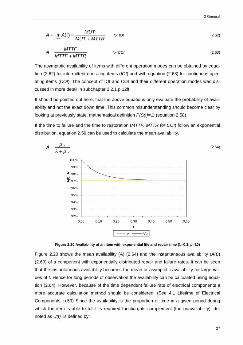
2 General
27
MTTRMUT
MUTtAAt
)(lim for IOI (2.62)
MTTRMTTF
MTTFA
for COI (2.63)
The asymptotic availability of items with different operation modes can be obtained by equa-
tion (2.62) for intermittent operating items (IOI) and with equation (2.63) for continuous oper-
ating items (COI). The concept of IOI and COI and their different operation modes was dis-
cussed in more detail in subchapter 2.2.1 p.12ff
It should be pointed out here, that the above equations only evaluate the probability of avail-
ability and not the exact down time. This common misunderstanding should become clear by
looking at previously state, mathematical definition P(S(t)=1) (equation 2.58)
If the time to failure and the time to restoration (MTTF, MTTR for COI) follow an exponential
distribution, equation 2.59 can be used to calculate the mean availability.
R
RA
(2.64)
Figure 2.20 Availability of an item with exponential life and repair time (=0,3, µ=10)
Figure 2.20 shows the mean availability (A) (2.64) and the instantaneous availability (A(t))
(2.60) of a component with exponentially distributed repair and failure rates. It can be seen
that the instantaneous availability becomes the mean or asymptotic availability for large val-
ues of t. Hence for long periods of observation the availability can be calculated using equa-
tion (2.64). However, because of the time dependent failure rate of electrical components a
more accurate calculation method should be considered. (See 4.1 Lifetime of Electrical
Components, p.59) Since the availability is the proportion of time in a given period during
which the item is able to fulfil its required function, its complement (the unavailability), de-
noted as U(t), is defined by:
92%
93%
94%
95%
96%
97%
98%
99%
100%
0,00 0,10 0,20 0,30 0,40 0,50 0,60
A(t)
, A
t
A A(t)

2.3 Reliability Theory
28
)(1)( tAtU (2.65)
The unavailability is also known as the forced outage rate (FOR) of an item or system.
2.3.3 Reliability of Systems
The previous section 2.3.2 focused on single items and how to evaluate their availability in a
quantitative way, on a single stochastic process basis. How to combine multiple stochastic
processes and therefore, how to evaluate whole systems (set of items) will be explained in
the following subchapter. Several methods are used to evaluate the reliability and availability
of more than just one item [38]. The most common ones are the failure mode and effect
analysis (FMEA), fault tree analysis (FTA) and reliability block diagrams (RBD). A short intro-
duction on how to apply the different methods is carried out over the next few pages.
Reliability Block Diagrams
Reliability block diagrams (RBD) are success-oriented networks describing the logic connec-
tion of components according to their physical function and not according to their structural
layout. Each component of the system that should be evaluated is illustrated as a block, see
Figure 2.21. It is important to note, if the system has more than just one function, each func-
tion must be modelled and evaluated individually. RBDs are must suitable for reliability
evaluations of non repairable items, or repairable items with very low MTTR and where the
order in which the failures occur is not important. When the systems are repairable (MTTR
cannot be neglected) and the order in which failures occur is important, Markov methods
(Markov-chains) are usually more suitable [44].
Series Systems
n
iinS tRtRtRtRtR
121 )()().....()()( (2.66)
Figure 2.21 RBD series system
For a system with a certain number of serial components (i), the average failure rate, aver-
age outage time and average annual outage time are defined by the following equations.
n
iiS
1 (2.67)
S
n
iii
S
rr
1
r = MTTR
(2.68)
1 2 3 n

2 General
29
n
iiiS rA
11 (2.69)
The index S denotes a serial system.
Parallel Systems
Within a parallel system all components must fail in order to cause an outage of the whole
system. Also in case more components fail, an intermediate level of availability is attained.
For a system with parallel, independent components, the following equations define the av-
erage failure rate, the average outage time and the average annual unavailability.
n
iiSS tRtQtR
1)(11)(1)( Q.... unreliability (2.70)
Figure 2.22 RBD parallel system
n
iiPP µU
1
(2.71)
n
i ii
iPP µ
AU1
1
(2.72)
P
PP
Ur
(2.73)
Index P denotes the parallel system.
It is obvious that in reality an electrical power system does not only consist of series or paral-
lel connected components. In order to calculate the reliability parameters of combined sys-
tems either the System Reduction Method or more accurate the Minimal Cut Set Method can
be applied. The Minimal cut set method can be implemented very easily to any electrical
power system layout and benefits from the minor calculation effort.
A short introduction of how to apply the minimal cut set method is given below.
1
2
n

2.3 Reliability Theory
30
Minimal Tie and Minimal Cut-Set Method
A cut set is a set of system components which, when failed, causes failure of the system.
That means that this set of components must fail in order to get the whole system to failure.
The minimal cut set is therefore the minimum subset which can cause system failure, but
only if every component of the subset is in the failure mode [5]. The tie set method is the
complement of the cut set method. Both methods, when implemented with reliability block
diagrams are equally to a parallel and series structure.
Example:
Figure 2.23 Minimal cut sets
The minimal cut sets from the reliability block diagram in Figure 2.23 are listed in the table
below. Since the minimal cut sets are always represented by a parallel structure, the unreli-
ability (Q) is used to evaluate the whole system in order to simplify the calculation effort.
Number of minimal cut set
Components of the cut set Cut Set #
1 A B C1
2 C D C2
3 A D E C3
4 B C E C4
Table 2.3 Minimal cut sets of figure 4.4-3
)( 4321 CCCCPQS …… (2.74)
n
iiS CPQ
1)( ……………….PS=1-QS (2.75)
A
D
E
B
C
E
A
B
C
D
C1 C2 C3 C4
Cx…cut set number x

2 General
31
Relationship between Reliability Block Diagrams and Fault Trees [5]
The Top-Event of the fault tree denotes the system failure condition. The events Ex that lead
to the top event are connected to the top event through a logic gate. The construction of a
fault tree always starts with the top event followed by the first level event which expresses for
example the prime fault causes of the system. Figure 2.26 - Figure 2.27 show some basic
fault trees which were established only by AND and OR gates. For further information see
[44] and [5].
Figure 2.24 Fault tree for a series structure Figure 2.25 Fault tree for a parallel structure
Figure 2.26 Fault tree for a combined structure Figure 2.27 Basic fault tree (metric) shapes
Simple rules when constructing fault trees:
An OR gate expresses system failure if any of the lower level failures occur (Series
Structure) The unavailability of the subsystem is the sum of the device unavailabil-
ity’s.
An AND gate is used if all of the lower levels failure have to occur in order to obtain
a system failure. The unavailability of the subsystem is the product of the items
E1 E2 E3 E4
AND
E1 E2 OR
E3 E4

2.3 Reliability Theory
32
unavailability. Used for redundancy.
If Top event is in the form of ‘System fails to operate’ event data in terms of un-
availability should be used.
For further information on qualitative evaluation methods see [44],[38],[33],[9],[8] and [5].
2.3.4 Summary of Definitions and Equations
This summary is intended to give an overview of the most important availability and reliability
parameters and how to calculate them. The equations in Table 2.4 Summary of definitions’
are used in the subsequent chapters to evaluate significant electrical components regarding
their availability. It should be noted, that the following equations are based on exponentially
distributed reliability data.
Calculated Data Equation
A , availability MTTRMTTF
MTTFA
, failure rate [1/yr] MTTFT
N 1
MUT , mean up time [h] see Figure 2.28 Calculation example
MDT , mean down time [h] see Figure 2.28 Calculation example
MTTF , mean time to failure [h] 1
nTMTTF
MTBF , mean time between failures [h] MTTFMTBF 2
MTTR , mean time to restoration [h] ndtRMTTR
MTTM , mean time to maintain [h] see appendix D
)(tR , reliability )()( tetR
Table 2.4 Summary of definitions
Interpretation
In subchapter 2.2 the concept of stochastic processes was introduced. It was shown, that the
probability of the component being in a particular state is equal to the proportion of time the
component remains in the required state (MTBF, MTTR) times the state transition rates ( )
[44]. The relationships between the different lifetime indices are graphically illustrated in Fig-
ure 2.28.
2 This can be assumed due to the fact that <<µ, as stated in chapter 2.3.2 (Reliability of Compo-
nents).

2 General
33
Figure 2.28 Calculation example
C
C
DU
U
TrT
AMTTRMTBF
MTBFTT
TA
TC…calculation period (e.g. 1 yr)
(2.76)
Equation 2.77 will be used to calculate the availability of components and systems within this
investigation. The particular restrictions that were made to ensure the accuracy of this equa-
tion its application to electrical power systems are summarized in subchapter 2.6.
2.4 Cost-Benefit Analysis
There are four basic methods to determine whether an investment is profitable or not. The
net-present value method (NPV), the annuity method, the internal rate of return (IRR) method
and the payback period (cash recovery, amortisation...etc.) These methods are part of dy-
namic investment calculation methods, dynamic because the compound interest factor (2.77)
is taken into account. Within the next subchapter, these methods and their application to
electrical power systems in general and wind energy systems in particular, will be introduced
very briefly.
2.4.1 Net Present Value and Internal Rate of Return
In order to ensure the profitability of a specific project investment the interest rate of an in-
vestment should be at least as high as its expected rate of return (yield) of. The corporate
costs of capital are equivalent to the rate of return and may be classified into equity capital
and dept capital. In order to estimate if a certain investment should be undertaken, the
weighted average cost of capital (WACC) will be calculated.. The WACC are thereby equal to
the least rate of return of the investment. For further information on how to calculate the
WACC, see [49]. At the beginning of 2010 the Energiekontor AG3 issued corporate bonds at
an interest rate of 6%. The WACC can be obtained by weighting the equity and debt costs
and amount to 6.78% [66]. This seems to be a realistic value for the interest rate. However,
for large investments the WACC should be evaluated individually because of their high risk
3 Energiekontor AG is one of Europe’s first company developing, realising and operating wind power
projects. http://www.energiekontor.de/

2.4 Cost-Benefit Analysis
34
relation. Generally, in order to take the inflation into account the real interest rate should be
used. Current Inflation in Germany: e=1,3% (10-2010)4
eri in [%] (2.77)
nn qiCIF )1( (2.78)
In general, the compound interest factor (CIF) in equation 2.78 can be used to evaluate the
present value (PV) of time dependent cash flows. For example, the following equation shows
the PV of a future payment (Sn) at a certain discount rate (q-n).
nnnn qS
iSPV
)1(1 (2.79)
At equal annual costs, the above equation simplifies to:
0)1(1)1( XSii
iSPV nn
n
n (2.80)
Where the character denotes the present value factor (PVF).
The concept of present value of time dependent payments is graphically illustrated in Figure
2.29, where the PVF is shown at different interest rates and over a period of 40 years.
Figure 2.29 PVF at different interest rates
It is obvious that the if the interest rate is high future payments or costs result in an low pre-
sent value. Therefore in case of high interest rates the life cycle costs of components are
lower and investments in general should be taken at a later date
4 Reference: Federal statistical office Germany. http://www.destatis.de/
00,10,20,30,40,50,60,70,80,9
1
0 5 10 15 20 25 30 35 40time [yr]
pres
ent v
alue
fact
or
i=5% i=7% i=9%
i real interest rate in % e inflation in % r nominal interest rate in %

2 General
35
With the present value factor future payments can be discounted to a reference date and
furthermore the calculated present values will be summarised in order to obtain the net pre-
sent value (NPV). The net present value is the value of a payment at the beginning of a pro-
ject, which is stated at the reference time t=0.
Net Present Value
The net present value (NPV) is the difference between the sum of all present values of out-
going payments and the sum of all present values of incoming payments over a certain time
interval. It can be calculated by the following equation:
N
nn
n
iSINPV
10 )1(
(2.81)
If the net present value of an investment is beyond or equal to zero, the outgoing payments
(investment) are less than the incoming payments (revenue) within the time interval, hence
the investment is profitable. Therefore if the NPV is less than zero, the investment will not be
profitable.
Capital Recovery Factor
The capital recovery factor (CRF) a certain amount of money (e.g. investment) into equal,
annual parts by taking the compound interest factor CIF and the time interval (n) into ac-
count.
1)1()1(
n
n
iiiCRF (2.82)
1)1()1(
00 n
n
A iiiICRFII equal annual costs (2.83)
The CRF can be interpreted as the amount of equal incoming payments to be received for n
years such that the total NPV of all payments is equal to are greater than zero. The CRF is
equal to the sinking fund debt plus the interest rate, or in other words it is the inverse of the
present value factor PVF.
Internal Rate of Return
The internal rate of return (IRR) of an investment is defined as the discount rate that results
in a zero NPV.
I0 investment Sn incoming payments

2.4 Cost-Benefit Analysis
36
0
011
0
),(
0)1(
10)1(
IRnQS
IR
SNPVIR
SNPVN
nn
N
nn
n
(2.84)
(2.85)
The IRR can be obtained by solving equation (2.84) with respect to R. This calculation can
be difficult, therefore a simplification is made by setting Sn (annual revenue) constant. Since
wind farm projects have almost constant annuities this simplification is valid. If the values of
Q and n are given the IRR can be found in economic tables.
From the previous explanations regarding basic investment analysis methods the following
simplifications weather an investment is profitable or not, can be derived:
If the NPV is greater or equal to zero the undertaken investment is profitable and visa
versa.
By looking at equation 2.84, the NPV is equal to zero if i=R. The IRR is always con-
stant and the NPV will be negative for all i>R and positive for all i<R. Hence R must
be greater than i in order to obtain a profitable investment. If more investment alterna-
tives have a NPV greater than zero, the investment with the highest IRR should be
undertaken [49].
Calculation Period of an Investment
Every technical product has its useful lifetime and therefore every investment has its useful
lifetime as well. Electrical power system components have different lifetimes according to
their required physical function, their purpose and their aging characteristic. The physical life
of a component is equal to the calculation period of an investment. The German federal min-
istry of finance provide specific AfA-tables5 for most industrial branches. The physical life of
significant components from the electricity supply sector is listed in Table 2.5.
Component Useful lifetime
Transformer 20 years
MV cable 40-45 years
MV Overhead lines 30-40 years
Substations 25-35 years
Table 2.5 Useful lifetime according to BMF-AfA
To evaluate a wind farm project regarding its profitability, the physical life of the project is
expected between 20 and 25 years. 5 Abschreibungstabelle für allgemein verwendbare Anlagegüter http://www.bundesfinanzministerium.de/nn_96040/DE/Wirtschaft__und__Verwaltung/Steuern/Veroeffentlichungen__zu__Steuerarten/Betriebspruefung/AfA-Tabellen/005.html

2 General
37
R
C
Rel
iabi
lity,
R
100 %
Investment costs, I0
Costs of Interruption, D
Investment, C0
Reliability, R in % ROpt. 100
Total Costs, C0+D
Cos
ts
2.4.2 Application to Reliability Engineering
The degree of reliability and the size of the investment for an electric network are closely
related. However, the relation between the investment costs and the degree of reliability of
the system is not linear. The first measures taken to increase the reliability within a system
can be made with a relatively small investment. For each additional quantity of reliability a
larger investment must be made. This is illustrated in Figure 2.30.
Figure 2.30 Incremental reliability (R) with respect to investment costs (C0)
A level of 100% reliability is from a technical point of view possible but not profitable because
of the large logistic and financial effort that has to be made. The reliability of a technical sys-
tem should be as high as possible with a limited amount of investment. Figure 2.31 shows
the relation between investment and interruption costs at different levels of reliability.
Figure 2.31. Relation of investment and interruption costs
This concept is a typical optimisation problem regarding reliability with a budget restriction.
Although the reliability of a certain layout is of most interest, the down time and more accu-
rate the repair time (MTTR) of components is also an essential parameter. The interruption
costs are subdivided into costs that increase with time, like lost revenue, material or penal-
ties, and costs that decrease with respect to time. These considerations together with

2.4 Cost-Benefit Analysis
38
general aspects about direct and indirect costs of interruptions are discussed in detail in [25],
[29], [32] and [34]. The typical relationship between availability and life cycle costs (LCC) for
the operation and maintenance phase is shown in Figure 2.32. Whereas the related costs
are classified into preventive and corrective maintenance costs, as well as consequential
costs.
Figure 2.32 Life cycle costs in terms of availability [25]
Investment for Logistics and Support
In case of a failure of the component or system it is a vast interest of the company to repair
the failure as soon as possible in order to keep the interruption costs as low as possible.
Since most failures occur on parts of components that can be repaired or replaced very
quickly at low costs, it is important that a certain amount of spare parts and replaceable units
(e.g. bushings, cable joints, switches....etc) should be in stock. According to [67] the cost of
Failures
Repair Preventive
maintenance Replacable
units, spares and facilities
Quantity x [(MPH x cost/h) + (materiial cost per unit)]
x [(average cost of maintenance support per failure) + (MPste x cost/h) + (MPwork x cost/h) + (average cost of spares per failure)]
Damage to image and reputation -> less revenue, service provision, warranty cost, liability cost
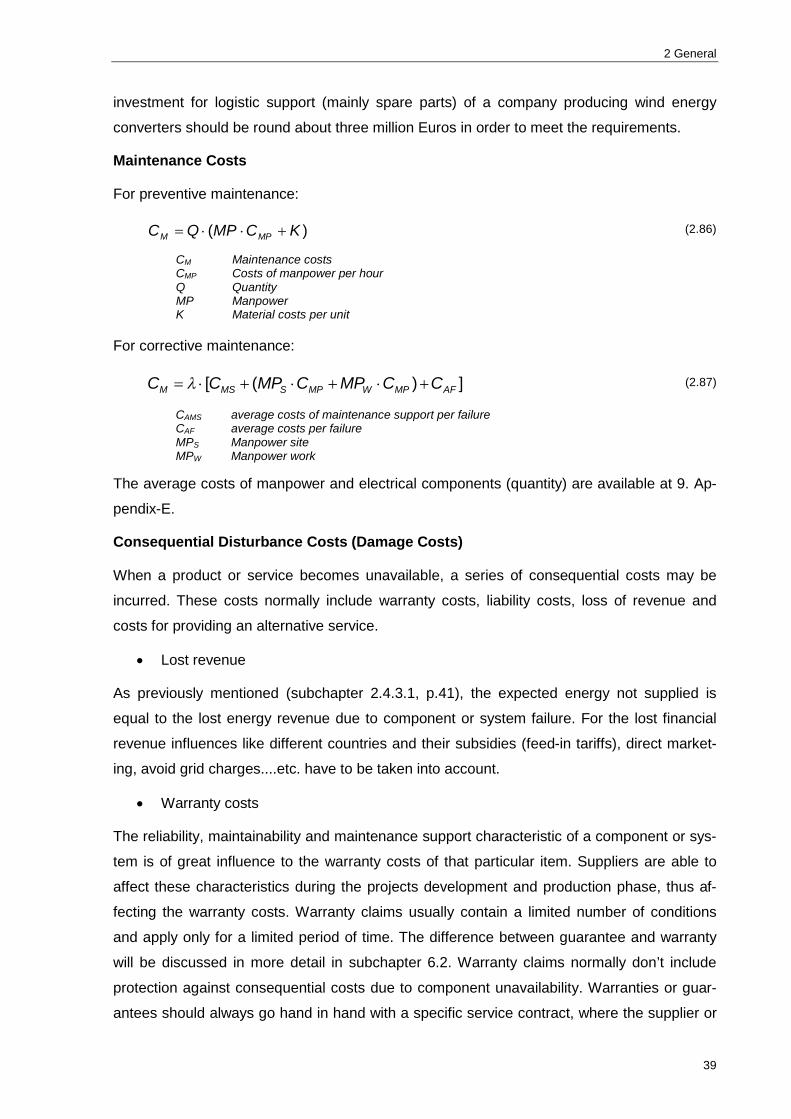
2 General
39
investment for logistic support (mainly spare parts) of a company producing wind energy
converters should be round about three million Euros in order to meet the requirements.
Maintenance Costs
For preventive maintenance:
)( KCMPQC MPM (2.86)
For corrective maintenance:
])([ AFMPWMPSMSM CCMPCMPCC (2.87)
The average costs of manpower and electrical components (quantity) are available at 9. Ap-
pendix-E.
Consequential Disturbance Costs (Damage Costs)
When a product or service becomes unavailable, a series of consequential costs may be
incurred. These costs normally include warranty costs, liability costs, loss of revenue and
costs for providing an alternative service.
Lost revenue
As previously mentioned (subchapter 2.4.3.1, p.41), the expected energy not supplied is
equal to the lost energy revenue due to component or system failure. For the lost financial
revenue influences like different countries and their subsidies (feed-in tariffs), direct market-
ing, avoid grid charges....etc. have to be taken into account.
Warranty costs
The reliability, maintainability and maintenance support characteristic of a component or sys-
tem is of great influence to the warranty costs of that particular item. Suppliers are able to
affect these characteristics during the projects development and production phase, thus af-
fecting the warranty costs. Warranty claims usually contain a limited number of conditions
and apply only for a limited period of time. The difference between guarantee and warranty
will be discussed in more detail in subchapter 6.2. Warranty claims normally don’t include
protection against consequential costs due to component unavailability. Warranties or guar-
antees should always go hand in hand with a specific service contract, where the supplier or
CM Maintenance costs CMP Costs of manpower per hour Q Quantity MP Manpower K Material costs per unit
CAMS average costs of maintenance support per failure CAF average costs per failure MPS Manpower site MPW Manpower work

2.4 Cost-Benefit Analysis
40
a stated subcontractor performs the required preventive and corrective maintenance actions.
In this case, the supplier is also motivated to optimise his system in order to keep the addi-
tional costs low. This concept is already common practice at REAG.
Availability or performance guarantees are only valid if an additional service contract is in-
cluded
Liability costs
A liability will arise where, for example, a supplier fails to comply with his legal obligations
[25]. Liability costs are also important for new products for which risks involved may not be
fully apparent and/or well understood. Where required, a risk analysis, together with past
experience and expert judgement, may be used to provide an estimate of these costs.
In addition, further consequential costs should be identified by applying risk analysis tech-
niques to determine costs of impacts on the company’s image, reputation or prestige. In a
worst case scenario these impacts can lead to loss of clients.
Equation for calculating damage costs (DC) based on the actual availability of the system
pEA
EADC
WF
G
)(
(2.88)
General equation to calculate the damage costs regarding supply interruptions caused by
component induced failures.
)]()([ DEDDPO TkTTkPDC (2.89)
Bonus-Penalty Solution
During the time where the integrated service package (ISP) contract is valid, a bonus-penalty
solution for the wind farms actual availability is offered. The mathematical evaluation meth-
ods for the liquid damage (LD) and the bonus payments (BP) are given below.
pAEAALDWF
WFG )( (2.90)
3,0)(
p
AEAABPWF
GWF
(2.91)
P0 Capacity out of service [kW] TD Down Time (~MTTR [h]) kP specific power based outage costs [€/kW] kE specific energy based outage costs €/kWh]
E energy production (seasonal weighted) AwF wind farm availability (measured, calculated) AG guaranteed availability p electricity price (feed-in tariff, subsidies)
LD liquid damages BP bonus payments

2 General
41
Life-Cycle Costs
The life cycle costs (LCC) of electrical components are defined by the following equation.
n
DROOPCMPMIE CCCCCCCCCLCC0
0 )( (2.92)
This equation presents the overhead costs and the variable costs of a component over its
lifetime. The costs for infrastructure as well as the costs for refurbishment and disposal will
not be taken into account within this investigation. The equations for the corrective and pre-
ventive maintenance costs were previously introduced and the operational costs which
mainly consist of lost revenue caused by active power losses are discussed in more detail
within the reliability modelling subsection. A brief introduction of life cycle costs of relevant
grid connection components is given in chapter 4, with a special focus on their variable costs.
2.4.3 Application to Wind Energy Systems
2.4.3.1 Generation Duration Curve In order to calculate the expected energy not supplied (EENS) the generation duration curve
as well as the capacity factor (cf) of WECs will be introduced in this subchapter. The genera-
tion duration curve displays the time share the WECs operates at a certain level of rated
power over a stated period of time. Normally over one year of observation. Figure 2.33
shows the generation duration curve for different wind farm locations.
Figure 2.33 Generation duration curve
Two parameters can be used to describe the generation duration curve adequately, the ca-
pacity factor and the full-load-hours.
0102030405060708090
100
0 10 20 30 40 50 60 70 80 90 100
time share in %
shar
e of
rate
d po
wer
in %
shore low mountain range offshore
C0 investment costs CE cost of erection CI cost of infrastructure CPM preventive maintenance costs CO outage costs CR costs of refurbishment CD costs of disposal CCM corrective maintenance costs COP operational costs (load/no load losses)
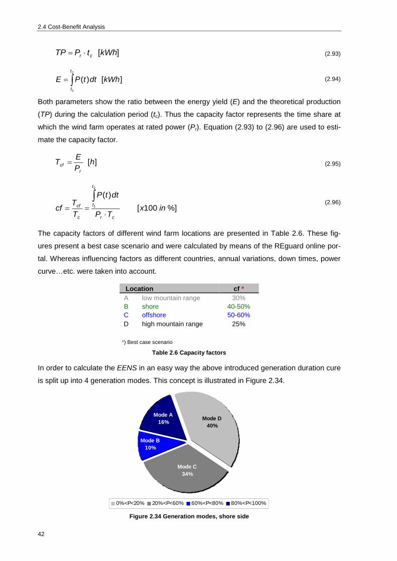
2.4 Cost-Benefit Analysis
42
][kWhtPTP cr (2.93)
][)(
2
1
kWhdttPEt
t (2.94)
Both parameters show the ratio between the energy yield (E) and the theoretical production
(TP) during the calculation period (tc). Thus the capacity factor represents the time share at
which the wind farm operates at rated power (Pr). Equation (2.93) to (2.96) are used to esti-
mate the capacity factor.
][h
PET
rcf (2.95)
%]100[)(
2
1 inxTP
dttP
TTcf
cr
t
t
c
cf
(2.96)
The capacity factors of different wind farm locations are presented in Table 2.6. These fig-
ures present a best case scenario and were calculated by means of the REguard online por-
tal. Whereas influencing factors as different countries, annual variations, down times, power
curve…etc. were taken into account.
Location cf * A low mountain range 30% B shore 40-50% C offshore 50-60% D high mountain range 25% *) Best case scenario
Table 2.6 Capacity factors
In order to calculate the EENS in an easy way the above introduced generation duration cure
is split up into 4 generation modes. This concept is illustrated in Figure 2.34.
Figure 2.34 Generation modes, shore side
Mode A16%
Mode B10%
Mode C34%
Mode D40%
0%<P<20% 20%<P<60% 60%<P<80% 80%<P<100%

2 General
43
Approximately 70% of the time the wind farm is operating at less than 60% of rated pow-
er.The concept of generation modes shall serve as basis for the estimation of active power
losses which will be discussed in detail in subchapter 5.3.
As mentioned above the generation duration curve depends on several influencing factors. In
order to estimate the different generation modes in an accurate way the project specific wind
assessment data should be used. How to calculate the required data from the measured
wind data is very briefly introduced below.
Figure 2.35 Approach for generation modes of different locations
Based on the Weibull distribution of the wind speed the cp factor of the relevant turbine can
be calculated. In a next step the power curve is determined. After a convolution between the
Weibull distribution and the power curve the relevant generation modes of the WEC can be
obtained. It is obvious that the whole process depends on the accuracy of the evaluated wind
data of the particular location. However, the wind speed is still the best estimator for wind
power project.
0,000
0,050
0,100
0,150
0,200
0,250
0,300
0,350
0,400
0,450
0,500
0,0 5,0 10,0 15,0 20,0 25,0
v [ m/s ]^
cp fa
ctor
power coefficient WEC MM92
0,00
0,02
0,04
0,06
0,08
0,10
0,12
0,0 2,0 4,0 6,0 8,0 10,0 12,0 14,0 16,0 18,0 20,0 22,0
v [ m/s ]
freq
uenc
y
0
20
40
60
80
100
120
prob
abili
ty [%
]
Section 1 Section 2 Mean P
0,0
250,0
500,0
750,0
1000,0
1250,0
1500,0
1750,0
2000,0
2250,0
0,0 5,0 10,0 15,0 20,0
v [ m/s ]
P [ k
W ]
power curve MM92
Mode A16%
Mode B10%
Mode C34%
Mode D40%
0%<P<20% 20%<P<60% 60%<P<80% 80%<P<100%
1
2
3

2.4 Cost-Benefit Analysis
44
2.4.3.2 Seasonal Energy Output Variations In order to estimate the damage costs in an accurate way the seasonal variations regarding
the energy output (yield) has to be taken into account. These variations are not only a func-
tion of time, but also a function of location, country…etc. Figure 2.36 below shall give an im-
pression on how strong the energy output of a wind farm with can vary over a period of four
years (2006-2010). The mean energy outputs of one month are represented in these figures,
whereas the black curve in Figure 2.36 as well as the red curve in Figure 2.37 represent the
trend line of the energy output.
Figure 2.36 Seasonal energy output variation of WF Lübke Koog6 06-10
Figure 2.37 Seasonal energy output variation of WF Lübke Koog 06-09
Figure 2.37 provides a closer look at the energy output during the years 2006 to 2009. As
mentioned above the seasonal variation has several influencing factors. Therefore the exact
6 ‚Lübke Koog’ is a German onshore-wind farm with one of the highest annual energy revenues. It is
located in the north of Germany at the shore of the North Sea, close to the Danish border. The capac-
ity factor of this wind farm is approximately 40%.
10000001500000200000025000003000000350000040000004500000500000055000006000000
11/2
010
09/2
010
07/2
010
05/2
010
03/2
010
01/2
010
11/2
009
09/2
009
07/2
009
05/2
009
03/2
009
01/2
009
11/2
008
09/2
008
07/2
008
05/2
008
03/2
008
01/2
008
11/2
007
09/2
007
07/2
007
05/2
007
03/2
007
01/2
007
11/2
006
month
Energy Output [kWh]Mean Energy Output [kWh]
0%
20%
40%
60%
80%
100%
02/2
009
01/2
009
12/2
008
11/2
008
10/2
008
09/2
008
08/2
008
07/2
008
06/2
008
05/2
008
04/2
008
03/2
008
02/2
008
01/2
008
12/2
007
11/2
007
10/2
007
09/2
007
08/2
007
07/2
007
06/2
007
05/2
007
04/2
007
03/2
007
02/2
007
01/2
007
12/2
006
11/2
006
month
Energy OutputMean Energy Output

2 General
45
relative deviation between operation during summer and winter periods cannot be derived.
However, a theoretical approach on how to obtain the deviation factor is presented below.
Interpretation
As mentioned above the seasonal variations are strictly related to single projects. Therefore
an exact evaluation regarding time dependent energy output should be done using the
measured wind data from the wind farm location.
Why is the energy output and its seasonal variation relevant? The two main wind farm pa-
rameters of most interest to the customer are the power curve of the wind energy converters
and the availability of the whole system. Now if the actual availability of the WF doesn’t meet
the guaranteed level the lost financial revenue has to be paid. In order to estimated this li-
quated damages in an accurate way the seasonal energy output variations have to be taken
into account. Furthermore if maintenance times are not included in the availability calculation
period, in other words if the time to maintain is considered as system unavailable the mainte-
nance actions should take place in periods with lower energy output.
Figure 2.38 Seasonal wind speed and energy output variations
In the previous subchapter, the evaluation of the WECs generation modes and the signifi-
cance of the wind data were introduced. It should be pointed out that in order to evaluate the
seasonal variations in a representative way the wind speed data of locations should be used.
0%
20%
40%
60%
80%
100%
120%
140%
Jan Feb Mar Apr May June July Aug Sep Oct Nov Dez
ener
gy o
utpu
t in
%
std. deviation mean Poly. (trend mean)

2.4 Cost-Benefit Analysis
46
2.4.3.3 Wind Energy Costs The cost structure of wind energy projects is briefly presented below, in order to get a better
understanding of wind and outage related costs.
The main influences on wind energy costs are:
the mean wind speed
the power curve of the WEC
the investment costs, which consists primarily of manufacturing costs of the WEC
the level of technical availability
operational costs, basically maintenance costs
The cost structure of large wind farms can be categorized into the following groups:
Investment Costs (C0):
Planning, infrastructure, financing ~30% of investment (C0)
Cost of WEC (CWEC)
Annual Costs:
Maintenance, Insurance ~4% of C0
Credit – Annuity: for i=6% - 8-14% Annuity depends on the calculation period
(10-20years)
Annual Energy Revenue:
97% availability,~12% technical losses and 5% safety discount:
cftPE cWECrWEC , (2.97)
Specific investment regarding annual energy revenue
Operational Costs.
ECC 0
(2.98)

2 General
47
2.5 Failure, Fault and Error
In everyday use the words failure, fault and error almost have the same meaning and there-
fore are used for similar conditions. However, in engineering disciplines a thorough under-
standing of signals and systems and their behaviour is needed. In order to evaluate a spe-
cific signal accurately a proper definition of the signal states (how the signal can vary with
respect to time) and their application is needed. Since the main focus of this investigation is
the reliability and availability of components, only the related terms failure, fault and error are
discussed in more detail. Figure 2.39 displays a signal (blue curve), how it can vary over time
and how it passes through different states.
Figure 2.39 Failure, fault and error
Error is the deviation between the actual amplitude and the target value within the acceptable
limits (area within the dotted line). A failure on the other hand describes the actual perform-
ance at the time the observed value exceeds the given limits. Thus the term failure doesn’t
refer to an actual state, but to an event. The state, beyond the given limits is denoted as
fault.
Basic Faults in electrical power systems are classified in longitudinal faults and transversal
Faults. (see Appendix – D)
Within a wind farm it can be distinguished between three different areas in which a failure
may occur:
HV-Network: fault ride through (FRT) has to be taken into account.
MV-Network (Collector System): FRT of other WECS has to be considered. Faults
have to be cleared selectively in order to protect the WEC and other MV components.
LV-Network (WEC): Coordination between LV and MV electrical protection to ensure
the operation of other WECs during a fault on the LV network.
acceptable deviation
Error
failure event
fault state
time
target value
actual performance
p.u.

2.5 Failure, Fault and Error
48
2.5.1 Common Cause Failures
This type of failure involves the simultaneous outage of two or more components due to a
common cause. A main focus of reliability assessments is to highlight this type of failure and
its probability of occurrence. If the probability is too high the system should be redesigned.
Common mode failures are usually not considered in reliability analysis
If the failure of any component is not inde-
pendent of any other, in other words if the
failure of components are not mutually ex-
clusive and independent, a common cause
failure can be assumed [8]. (See Figure
2.40) Figure 2.40 Common cause failures
Common cause failures need to be taken into account for redundant systems. The IEEE
subcommittee recommend a special common cause factor for electrical power systems ap-
plications. This factor will be used in subchapter 0 for the evaluation of redundant power
transformer layouts.
2.5.2 Single and Multiple Faults
The probability of occurrence of k faults out of N (set) within a given period of time can be
determined by the Poisson distribution. If λ is the failure rate for a given period of time (tc),
then the following equation applies
!)(),(k
ettkPctk
cc
(2.99)
By looking at equation 2.95 it is obvious, that the Poisson distribution is equal to the expo-
nential distribution for k=0.
Probability of occurrence of exactly two faults:
1
2!2)()2(
22
ct
c tetPc
(2.100)
If the extension of the grid (e.g. MV collector system) is small the occurrence of multiple fail-
ures can be neglected. It can be shown, that the frequency of occurrence of two faults within
a time interval of 10 days for the MV collector system is <1%. The time interval was chosen
to be 10 days because this represents the worst maintenance case and at the same time is a
common time interval for test runs within the commissioning phase. By looking at the reliabil-
ity figures, the same result can be assumed for MV switchgear and transformers. Since the
grid connection of large wind farms is not very complex, compared to, for example,

2 General
49
meshed transmission networks, and the failure rate of single components is low, the occur-
rence of multiple faults within a given time interval can be considered as not relevant.
2.5.3 Types of Faults and their Frequency of Occurrence
The figures are based on the disturbance and availability statistic from the German network
[53]. Due to the high rate of overhead lines and the compensated neutral-point treatment of
the MV network the frequency of phase to earth faults have to be reconsidered. The statistic
distinguishes between faults that lead to an interruption and those who occur but don’t affect
the function of the system. Since a fault occurs anyway the total number of occurrence is
used.
Figure 2.41 Types of faults and their frequency [54]
It can be seen in Figure 2.41 that multiple phase faults and phase to ground faults are the
most common faults types within electrical power systems.
Figure 2.42 Multiple phase faults [54]
1,36
4,66
0,96
3,46
0,57
0,20
0,710,73
0,71
0,110,05
0
1
2
3
4
5
6
MV HV EHV
freq
uenc
y
phase-to-earth fault multi-phase faults interruption without SC other faults
0,7460,246
0,538
2,174
0,25
0
0,5
1
1,5
2
2,5
3
3,5
MV HV EHV
freq
uenc
y
2 phase faults 3 phase faults short circuit (general)
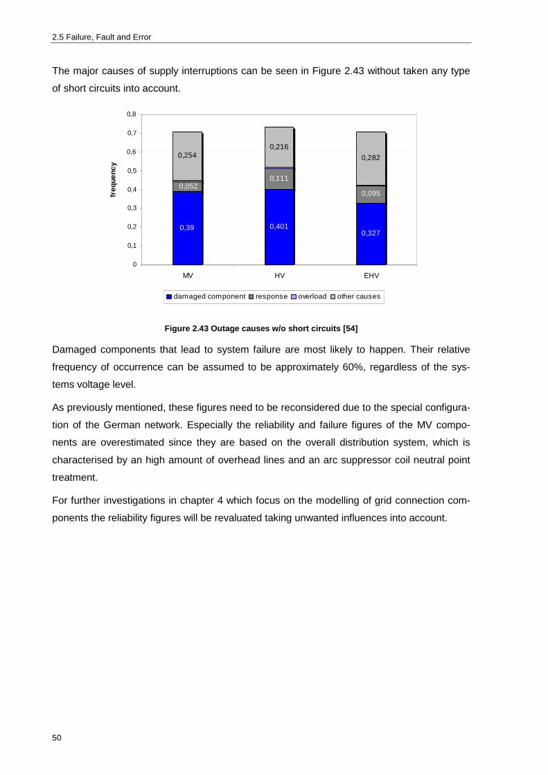
2.5 Failure, Fault and Error
50
The major causes of supply interruptions can be seen in Figure 2.43 without taken any type
of short circuits into account.
Figure 2.43 Outage causes w/o short circuits [54]
Damaged components that lead to system failure are most likely to happen. Their relative
frequency of occurrence can be assumed to be approximately 60%, regardless of the sys-
tems voltage level.
As previously mentioned, these figures need to be reconsidered due to the special configura-
tion of the German network. Especially the reliability and failure figures of the MV compo-
nents are overestimated since they are based on the overall distribution system, which is
characterised by an high amount of overhead lines and an arc suppressor coil neutral point
treatment.
For further investigations in chapter 4 which focus on the modelling of grid connection com-
ponents the reliability figures will be revaluated taking unwanted influences into account.
0,39 0,4010,327
0,095
0,2540,216
0,282
0,0520,111
0
0,1
0,2
0,3
0,4
0,5
0,6
0,7
0,8
MV HV EHV
freq
uenc
y
damaged component response overload other causes

2 General
51
2.6 Restrictions and Assumptions
Only repairable items with MTTR>0 are assumed.
During the components useful-life period, faults occur at random, which indicates a
constant failure rate. Therefore only the exponential distribution function is used to es-
timate the reliability and availability of components.
The outage time (MDT, MTTR) has an exponential distribution as well.
As previously mentioned, the failure rate of electrical components is significantly
lower than their repair rate (<<µ). The following simplification can be made:
MTTF=MTBF. (See 2.3.4 Summary of Definitions and Equations p.32)
The examples and calculations presented in this thesis are based on reliability figures
of the German electricity network [53]. Reliability figures from markets in which RE-
power is operating can be found in the appendix (Appendix C – Reliability Figures).
In this thesis the terms medium voltage (MV) and high voltage (HV) are referring to
30kV and 110kV. Since the installed capacity of onshore wind farms became larger
over the past years the above mentioned voltage levels are common practice nowa-
days. The MV collector system of offshore wind farms normally operates at the same
voltage level (30kV), for the same reasons
3.1 Data Preparation
52
3 Reliability Data
To evaluate the reliability of an item in a quantitative way, adequate models as well as accu-
rate data are needed. This section shall give a short introduction on how to obtain accurare
reliability data, how to process them and fit them to the adequate model.
Basically there are two major data sources, the electric utilities on the one hand and the
manufacturers (subcontractors) on the other hand. In electrical power systems reliability en-
gineering, the use of data from the utility sector is common practise nowadays, not only be-
cause of the quantity but also because of their wide range and neutrality. The reliability
evaluation and the optimization of components are based on figures from the German power
system [53]. For statistical data from other countries as listed below, see Appendix C
3.1 Data Preparation
The easiest method of fitting a set of data to a given distribution function is to directly com-
pute distribution parameters from statistical results. For most distribution function with one or
two parameters a reasonable fit can be found by using the mean and variance of the data
set.
3.1.1 Method of Moments
In statistics the Methods of Moments is used to estimate population parameters like mean,
variance …etc. A moment is therefore a quantitative parameter of the shape of a set of data.
The first two moments are the mean and the variance of the set. The sample mean is simply
the arithmetic average of a given set of data and is defined as the sum of the set values di-
vided by the set size. (3.1) The mean value is a good point estimate for the expected value.
n
iix
nx
1
1 (3.1)
The variance indicates the second moment and is known as the most common way to esti-
mate the dispersion in the data set. It is defined as
2
1
2 )(1
1
n
ii xx
n (3.2)
Another parameter for the variation or dispersion of a set of data is the standard deviation.
2 (3.3)
The main advantage of the standard deviation is that it is expressed in the same unit as the
n=size of data set Data Set….[x1,x2,…,xn]
n-1 – denominator - unbiased

3 Reliability Data
53
set data. According to this the standard deviation is commonly used to estimate the confi-
dence of statistical interpretations.
Additionally, there are two more moments which will not be introduced in this thesis, the Me-
dian and the Mode. (For further information see [3] and [38])
3.1.2 Maximum Likelihood
The likelihood (probability) function for a random sample is the joint probability density func-
tion (see Figure 2.2) of the random variables defined as
n
iin xfxxxL
121 );(),...,,;( (3.4)
The purpose of the maximum likelihood method is to find as an estimate of such that
),()ˆ,( xLxL (3.5)
The only value of that satisfies this particular inequality is the maximum value of ),( xL ,
denoted as called the maximum likelihood estimator of [38]. Therefore, to obtain the
following equation can be used.
0ln
ˆ
L (3.6)
Example:
Given: n…sample of n times to failure,
…failure rate (known to be exponentially distributed)
Find the maximum likelihood estimator for !
n
ii
n
ii
n
ii
tn
n
i
tn
ii
t
n
tnL
tnL
eetftL i
n
ii
i
1
1ˆ
1
11
ˆ
,0ˆln
,)(lnln
,);(),( 1
According to the above example the point estimate of the failure rate is the number of failures
(n) divided by the observation time.The maximum likelihood method is the most adequate
method for parameter estimation [67].

3.1 Data Preparation
54
3.1.3 Chi-Square Test (Goodness-of-Fit Test)
The chi square method is a Goodness of Fit Test. In other words, with this procedure can be
determined how well a given data sample belongs to a hypothesized theoretical distribution
model.
The chi-square test uses the statistic X2 which approximately follows a chi-square distribu-
tion. X2 is obtained from the equation below.
i
ii
eeoX
22 )(
(3.7)
Where, the magnitude of differences between ei and oi characterize the adequacy of the fit.
Hence, if the observed frequencies differ much from the expected frequencies, X2 will be
large and the fit is poor. The steps of the test process are:
Hypothesis: X have a known distribution, f(x)
Determine the significance of the test denoted by
Establish the rejection region )1(21 mkR . (see appendix TableB1)
If W>R, reject the distribution.
It should be noted, that in the above explanation α denotes the level of confidence.
3.1.4 Confidence Limits
The two most important reliability parameters of components in general are the failure rate
and the average outage duration, or repair time. As stated in the previous subchapter the
point estimate of e.g. the failure rate ( ) may differ from the true value (). Hence, it is always
advisable to determine a confidence level (γ=1-). If l and u denote the lower and upper
limits of the confidence interval the following equation applies.
)( ulP 10 confidence level (3.8)
Suppose a normally distributed data sample with mean µ and variance 2. Then the stan-
dardised random variable z follows a Student t-Distribution with n-1 degrees of freedom,
which is independent from µ and 2.
nµxT
/
)( cTcP )1(21)( cF (3.9)
oi…expected frequency ei…observed frequency

3 Reliability Data
55
nca
)( axµaxP (3.10)
Where the character c can be obtained from the t-distribution, according to F(c). Failure rate
confidence limits are upper and lower values of the estimated failure rate, according to the
following equations.
2
1)(
LP (3.11)
2
1)(
UP (3.12)
By use of the chi-square distribution with n degrees of freedom (see Appendix D) the lower
(L) and upper (U) confidence limit of failure rate can be expressed as follows:
ˆ
2)2(2
2/ T
nL (3.13)
ˆ
2)22(2
2/1
Tn
U (3.14)
The deviation of the upper and lower confidence level from in percent of is
ˆ1100 L
Ldev in % (3.15)
1ˆ100U
Udev in % (3.16)
The two sided confidence interval for an exponential distributed failure rate is
1)2
)22(2
)2((2
2/12
2/
Tn
Tn
P (3.17)
For further information regarding confidence limits on , MTBF, and R(t) see [29].
Figure 3.1 Failure rate confidence limits, shows the deviation of the failure rate as a function
of the observed failures. It is obvious that as the number of observed failures increases, the
confidence limits become narrower and thus the confidence that is a good estimate of ,
the true failure rate increases.
n…. number of observed failures 2n…. degree of freedom

3.1 Data Preparation
56
Figure 3.1 Failure rate confidence limits
The IEEE reliability subcommittee recommend a minimum of 8 to 10 observed failures for
‘good’ accuracy when estimating equipment failure rates [29].
Example: Low voltage cable for ETS connection.
Given: Cable below ground in conduit >600V, failures 46, unit years 19525 [yr] Find and the confidence limits of , MTBF and R(20yrs) at 95% confidence level.
From equation (3.7 002355,019525/46ˆ
Two-sided confidence limits on )195252
)94(195252
)92( 2975,0
2025,0
From Appendix D – Table D.1 14,118)94(
22,74)92(2
975,0
2025,0
Thus, 33 103109,1
Two-sided confidence limits on R(t) %96)20(%94
)(
RetRe tt UL
The following equations represent the upper and lower limit of the individual confidence level
in Figure 3.1.
75,0455% xndevU 95% upper limit (3.18)
74,0390% xndevU 90 % upper limit (3.19)
-100-80-60-40-20
020
406080
100120140160
1 6 11 16 21 26 31 36 41
number of observed failures
devi
atio
n of
failu
re r
ate
in %
95% confidence
90% confidence
80% confidence

3 Reliability Data
57
74,0300% xndevU 80 % upper limit (3.20)
100)ln(19% nxdevL 95% lower limit (3.21)
95)ln(5,19% nxdevL 90 % lower limit (3.22)
8520 )nln(x%devL 80 % lower limit (3.23)
Equations (3.18)-(3.21) were derived from Figure 3.1 Failure rate confidence limits’ and can
be used to estimate the confidence limits for different failure rates with given numbers of ob-
served failures in an easy way.
ˆˆ LL where %dev (3.24)
ˆˆ UU (3.25)
λL and λU represent the upper and lower failure rate at a given level of confidence.
As a technical note, a 95% confidence interval does not mean that there is a 95% probability
that the interval contains the true mean. The interval computed from a given sample either
contains the true mean or it does not. Instead, the level of confidence is associated with the
method of calculating the interval. The confidence coefficient is simply the proportion of sam-
ples of a given size that may be expected to contain the true mean. That is, for a 95% confi-
dence interval, if many samples are collected and the confidence interval computed, in the
long run about 95% of these intervals would contain the true mean.
Figure 3.2 presents the upper and lower failure rate of medium voltage XLPE cables with
respect to time and observed failures. The confidence level thereby is 95%. As reference
point serves the mean failure rate, represented as the dotted black line. The failure rate var-
ies over time, but gets narrower as the number of observed failures increase.
Figure 3.2 XLPE Cable failure rate
The same concept can be applied to any kind of failure rate (e.g. Areva GHA-Switchgear).
0
0,5
1
1,5
2
2,5
3
1 2 3 4 5
failu
re ra
te
95% Confidence limit failure rate mean
observed failures

3.2 Reliability Statistics
58
3.2 Reliability Statistics
3.2.1 Historical Data from Utilities
Electric utilities have a long history in troubleshooting and maintenance management. There-
fore most of them have a well established failure and reliability database of their assets. The
association of grid operators of each country usually provide a statistical report with a special
focus on interruptions and disturbances of the countrywide, electrical power system. The
annual ‘disturbance and availability statistic’ of the German network is provided by the
VDE(FNN) [53]. In order to evaluate the figures and use them for further calculation, it is im-
portant to understand the particular data acquisition process. The specific instruction for the
German process with all its classifications and definitions is available at [53].
Country specific informations
Europe: Germany VDE(FNN) http://www.vde.de/de/fnn/
Swiss VSE http://www.strom.ch/de/fachbereiche/technik/
Austria VEÖ http://oesterreichsenergie.at/
North America: USA IEEE Std. 493-2007 ‘Gold Book’ [29]
EPRI http://my.epri.com/portal/server.pt
Canada CEA http://www.electricity.ca/
3.2.2 Reliability Statistics from Subcontractors
Repower’s first source subcontractors regarding electrical components are Siemens AG and
Areva T&D. Both companies have large and well known research and development depart-
ments and a long history in electrical engineering. Especially Siemens with its internal guide-
line SH29500 provide detailed reliability figures. A short overview of reliability data from rele-
vant grid connection components is presented in Table B.1 (Appendix-C ‘Reliability Data’)
It is common practice nowadays to use data from utilities for reliability evaluations. This is
mainly because of the great amount of data obtained from actual performance and their great
variety. However, for further evaluations within REpower the use of the actual reliability fig-
ures from the manufacturers of the relevant components should be used.
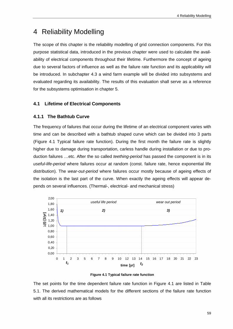
4 Reliability Modelling
59
4 Reliability Modelling
The scope of this chapter is the reliability modelling of grid connection components. For this
purpose statistical data, introduced in the previous chapter were used to calculate the avail-
ability of electrical components throughout their lifetime. Furthermore the concept of ageing
due to several factors of influence as well as the failure rate function and its applicability will
be introduced. In subchapter 4.3 a wind farm example will be divided into subsystems and
evaluated regarding its availability. The results of this evaluation shall serve as a reference
for the subsystems optimisation in chapter 5.
4.1 Lifetime of Electrical Components
4.1.1 The Bathtub Curve
The frequency of failures that occur during the lifetime of an electrical component varies with
time and can be described with a bathtub shaped curve which can be divided into 3 parts
(Figure 4.1 Typical failure rate function). During the first month the failure rate is slightly
higher due to damage during transportation, carless handle during installation or due to pro-
duction failures …etc. After the so called teething-period has passed the component is in its
useful-life-period where failures occur at random (const. failure rate, hence exponential life
distribution). The wear-out-period where failures occur mostly because of ageing effects of
the isolation is the last part of the curve. When exactly the ageing effects will appear de-
pends on several influences. (Thermal-, electrical- and mechanical stress)
Figure 4.1 Typical failure rate function
The set points for the time dependent failure rate function in Figure 4.1 are listed in Table
5.1. The derived mathematical models for the different sections of the failure rate function
with all its restrictions are as follows
0,00
0,20
0,40
0,60
0,80
1,001,20
1,40
1,60
1,80
2,00
0 1 2 3 5 6 7 8 9 10 12 13 14 15 16 17 18 20 21 22 23
time [yr]
(t)
[1/y
r]
1)
useful life period
2)
wear out period
3)
t1 t2

4.1 Lifetime of Electrical Components
60
a1 0,8 a3 0,1 d 0,2 b1 6 b3 0,3 t3 15
Table 4.1 Set points for Figure 4.1
)(333
221
111
33
1
)()3
.)()2)(0)1
ttbE
tb
eatttt
constdtttteattt
(4.1)
deataeatttt ttbtb )(
321321231)()()()( (4.2)
As mentioned before, the failure rate of electrical components is a function of time, thus the
availability is time dependent as well.(Figure 4.2)
Figure 4.2 WEC, Availability over its expected lifetime
Figure 4.3 WEC, Availability over one year
The above figures show the availability of the WEC (MM Series) over its
expected lifetime based on the failure rate function from Figure 4.1 as-
sumed that the number of expected failures during the teething period is
approximately 50% higher than the number of expected failures during
the useful-life period. Furthermore it was assumed that after fifteen
90,0%
91,0%
92,0%
93,0%
94,0%
95,0%
96,0%
97,0%
98,0%
99,0%
100,0%
0 1 2 3 5 6 7 8 9 10 12 13 14 15 16 17 18 20 21 22 23 24
time [yr]
A(t)
[%]
94,0%94,5%95,0%95,5%96,0%96,5%97,0%97,5%98,0%98,5%99,0%99,5%
100,0%
0,00 0,08 0,17 0,25 0,33 0,42 0,50 0,58 0,66 0,75 0,83 0,91 1,00
time [yr]
A(t)
[%]
abcd
3)
2)
1)
a…amplitude(>0) b…slope (>0) t1…start of period 2 (>0) t3…start of period 3 (>0) tE…end of lifetime

4 Reliability Modelling
61
years in operation certain ageing effects can be expected.
Hence, t3 in equation 4.1 is set to fifteen.
a) )))()(((
))()(()(
))()(()()( ttµte
tµtt
ttµtµtA
green curve
b) )()(
)()(ttµ
tµtA
red curve
c) )()(1)( trttA grey curve (if <<µ)
d) mean availability (reference point/lower limit)
(4.3)
(4.4)
(4.5)
In order to apply the derived equation easily, it is important to use relative values. In other
words, the equations are normalised (p.u.), thus by multiplying the above equations with the
actual relevant failure rate of the component, the absolute failure rate function can be ob-
tained. It should be also pointed out, that different components have different bathtub curves.
A survey made by IEC come to the conclusion, that the most common shape of the failure
rate function is the bathtub curve [29].
The different periods of the failure rate function and their characterisation shall be introduced
and discussed in more detail over the next few pages.
Burn-in Period (teething period)
This time interval is characterised by a high initial failure rate which is decreasing over time.
The initial high failure rate can be explained by early faults caused by transportation, installa-
tion, manufacture and product faults, design faults...etc. This period normally lasts for ap-
proximately 1-3 month, depending on the component. Measures that could be taken in order
to mitigate the failure rate related higher risk: pre-commissioning tests, process control, qual-
ity management.....etc.
Useful-Life Period
The useful-life period is determined by faults that occur at random, for example caused by
bad handling, dirt particles, maintenance actions and the related human errors...etc. Meas-
ures to be taken: correct handling and maintenance actions...etc.
Wear-Out Period (Ageing)
During this period faults occur due to wear-out and fatigue appearances. These types of
faults are caused by degradation of the electrical isolation strength of components. Stress
factors that affect the level of degradation are known as ageing stresses, which will be de-
scribed briefly over the next few pages.
Measures to be taken: Lifetime calculations, ageing tests, monitoring systems....etc.

4.1 Lifetime of Electrical Components
62
4.1.2 The Ageing Concept
The lifetime of electrical components is usually determined by the lifetime of its electrical in-
sulation system. Effects like thermal, electrical, mechanical or ambient influences (TEAM-
factors) can cause loss of isolation strength; therefore lead to lifetime degradation of the
component. In terms of components failure rates, the TEAM-factors can be described by an
increase after a particular time in operation. Figure 4.4 displays the ageing concept of electri-
cal isolation systems. Ageing stresses can either cause intrinsic or extrinsic ageing mecha-
nisms. Intrinsic ageing is the ageing of the isolation material itself due to ageing stress
(TEAM-factors), whereas extrinsic ageing mechanisms are irreversible changes of isolation
system due to ageing stress (TEAM-factors) on imperfections (bad spots) in the isolation
system. Extrinsic ageing mechanisms, ageing because of imperfections in the isolation sys-
tem, are the major cause of outages.
It should be noted, that the term ‘lifetime of electrical components’ refers to the economical
lifetime. In other words the lifetime is the time interval the costs for preventive and corrective
maintenance of the component are reasonable, compared to its investment costs.
Figure 4.4 The ageing concept according to IEC 60505 [26]
Different ageing stresses can occur individually and independent or simultaneously. Either
way will result in degradation of the components residual lifetime. The exact identification of
all operational ageing stresses and furthermore the evaluation of the lifetime degradation is
very difficult, since the conditions under which certain ageing mechanisms apply are not fully
understood yet. In order to compensate this lack of knowledge, a common practice
Ageing Stress
Electrical Insulation
Electrical Ambient Mechanical Thermal
Ageing Mechanism extrinsic / intrinsic
Direct / Indirect Interaction
Outage
Electrical Ambient Mechanical Thermal
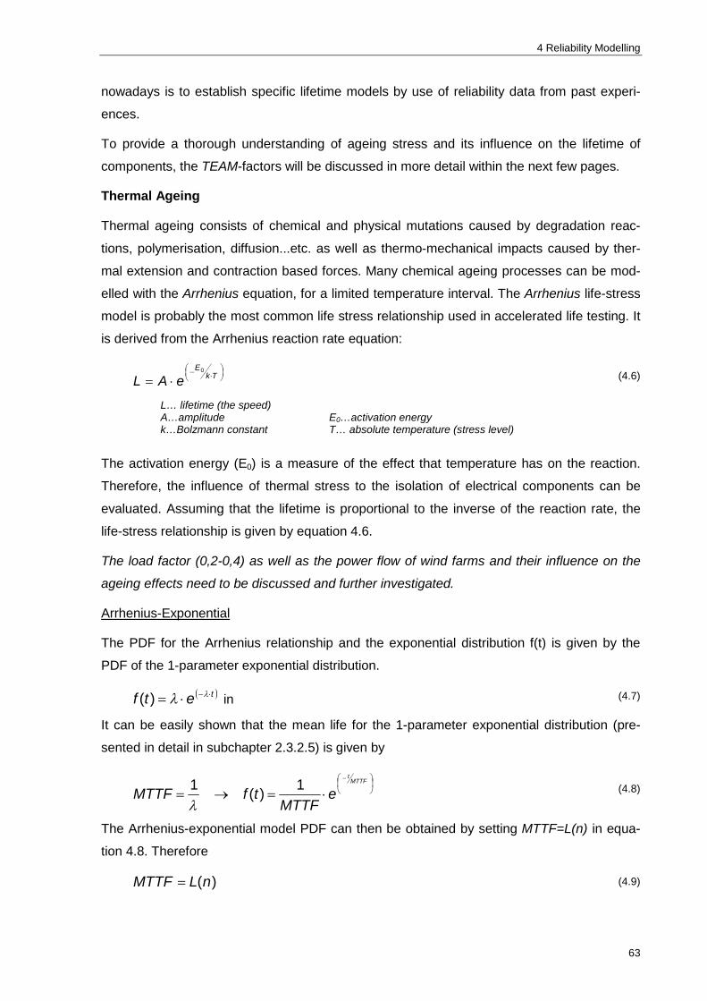
4 Reliability Modelling
63
nowadays is to establish specific lifetime models by use of reliability data from past experi-
ences.
To provide a thorough understanding of ageing stress and its influence on the lifetime of
components, the TEAM-factors will be discussed in more detail within the next few pages.
Thermal Ageing
Thermal ageing consists of chemical and physical mutations caused by degradation reac-
tions, polymerisation, diffusion...etc. as well as thermo-mechanical impacts caused by ther-
mal extension and contraction based forces. Many chemical ageing processes can be mod-
elled with the Arrhenius equation, for a limited temperature interval. The Arrhenius life-stress
model is probably the most common life stress relationship used in accelerated life testing. It
is derived from the Arrhenius reaction rate equation:
Tk
E
eAL0
(4.6)
The activation energy (E0) is a measure of the effect that temperature has on the reaction.
Therefore, the influence of thermal stress to the isolation of electrical components can be
evaluated. Assuming that the lifetime is proportional to the inverse of the reaction rate, the
life-stress relationship is given by equation 4.6.
The load factor (0,2-0,4) as well as the power flow of wind farms and their influence on the
ageing effects need to be discussed and further investigated.
Arrhenius-Exponential
The PDF for the Arrhenius relationship and the exponential distribution f(t) is given by the
PDF of the 1-parameter exponential distribution.
tetf )( in (4.7)
It can be easily shown that the mean life for the 1-parameter exponential distribution (pre-
sented in detail in subchapter 2.3.2.5) is given by
MTTF
t
eMTTF
tfMTTF 1)(1
(4.8)
The Arrhenius-exponential model PDF can then be obtained by setting MTTF=L(n) in equa-
tion 4.8. Therefore
)(nLMTTF (4.9)
L… lifetime (the speed) A…amplitude E0…activation energy k…Bolzmann constant T… absolute temperature (stress level)
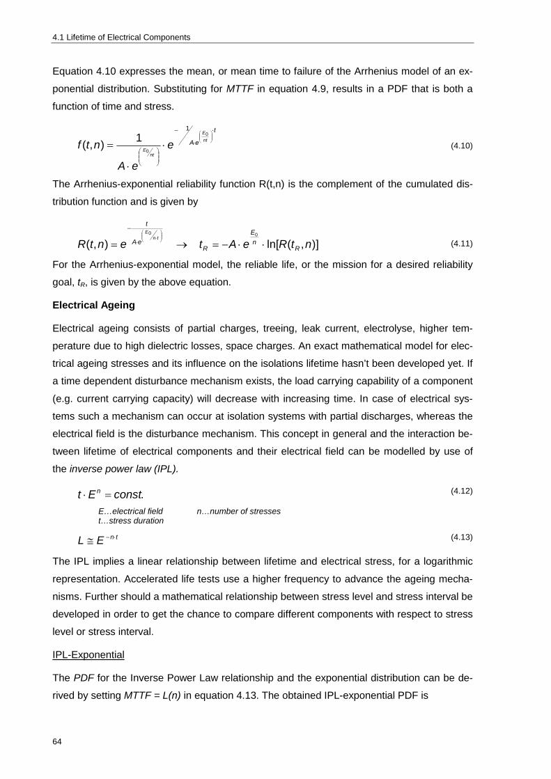
4.1 Lifetime of Electrical Components
64
Equation 4.10 expresses the mean, or mean time to failure of the Arrhenius model of an ex-
ponential distribution. Substituting for MTTF in equation 4.9, results in a PDF that is both a
function of time and stress.
t
eA ntE
ntE e
eA
ntf
0
0
1
1),( (4.10)
The Arrhenius-exponential reliability function R(t,n) is the complement of the cumulated dis-
tribution function and is given by
)],(ln[),(00
ntReAtentR Rn
E
ReA
t
tnE
(4.11)
For the Arrhenius-exponential model, the reliable life, or the mission for a desired reliability
goal, tR, is given by the above equation.
Electrical Ageing
Electrical ageing consists of partial charges, treeing, leak current, electrolyse, higher tem-
perature due to high dielectric losses, space charges. An exact mathematical model for elec-
trical ageing stresses and its influence on the isolations lifetime hasn’t been developed yet. If
a time dependent disturbance mechanism exists, the load carrying capability of a component
(e.g. current carrying capacity) will decrease with increasing time. In case of electrical sys-
tems such a mechanism can occur at isolation systems with partial discharges, whereas the
electrical field is the disturbance mechanism. This concept in general and the interaction be-
tween lifetime of electrical components and their electrical field can be modelled by use of
the inverse power law (IPL).
.constEt n (4.12)
tnEL (4.13)
The IPL implies a linear relationship between lifetime and electrical stress, for a logarithmic
representation. Accelerated life tests use a higher frequency to advance the ageing mecha-
nisms. Further should a mathematical relationship between stress level and stress interval be
developed in order to get the chance to compare different components with respect to stress
level or stress interval.
IPL-Exponential
The PDF for the Inverse Power Law relationship and the exponential distribution can be de-
rived by setting MTTF = L(n) in equation 4.13. The obtained IPL-exponential PDF is
E…electrical field n…number of stresses t…stress duration

4 Reliability Modelling
65
tentf ),( kns (4.14)
Note equation 4.14 is a 2-parameter model. The failure rate (the parameter of the exponen-
tial distribution) of the model is simply a function of stress. Hence, the mean time to failure for
the IPL of exponential distributions is only a function of stress as well.
The IPL-exponential reliability function is the complement of the cumulative distribution func-
tion and is given by
nEtentR ),( (4.15)
For the IPL-exponential model , the reliable life or the mission duration for a desired reliability
goal, tR is given by:
)],(ln[1 ntR
Et RnR (4.16)
An overview of parameter estimation concepts for the IPL- and the Arrhenius models can be
looked up in the appendix.
Note: Ageing effects due to mechanical and ambient influences shall not be considered
within this investigation. For further information on this particular topic see [26], [7]
and [50]..
Residual Life Time
The residual lifetime of components under certain stress levels were introduced in subchap-
ter 2.3.2.5, page 22.

4.2 Grid Connection Components
66
4.2 Grid Connection Components
As previously described the availability of a component over a period of one year can be cal-
culated using equation 4.17 under the restriction <<µ.
100)(1 r
TT
A FC
U in [%] 100)(1* mrA MF in [%] 7 (4.17)
For long observation times the above equation is an adequate evaluation method, however a
more accurate calculation method, which can be applied without any restrictions was intro-
duced in subchapter 2.3.2.
The reliability figures in the tables presented below are based on the disturbance and avail-
ability statistics from the German power system [53]. Whereas only events are taken into
account that lead to an interruption or to a switching action. The mean time to repair (MTTR)
and the mean time to maintain (MTTM) are related to the project location, the manufacturers
and their experience and other influencing factors. Hence they can vary within a broad range.
The repair and maintenance rates in this investigation were obtained from phone calls with
ABB’s and AREVA’s service departments.
Note: Unless stated otherwise, the reliability figures in this chapter are only valid for onshore
wind farms. Nevertheless each subchapter provides a short overview of reliability fig-
ures regarding offshore components as well.
4.2.1 The Wind Energy Converter
The reliability figures of the turbine were provided by the REAG service department and can
be seen in table 2-3. The failure rates of the turbine vary extremely over time and they are
related to several influences (season, country,…etc) hence they are extremely unstable. With
this background and due to the evaluation methods that were used to estimate these figures,
these data need to be discussed and furthermore used very carefully.
MTBF - Global Nov 09 Dez 09 Jan 10 Feb 10 Mrz 10 Apr 10 Mai 10 Jun 10 Jul 10 All Contracts [h] [h] [h] [h] [h] [h] [h] [h] [h]
total8 385 341 296 322 351 400 424 383 382 Indoor 745 585 501 550 676 859 878 578 726 Outdoor 798 821 724 780 729 747 819 1.138 805 MM total 325 299 275 269 304 375 377 407 523 MM Indoor 587 478 443 436 543 742 730 554 932 MM Outdoor 730 802 722 700 690 760 777 1.534 1.190
Table 4.2 WEC MTBF rates
7 A* denotes the technical availability considering the time to maintain as unavailability.
8 Referring to all WEC’s in operation.
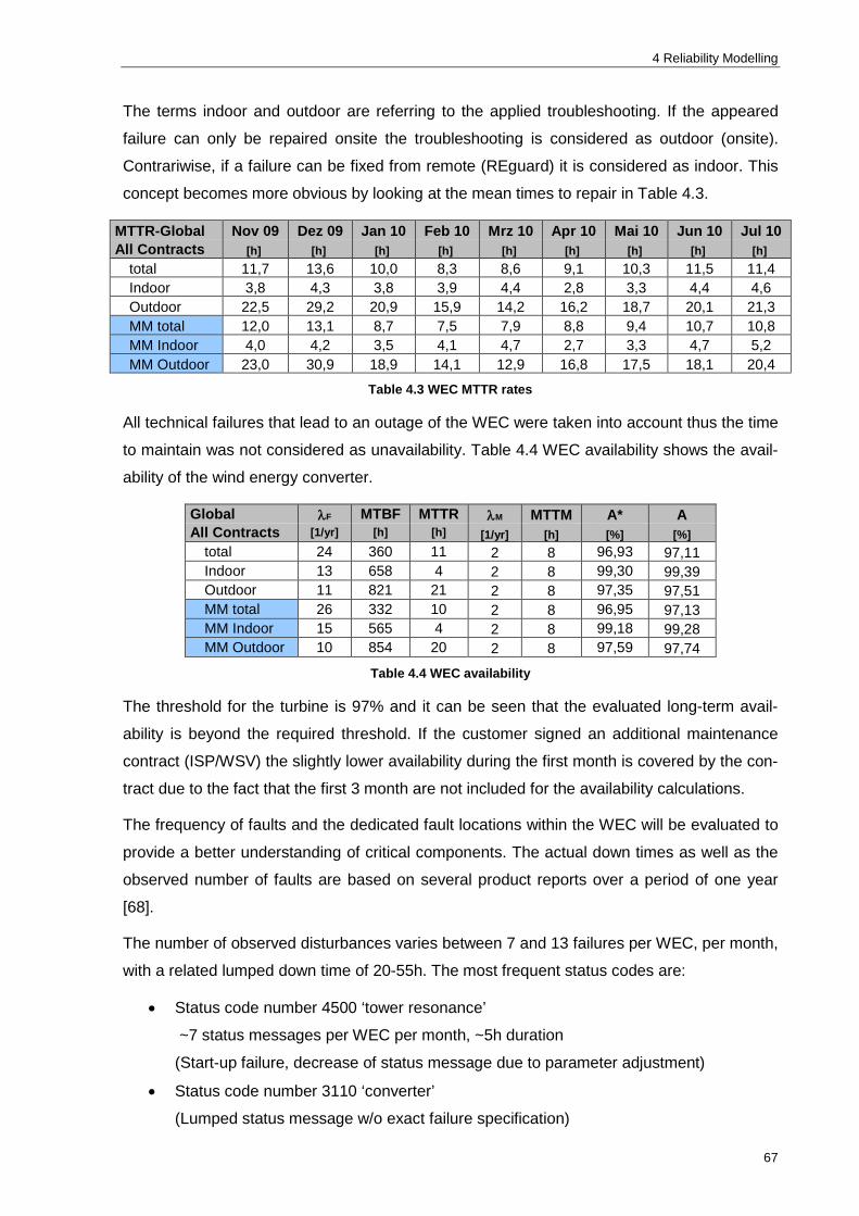
4 Reliability Modelling
67
The terms indoor and outdoor are referring to the applied troubleshooting. If the appeared
failure can only be repaired onsite the troubleshooting is considered as outdoor (onsite).
Contrariwise, if a failure can be fixed from remote (REguard) it is considered as indoor. This
concept becomes more obvious by looking at the mean times to repair in Table 4.3.
MTTR-Global Nov 09 Dez 09 Jan 10 Feb 10 Mrz 10 Apr 10 Mai 10 Jun 10 Jul 10 All Contracts [h] [h] [h] [h] [h] [h] [h] [h] [h]
total 11,7 13,6 10,0 8,3 8,6 9,1 10,3 11,5 11,4 Indoor 3,8 4,3 3,8 3,9 4,4 2,8 3,3 4,4 4,6 Outdoor 22,5 29,2 20,9 15,9 14,2 16,2 18,7 20,1 21,3 MM total 12,0 13,1 8,7 7,5 7,9 8,8 9,4 10,7 10,8 MM Indoor 4,0 4,2 3,5 4,1 4,7 2,7 3,3 4,7 5,2 MM Outdoor 23,0 30,9 18,9 14,1 12,9 16,8 17,5 18,1 20,4
Table 4.3 WEC MTTR rates
All technical failures that lead to an outage of the WEC were taken into account thus the time
to maintain was not considered as unavailability. Table 4.4 WEC availability shows the avail-
ability of the wind energy converter.
Global F MTBF MTTR M MTTM A* A All Contracts [1/yr] [h] [h] [1/yr] [h] [%] [%]
total 24 360 11 2 8 96,93 97,11 Indoor 13 658 4 2 8 99,30 99,39 Outdoor 11 821 21 2 8 97,35 97,51 MM total 26 332 10 2 8 96,95 97,13 MM Indoor 15 565 4 2 8 99,18 99,28 MM Outdoor 10 854 20 2 8 97,59 97,74
Table 4.4 WEC availability
The threshold for the turbine is 97% and it can be seen that the evaluated long-term avail-
ability is beyond the required threshold. If the customer signed an additional maintenance
contract (ISP/WSV) the slightly lower availability during the first month is covered by the con-
tract due to the fact that the first 3 month are not included for the availability calculations.
The frequency of faults and the dedicated fault locations within the WEC will be evaluated to
provide a better understanding of critical components. The actual down times as well as the
observed number of faults are based on several product reports over a period of one year
[68].
The number of observed disturbances varies between 7 and 13 failures per WEC, per month,
with a related lumped down time of 20-55h. The most frequent status codes are:
Status code number 4500 ‘tower resonance’
~7 status messages per WEC per month, ~5h duration
(Start-up failure, decrease of status message due to parameter adjustment)
Status code number 3110 ‘converter’
(Lumped status message w/o exact failure specification)

4.2 Grid Connection Components
68
in the past auto reset, but due to damage of several WECs - remote converter reset -
> ~1,5 status messages per WEC per month, ~2h down time per status messages
The component based evaluation of WEC failure causes over the past years of observation
shows that four components are the key failure source. The converter (SEG, Converteam),
the pitch system, the hydraulic system and the DFI-generator (VEM, Winergy). The actual
down time of each component is shown in Table 4.5
Component TD Ranking [h/month]
Converter 4,0 1 Pitch System 3,5 2 Generator (DFIG) 0,8 3 Hydraulic System 0,5 4
Table 4.5 MM failure causes and mean down time [68]
In order to improve the number of failures and their related down time a project (performance
improvement) has been established within REAG. The main difference of this project is the
high additional maintenance and its support effort, which obviously affects the project specific
operational wind farm costs. Such performance improvement processes provide good results
very fast but should be just used as a short term means. For long term improvements
changes should be made within the early project development process. (Layout, support
structure, quality management....etc.)
Performance vs. Availability Guarantee
There are two basic availability guarantee approaches to ensure the customer that the WEC
or the whole wind farm is a premium product that operates at a very high standard and there-
fore guarantees certain, predictable financial revenues. The first approach is time based,
whereas the second one is energy based. The later one guarantees a certain performance
over a stated period of time, in other words for a given time interval a certain energy output is
guaranteed. The time based availability guarantee on the other hand ensures that the prod-
uct is available over a certain percentage of a stated time interval.
Time Based (Availability guarantee)
Time related guarantee of technical availability. The actual guaranteed level of availability
depends on the project details and the customer. Any kind of project specific guarantee is
always related to a specific risk distribution, therefore the guaranteed level of availability
changes for different project locations. The most common levels of availabilities for onshore
projects are between 95 and 97 and 95 to 96% for offshore projects due to the higher risk.
(E.g. environmental influences)

4 Reliability Modelling
69
Pros
o Long experiences with mechanisms o No additional measurements o Simple contract and availability structure
Cons
o Repower pays liquid damages (LD) on flatrate based on time (no difference between high and low wind speeds)
o Customer calculates conservatively o Not attractive to customer, as revenue is based on energy yield and not time o No incentive/benefit for REpower to place O&M in low wind speed periods
Energy Based (Performance guarantee)
Energy related guarantee of performance, based on yield models. The actual guaranteed
performance level is commonly given as percentage of the theoretical production (yield over
one year). Typically the guaranteed level is round about 93 to 95%, depending on the project
location.
Pros
o Very attractive to customer o High incentive to customer to purchase efficient turbines o Takes the seasonal energy variations into account
Cons
o Complicated technical realisation Extremely difficult measurement issues Dependence on theoretical models (Wake effects…etc.) Necessity to store and analyse extreme weather data
o High risk of inaccurate measurement data and high measurement costs o High general effort to establish method o Higher failure rate at higher wind speeds (although not verified yet)
Furthermore it should be checked at which mean wind speed the energy based approach is
more reasonable than the time based approach. Relevant investigations have shown that if
the mean wind speed exceeds approximately 8m/s, the advantages of the performance
guarantee are predominant. If the entire wind farm is out of service pre-agreed production
estimates apply. The related lost production can either be caused by the customer, by RE-
power or by Repower but covered by energy credit for maintenance. It can be calculated by
the following equation.
Down
Down
WECWECWECAPLP
(4.18)
LP lost production AP actual production WEC number of WECs WECDown number of WECs out of service

4.2 Grid Connection Components
70
Note: In case of turnkey projects the above approaches apply for whole wind farms as well
as for single WECs.
4.2.2 Medium Voltage Equipment
Over the next few pages the reliability and availability figures of MV components are pre-
sented. It should be pointed out, that the MTTR and the investment costs (C0) are average
values which can be treated as accurate valuations.
4.2.2.1 MV-Cable The state of the art insulation system for MV cables nowadays is cross linked polyethylene
(XLPE), mainly because of its lower loss factor (tan). Due to economical reasons is the
most common conductor material is aluminium. Table 4.6 shows the reliability and mainte-
nance figures for different kinds of insulated MV cables.
Component F MTBF MTTR M MTBM MTTM C0 [1/km yr] [yr] [h] [1/yr] [yr] [h] [k€/km]
XLPE 0,0061 165,0 72 0,05 10 4 60. PE 0,0533 18,7 72 0,05 10 4 50. Oil filled 0,0308 32,5 96 0,2 5 8 80.
Table 4.6 MV-cable reliability figures
The synthetic insulated cable systems can be assumed to be maintenance free. However, in
this investigation it is assumed that particular parts of cable systems, for example the termi-
nations or the junction boxes should be inspected at least every ten years (mean time be-
tween maintenance MTBM). Therefore the maintenance rate (M) in Table 4.6 is 0,05 per
year. The evaluated reliability (R(20)) and availability (A) of the different cable systems using
the figures from Table 4.6 are presented in the following table.
Component R(20) A* A [%] [%] [%]
XLPE 88,59 99,992 99,995 PE 34,41 99,953 99,956 Oil filled 54,01 99,948 99,966
Table 4.7 MV-cable availability
The reliability (R(20)) is equal to the probability that one kilometre of the relevant cable sys-
tem doesn’t experience a failure within a period of twenty years. The availability on the other
hand is calculated twice. Once, where only the failure rate is taken into account (A) and an-
other time, where the maintenance time is considered as unavailability (A*).
Regardless of the significantly different failure rates of the cable systems, their level of avail-
ability in general is very high. Although the failure rates can be assessed as above-average,
due to the external urban influences which are the main failure cause for cable systems
within the German distribution network. Thus the evaluated reliability and availability repre-

4 Reliability Modelling
71
sents a worst case scenario. Outages of cable systems typically are caused by failures on
the conjunction between two separated systems, for example on joints, terminations, junction
boxes.....etc. The number of joints per kilometre cable length depends on the cross section of
the cable. However, a distribution of one joint every 0,8 kilometres is a good estimate, which
result in 3,5 joints per kilometre cable system length. Different failure mechanisms of cable
systems and their impact are discussed in detail at the end of this section.
In order to get a better understanding of different insulation systems, their general properties
are listed in the following table.
Parameter XLPE PVC PE OIL Loss factor very low very high high low Temperature threshold high- low medium medium Isolation strength very high medium medium low Relative permeability medium high high low
Table 4.8 Properties of insulation systems [53]
An important parameter for the design of cable systems is the ampacity, also known as cur-
rent carrying capability of different cross sections and the related load losses. The load
losses of cable systems can be evaluated by the following equation:
PSCL yyCRIP ))20(1(20
2 (4.19)
In subchapter 5.3 (Active Power Losses) the above equation is used to evaluate the load
losses for a given wind farm. It should be noted, that the proximity factor as well as the skin-
effect factor may be left out, due to the cables cross section. If the cable shields are
grounded just at the beginning and the end, the shield losses can attain 40% of the cable
losses [46]. In order to minimise the shield losses the concept of cross-bonding, where the
shields are additionally crossed and grounded after every third of the cable length, should be
applied so the shield voltages can compensate themselves. The inductivity of the positive-,
negative- and zero-sequence of cables is determined by the cable design (shield) and the
laying (flat vs. trefoil) The concept of cross-bonding is graphically illustrated in Figure 4.5.
Figure 4.5 The concept of cross-bonding
R=20 DC resistivity for 20°C α temperature coefficient of resistance ϧC conductor temperature yS skin-effect factor (for cross sections >185mm2) yP proximity-effect factor (>185mm2)
L1
L2
L3
L1
L1
L1
L1
L2
L3

4.2 Grid Connection Components
72
The influence of different parameters on the design and operation of cable systems is pre-
sented in Table 4.9 below. It can be seen that the treatment of the shield-grounding has a
major influence on the operational capabilities of cable system.
Parameter Invest-ment
Logis-tics
Excavation laying
Installa-tion
load ability note
Cross-bonding - - - - ++ especially for big cross sections
Flat vs. trefoil - - + (+) + no effect for small axial distance
Axial distance - - + (+) + For cross sections <300mm2
Depth - - ++ - (-) Standard depth (1,2-1,5m)
Thermal - - + (+) ++ recommended
Cross section + (+) - - + With applied cross-bonding
Diameter + (+) - - (+) With higher isolation strength
Table 4.9 Influences on loading capability of cables[46]
Regarding the failure caused down time of cable system one can distinguish between down
time related to damage or down time due to faults without damage. Both classifications are
common practice in disturbances and availability statistics from utilities [54]. The average
failure caused down time of cable systems of the German distribution system is shown in
Table 4.10.
Fault MTTR) [h]
w. damage 56,7 w/o damage 30,4
Table 4.10 MTTR of MV-cables
These figures are not quite applicable for wind farms, since the support structure and the site
accessibility are usually different. Therefore a slightly higher MTTR was chosen for this in-
vestigation, which can be seen in Table 4.6. In order to keep the MTTR low a thorough sup-
port and logistics structure as well as a certain amount of spare parts (e.g. joints, termina-
tions...etc.) is needed. With such simple measures the mean down time of cable systems can
be improved significantly.
Table 4.6 also provide the average investment costs of cable systems with different insula-
tions. These costs include the actual cable price, which depends on the metal price, and the
costs for excavation and lying (flat formation). There are various other methods for excava-
tion and lying, which would result in lower investment costs per kilometre. However, the ca-
ble trench together with a flat formation of the cable system is the most common excavation
and lying type. It is obvious that the civil works take a large contribution to the overall costs.
Approximately fifty percent of the total investment is necessary for excavation and lying.
Failure Mechanisms
The most common failure cause of synthetic insulated cables is water trees [47]. Trees in
general develop over a long period of time and accelerate the failure rate of cables.

4 Reliability Modelling
73
Trees in cable insulation systems can occur in two ways
Water Trees
Water trees are the major failure cause of polyethylene (PE) insulated cables and their low
MTBF. Water trees are small voids in the insulation system filled with water. The time until a
water tree has grown in a way that leads to a failure of the insulation system is rather long
(years) and independent of the electrical stress level.
Figure 4.6 Water tree in an PE isolated MV cable
[63]
Figure 4.6 shows water trees in a PE insu-
lated medium voltage cable. It is obvious
that this type of tree needs moisture to grow,
the actual growing rate depends on the tem-
perature, the voids, contaminants and volt-
age variations. Hence the occurrence of wa-
ter trees within the MV collector system of
wind farms is assumed to be very likely be-
cause of the seasonal variations and the low
load factor which results in a high absolute
temperature variation However, water trees
can easily be prevented by use of waterproof
cables.
The use of longitudinal or transversal waterproof cables is strictly project related. Thus in
case of rocky soil conditions the use of waterproof cables should be preferred. The additional
costs for transversal waterproof cables are rather low compared to those for longitudinal wa-
terproof cables.
Electrical Trees
Electrical trees develop from high electrical stress and typically grow over a rather short pe-
riod. (Hours or days) The major cause of electrical treeing are partial discharges that took
place in discrete voids and irregularities of the insulation system.
It should be noted, that water trees don’t need to cause failure of the insulation system, since
the water filled voids usually can maintain the insulation strength. Failures occur when a wa-
ter tree converts into an electrical tree where charges are trapped in the cables insulation
system. The main fault locations of cable systems are joints, terminations, elbows etc. where
the insulation is not always homogeneous and the electric field strength can be higher.
Especially under switching stress the frequency of failures is significantly higher.
Current surveys have shown that the failure rate of XLPE cables and accessories are signifi-
cantly lower than those provided by the individual utility statistics. For MV XLPE cables the

4.2 Grid Connection Components
74
average failure rate can be assumed to be 0,084 annual failures per hundred kilometres sys-
tem length. According to the same report the failure rate of XLPE joints is 0,028 annual fail-
ures per hundred joints [77]. Thus the total failure rate of MV XLPE cable systems is 0,112
failures per hundred kilometres system length, which is approximately six times lower than
the values from the German distribution system in Table 4.6. If failure caused by external
events (e.g. diggers) can be prevented the actual failure rate would be additionally improved
at a rate of approximately 40%. In order to achieve this goal the focus has to be on the exca-
vation and lying of the cable system. (See Figure 4.7)
Reliability Improvement Measures
A thorough lightning protection concept is essential for the reliable operation of the MV col-
lector system in order to limit the electrical stress level. The second most important measure
which can be applied to improve the reliable function of the MV cable system is the excava-
tion and lying type. Figure 4.7 shows a sketch of a cable trench and a flat formation of the
single core cable system.
Figure 4.7 Sketch of a cable trench (excavation and laying)
For further improvement measures, like filled strand conductors, silicon injection or Increase
of the insulation thickness see [22],[47],[50] and [63].
Ageing Effects
Most of the MV XLPE cable systems experience a failure within the first five years in opera-
tion [76]. Certain ageing effects can be observed after twenty years in operation, thus ageing
of XLPE cables is not further discussed in this investigation. Certain diagnostic tests can be
looked up in [47],[50] and [72].
LCC of MV Cables
The life cycle costs of cables mainly consist of lost revenue caused by active power losses
and costs for corrective maintenance, whereas preventive maintenance actions and their
related costs are rather low (See Table 4.6).
L1 L2 L3
Gravel layer
Sand layer
Cover sheet
~0,7
-1,5
m

4 Reliability Modelling
75
4.2.2.2 MV-Transformer MV transformers in wind farms are also known as step-up transformers which connect the
Generator to the MV collector system. In general one can distinguish between internal trans-
former systems (ITS) where the transformer and the related switchgear is located within the
tower and the external transformer system (ETS) where the transformer and the secondary
switchgear is located in a separated enclosure next to the WEC. The ITS transformer is a dry
transformer (casting resin), due to fire protection requirements. Whereas the transformer
used for ETS is oil insulated. The reliability figures of both types of transformers are repre-
sented in the following table.
Component F MTBF MTTR M MTBM MTTM C0 [1/yr] [yr] [h] [1/yr] [yr] [h] [€/kVA]
Trafo 0,0023 432,9 96 0,25 4 6 20 Oil-Trafo 0,0543 18,4 96 0,25 4 6 20 Dry-Trafo 0,0381 26,3 96 0,25 4 6 20
Table 4.11 MV transformer reliability figures [29][53]
The properties of standard network transformers are presented in the above table by the
term trafo. Oil / Dry is used for REAG ITS/ETS transformers. The evaluated reliability and
availability is given in Table 4.12. It should be pointed out, that the mean time between main-
tenance (MTBM) for ITS and ETS systems are four years and regulated by law [64].
Component R(20) A* A [%] [%] [%]
Trafo 95,49 99,979 99,996 Oil 33,76 99,938 99,955 Dry 46,69 99,941 99,958
Table 4.12 MV transformer availability
The failure rate of MV transformers within distribution systems can be assumed as rather
high, because of the high amount of pole-mounted transformers with low rated power which
are vulnerable for external influences. (E.g. lightning) Thus the failure rates can be assumed
to be slightly overestimated for the purpose of wind power applications. The MTTR figures of
MV transformers are from historical data and on the basis of a good support structure.
Failure Mechanisms
In order to evaluate the failure mechanisms of transformers in general, the impact of several
subcomponents has to be considered. Transformers can be divided into the following sub-
components:
Core
A failure of the core would result in a reduced efficiency of the transformer. The major causes
are mechanical faults due to improperly use during construction or due to low material qual-
ity.

4.2 Grid Connection Components
76
Windings
Dielectric stress and thermal requirements as well as mechanical stress cause failure of the
winding system. Mechanical stresses can either occur during short circuits and lightning
strikes or during transportation. A significant influence on the proper function of the winding
system is their insulation system, which usually consists of cellulose layers. This insulation
system can lose its strength through various thermal or electrical ageing mechanisms or
through material faults or falls handling during construction. However, in case a failure occurs
on the winding system, either the failed winding or the whole transformer needs to be
changed. This decision is made in terms of economical and technical restrictions. In case of
MV transformers, the replacement of windings can be done onsite and at a respectively low
repair time. Therefore Repower keeps a certain amount of winding systems in stock.
Bushings
There are various kinds of bushings according to their application. Basically it can be distin-
guished between capacitance-graded bushings and solid bushings [79]. The purpose of the
bushings is to connect the windings to the power system and at the same time to isolate the
tank against the windings. The major failure mechanism of the windings is the loss of isola-
tion strength due to ageing effects of the material or material faults which lead to partial dis-
charges and short circuits. Bushings are also very sensitive to mechanical stress, which can
occur during transportation and installation.
Tap Changer
Tap changers of transformers can be divided into on-load types, where the tap position can
be changed during operation without an interruption of supply and off-load types, which can
only be adjusted in case the transformer is out of service. On-load tap changers (OLTC) in
general have a much lower MTBF because of its mechanical deterioration. Thus the main
failure modes of Tap changers are mechanical damage (unable to change the voltage level)
and contact failure (short circuit).
Insulation System
o Solid
As previously mentioned, solid insulation systems of transformers are based on cellulose.
(Paper, board...etc.) It is obvious, that such an isolation system is vulnerable to certain age-
ing effects, whereas thermal ageing mechanisms apply the most. The solid insulation is the
weakest spot of the transformers insulation system due to the irreversible degradation of the
cellulose and the fact that a replacement is usually not economical [79]. The arrhenius life-
time model can be used to evaluate the thermal ageing effects and the residual lifetime of the
solid insulation system, which was introduced in subchapter 4.1.2.

4 Reliability Modelling
77
o Liquid (Oil)
The purpose of the oil insulation is first of all the electrical insulation between different parts
of the transformer and secondly the cooling of the active parts. It is obvious that the quality of
the oil directly affects the insulation strength and the load ability (cooling) of the transformer.
In case the oil contains undesirable particles like oxygen, water etc. the insulation deterio-
rates which increases the probability of short circuits. The major causes of oil pollutions are
ageing effects within the insulation system. Hence, the two main failure modes of liquid insu-
lation systems are short circuits due to deteriorated oil and overheated due to failed oil circu-
lation or failed cooling system.
Cooling System
The cooling system of transformers can either be based on natural or forced circulation of oil
and air or water. Whereas the air or water is used as cooling medium of the secondary circu-
lation. (ONAN/ONAF) It is obvious that pumps or fans are needed for forced cooling systems.
The two failure causes of the cooling system, whether it’s forced or natural, are the break-
down of the oil circulation and that the temperature of the second cooling medium is too high.
The later cause can either occur due to broken pumps or fans or because of high ambient
temperatures. However, it should be noted, that the design of the cooling system has a major
impact on the overload factor of the transformer.
These classification and failure mechanisms of subcomponents are generally valid, regard-
less of the transformers rated power or field of application. An evaluation of failure causes of
MV transformers and their frequency of occurrence is given below.
Most faults occur on mechanical subcomponents of transformers, like the on-load tap
changer or the bushings. However, step-up transformers typically have an off-load tap
changer, which cannot be adjusted during operation. It turned out that the windings and the
bushings are the main fault locations of MV transformers. Due to the relatively low invest-
ment costs and the high amount of MV transformers within a wind farm a fundamental stock
of spare parts is essential. (Windings and bushings)
Reliability Improvement Measures
As mentioned above, the most efficient measure to keep the MTTR low and therefore the
overall availability high is a thorough level of maintenance support. Especially spare parts of
subcomponents with a rather low MTBF should be stocked. Preventive maintenance actions
on MV transformers shall be performed after a stated time interval, which is four years for
German transformer systems. These maintenance actions typically include visual inspection,
cleaning and various stress tests if required.

4.2 Grid Connection Components
78
In order to keep the active power losses down and thus the overall efficiency high, the ratio
between no-load losses and load losses needs to be optimised taken the low load factor into
account.
Another technical possibility to improve the availability of transformers are hermetic sealed
vessels. Hermetic sealed transformer vessels reduce the ageing effects of the liquid and
solid insulation system and more important reduce the maintenance efforts significantly [80].
This technology is not very reasonable for MV transformers but will be discussed in more
detail for HV applications.
Furthermore, the protection concepts regarding voltage surges and overload need to be de-
signed in a way that keeps the electrical stress level at a minimum.
Ageing
The ageing of MV transformers will not be taken into account within this investigation.
LCC of Transformers
The life cycle costs of transformers in general consist mainly of lost revenue caused by ac-
tive power losses and maintenance actions and can be calculated by use of equation 2.93,
which was introduced in subchapter 2.4.3. [78]. The costs of erection and infrastructure will
be neglected within this thesis. The evaluation of the costs of preventive and corrective
maintenance as well as the outage related costs were introduced in subchapter 2.4.2. The
operational costs or in other words the costs for active power losses can be evaluated by the
following equation
LL
rEcPNLEcPO P
SS
cTlfcPcTcfcC
2max)()( (4.20)
The concept of evaluating the active power losses is discussed in more detail in subchapter
5.3.The criteria used in such an economic analysis also indirectly consider the following top-
ics: safety; condition of the assets; age; operation condition; availability; maintainability; envi-
ronmental and risk (consequential costs at fault).
4.2.2.3 MV-Switchgear There are two different types of MV switchgear within a wind farm. The MV switchgear that
connects the feeders to the power transformer, which is typically located within the wind farm
substation, called the primary MV switchgear. The secondary MV switchgear on the other
cP price for installed power cE electricity price (subsidies) cf capacity factor Tc calculation period PNL no load losses lf loss factor PLL load losses

4 Reliability Modelling
79
hand denotes the switchgear of the ITS/ETS system that connects each WEC to the MV col-
lector system. There are various kinds of primary and secondary switchgear which shall not
be further discussed in this investigation. Only relevant reliability figures for the MV switch-
gear used by Repower are shown in the table below.
Component Type F MTBF MTTR M MTBM MTTM C0
[1/bay yr] [yr] [h] [1/yr] [yr] [h] [k€/unit] Built-in GIS primary 0,0020 510,2 72 0,25 4 6 30. Compact GIS secondary 0,0013 800,0 72 0,25 4 6 30. Areva GHA primary 0,0104 96,0 72 0,25 4 6 25.
Table 4.13 MV-switchgear reliability figures [53]
The evaluated reliability and availability of the primary and secondary MV switchgear is pre-
sented in the following table.
Component R(20) A* A [%] [%] [%]
Compact GIS 96,16 99,981 99,998 Built-in GIS 97,53 99,981 99,999 GHA 81,19 99,974 99,991
Table 4.14 MV switchgear availability
From the above table, it can be assumed that the availability of MV switchgear in general is
very high. Furthermore, maintenance actions don’t really affect the availability of individual
switchgear panels, since the maintenance time is very small. However, due to the vast
amount of secondary MV switchgear these figures have to be reconsidered.
Failure Mechanisms
The basic types of MV switchgear regarding their type of insulation are magnetic air, mini-
mum oil, vacuum and SF6 insulated switchgear. Whereas, vacuum and SF6 insulated types
are the most common ones nowadays because of economical and technical reasons. Thus
the following failure mechanisms and their frequency of occurrence focus on these two types
in particular.
Loose Connections
Loos or faulty connections can cause a higher resistance which lead to an increasing tem-
perature, according to ohm’s law. Thus thermal ageing effects apply and reduce the lifetime
significantly. Approximately 25% of all switchgear failure causes are due to lose connections
and thermal breakdown [83].
Insulation Breakdown
o Busbar
Most MV switchgear types use solid insulation barriers to separate adjacent switchgear pan-
els and to support the busbar. These barriers may have small voids and air gaps between

4.2 Grid Connection Components
80
the busbar and the insulation, which cause a higher electrical stress level and can lead to
partial breakdown and furthermore to failure of the whole switchgear.
o Switchgear
The breakdown of the insulation of the switching device results in a failure to clear the actual
fault. The mechanical parts of the breaker will operate properly, but the breaker is unable to
interrupt the fault current (arc) due to lost insulation strength. Manufacturers typically recom-
mend blocking of the breaker tripping mode in case of loss of insulation strength in order to
prevent mechanical or electrical damage [84].
Failure to Trip
The breaker contacts do not open after the relevant circuit has been energised by the protec-
tion scheme. These failures are usually caused by the mechanical parts of the breaker.
However, when evaluating such fault conditions the impact of the overall protection concept
(relay, wiring, power supply etc.) needs to be taken into account (See subchapter 4.2.4.2).
Reliability Improvement Measures
In order to keep the availability of the secondary MV switchgear at a high level, a well con-
sidered maintenance support is essential. Furthermore, the maintenance related inspection
and testing of the mechanical parts of switching devices are an important mean to evaluate
the actual condition of the switchgear. Since the outage of a primary MV switchgear panel
has a major impact on the proper function of the wind farm, the use of reliable and redundant
systems is important to keep the outage time down. An additional switchgear panel for ex-
ample can be installed at low costs and would ensure a fast troubleshooting.
Ageing
The lifetime of switching devices (e.g. circuit breakers) is typically denoted by their switching
cycles. According to which type of switchgear is used the lifetime can vary significantly. Since
the main functional parts of switching devices operate mechanically, the wear-out period is
characterised by mechanical ageing effects.
LCC
The lifecycle costs of MV switchgear are determined by the costs for preventive and correc-
tive maintenance and not so much by the operational costs. Especially the costs for preven-
tive maintenance have to be taken into account (see subchapter 5.5). Thus the development
of a particular maintenance strategy is of vast interest.

4 Reliability Modelling
81
4.2.3 High Voltage Equipment
The share of HV components of the wind farm depends on the property boundary between
the owner of the wind farm and the HV grid owner, therefore it is strictly project related. Since
the HV grid connection (HV line) usually doesn’t belong to the owner of the wind farm the
main focus will be on the power transformer.
4.2.3.1 HV-Cable The insulation properties of HV cables are vitally important due to the significantly higher
electrical stress level compared to MV cables. Especially the loss factor (tan) has a major
impact on the operation of HV cables. Nowadays, XLPE is the most common insulation ma-
terial for HV cables because of its low loss factor. A general overview of the properties of
different insulation systems of cables are presented in subchapter 4.2.2.1 ‘MV Cable’. Table
4.15 shows the reliability figures of different types of HV cables.
Component F MTBF MTTR M MTBM MTTM C0 [1/km yr] [yr] [h] [1/yr] [yr] [h] [k€/km]
XLPE 0,0014 719,4 72 0 0 0 350. PE 0,1478 6,8 72 0 0 0 300. Oil filled 0,0124 80,6 96 0,2 5 8 ~
Table 4.15 HV-cable reliability figures
It can be assumed, that solid insulated HV cables are maintenance free, whereas oil insu-
lated cables are not due to their construction. Recent studies have shown that over 55% of
corrective maintenance actions of HV XLPE cables are done in less than one week. Only in
5% the repair lasts longer than one month [77]. The average failure related outage time of
extra high voltage (EHV) cables is 25 days. The MTTR of HV cable is assumed to be three to
four days, based on figures from subcontractors.
The availability and reliability of different HV cable types are presented in the table below.
Component R(20) A* A [%] [%] [%]
XLPE 97,26 99,998 99,998 PE 5,21 99,878 99,878 Oil filled 78,04 99,968 99,986
Table 4.16 HV cable availability
The availability and especially the reliability of PE insulated HV cables are significantly lower,
because of the poor properties of PE. (Subchapter 4.2.2.1)
Failure Mechanisms
Recent studies have shown that the frequency of external failures of HV cables is equal to
the frequency of internal failures, unlike the failure statistic of MV cables [77]. Furthermore,

4.2 Grid Connection Components
82
the share of internal failures of HV joints is significant, but needs to be reconsidered since
the number of observed failures is rather small. The failure rate of HV cable systems (incl.
accessories) is approximately 3 times higher than those of MV cable systems. However,
compared to the German availability and disturbance statistic the overall failure rate of XLPE
HV cables is approximately 50% lower.
LCC of HV Switchgear
The cost structure of HV cable systems is quite different to those of MV cable systems. Es-
pecially the investment costs, which basically consist of costs for material. Thus the excava-
tion and laying concept has less influence on the investment. Therefore, the whole cross
section optimisation process used to keep the operational costs (active power losses) at a
minimum need to be reconsidered.
For information about general properties (e.g. reliability improvement measures, ageing,
tests, insulation system...etc.) of HV cable systems see 4.2.2.1.
4.2.3.2 Power Transformer Power transformers connect the MV collector system to the upstream transmission network
and therefore are essential components for the proper function of the whole wind farm. Their
reliability is a key factor in profitable generation. Table 4.17 shows reliability figures for large
oil transformers in general and for their on-load tap changers (OLTCs) in particular.
Component F MTBF MTTR M MTBM MTTM C0 [1/yr] [yr] [h] [1/yr] [yr] [h] [€/kVA]
Trafo 0,0182 55,1 168 1 1 8 15 OLTC 0,0082 150 168 0,14285714 7 168 n.q.
Table 4.17 HV transformer reliability figures [53]
The reliability of power transformers can be assumed to be at a high level, according to Ta-
ble 4.18. However, there is a probability of thirty percent that the power transformer experi-
ences a failure within twenty years.
Component R(20) A* A [%] [%] [%]
Trafo 69,54 99,873 99,965 OLTC 85 99,87 99,97
Table 4.18 HV transformer availability
Recent studies have shown that the transformers subcomponents in general and the OLTC
in particular are major failure causes. Since the time to repair a failed OLTC is approximately
one week, regardless of factors like location, type...etc. the overall availability of power trans-
formers is very high. Figure 4.8 shows failure causes of power transformers and their related
frequency of occurrence. It can be seen, that almost eighty five percent of all failures that
lead to an outage are either caused by the OLTC, the Windings or the Bushings.
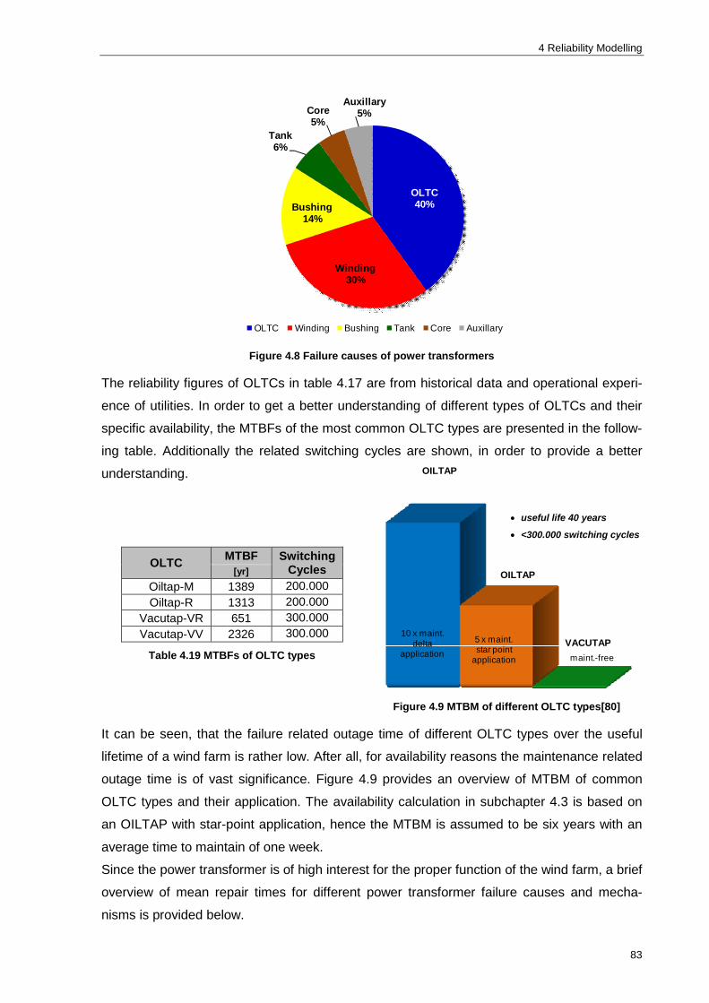
4 Reliability Modelling
83
Figure 4.8 Failure causes of power transformers
The reliability figures of OLTCs in table 4.17 are from historical data and operational experi-
ence of utilities. In order to get a better understanding of different types of OLTCs and their
specific availability, the MTBFs of the most common OLTC types are presented in the follow-
ing table. Additionally the related switching cycles are shown, in order to provide a better
understanding.
OLTC MTBF Switching Cycles [yr]
Oiltap-M 1389 200.000 Oiltap-R 1313 200.000
Vacutap-VR 651 300.000 Vacutap-VV 2326 300.000
Table 4.19 MTBFs of OLTC types
Figure 4.9 MTBM of different OLTC types[80]
It can be seen, that the failure related outage time of different OLTC types over the useful
lifetime of a wind farm is rather low. After all, for availability reasons the maintenance related
outage time is of vast significance. Figure 4.9 provides an overview of MTBM of common
OLTC types and their application. The availability calculation in subchapter 4.3 is based on
an OILTAP with star-point application, hence the MTBM is assumed to be six years with an
average time to maintain of one week.
Since the power transformer is of high interest for the proper function of the wind farm, a brief
overview of mean repair times for different power transformer failure causes and mecha-
nisms is provided below.
OLTC40%
Winding30%
Bushing14%
Tank6%
Core5%
Auxillary5%
OLTC Winding Bushing Tank Core Auxillary
10 x maint.delta
application5 x maint.star point
application maint.-free
OILTAP
OILTAP
VACUTAP
useful life 40 years
<300.000 switching cycles

4.2 Grid Connection Components
84
Failure location Info MTTR [weeks]
OLTC on-site 1
Windings/Tank on-site ~20 off-site 30-52
Bushings, Auxilliary....etc. n.q. (<2)
Table 4.20 MTTR of different failure causes
The different failure mechanisms of power transformers and MV transformers can be as-
sumed to be similar, thus for more information see 4.2.2.2 MV-Transformer.
Reliability Improvement Measures
The bushings and the tap changer are the first parts that experience a higher failure rate dur-
ing operation due to ambient and mechanical effects. The higher risk of these items can easi-
ly be covered with spare parts because of the low investment costs (e.g. bushings). Further
reliability improvement measures are:
Protection Concept
Hermetic vs. Liquid Tank
Repeated Testing
Maintenance Activities
Diagnostic and Monitoring System
Figure 4.10 Concept of an online monitoring system for power transformers
Figure 4.11 shows a basic concept of an online monitoring system for power transformers
with all the significant interfaces. The influence of such a system on the overall life cycle
costs can be seen in the table below. It should be pointed out, that the additional investment
costs are the only negative impact of monitoring systems on LCC. For more information on
diagnostic and monitoring systems for power transformers see [85][80].

4 Reliability Modelling
85
Ageing
Recent surveys have shown that network short circuits have no relevant impact on the trans-
formers thermal ageing. Even if the load factor is 1,2 p.u. and the short circuit lasts five se-
conds the reduced lifetime due to thermal ageing would be twenty one days, which is
neglectable compared to other effects. The overload of power transformers compared with
the low load factor due to the high wind fluctuation is a major factor when designing power
transformers of wind park applications. However, the exact impact of the rather high and fast
temperature deviations caused by the load factor is hard to estimate.
Figure 4.12 shows the relative failure rate over the lifetime of HV transformers. It can be
seen, that ageing effects can be expected after 25 years in operation.
Figure 4.11 Transformer bath tub curve [5]
Compared with the lifetime of the whole wind farm the ageing effects of HV transformers can
be neglected.
LCC of Power Transformers
LCC of power transformers are basically the same as those of MV transformers, except the
maintenance related costs. The costs for preventive maintenance actions are much higher
for power transformers, due to the mechanically operating parts (OLTC) as well as the higher
stress level during operation.
4.2.3.3 HV-Switchgear For the proper function of the wind farm the HV switchgear is as important as the power
transformer. There exist various types of HV switchgear, for economical and environmental
reasons gas insulated switchgear types are most frequently used for wind farm applications.
Reliability figures for GIS types indoor as well as outdoor and for interior AIS types are pre-
sented in table 4.22 below.
‘Lifetime‘of a WF
time in operation time [yr]
failu
re ra
te [%
]

4.2 Grid Connection Components
86
Component F MTBF MTTR M MTBM MTTM C0 [1/yr] [yr] [h] [1/yr] [yr] [h] [k€/panel]
GIS Indoor 0,0171 58,5 96 0,25 4 6 70. GIS Outdoor 0,0139 71,9 96 0,25 4 6 60. Interior AIS/open 0,0054 186,2 72 0,25 4 6 50.
Table 4.21 HVswitchgear reliability figures
The reliability over a period of twenty years of HV switchgear is higher than 71% and thus the
overall availability can be assumed to be very high. Even if the maintenance time is taken
into account the availability is beyond 99%.
Component R(20) A* A [%] [%] [%]
GIS Indoor 71,03 99,959 99,976 GIS Outdoor 75,73 99,963 99,981 Interior AIS/open 89,82 99,975 99,992
Table 4.22 HV switchgear availability
Since HV switchgear often belongs to the grid operator’s responsibility (property boundary) it
will not be discussed any further.
Failure Mechanisms
Failure mechanisms of different switchgear types were discussed in general in subchapter
4.2.2.3-MV switchgear, which can also be applied for HV components.
Ageing
HV Switchgear has rather low switching cycles during operation compared to primary and
secondary MV switchgear. Thus certain aging effects on current-carrying parts (e.g. contact
pin) are very rare. Nevertheless, the proper function of the isolation system should be
checked from time to time due to the high electrical stress level.
4.2.4 UPS and Protection Systems
4.2.4.1 Uninterruptable Power Supply
Within a wind farm there can be distinguished between uninterruptable power supply facilities
(UPS) for the WEC and the substation. The requirements for both applications extremely
differ from each other. However, since a specification for the WEC’s UPS system already
exists, the main focus here is on the evaluation of UPS systems for substations. Since the
continuous operation of emergency and safety systems (e.g. protection devices) depends on
the capabilities of the UPS, these systems together with the auxiliary power supply are a ma-
jor factor in availability and risk evaluation. The two most important design parameters for
UPS systems are the rated power and the time interval the system should be in operation. In
order to take the mean administrative delay and the travel time of service teams into account

4 Reliability Modelling
87
a reasonable operational time interval for UPS systems is between 4 and 7 hours. Battery
based systems and emergency power generators are the most common UPS systems
nowadays. In most cases, the battery based system is more suitable. Nevertheless, it is use-
ful to evaluate both system with respect to their LCC and availability.
Static UPS
Static UPS systems consist of accumulators to store the relevant amount of energy. These
accumulators usually use lead acid batteries. The mean lifetime of this kind of batteries
commonly lies between 8 and 10 years. Thus it can be assumed, that battery based UPS
system for wind farm applications need to be replaced at least once. Another issue of lead
acid batteries is, that in order to optimise their lifetime they should be put under stress at
least once a year. The second type of batteries, which should be considered, are the wet
batteries with a mean lifetime of 14 years. Although their lifetime is significantly higher, the
additional effort regarding maintenance actions and structural measurements should be
taken into account. Furthermore, wet batteries generally should operate under constant am-
bient temperature. (20-25°C) Figure 4.12 shows a sketch of a static UPS system with an ad-
ditional design example.
Figure 4.12 Static UPS
Design Example of a static UPS system for substations:
Pr=100kVA (80-90kW),
tr=3h full load (note: operating life is a function of stress)
Implementation with lead-acid batteries would require 4 x 32 battery blocks (physical dimensions: 4m x 2m framework), in-vestment 66.000 Euro.
Converter including all accessories would cost 15.000 Euro.
Overall investment costs ~80.000 Euro
=0,007 [1/yr], MTBF=125 [yr], MTTR=30 [h]
A=100,00%, R(20)=85%
The overall investment for static UPS systems for large wind farm substations is approxi-
mately 80.000 to 100.000 Euros without taking maintenance actions into account [21]. De-
pends on the rated power, the operation time and the type of batteries. Furthermore, static
UPS systems have a low mean time between failure at first sight but the mean time to repair
is very low. Thus the availability of such systems is very high [21].
Emergency Power Generator
Fuel driven emergency power generators (EPG) should be designed in a way that the load
doesn’t exceed 60-70% of the generators rated power, because of reactive power reserve

4.2 Grid Connection Components
88
issues and switching actions. The additional investment costs regarding structural measures,
air ventilation, fire protection or mitigation of exhaust gases should be taken into account.
Figure 4.13 shows a schematic single line diagram of an EPG unit with an additional design
example for a wind farm substation application.
Figure 4.13 Emergency power generator
EPG unit, design example:
Pr=200kVA (160kW)
tr depends on the size of the fuel tank
and the load (specific fuel consumption:
40 litre per hour at full load)
EPR investment costs: 24.000 Euro
Including accessories: 5.000 Euro
Annual maintenance costs: 1500 Euro
Overall investment costs ~30.000 Euro
=0,1235 [1/yr], MTBF=8 [yr], MTTR=18
[h], A=99,97%, R(20)=8%
The overall costs of emergency power generation systems including a combustion engine,
electrical generator; electrical switchgear and start up equipment are lower for high energy
demands compared to a static UPS system. However, the LCC of both Systems are similar
considering the additional maintenance and fuel effort for EPS and the relatively short life-
time of the UPS batteries. Due to technical reasons, it should be pointed out, that the imme-
diate readiness for use of both systems can differ significantly. Static systems commonly
operate online with additional bypasses for maintenance and automatic control issues.
Whereas EPS systems can operate either online or offline, which depends on the design
implementation. (E.g. with flywheel, rotary converter...etc.) Therefore a exact specification of
the preferred operation mode is necessary due to the very high investment costs for online
systems. A combination of both systems with different operation ranges would be a cost op-
timised solution to this problem.
It is a necessity that the coordination between the different UPS systems within a wind farm
is carried out thoroughly. Especially the coordination between the WECs and the substation
should be investigated in more detail.
Further investigation:
o Static UPS vs. emergency power generator?
o WECs that are close to the substation may be used for the substations auxiliary pow-
er supply?

4 Reliability Modelling
89
4.2.4.2 Protection Devices Fault trees are widely used to estimate the reliability of different protection configurations of
electrical power systems. (See chapter 2.3.3 and [59]) Figure 4.15 shows such a fault tree for
a simple protection system. (E.g. Instantaneous overcurrent protection device)
Figure 4.14 Protection System Figure 4.15 Fault tree of a protection system
The OR gate indicates that if any of the events occur, either the current transformer, the re-
lay, the battery, the wiring or the circuit breaker fails the whole protection system is going to
fail. The power supply of the relay can either come from the current transformer (Normally
used for LV protection devices) or from the 24V direct current network which is also con-
nected to the uninterruptable power supply (Normally used for MV protection devices). Be-
cause of the semi redundant design of the power supply it can be assumed that their failure
rate is very low. The same can be assumed for measurement transformers.[29] Thus the
main fault cause of protection systems is the relay and the circuit breaker itself. Protection
devices using relays with supervision, and with monitored alarm contacts have a better level
of availability if periodic testing is not performed, since the expected loss of service due to
automatically detected failures is much lower [58]. The MTBF of modern digital relays can be
assumed to be 100 years, which is conservative. If the relay has a monitoring system regard-
ing loss of voltage and loss of current the effectiveness increase to 98% due to the additional
coverage of the measurement transformers. Routine testing of protective relays has been the
primary method of detecting failures in relays. The only other way of determining that a relay
has failed is to actually observe a failure. Computer-based relays are often equipped with
automatic self-test functions that verify the correct operation of the relay. Improving the reli-
ability of protection systems can either be managed through redundancy, through the use of
back-up systems or by overlapping the protection zones. Since the most critical components
of protection systems are the relay and the circuit breaker, redundancy as well as overlap-
ping protection zones should be consider. Back-up systems on the other hand would require
a higher investment. .(General info: low MTBM ~ 5-10 years → low LCC)
52
52

4.3 Subsystems
90
4.3 Subsystems
This subchapter is intended to show the evaluation methods discussed in the previous chap-
ters applied to a wind farm example. The single line diagram of evaluated wind farm is shown
in Figure 4.16. This typical wind farm consists of 50 MM92 Wind turbines with a rated power
of 2,05MW per WEC. The collector system is designed with five feeders due to short circuit
capabilities and the optimised cable length for the interconnection of the turbines. Further-
more, a static reactive power compensation is connected to the medium voltage bus bar to
meet the utilities predetermined grid code requirements regarding reactive power control and
voltage stability capabilities….etc. A power transformer is used to connect the wind farm to
the high voltage grid, which is a common substation layout for wind farms at this level of in-
stalled capacity.
Figure 4.16 Wind farm SLD (Pr=102MW)

4 Reliability Modelling
91
4.3.1 The Wind Energy Converter
The different capacity levels and the associated probabilities of nonexistence can be seen in
Figure 4.17. The Capacity Outage Probability (COP) can be easily obtained using the bino-
mial distribution. The probability that all turbines are in an up state (functioning) is according
to Figure 4.17 ~35%. Considering any unit can be out of service the probability that all the
other turbines are functioning is round about 70%, or in other words 70% of the time more
than 98% of the installed capacity is available.
Figure 4.17 Capacity outage probability
)!(!!
)1()()(
knkn
kn
ppkn
kXPxf knk
(4.21)
(4.22)
ini
k
ipp
in
xF
)1()(
0 nk 0 (4.23)
Applied to the capacity outage probability, the probability of how many WECs (k out of n) are
out of service at time t is obtained by using equation (4.21). Whereas, equation (4.23) pro-
vides the probability that maximal k WECs (out of n) are out of service. (See CDF in Figure
4.17) The expected capacity out of service for this particular wind farm is 2,16MW, in num-
bers of turbines this would be one turbine which can be expected out of service at an arbi-
trary time. The standard deviation for the expected capacity out of service therefore is:
UnXE )( )1()( ppnX (4.24)
MWMWE 16,2)975,01(49)(
MWMW 45,1975,0)975,01(49)(
0%
10%
20%
30%
40%
50%
60%
0 2,05 4,1 6,15 8,2 10,3
capacity out of service [MW]
prob
abili
ty [%
]
0%
20%
40%
60%
80%
100%
Capacity Outage Probability (PDF) CDF
k = 1,2,….,n p = U…unavailability X = MW (capacity out of service)

4.3 Subsystems
92
The probability that any WEC is out of service is according to Figure 4.17 70%, or in other
words there is a 30% risk, that more than just one WECs are out of service.
Now since the guaranteed availability over a period of one year is 97% and the reliability fig-
ures from Table 4.4 WEC availability’ exactly meet this value, for further calculations an av-
erage availability of 96% is assumed. Thus, the failure rate of the WEC is assumed to be 0,5-
1 failure per year with a mean down time of approximately 85 hours.
Due to the fact that these assumptions (λWEC=0,5, MTTR=85h) are very rough the WECs will
not be taken into account in further calculations
4.3.2 MV Collector System
The MV collector system of the wind farm has a radial topology which consists of 5 feeders
to connect the wind turbines to the substations medium voltage busbar. The electrical single
line diagram of such a feeder is shown in Figure 4.18.
Figure 4.18 Single line diagram of one feeder (#1)
To calculate the reliability parameters of the collector system shown in Figure 4.18 a reliabil-
ity block diagram is used. In order to keep all wind turbines connected to the medium voltage
busbar each electrical component between the turbine itself and the busbar has to be in an
up state (functioning). This indicates a series structure of the components. Figure 4.19 dis-
plays the reliability block diagram of one feeder.
Figure 4.19 Feeder-reliability block diagram
In this reliability block diagram ITS denotes the internal transformer system which contains
the generators step-up transformer and the necessary MV switchgear. (See subchapter
2.3.2) The model for the ITS is shown in Figure 4.20. Furthermore the most important equa-
tions to calculate the failure rate, the mean repair time and the unavailability of the system
are summarised below.
// Ca-
ble#2/
ITS
#1
Ca-
ble#1/
ITS
#n
ITS
#2
Ca-
ble#n/
x
Feeder #1 (F#1)
PSG
#1

4 Reliability Modelling
93
Figure 4.20 ITS-reliability block diagram
The results for the collector system are shown in subchapter 4.3.5 ‘Availability and Expected
Energy Not Supplied’, page 99.
4.3.3 Substation
The common substation layout for wind farms is very simple, because of the budget restric-
tions and the lower reliability requirements of generation systems compared to the supply
reliability requirements of distribution systems. Figure 4.21 shows such a typical substation
layout for the 102 MW wind farm example. For simplicity reasons the disconnectors (DC00,
DC01 ect.) below to their respective circuit breakers are not shown in the following single line
diagram.
Figure 4.21 Windfarm substation SLD
Figure 4.22 RBD of the substations power trafo connection
n
iiF tRtR
11# )()(
n
iiF
11#
n
iiiF rU
11#
n
ii
FUr
1
1#
BB
CB10 DC10
MV Trafo feeder
MV panels incl. HV connection and busbar
CBc1
T1 CB00
HV connection incl. trafo
DC00
T#1 CB#1 LBS1
MV switchgear secondary
ITS/ETS (ITS/ETS)

4.3 Subsystems
94
The model of the power transformers HV and MV connection is presented in Figure 4.22,
which also considers the MV busbar. The reactive power compensation and its influence on
the reliability of the substation was thereby modelled as a parallel branch within the reliability
block diagram since an outage of the compensation doesn’t necessarily cause the whole
system to fail (see subchapter Fehler! Verweisquelle konnte nicht gefunden werden.). A
simplified model of the whole wind farm substation is shown in Figure 4.23. This figure fo-
cuses on the primary components.
Figure 4.23 RBD of the MV part of the substation
Details like, the auxiliary power supply, the UPS system etc. are not displayed in this figure,
in order to keep it simple.
4.3.4 Protection System
A wind farm can be divided into 3 different protection zones, the HV grid connection, the MV
collector system and the WEC (LV side) itself. It is obvious, that the protection systems of
these three protection zones must be coordinated adequately. Otherwise certain fault events,
for example a Fault Right Through (FRT) that has its origin within the upstream grid, can
cause undesired interactions between protection zones. Figure 4.24 shows a schematic sin-
gle line diagram of the basic protection concept for wind farm substations with one power
transformer. The main protection of the power transformer is usually realised by a differential
protection. The general protection settings used for the HV connection are: instantaneous,
directional and time delayed phase overcurrent, instantaneous and time delayed neutral
overcurrent, directional earth fault, over- and under-voltage and circuit breaker fail as well as
line differential protection for the power transformer MV cable connection. The protection
settings for feeder circuit breakers usually consist of: instantaneous, directional and time de-
layed phase and neutral overcurrent, directional and sensitive earth fault, metering and cir-
cuit breaker fail.
The protection concept of a wind farm is shown in Figure 4.24 for the substation and in Fig-
ure 4.25 for the ITS(ETS) system. The power supply for the WECs protection devices in par-
ticular for their relays are directly from the onsite current transformer unlike the protection
relays within the substation which are connected to the local UPS system.
F#1 CB01 DC01
MV Switchgear primary
MV panel incl. feeders (F)
F1
5x

4 Reliability Modelling
95
Figure 4.24 Substation protection concept
The protection concept of WEC step up transformer system is shown in Figure 4.25. The
Protection settings of several protection devices can be seen in Table 4.24.
Figure 4.25 ITS/ETS Protection concept (alternative 1)
Protection Device Description tR tI IT ANSI
Index [ms] [ms] [A] CB00-01 Diff.protection 150 200 n.q. 87 CB#1-10 Instantaneous overcurrent protection 40 100 n.q 50 CB01-CB05 Inverse time overcurrent 100 160 n.q. 51
Table 4.23 Protection settings
tR……response time tI……interruption time IT……current threshold

4.3 Subsystems
96
Zone Branch Concept
The zone branch concept can be used to evaluate the reliability of protection concepts and
therefore determine their share of system faults. This method assumes that all occurring
faults are permanent and the protection devices perfectly isolate all faults immediately.
Moreover the protection devices are perfectly coordinated, thus perfectly selective [12]. The
main advantage of the zone branch method is that it can immediately identify incorrect pro-
tection concepts including all components and at the same time estimate the reliability of the
system. Figure 4.26 represents the zone branches of the wind farm example. The zone
number represents the number of protective devices between the source (utility) and the ob-
served location.
Figure 4.26 Wind farm zone branches
The failure rates of the individual protec-
tion devices and their related unavailabil-
ity is shown in Table 4.24. Zone branch
(1,1) in Figure 4.25 refers to failures that
occur within the upstream HV grid (utility)
and affect the performance of the wind
farm.
The exact evaluation of each zone
branch is shown on the next page.
Component Info F MTTR U [1/yr] [h] [h/yr]
CB00 - 10 HV 0,01371 12 0,012 CB01-05 Feeder# 0,00105 10 0,01 DC01-05 Feeder# 0,001 10 0,01 CB a1 Aux.PS 0,001 10 0,01 CB c1 Compens. 0,001 10 0,01 CB#1-50 WEC# 0,001 8 0,008 LBS # WEC# 0,001 8 0,008 DC# WEC# ,0005 8 0,004 CBG WEC# 0,001 8 0,008 MV busbar 0,01371 8 0,008 utility 1 12 12
Table 4.24 Reliability figures of protection devices
CBaux. CBF#1 CBComp.S(3,0) S(3,1) S(3,6)
WEC #1
CB#1T#1
S(5,1)
S(4,1)DC1
WEC #10
S(1,1)
S(2,1)
Utility feeder
CB#10T#10
S(5,10)
S(4,10)DC10
S(3,2) S(3,3) S(3,4)
5x(5 feeders)
S(3,5)

4 Reliability Modelling
97
Zone 1 - Branch 1 (1,1) = u+cb00+hvc+t1+,5 cb10
HV Connection
(1,1) 0,026255 [1/yr] x r 1,44948 [h/yr] r 55,2077699 [h] Zone 2 - Branch 1
MV Busbar
(2,1) = mvbb = ,5 cb10+bb+,5 (cb01-cb05) (2,1) 0,01048 [1/yr] x r 0,20402 [h/yr] r 19,4675573 [h] Zone 3 - Branch 1
5 Feeders
(3,1) = F#1 = ,5 cb01+mvc+,5 lbs1 (3,1) 0,001025 [1/yr] x r 0,0103 [h/yr] r 10,0487805 [h] Zone 3 - Branch 2 (3,2) = F#2 = ,5 cb02+mvc+,5 lbs (3,2) 0,001025 [1/yr] x r 0,0103 [h/yr] r 10,0487805 [h] Zone 3 - Branch 3 (3,3) = F#3=,5 cb03+mvc+,5 lbs (3,3) 0,001025 [1/yr] x r 0,0103 [h/yr] r 10,0487805 [h] Zone 3 - Branch 4 (3,4) = F#4 = ,5 cb04+mvc+,5 lbs (3,4) 0,001025 [1/yr] x r 0,0103 [h/yr] r 10,0487805 [h] Zone 3 - Branch 5 (3,5) = F#5 = ,5 cb05+mvc+,5 lbs (3,5) 0,001025 [1/yr] x r 0,0103 [h/yr] r 10,0487805 [h] Zone 4 - Branch 1
50 ITS/ETS (4,1)= ITS#1 = ,5 (lbs1+lbs2)+ mvbb+,5 cb#1 (4,1) 0,0025 [1/yr] x r 0,02 [h/yr] r 8 [h] Zone 5 - Branch 1
50 WEC (5,1) = WEC#1 = ,5 cb#1+T#1+cbG (5,1) 0,007905 [1/yr] xr 0,17712 [h/yr] r 22,4060721 [h]

4.3 Subsystems
98
The evaluated reliability parameters of the individual zone braches according to Figure 4.26
are presented in Table 4.23 below. The upstream HV grid (utility) can be identified as the
major failure source that causes the wind farm to fail. The actual down time due to utility fail-
ures was evaluated 13 hours per year. If the HV grid is not taken into account, the second
most important failure causes are the WEC itself and the MV part of the substation with al-
most equally likely mean down times.
Zone F MTTR U=F x r Branch [1/yr] [h/f] [h/yr]
(1,1) 1,026 13,11 13,449 (2,1) 0,01048 19,47 0,20402 (3,1) 0,001025 10,05 0,0103 (3,2) 0,001025 10,05 0,0103 (3,3) 0,001025 10,05 0,0103 (3,4) 0,001025 10,05 0,0103 (3,5) 0,001025 10,05 0,0103 (4,1) 0,003 8,000 0,020 (5,1) 0,008845 20,02 0,17712
Table 4.25 Zone branches and their unavailability
The influence of the whole protection concept on the performance of the wind farm can now
be estimated by summarizing the individual braches in Table 4.23. The wind farm failure rate
due to protection relay faults can then be obtained by the following equation.
)1,5()1,4(10)1,3(5)1,2()1,1( F (4.25)
The reliability parameters of the protection system with and without taken failures from the
utility side into account are shown in Table 4.24. The number of failures on the upstream
transmission system that have an impact on the performance of the wind farm was assumed
to be one failure per year.
Component Info F MTBF MTTR U A R(20) R(1) [1/yr] [yr] [h] [h/yr] [%] [%] [%]
Protection system w/o utility 0,116 9 18 2 99,98 13 90 Protection system W utility 1,116 9 10 12 99,86 0 33
Table 4.26 Protection system availability
The MTBF of the whole wind farm protection system is approximately 20 years with a MTTR
of 40 hours per failure, thus the mean (operational) availability is 99,97% and the probability
that the protection system survives a period of 20 years with a failure is 35%. These results
can be assumed as accurate, since disturbance statistics show quite similar results. (See
[54] and [29])

4 Reliability Modelling
99
4.3.5 Availability and Expected Energy Not Supplied
The results of the wind farms reliability evaluation using the derived models from the previ-
ous subchapters are presented within the next few pages. The basis for this evaluation is the
failure rate of the individual electrical component, which were introduced in chapter 4.2 Grid
Connection Components’. To be able to evaluate the influence of different disturbances,
three scenarios of the failure rate were taken into account. The worst case scenario (WC)
where all observed disturbances are considered. The most likely case (MLC) scenario con-
siders only disturbances that were followed by any kind of switching action. And failures that
cause system damage were taken into account in the damage case (DC) scenario. In Figure
4.27 the lumped failure rates for the different scenarios are illustrated.
Figure 4.27 Lumped failure rate of components
The frequency of occurrence of wind farm failures and the influence of the WECs towards the
grid connection is presented in the following pie chart.
Figure 4.28 Wind farm failure causes
0
0,05
0,1
0,15
0,2
MV Cable XLPE
MV Transformer
MV switchgear secondary
MV switchgear
primary
HV Cable XLPE
HV Transformer
HV switchgear GIS
Protection System
abso
lut f
ailu
re r
ate
[1/y
r]
Worst Case Most Likely Case Damage Case
MV Cable XLPE44,3%
MV Trafo25,6%
MV switchgear secondary
14,5%
MV switchgear primary
3,7%
HV Cable XLPE3,2%
HV Transformer4,1%
HV switchgear GIS3,2%
Protection System1,5%
WEC98%
Grid Connection
2 %
MV Cable XLPE MV Transformer MV switchgear secondary
MV switchgear primary HV Cable XLPE HV Transformer
HV switchgear GIS Protection System WEC
Lumped failure rate
WC=0,488 [1/yr] MLC=0,440 [1/yr] D=0,247 [1/yr]

4.3 Subsystems
100
This particular pie chart just compares the lumped failure rates of electrical components and
the turbines. The following Tables (4.25, 4.26) present the evaluated availability for each
subsystem as well as for the whole wind farm. The table on the left takes the WEC into ac-
count, whereas the table on the right only considers the grid connection.
Availability
Feeder A F MTTR [%] 1/yr] [h]
1 95,82 5,08 72,06 2 95,82 5,08 72,06 3 95,82 5,08 72,06 4 95,82 5,08 72,06 5 95,23 4,58 72,06
HV 99,96 0,049 77,63
Feeder A F MTTR [%] 1/yr] [h]
1 99,932 0,078 76,18 2 99,932 0,078 76,18 3 99,932 0,078 76,18 4 99, 32 0,078 76,18 5 99,932 0,078 76,18
HV 99 96 0,049 77,63
System A F MTTR [%] 1/yr] [h]
Wind farm 81,10% 24,943 72,3
System A F MTTR [%] 1/yr] [h]
Grid connection 99,618% 0,4387 76,3
Table 4.27 Availability of the grid connection
(Most likely case w WEC)
Table 4.28 Availability of the grid connection
(Most likely case w/o WEC)
These values were calculated using the equations from Table 2.4. In order that the whole
subsystem (e.g. feeder1) is in an up state (functioning) it is assumed that each component is
in an up state (functioning) as well. Hence a series structure can be used to calculate the
availability.
Figure 4.28, on the previous page, shows the wind farm failure causes taken into account
just electrical components. In other words this particular pie chart just compares the lumped
failure rates of electrical components without considering the consequences and the signifi-
cance of the individual component itself. In order to estimate the availability in an accurate
way not only the time dependent operation, hence the failure rates shall be taken into ac-
count, but the Expected Energy Not Supplied (EENS) and the related financial consequenc-
es, the lost revenue (LR) shall serve as basis for the availability evaluation and optimization
in the following subchapters.
n
iiia ULEENS
1)( )( (4.26)
20
1 )1(nn
S
iCEENS
LR (4.27)
La(i)…average energy load connected to the load point i Ui unavailability, annual down time (FOR) in [h/yr] CS…revenue (subsidies, stock market, vNNE) in [€/kWh]

4 Reliability Modelling
101
The EENS and the LR can be obtained by the above equations. The calculation period of the
lost revenue is equal to the expected lifetime of the wind farm, as shown in subchapter 4.1.
(Twenty years)
Figure 4.29 EENS of components
The causes of the expected energy not supplied at PCC can be seen in the pie chart above.
More than 45% of the EENS are caused by faults on the HV connection, which is obviously
the bottleneck of the grid connection since it contains just one power transformer. The MV
collector system including primary and secondary switchgear as well as the step up trans-
formers have relatively low failure rates, but due to their quantity they have a great share of
EENS. However, the major cause of reduced power output at PCC is still the WEC itself.
Lost Revenue
Figure 4.30 lost revenue caused by MV compo-nents
Figure 4.31 lost revenue caused by HV compo-nents
The lost revenue in Figure 4.29 and Figure 4.30 was calculated for one year of observation
and with above introduced failure rate scenarios. To estimate the lost revenues over the life-
time of the wind farm equation 4.26 should be used.
WEC79%
Grid Connection
24%MV
Transformer18,8%
MV Cable XLPE24%
HV Transformer
26%
HV Cable 11,4%
MV switchgear primary2%MV switchgear
secondary8%
HV switchgear GIS8,5%
Protection System0,6%
MV Cable XLPE MV Transformer MV switchgear secondary
MV switchgear primary HV Cable XLPE HV TransformerHV switchgear GIS Protection System WEC
0
5.000
10.000
15.000
20.000
25.000
WC DC MLC
lost
reve
nue
in €
MV Cable MV Trafo
MV switchgear secondary MV switchgear primary
0
5.000
10.000
15.000
20.000
25.000
WC DC MLC
lost
reve
nue
in €
HV Cable XLPE HV Transformer HV switchgear GIS

4.4 Human and Environmental Factors
102
4.4 Human and Environmental Factors
4.4.1 Weather Effects
Atmospheric effects on the proper operation of electrical power systems are very difficult to
quantify. Thus their influence on the availability of wind farms can only be evaluated under
certain restrictions and with an undesirable high level of uncertainty. Most of these effects
like lightning, wind or the influence of temperature are relative to the wind farm location;
therefore the weather effects on each wind farm project have to be estimated individually.
However, a general assessment of certain weather effects and their influence on the avail-
ability of wind farms is given below.
Wind and Storms
The probability of component failures usually increases with increasing wind speed, not only
since the pressure on exposed components is proportional to the square of the wind speed
but also because the wind turbines operate at their limit. Hence a sudden additional gust of
wind can cause undesired mechanical and electrical conditions, e.g. voltage surge. Further-
more, exposed components may get in motion due to extreme wind speeds (e.g. conductor
swinging) and become reliability concerns. The relationship between base case wind speeds
(vB) and extreme wind speeds (vEX) is given by the following equation.
factoroverloadwindextremefactoroverloadinherentvv BEX (4.28)
The extreme wind rating of a structure is the maximum extreme wind speed that can be ap-
plied, still meeting the specific requirements [11].
The frequency of failures caused by storms and effecting MV distribution systems is accord-
ing to [54] 0,235 per year and per 100 km system length. Applied to the wind farm example in
the previous chapter this would result in a MTBF of ten years. Since the share of MV over-
head lines within the whole system is very high (35%), their contribution to the failure rate will
be not taken into account. Thus the influence of storms on MV collector systems can be
summarised with a MTBF of 16 years and a 30% probability of surviving 20 years without a
failure. The same evaluation was carried out for HV networks. The overall frequency of fail-
ures caused by storms is 0,021 failures per year and per 100km system length. The share of
HV cables is within HV networks significantly lower, as within MV networks and is approxi-
mately 4%. However, since the frequency of occurrence is very low, the influence of storms
on HV systems can be neglected.
Commonly storms are excluded from reliability calculations because the real performance is
without storms, during storms working in difficult conditions, increases the fault clearing time.
Thus the MTTR is much higher.

4 Reliability Modelling
103
For further investigations, the relationship between high wind speeds and failure rates of
components should be evaluated in more detail.
Thunderstorms
Basically the major influencing factor during thunderstorms are lightning strokes that can
cause not only undesired electrical conditions but also system damage. The most verified
model of lightning strikes to power systems in open ground was developed by Erikson [47].
In this model the number of strikes is a function of the object height. The equation below
shows the relationship between height, flash density and ground wire separation.
1028 6,0 bhNN g (4.29)
A thorough coordination of the overvoltage protection devices within a wind farm is vital to
the proper function and safety of the system. Especially at the junction between different
components (e.g. cable terminations, power transformer) in order to mitigate the impact of
travelling waves caused by direct or indirect lightning strokes. It should be pointed out, that a
deliberate protection concept is necessary but can’t fully prevent the system from fail.
The number of observed failures within a MV distribution system, caused by thunderstorms,
leads to an actual failure rate of 1,75 failures per year and per 100km system length. The
related MTBF for the wind farm example therefore is 1 year. Taken only the share of MV ca-
bles into account the MTBF changes to 2 years. The influence of thunderstorms on the HV
connection can be evaluated by the same means. The MTBF for wind farm HV systems is 2
years, with a failure rate of 0,764 failures per year and system length.
Temperature
The design requirements of electrical components regarding their operating location are very
high. Therefore the influence of different temperatures on the wind farms availability is as-
sumed to be insignificant, thus can be neglected. For different wind farm locations where the
temperature during winter seasons becomes very cold, certain icing effects on the WECs
rotor blades have to be considered. Such icing effects can be measured through a decreas-
ing efficiency of the turbine. Possibilities like specific coatings, chemical substances, heating
wires or convection of warm air within the blade can be applied to improve the blades anti-
icing sensitivity. Recent surveys showed that the icing on rotor blades can cause a decrease
of the turbines efficiency of up to 40%.Furthermore, it should be pointed out, that the air den-
sity in general is a function of the regional temperature and altitude. Whereas the wind tur-
N number of flashes per 100km per year to the object Ng ground flash density per km2 per year h height of the object in [m] b overhead ground wire separation (if existent)

4.4 Human and Environmental Factors
104
bines power curve is a function of the air density, since the wind related power is proportional
to the mass. Thus the WECs power curve is also a function of the air density.
The required time to perform certain maintenance actions within wind farms is strictly related
to weather effects and environmental factors. It should be also noted, that the MTTM be-
tween onshore and offshore locations extremely differ. The maintenance costs for offshore
wind farms are evidently much higher due to the additional efforts for maintenance support.
4.4.2 Human Factors
Humans are directly responsible for many operational interruptions, some may be intention-
ally (e.g. scheduled maintenance) others may be unintentionally (e.g. switching errors). Re-
cent surveys showed that approximately 20-30% of all system failures in power plants are
caused by human errors and the related maintenance errors account for nearly 50% of the
power plants annual lost revenue. However, human failures during maintenance and product
failures (hardware and software) are quite different from each other. The time to detect and
repair human errors is undefined, whereas the time to detect and repair hardware failures is
very low [11]. To provide a better understanding of what is meant by human errors and hu-
man reliability, their definition is given as follows [14].
Human reliability: this is the probability of accomplishing a specified task successfully by humans at any required state in system operation within a defined minimum time (if the time required is specified)
Human errors: this is the failure to perform a specific task (or the performance of a forbid-den action) that could result in disruption of scheduled operations or damage to equipment and property.
It can be seen from the above definitions, that the reliability concept is the same for humans
and products. The definition of human errors, however, is different as the performance error
definition of components. In sense of human factors an error means human induced faults,
whereas in sense of electrical components and their performance an error is the deviation of
the target value within a certain thresholds. The term human factors include all psychosocial
and biomedical considerations. Therefore it is a superior term which also includes personal
selection, staff training, helping means for task performance, life support......etc.
The general expression for the evaluation of human reliability, whether the human failure rate
is constant or not, is given by equation 4.30. It can also be applied if human errors are de-
scribed by certain statistical distributions.
t
dtt
etHR 0
)(
)(
(4.30)
For exponentially distributed random variables, additional reliability parameters may
becalculated using the equations derived in subchapter 2.3.2.5.

4 Reliability Modelling
105
Humans may have certain limitations in performing specific engineering tasks (time,
budget…etc.). Experiences indicate that when these limitations are violated, the probability
for a human error significantly increases. In order to reduce this probability the various
limitations and characteristics should be carefully considered. Some of these characteristics
are:
Performing tasks at high speed Poor feedback concerning the correctness of the performed tasks Short decision making time Working hours or tasks that require a long sequence of steps Stress level
It is obvious that a moderate stress level can be helpful to achieve a higher effectiveness of
human performances, otherwise the required task could be seen as unimportant and the
concentration would decrease significantly. Although a certain stress level is promotive, it is
also obvious that a very high stress level would result in considerable low performance effec-
tiveness. This concept is graphically illustrated in Figure 4.32.
Figure 4.32 Human performance vs. stress level
Typical human behaviours and their corresponding considerations are shown in following
table.
Human Behaviour Corresponding countermea-sures
Tend to hurry Develop design such that meets the element of human hurry
Confused by unfamiliar items Avoid designing totally unfamiliar items
Use sense of touch to explore the unknown Item handling aspects
See manufactured items as safe Design products that can be used incorrectly
Accustomed to certain colour meanings Meet existing colour code standards
Expectation of how thinks work Design products as per human ex-pectation (e.g. switches)
Table 4.29 Human behaviours and their corresponding considerations [14]
Hum
an p
erfo
rman
ce
effe
ctiv
enes
s

4.4 Human and Environmental Factors
106
The above table just covers the most common human behaviours that may result in a lower
system reliability. The corresponding considerations focus mostly on the products design and
development process. The main factors to reduce human induced consequences and their
probability of occurrence are:
Better recruitment and selection Staff Training Better design of procedures and work environment
Basically the failure rate of systems is subdivided into hardware failures and human induced
maintenance errors. The probability of occurrence of either hardware failures or maintenance
errors will be evaluated next.
Figure 4.33 System state space diagram incl. human errors
Markov methods and their application to reliability engineering were introduced in subchapter
2.2.2, page 15. The probabilities of entering a specific system state from Figure 4.33 can be
calculated by applying Markov methods shown in the following equations.
)()()()()(
22110210 tPµtPµtP
dttdP
(4.31)
)()()(
01111 tPtPµ
dttdP
(4.32)
)()()(
02222 tPtPµ
dttdP
(4.33)
1210 )t(P)t(P)t(P (4.34)
For long time intervals (t>>), equations 4.30-33 become the steady-state probability (asymp-
totic probability) and simplifies to:
)( 211221
210 µµµµ
µµP
(4.35)
)( 211221
121 µµµµ
µP
(4.36)
)( 211221
212 µµµµ
µP
(4.37)
P0, P1 and P2 are the steady-state probabilities of the system in Figure 4.33 being in state 0
(up state), 1 and 2. The common dominator of equations 4.30-33 is also known as the as-
ymptotic availability of the system.

4 Reliability Modelling
107
The presented state space diagram is just a general model to evaluate the influence of main-
tenance failures and hardware failures; it doesn’t provide information about the cause of
maintenance failures. However, certain models that present the performance of a mainte-
nance worker under certain influences, for example under fluctuating environment (weather),
may be elaborated in the same way to calculate the human reliability, the humans failure rate
etc. [14].
For further information on how to model human factors in engineering applications see [14].
Application to Wind Farms
Disturbances due to outside influences usually cover human factors, animals, construction
machines as well as fire. Thus the range of reliability data from outside influences is very
large. According to the German disturbance and availability statistic [54], the frequency of
occurrence of outside effects is for MV systems approximately 0,9 failures per year and per
100 km system length (MTBF=1 year). Taking only the human influences into account the
failure rated decreases to 0,15 failures per year. In other words, within a wind farm a failure
caused by human influences occur just once every 18 years. (MTBF=18 years).
Typically most of the human failures occur during inspection periods and maintenance ac-
tions. In order to prevent certain undesired events detailed operating instructions are very
useful. Especially in foreign countries or if the maintenance work is performed by subcontrac-
tors additional training and instructions can be essential, not only to reduce the probability of
human induced failures, but also to keep the down time and respectively the MTTR low.
At the beginning of this subchapter it was mentioned, that human errors are very hard to de-
tect and further more that they usually take a long time to repair. Thus the results from the
calculation example can be used as a reference point but should be handled very carefully.

5.1 Optimisation Methods
108
5 Availability Optimisation
The reliability and availability of systems can be improved by finding better components,
which mean to lower the individual failure rate, by establishing different designs, by adding
redundancy, or by maintenance actions. The Redundancy approach as well as the quality
approach require a higher initial investment and can be seen as short term measures. The
concept of improving the quality of individual components requires adequate quality man-
agement processes and the support of reliable subcontractors. The implementation of main-
tenance strategies for whole wind farms on the other hand requires not only the manpower,
which can also be established with subcontractors, but more significantly some experience.
Both measures, the quality of products and the maintenance actions, are long term im-
provement possibilities.
The main focus of this chapter is to evaluate the availability of several layout alternatives of
wind farm subsystems, according to the classification made in the previous subchapter. In
addition the impact of different maintenance strategies on the availability and the LCC of
wind farms will be elaborated.
5.1 Optimisation Methods
The relationship between the investment of a wind farm and its availability is non-linear. The
incremental availability of a redundant system, for example a second MV step-up trans-
former, decreases as the investment costs increase. This concept can be described by the
‘diminishing marginal unit’. In other words the marginal costs don’t decline as availability in-
creases. Thus there exists a point where additional benefit (availability) meets the additional
costs. This particular point is the optimum.
The optimum of the systems availability has been reached if the marginal benefit of the given
investment is equal to the marginal costs.
Marginal Benefit: is the increase of benefit for an infinitesimal additional investment.
Marginal Costs: are the incremental costs due to the infinitesimal additional investment
Calculation Steps
Optimisation is the search for the systems balance state where a objective function reaches
a desired quantity. Besides the maximisation of the objective function, certain constraints
have to be fulfilled. (E.g. guaranteed level of availability)
The simplest optimisation problem is given, if the revenue (N) is the difference of benefit (B)
and costs (C) and both are regulated by just one variable (x).(e.g. investment costs)
This concept is mathematically expressed as follows.

5 Availability Optimisation
109
)()()( xCxBxN
(5.1)
The marginal benefits (Nx) as well as the marginal costs (Cx) are therefore:
dxxdNNx
)(
dxxdCCx
)(
(5.2)
(5.3)
It is important to note, that the assumption that the costs are proportional to the investment is
made (scale costs), which is valid for wind power projects.
.~)( constcCcxcxC x
(5.4)
The optimisation problem is now to find the maximum of the function N(x), with the restriction
that the rate of return (RR) of the investment at least reaches the stated target value at this
maximum. The definition of the optimisation problem is given by equation 5.5 and 5.6.
.max)( xN
xNRR min (5.5)
xxxxx CBCBN 0
(5.6)
The concept of marginal costs and marginal benefits are graphically illustrated in Figure 5.1.
Figure 5.1 Marginal costs vs. marginal benefits
The intersection between the marginal benefit curve and the marginal costs curve represents
the optimum of the investment.
Summary:
The marginal benefit of an investment is the incremental benefit per additional invest-ment
The marginal costs of an investment are the additional costs per additional investment The optimum of the revenue of an investment is given by the point the marginal costs
are equal to the marginal benefits
Revenue, N=B-C
Investment, x xopt.
marginal costs, c
Ben
efit,
cos
ts
costs, C=c x
marginal benefit, Bx
Bopt.
benefit, B
with the restriction
marginal benefits = marginal costs

5.2 Grid Architecture
110
The above presented optimisation method is a typical approach used in electrical engineer-
ing. However, it is simple optimisation concept. For more optimisation problems especially for
evaluations with more than one variable, for example optimisation with respect to investment
and availability, more accurate calculation methods are needed. (e.g. Lagrange)
Within this investigation the optimisation of wind farms refers to choosing the best element
out of a set of available alternatives. The availability of the system and its related EENS are
the variables or in other words the functions that shall be optimised under the restriction of
lowest investment costs and LCC.
Thus the concept of NPV, which was introduced in subchapter 2.4.1, will be used to estimate
the profitability of different layouts. Since the NPV method evaluates the difference between
LCC and investment costs of a system, the layout with the lowest NPV should be chosen.
Furthermore, a sensitivity analysis will be performed, which will handle down times of com-
ponents. A sensitivity analysis is appropriate to use when input data suffer from a high de-
gree of uncertainty. The main objective for this sensitivity analysis is the uncertainty in out-
age time, due to influences like delivery time of new components, bad weather condi-
tions…etc.. Therefore, the failure rate of the different components is assumed to be the same
(MLC) in the sensitivity analysis, only the MTTR will be altered.
Note: Unless stated otherwise the evaluation is based on the MLC scenario for the failure
rate (subchapter 4.3.5, p.99), on the generation duration curve for shore re-
gions.(subchapter 2.4.3.1, p.41) and on an interest rate of 7% (subchapter 2.4, p.33).
5.2 Grid Architecture
According to the classification made in the previous chapter, the grid connection is subdi-
vided into two main parts. The MV collector system and the substation, whereas the substa-
tion is further divided into the MV and the HV part. For each subsystem different layout alter-
natives will be proposed and evaluated regarding their availability and LCC.
The design of wind farms depends on a several design considerations. The most important
ones are:
The cost and availability of physical space The optimal layout of the WEC itself with certain restrictions, like minimizing the inter-
action between adjacent WECs (wake effects) The type of excavation and laying for the MV collector system The results of electrical engineering studies such as load flow and short circuit analy-
sis. Environmental factors (weather, soil…etc.) The property boundary of the wind farm Reliability and economic effects

5 Availability Optimisation
111
Within this chapter the focus will be on the reliability and economic effects.
5.2.1 MV Collector System
The proposed layouts for the MV collector system will be evaluated with respect to their
availability and their additional investment costs for redundancy. (E.g. investment for addi-
tional interconnections) The general requirements when designing networks are: proper reli-
ability, adequate power quality and economic efficiency. The following layout alternatives for
the MV collector system deal with reliability parameters and their economic efficiency.
5.2.1.1 Radial Collector System This configuration is widely used for MV collector systems due to its simple structure and
therefore its low technical and economical efforts. Figure 5.2 shows a schematic concept of a
radial configuration. It should be noted that this layout serves as reference for layout alterna-
tives which will be introduced later on.
Figure 5.2 Radial MV collector system
Properties of radial networks:
Easy to operate
Low design complexity
Low investment costs
Outage of downstream components
100% load under normal conditions
No redundancy
Low maintenance required
High losses, can’t be optimized
Voltage regulation
Line protection with over current relay and
CB at the point of entry
Layout alternative F MTBF MTTR A R(1) ΔC0 EENS LCLR [1/yr] [yr] [h] [%] [%] [€] [MWh/yr] [k€]
w/o maintenance 0,476 2 23 99,87 62 0 343 398 w. preventive maintenance 0,476 2 23 99,57 62 0 882 991 w. preventive and cor-rective maintenance 0,476 2 23 99,57 62 0 882 973
Table 5.1 Radial collector system
ΔC0 additional investment [€] R(1) probability that the wind farm survives one year without a failure EENS expected energy not supplied per year [MWh/yr] LCLR life cycle lost revenue over a period of 20 years [k€] F wind farm failure rate

5.2 Grid Architecture
112
5.2.1.2 Redundant Collector System (Looped network) There are various kinds of ring networks for electrical power systems; Figure 5.3 shows the
simplest application of a redundant collector system. The terminations of the MV feeders are
connected to the MV substation. The load break switches at the point of disconnection are
normally open due to the easier operational handling.
Figure 5.3 Looped MV collector system with single substation (open loop)
Properties of looped networks:
open LBS / LDC
Normally with partial load (~50% Pr)
Medium design complexity
Easy to operate (open loop)
Redundancy
Medium investment costs
(can be less if CB on the line are reduced)
Low maintenance efforts
Loss optimization through variation of dis-
connecting point
The feeders must be designed in a way that if a failure occurs on one part of the feeder, the
other half has to be capable of carrying the load of the other half as well. Thus the load factor
of the feeder under normal conditions shouldn’t exceed 50%.
Layout alternative
F MTBF MTTR A R(1) ΔC0 EENS LCLR NPV [1/yr] [yr] [h] [%] [%] [k€] [MWh/y] [k€]
w/o maintenance 0,278 4 2 99,99 75 1.800 22 25 -1.200 w. preventive maintenance 0,278 4 2 99,97 75 1.800 757 800 -1.300 w. preventive and correc-tive maintenance 0,278 4 2 99,97 75 1.800 757 800 -1.300
Table 5.2 Redundant collector system
It should be pointed out, that the additional costs for the redundant collector system only take
the additional MV cable and the additional secondary MV switchgear into account. The addi-
tional costs for changes of primary equipment within the substation (e.g. circuit breakers with
higher rated breaking current) were not considered.
Table 5.2 presents the evaluated parameters. It can be seen, that the failure rate of the re-
dundant system is approximately half the failure rate of the radial system. The influence of
the reduced failure rate is reflected in the EENS, which reduced significantly. This layout is

5 Availability Optimisation
113
nowadays common practice for offshore wind farms due to the lower EENS but most of all
because of the reduced repair efforts.
In Figure 5.4 the concept of a redundant collector system with main and transfer station is
presented. This layout is applicable for wind farms with a long distance between the WECs
and the possibility of a second substation nearby.
Figure 5.4 Redundant collector system with main and
transfer substation
The properties of the redundant collector
system with main and transfer station are
basically the same as for the normal redun-
dant collector system. Thus this layout
doesn’t really provide an incremental in-
crease of availability.
However, it should be noted, that the points
for disconnection (LBS-normally open) have
to be designed and implemented thoroughly
due to short circuit and load flow considera-
tions.
The evaluated parameters are presented in the table below. Although the figures look very
similar to those of the previous redundant layout, the additional investment costs are higher
and therefore the NPV is significantly lower for this layout.
Layout alternative
F MTBF MTTR A R(1) ΔC0 EENS LCLR NPV [1/yr] [yr] [h] [%] [%] [k€] [MWh/y] [k€]
w/o maintenance 0,274 4 2 99,99 76 600. 16. 19. -443. w. preventive maintenance 0,274 4 2 99,79 76 600. 555. 626. -442. w. preventive and correc-tive maintenance 0,274 4 2 99,79 76 600. 555.. 601. -436
Table 5.3 Redundant collector system, main and transfer substation
5.2.1.3 Radial MV Collector System with Interconnections This layout alternative represents a compromise between the radial configuration and the
fully redundant configuration. The advantages of this particular layout are the minor lost
revenue and the possibility to realise the interconnection with respect to the lowest distance
in contrast to the looped configuration. In Figure 5.5 a MV collector system with interconnec-
tions (feeder ties) is schematically illustrated.

5.2 Grid Architecture
114
Figure 5.5 MV collector system with interconnections (feeder-ties)
Properties of radial networks with feeder-
ties
Partial redundancy
Low additional investment
Low maintenance efforts
Easy to operate
Loss optimisation is difficult
Outage of 50% of the downstream com-
ponents
In case of faults, higher switching ac-
tions required
Medium design complexity
Applicable for x<700m
(interconnection length)
This configuration is especially reasonable for long feeders, or for HV connections of the
wind farm.
Layout alternative
F MTBF MTTR A R(1) ΔC0 EENS LCLR NPV [1/yr] [yr] [h] [%] [%] [k€] [MWh/yr] [k€]
w/o maintenance 0,275 4 2 99,99 75 400 22. 25. -27. w. preventive maintenance 0,275 4 2 99,79 75 400 565. 636. -38 w. preventive and correc-tive maintenance 0,275 4 2 99,79 75 400 565. 624. -46
Table 5.4 MV collector system with interconnections (feeder ties)
5.2.2 Substation
Usually the design practices for substations and distribution systems of utilities are quite dif-
ferent than those for MV collector systems, substations and HV connections of wind farms.
This is because of the different economical issues and purposes of these two applications.
For example, the performance efficiency of wind farms is commonly measured by its avail-
ability, whereas utilities focus on the systems reliability, which requires an higher level of re-
dundancy [72]. Furthermore, the penalties for wind farms have to be considered. Due to the
variability of the wind the wind farm can be seen as a variability source of energy. Thus, the
requirements for reliability of grid connections concepts of wind farms are not as critical as
for utility systems [42].
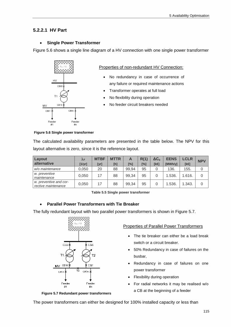
5 Availability Optimisation
115
5.2.2.1 HV Part
Single Power Transformer Figure 5.6 shows a single line diagram of a HV connection with one single power transformer
Figure 5.6 Single power transformer
Properties of non-redundant HV Connection:
No redundancy in case of occurrence of
any failure or required maintenance actions
Transformer operates at full load
No flexibility during operation
No feeder circuit breakers needed
The calculated availability parameters are presented in the table below. The NPV for this
layout alternative is zero, since it is the reference layout.
Layout alternative
F MTBF MTTR A R(1) ΔC0 EENS LCLR NPV [1/yr] [yr] [h] [%] [%] [k€] [MWh/y] [k€]
w/o maintenance 0,050 20 88 99,94 95 0 136. 155. 0 w. preventive maintenance 0,050 17 88 99,34 95 0 1.536. 1.616. 0 w. preventive and cor-rective maintenance 0,050 17 88 99,34 95 0 1.536. 1.343. 0
Table 5.5 Single power transformer
Parallel Power Transformers with Tie Breaker The fully redundant layout with two parallel power transformers is shown in Figure 5.7.
Figure 5.7 Redundant power transformers
Properties of Parallel Power Transformers
The tie breaker can either be a load break
switch or a circuit breaker.
50% Redundancy in case of failures on the
busbar,
Redundancy in case of failures on one
power transformer
Flexibility during operation
For radial networks it may be realised w/o
a CB at the beginning of a feeder
The power transformers can either be designed for 100% installed capacity or less than

5.2 Grid Architecture
116
100% installed capacity. The NPV of this layout is very low because of the high additional
investment of the second power transformer. However, if the maintenance time over the pe-
riod of 20 years and the related EENS is taken into account, the NPV changes significantly.
This is carried out in more detail in the sensitivity analysis.
Layout alternative
F MTBF MTTR A R(1) ΔC0 EENS LCLR NPV [1/yr] [yr] [h] [%] [%] [k€] [MWh/yr] [k€]
w/o maintenance 0,010 113 43 99,99 99 1.750 11. 12. -1.637. w. preventive maintenance 0,010 113 43 99,99 99 1.750 11. 12. -777 w. preventive and cor-rective maintenance 0,010 113 43 99,99 99 1.750 11. n.q. -777
Table 5.6 Redundant power transformers
Furthermore should be noted, that the active power losses of this particular layout are lower
than those of the layout with one power transformer if the installed capacity is >100MW and
the capacity factor of the wind farm location is beyond 35%. (See subchapter 5.3, p.121)
5.2.2.2 MV Part The simplest assembly of MV switchgear of a substation is the single busbar, single discon-
nectors, shown in Figure 5.8. This layout has no additional redundancy what so ever and
serves as reference layout for this investigation.
Single Busbar, Single Disconnectors
Figure 5.8 MV part of the substation, single busbar
Single bb without a tie breaker:
no redundancy
To isolate the bb an outage is
needed
no flexibility during operation
No CB on the busbar required
Make sense with an outstation
Bus bar with tie (switchable bb)
LDC or CB
HV-configuration-H-set-up
The availability and the related costs are presented in Table 5.7. Although this layout is very
simple the estimated availability and therefore the lost revenue is very high.
Layout alternative
F MTBF MTTR A R(1) ΔC0 EENS LCLR NPV [1/yr] [yr] [h] [%] [%] [k€] [MWh/yr] [k€]
w/o maintenance 0,007 137 13 99,99 99 0 3. 3,3 n.q. w. preventive maintenance 0,007 137 13 99,98 99 0 10. 9. n.q. w. preventive and cor-rective maintenance 0,007 137 13 99,98 99 0 10. 8. n.q.
Table 5.7 MV Substation, single busbar

5 Availability Optimisation
117
Reliability figures from REpowers standard primary switchgear (ABB, AREVA) are the basis
for these calculations. This type of switchgear is characterised by a very low failure and
maintenance rate, because of its design. (GIS compact switchgear)
Double Busbar, Double Disconnectors, Single Breakers
A redundant layout of the MV substation is shown in Figure 5.9. The investment costs for this
design are higher and thus just for important substations, or for substations with an high en-
ergy density (installed capacity).
Figure 5.9 MV part of the substation, double busbar, single breakers
The incremental increase of the level of availability compared to the single busbar design is
very low. This results in an significantly higher NPV. (See table below)
Layout alternative
F MTBF MTTR A R(1) ΔC0 EENS LCLR NPV [1/yr] [yr] [h] [%] [%] [k€] [MWh/yr] [k€]
w/o maintenance 0,003 381 14 99,99 99 380 1,3. 1,5. -378. w. preventive maintenance 0,003 381 14 99,99 99 380 1,3. 1,5. -372. w. preventive and cor-rective maintenance 0,003 381 14 99,99 99 380 1,3. 1,4. -670.
Table 5.8 MV Substation, double busbar, double disconnectors
Double Busbar, Double Disconnectors, Double Breakers
This special substation design won’t be considered in this investigation since the other lay-
outs for the MV part of the substation already show a very high level of availability. The fully
redundant layout would need a significantly higher investment that wouldn’t pay off during the
life time of the wind farm. This concept is especially for very important substation within dis-
tribution or transmission networks with a high energy density.

5.2 Grid Architecture
118
5.2.3 Summary of Layout Alternatives
Table 5.9 and Table 5.10 represent the availability and financial decision parameters for the
different layout alternatives. Layout redundancies are marked in the tables as ‘d’ (double,
redundant) whereas the single layout is labelled as ‘s’ (single). Furthermore should be noted,
that the availability parameters of the layout considering maintenance actions as system un-
availability are presented by characters with a star (e.g. A*). The probability that the layout
will survive one year without any failure is given by R(1).
Layout Alternative Info
F
[1/yr]
MTBF [yr]
MTTR [h]
A [%]
A* [%]
R(1) [%] # substation F
HV MV A s s s Ref. 0,529 2 29 99,82 99,28 58 B d s s 0,490 2 24 99,86 99,65 61 C s d s 0,525 2 29 99,82 99,31 59 D d d s 0,486 2 24 99,86 99,66 61 E s s d 0,324 3 14 99,94 99,59 72 F d s d 0,285 4 3 99,98 99,95 75 G s d d 0,320 3 14 99,94 99,42 72 H d d d 0,281 4 2 99,99 99,97 75
Table 5.9 Layout alternatives of the grid connection, availability
The main financial parameters for the layout alternatives can be seen in Table 5.10. As pre-
viously mentioned layout #A serves as reference since this layout is the most common one.
The additional investment costs (ΔC0) are therefore referring to the investment costs of lay-
out #A. This process is also valid for the net present value (NPV). The lost revenue over the
life cycle of the wind farm (life cycle lost revenue LCLR) is based on the expected energy not
supplied (EENS). The LCLR* (with maintenance action) therefore includes the maintenance
induced EENS as well as the manpower costs for preventive and corrective maintenance.
The NPVs were determined by use of equation 2.82 (page 37).
Layout Alternative ΔC0 [k€]
EENS [MWh/yr]
EENS* [MWh/yr]
LCLR [k€]
LCLR* [k€]
NPV [k€]
NPV* [k€] # substation F
HV MV A s s s 0 484 1.890 548 1.724 0 0 B d s s 1.830 368 914 418 739 -1.656 -515 C s d s 380 482 1.881 546 1.958 -378 -611 D d d s 2.210 367 905 416 989 -2.034 -1.142 E s s d 405 144 1.556 163 1.618 -1.286 -1.568 F d s d 2.235 28 579 32 624 -2.942 -2.073 G s d d 785 142 1.541 161 1.597 -1.664 -1.923 H d d d 2.615 17 570 34 641 -3.324 -2.469
Table 5.10 Layout alternatives of the grid connection, lost revenue
The LCLRs, the additional investment costs and the NPVs of the layout alternatives are
graphically illustrated in Figure 5.10 (without taking maintenance into account) and in Figure
5.11 (with maintenance actions)

5 Availability Optimisation
119
Figure 5.10 Lost revenue, investment costs and NPV of layout alternatives w/o maintenance
Figure 5.11 Lost revenue, investment costs and NPV of layout alternatives w. maintenance
MTTR and MTTM used for this evaluation:
Component F MTTR MTTM MTBM [1/yr] [h/yr] [h] [yr]
HV cable 0,00139 48 n.q n.q HV Trafo 0,0182 168 168 6 MV Busbar 0,001 8 n.q n.q MV Cable 0,0061 24 n.q n.q MV Trafo 0,0023 48 6 4 MV switchgear primary n.q 24 12 10 MV switchgear sec. n.q 48 6 4 HV switch ear n.q n.q 12 WEC n.q n.q 16 1 Protection devices See subchapter 4.3.4, p.94
Table 5.11 MTTR and MTTM
The MTTR and MTTM figures
that were used in the previous
evaluation are shown in Table
5.1. These figures are very con-
servative estimates. In order to
quantify their impact on the lay-
out decision (NPV) a sensitivity
analysis will be carried out over
the next few pages.
-4.000
-3.000
-2.000
-1.000
0
1.000
2.000
3.000
4.000
5.000
B C D E F G H
inve
stm
ent a
nd lo
st re
venu
e in
[k€]
Layout Alternative
additional investment lost revenue w/o maintenance NPV w/o maintenance
-3.000
-2.000
-1.000
0
1.000
2.000
3.000
4.000
5.000
B C D E F G H
inve
stm
ent a
nd lo
st re
venu
e in
[k€]
Layout Alternative
additional investment lost revenue w. maintenance NPV w. maintenance

5.2 Grid Architecture
120
5.2.4 Sensitivity Analysis
The sensitivity analysis is intended to provide a better understanding of the relevance of the
different reliability parameters and their impact on the layout decision process. During this
analysis the failure rate of components is assumed to be constant and equal to the previ-
ously presented most likely failure case scenario. Thus only the MTTR, the MTTM and the
investment costs will be altered.
Figure 5.12 shows the net present value and its variation under different MTTM. It is obvious
that the layout alternative with the redundant HV connection is directly related to the mainte-
nance induced expected energy not supplied, since the whole wind farm would be out of ser-
vice without the redundancy. Therefore this layout has a positive NPV for maintenance times
that exceed 150% of the normal MTTM.
Figure 5.12 NPV* for MTTM variations
In other words, the additional investment for the second power transformer in layout B will be
compensated by the additional revenue due to operation during maintenance actions, if the
MTTM is about 1,5 times the normal time.
The same concept was used to prepare Figure 5.13, which shows the NPVs of the layout
alternatives under variation of the MTTR without taking maintenance actions into account. It
can be assumed, that the layouts with the redundant MV collector systems vary the most,
since this part of the wind farm has the highest lumped failure rate due to the high MV cable
length and the amount of MV transformers. The most profitable layout alternatives, for uncer-
tain repair times can be assumed to be layout number C, E and F. Whereas layout E only
has a positive NPV for the configuration with interconnections (feeder ties), where the addi-
tional investment for the redundancy of the MV collector system is profitable over the lifetime
of the wind farm.
-3.000
-2.500
-2.000
-1.500
-1.000
-500
0
500
1.000
1.500
B C D E F G H
NPV
w. m
aint
enan
ce i
nn [k
€]
Layout Alternative
normal 150% MTTM 200% MTTM 150% MTTM and MTTR

5 Availability Optimisation
121
Figure 5.13 NPV for MTTR variations
Since the MTTR is proportional to the failure rate, Figure 5.13 is also valid for failure rate
assumptions.
Onshore vs. Offshore Wind Farms
At the beginning of subchapter 4.2 it was noted, that the reliability figures and thus the avail-
ability evaluations are only valid for onshore wind farms. In order to get a better understand-
ing between the differences of reliability figures of onshore and offshore wind farms some
significant points will be discussed below.
The failure rates of offshore and onshore components in general can be assumed to be simi-
lar. Mainly because literally the same components are used and since there don’t exist verifi-
able historical reliability data from offshore operation those from onshore components have
to be taken into account for availability evaluations. The main difference between onshore
and offshore wind farms is the mean time to maintain (MTTM) of components. It is obvious,
that offshore maintenance actions take a lot more economical and time dependent effort than
maintenance actions carried out onshore. Thus the time to maintain certain offshore compo-
nents can be assumed to be ten too twenty times longer. In order to prevent a high number
of maintenance actions the layout of offshore wind farms normally focus on redundancy.
(E.g. redundant MV collector system)
5.3 Active Power Losses
5.3.1 Calculation Process for Wind Farms
Active power losses are generally divided into load losses (PLL) and no load losses (PNL). The
no load losses are voltage dependent and therefore present practically all of the time. The no
-3.500
-3.000
-2.500
-2.000
-1.500
-1.000
-500
0 B C D E F G H
NPV
w/o
mai
nten
ance
in
[k€]
Layout Alternative
normal 150% MTTR 200% MTTR 150% MTTM and MTTR

5.3 Active Power Losses
122
load losses on the other hand are load dependent and primarily resistive losses. They are
proportional to the square of the current. The first step to estimating load losses is the calcu-
lation of the loss factor (lf). The loss factor is the ratio of average losses divided by the losses
at rated generation [42]. It is important to note, that the loss factor (lf) is not equal to the ca-
pacity factor (cf) of the wind farm because ohmic losses are proportional to the square of the
load. The loss factor can be obtained by the following equation:
2max
0
2
max )(
)(
tI
dttI
PET
cT
L
Llf
(5.7)
cT
cc
lf dttPTT
Tlf0
2)(1 (5.8)
The above equations show that the loss factor is equal to the integral of the square of the
transmitted active power at time t. The capacity factor is always higher than the loss factor.
For utility applications the loss factor may be evaluated by use of the capacity factor only and
with a highly approximately approach. This particular approach is only valid for systems that
capacity factor exceeds 50%. Thus this approach is only applicable for utility applications and
not for wind farms. The estimation of active power losses is based on the generation duration
curve of a wind farm at shore site. Figure 5.14 presents a pie chart of the different generation
modes and their time shares of the wind farm location.
Figure 5.14 Generation modes, shore site
Component Info PNL [kW]
PLL [kW]
LV Cable per WEC n.q 13 MV Cable 33 km n.q 150 HV Cable 10 km n.q 190 MV Trafo per unit 2,5 13 HV Trafo per unit 50 400
Table 5.12 Active power loss of components
Figure 5.15 shows the generation duration curve and the related loss duration curve. In addi-
tion, the loss factor as well as the capacity factor is displayed in order to provide a better un-
derstanding of the relationship between these parameters.
Mode A16%
Mode B10%
Mode C34%
Mode D40%
0%<P<20% 20%<P<60% 60%<P<80% 80%<P<100%
EL loss energy [kWh] Tlf equivalent loss hours PLmax max. active power losses [kW] Tc calculation period P(t) transmitted power output at time t

5 Availability Optimisation
123
Figure 5.15 Generation-duration curve vs. loss duration curve
The loss duration curve is based on figures from Table 5.12. The exact calculation of the
active power loss of several components will not be carried out in detail and further ex-
plained. A detailed graphical illustration of active power losses within a wind farm according
to the relevant generation mode is provided in Figure 5.16 below.
0
10
20
30
40
50
60
70
80
90
100
0 10 20 30 40 50 60 70 80 90 100
shar
e of
rat
ed p
ower
in %
time share in %
loss factor capacity factor shore (P(t)) losses (Pl(t))

5.3 Active Power Losses
124
Figure 5.16 Sankey Diagram
Overall efficiency
88%
681kW 641kW
712kW 440kW
190kW
334kW 379kW
349kW 230kW
90kW
28kW 146kW
29kW 65kW

5 Availability Optimisation
125
This figure also displays the level of efficiency and its decrease due to active power losses.
Although the level of efficiency of the generation modes A, B and C is not less than 94% the
overall level of efficiency of the wind farm over a period of one year is 88%, due to the no
load hours. (Generation mode D - internal consumption)
The lumped active power losses are presented in Table 5.13.
System Info PL [kW]
EL [MWh/yr]
LR [k€/yr]
LCLR [k€]
Wind farm w/o. LV cable 2.000 5.400 536. 6.086 Wind farm w LV cable 2.680 6.822 682. 7.733
Table 5.13 Active power loss of components
The active power losses are 2,6% of the installed capacity of the wind farm and the related
lost energy is about 2% of the total annual energy production of the wind farm. For this par-
ticular wind farm, the capacity factor is 40% and the load factor is 31% (shore, site). The
causes of active power losses and their overall share are presented as pie chart in Figure
5.17.
Figure 5.17 Causes of active power losses, generation mode A
Figure 5.17 is only valid for generation mode A where the wind farm operates at rated power.
The LV cable of WEC is one of the major causes of reduced active power output due to the
high amount of active power transmitted at low voltage levels. The second largest contribu-
tion to active power losses are from MV components. This is because of their large number.
The MV cable in general and the MV collector system may be optimised with regards to ac-
tive power losses by means of alternative cross sections, redundancy and alternative layout
configurations. Transformers for wind power applications in general should be optimised with
regards to their load and no load losses, because of the low capacity factor of wind power
systems. Therefore especially the no load losses should be reconsidered and improved by
means of different core materials of the transformer.
MV Cable27%
LV Cable25%
HV Cable7%
MV Trafo 24%
HV Trafo 17%
LV Cable MV Cable HV Cable MV Trafo HV Trafo

5.3 Active Power Losses
126
5.3.2 Economic Evaluation of Active Power Losses
No Load Losses:
No-load losses are present at all times. When the wind farm is not in production mode, such
as when the wind is calm, energy must be purchased to supply the no-load losses of the
wind farm. Normally, the price and terms of purchased power are different than the prices for
fed-in energy, and can include a demand charge [42].
ptccnNL
demandcpnNL
NL CTTqPsCpTTCT
qPPV
)()1()( 000 (5.9)
NLNL LCLRPV (5.10)
Load losses:
ptccn
LLCn
LLLL ClfT
qPsplfT
qPPV
)1( (5.11)
LLLL LCLRPV (5.12)
Redundancy and its Influence on Active Power Losses
It is obvious that the load losses may be reduced by redundant components because their
resistance gets divided into half. However, this concept is not applicable for every component
or subsystems due to economical restrictions. It can be shown, that fully redundant power
transformers would result in a 30% decrease of load losses (Pll) This 30% decrease is only
valid if the capacity factor of the wind farm location above 40% and the installed capacity is
larger than 80MW. The same concept can be applied for MV components, although a redun-
dancy there is not always practical, e.g. MV transformer. The no load losses cannot be re-
duced through redundancies, only by design changes. It should be noted, that for the above
evaluation only active power losses were considered. Furthermore, reactive power compen-
sations were not taken into account, but they generally have active power losses that cannot
be neglected. In order to estimate the losses accurately the technical availability of WECs as
well as for the grid connections should be used to get the precise time of operation.
PVLR present value of lost revenue [€] PNL no load losses [kW] qn present value factor (n…lifetime) T0 no load hours (mode D) Cp Cost of purchased energy [€/kWh] Cdem demand charge per kW peak per year s income tax rate Cptc production tax credit per kWh p € per kWh wind generation (subsidies) LCLR life cycle lost revenue [€]

5 Availability Optimisation
127
Certain improvement measures in order to mitigate the active power losses could be
Just one step up transformer for several WECs
A higher voltage level at the low voltage side
Transformer layout variations and optimisations regarding P0
5.4 Neutral-Point Treatment
The protection concept has a major impact on the availability of the wind farm (see subchap-
ter 4.3.4, p.94) To ensure a safe and correct operation of the wind farm, it is essential that
electrical failures get detected and isolated immediately. In order to meet these requirements
a thorough design of the systems neutral-point concept is needed. Figure 5.18 presents the
most common neutral point arrangements for electrical power systems. Note that arrange-
ment A,B and D require an additional investment, thus arrangement C (low resistance
grounding) serves as reference for this evaluation.
Isolated
(A)
Arc suppressor coil
(B)
Low resistance grounding
(C)
Current limiting
(D)
Figure 5.18 Neutral point arrangements
The isolated network in Figure 5.18 is only used for special applications, for example small
networks with high continuous supply requirements. Hence, this type is not reasonable for
wind farm applications and won’t be discussed any further. The properties of the individual
arrangements will not be discussed in this investigation. For further information see [17],[47]
and [48]. The objective here is to determine whether a compensated MV collector system (B
arc suppressor coil) would be profitable or not.
Rating of arc suppressor coils
ECE Cj
X
1
XCE wind farm (5.13)
]/[
ln18kmµF
dd
C
c
eE
(5.14)

5.4 Neutral-Point Treatment
128
)tan(
3
2
CE
CE XUQ (5.15)
Ac [mm2]
CE [µF/km]
IE [A/km]
l [km]
120 0,18 2,9 10 240 0,23 3,7 7,5 400 0,28 4,5 5 500 0,31 4,9 10
Table 5.14 Technical cable data [21]
][80,6][2,132][075,24 MVarQXµFC CECEE
CENP XX lumped values (tan()=1)
Arc suppressor coil – life cycle costs pertaining to failure on the collector system
Earth fault frequency: EF=1,851 [f/100km], due to the high amount of medium voltage over-
head lines in the German distribution system the average earth fault rate is too high. In order
to estimate the damage costs (loss of revenue) in an accurate way the failure rate of earth
faults only takes external causes, switching causes, environmental causes and reaction
causes into account. Hence the failure rate can be assumed to be 50% less of the actual
value.
][8,6 MVASNP €][700 kC
[€]
)1(120
1
n
nipEENSLCC p=Subsidies(€] , n=MTBF
][5,9.0 hMOFTCLCC opt .... ...mean operating fault time
Table 5.15 presents the results of the economic impact of earth fault induced outages of the
compensated MV collector system.
Scenario EF [1/yr]
MTBF [yr]
MOFT [h]
EF [kWh/fault]
LCR [€] NPV
Most likely case 0,244 4,09 2,5 98.880 23.574 <0 Worst case 0,601 1,66 2,5 98.880 50.565 <0
Table 5.15 EENS and NPV of compensated collector system
tan() loss angle dc conductor diameter de external (cable) diameter ᵋ relative permitivity of the insulation
Coil 30kV
1 MVA 30. – 60.k €
6,3 MVA 75. – 90. k€
Additional Parts
Controller 6. –10. k€ detection
for cheap UMZ 100 € per
feeder detection incl. control
for 10 feeders +current 15. – 20. k€
EF wind farm earth failure rate
5 Availability Optimisation
129
The additional energy production during the fault (mean operating fault time MOFT) is finan-
cially estimated over the lifetime of the wind farm. This is shown by the life cycle revenue
(LCR) in the above table. In both cases (Most likely and worst case), the life cycle revenues
are significantly lower than the additional investment costs. Thus the overall NPV is less than
zero and the investment is not profitable. Under this assumptions the additional time the wind
farm has to be connected in order to obtain a positive NPV would be 4,5 hours.
The additional energy produced during an earth fault was calculated with the assumption that
the whole wind farm would be out of service with a different neutral point treatment. There-
fore the estimated value of EF is too high. Assuming the earth fault would only effect the pro-
duction of one feeder, the life cycle revenue for the worst case scenario reduces to 8 k€. It
should also be noted, that additional investments for this arrangement, for example insulation
strength or various control, detection and switching devices were not taken into account.
Compared to the other two arrangements (current limiting and low resistance grounding) this
configuration has the highest investment costs. The whole protection concept and the addi-
tional effort for fault detection, fault clearing and therefore maintaining system stability cannot
be neglected. Furthermore, during the fault time, the risk of the occurrence of a multiple fail-
ure or an additional failure is higher, due to the high earth fault factor (εmax=1,73)
General
Low resistance grounding result in high earth fault currents, hence a selective, fast and sim-
ple protection concept can be implemented. The actual phase to earth short circuit current is
directly related to the zero sequence of the transformer. Therefore the high short circuit cur-
rents can be adjusted by changing the zero sequence of the transformer. The arrangement
with additional impedance at the neutral point is therefore known as current limiting neutral
point treatment. In general the earth fault factor should be less than 1,4 and the short circuit
current for earth faults should be as low as necessary [73].
Power plants in general and for wind farms in particular usually need an additional starpoint
builder (starpoint transformer), depending on the power transformers vector group and the
neutral point treatment of the upstream network. In order to fulfill the requirements regarding
earth fault factor and short circuit current, the starpoint transformer can either be implement-
ed with a higher impedance or with a neutral point impedance. However, it should be pointed
out that in case the starpoint transformer is out of service, the effective operation of the wind
farms grounding and protection concept can’t be ensured. Thus a second neutral point build-
er or a switching option (e.g. spare zero sequence impedance) is recommended.

5.5 Maintenance
130
5.5 Maintenance
Maintenance is the combination of all technical and administrative actions, including supervi-
sion actions intended to keep an item up to, or restore it to a state in which it can perform its
required function [28]. Maintenance actions can be classified according to their cause, in
preventive and corrective maintenance. Basically corrective maintenance is event based,
thus is only performed in case a failure occurs. Whereas preventive maintenance is based on
predetermined conditions and intend to reduce the probability of ageing induced failures. The
concept of maintenance is graphically illustrated in the following figure.
Figure 5.19 The concept of maintenance
5.5.1 Preventive Maintenance
Preventive maintenance is carried out at predetermined intervals or according to the condi-
tion of the item and focuses on the improvement of the degradation of the functioning of the
item and the reduction of the probability of failure. The major benefits of an effective preven-
tive maintenance strategy are that life cycle costs are low due to the minimising of compo-
nent down times and the improved safety and performance of the system. The efficiency of
preventive maintenance procedures can be classified into the following three levels:
A General inspection and routine maintenance
B Inspection, general tests and preventive maintenance
C Inspection, specific tests and predictive maintenance
Tests would usually include insulation tests, protective device tests, analytical tests as well
as grounding tests and functional tests [28].
Figure 5.20 shows the failure rate function with and without maintenance measures. The time
frame for this figure was chosen to be from the 10th to the 20th year of operation of the wind
farm, because the ageing effects are more visuable.

5 Availability Optimisation
131
Figure 5.20 Failure rate function with preventive maintenance
Preventive Maintenance Strategies:
Time based Maintenance (TBM)
TBM is characterised by fixed time intervals between maintenance actions. This concept
doesn’t take the actual condition of the component into account. It is essential to find the op-
timum time interval, which can only be achieved through experience. The relationship be-
tween costs and benefits of this maintenance strategy is rather low.
Condition based maintenance (CBM)
This approach takes the actual condition of the component into account which can be evalu-
ated during inspections. Experience and technological knowhow are a necessity to estimate
the condition of electrical components. Nowadays monitoring and diagnostic systems are
widely used to assess the condition online. Before a certain threshold is reached, the particu-
lar maintenance action may be carried out. In order to determine the threshold mathematical
models of ageing effects and their influence on degradation of different components need to
be established.
Reliability centred maintenance (RCM)
The reliability centred maintenance strategy is based on the probability of occurrence of cer-
tain fault events on components. Thus a thorough understanding of failure mechanisms and
even more important exact reliability models and evaluations of financial failure conse-
quences are needed. For components with an high level of reliability, but low financial failure
consequences a corrective maintenance approach is reasonable. Whereas for components
with a low level of reliability and high related failure consequences a condition based mainte-
nance strategy is more practical.
0,00
0,50
1,00
1,50
2,00
2,50
3,00
failu
re ra
te fu
nctio
n [p
.u.]
time [yr]
failure rate w/o maintenance failure rate w. maintenance
Mai
nten
ance
ac
tion
Threshold
Insp
ectio
ns

5.5 Maintenance
132
Other maintenance strategies, like risk based or forecast based...etc. will not be discussed
within this investigation. For more information see [50],[56],[57] and [28].
Influences on Maintenance Strategies
The following measures are essential for deciding which maintenance strategies to apply and
for life cycle cost analysis.
Personnel safety
Faults in electrical power systems must not affect personnel safety
Failure induced financial damage
The financial damage of the customer has to be as low as possible. In case the risk of com-
ponent outages is to high the maintenance strategy is intend to mitigate these risks.
Relevance of the component
Those components that have high failure related energy losses should be maintained in a
way that reduces the probability of failures. A condition based maintenance strategy is rec-
ommended, if monitoring and diagnostic systems are applicable. Otherwise a time based
approach should be considered.
Number of Components
For high amounts of components condition as well as time based maintenance strategies are
usually not applicable due to economical restrictions. Thus, MV components should be de-
signed with low maintenance requirements. Since a corrective maintenance approach seems
to be the most effective in case of many components, a certain amount of spare parts is
needed in order to keep the repair time low.
Operational experience with disturbances
Disturbance statistics and the evaluation of failure causes and mechanisms are the basis for
maintenance adjustments and lifetime estimations.
Legal requirements and standards
In almost every country there are some legal standards regarding the maintenance of electri-
cal components and systems. For example the German government regulate the MTBM of
step-up transformer systems (ITS/ETS) by law. Thus maintenance actions have to be carried
out every four years.
System Availability according to its Maintenance Time:
The following figure presents the availability with respect to maintenance related down time.
The dashed line represents the reference level of availability (97%)

5 Availability Optimisation
133
Figure 5.21 Availability with respect to MTTR and number of failures
In subchapter 5.2 (Grid Architecture) different layout alternatives were evaluated regarding
their availability and profitability. In the first place merely the failure induced consequences
were taken into account, but the second step also considered the influence of maintenance
related down time on the level of availability. It was shown, that under certain restrictions
(installed capacity, capacity factor) redundant configurations pay for their own additional in-
vestment costs. In other words if the lost energy due to maintenance actions is taken into
account the life cycle lost revenue of certain components are at least equal to their invest-
ment. This concept was proved valid for redundant power transformers. Some customer
claim the time to maintain as system down time. It is obvious that this has a major impact on
the systems availability. For example, a guaranteed availability of 97% indicates a down time
of 260hours. The worst case would now be if all components getting maintained within the
same year. This would result in a maintenance induced down time of approximately 220
hours. Hence there would be 40 hours left for corrective maintenance, which implies a high
risk that the mean availability is below 97%. This concept is graphically illustrated in figure
5.21 and is also valid for repair times (corrective maintenance)
It should also be noted, that human factors during maintenance actions cannot be neglected.
The relationship between human failures and system availability was shown in subchapter
4.4.2. However, the IEEE reliability subcommittee provided factors to quantify the influence
of maintenance quality on component failure rates. These factors are presented for some
components in the table below.
Maintenance quality Transformers Circuit breakers Motors Excellent 0,95 0,91 0,89
fair 1,05 1,06 1,07 Poor 1,51 1,28 1,97 All 1 1 1
perfect 0,89 0,79 0,84
Table 5.16 Equipment failure rate multipliers vs. maintenance quality [29]
90%
92%
94%
96%
98%
100%
102%
0 0,25 0,5 0,75 1 1,25 1,5 1,75 2 2,25 2,5 2,75 3
avai
labi
lity,
A in
[%]
failure rate [1/yr]
3 days down time 1 week down time2 weeks down time ref . A=97%1 month doen time

5.5 Maintenance
134
5.5.2 Maintenance Actions and Intervals of Electrical Components
The next subchapter provides a detailed overview of maintenance related figures of signifi-
cant electrical components in wind farms. It will be distinguished between maintenance activ-
ity, the task that has to be carried out and the intervals between the same activities.
5.5.2.1 HV Components Switchgear
Activity Task strategy interval Info
inspection Condition assessment Time based 2 month
maintenance Cleaning
Functional check adjustments
Time based Condition based
6 yr. Depends on
the condition
fault incident based n.q.
Table 5.17 Maintenance of HV switchgear
Power Transformer
Activity Task strategy interval Info
inspection
Condition assessment Time based 2 month
Protection control Time based 3 yr.
Oil analysis Time based 3 yr. Depends on the condition
maintenance against corrosion Condition based 10 yr.
OLTC time based 6 yr. foundation Condition based >20 yr.
Table 5.18 Maintenance of power transformers (ABB)
5.5.2.2 MV Components ITS/ETS
Activity Task strategy interval Info MV Switchgear secondary
inspection Condition assessment Time based 4 yr.
maintenance
Cleaning Painting
Replacement Functional control
Fault clearing Grounding check
Condition based
(Incident based)
4 yr.
MV Transformer inspection Condition assessment Time based 4 yr.
maintenance Cleaning painting Condition based 5-10 yr.
faults Incident based n.q. repair
Table 5.19 Maintenance of ITS/ETS

5 Availability Optimisation
135
MV Collector System
Activity Task strategy interval Info
inspection Control of ter-
minations Time based 5-10 yr. Commissioning Retrofit, fault
Measure Incident based n.q.
maintenance
Cleaning Painting Condition based
Replacement of terminations
and junction boxes
Incident based 1 yr.
Fault clearing Incident based n.q.
Table 5.20 Maintenance of MV cable systems
Substation MV primary switchgear
Activity Task strategy interval Info
inspection
Control of ter-minations Time based 2 month
Protection check Time based 4 yr. Type dependent
maintenance Switchgear bays Time based 10 yr. Type dependent
(Switching cycles) fault Incident based n.q.
Table 5.21 Maintenance of MV switchgear primary
WEC
Time based, if an additional service package has been signed (ISP,WSV), twice a year.
Maintenance Costs
For the sake of completeness it should be noted that the maintenance related costs were
already introduced in subchapter 2.4.2, p.38

5.6 Alternative Electrical Parameters
136
5.6 Alternative Electrical Parameters
5.6.1 Voltage Level Variation of the MV-Collector System
Since the rated power of wind turbine generators and therefore of entire wind farms became
larger over the past years the voltage level of the collector system also increases. Commonly
the collector systems operate at rated voltages of 10kV, 20kV or 30kV with slight deviation.
However, nowadays large wind farms are normally designed with a 30kV (-36kV) MV collec-
tor system.
The benefits of a higher voltage level are e.g. the lower active power losses, the additional
WECs that can be installed per feeder and of course the bigger areas that can be reach by
just one feeder. On the other hand there are also some obvious cons that speak against a
higher voltage level. First of all there is the increase of isolation necessary to maintain the
electrical strength. This leads directly to an additional effort not only in the investment costs,
but also in the number of accessories like joints.
Secondly there is the higher EENS due to more WECs on just one feeder, therefore a thor-
ough design of feeder-disconnectors to separate the collector system in several parts is nec-
essary, in order to improve and control the protection zones as well as the short circuit
power. Another con can be the increase of reactive power at PCC delivered from the MV
cable and thus the need for high performance facts which would result in significantly higher
investment costs. However, the last point can also be an advantage, depending on the ex-
ternal conditions (Grid Code, the country, condition of the upstream transmission sys-
tem...etc.)
5.6.2 Variation of the Rated Power of Transformers
Through variation of the transformers rated power the level of redundancy and therefore the
reliability will vary as well. For example in case of an 100MVA power transformer the addi-
tional investment for a redundant layout with two 50MVA transformers is approximately 50%,
which easily pays off during the wind farms useful lifetime.
The transformers cooling system is another way to slightly change the rated power and thus
the overall investment costs. Transformers especially oil transformers have a great overload
factor. Therefore, if the cooling system would be changed from ONAN to ONAF this would
result in an drop of approximately 10% regarding the rated power of the transformer.

6 Contract and Insurance Possibilities
137
6 Contract and Insurance Possibilities
The previous chapters focused on the availability evaluation of grid connection concepts for
wind farms and the related outage costs. It was shown, that although the level of availability
of the grid connection is very high, there are certain inherent risks related to each individual
layout that can’t always be mitigated in a technological way. This chapter is intended to pro-
vide a overview of risks regarding the grid connection of wind farms and how to mitigate
them. As mentioned in the previous chapter, the main focus during the design phase of elec-
trical power systems is that they are as reliable as possible (from a technological point of
view) and as expensive as necessary (from an economical point of view). Since there is usu-
ally a certain level of risk related to this compromise, the second half of this chapter includes
insurance possibilities for wind farms. The last part of this chapter shall give an overview of
different contractual definitions that can be applied.
Figure 6.1 Decision process for risk and insurance possibilities
of electrical BOP projects
The decision process, whether a proposed wind farm layout and its related risks are reason-
able, is shown in Figure 6.1 in a simplified way.

6.1 REpower Standard Contract
138
6.1 REpower Standard Contract
The mechanisms of the technical availability guarantee for the WECs as well as for the grid
connection are contractually defined within the integrated service package (ISP). Hence the
guarantee is only valid if the service and maintenance works are done by REpower itself.
The liability costs for general maintenance and repair actions are caped with five hundred
thousand Euros. Small repair or replacements of components that don’t exceed an invest-
ment of 1.500€ can immediately take place without the customers permission. Furthermore
the maintenance periods are defined by REpower and must take place within a time frame of
plus, minus four weeks based on the stated time. This should give the company the opportu-
nity to shift the maintenance actions in a low production period, usually during the summer
month. In case the maintenance of individual components is not done satisfactorily, or in a
worst case scenario even lead to a fault, the customer has the opportunity to claim warranty
within a period of twenty four month.
REpower guarantees an average technical availability level of ninety-seven percent (97%) in
respect of the Wind Farm, which shall be calculated by the customer using equation 6.1 and
6.2 as follows.
%100
c
AWEC T
TA (6.1)
n
AA
n
iWECi
WF
1
(6.2)
The technical availability of the wind farm (AWF) is calculated as the sum of the average tech-
nical availability of the individual WECs within the wind farm (AWEC) in percent, divided by the
total number of WECs. The technical availability guarantee applies on the day falling three
month after the commissioning date of the last WEC of the wind farm and normally lasts five
years. However, the precise time interval for the availability guarantee has to be negotiated;
nowadays a common period is 10 years. The bonus-penalty concept, where the customer
gets the liquid damages compensated if the availability doesn’t meet the guaranteed level
and REpower gets an bonus if the availability is beyond the guaranteed level was introduced
in subchapter 0.
Important aspects of operation and maintenance contracts that apply with respect to the sys-
tem availability (e.g. warranty liability product quality...etc.) are presented on the next page.
AWEC availability of the WEC AWF availability of the windfarm TA Time the WEC is available Tc calculation period (time interval) n number of WECs
6 Contract and Insurance Possibilities
139
Warranty
The warranty period for performed service or maintenance actions is twenty four month.
Within this period the customer is entitled to claim warranty of defected performances. RE-
power is responsible to take all necessary measures to mitigate the defects immediately.
Furthermore, the customer is entitled to act on its own responsibility to mitigate the defects if
REpower doesn’t respond after the customer has informed the company tree times.
Liability
REpower is liable for any damages exclusively for any physical damage to the property of
third parties or injury to persons. In case that any damage or injury is caused by both parties,
the customer and REpower, the damage shall be compensated by each party in proportion to
its degree of fault.
Final inspection assurance
At the end of the contract period (ISP) the nominal condition of the WECs and the whole
windfarm has to be verified. Therefore all necessary service and maintenance measures to
ensure that the components are able to perform their required function adequately shall be
applied. The customer may carry out an inspection of the WECs or the whole windfarm on
their own costs within three month before the ISP contract expires. If REpower has not ful-
filled its contractual obligations, the customer may notify REpower of any services required to
be remedied the latest until one month after the ISP contract period expired.
Guarantee of quality
Power curve
REpower guarantees that the relevant power curve is one hundred percent valid during the
warranty period for each WEC according to IEC standard 61400-121:2005, whereas the
measurements uncertainties are not taken into account. The power curve guarantee shall
commence on the date of commissioning of the WEC and end no later than twenty four
month after that date.
Sound emission
For the warranty period, an emission related sound level is guaranteed. If the customer can
prove, that the actual sound level exceeds the guaranteed level, REpower shall be entitled to
take mitigation measures three times. Any further claims for damage compensation of the
customer shall be excluded.
Electrical characteristics
REpower guarantees the electrical characteristics of the components as specified in the rele-
vant product descriptions and technical documents.

6.2 Warranty and Guarantee
140
6.2 Warranty and Guarantee
Warranty is the general liability of the debtor for defects, which the product (e.g. electrical
component, service) shows during its delivery (performance). The concept of warranty is
regulated by law, thus it has not to be contractually stipulated [64]. It has to be considered
that a charge for the delivery (component) is required; otherwise the legally bounded war-
ranty is not valid. It is possible to claim the warranty regardless of who caused or indebted
the defect. However, the warranty-defect has to be existent on delivery of the product (com-
ponent, service) Furthermore, the creditor is not obliged to accept the product regardless of
the kind of defect. If the creditor takes a defect product, because he didn’t see the defect,
warranty can be claimed as well, since it was a defectively delivery.
Type of defect
Material defects
Material defects are defects which are physically connected to the property, also
known as defects of quality.
Defects of title
These defects usually occur when the ownership or transfer of ownership is not prop-
erly recorded. Legal claim or circumstance, that hinders the identification of the true
owner of a property.
Primary warranty remedies
Improvement (rework, supplement)
Replacement (reasonable period of time, as less inconvenience for the customer as
possible)
If the defects can be corrected, the customer has the right to claim an improvement or a re-
placement. Improvements in form of reworks or supplements have to take place onsite and
without any additional financial efforts. (Additional payments) Furthermore, the transferee
can choose between improvement and replacement. The seller (transferor), on the other
hand, has the option to claim that the replacement is either impossible or connected to an
unreasonable high effort. If both primary warranty remedies (improvement and replacement)
are impossible to fulfil, the seller can refer to the secondary warranty remedies.
Secondary warranty remedies:
Price reduction if the defect is not negligible
Conversion
Compensation for the damage can only be claimed if the primary warranty remedies are im-
possible. The legal consequences of warranty don’t start automatically with the occurrence of

6 Contract and Insurance Possibilities
141
a defect, but have to be claimed by the customer within the respective warranty-period. The
warranty-period for movable properties is two years and for immovable properties three
years. According to warranty, companies can be seen as immovable.
Guarantee
The terms of guarantee normally exceeds the warranty conditions, but are only valid for a
short period of time (depends on the contract). However, guarantee is an additional service
that sellers or the manufacturers provide and is not legally bounded.
Guarantee of the seller
Guarantee of the manufacturer (producer
When speaking of guarantee the guarantee of the manufacturer is meant, in which a third
party (normally the manufacturer) covers all defects and therefore assures the property has
no defects, what so ever. Type, content and period of time of the guarantee has to be nego-
tiated and set up contractually. Guarantee and warranty are coexistent, in other words both
can be valid during the same period of time (normally the warranty-period is much longer)
and therefore can be claimed by the customer.
Application to Wind Power Systems
The warranty and guarantee periods for individual components should be outlined taking the
failure rate function of the relevant component into account. Due to the higher failure rate at
the beginning (teething period) it is recommended, that the first month the component is in
operation are excluded from the guarantee period. On the other hand the inverse can be
applied to subcontractors of REpower. For example the teething period of components
should be covered by the additional guarantee of the subcontractor. Especially HV compo-
nents should be considered separately because of their significance to the proper operation
of the windfarm and their high investment costs. Whereas the failure of MV components in
general and the related financial damage should be considered in the selling price, since
these components have lower investment costs, but mainly because of the high amount of
components.

6.3 Risk Assessment and Mitigation
142
Figure 6.2 Definition of risk [18]
6.3 Risk Assessment and Mitigation
Risk (R) is defined as the loss (C) that can occur
with a given probability (P). The loss can either be
financial, personal, energy based...etc. Figure 6.2
shows the concept of risk, its characterisation and
furthermore, its influences. It is important to note,
that loss can only be determined and evaluated in
reference to predefined goals or expectations.
The risk (Ri) associated with one particular event (i)
is assessed through the product between the prob-
ability (Pi) that the event takes place and the consequences (Ci) associated with the event.
iii CPR (6.3)
Risks must be related to a time frame (T), such as for example one year. Therefore the risks
associated with the number of a specific type of events (n(T)) within the defined time frame
(T) shall be considered. In that case Equation 6.1 is written as
0
))(()(i
iCiTnPTR (6.4)
P(n(T)=i) is the probability of i events of the actual considered type within the time T and C is
the consequence associated with the occurrence of one event. However, equation 6.5 may
also conveniently be written as:
CTnEtR )]([)( (6.5)
where E[n(t)] is the expected number of events of the considered type during the period T.
The expected number of events may be established by integration over the occurrences (f) as
dt)t(f)]T(n[E (6.6)
For different applications either of the two different formulations of risk may be convenient
i.e., Equation (6.4) or (6.4).
It is obvious that financial failure consequences also vary over time (C(t)) since they are pro-
portional to the failure rate. Thus the failure induced damage costs increase with respect to
time and have their peak during the wear-out period. Since the failure rate as well as the fi-
nancial failure consequences are statistically distributed, the related risk may be presented
as an distribution as well. The two figures below show the failure related risk during the burn-
in period and during the wear-out period of components. The inherent risk slightly decreases
after the component was put into operation and can assumed to be almost constant during

6 Contract and Insurance Possibilities
143
the components useful life period. During the wear-out period were certain aging effects oc-
cur, the risk will increase again due to the increasing probability of failures.
Figure 6.3 Reliability and related risk for the burn-in period
Figure 6.4 Reliability and related risk for the wear-out period
The risk distributions (Г(t)) in Figure 6.4 and Figure 6.3 were calculated using the following
equation:
)t(R
)tt(R)t(R)t,t( (6.7)
In general, the risk shall be passed to the customer with the commissioning of the WEC.
Where Delivery, Installation and commissioning are not possible for reasons beyond the con-
trol of REpower, the risk shall be passed to the customer not later than two months after the
notification of readiness for delivery.
In order to quantify the risk in an adequate way, the concept of risk analysis is divided into
two parts:
00,10,20,30,40,50,60,70,80,9
11,1
0,0 0,5 1,0 1,5 2,0
f(t),
R(t),
l(t)
, ris
k
time
failure density, f (t) risk (t) reliability (t) failure rate
00,10,20,30,40,50,60,70,80,9
11,1
0,0 0,5 1,0 1,5 2,0
f(t),
R(t),
l(t)
, ris
k
time
failure density, f (t) risk (t) reliability (t) failure rate

6.3 Risk Assessment and Mitigation
144
Determination of the probability of an undesirable event. (generated from detailed
analysis of past experience and historical data)
Evaluation of the consequences, Ci of the undesirable event.
The exact steps to perform a risk analysis are known as the risk triplet and exist of the follow-
ing stages:
Selection of a undesirable reference event or scenario
Estimation of the probability of occurrence, Pi
Estimation of the consequences of these events, Ci
6.3.1 EPC Project related Risks
The acronym EPC stands for engineering, procurement and construction and can also be
summarised by the term turnkey solutions. In other words when speaking of EPC projects
the company (contractor) is responsible for the whole project and thus barriers most of the
related risks. Regarding the risk of electrical components in particular figure 6.5 provides an
overview of different events, their probability and their related severity and how to mitigate
the risk in general.
Figure 6.5 Risk of component damage
The probability of occurrence of certain undesired events on electrical components has been
discussed in detail in previous subchapters. The severity on the other hand can basically be
categorised into following fields:
People
Assets
Environment
Image/Reputation

6 Contract and Insurance Possibilities
145
Within the next few pages, the related risk of important grid connection components will be
elaborated. Basically it is distinguished between high voltage and medium voltage compo-
nents. It should be pointed out, that only components that are relevant for the proper function
of the system are discussed, because of the vast amount of electrical components.
HV Components
It is obvious that the HV components are essential for the functioning of the wind farm, since
in case of a failure the whole wind farm would be unavailable, depending on the layout. The
risk of HV lines as well as for power transformer is presented in the following tables.
HV connection
Component Risk Consequences Preventive measures
Probability of occurrence
HV line fault Outage of the whole wind farm
Double the HV connection
Proj
ect r
elat
ed
(see
app
endi
x) Measuring
equipment
Failure on the HV/LV side
Temporary HV fault
Protection of the hv line disabled
Spare parts Preventive main-
tenance
Disconnector Fail to operate Outage of the whole wind farm
Spare disconnec-tor
Circuit breaker Fail to operate Outage of the
wind farm Spare circuit
breaker
Protection devices
Failure of the relay, power supply, current
transformer, ...etc. Spare parts
Table 6.1 Risk evaluation of HV components
Power Transformer
Component Risk Consequences Preventive measures
Probability of occurrence
HV line fault Outage of the whole wind farm
Double the HV connection
Proj
ect r
elat
ed
(see
app
endi
x)
Measuring equipment
Failure on the HV/LV side
Temporary HV fault
Protection of the hv line disabled
Spare parts Preventive main-
tenance
Disconnector Fail to operate Outage of the whole wind farm
Spare disconnec-tor
Circuit breaker Fail to operate Outage of the
wind farm Spare circuit
breaker
Protection devices
Failure of the relay, power supply, current
transformer, ...etc. Spare parts
Windings and core Internal failure Wind farm out of
service Redundancy
OLTC Mechanical or electrical failure
Wind farm out of service
Reliable type of OLTC (e.g. vac-
uum type)
bushings Electrical or mechanical failure
Wind farm out of service Spare parts
Table 6.2 Risk evaluation of power transformers

6.3 Risk Assessment and Mitigation
146
MV Components
Because of the vast amount of MV components, for this investigation only important compo-
nents with a significant impact on the systems performance will be considered. As previously
mentioned, the risk for the MV components are rather low due to the overall maintenance
support structure. (E.g. spare parts…etc.) However, the MV connection of the power trans-
former is the exception.
Substation MV part
Component Risk Consequences Preventive measures
Probability of occurrence
Power trans-former cable Failure on the MV cable Outage of the
whole wind farm Single phase spare
cable
Proj
ect r
elat
ed
(see
app
endi
x) Failure of the termina-
tion or joint Outage of the
whole wind farm
Spare parts Preventive mainte-
nance Switchgear
primary Failure on the main bus Outage of the whole wind farm
Sectionalised bus, tie breakers
Trafo protection device fails
Outage of the wind farm
Spare parts, or installa-tion of a spare bay
Feeder protection de-vice fails
Outage of the whole feeder
Spare parts, or installa-tion of a spare bay
Aux. Power supply fails Wind farm out of service
Redundant emergency power concept
Table 6.3 Risk evaluation of MV substation
Collector system
Component Risk Consequences Preventive measures
Probability of occurrence
feeder Failure on the MV cable Outage of the whole feeder
Interconnections, redundancies
Proj
ect r
elat
ed
(see
app
endi
x)
ITS/ETS Transformer failure Outage of the whole feeder
Spare parts Preventive mainte-
nance Switchgear secondary Failure on the busbar Outage of the down-
stream WECs Sectionalised bus,
tie breakers
Trafo protection device fails Outage of the WEC
Spare parts, or in-stallation of a spare
bay
WEC protection device fails Outage of the WEC
Spare parts, or in-stallation of a spare
bay
Aux. Power supply fails WEC out of service Redundant emer-gency power con-
cept
Table 6.4 Risk evaluation of MV collector systems
Logistics and Infrastructure
The risk related to general logistics, service and infrastructure issues includes topics like
transportation, site accessibility, installation and commissioning, service contracts with sub-
contractors, accuracy of wind reports, legal and market risks….etc..

6 Contract and Insurance Possibilities
147
6.3.2 Risk-Matrix for Grid Connection Components
The probability of occurrence and the related impact (severity) of certain events on grid con-
nection components is presented in the risk-matrix below.
Figure 6.6 Risk matrix of grid connection components
It can be seen, that the WECs and the MV collector system are still the subsystems with the
highest risk factors. This is because of the total number of WECs and the total cable length
of the collector system. The failure and availability evaluation in subchapter 4.3 has shown
similar results. In order to mitigate the high risk of these components certain preventive
measures are needed. In case of the MV collector system, preventive maintenance strate-
gies but more important spare parts of joints, terminations...etc. shall be applied. In order to
mitigated the risk of WECs a precise quality management of the components is necessary as
well as preventive maintenance works and a good support structure.
Interpretation
MV Collector system low risk
(Incl. trafo and secondary switchgear)
Substation (MV Part) low risk
(Unattended maintenance)
Substation (HV Part) high risk
(Insurance possibilities / Exclude trafo from availability guarantee?)
Maintenance need to be discussed
(WEC incl. ITS/ETS substation – strategy required)
102
12
15
2
3
0
1
2
3
4
5
0 1 2 3 4 5
Pro
babi
lity
(P)
Impact/Severity (S)
Power Transformer
HV Line
MV Collector System
WECs
MV Switchgear primary
MV Switchgear secondary

6.4 Insurance Possibilities
148
6.4 Insurance Possibilities
Nowadays almost every renewable energy project is insured in some way. For example the
machinery business interruption insurance applies to every power generation system and is
valid not only for the operation phase but also during erection (erection business interruption
insurance). There are various kinds of insurances that apply during the life cycle of wind
power systems. An overview of the most common ones is graphically illustrated in Figure 6.7.
Figure 6.7 Insurances over the life cycle of electrical components [75]
As shown in previous subchapter, the financial damage of customers caused by certain un-
desired events (e.g. failure of components) is calculated using the capacity factor, which can
be interpreted as the fluctuating wind speed. However, in case of insurance premium rates
this concept has limited significance, for example the correlation between high wind speeds
and the higher damage potential must be taken into account when evaluating whole wind
farms. The major influences on insurance rates are the building design and the redundancy
of components. The building design is relevant for example in case of fire, which can be seen
as a common cause failure. Thus if components are spatially divided in a way that a failure of
one component cannot effect the other component, the insurance rate can be assumed to be
the half. (E.g. Substations: fire protection, solid building design, various accesses, ventila-
tion...etc.) The second important influence on insurance rates is the level of redundancy. The
grid connection layout should be designed in a way that certain bottlenecks (e.g. HV connec-
tion) don’t occur. Actuarial speaking, significant components should be n-1 redundant, also
known as 50% components. In case of redundant power transformers this means, that if one
transformer trips only half of the wind farms installed capacity is still connected to the up-
stream grid. The application of this concept is only valid for individual significant components,
due to economical aspects. (E.g. full redundancy of MV collector system)

6 Contract and Insurance Possibilities
149
Furthermore the insurance premium rates are also related to the reputation of the compo-
nents manufacturers. In other words, the insurance rates for a premium component produced
from a well established company are much lower than those of a low-quality product. There-
fore it can be assumed that a fifty percent redundancy layout designed with two low-quality
products have lower lifecycle costs than the layout alternative with one premium-product and
an additional insurance policy beyond a certain installed capacity. In general it is important to
note, that the insurance taxes are different for individual countries. Furthermore, cash flows
to foreign insurance companies are prohibited by law in order to keep the cash flows local.
For example the insurance taxes for Germany are currently nineteen percent, whereas those
for the Australian market are thirty percent which represent the highest insurance taxes
worldwide. It is important to check the country specific insurance taxes in order to keep the
overall costs low, since the insurance premium rates normally don’t include taxes.
In addition it is always possible to get fired from the insurance company; hence in case the
insurance company covers for a significant damage or loss they cancel the insurance policy.
It is common practice that insurance companies just cover the occurrence of just one major
damage event. What should be also taken into account are the various kinds of deductibles
concerning individual components. Deductibles represent the own risk and normally are time
based. For example a typical deductable period for substations (power transformers) is two
to four weeks. Hence if the repair or replace time is less than the deductable period the in-
surance doesn’t cover the loss. Therefore components which have low MTTRs can be left
out of the insurance policy. (E.g. MV collector system)
For wind farms the level of availability cannot be insured in general only the business inter-
ruption resulting from insured property damage to the plant can be insured. During the opera-
tion period the operator exchanges machinery breakdown and business interruption insur-
ance covering external hazards such as natural catastrophes or terrorism. If REpower is lia-
ble for the property damage based on its supply contract, coverage is not provided under this
policy but the warrantee of REpower has priority - irrespective of whether REpower has tak-
en out warrantee insurance to cover this risk or not. If REpower is also liable for the availabil-
ity of the plant based on a service agreement, this warrantee has also priority to the machin-
ery business interruption insurance.
Components
The next section is intended to provide a basic overview of insurance possibilities for individ-
ual electrical components and subsystems within a wind farm. It should be noted, that the
insurance premium rates are expressed as the percentage of the overall annual turnover of
the wind farm. In addition the overall costs for insurance and the concept of binding offers is
going to be discussed.

6.4 Insurance Possibilities
150
Wind Energy Converter
REpower is responsible for the insurance which covers the transportation and assembly
risks. Furthermore, REpower has to provide a relevant insurance of the machinery of the
WEC that covers external risks. In case the customer already has such insurance this con-
cept doesn’t apply under the restriction that the customer informs Repower four weeks prior
to the passage of risk. In addition to the transportation and erection insurance a so called
guarantee and business interruption (BU) insurance should be closed up, which basically
covers the lost revenue caused by any damage to the insured property. The insured property
can be every product of Repowers scope of supply, regardless whether it’s new or not. The
insurance period starts subsequently to the insurance for erection after the commissioning of
the product. The liability of the insurance company typically ends at the end of the ISP con-
tract. The deductibles for WECs with an rated power up to 3,5 MW are 750.000 Euros. Thus
all financial damages less than 750.000 Euros are compensated by Repower. In case of fi-
nancial damages beyond 750.000 Euros the deductibles thereby incurred just three times.
The deductibles for facilities with an rated power beyond 3,5 MW are one million Euros and
the deductibles for serial damages are one and a half million Euros. It should be noted; that
the highest amount of compensation related to the BU insurance is twenty five million Euros
within one year. The evaluation of the insurance premium rate is based on the total installed
capacity of the wind farm and the annual turnover. Additionally a stop-loss-agreement of
2.250.000 Euros (WECs up to 3,5 MW) or 2.000000 Euros (WECs above 3,5 MW) per year
applies. Furthermore, individual components within one WEC may be covered by an addi-
tional machinery business interruption insurance (MBU), usually from a different insurance
company.
HV Components
Usually in Germany the premium rate of a business interruption insurance for a substation
amounts to 1 % of the annual turnover of the wind farm for a maximum period of one year
which is likely to happen in case of large substations. Since transformer claims are usually
not caused by external events, REpower might be liable for most of the claims based on the
service agreement. For this reason the premium rate for the limitation of REpower's liability
can only be reduced to a marginal extent and will be at least 0.8 % of the annual turnover
subject to a normal time excess of one or two weeks per claim.
MV Collector System
The risk of a failure to the MV cable system is much lower than that of the substations.
Therefore the premium rate should be reduced to 0.2 %. However, final clarifications can
only be done after detailed review of the grid connection layout. Due to the relatively low im-

6 Contract and Insurance Possibilities
151
pact of failures on the MV collector system an additional insurance is usually not reasonable.
It is recommended, that these failures are covered by maintenance support structures.
Availability Insurance
In case of a claim insured or to be insured under a warrantee policy of REpower, the availa-
bility can be insured under a warrantee business interruption policy. The costs of risk in form
of an insurance premium and the deductible of REpower have to be agreed. This is only
possible after a detailed risk assessment and clarification of the interdependencies of all
components of the wind farm. As a first calculation for an offer the following estimated values
can be taken into consideration:
Overall Insurance Premium
Based on the items mentioned above there will be a premium for the availability of BoP - of
course only in respect of insurable losses - totaling to 1.5 to 2 % of the annual turnover of the
wind farm plus insurance tax. In addition REpower has to consider for its calculation the un-
insured availability claims arising from a business interruption without property damage as
well as the deductible. Business disruptions are not that important because long term inter-
ruptions exceeding the deductible rather result from property damage. This risk should be
evaluated by REpower from a technical point of view. A deductible of 14 days accounts for 4
% of availability. This should be evaluated with the probability of occurrence. As the premium
rate shows the insurers expect one long term total failure in 50 years. Failures of one or two
months for parts of the plant however are possible more often. This should also be taken into
account by REpower when evaluating the calculation of an offer.
Binding Insurance
A binding insurance offer can only be made by means of a submission in the insurance mar-
ket after a detailed risk analysis and evaluation of all supply and service contracts as well as
the location of risk.
Example: Lifecycle Insurance Costs for Power Transformers
The insurance premium for a wind farm power transformer (Pr=100MVA) of high quality,
which is located in an ordinary accessible area can vary between seventy thousand and one
hundred and fifty thousand Euros per year. At a common interest rate of six percent, an in-
surance period of ten years (equal to the maintenance period) and a premium of one hun-
dred thousand Euros this would result in an overall paid insurance premium of seven hun-
dred thousand Euros. This is about the same as the total investment costs of the power
transformer.


7 Results and increase of Knowledge
153
7 Results and increase of Knowledge
General
This thesis presents the level of availability of single, significant electrical grid connection
components as well as the availability of whole wind farms according to their installed capac-
ity, layout and applied maintenance strategy.
The objective was to estimate the level of availability of the grid connection concept used by
Repower Systems AG, to find significant influences on the systems availability and the opti-
mum between technological and economical design requirements. Furthermore contractual
obligations should be derived, taking insurance possibilities into account.
Based on mathematical concept, introduced in the first chapter and by the use of reliability
and outage statistics from subcontractors and electric utilities the availability of individual
components was calculated. During the next steps the availability of a whole wind farm with
an installed capacity of 100MW was calculated which served as reference for the optimisa-
tion process in chapter six.
It is important to mention that the results are based on theoretical, analytical methods. Major
availability and reliability figures, like mean time to failure (MTTF) or mean time to repair
(MTTR) present long term arithmetic averages.
The results show that the wind energy converter itself is the major cause of reduced power
output at the point of common coupling. The level of availability of the grid connection is be-
yond the target value of 97% and can be assumed to be above 99%. The bottle neck of the
grid connection is still the high voltage part, not because of the high failure rate but because
of the high impact of failures and the maintenance related energy not supplied. The investi-
gation shows, that a redundant layout of the HV connection is reasonable for wind farms with
an installed capacity larger than 100MW and a capacity factor above 40%.
Grid Connection Layout
The incremental levels of availability of different grid connection configurations are summa-
rised in Table 7.1. It should be mentioned that the radial network configuration serves as
reference for this evaluation. This table shows the relative as well as the absolute increase of
availability over a period of one year. Additionally the incremental availability with respect to
preventive maintenance actions is taken into account which is represented within the last two
columns. The first three columns describe the grid connection configuration. (‘d’ stands for
double, redundant layout; ‘s’ stands for single, radial layout)

7 Results and increase of Knowledge
154
Layout ΔA [%]
ΔA [h]
ΔA* [%]
ΔA* [h]
# substation
feeder HV MV
B d s s 0,04% 4 0,37% 33 C s d s 0,00% 0 0,03% 3 D d d s 0,04% 4 0,38% 33 E s s d 0,12% 11 0,31% 27 F d s d 0,16% 14 0,67% 59 G s d d 0,12% 11 0,14% 12 H d d d 0,17% 15 0,69% 60
Table 7.1 Increase of availability
Table 7.1 presents only the technical availability of different system configurations and
doesn’t consider the financial impact at all. Since technical availability is directly related to
lost revenue and investment costs and therefore essential for the decision which layout alter-
native should be applied, or whether a certain wind farm is profitable or not, the following
figure shows the financial side of different grid connection configuration.
Figure 7.1 Additional investment, lost revenue and NPV of layout alternatives
The lost revenue, taking preventive maintenance actions into account (LCLR) as well as the
net present value (NPV) are estimated over the wind farms useful lifetime (twenty years). It
can be seen, that a redundant configuration for the collector system and the medium voltage
part of the substation for onshore wind farms with an installed capacity of less than 100MW
is not reasonable. Whereas a redundant high voltage connection for such wind farms seems
to be profitable, due to the maintenance related lost revenue of single power transformers.
On the other hand it should be noted that the additional investment for this configuration is
fifteen percent higher compared to single, radial layout.
BC
D EF
GH
-80%
-60%
-40%
-20%
0%
20%
40%
60%
80%
100%
∆C0,
LCL
R, N
PV in
[%]
Layout Alternative
additional Investment (∆C0) lost revenue w. maintenance (LCLR) NPV w. maintenance

7 Results and increase of Knowledge
155
Maintenance methods
Besides corrective maintenance actions the main influencing factor regarding the wind farms
availability are preventive maintenance actions. In particular preventive maintenance actions
on primary MV switchgear, as well as on high voltage components. It was shown, that over a
period of ten years a redundant high voltage connection is profitable for wind farms with an
installed capacity not less than 100MW. In other words the additional investment meets the
lost revenue due to preventive maintenance actions over a period of ten years.
Risk and Insurance Possibilities
The related risk of different electrical sections within a wind farm can be summarised as fol-
lows.
Medium Voltage Collector system low risk (Including transformer and secondary switchgear)
Substation (Medium Voltage Part) low risk (Unattended maintenance)
Substation (High Voltage Part) high risk (Insurance possibilities / Transformer excluded from the availability guarantee?)
Maintenance not quantifiable (WEC including Kiosk/Substation) – Strategy required

8 Conclusion and Outlook
156
8 Conclusion and Outlook
Over the next years the market requirements will certainly get even tougher for availability
and performance guarantees for wind farms. Therefore it is necessary for companies to pay
more attention to disturbance and failure mechanisms. A specific quality management proc-
ess to improve the long term performance is recommended with the special focus on failure
data acquisition and evaluation as well as maintenance strategies and support.
International Classification
For this investigation reliability figures from subcontractors and from the german network
were used. Compared to figures from other countries in which REpower operates, e.g. north
America, Australia ect. In general one can assume similar figures. Of course influencing fac-
tors like local network configuration, regional standards, geographical aspects have to be
taken into account and should be approached according to the specific wind farm project.
Recommended Procedures
The results of this investigation are based on analytical evaluation methods. Thus numerical
methods as well as simulation methods are recommended in order to verify the analytical
results and evaluate the availability parameters in a more accurate way.
The accuracy of reliability related failure data and statistics from single components are a
crucial part of availability calculations. Hence a special data acquisition process is recom-
mended for wind farms installed by REpower in order to obtain a better understanding of
wind farm failure mechanisms.
Further Investigations
Maintenance strategies in general have a high impact on the rate of energy not supplied and
therefore the wind farms life cycle revenue. Especially preventive maintenance actions in-
cluding maintenance support should be investigated further.
Within this thesis the failure rates or in other words the occurrence of different undesired
events were assumed to be exponentially distributed. Hence different failures occur at ran-
dom. The correlation between high wind speeds and the frequency of different faults as well
as their seasonal variations were not taken into account and should be investigated further.

A-1
Bibliography
[1] A. P. Leite, C. L. T. Borges, and M.Falcao: "Probabilistic Wind Farms Generation
Model for Reliability Studies Applied to Brazilian Sites", IEEE Transactions on Power
Systems Vol.21, No. 4, (2006).
[2] A. Underbrink and et al: "Probabilistic Reliability Calculations for the Grid Connection of
an Offshore Wind Farm", KTH, Stockholm, Schweden, 2006.
[3] A.G. Bruce: "RELIABILITY ANALYSIS OF ELECTRIC UTILITY SCADA SYSTEMS",
IEEE Transactions on Power Systems Vol.13, No.3, (1998).
[4] ABB Ltd. - Transformer Services: "TrafoAsset Management-ABB’s solution for im-
proved reliability and life extension of transformers Zürich, 2008.
[5] G. J. Anders: "Probability Concepts in Electric Power Systems", Wiley New York, 1990
ISBN 0471502294.
[6] H. Ascher and H. Feingold: "Repairable Systems Reliability", Dekker New York, 1984
ISBN 0824772768.
[7] B. Körbler: "Zustandsbewertung von elektrischen Betriebsmitteln in der Energietech-
nik", Dissertation, TU Graz, 2004.
[8] R. Billinton and R. N. Allan: "Reliability Evaluation of Engineering Systems", Plenum
Publishing Corporation New York, NY, 1983 ISBN 0306412969.
[9] R. Billinton and R. N. Allan: "Reliability Evaluation of Power Systems", Plenum Press
New York, 1996 ISBN 0306452596.
[10] R. Billinton and W. Li: "Reliability Assessment of Electric Power Systems using Monte
Carlo Methods", Plenum Press New York, 1994 ISBN 0306447819.
[11] R. E. Brown: "Electric Power Distribution Reliability", CRC Press Boca Raton, Fla.,
2009 ISBN 0849375673.
[12] A. A. Chowdhury and D. O. Koval: "Power Distribution System Reliability", Wiley [u.a.]
Hoboken, NJ, 2009 ISBN 0470292288.
[13] D.Nack: "Reliability of Substation Configurations", Iowa State University, 2005.
[14] B. S. Dhillon: "Human Reliability, Error, and Human Factors in Engineering Mainte-
nance", CRC Press/Taylor & Francis Boca Raton, Fla., 2009 ISBN 1439803838.
[15] DIN 3105:2003-06 "Fundamentals of Maintenance", Beuth, Berlin, juni 2003.
[16] J. Endrenyi: "Reliability Modeling in Electric Power Systems", Wiley Chichester, 1978
ISBN 0471996645.

2
[17] L. Fickert: "Planung und Betrieb von Energiesystemen", Vorlesungsskript LV 432.119,
TU Graz, 2007.
[18] L. Fickert: "Risikomanagement Teil 2", Vorlesungsskript LV 434.338, TU Graz, SS
2007.
[19] G. S. Fishman: "Monte Carlo", Springer New York, NY, 2008 ISBN 038794527X.
[20] Gerhard Theil: "Evaluation of the Influance of Repair-Joint Number Increase on the
Outage Frequency of Medium Voltage Cables", CIRED 20th International Conference
on Electricity Distribution, 2009.
[21] H. Gremmel: "Schaltanlagen Handbuch", Cornelsen Berlin, 2006 ISBN 3589241020.
[22] H.Brakelmann: "Interpretation der neuen CIGRE-Ausfallstatistik von VPE-Kabeln Uni-
versität Duisburg-Essen, 2009.
[23] I.S.Ilie et all: "Protections Impact on the Availability of a Wind Power Plant Operating in
Real Conditions", IEEE Power Tech Conference Bucharest, 2009.
[24] IEC 61703 ed.1.0 "Mathematical Expressions for Reliability, Availability, Maintainability
and Maintenance Support Terms", 00-2001.
[25] IEC 60300-3-3 ed2.0 "Dependability Management - Part 3-3: Application Guide - Life
Cycle Costing", 00-2004.
[26] IEC 60505 ed 3.0 "Evaluation and Qualification of Electrical Insulation Systems", 00-
2004.
[27] IEC 60300-3-11 ed 2.0 "Dependability Management - Part 3-11: Application Guide -
Reliability Centred Maintenance", 00-2009.
[28] IEEE Std 902-1998 "IEEE Guide for Maintenance, Operation, and Safety of Industrial
and Commercial Power Systems", New York, 1998.
[29] IEEE Std 493-2007 "Gold Book - Recommended Practice for the Design of Reliable
Industrial & Commercial Power Systems", New York, 2007.
[30] IEEE PES Wind Plant Collector System Design Working Group: "Wind Power Plant
Substation and Collector System Redundancy, Reliability, and Economics Calgary,
2009.
[31] L. B. J.Nilsson: "Maintenance Management of Wind Power Systems Using Condition
Monitoring Systems—Life Cycle Cost Analysis for Two Case Studies", IEEE Transac-
tions on Energy Conversion Vol.22, No.1, (2007).

3
[32] Jasper van Casteren: "Assessment of Interruption Costs in Electric Power Systems
using the Weibull-Markov Model", Ph.D, Chalmers University of Technology Göteborg,
Sweden,, 2003.
[33] Jimmy Ehnberg: "Generation Reliability for Isolated Power Systems with Solar, Wind
and Hydro Generation", Dissertation, Chalmers University of Technology Göteborg,
2003.
[34] S. Jonnavithula: "Cost/Benefit Analysis of Power System Reliability", Dissertation, Uni-
versity of Saskatchewan, 1997.
[35] L. Bertlin and R.Eriksson and R.N.Allan: "Impact of Maintenance Strategy on Cost and
Reliability of Distribution Systems", CIRED - 17th International Conference on Electric-
ity Distribution Barcelona, 2003.
[36] L.Geldenhuis, J.Jagers, and T.Gaunt: "LARGE POWER TRANSFORMER
RELIABILITY IMPROVEMENT IN ESKOM DISTRIBUTION", CIRED-19th International
Conference on Electricity Distribution Vienna, 2007.
[37] e. a. de M. Nigris: "Feed-Back of Medium Voltage Power Cables Reliability in Italy:
Systematic Analysis of Failed Components", CIRED 17th International Conference on
Electricity Distribution, 2003.
[38] M. Modarres: "What every Engineer should know about Reliability and Risk Analysis",
M. Dekker New York, 1993 ISBN 082478958X.
[39] P.Carer and C:Briend: "Weather impact on components reliability : a model for MV
electrical networks", IEEE - 8th international conference on probabilistic methods ap-
plied to power systems Rincon, 2008.
[40] L. B. P.Hilber: "Monetary Importance of Component Reliability in Electrical Networks for
Maintenance Optimization", IEEE 8th International Conference on Probabilistic Meth-
ods Applied to Power Systems Iowa State University, 2004.
[41] P.Jarman et all: "END-OF-LIFE MODELLING FOR POWER TRANSFORMERS IN
AGED POWER SYSTEM NETWORKS", 6th Southern Africa Regional Conference
CIGRE, 2009.
[42] R.A.Walling and T.Ruddy: "Economic Optimization of Offshore Windfarm Substations
and Collection Systems",
[43] R.t van de Sandt, J. Löwen, and I. Erlich: "Optimal neutral earthing in offshore wind
farm grids",
[44] M. Rausand and A. Høyland: "System Reliability Theory", Wiley-Interscience Hoboken,
NJ, 2004 ISBN 047147133X.

4
[45] H. Renner and M. Sakulin: "Power Quality", Vorlesungsskript LV 432.164, TU Graz,
2007.
[46] J. Schlabbach and D. Metz: "Netzsystemtechnik", VDE-Verl. Berlin, 2005 ISBN
9783800728213.
[47] T. A. Short: "Electric Power Distribution Handbook", CRC Press Boca Raton, 2004
ISBN 0849317916.
[48] W. D. Stevenson: "Elements of Power System Analysis", McGraw-Hill New York, NY,
1982 ISBN 0070612781.
[49] H. G. Stoll and L. J. Jordan: "Least-Cost Electric Utility Planning", Wiley New York,
1989 ISBN 0471636142.
[50] C. Sumereder: "Analyse und Bewertung von Betriebsmitteln in der Hochspannungs-
technik", Habilitationsschrift, TU Graz, 2010.
[51] T.A. Prevost et all: "Estimation of Insulation Life Based on a Dual Temperature Aging
Model", Weidmann-ACTI Inc. Fifth Annual Technical Conference Albuquerque, 2006.
[52] U.Zickler et all: "Asset management in Distribution Systems considering new Knowl-
edge on Component Reliability and Damage Costs",
[53] VDE (FNN) "Störungs- und Verfügbarkeitsstatistik -Anleitung", VDE-Verl., Berlin, 2010.
[54] VDE (FNN) „Disturbance and Availability Statistics, 2006“, VDE-Verl., Berlin, 2006
[55] VDI 3423 "Verfügbarkeit von Maschinen und Anlagen Begriffe, Definitionen, Zeiterfas-
sung und Berechnung", 01-2002.
[56] VDN: "Fachbericht- Instandhaltungsmanagement", VDE-Verl. Berlin, 2004.
[57] VDN "Technische Richtlinie für die Instandhaltung von Betriebsmitteln und Anlagen in
Elektrizitätsversorgungsnetzen", VDE-Verl., Berlin, Nov. 2006.
[58] W.H. Bartley P.E.: "Investigatiing Transformer Failures", Annual Technical Conference
for the International Association of Engineering Insurers Stockholm, 2003.
[59] E.O.Schweitzer et all: “Reliability Analysis of Transmission Protection Using Fault Tree
Methods”, USA 1998
[60] Edward N. Zalta (2010): Stanford Encyclopedia of Philosophy.
http://plato.stanford.edu/. Publisher: The Metaphysical Research Lab. Stanford Univer-
sity. URL: http://plato.stanford.edu/, zuletzt geprüft am 20-01-2011.

5
[61] Prof. Dmitry Panchenko (2005): Introduction to Probability and Statistics - Lecture
Notes. MIT Open Courseware. Massachusetts Institut of Technology. Online verfügbar
unter http://ocw.mit.edu/, zuletzt geprüft am 20-01-2011.
[62] D.D.Li, C.He, Y.Fu: “Optimization of Internal Electric Connection System of Large
Offshore Wind Farm with Hyprid Genetic and Immune Algorithm”, IEEE, Nanjing China,
DRPT April 2008
[63] Dr.F.Krähenbühl et.all: “Nexans - Technik der Mittelspannungskabel”, Nexans Schweiz
AG, Cordailod 2009
[64] Bundesministerium der Justiz: "Bürgerliches Gesetzbuch in der Fassung der Bekannt-
machung vom 2. Januar 2002 (BGBl. I S. 42, 2909; 2003 I S. 738), das durch Artikel 1
des Gesetzes vom 17. Januar 2011 (BGBl. I S. 34) geändert worden ist" BMJ:
http://bundesrecht.juris.de/bgb/index.html zuletzt geprüft am 31.01.2011
[65] A.Fritz: „Berechnung und Monte-Carlo Simulation der Zuverlässigkeit und Verfügbar-
keit technischer Systeme“, Dissertation, Universität Stutgart, 2001
[66] Energiekondor AG: „Stufenzinsanleihen 2010 – 20 Jahre Energiekondor“
http://www.energiekontor.de/downloads/stufenzins/VKP_SzA2.pdf
[67] Jörn Iken: „Im Focus Versicherungen Windindustrie – Die Aufregung ist vorbei“ Sonne
Wind & Wärme Nr. 16/2010, S.44ff
[68] Repower Systems AG: “Product Report – MM Series [Sep.09-Aug.10]” Hamburg No-
vember 2010
[69] P. Carer, C.Briend: “Weather impact on components reliability : a model for MV electri-
cal networks”, 10th International Conference on Probabilistic Methods Applied to Power
Systems, Rincon USA 2008
[70] H.Dobesch, G.Kury:“Basic Meteorological concepts and recommendations for the ex-
ploitation of wind energy in the atmospheric boundary layer” Vienna, 1999
[71] Daniel Nack: “Reliability of Substation Configurations”, Iowa State University, 2005
[72] IEEE PES Wind Plant Collector System Design Working Group: “Wind Power Plant
Substation and Collector System Redundancy, Reliability, and Economics” IEEE PES
General, Calgary 2009
[73] R.van de Sandt: “Optimal neutral earthing in offshore wind farm grids” ,University Duis-
burg-Essen, 2009
[74] A.Fritz: „Berechnung und Monte-Carlo Simulation der Zuverlässigkeit und Verfügbar-
keit technischer Systeme“ , Dissertation, Stuttgart 2001

6
[75] D.Schimana: “Infoveranstaltung-Projektversicherung“, MARSH, Hamburg 2009
[76] Michele de Nigris et all.: “FEED-BACK OF MEDIUM VOLTAGE POWER CABLES
RELIABILITY IN ITALY: SYSTEMATIC ANALYSIS OF FAILED COMPONENTS“
CIRED 17th IECD, Barcelona 2003
[77] H. Brakelmann: „NKT Cables Studie - Interpretation der neuen CIGRE-Ausfallstatistik
von VPE-Kabeln“ Universität Duisburg-Essen, 2009
[78] P. Lorin: “Lifetime decisions – Optimizing lifetime costs for Transformers“ ABB Trans-
formers, Geneva Switzerland
[79] A.Franzen, S.Karlsson: “Failure Modes and Effects Analysis of Transformers”, Royal
Institute of Technology KTH Stockholm, Sweden, 2007
[80] M.Argus: “ Hermetik-Leistungstransformatoren von der Vision zur Wirklichkeit”
VDE/ETG Tagung, Würzburg 2005
[81] E.H. Worthmann: “Improving Safety on Ageing Switchgear” ABB-Report, Zürich 2004
[82] K.J.Boser: “Medium Voltage Switchgear & Circuit Breaker Life Extension- a Compari-
son of MV Breaking Mediums and Options for Maximizing the Lifespan of MV Distribu-
tion Equipment” Magna Electric Corporation, Canada
[83] D.A.Genutis: „Top Five Switchgear Failure Causes and how to avoid them“ NETA
WORLD, Summer 2010, p.1ff
[84] IEEE PC37.119/D/ “Draft 7 – Guide for Breaker Failure Protection of Power Circuit
Breakers” New York 2005
[85] C.Neumann et all: “The Impact of Insulation Monitoring and Diagnostics on Reliability
and Exploitation of Service Life” CIGRE Paris 2006

Appendix
A-10
Appendix
A. Statistical Tables ......................................................................................................... 2
B. Reliability Figures ........................................................................................................ 3
C. Average Prices ............................................................................................................ 4
D. Risk and Severity Ratings ........................................................................................... 6
E. Types of Faults ............................................................................................................ 8
F. Availability Evaluation Project Mt.Mercer ................................................................... 11

A Statistical Tables
A 2
A. Statistical Tables
Chi-Square Percentage Points
99.0% 97.5% 95.0% 90.0% 10.0% 5.0% 2.5% 1.0% n
1 0.000 0.001 0.004 0.016 2.706 3.841 5.024 6.635 2 0.020 0.051 0.103 0.211 4.605 5.991 7.378 9.210 3 0.115 0.216 0.352 0.584 6.251 7.815 9.348 11.345 4 0.297 0.484 0.711 1.064 7.779 9.488 11.143 13.277 5 0.554 0.831 1.145 1.610 9.236 11.070 12.833 15.086 6 0.872 1.237 1.635 2.204 10.645 12.592 14.449 16.812 7 1.239 1.690 2.167 2.833 12.017 14.067 16.013 18.475 8 1.646 2.180 2.733 3.490 13.362 15.507 17.535 20.090 9 2.088 2.700 3.325 4.168 14.684 16.919 19.023 21.666 10 2.558 3.247 3.940 4.865 15.987 18.307 20.483 23.209 11 3.053 3.816 4.575 5.578 17.275 19.675 21.920 24.725 12 3.571 4.404 5.226 6.304 18.549 21.026 23.337 26.217 13 4.107 5.009 5.892 7.042 19.812 22.362 24.736 27.688 14 4.660 5.629 6.571 7.790 21.064 23.685 26.119 29.141 15 5.229 6.262 7.261 8.547 22.307 24.996 27.488 30.578 16 5.812 6.908 7.962 9.312 23.542 26.296 28.845 32.000 17 6.408 7.564 8.672 10.085 24.769 27.587 30.191 33.409 18 7.015 8.231 9.390 10.865 25.989 28.869 31.526 34.805 19 7.633 8.907 10.117 11.651 27.204 30.144 32.852 36.191 20 8.260 9.591 10.851 12.443 28.412 31.410 34.170 37.566 21 8.897 10.283 11.591 13.240 29.615 32.671 35.479 38.932 22 9.542 10.982 12.338 14.041 30.813 33.924 36.781 40.289 23 10.196 11.689 13.091 14.848 32.007 35.172 38.076 41.638 24 10.856 12.401 13.848 15.659 33.196 36.415 39.364 42.980 25 11.524 13.120 14.611 16.473 34.382 37.652 40.646 44.314 26 12.198 13.844 15.379 17.292 35.563 38.885 41.923 45.642 27 12.879 14.573 16.151 18.114 36.741 40.113 43.195 46.963 28 13.565 15.308 16.928 18.939 37.916 41.337 44.461 48.278 29 14.256 16.047 17.708 19.768 39.087 42.557 45.722 49.588 30 14.953 16.791 18.493 20.599 40.256 43.773 46.979 50.892 35 18.509 20.569 22.465 24.797 46.059 49.802 53.203 57.342 40 22.164 24.433 26.509 29.051 51.805 55.758 59.342 63.691 45 25.901 28.366 30.612 33.350 57.505 61.656 65.410 69.957
Table A.1 Percentage Points of the Chi-Square ( 2) Distribution
)( ,nzZP

Appendix
A 3
B. Reliability Figures
The table below show some significant reliability figures from the German electrical power
system. For further information regarding the evaluation methods used to obtain this figures
and the exact boundaries between adjacent components (e.g. Transformer and related
switchgear) see [5] [21]
Table B.1 Disturbance and Availability Statistics – VDN [53]
Reliability figures from other countries e.g. the US, Canada, Switzerland or Austria can be
obtained through [53], [29] and [72].
Due to the specific confidential agreement the reliability figures from subcontractors will not
be presented in this thesis.
Disturbances w
interruptions
sw itch offw /o
interruptions
Lumpedinterruptions
Disturbances w
interruptions
sw itch of fw /o
interruptions
Lumpedinterruptions
Disturbances w
interruptions
sw itch of fw /o
interruptions
Lumpedinterruptions
Nicht bekannt 100 km SCL 0,33 0,029 1,354 0,018 0,037 1,322 0,003 0,145
Overhead Lines 100km OHLL 3,271 0,215 6,326 0,166 0,296 4,321 1,086
Cable 100 km SCL 1,831 0,348 2,259 0,099 0,861 0,96 2,306Paper 100km p 2,839 0,61 3,541 1,399 1,399PE 100km pe 4,588 0,746 5,43 4,673 9,346 14,019XLPE 100km xlpe 0,468 0,138 0,627 0,139 0,139 6,098Miscellaneous Synthetic Cable 100km sk 1,771 0,59 2,362Oil 100km ök 2,197 0,879 3,808 0,124 1,119 1,243Gasaußendruckkabel 100km ga 0,132 1,32 1,452Gasinnendruckkabel 100km gi 0,737 0,737Miscellaneous Cable 100km sk 2,812 0,35 3,346 0,391 0,391
Substations 100 Felder ges 0,227 0,084 0,331 0,198 0,78 1,144 4,285Freiluft-SA 100 Felder fsa 3,67 0,229 3,899 0,196 0,934 1,392 4,406Innenraum-SA luftisoliert offen 100 Felder isa 0,458 0,117 0,627 0,107 0,403 0,537Innenraum-SA luftisoliert gekapselt100 Felder gsa 0,164 0,108 0,272 0,33 0,33 0,99 7,317Gasisolierte SA 100 Felder gis 0,165 0,09 0,27 0,206 1,371 1,714 1,613Sonstige SA 100 Felder ssa 0,049 0,033 0,095 0,296 0,46 0,756
Ortsnetzstationen Gesamt 100 ONS gesamt 0,424 0,064 0,512Maststation 100 ONS m 1,36 0,007 1,409Kompaktstation luftisoliert 100 ONS kl 0,307 0,042 0,354Kompaktstation gasisoliert 100 ONS kg 0,191 0,005 0,196Gebäudestation luftisoliert 100 ONS gl 0,344 0,103 0,466Gebäudestation gasisoliert 100 ONS gg 0,211 0,032 0,242Einbaustation luftisoliert 100 ONS el 0,242 0,228 0,493Einbaustation gasisoliert 100 ONS eg 0,1 0,025 0,125Sonstige ONS 100 ONS sonst 0,412 0,036 0,496
Transformers 100 Trafos 0,202 0,029 0,238 0,7 1,838 3,934
More Fault Locations 100km SKL 0,246 0,069 0,433 0,176 0,517 0,332Protection System 100km SKL 0,022 0,004 0,027 0,021 0,058 0,053Rückwirkung 100km SKL 0,199 0,049 0,36 0,142 0,327 0,162Übrige Fehlerorte 100km SKL 0,026 0,016 0,046 0,013 0,132 0,117
Lumped 100km SKL 3,472 0,5 6,118 0,469 6,487 2,016Lumped w/o force majeure 100km SKL 3,443 0,497 6,077 0,462 6,479 2,016
Anteil in MS, HS, HöS 56,80% 8,20% 100% 7,20% 100,00% 100%Mittlere Anzahl Fehlerorte/Störung 1,139 1,034 1,086 1,386 1,079 1,084Absolute Anzahl 11.146 2 19.640 291 4.027 722
Fault Category HV Fault Category EHV
Fault Location Reference
Fault Category MV

C Average Prices
A 4
C. Average Prices
In this section the average prices of electrical components and the related logistic costs are
presented. Furthermore the average costs for manpower are shown in Table C.3, which were
used to evaluate the preventive and corrective maintenance costs.
Component Prices
Source Component Infos Price unit Comments
HV Trafo >50 MVA 15 €/kVA Incl. Logistics
MV Trafo 1 > 1 MVA 20,00 €/kVA excl. Logistics MV Trafo 2 < 1 MVA 200,00 €/kVA
jules logistics up to 20MVA 1.500,00 €/unit 5* 2,5 MVA 51.500,00 €
nkt 150 MV Cable system lengh (SL) 45.000,00 €/km incl. Excavation & laying
Term per system (6) 1.620,00 €/set 270 Joints 3 per km SL €/km
nkt service excavation & install 25.000,00 €/km logistics per project 0,00 €
26.620,00
südkabel 500 MV Cable SL 65.000,00 €/km incl. Excavation & laying
Term per system (6) 2.070,00 €/set 345 Joints 3 per km SL €/km service excavation & install 25.000,00 €/km logistics per project 2.000,00 €
29.070,00 €
Nexans 1600 mm HV Cable system lengh (SL) 346.000,00 €/km
excl. Excavation & Installation
Term per system (6) 26.600,00 €/set Joints 4,15 per km SL 13.000,00 €/km service install, manhours… 22.000,00 k€/km logistics per project 0,00 €
1600 407.600,00
Nexans 800 mm HV Cable system lengh (SL) 210.000,00 €/km
excl. Excavation & Installation
Areva Term per system (6) 26.100,00 €/set Joints 2,25 per km SL 6.007,50 €/km 7000€ südwind service install, manhours… 22.000,00 k€/km 66000 nkt logistics per project 0,00 €
800 SL 264.107,50 €/km
Table C.1 Average component prices and the additional costs for logistics and installation

Appendix
A 5
FEU secondary
MV Switchgear double busbar per bay, with 2 dc, gis cb 20.000,00 €/bay
incl. SCADA & measurement
RMU secondary
MV Switchgear single busbar per bay, with 1 dc, gis cb 25.000,00 €/bay
incl. SCADA & measurement
logistics transp+instalation 15.000,00 €/wec RMU 90.000,00 €/wec
AIS aux.
p.supply
MV Switchgear xxx busbar 1LTS, 1ES, HH fuse,
SCADA 15.000,00 €/bay incl. SCADA & measurement
Areva
AIS primary entry
MV Switchgear xxx busbar 1CB,1ES,je3Wandler, UMZ 30.000,00 €/bay
incl. SCADA & measurement
AIS primary
outgoing
MV Switchgear xxx busbar 1CB, 1ES, je3Wandler, UMZ 30.000,00 €/bay
incl. SCADA & measurement
GIS primary
MV Switchgear xxx busbar per bay, with 2 dc, gis cb 50.000,00 €/bay
incl. SCADA & measurement
GIS primary
MV Switchgear xxx busbar per bay, with 2 dc, gis cb 50.000,00 €/bay
incl. SCADA & measurement
logistics transp+instalation 30.000,00 €/10bays
AIS
HV Switchgear single busbar 60.000,00 €/bay
Areva GIS
HV Switchgear single busbar per bay, with 2dc & gis cb 70.000,00 €/bay
incl. Scada & protection
SF6 CB 3~ 1600A, 40kA 27.000,00 €/unit DC with 1 earthing switch 9.000,00 €/unit x2 Measurement current&voltage trafo 30.000,00 €/unit overvoltage protection 2.000,00 €/unit x3 logistics 15.000,00 € 15-20 kE
83.000,00 trench MV arc suppressor coil MV 60.000,00 €/unit
additional earth flault protection €/unit
Areva MV NOSPE Resistor 24kV 8.000,00 €/unit
Areva DC aux. P.supply UPS 1 converter, 1 inverter, 30A
400V, 36 Cells 80.000,00 €/unit
dominit static Compensation Capacitance 8.000 €/Mvar
Compensation Inductance 5.000 €/Mvar
Table C.2 Average component prices and the additional costs for logistic and installation
Costs for Manpower
Profession Hourly wages in € Service technician 50.-
Electrical engineer 80.-
…working after 18 o‘clock +20% Working on saturdays +40% Working on Sundays and holidays +50%
Table C.3 Average manpower costs

D Risk and Severity Ratings
A 6
D. Risk and Severity Ratings
Table D.1 presents the probability of occurrence of certain events and their risk related
ratings.
Probability of occurence (P) P in [%] 1 = Low probability - unlikely to happen P < 10 % 2 = Lower Medium probability - might happen 10 % < P < 40 % 3 = Medium probability - quite possible 40 % < P < 60 % 4 = Higher Medium Probability - likely to happen 60 % < P < 75 % 5 = High probability - very likely to happen P > 75 %
Table D.1 Probability of occurrence
The following table shows the severity ratings for different areas of interest.
Severity Rating People Asset Environment Reputation
1 No health effect/injury No damage No effect No impact
2 Slight health effect/injury Slight damage Slight effect Slight impact
3 Minor health effect/injury Minor damage Minor effect Limited impact
4 Major health effect/injury
Localised damage
Localised effect
Considerable impact
5 Multiple fatalities Major damage Major effect National
impact
Table D.2 Severity ratings for different areas
The concept of the risk matrix is shown in Figure D.1. The different colored arrays and their
meaning are discussed below.
Figure D.1 Riskmatrix example
5 10 15 20 25
4 8 12 16 20
3 6 9 12 15
2 4 6 8 10
1 2 3 4 5Severity (S)
Risk Factor Unacceptable – must be reduced by mitigation
Risk Factor Unacceptable – reduce by mitigation
Risk Factor Acceptable – no mitigation required

Appendix
A 7
The introduced risk and severity ratings are commonly used nowadays. However, there exist
different rating concepts. For Example, a six step rating is presented below.
Probability
Level Descriptor Description 1 Almost impossible Has never happened anywhere, impossible sequence
2 Conceivable, but very unlikely Has never happened after many years, but is possible
3 Remotely possible Remotely possible coincidence, say 1 in 100-1000 chance
4 Unusual, but possible Unusual, but possible sequence of coincidence, say 1 in 10-100 chance
5 Quite possible Not unusual, say a 1 in 10 chance
6 Almost certain The most likely and expected result if the chosen sequence or scenario takes place
Table D.3 Probability of occurrence
Impact (Severity)
Level Descriptor Description 1 Insignificant No loss of any output power 2 Minor Loss of … % of generation for … time 3 Serious Loss of … % of generation for … time 4 Very serious Loss of … % of generation for … time 5 Disaster Loss of … % of generation for … time 6 Catastrophe Permanent loss of all generation for … time
Table D.4 The impact of certain events and their risk rating
From Table D.5 it can be seen, that this rating concept is more precisely than the one before,
due to the additional rating step.
Risk Score Risk Rating Required actions
1 to 5 Low risk No inmediate action required
6 to 11 Moderate risk Analyse cost effectiveness of implementing preventive measurement
12 to 23 Substantial risk Analyse cost effectiveness of implementing preventive measurement
24 to 29 High risk Implement preventive measurement 30 to 36 Very high risk Implement preventive measurement
Table D.5 sections oft he risk matrix

E Types of Faults
A 8
E. Types of Faults
Symmetrical Faults
Three phase fault Fault condition: Uph1=Uph2=Uph3, I1+ I2+ I3=0
Asymmetrical Faults
Three phase to earth fault Fault condition: Uph1=Uph2=Uph3=0
Two phase fault Fault condition: Uph2=Uph3 I1=0, I2=-I3,
Two phase to earth fault Fault condition: Uph2=Uph3=0 I1=0
Phase to earth fault Fault condition: Uph1=0 I2=I3=0,
Earth Fault
Fault condition: Uph1= Uph2= Uph~Uverk
Over Load
Currents that permanently exceeds their rated value under normal operating conditions, lead
to overload of components. Due to the high current items have to be protected against
thermal stress which can lead to a shorter lifetime (see ageing ) or disordered function. The
load of wind energy converter highly varies within one year, the load factor for example
normally lays between 0,2-0,41. Furthermore, wind energy projects are calculated with a
useful lifetime of 20 years, hence the single components can also be designed for 20 years
which is much less compared with the utility sector or the industry. But with the focus on
repowering2 this process has to be reconsidered.
Over Voltage (control disorder)
Unsymmetrical Load
Unbalance of Active Power
Voltage Dip
Is a sudden reduction of the voltage (90%-1% Ur) at a point in an electrical system followed
by voltage recovery after a short period of time from a few cycles to a few seconds (10ms-
1min).
1 Estimated from REpower Wind farms operating in different countries.
2 Repowering denotes the replacement of old inefficient WECs with new powerful WECs.

Appendix
A 9
Interruption of Supply
A state, were the voltage is less than 1% of the rated voltage on the pcc. Interruption of
supply can be classified in:
Planed Interruption
Random Interruption (Stochastic Events)
Sustained interruption – duration >3min, through a permanent fault
Momentary interruption – duration =<3min, through a temporary fault
Voltage Characteristics
Values Measure parameters
LV MV Reference Interval Period %
frequency 49,5Hz – 50,5 Hz Mean value 10s 1 week 95
Dips (<1min) Several 10th-
1000th per year (U<90%)
rms 10ms 1 yr 100
Momentary
Interruptions ( 3min)
Several 10 – 1000thper year
(U<1%) rms 10ms 1 yr 100
Random Sustained
Interruption (<3min)
Several 10 – 50 per year (U<1%) rms 10ms 1 yr 100
Temporary over voltages
(grid frequency) <1,5kV 1,7-2 Ur rms 10ms --- 100
Table E.1 Voltage characteristics according to EN50160
Characteristics of voltage dips and interruptions are the remaining voltage and the duration.
These two parameters basically determine a fault within an electric power system.


Appendix
A-11
F. Availability Evaluation Project Mt.Mercer
Grid Connection Availability and Risk Evaluation
Project Mt.Mercer
Jörg Schweighart
REpower Systems AG
SCPP-Electrical Engineering
+49-(0)-4841-662-8297
Project Mount Mercer Availability and Risk Evaluation
Page 2 of 14 Date: 16-11-2010
R.03
Contents
Abbreviations .................................................................................................................................. 3
1 General.................................................................................................................................... 3
2 Reliability Figures .................................................................................................................... 4
2.1 Worst Case ...................................................................................................................... 42.2 Most Likely Case ............................................................................................................. 42.3 The WEC (MM Series) .................................................................................................... 5
3 Charts ...................................................................................................................................... 6
3.1 Reliability of Components ................................................................................................ 63.2 Availability of Subsystems ............................................................................................... 7
4 Expected Energy Not Supplied [EENS] ................................................................................... 8
4.1 Capacity Outage Probability ............................................................................................ 84.2 EENS (Worst Case) ......................................................................................................... 84.3 Interpretation ................................................................................................................... 9
5 HV Connection ...................................................................................................................... 10
5.1 Power Transformer ........................................................................................................ 105.2 Transformer Ageing ....................................................................................................... 12
6 Conclusion ............................................................................................................................. 13
7 References ............................................................................................................................ 14
8 Appendix ............................................................................................................................... 14

Project Mount Mercer Availability and Risk Evaluation
Page 3 of 14 Date: 16-11-2010
R.03
Abbreviations LV Low Voltage (U<1kV) MV Medium Voltage (1kV<U<72,5kV) HV High Voltage (72,5kV<U<125kV) VDN German Utility Association CEA Canadian Electricity Association MTBF Mean Time Between Failure MTBM Mean Time Between Maintenance MTTM Mean Time to Maintain km SL Cable km System Length (L1+L2+L3) R(20) Reliability / Probability that the component survive 20 years w/o a failure.
LCMC Life Cycle Maintenance Cost (20 years) A Mean (Asymptotic) Availability over one year in % U Unavailability r (MTTR) Mean Time To Repair
Repair Rate M Maintenance Rate F Failure Rate (frequency)
1 General The frequency of failures that occur during the lifetime of an electrical component varies with time and can be described with a bathtub shaped curve which can be divided into 3 parts. During the first month the failure rate is slightly higher due to damage during transportation, carless handle during installation or due to production failures …etc. After this so called teething-period has passed the component is in its useful-life-period where failures occur at random (const. failure rate, hence exponential life distribution). Table 0 shows some useful equations to evaluate the availability of components in this particular period [2]. The wear-out-period where failures occur mostly because of ageing effects of the isolation is the last part of the curve. When exactly the ageing effects will appear depends on several influences. (Thermal-, electrical- and mechanical stress)
Calculated Data Equation Series System
AvailabilityMTTRMTBF
MTBFADU
U
TTT 1 n
iiS
1
Failure Rate MTBFT
N 1 2
S
n
iii
S
rr 1
MTBF1
nTMTBF
n
iiiS rU
1
Parallel System
Repair Rate MTTR
1 n
iiPP μU
1
Reliability )()( tetRn
i ii
iP μ
U1
][20)20( yrtRP
PS
Ur
table 0 Some useful equations [2]
1 Mean or asymptotic Availability. Evaluated over a period of 1 year. 2 Assumed the failure rate and the repair rate are exponentially distributed. Hence only the useful life pe-riod, were failures occur at random are considered.

Project Mount Mercer Availability and Risk Evaluation
Page 4 of 14 Date: 16-11-2010
R.03
2 Reliability Figures 2.1 Worst Case
The figures in the tables presented below are based on the disturbance and availability statistics from the German power system.[1] The mean time to repair or to maintain are related to the project location, the contractor and their experience and other influences, hence they can vary within a broad range. The repair and maintenance rates in this report were derived from phone calls with ABB’s and AREVA’s service department.
The figures presented in table 2-1 illustrate a worst case scenario, whereas the figures in table 2-2 can be seen as a most likely case scenario.
Component MTBF [yr] F [1/yr] MTTR [h] R(20) [%] A [%] ref.
MV Cable XLPE per km SL 159 0,00627 72 88% 99,995% vdn
MV Transformer Unit 420 0,00238 96 95% 99,997% vdn
MV secondary Switchg. GIS Unit 510 0,002 72 96% 99,998% vdn
MV primary Switchg. GIS per bay 368 0,00272 72 95% 99,998% vdn
HV Cable XLPE per km SL 719 0,00139 96 97% 99,998% vdn
HV Transformer Unit 54 0,01838 168 69% 99,965% vdn
HV switchgear GIS per bay 58 0,01714 72 71% 99,986% vdn
Protection System per 100km SL 77 0,013 12 77% 99,998% vdn
table 2-1 Reliability figures based on all occurred events [1]
In Table 2-1 all failures that occurred over a period of one year are taken into account, whether the particular event had led to an interruption of supply or not.
2.2 Most Likely Case
For the most likely case scenario only the events that had led to an interruption of supply or to damage are taken into account.
Component MTBF [yr] F [1/yr] MTTR [h] R(20) [%] A [%] ref.
MV Cable XLPE per km SL 217 0,00461 24 91% 99,999% vdn
MV Transformer Unit 1010 0,00099 48 98% 99,999% vdn
MV secondary Switchg. GIS Unit 1000 0,00025 24 98% 100,00% vdn
MV primary Switchg. GIS per bay 952 0,00105 24 98% 100,00% vdn
HV Cable XLPE per km SL 719 0,00139 48 97% 99,999% vdn
HV Transformer Unit 176 0,00569 168 89% 99,989% vdn
HV switchgear GIS per bay 73 0,01371 24 76% 99,992% vdn
Protection System per 100kmSL 200 0,005 6 90% 100,00% vdn
table 2-2 Reliability figures based on events that had led to damage [1]

Project Mount Mercer Availability and Risk Evaluation
Page 5 of 14 Date: 16-11-2010
R.03
2.3 The WEC (MM Series)
The reliability figures of the turbine were provided by the service department and can be seen in table 2-3. For further questions on the calculation method please call Anton Kupper.
The failure rates of the turbine extremely vary over time and they are related to several influ-ences (season, country,…etc) hence they are extremely unstable. With this background and due to the evaluation methods that were used to estimate this figures these data need to be dis-cussed and furthermore used very carefully.
Component MTBF [yr] F [1/yr] MTTR [h] R(120h) [%] A [%]
MM Total ISP/ISK 0,057 17,5 10 62 % 98,04%
MM Indoor ISP/ISK 0,086 11,6 4 73 % 99,47%
MM Outdoor ISP/ISK 0,097 10,3 17 75 % 98,04%
MM Total w/o ISP/ISK 0,046 21,9 11 55 % 97,34%
MM Indoor w/o ISP/ISK 0,063 15,9 4 65 % 99,28%
MM Outdoor w/o ISP/ISK 0,086 11,6 15 73 % 98,05%
table 2-3 WEC reliability figures
Now since the guaranteed availability over a period of one year is 97% and the reliability figures from table 2-3 exactly meet this value for this evaluation an average availability of 96% is as-sumed. According to this the failure rate of the WEC is assumed to be 0,5-1 failure per year with an mean down time of approximately 85 hours.
Figure 3.1-2 shows the share of failures on single components that lead to a reduced power out-put at PCC. ~97% of all failures that occur are caused by the turbine itself.
Due to the fact that the assumptions for this scenario ( WEC=0,5, MTTR=85h) are very rough the WECs will not be taken into account in further calculations.

Project Mount Mercer Availability and Risk Evaluation
Page 6 of 14 Date: 16-11-2010
R.03
3 Charts 3.1 Reliability of Components Figure 3-1-1 shows the failure rates from the worst case and most likely case scenario, based on table 2-1 and table 2-2.
0
0,05
0,1
0,15
0,2
0,25
0,3
0,35
MV CableXLPE
MVTrandformer
MVsw itchgearsecondary
MVsw itchgear
primary
HVTransformer
HVsw itchgear
GIS
ProtectionSystem
failu
re ra
te [1
/yr]
Worst Case
Most Likely Case
figure 3.1-1 Failure rate of single items
How many failures that lead to a reduced power output at PCC are caused by individual compo-nents can be seen in figure 3.1-2 taken the WECs into account and in figure 3.1-3 without the WECS. Evidently 97,4% of the failures that occur are caused by the wind energy converters.
MV Trafo 0,5%
MV Cable XLPE1,0%
Rest
HV Trafo0,1%
MV sw itchgear Primary0,1%
HV sw itchgear 0,1%
MV Switchgearsecondary
0,8%
WEC97,4%
HV Trafo3%
MV Cable XLPE47%
MV Trafo22%
MVsecondary switchgear
18%
MV primary switchgear
3%
HV switchgear
GIS5% Protection
System2%
figure 3.1-2 Wind farm failure causes figure 3.1-3 Failure rate of grid connection components
lumped failure rate: WC=0,6881 [1/yr] MLC=0,3601 [1/yr]

Project Mount Mercer Availability and Risk Evaluation
Page 7 of 14 Date: 16-11-2010
R.03
3.2 Availability of Subsystems
feeder A [%] yr F MTTR [h]
1 99,900% 0,128 68,3 2 99,930% 0,090 67,9 3 99,922% 0,101 68,0 4 99,937% 0,081 67,5 5 99,930% 0,090 67,9 6 99,936% 0,083 67,6 hv 99,919% 0,071 81,6
feeder A [%] [1/yr] MTTR [h] 1 99,974% 0,077 29,3 2 99,985% 0,039 33,0 3 99,985% 0,032 40,4 4 99,992% 0,025 28,6 5 99,983% 0,041 36,8 6 99,969% 0,068 39,8 hv 99,981% 0,020 78,9
System A [%] [1/yr] MTTR [h]
WF 99,47% 0,6881 ~73
System Awf wf [1/yr] MTTR [h]
WF 99,87% 0,3601 ~40
table 3-1 Availability of the grid connection
(Worst Case w/o WEC)
table 3-2 Availability of the grid connection
(Most likely Case w/o WEC)
The technical availability of each feeder as well as of the HV connection can be seen in the table 3-1 and 3-2, presented above.
These values were calculated using the equations from table 0 (page1). In order that the whole subsystem (e.g. feeder1) is in an up state (functioning) it is assumed that each component is in an up state (functioning) as well. Hence a series structure can be used to calculate the availabili-ty.

Project Mount Mercer Availability and Risk Evaluation
Page 8 of 14 Date: 16-11-2010
R.03
4 Expected Energy Not Supplied [EENS] Installed Capacity: 64 x 2050 [kW] Capacity factor: 36,9 %3
Theoretical Production w/o electrical losses: ETP=~483 [GWh] Theoretical Production with electrical losses: ETP=~425 [GWh]
4.1 Capacity Outage Probability The different capacity levels and the associated probabilities of nonexistence can be seen in fig-ure 4.1-1. The capacity outage probability can be easily obtained using the binomial distribution.
0,0%
10,0%
20,0%
30,0%
40,0%
50,0%
60,0%
70,0%
80,0%
0 2,05 4,1 6,15 8,2 10,3 12,3 14,4 16,4 18,5 20,5
Capacity out of service [MW]
prob
abili
ty [%
]
0,00
0,20
0,40
0,60
0,80
1,00
figure 4.1-1 Capacity outage probability
The probability that all turbines are in an up state (functioning) is according to figure 4.1-1 ~30%. Considering one unit can be out of service the probability that all the other turbines are function-ing is round about 66%, or in other words 66% of the time more than 98,5% of the installed ca-pacity is available.
4.2 EENS (Worst Case)
Wind farm failure rate [w/o WECs]: 0,688 [1/yr] EENS [w/o Wecs] ~ 603,2 [MWh] Energy availability [w/o Wecs] ~ 99,6 [%]
EENS [w WECs] ~3,1 [GWh]Energy availability [w WECs] ~98 [%]
3 The capacity factor was calculated based on the measured wind data from the document ‘site suitable wind assessment MT Mercer’.

Project Mount Mercer Availability and Risk Evaluation
Page 9 of 14 Date: 16-11-2010
R.03
4.3 Interpretation
Worst Case
HV Cable XLPE2,29%
HV Trafo5,31%
HV switchgear
4,24%
Protection System0,27%
MV SG secondary
1,70%MV Trafo
1,96%
MV Switchgearg
rrimary1,35%MV Cable
XLPE8,12%
WEC74,76%
MV switchgear
primary2%
Protection System
1%
MV Cable XLPE30%
MV Trandformer
19%
MV switchgear secondary
12%
HV switchgear
GIS16%
HV Transformer
20%
figure 3-4.3-1 EENS at PCC causes figure 3-4.3-2 EENS at PCC causes w/o WECs
The causes of the expected energy not supplied at PCC can be seen in the pie charts above. Unlike in figure 2.1-3 where only the failure rates were considered in figure 3-2/-3 also the related not supplied energy was taken into account. More than 45% of the EENS are caused by faults on the hv connection.
Most Likely Case
MV Trandformer
2% HV Transformer
4%
HV switchgear
GIS3%
MV Cable XLPE4%
WEC87%
Protection System
1%
MV switchgear
primary3%
MVswitchgear secondary
2%
HV Transformer
27%
HV switchgear
GIS18%
MV Trandformer
17%
MV Cable XLPE32%
figure 3-4.3-3 EENS at PCC causes figure 3-4.3-4 EENS at PCC causes w/o WECs

Project Mount Mercer Availability and Risk Evaluation
Page 10 of 14 Date: 16-11-2010
R.03
5 HV Connection 5.1 Power Transformer
Component MTBF [yr] F [1/yr] MTTR [h] R(20) [%] A [%] A* [%]4 ref.HV Trafo (110-149kV) Unit 16 0,0612 250 29% 99,826% 97,908% Canada HV Trafo (72,5-125kV) Unit 54 0,01838 168 69% 99,965% 98,047% Germany
HV Trafo Unit 65 0,0153 168 74% 99,971% 98,053% USA
table 5-1 Transformer Reliability Figures (Most likely case)
Table 5-1 shows the failure rate of high voltage transformers from different countries. The statis-tical values from the German network and those from the US vary in the same range. The figures from the Canadian electricity association are a little bit higher because in this case the subcom-ponents (Joints, ground wire…etc.) were taken into account.
Bushing, winding and tap changer related failures contribute to the largest percentage of the fail-ures recorded. Most transformer failures occur on the mechanical parts (~40% OLTC).
Scenario 1: Worst case ( 1/r1) / Most likely case (( 1/r1))
The worst case is of course if a failure occurs within a transformer for example on the windings. Due to the fact that approximately 40% of all transformer failures occur on the tap changer the probability of a failure within a transformer is very low (table 5-1). Table 5-2 gives an overview of mean times to repair and mean times to replace times regarding dif-ferent fault locations.
Fault location Strategy MTTR [h] Replace ref.OLTC Onsite 168 1-4 weeks ABB, Areva Bushings Onsite -- 1-4 weeks ABB, Areva Core (Windings…etc) Onsite 4-6 month -- ABB, Areva
Core (Windings…etc) Offsite 1 yr 1 yr ABB, Areva
table 5-2 Fault location and mean repair/replace time
If, for example the OLTC experience a failure that lead to damage and assumed it can be re-paired within one week (MTTR/MTTM) the technical availability of the transformer would be 98,1%.
Figure 5.1-1 shows a sensitivity analysis with different repair rates.
4 A* denotes the technical availability considering the time to maintain as unavailability.
TrT

Project Mount Mercer Availability and Risk Evaluation
Page 11 of 14 Date: 16-11-2010
R.03
80,0%
85,0%
90,0%
95,0%
100,0%
105,0%
0 0,5 1 1,5 2 2,5
failure rate [1/yr]
Avai
labi
lity
[%]
MTTR - 1 w eek
MTTR - 2 w eeks
MTTR - 1 month
required availability
figure 5.1-1 Transformer Availability with different repair times
Scenario 2: Transformer Redundancy
figure 5.1-2 Two parallel Transformers
The availability of a redundant transformer layout can be assumed to be 100%. (table 4-3)
Scenario 3: Transformer life cycle maintenance costs (LCMC)
Different maintenance strategies ( M/MTTM)The OLTC is the part of an hv transformer that has to be maintained continuously [3],[4]. Table 4-4 shows two different maintenance strategies for the OLTC. The first one with 7 years between maintenance and the second one with just 5 years between maintenance. Furthermore the ener-gy not supplied and the related lost revenue due to maintenance can be seen.
Component M [1/yr] MTBM [yr] MTTM [h] ENS [kWh] lost revenue [$] LCMC [$] Strategy 1 OLTC Offline 0,14286 7 168 8.155.392 815.539 1.284.223Strategy 2 OLTC Offline 0,2 5 168 8.155.392 815.539 1.839.323
General (Oil,…etc) Online 1 1 8
table 5-4 Transformer Maintenance5
5 Data source: ABB, Areva TD
AP [%] P [1/yr] MTTR [yr] 99,999988% 0,0000123 84
table 5-3 Availability of Scen.2
T1rT1
T2rT2
P,AP
97%

Project Mount Mercer Availability and Risk Evaluation
Page 12 of 14 Date: 16-11-2010
R.03
The lifecycle maintenance costs (LCMC) are the present values of the lost revenue over a period of 20 years due to maintenance.
It can be seen (table 5-4) that the life cycle maintenance costs of one transformer are almost as high as the investment of a second transformer.
The LCMC in table 5-4 are based on an interest rate of 5%.
5.2 Transformer Ageing This sub chapter is based on [4] [5] [6] and [7].
The risk evaluation of electrical components is based on two variables. The first one is the out-age risk estimated by data like age, time in operation, rated power, application, load history as and availability of spare parts. The second variable is the location within the power system. Dif-ferent maintenance strategies can be derived from these two variables. It has to be taken into account, that maintenance strategies like condition based, time based, reliability based….etc. are only visible after 15-20 years when the wear out period already had begun.
Ageing effects due to thermal, electrical, ambient and mechanical influences (TEAM-factors) can be described with an increasing failure rate after a particular time in operation. On which parts the ageing effects start and when can be seen in [7]. The bushings and the tap changer are the first parts that experience a higher failure rate mainly due to ambient and me-chanical effects. The higher risk of these items can be covered with spare parts due to the low investment costs (bushings).
figure 5.2-1 Transformer bath tube curve [5]
Figure 6.2-1 shows the relative failure rate over the lifetime of HV transformers. It can be seen, that ageing effects can be expected after 25 years in operation. Compared with the lifetime of the whole wind farm the ageing effects of HV transformers can be neglected.
The load factor (0,2-0,4) as well as the power flow of wind farms and their influence on the age-ing effects of HV transformers need to be discussed and further investigated.
‘Lifetime‘of the wind
Operation time [yr]
Failu
re ra
te [%
]

Project Mount Mercer Availability and Risk Evaluation
Page 13 of 14 Date: 16-11-2010
R.03
6 Conclusion
Collector system low risk(Incl. trafo and secondary switchgear)
Substation (MV Part) low risk(Unattended maintenance)
Substation (HV Part) high risk(Insurance possibilities / Trafo excluded from the availability guarantee?)
Maintenance need to be discussed(WEC incl. Kiosk / Substation) – Strategy required

Project Mount Mercer Availability and Risk Evaluation
Page 14 of 14 Date: 16-11-2010
R.03
7 References [1] VDN (FNN) "Disturbance and Availability Statistic 2006", VDE-Verl., Berlin, 2006.
[2] R.Billinton: „Reliability Evaluation of Power Systems“, Springer, Berlin 1996
[3] VDN: "Technical Report- Maintenance Management", VDE-Verl. Berlin, 2004.
[4] ABB: ‘Trafo Asset Management-ABB’s Solution for Improved Reliability and Life Extension of Transformers’, ABB Ldt., 2008. (www.abb.com/transformers)
[5] C.Summereder: “Analysis and Estimation of High Voltage Components”, professorial disser-tation, TU Graz, 2010
[6] William H. Bartley P.E.: “Investigating Transformer Failures”, Hartford CT.
[7] L.Geldenhuis: „Large Power Transformer Reliability Improvement in Eskom Distribution“, Cired 2007
[8] IEEE “Std. 493-2007 – Gold Book”, New York, 2007
8 Appendix The following single line diagrams (SLD) of the relevant electrical subsystems of the wind farm are attached:
Wind Turbine SLD Wind Farm Substation SLD Wind Farm Protection SLD Wind Farm Cable Routes SLD