Shallow waters viscous flows for

arbitrary topography

Marc Boutounet1 5, Laurent Chupin2,Pascal Noble3, Jean Paul Vila4

September 18, 2007

1 Institut de Mathematiques de Toulouse, CNRS, UMR 5219

INSA de Toulouse, 135 avenue de Rangueil

31077 Toulouse Cedex 4 - France

e-mail : boutounet@insa-toulouse.fr2 Pole de Mathematiques, Batiment Leonard de Vinci,

21, avenue Jean Capelle, 69 621 Villeurbanne cedex - France,

e-mail : Laurent.Chupin@insa-lyon.fr3 Universite de Lyon, Universite Lyon 1, CNRS, UMR 5208

Institut Camille Jordan, Batiment du Doyen Jean Braconnier,

43, blvd du 11 novembre 1918, F - 69622 Villeurbanne Cedex, France

e-mail : noble@math.univ-lyon1.fr4 Institut de Mathematiques de Toulouse, CNRS, UMR 5219

INSA de Toulouse, 135 avenue de Rangueil

31077 Toulouse Cedex 4 - France

e-mail : vila@insa-toulouse.fr5 ONERA, 2 Avenue E. Belin, 31055 Toulouse Cedex, France

Abstract. In this paper, we obtain new models for gravity driven shallowwater laminar flows in several space dimensions over a general topography.These models are derived from the incompressible Navier Stokes equationswith no-slip condition at the bottom and include capillary effects. No partic-ular assumption is made on the size of the viscosity and on the variations ofthe slope. The equations are written for an arbitrary parametrization of thebottom and an explicit formulation is given in the orthogonal courvilinearcoordinates setting and for a particular parametrization so called ”steepestdescent” curvilinear coordinates.

Keywords. Shallow water, arbitrary topography, capillary effects.

1

1 Introduction

Mathematical models and numerical simulations for the flow of a relativelythin layer of fluid under the influence of gravity over a complex relief haveimportant applications in natural processes such as ocean modeling, flowsin rivers and coastal areas, debris avalanches or industrial processes suchas coating flows with applications ranging from a single decorative layer onpackaging to multiple layers coating on photographic film. See the reviewpaper on thin fluid dynamics by Oron, Davis and Bankoff [8] and bibliogra-phy therein for further references.

Herein, we consider the slow motion of a thin liquid layer over an arbitrarytopography. The fluid is assumed to be incompressible and Newtonian. Itis submitted to capillary forces at the free surface and a no slip-condition isassumed at the bottom surface. Our particular interest is to take into accountas much as possible the influence of the topography in the flow equations.The dynamics are now well understood in the flat case. For completeness,let us summarize recent results obtained in the modelisation of flows down aflat bottom. Given the fact that three dimensional Navier Stokes equationsare difficult to treat both analytically and numerically, in particular if theboundary is free, it is important to obtain reduced models that are ableto capture the relevant features, but are mathematically more manageable.Modeling thin films flows down inclined plane leads to a hierarchy of models.The first stage of approximation are the lubrication models: under a suitablescaling, the fluid speed and pressure are determined by the local fluid heightand its dervatives. In that case we obtain a model for the local fluid heightin the form

∂t h = G(h, ∂xmh), (1)

where G involves various algebraic powers and differentiation orders of h.This type of equations is obtained by means of asymptotic expansions inpower of ε, usually called film parameter or aspect ratio between the width ofthe layer and the typical length of the phenomena in the streamwise direc-tion. The simplest model obtained in this way is the Benney’s equation [12].The simplification brought by this reduction has permitted a first study ofthe nonlinear development of waves using dynamical system theory [13]. Un-fortunately, Benney’s equation exhibits finite time singularities and is onlyvalid for small amplitude waves.

In order to obtain models valid for thicker flows, one considers shallowwater type flows: a specific shape for the velocity profile is assumed together

2

with a hydrostatic field assumption. Averaging the streamwise momentumequation and the divergence free condition, one obtains an evolution systemfor the local fluid height h and the local flow rate q =

∫ h

0u(z)dz. As a first

approximation, one can assume that the velocity is constant along the fluidheight: this approach is justified for shallow water flows of incompressibleNewtonian fluids with negligible viscosity: see Perthame and co-authors [7]for a formal derivation from the Navier Stokes equations and numerical sim-ulations of the resulting shallow water equations, Bouchut and co-authors[1, 2] for the case of non-flat bottoms. When the viscosity is not small anda no slip condition at the bottom is assumed, we are in a regime where thefluid layer is entirely a boundary layer: for inclined planes, the stationnarysolutions are of Nusselt type with a parabolic profile of velocity and constantheight. In that case, the first integral boundary layer model was derivedby Shkadov [11], assuming that the flow remains close to the Nusselt flow.More recently, Ruyer-Quil and Manneville [5, 6] generalized this approachand even derived second order models by introducing a third variable τ thatmeasures the departure of the wall shear from the shear predicted by theparabolic velocity profile. Up to order one, this variable is determined by thelocal fluid height h and the local disharge rate q: this yields a refined versionof the shallow water equations. The method of derivation is the following:the Navier Stokes solutions are expanded along a basis of polynomials inthe cross-stream variable with slowly varying coefficients, these coefficientsbeing determined under specific rules of projections (collocation methods orGalerkin methods): this leads to a family of models that differs one from theother through different coefficients. In fact, this method generates a familyof models, all accurate to the same order, the coefficients only depend on thebasis chosen to expand the solutions and the projection rules. J.-P. Vila [14]has unified the formulation of the different models into a family of shallowwater type models parametrized by free constants: under the shallow waterscaling, Navier Stokes solutions close to the Nusslet flow are expanded withrespect to ε, the film parameter, and different characteristic numbers of thefluid ( Reynolds, Froude, Weber numbers). The expansion is inserted intothe exact average equations for the fluid height h and the discharge ratehv =

∫ h

0u, u being the component of the fluid velocity in the streamwise

direction. Dropping small terms to a fixed order in ε, a family of shallowwater models in a closed form is obtained. A linear stability analysis of con-stant solutions is carried out and compared to the Orr-Sommerfeld stabilityequations for the full Navier-Stokes system in the limit of large wavelengthin order to check the accuracy of the shallow water models.

When the topography is arbitrary, this approach has been generalized

3

using the centre manifold framework [9, 10]: in that case the computationsare carried out in the neighbourhood of the Nusselt parabolic flow. Usingthe centre manifold reduction, Roberts and co-workers obtained formally lu-brication models [9] and shallow water type models [10] under the hypothesisthat the curvature of the underlying bottom surface is small. The models areformulated in a particular system of curvilinear coordinates, namely the Dar-boux coordinates, the two basis vectors tangent to the surface being pointedin the direction of maximal and minimal curvature. The Darboux systemof coordinates has the disadvantage not to be defined at umbilic points i.e.points where the principal curvatures coincide.

Whereas the situation is now well understood for the flat and almost flatcase from the modeling point of view, and also the mathematical theory be-comes settled now [3, 4], the situation is different for arbitrary topography:let us mention here the recent papers of Bouchut and co-authors [1, 2] on thederivation of one dimensional and multidimensional shallow water modelsfrom incompressible Euler equations (or Navier Stokes equations with smallviscous term) without any restriction on the topography and in the presenceof a Coulomb friction term. One of the interest of the approach proposed byBouchut and co-authors is that the derivation is valid for arbitrary topography

and the formulation does not depend on the parametrization of the surfacewhere the fluid flows. In this present paper, we consider the slow motion of arelatively thin layer of fluid over an arbitrary topography. The fluid is incom-pressible, Newtonian and the viscosity is not negligible. A no-slip conditionis assumed at the bottom surface. For completeness, we also assume that itis submitted to capillary forces at the free surface. In this paper, we deriveshallow water equations from the incompressible Navier Stokes equations: asa byproduct of the analysis, we will also obtain lubrication models.

The paper is organized as follows. In section 2, we formulate the NavierStokes equations and boundary conditions in a system of coordinates adaptedto the geometry of the bottom surface: during this step, we do not precisethe parametrization of the underlying surface where the fluid flows. We alsocompute an exact evolution system for the physical height of the fluid hand the average velocity, along the fluid height, parallel to the surface. Thisevolution system is not in a closed form and some modeling assumptions arenecessary: classically, the pressure is supposed to be hydrostatic and the flowis quasistationnary. In that paper, we follow the ideas introduced by J.-P.Vila in [14] and these assumptions will be a result of a dimensional analysisof the Navier Stokes system. In section 3, we rescale the equations: thecharacteristic height of the fluid H is supposed to be small compared to the

4

characteristic wavelength L of the flow variable in the streamwise direction.We introduce the ”aspect ratio” ε = H

L≪ 1. In the asymptotic regime

ε → 0, we compute an expansion, with respect to ε, of the Navier Stokessolutions close to a basic Nusselt type flow. As a byproduct of the dimensionalanalysis, we recover the classical modeling assumptions of the shallow waterequations. Inserting the asymptotic expansions of Navier Stokes solutions inthe evolution system for the fluid height h and the discharge rate

∫ h

0u and

dropping ”small terms”, we obtain a shallow water system in a closed form.In the scaling chosen, the fluid speed direction is mainly supported by the”steepest descent” direction. Thus it is natural to introduce a specific para-metrization of the surface where the fluid flows, so called ”steepest descent”curvilinear coordinates. The first vector of the basis is tangent to the surfaceand has the steepest descent direction, the third one is the upward normalto the surface and the second one is deduced from the others through adirect wedge product. In section 4, we write the shallow water system in the”steepest descent” curvilinear coordinates and in a standard set of orthogonalcurvilinear coordinates. Finally, we compute lubrication models from theshallow water system by eliminating the average velocity from the equations.

2 Navier Stokes equations with free surface

in curvilinear coordinates

In this section, we write the Navier Stokes equations in a system of coordi-nates adapted to the geometry of the fluid layer. We first describe the changeof variables from cartesian coordinates to a system of coordinates adaptedto the bottom surface geometry and show how the principal differential op-erators are transformed. We decompose the fluid speed in this new referenceframe and reformulate both the boundary conditions and the Navier Stokesequations with these new coordinates and variables.

2.1 Curvilinear coordinates

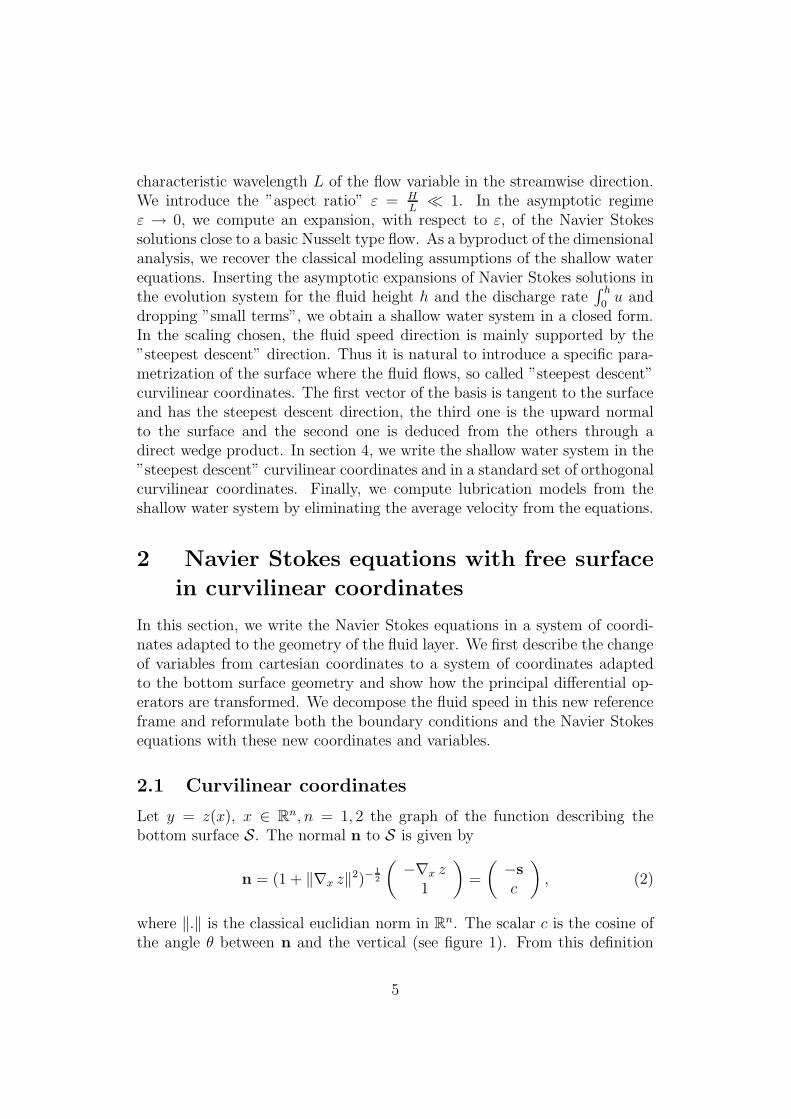
Let y = z(x), x ∈ Rn, n = 1, 2 the graph of the function describing the

bottom surface S. The normal n to S is given by

n = (1 + ‖∇x z‖2)−1

2

(−∇x z

1

)=

(−s

c

), (2)

where ‖.‖ is the classical euclidian norm in Rn. The scalar c is the cosine of

the angle θ between n and the vertical (see figure 1). From this definition

5

and c2 + ‖s‖2 = 1, we notice that

∂x c = −1

cst ∂x s, ∂xs = c(1 − sst) ∂2

xx z, ∂2xx z =

c2 Id + sst

c3∂x s. (3)

Here, Hb = c ∂2xx z denotes the curvature tensor of the bottom surface and

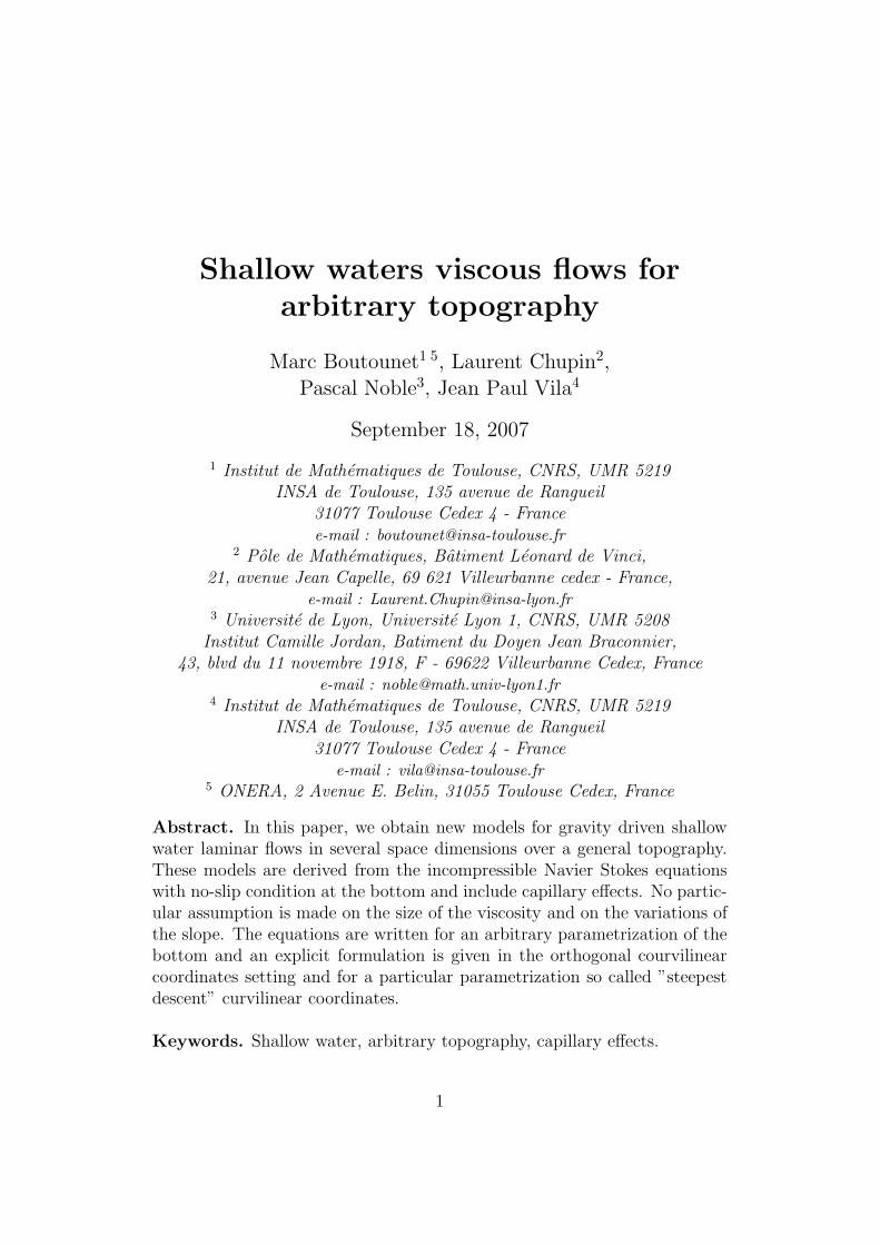
∂xs = (1 − sst)Hb. It is sometimes convenient not to work in cartesiancoordinates, but in a coordinate system adapted to the topography. This isthe point of view adopted here. In view of the fact that the models must besolved numerically, it is important to have some flexibility in the choice ofcoordinates and our models are written. In what follows, we assume that aparametrization of the bottom surface ξ ∈ R

n 7→ x(ξ) ∈ Rn is given.

xx

z(x)

ξ

h(ξ, t)

ξ

Ωt

θ

S

Figure 1: Curvilinear coordinates

Define ~ξ = (ξ, ξ), a new system of coordinates, where ξ ∈ Rn is a curvilinear

abscissa along the bottom and ξ ∈ R the signed distance in the directionof the normal. The horizontal coordinate x is given by the parametrizationξ 7→ x(ξ). Denote ∂ξ x the Jacobian matrix of the transformation. Weassume for convenience that det(∂ξ x) > 0. In what follows, the fluid domainΩt is defined as

~X ∈ Ωt ⇔ ~X(ξ, ξ) =

(x(ξ)

z(x(ξ))

)+ ξ

(−s(x(ξ))c(x(ξ))

), 0 ≤ ξ ≤ h(ξ, t), (4)

where h is the fluid height. In the sequel, we shall use the same notationsintroduced in [2].

6

It is natural to define new velocity components using a decomposition of thevelocity ~U by jacobian matrix:

~U =(∂~ξ

~X)

~V ⇐⇒

U = (∂ξX)V − V s,U = 1

cst (∂ξX) V + cV ,

(5)

with ∂ξX = (Id − ξ∂xs)∂ξ x, U, V ∈ Rn, U, V ∈ R. There are other possible

choices of decomposition: see [2] for further details.

Let us define the matrix A ∈ Mn+1(R) as

A =(∂~ξ

~X)−1

=

((∂ξX)−1 0

0 1

)(Id − s st c s

−st c

). (6)

For further reference, we compute M = AAt ∈ Mn+1(R):

M =

(M 00 1

), M = (∂ξ X)−1(Id − s st)(∂ξ X)−t ∈ Mn(R). (7)

The Jacobian J of the transformation is given by

J = det(∂~ξ~X) =

1

cdet(∂ξ X) = det(M)−

1

2 .

Let us describe how the principal differential operators used in the NavierStokes equations are transformed through this change of variables.

Lemma 1 For any vector field ~Z and any symmetric tensor σ = σt, the

differential operators transform according to

J∇ ~X . ~Z = ∇~ξ.(J A ~Z), ~U.∇ ~X = ~V .∇~ξ

, ∇ ~X = At ∇~ξ,

J A−t∇ ~X .σ = ∇~ξ.(JPA At) +J

2P : ∇~ξ(A At),

(8)

with P = A−tσA−1.

For the proof of this lemma, see [2].

2.2 Reformulation of the Navier Stokes equations

The Navier Stokes equations for the fluid velocity ~U and the pressure p inthe domain Ωt read

∂t~U + ~U.∇ ~X

~U + ∇ ~X p = −~g + µ∇ ~X . σ,

∇ ~X . ~U = 0.

(9)

7

Here σ = ∂ ~X~U + (∂ ~X

~U)t is the deformation tensor, µ measures the fluidviscosity and the vector ~g represents the gravity forces. The density of thefluid is supposed to be constant and set to 1. These equations come withboundary conditions. We aim to write the Navier Stokes equations (9) andboundary conditions in the reference frame introduced in the previous sectionwith the Jacobian decomposition of the velocity.

2.2.1 Boundary conditions

The Navier Stokes equations (9) come with boundary conditions at the bot-tom ξ = 0 and at the free surface ξ = h(ξ, t). More precisely, we assume ano-slip condition at the bottom

V (ξ, 0) = 0, V (ξ, 0) = 0, ∀ξ ∈ Rn. (10)

At the free surface ξ = h(ξ, t), we write that the fluid layer Ωt is advected by

the fluid speed ~V : this yields the mass conservation condition (or equivalentlyan impermeability condition):

ht + V (., h).∇ξ h = V (., h). (11)

The other boundary condition at the free surface ξ = h(ξ, t) is the continuityof fluid stress at that interface. For completeness, we take into account thecapillary effects. The atmospheric pressure patm is constant and set to zero.Then the continuity of fluid stress reads

(σ − p Id) ~N = κH ~N, ∀ξ = h(ξ, t). (12)

The scalar H is the mean curvature of the free surface, κ measures the capil-lary effects and ~N is the normal to the free surface. We are going to describemore precisely the continuity of fluid stress with the help of the new variablesand the Jacobian speed ~V . Let us first compute ~N .

Lemma 2 The unitary normal to the free surface ξ = h(ξ, t) is given by

~N = α At

(−∇ξ h

1

), (13)

where α−1 = ‖At

(−∇ξ h

1

)‖.

The proof of this lemma is straightforward and can be found in [2]. Nowassociated to the deformation tensor σ, introduce P as

P = A−t σ A−1 =

(P ZZt f

). (14)

8

Lemma 3 The terms P, Z, f of the tensor P = A−t σ A−1 with

σ = ∂ ~X~U + (∂ ~X

~U)t

are given by

Z = ∂ξ(M−1 V ) + ∇ξ V + 2 ∂xs

t(Id +s st

c2)(∂ξ X) V,

f = 2∂ξ V , P = Q + Qt,

where

Q = ∂ξ(M−1 V ) + ∂ξ

((∂ξ X)t

).((∂ξ X) V − V s

)

+(st

c(∂ξ X) V + cV

)∂ξ(

(∂ξ X)t

cs).

In the new system of coordinates, the continuity of the fluid stress (12) atthe free surface ξ = h(ξ, t) can be written

PhMh

(−∇ξ h

1

)− ph

(−∇ξ h

1

)= κH

(−∇ξ h

1

), (15)

where the subscript ph (resp. Ph,Mh) is the value of p (resp. P,M) at thefree surface. In the sequel, we shall note the value of flow unknowns at thefree surface with a similar subscript. Finally we can write the system (15) inthe form

µ Ph Mh ∇ξ h + µ Zh + ph Mh ∇ξ h = −κH∇ξ h,

−µ(Mh Zh)t ∇ξ h + µ fh − ph = κH.

(16)

2.2.2 Free divergence equation and momentum equation

In that section, we write the Navier Stokes equations using the curvilinearcoordinates and the Jacobian decomposition of the velocity. Using chainrules (8), the divergence free condition yields

J ∇ ~X . ~U = ∇~ξ.(J ~V ) = ∇ξ.(J V ) + ∂ξV = 0. (17)

Multiplying the momentum equation in (9) by the matrix A, one finds

∂t~V + A(~V .∇~ξ

)(A−1~V ) + M∇~ξp = −A~g

+µ

JM(∇~ξ

.(JPM) +J

2P : ∇~ξ

M). (18)

9

We decompose the advection term A(~V .∇~ξ)(A−1~V ) in the form

A(~V .∇~ξ)(A−1~V ) = ~V .∇~ξ

~V − ~Γ(~V ), (19)

with

~Γ(~V ) =

(Γ(~V )

Γ(~V )

)=

((∂ξ X)−1

(− (∂2

ξξX).V.V + 2V (∂ξs)V + Γ(~V )s)

−cV t(∂ξ x)t(∂2xx z) (∂ξ X) V

).

The momentum equation (18) can be written

∂t~V + ~V .∇~ξ

~V + M ∇~ξp =−A~g + ~Γ(~V )

+µ

JM(∇~ξ

. (JPM) +J

2P : ∇~ξ

M). (20)

Note that the vector ~Γ(~V ) has a physical interpretation: it represents thecentrifugal forces experienced by the fluid and associated to the change ofreference frame.

We aim to write a shallow water model for the fluid layer: that consists essen-tially in an equation of mass conservation and an equation for the streamwisevelocity averaged along the fluid height. For that purpose, we separate theequation on the horizontal (resp. vertical) velocity V (resp. V ) and obtainthe system

∂t V + ~V .∇~ξV + M ∇ξ p = −g c (∂ξ X)−1 s + Γ(~V )

+µ

JM(∇ξ.(JPM) + ∂ξ(JZ) +

J

2P : ∇ξM

), (21)

∂t V + ~V .∇~ξV + ∂ξ p = −g c + Γ(~V )

+µ

J

(∇ξ.(JMZ) + ∂ξ(J f) +

J

2P : ∂ξM

). (22)

2.3 Averaged equations

In what follows, we obtain exact evolution equations for the fluid height hand the streamwise velocity averaged along the fluid height. This system iscomposed of an equation on mass conservation and a momentum equation.Let us first write the equation on mass conservation with average quantities.

10

In the sequel, all the integrals computed are integrals of functions with respectto the crosstream variable ξ: for a function f(ξ, ξ), we shall note

∫f =

∫f(ξ, ξ) dξ, (23)

and the bounds of integration are specified for each calculation.

Integrating the divergence free condition (17) over (0, h) yields

Jh V h +

∫ h

0

∇ξ. (JV ) = Jh V h + ∇ξ.( ∫ h

0

J V)− Jh Vh.∇ξ h = 0. (24)

Here and in the sequel, the subscript Jh (resp. Vh, V h, ph,...) denotes thevalue of J (resp. V , V , p) at the free surface ξ = h(ξ, t). Using the massconservation condition (11), one finds

Jh∂t h + ∇ξ.( ∫ h

0

J V)

= 0. (25)

Since J is time independent, equation (25) can also be written

∂t(

∫ h

0

J) + ∇ξ.( ∫ h

0

J V)

= 0. (26)

In order to write the mass conservation equation in a simple form, we intro-duce the average quantities

h =

∫ h

0

J, h v =

∫ h

0

J V,

and the mass conservation equation (26) reads

ht + ∇ξ.(h v)

= 0. (27)

In the following, we shall write an evolution system for the more naturalquantities (h, hv). We will see later that under suitable hypothesis, we can

deduce h and∫ h

0V from h and hv. Integrating the left hand side of equation

(21) over the interval (0, h) yields

∫ h

0

J(∂t V + ~V .∇~ξV + M ∇ξ p) = ∂t(

∫ h

0

JV ) +∇ξ.(

∫ h

0

JV ⊗ V )

+∇ξ.(

∫ h

0

JM p)−∫ h

0

p∇ξ.(JM)

+Jh(ht + Vh.∇ξ h − V h)Vh − JhphMh∇ξh. (28)

11

Furthermore, we integrate the right hand side of (21) and use the boundaryconditions (16). We find

∂t

(∫ h

0

J V)

+∇ξ.(∫ h

0

JV ⊗ V + JpM)

=

−gc

∫ h

0

J(∂ξ X)−1s−µ J0M0Z0 +

∫ h

0

J Γ(~V ) +

∫ h

0

p∇ξ.(JM)

+µ

2

∫ h

0

JM(P : ∇ξM) − µ

∫ h

0

J (∂ξM) Z

+ µ∇ξ.

∫ h

0

JMPM − µ

∫ h

0

JPM :: ∂ξ M

+ µJhMhZh − µJhMhPhMh∇ξ h + JhphMh∇ξh,(29)

where (A :: ∂ξB) is the operator defined by (A :: ∂ξB)i = tr(A∂ξBi), Bi

being the i − th column of B. The continuity of the fluid stress at the freesurface yields

µJhMhZh − µJhMhPhMh∇ξ h + JhphMh∇ξh = −κHJhMh∇ξh.

As a consequence, the equation for the average momentum∫ h

0J V = hv

reads

∂t

( ∫ h

0

J V)+∇ξ.

(∫ h

0

JV ⊗ V + JpM)

+ κHJhMh∇ξh =

− gc

∫ h

0

J(∂ξ X)−1s − µ J0M0Z0 +

∫ h

0

J Γ(~V )

+

∫ h

0

p∇ξ.(JM) +µ

2

∫ h

0

JM(P : ∇ξM) − µ

∫ h

0

J (∂ξM) Z

+ µ∇ξ.

∫ h

0

JMPM − µ

∫ h

0

JPM :: ∂ξ M. (30)

This equation is exact and no approximation has been done for the momentin order to obtain an evolution system for (h, hv) in a closed form: this shallbe done in the forthcoming section.

3 Shallow water asymptotics

In the following, we derive the shallow water equations from the Navier Stokessystem (17,18) and boundary conditions (10,11,16): scaling these equations,

12

we shall precise in which parameter regime the classical assumptions madefor the derivation of the shallow water equations (hydrostatic pressure, qua-sistationnary flow) hold true. Then we compute an asymptotic expansionof the Navier Stokes equations with respect to the aspect ratio ε = H

L≪ 1

between the characteristic height of the fluid and L the characteristic wave-length of the solutions: inserting these approximations into the averagedequation (30) and dropping ”small” terms, we deduce an evolution system

for h and hv =∫ h

0J V in a closed form.

3.1 Scaling of the equations

Let U0 and H be respectively the characteristic velocity and height of a flow.We define classically some dimensionless numbers, respectively the Froudenumber F, the Reynolds number Re and the Weber number We:

F =U0√g H

, Re =H U0

µ, We =

H U20

κ. (31)

We do not precise here the characteristic speed U0: nevertheless, severalchoices are possible. As an example for an inclined plane with a non zeroslope φ, the stationnary Nusselt solution is given by

h = H, V = 0, V =g sin(φ)

µ(Hξ − ξ

2

2).

Thus in that case a typical choice of speed U0 could be U0 =g H2

2µsin(φ) and

F2 =Re

2.

In the sequel, we consider functions with a characteristic wavelength Lsuch that the aspect ratio ε = H/L ≪ 1. We introduce the scaling

x = Lx, ξ = Lξ, h = Hh, ξ = Hξ, t =L

U0

t

V = U0V , V =H

LU0V , p = gHp.

(32)

Let us describe the bottom surface in that scaling. In order to deal witharbitrary topography, we will suppose that s = O(1). This means that∇x z = O(1) and imposes the scaling on z = Lz. Let us describe the curva-ture of the bottom surface. Here, we want to separate the long wavelengthassumption on the free surface and the curvature of the bottom surface. For

13

that purpose, we assume that the curvature of the surface is of order O(1/R)where R is the characteristic radius of curvature of the bottom surface andis not necessarily of order O(L). Then, the derivatives ∂xs and ∂2

xxz areO(1/R). Let us introduce the ratio θR = L

Rbetween the characteristic wave-

length of flow variables and R the characteristic curvature of the bottomsurface, and define the rescaled bottom curvature Hb = θR

LHb. We shall see

later that chosing different values for θR yields different type of models, inparticular the influence of capillarity.

Here we have introduced the parameter θR coherent with the scaling, whichdescribes the typical curvature of the bottom surface. It is important tonote that we have made no restriction on the amplitude of the inclinationand curvature of the bottom: the size of these parameters with respect to ε,especially the characteristic curvature θR, will be discussed at the end of thepaper to distinguish different models.

For the other quantities Γ,H, P, Z, f , we choose the natural scaling:

Γ =U2

LΓ, H =

1

LH, P =

U

LP , f =

U

Lf , Z =

U

HZ.

Now we write the Navier Stokes equations in a non dimensional form. Drop-ping the ∼ from the equations (21),(22), we find:

∂t V + ~V .∇~ξV +

M

F2∇ξ p = − 1

εF2c(∂ξ X)−1s

+ (∂ξ X)−1(θRΓ(~V )s− (∂2

ξξX).V.V + 2ε θRV (∂ξs)V)

+1

JεRe

(∂ξ(JZ) + ε2

(∇ξ.(JPM) +

J

2P : ∇ξ M

)),(33)

∂tV + ~V .∇~ξV +1

ε2 F2∂ξp = − 1

ε2 F2c +

θR

εΓ(~V )

+1

JεRe

(∇ξ.(JMZ) + ∂ξ(Jf) +

J

2P : ∂ξM

). (34)

Note that, in these equations, the rescaled quantities related to the changeof reference frame are given by

J =det(∂ξ x)

cdet(Id − εθRξ(∂xs)

), ∂ξ X =

(Id − εθRξ(∂xs)

)∂ξ x,

M = (∂ξ x)−1(Id − εθRξ(∂xs)

)(Id − s st)

(Id − εθRξ(∂xs)

t)(∂ξ x)−t,

(35)

14

whereas the rescaled quantites associated to the flow variables read:

Z = ∂ξ(M−1V ) + 2εθR(∂ξs)

t(Id +s st

c)∂ξ X V + ε2∇ξV ,

f = 2∂ξV , P = Q + Qt,

(36)

with Q defined as

Q = ∂ξ(M−1V ) + ∂ξ

((∂ξ X)t

).((∂ξ X) V − εV s

)

+(st

c(∂ξ X) V + ε cV

)(∂ξ X)ts

c. (37)

The particular choice of characteristic velocity for the vertical velocity Vimplies that the divergence free condition (17) is preserved under that scaling

∇ξ. V + ∂ξV = 0. (38)

We write the rescaled boundary conditions at the bottom ξ = 0 and at thefree surface ξ = h(ξ, t). On the one hand, the no slip conditions at thebottom and the impermeability condition (see (10) and (11)) are unchangedunder the shallow water scaling:

V (., ξ = 0) = 0, V (., ξ = 0) = 0,

∂t h + Vh.∇ξ h = V h.(39)

On the other hand, the continuity of fluid stress (16) at the free surface reads

ε

F2phMh∇ξ h +

1

ReMhZh −

ε2

ReMhP hMh∇ξ h = −ε2H

WeMh∇ξ h,

ε

Re

(fh − (MhZh)

t∇ξ h)− 1

F2ph =

εHWe

.

(40)

Finally, we write the nondimensional counterpart of the averaged equations(26) and (30): this yields exact evolution equation for

h =

∫ h

0

J, hv =

∫ h

0

J V (41)

where h, J, V are the rescaled flow variables. The dimensionless continuityequation reads

∂t(

∫ h

0

J) + ∇ξ.( ∫ h

0

J V)

= 0. (42)

15

Integrating the equation (33) over the interval (0, h) and using the rescaledboundary conditions yields the averaged momentum equation:

∂t

( ∫ h

0

JV)

+ ∇ξ.(

∫ h

0

JV ⊗ V ) +1

F2∇ξ.(

∫ h

0

JpM) +εHWe

JhMh∇ξ h =

− 1

εF2c

∫ h

0

J(∂ξ X)−1s− 1

εReJ0∂ξV0

+

∫ h

0

J(∂ξ X)−1(θRΓ(~V )s− (∂2

ξξX).V.V + 2εθRV (∂xs)V)

(43)

+1

F2

∫ h

0

p∇ξ.(JM)− 1

εRe

∫ h

0

J(∂ξ M) Z

+ε

Re

(∇ξ.

∫ h

0

JMPM +

∫ h

0

J

2M(P : ∇ξ M) − JPM :: ∂ξM

).

3.2 Asymptotics

In the sequel, we write an evolution system for h =∫ h

0J and hv =

∫ h

0JV .

Recall the continuity equation (42)

∂t h + ∇ξ. (hv) = 0. (44)

We shall write an approximate evolution equation for hv using (43). For thatpurpose, we assume that the aspect ratio ε = H

L≪ 1 and we introduce the

dimensionless parameters

α =εF2

Re, β = εRe, δ =

εRe

F2, λ =

Re

F2, κ =

εF2

We. (45)

From the assumption ε ≪ 1 and considering that the Reynolds number Re

and the Froude number F are of order 1, we deduce that α, β, δ ≪ 1 andλ = O(1). In fact, we shall see later that the expansions carried out in whatfollows remain valid provided that α, β, δ ≪ 1: thus, the range of validity ofthe models obtained here is not restricted to Reynolds and Froude numbersof order one. In particular, we can choose Re → ∞ as ε → 0. To see theinfluence of the capillary effects, we shall assume that κ = O(1).

We now study the influence of the shallow water scaling on the Navier Stokesequations. Using the equation (34), a straightforward computation yields anequation for the pressure:

16

∂ξp + c=α

J

(∇ξ.(JMZ) + ∂ξ(Jf) +

J

2P : ∂ξM

)

+θRβ

λΓ(~V ) − αβ(∂tV + ~V .∇~ξV ) := Ψp(~V , ~ξ, t). (46)

In the asymptotic regime α, β ≪ 1, θR, λ = O(1), we clearly recover theclassical assumption of hydrostatic pressure made in the derivation of shallowwater equations. Moreover, the continuity of the fluid stress at the freeboundary ξ = h implies that the pressure at the free surface is given by (seeequation (39)):

ph = −κH + α(fh − (MhZh)

t∇ξ h)

:= Πp(~Vh, ξ, t). (47)

Integrating (46) with the boundary condition (47), one finds

p = c(h − ξ) + Πh(~Vh, ξ, t) −∫ h

ξ

Ψp(~V , ~ξ, t). (48)

If we consider that the derivatives of h, V, V are bounded and of order O(1),one can see that p is determined up to order one and that

p = c(h − ξ

)− κH + O

(α +

θR

λβ)

= p(0) + O(α +

θR

λβ). (49)

Let us now see the influence of the scaling assumption ε, α, β, δ ≪ 1 on thevelocity profile. Expanding rescaled quantities in (35),(36) with respect toε, α, β, δ ≪ 1 and λ, κ = O(1), we find for the rescaled quantities associatedto the change of reference frame

J = J(1 − εθR ξ tr(∂x s)

)+ O(ε2θ2

R),

∂ξ X = ∂ξ x − εθR ξ (∂ξs) + O(ε2θ2R),

M = M + 2εθR ξ (∂ξ x)−1((Id − s st)Hb(Id − s st)

)(∂ξ x)−t + O(ε2θ2

R),

with J =det(∂ξ x)

cand M = (∂ξx)−1(Id − sst)(∂ξx)−t. The rescaled quan-

tities related to the flow unknows have the expansion

h = Jh − εθRJtr(∂x s)h2

2+ O(ε2θ2

R)

Z = M−1

∂ξV − 2εθR (∂ξ x)tHb(∂ξ x) ξ (∂ξV ) + O(ε2θ2R + ε2), (50)

17

Note that from the expansion of h, we can easily obtain an expansion of thephysical fluid height h:

Jh = h + εθRtr(∂x s)h2

2J+ O(ε2θ2

R).

Now we insert the previous expansions into the equation (33) and find

∂2ξ ξ

(JV )−λ cJ(∂ξ x)−1s = βJ(∂t V + ~V .∇ξ V − Γ(~V )) + δJ M∇ξ p

− δθRξ cJ(∂ξ x)−1(tr(∂x s)Id + ∂xs

)s

+ εθRJ(tr(∂xs)∂ξ(ξ∂ξV ) − 2(∂ξ x)−1(∂xs)(∂ξ x) ∂ξV

)

+ 2εθRJ(∂ξ x)−1 (∂xs) (∂ξ x)∂2ξ ξ

(V ) + O(ε2 + ε2θ2R). (51)

In order to simplify the notations, we shall define the right hand side of(51) as ΨV (~V , p, ~ξ, t) and (51) reads

∂2ξ ξ

(JV ) − λ cJ(∂ξ x)−1s = ΨV (~V , p, ~ξ, t). (52)

The continuity of the fluid stress at the free boundary ξ = h implies (seeequation (39)):

Zh = αδ(P hMh −

(fh − (MhZh)

t∇ξ h)Id)∇ξ h = O(ε2),

∂ξVh = 2εθR(∂ξ x)−1(∂xs)(∂ξ x) h∂ξVh + O(ε2 + ε2θ2R) = Πv(~Vh, ξ, t). (53)

The no-slip condition yieldsV0 = 0. (54)

Integrating (52) with respect to the cross stream variable ξ with the boundaryconditions (53,54), one obtains

V = −λ c(hξ − ξ2

2) (∂ξ x)−1s− 1

J

∫ ξ

0

∫ h

z

ΨV (~V , p, ~ξ, t) + ξΠv(~Vh, ξ, t). (55)

It is easily seen that up to order one in ε, α, β, δ, the streamwise speed V isuniquely defined by

V = −λ c(hξ− ξ2

2) (∂ξ x)−1s+O(εθR +β + δ) = V (0) +O(εθR +β + δ). (56)

18

Up to order one, the profile of the streamwise speed V is parabolic with re-spect to the variable ξ, when the bottom surface is an inclined plane, thiscorresponds exactly to a Nusselt stationnary flow. In the present case, theflow is locally close to a Nusslet type flow which is a local equilibrium. Thusthe scaling assumption ε ≪ 1 implies that at each time, the solution is closeto a local equilibrium: that is the other classical assumption made in thederivation of shallow water equations.

Finally we obtain an asymptotic expansion for V by integration of the diver-gence free condition ∇ξ .V + ∂ξV = 0 with the no-slip condition V (ξ, 0) = 0.One easily obtains

V = −∫ ξ

0

∇ξ.V = V(0)

+ O(β + δ + εθR), (57)

with V(0)

= −∫ ξ

0∇ξ.V

(0).

We describe now the method to derive shallow water equations from theincompressible Navier Stokes equations in the parameter regime describedbefore: the method is mainly based on an iterative scheme. First, based on

equations (48,55,57), we define the sequence of functions (V (n), V(n)

, p(n))n∈N

by

V (0) =−λ c(hξ − ξ2

2) (∂ξ x)−1s,

V(0)

=

∫ ξ

0

∇ξ.V(0) dz,

p(0) = c(h − ξ

)− κH. (58)

Then at the (n + 1)-step, the functions (V (n+1), V(n+1)

, p(n+1)) are definedas

V (n+1) = V (0) − 1

J

∫ ξ

0

∫ h

z

ΨV (~V (n), p(n), ~ξ, t)ds dz + ξΠv(~V(n)h , ξ, t),

V(n+1)

=−∫ ξ

0

∇ξ.V(n+1) dz,

p(n+1) = c(h − ξ) + Πh(~V(n+1)h , ξ, t) −

∫ h

ξ

Ψp(~V(n+1), ~ξ, t) dz. (59)

19

Then, this sequence of functions converges formally to (V, V , p) a solution ofthe Navier Stokes equations. More precisely, denote F the operator so thatthe iterative scheme define previously reads

(V (n+1), V

(n+1), p(n+1)

)= F

(V (n), V

(n), p(n)

). (60)

Then any solution(V, V , p

)of the Navier Stokes equations with boundary

conditions is a fixed point of F . Moreover, this operator is O(α+β + δ + ε+εθR)-Lipschitz on any bounded set. As a consequence, and provided that the

sequence (V (n), V(n)

, p(n)) and the derivatives of the Navier Stokes solutionsremain uniformly bounded with respect to α, β, δ, ε, εθR, one can prove byinduction the following estimate

max(|V − V (n)|, |V − V(n)|, |p− p(n)|) = O

((α + β + δ + ε + εθR)n+1

). (61)

As a consequence, we obtain an asymptotic expansion of V, V , p with respectto ε, α, β, δ to any order in ε, α, β, δ. This step of the computation can beimplemented using a formal computation software. Using this expansion, weeasily deduce an expansion of v and compute an expansion of the differentterms in the average equation (43). Dropping terms in this equation of afixed order, we obtain a hierarchy of models. In what follows, we computethe shallow water model obtained by dropping all small terms in the averageequation. We shall see that an approximation of V, p up to order one isneeded to carry out such a computation. Let us first compute the zerothorder approximation of V, p and see which terms we keep in (43).

3.2.1 Asymptotic to order 0

In that section, we compute the zeroth order approximation of V, p and checkwhich terms we keep in (43). Recall that V = V (0) + O(β + δ + ǫθR) with

V (0) = −λ c(hξ − ξ2

2)(∂ξ x)−1s. (62)

We can compute an approximation of v:

hv =

∫ h

0

J V =

∫ h

0

J V (0) + O(εθR + β + δ)

=−λ c J(∂ξ x)−1s

∫ h

0

(hξ − ξ2

2) + O(εθR + β + δ)

=−λ c Jh3

3(∂ξ x)−1s + O(εθR + β + δ). (63)

20

Then up to zeroth order, we find that

v = −λ c(∂ξ x)−1sh2

3J2 .

We calculate the zeroth order approximation of the other terms in the lefthand side of (43) as functions of h, v.

The advection term∫ h

0J V ⊗ V reads:

∫ h

0

J V ⊗ V =J

∫ h

0

V (0) ⊗ V (0) + O(εθR + β + δ),

=λ2c2J(∂ξ x)−1s⊗ (∂ξ x)−1s

∫ h

0

(hξ − ξ2

2)2 + O(εθR + β + δ),

=2λ2c2

15

h5

J4 (∂ξ x)−1s⊗ (∂ξ x)−1s + O(εθR + β + δ),

=6

5hv ⊗ v + O(εθR + β + δ). (64)

Integrating the pressure equation (46) with the boundary condition (47), oneproves that the pressure p is given by

p = −κH + c(h − ξ) + O(εθR + α). (65)

Up to zeroth order, the average terms containing the pressure are given by:∫ h

0

J p M = J M(ch2

2− κHh

),

∫ h

0

p∇ξ.(J M) = ∇ξ.(J M)(ch2

2− κHh

).

(66)

As a consequence, the average equation (43) reads:

∂t (h v) +6

5∇ξ.(hv ⊗ v) +

δ

βJ M∇ξ(c

h2

2J) − κ

δ

βhM∇ξH =

− 1

β

(λc

∫ h

0

J(∂ξX)−1s + J∂ξV (0))

+

∫ h

0

J(∂ξX)−1(θRΓ(~V )s− (∂2

ξξX).V.V)

− 1

β

∫ h

0

J(∂ξM) Z + O((εθR + α)

δ

β+ β + δ + εθR

). (67)

21

It is a straightforward computation to prove that the zeroth order terms inthe right hand side of (67) read

∫ h

0

J(∂ξ X)−1(θRΓ(~V )s− (∂2ξξ X).V.V ) =

− 2h5

15J4λ2c2(∂ξ x)−1

((∂2

ξξx).(∂ξ x)−1s.(∂ξ x)−1s + θR (stHb s) s)

+ O(εθR + β + δ).

1

β

∫ h

0

J(∂ξ M) Z = − δ

βc(∂ξ x)−1 (∂x s) s

h2

J+ O

(εθR

β(δ + δθR + β + εθR)

).

Due to the presence of the factor − 1β

in front of λ c∫ h

0J(∂ξ X)−1s+J∂ξV (0),

we need an expansion of the wall shear ∂ξV (0) and the average velocity v upto order 1 in order to eliminate ∂ξV (0) from (67). This is done in the nextsection.

3.2.2 Asymptotic to order 1

This section is devoted to the computation of an asymptotic expansion of Vup to order one: this enables us to compute v and ∂ξV (0) as function of h, ξand ε, α, β, δ up to order one. We can then insert the resulting expressionsin (67): dropping small term, we find a shallow water model for arbitrarytopography.

We first prove that

λ c

∫ h

0

J(∂ξ X)−1s = λ ch(∂ξ x)−1s + δθR ch2

2J(∂ξ x)−1(∂xs) s + O(ε2θ2

R).

Using the iterative scheme described in the previous section, we find after anintegration on (ξ, h) and up to order one:

∂ξ(JV ) + λ cJ(∂ξ x)−1s(h − ξ) = J

∫ h

ξ

β(Γ(~V (0)) − ∂tV

(0) − ~V (0).∇~ξV (0)

)

− δM∇ξ p(0) + δθRcJ(∂ξ x)−1(tr(∂xs)Id + ∂xs)s

∫ h

ξ

z dz

+ εθRJtr(∂xs)ξ(∂ξV )(0) + 2εθRJ(∂ξ x)−1(∂xs)(∂ξ x) V (0)

+ 2εθRJ(∂ξ x)−1(∂xs)(∂ξ x)∂ξ(ξV(0))

+O(ε2θ2

R + β(β + δ + εθR) + δ(α + εθR)). (68)

22

Setting ξ = 0 in (68), one obtains an expansion for ∂ξV (0):

J∂ξV (0) + λ ch(∂ξ x)−1s = δ P1 + βλ P2 + P3, (69)

with Pi defined by

P1 = θR c(∂ξ x)−1 (∂xs) sh2

2J− J M

(∇ξ(ch − κH)h −∇ξ c

h2

2

)

P2 = Jc(∂ξ x)−1sht

h2

2− λc∇ξ.(Jc(∂ξ x)−1s)

h5

120+ λc∇ξ.(Jch(∂ξ x)−1s)

h4

120

− Jλc2(∂ξ x)−1((∂2

ξξx).(∂ξ x)−1s.(∂ξ x)−1s + θR(st Hb s)s)2h5

15

−λcJ(∂ξ x)−1s.∇ξ(ch(∂ξ x)−1s)5h4

24+ λcJ(∂ξ x)−1s.∇ξ(c(∂ξ x)−1s)

3h5

40.

P3 =O(ε2θ2

R + β(β + δ + εθR) + δ(α + εθR)), (70)

Let us now compute an asymptotic expansion for hv up to order one.

Integrating twice equation (68) on ∂ξV , we can prove that

∫ h

0

JV + λ cJ(∂ξ x)−1sh3

3= δQ1 + βλQ2 + Q3, (71)

with Qi given by

Q1 = θR cJ(∂ξ x)−1(∂xs) sh4

4− θR cJ(∂ξ x)−1(∂xs) s

5h4

12

+ θRJc(∂ξ x)−1(tr(∂xs)Id + (∂xs)

)s5h4

24− θRcJtr(∂xs)(∂ξ x)−1s

h4

12

− J M(∇ξ(ch − κH)

h3

3−∇ξ c

5h4

24

),

Q2 = cJ(∂ξ x)−1sht

5h4

24

− Jλ c2(∂ξ x)((∂2

ξξx).(∂ξ x)−1s.(∂ξ x)−1s + θR(stHbs)s)2h7

35

−λ cJ(∂ξ x)−1s.∇ξ(ch∂ξ x−1s)11h6

120+ λ cJ(∂ξ x)−1s.∇ξ(c(∂ξ x)−1s)

29h7

840

+ λ c∇ξ.(Jch(∂ξ x)−1s)(∂ξ x)−1sh6

60− λ c∇ξ.(Jc(∂ξ x)−1s)(∂ξ x)−1s

3h7

840,

Q3 =O(ε2θ2

R + β(β + δ + εθR) + δ(α + εθR)). (72)

23

Moreover, it is easily seen that we can deduce hv from∫ h

0JV dξ with the

equation:

hv =

∫ h

0

JV − εθR

∫ h

0

tr(∂xs)ξV(0) + O

(εθR(β + δ + ǫθR)

). (73)

Finally we have

λ cJ(∂ξ x)−1sh3

3= λ c(∂ξ x)−1s

h3

3J2 + δθR c tr(∂xs)(∂ξ x)−1s

h4

2J2 + O(ε2θ2

R).

(74)

Using equations (71), (73) and (74), one finds an expansion for hv up to

order one as function of h, ξ and (ε, α, δβ). Similarly, equation (69) givesan expansion of ∂ξV (0) up to order one: thus we can eliminate ∂ξV (0) fromequation (67) to obtain a shallow water model. We shall see later that thereare different ways of eliminating ∂ξV (0) which gives a family of models. Moreprecisely, from (71), (73), (74) and (69), we define R1 and R2 the terms oforder one such that

J∂ξV (0) =−λ ch(∂ξ x)−1s− R1(h, ξ)

+O(ε2θ2

R + β(β + δ + εθR) + δ(α + εθR)),

hv =λ ch3

3J2 (∂ξ x)−1s − R2(h, ξ)

+O(ε2θ2

R + β(β + δ + εθR) + δ(α + εθR)), (75)

From (75), we compute an expansion of ∂ξV (0) up to order one involving

the average quantities h, v, the variable ξ and the parameters α, β, δ, ε:

−J∂ξV (0) =−3J2

hv + R1(h, ξ) − 3J

2

h2R2(h, ξ)

+O(ε2θ2

R + β(β + δ + εθR) + δ(α + εθR)), (76)

Inserting (76) into (67), one finds

24

∂th +∇ξ.(hv) = 0,

∂t(hv) +6

5∇ξ.(hv ⊗ v) +

δ

βJM∇ξ (c

h2

2J) − κ

δ

βhM∇ξH =

− 1

β

(λ ch(∂ξ x)−1s +

3J2

hv)

+ T1 + R, (77)

with

R = O( 1

β

(ε2θ2

R + δ(α + εθR

)+ β + δ + εθR

).

The function T1 depends on ξ and h and reads:

T1 =δ

βT (1)

1 + λ2T (2)1 ,

with

T (1)1 =

(M

8∇ξ c +

3

4c(∂ξ x)−1(∂xs) s− 5

8c(∂ξ x)−1(∂xs)s −

c

2tr(∂xs)(∂ξ x)−1s

) h2

J

T (2)1 = c(∂ξ x)−1s.∇ξ(c(∂ξ x)−1s)

h5

35J4 − c(∂ξ x)−1s.∇ξ(c

h

J(∂ξ x)−1s)

h4

15J4

+(∇ξ.(c

h3

J3 (∂ξ x)−1s)

h2

24J2 + ∇ξ.(ch(∂ξx)−1s)

h4

120J4

)c(∂ξ x)−1s

−∇ξ.(Jc(∂ξ x)−1s)h5

420J5 c(∂ξ x)−1s

− 6

35c2(∂ξ x)−1

(∂2

ξξx.(∂ξ x)−1s.(∂ξ x)−1s + θR(st Hb s)s) h5

J4 . (78)

We easily see that provided that the dimensionless numbers Re, F, κ are oforder one, the high order terms are of order O(ε) and it is negligible in thescaling limit ε ≪ 1. Then dropping these high order terms, one finds ashallow water model for h, hv in a closed form. Furthermore, we clearly seethat the conclusion of the expansion remains true if we only suppose that

α, β, δ, εθR ≪ 1 andε2θ2

R

β, δ

βα, δ

βεθR ≪ 1. As a consequence, the model re-

mains is not only valid for Reynolds and Froude numbers of order one butalso for Re,F → ∞ as ε → 0 provided that we choose a suitable dependenceof Re,F with respect to ε.

25

This formulation has the advantage of being independent of the parametriza-tion of the bottom surface S but it is quite hard to work with that for-mulation. In order to carry out numerical simulations, we have to specifycurvilinear coordinates. In the sequel, we are going to choose particularparametrizations of the bottom surface S. Moreover, we shall be more pre-cise on the asymptotic expansion of the mean curvature of the free surfaceH with respect to ε, ξ and h,Hb: this will be done in the next section for aparticular parametrization.

4 Shallow water models for particular para-

metrizations

In this section, we parametrize the bottom surface with two systems of co-ordinates: the ”steepest descent” curvilinear coordinates and the classicalorthonormal coordinates. We write the shallow water equations in this frame-work for n-dimensional flows (n = 2 or n = 3) which gives (n−1)-dimensionalshallow water equations.

4.1 Shallow water equations in the steepest descent

parametrization

In what follows, we describe the ”steepest descent” curvilinear coordinatesand write the shallow water equations in that setting. First, we define θ, φsuch that the normal n to the surface S is given by (see part 2.1):

n =

− ∇x z√

1 + ‖∇x z‖2

1√1 + ‖∇x z‖2

⇐⇒ n =

sin(θ) cos(φ)sin(θ) sin(φ)

cos(θ)

. (79)

Here θ represents the local inclination of the bottom surface. We are goingto use the ”steepest descent” curvilinear coordinates ξ1, ξ2 so that we have

∂x

∂ξ1

= cos(θ) cos(φ),∂x

∂ξ2

= − sin(φ),

∂y

∂ξ1= cos(θ) sin(φ),

∂y

∂ξ2= cos(φ).

or equivalently

26

∂ξ x =

(cos(θ) cos(φ) − sin(φ)cos(θ) sin(φ) cos(φ)

).

This system of coordinates is uniquely defined provided that a ”steepestdescent” direction exists: this condition is satisfied if s 6= 0. This direction isat the intersection of the tangent plane to the bottom surface and the planespanned by the normal to the surface and the gravity vector: we shall see laterthat it is the principal direction where the fluid flows. As a consequence ofthat definition, we see that this system of coordinates is designed for gravitydriven flows but is not relevant for fluids driven by other external forces. Inthat system of coordinates, the rescaled quantities J, M associated to thechange of reference frame are particularly simple. It is easily proved that

J = 1, M = Id, c(∂ξ x)−1 s = − sin(θ) e1,

with e1 = (1, 0)t.

Let us now compute an asymptotic expansion for the rescaled curvature ofthe free surface. Using lemma 2, the rescaled unitary normal ~N to the free

surface reads ~N =~n

‖~n‖ with

~n =

(−s − ε(Id − sst)(∂ξx)−t∇ξh

c − ε(c(∂ξx)−1s

)t∇ξh

)+ O

(ε2θR

). (80)

Then the rescaled mean curvature is given by

(n − 1)H=divx

((sε(Id − sst)(∂ξx)−t∇ξh)/‖~n‖

),

= θRtr((∂ξx)−1∂ξs

)+ εtr

((∂ξx)−1∂ξ

((∂ξx)∇ξh

))+ O(ε2). (81)

As a consequence, the expansion of H with respect to ε is given by

H = θR Hb +ε

n − 1

(∆ξ h + θR∇ξh.Vθ,φ

)+ O(ε2), (82)

with Vθ,φ =(cos(θ) sin(2φ)∂2 φ − tan(θ)∂1 θ,− ∂1φ

cos(θ)

)t.

Here, θR Hb represents the mean curvature of the bottom surface. At thisstage, two situations occur. Either θR = O(1): in that case the mean curva-ture of the free surface is, up to order one, given by the mean curvature ofthe bottom surface:

27

H = −1

2

( ∂θ

∂ξ1+ sin(θ)

∂φ

∂ξ2

)+ O(ε).

In that particular case, the shallow water equations (77) have the more ex-plicit form:

∂th +∇ξ.(hv) = 0,

∂t(hv) +∇ξ.(6

5hv ⊗ v − λ2 sin2(θ)h5

75e1 ⊗ e1

)+

δ

2β∇ξ(cos(θ)h2) =

−κδθR

2βh∇ξ.(∂1θ + sin(θ)∂2φ) +

1

β

(λh sin(θ) e1 −

3v

h

)

+δ

βh2 sin(θ)

(−θR

2(∂1θ + sin(θ)∂2φ) + θR−1

8∂1φ

−18(∂2θ − θR sin(θ)∂1φ)

)

− 6

35λ2h5 sin2(θ)

((θR − 1) tan(θ)∂1θ

cos(θ)φ1

)

− 3

175λ2h5 sin(θ) cos(θ)∂1θ e1. (83)

If we restrict our attention to a 2-dimensional flow for the Navier Stokessystem and θR = 1, we easily get the one dimensional shallow water model

∂th + ∂ξ(hv) = 0,

∂t(hv) + ∂ξ

(6

5hv2 − λ2 sin2(θ)h5

75+

δ cos(θ)h2

2β

)+ κ

δ

βh∂2

ξξ θ =

1

β

(λh sin(θ) − 3v

h

)−( δ

2β+

3λ2h3

175cos(θ)

)sin(θ)∂ξθ. (84)

Here the ξ variable is the classical curvilinear coordinate. We clearly see thatno contribution including third order derivatives of h appears in the capil-lary term. In that case, the capillary effects are essentially supported by thecurvature of the bottom surface which is assumed to be not small: capillarityis not dispersive in that case and acts as a classical friction or damping term−κ h∇ξ Hb, depending on the mean curvature sign of the bottom surface.

In order to recover the classical ”dispersive” capillary term involving thirdorder derivatives of h, let us assume that the curvature of the bottom issmall: more precisely we consider θR = εθR. In this particular case, we find:

28

H = ε θR Hb +ε

n − 1∆ξ h + O(ε2). (85)

Then, the contribution of the capillarity term in (77) is negligible if κ = O(1):we only see the influence of the capillary terms provided that εκ = O(1).Denote κ = εκ, the capillary term in (77) reads:

−κδ

βh∇ξH = −κ

δ

βh∇ξ

(θR Hb +

1

n − 1∆ξ h

)+ O(ε). (86)

In the case of shallow water flows over a flat and horizontal bottom, weclearly recover the classical form of the capillary term −κ δ

βh∇∆ h found in

the literature: see [3, 4] for a mathematical analysis of shallow water modelswith this kind of capillary term and references therein.

4.2 Shallow water equation in orthogonal coordinates

In the literature, the shallow water equations or lubrication model over vary-ing topographies are usually written using orthogonal curvilinear coordinates.In order to compare our results with several shallow water equations obtainedpreviously [9, 10], we write the shallow water equations using the orthogonalcoordinates. In that setting, the basis vectors of the tangent plane to thebottom surface are directed along the directions of maximal and minimalcurvatures.

Denote mi = ‖∂ x(ξ)∂ξi

‖ and hi = mi(1 − εθR kiξ) where ki is the meancurvature of the bottom in the direction ξi. In order to simplify the discus-sion, let us choose an orthogonal system so that mi = 1. Then, if we denoten =

(sin(θ) cos(φ), sin(θ) cos(φ), cos(θ)

), we easily establish that

M = Id, J = 1, c(∂ξ x)−1s = − sin(θ)

(cos(φ)sin(φ)

)= − sin(θ)ι, (87)

where ι = (cos(φ), sin(φ))t. In this particular case, the shallow water equa-tions (77) have the more explicit form:

29

∂th +∇ξ.(hv) = 0,

∂t(hv) +∇ξ.(6

5hv ⊗ v

)+

δ

2β∇ξ(cos(θ)h2) = κ

δ

βh∇ξ.H +

1

β

(λh sin(θ) ι − 3v

h

)

+δ

β(1

4∇ξ cos(θ) + θR sin(θ)(k1 + k2)ι −

3

2θR sin(θ)diag(k1, k2)ι)

h2

2

+ λ2 sin2(θ)(ι.∇ξ h)ιh4

15

−λ2(4

5sin(θ)(ι.∇ξ)(ι sin(θ)) −∇ξ.(ι sin(θ))ι sin(θ)

) h5

21. (88)

An important remark is that the direction ι and the derivatives in thatdirection are important to describe the first terms describing the influence ofa varying topography: this is precisely the steepest descent direction which isat the intersection of the tangent plane to the surface and the plane spannedby the gravity vector ~g and the normal to the bottom surface ~n. The otherquantities depends only on θ the angle between the normal to the bottomsurface with the vertical and the principal curvatures of the surface. Allthese quantities are intrinsic and do not depend on the parametrization ofthe surface.

4.3 A family of models

In the sequel, we show that we can obtain a family of models from (77) whichhas the same accuracy. In order to simplify the discussion, we work with theshallow water equations in the steepest descent coordinates (77). First let usnote that inserting the equation

v = λ sin(θ)h2

3e1 + O(εθR + β + δ),

30

into the momentum equation of (83) yields, with the same accuracy and forany constant A,

∂t(hv) + ∇ξ.((6

5+ A)hv ⊗ v − (

1

75+

A

9)λ2 sin2(θ)h5e1 ⊗ e1

)

+δ

β∇ξ(

cos(θ)h2

2)−κ

δ

βh∇ξH =

1

β

((λh sin(θ)e1 −

3v

h

))

+δ

βh2 sin(θ)

(−θR

2(∂1θ + sin(θ)∂2φ) + θR−1

8∂1φ

−18(∂2θ − θR sin(θ)∂1φ)

)

− 6

35λ2h5 sin2(θ)

((θR − 1) tan(θ)∂1θ

cos(θ)φ1

)

− 3

175λ2h5 sin(θ) cos(θ)∂1θ e1. (89)

Using the same argument and the equation

hv = λ sin(θ)h3

3e1 − R2(h, ξ) + O

(ε2θ2

R + β(β + δ + εθR) + δ(α + εθR)),

one can split the term 1β(λh sin(θ)e1 − 3ev

eh) in two parts for any constant B

1

β(λh sin(θ)e1 −

3v

h) =

B

β(λh sin(θ)e1 −

3v

h) +

1 − B

β(λh sin(θ)e1 −

3v

h)

=B

β(λh sin(θ)e1 −

3v

h) +

3(1 − B)

βh2R2(h, ξ) + O(ε). (90)

The last term is order 0 since R2 is order one. If we choose B = 0, we cancompletely eliminate the stiff source term from (83) but in that case, we

lose the information that v = λ sin(θ)eh2

3e1 + (h.o.t) and the fact that this

asymptotic analysis was done in a quasistationnary regime.

4.4 Lubrication models

In this section, we propose a family of models with a single equation onthe variable h, the velocity v being determined by h. This kind of mod-els are frequently used in lubrication theory, such as the Benney’s equationor Kuramoto-Sivashinky equation obtained in the limit of small amplitudewaves (see [5, 6] for more details). The validity of these equations is limitedbecause of the limit on the amplitude of waves. Nevertheless, there are quiteuseful as a first approximation of the shallow water equations and more man-ageable from the numerical point of view. In the literature, they are directly

31

derived from the Navier Stokes equations or appear as a by product of thederivation of shallow water equations: see [11], [5, 6] for more details. Weproceed here in a similar way to obtain a hierarchy of models for the fluidheight h.

The first model equation valid up to order zero in ε is obtained by insertingthe equation

v = −λ cos(θ)h2

3(∂ξ x)−1s + O(εθR + β + δ),

into the ”exact” mass conservation law

∂t h + ∇ξ.(hv) = 0.

Dropping small terms, one finds the conservation law

∂t h −∇ξ.(λ cos(θ)h3

3(∂ξ x)−1s) = 0. (91)

In the ”steepest descent” coordinates system, equation (91) reads:

∂t h + ∂1(λ sin(θ)h3

3) = 0. (92)

An important remark is that, in the steepest descent coordinates, the flow isalmost one dimensional: this makes easier the numerical simulations of theflow in that setting. The equation obtained is nothing but a Burgers equationwhich exhibits singularities in finite time: in order to get a more accuratemodel, let us replace v by its asymptotic expansion up to order one. For thesake of simplicity, we write the model in the ”steepest descent” coordinatessystem. From the momentum equation (77) and equation (91), we deducethe order one lubrication model

∂th +∇ξ.(hv) = 0, with

hv =λh3

3sin(θ)e1 +

δh4

3sin(θ)

θR − 1

8∂1θ −

θR

2(∂1θ + sin(θ)∂2φ)

θR

8sin(θ)∂1φ − 1

8∂2θ

− δh2

6∇ξ(cos(θ)h2) + κδ

h3

3∇ξH− 2βλ2h7

35sin2(θ)

((θR − 1) tan(θ)∂1θ

cos(θ)∂1φ

)

+2βλ2h6

15

(2h

21sin(2θ)∂1θ + sin2(θ)∂1h

)e1. (93)

32

It is hard to see the effects of the curvature of the topography and those ofthe capillarity in that case: let us consider two cases where the lubricationequation has a simpler form. In the one dimensional case and for θR = 1,one finds the lubrication model

∂th + ∂ξ

(λh3 sin(θ)

3− κδh3

3∂2

ξξθ +4λ2h7

315sin(2θ)∂ξθ

)=

∂ξ

( h3

3

(δ cos(θ) − 2βλ2

5sin2(θ)h3

)∂ξh). (94)

In that case and up to order one, the main effects of capillarity and thecurvature of the topography is to introduce a corrective term in the advec-tion term of the equation. The dissipative term is completely similar to thedissipative term in the Benney’s equation obtained for flat bottom.

When the curvature of the bottom surface is order O(ε), let θR = εθR, thelubrication model reads

∂th + ∂1

(λh3

3sin(θ)

)= δ∇ξ.

( h4

8∇ξ

(cos(θ)

)+

h3

3cos(θ)∇ξh

)

− κδ∇ξ.( h3

3∇ξ

(θR Hb +

1

2∆ξh

))

− 2βλ2

15∂1

(2h7

21sin(2θ)∂1θ + sin2(θ)h6∂1h +

6h7

35sin2(θ) tan(θ)∂1θ

)

+2βλ2

35∂2

(h7 sin2(θ) cos(θ)∂1φ

). (95)

In that case the dispersive effects of the capillarity appears through the term

−κδ∇ξ.( h3

6∇ξ ∆ξh

)(96)

5 Conclusion

In that paper, we have investigated systematically the slow motion of a rel-atively thin layer of fluid over an arbitrary topography. From Navier Stokesequations to Benney equation, there is a wide range of models for shallowwater flows. Numerical simulations of the full Navier Stokes equations iscumbersome owing to the presence of the free boundary and does not givea good insight into the dynamic of the fluid layer. On the other hand, Ben-ney’s equation is an over simplified model for this kind of flow, only valid for

33

small amplitude wave and it exhibits finite time singularities. We achieveda subsequent level of modeling by considering the time evolution of h andthe local flow rate hv =

∫ h

0v: this yields the shallow water equations. We

have obtained an evolution system for h and hv =∫ h

0V where V is the

component of the fluid speed parallel to the bottom surface in a closed formthrough an asymptotic expansion, with respect to ε, of solutions of the fullNavier Stokes equations.

The existing models were derived from the full Navier Stokes equationsonly for small curvatures of the bottom surface [5, 6], [9, 10] or for a vanishingviscosity [1, 2] with or without capillarity. In this paper, the viscosity is notnegligible and the curvature of the bottom is not necessarily small: the layerof fluid is entirely a boundary layer and in a first approximation, the velocityprofile is parabolic provided that the bed slope never vanishes. Under anappropriate scaling of the equations, we justify (formally) the classical mod-eling assumptions made to derive shallow water equations: the dynamic ofthe layer is close to a local equilibrium (here a Nusselt flow) and the pressureis hydrostatic. We derived a family of new shallow water systems all equiva-lent and accurate to order one in ε, the film parameter.

We followed the approach of Bouchut et al. in order to give models inde-pendently of the parametrization of the bottom surface. The shallow watersystem obtained is written in conservative form: it has a hyperbolic part, anda stiff source term involving viscosity effects and gravity forces. The termsin front of κ represent the capillary effects whereas the terms in front of θR

are due to the curvature of the bottom surface and take into account cen-trifugal forces. The term involving h4, h5 are correction terms coming fromthe interaction between the global boundary layer and the model of frictionat the bottom (here a no-slip condition). The stiff source term relaxes thesystem to the quasistationnary Nusselt type flow.

As a first approximation the local average speed points in the steepest de-scent direction. Hence it is natural to write the shallow water equations for aparticular parametrization of the bottom surface so called ”steepest descent”curvilinear coordinates. As a by product of the analysis, we obtain lubrica-tion models valid for arbitrary topographies. Depending on the characteristicsize of the bottom curvature, the capillary terms have different effects: in thecase of a large curvature, the capillary force has the form −κ∇ξ Hb h: it isa classical forcing term linear in h: it has no dispersive effects. In orderto recover the classical dispersive effects of the capillary forces, one has to

34

assume that the bottom curvature is small: this yields capillary terms withthird spatial derivative of h.

To finish let us draw some perspectives for this work: first we need tomake some numerical simulations on the models obtained and compare theresults to the one obtained with a direct simulation of the full Navier Stokesequations. The approach proposed in this paper is only formal: it seems im-portant that this approach should be justified mathematically even in simplesituations: for that purpose, uniform estimates with respect to ε on the so-lutions of the Navier Stokes equations in the neighboorhood of Nusselt flowsare needed. Finally a mathematical analysis on the nonlinear waves of theshallow water equations obtained in this paper should give a good insight ofthe slow dynamic of shallow water flows.

References

[1] F. Bouchut, A. Mangeney-Castelnau, B. Perthame, and J.-P. Vilotte,A new model of Saint Venant and Savage-Hutter type for gravity driven

shallow water flow, C.R. Acad. Sci. Paris, serie I 336 (2003), p. 531-536.

[2] F. Bouchut, M. Westdickenberg, Gravity driven shallow water models

for arbitrary topography Comm. Math. Sci. 2 (2004), no. 3, p. 359-389.

[3] D. Bresch, B. Desjardins, Existence of global weak solutions for a 2D

viscous shallow water equations and convergence to the quasi-geostrophic

model Comm. Math. Phys. 238 (2003), no. 1-2, p. 211-223.

[4] D. Bresch, B. Desjardins, C.-K. Lin, On some compressible fluid mod-

els: Korteweg, lubrication, and shallow water systems Comm. PartialDifferential Equations 28 (2003), no. 3-4, p. 843-868.

[5] C.Ruyer-Quil, P. Manneville, Modeling film flows down inclined plane

Eur. Phys. J. B 6 (1998), p. 277-298.

[6] C. Ruyer-Quil, P. Manneville, Improved modeling of flows down inclined

plane Eur. Phys. J. B 15 (2000), p. 357-369.

[7] J.-F. Gerbeau, B. Perthame, Derivation of viscous Saint-Venant system

for laminar shallow water; numerical validation Discrete Contin. Dyn.Syst. Ser. B 1 (2001), no. 1, p. 89-102.

[8] A. Oron, S.H. Davis, S.G. Bankoff, Long-scale evolution of thin fluid

film, Rev. Mod. Phys. 69 (1997), p. 931-980.

35

[9] R. Valery Roy, A.J. Roberts, M.E. Simpson, A lubrication model of

coating flows over a curved substrate in space, J. Fluid. Mech 454 (2002),p.235-261.

[10] A.J. Roberts, Zhenquan Li, An accurate and comprehensive model of

thin fluid flows with inertia on curved substrate J. Fluid. Mech 553(2006), p.33-73.

[11] V.Y Shkadov, Wave conditions in the flow of a thin layer of a viscous

liquid under the action of gravity Izv. Ak. Nauk SSSR, Mekh. Zhi. Gaza2 (1967), p.43-51.

[12] B. Gjevik, Occurrence of finite-amplitude surface waves of falling liquid

films Phys. Fluids 13 (1970), p. 1918.

[13] A. Pumir, P. Manneville, Y. Pomeau, On solitary waves running down

on inclined plane J. Fluid Mech 135 (1983), p. 27-50.

[14] J.-P. Vila, Two moments closure equations of shallow water type for thin

film laminar flow gravity driven, in preparation.

36