1

Performance6. Airfoils and Wings

The primary lifting surface of an aircraft is its wing. The wing has a finite length called itswing span. If the wing is sliced with a plane parallel to the x-z plane of the aircraft, theintersection of the wing surfaces with that plane is called an airfoil. This airfoil shape can bedifferent if the slice is taken at different locations on the wing. However, for any given slice, wehave a given airfoil. We can now think of the airfoil as an infinitely long wing that has the samecross sectional shape. Such a wing (airfoil) is called a two dimensional (2-D) wing. Therefor,when we refer to an airfoil, you can think of an infinite wing with the same cross sectional shape.Since calculating lift and drag coefficients with a reference area of infinity, would not makesense, we base airfoil lift and drag coefficients for airfoils on the planform area, assuming thespan is unity.

Airfoil Geometry and Nomenclature (2-D)

The figure at the right is a 2-Dairfoil section. It consists of the leadingedge (LE), the trailing edge (TE) and theline joining the two called the chord (c).The angle-of-attack is generallymeasured between the velocity (orrelative velocity) vector V and the chordline.(Although the angle-of-attack can bedefined as the angle between the velocityvector and any fixed line in the airfoil).A line that is midway between the upper surface and lower surface is called the camber line. Themaximum distance from the chord line to the camber line is designated as the airfoil camber (�),generally expressed as a percent of the chord line, such as 5% camber. The maximum distancebetween the upper and lower surface is the airfoil thickness, , also designate as a percent of

chord length. The we have:

(1)

As defined earlier, the lift and drag on an airfoil are defined perpendicular and parallel tothe relative wind respectively. In addition, we can define the aerodynamic pitch-moment relativeto some point on the airfoil (usually located on the chord), with the sign convention that apositive pitch moment is in the direction that would move the nose up. (If we recall, that the ybody axis points out the right hand wing, then the moment about the y axis, using the right handrule, would give us a nose up moment as positive).

We generally designate airfoil 2-D aerodynamic properties by lower case letters. For

2

example the lift coefficient, 2-D is as compared to used for the 3-D lift coefficient. With

this in mind, we can define the 2-D lift, drag, and pitch moment in the following manner:

(2)

where c (1) is the chord times the unit width that we use for area in the case of 2-D bodies.We can also note that the pitch-moment requires an additional length in the denominator to retaina non-dimensional form; here we use the chord length.

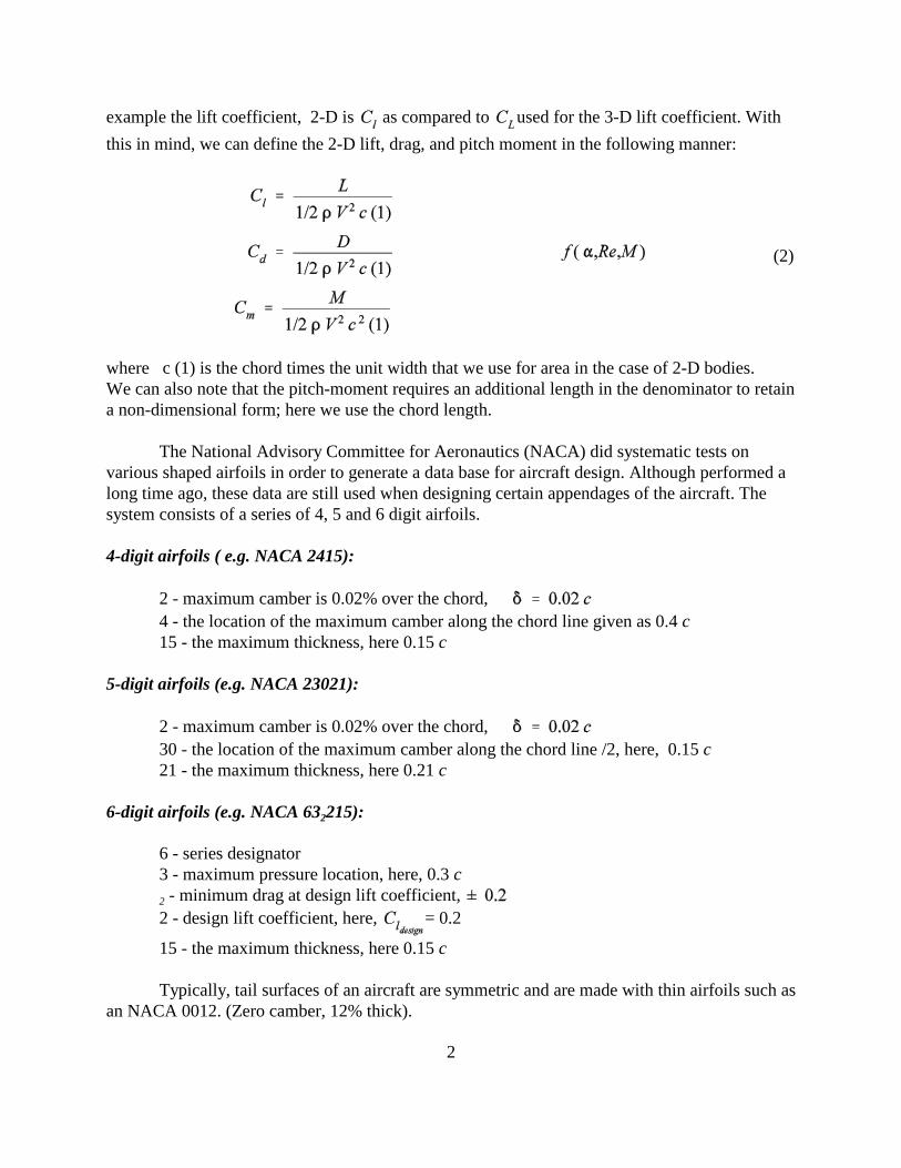
The National Advisory Committee for Aeronautics (NACA) did systematic tests onvarious shaped airfoils in order to generate a data base for aircraft design. Although performed along time ago, these data are still used when designing certain appendages of the aircraft. Thesystem consists of a series of 4, 5 and 6 digit airfoils.

4-digit airfoils ( e.g. NACA 2415):

2 - maximum camber is 0.02% over the chord,4 - the location of the maximum camber along the chord line given as 0.4 c15 - the maximum thickness, here 0.15 c

5-digit airfoils (e.g. NACA 23021):

2 - maximum camber is 0.02% over the chord,30 - the location of the maximum camber along the chord line /2, here, 0.15 c21 - the maximum thickness, here 0.21 c

6-digit airfoils (e.g. NACA 632215):

6 - series designator3 - maximum pressure location, here, 0.3 c

2 - minimum drag at design lift coefficient,2 - design lift coefficient, here, = 0.2

15 - the maximum thickness, here 0.15 c

Typically, tail surfaces of an aircraft are symmetric and are made with thin airfoils such asan NACA 0012. (Zero camber, 12% thick).

3

Aerodynamic Properties (2-D)

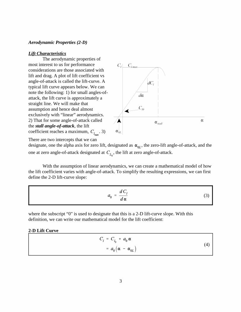
Lift CharacteristicsThe aerodynamic properties of

most interest to us for performanceconsiderations are those associated withlift and drag. A plot of lift coefficient vsangle-of-attack is called the lift-curve. Atypical lift curve appears below. We cannote the following: 1) for small angles-of-attack, the lift curve is approximately astraight line. We will make thatassumption and hence deal almostexclusively with “linear” aerodynamics.2) That for some angle-of-attack calledthe stall angle-of-attack, the liftcoefficient reaches a maximum, . 3)

There are two intercepts that we candesignate, one the alpha axis for zero lift, designated as , the zero-lift angle-of-attack, and the

one at zero angle-of-attack designated at , the lift at zero angle-of-attack.

With the assumption of linear aerodynamics, we can create a mathematical model of howthe lift coefficient varies with angle-of-attack. To simplify the resulting expressions, we can firstdefine the 2-D lift-curve slope:

(3)

where the subscript “0" is used to designate that this is a 2-D lift-curve slope. With thisdefinition, we can write our mathematical model for the lift coefficient:

2-D Lift Curve

(4)

4

where it is easily seen that or . My preference as to form is the one

that uses . However, both forms are used by various authors.

2 -D Moment

In order to calculate an aerodynamicmoment for an airfoil, we need to define areference point about which to define themoment. Typical reference points are theleading edge of the airfoil and the 1/4 chordlocation of the airfoil (for reasons to bedetermined later). The force and momentsystem on an airfoil is shown in the figure:

The drag is parallel to the relative wind, and the lift is perpendicular to the relative wind.The aerodynamic moment is positive nose up. Here we are taking the moment about point A.Once we pick a point, we can use some theorems from statics that say that we can represent andforce and moment system by assuming that the forces act thorough a given point and that there isa pure moment about that point.

Here we locate the reference point from the leading edge of the airfoil at a distance, hAcfrom the leading edge of the airfoil along the chord line. We could also select another point, Band assume the lift and drag act through that point, and that, in addition, there is a pure momentabout B (different from that about A). We can arrive at an equation that allows us to transfermoments from one point to another in the following way: Consider taking moments about theleading edge of the airfoil. Then we have:

However the forces are the same so that , and . The moments are

different and are related by the above equation that we can rewrite as:

(5)

This equation can be simplified by making a few observations: 1) the angle � is << �, so that thecosine of the angle is approximately 1 and the sine of the angle equals the angle, , and

, 2) the lift is much less than the drag, . With these two assumptions, we cannote that the last term in Eq. (5) is the product of two small quantities and is therefor secondorder compared to the first two terms, and can be neglected. With these assumptions we have the

5

equation that we are looking for:

(6)

If we put this in coefficient form (see Eq. (2)), then we have:

General Rule for Transferring Moments

(7)

Equation (7) is used for changing reference points for taking moments. Here h( ) is the non-dimensional location (in chord lengths) of the reference point from the leading edge of the wing.

ExampleHow is the moment about the leading edge of the wing related to the moment about point

A? All be need to do is let point B be the leading edge of the airfoil, then and we have:

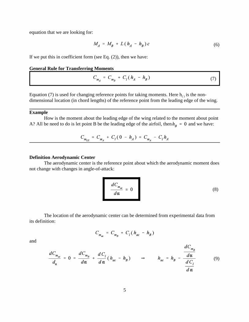
Definition Aerodynamic CenterThe aerodynamic center is the reference point about which the aerodynamic moment does

not change with changes in angle-of-attack:

(8)

The location of the aerodynamic center can be determined from experimental data fromits definition:

and

(9)

6

Consequently, if we took some wind tunnel data a measured the lift and the moment about somereference point and found how lift and moment would change with angle-of-attack, we coulddetermine the aerodynamic center.

ExampleWind tunnel data was taken on an airfoil and the following data taken at the 1/3 chord

location:

Cl 0.2 0.4 0.6 0.8

Cm1/3 -0.02 0.0 0.02 0.04

We can note that , hence we have . We can calculate the slope

from the data: , and

Therefor the aerodynamic center is located at the 23.3% chord location.

Since the pitch moment (coefficient) is constant at the aerodynamic center, it is evidentthat when the lift is zero, the pitch moment at the aerodynamic center is unchanged and is still thesame. However from Eq. (7), it is clear that when there is zero lift, the pitch moment is the sameabout any point on the airfoil (since there are no forces, it is a pure couple). Consequently, wecan note that:

(10)

From our example problem (extending the graph): .

Typically the aerodynamic center is very close to for subsonic flow and

for supersonic flow. From Eq. (9) it can be seen for linear aerodynamics (slopes are

constants) that the aerodynamic center location is also constant.

Definition - Center of PressureThe center of pressure is defined as the location on the airfoil where the pitch moment is

zero. We can determine an expression for the center of pressure from the general moment

7

equation, Eq. (7)

(11)

It would be convenient to make the point B the aerodynamic center so that

Then the center of pressure would be:

(12)

For our sample problem, for the case where the lift coefficient is 0.2, the center ofpressure would be located at

Note that unlike the aerodynamic center, the location of the center of pressure depends upon thelift coefficient.

Airfoil Drag Characteristics

The drag on an airfoil (2-D wing) is primarily due to viscous effects at low speed andcompressibility effects (wave drag) at high speed. In addition, at high angles of attack, the flowcan separate from the upper surface and cause additional drag. Hence as indicated in ourdimensional analysis, the drag coefficient depends on three quantities, Reynolds number, Machnumber, and the angle-of-attack. Typically the Reynolds number is important at low speeds, theMach number at high speeds and the angle-of-attack at all speeds. Some typical curves are shownbelow:

Here we see that the drag coefficient is nearly constant at subsonic speeds and tends to rise justbefore Mach = 1. The biggest variation is in the neighborhood of Mach 1, called the transonicregion. Above that region, say about Mach 1.2, the 2-D drag coefficient tends to be constant or itcould increase or decrease slightly. The figure on the right represents a typical change of dragcoefficient with angle-of-attack at a given Mach number. It tends to increase slightly with angle-

8

of-attack at low angles, and increases more rapidly at high angles-of-attack. The curve isapproximately quadratic in angle-of-attack.

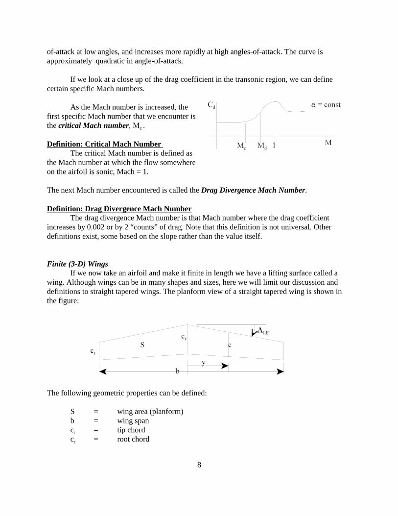
If we look at a close up of the drag coefficient in the transonic region, we can definecertain specific Mach numbers.

As the Mach number is increased, thefirst specific Mach number that we encounter isthe critical Mach number, Mc .

Definition: Critical Mach NumberThe critical Mach number is defined as

the Mach number at which the flow somewhereon the airfoil is sonic, Mach = 1.

The next Mach number encountered is called the Drag Divergence Mach Number.

Definition: Drag Divergence Mach NumberThe drag divergence Mach number is that Mach number where the drag coefficient

increases by 0.002 or by 2 “counts” of drag. Note that this definition is not universal. Otherdefinitions exist, some based on the slope rather than the value itself.

Finite (3-D) WingsIf we now take an airfoil and make it finite in length we have a lifting surface called a

wing. Although wings can be in many shapes and sizes, here we will limit our discussion anddefinitions to straight tapered wings. The planform view of a straight tapered wing is shown inthe figure:

The following geometric properties can be defined:

S = wing area (planform)b = wing spanct = tip chordcr = root chord

9

� = ct/cr = taper ratio�LE = leading edge sweep angle�n = Sweep angle at the n chord location (0 leading edge, 1

trailing edge)

Wc can also define several different chords that characterize the wing.

Definition: Mean Geometric Chord, cg

The mean geometric chord is the chord of a rectangular wing having the same span andthe same area as the original wing. It can be found for any general wing in the following way:

(13)

For a straight tapered wing:

(14)

Definition: Mean Aerodynamic Chord,The mean aerodynamic chord is (loosely) the chord of a rectangular wing with the span,

(not area) that has the same aerodynamic properties with regarding the pitch-momentcharacteristics as the original wing. It can be found for any general wing in the following way:

(15)

For a straight tapered wing this equation gives:

(16)

To characterize the general “shape” of the wing, we can define the aspect ratioL

10

Definition; Aspect Ratio, ARThe aspect ratio is the wing span divided by the mean geometric chord. It is a measure of

how long and narrow a wing is. A square wing would have an aspect ratio of 1! We can calculatethe aspect ratio in several ways:

(17)

Definition: Wing Sweep AngleThe wing sweep angle is the angle between a perpendicular to the centerline and the

leading edge of the wing. We can also define it as the angle to a line drawn through the nth cordlocation of every wing chord. For example, the quarter chord sweep angle. If we know the sweepangle at one chord location, we can find it an any other sweep location from:

Wing Aerodynamic Properties (3-D)

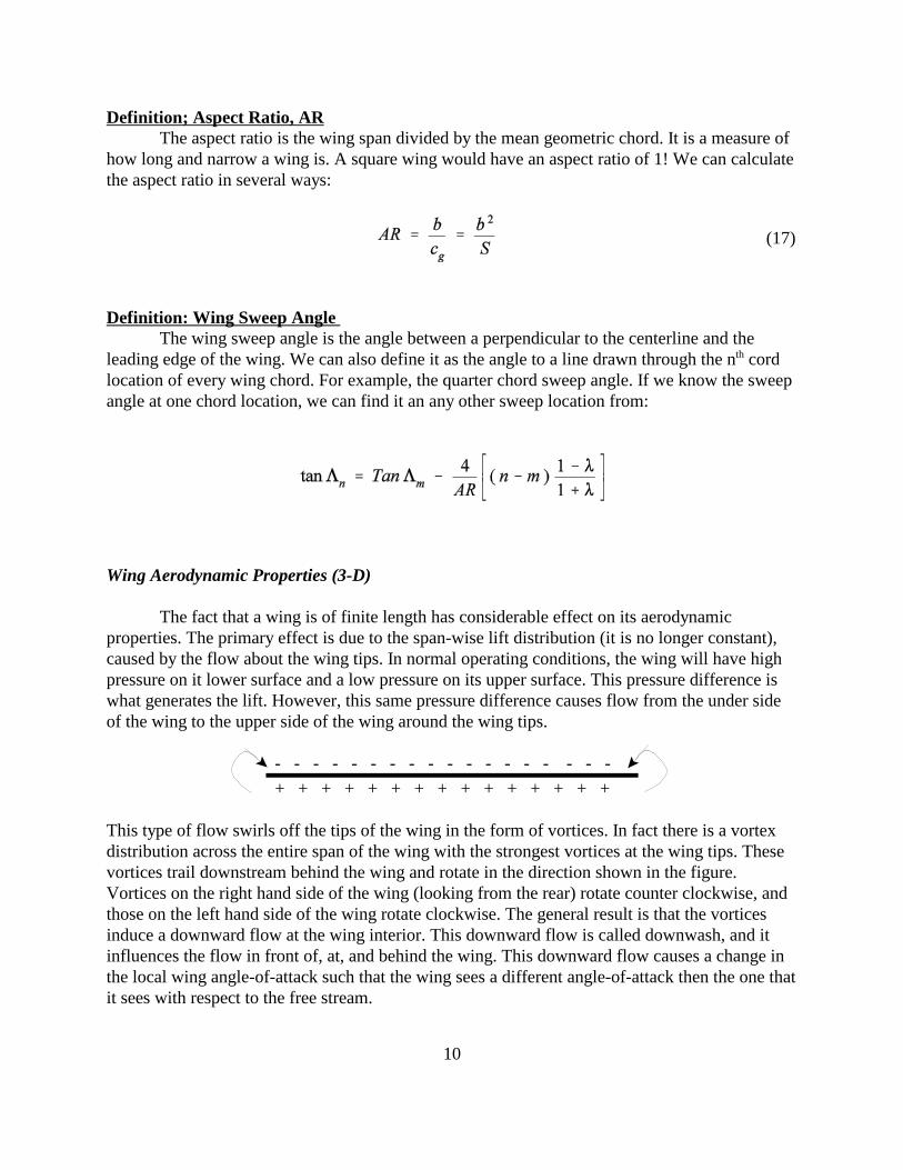
The fact that a wing is of finite length has considerable effect on its aerodynamicproperties. The primary effect is due to the span-wise lift distribution (it is no longer constant),caused by the flow about the wing tips. In normal operating conditions, the wing will have highpressure on it lower surface and a low pressure on its upper surface. This pressure difference iswhat generates the lift. However, this same pressure difference causes flow from the under sideof the wing to the upper side of the wing around the wing tips.

- - - - - - - - - - - - - - - - - -

+ + + + + + + + + + + + + + +

This type of flow swirls off the tips of the wing in the form of vortices. In fact there is a vortexdistribution across the entire span of the wing with the strongest vortices at the wing tips. Thesevortices trail downstream behind the wing and rotate in the direction shown in the figure.Vortices on the right hand side of the wing (looking from the rear) rotate counter clockwise, andthose on the left hand side of the wing rotate clockwise. The general result is that the vorticesinduce a downward flow at the wing interior. This downward flow is called downwash, and itinfluences the flow in front of, at, and behind the wing. This downward flow causes a change inthe local wing angle-of-attack such that the wing sees a different angle-of-attack then the one thatit sees with respect to the free stream.

11

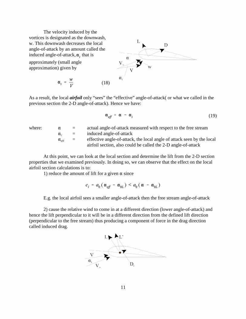
The velocity induced by thevortices is designated as the downwash,w. This downwash decreases the localangle-of-attack by an amount called theinduced angle-of-attack, that is

approximately (small angleapproximation) given by

(18)

As a result, the local airfoil only “sees” the “effective” angle-of-attack( or what we called in theprevious section the 2-D angle-of-attack). Hence we have:

(19)

where: � = actual angle-of-attack measured with respect to the free stream�i = induced angle-of-attack�eff = effective angle-of-attack, the local angle of attack seen by the local

airfoil section, also could be called the 2-D angle-of-attack

At this point, we can look at the local section and determine the lift from the 2-D sectionproperties that we examined previously. In doing so, we can observe that the effect on the localairfoil section calculations is to:

1) reduce the amount of lift for a given � since

E.g. the local airfoil sees a smaller angle-of-attack then the free stream angle-of-attack

2) cause the relative wind to come in at a different direction (lower angle-of-attack) andhence the lift perpendicular to it will be in a different direction from the defined lift direction(perpendicular to the free stream) thus producing a component of force in the drag directioncalled induced drag.

12

From the figure we have:

Therefor the finite wing causes a downwash that causes a change in the local relativewind direction so that the lift generated perpendicular to this local relative wind is no longerperpendicular to the free-stream velocity. It is tilted backward a small amount. The component ofthis lift parallel to the original free stream direction is called the induced drag.

We now consider estimating this induced angle-of-attack and the accompanying induceddrag. We will use the momentum theory developed previously. Consider a circular tube of airwhose diameter is equal to the span of the wing. The air enters and leaves the tube with the freestream velocity, V. It enters the tube, far upstream of the wing, with an angle equal to zero andleaves the tube, far downstream of the wing, deflected downward by a small amount, �. Thisangle is known to be twice the downwash angle at the wing, .

The momentum theory tells us that the force applied to the fluid must equal the change inmomentum in that direction. Here we are interested in the force that the wing applies to the fluidthat pushes the fluid down. The opposite of that force is the force on the wing by the fluid, or thelift. The momentum theory tells us that: (in the “z” direction)

(20)

where the momentum flux is the mass flow rate ( ) times the component of the velocity inthe direction of interest. Since the flow in is perpendicular to the “z” direction, there is nomomentum flux in, in the z direction. Hence we have:

13

But the force in the z direction (positive down) is the wing force on the fluid. Therefor the forceof the fluid is the negative of that force and acts upward and is called the lift (perpendicular to thefree-stream velocity). Accounting for the sign changes (force on wing opposite Fz, and lift havingthe opposite sign of Fz) we can write an expression for lift:

If we solve for the downwash angle at the wing, we get:

(21)

The induced drag is then obtained from:

(22)

The results in Eqs. (21, and 22) are somewhat restricted. They can be generalized in an“engineering” way, by introducing an engineering “factor” For the general case we can introducethe “span efficiency factor,” ew:

(23)

The total drag coefficient for a wing is then given by:

(24)

where:= 2-D drag coefficient due to skin friction, separation, wave drag

= span efficiency factor (usually less than 1)

14

AR = wing aspect ratio= wing lift coefficient

Aircraft Drag Coefficient

We can now consider the drag coefficient of the entire aircraft. One can note that thereare other lifting surfaces on the aircraft such as the tail or canard surface. Each of these surface’scontribution to the drag is similar to Eq.(24). Also the fuselage and other parts of the aircraftcontribute terms that look similar to Eq. (24). When we combine all these terms we can arrive ata single representative drag expression for the complete aircraft. This expression looks similar toEq. (24) and is given by:

Aircraft Drag Coefficient (Drag Polar)

(25)

where: = zero-lift drag coefficient, parasite drag coefficient

e = Oswald (aircraft) efficiency factorK = induced drag parameter

Drag Polars

The drag coefficient can be written as functions of many different variables. The strongestdependence of drag is on the lift coefficient because of the induced drag effect. If themathematical model for the drag coefficient contains the lift coefficient, that expression is calleda drag polar. Hence we can make the following definition:

Definition: Drag Polar A drag polar is a any mathematical expression the relates the drag tosome function of the lift coefficient, .

There are several different drag polars that are typically used to represent the drag of anaircraft. The following two are the most frequently used when Eq. (25) is not used:

15

(26)

where is the lift coefficient when the drag is a minimum. The last equation in Eq. 26, and

Eq. (25) are examples of a particular type of a drag polar, a parabolic drag polar. For themajority of this course we will use the parabolic drag polar given in Eq. (25)

In general the drag coefficient is a function of Reynolds number and Mach number. Ingeneral, for the normal flight regime, the dependence on these numbers is the similar to thedependence as observed on the airfoil previously. Typically, in the flight conditions of interest,the Reynolds number has only a small effect while that of the Mach number is prominent in highsubsonic, transonic, and supersonic flight. We can indicate this dependence on Mach number inour parabolic drag polar as follows:

(27)

where = Mach number dependent zero-lift drag

= Mach number dependent induced drag parameter

We could also write: , where the oswald efficiency factor is a function of the

Mach number.

Example

An aircraft weighs 40,000 lbs, wing area of 350 ft2 and a wing span of 50 ft. At sea-levelthe aircraft flies at 200 and 600 ft/sec. What are the values of the induced drag and the associateddrag coefficients for this case. Noting that Lift = weight in level flight:

Also assume e = 0.85

16

Induced drag only!

Induced drag only!

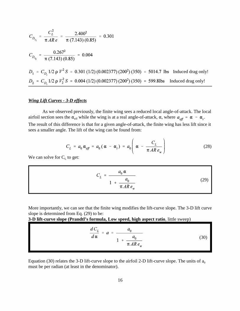
Wing Lift Curves - 3-D effects

As we observed previously, the finite wing sees a reduced local angle-of-attack. The localairfoil section sees the �eff while the wing is at a real angle-of-attack, �, where .

The result of this difference is that for a given angle-of-attack, the finite wing has less lift since itsees a smaller angle. The lift of the wing can be found from:

(28)

We can solve for CL to get:

(29)

More importantly, we can see that the finite wing modifies the lift-curve slope. The 3-D lift curveslope is determined from Eq. (29) to be:3-D lift-curve slope (Prandtl’s formula, Low speed, high aspect ratio, little sweep)

(30)

Equation (30) relates the 3-D lift-curve slope to the airfoil 2-D lift-curve slope. The units of a0

must be per radian (at least in the denominator).

17

Example:

The aircraft from the previous example has a wing with a 2-D airfoil section that has alift-curve slope of . What is the lift-curve slope of the wing?

The wing aspect ratio was calculated to be AR = 7.143. We will assume that ew = 0.85.Then the wing lift-curve slope is calculated from:

We see that /rad, while /rad,

The above equation (Eq. 30) is generally valid for low speed high aspect ratio wings. Analternate expression for the 3-D lift-curve slope for straight tapered wings performing both highor low speed subsonic flight, that includes the effects of Mach number and wing sweep is givenby the following expression:

DATCOM FormulaStraight tapered wing lift-curve slope (subsonic, all speeds and AR)

(31)

Where , and a0 = actual 2-D lift-curve slope of airfoil section. If unknown

assume k = 1.

For supersonic flow, low aspect ratio, straight tapered wings we have the followingmathematical model for the lift-curve slope:

Straight tapered wing lift-curve slope (supersonic, low aspect ratio)

(32)

18