7 6 int jrnl 6(2012)

Int. J. Automation and Control, Vol. 6, No. 1, 2012 39

Copyright © 2012 Inderscience Enterprises Ltd.

Optimal trajectory planning for industrial robot along a specified path with payload constraint using trigonometric splines

Shital S. Chiddarwar* Department of Mechanical Engineering, Shri Ramdeobaba Kamla Nehru Engineering College, Ramdeo Tekadi, Katol Road, Nagpur 440013, Maharashtra, India E-mail: [email protected] *Corresponding author

N. Ramesh Babu Manufacturing Engineering Section, Department of Mechanical Engineering, Indian Institute of Technology Madras, Chennai 600036, Tamil Nadu, India E-mail: [email protected]

Abstract: This paper presents a general methodology for the offline planning of trajectory of a six axis serial robot along a specified path. The objective of trajectory planning is to minimise a cost function when subjected to joint angles, joint velocities, acceleration, jerks, torques and gripping force constraints by considering dynamic of the robot. A trigonometric spline is used to represent the trajectory. This non-linear constrained optimisation problem consists of 6 objectives, 67 constraints and 48 variables. The cost function is a weighted balance of travelling time, actuator torques, singularity avoidance, joint jerks, joint accelerations and gripping force. The optimisation problem is solved by using two methods, namely sequential quadratic programming and genetic algorithm. The proposed methodology is implemented for trajectory planning of six degree of freedom industrial robot and results obtained with two optimisation techniques are compared.

Keywords: optimal trajectory planning; SQP; sequential quadratic programming; trigonometric spline; multi-objective optimisation; GA; genetic algorithm.

Reference to this paper should be made as follows: Chiddarwar, S.S. and Babu, N.R. (2012) ‘Optimal trajectory planning for industrial robot along a specified path with payload constraint using trigonometric splines’, Int. J. Automation and Control, Vol. 6, No. 1, pp.39–65.

Biographical notes: Shital S. Chiddarwar is a Mechanical Engineering Graduate from VNIT Nagpur. She completed her PhD from the Indian Institute of Technology Madras, Chennai, India. Her areas of interest are multiple robot motion planning, control of mobile manipulators, development of robot teaching techniques and soft computing methods for optimisation. She is

40 S.S. Chiddarwar and N.R. Babu

working as an Assistant Professor in the Department of Mechanical Engineering of Shri Ramdeobaba College of Engineering and Management, Nagpur.

N. Ramesh Babu completed his PhD in Manufacturing Technology from the Indian Institute of Technology Madras, Chennai, India. He is the Professor of Manufacturing Engineering and heads the laboratory. He is involved in various research and development activities. His areas of expertise are laser beam machining (LBM), abrasive finishing processes, abrasive waterjet machining (AWJM), process modelling, computer-aided manufacturing, CNC, PLC and robotics. He has published many papers in international journals, conferences and symposiums. He is an eminent researcher and academician in the area of manufacturing engineering.

1 Introduction

Industrial robots have been used for decade in place of human workers in automatic production lines due to their great ability of speed and precision and their cost-effectiveness in repetitive tasks. However, these powerful machines are hardly autonomous in the sense that they require preliminary actions such as calibration or motion planning to achieve specified tasks. The control of such a machine using computer software makes it both flexible in the way it works and versatile in the variety of tasks it can achieve. However, the full benefits of a robot can be obtained only if the programming phase is well accomplished. In general, the process of programming industrial robots is divided into two major levels: trajectory planning and trajectory control. The first consists of determining the time history of the robot kinodynamic parameters (position, velocity, acceleration and effort) that correspond to the desired task. The second consists of converting these computed parameters into control signals to command the actuators during the execution of the task and to compensate for any deviation.

For successful execution of the task, it is necessary to generate accurate trajectory. Hence, the fundamental problem of robotics, i.e. trajectory planning, may be defined as finding temporal motion law along the given geometric path such that certain constraints set on the trajectory properties are fulfilled. Trajectory planning is devoted to generate the reference inputs for the control system of the manipulator to execute the motion. The algorithm used for trajectory planning considers geometric path, kinematic and dynamic constraints as the input to generate the trajectory of the joints (or the end-effector), expressed as a time sequence of position, velocity and acceleration values. The geometric path is usually defined in the workspace with reference to the end-effector of the robot because task performance and obstacle avoidance can be obviously described in this space. On the other side, trajectory planning is normally carried out in the joint space of the robot, after a kinematic inversion of the given geometric path is obtained. The joint trajectories are then obtained by means of interpolating functions, which meet the imposed kinematic and dynamic constraints. Planning a trajectory in the joint space rather than in the operating space has a major advantage, namely that the control system acts on the manipulator joints rather than on the end-effector, so it would be easier to adjust the trajectory according to the design requirements if working in the joint space.

Optimal trajectory planning for industrial robot 41

Moreover, trajectory planning in the joint space would allow avoidance of problems arising with kinematic singularities and manipulator redundancy. The main disadvantage of planning the trajectory in the joint space is that, given the planned trajectory in the joint space, the motion actually performed by the robot end-effector is not easily predictable. This problem arises due to the non-linearities introduced when transforming the trajectories of the joints into the trajectories of the end-effector through direct kinematics.

Apart from the particular strategy adopted, the motion laws generated by the trajectory planner must fulfil the constraints set a priori on the maximum values of the generalised joint torques, and must be such that no mechanical resonance mode is excited. This can be achieved by forcing the trajectory planner to generate smooth trajectories, i.e. trajectories with good continuity features; in particular, continuous joint displacement, velocity, accelerations and jerks, so that the absolute values of these features can be kept bounded.

Almost every technique found in the literature on the trajectory planning problem is based on the optimisation of some parameter or some objective function. The most significant optimality criteria are:

1 minimum execution time

2 minimum energy (actuator efforts)

3 minimum jerk

4 minimum acceleration

5 maximum manipulability.

1.1 Minimum execution time

Minimum-time algorithms were the first trajectory planning techniques proposed in the literature because they were tightly linked to the need of increasing the productivity in the industrial sector. The first interesting method of this kind was developed in the position-velocity phase plane by Bobrow et al. (1985) and Shin and McKay (1985). The main idea was to use the curvilinear abscissa of the path as a parameter, to express the dynamic equation of the manipulator in a parametric form. An alternative approach was proposed by Balkan (1998), where he employed dynamic programming technique for optimisation. However, the above-mentioned technique generates trajectories with discontinuous values of accelerations and joint torques, because the dynamic models used for trajectory computation assume the robot members as perfectly rigid and neglect the actuator dynamics. This leads to two undesired effects: firstly, the real actuators of the robot cannot generate discontinuous torques, which cause the joint motion to be always delayed with respect to the reference trajectory. The accuracy in trajectory following is then greatly reduced and the so-called chatter phenomenon may eventually occur, consisting in high frequency vibrations that can damage the manipulator structure. Secondly, the time-optimal control requires saturation of at least one robot actuator at any time instant, so the controller cannot correct the tracking errors arising from disturbances or modelling errors.


To overcome such problems, Constantinescu and Croft (2000) developed alternate approach which imposes some limits on the actuator jerks defined as the variation rates of the joint torques. In this way, the generated trajectory will not be exactly time-optimal, though close to the optimality value; however, the generated trajectories can be effectively implemented and more advanced control strategies can be applied. To generate trajectories with continuous accelerations, a common strategy is to use smooth trajectories, like the spline functions, that have been extensively employed in the literature on both kinematic and dynamic trajectory planning. Lin et al. (1983) gave the first formalisation of the problem of finding the optimal curve interpolating a sequence of nodes in the joint space. It was obtained through kinematic inversion of a discrete set of points representing position and orientation of the reference frame linked to the end-effector of the robot. Wang and Horng (1990) presented same algorithm, but the trajectories were expressed by means of cubic B-splines.

Jamhour and Andre (1996) modified the optimisation algorithm proposed by Wang and Horng (1990), so that it can also deal with dynamic constraints and with objective functions of a more general type; however, the reported simulations still refer to the trajectory planning problem with kinematic constraints. Chen (1991) proposed a method to compute point-to-point minimum-time trajectories using uniform B-splines. The dynamic model of the manipulator was considered, and the problem of semi-infinite constraints resulting from the algorithm was bypassed by sampling a certain number of points. Shiller and Dubowsky (1989) presented a method, which has found the minimum-time motion for a manipulator between given end states, by considering the full non-linear manipulator’s dynamics, actuator saturation characteristics, end-effector and payload constraints. Choi et al. (2000) have discussed the problem of the minimum-time trajectories and the control strategy to drive the robots along the trajectories when the exact dynamics equations of robots were unavailable. In each time interval, the trajectory was optimised by means of the use of evolution strategy so that the total travelling time was minimised under the kinematic constraints.

1.2 Minimum-energy trajectory planning

Planning the robot trajectory using energetic criteria provides several advantages. On the one hand, it yields smooth trajectories resulting easier to track and reduce the stresses to the actuators and to the manipulator structure. Moreover, saving energy may be desirable in several applications, like those with a limited capacity of the energy source (e.g. robots for spatial or submarine exploration). Examples of energy optimal trajectory planning are provided by Von stryk and Schelemmer (1994), Field and Stepanenko (1996), and Martin and Bobrow (1999).

Von stryk and Schelemmer (1994), and Field and Stepanenko (1996) considered point-to-point trajectories with minimal energy, with upper bounds on the amplitude of the control signals and the joint velocities. Martin and Bobrow (1999) optimised a trajectory with motion constraints set on the end-effector. The cost function was given by the time integral of the squared joint torques, and the trajectories were expressed by means of cubic B-splines. The resulting motion minimises the actuators effort. Other examples of time-energy optimal trajectories are given by Saramago and Steffen (1998, 2000). Saramago and Steffen (1998) considered a cubic spline trajectory which was subjected to kinematic constraints on the maximum values of velocity, acceleration and


jerk. Saramago and Steffen (2000) considered a point-to-point trajectory parameterised by means of cubic B-splines.

Both the optimal travelling time and the minimum mechanical energy of the actuators were considered as an objective function in some literatures (Chettibi et al., 2004; Saramago and Steffen, 2000; Shiller, 1996). Shiller (1996) dealt with the time–energy optimal trajectories, i.e. the cost function has a term linked to the execution time and a term expressing the energy spent. The trade-off between the two needs can be adjusted by changing the respective weights. Chettibi et al. (2004) used a sequential quadratic programming (SQP) method for obtaining optimal motion planning for PUMA 560 manipulator. Their objective function was a weighted balance of the transfer time and the mean average of actuator efforts and power.

Saramago and Steffen (2000) proposed a method based on SQP to obtain an optimal motion planner for the STANFORD manipulator in the presence of fixed, moving and oscillating obstacles. Their objective function was a weighted balance of transfer time, mechanical energy of the actuators and penalty for collision-free motion. They have taken in to account the physical constraints, such as joint displacements, velocities, accelerations, jerks and torques, and collision avoidance.

1.3 Minimum-jerk trajectory planning

Apart from the particular strategy adopted, the motion laws generated by the trajectory planner must fulfil the constraints set a priori on the maximum values of the generalised joint torques, and must be such that no mechanical resonance mode is excited. This can be achieved by forcing the trajectory planner to generate smooth trajectories, i.e. trajectories with good continuity features: in particular, it would be desirable to obtain trajectories with continuous joint accelerations, so that the absolute value of the jerk (i.e. of the derivative of the acceleration) keeps bounded. Limiting the jerk is very important, because high jerk values can wear out the robot structure and heavily excite its resonance frequencies. Vibrations induced by non-smooth trajectories can damage the robot actuators and introduce large errors, while the robot is performing tasks like trajectory tracking. Moreover, low-jerk trajectories can be executed more rapidly and accurately. The importance of generating trajectories that do not require abrupt torque variations have already been remarked. Constantinescu and Croft (2000) generated the trajectories that do not require abrupt torque variations by setting upper bounds on the rate of torque variations, but in this way the third-order dynamics of the manipulator must be computed. An indirect method to get the same results is to set an upper limit on the jerk, defined as the time derivative of the acceleration of the manipulator joints.

The positive effects induced by a jerk minimisation are:

Errors during trajectory tracking are reduced.

Stresses to the actuators and to the structure of the manipulator are reduced.

Excitation of resonance frequencies of the robot is limited.

A very coordinated and natural robot motion is yielded.

The last effect appears very interesting; indeed, some studies (Bobrow et al., 2001; Simon, 1993) show that the movement of a human arm seems to satisfy an optimisation criterion linked to the rate of variation of the joint acceleration. So, it may be inferred that


the minimum-jerk trajectories are an example of optimisation according to physical criteria imitating the capacity of natural coordination of a human being. Kyriakopoulos and Saridis (1988) obtained the solutions for two point-to-point minimum-jerk trajectories analytically and the optimisation obtained through the Pontryagin principle considered two objective functions, namely the time integral of the squared jerk and the maximum absolute value of the jerk (minimax approach). Simon and Isik (1991) proposed an interesting approach, where the interpolation was done through trigonometric splines that ensure the continuity of the jerk. The interpolation through trigonometric splines featured a sound neighbourhood property, i.e. if the value of some node in the input sequence is changed, only the two splines having that node as their common point should be computed again, not the whole trajectory. This property can be usefully exploited for instance to bypass an obstacle in real time. Piazzi and Visioli (1998) used interval analysis to develop an algorithm that globally minimises the maximum absolute value of the jerk along a trajectory whose execution time is set apriori; hence, an approach of the type minimax was used. The trajectories were expressed by means of cubic splines and the intervals between the via-points were computed so that the lowest possible jerk peak is produced. However, these techniques consider the execution time as known (and set a priori); moreover, it is not possible to set any kind of kinematic constraints on the trajectory, as they are not taken into account.

Gasparetto and Zanotto (2007, 2008) presented a method based on SQP for the smooth trajectory planning of robot manipulators. Their objective function was a weighted balance function between the travelling time and the integral of squared joint jerks. They used cubic spline (Gasparetto and Zanotto, 2007) and quintic spline (Gasparetto and Zanotto, 2008) for trajectory planning along specified path. However, their method considered only kinematic constraints; it did not consider dynamic constraints like joint torques.

1.4 Minimum acceleration

Elnagar and Hussein (2000) proposed an approach to generate acceleration-based optimal smooth piecewise trajectories. Given two configurations (position and orientation) in 3D, their algorithm searched for the minimal energy trajectory that minimises the integral of the squared acceleration. A numerical iterative procedure was used for computing the optimal piecewise trajectory as a solution of a constrained boundary value problem. The resulting trajectories were not only smooth but also safe with optimal velocity (acceleration) profiles and, therefore, were suitable for robot motion planning applications. They demonstrated this fact with experimental results.

1.5 Maximum manipulability

A measure of manipulability is very useful for manipulator design, task planning and fast recoverability from the escapable singular points for robot manipulators. To obtain a practical trajectory (the robot need not lose any degree of freedom at any stage), the manipulability measure can be used as the design criteria. Lin (2004), using a perturbation method, experimented on an optimal path planning approach to minimise the cost of moving an MITSUBISHI RVM2 robot (five degrees of freedom) along a specified geometric path subject to angle change constraints. Their objective function included obstacle avoidance and singularity avoidance. Mayorga and Wong (1987) dealt


with the importance of the singularity avoidance method for the trajectory planning of redundant and non-redundant robot manipulators. Lloyd and Hayward (2001) presented a robust trajectory generator for a PUMA 560 robot to generate singularity-free trajectories by taking the objective function as time minimisation using a path-time scaling method.

1.6 Grasping forces

Grasping can be defined as the capability of a mechanical end-effector to establish a contact between its fingers and object. Grasp configurations are achieved so that a static equilibrium exists between the grasping forces due to the fingers on the object. The grasping forces can be determined based on the characteristics of the object, such as its weight and shape. However, in most manipulator tasks, inertia forces are also considered as depending on the specifications of the motion trajectories. Shiller and Dubowsky (1989) has found the minimum-time motion for a manipulator between given end states, by considering the full non-linear manipulator’s dynamics, actuator saturation characteristics, end-effector and payload constraints. Chevallier and Payandeh (1998) have proposed an approach for modelling and computing the grasping force as a function of the external forces (e.g. like inertia actions), which can act on the grasped object. The contact between the fingers and the object has been modelled as a point of contact with friction. Zhao and Bai (1999) have proposed optimal schemes, minimum load method, minimum torque method and multiple criterion method. In the last method, a weighted linear combination of joint torques and component loads is used as an objective function to formulate load distribution and joint trajectory planning.

1.7 Minimum time, energy, acceleration, velocity, maximum manipulability and payload constraints

Saravanan and Ramabalan (2008) and Saravanan et al. (2008a) presented optimisation procedure based on evolutionary algorithms for solving trajectory planning problem of five and six degree of freedom robots, respectively. The aim was minimisation of combined objective function with constraints being actuator constraint, joint limits and the obstacle avoidance constraint by considering dynamic equations of motion. They also considered payload constraint (Saravanan et al., 2008b) along with above-mentioned constraints.

After extensive literature survey, it was found that

1 None of the literature considered all the important objective functions (minimisation of travelling time, energy, joint jerks, joint accelerations, griping forces and maximisation of manipulability measure) in a combined manner for optimal trajectory planning along the specified path.

2 Very few researches showed consideration towards minimisation of gripping forces which become a critical issue in handling the materials.

3 Most of the earlier approaches do not consider the constraint of moving end-effector through a particular sequence.

In view of these aspects, the trajectory planning technique proposed in this paper carries out optimisation of trajectory along the specified path with due consideration to all these issues. The trajectory planning technique described in this paper assumed the geometric


path, generated a priori by an upper-level path planner presented by Chiddarwar and Babu (2007, 2009) which resolved the obstacle avoidance problem before hand. This geometric path is given in the form of a sequence of via-points in the operating space of the robot, which represents successive positions and orientations of the end-effector of the manipulator. The joint angle configurations at these via-points are obtained using inverse kinematics technique elaborated by Chiddarwar and Babu (2008). The proposed technique generates an optimal trajectory for the robot, by associating temporal information to the pre-planned geometric path. It makes use of an optimality criterion based on the minimisation of some objective function that will be defined below, and by taking into account any kinematic constraints expressed by means of upper bounds on velocity, acceleration and jerk. The overall strategy adopted by the proposed approach for generation of optimal trajectory along the specified path is given in Figure 1. In this paper, an attempt is made to determine the appropriate trajectory optimisation technique. Hence, modelling of trajectory is done using trigonometric spline, optimal values of the coefficients of the trajectory are obtained using SQP and genetic algorithm (GA), and results are compared. The vital issues such as formulation of problem and objective function, modelling of the trajectory using trigonometric splines and optimisation technique, which makes use of SQP and GA, are explained in Sections 2 and 3.

Figure 1 Synoptic diagram of optimal trajectory planner for robot manipulator

2 Problem formulation

In case of multiple robot motion planning problem, collision and conflict free path will be given by the coordination strategy. The target of trajectory planner is to find out the optimal trajectory to be followed by end-effector while following the predefined geometric path, while minimising a combined objective function of the robot, and considering the physical constraints and actuator as well as payload limits. Minimisation of travelling time, mechanical energy, joint jerks, joint accelerations, gripping forces and maximum manipulability are considered to build a combined objective function. The singularity avoidance is achieved in the form of manipulability measure. These objectives are considered while framing multi-objective function as minimisation of these aspects has certain inherent advantages. Minimisation of travelling time guarantees increase in productivity by reducing cycle time, whereas trajectory determined with objective of minimum energy yields smooth and easy to track trajectories by reducing stresses in actuators and robot structure. Consideration of minimum jerk objective avoids excitation of resonance frequencies of robots, whereas minimisation of acceleration makes certain


that robot moves along the determined trajectory safely with optimal velocity/ acceleration. Maximising the manipulability measure will keep robot away from the singular configurations.

Hence, objective function can be written as: vp 1

22min T j

0 01 1 1

2a s p 1 1 2 2

0 01 1

( ( )) d ( ) d

( ) d det + ( ) ( ) ( ) ( ) d

f f

f f

N Nt t

i ji j j

N Nt t

jj j

Z w h w t t w u t t

w t t w j w F t v t F t v t t

(1)

max

max

max

max

max

min max

s.t. constraints

= displacement constraint

= velocity constraint

= acceleration constraint

= jerk constraint

( ) = force/torque constraint

Fg Fg = payload

j j

j j

j j

j j

j

k

u t u

Fvia-point

, ,

, 1 ,max1, ,

constraint for =1,2

= via-point costraint for =1, , number of via-points

max = lower bound constraint for execution time

j i j i

j i j ii

j N j

k

i

h

min

where,objective function

=number of jointsvp=number of via-points

time interval between consecutive via-points( ) displacement of th joint

( ) velocity of th joint

( ) acceleration of

i

j

j

j

ZN

ht j

t j

t

T

j

a

th joint

( ) jerk of th joint

weight of term proportional to travelling timeweight of term proportional to jerk

weight of term proportional to torque/generalised forceweight of term pr

j

j

t j

ww

ww

s

p

oportional to accelerationweight of term proportional to singularity conditionweight of term proportional to payload constraint

ww


The various details about the optimisation parameters considered in the objective function are explained in Sections 2.1–2.3.

2.1 Computation of time interval between via-points

The optimisation parameter hi must be lower bound, because any interval between a pair of consecutive via-points cannot run at the infinite velocity. Hence, for each interval, the relation max

, 1 ,(( ) / )j i j i i jh must hold and hence hi must be like max

, 1 ,1, ,max { / } 0i j i j i j

j Nh . In other words, execution time of every trajectory time

should be computed corresponding to maximum allowed velocity for each joint. The largest execution time corresponding to the most restrictive condition is picked to obtain the constraint value.

2.2 Computation of generalised forces/torques

The generalised forces are calculated using dynamic equations as follows, which are deduced from Saramago and Steffen (2002).

diss1 1 1

N N i

j ij j ijk j k jj i k

u D C G F (2)

Tmax( , )

2 Tm

where1,2 , = number of joints

inertial system matrix = tr[( / ) ( / ) ]

Coriolis,centripetal force matrix due to velocity at joint and

= tr[( / ) ( / ) ]

Nij l j l l il i j

ijk

l j k l l il

j N

D T U T

C i k

T U Tax( , , )

N

i j k

ravity loading vector = ( / )

mass of link

centre of mass of link according to its own coordinates4 4 link transformation matrix or DH matrixgravitational vector

tr tra

N T lj l l il i

ll

l

G g m g T r

m l

r lTg

ce operator of a matrix

diss c d

c

d

dissipation force = sign( )

coefficient of coulomb frictioncoefficient of viscous friction

-dimensional vector of applied torque

j j

j

F f f

ffu N


The influence of the payload on the dynamic model of a robot can be considered by adding the mass of grasped object to the mass of the last link. Similarly, the inertial moments of given object can be added to the inertial moments of the last link.

2.3 Formulation of gripping forces in the gripper

In this paper, two-finger gripper statics developed by Cuadrado et al. (2002) is used. Usually, industrial robots use two-finger grippers for grasping purpose, hence a two-finger gripper is considered in this work to grasp the object. The force configuration for the two-finger gripper planar grasp is considered as shown in Figure 2. Grasping can be defined as the capability of a mechanical end-effector to establish contact between its fingers and an object. Grasp configurations are achieved so that a static equilibrium exists between the grasping forces by the fingers and the object. The grasping forces can be determined based on the characteristic of the object such as shape and weight. However, in most manipulator tasks inertial forces are also considered depending upon the specification of motion trajectories. This paper also uses an approach for computing the grasping forces as a function of the inertia forces. Let F1 and F2 be the grasping forces exerted by the fingers. Usually these forces are not equal as the contact point A and B are not generally located in same relative position on the two fingers. However, for sake of simplicity and because indeed the difference in position can be very small, the grasping forces can be thought with a common value. Similar observations can be developed for the friction evaluation at the points A and B through the coefficients μ1 and μ2 which can be assumed with a common value. The angles 1 and 2 represent the angles of the friction cones at the contact points A and B, respectively, and they are related to the friction coefficients by μ1 = tan 1 and μ2 = tan 2. The grasping configuration of the object with respect to the fingers gives the angles 1 and 2, which strongly depend on the orientation of the fingers, the position of the contact points and the shape of the object and the fingers. Although the contact points, which define the contact line, can be located in the same relative position on the fingers, the angles 1 and 2 can differ from each other. However, because of symmetry of a two-finger gripper, it can be considered similar. In addition, rA and rB represent the distances of A and B, respectively, from the squeezing line, rG is the distance of G from the contact line and W = mobjectg is the weight vector of object and it is oriented with an angle w with respect to perpendicular axis to the plane yz, being Gxyz a suitable fame fixed on the grasped object as shown in Figure 2. The static equilibrium of a grasped object can be expressed along the direction of the contact and squeezing lines, as outlined by Saramago and Ceccarelli (2002), in terms of forces as:

1 1 2 2 1 1 1 2 2 2

object

cos cos sin sin

cos sin 0w w y

F F F F

m g a (3)

1 1 2 2 1 1 1 2 2 2

object

sin sin cos cos

cos cos 0w w z

F F F F

m g a (4)


where the acceleration components ay and az of the centre point on the manipulator extremity can be computed as given by Saramago and Ceccarelli (2004):

G2

G

G1 11 1

x xi ii i

y yo oj j k

j j kz zj j

a ra rT T

q q qq q qa r

(5)

The distance of the gravity centre of the grasped object is indicated through vector rG

with components rGx, rGy, rGz and ioT is the homogenous transformation matrix. The

corresponding velocity components of the gravity centre point can be calculated as:

G

G

G11 1

x xi i

y yoj

jz zj

V rV rT

qqV r

(6)

Figure 2 Force model for planar grasp with two fingers


3 Modelling of trajectory using trigonometric spline

The trajectory planning task of a robot manipulator is generally specified in terms of the motion of the end-effector in the Cartesian space. To implement a typical motion controller in the joint space, the trajectory in the Cartesian space has to be mapped in the joint space by applying the inverse kinematics. A way to specify a trajectory is to give a sequence of intermediate points in the Cartesian space to be passed through by the end-effector and therefore a corresponding sequence of angles to be assumed by each joint at given time instants.

In this context, if it is not strictly necessary that the manipulator assumes exact the desired poses, a simple technique is to connect via-points with linear functions and then add parabolic blend regions around each via-point. Conversely, if it is required that the robot passes exactly through the intermediate points, a suitable solution is to use splines. By choosing an appropriate order of the spline, the user can guarantee the continuity of velocity, acceleration and jerk signals along the whole trajectory.

The use of trigonometric spline is very advantageous because it has continuous derivative up to the third order on interior of the trajectory, which means that continuous velocity, acceleration and jerk can be obtained. Moreover, trigonometric splines have zero jerk at the end points. Hence, it does not present problems such as excessive oscillation and overshoot between any pair of reference points. Trigonometric polynomials are very much smooth because cosine and sine terms form an orthogonal set of functions. One of the main advantages claimed for trigonometric splines is the prevention of large overshoots despite the fact that the continuity of the function can be imposed until a high-order trigonometric spline is used. By using, fourth-order trigonometric spline the continuity of the jerk function is guaranteed and the overshoots are significantly reduced (Visioli, 2000).

The formal definition of trigonometric spline function y(t) with a total of 2mconstraints in each of the n closed arcs [ti 1,ti] (i = 1,…,n) is defined as y(t) = yi(t)t [ti 1,ti] where y(t) is given by:

1

,0 , , ,1

2 1

10

( ) sin cos

for , where 2

m

i i k i k i m ik

mij

i i ij

y t a a kt b kt a m t

t t tm

(7)

The time-scaled trigonometric spline can be defined as:

( ( 1)) ( ), 0, ( =1, , )4 4iy t i y t t i n

Unscaled trigonometric spline

( )4n t

t yT


Derivative of unscaled trajectory can be obtained as:

( )4 4

rr n t n t

t yT T

where

m = order of trigonometric spline.

ij = values of t where the yi(t) has a constraint applied.

In the optimisation of the trajectories, the coefficients of the trigonometric spline are considered as optimisation variables.

4 Numerical procedure for optimal trajectory planning

The steps required for optimisation are as follows:

1 The numeric values of kinematic and dynamic constraints are set for the robot.

2 A suitable initial solution is determined to start the process.

3 The expression of the objective function and the kinematic constraints are input to the optimisation.

4 The solution of the optimisation problem is then obtained using SQP techniques and multi-objective GA.

As for all iterative routines, a crucial point is the choice of a suitable initial solution, because a wrong choice would affect the execution time and even the final result of the algorithm. A suitable initial solution can be found by considering the lower bound of interval hi and maximum values of velocity, acceleration and jerk for every joint and every time interval.

Let t be the independent time variable. (t) is the trajectory and ( )t , ( )t and ( )tare derivatives of the trajectory. If a scaled time variable is defined as = sf(t) and the following holds:

( )( )

sft

2( )( )

sft

3( )( )

sft

A set of coefficients {sf1, sf2, sf3, sf4} is determined and maximum of that set is considered as a scaling factor.

1For displacement, sf 1


2max

( )For velocity, sf

t

3max

( )For acceleration, sf t

4max

( )For jerk, sf t

A scaling factor sf can be chosen as sf = max {sf1, sf2, 23sf , 3

4sf } which is multiplied to lower bound values of optimisation variables and initial solution is obtained. Lower bounds and upper bounds of the optimisation variables are obtained by considering lower and upper bounds of various constraints and solving the simultaneous equations. This initial solution is necessary to implement SQP method for optimisation. The SQP is implemented by using fmincon function of MATLAB and this optimisation process works as per flowchart presented in Figure 3.

Figure 3 Optimisation process followed by SQP


To compare the obtained results, optimisation is also done using the multi-objective GA. Function gamultiobj of MATLAB is used to solve minimisation problem. The methodology adopted for optimisation process is given in Figure 4. The multi-objective GA function gamultiobj uses a controlled elitist GA (a variant of non-dominated sorting genetic algorithm-II). An elitist GA always favours individuals with better fitness value (rank), whereas a controlled elitist GA also favours individuals that can help increase the diversity of the population even if they have a lower fitness value. It is very important to maintain the diversity of population for convergence to an optimal Pareto front. This is done by controlling the elite members of the population as the algorithm progresses. Two options ‘ParetoFraction’ and ‘DistanceFcn’ are used to control the elitism. The Pareto fraction option limits the number of individuals on the Pareto front (elite members) and the distance function helps to maintain diversity on a front by favouring individuals that are relatively far away on the front.

Figure 4 Optimisation process followed by genetic algorithm

5 Numerical example

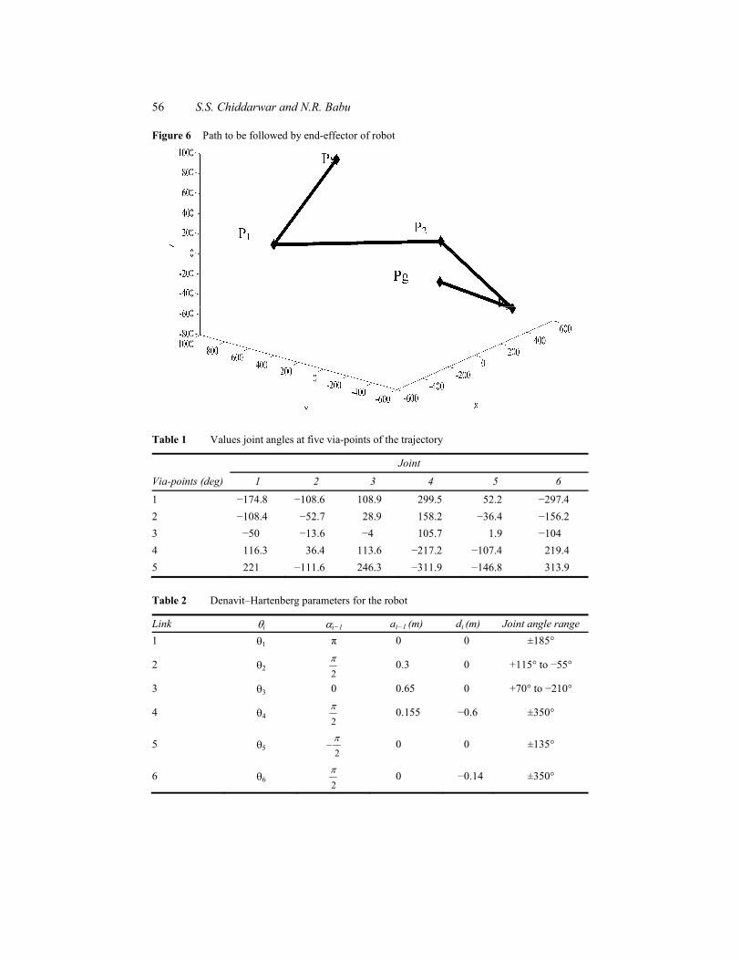
A numerical example has been developed by referring to a KUKA-Kr robot (Figure 5) with six revolute joints. The illustrative robot task consists of transporting a payload from an initial point to a final one along a pre-specified path as shown in Figure 6. This geometric path is generated a priori by an upper-level path planner. Obstacle avoidance problem are already solved by upper-level path planner. Geometric path is given in the form of a sequence of via-points in the operating space of the robot, which represent successive positions and orientations of the end-effector of the manipulator. The joint


angle coordinates corresponding to these via-points are computed from suitable inverse kinematics technique and it is given in Table 1. The Denavit–Hartenberg parameters for the robot are given in Table 2 and the robot dynamic characteristics are given in Tables 3 and 4 as deduced from Verdonck (2004). The positions of centres of gravity are reported as Cx, Cy and Cz referring to x, y and z coordinates of a centre of gravity in the coordinate frame attached to the corresponding link. Ixx, Iyy and Izz represent the diagonal terms of inertia tensor for each link when the coordinate frames for inertia tensor term is fixed at the centre of gravity. Im gives the motor inertia terms. The limits of each joint actuator in terms of maximum joint angle ( max), maximum velocity max ,

maximum acceleration max and maximum torque ( max) are given in Table 5 as

deduced from Verdonck (2004). The payload constraints are expressed in terms of feasible range for grasping forces given by Fgmin = 0 and Fgmax = 75 N. The mass of grasped object is 1.0 kg. In this example, the robot is initially at rest and stops at the end of the trajectory. Thus, the initial and final values of velocity, acceleration and jerk are zero. The weightage to be given for objective function depends upon the type of application of the robot. This numerical example considers pick and place operation. The aim is to transfer a part from initial point to final point along a specified path safely by spending minimum energy and also within short period of time. Therefore, the first priority is given for saving energy (reducing total energy involved in the motion). The second priority is given for minimising operation time (minimum travelling time). The next priority is given for safety (reducing vibrations of robot joints by minimising accelerations and jerks). The last but one priority is given to minimisation of gripping forces and lastly to the manipulability measure. So in this problem, values of weight factors are chosen as:

T j a p s0.2, 0.25, 0.175, 0.15, 0.125, 0.1w w w w w w

Figure 5 Coordinate frames attached to the rigid body of KUKA-Kr robot


Figure 6 Path to be followed by end-effector of robot

Table 1 Values joint angles at five via-points of the trajectory

Via-points (deg)

Joint

1 2 3 4 5 6

1 174.8 108.6 108.9 299.5 52.2 297.4 2 108.4 52.7 28.9 158.2 36.4 156.2 3 50 13.6 4 105.7 1.9 104 4 116.3 36.4 113.6 217.2 107.4 219.4 5 221 111.6 246.3 311.9 146.8 313.9

Table 2 Denavit–Hartenberg parameters for the robot

Link i i 1 ai 1 (m) di (m) Joint angle range1 1 0 0 ±185°

2 22

0.3 0 +115° to 55°

3 3 0 0.65 0 +70° to 210°

4 4 20.155 0.6 ±350°

5 5 20 0 ±135°

6 6 20 0.14 ±350°


Table 3 Dynamic parameters of the robot

M(kg)

Cx (m)

Cy (m)

Cz(m)

Ixx (kg m2

)

Iyy (kg m2

)

Izz(kg m2

)

Ixy (kg m2

)

Ixz (kg m2

)

Iyz (kg m2

)

Im(kg m2

)

Link 1 – – – – – – 4.4 – – – 6.2

Link 2 33 0.245 0 0 0.09 1.98 2 0 0 0 6.1

Link 3 32 0.155 0.026 0 0.6 0.31 0.68 0 0 0 6.6

Link 4 19 0 0 0.15 0.5 0.46 0.12 0 0 0 2.9

Link 5 9 0 0.024 0 0.05 0.02 0.04 0 0 0 3.91

Link 6/payload 15 0.12 0 0.29 0.225 0.225 0.225 0 0 0 0.62

Table 4 Coefficients of viscous (fd) and coulomb (fc) friction

Joint Joint 1 Joint 2 Joint 3 Joint 4 Joint 5 Joint 6fd (Nm s) 99.1 121.8 58.8 32.5 10.4 3.6 fc (Nm) 33.4 32.6 19.6 28.3 21.9 18.6

Table 5 Kinematic constraints for the robot

Constraints Joint 1 Joint 2 Joint 3 Joint 4 Joint 5 Joint 6 max (deg) 370 170 280 700 270 700

max (deg sec 1) 152 152 152 284 293 604

max (deg sec 2) 330 195 550 590 590 590

max (Nm) 77 133 66 13 12 13

6 Results and discussions

Figure 6 shows the path to be followed by end-effector of robot to accomplish the desired task. To realise the task, end-effector should move from start node to goal node by visiting three via-points node1, node2 and node3. The dynamics of the robot is considered while solving the trajectory optimisation along the specified path. The formulated objective function is solved using SQP and GA. The values of optimisation variables obtained after optimisation process using SQP are presented in Table 6 and that of using GA are presented in Table 7. The objective function and the constraints are expressed in terms of these optimisation variables which are nothing but the coefficients of the trigonometric spline used for the modelling the trajectory. Hence, the values of the kinematic parameters depend upon the values of these variables determined by optimisation process. From data presented in Tables 6 and 7, it can be observed that the values of optimisation variables obtained from the SQP and GA are varying. The main reason behind this variation is the diverse nature of optimisation procedure followed by SQP and GA. The values of joint angles, joint velocity, joint acceleration, joint jerk, torque and value of gripping force obtained after optimisation process using SQP are given in Figure 7(a)–(g) and that of GA are given in Figure 8(a)–(g). The total time required for execution of trajectory is found to be 1.4 sec using SQP, whereas using GA


for optimisation this time is found to be 1.1 sec. Some unexpected variations in the velocity, acceleration and jerk can be observed from Figures 7(b)–(d) and 8(b)–(d). They can be considered due to numerical problems in solving manipulator dynamics and natural behaviour of the robot. Numerical problems are due both to the used numerical technique with its errors and additional condition of predefined path constraint. Nevertheless, the obtained solutions meet the prescribed condition of no velocity, acceleration and jerk at the end point, although overshooting problems are observable mainly in acceleration and jerk profiles. Table 6 Optimum values of variables obtained from SQP

Jointj

0a j1a j

2a j3a j

4a j0b j

1b j2b

Joint 1 0.2576 2.5401 0.30238 2.6191 0.742 0.0528 0.0921 0.2267 Joint 2 0.4332 5.6203 7.4248 0.22402 0.28 7.505 2.4869 0.62174 Joint 3 1.258 3.7693 2.3173 3.5722 0.7145 2.7534 6.5637 0.5419 Joint 4 1.737 1.79929 8.2937 1.55242 0.2519 1.0139 2.6612 2.0259 Joint 5 1.2558 1.5646 3.0426 0.54544 0.2023 2.2632 1.7975 1.0523 Joint 6 1.2634 0.2172 1.5049 1.191 0.993 1.0132 0.97423 0.6584

Table 7 Optimum values of variables obtained from GA

Jointj

0a j1a j

2a j3a j

4a j0b j

1b j2b

Joint 1 0.1975 1.7631 0.28 1.123 0.737 0.0118 0.02023 0.283 Joint 2 0.2703 4.7114 6.1087 0.3531 0.218 6.6567 2.2632 0.591 Joint 3 1.157 2.6704 1.61 3.7145 0.6503 2.2558 4.209 0.4993 Joint 4 1.3352 1.4521 7.6217 1.2046 1.9548 1.5646 1.4448 2.013 Joint 5 1.1249 1.2078 2.258 0.1867 0.1519 2.5493 1.2634 1.668 Joint 6 1.2528 0.1239 1.38 0.64 0.963 1.1345 0.9217 0.8021

Figure 7 Results for designed optimal trajectory along the geometric path shown in Figure 5 using SQP in terms of time history of (a) joint angles; (b) joint velocity; (c) joint acceleration; (d) joint jerk; (e) joint torque (Nm) for joints 1–3; (f) joint torque (Nm) for joints 4–6 and (g) gripping force (N)

(a) (b)


Figure 7 Results for designed optimal trajectory along the geometric path shown in Figure 5 using SQP in terms of time history of (a) joint angles; (b) joint velocity; (c) joint acceleration; (d) joint jerk; (e) joint torque (Nm) for joints 1–3; (f) joint torque (Nm) for joints 4–6 and (g) gripping force (N) (see online version for colours) (continued)

(c) (d)

(e) (f)

(g)


Figure 8 Results for designed optimal trajectory along the geometric path of Figure 5 using genetic algorithm in terms of time history of (a) joint angles; (b) joint velocity; (c) joint acceleration; (d) joint jerk; (e) joint torque (Nm) for joints 1–3; (f) joint torque (Nm) for joints 4–6 and (g) gripping force (N)

(a) (b)

(c) (d)

(e) (f)


Figure 8 Results for designed optimal trajectory along the geometric path of Figure 5 using genetic algorithm in terms of time history of (a) joint angles; (b) joint velocity; (c) joint acceleration; (d) joint jerk; (e) joint torque (Nm) for joints 1–3; (f) joint torque (Nm) for joints 4–6 and (g) gripping force (N) (see online version for colours) (continued)

(g)

The grasping force variation with respect to time presented in Figures 7(g) and 8(g) shows that the grasping force must be adapted smoothly to the manipulator dynamics to ensure static equilibrium of the grasping.

The mean and maximum values of the kinematics parameters obtained using SQP and GA are shown in Table 8. The values of these parameters are within the kinematic constraints imposed on the robot. The velocity, acceleration and jerk values obtained using SQP have higher values than those obtained with GA. This may be owing to the nature of SQP, which considers one objective function at a time. Its sequential way of solving optimisation problem leads to introduction of error in the value of optimisation variables. This aspect also plays vital role in computation of the mechanical energy required for accomplishing the task. From the energy values presented in Table 9, it can be concluded that the minimum of the energy consumption in the joint movement can be ensured by having minimum variations in joint velocities and joint torques. From the velocity and torque profile shown in Figure 8(b), (e) and (f), it can be observed that these profiles are smooth when compared to the profiles obtained with SQP (Figure 7(b), (e) and (f)). Hence, the total energy consumed for accomplishing task is less when optimisation is done using GA.

The SQP completes the optimisation process in 8,500 iterations, whereas GA utilises 7,200 iterations to accomplish this task. The trajectory time obtained using GA is lesser than the obtained with SQP. The value of multi-criteria objective function is obtained using SQP is more than obtained with GA as it depends upon the values of the optimisation variables. The manipulability measure is found to be within the acceptable range with both the approaches. Both SQP and GA need almost same time to compute the optimised values of the optimisation variables. For computation purpose, system with P4 processor 256 MB RAM and 2.4 GHz speed was used. The GA shows upper hand in the overall performance over the SQP. The basic reason behind this issue is the dependency of SQP on the accuracy of the initial guess solution unlike GA. Moreover, SQP involves computation of the gradient and the Hessian of the objective function and its constraints, which implies that continuity of second order is to be ensured. The accuracy of the optimisation can be further improved by computing more initial guess values and finding the most suitable one. Though the overall results obtained are comparable, there is scope for improvement in the solutions using SQP optimisation process.


Table 8 Values of various kinematic parameters after optimisation using SQP and GA and using trigonometric spline and quintic B-spline

Joint 1 Joint 2 Joint 3 Joint 4 Joint 5 Joint 6

Velocity (deg sec 1)Trigonometric spline + SQP

Mean 25.590 33.36 40.19 21.18 23.48 14.18 Max 37.17 41.77 48.61 29.26 28.78 18.80

Trigonometric spline + GA

Mean 20.43 32.61 39.27 21.20 22.00 13.91 Max 24.84 37.31 45.76 25.22 25.44 16.32

Acceleration (deg sec 2)Trigonometric spline + SQP

Mean 22.91 25.52 44.44 13.20 18.57 8.45 Max 66.97 79.33 39.22 28.88 26.44 34.69


Mean 22.91 25.52 44.44 13.20 18.57 8.45 Max 43.39 45.61 97.48 20.76 37.57 12.27

Jerk (deg sec 3)Trigonometric spline + SQP

Mean 41.74 29.99 55.43 14.14 13.83 11.46 Max 99.76 42.22 75.23 23.81 33.36 36.34


Mean 41.53 25.79 52.48 13.49 11.77 8.66 Max 76.39 33.11 80.35 31.52 23.65 19.35

Table 9 Comparison of results obtained after optimisation

Optimisation technique

No. of iterations

Trajectory time (sec)

Multi-criteria objective function

Total energy Manipulability Computational

time (sec)

SQP 8,500 1.4744 2.017 1,210.2 3.4862 × 10 4 3,370 GA 7,200 1.1792 0.856 936.127 3.4862 × 10 4 515

7 Conclusions

This paper presented a general methodology based on trigonometric representation of the trajectory for offline tri-dimensional trajectory planning along the specified path of the industrial robot with payload constraints. A multi-objective optimisation function proposed in this work by considering the objective of minimisation of total travelling time, total energy involved in the motion, joint jerks, joint accelerations, maximisation of the manipulability with due consideration to the contribution of the gripping forces in the total energy. Optimisation method has been successfully implemented for KUKA-Kr robot by a numerical example illustration. After formulating trajectory optimisation function and all the related constraints using trigonometric spline, the optimisation process has been carried out using SQP and GA. Optimum solutions obtained SQP and GA are compared and analysed. It is found that GA gives better results than SQP (Table 9). In addition, GA converges faster than the SQP. The resulting optimised trajectories from GA and SQP are having joint accelerations and joint jerks within their bounds, minimal travelling time, joint velocities are within their bounds and need only minimum actuator effort. However, the method of weighted objective function used for


treating the multi-objectives is based on the utility function method. Thus, the results depend on the weighting coefficient used to formulate the scalar multi-objective optimisation function.

References Balkan, T. (1998) ‘A dynamic programming approach to optimal control of robotic manipulators’,

Mechanics Research Communications, Vol. 25, No. 2, pp.225–230. Bobrow, J.E., Dubowsky, S. and Gibson, J.S. (1985) ‘Time-optimal control of robotic manipulators

along specified paths’, Int. J. Robotics Research, Vol. 4, No. 3, pp.554–561. Bobrow, J.E., Martin, B., Sohl, G., Wang, E.C., Park, F.C. and Kim, J. (2001) ‘Optimal robot

motion for physical criteria’, Journal of Robotic Systems, Vol. 18, No. 12, pp.785–795. Chen, Y.C. (1991) ‘Solving robot trajectory planning problems with uniform cubic B-splines’,

Optimal Control Applications & Methods, Vol. 12, pp.247–262. Chettibi, T., Lehtihet, H.E., Haddad, M. and Hanchi, S. (2004) ‘Minimum cost trajectory planning

for industrial robots’, European Journal of Mechanics A/Solids, Vol. 23, No. 4, pp.703–715. Chevallier, D.P. and Payandeh, S. (1998) ‘On computation of grasping forces in dynamic

manipulation using a three-fingered grasp’, Mechanism and Machine Theory, Vol. 33, No. 3, pp.225–244.

Chiddarwar, S.S. and Babu, N.R. (2007) ‘Coordination strategy for path planning of multiple manipulators in workcell environment’, Proceedings of 24th International Symposium on Automation and Robotics in Construction, ISARC 07, Kochi, 19–21 September, pp.185–192.

Chiddarwar, S.S. and Babu, N.R. (2008) ‘Inverse kinematics of 6R serial robot using radial basis function based approach’, Proceedings of 2nd International & 23rd All India Manufacturing Technology, Design and Research Conference, (AIMTDR), IIT Madras, Chennai, 15–17 December, Vol. 2, pp.901–906.

Chiddarwar, S.S. and Babu, N.R. (2009) ‘Off-line decoupled path planning approach for effective coordination of multiple robots’, Robotica, Vol. 28, pp.477–491.

Choi, Y.K., Park, J.H., Kim, H.S. and Kim, J.H. (2000) ‘Optimal trajectory planning and sliding mode control for robots using evolution strategy’, Robotica, Vol. 18, pp.423–428.

Constantinescu, D. and Croft, E.A. (2000) ‘Smooth and time-optimal trajectory planning for industrial manipulators along specified paths’, Journal of Robotic Systems, Vol. 17, No. 5, pp.233–249.

Cuadrado, J., Naya, M.A., Ceccarelli, M. and Carbone, G. (2002) ‘An optimum design procedure for two-finger grippers: a case of study’, IFToMM Electronic Journal of Computational Kinematics, Vol. 15403, No. 1, p.2002.

Elnagar, A. and Hussein, A. (2000) ‘On optimal constrained trajectory planning in 3D environments’, Int. J. Robot Autonomous system, Vol. 33, No. 4, pp.195–206.

Field, G. and Stepanenko, Y. (1996) ‘Iterative dynamic programming: an approach to minimum energy trajectory planning for robotic manipulators’, IEEE International Conference on Robotics and Automation, 22 April 1996, Minneapolis, MN, USA, Vol. 3, pp.2755–2760.

Gasparetto, A. and Zanotto, V. (2007) ‘A new method for smooth trajectory planning of robot manipulators’, Mechanism and Machine Theory, Vol. 42, pp.455–471.

Gasparetto, A. and Zanotto, V. (2008) ‘A technique for time jerk optimal planning of robot trajectories’, Robotics and Computer-Integrated Manufacturing, Vol. 24, pp.415–426.

Jamhour, E. and Andre, P.J. (1996) ‘Planning smooth trajectories along parametric paths’, Mathematics and Computers in Simulation, Vol. 41, pp.615–626.

Kyriakopoulos, K.J. and Saridis, G.N. (1988) ‘Minimum jerk path generation’, Proceedings of IEEE Conference on Robotics and Automation, Philadelphia, PA, pp.364–369.


Lin, C.J. (2004) ‘Motion planning of redundant robots by perturbation method’, Mechatronics,Vol. 14, No. 3, pp.281–297.

Lin, C.S., Chang, P.R. and Luh, J.Y.S. (1983) ‘Formulation and optimization of cubic polynomial joint trajectories for industrial robots’, IEEE Transactions on Automatic Control, Vol. 28, No. 12, pp.1066–1073.

Lloyd, J.E. and Hayward, V. (2001) ‘Singularity-robust trajectory generation’, Int. J. Robotic Research, Vol. 20, No. 1, pp.38–56.

Martin, B.J. and Bobrow, J.E. (1999) ‘Minimum effort motions for open chain manipulators with task-dependent end-effector constraints’, Int. J. Robotics Research, Vol. 18, No. 2, pp.213–224.

Mayorga, R.V. and Wong, A.K.C. (1987) ‘A singularities avoidance method for the trajectory planning of redundant and nonredundant robot manipulators’, IEEE International Conference on Robotics and Automation (ICRA’87), Raleigh, NC, March–April 1987, pp.1707–1712.

Piazzi, A. and Visioli, A. (1998) ‘Global minimum-time trajectory planning of mechanical manipulators using interval analysis’, Int. J. Control, Vol. 71, No. 4, pp.631–652.

Saramago, S.F.P. and Ceccarelli, M. (2002) ‘An optimum robot path planning with payload constraints’, Robotica, Vol. 20, pp.395–404.

Saramago, S.F.P. and Ceccarelli, M. (2004) ‘Effect of numerical parameters on a path planning of robots taking into account actuating energy’, Mechanism and Machine Theory, Vol. 39, No. 3, pp.247–270.

Saramago, S.F.P. and Steffen Jr., V. (1998) ‘Optimization of the trajectory planning of robot manipulators taking into account the dynamics of the system’, Mechanisms and Machine Theory, Vol. 33, No. 7, pp.883–894.

Saramago, S.F.P. and Steffen Jr., V. (2000) ‘Optimal trajectory planning of robot manipulators in the presence of moving obstacles’, Mechanisms and Machine Theory, Vol. 35, pp.1079–1094.

Saramago, S.F.P. and Steffen Jr., V. (2002) ‘Trajectory modeling of robots manipulators in the presence of obstacles’, Journal of Optimization Theory and Applications, Vol. 110, No. 1, pp.17–34.

Saravanan, R. and Ramabalan, S. (2008) ‘Evolutionary minimum cost trajectory planning for industrial robot’, Journal Intelligent Robot System, Vol. 52, pp.45–77.

Saravanan, R., Ramabalan, S. and Balamurugan, C. (2008a) ‘Evolutionary collision free optimal trajectory planning for intelligent robots’, Int. J. Advanced Manufacturing Technology,Vol. 36, pp.1234–1251.

Saravanan, R., Ramabalan, S. and Balamurugan, C. (2008b) ‘Multiobjective trajectory planner for industrial robots with payload constraints’, Robotica, Vol. 26, pp.753–765.

Shiller, Z. (1996) ‘Time-energy optimal control of articulated systems with geometric path constraints’, ASME Journal of Dynamic Systems, Measurement, and Control, Vol. 118, pp.139–143.

Shiller, Z. and Dubowsky, S. (1989) ‘Robot path planning with obstacles, actuator, gripper and payload constraints’, Int. J. Robotics Research, Vol. 8, No. 6, pp.3–18.

Shin, K.G. and McKay, N.D. (1985) ‘Minimum-time control of robotic manipulators with geometric path constraints’, IEEE Transactions on Automatic Control, Vol. 30, No. 6, pp.531–541.

Simon, D. (1993) ‘The application of neural networks to optimal robot trajectory planning’, Robotics and Autonomous Systems, Vol. 11, pp.23–34.

Simon, D. and Isik, C. (1991) ‘Optimal trigonometric robot joint trajectories’, Robotica, Vol. 9, pp.379–386.

Verdonck, W. (2004) ‘Experimental robot payload identification with application to dynamic trajectory compensation’, PhD Thesis, Katholieke University, Belgium.

Visioli, A. (2000) ‘Trajectory planning of robot manipulators by using algebraic and trigonometric splines’, Robotica, Vol. 18, pp.611–631.


Von stryk, O. and Schelemmer, M. (1994) ‘Optimal control of the industrial robot Manutec r3’, International Series of Numerical Mathematics, Vol. 115, pp.367–380.

Wang, C.H. and Horng, J.G. (1990) ‘Constrained minimum-time path planning for robot manipulators via virtual knots of the cubic B-Spline functions’, IEEE Transactions on Automatic Control, Vol. 35, No. 35, pp.573–577.

Zhao, J. and Bai, S.X. (1999) ‘Load distribuition and joint trajectory planning of coordinated manipulation for two redundant robots’, Mechanism and Machine Theory, Vol. 34, pp.1155–1170.

7 6 int jrnl 6(2012)

Documents

Transcript of 7 6 int jrnl 6(2012)