Investigation of Different Airfoils on Outer Sections of Large ...

Bachelor Thesis in Aeronautical Engineering

15 credits, Basic level 300

School of Innovation, Design and Engineering

Investigation of Different Airfoils on Outer Sections of Large Rotor Blades

Authors: Torstein Hiorth Soland and Sebastian Thuné Report code: MDH.IDT.FLYG.0254.2012.GN300.15HP.Ae

Sammanfattning Vindkraft står för ca 3 % av jordens produktion av elektricitet. I jakten på grönare kraft, så ligger mycket av uppmärksamheten på att få mer elektricitet från vindens kinetiska energi med hjälp av vindturbiner. Vindturbiner har använts för elektricitetsproduktion sedan 1887 och sedan dess så har turbinerna blivit signifikant större och med högre verkningsgrad. Driftsförhållandena förändras avsevärt över en rotors längd. Inre delen är oftast utsatt för mer komplexa driftsförhållanden än den yttre delen. Den yttre delen har emellertid mycket större inverkan på kraft och lastalstring. Här är efterfrågan på god aerodynamisk prestanda mycket stor. Vingprofiler för mitten/yttersektionen har undersökts för att passa till en 7.0 MW rotor med diametern 165 meter. Kriterier för bladprestanda ställdes upp och sensitivitetsanalys gjordes. Med hjälp av programmen XFLR5 (XFoil) och Qblade så sattes ett blad ihop av varierande vingprofiler som sedan testades med bladelement momentum teorin. Huvuduppgiften var att göra en simulering av rotorn med en aero-‐elastisk kod som gav information beträffande driftsbelastningar på rotorbladet för olika vingprofiler. Dessa resultat validerades i ett professionellt program för aeroelasticitet (Flex5) som simulerar steady state, turbulent och wind shear. De bästa vingprofilerna från denna rapportens profilkatalog är NACA 63-‐6XX och NACA 64-‐6XX. Genom att implementera dessa vingprofiler på blad design 2 och 3 så erhölls en mycket hög prestanda jämfört med stora kommersiella HAWT rotorer.

Abstract Wind power counts for roughly 3 % of the global electricity production. In the chase to produce greener power, much attention lies on getting more electricity from the wind, extraction of kinetic energy, with help of wind turbines. Wind turbines have been used for electricity production since 1887 and have since then developed into more efficient designs and become significantly bigger and with a higher efficiency. The operational conditions change considerably over the rotor length. Inner sections are typically exposed to more complex operational conditions than the outer sections. However, the outer blade sections have a much larger impact on the power and load generation. Especially here the demand for good aerodynamic performance is large. Airfoils have to be identified and investigated on mid/outer sections of a 7.0 MW rotor with 165 m diameter. Blade performance criteria were determined and investigations like sensitivity analysis were made. With the use of XFLR5 (XFoil) and Qblade, the airfoils were made into a blade and tested with the blade element momentum theory. This simulation gave detailed information regarding performance and operational loads depending on the different airfoils used. These results were then validated in a professional aero-‐elastic code (Flex5), simulating steady state, turbulent and wind shear conditions. The best airfoils to use from this reports airfoil catalogue are the NACA 63-‐6XX and NACA 64-‐6XX. With the implementation of these airfoils, blade design 2 and 3 have a very high performance coefficient compared to large commercial HAWT rotors.

Carried out at: Statoil ASA, R&D NEH OWI

Advisor at MDH: Sten Wiedling (KTH)

Advisor at Statoil ASA: Andreas Knauer, Dr.-‐Ing.

Examiner: Mirko Senkovski

Nomenclature B – Number of Blades BEM – Blade Element Momentum theory c – Chord length (m) Cd – Section Drag Coefficient CD – Total Drag Coefficient Cl – Section Lift Coefficient CL – Total Lift Coefficient Cl/Cd – L/D – Lift to drag ratio Cm – Pitching Moment Coefficient CP – Pressure Coefficient / Performance Coefficient H12, H32 – Shape factor HAWT – Horizontal-‐Axis Wind Turbine M – Mach number NACA – National Advisory Committee for Aeronautics P – Power output (W) p – Pressure (Pa) R – Global radius (m) r – Local radius (m) RPM – Revolutions Per Minute S.U., S.L. – Separation Upper and Separation Lower T.U., T.L – Transition Upper and Transition Lower t/c – Thickness to chord ratio (%) V – Free stream wind speed (m/s) W – Relative blade velocity (m/s)

x/c – Location along the chord (m) α – AoA – Angle of Attack (degrees °) β – Inflow angle (degrees °) Γ – Circulation γ – Twist angle (degrees °) δ1, δ2, δ3 – Displacement, Momentum and Energy thickness η – Efficiency λ -‐ TSR – Tip Speed Ratio μ – Dynamic viscosity (𝑃𝑎 ⋅ 𝑠) ρ – density (kg/m3) Ω – Angular velocity (rad/s)

SAMMANFATTNING 2

ABSTRACT 3

NOMENCLATURE 5

1. INTRODUCTION 9

2. HISTORICAL PERSPECTIVE 10

3. AIRFOILS 15 3.1 National Advisory Committee for Aeronautics (NACA) 15 3.2 National Renewable Energy Laboratory (NREL) 17

4. METHODS 18

4.1 Historical Turbines 18

4.2 General Blade Design Criteria 18 4.2.1 Blade Performance Criteria 19 4.2.2 Inner Root Section Criteria 20 4.2.3 Middle Section Criteria 21 4.2.4 Outer Section Criteria 21 4.2.5 Blade Section Calculation 21 4.2.6 Specific Blade Design 22 4.2.7 Blade Design Procedure 23

4.3 Airfoil Catalogue and Roughness Insensitivity Analysis 24 4.3.1 Airfoil Design for Wind Turbines With Roughness Insensitivity 25 4.3.2 Boundary Layer Theory 28

4.4 Blade Element Momentum (BEM) Theory 32 4.4.1 Momentum Theory 32 4.4.2 Blade Element Theory 33

4.5 Qblade 38 4.5.1 General Validation of Simulation Results 38

4.6 Javafoil 39 4.6.1 Roughness analyses 39 4.6.2 Limitations 40

4.7 Flex5 41

5. RESULTS 42

5.1 Historical Turbines 42 5.1.1 Gedser Wind Turbine 42 5.1.2 MOD-‐2 Turbine 44

5.2 Blade Design Criteria 47

5.3 Roughness Insensitivity Analysis 48

5.4 Qblade Blade Design and Turbine Simulation 50 5.4.1 Blade Design 1 50 5.4.2 Blade Design 2 56 5.4.3 Blade Design 3 61

5.5 Flex5 66 5.5.1 Blade Design 2 67 5.5.2 Blade Design 3 71

6. DISCUSSION 74

6.1 Historical Turbines 74 6.1.1 Gedser Wind Turbine 74 6.1.2 MOD-‐2 Turbine 74

6.2 Roughness Insensitivity Analysis 76

6.3 Qblade 76 6.3.1 Blade Design 1 76 6.3.2 Blade Design 2 77 6.3.3 Blade Design 3 78

6.4 Flex5 79 6.4.1 Blade Design 2 80 6.4.2 Blade Design 3 81

6.5 Comparison of Qblade and Flex5 82

7. CONCLUSION 83

8. FURTHER WORK 84

APPENDIX A 85 Airfoil Catalogue 85

APPENDIX B 104 Use of Qblade 104

APPENDIX C 108 Airfoil Catalogue 108

APPENDIX D 111 Example of Aerodynamic Data and Blade Geometry Input for Flex5 111

APPENDIX E 113 Wind Shear Simulation in Flex5 113 Turbulence Simulation in Flex5 115

REFERENCES 117

9

1. Introduction The selection of airfoil shape directly influences the efficiency and loading of wind turbine rotors. In this graduate project at Mälardalens Högskola and carried out at Statoil Research Center in Bergen, Norway, several airfoils have been investigated for use in offshore wind turbine operation. The selected airfoils are for the use on a 7.0 MW turbine with a diameter of 165 m. Statoil, primary an oil company, is also involved in the offshore wind turbine industry, especially as an operator of wind farms. Statoil has an interest in the trends in turbine size and airfoils being used. The first part of the report is a study of performance criteria for airfoils and blade design. Since wind turbine operation is somewhat different to aircraft operation, a literature study was performed. An introduction to the history of wind energy and development trends is also included. Historical wind turbine blades were studied and analyzed, so that operational/test data and software data could be compared to newer turbines. The second part consists of airfoil analyses, primarily for the middle and outer sections of a large rotor blade, based on performance criteria. An airfoil catalogue was developed including aerodynamic performance data and roughness insensitivity. Experimental data and analysis tools, such as XFoil (XFLR5) and Javafoil were used. The third part of the report is the main part. Blade design optimization was developed in Qblade. By combining 2D airfoil aerodynamic performance coupled with the Blade element momentum theory and a 3D correction, a viable result was achieved. The last part is a rotor investigation of the results from part three. This was done in aero-‐elastic simulation with Flex5. The blade optimized in Qblade was verified by employing professional software. Since this is a public report in collaboration with industry, there were certain limitations to the use of airfoil geometry. Because of license and other limitations, only airfoil geometry found easily on the Internet was investigated. Therefore, a handful of different airfoils have not been studied in this project and entire airfoil families have been excluded, especially the Risøe A-‐ family, which is licensed, tailored wind turbine airfoils. Since the airfoils used were open source, there was no opportunity to validate the correctness of the airfoil geometry. An assumption was made that they are. XFoil, Qblade and Javafoil only account for steady state, incompressible laminar flow while the real operational state would differ from this. Compressibility was not taken account of, since the blade rotation will be less than Mach 0.3. As for

10

turbulent flow and wind shear, which a real turbine will encounter during normal operation, this is checked in Flex5. A wind turbine blade designer has to take account of structural limitations. Because of the limited time, the project did not include a structural investigation of the blades. Avoiding very sophisticated blade structures and keeping to industry standards, the structural limitations would presumably not need detailed investigation. General losses due to mechanical and electrical efficiencies have not been analyzed. Losses have been set at 3 % for calculations, except when other values were given.

2. Historical Perspective A wind turbine is a machine that converts kinetic energy into mechanical energy and the mechanical energy is then usually converted into electrical energy through a generator. There are two major types of wind turbines:1 Horizontal-‐axis and Vertical-‐axis, the horizontal being the primary type used. The first use of windmills where in old Persia in the 7th century, introduced in Europe during the 15th century. The windmills got towers, twisted blades, tapered planforms and control devices to point the mill into the wind in the 17th century. The Dutch brought the windmill expertise to North America in the 18th century, where wind energy was used to pump water. The first horizontal-‐axis wind turbine (HAWT) for generating electricity was built in Scotland, in 1887. In the early 1890s, the Danish scientist Poul la Cour was the first to discover that fast rotating turbines with fewer rotor blades were more efficient in generating electricity over slow rotating drag or impulse wind turbines. In 1931 in Yalta, in the Soviet Union, a predecessor to the modern HAWT was built. It had a 30 m high tower producing 100 kW. The wind turbine had a maximum efficiency of 32 %, which is still respectable at today’s standards. Ten years later, the pioneering Smith Putman wind turbine was built in Pennsylvania and ran for four years, until it encountered a blade failure. The device had a two-‐bladed variable pitch rotor working downwind of the tower. The rotor was 53 meters in diameter with a rotational speed of 28 rpm, giving a peak output rating of 1.25 MW and was therefore the first producing in excess of 1 MW. The blades were untwisted and rectangular with a chord of 3.7m and consisted of NACA 4418 airfoil. Ulrich Hütter pioneered the industry in Germany during the 1950´s using innovative materials and designs for several different horizontal axis wind turbines. The turbines were medium sized with rotors made of glass fiber

11

reinforced plastic and had an airfoil shape. This, combined with variable pitch system, resulted in a lightweight and efficient wind turbine. Hütter also developed a load shedding design (teeter hinge) that decouples the gyroscopic force from the turbine, which is still being employed today. Through the work of Ulrich Hütter the European wind turbine industry had a great advantage over the rest of the world for several years. Johannes Juul developed and built the Gedser wind turbine (Figure 1) in Denmark in the early 1950s2. It operated for eleven years and was shut down in 1966. During these years it generated an annual average of 450 MWh. At the request of NASA, the turbine was repaired and ran for another three years in the 1980´s for testing purposes. 3

Figure 1: Gedser wind turbine4

12

The Gedser turbine had three twisted fixed pitch rotor blades mounted upwind of the tower with a diameter of 24 m where the outer 9 m of each blade was of useful surface having the NACA 4312 and later the CLARK Y airfoil shape. An asynchronous generator held the nominal rotation speed of the rotor. In case of disconnection from the grid and racing, ailerons placed at the tip turned 60 degrees by the action of a servomotor controlled by a flywheel regulator. The Gedser turbine was at that time the largest turbine in the world and operated without any significant maintenance for eleven years. More specifications are found in Table 1.

Table 1: Gedser wind turbine specifications

After the Smith Putman wind turbine was decommissioned due to economies and the failure of a rotor blade, development in wind energy in the US laid dormant until the oil crisis in 1973. Since 1940 the development in the aerospace sector had skyrocketed with the introduction of jet airliners. With more powerful computers, better materials and better general engineering skills in designing large aluminum structures, the wind energy industry had better opportunities for success. The MOD turbine family5 (Table 2) developed in cooperation between NASA and aircraft makers, was a two bladed design with blade diameters and design power ranging from 37.5 m and 0.1 MW to 128 m and 7.2 MW. This family of turbines did not result in sufficient reliability and an economic producer of electricity. They were merely used to understand what was going to work and what was not. The first design only lasted four weeks, before failure, as opposed to the earlier Smith Putman design, that lasted four years.

Gedser Wind Turbine Rotor blades Three fixed twisted blade Rotor position Upwind Airfoil NACA 4312, CLARK Y Useful blade length 9 meters Diameter 24 meters Blade chord 1.54 meters Rotational speed, rpm 30 Design tip speed ratio, TSR 4.4 Twist 16 degrees at root, 3 degrees at tip Cut-‐in wind speed Self starting at 5 m/s Cut-‐out wind speed 20 m/s Rated power 200 kW at 15 m/s

13

Table 2: MOD turbine family specifications

Problems Boeing and NASA encountered during the development were the weight of the turbines and the cost of producing them. Also, the MOD-‐1 turbine produced audible vibrations, because of the interaction between rotor and tower. Therefore, the next generation turbine model MOD-‐2 (Figure 2) was built with the rotor upstream of the tower. General Electric and Boeing designed the third generation MOD-‐5A and MOD-‐5B having diameters of 122 m and 128 m respectively giving 6.2 and 7.2 MW output. The 5B version also used a variable speed generator instead of constant speed generators, as used on earlier models. After this model the MOD project was terminated due to ending of government funding in the mid 1980s. During the MOD period, a lot of smaller wind turbine producers gained experience in smaller scale wind turbines powering 50 – 100 kW generators.

Figure 2: Mod-‐2 turbine

MOD-‐0 MOD-‐0A MOD-‐1 MOD-‐2 Number of rotor blades 2 2 2 2 Rotor position Downwind Downwind Downwind Upwind Rotational speed, rpm 40 40 34.7 17.5 Generator output, MW 0.1 0.2 2.0 2.5 Airfoil section NACA-‐23000 NACA-‐23000 NACA-‐44XX NACA-‐23024 Effective swept area, m2

1.072 1.140 2.920 6.560

Rotor diameter, m 37.5 37.5 61 91.5 Max rotor performance coefficient, Cp, max

0.375 0.375 0.375 0.382

14

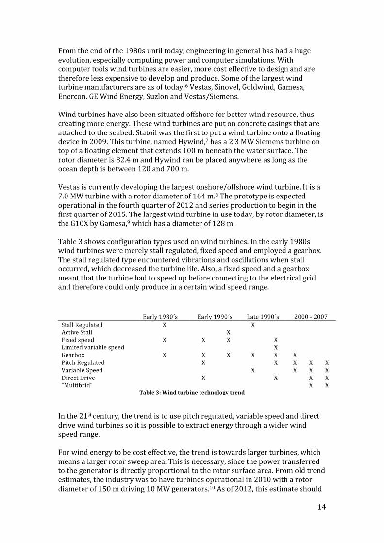
From the end of the 1980s until today, engineering in general has had a huge evolution, especially computing power and computer simulations. With computer tools wind turbines are easier, more cost effective to design and are therefore less expensive to develop and produce. Some of the largest wind turbine manufacturers are as of today:6 Vestas, Sinovel, Goldwind, Gamesa, Enercon, GE Wind Energy, Suzlon and Vestas/Siemens. Wind turbines have also been situated offshore for better wind resource, thus creating more energy. These wind turbines are put on concrete casings that are attached to the seabed. Statoil was the first to put a wind turbine onto a floating device in 2009. This turbine, named Hywind,7 has a 2.3 MW Siemens turbine on top of a floating element that extends 100 m beneath the water surface. The rotor diameter is 82.4 m and Hywind can be placed anywhere as long as the ocean depth is between 120 and 700 m. Vestas is currently developing the largest onshore/offshore wind turbine. It is a 7.0 MW turbine with a rotor diameter of 164 m.8 The prototype is expected operational in the fourth quarter of 2012 and series production to begin in the first quarter of 2015. The largest wind turbine in use today, by rotor diameter, is the G10X by Gamesa,9 which has a diameter of 128 m. Table 3 shows configuration types used on wind turbines. In the early 1980s wind turbines were merely stall regulated, fixed speed and employed a gearbox. The stall regulated type encountered vibrations and oscillations when stall occurred, which decreased the turbine life. Also, a fixed speed and a gearbox meant that the turbine had to speed up before connecting to the electrical grid and therefore could only produce in a certain wind speed range.

Table 3: Wind turbine technology trend

In the 21st century, the trend is to use pitch regulated, variable speed and direct drive wind turbines so it is possible to extract energy through a wider wind speed range. For wind energy to be cost effective, the trend is towards larger turbines, which means a larger rotor sweep area. This is necessary, since the power transferred to the generator is directly proportional to the rotor surface area. From old trend estimates, the industry was to have turbines operational in 2010 with a rotor diameter of 150 m driving 10 MW generators.10 As of 2012, this estimate should

Early 1980´s Early 1990´s Late 1990´s 2000 -‐ 2007 Stall Regulated X X Active Stall X Fixed speed X X X X Limited variable speed X Gearbox X X X X X X Pitch Regulated X X X X X Variable Speed X X X X Direct Drive X X X X “Multibrid” X X

15

have been a bit lower, with the introduction of the Vestas V164-‐7.0 MW turbine in the fourth quarter of 2012. The trend estimate for 2020 is for wind turbines up to 20 MW with rotor diameters of 250 meters, which is shown in Figure 3. Wind turbines rotor diameter is expected to increase by around 5 m per year starting the upcoming decade. Wind energy power plants at onshore locations are expected to prove viable as an economic source of energy, as opposed to offshore wind power having difficulties to overcome. Risø DTU (Technical University of Denmark) set the target for cost reduction to 50 % for offshore wind power, to be competitive to coal-‐fired power by 2020.11

Figure 3: Wind turbine size trend estimate (1980 -‐ 2020)12

3. Airfoils Different airfoil shapes have been developed over the years with NACA as the first systematic numerically defined standard and numerous other designs later on. There also exist airfoils developed for wind turbines only.

3.1 National Advisory Committee for Aeronautics (NACA) Before NACA developed their famous airfoil series, they used theoretical methods instead of geometrical methods to design their profiles. The designs were rather arbitrary with the only thing to guide NACA being past experience with known shapes and experimentation with modifications to those shapes. Those methods began to change in the early 1930s when NACA published a report titled ‘The Characteristics of 78 Related Airfoil Sections from Tests in the Variable Density Wind Tunnel’. This report noted that there were many

16

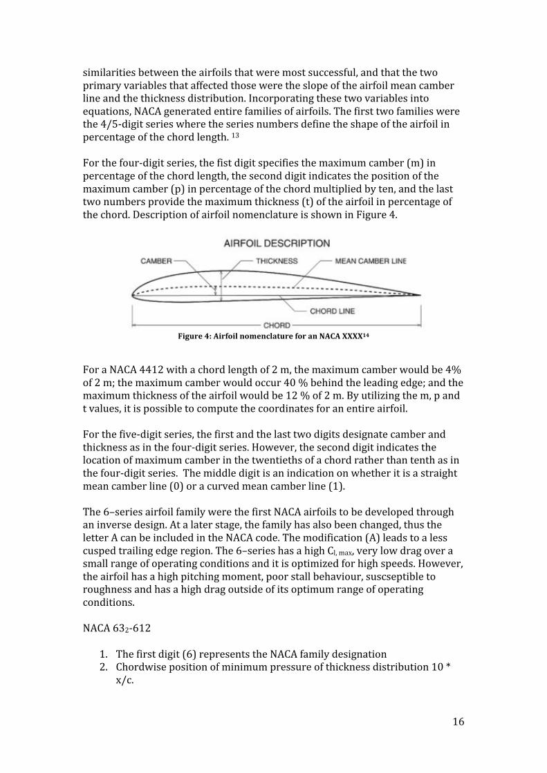
similarities between the airfoils that were most successful, and that the two primary variables that affected those were the slope of the airfoil mean camber line and the thickness distribution. Incorporating these two variables into equations, NACA generated entire families of airfoils. The first two families were the 4/5-‐digit series where the series numbers define the shape of the airfoil in percentage of the chord length. 13 For the four-‐digit series, the fist digit specifies the maximum camber (m) in percentage of the chord length, the second digit indicates the position of the maximum camber (p) in percentage of the chord multiplied by ten, and the last two numbers provide the maximum thickness (t) of the airfoil in percentage of the chord. Description of airfoil nomenclature is shown in Figure 4.

Figure 4: Airfoil nomenclature for an NACA XXXX14

For a NACA 4412 with a chord length of 2 m, the maximum camber would be 4% of 2 m; the maximum camber would occur 40 % behind the leading edge; and the maximum thickness of the airfoil would be 12 % of 2 m. By utilizing the m, p and t values, it is possible to compute the coordinates for an entire airfoil. For the five-‐digit series, the first and the last two digits designate camber and thickness as in the four-‐digit series. However, the second digit indicates the location of maximum camber in the twentieths of a chord rather than tenth as in the four-‐digit series. The middle digit is an indication on whether it is a straight mean camber line (0) or a curved mean camber line (1). The 6–series airfoil family were the first NACA airfoils to be developed through an inverse design. At a later stage, the family has also been changed, thus the letter A can be included in the NACA code. The modification (A) leads to a less cusped trailing edge region. The 6–series has a high Cl, max, very low drag over a small range of operating conditions and it is optimized for high speeds. However, the airfoil has a high pitching moment, poor stall behaviour, suscseptible to roughness and has a high drag outside of its optimum range of operating conditions. NACA 632-‐612

1. The first digit (6) represents the NACA family designation 2. Chordwise position of minimum pressure of thickness distribution 10 *

x/c.

17

3. The subscript digit gives the range of the lift coefficient in tenths above and below the design lift coefficient. Favorable pressure gradients exist on both surfaces.

4. A hyphen. 5. One digit giving the design lift coefficients in tenths. 6. Two last digits describe the maximum thickness as a percentage of the

chord. There are also the 7-‐ and 8-‐digit series where each series were an attempt to maximize the region of laminar flow on the airfoil.15

3.2 National Renewable Energy Laboratory (NREL)16 NREL started the development on airfoils that were specially made for horizontal-‐axis wind turbines in 1984. Since then NREL has come up with nine airfoil families that have been designed for different rotor sizes. The families consist of twenty-‐five airfoils with their designation starting at S801 and ending with S828. The designations represent the numerical order, which the airfoils were designed during 1984-‐1995. After this period there have been some modifications to the airfoils. Some of the airfoils have been improved after wind tunnel testing and other have undergone more comprehensive testing at the Technical University of Delft (TUDelft), in their low-‐turbulence wind tunnel. All these airfoils, except the early blade-‐root airfoils (S804, S807, S808, S811), are designed to have a Cl, max which is relatively insensitive to roughness effects.17 This is accomplished by ensuring that the transition point from laminar to turbulent flow is near the leading edge on the suction side of the airfoil, just prior to reaching Cl, max. At its clean condition, the airfoil achieves low drag through the extensive laminar flow. The tip-‐region airfoils have close to 50 % laminar flow on the suction surface and over 60% laminar flow on the pressure surface. The pitching moment coefficient (Cm) is mostly proportional to Cl, max for the NREL airfoils. Therefore, the tip region airfoils with its low Cl, max exhibits lower Cm than other modern aft-‐cambered aircraft airfoils. The NREL airfoils are also designed to have a soft-‐stall characteristic, which is a result from the progressive separation at the trailing edge. This helps the blade in turbulent wind conditions, by mitigating power and load fluctuation. Other institutions have designed and developed airfoil families as well. Table 4 displays these institutions and their most popular airfoils.18

Table 4: Other wind turbine airfoil families

FFA – Sweden TU Delft RISØE (Denmark) NASA FFA-‐W3-‐211 DU91-‐W2-‐250 A1-‐18 LS1-‐0413 FFA-‐W3-‐241 DU93-‐W-‐210 A1-‐21 LS1-‐0417 FFA-‐W3-‐301 A1-‐24

18

4. Methods

4.1 Historical Turbines Analyzing historical turbines will present an introduction and validation of the Qblade software. Comparing the results to the real operational data, could determine how trustworthy and accurate the software is. The MOD-‐219 and the Gedser turbine were selected for this process due to having the most specifications and references to give a valid comparison.

4.2 General Blade Design Criteria The blade of a wind turbine is the most important part of the structure. If the blade has a poor aerodynamic design it will not be efficient. Therefore, it is very important that the blade exhibits good aerodynamic extraction of energy. But the best aerodynamic design is certainly not always the best solution for the wind turbine as a whole, since a turbine that exhibits good aerodynamic performance may not meet the structural limitations. For a variable speed and variable pitch wind turbine, the blade geometry is designed to give the maximum power at a given TSR, while also a good off-‐design. Good off-‐design provides a high performance over a greater TSR interval. The variables for the optimization are a fixed number of sectional airfoil profiles, chord lengths and twist angles along the blade span. The aerodynamic data is extracted from the respective airfoil database, which has experimental and computed lift and drag coefficients and other data for different Reynolds numbers. There are three different approaches to the blade design for handling wind loads:20 - Withstanding the loads - Shedding/managing the loads - Managing loads mechanically/electrically

A design that is built to withstand the wind loads is the Paul la Cour turbine from 1890. This design is reliable, has a low TSR with three or more blades, high solidity but non-‐optimum blade pitch. Design built after the shedding/managing of the loads principle is optimized for performance, optimum blade pitch, high TSR and a low solidity. The third design principle has innovative mechanical or electrical systems to protect the turbine. It is optimized for control, either two-‐ or three-‐bladed and has a medium TSR. IEC is a worldwide organization for standardization, and offshore wind turbines have to follow certain wind turbine design requirements given in IEC 61400-‐3.21 The turbines have to withstand several of different extreme design load cases for wind and wave conditions. For wind regime the load and safety considerations are divided into two groups: the normal wind conditions which will occur more

19

frequently than once per year during normal operation and the extreme wind conditions which are defined as a 1-‐year or 50-‐year reoccurrence period. The wind turbine rotor is designed to work through a wind speed envelope and to have a maximum power output at a desired wind speed, usually in the high region of that speed envelope. The cut-‐in speed is the beginning of the envelope and the desired wind speed is the rated wind speed. The turbine also has a cutout wind speed, which is the maximum wind speed allowed when the turbine is operational (Figure 5). The turbine also has to withstand increasing wind speed while the rotor is not rotating.

Figure 5: Power curve versus wind speed (m/s)

4.2.1 Blade Performance Criteria The major focus in this project has been on the middle and outer sections of the rotor blade. The turbine is a HAWT design with three blades upstream of the tower. The rotor diameter is given with a length of 165 m powering a 7.0 MW turbine. The turbine is a variable pitch and variable speed design, so it can operate efficiently through a wind speed envelope. The inner section airfoil is predetermined to consist of FFA-‐W3-‐XX1. Since this is an offshore wind turbine, the blade design has to have very low maintenance requirements, resulting in 220 000 hours or 25 years of operating time between maintenance.22 Therefore, the selected airfoils for the blade need to be insensitive to leading edge and upper surface build-‐ups. This build-‐up is particles in the air, ice, salt crystals and bugs.23 The blade should also have an airfoil that has a benign post-‐stall behavior to reduce the dynamic loading on the support structure during wind gusts. Therefore, it is reasonable to look at post-‐stall behavior for different airfoils, where this is possible.

20

Since the blade structure is designed with the blade loading capabilities in mind, the aerodynamic blade loading should be somewhat linear locally along the span. Random Cl peaks along the span of the blade would create stress loading along the blade. A comparison of various airfoil types in a Cl – α diagram should reveal which airfoils have similar Cl at given angles of attacks. Twisting the blade can help generate a loading that is somewhat linear along the span. The downside is higher production cost when twisting the blade. Therefore, similar airfoils should be used over a certain length of the span, with minor amount of local twisting, so that design CL for the whole blade can be obtained through the entire pitching envelope.24 The zero-‐lift pitching-‐moment coefficient for the selected airfoils should be in a reasonably negative range but not too low, since it would give the blade higher stress to withstand. Using an airfoil with an increased leading edge camber would decrease the pitching moment coefficient. The pitching moment coefficient is however neglected in this project. For onshore wind turbines, the noise levels from the blade should be low. Since this blade is for an offshore wind turbine, the noise levels are not taken into account. A higher tip speed will increase noise levels. There are also major limitations when designing a rotor blade. The forces acting on the blade can not be larger than the structural limitations. The bending of the blade is limited to the distance to the tower. If the blades were designed for aerodynamic efficiency, which means thinner profiles towards the tip, the consequence would be increased bending, increased weight and higher production cost. Using thicker airfoils towards the tip can reduce these factors, but also reduced aerodynamic efficiency. Airfoils with the best Cl/Cd are used for the middle and outer section of the rotor to get the highest efficiency within the limitations. Airfoils with high Cl max are used for the inner section, since the drag penalty is negligible in that area.

4.2.2 Inner Root Section Criteria The inner section of the rotor blade is the part that takes up all the forces put upon the entire blade length and therefore has to be designed to withstand these forces. A large blade results in a very thick root section (≈ 0.4 t/c), which is not positive aerodynamically, but the thickness also stiffens the blade, resulting in blade deflection. The inner section has a low tangential speed, since it is near the hub and with a variable incoming wind speed, the relative wind component would have a wide angle of attack. This variation of angle of attack and a thick airfoil is a compromise because of the design criteria to withstand the blade loads. Because of this design compromise together with the low tangential speed,25 the inner section of the blade develops a minor part of the total bending moment for the blade. In this section the lift-‐drag ratio is of less importance, but the Cl, max should be high in order to reduce the blade area.26

21

4.2.3 Middle Section Criteria The middle section has to withstand the forces put upon itself and forces from the outer section. This section would consist of a decreasing thickness to cord ratio towards the outer section. At high tangential speed, the angle of attack for the relative wind component changes less than for the inner section. Normal t/c is between 18 and 30 %.

4.2.4 Outer Section Criteria The most torque generated on a wind turbine is at the outer section. With a very high tangential speed (80 – 90 m/s) at the tip, the wind speed has little effect on the angle of which the relative wind speed is attacking the blade. Since this section only needs to take up its own forces, which results in a thinner structure, a good aerodynamic design can be achieved. The outer section is optimized with L/D at maximum. t/c should be somewhere between 8 and 18 %.

4.2.5 Blade Section Calculation The entire blade is divided into 18 sections which gives around 5 m spacing between them throughout the blade. Each station was analyzed before selecting suitable airfoils for further testing. Known parameters at each station is the tangential and the incoming free stream wind speed, so the relative velocity of the blade can be calculated through Pythagoras equation and thus

𝛼 = arctan 𝑉𝑊 (1)

can be calculated. α is angle of attack in degrees, V is the free stream wind speed and W the relative velocity for the blade at the applicable radius section. Reynolds number can be approximated, giving an estimate of the blade chord at each section.

𝑅𝑒 = 𝜌 𝑊 𝑐𝜇 (2)

Re is dimensionless, ρ is the density of the air, c is the chord and μ is the dynamic viscosity of the air. With the known variables above and an estimate of the chord length at each section, a number of airfoils can be analyzed for performance. With Cl max and at which α it occurs for airfoils, a twist for each section can be selected. Further on, a study of the selected airfoil has to be made to check if this is the best solution for the blade.

22

4.2.6 Specific Blade Design In this project, an offshore wind turbine blade was to be designed in open source software and verified in professional wind turbine software. With a diameter of 165 meter the blade design has to deliver 7.0 MW. Since the size of this turbine is somewhat similar to other commercial wind turbines, it was reasonable to use some of these operational data, given in Table 5.

Example of commercial wind turbine operational data Power regulation Pitch regulated with variable speed Operational data Rated power 7.0 MW Cut-‐in, cut-‐out wind speed 4 m/s – 25 m/s Operational rotational speed 4.8 – 12.1 rpm Nominal rotational speed 10.5 rpm Design parameters Wind Class IEC S Annual avg. wind speed 11 m/s Weibull shape parameter, k 2.2 Weibull scale parameter 12.4 m/s Turbulence intensity IEC B Max inflow angle (vertical) 0 degrees Rotor Rotor diameter 164 m Blade length 80 m

Max chord 5.4 m

Table 5: Example of turbine specification

23

Figure 6: Vestas v164 power curve

Using these specifications, a reasonable comparison could be made of the power curve (Figure 6) of professionally designed wind turbines. There is no information of airfoil, chord and twist distribution available.

4.2.7 Blade Design Procedure The whole blade design procedure was done through computer software, but essential initial values for the procedure were calculated using an excel spreadsheet. The following procedure shows a simple theoretical aspect when designing and optimizing a rotor blade.

• With the given parameters and design criteria, the power coefficient can be extracted from the following equation:

𝑃 = 𝐶!𝜂12𝜌𝜋𝑅

!𝑉! (3)

P is the power output, Cp is the power coefficient, η is the electrical and mechanical efficiencies where 0.9 is a reasonable number, ρ is the density, R is the radius of the rotor and V is the design wind speed.

24

Solving for CP, the whole rotor has to have a power coefficient of 0.304 with a wind speed of 12.5 m/s or 0.446 at a wind speed of 11 m/s, if it is to produce 7.0 MW.

• A blade tip speed ratio (TSR) and the number of blades have to be

selected.

• Airfoils have to be selected for their respective radial blade section for their respective performance and geometry so that the overall performance requirements can be attained.

• The first step is to choose an initial chord distribution for the blade. The

following equation is very susceptible to large chord lengths and is normally only used on middle and outer section for large turbines.

- 𝐶!"# =

!!"!

!!!!

!!"#$%&!!!

(4)

• • COpt – optimum chord length (initial) • vdesign – design wind speed • vr – local effective velocity • λ – local tip speed ratio • Cl – local design lift coefficient • r – local blade length • B – number of blades

• The solution for the flow around the blade is optimized employing the

blade element momentum theory. This procedure is only a simple road map on how to develop a blade. The full design of a rotor blade, including the twist and chord distribution has to go through an iterative process that is very time-‐consuming. The design of rotor blades is in this project was mainly developed with the freeware software Qblade and verified in the professional software Flex5.

4.3 Airfoil Catalogue and Roughness Insensitivity Analysis The airfoils under consideration for a wind turbine were the NACA 63-‐XXX, 64-‐XXX, DU and FFA profiles, as these are available on the Internet and in published airfoil catalogues.27 The airfoil catalogue therefore consists of almost 40 different airfoils. Some of them are tailored for use on wind turbines,28 while other were designed for aircraft. The roughness insensitivity analysis is performed at two Reynolds numbers and forced transition at 2 % of the chord. The first Reynolds number at 4 millions

25

indicates a thin boundary layer while at 500 000 Reynolds number indicates a thick turbulent boundary layer, the latter one simulating a rough surface and increased drag. The comparison between the two simulations was done at Cl, max. There is also a comparison of the roughness insensitivity when the airfoil has the best Cl/Cd. The difference in performance between the results in the first simulation would be an indicator on how insensitive the airfoils are against surface roughness.

4.3.1 Airfoil Design for Wind Turbines With Roughness Insensitivity The desired behavior of an airfoil for wind turbines differs from the expected behavior for airfoils designed for airplanes. As wind turbines are built to operate over an extensive period of time between maintenance, the airfoil selected should be insensitive to surface roughness. Therefore, the goal when selecting an airfoil for a wind turbine is to pick a design that gives a maximum lift coefficient that is relatively insensitive to leading-‐edge roughness. Figure 7 shows the drag polar that meets these design requirements.29 The figure shows the S902 airfoil design where point A is the lower limit of low drag, lift coefficient range, while B is the upper limit. Point C however, is outside the low-‐drag range and thus drag increases, because the boundary layer transition (laminar to turbulent flow) moves rapidly towards the leading edge with increasing (or decreasing) lift coefficient. By this design, the profile produces a suction peak close to the leading edge at higher lift coefficients, ensuring that transition will occur at the leading edge. Therefore, point C in Figure 7 shows the maximum lift coefficient with turbulent flow along the whole upper surface. This design, at max lift coefficient, is therefore relatively insensitive to surface roughness at the leading edge.

Figure 7: Cl/Cd for the S902 airfoil

26

Figure 8 shows the pressure distribution of the same airfoil at operating point A. In Figure 7, the airfoil has a favorable pressure gradient along the upper surface to about 45 % of the chord. Behind this point, the pressure has a negative gradient, which encourages the transition from laminar to turbulent flow. After this pressure gradient (last 90 % of the chord) is an almost linear pressure recovery. This linear pressure area restricts the separation at high angles of attack, resulting in a higher maximum lift coefficient while maintaining low drag. This feature has added some benefit of promoting docile stall characteristics.30 At the front of the lower surface the pressure gradient is adverse, then zero to about 65 % of the chord while the pressure is favorable after this point. Therefore, the transition is imminent for the lower surface, which allows for a wide low-‐drag range to be achieved and the camber increases in the leading-‐edge region. Increasing the camber results in better balance with respect to pitching moment and the aft camber, which both contribute to a high maximum lift coefficient and low profile drag. The trailing edge has a concave pressure recovery, which gives the airfoil lower drag and later separation.

Figure 8: Pressure distribution for the S902 airfoil at operating point A

Figure 9 shows the pressure distribution at point B in Figure 7. There is no spike in the pressure field at the upper leading edge, rather a rounded peak occurs. This allows an increase in lift coefficient with no significant separation. At higher angles of attack, the peak becomes sharper and the transition starts to move towards the leading edge, which results in roughness insensitivity of the maximum lift coefficient.

27

Figure 9: Pressure distribution for S902 airfoil at operating point B

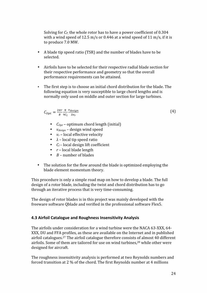
Figure 10 shows the same S902 profile results from a wind tunnel test with a maximum lift coefficient at 13.9 degrees. This is at operating point C in Figure 7. The pressure peak is evident at the leading edge with separation relatively confined over the last 25 % of the cord. The conclusion is that there is a connection between airfoil thickness, maximum lift coefficient and the airfoil surface roughness sensitivity. The effect of roughness on the maximum lift coefficient increases with increasing airfoil thickness and decreases slightly with increasing maximum lift coefficient.

28

Figure 10: Experimental wind tunnel test of the S902 airfoil at operating point C

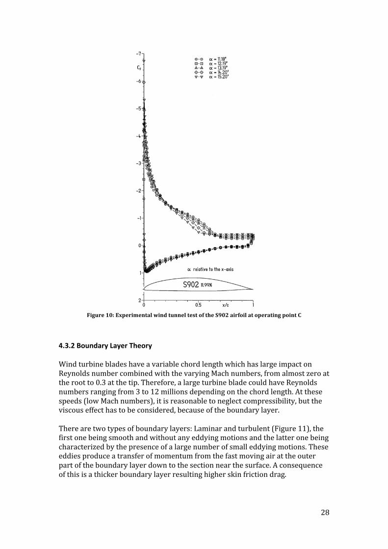
4.3.2 Boundary Layer Theory Wind turbine blades have a variable chord length which has large impact on Reynolds number combined with the varying Mach numbers, from almost zero at the root to 0.3 at the tip. Therefore, a large turbine blade could have Reynolds numbers ranging from 3 to 12 millions depending on the chord length. At these speeds (low Mach numbers), it is reasonable to neglect compressibility, but the viscous effect has to be considered, because of the boundary layer. There are two types of boundary layers: Laminar and turbulent (Figure 11), the first one being smooth and without any eddying motions and the latter one being characterized by the presence of a large number of small eddying motions. These eddies produce a transfer of momentum from the fast moving air at the outer part of the boundary layer down to the section near the surface. A consequence of this is a thicker boundary layer resulting higher skin friction drag.

29

Figure 11: Boundary Layer around an airfoil where the thickness is greatly exaggerated.31

When the pressure increases in the direction of flow along the surface of the wing, a general deceleration takes place. For the outer part of the boundary layer this is in accordance with Bernoulli´s law.32 For the innermost part no simple law exists for their behavior because of the viscous effects. The relative loss of speed is somewhat greater for the particles of fluid closer to the surface than for those at the outer part of the boundary layer. This is since the reduced kinetic energy of the boundary-‐layer air restricts its own ability to flow against the adverse pressure gradient. If the pressure in the boundary layer increases, the motion of the fluid can be reversed and could move upstream again. This causes a separation of the turbulent layer from the surface. Because of the higher change of momentum inside the turbulent boundary layer than in the laminar, the turbulent layer is more resistant to separation. When separation occurs, the boundary layer can either be separated or reattach again to the surface, as a turbulent boundary layer. Laminar separation can occur33, usually on wing sections near the leading edge at maximum lift. This local separation decreases in size when the Reynolds number increases. Smooth airfoils used on airplanes with low and moderate lift coefficients under normal flight conditions, normally has a laminar boundary layer from the leading edge and back to approximately the location of the first minimum-‐pressure point. This is for both surfaces (upper and lower). If the laminar region is extensive, separation occurs immediately downstream of the minimum-‐pressure point. The boundary layer then returns to the surface as a turbulent layer almost immediately. If the surface is not smooth enough, the air is turbulent or has a high Reynolds number, transition from laminar to turbulent flow may occur anywhere upstream of the calculated laminar separation point.34 For airfoils where low and moderate lift coefficients and non-‐appreciable separation occurs, the main part of the profile drag is caused by skin friction. Therefore, the drag coefficients depend on the amount of laminar and turbulent flow. If the transition point is known, the drag coefficient can be calculated from boundary-‐layer theory. For airfoils with increasing lift coefficients due to a positive change in angle of attack, the minimum-‐pressure point shifts upstream towards the leading edge, thus reducing the amount of laminar boundary layer and increasing the amount

30

of turbulent flow. The combination of increasing flow velocity over the surface and the turbulent layer results in an increased drag coefficient. When developing high lift coefficients, the form drag resulting from separation of the flow from the surface is the main part of the drag. Laminar separation occurs near the leading edge with a returning turbulent boundary layer. A high Reynolds number is favorable when trying to develop the turbulent boundary layer.35 Low Reynolds numbers is a factor when the turbulent layer separates from the surface, resulting in a loss in lift and increased drag, stall occurs. Figure 12 shows three different equations, which show relations between laminar and turbulent flow for a range of Reynolds number and the resulting skin friction. These equations are outside the scope of this report so the figure only shows an indication on the relationship.

Figure 12: Turbulent and laminar boundary layer for skin friction and Reynolds numbers

Since the profile drag on an airfoil is strongly connected to the thickness of the boundary layer, it is desirable to know where transition and separation occur and the thickness of the boundary layer. It is also desirable to know how stable the boundary layer is. Therefore it is reasonable to look at the shape factor36 when comparing the size and shape of boundary layer for different airfoils. The shape factor H12 and H32 (first and second shape factor) for the boundary layer increases towards the separation point. H is given by displacement thickness δ1 (m) over the momentum thickness δ2 (m) and energy thickness of boundary layer δ3 (m).

𝐻!" = 𝛿!𝛿!, 𝐻!" =

𝛿!𝛿!

(5)

The displacement thickness is a measure how far the streamlines are pushed away from the solid surface compared to a frictionless potential flow for the same configuration, while the momentum thickness is a measure of how much

31

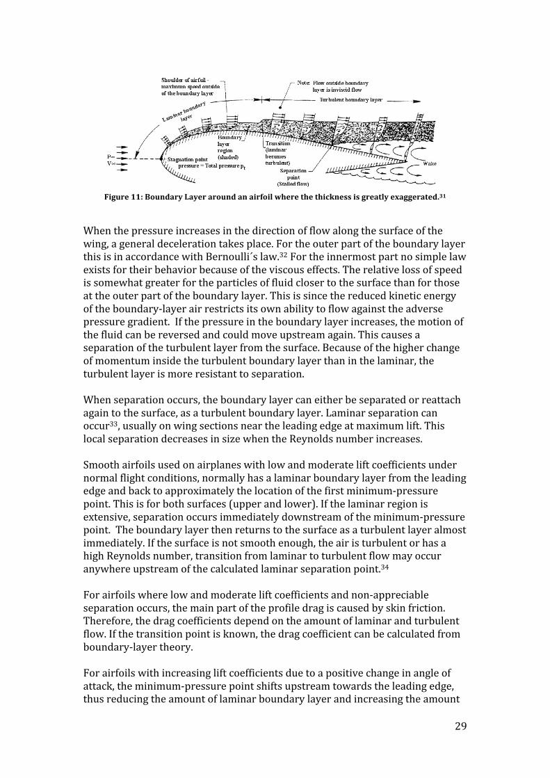
momentum is lost through friction compared to a frictionless potential flow for the same configuration. For laminar boundary layers, the first shape factor, H12, is between 3.5 and 2.3. Transition brings a considerable drop in H12 resulting in a turbulent boundary layer with H12 between 1.3 and 2.2. Laminar separation takes place at a value of H12 near 3.5 while turbulent separation takes place at a value of H12 near 2.2. For airfoils used on airplanes it is normal to try delay the transition from laminar to turbulent flow as long as possible to make drag coefficient as low possible. For higher values of Reynolds numbers the only way to delay this transition is to reduce all disturbances such as stream turbulence, unsteadiness and surface roughness. With this knowledge of the relation of the shape factor as an indication of laminar and turbulent flows, it is possible to extract data from Javafoil diagrams, where the shape factor over the chord is plotted. T.U and S.U are transition and separation upper while T.L and S.L are the lower transition and separation. As an example, Figure 13 shows an NACA 63-‐612 profile at an α of 2 degrees, Reynolds number of 4 millions and free transition. H12 drops at 40 % of the chord from 3.75 to 1.4, which indicates a transition from laminar to turbulent boundary layer. For the last 10 % of the chord, the shape factor increases again, indicating a separation in the area.

Figure 13: Shape factor H vs. x/c in Javafoil.

32

4.4 Blade Element Momentum (BEM) Theory The blade element momentum theory is a well-‐used theory to easily calculate the effect and efficiency of wind turbines. The theory is very simple compared to the complex flow in the turbine, but gives somewhat accurate numbers compared to experimental data. Because of the simplicity and good results, this theory is widely used in both free and in professional wind turbine software.

4.4.1 Momentum Theory Consider a stream tube around a wind turbine as shown in Figure 14. There are four stations in the figure, 1-‐4.37 Energy is extracted from the wind between stations 2 and 3, resulting in a change in pressure. With the assumption that station 1 is placed some distance upstream and station 4 is placed some distance downstream in the undisturbed free stream, it can be assumed that pressure p1 = p4. Velocity V2 = V3 can also be assumed. The third and final assumption is that the flow is frictionless between stations 1 to 2 and 3 to 4. With this final assumption, Bernoulli’s equation can be applied and note that 𝐹 = 𝑃𝐴, where P is pressure and A is area. This yields

Figure 14: Stream tube around a wind turbine

𝑑𝐹! =12𝜌 𝑉!! − 𝑉!! 𝑑𝐴

(6)

By defining a (the axial induction factor) as

𝑎 =𝑉! − 𝑉!𝑉!

or 𝑉! = 𝑉!(1− 𝑎) 𝑉! = 𝑉!(1− 2𝑎)

(7)

(8) (9)

Substitution yields

Wind Turbine Blade Analysis Durham University

1 2 3 4

V1 V

4

Hub

Blades

Figure 1: Axial Stream tube around a Wind Turbine

1 Introduction

This short document describes a calculation method for wind turbine blades, thismethod can be used for either analysis of existing machines or the design of newones. More sophisticated treatments are available but this method has the advan-tage of being simple and easy to understand.

This design method uses blade element momentum (or BEM) theory to com-plete the design and can be carried out using a spreadsheet and lift and drag curvesfor the chosen aerofoil.

The latest version of this document should be available from the author’s website1Any comments on the document would be gratefully received. Further details onWind Turbine Design can be found in Manwell et al. (2002) which provides com-preshensive coverage of all aspects of wind energy. Walker and Jenkins (1997) alsoprovide a comprehensive but much briefer overview of Wind Energy.

2 Blade Element Momentum Theory

Blade Element Momentum Theory equates two methods of examining how a windturbine operates. The first method is to use a momentum balance on a rotatingannular stream tube passing through a turbine. The second is to examine the forcesgenerated by the aerofoil lift and drag coefficients at various sections along theblade. These two methods then give a series of equations that can be solved itera-tively.

3 Momentum Theory

3.1 Axial Force

Consider the stream tube around a wind turbine shown in Figure 1. Four stationsare shown in the diagram 1, some way upstream of the turbine, 2 just before the

1http://www.dur.ac.uk/g.l.ingram

5

33

𝑑𝐹! =12𝜌𝑉!

! 4𝑎(1− 𝑎) 2𝜋𝑑𝑟 (10)

Consider that the annular stream tube receives a rotation from the turbine between stations 2 and 3 that imparts rotation onto the blade wake. If the angular momentum in the annular stream tube is conserved, the blade wake rotates by the angular velocity ω and the blade rotates at an angular velocity Ω. Then torque will be 𝑑𝑇 = 𝜌𝑉!𝜔𝑟!2𝜋𝑑𝑟 (11) By defining a’ (the angular induction factor) as 𝑎! =

𝜔2Ω

(12)

Substitution with equation 6 yields 𝑑𝑇 = 4𝜋𝑟!𝜌𝑉Ω 1− 𝑎 𝑎′𝑑𝑟 (13) Thus the momentum theory provides equations for the axial (equation 8) and tangential forces (equation 11)

4.4.2 Blade Element Theory This theory relies on two assumptions: There are no aerodynamic interactions between different blade elements and the forces on the blade elements are only determined by the lift and drag coefficients. Consider a blade divided into N elements along the span. Each of the elements will experience a different flow because they have a different tangential speed (Ωr), chord (c) and a different twist angle (γ). Let the wind speed be V. The theory involves dividing the blade into a sufficient number of elements and calculating the flow for each one. The overall performance characteristics are determined by numerical integrations along the blade span. Figure 15 shows how the blade rotation and wake rotation together with V2 (wind speed) yield the relative wind speed W.

34

Figure 15: Relative, rotational and incoming wind speed

𝑡𝑎𝑛 𝛽 =𝛺𝑟 1+ 𝑎!

𝑉 1− 𝑎

relative velocity W is

(14)

𝑊 =V(1− 𝑎)cos𝛽 (15)

In Figure 16 the lift and drag forces are by definition perpendicular and parallel to the incoming flow. The forces on the blade elements are also shown, and for each blade element the forces will be

Figure 16: Forces on a turbine blade

𝑑𝐹! = 𝑑𝐿 sin𝛽 − 𝑑𝐷 cos𝛽 𝑑𝐹! = 𝑑𝐿 cos𝛽 + 𝑑𝐷 sin𝛽

(16) (17)

dL and dD are lift and drag forces on the blade element. By applying the definition of L and D, adding the number of blades B to these equations and making the equation more useful by expressing W in the terms of induction factors yield


V(1-a)W

r

r r

2

x

r

blade rotation

wake rotation

Figure 5: Flow onto the turbine blade

4.1 Relative Flow

Lift and drag coefficient data area available for a variety of aerofoils from windtunnel data. Since most wind tunnel testing is done with the aerofoil stationary weneed to relate the flow over the moving aerofoil to that of the stationary test. To dothis we use the relative velocity over the aerofoil. More details on the aerodynam-ics of wind turbines and aerofoil selection can be found in Hansen and Butterfield(1993).

In practice the flow is turned slightly as it passes over the aerofoil so in orderto obtain a more accurate estimate of aerofoil performance an average of inlet andexit flow conditions is used to estimate performance.

The flow around the blades starts at station 2 in Figures 2 and 1 and ends atstation 3. At inlet to the blade the flow is not rotating, at exit from the blade rowthe flow rotates at rotational speed ω. That is over the blade row wake rotation hasbeen introduced. The average rotational flow over the blade due to wake rotation istherefore ω/2. The blade is rotating with speed Ω. The average tangential velocitythat the blade experiences is therefore Ωr+ 1

2ωr. This is shown in Figure 5.Examining Figure 5 we can immediately note that:

Ωr+ωr2

=Ωr(1+a!) (18)

Recall that (Equation 5): V2 =V1(1"a) and so:

tanβ=Ωr(1+a!)V (1"a)

(19)

WhereV is used to represent the incoming flow velocityV1. The value of βwillvary from blade element to blade element. The local tip speed ratio λr is definedas:

λr =ΩrV

(20)

9


L

x

F

Fx

i

D

Figure 6: Forces on the turbine blade.

So the expression for tanβ can be further simplified:

tanβ=λr(1+a!)(1"a)

(21)

From Figure 5 the following relation is apparent:

W =V (1"a)cosβ

(22)

4.2 Blade Elements

The forces on the blade element are shown in Figure 6, note that by definition thelift and drag forces are perpendicular and parallel to the incoming flow. For eachblade element one can see:

dFθ = dLcosβ"dDsinβ (23)dFx = dLsinβ+dDcosβ (24)

where dL and dD are the lift and drag forces on the blade element respectively.dL and dD can be found from the definition of the lift and drag coefficients asfollows:

dL=CL12ρW 2cdr (25)

dD=CD12ρW 2cdr (26)

Lift and Drag coefficients for a NACA 0012 aerofoil are shown in Figure 7, thisgraph shows that for low values of incidence the aerofoil successfully produces a

10

35

𝑑𝐹! = 𝜎′𝜋𝜌𝑉!(1− 𝑎)!

cos!𝛽 𝐶! sin𝛽 + 𝐶! cos𝛽 𝑟𝑑𝑟

(18)

𝑑𝑇 = 𝜎′𝜋𝜌𝑉!(1− 𝑎)!

cos!𝛽 𝐶! cos𝛽 − 𝐶! sin𝛽 𝑟𝑑𝑟

(19) σ’ is called the local solidity factor and is defined as

𝜎! =𝐵𝑐2𝜋𝑟

(20)

The axial induction factor a is obtained by equalizing two dFx equations, equation (8) and (16)

𝑎 =1

4sin!𝛽𝜎𝐶!

+ 1

(21)

a’ is obtained by equalizing two dT equations, equation (11) and (17)

𝑎′ =1

4 sin𝛽 cos𝛽𝜎𝐶!

− 1

(22)

Where 𝐶! = 𝐶! sin𝛽 − 𝐶! cos𝛽

(23)

𝐶! = 𝐶! cos𝛽 + 𝐶! sin𝛽 (24) These are the basics of the BEM theory. However, before the system of equations can be solved, several corrections to the theory have to be taken in for account. These corrections include tip-‐ and hub-‐loss to account for vortices shed at these locations, the Glauert correction to account for large induced velocities (a>0.4), and the skewed wake correction to model the effect of incoming flow that is not perpendicular to the rotor plane.

4.4.3 Prandtl’s Tip Loss Factor Prandtl’s tip loss factor corrects the assumption of an infinite number of blades. The vortex system in a wake differs as to a finite number of blades in comparison to a rotor with an infinite number of blades. Prandtl derived a correction factor F to equations (8) and (11).

36

𝑑𝐹! = 4𝜋𝑟𝜌𝑉!(1− 𝑎)𝑎𝐹𝑑𝑟

(25)

𝑑𝑇 = 4𝜋𝑟!𝜌𝑉!Ω 1− 𝑎 𝑎′𝐹𝑑𝑟 (26) where

𝐹 =2𝜋 cos

!!(𝑒!!) (27)

and

𝑓 =𝐵2𝑅 − 𝑟𝑟 sin𝛽

(28)

B is the number of blades, R is the radius of the rotor, r is the local radius for the element and β is the inflow angle.

4.4.4 Glauert correction The Glauert correction for high values of a is a correction that comes into place when the axial induction factor becomes larger than approximately 0.4. This means that the simple momentum theory breaks down. Different relations between the thrust coefficient CF and a can be made to fit with measurement

𝐶! =4𝑎 1− 𝑎 𝐹 𝑎 ≤ 𝑎!4(𝑎!! + 1− 2𝑎! 𝑎)𝐹 𝑎 > 𝑎!

(29)

ac is approximately 0.2 and F is Prandtl’s tip loss factor. Through definitions and equation CF therefore becomes

𝐶! =(1− 𝑎)!𝜎𝐶!

sin!𝛽 (30)

The expression for CF can now be equated into expression (27). The corrected equation for a is: If a<ac:

𝑎 =1

4𝐹sin!𝛽𝜎𝐶!

+ 1

(31)

37

which is equation (19) with the tip loss correction If a>ac:

𝑎 =12 2+ 𝐾 1− 2𝑎! − (𝐾 1− 2𝑎! + 2)! + 4(𝐾𝑎!! − 1)

where

𝐾 =4𝐹sin!𝛽𝜎𝐶!

(32)

(33)

All the necessary equations for the BEM theory are now displayed. The algorithm can now be summarized as the eight steps below (1) Initialize a and a’, typically a = a’ = 0 (2) Compute the inflow angle β Equation (12) (3) Compute the local angle of attack (4) Read Cl (α) and Cd (α) from table (5) Compute Cn and Ct Equation (21) and (22) (6) Calculate a and a’ Equation (30) and (31) (7) If a and a’ have changed more than a certain

tolerance, go to step (2) or else finish

(8) Compute the local loads on the segment of the blades After applying the BEM algorithm to all control volumes, the tangential and axial load distributions are known and global parameters such as the mechanical power, thrust and root bending moment can be computed. The power coefficient CP for the whole turbine without general losses such as generator loss, can be calculated through the following equation:

𝐶! = (8𝜆!) 𝜆!! 𝑎

!

!!´(1− 𝑎) 1−

𝐶!𝐶!

cot𝜃 𝑑𝜆! (34)

λh is the local tip speed ratio at the hub, λ is the global tip speed ratio and λr is the tip speed ratio at radius r from the hub.

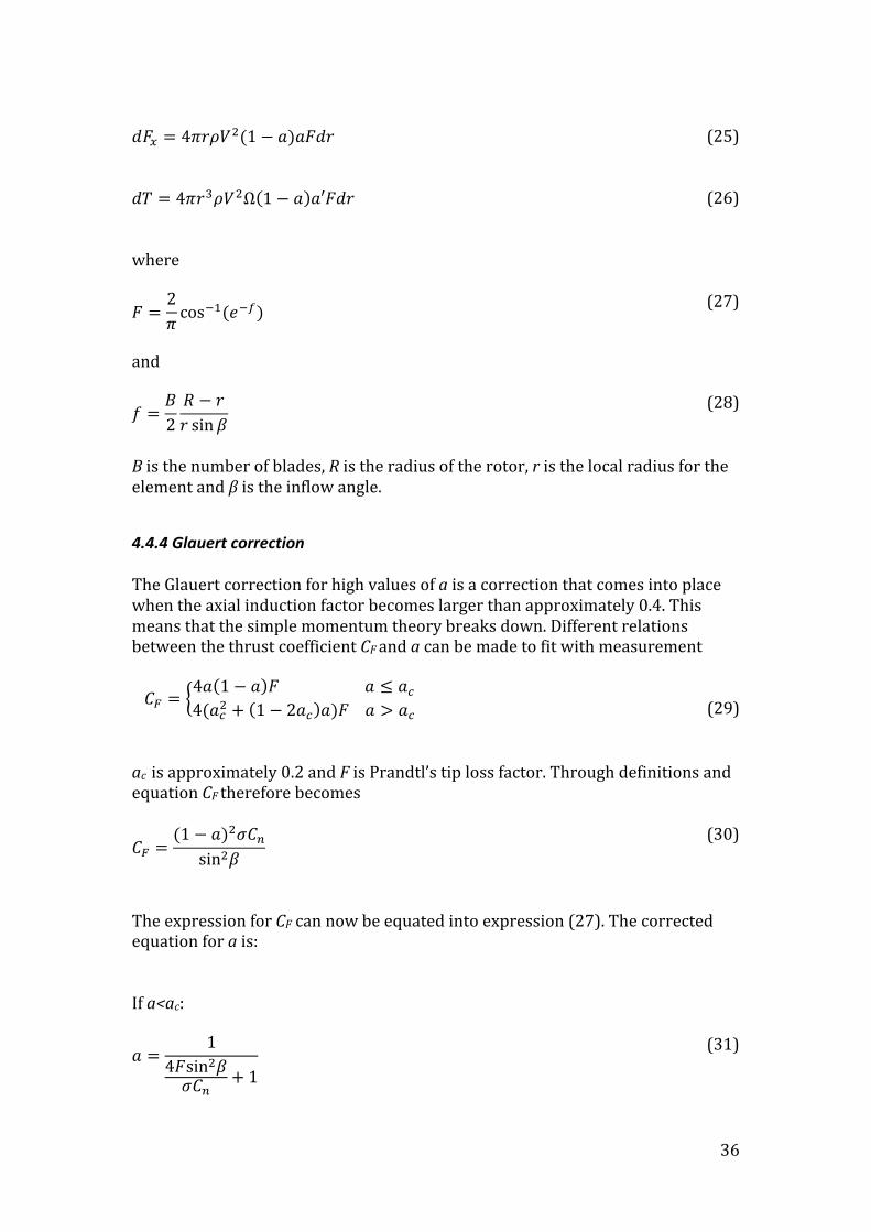
Figure 17 shows the relation between the power coefficient and the tip speed ratio. An increase of the tip speed ratio is favorable until a certain limit is reached. Betz’ limit says that an ideal wind turbine with no losses has a theoretical maximum efficiency of 0.593. The most modern and efficient wind turbines today can reach around 0.45 to 0.49. Everything over 0.5 is considered very good.

38

Figure 17: Power coefficient versus tip-‐speed ratio

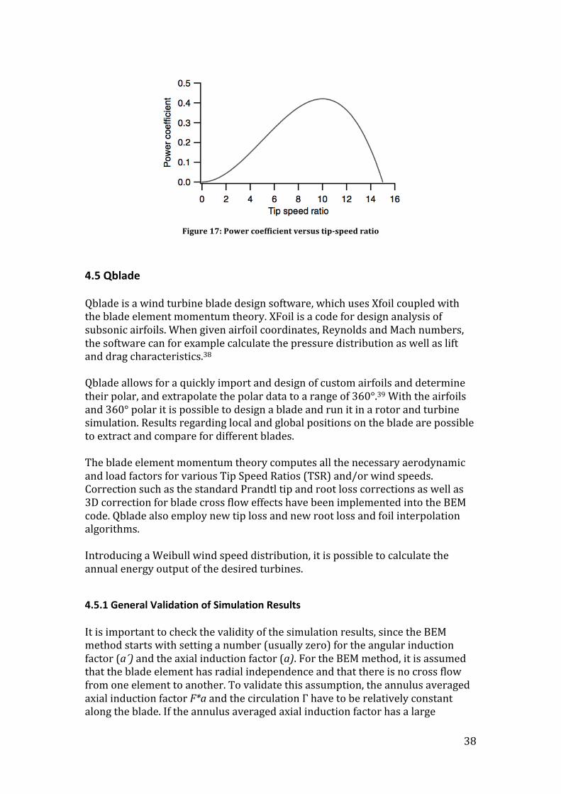
4.5 Qblade Qblade is a wind turbine blade design software, which uses Xfoil coupled with the blade element momentum theory. XFoil is a code for design analysis of subsonic airfoils. When given airfoil coordinates, Reynolds and Mach numbers, the software can for example calculate the pressure distribution as well as lift and drag characteristics.38 Qblade allows for a quickly import and design of custom airfoils and determine their polar, and extrapolate the polar data to a range of 360°.39 With the airfoils and 360° polar it is possible to design a blade and run it in a rotor and turbine simulation. Results regarding local and global positions on the blade are possible to extract and compare for different blades. The blade element momentum theory computes all the necessary aerodynamic and load factors for various Tip Speed Ratios (TSR) and/or wind speeds. Correction such as the standard Prandtl tip and root loss corrections as well as 3D correction for blade cross flow effects have been implemented into the BEM code. Qblade also employ new tip loss and new root loss and foil interpolation algorithms. Introducing a Weibull wind speed distribution, it is possible to calculate the annual energy output of the desired turbines.

4.5.1 General Validation of Simulation Results It is important to check the validity of the simulation results, since the BEM method starts with setting a number (usually zero) for the angular induction factor (a´) and the axial induction factor (a). For the BEM method, it is assumed that the blade element has radial independence and that there is no cross flow from one element to another. To validate this assumption, the annulus averaged axial induction factor F*a and the circulation Γ have to be relatively constant along the blade. If the annulus averaged axial induction factor has a large

39

gradient it means that a cross flow exists while a large gradient in circulation causes a radial dependent downwash. This validation should especially be checked at the outer part of the blade while the turbine is operated at rated power. It is also important to check the validity of the airfoil polars. If a polar made for a different Reynolds number is used, the simulation results could be inconsistent with reality. If the difference in Reynolds number is higher than 10!, then a polar closer to the Reynolds number obtained in the simulation should be used.

4.6 Javafoil The Javafoil program is built up using two main methods:

• Potential flow analysis • Boundary layer analysis

The potential flow analysis is done through a higher order panel method. When given a set of airfoil coordinates, the program calculates the local and inviscid flow velocities along the surface of the airfoil at any angle of attack. The boundary layer analysis module starts from the stagnation point and steps along the upper and lower surfaces of the airfoil. It solves a set of differential equations to find the various boundary layer parameters (integral method). The equations and criteria for separation and transition are based on the procedures described by Eppler. When supplied with an airfoil or coordinates to an airfoil, the program will examine it. It will first calculate the distribution of the velocity on the airfoil surface to get the lift and moment coefficients. Then it will calculate the behavior of the boundary layer. These data can be used to calculate the friction drag. Javafoil also has a helpful function where it is possible to create an airfoil getting the airfoil coordinates, since the program has equations and functions to extract the coordinates from several airfoil families.

4.6.1 Roughness analyses In Javafoil it is possible to perform a sensitivity analysis of an airfoil where the surfaces are either smooth, NACA standard or rough. This roughness effect analysis is executed based on two different models.

-‐ Laminar flow on a rough surface will be stabilized leading to premature transition

-‐ Laminar as well as turbulent flow on rough surfaces produce a higher skin friction drag.

40

The global effect of roughness on the drag is calculated into the total drag coefficient 𝐶! = 𝐶! (1+

𝑟10)

(35)

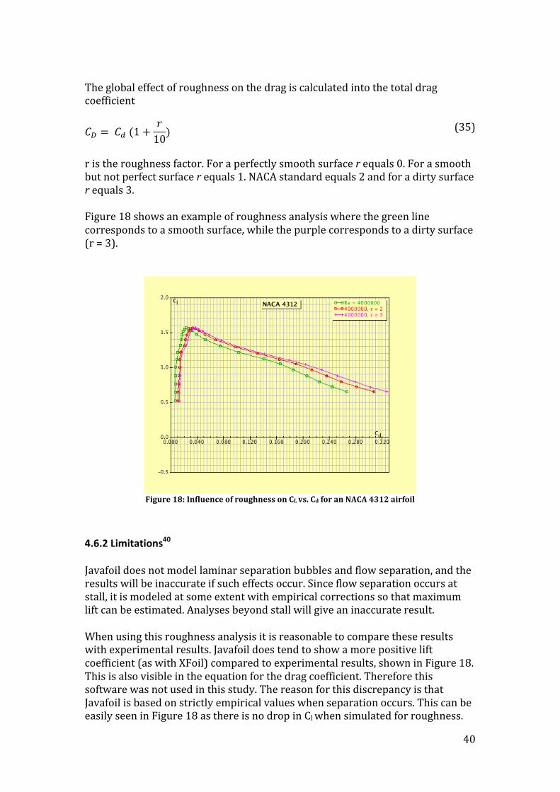
r is the roughness factor. For a perfectly smooth surface r equals 0. For a smooth but not perfect surface r equals 1. NACA standard equals 2 and for a dirty surface r equals 3. Figure 18 shows an example of roughness analysis where the green line corresponds to a smooth surface, while the purple corresponds to a dirty surface (r = 3).

Figure 18: Influence of roughness on CL vs. Cd for an NACA 4312 airfoil

4.6.2 Limitations40 Javafoil does not model laminar separation bubbles and flow separation, and the results will be inaccurate if such effects occur. Since flow separation occurs at stall, it is modeled at some extent with empirical corrections so that maximum lift can be estimated. Analyses beyond stall will give an inaccurate result. When using this roughness analysis it is reasonable to compare these results with experimental results. Javafoil does tend to show a more positive lift coefficient (as with XFoil) compared to experimental results, shown in Figure 18. This is also visible in the equation for the drag coefficient. Therefore this software was not used in this study. The reason for this discrepancy is that Javafoil is based on strictly empirical values when separation occurs. This can be easily seen in Figure 18 as there is no drop in Cl when simulated for roughness.

41

In this project the software was used to build airfoils and check the transition and separation points along the chord, when analyzing the roughness insensitivity.

4.7 Flex5 Flex5 is a highly protected and licensed software developed by Stig Øye and DTU. Therefore, Statoil employee, Andreas Knauer, has performed all simulations presented in this report. The authors of this report have set up all the input files for flex5, after a template given by Statoil. Flex5 is an advanced wind turbine simulator that accounts for every aspect of the turbine and its surroundings. For aerodynamic calculations, it employs a heavy BEM code. Flex5 is dependent on input of aerodynamic data, so 360 degrees polar from Qblade for Cl, Cd and Cm for each airfoil used in the blade has to be extracted. Qblade does not calculate Cm outside the proper lift curve, typically -‐2 to 25 degrees, so a standard value (flat plate) has to be set for the rest of the polar range. Flex5 is also very sensitive, so all the different airfoils must have the exact same amount of polar points at the same angle for the 360 degrees polar. A text file with the blade geometry has to be created containing span position, twist and chord for the different airfoils used in the blade design. These files are used in Flex5 to create the blade used in Qblade. An example of a text file geometry is shown in Appendix D. In Flex5, simulations are executed with an aero-‐elastic code with conditions set by the user. The time period for the simulations is set to either 3600 seconds (1 hour) because of the offshore conditions or 600 seconds when in turbulence or wind shear. These intervals are IEC standards. The 60 minutes simulation is performed because the largest significant wave height can occur in this time period. If the simulation period is decreased, these waves could then easily be missed. For onshore wind turbines, the simulation period is shorter. Design load cases are simulated with different wind shear and turbulence intensity. For wind shear, the power exponent (a) is used to simulate different locations and stability of the air. Different locations and wind stability is shown for the power exponent in Table 6.

Location a Unstable air above open water surface 0.06 Neutral air above open water surface 0.10 Unstable air above flat open coast 0.11 Neutral air above flat open coast 0.16 Stable air above open water surface 0.27 Unstable air above human inhabited areas 0.27 Neutral air above human inhabited areas 0.34 Stable air above flat open coast 0.40 Stable air above human inhabited areas 0.60

Table 6: Wind shear power exponent

42

5. Results

5.1 Historical Turbines With the introduction to the historical aspect of wind turbines, two turbines were thoroughly investigated in a literature study and reconstructed in Qblade. With real operational information about these wind turbines, a comparison between real operation and Qblade could be made.

5.1.1 Gedser Wind Turbine Since the Gedser turbine was refurbished in the early 1980´s there exist a lot of different information about the type of airfoils used, operational speed and power output. So this simulation and corresponding results consists off the NACA 4312 and the CLARK Y airfoils, which is given in Figure 19. The blade has a length of 12 m but only 9 m are used to produce power as shown in Figure 20. With a chord of 1.54 m and a linear twist from 16 degrees at the root to 3 degrees at the tip, the blade is relatively easy to design and produce.

Figure 19: NACA 4312 in red and CLARK Y in blue

Figure 20: Gedser rotor blade design

43

When comparing the Gedser turbine real operational numbers with results from Qblade, there were some discrepancies. Table 7 shows the difference between operational data for the turbine and Qblade simulations.

Table 7: Results from Gedser simulation

Table 7 shows that for the simulations, where the airfoil had a smooth surface, the results are off by 9 and 15 %. Simulations where the airfoil had a rough surface: Simulated roughness with a decreased Reynolds number from 610 000 to 660 000 derived from real Reynolds numbers and forced transition at 2 % of the chord, the difference between operational power output and simulated were 5 % and 1 %. This is a reasonable difference since there is no information about fixed (mechanical) and variable (electrical) losses. The simulations ran with variable losses at 20 % and 1 kW in fixed losses, which is reasonable due to the old technology and rotor design. CP, max given in Table 7 includes losses.

Figure 21: Simulation of the Gedser turbine at 15 m/s

Airfoil Operational No roughness Roughness Difference TSR CP, max Wind speed m/s Operational 200 kW 4.4 0.32 8.5 NACA 4312 235 kW 210 kW 15 %, 5 % 4.4, 4.4 0.36, 0.34 8.5, 8.5 CLARK Y 218 kW 202 kW 9 %, 1 % 4.4, 4.4 0.33, 0.33 8.5, 8.5

44

The blue outlined line in the lower graph of Figure 21 shows that the entire blade is in stall at 15 m/s except the blade tip (1 m). At design TSR it is only the first meter of the inner section that is at stall. This is shown in Figure 22 as the green line increasing from 3 to 4 m and then decreasing out to the tip of the blade. The blade has an angle of attack ranging from 14 to 1 degree (root to tip) at optimum TSR and from 30 to 5 degrees at 15 m/s. As a validation of the results the circulation Γ and annulus averaged axial induction were checked and they stay somewhat linear at optimum TSR. At 15 m/s the circulation is increasing and that could be an indication of a radial dependent downwash and that cross flow exists.

Figure 22: Gedser simulation at optimal TSR

5.1.2 MOD-‐2 Turbine The 42.72 meter long MOD-‐2 turbine blade consists of three primary sections: The hub, mid and tip section. The mid and tip sections are built using two airfoils: NACA 23028 and NACA 23012. The hub section consists of an oval cross-‐section.

45

Figure 23 contains more profiles than the three mentioned above. Since the thickness and distance between the two main airfoils is quite large, which results in an increased interpolation and different Reynolds number along the blade, more sections along the blade have to be calculated for a better result. Therefore four more sections were created by manually interpolating airfoils that resulted in section 6, section 7, section 8 and section 9. Figure 24 shows the finished blade in Qblade.

Figure 23: Airfoil profiles that will make up the design of the blade.

Figure 24: MOD-‐2 blade design

Comparing the results in Qblade with real operational data for MOD-‐2 turbine there were some differences. Table 8 shows that simulations where the airfoil had a smooth surface, the result is off by 7.5 % in power output, seen in Table 8. The simulation with a rough surface: simulated roughness with downscaled Reynolds number from 673 000 to 692 000 and forced transition at 2% of the chord, the difference between the design power and the simulated was 4.8%. The simulations ran with 5% variable losses.

Design power No roughness Roughness Wind speed m/s

Difference CP, max TSR

Design 1.06 MW 8.9 0.38 9.41 Qblade 1.14 MW 1.01 MW 8.9, 8.9 7.5%, 4.8% 0.43, 0.38 9.41, 9.41

46

Table 8: Results from simulation of MOD-‐2 turbine in Qblade

The Mod-‐2 simulation shown in grey in Figure 25, is a simulation made to get the right rated power output of 2.5 MW at the right wind speed of 12.5 m/s according to references. The roughness and no roughness simulations under-‐ and over-‐shot the rated power output at the given rated wind speed: No roughness 12 m/s, roughness 13 m/s.

Figure 25: Simulation of MOD-‐2 turbine at 8.9 m/s

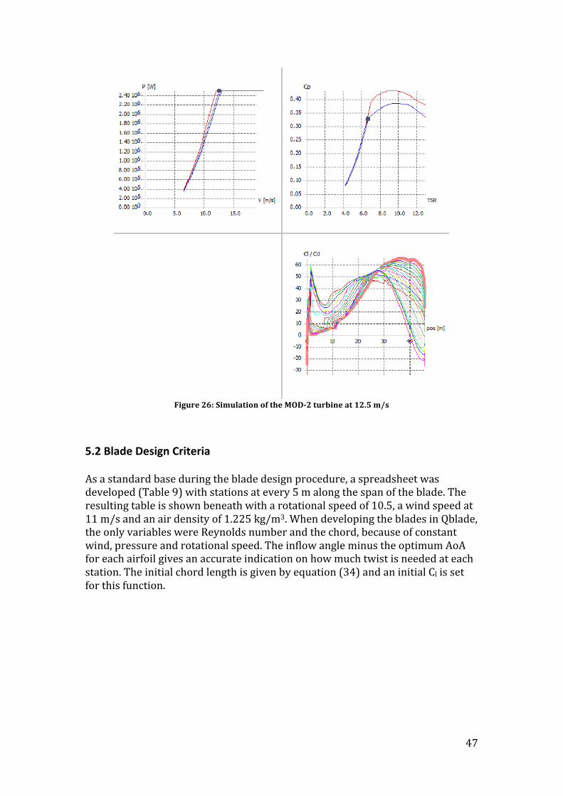
The graph located in the lower right corner of Figure 26 shows that the blade has a Cl/Cd maximum at the rated wind speed, 12.5 m/s. After reaching the rated power output, the pitch regulator starts pitching the blade to keep the power output stable. For the optimum TSR at 8.9 m/s, the blade has an angle of attack ranging from 28 to 0 degrees.

47

Figure 26: Simulation of the MOD-‐2 turbine at 12.5 m/s

5.2 Blade Design Criteria As a standard base during the blade design procedure, a spreadsheet was developed (Table 9) with stations at every 5 m along the span of the blade. The resulting table is shown beneath with a rotational speed of 10.5, a wind speed at 11 m/s and an air density of 1.225 kg/m3. When developing the blades in Qblade, the only variables were Reynolds number and the chord, because of constant wind, pressure and rotational speed. The inflow angle minus the optimum AoA for each airfoil gives an accurate indication on how much twist is needed at each station. The initial chord length is given by equation (34) and an initial Cl is set for this function.

48

Section (m)

Section number

V rel (m/s) Rotational speed (m/s)

Inflow Angle, β

Chord (m)

Reynolds number

Local TSR

Cl (estimated)

Mach

2.00 1 11.22 2.20 78.69 12.18 9 399 362 0.20 1.50 0.03 5.00 2 12.30 5.50 63.44 11.11 4 202 169 0.50 1.50 0.04

10.00 3 15.55 11.00 45.01 8.78 9 399 362 1.00 1.50 0.05 15.00 4 19.83 16.49 33.70 6.89 7 819 773 1.50 1.50 0.06 20.00 5 24.59 21.99 26.57 4.06 6 875 856 2.00 1.50 0.07 25.00 6 29.61 27.49 21.81 4.61 8 726 604 2.50 1.50 0.09 30.00 7 34.77 32.99 18.44 3.93 9 399 362 3.00 1.50 0.10 35.00 8 40.03 38.48 15.95 3.41 9 037 437 3.50 1.50 0.12 40.00 9 45.34 43.98 14.04 3.01 9 399 362 4.00 1.50 0.13 45.00 10 50.69 49.48 12.53 2.69 9 175 362 4.50 1.50 0.15 50.00 11 56.07 54.98 11.31 2.44 9 399 362 5.00 1.50 0.16 55.00 12 61.47 60.48 10.31 2.22 9 247 630 5.50 1.50 0.18 60.00 13 66.88 65.97 9.47 2.19 10 070 745 6.00 1.40 0.20 65.00 14 72.31 71.47 8.75 1.89 9 289 977 6.50 1.50 0.21 70.00 15 77.75 76.97 8.13 1.65 8 723 267 7.00 1.60 0.23 75.00 16 83.20 82.47 7.60 1.45 8 220 745 7.50 1.70 0.24 80.00 17 88.65 87.96 7.13 1.28 7 832 802 8.00 1.80 0.26

82.50 18 91.38 90.71 6.91 1.25 7 832 802 8.25 1.80 0.27 Table 9: Basic spreadsheet for blade optimization

5.3 Roughness Insensitivity Analysis Table 10 and Table 11 show some of the result from the roughness insensitivity analysis with the most relevant airfoils ranging from smallest decrease in efficiency to the highest decrease due to roughness sensitivity. The full sensitivity analysis is shown in Appendix C, while all the diagrams for each airfoil can be found in Appendix A. When the relevant airfoils were at Cl, max the wind turbine tailored airfoils had a loss between 7.09 % and 22.3 % while NACA airfoils had a loss between 16.5 % and 21.6 %. AIRFOIL Alfa Cl, max Cd Cl/Cd at Clmax T.U., Clmax Delta Cl,max Reynolds

FFA-‐W3-‐241 27.00 1.61 0.18 8,86 0.02 4 000 000 FFA-‐W3-‐241 34.00 1.50 0.28 5,41 0.02 -‐7.09 % 500 000 FFA-‐W3-‐211 16.50 1.71 0.05 32,23 0.02 4 000 000 FFA-‐W3-‐211 29.00 1.53 0.25 6,20 0.02 -‐10.15 % 500 000 FFA-‐W3-‐351 39.00 1.56 0.27 5.68 0.02 4 000 000 FFA-‐W3-‐351 36.00 1.37 0.28 4.98 0.02 -‐11.89 % 500 000 FFA-‐W3-‐301 37.50 1.60 0.27 6.02 0.03 4 000 000 FFA-‐W3-‐301 35.50 1.41 0.28 5.02 0.02 -‐12.22 % 500 000 NACA 64-‐621 22.50 1.78 0.13 14.03 0.01 4 000 000 NACA 64-‐621 23.50 1.48 0.18 8.34 0.02 -‐16.54 % 500 000 NACA 64-‐618 20.00 1.84 0.09 20.61 0.01 4 000 000 NACA 64-‐618 23.00 1.53 0.16 9.34 0.02 -‐16.67 % 500 000 NACA 63-‐618 18.50 1.85 0.07 26.58 0.01 4 000 000 NACA 63-‐618 25.00 1.53 0.20 7.64 0.01 -‐17.21 % 500 000 NACA 64-‐612 18.50 1.90 0.06 30.82 0.00 4 000 000 NACA 64-‐612 16.00 1.49 0.08 19.19 0.02 -‐21.60 % 500 000 NACA 63-‐612 17.00 1.90 0.05 40.85 0.00 4 000 000 NACA 63-‐612 14.50 1.49 0.06 23.43 0.01 -‐21.63 % 500 000 FFA-‐W3-‐401 41.00 1.61 0.22 7.23 0.09 4 000 000 FFA-‐W3-‐401 36.00 1.25 0.26 4.74 0.02 -‐22.31 % 500 000

Table 10: Airfoil roughness insensitivity analysis at Cl max

49

At best L/D, the tailored wind turbine airfoils had a reduction in L/D between 29.9 and 67.6 % while the NACA airfoils encountered a loss between 41.3 and 47.3 %. AIRFOIL Reynolds Alfa L/D max L/D max T.U., L/D max Delta L/D max

FFA-‐W3-‐401 4 000 000 0.50 13.43 0.28 FFA-‐W3-‐401 500 000 -‐0.50 9.41 0.02 -‐29.90 % NACA 63-‐612 4 000 000 9.00 113.11 0.01 NACA 63-‐612 500 000 7.00 66.41 0.02 -‐41.29 % NACA 64-‐612 4 000 000 9.00 111.97 0.01 NACA 64-‐612 500 000 6.50 65.47 0.02 -‐41.53 % NACA 63-‐618 4 000 000 9.50 96.04 0.41 NACA 63-‐618 500 000 6.00 53.44 0.02 -‐44.36 % FFA-‐W3-‐211 4 000 000 9.00 96.68 0.30 FFA-‐W3-‐211 500 000 7.00 52.17 0.02 -‐46.03 % NACA 64-‐618 4 000 000 8.50 97.61 0.43 NACA 64-‐618 500 000 5.50 51.62 0.02 -‐47.12 % FFA-‐W3-‐241 4 000 000 8.50 87.82 0.23 FFA-‐W3-‐241 500 000 6.50 42.78 0.02 -‐51.29 % FFA-‐W3-‐301 4 000 000 7.50 57.27 0.23 FFA-‐W3-‐301 500 000 7.00 25.07 0.02 -‐56.23 % FFA-‐W3-‐351 4 000 000 6.50 31.95 0.02 FFA-‐W3-‐351 500 000 7.50 10.35 0.02 -‐67.60 %

Table 11: Roughness insensitivity analysis at optimal L/D

As a result from this airfoil roughness insensitivity analysis, two airfoil families, the NACA 63-‐6XX and NACA 64-‐6XX, were chosen for further implementation in rotor blade design. These two were chosen, since they have been used on wind turbine blades before and gave reasonable results in the roughness insensitivity analysis.

50

5.4 Qblade Blade Design and Turbine Simulation Three different blade designs were developed with Qblade. All three blade designs consists of either the NACA 63-‐6XX or the NACA 64-‐6XX airfoil family at the middle and outer section. The difference in these three designs is chord length, twist and thickness.

5.4.1 Blade Design 1

Figure 27: Blade design 1 showing profile-‐, top-‐, iso-‐ and top/root-‐view.

Section Position Chord Offset Twist Foil Re/Mach 1 2,000 4,000 0 13,00 Circle -‐ 2 10,000 5,000 0 8,00 FFA-‐W3-‐401 5/0,06 3 20,000 5,500 0 3,00 FFA-‐W3-‐351 8/0,07 4 30,000 5,000 0 2,00 FFA-‐W3-‐301 10/0,10 5 40,000 4,200 0 1,00 FFA-‐W3-‐241 11/0,13 6 50,000 3,600 0 1,00 FFA-‐W3-‐211 11/0,17 7 60,000 3,200 0 0,96 NACA64-‐618 12/0,20 8 70,000 2,830 0 -‐0,09 NACA64-‐618 12/0,23 9 75,000 2,660 0 -‐0,52 NACA64-‐618 12/0,23 10 80,000 2,410 0 -‐0,89 NACA64-‐618 12/0,26 11 80,625 2,292 0 -‐0,93 NACA64-‐618 12/0,26 12 81,250 2,000 0 -‐0,98 NACA64-‐618 10/0,26 13 81,875 1,500 0 -‐1,52 NACA64-‐618 8/0,26

14 82,500 0,500 0 -‐1,52 NACA64-‐618 3/0,26

Table 12: Blade design 1 with NACA 64-‐618 and FFA-‐W3-‐XX1. Position and chord in meters, twist in degrees, Re in millions.

51

Section Position Chord Offset Twist Foil Re/Mach 1 2.000 4.000 0 13.00 Circle -‐ 2 10.000 5.000 0 8.00 FFA-‐W3-‐401 5/0.06 3 20.000 5.500 0 3.00 FFA-‐W3-‐351 8/0.07 4 30.000 5.000 0 2.00 FFA-‐W3-‐301 10/0.10 5 40.000 4.200 0 1.00 FFA-‐W3-‐241 11/0.13 6 50.000 3.600 0 1.00 FFA-‐W3-‐211 11/0.17 7 60.000 3.200 0 -‐0.04 NACA63-‐618 12/0.20 8 70.000 2.830 0 -‐1.1 NACA63-‐618 12/0.23 9 75.000 2.660 0 -‐1.52 NACA63-‐618 13/0.23 10 80.000 2.410 0 -‐1.89 NACA63-‐618 12/0.26 11 80.625 2.292 0 -‐1.93 NACA63-‐618 12/0.26 12 81.250 2.000 0 -‐1.98 NACA63-‐618 10/0.26 13 81.875 1.500 0 -‐2.52 NACA63-‐618 8/0.26

14 82.500 0.500 0 -‐2.52 NACA63-‐618 3/0.26

Table 13: Blade design 1 With NACA 63-‐618 and FFA-‐W3-‐XX1. Position and chord in meters, Twist in degrees, Re in millions.

The blade starts (section 1) at 2 meters, since the hub radius is 2 meters. The root (section 1-‐4) has a design twist for Cl, max and the rest of the blade (section 5-‐14) a twist designed for the optimum L/D. The root and mid chord are determined by analyzing available standard blade geometries, both visually and by description. An empirical chord equation was also used to determine the chord length distribution. The final design is seen in Figure 27. Blade design 1 was tested with two different airfoils at the mid and outer section is: NACA 64-‐618 (Table 12) and NACA 63-‐618 (Table 13). Both of these designs employ the FFA family at the root and at the opening mid section. The difference in airfoil selection at the mid and outer section is performed so it is possible to see a comparison in performance of a blade design with NACA 64-‐618 and NACA 63-‐618.

52

Figure 28: TSR vs. CP rotor simulation

Figure 28 displays the blade with NACA 64-‐618 and NACA 63-‐618 airfoils TSR versus Cp in a rotor simulation. Blade CP TSR NACA 64-‐618 blade 0.481 7.0 NACA 63-‐618 blade 0.480 6.8 The NACA 64-‐618 blade is, as shown, outperforming the NACA 63-‐618 blade. Further, in this report only the NACA 64-‐618 blade will be displayed because of the better performance. Figure 29 displays the lift coefficient distribution along the blade span for different TSR. The thick line in Figure 29 is the lift coefficient for the highest CP the blade reaches. There occurs a dip in the lift distribution at 10 meters because of the compromise in twist angle. The maximum Cl is 1.5 and at 20 m of the blade span.

Figure 29: Lift coefficient distribution in rotor simulation for blade 1 with NACA 64-‐618 airfoil

53

Figure 30 displays the lift to drag ratio distribution over the blade span in a rotor simulation. Since the blade is designed to operate at Cl, max along the inner section, the L/D ratio at those sections will be lower and start to increase further out along the blade and stay reasonably linear until the tip. Because of tip loss, corrected with Prandtl’s tip loss correction, there is a decrease in L/D ratio at the tip. The highest L/D is 122 and is reached at 65 meters.

Figure 30: L/D ratio distribution in rotor simulation for blade 1 with NACA 64-‐618 airfoil

The Cl/Cd distribution displayed in Figure 31 has a similar curve to the L/D ratio in Figure 30. The difference between the curves is because in turbine simulation, there is a pitch variable simulated.

Figure 31: Cl/Cd along the span of the blade in turbine simulation for blade 1 NACA 64-‐618 airfoil

The power curve in Figure 32 displays how the power is increasing until it reaches the limit set at 7 MW where the variable pitch starts to compensate, to

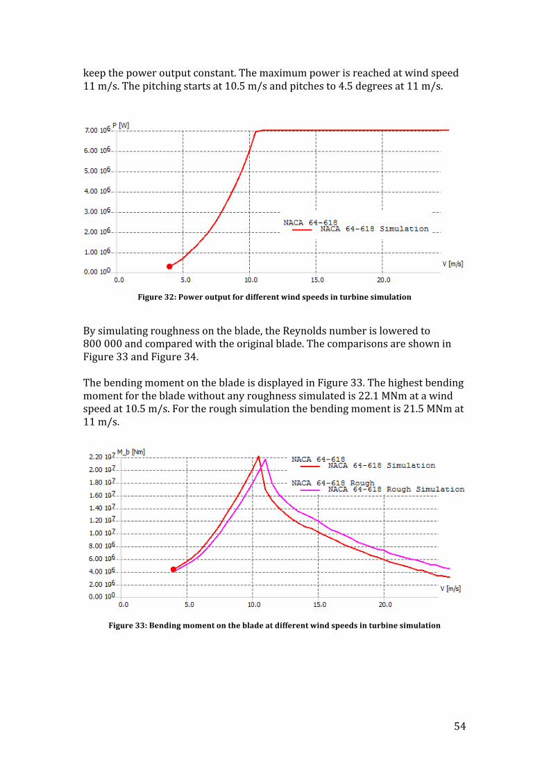
54

keep the power output constant. The maximum power is reached at wind speed 11 m/s. The pitching starts at 10.5 m/s and pitches to 4.5 degrees at 11 m/s.

Figure 32: Power output for different wind speeds in turbine simulation

By simulating roughness on the blade, the Reynolds number is lowered to 800 000 and compared with the original blade. The comparisons are shown in Figure 33 and Figure 34. The bending moment on the blade is displayed in Figure 33. The highest bending moment for the blade without any roughness simulated is 22.1 MNm at a wind speed at 10.5 m/s. For the rough simulation the bending moment is 21.5 MNm at 11 m/s.

Figure 33: Bending moment on the blade at different wind speeds in turbine simulation

55

Figure 34 shows a reduction of CP when roughness is simulated and also at what TSR the maximum CP occurs.

Figure 34: CP vs. TSR rotor simulation with and without simulated roughness on the NACA 64-‐618

blade

The roughness simulation (NACA 64-‐618 Rough) has a CP of 0.415 at 7.4 TSR. To analyze the difference in power output for the two turbines, the annual yield is calculated from Qblade. Turbine Annual yield Loss due to roughness NACA 63-‐618 Turbine 40.18 GWh NACA 63-‐618 Rough Turbine 38.40 GWh -‐ 4.43% NACA 64-‐618 Turbine 40.30 GWh NACA 64-‐618 Rough Turbine 38.43 GWh -‐ 4.59%

56

5.4.2 Blade Design 2

Figure 35: Blade design 2 showing profile-‐, top-‐, iso-‐ and 2D profile-‐view

Section Position Chord Offset Twist Foil Re/Mach 1 2.000 4.000 0 13 Circle -‐ 2 10.000 5.000 0 8 FFA-‐W3-‐401 5/0.06 3 20.000 5.500 0 3.00 FFA-‐W3-‐351 8/0.07 4 30.000 5.000 0 2.00 FFA-‐W3-‐301 10/0.10 5 40.000 4.200 0 1.00 FFA-‐W3-‐241 11/0.13 6 50.000 3.633 0 1.00 FFA-‐W3-‐211 11/0.17 7 60.000 3.066 0 0.56 NACA64-‐618 12/0.20 8 70.000 2.500 0 -‐0.97 NACA64-‐618 11/0.23 9 75.000 2.200 0 -‐1.38 NACA64-‐618 11/0.23 10 80.000 1.600 0 -‐2.25 NACA64-‐618 9/0.26 11 80.625 1.400 0 -‐2.29 NACA64-‐618 7/0.26 12 81.250 1.200 0 -‐2.33 NACA64-‐618 6/0.26 13 81.875 1.000 0 -‐2.37 NACA64-‐618 5/0.26

14 82.500 0.500 0 -‐2.40 NACA64-‐618 3/0.26

Table 14: Blade design 2 geometry with position and chord in meters, twist in degrees and Reynolds number in millions

Blade 2 is designed with the FFA-‐W3-‐XX1 family at the root and beginning of the middle section. The rest of the blade consists of the NACA 64-‐618 airfoil. NACA 64-‐618 was selected based on the results and comparisons made in Blade design 1 between NACA 64-‐618 and NACA 63-‐618. Since the hub radius is 2 meters, the first section begins at 2 meters with a circular profile.

57

The geometry of the chord is based on standards from very large commercial wind turbine specification. The final design is seen in Figure 35. The root section is designed with a twist for Cl, max and the rest of the blade is twisted to get the best L/D ratio. Figure 36 show CP vs. TSR curve with a slight peak at optimum.

Figure 36: CP vs. TSR rotor simulation

The blade has a maximum power coefficient CP of 0.489 at a TSR of 7.40. Displayed in Figure 37 is the lift coefficient distribution over the blade span for different TSR. The thicker line in Figure 37 is the distribution at the highest TSR the blade reaches. Maximum Cl is 1.5 at the radial position of 20 m.

Figure 37: Lift coefficient distribution over the blade span in rotor simulation

58

Figure 38 shows the lift to drag ratio distribution over the blade span. Since the blade is designed to operate at Cl, max at the inner section, the L/D ratio at those sections will be lower and start to increase further out along the blade and stay reasonably linear until the tip. Because of tip loss, corrected with Prandtl’s tip loss correction, there is a decrease in L/D ratio at the tip. The highest L/D is 122 at 62 meters.

Figure 38: L/D distribution over the blade span in rotor simulation

The Cl/Cd distribution displayed in Figure 39 has a similar curve as the L/D ratio in Figure 38. The difference is that Figure 39 is a turbine simulation that simulates a variable pitch.

Figure 39: Cl/Cd distribution over the blade span in turbine simulation

The power curve in Figure 40 increases until it reaches the satisfied power output of 7 MW. At that time, variable pitch is applied to keep a constant power output and reduce the loads. The maximum power is reached at a wind speed of 11 m/s. The variable pitch is applied at 10.5 m/s and at 11 m/s it has pitched to 4.4 degrees.

59

Figure 40: Power output for different wind speeds in turbine simulation

By simulating roughness on the blade, the Reynolds number is lowered to 800 000 and compared to the original blade. The comparisons are shown in Figure 41 and Figure 42. The bending moment on the blade is displayed in Figure 41. The highest bending moment for the blade without any roughness simulated is 21.0 MNm at wind speed 10.5 m/s. For the rough simulation it is 21.3 MNm at 11 m/s.

Figure 41: Bending moment on the blade with and without roughness simulated

60

Figure 42: CP vs. TSR rotor simulation with and without simulated roughness

The Roughness simulation has a performance coefficient of 0.431 at 8.2 TSR. That is a decrease of 13.97% To analyze the loss in power output due to roughness, the annual yield is calculated with Qblade. Turbine Annual yield Loss due to roughness Blade turbine 40.48 GWh Blade Rough turbine 38.56 GWh -‐ 4,74%

61

5.4.3 Blade Design 3 A blade was developed with two different airfoils at the middle and outer sections due to the need to check the difference in performance between NACA 63-‐6XX and 64-‐6XX series. The root section consisted of the FFA-‐W3-‐XXX airfoil family. For better aerodynamic results, the airfoil thickness was decreased to 12 t/c for the outer section. The final blade geometry is shown in Figure 43.

Figure 43: Blade and airfoil geometry

The chord geometry was designed after the outlines of a standard large commercial rotor blade and the initial empirical chord equation. The final design is seen in Figure 43. The inner section (sections 1-‐4) is optimized for Cl, max while the rest of the blade (sections 4-‐20), is optimized for best L/D. The inner twists are calculated through a spreadsheet while the middle and outer sections were initially optimized with the twist tool in Qblade and changed after numerous user inputs. Compromises were made regarding the change in twist for L/D and Cl, max and the structural side for an overall best solution. The blade geometry is displayed in Table 15.

62

Section Position Chord Offset Twist Foil Re / M 1 2.000 4000 0 40 Circle -‐ 2 10.000 5500 0 36.5 FFA-‐W3-‐401 5 /0.06 3 20.000 5300 0 11.8 FFA-‐W3-‐351 8/0.07 4 30.000 4550 0 2.8 FFA-‐W3-‐301 10/0.10 5 35.000 4250 0 2.0 FFA-‐W3-‐241 11/0.13 6 40.000 4000 0 1.8 FFA-‐W3-‐211 11/0.17 7 50.000 3550 0 1.7 NACA 64-‐618 12/0.20 8 55.000 3300 0 1.5 NACA 64-‐618 12/0.23 9 60.000 3000 0 0.86 NACA 64-‐618 12/0.23 10 70.000 2450 0 0.8 NACA 64-‐612 11/0.26 11 73.000 2280 0 0.8 NACA 64-‐612 11/0.26 12 76.250 2050 0 0.8 NACA 64-‐612 10/0.26 13 78.750 1800 0 0.6 NACA 64-‐612 9/0.26 14 80.000 1600 0 0.6 NACA 64-‐612 8/0.26 15 81.000 1400 0 0.6 NACA 64-‐612 7/0.26 16 81.500 1200 0 0.6 NACA 64-‐612 6/0.26 17 82.200 800 0 0.6 NACA 64-‐612 5/0.26 18 82.400 400 0 0.6 NACA 64-‐612 3/0.26 19 82.500 0

0 0.6 NACA 64-‐612 1/0.26

Table 15: Blade geometry for the NACA 64-‐6XX where position, chord is in meters, twist in degrees and Reynolds number in millions

The first position on the blade starts at 2 meters since the hub is 4 meters in diameter. Figure 44 shows the comparison of the two blades with the 64-‐6XX airfoils being most efficient when comparing CP but this could differ when comparing the annual yield.

Figure 44: TSR -‐ Cp curve from Rotor simulation

Blade CP TSR NACA 64-‐6XX blade 0.513 7.6 NACA 63-‐6XX blade 0.509 7.6 Since the difference between the blades is very small, only results from the NACA 64-‐6XX blade will be shown.

63

Figure 45 shows the lift coefficient along the blade for the rotor simulation at different TSR and the yellow line indicates the lift coefficient at maximum CP. The drop in lift coefficient in the root area is a compromise between thickness, inflow angle and twist.

Figure 45: Lift Coefficient along the NACA 64-‐6XX blade 3 rotor simulation

The yellow line in Figure 46 shows the L/D ratio at maximum CP along the blade in rotor simulation. From 15 m the L/D increase from around zero to 118 at 40 m and increase slightly to 127 towards the tip, before decreasing due to tip loss.

Figure 46: L/D ratio along the span of the NACA 64-‐6XX blade in rotor simulation

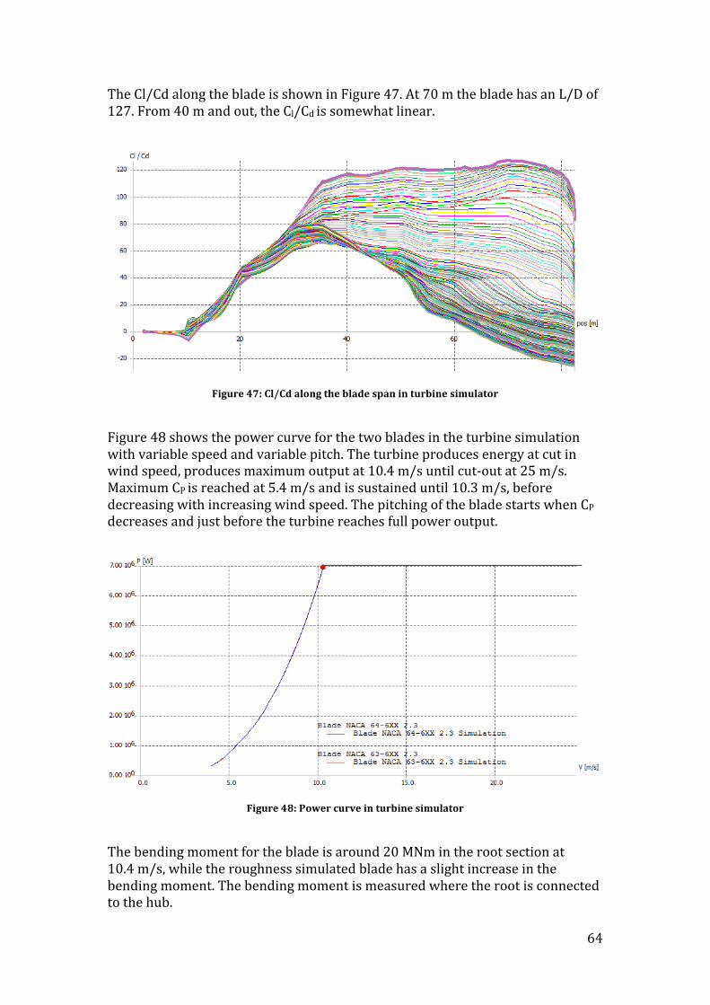
64

The Cl/Cd along the blade is shown in Figure 47. At 70 m the blade has an L/D of 127. From 40 m and out, the Cl/Cd is somewhat linear.

Figure 47: Cl/Cd along the blade span in turbine simulator

Figure 48 shows the power curve for the two blades in the turbine simulation with variable speed and variable pitch. The turbine produces energy at cut in wind speed, produces maximum output at 10.4 m/s until cut-‐out at 25 m/s. Maximum CP is reached at 5.4 m/s and is sustained until 10.3 m/s, before decreasing with increasing wind speed. The pitching of the blade starts when CP decreases and just before the turbine reaches full power output.

Figure 48: Power curve in turbine simulator

The bending moment for the blade is around 20 MNm in the root section at 10.4 m/s, while the roughness simulated blade has a slight increase in the bending moment. The bending moment is measured where the root is connected to the hub.

65

Figure 49: Comparison of bending moment in the root/hub area for blade with two different airfoil

families

Figure 50 shows the difference with normal Reynolds number and forced transition at 0.05 % of the chord, while the roughness simulated blade has Reynolds number at 800 000 and the same forced transition.

Figure 50: Simulations for blade 3 with NACA 63-‐6XX and NACA 64-‐6XX airfoil

With Weibull parameters k = 2.2 and annual wind at 12.1 m/s, the turbine produces 40.93 GWh of electricity annually with the NACA 64-‐6XX blade.

66

Turbine Annual yield Loss due to roughness NACA 63-‐6XX Turbine 40.914 GWh NACA 63-‐6XX Rough Turbine 39.05 GWh -‐ 4.55% NACA 64-‐6XX Turbine 40.93 GWh NACA 64-‐6XX Rough Turbine 38.98 GWh -‐ 4.77% The NACA 64-‐6XX is therefore 0.3 % more efficient annually than the NACA 63-‐6XX blade. The roughness simulation encountered a drop in annual power generation of 4.55 % and 4.77% for the two blades.

5.5 Flex5 The simulations were performed to simulate normal operating conditions for offshore wind turbines and therefore the simulations will show significant differences in power output compared to steady state conditions. For wind shear, the simulations were performed at 10 m/s, turbulence intensity at 14% and with different wind shear power exponent (a), which describes the location (terrain) and the stability of the wind. The turbulent simulations were performed at 10 m/s, wind shear power exponent (a) at 0.08 and turbulence intensity at 8 %, 14 % and 20 %.

67

5.5.1 Blade Design 2 Figure 51 shows the power curve for Blade 2 from steady state simulation in Flex5. The turbine produces power at 4 m/s and full power output at 11 m/s.

Figure 51: Power curve for Blade 2 in Flex5 simulation

Figure 52 displays the bending moment in the flap wise direction for one blade on the turbine. The bending moment has a maximum of 24 MNm at 11 m/s.

Figure 52: Flap-‐wise bending moment during a time period.

68

Figure 53 displays power output with wind shear simulation at different wind shear power exponents ranging from 0.08 to 0.20.41 The wind speed (around 10 m/s) for the same time period is displayed in the graph as well to give an indication on how the wind is behaving during different wind shear. The value of the wind speed is displayed on the right y-‐axis, and the value of the power is displayed along the left y-‐axis. The turbine is producing a maximum of 7000 kW but has a maximum decrease of 3800 kW during heavy wind shear.

Figure 53: Wind shear simulation for power generation during a time period (t) with different wind

shear power exponents (a)

Figure 54 shows the bending moment flap-‐wise over a timer period with different wind shear ranging from 0.08 to 0.20. The wind speed for the same period of time is also displayed in the graph to indicate how the wind is behaving during the wind shear. The bending moment and wind speed are respectively given in the left and right y-‐axis. The maximum bending moment almost reaches 30 000 kNm, while the minimum bending is less than 9 000 kNm.

69

Figure 54: Wind shear simulation for bending moment flap-‐wise during a time period (t) at different

wind shear power exponents (a)

Figure 55 shows the power output during turbulence simulation over a time period of 600 seconds. The simulation was made at turbulence intensities of 8 %, 14 % and 20 %. The wind speed for the same time period is also displayed in the graph, to indicate how the wind speed behaves during turbulence. The power output and wind speed are respectively displayed on the left and right y-‐axis. The power output is almost reduced to maximum power output (7000 kW) with a significant reduction in power output when the wind speed decreases due to turbulence. The largest reduction in power output is for a turbulence intensity of 20 % with a reduction of around 4000 kW, while the 8 % turbulence intensity only decreases the power output by around 2700 kW.

70

Figure 55: Turbulence simulation for power output during a time period (t) with varying turbulence

intensities

Figure 56 shows the flap-‐wise bending moment during a time period of 600 seconds. The simulation was performed with turbulence intensities of 8 %, 14 % and 20 %. The largest bending moment is reached at 31 000 kNm while the smallest is around 2500 kNm.

Figure 56: Turbulence simulation of bending moment flap-‐wise during a period of time (t) with

varying turbulence, compared to the wind speed at the same period of time

71

5.5.2 Blade Design 3 Figure 57 shows the power curve for blade 3 in Qblade and Flex5 and blade 2 from Flex5. The three power curves follow the same pattern where results from Qblade are more positive than Flex5 results. At 4 m/s they all give the same power output while they reach full power output at slightly different wind speeds.

Figure 57: Comparison of power curve of blade 2 and 3 from Qblade and Flex 5

Figure 58 shows the power output at different turbulence intensities. When the wind speed increases, the power output will be reduced to 7000 kW by pitching, while when the wind speed decreases, the power output is reduced. The highest turbulence intensity decreases the power output by almost 4000 kW while the lowest turbulence intensity only decreases the power output by 3000 kW.

72

Figure 58: Power output for blade 3 for different turbulence intensities

Figure 59 shows the power output for different wind shear simulations. As with the turbulence simulation, the maximum power output is reduced to 7000 kW. When the wind speed is reduced, the power output decreases. The largest decrease is similar for all wind shear power exponents, with a decrease of almost 3000 kW.

Figure 59: Power output for blade 3 for different wind shear

Figure 60 shows the flap-‐wise bending moment for different turbulence intensities. For a turbulence intensity of 20 % the bending moment peaks at 30 000 kNm and with the lowest bending moment at 5 000 kNm.

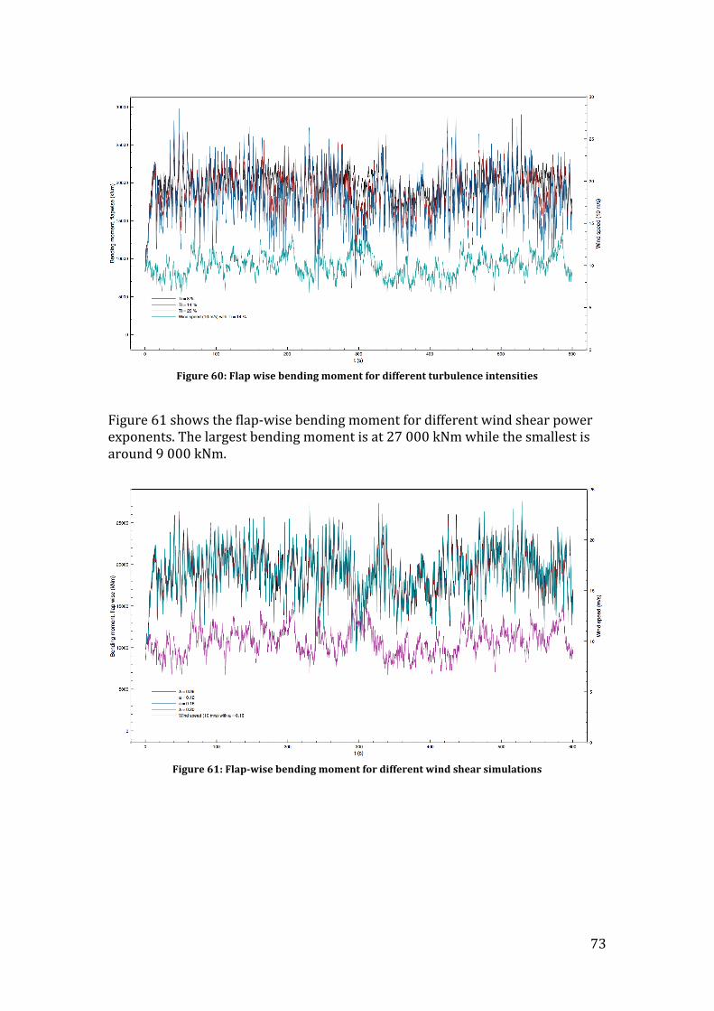
73

Figure 60: Flap wise bending moment for different turbulence intensities

Figure 61 shows the flap-‐wise bending moment for different wind shear power exponents. The largest bending moment is at 27 000 kNm while the smallest is around 9 000 kNm.

Figure 61: Flap-‐wise bending moment for different wind shear simulations

74

6. Discussion

6.1 Historical Turbines The historical turbines show a similar production of electricity compared to existing operational data and also show that Qblade is a reliable wind turbine simulator with somewhat accurate results.

6.1.1 Gedser Wind Turbine The results from Qblade compared to actual operational figures from the Gedser wind turbine prove sufficient when roughness is taken into account. At 15 m/s the roughness decreases the power output by 25 kW for the NACA 4312 while the roughness on the CLARK-‐Y airfoil decreases power by 16 kW. At optimum TSR, the loss in power output due to roughness is minimal. With roughness both airfoils have acceptable solutions compared to operational data and it is therefore reasonable to conclude that the real life turbine ran with surface roughness, which decreased the power output. What also decreased its efficiency were the stays that held the turbine blades together and probably the low aspect ratio of the blade resulting in more induced drag. The stays that held the rotor together are comparable to struts that support airplane wings attached to the fuselage, and are an important drag factor, which has been taken into account for in variable losses.

6.1.2 MOD-‐2 Turbine Dividing the blade into more sections than just the airfoil sections in the design allowed a better result, because of the increased amount of Xfoil analysis being executed for the different, now increased, sections of the blade. In this case, where the chord and twist are decreasing/increasing linearly with span, the differences in the results between the blade with more sections and the blade with fewer sections was not that large (Figure 62). The increased accuracy of the result was not significant enough compared to the time spent making the sections and the multiple extra analyses in Xfoil.

75

Figure 62: Simulation of MOD-‐2 with and without interpolated sections

The hub section with the oval cross-‐section profile was not a normal airfoil and had to be customized in Javafoil and Qblade after the description in MOD-‐2 reference document.42 The accuracy of the design of this profile can not be assured and might have altercations in the final results. The result from Qblade compared to the actual designed results from the MOD-‐2 turbine proves to be sufficient when taking the roughness into account. The power output does not vary that much between the simulations with and without roughness. The same goes for the difference in the rated wind speed. The maximum system power coefficient, CP,max, has a notable difference: Roughness: 0.38, no roughness 0.43 and the design result is 0.38. A difference between the simulations and the real turbine is that the real turbine pitch regulation only regulated 30% of the outer portion of the blade, while the simulations were done with the whole blade pitching to perform at the rated power through to the cut out wind speed. This may have some altercations on the blade performance and power output and it does not seem to be a function to just regulate the tip of the blade in Qblade.

76

The results from Qblade were also validated through analyzing the circulation and annulus average axial induction confirming that they were somewhat linear and had no excessive irregularities.

6.2 Roughness Insensitivity Analysis For the roughness insensitivity analysis there were no data to compare the results with, merely since roughness analysis is a very experimental part of aerodynamics and the theoretical aspect is done with empirical values. With this in mind, two different values for Reynolds number were chosen for all the airfoils with a forced transition at 5 % of the chord. Since all the airfoils then had the same parameter input, it was possible to see the difference in sensitivity and thus see which had the best roughness insensitivity. Therefore, these simulations shall not be compared to real experimental testing with actual roughness incorporated on the airfoil. It is only an estimate on the airfoils behavior with a thicker boundary layer, simulating a rough surface. What the results show is only the difference between the airfoils that were investigated and can not be compared to any operational conditions. For real operational conditions, the decrease in efficiency can either be more or less than the predictions from the simulations with low Reynolds number and forced transition.

6.3 Qblade

6.3.1 Blade Design 1 The blade was designed to be cost friendly and as efficient and stable as possible. Designing the blade with a longer chord length at the tip, it will reduce cost by not being necessary to reinforce the blade structurally, since it is thicker allowing it to withstand a higher bending moment. A standard commercial blade design inspired the rest of the blade chord geometry. The twist was determined by selecting the blade to reach Cl,max from section 1-‐4 and to optimize the rest of the blade for the highest L/D ratio. Making the optimization in Qblade for these sections, the blade had a tendency to get a wavy twist, since the twist for every section was very inconsistent. Making the blade as realistic and constructible as possible, the twist hade to be compromised and changed to get an even and smooth twist as displayed in Table 12. The consequence of this compromise is shown in Figure 29, were the lift coefficient dips. The same consequence can be seen in the L/D ratio (Figure 30) and Cl/Cd graph (Figure 31). Another solution could be to change to another airfoil that would have another Cl,max at the twist set for the blade. But limitations in available airfoils made this impossible, without losing thickness in the root or getting an enormous chord length. Between radial sections 7 and 14 the airfoil NACA 64-‐618 was selected to be the best fit, by analyzing Table 11. The NACA 64-‐618 and NACA 63-‐618 had a similar characteristic and performance, so both these airfoils were tested for this blade

77

design. After the Qblade simulations the result was that NACA 64-‐618 was a better fit for this design and NACA 63-‐618 was excluded from the graph results. The difference in the L/D and Cl/Cd maximum is because of the different simulations modes they were extracted from. The L/D is simulated in the rotor simulation and compared to the highest TSR, while the Cl/Cd, simulated in the turbine simulation, is compared to the wind speed at maximum power output. Since the power output is set to be maximum 7 MW, the variable pitch is applied when reaching this output. Instead of the blade accelerating, the variable pitch twists the blade to the decreased Cl/Cd that keeps the blade at the 7 MW limit (Figure 31 and Figure 32). If the variable pitch were not used, the blade would have to be stall regulated or shut down to not reach too high rotational speeds, which would increase the stress on the blade structure and eventually lead to failure. The variable pitch also starts to pitch the blade before the rated wind speed of 11 m/s is reached, to avoid high thrust. The blade station polar curves were changed to a Reynolds number of 800 000 in order to simulate roughness. The blade was then compared to the original blade to check how sensitive the blade design was to roughness. This comparison was also made for the NACA 63-‐618 blade. The roughness simulation gave the blade a lower performance coefficient, lower bending moment and a lower annual yield. The rough blade also reached the 7 MW limit at a higher wind speed, 11.5 m/s. These are obvious outcomes, since a lower Reynolds number increases the thickness of the boundary layer, thus simulating rough surface, which leads to a reduction in L/D and Cp. The difference in annual yield between the rough blade and the original blade is 4.74%. Noticeable is that the NACA 63-‐618 blade has a lower decrease when simulating roughness. It had a decrease of 4.43% in annual yield when simulating roughness. From this perspective, the NACA 63-‐618 blade is preferable, but it still has a 0.2 % lower annual yield, a higher bending moment requiring the blade to be more structurally reinforced, thereby getting a higher weight and load including a higher cost to build the blade.

6.3.2 Blade Design 2 This blade design is a modification of blade design 1. The whole blade geometry design is inspired by standard commercial rotor design. Reducing the chord length at the outer sections (section 10-‐14) presented a blade with a sharper more distinguished tip (Figure 35). 43 Since the tip only has to take up its own bending moment and forces there was no need to keep the chord as long as in blade 1.

78

As in blade design, 1 the twist is set to come as close to Cl, max as possible at the inner sections and to give a maximum L/D ratio at the rest of the blade. There had to be some compromises with the twist angle at the inner sections to get an as smooth and realistic twist as possible. The consequence of this compromise can be seen in Figure 37, were there occurs a dip in the lift coefficient at 10 meter span length. Since the NACA 64-‐618 in blade design 1 was outperforming the NACA 63-‐618, the decision was made to stay with NACA 64-‐618 in this blade design. By reducing the chord at the tip, the performance coefficient increased to 0.489. However, instead of having smooth performance to tip speed ratio curve, the curve gets a little peak at TSR 7.2 – 7.6. The reason for the sudden peak in performance is the reduction in chord lengths at the tip, which will decrease the Reynolds number according to equation 2. Altering the twist held the peak down to a minimum but at a cost of a lower CP. Eliminating a peak will allow the blade to have a larger interval of TSR to be active without any power peaks, and it would therefore be more insensitive to wind gusts. Blade 2 has its advantages and disadvantages comparing it to blade 1. Blade 2 has a higher annual yield, higher performance coefficient, lower bending moment and lower thrust, which all play in the advantages of blade 2. However, when analyzing the roughness simulation, blade 2 has a bigger decrease in annual yield (5.06 %) than blade 1 (4.74 %). This indicates that blade 1 has better roughness insensitivity, but blade 2 is still outperforming blade 1 nonetheless.

6.3.3 Blade Design 3 The CP – TSR curve shows a peak around 7.6 TSR. The reason for this is a rapid increase in performance at this certain TSR. Where this sudden rise of performance happens along the blade span is not known and this increase can therefore be considered all along the blade. Also, the chord distribution along the span could have a large impact on the CP -‐TSR. A longer chord towards the tip would probably make the CP – TSR line a lot smoother, but the peak would then be decreased. Why this blade has a high annual yield is because of the steady state simulations. A real turbine will probably encounter problems keeping the blade at its optimum TSR, because of varying wind speeds, so the real performance would probably be lower. The power curve (Figure 48) looks quite similar to conventional commercial power curves seen in Figure 6 but the difference is that the commercial power curve is not so steep towards rated power. This is probably because the turbine starts to pitch somewhere before it reaches full power output in order to decrease loading.

79

When the twist of the blade was calculated some limitations occurred. Qblade only optimizes for the best L/D and stall at a given TSR. With the middle and outer blade optimized for L/D, the inner section had no good solution for optimization. The root section was therefore optimized with calculations from the spreadsheet and a usable solution was chosen for the blade with concerns for the structural and cost limitations to twist. The middle and outer sections have a very linear twist and this blade is therefore very cost and design friendly, while having a very good aerodynamic efficiency. L/D does tend to vary a bit along the span of the blade. The reason for these changes is different airfoil geometry and different Reynolds number interpolating between each other. Trying to get these to be linear along the span is very iterative and time consuming. The final result is therefore acceptable. The bending moment is somewhat high, but in line with other blades that have been investigated. With the industry operating with a blade performance between 0.45 and 0.5, blade design 3 shows a very promising performance coefficient at 0.513, which is higher than for blade designs 1 and 2.

6.4 Flex5 Flex5 is very sensitive regarding the input parameters of aerodynamic data. When developing airfoil polars in Qblade, there was no convergence for certain angles, and this happened at different angles for different airfoils. Therefore, if one airfoil did not have a certain angle, the same angle sshad to be deleted from the other airfoils. This resulted in less accurate aerodynamic data, especially in the -‐2 to 25 degree range where this is very important. The inner airfoils, FFA-‐W3-‐401 and FFA-‐W3-‐351, never seemed to work in Flex5 and were therefore skipped during the simulations. Instead, the simulations ran with 30 t/c interpolating with the cylinder at the root. This solution was acceptable since the power production is minimal at this area of the blade. The reason why the airfoils were not approved is uncertain, but since they were up-‐scaled from 24 t/c, there could be some faulty geometry. Flex5 allows for simulations with wind shear and turbulence, which Qblade did not. This would give an indication on how the turbine and the blades would behave during a more realistic state. These graphs are displayed in Flex5 results and in Appendix E. Figure 63 shows the performance coefficient versus the wind speed for blade 2 and 3. The performance coefficient has a narrow peak with blade 2 actually having a higher CP than blade 3. For Qblade, the results were opposite. The reason for this sudden change is because of the generator used in the Flex5 simulation. A normal 5 MW generator were up-‐scaled to 7 MW and variable and fixed losses do tend to make some discrepancies in the results. Figure 63, which

80

rely on the generator power output, will then show results that are not correct. Since the power curve for blade 2 shows a peak above 7 MW, because of generator misbehavior, it will then also have better performance. In reality, blade 3 will have a better performance, as stated in Qblade.

Figure 63: Cp vs wind speed for blades 2 and 3 in Flex5

6.4.1 Blade Design 2 The power curve in Figure 51 shows a detailed and accurate picture of the turbine behavior. The power curve shows a slight overproduction when the turbine reaches maximum power output. The simulations are run with an up-‐scaled 5 MW generator with fixed and variable losses. Because of this up-‐scale of the generator, it will generate discrepancies in the power curve, such-‐as rapid power increase and overproduction. A real overproduction could damage the generator and put more loading on the whole turbine. An easy way to decrease a real overproduction is to start pitching the blades a bit earlier. The flap wise bending moment for the steady state simulation in Figure 52 shows a maximum moment of 24 MNm at 11 m/s, which differs compared to the simulation in Qblade. In the Qblade simulation, the bending moment reached a maximum of 21 MNm at 10.5 m/s and 17 MNm at 11 m/s. The reason for this difference is that in Qblade, the variable pitch starts to pitch the blade at 10.5 m/s to avoid peaks in the power output, but in Flex5 it seems to not start pitching until the rated wind speed is reached, and therefore getting a peak in power output (Figure 51), and the maximum bending moment at that wind speed. The oscillations that occur in Figure 52 are probably because of tower shadow and/or wind shear being simulated. Tower shadow is a more common problem for a downwind turbine, nonetheless it occur on an upwind turbine as well. It occurs when the wind starts to bend upstream of the tower before passing it. The theory is backed up by the fact that the oscillation occurs 10 to 11

81

times per minute at rated wind speed, which is the rotational speed of the turbine. Since this graph only covers one of the three blades, it seems to coincide with this theory. Comparing Figure 53 to the power output from the steady state in Figure 51, it is clear that wind shear has a big effect on the power output. When the wind speed decreases due to wind shear, the power output decreases as well with a small delay between the two. However, as long as the wind is over the rated wind speed of 11 m/s, the power output is somewhat stable as seen in the simulation at 280 to 320 sec. Different wind shear power exponents for the different wind shear simulations did not have any major effects on the power output but there would be a considerable difference in power output when the blade is at the top rotor position versus the bottom position. Wind shear in Figure 54 shows that the variety in different wind speeds has a major effect on the flap wise bending moment, which is frequently changing during the simulation between 10 and 30 MNm. The turbulence simulations had, as well as the wind shear simulation, a major effect on the power output, compared to the steady state power output in Figure 51. Very seldom was the turbine producing a steady power output, which became even more rare when the turbulence intensity increased from 8 to 20 %. The turbulence simulation differs from the wind shear in how the different turbulence intensities seem to give very different power outputs.

6.4.2 Blade Design 3 As blade design 2, this design also used the up-‐scaled 5 MW generator, which gave some discrepancies in the results. In the power curves for steady state, the power curve looks good until it nearly reaches full power output. The power starts to oscillate before it produces full power output. This is probably due to of the generator as it is not a normal physical behavior. For the power curve from the turbulence simulations there exist short periods of overproduction, when turbulence rapidly increases the wind speed. This overproduction is probably because the simulation used a standard pitch controller, which did not react fast enough to the change in wind speed. For a turbulence intensity at 8 %, a reasonable maximum constant power output was achieved, but at a higher turbulence intensity, the turbine had difficulties keeping a constant output. For the wind shear simulation the results did not differ between the different wind shear simulations, as opposed to the turbulence simulation. The turbine has certain short periods of overproduction and this could, as with the turbulence case, be because of the standard pitch controller used.

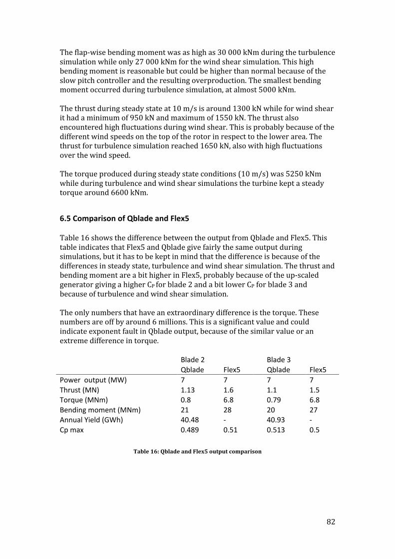
82

The flap-‐wise bending moment was as high as 30 000 kNm during the turbulence simulation while only 27 000 kNm for the wind shear simulation. This high bending moment is reasonable but could be higher than normal because of the slow pitch controller and the resulting overproduction. The smallest bending moment occurred during turbulence simulation, at almost 5000 kNm. The thrust during steady state at 10 m/s is around 1300 kN while for wind shear it had a minimum of 950 kN and maximum of 1550 kN. The thrust also encountered high fluctuations during wind shear. This is probably because of the different wind speeds on the top of the rotor in respect to the lower area. The thrust for turbulence simulation reached 1650 kN, also with high fluctuations over the wind speed. The torque produced during steady state conditions (10 m/s) was 5250 kNm while during turbulence and wind shear simulations the turbine kept a steady torque around 6600 kNm.

6.5 Comparison of Qblade and Flex5 Table 16 shows the difference between the output from Qblade and Flex5. This table indicates that Flex5 and Qblade give fairly the same output during simulations, but it has to be kept in mind that the difference is because of the differences in steady state, turbulence and wind shear simulation. The thrust and bending moment are a bit higher in Flex5, probably because of the up-‐scaled generator giving a higher CP for blade 2 and a bit lower CP for blade 3 and because of turbulence and wind shear simulation. The only numbers that have an extraordinary difference is the torque. These numbers are off by around 6 millions. This is a significant value and could indicate exponent fault in Qblade output, because of the similar value or an extreme difference in torque.

Blade 2

Blade 3

Qblade Flex5

Qblade Flex5 Power output (MW) 7 7

7 7

Thrust (MN) 1.13 1.6

1.1 1.5 Torque (MNm) 0.8 6.8

0.79 6.8

Bending moment (MNm) 21 28

20 27 Annual Yield (GWh) 40.48 -‐

40.93 -‐

Cp max 0.489 0.51

0.513 0.5

Table 16: Qblade and Flex5 output comparison

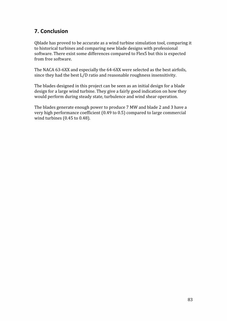
83

7. Conclusion Qblade has proved to be accurate as a wind turbine simulation tool, comparing it to historical turbines and comparing new blade designs with professional software. There exist some differences compared to Flex5 but this is expected from free software. The NACA 63-‐6XX and especially the 64-‐6XX were selected as the best airfoils, since they had the best L/D ratio and reasonable roughness insensitivity. The blades designed in this project can be seen as an initial design for a blade design for a large wind turbine. They give a fairly good indication on how they would perform during steady state, turbulence and wind shear operation. The blades generate enough power to produce 7 MW and blade 2 and 3 have a very high performance coefficient (0.49 to 0.5) compared to large commercial wind turbines (0.45 to 0.48).

84

8. Further work These blade designs were made with limited time available. It should be noted that these designs would only prove as an initial design for further analyses. Further iterations should be performed to get the best possible result. The airfoil catalogue should be extended to include more high performance airfoil families and the missing tailored airfoil families. Many of the thick airfoils are up-‐scaled versions and should be replaced with the original geometry. Experimental tests should be performed on the selected airfoils for further investigations on roughness insensitivity, in order to validate the analytic results from the airfoil catalogue. During the design of these blades, no structural limitations for the design have been considered. An extensive structure analysis has to be performed for the blades. The blades should also be tested to withstand the offshore IEC design load cases.

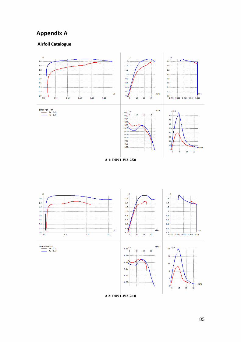
85

Appendix A

Airfoil Catalogue

A 1: DU91-‐W2-‐250

A 2: DU91-‐W2-‐210

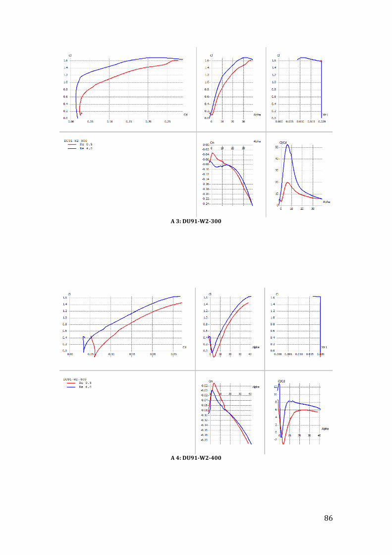
86

A 3: DU91-‐W2-‐300

A 4: DU91-‐W2-‐400

87

A 5: DU93-‐W-‐210

A 6: DU93-‐W-‐300

88

A 7: DU93-‐W-‐400

A 8: FFA-‐W3-‐211

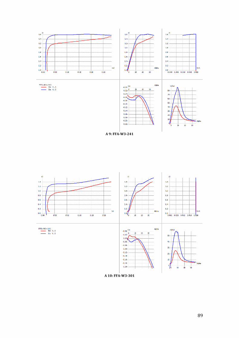
89

A 9: FFA-‐W3-‐241

A 10: FFA-‐W3-‐301

90

A 11: FFA-‐W3-‐351

A 12: FFA-‐W3-‐401

91

A 13: NACA 63-‐612

A 14: NACA 63-‐614

92

A 15: NACA 63-‐615

A 16: NACA 63-‐616

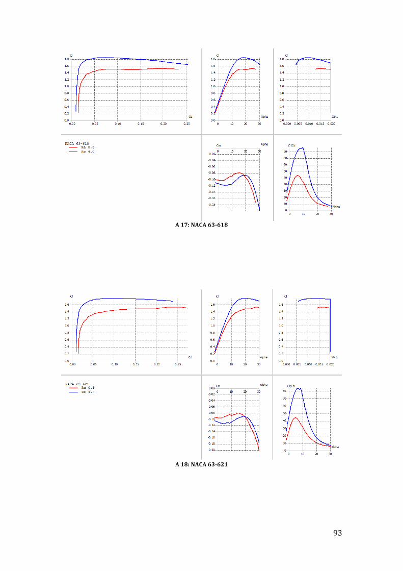
93

A 17: NACA 63-‐618

A 18: NACA 63-‐621

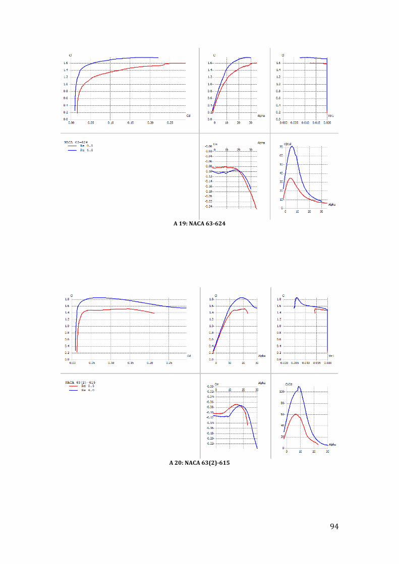
94

A 19: NACA 63-‐624

A 20: NACA 63(2)-‐615

95

A 21: NACA 63(2)A-‐015

A 22: NACA 63(3)-‐618

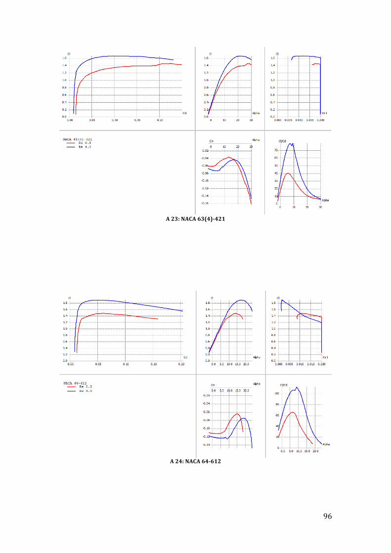
96

A 23: NACA 63(4)-‐421

A 24: NACA 64-‐612

97

A 25: NACA 64-‐614

A 26: NACA 64-‐615

98

A 27: NACA 64-‐616

A 28: NACA 64-‐618

99

A 29: NACA 64-‐621

A 30: NACA 64(1)-‐212

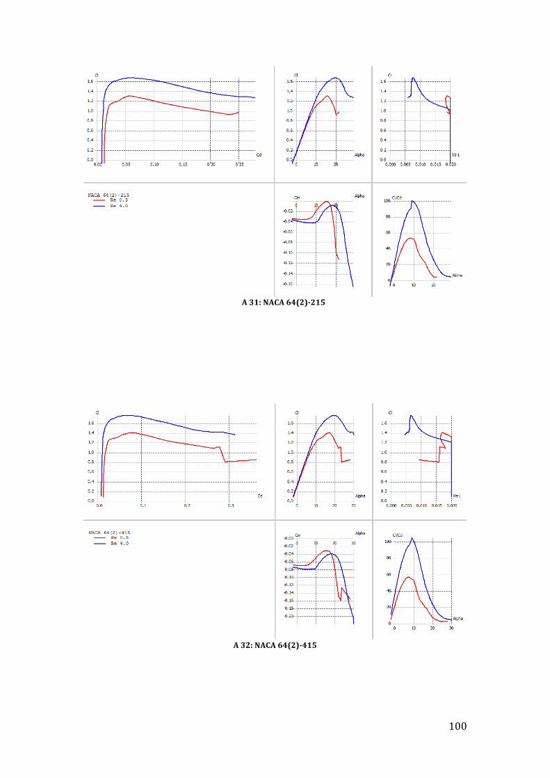
100

A 31: NACA 64(2)-‐215

A 32: NACA 64(2)-‐415

101

A 33: NACA 64(3)-‐218

A 34: NACA 64(3)-‐418

102

A 35: NACA 64(3)-‐618

A 36: NACA 64(4)-‐421

103

A 37: NACA 63-‐430(V)

A 38: DU93-‐W-‐350

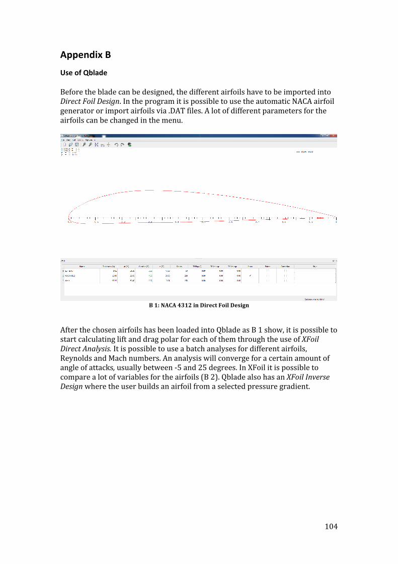
104

Appendix B

Use of Qblade Before the blade can be designed, the different airfoils have to be imported into Direct Foil Design. In the program it is possible to use the automatic NACA airfoil generator or import airfoils via .DAT files. A lot of different parameters for the airfoils can be changed in the menu.

B 1: NACA 4312 in Direct Foil Design

After the chosen airfoils has been loaded into Qblade as B 1 show, it is possible to start calculating lift and drag polar for each of them through the use of XFoil Direct Analysis. It is possible to use a batch analyses for different airfoils, Reynolds and Mach numbers. An analysis will converge for a certain amount of angle of attacks, usually between -‐5 and 25 degrees. In XFoil it is possible to compare a lot of variables for the airfoils (B 2). Qblade also has an XFoil Inverse Design where the user builds an airfoil from a selected pressure gradient.

105

B 2: NACA 4312 polar diagram for different Reynolds numbers

The airfoil polar has to be extrapolated for the whole 360 degrees instead of the usual -‐5 to 25 degrees range because of the BEM code. This is done in the Rotor and turbine design 360° polar view (B 3). The sliders on the left in the figure are used so the extrapolations match with the polar for the airfoil.

B 3: NACA 4312 360 polar view

In blade view (B 4) the blade can now be designed. It is possible to set the blade pitch, choose the section position, chord length, offset, twist, airfoil and the airfoil polar. It is possible to optimize the blade for the tip-‐speed ratio, linear

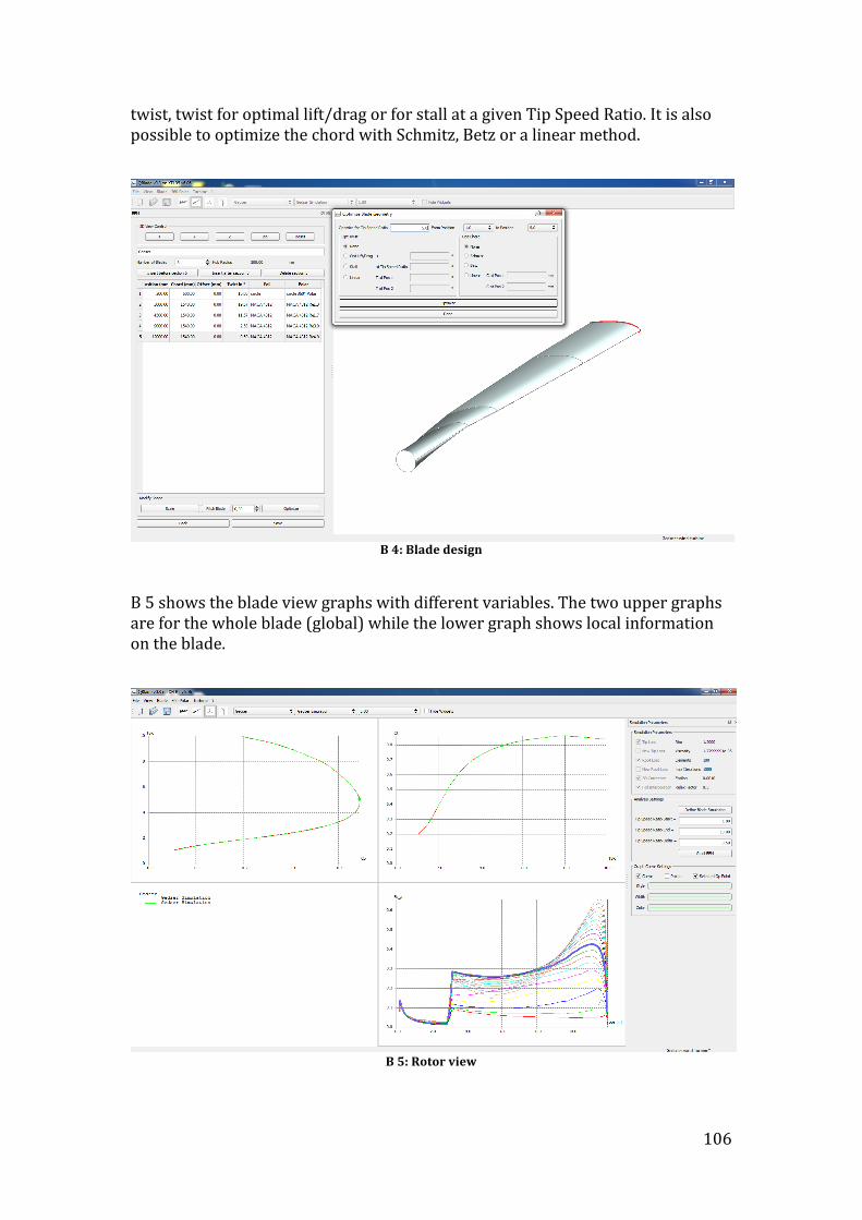
106

twist, twist for optimal lift/drag or for stall at a given Tip Speed Ratio. It is also possible to optimize the chord with Schmitz, Betz or a linear method.

B 4: Blade design

B 5 shows the blade view graphs with different variables. The two upper graphs are for the whole blade (global) while the lower graph shows local information on the blade.

B 5: Rotor view

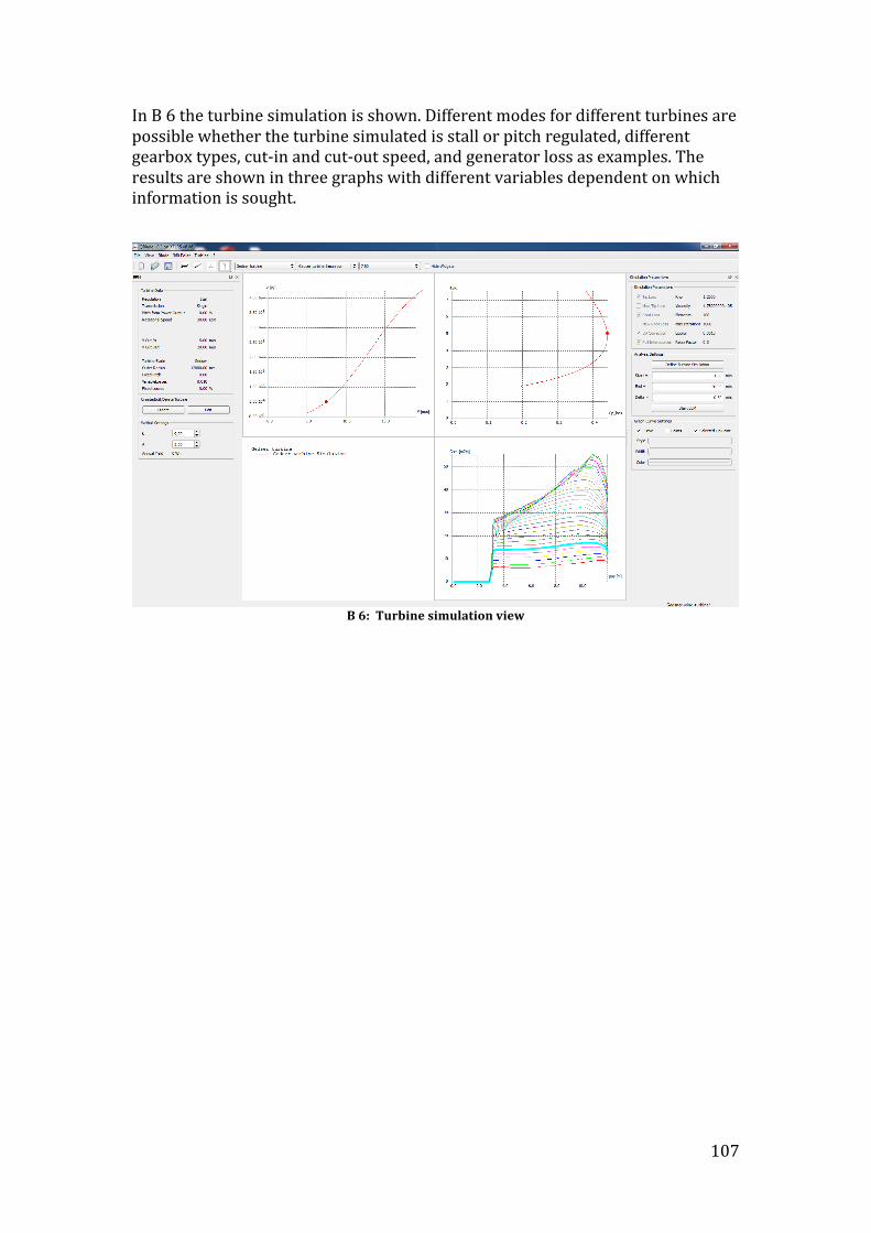
107

In B 6 the turbine simulation is shown. Different modes for different turbines are possible whether the turbine simulated is stall or pitch regulated, different gearbox types, cut-‐in and cut-‐out speed, and generator loss as examples. The results are shown in three graphs with different variables dependent on which information is sought.

B 6: Turbine simulation view

108

Appendix C

Airfoil Catalogue Table C 1 and table C 2 show the full result of the sensitivity analysis for airfoils at Cl, max and at best L/D. The list ranks from the least decrease in efficiency to highest decrease in efficiency, show in percentage. AIRFOIL Alfa Cl, max Cd Cl/Cd at Clmax T.U., Clmax Delta Cl,max Reynolds

DU91-‐W2-‐300 31.50 1.68 0.22 7,64 0.11 4 000 000 DU91-‐W2-‐300 36.50 1.61 0.27 5,91 0.02 -‐4.35 % 500 000 FFA-‐W3-‐241 27.00 1.61 0.18 8,86 0.02 4 000 000 FFA-‐W3-‐241 34.00 1.50 0.28 5,41 0.02 -‐7.09 % 500 000 DU93-‐W-‐350 38.00 1.66 0.26 6,32 0.01 4 000 000 DU93-‐W-‐350 38.00 1.52 0.28 5,44 0.02 -‐8.15 % 500 000 NACA 63-‐624 26.50 1.75 0.18 9,74 0.01 4 000 000 NACA 63-‐624 33.50 1.60 0.28 5,72 0.01 -‐8.90 % 500 000 NACA 63-‐430(V) 33.00 1.54 0.22 7,10 0.02 4 000 000 NACA 63-‐430(V) 37.50 1.40 0.24 5,75 0.02 -‐9.47 % 500 000 DU91-‐W2-‐250 26.50 1.71 0.17 9,84 0.01 4 000 000 DU91-‐W2-‐250 28.00 1.55 0.21 7,35 0.02 -‐9.49 % 500 000 FFA-‐W3-‐211 16.50 1.71 0.05 32,23 0.02 4 000 000 FFA-‐W3-‐211 29.00 1.53 0.25 6,20 0.02 -‐10.15 % 500 000 DU91-‐W2-‐400 40.50 1.64 0.26 6.21 0.02 4 000 000 DU91-‐W2-‐400 38.00 1.45 0.27 5.34 0.02 -‐11.64 % 500 000 FFA-‐W3-‐351 39.00 1.56 0.27 5.68 0.02 4 000 000 FFA-‐W3-‐351 36.00 1.37 0.28 4.98 0.02 -‐11.89 % 500 000 FFA-‐W3-‐301 37.50 1.60 0.27 6.02 0.03 4 000 000 FFA-‐W3-‐301 35.50 1.41 0.28 5.02 0.02 -‐12.22 % 500 000 NACA 64(4)-‐421 23.50 1.65 0.13 13.19 0.01 4 000 000 NACA 64(4)-‐421 26.50 1.44 0.19 7.49 0.02 -‐12.90 % 500 000 NACA 63-‐621 19.00 1.77 0.09 19.93 0.01 4 000 000 NACA 63-‐621 29.00 1.54 0.25 6.12 0.02 -‐13.42 % 500 000 NACA 63(3)-‐618 20.00 1.79 0.09 19.55 0.01 4 000 000 NACA 63(3)-‐618 26.00 1.53 0.21 7.26 0.01 -‐14.52 % 500 000 DU93-‐W-‐300 36.00 1.71 0.24 7.09 0.02 4 000 000 DU93-‐W-‐300 37.50 1.46 0.29 5.10 0.02 -‐14.60 % 500 000 NACA 64(3)-‐618 21.00 1.78 0.10 17.50 0.01 4 000 000 NACA 64(3)-‐618 23.50 1.51 0.17 8.92 0.02 -‐14.74 % 500 000 DU91-‐W2-‐350 40.00 1.68 0.26 6.53 0.02 4 000 000 DU91-‐W2-‐350 36.50 1.43 0.26 5.50 0.02 -‐15.15 % 500 000 NACA 63(4)-‐421 21.00 1.66 0.10 16.88 0.01 4 000 000 NACA 63(4)-‐421 25.00 1.40 0.19 7.36 0.19 -‐15.60 % 500 000 DU93-‐W-‐210 26.00 1.75 0.15 11.53 0.01 4 000 000 DU93-‐W-‐210 28.50 1.48 0.23 6.51 0.02 -‐15.72 % 500 000 NACA 64(1)-‐212 16.00 1.51 0.04 40.00 0.00 4 000 000 NACA 64(1)-‐212 14.50 1.27 0.05 25.75 0.01 -‐15.83 % 500 000 DU93-‐W-‐400 41.50 1.66 0.26 6.43 0.03 4 000 000 DU93-‐W-‐400 38.50 1.39 0.27 5.25 0.02 -‐16.05 % 500 000 DU91-‐W2-‐210 19.50 1.75 0.07 24.85 0.11 4 000 000 DU91-‐W2-‐210 22.00 1.47 0.15 9.49 0.15 -‐16.17 % 500 000 NACA 64-‐621 22.50 1.78 0.13 14.03 0.01 4 000 000 NACA 64-‐621 23.50 1.48 0.18 8.34 0.02 -‐16.54 % 500 000 NACA 64-‐618 20.00 1.84 0.09 20.61 0.01 4 000 000 NACA 64-‐618 23.00 1.53 0.16 9.34 0.02 -‐16.67 % 500 000 NACA 64(3)-‐418 21.50 1.70 0.10 17.36 0.01 4 000 000 NACA 64(3)-‐418 21.00 1.41 0.13 10.88 0.02 -‐16.92 % 500 000 NACA 63-‐618 18.50 1.85 0.07 26.58 0.01 4 000 000 NACA 63-‐618 25.00 1.53 0.20 7.64 0.01 -‐17.21 % 500 000 NACA 63(2)-‐615 19.00 1.84 0.07 24.86 0.01 4 000 000 NACA 63(2)-‐615 21.00 1.51 0.15 10.22 0.01 -‐17.77 % 500 000 NACA 64(2)-‐415 19.50 1.73 0.07 25.36 0.01 4 000 000 NACA 64(2)-‐415 17.00 1.41 0.08 17.71 0.02 -‐18.38 % 500 000 NACA 64(3)-‐218 21.00 1.62 0.08 20.08 0.01 4 000 000 NACA 64(3)-‐218 21.00 1.32 0.12 10.85 0.02 -‐18.57 % 500 000

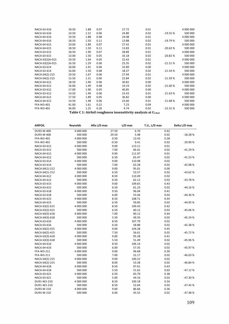
109

NACA 63-‐616 18.50 1.88 0.07 27.72 0.01 4 000 000 NACA 63-‐616 14.50 1.52 0.06 24.80 0.02 -‐19.55 % 500 000 NACA 64-‐616 19.50 1.88 0.08 24.08 0.01 4 000 000 NACA 64-‐616 18.50 1.50 0.11 13.88 0.02 -‐19.79 % 500 000 NACA 64-‐615 19.00 1.89 0.07 27.42 0.01 4 000 000 NACA 64-‐615 18.50 1.50 0.11 13.83 0.01 -‐20.63 % 500 000 NACA 63-‐615 18.50 1.90 0.07 28.89 0.01 4 000 000 NACA 63-‐615 13.00 1.50 0.05 33.18 0.02 -‐20.82 % 500 000 NACA 63(2)A-‐015 19.50 1.64 0.05 32.43 0.01 4 000 000 NACA 63(2)A-‐015 16.50 1.29 0.06 23.35 0.02 -‐21.51 % 500 000 NACA 63-‐614 18.00 1.91 0.06 32.89 0.00 4 000 000 NACA 63-‐614 16.00 1.50 0.08 18.37 0.02 -‐21.54 % 500 000 NACA 64(2)-‐215 19.50 1.67 0.06 27.94 0.01 4 000 000 NACA 64(2)-‐215 15.50 1.31 0.06 22.84 0.02 -‐21.59 % 500 000 NACA 64-‐612 18.50 1.90 0.06 30.82 0.00 4 000 000 NACA 64-‐612 16.00 1.49 0.08 19.19 0.02 -‐21.60 % 500 000 NACA 63-‐612 17.00 1.90 0.05 40.85 0.00 4 000 000 NACA 63-‐612 14.50 1.49 0.06 23.43 0.01 -‐21.63 % 500 000 NACA 64-‐612 17.50 1.89 0.05 36.82 0.00 4 000 000 NACA 64-‐612 14.50 1.48 0.06 23.60 0.01 -‐21.68 % 500 000 FFA-‐W3-‐401 41.00 1.61 0.22 7.23 0.09 4 000 000 FFA-‐W3-‐401 36.00 1.25 0.26 4.74 0.02 -‐22.31 % 500 000

Table C 1: Airfoil roughness insensitivity analysis at Cl max

AIRFOIL Reynolds Alfa L/D max L/D max T.U., L/D max Delta L/D max

DU93-‐W-‐400 4 000 000 27.50 6.70 0.42 DU93-‐W-‐400 500 000 29.50 5.48 0.02 -‐18.28 % FFA-‐W3-‐401 4 000 000 0.50 13.43 0.28 FFA-‐W3-‐401 500 000 -‐0.50 9.41 0.02 -‐29.90 % NACA 63-‐612 4 000 000 9.00 113.11 0.01 NACA 63-‐612 500 000 7.00 66.41 0.02 -‐41.29 % NACA 64-‐612 4 000 000 9.00 111.97 0.01 NACA 64-‐612 500 000 6.50 65.47 0.02 -‐41.53 % NACA 63-‐614 4 000 000 9.00 110.98 0.02 NACA 63-‐614 500 000 7.00 63.28 0.02 -‐42.98 % NACA 64(1)-‐212 4 000 000 9.00 95.01 0.00 NACA 64(1)-‐212 500 000 6.50 53.57 0.02 -‐43.62 % NACA 64-‐612 4 000 000 8.50 110.49 0.02 NACA 64-‐612 500 000 6.50 62.12 0.02 -‐43.78 % NACA 63-‐615 4 000 000 9.00 109.65 0.43 NACA 63-‐615 500 000 6.50 61.23 0.02 -‐44.16 % NACA 63-‐618 4 000 000 9.50 96.04 0.41 NACA 63-‐618 500 000 6.00 53.44 0.02 -‐44.36 % NACA 64-‐615 4 000 000 8.50 108.71 0.44 NACA 64-‐615 500 000 6.50 59.85 0.02 -‐44.95 % NACA 63(2)-‐615 4 000 000 8.50 109.43 0.42 NACA 63(2)-‐615 500 000 6.50 60.12 0.02 -‐45.06 % NACA 64(3)-‐618 4 000 000 7.00 90.12 0.44 NACA 64(3)-‐618 500 000 5.50 49.35 0.02 -‐45.24 % NACA 63-‐616 4 000 000 8.50 107.79 0.02 NACA 63-‐616 500 000 6.50 58.88 0.02 -‐45.38 % NACA 64(2)-‐415 4 000 000 9.00 104.28 0.45 NACA 64(2)-‐415 500 000 7.50 56.61 0.02 -‐45.72 % NACA 63(3)-‐618 4 000 000 9.00 95.28 0.41 NACA 63(3)-‐618 500 000 5.50 51.49 0.02 -‐45.96 % NACA 64-‐616 4 000 000 8.50 106.14 0.02 NACA 64-‐616 500 000 6.00 57.35 0.02 -‐45.97 % FFA-‐W3-‐211 4 000 000 9.00 96.68 0.30 FFA-‐W3-‐211 500 000 7.00 52.17 0.02 -‐46.03 % NACA 64(2)-‐215 4 000 000 9.00 100.22 0.02 NACA 64(2)-‐215 500 000 8.00 53.28 0.02 -‐46.84 % NACA 64-‐618 4 000 000 8.50 97.61 0.43 NACA 64-‐618 500 000 5.50 51.62 0.02 -‐47.12 % NACA 63-‐621 4 000 000 6.50 83.79 0.38 NACA 63-‐621 500 000 5.00 44.16 0.02 -‐47.30 % DU91-‐W2-‐210 4 000 000 8.50 100.18 0.34 DU91-‐W2-‐210 500 000 8.50 52.64 0.02 -‐47.45 % DU93-‐W-‐210 4 000 000 9.00 86.66 0.36 DU93-‐W-‐210 500 000 6.00 45.52 0.02 -‐47.48 %

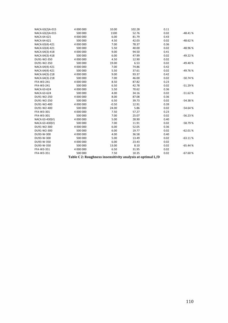
110

NACA 63(2)A-‐015 4 000 000 10.00 102.28 0.11 NACA 63(2)A-‐015 500 000 1100 52.76 0.02 -‐48.41 % NACA 64-‐621 4 000 000 6.00 81.79 0.43 NACA 64-‐621 500 000 4.50 42.03 0.02 -‐48.62 % NACA 63(4)-‐421 4 000 000 7.00 78.37 0.36 NACA 63(4)-‐421 500 000 5.50 40.00 0.02 -‐48.96 % NACA 64(3)-‐418 4 000 000 9.00 94.50 0.41 NACA 64(3)-‐418 500 000 6.00 47.99 0.02 -‐49.22 % DU91-‐W2-‐350 4 000 000 4.50 12.90 0.02 DU91-‐W2-‐350 500 000 19.00 6.53 0.02 -‐49.40 % NACA 64(4)-‐421 4 000 000 7.00 74.86 0.42 NACA 64(4)-‐421 500 000 5.50 37.61 0.02 -‐49.76 % NACA 64(3)-‐218 4 000 000 9.00 93.37 0.42 NACA 64(3)-‐218 500 000 7.00 46.00 0.02 -‐50.74 % FFA-‐W3-‐241 4 000 000 8.50 87.82 0.23 FFA-‐W3-‐241 500 000 6.50 42.78 0.02 -‐51.29 % NACA 63-‐624 4 000 000 5.50 70.62 0.36 NACA 63-‐624 500 000 4.00 34.16 0.02 -‐51.62 % DU91-‐W2-‐250 4 000 000 8.00 87.08 0.36 DU91-‐W2-‐250 500 000 6.50 39.73 0.02 -‐54.38 % DU91-‐W2-‐400 4 000 000 -‐0.50 12.91 0.39 DU91-‐W2-‐400 500 000 24.00 5.86 0.02 -‐54.64 % FFA-‐W3-‐301 4 000 000 7.50 57.27 0.23 FFA-‐W3-‐301 500 000 7.00 25.07 0.02 -‐56.23 % NACA 63-‐430(V) 4 000 000 5.00 28.90 0.40 NACA 63-‐430(V) 500 000 7.00 11.91 0.02 -‐58.79 % DU91-‐W2-‐300 4 000 000 6.00 52.05 0.36 DU91-‐W2-‐300 500 000 6.00 19.77 0.02 -‐62.01 % DU93-‐W-‐300 4 000 000 4.00 36.58 0.40 DU93-‐W-‐300 500 000 5.00 13.49 0.02 -‐63.11 % DU93-‐W-‐350 4 000 000 6.00 23.43 0.02 DU93-‐W-‐350 500 000 13.00 8.10 0.02 -‐65.44 % FFA-‐W3-‐351 4 000 000 6.50 31.95 0.02 FFA-‐W3-‐351 500 000 7.50 10.35 0.02 -‐67.60 %

Table C 2: Roughness insensitivity analysis at optimal L/D

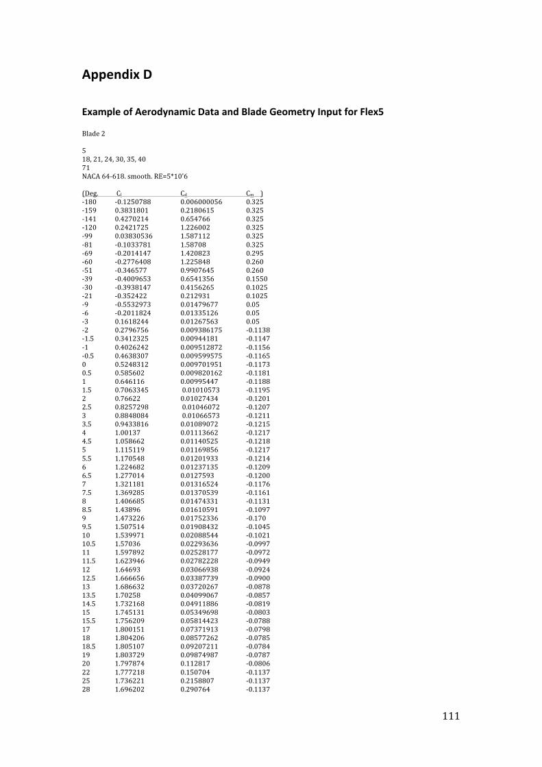
111

Appendix D

Example of Aerodynamic Data and Blade Geometry Input for Flex5 Blade 2 5 18, 21, 24, 30, 35, 40 71 NACA 64-‐618. smooth. RE=5*10'6 (Deg. Cl Cd Cm ) -‐180 -‐0.1250788 0.006000056 0.325 -‐159 0.3831801 0.2180615 0.325 -‐141 0.4270214 0.654766 0.325 -‐120 0.2421725 1.226002 0.325 -‐99 0.03830536 1.587112 0.325 -‐81 -‐0.1033781 1.58708 0.325 -‐69 -‐0.2014147 1.420823 0.295 -‐60 -‐0.2776408 1.225848 0.260 -‐51 -‐0.346577 0.9907645 0.260 -‐39 -‐0.4009653 0.6541356 0.1550 -‐30 -‐0.3938147 0.4156265 0.1025 -‐21 -‐0.352422 0.212931 0.1025 -‐9 -‐0.5532973 0.01479677 0.05 -‐6 -‐0.2011824 0.01335126 0.05 -‐3 0.1618244 0.01267563 0.05 -‐2 0.2796756 0.009386175 -‐0.1138 -‐1.5 0.3412325 0.00944181 -‐0.1147 -‐1 0.4026242 0.009512872 -‐0.1156 -‐0.5 0.4638307 0.009599575 -‐0.1165 0 0.5248312 0.009701951 -‐0.1173 0.5 0.585602 0.009820162 -‐0.1181 1 0.646116 0.00995447 -‐0.1188 1.5 0.7063345 0.01010573 -‐0.1195 2 0.76622 0.01027434 -‐0.1201 2.5 0.8257298 0.01046072 -‐0.1207 3 0.8848084 0.01066573 -‐0.1211 3.5 0.9433816 0.01089072 -‐0.1215 4 1.00137 0.01113662 -‐0.1217 4.5 1.058662 0.01140525 -‐0.1218 5 1.115119 0.01169856 -‐0.1217 5.5 1.170548 0.01201933 -‐0.1214 6 1.224682 0.01237135 -‐0.1209 6.5 1.277014 0.0127593 -‐0.1200 7 1.321181 0.01316524 -‐0.1176 7.5 1.369285 0.01370539 -‐0.1161 8 1.406685 0.01474331 -‐0.1131 8.5 1.43896 0.01610591 -‐0.1097 9 1.473226 0.01752336 -‐0.170 9.5 1.507514 0.01908432 -‐0.1045 10 1.539971 0.02088544 -‐0.1021 10.5 1.57036 0.02293636 -‐0.0997 11 1.597892 0.02528177 -‐0.0972 11.5 1.623946 0.02782228 -‐0.0949 12 1.64693 0.03066938 -‐0.0924 12.5 1.666656 0.03387739 -‐0.0900 13 1.686632 0.03720267 -‐0.0878 13.5 1.70258 0.04099067 -‐0.0857 14.5 1.732168 0.04911886 -‐0.0819 15 1.745131 0.05349698 -‐0.0803 15.5 1.756209 0.05814423 -‐0.0788 17 1.800151 0.07371913 -‐0.0798 18 1.804206 0.08577262 -‐0.0785 18.5 1.805107 0.09207211 -‐0.0784 19 1.803729 0.09874987 -‐0.0787 20 1.797874 0.112817 -‐0.0806 22 1.777218 0.150704 -‐0.1137 25 1.736221 0.2158807 -‐0.1137 28 1.696202 0.290764 -‐0.1137

112

31 1.66387 0.3730351 -‐0.1625 34 1.640206 0.4607482 -‐0.1625 37 1.623247 0.5523155 -‐0.1625 40 1.609902 0.6464085 -‐0.1625 52 1.532437 1.025955 -‐0.260 61 1.390591 1.286376 -‐0.2925 70 1.148432 1.499372 -‐0.2925 79 0.8094009 1.645347 -‐0.325 100 -‐0.1964295 1.664437 -‐0.325 121 -‐1.06679 1.2602 -‐0.325 139 -‐1.261789 0.73708 -‐0.325 160 -‐0.861352 0.2030205 -‐0.325 178 -‐0.3186824 0.008052249 -‐0.325 Blade 2 NACA 64-‐618, 3-‐blades, L=8, ng=110, cl_opt=1.4 14 NS 2.00 20.0E9 20.0E9 4500 0 1 0 0 X EI1 EI2 m fi Iuskr Uf0 Uk0 10.00 20.0E9 20.0E9 1500 0 0 0 0 20.00 6.0E9 6.0E9 500 0 0 0 0 30.00 3.0E9 4.0E9 400 0 0 0 0 40.00 2.0E9 4.0E9 380 0 0 0 0 50.00 7.0E8 3.0E9 340 0 0 0 0 60.00 6.0E8 2.0E9 300 0 0 0 0 70.00 4.0E8 1.5E9 250 0 0 0 0 75.00 2.0E8 7.0E8 220 0 0 0 0 80.00 1.5E8 5.0E8 200 0 0 0 0 80.63 7.0E7 3.0E8 180 0 0 0 0 81.25 3.0E7 1.5E8 130 0 0 0 0 81.88 7.0E6 7.0E7 90 0 0 0 0 82.50 1.5E5 3.0E5 50 0 0 0 0 1 betac (average structural pitch, deg) 0.03 0.03 0.03 0.03 struct.damp. log.decr. blade-‐mode 1F 2F 1K 2K 2.00 4.000 13 100.0 0 X c beta t/c yac/c (m,m,deg,%,-‐) 10.00 5.000 8 40.0 0 20.00 5.500 3 35.0 0 30.0 5.000 2 30.0 0 40.0 4.200 1 24.0 0 50.0 3.633 1 21.0 0 60.0 3.066 0.56 18.0 0 70.0 2.500 -‐0.97 18.0 0 75.0 2.200 -‐1.38 18.0 0 80.0 1.600 -‐2.25 18.0 0 80.63 1.400 -‐2.29 18.0 0 81.25 1.200 -‐2.33 18.0 0 81.88 1.000 -‐2.37 18.0 0 82.5 0.500 -‐2.40 18.0 0 B2N64.pro airfoil data filename 71 X-‐tipbrake ( > R_tip => none)

113

Appendix E

Wind Shear Simulation in Flex5

E 1: Blade 2 wind shear simulation for torque (kNm) during a period of time at different wind shear,

compared to wind speed for the same time period (right y-‐axis)

E 2: Blade 2 wind shear simulation for thrust (kN) over a duration of time (t) for different wind

shear, compared to wind speed for the same time period (right y-‐axis)

114

Figure 64: Thrust for blade 3 for different wind shear

Figure 65: Torque for blade 3 for different wind shear

115

Turbulence Simulation in Flex5

E 3: Blade 2 turbulence simulation for torque (kNm) during a time period (t) with different

turbulence intensities

E 4: Blade 2 turbulence simulation for thrust (kN) during a period of time (t) for different turbulence

intensities

116

E 5: Thrust for Blade 3 at different turbulence intensities

Figure 66: Torque for blade 3 at different turbulence intensities

117

References 1 https://engineering.purdue.edu/~aerodyn/AAE515/Chapter13-‐10.pdf (05/06-‐2012) 2 Lundsager, P., Frandsen, S., Christensen, C. J., (1980), Analysis of data from the Gedser wind turbine, Risø-‐m-‐2242, ISBN – 87-‐550-‐0693-‐0 3https://netfiles.uiuc.edu/mragheb/www/NPRE%20475%20Wind%20Power%20Systems/Historical%20Wind%20Generators%20Machines.pdf (15/05-‐2012) 4http://www.motiva.fi/myllarin_tuulivoima/windpower%20web/res/gedser2.jpg (05/06-‐2012) 5http://www.boeing.com/history/boeing/windturbine.html (22/05-‐2012) 6http://en.wikipedia.org/wiki/List_of_wind_turbine_manufacturers (05/06-‐2012) 7http://www.statoil.com/en/TechnologyInnovation/NewEnergy/RenewablePowerProduction/Offshore/Hywind/Pages/HywindPuttingWindPowerToTheTest.aspx (05/06-‐2012) 8http://nozebra.ipapercms.dk/Vestas/Communication/Productbrochure/V16470MW/V16470MW/ (05/06-‐2012) 9 http://en.wikipedia.org/wiki/Wind_turbine (05/06-‐2012) 10http://www.folkecenter.dk/mediafiles/folkecenter/pdf/Market_and_Manufacturer_Trends.pdf (05/06-‐2012) 11http://www.ewec2011.info/fileadmin/ewec2011_files/images/conference/Side_Events/Research_over_from_Risoe_-‐_P.H._Madsen.ppt (11/06-‐2012) 12http://dancass.com/static/files/assets/653e5f65/Increase_in_the_rotor_size_of_Wind_blades_over_the_years.png (15/05-‐2012) 13http://www.centennialofflight.gov/essay/Evolution_of_Technology/airfoils/Tech5.htm (15/05-‐2012) 14http://twoscenarios.typepad.com/.a/6a00d8341c1ad753ef011570169b50970b-‐450wi (15/05-‐2012) 15http://people.clarkson.edu/~pmarzocc/AE429/The%20NACA%20airfoil%20series.pdf (15/05-‐2012) 17 Tangler, J. L., Somers, D. M., (1995), NREL Airfoil Families for HAWT´S, NREL, TP-‐442-‐7109 18http://www.risoe.dtu.dk/Research/sustainable_energy/wind_energy/projects/Profcat/airfoil_index.aspx?sc_lang=en (15/05-‐2012) 19http://ntrs.nasa.gov/archive/nasa/casi.ntrs.nasa.gov/19830025072_1983025072.pdf 20 http://www.worldscibooks.com/etextbook/7489/7489_chap01.pdf (05/06-‐2012) 21 IEC, (2007), IEC 61400-‐3 Ed.1: Wind turbines – Part 3: Design requirements for offshore wind turbines. IEC, 88/308/CDV 22 Jonkman, J., Butterfield, S., Musial, W., Scott, G., (2009), Definition of a 5-‐MW Reference Wind Turbine for Offshore Systems Development, NREL, TP-‐500-‐38060

118

23 Manwell, J.F., et. al., (2009), Wind Energy Explained, Theory, Design and Application 2nd edition, Wiley, West Sussex, ISBN-‐978-‐0-‐470-‐01500-‐1 24 Hansen, M. O. L., (2008), Aerodynamics of Wind Turbines, 2nd edition, Earthscan, London 25 Eppler, R., Somers, D.M., Low Speed Airfoil Design and Analysis, NASA Langley Research Center, N79-‐20036 26 Dahl, K. S., Fuglsang, P., (1998), Design of the Wind Turbine Airfoil Family RISØ-‐A-‐XX, Risø-‐R-‐1024 27 Bertagnolio, F., Sørensen, N.N., Johansen, J., Fuglsang, P., (2001), Wind Turbine Airfoil Catalogue, Risø-‐R-‐1280 28 Bertagnolio, F., Sørensen, N. N., Johansen, J., (2006), Profile Catalogue for Airfoil Sections Based on 3D Computations, Risø-‐R-‐1581 29 Somers, D. M., (2005), Effects of Airfoil Thickness and Maximum Lift Coefficient on Roughness Sensitivity, National Renewable Energy Laboratory (NREL), SR-‐500-‐36336 30 Somers, D. M., (2005), Design and Experimental Results for the S827 Airfoil, NREL, SR-‐500-‐36345 31http://www.centennialofflight.gov/essay/Theories_of_Flight/Skin_Friction/TH11G3.htm (05/06-‐2012) 32 Abbot, I. H., Von Doenhoff, A. E., (1949), Theory of Wing Sections, including a Summary of Airfoil Data, Dover Publications, New York 33 http://www.mh-‐aerotools.de/airfoils/bubbles.htm (15/05-‐2012) 34 Kraemer, K., (1973), Airfoil Profiles in a Critical Reynolds Number Region, NASA, TT F-‐14, 959 35 Sommers, D.M., Tangler, J. L., (2000), Wind-‐Tunnel Tests of Two Airfoils for Wind Turbines Operating at High Reynolds Number, NREL, CP-‐500-‐27891 36http://www.aer.mw.tum.de/fileadmin/tumwaer/www/pdf/lehre/grenzschicht/lectures/lecture_03.pdf (05/06-‐2012) 37 http://www.dur.ac.uk/g.l.ingram/download/wind_turbine_design.pdf (15/05-‐2012) 38 http://web.mit.edu/drela/Public/web/xfoil/ (15/05-‐2012) 39 http://qblade.de.to/ (15/05-‐2012) 40http://www.mh-‐aerotools.de/airfoils/javafoil.htm (15/05-‐2012) 41 http://en.wikipedia.org/wiki/Wind_gradient (10/05-‐2012) 42 http://ntrs.nasa.gov/archive/nasa/casi.ntrs.nasa.gov/19830025072_1983025072.pdf (15/04-‐2012) 43 Johansen, J., Sørensen, N. N., (2002), Numerical Investigation of Three Wind Turbine Blade Tips, Risø-‐R-‐1353

Investigation of Different Airfoils on Outer Sections of Large ...

Documents

Transcript of Investigation of Different Airfoils on Outer Sections of Large ...