AN APPROACH TO THE DESIGN

OF AIRFOILS WITH HIGH LIFT TO DRAG RATlOS

NOVEMBER, 1983

BY

DAVID WALTER ZINGG

TECHNISCHE HOGESCHOOL D[lFT -LUCHTVAART- EN RUIMTEVAARTTECHNIEK

BIBLIOTHEEK Kluyverweg 1 - DELFT

UTIAS TECHNICAL NOTE NO. 245 CN ISSN 0082-5263

•

t

AN APPROACH TO THE DESIGN

OF AIRFOILS WITH HIGH LIFT TO DRAG RATlOS

BY

DAVID WALTER ZINGG

SUBMITTED MARCH~ 1983

NOVEMBER, 1983 UTIAS TECHNICAL NOTE NO. 245 CN ISSN 0082-5263

Summary

A procedure for the design of low-speed, single-element airfoi1s with high lift to drag ratios is presented. The p r ocedure uses an inverse approach which proceeds from a set of desiraó1e boundary 1ayer characteristics, which are determined from the performance objectives, to a velocity distribution and, fina11y, to an airfoi1 shape. The boundary 1ayer shape factor, whi ch is a measure of the nearness of the boundary 1ayer to separation, is used to de fine the boundary 1ayer characteristics in the upper surface pressure recovery region. The turbulent boundary 1ayer equations are solved in inverted form to ca1cu1ate the velocity distribution which corresponds to a shape factor variation. The ve10cities on the upper surface prior to pressure recovery are chosen to cause boundary 1ayer transition at a desired location. The lower surface velocity distribution is se1ected to satisfy the requirement that a c1osed, non­reentrant shapewhich meets the specified structura1 requirements resu1ts. The design procedure described can be uti1ized for the design of high performance airfoi1s for a variety of performance objectives, operating conditions, and practical constraints.

Using this procedure, an airfoi1 has been designed which achieves a lift to drag ratio of 180 at a lift coefficient of 1.2 and a Reyno1ds number of one mi11ion. Through this design study, a set of guide1ines for the design of a1rfoi1s with high lift to drag ratios is estab11shed.

ii

',..

AcknowTedg'ement s

The author wishes to thank Dr. G. W. Johnston of

the University of Toronto Institute for Aerospace Studies

for his supervision. In addition, the author is grateful

to Mr. B. Egglestone of de Havilland Aircraft for his

advice and for the use of his computer programs.

iii

•

't

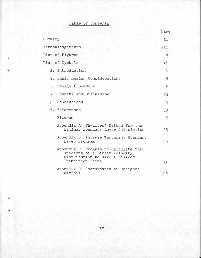
Ta'bleof Contents

Page

Summary ii

Acknow1edgements iii

List of Figures v

List of Symbols vi

1. Introduction 1

2. Basic Design Considerations 4

3. Design Procedure 6

4. Resu1ts and Discussion 23

5. Conclusions 35

6. References 39

Figures 42

Appendix A: Thwaites' Method for the Laminar Boundary Layer Calculation 53

Appendix B: Inverse Turbulent Boundary Layer Program 55

Appendix C: Program to Calculate the Gradient of a Linear Velocity Distribution to Give a Desired Transition Point 57

Appendix D: Coordinates of Designed Airfoil 58

iv

. L~&~bf F~gures

Fig. 1. Drag on a flat p1ate with different transition points

Fig. 2. Velocity gradients fo r transition at x/c = 0.7

Fig. 3. Shape factor variation on the NAGA 633-018

Fig. 4. Boundary 1ayer characteristics of Liebeck L1003 and Wortmann FX 74-GL6-140 airfoi1s

Fig. 5. Experimenta1 lift, drag, and pitching moment data for Liebeck L1003 airfoi1

Fig. 6. Deve10pment of Rg and Rgtr for a constant velocity

distribution with Re = 2.0 X 10 6

Fig. 7. Fami1y of upper surface velocity distributions

Fig. 8. Variation of lift coefficient and lift to drag ratio with recovery point 10cation

Fig. 9. NAGA 67-015 thickness form cambered to give design upper surface velocity distribution with xr/c = 0.7

Fig. 10. Velocity distribution on above section at ~ = 30

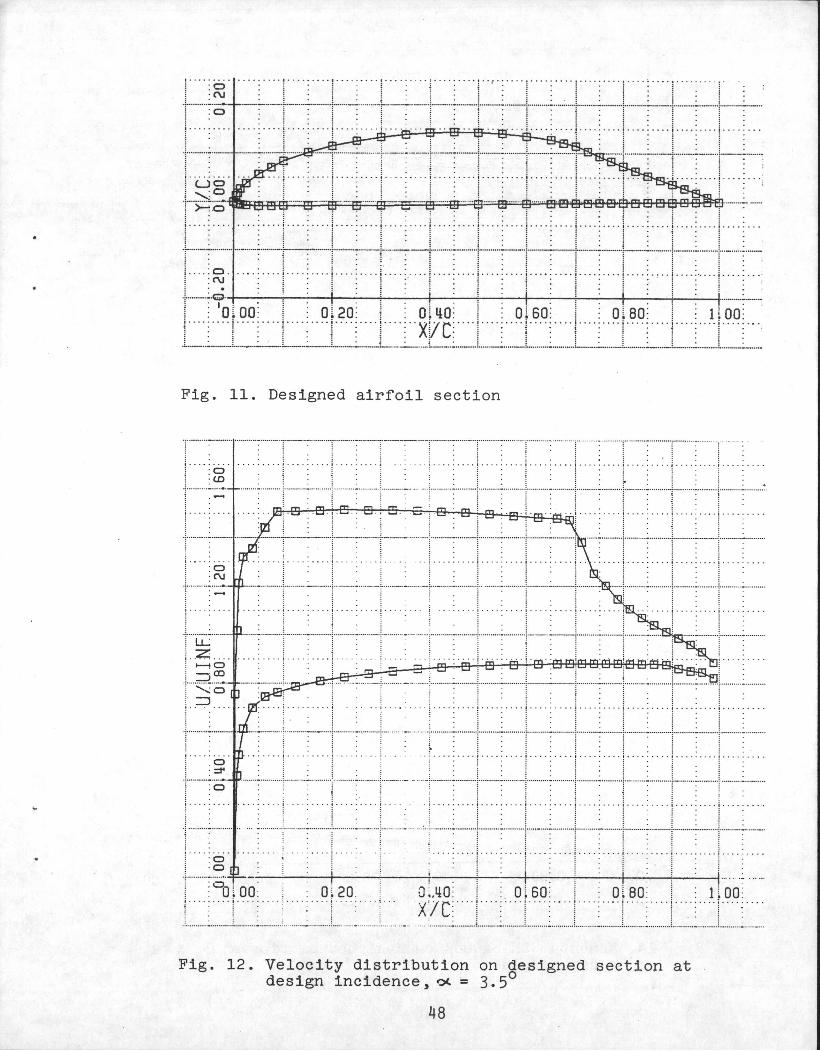
Fig. 11. Designed airfoi1 section

Fig. 12. Velocity distribution on designed section at design incidence, ,~= 3.50

Fig. 13. Shape factor variation on designed section at design incidence

Fig. 14. Momentum thickness on designed section at design incidence

Fig. 15. Velocity distribution on designed section at ~= 1.00

Fig. 16. Ga1cu1ated lift, drag, and pitching moment 6 characteristics of the designed airfoi1 at Re = 10

Fig. 17. Velocity distribution on designed section at ~ = 40

Fig. 18. Velocity distribution on Liebeck L1003 airfoi1 at design incidence

v

, .

'.

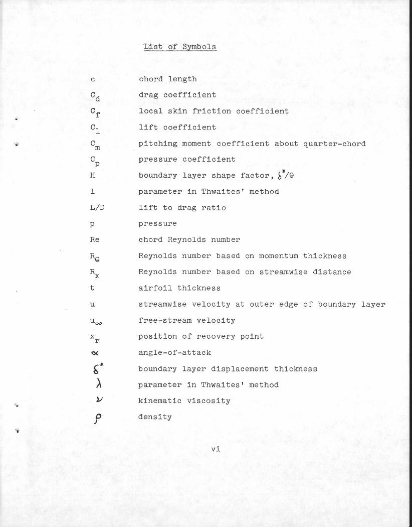
c

H

1

LID

p

Re

u

UQ()

x r

f

List Of Symbols

chord length

drag coefficient

local skin friction coefficient

lift coefficient

pitching moment coefficient about quarter-chord

pressure coefficient

.­boundary layer shape factor, ~ ;9

parameter in Thwaites' method

lift to drag ratio

pressure

chord Reynolds number

Reynolds number based on momentum thickness

Reynolds number based on streamwise distance

airfoil thickness

streamwise velocity at outer edge of boundary layer

free-stream velocity

position of recovery point

angle-of-attack

boundary layer displacement thickness

parameter in Thwaites' method

kinematic viscosity

density

vi

SUb scripts

i

te

tr

ooundary layer momentum thickness

wall shear stress

denotes a value at the start of the recovery region

denotes a value at the trailing edge

denotes a value at the transition point or a value required for transition

vii

.'

1. Introduction

The advent of high-speed computers and advanced

numerical methods has led to new possibi1ities in airfoi1

design. Prior to 1930, airfoi1 design was primari1y an

empirica1 process aided somewhat by potentia1 flow theory.

In the 1~30's, boundary 1ayer considerations were

qua1itative1y integrated into the design of "low-drag"

sections such as the NACA 6-series airfoi1s. Significant

improvements upon these sections were not achieved unti1

the late 1950's, when large computers became avai1ab1e.

Since that time, the performance of the NACA 6-series has

been consistent1y exceeded by sections such as the Wortmann

FX-series (Ref. 1).

The present~day designer has at hand an extensive array

of numerical ca1cu1ation techniques. Singu1arity methods

are a general, accurate, and efficient way of performing

a potentia1 flow ca1cu1ation. Boundary 1ayer characteristics

can be accurate1y determined by a variety of techniques,

inc1uding integra1 and finite-difference methods (which

invo1ve some empiricism). Empirica1 corre1ations adequately

predict boundary 1ayer transition and separation. Fina1ly,

iterative schemes are avai1ab1e to combine potentia1 flow

and viscous solutions so the ana1ysis of ful1y attached

1

viscous flow about two-dimensional sections can be

performed.

The recent advances in airfoil design, however, are

primarily the result of a change in the fundamental

design approach from an iterative cut and try procedure

to a synthesis or inverse technique. The traditional

empirical approach consists of modifying an initial

shape by trial and error until given performance

objectives are achieved. The inverse approach, in

contrast, begins with a set of boundary layer characteristics

which are derived from the performance objectives. The

velocity distribution which results in these characteristics

is determined and, finally, the shape which produces this

velocity distribution is calculated. The airfoil section

shapes generated by such an inverse design approach, such

as the Liebeck high-lift sections (Ref. 2), are generally

unique and are not likely to be obtained using an

empirical approach.

This thesis describes an example of an inverse approach

applied to the design of an airfoil with a high lift to

drag ratio. As energy costs continue to rise, low fuel

consumption is becoming an increasingly high priority

in aircraft design and hence such sections are required.

In general, an airfoil design problem involves several

conflicting requirements and therefore the final solution

2

must include some compromises. The design criteria and

their relative importance must be determined from the

intended application. While the airfoil designed in this

study reflects the specific priorities chosen, the design

procedure described can be applied to the design of

airfoils for a variety of applications. Some basic airfoil

design considerations are discussed in the following

section.

3

2. Basic Design Considerations

The design of a new low-speed, single-element

airfoil involves finding a section with desired performance

characteristics under specific operating conditions within

certain practical constraints, i.e. a section tailored to

a given application. However, because there are many

design trade-offs, different section shapes can be found

for a single application, each the re sult of different

priorities.

The performance objectives normally considered are

high lift, high lift to drag ratio, low drag, or a

specific pitching moment coefficient. When high lift is

desired, such as for STOL aircraft, the importance of

the nature of the stall break must be assessed, i.e.

should the maximum lift coefficient be sacrificed somewhat

to achieve "gentle" stall? Similarly, if a high lift to

drag ratio is the goal (or simply low drag, such as for

a strut), a compromise must be reached between the minimum

drag and the width of the low drag bucket, since a

decrease in drag is generally accompanied by a reduction

in bucket width. Possible pitching moment characteristics

which may be desired, though usually a low priority, are

a positive moment for flying wing type aircraft or a low

4

, .

------------ - - -- - ----------- - -------- ------ ------

moment to reduce trim loads and aeroelastic effects.

The operating conditions which must be specified are

the design lift coefficient, Re ynolds number, and Mach

number. In addition, off-des ign con siderations lead to

a range of these quantities under which adequate performance

is expected.

Practical constaints include a structural requirement

such as a minimum section modulus. Of ten simply a minimum

thickness/chord ratio is stipulated. Also, the type of

wing construction is a practical consideration for the

surface quality has a significant effect on the location

of boundary layer trans ition.

The criteria for this design study were not chosen

with a specific application in mind but rather to prove

the validity and accuracy of the design procedure in

general. The design goal was to maximize the section lift

to drag ratio with no restriction imposed upon the design

lift coefficient. Minimal consideration was given to

off-design performance and the stall break. The design

Reynolds number was chosen to be one million corresponding

to the aval1able test facillty. Compresslbility effects

were neglected. The thickness/chord ratio was required

to be fifteen percent, typlcal of a practical section,

and the surface was assumed to be smooth.

5

3. Design Procedure

An inverse airfoil design approach begins with a set

of boundary layer characteristics which are determined

from the performance objectives. The boundary layer

characteristics of primary interest are the location of

transition and the local proximity to separation in the

pressure recovery region, i.e. the angle-of-attack

perturbation which can be tolerated without flow sepa­

ration. Calculating the velocity distribution which

results in the desired boundary layer characteristics

constitutes the inverse boundary layer problem. The

d"irect problem is to solve the boundary layer equations

for the boundary layer parameters, H, Q, and Cf' given

a velocity distribution. In inverted form, these equations

can be solved for a velocity distribution if the variation

of one of the parameters is specified.

The airfoil shape is determined from the calculated

velocity distribution by an inverse potential flow

calculation. However, a velocity distribution can be

produced by a real, i.e. closed and non-reentrant, shape

only if certain conditions derived from conformal mapping

theory are satisfied (Ref. 3). The structural requirements

introduce a further constraint. Therefore the boundary

6

layer characteristics cannot be specified on the entire

airfoi1. Hence it is practical to define a form for the

velocity distribution, exp1icit1y uti1izing the inverse

boundary 1ayer equations on1y in regions where the boundary

1ayer characteristics are particu1arly important.

For most app1ications, the upper, or 1ifting, surface

is more critical. Thus the upper surface velocity distri­

bution can be defined whi1e the lower surface ve10cities

are allowed some freedom in order that a physica11y

rea1izab1e shape which satisfies the structura1 requirements

wil1 result. On the upper surface, the boundary 1ayer

deve10pment in the pressure recovery region is extreme1y

important. In this region the boundary 1ayer characteristics

shou1d be specified and the ve10cities exp1icit1y ca1cu1ated.

Prior to pressure recovery, a form is norma11y assumed

for the velocity distribution, though the inverse laminar

boundary 1ayer equations can be app1ied in the transition

region to achieve the desired location and type of

transition.The construction of the upper surface velocity

distribution, inc1uding the specification of the transition

point and the boundary 1ayer characteristics in the

recovery region, represents the key element in the design

process. The remainder of the prob1em is to a large extent

computationa1.

The performance objective in this study is a high lift

7

to drag ratio. The primary consideration in the design

of a low drag airfoil is the location of the transition

from laminar to turbulent flow. As shown in Figure 1, the

skin friction drag of a turbulent boundary layer is much

greater than that of a laminar layer. Thus transition

must be delayed as long as possible on both surfaces of

the airfoil.

The transition point location is dependent primarily

upon the Reynolds number and the pressure distribution.

Secondary influences are the free-stream turbulence level

and the roughness of the airfoil surface. In general, an

increase in Reynolds nurnber reduces the stability of the

laminar boundary layer and a negative velocity gradient

adds a further destabilizing influence. These effects are

shown in Figure 2, which displays three linearly varying

velocity distributions which re sult in the same transition

point (at x/c=0.7, where u/u~=1.5) at three different chord

Reynolds numbers. At a Reynolds number of 1.5 X 10 6 , a

constant velocity leads to transition at x/c=0.7. In order

to achieve the same transition point at a Reynolds nurnber

ten times higher, the stabilizing effect of a positive

velocity gradient is required while a negative gradient

canbe tolerated at a Reynolds number ten times lower.

For the usual range of chord Reynolds numbers, the boundary

layer cannot remain laminar in a region of substantial

8

adverse pressure gradient. Thus a turbulent boundary

layer is inevitable on the aft portion of the upper

surface of a lifting airfoil without active boundary

layer control as the pressure recovers to its trailing

edge value.

The rate at which the pressure can recover is limited

by the possibility of turbulent separation which results

if the adverse pressure gradient is too steep and must

be avoided on a low drag airfoil. Therefore the shortest

possible distance for a given velocity decrease is that

for a velocity distribution which is on the verge of

separation throughout. Such velocity distributions, which

have a concave shape in contrast to the roughly linear

recovery regions of the NACA 6-series, have been employed

in the design of high lift sections (Ref. 2). If transition

is avoided until pressure recovery begins, the length of

the turbulent boundary layer region is minimized by this

form of pressure recovery. Alternatively, for a given

transition point and hence a given length for the pressure

recovery region, such a pressure distribution allows the

highest possible velocity prior to recovery to a given

trailing edge velocity. Hence this form of pressure recovery

is suitable for the design of airfoils with high lift to

drag ratios as weIl. From a practical standpoint, though,

the flow about an airfoil should not be on the verge of

9

separation when the airfoil is operating at its design

incidence. However, a similar argument also applies to

a velocity distribution which has a cons tant local

proximity to separation in the recovery region. For a

given danger of separation, such a pressure recovery

region, which is also concave, results in the shortest

possible recovery region and hence a high lift to drag

ratio.

A pressure distribution with a constant local proximity

to separation in the recovery region leads to a sudden

stall break. In general, it is preferabIe for the onset

of separation .to begin at the trailing edge and to proceed

forwards on the airfoil as the angle-of-attack is further

increased. Therefore, at the design incidence, the boundary

layer should become nearer to separating as the trailing

edge is approached.

Several criteria exist for predicting turbulent

separation (Ref. 4), including Stratford's method (Ref. 5)

and a shape factor criterion which predicts separation

when H reaches a value between 1.8 and 2.4. A pressure

distribution which exactly satisfies Stratford's criterion

throughout can be calculated without recourse to the

inverse boundary layer equations, as given by the following

equations (the "Stratford distribution", Refs. 5 and 6):

10

,-'

1

C "T 1-a/(x+b)~, p

- n-2 C ~-­P - n+l (3.1 )

(3.2)

n =

s = o

10glORo

38.2(VIXtrUtr)3/8(Uo/Utr)1/8[~Xtr(U/Uo)5d(it~5/8Xtr o r

+ ( x 0 ( ui u ) 3 dx Jx 0 tr

The constants a and bare determined by the requirement

of continuity between equations 3.1 and 3.2. The subscript

o denotes a quantity at the start of pressure recovery. The

quantity So accounts rough1y for a favourable pressure

gradient or a laminar boundary layer prior to pressure

recovery.

The shape factor criterion requires a complete boundary

layer calculation and hence takes into account more

accurately the boundary layer development prior to the

recovery region (Ref. 4). A velocity distribution can

be calculated from a shape factor variation through the

inverse turbulent boundary layer equations. Since the

value of the shape factor quantifies the local proximity

to separation, its use allows considerably more flexibility

11

than the use of Stratford's criterion. The shape factor

thus provides an ideal link between the desired boundary

layer characteristics and the velocity distribution in

the recovery region. Figure 3 displays the shape factor

variation of a NACA 6-series section, which is typical

of roughly linear pressure recovery. The boundary layer

becomes much nearer to separating as the trailing edge

is approached, particularly at the lowest Reynolds number

shown. Steeper recovery is possible early in the recovery

region without a reduction in the angle-of-attack at which

the airfoil stalls.

The criterion that separation occurs when H reaches a

value between 1.8 and 2.4 was developed for conventional

shapes, which generally have a rapidly increasing shape

factor in the vicinity of the separation point. For a

roughly constant shape factor, the critical value appears

to be close to 2.4. The shape factor development of a

Liebeck high-lift section at its design incidence (Fig. 4(a)),

which is typical of aStratford velocity distribution, has

a constant value of H of roughly 2.2 in the recovery

region. Yet the stall for this section, which is extremely

sudden, occurs at an angle-of-attack about four degrees

above the design incidence (Fig. 5). The shape factor

development of an airfoil designed for a more gradual

stall break typically has higher values of H in the

12

vicinity' of the trailing edge, as shown in Figure 4 (b) .

The use of the shape factor as the input to the inverse

Doundary' layer equations is ideal for the design of an

airfoil with given stall characteristics.

Since the nature of the stall break was not a high

priority in this particular design study, a constant

value of H equal to 1.8 was selected for the pressure

recovery region. While a higher value would lead to

steeper recovery and hence improved performance at the

design incidence, this value was considered to be more

suitable for a practical section, of which adequate

performance at off-design Reynolds nurnbers and angles-of­

attack is expected.

A linear variation in velocity was chosen to precede

the pressure recovery region, the slope to be determined

such that boundary layer transition occurs in an orderly

fashion just prior to the start of recovery. Transition

by laminar separation and reattachment, although used

successfully by Wortmann (Ref. 7), can lead to an initially

thick turbulent boundary layer. Orderly transition can

be predicted with reasonable accuracy by the simple

correlation given by Cebeci et al (Ref. 8) which accounts

for the effects of the pressure distribution and the

Reynolds nurnber only. Transition is predicted when the

Reynolds number based on the momentum thickness of the

13

laminar boundary layer exceeds the value calculated from

the Reynolds number based on the steamwise distance by

the following formula:

Figure 6 shows the development of RQ and RQtr for a

constant velocity distribution at a chord Reynolds number

6 of 2 X 10 , transition being predicted at x/c = 0.8.

Using the approach described in Reference 9, an inverse

turbulent boundary layer program was written to determine

a velocity distribution from a specified shape factor

variation (Appendix B). If the shape factor variation is

given, three equations are required to solve for the

unknowns u, Q, and ~ . Garner's equation for the shape o

factor is (Ref. 10):

This equation can be manipulated to give:

O.0135(H-1.4)u R 1/6Q

Q

(3.4)

(3.5)

The momentum integral equation for the boundary layer can

be written as:

14

----.~--~--------~------~~--------------------------------------------~

1:0 .. CH+.2 }Q~ ou2 - u

(3.6) dQ -= dx

;

The wall shear stress coefficient is determined from the

following empirical algebraic expression~ the Ludwig-

Tillman equation, which completes the set of equations:

Lo _ b.123R~O.268 X lO-O.678H -2 - '='

·~u j

Using equation 3.7~ equations 3.5 and 3.6 are integrated

numerically by a Runge-Kutta methode

Besides the H variation, additional input data required

by the program are the location of the start of the recovery

region~ the chord Reynolds number~ and the trailing edge

velocity. Initial values of the velocity and the momentum

thickness, needed to begin the numeri cal integration~ are

computed by the program. Some iteration is required to

determine the initial velocity which results in the desired

t~aillng edge velocity. Since it is assumed that transition

occurs just prior to the recovery region~ the initial value

of the momentum thickness can be determined from the

transition criterion once the velocity at transition is

known. The transition Reynolds number based on the momentum

thickness is calculated from equation 3.3; the momentum

thickness is then given by:

15

(3.8)

For the more general case in whlch the bbundary layer

becomes turbulent before the start of the recovery region,

the boundary layer development must be calculated up to

the start of recovery and the resulting momentum thickness

must be input to the program.

A second computer program was written to determine

the gradient of the linear portion of the velocity

distribution which results in the desired transition

point, given the velocity at transition found from the

p~ogram described above (Appendix C). Thwaites' method

is used to calculate the laminar boundary layer development

(Ref. 11, Appendix A). This program is also iterative,

adjusting the gradient until the necessary momentum thick-

ness for transition is achieved at the desired point. The

chord Reynolds number, the transition point, and the

velocity at transition comprise the input data. The program

is not restricted to linear velocity distributions, since

Thwaites' method is applicable to laminar flows in general.

Having selected a general form for the velocity distri-

bution and a shape factor variation in the recovery region,

two variables remain to be specified to allow' the calculation

of the upper surface velocity distribution, the trailing

16

edge velocity and the recovery point. A1though the

trailing edge velocity is severe1y constrained, it can

have a powerful effect on the performance of a section

(Ref. 12). However, the effects of varying this parameter

were not examined in this study. A trailing edge velocity

of 0.95, which is typica1 of existing sections, was input

to the inverse turbulent boundary layer calculation.

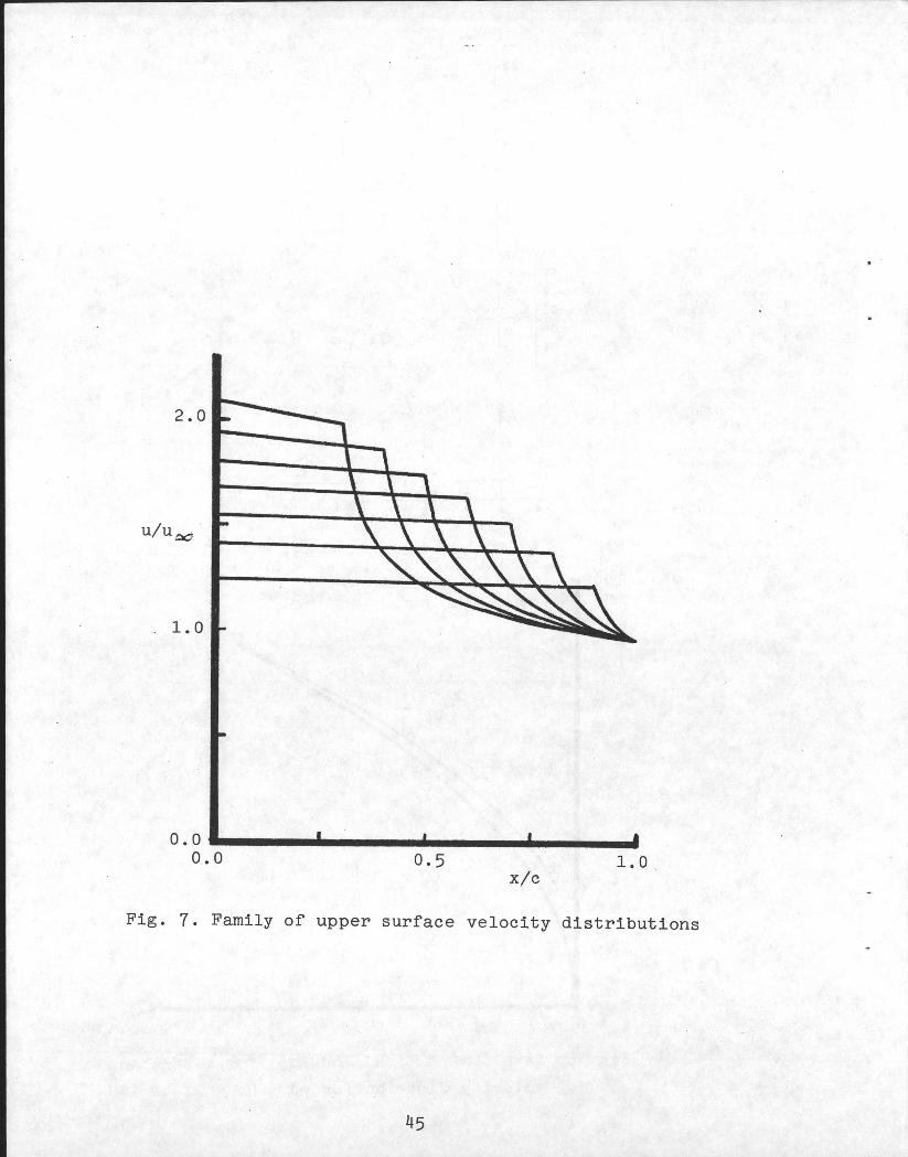
In order to investigate the effect of the recovery

point location, a family of upper surface velocity

distributions was calculated with the recovery point

varying from x/c= 0.30 to x/c= 0.90 (Fig. 7).

On the lower surface, two basic features are generally

desirabIe for the velocity distribution. The velocity

should be minimized to contribute to the section lift

coefficient and to keep the boundary layer thin, thereby

reducing the section drag coefficient as weIl. Unlike

the upper surface, there is no trade-off between lift

and drag on the lower surface, except possibly with

regard to the transition point. In addition, the velocity

should increase as long as possible to delay transition.

The lower surface velocity distribution can also be used

to achieve desired pitching moment characteristics.

However, since the overall velocity distribution must

be achieved by a real shape, the lower surface velocity

distr1bution cannot be specified independently of that

17

on the upper surface. ~or example, on a fifteen percent

thick airfoil, the mea,n of' the upper and lower surface

velocity ratios, u!u_, must in gener al be greater than

1.1 from roughly x/c=O.lO to x/c=O.60. Referring to

figure 7, the design upper surface velocity- ratio in

this region is about 1.2 ~or a recovery point at x/c=O.90.

Thus the lower surface velocity cannot be less than the

freestream valuein this region so the lift coefficient

which can be achieved by a section with this recovery

point location is limited. Therefore different upper

surface velocity distributions can only be properly

compared if their effect on the lower surface velocities

is accounted for.

An initial lower surface velocity distribution which

results in a real shape can be determined by recambering

a thickness form with the desired maximum thickness/chord

ratio to achieve the given upper surface velocity distri­

bution. While the resulting lower surface boundary layer

characteristics are generally unsatisfactory, this lower

surface velocity distribution provides a basis from which

an improved distribution can be found.

In order to investigate the effect of the location of

the recovery point on the section lift coefficient and

lift to drag ratio, NACA thickness forms with (t/c)max=O.15

wereeambered to give the upper surface velocity

18

..

's

dlstributlons s-h.own in figure 7. Whenever possible, a

thicknes-s' t'orin was us-ed which begins press-ure recovery

at the same point as the design velocity distribution.

Therefore the NACA 63-015 th1ckness- form was recambered

to give the design velocity distribution wlth recovery

point at x/c=0.3, the NACA 64-015 form was used for the

distribution with recovery point at x/c=0.4, etc. For

recovery points aft of x/c=0.7, the NACA 67-015 thickness

form was used. The computer programs described in Refs. 13

and 14 were utilized for the analysis and design computa­

tions. To allow for an acceleration region, the velocity

was not specified on the first three percent of th.e chord.

The design program assumes inviscid flow; hence the designed

sections do not achieve the design upper surface velocities

exactly when viscous floweffects are included in the

analysis. Also, due to a shortcoming of the design program,

upper surface transition occurs somewhat prior to the

start of pressure recovery on all of the sections, causing

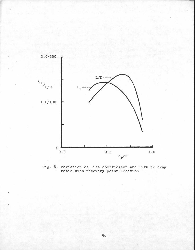
higher drag values than expected. Figure 8 shows the lift

coefficients and lift to drag ratios of the designed

sections as a function of recovery point location.

If a design lift coefficient were specified, the recovery

point location would be chosen to satisfy this requirement.

Note that this design approach is not applicable to an

extremely low design lift coefficient since th1s would

19

require that the pres,sure recovery reglon on the lower

surf'ace als-o De cons-ldered in detail. As the lift

coefficient was not constrained in this study, the

recovery point location which results in the maximum

lift to drag ratio could De chosen. Hence the section

with recovery point at x/c=0.7 was selected for further

study and refinement.

Figures 9 and 10 display this section and the correspond­

ing velocity distribution. The upper surface trailing edge

velocity ratio is considerably lower than the design

value of 0.95. The trailing edge velocity is constrained

by limitations on the physical shape of the trailing edge

region and by viscous effects. In order to achieve the

exact H variation specified, the trailing edge velocity

obtained should be input into the inverse boundary layer

program, resulting in a new velocity distribution, a new

section shape, and a new trailing edge velocity. This

iterative procedure usually converges satisfactorily

af ter one or two iterations if the initially specified

trailing edge velocity is reasonably weIl chosen. In

this case, however, the effect of the low trailing edge

velocity is to cause an increase in the shape factor

near the upper surface trailing edge. Since this should

improve the section stall break, no iteration was performed.

The lower surface velocity distribution has the desired

20

~'

characterist;tcs: unt1.1 roughly- x!c=.O.7 CF;tg. io). Since

the upper surface velocity initia11y recovers more quick1y

than on the NACA 67-015 and the mean velocity is constrained

by the thickness form,there is a corresponding increase

in the lower surface velocity af ter x!c=0.7. This loca1

velocity increase reduces the section lift coefficient

and causes premature boundary 1ayer transition, thereby

increasing the drag coefficient. Referring to figure 9,

the physica1 cause of this velocity increase is apparent:

there is a sma11 protruberance on the lower surface of

the airfoi1 between x/c=0.7 and x/c=0.9. Remova1 of this

protruberance and hence the associated velocity perturbation

shifts the transition point to x/c=0.89 from x/c=0.76,

improving the section lift to drag ratio by about seven

percent. The a1tered thickness form must be slight1y

recambered to restore the upper surface velocity distribution.

At ang1es-of-attack above the design incidence for

this section, a velocity peak resu1ts on the upper surface

near the 1eading edge, causing transition by 1aminar

separation and reattachment. Since a turbulent boundary

1ayer grows more quick1y than a 1aminar one, this ear1y

transition resu1ts in a thicker boundary 1ayer at the

recovery point. The thicker boundary cannot to1erate the

steep gradient at the beginning of the pressure recovery

region 50 the flow separates. In order to improve the

21

off-design performance, the airfoi1 was redesigned to

give a flat velocity distrioution near the 1eading edge

at an ang1e-of-attack rough1y three degrees above the

design va1ue. Thus at the design incidence, the ve10cities

near the 1eading edge are reduced, the flow acce1erating

more gradua11y to its peak ve loci ty (compare Figs. 10

and 12). This reduces the lift to drag ratio somewhat.

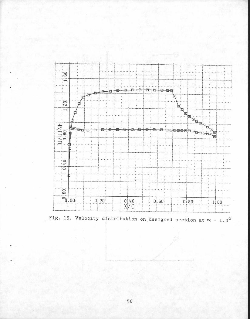
The lower surface was simi1ar1y redesigned near the

1eading edge to remove the velocity peak 2.5 degrees

be10w the design incidence (Fig. 15).

The a1teration of the upper surface ve10cities near

the 1eading edge affects the location of the transition

point. A1so inaccuracies in the design program resu1t in

premature transition. Therefore the fina1 step in the

design process was to modify the velocity distribution

on the upper surface in the vicinity of the transition

point by trial and error unti1 transition occurs at the

desired location. This reduced the section drag by ten

percent. Figures 11 and 12 show the fin al section shape

and the velocity distribution at design incidence.

22

Ol

i.

4' • Resultsand Dis·cus.s.1on

Figure 16 displays the calculated lift, drag, and I

pitchirig moment characteristics of the designed airfoil

at the design. Reynolds number of one million. The computer

program used is applicable to the analysis of fully

attached flow only (Ref. 14). At angles-of-attack above

four degrees, turbulent separation is predicted on the

upper surface while at angles below zero degrees, laminar

separation occurs at the lower surface leading edge

without subsequent reattachment. Since the performance

in these regions could not be calculated, the dotted

lines on the figure roughly indicate the expected trends.

The skin friction drag remains roughly constant

throughout the angle-of-attack range for attached flow,

contributing roughly 2/3 of the drag at the design incidence.

The maximum section lift to drag ratio, which occurs

at a lift coefficient of 1.2, is over 180. This value is

higher than that achieved at a Reynolds number of one

million by sections designed in the earlier empirical

manner and most modern sections as weIl, such as those

designed by Wortmann for a similar performance objective

and similar operating conditions, described in Reference

15. However, the off-design performance is inferior to

23

that of many' sectlons of the same thickness, such as

those of Wortmann. Thes'e resul ts are a reflection of

the design priorities, since the performance objective,

a high lift te drag ratio, was emphasized while minimal

consideration was given to off-design performance. However,

even in light of these priorities, the airfoil's performance

is not entirely as desired.

The problem is that the airfoil begins to stal1 at an

angle-of-attack only 1.5 degrees above the design incidence.

The highe st lift to drag ratio experimentally verified

at a Reynolds number of one million (to the author's

knowledge) is about 220, achieved by the 1iebeck high-lift

airfoil, 11003, shown in figures 4(a) and 5 (Ref. 2). This

value occurs at the maximum lift coefficient, i.e. just

prior to the onset of stall. At the design incidence,

roughly four degrees lower, a lift to drag ratio of 180

is obtained. Therefore, no advance can be claimed until

either a lift to drag ratio greater than 220 is achieved

or a somewhat lower value is obtained with an increased

margin from stall. An example of the latter would be an

airfoil which has a lift to drag ratio of 180 at an

angle-of-attack more than four degrees below the value

at which stall cemmences.

As shown in Figures 4(a) and 13, the shape factor in

the recovery region of the designed airfoil is roughly

24

1.8 at the design incidence whereas on the Liebeck airfoi1

it is about 2.2. Thus it might be expected that the designed

airfoi1 wou1d have an increased margin from sta11. However,

while the Liebeck airfoil can tolerate an increase in

angle-of-attack of four degre e s, the flow separates on

the designed section on1y 1.5 degrees above the design

incidence. Clear1y this separation is not caused simply

by the pressure gradient in the recovery region. Rather

it is caused by a shift in the upper surface transition

point forwards from the recovery point, resulting in a

thicker boundary 1ayer which cannot withstand such steep

pressure recovery. The transition point moves from x/c=O.69

at the design incidence,a=3.5°, to -x/c=o.63 at~=4°, where

a consequent drag rise is seen (Fig. 16), to x/c=O.53

at ct=5°, where separation first occurs.

Figure 17 shows that an increase in the section incidence

above 3.50 resu1ts in an increased negative velocity

gradient in the laminar region of the velocity distribution.

Hence the 1aminar boundary 1ayer thickens more quickly

and is prematurely destabilized, causing transition prior

to the recovery point. At angles-of-attack below 30, the

velocity gradient is reduced so the boundary layer does

not transition prior to the recovery point. Thus a laminar

separation bubble is formed when the laminar boundary

1ayer is exposed to the steep initial pressure gradient

25

in the recovery region. Accurately calculating the

effect of this bubble, which results from laminar

separation and subsequent reattachment, is beyond the

capabilities of the computer program used so the results

shown in Figure 16 include only a rough approximation.

In order to restriet the movement of the transition

point with changes in angle-of-attack, the destabilization

of the laminar boundary layer must be accomplished over

a much shorter region. For example, at its design

incidence, the Liebeck airfoil has a positive velocity

gradient until just short of the recovery point, where

a transition ramp with a negative velocity gradient is

used to provoke transition (Fig. 18). As the angle-of­

attack is increased, the positive velocity gradient is

reduced but not sufficiently to cause transition prior

to the transition ramp. At lower angles-of-attack, the

transition ramp is steep enough to ensure that transition

occurs before the recovery point, thereby avoiding a laminar

separation bubble. Thus the location of the transition

point is confined to the transition ramp for a wide range

of angles-of-attack.

At low Reynolds numbers, such as one- million, the

laminar boundary layer is difficult to destabilize. Hence

a substantial negative velocity gradient is required to

provoke transition within a sufficiently short distance.

26

A 1engthy transition ramp does not fu1fi1 its purpose,

which is to minimize the movement of the transition point

with changes in ang1e-of-attack. However, the negative

velocity gradient needed f or a short ramp cou1d cause the

1aminar boundary 1ayer to separate.

The inverse 1aminar boundary 1ayer equations must be

solved to determine the velocity distribution for the

transition ramp which resu1ts in a given shape factor

variation. Reference 9 gives the fo110wing simp1ified

solution:

u -u ,y:;

(1-H/2.55) C(~) 0.94

c (4.1)

and the subscript ( )0 denotes a va1ue at the start of

the ramp.

Laminar separation is predicted when the shape factor

reaches a va1ue of 3.5. Thus the steepest possible ramp

without separation has a constant shape factor with a

value slightly under 3.5, analogous to a pressure recovery

region which is on the verge of separation throughout.

Substituting a shape factor of 3.5 into equation 4.1 gives:

u = u oo

(U/U~)o (x/c)-0.40 (x/c).-0.40

o

27

(4.2)

A lower value of H must be chosen at the design

incidence so that laminar separation is avoided over a

range of angles-of-attack. A more practical value such

as 3.2 results in:

u uD<; =

(x/c)-O.27 o

(x/c)-O.27 (4.3)

From equation 4.1, the negative velocity gradient for

a given shape factor greater than 2.55 is reduced for a

tiansition ramp which is located towards the aft end of

the airfoil section. Since it is difficult to destabilize

a laminar boundary 1ayer at low Reynolds numbers, the

combination of a low Reynolds number and a late recovery

point therefore causes an excessively long ramp to be

required to provo~e transition if laminar separation is

to be avoided.

Under these circumstances it may be desirabIe to fix

the transition point through the use of a controlled

laminar separation bubble as in Figure 4(b). The transition

ramp required required to cause a small bubble can be

determined by substituting a value of H slightly above

3.5 into equation 4.1. The exact value of H at the design

point again depends on the range of angles-of-attack at

which transition must be provoked. While this approach

leads to minimal movement of the transition point with

28

changes in angle-of-attack, the laminar separation bubble

can be detrimental to performance if it becomes too large.

Also the bubble cannot be allowed to burst at high angles-

of-attack before turbulent separation has begun in the

recovery region.

By restricting the movement of the upper surface

transition point, the performance of the designed airfoil

at angles-of-attack above the design value could be

great l y improved upon, with a small sacrifice in the

performance at the design incidence. At angles below 0°,

the performance could be somewhat ameliorated through an

improved design of the nose region. This .is required to

reduce the velocity spike at the lower surface leading

edge, which causes laminar separation. As a consequence

of the low design Reynolds number, the boundary layer

does not subsequently reattach, resulting in a rapid drag

rise at angles-of-attack below 0°.

The drag coefficient is calculated by the Squire-Young

formula (Ref. 19):

Hte+5 2

Cd = 2(9/c)te(u/u~)te (4.4)

This equation reveals the significance of the boundary

layer development, particularly in the pressure recovery

region, where the boundary layer grows most rapidly.

29

Figure 14 displays the deve10pment of the momentum

thickness on the designed section at the design incidence.

The 1inear rise of the momentum thickness in the recovery

region is characteristic of a velocity distribution with

a constant shape factor in this region. The difference

in the rate of increase of the momentum thickness between

the 1aminar and turbulent portions on both surfaces shows

the importance of de1aying transition. The large increase

in the momentum thickness at the trai1ing edge of the

upper surface, which is associated with a rise in the

shape factor (Fig. 13), is a re sult of the fact that the

trailing edge velocity is lower than the design value.

This has virtually no effect on the drag coefficient

because the lower velocity, which is raised to a power

of roughly 3.5 in the drag expression, compensates for

the increased momentum thickness at the trailing edge .

. For a given shape factor variation in the recovery

region, an increase in the design trailing edge velocity

results in higher velocities on the entire upper surface

and thus an increase in lift coefficient (Ref. 12). In

Reference 16 it is shown that the contribution of the

upper surface to the lift coefficient varies roughly

linearly with the trailing edge velocity for a specified

form of the upper surface velocity distribution. The

upper surface contribution to the drag coefficient also

30

rises with. an increase in the trailing edge velocity as

s'hown by equation 4.4. Therefore there exists a value of

the trailing edge velocity which maximizes the upper

surface contribution to the lift to drag ratio. However,

the increase in the velocities on the upper surface

associated with a rise in the trailing edge velocity

causes a reduction in the lower surface velocities for

a given thickness form, thus improving the section lift

to drag ratio. Hence the optimum value of the trailing

edge velocity can only be determined through a parametric

study in which a family of sections is designed, similar

to that used to find the optimum recovery point location.

The range of possible values is limited, however, especially

since the shape of the upper surface of the airfoil near

the trailing edge is determined by the nature of the

pressure recovery.

The lower surface velocity distribution displays the

desired characteristics at the design incidence (Fig. 12).

The velocity increases until x/c=O.89, where boundary

layer transition occurs. The section lift coefficient

could be improved by decreasing the airfoil thickness

aft of the location of maximum thickness, which is x/c=O.45.

This reduces the velocity on the aft portion of th.e lower

surface , causing earlier transition. At the design Reynolds

number, the resulting increase in drag was found to offset

31

the increase in lift.

Increasing the Reynolds number beyond the design

value of one million has two contradictory effects. The

transition point moves forwards but the skin friction

drag is reduced 50 the lift to drag ratio at the design

1ncidence is slightly increased. At a Reynolds number of

ten million, the lift to drag ratio is 192, although the

upper surface transition point is located at x/c=0.38,

compared to 183 at the design Reynolds number. At lower

Reynolds numbers, the transition point does not move aft

of x/c=0.7, since transition occurs by laminar separation

and reattachment when the laminar boundary layer is

exposed to the adverse pressure gradient at the start of

the recovery region. Therefore the increased rate of

growth of the boundary layer associated with a decrease

in the Reynolds number causes higher drag and eventually

flow separation, which is predicted at a Reynolds number

of 5 X 105 .

An extended transition ramp can be used to reduce the

sensitivity of a section to changes in Reynolds number. Ir transition occurs midway along the ramp at the design

Reynolds number, then the effect of changes in Reynolds

number on the boundary layer development are offset by

the movement of the transition point along the ramp. On

the designed section, the laminar boundary lay€r is

32

destaqilized over a very long region. However, transition

occurs just prior to the pressure recovery region at the

design incidence. Therefore this section is insensitive

to increases in Reynolds number but very sensitive to

decreases.

At the design Reynolds number, a forward shift in the

upper surface transition point results in a thicker boundary

layer at the recovery point and thus flow separation in

the pressure recovery region. Therefore this section

requires a smooth surface and cannot tolerate high free­

stream turbulence levels, reflecting the initial assumptions

of the design study. On general aviation airplanes, the

type of wing construction of ten eliminates the possibility

of extended regions of laminar flow. For such applications

a similar design procedure can be used with a constant

velocity on the upper surface prior to pressure recovery,

assuming that transition occurs near the leading edge

regardless of the velocity gradient. As a consequence of

the resulting increased thickness of the boundary layer

at the recovery point, pressure recovery must be more

gradual to achieve a given shape factor variation. Thus

the performance of a section with a rough surface is

greatly reduced. For the lower surface, an aft portion

of reduced thickness, as discussed previously, is

advantageous since early transition is inevitable.

33

At high design Reynolds numbers, a substantial

positive velocity gradient is required to avoid transition.

Hence, for a given shape factor variation in the recovery

region, the recovery point location which maximizes the

lift to drag ratio moves forward as the Reynolds number

increases. An increase in the design Reynolds number has

a beneficial effect on the boundary layer development

and a detrimental errect on the stability of the laminar

boundary layer. Since the former effect has a greater

influence, the section lift to drag ratio which can be

achieved with given orr-design performance improves with

increasing design Reynolds number.

34

...

5." Conclusîons

The designed airfoil section is a reflection of the

design priorities which were initially established. At

the design Reynolds number, the section achieves a high

lift to drag ratio at the expense of the off-design

performance. The flow separation at the lower surface

leading edge at a relatively high positive lift coefficient

can be attributed to the design emphasis. However, the

separation of the flow on the upper surface is premature

even in light of the design priorities. The value of the

shape factor chosen for the pressure recovery region at

the design incidence was expected to allow a substantial

increase in angle-of-attack without separation. Early

separation is caused by a forward shift in the location

of transition, revealing the need for a short transition

ramp to restrict the movement of the transition point.

The importance of an appropriate recovery point location

in achieving high lift to drag ratios at low Reynolds

numbers is shown by comparing the performance of the

designed section with that of the Liebeck section, LI003.

Since the Liebeck section was designed for high lift, it

has a much earlier recovery point than the designed section

(See Figs. 8 and 18). At their design angles-of-attack,

35

the two sections exhibit approximately the same lift to

drag ratio Brit the designed airfoil has a considerably

lower shape factor in the pressure recovery region. Hence

it displays superior performance at reduced Reynolds

numbers. In addition, if the transition point were

adequately fixed, the designed section would have a

larger margin from stall and a higher maximum lift to

drag ratio, since this is obtained just prior to the

onset of stal 1 if the shape factor in the recovery region

is constant.

The use of the inverse turbulent boundary layer

equations rather than the Stratford distribution has

several advantages, including the ease with which desired

stall characteristics can be achieved. The shape factor

is an ideal link between the desired boundary layer

characteristics and the velocity distribution as it

quantifies the local proximity of both laminar and

turbulent boundary layers to separation. Because of their

simplicity, empirical criteria for boundary layer transition

and separation are weIl suited to the inverse design

approach. A simple transition criterion which accounts

for the effects of surface roughness and free-stream

turbulence would be helpful.

The use of a thickness distribution to determine an

initial lower surface velocity distribution led to a

36

favourahle final distribution. A more sophisticated

approach is required, however, to achieve an optimal

rorm for the lower surface, particularly at low lift

coefficients.

In addition, an analysis technique capable of handling

separated flows is needed to properly assess off-design

performance.

The basic design procedure described can be utilized

for the design of airfoil sections for many different

applications with various performance objectives, operating

conditions, and practical constraints. The inverse design

approach is extremely powerful, leading to high performance

airfoils which are not likely to be obtained by empirical

methods. As it begins with a set of boundary layer

characteristics, the inverse approach allows the design

priorities to be readily incorporated into the design.

The effect of different priorities can thus be easily

studied.

Several guidelines can be established for the design

of airfoils with high lift to drag ratios using an inverse

approach:

1. A constant shape factor variation in the pressure

recovery reg ion leads to high performance but a sudden

stall break. A more gradual stall break can be achieved

by increasing the shape factor towards the trailing edge.

37

2. A high. value of' the shape factor results in a high

lift to drag ratio at the design incidence but limited

performance at increased angles-of-attack and reduced

Reynolds numbers.

3. A short transition ramp leads to good performance

at off-design angles-of-attack while a longer ramp reduces

the sensitivity .of a section to changes in Reynolds number.

4. Optimum values of the recovery point and the trailing

edge velocity depend upon the operating conditions,

particularly the Reynolds number, and must be determined

through a study which accounts for the effect of these

parameters on the velocities on both surfaces.

Using these guidelines, an airfoil can be designed to

produce a high lift to drag ratio while achieving the

required off-design performance for a wide range of

operating conditions and practical constraints.

38

B. References

1. MeMasters, J. H. and Henderson, M. L., "Low-Speed

Single-Element Airfoil Synthesis", Science and

Techno1ogy of Low Speed and Motor1ess Flight, Part I,

NASA CP-2085, Mareh, 1979.

2. Liebeck, R. H., "A Class of Airfoi1s Designed for

High Lift in Incompressible Flow", J. Aircraft, Vol. 10,

No. 10, 1973, pp. 610-617.

3. Eppler, R., "Direkte Berechnung von Tragfluge1profilen

aus der Druckverteilung", Ing. Arch., Vol. 25, No. 1,

1957, pp. 32-57.

4. Cebeci, T., Mosinskis, G. J. and Smith, A. M. 0.,

"Calcu1ation of Separation Points in Incompressible

Turbulent Flows", J. Aircraft, Vol. 9, No. 9, 1972.

5. Stratford, B. S., "The Prediction of Separation of the

Turbulent Boundary Layer", J. of Fluid Mechanics,

Vol. 5, ~959, pp. 1-16.

6. Stratford, B. S., "An Experimenta1 Flow with Zero Skin

Friction Throughout its Region of Pressure Rise", J.

of Fluid Mechanics, Vol. 5, 1959, pp. 17-35.

7. Wortmann, F. X., "A Critical Review of the Physical

Aspects of Airfoil Design at Low Mach Numbers", Proc.

of Symposium on the Technology and Science of Motorless

Flight, M. I. T., Cambridge, Mass., 1972.

39

8. Cebeci, T., Mosinskis, G. J. and Smith, A. M.O.,

"Calculation of Viscous Drag and Turbulent Boundary

Layer Separation on Two-Dimensiona l and Axisymmetric

Bodies in Incompressible Flows", Rept. No. MDCJ0973-01,

Douglas Aircraft Co., Long Beach, California, 1970.

9. Henderson, M. L., "Inverse Boundary Layer Technique

for Airfoil Design", Advanced Technology Airfoil Research,

Vol. I, NASA CP-2045, Part 1, 1978, pp. 383-397.

10. Schlichting, H., Boundary Layer Theory, McGraw-Hill, 1960.

11. Cebeci, T. and Bradshaw, P., Momentum Transfer in

Boundary Layers, Hemisphere, 1977.

12. Liebeck, R. H. and Ormsbee, A. I., "Optimization of

Airfoils for Maximum Lift", J. of Aircraft, Vol. 7,

No. 5, 1970, pp. 409-416.

13. Egglestone, B. and Saville, H. G., "A Method for

Predicting the Aerodynamic Characteristics of Multi­

.Element Airfoi1s with Viscous Attached Flow at Low

Mach Numbers", de Havilland Rept. DHC-PILP 78-3, 1978.

14. Zingg, D. W., Johnston, G. W. and Haasz, A. A.,

"Development of Computer Programs for Analysis and

Design of Two-Dimensional Hydrodynamic Sections",

Interna1 Rept., D. R. E. A., 1981.

15. Wortmann, F. X., "Airfoils with High Lift/Drag Ratio

at a Reynolds Number of about One Million", Proc. of

Symposium on the Technology and Science of Motorless

Flight, M. I. T., Cambridge, Mass., 1972.

40

16. Kennedy, J. L. and Marsden, D. J., "The Deve10pment

of High Lift, Single-Component Airfoi1 Sections",

Feb. 1979.

17. Abbot, I. H. and Von Doenhoff, A. E., Theory of Wing

Sections, Dover, 1959.

18. Wortmann, F. X., "Progress in the Design of Low Drag

Aerofoi1s", Boundary Layer and Flow Control, Vol. 2,

Pergamon, 1961.

19. Squire, H. B. and Young, A. D., "The Ca1cu1ation of

the Profile Drag of Aerofoi1s", A.R.C., R & M 1838,1937.

41

u/u

6

5. , J

2

I

.B·

.9

Fig. 1. Drag on a flat plate with different transition points (Ref. 7)

2.0

c 00 , , 1.0 "-

A Re = 1.5 X 105

B Re = 1.5 X 10 6

C Re = 1.5 X 107

......

O.O .... ____________ -A ______________ __

0.0 0.5 1.0 x/c

Fig. 2. Velocity gradients for transition at x/c = 0.7

42

C-3 6

H

Z 4

SIc x 103

1 Z

3

H

2

1

I I I I Upper Surface @ Q = 2°

I I

:: _-- 8xl04

} I I ... ' I I _ - - 6 Rn : 1 ___ ------- __ 3xl0 6 , ______ I _____ ---------- 20xlO

I tr

xlc

I1 trtr

. 5

Recovery Region •

1.0

Fig. 3. Shape factor variation on the NACA 633-018 (Ref. 1)

~llOOJ

(a)

/ /'

/ /

/

/' Upper

., SIc /

H

/ Surface

.5 1.0 xlc

3 6

H

2 4

1 2

Sic x 103

(b)

FX 74 - Cl6-140

laminar Bubble Predicted

xlc

Fig. 4. Boundary 1ayer characteristics of Liebeck L1003 andWortmann FX 74-CL6-140 airfoi1s (Ref. 1)

43

H

.0

.02

2.2

2.0

1.8

1.6 c,.

IA

1'----

i DESIGN . CTI;EORJ . .

Re-"Zxlcf

I Re.= 1.0 x 10' .04 L2 . 'fr', r.. c,. vs Cl

c..t./IC 0 1.0

- .02 ~ ~-=7=-C--:---.04 .8 . ' . L. C

u_ .. VI CI\

- .06 .-- \.. - .08 - c... vs C:> '"I'

! ,

o+---~---~~~-, __ ~ __ ~~~ .01 .02 .03 .04 .05 .05 .07

-4 -.2 <; 8 12 16 Co

Cl

Fig. 5. Experimenta1 lift, drag, and pitching

1000 moment data for Liebeck L1003 airfoi1 (Ref. 2)

tr

500

o--------~------~--__________ __ o 0.5 x/c 1.0

Fig. 6. Deve10pment of Rg ~nd Rgtr for a constan~

velocity distribution with Re = 2.0 X 10

44

2.0

. 1.0

o.o .......... ________________ .. ______ ~ 0.0 0.5 1.0

x/c

Fig. 7. Fami1y of upper surface velocity distributions

45

2.0/200 .

1.0/100

o 0.0

c1----

0.5 1.0

Fig. 8. Variation of lift coefficient and lift to drag ratio with recovery point location

46

!. . 0 .. : . . .. ! .... : ... "i .. .... .. ~ ... ..... ! .. . .... . . ! .. .. ..... : ..... . . . . ! . . . ...... ! ..•...• .. ! .. . .. ... . , . ...... .

i ....• ~ . ---:-~:-+--- ~----t - -'-+ - -t ---- - t - -T--:I~ - ---I - ~-·- , . ' : ~ : 1 : i

: . : ~ - _ •• 2 •••••••••.• .:. •........•. : ..•.•.••••• _ •.• _ •• _.: ..•••..•... _ •••••••.••• :.. . . ..•..... ~ .•..••.•.• . : . • ·_.·· •••• f,,: ... . . .. . . . ; .... . . _ .. . j .. _ ....... _ •........ .. ·······,······· .. _··_··-T-·· ... . . ! ~ i : : i _ooi, ·• • · •• · . 1·· ... . ·. ·,· ·· · · · · .· 1·· . j • •• :- ·UO .. : .. .. ,... ..... '::. i ..

i.. . ~.~ ..... ....... ....... .., ......... _ .......... L .... .. ... ~ ..

i;~ ~+~f:-:l+f-l-T+ -+::-~J~-Hifi~ I-F r······ ~ ~o ~ oo : I : 0~20 : I : O ~ llO : i ~ 0 ~ 60: I : 0 ~ 80~ i ~ 1~00 : L.: ... I~: . ! ..... . i ~. '1' ~~~~~I .. ·.: .. I.~ ·1 ~_:l~_X..I~.~L· .. · .. :.L .... · .. :.L .. : .. l· .. : .. · .. j.:.~~:J.·~~.:.L_:.:.L_:.: .L.~:.J: .. :.: .. :.L~.: .. J: .. :.: .. I.:_:.

Fig. 9. NACA 67-015 thickness form cambered to give design upper surface velocity distribution with x je = 0.7

r

1·······_·: ········· '--',-. -1---''':-'''-'' f"' ...... ~ ..... . .

j . ... : g .. ·· ·;····1· · '.j ' '.'! .... ! .... ~ .... ; .... ~ .. .. ~ ... ·1· ···:··· ·l····j·· ·· 1· ·· ·:··· · i· ·· · ~ ····i ···· j'" ., .. .. : .. .. t······_·:-······ i _

. . . j .... ~ .... !

........ _ .. __ ._ .... -

j .... :g. ·· · :··· · l··· · ·· ··· : · ··· ~ · · · · · · · · ·: ··· · l· · ·· ~ · ··· l····~····i""··· i ···· o ·· · ·j···· l · ··· :· · · · ~ ··· · :···· ~ · ·· ·:··· ·

·l:~::::=r~~~~~;-T--~ - • ·_-i::-I~i:~:ITEt~I~_~T:--~- _Er~~~~: : .. . . . ! .. .. : ... ! .... : .. , ... L ... : ... . :. . .. . · 0· ·· ·· ···· 0· ·· ·· ·· · · 0·· · ······ 0···· · . · · 0 . . ·.···.·

....... _.~._ ; :: i :: l I : l .......... ~ .......... . °OlOO: : 0~20 : Oi llO : : 0~60 : . : 0;80: . : l~OO :

! . ... . . . . .. , .i, .. • . . . .. . . ! ... .... , . • . . ·· X!",·. /C ·:. · ··' !",·.·· . .....•......... •. . ... .. ..• . .. ... ... , . .. . ..... , . . ... .. . . : : :. t.. ~..:::. i : . . : ........................ : .. .. ....... .:_ ........ 1 ........................ : ........... : .... ....... : .......... _ ........... L ........................ : ........... .: ........... t .......... _ .. _ ...... : ........................ : .................. ....... : ........... _ .......... : ..... .......... _ ... _ ..

Fig. 10. Velocity distribution on section shown above at ~= 3°

.. :.: .. :.~.:.:.~.: .. ~_~ .. :~.:.: .. :.·.L.:.:~.: .. · .. ~L~~~1 .. :~.:.~.:.: .. ~:.r··:·'· ···~·:·: .. ·.:·r .. :.: .. :.~.:.: .. :.J.· .. · ...... ~.·.: .. :.: .. l· .... · .. :.~:~ .. :~.I.: .. : ... ::.:~ ..... l. ........ ~._ .. .

.. . . : .... ~ ... . : .... ! .. . . : .... i ........ : ! ··.I. ... : ... t.--:· ... I.. ... ~ .... L ... ~.·.i .. ·-: .. .

. i . i . . ........ j ... ........ : .....•.•..• j ........... : ........... i ........... : ....... .

. . • i .. ·:~~~: ~:·· ·~·~--~··· ~i . --·~l·~ · ~r .... · .... i . . . · .... · .... ! .. .L.B.~.· 1 ~.o .! 1····: ··· · .... : .... ; .... : .... i .. .. : . . .. i .... : .. . . i ... . : .... ; .... : .... ; .... : .... ; . .. . : ... . ; . ... : .. .. ; . . . . : .... ; . ... : ...

.. ::.: . I . I : I : I : I : I : I ; I :

Fii·;·:o=r~:i 2:--T~;=~·T·~;·~~~---r--~ ~r:-·r· ·· l : ~~·~~ i··· · ~ .. .. i' .. . ~ .... j ... . ; .... j ... . ~ .... i···· ~ .. XV C ~ ·· . 'I'" . ~ ... . ~ .... ~ .... i' " . ~ .... i'" . ~ .... f···· ~ ... 'I' ... ~' . ' .

1 .. _ ..... : ........... !. .......... .:.. ... _L... ___ .:.._._ .. L ... _ . .:.. ___ L_~_ .. _i_ .... .... .:. ........... i. .•........ .: ........... L .......... .:. ........ _ .. L ......... .:._ ......... L .......... .:._ .. _.i ........... .:. ........... !. .......... : _ ...... .

Fig. 11. Designed airfoi1 section

.. : ........... :-........... ········· __ ······_·l·_·_·· ... ·· .. ······T·····_···:-····_-;---. - ··--i···········:-···········r···· .... _ ....................... _ ....................... _ ... ······f··········_···········:···········;·

I" ' .~ g . ·······T··· , .......... . : ... i .... : .... ! .. .. ;.- .. ; .. ..; .... i ... .; .... i .... · .. ··i· ... : .... ;. " ........ ~.:;::: . . ... .... ......... , ............ .. .. .... , ...... \ .......... _.. ..L······:···· .. ·····!· .. · .. ··: .. ·· .. · .. ·!······ .... :·· .. · .. ···r···· .. .. :······ .. ··T"···· .. ·~ ··· ·· .... ·i····· .. ·:· .. ····r ······ ... : ......... : i····· .. ·,·, .; ... ·· ! .. ·· · · .. ·!· .. ·· .. ·j" .. ····T· .. ·· ·· . . . . .. : ...... _ ... _ .. _.-1. ___ ... __ : ........ _._ ........... 1. .......... _ ..•...•.... : ........... _ ........... : ................... .. ;, ........... -............ ~::: .. · .......... 7.· .•• _._ •.• :,:" . . .......... .:. ..••. . .••.. . ; ........... _ ............... _ ... ···.··--T·----··-·..: .; " . ~" : j .

~ : : : : • • • • • • .! • • • • •• • • • • .~, • • • • ': • • • • '!, • • • • '. • • • • .!.'. • • I • •• •• . • . • • • . l ........ . ~, .......... I . • .. . • . !" .. • ...... ! .... : . ... ~ . . ... : ... .

j .. ~ ~ i : . . ~ ........... :.~. .. .. ··_···· ...... ·I .... · .. ·· .. .:. .. ···· .. ··~· .... · .. · .. _ .. · .. -··_~· .. ·_·_· .... -r .. _ .. ·· .. .:.· .. ··· .. · .. :·· ........ : .. _ ....... : ........................ (........... . ..... l·· .. · .. ·· .. .. · .... ··· .. ·1 .... ·· .. · .. :·· .... · .. ·"i'··· .. ·· .. · .. ···· ..... .

. : . ~ : : ;: 1 : l : 1 . : . : : 1 : ~ .

, u....;

j·~6 · L .. ~.~. j '-.:o

'" .:::J . . . ... i .. ; . . . . i,.:: . . . . . 1 . l ' . ~ . : . I . ............. _........... . ... : ........... ~ .... __ ... _ .. _ ..... ~, ........... _: ' ___ '-:',' _' ... ; : . . : '. l· . .' '. . · .. ·:·· .. ·· .. · .. :-·· .... ·····:····· .... ··:-.. · .. · .. · .. 1 .. ····· .. ··:-...... ·· .. ·r .... · .. · .. :- ·· .. ····· .. !· .. • · .. • .. ·:· .. • . .... ! . .. ... ..... : .. ........ : ........... :-......... .

. . . . i .... ~ . ..• i ..•. : . . •. i .... : .... i ... . : •... i .... : .... i .. .. : ... . i . . • . : ... .

. : . : .... . . , ......... , . . : : : • ; . ~ . . . 1 . : :.

........ : ........... , ........... : .......... ' ........... : ........... , ... _ .. - ... ··;···········:··········1··········:···········\···········:········· .. !······················1··········: ···········r·········:···········!·····················

. : .... ; . . : .... ~ ... . :- . . ! . . . : ... . : .... i ... .. ... . ! .... : .... ! •... : ... . ! ....... . T ... : .... :- ....... . ! . . . . . . . . .

.. : ....... ......... . ..... ...... L ..........•...•. .• i.. . .:.1.. ....... .. : .... ...... : ......... .. : .. ....... , .......... : ....... .... , .... ..... ; ......... , ....................... L. .............................. : ........ .

.. • . . . •..• !".... .j. : . . • • : .••• !:.· ..•. .•. · .... ~" .... : .... 1 .... : •...• , ..•..... • i . . .. . .... l .... : ... . !'''': o ' ..... .. · ·i· : . : : 0 ! ! .

i i. i . i i· .. " .: ...... ...... q ; 20 . ... i .. . ~}C : ··· . i .. ··:·· q r.6.0 : .. .. ! . . . : . . 9Lsq: ... '/"' .. :.' n.o.o;.- ..

. : ! : . .. .

. : .. ... .. .... _. ....... -:-=t ; 00:

i . ........ ! ....... .

. L .. .. ...... : ....... .... L .......... : ........... ! ... ....... ~ ........... L .............................. __ ................ : ........... : ........... : ........... 1. ....................... : ........... _ ........... L .......... _ ........... L ........ .. _ ..... ...... E ........... : .

Fig. 12. Velocity distribution on designed section at design incidence, 0(. = 3.50

48

: (1')

! · ···: o · :0

f-._._ .. _ ... .. -:. N , .

~ . ... : ... .

Fig. 13. Shape factor variation on designed section at design incidence

0 "-' ••••••• • • • •. I .: ~ . , r···_····~·o·

. ' . ': ~ . . . . . . • .. .. ••• ...•. I •.•••••• • I ....•

~~ :"';,;;::."-" : I :

: cj .... : --,::1' L .. x:,~.

. :. . ........ . , ....... . . , .. . .. . .. 1 · ··. l . 1

: '--: 0 .. , ........... .

~ ~ ._.T.---+---+ ---; - --, ----•

l .. ~ ~ . . ... ; .... ~ .. .. : .. .. ~ .. .. ; .... ~ . .. .. . .... '. _:~,; .· ... · .. · ... ·.·.: .. ,·.,·._· .. · ... ':i .. · . .. · . . · ... ·. _~ . . · .. · ... · .,·,.' .. ,~,: . . ' . . · . . . · .. · .. l.·",·.,·,',· .... , .... ! ........ ,., ... ,!, ..... , .......... :::,' ........ ----- , ------·r: r ......... -..... .. ... ; .......... ; ......... : .......... : ........... : ..... _.+ ..... - .. - - ",'

.,:".~, ........ _~: =. .;:: ...... :.,.J ..... : .. : .. ~ .... :.~ .'. ' ... : ...... ~ .. . . : . . . . . . , ... . ! . , .. i ' . , . : .... ! ' . .. : .. . ·l·· ': ............ î.. ... ,'" ....... :._: •. •• • •••.. ,' •• . :.--T· .. i' ...... : .. · .. ,· ........ : .......... I .......... ·: .... · ...... I ...... · .. : .. t·~· .... ,

;· .. ·: 6 .... : .... I .. .. : .. .. ! .. ·~·i .. . . .; , ·l .. ~~~lowèr : 0 : t :d surf'ace

.......... :.00 : 00 : : : 0' 20: 0: !t0 : ~ 0160: ol 80 ~ 1 I'ö'ü: ! . ... : .... i. . . . : .... i . .. . : .... i .... · . ~,.. . X'/C' .. . , .. .. ..... , ....... . i····:· ·· . j .. . ...... i •... : . .

: ~ 1 ~ :' . ,:.~: .':;. :.: . . :", . . . . . t .......... : ........... L .......... : ........... L ......... : ........... L .......... _ ...... __ , .. ~ ... ....... : .. ... ;.. .......... _ ........... : ........... .: ........... : ......................... : ................... ... ... :. .......... : ........... : ... .................... : ........... .

Fig. 14. Momentum thickness on designed section at design incidence

49

.. .... ..... ': .•. : ..... : ................ ~ ........... j ........... ~ ........ -~ ....... __ .· .. · .. · .. :· .. ·_··~~~··.r .. ·:·· .. ··~······: · ·.·O · ·. ·.·· ··:·~·:·· .. ·.··.T .. ·.-.... ·~·:· · .. ·:·· .. r .. ·:·· .. ·:·~·:·· .. ·:··.·;··.': ·.·:·~·.·· .. ·:··.··o·· .. ·.· ·.· -~· ·····: ·· .. ~·· .. ····.··.···:·· .. ·.·· .. ·1

' 0 ·· ·l··· ·: ····:··· ! 1 1 1. 1 j ,

,·· · · · ··· · ·f·~· ·· ·· ····~·· .. ·····j········ .. ~··········r····-~ .. _·· .... ·· ...... ~~ ........ ; .......... -........... ! .......... ~ ....... ··T··········-·········i .......... ~ ........... ! ...................... .' ....................... , ........... : .......... ~

;~---~-----: •••• : ••• ~~=:-~~i---:-}-:-::-::_:I~-: -[~::;::~: ~-.. .. . i ~ . ~ i l 1 1 l ~ j ~ ~ ........... ~.:;:::. . ........ ······ .... i·· .. ····· .. ~··· ······1---.. ··~--+··_:._-·+········ .. : ......... -+ .......... : .... ······,···········:···········i··········· .... -+ ...................... j ..... .. ................ l ...................... . i .. j • • • • •• ••• j • • . •• . • •• , • •• • . • .••• ;': •••••••.. . ; . •• ••• ••• i ....•.... i ......... 1 • • •• • • • i". : . . . . . . . . . l: j': ~

t····CL····· .. ···· ... ······-······ .. ·· ·~········· · ·- · .. ····· ·4········---···· .... ~ ........ --.-...... j .......... : .......... ! ........... -......... + ......... -........... ! ........... -........... ~ ................. .

~ ..... ·3 .. ~. · '0 ;. ::J

, . ~ ........... _ .......... .

j ••

' 0 : ;:1'

~ ........... _ ...... . : 0

. ....... ~ .......... + ......... -.......... ~.-.... -.. _ .... -... , ...... -.----.... ~··········-··········r·········· · ··· ··· ····1·· · ···· ·· ··: ·· ········ · 1· ··· ··· · ·· ·:· · .. ··· · · · · ~ ··· ········7·· ··· · ····~····· · ·····-··· · ·······l·· · ........ -.... .

o . .. . ! . .. ...... ! . .. - . ~ .. ······i ·········i ......... ! ..

...................... : .................... _.-: ........... -·_····~···········_··_· · ···i·· ........ _ ........... : ..... ... _._ ........... ~ .. ........ ·_ · ·_·······~··········· _· · ·········i·· · ········_····· ...... ;

··i· · ·· ·· ... j. · ·· · l ··· ···· ··j·· . ... . .. ! . . .

...••..• _ ...•..•.••. ~ .•••.•... _ •.•••. .... : ........ _._ .... . _.~ ..•...•..• _ ....................... _." ....... j .. ......... _ ........... j ........... _ .. ......... j ........... _ ........... : ........... _ ........... ~ ........ ... _-_ ....... ~ .......... _ .......... .

. j · i .... .. , . .. ···· ··i.·· ···· · ·,·· ···I . ·· .. . · ·· j· · . . . ! . . . . . . . . . ~ . . . , .

.......... _ ...................... _ ....... " .. : ... ··· .. ··_· ...... ·· .. :· .. · .. • .. ··_ .. _·_· .. j_· .. ·_ .. __ ·····_·i ...... ·· .. ·_ ....... . .......... ~ ........... _ ........... : ........... _ ........... : ........... _ .. ·· .. ·· .. ·l .. · .. · .... ·_· .. · .. · .... :·· .. · .... ··_·· .. ···· .. ·

· 0 : 0

. ~ . , .

. . ! . . . . . .. . ~

., ........... -...... -+----.:...-.;.-.....:.-.--+---'-..----..:-+-~-'----+---+---+--_+---f ........... -.......... . ai ilO : Ol60: ·· ·XilC:·· ··o

• •• • ••••• ! . 0; 20 : . I • . .•.. .. . ! . . Oi 80 :

·t·········,· ·····1 ·

,:._ .... .... _ .......... :_ ......... _ ........... :.. .......... _ ......... ............. _ .. _ ......... . . .. _ ...................... _ ....................... _ ................... .... _ ......... J .. " ....... _ .. ......... l ........... _ ..... .... _ ......... _ .......... .

Fig. 15. Velocity distribution on designed section at ~ = 1.00

50

0"': Design point

1.5 1.5 1.5

Cl / ....•. Cl .f····· Cl

1.0 1.0 1.5

•• •••• ... I I •• •• •• --. •• .

\.T1 0.5" 0.51- 0.5 ~

0.0 • , . 0.0 0.0 0.0 5.00 10.00 0.0 0.005 0.010 0.015 0.0 -0.2

oe: Cd Cm

Fig. 16. Ca1cu1ated lift, drag, and pitching moment characteristics of the deslgned airfol1 at Re = 106

·0

r·:J;-~·J~~T"~L:):-I~=8JITI:i:.I.""· .••. -.••. :.i ... · .••.••. ~:· . • ·.-.·.~.· •. :i .. :: .. ~. ~· .• ·-.. -.·:.~.·.···.-:.-.:· _".·.··~. · :.·:.J.l.-·.-:.·~.~ •.•.. : ...... ~."" .. ~ .... : ..... ... : .... l' · .. :·· ·· ~"":'" '1' " :' .:. :. :::::' ;'. .: l . ! . 1 . I . ~

! . . . . : ....

t}· I~i=Id~~ •• i-:FJ-I::~±lT:f+Jtq~l;fIJ ~--~. --.:-~-I~::~I:-J::t=1J:I::i~:.l~.:T~~:~g-:. -4I:.Ii::ç, .:_ ... _._.l.~ : . ~; '~i I i' i . I : I . I .......... ~ ....... _.: j :9roo: : Oi 20 : : Oi llO: : 01 60 : : olaD: : L OD: L.·.~~.l.:_·.~ . ..J.·_~·~~.·.: .. : .. J: .. : .... :.L· ..... .J..· ....... :L.: .. : .. J.~_i_·_~.r~ .. ~L.:.: .. :L .. ·.: .... L .. ~.J. ... · .. :.:.:.· .. :. ·..1..· .. : ...... :.:.· .. ·.: .. : .... .. : ... 1 ........ :.L ... : .. :.~.:.· .. : .. :.L: ... ~.~.:~:.~~ Fig. 17. Velocity dist r ibution on designed section at ~ = 40

-3 Rn • 1 x 106

C; • 1.8

Cp -2

-1

o+-------------~--~~~--~

___ .-:.:-_--;---r . 0 xtc

+1

Fig. 18. Velocity distribution on Liebeck L1003 airfoi1 at design incidence (Ref. 2)

52

· Appendix A. Thwaites' Method for the Laminar Boundary

. Layer Gal c ulati on

The computer program which determines the velocity

gradient required for a given transition point (Appendix C)

utilizes Thwaites' integral method to perform the laminar

boundary layer calculation.

The momentum thickness is calculated from the following

equation:

2 (~) Re c

This allows the determination of the parameter A :

g du

From known solutions of the boundary 1ayer equations,

(A.1)

(A.2)

Thwaites found the following reasonab1y valid universal

functions l(À) and H(À):

2

1 1 = 0.22 + 1.57À - 1.SA

3.75-\ + 5.24A2 O!: À~ 0.1

H = 2.61 -

O.OlSÀ (A. 3)

1 = 0.22 + 1.402À + O.107+,À

0.0731 + 2 088 -0.1~).~0

H = 0.14+,\ .

53

The shape factor is given by the function H(A). The skin

friction coefficient is found from:

(A.4)

54

Appendix B. Inverse Turbulent Boundary Layer Program

C INVERSE TURaULENT 8JUNCARY LAYER PRUGRAM C. C. CALCuLATCS VELOCITY ~ISTRI D UTION CORRESPONDING Ta A GIVE~ C SHAPE FACT:JR VAr.:IATICJ'-' AFTER TRAN3ITION

1 IMPLICIT REAL:!r8 (A-H.O-Z) 2 :,HI-1cNSION C(24),W(Z,C;),Y(2),YP(2) 3 EX H:.RNAL FCN 4 COMMON "i(JOO),DHDX(lOO),RE.I 5 IT=1 6 N\'.=2 7 TjL~.OOI 8 ITMAX=20 9 TOl2~.OOOl

C. READ I N NUlv\ijER CF PCINTS. L:JCATIUN Of TRANSITION, I:'IIITIA_ GUESS C. AT ~TA~TING VELOCITY. AND TRAILING EDGE VELOCITY

10 RE:AD(5.100) NT.XR.URI,UTE 11 100 F~RMAT(14,3F8.0)

C. RCAD IN CHCKD PEYNOLiJS I\O~LlER 12 P CAu(5,110) RE 13 110 FUK,.l ATCFB.O)

C ~EAD l~ H VHRIATION (AND DH/DS) 14 REAi)(5.120)CHCI),I=I,NT) 15 PCA l> (!:>,120)CDHOXCI),I=I.NT) 16 120 F 0 R:-lA T ( 1 OF a. 0) 17 ~RITE(6,230) RE 18 230 FORMAT(OI5.3)

C CA:.... CU LAT E r< T ii ETA F 0 R TRA hl SI TI 0 NAT X R 19 1 HXl= RE*URI*XP 20 RTH! =1.174*( 1. +22400 ./RX I) *RXI**0.46 2 1 H R IJ E C (). 2 4 0) R Xl, f.! T H I 22 240 FUR~AT(2DlS.6)

L CA~CULATE INITIAL THETA 23 THI=RTHI/~C/URI 24 YCl)=URI 25 X= XR 26 V(2)=THI 27 .... r:l I lt:::( 6,200)X,URI .TH I,HC 1) ,DHDX Cl) 28 200 FJR~ATC5FI0.5)

C INTEGRATE USING A RUNGE KUTTA-METHOD 29 :) 0 2 I =1 , NT 30 XEND=X+.0125 31 IND=l 32 CALL DVEr<KC2,FCN,X,Y,XEND.TOL,IND,C.NW,~.IER) 33 X=XCND 34 IFClNO.LT.O.O~.IER.GT.O) GO TO 3 35 -'.;.(ITlC6.2JO) X.YCl).V(2),H(2).DHDX(I) 3ó 2 CONTINUE

C AOJUST INITIAL VELOCITY AND ITERATE UNTIL DESIRED TRAILI'-'G C EDGE VFLUCITY IS ACHIEVEO

37 IF(DABSCY(1)-JTE).LT.TOL2} STOP 38 LJt<I=URI+UTE-Y( 1) 39 lT=I1+1 40 IFCIT.GT.IP,.,AX) GiJ TO 4

55

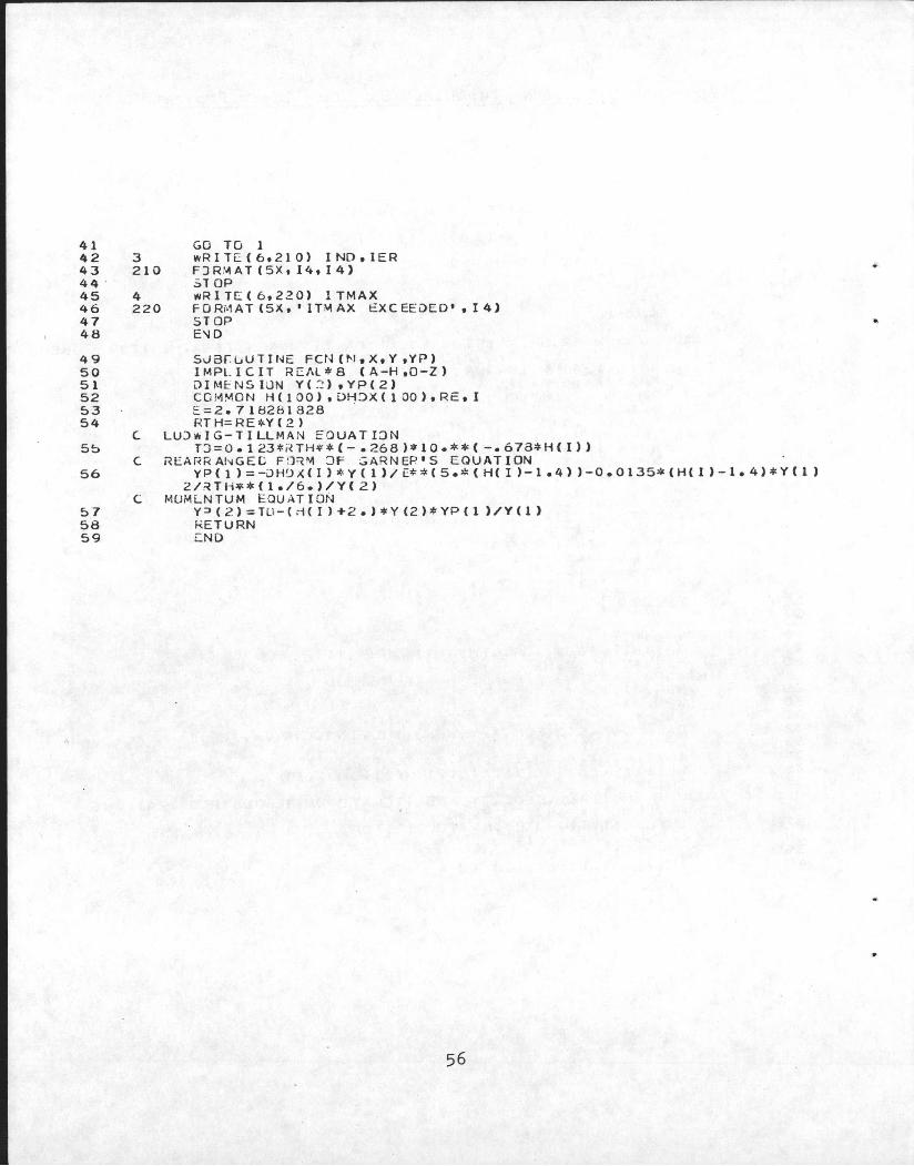
3 210

GO TG 1 w RIT E ( b. 2 1 0 ) I ND • IER FJRMATC5X,I4.14} ST OP l'IRITCC6.220) lTMAX

41 42 43 44 ' 45 46 47 48

4 220 F 0 Ri·1AT (5X. • ITt.1 AX EXC EEL>EO' • 14)

STOP E\I 0

49 S0aruUTINE FCNCN.X.Y.YP) 50 lMPLICIT RC/ll*B (A-H.O-Z) 51 DIME:'NSlûN Y(:-~).Y?(2) 52 COMMON H(100).DH~X(lOO).RE.I 53 E=2.71H281B28 · 54 RT H= RE * Y ( 2 )

L LUJ~IG-TILLMAN EQUATI3N 5~ TJ=O.123*~TH.*'-.268)*10.**(-.67B*H(I»

C REARRANGEC FD~M ~F GARNEP'S EQUATION 56 Y P ( 1 ) = -L) H ~ X ( I ) *' Y ( 1 ) / E* * ( 5. >I: ( H ( I ) - 1 • 4 ) ) - 0 • 0 1 35* ( H Cl) - 1 • 4} * Y ( 1 )

2/~TH**(1./6.)/Y(2) C MUMLNTUM EaUATIO~

57 Y=>(2)=TU-(rlCI)+2.>*Y(2)*YPCl )/Y(l) 58 RETURN 59 CND

56

.,

. Appendix D .COOrdinates Of Designed Airf'oil

x/c y/cupper y/clower

• 1. 000 0.00000 0.00000

0.975 0.00959 -0.00030

0.950 0.01872 -0.00059

0.925 0.02737 -0.00089

0.900 0.03603 -0.00119

0.875 0.04485 -0.00148

0.850 0.05395 -0.00178

0.825 0.06337 -0.00207

0.800 0.07313 -0.00237

0.775 0.08319 -0.00267

0.750 0.09349 -0.00296

0.725 0.10360 -0.00326

0.700 0.11470 -0.00356

0.675 0.12080 -0.00385

0.650 0.12710 -0.00415

0.600 0.13496 -0.00474

0.550 0.14010 -0.00533

0.500 0.14287 -0.00593

0.450 0.14348 -0.00652

0.400 0.14206 -0.00700

58

x/c Y/Cupper y/clower

0.350 0.13863 -0.00740

0.300 0.13310 -0.00770

0.250 0.12525 -0.00800 •

0.200 0.11500 -0.00830

0.150 0.10140 -0.00860

0.100 0.08400 -0.00890

0.075 0.07100 -0.00900

0.050 0.05700 -0.00907

0.025 0.03800 -0.00798

0.0125 0.02700 -0.00633

0.0075 0.01800 -0.00500

0.005 0.01300 -0.00400

0.000 0.00000 0.00000

59

..

UTIAS Technical Note No. 245

Institute for Aerospace Studies, University of Toronto (UTlAS) 4925 Dufferin Street, Downsview, Ontario, Canada, M3H 5T6

AN APPROACH TO THE DESIGN OF AIRFOILS WITH HIGH LIFT TOORAG RATIOS

Zingg, David Walter

1. Subsonic airfoil design

1. Zingg, David Walter

2. Two-dimensional inverse/design

II. UTIAS Teehnical Note No. 245

~ 3. Panel methods

A procedure for the design of low-speed, single-element airfoils with high lift to drag ratios is presented. The procedure us es an inverse approach which proceeds from a set of desirabie boundary layer characteristics, which are determined from the performance objectives, to a velocity distribution and, finally, to an airfoil shape . The boundary layer shape factor, which is a measure of the neamess of the boundary layer to separation, is used to define the boundary layer eharacteristics in the upper surface pressure recovery region. The turbulent boundary layer equations are solved in inverted form to calculate the velocity distribution which corresponds to a shape factor variation . The veloeities on the upper surface prior 'to pressure recovery are chosen to cause boundary layer transit ion at a desired location. The lower surface velocity distribution is selected to satisfy the requirement that a closed, non-reentrant shape which meets the specified structural requirements resul ts . The design procedure described can be utilized for the design of high performance airfoils for a variety of performance objectives. operating conditions, and practical constraints.

Using this procedure, an airfoil has been designed which achieves a lift to drag ratio of 180 at a lift coefficient of 1.2 and a Reynolds number of one million. Through this design study, a set of guidelines for the design of airfoils with high lift to drag ratios is established.

Available copies of this report are limited. Return this card to UTIAS, if you require a copy.

UTIAS Technical Note No. 245

Institute for Aerospace Studies, University of Toronto (UTlAS) 4925 Dufferin Street, Downsview, Ontario, Canada, M3H 5T6

AN APPROACH TO THE DESIGN OF AIRFOILS WITH HIGH LIFT TOORAG RATIOS

Zingg, David Wal ter

1. Subsonic airfoil design 2. Two-dimensional inverse/design

I. Zingg, David Walter II. UTIAS Technical Note No. 245

~ 3. Panel methods

A procedure for the design of low-speed, single-element airfoils with high lift to drag ratios is presented. The procedure uses an inverse approach which proceeds from a set of desirable boundary layer characteristics, which are determined from the performance objectives, to a velocity distribution and, finally, to an airfoil shape. The boundary layer shape factor, which is a measure of the neamess of the boundary layer to separation, is used to define the boundary layer characteristics in the upper surface pressure recovery region. The turbulent boundary layer equations are solved in inverted f arm to calculate the velocity distribution which corresponds to a shape factor variation. The ve loeit i es on the upper surface prior to pressure recovery are chosen to cause boundary layer trans i tion at 8

desired location. The lower surface velocity distribution is selected to satisfy the requirement that a closed, non-reentrant shape which meets the specified structural requirements resul ts . The design procedure described can be utilized for the design of high performance airfoils for a variety of performance objectives. operating conditions, and practical constraints .

Using this procedure, an airfoil has been designed which achieves a lift to drag ratio of 180 at a lift coefficient of 1. 2 and a Reynolds number of one million. Through this design study, a set of guidelines for the design of airfoils with high lift to drag ratios is established.

Available copies of this report are limited: Return this card to UTIAS, if you require a copy.

UTIAS Technical Note No. 245

Institute for Aerospace Studies, University of Toronto (UTlAS) 4925 Dufferin Street, Downsview, Ontario, Canada, M3H 5T6

AN APPROACH 1'0 THE DESIGN OF AIRFOILS WITH HIGH LIFT TO DRAG RATlOS

Zingg, David walter

1. Subsonic airfoil design 2. Two-dimensional inverse/design

I . Zingg. David Walter Ir. UTIAS Technical Note No. 245

~ 3 . Panel methOds

A procedure for the design of low-speed, single-element airfoils with high lift to drng ratios is presented . The procedure uses an inverse approach which proceeds from a set of desirabic boundary layer characteristics, which are determined from the performance objectives, to a velocity distribution and, finally, to an airfoil shape. The boundary layer shape factor, which is a measure of the neamess of the boundary layer to separation, is used to define the boundary layer characteristics in the upper surface pressure recovery region. The turbulent boundary layer equations are solved in inverted form to calculate the velocity distribution which corresponds to a shape factor variation. The veloeities on the upper surface prior 'to pressure recovery are chosen to cause boundary layer transition at a desired location. The lower surface velocity distribution is selected to satisfy the requirement that a closed, non-reentrant shape which meets the specified structural requirements resul ts. The design procedure described can be utilized for the design of high performance airfoils for a variety of performance objectives. operating conditions, and practical constraints .

Using this procedure, an airfoil has been designed which achieves a lift to drag ratio of 180 at a lift coefficient of 1.2 and a Reynolds number of one million . Through this design study, a set of guidelines for the design of airfoils with high lift to drag ratios is established.

Available copies of th is report are limited. Return this card to UTIAS, if you require a copy.

UTIAS Technical Note No. 245

Institute for Aerospace Studies, University of Toronto (UTlAS) 4925 Dufferin Street, Downsview, Ontario, Canada, M3H 5T6

AN APPROACH TO THE DESIGN OF AIRFOILS WITH HIGH LIFT TO DRAG RATlOS

Zingg, David Walter

1. Subsonic airfoil design

I. Zingg, David Wnlter

2. Two-dimensional inverse/design

I I. UTIAS Technical Note No. 245

~ 3. Panel methods

A procedure for the design of low-speed, single-element airfoils with high lift to drag ratios is presented. The procedure uses an inverse approach which proceeds from a set of desirable boundary layer characteristics, which are determined from the performance objectives, to a velocity distribution and, finally, to an airfoil shape. The boundary layer shape factor, which is a measure of the neamess of the boundary layer to separation, is used to define the boundary layer characteristics in the upper surface pressure recovery reg ion . The turbulent boundary layer equations are sol ved in inverted form to calculate the velocity distribution which corresponds to a shape factor variation. The veloeities on the upper surface prior 'to pressure recovery are chosen to cause boundary layer transition at a desired location . The lower surface velocity distribution is selected to satisfy the requi rement that a closed, non-reentrant shape which meets the specified structural requirements results. The design procedure described can be utilized for the design of high performance airfoils for a variety of performance obj ectives, operating conditions • and practical constraints .

Using this procedure, an airfoil has been designed which achieves a lift to drag ratio of 180 at a lift coefficient of 1. 2 and a Reynolds number of one million . Through this design study, a set of guidelines for the design of airfoils with high lift to drag ratios is established.

Available copies of th is report are limited. Return this card to UTIAS, if you require a copy.