On Coulomb drag in double layer systems

arX

iv:1

203.

6777

v3 [

cond

-mat

.mes

-hal

l] 2

8 Ju

l 201

2 On Coulomb drag in double layer systems

Bruno Amorim1 and N M R Peres2

1 Instituto de Ciencia de Materiales de Madrid, CSIC, Cantoblanco, E-28049 Madrid,

Spain.2 Physics Department and CFUM, University of Minho, P-4710-057, Braga, Portugal.

E-mail: [email protected]

Abstract. We argue, for a wide class of systems including graphene, that in the

low temperature, high density, large separation and strong screening limits the drag

resistivity behaves as d−4, where d is the separation between the two layers. The results

are independent of the energy dispersion relation, the dependence on momentum of

the transport time, and the electronic wave function structure. We discuss how a

correct treatment of the electron-electron interactions in an inhomogeneous dielectric

background changes the theoretical analysis of the experimental drag results of Kim

et al (2011 Phys. Rev. B 161401). We find that a quantitative understanding of

the available experimental data (Kim et al 2011 Phys. Rev. B 161401) for drag in

graphene is lacking.

PACS numbers: 72.80.Vp

http://arxiv.org/abs/1203.6777v3

On Coulomb drag in double layer systems 2

1. Introduction

Coulomb drag [1, 2] occurs when driving a current through a metallic layer, referred

to as the active layer (and which will be denoted by 2), induces a current in another

metallic layer, separated by a distance d, referred to as the passive layer (and which

will be denoted by 1). This phenomenon is caused by the transference of momentum

between electrons in different layers due to the interlayer electron-electron interaction.

In experimental situations no current is allowed to flow in the passive layer, so that an

electrical field, E1, builds up in that layer. In this situation, the drag resistivity, ρD, is

obtained from the ratio

ρD =E1

j2, (1)

where j2 is the current driven through the active layer.

Recently there has been great deal of interest on the phenomenon of Coulomb

drag in graphene double layers. Although the number of experimental works on drag

in graphene is still scarce [3, 4, 5], there are already plenty of theoretical works on

the topic [6, 7, 8, 9, 10, 11, 12]. However, among the theoretical literature we find

contradictory statements, particularly in the limit of low temperature, high density,

large layer separation and strong screening. In this limit, it is a well established result

that the drag resistivity between two 2DEG’s (two dimensional electron gases), with

parabolic dispersion relations and a constant transport time, depends on temperature

as T 2 and on the interlayer separation as d−4 [13] (a result previously given in [14]

without derivation). Graphene is distinct from the 2DEG in three ways: (i) the low

energy dispersion relation is linear, instead of parabolic; (ii) the electron wave function

has a spinorial structure, instead of being a scalar; (iii) the transport time for the

dominant kind of impurities is proportional to the momentum, τ(k) ∝ k, [15]. There is

agreement [7, 8, 9, 10, 11, 12] that in the low temperature/high density limit, the T 2

dependence should still hold in graphene. However, there are a few contradictory results

on the dependence of the drag resistivity on the layer separation, and how considering a

constant or a momentum dependent transport time changes the result. In this paper we

will give special attention to the limit of low temperature, high density, large interlayer

separation and strong screening. Therefore, we will make a brief overview of the available

results in the literature in this limit.

(i) Tse et al [7] assumes a constant transport time, and a dependence of d−4 is obtained.

(ii) Peres et al [8] considers a momentum dependent transport time, τ(k) ∝ k, obtaining

a d−6 dependence (as we explain later this result is due to an algebraic error at the

end of the asymptotic calculation; correcting this gives a d−4 dependence).

(iii) Katsnelson [9] considers a constant transport time and obtains a d−4 dependence.

(iv) Hwuang et al [10] considers both cases of a constant transport time and a transport

time proportional to the momentum, τ(k) ∝ k. For a constant transport time a

d−6 dependence is obtained (in contradiction with the result from [7]). For the


case of a momentum dependent transport time a d−4 behaviour is obtained. The

case of drag between two bilayer graphene layers is also studied. Using a constant

transport time a d−4 behaviour is obtained in this same limit.

(v) Narozhny et al [11] considers both cases of a constant and a linearly momentum

dependent transport time. For the case of a constant transport time it is obtained

a d−4 dependence. It is argued that in the low temperature, high density limit, this

result still holds, regardless of the momentum dependence of the transport time.

(vi) Carrega et al [12], in a recent independent work, studies drag between massless

Dirac electrons. It is proved that in the low temperature/high density limit, the

dependence on momentum of the transport time is irrelevant and a d−4 dependence

is obtained for large interlayer separations.

In this paper, we attempt to clarify this situation by presenting a clear proof that

in the limit of low temperature, high density, large interlayer separation and strong

screening the drag resistivity should always depend on temperature as T 2 and on

distance separation as d−4. Our analysis is independent of the energy dispersion relation,

electron wave function structure and dependence on momentum of the transport time.

The structure of the paper is as follows: in section 2, we present the general theory

of Coulomb drag. In section 3, we present a general argument proving that the drag

resistivity in the limit of low temperature, high density, large separation between layers

and strong screening should always depend on temperature as T 2 and on the interlayer

separation as d−4. We also study the case of graphene for small interlayer separation.

In section 4, we specialize to graphene and re-analyze the asymptotic result derived in

[8]. Finally, in section 5 we look into the experimental data of [3] using a more careful

treatment of the bare Coulomb interactions.

2. General formulation of Coulomb drag

Theoretically, it is convenient to compute conductivities instead of resistivities. For

isotropic systems the drag resistivity is related to the conductivities by

ρD = − σ12

σ11σ22 − σ12σ21≃ − σ12

σ11σ22, (2)

where σ11 and σ22 are the intralayer conductivities of the passive and active layers and

σD ≡ σ12 = σ21 is the drag conductivity; in (2) it was assumed that σ11, σ22 ≫ σD.

Considering that tunnelling between layers does not occur and that the intralayer

transport is dominated by impurity scattering, the drag conductivity can be computed

in second order in the interlayer interaction using either Boltzmann’s kinetic equation

[10, 8, 13, 16], the memory-function formalism [17] or Kubo’s formula [10, 11, 18], and

is given by

σijD =

e1e216πkBT

∫

d2q

(2π)2

∫ +∞

−∞

dω |U12(~q, ω)|2

sinh2 (β~ω/2)Γi1(~q, ω)Γ

j2(~q, ω), (3)


where ea is the charge of carriers in layer a, U12(~q, ω) is the interlayer electron-electron

interaction and Γia(~q, ω) is the i-th component of non-linear susceptibility of layer a. In

the weak impurity limit, the non-linear susceptibility reads [7, 10] (the layer index is

omitted for simplicity)

~Γ(~q, ω) = −2πg∑

λ,λ′

∫

d2k

(2π)2fλ,λ′

~k,~k+~q

[

nF (ǫ~k,λ)− nF (ǫ~k+~q,λ′)]

×(

~v~k,λτ~k,λ − ~v~k+~q,λ′τ~k+~q,λ′

)

δ(

ǫ~k,λ − ǫ~k+~q,λ′ + ~ω)

, (4)

where g is the flavour degeneracy, λ, λ′ are band indices, fλ,λ′

~k,~k′=

∣

∣

∣

⟨

~k, λ | ~k′, λ′⟩∣

∣

∣

2

is the

electron wave function overlap factor (which encodes the structure of the wave function),

nF (ǫ) is the Fermi-Dirac distribution function, ~v~k,λ is the particle’s group velocity, τ~k,λis the impurity transport time, and ǫ~k,λ is the energy dispersion.

For the interlayer interaction one usually uses the RPA dynamically screened

Coulomb interaction [16],

U12(~q, ω) =V12(~q)

ǫRPA(~q, ω), (5)

where Vab(~q) is the bare Coulomb interaction between electrons in layer a and b, and

ǫRPA(~q, ω) is the RPA dielectric function for the double layer system, which is given by

[16, 19]

ǫRPA(q, ω) = [1− V11(~q)χ1(~q, ω)] [1− V22(~q)χ2(~q, ω)]

−V12(~q)V21(~q)χ1(~q, ω)χ2(~q, ω), (6)

and χa(~q, ω) is the polarizability of layer a. The bare Coulomb interactions can in

general be written as (see Appendix A)

Vab(~q) =1

ǫab(q)

e2

2ǫ0qe−qd(1−δab), (7)

where ǫ0 is the vacuum permittivity and ǫab(q) are effective dielectric functions. If

the metallic layers are immersed in a homogeneous dielectric with constant ǫr then

ǫab(q) = ǫr.

3. Low temperature behaviour

We now study the behaviour of the drag conductivity in the limit of low temperature,

ǫF1(2) ≫ kBT , where ǫF1(2) is the Fermi energy of layer 1(2). Unless specified otherwise,

we will keep the energy dispersion relation, ǫ~k,λ, the transport time, τ~k,λ, and wave

function overlap factors, fλ,λ′

~k,~k+~q, general. We assume isotropy and that there is only

one band at the Fermi level. Central to the analysis it the realization that the energy

dispersion relation close to the Fermi energy is always linear in momentum, that is, the

dispersion can be approximated by:

ǫ~k,c − ǫF ≃ ~vF (k − kF ) , (8)


where vF is the slope of the band at the Fermi energy, termed Fermi velocity, and the

label c refers to the conduction band. For graphene (8) is exact. We also assume that

the two metallic layers are placed in vacuum, such that

ǫRPA(q, ω) = 1 + χ1(~q, ω)χ2(~q, ω)

(

e2

2ǫ0q

)2

2 sinh (qd) e−qd

− e2

2ǫ0q[χ1(~q, ω) + χ2(~q, ω)] . (9)

Due to the factor sinh−2 (β~ω/2) in (3), the main contribution to the integral in

ω comes from ~ω . kBT . Since ǫF1(2) ≫ kBT , we can therefore expand the remaining

integration kernel to lowest order in ω and set T = 0. Therefore we replace the

dynamically screened dielectric function, ǫRPA(~q, ω), by its static value, ǫRPA(~q, 0), and

expand the non-linear susceptibility of each layer, (4), to lowest order in ω. Using the

energy conserving δ-function in (4), δ(

ǫ~k,λ − ǫ~k+~q,λ′ + ~ω)

, we expand to lowest order

in ω:

nF

(

ǫ~k,λ

)

− nF

(

ǫ~k+~q,λ′

)

= nF

(

ǫ~k,λ

)

− nF

(

ǫ~k,λ + ~ω)

≃ −~ω∂nF

(

ǫ~k,λ

)

∂ǫ≃ ~ωδ

(

ǫF − ǫ~k,λ

)

. (10)

Therefore ~Γ(~q, ω) has a linear contribution in ω. Since we want ~Γ(~q, ω) to lowest order

in ω we can now set ω = 0 in δ(

ǫ~k,λ − ǫ~k+~q,λ′ + ~ω)

, obtaining

~Γ(~q, ω) = −g~ω

2π

∫

d2kf c,c~k,~k+~q

δ(

ǫF − ǫ~k,c

)

δ(

ǫF − ǫ~k+~q,c

)

×(

~v~k,cτ~k,c − ~v~k+~q,cτ~k+~q,c

)

. (11)

Since we have isotropy we can write ~v~k,cτ~k,c =~kg(k), where g(k) is a general function

that satisfies kF g(kF ) = vF τF , τF being the transport time at the Fermi level. The

δ-functions set∣

∣

∣

~k∣

∣

∣=

∣

∣

∣

~k + ~q∣

∣

∣= kF , and therefore we can take g(k) outside the integral,

obtaining to lowest order in ω

~Γ(~q, ω) = g~ωvFτF2πkF

~q

∫

d2k f c,c~k,~k+~q

δ(

ǫF − ǫ~k,c

)

δ(

ǫF − ǫ~k+~q,c

)

. (12)

Note that in this limit q is restricted to q < 2kF . To perform the integration in ~k, we

choose, without loss of generality, ~q = (q, 0) and write

u ≡ cos θ =~k · ~qkq

,

∫

d2k = 2kF

∫ ∞

0

dk

∫ 1

−1

du√1− u2

,

δ(

ǫF − ǫ~k,c

)

=1

~vFδ (k − kF ) ,

δ(

ǫF − ǫ~k+~q,c

)

=1

~vF qδ

(

u+q

2kF

)

.


Therefore the following result is obtained

~Γ(~q, ω) = gωτFπ~vF

~q

q

[

f c,c~k,~k+~q√1− u2

]

k=kF ,u=− q

2kF

. (13)

This result is central to this paper. It shows that in the limit of low temperature and

high density, the non-linear susceptibility is independent of both the energy dispersion

relation and the dependence of the transport time on momentum, depending only in

the particular form of the overlap factor. Therefore, this result can be readily applied

for the case of a 2DEG, graphene, bilayer graphene and other systems. Although it

was already pointed out in [11, 12] that the non-linear susceptibility is independent

of the momentum dependence of the transport time, in those works this result was

obtained for the particular case of massless Dirac electrons. Here, we show that this is

a general result also independent of the energy dispersion relation. Note that this result

contradicts [10], where different results for the non-linear susceptibility are obtained for

different transport times in the low temperature limit.

Since in the low temperature limit we have ~Γ(~q, ω) ∝ ω, the integration in ω in (3)

reads∫ ∞

0

dωω2

sinh2 (β~ω/2)= 23

(

kBT

~

)3π2

6, (14)

which gives the T 2 dependence of the drag conductivity and resistivity in the low

temperature limit. The T 2 behaviour is independent of the details of the energy

dispersion relation, the transport time and the wave function overlap factors. Notice,

however, that the T 2 behaviour might be modified if one includes corrections to the

drag conductivity due to higher order terms in the interlayer interaction [20].

3.1. General system at large interlayer distance and strong screening

We now assume that the interlayer separation is large, kFd ≫ 1. The interlayer Coulomb

interaction decays exponentially with d, thus the integration kernel of (3) is dominated

by values of q such that q . d−1. Therefore the condition kFd ≫ 1 allow us to expand

the remaining integration kernel to lowest order in q. To lowest order, the overlap factor

f c,c~k,~k+~q

is 1. Therefore at low temperature and for small q and ω, with ω < vF q, we have

~Γ(~q, ω) = gωτFπ~vF

~q

q, (15)

a universal result that is independent of all the details of the system. Note, that although

it is clear that in this limit ~Γ should only depend on quantities defined at the Fermi

level (kF , τF ), it is not obvious at first that changing the momentum dependence of

ǫ~k or τ~k will not change the momentum dependence of ~Γ. For small q we approximate

χa(q, 0) ≃ −ρa (ǫFa), where ρa(ǫ) is the density of states of layer a, and the RPA

dielectric function (9) becomes

ǫRPA(q, 0) = 1 +qTF1qTF2

q22 sinh (qd) e−qd +

qTF1 + qTF2

q, (16)


with qTFa = ρa(ǫFa)e2/(2ǫ0), the Thomas-Fermi screening momentum in 2D of layer a.

If we assume that we have strong screening, qTF1(2)d ≫ 1, we further approximate [13]

ǫRPA(q, 0) = 2qTF1qTF2

q2sinh (qd) e−qd. (17)

If the dispersion relation of layer a is given by a power law, ǫa~k,c = Cakβa , then

we have qTFa ∝ k2−βa

Fa . Therefore, for a linear dispersion relation the condition

qTFad ≫ 1 is equivalent to kFad ≫ 1; while for a parabolic dispersion relation qTFa is

independent of kFa, and therefore qTFad ≫ 1 becomes an extra assumption. Assuming

qTF1(2)d ≫ 1, and using (15) and (17) in (3) we obtain the following expression for the

drag conductivity:

σD =e1e2~

ζ(3)g1g224

e214πǫ0vF1~

e224πǫ0vF2~

τF1τF2 (kBT )2

~2 (qTF1d)2 (qTF2d)

2 . (18)

This expression is valid for ǫF1(2)β, kF1(2)d, qTF1(2)d ≫ 1 and is universal in the sense

that is does not depend on the particular forms of the energy dispersion relations,

transport time dependence on momentum or wave function structure. We obtain the

familiar 2DEG T 2 and d−4 behaviour for the drag conductivity, proving that it is indeed

a much more general result. If the metallic layers are immersed in a homogeneous

dielectric medium, with dielectric constant ǫr, one should multiply (18) by ǫ2r. Now, we

notice that in the low temperature limit the intralayer conductivity for isotropic systems

is given by the Boltzmann result

σaa =e2a2ρ(ǫFa)v

2F τF , (19)

where the factor of 1/2 comes from the fact that we are in two dimensions, the density

of states at the Fermi energy is given by

ρ(ǫFa) =ga2π

kFa

~vFa, (20)

and that the carrier density is related to the Fermi momentum in two dimensions by

kFa =

√

4πna

ga. (21)

This allow us to express the drag resistivity in terms of the carrier densities as

ρD = − ~

e1e2

ζ(3)

26π√g1g2

(

4πǫ0e21

)(

4πǫ0e22

)

(kBT )2

n3/21 n

3/22 d4

. (22)

It is also usual to express the drag resistivity in this limit in terms of the Fermi energy,

momentum and Thomas-Fermi screening momentum. To do this we assume a power

law energy dispersion relation, ǫa~k,c(k) = Cakβa , obtaining

ρD = − ~

e1e2

ζ(3)π2

β1g1β2g2

(kBT )2

ǫF1ǫF2

1

(kF1d) (kF2d) (qTF1d) (qTF2d). (23)

For drag between two 2DEG, β1(2) = 2, g1(2) = 2 (spin degeneracy), we re-obtain

the known formula from [13]. For graphene we obtain exactly the same result, since


β1(2) = 1, g1(2) = 4 (spin and valley degeneracy). Finally, for the case where each of

the two layers are formed by graphene bilayers, β1(2) = 2, g1(2) = 4 (spin and valley

degeneracy), we have an extra factor of 14.

3.2. The case of graphene at small interlayer distance

Now we specialize to the case where both metallic layers are formed by single layer

graphene, SLG, and analyze the behaviour of the drag conductivity when the layer

separation is small, kFd ≪ 1. In this situation we can no longer expand the non-linear

susceptibilities for small q and need to consider its full dependence on q. In graphene

the wave function overlap factor is

fλ,λ′

~k,~k+~q=

1

2

1 + λλ′~k ·

(

~k + ~q)

∣

∣

∣

~k∣

∣

∣

∣

∣

∣

~k + ~q∣

∣

∣

, (24)

with λ = +,− for the conduction and valence band, respectively. Therefore, the non-

linear susceptibility in the low temperature limit (13) reads

~ΓSLG(~q, ω) = 4ωτFπ~vF

~q

q

√

1−(

q

2kF

)2

, (25)

where the factor of 4 comes from the spin and valley degeneracies. Equation (25) is in

disagreement with the expressions obtained in [10] both for the momentum independent

and for the linearly momentum dependent transport time cases. However, we emphasize

that in the low temperature limit (25) holds for an arbitrary transport time. Now we

notice that for q < 2kF , the static polarizability for graphene is given by [21]

χSLG(q < 2kF , 0) = − 2kFπ~vF

= −qTF2ǫ0e2

. (26)

Therefore the dielectric function ǫRPA(q, 0) still has the form given by (16), even if we

do not assume that q is small. Since we have kF1(2)d ≪ 1, we expand to first order in d

|U12(q, 0)|2 =

∣

∣

∣

∣

V12(q)

ǫRPA(q, 0)

∣

∣

∣

∣

2

(27)

≃(

e2

2ǫ0

)2 [1

(q + qTF1 + qTF2)2− d

2(2qTF1qTF2 + q(q + qTF1 + qTF2))

(q + qTF1 + qTF2)3

]

,

and the drag conductivity becomes

σD =e2

~

23

3α2g

τ 2F (kBT )2

~2

[

I(0) (kF1, kF2)− dI(1) (kF1, kF2)]

, (28)

where αg = e2/(4πǫ0vF~) is the fine structure constant of graphene and we have defined

the functions

I(0) (kF1, kF2) =

∫ K

0

dqq

(q + (qTF1 + qTF2))2

√

1− q2

4k2F1

√

1− q2

4k2F2

(29)

I(1) (kF1, kF2) =

∫ K

0

dq2(2qTF1qTF2 + q(q + qTF1 + qTF2))

(q + qTF1 + qTF1)3

√

1− q2

4k2F1

√

1− q2

4k2F2

,


ç ç ç ç çç

ç

ç

ç

ç

ç

ç

ç

ç

ç

ç

ç

ç

ç

0.1 1 10 100d�nm

10-9

10-7

10-5

0.001

0.1

ÈΡDragÈ�W

T=50K

n=0.02nm-2

T�TF>0.02

Low T + Large d

Low T + Small d

ç ç ç Low T

Full

Figure 1. Comparison between computed drag resistivity for graphene in vacuum

using the full expression from equations (33) and (34), and several asymptotic limits

as a function of the interlayer spacing. The curve Low T was computed setting y = 0

in ǫRPA and expanding to first order in y the functions Φ in (34). The curve Low T

+ Small d was computed using (30) and Low T + Large d using (22). We can see

that the agreement between the full expression and the low temperature one is good

for most of the range, but that the small discrepancy is enhanced as d increases.

where K = 2min (kF1, kF2), and for graphene qTF = 4αgkF . The drag resistivity

becomes

ρD = − ~

e223π2

3

(kBT )2

ǫF1ǫF2

α2g

[

I(0) (kF1, kF2)− dI(1) (kF1, kF2)]

. (30)

Identical result for d = 0 has recently been derived in an independent work [12]. For

the case where both layers are at the same carrier density kF1 = kF2 = kF the functions

I(0) and I(1) simplify considerably and we obtain,

I(0) (kF , kF ) = 12αg −3

2+(

1− 48α2g

)

log

(

1 +1

4αg

)

(31)

I(1) (kF , kF ) /kF =2

3+ 44(1− 8αg)αg +

2

1 + 4αg+ 32αg

(

44α2g − 1

)

log

(

1 +1

4αg

)

,

Therefore, for drag between two SLG layers as the interlayer separation is increased, the

behaviour of the drag resistivity changes from a linear dependence on d for qTFd ≪ 1 to

a d−4 dependence at large qTFd ≫ 1. In figure 1, we can see that the small separation

expression (30) is only reliable for qTFd . 0.2 and the large separation expression (22)

for qTFd & 20. If the graphene layers are immersed in a homogeneous dielectric with

constant ǫr this would correspond to kFd . 0.02ǫr and kFd & 2ǫr, respectively. We

therefore see, that these limits are not easy to be achieved experimentally.

4. Drag in graphene: general formula and asymptotic limit

As we have just seen, the dependence on momentum of the transport time is irrelevant

in the low temperature and high density limits, but it will be important in general


however. The dependence of the transport time on momentum in graphene depends

on the dominant scattering mechanism. Both for strong short-range impurities

(resonant scatterers) and Coulomb impurities the transport time depends linearly on

the momentum, τ~k,λ = τ 0 |k|, where τ 0 is a constant with units of length × time [15].

The linear dependence of the transport time is assumed in [8] and we make the same

assumption here. In this case, the non-linear susceptibility for graphene becomes:

~Γ(~q, ω) = −8πvF τ0∑

λ,λ′

∫

d2k

(2π)2fλ,λ′

~k,~k+~q

(

nF (ǫ~k,λ)− nF (ǫ~k+~q,λ′))

×(

(λ− λ′)~k − λ′~q)

δ(

ǫ~k,λ − ǫ~k+~q,λ′ + ~ω)

. (32)

We will follow the steps of [8] and assume that both layers are with high electron doping,

so that the existence of the valence band can be ignored. In this case, we take only the

λ, λ′ = +,+ contribution into account. Taking the non-linear susceptibilities at zero

temperature, the drag resistivity can be written as

ρD = − 1

25~

e2

√ǫF1ǫF2

kBTα2gF (kF1, kF2, d) . (33)

The function F is defined as

F (kF1, kF2, d) =

∫ ∞

0

dxx3

∫ ∞

0

dy

sinh2(

y ~vF√kF1kF2

2kBT

)

e−2d√kF1kF2x

ǫ212 |ǫRPA(x, y)|2

×Φ1(x, y)Φ2(x, y)

1−(

yx

)2 , (34)

where the functions Φa(x, y) are introduced in Appendix B and x = q/√kF1kF2 and y =

q/(vF√kF1kF2). This is exactly the same expression derived in [8] if one notices that the

function ǫ(x, y) used there is related to ǫRPA(x, y) by ǫ(x, y) = x2 (x2 − y2) ǫRPA(x, y).

So far no approximation has been made in the sense that no asymptotic limit has

been considered. A comparison of the different asymptotic behaviours computed in the

previous section with the exact result, (33), is given in figure 1.

By the general arguments given in the previous section, the drag resistivity in the

low temperature, high density, large separation limit should behave as d−4. However, in

[8] and in this same limit a dependence of d−6 was obtained. In [10], the d−6 result is

attributed to scaling of the vertex function ~v~k,λτ~k,τ used in [8] with q2, while it should

scale with q for a constant group velocity and a transport time linearly dependent on

the momentum, implying that the carrier group velocity used in [8] depends linearly on

momentum. We clarify that in [8], as in this paper, the group velocity used is constant

and the transport time depends linearly in momentum, so that the vertex function

depends linearly in momentum, ~v~k,λτ~k,λ = λvF τ0~k. However, as we have argued in

the previous section, the momentum dependence of the vertex function is irrelevant in

this limit. The incorrect d−6 dependence was obtained in [8] due to an error at the

end of the asymptotic calculation: for small x and y with y < x the function Φ(x, y)

was taken to behave as Φ(x, y) ∼ yx, when it actually behaves as Φ(x, y) ∼ y

x2 . This


changes the integration kernel obtained in [8] in the asymptotic limit from q5 sinh−2 (qd)

to q3 sinh−2 (qd), which changes the dependence from d−6 to the correct behaviour of

d−4. Therefore, for ǫF1(2)β, kF1(2)d ≫ 1, the exact (33) and (34) give

ρD = − ~

e2ζ(3)π2

24(kBT )

2

ǫF1ǫF2

1

(kF1d) (kF2d) (qTF1d) (qTF2d), (35)

in agreement with the general result discussed in the previous section. Expressing (35)

in terms of the carrier density we get

ρD = − ~

e2ζ(3)

28π

1

α2g

(kBT )2

(vF~)2 n

3/21 n

3/22 d4

, (36)

as obtained before, but here we have started from the general expression for the drag,

that is, (33). Note that, in this limit the drag resistivity decreases as αg is increased.

We can understand this as follows: as αg increases the screening becomes more effective

making the momentum transfer between layers less effective.

5. Comparison with experiments

In the experimental setup of [3] we have two graphene layers, which we denote by t (top)

and b (bottom). Between the two graphene sheets we have a layer of Al2O3, thickness

d = dt = 7 nm (in [8] it was used a value of 14 nm). The bottom layer is on top of

a db = 280 nm thickness SiO2. Finally, these layers are on top of a silicon wafer. The

carrier density in the graphene sheets is controlled using a back gate voltage between

the silicon wafer and the bottom layer. For the relation between the gate voltage and

the carrier densities the reader is referred to [3, 8]. Given the carrier densities, one

can compute the drag resistivity using (33) and (34). For the fine structure constant

of graphene we will use the accepted value of αg = 2. To compute the drag, we must

determine the form of the bare Coulomb interactions, Vab(~q) (7), with a, b = t, b. In a

naive treatment of the Coulomb interactions one could write [8]:

ǫ(naive)tt =

ǫair + ǫAl2O3

2ǫ(naive)tb = ǫAl2O3

ǫ(naive)bb =

ǫAl2O3+ ǫSiO2

2(37)

with ǫair, ǫAl2O3and ǫSiO2

the dielectric constants of air, Al2O3 and SiO2, respectively.

Using the values of ǫair = 1, ǫSiO2= 3.8 and ǫAl2O3

= 5.6 [22] we computed the drag

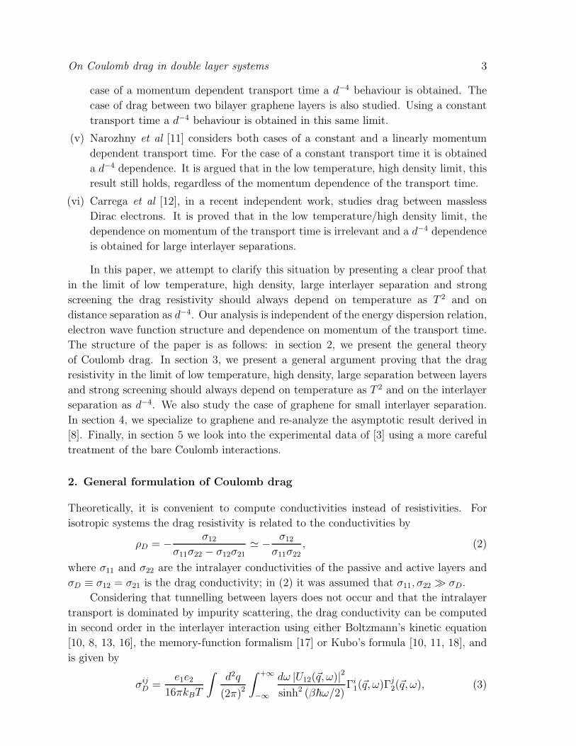
resistivity curves with this model for the interactions. In figure 2(a), we can see the

comparison between the experimental results from [3] and this calculation. Clearly

the agreement is not very good. Although (37) is correct is some limits, to obtain

the exact form of the Coulomb interactions in layered dielectric medium one must

solve Poisson’s equation (see Appendix A). For a 3 layered dielectric structure, for the

effective dielectric constants ǫab(q) in (7) we would have to use the functions ǫ(3)ab (q)

defined in Appendix A, with ǫ1 = ǫair = 1, ǫ2 = ǫAl2O3= 5.6 and ǫ3 = ǫSiO2

= 3.8.

In figure 2(b), we can see the comparison between the computed resistivity using this

interactions and the experimental results. Although this is a more rigorous treatment

for the interactions than the naive one, (37), the computed drag curves deviate even


àààààààà

à à

ààààààààààààààààààààààààààààààààààààààààààààààà

æææææææææææææææææææææææææææææææææææææææææææææææææææææææææææ

òòòòòòòòòòòòòòòòòòòòòòòòòòòòòòòòòòòòòòòòòòòòòòòòòòòòòòòòòòòò

ôôôôôôôôôôôôôôôôôôôôôôôôôôôôôôôôôôôôôôôôôôôôôôôôôôôôôôôôôôôôôôôôôôôôôôôôôôôô

ìììììììììììììììììììììììììììììììììììììììììììììììììììììììììì

ììììì

ììììì

0 5 10 15 20Vg�V

-5

-4

-3

-2

-1

0ΡDrag�WHaL

ì T=250K

ô T=200K

ò T=150K

æ T=100K

à T=77K

àæòôì Experimental

Theoretical

àààààààààààààààààààààààààààà

à à à à à

ààààààààààààààààààààààààààà





ììììì

ììììì

0 5 10 15 20Vg�V

-5

-4

-3

-2

-1

0ΡDrag�WHbL

SiO2

Al2O3

air

d

t

b

ì T=250K

ô T=200K

ò T=150K

æ T=100K

à T=77K


Theoretical

àààààààààààààààààààààà

à à à à

ààààààààààààààààààààààààààààààààà





ììììì

ììììì

0 5 10 15 20Vg�V

-5

-4

-3

-2

-1

0ΡDrag�WHcL

SiO2

AlOx

ALD Al2O3

air

dw

t

b

ì T=250K

ô T=200K

ò T=150K

æ T=100K

à T=77K


Theoretical

Figure 2. Comparison between computed and measured drag resistivity. The dotted

marks are the experimental results from [3]. The solid lines are the computed curves.

Curves with the same colour correspond to the same temperature. (a) The computed

curves were calculated using the naive interactions(

ǫ(naive)ab

)

. (b) The computed curves

were calculated using the Coulomb interactions obtained by solving Poisson’s equation

in a 3 layered dielectric depicted in the inset(

ǫ(3)ab (q)

)

. (c) The computed curves were

calculated using the Coulomb interactions obtained by solving Poisson’s equation in

a 4 layered dielectric as depicted in the inset(

ǫ(4)ab (q)

)

. The value used for the fine

structure of graphene, αg, was αg = 2 in all plots. No attempt to fit the data was

made.


further from the experimental results. One could proceed as in [8] and use αg as a

fitting parameter. We found, however, that it would be necessary a value of the order

αg ∼ 5 and αg ∼ 16, for the interactions with ǫ(naive)ab and ǫ

(3)ab , respectively, to fit the

data; both values are unrealistic. Taking into account that the SiO2 layer is finite when

solving Poisson’s equation has virtually no effect in the computed drag resistivity. This

situation is puzzling at least. However, more attention must be paid to how the devices

from [3] are constructed. The Al2O3 dielectric layer is deposited in two steps. (i) First

a 2 nm aluminium layer is deposited on top of the bottom graphene layer, being later

oxidized. We will refer to this as AlOx layer. (ii) On top of the oxidized aluminium

layer, a 5 nm Al2O3 layer is directly deposited through atomic layer deposition. We will

refer to this as ALD layer. Completed the procedure a 7 nm Al2O3 is obtained. The

reason the Al2O3 is not directly deposited on top of graphene is due to graphene being

chemically inert. In [22], the dielectric constant of the ALD alumina was determined

by studying how the capacitance of devices similar to the ones from [3] scales with the

tickness of the ALD layer keeping the AlOx layer thickness fixed, obtaining the already

referred value of ǫAl2O3= 5.6. The AlOx layer contributed with a finite capacitance,

which corresponds to a dielectric constant of ǫAlOx= 2.7. The reason why ǫAlOx

differs

from ǫAl2O3is not clear but it is most likely due to interface effects between the graphene

layer and the dielectric or between the ALD and the AlOx layers. In this case, it is not

clear if we can attribute a bulk value for ǫAlOx. Nevertheless, we still considered this

situation. For this situation of a 4 layered dielectric we use the functions ǫ(4)ab (q) from

Appendix A, now with ǫ′2 = ǫAlOx= 2.7 and w = 2 nm. The comparison between the

drag curves computed this way and the experimental data can be seen in figure 2(c).

We can see that there is a better approximation with the experimental results, but this

should be regarded with caution.

6. Conclusions

In this paper we have showed that in the limit of low temperature, high density, large

interlayer distance and strong screening, the drag resistivity should always behave

with T 2 and d−4. This result was obtained for general dispersion relation, momentum

dependence of the transport time and electronic wave function structure. It is therefore

a more general result than previous ones. Central to this fact is the general expression

derived for the non-linear susceptibility, (13), in the low temperature limit to lowest

order in frequency. Being general, this result also applies to graphene, and should close

the ongoing debate regarding the behaviour of drag for this system in the aforementioned

limit. We also derived an asymptotic expression for drag in graphene in the limit of

low temperature, high density and small layer separation. Finally, we compared the

available experimental data on drag in graphene from [3] with our theoretical model

and found out that if one insists in the conventional value for graphene fine structure

constant, αg = 2, a quantitative understanding of the data is still lacking. This is most

likely due to the complexity of the dielectric substrate used and one hopes that the


theoretical model will be quantitatively more successful in devices built using simpler

substrates, such as boron nitride [23]. Another possibility to account for this discrepancy

could be spacial inhomogeneities in the chemical potential of the graphene layers, which

are not taken into account with the present formalism. Although, it is not clear if these

should be important in the experimental range investigated, spacial inhomogeneities in

graphene’s carrier density will for sure play an important role in the electron-hole puddle

regime and should be object of future work.

Acknowledgments

We thank useful discussions with F. Guinea, J.M.B. Lopes dos Santos and A.H. Castro

Neto. Special thanks to E. Tutuc for helpful discussions regarding the construction

of graphene double layer structures. B. Amorim was supported by Fundacao para a

Ciencia e a Tecnologia (FCT) through Grant No. SFRH/BD/78987/2011.

Appendix A. Electron-electron Coulomb interaction

To obtain the correct form of the electron-electron interaction in a dielectric material

one must solve Poisson’s equation, −∇(ǫ∇φ) = ρfree/ǫ0, where ρfree is the free charge

density. We are interested in situations where the dielectric constant is a piecewise

constant function of the z coordinate, with discontinuities at positions zi. Since, we

want the interaction matrix element between states with well defined momentum in

the x, y directions and well defined position in the z direction, it is useful to introduce

φ(q, z) =∫

d2xφ(~x, z)e−i~q·~x, where ~q = (qx, qy) and ~x = (x, y). For a point charge

located at (~x, z) = (~0, zp), ρfree = eδ(~0)δ(zp), we obtain the following equation

− ∂

∂z

(

ǫ(z)∂

∂zφ(q, z)

)

+ q2φ(q, z) =e

ǫ0δ(zp). (A.1)

The potential φ(q, z) is continuous everywhere, and the the function ǫ(z)∂φ(q,z)∂z

is

continuous except at the position of the point charge. Therefore we have the boundary

conditions

φ(q, z+i ) = φ(q, z−i ),

ǫ(z−i )∂φ(q, z−i )

∂z− ǫ(z+i )

∂φ(q, z+i )

∂z=

e

ǫ0δzi,zp . (A.2)

Solving equation (A.1) together with the boundary conditions (A.2) and imposing that

φ(q, z) decays at infinity, we can obtain the potential created by the point charge and

from that the bare electron-electron Coulomb interaction. Let us consider that the

metallic plates are located at z = 0 and z = d. The electron-electron interaction can be

cast in the form given in (7) with a, b = t, b, where t refers to the top layer and b refers


to the bottom layer. For a 3 layered dielectric:

ǫ(3)(z) =

ǫ1 , z > d

ǫ2 , d > z > 0,

ǫ3 , 0 > z

(A.3)

solving Poisson’s equation gives

ǫ(3)tt (q) =

e2qd(ǫ3 + ǫ2)(ǫ1 + ǫ2)− (ǫ3 − ǫ2)(ǫ1 − ǫ2)

2 (1 + e2qd) ǫ2 − 2 (1− e2qd) ǫ3,

ǫ(3)tb (q) =

e2qd(ǫ1 + ǫ2)(ǫ2 + ǫ3)− (ǫ1 − ǫ2)(ǫ3 − ǫ2)

4e2qdǫ2, (A.4)

ǫ(3)bb (q) =

e2qd(ǫ1 + ǫ2)(ǫ3 + ǫ2)− (ǫ1 − ǫ2)(ǫ3 − ǫ2)

2 (1 + e2qd) ǫ2 − 2 (1− e2qd) ǫ1.

This result was previously given in [9] and [24]. If we consider a 4 layered dielectric,

ǫ(4)(z) =

ǫ1 , z > d

ǫ2 , d > z > w

ǫ′2 , w > z > 0

ǫ3 , 0 > z

, (A.5)

we obtain,

ǫ(4)tt (q) =

D(4)(q)

2

[

e2q(d+w) (ǫ2 + ǫ′2) (ǫ3 + ǫ′2) + e2dq (ǫ2 − ǫ′2) (ǫ′2 − ǫ3)

+e4qw (ǫ2 − ǫ′2) (ǫ3 + ǫ′2) + e2qw (ǫ2 + ǫ′2) (ǫ′2 − ǫ3)

]−1,

ǫ(4)tb (q) =

D(4)(q)

8e2q(d+w)ǫ2ǫ′2, (A.6)

ǫ(4)bb (q) =

D(4)(q)

2

[

e2q(d+w) (ǫ1 + ǫ2) (ǫ2 + ǫ′2)− e2dq (ǫ1 + ǫ2) (ǫ2 − ǫ′2)

+e4qw (ǫ2 − ǫ′2) (ǫ3 + ǫ′2)− e2dq (ǫ1 + ǫ2) (ǫ2 − ǫ′2)]−1

,

where D(4)(q) is defined as

D(4)(q) = e2q(d+w) (ǫ1 + ǫ2) (ǫ2 + ǫ′2) (ǫ′2 + ǫ3) + e2dq (ǫ1 + ǫ2) (ǫ2 − ǫ′2) (ǫ

′2 − ǫ3)

+e4qw (ǫ1 − ǫ2) (ǫ2 − ǫ′2) (ǫ′2 + ǫ3) + e2qw (ǫ1 − ǫ2) (ǫ2 + ǫ′2) (ǫ

′2 − ǫ3) . (A.7)

Appendix B. Details of the computation of the drag resistivity in graphene

The contribution to the non-linear susceptibility of graphene (32) coming only from the

conductance band, λ, λ′ = +,+ is

~Γ(~q, ω) = 8πvF τ0~q

∫

d2k

(2π)2f+,+~k,~k+~q

(

nF (ǫ~k,+)− nF (ǫ~k+~q,+))

δ(

ǫ~k,+ − ǫ~k+~q,+ + ~ω)

= −2vF τ0~qImχ++ (q, ω) (B.1)


where χ++(q, ω) is the contribution to the graphene polarizability coming only from the

conductance band,

χ++(q, ω) = 4

∫

d2k

(2π)2f+,+~k,~k+~q

nF (ǫ~k,+)− nF (ǫ~k+~q,+)

ǫ~k,+ − ǫ~k+~q,+ + ~ω + i0+. (B.2)

At zero temperature, this can be computed analytically and the result can be written

as

Imχ++(~q, ω) =1

4πvF~

q√

1−(

ωqvF

)2Φ(q, ω), (B.3)

where the function Φ(q, ω) is defined as

Φ(q, ω > 0) = Φ+(q, ω)Θ

(

ω

vF− q + 2kF

)

Θ

(

q − ω

vF

)

+Φ−(q, ω)Θ

(

kF − ω

vF− |kF − q|

)

, (B.4)

where

Φ±(q, ω) = ± cosh−1

(

2kF ± ω/vFq

)

∓ 2kF ± ω/vFq

√

(

2kF ± ω/vFq

)2

− 1. (B.5)

The drag conductivity therefore becomes

σD =e2(τ 0)2

27π4~3kBT

∫ ∞

0

dqq5∫ ∞

0

dω |U12(~q, ω)|2

sinh2 (β~ω/2)

Φ1(q, ω)Φ2(q, ω)

1−(

ωqvF

)2 . (B.6)

The intralayer graphene conductivity of layer a at low temperature is given by σaa =

e2vFnaτ0/~ = e2ǫF τF/(π~

2) where kFaτ0 = τFa is the transport time at the Fermi

level. We write the interlayer interaction as U12 = e2 exp(−qd)/(2ǫRPA(~q, ω)ǫ12(q)ǫ0q).

Introducing the adimensional quantities, x = q/√kF1kF2 and y = ω/(vF

√kF1kK2), the

drag resistivity becomes

ρD = − 1

25~

e2

√ǫF1ǫF2

kBTα2g

∫ ∞

0

dxx3

∫ ∞

0

dy

sinh2(

y ~vF√kF1kF2

2kBT

)

× e−2d√kF1kF2x

ǫ12(q)2 |ǫRPA(x, y)|2Φ1(x, y)Φ2(x, y)

1−(

yx

)2 , (B.7)

where αg is the fine structure constant of graphene.

References

[1] Pogrebinskii M 1977 Fiz. Tekh. Poluprovodn. 11 637 [1977 Sov. Phys. Semicond. 11 372]

[2] Price P 1983 Physica (Amsterdam) B 117 750

[3] Kim S, Jo I, Nah J, Yao Z, Banerjee S and Tutuc E 2011 Phys. Rev. B 83 161401

[4] Geim A 2012 Electronic properties of graphene-bn heterostructures. talk at KITP Conference

Fundamental Aspects of Graphene and Other Carbon Allotropes

[5] Kim S and Tutuc E 2012 Solid State Communications 152 1283 – 1288


[6] Narozhny B 2007 Phys. Rev. B 76 153409

[7] Wang-Kong T, Hu B and Das Sarma S 2007 Phys. Rev. B 76 081401

[8] Peres N, Lopes dos Santos N and Castro Neto A 2011 EPL (Europhysics Letters) 95 18001

[9] Katsnelson M 2011 Phys. Rev. B 84 041407

[10] Hwang E, Sensarma R and Das Sarma S 2011 Phys. Rev. B 84 245441

[11] Narozhny B, Titov M, Gornyi I and Ostrovsky P 2012 Phys. Rev. B 85 195421

[12] Carrega M, Tudorovskiy T, Principi A, Katsnelson M and Polini M 2012 ArXiv e-prints (Preprint

1203.6777)

[13] Jauho A and Smith H 1993 Phys. Rev. B 47 4420–8

[14] Gramila T, Eisenstein J, MacDonald A, Pfeiffer L and West K 1991 Phys. Rev. Lett. 66 1216–9

[15] Peres N 2010 Rev. Mod. Phys. 82 2673–700

[16] Flensberg K and Hu B 1995 Phys. Rev. B 52 14796–808

[17] Zheng L and MacDonald A 1993 Phys. Rev. B 48 8203–9

[18] Kamenev A and Oreg Y 1995 Phys. Rev. B 52 7516–27

[19] Hu B and Das Sarma S 1993 Phys. Rev. B 48 5469–504

[20] Levchenko A and Kamenev A 2008 Phys. Rev. Lett. 100 026805

[21] Wunsch B, Stauber T, Sols F and Guinea F 2006 New Journal of Physics 8 318

[22] Fallahazad B, Lee K, Lian G, Kim S, Corbet C, Ferrer D, Colombo L and Tutuc E 2012 Appl.

Phys. Lett. 100 093112

[23] Ponomarenko L A et al 2011 Nat. Phys. 7 958–61

[24] Profumo R, Polini M, Asgari R, Fazio R and MacDonald A 2010 Phys. Rev. B 82 085443

1203.6777

On Coulomb drag in double layer systems

Documents

Transcript of On Coulomb drag in double layer systems