buffet investigation on airfoils - Open METU
126
BUFFET INVESTIGATION ON AIRFOILS A THESIS SUBMITTED TO THE GRADUATE SCHOOL OF NATURAL AND APPLIED SCIENCES OF MIDDLE EAST TECHNICAL UNIVERSITY BY KEZBAN GİZEM ALGÜL IN PARTIAL FULFILLMENT OF THE REQUIREMENTS FOR THE DEGREE OF MASTER OF SCIENCE IN AEROSPACE ENGINEERING APRIL 2021
-
Upload
khangminh22 -
Category
Documents
-
view
0 -
download
0
Transcript of buffet investigation on airfoils - Open METU
BUFFET INVESTIGATION ON AIRFOILS
A THESIS SUBMITTED TO
THE GRADUATE SCHOOL OF NATURAL AND APPLIED SCIENCES
OF
MIDDLE EAST TECHNICAL UNIVERSITY
BY
KEZBAN GİZEM ALGÜL
IN PARTIAL FULFILLMENT OF THE REQUIREMENTS
FOR
THE DEGREE OF MASTER OF SCIENCE
IN
AEROSPACE ENGINEERING
APRIL 2021


Approval of the thesis:
BUFFET INVESTIGATION ON AIRFOILS
submitted by KEZBAN GİZEM ALGÜL in partial fulfillment of the requirements
for the degree of Master of Science in Aerospace Engineering, Middle East
Technical University by,
Prof. Dr. Halil Kalıpçılar
Dean, Graduate School of Natural and Applied Sciences
Prof. Dr. İsmail Hakkı Tuncer
Head of the Department, Aerospace Engineering
Prof. Dr. Serkan Özgen
Supervisor, Aerospace Engineering, METU
Examining Committee Members:
Prof. Dr. Zafer Dursunkaya
Mechanical Engineering, METU
Prof. Dr. Serkan Özgen
Aerospace Engineering, METU
Prof. Dr. İsmail Hakkı Tuncer
Aerospace Engineering, METU
Prof. Dr. Yusuf Özyörük
Aerospace Engineering, METU
Prof. Dr. Kürşad Melih Güleren
Faculty of Aeronautics and Astronautics, ESTU
Date: 30.04.2021

iv
I hereby declare that all information in this document has been obtained and
presented in accordance with academic rules and ethical conduct. I also declare
that, as required by these rules and conduct, I have fully cited and referenced
all material and results that are not original to this work.
Name, Last name : Kezban Gizem Algül
Signature :
v
ABSTRACT
BUFFET INVESTIGATION ON AIRFOILS
Algül, Kezban Gizem
Master of Science, Aerospace Engineering
Supervisor: Prof. Dr. Serkan Özgen
April 2021, 108 pages
The aim of the present thesis is to investigate buffet onset characteristics in two-
dimensional flow. NACA0012 airfoil was chosen as the geometry in this study since
the profile is frequently used for the lifting surfaces of aircraft, which are exposed to
high flight loads during transonic flight and this causes buffet and flutter. In addition,
it is one of the very few models which was studied for the buffet onset investigation
in the literature and detailed wind tunnel test data is available. In the present study,
after determining the optimum mesh resolution and the appropriate turbulence
model, the results of the steady flow numerical analysis for low and high Reynolds
numbers were validated with wind tunnel data. The transient flow is investigated for
the buffet onset region of the NACA0012 airfoil and the results are verified with
wind tunnel data. The oscillating behavior of the shock wave on the airfoil is
investigated through the frequency and the Strouhal numbers of lift, drag, moment
and static pressure distributions through time and frequency.
The study investigates the primary effectors that stimulate buffet onset and the
behavior of the flow during buffet through numerical analyses using Unsteady
Reynolds-Averaged Navier-Stokes (U-RANS) Equations. The effects of Mach
vi
number, angle of attack and Reynolds number on buffet onset is investigated for the
examination of buffet characteristics in detail.
Keywords: Buffet, Buffet Onset, Shock Induced Oscillation, Unsteady Transient
Flow Physics, Aeroelasticity
vii
ÖZ
KANAT PROFİLLERİNDE BUFFET ARAŞTIRMASI
Algül, Kezban Gizem
Yüksek Lisans, Havacılık ve Uzay Mühendisliği
Tez Yöneticisi: Prof. Dr. Serkan Özgen
Nisan 2021, 108 sayfa
Bu tezin amacı, iki boyutlu akışta buffet başlangıç özelliklerini incelemektir. Bu
çalışmada transonik uçuş sırasında yüksek uçuş yüklerine maruz kalan uçakların
kaldırma yüzeylerinde sıklıkla kullanılması ve bu durumun buffet ve çırpınmaya
neden olması sebebiyle geometri olarak NACA0012 kanat profili seçilmiştir. Ayrıca,
literatürde buffet başlangıç araştırması için incelenen çok az sayıda modelden biridir
ve detaylı rüzgar tüneli test verileri mevcuttur. Optimum ağ çözünürlüğü ve uygun
türbülans modelinin belirlenmesi için öncelikle sabit akış analizleri yapılmıştır.
Mevcut çalışmada, optimum ağ çözünürlüğü ve uygun türbülans modeli
belirlendikten sonra, düşük ve yüksek Reynolds sayıları için sürekli akış sayısal
analizlerinin sonuçları rüzgar tüneli verileri ile doğrulanmıştır. Zamana bağlı akış
ise, NACA0012 kanat profilinin buffet başlangıç bölgesi için araştırılmış ve sayısal
analizlerden elde edilen sonuçlar rüzgar tüneli verileri ile doğrulanmıştır. Şok
dalgasının kanat üzerindeki salınım davranışı, kaldırma ve sürükleme kuvvetlerinin,
yunuslama momentinin ve statik basıncın zamana ve frekansa göre dağılımlarından
elde edilen güç spektral yoğunlukları ve Strouhal sayıları kullanılarak araştırılmıştır.

viii
Çalışmada, buffet başlangıcını uyaran birincil efektörler ve buffet sırasındaki akış
davranışı Reynolds-Ortalamalı Navier-Stokes denklemleri kullanılarak sayısal
analizlerle araştırılmıştır. Buffet özelliklerinin detaylı incelenmesi için Mach sayısı,
hücum açısı ve Reynolds sayısının buffet başlangıcına etkileri araştırılmıştır.
Anahtar Kelimeler: Buffet, Buffet Başlangıcı, Şok Kaynaklı Salınım, Zamana Bağlı
Kararsız Akış Fiziği, Aeroelastisite

ix
To my family

x
ACKNOWLEDGEMENTS
I would like to express my deepest gratitude to my supervisor Prof. Dr. Serkan Özgen
for his guidance, advice, criticism, encouragement and insight throughout the
research. I am grateful not only for his support by sharing his vast knowledge and by
giving morale where I fell into despair throughout my thesis, but also the support
that he gave me in my business life whenever I demanded help and guidance.
I would like to thank my friends, for their support, encouragement and help when I
was struggling and got stuck during my thesis work.
I would like to express my deepest love and gratitude to my dear father Ali Parlak,
my dear mother Gülsüm Parlak, my brother Mehmet Alper and my sister Mehtap
Ayfer, for their endless, complimentary love and support throughout my thesis and
most importantly throughout my whole life.
I would like to express my deepest love to my dear beloved husband, Kadir Algül
for his endless support and love even in the most difficult times during thesis studies
and most importantly during my whole life.
xi
TABLE OF CONTENTS
1.
ABSTRACT ............................................................................................................... v
ÖZ ........................................................................................................................... vii
ACKNOWLEDGEMENTS ....................................................................................... x
TABLE OF CONTENTS ......................................................................................... xi
LIST OF TABLES ................................................................................................. xiii
LIST OF FIGURES ............................................................................................... xiv
LIST OF ABBREVIATIONS ............................................................................... xvii
LIST OF SYMBOLS ........................................................................................... xviii
CHAPTERS
1 INTRODUCTION ............................................................................................. 1
1.1 General Overview ...................................................................................... 1
1.2 The Motivation and Outline of the Thesis ................................................. 3
2 LITERATURE REVIEW .................................................................................. 5
2.1 Experimental Studies .................................................................................. 7
2.2 Numerical Studies .................................................................................... 11
3 COMPUTATIONAL SOLUTION METHOD ................................................ 13
3.1 Navier-Stokes Equations for Compressible Flow .................................... 13
3.1.1 Continuity Equation .......................................................................... 13
3.1.2 Momentum Equation ........................................................................ 13
3.1.3 Energy Equation ................................................................................ 14
3.1.4 Thermodynamic Relation .................................................................. 14
3.1.5 Mach Number and Speed of Sound .................................................. 15
xii
3.1.6 Reynolds Number and Strouhal Number .......................................... 16
3.2 Reynolds Averaged Navier-Stokes (RANS) Equations ............................ 16
3.3 RANS Equations Turbulence Models ....................................................... 19
3.3.1 Spalart-Allmaras Turbulence Model ................................................. 20
3.3.2 k-ε Turbulence Model ....................................................................... 22
3.3.3 k-ω SST Turbulence Model ............................................................... 23
3.4 ANSYS Fluent .......................................................................................... 26
4 STEADY ANALYSES ................................................................................... 29
4.1 Reynolds Number and Grid Spacing ........................................................ 30
4.2 Mesh Independence .................................................................................. 32
4.3 Turbulence Model Set ............................................................................... 40
4.4 Verification of the Numerical Analysis with Wind Tunnel Data ............. 42
4.4.1 Verification of the Results for Low Reynolds Numbers ................... 42
4.4.2 Verification of the Results for High Reynolds Numbers .................. 46
5 TRANSIENT ANALYSES ............................................................................. 55
5.1 Steady Flow .............................................................................................. 56
5.2 Unsteady Flow .......................................................................................... 63
5.3 Verification of the Numerical Analysis with Wind Tunnel Data ............. 81
6 CONCLUSIONS ........................................................................................... 101
6.1 Concluding Remarks ............................................................................... 101
6.2 Future Work ............................................................................................ 103
REFERENCES ...................................................................................................... 105
xiii
LIST OF TABLES
TABLES
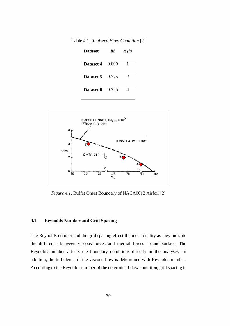
Table 4.1. Analyzed Flow Condition [2] ................................................................ 30
Table 4.2. Standard Atmospheric Conditions of the Streamflow over Airfoil ....... 31
Table 4.3. Analyzed Flow Conditions of Dataset 4 ................................................ 37
Table 4.4. Sizing Features of Grid Spacing with Different Mesh Resolutions ....... 38
Table 4.5. Analyzed Flow Conditions at Low Reynolds Number .......................... 43
Table 4.6. Sizing Features of Grid Spacing with 428K Mesh Elements ................ 49
Table 4.7. Analyzed Flow Conditions at High Reynolds Number ......................... 50
Table 5.1. Analyzed Flow Conditions for Steady Flow [2] .................................... 56
Table 5.2. Analyzed Flow Conditions for Unsteady Flow [2] ................................ 63
Table 5.3. Analyzed Flow Conditions for High Reynolds Number[2] ................... 82
xiv
LIST OF FIGURES
FIGURES
Figure 1.1. Buffet Onset of NACA0012 Airfoil [2] .................................................. 2
Figure 2.1. Sample of Kelvin-Helmholtz Type Instability on PSD of Pressure from
Different Chordwise Locations, OAT15A Airfoil [23] ........................................... 10
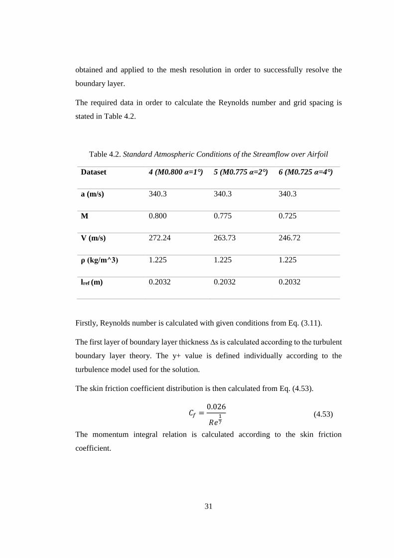
Figure 4.1. Buffet Onset Boundary of NACA0012 Airfoil [2] ............................... 30
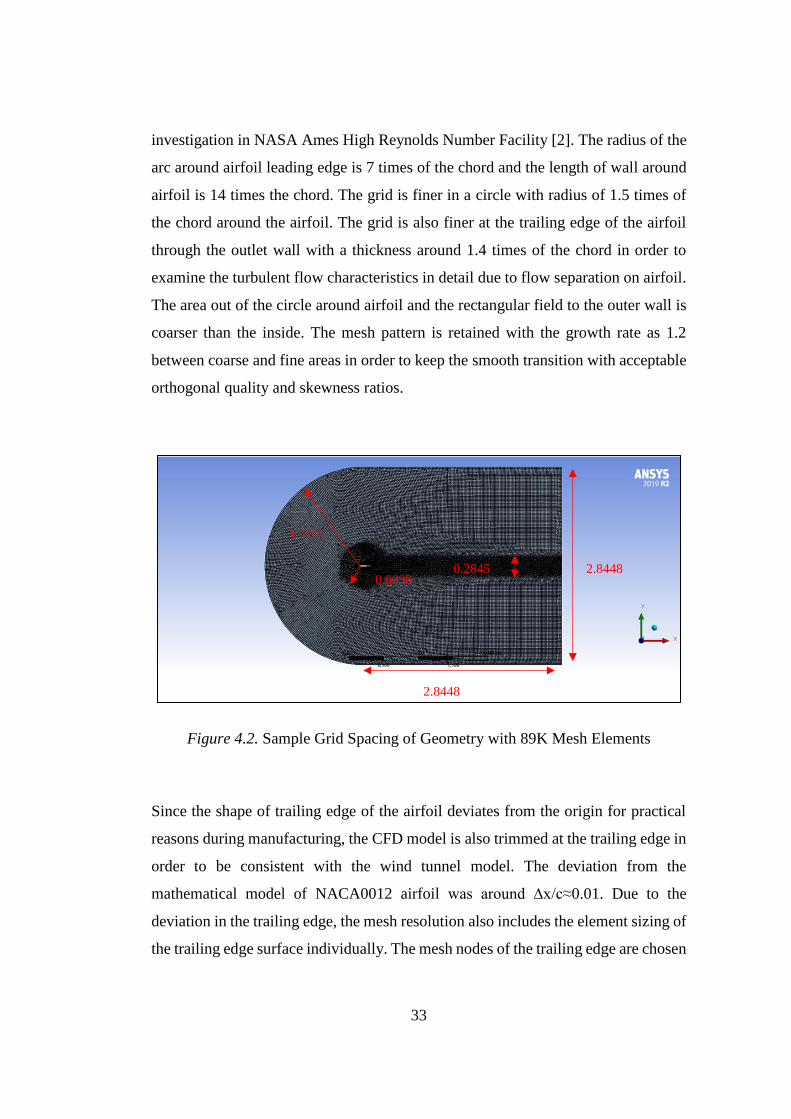
Figure 4.2. Sample Grid Spacing of Geometry with 89K Mesh Elements ............. 33
Figure 4.3. Grid Spacing of Geometry around Airfoil with 89K Mesh Elements .. 34
Figure 4.4. Grid Spacing of Geometry around Airfoil with 138K Mesh Elements 35
Figure 4.5. Grid Spacing of Geometry around Airfoil with 209K Mesh Elements 36
Figure 4.6. Grid Spacing of Geometry around Airfoil with 61K Mesh Elements .. 36
Figure 4.7. Comparison of Pressure Coefficient Distribution over Airfoil among
61K, 89K, 138K and 209K Mesh Resolution .......................................................... 40
Figure 4.8. Comparison of Pressure Coefficient Distribution over Airfoil among
Spalart-Allmaras, k-ε and k-ω SST Turbulence Models ......................................... 42
Figure 4.9. Verification of the Numerical Result of Dataset 4 with Wind Tunnel Data
................................................................................................................................. 44
Figure 4.10. Verification of the Numerical Result of Dataset 5 with Wind Tunnel
Data .......................................................................................................................... 45
Figure 4.11. Verification of the Numerical Result of Dataset 6 with Wind Tunnel
Data .......................................................................................................................... 46
Figure 4.12. Sample Grid Spacing of Geometry with 428K Mesh Elements ......... 48
Figure 4.13. Grid Spacing of Geometry around Airfoil with 428K Mesh Elements
................................................................................................................................. 48
Figure 4.14. Verification of the Numerical Result of Dataset 4 with Wind Tunnel
Data at High Reynolds Number .............................................................................. 51
Figure 4.15. Verification of the Numerical Result of Dataset 5 with Wind Tunnel
Data at High Reynolds Number .............................................................................. 52
xv
Figure 4.16. Verification of the Numerical Result of Dataset 6 with Wind Tunnel
Data at High Reynolds Number .............................................................................. 53
Figure 5.1. Transient Flow Analysis Conditions [2] ............................................... 56
Figure 5.2. Lift, Drag, Moment Coefficient and Static Pressure Variation over Time
at M0.800, α=1°, Re=3.7E+06 ................................................................................ 58
Figure 5.3. Lift, Drag, Moment Coefficient and Static Pressure Variation over Time
at M0.775, α=2°, Re=3.7E+06 ................................................................................ 60
Figure 5.4. Lift, Drag, Moment Coefficient and Static Pressure Variation over Time
at M0.725, α=4°, Re=3.4E+06 ................................................................................ 62
Figure 5.5. Lift, Drag, Moment Coefficient and Static Pressure Variation over Time
and the Power Spectral Density Variations over Frequency at M0.800, α=4°,
Re=4E+06 ............................................................................................................... 65
Figure 5.6. Comparison of Upper and Lower Surface Pressure and Velocity u
Waveforms over Time at M0.800, α=4°, Re=4E+06 .............................................. 67
Figure 5.7. Pressure Waveforms over Time at M0.800, α=4°, Re=4E+06 ............. 68
Figure 5.8. Lift, Drag, Moment Coefficient and Static Pressure Variation over Time
and the Power Spectral Density Variations over Frequency at M0.775, α=4°,
Re=4E+06 ............................................................................................................... 70
Figure 5.9. Comparison of Upper and Lower Surface Pressure and Velocity u
Waveforms over Time at M0.775, α=4°, Re=4E+06 .............................................. 72
Figure 5.10. Pressure Waveforms over Time at M0.775, α=4°, Re=4E+06 ........... 73
Figure 5.11. Velocity u Contour of Unsteady Analysis at Various Timesteps at
M0.775, α=4°, Re=4E+06 ....................................................................................... 75
Figure 5.12. Lift, Drag, Moment Coefficient and Static Pressure Variation over Time
and the Power Spectral Density Variations over Frequency at M0.725, α=6°,
Re=4E+06 ............................................................................................................... 77
Figure 5.13. Comparison of Upper and Lower Surface Pressure and Velocity u
Waveforms over Time at M0.725, α=6°, Re=4E+06 .............................................. 79
Figure 5.14. Pressure Waveforms over Time at M0.725, α=6°, Re=4E+06 ........... 80
xvi
Figure 5.15. Lift, Drag, Moment Coefficient and Static Pressure Variation over Time
and the Power Spectral Density Variations over Frequency at M0.80, α=4°,
Re=10E+06 .............................................................................................................. 83
Figure 5.16. Comparison of Upper and Lower Surface Pressure and Velocity u
Waveforms over Time at M0.80, α=4°, Re=10E+06 .............................................. 85
Figure 5.17. Pressure Waveforms over Time at M0.80, α=4°, Re=10E+06 ........... 86
Figure 5.18. Lift, Drag, Moment Coefficient and Static Pressure Variation over Time
and the Power Spectral Density Variations over Frequency at M0.77, α=4°,
Re=10E+06 .............................................................................................................. 88
Figure 5.19. Comparison of Upper and Lower Surface Pressure and Velocity u
Waveforms over Time at M0.77, α=4°, Re=10E+06 .............................................. 90
Figure 5.20. Pressure Waveforms over Time at M0.77, α=4°, Re=10E+06 ........... 91
Figure 5.21. Velocity u Contour of Unsteady Analysis at Various Timesteps at
M0.77, α=4°, Re=10E+06 ....................................................................................... 93
Figure 5.22. Lift, Drag, Moment Coefficient and Static Pressure Variation over Time
and the Power Spectral Density Variations over Frequency at M0.72, α=6°,
Re=10E+06 .............................................................................................................. 95
Figure 5.23. Comparison of Upper and Lower Surface Pressure and Velocity u
Waveforms over Time at M0.72, α=6°, Re=10E+06 .............................................. 97
Figure 5.24. Pressure Waveforms over Time at M0.72, α=6°, Re=10E+06 ........... 98
xvii
LIST OF ABBREVIATIONS
ABBREVIATIONS
CFD : Computational Fluid Dynamics
Hz : Hertz
MTE : Mean Turbulent Energy
MVF : Mean Velocity Field
NLEVM : Nonlinear Eddy Viscosity Models
PSD : Power Spectral Density
RANS : Reynolds Averaged Navier-Stokes Equations
SST : Shear Stress Transport
U-RANS : Unsteady Reynolds-Averaged Navier-Stokes Equations
xviii
LIST OF SYMBOLS
SYMBOLS
𝑎 : Speed of Sound (m/s)
𝑘 : Turbulent Kinetic Energy (J/kg)
𝐾 : Thousands (x1000)
𝑙𝑟𝑒𝑓 : Reference Length (m)
𝑀 : Mach number
𝑝 : Pressure (Pa)
𝑅 : Gas Constant (JK-1mol-1)
𝑅𝑒 : Reynolds Number
𝑆𝑡 : Strouhal Number
𝑡 : Timestep (sec)
𝑇 : Period of Oscillation (sec)
𝑇 : Temperature (K)
𝑢 : Flow Velocity Components (m/s)
𝑉 : Freestream Velocity (m/s)
y+ : Dimensionless Wall Distance
GREEK SYMBOLS
α : Angle of Attack (°)
β : Sideslip Angle (°)
ε : Turbulence Dissipation Rate (m2/s3)
𝜇𝑡 : Turbulent Viscosity (Pa s)
ρ : Density (kg/m3)
𝜏𝑖𝑗 : Stress Tensor
ω : Turbulence Specific Dissipation Rate (1/s)
1
CHAPTER 1
1 INTRODUCTION
1.1 General Overview
Transonic buffet is defined as the shock induced oscillations that interact with
turbulent boundary layer and cause separation especially in the region close to the
trailing edge of the wing/airfoil [1]. The instabilities in the flow field interacting with
turbulent boundary layer cause oscillations in the shock wave. The critical flow
variables that trigger transonic buffet are Mach number and angle of attack. These
two parameters construct the buffet onset region, in which the critical flight
conditions that cause the buffet phenomenon are stated. The relation of the critical
Mach number and angle of attack that cause buffet onset is actually inversely
proportional. The critical maximum angle of attack that stimulates the buffet
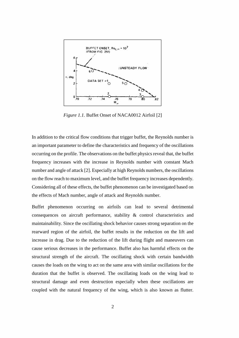
decreases when the critical Mach number increases. As it is seen on Figure 1.1, the
resultant curve separates the stability behavior of the flow field around the airfoil
into two regions as steady and unsteady flow. The flow conditions that are on the
lower region of the buffet onset represents the steady flow and no such characteristics
as oscillating shocks are observed in that region. When the flow conditions are
reached on and above the buffet onset, the unsteady flow starts to be observed and
the shock oscillations can be observed in that region.
2
Figure 1.1. Buffet Onset of NACA0012 Airfoil [2]
In addition to the critical flow conditions that trigger buffet, the Reynolds number is
an important parameter to define the characteristics and frequency of the oscillations
occurring on the profile. The observations on the buffet physics reveal that, the buffet
frequency increases with the increase in Reynolds number with constant Mach
number and angle of attack [2]. Especially at high Reynolds numbers, the oscillations
on the flow reach to maximum level, and the buffet frequency increases dependently.
Considering all of these effects, the buffet phenomenon can be investigated based on
the effects of Mach number, angle of attack and Reynolds number.
Buffet phenomenon occurring on airfoils can lead to several detrimental
consequences on aircraft performance, stability & control characteristics and
maintainability. Since the oscillating shock behavior causes strong separation on the
rearward region of the airfoil, the buffet results in the reduction on the lift and
increase in drag. Due to the reduction of the lift during flight and maneuvers can
cause serious decreases in the performance. Buffet also has harmful effects on the
structural strength of the aircraft. The oscillating shock with certain bandwidth
causes the loads on the wing to act on the same area with similar oscillations for the
duration that the buffet is observed. The oscillating loads on the wing lead to
structural damage and even destruction especially when these oscillations are
coupled with the natural frequency of the wing, which is also known as flutter.
3
Besides, transonic buffet occurs in transonic Mach numbers with critical angles of
attack of small magnitude. For that reason, the aircraft flies in that region very
frequently. Due to all of these reasons, the determination of the buffet onset of the
configuration is crucially important for the aircraft. The investigations on the buffet
onset is conducted for several planforms, and the current results are mainly focused
on the airfoil and wing buffet characteristics. In this aim, the transonic buffet is
investigated in two-dimensional environment.
1.2 The Motivation and Outline of the Thesis
The aim of the study is to obtain the transonic buffet onset characteristics of the
NACA0012 airfoil with the Computational Fluid Dynamics using the commercial
solver ANSYS Fluent. The results from the numerical solutions are compared with
wind tunnel test results in the literature [2].
For this purpose, the steady analyses of the NACA0012 airfoil is conducted first.
The three independent points as Dataset 4, Dataset 5 and Dataset 6 in Figure 1.1 are
investigated and the characteristics of the flow at these points are examined for the
investigation of the buffet onset characteristics of NACA0012 airfoil. The transonic
buffet conditions are mainly determined by the critical Mach number and angle of
attack conditions and these variables create buffet onset curve. The line at the buffet
onset curve divides the flow characteristics of the NACA0012 airfoil into two region
as steady and unsteady flow characteristics, and the thesis includes the assessment
of both regions in terms of flow behavior. At this phase, the mesh quality,
independence from the resolution and turbulence models are investigated and
validated with the wind tunnel data. The verification of the numerical solutions is
conducted for two different Reynolds number conditions for the steady flow. Then,
the transient flow analyses are conducted for both steady and unsteady regions. The
steady analyses are conducted at the Dataset 4, Dataset 5 and Dataset 6 flow
4
conditions. The unsteady flow is analyzed by adding approximately 2 degrees of
angle of attack and keeping Mach number constant in Dataset 4, Dataset 5 and
Dataset 6 flow conditions. In this way, the characteristics of the flow can be observed
in the steady region, and the change can be better observed when going through the
unstable region after buffet onset. The transition from steady to unsteady flow is
conducted by increasing the angle of attack when the Mach number is kept the same.
Then, the validation of the buffet onset for the unsteady transonic flow is carried out
with high Reynolds number.
The study of the buffet onset starts with the steady analyses. The pressure distribution
around airfoil is investigated at stable region of the buffet onset curve at Figure 1.1,
and then the results are verified with the wind tunnel data [2]. The second phase of
the study includes the transient analyses. Firstly, variance in the flow characteristics
with time is examined in the steady region of buffet onset, and then the same
examination is conducted for the unstable region. Finally, the buffet characteristics
of the NACA0012 airfoil is verified with wind tunnel data at high Reynolds number
[2].
5
CHAPTER 2
2 LITERATURE REVIEW
The buffet onset investigations are generally carried out in experimental studies and
numerical analyses. The experimental studies are conducted for several airfoil types
and the measurements and analyses of the data are published. The numerical analyses
are based on the Computational Fluid Dynamics results with several types of tools
and sources. The results of the numerical analyses are compared with experimental
studies so as to be verified with physical data.
Even though Hilton & Fowler [3] performed experiments on transonic shock induced
oscillations sixty years ago, the physical mechanisms behind them still could not be
fully understood. By various experiments and numerical analysis, two different types
of shock buffet on airfoils have been identified. The first type of buffet includes
shock oscillations on both the pressure and suction surfaces of an airfoil, which
typically occur at zero incidence on biconvex sections. Mabey [4] investigated a
model of the first type shock buffet where shock wave/boundary layer interactions
on both surfaces initiate phaselocked shock oscillations in opposing directions. The
shock moving upstream on the upper surface weakens so that the separated zone
becomes reattached and this propels the shock downstream. The first type buffet is
strongly dependent on the shock which can produce separation. Mabey suggested the
prediction for buffet onset with the Mach number just ahead of the shock [4] .
The second type of the buffet is common in modern supercritical airfoils and is
characterized by the shock oscillations on the upper surface of the airfoil at angles
of attack which are different than zero. Pearcey [5], [6] characterized the shock
induced separation forms, which are defined as the separation bubbles on the upper
surfaces, experienced by conventional airfoils at transonic speed. He identified two
6
different types of separation; shock induced separation bubble and rear separation,
which is either additionally present or in its initial state. Also three variants of rear
separation were identified; first rear separation is provoked by the formation of a
bubble, second is provoked by the shock and the third is present from the outset.
Research by Pearcey et al led to the creation of the first model to initiate predictions
of the shock oscillations that are observed on supercritical airfoils. The model makes
a relation between trailing edge pressure divergence and large scale unsteadiness.
For airfoils that contain separation bubbles, Pearcey et al [6] associate the onset of
buffets with the Mach number or angle of attack at which the separation bubble
expands to the trailing edge and bursts. This mechanism of bubble bursting leading
to buffet onset is identified by the divergence of trailing edge pressure. At first,
bubble bursting was thought as the cause of onset by experimental and computational
support, however conflicting evidence are found during latest research [7], which
discounts the bubble bursting as a potential leading factor for shock buffet.
In the advanced work of Tijdeman [8], three different modes of shock motion with
the effect of sinusoidal flap deflections were experimentally demonstrated on the
NACA 64A006 airfoil. Shock movement of the first type is represented near
sinusoidal shock oscillations on the upper surface of the airfoil, for which the shock
is present throughout the entire buffet cycle, but varies in strength, while the
maximum shock strength is achieved during the upstream excursion. The magnitude
of the difference in shock strength is quite large in the second type when compared
to the first type, and as a result the shock disappears during the downstream
excursion. The behavior in the third type is quite different from the others. The shock
moves upstream, at first strong and then weakening, but continues to move,
eventually moving onto the oncoming flow as a free shock wave. Although these
shock wave motions were initially identified with oscillating airfoils, observations
in rigid wing sections at certain flight conditions have been performed for each of
them [9].
For the Tijdeman’s first type of shock movements [8], an acoustic wave-propagation
feedback model is proposed by Lee [1] explaining the mechanism governing the
7
autonomous shock oscillations. According to this model, the shock wave motion
generates downstream propagating pressure waves, with the instability growing as it
travels from the separation point through the shear layer. The separated flow induces
a de-cambering effect, because of the interactions with the flow on reaching the
trailing edge, upstream moving pressure waves are produced in the subsonic flow
above the boundary layer. These waves interact with the shock and impart energy to
maintain its oscillation. The loop is then completed resulting in sustained shock
motion. There is conflicting evidence in the literature regarding the validity of the
Lee model [1], according to Pearcey bubble bursting mechanism [6].
Raghunathan et al [10] also proposed a mechanism based on an instable interaction
between shock wave and separation bubble like Tijdeman’s second type shock
oscillations on the NACA0012 airfoil [8]. Shock strength sufficiency for inducing a
separation bubble is highlighted by the authors which initiates periodic motion of the
shock. This motion is sustained on the upper airfoil surface by the alternating
expansion and collapse of the bubble. Throughout the cycle, the varying size of the
separated zone changes the effective curvature of the airfoil and the trailing edge
plays an integral role in the communication of flow states between the suction and
pressure surfaces.
The phenomenon of transonic shock buffet described until now reflects a classical
perspective, including most of the early experimental and numerical investigations
which tries to model the underlying flow mechanisms. An overall review of these
works is provided by Lee [9].
2.1 Experimental Studies
There are several distinctive experimental studies addressing buffet investigation.
One of these is Tijdemann's work [8], which examined the NACA64A006 airfoil
with several flap movements and deflections during the experiments. By this way,
the work is intended to study the effect of sinusoidal flap behavior on the airfoil
8
profile. Each of the writers McDevitt et al [11], McDevitt [12], Mabey [4] tested a
biconvex airfoil in wind tunnel. Tests taking into account shock oscillations in
supercritical airfoils were performed by Lee [13], [14].
McDevitt & Okuno [2] reviewed NACA0012 buffet on NASA Ames High Reynolds
number facility. The chord of the model was 20.32 cm; the trailing edge thickness
was 0.002c. The tests were conducted for the Mach numbers that are ranging from
0.7 to 0.8, and the Reynolds numbers that are ranging from 1 million to 14 million.
The static pressure measurements are conducted from the 40 static pressure orifices
that are placed on the airfoil surface, and the unsteady behavior of the flow is
characterized by the measurements from the 6 dynamic pressure transducers.
Schlieren images were also added to the work in order to reflect the visual behavior
of the flow field during buffet. The authors examined not only the factors that affect
the buffet onset, but also the Reynolds number effect on the buffet characteristics.
The Strouhal number values of the shock oscillations during the buffet are measured
from the experimental results with high Reynolds number.
Dandois et al give detailed information about the experimental tests in ONERA about
examining and reducing the possible effects of the buffet phenomenon in his works
[15]. Especially, the tests of the supercritical OAT15A airfoil conducted in the S3Ch
continuous investigation wind tunnel at the ONERA Chalais-Meudon-Center have
been described by Jacquin et al [16], [17].
In order to obtain a wide range of experimental database for the verification of the
numerical results, the tests were conducted with varying test conditions and results.
In this manner, in addition to the surface static and dynamic pressure measurements,
mean and RMS pressure data with spectral content for pressure fluctuations were
produced.
Tests performed by Jacquin et al [16] include varying angles of attack with constant
Mach number as M = 0.73, varying Mach numbers with constant angles of attack as
α = 3° and α = 3.5° and constant Reynolds number as Re≈3x10⁶ for all test conditions.
OAT15A has become the benchmark for transonic buffet test case in recent years
9
according to the measurements of the tests and the numerical studies that are
conducted in the same conditions of the tests for this category [18], [19], [20], [21].
The detailed analysis by Jacquin et al [16] also provided new insights into the physics
of transonic shock oscillations. Spectral analysis of unsteady pressure signals reveals
that a two-dimensional buffet phenomenon is time-invariant and mostly modal in
nature. The spectra are monitored by a single frequency, excluding the fact that the
frequency propagation is caused by low frequency shock wave oscillations. This
behavior confirms the global instability theory proposed by Crouch et al [22].
In a study of the two-dimensional characteristics of the buffet, somehow conflicting
results have been observed. Jacquin et al [16] firstly observed that the spectral
density of the sound pressure level in the central span distributes evenly and this is
the evidence of a two dimensional buffet mechanism occurring on the airfoil. Yet,
the three dimensional effects have been realized in the oil flow visualizations. At this
point, the values and the order of magnitudes of the measurements from the pressure
taps and the oil flow visualizations should be taken into account. The study revealed
that the pressure occurs from the Euler flow around viscous layers and the order of
magnitude is equivalent to the dynamic pressure. On the other hand, the oil flow
visualizations reveal the wall velocity field and the order of magnitude is obviously
less than that of dynamic pressure. As a result, although three dimensional
characteristics have been observed in the oil flow, since the order of magnitude is
significantly small compared to the two dimensional buffet characteristics, this effect
is considered as a weak impact and it should be investigated in detail. Thus, Jacquin
et al [16] conclude that the buffet instability may be the result of a combination of
strong two-dimensional and weaker three-dimensional global modes.
Jacquin et al [16] also agree with Lee's argument [1] that the buffet period observed
for airfoils was the sum of the disturbance convection time scales. Additional
timescales include the amount of disturbance time that emerges at the shock foot and
proceeded to the trailing edge and an acoustic time delay between the perturbations
that come from the trailing edge and hit to the shock. The authors note that the
absence of a global physics that conducts the buffet phenomenon in a general
10
empirical model poses a number of difficulties, especially in measuring the
corresponding convection velocities.
While Lee [1] assumes that acoustic time delay is the time spent for acoustic waves
transferred upstream over the upper surface of the airfoil from the trailing edge,
Jacquin et al [16] claims that this kind of disturbances can move toward the shock
along the lower surface, turn around leading edge and cause shock from upstream.
Jacquin et al [16] mentioned the problems of accuracy in calculating the convection
velocity while computing disturbance time. The authors use a two-point cross-
correlation of the pressure fluctuations for calculating convection velocity, with
velocities similar to the values obtained by Lee [1]. The observation of the
perturbations affects the values of the convective speeds taking into account the local
stability theory and were characterized by an increase in the Kelvin-Helmholtz type
instability. Kelvin-Helmholtz type instability occurs on the higher band of frequency
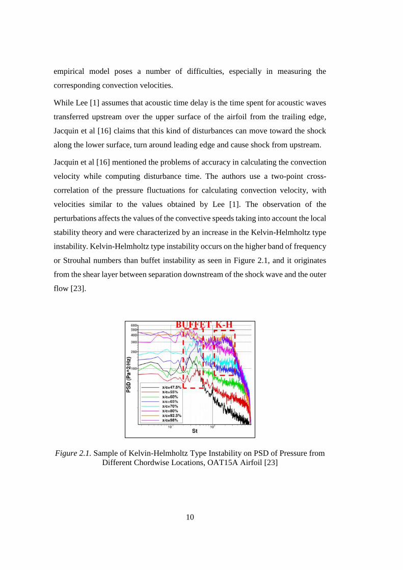
or Strouhal numbers than buffet instability as seen in Figure 2.1, and it originates
from the shear layer between separation downstream of the shock wave and the outer
flow [23].
Figure 2.1. Sample of Kelvin-Helmholtz Type Instability on PSD of Pressure from
Different Chordwise Locations, OAT15A Airfoil [23]
11
While the modified multiplication model better reflects the flow characteristics
observed in the experiments, the authors united into a common decision that a simple
and robust model is not able to fully reflect the characteristics of the flow. Shock
oscillations are caused by two modes of interaction; propagation of the disturbances
that arise from sensitive region of the shock foot and the propagation of these
disturbances through the convection of acoustic waves. A generalized common
model cannot be constructed due to the complex mechanisms of the constituent flow
according to the judgements of the authors.
2.2 Numerical Studies
In order to reflect the characteristics of the buffet phenomenon, several numerical
studies were conducted for examining the efficiency of U-RANS models [24], [25].
Moreover, several authors have reported good correlations for investigating buffet
characteristics with a Reynolds-averaged formulation [26]. The low frequency shock
of the transonic buffet explains the success of the U-RANS approach. Crouch et al
[7] have noted that global instability occurs in longer timescales than the
characteristic eddy timescales, at which mostly turbulent viscous shear layer flow is
seen on high Reynolds numbers. Thus, the fundamental buffet characteristics can be
predicted with high accuracy with U-RANS simulations. The representation of
complex characteristics of the buffet phenomenon involving turbulence with varying
scales with U-RANS simulations is highly dependent on the turbulence model,
spatial and temporal discretization, and the numerical scheme used.
The U-RANS models of the shock buffet phenomenon is especially affected by the
turbulence model. Barakos & Drikakis [27] studied the efficiency of various linear
and nonlinear eddy viscosity models (NLEVM) using a nonlinear regenerative
solution of Riemann solver of the third order spatial and second order temporal
accuracy [28]. The authors applied the experiments of McDevitt and Okuno [2] to
evaluate the performance of Baldwin-Lomax [29], Spalart-Allmaras [30], Launder-
12
Sharma [31] and Nagano-Kim [32] linear k-ε model and Sofialidis-Prinos k-ω
version [33] of the Craft-et al [34] nonlinear eddy-viscosity model for capturing
transonic shock oscillations on the NACA0012 airfoil. The results show that for high
angle of attack and Mach number conditions, Spalart-Allmaras and NLEVM models
can only give acceptable behavior of unsteady flow due to shock oscillation when
compared to the experimental results.
Baracos and Drikakis [27] stated that the k-ω model is not a very successful
turbulence model for reflecting unsteadiness for the buffet onset at low levels. In
addition, introducing a realizability correction to the model significantly improves
the behavior. The Spalart-Allmaras model can only predict the unsteady flow
behavior over the well-known frequency and amplitude characteristics of the buffet.
The Kok k-ω exhibits unsteady flow, although the onset of the oscillation is delayed
to a higher angle of attack. Wilcox and Menter's k-ω models cannot reproduce shock
oscillation without SST correction.
Kourta et al [35] found a time-dependent k-ε model [36] in which the model
coefficient 𝐶𝜇 is related to local levels of deformation and strain stress, which is well
achieved by calculating buffet on the OAT15A airfoil.
Xiao et al [37] have revealed that the lagged k-ω model of Olsen & Coakley [38]
showed a good prediction of the airfoil pressure distribution of BGK No. 1 airfoil in
buffet, but the magnitude of the oscillations is highly overestimated at the shock
wave. Carresse et al [39] and Giannelis & Vio [40] also discovered that the SST
model works significantly well with OAT15A airfoil.
13
CHAPTER 3
3 COMPUTATIONAL SOLUTION METHOD
Turbulence modeling is defined as computation of the turbulent flow using partial
differential equations [41]. The resultant approaches of turbulence modeling are
applicable for the Navier-Stokes equations. The flow variables are split into averaged
and unstable parts in the first place for the approach in the Reynolds Averaged
Navier-Stokes (RANS) equations. The stress tensor parameter is obtained by
addition of the Reynolds variables into the equation.
3.1 Navier-Stokes Equations for Compressible Flow
3.1.1 Continuity Equation
The continuity equation defines the conservation of mass of a moving fluid. The
change in density is obtained from the masses entering and leaving per unit time
[42]. The equation can be stated in tensor notation.
𝜕𝜌
𝜕𝑡+
𝜕
𝜕𝑥𝑖
(𝜌𝑢𝑖) = 0 (3.1)
𝜌 represents the gas density and 𝑢𝑖 are the flow velocity components.
3.1.2 Momentum Equation
Momentum equation states the motion of the gas flow according to Newton’s Second
Law of Motion. The summation of the external forces acting on the body gives the

14
product of the mass and acceleration [42] as it is represented using tensor notation
below:
𝜕
𝜕𝑡(𝜌𝑢𝑖) +
𝜕
𝜕𝑥𝑗(𝜌𝑢𝑖𝑢𝑗 + 𝑝𝛿𝑖𝑗 − 𝜏𝑖𝑗) = 𝜌𝑓𝑖 (3.2)
𝑝 is the gas pressure and 𝜏 is stress tensor, while 𝑓𝑖represents the acceleration of the
gas due to the body forces.
3.1.3 Energy Equation
The first law of thermodynamics is applied to the motion of the gas in order to obtain
the rate of change of the total energy of the gas with time in the equation. The energy
equation can be stated in tensor notation.
𝜕
𝜕𝑡(𝜌𝐸) +
𝜕
𝜕𝑥𝑖[ 𝜌𝑢𝑖𝑗 (𝐸 +
𝑝
𝜌) − 𝑟𝑖𝑗𝑢𝑖𝑗 + 𝑞𝑖] = 𝜌𝑓𝑖𝑢𝑖 (3.3)
The total specific energy of gas is represented as 𝐸 and the heat flux leaving the gas
as 𝑞 in the equation. The total specific energy consists of the internal and kinetic
energies.
𝐸 = 𝑒 +𝑈2
2 (3.4)
3.1.4 Thermodynamic Relation
For the thermodynamics relation through the fluid flow, the gas is considered as ideal
gas. The pressure, 𝑝 is related to the density 𝜌 and temperature 𝑇 of the ideal gas.
𝑝 = 𝜌𝑅𝑇 (3.5)
15
The specific energy can be obtained in relation with temperature and specific heat at
constant volume, 𝑐𝑣 for ideal gas. In a similar relation, the total specific energy can
be obtained by the relation of temperature and specific heat at constant pressure, 𝑐𝑝
for ideal gas.
𝑒 = 𝑐𝑣𝑇 =𝑝
(γ − 1) 𝜌 (3.6)
and,
ℎ = 𝑒 +𝑝
𝜌= 𝑐𝑝𝑇 =
γ𝑝
(γ − 1)𝜌 (3.7)
where 𝛾 is the ratio of specific heats defined as
𝛾 =𝐶𝑝
𝐶𝑣 (3.8)
3.1.5 Mach Number and Speed of Sound
The speed of sound for ideal gas is related to the heat capacity ratio 𝛾 and
temperature.
𝑎 = √γp
𝜌= √γRT (3.9)
Mach number is basically division of the flow speed by speed of sound.
𝑀 =𝑢
𝑎=
𝑢
√γRT (3.10)
16
3.1.6 Reynolds Number and Strouhal Number
The Reynolds number is basically defined as the ratio between inertia forces to the
viscous forces.
𝑅𝑒 =𝜌𝑢𝑙𝑟𝑒𝑓
𝜇 (3.11)
Where 𝜇 represents the dynamic viscosity. The Reynolds number is used for the
determination of the flow transition from laminar to turbulent [42].
On the other hand, for the separation and vortex formation, the dimensionless
frequency as Strouhal number is defined.
𝑆𝑡 =2𝜋𝑓𝑙𝑟𝑒𝑓
𝑢 (3.12)
Where 𝑓 is defined as the frequency of the vortex shedding. Strouhal number is used
for the determination of the characteristics of the buffet phenomenon on airfoils and
wings. It is a discriminative parameter for the identification of the buffet onset on
airfoil.
3.2 Reynolds Averaged Navier-Stokes (RANS) Equations
Reynolds Averaged Navier-Stokes equations are obtained as the implementation of
the Reynolds time average to the incompressible form of the Navier-Stokes
equations. The additional terms due to time average in the continuity equation is
stated in Eq. (3.13).
𝜕𝑢𝚤
𝜕𝑡+ 𝑢𝑗
𝜕𝑢𝚤
𝜕𝑡+
1
𝜌
𝜕𝑝
𝜕𝑥𝚤
=
𝜕𝑢𝚤
𝜕𝑡
+ 𝑢𝑗
𝜕𝑢𝚤
𝜕𝑥𝑗
+
1
𝜌
𝜕𝑝
𝜕𝑥𝚤
=
1
𝜌
𝜕𝜏𝚤𝑗
𝜕𝑥𝑗
(3.13)
Each term that is averaged over time can be expressed with index.
17
𝜕𝑢𝚤
𝜕𝑡
=
𝜕𝑈𝑖
𝜕𝑡 (3.14)
1
𝜌
𝜕𝑝
𝜕𝑥𝚤
=
1
𝜌
𝜕𝑝
𝜕𝑥𝚤
=
1
𝜌
𝜕𝑃
𝜕𝑥𝑖 (3.15)
1
𝜌
𝜕𝜏𝚤𝑗
𝜕𝑥𝑗
=
1
𝜌
𝜕𝜏𝚤𝑗
𝜕𝑥𝑗
=
2
𝜌𝜌𝑣
𝜕𝑆𝚤𝑗
𝜕𝑥𝑗
= 2𝑣
𝜕𝑆𝚤𝑗
𝜕𝑥𝑗 (3.16)
𝑆𝚤𝑗 =
1
2[𝜕𝑈𝑖
𝜕𝑥𝑗+
𝜕𝑈𝑗
𝜕𝑥𝑗] (3.17)
Where 𝑆𝚤𝑗 represents the time average of stress.
𝑢𝑗
𝜕𝑢𝚤
𝜕𝑥𝑗
=
𝜕
𝜕𝑥𝑗(𝑢𝚤𝑢𝑗)
− 𝑢𝚤
𝜕𝑢𝑗
𝜕𝑥𝑗
=
𝜕
𝜕𝑥𝑗(𝑈𝑖𝑈𝑗) + 𝑢𝚤
′𝑢𝑗′
=𝜕
𝜕𝑥𝑗(𝑈𝑖𝑈𝑗) +
𝜕
𝜕𝑥𝑗(𝑢𝚤
′𝑢𝑗′ )
= 𝑈𝑗
𝜕𝑈𝑖
𝜕𝑥𝑗+ 𝑈𝑖
𝜕𝑈𝑗
𝜕𝑥𝑗+
𝜕
𝜕𝑥𝑗(𝑢𝚤
′𝑢𝑗′ )
= 𝑈𝑗
𝜕𝑈𝑖
𝜕𝑥𝑗+
𝜕
𝜕𝑥𝑗(𝑢𝚤
′𝑢𝑗′ )
(3.18)
Finally,
𝜕𝑈𝑖
𝜕𝑡+ 𝑈𝑗
𝜕𝑈𝑖
𝜕𝑥𝑗+
1
𝜌
𝜕𝑃
𝜕𝑥𝑖=
1
𝜌
𝜕
𝜕𝑥𝑗(2𝜇𝑆𝚤𝑗
− 𝜌𝑢𝚤′𝑢𝑗
′ ) (3.19)
The amount of averaged flow is defined from 𝑈𝑖 and 𝑃.
𝜕𝑈𝑖
𝜕𝑥𝑗= 0 (3.20)
18
𝜕𝑈𝑖
𝜕𝑡+ 𝑈𝑗
𝜕𝑈𝑖
𝜕𝑥𝑗+
1
𝜌
𝜕𝑃
𝜕𝑥𝑖=
1
𝜌
𝜕
𝜕𝑥𝑗(𝜏𝚤𝑗 − 𝜆𝑖𝑗) (3.21)
𝜏𝚤𝑗 symbolizes the stress tensor of the fluid in terms of average flow amount and 𝜆𝑖𝑗
symbolizes the eddy stress tensor.
𝜆𝑖𝑗 = 𝜌𝑢𝚤′𝑢𝑗
′ (3.22)
The RANS equations for the compressible flow is stated as in the following
equations as the final form.
𝜕��
𝜕𝑡+
𝜕
𝜕𝑥𝑗(��𝑢𝑗) = 0 (3.23)
𝜕��𝑢𝑖
𝜕𝑡+
𝜕
𝜕𝑥𝑗(𝑢𝑗��𝑢𝑗) = −
𝜕𝑃
𝜕𝑥𝑖+
𝜕𝜎𝚤𝑗
𝜕𝑥𝑗+
𝜕𝜏𝑖𝑗
𝜕𝑥𝑗 (3.24)
𝜕��𝑒
𝜕𝑡+
𝜕
𝜕𝑥𝑗(𝑢𝑗��ℎ) =
𝜕
𝜕𝑥𝑗(𝜎𝚤𝑗 𝑢𝑖 + 𝜎𝚤𝑗𝑢𝚤
′′ )
−𝜕
𝜕𝑥𝑗(𝑞�� + 𝑐𝑝𝜌𝑢𝑗
′′𝑇′′ − 𝑢𝑖𝜏𝑖𝑗 +1
2𝜌𝑢𝚤
′′𝑢𝚤′′𝑢𝑗
′′ )
(3.25)
The energy equation includes the viscous stress tensor and the approximation of the
term for the compressible fluid with the Stoke’s hypothesis [42] and can be stated as
in Eq. (3.26).
𝜎𝚤𝑗 ~2𝜇(𝑆𝑖𝑗 −1
3
𝜕𝑢𝑘
𝜕𝑥𝑘𝛿𝑖𝑗) (3.26)
From the assumption of
𝜆 = −2
3𝜇 (3.27)
19
3.3 RANS Equations Turbulence Models
RANS turbulence models are divided into 4 different classes. The classification is
mainly constructed based on the equation number that is used on the model and the
convection relation.
i. Zero Equation Model: Mean Velocity Field MVF Model is developed by
Mellor and Herring [43]. There are four main models which represent
Mean Velocity Field.
a. Eddy-Viscosity Model for Reynolds Stress Tensor
b. Vortex Model with Zero Equations
c. Eddy-Viscosity Form
i. Cebeci-Smith Model
ii. Baldwin-Lomax Model
d. Half Equation Model
ii. One Equation Model: The velocity ratio is calculated by taking into
account the transport equation in this model, apart from Zero Equation
Model. There are four main models which represent One Equation
Model.
a. Full Kinetic Energy Transport Equation
b. Modeled Kinetic Energy Transport Equation
c. One Equation Vortex Model
d. Modeled Eddy-Viscosity Transport Equation
e. Spalart-Allmaras Model
iii. Two Equation Model: Calculation of the turbulence length ratio by taking
into account the convection equation is added as the second equation to
the Single Equation Model. One and Two Equation Models are also
called Mean Turbulent Energy (MTE) Models. There are seven main
models which represent Two Equation Model.
a. Kinetic Energy Transport Equation
b. Full Diffusion-Rational Transport Equation
20
c. Modeled Diffusion-Rational Transport Equation
d. k-ε Model
e. k-kL Model
f. k-ω Model
g. Irregular Eddy-Viscosity Model
iv. Stress Equation Model: The model is obtained through adding convection
equations as Reynolds stress tensor (𝜏𝑖𝑗 ) and scalar propagation rate
(𝜏𝑖𝑗 − 휀) to the Zero Equation Model. There are seven main models
which represent Stress Equation Model.
a. Diffusion-Rational Transport Equation
b. Full Reynolds-Stress Transport Equation
c. Pressure Detached Correlation
d. Diffusion-Rational Correlation
e. Diffusion Correlation
f. Stress-Equation Vortex Model
g. Irregular Pressure-Stress Correlation Model
In order to obtain the most applicable representation of the turbulent flow around
buffet onset on airfoil, three different types of turbulence models were used in this
study. Spalart-Allmaras, k-ω SST and k-ε models are used and the comparative
results are stated for the most suitable solution.
3.3.1 Spalart-Allmaras Turbulence Model
The Spalart-Allmaras model is a one-equation model that has a single transport
equation for eddy viscosity. The implementation of the model in aerodynamics gives
satisfactory results, especially for wall limited flows and reverse flows.
21
The boundary layer flows with a pressure gradient is the main design point of the
model. The Spalart-Allmaras model is generally effective at low Reynolds numbers
where viscosity affects the boundary layer (y +~1 solution networks).
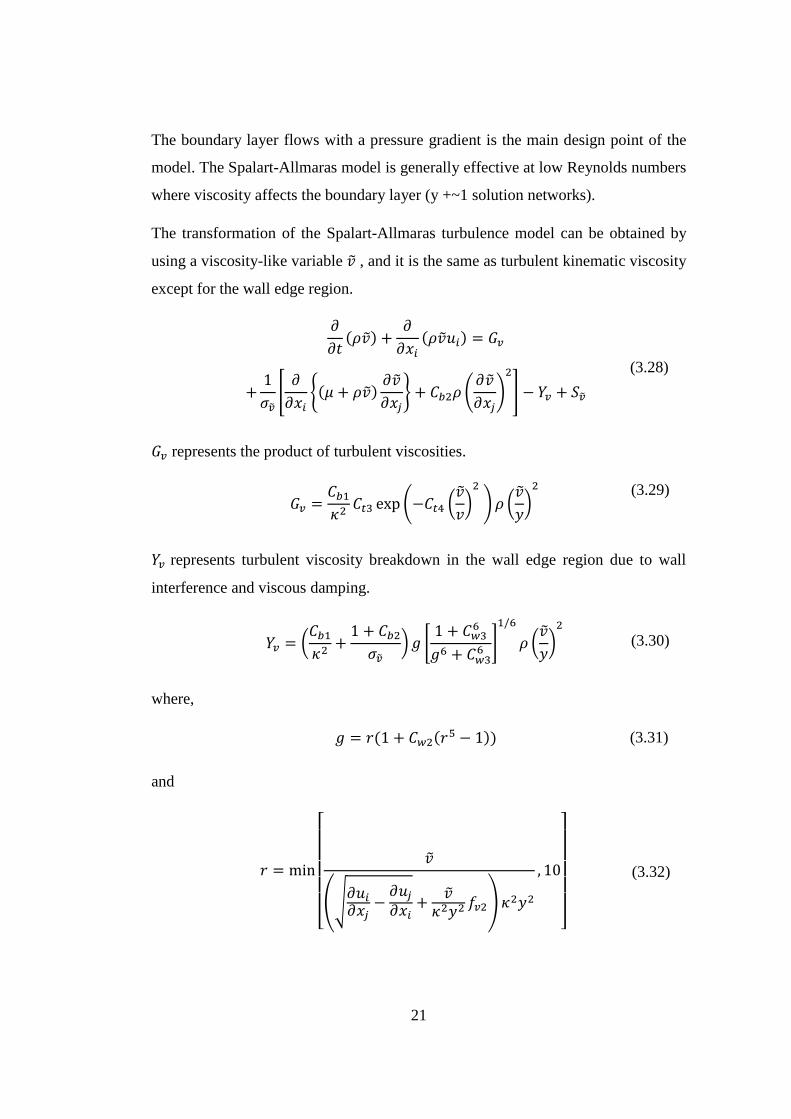
The transformation of the Spalart-Allmaras turbulence model can be obtained by
using a viscosity-like variable �� , and it is the same as turbulent kinematic viscosity
except for the wall edge region.
𝜕
𝜕𝑡(𝜌��) +
𝜕
𝜕𝑥𝑖
(𝜌��𝑢𝑖) = 𝐺𝑣
+1
𝜎��[
𝜕
𝜕𝑥𝑖{(𝜇 + 𝜌��)
𝜕��
𝜕𝑥𝑗} + 𝐶𝑏2𝜌 (
𝜕��
𝜕𝑥𝑗)
2
] − 𝑌𝑣 + 𝑆��
(3.28)
𝐺𝑣 represents the product of turbulent viscosities.
𝐺𝑣 =
𝐶𝑏1
𝜅2𝐶𝑡3 exp (−𝐶𝑡4 (
��
𝑣)2
) 𝜌 (��
𝑦)2
(3.29)
𝑌𝑣 represents turbulent viscosity breakdown in the wall edge region due to wall
interference and viscous damping.
𝑌𝑣 = (𝐶𝑏1
𝜅2+
1 + 𝐶𝑏2
𝜎��)𝑔 [
1 + 𝐶𝑤36
𝑔6 + 𝐶𝑤36 ]
1/6
𝜌 (��
𝑦)2
(3.30)
where,
𝑔 = 𝑟(1 + 𝐶𝑤2(𝑟5 − 1)) (3.31)
and
𝑟 = min
[
��
(√𝜕𝑢𝑖
𝜕𝑥𝑗−
𝜕𝑢𝑗
𝜕𝑥𝑖+
��𝜅2𝑦2 𝑓𝑣2)𝜅2𝑦2
, 10
]
(3.32)
22
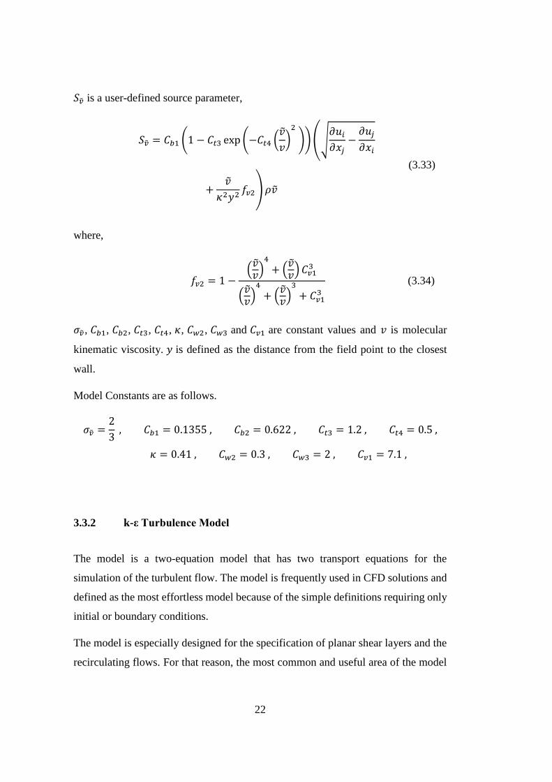
𝑆�� is a user-defined source parameter,
𝑆�� = 𝐶𝑏1 (1 − 𝐶𝑡3 exp (−𝐶𝑡4 (��
𝑣)2
))(√𝜕𝑢𝑖
𝜕𝑥𝑗−
𝜕𝑢𝑗
𝜕𝑥𝑖
+��
𝜅2𝑦2𝑓𝑣2)𝜌��
(3.33)
where,
𝑓𝑣2 = 1 −(��𝑣)
4
+ (��𝑣)𝐶𝑣1
3
(��𝑣)
4
+ (��𝑣)
3
+ 𝐶𝑣13
(3.34)
𝜎�� , 𝐶𝑏1, 𝐶𝑏2, 𝐶𝑡3, 𝐶𝑡4, 𝜅, 𝐶𝑤2, 𝐶𝑤3 and 𝐶𝑣1 are constant values and 𝑣 is molecular
kinematic viscosity. 𝑦 is defined as the distance from the field point to the closest
wall.
Model Constants are as follows.
𝜎�� =2
3 , 𝐶𝑏1 = 0.1355 , 𝐶𝑏2 = 0.622 , 𝐶𝑡3 = 1.2 , 𝐶𝑡4 = 0.5 ,
𝜅 = 0.41 , 𝐶𝑤2 = 0.3 , 𝐶𝑤3 = 2 , 𝐶𝑣1 = 7.1 ,
3.3.2 k-ε Turbulence Model
The model is a two-equation model that has two transport equations for the
simulation of the turbulent flow. The model is frequently used in CFD solutions and
defined as the most effortless model because of the simple definitions requiring only
initial or boundary conditions.
The model is especially designed for the specification of planar shear layers and the
recirculating flows. For that reason, the most common and useful area of the model
23
is the cases with planar shear layers with small pressure gradients or with the
Reynolds shear stresses are fundamental. The cases with complex shear layers or
large pressure gradients could not be modeled easily and accurately with k-ε model
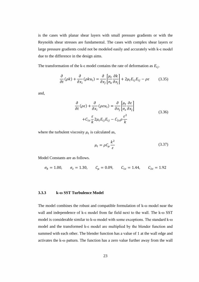
due to the difference in the design aims.
The transformation of the k-ε model contains the rate of deformation as 𝐸𝑖𝑗.
𝜕
𝜕𝑡(𝜌𝑘) +
𝜕
𝜕𝑥𝑖
(𝜌𝑘𝑢𝑖) =𝜕
𝜕𝑥𝑗[𝜇𝑡
𝜎𝑘
𝜕𝑘
𝜕𝑥𝑗] + 2𝜇𝑡𝐸𝑖𝑗𝐸𝑖𝑗 − 𝜌휀 (3.35)
and,
𝜕
𝜕𝑡(𝜌휀) +
𝜕
𝜕𝑥𝑖
(𝜌휀𝑢𝑖) =𝜕
𝜕𝑥𝑗[𝜇𝑡
𝜎𝜀
𝜕휀
𝜕𝑥𝑗]
+𝐶1𝜀
휀
𝑘2𝜇𝑡𝐸𝑖𝑗𝐸𝑖𝑗 − 𝐶2𝜀𝜌
휀2
𝑘
(3.36)
where the turbulent viscosity 𝜇𝑡 is calculated as,
𝜇𝑡 = 𝜌𝐶𝜇
𝑘2
휀 (3.37)
Model Constants are as follows.
𝜎𝑘 = 1.00, 𝜎𝜀 = 1.30, 𝐶𝜇 = 0.09, 𝐶1𝜀 = 1.44, 𝐶2𝜀 = 1.92
3.3.3 k-ω SST Turbulence Model
The model combines the robust and compatible formulation of k-ω model near the
wall and independence of k-ε model from far field next to the wall. The k-ω SST
model is considerable similar to k-ω model with some exceptions. The standard k-ω
model and the transformed k-ε model are multiplied by the blender function and
summed with each other. The blender function has a value of 1 at the wall edge and
activates the k-ω pattern. The function has a zero value further away from the wall
24
and causes activation of the k-ε model. Another difference between standard k-ω and
SST is that in the equation, SST model includes the effect of the damped cross
diffusion. For the SST model, the turbulent viscosity is redefined by taking into
account the turbulent shear stress transport. As SST model has some additional
features compared to standard k-ω model, the modelling constants are different from
each other and the SST model can be considered as more reliable and compatible
with several flow cases than k-ω model, especially at adverse pressure gradient
flows.
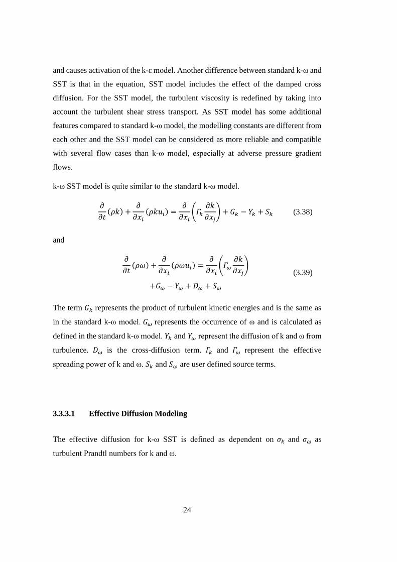
k-ω SST model is quite similar to the standard k-ω model.
𝜕
𝜕𝑡(𝜌𝑘) +
𝜕
𝜕𝑥𝑖
(𝜌𝑘𝑢𝑖) =𝜕
𝜕𝑥𝑖(𝛤𝑘
𝜕𝑘
𝜕𝑥𝑗) + 𝐺𝑘 − 𝑌𝑘 + 𝑆𝑘 (3.38)
and
𝜕
𝜕𝑡(𝜌𝜔) +
𝜕
𝜕𝑥𝑖
(𝜌𝜔𝑢𝑖) =𝜕
𝜕𝑥𝑖(𝛤𝜔
𝜕𝑘
𝜕𝑥𝑗)
+𝐺𝜔 − 𝑌𝜔 + 𝐷𝜔 + 𝑆𝜔
(3.39)
The term 𝐺𝑘 represents the product of turbulent kinetic energies and is the same as
in the standard k-ω model. 𝐺𝜔 represents the occurrence of ω and is calculated as
defined in the standard k-ω model. 𝑌𝑘 and 𝑌𝜔 represent the diffusion of k and ω from
turbulence. 𝐷𝜔 is the cross-diffusion term. 𝛤𝑘 and 𝛤𝜔 represent the effective
spreading power of k and ω. 𝑆𝑘 and 𝑆𝜔 are user defined source terms.
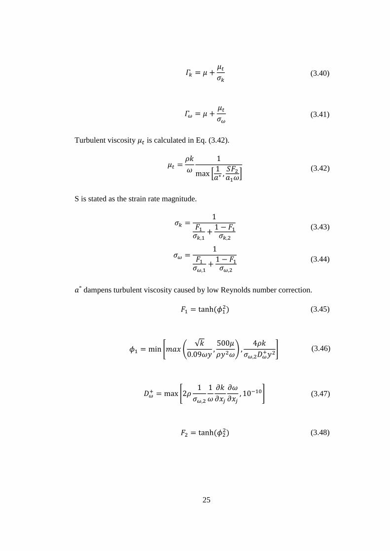
3.3.3.1 Effective Diffusion Modeling
The effective diffusion for k-ω SST is defined as dependent on 𝜎𝑘 and 𝜎𝜔 as
turbulent Prandtl numbers for k and ω.
25
𝛤𝑘 = 𝜇 +𝜇𝑡
𝜎𝑘 (3.40)
𝛤𝜔 = 𝜇 +𝜇𝑡
𝜎𝜔 (3.41)
Turbulent viscosity 𝜇𝑡 is calculated in Eq. (3.42).
𝜇𝑡 =
𝜌𝑘
𝜔
1
max [1𝑎∗ ,
𝑆𝐹2
𝑎1𝜔]
(3.42)
S is stated as the strain rate magnitude.
𝜎𝑘 =
1
𝐹1
𝜎𝑘,1+
1 − 𝐹1
𝜎𝑘,2
(3.43)
𝜎𝜔 =
1
𝐹1
𝜎𝜔,1+
1 − 𝐹1
𝜎𝜔,2
(3.44)
𝑎* dampens turbulent viscosity caused by low Reynolds number correction.
𝐹1 = tanh (𝜙12) (3.45)
𝜙1 = min [𝑚𝑎𝑥 (√𝑘
0.09𝜔𝑦,500𝜇
𝜌𝑦2𝜔) ,
4𝜌𝑘
𝜎𝜔,2𝐷𝜔+𝑦2
] (3.46)
𝐷𝜔+ = max [2𝜌
1
𝜎𝜔,2
1
𝜔
𝜕𝑘
𝜕𝑥𝑗
𝜕𝜔
𝜕𝑥𝑗, 10−10] (3.47)
𝐹2 = tanh (𝜙22) (3.48)
26
𝜙2 = max [2√𝑘
0.09𝜔𝑦,500𝜇
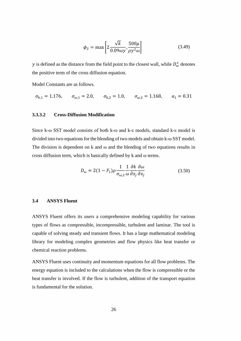
𝜌𝑦2𝜔] (3.49)
𝑦 is defined as the distance from the field point to the closest wall, while 𝐷𝜔+ denotes
the positive term of the cross diffusion equation.
Model Constants are as follows.
𝜎𝑘,1 = 1.176, 𝜎𝜔,1 = 2.0, 𝜎𝑘,2 = 1.0, 𝜎𝜔,2 = 1.168, 𝑎1 = 0.31
3.3.3.2 Cross-Diffusion Modification
Since k-ω SST model consists of both k-ω and k-ε models, standard k-ε model is
divided into two equations for the blending of two models and obtain k-ω SST model.
The division is dependent on k and ω and the blending of two equations results in
cross diffusion term, which is basically defined by k and ω terms.
𝐷𝜔 = 2(1 − 𝐹1)𝜌1
𝜎𝜔,2
1
𝜔
𝜕𝑘
𝜕𝑥𝑗
𝜕𝜔
𝜕𝑥𝑗 (3.50)
3.4 ANSYS Fluent
ANSYS Fluent offers its users a comprehensive modeling capability for various
types of flows as compressible, incompressible, turbulent and laminar. The tool is
capable of solving steady and transient flows. It has a large mathematical modeling
library for modeling complex geometries and flow physics like heat transfer or
chemical reaction problems.
ANSYS Fluent uses continuity and momentum equations for all flow problems. The
energy equation is included to the calculations when the flow is compressible or the
heat transfer is involved. If the flow is turbulent, addition of the transport equation
is fundamental for the solution.

27
The typical vector notation is used for the definition of the continuity equation in
ANSYS Fluent environment and the equation is applicable for both compressible
and incompressible flows.
𝜕𝜌
𝜕𝑡+ ∇. (𝜌�� ) = 𝑆𝑚 (3.51)
The source 𝑆𝑚 is the mass added to the continuous side from the discrete side or
user-defined source.
Conservation of momentum equation can be stated as vector notation.
𝜕𝜌
𝜕𝑡. (𝜌�� ) + ∇. (𝜌�� �� ) = −∇p + ∇. (𝜏) + 𝜌𝑔 + 𝐹 (3.52)

29
CHAPTER 4
4 STEADY ANALYSES
The steady analyses are conducted for several flight conditions. The purpose is to
investigate the optimum mesh and boundary conditions for converged and validated
steady flow results, together with the examination of the flow field in the stable
region, which is just before the buffet onset. For this purpose, the two dimensional
NACA0012 airfoil model is constructed in Ansys Fluent Design Modeler
environment. The mesh is constructed using the unstructured quadrilateral grid
method. After the mesh is obtained, the boundary conditions for the required flight
characteristics are applied to the flow for the analysis. All the analyses are conducted
with density-based solver for viscous fluids. Several mesh resolutions and turbulence
models have been applied in order to investigate the converged solution, which has
the closest results to the wind tunnel data.
The three flow conditions corresponding to the conditions of the wind tunnel data
[2] have been analyzed in the Ansys Fluent environment, marked with red in Figure
4.1 and listed in Table 4.1. Detailed explanation of all analyses and the detailed
results made throughout the study was made on Dataset 4. For the other two
conditions of Dataset 5 and 6, only the apparent results were shared. The grid spacing
and Reynolds numbers for the condition are calculated as an input to the mesh and
boundary conditions.
30
Table 4.1. Analyzed Flow Condition [2]
Dataset M α (°)
Dataset 4 0.800 1
Dataset 5 0.775 2
Dataset 6 0.725 4
Figure 4.1. Buffet Onset Boundary of NACA0012 Airfoil [2]
4.1 Reynolds Number and Grid Spacing
The Reynolds number and the grid spacing effect the mesh quality as they indicate
the difference between viscous forces and inertial forces around surface. The
Reynolds number affects the boundary conditions directly in the analyses. In
addition, the turbulence in the viscous flow is determined with Reynolds number.
According to the Reynolds number of the determined flow condition, grid spacing is
31
obtained and applied to the mesh resolution in order to successfully resolve the
boundary layer.
The required data in order to calculate the Reynolds number and grid spacing is
stated in Table 4.2.
Table 4.2. Standard Atmospheric Conditions of the Streamflow over Airfoil
Dataset 4 (M0.800 α=1°) 5 (M0.775 α=2°) 6 (M0.725 α=4°)
a (m/s) 340.3 340.3 340.3
M 0.800 0.775 0.725
V (m/s) 272.24 263.73 246.72
ρ (kg/m^3) 1.225 1.225 1.225
lref (m) 0.2032 0.2032 0.2032
Firstly, Reynolds number is calculated with given conditions from Eq. (3.11).
The first layer of boundary layer thickness ∆s is calculated according to the turbulent
boundary layer theory. The y+ value is defined individually according to the
turbulence model used for the solution.
The skin friction coefficient distribution is then calculated from Eq. (4.53).
𝐶𝑓 =0.026
𝑅𝑒17
(4.53)
The momentum integral relation is calculated according to the skin friction
coefficient.
32
τwall =𝐶𝑓ρU∞
2
2 (4.54)
The friction velocity is obtained from the law of the wall in Eq. (4.55).
𝑈𝑓𝑟𝑖𝑐 = √τwall
ρ (4.55)
Finally, the first layer of boundary layer thickness is obtained in relation with y+
and friction velocity.
∆𝑠 =𝑦+μ
Ufricρ (4.56)
The total thickness of boundary layer is calculated from turbulent boundary layer
theory, in relation with Reynolds number and reference length.
𝛿 =0.37𝐿
𝑅𝑒0.2 (4.57)
The layer number is defined so as to obtain the required total thickness of the
boundary layer from the first layer thickness. In order to obtain a smooth transition,
a constant growth rate is used for the transition layers. In all of the mesh models of
this study, growth rate is chosen as 1.2 for the transition layers.
Grid spacing values vary due to each analyzed flow condition. Thus, for each flow
condition, the grid spacing value differs in the mesh resolution.
4.2 Mesh Independence
The solid model of the NACA0012 airfoil is constructed in Design Modeler tool of
Ansys Fluent. The nodes on the airfoil are obtained as 201 points from Javafoil tool.
O Type grid around airfoil and C Type grid through the control volume is applied.
The airfoil chord is chosen as 0.2032 meters (8 inch) in order to be consistent with
the wind tunnel model which is used for the wind tunnel tests of buffet onset
33
investigation in NASA Ames High Reynolds Number Facility [2]. The radius of the
arc around airfoil leading edge is 7 times of the chord and the length of wall around
airfoil is 14 times the chord. The grid is finer in a circle with radius of 1.5 times of
the chord around the airfoil. The grid is also finer at the trailing edge of the airfoil
through the outlet wall with a thickness around 1.4 times of the chord in order to
examine the turbulent flow characteristics in detail due to flow separation on airfoil.
The area out of the circle around airfoil and the rectangular field to the outer wall is
coarser than the inside. The mesh pattern is retained with the growth rate as 1.2
between coarse and fine areas in order to keep the smooth transition with acceptable
orthogonal quality and skewness ratios.
Figure 4.2. Sample Grid Spacing of Geometry with 89K Mesh Elements
Since the shape of trailing edge of the airfoil deviates from the origin for practical
reasons during manufacturing, the CFD model is also trimmed at the trailing edge in
order to be consistent with the wind tunnel model. The deviation from the
mathematical model of NACA0012 airfoil was around ∆x/c≈0.01. Due to the
deviation in the trailing edge, the mesh resolution also includes the element sizing of
the trailing edge surface individually. The mesh nodes of the trailing edge are chosen
1.4224
0.6096 2.8448 0.2845
2.8448
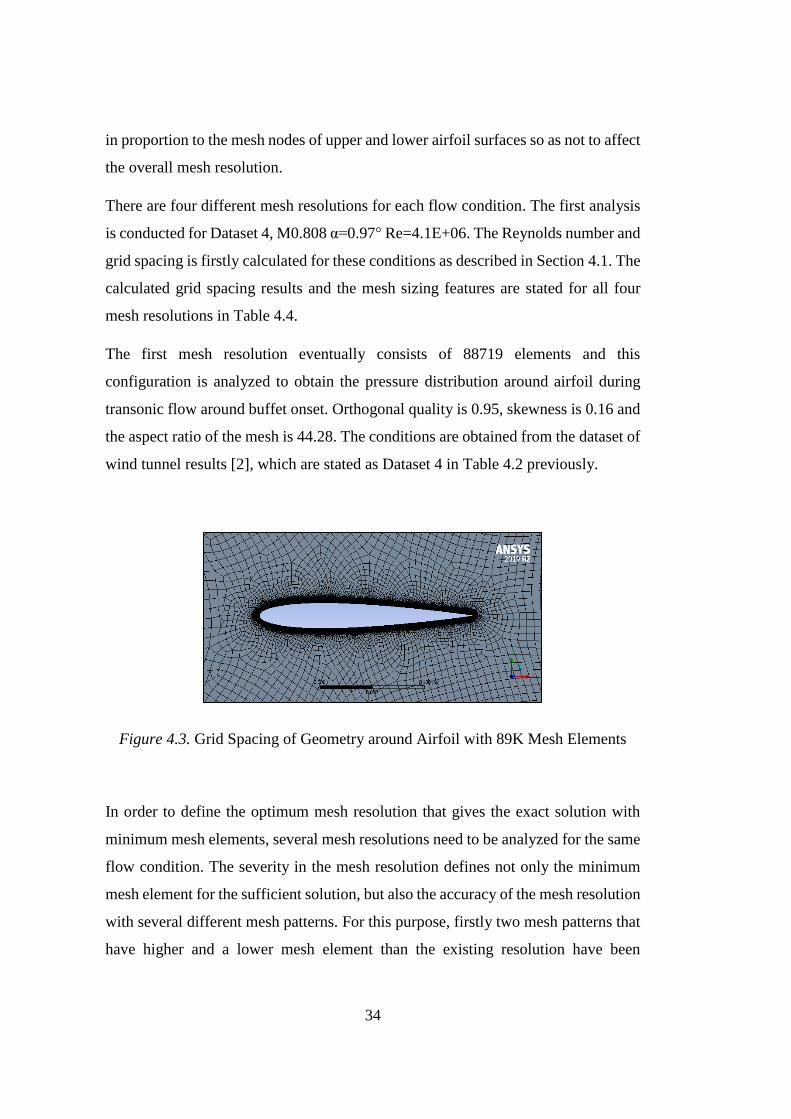
34
in proportion to the mesh nodes of upper and lower airfoil surfaces so as not to affect
the overall mesh resolution.
There are four different mesh resolutions for each flow condition. The first analysis
is conducted for Dataset 4, M0.808 α=0.97° Re=4.1E+06. The Reynolds number and
grid spacing is firstly calculated for these conditions as described in Section 4.1. The
calculated grid spacing results and the mesh sizing features are stated for all four
mesh resolutions in Table 4.4.
The first mesh resolution eventually consists of 88719 elements and this
configuration is analyzed to obtain the pressure distribution around airfoil during
transonic flow around buffet onset. Orthogonal quality is 0.95, skewness is 0.16 and
the aspect ratio of the mesh is 44.28. The conditions are obtained from the dataset of
wind tunnel results [2], which are stated as Dataset 4 in Table 4.2 previously.
Figure 4.3. Grid Spacing of Geometry around Airfoil with 89K Mesh Elements
In order to define the optimum mesh resolution that gives the exact solution with
minimum mesh elements, several mesh resolutions need to be analyzed for the same
flow condition. The severity in the mesh resolution defines not only the minimum
mesh element for the sufficient solution, but also the accuracy of the mesh resolution
with several different mesh patterns. For this purpose, firstly two mesh patterns that
have higher and a lower mesh element than the existing resolution have been
35
analyzed with the same flow condition. The ratio between new and existing mesh
resolutions is kept as 1.5 as a rule of thumb.
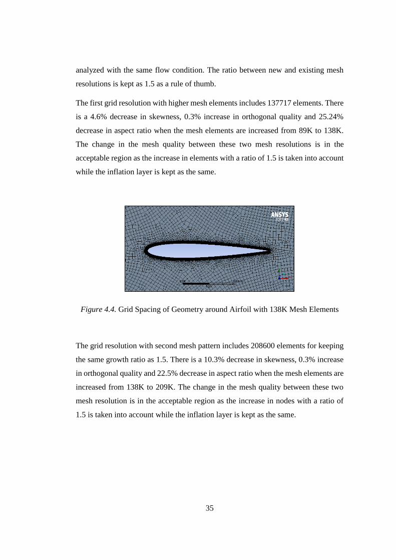
The first grid resolution with higher mesh elements includes 137717 elements. There
is a 4.6% decrease in skewness, 0.3% increase in orthogonal quality and 25.24%
decrease in aspect ratio when the mesh elements are increased from 89K to 138K.
The change in the mesh quality between these two mesh resolutions is in the
acceptable region as the increase in elements with a ratio of 1.5 is taken into account
while the inflation layer is kept as the same.
Figure 4.4. Grid Spacing of Geometry around Airfoil with 138K Mesh Elements
The grid resolution with second mesh pattern includes 208600 elements for keeping
the same growth ratio as 1.5. There is a 10.3% decrease in skewness, 0.3% increase
in orthogonal quality and 22.5% decrease in aspect ratio when the mesh elements are
increased from 138K to 209K. The change in the mesh quality between these two
mesh resolution is in the acceptable region as the increase in nodes with a ratio of
1.5 is taken into account while the inflation layer is kept as the same.
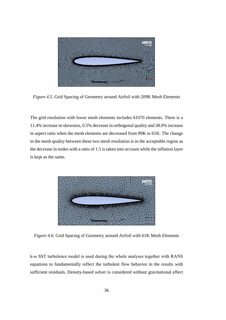
36
Figure 4.5. Grid Spacing of Geometry around Airfoil with 209K Mesh Elements
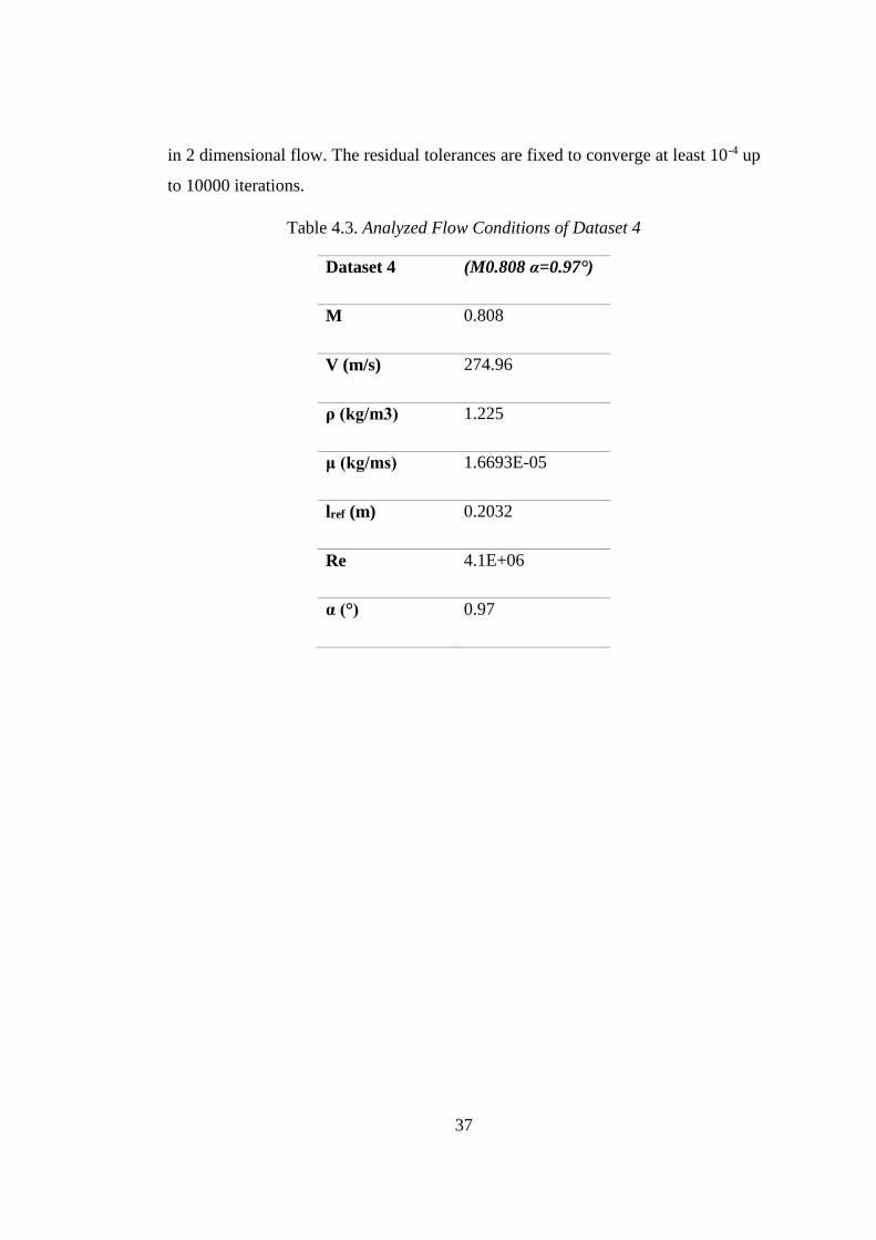
The grid resolution with lower mesh elements includes 61070 elements. There is a
11.4% increase in skewness, 0.5% decrease in orthogonal quality and 38.0% increase
in aspect ratio when the mesh elements are decreased from 89K to 61K. The change
in the mesh quality between these two mesh resolution is in the acceptable region as
the decrease in nodes with a ratio of 1.5 is taken into account while the inflation layer
is kept as the same.
Figure 4.6. Grid Spacing of Geometry around Airfoil with 61K Mesh Elements
k-ω SST turbulence model is used during the whole analyses together with RANS
equations to fundamentally reflect the turbulent flow behavior in the results with
sufficient residuals. Density-based solver is considered without gravitational effect
37
in 2 dimensional flow. The residual tolerances are fixed to converge at least 10-4 up
to 10000 iterations.
Table 4.3. Analyzed Flow Conditions of Dataset 4
Dataset 4 (M0.808 α=0.97°)
M 0.808
V (m/s) 274.96
ρ (kg/m3) 1.225
μ (kg/ms) 1.6693E-05
lref (m) 0.2032
Re 4.1E+06
α (°) 0.97
38
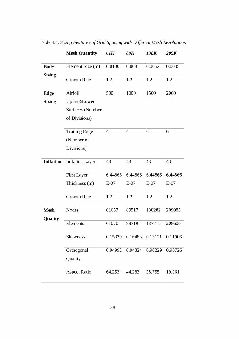
Table 4.4. Sizing Features of Grid Spacing with Different Mesh Resolutions
Mesh Quantity 61K 89K 138K 209K
Body
Sizing
Element Size (m) 0.0100 0.008 0.0052 0.0035
Growth Rate 1.2 1.2 1.2 1.2
Edge
Sizing
Airfoil
Upper&Lower
Surfaces (Number
of Divisions)
500 1000 1500 2000
Trailing Edge
(Number of
Divisions)
4 4 6 6
Inflation Inflation Layer 43 43 43 43
First Layer
Thickness (m)
6.44866
E-07
6.44866
E-07
6.44866
E-07
6.44866
E-07
Growth Rate 1.2 1.2 1.2 1.2
Mesh
Quality
Nodes 61657 89517 138282 209085
Elements 61070 88719 137717 208600
Skewness 0.15339 0.16483 0.13121 0.11906
Orthogonal
Quality
0.94992 0.94824 0.96229 0.96726
Aspect Ratio 64.253 44.283 28.755 19.261
39
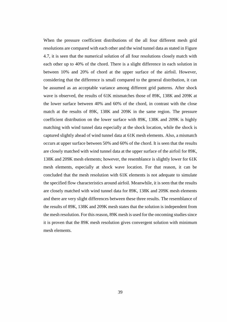
When the pressure coefficient distributions of the all four different mesh grid
resolutions are compared with each other and the wind tunnel data as stated in Figure
4.7, it is seen that the numerical solution of all four resolutions closely match with
each other up to 40% of the chord. There is a slight difference in each solution in
between 10% and 20% of chord at the upper surface of the airfoil. However,
considering that the difference is small compared to the general distribution, it can
be assumed as an acceptable variance among different grid patterns. After shock
wave is observed, the results of 61K mismatches those of 89K, 138K and 209K at
the lower surface between 40% and 60% of the chord, in contrast with the close
match at the results of 89K, 138K and 209K in the same region. The pressure
coefficient distribution on the lower surface with 89K, 138K and 209K is highly
matching with wind tunnel data especially at the shock location, while the shock is
captured slightly ahead of wind tunnel data at 61K mesh elements. Also, a mismatch
occurs at upper surface between 50% and 60% of the chord. It is seen that the results
are closely matched with wind tunnel data at the upper surface of the airfoil for 89K,
138K and 209K mesh elements; however, the resemblance is slightly lower for 61K
mesh elements, especially at shock wave location. For that reason, it can be
concluded that the mesh resolution with 61K elements is not adequate to simulate
the specified flow characteristics around airfoil. Meanwhile, it is seen that the results
are closely matched with wind tunnel data for 89K, 138K and 209K mesh elements
and there are very slight differences between these three results. The resemblance of
the results of 89K, 138K and 209K mesh states that the solution is independent from
the mesh resolution. For this reason, 89K mesh is used for the oncoming studies since
it is proven that the 89K mesh resolution gives convergent solution with minimum
mesh elements.
40
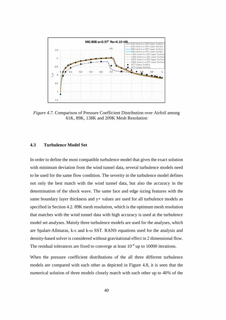
Figure 4.7. Comparison of Pressure Coefficient Distribution over Airfoil among
61K, 89K, 138K and 209K Mesh Resolution
4.3 Turbulence Model Set
In order to define the most compatible turbulence model that gives the exact solution
with minimum deviation from the wind tunnel data, several turbulence models need
to be used for the same flow condition. The severity in the turbulence model defines
not only the best match with the wind tunnel data, but also the accuracy in the
determination of the shock wave. The same face and edge sizing features with the
same boundary layer thickness and y+ values are used for all turbulence models as
specified in Section 4.2. 89K mesh resolution, which is the optimum mesh resolution
that matches with the wind tunnel data with high accuracy is used at the turbulence
model set analyses. Mainly three turbulence models are used for the analyses, which
are Spalart-Allmaras, k-ε and k-ω SST. RANS equations used for the analysis and
density-based solver is considered without gravitational effect in 2 dimensional flow.
The residual tolerances are fixed to converge at least 10-4 up to 10000 iterations.
When the pressure coefficient distributions of the all three different turbulence
models are compared with each other as depicted in Figure 4.8, it is seen that the
numerical solution of three models closely match with each other up to 40% of the
41
chord. The results mismatches from each other at the lower surface between 40%
and 60% of the chord and at the upper surface between 50% and 70% of the chord.
At the lower surface, the shock capturing is quite close to each other for k-ε and
Spalart-Allmaras models, while k-ω SST model predicts the pressure drop
downstream of the shock approximately 2% of chord than the other two models. The
prediction of the shock wave location is quite different for each turbulence model at
the upper surface. The shock wave starts firstly at k-ω SST, then at k-ε and finally at
Spalart-Allmaras turbulence model and the difference between the location of each
pressure drop is approximately 2% of chord. k-ω SST turbulence model predicts the
pressure drop at shock wave with the smallest chordwise distance between upper and
lower surfaces of the airfoil (crisp shock capturing). When looking at the other
turbulence models, it is seen that the distances between the locations of pressure
drops of each airfoil surfaces have extended and the longest distance occurs at
Spalart-Allmaras turbulence model (shock is smeared). The comparison between the
numerical solution and wind tunnel data reveals that with k-ω SST, the shock is
captured for both upper and lower surfaces with highest accuracy among all
turbulence models. In this situation, it can be concluded that the most realistic
prediction of the shock wave is obtained from the k-ω SST turbulence model due to
slightly crisper resolution of the shock.
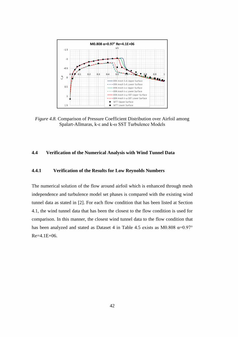
42
Figure 4.8. Comparison of Pressure Coefficient Distribution over Airfoil among
Spalart-Allmaras, k-ε and k-ω SST Turbulence Models
4.4 Verification of the Numerical Analysis with Wind Tunnel Data
4.4.1 Verification of the Results for Low Reynolds Numbers
The numerical solution of the flow around airfoil which is enhanced through mesh
independence and turbulence model set phases is compared with the existing wind
tunnel data as stated in [2]. For each flow condition that has been listed at Section
4.1, the wind tunnel data that has been the closest to the flow condition is used for
comparison. In this manner, the closest wind tunnel data to the flow condition that
has been analyzed and stated as Dataset 4 in Table 4.5 exists as M0.808 α=0.97°
Re=4.1E+06.
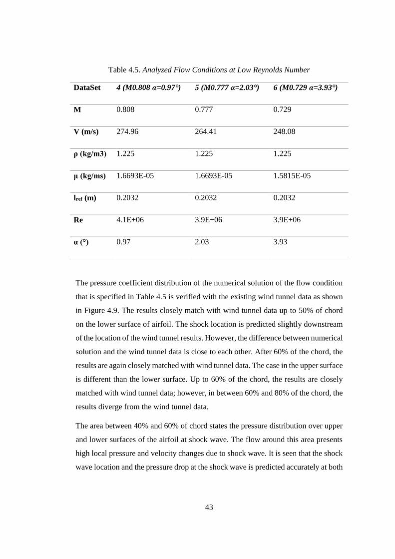
43
Table 4.5. Analyzed Flow Conditions at Low Reynolds Number
DataSet 4 (M0.808 α=0.97°) 5 (M0.777 α=2.03°) 6 (M0.729 α=3.93°)
M 0.808 0.777 0.729
V (m/s) 274.96 264.41 248.08
ρ (kg/m3) 1.225 1.225 1.225
μ (kg/ms) 1.6693E-05 1.6693E-05 1.5815E-05
lref (m) 0.2032 0.2032 0.2032
Re 4.1E+06 3.9E+06 3.9E+06
α (°) 0.97 2.03 3.93
The pressure coefficient distribution of the numerical solution of the flow condition
that is specified in Table 4.5 is verified with the existing wind tunnel data as shown
in Figure 4.9. The results closely match with wind tunnel data up to 50% of chord
on the lower surface of airfoil. The shock location is predicted slightly downstream
of the location of the wind tunnel results. However, the difference between numerical
solution and the wind tunnel data is close to each other. After 60% of the chord, the
results are again closely matched with wind tunnel data. The case in the upper surface
is different than the lower surface. Up to 60% of the chord, the results are closely
matched with wind tunnel data; however, in between 60% and 80% of the chord, the
results diverge from the wind tunnel data.
The area between 40% and 60% of chord states the pressure distribution over upper
and lower surfaces of the airfoil at shock wave. The flow around this area presents
high local pressure and velocity changes due to shock wave. It is seen that the shock
wave location and the pressure drop at the shock wave is predicted accurately at both
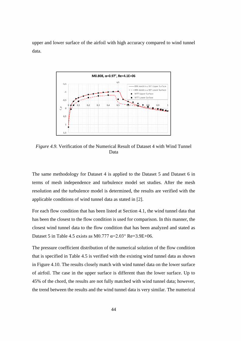
44
upper and lower surface of the airfoil with high accuracy compared to wind tunnel
data.
Figure 4.9. Verification of the Numerical Result of Dataset 4 with Wind Tunnel
Data
The same methodology for Dataset 4 is applied to the Dataset 5 and Dataset 6 in
terms of mesh independence and turbulence model set studies. After the mesh
resolution and the turbulence model is determined, the results are verified with the
applicable conditions of wind tunnel data as stated in [2].
For each flow condition that has been listed at Section 4.1, the wind tunnel data that
has been the closest to the flow condition is used for comparison. In this manner, the
closest wind tunnel data to the flow condition that has been analyzed and stated as
Dataset 5 in Table 4.5 exists as M0.777 α=2.03° Re=3.9E+06.
The pressure coefficient distribution of the numerical solution of the flow condition
that is specified in Table 4.5 is verified with the existing wind tunnel data as shown
in Figure 4.10. The results closely match with wind tunnel data on the lower surface
of airfoil. The case in the upper surface is different than the lower surface. Up to
45% of the chord, the results are not fully matched with wind tunnel data; however,
the trend between the results and the wind tunnel data is very similar. The numerical
45
solution predicts the pressure distribution slightly lower than real value; however,
the difference can be considered as small. Between 45% and 55% of the chord, the
shock capturing of the numerical solution is highly accurate when it is compared to
the wind tunnel data. After 55% of the chord, the pressure distribution is predicted
lower than the wind tunnel data. When looking the overall pressure distribution
results, it is seen that the numerical results predict consistently lower pressure
coefficients relative to the wind tunnel data. It is seen that the numerical results
predict the pressure drop at the shock wave at the upper surface of the airfoil with
high accuracy based on wind tunnel data.
Figure 4.10. Verification of the Numerical Result of Dataset 5 with Wind Tunnel
Data
For each flow condition that has been listed at Section 4.1, the wind tunnel data that
has been the closest to the flow condition is used for comparison. In this manner, the
closest wind tunnel data to the flow condition that has been analyzed and stated as
Dataset 6 in Table 4.5 exists as M0.729 α=3.93° Re=3.9E+06.
The pressure coefficient distribution of the numerical solution of the flow condition
that is specified in Table 4.5 is verified with the existing wind tunnel data as shown
in Figure 4.11. The results closely match with wind tunnel data up to 90% of chord
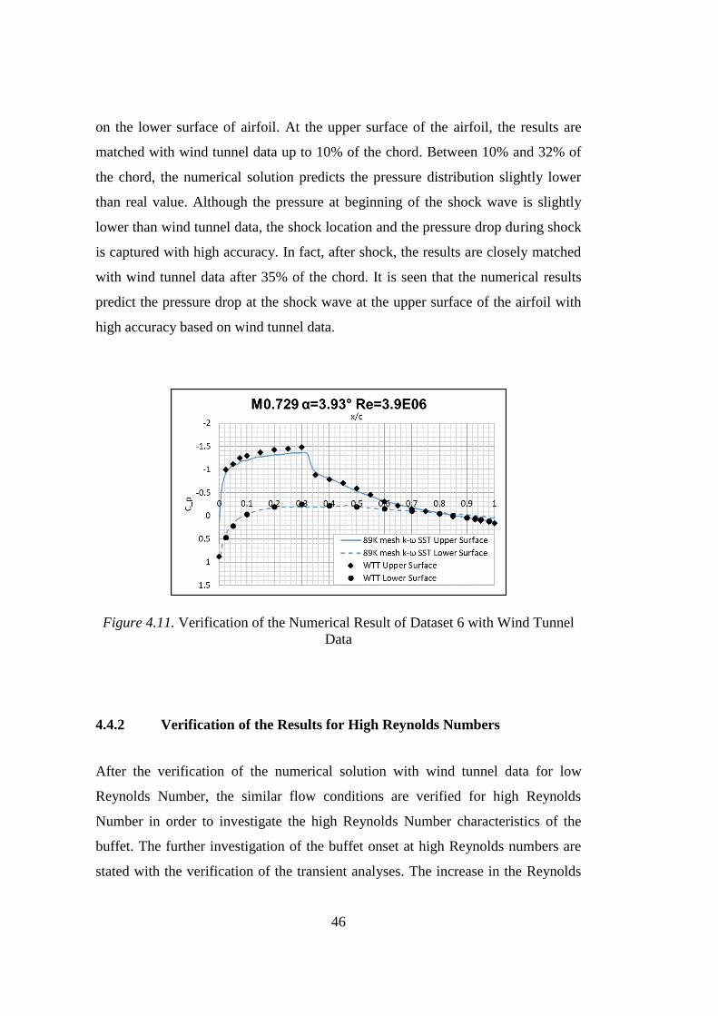
46
on the lower surface of airfoil. At the upper surface of the airfoil, the results are
matched with wind tunnel data up to 10% of the chord. Between 10% and 32% of
the chord, the numerical solution predicts the pressure distribution slightly lower
than real value. Although the pressure at beginning of the shock wave is slightly
lower than wind tunnel data, the shock location and the pressure drop during shock
is captured with high accuracy. In fact, after shock, the results are closely matched
with wind tunnel data after 35% of the chord. It is seen that the numerical results
predict the pressure drop at the shock wave at the upper surface of the airfoil with
high accuracy based on wind tunnel data.
Figure 4.11. Verification of the Numerical Result of Dataset 6 with Wind Tunnel
Data
4.4.2 Verification of the Results for High Reynolds Numbers
After the verification of the numerical solution with wind tunnel data for low
Reynolds Number, the similar flow conditions are verified for high Reynolds
Number in order to investigate the high Reynolds Number characteristics of the
buffet. The further investigation of the buffet onset at high Reynolds numbers are
stated with the verification of the transient analyses. The increase in the Reynolds
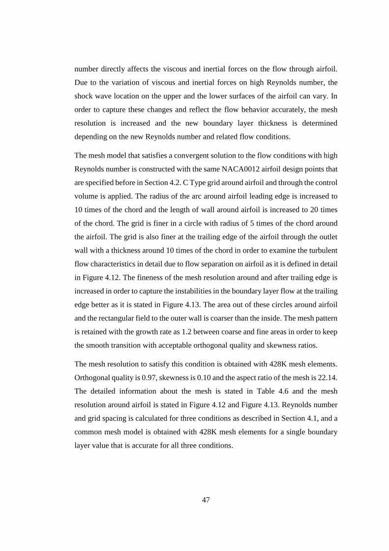
47
number directly affects the viscous and inertial forces on the flow through airfoil.
Due to the variation of viscous and inertial forces on high Reynolds number, the
shock wave location on the upper and the lower surfaces of the airfoil can vary. In
order to capture these changes and reflect the flow behavior accurately, the mesh
resolution is increased and the new boundary layer thickness is determined
depending on the new Reynolds number and related flow conditions.
The mesh model that satisfies a convergent solution to the flow conditions with high
Reynolds number is constructed with the same NACA0012 airfoil design points that
are specified before in Section 4.2. C Type grid around airfoil and through the control
volume is applied. The radius of the arc around airfoil leading edge is increased to
10 times of the chord and the length of wall around airfoil is increased to 20 times
of the chord. The grid is finer in a circle with radius of 5 times of the chord around
the airfoil. The grid is also finer at the trailing edge of the airfoil through the outlet
wall with a thickness around 10 times of the chord in order to examine the turbulent
flow characteristics in detail due to flow separation on airfoil as it is defined in detail
in Figure 4.12. The fineness of the mesh resolution around and after trailing edge is
increased in order to capture the instabilities in the boundary layer flow at the trailing
edge better as it is stated in Figure 4.13. The area out of these circles around airfoil
and the rectangular field to the outer wall is coarser than the inside. The mesh pattern
is retained with the growth rate as 1.2 between coarse and fine areas in order to keep
the smooth transition with acceptable orthogonal quality and skewness ratios.
The mesh resolution to satisfy this condition is obtained with 428K mesh elements.
Orthogonal quality is 0.97, skewness is 0.10 and the aspect ratio of the mesh is 22.14.
The detailed information about the mesh is stated in Table 4.6 and the mesh
resolution around airfoil is stated in Figure 4.12 and Figure 4.13. Reynolds number
and grid spacing is calculated for three conditions as described in Section 4.1, and a
common mesh model is obtained with 428K mesh elements for a single boundary
layer value that is accurate for all three conditions.
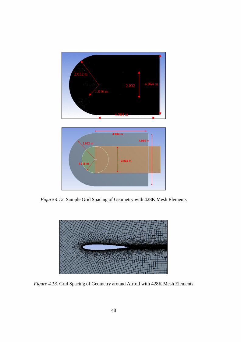
48
Figure 4.12. Sample Grid Spacing of Geometry with 428K Mesh Elements
Figure 4.13. Grid Spacing of Geometry around Airfoil with 428K Mesh Elements
2.032 m
1.016 m
4.064 m 2.032
4.064 m
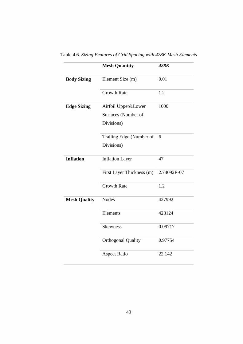
49
Table 4.6. Sizing Features of Grid Spacing with 428K Mesh Elements
Mesh Quantity 428K
Body Sizing Element Size (m) 0.01
Growth Rate 1.2
Edge Sizing Airfoil Upper&Lower
Surfaces (Number of
Divisions)
1000
Trailing Edge (Number of
Divisions)
6
Inflation Inflation Layer 47
First Layer Thickness (m) 2.74092E-07
Growth Rate 1.2
Mesh Quality Nodes 427992
Elements 428124
Skewness 0.09717
Orthogonal Quality 0.97754
Aspect Ratio 22.142
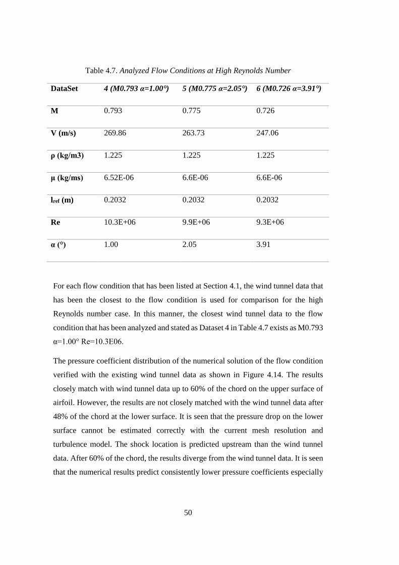
50
Table 4.7. Analyzed Flow Conditions at High Reynolds Number
DataSet 4 (M0.793 α=1.00°) 5 (M0.775 α=2.05°) 6 (M0.726 α=3.91°)
M 0.793 0.775 0.726
V (m/s) 269.86 263.73 247.06
ρ (kg/m3) 1.225 1.225 1.225
μ (kg/ms) 6.52E-06 6.6E-06 6.6E-06
lref (m) 0.2032 0.2032 0.2032
Re 10.3E+06 9.9E+06 9.3E+06
α (°) 1.00 2.05 3.91
For each flow condition that has been listed at Section 4.1, the wind tunnel data that
has been the closest to the flow condition is used for comparison for the high
Reynolds number case. In this manner, the closest wind tunnel data to the flow
condition that has been analyzed and stated as Dataset 4 in Table 4.7 exists as M0.793
α=1.00° Re=10.3E06.
The pressure coefficient distribution of the numerical solution of the flow condition
verified with the existing wind tunnel data as shown in Figure 4.14. The results
closely match with wind tunnel data up to 60% of the chord on the upper surface of
airfoil. However, the results are not closely matched with the wind tunnel data after
48% of the chord at the lower surface. It is seen that the pressure drop on the lower
surface cannot be estimated correctly with the current mesh resolution and
turbulence model. The shock location is predicted upstream than the wind tunnel
data. After 60% of the chord, the results diverge from the wind tunnel data. It is seen
that the numerical results predict consistently lower pressure coefficients especially
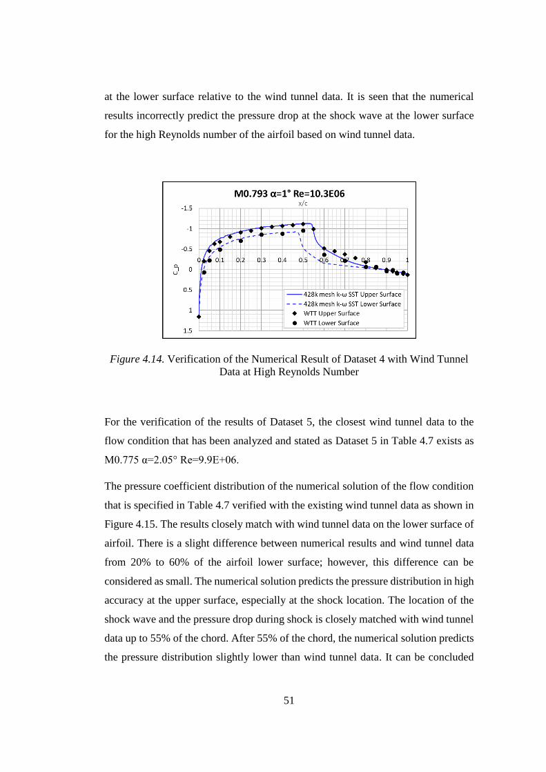
51
at the lower surface relative to the wind tunnel data. It is seen that the numerical
results incorrectly predict the pressure drop at the shock wave at the lower surface
for the high Reynolds number of the airfoil based on wind tunnel data.
Figure 4.14. Verification of the Numerical Result of Dataset 4 with Wind Tunnel
Data at High Reynolds Number
For the verification of the results of Dataset 5, the closest wind tunnel data to the
flow condition that has been analyzed and stated as Dataset 5 in Table 4.7 exists as
M0.775 α=2.05° Re=9.9E+06.
The pressure coefficient distribution of the numerical solution of the flow condition
that is specified in Table 4.7 verified with the existing wind tunnel data as shown in
Figure 4.15. The results closely match with wind tunnel data on the lower surface of
airfoil. There is a slight difference between numerical results and wind tunnel data
from 20% to 60% of the airfoil lower surface; however, this difference can be
considered as small. The numerical solution predicts the pressure distribution in high
accuracy at the upper surface, especially at the shock location. The location of the
shock wave and the pressure drop during shock is closely matched with wind tunnel
data up to 55% of the chord. After 55% of the chord, the numerical solution predicts
the pressure distribution slightly lower than wind tunnel data. It can be concluded
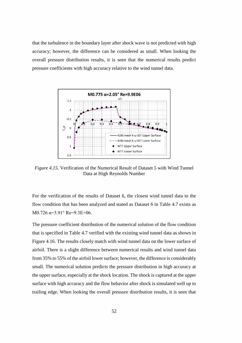
52
that the turbulence in the boundary layer after shock wave is not predicted with high
accuracy; however, the difference can be considered as small. When looking the
overall pressure distribution results, it is seen that the numerical results predict
pressure coefficients with high accuracy relative to the wind tunnel data.
Figure 4.15. Verification of the Numerical Result of Dataset 5 with Wind Tunnel
Data at High Reynolds Number
For the verification of the results of Dataset 6, the closest wind tunnel data to the
flow condition that has been analyzed and stated as Dataset 6 in Table 4.7 exists as
M0.726 α=3.91° Re=9.3E+06.
The pressure coefficient distribution of the numerical solution of the flow condition
that is specified in Table 4.7 verified with the existing wind tunnel data as shown in
Figure 4.16. The results closely match with wind tunnel data on the lower surface of
airfoil. There is a slight difference between numerical results and wind tunnel data
from 35% to 55% of the airfoil lower surface; however, the difference is considerably
small. The numerical solution predicts the pressure distribution in high accuracy at
the upper surface, especially at the shock location. The shock is captured at the upper
surface with high accuracy and the flow behavior after shock is simulated well up to
trailing edge. When looking the overall pressure distribution results, it is seen that
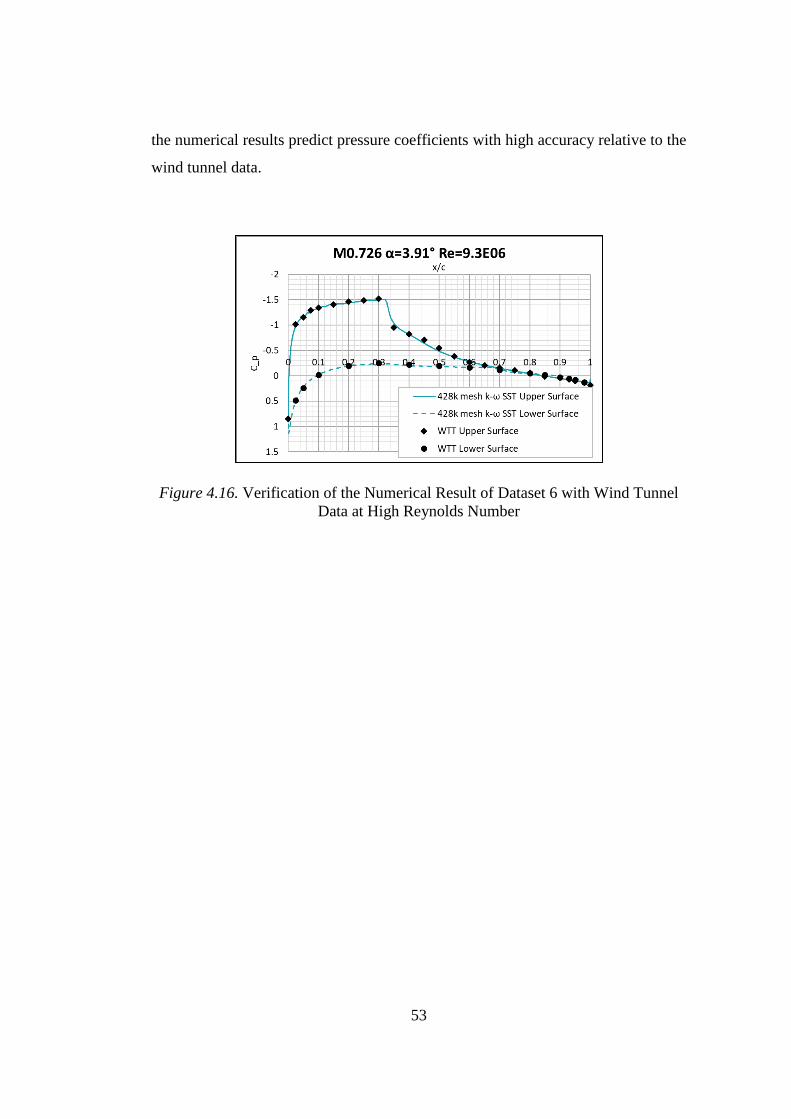
53
the numerical results predict pressure coefficients with high accuracy relative to the
wind tunnel data.
Figure 4.16. Verification of the Numerical Result of Dataset 6 with Wind Tunnel
Data at High Reynolds Number

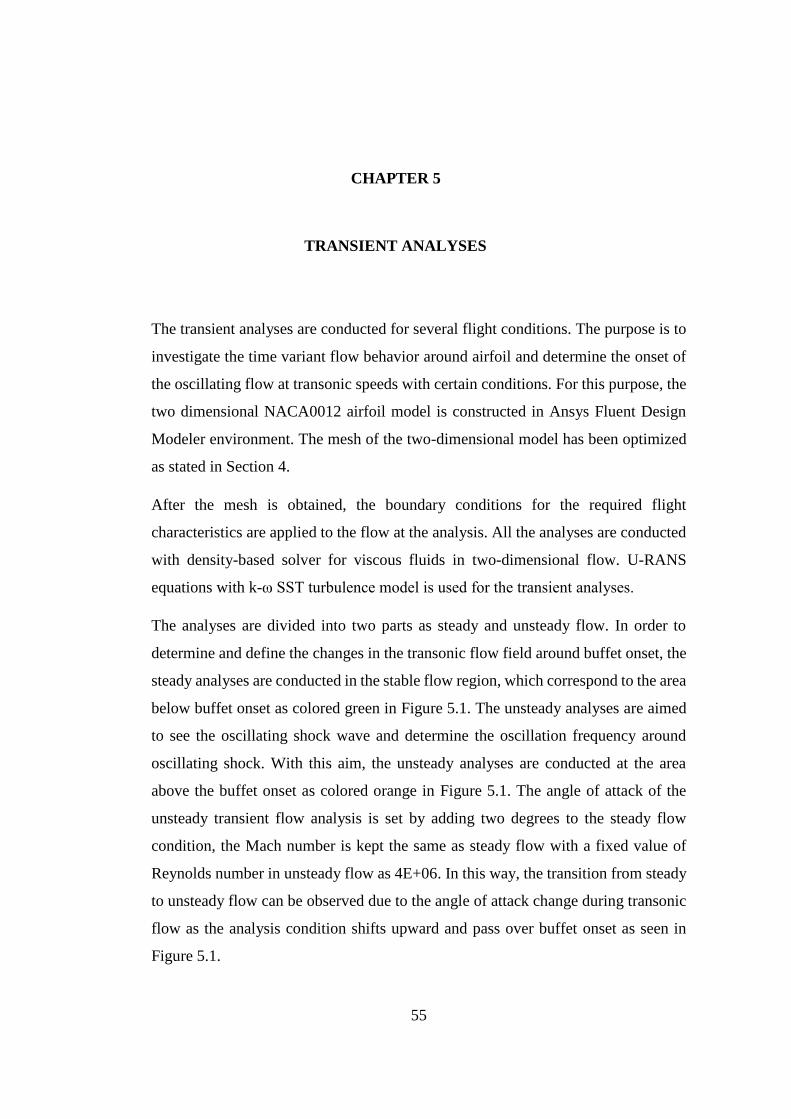
55
CHAPTER 5
5 TRANSIENT ANALYSES
The transient analyses are conducted for several flight conditions. The purpose is to
investigate the time variant flow behavior around airfoil and determine the onset of
the oscillating flow at transonic speeds with certain conditions. For this purpose, the
two dimensional NACA0012 airfoil model is constructed in Ansys Fluent Design
Modeler environment. The mesh of the two-dimensional model has been optimized
as stated in Section 4.
After the mesh is obtained, the boundary conditions for the required flight
characteristics are applied to the flow at the analysis. All the analyses are conducted
with density-based solver for viscous fluids in two-dimensional flow. U-RANS
equations with k-ω SST turbulence model is used for the transient analyses.
The analyses are divided into two parts as steady and unsteady flow. In order to
determine and define the changes in the transonic flow field around buffet onset, the
steady analyses are conducted in the stable flow region, which correspond to the area
below buffet onset as colored green in Figure 5.1. The unsteady analyses are aimed
to see the oscillating shock wave and determine the oscillation frequency around
oscillating shock. With this aim, the unsteady analyses are conducted at the area
above the buffet onset as colored orange in Figure 5.1. The angle of attack of the
unsteady transient flow analysis is set by adding two degrees to the steady flow
condition, the Mach number is kept the same as steady flow with a fixed value of
Reynolds number in unsteady flow as 4E+06. In this way, the transition from steady
to unsteady flow can be observed due to the angle of attack change during transonic
flow as the analysis condition shifts upward and pass over buffet onset as seen in
Figure 5.1.
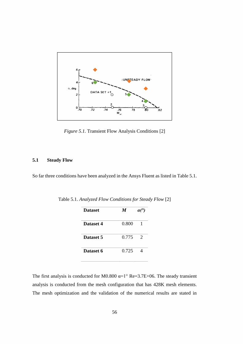
56
Figure 5.1. Transient Flow Analysis Conditions [2]
5.1 Steady Flow
So far three conditions have been analyzed in the Ansys Fluent as listed in Table 5.1.
Table 5.1. Analyzed Flow Conditions for Steady Flow [2]
Dataset M α(°)
Dataset 4 0.800 1
Dataset 5 0.775 2
Dataset 6 0.725 4
The first analysis is conducted for M0.800 α=1° Re=3.7E+06. The steady transient
analysis is conducted from the mesh configuration that has 428K mesh elements.
The mesh optimization and the validation of the numerical results are stated in
57
Section 4.4.2. The model is analyzed for 2 seconds with a 0.0001 second timestep.
The residual tolerances are fixed to converge at least 10-6 up to 20 iterations per
timestep.
The time variant lift, drag, moment coefficients and static pressure distribution for
the airfoil are presented in Figure 5.2. Static pressure is the average of the
measurements of the airfoil upper and lower surface pressure values. The oscillations
occurring on all of the coefficients and static pressure in the first 0.25 seconds are
caused by the disturbance of the streamflow when it suddenly reaches the airfoil. The
oscillations are damped up to 0.5 seconds when the flow balances and the uniform
flow is reached as streamflow. After 0.5 seconds, it is seen that there is no evidence
of a shock oscillation on the flow as all of the coefficients and static pressure
distribution over time on airfoil reach a constant value.
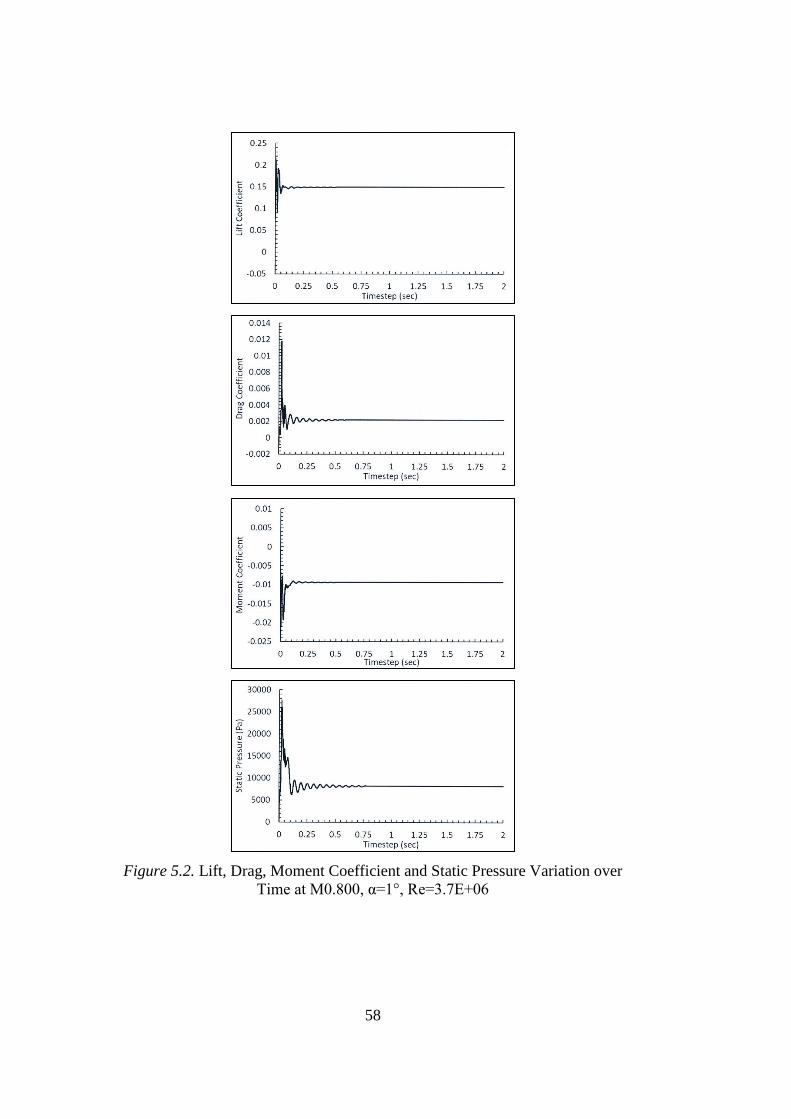
58
Figure 5.2. Lift, Drag, Moment Coefficient and Static Pressure Variation over
Time at M0.800, α=1°, Re=3.7E+06
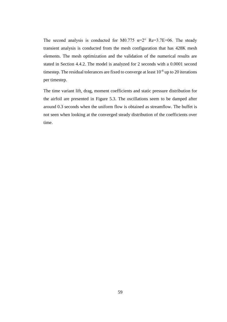
59
The second analysis is conducted for M0.775 α=2° Re=3.7E+06. The steady
transient analysis is conducted from the mesh configuration that has 428K mesh
elements. The mesh optimization and the validation of the numerical results are
stated in Section 4.4.2. The model is analyzed for 2 seconds with a 0.0001 second
timestep. The residual tolerances are fixed to converge at least 10-6 up to 20 iterations
per timestep.
The time variant lift, drag, moment coefficients and static pressure distribution for
the airfoil are presented in Figure 5.3. The oscillations seem to be damped after
around 0.3 seconds when the uniform flow is obtained as streamflow. The buffet is
not seen when looking at the converged steady distribution of the coefficients over
time.
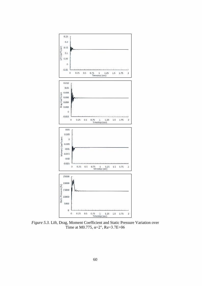
60
Figure 5.3. Lift, Drag, Moment Coefficient and Static Pressure Variation over
Time at M0.775, α=2°, Re=3.7E+06
61
The third analysis is conducted for M0.725 α=4° Re=3.4E+06. The steady transient
analysis is conducted from the mesh configuration that has 428K mesh elements.
The mesh optimization and the validation of the numerical results are stated in
Section 4.4.2. The model is analyzed for 2 seconds with a 0.0001 second timestep.
The residual tolerances are fixed to converge at least 10-6 up to 20 iterations per
timestep.
The time variant lift, drag, moment coefficients and static pressure distribution for
the airfoil are presented in Figure 5.4. Like the steady analyses of Dataset 4 and
Dataset 5, the streamflow is reached after around 0.25 seconds. As the stable
variations of the coefficients indicated, the buffet is not seen at this flow conditions.
62
Figure 5.4. Lift, Drag, Moment Coefficient and Static Pressure Variation over
Time at M0.725, α=4°, Re=3.4E+06
63
Considering all three flow conditions that are analyzed with numerical solutions, it
is seen that the flow is settled and streamflow is obtained for all three conditions that
are in the stable region of buffet onset curve. However, the convergence obtained in
different durations for all three conditions. The convergence durations continuously
decrease as the flow conditions change from Dataset 4 to Dataset 5 and then Dataset
6. It is seen that, as the Mach number decreases, and the critical angle of attack
increases as a function of the critical Mach number, the convergence of the flow
through a stable region occurs in a shorter duration.
5.2 Unsteady Flow
So far three conditions have been analyzed in the Ansys Fluent as listed in Table 5.2.
Table 5.2. Analyzed Flow Conditions for Unsteady Flow [2]
Dataset M α (°) Re
Dataset 4 0.800 4 4E+06
Dataset 5 0.775 4 4E0+6
Dataset 6 0.725 6 4E+06
The first analysis is conducted for M0.800 α=4° Re=4E+06. The steady transient
analysis is conducted from the mesh configuration that has 428K mesh elements.
The mesh optimization and the validation of the numerical results are stated in
Section 4.4.2. The model is analyzed for 2 seconds with a 0.0001 second timestep.
The residual tolerances are fixed to converge at least 10-6 up to 20 iterations per
timestep.
64
The time variant lift, drag and moment coefficients and static pressure distribution
for the airfoil are illustrated in Figure 5.5, together with the power spectral density
variations of the same coefficients over logarithmic scale of frequency. The constant
oscillating behavior of the flow is seen from lift, drag and moment coefficients and
additionally, static pressure fluctuations. The first peak on the frequency around 0.1
seconds is due to the disturbance of the streamflow when it suddenly reaches the
wing. The undamped oscillating behavior which is common in lift, drag, moment
coefficient and static pressure variations over time is the evidence of a shock
oscillation.
When the power spectral density variations of lift, drag, moment coefficients and
static pressure is investigated, the peak point is seen at 29.7 Hz. The peak point
indicates the dominant frequency of the buffet. The other bumps on the curve is due
to the noise on the data.
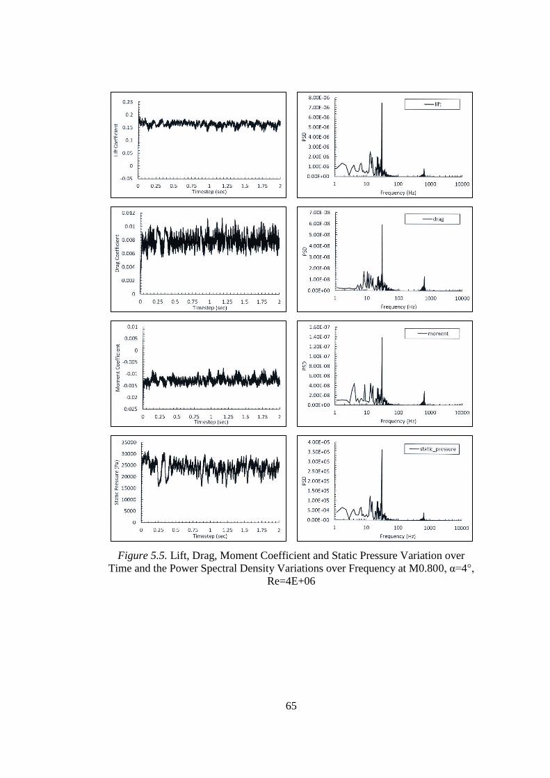
65
Figure 5.5. Lift, Drag, Moment Coefficient and Static Pressure Variation over
Time and the Power Spectral Density Variations over Frequency at M0.800, α=4°,
Re=4E+06
66
The dominant frequency is measured as 29.7 Hz in all power spectral density plots
of lift, drag, moment and static pressure. Since the measured frequency is the same
for all parameters, it is determined as the buffet frequency. The numerical results
cannot be compared with wind tunnel data for the current flow condition with low
Reynolds number due to lack of wind tunnel data.
The pressure and velocity u waveforms of the upper and lower surfaces of the airfoil
at 50% and 80% of the chord is depicted in Figure 5.6. The waveforms are calculated
especially at 50% and 80% of the chord, since the shock is generated at 50% of the
chord and its interaction with the boundary layer becomes significant towards
trailing edge. The frequency of the oscillations is higher at the upper surface then
lower surface for the pressure waveforms. The frequency of velocity u waveform at
50% of the chord is quite low on upper surface. In addition, the difference in the
frequencies between 50% and 80% of the chord indicates that at the upper surface,
the oscillation frequency increases when the flow approaches to the trailing edge. It
is observed that the oscillation behaviors of the pressures and u velocities vary for
each individual location on airfoil at both surfaces. The dominant frequencies of each
four locations are different than each other. For that reason, it is highly difficult to
obtain a dominant buffet frequency from a local point on airfoil. Instead, the
approach for the determination of the buffet frequency is to obtain the dominant
frequency from the variations of the static pressure or lift, drag, moment coefficients
with time.
The average location of the shock oscillations can be predicted from the variations
in the frequencies of the wavelengths. In this manner, the oscillations are not started
at 50% of the airfoil on upper surface due to the low frequencies of wavelengths at
this point. The frequencies are increased highly at 80% of the chord, which is the
indication of the higher oscillations at boundary layer. The shock oscillations started
at a point in between 50% and 80% of the chord on upper surface. The oscillation
frequencies at the lower surface are not quite different from each other, which
indicates that oscillating shock does not exist at the lower surface.
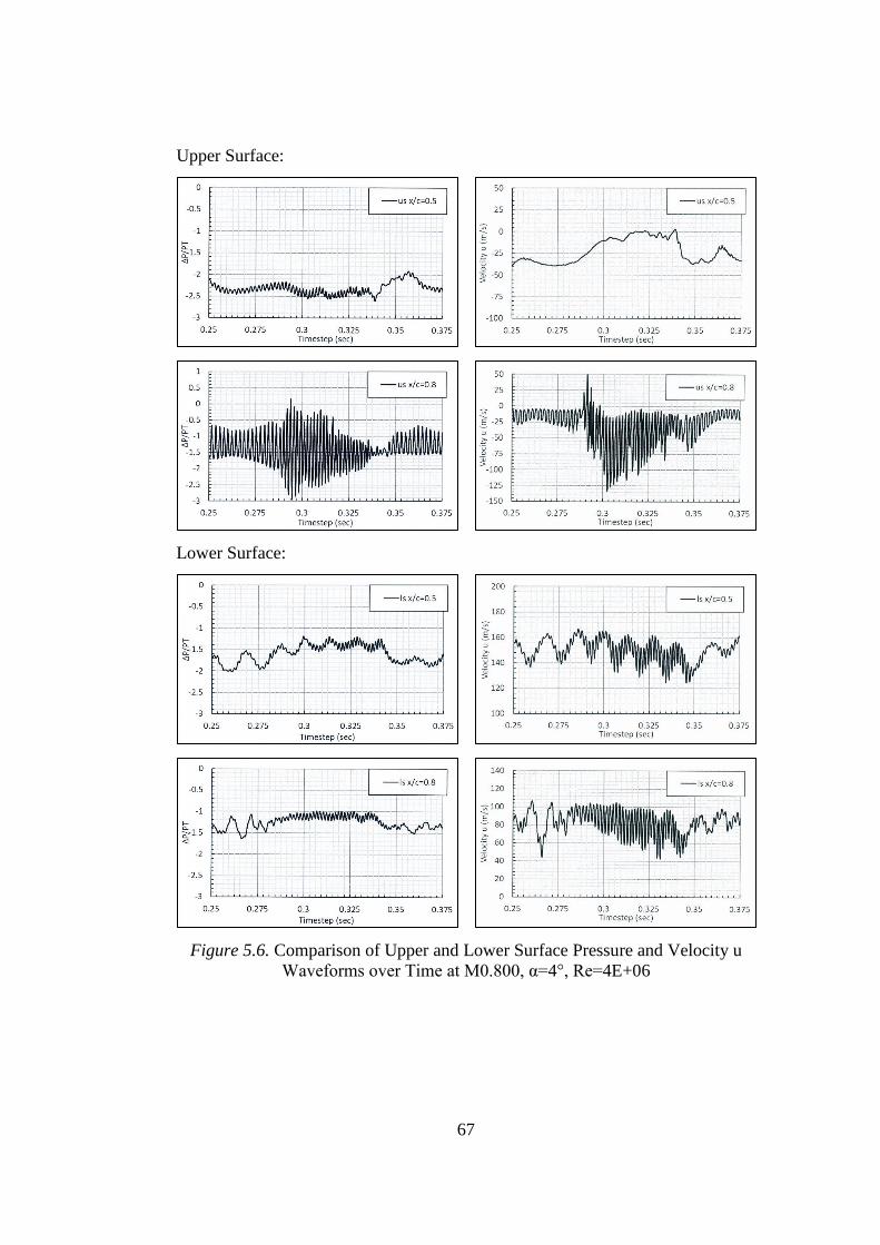
67
Upper Surface:
Lower Surface:
Figure 5.6. Comparison of Upper and Lower Surface Pressure and Velocity u
Waveforms over Time at M0.800, α=4°, Re=4E+06

68
The pressure waveforms at 50% and 80% of the chord is depicted in Figure 5.7. The
difference of the results between Figure 5.6 and Figure 5.7 is that the mean value is
obtained by the subtraction of the pressure waveforms at the upper surface from the
lower surface for 50% and 80% of the chord. The results give better information
about the mean pressure variations at 50% and 80% of the chord. Hence, the change
in oscillation frequency can be observed better as the flow moves towards the trailing
edge. The oscillation frequency on the flow increases when moving from 50% of the
chord to the 80% of the chord. Since the separation on the boundary layer due to the
interaction with shock wave oscillation increases when the flow approaches to the
trailing edge, the increase in the frequency is an expected result.
Figure 5.7. Pressure Waveforms over Time at M0.800, α=4°, Re=4E+06
The frequency of the oscillating behavior of buffet is measured as 29.7 Hertz for the
unsteady transient flow. The oscillation about 29.7 Hertz in this flow condition
creates a Strouhal number as 0.14. A complete comparison cannot be made since
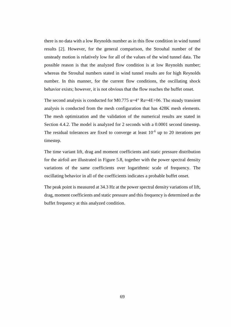
69
there is no data with a low Reynolds number as in this flow condition in wind tunnel
results [2]. However, for the general comparison, the Strouhal number of the
unsteady motion is relatively low for all of the values of the wind tunnel data. The
possible reason is that the analyzed flow condition is at low Reynolds number;
whereas the Strouhal numbers stated in wind tunnel results are for high Reynolds
number. In this manner, for the current flow conditions, the oscillating shock
behavior exists; however, it is not obvious that the flow reaches the buffet onset.
The second analysis is conducted for M0.775 α=4° Re=4E+06. The steady transient
analysis is conducted from the mesh configuration that has 428K mesh elements.
The mesh optimization and the validation of the numerical results are stated in
Section 4.4.2. The model is analyzed for 2 seconds with a 0.0001 second timestep.
The residual tolerances are fixed to converge at least 10-6 up to 20 iterations per
timestep.
The time variant lift, drag and moment coefficients and static pressure distribution
for the airfoil are illustrated in Figure 5.8, together with the power spectral density
variations of the same coefficients over logarithmic scale of frequency. The
oscillating behavior in all of the coefficients indicates a probable buffet onset.
The peak point is measured at 34.3 Hz at the power spectral density variations of lift,
drag, moment coefficients and static pressure and this frequency is determined as the
buffet frequency at this analyzed condition.
70
Figure 5.8. Lift, Drag, Moment Coefficient and Static Pressure Variation over
Time and the Power Spectral Density Variations over Frequency at M0.775, α=4°,
Re=4E+06
71
The buffet frequency of this flow condition is determined as 34.3 Hz based on the
approach in the analysis of the previous flow condition. The numerical results cannot
be compared with wind tunnel data for the current flow condition with low Reynolds
number due to lack of wind tunnel data in terms of buffet frequency or Strouhal
number.
The pressure and velocity u waveforms of the upper and lower surfaces of the airfoil
at 50% and 80% of the chord is depicted in Figure 5.9. Between 50% and 80% of the
chord, the oscillation frequency of the pressure waveforms increases at the upper
surface, whereas it decreases at the lower surface when the flow approaches to the
trailing edge. The oscillation characteristics of the pressure waveforms and u
velocities are different than the ones at Dataset 4. The frequency and amplitude of
the oscillations increase at 50% and 80% of the chord at upper surface and 50% of
the chord at lower surface when the results are compared between Dataset 4 and
Dataset 5. The change in the 80% of the chord at lower surface is not remarkable as
other points.
The low frequency at the 50% of the chord and the higher frequency at the 80% of
the chord on upper surface indicates that the shock oscillations start in a location
after 50% of the chord. However, when the pressure and velocity u waveforms at
50% of the chord are compared, the ones at Dataset 5 are higher than Dataset 4. The
probable reason is that the shock oscillations start in an earlier location than Dataset
4, which is closer to 50% of the chord. The oscillation frequencies at the lower
surface are not quite different from each other, which indicates that oscillating shock
does not exist at the lower surface.
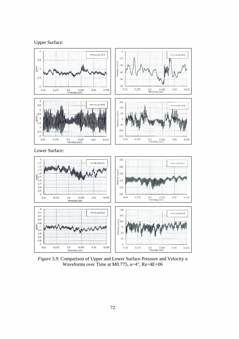
72
Upper Surface:
Lower Surface:
Figure 5.9. Comparison of Upper and Lower Surface Pressure and Velocity u
Waveforms over Time at M0.775, α=4°, Re=4E+06
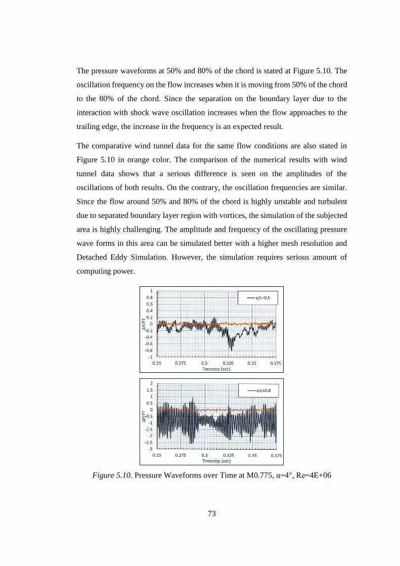
73
The pressure waveforms at 50% and 80% of the chord is stated at Figure 5.10. The
oscillation frequency on the flow increases when it is moving from 50% of the chord
to the 80% of the chord. Since the separation on the boundary layer due to the
interaction with shock wave oscillation increases when the flow approaches to the
trailing edge, the increase in the frequency is an expected result.
The comparative wind tunnel data for the same flow conditions are also stated in
Figure 5.10 in orange color. The comparison of the numerical results with wind
tunnel data shows that a serious difference is seen on the amplitudes of the
oscillations of both results. On the contrary, the oscillation frequencies are similar.
Since the flow around 50% and 80% of the chord is highly unstable and turbulent
due to separated boundary layer region with vortices, the simulation of the subjected
area is highly challenging. The amplitude and frequency of the oscillating pressure
wave forms in this area can be simulated better with a higher mesh resolution and
Detached Eddy Simulation. However, the simulation requires serious amount of
computing power.
Figure 5.10. Pressure Waveforms over Time at M0.775, α=4°, Re=4E+06
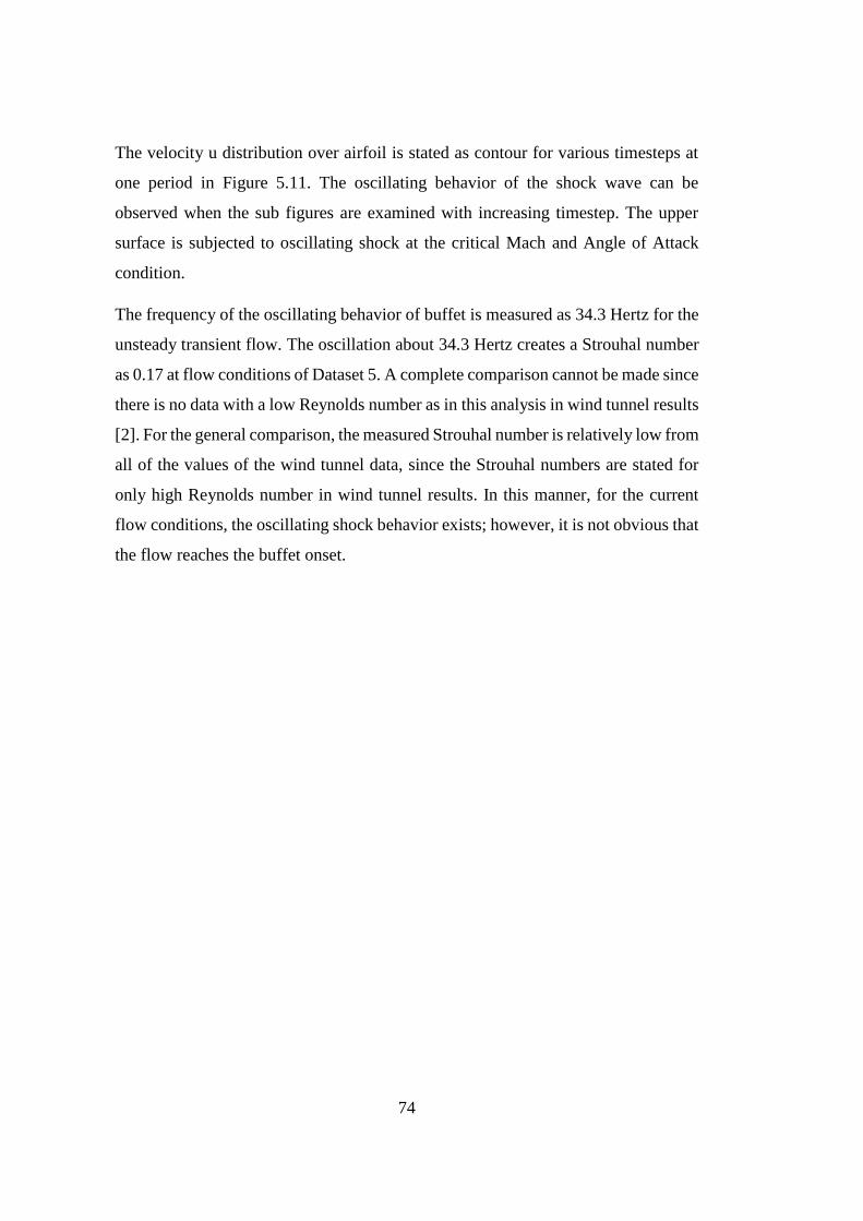
74
The velocity u distribution over airfoil is stated as contour for various timesteps at
one period in Figure 5.11. The oscillating behavior of the shock wave can be
observed when the sub figures are examined with increasing timestep. The upper
surface is subjected to oscillating shock at the critical Mach and Angle of Attack
condition.
The frequency of the oscillating behavior of buffet is measured as 34.3 Hertz for the
unsteady transient flow. The oscillation about 34.3 Hertz creates a Strouhal number
as 0.17 at flow conditions of Dataset 5. A complete comparison cannot be made since
there is no data with a low Reynolds number as in this analysis in wind tunnel results
[2]. For the general comparison, the measured Strouhal number is relatively low from
all of the values of the wind tunnel data, since the Strouhal numbers are stated for
only high Reynolds number in wind tunnel results. In this manner, for the current
flow conditions, the oscillating shock behavior exists; however, it is not obvious that
the flow reaches the buffet onset.
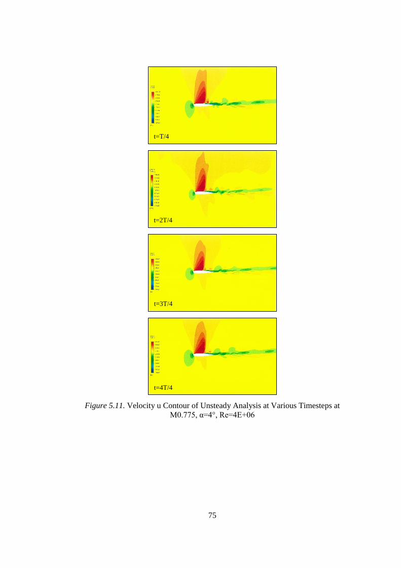
75
Figure 5.11. Velocity u Contour of Unsteady Analysis at Various Timesteps at
M0.775, α=4°, Re=4E+06
t=T/4
t=2T/4
t=3T/4
t=4T/4

76
The third analysis is conducted for M0.725 α=6° Re=4E+06. The steady transient
analysis is conducted from the mesh configuration that has 428K mesh elements.
The mesh optimization and the validation of the numerical results are stated in
Section 4.4.2. The model is analyzed for 2 seconds with a 0.0001 second timestep.
The residual tolerances are fixed to converge at least 10-6 up to 20 iterations per
timestep.
The time variant lift, drag and moment coefficients and static pressure distribution
for the airfoil are illustrated in Figure 5.12, together with the power spectral density
variations of the same coefficients over logarithmic scale of frequency. the curves
illustrate distinct oscillations indicating the buffet onset.
When the power spectral density variations of lift, drag, moment coefficients and
static pressure are investigated, the peak point is measured at 36 Hz.
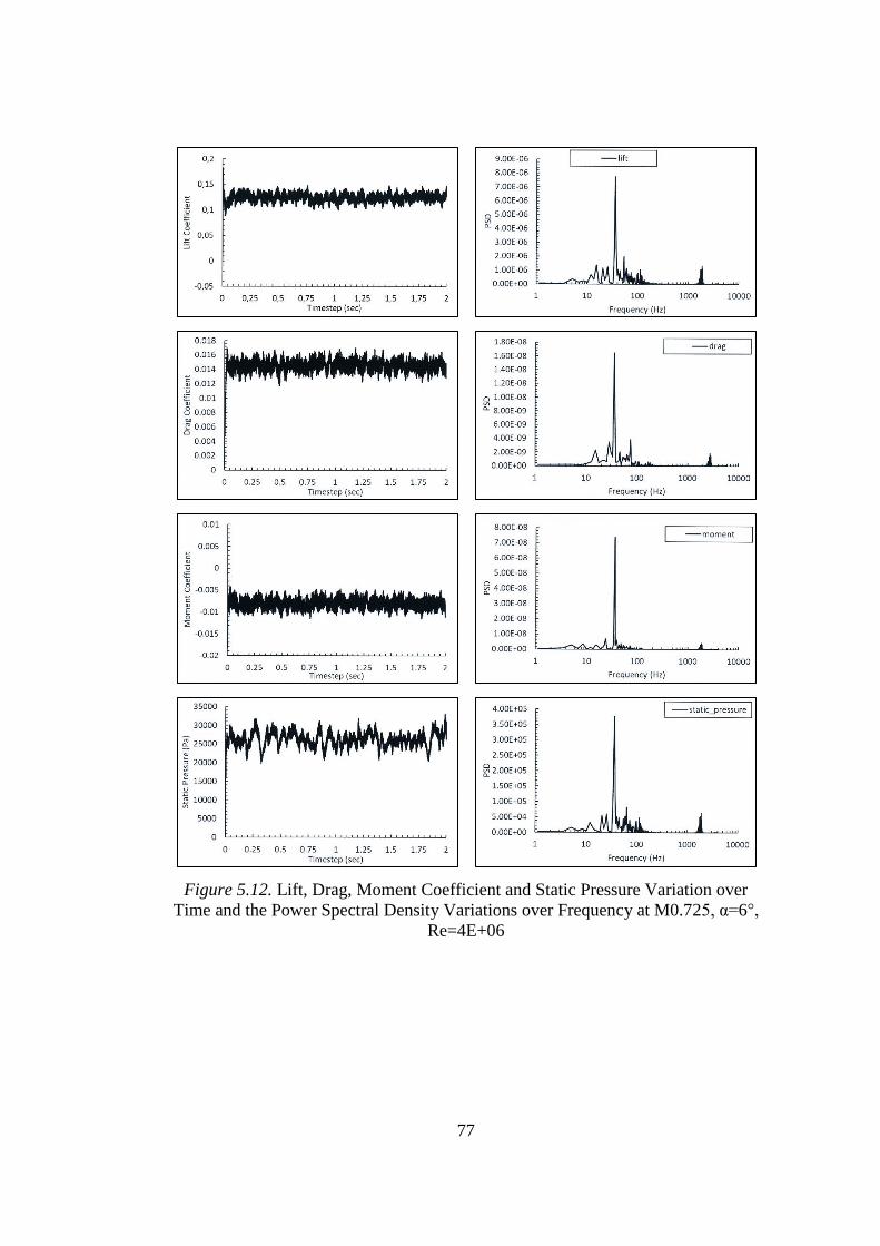
77
Figure 5.12. Lift, Drag, Moment Coefficient and Static Pressure Variation over
Time and the Power Spectral Density Variations over Frequency at M0.725, α=6°,
Re=4E+06
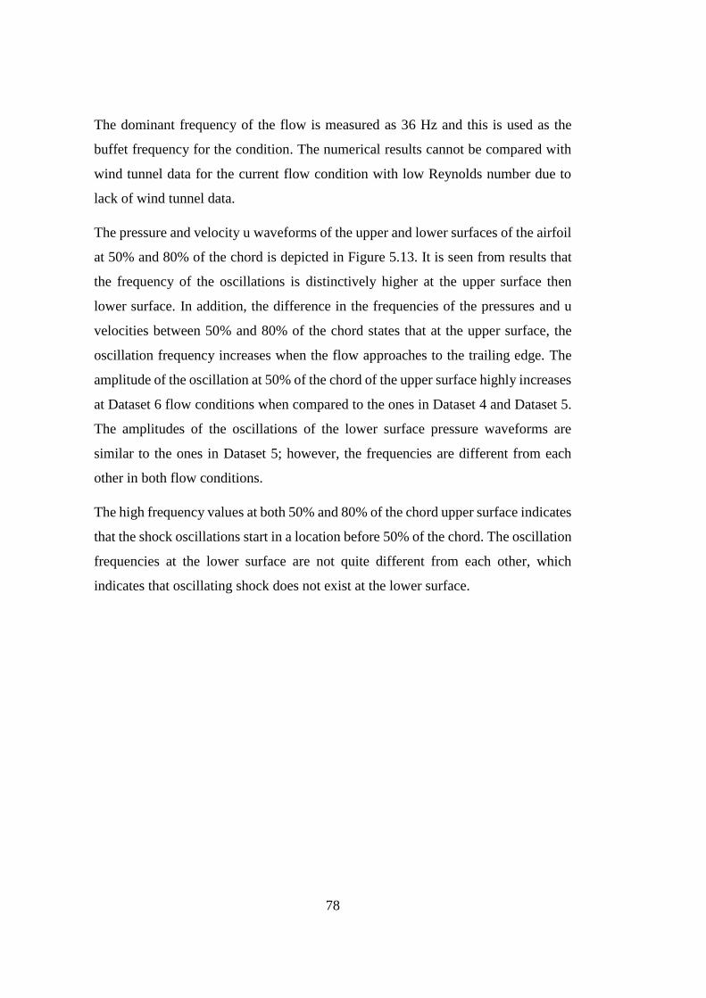
78
The dominant frequency of the flow is measured as 36 Hz and this is used as the
buffet frequency for the condition. The numerical results cannot be compared with
wind tunnel data for the current flow condition with low Reynolds number due to
lack of wind tunnel data.
The pressure and velocity u waveforms of the upper and lower surfaces of the airfoil
at 50% and 80% of the chord is depicted in Figure 5.13. It is seen from results that
the frequency of the oscillations is distinctively higher at the upper surface then
lower surface. In addition, the difference in the frequencies of the pressures and u
velocities between 50% and 80% of the chord states that at the upper surface, the
oscillation frequency increases when the flow approaches to the trailing edge. The
amplitude of the oscillation at 50% of the chord of the upper surface highly increases
at Dataset 6 flow conditions when compared to the ones in Dataset 4 and Dataset 5.
The amplitudes of the oscillations of the lower surface pressure waveforms are
similar to the ones in Dataset 5; however, the frequencies are different from each
other in both flow conditions.
The high frequency values at both 50% and 80% of the chord upper surface indicates
that the shock oscillations start in a location before 50% of the chord. The oscillation
frequencies at the lower surface are not quite different from each other, which
indicates that oscillating shock does not exist at the lower surface.
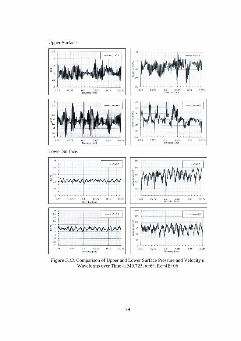
79
Upper Surface:
Lower Surface:
Figure 5.13. Comparison of Upper and Lower Surface Pressure and Velocity u
Waveforms over Time at M0.725, α=6°, Re=4E+06
80
The pressure waveforms at 50% and 80% of the chord is stated at Figure 5.14. The
oscillation frequency on the flow increases when it is moving from 50% to 80% of
the chord, similar to the ones in Dataset 4 and Dataset 5.
Figure 5.14. Pressure Waveforms over Time at M0.725, α=6°, Re=4E+06
The frequency of the oscillating behavior of buffet is measured as 36 Hertz for the
unsteady transient flow. The oscillation about 36 Hertz creates a Strouhal number as
0.19. A complete comparison cannot be made since there are no data containing a
low Reynolds number as in this analysis in wind tunnel results[2]. For the current
flow conditions, the oscillating shock behavior exists; however, it is not obvious that
the flow reaches the buffet onset.
Considering all three flow conditions that are analyzed with numerical solutions, it
is seen that the frequency of the shock oscillations increases when the critical Mach
number decreases. The possible reason behind this feature is that the shock location
81
moves downstream as the Mach number decreases. This leads to an increase distance
on the chord which is subjected to oscillating shock with boundary layer interaction.
As the distance which subjected to oscillation increases, the resultant oscillation
frequency increases. It is also seen that the pressure and velocity u waveform
characteristics of each location is highly different for all of the flow conditions. The
variance at the frequencies of wavelengths indicates the starting location of the shock
oscillations. The common characteristics for all flow conditions is that the flow
reaches more unstable phase at the upper surface than lower surface. The probable
reason is that in the steady results, the shock was observed on the upper surface for
all three conditions.
5.3 Verification of the Numerical Analysis with Wind Tunnel Data
Since the unsteady shock wave oscillations are significantly observable for the
conditions that have high Reynolds numbers [2], the verification of the unsteady
transient flow is conducted on the similar flow conditions of unsteady transient
analyses with Re=10E+06. In this manner, the flow conditions that are listed in Table
5.3 are analyzed for the verification of the buffet onset flow conditions at high
Reynolds number in order to be consistent with the tested conditions are the wind
tunnel as stated in [2]. The mesh resolution which is used at the verification of the
steady analyses is basically kept the same as 428K elements, which is defined in
detail in Section 4.4.2.
The verification of the transient unsteady flow with high Reynolds number is
conducted with U-RANS equations with k-ω SST turbulence model. The results are
compared for both simulation models and the wind tunnel dataset [2]. The model is
analyzed for 2 seconds with a 0.0001 second timestep. The residual tolerances are
fixed to converge at least 10-6 up to 20 iterations per timestep.
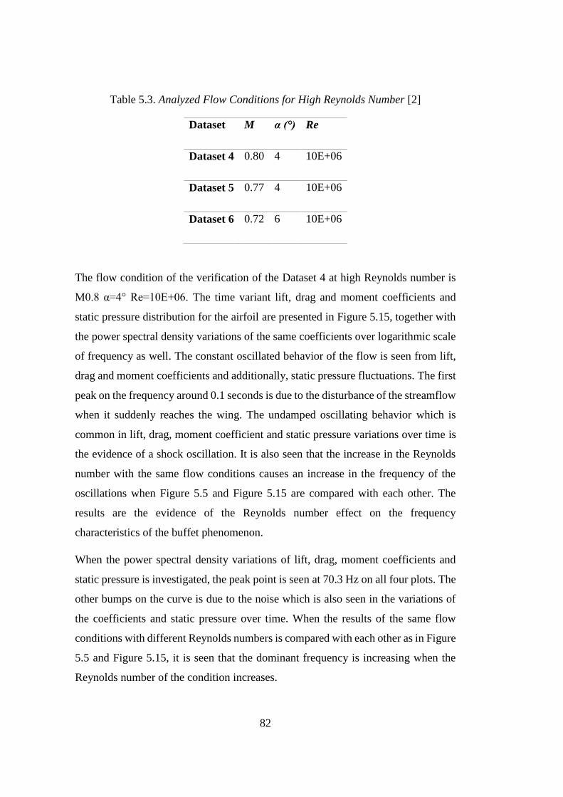
82
Table 5.3. Analyzed Flow Conditions for High Reynolds Number [2]
Dataset M α (°) Re
Dataset 4 0.80 4 10E+06
Dataset 5 0.77 4 10E+06
Dataset 6 0.72 6 10E+06
The flow condition of the verification of the Dataset 4 at high Reynolds number is
M0.8 α=4° Re=10E+06. The time variant lift, drag and moment coefficients and
static pressure distribution for the airfoil are presented in Figure 5.15, together with
the power spectral density variations of the same coefficients over logarithmic scale
of frequency as well. The constant oscillated behavior of the flow is seen from lift,
drag and moment coefficients and additionally, static pressure fluctuations. The first
peak on the frequency around 0.1 seconds is due to the disturbance of the streamflow
when it suddenly reaches the wing. The undamped oscillating behavior which is
common in lift, drag, moment coefficient and static pressure variations over time is
the evidence of a shock oscillation. It is also seen that the increase in the Reynolds
number with the same flow conditions causes an increase in the frequency of the
oscillations when Figure 5.5 and Figure 5.15 are compared with each other. The
results are the evidence of the Reynolds number effect on the frequency
characteristics of the buffet phenomenon.
When the power spectral density variations of lift, drag, moment coefficients and
static pressure is investigated, the peak point is seen at 70.3 Hz on all four plots. The
other bumps on the curve is due to the noise which is also seen in the variations of
the coefficients and static pressure over time. When the results of the same flow
conditions with different Reynolds numbers is compared with each other as in Figure
5.5 and Figure 5.15, it is seen that the dominant frequency is increasing when the
Reynolds number of the condition increases.
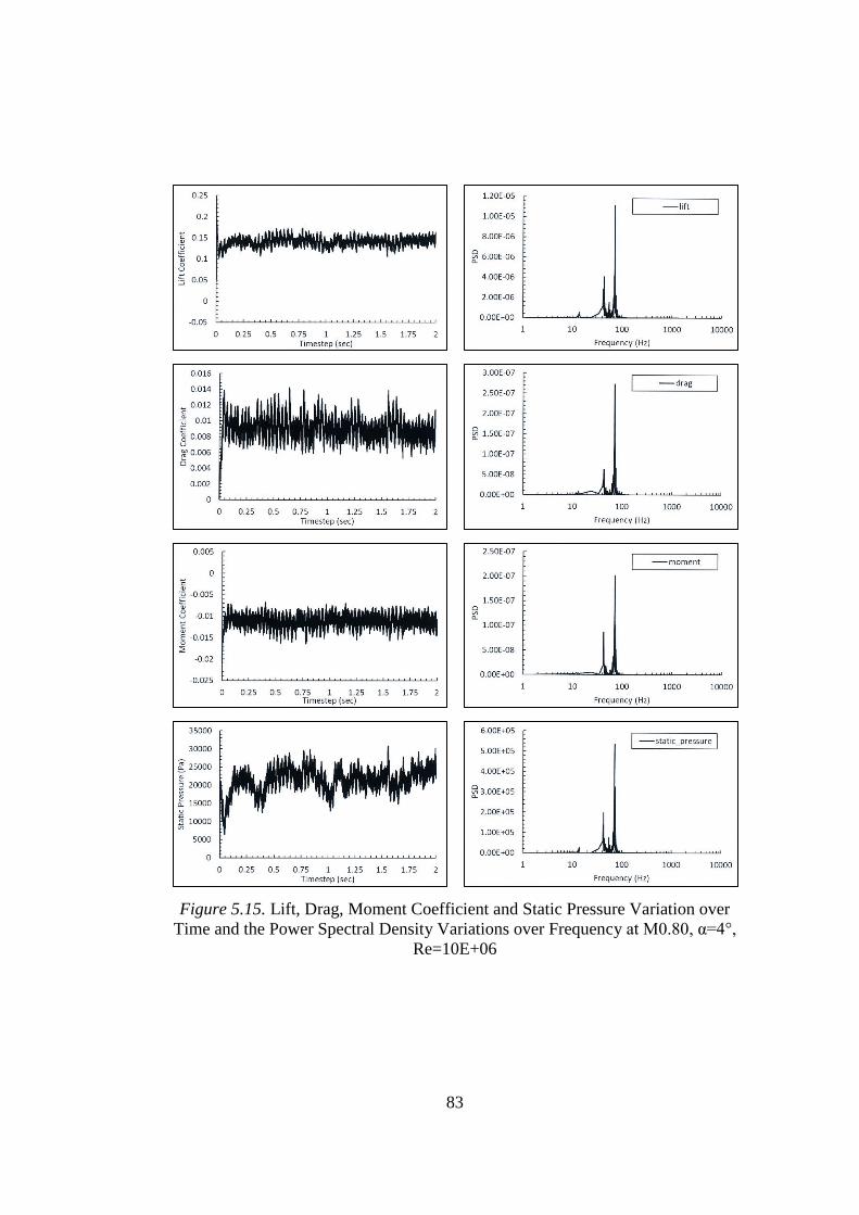
83
Figure 5.15. Lift, Drag, Moment Coefficient and Static Pressure Variation over
Time and the Power Spectral Density Variations over Frequency at M0.80, α=4°,
Re=10E+06
84
The dominant frequency of the flow is measured as 70.3 Hz for the condition and
this is used as the buffet frequency at this flow condition. When the results of the
numerical simulation and the wind tunnel data is compared, it is seen that the buffet
frequency is measured as about 80 Hz at M0.8 α=4° Re=10E+06. The numerical
results are not matched with wind tunnel data completely in this manner; however,
it is seen that the similarity is high considering the relatively small difference
between the frequencies.
The pressure and velocity u waveforms of the upper and lower surfaces of the airfoil
at 50% and 80% of the chord is stated at Figure 5.16. It is seen from results that the
frequency of the oscillations is higher at the upper surface then lower surface. In
addition, as can be seen by the difference in the frequencies of the pressures and u
velocities between 50% and 80% of the chord at the upper surface, the oscillation
frequency increases when the flow approaches to the trailing edge. In the lower
surface, it is seen that the frequency of the wavelengths at 50% of the chord is
relatively higher than 80% of the chord. When the results are compared with the
same versions with low Reynolds number, it is seen that the characteristics of the
oscillations have changed. The amplitude and the frequency of the oscillations in
each point increases with Reynolds number increase. The increase in the buffet
frequency due to increase in Reynolds number is highly observable in pressure and
velocity u waveform comparisons for both conditions.
Since the oscillation frequency increases abruptly from 50% to 80% of the chord at
the lower surface, it can be concluded that the shock oscillation started in between
50% and 80% of the chord. The shock location is closer to the 50% of the chord since
the oscillation frequency is higher at 50% of the chord when it is compared with the
low Reynolds number condition of Dataset 4. The oscillation frequencies at the lower
surface are not quite different from each other, which indicates that oscillating shock
does not exist at the lower surface; however, the frequencies are distinctively larger
than the low Reynolds number condition. The reason of this increase is the increase
in the separation of the boundary layer at the lower surface.
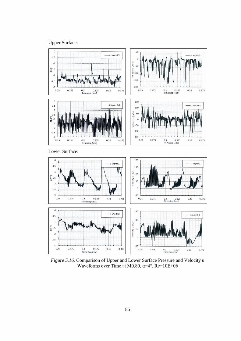
85
Upper Surface:
Lower Surface:
Figure 5.16. Comparison of Upper and Lower Surface Pressure and Velocity u
Waveforms over Time at M0.80, α=4°, Re=10E+06
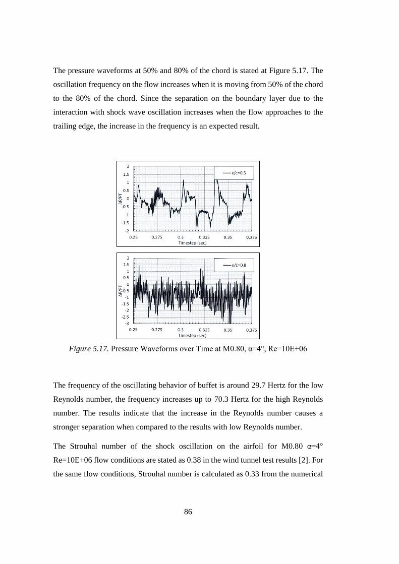
86
The pressure waveforms at 50% and 80% of the chord is stated at Figure 5.17. The
oscillation frequency on the flow increases when it is moving from 50% of the chord
to the 80% of the chord. Since the separation on the boundary layer due to the
interaction with shock wave oscillation increases when the flow approaches to the
trailing edge, the increase in the frequency is an expected result.
Figure 5.17. Pressure Waveforms over Time at M0.80, α=4°, Re=10E+06
The frequency of the oscillating behavior of buffet is around 29.7 Hertz for the low
Reynolds number, the frequency increases up to 70.3 Hertz for the high Reynolds
number. The results indicate that the increase in the Reynolds number causes a
stronger separation when compared to the results with low Reynolds number.
The Strouhal number of the shock oscillation on the airfoil for M0.80 α=4°
Re=10E+06 flow conditions are stated as 0.38 in the wind tunnel test results [2]. For
the same flow conditions, Strouhal number is calculated as 0.33 from the numerical
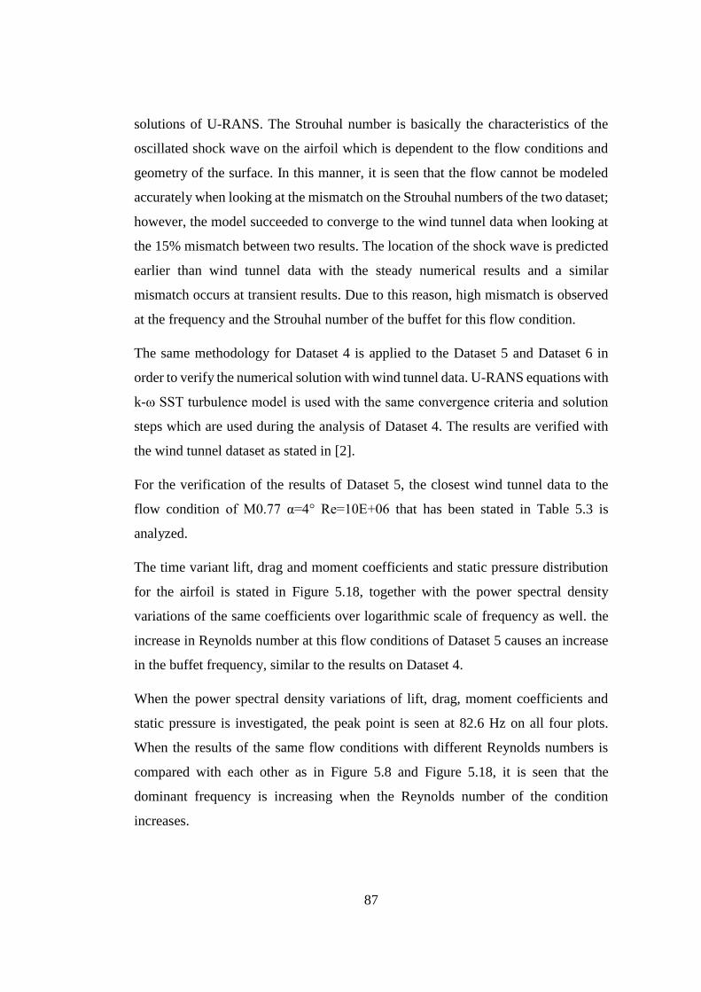
87
solutions of U-RANS. The Strouhal number is basically the characteristics of the
oscillated shock wave on the airfoil which is dependent to the flow conditions and
geometry of the surface. In this manner, it is seen that the flow cannot be modeled
accurately when looking at the mismatch on the Strouhal numbers of the two dataset;
however, the model succeeded to converge to the wind tunnel data when looking at
the 15% mismatch between two results. The location of the shock wave is predicted
earlier than wind tunnel data with the steady numerical results and a similar
mismatch occurs at transient results. Due to this reason, high mismatch is observed
at the frequency and the Strouhal number of the buffet for this flow condition.
The same methodology for Dataset 4 is applied to the Dataset 5 and Dataset 6 in
order to verify the numerical solution with wind tunnel data. U-RANS equations with
k-ω SST turbulence model is used with the same convergence criteria and solution
steps which are used during the analysis of Dataset 4. The results are verified with
the wind tunnel dataset as stated in [2].
For the verification of the results of Dataset 5, the closest wind tunnel data to the
flow condition of M0.77 α=4° Re=10E+06 that has been stated in Table 5.3 is
analyzed.
The time variant lift, drag and moment coefficients and static pressure distribution
for the airfoil is stated in Figure 5.18, together with the power spectral density
variations of the same coefficients over logarithmic scale of frequency as well. the
increase in Reynolds number at this flow conditions of Dataset 5 causes an increase
in the buffet frequency, similar to the results on Dataset 4.
When the power spectral density variations of lift, drag, moment coefficients and
static pressure is investigated, the peak point is seen at 82.6 Hz on all four plots.
When the results of the same flow conditions with different Reynolds numbers is
compared with each other as in Figure 5.8 and Figure 5.18, it is seen that the
dominant frequency is increasing when the Reynolds number of the condition
increases.
88
Figure 5.18. Lift, Drag, Moment Coefficient and Static Pressure Variation over
Time and the Power Spectral Density Variations over Frequency at M0.77, α=4°,
Re=10E+06
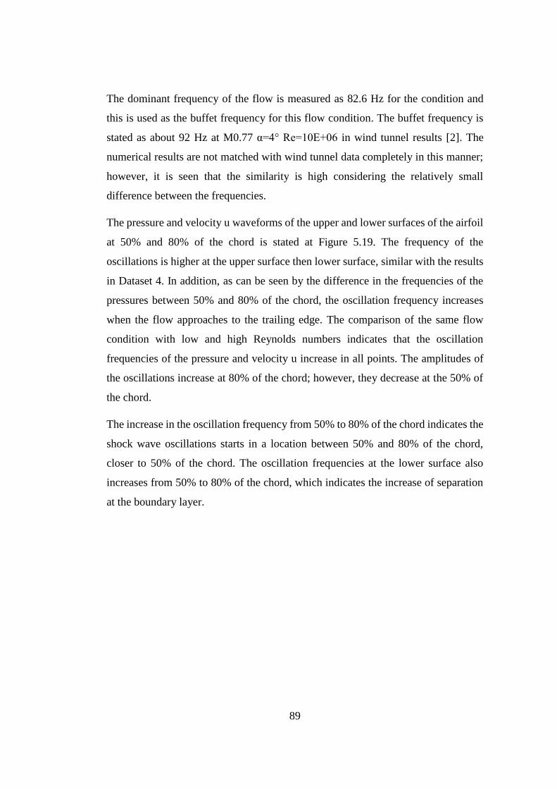
89
The dominant frequency of the flow is measured as 82.6 Hz for the condition and
this is used as the buffet frequency for this flow condition. The buffet frequency is
stated as about 92 Hz at M0.77 α=4° Re=10E+06 in wind tunnel results [2]. The
numerical results are not matched with wind tunnel data completely in this manner;
however, it is seen that the similarity is high considering the relatively small
difference between the frequencies.
The pressure and velocity u waveforms of the upper and lower surfaces of the airfoil
at 50% and 80% of the chord is stated at Figure 5.19. The frequency of the
oscillations is higher at the upper surface then lower surface, similar with the results
in Dataset 4. In addition, as can be seen by the difference in the frequencies of the
pressures between 50% and 80% of the chord, the oscillation frequency increases
when the flow approaches to the trailing edge. The comparison of the same flow
condition with low and high Reynolds numbers indicates that the oscillation
frequencies of the pressure and velocity u increase in all points. The amplitudes of
the oscillations increase at 80% of the chord; however, they decrease at the 50% of
the chord.
The increase in the oscillation frequency from 50% to 80% of the chord indicates the
shock wave oscillations starts in a location between 50% and 80% of the chord,
closer to 50% of the chord. The oscillation frequencies at the lower surface also
increases from 50% to 80% of the chord, which indicates the increase of separation
at the boundary layer.
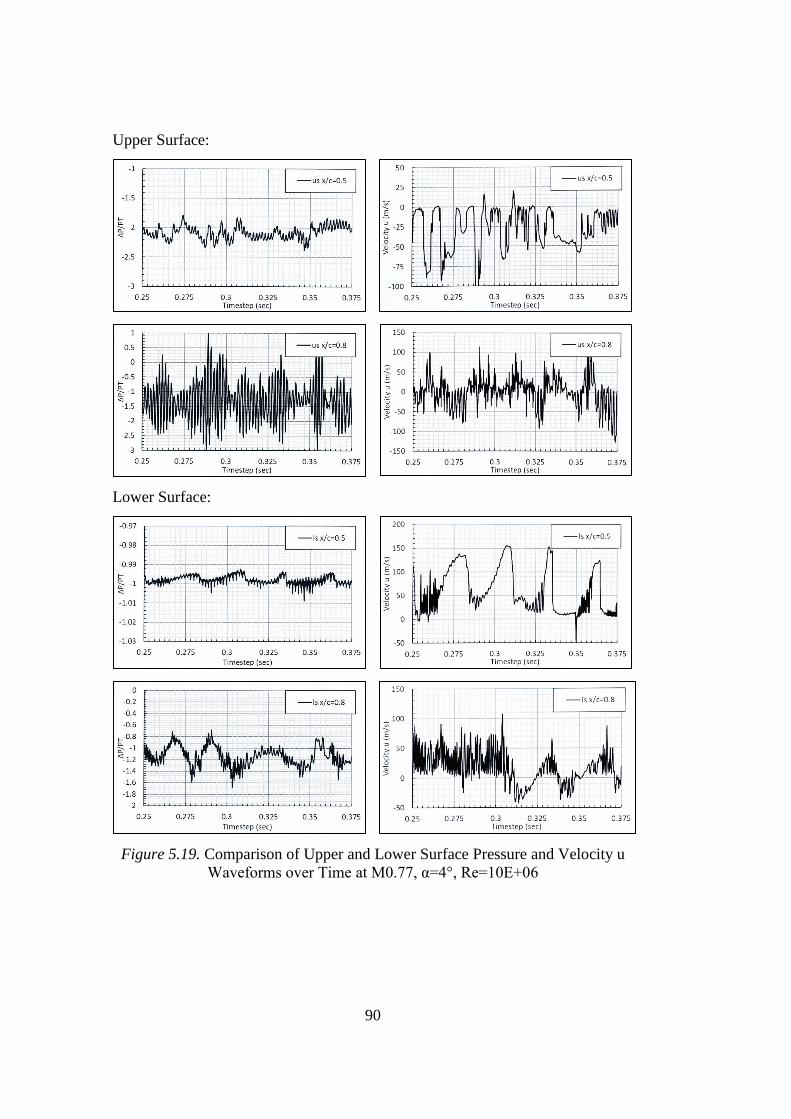
90
Upper Surface:
Lower Surface:
Figure 5.19. Comparison of Upper and Lower Surface Pressure and Velocity u
Waveforms over Time at M0.77, α=4°, Re=10E+06
91
The pressure waveforms of the at 50% and 80% of the chord is stated at Figure 5.20.
The oscillation frequency on the flow increases when it is moving from 50% of the
chord to the 80% of the chord.
The comparative wind tunnel data for the same flow conditions are also stated in
Figure 5.20 in orange color. The comparison of the numerical results with wind
tunnel data shows that a serious difference is seen on the amplitudes of the
oscillations of both results. On the contrary, the oscillation frequencies are similar.
Since the flow around 50% and 80% of the chord is highly instable and turbulent due
to separated boundary layer region with vortexes, the simulation of the subjected
area is highly challenging. The amplitude and frequency of the oscillating pressure
wave forms in these area can be simulated better with a higher mesh resolution and
Detached Eddy Simulation. However, the simulation requires serious amount of
computing power.
Figure 5.20. Pressure Waveforms over Time at M0.77, α=4°, Re=10E+06
92
The velocity u distribution over airfoil is stated as contour for various timesteps at
one period in Figure 5.21. The oscillating behavior of the shock wave can be
observed when the sub figures are examined with increasing timestep. The upper
surface is subjected to oscillating shock at the critical Mach and Angle of Attack
condition. The comparison between Figure 5.11 and Figure 5.21 shows that the rank
in separation at the boundary layer and the shock wave oscillation characteristics
differs as the Reynolds number increase for the same flow condition.
The frequency of the buffet is measured as around 34.3 Hertz for low Reynolds
number, the frequency increases up to 82.6 Hertz for the high Reynolds number. The
results indicate that the increase in the Reynolds number causes an increase in the
oscillation frequency at the trailing edge.
The Strouhal number for M0.77 α=4° Re=10E+06 flow conditions is stated as 0.45
in the wind tunnel test results [2]. For the same flow conditions, Strouhal number is
calculated as 0.40 from the numerical solutions. The flow cannot be modeled
accurately when looking at the mismatch on the Strouhal numbers of the two data.
However, the model succeeded to converge to the wind tunnel data when looking at
the 13% mismatch.
The frequency and the Strouhal number of the buffet cannot be matched and verified
with wind tunnel data. However, the increase in the frequency of the shock
oscillation is observed and the results approach the wind tunnel data. The possible
reason behind this mismatch is that the mesh resolution is not satisfactory for the
simulation of all the shock wave oscillations and the separations around boundary
layer.
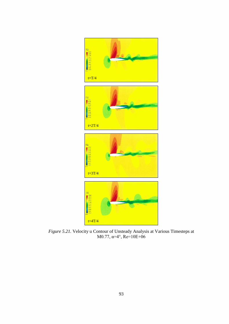
93
Figure 5.21. Velocity u Contour of Unsteady Analysis at Various Timesteps at
M0.77, α=4°, Re=10E+06
t=T/4
t=2T/4
t=3T/4
t=4T/4
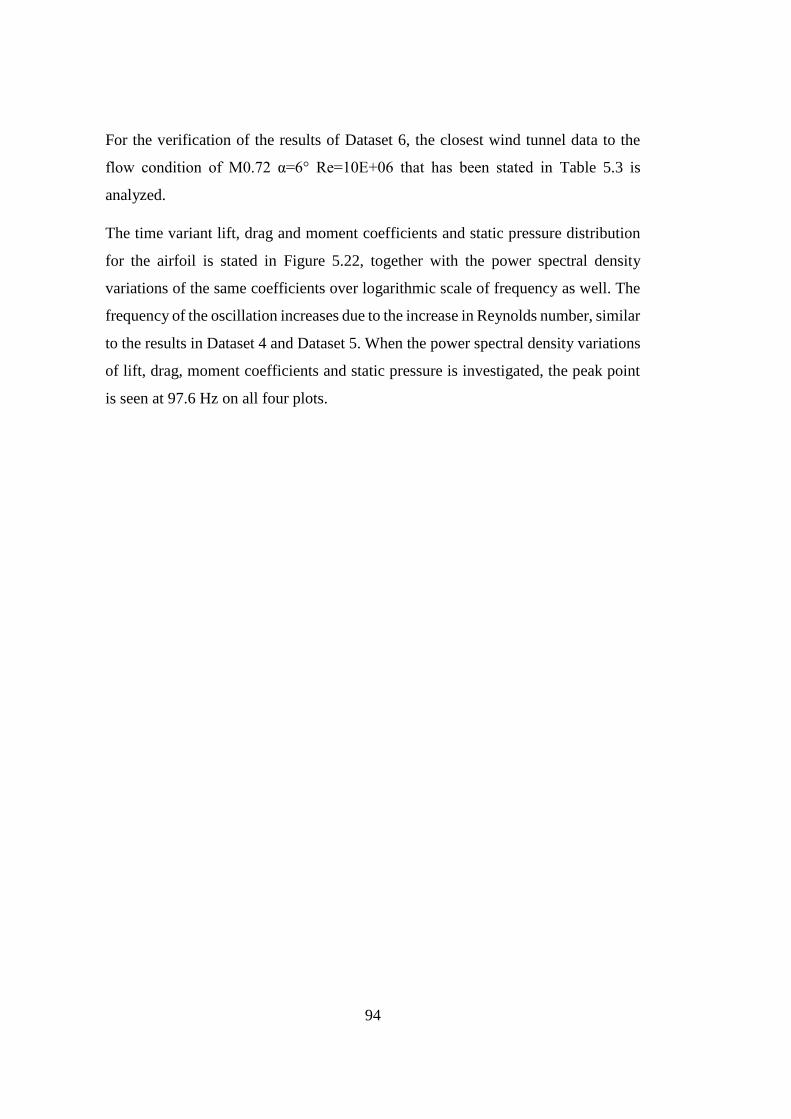
94
For the verification of the results of Dataset 6, the closest wind tunnel data to the
flow condition of M0.72 α=6° Re=10E+06 that has been stated in Table 5.3 is
analyzed.
The time variant lift, drag and moment coefficients and static pressure distribution
for the airfoil is stated in Figure 5.22, together with the power spectral density
variations of the same coefficients over logarithmic scale of frequency as well. The
frequency of the oscillation increases due to the increase in Reynolds number, similar
to the results in Dataset 4 and Dataset 5. When the power spectral density variations
of lift, drag, moment coefficients and static pressure is investigated, the peak point
is seen at 97.6 Hz on all four plots.
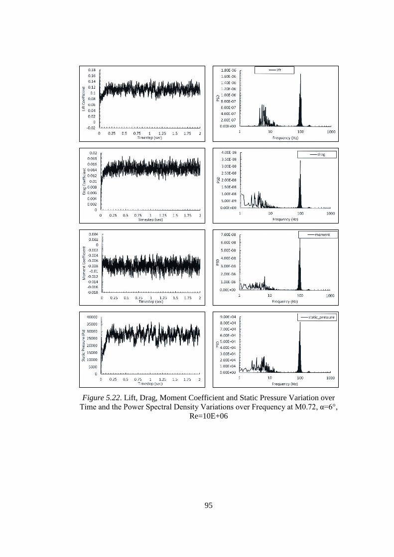
95
Figure 5.22. Lift, Drag, Moment Coefficient and Static Pressure Variation over
Time and the Power Spectral Density Variations over Frequency at M0.72, α=6°,
Re=10E+06
96
The dominant frequency of the flow is measured as 97.6 Hz for the condition and
this is used as the buffet frequency for this flow condition. The buffet frequency is
stated as about 106 Hz at M0.72 α=6° Re=10E+06 in wind tunnel data. The
numerical results are not matched with wind tunnel data completely in this manner;
however, it is seen that the similarity is high considering the relatively small
difference between the frequencies.
The pressure and velocity u waveforms of the upper and lower surfaces of the airfoil
at 50% and 80% of the chord is stated at Figure 5.23. It is seen from results that the
frequency of the oscillations is higher at the upper surface then lower surface. The
increase in Reynolds number leads to increase in both frequency and the amplitude
of the wavelengths of all four points.
The high frequency values at both 50% and 80% of the chord upper surface indicates
that the shock oscillations start in a location before 50% of the chord. The difference
at the frequencies between 50% and 80% of the chord is due to the boundary layer
separation occurs at near trailing edge.
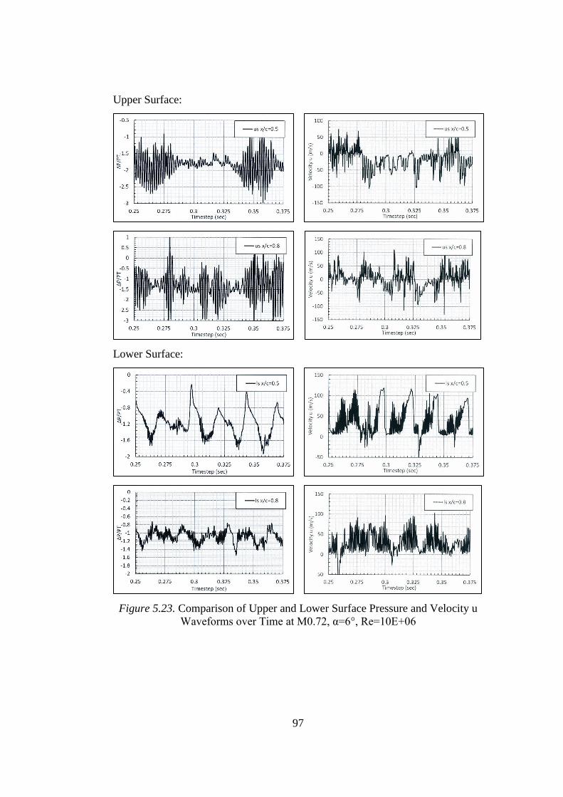
97
Upper Surface:
Lower Surface:
Figure 5.23. Comparison of Upper and Lower Surface Pressure and Velocity u
Waveforms over Time at M0.72, α=6°, Re=10E+06
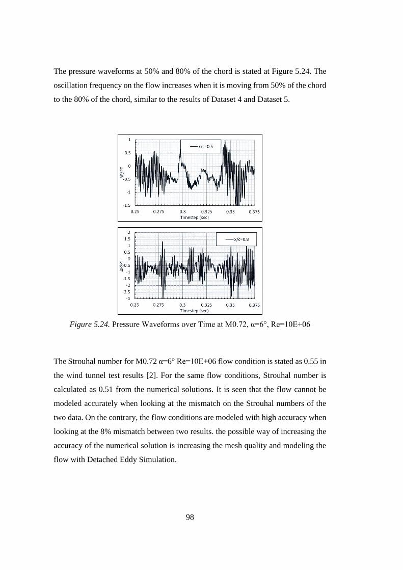
98
The pressure waveforms at 50% and 80% of the chord is stated at Figure 5.24. The
oscillation frequency on the flow increases when it is moving from 50% of the chord
to the 80% of the chord, similar to the results of Dataset 4 and Dataset 5.
Figure 5.24. Pressure Waveforms over Time at M0.72, α=6°, Re=10E+06
The Strouhal number for M0.72 α=6° Re=10E+06 flow condition is stated as 0.55 in
the wind tunnel test results [2]. For the same flow conditions, Strouhal number is
calculated as 0.51 from the numerical solutions. It is seen that the flow cannot be
modeled accurately when looking at the mismatch on the Strouhal numbers of the
two data. On the contrary, the flow conditions are modeled with high accuracy when
looking at the 8% mismatch between two results. the possible way of increasing the
accuracy of the numerical solution is increasing the mesh quality and modeling the
flow with Detached Eddy Simulation.
99
Considering all three flow conditions that are analyzed with numerical solutions, it
is seen that the frequency of the shock oscillations increases when the critical Mach
number decreases. The possible reason behind this feature is the same with the low
Reynolds number conditions. It is also seen that the pressure waveform
characteristics of each location is highly different for all of the flow conditions. The
common characteristics for all flow conditions is that the flow reaches more unstable
phase at the upper surface than lower surface. It is also seen that the frequency of the
oscillations increases when the Reynolds number increases, and the buffet frequency
is better observed from the Strouhal numbers.
The fluctuations in the moment coefficient affects the stability behavior. This kind
of frequent oscillations on the wing as seen in all moment results stimulate the short
period oscillation of the aircraft. The short period oscillations are highly critical for
the augmented fighter type aircrafts since the short period characteristics defines the
time to double amplitude and the time to double amplitude purely defines the
instability limitations of the aircraft [44]. As the characteristics of the moment
coefficient oscillations have been examined, it is seen that the shock oscillations of
buffet can be an additional criterion for the definition of the instability limit of the
aircraft since the frequency of the oscillations of the moment coefficient of the airfoil
are high enough to be able to stimulate the short period characteristic. It is also seen
that, especially at high Reynolds numbers, the frequency of the oscillations increases
and the higher the frequency becomes even more critical as the effect of the increase
in the oscillation on the instability limit increases even more.

101
CHAPTER 6
6 CONCLUSIONS
6.1 Concluding Remarks
The buffet onset characteristics of the NACA0012 airfoil is investigated through
several conditions with the commercial computational fluid dynamics tool as
ANSYS Fluent and the results are verified with wind tunnel test data in this study.
The study first investigates steady conditions through pressure coefficient
distributions. The mesh independency and turbulence model that is suitable for the
analysis of the unsteady characteristics of the buffet is investigated for the several
mesh and turbulence models. The results are closely matched with wind tunnel data
with the k-ω SST turbulence model. The pressure coefficient distribution is predicted
as coherent with the wind tunnel data and the location of the shock wave and pressure
drop on both upper and lower surfaces of the airfoil are predicted fairly accurately.
The k-ε and Spalart-Allmaras models have also a close match with the pressure
coefficient distribution especially before the shock location. However, the shock
location is predicted upstream of the location of the wind tunnel results with the
Spalart-Allmaras and downstream the real value with k-ε turbulence model. k-ω SST
turbulence model is especially successful at predicting the shock wave location
around upper and lower surfaces of the airfoil. The steady analyses are verified with
the wind tunnel test results for two different Reynolds numbers. As the Reynolds
number increases, the shock wave oscillations during buffet is highly observable and
predictable, the high Reynolds number is preferred for the verification. The
numerical results for the low Reynolds number is highly compatible with wind tunnel
results. However, for the high Reynolds number, the shock wave is predicted
upstream of the true location when compared to the wind tunnel data for one flow
102
condition. The other two flow conditions are predicted with high accuracy, in terms
of both pressure distributions and the shock wave location. The difference between
numerical solution and wind tunnel results could originate from several reasons;
however, it should be considered that there is a significant increase in the Reynolds
number of the analyzed condition which is from 3.7E+06 to 10E+06. The prediction
of the shock wave with such high Reynolds number can be a challenge for
computational methods even in two dimensional analyses.
The steady and unsteady transient analyses are conducted after the verification of the
steady analyses. The steady flow around airfoil before the buffet onset is investigated
with transient analyses. It is identified that no oscillation occurs on the shock wave
at upper and lower surfaces of the airfoil after the flow is settled on the geometry.
The flow is settled after 0.25 seconds and the steady flow can be seen clearly from
pressure distributions. The unsteady shock oscillated flow characteristics is
investigated through unsteady transient analyses. The angle of attack of the steady
analyses are conducted with approximately 2-degree increment for the unsteady
analyses. The analysis results have shown that after the buffet onset the shock
oscillation continues with nearly constant bandwidth after the flow is settled. The
oscillating characteristics of the shock wave can be seen on the pressure
distributions. The drag and lift coefficient distributions over time also indicated the
oscillating behavior of the shock wave. The Strouhal numbers of the unsteady
transient flow with low Reynolds number might seem less to trigger buffet; however,
the flow conditions are for the low Reynolds number. It is obvious that the increase
in the Reynolds number would lead to higher oscillations on the airfoil with the same
flow conditions. Indeed, the verification results of the unsteady transient flow have
shown that the oscillations of the shock wave are highly increased. The resultant
Strouhal numbers for high Reynolds number highly compatible with the wind tunnel
data.
The overall investigation of the buffet onset on two dimensional airfoil analyses have
shown that the shock oscillation is highly dependent on Mach number, angle of
attack and Reynolds number. The critical Mach number for the transonic buffet is
103
reached at the transonic flow condition at a specific angle of attack. The relation
between Mach number and the angle of attack is inversely proportional. As the Mach
number is increased, the angle of attack that triggers buffet starts to decrease. The
Reynolds number increase directly affects the buffet characteristics. As the Reynolds
number for the flow condition increases, the oscillation of the shock wave increases,
which provides basis for reaching the critical bandwidth for the buffet.
6.2 Future Work
The investigation of the buffet onset on two dimensional flow is the fundamental
step through understanding of the basic characteristics of the oscillating behavior of
the flow on buffet phenomenon. The turbulent, unsteady behavior of the flow at high
Reynolds numbers with critical Mach and angle of attack conditions is a challenging
case for the modelling of buffet characteristics on the airfoil even in two dimensional
motion. Since the analyses are conducted for a limited computational power, the
verification and transient analyses will be enhanced with the use of a computer of
increased processor and memory. After investigation of the NACA0012 airfoil buffet
onset characteristics, it is crucial for investigation of an alternative airfoil profile for
the further analyses.

105
REFERENCES
[1] B.H.K. Lee, “Oscillatory shock motion caused by transonic shock
boundary-layer interaction,” J. AIAA., vol. 28, no. 5, 1990, pp. 942–944.
[2] J.B. McDevitt, A.F. Okuno, “Static and dynamic pressure measurements on
a naca0012 airfoil in the ames high reynolds number facility,” in Tech.
Paper NASA TP-2485, National Aeronautics and Space Administration,
1985.
[3] W.F. Hilton and R.G. Fowler, “Photographs of shock wave movement,” in
Tech. Paper NPL R&M No. 2692, National Physical Laboratories, 1947.
[4] D.G. Mabey, “Oscillatory flows from shock induced separations on
biconvex aerofoils of varying thickness in ventilated wind tunnels,” in
Tech. Paper AGARD CP-296, Boundary layer effects on unsteady airloads,
Aix-en-Provence, France, 1981, pp. 1–14.
[5] H.H. Pearcey, “Some effects of shock-induced separation of turbulent
boundary layers in transonic flow past aerofoils,” in Tech. Paper ARC
R&M-3108, Aeronautical Research Council, 1955.
[6] H.H. Pearcey, “A method for the prediction of the onset of buffeting and
other separation effects from wind tunnel tests on rigid models,” AGARD
TR 223, National Physics Laboratory, 1958.
[7] J.D. Crouch, A. Garbaruk, D. Magidov, A. Travin, “Origin of transonic
buffet on aerofoils,” J. Fluid Mech., 2009, pp. 357–369.
[8] H. Tijdeman, “Investigations of the transonic flow around oscillating
Airfoils,” Ph. D. dissertation, Delft Univ. Technology, TU Delft, 1977.
[9] B.H.K. Lee, “Self-Sustained shock oscillations on airfoils at transonic
speeds,” in Prog. Aerosp. Sci., 2001.
[10] S. Raghunathan, R.D. Mitchell, M.A. Gillan, “Transonic shock
oscillations on NACA0012 aerofoil,” J. Shock Waves, 1998, pp. 191–202.
106
[11] J.B. McDevitt, L.L. Levy Jr., G.S. Deiwert, “Transonic flow about a thick
circular-arc airfoil,” J. AIAA, 1976, pp. 606–613.
[12] J.B. McDevitt, “Supercritical flow about a thick circular-arc airfoil,” in
Tech. Paper NASA-TM 78549, National Aeronautics and Space
Administration, 1979.
[13] B.H.K. Lee, “Investigation of flow separation on a supercritical airfoil,” J.
Aircr., 1989, pp. 1032–1037.
[14] B.H.K. Lee, F.A. Ellis, J. Bureau, “Investigation of the buffet
characteristics of two supercritical airfoils,” J. Aircr., 1989, pp. 731–736.
[15] J. Dandois, P. Molton, A. Lepage, A. Geeraert, V. Brunet, J.B. Dor, et al,
“Buffet characterization and control for turbulent wings,” in Tech. Paper
AerospaceLab, 2013, pp. 1–17.
[16] L. Jacquin, P. Molton, S. Deck, B. Maury, D. Soulevant, “Experimental
study of shock oscillation over a transonic supercritical profile,” J. AIAA,
2009, pp. 1985–1994.
[17] L. Jacquin, P. Molton, S. Deck, B. Maury, D. Soulevant, “An experimental
study of shock oscillation over a transonic supercritical profile,”in Proc.
35th AIAA Fluid Dynamics Conference and Exhibit, Toronto, Ont., 2005.
[18] S. Deck, “Numerical simulation of transonic buffet over a supercritical
airfoil,” J. AIAA, 2005, pp. 1556–1566.
[19] J.D. Crouch, A. Garbaruk, D. Magidov, L. Jacquin, “Global structure of
buffeting flow on transonic airfoils,” in IUTAM Symp. Unsteady Separated
Flows and Their Control, Springer, 2009.
[20] M. Thiery, E. Coustols, “URANS computations of shock-induced
oscillations over 2d rigid airfoils: influence of test section geometry,” J.
Flow, Turbul. Combust., 2005, pp. 331–354.
[21] N.F. Giannelis, G.A. Vio, “Aeroelastic interactions of a supercritical
aerofoil in the presence of transonic shock buffet,” in Proc. 54th AIAA
Aerospace Sciences Meeting, San Diego, CA, 2016.
107
[22] J.D. Crouch, A. Garbaruk, D. Magidov, “Predicting the onset of flow
unsteadiness based on global instability,” J. Comput. Phys., 2007, pp. 924–
940.
[23] J. Dandois, “Experimental study of transonic buffet phenomenon on a 3d
swept wing,” J. Physics of Fluids., 2016.
[24] L.L. Levy Jr., “Experimental and computational steady and unsteady
transonic flows about a thick airfoil,” J. AIAA, 1978, pp. 564–572.
[25] C.M. Maksymiuk, T.H. Pulliam, “Viscous transonic airfoil workshop
results using ARC2D,” in Proc. 25th AIAA Aerospace Sciences Meeting,
Reno, NV, 1987.
[26] F. Grossi, M. Braza, Y. Hoarau, “Prediction of transonic buffet by delayed
detached eddy simulation,” J. AIAA, 2014, pp. 2300–2312.
[27] G. Barakos, D. Drikakis, “Numerical simulation of transonic buffet flows
using various turbulence closures,” Int. J. Heat Fluid Flow, 2000, pp. 620–
626.
[28] G. Barakos, D. Drikakis, “An implicit unfactored method for unsteady
turbulent compressible flows with moving boundaries,” J. Comput. Fluids,
1999, pp. 899–922.
[29] B.S. Baldwin, H. Lomax, “Thin layer approximation and algebraic model
for separated turbulent flows,” in Proc. 16th AIAA Aerospace Sciences
Meeting, Hunstville, AL, 1978.
[30] P.R. Spalart, S.R. Allmaras, “A one-equation turbulence model for
aerodynamic flows,” J. La Rech. Aerosp., 1994.
[31] B.E. Launder, B.I. Sharma, “Application of the energy-dissipation model
of turbulence to the calculation of flow near a spinning disc,” J. Lett. Heat
Mass Transf., 1974, pp. 131–137.
[32] Y. Nagano, C. Kim, “A two-equation model for heat transport in wall
turbulent shear flows,” J. Heat Transf., 1988, pp. 583–589.
108
[33] D. Sofialidis, P. Prinos, “Development of a non-linear, strain-sensitive k-ω
turbulence model,” in Proc. 11th Symposium on Turbulent Shear Flows,
Grenoble, France, 1997, pp. 89–94.
[34] T.J. Craft, B.E. Launder, K. Suga, “Development and application of a cubic
eddyviscosity model of turbulence,” Int. J. Heat Fluid Flow, 1996, pp. 108–
115.
[35] A. Kourta, G. Petit, J.C. Courty, J.P. Rosenblum, “Buffeting in transonic
flow prediction using time-dependent turbulence model,” Int. J. Numer.
Methods Fluids, 2005, pp. 171–182.
[36] A. Kourta, “Computation of vortex shedding in solid rocket motors using
timedependent turbulence model,” J. Propuls. Power, 1999, pp. 390–400.
[37] Q. Xiao, H.M. Tsai, F. Liu, “Numerical study of transonic buffet on a
supercritical airfoil,” J. AIAA, 2006, pp. 620–628.
[38] M.E. Olsen, T.J. Coakley, “The lag model, a turbulence model for non
equilibrium flows,” in Proc. 15th AIAA Computational Fluid Dynamics
Conference, Anaheim, CA, 2001.
[39] R. Carrese, P. Marzocca, O. Levinski, N. Joseph, “Investigation of
supercritical airfoil dynamic response due to transonic buffet,” in Proc.
54th AIAA Aerospace Sciences Meeting, San Diego, CA, 2016.
[40] N.F. Giannelis, G.A. Vio, “Aeroelastic interactions of a supercritical
aerofoil in the presence of transonic shock buffet,” in Proc. 54th AIAA
Aerospace Sciences Meeting, San Diego, CA, 2016.
[41] G. Alfonsi, "Reynolds-Averaged Navier–Stokes equations for turbulence
modeling," J. Appl. Mech. Rev, 2009.
[42] H. Schlichting, Boundary-Layer Theory, Seventh Edition, McGraw Hill Inc
1979.
[43] G. L. Mellor and H. J. Herring, "A survey of the mean turbulent field
closure models," J. AIAA, 1973, pp. 590–599.
[44] U. Kutluay, T. Cimen and K. G. Parlak, “A study on controllability of an
augmented stability fighter aircraft,” in AIAC Conf., 2017.