DESIGN AND IMPLEMENTATION OF MAGNETIC FIELD SENSORS FORBIOMEDICAL APPLICATIONS

A THESIS SUBMITTED TOTHE GRADUATE SCHOOL OF NATURAL AND APPLIED SCIENCES

OFMIDDLE EAST TECHNICAL UNIVERSITY

ULAS CAN INAN

IN PARTIAL FULFILLMENT OF THE REQUIREMENTSFOR

THE DEGREE OF MASTER OF SCIENCEIN

ELECTRICAL AND ELECTRONICS ENG.

FEBRUARY 2015

Approval of the thesis:

DESIGN AND IMPLEMENTATION OF MAGNETIC FIELD SENSORS FORBIOMEDICAL APPLICATIONS

submitted by ULAS CAN INAN in partial fulfillment of the requirements for the de-gree of Master of Science in Electrical and Electronics Eng. Department, MiddleEast Technical University by,

Prof. Dr. Gülbin DuralDean, Graduate School of Natural and Applied Sciences

Prof. Dr. Gönül Turhan SayanHead of Department, Electrical and Electronics Eng.

Prof. Dr. Nevzat G. GençerSupervisor, Electrical and Electronics Eng Dept,METU

Examining Committee Members:

Prof. Dr. Murat EyübogluElectrical and Electronics Engineering Dept., METU

Prof. Dr. Nevzat G. GençerElectrical and Electronics Engineering Dept., METU

Assoc. Prof. Dr. Yesim SerinagaogluElectrical and Electronics Engineering Dept., METU

Assoc. Prof. Dr. Lale AlatanElectrical and Electronics Engineering Dept., METU

Assoc. Prof. Dr. Süha YagcıogluBiophysics, Hacettepe University

Date: 10.02.2015

I hereby declare that all information in this document has been obtained andpresented in accordance with academic rules and ethical conduct. I also declarethat, as required by these rules and conduct, I have fully cited and referenced allmaterial and results that are not original to this work.

Name, Last Name: ULAS CAN INAN

Signature :

iv

ABSTRACT

DESIGN AND IMPLEMENTATION OF MAGNETIC FIELD SENSORS FORBIOMEDICAL APPLICATIONS

Can Inan, Ulas

M.S., Department of Electrical and Electronics Eng.

Supervisor : Prof. Dr. Nevzat G. Gençer

February 2015, 85 pages

In this work, firstly the magnetic sensor types and their feasibility for biomedical ap-

plications are investigated. Then the air-cored induction coil sensor is chosen due to

its advantages. Afterwards the usage of induction coils combined with amplifiers and

connection types are studied. The biomedical applications requiring the use of mag-

netic field sensors are introduced. One of them, Lorentz Field Electrical Impedance

Tomography (LFEIT) is explained in detail and experimental work is done for this ap-

plication. In the second part, formulation of the magnetic sensor and the amplification

circuitry, its frequency related components and frequency response is introduced. An

optimization algorithm using MATLAB software is prepared to be able to determine

the most sensitive disk shaped air-cored induction coil by its size parameters. This

software is tested before moving further forward, according to the formulations given.

After explaining the discrepancies caused by the problems encountered through the

experimental process, an optimum induction coil sensor is designed for LFEIT ap-

plication. The sensitivity and linearity of the system are analyzed. Two different

amplifier configurations are used. First one includes AD797 as voltage amplifier and

v

the sensitivity of this system is measured to be 17.1 (V m/A). The amplification factor

obtained is 20. The maximum deviation from linearity for this case is computed as

%15.3. Second one includes two cascaded amplifiers namely, AD600 and AU-1291.

The sensitivity of this configuration is measured as 5.45 (V m/A). The maximum de-

viation from linearity is computed as %2.7. Second configuration is preferred since

with the use of cascaded amplifiers, the amplification is increased to 160000. Al-

though the coil with the best sensitivity using the present equipment is wound, the

performance of the sensor is still inadequate and it is concluded that better sensitivity

is required. There are also other promising coil designs obtained using the software

developed, however they are not wound yet. Still, the performance is not expected

to increase significantly. A sensitivity of about 107 is itself a great challenge which

cannot be overcome by adjusting the amplifier since the signal to noise ratio (SNR)

does not improve and the signal to be observed remains smaller than the noise level.

However the software providing the optimum coil parameters for a specific case is

useful in more than one application. Furthermore it can be modified to optimize other

coil types such as rectangular coil, flat-spiral coil etc. allowing a very wide range

of possible sensor designs. Other than LFEIT, wireless power transfer application

of magnetic sensors is also investigated. The conditions that maximizes the power

transfer efficiency are studied. The same algorithm used in determining the coil size

parameters with maximum sensitivity is also applied to find the coil with the optimum

quality factor, which is the most important condition for obtaining the best efficiency

in power transfer. Four coil wireless power transfer is chosen, designed and imple-

mented to compare with the analytical results. The efficiency of the designed system

is measured as %7.6. This value is increased to %39 by using litz wire at the windings

instead of enamel copper wire.

Keywords: Magnetic Field Sensors, Biomedical Applications, LFEIT, Lorentz Field,

Induction Coil, Coil design

vi

ÖZ

BIYOMEDIKAL UYGULAMALARI IÇIN MANYETIK ALAN SENSÖRTASARIMI VE YAPIMI

Can Inan, Ulas

Yüksek Lisans, Elektrik ve Elektronik Mühendisligi Bölümü

Tez Yöneticisi : Prof. Dr. Nevzat G. Gençer

Subat 2015, 85 sayfa

Bu çalısmanın ilk kısmında, manyetik sensör türleri ve bunların biyomedikal uygula-

malarında kullanılabilirligi arastırılmaktadır. Sagladıgı avantajlar göz önünde bulun-

durularak hava çekirdekli endüksiyon bobini seçildi. Çalısmanın devamında endük-

siyon bobini ile amplifikatör kombinasyonu ve baglantı türleri incelendi. Manyetik

alan sensörü kullanımı gerektiren biyomedikal uygulamaları tanıtıldı. Bunlardan biri,

Lorentz Alanı Elektriksel Empedans Tomografisi detaylı bir sekilde açıklandı ve bu

uygulama ıçın deneysel çalısma gerçeklestirildi. Ikinci kısımda manyetik sensör ve

amplifikatör devresinin frekansa baglı elemanları ve bunların frekansı cevabı, ayrıca

ilgili formüller verildi. En hassas ölçümü yapabilecek disk seklindeki hava çekirdekli

endüksiyon bobininin boyut degiskenlerini belirlemek amacıyla MATLAB yazılımı

kullanılarak bir optimizasyon algoritması gelistirildi. Daha fazla ilerlemeden önce bu

yazılım, verilmis olan formüllerden yararlanarak test edildi. Deneysel süreç boyunca

karsılasılan problemlerden dogan farklılıklar açıklandıktan sonra, LAEET uygula-

masında kullanılmak üzere bir optimum endüksiyon bobini dizayn edildi. Iki farklı

vii

yükseltici düzenegi kullanıldı. Bunlardan birincisinde AD797 isimli voltaj yükselti-

cisi bulunmaktadır ve bu sistemin duyarlılıgı 17.1 (V m/A) olarak ölçüldü. Yükseltme

faktörü 20 olarak elde edildi. Maksimum çizgisellikten sapma bu sistem için %15.3

olarak hesaplandı. Ikinci düzenekte ise iki yükseltici seri baglı ve bu yükselticilerin

isimleri AD600 ve AU-1291’dir. Bu sistemin duyarlılıgı 5.45 (V m/A) olarak ölçüldü.

Maksimum çizgisellikten sapma %2.7 olarak hesaplandı. Seri baglı yükselticilerin

varlıgı yükseltme faktörünü 160000’e çıkardıgı için ikinci sistem tercih edildi. Mev-

cut ekipman ile en yüksek duyarlılıga sahip bobin sarılmıs olsa da performans yine

de yetersiz kaldı ve daha yüksek duyarlılıgın gerekli oldugu sonucuna varıldı. Gelis-

tirilmis olan yazılım ile ümit verici baska bobinler dizayn edildi, ancak bunlar sarıl-

madı. Yine de performansın etki yaratacak kadar artması beklenmemektedir. 107’ye

varan bir duyarlılık oranı, yükselticinin ayarlanması ile asılması mümkün olmayan

bir güçlük teskil etmektedir, çünkü sinyal gürültü oranında iyilesme gözlenmemekte

ve ölçülmek istenen sinyal gürültü seviyesinin altında kalmaktadır. Ancak bir durum

için optimum bobin degiskenlerini veren yazılım birden fazla uygulama için yararlı

olabilmektedir. Ayrıca bu yazılım dikdörtgen bobin, düz-spiral bobin gibi farklı bobin

türlerini optimize etmek üzere modifiye edilebilir, böylece olası sensör dizaynlarının

yelpazesinin genis tutulmasına olanak saglanabilir. Sistemin duyarlılıgı ve çizgiselligi

analiz edildi. LAEET’in yanısıra, manyetik sensörlerin kablosuz güç aktarımı uygu-

laması da arastırıldı. Güç aktarımı verimliligini maksimize eden kosullar incelendi.

Güç aktarımında verimliligin en önemli kosulu olan optimum kalite faktörüne sahip

bobini bulmak için maksimum duyarlılıgı veren bobin boyut degiskenlerini elde et-

memizi saglayan algoritma burada da kullanıldı. Dört bobinli kablosuz güç aktarımı

sistemi seçildi, dizayn edildi ve uygulamaya geçirilerek analitik sonuçlarla karsılas-

tırma yapıldı. Dizayn edilen sistemin verimliligi %7.6 olarak ölçüldü. Bu deger, sa-

rımlarda enamel bakır tel yerine litz teli kullanılmak suretiyle %39’a yükseltildi.

Anahtar Kelimeler: Manyetik Alan Sensörleri, Biyomedikal Uygulamaları, LAEET,

Lorentz Alanı, Endüksiyon Bobini, Bobin Dizaynı

viii

My mother and father, I will love you forever

ix

ACKNOWLEDGMENTS

I would like to express my gratitude to Prof. Dr. Nevzat G. GENÇER for his support,

guidance and patience through this study. He did not stop believing in me even after

all the misfortune I have been through. As I applied the improvements he suggested,

I understood the value of his guidance. I also got a head start thanks to the resources

he provided. I would like to thank Mürsel KARADAS for his contributions to the

experimental work of this study, since one of the applications included a collaborative

study with him. I would like to thank Dr. Reyhan (TUTUK) ZENGIN for her always

helpful attitude, and also Dr. Balkar ERDOGAN for his support and advices through

this study. Finally I want to thank my mother Canan INAN for all of her emotional

support and patience.

x

TABLE OF CONTENTS

ABSTRACT . . . . . . . . . . . . . . . . . . . . . . . . . . . . . . . . . . . . v

ÖZ . . . . . . . . . . . . . . . . . . . . . . . . . . . . . . . . . . . . . . . . . vii

ACKNOWLEDGMENTS . . . . . . . . . . . . . . . . . . . . . . . . . . . . . x

TABLE OF CONTENTS . . . . . . . . . . . . . . . . . . . . . . . . . . . . . xi

LIST OF TABLES . . . . . . . . . . . . . . . . . . . . . . . . . . . . . . . . xiv

LIST OF FIGURES . . . . . . . . . . . . . . . . . . . . . . . . . . . . . . . . xv

CHAPTERS

1 INTRODUCTION . . . . . . . . . . . . . . . . . . . . . . . . . . . 1

1.1 Magnetic Sensors . . . . . . . . . . . . . . . . . . . . . . . 1

1.2 Induction Coil Sensors . . . . . . . . . . . . . . . . . . . . . 3

1.3 Air-Cored Induction Coil in Biomedical Applications . . . . 7

1.4 Objectives of the Thesis . . . . . . . . . . . . . . . . . . . . 11

1.5 Outline of the Thesis . . . . . . . . . . . . . . . . . . . . . . 11

2 THEORY . . . . . . . . . . . . . . . . . . . . . . . . . . . . . . . . 13

2.1 Introduction . . . . . . . . . . . . . . . . . . . . . . . . . . 13

2.2 Formulation for Induced Voltage on an Air Cored InductionCoil . . . . . . . . . . . . . . . . . . . . . . . . . . . . . . 13

2.2.1 Multilayer Coil . . . . . . . . . . . . . . . . . . . 14

xi

2.2.2 Flat Spiral Coil . . . . . . . . . . . . . . . . . . . 16

2.3 Formulation for Induced Voltage on an Air Cored InductionCoil . . . . . . . . . . . . . . . . . . . . . . . . . . . . . . 17

2.3.1 Parallel Resonant Circuit . . . . . . . . . . . . . . 20

2.3.2 Series Resonant Circuit . . . . . . . . . . . . . . . 21

2.3.3 Frequency Response Comparison of Parallel andSeries Resonant Circuit . . . . . . . . . . . . . . . 22

2.4 Frequency Related Parameters . . . . . . . . . . . . . . . . . 24

2.4.1 K Parameter . . . . . . . . . . . . . . . . . . . . . 25

2.4.2 Inductance Parameter . . . . . . . . . . . . . . . . 27

2.4.3 Capacitance Parameter . . . . . . . . . . . . . . . 28

2.5 Magnetic Field Produced by an Induction Coil . . . . . . . . 30

3 DESIGN OF THE MAGNETIC SENSOR . . . . . . . . . . . . . . . 35

3.1 Introduction . . . . . . . . . . . . . . . . . . . . . . . . . . 35

3.2 The Effect of Coil Parameters . . . . . . . . . . . . . . . . . 35

3.2.1 Coil Diameter . . . . . . . . . . . . . . . . . . . . 36

3.2.2 Coil Length . . . . . . . . . . . . . . . . . . . . . 37

3.2.3 Wire Diameter . . . . . . . . . . . . . . . . . . . 37

3.3 Coil Parameter Optimization . . . . . . . . . . . . . . . . . 37

3.4 Amplifier Design . . . . . . . . . . . . . . . . . . . . . . . 40

3.5 Frequency Response of the System and Noise Analysis . . . 43

4 EXPERIMENTAL WORK . . . . . . . . . . . . . . . . . . . . . . . 47

4.1 Introduction . . . . . . . . . . . . . . . . . . . . . . . . . . 47

4.2 Test of the Induction Coil Design . . . . . . . . . . . . . . . 47

xii

4.3 LFEIT Application . . . . . . . . . . . . . . . . . . . . . . . 55

4.4 Wireless Power Transfer (WPT) Application . . . . . . . . . 65

5 CONCLUSION AND DISCUSSION . . . . . . . . . . . . . . . . . 79

REFERENCES . . . . . . . . . . . . . . . . . . . . . . . . . . . . . . . . . . 83

xiii

LIST OF TABLES

TABLES

Table 1.1 Magnitude and frequency range of different magnetometers . . . . . 3

Table 4.1 Comparison of theoretical and measured inductance/resistance val-

ues for different coils. . . . . . . . . . . . . . . . . . . . . . . . . . . . . 50

Table 4.2 Comparison of the theoretical and experimental capacitance values

and resonance frequencies for different coils. . . . . . . . . . . . . . . . . 50

Table 4.3 Measured and calculated voltage output for different magnetic field

input at respective measurement distances . . . . . . . . . . . . . . . . . 51

Table 4.4 Measured and calculated voltage outputs after modification of in-

ductance by including mutual inductances and respective coupling coeffi-

cient value measurements . . . . . . . . . . . . . . . . . . . . . . . . . . 53

Table 4.5 Measured voltage outputs at two different frequencies of importance

for a range of measurement distance and respective coupling coefficient

values . . . . . . . . . . . . . . . . . . . . . . . . . . . . . . . . . . . . 63

Table 4.6 Size parameters of the coils with optimum quality factor . . . . . . . 72

Table 4.7 Critical parameters of the coils modified to include Litz wires as

their windings . . . . . . . . . . . . . . . . . . . . . . . . . . . . . . . . 77

Table 4.8 Critical parameters of the secondary coil modified further to have

high loaded quality factor . . . . . . . . . . . . . . . . . . . . . . . . . . 77

xiv

LIST OF FIGURES

FIGURES

Figure 1.1 Types of Magnetometers . . . . . . . . . . . . . . . . . . . . . . 2

Figure 1.2 Air-cored induction coil (Disk coil) a) Side view, b) Top view . . . 4

Figure 1.3 Air-cored induction coil (Rectangular multilayer coil) a) Side view,

b) Top view . . . . . . . . . . . . . . . . . . . . . . . . . . . . . . . . . 5

Figure 1.4 Induction coil (Disk coil) with ferromagnetic core . . . . . . . . . 5

Figure 1.5 Spiral Planar coil a) Top view, b) Side view . . . . . . . . . . . . . 6

Figure 1.6 The main configuration of the system . . . . . . . . . . . . . . . . 7

Figure 1.7 The electrical signal detected by the measurement electrodes and

its relation with conductivity gradient . . . . . . . . . . . . . . . . . . . . 9

Figure 1.8 Sketch of the WPT system . . . . . . . . . . . . . . . . . . . . . . 11

Figure 2.1 Coil parameters for multilayer coil . . . . . . . . . . . . . . . . . . 15

Figure 2.2 Packing Factors of Two Different Winding Configurations . . . . . 16

Figure 2.3 Coil parameters for flat spiral coil . . . . . . . . . . . . . . . . . . 17

Figure 2.4 α Representing the Angle Between Sensor Coil and Magnetic Field

(B) . . . . . . . . . . . . . . . . . . . . . . . . . . . . . . . . . . . . . . 18

Figure 2.5 The Equivalent Circuit of Three Different Configurations . . . . . . 19

Figure 2.6 Induction Coil Connected to a Voltage Amplifier . . . . . . . . . . 21

xv

Figure 2.7 Induction Coil Connected to a Current Amplifier . . . . . . . . . . 23

Figure 2.8 Comparison between the Frequency Responses of Parallel Reso-

nance and Series Resonance Configurations. Results are obtained for 1

nT input and an amplification factor of 20. The parallel resistance RII is

100 Ω. . . . . . . . . . . . . . . . . . . . . . . . . . . . . . . . . . . . . 24

Figure 2.9 Magnetic Field on the Axis of a Current Loop . . . . . . . . . . . . 32

Figure 2.10 Magnetic Field on the Axis of a Multilayer Air-Core Solenoid . . . 33

Figure 2.11 Magnetic Field on the Axis of an Induction Coil vs position . . . . 33

Figure 3.1 Output voltage versus coil diameter for different coil lengths . . . . 36

Figure 3.2 The effect of coil length . . . . . . . . . . . . . . . . . . . . . . . 38

Figure 3.3 Wire diameter vs output voltage for different coil diameter and

length combinations . . . . . . . . . . . . . . . . . . . . . . . . . . . . . 39

Figure 3.4 Optimization GUI Software . . . . . . . . . . . . . . . . . . . . . 41

Figure 3.5 Improved optimization GUI software example 1 . . . . . . . . . . 41

Figure 3.6 Improved optimization GUI software example 2 . . . . . . . . . . 42

Figure 3.7 Transient analysis of amplifier circuitry. Simulation software used

is multisim. Green signal is the input of the amplifier, indicated as V6.

Red signal is the output of the amplifier, indicated as V1. The operating

frequency used in the simulation is 2.2 MHz . . . . . . . . . . . . . . . . 43

Figure 3.8 Noise equivalent circuit [10]. U2R

∆fand i2R

∆fare the noise voltage rep-

resenting the thermal noise of the coil resistance R and the noise current

representing the damping resistor RII respectively. U2

∆fand I2R

∆frepresent

the internal noise voltage and internal noise current of the amplifier . . . . 45

xvi

Figure 3.9 Signal, noise and magnetic noise comparison for the first system

designed for LFEIT application. Simulation software used is MATLAB.

Input magnetic flux density is 1 nT. Amplifier used is AD797. Parallel

resistance RII is 100 Ω. . . . . . . . . . . . . . . . . . . . . . . . . . . . 46

Figure 4.1 Transmitter coil circuit. Signal given from function generator is

measured on 1.2 kΩ resistance in order to determine the current through

the transmitter coil later to be used in (2.47) to calculate the input magnetic

field of the sensor. . . . . . . . . . . . . . . . . . . . . . . . . . . . . . . 49

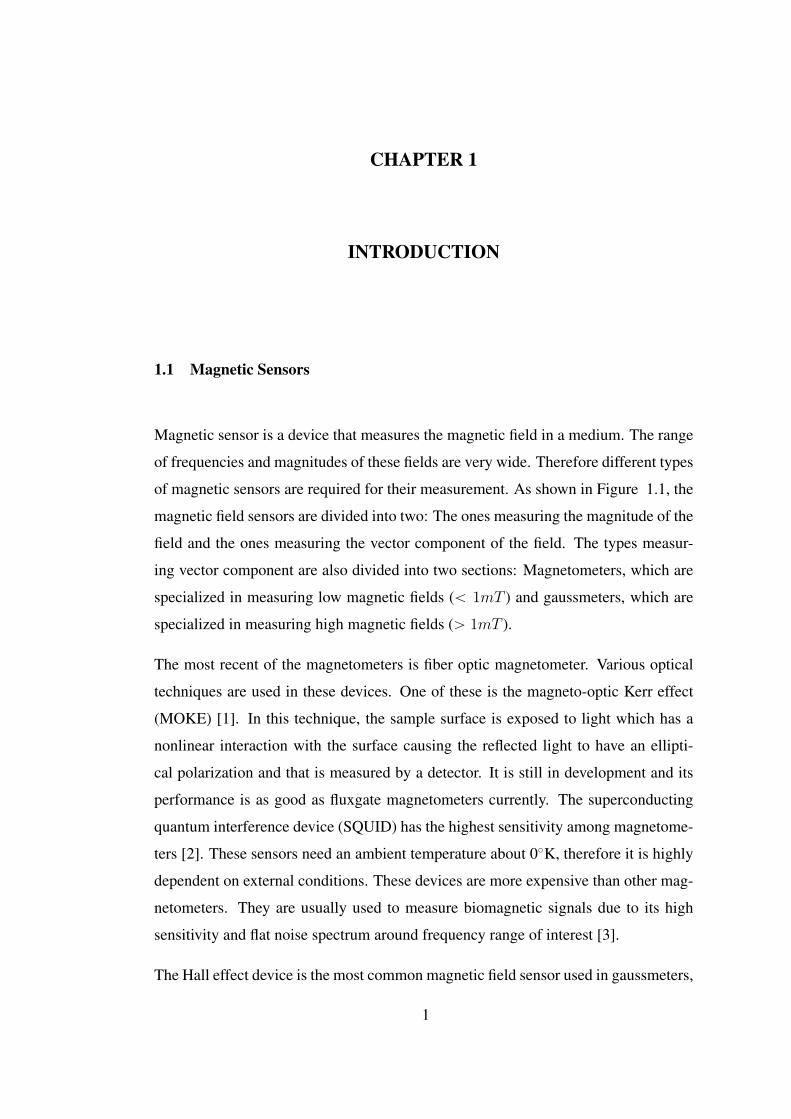
Figure 4.2 Receiver stage. Low noise high input impedance amplifier AD 797

is used. . . . . . . . . . . . . . . . . . . . . . . . . . . . . . . . . . . . . 52

Figure 4.3 Comparison of the theoretical and measured output voltages for

a range of magnetic flux density values (on the order of nT) as given in

Table 4.3. The operation frequency is 2.8 MHz. . . . . . . . . . . . . . . 52

Figure 4.4 Data obtained through measurement and its linear approximation . 54

Figure 4.5 Experiment setup without test tube, sensor and ultrasound input,

the width of the mid section is greater than the diameter of the test tube

and 2.5 cm [15] . . . . . . . . . . . . . . . . . . . . . . . . . . . . . . . 56

Figure 4.6 Optimum coil designed for LFEIT application (20 mm coil diam-

eter, 2.5 mm coil height (length), 0.6 mm wire diameter) a) Top view, b)

Side view . . . . . . . . . . . . . . . . . . . . . . . . . . . . . . . . . . . 57

Figure 4.7 Simulation results for the amplifier circuitry designed for LFEIT

application. The left hand side shows the input signal characteristics(20

uV, 1 MHz). On the right hand side, the output signal is observed at chan-

nel B. The amplification can be calculated as 40mV/20uV=2000. Input

signal (channel A) is too small to be revealed on the oscilloscope screen. . 58

xvii

Figure 4.8 Simulation results for the amplifier circuitry designed for LFEIT

application(second AD600 excluded). The left hand side shows the input

signal characteristics (20 uV, 1 MHz). On the right hand side, the output

signal is observed at channel B. The amplification can be calculated as

2.25/20mV=112.5. Input signal (channel A) is also shown on the oscillo-

scope screen and it is 20 mV in amplitude. . . . . . . . . . . . . . . . . . 59

Figure 4.9 Amplifier circuitry designed for LFEIT application . . . . . . . . . 59

Figure 4.10 The detailed schematic of the first stage of the amplifier circuit . . . 60

Figure 4.11 Pin configuration and internal structure of AD600 . . . . . . . . . 60

Figure 4.12 The amplifier circuit board . . . . . . . . . . . . . . . . . . . . . . 61

Figure 4.13 GUI results for LFEIT application (with 10 pT input and maximum

coil and wire diameter constraints) . . . . . . . . . . . . . . . . . . . . . 61

Figure 4.14 Data obtained through measurement and its linear approximation . 64

Figure 4.15 GUI results for LFEIT application with 0.1 pT input and maximum

coil diameter and wire diameter constraints of 2 cm and 0.6 mm respec-

tively. Operation frequency is 1 MHz. Output voltage is calculated as 0.37

mV. Optimum coil length is computed as 2.5 mm. Wire diameter of the

optimized coil is 0.6 mm. . . . . . . . . . . . . . . . . . . . . . . . . . . 64

Figure 4.16 GUI results for LFEIT application with 6 mm wire diameter con-

straint. This value is chosen high enough to check whether there is a better

coil if there were no wire diameter constraint. Output voltage for the de-

termined optimum coil is calculated as 0.7 mV. Wire diameter is computed

as 1.57 mm. Optimum coil length is also changed and it is 2 cm. . . . . . 65

xviii

Figure 4.17 Improved GUI results for LFEIT application with 0.6 mm wire di-

ameter constraint. Improved GUI includes additional software that deter-

mines whether flat spiral coil or air-cored multilayer coil performs better.

It is observed that a flat spiral coil provides a slightly better output voltage

(0.4 mV) compared to the results given in Figure 4.15. Since the optimum

coil type is determined as flat spiral, instead of coil length parameter, the

turn spacing parameter is included. Wire diameter of the optimum coil is

calculated as 0.2 mm and the turn is spacing is 0.004 mm. . . . . . . . . . 66

Figure 4.18 Improved GUI results for LFEIT application with 6 mm wire diam-

eter constraint. The results are same as in Figure 4.16 since the optimum

coil type for this case is air-cored multilayer coil. . . . . . . . . . . . . . 66

Figure 4.19 The schematic of the final version of the experiment setup. Dc

magnetic field is seen at inward direction which is perpendicular to the

measurement axis. Induction coil sensor is placed adjacent to the tube in

order to obtain best sensitivity performance. . . . . . . . . . . . . . . . . 67

Figure 4.20 The illustration of expected results of the experiment. The scale

among the signals to be measured is represented in this figure. The sig-

nals with greater amplitude correspond to outer boundaries with higher

conductivity gradient namely the boundary between air and oil, salt water

and tube respectively. These expected signals are out of phase 180 de-

grees. The waveform in the middle corresponds to the conductivity gradi-

ent between salt water and oil therefore it is smaller. The aim is to observe

this smaller signal since it will prove whether the conductivity difference

between two different tissues can be distinguished. . . . . . . . . . . . . . 68

Figure 4.21 The illustration of results of the experiment. The outer boundary

signals are obtained at a scale of 5 V. However the noise signal obtained is

greater than the expected inner boundary waveform, therefore it was not

possible to distinguish this signal from the noise. . . . . . . . . . . . . . . 69

xix

Figure 4.22 Theoretical results for noise analysis of the experiment setup for

0.1 pT input magnetic flux density. It is observed that the output voltage

of the sensor is below the noise level. . . . . . . . . . . . . . . . . . . . . 69

Figure 4.23 Theoretical results for noise analysis of the experiment setup for

10 pT input magnetic flux density. This simulation indicates that if it is

possible to increase the input flux density by using a higher magnitude

DC field or placing the sensor closer to the source with a different con-

figuration, output signal reaches above the noise level at the resonance

frequency. . . . . . . . . . . . . . . . . . . . . . . . . . . . . . . . . . . 70

Figure 4.24 Four coil wireless power transfer system. In the figure, kmn is the

coupling factor between coil m and coil n, and Qm is the quality factor of

coil m . . . . . . . . . . . . . . . . . . . . . . . . . . . . . . . . . . . . 71

Figure 4.25 Four coil wireless power transfer system circuitry schematic in-

cluding components with their respective values . . . . . . . . . . . . . . 73

Figure 4.26 Optimum quality factor coil designed for WPT application (30 mm

coil diameter, 5 mm coil height(length), 1 mm wire diameter ) a) Top view,

b) Side view . . . . . . . . . . . . . . . . . . . . . . . . . . . . . . . . . 74

Figure 4.27 Optimum quality factor coil with litz wire windings designed for

WPT application (30 mm coil diameter, 5 mm coil height(length), 1 mm

wire diameter ) a) Top view, b) Side view . . . . . . . . . . . . . . . . . . 76

xx

CHAPTER 1

INTRODUCTION

1.1 Magnetic Sensors

Magnetic sensor is a device that measures the magnetic field in a medium. The range

of frequencies and magnitudes of these fields are very wide. Therefore different types

of magnetic sensors are required for their measurement. As shown in Figure 1.1, the

magnetic field sensors are divided into two: The ones measuring the magnitude of the

field and the ones measuring the vector component of the field. The types measur-

ing vector component are also divided into two sections: Magnetometers, which are

specialized in measuring low magnetic fields (ă 1mT ) and gaussmeters, which are

specialized in measuring high magnetic fields (ą 1mT ).

The most recent of the magnetometers is fiber optic magnetometer. Various optical

techniques are used in these devices. One of these is the magneto-optic Kerr effect

(MOKE) [1]. In this technique, the sample surface is exposed to light which has a

nonlinear interaction with the surface causing the reflected light to have an ellipti-

cal polarization and that is measured by a detector. It is still in development and its

performance is as good as fluxgate magnetometers currently. The superconducting

quantum interference device (SQUID) has the highest sensitivity among magnetome-

ters [2]. These sensors need an ambient temperature about 0˝K, therefore it is highly

dependent on external conditions. These devices are more expensive than other mag-

netometers. They are usually used to measure biomagnetic signals due to its high

sensitivity and flat noise spectrum around frequency range of interest [3].

The Hall effect device is the most common magnetic field sensor used in gaussmeters,

1

Figure 1.1: Types of Magnetometers

that is designed to measure very high fields (ą 1T ) [4]. Its basic principle is varying

its output voltage due to the change in the input magnetic field. Therefore it can be

used in switches, current sensors, position sensors, etc [5].

The magnetoresistive sensors are both used in gaussmeter and magnetometer appli-

cations due to their wide range of operating magnetic field strengths (10´3´ 10 mT).

Anisotropic magnetoresistors (AMR) are used in magnetometers for some applica-

tions. The giant magnetoresistive effect (GMR) provides better sensitivity and may

be used instead of fluxgate magnetometers in some of the applications [6], [7]. The

proton precession magnetometer is the most widely used device to measure only the

strength of the magnetic field. Its principle is related to the atomic constants; therefore

it is also used for calibration purposes. The optically pumped magnetometer operates

slightly better than proton precession magnetometer but it is more expensive. The

fluxgate magnetometer is composed of a ring shaped core with high magnetic perme-

ability and two windings wound around it. One of the windings is for driving and

the other is for sensing. AC current is introduced to the driving winding, causing the

magnetic saturation of the core to alternate. This alternating magnetic field causes an

2

induced

Table 1.1: Magnitude and frequency range of different magnetometers

Instrument Range (mT) Resolution (nT) Bandwidth (Hz)Induction Coil 10´10 to 106 Variable 10´1 to 106

Fluxgate 10´4 to 0.5 0.1 dc to 2ˆ 103

SQUID 10´9 to 0.1 10´4 dc to 5Hall effect 0.1 to 3ˆ 104 100 dc to 108

Magnetoresistance 10´3 to 5 10 dc to 107

Proton precession 0.02 to 0.1 0.05 dc to 2Optically pumped 0.01 to 0.1 0.005 dc to 5

voltage, which is picked up by sensor windings. Fluxgate magnetic sensors are widely

used, high performance, not expensive sensors. Another magnetic sensor with high

performance and low cost is induction coil (search coil) magnetometer [8]. Induction

coil magnetometer is based on Faraday’s Law. Induction coil magnetometer sensi-

tivity and resolution are variable and can be adjusted; therefore it can be used in a

great variety of applications. It cannot measure DC magnetic fields or very slowly

varying magnetic fields. Table 1.1 illustrates the magnitude and frequency range of

the sensors mentioned above [9].

1.2 Induction Coil Sensors

Induction coil sensor [10], [11] is a magnetic field sensor whose working principle is

based on Faraday’s law of induction. The description of the coil sensor was given in

1960s [12]. In time, the coil sensors have become more popular and used in various

applications such as proximity sensors, traffic light sensors, metal detection, biomag-

netic measurements. There are mainly two types of induction coil sensors: Air-cored

and ferromagnetic core coil types. First one does not have core material. On the other

hand, ferromagnetic core coil has soft magnetic material as core such as silicon iron

or mu-metal. The coils are classified by their shapes according to the applications

they are used in. An air-cored disk coil side view is shown in (Figure 1.2a) and top

view in (Figure 1.2b). A disk coil with ferromagnetic core is illustrated in (Fig-

3

(a)

(b)

Figure 1.2: Air-cored induction coil (Disk coil) a) Side view, b) Top view

ure 1.4). Instead of a disk coil, a rectangular multilayer coil is sometimes preferred

(Figure 1.3a, Figure 1.3b). A spiral planar coil is shown in (Figure 1.5a, Figure 1.5b).

The air coil sensor has lower sensitivity, especially when it is small in size. The rel-

ative magnetic permeability introduced by the ferromagnetic core element increases

the sensitivity greatly. Let us consider a search coil sensor with high sensitivity,

including an amorphous ribbon (Metglas 2714AF) core which is described in [13].

Its sensitivity is measured to be about 300 times larger in comparison with an air

coil sensor with the same dimensions [8]. The ferromagnetic core coils has increased

sensitivity compared to air-cored coils of same dimensions. However this increase

in the sensitivity costs one of the most important features of air-cored coil, which

is linearity. Even the best ferromagnetic material core performs poorly in terms of

linearity since many non-linear factors including temperature, frequency, flux den-

4

(a)

(b)

Figure 1.3: Air-cored induction coil (Rectangular multilayer coil) a) Side view, b)Top view

Figure 1.4: Induction coil (Disk coil) with ferromagnetic core

5

(a)

(b)

Figure 1.5: Spiral Planar coil a) Top view, b) Side view

6

Figure 1.6: The main configuration of the system

sity etc. are introduced by core to the transfer function of the sensor. Besides, the

use of ferromagnetic core increases the noise (e.g. Barkhausen noise), which further

decreases the sensor’s output performance. Another very important hindrance is the

disturbance in the magnetic field to be measured, caused by the ferromagnetic core.

Due to the problems mentioned above and the strong requirement of linearity for

biomedical applications of magnetic sensors, air-cored induction coil sensor is pre-

ferred over others. These applications require measurement of magnetic fields of

specific range and frequency. The coil and the amplification stage are to be designed

accordingly.

1.3 Air-Cored Induction Coil in Biomedical Applications

The applications of air-cored induction coil in biomedical area are challenging due

to the reasons such as the magnetic field to be measured having relatively high fre-

quency (kHz-MHz range) or low magnitude (pT range). Therefore a specific coil

design combined with amplifier circuitry is required for each application. The main

configuration of the system (Figure 1.6) also includes a tuning circuit part which tunes

the circuit to the resonance frequency.

Biomedical applications of air-cored induction coils include Magnetic Induction To-

7

mography (MIT), Contactless conductivity imaging, Lorentz field electrical impedance

tomography (LFEIT), wireless power transmission, etc.

One of the applications that will be investigated through this study is Lorentz force

electrical impedance tomography (LFEIT) [14], [15]. Tissues in the body have dif-

ferent conductivities. The contrast between neighboring tissues allow them to be

distinguished by conductivity. LFEIT is a technique of Electrical impedance tomog-

raphy(EIT) method to measure the conductivity of different tissues which is then used

for imaging purposes [16]. EIT method includes electrodes being placed around the

body or the organ of interest. Then by injecting electrical current through one of the

electrodes and measuring its distribution through tissues with the others, electrical

impedance properties of different areas are obtained. This information then leads to

an image reconstruction process. This technique has a weakness that is the low spatial

resolution due to positional problems [17]. In order to increase the spatial resolution

for this technique which can image the body through a specific property, improve-

ments are sought. It is observed that causing vibration inside a magnetic field using

ultrasound waves, induces a current proportional to the electrical conductivity of the

conductor by Lorentz force [18]. This method is called LFEIT. Its alternative names

are: Magneto-Acousto-Electrical-Tomography [19] or scan of electric conductivity

gradients with ultrasonically induced Lorentz force [20]. The advantage of LFEIT

is that its spatial resolution is close to ultrasound imaging applications. The disad-

vantage however is the magnitude of induced current being very small. Thus a very

sensitive induction coil with good signal-to-noise ratio (SNR) is required to obtain

this current. An illustration of the expected signal is given in Figure 1.7. As observed

from this figure, in order to obtain the electrical signal, a change in the conductivity,

leading to a conductivity gradient is required. The phase of this signal depends on the

sign of the conductivity gradient. The illustration also shows that the magnitude and

phase of the electrical signal obtained is proportional to the convolution product of

conductivity gradients and the ultrasound pressure wave [16]. Therefore the signal

strength is proportional to the difference of conductivity between two neighboring

medium. This difference is high at the boundary between tissues. Detecting the sig-

nal at these locations are the main objective. A very high quality current sensor is

required to achieve this.

8

Figure 1.7: The electrical signal detected by the measurement electrodes and its rela-tion with conductivity gradient

9

Another biomedical application of air-cored induction coil is wireless power trans-

fer [21]. The charging through wireless induction with ferromagnetic core should be

avoided due to core increasing the size of the device as well as posing danger of inter-

acting with its environment. These environments include wet and chemical medium

such as humid air or human body. Therefore it is possible to implement wireless

power transfer with air core induction in biomedical systems [22], [23]. Secondary

coil implanted inside the human body can be powered by the external primary coil,

providing power for the device. The advantage of this is the disappearance of the need

for invasive methods such as changing a battery inside of a body or placing wires to

charge the battery.

Wireless power transfer (WPT) applications may require various types of coils ac-

cording to the device it is implemented in. In [21], a multilayer coil is designed to

resonate at 125 kHz operating frequency whereas in [24], a chain of coils are used

all tuned to 7.65 MHz in order to transfer power more efficiently. The choice of type

and size of coil depends on the conditions providing the maximum power transfer at

the operating frequency. The system includes a single loop driving coil, transmitter

(Tx) coil, receiver (Rx) coil and another loop (Load loop) between the Rx coil and

load. The sketch of the system is given in Figure 1.8. Both transmitter and receiver

parts are to be designed in order to obtain an optimum result. In order to maximize

power transfer, transmitter and receiver parts should be in resonance. So in addition

to other magnetic sensor applications where adjusting the transmitter part is enough,

the receiver part should also be tuned in wireless power transfer applications. LFEIT

application of induction coil sensor did not require this, because it is a current sensing

application where the magnetic field is obtained in order to sense the current causing

it. In WPT applications however, the goal is to sense the magnetic field itself, there-

fore generation of the magnetic field to be sensed is also adjusted according to the

specific application. Due to the need for induction coil sensors to be used in appli-

cations with various specifications, a flexible design is required to cover a wide range

of operating frequency and include some size related constraints. This design should

also check the different coil types given in the previous section(multilayer coil, flat

spiral coil) for their advantages.

10

Figure 1.8: Sketch of the WPT system

1.4 Objectives of the Thesis

The objectives of the thesis are listed below:

‚ To design an air-cored induction coil with best sensitivity for various cases in

biomedical applications. A software should be developed to specify the geom-

etry of the coil that gives the optimum performance for a specific application.

‚ To perform experiments to verify the design in detail in order to be able to use

it in different applications.

‚ To implement certain biomedical applications and to determine the perfor-

mance of the sensors including amplifiers.

1.5 Outline of the Thesis

Chapter 1 is an introduction on magnetic sensor types, induction coils, and biomed-

ical applications of interest. In Chapter 2, the theory of designing an induction coil,

its important parameters and the relationship between them are given. Afterwards in

11

Chapter 3, the formulations given in Chapter 2 are used in order to develop an op-

timization software whose mechanism is explained in detail. Chapter 4 includes all

the experimental work done for both verification and implementation of the design.

Chapter 5 concludes with discussion of the performance of the design and the results

of the applications.

12

CHAPTER 2

THEORY

2.1 Introduction

The measurement of magnetic fields of high frequency and low magnitude requires

careful design of the sensor coil and the amplification circuitry. The main challenges

that need to be overcome are the tuning of the circuit to the resonance frequency and

designing a low noise amplifier stage. The maximum sensitivity is needed at high

frequency (kHz-MHz). There are also challenges caused by the specific application

that the magnetic sensor is desired to use. These are usually caused by the system

restrictions affecting the sensor geometry or small source of magnetic field.

Firstly, formulations related to output voltage of an air cored induction coil due to an

AC magnetic field, including coil parameters will be given. Frequency response with

additional amplifier circuitry and tuning methods will be observed. Then the different

coil types and their frequency related parameters will be investigated. Finally, the

magnetic field produced by an induction coil as a function of distance will be studied.

2.2 Formulation for Induced Voltage on an Air Cored Induction Coil

Formulations differ among the types of air cored induction coils, therefore there will

be two subsections related to each type: Multilayer coil and flat spiral coil.

13

2.2.1 Multilayer Coil

As stated by the Faraday’s Law, the voltage output U of an induction coil with n turns

is calculated according to the formula below:

U “ ´ndφ

dt(2.1)

where n is the turn number and φ is the time varying magnetic flux through each turn.

For a sinusoidal flux variation:

φ “ φmaxcospwtq (2.2)

where w is the angular frequency. Combining (2.2) with (2.1), voltage induced on the

coil takes the following form:

U “ nwφmaxsinpwtq (2.3)

The magnitude of the resulting signal is:

U0 “ nwφmax (2.4)

where U0 is the open-loop peak value of the coil output voltage. The turn number n

depends on the size parameters of the coil and diameter of the wound wire. These

parameters are shown in Figure 2.1. The formulation relating the turn number to the

coil size and wire size is:

n “ lD ´Di

2kd2(2.5)

k is called the packing factor, which is a constant determined by the winding style,

usually around 0.8-0.9. It can be obtained by dividing the total wire cross-sectional

area to the winding cross sectional area. Obtaining the packing factor is illustrated

in Figure 2.2 by illustrating two extreme cases. In the experiments, this factor is

calculated by the ratio of real turn number to the turn number according to Equation

14

Figure 2.1: Coil parameters for multilayer coil

(2.5) since the coils of our interest are wound by hand. This turn number determined

by Equation (2.5) is the maximum turn number that can be wound on a designed

coil. However the coil may not be fully wound, resulting in less turn number. This

may be useful for tuning the coil, however it will decrease the sensitivity and the

applications of interest usually require high sensitivity. Therefore winding the coil

with the maximum turn number will be necessary.

φmax is the peak value of the magnetic flux through single turn. Magnetic flux de-

pends on flux density, sensor coil area and the angle between coil and input magnetic

field. This angle is illustrated in Figure 2.4. In order to maximize the measurement

signal, φmax can be expanded as:

φmax “ BmaxScosα (2.6)

where S is the sensor coil area. Therefore combining equations (2.1) to (2.6), the

induced voltage on the multilayer sensor coil in terms of coil parameters is:

U0 “1

2π2fl

D ´Di

2kd2FBmax

pD `Diq2

4cosα (2.7)

where F is the transfer function which depends on the operating frequency and the

15

Figure 2.2: Packing Factors of Two Different Winding Configurations

resonance frequency. This term is related to the tuning of the circuit and therefore

will be explained in detail in the next section (section 2.3).

2.2.2 Flat Spiral Coil

The formulations (2.1) to (2.4) are also valid for flat spiral coil. However the relation

of turn number to coil geometry differs for this case. Instead of (2.5), for a flat spiral

coil, the equation for turn number becomes:

n “D ´Di

2pd` sq(2.8)

where D is the outer spiral diameter, Di is the inner spiral diameter, d is the wire

diameter and s is the spacing between two turns all in meters. These parameters are

illustrated in Figure 2.3. Another difference from equation (2.5) is the absence of

packing factor k since the spiral coil is loosely wound for most of the applications.

Therefore a more general equation for induced voltage on the sensor coil:

U0 “1

2π2fnFBmax

pD `Diq2

4cosα (2.9)

where n is obtained using (2.5) for multilayer coil and (2.8) for flat spiral coil.

16

Figure 2.3: Coil parameters for flat spiral coil

2.3 Formulation for Induced Voltage on an Air Cored Induction Coil

There are three common configurations of coil circuits: Series resonant circuit (Fig-

ure 2.4(a)), parallel resonant circuit (Figure 2.4(b)) and transformer coupled circuit

(Figure 2.4(c)). The series resonant circuit, at the resonance frequency, draws max-

imum current due to the minimized impedance. On the other hand, parallel reso-

nant circuit has maximum impedance; therefore the output voltage is maximized.

Even though the resonant current is minimum, the current circulating around the

coil loops is strong. The series resonant circuit should be connected to a low in-

put impedance (current) amplifier. Other configurations are to be connected to a high

input impedance (voltage) amplifier.

Figure 2.4 shows the equivalent circuit of air-cored induction coil. The coil induc-

tance L, coil resistance R, series capacitance Cs, parallel capacitance Cp, tuning ca-

pacitance CII are the parameters of interest. These parameters are to be determined

as accurate as possible to design the amplifier properly. The capacitance and induc-

17

Figure 2.4: α Representing the Angle Between Sensor Coil and Magnetic Field (B)

tance of the coil are the main parameters that affect the resonance frequency. They

are mainly determined by the coil geometry and wire size. The methods to determine

these parameters will be given in detail in the next section of this chapter.

The impedance of a coil is defined in terms of the effective inductance L, the fre-

quency f and the tangent of the phase angle denoted by Q. This value is called the

quality factor of the coil at the resonant frequency. For all frequencies, Q can be

modified as:

Q1 “ Qp1´ w2LCq (2.10)

When w2LC term is equal to 1, Q’ is equal to 0. Therefore the frequency where:

w0 “1

?LC

(2.11)

is called the self resonant frequency [25].

The frequency response of the circuit depends not only on the coil but also on the

circuit configurations. Figure 2.5 shows equivalent circuits for three different con-

figurations. Although in the figure, three configurations are shown, the transformer

18

(a) Series Resonant Circuit

(b) Parallel Resonant Circuit

(c) Transformer Coupled Circuit

Figure 2.5: The Equivalent Circuit of Three Different Configurations

19

coupled circuit is also considered as parallel resonant type, therefore the main focus

will be on the comparison between the series and parallel resonant circuits.

2.3.1 Parallel Resonant Circuit

The parallel resonant circuit is to be connected to a high input impedance amplifier

stage. This is also called voltage amplifier. The schematic of the circuit including

a basic voltage amplifier stage is shown in Figure 2.6. Ri is the input impedance

of the amplifier, Ci is the input capacitance of the amplifier and RII is the external

resistance for further adjusting the damping of the circuit. CII is the total parallel

capacitance seen on the coil. The contributions to this component are from the coil

and the external capacitance used for tuning. Output voltage of the circuit with respect

to angular frequency, using the expression from (2.7) is:

UApwq “ AV0pwq (2.12)

where A is the amplification factor, V0 is the output voltage of coil and the transfer

function F pwq from (2.7) can be expressed as:

F pwq “K

1´ p wwrq2 ` i2D w

wr

(2.13)

where K is a voltage division factor:

K “RII

R `RII

(2.14)

and wr is the resonant angular frequency

wr “1

?KLCII

(2.15)

The damping of the resonant circuit is represented by D, and it is expressed as [10]:

D “

?K

2p

b

LCII

RII

`R

b

LCII

q (2.16)

For a low noise coil R ăă RII , so K can be assumed to be 1. Therefore the approx-

imated damping coefficient becomes:

D “

b

LCII

2RII

(2.17)

20

Figure 2.6: Induction Coil Connected to a Voltage Amplifier

If the sensor is tuned to resonance frequency wr, then the magnitude of F pwq be-

comes:

|F pwrq| “RIIb

LCII

“ RII

c

CIIL

(2.18)

Then using (2.15):

RII

c

CIIL“

R

wrL(2.19)

which indicates that the quality factor of the induction coil that is connected to a

parallel resonant circuit is inversely proportional to its frequency dependent transfer

function F pwq at the resonance frequency [26]. However, F pwq reaches its maximum

value at resonance since the denominator term is minimized.

2.3.2 Series Resonant Circuit

The series resonant circuit is to be connected to a low input impedance (current)

amplifier. The schematic of the circuit including a basic current amplifier stage is

shown in Figure 2.7. R1 is the feedback resistance in this configuration and series

capacitance of the coil can be neglected. Output voltage of the circuit with respect to

angular frequency can be assumed as in equation (2.8), however the transfer function

21

F pwq in V0 changes:

iF pwq “ ´R1

ApRs ` iwLq(2.20)

where Rs term is the total resistance in series with the coil inductance L and the

denominator term in (2.18) indicates that the quality factor is in the form of voltage

division. Rs can be expressed as:

Rs “ R ` pR1

Aq (2.21)

In this configuration there is no shunt capacitance, the high pass filtering will not be

observed. In order to obtain the ideal results, the amplifier should have a large band-

width. In order to satisfy this condition, R1R ratio cannot be very high. However

R and R1A can be neglected compared to wL term especially at higher frequen-

cies at resonance frequency. Therefore at the resonance frequency, transfer function

becomes:

iF pwq “ ´R1

ApiwLq“ i

R1

ApwLq(2.22)

Then in final form F is:

F pwq “R1

ApwLq(2.23)

The Q of the series resonant circuit is:

Q “w0L

R(2.24)

which indicates that the quality factor of the induction coil that is connected to a series

resonant circuit is actually inversely proportional to its frequency dependent transfer

function F pwq at the resonance frequency.

2.3.3 Frequency Response Comparison of Parallel and Series Resonant Circuit

For both series and parallel configurations, the output voltage is inversely proportional

to the quality factor of the circuit. To maximize the absolute value of F pwq, the circuit

is required to be tuned to the resonance frequency.

The parallel resonant circuit includes components RII and CII which introduces a

low-pass filter to the circuit, also leading to frequency response having a peak value

at the resonance frequency. Therefore tuning the circuit to the resonance frequency is

22

Figure 2.7: Induction Coil Connected to a Current Amplifier

extremely critical for the best performance in terms of sensitivity for this configura-

tion.

The series resonant circuit has no shunt capacitance or resistance, causing the fre-

quency response to have no upper band limitation. This provides a very wide band-

width, however it has a drawback in terms of sensitivity. The comparison between the

frequency responses of series resonant circuit and parallel resonant circuit is given in

Figure 2.7. The same coil is used in both configuration types and the results are ob-

tained with a software developed on MATLAB platform. Another difference between

the two configurations is the tuning method. In parallel configuration, tuning capac-

itance is connected in parallel to the capacitance in the equivalent circuit. Therefore

the total capacitance in the system is increased in an attempt to increase the value of

the transfer function according to (2.18). This is more beneficial when the coil self

resonance frequency is greater than the operating frequency since the increase in sen-

sitivity comes both from the system approaching resonance(2.15) and the increase in

the transfer function.

In series configuration, the shunt capacitance of the coil is neglected and the tuning

capacitance is connected in series to the equivalent circuit of the coil. In this con-

figuration, the total capacitance is decreased in an attempt to increase the resonance

23

−7 −6 −5 −4 −3 −2 −1 0 1−180

−160

−140

−120

−100

−80

−60

−40Frequency Response

log(f/f0)

dB

Vparallelresonance

Vseriesresonance

Figure 2.8: Comparison between the Frequency Responses of Parallel Resonanceand Series Resonance Configurations. Results are obtained for 1 nT input and anamplification factor of 20. The parallel resistance RII is 100 Ω.

frequency, tuning the circuit at a higher frequency level. This also provides a low-pass

filtering effect which can increase the sensitivity at the newly obtained resonance fre-

quency while losing bandwidth.

Although series resonant connection can benefit from improvements due to its fre-

quency response and the biomedical applications requiring high operating frequency,

in terms of sensitivity, the performance decrease significantly as suggested in Fig-

ure 2.8. Another reason for choosing the parallel configuration is that the applica-

tions of interest do not require high bandwidth. Therefore if the circuit can be tuned

at a sufficiently high frequency, parallel resonant circuit provides a greater sensitivity,

which is critical for almost every biomedical magnetic sensor application.

2.4 Frequency Related Parameters

As indicated in (2.15), there are three main parameters that affect the frequency re-

sponse of the circuit. These are the voltage division factor K, coil inductance L and

the total capacitance C of the amplifier circuit.

24

2.4.1 K Parameter

The K parameter as given in (2.14), depends on the resistance of the coil and the

damping resistor whose purpose is to adjust the frequency dependent transfer function

F pwq. However the addition of the damping resistor is based on the assumption

that the input resistance of the amplifier stage is high, therefore when connected in

parallel, effect of Ri would be negligible. If Ri is not sufficiently high, then the total

shunt resistance RII is actually a combination of Ri and the damping resistance.

In biomedical applications of induction coil, requirements due to the sensitivity and

SNR properties encourage the use of low-noise coils. The noise caused by the induc-

tion coil is mainly the thermal noise that is directly proportional to the DC resistance

of the circuit. Since obtaining the minimum noise is critical, coil resistance should be

kept as small as possible leading the K value to be approximately 1.

The resistance of an induction coil has two components namely: DC resistance and

AC resistance. The DC resistance depends on the resistance of the wire wound in the

coil. It can be expressed as:

Rdc “lwσA

(2.25)

where lw is the total wire length, σ is the conductivity of the wire, and A is the wire

area. For multilayer coil lw would be:

lw “ πD `Di

2n (2.26)

The cross sectional area of the wound wire in terms of its diameter is:

A “ π

ˆ

d

2

˙2

(2.27)

Then combining (2.26) and (2.27) into (2.25) and recalling (2.5), DC resistance is

then in terms of coil parameters [8]:

Rdc “pD `DiqpD ´Diql

σkd4(2.28)

25

For flat spiral coil, lw would be:

lw “ πnpD ` pd` sqpn´ 1qq (2.29)

leading to DC resistance to become:

Rdc “πnpD ` pd` sqpn´ 1qq

σπd2(2.30)

The thermal noise caused by the DC resistance of the coil in terms temperature and

frequency is:

Un “a

punq2 “a

4kBTRdc∆f (2.31)

where kB is the Boltzmann constant, T is temperature in Kelvin and ∆f is the fre-

quency bandwidth. Therefore from (2.31), it can be observed that temperature, band-

width and the DC resistance are the factors that can increase the thermal noise of the

induction coil. This also proves that the DC resistance of the coil should be mini-

mized for the induction coil sensor to be able to sense signals of small magnitude.

The noise level of the induction coil and its comparison to the signal level will be

discussed thoroughly in the next chapter.

The AC resistance of the induction coil is caused by the variation of the magnetic

field through the inductor leading to change in current density in different regions

of the wire. This difference in current density between inner and outer regions of

the wire is called skin effect. However when multilayer coils are the case, there is

another dominating modification on the resistance which is called proximity effect. It

is caused by the constrain of current distribution within the first conductor to smaller

regions. There is a model that includes both effects and modify the DC resistance

accordingly. It is called Dowell Method [27], where the round wires are approximated

by an equivalent foil of rectangular wires, and a one dimensional solution is done

afterwards.

The total resistance of a multilayer coil is in terms of DC resistance:

RAC “ RDC

ˆ

φ

„

G1pφq `2

3pn2

l ´ 1qpG1pφq ´ 2G2pφqq

˙

(2.32)

26

where nl is the number of layers and phi is the correction factor due to the rectangular

wire replacement which is:

φ “

ˆ?π

2

˙ˆ

d

δ

˙

(2.33)

In this equation, δ represents skin depth, which proves that the skin effect is covered

in (2.32). Skin depth can be expressed as:

δ “1

?πfµσ

(2.34)

G1 and G2 are equations expressing the geometry of infinite conducting foil:

G1pφq “sinhp2φq ` sinp2φq

coshp2φq ´ cosp2φq(2.35)

G2pφq “sinhpφqcospφq ` coshpφqsinpφq

coshp2φq ´ cosp2φq(2.36)

Therefore computing (2.33), (2.34), (2.35), (2.36) and (2.30), then using the results in

(2.32) gives the approximate resistance of a multilayer coil. However discrepancy is

expected since the approximation is one dimensional to a three dimensional problem.

The model is accurate enough to use in design equations and the include of proximity

effect is extremely important in high frequency sensor applications that is affected by

quality factor such as wireless power transfer, since it depends heavily on resistance.

The accuracy of the Dowell method will be further discussed in experimental work

part by comparing the measured and calculated coil resistance values.

2.4.2 Inductance Parameter

The inductance of an air-cored coil is highly dependent on turn number, coil diameter

and slightly dependent on inner coil diameter and wire diameter. Inductance increases

with the square of the turn number and diameter.

Inductance of a single turn circular loop if D ąą d [9]:

27

L “ 6.28D

ˆ

ln8D

d´ 2` a

˙

10´9rHs (2.37)

where a is the factor representing the skin effect. Since the induction coils with mul-

tilayer winding design is of interest, the inductance of such a coil can be calculated

under the assumption D ąą l using:

L “78.7

`

D`Di

2

˘2n2

3D`Di

2` 9l ` 10pD ´Diq

nH (2.38)

This formula is very critical for designing a multilayer disk shaped induction coil and

a small experiment to prove the accuracy of this formula will also be given at the

experimental work section.

For the case of flat spiral coil, the inductance is calculated using [28]:

L “an2

8a` 11buH (2.39)

where a “ pD `Diq4 and b “ pD ´Diq2, all dimensions are in inches.

Increase in inductance is extremely undesirable since it both reduces the resonance

frequency, forcing the operating frequency to be also lowered and recalling (2.18),

the inductance also decreases the transfer function F pwq output of the coil. Therefore

according to (2.38), even though mean diameter of the coil greatly increase the output

signal of the sensor, the need to minimize the turn number can be understood. This

is one of the reasons thicker wires are preferred in the probable coil designs in some

biomedical applications.

2.4.3 Capacitance Parameter

The final parameter to be examined in (2.15) is the capacitance of the coil. In a

multilayer solenoid, there are two kinds of capacitance: Distributed capacitance be-

tween two adjacent turns and two adjacent layers. The lumped self capacitance of

the coil depends on the operating frequency and reaches its maximum at the reso-

nance frequency. However this variation with the frequency is relatively small and

can be neglected, leading to a constant frequency capacitor model. However it is very

28

difficult to obtain a formula that gives the self capacitance C due to the fact that it

is affected by many internal parameters like style of winding, presence of insulation

etc. This is actually the most challenging aspect of the coil design.

Due to the need of high resonance frequency in the applications of interest, capac-

itor should be minimized. This also improves sensitivity in a way by avoiding the

restriction of minimizing the inductance, further allowing the increase in turn number

and coil mean diameter which will provide valuable increase in the output voltage of

induction coil as indicated in (2.9). Therefore it is important to be able to design the

coil capacitance as accurate as possible.

There are various formulas for self-capacitance of an air-cored multilayer solenoid

which are relatively accurate for certain conditions. Due to these formulas being un-

reliable, the experimental way to obtain the capacitances is used to verify the accuracy

of the formulas. This method is explained in the experimental work section in detail.

Three equations to obtain the self-capacitance of the induction coil are to be examined

and compared in this study. First one is [10]:

C “πε0εrl

tpnl ´ 1q

ˆ

D `Di

2` 2nl pd` tq

˙

(2.40)

where ε0 is the electric permittivity of free space and εr is the relative electric permit-

tivity and t is the thickness of the wire insulation. All dimensions in (2.40) are to be

measured in meters. Moving on to the second equation [1]:

C “0.37D`Di

2εrl

2tnlrpF s (2.41)

All dimensions in (2.41) are to be measured in cm. Third and final equation [12]:

C “0.3Plεrtnl

rpF s (2.42)

P is the mean circumference of the coil and all the dimensions to be measured in

(2.42) are in inches.

29

All three formulas indicate that the capacitance is directly proportional to the axial

length and the mean diameter of the coil. On the other hand, it is inversely propor-

tional to the number of layers and the insulator thickness. Relative electric permittiv-

ity of the insulator also increases the capacitance. The effect of the parameters for all

three equations are the same, however different constants are used in these equations

which make them more accurate at certain frequency ranges. These will be analyzed

along with the experimental capacitance measurement technique in the experimental

work chapter.

For flat spiral coil case, turn to turn capacitance is calculated according to the equation

[29]:

C “ ε0lw

2εrarctanpp´1`

?3qp2εr`ln

dodq

p1`?3q?ln do

dp2εr`ln

dodqq

b

lndodp2εr ` ln

dodq

rpF s (2.43)

Total capacitance can be obtained by multiplying the turn to turn capacitance with

n´ 1.

2.5 Magnetic Field Produced by an Induction Coil

To be able to calculate the magnetic field produced by an induction coil is useful and

necessary for some applications. This calculation will also be necessary for the basic

test setup that will be given in the experimental work part.

From Ampere’s Law, the magnetic field at the center of a current loop is:

B “µ0In

l(2.44)

where I is the current per turn. The magnetic field on the axis of a current loop which

is illustrated in figure 2.9 can be obtained using Biot-Savart Law:

dBx “µ0IadL

4πpρ2 ` a2q32(2.45)

30

dBy components around the x-axis cancel out each other due to the symmetry along

x axis therefore the only component of the on-axis field is the dBx component. Af-

terwards, integrating along the x axis results in:

Bx “

ż

dBx “µ02πIa

2

4πpρ2 ` a2q32“

µ0Ia2

2pρ2 ` a2q32(2.46)

However in the case of a multilayer solenoid, dI changes due to the included pa-

rameters such as D and Di. The magnetic field produced on the axis of an air-cored

multilayer solenoid can be obtained from the sum of the fields on the individual turns.

The current inside the area dxdy on the coil can be expressed as [11-12]:

dI “nIdxdy

b´ a(2.47)

Therefore dB now becomes:

dB “µ0nIy

2dxdy

2pb´ aqpx2 ` y2q32l(2.48)

Integrating over the cross section of the coil, total field can be obtained as:

B “µ0nI

2pb´ aql

aż

b

y2dy

x2ż

x1

dx

px2 ` y2q32(2.49)

In order to integrate, first x “ ytanθ substitution is used leading to second integral to

be:«

x

y2a

x2 ` y2

ffx2

x1

(2.50)

then the first integral can be obtained using:

ż

dya

x2 ` y2“ lnpy `

a

x2 ` y2q (2.51)

Therefore the resultant equation for B at any point on the axis of the solenoid is:

31

Figure 2.9: Magnetic Field on the Axis of a Current Loop

B “µ0nI

2pb´ aql

«

x2ln

˜

b`a

b2 ` x22

a`a

a2 ` x22

¸

´ x1ln

˜

b`a

b2 ` x21

a`a

a2 ` x21

¸ff

(2.52)

The parameters are illustrated in figure 2.10

In the figure 2.10, specified parameters x1 and x2 are indicating the position of the

both ends of the solenoid. b is the outer radius and a is the inner radius. r is the

distance between a point inside the solenoid and a point on the axis of the solenoid.

The use of (2.52) in a simulation software developed using MATLAB with varying

position on the axis, after being applied to an air-cored solenoid with 0.25 cm length,

2 cm outer and 0.4 cm inner diameter, the resultant magnetic field behavior versus

the position is illustrated in figure 2.11. x1 is the x2 is the addition of the values of

position x starting from the center of the coil and the coil length l.

32

Figure 2.10: Magnetic Field on the Axis of a Multilayer Air-Core Solenoid

−1 −0.5 0 0.5 10

0.5

1

1.5

2

2.5

x 10−10 Bx vs distance from center

x(cm)

Bx(

T)

Figure 2.11: Magnetic Field on the Axis of an Induction Coil vs position

33

34

CHAPTER 3

DESIGN OF THE MAGNETIC SENSOR

3.1 Introduction

The next step is the design of magnetic sensor using a multi-turn circular coil (Figure

2.1). To be able to provide an accurate design procedure, MATLAB is used, first

to investigate the effects of certain coil parameters, then to develop an optimization

software using all equations given so far.

Therefore, firstly the coil parameters and their effects will be discussed. Then the

optimization software will be explained. After a brief explanation is given about the

experimental work that is intended to be done in this study, the amplifier design and

requirements will be examined. Finally, the frequency response of the sensor circuit

connected to the amplifier will be illustrated.

3.2 The Effect of Coil Parameters

There are mainly three multilayer induction coil parameters: mean diameter, coil

length and wire diameter. Their effects on measurement performance is observed in

this section. In order to provide an accurate design, the circuit is actually tuned at

the resonance. So for every parameter, it is expected that an optimum point is to be

reached.

35

0 0.01 0.02 0.03 0.04 0.050

0.02

0.04

0.06

D(m)

V(V

olts

)Voltage vs Diameter

l=0.001ml=0.002ml=0.003m

Figure 3.1: Output voltage versus coil diameter for different coil lengths

3.2.1 Coil Diameter

As indicated in equation (2.7), the output voltage of an induction coil is directly pro-

portional to the mean diameter. However, too much increase can result in a decrease

in the resonance frequency, forcing the designer to work at a lower operating fre-

quency. The tests in this section are made at 1 MHz operating frequency condition.

This balanced structure is illustrated in Figure 3.1. It can be observed that the output

voltage is better for different coil lengths at certain D values, for example at D=0.02

m, l=0.002 m should be chosen among the three, however at D=0.04 m, l=0.001 m

should be chosen for a better performance. For instance at D=0.016m, 0.002m long

coil performs the best, however for lower coil diameters a longer coil performs better

and at higher coil diameters, a shorter coil performs much better. This implies an

optimum range of turn number. Wire diameter d is constant and 0.6 mm through the

process. This information is useful while developing the optimization software.

36

3.2.2 Coil Length

In equation (2.7), it is observed that the coil length has relatively smaller effect. It has

a contribution though, through the increase in turn number. It also increases induc-

tance and capacitance which decreases the resonance frequency, and is undesirable.

Figure 3.2 shows coil voltage V versus coil length l plots for different coil diameters

D. Results are similar to the previous case in terms of coils of different diameters

performing the best at different coil length ranges. This again implies the existence

of an optimum turn number.

3.2.3 Wire Diameter

Wire diameter d, as mentioned in equation (2.7), has a great effect on turn number

n, however, it does not affect other parameters individually. Due to its effect on

the turn number, there is a clear optimum point for every coil diameter and length

combination. Two different examples are given in Figure 3.3a and b. These and

other results suggest that wire diameter is the parameter to start the optimization. It

is computationally easier to get a maximum point for every parameter combination

when the wire diameter varies since it only affects the turn number. Therefore the

variation of wire diameter is used as the inner member of the loop hierarchy. The

next section will include a MATLAB software developed to obtain the parameters for

the best sensitivity.

3.3 Coil Parameter Optimization

According to the data obtained through previous sections, it can be deduced that the

design of a coil with optimum sensitivity for a specified operating frequency can be

achieved. The behavior of the output voltage due to the change in wire diameter

shapes the code yielding the d loop as the inner loop. Outer loops are the coil di-

ameter D and coil length l. The maximum output voltage value is obtained among d

variation for each D and stored according to the indices of D. Then the same proce-

dure is applied for l until the greatest output voltage is obtained. Then using all of the

37

0 1 2 3 4 5 6x 10

−3

0

0.02

0.04

0.06

l(m)

V(V

olts

)Voltage vs length

D=0.02mD=0.03mD=0.04m

Figure 3.2: The effect of coil length

stored indices, the coil parameters for the maximum voltage is obtained, rendering

the optimization complete for a given frequency.

Therefore, it is possible to design an optimized coil for various operation frequencies

and applications. This software is used to design measurement coils for LFEIT and

after the optimum coil is specified, its performance will be discussed.

Figure 3.4 shows the graphical user interface (GUI) of the MATLAB software for a

specific set of coil parameters. This software determines the optimum coil size pa-

rameters for an operating frequency and size constraints. Graphs on the figure further

verifies the size parameters that provide optimum sensitivity. The input magnetic field

is 100 pT and amplifier gain A is set to a value of 2000 V/V. Operating frequency of

this test case is chosen as 0.5 MHz. Maximum coil diameter is given as 0.01 m and

maximum wire diameter is specified as 0.002 m. The graphs indicate that there is an

optimum point in terms of coil diameter at 0.01 m. This means that in order for the

optimization to occur, a maximum coil diameter constraint is necessary. This is also

meaningful since the output voltage of the coil sensor increases with coil diameter.

The diameter of the coil will be limited due to the nature of the application where

the sensor is used. After the maximum coil diameter constraint is applied, an appro-

38

0 0.2 0.4 0.6 0.8 1x 10

−3

0

0.005

0.01

0.015

0.02

0.025Voltage vs Wire diameter

d(m)

V(V

olts

)

(a) l “ 0.0012m,D “ 0.02m

0 0.2 0.4 0.6 0.8 1x 10

−3

0

0.01

0.02

0.03

0.04

0.05Voltage vs Wire diameter

d(m)

V(V

olts

)

(b) l “ 0.002, D “ 0.03m

Figure 3.3: Wire diameter vs output voltage for different coil diameter and lengthcombinations

39

priate coil length and wire diameter for the optimum output voltage is determined

by the software. These parameter values for maximum output voltage are the results

of interest. The magnitude of the maximized voltage is also computed. Therefore

as shown by the test case results, a maximum output voltage of 0.0024 Volts can be

obtained using an air-cored multilayer coil.

Specifications of different wireless power transfer applications require coil sensor de-

signs for a wide range of operating frequencies. Therefore, further improvement on

the GUI software is done to determine the optimum coil type and its parameters. Im-

proved GUI determines whether air-cored multilayer coil or flat spiral coil performs

better and specifies an optimum coil, also providing its parameters. These features

are added and new GUI with two different example cases are given in Figure 3.5 and

Figure 3.6. These examples show that at 10 MHz operating frequency, using flat spi-

ral coil is more advantageous, whereas at 100 kHz operating frequency, multilayer

coil holds better results. Note that, flat spiral coil does not have a coil length param-

eter and multilayer coil does not have turn spacing parameter. This improved GUI

will prove very useful due to the fact that certain wireless power transfer applications

work at higher operating frequencies, flat spiral coil is proven to perform much better

than its multilayer counterpart.

3.4 Amplifier Design

Due to their low pass filter behavior, OP-AMPs will have their gain reduced after a

certain frequency. Since the operating frequency required by the biomedical appli-

cations are usually high, the amplifier should be chosen carefully in order to obtain

sufficient gain. AD797, which is actually a low-noise, high input impedance OP-AMP

that suits very well for the desired purpose except for its insufficient bandwidth. This

causes AD797 to perform better than many of its counterparts, however its gain is

still not enough for applications which require high sensitivity..

The high frequency behavior of a voltage amplifier OP-AMP can be explained with

the following equation [13]:

40

Figure 3.4: Optimization GUI Software

Figure 3.5: Improved optimization GUI software example 1

41

Figure 3.6: Improved optimization GUI software example 2

Av “G0

1`G0γ(3.1)

where Av is the closed loop gain of the OP-AMP, G0 is the open loop gain and the γ

is the feedback factor. Closed loop gain Av also has a relationship with the frequency

such as:

GBP “ AvBW (3.2)

where GBP is the gain-bandwidth product and BW is the bandwidth. The gain-

bandwidth product is constant, and for AD797, it is specified in the datasheet as 110

MHz. G0 and Av decreases as the frequency increases for the whole frequency range

for this OP-AMP. Therefore, for the case when the operating frequency is 2.2 MHz,

G0 is obtained as 52.2 using AD797 datasheet. According to this information, for

γ “ 10´3, Av is calculated as 50 using equation (3.2).

The circuit from Figure 2.6 is drawn in the simulation program multisim for its tran-

sient analysis. The results are shown in Figure 3.7. The smaller signal (V6) is the

42

Figure 3.7: Transient analysis of amplifier circuitry. Simulation software used ismultisim. Green signal is the input of the amplifier, indicated as V6. Red signal isthe output of the amplifier, indicated as V1. The operating frequency used in thesimulation is 2.2 MHz

input voltage and the greater one (V1) is the output voltage. After the signal is stable,

V1 is obtained as 1.2 Vpp and V6 is obtained as 24 mVpp then their ratio becomes 50,

which proves the relationship between the frequency and the open loop gain.

3.5 Frequency Response of the System and Noise Analysis

The sensor system has a bandpass characteristic. On the logarithmic frequency scale,

the output reaches its maximum when f “ f0, as was illustrated in Figure 2.8.

The bandwidth of the system is important and the requirements change for different

applications. If the bandwidth is high, the frequency range of operation for the system

becomes wide. However it should be noted that high bandwidth causes the system

noise to increase. Figure 3.8 shows the amplifier circuit with its equivalent noise

sources referred to the input [10]. In this figure,b

U2R

∆fterm is the thermal noise

voltage caused by the coil resistance,b

i2R∆f

term is the thermal noise current due to

the total shunt resistance,b

U2

∆fand

b

I2

∆fare the series and shunt noise components

caused by the amplifier.

43

The total noise power density can be expressed in terms of total noise voltageUN [10]:

U2N

∆f“U2

∆f`U2R

∆frF pwqs2 `

„

I2

∆f`

I2R∆f

|Z|2rF pwqs2 (3.3)

where Z is the impedance of the coil. By neglecting the contribution of the capac-

itance at high operating frequencies, the coil impedance can be written simply as

follows::

Z “ R ` jwL (3.4)

The coil is designed to be low noise by keeping its resistance around a few ohms

at maximum, which is another restriction upon the turn number recalling (2.20) and

(2.21). As seen by the combined noise equation (3.3), there is also the need to use

a low noise amplifier. It should also be noted that the noise is mainly of thermal

characteristic and determined by the resistances included in the system. Thus it is

nearly DC throughout the frequency band due to its AC component being too small

to affect , except around the resonance frequency. This is because of the effect of

F pwq in (3.3).

The noise equivalent magnetic field can be obtained using the relationship between

the sensitivity and the voltage:

S0 “U0

fH(3.5)

where U is the voltage induced on the sensor coil due to the applied magnetic field H.

If the sensor is assumed to be free of internal noise, the noise voltage at the output of

the coil is:

U20

∆f“

1

F pwq2U2N

∆f(3.6)

Therefore combining (3.3), (3.5) and (3.6), the resultant equation for the noise equiv-

alent magnetic field power spectral density is [10]:

H2N

∆f“

ˆ

1

S0f

˙2 „U2

∆frF pwqs´2 `

U2R

∆f`

ˆ

I2

∆f`

I2R∆f

˙

|Z|2

(3.7)

44

Figure 3.8: Noise equivalent circuit [10]. U2R

∆fand i2R

∆fare the noise voltage represent-

ing the thermal noise of the coil resistance R and the noise current representing thedamping resistorRII respectively. U2

∆fand I2R

∆frepresent the internal noise voltage and

internal noise current of the amplifier

An illustration of the above explanations and equations is required. Thus a frequency

sweep MATLAB code for the induction coil sensor is developed. The coil designed

for LFEIT application is used in the simulation. The results are shown in Figure 3.9.

It is observed that the noise does not depend on the frequency except around the

resonance frequency for this application. This figure is obtained for 1 nT magnetic

flux density as an input. The parallel resistance RII is 100 Ω, causing the system to

have relatively high bandwidth at the cost of lower sensitivity.

45

−7 −6 −5 −4 −3 −2 −1 0 1−300

−250

−200

−150

−100

−50Frequency Response

log(f/f0)

dB

Output voltage signal

Noise signal

Noise equivalent magnetic field

Figure 3.9: Signal, noise and magnetic noise comparison for the first system designedfor LFEIT application. Simulation software used is MATLAB. Input magnetic fluxdensity is 1 nT. Amplifier used is AD797. Parallel resistance RII is 100 Ω.

46

CHAPTER 4

EXPERIMENTAL WORK

4.1 Introduction

In this chapter, the implementation of the designed coil and amplifier combination is

presented. Based on the design principles outlined in the previous chapters, two ex-

periments are performed, namely, "Lorentz Field Electrical Induction Tomography"

and "Wireless Power Transfer". The circuit schematics for both designs, experimental

results and a comparison with the theoretical data is provided.

4.2 Test of the Induction Coil Design

The first experimental work is to test the designed coil in a simple amplifier circuit,

to verify the design further before moving on to the biomedical applications.

In this experiment, the input AC magnetic field is given through a transmitter coil

system where another induction coil identical to the sensor coil is used to be able to

reach more accurate results. The transmitter part is shown in Figure 4.1. Induction

coil is connected in series to the function generator and a resistance to control the

current flowing through it. The impedance of the coil at the frequency range of inter-

est is composed of inductance and resistance. The resistance and the capacitance of

the coil are neglected due to relatively high operation frequency and low coil resis-

tance. Therefore the inductance formula (2.35) can be tested by simply changing the

frequency and measuring the peak voltage over the test resistance which is chosen as

1.2kΩ. Likewise, the DC resistance formula (2.27) can be tested measuring the resis-

47

tance of the coil with a multimeter. Both parameters can be obtained experimentally

using Agilent E4980A Precision LCR-meter alternatively. Both experimental meth-

ods give the same results. The results of the comparison of theoretical inductance

and resistance values are given in Table 4.1. The coil designed for LFEIT is referred

as coil 1. The coils used in [30] are named coil 2-3, other examples from [31] are

the coils 4 and 5. Lmeas and Lcalc indicate the measured and calculated inductance

values. Rmeas and Rcalc are likewise. In Table 4.1 measured and calculated param-

eters are seen. The discrepancies are mainly due to windings not being as tidy as

designed since even a machine is used to wind the coil, it will only increase the speed

of winding process. This causes the turn number for same coil size and wire diame-

ter to differ from calculations which leads to changes in the resistance and inductance

values. The measurement results indicate that equations used to obtain the inductance

and resistance of the coil are accurate with 20-30 percent deviation.

This experiment led to an important correction. The calculation of the turn number,

as obtained from equation (2.5), is not accurate in most cases. This is caused by the

insulation of the wire. The wire cross-sectional area in resistance equation (2.24)

is the area of the conducting part. However while calculating the turn number, this

extra thickness from wire insulation need to be included. Then the new turn number

becomes:

n “ lD ´Di

2kv2d2(4.1)

where v is the ratio of the total wire diameter to the conducting diameter. This is also

mentioned in [32]. The equation related to the coil resistance should also be modified

as:

Rdc “pD `DiqpD ´Diql

σv2d4(4.2)

Note that after these corrections, the results matched with 20-30 percent deviation.

The next stage is to determine the self capacitance of the coil in order to find the

location of the resonance frequency. There are again two experimental methods to

obtain the self capacitance of an induction coil and three equations are available for

48

Figure 4.1: Transmitter coil circuit. Signal given from function generator is measuredon 1.2 kΩ resistance in order to determine the current through the transmitter coil laterto be used in (2.47) to calculate the input magnetic field of the sensor.

designing purposes which are mentioned in the previous chapters. In this part how-

ever the equation that performs best will be determined through comparison with the

results obtained using experimental methods. First method is to find the resonance

frequency of the coil using oscilloscope, then using the obtained resistance and in-

ductance of the coil to get the capacitance. Second method is actually an improved

version of the first one. It includes connecting two different external test capacitors

to the coil and comparing the resonance frequency of the system for both cases. The

advantage of using this method is that the inductance and resistance information is

not required. However, the first method will be used to determine the capacitance be-

cause the resonance frequency of the coil is also of interest. Equation for calculating

the capacitance of the coil is [33]:

C “ C1

C2

C1

´

f2f1

¯2

´ 1

1´´

f2f1

¯2 rpF s (4.3)

The coils used in this experiment are coil 1 and 4 from Table 4.1. The results are pre-

49

Table 4.1: Comparison of theoretical and measured inductance/resistance values fordifferent coils.

Parameter Coil 1 Coil 2 Coil 3 Coil 4 Coil 5l(m) 0.0025 0.005 0.005 0.007 0.002D(m) 0.02 0.03 0.03 0.05 0.03Di(m) 0.004 0.007 0.007 0.015 0.01d(mm) 0.6 0.06 0.5 0.45 0.1n 70 10000 200 300 1000Lmeas 31µH 1.22 H 361µH 2.6 mH 21 mHLcalc 27µH 1.14 H 320µH 2.2 mH 17.3 mHRmeas 0.2Ω 3.5 kΩ 1.02Ω 3.8Ω 157ΩRcalc 0.155Ω 3.22 kΩ 0.79Ω 3.22Ω 132Ω

sented in Table 4.2. The capacitances calculated using (2.40), (2.41) and (2.42) are

referred as C1, C2 and C3, respectively. f1, f2 and f3 are the resonance frequencies

calculated using these capacitances, respectively. Cexp is the capacitance obtained

using f0, the experimentally determined self resonance frequency of the coil. Note

that when calculating the capacitance, the additional 20 pF emerging from the oscil-

loscope probe at the measurement side is also included.

Table 4.2: Comparison of the theoretical and experimental capacitance values andresonance frequencies for different coils.

Parameter Coil 1 Coil 4l(m) 0.0025 0.007D(m) 0.02 0.05Di(m) 0.004 0.015d(mm) 0.6 0.45n 70 300C1 110.1 pF 108.8 pFC2 62 pF 62 pFC3 14 pF 11.6 pFf1 2.69 MHz 290 kHzf2 3.81 MHz 382 kHzf3 5.31 MHz 605 kHzCexp 76 pF 77 pFf0 2.80 MHz 330 kHz

It is observed that the capacitance value C2 which is calculated using equation (2.41)

is closer to the measured capacitance value. However due to the discrepancies in

50

the inductance calculation, capacitance C1 that is calculated using (2.42) results in

a much more accurate resonance frequency, namely f1. This means that the dis-

crepancy in capacitance compensates the inductance error returning a resonance fre-

quency value closer to the experimentally measured f0. The accuracy in obtaining the

resonance frequency is more critical, therefore (2.41) is slightly more advantageous

and used in design.

Next part presents an experiment to compare the measured voltages with the the-

oretically calculated values. To conduct this experiment, the circuit illustrated in

Figure 4.1 is used as the transmission stage where the transmitter coil has the same

properties as the receiver coil. Selected coil for the experiment is the coil 1 whose

properties are given in the first column of Table 4.1. The receiving stage is shown

in Figure 4.2 R and L values are given in Table 4.1. In this configuration, because

the amplifier has a high input impedance, the transfer function F of the coil could be

modified. Parallel resistance used is 4.1 kΩ and parallel capacitance is 2 pF.

Input magnetic field of the receiving stageB is calculated using equation (2.52). Then

using this input, output voltage is calculated using MATLAB software. Theoretical

and experimental results are given in Table 4.3 (i.e., coil 1) . The output voltage for

different measurement distances (existing between transmitter and receiver coils) are

compared through this experiment. The measurements are obtained at the coil self

resonance frequency (2.8 MHz). Vmeas is the experimental and Vcalc is the calculated

output voltage of the sensor.

Table 4.3: Measured and calculated voltage output for different magnetic field inputat respective measurement distances

Parameter d1=2 cm d2=1.75 d3=1.5 cm d4=1.25 cm d5=1 cmB 16 nT 19.5 nT 27.1 nT 41.6 nT 67.4 nTVmeas 0.27 Vpp 0.32 Vpp 0.45 Vpp 0.64 Vpp 0.81 VppVcalc 0.31 Vpp 0.38 Vpp 0.534 Vpp 0.82 Vpp 1.3 Vpp

There is significant discrepancy between the results which further increase with the

closer measurement distance. To visualize these data and the discrepancy better, Fig-

ure 4.3 is obtained. This difference is mainly caused by the effect of mutual coupling

51

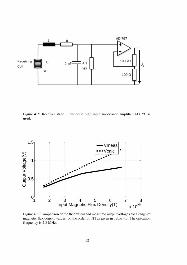
Figure 4.2: Receiver stage. Low noise high input impedance amplifier AD 797 isused.

1 2 3 4 5 6 7 8

x 10−8

0

0.5

1

1.5

Input Magnetic Flux Density(T)

Out

put V

olta

ge(V

)

VmeasVcalc

Figure 4.3: Comparison of the theoretical and measured output voltages for a range ofmagnetic flux density values (on the order of nT) as given in Table 4.3. The operationfrequency is 2.8 MHz.

52

coefficient on inductance that should be included because of the existence of a trans-

mitter coil in order to create input magnetic field. This not only affects the sensitivity

directly, but also changes it due to the slight change in the resonance frequency. To

show this, mutual coupling for every distance value is measured and the calculation

results are modified accordingly as Lactual “ M ` L where M represents the mu-

tual inductance. The corrected set of output voltage values along with the respective

coupling coefficients are given in Table 4.4.

Table 4.4: Measured and calculated voltage outputs after modification of inductanceby including mutual inductances and respective coupling coefficient value measure-ments

Parameter d1=2 cm d2=1.75 d3=1.5 cm d4=1.25 cm d5=1 cmB 16 nT 19.5 nT 27.1 nT 41.6 nT 67.4 nTVmeas 0.27 Vpp 0.32 Vpp 0.45 Vpp 0.64 Vpp 0.81 VppVcalc 0.28 Vpp 0.34 Vpp 0.47 Vpp 0.65 Vpp 0.84 Vppk 0.062 0.063 0.065 0.09 0.15

As observed, the coupling coefficient becomes almost constant when the distance be-

tween the coils is higher than 1.5 cm. However, some discrepancy is still not cleared.

This is due to calculation of the input magnetic field using equation (2.52). It should

be noted that B is obtained through calculation however it was not verified using an

experimental technique. This second reason for the discrepancy is caused by the as-

sumption of uniform flux across the coaxial solenoids. Although coils were placed

coaxially in order to obtain smooth comparison between measured and calculated val-

ues, the measurement results can only be approximately accurate due to assumptions

calculating input magnetic field. Table 4.4 also shows that the output voltage of a de-

signed induction coil magnetic field sensor can be approximately determined without

experimental work.

The linearity performance of the sensor is analyzed using the least squares best fit

straight line method. This method fits the input output characteristics on an optimum

line by selecting the minimum squares of the differences between linear fit and actual

values. First step is to determine the slope of the best linear approximation. It is done

by taking n data points and then using the following formula:

53

1 2 3 4 5 6 7 8

x 10−8

0.2

0.4

0.6

0.8

1

Input Magnetic Flux Density (T)

Out

put V

olta

ge(V

)

DataLinear fit

Figure 4.4: Data obtained through measurement and its linear approximation

m “

řnk“1XkYkřnk“1X

2k

(4.4)

where m is the slope, Xk and Yk representing the input and output data points respec-

tively. After mathematically determining the slope of the best fit straight line, it is

then possible to obtain the maximum deviation percentage of any point from this line

using the equation:

%d “Yk ´mXk

mXfr

(4.5)

where Xfr is full working range of the input data. According to (4.4), the linear

approximation obtained is shown in Figure 4.4. The approximated sensitivity can be

obtained by multiplying the slope of the line with µ0. Sensitivity of the magnetic

field sensor (output voltage/magnetic field intensity) is computed as 17.1 (V m/A).

The maximum deviation from linearity is calculated using equations (4.4) and (4.5).

It occurs at 67.4 nT magnetic flux density (0.0536 A/m magnetic field intensity) and

is %15.3. The aim of this part was to verify whether it is possible to determine the

output voltage of an induction coil sensor and amplifier combination with the aid of

54

a design software. The next section will include the optimization of both coil and

amplifier using the software mentioned in this section.

4.3 LFEIT Application

The details about LFEIT are given in the introduction chapter. This section will

mainly focus on the experimental work relating to LFEIT. As mentioned before,

LFEIT aims to reconstruct the conductivity distribution of body using the magnetic

fields of ultrasonically induced electrical currents. Thus, a strong amplifier (A=10000-

100000) and an induction coil with high sensitivity are required. The contribution of

this study to the LFEIT application is to design the optimum coil for given circum-

stances.

The experimental setup includes two magnets producing DC magnetic field horizon-

tally while an ultrasound source is introduced to the system vertically (perpendicular

to the magnetic field axis). The system is illustrated in Figure 4.5 [15]. A test tube

including two immiscible substances with different conductivities, namely salt water

and oil in this case, is attached to the mid section of the system. The sensor coil is

placed next to the tube over the boundary area of the two liquids. The important ob-

servation here would be the maximum area that sensing can be done. The induction

coil sensor diameter will be limited by the tube diameter. If the sensor area is greater

than the source area, then S in equation (2.6) is determined by the smaller of the two,

rendering a portion of the sensor useless. Therefore there is an upper limitation to the

coil diameter. In this experiment it is set to 2 cm. This is one of the reasons a maxi-

mum coil diameter input parameter is added to the GUI software. There were also a

limited variety of wire while conducting the experiment, so maximum wire diameter

is also added to the GUI. There may be cases where an upper limitation to the coil

length exist or lower limitations to every parameter can also be taken into account ac-

cording to the type of the application. After considering all the factors, the results of

the GUI software is given in Figure 4.13. The numerical input-output part of the GUI

is not the source of data for the graphs. The purpose of the graphs is to verify if there

is an optimum result for the induction coil. Therefore they are obtained under the

condition where a single parameter is varied while others are fixed at their optimum

55

Figure 4.5: Experiment setup without test tube, sensor and ultrasound input, the widthof the mid section is greater than the diameter of the test tube and 2.5 cm [15]

values, which are already determined by the GUI. These results are obtained for 10

pT magnetic field input and a gain of 160000 obtained by the chain amplifier circuit

designed specifically for this case. The resulting optimum sensor coil is wound and

shown in Figure 4.6a and b.

The schematic of the amplifier circuitry is given in Figure 4.9. AD600 is used as

amplifier. Its pin configuration and internal structure is illustrated in Figure 4.11. Two

AD600 are connected using TL072 as buffer in the first stage. TL072 is chosen due

its bandwidth compatibility with AD600. The second stage includes the amplifier

block AU-1291. AD600 is an IC component with low input impedance, causing

the adjustment of the transfer function F of the sensor to be challenging. On the

other hand, it became possible to adjust the operating frequency band by designing

appropriate filters. The circuit board is shown in Figure 4.12. AU-1291 has high

input impedance, allowing it to be considered as a first stage in an amplifier chain.

However this component can not be classified as low-noise, therefore it is used as

second stage. AU-1291 has 63 dB gain which corresponds to 1415. The detailed

56

(a)

(b)

Figure 4.6: Optimum coil designed for LFEIT application (20 mm coil diameter, 2.5mm coil height (length), 0.6 mm wire diameter) a) Top view, b) Side view

57

Figure 4.7: Simulation results for the amplifier circuitry designed for LFEIT applica-tion. The left hand side shows the input signal characteristics(20 uV, 1 MHz). On theright hand side, the output signal is observed at channel B. The amplification can becalculated as 40mV/20uV=2000. Input signal (channel A) is too small to be revealedon the oscilloscope screen.

schematic of the first stage of the amplifier circuit is given in Figure 4.10. As observed

from the schematic, a high pass filter of cutoff frequency 723 kHz is added between

the AD600 and buffers to adjust the bandwidth of the system. A low pass filter is

not necessary for the application since the frequency of interest is around 1 MHz for

LFEIT application. The total amplification factor gained from this circuit is actually

greater than 160000. However as the gain increases to a value around 130 dB, it is

observed that the input signal to be given for test purpose is below the noise value.

Therefore the signal that is observed at the output included significant noise due to

the amplification of the noise. As a solution, the second AD600 is excluded in the

experiments, leading to an amplification factor of 160000 (104 dB). This amplifier

circuit is tested using the simulation software of PROTEUS. The results for the two

AD600 case are shown in Figure 4.7. This suggests that if this circuit is used as

amplifier as it is, with the additional gain from the second stage total gain will reach

2000*1415=2830000. This corresponds to 129 dB. Results for the case with second

AD600 excluded is given in Figure 4.8. The total amplification including the cascaded

second stage is 112.5*1415=159200. Therefore in the design simulations, 160000 is

used.

The input signal is given through the function generator Agilent HP33120A in the

58

Figure 4.8: Simulation results for the amplifier circuitry designed for LFEIT applica-tion(second AD600 excluded). The left hand side shows the input signal characteris-tics (20 uV, 1 MHz). On the right hand side, the output signal is observed at channelB. The amplification can be calculated as 2.25/20mV=112.5. Input signal (channelA) is also shown on the oscilloscope screen and it is 20 mV in amplitude.

Figure 4.9: Amplifier circuitry designed for LFEIT application

59

Figure 4.10: The detailed schematic of the first stage of the amplifier circuit

Figure 4.11: Pin configuration and internal structure of AD600

60

Figure 4.12: The amplifier circuit board

Figure 4.13: GUI results for LFEIT application (with 10 pT input and maximum coiland wire diameter constraints)

61

form of 1 MHz 3 cycles sinusoid bursts at a pulse repetition frequency of 50 Hz. This

signal is amplified using the RF power amplifier. Afterwards it is sent to a 1 MHz 20

mm in diameter transducer focused at 50 mm. The ultrasound pressure was 1 MPa

at the focal point. A cylindrical test tube of diameter 20 mm and height 100 mm is

placed in the middle of the experiment setup. This test tube is filled with a mixture

of salt water and oil, each filling half of the tube. The magnetic field is introduced

from both sides by two identical magnets, centering the focal point with a magnitude

of 0.5 T.

GUI results given in Figure 4.13 are based on 10 pT input as indicated. However,

this magnetic field is induced at the center of the boundary of two liquids inside the

test tube. Therefore the magnetic field at the surface of the tube decreases to 0.1 pT.

Therefore after administering new input magnetic flux density to the simulation, re-

sults shown in Figure 4.15 are obtained. The output voltage is reduced in magnitude

by a factor of 100 and the coil parameters are the same as expected. Output volt-

age is computed as 0.37 mV. However this simulation is done using a wire diameter

constraint of 0.6 mm. The case where the wire diameter is not limited is also inves-

tigated by adjusting the maximum wire diameter parameter to a greater value. The

GUI results for this case are given in Figure 4.16. These new results suggest that the

output voltage can be further increased to 0.7 mV by using a 1.6 mm diameter wire

and using a 2 cm length coil.

The schematic of the final version of the whole experiment setup is given in Fig-

ure 4.19. Expected results are as shown at the introduction part and they are also

shown with better quality in Figure 4.20. Two high amplitude signals on the sides are

phase inverted and the smaller signal in the middle is to be detected by the magnetic

sensor. However, the waveforms obtained at the experiment results are in the form of

Figure 4.21. After not being able to distinguish a signal from the noise, an analysis

using (3.3) inside MATLAB software gives the results illustrated in Figure 4.22. The

bandwidth ∆f is calculated as 42 kHz. Resonance frequency f0 of the overall system

is 1.287 MHz. The comparison of the output signal without the amplification and the

noise shows that it is not possible to distinguish the signal from noise level with any

amount of amplification. However if the input magnetic flux density is increased to

10 pT, the output signal of the sensor can be observed. Figure 4.23 shows that the

62

signal is barely above the noise level around the frequency of interest (1 MHz). Input

spectral noise density of AD600 is given as 1.4nV ?Hz which actually becomes the

dominant factor in system noise. The reason that the second AD600 is excluded from

the system is related to this noise doubling for two AD600 and since noise level is

already critical, it should be minimized.

The sensor designed to use in LFEIT application along with the amplification cir-

cuitry is also tested in terms of sensitivity and linearity. Using the same arrangement

from the previous section, an identical test coil is used to generate AC magnetic field

at distances from 1 cm to 2 cm. Output is obtained without amplifier block cir-

cuitry(Amplification factor A=112.5) The results include the data set for the target

operating frequency (1 MHz). They are shown in Table 4.5. The linearity perfor-

mance of the sensor is illustrated in Figure 4.14. Maximum deviation from linearity

is %2.7 at the 1 cm distance which is the closest. Again as in the case of test system

constructed in the previous section, linearity gets distorted as the measurement dis-

tance decreases. The sensitivity with amplification factor of A=112.5 is computed as

5.45 (V m/A). This indicates that in terms of sensitivity, this system performs worse

than the test case since the measurements are already done at the resonance frequency.

This is due to low input resistance of AD600 amplifier which has a negative effect on

the system. However it was chosen in order to be compatible with AU-1291 since

very high amplification at 1 MHz operating frequency was required for the applica-

tion.

Table4.5: Measured voltage outputs at two different frequencies of importance for arange of measurement distance and respective coupling coefficient values

Parameter d1=2 cm d2=1.75 d3=1.5 cm d4=1.25 cm d5=1 cmB 16 nT 19.5 nT 27.1 nT 41.6 nT 67.4 nTVf“1MHz 0.072 Vpp 0.088 Vpp 0.122 Vpp 0.184 Vpp 0.286 Vppk 0.062 0.063 0.065 0.09 0.15

63

1 2 3 4 5 6 7 8

x 10−8

0.05

0.1

0.15

0.2

0.25

0.3

Input Magnetic Flux Density(T)

Out

put V

olta

ge(V

)

Actual dataLinear fit

Figure 4.14: Data obtained through measurement and its linear approximation

Figure 4.15: GUI results for LFEIT application with 0.1 pT input and maximum coildiameter and wire diameter constraints of 2 cm and 0.6 mm respectively. Operationfrequency is 1 MHz. Output voltage is calculated as 0.37 mV. Optimum coil length iscomputed as 2.5 mm. Wire diameter of the optimized coil is 0.6 mm.

64

Figure 4.16: GUI results for LFEIT application with 6 mm wire diameter constraint.This value is chosen high enough to check whether there is a better coil if therewere no wire diameter constraint. Output voltage for the determined optimum coil iscalculated as 0.7 mV. Wire diameter is computed as 1.57 mm. Optimum coil lengthis also changed and it is 2 cm.

4.4 Wireless Power Transfer (WPT) Application

Although WPT is a form of magnetic sensor application, it requires a different ap-

proach. In magnetic sensor applications, the goal is to maximize the voltage sensi-

tivity. However in WPT, it is necessary to maximize the power transfer. To achieve

this, the efficiency should be maximum. It is given for two coil system in equa-

tion [34], [35], [36]:

η “k2QpQs

1` k2QpQs

(4.6)

where η is the efficiency, k is the mutual coupling between the coils and Qp and

Qs are the quality factor of the primary and secondary coils respectively. However,

the low Q-factor especially observed under loaded condition and the low coupling

between the coils, two coiled system has relatively low efficiency. This efficiency also

decreases exponentially with the distance between coils. This limits the maximum

distance both coils could be placed from each other. Therefore four coiled system

is preferred. The schematic of such design is given in Figure 4.24 where all the

65

Figure 4.17: Improved GUI results for LFEIT application with 0.6 mm wire diameterconstraint. Improved GUI includes additional software that determines whether flatspiral coil or air-cored multilayer coil performs better. It is observed that a flat spiralcoil provides a slightly better output voltage (0.4 mV) compared to the results givenin Figure 4.15. Since the optimum coil type is determined as flat spiral, instead ofcoil length parameter, the turn spacing parameter is included. Wire diameter of theoptimum coil is calculated as 0.2 mm and the turn is spacing is 0.004 mm.

Figure 4.18: Improved GUI results for LFEIT application with 6 mm wire diameterconstraint. The results are same as in Figure 4.16 since the optimum coil type for thiscase is air-cored multilayer coil.

66

Figure 4.19: The schematic of the final version of the experiment setup. Dc magneticfield is seen at inward direction which is perpendicular to the measurement axis. In-duction coil sensor is placed adjacent to the tube in order to obtain best sensitivityperformance.

parameters illustrated will be used in its efficiency equation [37], [38], [39], [40]:

η “pk212Q1Q2qpk

223Q2Q3qpk

234Q3Q4q

rp1` k212Q1Q2q p1` k234Q3Q4q ` k223Q2Q3s r1` k223Q2Q3 ` k234Q3Q4s(4.7)

where kmn is the coupling factor between coil m and coil n, and Qm is the quality

factor of coil m. Equation (4.7) is valid assuming all coils are tuned to the same

resonance frequency and operating at this frequency. Also for this equation to hold,

coupling coefficients between nonadjacent coils k13, k14 and k24 should be negligible

compared to the coupling coefficients between adjacent coils. Since the interaction

between nonadjacent coils would be weaker, equation (4.7) performs better as the dis-

tance between primary and secondary coils increases. Coupling factor k has a value

between 0 and 1. It is 1 for two identical coils placed next to each other. However as

the geometry of the coils differ and as they become more distant, k decreases. Since

the distance between Tx and Rx coils is relatively greater, their coupling coefficient

k23 is small compared to k12 and k34. Hence the quality factors of these coils Q2 and

67

Figure 4.20: The illustration of expected results of the experiment. The scale amongthe signals to be measured is represented in this figure. The signals with greateramplitude correspond to outer boundaries with higher conductivity gradient namelythe boundary between air and oil, salt water and tube respectively. These expectedsignals are out of phase 180 degrees. The waveform in the middle corresponds to theconductivity gradient between salt water and oil therefore it is smaller. The aim isto observe this smaller signal since it will prove whether the conductivity differencebetween two different tissues can be distinguished.

68

Figure 4.21: The illustration of results of the experiment. The outer boundary signalsare obtained at a scale of 5 V. However the noise signal obtained is greater than theexpected inner boundary waveform, therefore it was not possible to distinguish thissignal from the noise.

−7 −6 −5 −4 −3 −2 −1 0−300

−250

−200

−150

−100Frequency Response

log(f/f0)

dB

Output voltageNoise signalMagnetic noise

Figure 4.22: Theoretical results for noise analysis of the experiment setup for 0.1 pTinput magnetic flux density. It is observed that the output voltage of the sensor isbelow the noise level.

69

−7 −6 −5 −4 −3 −2 −1 0−250

−200

−150

−100

−50Frequency Response

log(f/f0)

dB

Output voltageNoise signalMagnetic noise

Figure 4.23: Theoretical results for noise analysis of the experiment setup for 10 pTinput magnetic flux density. This simulation indicates that if it is possible to increasethe input flux density by using a higher magnitude DC field or placing the sensorcloser to the source with a different configuration, output signal reaches above thenoise level at the resonance frequency.

Q3 are required to be maximized in order to compensate the reduction in the effi-

ciency caused by low coupling. In order to achieve this, the optimization algorithm

designed in the previous sections is modified into determining the coil parameters for

maximum quality factor.

The quality factors of driving and load coils (Q1 and Q4 respectively), cannot reach

the level of unloaded Q2 and Q3 because of source and load resistances. Therefore

their effects on efficiency are limited. Q of an unloaded coil is:

Q “2πfLeff

R(4.8)

where R is the total resistance and Leff is the effective inductance which is obtained

by:

Leff “ L

˜

1´

ˆ

f

f0

˙2¸

(4.9)

f0 is the self resonance frequency of the coil as mentioned in the sections before.

Therefore quality factor also depends on the operating frequency. To determine this

frequency, the structure of overall system and its relation with human body should

70

Figure 4.24: Four coil wireless power transfer system. In the figure, kmn is the cou-pling factor between coil m and coil n, and Qm is the quality factor of coil m

be considered. The receiver coil, as mentioned, is to be placed inside the tissue.

The permeability of the tissue can be assumed to be close to free space [41]. This

indicates that the coil inductance inside a tissue will not be affected. However, the

tissue has high dielectric constant [42], [43], and hence, introduces more capacitance

to the system. This further reduces the quality factor of the implanted coil, which

has relatively small size causing its capacitance to be small. Therefore a possible

tuning capacitor at the receiving end has very little effect on operating frequency of

the system. The tissue and the high frequency magnetic field is rather close to each

other, resulting in tissue absorbing part of magnetic field input due to the eddy current

generation. This absorption is lower for a frequency range of 100 kHz-4 MHz, leading

to an improvement in the efficiency due to minimizing the effects of tissue. Operating

frequency of a wireless power transfer system to be used in biomedical applications

should be in this range. For this application, 1 MHz is chosen due to practical reasons.

The distance between the transmitter and receiver coils is determined using the equa-

tion (2.52). To maximize Bx, a “ ρ?

2 condition should be met. This means that

in order to maximize the magnetic field transfer, the diameter of the transmitter coil

should be chosen as D “ 2?

2ρ.

71

It is not possible to accurately model the coupling factor between two multilayer coils,

therefore it is measured experimentally. The method is as follows: The inductance of

the primary coil is measured while the secondary coil is under open circuit and short

circuit conditions. Then using the equation:

k “

c

1´LsLo

(4.10)

where Ls indicating the primary coil inductance for short circuited secondary coil and

Lo indicating the open circuited secondary.

The optimization algorithm from previous section is also used here to obtain coil

parameters for maximum Q. Calculated and measured quality factors of selected coils

and their size parameters are given in Table 4.6. LCR meter is used to measure the

quality factor parameter. The loaded quality factors are not measured, only calculated

due to discrepancy being relatively low. In the table, it can also be seen that the

calculation of the multilayer coil resistance using Dowell method, results are accurate

with the resistance measurement with some discrepancy.

Table 4.6: Size parameters of the coils with optimum quality factor

Parameter Coil 1 Coil 2 Coil 3 Coil 4Coil Outer Diameter(D)-mm 30 25.5 17 20Coil Inner Diameter(Di)-mm 25.5 6 4 17Coil Length(l)-mm 5 5 2.5 2.5Wire Diameter(d)-mm 1 1 0.6 0.6Number of Turns 8 36 44 12Inductance(L)µ H 3.4 13.4 15.8 4.4Calculated Resistance(Rcalc)Ω 1.5 3.77 6.35 2.57Measured Resistance(Rmeas)Ω 1.87 4.5 6.25 2.85Q(calculated-loaded) 0.216 17 13 0.16Q(measured) 11.5 18 12.7 9.7

Using the method indicated above, k12 is found as 0.62, k23 is 0.0675, k34 is 0.55 for

8.5 mm distance and 1 MHz operating frequency for the selected coils. Then using

(4.5) since all the parameters included are revealed, the efficiency is calculated as

%6.8. Coil 1 is loaded with 5.6 Ω in series to represent the source impedance and coil

72

Figure 4.25: Four coil wireless power transfer system circuitry schematic includingcomponents with their respective values

4 is loaded with 100 Ω in series to represent the load. The schematic of the whole

circuitry is given in Figure 4.25

The coil 3 of the selected coils is the one used as induction coil sensor in LFEIT appli-

cation in the previous section. The optimum coil parameters were actually, D=2 cm,

l= 0.3 cm, d=0.06 cm andDi=0.4 cm. However since there is no significant difference

in quality factor, the sensor coil from LFEIT application is used as the receiver. Coil

2 on the other hand, is newly designed for this application. It is shown in Figure 4.26a

and 4.26b as top view and side view. The driver and load coils are concentric with the

transmitter and receiver coil respectively by forming the outermost layers of them.

The driver coil and load coil are designed with relatively low turn number due to the

fact that their quality factor will be already small due to loading. Their inductance

values are also of importance since they need to resonate at the selected operating

frequency which is 1 MHz for this case. The tuning capacitance can be calculated

73

(a)

(b)

Figure 4.26: Optimum quality factor coil designed for WPT application (30 mm coildiameter, 5 mm coil height(length), 1 mm wire diameter ) a) Top view, b) Side view

74

using:

jwL´1

jwC“ 0 (4.11)

C “1

p2πfq2L(4.12)

The inductance of the driver coil is 3.4 µH and the load coil is 4.4 µH . Therefore

the tuning capacitances for driving and load parts are 9 nF and 7.6 nF respectively.

The tuning capacitances of primary and secondary coils are close being 1.9 nF and

1.6 nF respectively. Remembering the condition D “ 2?

2ρ, the distance between

the coils is adjusted as 8.5 mm. Afterwards the experiment setup included the four

coil system, specified tuning capacitances and load resistances connected to driving

and load coils in series. Input signal given has 1 MHz frequency and 10 Vpeak

amplitude and as the load, 100 Ω is connected in series. The input power is measured

as 0.15 Watts, which is inversely proportional with the load impedance seen by the

source. The output voltage on the 100 Ω is measured as 1.5 Vpeak, using average

power equation P “ V 2

2R, leading to an output power of 0.0113 Watts. Therefore the

efficiency calculated using measurement values is %7.7. This shows that although the

efficiency is low in this case, the discrepancy of the design is also low. The reason for

low output power is the low input power transfer from voltage source which has 50 Ω

internal resistance.

The efficiency can be improved by using litz wires which provide significant improve-

ment in coil quality factor. Litz wire is composed of many wire strands. It increases

quality factor by providing very low resistance compared to regular copper wire. To

prove this, the windings of primary and secondary coils mentioned are changed to

1 mm diameter litz wire with number of strands as 66. The resulting coils have the

properties mentioned in Table 4.7. These coils are shown in Figure 4.27a and b.

It is shown that the usage of litz wire as windings increase the quality factor greatly.

The coupling coefficients for this case are computed as: k12 =0.515, k23 =0.043, k34

=0.43. Then using (4.7), efficiency is increased up to %13.8. This is verified through

implementation by obtaining an output voltage of 2.3 Vpeak for 0.18 W input power,

therefore resulting in %14.7 efficiency. Although by only changing the windings

75

(a)

(b)

Figure 4.27: Optimum quality factor coil with litz wire windings designed for WPTapplication (30 mm coil diameter, 5 mm coil height(length), 1 mm wire diameter ) a)Top view, b) Side view

76

Table 4.7: Critical parameters of the coils modified to include Litz wires as theirwindings

Parameter Coil 1 Coil 2 Coil 3 Coil 4Inductance(L)µ H 1.76 3.25 0.53 0.23Resistance(Rcalc)Ω 0.19 0.176 0.045 0.047Q(loaded) 1.94 134 81 0.015

into litz wire without any coil design process the efficiency is doubled, the resulting

efficiency is still relatively weak. This is due to the low loaded quality factor of

the load coil. Therefore assuming there is further space for improvement, another

secondary coil with better loaded quality factor is wound. The 0.3 mm diameter 40

strand litz wire is used in the windings. The properties of this coil along with its load

counterpart is given in Table 4.8.

Table 4.8: Critical parameters of the secondary coil modified further to have highloaded quality factor

Parameter Coil 3 Coil 4Inductance(L)µ H 65 41Resistance(Rcalc)Ω 23 23Q(loaded) 17 2.094

Afterwards, considering mutual coupling coefficient values, k12 and k34 are measured

as same, however k23 is measured as 0.052. Then using (4.7), the efficiency is calcu-

lated as %37.1. This is again verified as 3.3 Vpeak is observed on the 100Ω load at

0.14 W input power resulting in %38.9 efficiency. This is the best efficiency obtained

so far, even so the quality factor of the secondary coil is relatively low. It should be

noted that in the litz wire winding part of the WPT application, coil design was not

required since there were two different types of litz wire available during the exper-

iments. The coil design of WPT application with enamel copper wire can be easily

modified to design litz wire coils by changing the resistance and inductance equa-

tions. This part is only done to prove that the efficiency can be greatly increased by

usage of litz wire.

77

78

CHAPTER 5

CONCLUSION AND DISCUSSION

A magnetic sensor system with the best sensitivity under certain circumstances, in-

cluding an air-cored induction coil connected to an amplifier circuit is designed. A

MATLAB based graphical user interface software is developed for this purpose. This

software is verified by checking with numerous coils designed for various biomedical

applications like MIT or contactless conductivity imaging. The precision of calcu-

lations and the discrepancies are investigated thoroughly. The linearity of sensitivity

is New parameters such as wire insulation thickness are understood through exper-

imental work. The optimum coil is designed using the present equipment and its

parameters are: Diameter(D): 2 cm, length(l): 0.25 cm, wire diameter(d): 0.6 mm,

inner diameter(Di): 0.4 cm. However the performance of the system designed for the

LFEIT application is found to be inadequate. This is both due to requirement of very

high sensitivity and signal being so small that its level remaining below noise level.

The sensitivity can be increased by using another low noise amplifier circuit with high

input impedance through placing an adjusting resistance in parallel, but at the cost of

bandwidth. One of the suggestions to improve the results would be to find a way to

get close to the source. This might be achieved if the sensor coil is placed inside the

test tube, by using a wider tube. However fixing its position inside the liquids would

be challenge and it would also introduce another boundary area. Another suggestion

is to use the improved GUI to determine whether the coil type used is optimum or not.

The results of related simulations are given in Figure 4.17. This proves that under the

wire diameter limitation, the use of flat spiral coil gives better results. However this

is not the case when the wire diameter is not limited as shown in Figure 4.18. There-

fore multilayer air cored coil is the optimum coil type choice for LFEIT application

79

given that all required material such as wire with appropriate diameter is accessible.

A noise shielding metal casing is also necessary in the final design of the system in

order to minimize the noise from the coil, both thermal noise and interference from

the environment, however it is not implemented in this study.

After the LFEIT application, the properties of wireless power transfer is also inves-

tigated. Four coil structure is chosen due to having more flexible design constraints.

The maximum efficiency of the power transfer is required to be achieved. In order to

accomplish this, quality factor of the transmitter and receiver coils should be maxi-

mized according to the equation given. To obtain the size parameters of the maximum

quality factor, optimization software designed in MATLAB is modified into providing

size parameters for the greatest quality factor. Afterwards, coupling factors between

the coils are measured by separating coils two by two. Then the tuning capacitances

are determined. Finally, the distance of greatest magnetic flux transfer and tuning ca-

pacitances for driving and load sides are determined and the system is implemented.

Expected efficiency was %6.8, which can be considered as rather poor performance,

however the resulting practical efficiency value was obtained as %7.6. Afterwards,

litz wires is used at windings instead of enamel copper wire. The efficiency of the

system is increased up to %39 through the improvement observed in the coil quality

factors.

As an improvement, litz wire coils should be designed in detail in order to increase

the quality factor which greatly affect the efficiency of the system, while improving

the loaded conditions. As another improvement, there are other coil types than the

disk shaped air-cored induction coil such as rectangular coil, ferromagnetic-core coil.

These coils can also be optimized for the desired applications since their inductance

and capacitance can also be formulated or derived from the air-cored coil. An im-

provement for wireless power transfer could be the use of coils with better coupling

coefficients, especially the coupling between transmitter coil and receiver coil needs

improvements. This can be done by making the transmitter and receiver coils’ turn

number close hence adjust their inductance closer to each other. This application also

requires the coils to be shielded by a metal casing, not because of noise this time but

in order to prevent the resistance from changing due to temperature. Again this is

not implemented, but mentioned as a suggestion to improve the system further, espe-

80

cially in the final implementation stage. There are also other applications that can be

studied such as MIT, contactless conductivity imaging etc. These applications can be

studied in detail and suggestions about various types of coil for every application can

be made.

81

82

REFERENCES

[1] T. C. Oakberg, “Magneto-optic kerr effect,” HINDS Instruments, vol. 1, no. 1,2005.

[2] C. M. Falco and I. K. Schuller, “Squids and their sensitivity for geophysicalapplications,” SQUID Applications to Geophysics, pp. 13–18, 1980.

[3] J. Clarke, “Squid fundamentals,” in SQUID sensors: fundamentals, fabricationand applications. Springer, 1996, pp. 1–62.

[4] J. E. Lenz, “A review of magnetic sensors,” Proceedings of the IEEE, vol. 78,no. 6, pp. 973–989, 1990.

[5] E. Ramsden, Hall-effect sensors: theory and application. Newnes, 2011.

[6] T. Casselman and S. Hanka, “Calculation of the performance of a magnetore-sistive permalloy magnetic field sensor,” Magnetics, IEEE Transactions on,vol. 16, no. 2, pp. 461–464, 1980.

[7] W. Kwiatkowski and S. Tumanski, “The permalloy magnetoresistive sensors-properties and applications,” Journal of Physics E: Scientific Instruments,vol. 19, no. 7, p. 502, 1986.

[8] S. Tumanski, “Induction coil sensors—a review,” Measurement Science andTechnology, vol. 18, no. 3, p. R31, 2007.

[9] S. A. Macintyre, “Magnetic field measurement,” ENG Net Base, 2000.

[10] G. Dehmel, “Magnetic field sensors: induction coil (search coil) sensors,” Sen-sors Set: A Comprehensive Survey, pp. 205–253, 1989.

[11] P. Ripka, Magnetic sensors and magnetometers. Artech House on Demand,2001.

[12] H. Zijlstra, “Experimental methods in magnetism,” 1967.

[13] R. Prance, T. Clark, and H. Prance, “Compact room-temperature induction mag-netometer with superconducting quantum interference device level field sensi-tivity,” Review of scientific instruments, vol. 74, no. 8, pp. 3735–3739, 2003.

[14] R. Zengin, “Electrical impedance tomography using lorentz fields,” METU, M.Sc. Thesis, 2012.

[15] M. Karadas, “Development of novel reconstruction algorithms for eit usinglorentz fields,” METU, M. Sc. Thesis, 2014.

[16] P. Grasland-Mongrain, J.-M. Mari, J.-Y. Chapelon, and C. Lafon, “Lorentz forceelectrical impedance tomography,” IRBM, vol. 34, no. 4, pp. 357–360, 2013.

[17] H. Ammari and H. Kang, Reconstruction of small inhomogeneities from bound-ary measurements. Springer, 2004, no. 1846.

83

[18] L. Filipczynski, “Absolute measurements of particle velocity, displacement orintensity of ultrasonic pulses in liquids and solids,” Acta Acustica united withAcustica, vol. 21, no. 3, pp. 173–180, 1969.

[19] S. Haider, A. Hrbek, and Y. Xu, “Magneto-acousto-electrical tomography: apotential method for imaging current density and electrical impedance,” Physi-ological measurement, vol. 29, no. 6, p. S41, 2008.

[20] A. Montalibet, J. Jossinet, and A. Matias, “Scanning electric conductivity gra-dients with ultrasonically-induced lorentz force,” Ultrasonic imaging, vol. 23,no. 2, pp. 117–132, 2001.

[21] B. Soong, Y. Sum, W. Liu, and S. Ramachandran, “Characterizing wire woundinductor coils for optimized wireless power transfer,” in Advanced Intelli-gent Mechatronics, 2009. AIM 2009. IEEE/ASME International Conference on.IEEE, 2009, pp. 469–474.

[22] P. Si, A. P. Hu, D. Budgett, S. Malpas, J. Yang, and J. Gao, “Stabilizing theoperating frequency of a resonant converter for wireless power transfer to im-plantable biomedical sensors,” in Proc. 1st Int. Conf. Sensing Technology, 2005,pp. 477–482.

[23] Y.-M. Gimm, H.-S. Yoo, M.-J. Kim, J.-S. Yoo, and S.-H. Park, “Receiving coilanalysis of wireless power transmission with inductive coupling,” in MicrowaveConference, 2007. KJMW 2007. Korea-Japan. IEEE, 2007, pp. 117–120.

[24] A. P. Sample, D. A. Meyer, and J. R. Smith, “Analysis, experimental results, andrange adaptation of magnetically coupled resonators for wireless power trans-fer,” Industrial Electronics, IEEE Transactions on, vol. 58, no. 2, pp. 544–554,2011.

[25] V. G. Welsby, The theory and design of inductance coils. Macdonald, 1950.

[26] Y. Lee, “Antenna circuit design,” Application manual of Microchips Technology,1999.

[27] P. Dowell, “Effects of eddy currents in transformer windings,” Electrical Engi-neers, Proceedings of the Institution of, vol. 113, no. 8, pp. 1387–1394, 1966.

[28] H. A. Wheeler, “Simple inductance formulas for radio coils,” Radio Engineers,Proceedings of the Institute of, vol. 16, no. 10, pp. 1398–1400, 1928.

[29] A. Massarini and M. K. Kazimierczuk, “Self-capacitance of inductors,” PowerElectronics, IEEE Transactions on, vol. 12, no. 4, pp. 671–676, 1997.

[30] L. E. M. ÇOLAK, “An improved data acquisition system for contactless conduc-tivity imaging,” Ph.D. dissertation, MIDDLE EAST TECHNICAL UNIVER-SITY, 2005.

[31] K. Ö. Özkan, “Multi-frequency electrical conductivity imaging via contactlessmeasurements,” METU, M. Sc. Thesis, 2006.

[32] E. C. Snelling, “Soft ferrites,” 1969.

[33] Q. Yu and T. W. Holmes, “A study on stray capacitance modeling of induc-tors by using the finite element method,” Electromagnetic Compatibility, IEEETransactions on, vol. 43, no. 1, pp. 88–93, 2001.

[34] A. Kumar, S. Mirabbasi, and M. Chiao, “Resonance-based wireless power de-livery for implantable devices,” in Biomedical Circuits and Systems Conference,2009. BioCAS 2009. IEEE. IEEE, 2009, pp. 25–28.

84

[35] L. Rindorf, L. Lading, and O. Breinbjerg, “Resonantly coupled antennas forpassive sensors,” in Sensors, 2008 IEEE. IEEE, 2008, pp. 1611–1614.

[36] M. Catrysse, B. Hermans, and R. Puers, “An inductive power system with in-tegrated bi-directional data-transmission,” Sensors and Actuators A: Physical,vol. 115, no. 2, pp. 221–229, 2004.

[37] H. Haus and W. Huang, “Coupled-mode theory,” Proceedings of the IEEE,vol. 79, no. 10, pp. 1505–1518, 1991.

[38] A. Karalis, J. D. Joannopoulos, and M. Soljacic, “Efficient wireless< i> non-radiative mid-range</i> energy transfer,” Annals of Physics, vol. 323, no. 1, pp.34–48, 2008.

[39] A. Kurs, A. Karalis, R. Moffatt, J. D. Joannopoulos, P. Fisher, and M. Soljacic,“Wireless power transfer via strongly coupled magnetic resonances,” science,vol. 317, no. 5834, pp. 83–86, 2007.

[40] A. K. RamRakhyani, S. Mirabbasi, and M. Chiao, “Design and optimization ofresonance-based efficient wireless power delivery systems for biomedical im-plants,” Biomedical Circuits and Systems, IEEE Transactions on, vol. 5, no. 1,pp. 48–63, 2011.

[41] J. Malmivuo and R. Plonsey, Bioelectromagnetism: principles and applicationsof bioelectric and biomagnetic fields. Oxford University Press, 1995.

[42] M. W. Baker and R. Sarpeshkar, “Feedback analysis and design of rf powerlinks for low-power bionic systems,” Biomedical Circuits and Systems, IEEETransactions on, vol. 1, no. 1, pp. 28–38, 2007.

[43] U.-M. Jow and M. Ghovanloo, “Modeling and optimization of printed spiralcoils in air, saline, and muscle tissue environments,” Biomedical Circuits andSystems, IEEE Transactions on, vol. 3, no. 5, pp. 339–347, 2009.

85