product mix determination under uncertainty - METU

PRODUCT MIX DETERMINATION UNDER UNCERTAINTY

WITHIN A FRAMEWORK PROPOSED FOR

EFFECTIVE PRODUCT MANAGEMENT

A THESIS SUBMITTED TO

THE GRADUATE SCHOOL OF NATURAL AND APPLIED SCIENCES

OF

MIDDLE EAST TECHNICAL UNIVERSITY

BY

N. NİLGÜN FEŞEL

IN PARTIAL FULFILLMENT OF THE REQUIREMENTS

FOR

THE DEGREE OF DOCTOR OF PHILISOPHY

IN

OPERATIONAL RESEARCH

SEPTEMBER 2013

Approval of the thesis:




submitted by N. NİLGÜN FEŞEL in partial fulfillment of the requirements for the degree

of Doctor of Philosophy in Operational Research, Department of Industrial

Engineering, Middle East Technical University by,

Prof. Dr. Canan Özgen Dean, Graduate School of Natural and Applied Sciences ___________________

Prof. Dr. Murat Köksalan

Head of Department, Industrial Engineering ___________________

Prof. Dr. Gülser Köksal

Supervisor, Industrial Engineering Department ___________________

Prof. Dr. Nazlı Wasti Pamuksuz

Co-Supervisor, Dept. of Business Administration ___________________

Examining Commitee Members:

Assoc. Prof. Dr. Haldun Süral

Industrial Engineering Dept., METU _____________________

Prof. Dr. Gülser Köksal

Industrial Engineering Dept., METU _____________________

Assoc. Prof. Dr. Ferda Can Çetinkaya

Industrial Engineering Dept., Çankaya University ______________________

Assoc. Prof. Dr. M. Sinan Gönül

Dept. of Business Administration, METU ______________________

Assist. Prof. Dr. Seçil Savaşaneril

Industrial Engineering Dept., METU ______________________

Date: September 11, 2013

iv

I hereby declare that all information in this document has been obtained and presented

in accordance with academic rules and ethical conduct. I also declare that, as required

by these rules and conduct, I have fully cited and referenced all material and results

that are not original to this work.

Name, Surname: N. Nilgün FEŞEL

Signature:

v

A B S T R A C T




Feşel, N. Nilgün

Ph. D., Operational Research, Department of Industrial Engineering

Supervisor: Prof. Dr. Gülser Köksal

Co-Supervisor: Prof Dr. Nazlı Wasti Pamuksuz

September 2012, 275 pages

In many real life problems, uncertainty is a major complexity for decision makers. A typical

example to such a case is product mix problem. In this study, we develop a methodology to

aid the decision makers in product mix determination at the strategic level of product

management under uncertainty. The methodology is based on a simulation optimization

approach by which scenarios are generated using a statistical design of experiment approach.

To the best of our knowledge, this methodology developed to aid the decision maker in

product mix determination is a novel and original approach.

Our product mix model determines “how many” to produce from each product for each

market where it will be sold. The decision maker questions the financial performance (profit)

of the company by the results of the model. The product level is considered as product line

and/or family since the product mix problem is handled at the strategic level of the product

management framework. Depending on the best product mix and expected financial

performance (profit) brought by the mix, the decision makers may choose to change their

candidate product set and re-use our approach to find a new optimal product mix and its

expected profit. In that sense the method developed in this study aids the decision maker by

answering several “what-if” questions such as what profit level is obtained if the set of

candidate products is changed, what happens to the profit level if a new market entrance is

considered with the existing products, or if market conditions are volatile, what is the effect

of these conditions to the level of profit, and so on. The model can also be used for

budgeting purposes considering product breakdown and market disaggregation if and when

necessary. The variants of the model are presented to serve these purposes. This

information can be used as an input for aggregate production planning (APP) in which

deterministic forecasts of demand for the aggregate products are used traditionally. In that

sense, our method improves the traditional production management information system in

APP. Further research directions involving extensions of the model and the solution

approach are provided.

Key words: product-mix, uncertainty, product management, simulation optimization

vi

Ö Z

ETKİN ÜRÜN YÖNETİMİ İÇİN ÖNERİLEN BİR ÇERÇEVEDE

BELİRSİZLİK ALTINDA ÜRÜN KARMASI SAPTANMASI

Feşel, N. Nilgün

Doktora, Yöneylem Araştırması, Endüstri Mühendisliği Bölümü

Tez Yöneticisi : Prof. Dr. Gülser Köksal

Ortak Tez Yöneticisi: Prof . Dr. Nazlı S. Wasti

Eylül 2013, 275 sayfa

Pek çok gerçek hayat probleminde, karar vericiler için başlıca güçlük belirsizliktir. Ürün

karması problemi böylesi bir durum için tipik bir örnektir. Bu çalışmada, ürün yönetiminin

stratejik seviyesinde ele alınan belirsizlikte ürün karması saptanmasında karar vericiye

yardımcı bir yöntembilim geliştirilmiştir. Bu yöntembilim, istatistiksel deney tasarımı

kullanılarak senaryoların türetildiği benzetim eniyileme yaklaşımına dayanmaktadır.

Bildiğimiz kadarı ile karar vericiye yardımcı olarak geliştirilen bu yöntembilim, ürün

karması saptanmasında yeni ve özgün bir yaklaşımdır.

Ürün karması modelimiz, satıldığı her pazarda, her üründen “ne kadar” üretileceğini saptar.

Karar verici, modelin sonuçları ile firmanın mali performansını (kârını) sorgular. Ürün

karması problemi ürün yönetiminin stratejik düzeyinde ele alındığı için, ürün seviyesi ürün

hattı ve/veya ürün ailesi olarak göz önüne alınmıştır. En iyi ürün karması ve onun getirisi

olan beklenen mali performansa (kâra) dayalı olarak, karar vericiler aday ürünler kümesini

değiştirebilirler ve yeni en iyi ürün karması ve onun beklenen kârını bulmak için

yaklaşımımızı tekrar kullanabilirler. Bu bağlamda, bu çalışmada geliştirilen yöntembilim,

eğer aday ürünler kümesi değişirse, kâr düzeyi ne olur, ya da eğer mevcut ürünlerle yeni bir

pazara girilirse, kâr düzeyi ne olur, veya eğer pazar koşulları hızlı değişkenlik gösteriyorsa,

bu koşulların kâr üzerindeki etkisi ne olur gibi “ne-eğer” türü çeşitli sorulara yanıt vererek

karar vericiye yardımcı olur. Model, gerektiğinde ürün kırılımı ve pazar ayrıştırması göz

önüne alınarak bütçelendirme amacı için de kullanılabilir. Modelimizin bu amaca yönelik

olarak çeşitlemeleri sunulmuştur. Bu bilgi, geleneksel olarak bütünleşik ürünlerin gerekirci

tahminlerini girdi olarak kullanan bütünleşik üretim planlamasında girdi olarak

kullanılabilir. Bu bağlamda, modelimiz bütünleşik üretim planlamasında geleneksel üretim

yönetimi bilişim sistemini iyileştirici olarak görülebilir. Modelin uzantıları ve çözüm

yaklaşımına ilişkin yapılabilecek gelecekteki araştırmalar için yön gösterilmiştir.

Anahtar kelimeler: ürün-karması, belirsizlik, ürün yönetimi, benzetim eniyileme

vii

To the loving memory of my parents,

A.Galip FEŞEL

and

M.Ülker FEŞEL

viii

ACKNOWLEDGMENTS

After more than twenty years of a break, my work on this thesis consumed much of my time

for a number of years during the fifties of my life, and I wish to acknowledge the many

people who have encouraged and supported me during this time.

First and foremost I wish to acknowledge my advisor Professor Gülser Köksal. Professor

Köksal provided constant support and guidance during my thesis studies and she has been

always very generous with her time despite her busy schedule. Without her patience,

understanding and enthusiastic involvement, this thesis would not have reached its fruition.

I thank my co-advisor Professor Nazlı Wasti Pamuksuz in exposing me to some of essential

literature.

I wish to acknowledge the critical input of my thesis monitoring committee members

Associate Professor Haldun Süral and Associate Professor M. Sinan Gönül, each of whom

shared unique insight from their particular field of specialization. My chair, Associate

Professor Haldun Süral was a generous mentor whose ongoing interest in my research and

availability to discuss ideas were a continual source of support. I thank my committee

members Associate Professor Ferda Can Çetinkaya and Assistant Professor Seçil

Savaşaneril for their perceptive comments.

I wish to acknowledge Dr. Hakan Polatoğlu and Mrs. Çiğdem Yıldız for sharing with me

their valuable insight in the conduct of my field research in their business environment.

Particular thanks go to my primary contact, Mr. M. Kani Tibet who patiently answered my

endless questions, so I could learn from his experience and knowledge which was a great

support for validating the conceptual model in my research.

I wish to express my deepest gratitude to Professor Halim Doğrusöz who introduced and

connected me to the Operational Research community when I was a young student. I

especially want to thank Ms. Şule Çimen, department secretary and friend, and all other

administrative people working in Industrial Engineering department of METU for their

ongoing moral support during my study. I also want to thank Ms. Tuğba Canyurt and her

team in the library for their kind understanding and professional help.

I gratefully acknowledge the assistance of Mr. Onur Tavaslıoğlu in writing the codes of

MATLAB.

Finally, I want to acknowledge the support of my loving husband Hayati who has lived

gracefully with the stresses and got me through the hard times and sacrificed much to help

me.

Although they are not with me anymore, I acknowledge my parents who gave me the best

possible education and start to life. I dedicate this dissertation to my parents, Galip and

Ülker Feşel.

ix

TABLE OF CONTENTS

ABSTRACT …………………………………………..………………………………….….v

ÖZ ………………………………………………………...……………………………........vi

ACKNOWLEDGMENTS………………………………..…….…………………………viii

TABLE OF CONTENTS…………………………………...…………...…………………ix

LIST OF TABLES …………………………………………..……...…………………… xii

LIST OF FIGURES ………………………………………………...……………………xiv

CHAPTERS

1. INTRODUCTION …………………………………………...…………………......1

2. LITERATURE SURVEY AND BACKGROUND ………...……………………..5

2.1 PRODUCT MANAGEMENT PROBLEM ……………...……………………..5

2.1.1 Definition and Historical Background ……………...…………………..5

2.1.2 Domains of Literature ………………………………...………………...9

2.1.3 Major Themes in Product Management ………………..……………..11

2.1.4 Complexity Sources of Product Management Problem…..…………...18

2.1.5 Tools and Techniques Used in Product Management ……...…………19

2.1.6 Gaps and Weaknesses in the Literature ……………………...………. 26

2.2 PRODUCT MIX PROBLEM …………………………………………...….....27

2.2.1 Modeling Approaches of Product Mix Problem …………………........28

2.2.1.1 Deterministic Product Mix Problem ……………………...28

2.2.1.2 Product Mix Problem Under Uncertainty..……………......35

2.2.2 Cost Structure and Costing Approach ………………..……………….43

2.2.3 Models of Price-Demand Relations …………………...………............48

3. PROPOSED PRODUCT MANAGEMENT FRAMEWORK ............................53

3.1 A SURVEY OF REAL LIFE PRACTICES ……………………...………….. 53

3.1.1 Research Methodology of the Field Study ………………...………….54

3.1.2 Field Study Results …………………………………………................57

3.1.3 General Conclusive Remarks …………………………………...…….67

3.2 THE PROPOSED PRODUCT MANAGEMENT FRAMEWORK . ……..….73

3.2.1 Description of the Proposed Product Management System …..............73

3.2.2 Decision Framework of Proposed Product Management

System ………………………………………………………………...77

x

3.2.2.1 Methodology and Approach ……………………………...78

3.2.2.2 Basic Structure of the Flow Model ……………………….80

3.2.3 Detailed Description of the Flow Model …………………………...... 82

3.2.4 Overview: Major Decisions in Product Management ………… ……102

3.2.5 Validity of the Flow Model ………………………………………….109

3.2.6 Concluding Remarks …………………………………………….......110

4. PROPOSED PRODUCT MIX DECISION SUPPORT SYSTE ……………...113

4.1 DESCRIPTION OF PRODUCT MIX PROBLEM WITHIN

PRODUCT MANAGEMENT CONTEXT …………………………………. 113

4.1.1 Problem Setting ……………………………………………………...114

4.1.2 Complexity of the Problem ………………………………………… 120

4.1.3 Interactions with Other Decision Making Problems ………………...120

4.2 FRAMEWORK OF PROPOSED DECISION SUPPORT SYSTEM …….....122

4.2.1 Purpose of the Proposed Decision Support System …………………122

4.2.2 Working Mechanism of the Proposed Decision Support

System ……………………………………………………………….125

4.3 FORMULATION OF THE PROBLEM ……………………………………. 128

4.3.1 Assumptions ……………………………………………………........128

4.3.2 Formulation Approach ……………………………………………....129

4.3.3 Models …………………………………………………………….....130

4.3.3.1 Deterministic Model ………………………………….…130

4.3.3.2 Probabilistic Model ……………………………..………136

4.4 SOLUTION APPROACH …………….. .. ………………………...………...141

4.4.1 Scenario Generation ……………………………. …………...……...141

4.4.2 Finding the Results …………………………………………...…......144

4.4.3 Determining Optimal Product Mix…………………….……..……...148

5. EXPERIMENTAL RESULTS ……………………………………………...…..153

5.1 DESCRIPTION OF THE CASES STUDIED …………………………..…...153

5.2 NUMERICAL RESULTS …………………………………………...………156

5.3 ANALYSIS OF RESULTS …………………………………………...……...183

5.4 DISCUSSION ………………………………………………………..………192

6. CONCLUSIONS AND FUTURE RESEARCH ……………………...………. 197

6.1 CONCLUSIONS ……………………………………………………...…….. 197

6.2 FUTURE RESEARCH ……………………………………………...………198

xi

REFERENCES …………………………………………………………...........................203

APPENDICES

A. PRODUCT MANAGEMENT GLOSSARY ………………………………………213

B. QUESTIONNAIRE USED IN THE FIELD STUDY …………..…………………223

C. FLOWCHART OF PRODUCT MANAGEMENT FRAMEWORK

(FLOW MODEL) ………………………………………………….……………....237

D. MATLAB 7.0 CODE ………………………………………………………………245

E. OUTPUT EXAMPLE ………………………………...……………………………251

VITA …………………………………………………………………………………........275

xii

LIST OF TABLES

TABLES

Table 2.1-a: Tools and Techniques with respect to PLC Stages ……...………………….19

Table 2.1-b: Tools and Techniques with respect to Management Levels ……………......20

Table 2.2: Comparison of Management Accounting Systems ………………………….47

Table 3.1: Outline of the Questions for the Interviews …………………………………56

Table 3.2: Summary of Interview Results ……………………………………...………64

Table 3.3: Internal Inputs ……………………………………………………………… 90

Table 3.4: External Inputs ……………………………………………………………... 91

Table 3.5: Major Decisions in Strategic Level of Product Management ……………..107

Table 3.6: Major Decisions in Tactical and Operational Levels of Product

Management ……………………………………………………………… 108

Table 4.1: Demand Management Framework ………………………………………. .116

Table 4.2: Description of Product-Market Relation …………………………………. 130

Table 4.3: Levels of Factors …………………………………………………………..143

Table 4.4: An Example for Levels of Factors ………………………………………...143

Table 4.5: Full Factorial DOE-Scenario Matrix ………………………………...……145

Table 4.6: Combined Scenarios Matrix ……………………………………...………146

Table 4.7: Optimal Solutions under the Scenarios ……………………………………148

Table 4.8: Objective Function Values Matrix ………………………………………...147

Table 4.9: Regret Matrix ……………………………………………………………...148

Table 4.10: Regret Data …………………………………………………...…………...149

Table 5.1-a: Illustrative Product-Market Relations for Product Lines ……………...….155

Table 5.1-b: Illustrative Product-Market Relations for Families of White Goods ……..155

Table 5.2: Scenario Matrix (Example 1) ……………………………………………...160

Table 5.3: Optimal Solutions under Each Scenario (Example 1) ………………...… ..161

Table 5.4: Profit Matrix (Example 1) ………………………………………………….162

Table 5.5: Regret Matrix (Example 1) ………………………………………………...163

Table 5.6: Regret Data (Example 1) ………………………………………...………...164

Table 5.7: Results of Example 1 (Product Mix Example with 2 Product Lines) …….. 165

xiii

Table 5.8: Results of Example 2 (Family Mix with 3 Families) ………………………169

Table 5.9: Results of Example 3 (Different Candidate Products Set) ………...………173

Table 5.10: Results of Example 4 (Volatile Market Conditions) …………………...….177

Table 5.11: Results of Example 5 (New Market Entrance) ………………………...…. 181

Table 5.12: Mean Regret Values of Deterministic versus Probabilistic Approaches …..184

Table 5.13: Mean Profit and Mean Regret Free Profit of Deterministic versus

Probabilistic Approaches…………………………………………………...184

Table 5.14: Output of Wilcoxon Signed Rank Test (Example 1) ………………………191



Table 5.17: Output of Wilcoxon Signed Rank Test (Example 4) …………………….. 191


Table 5.19 Number of Factors versus Number of Scenarios ……………………...…...193

xiv

LIST OF FIGURES

FIGURES

Figure 2.1: Traditional Product Life Cycle (PLC) ……………………………………… 12

Figure 2.2: Holistic View of Product Life Cycle ………………………………………...12

Figure 2.3: Typical Hierarchy of Products ………………………………………………13

Figure 2.4: An Example of Strategic Buckets Tool ………………………………….…..21

Figure 2.5: Approaches to Planning ……………………………………………….….....23

Figure 2.6: Simulation Optimization Procedure …………………………………………37

Figure 2.7: Checklist for the Usage of the TOC-Based Approach ……………...……….45

Figure 3.1: Product Management Model of Company A …………………………..........57

Figure 3.2: Innovation Process of Company B …………………………………………..59

Figure 3.3: Product Management Model of Company D ………………………………..61

Figure 3.4: Product Management Activities of Company D ………………………...…..62

Figure 3.5: Major Aspects of Product Management-Elemental PM Model (EPMM)…....74

Figure 3.6: Proposed Activity Model of Product Management ………………………….74

Figure 3.7: Proposed Product Management System …………………………………......76

Figure 3.8: Description of the Methodology of Proposed Product Management

Framework …………………………………………………………………..78

Figure 3.9: Methodology Used in Constructing the Framework of the Product

Management Problem …………………………………………………….....79

Figure 3.10: Basic Structure of Product Management Decision Making Process ………..80

Figure 3.11: Description of Flow Model Structure ……………………………………….83

Figure 3.12: Main Frame of Product Management at the Corporate Level ………………84

Figure 3.13: Levels of Major Activities and Decisions in Product Management ………...86

Figure 3.14: Major Functional Departments in Product Management Organization …….87

Figure 3.15: Organization of PM Decisions ………………………………………….....105

xv

Figure 4.1: Product Mix Problem within Product Management Framework …………..114

Figure 4.2: The Hierarchy of Production Planning Decisions ………………………….115

Figure 4.3: Product Profile (Product Range) for A Typical Manufacturer of Consumer

Durables Goods …………………………………………………………... 118

Figure 4.4: Product Aggregation Scheme (Product Hierarchy) of Company D ………..119

Figure 4.5: The Composition of the Set of Candidate Products …………………...…...121

Figure 4.6: Major Interdependencies of Product Mix Problem within Product

Management Context……………………………………………………….122

Figure 4.7: The Working Mechanism of the Proposed DSS …………………...………126

Figure 4.8: Formulation and Solution Approach of the Product Mix Problem under

Uncertainty ………………………………………………………...………129

Figure 4.9: Input-Output Model of Deterministic Product Mix Model ………………...132

Figure 4.10: Input-Output Model of Probabilistic Approach ………………………...….137

Figure 4.11: An Example for Full Factorial Design Tree ………………………………..144

Figure 4.12: The Solution Procedure …………………………………………………….145

Figure 4.13: Discrete Distribution of Random Variable ijSP ……………………...……150

Figure 5.1: Product Hierarchy Illustration for Numerical Examples …………………...154

Figure 5.2: Box Plot of Regret Free Profits of Deterministic and Probabilistic

Approaches (Example 1)…………………………………………………….185









Figure 5.7: Normality Test of Regret Free Profits Differences (Example 1) …………..188

Figure 5.8: Normality Test of Regret Free Profits Differences (Example 2) …………..189

Figure 5.9: Normality Test of Regret Free Profits Differences (Example 3) ………… 189

Figure 5.10: Normality Test of Regret Free Profits Differences (Example 4) ………….190

Figure 5.11: Normality Test of Regret Free Profits Differences (Example 5) ………….190

xvi

Figure 6.1: Generation of Set of Candidate Products (Use of Tools & Techniques) …..200

1

CHAPTER 1

INTRODUCTION

In today’s business world, companies face an increasingly competitive environment and thus

strong pressure to perform in such an environment. Each company is challenged to offer the

right products to satisfy its customers with a profitable product mix that can be efficiently

manufactured. This requires a higher level of sophistication and effectiveness in their

product management. The ultimate goal in effective product management is defined as the

planning and shaping the optimum product mix. Therefore, among the several

responsibilities of a firm’s top management, the determination of the mix of the products to

be marketed is very important regarding the survival and success of the company. So, the

strategic implementation of product mix aims at identifying products which assure a

profitable future for the company. In order to achieve this, the decision maker needs to get

the necessary, fast and accurate information. In this study, we develop a methodology to aid

such decision makers in product mix determination at the strategic level of product

management under uncertainty.

As in many real life problems, uncertainty is a major complexity for decision makers in

product management. The product mix problem within the product management context,

which is finding the best amounts of products to be produced for different markets in a given

planning horizon, is a typical example for such a decision making situation. Key parameters

of the product mix problem are typically unknown to the decision maker at the time the

decision has to be made. The product prices, costs of production and demands for products

change depending on market dynamics such as behaviors of the customers, prices of

suppliers and competitors, and new regulations imposed by the government. Therefore,

product managers can neither be certain about future realizations of financial performance of

the company caused by a specific product mix decision of them nor decide on the best

product mix easily.

Our primary goal in the modeling of the problem is to present an approach of dealing with

uncertainty and a methodology developed for this purpose. Therefore, the product mix

optimization model is kept as simple as possible in order to highlight the importance of the

methodological approach. To the best of our knowledge, our methodology developed to aid

the decision maker in product mix determination is a novel and original approach

implemented in product mix problem under uncertainty. Therefore, it represents the major

contribution of this study.

The methodology is based on a simulation optimization approach where scenarios are

generated using a statistical design of experiment approach. Major parameters of the

product mix problem are taken as factors in the experimental design. Two levels for these

factors are chosen using systematic sampling from assumed continuous probability

distributions of the factors. As a result, a two-level full factorial design of experiments

2

obtained each experimental trial of which corresponding to a scenario. The optimal

product mix solution for each of these scenarios is obtained and is tested under all of the

other scenarios. The best of the optimal solutions is selected using certain performance

measures such as net profit after regret.

Our product mix model under a given scenario is constructed assuming that there is a given

set of candidate products to produce for the next planning horizon, outsourcing decisions

are already made, and a new investment for capacity building or expansion is out of the

question. In short, our model determines “how many” to produce from each product for

each market where it will be sold. The decision maker questions the financial performance

(profit) of the company by the results of the model. In this study, the product level is

considered as product line and/or family since the product mix problem is handled at the

strategic level of the product management framework. Depending on the best product mix

and expected financial performance (profit) brought by the mix, the decision makers may

choose to change their candidate product set and re-use our approach to find a new optimal

product mix and its expected profit. In that sense the method developed in this study aids

the decision maker by answering several “what-if” questions such as what profit level is

obtained if the set of candidate products is changed, what happens to the profit level if a

new market entrance is considered with the existing products, or if market conditions are

volatile, what is the effect of these volatile market conditions to the level of profit, and so

on. The model can also be used for budgeting purposes considering product breakdown

and market disaggregation if and when necessary. The variants of the model are presented

to serve these purposes. This information can be used as an input for aggregate production

planning (APP) in which deterministic forecasts of demand for the aggregate products are

used traditionally. In that sense, our method improves the traditional production

management information system in APP.

Analysis of the results and the statistical inferences show that our methodology of

probabilistic approach provides better results in terms of net profit after regret when it is

compared with the deterministic solutions. So, it is proven that the best solution to the

product mix problem obtained by the developed methodology represents the most

consistent results in an uncertain environment. While the model developed in this study is

mainly geared towards the product mix problem, the decision aid method developed here is

general and can be used in many decision making problems involving uncertainty, such as

investment planning, financial portfolio planning, capacity planning, etc.

Of course, understanding the product management decision framework is essential to study

the product mix problem in this context. In order to achieve this, both literature and field

surveys were conducted in an integrative way. During this study, it has been realized that

there is no comprehensive study dealing with the decision framework of product

management from a holistic perspective. Therefore it has been intended to make an

attempt to provide the major decisions in the product management framework by using the

holistic perspective and system approach. As a result, a product management system was

proposed, and based on this proposal; some efforts have been made to integrate the

existing literature which only covers the development subsystem of the whole product

management system. The major decisions are extracted, clarified and then presented in a

structured and comprehensive way. We believe that all these efforts also represent a

3

contribution to the existing literature of product management. The proposed decision

framework of product management can be viewed as an initial attempt to fill the gap in the

existing literature, so that this work can be improved further for the forthcoming studies in

this area.

The structure of the dissertation is as follows: Chapter 2 presents the literature survey and

background information in two sections. Background information of product management

and related literature are presented in the section 2.1. Section 2.2 presents the literature

survey of product mix problem.

The proposed product management system and the integrative decision framework of

product management are presented in Chapter 3. The proposed product mix decision

support system, including the developed methodology and the models, are explained in

Chapter 4. Numerical results obtained by using the methodology are provided in Chapter

5. Chapter 6 presents conclusive remarks and offers the topics for the future studies.

The glossary which shows the terminology used in the study is provided in Appendix A.

The questionnaire used in the field study is presented in Appendix B. The flow model

developed for the decision framework of product management is given in Appendix C.

Appendix D presents the computer coding by MATLAB developed to obtain the numerical

results. Finally, an example output of MATLAB is given in Appendix E.

5

CHAPTER 2

LITERATURE SURVEY AND BACKGROUND

In this chapter, the related literature is presented in two main parts. In the first part, the

general framework of the product management problem is described concerning the

definition and origin of product management, the historical background, the general areas

of interest in the literature, the major themes in the general context of product

management, the sources of complexity, and the tools and techniques frequently used. It

should be noted that this section does not attempt an exhaustive review of product

management literature. Rather it focuses on the themes which are related to, have an

impact on, and/or provide a background to our research problem. In the second part, the

literature survey on the product mix problem is presented in detail.

2.1 PRODUCT MANAGEMENT PROBLEM

Product management (PM), as a profession, has its origin some 80 years or so ago. Haines

(2009) calls product management as an “accidental profession” because, although there are

many product managers in business life, no one has the degree in product management; but

instead product managers may have backed into product management from another field or

business discipline. Indeed, the literature supports Haines’s statement, since there are

relatively few books on the subject. Below, the general framework of product

management is described through the related literature.

2.1.1 Definition and Historical Background

Product management begun as a management style in leading consumer product

companies. Procter & Gamble has been credited with the creation of the product

management concept. In 1931, the sales of Camay soap were diminishing, while the

performance of Ivory soap was increasing. A Procter & Gamble executive suggested the

assignment of an individual manager to be responsible for Camay, in order to pit the

brands against each other. Thus, the brand management system has been created, and it

was so successful so that it has been copied by most fast moving consumer goods (FMCG)

companies (Dominguez, 1971; Gorchel, 2006).

Despite this early beginning, many years passed before any spreading influence was seen.

Then, subsequent development was recognized in the chemical and the detergent

industries. All these firms were successful in their initial efforts of applying the

philosophy of product management to their operations. After a while, most industrial and

consumer goods firms adopted product management on a wide scale (Dominguez, 1971).

6

During the 1950s and early 1960s, which was a period of rapid economic growth, many

FMCG companies faced with some opportunities, because high consumer income have

driven competition which resulted in an explosion of new product and brand offering.

Thus, the modern product management system emerged (Wood and Tandon, 1994).

During the 1970s and 1980s, product management mainly focused on quality aspects

of the products and production cost minimization efforts within long product life-cycles.

During the 1980s, variations in product management structures, systems and styles of

management emerged (Handscombe, 1989). Market dynamics, however, have been

changing dramatically in the sense that popular strategies of the 1980s, such as cost

saving and quality improvement, are no longer sufficient. Market conditions in the

1990s pushed the companies in competitive battles, and the winners were the companies

which could create and dominate new markets by developing new products.

(Handscombe,1989;Wood and Tandon, 1994). So, new product development management

(NPD) gained an utmost importance in those years in the product management context.

Dominguez (1971) states that “product management has evolved from the need to

centralize all data relative to individual products or product lines in one area in order to

optimize operations and profits of the company”. Since the beginning, product

management has been viewed as an organizational response to market opportunities. It

was a new approach which harmonized many aspects considering multiple products and

brands of the companies in their business.

According to Gorchels (2006), product management has been viewed as an effective

organizational form for multiproduct firms. Gorchels (2006) also states that considerable

evolution was seen over the past few decades. Evolution in product management has been

achieved by emphasizing customer management and value chain analysis, which put the

product management in a more holistic position. Thus, “the overall responsibility of a

product manager is to integrate the various segments of a business into a strategically

focused whole in order to maximize the value of a product by coordinating the production

of a product offer with an understanding of market needs” (p. 305). So, product

management deals with not only products themselves, but also the product projects and

development processes.

Product management is a matrix organizational structure in which a product manager is

charged with the success of a product or product line, but has no direct authority over the

individuals producing and selling the product. Much of the work of a product manager is

through various departments and cross functional teams. The use of such cross functional

product management teams to make product related decisions has grown recently. The

widespread use of teams started in 1980s, with the growth of quality circles used in

primarily in the auto and steel industries to combat Japanese competition (Gorchels, 2006).

Today, product management as an organizational form has moved into a variety of

business-to-business firms, as well as into service organizations. Although traditional

product management was successful, companies have increasingly modified their product

management approach incorporating a focus on the customer. So the customer is the king

of the market in the competitive environment which has an important impact on the

manufacturing capabilities of the companies. The capabilities of manufacturing in addition

7

to the expectations of customers have led to increased pressure for both speed of

production and hence time-to-market and variety of products. Today, customers demand

more tailoring in the products and want them faster than ever. This is derived partly the

shortened product life cycles and partly from the demand of more customized products

(Vollman et al., 2005).

Another major change in today’s business world is globalization. Today many companies

have manufacturing facilities in different countries other than their home country. In some

cases this is a complex network of facilities which includes manufacturing and marketing

subsidiaries. Besides internationalization, some companies, namely virtual companies are

focusing on their core competencies and outsourcing their products. Partly as a

consequence of globalization and partly as a response to outsourcing, interconnectedness

of manufacturing firms has increased substantially in today’s business world. This implies

that companies are integrated as customers of their suppliers which results in very

sophisticated supply chains or networks (Vollman et al., 2005). So, today’s product

management requires the management of these complex supply chains so that they may

have to compete with customers and suppliers, but at the same time they may have to

establish mutually beneficial relationships for their product mix.

Shortly, from the historical standpoint, the principles of product management remain the

same mostly. However, the importance of product management and the recognition of this

importance have been changed in both academic and business life.

Now, several definitions of product management to reflect different perspectives are

presented. Then, an integrated definition of product management is provided from a

broader point of view.

Dominguez (1971) defines product management as follows: “(product management)

represents any given product in a hypothetical company as it is fed through the structure

from conception to sale” (p.7). It can be noted that it is not a clear definition; however, it

implies a holistic view. Later on, Dominguez attempts to expand this definition defining

what product manager does. Dominguez (1971) defines the “Product Management

Hexagram” considering the following principal areas: product, market, profit, forecasting,

coordination, and planning. It is stated that these six key words provide the nucleus of the

product management concept theoretically and functionally. These six entities are directly

interrelated and have continuity. These also reflect the major responsibility areas of the

product manager (Dominguez, 1971).

Baker and Hart (1989) state that their book has a distinguishing feature which it takes a

holistic approach. Thus, they point out that, while many authors and texts see

commercialization as the final step in the New Product Development (NPD) process, they

regard it as the first step of a management process which only ends when the product is

eliminated from the firm’s product mix. However, under the title of “Product

Management”, the following subjects are examined:

Commercialization: test marketing and launching the new product

Managing growth

Managing the mature product

8

This description simply reflects the marketing view, which we also see in Rainey’s

definition (2005): “Product management is the approach used for managing existing

products and services” (p. 9).

Handscombe (1989) provides the following definition: “Product management is defined as

the dedicated management of a specific product or service to increase its profit

contribution from current and potential markets, in both the long and short term, above that

which would otherwise be achieved by means of traditional approaches to the management

of territorial sales activity, marketing and product development” (p.1). This definition

reflects organizational perspective. In our opinion, it is ambiguous and not comprehensive

although great effort is seen to include many things. Later, Handscombe (1989) provides

the definition of an “effective” product management which is clearer in terms of the

activities of product management which is as follows: “Effective product management is a

practical, purposeful and positive approach to improve company results through the efforts

of a competent and committed team coordinating and progressing the development,

manufacturing, marketing, sales and sales support of a strategically important group of

products” (p.1).

Gorchels (2003) presents a general definition of product management: “product

management is the entrepreneuiral management of a piece of business (product, product

line, service, brand, segment, etc.) as a “virtual” company, with a goal of long-term

customer satisfaction and competitive advantage” (p. 2). Gorchels, in another book

(2006), gives the following definition: “Product management deals with managing and

marketing the existing products and developing new products for a given product line,

brand, or service” (p. xii). It is also stated that “product management is the holistic job of

product managers, including planning, forecasting, and marketing products or services (p.

xii). So, Gorchels indicates three main activities in product management which are

planning, forecasting and marketing. Note that “forecasting” can be accepted as a

“planning” tool. Therefore, it may not be considered as one of the major activities. Later

on, the scope of product management is viewed as follows:

1. Preparing strategic foundations.

2. Product planning and implementation.

3. Managing existing and mature products.

Note that “product planning and implementation” includes the new product planning and

its phases till the commercialization of the product. The major objective of product

management is denoted as “to achieve profit through superior customer satisfaction with

their products” (Gorchels, 2006).

Haines (2009) defines product management simply as follows: “Product Management is

the holistic business management of the product from the time it is conceived as an idea to

the time it is discontinued and withdrawn from the market” (p. 5). He continues by stating

that product management is business management at the product, product line, or product

portfolio level. Note that “product portfolio” and “product mix” are used interchangeably

in most of the texts, to describe the entire set of the products of the company. It is also

stated that “product management transforms good ideas into successful products”, which

actually defines simply the new product development part of the product management.

Haines (2009) proposes to use “Product Management Life Cycle Model” in which three

areas of works are defined. These three areas are;

9

1. New product planning,

2. New product introduction,

3. Post-launch product management

The hierarchical management levels are considered in this model, as “Strategic” and

“Tactical”. Note that post-launch product management represents the management of

existing products of the company which is also considered as “day-to-day business”. It

should be pointed out that, even at that area, only strategic and tactical management levels

are considered in Haines’ model. In our opinion, this work area should include the

activities of all levels, i.e., strategic, tactical and operational.

Finally, Steinhardt (2010) defines product management “as an occupational domain that is

based on general management techniques that are focused on product planning and product

marketing activities” (p. xi).

Considering all these definitions, the following integrative definition of product

management can be proposed from holistic point of view:

Product management is a function which mainly deals with the development of new

products/technology and markets, and/or improve existing products/technologies and

extending product lines in order to create profitable portfolio (mix) of products satisfying

the customers.

Rainey (2005), in his book on the subject of innovation, states that the assessment of

product portfolio is very important for determining new product choices. He adds the

following:

“The portfolio of existing products typically has a powerful influence on the choices for

new products and the criteria used in the selection process. Existing product lines

normally fit into a well-defined business or industry structure, providing the means to

identify how products and services are related to the organization’s mission, objectives

and strategies” (p. 79).

Thus, product portfolio assessment includes an evaluation of existing products and a

determination of the types of products. Later, we will call this problem area as the

“determination of the candidate product set” for the selection of the strategic product mix

of the company.

So, it can be concluded that the scope of product management concerns the complete set of

products of the company, so-called Product Mix. The ultimate goal in effective product

management is defined as the planning and shaping the optimum product mix.

2.1.2 Domains of Literature

Loch and Kavadias (2008) deal with a challenging issue in the NPD area of PM; “What is

the theory of NPD?” It is stated that there is no “body of theory” of NPD. Loch and

Kavadias (2008) explain this as follows: “The problems associated with NPD are so

different (short- and long-term, individual and group, deterministic and uncertain,

technology dependent, etc.) that we need different theories for different decision

challenges related to NPD rather than a theory of NPD” (p.xv). This question has

important implications for both product managers in real business life, and for the

10

academic research community. Loch and Kavadias ask “If there is no theory of NPD, does

an academic field of NPD even exist?” (Loch and Kavadias, 2008; p.xv). The answer is

“Yes”; however, they realized that there has not been a lot of activity in book-length

studies of NPD in recent years although NPD has made significant progress. This is

consistent with what Haines (2009) states about the PM as a profession as mentioned

above. Loch and Kavadias (2008) state that the idea of their book has come out through

this triggering disscussion. Indeed, there is a vast and complex body of literature relating to

the various elements of NPD. However, Product Management (PM) in a holistic view is

not as lucky as NPD, because there are relatively few books on PM literature. Accepting

NPD is an important part of the holistic PM, it can be stated that PM problem has a

challenging nature and it pursues to exercise the minds of researchers across various

academic disciplines. From economics to engineering, manufacturing to marketing

sciences, organizational behavior to strategy, operations management to operations

research, a large number of studies cover many issues within the PM context, reflecting

their own perspective and using their own terminology.

Krishnan and Ulrich (2001) present a review paper, which is highly cited, on product

design and development. Their review is a broad and an encompassing work in the

academic fields of

Marketing,

Operations Management,

Engineering Design, and

Organization.

They point out that there are significant differences among papers within each of the

perspectives, not only in the methodology used and assumptions made, but also in the

conceptualization of how product development is executed (Krishnan and Ulrich, 2001).

Let us consider the definition of “Product” in these academic fields from their

perspectives:

Marketing: “A product is a bundle of attributes”.

Organizations: “A product is an artifact resulting from an organizational process”.

Engineering Design: “A product is a complex assembly of interacting

components”.

Operations Management: “A product is a sequence of development and/or

production process steps” (Krishnan and Ulrich, 2001; p.3).

However, a generalization has been made that while how products are developed differs,

what is being decided is fairly consistent at a certain level of abstraction. This study will

be examined in detail when the decision framework of product management is discussed in

Chapter 3.

In sum, the product management problem shows a multidisciplinary nature covering

mostly the following disciplines:

Organizational Behavior

Marketing Sciences

Economics

Engineering

Strategy

Management Sciences/Operations Research

11

This domain of literature gives an idea about the range of the research in product

management. So, the research in this area requires interdisciplinary research due to the

multidisciplinary nature of the problem. Since it is a large body of knowledge, it is

necessary to choose a focus. Therefore, concerning the goal of the product management

problem presented in the previous section, we choose to center this research study in

strategic product mix problem within the product management context.

2.1.3 Major Themes in Product Management

This section briefly offers the major themes in product management. The “product

management” subject is very broad, therefore only the ones that play important role in

establishing a baseline for the “Proposed Product Management System-PMS (see Chapter

3) are emphasized. For a moment, let us consider the breakdown of the word “Product

Management”; so that the themes for the “product” and its “management”, and finally

external context of product management related themes are considered. Thus, the themes

are grouped as follows:

1) “Product” Related Themes

2) “Management” Related Themes

3) Contextual Themes

1) Product Related Themes:

Let us consider the definition of product: “A term used to describe all goods, services, and

knowledge sold” or Webster’s online dictionary says “A product is something that is

produced” (Haines, 2009; p.6). In a product management context, these definitions are not

sufficient to establish a base for the discussion. Therefore, we consider some key concepts

related to the term “product” below.

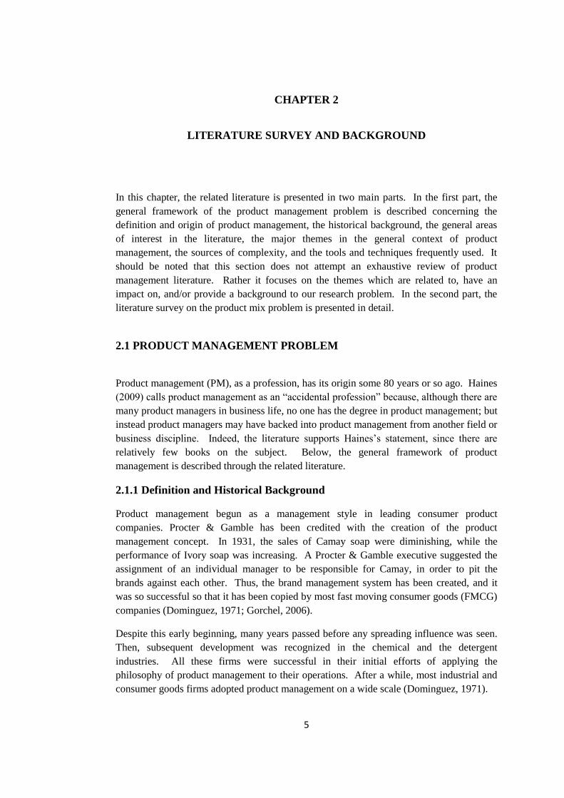
a) Product Life Cycle (PLC):

“Product Life Cycle” (PLC) is simply the whole life span of the product. A traditional PLC

model is illustrated in Figure 2.1 in which cash flow (or sales revenues) is plotted against

time. The PLC model in Figure 2.1 reflects purely the marketing view which considers the

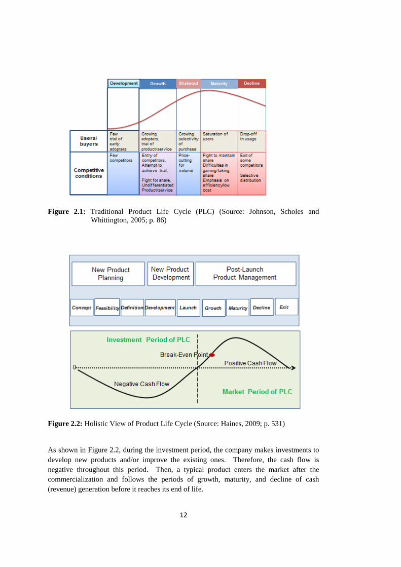
product after the commercialization and entrance into the market. The holistic product

management view, as shown in Figure 2.2, considers the PLC starting from the “idea”

phase till the end of its life, i.e., disposal of the product.

12

Figure 2.1: Traditional Product Life Cycle (PLC) (Source: Johnson, Scholes and

Whittington, 2005; p. 86)

Figure 2.2: Holistic View of Product Life Cycle (Source: Haines, 2009; p. 531)

As shown in Figure 2.2, during the investment period, the company makes investments to

develop new products and/or improve the existing ones. Therefore, the cash flow is

negative throughout this period. Then, a typical product enters the market after the

commercialization and follows the periods of growth, maturity, and decline of cash

(revenue) generation before it reaches its end of life.

13

During the market period, there are several marketing strategies to extend the successful

product’s life in the market. Usually, components of the strategic marketing mix (4 P:

Product, Price, Promotion, Place) are used as the tools for this purpose. Additionally,

spending efforts through a series of continuous improvement projects (CIP) is another

effective strategy to extend the market life of a successful product. The decline of product

revenue occurs in the period following the maturity phase. This is often averted by using a

CIP strategy which extends the product’s life (Rafinejad, 2007).

b) Product Hierarchy:

A product may not be just a single entity. A product may be a part of other products, a part

of a product line, or included in a product mix. “Alternatively, products can be broken

down into product elements, modules or terms. Products may be built upon product

platforms or product architectures” (Haines, 2009; p.6). The hierarchy of products is

illustrated in Figure 2.3.

Figure 2.3: Typical Hierarchy of Products (Sources: a) Haines (2009); p.7; b) Steinhardt

(2010), p.109)

c) Product Manufacturing:

Planning activities in product management involve evaluating manufacturing environment

and capabilities to make sure the planned product can be produced. “A manufacturing

system is an objective-oriented network of processes through which entities flow” (Hopp

and Spearman, 2000; p.190). So, a manufacturing system has an objective, and contains

processes. We emphasize the word “entities” in this definition. Entities include not only

the parts being manufactured, but also the information that is used to control the system.

The flow of the entities through the system describes how materials and information are

processed. The processes in the flow of information can be matched to the purpose of the

demand management system provided in Vollman et al. (2005); the demand management

system provides information that helps to integrate the needs of customers with the

manufacturing capabilities of the firm.

Depending on this property, the major characteristics of the different manufacturing

environments are presented below (Vollman et al., 2005; pp.21-24):

14

Make-to-Stock (MTS) Environment:

“Customers buy directly from available inventory” (p.21).

“The essential issue in an MTS environment is to balance the level of inventory

against the level of service to the customer”. Therefore, “a trade-off between the

costs of inventory and the level of customer service should be made” (p.21).

Shifting the trade-off can be achieved by better forecasts of customer demand, by

more fast transportation/distribution alternatives, “by speedier production, and by

more flexible manufacturing” (p.22).

To achieve higher service levels to the customers for a given inventory level, MTS

firms consider investing in lean manufacturing programs.

“Regardless of how the trade-off comes out, the focus of demand management in

MTS environment is on providing (forecasts) of finished goods” (p.22).

The company may know what customers can buy in an MTS environment, but it

may not know if, when, or how many.

Assemble-to-Order (ATO) Environment:

“The primary task of demand management is to define the customer’s order in

terms of alternative components and options” (p.22). Therefore, “the inventory

that defines customer service is the inventory of components, not the inventory of

finished product, because, the number of finished products is usually substantially

greater than the number of components that are combined to produce the finished

product” (p.22).

One of the critical success factors of a company in ATO environment is

engineering design that enables flexibility in combining components, options, and

modules into finished products. Therefore, “it is also important to assure that they

can be combined into a viable product in a process known as configuration

management” (p.22).

“An ATO environment illustrates the two-way nature of the communication

between customers and demand management” (p.22). Customers need to be

informed about the possible combinations, which should support the needs of the

marketplace.

In order to deliver the customers’ orders quickly, some ATO companies have

applied lean manufacturing principles to decrease the time required to assemble

the finished goods.

Make-to-Order (MTO) or Engineer-to-Order (ETO) Environment:

In MTO/ETO environment, the company is not sure what the customers are going

to buy.

The company needs, therefore, to get the product specifications from the

customers and translate them into manufacturing.

The task of demand management in an MTO environment is to coordinate

information on customers’ product needs with engineering.

Engineering should determine what materials are required, what steps will be

taken in manufacturing, and the costs involved in an MTO environment.

15

Demand management’s forecasting task includes determining how much

engineering and production capacity will be required to meet future customer

needs in an MTO/ETO environment.

2) Management Related Themes:

The decisions regarding acquisitions, mergers and establishing other business

relationships, such as joint venture, strategic investments, licensing, etc., are in the domain

of strategic aspects of executive management. This domain is directly related to the core

vision of the corporate which also specifies the corporate goals. “Growth” is the dominant

goal for a typical company. Growth opportunities are almost unlimited. Developing new

products is one of the many ways for realizing the vision of the company. In the product

management framework, new product development is a primary mechanism for improving

or transforming a company’s performance into a more productive and rewarding

dimension in business life. Clearly, there are other means to realize business goals and

objectives, including acquisitions and mergers, or strategic outsourcing. These strategic

growth means in PM are described briefly below:

a) Acquisitions/Mergers and Other Business Relationships:

A company can go in several different directions to find opportunities to increase revenues.

These opportunities are different, so are the risks and the levels of investment. Rapid

growth companies regularly scan these opportunities then choose one or more. Many

rapidly growing companies, like Unilever, have followed acquisition to grow. As a growth

strategy, driving the acquisition can be powerful, but it must be integrated with the core

vision (McGrath, 2001).

Acquisitions can be an integral part of product strategy. There are different strategic

implications of acquisition types in the sense that each enables product strategy differently.

When correctly handled, acquisitions and other business relationships such as mergers,

joint ventures, partnerships, strategic investments can provide opportunities for growth.

Through an acquisition, the company can easily access the desired technology that it needs

to expand into a new market. Acquisitions can also be used to strengthen a competitive

position in the marketplace. Some acquisitions are made to improve operational efficiency

through increased economies of scale in production and consolidation of activities

(McGrath, 2001).

In a joint venture, “two companies come together to form a third business owned jointly”

(McGrath, 2001; p. 299). The joint venture typically develops a new platform for a new

market but related to both companies. “A joint venture needs to combine sufficient market

and channel capabilities with the necessary technology and technical skills from the two

companies” (McGrath, 2001).

With a strategic investment, one company makes an investment in another in order to get

an access to that company’s market or technology. The main idea is that the company

making the investment gets the same return as other investors, but also gets other

advantages. In order to get these advantages company must make larger investments,

frequently at more than the market price (McGrath, 2001).

16

b) Outsourcing (Make versus Buy):

During the product development phase, as the definition of the product evolves the

management decides where the product will be built. This decision is simply called as

“sourcing” or the “make versus buy” decision. Outsourcing is defined as follows:

“Outsourcing is the word used when a function that may normally be carried out by the

company in-house is actually carried out elsewhere by another party” (Haines, 2009; p.

337).

Outsourcing is usually accepted as a tactical level decision. In addition to this view,

outsourcing is defined as one of the important manufacturing and operations strategies

(Rainey, 2005). Rainey (2005) states that “an efficient and appropriate production system

for a given product can be a strategic weapon and competitive advantage”. He also

considers outsourcing as an issue in the supply-network design of the company. Supply

chain management (SCM) describes the aspect of operations management that deals with

converting raw materials into final products, and the delivery of those final products to

customers. For many companies, SCM refers to maintaining and operating a network of

suppliers, manufacturing and distribution facilities not only in the home country but also

around the world.

Rainey (2005) also states “An important strategic issue in production is “make versus buy”

dilemma” (p. 413). Outsourcing frequently offers a cost competitive alternative to

performing the required activities in–house. The impact of this decision is stated as

follows: “The decision whether or not to produce an item internally can influence short-

term market share, as well as long-term competitiveness and corporate survival” (Rainey,

2005; p.413). In recent years, outsourcing has been suggested for many activities, except

the activities by which the company can provide unique value to its customers and/or those

which the company may have strategic need. The popularity of outsourcing depends on

several reasons:

1. The company is downsizing (possibility of using fewer employees).

2. The outsourcing of an activity is often less costly.

3. Outsourcing has become a part of the companies’ philosophy and strategy.

In today’s business world, extreme applications of outsourcing can be seen among the

companies; outsourcing the entire product and maintain no in-house manufacturing

capability is a popular manufacturing strategy. This is the so-called “virtual company”

approach (Rainey, 2005). Nike is a well-known example of this type of company.

Outsourcing can accelerate product development projects and shorten time-to-market by

leveraging the suppliers’ resources, technology and manufacturing capabilities. “The

outsourcing strategy should be regularly reviewed and updated to reflect the realities of the

marketplace, including changes in the bases of competitive advantage, technological

maturity, competitive landscape, and evolution of the firm’s core and context. Some

companies form a strategic outsourcing council that regularly reviews the firm’s core and

context and updates the outsourcing strategy and decision process” (Rafinejad, 2007; p.

284).

17

3) Contextual Themes in PM:

a) Environmental Sustainability:

Environmental sustainability has become a crucial requirement in product development in

the twenty-first century. “Environment refers to air, water, soil, and all other natural

resources of the earth (including raw material) that are endowed for the well-being of

living species (people, animals, and plants) locally, globally, at present, and in the future.

Environmental sustainability refers to being in harmony with the ecological system of the

earth, ensuring that manufacturing resource utilization and effluents do not harm the

ecosystem equilibrium” (Rafinejad, 2007; p. 218).

The “green-house theory” and “global warming” are both environmental concerns which

have strong effects in the design and manufacturing activities of the companies in many

industries. Therefore, environmentally friendly design is encouraged by the recognition

that sustainable economic growth can occur without consuming the earth’s resources.

Customers are also affected by this trend and thus manufacturers make an evaluation of

how the environment should be considered in the design of their products. “Design for

Environment” (DFE) (or “Design for Environmental Sustainability (DFES)) addresses

environmental concerns as well as postproduction activities, such as transport,

consumption, maintenance, and repair. “The aim is to minimize environmental impact,

including strategic level of policy decision making and design development. Since the

introduction of DFE, one can view the environment as a customer. Therefore the

definition of defective design should encompass the designs that negatively impact the

environment. As such, DFE usually comes with added initial cost, causing an increment of

total life cost” (Yang and El-Halik, 2009; p. 378).

In product design and development of a manufacturing process, the major goal is to

achieve meeting the environmental laws and standards, global protocols. Designing for

maximum efficiency and for minimal waste means “the usage of process consumables,

manufacturing material, and packing sustainable product does not include hazardous

material or material that cannot be recycled” (Rafinejad, 2007; p. 218). To meet all these

requirements DFES is used in product design phase of the development process. In this

approach, the product design must start with a life cycle analysis that assesses the

environmental impact of the product throughout its life cycle which starts with raw

material extraction and goes on with manufacturing, use, and end-of-life disposal. Shortly,

DFES minimizes the environmental impact throughout the cycle (Rafinejad, 2007).

b) Globalization:

In today’s business world, many companies operate in a global marketplace. Customers,

competitors, employees, suppliers, contractors and partners are located worldwide. Global

strategy in product management requires providing products by applying both domestic

and international standards into products. Therefore, designing and manufacturing of

products should meet world standards. So, global manufacturing brings both opportunities

and some complexities to the companies. Today, globalization has strategic value for

business growth across the board.

If the company is based in the country where its business resides and sells to its customers

from the home office, product management in this case is called “domestically based

18

global PM” (Gorchels, 2006). On the other hand, if the company is located in the country

or region where its sales take place, the product management function is a “locationally

based global PM”. Domestically based global PM typically employs “upstream” product

development efforts. Locationally based global PM can fall along a continuum from

downstream activities to full-stream. In full-stream PM, unique product offerings are

created for the global markets from design through sale. Note that full stream activities

contain both strategic and tactical activities. In this case, profit and loss (P&L)

responsibility belongs to the global management. For example, Unilever has a similar

structure, except that P&L responsibility resides with the regional presidents rather than

the global category organization,that controls marketing, product mixes, and strategy

(Gorchels, 2006).

As a result, today’s global manufacturers’ goal is to achieve accelerating time-to-market

and process cycle times, reducing product development costs, maximizing productivity,

improving product quality, driving innovation and optimizing operational efficiency, by

leveraging global networks of employees, partners and suppliers across the manufacturing

starting the design phase (PTC.com).

Regardless of whether a company has multinational locations, long-term product strategies

on a global basis are developed and similarities of the customer needs across different

world markets are searched if standardizing is possible and customizing is necessary.

Through this, companies have opportunities to expand their future foreign sales and also

develop competitive strategies against global competitors. In global PM, “many planning

principles are common across all these situations although the implementation of the

principles might vary” (Gorchels, 2006).

2.1.4 Complexity of the Product Management Problem

Kavadias and Chao (2008) discuss the difficulties and complexity of the NPD portfolio

management problem in their study. As it was mentioned before, NPD is an important

sub-system of the product management system (PMS) from a holistic point of view.

Therefore, the complexity in the context of NPD is also valid in the PMS even with

additional dimensions of complexity. Kavadias and Chao (2008; pp.138) raise the

following considerations:

“Strategic alignment: The NPD portfolio problem entails a large ambiguity and

complexity, since the firm’s success factors and their interactions are rarely

known. Therefore, strategic alignment should be considered effectively to

communicate the firm strategy and cascade it down to an implementable NPD

program level”.

At the product management level, this strategic alignment is considered with the corporate

strategic plan.

“Resource scarcity: Scarce resources critically constrain the NPD portfolio

problem”. In order to achieve broader product lines the resource allocation

decision is a critical success factor.

At the product management level, the earmarking of the resources is considered in the

strategic context. Through such an earmarking activity, NPD program budgets are

19

determined. The allocation of budgeted (constrained) resources among the projects is still

a challenging problem in of decision making at the NPD level.

Project interactions: In a multi-project environment, synergies and

incompatibilities in technical aspects are important in investment decision making.

“Interactions between success determinants play a critical role in the resource

allocation decision”.

At the product management decision level, product interactions are one of the sources of

complexity.

“Outcome uncertainty: NPD projects are characterized by a lack of precise

knowledge regarding their outcomes. Therefore, management (decision makers)

face the uncertainty of the potential market value and technical output of any given

project”.

In addition to technical uncertainty, market uncertainty is considered as the major source

of complexity in product management decision level.

“Dynamic nature of the problem: Decision makers must allocate resources and

NPD programs evolve over time” (pp.139).

In short, strategic alignment with the corporate goals, resource scarcity in general, product

interactions, market uncertainty and other environmental uncertainty issues in addition to

the technical outcome uncertainty, and dynamic and cyclical nature of the problem are the

major complexity sources in the PM problem.

2.1.5 Tools and Techniques Used in Product Management

It is evident that the product management problem is a large scale and complex problem.

Hundreds of decisions are made in several decision making areas, concerning different

objectives, at different levels of management, and at different phases of the PLC of the

products. Below, the major tools and techniques which are commonly used as the solution

approaches considering the specific goals of different problem areas of product

management are presented in two tables. Table 2.1-a presents the techniques and tools in

accordance with the stages in PLC. In Table 2.1-b, they are presented according to the

management levels in product management. We focus on some of the strategic PM tools

which are directly related to our study.

Table 2.1-a: Tools and Techniques with respect to PLC Stages

Product Development Phase

(Investment Period)

Tools/Techniques/Methods

(Development/Engineering Tools)

Discovering market opportunities

(Ideation)

Market research methods (e.g. Surveys,

Focus groups, Benchmarks, Conjoint

Analysis)

Kano model

Customer needs/requirements

study

Concept development and

Product design

Manufacturing process/Product

launch and Production

Quality function deployment (QFD)

CAE, CAD, CAM, CAD-CAM,TRIZ

Axiomatic design

DOE

DOE

Taguchi method, Forecasting

20

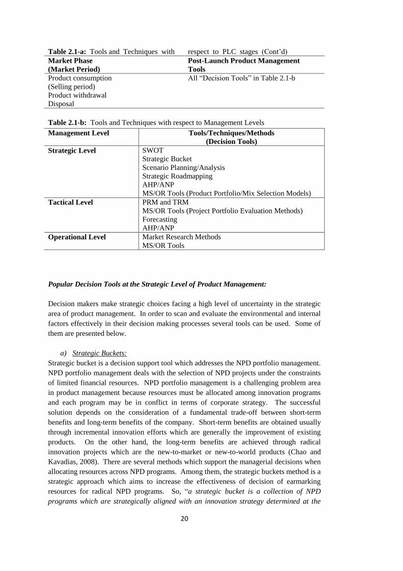
Table 2.1-a: Tools and Techniques with respect to PLC stages (Cont’d)

Market Phase

(Market Period)

Post-Launch Product Management

Tools

Product consumption

(Selling period)

Product withdrawal

Disposal

All “Decision Tools” in Table 2.1-b

Table 2.1-b: Tools and Techniques with respect to Management Levels

Management Level Tools/Techniques/Methods

(Decision Tools)

Strategic Level SWOT

Strategic Bucket

Scenario Planning/Analysis

Strategic Roadmapping

AHP/ANP

MS/OR Tools (Product Portfolio/Mix Selection Models)

Tactical Level PRM and TRM

MS/OR Tools (Project Portfolio Evaluation Methods)

Forecasting

AHP/ANP

Operational Level Market Research Methods

MS/OR Tools

Popular Decision Tools at the Strategic Level of Product Management:

Decision makers make strategic choices facing a high level of uncertainty in the strategic

area of product management. In order to scan and evaluate the environmental and internal

factors effectively in their decision making processes several tools can be used. Some of

them are presented below.

a) Strategic Buckets:

Strategic bucket is a decision support tool which addresses the NPD portfolio management.

NPD portfolio management deals with the selection of NPD projects under the constraints

of limited financial resources. NPD portfolio management is a challenging problem area

in product management because resources must be allocated among innovation programs

and each program may be in conflict in terms of corporate strategy. The successful

solution depends on the consideration of a fundamental trade-off between short-term

benefits and long-term benefits of the company. Short-term benefits are obtained usually

through incremental innovation efforts which are generally the improvement of existing

products. On the other hand, the long-term benefits are achieved through radical

innovation projects which are the new-to-market or new-to-world products (Chao and

Kavadias, 2008). There are several methods which support the managerial decisions when

allocating resources across NPD programs. Among them, the strategic buckets method is a

strategic approach which aims to increase the effectiveness of decision of earmarking

resources for radical NPD programs. So, “a strategic bucket is a collection of NPD

programs which are strategically aligned with an innovation strategy determined at the

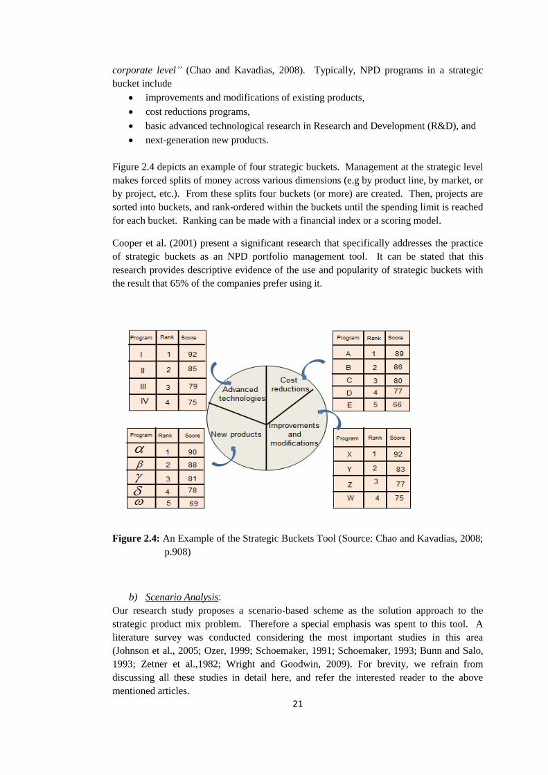
21

corporate level” (Chao and Kavadias, 2008). Typically, NPD programs in a strategic

bucket include

improvements and modifications of existing products,

cost reductions programs,

basic advanced technological research in Research and Development (R&D), and

next-generation new products.

Figure 2.4 depicts an example of four strategic buckets. Management at the strategic level

makes forced splits of money across various dimensions (e.g by product line, by market, or

by project, etc.). From these splits four buckets (or more) are created. Then, projects are

sorted into buckets, and rank-ordered within the buckets until the spending limit is reached

for each bucket. Ranking can be made with a financial index or a scoring model.

Cooper et al. (2001) present a significant research that specifically addresses the practice

of strategic buckets as an NPD portfolio management tool. It can be stated that this

research provides descriptive evidence of the use and popularity of strategic buckets with

the result that 65% of the companies prefer using it.

Figure 2.4: An Example of the Strategic Buckets Tool (Source: Chao and Kavadias, 2008;

p.908)

b) Scenario Analysis:

Our research study proposes a scenario-based scheme as the solution approach to the

strategic product mix problem. Therefore a special emphasis was spent to this tool. A

literature survey was conducted considering the most important studies in this area

(Johnson et al., 2005; Ozer, 1999; Schoemaker, 1991; Schoemaker, 1993; Bunn and Salo,

1993; Zetner et al.,1982; Wright and Goodwin, 2009). For brevity, we refrain from

discussing all these studies in detail here, and refer the interested reader to the above

mentioned articles.

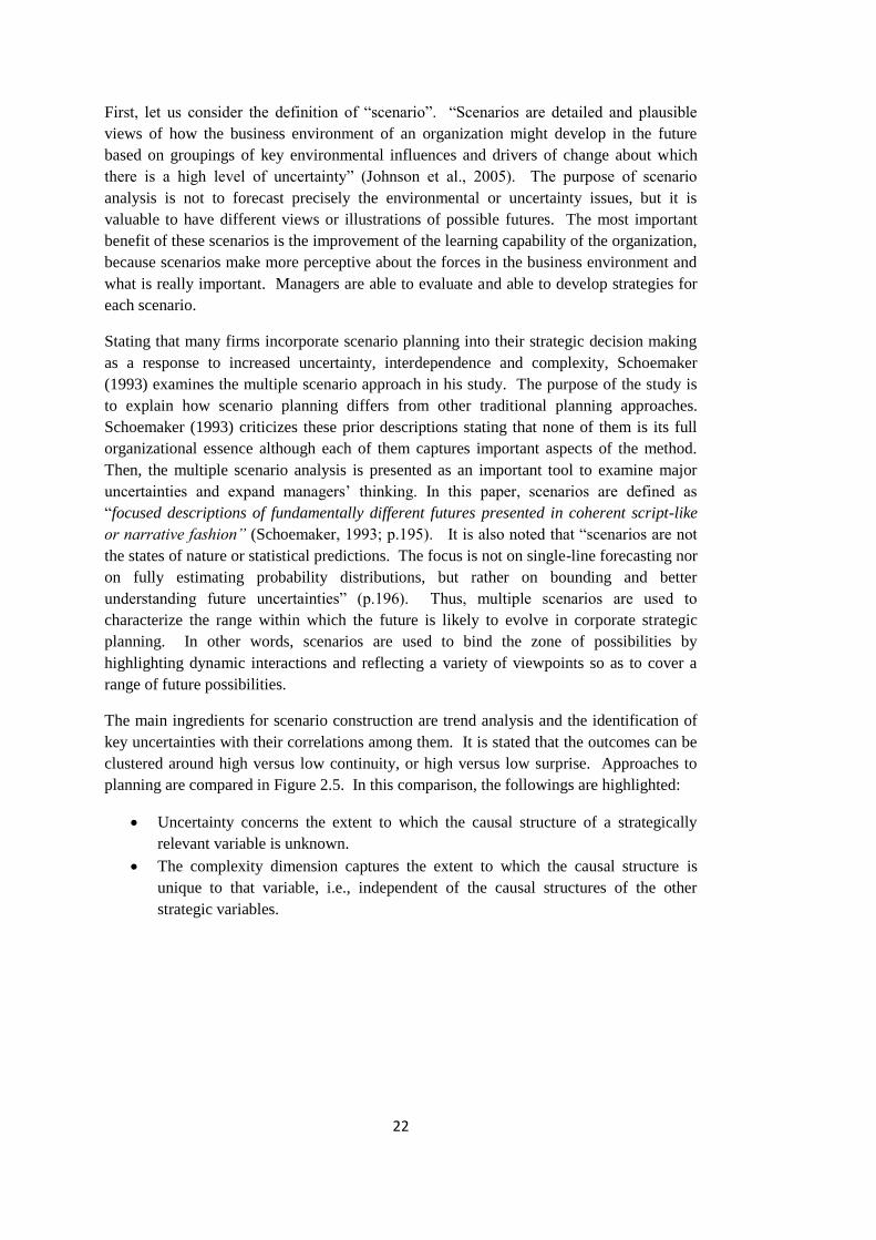
22

First, let us consider the definition of “scenario”. “Scenarios are detailed and plausible

views of how the business environment of an organization might develop in the future

based on groupings of key environmental influences and drivers of change about which

there is a high level of uncertainty” (Johnson et al., 2005). The purpose of scenario

analysis is not to forecast precisely the environmental or uncertainty issues, but it is

valuable to have different views or illustrations of possible futures. The most important

benefit of these scenarios is the improvement of the learning capability of the organization,

because scenarios make more perceptive about the forces in the business environment and

what is really important. Managers are able to evaluate and able to develop strategies for

each scenario.

Stating that many firms incorporate scenario planning into their strategic decision making

as a response to increased uncertainty, interdependence and complexity, Schoemaker

(1993) examines the multiple scenario approach in his study. The purpose of the study is

to explain how scenario planning differs from other traditional planning approaches.

Schoemaker (1993) criticizes these prior descriptions stating that none of them is its full

organizational essence although each of them captures important aspects of the method.

Then, the multiple scenario analysis is presented as an important tool to examine major

uncertainties and expand managers’ thinking. In this paper, scenarios are defined as

“focused descriptions of fundamentally different futures presented in coherent script-like

or narrative fashion” (Schoemaker, 1993; p.195). It is also noted that “scenarios are not

the states of nature or statistical predictions. The focus is not on single-line forecasting nor

on fully estimating probability distributions, but rather on bounding and better

understanding future uncertainties” (p.196). Thus, multiple scenarios are used to

characterize the range within which the future is likely to evolve in corporate strategic

planning. In other words, scenarios are used to bind the zone of possibilities by

highlighting dynamic interactions and reflecting a variety of viewpoints so as to cover a

range of future possibilities.

The main ingredients for scenario construction are trend analysis and the identification of

key uncertainties with their correlations among them. It is stated that the outcomes can be

clustered around high versus low continuity, or high versus low surprise. Approaches to

planning are compared in Figure 2.5. In this comparison, the followings are highlighted:

Uncertainty concerns the extent to which the causal structure of a strategically

relevant variable is unknown.

The complexity dimension captures the extent to which the causal structure is

unique to that variable, i.e., independent of the causal structures of the other

strategic variables.

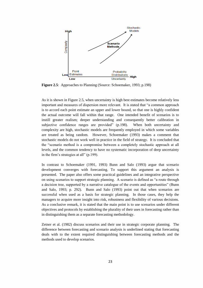
23

Figure 2.5: Approaches to Planning (Source: Schoemaker, 1993; p.198)

As it is shown in Figure 2.5, when uncertainty is high best estimates become relatively less

important and measures of dispersion more relevant. It is stated that “a common approach

is to accord each point estimate an upper and lower bound, so that one is highly confident

the actual outcome will fall within that range. One intended benefit of scenarios is to

instill greater realism; deeper understanding and consequently better calibration in

subjective confidence ranges are provided” (p.198). When both uncertainty and

complexity are high, stochastic models are frequently employed in which some variables

are treated as being random. However, Schoemaker (1993) makes a comment that

stochastic models do not work well in practice in the field of strategy. It is concluded that

the “scenario method is a compromise between a completely stochastic approach at all

levels, and the common tendency to have no systematic incorporation of deep uncertainty

in the firm’s strategies at all” (p.199).

In contrast to Schoemaker (1991, 1993) Bunn and Salo (1993) argue that scenario

development converges with forecasting. To support this argument an analysis is

presented. The paper also offers some practical guidelines and an integrative perspective

on using scenarios to support strategic planning. A scenario is defined as “a route through

a decision tree, supported by a narrative catalogue of the events and opportunities” (Bunn

and Salo, 1993; p. 292). Bunn and Salo (1993) point out that when scenarios are

successful when used as a basis for strategic planning. In those cases, they help the

managers to acquire more insight into risk, robustness and flexibility of various decisions.

As a conclusive remark, it is stated that the main point is to use scenarios under different

objectives and protocols by establishing the plurality of their uses in forecasting rather than

in distinguishing them as a separate forecasting methodology.

Zetner et al. (1982) discuss scenarios and their use in strategic corporate planning. The

difference between forecasting and scenario analysis is underlined stating that forecasting

deals with to the extent required distinguishing between forecasting methods and the

methods used to develop scenarios.

24

c) Product Roadmap/Technolgy Roadmap (PRM/TRM):

Road-mapping is a verb that describes the process of roadmap development. Thus, it can

be said that “the roadmap is simply the outcome of road-mapping” (Kostoff and Schaller,

2001). It can be stated that the road-mapping is proposed as a tool/technique which can

help companies to survive in turbulent environments by providing a focus for scanning the

environment and a means of tracking the performance and individual technologies.

It has been indicated in the related literature that the concept of roadmap has been

developed and used by Motorola in the late 1970s (Kostoff and Schaller, 2001; Phaal et al.,

2003; Ma et al., 2007; Gindy et al., 2006). Starting from early the 1980s, the Motorola

approach has been more widely recognized and practiced in Philips, Lucent Technologies,

etc. (Ma et al., 2007). Therefore, it can be stated that Motorola is the original creator and

user of roadmaps. Although its original field is strategic planning for technology and

product development at the enterprise level, it is also used in industry, in science to support

sector-level research and decision making in both national and international context

(Kostoff and Schaller, 2001; Phaal et al., 2003; Ma et al., 2007; Gindy et al., 2006).

As in the case of ordinary highway maps, a “Technology Roadmap” (TRM) can be viewed

as consisting of nodes and links. These roadmap nodes and links have quantitative and

qualitative attributes. Kostoff and Schaller (2001) give the following simple example to

clarify the idea behind TRM. For example, in a highway map, a link (road) has a direction,

a length, and sometimes an effective width (two lanes etc.). These are essentially

quantitative attributes. However, sometimes a highway map will show a dotted line next

to a road, denoting that road as scenic. This is a qualitative attribute (Kostoff and Schaller,

2001). Thus, the following classification, which represents independent roadmap

application areas, has been introduced:

1. Science and Technology (S&T) roadmaps

2. Industry technology roadmaps (TRM)

3. Corporate or product-technology roadmaps (PRM)

4. Product-portfolio management roadmaps (Strategic roadmapping)

There are many definitions which are given considering the application areas, the formats

of presentation, the objectives of the driver, etc.. The common point that we can note is

that TRM is a tool/technique which link or integrates the business planning to technology

planning. Or, a more comprehensive definition can be as follows: Technology road-

mapping is a strategic/tactical management tool to help organizations in effectively

identifying potential products or services for the future, determining proper technology

alternatives and mapping them with resource allocation plans. A strategic TRM definition

is provided as follows: “A TRM specifies the technological requirements that a firm needs

to enable its aggregate strategy, irrespective of how the firm will access the technology”

(Rafinejad, 2007; p.36).

The purpose of a PRM is to define how existing products will evolve and what new

products will be developed and when they are commercialized over the planned period. In

case of a new technology, the PRM should reflect the diffusion of technology and should

identify the evolution on the basis of competition and marketing mix components. “The

PRM consolidates the business, market, and technology strategies into a product and

25

market development vision and guides the firm’s product commercialization and

marketing programs” (Rafinejad, 2007; p.92).

Recently, research on TRM as a theoretical methodology has started to appear, providing

road-mapping guidelines and linking TRM to other management tools such as QFD,

Scenario mapping, AHP, TRIZ, etc. QFD offers a reliable starting point for road-mapping

and building the required cross-functional cooperation. The outcome of the QFD process

corresponds with the roadmap planning phase, which is completed by determining the

corresponding technologies (Rafinejad, 2007; Gerdsri and Kocaoğlu, 2007).

d) Management Science and Operations Research Tools (MS/OR Tools):

Below project evaluation/product selection models are presented briefly. There are four

main approaches to project portfolio evaluation:

Benefit measurement models,

Economic models,

Portfolio selection models, and

Market research models

“Benefit measurement models rely on subjective assessment of strategic variables, such as

strategic alignment (fit) with corporate objectives, competitive advantage and market

attractiveness” (Cooper, 1993; p.170). Checklists and their extensions and scoring models

are the ones in this category which are frequently used in business life. Project

interdependency is not considered on the overall resource allocation question.

Economic models treat project evaluation as a traditional investment decision.

Computation approaches, such as payback period, break-even analysis, return on

investment, and discounted cash flow (capital budgeting methods) are used. To handle the

uncertainty, probability-based techniques, such as decision tree analysis and Monte Carlo

risk assessment are proposed. They require reliable data, but such data usually are not

available. These models are generally considered most relevant for “known” projects

(incremental projects, improvements and modifications). Project independency is assumed

in the models of this category.

Mathematical programming models and techniques such as linear, dynamic and integer

programming are employed in (Product/Project) Portfolio Selection models. The objective

is to develop a portfolio of new and existing projects (products) to maximize the objective

function (expected profits) subject to a set of resource constraints.

Market research approaches are usually used for simple consumer goods. Market research

techniques, when used as a decision tool, assume that there exists market acceptance of the

new product. The assumption here is that strategic, technological and production issues

are not relevant. “Given a strictly market based screening decision, it makes sense to use a

variety of market research based techniques ranging from consumer panels and focus

groups to perceptual and preference mapping” (Cooper, 1993; p.171).

e) Combination of Several Tools:

In the product management context, an appropriate combination of these tools can be used

according to the decision making problem under consideration. In Hou and Su’s study

(2007), they present “an approach for efficiently analyzing customers’ preferences and the

26

capabilities of a manufacturer and its competitors, in order to provide appropriate solutions

based on the information gained from each particular PLC stage”. The issues such as

market intelligence, core competence, organizational strength, market attractiveness,

product strategy and product position are analyzed in each stage of the PLC. To achieve

this, a model named “Customer-Manufacturer-Competitor (CMC) orientation analysis for

PLC” is developed. To effectively analyze information and to provide solutions, QHD,

TRIZ and AHP/ANP have been applied to implement the model.

In another study, a modeling framework for product development decision making is

proposed which incorporates knowledge-based and decision support systems with MS

methods for project evaluation (Liberatore and Stylianou, 1995). At the core of the

framework, the methods and techniques are used to acquire and process the expert

knowledge. These methods include scoring models, logic tables, AHP, discriminant

analysis and rule-based systems. Through a series of case studies the framework is applied

and the results are presented.

2.1.6 Gaps and Weaknesses in the Product Management Literature

In most marketing texts, the product is regarded as only one of the components of the

marketing mix (“4P”) and major emphasis is given to the selling and promotion activities

in the product management framework. Since the marketing view deals with the market

period of PLC of a product, the product development phase is largely ignored.

On the other hand, the studies dealing with NPD focus on the development process and

neglect all other aspects (Baker and Hart, 1999). However, NPD represents only one

aspect of the firm’s business and is highly dependent on the successful management of

existing products for its funding.

Even in books which deal with product strategy and management, the emphasis is given

largely on the process of new product development with little attention given to any other

aspects. “In the real world, product management is the day-to-day management of the

product through its life cycle which is the primary concern of an organization” (Baker and

Hart, 1999).

Haines (2009), as an old product management practitioner and a new academician, makes

an important observation which we totally agree with. “Product Management has no well-

defined framework and is often treated as a transient discipline in many companies” (p.

xxviii). Emphasizing knowledge available to a practitioner in product management,

Haines (2009) also states “Individuals and companies struggle with Product Management

because there has not yet been a codified body of knowledge available to the Product

Management practitioner”, and he adds; “Absent from the curriculum, however, is an

overall framework or “anatomical structure” to look at Product Management holistically

and there is no holistic framework within which to manage and grow your career” (p.

xxix).

Firstly, this comment must be true, because our literature survey on the subject supports it

in the sense that there is no a well-defined, structured and comprehensive study regarding

the framework of product management from a holistic point of view. Realizing this gap in

27

the product management literature after an extensive literature survey, it is intended to

make an attempt to fill this gap in the literature. Chapter 3 presents this effort.

Secondly, it is realized that an important weakness exists in the literature regarding the

selection of products at the strategic level of product management. Kavadias and Chao

(2008), related to NPD portfolio selection, state that “quantitative research efforts have

been restrained at the tactical level of analysis and they have not been widely adopted in

practice because of the complexity associated with the decision”. Within this context, they

offer a comprehensive literature review, and highlight several of the previous research

findings, and some of the lessons drawn for researchers and practitioners. As a conclusive

remark, we consider the following: The NPD portfolio selection problem remains largely

an open problem especially at the top management decision making level (Kavadias and

Chao, 2008). Note that NPD portfolio determines minor improvements, new product

introductions, or radical developments associated with the product mix of a company. This

issue partly represents the determination of set of candidate products of the product mix of

a company. Including the candidate existing products which are to be kept to the NPD

portfolio will result the complete set of candidate products which is a major input of the

strategic product mix problem.

Finally, to determine the mix of products at the strategic level of PM describes our

research problem. It was seen that this problem is usually handled in production

management framework in the literature. So, it is decided to develop and propose a

product mix Decision Support System (DSS) to aid the strategic level of management,

which is based on quantitative methods and aims to be implemented practically and

effectively. The proposed DSS is presented in Chapter 4. In the subsequent section, a

detailed literature survey on the product mix problem is presented.

2.2 PRODUCT MIX PROBLEM

For many firms, the most important decisions relating to production are those that

determine the product mix for a given period of time. The following features characterize

a product mix problem:

1. Maximization of contribution to financial performance.

2. Constraints resulting from resource limitations.

3. Bound constraints on planned production.

The product mix problem is modeled as a mathematical programming problem (Johnson

and Montgomery, 1974). It is a classic example of the direct application of Linear

Programming (LP) approach (Ravindran, 2008), and this kind of product mix problems are

called as “deterministic product mix problems”.

Normally any manufacturing company makes a variety of products using raw materials,

machinery, labor force, and other available resources. Traditionally, the problem of

deciding how much of each product to manufacture in a period, to maximize the total

profit of the company, subject to the availability of required resources is defined as the

product mix problem, which is a common problem area in many industries (Ravindran,

28

2008). The problem is defined as the quantity determination of a given set of products

subject to resource constraints in order to maximize profit, which can be seen as the

“traditional production planning problem”. The same kind of problem related with the

product selection decision is defined as “strategic production planning problem” in the

study Alonso-Ayuso et al., (2005).

It is stated that “explicit consideration of uncertainty about the demand for a product is

difficult in constrained problems, such as product mix determination” (Johnson and

Montgomery, 1974). These kinds of problems are called as “stochastic (or probabilistic)

product mix problems”. Direct treatment of uncertainty about demand involves making

probability statements about the desired relationships between production and demand and

then translating these probability statements into linear inequality constraints. This

approach is called chance constrained programming (Johnson and Montgomery, 1974).

Secondly, the probability distributions of demand are used in formulating a model for the

expected total contribution to profit and overhead during the period, and then optimized

subject to a single resource constraint (probabilistic model with a single resource

constraint). In the case of discrete demand, the “knapsack problem”, can be considered

(Johnson and Montgomery, 1974).

There is a vast amount of literature regarding the product mix problem. We present a

review of this literature in following sections, based on the modeling approaches of

product mix problem in the literature.

2.2.1 Modeling Approaches of Product Mix Problem

The modeling approaches of the product mix problem are presented in two groups

according to the treatment of the contextual variables considered in the problem. These

are:

1) The models of the deterministic product mix problem.

2) The models of the stochastic or probabilistic product mix problem (in which

uncertainty is considered).

Various examples are given for the first group of studies concerning the modeling

approaches of optimization and some other methods such as AHP and ANP. Similarly, the

product mix problem under uncertainty was searched in the literature under the

optimization approaches in which uncertainty is considered and also a few examples are

provided which handle uncertainty through different optimization methods.

2.2.1.1 Deterministic Product Mix Problem

The studies presented in this group represent the extended examples of the traditional

product mix problem. Most of them are the examples of the optimization modeling

approach.

Product Line Decision Making:

Product Line Decision/Design (PLD) problems constitute a domain of literature related to

product mix problems. Most articles on product line optimization are based on the max-

29

surplus-choice models, a deterministic rule under which each customer chooses the

available product that provides him the highest surplus (Kraus and Yano, 2003). The

typical objective is either to maximize the seller’s profit or to maximize some measure of

welfare (total benefit to seller and customers). We have several examples presented below.

Kraus and Yano (2003) indicate that Zufryden (1982) is the first to formulate the problem

as an integer program. His objective is to maximize the weighted sum of consumers

choosing a product line under the max-utility choice rule. They state that a solution

procedure is not provided.

Green and Krieger’s (1985) model differs from Zufryden’s model in the sense that it

considers a set of products whose composite utilities have been obtained by presenting

these product profiles to consumers for evaluation. The objective is to maximize either

seller value or buyer welfare by deciding which products to offer under the max-utility

choice. This model does not explicitly incorporate prices or costs, and fixes the number of

offered products.

McBride and Zufryden (1988) formulate Green and Krieger’s problem as an integer

program and develop optimization-based heuristic procedures to solve the simpler welfare

maximization problem and the more difficult seller value maximization problem. They

report the optimal solutions for small cases of both problems.

As indicated by both Kraus & Yano (2003) and Morgan et al. (2001), Dobson and Kalish

extend Green and Krieger’s model to allow price setting and choice of the number of

products, as well as per product fixed costs. The goal is to maximize welfare or profit

under the max-surplus choice rule. They show that the welfare maximization problem is

equivalent to the uncapacitated plant location problem. They also propose and test several

heuristic methods for the profit maximization problem.

Recent product line design models allow for more complex cost structures. Raman and

Chhajed (1995) consider a scenario in which, in addition to choosing which products to

produce, one must also choose the process by which these products are manufactured.

Ramdas and Sawhney (2001) consider situations where the fixed cost of a component is

shared by two products. Kraus and Yano (2003) state that Dobson and Yano allow for a

wider range of complex interactions by admitting per-product fixed costs, resources that

can be shared by multiple products, as well as technology choices for each.

Chen and Hausman (2000) present a model in which only a limited number of candidate

products will be offered and that prices can take only a set of discrete values. The

objective is to maximize profits by deciding product selection and pricing simultaneously.

The special structure of the problem allows them to relax the integrality constraints for the

discrete price choices and use standard non-linear programming software to find optimal

solutions for problems of realistic sizes.

Product Mix Problem and Product Variety Management (Family Line Decisions):

Product variety management is another domain of literature related to the product mix

problem. Ramdas (2003) provides an excellent integrative review in his study introducing

a framework for managerial decisions about product variety. It is pointed out that

30

managing product variety requires decision making at different organizational levels, over

different time horizons, before and after product launch. In his framework, the following

common set of decision themes is considered:

a) variety-creation; includes four decision themes which are

dimensions of variety,

product architecture,

degree of customization, and

timing.

b) variety-implementation; includes three decision themes which are

process and organizational capabilities,

points of variegation (or decoupling),

day-to-day decisions.

Note that variegation is defined as describing “how a firm’s products are perceived as

distinct from one another” (Ramdas, 2003). Product line decisions and specifically

product mix decisions are seen in the major decision theme of dimensions of variety in the

common set of variety-creation theme, which involves deciding

what and how many products to offer,

the target markets, and

introduction timing of each product.

There are several research studies which focus on family line decisions (Tucker and Kim,

2008; Tucker and Kim, 2009; Jiao et al., 2007; Hopp and Xu, 2005; Kokkolaras et al.,

2002). Tucker and Kim (2008) address two fundamental areas in product family design in

their study:

1. Incorporation of market demand

2. Product architecture reconfiguration

In order to incorporate market demand into the formulation of a family line, they use a data

mining approach where customer preference data are translated into performance design

targets. Product architecture reconfiguration is modeled as a dynamic optimization design

entity, that is, the initial stage of product design is not kept as fixed, and instead it evolves

with fluctuations in customer performance preferences. So, they use a multilevel

optimization model to link product design and product planning, which maximizes

company profit. In their subsequent study (Tucker and Kim, 2009), the set of product

concepts are generated through a decision tree data mining technique, and subsequently

validated in the engineering design using again multilevel optimization technique. It is

stated that the incorporation of decision tree data mining technique into the model leads to

a tremendous savings in time and resources in product portfolio design and selection

process.

Product Mix Problem and Technology Decision Making:

Additional contributions are included in the studies of Morgan and Daniels (2001) and

Morgan et al. (2001). Morgan and Daniels (2001) present a technology adoption decision

model that integrates product mix and technology adoption decisions for the automobile

industry, recognizing that product mix and volume are important variables in determining

31

the cost effectiveness of new technologies. Customer demand projections reflecting

market trends are also included in their model. They state that “a key element that

differentiates this framework from traditional technology adoption decision models is

explicit consideration of the interrelationships between the product line decisions that

ultimately dictate the portfolio of products offered by the firm, and the technology

decisions that drive both functionality and manufacturability of the firm’s product mix”. A

multi-period integer programming approach is used in the modeling. The objective is to

identify a mix of products to offer and to assign a technology for each selected product

such that total profits are maximized over a time horizon.

Product Mix Problem and Manufacturing Process Selection:

Morgan et al. (2001) present a model which can be seen in the area of the models that

integrate product and process selection which are given above. However, they extend the

literature by explicitly considering manufacturing cost interactions among candidate

products. By using binary decision variables, the model is constructed to select the subset

of products that maximizes the objective function. The objective function represents the

total contribution to profits from the products included in the product line by subtracting

the associated variable costs, holding costs, and individual product and manufacturing

class set-up costs from the total revenue earned satisfying demands from the targeted

customer segments. This model is used to examine how the optimal product mix is

affected by a firm’s cost structure, and to study product line characteristics including

profitability, breadth, and diversity of manufacturing requirements associated with the

selected mix and market share captured. Although it is stated that demand uncertainty is

considered as an extension to their basic model, an explicit form does not exist. It is only

stated that the basic model can be modified to incorporate uncertainty with respect to each

customer segment.

Product Mix Problem and Product Interactions:

Although the decision model is not a product mix model, one can note Urban (1969) as one

of the pioneering studies dealing with product interactions in the context of a marketing

mix model, considering the following criteria:

1. decision relevance, i.e., the model should encompass the major factors and market

phenomena affecting the best marketing mix for a product line, and

2. simplicity of the model whenever possible.

So, the following factors are identified as decision relevance:

1. aggregate product class marketing mix effects,

2. product class interdependencies, and

3. intragroup relative competitive brand effects.

First, a linear log function is established to capture marketing mix effects which allow

nonlinearity in response to the marketing variable. Secondly, two basic kinds of

interdependencies are considered, namely complementarity and substitutability, and

another equation is formed by using cross elasticities as parameters which are the measures

of product interdependency. Then, the group marketing mix and intergroup product

interdependencies are combined to specify the total sales of one product class. Next, the

32

market share expression is formed using the same format in the first step. These are called

sub-models in the study. These sub-models are combined into one equation to describe the

sales of the firm’s brand in a product class, which also represents the demand for one

product of a firm’s product line. Finally an objective function is formed as the total profit

of the firm. It is stated that “assuming the firm’s problem in the short run is to maximize

the total profit subject to existing technical, managerial, financial, and production

constraints, the output of the model should be the best marketing mix for each brand in the

firm’s product line. This requires the optimization of the model which is difficult since the

model is not amenable to mathematical programming or other analytical techniques.

However, it may be solved by an iterative search routine”.

Since Urban’s study, the product interaction issue has received attention from researchers

to incorporate into their models. Another study which considers product interactions is

introduced by Monroe et al. (1976). In this article, an integer programming approach to

the product mix problem is used by considering pairwise revenue interactions among

products, as opposed to Morgan (2001), in which the product interaction effect is

considered in the cost structure for substitutable products only. In Monroe et al. (1976),

the interaction effects between revenues earned by the various products are explicitly

considered. Product introduction and deletion decisions are simultaneously determined to

maximize the firm’s objective function over the planning horizon subject to specific

resource constraints.

Product Mix Problem and Production Bottlenecks:

Many researchers have discussed the product mix problems and their solutions through

Theory of Constraints (TOC), introduced by Goldratt and Cox (Lea and Fredendall, 2002;

Sing et al., 2006; Linhares, 2009; Lee and Plenert, 1996; Perkins et al., 2002; Tsai et al.,

2008; Souren et al., 2005). The TOC approach focuses on the bottleneck constraint in

production processes and proposes a set of principles and concepts to manage the

constraints. The concept of TOC is based on three operational measures: throughput,

inventory and operating expense. The TOC approach consists of five steps to identify and

manage the system constraints:

1. Identify system constraint(s),

2. Decide how to exploit system constraint(s),

3. Subordinate everything else to the above decision,

4. Elevate system constraints, and

5. Go back to step (1) and do not allow inertia to be constraint.

Thus, identifying and exploiting the resource constraint to adjust the capacity of that

resource, it is possible to increase the production and profit of the company (Köksal, 2004;

Nikumbh et al., 2009). As a tool for product mix decisions, the TOC-based approach is

often used alternatively (or parallel) to optimization tools, such as the contribution margin

per constraint unit method or LP approaches (Souren et al., 2005). Souren et al. (2005)

discuss some premises to generate optimal product-mix decisions using a TOC-based

approach, and show the reasons for the non-optimality of the TOC-based approach. Lee

and Plenert (1996) examine the case of the introduction of a new product.

33

Lea and Fredendal (2002) examine how three types of management accounting systems

and two methods to determine product mix interactions in both the short term and the long

term affecting the manufacturing performance. Lea and Fredendal’s (2002) study provides

insights into the product mix decision considering fluctuations caused by environmental

uncertainty, using an integrated information system which integrates a manufacturing

system and a management accounting system.

Variations of Goldratt’s product mix problem are proposed by several researchers

(Onwubolu and Muting, 2001; Köksal, 2004). Köksal (2004) provides a comprehensive

literature survey on TOC and questions the power of the TOC-based approach in focusing

quality improvement for bottom line results, and thereafter develops an LP model which

aims to maximize throughput and minimize quality loss to find the product mix for a

specific period under known or predicted levels of quality of processes. Hence, Köksal

(2004) proposes an improvement of a TOC-based algorithm.

Product Mix Problem and Sourcing Decision:

Although the sourcing decision (i.e., make or buy decision) has an important impact on the

product mix decision, few studies take place in the optimization research area in the

literature (Küttner, 2004; Arya et al., 2008). Küttner (2004) considers aggregate

production planning with and without outsourcing, which are formulated as LP models in

his study. The model to solve the problem of optimal product mix is demonstrated

explicitly, and then the conditions are determined under which outsourcing is profitable for

a firm. In other words, the model needed to consider outsourcing is not given in an explicit

form, but instead it is stated that “the model based on aggregate production planning (APP)

is needed to determine the decision of what fraction of components to produce in-house

and what fraction to outsource” (Küttner, 2004).

Product Mix Problem and Environmental Sustainability:

Nowadays, several recent developments in environmental awareness and control have

contributed to increased environmental concern. In addition, new governmental

regulations may obligate companies to consider taking back and recycling their products.

Additionally, environmentally friendly products and processes also contribute to

stakeholders’ satisfaction since environmental attributes of products are becoming

increasingly relevant for consumers’ demand preferences. Today, many firms are

environmentally aware and they start to deal with these issues systematically, because

these developments have negative impacts on their cost structures and competitiveness. In

short, a firm’s strategic, tactical and operational decisions are affected by the impact of

environmental considerations. We review a few studies which address this important

concern of the firms below.

Letmathe and Balakrishnan (2005) addressing this issue, present a study to illustrate how

environmental concerns affect the product mix and profitability of the firm. It is stated that

the environmental impact of a firm’s products, processes, and resource usage are typically

measured by the amount of emissions of waste water and other industrial wastes and

pollutants. They present two mathematical models to determine the optimal product mix

and production quantities in the presence of several different types of environmental

constraints, in addition to typical production constraints. The first model assumes that

34

each product has just one operating procedure, which is formulated as an LP problem. The

second model, which assumes that the firm has the option of producing each product using

more than one operating procedure, is a mixed integer linear programming (MILP) model.

The solutions of both models identify the products that the firm should produce along with

their production quantities. It is concluded that these models can be used by firms to

quickly analyze several “what-if” scenarios such as the impact of changes in emission

threshold values, emission taxes, trading allowances, and trading transaction costs.

Stuart et al. (1999) point out that a few quantitative approaches for the selection of

manufacturing processes with environmental considerations have been presented in the

literature. They also state that “in general, these quantitative models for business-focused

decisions that include environmental considerations are limited to either assembly or

disassembly decisions”. So, in their study they propose a comprehensive product and

process mix model, which extends the existing product and process mix approaches to

include environmental costs, variables, and constraints. It is stated that their study is the

first attempt which handles the complexities of life cycle product design by incorporating

varying recycling market prices and limits, legislated limits, and product take-back rates

over the product life cycle, i.e., the time horizon for the problem is over the product life

cycle. The model is able to compare the profitability and environmental impacts of

designs for product life extension to designs for shorter product lives, which is also stated

as a unique approach in the paper which links product design and take-back decisions. In

other words, their innovative take-back approach considers both the date of manufacture

and date of take-back.

In their problem statement, the following questions are asked which are translated into a

type of decision variable in their model:

1. Which feasible product and process design combinations should be selected for

production during each time period? (This question characterizes a strategic long

term issue.)

2. What manufacturing configuration (number of workstations) should be used?

(This question links the strategic and operational issues.)

3. In what quantities should the selected product and process design combinations be

produced each time period?

4. What assembly, repair, and reclamation inventories result from these production

strategies?

5. By what quantities will process wastes and packaging wastes exceed recycling

capacities?

They construct a MIP model with the objective of maximizing net revenues of the

company.

Product Mix Problem Under Different Approaches from Optimization:

Product mix decision problems have been examined by using approaches different from an

optimization approach (Wind; 1974; Chen et al., 2006; Taylor et al., 1994; Chung et al.,

2005; Nikumbh et al., 2009).

Chung et al. (2005) propose an application of the analytic network process (ANP) for the

selection of product mix for efficient manufacturing in a semiconductor fabricator. In

35

order to evaluate different product mixes, a hierarchical network model based on various

factors and the interactions of factors is presented. By incorporating experts’ opinion, a

priority index is calculated for each product mix studied, and a performance ranking of

product mixes is generated.

Miscellaneous Examples of the Product Mix Problem:

There are several studies of product mix problems which address specific industrial issues,

like product mix of an insurance company, product mix decision in a mixed-yield wafer

fabrication, product mix in the TFT-LCD industry, product mix planning in semiconductor

manufacturing, product mix in plywood manufacturing, and tool planning in multiple

product mix for wafer foundries (Kahane, 1977; Wu et al., 2006; Wang et al. 2007; Chou,

2000; Roy et al., 1982; Hsiung et al., 2006).

In a recent study of Wang et al. (2007), the traditional product mix problem has been

studied considering a number of unique characteristics of the TFT-LCD industry (i.e., in

the consumer durables sector), such as the supply of key components, the process yield, the

committed orders, and the efficiency of resource utilization. It is stated that the primary

interest of decision makers in this industry is not only to improve production performance

but also to effectively make product mix changes using flexible production and business

operation. Therefore, determining the optimum product mix and analyzing its implications

is an essential part of the design process for the achievement of a robust and flexible

production system. A company’s product mix is defined as the percentage of total

throughput devoted to each product. Product mix analysis focuses on determining the

optimum product mix and highlights the implications of varying the percentage of each

product on different production activities. The problem encountered here is to determine

product demand allocations that are suitable for production factories. A MILP is used to

determine the optimal product mix for all available resources for a monthly production

plan in order to maximize the net profit subject to constraints imposed by resource

limitations, fulfill orders, and inventory costs. They extend the model for multiple

production planning periods.

It can be concluded that there are many rich models for the product mix decision problem.

However, the main issue of uncertainty remains the same. In other words, product mix

planning using deterministic models has the disadvantage that the uncertainties are not

considered. Hence the decisions will not be optimal, and there is no guarantee that the

decision makers of the firm will not run into very unfavorable situations because of the

discrepancies between the assumed and the real evolution of the critical parameters of

product mix decision (Cui and Engel, 2010).

2.2.1.2 Product Mix Problem under Uncertainty

In general, research on optimization that considers uncertainty can be categorized

according to the four primary approaches:

1) Stochastic programming approach,

2) Fuzzy programming approach,

3) Robust optimization approach,

4) Simulation optimization approach

36

In the stochastic programming approach, some parameters are regarded as random

variables with known probability distributions (Ravindran, 2008). It should be noted that

the stochastic programming approach focuses on optimizing the expected performance

(e.g. profit) over a range of possible scenarios for the random parameters. In this

optimization approach, stochastic problems are divided into two-stage and multi-stage

problems. In the first sub-class of this category, the initial decisions are taken first, which

are followed by a random event. Next, the recourse decisions, which are based on this

random event, are taken. As the second sub-class of this category, the stochastic dynamic

programming approach includes applications of random variables in dynamic

programming which can be found essentially in all areas of multi-stage decision making.

It is assumed that a system evolves over a set of stages, between which a stochastic event

occurs; a corrective control action (or a recourse action) can be taken in the next stage.

This kind of an approach is also called as multi-stage stochastic programming (Zima,

2009). In this case, decisions are made at each stage.

The fuzzy programming approach seeks the solution considering some variables as fuzzy

numbers.

Robust optimization approach represents uncertainty through setting up different scenarios

which demonstrate realizations of uncertain parameters. The aim of this approach is to

find a robust solution which ensures that all specified scenarios are “close” to the optimum

in response to changing input data (Mirzapour Al-e-hashem et al., 2011). In contrast to

stochastic programming, in which data uncertainty is modeled in stochastic nature, robust

optimization does not assume the stochastic nature of the uncertain data (Ben-Tal and

Hertog, 2011). In the robust optimization approach, an uncertainty region is defined on

constraints while keeping the objective as certain.

Due to the similarity of our problem formulation approach, we will give a special emphasis

to the simulation optimization approach. Better et al. (2008) present some new approaches

of the simulation optimization for managing risk. The advantages and disadvantages of

traditional optimization approaches are discussed in the study, and they illustrate the

advantages of simulation optimization through two practical example problems. It is stated

that traditional scenario-based approaches, like scenario optimization and robust

optimization consider only a small subset of possible scenarios, and therefore the size and

complexity of the models handled by these approaches are very limited. The scenario

optimization approach is summarized as follows:

1) Compute the optimal solution to each deterministic scenario sub-problem.

2) Solve a tracking model to find a single, feasible decision for all scenarios.

The key aspect of scenario optimization is the tracking model in step 2, which has the

purpose of finding a feasible solution under all scenarios by penalizing the solutions that

differ greatly from the optimal solution. Note that we use step 1 above in our formulation

approach. It is pointed out that robust optimization may be used when the parameters of

the optimization problem are known within a finite set of values, and hence, it has been

concluded that “most traditional optimization techniques that attempt to deal with

uncertainty, is their inability to handle a large number of possible scenarios” (Better et al.,

37

2008). The authors argue that some recent innovative approaches in simulation

optimization can overcome the limitations stated above by providing a practical and

flexible framework for decision making under uncertainty.

In the simulation optimization approach, the optimization problem is defined outside the

complex system. Therefore the simulation model can change and evolve to incorporate

additional elements of the complex system, while the optimization procedures remain the

same. Better et al. (2008), providing a general form of an optimization problem, state that

simulation optimization tools are designed to solve the type of optimization problems in

which the vector of decision variables includes both integer values and variables that range

over continuous values.

The optimization procedure in the simulation optimization approach uses the outputs from

the system evaluator, which measures and evaluates the merit of inputs. Better et al.

(2008) illustrate the optimization procedure as in Figure 2.6.

Figure 2.6: Simulation Optimization Procedure (Source: Better et al., 2008)

The process depicted in figure 2.6 continues until an appropriate termination criterion is

satisfied. It is stated that this criterion is usually based on the analyst’s preference for the

amount of time devoted to the search.

Finally, Better et al. (2008) point out an important remark about the solution space of the

problem. It is stated that the uncertainties and complexities modeled by the simulation are

often such that the analyst has no idea about the shape of the response surface, i.e., the

solution space. Since there is no closed-form mathematical expression to represent the

space, there is no way to gauge whether the region being searched is smooth,

discontinuous, etc. In short, this study views the simulation optimization approach as

more efficient, flexible and practical than the traditional optimization approaches under

uncertainty, stating the following:

38

“While this is enough to make most traditional optimization algorithms fail, meta-

heuristic optimization approaches, such as tabu search and scatter search, overcome

this challenge by making use of adaptive memory techniques and population sampling

methods that allow the search to be conducted on a wide area of the solution space,

without getting stuck in local optima” (Better et al., 2008).

Below we review some specific research studies as the application examples of the general

approaches described briefly above.

Cui and Engel (2010) deal with the medium-term planning of a polymer production plant,

considering demand, plant capacity and yield uncertainties. They consider the following

approaches as the treatment of uncertainty caused by demand, capacities, revenues, etc.:

event-driven or periodic re-planning,

reactive re-planning,

robust planning,

multi-stage or two-stage stochastic planning.

They state that robust planning and multi-stage planning are variants of stochastic

optimization, in which models take uncertainty explicitly into account. Moreover, it is

stated that stochastic models with recourse consider the corrective measures that can be

taken after the realization of some uncertain parameters while in robust planning and this

option is not included. They have also a criticism about the multi-stage stochastic

approach regarding the solution algorithm of this kind of decision problems which leads to

a complex nested structure, because at each stage, the reaction of the algorithm to the

information obtained at later stages must be taken into account. It is pointed out that this

is the main reason of multi-stage problems approximations into two-stage problems. After

the discussion of this kind of issues, they propose a stochastic dynamic MILP formulation

with two-stage. They consider a moving horizon strategy in their model which is stated

that it represents a contribution to this area of the literature.

Mirzapour-Al-e-hashem et al. (2011) present a multi-objective APP model to solve the

multi-period multi-product multi-site APP problem for a medium-term planning horizon

based on existing conflict between the total losses of supply chain and customer

satisfaction level over the planning horizon under different scenarios using the robust

optimization approach. The main features of the proposed model are as follows:

1) It considers the majority of supply chain cost parameters such as transportation

cost, inventory holding cost, shortage cost, production cost and human related

cost;

2) It considers employment, dismissal and workers’ productivity;

3) It considers the working levels and possibility of staff training and upgrading;

4) It considers lead time between suppliers and sites and between sites and

customers’ zones;

5) Cost parameters and demand fluctuations are subject to uncertainty.

This problem is formulated as a multi-objective mixed integer nonlinear programming

problem and then transformed into a linear one and reformulated as a robust counterpart as

multi-objective linear programming in which the risk of solution is measured through the

39

absolute deviation method instead of sum of square error to maintain model linearity.

Finally this robust multi-objective model is solved by applying the LP-metrics method.

They apply the model to a company in order to demonstrate its practical use.

Alonso-Ayuso et al. (2005) deal with the problem of determining what products to produce

and market, and with the plant selection and production capacity dimensioning. They call

the problem strategic production planning under uncertainty. They consider the product

price, demand and production cost as the uncertain parameters in their two-stage stochastic

optimization model. The uncertainty is represented by a set of scenarios. It is stated that

most stochastic approaches to production planning only consider tactical decisions. In

order to include the strategic level of decision making to their problem, they present a

mixed 0-1 deterministic equivalent model for the two-stage stochastic optimization

problem, in which the first stage variables are strategic 0-1 variables to determine product

selection and plant dimension. Then, the second stage variables are tactical continuous

variables to determine the production, stock and market shipment of the products for each

period throughout the time horizon under each scenario. Due to the combinatorial nature

of the problem and large number of scenarios, getting the optimal solution is impossible

and even not realistic. Therefore, they present a Branch-and-Fix-Coordination (BFC)

scheme to exploit the structure of the problem in a stochastic environment, specifically the

structure of the non-anticipativity constraints for the 0-1 variables. It is stated that the

proposed BFC scheme provides the optimal solution with less computational effort.

Cristobal et al. (2009) outlines the stochastic dynamic programming approach in their

study and present an application for modeling using this approach. They use the scenario

tree in a back-to-front scheme. In other words, they consider the multi-period stochastic

mixed 0-1 sub-problems related to the sub-trees whose nodes are the starting nodes (i.e.,

scenario groups) in each state along the time horizon. Each sub-problem considers the

effect of stochasticity of uncertain parameters from the given stage by using the curves that

give the expected future value (EFV) of the objective function. Each sub-problem is

solved for a representative set of reference levels of the linking variables between the

previous stages and a given one. They use a pilot case which is a classical tactical

production planning problem, consisting of deciding how much production, and where

applicable, how much loss in product demand can be expected at each period along a time

horizon.

Hasuike and Ishii (2009) consider a product mix problem both maximizing the total future

profit and minimizing excessive inventories under uncertainty with respect to future profits

and customers’ demands. The proposed product mix problem is formulated as a multi-

criteria programming problem considering maximizing all aspiration levels, regarding the

goal of the decision maker of the total future profit and each inventory levels, assumed to

be fuzzy goals. They assume a single period case in this study. Hasuike and Ishii (2009)

extend their former model in their study by considering a multi-period and multi-criteria

product mix problem minimizing the total cost, maximizing the total profit and minimizing

the inventory levels under various random and ambiguous conditions. In order to reflect

the real problem situation, a standard product mix problem is integrated with

manufacturing and distribution planning decisions in the supply chain. To do this, they

formulate a random/fuzzy model which contains a mixture of both random and fuzzy

parameters. It is stated that the problem is not a well-defined problem due to the inclusion

40

of these random variables and fuzzy numbers and it is hard to solve it directly. In order to

overcome the computational inefficiency and complexity, they introduce chance

constraints so that the main problem is transformed into a nonlinear programming problem.

Consequently, using the stochastic programming approach and fuzzy programming

approach, the problem is converted to a deterministic equivalent problem. Furthermore, to

solve it more efficiently, the solution method using the mean absolute deviation is

constructed.

In another research study, Hasuike and Ishii (2009) considers the product mix problem

including randomness of future returns, ambiguity of coefficients and flexibility of upper

value with respect to each constraint. The flexibility of the upper value of each constraint

is taken into account by assuming that they are not fixed values but variable including a

measure of range. Therefore, they introduce aspiration levels to each constraint and

several models based on maximizing total future profits under a level of satisfaction to

each fuzzy goal are proposed. Basically they propose three models under several

randomness, fuzziness and flexibility:

1) Probability fractile optimization model to future profits; the case where decision

makers plan to maximize the total future return as much as possible under holding

more than the target probability.

2) Probability maximization model to total future profits; the case where decision

makers want to earn more than target value in almost all situations.

3) Preference ranking model; the case where the decision maker has a preference

ranking among all the fuzzy goals. So, this model is constructed considering the

aspiration level of future returns is higher than the minimum aspiration levels of all

constraints.

Similar to the studies mentioned above, all these models are basically nonlinear

programming problems and are transformed into deterministic equivalent problems in

order to make them solvable. Hasuike and Ishii (2009) extend their earlier studies

mentioned above by using risk management methods used in the portfolio theory to

product mix decision problems, indicating that “since product mix decision problems are

considered part of resource allocation problems, product mix decision problems and

portfolio selection problems are regarded as similar problems” (Hasuike and Ishii, 2009).

They also state that “particularly in the supply chain management, the product mix is the

most important problem, but as yet; only a few studies addressed product mix decision

problems under uncertainty based on portfolio theory and supply chain flexibility”.

However, in most approaches to product-mix decision problems through TOC, randomness

and fuzziness are considered separately, but to represent real product-mix decision cases

under the changes of future customers’ demands and a large amount of efficient and

inefficient information in the real market, it may not be valid to consider future profits as

fixed values, random variables, or fuzzy variables. Rather, they should be considered as

product-mix decision problems that integrate randomness and fuzziness. Furthermore, in

most previous studies, the main focus is not on the concept of flexibility in responding to

many different future scenarios. It is important to introduce flexibilities such as

considering several future scenarios and their levels of satisfaction, in terms of the target

total profit and the upper values of constraints.

41

These are the main reasons why they address this specific issue of flexible product mix

decision problem under uncertainty. This paper proposes, using stochastic and fuzzy

modeling to address probabilistic and ambiguous factors, flexibility to deal with demand

volatility and readiness to make various changes from the original product-mix decision,

and TOC to identify bottlenecks and portfolio selection to deal with risk management.

They propose two mathematical programming problems similar to the models (1) and (2)

given above. Similarly, these models are called stochastic and fuzzy programming models,

and are transformed into nonlinear programming problems by setting the target values and

using chance constraints.

In the work of Vasant and Barsoum (2006), the product mix problem is considered in the

production planning management where the decision maker plays an important role in

making decision in an uncertain environment. So, the objective of this paper is to find

optimal units of products with higher level of satisfaction with vagueness as a key factor.

In other words, they try to find a good enough solution for the decision maker to make a

final decision. An industrial application of fuzzy LP (FLP) through the S-curve

membership function is investigated using a set of real life data collected from a chocolate

manufacturing company.

In a more recent study, Bhattacharya et al. (2008) have studied a fuzzified approach using

FLP with a logistic membership function (MF) to find fuzziness patterns at disparate levels

of satisfaction for TOC-based product mix decision problems. The main objectives of the

study are as follows:

To find fuzziness patterns of product mix decisions with disparate levels of

satisfaction of the decision maker.

To provide a robust, quantified monitor of the level of satisfaction among decision

makers and to calibrate these levels of satisfaction against decision maker

expectations.

They call their approach “Human-machine intelligent” (HMI) approach which uses FLP.

They conclude that the HMI-FLP approach is suitable for improving solutions obtained

from TOC product mix decisions.

Under the headline of product line selection under uncertainty, we present first the study of

Kraus and Yano (2003). They address the problem of selecting a set of products and their

prices when customers select among the offered products according to a share-of-surplus

choice model. They define the customer surplus as “the difference between his utility

(willingness to pay) and the price of the product”. The share-of-surplus model considers

the fraction of a customer segment that select a particular product, as the ratio of the

segment’s surplus from this particular product to the segment’s total surplus across all

offered products with positive surplus for that segment. A mixed integer optimization

model is constructed and they develop a heuristic to get the solution. Next they develop a

variant of their procedure to handle the uncertainty in customer utilities, which is so-called

probabilistic choice behavior. Their reasons underlying the using of a share-to-surplus

choice model are explained as follows:

This model explicitly accounts for prices which they want to optimize for the

offered products.

42

As compared to the choice models in which customers purchase products even

when their surplus is negative may lead to an undesirable situation for the

manufacturer.

It is stated that their aim is to optimize both binary product selection decisions and

continuous pricing decisions, so they need a tractable representation of customer

choice.

Indicating that there is only one study addressing simultaneous product offering and

pricing for a large set of potential products under a probabilistic choice model, they view

their work as an important initial step in the direction of solving the general problem in

cases where the customer purchase only products for which their surplus is positive.

Schön (2010) proposes an alternative modeling structure to the probabilistic choice

behavior mentioning the Kraus and Yano (2003) study. In the proposed model, a

convenient structure is achieved by viewing demand rather than price as the decision

variable. Instead of offering binary variables for product selection, the decisions about

which products to offer are simultaneously controlled with continuous pricing decisions by

determining the optimal price and demand level, respectively. In other words, “each

pricing decision is simultaneously a decision about offering or not offering a product if

there exists a so-called null price sufficiently high to exceed willingness-to-pay and thus to

turn down demand for the product”. Then not offering a product corresponds to turning

down demand for it, or equivalently raising its price sufficiently high, i.e., to the null price.

Li and Azarm (2002), focusing on the design phase of product development, extend their

previous study for design selection of a single product with multiple attributes. In their

study they seek the answer to the following question: “How should we generate the design

alternatives that are the best possible and devise from them a product line whose market

potential is accounted for, given customers’ preferences, market competitions, and

uncertainties in several parameters?” Their purpose is to integrate the engineering design

perspective, and the management and marketing perspective. They present an integrated

approach for a product line design selection problem based upon the marketing potential of

the candidate product lines. Their overall framework of the approach can be summarized

as follows:

The product line design selection is divided into two stages:

1. Design alternative generation stage: In this stage, the best possible design

alternatives for variants that form a candidate product line are generated. In order

to take into account commonality among variants in a product line, different

scenarios (i.e., with or without commonality) can be considered. The multi-

objective optimization problem is formulated and solved to obtain Pareto design

alternatives. They assume there are analysis (or simulation) models available that

evaluate performance metrics of design alternatives from an engineering point of

view. This optimization is repeated for every scenario.

2. Product line design evaluation: The goal in this stage is to select a set of variants

to form the best product line. Candidate product lines are formed and evaluated in

order to account for:

Achievement of business goals (NPV of profit and market share);

43

Large variety of customers’ preferences;

Market competitions, represented by competitive products in the market;

Product life cycle; and,

Uncertainties in parameters such as cost, market size, discount rate etc.

Uncertainties exist in customer preference data, market size, product cost, yearly change in

variable cost, yearly change in price, and discount rate, among others. To handle the

uncertainties a Monte Carlo simulation is used. To estimate the designer’s expected utility

for a candidate product line, a large number of Monte Carlo trials are performed to obtain

the probability distribution of business goals (NPV of profit and market share) and also

that of the designer’s utility. Based on the expected utility theorem, the designer’s

expected utility is found, which is used as the criterion to evaluate different candidate

product lines. Note that there are some similarities in this approach to our approach of

problem formulation despite the fact that the problems statements are totally different.

The product mix problem under uncertainty has also been examined using different

approaches other than the optimization approaches mentioned above (Chen et al., 2006;

Chen et al., 2007; Bayou, 2005). Chen et al. (2006) analyze the product mix decision

problem in the framework of new products, by using the analytic hierarchy process (AHP)

introducing fuzzy numbers. AHP is a popular multi-criteria decision making (MCDM)

method. This model considers the vagueness and the uncertainty of experts’ judgment. In

their subsequent article (Chen et al., 2007), they propose fuzzy AHP using triangular fuzzy

numbers, in order to determine NPD mix, by including a confidence level and a risk index

to capture the effects of market risks, technological complexity, controllability and

creditability of resources data.

Finally, it should be noted there are several product mix under uncertainty studies which

are conducted for specific industrial manufacturing companies, like product mix capacity

planning model for semiconductor industry (Stafford, 1997), product mix problem in a

Dip Molding company (Nikumbh et al., 2009), and capacity planning in the face of product

mix uncertainty for wafer fabrication facilities (Kotcher and Chance, 1999) where each

considers the special properties of manufacturing in those industries for the formulation

of the product mix problem.

2.2.2 Cost Structure and Costing Approaches in the Product Mix Problem

The cost structure and costing approaches are important relevant subjects in the context of

the strategic product mix problem. As it is explained in Chapter 3, the proposed product

mix DSS provides input to the aggregate production planning within the framework of the

product management context. Below the choice of cost content and costing approaches in

the literature is presented related to the product mix problem.

In the aggregate production planning context, the following specific costs are considered

(Nahmias, 2001):

1. Smoothing costs. Smoothing costs are accrued as a result of changing the

production levels from one period to the next. The most important source of the

change is the changing the size of the work force.

44

2. Holding costs. These are the costs that accrue as a result of having capital tied

up in inventory.

3. Shortage costs. Shortages are represented by a negative level of inventory.

Shortages occur when demand exceeds the capacity of the production facility or

when demands are higher than anticipated. In APP, it is generally assumed that

demand is backlogged and filled in a future period. In a highly competitive

environment, that excess demand is lost and the customer goes somewhere else.

This case is known as lost sales.

4. Regular time costs. They are the costs of producing one unit of product during

regular working hours. These costs include actual payroll costs of regular

employees working on regular time, the direct and indirect costs of materials,

and other manufacturing expenses. When all production is carried out on

regular time, regular payroll costs become a “sunk cost” over a planning horizon

of sufficiently long. If there is no overtime or worker idle time, regular payroll

costs do not have to be included in the evaluation of different strategies.

5. Overtime and subcontracting costs. They are the costs of production of units

not produced on regular time.

6. Idle time costs. “The complete formulation of the APP problem includes a cost

for underutilization of the workforce, or idle time. In most contexts, the idle

time cost is zero, as the direct costs of idle time would be taken into account in

labor costs and lower production levels” (Nahmias, 2001; p.119).

Hence, we consider only “regular time costs” in our mathematical model depending on the

single planning period, zero inventory, and stable workforce assumptions. The cost of

producing one unit of product is one of the key inputs in product mix problem. The choice

of cost content has been extensively studied in the product mix literature. We will

concentrate on a few ones which are most relevant to us (Lea and Fredendall, 2002; Lee

and Plenert, 1996; Sridharan et al., 2008; Souren et al., 2005; Köksal, 2004).

The content of the unit production cost depends on the types of management accounting

systems. Therefore, we will briefly discuss the impact of management accounting systems

on product mix decisions below.

Theory of Constraints (TOC), which was developed by Goldratt at the beginning of the

1980s as a new management philosophy, has received increasing attention from

researchers. Souren et al. (2005) analyze the impact of the Theory of Constraints (TOC)

and Throughput Accounting on product mix decisions. It is pointed out that many

applications and management tools in different management fields have been developed

based on the TOC philosophy. One of these applications is the Throughput Accounting

(TA) approach. TA approach is focused on constraints and it is designed as a direct

costing approach. Therefore, product mix decisions constitute a main application area of

TA. The main aim of Souren et al.’s (2005) paper is to provide an “insight into the TOC-

based approach by analyzing the main premises of product mix decisions” (p.362). As

mentioned before, TOC approach has five major steps. Souren et al. (2005) indicate that

only the first two steps of the TOC approach support short-term product mix decisions,

45

while the other steps are aimed more towards the medium or long–term planning issues of

the production system. In this study, throughput is simply defined as follows:

Throughput = Sales price – Material costs

Köksal (2004) considers the following definition of throughput: “the rate at which a system

generates money through sales”, mathematically

Throughput = Sales revenues – Totally variable costs (TVC)

TVC include raw material inventory content of the sales and any other costs that increase

directly because of an increased level of production. Inventory is “all the money that the

system has invested in purchasing things that it intends to sell”, which includes items like

raw materials, buildings, machinery and such under its heading. Operating expense is

defined as “all the money the system spends in order to turn inventory into throughput”,

which includes wages, overhead costs, maintenance and depreciation (Köksal, 2004; p.

5011).

Through several examples, Souren et al. (2005) analyze

1. the solution space in product mix decisions, influenced by the types and number of

constraints, integer versus non-integer solutions, and

2. the objective function in product mix decisions, in view of decision centric

allocation of costs to products, considering linear versus non-linear objective

functions.

Souren et al. (2005) present the conclusions derived from their analyses in the form

of a checklist, which is illustrated in Figure 2.7.

Figure 2.7: Checklist for the usage of the TOC-based approach (Source: Souren et. al.,

2005; p.373)

46

Sridharan et al. (2008) examine TOC-based costing and Activity-Based Costing (ABC) in

relation to the product mix decision concept in their study. Eloborating the contrasting

features of both costing approaches, the selection problem of TOC and ABC in a product

mix context is clarified, and they introduce an economic concept namely “asset specifity”

as an alternate explanation to a firm’s specific choice. It is stated that the major reason of

constrasting these two costing system is the differences in the main purpose of the two

systems:

“TOC seeks to optimize production by managing the constraints and thus obtain

higher throughput.

ABC aims to increase the accuracy of product costs by a systematic allocation of

costs to activities consumed by the products” (Sridharan et al., 2008; p.105).

Since TOC’s focus is throughput, it aims to reduce the costs of inefficiency in constraining

resources such as bottlenecks so as to increase the throughput. However, ABC aims to

build the costs of most resources into the product costs regardless of resource bottlenecks.

Other than the differences in the purposes of the TOC-ABC costing systems, the following

contrasting features of TOC-ABC and ABC-Traditional Costing are provided in Sridharan

et al. (2008) considering the suggestions in the accounting literature:

In a TOC-based system, as long as the market price of a product covers the material and

other out-of-pocket costs, the product can be accepted as profitable.

ABC first traces costs to activities and then allocates the cost of activities to the

products, which is in contrast to traditional costing where costs are traced to

departments before getting allocated to the products regardless of whether the

resource is actually consumed by the product or not. ABC charges the costs of

only those activities that are demanded by the products. So ABC product cost can

be considered to be more accurate than traditional costing.

The constracting characteristics of TOC-ABC are grouped as follows:

1. Cost variability. While TOC considers only material and related out-of-

pocket costs as truly variable, ABC seeks to include most costs as variable

with respect to multiple activity drivers.

2. Constraint location. While TOC considers the existence of at least one

constraint which may be either within the firm (e.g., manufacturing

process) or outside of the firm (e.g., market demand), ABC does not

generally recognize any constraint.

Considering the accounting literature, the following is suggested: TOC is a short term

decision tool since most costs remain fixed in short run while ABC is more of a long term

tool since most costs are variable in the long run (Sridharan et al., 2008).

One of the most relevant studies to us is Lea and Fredendal (2002) which “examines how

three types of management accounting systems and two methods to determine product mix

interact in both the short term and the long term to affect the manufacturing performance

of two shops – one with flat and the other with a deep product structure” (p. 279). Stating

47

that researchers have some disagreement about the best method of determining the product

mix and the best management accounting system to use, it is aimed to analyze the

interaction of the product mix decision not only with ABC and TA, but also with

traditional cost accounting (Lea and Fredendal, 2002). We highlight the major points in

the study below.

The management accounting system has an important effect on the product mix decision

by calculating the product cost and the product’s contribution margin. Without going into

the details of these three costing systems, we prefer to present them in Table 2.2, which

outlines a comparison of these accounting systems provided in Lea and Fredendal (2002).

An important feature of the study is the handling of uncertainty involved in the system

such as demand variation, purchasing price fluctuation, and processing time variation to

better represent the reality. Therefore, the authors state that, product costs determined by

the accounting system are based on real time production data, then the updated product

costs are input to the manufacturing system to make product mix decisions. A simulation

environment for three multi-level products in seven work centers in a make-to-stock

manufacturing environment for each shop is created. They perform a 3x2x2 factorial

design with one repeat measure. The results are obtained from 6 replications.

Table 2.2: Comparison of management accounting systems (Source: Lea and Fredendal,

2002; p. 281)

Traditional full

costing

Activity-based

costing

Throughput

accounting

Time of introduction

Type of production

Variety of products

Automation/technology

usage

Overhead allocation

Costs included in

product cost

computation

(the difference between

cost and selling price is

the profit used product

mix algorithm)

1900s

Mass production

that has volume

related overhead

Homogeneous and

limited variety

Low and limited

Usually volume

related

Direct material

Direct labor

Factory overhead

(both variable and

fixed)

1970s

Any type of

production

Homogeneous and

heterogeneous

Low to high

Based on activity

usage

Direct material

Direct labor

Factory overhead

(both variable and

fixed)

Sales, general, and

administration

Late 1980s

Production that

has insignificant

overhead and

labor costs

Homogeneous

and

heterogeneous

Low

None

Direct material

48

The major conclusions and suggestions are summarized below:

1. It is suggested that ABC is more sensitive to environmental uncertainty than

traditional costing. However, traditional costing is not outdated and irrelevant as

some researchers suggested.

2. It is also suggested that LP may be more sensitive to environmental uncertainty

than TOC, which explains the reason that TOC is valuable tool in practice.

All three accounting systems are performed in both short-term and long-term decisions

when the performance measure is profitability. So,

1. “A very important finding of this research is that management accounting systems

which lead to higher short-term profits will generate higher long-term profit,

contrary to findings by some researchers that suggest that short-term and long-

term decision making may be in conflict” (p. 296).

2. Furthermore, the performance of product structures or product mix algorithms is

not different in the short and long-term.

3. When TOC is used in combination with any accounting system, it reduces the

bottleneck shiftiness for both the flat and deep product structures, which means

that using TOC increases the shop manageability.

The details of the results are given in the form of a decision tree with respect to the

decision factors, namely, management accounting system (3 levels), product mix algorithm

(2 levels), and product structure (2 levels) (Lea and Fredendal, 2002).

Finally, we will consider the article of Lee and Plenert (1996) which compares LP-based

and TOC-based methodologies for selecting the optimal product mix concerning the

profitability. Our major interest in this study is the evaluation of introducing a new product

alternative which is analyzed using the LP-based, TOC-based and traditional accounting

methodologies. They simply conclude that the traditional costing methodology is inferior

in evaluating the introduction of new products comparing to the other two methods, they

are indifferent for the rest of the two methods, namely LP-based and TOC-based

methodologies.

2.2.3 Models of Price-Demand Relations

Our main purpose is to search and understand the demand-price relations in order to

determine an appropriate transfer function of these inputs of our product mix model which

we use in our probabilistic approach. Therefore, our major focus is on the explicit forms

of demand functions in the literature.

The relationships between demand and price are studied heavily in the context of pricing

theory in the literature (Ferrer et al., 2010; Hamister and Suresh, 2008; Tang et al., 2011;

Koenig and Meissner, 2010; Chen et al., 2010). Many applications of pricing theory has

appeared to manage supply chains (Chen et al., 2010; Tang et al., 2011; Hamister and

Suresh, 2008) and in revenue management (Koenig and Meissner, 2010; Shakya et al.,

2012). There are also several articles directly adressing the demand models (Soon et al.,

49

2009; Soon, 2011; Shakya et al., 2012). Among them, Soon (2011) presents an excellent

review of pricing models in his recent study. Below we will highlight the main points of

this literature which are most relevant to us.

Pricing is a significant tool used in the profit maximization of firms, which represents also

an important problem area for those firms. Pricing, and particularly pricing strategies are

used in day-to-day market operations of firms to manipulate demand, and to regulate the

production and distribution of products.

Soon (2011) states that much of the research focuses on the pricing of single products

because of the complexity of multi-product demand functions. Let us consider the

following important remark existing in the study:

“As more firms enters the markets, and due to the heterogeneous tastes of consumers,

it became necessary to incorporate product differentiation and competition into

pricing models. In these competitive and multi-product pricing models, the demand –

price relationships (or demand functions) of multiple products are among the core

ingredients. As products are commonly substitutable for or complementary to one

another, the demand for each product should depend on the prices of all products in

the same market” (Soon, 2011; p.8149).

According to him, his study is the first one discussing a review of pricing models with

focus on explicit demand functions of prices. His main purpose is to provide his work to

the use of researchers who require knowledge of the different aspects of multi-product

pricing involving the modelling of demand for products. The study focuses on pricing

strategies for multiple products that are necessary to consider in a competitive market with

multiple sellers and product differentiation.

He first presents the common types of pricing models relevant to his focus in this work.

Next, various-types of demand models are introduced (both deterministic and stochastic).

Various types of pricing models are summarized below:

1. Static-non-competitive pricing models

2. Dynamic non-competitive pricing models

3. Competitive pricing models

Static-non-competitive pricing models involve the simultaneous pricing of multiple

products offered by a single seller, where a fixed price is set for each product. Different

varieties of single product offered are considered with corresponding different prices set in

different literature. In the paper, however, all these different varieties are considered as

different products. In other words, the number of products corresponds to the number of

price variables considered.

Dynamic non-competitive pricing models reflect the strategy where the pricing of products

changes over time. In multiple-period or discrete-time models, the prices change from

period to period, while remaining constant within each period. Such a pricing strategy

considers the changes in demand over time.

In competitive pricing models, each seller’s objective depends on his and other sellers’

decisions. The demand function facing each seller is thus commonly a function of other

50

sellers’ choice variables as well. An example of one of the simplest model called Bertrand

oligolpoly game, is as follows:

Each seller i maximizes his profit, πi = (pi – ci )Di(pi , p-i) with pi, ci and Di as the

price, cost(constant) and a demand for product i, respectively, and p-i as the price

vector of all other products. Note that pi is the only decision variable for seller i

and there may be restrictions on it, like upper and lower bound constraints.

Several variants and extensions of the competitive pricing models are presented, for

example,

sellers offering multiple products each and multiple-period pricing scheme,

limited capacity of firms and a two-firm model,

revenue maximization problem of seller,

retail pricing strategies under centralized and decentralized supply chain setting,

simultaneous pricing policies of oligopolistic manufacturers and a common

retailer,

a model which combines the complexity of time-dependent demand and cost

functions with that arising from dynamic lot sizing costs,

a Stacelberg game where the price leader and the follower offers one brand each in

the market. The objectives of the leader and follower are to set prices so as to

minimize the deviations of sales in each period ,

a bi-level transit fare equilibrium model for a deregulated transit system,

a model in a homogeneous product market, i.e., the firms offer exactly the same

product and the consumers usually purchase the product from the firm offering it

at the lowest price.

Types of Demand Models:

Demand models are fundamental tools in pricing models. Soon (2011) states that there

exist many formulations in the literature whether they are solely price-dependent or

dependent on other attributes as well, either with deterministic or stochastic parameters.

The most commonly considered demand model is the linear demand function (Soon et al.,

2009; Soon, 2011; Shakya et al., 2012). Before going into the detail about the functional

forms presented in Soon (2011), we present general linear demand system in matrix

notation (Soon et al., 2009):

Linear demand system:

d(p) = b – Ap, where d and p are the demand and price vectors, respectively, b is a constant

vector and A is a matrix of appropriate dimensions. By the law of demand, i.e. the demand

di decreases in its own price pi , the demand function di will be negative for a large value

of pi.

All the vectors are column vectors. Because the products are substitutable for each other

or complementary to each other, demand depends on the prices of all products, thus it is a

function of price.

51

1

N

b

b

b

11 1

1

N

N NN

a a

A

a a

The diagonal entry aij of A is the decrement in demand for product j when the price pj

increases by one unit, and the (j,k) entry ajk of A represents the change in the demand for

product j as the pk changes. When the price of product j increases, the demand dj should

decrease.

Deterministic Demand Models:

In deterministic demand models, it is assumed that the sellers have perfect knowledge of

the demand processes, i.e., customer behavior is known throughout the time horizon

considered. They are simple and can provide a good approximation for the more realistic

stochastic models. We grouped the demand models as follows:

1. Linear demand functions

a) Single Linear Demand Models

b) Piece-wise Linear Demand Models

c) Log-Linear Demand Models

2. Concave demand functions

3. Logit Models

We briefly explain them below.

Soon (2011) gives the typical explicit form of the single demand function as follows:

di(p) = bi – aiipi + ∑j≠i aijpj,

where di(p) is the demand for product i at the price vector p of all products, aii > 0 reflects

the effect of its own price on its demand, and aij represents the dependence of its demand

on other products’ prices (if they exist). Note that the parameters aij > 0 (or aij < 0) imply

that the product j is substitutable for (or complement to) product i. Soon (2011) notes that

such a demand function can also be derived from the quadratic utility function of a

representative consumer.

Piecewise linear demand functions are considered in the form of

max { bi – aiipi + ∑j≠i aijpj, 0},

where linear functions with different parameters over different price ranges , i.e., each

piece corresponds to a different price range.

Shakya et al. (2012) mention exponential demand functions in their study which we group

as the log-linear demand model. Shakya et al. (2012) consider the commonly used

demand models for single product case in their article. So, for the sake of convenience, we

adopted the model for single product case to the multiple product case using the same

notation given in Soon’s (2011) review article as follows:

( ) ii j i ij ja a p

id p e

52

Here, aii and aij are the parameters similar to the linear model representing the impact of the

price on the demand.

Another commonly used demand form is concave demand functions in which demand is a

concave function of all products’ prices and decreases in pi’s.

Apart from linear or concave demand models another type of frequently employed demand

functions are the functions which satisfy the “increasing differences” (ID) or “logarithmic

increasing differences” (LID) property (Soon, 2011). “A function f(x1,…,xn) is said to have

(ID) in (xi,xj) if f(x1,…,xi´,…,xn) – f(x1,…,xi,…,xN) is nondecreasing in xj for all xi< xi

´.

When log f satisfies (ID) property, f is said to possess the (LID) property” (Soon, 2011;

p.8154). Logit demand functions are common examples of these types of functions. An

example is provided for this type of function:

1

( )i

j

p

ii pN

i j j

k ed p

C k e

, with λ > 0, Ci > 0, ki > 0 for all i.

Shakya et al. (2012) indicate that logit model is one of the most popular demand model

used in practice where it is possible to explicitly model the consumer’s choice.

Stochastic Demand Models:

These models are more complicated as they are employed to handle the uncertainty of

demand. Demand function is modeled based on a given probability distribution. We

present the different formulations of stochastic demand models based on Soon’s (2011)

review paper. Soon (2011) considers two basic classes of price-demand relations:

1. Linear Demand – Price Relations

As mentioned before, linear demand is often used to represent the relation of

demand and price. Randomness of demand is incorporated into these models

that the mean of demand is a linear function of prices. Usually, demand follows

a normal distribution.

2. Logarithmic Demand – Price Relations

Demand and prices of product i (i=1,…,n) have the logarithmic relationship;

,0 ,

, 1 ,iji i tun

i t j j td e p e

, at time t, where βij (j≠i) represents the cross-elasticity between

product i and others, and ui,t is the error term. In this model, instead of considering a

normal demand distribution, the error term is assumed normally distributed (for each i and

t). Correlation among the error terms of different products is also allowed.

Soon (2011) states that many studies consider varied forms of these two models of

uncertain demand:

a) a multiplicative model

dt(p) = βt δt(p),

b) an additive model,

dt(p) = δt(p) + βt

where δt(p) is the demand function and βt is the uncertainty parameter at time t.

In our problem case, the linear demand system will be considered in modeling.

53

CHAPTER 3

PROPOSED PRODUCT MANAGEMENT FRAMEWORK

The research problem in this study can be stated simply as the strategic implementation of

product mix problem under uncertainty in the product management (PM) context. To

understand the importance and the position of the product mix problem within the product

management context requires deep understanding of product management in its entirety,

such as the scope of activities, its context, difficulties, major decisions, critical success

factors, organizational characteristics, etc. One source of getting this knowledge is to

investigate the related literature. Therefore, through an extensive literature review, a

knowledge platform was established to understand and analyze the basic characteristics of

product management. This knowledge platform is called the “Literature - Based

Perspective of Product Management” in this study. The second source of this knowledge

is, undoubtedly, the real business life itself. Management practitioners clearly recognize a

field of expertise in product management. Those practising experts, i.e., managers, in the

real business life have accumulated experiences and observations in this management

field. Therefore, it is very important to see and understand the “Managerial Perspective of

Product Management” in real life. So, to gain an insight of product management in real

life and also to see if there is a gap between the literature-based perspective of PM, a field

study has been conducted. It is also believed that such a field study contributes to realize

the major difficulties and decision making problems ,and hence, the relative position of

the strategic product mix problem among these major problems within the product

management context. Additionally, the types of information or knowledge which may

support the decision makers in developing the solutions for these problems have been

detected. Thus, it can be stated that the field study findings are beneficial and helpful to

determine the needs of the managers which in turn guide the development of the solution

approach and the construction of the decision support system for the research problem

under consideration.

In this chapter, first, the details of the field study and its results are presented. Next, based

on both the literature and field study findings, a proposed product management framework

is presented. Later, a Flow Model which is the pictorial description of the decision making

process of PM is described in detail. Following this description, the major decisions in the

PM framework are reviewed. Finally, the major contributions to the PM literature are

outlined.

3.1 A SURVEY OF REAL LIFE PRACTICES: MANAGERIAL

PERSPECTIVE OF PRODUCT MANAGEMENT

The main objective of the field study is to extract and gather information which enable us

to define the product management problem, and to see the relative position of the product

54

mix problem under uncertainty in this complex decision making framework. Contributing

to this main aim, the research objectives in the field study are outlined as follows:

1. To investigate the perception of product management in the companies,

2. To understand the product management practices,

3. To identify the factors which are influencing the decision making process of

product management,

4. To identify the major decisions in product management, and

5. To identify the critical success factors of effective product management.

The methodology of field study, the design of the research, survey procedure and selection

approach of the case studies are presented in the next section.

3.1.1 Research Methodology of the Field Study

The design of the research requires determination of the method to be used in the study.

For this purpose, the empirical research literature is overviewed focusing on the research

objectives and the methodologies applied in the studies (Kaynak, 2003; Wayhan and

Balderson, 2007; Tuominen et al., 1999). One methodology is to conduct a cross-sectional

mail survey to test a proposed research model and hypotheses (Kaynak, 2003). For this

purpose, the domain of constructs are identified based on a comprehensive literature

review. Data are collected through a cross-sectional mail survey methodology, then the

research questions posed in the study lend themselves to investigate the relationships

between multiple variables. A large sample size is required to obtain reliable and valid

results in this methodology. There are some proposals to conduct a robust empirical

methodology standards in empirical research literature (Wayhan and Balderson, 2007). It

is pointed out that self-reported data from management may be subject to bias.

Empirical research studies are extensively performed in NPD area of the literature.

Among these studies, the study of Tuominen et.al (1999) reflects some similarities to

our research objective and planned field work. It aims at analyzing the basic

characteristics of the product innovation systems in organizations. For this purpose, the

basic elements and their relations to the innovation management system have been

extracted from the literature, and the basic model and items to be investigated are

proposed. Investigations have been performed in three companies from electronics

industry. According to the proposed model, the authors establish items and questions and

conduct structured interviews in those companies in order to clarify the characteristics of

their innovation management system.

As a result, an insight was obtained from the overview of this literature, although it covers

a limited number of studies. Then, it was decided that it would be appropriate to conduct a

multi-case study approach in our study. In addition, the general rules and principles of the

survey methods are examined in empirical research tools in the statistical survey analysis

literature in order to avoid the possible errors in research design (Rossi, Wright and

Anderson, 1983; Fink, 1995; Alreck and Settle, 1995; Rea and Parker, 2005; Fowler,

2009).

55

Research Design:

Firstly, on the basis of previous studies in the literature, the Elemental Product

Management Model, the basic structure of Proposed Product Management System and an

Input-Output Model for PM were established, and based on these, the items to be

investigated were extracted in our field study. The Elemental Product Management Model

and Proposed Product Management System are described in section 3.2.

Secondly, the cases of field research were determined. The rationale for using case studies

was to observe and describe product management decisions, activities, factors influencing

decisions, difficulties, major decisions, successes, required information, management

organization, planning tools, decision making tools, etc. within their real life settings.

Four companies were selected that would help to conceptualize and describe the product

management in real life. The case study companies are referred to as Company A,

Company B, Company C and Company D. The selection criteria of those companies are

given below:

1. Be different industry segments of the manufacturing sector,

2. Have substantial experience in product management,

3. Be classified as producing at least relatively incremental innovations.

Survey Procedure:

It was decided to employ structured interview in our study, which is also known as a

“standardized interview” or a “researcher-administered survey”, realizing that it is

commonly used in survey research studies (Rea and Parker,2005; Fowler, 2009). The aim

of this approach is to ensure that each interview is presented with the same questions in the

same order so the answers can be reliably aggregated. This is important for minimizing

the impact of the context effect (Oppenheim, 2000). The interviews had two aims:

1. To overcome the limitations of self-administered questionnaire surveys, such as

item nonresponse bias (Wayhan and Balderson, 2007) and inconsistency in

understanding of questions.

2. To achieve a deeper understanding about product management practices.

In addition to the interviews, annual reports, company brochures and corporate websites

were also analyzed to gather background information about the case companies. After

completing the interviews, the summary reports were sent to the interviewees for their

confirmation.

Questionnaire Construction:

The questionnaire was used to design structured interviews for each of the case

organizations. With the help of the form, the same basic questions were asked to every

interviewed person from every company. The senior managers and directors who are

responsible for product management were interviewed and they completed the

questionnaires.

56

While constructing the questionnaire, the context analysis and content analysis and also the

general rules, like the format, the order of the questions, wording, etc., for the survey were

considered (Frazer and Lawley, 2000; Fowler, 1995; Oppenheim, 2000; Gillham, 2007;

Brace, 2004). Following the general principles, a cover letter was prepared explaining the

purpose of the research, and an explanatory note was provided for the interviewed

manager.

Based on the content analysis, the questionnaire was structured in three basic groups:

1. Company profile questions: The respondent has asked to describe its organization

type and size.

2. Direct product management questions: Management practices are examined

related with the major activities, decisions, internal and external decision factors,

information used, analytical tools.

3. Generalization questions: The general perception and definition, critical success

factors, expected results of product management are examined.

Except for a couple of questions, the questionnaire is composed of closed questions, to be

answered through a Likert scale using the values 0-100. Table 3.1 shows an outline of the

questions used in the interviews and the questions are presented in Appendix B.

Table 3.1: Outline of the Questions for the Interviews

Personal task and role, in how one is connected to product management.

Company profile information: type of products, sector, sales composition (domestic,

international), mission statement, strategic goals, strategies etc.

The critical success factors of the company in performing the management of its

products.

The general perception of product management in their practical management.

Goal setting for product management.

Measurement of R&D and selection of R&D projects.

The driving forces and factors that considered in product management.

Assessment of competitive situation.

The links of product management to strategic planning.

Assessment of customer needs in product management.

The analytical tools and techniques used in information generation and flowing of

information in decision making process of product management.

The strengths and difficulties in product management of the company.

Assessment of environmental protection efforts of the company.

57

3.1.2 Field Study Results

Based on the questionnaire constructed, semi-structured interviews were conducted with

five individuals from four companies. To ensure consistency, interviews were chosen on

the basis of either representing the product management function, or direct involvement in

the product management performance. All interviewees were high rank holders in their

companies, and the questionnaire was completed by these senior managers. Interviews

lasted 90-120 minutes at each company.

Below, the results of individual company interviews are provided emphasizing the decision

making process of product management in those companies. Next, some general

conclusive remarks are given to point out the common observations in the companies

regarding the relevant issues with our research problem in an integrative way with the

literature findings.

Company Interviews:

Below, the major findings obtained from the interviews are presented for each case

focusing mainly on the decision making process in their product management. After the

interviews, the product management experts are asked for replying the questionnaire. The

answers of all companies are summarized comparatively in Table 3.2.

CASE-1: Company A

We conducted our interview with the Sales Manager and his deputy. The Company

operates in the Consumer Durables Sector, and has a traditional family type of

organizational structure.

The product management model of Company A can be described by the following diagram

(Figure 3.1):

Figure 3.1: Product Management Model of Company A

58

Company A has a large set of products and it is pointed out that technological changes are

not rapid in the market. Market share distribution over the players in the market is quite

stable. Product strategy formulation is made based on:

customer requirements,

competitors’ behavior in the market, and

products in the market.

They use budgeting as the planning tool. The actual sales figures are impulses for the new

products and/or improvement of existing products, and their NPD decisions are generally

modifications and/or improvements on existing products. It is stated that “innovative”

products in the market are actually “imitative” products.

CASE-2 : Company B

Our interviewee was the “Technology and R&D Group President” who was also a member

of the Executive Committee, the decision making unit of new product development.

The company operates in Fast Moving Condumer Goods (FMCG) Sector and has a good

and prestigious brand name. Altough it is a family type of organization, it has been

managed by professional managers. The company has five plants and $ 1 Billion net sales

has been generated, in which the international sales share is about 20%.

Product management activities include strategic product plan of 5 years, which is called as

the “Master Plan”. Sales and supply chain activities are described as the major activities,

and these activities are supported by

Marketing,

Finance and IT,

Human Resources,

Product Development and Technology (PD).

26% of total sales is provided by the new products of the company. NPD is the combined

activity of R&D and PD, where R&D is dealing with mainly fundamental research and

experimental research. In PD, creativity stimulation activities take place. The background

and culture of the organization has an important role in these activities. Brainstorming and

benchmarking are the major tools in developing the ideas for the new products. The

illustration of innovation process in NPD is presented in Figure 3.2.

59

Figure 3.2: Innovation Process of Company B

Investment decisions are taken by the Executive Committee of New Products, whose

members are the presidents of

Marketing Group,

Sales Group,

Technology and R&D Group,

Production.

Budgeting, product portfolio analysis, trend analysis (using the past three years) are the

basic decision tools. Continuous systematic follow-up of sales are made on line for

200,000 sales points. The assessment of consumer needs is made through the consumer

panels and using the focus groups. Product safety is considered in innovation efforts.

CASE-3: Company C

Company C operates in FMCG sector in Turkey since 1953. We conducted our interview

with one of the most experienced category managers in Company C. There are two main

groups of products and each product is called by its brand name, i.e., “product” and

“brand” terms are used synonymously in the company.

The company is a part of a bigger corporation. Turkey is one of the countries in the “Asia,

Africa and Central & Eastern Europe” region. So Company C calls itself as “Local” , and

the mother company is called as “Global”. The mother corporation defines itself as a

“multi-local multi-national” corporation. Turkey’s region is the most successful region

among three regions of the Global corporation with respect to both sales volume and sales

growth in 2008.

It will not be wrong to define the Global corporation as a “giant” in its sector over the

world, with its 174,000 employees, 40.5 billion Euro turnover, around 100 countries in

which they operate, 1 billion Euro R&D investment and 6000 researchers in one unified

R&D center. The Local company has a very dynamic working environment, and the

average age of management of 50 people is 34. The main activities can be described

shortly as “producing and selling”, because strategic decisions and technology, innovation,

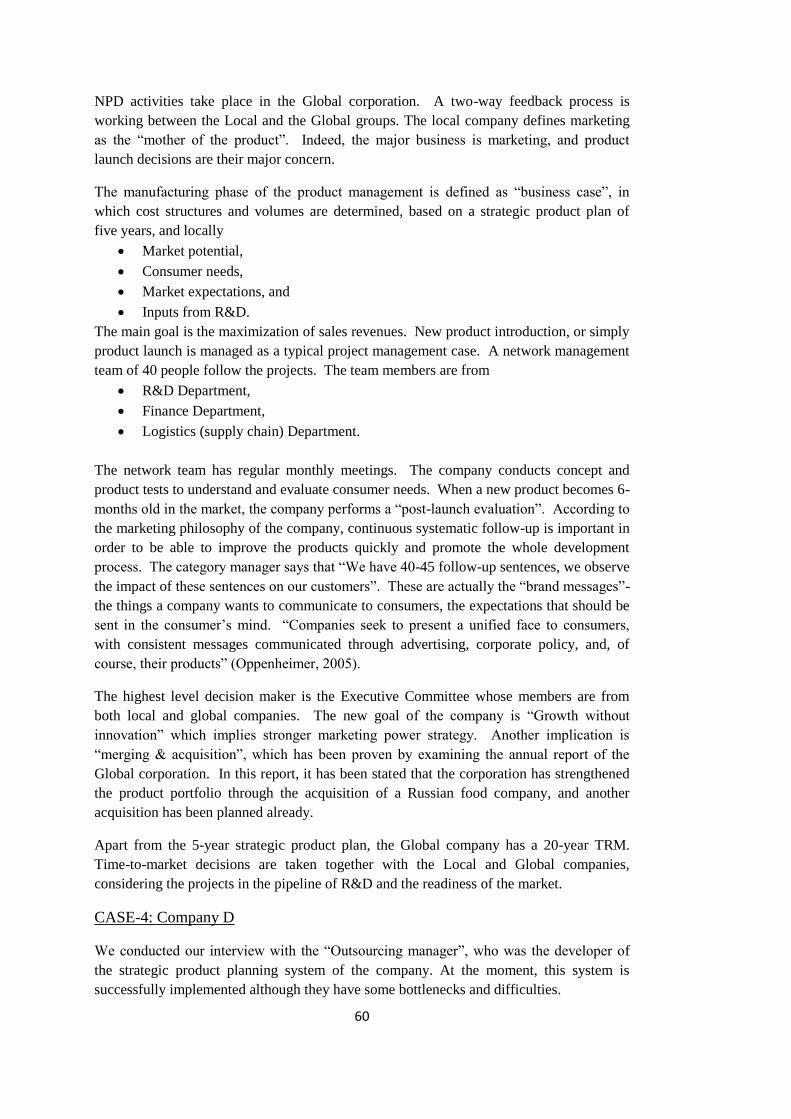
60

NPD activities take place in the Global corporation. A two-way feedback process is

working between the Local and the Global groups. The local company defines marketing

as the “mother of the product”. Indeed, the major business is marketing, and product

launch decisions are their major concern.

The manufacturing phase of the product management is defined as “business case”, in

which cost structures and volumes are determined, based on a strategic product plan of

five years, and locally

Market potential,

Consumer needs,

Market expectations, and

Inputs from R&D.

The main goal is the maximization of sales revenues. New product introduction, or simply

product launch is managed as a typical project management case. A network management

team of 40 people follow the projects. The team members are from

R&D Department,

Finance Department,

Logistics (supply chain) Department.

The network team has regular monthly meetings. The company conducts concept and

product tests to understand and evaluate consumer needs. When a new product becomes 6-

months old in the market, the company performs a “post-launch evaluation”. According to

the marketing philosophy of the company, continuous systematic follow-up is important in

order to be able to improve the products quickly and promote the whole development

process. The category manager says that “We have 40-45 follow-up sentences, we observe

the impact of these sentences on our customers”. These are actually the “brand messages”-

the things a company wants to communicate to consumers, the expectations that should be

sent in the consumer’s mind. “Companies seek to present a unified face to consumers,

with consistent messages communicated through advertising, corporate policy, and, of

course, their products” (Oppenheimer, 2005).

The highest level decision maker is the Executive Committee whose members are from

both local and global companies. The new goal of the company is “Growth without

innovation” which implies stronger marketing power strategy. Another implication is

“merging & acquisition”, which has been proven by examining the annual report of the

Global corporation. In this report, it has been stated that the corporation has strengthened

the product portfolio through the acquisition of a Russian food company, and another

acquisition has been planned already.

Apart from the 5-year strategic product plan, the Global company has a 20-year TRM.

Time-to-market decisions are taken together with the Local and Global companies,

considering the projects in the pipeline of R&D and the readiness of the market.

CASE-4: Company D

We conducted our interview with the “Outsourcing manager”, who was the developer of

the strategic product planning system of the company. At the moment, this system is

successfully implemented although they have some bottlenecks and difficulties.

61

The company represents a part of a bigger corporation in Turkey and operates in the

Consumer Durables Sector. It provides products and services to consumers in more than

100 countries with its 12 production plants in 4 different countries, 12 sales and marketing

companies and 10 brands. The CEO is from marketing branch of the company and he is

the highest level decision maker of the product management.

First of all, it should be noted that the company has very well-defined and well-established

strategic module of product management. The corporate goals, mission statements, vision,

strategic targets and value chain (shared values) are clearly stated and exist as written

documents. As an example, the vision statement is as follows:

“To possess one of the 10 most preferred global brands in our sector by the year 2010”,

and their slogan is “TARGET 2010 – TOP 10”.

Our interview was supplemented by the written documents of the company. It can be

easily stated that the product management system of Company D is parallel to what we

have described in Section 3.2 based on the literature. The descriptive model of product

management of the company is shown in Figure 3.3. This model was provided by the

company itself. It was stated that there are strong interactions between the technical and

marketing aspects of the product management. The company has some difficulty of

having an integrated working mechanism in those broad areas of PM in harmony. It was

realized that the company’s perception of PM covers all the theoretical aspects in a broad

sense, namely product planning and product marketing.

Figure 3.3: Product Management Model of Company D

In another diagram (Figure 3.4) provided by the company, the major activities of PM are

shown. It was realized that the source of the diagram presented in Figure 3.4 belongs to

the book of Steinhardt (2010) which is one of the recently published books in PM

literature. It should be noted that these diagrams do not show the strategic considerations

in PM. However, it can be stated that Company D has spent great efforts trying to get the

benefits from the PM literature in order to establish an effective PM system in their

62

organization. Another important observation is that the decision framework what we have

proposed in section 3.2.2 totally covers the decisions of Company D.

Figure 3.4: Product Management Activities of Company D (Source: Translation of the

document provided by Company D)

In their product management, “make/buy”decisions take place depending on quantity,

urgency, and

productivity

considerations. So it was seen that the “outsourcing” decision is an important dimension in

their decision space. Outsourcing decision may take place in different levels of decision

making;

Decision on product itself.

Decision on product components.

Decision on inputs of products.

In their product range, 30 % of “Heating, Ventillation and Air Conditioning” products as

quantity are provided through outsourcing, which represent a 20 % share in turnover. In

addition to outsourcing, the company has tried to enlarge its product range by taking

merging & acquisition decision. As we have learnt, the negotiated company was an Italian

company which was one of their competitors in the global market.

All these decisions represent the strategic level of decisions of the company. At this level,

a cross-functional team contributes to the decisions of CEO at the highest level. The

members of this team are from the departments of

R&D,

Marketing,

Sales, and

Production.

63

The company has a separate “Product Management Department” which is totaly

responsible for planning, coordination and execution of the activities related with PM.

The company is the business leader in the domestic market with over 50% market share.

Their products’ major competitors are imported goods. This is the reason why company’s

main objective is to increase the market share in the global market.

Technology leadership, powerful sales force with approximately 4500 dealers, a service

network with 600 after-sales service stations, and financial structure are their main major

strengths in the national market. The company gives a special emphasis to service

activities as an important factor to understand and assess the customer requirements.

Home visits and questionnaires are other sources of information in evaluating the

consumer needs. Although the company can be seen as “business-to-business”(B2B) type

of company, its considerable efforts to have connections and contacts with the end-users

show us the company’s marketing view and the importance of achievement the goal of

keeping the leading market position in theTurkish market.

Technology and innovation, as one competitive power, is the most important critical

success factor in their PM. Another success factor is undoubtedly the capability of

generating knowledge and using scientific tools. As mentioned before, the company has

developed a strategic product plan for a 5-year planning horizon. In implementation, the

regular revisions and updating is being done for the coming periods. In addition to this

planning activity, a TRM has been developed in the R&D department, and NPD projects

and processes are followed by means of these tools. The NPD process starts with the idea

generation phase. The company is organizing “creativity triggering activities” and

consumers are invited to those activities. Voice of customers (VOC) are deployed to the

product design phase by QFD. Brainstorming and benchmarking are also used in product

development. Financial restrictions are considered in project prioritization phase, and

sometimes the project priority list is changed based on the availability of financial

resources. The company uses nano technology to implement changes in micro scales.

Modifications and improvements in existing products are made under the name of

“updating”.

The company is quite sensitive to environmental sustainability and this sensitivity has been

reflected in their new innovative products.

Table 3.2 presents the summary of the interview results comparatively for all companies

Table 3.2: Summary of Interview Results

Feature Company A Company B Company C Company D

Type of Product

Consumer Durables

FMCG

FMCG

Consumer Durables

Turnover of Company

$ 100 Million

$ 100 Million

Euro 40.5 Billion – Global

Euro 14.5 Billion Local’s

group

Euro 3.7 Billion

Number of employees

700

3000

174,000 Global

3,000 Local

Over 18,000

Share of International

Sales

% 10

% 15 – 18

100 countries local-

multinational business

% 50

Strengths & Core

capabilities

Technical capabilities, large

product portfolio, human

resources

Organizational culture,

skillful R&D and PD

personnel, deep customer

knowledge

Strong portfolio of products,

global leader in R&D,

technology superiority,

patents

Market leadership, quick

response to market

requirements, technological

capabilities and innovation,

corporate culture

Success factors of PM

Market penetration,

understanding of customers’

needs

Understanding of customers’

requirements, creativity &

open minded-ness,

continuous follow-up of

market

Customer satisfaction, best

products, value based

management, continuous

follow-up of market

Formal PM system, value

based management, creativity

triggering activities,

understanding of customers’

needs, wide product range,

high quality products, after

sales services network

64

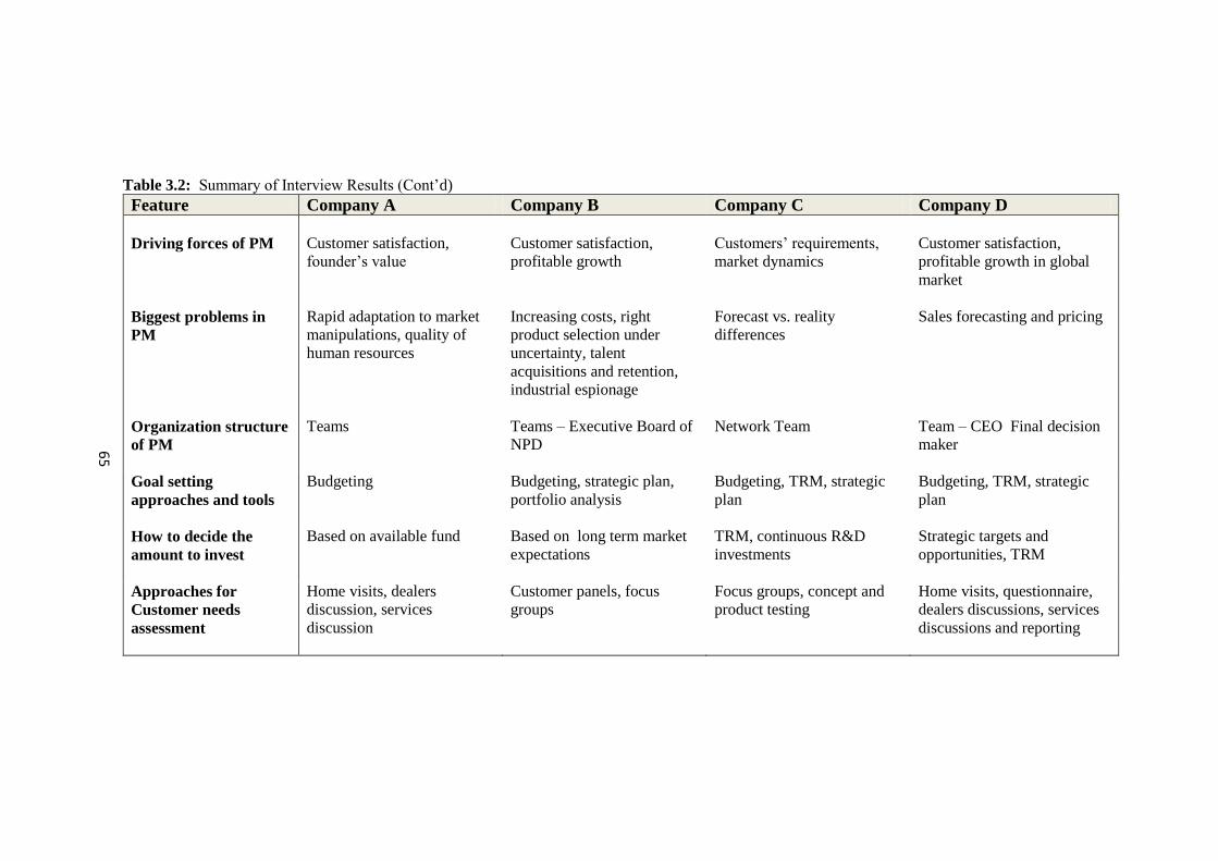
Table 3.2: Summary of Interview Results (Cont’d)


Driving forces of PM

Biggest problems in

PM

Organization structure

of PM

Customer satisfaction,

founder’s value

Rapid adaptation to market

manipulations, quality of

human resources

Teams


profitable growth

Increasing costs, right

product selection under

uncertainty, talent

acquisitions and retention,

industrial espionage

Teams – Executive Board of

NPD

Customers’ requirements,

market dynamics

Forecast vs. reality

differences

Network Team


profitable growth in global

market

Sales forecasting and pricing

Team – CEO Final decision

maker

Goal setting

approaches and tools

Budgeting

Budgeting, strategic plan,

portfolio analysis

Budgeting, TRM, strategic

plan

Budgeting, TRM, strategic

plan

How to decide the

amount to invest

Based on available fund

Based on long term market

expectations

TRM, continuous R&D

investments

Strategic targets and

opportunities, TRM

Approaches for

Customer needs

assessment

Home visits, dealers

discussion, services

discussion

Customer panels, focus

groups

Focus groups, concept and

product testing

Home visits, questionnaire,

dealers discussions, services

discussions and reporting

65

Table 3.2: Summary of Interview Results (Cont’d)


Approaches for

Competitive Analysis

NPD Approach

R&D measurement &

selection of project

Dealers and services

discussions, no systematic

tools

PLC consideration observing

sales figures, incremental

Fixed amounts based on

earlier years, predetermined

projects

Benchmarking, systematic

analysis for technology

competitiveness

Innovative products,

development projects on a

continuous base, innovation

concerning product safety

Business impact, sales

opportunities

Strong, lasting relations with

customers and suppliers,

systematic analysis for

technology competitiveness,

new products in R&D

pipeline

Incremental, mergers &

acquisitions, “green”

innovative products

On a continuous base, 3% of

net sales

Systematic analysis for

technology competitiveness

in global market, technology

leadership in domestic

market, patent analysis

Innovative products,

environmental impact

analyses for new investments,

environment-friendly

products, outsourcing,

mergers & acquisition

Resource planning and

prioritize the projects with

financial resources

management

Product proposal

system

No formal proposal system Formal proposal system, idea

bank

Formal proposal system

Formal proposal system

66

67

3.1.3 General Conclusive Remarks

The common observations on the results of the field study, together with the literature

knowledge, point out some important major findings which constitute the cornerstones of

our proposed product management system presented in section 3.2. These conclusive

findings are summarized below.

1. Product Management Approach

In the literature, there are several approaches in product management regarding the major

product strategy driving the company (Steinhardt, 2010; pp.5-6). These approaches are

stated as follows:

Technology-driven

Sales-driven

Market-driven

Technology-driven companies focus on providing better technology instead of “focusing

on closely matching customer needs and abilities with that technology” (p.5), believing

that they know what is best for the customer. A sales-driven company is focused on

maximizing short-term return on investment. This product strategy is defined as the

“conservative or lifesaver strategy and it is used as a survival mode tactic” (p.5). These

types of companies use price as the primary marketing tool to differentiate their products

from their competitors’, which may put these companies in difficulty in the long-run.

Market-driven approach requires a proactive product management, i.e., “they engage

customers before the product is planned, defined, designed and developed” (p.6). Market-

driven companies produce sustainable products which “help establish market leadership

and revenue growth potential” (Steinhardt, 2010; p.6). This approach requires a formal

work culture and an effective organizational structure.

In the field study conducted, it was observed that all companies define themselves as

market-driven companies. As it was mentioned above, all companies are in the

manufacturing industry. Two of them are operating in the “Fast Moving Consumer

Goods” (FMCG) sector; the others are in the “Consumer Durables” (CD) sector. It has

been observed that FMCG companies are more “market oriented” than CD companies,

although they show innovative efforts in their product management. These are mostly

incremental innovation in which existing technological platforms are used.

Although the companies define themselves as market-driven companies, it has been

observed that Company A is a more sales-driven company because they have no formal

product proposal system, they do not use TRM/PRM tools, their organizational structure is

looser than the other companies, the product variants are heavily modified core products

and they are a follower in the market.

It can be concluded that a successfully implemented market-driven approach with properly

structured product management team produces successful products and hence an effective

product management system. Thus, a well-defined product planning starts with listening

the voices of customers in the market through the problem tellers of the PM system. Note

68

that the market-driven approach to PM is the underlying approach of our proposed PMS

presented in section 3.2.

2. Product Management Organization

Two companies are representing parts of bigger corporations; the others are family type

organizations. So, it was worthwhile to observe the differences of organizational cultures

and management philosophy. As expected, the companies which are a part of bigger

companies have more formal and systematically described models of product management.

Surprisingly, one family company (Company B) was really institutional in their product

management.

In large enterprises, an “empowered cross-functional product team with a strong team

leader” is accepted as one of the most important success factor of the company (Haines,

2009; Steinhardt, 2010). Haines (2009) states that

“The purpose of a cross-functional product team is to manage all the elements needed to

achieve the financial, market, and strategic objectives of the product, as a business. The

cross-functional product team is made up of delegated representatives from their

respective business functions. This team is the primary mechanism through which an

organization initiates product strategies and plans,… Finally, the product team is

responsible for the profitability of the product in the marketplace” (p.62).

According to Haines (2009), maintaining the cross-functional team across the product life

cycle is the most effective approach. This approach was clearly observed in Company D

in our field study; every product manager is responsible for 1000-1200 products and those

products are followed-up through their product life cycles. A similar approach was used in

Company B and Company C. These FMCG companies use the “Category Managers” title

instead of “Product Managers” and they group certain products in their follow-up

activities. Company A follows sales figures of the products and collects the customer

complaints through the Sales department and Service department, respectively. In this

company, product managers communicate with these departments mentioned above to

monitor the products. Therefore, it can be said that product management department in

Company A has no direct involvement in follow-up and monitoring the products in the

market.

In the literature, there are three different levels of cross-functional product teams running

the product management business: strategic, tactical and operational. Management

communicates their strategic intent up and down the organization. It is stated that this

structure reduces organizational ambiguity and provides better alignment of the product

portfolio and product line investment decisions (Haines, 2009). It was observed that all

companies have such a structure in their organizations. Company C mainly performs

marketing activities in Turkey as the “Local” company and therefore their organizational

structure reflects mainly tactical and operational product teams, because it was stated that

strategic decisions such as new product selection from the pipeline of TRM are imposed by

the “Global” company. However, the Local and Global companies make the decision of

“time-to-market” together. In other words, strategic “marketing-mix” decisions are made

in the Local Company providing market feedback to the Global Company.

69

In the literature, it is stated that within the best-in-class companies, organizational

structures typically have product managers reporting to the marketing department (Haines,

2009; Steinhardt, 2010). The main reason behind this is that the customer needs of market

segments and market trends can be recognized easily which may affect the product and

market strategies. As it was mentioned above, Company C is mainly a marketing

organization. Company D has a difficulty in their organization regarding the effectiveness

of management of the teams in the technical and marketing parts of the product

management in an integrated manner. It has been learnt that this bottleneck in their

product management has been solved recently by reorganizing the product management

department under the marketing department. The CEO of the company is the product

management leader who is also the Marketing Director of the company. The product

management department is directly connected to the corporate Board of Directors in

Company A. Company B has also cross-functional teams and the leader is the CEO of the

company who is the ex-R&D Director of the company.

So in the context of product management, the leadership of this cross-functional team is

represented by the Executive Management of the company and generally called as

“Product Review Board” or “Product Portfolio Council” (Haines, 2009).

It can be concluded that the organizational structures of all companies in the field study are

quite similar to the one described in the literature. Note that this hierarchical structure of

the decision making framework is adapted in developing the proposed product

management decision framework presented in section 3.2.

3. Product Planning Tools

Typically all companies are using budgeting as short-term planning tool. Except for one

company, all companies are developing a strategic product plan for a five-year planning

horizon.

The strategy which can be defined as the “coordinated set of long-term decisions” of a

company is formulated by its executives (Steinhardt, 2010; p.50). So a strategic plan at the

product level in the product management context first creates a vision and strategy for the

products of the company consistent with the company’s strategy. The strategic product

planning is a complex, interrelated group of activities which creates strategic relationships

with technological, development, manufacturing, logistics and marketing to generate the

most advantageous strategic mix for the products of the company (Haines, 2009). More

explicitly, the generation of this strategic mix requires the decision on the paired function

of “market-product” in order to maximize the profits of the company (Ansoff, 1972). Thus,

it can be stated that strategic product planning is the main tool to select the right products

which generate the possible highest profits for the company for a pre-determined target

market.

It should be noted that information on market share and size of the market are very

important for all companies for their market related decisions and also daily business

follow-up activities. Three of them are getting consultancy services externally. A.C.

Nielsen is the common address providing market research analysis and also support to

product launch decisions.

70

The strategic product planning is the highest management level of activity in product

management. Except for Company A, this activity has been observed in all the companies

in the field study. As mentioned before, Company C is the implementer of this activity as

the marketing company of the Global Company. However, they do manufacturing in

Turkey and the volume decisions in their production activity are based on the strategic

product plan of the Global Company. Company B also prepares five year term strategic

product plan and the Executive Management’s product portfolio decisions with respect to

targeted markets are based on this plan. Similarly, Company D has a five-year term

strategic product plan in which TRM/PRM constitute the basic inputs. TRM/PRM are

prepared for the product groups showing important milestones in terms of financial and

technological data considering the time dimension with respect to the targeted markets in

which those product groups are sold. Note that a product group is composed of the

products which are using the same production technology, the same assembly line and the

same key components.

It can be concluded that the existence of strategic product planning is a proof for the

existence of a formal and proactive product management system in the companies studied

in the field work. It provides a formal goal setting mechanism in the lower levels of

product management, strategic link to corporate goals and strategies, a formal NPD

approach and a systematic product and project proposal system. Strategies developed at

the highest level of the product management are tied to more specific markets or segments

and also include financial objectives that focus on an optimal portfolio of products and

product investment options.

4. Major Difficulties in Product Management

In order to recognize the major decision making problem(s) in real life product

management, the interviewers were asked several questions (See Appendix B). It was also

asked to verbally define the biggest problem in their companies’ product management.

Company A defined the adaptation to rapid market changes as the biggest problem. This

reply is quite consistent with their other answers, since

they are in the “follower” position in the market,

their major goal in their product management is “growth with market penetration”

which implies a “maintaining” product strategy,

their innovation efforts are heavily on modifications on their existing products;

they produce “imitative” products,

since they have weak NPD efforts, product line extensions and product

diversifications are made through acquisitions and outsourcing,

they have no formal product management work organization.

Company B has designated several problem areas as “the biggest difficulty” in their

product management decision framework. One of them is the cost management area which

is consistent with the other answers of the company, because

they are also in “follower” position in the market, and

the market leader puts a high competitive pressure to introduce new products so

that Company B has to invest to in both NPD projects and in cost reduction in their

71

production technologies simultaneously which brings additional difficulty in

allocation of resources in their product investment decisions. Note that a market

leader company generally achieves cost effectiveness in their production.

Another important difficulty in their PM decision making process of Company B is stated

as follows: selection of right products under uncertainty. So Company B explicitly states

the product mix problem under uncertainty as one of the most important problems of

product management framework.

Both Company C and Company D represent the market leader positions in their markets

respectively. These companies identified inaccurate results in forecasting as the biggest

problem in their product management frameworks. Forecasting is used by these

companies to calculate the market potential, depict sales, and meet demand.

Regarding the existing products of the company data-driven forecasting approaches may

create more realistic forecasts with the support of the common sense of the managers.

Judgmental forecasting is another technique which is popular in real life in order to

formulate the complex future state models of the company (Haines, 2009). However, it is

known that most forecasts are not accurate. In the case of new products, forecasting is

more difficult due to non-availability of the past information of the new products. This is

really a big problem for the companies because product investment decisions need to

derive forecasts and deliver the expected returns on these product investments. In short,

without accurate forecasts, a product’s market potential cannot be determined in a realistic

way, because forecasting is a tool which links the market research to the strategic

possibilities for the product. So, as Haines (2009) states, there is a need to find a better

way.

It can be concluded that the difficulty of forecasting stated by the companies in the field

study implies an important decision making problem in product management framework:

Decision making under uncertainty. Several types of uncertainty are considered in product

management, such as technological uncertainty, market uncertainty, regulatory uncertainty,

social and political uncertainty, etc. which represent the environmental conditions of the

product management framework. The term “uncertainty” refers to “market uncertainty”

here. Market uncertainty reflects the unknown conditions of the market environment;

unknown behavior of the customers, unknown actions of the competitors, unknown prices

of the substitutive products can be considered as the main sources.

Forecasting the sales of the products requires

to determine total size of the targeted market,

to determine the attainable market share,

to determine the number of products that the sales team commit to sell,

to determine the number of units that can be produced,

to determine the realistic pricing for the product,

to translate the sales and demand forecasts into a realistic budget for the product

(Haines, 2009).

As it was stated by the companies that forecasting is a cross-functional exercise which

requires many interrelated activities carried through up and down the product management

72

organization. The selection of the target market, and then, the strategic selection of the

products should be made beforehand which is the major task of the “Executive Product

Team”, namely “Product Review Board” or “Product Portfolio Council” of the company.

Later, mainly the Marketing and Sales departments work on demand forecasting, the

Manufacturing department works on production to meet the demand, and the Finance

department contributes to convert all these into a realistic budget for the planning period.

These findings point out that the product mix problem under uncertainty is one of the most

important problems in the product management framework and it involves determining

which products should be selected for the coming planning period and the number of units

to be produced from those selected products. It has been observed that the main body of

the problem belongs to the strategic level of the product management framework which

requires the determination of products to be served to the customers in the targeted market.

Naturally, the product selection decision requires having a bundle of candidate products

which are composed of new products as well as the existing products of the company. To

determine the bundle of candidate products is, undoubtedly, another decision making

problem which requires the project prioritization decision among all the project proposals

and product killing decision among the existing products of the company. This important

task belongs to the Product Review Board or Product Portfolio Council as it was

mentioned before, and this is performed through the feedback mechanism from the lower

levels of the product management organization. The decision on the mix of the products

provides the input for the production planning framework of the company in which the

detailed production plans are prepared to meet the targets given by the upper levels of the

management considering the properties of the production system of the company such as

characteristics of the manufacturing environment (make-to-order and/or make-to-stock),

capacity of plants, human resources, etc. The issues concerned with how a company

integrates customers related information into the manufacturing system is called as demand

management which includes activities determining or forecasting the demand from

customers (Vollmann et al., 2005). It is also understood that demand management

activities should be in conformity to the corporate strategy, the manufacturing capabilities

of the firm and the needs of customers in the product management framework.

In sum, professional product management is essentially a matter of well-organized

processing of issues related to the products offered by the company. In other words, the

scope of product management concerns the complete set of products for a company, the so-

called the product mix. It should be noted that the terms product mix and product portfolio

are used synonymously in the literature in some cases. In this study, product portfolio

refers the set of products investments, i.e., the products under development. Thus, product

management encompasses decision-making about the set of existing products, introducing

new products by examining market trends, customer needs and product strategy, making

decisions about the product life cycle, establishing partnerships and making decisions on

the potential acquisitions and merging opportunities. So, it can be said that successful

product management is about achieving the goal of maximizing the financial value (profit)

of the mix of the products by linking to the corporate strategy.

Thus, our main conclusion is that the “Product Mix Problem under Uncertainty” should be

positioned at the strategic level in the framework of product management. It has been

realized that the formulation of the problem under consideration requires some further

73

information, such as which product level is considered for the product selection decision at

the strategic level. For this purpose, after the completion of the field study, several

discussions and meetings have been organized with the product management expert of

Company D which has the most formal organization of product management in our field

study, during the formulation phase of the problem.

In the subsequent section, considering both the findings of the field study and the literature

survey, a proposal for the product management framework is presented in detail. This

developed framework constitutes the base for the formulation of Product Mix Problem

under Uncertainty which is presented in Chapter 4.

3.2 THE PROPOSED PRODUCT MANAGEMENT FRAMEWORK

In this section, first a broad description of the proposed product management framework is

described depending on the extensive literature survey and the findings obtained from the

field study. The detailed description of the proposed product management framework is

provided in the subsequent sections.

3.2.1 Description of the Proposed Product Management System

The proposed product management framework is developed considering both holistic and

systemic views. While the holistic view requires to look at the activities in product

management by integrating the “planning” phase (investment period in Figure 2.2) and

“implementing” phase (market period in Figure 2.2), the systemic view requires the

analysis of the components of the whole product management system, and identification of

the interactions among these components. It has been also realized in conducting the field

study that there are strong interactions and complicated relations among the activities and

outcomes in product management. Hence, it is not possible to think of a linear framework

in product management, which represents a sequential and ordered process of several

stages of activities and decisions. Instead, there are many feedback loops which create

disorder in planning and implementation activities and decisions. Remembering this

reality, however, for the sake of simplicity, the activities are represented in a linear order

for descriptive purposes. When necessary, the feedback mechanism and the revisions are

shown in the detailed flowchart of the product management framework provided in

Appendix C.

The scope of the product management (PM) concerns the complete set of products which

are current and planned. In a broad sense, PM has two major aspects (activities):

(a) Product planning

(b) Product marketing

Product planning deals with mainly product strategy formation, gathering the market

requirements, building the roadmaps (PRM and TRM), product defining and development,

product differentiation and product selection. Product marketing deals with the product

positioning, implementing the market plans to bring the new products, monitoring the

competition and promoting the product externally. Note that the scope of our study

focuses mainly on the product planning aspect of PM in the sense that we are not going

74

into the details of product marketing issues. Concerning these broad activities, PM can be

described as depicted in Figure 3.5. We may call this model as the “Elemental Product

Management Model” (EPMM). Note that the product development phase in Figure 3.5 is

based on Krishnan and Ulrich’s (2001) study and the two-sided arrow represents the close

interactions between product planning and product marketing (Figure 3.5).

Figure 3.5: Major Aspects of Product Management–Elemental PM Model (EPMM)

One step further, an “activity model” in the corporate management context can be

proposed considering the major activities of PM. The activity model is illustrated in Figure

3.6.

Figure 3.6: Proposed Activity Model of Product Management

75

The activity model of PM reflects mainly the following:

The mission, strategic intent and corporate goals control the product management process.

In our approach, the first phase is called the “product strategy and planning” phase, in

which the vision, product management strategies and objectives are established. The

appropriate performance measures are also set in this phase. The output of this phase is the

product and competition strategies, mission statements and roadmaps (PRM and TRM),

hence the strategic product plan. The second phase represents the new product

development and existing products improvement processes, which starts with idea

generation, continues with the product definition and design, manufacturing, prototyping

and production planning, and ends with the product launch planning activities. Phase-3

represents the implementation of the plans developed previously and the

commercialization of the products is realized. The final phase is “day-to-day business” of

PM , in which selling activities of products, promoting, contacts with customers, follow-up

and monitoring activities take place. One should observe the cyclical nature of the PM

activities is an important characteristic of PM. The mechanism of feedback and revisions

reflect somehow the existence of a hierarchical management process of PM.

The purpose of generating the PM activity model is to describe the activities of PM

comprehensively, but in a broad sense. Although it may show some differences from one

company to another, the main stream of the activities remains the same as described in

Figure 3.6, which represents integrated knowledge extracted from the literature-based

survey and obtained from the field study.

The product management system (PMS) is developed by using the same approach which is

followed in activity model development. In the literature, the main focus is NPD or

innovation, which is accepted as the most important task in the companies for their

success, even their survival. The companies extend their product ranges by means of NPD

to satisfy the needs of their customers, to increase their market shares, to compete with the

competitors and hence to achieve their goals. The main goal of the company is “growth”.

Although NPD is an important success factor to achieve the goals of the companies, there

are other business opportunities and tools serving the same purpose. In sum, in addition to

“growth with innovation”, we consider the possibility of “growth without innovation”, in

our proposed product management system, which is described below (see Figure 3.7). It

may be worthwhile to remember that it is an option which is intensively used by the

companies studied in the field study, especially in Company C and D.

The proposed PMS is composed of three important sub-systems:

Existing Product Management System (EPMS)

New Product Management System (NPMS)

Product Innovation Management System (PIMS)

PIMS serves both EPMS and NPMS. Traditionally, R&D works in this sub-system, which

basically provides basic research (e.g., technology development) and product

development/improvement research. If the innovation proposes radical change, this effort

brings a new product to the company. This activity is shown as the intersection part of

PIMS and NPMS in Figure 3.7. On the other hand, the innovation effort may be

incremental in the sense that it proposes an improvement or modification in the existing

76

product. This activity is the intersection part of two sub-systems of PIMS and EPMS. The

activities broadly described up to now represent the main activity of “growth with

innovation” of the company in our PMS.

Figure 3.7: Proposed Product Management System (PMS)

“Growth without innovation” can be achieved in several ways:

(Strategic) outsourcing

Acquisitions and mergers, and other business relationships (joint venture,

licensing, partnership, etc.)

Market penetration (with existing products)

New market acquirement (with existing products)

A typical product can be an extension of a base (core) product or a new product requiring a

new technology. It can be developed internally or with outside sources. So, companies

may consider “outsourcing” to develop their product lines externally. Although mergers

and acquisitions are considered at the strategic level to extend the product range, they can

be also considered for a critical supplier who provides input to the system.

It should be pointed out that the “new product” definition in our proposed PMS is different

from the one in the literature. If one of the attributes of the product has been changed

incrementally or radically, it is called a “new product” and it is referred as “new-to-

market” and “new-to-world” respectively. In our PMS, we refer to “new product” as

“new-to-company”. Figure 3.7 depicts the the proposed PMS in our study.

77

The outputs of the NPMS and EPMS define the main input of the product mix decision

which can be called as the the bundle of candidate products among which the products are

selected to serve the targeted market(s). In this sense, the company may assign the

products for each targeted market, or equivalently, the company considers the same

working mechanism for each market before the product mix decision the target market

decision is made by the company management.

The context analysis of the proposed PMS requires the identification of the factors

affecting the decision making process of PMS, and specifically the product mix decision.

These factors are extracted based on the existing literature of strategic planning, market

research analysis, competitive analysis, NPD and technology management (Johnson,

Scholes and Whittington, 2005; Brace, 2004 ; Porter, 1985 ; Szakonyi, 1999 ; Chien et al.

,1999). Some TRM studies were also considered in which the context analysis was

employed to explore and articulate the nature of the planning and design issues of TRM

(Phaal, Farrukh and Probert, 2004 ; McMillan, 2003). As a result, a long list of factors was

obtained bringing out all the factors which should be taken into consideration in the

decision making process of the PMS. Considering the major players of PMS, the

following classification was made to present the factors:

1. Internal Factors

Strategic

Organizational

Information/Knowledge

Core competences

Resources

2. External Factors

Market-pull factors

Technology-push factors

Regulatory-push factors

Market-pull factors describe all the factors related to the market and the players

(customers, suppliers, distributors, and competitors) in the market, which create impulses

to the company decisions. Technology-push factors describe all the factors related to the

technology except the technological capability of the company, which have been

considered internally. Regulatory-push factors describe the macro-environmental

conditions of the company. The term “regulatory-push” has been borrowed from the study

of Brem and Voigt (2009). The detailed description of the factors is presented in section

3.2.3.

3.2.2 Decision Framework of Proposed Product Management System

In this section, our major goal is to establish a well-defined decision framework in product

management (PM) of the organization, which enables us to articulate and specify our

research problem with its all dimensions. Although the related literature on product

management is vast, it was realized that there has been no comprehensive study regarding

the subject. So we intend to fill this gap in the literature besides the constitution of the

base for the product mix problem formulation.

78

There are several excellent review articles in some areas of product management (Ramdas,

2003; Krishnan and Ulrich, 2001; Loch and Kavadias, 2008). Among them, the article by

Krishnan and Ulrich (2001) presents a comprehensive review of literature for product

development decisions. The approach used in their study has considerable similarities to

our methodology and approach, as explained in subsequent section. As it was mentioned

in previous section, new product development (NPD) represents a subset of our proposed

product management system (PMS). Therefore, these studies complement our efforts. The

subsequent section describes the general methodology and approach used in constructing

the decision framework of the PM problem.

The rest of the chapter is organized as follows: The detailed PM decision framework is

illustrated by a flowchart which we simply call the Flow Model of PM. The Flow Model

of PM is provided in Appendix C. The working mechanism in a typical organization is

illustrated by an abstract form of the Flow Model is presented in the second section of this

chapter, and it shows the basic structure of the decision framework of PM from a broad

perspective. The detailed description of the Flow Model is given in section 3.2.3. An

overview of the major problem areas and decisions and the validation of the Flow Model

are presented in the sections 3.2.4 and 3.2.5 respectively. Section 3.2.6 contains our

concluding remarks.

3.2.2.1 Methodology and Approach

We decided to use a methodology which combines both literature-based knowledge and the

PM experts’ knowledge in such a way that literature-based knowledge is supported by the

PM experts’ knowledge by a series of interviews at certain phases of the analysis. In our

approach, the validation of the proposed decision framework is provided by the PM

experts (Figure 3.8). The implementation steps of this methodology are shown in Figure

3.9.

Figure 3.8: Description of the Methodology of the Proposed Product Management

Framework

79

Figure 3.9: Methodology Used in Constructing the Framework of the Product

Management Problem

We limit our literature review in the following ways:

1) We focus on product management within a single firm. So we exclude the studies

which address at the level of an entire industry.

2) We devote our attention to physical goods. So we also exclude the studies which

address the “service” types of products.

3) Finally, we focus on decision making in product management. Therefore, we are

interested mostly in “which” and “what” types of questions.

Research Method:

As it was mentioned above, the Flow Model was developed conceptually through a review

of literature and was supported by a series of interviews with PM experts. Following this

methodology, we aim to identify the relationships of components of the problem at

different levels of the management in their decision making processes. In this sense, the

Flow Model is considered as the basis of our formulation of the problem. While following

this methodology, “top-down” (deductive reasoning) and “bottom-up” (inductive

reasoning) approaches are used simultaneously for information processing and knowledge

ordering in constructing the Flow Model.

Using the “top-down” approach, the basic components of product management are

analyzed which allow us a complete understanding of the system working in product

management. Combining the “top-down” approach with “bottom-up” approach, a

synthesis is made to extract the major problem areas and decisions in product management

decision framework. Therefore, our approach for developing the decision framework of

PM is initially deductive, and then we use inductive reasoning to make systematic

generalizations of product management practice, on both our observations and results

extracted during the field study conducted for industrial product management expertise,

and our review of the literature. Besides, we had interviews with the PM expert at certain

phases of our research study.

80

In a broad sense, a top-down approach is essentially the breaking down of a system to gain

insight into its compositional sub-systems. So, deductive reasoning works from the more

general to the more specific. On the other hand, a bottom-up approach is a type of

information processing based on incoming data (input) from the environment to form a

perception (output) so that inductive reasoning works the other way, moving from specific

observations to broader generalizations. In other words, the term “top-down” is used

generally as a synonym of analysis (or decomposition), and “bottom-up” of synthesis. In

management and organizational arenas, the terms “top-down” and “bottom-up” are used to

indicate how decisions are made. So we use an “organizational search perspective” to

interpret simultaneous top-down and bottom-up approaches which allow us to determine

the major decision areas in product management (Sting and Loch, 2009).

In the following section, the basic decision making structure in product management is

presented in view of these approaches.

3.2.2.2 Basic Structure of Product Management Decision Making

Many organizations set up a hierarchy for making and revising product management

processes. “A hierarchy refers to a system that is composed of interrelated subsystems, in

which decisions in certain subsystems are subordinated to decisions in other parts of the

system” (Joglekar et al.; appear in Loch and Kavadias, 2008; p.291). The complex and

uncertain nature of the PM problem requires decisions at different managerial activity

levels (Ansoff, 1972; Loch and Kavadias; appear in Loch and Kavadias, 2008). Figure

3.10 depicts this property of the PM problem. We will follow this hierarchical decision

making structure in analyzing the PM system. We will touch the elements of the Figure

3.10 in a broad sense in this section. The details for each level are presented in the

subsequent section.

Figure 3.10: Basic Structure of Product Management Decision Making Process (Adapted

from Joglekar et al., 2008)

Joglekar et al. (2008) use the “hierarchy” concept in constructing the product development

planning framework. It is stated that hierarchical structures reduce planning complexity

81

through a modular management of a network of NPD decisions. So we adopted this

approach to our analysis of the PM decision making processes which is also in parallel to

the top-down approach research method.

Figure 3.10 highlights PM decisions which are disaggregated into four different but linked

levels – strategic, tactical, operational, and infrastructural. The frequency of reviews,

choice of objectives, decision variables, and decision makers at each level are different.

The decisions at each level inform each other through feed-back mechanism shown by

arrows in the Figure 3.10. The abstract form of the PM decision framework illustrated by

this figure shows the identification of typical constraints, decisions, feedbacks, objectives,

and uncertainties at each level, and is briefly explained as follows:

Strategic Level: The major activity is to prepare a long term strategic product planning.

During the strategic product planning, senior (top level) managers select and shape the

product portfolio and product mix so that the profits of the company can be maximized.

Tactical Level: The major activity is NPD management which includes both new

product development and the improvement of existing products of the firm. Tactical

managers (level 2) are concerned with capacity acquisition, allocation and utilization of

resources across all the projects, under the constraints imposed by the upper level

management.

Operational Level: The operational level (level 3) managers are charged with the fastest

and high quality execution of the individual projects. Aggregate production planning

(APP) is the major activity at this level which has great importance in fulfilling the market

demand. APP traditionally implements the long term business policy of an organization

over a horizon of one year (or more) considering only the overall constraint of the business

(Das et al., 2000). In other words, APP is considered at the tactical or top level activity of

management in the framework of the production management system (Tang et al., 2010).

However, production and related issues are considered at the operational level in the

framework of the product management system. This is the reason why we considered APP

at the operational level of the hierarchical structure of the decision making process of PM.

We will go into details of APP and related issues in the appropriate place of the Flow

Model in section 3.2.3.

Operating Assumptions: Operating assumptions can be general (system wide) and

company specific (local). They represent the environmental conditions of the product

management problem of the organization. The sources and nature of uncertainty are also

quite different between the levels. Strategic product planning addresses uncertainty in the

market (price and quantity to be sold), along with suitable choices of products in aggregate

(Joglekar et al., 2008). Joglekar et al. (2008) point out that tactical PM activities are

subject to fluctuations in the demand and availability of skilled labor which bring difficulty

in their forecasting task.

Operating Results: They represent the bottom-up initiatives and execution or running the

ongoing business. They provide a necessary feed-back mechanism to the higher level

management in their decision making processes. So the decisions at any level feed into the

82

uncertainty and shape the options (or decision making alternatives) available to the next

level.

From the organizational perspective, top-down alignment and bottom-up initiatives are

important and there should be interaction and coordination among the different levels of

management of the organizations in complex and dynamic environments as in product

management. In other words, different managerial levels of the organizations have vertical

alignment by understanding and agreeing with the strategic priorities. However, vertical

alignment is insufficient due to the complexity and ambiguity of strategic problems.

Therefore problem solving is distributed across many actors which is called as

decentralized problem solving and necessitates horizontal alignment or coordination (Sting

and Loch, 2009).

In sum, the decision making process is distributed across layers and hence problem solving

expertise is also distributed accordingly. Thus vertical alignment and horizontal

coordination must co-exist and interact. As it was mentioned in the previous section, this is

achieved through cross-functional product teams in the organization.

3.2.3 Detailed Description of the Flow Model

The illustration of the PM decision making framework is done by a flowchart which we

call as the Flow Model. While developing the Flow Model, we aim to identify the

relationships of the components of the problem under consideration at different levels of

the management in their decision making processes. Therefore, the Flow Model can be

seen as the basis of our formulation of the problem. In developing the Flow Model, we

tackle the main question of which problem and decision areas exist in the product

management of a typical manufacturing organization. Therefore we examine in detail

which activities and decisions of product management are distributed and orchestrated.

The Flow Model consists of two main stages:

1. Strategic Product Planning and Management

Strategic Product Planning (SPP)

Strategic Level Review

2. Tactical and Operational Product Planning and Management

New Product Development Management

Post-Launch Product Management: Running the Business/Existing

Product Management

Those two stages describe the main frame of PM at the corporate level which is located as

the first page of Flow Model. Each page after the first page shows more detailed activity

and decision levels than the activities of the levels seen in the preceding pages. Thus,

Strategic Product Planning and Strategic Level Review, and New Product Development

and Post-Launch Product Management are simply the sub-levels of Strategic Product

Planning and Management and Tactical and Operational Product Management levels

83

respectively. Figure 3.11 simply describes the structure of the Flow Model which is

composed of seven pages in total, and it is presented in Appendix C.

Figure 3.11: Description of the Flow Model Structure

In parallel to the structure of the Flow Model, the plan of its detailed description is as

follows:

Main Frame of PM

Major Activity Levels in PM

Strategic Sub-Levels

Tactical and Operational Sub-Levels

Below, Figure 3.12 illustrates the main frame of PM at the corporate level and represents

the most general layer (first page) of our Flow Model. Next, Figure 3.13 shows the levels

of major activities and decisions included in the main frame. The cyclical nature of the PM

function of the organization can be observed from these figures.

Main Frame of Product Management at the Corporate Level:

The first page of the Flow Model shows the main frame of PM at Corporate level (Figure

3.12). In the literature it is stated that complex and uncertain product development, and

more generally product management processes are often modularized into multiple levels

of decision making (Loch and Kavadias, 2008; Bean and Radford, 2000; Ansoff, 1972;

Haines, 2009). Many organizations set up a hierarchy of planning levels for making and

revising complex product management decisions: strategic, tactical and operational.

Based on the discussions of our Flow Model with the PM experts, we can say that this

hierarchical planning and management process reflects organizational realities.

84

Figure 3.12: Main Frame of Product Management at the Corporate Level

Ansoff (1972) defines the strategic decision area as follows: “The strategic decision area is

concerned with establishing the relationship between the firm and its environment”

(Ansoff, 1972; p.14). In other words, the sources of uncertainty and also the degree of

uncertainty are different at each level of management. Kavadias and Chao (appear in Loch

and Kavadias, 2008) define a hierarchical perspective to the NPD decision framework

which can be valid in our holistic view of PMS as well. They define the NPD problem in

different ways at different management levels, stating that “across different organizational

levels the decisions relate to

the degree of knowledge regarding the solution space,

the degree of knowledge regarding the underlying performance structure, and

resource availability and flexibility” (Loch and Kavadias, 2008; p.142).

The key word above is “the degree of knowledge” and simply defines the degree of

uncertainty. Considering Ansoff’s definition of the strategic decision area (Ansoff, 1972)

given above, we may conclude that at the strategic level, the degree of uncertainty is high

and the decisions at this level involve several dimensions of complexity. These decisions at

the strategic level include target market decisions, selection of products to be offered to

those markets, selection of basic technologies and/or revolutionary technologies, strategic

considerations of the organization, and external influences, like governmental law and

regulations (Kavadias and Chao; Loch and Kavadias, 2008). In spite of the complexity of

the decisions, the resources are regarded as flexible at the strategic level (Kavadias and

Chao; Loch and Kavadias, 2008). The availability of the resources for the other levels are

determined in the strategic level decision making process.

85

The decision making process differs across levels not only in its sources of uncertainty but

also in its frequency of decisions, objectives and information available. Therefore the

nature of the PM problem has different characteristics at each level. Ansoff (1972) points

out the following generic properties of the decisions at each level:

At the strategic level, decisions are centralized and usually non-repetitive.

Tactical level decisions are usually triggered by strategic and operating problems.

Operational level decisions can be a large volume of decisions and these decisions

are repetitive decisions.

More explicitly, during strategic product planning and management, top managers select

and shape the product combinations so that the revenues and profits can be maximized.

Tactical managers are concerned with capacity acquisition and allocation and utilization of

resources across all the projects. The operational managers are charged with the fastest

and highest quality execution of individual projects (Ansoff, 1972). Consequently, the

nature of uncertainty, the decisions and the frequency of planning are quite different

between levels. Although the management and planning activities are disaggregated into

three different levels, they are linked to each other and they are not separable (Bean and

Radford, 2000), since the decisions at any one level of planning feed into the uncertainty

and shapes the decision options available to next level. In short, the decisions at each level

inform each other through feedback mechanism. Haines (2009) calls this mechanism as

the “waterfall effect” of decisions existing among these levels. The starting point is

“Strategic Product Planning and Management” which is the first stage in our Flow Model.

Hence, we show the Strategic Product Planning and Management as the higher level box,

and other levels of the PM as the second box in the diagram.

We assume that there exists a well-developed Strategic Plan at the corporate level which is

the key input to the Strategic Product Planning and Management level of PM, in the sense

that all the activities and decisions in this level should be in line with the corporate

background, mission, corporate goals and objectives, culture and strategies. Gorchels

(2006) states that “determining the vision and strategy of the overall company is a basic

part of this analysis” (p.9). Therefore, the assessment of corporate goals, vision,

organizational culture and strategies is an important input for strategic product

management, because it identifies how the firm operates by showing the general operating

philosophy, management style, etc. (Gorchels, 2006). Besides, the existence of a corporate

SWOT analysis provides additional inputs for strategic level operations. A corporate

SWOT analysis is helpful to understand the corporate strengths and weaknesses which are

considered in strategy formulation processes. Strategies are the key decisions at the

strategic level of PM and they should be consistent with the vision and strategies of the

company. Corporate strengths which provide core competences and weaknesses that

should be minimized are considered in the internal inputs category in our PM Flow Model.

Similarly, the SWOT analysis also provides an understanding about the threats and

opportunities outside the firm, which are also considered as the inputs in strategy

formulation. Since the sources of these inputs are beyond the boundaries of the firm, we

consider them as external inputs. Customers, competitors, industry, suppliers,

technological factors and regulatory-push factors are all the external inputs which will be

explained later.

86

The outcomes of strategic level activities provide inputs for the decisions made in the

tactical and operational levels of PM. The operating results of these levels usually create

revision needs and provide the inputs for updating the higher level decisions. Hence, a

cyclical feedback mechanism reflects the linkages between the levels in a business

environment.

Levels of Major Activities and Decisions in PM:

The levels of major activities and decisions in the main frame of PM are shown in the

second page of the Flow Model (Figure 3.13). In this page, Strategic Product Planning and

Management is disaggregated into:

1. Strategic Product Planning (SPP), and

2. Strategic Level Review.

Strategic PM decisions are taken during the Strategic Level Review executed by the

Product Review Board (PRB), using the required information provided through the SPP

process.

Strategic PM decision is defined broadly as follows:

Strategic Decision = f (Market, Product)

In other words, the PM problem at this level is “to select market-product mix which

optimizes firm’s profits” (Ansoff, 1972; p.16). So, the PRB’s major decisions are the

selection of target market(s) and the selection of the products to be served in this

market(s).

Figure 3.13: Levels of Major Activities and Decisions in Product Management

87

The “Tactical and Operational Product Planning and Management” levels of PM are

shown by the numbers (3) and (4) together in Figure 3.13. In other words, Tactical and

Operational Product Planning and Management are represented by two sub-levels:

New Product Development Management, and

Post-Launch Product Management.

New Product Development (NPD) Management (3) is an important area of PM. Krishnan

and Ulrich (2001) define product development as “the transformation of a market

opportunity into a product available for sale” (p.1). They also state that the product

development process (i.e., how products are developed) may differ not only across firms

but also within the same firm over time. However, they point out that what is being

decided remains fairly consistent. Therefore, without being concerned about how these

decisions are made, they identify several generic decisions in their study (Krishnan and

Ulrich, 2001). Later we will briefly outline these decisions. In this activity level, tactical

and operational decisions take place considering the “Growth” objective of the company

which refers to the strategic alignment with the higher level of management, and requires

the strategic considerations in the decision making process of this level. Project proposals

regarding the development of new products and/or improvements to existing products are

determined and presented to the PRB for strategic level review. These projects refer to

investment proposals where the budgets for those investments are determined by the PRB.

Finally, we see the “Post-Launch Product Management” or “Existing Products

Management” level of PM (4), which actually represents running the day-to-day business.

In addition to the tactical and operational management of existing products, due to the

cyclical nature of PM, the strategic management of existing products is handled. This part

reflects the situation where all the products are in the market, they are followed up with

continuous monitoring, and proposals are developed for the ones to be deleted from the

market place.

All these activities shown in this page of the Flow Model are performed by the following

major functional departments depicted in Figure 3.14.

Figure 3.14: Major Functional Departments in the Product Management Organization

88

The product management is cross functional in nature and bridges many departments. A

team structure allows both vertical and horizontal process flows. These cross-functional

teams may be in a network team structure (e.g. Company C), or in a matrix structure (e.g.

Company D) which is the most complex organizational structure in which dual reporting

system takes place. This is a structure which is a combination of function and product

structure and the product manager has no direct authority over the products being produced

and sold. The overall responsibility of a product manager in this organization is “to

integrate the various segments of a business into a strategically focused whole, maximizing

the value of a product by coordinating the “production” of an offering with an

understanding of market needs” (Gorchels, 2006; p.305).

The Product Review Board (PRB) members are the heads of the functional departments

shown in Figure 3.14, and there may be also advisory members like legal, regulatory, or

public relations. The Chairman of PRB is usually the CEO of the company as in the cases

of our field study and stated in the literature (Haines, 2009; Steinhardt, 2010; Gorchels,

2006).

Strategic Sub-Levels:

The subsequent two pages of the Flow Model explain the two sub-levels of the Strategic

Product Planning and Management activity level respectively as presented below:

(1) Strategic Product Planning

The third page of the PM Flow Model presents the basic elements of the strategic planning

process for the products.

Ideally, corporate strategy sets the position in terms of market dominance (industry,

technology, or demographics); financial objectives; and corporate “identity” positions such

as culture, values, mission, and overarching goals (Haines, 2009).

The initial step of strategic product planning (SPP) is the creation of the vision for the

product in the future. The company must be sure where it intends to focus its efforts to

accomplish this. In sum, the strategic product plan development process begins with the

creation or refinement of the long-term PM vision. Long-term planning requires usually

considering more than three years into the future. The PM expert of Company D which

supported our PM Flow Model construction denoted that they developed a five-year

Strategic Product Plan, where the final 3 years of the planning horizon is subject to a

continuous updating process.

The second step in the SPP development process is setting the PM goals and objectives.

With the condition of being in line with the corporate goals and objectives, at the highest

level, the usual PM objectives can be stated as follows:

(1) Growth

(2) Revenue and/or profit maximization

(3) Market share increase

These objectives represent the major generic objectives of a typical firm (Crawford and Di

Benedetto, 2008). Besides, customer satisfaction, market leadership, minimizing product

launch time, etc. can be considered and may have special importance in some companies.

89

In our case, we will consider the generic objective statement “to maximize the profit of the

firm”.

The final step in the SPP development process is to establish PM strategies. A strategy

defines what is going to be done and how it is going to be done, so it requires a plan of

action that encompasses a future time frame (Haines, 2009). Haines (2009) states that

strategies formulated by the PRB propose the execution parameters for a product or for the

portfolio of products to achieve the objectives. Well-formulated strategies set the stage for

robust, ongoing planning and decision making throughout the PLC. SPP should take both

current product mix and the future strategic direction into account in order to achieve the

long-term goals of the company (Bean and Radford, 2000).

SPP is based on several inputs of which some provided internally, and some others are

collected through the analysis of the environment of the company (the contextual analysis

of the company). The factors affecting PM decisions have been determined in this study

through a combined study of a literature survey and a field study conducted earlier. These

inputs are broadly classified as internal and external inputs and the description of those

inputs are provided briefly in Table 3.3 and Table 3.4 respectively.

Internal inputs are grouped mainly as follows:

Strategic inputs

Organizational inputs

Information/Knowledge

Core competences owned by the company

Resources of the company

Product performance data

The role of strategic inputs has been discussed briefly before; therefore we have just

mentioned the items here.

Considering the cases of the field study and in the previous page of the Flow Model, major

organizational characteristics of PM were discussed. Regarding our research problem, we

assume simply the company has adequate organizational capabilities to perform PM

effectively and the product mix decision is made in such an effective PM environment.

Therefore, further aspects of PM organization and related issues are considered as beyond

the scope of our work. Similarly, we assume the company is capable of managing the

information/knowledge well. In sum, the most relevant inputs for our problem case have

been shown in our PM Flow Model presented in Appendix C.

It should be pointed out that the company should also have adequate financial resources to

support future investments in products. Therefore, the availability of resources is

important in general so that activities of investment, manufacturing, marketing, etc. should

be planned considering the availability of the resources of the company.

Capturing the product performance data is an important task for evaluating the existing

products of the company. This information is the key input in generating the product

strategy, and also provides the base information for future product investments.

90

Table 3.3: Internal Inputs

Strategic Organizational Information/Knowledge Core Competences Resources Product Performance

Data (Haines,2009)

Long-term view

(3years

or more),

Goals and objectives,

corporate strategy,

Mission, corporate

culture, corporate

background,

Corporate strengths

and weaknesses,

Existing procedures

and processes

(corporate charter).

Top management

involvement,

Role of the PM

department,

Teamwork,

Integral involvement,

Good communication,

Close cooperation among

different departments,

A degree of trust,

Customer-focused culture,

Organizational strengths,

such as marketing,

manufacturing,

technology, etc.,

Creative, adaptive,

interactive and responsive

organizational structure.

Quality of data collection

and reporting,

Usage of supporting tools

(e.g. SWOT, QFD)

Information management.

Management competence,

Quality of corporate staff,

Planning and control

systems,

Business image,

reputation, brands,

R&D facilities,

Patents, skills, infra-

structure, standards,

Scientific knowledge,

Relationships, contracts,

Cost leadership,

Ecosystems.

Financial resources,

financial status,

Capabilities, such as

technological capabilities,

innovation, commercial,

analyzing capabilities.

Product life cycle

performance:

Revenue

Profit

Market share

Pricing programs

Promotional activity

Distribution channel

activity

Product operational

performance

Product quality

Customer satisfaction

Repair and return data

Inventory turns

91

Table 3.4: External Inputs

Industry/Market Customers Competitors Suppliers Distributors

Market-Pull

Factors

Structure of the

market.

Market potential.

Market demand.

Market attractiveness

in terms of market

share.

Market growth rate.

Industry profitability.

Customer needs and

preferences.

Customer satisfaction

level in terms of

brand loyalty,

quality, price, service

ability.

Competitive factors

in terms of

competitive

intensity, barriers to

entry, barriers to exit,

share volatility,

availability of

substitutes.

New products and/or

processes developed

by competitors.

Suppliers’ relationship.

Supplier power.

Supplier loyalty.

Bargaining power.

Distribution channels.

Sales force.

Bargaining power.

Technology-Push

Factors

Nature of change in

Technology. Competitors’

activity.

Rate of technological

change.

Technological

opportunities.

Political Economic Legal Sociocultural Macro-technological Environmental

Regulatory-Push

Factors

Government stability.

Taxation policy.

Regulations.

Social welfare

projects.

Business cycles.

GNP trends.

Interest rates.

Money supply.

Inflation.

Unemployment.

Disposable income.

Competition law.

Employment law.

Health and safety.

Product safety.

Population.

Income distribution.

Social mobility.

Lifestyle changes.

Attitudes to work and

leisure.

Consumerism.

Levels of education.

Government spending

on research.

Government and

industry focus on

technological effort.

New discoveries.

Speed of technology

transfer.

Rates of obsolescence.

Environmental

protection laws.

Waste disposal.

Energy

consumption.

92

External inputs are presented in three groups as follows:

1) Market-pull factors

2) Technology–push factors

3) Regulatory-push factors

All these external inputs represent the sources of uncertainty for the PM problem, and they

are uncontrollable variables for the decision maker(s). Proactive management needs to

consider them in the strategic product planning activities and decision making processes.

More specifically, SPP is developed considering both internal and external inputs, and it

has three basic components:

1. Product Roadmap (PRM) for each product group/product,

2. Product technologies / Technology Roadmap (TRM),

3. Marketing and sales plans.

PRM is a framework for developing a product plan which is aligned with the firm’s

aggregate product strategy (Rafinejad, 2007). The PRM is developed under the full

responsibility of the PM group of the company, and contains the following product

information over the years (Haines, 2009):

Product attributes/features

Models/versions

Design/styles

Colors/sizes

Technology used

Market segment

Performance levels/targets

Safety elements

Market/competitive positioning

Outsourcing options

Product budget progresses/targeted level

On the other hand, the TRM specifies the technological requirements for the products that

a firm needs to enable its aggregate strategy (Rafinejad, 2007). McNally et al. (2009)

examine the impact of managers’ dispositional factors in product strategy implementation

in the context of new product portfolio management context. They select three different

strategic business units (SBU) to analyze the impact of managers’ dispositional factors.

One of them which is successfully positioned in its industry develops PRMs. The PRM

identifies what products will be released, when they will be released, and who will be

working on the projects. It is stated that the other firms which do not develop PRMs in

their decision making processes show poorer performances in general. The authors

conclude that developing product roadmaps helps to achieve “balancing product

innovativeness, release dates and resource allocations for products differentiated through

meeting latent customer need (strategic fitness in their case) and that target much higher

price points than existing products (financial returns)” (McNally et al., 2009).

In our case, the PM expert indicated that a PRM is developed for each product group and is

presented to the PRB in their organization. Additionally, the product R&D group builds a

TRM for each product where four or five technologies are used/adapted in order to make

93

the finished product item. The cooperation of the manufacturing group can be solicited

when needed.

Marketing and sales plans are prepared together with the marketing and sales departments

and contributed to by the PM group, manufacturing, customer service and finance

departments. Product teams use the marketing plan to map the product’s pathway into the

market. It describes a variety of investments that need to be made and sets up a marketing

budget for the products. “In many companies product managers and marketing managers

report to the same person” (Haines, 2009; p.386). We see a similar organizational

structure in the PM expert’s company.

In general, the marketing function can be divided into two major activities:

Inbound marketing

Outbound marketing

Inbound marketing functions as the radar of the organization. The marketing people who

are responsible of these activities constantly monitor and record the market place, identify

market-based issues such as general industry trends, macro-economic signals and activities

of competitors, and they conduct field research studies to collect the voice of the customers

(VOC).

Outbound marketing deals with activities carried out to create programs that communicate

the company’s and product’s messages to customers using advertising and public relations

activities.

In short, the marketing plan is a contribution toward the future business of the product

because it focuses on marketing mix elements (Product, Price, Promotion and

Place/Distribution channel, i.e., 4 P’s) (Haines, 2009).

In fact, market research and market segmentation are joint efforts, involving not only the

cross functional team of the organization but also outside research firms (e.g. A.C.

Nielsen). It is understood from both the literature and the PM expert that market research

companies are much like consumer products rating organizations, they often provide

relevant, useful data on market size and growth rates. Especially, prior to a new product

launch period, an outside research firm is hired. In those cases, the organization has an

explicit goal for its particular project. In such a case, it is expected that the research

company should provide the organization with a detailed statement of work, a project plan,

and a project estimate. The outcomes of such a study may require a revision in the

marketing plan, and hence in the SPP. Other sources of revision in the SPP may be the

requirements/warnings which are pointed out by product R&D, Marketing, Sales and

Customer Service departments, as indicated by our PM expert.

(2) Strategic Level Review

The fourth page of the PM Flow Model describes the strategic level decisions. As it has

been mentioned before, strategic decision requires the determination of the “Market-

Product Mix” of the company. The Product Review Board (PRB) is the decision maker of

this problem. The PRB actually represents a cross-functional team of the organization and

the members are shown at the bottom of this page of the Flow Model (see also Figure

3.14). This board is an executive level team established for ongoing, periodic reviews of

94

product portfolios or product line portfolios within the company. The PRB is the decision

making body, guiding, prioritizing product investments for existing products, products in

development, and product projects in various planning phases. The Chairman of the PRB is

usually the CEO of the company (Haines, 2009). In the PM expert’s company, the

Director of Marketing group is the Chairman of the PRB, who is the CEO of the company

as well. The PRB’s meeting period is usually twice a year; every six-month or they have

annual meeting.

Krishnan and Ulrich (2001) define the following categories of decisions in the context of

product development:

1. Single project development decisions.

2. Decisions in an organizational context and in planning development projects.

Although product development decisions take place as NPD Management in the tactical

level of our Flow Model, they have strategic components that we will briefly explain here.

At this moment, we consider the second category of decisions in the Krishnan and Ulrich

(2001) study mentioned above, which is further divided as follows:

a) Product strategy and planning,

b) Product development organization, and

c) Project management.

We focus on the decisions related to “product strategy and planning” that include strategic

decisions in setting up a new product development project. In a structured or formal

product management environment, product planning results in “mission statements for

projects and a product plan, namely product roadmap – a diagram illustrating the timing of

planned projects” (Krishnan and Ulrich, 2001). They define five major generic decisions

in the “Product Strategy and Planning” decision making process. This phase of the

decision making process involves decisions about the firm’s

target market (“What is the firm’s target market?”)

product/project portfolio (“What portfolio of product opportunities will be

pursued?”)

project prioritization (“What is the timing of product development projects?”)

resource allocation, (“What assets will be shared across products?”), and

technology selection (“Which technologies will be employed in the planned

products?”).

Cooper and Edgett (2010) propose a conceptual methodology for product innovation

practices for the firms. It is understood that the firms which face this issue in real life

prefer soft methods that are easily implementable in their decision making processes

(Cooper et al., 2001). Cooper and Edgett (2010) develop such a framework which

supports the decision makers by providing fast and practical solutions for the NPD

portfolio management problem. The framework begins with the product innovation goals

at the top and moves down to the tactical project selection decisions. Through the industry

analysis and company analysis, first, they define “arenas of strategic focus”. Then

competitive strategies are defined (Attack/Entry strategy). Resource allocation and

Strategic Portfolio decisions take place. The tool “Strategic Buckets” is used in

earmarking the available funds for major development/R&D projects (NPD programs).

The results are shown in a strategic product roadmap, which only shows the major

95

initiatives of the company. In other words, the strategic product roadmap uses the tactical

level PRM as an input, and does not show all details for the products. Chao and Kavadias

(2008) criticize both mixed integer programming techniques at the operational level due to

the “in” or “out” nature of the projects, and the strategic bucket tool due to the

nonexistence of any theoretical background. However, they emphasize the results of a

survey which specifically addresses the practice of strategic buckets as an NPD portfolio

management tool, stating that “this research provides descriptive evidence of the use,

benefits, and popularity of strategic buckets” (Chao and Kavadias, 2008; p. 909). Hence,

Chao and Kavadias (2008) propose a theoretical framework for using strategic buckets,

considering environmental complexity and environmental instability which are the

important factors in balancing the radical and incremental innovation efforts. According to

their proposal, if environmental complexity is high, the company should use radical

product development strategy, and if environmental instability is high then the company

should consider incremental product development strategy, in order to reduce risk (Chao

and Kavadias, 2008).

In our Flow Model, the SPP is the key input for the strategic decision of “Market-Product

Mix” of the company. Moreover, NPD projects prepared by the PM group and proposals

for the “Problem Children”, i.e., the candidate products to be considered for deletion from

the current Product-Mix of the company, which are prepared by each member of PRB, are

the other inputs for this strategic decision.

The PRB first determines the target market (Bean and Radford, 2000). Then the products

are selected for the targeted market, because these products are served to the customers in

this targeted market. This is the usual way of taking this strategic decision especially in

market-driven or customer-driven companies, which also reflects the situation in our case

as indicated by the PM expert.

Markets can be segmented based on a variety of characteristics, such as demographics

indicators, values and beliefs of people, and loyalty indicators. In short, the common

factor in segmentation is customer needs. Each customer segments is dominated by its

own distinctive set of needs. Actually, any specific customer segment represents the target

market for the company. So, the PRB needs to know about each of the market segments so

that they can define which customers they should focus on to satisfy the needs of that

specific group.

The target market selection decision is closely related to the market attractiveness which is

based on the following major factors (Haines, 2009):

(1) The degree to which the segment is growing,

Higher growth rates offer sizeable opportunities for companies.

(2) The number of competitors,

If there are too many competitors in a given market area, customers may

have too much choice and it may be more difficult to establish a

differential advantage with the company products.

(3) The manner in which a segment is accessible by known distribution channels,

(4) The profit to be gained by bringing products to those segments.

We assume that the PRB selects the target market by evaluating all these factors properly.

96

Secondly, the PRB selects the combination of products to be served in the targeted market,

which is the main focus in our problem case. The PM group is responsible for proposing a

reasonable number of candidate new products or improvement projects for the existing

products to the PRB. These projects can be considered as feasible product projects because

all of them are filtered by the PM group before the evaluation of the PRB. Therefore, the

PRB evaluates technological and financial resources in order to prioritize the product

projects. Before the prioritization decision, the outsourcing decision may come into the

picture as an option. The outsourcing decision is usually considered as tactical level issue

in the literature (Krishnan and Ulrich, 2001; Haines 2009). Only a few studies in the

literature consider this decision making area as a strategic issue (Arya et al., 2008;

Humpreys et al., 2002). Regarding such a decision making situation, the PM expert of

Company D told us the following outsourcing decision option: the company determines a

specific customer need in the target market. They realize that to develop the product in-

house requires a strategic long term capacity expansion decision which means that the

competitor may introduce the product before the focal company during this period. So the

company takes the outsourcing option to satisfy the perceived customer need. This

decision making situation reflects the strategic “bottleneck” problem in the company.

Product projects in the bucket should be evaluated simultaneously with the products to be

deleted from the bundle of existing products. The PRB makes decisions by evaluating

existing products, product projects proposals from three broad perspectives (Haines, 2009):

1. Economic value,

2. Strategic impact,

3. Available resources (both financial and technological)

In the study by Banville and Pletcher (1986), it is stated that “the optimal product mix has

been achieved when any change due to addition, modification, or elimination of a product,

would detract from the attainment of the firm’s goals. It follows then, that product

management involves the manipulation of the product mix through the addition of new

products, the modification of existing product lines, and the elimination of products no

longer contributing toward the goals” (Banville and Pletcher, 1986; p.432).

Bean and Radford (2000) ask the following three questions in analyzing the existing

products:

1. Which products can be kept without any alteration?

2. Which products should be improved to fit the target market?

3. Which products should be deleted?

Banville and Pletcher (1986) analyze the factors that affect product deletion decisions

stating that the product management area neglects the elimination phase of the product life

cycle. They outline four basic situations under which a product may be evaluated for

possible elimination, which are given below:

1. Declining demand on an industry,

2. Coercion by external forces,

3. Incompatibility of distribution,

4. Poor product performance despite a generally viable market.

The results of their analysis indicate that: “following the primary consideration of financial

data and overall profitability to the firm and secondary consideration of the market

97

including growth potential and stability, the decision maker turns again to internal

considerations based essentially on the product mix” (Banville and Pletcher, 1986; p. 438).

In our case, the PM expert of Company D indicated that the PLC performance of the

existing products was evaluated to take the decision of withdrawing the product from the

market. He stated that the candidate products to be deleted are called as “Problem

Children” in the company. All members of the cross-sectional team of the PRB evaluate

the existing products from their functional points of view, identify the problems regarding

the existing products in the market, and prepare proposals for these products. “Problem

Children” are usually two types of products:

(a) Passive products: They are not manufactured anymore, but they exist in inventory

as finished items.

(b) Out dated products: They are not manufactured anymore, but their components

exist in inventory.

Based on the number of deleted products and resource availability of the company, a

number of new products/improvements are introduced as candidate products to be

considered to determine the new product mix of the company. This decision constitutes

the basis for forecasting and demand planning in order to determine the required quantities

in the market which is in turn the necessary input for production planning of the selected

products.

Tactical and Operational Sub-Levels:

In the fifth page of our PM Flow Model, two major management areas or the sub-levels of

Tactical and Operational Product Management are presented denoting the major activities

performed in each. These are namely,

(3) New Product Development Management (NPD)

(4) Existing Products Management (Post-Launch Product Management)

Actually this page of the Flow Model finalizes the description of PM, but NPD, as one of

the most important management activity of PM, requires describing some further details

which are shown in page 6 and page 7 of the Flow Model.

In general, strategic decisions taken by the PRB provide inputs for the activities of those

management areas. Columns show the cross-sectional team members/departments/groups

of the company. The major activities performed in those departments are shown for each

department respectively. The outcomes of these activities, such as new product project

proposals, “Problem Children” proposals, inbound market research results, marketing plan,

VOC reports, repair and return reports, provide inputs for the SPP and hence decision

factors for the PRB. A feedback mechanism is seen as it was mentioned before. So,

through such a feedback mechanism the PRB receives the necessary supportive knowledge

and required inputs for the decision making process. One of the major decisions is the

product portfolio plan which specifies the mix of the products of the company and it

includes both new and existing products. A product portfolio is a group of product

investments which consists the investments of improvements on existing products and/or

98

investments of the new ones. The NPD management area of PM mainly deals with

management of those investment projects considering the strategic link to the upper level

of PM and the constraints imposed by the executive management.

The PM group has the major responsibility in NPD management area. For any company

having “Growth” objective, NPD has a vital importance. In the subsequent two pages of

the PM Flow Model, PM group activities and interrelationships with other functional

groups will be presented in more detail.

(3) New Product Development (NPD) Management

In order to gain a comprehensive understanding of PM, it is necessary to illustrate the way

that PM transforms “good ideas” into successful products (Haines, 2009). This simply

expresses the main function of NPD. NPD depends on both existing products and projects

under development. The major functions of NPD management are shown in page 5 of the

Flow Model. The subsequent pages 6 and 7 present the details of the NPD management

area of PM.

For a given level of financial resources, managing the new product portfolio is a dynamic

decision process which includes evaluating, selecting, and allocating resources to product

development and improvement projects. These decisions are also called as

“predevelopment pipeline decisions” (McNally et al., 2012). McNally et al. (2012) state

that these decisions requires trade-offs across maximizing expected economic returns,

minimizing risk, and maintaining product mix diversity. During this dynamic decision

making process, the use of personal judgments of individual managers and their previous

experience are still used as the dominant criteria on which potential projects are judged.

Thus, McNally et al. (2012) emphasizing these factors, “focuses on the psychological and

social-psychological characteristics of organizational members as the contextual factor

affecting information processing” (p.246).

Crawford and Di Benedetto (2008) divide the NPD management into the following parts:

1. Opportunity identification/selection,

2. Concept generation

3. Concept/Project evaluation,

4. Development, and

5. Launch.

Haines (2009) defines NPD management through the following stages:

1. New Product Planning

Concept

Feasibility

Definition

2. New Product Introduction

Development

Launch

Although there are a few terminological differences in these descriptions of NPD, the basic

stages are the same. In our Flow Model, the elemental PM model (Figure 3.5) presented in

section 3.2.1 is considered to describe NPD management. Remember that “Product

Development and Improvement” is based on the definition provided by Krishnan and

Ulrich (2001) and it covers the main stages above given by Crawford and Di Benedetto

99

(2008) and Haines (2009). Below the details of NPD management is described placed on

the sixth and seventh pages of Flow Model presented in Appendix C.

The PM group plays the key role in this management area together with the other

functional groups. The major work area of PM group is New Product Planning which

covers the “Front-End Activities of NPD”. However, it should be pointed out that the

phases in the NPD process do not have clear end lines, or do not follow a linear sequential

process, in the sense that early phases may require movement with the later ones, while

later phases may require re-evaluation of the earlier phases of the process. Therefore, there

may be several loops in the product development process. The initial step in the process is

the hard work of discovering customer needs. The key input for this work is “Voice of

Customers” (VOC) which is collected by the marketing department through field research,

opinions of the sales force in the market and also complaints/desires of customers obtained

by the customer service department. There are three phases and three gates within this

area:

1) Concept phase

2) Feasibility phase

3) Definition phase

The concept phase includes the assessment of ideas for new products as well as for line

extensions, feature improvements of existing products. It is a process of screening ideas.

At the conclusion of that phase, a decision review takes place:

Either the concept/idea proceeds to the next phase, or

It is rejected and the work stops.

For the ideas that pass the Concept phase, the Feasibility phase provides a more in-depth

review of the market and the technical and financial dimensions of the proposal. The input

to this phase is the opportunity statement and the outputs are preliminary business cases for

the feasible product opportunities. A business case can be defined as a formal document

used to justify investments in new products, product improvements and marketing

expenditures. The term investment here is used as the required money to develop and

launch the product. Therefore a business case should prove that the product can deliver a

positive return to the company, and is forwarded to the PRB to request the required

financial resource. The finance department and the PM group together work on feasibility

studies. Meanwhile, the Product R&D group provides information on the technological

feasibility to the PM group. If a project is considered feasible from the market, technical

and financial points of view, it can move to the definition phase. If the opportunity does

not meet the established criteria for acceptance, the project is stopped.

The product definition phase represents the following activities:

In order to translate customer needs into product requirements, the PM group,

together with the Product R&D group establishes a QFD team, and this team

develops a feature matrix for the product.

The PM group carries out a make-buy analysis for the outsourcing option,

considering both the technological and manufacturing capabilities of the company.

For this study, the Sales group provides the forecasted quantity, the Product R&D

100

group evaluates availability and adaptability of the existing technologies, and the

Manufacturing group conducts an operational analysis regarding production

resources, capacity and labor force.

If the product is decided to be developed in-house, the product R&D and

manufacturing group work together to design, build, prototype, validate and test

the product.

Meanwhile market research is completed and the future marketing mix is finalized.

A final business case, marketing plan and a set of baseline product requirements are the

primary outputs of the definition phase. We should note that the development phase begins

after the project is approved and funded. This phase can be characterized by a series of

projects. It also includes production planning for manufacturing, quality control programs,

software development and other programs with the actual delivery of the product in

accordance with the product requirements. The product development phase for Company B

which is depicted in Figure 3.2 is an example for this group of activities.

Manufacturing department has an important task at this phase which is the planning the

production for the products decided to be produced in-house. Production planning requires

several tactical and operational decisions considering the characteristics of the

manufacturing system of the company and production strategies – make-to-stock and/or

make-to-order. In traditional production planning literature, tactical decisions are

concerned with the allocation of the resources available for production purposes. An

appropriate planning horizon for these decisions is usually one year (Bitran et al., 1981).

The basic operational decisions of production planning consist in establishing the quantity

of each product that must be produced and the corresponding resources needed.

Operational decisions are made subject to the limitations imposed by the upper level. This

multilevel decision process in production planning is called “hierarchical production

planning” in the literature (Nahmias, 2001; Mula et al., 2006; Bitran et al., 1981) in which

APP represents top level planning in the framework of production planning decisions.

Nahmias (2001) points out that the aggregation scheme for the products should be

consistent with the firm’s organizational structure and product line. Aggregate plans

should be converted into detailed master schedules in which production levels are

determined item by item (Master Production Schedule). As it was mentioned before, the

PM decision framework is broader than the production decision framework and the issues

related to production can be handled in operational level of the PM hierarchical decision

making perspective.

The “Launch” is an integral part of PM which represents the activities to introduce the

product to market. The management of the Launch is often driven by the Marketing group

in organizations.

(4) Existing Product Management:

Existing Products Management is also called as “Post-Launch Product Management”

which actually represents running the business of the company reflecting the cycling

nature of PM. The main task of the PM group is to optimize the performance of existing

products, consistent with the strategies of the organization. For this reason the PM group

monitors and follows up the market performance of the existing products in a continuous

101

manner. By analyzing the performances of the products, several strategic, tactical and

operational decisions take place. The identification of the “in-market” life cycle state of

the products is an important performance measurement tool in this management area of

PM.

Financial and market-based performance measurement for the products is essential to

understand and define the status of the products in the market. Each member of the cross

functional PM team evaluates the market status of the product from their own point of

views. For instance, the Finance department makes assessments of how well the product is

performing against established plans. The post-feasibility studies and product audits are

the major analytical tools employed for this purpose. The service department collects

VOC for the products, thus the satisfaction of the customers or complaints about the

products are important signals and inputs for product performance evaluation. Product

R&D uses these inputs given by the front line people in cross functional team members,

like service people, sales people and marketing people, and the product

revision/improvement decision can take place. Sales and Marketing departments members

check and follow the trends that shape the industry, current actions of competitors, and the

evolution of customers’ needs.

In addition to the examination of industry and competitive effects, customer satisfaction

analysis is done in targeted market/segment. As an important part of the running business,

the cross sectional team review the outcomes of customer visit reports, and VOC

documents as the means to validate customer needs.

As the product is active and moves through the market, marketing performance

measurement and operational performance are the focus points for the team members. As it

could be remembered, marketing mix is the strategic combination of investments in the

product, its pricing schemes, promotional programs, and path to the end customer via the

most efficient distribution channel. For this purpose, various combinations of marketing

mix options are examined, executed and tracked.

Operational efficiency is important to support the success of the product in the market.

Sourcing of materials and production of products and servicing customers are important

operational elements in running the business of PM. These operational elements are

referred to as “supply chain activities, and order processing time, on-time shipment, repair

and return data, customer trouble reports, plant utilization statistics” and these operational

data can be used as the operational performance measurements (Haines, 2009).

Depending on the financial and market-based inputs mentioned above, the members of

cross sectional team prepare their own evaluation reports on current products, and

“problem children” proposals are presented to PRB.

As mentioned before, “Existing Product Management” or “Post-Launch Product

Management” represents running the ongoing business. Therefore, this level of

management includes all kinds of decisions: strategic, tactical and operational, although we

show this level under the “Tactical and Operational Product Planning and Management”

stage of the main frame of PM. The main reason underlying this is the cycling nature of

the PM problem.

102

The book of Haines (2009) is frequently used as one of the references in our study since

the definition and approach used in PM is very close to our PMS, in the sense that the

definition of PLC, which is the main underlying concept of PM, contains both

“investment” and “market” phases of the product. However, Haines (2009) considers only

strategic and tactical decisions in Post-Launch Product Management in his book –an

approach with which we disagree at this point. He states that “Product management is “an

ongoing, multi-dimensional, multi-phase decision-making methodology that allows a

business to achieve strategic, market, financial, and operational balance across each and

every product in an organization, across all life cycle phases” (Haines, 2009; p.524).

As a result, existing product management deals with the mix of new and old products.

Existing products are evaluated on an ongoing basis to determine the product performance

and spend efforts to increase revenues, reduce costs, or eliminate obsolete products by

using the strategies maintain (good income stream), revitalize (market penetration) or

rationalize (candidates to be deleted) for the existing products which are called as the

generic product management strategies for the existing products (Gorchels, 2006).

3.2.4 Overview: Major Decisions in Product Management

In this section, we aim to express the generic product management decisions in an abstract

form which is organized under certain groups in parallel to the functional logic of the Flow

Model. We consider the studies by Krishnan and Ulrich (2001), Ramdas (2003), Yahaya

and Abu-Bakar (2007) and Loch and Kavadias (2008) in organizing the PM decisions. All

of the studies mentioned above are in the area of the NPD of PM. Among them, Ramdas

(2003) presents a broader framework related to the product varieties.

Krishnan and Ulrich (2001) state that different organizations make different choices and

may use different methods in their product development process, but all of them make

decisions about a collection of common issues. In other words, “while how products are

developed differs not only across firms, but within the same firm over time, what is being

decided seems to remain fairly consistent at a certain level of abstraction”. These

decisions are called generic decisions, and the perspective that product development is a

business process involving scores of such generic decisions, is called the decision

framework (Krishnan and Ulrich, 2001). In the same review paper, in order to be able to

see the interdependencies among the decisions, the authors handle the product

development problem as a “cross-functional research problem”. The product development

decisions, encompassing the major steps in the development process, are grouped in two

broad categories (Krishnan and Ulrich, 2001):

1. Product development decisions within a project

1.1 Concept development

1.2 Supply-chain design

1.3 Product design

1.4 Performance testing and validation

1.5 Production ramp-up and launch

103

2. Decisions in setting up a development project

2.1 Product strategy and planning

2.2 Product development organization

2.3 Project management

Another excellent integrative review paper is provided by Ramdas (2003) in which a

framework for managerial decisions about product variety is introduced. It is pointed out

that managing product variety requires decision making at different organizational levels,

over different time horizons, before and after product launch. Therefore, we can say that

Ramdas (2003) presents a broader framework. He defines the variety decisions as follows:

“variety-related decisions can be viewed as focusing on how to create variety in a

product line, and on managing a firm’s processes and supply chain to implement

variety” (Ramdas, 2003; p.80).

Rather than examine variety management from a functional perspective, or a

methodological perspective based on the use of specific decision techniques, he uses the

recurring decision themes and interdependencies among them, to examine both the key

practical issues and the research in variety management. He focuses on understanding the

spectrum of variety related decisions faced in practice. In his framework, the following

common set of decision themes is considered:

1. Variety-creation decisions

1.1 Dimensions of variety

1.2 Product architecture

1.3 Degree of customization

1.4 Timing

2. Variety-implementation decisions

2.1 Process and organizational capabilities

2.2 Points of variegation (or decoupling)

2.3 Day-to-day decisions

Variegation is defined as describing “how a firm’s products are perceived as distinct from

one another” (Ramdas, 2003; p.80). Note that product line decisions and specifically

product mix decisions are seen in the major decision theme of dimensions of variety in the

common set of variety-creation theme.

Thirdly, Yahaya and Abu-Bakar (2007) report their findings related to NPD management

issues and their corresponding decision-making approaches. The study adopts grounded

theory research method in which interview is used as the primary data source. They

identify about a hundred management issues, sourced from sixteen senior managers from

six organizations. These findings are presented in four categories of NPD management

issues as follows:

1. Strategic NPD management issues

2. NPD project management issues

3. NPD process and structural issues

4. NPD people management issues

104

Finally, we consider the study by Loch and Kavadias (2008) which introduces “a

theoretical framework that integrates research from various disciplines on different areas of

NPD in a common context” (p.1). They describe the following elements of the NPD

system:

1. A variant generation process which identifies new combinations of technologies,

processes, and market opportunities with the potential to create economic value.

2. A selection process, which chooses the most promising among the new

combinations for further investment.

3. A transformation process, which develops opportunities into economic goods, i.e.,

products.

4. A coordination process, which ensures the information flow, collaboration and

cooperation among multiple parties, involved in the NPD activities.

The authors view NPD in an evolutionary framework. Thus, the multi-level evolutionary

theory framework is proposed which sets the stage for grouping and comparing the

different theories that have studied NPD phenomena. For this purpose, they provide a

review of research which mainly contains the research efforts to organize research into

frameworks. Their past overviews include Krishnan and Ulrich (2001) study and they state

the following: “In summary, each of these frameworks have emphasized certain theories

and phenomena within NPD but not targeted an overall view” (Loch and Kavadias, 2008;

p.11). So in the context of their evolutionary theory, they present NPD-related theories as

follows:

1. Industry Level

Industrial organization

Industry life cycles, network externalities, dominant design

Population ecology of firms

2. Firm Level

Technology strategy, including technology sourcing, first mover

advantage, NPD contribution to strategy (features, cost, variants, new

markets, etc.)

Theory of the firm, firm boundaries

Transaction cost economics

Architecture platforms and product variants

Complexity theory

3. NPD Process Level

Search and creativity theory

Design of experiments

Customer need identification

Portfolio theory, mathematical programming

Engineering design optimization

Organizational structure and collaboration across functions

Project management

New product diffusion theory

In sum, they outline an evolutionary view of NPD, including three levels of the “vary-

select-elaborate-and inherit” cycle, they identify academic theories that aim to explain the

105

dynamics and success factors of NPD. Thus, they believe it may help to better understand

how the levels of aggregation interacts, how decisions at a higher level become constraints

at a lower level, how new variants at the lower levels influence the choices at the higher

level, etc.

Through the benefits obtained from all these studies in the existing literature, it is believed

that the decision framework illustrated by the Flow Model in this study, without getting

involved in the functional details of how the decisions are made, also seems to provide a

comprehensive description of product management. Considering the complexity and

broadness of the subject, to provide an integrative form of the major decisions in PM can

be accepted as an initial attempt to fill this gap in PM literature. Therefore, it is aimed to

express the abstract form of the generic decisions of PM in this section.

We organize the PM decisions considering the basic philosophy of product life cycle

concept (holistic approach) and management levels within a typical multi-product

manufacturing firm, which is also in parallel to the construction of the Flow Model. Figure

3.11 illustrates the organization of the major decisions of PM in our case.

Figure 3.15: The organization of PM decisions

The double arrows in the figure represent the interdependency of the decisions, and the

arrow between “Managing” and “Strategizing” decisions reflects both the interdependency

between two decision groups and the cyclical nature of the PM decisions. These broad

categories are subdivided as follows:

1. Strategizing decisions (Long term strategy formulation decisions)

2. Development decisions (NPD and Improvement decisions) (Krishnan and Ulrich,

2001)

2.1 Strategic development decisions

2.2 Tactical and operational development decisions

3. Managing decisions (Ongoing business decisions)

3.1 Strategic managing decisions

3.2 Tactical and operational managing decisions

106

Note that the third group of decisions represents the decisions in post-launch management

or ongoing business of the firm. Normally any ongoing business of a manufacturing firm

with existing products has two major functions in which marketing is responsible for

generating demand and operations is responsible for fulfilling that demand. Krishnan and

Ulrich (2001) considers the task of developing new products as a discontinuity in ongoing

operations, which we totally agree with.

We express the decisions by questions in each group below. The decisions in the second

group are mostly the decisions in the study Krishnan and Ulrich (2001) which are adopted

to our classification.

As a result, by combining, refining, organizing, and synthesizing this set of decisions, we

ended up with about 60 generic decisions. About half of this belongs to the broad area of

PM, namely NPD and improvement area of PM. This set is the result of judgments about

the appropriate level of detail of the decisions. The abstract form of the generic decisions

of PM is presented in Tables 3.5 and 3.6 below.

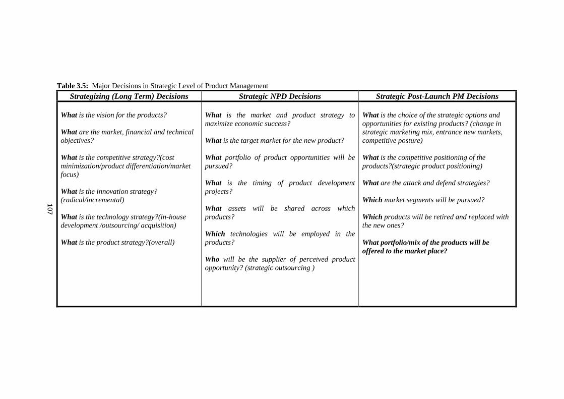
10

7

Table 3.5: Major Decisions in Strategic Level of Product Management

Strategizing (Long Term) Decisions Strategic NPD Decisions Strategic Post-Launch PM Decisions

What is the vision for the products?

What are the market, financial and technical

objectives?

What is the competitive strategy?(cost

minimization/product differentiation/market

focus)

What is the innovation strategy?

(radical/incremental)

What is the technology strategy?(in-house

development /outsourcing/ acquisition)

What is the product strategy?(overall)

What is the market and product strategy to

maximize economic success?

What is the target market for the new product?

What portfolio of product opportunities will be

pursued?

What is the timing of product development

projects?

What assets will be shared across which

products?

Which technologies will be employed in the

products?

Who will be the supplier of perceived product

opportunity? (strategic outsourcing )

What is the choice of the strategic options and

opportunities for existing products? (change in

strategic marketing mix, entrance new markets,

competitive posture)

What is the competitive positioning of the

products?(strategic product positioning)

What are the attack and defend strategies?

Which market segments will be pursued?

Which products will be retired and replaced with

the new ones?

What portfolio/mix of the products will be

offered to the market place?

10

8

Table 3.6: Major Decisions in Tactical and Operational Levels of Product Management

NPD Post-Launch PM

Planning

Organizational (1) Will a functional, project, or matrix organization

be used?

How will the team be staffed?

How will be the physical arrangement and

location of the team?

What investments in infrastructure, tools, and

training will be made?

What type of development process will be

employed?

Project Management (2) What is the relative priority of development

objectives?

What is the planned timing and sequence of

development activities?

What are the major project milestones and

planned prototypes?

What will be the communication mechanisms

among team members?

How will the project be monitored and controlled?

What are the required technologies,

architectures, or platforms to support new

functionality?

What pricing strategies are to be used to

support product?

What are the financial requirements for

ongoing work?

Development

Concept (1) What are the target values of the product

attributes, including price?

What is the core product concept?

What is the product architecture?

What variants of the product will be offered?

Which components will be shared across which

variants of the product?

What will be the overall physical form and

industrial design of the product?

and equipment?

Design (3) What are the values of the key design

parameters?

What is the configuration of the components and

assembly precedence relations?

What is the detailed design of the components,

including material and process selection?

Supply Chain (2) Which components will be designed and which

will be selected? Who will design the

components?

Who will produce the components and assemble

the product? (Make/Buy decision)

What is the configuration of the physical supply

chain?

What type of process will be used to assemble the

product?

Who will develop and supply process technology

and equipment?

Testing & Validation (4) What is the prototyping plan?

What technologies should be used for prototyping

plan?

Ramp-up and Launch (5) What is the plan for market testing and launch?

What is the plan for production ramp-up?

What is the improvement project for the

existing products? (functionally,

aesthetically) With which features or

attributes?

What promotional strategies are to be

used to support product?

What distribution strategies are to be

used to support product?

What is volume of the product to be

produced?

What are the quality guidelines?

What are the customer satisfaction

targets?

What are repair and return goals?

What is the inventory turns goals?

109

3.2.5 Validity of the Flow Model

In general terms, validity is the assessment of how well a survey measures what is intended

to measure. The validity of the Flow Model has been tested by the comments of PM

experts. Hence, while we were developing the Flow Model, we communicated with the

PM expert at certain phases, and evaluating his comments, we revised the Flow Model

when necessary. Most of the comments were related to the clarity of the Flow Model.

However, one revision has been made in “Strategic Level Review” part of the Flow Model

which was in conflict with the literature-based knowledge: We added the “strategic

outsourcing decision” to the decisions on the strategic level by the comment of the PM

expert which was explained in the relevant part of the Flow Model. Contrary to the PM

expert’s comment, outsourcing decisions take place only on the tactical level of PM in the

literature except in a few ones. Another important comment was related to the target

market decision in the strategic level review. In our flowchart, the target market decision

is represented by “left arrow”, but together with the “right arrow” (strategic product

selection decision) it was misleading the reader because these two arrows together were

representing a parallel decision. By the comment of the PM expert we numbered the target

market decision as the first decision, which was in line with the literature. When we

completed our flowchart, we asked for the PM expert to evaluate our Flow Model in terms

of

a) relevance,

b) clarity, and

c) ambiguity.

He established a cross-sectional team within the company and this team examined and

evaluated the Flow Model. Finally, he confirmed the model in written form. Hence, we

can say that the Flow Model is a joint work of the PM expert and us.

Specifically, the assessment of content validity typically involve an organized review of

the survey’s contents to ensure that it includes everything it should and does not include

anything it should not (Litvin, 1995). “Content validity is a subjective measure of how

appropriate the items to a set of reviewers who have some knowledge of the subject

matter”. It is also stated that “Although it is not a scientific measure of a survey

instrument’s accuracy, it provides a good foundation on which to build a methodologically

rigorous assessment of a survey instruments’ validity (Litvin, 1995; p.35).

Litvin (1995) strictly states that content validity is not quantified with statistics, rather it is

presented as an overall opinion of a group of trained judges. However, over the years,

some efforts have been made to find more quantifiable methods for determining the

content validity. “Content Validity Index” (CVI), or “proportion agreement”, is the one

which is used as an objective method for quantitatively measuring the content validity

(Wynd et al., 2003). The CVI allows two or more raters to independently review and

evaluate the relevance of the domain of content. During the progress of the thesis study,

the academic experts of the subject used their judgments about the degree of relevance of

the domain of the content, i.e., literature-based knowledge obtained through a

comprehensive literature survey. Getting the comments of the academic experts, the final

form of the Flow Model is constructed and shaped, as given in Appendix C.

110

3.2.6 Concluding Remarks

To formulate the strategic product mix problem in product management context requires

answering the following important questions:

Who is the decision maker?

What are the decision factors?

What are the environmental (external) factors affecting the decision(s)?

What should be the time period to be considered for the decision(s)?

What types of interactions do exist in decisions which may affect the product mix

decision?

What are the priorities for those decisions? Is there a sequential decision making

process?

What are the objectives of the organizations?

What is relative importance of the product mix decision among the other decision

making problems?

In short, to clarify these questions, and hence, to understand the context of product mix

problem requires to analyze and understand the product management in its entirety.

Besides, in order to be able to locate properly the product mix problem in product

management framework necessitates detecting and extracting the major decision making

problem areas in product management. For these purposes, the product management

literature was surveyed deeply. During the literature survey, it was realized that there is no

a comprehensive study considering requirements of the holistic approach to product

management. Realizing this gap in the existing literature, it was decided to make an

attempt to fill it. In sum, the accumulated knowledge obtained in the literature survey

study, with the contributions of the field study, was evaluated to develop an exhaustive

decision framework of product management.

Our aim in developing this decision framework of product management is mainly twofold:

1. to understand the PM problem deeply that enables us to formulate our research

problem efficiently,

2. to serve as a pointer to this vast body of literature on product management which

requires dealing with several domains of literature.

As a result, our contribution in this work can be outlined as follows:

The Proposed Product Management System (PMS) presented in section 3.2.1

(Figure 3.7), is based on a holistic approach to the product management at

corporate level. It was realized that most of the existing literature is in the area of

new product development. This literature considers mainly the pre-market

(investment) period of the product. On the other hand, a large literature in

marketing area of the product considers only the market period of the product

regarding marketing strategies, product positioning in the market, promotional

activities, etc. However, the holistic approach requires considering the whole life

111

cycle (PLC) of the product. The PLC starts with the product idea and continues

till the withdrawal of the product from the market. To the best of our knowledge

there is no a comprehensive study concerning such a holistic and an integrative

systemic approach. We should point out an exception of Haines’ (2009) book in

which a similar conceptual definition for PLC is used, and it is written as a desk

reference for a product manager from practical implementation point of view. It

should be pointed out that it does not cover a systemic view to the decision

framework of product management.

A structured approach is presented to organize the product management literature

what we call the decision framework.

The existing literature of new product development is integrated to our additional

efforts on the other areas of product management so that the interested reader is

able to follow the whole journey of the product and the major decisions taken

during this journey in a typical manufacturing company.

The author believes that all the efforts to integrate the existing literature in this study and

to present it in a comprehensive way can be viewed as an initial attempt to clarify the

decision framework of product management based on holistic approach which does not

exist in the existing literature. Since our focus is the strategic product mix problem in

product management framework, it is thought that the decision framework of product

management can be bounded as it is given above. Additionally, the work presented in this

chapter can be improved further for the forthcoming studies in this area.

113

CHAPTER 4

PROPOSED PRODUCT MIX DECISION SUPPORT SYSTEM

As mentioned before, shaping and planning the optimum product mix is ultimate goal in an

effective product management. Therefore, strategic product mix determination is a

challenging problem for companies in all industries. Although the problem may vary from

one industry to another or even one company to another company in the same industry, the

fundamental issue remains the same: Which products should be selected for the coming

period and how many should be produced from each in order to maximize the financial

performance of the firm in that period? The first part of this question is related to shaping

the product mix which requires the selection of the right products to be served to the

customers. We mainly focus on the second part of the above question, that is “to

determine the quantities of the products” in order to maximize the financial performance of

the company. While doing this, the method proposed here aids the decision maker in

deciding the selection of the right products providing fast and necessary information which

assure a profitable future for the company.

This chapter covers, first, the definition and clarification of Product Mix Problem within

the product management context. Then the working mechanism of the proposed decision

support system in this framework is described in section 4.2. In section 4.3, formulation

approach of the problem is explained including the mathematical models constructed in

accordance to the framework of the formulation approach. Section 4.4 presents the

scenario generation method and determining the optimal product mix.

4.1 DESCRIPTION OF THE PRODUCT MIX PROBLEM WITHIN

PRODUCT MANAGEMENT CONTEXT

Up to this point, it has frequently been stated that the formulation of product mix problem

is based on the detailed decision framework of the product management problem. Thus,

the problem setting within the product management context is very important to be clearly

defined before passing through the formulation phase of the problem. Below, the product-

mix problem within the product management context is defined. In this definition, the

production management relevance of the product-mix problem, the product level in the

mix and different types of production strategies or systems existing in manufacturing

environments of the companies and industries are considered. Next, the complexities of the

problem are outlined. Finally, the major interdependencies of product-mix problem with

the other decision making problems in PM context are briefly described.

114

4.1.1 Problem Setting

As it was mentioned before, the nature of product-mix problem requires decisions at

different activity levels of the management. So, the product mix decision at the strategic

level can be made evaluating the results of the lower levels of this framework, and lower

level decisions are made considering the strategic alignment as discussed before. In other

words, strategic level decisions are the inputs for the tactical and operational level

activities. In that sense, the best results obtained for the strategic product mix problem

provide valuable inputs for the lower level decisions and activities in the product

management context. Therefore, strategic product mix problem is formulated from a macro

point of view within the product management context. This macro perspective is depicted

in Figure 4.1. Considering this macro view it can be stated that the details of production

processes and the components of the products are out of our concern. Detailed

explanations about this perspective are given below. Note that these issues have also been

discussed in detail at the formulation phase of the problem.

Figure 4.1: Product Mix Problem within Product Management Framework

As mentioned in Chapter 3, aggregate production planning (APP) is the major activity at

the operational level of PM. It is knownt that, in the traditional approach, APP addresses

the problem of deciding on the quantity and the mix of products to be produced and the

staff level (Nahmias, 2001). Nahmias (2001) states that APP is generally considered as a

macro planning tool for determining the overall workforce and production levels, and

therefore macro planning strategies are seen as a fundamental part of the firm’s overall

business strategy in production planning decision framework. Therefore, APP is accepted

as a top level activity in this latter framework, while it is seen as an operational level

activity in product management framework which is accepted as a higher level of

business activity.

115

Although APP is generally considered as a macro-planning tool, large companies may find

APP useful at the plant level as well (Nahmias, 2001). Traditionally, APP begins with the

forecast of demand (Figure 4.2). However, in PM decision framework, forecasting demand

is the main task of the front line people, particularly sales department. Sales department

prepares sales plan of the corporate which is based on these forecasts (see Appendix C:

Flow Model, page 7) and shows the forecasted quantities and suggested prices of the

products in this plan. Therefore, it is seen in tactical and operational planning and

management level of the main frame of product management at the corporate level. This is

the main reason why APP is considered at the operational level of our problem within the

product management context.

Figure 4.2: The Hierarchy of Production Planning Decisions (Source: Nahmias, 2001;

p.116)

Forecasting demand is an important issue for the firms, which is used in their production

planning to coordinate manufacturing capacity in order to be able to balance demand with

supply. Vollman et. al (2005) considers forecasting issue in “demand management

system” of “Manufacturing Planning and Control” (MPC) system in their book.

Remember that it is also one of the most important problems considered in the product

management of the companies studied in the field study. At this point it is worthy to

discuss the role of demand management system in production planning framework,

because it provides the link to the marketplace, plants, warehouses, and generally

“customers”, as the initial task in production planning. Demand management is defined as

“the activities that range from determining or estimating the demand from customers,

through converting specific customer orders into promised delivery dates, to helping

balance demand with supply” (Vollman et al., 2005; p.17). So, it can be said that demand

management plays a critical linkage role in both production management and in sales and

operations in product management. The information provided through demand

management to sales “is used to develop sales plans covering a year or more in a duration

at a fairly high level of aggregation” (Vollman et al., 2005; p.24). Remember that in the

proposed PM framework sales plans are prepared for the major product groups and

116

presented to PRB for their strategic selection. Table 4.1 shows the summary of demand

management framework in production management framework which is partly borrowed

from Vollman et al. (p.30, 2005). It is indicated as the general principle that the nature of

the forecast must be matched with the nature of the decision. In this table, the second

column shows the strategic decisions, the third column indicates the tactical level decisions

and the last column shows the operational decisions in production management

framework. It is noted that source of the forecast can vary by needs of the company. In our

research problem case, we do not consider MPS, but instead, consider APP in product

management framework. Constructing a new plant, developing more supplier capacity,

expanding internationally and other long-run company-wide considerations are some

examples for the strategic decisions which can be considered both in product and

production frameworks.

Table 4.1: Demand Management Framework

Nature of the

Decision

Strategic Business

Planning

Sales and

Operations Planning

Master Production

Scheduling (MPS)

Level of aggregation

Top management

involvement

Forecast frequency

Length of forecast

Useful techniques

Total sales or output

volume

Intensive

Annual or less

Years by years or

quarters

Management

judgement,

economic growth

models

Product family units

When reconciling

functional plants

Monthly or

quarterly

Several months to a

year by months

Aggregation of

detailed forecasts,

customer plans

Individual finished

goods or

components

Very little

Constantly

A few days to weeks

Projection

techniques(moving

averages,

exponential

smoothing)

Hence, demand management activities should be in conformity with the strategy of the

firm, the production capabilities and customer needs. Moreover, different manufacturing

environments may shape differently the demand management activities. Below, the role of

demand management in different production systems is described briefly referring to the

definitions provided in section 2.1.3.

“In the make-to-stock (MTS) manufacturing environment, the key focus of the demand

management activities is on the maintenance of finished goods inventories” (Vollman et

al., 2005; p.21). This is because the customers buy directly from the available inventory.

Moreover, there may be several locations from which the customers can buy the products.

Therefore, the physical distribution of the products is an important concern in MTS

environment in which replenishment of the inventories at each location should be

determined. The important issue in satisfying the demand in MTS environment is to

balance the level of inventory against the level of service to the customer. So, a trade-off

117

between the cost of inventory and the level of customer service should be made. As a

result, such a trade-off can be improved by better forecasts or knowledge of customer

demand. Therefore the focus of demand management in MTS environment is on providing

finished goods where and when the customers want them (Vollman et al., 2005).

“In the assemble-to-order (ATO) environment, the primary task of demand management is

to define the customer’s order in terms of alternative components and options” (Vollman et

al., 2005; p.22). In ATO environment, customers should be informed of the allowable

combinations. On the other hand, these combinations should be in parallel to the

customers’ desires in the marketplace. For example, a two-door versus four-door car, with

or without antilock brakes are the options which may define customer’s order in

automative sector. In ATO environment, product configuration management is critical for

the company. The inventory for such a company is the inventory of components, not the

inventory of finished products. The main reason is that the inventory of finished products

is usually greater than the inventory of components that are combined to produce the

finished product. Consider for example, a personal computer for which there are 3

processor alternatives, 3 hard disk drive choices, 3 CD-DVD alternatives, 2 speaker

systems, and 2 monitors available. Let us assume that all combinations of these 13

components are valid, then they can be combined into a total of 108 different PC

configurations. Obviously, it is much easier to manage the forecast of the demand for 13

components than 108 computers. As a result, the primary task of demand management is

to define the customer’s order in terms of alternative components and options.

It is seen that the demand management in MTS and ATO environments considers the

customer satisfaction from the appropriate inventory of finished goods and components,

respectively. So, the company may know “what” the customers buy in MTS and ATO

environments, but it may not know “if”, “when”, or “how many”. On the other hand, in

the make-to-order (MTO) manufacturing environment, company may not know “what” the

customers will buy. Therefore, to get the information about the product specifications

from the customers is an essential task in order to translate them to manufacturing terms in

the company. In this environment, demand management task requires to determine how

much engineering capacity is necessary to meet the future demand of customers. More

generally, capacity management issue is considered as the most important task in MTO

environment.

The goal of APP is to develop a production plan for the firm that maximizes profit over the

planning horizon subject to constraints on capacity. The major simplifying assumption is

that the demands are treated as known constants. APP is closely related to hierarchical

production planning, in which purchasing, production and staffing decisions are made at

several levels in the firm. In this approach, APP is accepted on the existence of an

aggregate unit of production, which depends on the context of particular planning problem.

For APP purposes, the following product hierarchy is recommended (Nahmias, 2001):

1. Items. They are defined as the end products to be delivered to the customer (e.g an

individual model of washing machines).

2. Families. These are defined as a group of items that share a common

manufacturing set up (e.g all washing mashines).

118

3. Types. They are groups of families with production quantities that are determined

by a single APP (e.g Major Household Appliances).

Figure 4.2 shows the hierarchy of production planning decisions in parallel to above

product hierarchy. Nahmias (2001) makes an important remark about this aggregation

scheme: He states that such an aggregation method will not necessarily work in every

business organization. He concludes that the aggregation method should be consistent

with the firm’s organizational structure and product line. As a result, it is understood that

the definitions and implementations of APP can be adopted or changed to the problem

situations accordingly. In short, our problem is formulated in view of this flexibility.

Considering this perspective of the Product Mix Problem, strategies formulated by the

executive (top level) management of the company at the strategic level propose the

execution of the parameters for the families of products. In other words, this level of the

mix of the products will result in the mix of the families of products. As an example, let us

consider a manufacturer who is a producer of consumer durables goods. The product

profile (product range) for such a company is assumed as the composition of different

product lines (“types” in Nahmias’ definition) which is illustrated in Figure 4.3.

Figure 4.3: Product Profile (Product Range) for a Typical Manufacturer of Consumer

Durables Goods (Source: Field Study-Company D)

119

Note that each product line is composed of the product units which are technologically

different, serve to the same target market and have similar functionality. Traditionally,

product mix is defined as the entire set of the products produced by the company

(Steinhardt, 2010). In this case the composition of all the lines represent the product mix

of this company. However, depending on the size of the company and the purpose of the

management, product mix can be considered for each product line (Haines, 2009). In that

case, the composition of families of products is defined as the product mix. Each family

under the product lines are the product units which have the same technological foundation

and each family has different types, styles, or models of product units which are called as

product variants (Steinhardt, 2010). Similarly, each family can be considered as the mix

of the product variants depending on the size of the company and the purpose of the

management. Let us consider the “white goods” aggregation scheme of Company D as

another example which represents the purpose of Company D in their product hierarchy

presentation. The product line “white goods” is depicted in Figure 4.4.

Figure 4.4: Product Aggregation Scheme (Product Hierarchy) of Company D

In Company D, families are composed of homogeneous groups. Homogeneous group is

defined as the group of products which has the same production technology, the same

assembly line and the same key components. The key components are “volume”, “carcase”

and “boiler” for the refrigerator, dish washer and washing machine respectively. For

example, if the volume of the refrigerator changes, Company D uses different production

technology or different assembly line. In such a case, the mix of different homogeneous

groups in a family can be questioned by the company in order to consider the financial

performance of these groups.

In our case, we assume the product mix as the mix of the lines and/or families of the

product units believing that the definition and execution of the parameters of the problem

are more meaningful at the strategic level decision making process.

120

4.1.2 Complexity of the Problem

Regarding the product management, the sources of complexity are outlined in section

2.1.5. These complexity sources are directly related, and hence, define the complexity of

product mix problem since it exists in the boundary of the framework of product

management. Thus, associated with the product mix decision problem, the sources of

complexities can be outlined as follows:

1. Strategic alignment

2. Scarcity of resources

3. Product interactions

4. Uncertainty

Strategic alignment is considered in the formulation of the product mix decision problem

through the fundamental input component of the product mix problem, namely, the set of

candidate products. Product strategy of the corporate is reflected in selecting those

candidate products. So, the strategic alignment issue can be considered when the set of

candidate products are constructed as the input of the product mix problem. Scarcity of

resources is considered by the limited production resources as in any product mix problem.

Product interaction is one of the major complexities in the product mix problem.

Substitutability and complementarity are two major interaction types among the products.

Moreover, cannibalization effect of any product, which can occur among substitutable

products, if it is selected into the mix, should be considered in making the product mix

decision. Studying different candidate products sets while getting the solution to the

product mix problem may give an insight to the management regarding this issue. The

uncertainty is crucial for the formulation of the product mix problem. In our case, market

uncertainties, regarding the costs and prices of products and also demands for the products,

are the major sources of uncertainty to be considered in the formulation of the problem.

Finally, note that we consider the families of (end) products (variants) of the company in

the product mix problem of our study, in the sense that we do not have evolving nature of

the NPD problem which necessarily requires the consideration of dynamic nature of the

product management problem. So, we consider a single period product mix problem in our

study. However, our problem can be extended to the multi-period case.

At the moment, our major concern is uncertainty in dealing with the product mix decision

problem. We discuss this issue more in explaining the framework of the proposed decision

support system. The way of handling this issue is explained in formulation phase of the

problem.

4.1.3 Interactions with Other Decision Making Problems

Product mix decision making involves the simultaneous determination of the answers to

the following major questions:

1. Which products are to be produced from a given set of candidate products?

2. What quantities of those products are to be produced?

121

The answer to the first question requires to know the set of candidate products from which

the best products should be selected. Hence, to determine the set of candidate products is

another major decision making problem which is closely related to the product mix

problem. The set of candidate products are composed of both new and/or improved

products of existing products and the kept products already existing in the line. Actually,

new and/or improved products of existing products can be considered as the product

investments of the company. Additionally, management of the company should evaluate

the existing products in order to make product withdrawal/deletion decision. Figure 4.5

illustrates the composition of the set of candidate products.

Figure 4.5: The Composition of the Set of Candidate Products (Adapted from Haines,

2009)

The answer to the second question requires the consideration of several issues. First, the

company should determine sources of the products. Therefore, the question of “Who will

produce?” should be answered by the company. If the source of the products is inhouse

production, the market uncertainty and capacity issues should be considered. In sum, the

framework of the product mix problem within product management context requires to

consider the interactions of some other decision problems of product management. The

major interdependencies of product mix problem with the other product management

issues are shown in Figure 4.6.

122

Figure 4.6: Major Interdependencies of Product Mix Problem within Product Management

Context

One can observe from Figure 4.6 that most of the problems can be integrated under the

headline of “product investment planning” of the company. Product investment planning

implementation decisions and product mix decision together determine the company’s

responsiveness to demand, or more generally, market uncertainty, and hence improve the

ability to maximize the company’s profits. The framework of the proposed product mix

decision support system (DSS) is developed focusing on this main idea which is explained

in detail in the next section.

4.2 FRAMEWORK OF THE PROPOSED DECISION SUPPORT SYSTEM

4.2.1 Purpose of the Proposed Decision Support System

In a competitive environment, product mix determination is very critical decision for

companies. Often, companies try to handle this problem by expanding their product lines.

Competitors’ pressure and willingness to respond to detailed customer preferences may

lead the companies overextending their product lines which may have negative impact on

manufacturing effectiveness (Quelc and Kenny, 1994). Moreover, overextended product

lines can overload customers with information, which often makes it more difficult for

them to find their favored product (Kuester, 2000). In fact, instead of extending product

lines, extending the profits of the company is important. Product mix determination

requires first the selection of right products as candidates. Then, the mix of products

should be evaluated in terms of profits in order to achieve the maximum profit for the

company. The selection of the right products is a difficult decision making problem. In

case the decision maker would know the profit generated by the optimal mix of the

products selected, she would easily decide on the products which the company should offer

to the market to make their customers satisfied and earn maximum profit. Besides, the

existence of such a decision mechanism would also help making the decision on budgeting

properly. As a result, in this study, we aim to present a decision method to aid the decision

makers

123

to determine the optimal mix of the predetermined candidate products, so that

using the proposed decision mechanism by changing the set of candidate products

several times as required; the selection of right products to be offered to the

market with the maximum profit can be made by evaluating the profit values

under each of the different cases considered.

In addition to this purpose, the proposed decision method can be used for

budgeting purposes.

It also provides a support to the decision maker for different product planning

issues under “what-if” type of questions.

Finally, it provides a valuable input for the demand management system of APP

work.

It should be noted that uncertainties are a major element in any real-life decision problem

where the information about the presence and the future unfolds iteratively. So, any

system which is designed without considering uncertainty may not sufficiently reflect real

life.

If uncertainty is not taken into consideration, the outputs of the decision support system

might mislead the decision makers because the chosen product which is found to be the

best one maximizing the sales revenues or profits by such a system might prove itself to be

the poorest choice of all in reality later on. Therefore, uncertainty which is a significant

attribute of the real life should be taken into consideration.

In reality, firms are faced with unknown demand for their products, and likewise the prices

and costs of the products cannot be known precisely beforehand in a competitive

environment. Therefore forecasting demands, prices and costs is a difficult task which is

always subject to error. Sales of the products depend on unknown demands, and hence,

profits derived from the sales also rely on unknown demands for the products, which in

turn predict inaccurate and/or misleading results for the firm. In short, uncertainty is the

major complexity of the problem and it may cause wrong decisions for the products to be

chosen in the product mix of the company which results in sub-optimality regarding the

financial performance measures of the firm.

As it was discussed briefly before, the primary function of demand management system in

production management framework is forecasting demand in uncertain environmental

conditions. The types of uncertainty also differ with respect to the different

manufacturing environments. In MTS case, uncertainty is largely in the demand variations

around the forecast. As it is known, the company having the MTS production system sells

its products from the available inventory. So, these companies hold stocks in order to

provide products to their customers. In ATO case, “the uncertainty involves not only the

quantity and timing of customer orders but product mix as well” (Vollman et al., 2005;

p.26). If timely and honest customer order promises are assumed, it can be said that for the

MTO environment, the uncertainty of quantity and timing of customer order may not be

high. In this case, the level of company resources and capacity adjustment issues should be

the concern of the company to produce the products (Vollman et al., 2005). It should be

noted that firms may produce their products in a combination of these environments. In all

these environments, the most important issue is the quality of the information gathered in

demand management system to enhance the performance of the firm. Therefore, to support

124

the decision makers with high quality knowledge on time is very important in their real life

decision making situations.

Our study considers a product mix problem under uncertainty of demand, product price

and production cost parameters. This implies that the problem is more realistic since

demand, price and cost forecasts are not precise, and they are usually given as more than a

single value. Furthermore, due to demand uncertainty it may not be possible to meet all

demands with the firm’s available capacity. In our study, we assume MTS production

system in which volatile demand conditions in the market appear as variations in demand

of the “finished products”. Since we do not deal with the “component” level of the

products, ATO production system does not suit the case under consideration. It can be

stated that MTO production system can be partly considered in our study, only by the

inclusion of predetermined level of taken orders. Engineering and production capacities

should be studied further in MTO case.

In order to deal with uncertainty, we develop a scenario-based scheme by generating

different scenarios focusing on the major inputs or sensitive parameters of product mix

model. The problem is introduced in detail further in the subsequent sections.

So, our primary goal in modeling the product mix problem is to present an approach of

dealing with uncertainty and the methodology developed for this purpose. Therefore, the

product mix optimization model is kept simple to capture the desired importance on the

methodological approach which is unique for this problem to the best of our knowledge.

Hence, it represents the major contribution of this Ph. D study. Although the approach has

some similarities to simulation optimization approaches such as the one developed by

Kaya et al. (2011), which considers an investment planning problem under uncertainty for

a telecommunications company, these approaches have significant differences from ours.

By definition, a decision support system, which we aim to develop for this specific

problem, requires a practical implementation for the decision makers, and it should provide

fast and reliable results in their decision making process. Consider the following

comments and conclusive remarks given in Kavadias and Chao (2008):

“Management researchers and practitioners have proposed many methodologies

for tackling the complexity of the portfolio selection problem. The literature

review suggests that quantitative research efforts have been restrained at the

tactical level of analysis and they have not been widely adopted in practice

because of the complexity associated with the decision” (pp.154-155), and

“Although mathematical programming is a sound methodology for optimization

problems, and it has been successfully applied in several specific cases, it has not

found widespread acceptance by practitioners. This gap stems partly from the

complexity and sophistication of the methods, which are difficult to understand

and to adopt for people who are not trained in OR, and partly from the lack of

transparency and from the sensitivity of the results to changes of the problem

parameters. In addition, mathematical formulations in order to retain some level

of analytical tractability they rarely account for dynamic decision making” (p.

152) (i.e., different points in time).

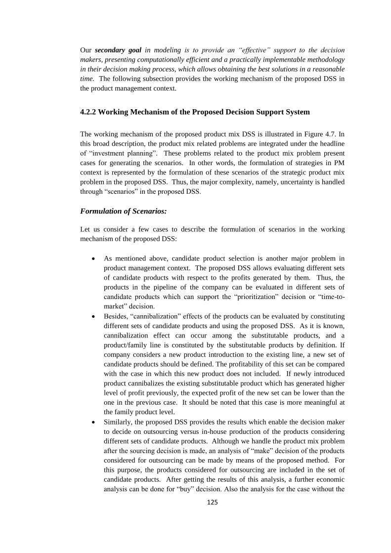
125

Our secondary goal in modeling is to provide an “effective” support to the decision

makers, presenting computationally efficient and a practically implementable methodology

in their decision making process, which allows obtaining the best solutions in a reasonable

time. The following subsection provides the working mechanism of the proposed DSS in

the product management context.

4.2.2 Working Mechanism of the Proposed Decision Support System

The working mechanism of the proposed product mix DSS is illustrated in Figure 4.7. In

this broad description, the product mix related problems are integrated under the headline

of “investment planning”. These problems related to the product mix problem present

cases for generating the scenarios. In other words, the formulation of strategies in PM

context is represented by the formulation of these scenarios of the strategic product mix

problem in the proposed DSS. Thus, the major complexity, namely, uncertainty is handled

through “scenarios” in the proposed DSS.

Formulation of Scenarios:

Let us consider a few cases to describe the formulation of scenarios in the working

mechanism of the proposed DSS:

As mentioned above, candidate product selection is another major problem in

product management context. The proposed DSS allows evaluating different sets

of candidate products with respect to the profits generated by them. Thus, the

products in the pipeline of the company can be evaluated in different sets of

candidate products which can support the “prioritization” decision or “time-to-

market” decision.

Besides, “cannibalization” effects of the products can be evaluated by constituting

different sets of candidate products and using the proposed DSS. As it is known,

cannibalization effect can occur among the substitutable products, and a

product/family line is constituted by the substitutable products by definition. If

company considers a new product introduction to the existing line, a new set of

candidate products should be defined. The profitability of this set can be compared

with the case in which this new product does not included. If newly introduced

product cannibalizes the existing substitutable product which has generated higher

level of profit previously, the expected profit of the new set can be lower than the

one in the previous case. It should be noted that this case is more meaningful at

the family product level.

Similarly, the proposed DSS provides the results which enable the decision maker

to decide on outsourcing versus in-house production of the products considering

different sets of candidate products. Although we handle the product mix problem

after the sourcing decision is made, an analysis of “make” decision of the products

considered for outsourcing can be made by means of the proposed method. For

this purpose, the products considered for outsourcing are included in the set of

candidate products. After getting the results of this analysis, a further economic

analysis can be done for “buy” decision. Also the analysis for the case without the

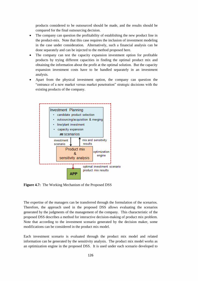
126

products considered to be outsourced should be made, and the results should be

compared for the final outsourcing decision.

The company can question the profitability of establishing the new product line in

the product-mix. Note that this case requires the inclusion of investment modeling

in the case under consideration. Alternatively, such a financial analysis can be

done separately and can be injected to the method proposed here.

The company can test the capacity expansion investment option for profitable

products by trying different capacities in finding the optimal product mix and

obtaining the information about the profit at the optimal solution. But the capacity

expansion investment costs have to be handled separately in an investment

analysis.

Apart from the physical investment option, the company can question the

“entrance of a new market versus market penetration” strategic decisions with the

existing products of the company.

Figure 4.7: The Working Mechanism of the Proposed DSS

The expertise of the managers can be transferred through the formulation of the scenarios.

Therefore, the approach used in the proposed DSS allows evaluating the scenarios

generated by the judgments of the management of the company. This characteristic of the

proposed DSS describes a method for interactive decision-making of product mix problem.

Note that according to the investment scenario generated by the decision maker, some

modifications can be considered in the product mix model.

Each investment scenario is evaluated through the product mix model and related

information can be generated by the sensitivity analysis. The product mix model works as

an optimization engine in the proposed DSS. It is used under each scenario developed to

127

find the optimal product mix under that scenario. Then these product mix solutions are

tested under all scenarios to find the most robust product mix that yields consistently high

profits over all scenarios. The latter product mix and expected profits and ranges of profits

can be chosen by the decision makers as inputs for APP so that disaggregation of this mix

is considered for detailed production planning of the company. Thus APP may start with

the optimal product mix results in the proposed approach. It means that the results

provided by the proposed DSS improve the traditional demand management system of

APP work which assumes deterministic demand values.

A well-developed demand management system within the production management system

brings significant benefits to the company. In this case, capacity and the production of the

company can be better managed and controlled. The capabilities of the firm can be

developed better with better information. Additionally, the physical distribution activities

can be improved significantly.

Appropriateness of the Proposed Approach for Different Types of Production

Systems:

Remember that demand management activities are handled with the Sales and Operations

(SOP) in PM framework (Appendix C: Flow Model, p.7). In these activities all sources of

demand must be accounted for quantity in a certain planning period. It means that it may

not be sufficient to simply determine the market needs for the product. To get a complete

picture of the requirements for the production system, manufacturing capacity, engineering

resources, material needs, pipeline profile, quality assurance needs and promotional

requirements should be studied. All these issues are shown Sales and Marketing Plans. In

the proposed DSS approach, product mix model is an appropriate tool for considering

these requirements to communicate with the demand management system and SOP. It is

essential to use proper units in this communication. Choosing the appropriate measures can

vary with different production systems. For example, determining the capacity

requirements can be different in these manufacturing environments. For instance, material

capacity may be the most important in a MTS company. In this case, it should be included

in product-mix model for such a company. Production capacity may be machine hours or

labor hours in MTO case. In short, the product mix model can be modified in accordance

with the significant measures for the company.

Vollman et al., (2005) states that the nature of information or demand management

communication activity with SOP for different manufacturing environments is as follows:

In MTS; Demand forecasts

In ATO; Demand forecasts, product family mix

In MTO; Demand forecasts, engineering (capacity)

SOP may “develop plans by product families, geographical regions, organizational units,

or even combinations of these and other categories” (Vollman et al., 2005; p.25). As

mentioned before, we assume MTS manufacturing environment in our study. In this case,

the set of candidate products are constituted by the finished products. The main task of

SOP is to get the reliable forecasts for aggregate units for these finished products. These

results constitute the initial step in APP. SOP, after getting the results of APP, prepares the

128

sales budget with the suggested prices to present the PRB of the company. In ATO

manufacturing environment, the possible configurations of the components of the products

can be grouped as the candidate family products if the number of possible configurations is

not too high. In such a case, the proposed method can be used to get the optimum mix of

families. Similarly, if the set of candidate products are properly constructed, the method

proposed here can be used in MTO manufacturing environment. The modification in

product mix model which include more detailed considerations in capacity issues of the

company may require in this case.

As a result, the proposed DSS approach provides the major input to APP through the

product mix model. The best result provided by this DSS is the optimal line or family mix

for the company. Thus, the company starts with this result to APP work in production

management, SOP may develop plans based on this result, regardless of the environment.

In other words, the proposed approach is appropriate for different manufacturing

environments. The most important issue is the quality of information/knowledge gathered

in demand management system to develop APP and SOP plans in all these environments.

So, the proposed approach improves the quality of this information by handling the issue

of uncertainty.

4.3 FORMULATION OF THE PROBLEM

4.3.1 Assumptions

For a moment, let us consider the basic structure of PM framework depicted in Figure

3.10. As it is seen in this figure, operating assumptions in PM context should be considered

in formulating the product mix problem. Operating assumptions of this research problem

can be considered as general and company specific. The following general operating

assumptions are considered in PM context:

1) The company is a commercial enterprise in the sense that it is a profit organization.

2) The primary business of the company is manufacturing.

3) The industry in which company operates is competitive.

4) The company has a formal (or well-structured) product management environment

in the organization.

In this context, product mix problem is formulated considering the company specific

assumptions regarding the following problem components:

Product profile,

Market profile,

Product-market relations,

Manufacturing environment (make-to-order, make-to-stock),

Supply chain structure/channel map,

Management/organization.

These problem components are explicitly described in modeling.

129

4.3.2 Formulation Approach

In general terms, the formulation and solution approach of the product mix problem under

uncertainty can be seen as similar to the “simulation optimization approach”. The DSS

model embodies two basic types of formal models, namely;

Deterministic Product Mix Model, and

Simulation Model.

The first model represents a deterministic approach and constructs the decision support

system that will take prices, demands and costs of the products as well as the production

capacity as given and suggests the optimal product mix. The simulation model represents

the probabilistic approach. In this approach the system is upgraded to another one which

considers the uncertainty in the parameters mentioned above. Optimal product mix

solutions are found using the deterministic model repeatedly under various scenarios

defined as possible realizations of the uncertain parameters. Then, these optimal solutions

are tested under the same set of scenarios and their performances are measured. The final

step requires the analysis of these results by using the various solution approaches to get

the optimal product mix. This approach is illustrated in Figure 4.8.

Figure 4.8: Formulation Approach of the Product Mix Problem under Uncertainty

In the subsequent section, the Deterministic Model and the Probabilistic Model are

presented and the solution approach is explained in detail.

130

4.3.3 Models

4.3.3.1 Deterministic Model

The deterministic model works as an optimization engine for the probabilistic model in the

framework of the proposed DSS (See Figure 4.8). In this subsection, the mathematical

model of the deterministic approach is presented under the “company specific

assumptions” established for a typical manufacturing company.

Problem Statement:

In the PM decision framework, we consider a typical manufacturing firm having a well-

established organizational and managerial structure and efficiency, having the necessary

access channels for the distribution of the products, and having the following product,

market, and manufacturing environment profiles:

Product Profile:

It is assumed that the company is a multi-product producer. These products are considered

in a certain aggregation scheme as described in Figure 4.4. Thus, the proposed DSS

suggests the optimal mix of families of in the product line of, say, “white goods”. Note that

the company may question the “optimal mix of groups” in the family of, let us say “Hot”.

The appropriateness of the proposed DSS in different product schemes is discussed in the

final Chapter of the study in detail.

Market Profile:

A typical multi-product company may serve its products in different markets. For

example, Company D in our field study, sells certain products to certain countries, and

some of the products are served only to the national market. Therefore, the proposed DSS

model considers a multi-market company.

Product-Market Relations:

Product-market relations simply indicate which product(s) are sold in which market(s). As

an example, let us consider a case for the Company D as illustrated in Table 4.2.

Table 4.2: Description of Product-Market Relation

Product Family National Market Global Market

HOT

COLD

WET

In this descriptive example, “Hot” family is served only domestically, and “Wet” family is

exported and not produced for national market, and “Cold” family is produced for both

national and global markets. Note that the markets can be disaggregated for special

purposes of the company. For example, Company D can disaggregate the Global market

131

considering the individual countries, like Germany, United Kingdom, France, Romania,

Litvania, etc. Also, instead of countries, the regions can be considered for structuring the

markets. As an example, Company D has consolidated the markets of Germany, United

Kingdom and France as “West Europe” market. Thus, depending on the purpose of the

company, countries, regions, or market segments can be used in structuring the markets.

Manufacturing Environment:

As discussed in working mechanism of the proposed DSS approach, the major input item

“the set of candidate products” can be considered differently for these different

manufacturing environments through the formulation of scenarios. For example, different

products having different configurations can be determined by the management in ATO

manufacturing environment to be considered in the candidate products set. The

interactive decision making characteristic of the proposed approach allows these

formulations. Besides, deterministic product mix model can be adapted to different

manufacturing environments. Since inventory management is important in MTS and ATO

manufacturing environments, the mathematical model can include more detailed cost

structures to handle this issue. On the other hand, committed orders in MTO manufacturing

environment can be handled by the inclusion of lower bounds for the quantity to be

produced. In MTO environment, the capacity issue may be more important for the

company. Therefore, capacity requirements and availibility of the resources of the

company can be considered in detail in modeling. In addition to this, capacity related

scenarios can be formulated and tested in the proposed DSS through the deterministic

product mix model.

For a single predetermined period of time, the product mix problem under consideration

asks the following major questions which are translated into a type of decision variable in

our deterministic product mix model. Hereinafter, this model will be named as the Basic

Model in the total framework of DSS model.

a) Which feasible product combinations should be selected from a set of

candidate products for production for each marketplace for the specified

period of time?

b) In what quantities should the selected products be produced for each

marketplace for the specified time period?

The input/output structure of the Basic Model is depicted in Figure 4.9.

132

Figure 4.9: Input-Output Model of Deterministic Product Mix Model

Mathematical Model:

The outputs of the model are:

1) The optimal set of new/improved products (lines/families) and existing products

(lines/families) to be kept in the product mix for each market in which this product

set is sold.

2) The optimal amount of products (lines/families) to be produced for each market

where these products are sold.

Since the main focus of the study is to guide product management decisions and to show

the methodology developed for determining the best product mix under uncertainty, the

deterministic model is kept as simple as possible. Therefore, a comprehensive

optimization model is avoided. Thus, for the sake of simplicity, the model is constructed

under the following assumptions:

1. Products are independent from each other.

2. All of the products produced are sold (zero inventory).

3. Company retains a stable workforce (out of planning consideration).

4. Single planning period is taken into consideration (say, one year).

Notation and Definitions:

i : identifying number to denote candidate products which are composed of new/improved

products and existing ones, i = 1,2,…,k

j : identifying number to denote markets in which products are to be sold, j = 1,2,…,J

Decision Variables:

xij : number of units produced of product (family) i for market j

133

Parameters:

mi : number of markets of product (family) i,

Mi : a set of markets in which product (family) i is to be sold

Pij : unit profit of product (family) i in market j , and

Pij = SPij - PCi , where

SPij : (average) unit selling price of product (family) i in market j

PCi : (average) unit production cost of product (family) i

cij : (average) capacity (machine hours) needed to produce one unit of product (family)

i in market j

Ci : total production capacity (machine hours) for product (family) i

dij : total demand for product (family) i in market j (upper bound)

lij : minimum demand/committed order of product (family) i (lower bound)

Objective:

The objective of the problem is to maximize the total profit of the product lines/families

composed of the selected products. So, the Basic Product Mix Model is as follows:

1

i

i

mk

ij ij

i j M

Maximize P x

Subject to

Capacity constraints:

, 1, 2,...,i

ij ij i

j M

c x C i k

Demand constraints and committed orders:

, integers , 1, 2,...., ij ij ij ij il x d x i k j M

The model presented above is simply a bounded “knapsack” problem which is a well

known combinatorial optimization (Johnson and Montgomery, 1974; Ravindran, 2008).

These types of problems require complex solution algorithms and computational effort.

The standard knapsack problem in the literature is defined as follows:

“We are given an instance of the knapsack problem with item set N, consisting of n (or

k) items j with profit pj and weight wj , and the capacity value c. Usually, all these

134

values are taken from the positive integer numbers. Then the objective is to select a

subset of N such that the total profit of the selected items is maximized and the total

weight does not exceed c” (Kellerer, Pferschy and Psinger, 2004, p. 2).

Alternatively, a knapsack problem can be formulated as a linear integer programming

(LIP) problem. The resulting problem is the simplest non-trivial integer programming

model with binary variables, only one single constraint and only positive coefficients.

Adding the integrality condition to the simple LP puts KP into the class of “difficult”

problems. Complexity is in the context of the solution methods or algorithms and their

implementation or running time. There are several solution methods developed for LIP

problems. Most of them can be grouped as follows (Ravindran, 2008):

Enumeration techniques,

Cutting-plane techniques, or

A combination of these.

Ravindran (2008) points out that none of these methods is totally reliable in view of

computational efficiency, particularly in cases of high number of integer variables. The

efficiency of the solution method or algorithm is usually measured in terms of the running

time of an algorithm. The most efficient algorithms are those so-called poynomial time

algorithms (Kellerer et al., 2004). As mentioned in section 4.2.1, the secondary goal of

this research is to develop an effective DSS which provides fast and reliable results to the

decision maker. Therefore, we clearly prefer to have polynomial time algorithm for our

problem. However, Kellerer et al. (2004) states the following:

“…there is very strong theoretical evidence that for the knapsack problem and hence for

its generalizations no polynomial time algorithm exists for computing its optimal

solution. In fact, all these problems belong to a class of so-called NP-hard

optimization problems. It is widely believed that there does not exist any polynomial

time algorithm to solve an NP-hard problem to optimality”…(p.14).

In order to decrease the level of computational difficulty, we assume the unit production

capacity as follows:

ci : (average) capacity (machine hours) needed to produce one unit of product (family) i

In this case, the capacity constraints of the model are as follows:

, 1, 2,...,i

i

m

i ij i

j M

c x C i k

Furthermore, considering the demand constraints, we can define

i

i i ij

j M

Z C l

for ij ijx l

Additionally, we can define a new measure of total capacity for product i, '

iC , in terms of

the total number of units produced and sold in all markets ij M which is given as

follows:

135

' /i i iC Z c

where ci is the unit production capacity for product i which is indifferent of market j in this

case. So the model can be transformed into the following form,

1

'

.

, 1,2,...,

, integers, 1,2,..., ,

i

i

k

ij ij

i j M

ij i

j M

ij ij ij i

Maximize P x

s t

x C i k

x d x i k j M

Although it can be easier to get the solution to LIP problem in the transformed case, it

may still have a very long running time and therefore it may not good for practicle cases.

On the other hand, as mentioned above, deterministic product mix model functions as the

optimization engine of our probabilistic approach. Therefore, we need to obtain hundreds

and even thousands of solutions in only one scenario (formulated problem case) by using

the above model. In order to be able to get easier and faster solutions for our probabilistic

model, we may consider the LP relaxation of the above model. In general, due to the

computational inefficiency of LIP, LP relaxation is often used for solving LIP problems.

Note that if all integer variables are allowed to take continuous values, a LIP problem

becomes an LP problem, which is called its LP relaxation (Ravindran, 2008). It is known

that the feasible region of a LIP problem is a subset of the feasible region of its LP

relaxation. Therefore, the optimal objective function value of a LIP is not better than that

of its LP relaxation. However, the optimal solution to the LP relaxation will not satisfy all

the integer restrictions in general. Once the optimal solution to the LP relaxation is

obtained, we may round the noninteger values of integer variables to the closest integers.

The possibility of infeasibility caused by rounding can be tolerated in the case that an

integer variable assumes large values so that rounding up or rounding down will not lead to

a significant financial impact on the optimal value of the objective function (Ravindran,

2008). The LP-relaxation of our model is presented below.

LP Relaxation of Bounded “Knapsack”Problem:

1

i

i

mk

ij ij

i j M

Maximize P x

Subject to:

Capacity constraints:

, 1,2,...,i

i ij i

j M

c x C i k

136

Demand constraints and committed orders:

, 1,2,...., ij ij ij il x d i k j M

Nonnegativity constraints:

xij ≥ 0 1, 2,....,i k ij M

Note that we use LP- relaxation of the model in numerical experiments considering regular

time costs, single planning period, zero inventory, and stable workforce assumptions.

Besides, the linear demand system is assumed.

4.3.3.2 Probabilistic Model

In this section, the probabilistic model is presented where uncertainty is treated via a

scenario based scheme using simulation. In the proposed scheme, in order to make

analysis in a probabilistic environment, different price, demand and cost realizations, or

scenarios, are generated. We focus on the following methods of scenario generation in our

probabilistic model:

a) systematic sampling, and

b) judgmental forecasting.

The scenarios generated through systematic sampling are called as structured scenarios in

our probabilistic model. In addition to the structured scenarios, different price, demand

and cost values can be defined by the management of the company through judgemental

forecasting. These scenarios are called as unstructured or extreme scenarios in our

probabilistic model.

Definitions:

We define the following parameters in the probabilistic model:

k : number of products

mi : total number of markets in which product i is sold

m : total number of different markets

hij : jth market of product i; hij is 1 if product i is sold in market j, otherwise it

takes the value 0.

The input-output model considered in the probabilistic model is described in Figure 4.10.

137

Figure 4.10: Input-Output Model of Probabilistic Model

Distributional Assumptions of Random Variables:

Referring to the input-output model in Figure 4.10, we consider the following random

variables for each product i at each market j which are normally distributed for all

products i i = 1,2,…,k and ij M .

SPij : Selling price for product i in market j

2~ ( , )

ij ijij SP SPSP N

dij : Demand for product i in market j

2~ ( , )

ij ijij d dd N

PCi : Production cost for product i

2~ ( , )

i ii PC PCPC N

and, the response variable (or output) is profit Pij.

Then, the 3-dimensional multivariate normal distribution has the following joint density

function

1/23/2

2 exp2

T

f

ij ij

1

ij Y ij Y

ij

Y μ Y - μY

where ( , , )T

ij ij ij iSP d PCY is any point in the 3-dimensional real space, is the

determinant of the covariance matrix , and ( , , )ij d iij

T

SP PC ijYμ is the mean of

the distribution.

138

Relationships between Random Variables:

It is assumed that the random variables of price and cost of the products are independentfor

the same product as well as for all products.Similarly, a product’s price is assumed to be

independent of another product’s price or demand. However, the random variable of

demand is assumed to be dependent on the price of the corresponding products. The

functional relationship between demand and price random variables is assumed as linear.

So, by the law of demand, the downward–sloping linear demand functions are considered

for all products in all markets.

Let us remember the linear demand-price relationship in the literature which is presented in

section 2.2.3. This linear model in matrix notation is represented as follows:

d = b – A (s), where d and s are the demand and price vectors respectively, b is a constant

vector representing the vector of demand function intercept, and matrix A captures the

demand sensitivity to prices. Note that all vectors are column vectors. This model

represents the deterministic multiproduct case. For a single product i, single demand

function is given as follows (Soon, 2011):

di (SPi) = bi – aiiSPi + ∑j≠i aij SPj

In the case of product independence, we simply ignore the last term of the above equation.

In our multi-market probabilistic model, the above relation is reformed considering the

market dimension in addition to the products as shown below.

Demand-Price Relation in Probabilistic Multimarket Model:

Assuming that the products are independent, the linear model for the random variables of

demand and price for product i in market j can be written as follows:

where

ij is the random error component which is considered in the experimental environment.

Note that to determine the value of the response function at each treatment in simulation

model requires the consideration of random error of the experiment. Generation of the

combinations of these treatments and determining the levels of factors used in these

combinations are discussed in the following subsection. Before passing this subject, let us

show the general form of matrix notation of the individual product-market linear model of

demand-price relation as;

Below the derivation of this general matrix notation for the multi-market probabilistic

model is presented step by step including the definition of the notation.

,( )ij ij ij ii j ij ijd SP b a SP

2 2~ ( , ), ~ (0, )ij ij ijij SP SP ijSP N N

k k k k k k d b J S h e

139

Define a binary “market” matrix H;

so that the number of markets where product i is sold is

Define “demand” matrix D, and convert it into a column vector d with k partitions;

Define “intercept” matrix B, and convert it into a column vector b with k

partitions;

Define the matrix A and J as follows:

, and for independent products

11 1

1

m

k km

h h

h h

H

1

m

i ij

j

m h

11

1

1

m

k

k

km

d

d

d

d

d

11 1

1

m

k km

d d

d d

D

11

1

1

m

k

k

km

b

b

b

b

b11 1

1

m

k km

b b

b b

B

11 1

1

k

k kk

a a

a a

A

11 0

0 kk

a

a

A

11 11 11 1 11,1 11,

1 ,1 ,

m m

kk k kk kk kk kk m

a h a h a a

a h a h a a

J AH

140

and convert matrix J into a diagonal matrix with k diagonal partitions,

Define “price” matrix S, and convert it into a diagonal matrix with k diagonal

partitions;

Convert matrix H and “random error” matrix E into column vectors with k partitions;

Obtain the matrix equation

11,1

11,

,1

,

0 0 0 0 0 0

0 0 0 0 0 0

0 0 0 0 0 0

0 0 0 0 0 0

0 0 0 0 0 0

0 0 0 0 0 0

0 0 0 0 0 0

m

k

kk

kk m

a

a

a

a

J

11

1

1

0 0 0 0 0 0

0 0 0 0 0 0

0 0 0 0 0 0

0 0 0 0 0 0

0 0 0 0 0 0

0 0 0 0 0 0

0 0 0 0 0 0

m

k

k

km

SP

SP

SP

SP

S11 1

1

m

k km

SP SP

SP SP

S

11

1

1

m

k

k

km

h

h

h

h

h

11

1

1

m

k

k

km

e

11 1

1

m

k km

E

k k k k k k d b J S h e

11

1

1

m

k

km

11

1

1

m

k

km

h

h

h

h

11

1

1

0 0 0 0 0 0

0 0 0 0 0 0

0 0 0 0 0 0

0 0 0 0 0 0

0 0 0 0 0 0

0 0 0 0 0 0

0 0 0 0 0 0

m

k

km

SP

SP

SP

SP

11,1

11,

,1

,

0 0 0 0 0 0

0 0 0 0 0 0

0 0 0 0 0 0

0 0 0 0 0 0

0 0 0 0 0 0

0 0 0 0 0 0

0 0 0 0 0 0

m

kk

kk m

a

a

a

a

11

1

1

m

k

km

b

b

b

b

11

1

1

m

k

km

d

d

d

d

141

4.4 SOLUTION APPROACH

In many practical applications of scenario-based mathematical optimization models such

as simulation optimization, discretization of continuous random variables is required to

generate the scenarios. It is known that the objective function values obtained from a

discrete approximation of the probabilistic variables become random variables (D’Errico

and Zaino, 1988; Köksal and Fathi, 2003;Balibek and Köksalan, 2012; Better et al. 2008).

Monte Carlo simulation is a commonly used method in generating the scenarios. This

method of scenario generation is based on random sampling. As pointed out in the study

of Balibek and Köksalan (2012), the quality of the scenario generation method is

emphasized to make statistical inferences about the objective function values at a desirable

level of confidence. Balibek and Köksalan (2012) use random sampling method for

generating scenario instances, deal with the randomness in scenario generation, and

develop a visual interactive method for scenario-based stochastic multi-objective problems

in their study. The authors construct joint confidence regions for the objective function

values using multi-variate statistical analysis of solutions obtained from their model. By

the developed method, the effects of estimation errors in the scenario generation

mechanism on the objective function values are demonstrated. In random sampling, a

large number of scenarios is required to remove or minimize these estimation errors.

In our study, structured scenarios are generated through systematic sampling of levels of

the problem parameters (factors) and design of experiments for use in a simulation study.

Systematic sampling is based on a two-level full factorial design of experiment in our case.

Each simulation run is performed according to a setup in the experiment. Each

experimental setup or run corresponds to a scenario in which we have certain price, cost

and demand realizations. So, under each scenario we can generate a product mix solution

by using the deterministic product mix model. Then, it is possible to select the most robust

solution that consistently yield high profits under all scenarios. In the subsequent section,

scenario generation method is presented emphasizing the determination of the levels of

factors and experimental design. Section 4.4.2 covers the solution procedure in findings

the results. Finally, determining the optimal product mix is presented using the proposed

performance criteria in section 4.4.3.

4.4.1 Scenario Generation

The settings of a factor in the experiment are called levels (Yang and El-Halik, 2009). For

a continuous factor, as in our case, these levels correspond to different numerical values.

For continuous factors, the range of variables is also important, because if it is too narrow,

we may miss important and useful information. On the other hand, if the range is too

large, the extreme values may give infeasible experimental runs. We have three factors

(price, demand and cost) for each product at each market. Note that the cost factor is

indifferent of market.

As mentioned before, we use systematic sampling to determine the levels of the factors.

For this purpose, we use results of Köksal and Fathi (2003) and D’Errico and Zaino

142

(1988). In both studies, experimental design technique is discussed in statistical

tolerancing analysis. Although the emphasis is on tolerance analysis, the techniques are

generally applicable in the systems involving the evaluation of uncertainty to profitability

predictions based on uncertain factors as in our problem case. In those cases, the important

technical problem is to determine the probability distribution (or the moments of this

distribution) of the response variable for a given set of factors which are statistically

independent random variables. The methods used for solving this technical problem are

listed as follows (D’Errico and Zaino, 1988; Köksal and Fathi, 2003):

1) Taylor-series methods

2) Monte Carlo methods

3) Numerical integration methods (quadrature methods)

4) Experimental design techniques (Taguchi’s method)

The experimental design approach, which is attributed to Taguchi, is widely used due to

its simplicity (D’Errico and Zaino, 1988). Taguchi’s method is simply described as the

procedure for assigning the levels for the factors considered in the experiments. To apply

the method, it is assumed that the factors are statistically independent and normally

distributed, and the system response function is known. In the original Taguchi’s method,

a three-level full factorial experiment is created and response variable is evaluated at all

combinations of levels.

D’Errico and Zaino (1988) and Köksal and Fathi (2003) discuss the Taguchi’s

discretization approach. They state that a continuous random variable Y can be

represented by a discrete random variable Y’ so as to match the first few moments of them.

If Y is normally distributed with mean µ and variance σ2 then a two-point discrete

distribution with equal mass at points µ−σ and µ+σ have the same first three moments as

those of Y. Furthermore, if a two-level full factorial experiment of several independent

normally distributed factors each at these two levels are conducted, then the first three

moments of a linear function of these factors (and the first moment of a quadratic function

of these factors) match with the corresponding sample moments of the function based on

the experimental observations. Discretization at three or more levels with different

weights are suggested by Köksal and Fathi (2003) and D’Errico and Zaino (1988) for

better results. However, to keep the experiments to a minimum size we have chosen to

experiment with two-levels in this study.

The factors and the response function of these considered in this study are given below.

Price: 2~ ( , )

ij ijij SP SPSP N

Cost :

Demand: 2~ ( , )

ij ijij dd N and ,( )ijd ij ij ii j ijg SP b a SP

dij = g(SPij) + εij, and

2~ ( , )i ii PC PCPC N

2~ (0, )ijij N

143

Response function : Profit = f (Price, Demand, Cost)= f ( ijSP , ijd , iPC )

Note that our response function is a linear function of the factors. As a result, using the

results of the study Köksal and Fathi (2003), we consider the typical levels of each factor

as shown in Table 4.3.

Table 4.3: Levels of Factors

Factors High (H) Low (L)

Price ij ijSP SP

ij ijSP SP

Demand ( )ijijg SP ( )

ijijg SP

Cost i iPC PC

i iPC PC

As mentioned above, the values for the levels for each factor can also be determined by

management using judgmental forecasting approach. These levels are considered as

“extreme scenarios” in our model. One of these latter scenarios is the one when all factors

assume their mean levels. An example for a typical product (say i=1), the level matrix for

multimarket probabilistic model is given in Table 4.4.

Table 4.4: An Example for Levels of Factors

As an example, the full factorial design of experiments for two products which both are

sold in two markets (k =2, m1 =2 and m2 =2) is partially illustrated in Figure 4.11.

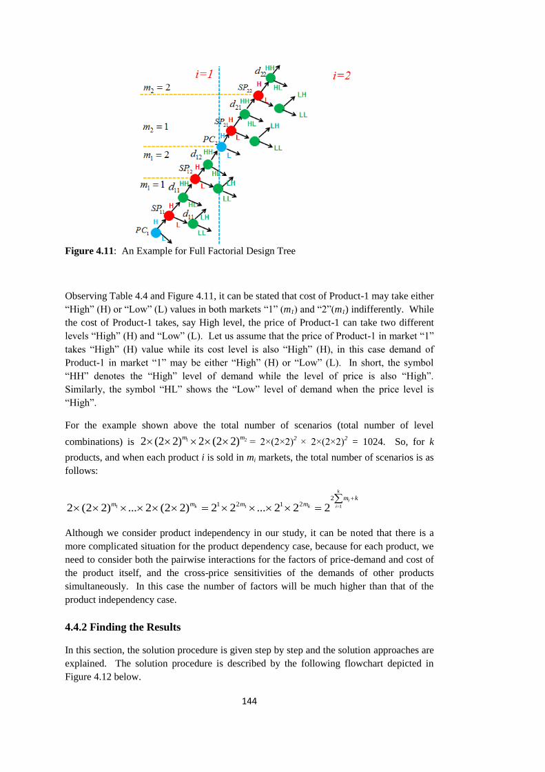
144

Figure 4.11: An Example for Full Factorial Design Tree

Observing Table 4.4 and Figure 4.11, it can be stated that cost of Product-1 may take either

“High” (H) or “Low” (L) values in both markets “1” (m1) and “2”(m1) indifferently. While

the cost of Product-1 takes, say High level, the price of Product-1 can take two different

levels “High” (H) and “Low” (L). Let us assume that the price of Product-1 in market “1”

takes “High” (H) value while its cost level is also “High” (H), in this case demand of

Product-1 in market “1” may be either “High” (H) or “Low” (L). In short, the symbol

“HH” denotes the “High” level of demand while the level of price is also “High”.

Similarly, the symbol “HL” shows the “Low” level of demand when the price level is

“High”.

For the example shown above the total number of scenarios (total number of level

combinations) is 1 22 (2 2) 2 (2 2)m m

= 2×(2×2)2

× 2×(2×2)2 = 1024. So, for k

products, and when each product i is sold in mi markets, the total number of scenarios is as

follows:

11 1

2221 12 (2 2) ... 2 (2 2) 2 2 ... 2 2 2

k

i

k k i

m km mm m

Although we consider product independency in our study, it can be noted that there is a

more complicated situation for the product dependency case, because for each product, we

need to consider both the pairwise interactions for the factors of price-demand and cost of

the product itself, and the cross-price sensitivities of the demands of other products

simultaneously. In this case the number of factors will be much higher than that of the

product independency case.

4.4.2 Finding the Results

In this section, the solution procedure is given step by step and the solution approaches are

explained. The solution procedure is described by the following flowchart depicted in

Figure 4.12 below.

145

Figure 4.12: The Solution Procedure

In order to generate scenarios, we consider two levels for each factor, and a full factorial

design of experiment is used. The first three steps in the solution procedure are described

in detail in the previous section of the probabilistic model. So, we continue to explain the

solution procedure with the fourth step, namely generation of scenarios. The scenario

matrix is shown in Table 4.5.

Table 4.5: Full Factorial DOE-Scenario Matrix

146

The total number of experiments (runs) in scenario matrix is . These are the

structured scenarios. Extreme (unstructured) scenarios (n*) can be added to the structured

scenarios to obtain more alternative solutions (Table 4.6).

Table 4.6: Combined Scenario Matrix

Next, under each scenario the product mix problem is solved by using deterministic

product mix model and optimal solution set is found for every scenario. Table 4.7 shows

these results.

Table 4.7: Optimal Solutions under the Scenarios

1

2

2

k

i

i

m k

n

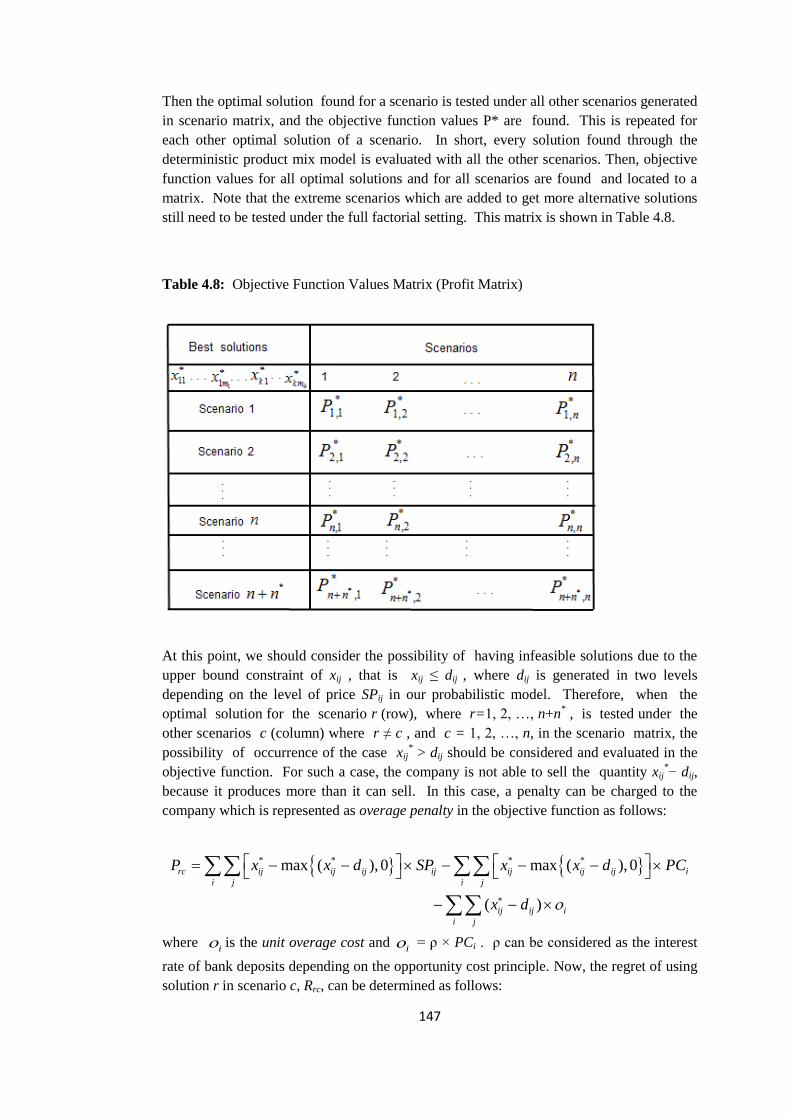
147

Then the optimal solution found for a scenario is tested under all other scenarios generated

in scenario matrix, and the objective function values P* are found. This is repeated for

each other optimal solution of a scenario. In short, every solution found through the

deterministic product mix model is evaluated with all the other scenarios. Then, objective

function values for all optimal solutions and for all scenarios are found and located to a

matrix. Note that the extreme scenarios which are added to get more alternative solutions

still need to be tested under the full factorial setting. This matrix is shown in Table 4.8.

Table 4.8: Objective Function Values Matrix (Profit Matrix)

At this point, we should consider the possibility of having infeasible solutions due to the

upper bound constraint of xij , that is xij ≤ dij , where dij is generated in two levels

depending on the level of price SPij in our probabilistic model. Therefore, when the

optimal solution for the scenario r (row), where r=1, 2, …, n+n* , is tested under the

other scenarios c (column) where r ≠ c , and c = 1, 2, …, n, in the scenario matrix, the

possibility of occurrence of the case xij* > dij should be considered and evaluated in the

objective function. For such a case, the company is not able to sell the quantity xij*− dij,

because it produces more than it can sell. In this case, a penalty can be charged to the

company which is represented as overage penalty in the objective function as follows:

where i is the unit overage cost and

i = ρ × PCi . ρ can be considered as the interest

rate of bank deposits depending on the opportunity cost principle. Now, the regret of using

solution r in scenario c, Rrc, can be determined as follows:

* * * *max ( ), 0 max ( ), 0

( )

rc ij ij ij ij ij ij ij i

i j i j

ij ij i

i j

P x x d SP x x d PC

x d

148

Rrc = P*cc – Prc , and since P

*rc = Prc for r = c, Rrc = 0.

New results can be shown in a regret matrix presented in Table 4.9.

Table 4.9: Regret Matrix with Maximum Regrets

4.4.3 Determining Optimal Product Mix

Optimal product mix can be found by using the following performance criteria:

1. Minimax Regret Criterion:

The concept of regret is based on the lost opportunities. Once the regret matrix is obtained

(see Table 4.8) the minimax criterion is applied that advices to take the maximum value of

each row and then choose the solution which gives minimum of the row maximums

(Ravindran, 2008).

2. Signal-to-Noise Ratio of Regret Values:

Taguchi proposes a summary statistic which combines information about the mean and

variance, called signal-to-noise ratio (SNR) (Montgomery, 2009; p. 490). For a smaller-

the-better measure such as regret, Signal-to-Noise Ratio is defined in such a way that a

maximum value of the ratio minimizes the mean as well as variability transmitted from the

noise variables. The formula of Signal-to-Noise ratio of regret values is as follows:

2 2

1010log ( )R R RSNR where R is the mean of the regret values, and 2

R is the

variance of regret values.

149

3. Signal-to-Noise Ratio of Regret Free Profit (P-R) Values:

We propose an SNR measure for regret free profit values (P−R) in order to protect against

a solution at which both regret and profit values are high. In such a case, the decision

maker can be in a trade-off situation that a higher value of profit may be attainable with a

higher value of regret. Subtracting the regret values from the corresponding profit values,

we first obtain the mean square reciprocal of the regret free profits. Then the SNR

measure for the regret free profit ( P RSNR ) is given as follows:

2

10 102 2 21

1 1 110log 10log 1 3

( )

nP R

P R

j ij ij P R P R

SNRn P R

where n is the total number of structured scenarios, P R is the mean value of regret free

profits and 2

P R is the variance of regret free profit values. The second part of this

equation can be claimed based on Phadke (1989, p.111). This is a larger-the-better type of

a measure, and maximization of it requires that P R is maximized while 2

P R is

minimized.

A a result, the optimal product mix with the smallest maximum regret and/or the best SNRR

and/or SNRP-R value can be chosen according to these approaches.

Some statistics are generated for the measures of regrets, profits and regret free profits. An

example of these statistics is shown in Table 4.10 for the regret values.

Table 4.10: Regret Data

The final three columns of Table 4.10 represent the estimates for the first three moments of

the random variable Regret. These estimates are obtained from systematic sampling as

mentioned before. Regret values are the results obtained from the objective functions

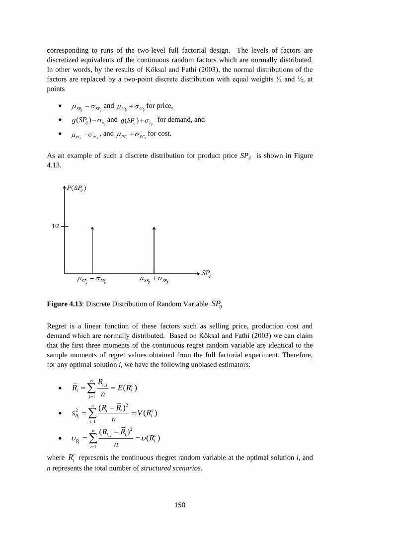
150

corresponding to runs of the two-level full factorial design. The levels of factors are

discretized equivalents of the continuous random factors which are normally distributed.

In other words, by the results of Köksal and Fathi (2003), the normal distributions of the

factors are replaced by a two-point discrete distribution with equal weights ½ and ½, at

points

ij ijSP SP and

ij ijSP SP for price,

( )ijijg SP and ( )

ijijg SP for demand, and

i iPC PC , and

i iPC PC for cost.

As an example of such a discrete distribution for product price SPij is shown in Figure

4.13.

Figure 4.13: Discrete Distribution of Random Variable ijSP

Regret is a linear function of these factors such as selling price, production cost and

demand which are normally distributed. Based on Köksal and Fathi (2003) we can claim

that the first three moments of the continuous regret random variable are identical to the

sample moments of regret values obtained from the full factorial experiment. Therefore,

for any optimal solution i, we have the following unbiased estimators:

,

1

( )n

i j c

i i

j

RR E R

n

22

1

( )( )

i

nci i

R i

i

R Rs V R

n

3

,

1

( )( )

i

ni j i c

R i

i

R RR

n

where c

iR represents the continuous rbegret random variable at the optimal solution i, and

n represents the total number of structured scenarios.

151

Let us consider the example illustrated in Figure 4.11. In this case, for two products (k =2)

where each product is sold in two markets (m1=1,2 and m2=1,2), the total number of

structured scenarios is n = 1024 and the total number of factors in the experiments is

2 (m1 + m2) + k = 2(4) + 2 = 10.

Using the Bayes Theorem of conditional probabilities, we can write

1024

,1024 1024 1024110 10

, , ,

1 1 1

1 1 1( ) ( ) ( )

2 2 1024 1024

i j

j

i j i j i j i

j j j

R

E R R R R R

Note that 1

21( ) 12

k

i

i

m k

n

, and 1

21( )2

k

i

i

m k

ip

which is the probability of occurrence

of scenario i. As it can be observed from Table 4.9, extreme scenarios are excluded for the

calculation of the moments of the regret values, since these scenarios are assumed to have

zero probability in the experimental setup based on two-level discretization of the factors

and inclusion of them may cause the bias and disturb the distributional assumptions of the

factors.

The final step in our methodology is to obtain experimental results with these three

approaches and to analyze them to get the best solution to the problem. A MATLAB code

was written to conduct all these experiments and collect the necessary regret and SNR data

(Appendix D). Experimental results and the suggested approaches for various different

numerical cases are presented in Chapter 5.

153

CHAPTER 5

EXPERIMENTAL RESULTS

This chapter covers the numerical examples and their experimental results that are

presented to show the implementation of the methodology developed to solve the product

mix problem under uncertainty. First, the cases studied in the examples are described

including the formulation of the scenarios. Next, numerical results are presented for these

cases showing the stages of the methodology. Finally, the results are analyzed and

discussed.

5.1 DESCRIPTION OF THE CASES STUDIED

During the field study conducted in this research and developing the proposed framework

for product management, we have had several contacts with the experts in Company D

operating in “consumer durables” sector. These discussions contributed a lot to construct

the DSS developed to solve the product mix problem under uncertainty in the product

management framework. The information obtained in these contacts helped to clarify the

product aggregation schemes, the product and market profiles in formulating and modeling

the research problem. Due to this familiarity, we prefer to consider a typical manufacturer

operating in “consumer durables” sector to get the numerical results for the developed

methodology in our study.

Before passing to the description of the specific cases, let us describe a general company

case, focusing on the product and market profiles which constitute the base scenario. Note

that this description does not reflect the real case for the Company D.

Base Case Description:

Base case simply describes the existing conditions of the company regarding the product

mix problem under uncertainty. Let us suppose that the company has the product mix

which is composed of two broad lines;

Major Household Appliances (White Goods)

Small Household Appliances

It is known that each product line has several families, and each family has several groups

which are composed of hundreds of variants. Although our research problem considers the

determination of “family mix” under uncertainty, the strategic product mix composed of

product lines can also be studied with the methodology developed in this research study.

Thus, the following product scheme of the company (Figure 5.1) is considered in

154

formulating the scenarios for the experiments. Note that we consider the families of

“White Goods” line in the numerical examples, therefore the families of “Small Household

Appliances” are not shown in Figure 5.1.

Figure 5.1: Product Hierarchy Illustration for Numerical Example

We assume two broad classifications for market structure of the company; National and

Global. This market structure can be detailed depending on the purpose of the analysis.

For instance, Company D is a market leader with more than 50% market share in national

market. Uncertainty of the national market is relatively lower than the uncertainty in

global market regarding the product prices, production costs and demands for the products.

In spite of this, some of the products may be quite sensitive to some demographic

indicators in the national market, like income levels. We have learned that the freezers in

Cold family and dish washers in Wet family are sensitive products in the national market

in the sense that customers can easily sacrifice these products in crisis periods of the

economy. If a deeper analysis is required, the national market can be disaggregated into

sub-segments, like “High Income”, “Average Income” and “Low Income” segments.

Similarly, global market can be subdivided into several segments depending on the

purpose of the formulation of the scenario. Actually, Company D sells its products in

more than 70 countries other than Turkey. For example, 64% of the total production of

refrigerators is sold to 70 countries. However, it was also learnt that more than 80% of

global selling activities is realized in 5 big markets. In such a case, these countries can be

restructured as the regions which can provide reasonable and satisfactory consolidation for

the global market in terms of total sales. As an example, Company D considers the

following regions in its global market structure:

West Europe: Italy, Spain, Germany, France, United Kingdom, Belgium

East Europe : Russia, Poland, Romania, Ukraine, Lithuania

Other : South Africa, etc.

So, the following product-market relations are considered in the experiments:

155

Table5.1-a: Illustrative Product-Market Relations for Product Lines

Product Line

National Market Global Market

Major Household

Appliances

(White Goods)

Small Household

Appliances

Table 5.1-b: Illustrative Product-Market Relations for Families of White Goods

Families of White Goods

National Market Global Market

HOT COLD WET

The product-market matrix will be provided separately for each case in numerical results.

As mentioned before, both MTS and MTO manufacturing environments can be studied in

the proposed DSS. Depending on the specific case under consideration, some

modifications can be employed in the deterministic product mix model when necessary. In

fact, many firms may serve a combination of these environments in real life. This is the

case in Company D. It is known that although Company D keeps both component and

finished item inventories, the levels of these inventories are not at the significant levels.

The Company D expert stated that the major underlying reason is the powerful supply

chain activities and distribution system. It is also understood that globalization has forced

Company D to establish stronger supply chain and distribution systems.

Formulation of the Scenarios:

In order to provide the numerical results for the developed methodology, we consider

several cases in formulating the scenarios. Note that these cases do not limit the

applicability of the methodology, but just aim at showing the working mechanism of DSS

by means of some descriptive cases. The cases are as follows:

1. Product Mix Example with 2 Product Lines

2. Family Mix Example with 3 Families

3. Different Candidate Products Set Example with 2 Product Lines

4. Volatile Market Conditions Example with 2 Product Lines

5. New Market Entrance Example with 2 Product Lines

Product Mix and Family Mix examples describe simply the existing conditions of the

company. The company may study the performance of the company with its existing

products for the coming fiscal period by means of our methodology. So, the methodology

156

can be applied for budgeting purposes for these cases. These examples provide also a

basis for the other numerical examples.

By introducing different candidate products sets, the following decision making cases can

be studied by means of the developed methodology:

a) To support “Time-to-Market” decision

b) To support “Outsourcing” decision

Time-to-market decision is closely related to the “Prioritization” decision and

“Cannibalization” issue in Product Management. Regarding the product mix problem in

this framework, considering the different sets of candidate products in the proposed DSS

supports this decision. The company may consider different product projects for the

coming period and test their profitability by constituting different sets of candidate

products accordingly. For this purpose, mean values and variances of the prices and the

production costs of the products should be reconsidered in the targeted market(s).

Considering different sets of candidate products may require considering the impact of

new product introduction to the production side of the company. This issue is briefly

discussed in the final section.

On the other hand, the analysis of “Make versus Buy” can be done by means of the

proposed DSS considering the different sets candidate products. Our model used in the

proposed DSS determines the products produced in-house. Therefore, the company is able

to evaluate the case “Make” by using the proposed approach. Then, the optimum quantities

determined by the model can be analyzed for the option “Buy” spending some additional

efforts. Thus, outsourcing decision is supported under uncertainty conditions of product

prices, costs and demand values.

Volatile market conditions require considering higher uncertainty in the market in terms of

product prices of competitors and instability of the customers’ demands. These conditions

can be reflected by the higher variances of product prices and demands. In addition to

higher variances of product prices and demands, variances of product costs can also be

higher than those at a stable market due to the frequently changeable prices of the

suppliers. So, this case is formulated by introducing higher values of variances of the three

parameters in the market(s) which is (are) considered as volatile.

Entrance of a new market requires considering higher uncertainty for the existing products

of the company for the desired market under consideration. This issue can be handled by

the proposed DSS introducing higher values of variances of product prices and so the

demand values for the targeted market.

5.2 NUMERICAL RESULTS

Suppose that the company has the product scheme shown in Figure 5.1. The existing

product-market profile of the company is assumed as the illustrative cases shown in Table

5.1-a and Table 5.1-b for the product line mix description and the family mix description,

respectively. The data required to obtain the numerical results are established through

157

internet searches and the discussions with the PM expert of Company D. The numerical

results are presented in the format of the methodology stages of the experiments. For the

purpose of brevity and convenience, we present Example 1, which is the case with the

smallest size, in accordance with this format in detail. The output obtained via MATLAB

for this case is provided in Appendix E. The results for the other numerical examples are

presented in some appropriate summary tables. Note that all the results are reproducible

by the data given below for each example and the MATLAB code provided in Appendix

D.

EXAMPLE 1: Product Mix Example with 2 Product Lines

This example describes the existing conditions of the company.

Parameters:

k=2 (White Goods (WG), Small Household Appliances (SHA))

m1 =1,2 and m2 =1 (“1”: National market (N), “2”: Global market (G))

Product-Market Matrix (H)

1 1

1 0

H

Product Prices ( ijSP ): (Average prices for each product line at each market)

2~ ( , )

ij ijij SP SPSP N

ijSP (TL) j= 1

(N)

j= 2

(G)

i= 1(WG) 1 580 1 975

i =2 (SHA) 190 0

where it is assumed that 2 0.10

ij ijSP SP .

2

ijSP (TL) j= 1

(N)

j= 2

(G)

i= 1 (WG) 158 197.5

i =2 (SHA) 19 0

Demand ( ijd ):

2

,( ) , ~ (0, )ijij ij ij ii j ij ij ijd SP b a SP N

where 2

,0.10 , ( )ij ij ijd d ij ij ii j ijg SP b a SP

ijb (units)

(intercept)

j= 1

(N)

j= 2

(G)

i= 1 (WG) 11 200 13 400

i =2 (SHA) 4 800 0

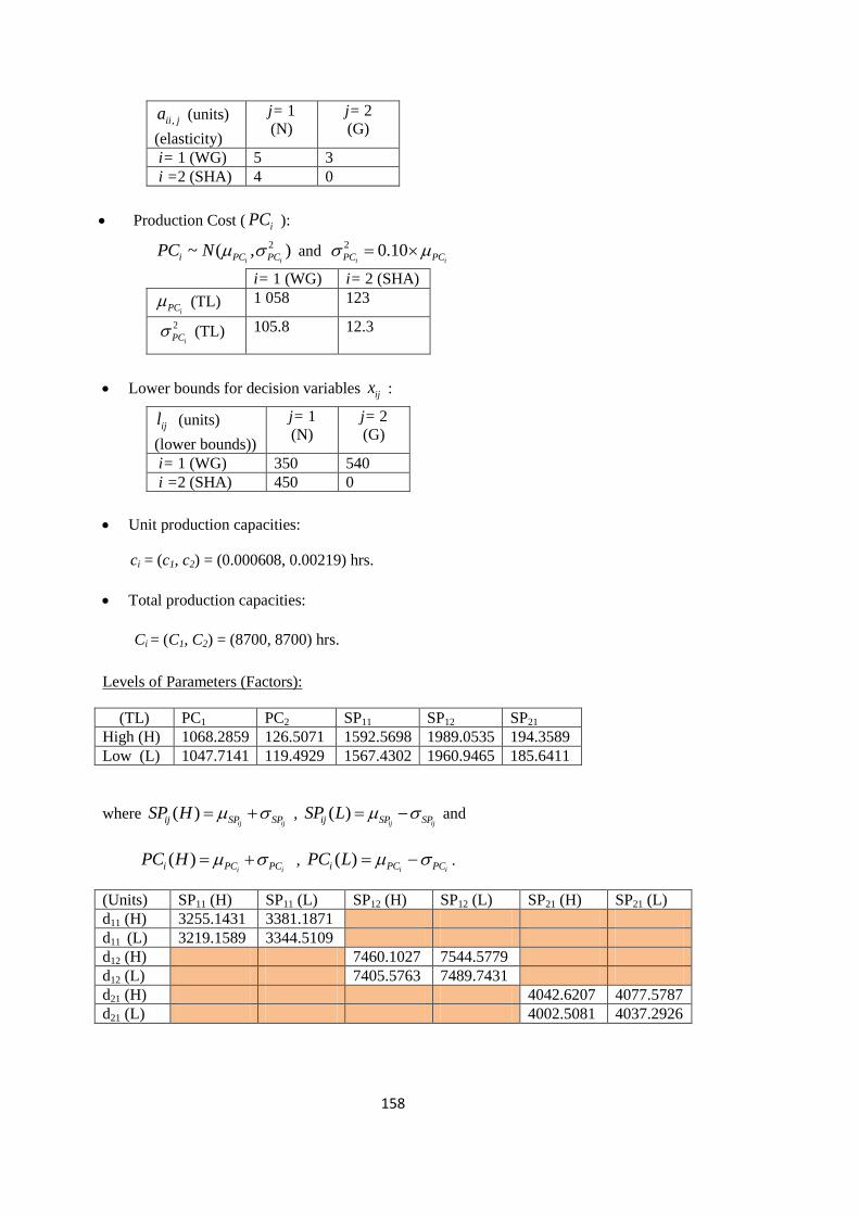
158

,ii ja (units)

(elasticity)

j= 1

(N)

j= 2

(G)

i= 1 (WG) 5 3

i =2 (SHA) 4 0

Production Cost ( iPC ):

2~ ( , )

i ii PC PCPC N and 2 0.10

i iPC PC

i= 1 (WG) i= 2 (SHA)

iPC (TL) 1 058 123

2

iPC (TL) 105.8

12.3

Lower bounds for decision variables ijx :

ijl (units)

(lower bounds))

j= 1

(N)

j= 2

(G)

i= 1 (WG) 350 540

i =2 (SHA) 450 0

Unit production capacities:

ci = (c1, c2) = (0.000608, 0.00219) hrs.

Total production capacities:

Ci = (C1, C2) = (8700, 8700) hrs.

Levels of Parameters (Factors):

(TL) PC1 PC2 SP11 SP12 SP21

High (H) 1068.2859 126.5071 1592.5698 1989.0535 194.3589

Low (L) 1047.7141 119.4929 1567.4302 1960.9465 185.6411

where ( )ij ijij SP SPSP H , ( )

ij ijij SP SPSP L and

( )i ii PC PCPC H , ( )

i ii PC PCPC L .

(Units) SP11 (H) SP11 (L) SP12 (H) SP12 (L) SP21 (H) SP21 (L)

d11 (H) 3255.1431 3381.1871

d11 (L) 3219.1589 3344.5109

d12 (H) 7460.1027 7544.5779

d12 (L) 7405.5763 7489.7431

d21 (H) 4042.6207 4077.5787

d21 (L) 4002.5081 4037.2926

159

where ( ) ( )ijij ijd H g SP , ( ) ( )

ijij ijd L g SP and ,( )ij ij ii j ijg SP b a SP ,

2 0.10 ( )ij ijg SP .

Number of Structured Scenarios:

1 1 2

22( ) 2(3) 2 82 2 2 2 256

k

i

i

m km m k

n

Scenario Matrix: See Table 5.2.

Optimal Solutions under each Scenario: See Table 5.3.

Profit Matrix: See Table 5.4.

Regret Matrix: See Table 5.5.

Regret Data: See Table 5.6.

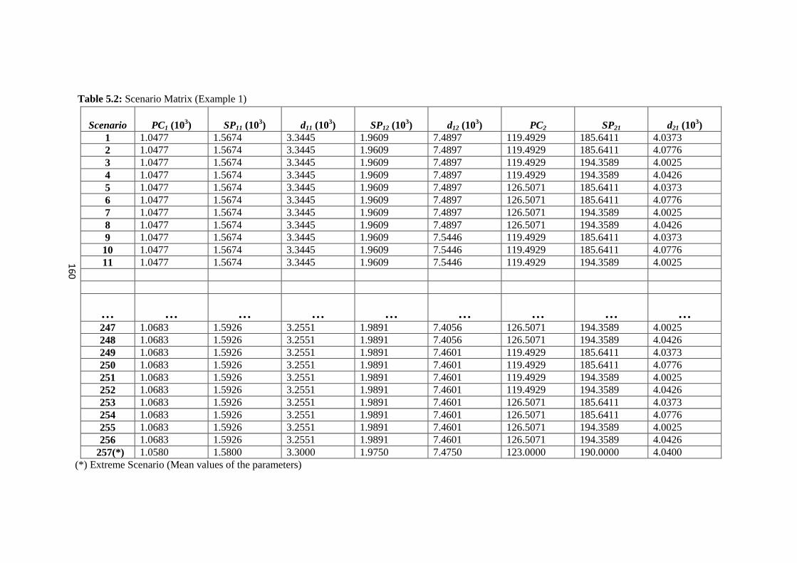
16

0

Table 5.2: Scenario Matrix (Example 1)

Scenario

PC1 (103)

SP11 (103)

d11 (103)

SP12 (103)

d12 (103)

PC2

SP21

d21 (103)

1 1.0477 1.5674 3.3445 1.9609 7.4897 119.4929 185.6411 4.0373

2 1.0477 1.5674 3.3445 1.9609 7.4897 119.4929 185.6411 4.0776

3 1.0477 1.5674 3.3445 1.9609 7.4897 119.4929 194.3589 4.0025

4 1.0477 1.5674 3.3445 1.9609 7.4897 119.4929 194.3589 4.0426

5 1.0477 1.5674 3.3445 1.9609 7.4897 126.5071 185.6411 4.0373

6 1.0477 1.5674 3.3445 1.9609 7.4897 126.5071 185.6411 4.0776

7 1.0477 1.5674 3.3445 1.9609 7.4897 126.5071 194.3589 4.0025

8 1.0477 1.5674 3.3445 1.9609 7.4897 126.5071 194.3589 4.0426

9 1.0477 1.5674 3.3445 1.9609 7.5446 119.4929 185.6411 4.0373

10 1.0477 1.5674 3.3445 1.9609 7.5446 119.4929 185.6411 4.0776

11 1.0477 1.5674 3.3445 1.9609 7.5446 119.4929 194.3589 4.0025

…

…

…

…

…

…

…

…

…

247 1.0683 1.5926 3.2551 1.9891 7.4056 126.5071 194.3589 4.0025

248 1.0683 1.5926 3.2551 1.9891 7.4056 126.5071 194.3589 4.0426

249 1.0683 1.5926 3.2551 1.9891 7.4601 119.4929 185.6411 4.0373

250 1.0683 1.5926 3.2551 1.9891 7.4601 119.4929 185.6411 4.0776

251 1.0683 1.5926 3.2551 1.9891 7.4601 119.4929 194.3589 4.0025

252 1.0683 1.5926 3.2551 1.9891 7.4601 119.4929 194.3589 4.0426

253 1.0683 1.5926 3.2551 1.9891 7.4601 126.5071 185.6411 4.0373

254 1.0683 1.5926 3.2551 1.9891 7.4601 126.5071 185.6411 4.0776

255 1.0683 1.5926 3.2551 1.9891 7.4601 126.5071 194.3589 4.0025

256 1.0683 1.5926 3.2551 1.9891 7.4601 126.5071 194.3589 4.0426

257(*) 1.0580 1.5800 3.3000 1.9750 7.4750 123.0000 190.0000 4.0400

(*) Extreme Scenario (Mean values of the parameters)

16

1

Table 5.3: Optimal Solutions under Each Scenario (Example 1)

Scenario

*

11x (103 units) *

12x (103 units) *

21x (103 units) Profit (10

6 TL.)

1 3.3445 7.4897 4.0373 8.8451

2 3.3445 7.4897 4.0776 8.8478

3 3.3445 7.5446 4.0025 8.8777

4 3.3445 7.5446 4.0426 8.8807

5 3.3445 7.5446 4.0373 8.8168

6 3.3445 7.5446 4.0776 8.8192

7 3.3445 7.5446 4.0025 8.8496

8 3.3445 7.5446 4.0426 8.8524

9 3.3445 7.5446 4.0373 8.8952

10 3.3445 7.5446 4.0776 8.8979

…

…

…

…

…

247 3.2551 7.4056 4.0025 8.7970

248 3.2551 7.4056 4.0426 8.7997

249 3.2551 7.4601 4.0373 8.8427

250 3.2551 7.4601 4.0776 8.8454

251 3.2551 7.4601 4.0025 8.8753

252 3.2551 7.4601 4.0426 8.8783

253 3.2551 7.4601 4.0373 8.8144

254 3.2551 7.4601 4.0776 8.8168

255 3.2551 7.4601 4.0025 8.8472

256 3.2551 7.4601 4.0426 8.8499

257 (*) 3.3000 7.4750 4.0400 8.8479

(*) Extreme scenario solution

16

2

Table 5.4: Profit Matrix (106 TL.) (Example 1)

Scenario 1 2 3 4 5 … 252 253 254 255 256

1 8.8451 8.8451 8.8734 8.8803 8.8168 … 8.7444 8.6809 8.6809 8.7091 8.7161

2 8.8401 8.8478 8.8683 8.8763 8.8115 … 8.7404 8.6755 8.6833 8.7038 8.7118

3 8.8428 8.8428 8.8777 8.8777 8.8148 … 8.7418 8.6788 8.6788 8.7137 8.7137

4 8.8445 8.8455 8.8727 8.8807 8.8161 … 8.7448 8.6802 8.6812 8.7084 8.7164

5 8.8451 8.8451 8.8734 8.8803 8.8168 … 8.7444 8.6809 8.6809 8.7091 8.7161

6 8.8401 8.8478 8.8683 8.8763 8.8115 … 8.7404 8.6755 8.6833 8.7038 8.7118

7 8.8428 8.8428 8.8777 8.8777 8.8148 … 8.7418 8.6788 8.6788 8.7137 8.7137

8 8.8445 8.8455 8.8727 8.8807 8.8161 … 8.7448 8.6802 8.6812 8.7084 8.7164

9 8.7848 8.7848 8.8130 8.8200 8.7565 … 8.6829 8.6194 8.6194 8.6476 8.6546

10 8.7798 8.7875 8.8080 8.8160 8.7511 … 8.6789 8.6140 8.6218 8.6422 8.6503

… … … … … … … … … … … …

248 8.7212 8.7222 8.7494 8.7574 8.6928 … 8.8281 8.7635 8.7645 8.7917 8.7997

249 8.7716 8.7716 8.7998 8.8068 8.7433 … 8.8779 8.8144 8.8144 8.8426 8.8496

250 8.7666 8.7743 8.7948 8.8028 8.7379 … 8.8739 8.8090 8.8168 8.8372 8.8453

251 8.7693 8.7693 8.8042 8.8042 8.7412 … 8.8753 8.8123 8.8123 8.8472 8.8472

252 8.7709 8.7702 8.7992 8.8072 8.7426 … 8.8783 8.8137 8.8147 8.8419 8.8499

253 8.7716 8.7716 8.7998 8.8068 8.7433 … 8.8779 8.8144 8.8144 8.8426 8.8496

254 8.7666 8.7743 8.7948 8.8028 8.7379 … 8.8739 8.8090 8.8168 8.8372 8.8453

255 8.7693 8.7693 8.8042 8.8042 8.7412 … 8.8753 8.8123 8.8123 8.8472 8.8472

256 8.7709 8.7720 8.7992 8.8072 8.7426 … 8.8783 8.8137 8.8147 8.8419 8.8499

257 (*) 8.7195 8.7195 8.7544 8.7544 8.6914 … 8.8111 8.7470 8.7475 8.7752 8.7827

(*): Profit value of extreme scenario

16

3

Table 5.5: Regret Matrix (Example 1)

Scenario 1 2 3 4 … 253 254 255 256

1 0 2.6649×103

4.3643×103

398.9025 … 1.3349×105

1.3587×105

1.3811×105 1.3385×10

5

2 5.0546×103

0 9.4189×103

4.3861×103

… 1.3884×105 1.3349×10

5 1.4346×10

5 1.3813×10

5

3 2.3009×103

4.9658×103

0 3.0031×103

… 1.3555×105 1.3793×10

5 1.3349×10

5 1.3621×10

5

4 668.5181 2.3124×103

5.0328×103

0 … 1.3420×105 1.3556×10

5 1.3882×10

5 1.3349×10

5

5 3.2969×10-7

2.6649×103 4.3643×10

3 398.9025 … 1.3349×10

5 1.3587×10

5 1.3811×10

5 1.3385×10

5

6 5.0546×103 3.4086×10

-7 9.4189×10

3 4.3861×10

3 … 1.3884×10

5 1.3349×10

5 1.4346×10

5 1.3813×10

5

7 2.3009×103 4.9658×10

3 1.7695×10

-7 3.0031×10

3 … 1.3555×10

5 1.3793×10

5 1.3349×10

5 1.3621×10

5

8 668.5181 2.3124×103 5.0328×10

3 1.7881×10

-7

… 1.3420×105 1.3556×10

5 1.3882×10

5 1.3349×10

5

9 6.0324×104

6.2989×104

6.4688×104

6.0723×104

… 1.9500×105 1.9738×10

5 1.9962×10

5 1.9536×10

5

10 6.5378×104

6.0324×104

6.9743×104

6.4710×104

… 2.0035×105 1.9500×10

5 2.0497×10

5 1.9964×10

5

… … … … … … … … … … 248 1.2398×10

5 1.2562×10

5 1.2834×10

5 1.2331×10

5 … 5.0914×10

4 5.2273×10

4 5.5534×10

4 5.0206×10

4

249 7.3514×104 7.6179×10

4 7.7879×10

4 7.3913×10

4 … -3.1106×10

-7 2.3823×10

3 4.6205×10

3 361.5289

250 7.8569×104 7.3514×10

4 8.2933×10

4 7.7900×10

4 … 5.3513×10

3 -3.2037×10

-7 9.9718×10

3 4.6435×10

3

251 7.5815×104 7.8480×10

4 7.3514×10

4 7.6517×10

4 … 2.0569×10

3 4.4392×10

3 -1.6950×10

-7 2.7217×10

3

252 7.4183×104 7.5827×10

4 7.8547×10

4 7.3514×10

4 … 707.7604 2.0672×10

3 5.3283×10

3 -1.7323×10

-7

253 7.3514×104 7.6179×10

4 7.7879×10

4 7.3913×10

4 … 0 2.3823×10

3 4.6205×10

3 361.5289

254 7.8569×104 7.3514×10

4 8.2933×10

4 7.7900×10

4 … 5.3513×10

3 0 9.9718×10

3 4.6435×10

3

255 7.5815×104 7.8480×10

4 7.3514×10

4 7.6517×10

4 … 2.0569×10

3 4.4392×10

3 0 2.7217×10

3

256 7.4183×104 7.5827×10

4 7.8547×10

4 7.3514×10

4 … 707.7604 2.0672×10

3 5.3283×10

3 0

257(*) 3.6937×104 3.9083×10

4 4.1301×10

4 3.6793×10

4 … 6.7386×10

4 6.9248×10

4 7.2006×10

4 6.7204×10

4

(*): Regret values of extreme scenario

16

4

Table 5.6: Regret Data (Example 1)

Scenario

Maximum

Regrets

Mean of Regrets Standard Deviation

of Regrets

Regret SNR

(SNRR)

Skewness of

Regrets

Regret Free

Profit SNR

(SNRP-R)

1 2.3964×105 1.1014×10

5 6.6359×10

4 -235.2868 0.1189 319.3943

2 2.4499×105 1.1314×10

5 6.6424×10

4 -235.6895 0.1185 319.3803

3 2.3998×105 1.1073×10

5 6.6356×10

4 -235.3647 0.1189 319.3915

4 2.4035×105 1.1030×10

5 6.6364×10

4 -235.3093 0.1189 319.3935

5 2.3964×105 1.1014×10

5 6.6359×10

4 -235.2868 0.1189 319.3943

6 2.4499×105 1.1314×10

5 6.6424×10

4 -235.6895 0.1185 319.3803

7 2.3998×105 1.1073×10

5 6.6356×10

4 -235.3647 0.1189 319.3915

8 2.4035×105 1.1030×10

5 6.6364×10

4 -235.3093 0.1189 319.3935

9 3.0115×105 1.4345×10

5 7.9912×10

4 -240.1773 0.0500 319.2375

10 3.0650×105

1.4645×105 7.9965×10

4 -240.4983 0.0499 319.2235

… … … … … … …

247 1.9741×105 1.0293×10

5 5.1003×10

4 -233.0322 -0.0731 319.4249

248 1.9778×105 1.0251×10

5 5.1014×10

4 -232.9672 -0.0730 319.4269

249 1.4727×105 8.0180×10

4 3.7812×10

4 -227.8488 -0.2392 319.5337

250 1.5262×105 8.3185×10

4 3.7925×10

4 -228.4648 -0.2371 319.5199

251 1.4762×105 8.0767×10

4 3.7806×10

4 -227.9677 -0.2393 319.5310

252 1.4798×105 8.0346×10

4 3.7821×10

4 -227.8834 -0.2390 319.5330

253 1.4727×105 8.0180×10

4 3.7812×10

4 -227.8488 -0.2392 319.5337

254 1.5262×105 8.3185×10

4 3.7925×10

4 -228.4648 -0.2371 319.5199

255 1.4762×105 8.0767×10

4 3.7806×10

4 -227.9677 -0.2393 319.5310

256 1.4798×105 8.0346×10

4 3.7821×10

4 -227.8834 -0.2390 319.5330

257

(*)

1.7353×105 9.5304×10

4 3.7273×10

4 -230.7197 0.2104 319.4659

(*) Extreme scenario

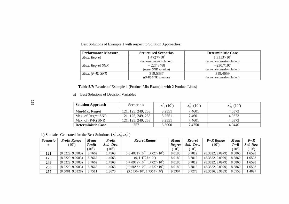
16

5

Best Solutions of Example 1 with respect to Solution Approaches:

Performance Measure Structured Scenarios Deterministic Case

Max. Regret 1.4727×105

(min-max regret solution)

1.7353×105

(extreme scenario solution)

Max. Regret SNR − 227.8488 (regret SNR solution)

−230.7197 (extreme scenario solution)

Max. (P-R) SNR

319.5337 ((P-R) SNR solution)

319.4659 (extreme scenario solution)

Table 5.7: Results of Example 1 (Product Mix Example with 2 Product Lines)

a) Best Solutions of Decision Variables

b) Statistics Generated for the Best Solutions * * *

11 12 21( , , )x x x

Scenario

Profit Range

(106)

Mean

Profit

(106)

Profit

Std. Dev.

(105)

Regret Range

Mean

Regret (10

4)

Regret

Std. Dev.

(104)

P−R Range

(106)

Mean

P−R (10

6)

P−R

Std. Dev. (10

5)

121 (8.5229, 9.0983) 8.7662 1.4563 (−3.4831×10-7

, 1.4727×105) 8.0180 3.7812 (8.3822, 9.0979) 8.6860 1.6528

125 (8.5229, 9.0983) 8.7662 1.4563 (0, 1.4727×105) 8.0180 3.7812 (8.3822, 9.0979) 8.6860 1.6528

249 (8.5229, 9.0983) 8.7662 1.4563 (−4.0978×10-7

, 1.4727×105) 8.0180 3.7812 (8.3822, 9.0979) 8.6860 1.6528

253 (8.5229, 9.0983) 8.7662 1.4563 (−9.6858×10-8

, 1.4727×105) 8.0180 3.7812 (8.3822, 9.0979) 8.6860 1.6528

257 (8.5081, 9.0328) 8.7511 1.3670 (3.5556×104, 1.7353×10

5) 9.5304 3.7273 (8.3536, 8.9839) 8.6558 1.4897

Solution Approach Scenario *

11x (103)

*

12x (103)

*

21x (103)

Min-Max Regret 121, 125, 249, 253 3.2551 7.4601 4.0373

Max. of Regret SNR 121, 125, 249, 253 3.2551 7.4601 4.0373

Max. of (P-R) SNR 121, 125, 249, 253 3.2551 7.4601 4.0373

Deterministic Case 257 3.3000 7.4750 4.0440

166

EXAMPLE 2: Family Mix Example

This example describes the existing conditions of the company on family base of White

Goods product line.

Parameters:

k=3 ( HOT, COLD and WET Families)

m1 =1, m2 =1,2 and m3 = 1,2 (“1”: N and “2”: G)


01

1 1

1 1

H

Product Prices ( ):

2~ ( , )

ij ijij SP SPSP N and

(TL) j= 1

(N)

j= 2

(G)

i= 1 (HOT) 896 0

i =2 (COLD) 2224 2780

i =3 (WET) 1420 1775

(TL) j= 1

(N)

j= 2

(G)

i= 1 (HOT) 89.6 0

i =2 (COLD) 222.4 278.0

i =3 (WET) 142.0 177.5

Demand ( ):

2


2


ijb (units)

(intercept)

j= 1

(N)

j= 2

(G)

i= 1 (HOT) 3800 0

i =2 (COLD) 13700 14500

i =3 (WET) 6500 7200

ijSP

2 0.10ij ijSP SP

ijSP

2

ijSP

ijd

167

(units)

(elasticity)

j= 1

(N)

j= 2

(G)

i= 1 (HOT) 3 0

i =2 (COLD) 5 4

i =3 (WET) 4 3

Production Cost ( ):

2~ ( , )

i ii PC PCPC N and

i= 1 (HOT) i= 2 (COLD) i= 3 (WET)

(TL) 627.0 1334.0 923.0

(TL) 62.7

133.4 92.3

Lower bounds for decision variables :

(units)

(lower bounds))

j= 1

(N)

j= 2

(G)

i= 1 (HOT) 380 0

i =2 (COLD) 650 750

i =3 (WET) 420 500


ci = (c1, c2, c3) = (0.00438, 0.00122, 0.00168) hrs.


Ci = (C1, C2, C3) = (8700, 8700, 8700) hrs.


(TL) PC1 PC2 PC3

High (H) 634.9183 1345.5499 932.6030

Low (L) 619.0817 1322.4501 913.3927

(TL) SP11 SP21 SP22 SP31 SP32

High (H) 905.4657 2238.9131 2796.6733 1431.9164 1788.3229

Low (L) 886.5343 2209.0869 2763.3267 1408.0836 1761.6771

,ii ja

iPC

2 0.10i iPC PC

iPC

2

iPC

ijx

ijl

168

(Units) SP11 (H) SP11 (L)

d11 (H) 1094.0125 1151.0760

d11 (L) 1073.1933 1129.7182


d21 (H) 2521.2631 2670.8583

d21 (L) 2489.6059 2638.2727


d22 (H) 3331.5093 3465.2585

d22 (L) 3295.1043 3428.1279


d31 (H) 781.1227 876.9805

d31 (L) 763.5461 858.3507


d32 (H) 1848.5776 1928.5242

d32 (L) 1821.4850 1900.8498


1 1 2 3

22( ) 2(1 2 2) 2 122 2 2 2 8192

k

i

i

m km m m k

n




(min-max regret solution) 4.5609×10

5

3.8215×105


Max. Regret SNR −248.6079 (regret SNR solution)


Max. (P-R) SNR

320.2827 ((P-R) SNR solution)


16

9

Table 5.8: Results of Example 2 (Family Mix with 3 Families)



11x (103)

*

21x (103)

*

22x (103)

*

31x *

32x (103)

Min-Max Regret 8193 1.1120 2.5800 3.3800 820.0000 1.8750

Max. of Regret SNR 3472, 3488,3984, 4000 1.0940 2.5213 3.4281 781.1228 1.8486

7568, 7584, 8080, 8096 1.0940 2.5213 3.4281 781.1228 1.8486

Max. of (P-R) SNR 3568, 3584, 4080, 4096 1.0940 2.5213 3.3315 781.1228 1.8486 7664, 7680, 8176, 8192 1.0940 2.5213 3.3315 781.1228 1.8486 Deterministic Case 8193 1.1120 2.5800 3.3800 820.0000 1.8750

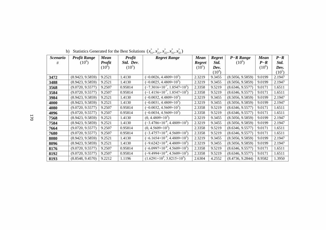
17

0

b) Statistics Generated for the Best Solutions * * * * *

11 21 22 31 32( , , , , )x x x x x

Scenario

Profit Range

(106)

Mean

Profit

(106)

Profit

Std. Dev.

(105)

Regret Range

Mean

Regret (10

5)

Regret

Std.

Dev.

(104)

P−R Range

(106)

Mean

P−R (10

6)

P−R

Std.

Dev. (10

5)

3472 (8.9423, 9.5859) 9.2521 1.4130 (−0.0026, 4.4809×105) 2.3219 9.3455 (8.5056, 9.5859) 9.0199 2.1947

3488 (8.9423, 9.5859) 9.2521 1.4130 (−0.0025, 4.4809×105) 2.3219 9.3455 (8.5056, 9.5859) 9.0199 2.1947

3568 (9.0720, 9.5577) 9.2507 0.95814 (−7.3016×10-7

, 1.8547×105) 2.3358 9.5219 (8.6346, 9.5577) 9.0171 1.6511

3584 (9.0720, 9.5577) 9.2507 0.95814 (−1.4156×10-7

, 1.8547×105) 2.3358 9.5219 (8.6346, 9.5577) 9.0171 1.6511

3984 (8.9423, 9.5859) 9.2521 1.4130 (−0.0032, 4.4809×105) 2.3219 9.3455 (8.5056, 9.5859) 9.0199 2.1947

4000 (8.9423, 9.5859) 9.2521 1.4130 (−0.0031, 4.4809×105) 2.3219 9.3455 (8.5056, 9.5859) 9.0199 2.1947

4080 (9.0720, 9.5577) 9.2507 0.95814 (−0.0032, 4.5609×105) 2.3358 9.5219 (8.6346, 9.5577) 9.0171 1.6511

4096 (9.0720, 9.5577) 9.2507 0.95814 (−0.0034, 4.5609×105) 2.3358 9.5219 (8.6346, 9.5577) 9.0171 1.6511

7568 (8.9423, 9.5859) 9.2521 1.4130 (0, 4.4809×105) 2.3219 9.3455 (8.5056, 9.5859) 9.0199 2.1947

7584 (8.9423, 9.5859) 9.2521 1.4130 (−3.4786×10-4

, 4.4809×105) 2.3219 9.3455 (8.5056, 9.5859) 9.0199 2.1947

7664 (9.0720, 9.5577) 9.2507 0.95814 (0, 4.5609×105) 2.3358 9.5219 (8.6346, 9.5577) 9.0171 1.6511

7680 (9.0720, 9.5577) 9.2507 0.95814 (−3.4757×10-4

, 4.5609×105) 2.3358 9.5219 (8.6346, 9.5577) 9.0171 1.6511

8080 (8.9423, 9.5859) 9.2521 1.4130 (−6.1654×10-4

, 4.4809×105) 2.3219 9.3455 (8.5056, 9.5859) 9.0199 2.1947

8096 (8.9423, 9.5859) 9.2521 1.4130 (−9.6242×10-4

, 4.4809×105) 2.3219 9.3455 (8.5056, 9.5859) 9.0199 2.1947

8176 (9.0720, 9.5577) 9.2507 0.95814 (−6.0997×10-4

, 4.5609×105) 2.3358 9.5219 (8.6346, 9.5577) 9.0171 1.6511

8192 (9.0720, 9.5577) 9.2507 0.95814 (−9.4994×10-4

, 4.5609×105) 2.3358 9.5219 (8.6346, 9.5577) 9.0171 1.6511

8193 (8.8548, 9.4570) 9.2212 1.1196 (1.6291×105, 3.8215×10

5) 2.6304 4.2552 (8.4736, 9.2844) 8.9582 1.3950

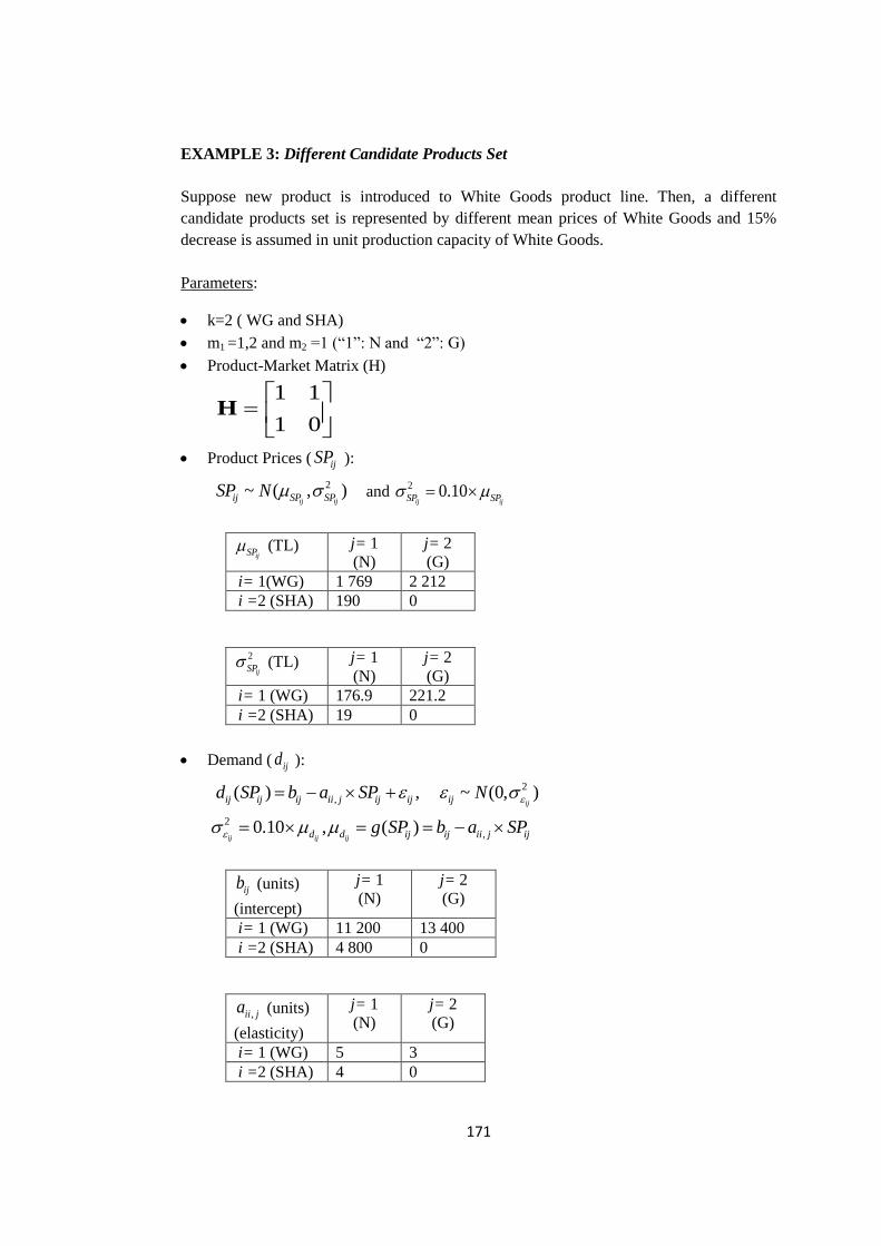
171

EXAMPLE 3: Different Candidate Products Set

Suppose new product is introduced to White Goods product line. Then, a different

candidate products set is represented by different mean prices of White Goods and 15%

decrease is assumed in unit production capacity of White Goods.

Parameters:

k=2 ( WG and SHA)

m1 =1,2 and m2 =1 (“1”: N and “2”: G)


1 1

1 0

H

Product Prices ( ):

2~ ( , )

ij ijij SP SPSP N and

(TL) j= 1

(N)

j= 2

(G)

i= 1(WG) 1 769 2 212

i =2 (SHA) 190 0

(TL) j= 1

(N)

j= 2

(G)

i= 1 (WG) 176.9 221.2

i =2 (SHA) 19 0

Demand ( ):

2


2


ijb (units)

(intercept)

j= 1

(N)

j= 2

(G)

i= 1 (WG) 11 200 13 400

i =2 (SHA) 4 800 0

(units)

(elasticity)

j= 1

(N)

j= 2

(G)

i= 1 (WG) 5 3

i =2 (SHA) 4 0

ijSP

2 0.10ij ijSP SP

ijSP

2

ijSP

ijd

,ii ja

172


2~ ( , )

i ii PC PCPC N and

i= 1 (WG) i= 2 (SHA)

(TL) 1 132 123

(TL) 113.2

12.3


(units)

(lower bounds))

j= 1

(N)

j= 2

(G)

i= 1 (WG) 450 620

i =2 (SHA) 450 0


ci = (c1, c2) = (0.0052, 0.00219) hrs.


Ci = (C1, C2) = (8700, 8700) hrs.


(TL) PC1 PC2 SP11 SP12 SP21

High (H) 1142.6395 126.5071 1782.3004 2226.8728 194.3589

Low (L) 1121.3605 119.4929 1755.6996 2197.1272 185.6411

(Units) SP11 (H) SP11 (L) SP12 (H) SP12 (L) SP21 (H) SP21 (L)

d11 (H) 2303.6258 2437.0632

d11 (L) 2273.3702 2405.9408

d12 (H) 6745.3034 6834.7117

d12 (L) 6693.4598 6782.5251

d21 (H) 4042.6207 4077.5787

d21 (L) 4002.5081 4037.2926


iPC

2 0.10i iPC PC

iPC

2

iPC

ijx

ijl

1 1 2

22( ) 2(3) 2 82 2 2 2 256

k

i

i

m km m k

n

173




(min-max regret solution) 1.8755×10

5




Max. (P-R) SNR 319.9787 ((P-R) SNR solution)


Table 5.9: Results of Example 3 (Different Candidate Products Set)



11x (103)

*

12x (103)

*

21x (103)

Min-Max Regret 121, 125 2.3036 6.7453 4.0373

249, 253 2.3036 6.7453 4.0373

Max. of Regret SNR 121, 125 2.3036 6.7453 4.0373

249, 253 2.3036 6.7453 4.0373

Max. of (P-R) SNR 121, 125 2.3036 6.7453 4.0373

249, 253 2.3036 6.7453 4.0373

Deterministic Case 257 2.3550 6.7640 4.0440

17

4

b) Statistics Generated for the Best Solutions * * *

11 12 21( , , )x x x

Scenario

Profit Range

(106)

Mean

Profit

(106)

Profit

Std. Dev.

(105)

Regret Range

Mean

Regret (10

4)

Regret

Std.

Dev.

(104)

P−R Range

(106)

Mean

P−R (10

6)

P−R

Std.

Dev. (10

5)

121 (8.7638, 9.2818) 8.9776 1.3096 (−6.2957×10-7

, 1.8547×105) 9.6724 4.6699 (8.5854, 9.2814) 8.8809 1.5818

125 (8.7638, 9.2818) 8.9776 1.3096 (0, 1.8547×105) 9.6724 4.6699 (8.5854, 9.2814) 8.8809 1.5818

249 (8.7638, 9.2818) 8.9776 1.3096 (−7.3016×10-7

, 1.8547×105) 9.6724 4.6699 (8.5854, 9.2814) 8.8809 1.5818

253 (8.7638, 9.2818) 8.9776 1.3096 (−1.4156×10-7

, 1.8547×105) 9.6724 4.6699 (8.5854, 9.2814) 8.8809 1.5818

257 (8.7272, 9.2313) 8.9618 1.2399 (5.0942×104, 1.8755×10

5) 1.1247×10

5 3.7874 (8.5530, 9.1768) 8.8494 1.4133

175

EXAMPLE 4: Volatile Market Conditions

Suppose that “Global” market is defined as a volatile market due to economic crisis in

Europe. Then company wants to see the results of Global market in two broad regions:

West Europe Market and East Europe Market. The variances of the parameters in these

markets are higher than the existing conditions of the company.

Parameters:

k=2 ( WG and SHA)

m1 =1,2,3 and m2 =1 (“1”: N, “2”: West Europe (WE), “3”: East Europe(EE) )

Product-Market Matrix (H):

1 1 1

0 01

H

Product Prices ( ):

2~ ( , )

ij ijij SP SPSP N , 2 0.25

ij ijSP SP for i =1 and j = 2, 3

2 0.10

ij ijSP SP for i = 1, j = 1, and i = 2, j = 1

ijSP (TL) j= 1

(N)

j= 2

(WE)

j= 3

(EE)

i= 1(WG) 1 580 2 170 1 780

i =2 (SHA) 190 0 0

2

ijSP (TL) j= 1

(N)

j= 2

(WE)

j= 3

(EE)

i= 1 (WG) 158 542.5 445

i =2 (SHA) 19 0 0

Demand ( ):

2


2


ijb (units)

(intercept)

j= 1

(N)

j= 2

(WE)

j= 3

(EE)

i= 1 (WG) 11 200 7 800 5 600

i =2 (SHA) 4 800 0 0

,ii ja (units)

(elasticity)

j= 1

(N)

j= 2

(WE)

j= 3

(EE)

i= 1 (WG) 5 3 2

i =2 (SHA) 4 0 0

ijSP

ijd

176


2~ ( , )

i ii PC PCPC N and 2 0.15

i iPC PC for i =1, 2 0.10

i iPC PC for i =2.

i= 1 (WG) i= 2 (SHA)

(TL) 1 058 123

(TL) 158.7

12.3


ijl (units)

(lower bounds))

j= 1

(N)

j= 2

(WE)

j= 3

(EE)

i= 1 (WG) 350 340 200

i =2 (SHA) 450 0 0


ci = (c1, c2) = (0.000608, 0.00219) hrs.


Ci = (C1, C2) = (8700, 8700) hrs.


(TL) PC1 PC2 SP11 SP12 SP13 SP21

High (H) 1070.5976 126.5071 1592.5698 2193.2916 1801.0950 194.3589

Low (L) 1045.4024 119.4929 1567.4302 2146.7084 1758.9050 185.6411


d11 (H) 3265.5990 3391.8440

d11 (L) 3208.7030 3333.8540


d12 (H) 1237.5903 1378.3130

d12 (L) 1202.6701 1341.4366


d13 (H) 2020.1584 2105.0055

d13 (L) 1975.4616 2059.3745


d21 (H) 4054.2762 4089.2846

d21 (L) 3990.8526 4025.5866

iPC

iPC

2

iPC

ijx

177


1 1 2

22( ) 2(3 1) 2 102 2 2 2 1024

k

i

i

m km m k

n





2.7989×105






Table 5.10: Results of Example 4 (Volatile Market Conditions)



11x (103)

*

12x (103)

*

13x (103)

*

21x (103)

Max-Min Regret 1025 3.3000 1.2900 2.0400 4.0400

Max. of Regret SNR 505, 509 3.2656 1.2376 2.0202 4.0256

1017,1021 3.2656 1.2376 2.0202 4.0256 Max. of (P-R) SNR 505, 509 3.2656 1.2376 2.0202 4.0256 1017,1021 3.2656 1.2376 2.0202 4.0256 Deterministic Case 1025 3.3000 1.2900 2.0400 4.0400

178

178

b) Statistics Generated for the Best Solutions * * * *

11 12 13 21( , , , )x x x x

Scenario

Profit Range

(106)

Mean

Profit

(106)

Profit

Std. Dev.

(105)

Regret Range

Mean

Regret (10

5)

Regret

Std. Dev.

(104)

P−R Range

(106)

Mean

P−R (10

6)

P−R

Std. Dev. (10

5)

505 (4.5504, 5.0354) 4.7436 1.3098 (-0.0084, 2.8603×105) 1.5362 6.9586 (4.2937, 5.0333) 4.5900 1.4304

509 (4.5504, 5.0354) 4.7436 1.3098 (0, 2.8603×105) 1.5362 6.9586 (4.2937, 5.0333) 4.5900 1.4304

1017 (4.5504, 5.0354) 4.7436 1.3098 (-0.0073, 2.8603×105) 1.5362 6.9586 (4.2937, 5.0333) 4.5900 1.4304

1021 (4.5504, 5.0354) 4.7436 1.3098 (−0.0047, 2.8603×105) 1.5362 6.9586 (4.2937, 5.0333) 4.5900 1.4304

1025 (4.4309, 4.9771) 4.7282 1.1242 (8.6476×104, 2.7989×10

5) 1.6907 4.3278 (4.1556, 4.8598) 4.5591 1.3482

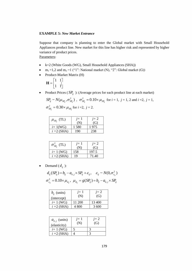
179

EXAMPLE 5: New Market Entrance

Suppose that company is planning to enter the Global market with Small Household

Appliances product line. New market for this line has higher risk and represented by higher

variance of product prices.

Parameters:

k=2 (White Goods (WG), Small Household Appliances (SHA))

m1 =1,2 and m2 =1 (“1”: National market (N), “2”: Global market (G))


1 1

1 1

H

Product Prices ( ijSP ): (Average prices for each product line at each market)

2~ ( , )

ij ijij SP SPSP N , 2 0.10

ij ijSP SP for i = 1, j = 1, 2 and i =2, j = 1,

2 0.30

ij ijSP SP for i =2, j = 2.

ijSP (TL) j= 1

(N)

j= 2

(G)

i= 1(WG) 1 580 1 975

i =2 (SHA) 190 238

2

ijSP (TL) j= 1

(N)

j= 2

(G)

i= 1 (WG) 158 197.5

i =2 (SHA) 19 71.40

Demand ( ijd ):

2


2


ijb (units)

(intercept)

j= 1

(N)

j= 2

(G)

i= 1 (WG) 11 200 13 400

i =2 (SHA) 4 800 3 600

,ii ja (units)

(elasticity)

j= 1

(N)

j= 2

(G)

i= 1 (WG) 5 3

i =2 (SHA) 4 3

180

Production Cost ( iPC ):

2~ ( , )

i ii PC PCPC N and2 0.10

i iPC PC

i= 1 (WG) i= 2 (SHA)

iPC (TL) 1 058 123

2

iPC (TL) 105.8

12.3

Lower bounds for decision variables ijx :

ijl (units)

(lower bounds))

j= 1

(N)

j= 2

(G)

i= 1 (WG) 350 540

i =2 (SHA) 450 350


ci = (c1, c2) = (0.000608, 0.00219) hrs.


Ci = (C1, C2) = (8700, 8700) hrs.


(TL) PC1 PC2 SP11 SP12 SP21 SP22

High (H) 1068.2859 126.5071 1592.5698 1989.0535 194.3589 246.4498

Low (L) 1047.7141 119.4929 1567.4302 1960.9465 185.6411 229.5502

( )ij ijij SP SPSP H , ( )

ij ijij SP SPSP L and

( )i ii PC PCPC H , ( )

i ii PC PCPC L .


d11 (H) 3255.1431 3381.1871

d11 (L) 3219.1589 3344.5109


d12 (H) 7460.1027 7544.5779

d12 (L) 7405.5763 7489.7431


d21 (H) 4042.6207 4077.5786

d21 (L) 4002.5081 4037.2926

181


d22 (H) 2877.5641 2928.4121

d22 (L) 2843.7371 2894.2867

( ) ( )ijij ijd H g SP , ( ) ( )

ijij ijd L g SP and ,( )ij ij ii j ijg SP b a SP ,

2 0.10 ( )ij ijg SP .


1 1 2

22( ) 2(2 2) 2 102 2 2 2 1024

k

i

i

m km m kn





1.7915×105






Table 5.11: Results of Example 5 (New Market Entrance)



11x (103)

*

12x (103)

*

21x (103)

*

22x (103)

Max-Min Regret 484, 500,

996,1012

3.2551 7.4601 4.0373 2.8776

Max. of Regret

SNR

484, 500,

996,1012

3.2551 7.4601 4.0373 2.8776

Max. of (P-R) SNR 484, 500,

996,1012

3.2551 7.4601 4.0373 2.8776

Deterministic Case 1025 3.3000 7.4750 4.040 2.8860

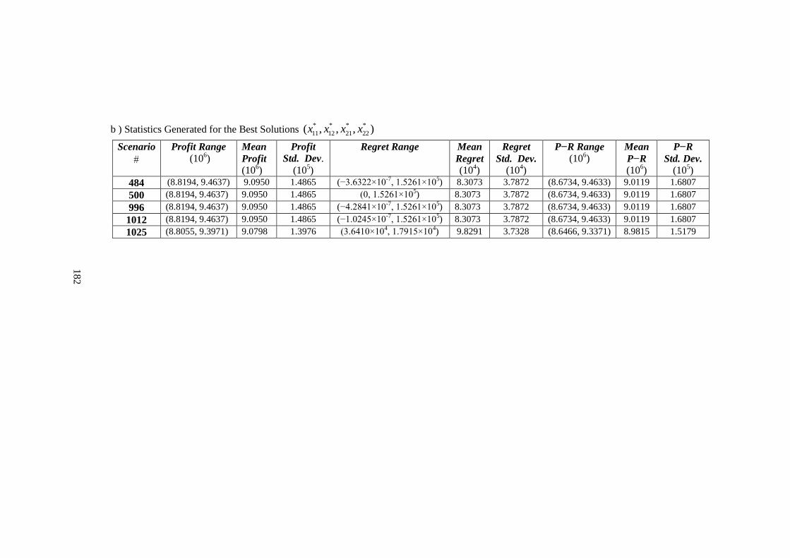
182

b ) Statistics Generated for the Best Solutions * * * *

11 12 21 22( , , , )x x x x

Scenario

Profit Range

(106)

Mean

Profit

(106)

Profit

Std. Dev.

(105)

Regret Range

Mean

Regret (10

4)

Regret

Std. Dev.

(104)

P−R Range

(106)

Mean

P−R (10

6)

P−R

Std. Dev. (10

5)

484 (8.8194, 9.4637) 9.0950 1.4865 (−3.6322×10-7

, 1.5261×105) 8.3073 3.7872 (8.6734, 9.4633) 9.0119 1.6807

500 (8.8194, 9.4637) 9.0950 1.4865 (0, 1.5261×105) 8.3073 3.7872 (8.6734, 9.4633) 9.0119 1.6807

996 (8.8194, 9.4637) 9.0950 1.4865 (−4.2841×10-7

, 1.5261×105) 8.3073 3.7872 (8.6734, 9.4633) 9.0119 1.6807

1012 (8.8194, 9.4637) 9.0950 1.4865 (−1.0245×10-7

, 1.5261×105) 8.3073 3.7872 (8.6734, 9.4633) 9.0119 1.6807

1025 (8.8055, 9.3971) 9.0798 1.3976 (3.6410×104, 1.7915×10

4) 9.8291 3.7328 (8.6466, 9.3371) 8.9815 1.5179

183

5.3 ANALYSIS OF THE RESULTS

In order to deal with the uncertainty, the scenarios were created according to the

methodology explained in Chapter 4 (Table 5.2). The MATLAB code was used to run and

get the experimental results. For each scenario generated by full factorial design of

experiment, an optimal solution set is found through the deterministic product mix model

(Table 5.3). Then the optimal set found for a scenario is tested for different scenarios. In

short, each solution found by the deterministic model is evaluated under different

predetermined scenario realizations. Next, objective function values for all optimal product

sets and for all scenarios are found and located to a matrix (Table 5.4). Then, the maximum

values of each scenario are determined in order to find the best solutions by using Min-

Max Regret approach. Afterwards, every objective function value is subtracted from the

maximum value of the corresponding scenario, and the new results are formed the regret

matrix (Table 5.5). After that, the maximum of the regret values is found for each product

set (row), and a column for maximum regrets is formed (Table 5.6). Meanwhile, for each

product set, Signal-to-Noise Ratios of Regrets (SNRR) and Signal-to-Noise Ratios of Regret

Free Profits (SNRP-R) are found in order to find the solutions to these approaches. Finally,

SNRR and SNRP-R columns are formed (Table 5.6). As a result, the set(s) of the products

with the smallest maximum regret,

with the largest SNRR, and

with the largest SNRP-R

are chosen as the best solution to the product mix problem under uncertainty. The results

by three approaches can be either the same or different. These results are discussed below.

In analysis of the results, our major interest is to compare the results of deterministic and

probabilistic approaches. In order to make this comparison, the mean values of the

parameters of prices, costs and demand values are taken as deterministic. It is seen that the

results obtained by three approaches are very close to each other most of the time. When

the maximum regrets of the chosen product mixes are analyzed, it is observed that the

maximum regret value of the product mix of the deterministic approach is greater than that

of the product mix of the probabilistic approach by 1.13% to 17.8%. Among five example

cases, two examples show different results regarding the min-max regret approach: In

Example 2 and Example 4, min-max regret approach yields the solution of the

deterministic case as the best solution. In such a case, one may also consider looking at the

expected value of regret values to check the validity of the solution proposed by the min-

max regret approach. If the expected regret value of deterministic case solution were

smaller than that of the other chosen solutions, it would be possible to say that the solution

of deterministic case was a better solution. However, when the regret data of the

deterministic case is analyzed, it is seen that mean regret value of the deterministic case

solution is greater than those of the other chosen product mix solutions. At the same time,

mean profit value and mean regret free profit value of the deterministic case solution are

smaller than those of the other chosen product mix solutions. This indicates that it is

possible to obtain higher profit on the average with other chosen product mix solutions.

Therefore, the acceptance of the solution indicated by the min-max regret approach would

lead to an inferior decision because there are other solutions which provide higher profit

values on the average. The mean regret values of the deterministic case solution are

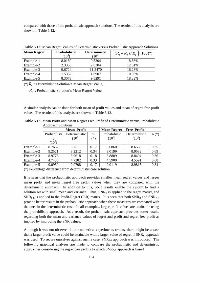
184

compared with those of the probabilistic approach solutions. The results of this analysis are

shown in Table 5.12.

Table 5.12: Mean Regret Values of Deterministic versus Probabilistic Approach Solutions

Mean Regret Probabilistic

(104)

Deterministic

(104)

( ) / 100d p pR R R (*)

Example-1 8.0180 9.5304 18.86%

Example-2 2.3358 2.6304 12.61%

Example-3 9.6724 11.2470 16.28%

Example-4 1.5362 1.6907 10.06%

Example-5 8.3073 9.8291 18.32%

(*) dR : Deterministic Solution’s Mean Regret Value,

pR : Probabilistic Solution’s Mean Regret Value

A similar analysis can be done for both mean of profit values and mean of regret free profit

values. The results of this analysis are shown in Table 5.13.

Table 5.13: Mean Profit and Mean Regret Free Profit of Deterministic versus Probabilistic

Approach Solutions

Mean Profit Mean Regret Free Profit

Probabilisti

c

(106)

Deterministic

(106)

%

(*)

Probabilistic

(106)

Deterministic

(106)

% (*)

Example-1 8.7662 8.7511 0.17 8.6860 8.6558 0.35

Example-2 9.2521 9.2212 0.34 9.0199 8.9582 0.69

Example-3 8.9776 8.9618 0.18 8.8809 8.8494 0.36

Example-4 4.7436 4.7282 0.33 4.5900 4.5591 0.68

Example-5 9.0950 9.0798 0.17 9.0119 8.9815 0.34

(*) Percentage difference from deterministic case solution

It is seen that the probabilistic approach provides smaller mean regret values and larger

mean profit and mean regret free profit values when they are compared with the

deterministic approach. In addition to this, SNR results enable the system to find a

solution set with small mean and variance. Thus, SNRR is applied to the regret matrix, and

SNRP-R is applied to the Profit-Regret (P-R) matrix. It is seen that both SNRR and SNRP-R

provide better results in the probabilistic approach when these measures are compared with

the ones in the deterministic case. In all examples, larger profit values are attainable using

the probabilistic approach. As a result, the probabilistic approach provides better results

regarding both the mean and variance values of regret and profit and regret free profit as

implied by improving the SNR values.

Although it was not observed in our numerical experiments results, there might be a case

that a larger profit value could be attainable with a larger value of regret if SNRR approach

was used. To secure ourselves against such a case, SNRP-R approach was introduced. The

following graphical analyses are made to compare the probabilistic and deterministic

approaches considering the regret free profits to which SNRP-R approach is based.

185

DeterministicP-R Values

9100000

9000000

8900000

8800000

8700000

8600000

8500000

8400000

8300000

Da

ta

P-R Values Under Tested Scenarios

Figure 5.2: Box Plot of Regret Free Profits of Deterministic and Probabilistic Approaches

(Example-1)


9500000

9250000

9000000

8750000

8500000

Da

ta



(Example-2)

186


9300000

9200000

9100000

9000000

8900000

8800000

8700000

8600000

8500000

Da

taP-R Values Under Tested Scenarios


(Example-3)


5100000

5000000

4900000

4800000

4700000

4600000

4500000

4400000

4300000

4200000

Da

ta



(Example-4)

187


9500000

9400000

9300000

9200000

9100000

9000000

8900000

8800000

8700000

8600000

Da

ta



(Example-5)

Box-plots are used to assess and compare the sample distributions. In our case, “P-R

Values” represents the first sample distribution which is the regret free profit values of the

chosen product mix under the other scenarios. The second sample distribution

“Deterministic” consists of data of the regret free profit values obtained by the product mix

of the deterministic case under the other scenarios. Firstly, it is seen that box-plots of all

examples show that the mean values of the probabilistic P-R values are higher than the

corresponding mean value of the deterministic case. Box-plots of Example 1, Example 3

and Example 5 show similar characteristics. The probabilistic P-R values and

deterministic P-R values in those examples have both a slight negative skewness, since

larger box areas are observed under the median in box-plots of these examples. Also, no

outliers are present in these box-plots of the mentioned examples. However, the box-plots

of Example 2 and Example 4 show totally different picture. In these box-plots, while

probabilistic P-R values have positive skewness, deterministic P-R values have negative

skewness. Besides, probabilistic P-R values consist of some unusual large observations

and deterministic P-R values consist of some unusual small observations. It means that

reverse situation exists regarding the regret values of those examples. In Example 2 and

Example 4, the values of skewness statistic of the regret values of the chosen set of

products by the probabilistic approach are (− 0.0348) and (−0.0378) respectively. On the

other hand, skewness statistics of regret values of the deterministic case are 0.1297 and

0.3316 for Example 2 and Example 4 respectively. Remember that Example 4 is a

descriptive case for volatile market conditions which reflects the environment with high

degree of uncertainty. Higher uncertainty is represented by higher variances of the

parameters of prices, costs and demands in this example. It is seen that skewness statistics

of this example are relatively higher than the others. The results of Example 4 show that

we have the possibility of obtaining higher regret free profits by probabilistic approach in

high uncertainty cases than those obtained by the deterministic approach.

188

A further analysis can be done to check the normality of the regret free profit values of the

chosen product mix solutions in the examples. For this purpose, the paired differences are

obtained and their normality is tested (Figure 5.7). This analysis is presented below.

3000002000001000000-100000-200000

99,9

99

95

90

80

7060504030

20

10

5

1

0,1

Paired Difference

Pe

rce

nt

Mean 30246

StDev 78797

N 256

AD 13,705

P-Value <0,005

Normality Test for Paired DifferenceNormal

Figure 5.7: Normality Test of Regret Free Profits Differences (Example-1)

Normality test was made by MINITAB which was depicted in Figure 5.7. Normality test

generates a normal probability plot and performs a hypothesis test to examine whether or

not the observations of the sample distribution follow a normal distribution. The result of

the normality test performed for paired differences (probabilistic-deterministic) of P-R

values of the chosen product mix of Example 1 provides us strong evidence to reject the

hypothesis of the normal distribution of paired differences of P-R values. Similar results

for the other examples are presented below.

189

10000005000000-500000-1000000

99,99

99

95

80

50

20

5

1

0,01

Paired Difference

Pe

rce

nt

Mean 58925

StDev 206069

N 8192

AD 45,470

P-Value <0,005



4000003000002000001000000-100000-200000-300000

99,9

99

95

90

80

7060504030

20

10

5

1

0,1

Paired Difference

Pe

rce

nt

Mean 31498

StDev 102410

N 256

AD 12,706

P-Value <0,005



190

5000002500000-250000-500000

99,99

99

95

80

50

20

5

1

0,01

Paired Difference

Pe

rce

nt

Mean 30885

StDev 133124

N 1024

AD 18,074

P-Value <0,005



4000003000002000001000000-100000-200000-300000

99,99

99

95

80

50

20

5

1

0,01

Paired Difference

Pe

rce

nt

Mean 30437

StDev 78707

N 1024

AD 51,671

P-Value <0,005



191

Since the normality assumption is not justified, some type of nonparametric inference for

mean location of the differences is more appropriate. For this purpose, Wilcoxon signed-

rank test can be applied which is not based on normality assumption.

Table 5.14: Output of Wilcoxon Signed Rank Test (Example-1)

Wilcoxon Signed Rank Test: Difference Test of median = 0,000000 versus median > 0,000000

N for Wilcoxon Estimated

N Test Statistic P Median

Difference 256 256 23104,0 0,000 30246





Difference 8192 8192 21889536,0 0,000 58925





Difference 256 256 20544,0 0,000 31498





Difference 1024 1024 321856,0 0,000 30887





Difference 1024 1024 366208,0 0,000 30437

192

In all examples, Wilcoxon Signed Rank test rejects the null hypothesis that the median of

the differences is zero, with strong evidence which is reflected by large Wilcoxon statistic

value and very small p-value. Therefore, the median of the differences between the

probabilistic P-R values and the corresponding deterministic P-R values can be considered

as greater than zero.

5.4 DISCUSSION

The methodology developed in this study has been implemented to the product mix

problem at the strategic level of product management to handle the complexity imposed by

uncertainty. Therefore, the main focus is to resolve this issue justifying the results

provided by the implementation of the methodology. The probabilistic approach of the

methodology involves generating several scenarios as the future realizations. Then, these

scenarios are solved by means of a deterministic model. All these solutions of the

scenarios are the candidate best solutions to the product mix problem. Then, these

solutions are tested under different scenarios for assessment of the feasibility and

robustness of the method. Finally, the best product mix is selected applying three

alternative solution approaches. The concept of regret free profit (P-R) and SNRP-R

measure based on this concept is used heavily in analyzing the results and making the

statistical inferences using this approach is found to be the most powerful approach. As a

result, analysis of the results and the statistical inferences show that the probabilistic

approach provides better results in terms of regret free profits. So, it is proven that the

selected product mix by the probabilistic approach give the most consistently better results

under uncertain environment.

In the examples studied, the consumer durables sector was considered. The only reason for

this is the familiarity of this sector gained during the field study, which has been helpful in

formulating the cases for the numerical examples. Implementation of the methodology

developed in this study is possible in all sectors producing physical goods. For example,

BMW Group has three main product lines which are BMW automobiles, Mini and Rolls

Royce. So, BMW Group may use the methodology to find the best product mix of these

lines in their markets which these lines are served. Mini line has Mini 1, Mini Cooper, and

Mini 1 Cabrio families, and these families have several variants having different options.

According to the different preference options of these families, candidate product sets can

be constructed and deterministic model can be modified if necessary, and the methodology

can be used to find the best family mix for Mini product line. Similarly, a medical device

company may divide its product mix in the lines of hearing aids, reading glasses and

motorized wheelchairs. Or, a cookware company might divide its entire set of products by

type of metal such as the line of cast-iron products, line of aluminum products, and so

forth. In short, for each company specific case, considering the purpose of the company,

the product hierarchy is established, product-market structure is defined, and the best

product mix is determined at the desired product level by using our methodology. It

should be noted that the number of factors is limited in our problem case. Since the product

mix problem is handled at the strategic level in our case, the number of products (line or

family) and the number of markets are also limited. Table 5.19 shows the number of

scenarios generated by two-level full factorial design of experiments in accordance with

the number of factors considered in the experiments.

193

Table 5.19: Number of Factors versus Number of Scenarios

a) Number of products, k = 2

Case

No. 1m 2m

1

k

i

i

m

No. of Factors

1

2k

i

i

n m k

No. of Scenarios

2n

1 1 1 2 6 64

2 2 1 3 8 256

3 2 2 4 10 1,024

4 2 3 5 12 4,096

5 3 3 6 14 16,384

6 4 3 7 16 65,536

7 4 4 8 18 262,144

8 5 4 9 20 1,048,576

9 5 5 10 22 4,194,304

10 6 5 11 24 16,777,216

b) Number of products, k=3

Case

No. 1m 2m 3m

1

k

i

i

m

No. of Factors

1

2k

i

i

n m k

No. of Scenarios

2n

1 1 1 1 3 9 512

2 2 1 1 4 11 2,048

3 2 2 1 5 13 8,192

4 2 2 2 6 15 32,768

5 3 2 2 7 17 131,072

6 3 3 2 8 19 524,288

7 3 3 3 9 21 2,097,152

8 4 3 3 10 23 8,388,608

9 4 4 3 11 25 33,554,432

10 4 4 4 12 27 134,217,728

The method, including probabilistic scenario generation and deterministic model, is

constructed in MATLAB 7.10. So, MATLAB 7.10 linear programming solver is used to

get the results. Numerical results obtained on Intel Core I-7, 8 GB RAM. The largest

model size for the problem based on 13 factors is 8193 rows and 8192 columns. It takes

around 3 minutes to solve and prepare the output matrices. When the factor number is

increased, the memory capacity of MATLAB 7.10 becomes insufficient. In the examples

presented here, products are aggregated at line and family levels in the sense that higher

level product aggregation is not possible. Therefore, it can be stated that the model is

efficient for the strategic level of product mix decision problem. However, if more

detailed product schemes are needed to be studied, the variants of the model which are

presented below can be used. Product breakdown, market disaggregation or single market

variants of the model can be used to obtain the optimum product mix solution for detailed

product schemes or market segments. For example, optimum mix of variants (models) of

“Hot” family in a single market can be obtained iteratively by using the “product

breakdown in a single market” variant of the model. Thus, optimum product mix solutions

can be obtained at desired level of product aggregation at each market. We present three

variants of the deterministic product mix model as follows:

194

Variant-1: Product-Mix Model with Shared Capacity

In our basic product mix model, capacity constraints show that product i cannot be

allocated more than Ci hrs. assuming each product has a distinct facility (or allocated

capacity) of production. While dealing with the mix of lines or families, the assumption of

distinctly allocated capacities can be meaningful. However, if the problem requires

finding the mix of variants in a family, the case where the total capacity is shared by the

variants should be considered in the model. Therefore, the following constraint can be

added to the model in which all products cannot be allocated more than Cmax hrs

(maximum capacity available).

Additional Constraint:

max

1 1

imk

i ij

i j

c x C

Variant-2: Breakdown of Products with Product Mix Model

Specifically, basic product mix model can be used for budgeting purpose iteratively. In the

first run, the optimum solution is found for the mix of lines. Then, the lines can be broken

into families, and for each line, optimum mix of families can be found. At the second

iteration, the results of the first run can be used as an additional constraint in order to

guarantee the optimum total profit value for the company as follows:

Additional Constraint:

*

1 i

k

ij ij op

i j M

P x P

*

opP : Optimum objective value of higher level of product determined in the previous

iteration

Similarly, for each family, optimum mix of variants can be obtained combining both the

first and second variants of the model.

Variant-3: Product Breakdown in a Single Market with Product Mix Model

Another special case can be considered for a single market case. In this case, the first

iteration results obtained for the mix of lines can be detailed for the families or variants of

a family by modifying the model as follows:

Additional Constraints:

*

1

k

i i op

i

P x P

195

*

1

k

i op

i

x x

, i

i ij

j M

x x

Pi is the unit profit value (SPi – PCi) of product i, and x*op is the optimum value of total

number of units of the higher level of product obtained in previous iteration.

In short, at the levels lower than the strategic level, full factorial design of experiments

may cause to limit the number of factors. In our experiments, the maximum number of

factors is 13 as mentioned above. If the number of factors is small to moderate (n≤10)

(D’Errico and Zaino, 1988), the model can be used efficiently. For higher number of

factors, the variants of the model can be used as explained above. Alternatively, there may

be a need to consider fractional factorial experiments or Taguchi’s orthogonal arrays

instead of full design experiments to reduce the number of experiments or objective

function evaluations. However, in such a case, since we are not able to see all

combinations of the levels, a discrepancy may happen for the optimal product mix

solution. For this reason, fractional factorial design can be supported by a multi-regression

analysis and ANOVA test analysis.

The examples are descriptive cases formulated to get the numerical results. In these cases,

different values of means and variances of the parameters are used. For example, volatile

market conditions are represented by higher values of variances of the parameters.

Similarly, different set of candidate products example is described using different means of

prices and also unit production capacity is decreased by 15%, assuming that new product

introduction changes the bundle of candidate products and decreases the production

efficiency. This assumption is based on the findings of a very recent article (Gopal et al.,

2013). In this article, it is stated that the new product introduction disrupts manufacturing

operations which results in productivity losses. The average productivity loss is about 12-

15% which is measured in terms of hrs./unit product. Gopal et al. (2013) point out the

following remarks: It is interesting that product development books focus on profit impact

of new product introduction to throughput improvement, but ignore the effect on plant

productivity. On the other hand, it is understood that productivity loss escapes the

attention of manufacturing focused books. It is also indicated that there are no rigorous

assessments of the impact of new product launches on a plant’s productivity. Several ways

are identified to mitigate the loss of productivity. The most important one for us is

“product mix flexibility”. It is stated that product mix flexibility is critical for reducing the

productivity loss. Product mix flexibility is a strategic tool under competition and

mitigating demand uncertainty, which entails the ability to manufacture more than one

product in a single manufacturing facility (Gopal et al., 2013). Therefore, it is more

convenient to use the “Shared Capacity” variant of our deterministic model presented

above. This model was not used in numerical results. The aim of using this example of

productivity loss is just to make the reader informed about this important concept. The

detailed study on the subject is left to the future research.

Finally, it is seen that rounding up or rounding down of the results obtained by LP-

relaxation of the deterministic product mix model have negligible impact on the optimal

value of the objective function. For example, the results of Example-1 show that the

optimum product mix is 3255.1 units of WG in National market 7460.1 units in Global

196

market and 4037.3 units of SHA in National market. The profit range is (8.5229-

9.0983)×106 TL. The price value of WG in National market is 1592.6 TL. and cost value

of WG in this market is 1068.3 TL. for one of the scenario which gives the optimal results.

In this case, it can be easily stated that rounding down the value of WG will not lead a

significant impact on profit. Therefore, we may conclude that LP-relaxation of the

knapsack model can be used to get fast and reliable results.

197

CHAPTER 6

CONCLUSIONS AND FUTURE RESEARCH

6.1 CONCLUSIONS

In many real life problems, uncertainty is the major complexity for the decision makers. A

typical example to such a case is the product mix problem. Key parameters of the product

mix problem are unknown to the decision maker at the time the decision has to be made.

The product prices, costs of production and demands for products move by market

dynamics such as unknown behaviors of the customers, changeable prices of suppliers,

prices of competitors and new regulations imposed by the government. Therefore, the

decision maker cannot be certain about the future realizations of financial performance of

the company. In this study, we develop a methodology to aid the decision maker in

product mix determination at the strategic level of product management under uncertainty.

We use simulation optimization approach to formulate the product mix problem under

uncertainty. Our decision support system (DSS) model embodies two basic formal models:

Deterministic Product Mix Model, and

Probabilistic Model (simulation model).

The first model represents a deterministic approach and constructs the DSS that takes

prices, demands and costs of the products as given and suggests the optimal product mix.

So, it works as an optimization engine in our proposed DSS. The simulation model is

constructed as a result of the probabilistic approach. In this approach the system is

upgraded to another one which considers the uncertainty in the parameters. We develop a

scenario-based scheme in the probabilistic approach by generating different scenarios

focusing on the major inputs of the product mix model. Scenario generation method relies

on systematic sampling obtained by a two-level full factorial design of experiment. In

order to determine the levels of factors (parameters) discrete approximations of normally

distributed random parameters of prices, costs and demands are used. A linear relationship

is assumed between the prices of products and the level of demands by the law of demand.

Then, optimal product mix solutions are found using the deterministic model repeatedly

under various scenarios defined as possible realizations of the uncertain parameters. In the

next stage, these optimal solutions are tested under the same set of scenarios and their

performances are measured. The final stage requires the analysis of these results by using

the various solution approaches to get the optimal product mix.

198

Analysis of the results and the statistical inferences show that the probabilistic approach

provides better results in terms of objective function values. So, it is shown through

examples that the selected product mixes by the probabilistic approach give the most

consistently high profit results under uncertain environment.

Our primary goal in this study is to present an approach of dealing with uncertainty and the

methodology developed for this purpose. Therefore, the product mix optimization model is

kept as simple as possible in order to highlight the importance of the methodological

approach. To the best of our knowledge, our methodology developed to aid the decision

maker in product mix determination is a novel and original approach and it is the first study

implemented for the product mix problem under uncertainty at the strategic product

management level. Therefore, it represents the major contribution of this study. While the

model developed in this study is mainly geared towards the product mix problem, the

decision aid method developed here is general and can be used in many decision making

problems involving uncertainty, such as investment planning, financial portfolio planning,

capacity planning, etc.

As it is known, product mix problem is a very well-known problem in the literature.

However, most of the literature handles the problem in the production management decision

framework. We consider the problem in the framework of product management. To

properly locate the product mix problem in the product management framework properly

necessitates understanding the product management framework deeply. For this purpose,

both a broad literature survey and a field study have been conducted. As a result, it has been

realized that the product mix problem is one of the most important strategic decision making

areas of product management framework. During this effort of understanding the product

management framework, it is also realized that there is no comprehensive study dealing with

the decision framework of product management from holistic perspective. Thus, using an

integrative system approach, a product management system has also been proposed (Figure

3.7), and based on this proposal; some efforts have been spent to integrate the existing

literature to extract and clarify the major decisions in product management and to present

them in a structured and comprehensive way. The author believes that all these efforts

represent some contribution to the existing literature of product management. The proposed

decision framework of product management can be viewed as an initial attempt to fill the

gap in the existing literature, so that this work can be improved further for the forthcoming

studies in this area.

6.2 FUTURE RESEARCH

The following topics for the future research can be suggested regarding the strategic product

mix problem under uncertainty:

1. Alternative Solution Approach to the DSS Model

Multiple response surface optimization approach can be suggested as another appropriate

one. For this purpose, first, empirical models of the mean and variance of the regret (or

regret free profit) values are found by means of multiple linear regression;

199

* *

1 1

* *

2 1

( ) ( ,..., )

( ) ( ,..., )

k

k

E regret f x x

V regret f x x

Consequently, the following multiobjective optimization problem is solved:

Minimize * *

1 1( ,..., )kf x x

Minimize * *

2 1( ,..., )kf x x

subject to

* *

1 ,..., kx x

Here, a major problem is possibility of obtaining poor empirical models. In that case, this

approach cannot be trusted to yield better results than the proposed one.

2. Extension of the Model with Price as a Decision Variable

Pricing is another important decision making area in product management framework

involving the consideration of uncertainty. In this case, a consumer utility function of the

pair of (x, px) can be derived for each product at each market. Maximization of the utility for

the consumers may be in conflict with maximizing the profits of the company. In such a

case, a trade-off should be considered and formulated as a multi-objective problem.

Deterministic model should be modified accordingly. The methodology can be applied with

its main stages.

3. Extension of the Model for Line Addition to the Product Mix

Line addition (capacity expansion) requires considering the establishment of a new plant or

an investment in the existing facility to produce the products in the new line. Therefore, the

deterministic model should be modified according to an investment planning model

considering the initial investment cost, expected net inflows injected by the new product

investment, salvage value of the investment over the forecasted life cycle of the new

product(s), etc. A multi-period extension of the modified model can be more appropriate in

which these inflows and outflows of the new product investment are modeled. In addition to

this, a new bundle of candidate products should be considered with different mean values

and variances of the prices, costs and demands.

4. Product Breakdown and Market Disaggregation Extension of the Model

The product breakdown extension of the model can be useful for traditional budgeting

activities of the company. For this purpose, this extension of the model, which is presented

in Chapter 4, can be used iteratively at the expense of some efficiency loss. For example,

first, the line mix is determined. After getting the optimum results for the line mix at the

first iteration, each line can be broken down into the families of corresponding lines. At the

second iteration, using the optimum results obtained in the first iteration as an additional

constraint, the optimum results of the family mix are obtained for each line. Then, similarly,

families are broken into the variants and by using the optimum results obtained for the mix

of families as additional constraints, the optimum mix of variants are found for each family.

200

The constraints added iteratively are the minimum profit requirements of the lines and

families accordingly.

However, if the number of factors is too high, the fractional factorial design of experiment

can be suggested instead of full factorial design of experiment. In this case, the levels of the

factors should be determined so as to match as many moments as possible of the continuous

and discrete approximating distributions.

5. The Problem of Determining the Set of Candidate Products

Determining the set of candidate products is an important decision making problem in

product management framework which involves sub-decisions and parallel decisions in

different levels of management in the company. Set of candidate products is assumed as pre-

determined information and therefore it is a given input in our model. The solution to this

problem may require using the combination of several decision tools. Figure 6.1 depicts a

suggested solution framework where the use of combination of several decision tools is

shown as an example. More research is needed to develop a methodology for determining

the candidate set of products.

Figure 6.1: Generation of Set of Candidate Products (Use of Tools & Techniques)

6. Product Dependency Extension of the Model

The relationships among the products bring additional complexity to the product mix

problem. If substitutable products and complementary products are considered in the

problem, dependency occurs in the random parameters of the model. In this case, for each

product, we need to consider both pairwise interactions for the factors of price, demand and

cost of the product itself, and the cross price sensitivities of demands of other products

simultaneously. Therefore, the number of factors will be much higher than that of the

product independency case.

201

7. Multi-Objective - Multi-Candidate Set Extension of the Model

Global companies may consider different goals in different markets for its products. For

example, Company D considers the maximization of market share in Global market, while it

is a profit maximizing firm in the National market. Therefore, although the traditional

product mix problem is solved with the profit maximization objective, upon the company’s

different goals in different markets, the model can be modified. In this case, for each market,

different candidate set identification may be required.

8. The Possibility of Different Production Costs at Different Markets

Market indifference is assumed for production costs of products in our study. However, a

global firm may have production facilities in different market places to produce the same

product. For example, Company D has dish washer factory in both Turkey and China and

these products are sold in these locations. In that case, the production cost of producing one

unit of dish washer may be different in these locations. In such a case, production cost

should be considered not only for each product but also for each market which causes to

consider higher number of factors in the experiments. Besides, the deterministic model

should be modified accordingly.

9. Consideration of Manufacturing Efficiency Loss caused by New Product

Introduction to the Set of Candidate Products

As discussed in section 5.4, new product introduction distrupts manufacturing operations

which results in productivity losses. The productivity loss caused by new product

introduction was roughly described in our numerical examples (see Example 3) to make the

reader informed about this important concept. Therefore, the loss of productivity should be

studied and detailed further in product mix model which may require making some

modifications considering product mix flexibility, capacity sharing among products

(variants), the impact on production cost and profit and so on.

10. Implementation of Product Mix Model for Service Sector

The methodology developed in this research study is general and applicable in many

decision making problems involving uncertainty. Depending on the problem case under

consideration the deterministic part of the approach may require some modifications. In this

research, product mix model as the deterministic part of the approach is constructed

considering the physical goods produced in manufacturing sector. The same model can be

modified for service sector considering different measurement and definitions of the

parameters in the model. For example, the product lines of a hotel producing services in the

hospitality sector can be considered as the rooms, food and beverage service, business

assistance service, etc. The total number of accomodations of the rooms in terms of

day/night can be taken as the total capacity for the rooms. The families for the rooms can be

considered as “single”, “double”, “suite”, “presidential suit” etc. The seasonal variations in

demand can be important for this sector, therefore piecewise linear functional relationship

may be more appropriate for defining price-demand relation in probabilistic part of the

approach.

203

REFERENCES

Alonso-Ayuso, A., L.F. Escudero, A. Garin, M.T. Ortuno, G. Perez, (2005), On the Product

Selection and Plant Dimensioning Problem under Uncertainty, Omega 33, 307-318.

Alreck, P. L and R. B Settle (1995), The Survey Research Handbook: Guidelines and

Strategies for Conducting a Survey, 2nd

ed., McGraw Hill.

Ansoff, H.I.,(ed.) (1972), Business Strategy, Penguin Modern Management Readings,

Penguin Books.

Arya, A., B. Mittendorf and D.E.M. Sappington (2008), The Make-or-Buy Decision in the

Presence of a Rival: Strategic Outsourcing to a Common Supplier, Management

Science 54 (10), 1747-1758.

Baker,M. and S. Hart (1999), Product Strategy and Management, Prentice Hall, Pearson

Education.

Balibek, E. and M. Köksalan (2012), A Visual Interactive Approach for Scenario-Based

Stochastic Multi-Objective Problems and an Application, Journal of Operational

Research Society, 1-15.

Banville, G. R. and B. Pletcher (1974), The Product Elimination Function, Academy of

Marketing Science Journal (pre-1986) (2, 3), ABI/INFORM Global, 432.

Bayou,M. E. (2005), Analyzing the Product-Mix Decision by Using a Fuzzy Hierarchical

Model, Managerial Finance, 31(3).

Bean,R. and R. Radford (2000), Powerful Products–Strategic Management of Successful

New Product Development, AMACOM American Management Association.

Ben-Tal, A. and D. Den Hertog (2011), Robust Optimization at Work-An Introduction,

Technion-Israel Institute of Technology, Hafia, Israel.

Better, M., F. Glover, G. Kochenberger, H. Wang (2008), Simulation Optimization:

Applications in Risk Management, International Journal of Information Technology

& Decision Making 7(4), 571-587.

Bitran, G. R., E. A. Haas, A. C. Hax (1981), Hierarchical Production Planning: A Single

Stage System, Operations Research 29 (4), Operations Management, 717-743.

Bhattacharya, P. Vasant, B. Sarkar and S. K. Mukherjee (2008), A Fully Fuzzified,

Intelligent Theory-of-Constraints Product-Mix Decision, International Journal of

Production Research, 46 (3), 789-815.

Brace, I. (2004), Questionnaire Design: How to Plan, Structure and Write Survey Material

for Effective Market Research, Kogan Page.

204

Brem, A. and Voigt, K. (2009), Integration of Market-Pull and Technology-Push in the

Corporate Front End and Innovation Management – Insights from German software

industry., Technovation 29, 351-367.

Bunn, D.W and A. A. Salo (1993), Forecasting with Scenarios, European Journal of

Operational Research, 68, 291-303.

Chao, R. O. S. Kavadias (2008), A Theoretical Framework for Managing the New Product

Development Portfolio: When and How to Use Strategic Buckets, Management

Science 54 (5), 907-921.

Chen, H., Y (F). Chen, C- H. Chiu, T- M. Choi and S. Sethi (2010), Coordination

Mechanism for the Supply Chain with Lead-Time Consideration and Price-Dependent

Demand, European Journal of Operational Research 203, 70-80.

Chen, K.D., W.H. Haussman (2000), Technical Note: Mathematical Properties of the

Optimal Product Line Selection Problem Using Choice-Based Conjoint Analysis,

Management Science, 46 (2), 327-332.

Chen, H. H., A. H. I. Lee, Y. Tong (2007), Prioritization and Operations NPD Mix in a

Network with Strategic Partners under Uncertainty, Expert Systems with Applications

33, 337-346.

Chen, H. H. A. H. I. Lee, Y. Tong (2006), New Product Mix Selection for a High

Technology Company in a Technology Innovation Network, Journal of Technology

Management in China, 1 (2), 174-189.

Chen, H. H., A. H.I. Lee, Y. Tong (2006), Analysis of New Product Mix Selection at TFT-

LCD Technological Conglomerate Network under Uncertainty, Technovation 26,

1210-1221.

Chien, T. W., C. Lin, B. Tan and W. C Lee (1999), A Neural Networks- Based Approach

for Strategic Planning, Information & Management, 35, pp. 357-364.

Chod, J., D. Pyke and N. Rudi (2010), The Value of Flexibility in Make-to-Order Systems:

The Effect of Demand Correlation, Operations Research 58 (4), 834-848.

Chou Y-C (2000), Product Mix Planning in Semiconductor Foundry Manufacturing, IEEE,

91-98.

Chung, S. -H. A. H.I. Lee, W. L. Pearn (2005), Analytic Network Process (ANP) Approach

for Product Mix Planning in Semiconductor Fabricator, International Journal of

Production Economics 96, 15-36.

Cooper, R. G. (1993), Winning at New Products, Addison-Wesley Publishing Company.

Cooper, R. G., S. J. Edgett and E. J. Kleinschmidt (2001), Portfolio Management for New

Product Development: Results of an Industry Practices Study, R&D Management, 31

(4), 361.

Cooper, R.G., S. J. Edgett (2010), Developing a Product Innovation and Technology

Strategy for Your Business, Research Technology Management 53 (3), 33-40.

205

Crawford,M. and A. Di Benedetto (2008), New Products Management, Ninth Edition,

McGraw - Hill International Edition.

Cristobal, M. P., L.F. Escudero, J. F. Monge (2009), On Stochastic Dynamic Programming

for Solving Large-Scale Planning Problems under Uncertainty, Computers &

Operations Research 36, 2418-2428.

Cui, J. and S. Engell (2010), Medium-Term Planning of a Multiproduct Batch Plant under

Evolving Multi-Period Multi-Uncertainty by Means of A Moving Horizon Strategy,

Computers and Chemical Engineering 34, 598-619.

Das, B.P, J.G. Rickard, N. Shah and S. Macchietto (2000), An Investigation on Integration of

Aggregate Production Planning, Master Production Scheduling and Short-Term

Production Scheduling of Batch Process Operations Through a Common Data Model,

Computers and Chemical Engineering 24, pp. 1625-1631.

D’Errico, J. R. and N. A. Zaino (1988), Statistical Tolerancing Using a Modification of

Taguchi’s Method, Technometrics, 30:4, 397-405.

Dominguez, G. S. (1971), Product Management, American Management Association, Inc.

Ferrer, J-C, H. Mora and F. Olivares (2010), On Pricing of Multiple Bundles of Products and

Services, European Journal of Operational Research 206, 197-208.

Fink,A. (1995), How to Design Surveys, Sage.

Fowler, F. J (2009), Developing a Questionnaire, 2nd

ed., Continuum Int’l. Publishing

Group.

Fowler, F. J (1995), Improving Survey Questions: Design and Evaluation, Sage.

Frazer,L. and M. Lawley (2000), Questionnaire Design and Administration, Wiley.

Gerdsri, N. and D. F. Kocaoğlu (2007), Applying the Analytic Hierarchical Process (AHP)

to Build a Strategic Framework for Technology Roadmapping, Mathematical and

Computer Modeling, 46, pp.1071-1080.

Gillham, B. (2007), Developing a Questionnaire, 2nd

ed., Continuum Int’l. Publishing Group.

Gindy, N. N. Z., B. Cerit and A. J. Hodgson (2006), Technology Roadmapping for the Next

Generation Manufacturing Enterprise, Journal of Manufacturing Technology

Management,17(4), pp.401-416.

Green, P.E. and A.M. Krieger (1985), Models and Heuristics for Product Line Selection,

Marketing Science, 4, 1-9.

Gopal, A., M. Goyal, S. Netessine and M. Reindrop (2013), The Impact of New Product

Introduction on Plant Productivity, Management Science, Articles in Advance, pp.1-

20.

Gorchels, L. (2003), The Product Manager’s Field Guide, McGraw Hill.

Gorchels, L. (2006), The Product Manager’s Handbook, 3rd Ed., McGraw-Hill.

206

Haines,S. (2009), The Product Manager’s Desk Reference, McGraw-Hill.

Hamister, J.W. and N.C. Suresh (2008),The Impact of Pricing Policy on Sales Variability in

a Supermarket Retail Context, Int. J. Production Economics, 111, 441-455.

Handscombe, R.S (1989),The Product Management Handbook – Your Practical Guide to

Improving and Sustaining Results, McGraw Hill Book Company, 1989.

Hasuike, T. and H. Ishii (2009), On Flexible Product-Mix Decision Problems under

Randomness and Fuzziness, Omega 37, 770-787.

Hasuike,T. and H. Ishii (2009), A Multi-Criteria Product Mix Problem Considering Multi-

Period and Several Uncertainty Conditions, International Journal of Management

Science and Engineering Management, 4 (1), 60-71.

Hasuike,T. and H. Ishii (2009), Product Mix Problems Considering Several Probabilistic

Conditions and Flexibility of Constraints, Computers & Industrial Engineering 56,

918-936.

Hodges, S. D. and P. G. Moore (1970), The Product-Mix Problem under Stochastic Seasonal

Demand, Management Science, 17 (2), Application Series, Educational Issues in the

Management Sciences and Operational Research, B107-B114.

Hopp,W. J and M. L. Spearman (2000), Factory Physics, 2nd

Ed., McGraw Hill.

Hopp, J. W., X. Xu (2005), Product Line Selection and Pricing with Modularity in Design,

Manufacturing & Service Operations Management, 7 (3), 172-187.

Hou, J., and Su, D. (2007), A Customer-Manufacturer-Competitor Orientation Model for

Product Life Cycle Analysis Based on QFD, AHP/ANP and TRIZ, Int. J. Design

Engineering 1 (1), 104-125.

Hsiung, Y. M.-C.Wu and H. -M. Hsu (2006), Tool Planning in Multiple Product-Mix Under

Cycle Time Constraints for Wafer Foundries Using Genetic Algorithm, Journal of the

Chinese Institute of Industrial Engineers 23 (2), 174-183.

Humpreys, P., R. McIvor, G. Huang (2002), An Expert System for Evaluating the Make or

Buy Decision, Computers & Industrial Engineering 42, 567-585.

Jiao, J. (R), T. W. Simpson, Z. Siddique (2007), Product Family Design and Platform-Based

Product Development: A State-of-the-Art Review, J. Intell. Manuf. 18, 5-29.

Johnson, L.A. and D. C. Montgomery (1974), Operations Research in Production Planning,

Scheduling and Inventory Control, John Wiley & Sons.

Johnson, G., Scholes, K. and Whittington R. (2005), Exploring Corporate Strategy, Prentice

Hall, Seventh Edition.

Joglekar, N. T., N. R. Kulatilaka, and E. G. Anderson Jr. (2008), Hierarchical Planning under

Uncertainty: Real Options and Heuristics, Appear in: Loch, C. H. Kavadias,

Handbook of New Product Development Management, Elsevier, 291-313.

Kahane, Y. (1977), Determination of the Product Mix and the Business Policy of an

Insurance Company – A Portfolio Approach, Management Science 23 (10),1060-1069.

207

Kavadias, S., R.O. Chao (2008), Resource Allocation and New Product Development

Portfolio Management, Appear in: Loch, C.H. and Kavadias S. (eds.), Handbook of

New Product Development Research, Oxford: Elsevier/Butterworth.

Kaya, O., S. Kendirci, Ç. Kılcıoğlu, B. Okay, C. Özüretmen, C. İyigün, S. Kayalıgil, G.

Köksal (2010), Baz İstasyonu Yatırım Planlaması, Endüstri Mühendisliği Dergisi

21(3), 2-24.

Kaynak, H. (2003). The Relationship between Total Quality Management Practices and

Their Effects on Firm Performance, Journal of Operations Management, 21: 405-435.

Kellerer, H., U. Pferschy and D. Pisinger (2004) Knapsack Problems, Springer, 505-512.

Koenig, M. and J. Meissner (2010), List Pricing versus Dynamic Pricing: Impact on the

Revenue Risk, European Journal of Operational Research, 204, 505-512.

Kokkolaras M., R. Fellini, H. M. Kim, N.F. Michelena, and P.Y. Papalambros (2002),

Extension of the Target Cascading Formulation to the Design of Product Families,

Struct.Multidisc. Optim. 24, 293-301.

Kostoff, R. N. and R. R. Schaller (2001), Science and Technology Roadmaps, IEEE

Transactions on Engineering Management, 48 (2), pp. 132-143.

Kotcher,R. and F. Chance (1999), Capacity Planning in the Face of Product-Mix

Uncertainty, IEEE, 73-76.

Köksal, G. and Y. Fathi (2003), Statistical Tolerancing Using Designed Experiments in a

Noisy Environment, Computers & Industrial Engineering, 44, 515-526.

Köksal, G. (2004), Selecting Quality Improvement Projects and Product Mix Together in

Manufacturing: An Improvement of a Theory of Constraints-Based Approach by

Incorporating Quality Loss, Int. J. Prod. Res. 42 (23), 5009-5029.

Kraus, U.G. and C. A. Yano (2003), Product Line Selection and Pricing under a Share-of-

Surplus Choice Model, European Journal of Operations Research, 150, 653-671.

Krishnan, V. and K. T. Ulrich (2001), Product Development Decisions: A Review of the

Literature, Management Science 47 (1) Design and Development 1-21.

Kuester, S. and S. Buys (2010), Customer Confusion and Product Line Size: Implications for

Product Line Management, American Marketing Association Winter, 121-122.

Küttner, R. (2004), Optimal Planning of Product Mix for Subcontracting Companies, 4th

International DAAAM Conference, “Industrial Engineering–Innovation as

Competitive Edge for SME”, 29-30 April 2004, Tallinn, Estonia.

Lea, B.-R., L.D. Fredendall (2002), The Impact of Management Accounting, Product

Structure, Product Mix Algorithm, and Planning Horizon on Manufacturing

Performance, International Journal of Production Economics 79, 279-299.

Lee T., and G. Plenert (1996), Maximizing Product Mix Profitability – What’s the Best

Analysis Tool, Production Planning & Control, 7 (6), 547-553.

208

Letmathe, P., N. Balakrishnan (2005), Environmental Considerations on the Optimal Product

Mix, European Journal of Operational Research 167, 398-412.

Li, H. And S. Azarm (2002), An Appproach for Product Line Design Selection Under

Uncertainty and Competition, Journal of Mechanical Design 124, 385-392.

Liberatore, M.J. and A.C. Stylianou (1995), Expert Support Systems for New Product

Development Decision Making: A Modeling Framework and Applications,

Management Science 41 (8), pp.1296-1316.

Linhares, A. (2009), Theory of Constraints and the Combinatorial Complexity of the

Product-Mix Decision, Int. J. Production Economics 121, 121-129.

Litvin, M.S. (1995), How to Measure Survey Reliability and Validity, Sage, 1995.

Liu, H., W. Chen, M. Kokkolaras, P.Y. Papalambros, H. M. Kim (2006), Probabilistic

Analytical Target Cascading: A Moment Matching Formulation for Multilevel

Optimization Under Uncertainty, Journal of Mechanical Design 128, 991.

Loch, C.H. and S. Kavadias (2008), Managing New Product Development: An Evolutionary

Framework, Appear in: Loch, C.H. and S. Kavadias (2008), Handbook of New

Product Development Management, Elseiver, pp.1-26.

Loch, C. H. and S. Kavadias (2008), Handbook of New Product Development Management,

Elsevier.

Ma, T., J. Yan, Y. Nakamori and A. Wierzbicki (2007), Creativity Support for

Roadmapping, Studies in Computer Intelligence, 59, pp.155-189.

McBride, R. D, and Zufryden, F.S. (1988), An Integer Programming Approach to the

Optimal Product Line Selection Problem, Marketing Science 7, 126-140.

McGrath, M. E. (2001), Product Strategy – For High Technology Companies, 2nd Edition,

McGraw Hill.

McMillan, A. (2003), Roadmapping-Agent of Change, Research and Technology

Management, March-April, 40-47.

McNally R. C., S. S. Durmusoglu, R. J. Calantone and N. Harmancioglu (2009), Exploring

New Product Portfolio Management Decisions: The Role of Managers’ Dispositional

Traits, Industrial Marketing Management 38,127-143.

McNally, R. C., S. S. Durmuşoğlu, and R. J. Calantone (2013), New Product Portfolio

Management Decisions: Antecedents and Consequences, J. Prod. Innov. Manag.,

30(2):245-261.

Mirzapour Al-e-hashem,S.M.J., H. Malekly, M.B. Aryanezhad (2011), A Multi-Objective

Robust Optimization Model for Multi-Product Multi-Site Aggregate Production

Planning in a Supply Chain under Uncertainty, Int. J. Production Economics 134, 28-

42.

Monroe, K. B.,S. Sundar, W. A. Wells and A. A. Zoltners, (1976), A Multi-Product Integer

Programming Approach to the Product Mix Problem, Proceedings of the 1976 AMA

Meeting, Bernhardt, K.(ed.), American Marketing Association, Chicago, IL, 493-497.

209

Montgomery,D.C.(2009), Design and Analysis of Experiments, Seventh Edition,

International Student Version, John Wiley & Sons, Inc.

Morgan, L.O., R.L. Daniels (2001), Integrating Product Mix and Technology Adoption

Decisions: A Portfolio Approach for Evaluating Advanced Technologies in the

Automobile Industry, Journal of Operations Management 19, 219-238.

Morgan, L. O., R. L. Daniels and P. Kouvelis (2001), Marketing/Manufacturing Trade-Offs

in Product Line Management, IIE Transactions 33, 949-962.

Mula, J., R. Poler, J.P. Garcia-Sabater, F.C. Lario (2006), Models for Production Planning

under Uncertainty: A Review, Int. J. Production Economics, 103 271-285.

Nahmias, S. (2001), Production and Operations Analysis 4th Edition, McGraw-Hill Irwin.

Neoh,S.-C., N. Morad, C.-P. Lim, and Z. A. Aziz (2010), A Layered-Encoding Cascade

Optimization Approach to Product-Mix Planning in High-Mix-Low-Volume

Manufacturing, IEEE Transactions on Systems, Man, and Cybernetics-Part A:

Systems and Humans 40 (1).

Nikumbh, P. J., S. K. Mukhopadhyay, B. Sarkar and A. K. Datta (2009), Solving Product-

Mix Problem – A Holistic Method under Unstructured Environment, IEEE 437-442.

Nikumbh, P. J., S. K. Mukhopadhyay, B. Sarkar and A. K. Datta (2009), Product-Mix

Optimization Through Soft Computing, IEEE 443-448.

Onwubolu G. C., and M. Muting (2001), Optimizing the Multiple Constrained Resources

Product Mix Problem Using Genetic Algorithms, Int. J. Prod. Res. 39 (9), 1897-1910.

Oppenheim, A. N (2000), Questionnaire Design, Interviewing and Attitude Measurement,

New Edition, Continuum.

Oppenheimer, A. (2005), From Experience: Products Talking to People-Conversation Closes

the Gap between Products and Consumers, Journal of Product Innovation

Management, 22: 82-91.

Ozer, M. (1999), A Survey of New Product Evaluation Models, J. Prod. Innov. Management

16, 77-94.

Perkins,D., J. Stewart and S. Stovall (2002), Using Excel, TOC and ABC to Solve Product

Mix Decisions with More than One Constraint, Management Accounting Quarterly 3

(3), 1-10.

Phaal, R., C. J. P. Farrukh and D. R Probert (2003), Technology Roadmapping-A Planning

Framework for Evolution and Revolution, Technological Forecasting and Social

Change, May, pp.1-22.

Phaal, R., C. Farrukh and D. Probert (2004), Customizing Roadmapping, Research and

Technology Management, 26-37.

Phadke, M.S (1989), Quality Engineering Using Robust Design, Prentice Hall.

Porter, M. (1985),Competitive Advantage, McMillan.

210

PTC. com (Parametric Technology Corporation), Mastering Global Product Development for

Business, 2012 (13 pages).

Rainey, D. (2005), Product Innovation- Leading Change through Integrated Product

Development, Cambridge University Press.

Rafinejad, D.(2007), Innovation, Product Development and Commercialization-Case Studies

and Key Practices for Market Leadership, J. Ross Publishing.

Raman, N. and Chhajed, D. (1995), Simultaneous Determination of Product Attributes and

Prices, and Production Processes in product line design, Journal of Operations

Management 12, 187-204.

Ramdas, K. (2003), Managing Product Variety: An Integrative Review and Research

Directions, Production and Operations Management 12 (1), 79-101.

Ramdas, K. and M.S. Sawhney (2001), A Cross-Functional Approach to Evaluating Multiple

Line Extensions for Assembled Products, Management Science 47 (1), 22-36.

Ravindran, A.R. (2008), Operations Research and Management Science, CRC Press,

Taylor & Francis Group.

Rea, L. M and R.A Parker (2005), Designing and Conducting Survey Research: A

Comprehensive Guide, Jossey-Bass.

Roy, A., E. E. De Falomir, and L. Lasdon (1982), An Optimization-Based Decision Support

System for a Product Mix Problem, Interfaces 12 (2), 26-33.

Rossi, P. H., J. D. Wright and A. B. Anderson (1983), Handbook of Survey Research,

Academic Press.

Quelch, J. A. and D. Kenny (1994), Extend Profits, Not Product Lines, Harward Business

Review, 153-160.

Schön, C. (2010), On the Product Line Selection Problem under Attraction Choice Models of

Consumer Behavior, European Journal of Operational Research 206 260-264.

Schoemaker, P.J.H. (1991),When and How to use Scenario Planning: A Heuristic Approach

with Illustration, Journal of Forecasting 10, 549-564.

Schoemaker, P.J.H. (1993), Multiple Scenario Development: Its Conceptual and Behavioral

Foundation, Strategic Management Journal 14 (3), 193-213.

Shakya, S., M. Kern, G. Owusu and C.M. Chin (2012), Neural Network Demand Models and

Evolutionary Optimizers for Dynamic Pricing, Knowledge-Based Systems, 29, 44-53.

Singh, R. K., Prakash, S. Kumar, M.K. Tiwari (2006), Psycho-Clonal Based Approach to

Solve a TOC Product Mix Decision Problem, Int. J. Adv. Manuf. Technol. 29, 1194-

1202.

Soon, W., G. Zhao and J. Zhang (2009), Complementarity Demand Functions and Pricing

Models for Multi-product Markets, Euro. Jnl. of Applied Mathematics, 20, pp. 399-

430.

211

Soon,W. (2011), A Review of Multi-Product Pricing Models, Applied Mathematics and

Computation 217 8149-8165.

Souren, R., H. Ahn and C. Schmitz (2005), Optimal Product Mix Decisions Based on the

Theory of Constraints? Exposing Rarely Emphasized Premises of Throughput

Accounting, International Journal of Production Research 43 (2), 361-374.

Sridharan, VG., R. Krishnan, P. Vergauwen and T. Arthanari (2008), The TOC – ABC

Choice Debate for Product Mix Decisions: Introducing Asset Specifity as an

Alternate Explanation, The Journal of Global Business Issues 3 (1), 105-110.

Stafford, M. (1997), A Product-Mix Capacity Planning Model,1-8.

Steinhardt, G. (2010), The Product Manager’s Toolkit – Methodologies, Processes and

Tasks in High–Tech Product Management, Springer.

Sting, F. And C. Loch (2009), How Top-Down and Bottom-Up Strategy Processes are

Combined in Manufacturing Organizations, Working paper in INSEAD, 1-35.

Stuart, J. A., J. C. Ammons, L. J. Turbini (1999), A Product and Process Selection Model

with Multidisciplinary Environmental Considerations, Operations Research 47 (2),

221-234.

Szakonyi, R. (ed.) (1999), Technology Management, CRC Press.

Tang, O., S. N. Musa and J. Li (2011), Dynamic Pricing in the Newsvendor Problem with

Yield Risks, Int. J. Production Economics, doi: 10.1016/j.ijpe.2011.01.018.

Taylor, G. D., J. R. English and R. J. Graves (1994), Designing New Products: Compatibility

with Existing Production Facilities and Anticipated Product Mix, Integrated

Manufacturing Systems 5 (4/5), 13-21.

Tucker, C.S. , H.M. Kim (2008), Optimal Product Portfolio Formulation by Merging

Predictive Data Mining With Multilevel Optimization, Journal of Mechanical

Design 130 / 041103-1-15.

Tucker, C.S., H.M. Kim (2009), Data-Driven Decision Tree Classification for Product

Portfolio Design Optimization, Journal of Computing and Information Science in

Engineering 9 / 041004-1-14.

Tuominen, M.,Piippo, P., Ichimura, T. and Matsumoto, Y. (1999), An Analysis of

Innovation Management Systems’ Characteristics, International Journal of

Production Economics 60-61, 135-143.

Tsai,W.-H., C-W.Lai, L-J., Tseng, W-C. Chou (2008), Embedding Management

Discretionary Power into an ABC Model for a Joint Products Mix Decision, Int. J.

Production Economics 115, 210-220.

Urban, G. L. (1969), A Mathematical Modeling Approach to Product Line Decisions,

Journal of Marketing Research 6 (1), 40-47.

Vasant, P. and N. N. Barsoum (2006), Fuzzy Optimization of Units Products in Mix-Product

Selection Problem Using Fuzzy Linear Programming Approach, Soft Comput. 10,

144-151.

212

Vollmann, T. E., W. L. Berry, D. C. Whybark, F. R. Jacobs (2005), Manufacturing Planning

and Control for Supply Chain Management, Fifth Edition, McGraw Hill.

Wang, F. K., T. Du and F. C. Wen (2007), Product Mix in the TFT-LCD Industry,

Production Planning & Control 18 (7), 584-591.

Wayhan, V.B., Balderson, E.L., (2007). TQM and Financial Performance: A Research

Standard, Total Quality Management & Business Excellence, 18 (3), 393-400.

Wind, Y. (1974), Product Portfolio Analysis: A New Approach to the Product Mix Decision,

American Marketing Association, Proceedings.

Wood, V.R., and Tandon, S. (1994), Key Components in Product Management Success (and

Failure), Journal of Product & Brand Management 3 (1), 19-38.

Wright, G. and P. Goodwin (2009), Decision Making and Planning under Low Levels of

Predictability: Enhancing the Scenario Method, International Journal of

Forecasting, 25, 813-825.

Wu, M.-C.,W.-J.Chang and C.-W. Chiou (2006), Product-Mix Decision in a Mixed-Yield

Wafer Fabrication Scenario, Int. J. Adv. Manuf. Technol. 29, 746-752.

Wynd, C. A., B. Schmidt and M.A. Schaefer (2003), Two Quantitative Approaches for

Estimating Content Validity, Western Journal of Nursing Research, 25(5), 508-518.

Yahaya, S-Y. and N. Abu-Bakar (2007), New Product Development Management Issues and

Decision-Making Approaches, Management Decision 45 (7), 1123-1142.

Yang, K. B. S. El-Haik (2009), Design for Six Sigma– A Roadmap for Product Development,

2nd Edition, McGraw Hill.

Yüksel, I., and Dagdeviren, M. (2007), Using the Analytic Network Process (ANP) in a

SWOT analysis-A case study for a Textile firm, Information Sciences 177, 3364-

3382.

Zima, M. (2009), Tutorial Application of Stochastic Programming: Optimization of

Covering Gas Demand, ETH Zurich, EEH-Power Systems Laboratory.

Zentner, R. D. (1982), Scenarios, Past, Present and Future, Long Range Planning 15 (3), 12-

20.

213

APPENDIX A

PRODUCT MANAGEMENT GLOSSARY

It was realized during the literature survey that there are many perspectives to product

management as a professional discipline and a management approach. The definitions and

interpretations vary significantly among these perspectives. It is therefore useful to have a

set of clear definitions that help establish a common understanding. This glossary presents

term definitions that are integrated of the definitions provided in Steinhardt (2010) and

Haines (2009). It can be stated that Haines (2009) provides professional terminology which

shapes corporate processes. On the other hand, Steinhardt (2010) presents the definitions

from marketing point of view. In this research study, a few definitions are proposed

considering the integrated literature review. These definitions are remarked by (*) in this

Appendix. Additionally, if a term is defined differently by the authors mentioned above, (S)

and (H) letters are used to indicate the references Steinhardt (2010) and Haines (2009)

respectively.

Term Definition Activity-based costing

Architecture

Allowances(Pricing)

Attainable market share

Attribute

Bait pricing

Barrier to entry

Base price

A technique that logically allocates overhead to products based on

actual usage of factory facilities or machinery.

See product architecture

A conditional refund only in form of a deduction from the list

price in exchange for customer action. Allowances are often

accomplished in two forms: Trade-in (Pricing)- An item of

property given in part payment upon purchase. Rebate (Pricing)-

Customer receives reimbursement for a portion of the purchase

price , in exchange for customer information.

The market share you could potentially, or realistically achieve

(attain) in volume and/or revenue.

A characteristic of a product that can include a color, design, style,

form, shape or feature.

Pricing that aims to attract customers with low prices with intent

to sell higher priced items.

A condition that exists in a market that makes it difficult for

another business to establish a foothold. A barrier can include

intense competition, governmental regulation, a shortage of

skilled labor, or other obstacles.

Initial price of a product before any alteration.

214

Benchmark

Benefits

Beta test (or trial)

Brand

Business case

Business competence

Business development

Business plan

Business products

Business strategy

Business- to- business

Business- to- consumer

Buyer

Cannibalization

A study that compares the actual or observed performance of a

business activity, process, method, or function to a standard of

competence.

Product features that are desirable to the customer (S).

Something of value as perceived by a customer (H).

Testing of a product by a friendly customer or customers who are

willing to use the product as intended so that any issues or

problems can be uncovered and resolved.

An identity made of symbols and ideas, which portray a specific

offering from a known source (S).

A brand represents the shared or combined set of perceptions

formed in the minds of a market segment about a company and/or

a product (H).

Examination of a potential market opportunity on a product level

(S).

It is a formal document used to justify investments in new

products, product enhancements, and marketing expenditures (H).

Set of professional skills and knowledge that relate directly to

performing product management.

Actions that improve the performance of the enterprise, its access

to markets, and its ability to compete by creating strategic

relationships with logistical, content and technological partners.

Examination of a potential business opportunity on a company

level.

Products intended for resale, for use in producing other products,

or for providing services in an organization.

Decisions that support being a leader, follower or innovator in a

specific line of business.

The transaction of goods or services between businesses (B2B)

(S).

A business model where a company (a business) sells its products

to other businesses (H).

The transaction of goods or services between business and private

individuals (B2C) (S).

A business model where a company (a business) sells its products

to consumers (H).

The entity that decides to obtain the product (S).

A customer type in a business who becomes the ultimate

purchaser of a product (H).

When products from a product portfolio are sold in the market

together, and one product draws sales away from the other. In this

case, one product is said to cannibalize the potential sales of the

other product. Overall, this may have a negative impact on the

portfolio.

215

Captive product(Pricing tactic)

Client

Company core competency

Competitive advantage

Complementary products

Conditional license

Consumer

Consumer problem

Consumer products

Corporate branding

Corporate marketing

Corporate mission statement

Corporate vision statement

Customer

Customers’ expectations

An imbalanced price ratio between product’s components which

are sold separately. The main system component is underpriced

and the consumables or support services are overpriced. The

“Captive Product” pricing tactic can be quickly and easily

accomplished via product system decoupling.

The entity that is the receiver of goods or services.

A company’s unique ability to deliver value, while differentiating

itself from the competition.

A depiction that the company or its products are each doing

something better than their competition in a way that could benefit

the customer (S).

The relative advantage that one product or product line has over

those products offered by other companies (H).

Products in a product portfolio that are sold together in the market,

where one product’s existence may induce the sale of the other

product (the complement).

Expiring ownership and usage rights to a product. Can be

renewable and non-renewable.

An individual or household that buy and use goods and services

created by industries (S).

Typically used in defining an individual or household that will

benefit from using a product or service (H).

A marketplace situation in which consumer needs remain

unsatisfied (B2C). The solution is a whole product.

Products intended for use by household consumers for non-

business purposes. Consumer Products are used for personal gain.

The process of building and maintaining a brand at the

institutional level.

An outbound activity aimed at generating awareness and

differentiation to the company.

A formal statement that a company makes about their reason for

existing and briefly describes the company’s general business

direction of the value customers should expect to receive.

A message that summarizes the company’s purpose and intent and

describes how, in the future, its products and activities shall affect

the world.

The entity (consumer or company) that takes (financial)

responsibility for purchasing the product. Often the realm to

which the buyer and user belong.

The hopes for deriving benefits from the product and establishing

a rewarding relationship with the vendor.

216

Demand(Economics)

Demand(Marketing)

Demand-based pricing

(Pricing Tactic)

Discrimination

(Pricing Tactic)

Distribution channel map

Diversification

(Pricing Tactic)

Durability(Product)

Dynamic pricing

(Pricing Tactic)

Feature

Focus group

Goods

Holistic

Inbound marketing

Industry

Innovation

Invention

Quantity of a product that will be bought in the market at various

prices for a specified period.

Wants for a specific products coupled by an ability to pay for

them.

Rapidly adjust prices per customer according to market

characteristics.

Charging different market segments with different prices for same

product. There are several levels of discrimination.

A drawing or visual diagram used to portray the movement of

goods through a company’s distribution channels.

Creating product variants with distributed price points.

How long the product maintains a level of performance without

degradation.

Rapidly adjust prices per customer according to customer

characteristics.

A product capability or attribute that fulfills a specific customer or

market need and provides an appropriate benefit.

A small group of invited individuals (possibly current or

prospective customers) who are guided by a moderator to discuss

or evaluate a product or product concept.

Tangible products we can possess. Segmented to durable and non-

durable.

An expression applied to looking at an organization or a process

completely and systematically.

The efforts devoted to securing data and information from a

variety of sources so that it can be used to guide marketing plan

and programs.

A group companies which produce and sell a particular product

type (S).

A set of organizations or companies who focus their selling and

marketing efforts on meeting the needs of similar market

segments (H).

The introduction of a product that is new or substantially

improved. Innovation is the process of converting and

commercializing an invention into a product (S).

Refers to the solving of a customer or market problem in a way

that is more unique than anything else that exists in the market.

The solution can include either or incremental change to a product

or service (H).

An idea which represents a revolutionary or evolutionary change.

Invention is an idea that improves an existing solution or offers a

217

Licensing

Line extension

Market attractiveness

Market focus

Market penetration

Market opportunity

Market plan

Market problem

Market requirement

Market segmentation

Market share

Market strategy

Market-driven

Marketing

Marketing mix

conceptually new solution to a problem.

A method of providing rights to usage and ownership to a product,

for a specified price and/or term.

A product that is added to an existing product line either as a

newer version or derivative of a current product.

The appeal of a market area based on the customer types in that

market area or market segment. Furthermore, an attractive market

can be identified by the ease of access (limited competitive

activity).

A strategic orientation of an organization or product team that

holistically considers the dimensions of the industry, the dynamics

of the competitive environment, and customers’ needs in

determining the appropriate product portfolio investments.

The degree to which a product is being sold in a given market

area. Higher penetration means that more people in a currently

pursued market area are purchasing the product, or that the

product is being sold in other market areas.

A lucrative, lasting and sizeable market problem.

A description of the long-term goals and messages delivered to the

target market relative to a particular company or product.

A “consumer”, “product” or “technology” problem in the target

market.

An aggregate unit of information which represents with sufficient

detail the functionality that is sought to address a specific facet of

a particular market problem.

A division of the overall market for a product, into groups of

common characteristics (S).

Identification of customer types based on specific categories such

as common needs or similar buying behaviors (H).

The amount of market demand that can be captured by a product

or product line. Market share is expressed as a percentage of the

total addressable market.

Decisions that define target markets, set marketing objectives, and

outline how to build a corporate competitive advantage.

A product delivery strategy that is based on producing and

delivering products that the market needs.

An instructive business domain that serves to inform and educate

target markets about the value and competitive advantage of a

company and its products.

A combination of product, price, place (distribution), and

promotion activities that are applied to a particular target market

(S).

218

Marketing plan

Marketing program

Marketing strategy

Offshoring

Opportunity

Organizational culture

Outbound marketing

Penetration(Pricing Tactic)

Platform

Positioning

Price

Price discounts

Price elasticity of demand

Pricing strategies

Pricing tactics

Product

A combined set of strategic or tactical tools-often referred to as

the “four Ps”. The mix elements include the product itself, its

pricing, the promotional programs that support the product, and

the place (meaning distribution channel) (H).

A description of the selection and application of marketing mixes

in the target market.

A short-term marketplace effort designed to obtain a specific

marketing goal.

The decisions that determine how to achieve marketing’s goal in a

particular target market, through the selection and application of

marketing mixes.

A special case of outsourcing in which business operations or

overhead activities are moved to other countries to reduce costs.

Sometimes referred to euphemistically as globalization of

operations.

An idea or a concept derived from a variety of methods such as

strategy formulation from market research activities, or ideation.

The collective set of attitudes, activities, and behaviors that,

collectively, tend to give an organization its personality.

Encompasses the work activities carried out to create programs

that communicate messages or position products to customers and

analysts, using advertising, public relations activities, and other

events.

Briefly charging a relatively low price upon product launch.

The underlying foundations, technology frameworks, base

architectures, and interfaces upon which products are built.

The customer’s unique psychological placement of the relative

qualities of a product or company with respect to its competitors.

A specification of what a seller wants in exchange for granting

right of ownership or use to a product (S).

The amount of money charged for a product; one of four Ps of the

marketing mix (H).

Deductions from the list price.

Percentage change in quantity demanded that occurs in response

to a percentage change in price.

The primary method to pricing that relies on a particular pricing

decision factor.

Pricing actions which are dependent on the particular life cycle

stage of the product that is being priced.

Any offering that satisfies needs. Represents a collection of

tangible and intangible assets (S). Something that is offered for

219

Product architecture

Product attribute

Product branding

Product bundling

Product category or class

Product customization

Product family

Product feature

Product group

Product life cycle

Product line

Product management

Product marketing

Product mix

sale, either tangible or intangible (H).

The product’s fundamental structure or platform that enables the

product to achieve its desired functionality.

A real characteristic or property of the product.

The process of building and maintaining a brand at the product

level.

An aggregate of products sold collectively at a price that is lower

than the sum of their prices. The price of the set of products is

lower than the total of individual products.

A term synonymous to “product line” in the context of competing

products.

The process of adding special features or components to an

existing platform, product line, or product to meet newly

discovered needs of a target market or market segment, or of an

individual customer.

A set of derived products that share the same technological

foundation. Members of a product family are called “product

variants”.

A product capability that satisfies a specific user/buyer need.

A set of products coupled or packaged together to form a new

unified offering. Members of a product group are called “product

members”.

A term to describe a product, from its conception to its

discontinuance and ultimate market withdrawal.

A set of products that are technologically different yet provide

similar functionality that serves the same target market needs (S).

A grouping of products focused on similar markets or on solving a

particular type of problem (H).

An occupational domain which contains two professional

disciplines: product planning and product marketing.

An organizational life-cycle function which deals with mainly

development of new products/technology and markets, and/or

improve existing products/technologies and extend product lines

in order to create profitable portfolio (mix) of products satisfying

the customers (*).

Outbound activities aimed at generating product awareness,

differentiation and demand.

An entire set of products offered by a company. Collection of

product units, product lines, and product groups (S).

The combination of all products sold within a given portfolio.

Very often, the term product mix is used for budgeting or portfolio

tracking because it describes how many of each product are to be

sold or actually sold (H).

220

Product planning

Product portfolio

Product problem

Product roadmap

Product strategy

Product unit

Sales-driven

Scenario

Strategy

Supply

Tactical activities

Tactics

Target market

Technical specification

Technology problem

Technology-driven

The ongoing process of identifying and articulating market

requirements that define a product’s feature.

A product line in which the products are properly diversified and

balanced along the timeline and stages of the product life cycle

model (S).

Several products or product lines may be grouped into a related

collection called a product portfolio (H).

The set of products investments, i.e., the products under

development (*).

An industry situation in which product requirements’ are unmet

(B2B). The solution is a product component.

A high level schedule of future product releases with brief

descriptions of market requirements and features for those

releases.

Decisions that build and enhance products to fit market needs, and

outline how to build a product competitive advantage.

An individual product that may be offered separately from any

other product.


delivering products that a customer wants.

A succession of uses cases (S).

A specific sequence of hypothetical events and contingencies,

used for planning and forecasting purposes. A scenario can be

thought of as a possible story about the future (H).

A coordinated set of long-term decisions that help achieve

corporate objectives (S).

A strategy is a series of planned actions and objectives designed to

achieve a specified future outcome (H).

Quantity of a product that will be offered to the market by

suppliers at various prices for a specific period.

Assignments, usually self-contained and specific that fulfill short-

term business needs.

A set of actions taken to fulfill a strategy.

The group or groups of customers selected by a firm to sell to (S).

The grouping of target customer types (by geography,

demographic, or other segment definition), who exhibit a common

set of needs (H).

A highly detailed description of the solution’s design, attributes

and standards.

Challenges in applied science. The solution is scientific research.


221

User

Value

Voice of customer(VOC)

Want

delivering products that we conceive.

The entity that interacts with the product.

The worth derived by the customer from owning and using the

product.

The process for eliciting needs from customers. It embodies a

market-driven approach that involves spending time with current

and future customers to determine past, present and future market

problems that customers need to solve in order to meet their

business goals and objectives (S).

A technique that captures customer needs either through explicit

or direct interactions with customers using surveys, focus groups,

or observations as made on a visit to a customer’s location (H).

A request for specific objects that might satisfy the need.

223

APPENDIX B

QUESTIONNAIRE USED IN THE FIELD STUDY

C.1 COVER LETTER

Sayın Yetkili,

ODTÜ Endüstri Mühendisliği Yöneylem Araştırması programında “Etkin bir Ürün Yönetimi için

Karar-Destek Sistemi” başlıklı doktora tezi çalışmamı yapmaktayım. Literatürde belirtildiği üzere,

Ürün Yönetimi, son elli yıldır akademik çalışma platformunda yer almış bir konu olmakla birlikte,

halen çözüm bekleyen çok boyutlu bir karar verme problemi olma özelliğini korumaktadır. Özellikle

teknolojik değişimlerin çok hızlı yaşandığı günümüzün zor piyasa koşullarında Ürün Yönetimi

Problemi olarak adlandırabileceğimiz bu konunun firmalar için stratejik öneme sahip olduğu

anlaşılmaktadır. Tezimin mevcut aşamasında, piyasada Ürün Yönetimi kararlarının nasıl alındığına

ilişkin bir “Saha Çalışması” yapmam gerekmektedir. Saha çalışmasından hedeflenen, literatürde yer

alan teorik bilgiler ile piyasadan edinilen bilgiler arasındaki farklılıkları görmek ve probleme yönelik

çözüm arayışlarını, piyasanın gerçek ihtiyaçlarını saptayarak oluşturmaktır. Diğer bir deyişle, bu

problem ile içiçe yaşayan yöneticilerin deneyimledikleri karar verme sürecinin literatür ile ne şekilde

örtüştüğünü belirlemeye yönelik bir fark analizi (“gap analysis”) yapmaktır. Literatüre göre, bu

kararlar kapsamında firmalar her gelecek planlama dönemi için yeni veya eski ürünlerinden

hangilerini ve ne miktarlarda üretecekleri veya müşterilerine sunacakları konusunda stratejik

değerlendirmeler yapmaktadır. Bu değerlendirmelerde rol oynayan önemli faktörlerlerdeki

farklılıklar, karar vericiler ve organizasyonel farklılıklar, izlenilen yaklaşımlar, yöntemlerdeki

farklılıklar, kısıtlar, terminoloji farklılıkları ve benzeri konularda siz değerli yöneticilerin görüşlerini

almak üzere firmanızı ziyaret etmek istemekteyim.

Bu çalışma, tezimin bundan sonraki aşamaları için bir hareket noktası niteliğini taşımaktadır. Bu

nedenle, tarafınızca uygun görüleceğini ümit ettiğim bu karşılıklı görüşme, yaptığım çalışmanın

başarısına çok önemli katkılarda bulunacaktır. Şahsınız ve katkısı olacağını düşündüğünüz diğer

katılımcılarla yapılacak bu görüşmenin yaklaşık bir saat sürebileceğini tahmin etmekteyiz.

Konuşulacak konuların kapsamını belirten soru/konu listesi ekte bilgilerinize sunulmuştur. Tümüyle

bilimsel amaçlar için edinilen firmanıza ait tüm bilgilerin gizliliğine kesinlikle riayet edilecektir.

Buna rağmen, üçüncü şahıslarla paylaşmayı uygun bulmadığınız bir konu olur ise buna saygı

duyacağımızı belirtmek isterim. Yıl sonunda, yapmış olduğum “Saha Çalışması” raporundan, arzu

ettiğiniz takdirde, size de bir kopya sunmak isterim.

Yoğun iş temponuz içinde kısıtlı ve değerli zamanınızı ayırdığınız için, ve ayrıca verdiğiniz katkı ve

destekden dolayı şimdiden teşekkürlerimi sunarım.

Saygılarımla,

224

C.2 QUESTIONNAIRE EXPLANATIONS

ANKETE İLİŞKİN AÇIKLAMALAR:

1. Yazmanız gereken bölümlerde yer kısıtlı gelirse ayrı bir sayfaya soru numarasını belirterek

yazabilirsiniz.

2. Soru A-3, B-2, C-2, C-4, D-2, E için firmanıza ait basılı doküman verilebilir. (Yıllık Faaliyet

Raporu vb.)

3. Görüşünüzün sorulduğu ve düz cümle ile yer alan ifadelerde gördüğünüz (0--- 100) gösterge

çizelgesinde;

“0” : “Kesinlikle katılmıyorum”

“100” : “Tümüyle katılıyorum”

anlamını taşımaktadır. Bu aralıkta yer alan tüm değerleri kullanabilirsiniz.

4. BÖLÜM-2, Soru 2-5’ de bu gösterge çizelgesini size göre en önemli faktör için “100”,

hiçbir önemi olmayan faktör için “0” değerini kullanarak cevaplandırınız.

225

C.3 QUESTIONNAIRE

Tarih:

YANITLAYAN

Adı, Soyadı :

Ünvanı :

Departman :

A.GENEL

A.1 Firma adı, Unvanı:

A.2 Kuruluş Yılı:

A.3 Ortaklık Yapısı:

B. STRATEJİK KONULAR

B.1 Firmanızın varoluş nedenini açıklayan ve bir cümle ile ifade edebileceğiniz birincil amacı nedir?

(Örnek: Firmamız, istihdama katkıda bulunarak, müşterilerine en üst kalitede ve doğa dostu ürünler

sunmayı amaçlamaktadır.)

B.2 Firmanızın temel ilkeleri nelerdir?

(Örnek: Kısa vadeli kazançlar uğruna etik değerlerimizden ödün vermeyiz.)

B.3 Firmanızın mevcut stratejisi nedir?

(Örnek: Önümüzdeki beş yıl içinde toplam gelirimizin %50’si yeni ürünlerden gelecektir.)

ANKET FORMU

BÖLÜM 1

ŞİRKET PROFİLİ BİLGİLERİ

226

C. SEKTÖR/PAZAR/ÜRÜN BİLGİLERİ

C.1 Firmanın faaliyet gösterdiği sektör:

C.2 Pazar Yapısı (Firmanız ve Rakipleriniz):

(Bugün itibariyle)

PAZARI PAYLAŞANLAR

Pazar Payı (%)

C.3 Firmanızın Üretimi:

a) Stoka üretim b) Siparişe dayalı üretim

c) Diğer (Açıklayınız)

C.4 Başlıca Ürünleriniz:

Ürün adı

Yıllık Üretim

Miktar ( )

Yıllık Satış

Miktar ( )

Pazar Yaşı

(*)

Ürün Geliştirme

Süresi (**)

(*) Pazara sunulduğu tarihten bugüne kadar geçen süre

(**) Fikir, tasarım, test, üretim için geçen süre

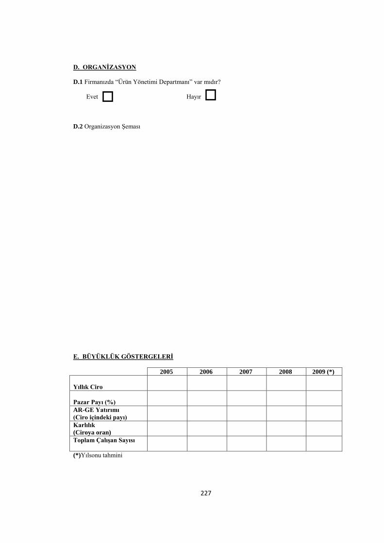
227

D. ORGANİZASYON

D.1 Firmanızda “Ürün Yönetimi Departmanı” var mıdır?

Evet Hayır

D.2 Organizasyon Şeması

E. BÜYÜKLÜK GÖSTERGELERİ

2005 2006 2007 2008 2009 (*)

Yıllık Ciro

Pazar Payı (%)

AR-GE Yatırımı

(Ciro içindeki payı)

Karlılık

(Ciroya oran)

Toplam Çalışan Sayısı

(*)Yılsonu tahmini

228

2.1 Firmanızın Ürün Yönetimi hangi faaliyetleri kapsar?

a) Ürün Yönetiminde ürün planlaması yapıyoruz. (0 … 100)

b) Ürün Yönetimimiz ürünün pazarlanması faaliyetlerini kapsar. (0 … 100)

c) Diğer (Açıklayınız) (0 … 100)

2.2 Firmanızın Ürün Yönetiminde amaçlar/hedefler nelerdir?

a) Pazar payını artırmak (0 … 100)

b) Pazara rakiplerimizden önce ürün sunmak (0 … 100)

c) Ürün maliyetlerini düşürmek (0 … 100)

d) Karlılığı artırmak (0 … 100)

e) Diğer (Açıklayınız) (0 … 100)

2.3 Firmanızın Ürün Yönetiminde alınan kararlar nelerdir?

a) Gelecek dönemlerde yeni ürün geliştirilmesi, ya da mevcut ürünlerde

iyileştirme/modifikasyon yapılması kararı (0 … 100)

b) Mevcut Pazar ya da yeni Pazar/Segment kararı (0 … 100)

c) Fiyatlandırma kararı (0 … 100)

d) Ürünün firma içinde üretilmesi ya da dışarıdan satın alınması kararı (0 … 100)

e) Üretim için hangi teknolojinin kullanılacağı kararı (0 … 100)

f) AR-GE projelerinin seçilmesi, önceliklerinin saptanması (0 … 100)

g) Yeni ürünün ne zaman imalata girmesi gerektiği kararı (0 … 100)

h) Yeni ürünün ne zaman piyasaya sunulacağı kararı (0 … 100)

i) AR-GE projelerine, proje bazında ayrılması gereken mali kaynakların saptanması kararı

(0 … 100)

j) Diğer (Açıklayınız) (0 … 100)

229

2.4 Firmanızın organizasyon yapısı içinde Ürün Yönetimine ilişkin kararlar hangi yönetim

kademesinde alınıyor?

a) Tüm kararları Yönetim Kurulu alır ve uygulamaya koyar (0 … 100)

b) Pazarlama Ve Satış Bölümü kararları tespit eder ve Yönetim Kurulunu onayına sunar

(0 … 100)

c) AR-GE, Pazarlama/Satış ve İmalat Bölümleri yetkilileri ekip olarak karar verirler ve

Yönetim Kurulu onayına sunarlar (0 … 100)

d) Ürün Yönetimi departmanı liderliğinde, AR-GE, Pazarlama ve İmalat bölümleri ekip olarak

kararları oluştururlar ve Yönetim Kurulunun onayına sunarlar (0 … 100)


230

2.5 Ürün Yönetimi kararlarınızı etkileyen başlıca faktörler nelerdir?

Faktör

A Ç I K L A M A

(0 … 100)

Pazar

Pazar yapısı, ürünün Pazar pozisyonu, talep,

pazarın cazibesi, vb.

Müşteriler

Müşteri istekleri, müşteri memnuniyeti, vb.

Rakipler

Rekabetin yoğunluğu, Pazar payı değişkenliği,

yeni ürünler, vb.

Teknoloji

Teknolojik değişim hızı, fırsatlar, teknolojik

değişimin türü

Tedarikçiler

İlişkiler, pazarlık gücü, sadakat

Distribütörler

Satış ağı, pazarlık gücü, satış gücü

Stratejik Planlama

Uzun dönem perspektif, stratejik amaçlar, ürün

stratejisi

Organizasyon

Üst yönetim desteği, ekip çalışması, iyi

iletişim, esnek yapı

Enformasyon

Data toplama, bilgi üretme, analiz

Öz Değerler

Kompetan yönetim, kaliteli personel,

bilimsellik, AR-GE, repütasyon, marka değeri

Kaynaklar

Mali kaynaklar, teknolojik yeterlilik, keşif

kabiliyeti

Makro/Çevresel Faktörler

Politik, yasal, çevreyi koruma, enerji tüketimi,

vb. dış etkiler

Diğer (Açıklayınız)

2.6 Ürünlerimizin Pazar içindeki pozisyonu aşağıdaki kararlarımız için önemlidir.

a) Fiyatlandırma (0 … 100)

b) Yeni ürüne geçiş kararı (0 … 100)

c) Mevcut ürünleri iyileştirme kararı (0 … 100)

d) Pazarlama stratejilerinde değişiklik (0 … 100)


231

2.7 Pazar talebi tahminlerini hangi sıklıkla yapıyorsunuz?

a) Siparişe dayalı üretim yaptığımız için ihtiyaç duymuyoruz. (0 … 100)

b) Aylık tahminlerde bulunuyoruz. (0 … 100)

c) Üçer aylık dönemlerde yapıyoruz. (0 … 100)

d) Yılda iki kez yapıyoruz. (0 … 100)

e) Yıllık yapıyoruz. (0 … 100)

f) Diğer (Açıklayınız) (0 … 100)

2.8 Müşterilerimizin istekleri/ihtiyaçları/tercihleri ile ilgili bilgiler düzenli olarak topluyoruz.

(0 … 100)

2.9 Şirketimizin amaç ve politikaları, müşterilerimizin memnuniyeti üzerine tesis edilmiştir.

(0 … 100)

2.10 Müşteri memnuniyeti seviyesini düzenli olarak değerlendirerek, iyileştirmeye yönelik

kararlarımızı derhal alıyoruz. (0 … 100)

2.11 Önemli müşterilerimiz/müşteri gruplarımızla kuvvetli ilişkiler kurmaya ve korumaya gayret

ediyoruz. (0 … 100)

2.12 Pazarımızda farklı ihtiyaçları olan farklı grup ve segmentlerin varlığını idrak ederek, kendimizi

buna göre adapte ediyoruz. (0 … 100)

2.13 Rakiplerimizin faaliyetleri hakkında düzenli olarak bilgi topluyoruz. (0 … 100)

2.14 Rakiplerimizin pazara sunumlarını takip edebilmek için düzenli olarak “Benchmarking” tatbik

ediyoruz. (0 … 100)

2.15 Önem verdiğimiz rakiplerimizin ataklarına hızlı cevap verebiliyoruz. (0 … 100)

2.16 Müşterilerimizin, rakiplerimizde önem verdiği konular hakkında kendimizi farklılaştırmaya çok

önem veriyoruz. (0 … 100)

2.17 AR-GE projelerimizi,

a) Rakiplerimizin teknolojik faaliyetlerine göre saptıyoruz. (0 … 100)

b) Pazardaki teknolojik değişim hızına göre saptıyoruz. (0 … 100)

c) Teknolojik değişimin radikal mi yoksa mevcutta iyileştirme mi olduğuna bakarak

saptıyoruz.

(0 … 100)

d) Müşterilerden gelen isteklere cevap verecek şekilde saptıyoruz. (0 … 100)


232

2.18 En büyük önceliğimiz, kısa dönemdeki karlılık değil, uzun vadedeki pazar payımızı artırmaktır.

(0 … 100)

2.19 İç bünyeye yönelik verimliliği artırmaktan çok, pazar performansımızı artırmaya önem

veriyoruz. (0 … 100)

2.20 Kararlarımızda kısa vadeli kazançları değil, uzun vadeli faydaları önemseriz. (0 … 100)

2.21 Müşterilerle ilgili bilgiler, organizasyon içinde sirküle edilir ve paylaşılır. (0 … 100)

2.22 Organizasyonda farklı departmanlarda müşterilerin ihtiyaçlarına hizmet etmek için etkin bir

şekilde birlikte çalışılır. (0 … 100)

2.23 Müşteri hizmetlerinin etkinliği için departmanlar arası gerilim ve çekişmeye izin verilmez.

(0 … 100)

2.24 Organizasyonumuz katı hiyerarşi ile kısıtlanmadan, fırsatları yakalayarak deperlendirebilecek

esnekliğe sahiptir. (0 … 100)

2.25 Çalışanlarımızın tümü, müşteri memnuniyeti için üslendikleri rolün bilincindedir. (0 … 100)

2.26 Çalışanı ödüllendirme sistemi pazar performansı ve müşteri memnuniyetine uygun kurulmuştur.

(0 … 100)

2.27 Üst yönetim, her zaman müşteri memnuniyetine ilişkin konulara öncelik verir. (0 … 100)

2.28 Tedarikçilerle olan ilişkilerimiz pazarda bizi avantajlı konumda tutmaktadır. (0 … 100)

2.29 Tedarikçilerle olan pazarlık gücümüz, rakiplerimize kıyasla bize üstünlük sağlar. (0 … 100)

2.30 Satış gücümüz, pazardaki en büyük kozumuzdur. (0 … 100)

2.31 Distribütörler/Perakendeciler satış gücümüzün en önemli parçasıdır. (0 … 100)

233

2.32 Kararlarınızı alırken hangi bilgilere ihtiyaç duyuyorsunuz?

a) Tüketici istekleri (0 … 100)

b) Rakiplerin faaliyetleri (0 … 100)

c) Talep tahminleri/Pazar araştırmaları (0 … 100)

d) Genel ekonomik veriler (0 … 100)

e) Maliyetler (0 … 100)

f) Kullanılabilir mali kaynaklar (0 … 100)

g) Diğer (Açıklayınız) (0 … 100)

2.33 Kararlarınızda kullandığınız bilgileri türetirken hangi teknikleri ve araçları kullanıyorsunuz?

a) “Beyin fırtınası” (Brainstorming) (0 … 100)

b) Tüketici analizleri (0 … 100)

c) “Benchmarking” (0 … 100)

d) Teknoloji tahminleri (0 … 100)

e) Trend analizleri (0 … 100)

f) Patent analizleri (0 … 100)

g) Regresyon (0 … 100)

h) Diğer (Açıklayınız) (0 … 100)

2.34 Kararlarınızı alırken göz önüne aldığınız kısıtlar nelerdir?

a) Mali kaynakların sınırları (0 … 100)

b) Teknolojik yeterlilik (0 … 100)

c) İnsan kaynakları (0 … 100)

d) Bilimsel bilgi ve analiz gücü (0 … 100)

e) AR-GE imkanları (0 … 100)

f) Yasal zorunluluklar (0 … 100)

g) Diğer (Açıklayınız) (0 … 100)

234

2.35 Aşağıdaki diyagramda, ürün yönetimi kararlarını etkileyebilecek makro-çevresel faktörler

gösterilmiştir. Firmanızda ürün yönetimi kararlarınızı etkileyen bu kategorideki faktörleri

(0-100) aralığında derecelendiriniz.

1. Politik (0 … 100) 4. Sosyo-kültürel (0 … 100)

2. Yasal (0 … 100) 5. Makro-teknolojik (0 … 100)

3. Ekonomik (0 … 100) 6. Çevresel (0 … 100)

Dış ticaret politikası

Vergi politikası

Politik istikrar

Sosyal refah

projeleri

Demografik nüfus

Gelir dağılımı

Sosyal hareketlilik

Yaşam tarzı değişiklikleri

İşve eğlence davranışları

Tüketici trendleri

Eğitim düzeyi

Rekabet piyasası

kanunları

İşçi yasaları

Ürün güvenliği yasası

Kamu sağlığı ve

güvencesi yasası

Hükümetin kendi yaptığı

araştırmalar

Hükümet ve endüstrinin

teknolojik eforları

Keşifler

Teknoloji transfer hızı

Dalgalanmalar

Büyüme trendi

Faiz oranları

Piyasanın para arzı

Enflasyon

İşsizlik

Harcanabilir gelir

Çevreyi koruma yasası

Geri kullanım/dönüşüm

Enerji ve doğal kaynaklar

tüketimi

ÜRÜN

YÖNETİMİ

235

3.1 Ürün yönetimi üç yıl ya da sonrası dönemleri kapsayan uzun vadeli planlama ve stratejik

kararlar almayı gerektirir. (0 … 100)

3.2 Etkin ve başarılı bir ürün yönetiminden beklenen, doğru zamanda doğru ürünlerle

piyasada olmak ve kaynakları en doğru şekilde kullanmaktır. (0 … 100)

3.3 Ürün yönetiminde ilk hareket noktası,

a) Tüketici istekleri/talepleridir. (0 … 100)

b) AR-GE’nin geliştirdiği projelerdir. (0 … 100)

3.3 Ürün yönetiminde sizi en çok zorlayan karar problemi hangisidir?

3.4 Sizce ideal/etkin ürün yönetimi nasıl olmalıdır?

BÖLÜM 3: GENELLEME

T E Ş E K K Ü R L E R

237

APPENDIX C

FLOWCHART OF PRODUCT MANAGEMENT FRAMEWORK

(FLOW MODEL)

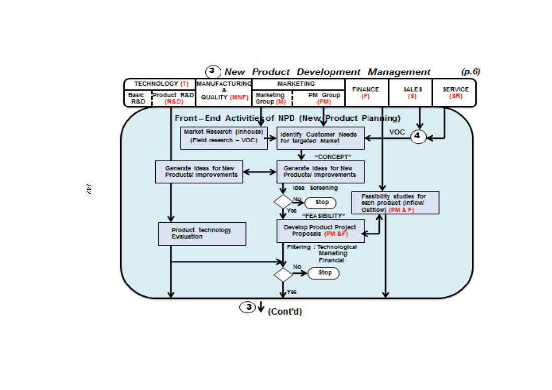
245

APPENDIX D

MATLAB 7.0 – CODE

function Victory = CombinedExpFinal1

% INPUT DEFINITIONS

P = xlsread('Parameters1-Com'); %Fixed Inputs

k = P(1); %number of products

ep = P(2); %coefficient

interest = P(3);

varep = P(4);

noe = P(5);

Exp = xlsread('Experiments3');% should be in Scenario matrix format

K = xlsread('Parameters2-Com'); %Product dependent inputs-array inputs

meancost = K(1,:);

varcost = K(2,:);

sigmacost = sqrt(varcost);

unitcap = K(3,:);

totcap = K(4,:);

meanp = xlsread('meanp');

varp = xlsread('varp');

sigmap = sqrt(varp);

intercept = xlsread('intercept');

elasticity = xlsread('elasticity');

lowbound = xlsread('lowbound');

marketmat = xlsread('marketmat');

Scenario =

scenario(k,ep,meancost,sigmacost,meanp,sigmap,intercept,elasticity,marketmat

,varep);

ComScenario = cat(1,Scenario,Exp);

Optimization =

optimization(k,ComScenario,lowbound,marketmat,unitcap,totcap,interest,noe);

Victory = 35;

% STRUCTURED SCENARIO GENERATION

function Scenario =

scenario(k,ep,meancost,sigmacost,meanp,sigmap,intercept,elasticity,marketmat

,varep)

m = sum(marketmat,2);

summ = sum(m);

n = 2*summ + k;

Scenario = ff2n(n);

xlswrite('ComResults',Scenario,'First');

for j = 1:k

col = 1;

if j == 1

col = 1;

else

for l = 1:j-1

col = col + 2*m(l) + 1;

end

end

for i = 1:2^n

if Scenario(i,col) == 1

Scenario(i,col) = meancost(j) + ep * sigmacost(j);

else

Scenario(i,col) = meancost(j) - ep * sigmacost(j);

246

end

end

end

xlswrite('ComResults',Scenario,'Second');

for j = 1:k

col = 1;

if j == 1

col = 1;

else

for l = 1:j-1

col = col + 2*m(l) + 1;

end

end

indices = find(marketmat(j,:));

for l = 0:m(j)-1

for i = 1:2^n

if Scenario(i,col + 2*l + 1) == 1

Scenario(i,col + 2*l + 1) = meanp(j,indices(l+1)) + ep *

sigmap(j,indices(l+1));

else

Scenario(i,col + 2*l + 1) = meanp(j,indices(l+1)) - ep *

sigmap(j,indices(l+1));

end

end

end

end

xlswrite('ComResults',Scenario,'Third');

for j = 1:k

col = 1;

if j == 1

col = 1;

else

for l = 1:j-1

col = col + 2*m(l) + 1;

end

end

indices = find(marketmat(j,:));

for l = 0:m(j)-1

for i = 1:2^n

temp = intercept(j,indices(l+1)) - elasticity(j,indices(l+1)) *

Scenario(i,col + 2*l + 1);

if Scenario(i,col + 2*l + 2) == 1

Scenario(i,col + 2*l + 2) = temp + sqrt(varep * temp);

else

Scenario(i,col + 2*l + 2) = temp - sqrt(varep * temp);

end

end

end

end

savefile = 'ComScenario.mat';

save(savefile, 'Scenario');

%xlswrite('ComResults',Scenario,'Forth');

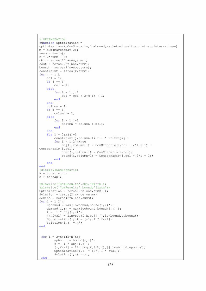
247

% OPTIMIZATION

function Optimization =

optimization(k,ComScenario,lowbound,marketmat,unitcap,totcap,interest,noe)

m = sum(marketmat,2);

summ = sum(m);

n = 2*summ + k;

obj = zeros(2^n+noe,summ);

cost = zeros(2^n+noe,summ);

bound = zeros(2^n+noe,summ);

constraint = zeros(k,summ);

for j = 1:k

col = 1;

if j == 1

col = 1;

else

for l = 1:j-1

col = col + 2*m(l) + 1;

end

end

column = 1;

if j == 1

column = 1;

else

for l = 1:j-1

column = column + m(l);

end

end

for l = 0:m(j)-1

constraint(j,column+l) = 1 * unitcap(j);

for i = 1:2^n+noe

obj(i,column+l) = ComScenario(i,col + 2*l + 1) -

ComScenario(i,col);

cost(i,column+l) = ComScenario(i,col);

bound(i,column+l) = ComScenario(i,col + 2*l + 2);

end

end

end

%display(ComScenario)

A = constraint;

b = totcap';

%xlswrite('ComResults',obj,'Fifth');

%xlswrite('ComResults',bound,'Sixth');

Optimization = zeros(2^n+noe,summ+1);

Solution = zeros(2^n+noe,summ);

demand = zeros(2^n+noe,summ);

for i = 1:2^n

upbound = max(lowbound,bound(i,:)');

demand(i,:) = max(lowbound,bound(i,:)');

f = -1 * obj(i,:)';

[x,fval] = linprog(f,A,b,[],[],lowbound,upbound);

Optimization(i,:) = [x',-1 * fval];

Solution(i,:) = x';

end

for i = 2^n+1:2^n+noe

upbound = bound(i,:)';

f = -1 * obj(i,:)';

[x,fval] = linprog(f,A,b,[],[],lowbound,upbound);

Optimization(i,:) = [x',-1 * fval];

Solution(i,:) = x';

end

248

xlswrite('ComResults',Optimization,'Result');

% TESTING THE SOLUTIONS UNDER ALL STRUCTURED SCENARIOS-Objective Function

Rmatrix = zeros(2^n+noe,2^n);

for i = 1:2^n+noe

for j = 1:2^n

Rmatrix(i,j) = (Solution(i,:) - max(Solution(i,:) - demand(j,:), 0)

) * obj(j,:)' - interest * max(Solution(i,:) - demand(j,:), 0) * cost(j,:)'

;

end

end

%xlswrite('ComResults',Rmatrix,'Rmatrix');

Profitmin = min(Rmatrix,[],2);

Profitmax = max(Rmatrix,[],2);

Profitmean = mean(Rmatrix,2);

Profitstd = std(Rmatrix,1,2);

Profitdata = zeros(2^n+noe,4);

Profitdata(:,1)= Profitmin;

Profitdata(:,2)= Profitmax;

Profitdata(:,3)= Profitmean;

Profitdata(:,4)= Profitstd;

savefile = 'ComProfit.mat';

save(savefile,'Profitdata');

% REGRET MATRIX CONSTRUCTION

Regretmat = zeros(2^n,2^n);

for i = 1:2^n

for j=1:2^n

Regretmat(i,j) = Rmatrix(j,j) - Rmatrix(i,j);

end

end

for i = 2^n+1:2^n+noe

for j=1:2^n

Regretmat(i,j) = Optimization(j,summ+1) - Rmatrix(i,j);

end

end

%xlswrite('ComResults',Regretmat,'Regretmat');

% REGRET FREE PROFIT

Pdistance = zeros (2^n+noe,2^n);

for i = 1:2^n+noe

Pdistance (i,:) = Rmatrix (i,:)- Regretmat (i,:);

end

%xlswrite('ComResults',Pdistance,'Pdistance');

Pdistancemin = min(Pdistance,[],2);

Pdistancemax = max(Pdistance,[],2);

Pdistancemean = mean(Pdistance,2);

Pdistancestd = std(Pdistance,1,2);

Pdistanceskew = skewness(Pdistance,1,2);

Pdistancesq = Pdistance .* Pdistance;

Reciprocal = zeros (2^n+noe,2^n);

for i = 1:2^n+noe

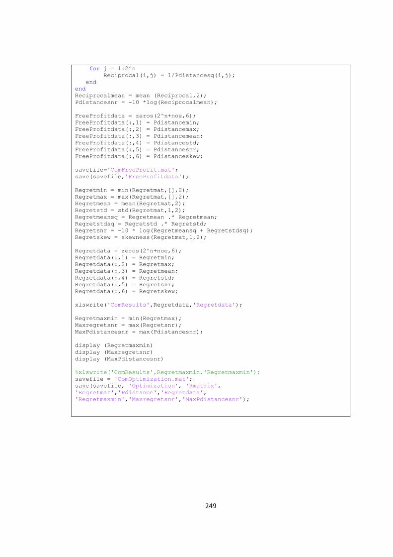
249

for j = 1:2^n

Reciprocal(i,j) = 1/Pdistancesq(i,j);

end

end

Reciprocalmean = mean (Reciprocal,2);

Pdistancesnr = -10 *log(Reciprocalmean);

FreeProfitdata = zeros(2^n+noe,6);

FreeProfitdata(:,1) = Pdistancemin;

FreeProfitdata(:,2) = Pdistancemax;

FreeProfitdata(:,3) = Pdistancemean;

FreeProfitdata(:,4) = Pdistancestd;

FreeProfitdata(:,5) = Pdistancesnr;

FreeProfitdata(:,6) = Pdistanceskew;

savefile='ComFreeProfit.mat';

save(savefile,'FreeProfitdata');

Regretmin = min(Regretmat,[],2);

Regretmax = max(Regretmat,[],2);

Regretmean = mean(Regretmat,2);

Regretstd = std(Regretmat,1,2);

Regretmeansq = Regretmean .* Regretmean;

Regretstdsq = Regretstd .* Regretstd;

Regretsnr = -10 * log(Regretmeansq + Regretstdsq);

Regretskew = skewness(Regretmat,1,2);

Regretdata = zeros(2^n+noe,6);

Regretdata(:,1) = Regretmin;

Regretdata(:,2) = Regretmax;

Regretdata(:,3) = Regretmean;

Regretdata(:,4) = Regretstd;

Regretdata(:,5) = Regretsnr;

Regretdata(:,6) = Regretskew;

xlswrite('ComResults',Regretdata,'Regretdata');

Regretmaxmin = min(Regretmax);

Maxregretsnr = max(Regretsnr);

MaxPdistancesnr = max(Pdistancesnr);

display (Regretmaxmin)

display (Maxregretsnr)

display (MaxPdistancesnr)

%xlswrite('ComResults',Regretmaxmin,'Regretmaxmin');

savefile = 'ComOptimization.mat';

save(savefile, 'Optimization', 'Rmatrix',

'Regretmat','Pdistance','Regretdata',

'Regretmaxmin','Maxregretsnr','MaxPdistancesnr');

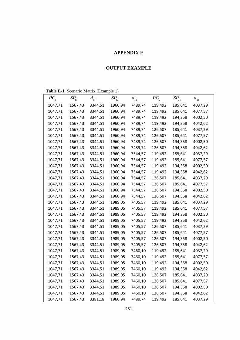
251

APPENDIX E

OUTPUT EXAMPLE

Table E-1: Scenario Matrix (Example 1)

1PC 11SP 11d 12SP 12d

2PC 21SP 21d

1047,71 1567,43 3344,51 1960,94 7489,74 119,492 185,641 4037,29

1047,71 1567,43 3344,51 1960,94 7489,74 119,492 185,641 4077,57

1047,71 1567,43 3344,51 1960,94 7489,74 119,492 194,358 4002,50

1047,71 1567,43 3344,51 1960,94 7489,74 119,492 194,358 4042,62

1047,71 1567,43 3344,51 1960,94 7489,74 126,507 185,641 4037,29

1047,71 1567,43 3344,51 1960,94 7489,74 126,507 185,641 4077,57

1047,71 1567,43 3344,51 1960,94 7489,74 126,507 194,358 4002,50

1047,71 1567,43 3344,51 1960,94 7489,74 126,507 194,358 4042,62

1047,71 1567,43 3344,51 1960,94 7544,57 119,492 185,641 4037,29

1047,71 1567,43 3344,51 1960,94 7544,57 119,492 185,641 4077,57

1047,71 1567,43 3344,51 1960,94 7544,57 119,492 194,358 4002,50

1047,71 1567,43 3344,51 1960,94 7544,57 119,492 194,358 4042,62

1047,71 1567,43 3344,51 1960,94 7544,57 126,507 185,641 4037,29

1047,71 1567,43 3344,51 1960,94 7544,57 126,507 185,641 4077,57

1047,71 1567,43 3344,51 1960,94 7544,57 126,507 194,358 4002,50

1047,71 1567,43 3344,51 1960,94 7544,57 126,507 194,358 4042,62

1047,71 1567,43 3344,51 1989,05 7405,57 119,492 185,641 4037,29

1047,71 1567,43 3344,51 1989,05 7405,57 119,492 185,641 4077,57

1047,71 1567,43 3344,51 1989,05 7405,57 119,492 194,358 4002,50

1047,71 1567,43 3344,51 1989,05 7405,57 119,492 194,358 4042,62

1047,71 1567,43 3344,51 1989,05 7405,57 126,507 185,641 4037,29

1047,71 1567,43 3344,51 1989,05 7405,57 126,507 185,641 4077,57

1047,71 1567,43 3344,51 1989,05 7405,57 126,507 194,358 4002,50

1047,71 1567,43 3344,51 1989,05 7405,57 126,507 194,358 4042,62

1047,71 1567,43 3344,51 1989,05 7460,10 119,492 185,641 4037,29

1047,71 1567,43 3344,51 1989,05 7460,10 119,492 185,641 4077,57

1047,71 1567,43 3344,51 1989,05 7460,10 119,492 194,358 4002,50

1047,71 1567,43 3344,51 1989,05 7460,10 119,492 194,358 4042,62

1047,71 1567,43 3344,51 1989,05 7460,10 126,507 185,641 4037,29

1047,71 1567,43 3344,51 1989,05 7460,10 126,507 185,641 4077,57

1047,71 1567,43 3344,51 1989,05 7460,10 126,507 194,358 4002,50

1047,71 1567,43 3344,51 1989,05 7460,10 126,507 194,358 4042,62

1047,71 1567,43 3381,18 1960,94 7489,74 119,492 185,641 4037,29

252

1047,71 1567,43 3381,18 1960,94 7489,74 119,492 185,641 4077,57

1047,71 1567,43 3381,18 1960,94 7489,74 119,492 194,358 4002,50

1047,71 1567,43 3381,18 1960,94 7489,74 119,492 194,358 4042,62

1047,71 1567,43 3381,18 1960,94 7489,74 126,507 185,641 4037,29

1047,71 1567,43 3381,18 1960,94 7489,74 126,507 185,641 4077,57

1047,71 1567,43 3381,18 1960,94 7489,74 126,507 194,358 4002,50

1047,71 1567,43 3381,18 1960,94 7489,74 126,507 194,358 4042,62

1047,71 1567,43 3381,18 1960,94 7544,57 119,492 185,641 4037,29

1047,71 1567,43 3381,18 1960,94 7544,57 119,492 185,641 4077,57

1047,71 1567,43 3381,18 1960,94 7544,57 119,492 194,358 4002,50

1047,71 1567,43 3381,18 1960,94 7544,57 119,492 194,358 4042,62

1047,71 1567,43 3381,18 1960,94 7544,57 126,507 185,641 4037,29

1047,71 1567,43 3381,18 1960,94 7544,57 126,507 185,641 4077,57

1047,71 1567,43 3381,18 1960,94 7544,57 126,507 194,358 4002,50

1047,71 1567,43 3381,18 1960,94 7544,57 126,507 194,358 4042,62

1047,71 1567,43 3381,18 1989,05 7405,57 119,492 185,641 4037,29

1047,71 1567,43 3381,18 1989,05 7405,57 119,492 185,641 4077,57

1047,71 1567,43 3381,18 1989,05 7405,57 119,492 194,358 4002,50

1047,71 1567,43 3381,18 1989,05 7405,57 119,492 194,358 4042,62

1047,71 1567,43 3381,18 1989,05 7405,57 126,507 185,641 4037,29

1047,71 1567,43 3381,18 1989,05 7405,57 126,507 185,641 4077,57

1047,71 1567,43 3381,18 1989,05 7405,57 126,507 194,358 4002,50

1047,71 1567,43 3381,18 1989,05 7405,57 126,507 194,358 4042,62

1047,71 1567,43 3381,18 1989,05 7460,10 119,492 185,641 4037,29

1047,71 1567,43 3381,18 1989,05 7460,10 119,492 185,641 4077,57

1047,71 1567,43 3381,18 1989,05 7460,10 119,492 194,358 4002,50

1047,71 1567,43 3381,18 1989,05 7460,10 119,492 194,358 4042,62

1047,71 1567,43 3381,18 1989,05 7460,10 126,507 185,641 4037,29

1047,71 1567,43 3381,18 1989,05 7460,10 126,507 185,641 4077,57

1047,71 1567,43 3381,18 1989,05 7460,10 126,507 194,358 4002,50

1047,71 1567,43 3381,18 1989,05 7460,10 126,507 194,358 4042,62

1047,71 1592,57 3219,15 1960,94 7489,74 119,492 185,641 4037,29

1047,71 1592,57 3219,15 1960,94 7489,74 119,492 185,641 4077,57

1047,71 1592,57 3219,15 1960,94 7489,74 119,492 194,358 4002,50

1047,71 1592,57 3219,15 1960,94 7489,74 119,492 194,358 4042,62

1047,71 1592,57 3219,15 1960,94 7489,74 126,507 185,641 4037,29

1047,71 1592,57 3219,15 1960,94 7489,74 126,507 185,641 4077,57

1047,71 1592,57 3219,15 1960,94 7489,74 126,507 194,358 4002,50

1047,71 1592,57 3219,15 1960,94 7489,74 126,507 194,358 4042,62

1047,71 1592,57 3219,15 1960,94 7544,57 119,492 185,641 4037,29

1047,71 1592,57 3219,15 1960,94 7544,57 119,492 185,641 4077,57

1047,71 1592,57 3219,15 1960,94 7544,57 119,492 194,358 4002,50

1047,71 1592,57 3219,15 1960,94 7544,57 119,492 194,358 4042,62

253

1047,71 1592,57 3219,15 1960,94 7544,57 126,507 185,641 4037,29

1047,71 1592,57 3219,15 1960,94 7544,57 126,507 185,641 4077,57

1047,71 1592,57 3219,15 1960,94 7544,57 126,507 194,358 4002,50

1047,71 1592,57 3219,15 1960,94 7544,57 126,507 194,358 4042,62

1047,71 1592,57 3219,15 1989,05 7405,57 119,492 185,641 4037,29

1047,71 1592,57 3219,15 1989,05 7405,57 119,492 185,641 4077,57

1047,71 1592,57 3219,15 1989,05 7405,57 119,492 194,358 4002,50

1047,71 1592,57 3219,15 1989,05 7405,57 119,492 194,358 4042,62

1047,71 1592,57 3219,15 1989,05 7405,57 126,507 185,641 4037,29

1047,71 1592,57 3219,15 1989,05 7405,57 126,507 185,641 4077,57

1047,71 1592,57 3219,15 1989,05 7405,57 126,507 194,358 4002,50

1047,71 1592,57 3219,15 1989,05 7405,57 126,507 194,358 4042,62

1047,71 1592,57 3219,15 1989,05 7460,10 119,492 185,641 4037,29

1047,71 1592,57 3219,15 1989,05 7460,10 119,492 185,641 4077,57

1047,71 1592,57 3219,15 1989,05 7460,10 119,492 194,358 4002,50

1047,71 1592,57 3219,15, 1989,05 7460,10 119,492 194,358 4042,62

1047,71 1592,57 3219,15 1989,05 7460,10 126,507 185,641 4037,29

1047,71 1592,57 3219,15 1989,05 7460,10 126,507 185,641 4077,57

1047,71 1592,57 3219,15 1989,05 7460,10 126,507 194,358 4002,50

1047,71 1592,57 3219,15 1989,05 7460,10 126,507 194,358 4042,62

1047,71 1592,57 3255,14 1960,94 7489,74 119,492 185,641 4037,29

1047,71 1592,57 3255,14 1960,94 7489,74 119,492 185,641 4077,57

1047,71 1592,57 3255,14 1960,94 7489,74 119,492 194,358 4002,50

1047,71 1592,57 3255,14 1960,94 7489,74 119,492 194,358 4042,62

1047,71 1592,57 3255,14 1960,94 7489,74 126,507 185,641 4037,29

1047,71 1592,57 3255,14 1960,94 7489,74 126,507 185,641 4077,57

1047,71 1592,57 3255,14 1960,94 7489,74 126,507 194,358 4002,50

1047,71 1592,57 3255,14 1960,94 7489,74 126,507 194,358 4042,62

1047,71 1592,57 3255,14 1960,94 7544,57 119,492 185,641 4037,29

1047,71 1592,57 3255,14 1960,94 7544,57 119,492 185,641 4077,57

1047,71 1592,57 3255,14 1960,94 7544,57 119,492 194,358 4002,50

1047,71 1592,57 3255,14 1960,94 7544,57 119,492 194,358 4042,62

1047,71 1592,57 3255,14 1960,94 7544,57 126,507 185,641 4037,29

1047,71 1592,57 3255,14 1960,94 7544,57 126,507 185,641 4077,57

1047,71 1592,57 3255,14 1960,94 7544,57 126,507 194,358 4002,50

1047,71 1592,57 3255,14 1960,94 7544,57 126,507 194,358 4042,62

1047,71 1592,57 3255,14 1989,05 7405,57 119,492 185,641 4037,29

1047,71 1592,57 3255,14 1989,05 7405,57 119,492 185,641 4077,57

1047,71 1592,57 3255,14 1989,05 7405,57 119,492 194,358 4002,50

1047,71 1592,57 3255,14 1989,05 7405,57 119,492 194,358 4042,62

1047,71 1592,57 3255,14 1989,05 7405,57 126,507 185,641 4037,29

1047,71 1592,57 3255,14 1989,05 7405,57 126,507 185,641 4077,57

1047,71 1592,57 3255,14 1989,05 7405,57 126,507 194,358 4002,50

254

1047,71 1592,57 3255,14 1989,05 7405,57 126,507 194,358 4042,62

1047,71 1592,57 3255,14 1989,05 7460,10 119,492 185,641 4037,29

1047,71 1592,57 3255,14 1989,05 7460,10 119,492 185,641 4077,57

1047,71 1592,57 3255,14 1989,05 7460,10 119,492 194,358 4002,50

1047,71 1592,57 3255,14 1989,05 7460,10 119,492 194,358 4042,62

1047,71 1592,57 3255,14 1989,05 7460,10 126,507 185,641 4037,29

1047,71 1592,57 3255,14 1989,05 7460,10 126,507 185,641 4077,57

1047,71 1592,57 3255,14 1989,05 7460,10 126,507 194,358 4002,50

1047,71 1592,57 3255,14 1989,05 7460,10 126,507 194,358 4042,62

1068,28 1567,43 3344,51 1960,94 7489,74 119,492 185,641 4037,29

1068,28 1567,43 3344,51 1960,94 7489,74 119,492 185,641 4077,57

1068,28 1567,43 3344,51 1960,94 7489,74 119,492 194,358 4002,50

1068,28 1567,43 3344,51 1960,94 7489,74 119,492 194,358 4042,62

1068,28 1567,43 3344,51 1960,94 7489,74 126,507 185,641 4037,29

1068,28 1567,43 3344,51 1960,94 7489,74 126,507 185,641 4077,57

1068,28 1567,43 3344,51 1960,94 7489,74 126,507 194,358 4002,50

1068,28 1567,43 3344,51 1960,94 7489,74 126,507 194,358 4042,62

1068,28 1567,43 3344,51 1960,94 7544,57 119,492 185,641 4037,29

1068,28 1567,43 3344,51 1960,94 7544,57 119,492 185,641 4077,57

1068,28 1567,43 3344,51 1960,94 7544,57 119,492 194,358 4002,50

1068,28 1567,43 3344,51 1960,94 7544,57 119,492 194,358 4042,62

1068,28 1567,43 3344,51 1960,94 7544,57 126,507 185,641 4037,29

1068,28 1567,43 3344,51 1960,94 7544,57 126,507 185,641 4077,57

1068,28 1567,43 3344,51 1960,94 7544,57 126,507 194,358 4002,50

1068,28 1567,43 3344,51 1960,94 7544,57 126,507 194,358 4042,62

1068,28 1567,43 3344,51 1989,05 7405,57 119,492 185,641 4037,29

1068,28 1567,43 3344,51 1989,05 7405,57 119,492 185,641 4077,57

1068,28 1567,43 3344,51 1989,05 7405,57 119,492 194,358 4002,50

1068,28 1567,43 3344,51 1989,05 7405,57 119,492 194,358 4042,62

1068,28 1567,43 3344,51 1989,05 7405,57 126,507 185,641 4037,29

1068,28 1567,43 3344,51 1989,05 7405,57 126,507 185,641 4077,57

1068,28 1567,43 3344,51 1989,05 7405,57 126,507 194,358 4002,50

1068,28 1567,43 3344,51 1989,05 7405,57 126,507 194,358 4042,62

1068,28 1567,43 3344,51 1989,05 7460,10 119,492 185,641 4037,29

1068,28 1567,43 3344,51 1989,05 7460,10 119,492 185,641 4077,57

1068,28 1567,43 3344,51 1989,05 7460,10 119,492 194,358 4002,50

1068,28 1567,43 3344,51 1989,05 7460,10 119,492 194,358 4042,62

1068,28 1567,43 3344,51 1989,05 7460,10 126,507 185,641 4037,29

1068,28 1567,43 3344,51 1989,05 7460,10 126,507 185,641 4077,57

1068,28 1567,43 3344,51 1989,05 7460,10 126,507 194,358 4002,50

1068,28 1567,43 3344,51 1989,05 7460,10 126,507 194,358 4042,62

1068,28 1567,43 3381,18 1960,94 7489,74 119,492 185,641 4037,29

1068,28 1567,43 3381,18 1960,94 7489,74 119,492 185,641 4077,57

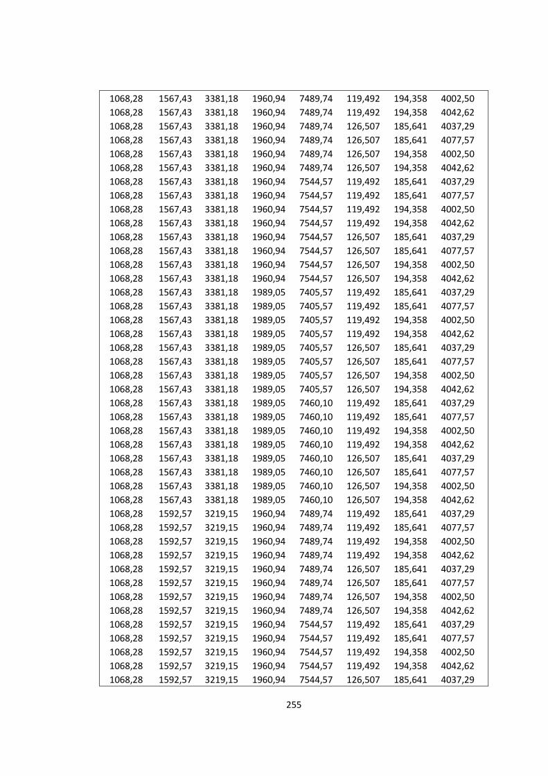
255

1068,28 1567,43 3381,18 1960,94 7489,74 119,492 194,358 4002,50

1068,28 1567,43 3381,18 1960,94 7489,74 119,492 194,358 4042,62

1068,28 1567,43 3381,18 1960,94 7489,74 126,507 185,641 4037,29

1068,28 1567,43 3381,18 1960,94 7489,74 126,507 185,641 4077,57

1068,28 1567,43 3381,18 1960,94 7489,74 126,507 194,358 4002,50

1068,28 1567,43 3381,18 1960,94 7489,74 126,507 194,358 4042,62

1068,28 1567,43 3381,18 1960,94 7544,57 119,492 185,641 4037,29

1068,28 1567,43 3381,18 1960,94 7544,57 119,492 185,641 4077,57

1068,28 1567,43 3381,18 1960,94 7544,57 119,492 194,358 4002,50

1068,28 1567,43 3381,18 1960,94 7544,57 119,492 194,358 4042,62

1068,28 1567,43 3381,18 1960,94 7544,57 126,507 185,641 4037,29

1068,28 1567,43 3381,18 1960,94 7544,57 126,507 185,641 4077,57

1068,28 1567,43 3381,18 1960,94 7544,57 126,507 194,358 4002,50

1068,28 1567,43 3381,18 1960,94 7544,57 126,507 194,358 4042,62

1068,28 1567,43 3381,18 1989,05 7405,57 119,492 185,641 4037,29

1068,28 1567,43 3381,18 1989,05 7405,57 119,492 185,641 4077,57

1068,28 1567,43 3381,18 1989,05 7405,57 119,492 194,358 4002,50

1068,28 1567,43 3381,18 1989,05 7405,57 119,492 194,358 4042,62

1068,28 1567,43 3381,18 1989,05 7405,57 126,507 185,641 4037,29

1068,28 1567,43 3381,18 1989,05 7405,57 126,507 185,641 4077,57

1068,28 1567,43 3381,18 1989,05 7405,57 126,507 194,358 4002,50

1068,28 1567,43 3381,18 1989,05 7405,57 126,507 194,358 4042,62

1068,28 1567,43 3381,18 1989,05 7460,10 119,492 185,641 4037,29

1068,28 1567,43 3381,18 1989,05 7460,10 119,492 185,641 4077,57

1068,28 1567,43 3381,18 1989,05 7460,10 119,492 194,358 4002,50

1068,28 1567,43 3381,18 1989,05 7460,10 119,492 194,358 4042,62

1068,28 1567,43 3381,18 1989,05 7460,10 126,507 185,641 4037,29

1068,28 1567,43 3381,18 1989,05 7460,10 126,507 185,641 4077,57

1068,28 1567,43 3381,18 1989,05 7460,10 126,507 194,358 4002,50

1068,28 1567,43 3381,18 1989,05 7460,10 126,507 194,358 4042,62

1068,28 1592,57 3219,15 1960,94 7489,74 119,492 185,641 4037,29

1068,28 1592,57 3219,15 1960,94 7489,74 119,492 185,641 4077,57

1068,28 1592,57 3219,15 1960,94 7489,74 119,492 194,358 4002,50

1068,28 1592,57 3219,15 1960,94 7489,74 119,492 194,358 4042,62

1068,28 1592,57 3219,15 1960,94 7489,74 126,507 185,641 4037,29

1068,28 1592,57 3219,15 1960,94 7489,74 126,507 185,641 4077,57

1068,28 1592,57 3219,15 1960,94 7489,74 126,507 194,358 4002,50

1068,28 1592,57 3219,15 1960,94 7489,74 126,507 194,358 4042,62

1068,28 1592,57 3219,15 1960,94 7544,57 119,492 185,641 4037,29

1068,28 1592,57 3219,15 1960,94 7544,57 119,492 185,641 4077,57

1068,28 1592,57 3219,15 1960,94 7544,57 119,492 194,358 4002,50

1068,28 1592,57 3219,15 1960,94 7544,57 119,492 194,358 4042,62

1068,28 1592,57 3219,15 1960,94 7544,57 126,507 185,641 4037,29

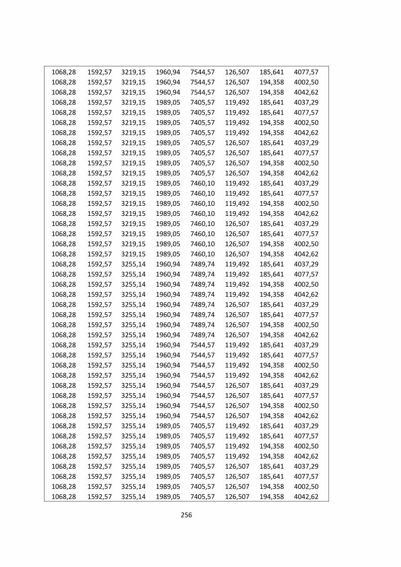
256

1068,28 1592,57 3219,15 1960,94 7544,57 126,507 185,641 4077,57

1068,28 1592,57 3219,15 1960,94 7544,57 126,507 194,358 4002,50

1068,28 1592,57 3219,15 1960,94 7544,57 126,507 194,358 4042,62

1068,28 1592,57 3219,15 1989,05 7405,57 119,492 185,641 4037,29

1068,28 1592,57 3219,15 1989,05 7405,57 119,492 185,641 4077,57

1068,28 1592,57 3219,15 1989,05 7405,57 119,492 194,358 4002,50

1068,28 1592,57 3219,15 1989,05 7405,57 119,492 194,358 4042,62

1068,28 1592,57 3219,15 1989,05 7405,57 126,507 185,641 4037,29

1068,28 1592,57 3219,15 1989,05 7405,57 126,507 185,641 4077,57

1068,28 1592,57 3219,15 1989,05 7405,57 126,507 194,358 4002,50

1068,28 1592,57 3219,15 1989,05 7405,57 126,507 194,358 4042,62

1068,28 1592,57 3219,15 1989,05 7460,10 119,492 185,641 4037,29

1068,28 1592,57 3219,15 1989,05 7460,10 119,492 185,641 4077,57

1068,28 1592,57 3219,15 1989,05 7460,10 119,492 194,358 4002,50

1068,28 1592,57 3219,15 1989,05 7460,10 119,492 194,358 4042,62

1068,28 1592,57 3219,15 1989,05 7460,10 126,507 185,641 4037,29

1068,28 1592,57 3219,15 1989,05 7460,10 126,507 185,641 4077,57

1068,28 1592,57 3219,15 1989,05 7460,10 126,507 194,358 4002,50

1068,28 1592,57 3219,15 1989,05 7460,10 126,507 194,358 4042,62

1068,28 1592,57 3255,14 1960,94 7489,74 119,492 185,641 4037,29

1068,28 1592,57 3255,14 1960,94 7489,74 119,492 185,641 4077,57

1068,28 1592,57 3255,14 1960,94 7489,74 119,492 194,358 4002,50

1068,28 1592,57 3255,14 1960,94 7489,74 119,492 194,358 4042,62

1068,28 1592,57 3255,14 1960,94 7489,74 126,507 185,641 4037,29

1068,28 1592,57 3255,14 1960,94 7489,74 126,507 185,641 4077,57

1068,28 1592,57 3255,14 1960,94 7489,74 126,507 194,358 4002,50

1068,28 1592,57 3255,14 1960,94 7489,74 126,507 194,358 4042,62

1068,28 1592,57 3255,14 1960,94 7544,57 119,492 185,641 4037,29

1068,28 1592,57 3255,14 1960,94 7544,57 119,492 185,641 4077,57

1068,28 1592,57 3255,14 1960,94 7544,57 119,492 194,358 4002,50

1068,28 1592,57 3255,14 1960,94 7544,57 119,492 194,358 4042,62

1068,28 1592,57 3255,14 1960,94 7544,57 126,507 185,641 4037,29

1068,28 1592,57 3255,14 1960,94 7544,57 126,507 185,641 4077,57

1068,28 1592,57 3255,14 1960,94 7544,57 126,507 194,358 4002,50

1068,28 1592,57 3255,14 1960,94 7544,57 126,507 194,358 4042,62

1068,28 1592,57 3255,14 1989,05 7405,57 119,492 185,641 4037,29

1068,28 1592,57 3255,14 1989,05 7405,57 119,492 185,641 4077,57

1068,28 1592,57 3255,14 1989,05 7405,57 119,492 194,358 4002,50

1068,28 1592,57 3255,14 1989,05 7405,57 119,492 194,358 4042,62

1068,28 1592,57 3255,14 1989,05 7405,57 126,507 185,641 4037,29

1068,28 1592,57 3255,14 1989,05 7405,57 126,507 185,641 4077,57

1068,28 1592,57 3255,14 1989,05 7405,57 126,507 194,358 4002,50

1068,28 1592,57 3255,14 1989,05 7405,57 126,507 194,358 4042,62

257

1068,28 1592,57 3255,14 1989,05 7460,10 119,492 185,641 4037,29

1068,28 1592,57 3255,14 1989,05 7460,10 119,492 185,641 4077,57

1068,28 1592,57 3255,14 1989,05 7460,10 119,492 194,358 4002,50

1068,28 1592,57 3255,14 1989,05 7460,10 119,492 194,358 4042,62

1068,28 1592,57 3255,14 1989,05 7460,10 126,507 185,641 4037,29

1068,28 1592,57 3255,14 1989,05 7460,10 126,507 185,641 4077,57

1068,28 1592,57

3255,14

1989,05

7460,10

126,507

194,358

4002,50

1068,28 1592,57 3255,14 1989,05 7460,10 126,507 194,358 4042,62

Table E-2: Optimal Solutions under Each Scenario (Example 1)

*

11x *

12x *

21x *

.opP

3344,511 7489,743 4037,293 8845132

3344,511 7489,743 4077,579 8847797

3344,511 7489,743 4002,508 8877724

3344,511 7489,743 4042,621 8880727

3344,511 7489,743 4037,293 8816814

3344,511 7489,743 4077,579 8819196

3344,511 7489,743 4002,508 8849650

3344,511 7489,743 4042,621 8852371

3344,511 7544,578 4037,293 8895209

3344,511 7544,578 4077,579 8897874

3344,511 7544,578 4002,508 8927801

3344,511 7544,578 4042,621 8930804

3344,511 7544,578 4037,293 8866891

3344,511 7544,578 4077,579 8869273

3344,511 7544,578 4002,508 8899727

3344,511 7544,578 4042,621 8902448

3344,511 7405,576 4037,293 8976417

3344,511 7405,576 4077,579 8979082

3344,511 7405,576 4002,508 9009009

3344,511 7405,576 4042,621 9012012

3344,511 7405,576 4037,293 8948098

3344,511 7405,576 4077,579 8950480

3344,511 7405,576 4002,508 8980934

3344,511 7405,576 4042,621 8983656

3344,511 7460,103 4037,293 9027745

3344,511 7460,103 4077,579 9030409

3344,511 7460,103 4002,508 9060337

3344,511 7460,103 4042,621 9063340

3344,511 7460,103 4037,293 8999426

258

3344,511 7460,103 4077,579 9001808

3344,511 7460,103 4002,508 9032262

3344,511 7460,103 4042,621 9034984

3381,187 7489,743 4037,293 8864193

3381,187 7489,743 4077,579 8866858

3381,187 7489,743 4002,508 8896786

3381,187 7489,743 4042,621 8899789

3381,187 7489,743 4037,293 8835875

3381,187 7489,743 4077,579 8838257

3381,187 7489,743 4002,508 8868711

3381,187 7489,743 4042,621 8871433

3381,187 7544,578 4037,293 8914270

3381,187 7544,578 4077,579 8916935

3381,187 7544,578 4002,508 8946863

3381,187 7544,578 4042,621 8949866

3381,187 7544,578 4037,293 8885952

3381,187 7544,578 4077,579 8888334

3381,187 7544,578 4002,508 8918788

3381,187 7544,578 4042,621 8921510

3381,187 7405,576 4037,293 8995478

3381,187 7405,576 4077,579 8998143

3381,187 7405,576 4002,508 9028070

3381,187 7405,576 4042,621 9031073

3381,187 7405,576 4037,293 8967159

3381,187 7405,576 4077,579 8969541

3381,187 7405,576 4002,508 8999995

3381,187 7405,576 4042,621 9002717

3381,187 7460,103 4037,293 9046806

3381,187 7460,103 4077,579 9049471

3381,187 7460,103 4002,508 9079398

3381,187 7460,103 4042,621 9082401

3381,187 7460,103 4037,293 9018487

3381,187 7460,103 4077,579 9020869

3381,187 7460,103 4002,508 9051323

3381,187 7460,103 4042,621 9054045

3219,159 7489,743 4037,293 8860913

3219,159 7489,743 4077,579 8863578

3219,159 7489,743 4002,508 8893505

3219,159 7489,743 4042,621 8896508

3219,159 7489,743 4037,293 8832595

3219,159 7489,743 4077,579 8834977

3219,159 7489,743 4002,508 8865431

3219,159 7489,743 4042,621 8868152

259

3219,159 7544,578 4037,293 8910990

3219,159 7544,578 4077,579 8913655

3219,159 7544,578 4002,508 8943582

3219,159 7544,578 4042,621 8946585

3219,159 7544,578 4037,293 8882672

3219,159 7544,578 4077,579 8885054

3219,159 7544,578 4002,508 8915508

3219,159 7544,578 4042,621 8918229

3219,159 7405,576 4037,293 8992198

3219,159 7405,576 4077,579 8994862

3219,159 7405,576 4002,508 9024790

3219,159 7405,576 4042,621 9027793

3219,159 7405,576 4037,293 8963879

3219,159 7405,576 4077,579 8966261

3219,159 7405,576 4002,508 8996715

3219,159 7405,576 4042,621 8999437

3219,159 7460,103 4037,293 9043525

3219,159 7460,103 4077,579 9046190

3219,159 7460,103 4002,508 9076118

3219,159 7460,103 4042,621 9079121

3219,159 7460,103 4037,293 9015207

3219,159 7460,103 4077,579 9017589

3219,159 7460,103 4002,508 9048043

3219,159 7460,103 4042,621 9050765

3255,143 7489,743 4037,293 8880519

3255,143 7489,743 4077,579 8883184

3255,143 7489,743 4002,508 8913111

3255,143 7489,743 4042,621 8916115

3255,143 7489,743 4037,293 8852201

3255,143 7489,743 4077,579 8854583

3255,143 7489,743 4002,508 8885037

3255,143 7489,743 4042,621 8887759

3255,143 7544,578 4037,293 8930596

3255,143 7544,578 4077,579 8933261

3255,143 7544,578 4002,508 8963188

3255,143 7544,578 4042,621 8966192

3255,143 7544,578 4037,293 8902278

3255,143 7544,578 4077,579 8904660

3255,143 7544,578 4002,508 8935114

3255,143 7544,578 4042,621 8937836

3255,143 7405,576 4037,293 9011804

3255,143 7405,576 4077,579 9014469

3255,143 7405,576 4002,508 9044396

260

3255,143 7405,576 4042,621 9047399

3255,143 7405,576 4037,293 8983485

3255,143 7405,576 4077,579 8985867

3255,143 7405,576 4002,508 9016321

3255,143 7405,576 4042,621 9019043

3255,143 7460,103 4037,293 9063132

3255,143 7460,103 4077,579 9065797

3255,143 7460,103 4002,508 9095724

3255,143 7460,103 4042,621 9098727

3255,143 7460,103 4037,293 9034813

3255,143 7460,103 4077,579 9037195

3255,143 7460,103 4002,508 9067649

3255,143 7460,103 4042,621 9070371

3344,511 7489,743 4037,293 8622252

3344,511 7489,743 4077,579 8624917

3344,511 7489,743 4002,508 8654844

3344,511 7489,743 4042,621 8657847

3344,511 7489,743 4037,293 8593933

3344,511 7489,743 4077,579 8596316

3344,511 7489,743 4002,508 8626769

3344,511 7489,743 4042,621 8629491

3344,511 7544,578 4037,293 8671201

3344,511 7544,578 4077,579 8673866

3344,511 7544,578 4002,508 8703793

3344,511 7544,578 4042,621 8706796

3344,511 7544,578 4037,293 8642882

3344,511 7544,578 4077,579 8645264

3344,511 7544,578 4002,508 8675718

3344,511 7544,578 4042,621 8678440

3344,511 7405,576 4037,293 8755268

3344,511 7405,576 4077,579 8757933

3344,511 7405,576 4002,508 8787860

3344,511 7405,576 4042,621 8790863

3344,511 7405,576 4037,293 8726949

3344,511 7405,576 4077,579 8729331

3344,511 7405,576 4002,508 8759785

3344,511 7405,576 4042,621 8762507

3344,511 7460,103 4037,293 8805474

3344,511 7460,103 4077,579 8808139

3344,511 7460,103 4002,508 8838066

3344,511 7460,103 4042,621 8841069

3344,511 7460,103 4037,293 8777155

3344,511 7460,103 4077,579 8779538

261

3344,511 7460,103 4002,508 8809991

3344,511 7460,103 4042,621 8812713

3381,187 7489,743 4037,293 8640559

3381,187 7489,743 4077,579 8643223

3381,187 7489,743 4002,508 8673151

3381,187 7489,743 4042,621 8676154

3381,187 7489,743 4037,293 8612240

3381,187 7489,743 4077,579 8614622

3381,187 7489,743 4002,508 8645076

3381,187 7489,743 4042,621 8647798

3381,187 7544,578 4037,293 8689508

3381,187 7544,578 4077,579 8692172

3381,187 7544,578 4002,508 8722100

3381,187 7544,578 4042,621 8725103

3381,187 7544,578 4037,293 8661189

3381,187 7544,578 4077,579 8663571

3381,187 7544,578 4002,508 8694025

3381,187 7544,578 4042,621 8696747

3381,187 7405,576 4037,293 8773574

3381,187 7405,576 4077,579 8776239

3381,187 7405,576 4002,508 8806167

3381,187 7405,576 4042,621 8809170

3381,187 7405,576 4037,293 8745256

3381,187 7405,576 4077,579 8747638

3381,187 7405,576 4002,508 8778092

3381,187 7405,576 4042,621 8780814

3381,187 7460,103 4037,293 8823781

3381,187 7460,103 4077,579 8826445

3381,187 7460,103 4002,508 8856373

3381,187 7460,103 4042,621 8859376

3381,187 7460,103 4037,293 8795462

3381,187 7460,103 4077,579 8797844

3381,187 7460,103 4002,508 8828298

3381,187 7460,103 4042,621 8831020

3219,159 7489,743 4037,293 8640612

3219,159 7489,743 4077,579 8643276

3219,159 7489,743 4002,508 8673204

3219,159 7489,743 4042,621 8676207

3219,159 7489,743 4037,293 8612293

3219,159 7489,743 4077,579 8614675

3219,159 7489,743 4002,508 8645129

3219,159 7489,743 4042,621 8647851

3219,159 7544,578 4037,293 8689560

262

3219,159 7544,578 4077,579 8692225

3219,159 7544,578 4002,508 8722153

3219,159 7544,578 4042,621 8725156

3219,159 7544,578 4037,293 8661242

3219,159 7544,578 4077,579 8663624

3219,159 7544,578 4002,508 8694078

3219,159 7544,578 4042,621 8696800

3219,159 7405,576 4037,293 8773627

3219,159 7405,576 4077,579 8776292

3219,159 7405,576 4002,508 8806220

3219,159 7405,576 4042,621 8809223

3219,159 7405,576 4037,293 8745309

3219,159 7405,576 4077,579 8747691

3219,159 7405,576 4002,508 8778145

3219,159 7405,576 4042,621 8780867

3219,159 7460,103 4037,293 8823834

3219,159 7460,103 4077,579 8826498

3219,159 7460,103 4002,508 8856426

3219,159 7460,103 4042,621 8859429

3219,159 7460,103 4037,293 8795515

3219,159 7460,103 4077,579 8797897

3219,159 7460,103 4002,508 8828351

3219,159 7460,103 4042,621 8831073

3255,143 7489,743 4037,293 8659477

3255,143 7489,743 4077,579 8662142

3255,143 7489,743 4002,508 8692070

3255,143 7489,743 4042,621 8695073

3255,143 7489,743 4037,293 8631159

3255,143 7489,743 4077,579 8633541

3255,143 7489,743 4002,508 8663995

3255,143 7489,743 4042,621 8666717

3255,143 7544,578 4037,293 8708426

3255,143 7544,578 4077,579 8711091

3255,143 7544,578 4002,508 8741019

3255,143 7544,578 4042,621 8744022

3255,143 7544,578 4037,293 8680108

3255,143 7544,578 4077,579 8682490

3255,143 7544,578 4002,508 8712944

3255,143 7544,578 4042,621 8715666

3255,143 7405,576 4037,293 8792493

3255,143 7405,576 4077,579 8795158

3255,143 7405,576 4002,508 8825085

3255,143 7405,576 4042,621 8828089

263

3255,143 7405,576 4037,293 8764175

3255,143 7405,576 4077,579 8766557

3255,143 7405,576 4002,508 8797011

3255,143 7405,576 4042,621 8799732

3255,143 7460,103 4037,293 8842700

3255,143 7460,103 4077,579 8845364

3255,143 7460,103 4002,508 8875292

3255,143 7460,103 4042,621 8878295

3255,143 7460,103 4037,293 8814381

3255,143 7460,103 4077,579 8816763

3255,143 7460,103 4002,508 8847217

3255,143 7460,103 4042,621 8849939

3300 7475 4040 8847855

Table E-3: Regret Data (Example 1)

Min.

Regret

Max.

Regret

Regret

Mean

Regret Std.

Dev.

Regret

SNR Skewness

P-R

SNR

-3,00E-07 239637,6 110138,4 66358,96 -235,287 0,118895 319,394

-3,07E-07 244989 113142,6 66423,53 -235,689 0,118541 319,380

-1,62E-07 239982,9 110725,3 66355,88 -235,365 0,118902 319,391

-1,66E-07 240345,4 110303,9 66364,33 -235,309 0,118877 319,393

0 239637,6 110138,4 66358,96 -235,287 0,118895 319,394

0 244989 113142,6 66423,53 -235,689 0,118541 319,380

0 239982,9 110725,3 66355,88 -235,365 0,118902 319,391

0 240345,4 110303,9 66364,33 -235,309 0,118877 319,393

-2,96E-07 301145,9 143447,2 79911,81 -240,177 0,050031 319,237

-3,09E-07 306497,3 146451,4 79965,44 -240,498 0,049926 319,223

-1,62E-07 301491,2 144034,1 79909,26 -240,24 0,05003 319,234

-1,68E-07 301853,7 143612,7 79916,27 -240,195 0,050028 319,236

0 301145,9 143447,2 79911,81 -240,177 0,050031 319,237

264

0 306497,3 146451,4 79965,44 -240,498 0,049926 319,223

0 301491,2 144034,1 79909,26 -240,24 0,05003 319,234

0 301853,7 143612,7 79916,27 -240,195 0,050028 319,236

-3,28E-07 269461 129222,1 72918,38 -238,15 0,061791 319,299

-3,37E-07 274812,3 132226,3 72977,15 -238,504 0,061636 319,285

-1,83E-07 269806,2 129809 72915,58 -238,219 0,06179 319,296

-1,84E-07 270168,7 129387,7 72923,27 -238,17 0,061786 319,298

0 269461 129222,1 72918,38 -238,15 0,061791 319,299

0 274812,3 132226,3 72977,15 -238,504 0,061636 319,285

0 269806,2 129809 72915,58 -238,219 0,06179 319,296

0 270168,7 129387,7 72923,27 -238,17 0,061786 319,298

-3,26E-07 220635,5 107056,5 64390,71 -234,71 0,078652 319,405

-3,37E-07 225986,8 110060,7 64457,25 -235,125 0,0784 319,392

-1,83E-07 220980,7 107643,4 64387,54 -234,79 0,078653 319,403

-1,84E-07 221343,2 107222 64396,24 -234,733 0,078643 319,405

0 220635,5 107056,5 64390,71 -234,71 0,078652 319,405

0 225986,8 110060,7 64457,25 -235,125 0,0784 319,392

0 220980,7 107643,4 64387,54 -234,79 0,078653 319,403

0 221343,2 107222 64396,24 -234,733 0,078643 319,405

-2,98E-07 280777,3 136025 80136,8 -239,391 0,014691 319,270

-3,09E-07 286128,6 139029,3 80190,28 -239,721 0,014657 319,256

-1,62E-07 281122,6 136611,9 80134,26 -239,455 0,014686 319,267

-1,64E-07 281485 136190,6 80141,25 -239,41 0,014694 319,269

0 280777,3 136025 80136,8 -239,391 0,014691 319,270

0 286128,6 139029,3 80190,28 -239,721 0,014657 319,256

265

0 281122,6 136611,9 80134,26 -239,455 0,014686 319,267

0 281485 136190,6 80141,25 -239,41 0,014694 319,269

-2,96E-07 342285,6 169333,8 91677,43 -243,363 -0,00202 319,112

-3,07E-07 347636,9 172338,1 91724,18 -243,638 -0,00202 319,098

-1,62E-07 342630,9 169920,7 91675,21 -243,417 -0,00202 319,109

-1,64E-07 342993,3 169499,4 91681,32 -243,378 -0,00202 319,111

0 342285,6 169333,8 91677,43 -243,363 -0,00202 319,112

0 347636,9 172338,1 91724,18 -243,638 -0,00202 319,098

0 342630,9 169920,7 91675,21 -243,417 -0,00202 319,109

0 342993,3 169499,4 91681,32 -243,378 -0,00202 319,111

-3,28E-07 310448,7 155108,8 85643,43 -241,699 -0,00537 319,174

-3,33E-07 315800 158113 85693,47 -241,997 -0,00536 319,160

-1,81E-07 310794 155695,7 85641,04 -241,756 -0,00537 319,171

-1,84E-07 311156,5 155274,4 85647,59 -241,715 -0,00536 319,173

0 310448,7 155108,8 85643,43 -241,699 -0,00537 319,174

0 315800 158113 85693,47 -241,997 -0,00536 319,160

0 310794 155695,7 85641,04 -241,756 -0,00537 319,171

0 311156,5 155274,4 85647,59 -241,715 -0,00536 319,173

-3,28E-07 261775,1 132943,1 78513,15 -238,946 -0,01289 319,282

-3,37E-07 267126,4 135947,4 78567,73 -239,282 -0,01287 319,268

-1,79E-07 262120,4 133530 78510,55 -239,011 -0,0129 319,279

-1,84E-07 262482,9 133108,7 78517,69 -238,964 -0,01289 319,281

0 261775,1 132943,1 78513,15 -238,946 -0,01289 319,282

0 267126,4 135947,4 78567,73 -239,282 -0,01287 319,268

0 262120,4 133530 78510,55 -239,011 -0,0129 319,279

266

0 262482,9 133108,7 78517,69 -238,964 -0,01289 319,281

-3,20E-07 181420,8 87243,33 47326,86 -230,109 0,081177 319,503

-3,30E-07 186772,2 90247,57 47417,36 -230,644 0,080692 319,489

-1,77E-07 181766,1 87830,24 47322,55 -230,212 0,081172 319,500

-1,81E-07 182128,6 87408,9 47334,4 -230,139 0,081167 319,502

0 181420,8 87243,33 47326,86 -230,109 0,081177 319,503

0 186772,2 90247,57 47417,36 -230,644 0,080692 319,489

0 181766,1 87830,24 47322,55 -230,212 0,081172 319,500

0 182128,6 87408,9 47334,4 -230,139 0,081167 319,502

-3,20E-07 241744,7 120552,1 64966,73 -236,546 -0,00358 319,347

-3,28E-07 247096 123556,4 65032,69 -236,934 -0,00358 319,333

-1,77E-07 242090 121139,1 64963,59 -236,622 -0,00359 319,344

-1,79E-07 242452,4 120717,7 64972,22 -236,568 -0,00357 319,346

0 241744,7 120552,1 64966,73 -236,546 -0,00358 319,347

0 247096 123556,4 65032,69 -236,934 -0,00358 319,333

0 242090 121139,1 64963,59 -236,622 -0,00359 319,344

0 242452,4 120717,7 64972,22 -236,568 -0,00357 319,346

-3,48E-07 215769,8 106327,1 56175,87 -233,947 -0,00903 319,408

-3,59E-07 221121,2 109331,3 56252,14 -234,391 -0,00901 319,394

-1,94E-07 216115,1 106914 56172,24 -234,033 -0,00905 319,405

-1,97E-07 216477,6 106492,7 56182,22 -233,972 -0,00901 319,407

0 215769,8 106327,1 56175,87 -233,947 -0,00903 319,408

0 221121,2 109331,3 56252,14 -234,391 -0,00901 319,394

0 216115,1 106914 56172,24 -234,033 -0,00905 319,405

0 216477,6 106492,7 56182,22 -233,972 -0,00901 319,407

267

-3,50E-07 165974,5 84161,44 44534,33 -229,278 -0,05572 319,514

-3,61E-07 171325,8 87165,68 44630,49 -229,84 -0,05538 319,500

-1,92E-07 166319,8 84748,35 44529,74 -229,387 -0,05577 319,511

-1,97E-07 166682,3 84327,02 44542,34 -229,31 -0,05565 319,513

0 165974,5 84161,44 44534,33 -229,278 -0,05572 319,514

0 171325,8 87165,68 44630,49 -229,84 -0,05538 319,500

0 166319,8 84748,35 44529,74 -229,387 -0,05577 319,511

0 166682,3 84327,02 44542,34 -229,31 -0,05565 319,513

-3,20E-07 162719,3 83262,31 41066,8 -228,772 0,009356 319,522

-3,30E-07 168070,6 86266,55 41171,06 -229,356 0,009253 319,508

-1,75E-07 163064,6 83849,22 41061,83 -228,885 0,009317 319,519

-1,79E-07 163427,1 83427,88 41075,48 -228,805 0,009393 319,521

0 162719,3 83262,31 41066,8 -228,772 0,009356 319,522

0 168070,6 86266,55 41171,06 -229,356 0,009253 319,508

0 163064,6 83849,22 41061,83 -228,885 0,009317 319,519

0 163427,1 83427,88 41075,48 -228,805 0,009393 319,521

-3,22E-07 223452,7 116571,1 60562,08 -235,715 -0,03984 319,366

-3,28E-07 228804 119575,4 60632,83 -236,122 -0,03972 319,352

-1,73E-07 223798 117158 60558,71 -235,794 -0,03986 319,363

-1,79E-07 224160,4 116736,7 60567,97 -235,737 -0,03982 319,365

0 223452,7 116571,1 60562,08 -235,715 -0,03984 319,366

0 228804 119575,4 60632,83 -236,122 -0,03972 319,352

0 223798 117158 60558,71 -235,794 -0,03986 319,363

0 224160,4 116736,7 60567,97 -235,737 -0,03982 319,365

-3,48E-07 197068,3 102346,1 51007,05 -232,941 -0,07306 319,427

268

-3,61E-07 202419,6 105350,3 51091,03 -233,413 -0,07272 319,413

-1,94E-07 197413,6 102933 51003,05 -233,032 -0,0731 319,424

-1,97E-07 197776,1 102511,6 51014,04 -232,967 -0,07301 319,426

0 197068,3 102346,1 51007,05 -232,941 -0,07306 319,427

0 202419,6 105350,3 51091,03 -233,413 -0,07272 319,413

0 197413,6 102933 51003,05 -233,032 -0,0731 319,424

0 197776,1 102511,6 51014,04 -232,967 -0,07301 319,426

-3,48E-07 147273 80180,42 37811,67 -227,849 -0,23919 319,533

-3,59E-07 152624,3 83184,66 37924,88 -228,465 -0,2371 319,519

-1,92E-07 147618,2 80767,33 37806,27 -227,968 -0,23935 319,531

-1,97E-07 147980,7 80346 37821,1 -227,883 -0,23896 319,533

0 147273 80180,42 37811,67 -227,849 -0,23919 319,533

0 152624,3 83184,66 37924,88 -228,465 -0,2371 319,519

0 147618,2 80767,33 37806,27 -227,968 -0,23935 319,531

0 147980,7 80346 37821,1 -227,883 -0,23896 319,533

-3,52E-07 239637,6 110138,4 66358,96 -235,287 0,118895 319,394

-3,63E-07 244989 113142,6 66423,53 -235,689 0,118541 319,380

-1,97E-07 239982,9 110725,3 66355,88 -235,365 0,118902 319,391

-1,99E-07 240345,4 110303,9 66364,33 -235,309 0,118877 319,393

-8,94E-08 239637,6 110138,4 66358,96 -235,287 0,118895 319,394

-9,13E-08 244989 113142,6 66423,53 -235,689 0,118541 319,380

-5,22E-08 239982,9 110725,3 66355,88 -235,365 0,118902 319,391

-5,22E-08 240345,4 110303,9 66364,33 -235,309 0,118877 319,393

-3,50E-07 301145,9 143447,2 79911,81 -240,177 0,050031 319,237

-3,61E-07 306497,3 146451,4 79965,44 -240,498 0,049926 319,223

269

-1,96E-07 301491,2 144034,1 79909,26 -240,24 0,05003 319,234

-2,01E-07 301853,7 143612,7 79916,27 -240,195 0,050028 319,236

-8,38E-08 301145,9 143447,2 79911,81 -240,177 0,050031 319,237

-8,75E-08 306497,3 146451,4 79965,44 -240,498 0,049926 319,223

-5,22E-08 301491,2 144034,1 79909,26 -240,24 0,05003 319,234

-5,40E-08 301853,7 143612,7 79916,27 -240,195 0,050028 319,236

-3,86E-07 269461 129222,1 72918,38 -238,15 0,061791 319,299

-3,99E-07 274812,3 132226,3 72977,15 -238,504 0,061636 319,285

-2,16E-07 269806,2 129809 72915,58 -238,219 0,06179 319,296

-2,20E-07 270168,7 129387,7 72923,27 -238,17 0,061786 319,298

-9,13E-08 269461 129222,1 72918,38 -238,15 0,061791 319,299

-9,31E-08 274812,3 132226,3 72977,15 -238,504 0,061636 319,285

-5,59E-08 269806,2 129809 72915,58 -238,219 0,06179 319,296

-5,59E-08 270168,7 129387,7 72923,27 -238,17 0,061786 319,298

-3,86E-07 220635,5 107056,5 64390,71 -234,71 0,078652 319,405

-3,99E-07 225986,8 110060,7 64457,25 -235,125 0,0784 319,392

-2,18E-07 220980,7 107643,4 64387,54 -234,79 0,078653 319,403

-2,22E-07 221343,2 107222 64396,24 -234,733 0,078643 319,405

-9,31E-08 220635,5 107056,5 64390,71 -234,71 0,078652 319,405

-9,50E-08 225986,8 110060,7 64457,25 -235,125 0,0784 319,392

-5,96E-08 220980,7 107643,4 64387,54 -234,79 0,078653 319,403

-5,77E-08 221343,2 107222 64396,24 -234,733 0,078643 319,405

-3,52E-07 280777,3 136025 80136,8 -239,391 0,014691 319,270

-3,61E-07 286128,6 139029,3 80190,28 -239,721 0,014657 319,256

-1,96E-07 281122,6 136611,9 80134,26 -239,455 0,014686 319,267

270

-1,99E-07 281485 136190,6 80141,25 -239,41 0,014694 319,269

-8,57E-08 280777,3 136025 80136,8 -239,391 0,014691 319,270

-8,94E-08 286128,6 139029,3 80190,28 -239,721 0,014657 319,256

-5,40E-08 281122,6 136611,9 80134,26 -239,455 0,014686 319,267

-5,22E-08 281485 136190,6 80141,25 -239,41 0,014694 319,269

-3,54E-07 342285,6 169333,8 91677,43 -243,363 -0,00202 319,112

-3,59E-07 347636,9 172338,1 91724,18 -243,638 -0,00202 319,098

-1,96E-07 342630,9 169920,7 91675,21 -243,417 -0,00202 319,109

-1,97E-07 342993,3 169499,4 91681,32 -243,378 -0,00202 319,111

-8,75E-08 342285,6 169333,8 91677,43 -243,363 -0,00202 319,112

-8,94E-08 347636,9 172338,1 91724,18 -243,638 -0,00202 319,098

-5,22E-08 342630,9 169920,7 91675,21 -243,417 -0,00202 319,109

-5,03E-08 342993,3 169499,4 91681,32 -243,378 -0,00202 319,111

-3,86E-07 310448,7 155108,8 85643,43 -241,699 -0,00537 319,174

-3,95E-07 315800 158113 85693,47 -241,997 -0,00536 319,160

-2,16E-07 310794 155695,7 85641,04 -241,756 -0,00537 319,171

-2,22E-07 311156,5 155274,4 85647,59 -241,715 -0,00536 319,173

-9,13E-08 310448,7 155108,8 85643,43 -241,699 -0,00537 319,174

-9,31E-08 315800 158113 85693,47 -241,997 -0,00536 319,160

-5,77E-08 310794 155695,7 85641,04 -241,756 -0,00537 319,171

-5,77E-08 311156,5 155274,4 85647,59 -241,715 -0,00536 319,173

-3,86E-07 261775,1 132943,1 78513,15 -238,946 -0,01289 319,282

-3,97E-07 267126,4 135947,4 78567,73 -239,282 -0,01287 319,268

-2,14E-07 262120,4 133530 78510,55 -239,011 -0,0129 319,279

-2,22E-07 262482,9 133108,7 78517,69 -238,964 -0,01289 319,281

271

-9,31E-08 261775,1 132943,1 78513,15 -238,946 -0,01289 319,282

-9,31E-08 267126,4 135947,4 78567,73 -239,282 -0,01287 319,268

-5,59E-08 262120,4 133530 78510,55 -239,011 -0,0129 319,279

-5,77E-08 262482,9 133108,7 78517,69 -238,964 -0,01289 319,281

-3,80E-07 181420,8 87243,33 47326,86 -230,109 0,081177 319,503

-3,89E-07 186772,2 90247,57 47417,36 -230,644 0,080692 319,489

-2,12E-07 181766,1 87830,24 47322,55 -230,212 0,081172 319,500

-2,16E-07 182128,6 87408,9 47334,4 -230,139 0,081167 319,502

-9,31E-08 181420,8 87243,33 47326,86 -230,109 0,081177 319,503

-9,50E-08 186772,2 90247,57 47417,36 -230,644 0,080692 319,489

-5,77E-08 181766,1 87830,24 47322,55 -230,212 0,081172 319,500

-5,77E-08 182128,6 87408,9 47334,4 -230,139 0,081167 319,502

-3,78E-07 241744,7 120552,1 64966,73 -236,546 -0,00358 319,347

-3,87E-07 247096 123556,4 65032,69 -236,934 -0,00358 319,333

-2,10E-07 242090 121139,1 64963,59 -236,622 -0,00359 319,344

-2,14E-07 242452,4 120717,7 64972,22 -236,568 -0,00357 319,346

-9,31E-08 241744,7 120552,1 64966,73 -236,546 -0,00358 319,347

-9,50E-08 247096 123556,4 65032,69 -236,934 -0,00358 319,333

-5,77E-08 242090 121139,1 64963,59 -236,622 -0,00359 319,344

-5,96E-08 242452,4 120717,7 64972,22 -236,568 -0,00357 319,346

-4,14E-07 215769,8 106327,1 56175,87 -233,947 -0,00903 319,408

-4,23E-07 221121,2 109331,3 56252,14 -234,391 -0,00901 319,394

-2,31E-07 216115,1 106914 56172,24 -234,033 -0,00905 319,405

-2,38E-07 216477,6 106492,7 56182,22 -233,972 -0,00901 319,407

-9,87E-08 215769,8 106327,1 56175,87 -233,947 -0,00903 319,408

272

-1,01E-07 221121,2 109331,3 56252,14 -234,391 -0,00901 319,394

-5,96E-08 216115,1 106914 56172,24 -234,033 -0,00905 319,405

-6,33E-08 216477,6 106492,7 56182,22 -233,972 -0,00901 319,407

-4,12E-07 165974,5 84161,44 44534,33 -229,278 -0,05572 319,514

-4,25E-07 171325,8 87165,68 44630,49 -229,84 -0,05538 319,500

-2,33E-07 166319,8 84748,35 44529,74 -229,387 -0,05577 319,511

-2,37E-07 166682,3 84327,02 44542,34 -229,31 -0,05565 319,513

-9,87E-08 165974,5 84161,44 44534,33 -229,278 -0,05572 319,514

-1,02E-07 171325,8 87165,68 44630,49 -229,84 -0,05538 319,500

-6,15E-08 166319,8 84748,35 44529,74 -229,387 -0,05577 319,511

-6,33E-08 166682,3 84327,02 44542,34 -229,31 -0,05565 319,513

-3,78E-07 162719,3 83262,31 41066,8 -228,772 0,009356 319,522

-3,89E-07 168070,6 86266,55 41171,06 -229,356 0,009253 319,508

-2,10E-07 163064,6 83849,22 41061,83 -228,885 0,009317 319,519

-2,14E-07 163427,1 83427,88 41075,48 -228,805 0,009393 319,521

-9,13E-08 162719,3 83262,31 41066,8 -228,772 0,009356 319,522

-9,31E-08 168070,6 86266,55 41171,06 -229,356 0,009253 319,508

-5,59E-08 163064,6 83849,22 41061,83 -228,885 0,009317 319,519

-5,59E-08 163427,1 83427,88 41075,48 -228,805 0,009393 319,521

-3,78E-07 223452,7 116571,1 60562,08 -235,715 -0,03984 319,366

-3,87E-07 228804 119575,4 60632,83 -236,122 -0,03972 319,352

-2,09E-07 223798 117158 60558,71 -235,794 -0,03986 319,363

-2,14E-07 224160,4 116736,7 60567,97 -235,737 -0,03982 319,365

-9,31E-08 223452,7 116571,1 60562,08 -235,715 -0,03984 319,366

-9,50E-08 228804 119575,4 60632,83 -236,122 -0,03972 319,352

273

-5,59E-08 223798 117158 60558,71 -235,794 -0,03986 319,363

-5,96E-08 224160,4 116736,7 60567,97 -235,737 -0,03982 319,365

-4,10E-07 197068,3 102346,1 51007,05 -232,941 -0,07306 319,427

-4,27E-07 202419,6 105350,3 51091,03 -233,413 -0,07272 319,413

-2,31E-07 197413,6 102933 51003,05 -233,032 -0,0731 319,424

-2,38E-07 197776,1 102511,6 51014,04 -232,967 -0,07301 319,426

-9,69E-08 197068,3 102346,1 51007,05 -232,941 -0,07306 319,427

-1,02E-07 202419,6 105350,3 51091,03 -233,413 -0,07272 319,413

-5,96E-08 197413,6 102933 51003,05 -233,032 -0,0731 319,424

-6,33E-08 197776,1 102511,6 51014,04 -232,967 -0,07301 319,426

-4,10E-07 147273 80180,42 37811,67 -227,849 -0,23919 319,533

-4,23E-07 152624,3 83184,66 37924,88 -228,465 -0,2371 319,519

-2,31E-07 147618,2 80767,33 37806,27 -227,968 -0,23935 319,531

-2,37E-07 147980,7 80346 37821,1 -227,883 -0,23896 319,533

-9,69E-08 147273 80180,42 37811,67 -227,849 -0,23919 319,533

-1,01E-07 152624,3 83184,66 37924,88 -228,465 -0,2371 319,519

-5,96E-08 147618,2 80767,33 37806,27 -227,968 -0,23935 319,531

-6,33E-08 147980,7 80346 37821,1 -227,883 -0,23896 319,533

35555,68 173532,2 95303,57 37272,58 -230,72 0,210362 319,465

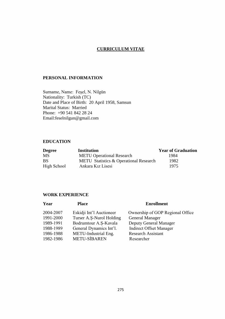
275

CURRICULUM VITAE

PERSONAL INFORMATION

Surname, Name: Feşel, N. Nilgün

Nationality: Turkish (TC)

Date and Place of Birth: 20 April 1958, Samsun

Marital Status: Married

Phone: +90 541 842 28 24

Email:[email protected]

EDUCATION

Degree Institution Year of Graduation

MS METU Operational Research 1984

BS METU Statistics & Operational Research 1982

High School Ankara Kız Lisesi 1975

WORK EXPERIENCE

Year Place Enrollment

2004-2007 Eskidji Int’l Auctioneer Ownership of GOP Regional Office

1991-2000 Turser A.Ş-Nurol Holding General Manager

1989-1991 Bodrumtour A.Ş-Kavala Deputy General Manager

1988-1989 General Dynamics Int’l. Indirect Offset Manager

1986-1988 METU-Industrial Eng. Research Assistant

1982-1986 METU-SİBAREN Researcher

product mix determination under uncertainty - METU

Documents

Transcript of product mix determination under uncertainty - METU