
MODELING ADVANCED FUND TRANSFER PRICING ... - METU
84
MODELING ADVANCED FUND TRANSFER PRICING WITH AN APPLICATION OF HULL-WHITE INTEREST-RATE TREE IN TURKISH BANKING SECTOR A THESIS SUBMITTED TO THE GRADUATE SCHOOL OF APPLIED MATHEMATICS OF MIDDLE EAST TECHNICAL UNIVERSITY BY BEGZOD SHAKIROV IN PARTIAL FULFILLMENT OF THE REQUIREMENTS FOR THE DEGREE OF MASTER OF SCIENCE IN FINANCIAL MATHEMATICS SEPTEMBER 2017
-
Upload
khangminh22 -
Category
Documents
-
view
3 -
download
0
Transcript of MODELING ADVANCED FUND TRANSFER PRICING ... - METU

MODELING ADVANCED FUND TRANSFER PRICINGWITH AN APPLICATION OF HULL-WHITE INTEREST-RATE TREE
IN TURKISH BANKING SECTOR
A THESIS SUBMITTED TOTHE GRADUATE SCHOOL OF APPLIED MATHEMATICS
OFMIDDLE EAST TECHNICAL UNIVERSITY
BY
BEGZOD SHAKIROV
IN PARTIAL FULFILLMENT OF THE REQUIREMENTSFOR
THE DEGREE OF MASTER OF SCIENCEIN
FINANCIAL MATHEMATICS
SEPTEMBER 2017


Approval of the thesis:
MODELING ADVANCED FUND TRANSFER PRICINGWITH AN APPLICATION OF HULL-WHITE INTEREST-RATE TREE
IN TURKISH BANKING SECTOR
submitted by BEGZOD SHAKIROV in partial fulfillment of the requirements forthe degree of Master of Science in Department of Financial Mathematics, MiddleEast Technical University by,
Prof. Dr. Bulent KarasozenDirector, Graduate School of Applied Mathematics
Assoc. Prof. Dr. Yeliz Yolcu OkurHead of Department, Financial Mathematics
Prof. Dr. Gerhard-Wilhelm WeberSupervisor, Financial Mathematics, METU
Examining Committee Members:
Assoc. Prof. Dr. A. Sevtap KestelActuarial Sciences, METU
Assoc. Prof. Dr. Umit AksoyMathematics, Atilim University
Prof. Dr. Gerhard-Wilhelm WeberFinancial Mathematics, METU
Assoc. Prof. Dr. Seza DanısogluBusiness Administration, METU
Assoc. Prof. Dr. Ali Devin SezerFinancial Mathematics, METU
Date:


I hereby declare that all information in this document has been obtained andpresented in accordance with academic rules and ethical conduct. I also declarethat, as required by these rules and conduct, I have fully cited and referenced allmaterial and results that are not original to this work.
Name, Last Name: BEGZOD SHAKIROV
Signature :
v

vi
ABSTRACT
MODELING ADVANCED FUND TRANSFER PRICINGWITH AN APPLICATION OF HULL-WHITE INTEREST-RATE TREE
IN TURKISH BANKING SECTOR
Shakirov, Begzod
M.S., Department of Financial Mathematics
Supervisor : Prof. Dr. Gerhard-Wilhelm Weber
September 2017, 59 pages
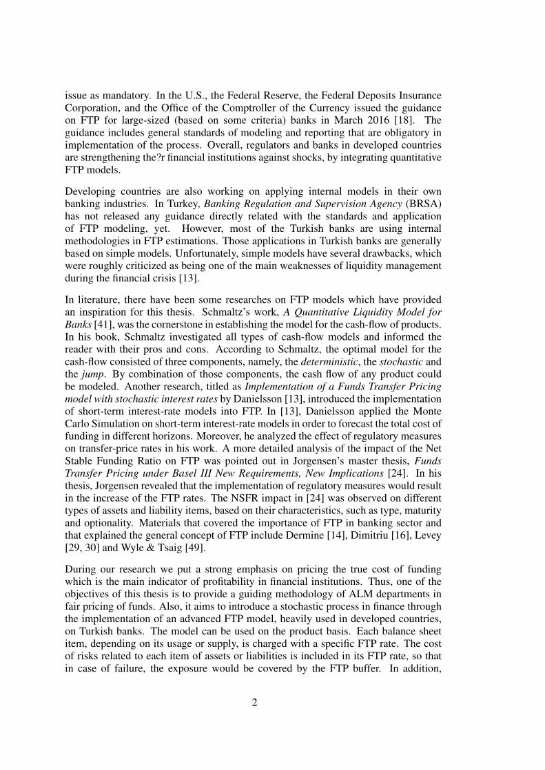
The Financial Crisis in 2008 has revealed the need for a more advanced management ofliquidity risk in financial institutions. This thesis aims to introduce and implement anadvanced Fund Transfer Pricing (FTP) model into banking industries of the developingcountries. The methodology of the FTP model, constructed in this research, measuresthe cost of a product’s cash-flows by splitting them into a deterministic and a stochasticcomponent. The cost of the deterministic part is assessed as an equivalent of thecredit-default premium of an institution, whereas the cost of the stochastic componentis modeled by a Brownian Motion. Moreover, in order to forecast the future outlook ofFTP rates, a simulation of benchmark Interest Rates with an application of Hull-Whitemodel has been performed. The information provided by the expected cost of fundingcould be a guide to the management of a financial institution. The cost of Basel IIIliquidity metrics have also been applied into the model, which is one of the maincontributions of this thesis to the field of Financial Mathematics. This thesis ends witha conclusion and a preview to future investigations and applications.
Keywords : Fund Transfer Pricing, Hull-White, Interest-Rate Models, Funding Cost,Liquidity
vii

viii

OZ
TURK BANKACILIK SEKTORUNDEHULL-WHITE FAIZ ORANI ORGUSUNU UYGULAYARAKGELISMIS FON TRANSFER FIYATLAMA MODELLEMESI
Shakirov, Begzod
Yuksek Lisans, Finansal Matematik Bolumu
Tez Yoneticisi : Prof. Dr. Gerhard-Wilhelm Weber
Eylul 2017, 59 sayfa
2008’deki Finansal Kriz, finansal kuruluslarda likidite riskinin daha gelismisyonetimine duyulan ihtiyacı ortaya koymustur. Bu tez, gelismis bir Fon TransferFiyatlandırması (FTF) modelinin gelismekte olan ulkelerin bankacılık sektorlerinetanıtılmasını ve uygulanmasını amaclamaktadır. Bu arastırmada olusturulan FTFmodelinin metodolojisi, bir urunun nakit akıslarının maliyetini, deterministik vestokastik bilesenlere bolerek olcmektedir. Deterministik kısmın maliyeti, bir kurumunkredi temerrut primi karsılıgı olarak degerlendirilirken, stokastik kısmın maliyetiBrown Devinimi ile modellenmistir. Ayrıca, gelecekteki FTF oranlarının gorunumunutahmin edebilmek icin, Hull-White modeli uygulanarak benchmark faiz oranlarınınsimulasyonu gerceklestirilmistir. Beklenen finansman maliyeti ile saglanan bilgiler,bir finansal kurumun yonetimine rehberlik edebilir. Basel III likidite olcumlerininmaliyetinin modele uygulanması da bu tezin Finansal Matematik alanına temelkatkılarından biridir. Tez gelecek arastırmalara ve uygulamalara yonelik bir sonucve onizleme ile sona ermektedir.
Anahtar Kelimeler : Fon Transfer Fiyatlaması, Hull-White, Faiz Oranı Modelleri,Fonlama Maliyeti, Likidite
ix

x

To My Family
xi

xii

ACKNOWLEDGMENTS
I would like to thank Prof. Dr. Gerhard-Wilhelm Weber for all his support, helpfulsuggestions and encouragement, which motivated me during my study. I wish toexpress my gratitude to him for the honour of writing this thesis under his guidance.
Furthermore, I would like to thank the members of the Institute of AppliedMathematics at Middle East Technical University and my colleagues from DenizbankA. S. for their worthwhile advice and support. I also owe special thanks to Assoc.Prof. Dr. Sevtap Kestel, Ali Devin Sezer, Seza Danısoglu and Umit Aksoy for theirvaluable suggestions and comments.
I wish to express my deepest gratitude to my parents for their guidance in my studies.
Last but not least, I am deeply grateful to my wife Nigar, for her endless love andencouragement throughout my life.
xiii

xiv

TABLE OF CONTENTS
ABSTRACT . . . . . . . . . . . . . . . . . . . . . . . . . . . . . . . . . . . . vii
OZ . . . . . . . . . . . . . . . . . . . . . . . . . . . . . . . . . . . . . . . . . ix
ACKNOWLEDGMENTS . . . . . . . . . . . . . . . . . . . . . . . . . . . . . xiii
TABLE OF CONTENTS . . . . . . . . . . . . . . . . . . . . . . . . . . . . . xv
LIST OF FIGURES . . . . . . . . . . . . . . . . . . . . . . . . . . . . . . . . xix
LIST OF TABLES . . . . . . . . . . . . . . . . . . . . . . . . . . . . . . . . xxi
LIST OF ABBREVIATIONS . . . . . . . . . . . . . . . . . . . . . . . . . . . xxiii
CHAPTERS
1 INTRODUCTION . . . . . . . . . . . . . . . . . . . . . . . . . . . 1
2 PRELIMINARIES . . . . . . . . . . . . . . . . . . . . . . . . . . . 5
2.1 Financial Tools . . . . . . . . . . . . . . . . . . . . . . . . . 5
2.1.1 Liquidity . . . . . . . . . . . . . . . . . . . . . . 5
2.1.2 Funding . . . . . . . . . . . . . . . . . . . . . . . 7
2.1.3 Regulatory Measures . . . . . . . . . . . . . . . . 8
2.2 Mathematical Tools . . . . . . . . . . . . . . . . . . . . . . 10
2.3 Model Frameworks . . . . . . . . . . . . . . . . . . . . . . 12
2.3.1 Cash Flow (CF) . . . . . . . . . . . . . . . . . . . 12
2.3.2 Funding Capacity (FC) . . . . . . . . . . . . . . . 14
xv
2.4 Liquidity-Model Framework . . . . . . . . . . . . . . . . . 14
2.4.1 Cash-Flow Model . . . . . . . . . . . . . . . . . . 14
2.4.2 Funding-Capacity Model (FC) . . . . . . . . . . . 17
2.5 Interest-Rate Models . . . . . . . . . . . . . . . . . . . . . . 17
3 FUND TRANSFER PRICING MODEL . . . . . . . . . . . . . . . . 23
3.1 Pooled Average . . . . . . . . . . . . . . . . . . . . . . . . 24
3.2 Matched Maturity . . . . . . . . . . . . . . . . . . . . . . . 25
3.3 Advanced FTP model . . . . . . . . . . . . . . . . . . . . . 26
3.3.1 Deterministic Fund Transfer Pricing . . . . . . . . 27
3.3.2 Stochastic Fund Transfer Pricing . . . . . . . . . . 28
3.3.2.1 Transfer Price of Aggregate Exposure 28
3.3.2.2 Transfer Price of an Individual Product 29
3.3.2.3 Optionality . . . . . . . . . . . . . . . 33
3.3.3 Regulatory Impact . . . . . . . . . . . . . . . . . 34
4 APPLICATION . . . . . . . . . . . . . . . . . . . . . . . . . . . . . 39
4.1 Numerical Example . . . . . . . . . . . . . . . . . . . . . . 39
4.2 Simulation . . . . . . . . . . . . . . . . . . . . . . . . . . . 42
5 CONCLUSION AND OUTLOOK . . . . . . . . . . . . . . . . . . . 45
REFERENCES . . . . . . . . . . . . . . . . . . . . . . . . . . . . . . . . . . 47
APPENDICES
A Proof of Vasicek’s Explicit Solution . . . . . . . . . . . . . . . . . . 51
B Derivation of Aggregate-Risk Exposure . . . . . . . . . . . . . . . . 53
xvi

C Matlab Code . . . . . . . . . . . . . . . . . . . . . . . . . . . . . . . 55
D Simulation Results . . . . . . . . . . . . . . . . . . . . . . . . . . . 59
xvii

xviii

LIST OF FIGURES
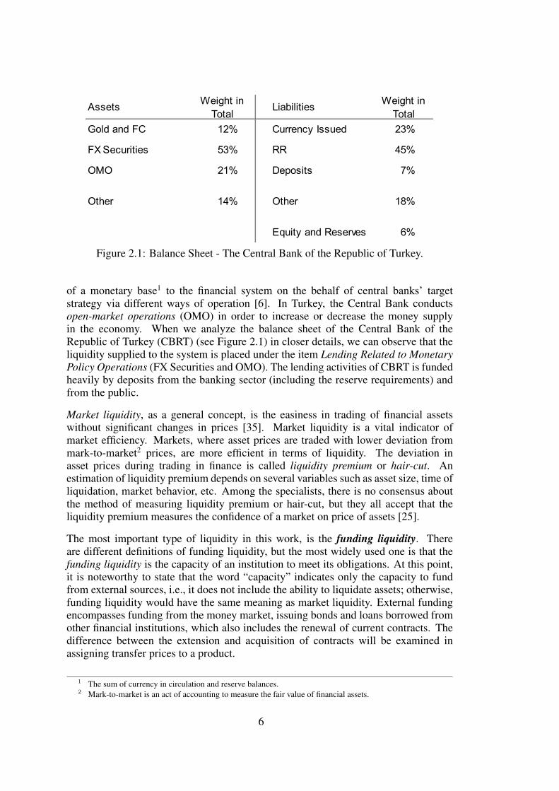
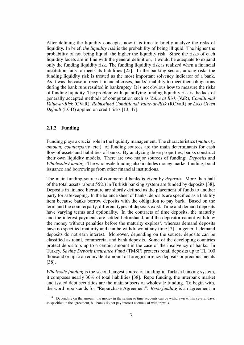
Figure 2.1 Balance Sheet - The Central Bank of the Republic of Turkey. . . . . 6
Figure 2.2 Balance Sheet - Stock [41]. . . . . . . . . . . . . . . . . . . . . . 13
Figure 2.3 Balance Sheet - Cash Flow [41]. . . . . . . . . . . . . . . . . . . . 13
Figure 2.4 Cash-Flow Maturity Ladder [41]. . . . . . . . . . . . . . . . . . . 13
Figure 2.5 Required Funding Capacity [41]. . . . . . . . . . . . . . . . . . . 18
Figure 3.1 Mechanic of FTP within a typical bank [9]. . . . . . . . . . . . . . 24
Figure 3.2 Matched-Maturity approach of FTP [30]. . . . . . . . . . . . . . . 26
Figure 4.1 Turkish Lira-Swap Yield. . . . . . . . . . . . . . . . . . . . . . . 43
xix

xx

LIST OF TABLES
Table 2.1 Yield curves and market expectations according to liquidity-premiumtheory [34]. . . . . . . . . . . . . . . . . . . . . . . . . . . . . . . . . . . 19
Table 4.1 Summary: Total Cost of Funding. . . . . . . . . . . . . . . . . . . . 43
Table 4.2 Simulation Summary: Short-term interest rates. . . . . . . . . . . . 44
xxi

xxii

LIST OF ABBREVIATIONS
ALM Asset Liability Management
ASF Available Stable Funding
FTP Fund Transfer Pricing
GPL General Purpose Loan
HQLA High Quality Liquid Assets
i.i.d. Independent and Identically Distributed
LCR Liquidity Coverage Ratio
LIBOR London Interbank Offered Rate
NII Net Interest Income
NIM Net Interest Margin
NSFR Net Stable Funding Ratio
R Set of Real Numbers
RSF Required Stable Funding
st. dev. Standard Deviation
TNCO Total Net Cash Outflows
xxiii

xxiv

CHAPTER 1
INTRODUCTION
The fundamental function of financial institutions is borrowing funds and lendingloans. Institutions pay for funds and gain from loans, and these operations in financeliterature are denoted as funding cost and assets return, respectively. The marginbetween return from assets and cost of funding is the profit of the financial institutions.The larger the margin, the higher the profit. However, this estimation is too broad forspecifying the profitability of the institutions. In order to find the ideal margin, one hasto set up a one-to-one map of assets with funds. In other words, each asset with specificmaturity, risk and costs should be financed by funds having similar characteristics. Inreal practice, it is impossible to find the exact matching and this was one of the mainreasons for the financial crisis in 2008.
Although the crisis in 2008 was the chain reaction of several failures, themismanagement of risk and liquidity severely worsened the situation. However, banksdid not declare insolvency when problem assets were identified, but when a bankrun occurred [31]. No matter how strong deposits base banks had, the harshness ofrun on deposits put financial institutions out of business. The reason for liquidityshortage was threefold. First, demand for asset-backed securities dropped. Second,investors were reluctant to lend money against mortgage backed security as collaterals.Third, mark-to-market assessment of securities caused a huge amount of losses whichinfluenced the funding structure [41]. It is important to note that during the crisis,interbank lending - the source of short-term funding - almost evaporated.
The aftermath of Liquidity Financial Crisis in 2008 has revealed the need for amodification of Fund Transfer Pricing (FTP) methodology [9]. FTP plays a keyrole in liquidity risk pricing. It is a system created to assess the cost of funds bytaking liquidity, interest rate and currency risks associated with lending and takingactivities into account [9]. In other words, FTP is an internal pricing system, thatencompasses all risks during pricing each balance sheet item, based on its supply orusage [37]. Assets and Liabilities Management (ALM) department or the treasuryof banks, which are the central risk management hubs, are generally responsiblefor setting the FTP rates of all businesses, such as corporate, retail and small andmedium-sized enterprises.
Nowadays, banking regulators are closely monitoring the development of internalFTP models and their applications. Germany is the first country to bring up the
1
issue as mandatory. In the U.S., the Federal Reserve, the Federal Deposits InsuranceCorporation, and the Office of the Comptroller of the Currency issued the guidanceon FTP for large-sized (based on some criteria) banks in March 2016 [18]. Theguidance includes general standards of modeling and reporting that are obligatory inimplementation of the process. Overall, regulators and banks in developed countriesare strengthening the?r financial institutions against shocks, by integrating quantitativeFTP models.
Developing countries are also working on applying internal models in their ownbanking industries. In Turkey, Banking Regulation and Supervision Agency (BRSA)has not released any guidance directly related with the standards and applicationof FTP modeling, yet. However, most of the Turkish banks are using internalmethodologies in FTP estimations. Those applications in Turkish banks are generallybased on simple models. Unfortunately, simple models have several drawbacks, whichwere roughly criticized as being one of the main weaknesses of liquidity managementduring the financial crisis [13].
In literature, there have been some researches on FTP models which have providedan inspiration for this thesis. Schmaltz’s work, A Quantitative Liquidity Model forBanks [41], was the cornerstone in establishing the model for the cash-flow of products.In his book, Schmaltz investigated all types of cash-flow models and informed thereader with their pros and cons. According to Schmaltz, the optimal model for thecash-flow consisted of three components, namely, the deterministic, the stochastic andthe jump. By combination of those components, the cash flow of any product couldbe modeled. Another research, titled as Implementation of a Funds Transfer Pricingmodel with stochastic interest rates by Danielsson [13], introduced the implementationof short-term interest-rate models into FTP. In [13], Danielsson applied the MonteCarlo Simulation on short-term interest-rate models in order to forecast the total cost offunding in different horizons. Moreover, he analyzed the effect of regulatory measureson transfer-price rates in his work. A more detailed analysis of the impact of the NetStable Funding Ratio on FTP was pointed out in Jorgensen’s master thesis, FundsTransfer Pricing under Basel III New Requirements, New Implications [24]. In histhesis, Jorgensen revealed that the implementation of regulatory measures would resultin the increase of the FTP rates. The NSFR impact in [24] was observed on differenttypes of assets and liability items, based on their characteristics, such as type, maturityand optionality. Materials that covered the importance of FTP in banking sector andthat explained the general concept of FTP include Dermine [14], Dimitriu [16], Levey[29, 30] and Wyle & Tsaig [49].
During our research we put a strong emphasis on pricing the true cost of fundingwhich is the main indicator of profitability in financial institutions. Thus, one of theobjectives of this thesis is to provide a guiding methodology of ALM departments infair pricing of funds. Also, it aims to introduce a stochastic process in finance throughthe implementation of an advanced FTP model, heavily used in developed countries,on Turkish banks. The model can be used on the product basis. Each balance sheetitem, depending on its usage or supply, is charged with a specific FTP rate. The costof risks related to each item of assets or liabilities is included in its FTP rate, so thatin case of failure, the exposure would be covered by the FTP buffer. In addition,
2
the model enables banks to increase Net Interest Margin (NIM) by optimizing bothinterest income and expenses. It separates the cash flow into two parts: deterministicand stochastic. The deterministic part of cash flow is predictable and has no varyingcost, whereas the stochastic part is volatile and incurs cover costs for possible outflows.Unlike simple methods, the advanced method is trying to capture the real cost of thestochastic component, which generally constitutes a small part of the total cash flow.
Furthermore, the advanced FTP model in conjunction with interest rate models can beactively used in the projection of business plans. Precise modeling of an interest rate,which serves as a risk-free rate in advanced FTP methods, will render the managementof banks to forecast the true cost of funding. Consequently, banks can take optimaldecisions that will provide a higher profit and a lower risk exposure. A short-terminterest rate model used in this thesis is constructed by the Hull-White stochasticinterest-rate model [43]. Adding the liquidity cost to the acquired risk-free yield curvewill result in the total cost of funding, applicable to all sorts of analyses.
In addition to the primary objectives that have been emphasized above, one of the maincontribution of this thesis is the implementation of Basel III regulatory measures onto the FTP rates. The model of the Net Stable Funding Ratio’s (NSFR) effect on FTPrates has first been introduced in this work. Due to lack of studies in the literature aboutthe impact of NSFR metric on FTP, the model in this thesis hopefully will emphasizefurther researches in the area.
The thesis is organized as follows. Chapter 2 begins with the introduction of financialand mathematical concepts that are applied in the models. Then, the framework ofthe cash flow model is designed. It ends with an analysis of the stochastic interestmodel for simulating future risk free rates. Chapter 3 covers the establishment ofthe FTP model. First, it compares the simple methods in terms of advantages anddisadvantages. Then, the advanced FTP model is constructed in two parts, namely,the deterministic one and the stochastic one. The stochastic part is modeled bya Brownian motion, whereas the deterministic one is stated as a linear estimationwith zero variance. Before applying the model on a product from Turkish banks,the effect of regulatory limits is included. In regulatory part the NSFR impact, oneof the main contributions of the thesis, is modeled. Chapter 4, is the applicationpart, where the estimation of the total cost of funding is computed by simulatingthe benchmark-interest rate curves. Finally, Chapter 5 summarizes the strengths andweaknesses of the model and its application in real circumstances and proposes thepathway for consequent researches. The findings of the NSFR impact on the FTP ratesare also clearly mentioned in the last chapter. The appendices of the thesis includesthe proof of Vasicek’s model’s explicit solutions and the derivation of aggregate riskexposure.
3

4

CHAPTER 2
PRELIMINARIES
This chapter will introduce both the financial and mathematical tools applied in ourFTP model. In the financial tools part, liquidity, the funding items of banks and theregulatory measures are described. It is important to note that the term liquidity in thiswork refers to the flow concept, not to a stock concept. The part on mathematical toolsexplained the basic principles of probability theory and the stochastic process. Next,we construct the framework of the model, consisting of the cash flow and the fundingcapacity of the institution. The prototype of our liquidity model is designed in the lastpart of this section.
2.1 Financial Tools
In order to understand the general concept of the thesis, it is vital to be familiar withthe financial tools, since they describe the behavior of the financial institutions in theiroperations. This subsection illustrates an overview of banking activities. The parton liquidity shows how banks arrange their resources, whereas the part on fundingdemonstrates the sources of the funds. The last part of the subsection - regulatorymeasures - describes the rules of the bank management.
2.1.1 Liquidity
In everyday life the term “liquidity” is mentioned regularly in different sectors offinance. Although they are “interdependent”, the meanings differ depending on thearea of their use. For this reason, it is important to define the context of the liquidity.In finance literature there are three facets of liquidity - such as central bank, marketand funding liquidity [35]. In this thesis, the funding liquidity is the major conceptsubject to our analysis; however, for the broad understanding of the issue, other facetsof liquidity are also defined.
Central bank liquidity (the basis of national liquidity) is the ability of a central bankto provide liquidity for the economy through financial institutions. It is the supply
5
Assets Liabilities
Gold and FC 12% Currency Issued 23%
FX Securities 53% RR 45%
OMO 21% Deposits 7%
Other 14% Other 18%
Equity and Reserves 6%
Weight in Total
Weight in Total
Figure 2.1: Balance Sheet - The Central Bank of the Republic of Turkey.
of a monetary base1 to the financial system on the behalf of central banks’ targetstrategy via different ways of operation [6]. In Turkey, the Central Bank conductsopen-market operations (OMO) in order to increase or decrease the money supplyin the economy. When we analyze the balance sheet of the Central Bank of theRepublic of Turkey (CBRT) (see Figure 2.1) in closer details, we can observe that theliquidity supplied to the system is placed under the item Lending Related to MonetaryPolicy Operations (FX Securities and OMO). The lending activities of CBRT is fundedheavily by deposits from the banking sector (including the reserve requirements) andfrom the public.
Market liquidity, as a general concept, is the easiness in trading of financial assetswithout significant changes in prices [35]. Market liquidity is a vital indicator ofmarket efficiency. Markets, where asset prices are traded with lower deviation frommark-to-market2 prices, are more efficient in terms of liquidity. The deviation inasset prices during trading in finance is called liquidity premium or hair-cut. Anestimation of liquidity premium depends on several variables such as asset size, time ofliquidation, market behavior, etc. Among the specialists, there is no consensus aboutthe method of measuring liquidity premium or hair-cut, but they all accept that theliquidity premium measures the confidence of a market on price of assets [25].
The most important type of liquidity in this work, is the funding liquidity. Thereare different definitions of funding liquidity, but the most widely used one is that thefunding liquidity is the capacity of an institution to meet its obligations. At this point,it is noteworthy to state that the word “capacity” indicates only the capacity to fundfrom external sources, i.e., it does not include the ability to liquidate assets; otherwise,funding liquidity would have the same meaning as market liquidity. External fundingencompasses funding from the money market, issuing bonds and loans borrowed fromother financial institutions, which also includes the renewal of current contracts. Thedifference between the extension and acquisition of contracts will be examined inassigning transfer prices to a product.
1 The sum of currency in circulation and reserve balances.2 Mark-to-market is an act of accounting to measure the fair value of financial assets.
6
After defining the liquidity concepts, now it is time to briefly analyze the risks ofliquidity. In brief, the liquidity risk is the probability of being illiquid. The higher theprobability of not being liquid, the higher the liquidity risk. Since the risks of eachliquidity facets are in line with the general definition, it would be adequate to expandonly the funding liquidity risk. The funding liquidity risk is realized when a financialinstitution fails to meets its liabilities [25]. In the banking sector, among risks thefunding liquidity risk is treated as the most important solvency indicator of a bank.As it was the case in recent financial crises, banks’ inability to meet their obligationsduring the bank runs resulted in bankruptcy. It is not obvious how to measure the risksof funding liquidity. The problem with quantifying funding liquidity risk is the lack ofgenerally accepted methods of computation such as Value at Risk (VaR), ConditionalValue-at-Risk (CVaR), Robustified Conditional Value-at-Risk (RCVaR) or Loss GivenDefault (LGD) applied on credit risks [13, 47].
2.1.2 Funding
Funding plays a crucial role in the liquidity management. The characteristics (maturity,amount, counterparty, etc.) of funding sources are the main determinants for cashflow of assets and liabilities of banks. By analyzing those properties, banks constructtheir own liquidity models. There are two major sources of funding: Deposits andWholesale Funding. The wholesale funding also includes money market funding, bondissuance and borrowings from other financial institutions.
The main funding source of commercial banks is given by deposits. More than halfof the total assets (about 55%) in Turkish banking system are funded by deposits [38].Deposits in finance literature are shortly defined as the placement of funds to anotherparty for safekeeping. In the balance sheet of banks, deposits are specified as a liabilityitem because banks borrow deposits with the obligation to pay back. Based on theterm and the counterparty, different types of deposits exist. Time and demand depositshave varying terms and optionality. In the contracts of time deposits, the maturityand the interest payments are settled beforehand, and the depositor cannot withdrawthe money without penalties before the maturity expires3, whereas demand depositshave no specified maturity and can be withdrawn at any time [7]. In general, demanddeposits do not earn interest. Moreover, depending on the source, deposits can beclassified as retail, commercial and bank deposits. Some of the developing countriesprotect depositors up to a certain amount in the case of the insolvency of banks. InTurkey, Saving Deposit Insurance Fund (TMSF) protects retail deposits up to TL 100thousand or up to an equivalent amount of foreign currency deposits or precious metals[38].
Wholesale funding is the second largest source of funding in Turkish banking system,it composes nearly 30% of total liabilities [38]. Repo funding, the interbank marketand issued debt securities are the main subsets of wholesale funding. To begin with,the word repo stands for “Repurchase Agreement”. Repo funding is an agreement in
3 Depending on the amount, the money in the saving or time accounts can be withdrawn within several days,as specified in the agreement, but banks do not pay interest accruals of withdrawals.
7
which one party sells securities to another, and simultaneously agrees to repurchasethem (or sometimes similar securities) in the future [17]. Another subset of wholesalefunding is the interbank market, where the banks short in liquidity4 borrow from otherbanks with excess liquidity at specified interest rates [39]. The rates are set by largeliquidity provider banks, and used as a benchmark such as London Interbank OfferedRate (LIBOR) [21]. Finally, issued debt securities are the instruments such as bonds,debenture or promissory notes issued with an obligation to repay on a certain date ata specific rate. In Turkey, the share of issued debt securities composes only 4% of thetotal liabilities [39].
Term and collateral are the two main characteristics of the wholesale funding. Fundingwith less than or equal to 1 year to maturity is defined as short-term, whereas the onewith higher than 1 year to maturity is named as long-term. In terms of collateral, thewholesale funding can be classified as secured and unsecured. In secured funding, aborrower has to post collateral, while in unsecured funding, funds are obtained withoutany collateral. Repo is an example of secured funding, where securities under repoagreement are used as a collateral. In contrast, in interbank markets, transactions aregenerally conducted without posting collaterals (except for some rare cases).
2.1.3 Regulatory Measures
Any financial crisis has always had global contingent effects. In order to minimisenegative outcomes, there has been a need for a standardised approach of management.In 1974, Basel Committee - formerly called as the Committee of Banking Regulationsand Supervisory Practices, was founded by the governors of Central Banks of tencountries. Since then, the number of the member countries has increased to 28,including Turkey.5 The regulations are not binding, rather they function as policyrecommendations for the development of financial stability. The committee hasreleased a series of regulatory standards of which the most notable publications areBasel I, Basel II and Basel III.
Basel I: “The Basel Capital Accord” was released in 1988 and it has set minimum ratiofor Capital Adequacy. In 1999, the Basel I was replaced by Basel II: “The New CapitalFramework”. According to this framework, three main principles were established:“expansion of minimum capital requirements set in 1988 accord, supervisory reviewof a capital adequacy and internal assessment process, and effective use of disclosureas a lever to strengthen market discipline and encourage sound banking practices” [3].
After Lehman Brother’s collapse in 2008, it was obvious that the standards of BaselII were not enough to cover the severe stresses. Therefore, in December 2010, thecommittee set out the final version of Basel III: “International framework for liquidityrisk measurement, standards and monitoring” and “A global regulatory framework formore resilient banks and banking systems”. Unlike the previous two publications,Basel III also treats liquidity risk management standards. Within the guidance of the
4 Banks facing shortage in their liquidity portfolio.5 For more details visit https://www.bis.org/bcbs/history.htm.
8
liquidity risk, the two key metrics, the Liquidity Coverage Ratio (LCR) and the NetStable Funding Ratio (NSFR), were released.
According to Bank for International Settlements (BIS), LCR measures a bank’sshort-term capacity to withstand liquidity risks. LCR has two components, HighQuality Liquid Assets (HQLA) and Total Net Cash Outflows (TNCO). A formula forthe calculation of LCR is given as follows:6
LCR =Stock of HQLA
TNCO over the next 30 Calendar Days> 100%.
HQLA based on the liquidity condition is divided into two main subcategories, namely,level 1 and level 2 assets. Level 1 assets are the most liquid assets such as cash andcentral bank reserves and should consist of at least 60% of the stock of HQLA. Level2 assets are less liquid and cannot cover more than 40% of total HQLA. Examples forlevel 2 assets are bonds rated AA- or higher, and qualifying common equity shares.The difference between the two subcategories is that the level 2 assets are subject tohair-cut:7
TNCO over the next 30 Calendar Days = Total Expected cash outflows- mintotal expected cash inflows, 75% of total expected cash outflows.
Total expected cash outflows are calculated by multiplying outstanding balances ofrelated liabilities and off-balance sheet items, and their expected run-off rates. On theother hand, total cash inflows are calculated by multiplying contractual receivables byexpected flow in rates.
On the other hand, the main objective of NSFR metric in BIS working paper is definedas the requirement for banks to preserve a stable funding with regard to their assets andoff-balance sheet items [5]. The calculation of NSFR ratio is executed by the followingformula:
ASF
RSF> 100, (2.1)
where
ASF: Available Stable Funding,RSF: Required Stable Funding.
ASF is measured by applying specified factors according to stability characteristicsof an institution’s funding resources. More stable funding resources receive higherthe ASF factors.8 On the other hand, RSF calculation is based on the liquidity
6 The minimum requirement was set up in an increasing order as follows: In 2015: 60%; in 2016: 70%; in2017: 80%; in 2018: 90%; in 2019: 100%.
7 The detailed table of assets categories and related weight factor can be found in “Basel III: The LiquidityCoverage Ratio and liquidity risk monitoring” document [4].
8 The detailed factors of each balance sheet item can be analyzed in the NSFR document [5].
9

characteristics of assets and its factors have a negative relationship with liquidityproperties of the assets. The bank with a better liquidity profile of assets has a loweramount of RSF than the bank with a weaker liquidity profile. It is important to notethat the NSFR metric will come into force at the beginning of 2018.
2.2 Mathematical Tools
In this section, the mathematical tools used in the model are introduced. It beginswith the introduction of basic fundamentals of probability theory and then defines aBrownian Motion and its properties.
Definition 2.1. (Sigma algebra) A collection F of subsets of Ω (sample space orevent) is called a σ-algebra if it satisfies the following conditions:
a) ∅ ∈ F ;
b) if A1, A2, A3, . . . , ∈ F , then⋃∞i=1Ai ∈ F ;
c) if A ∈ F , then AC ∈ F . 9
Remark. σ-algebras are closed under the operation of taking countable intersections.
Definition 2.2. (Probability measure and space) A probability measure P on (σ,F)is a function P : F −→ [0, 1] satisfying:
a) P(∅) = 0,P(Ω) = 1;
b) ifA1, A2, A3, . . ., is a collection of disjoint members ofF , such thatAi⋂Aj =
∅ for all pairs i, j satisfying i 6= j, then
P(∞⋃i=1
Ai) =∞∑i=1
P(Ai).
The triple (Ω,F ,P), comprising a set Ω, a σ-algebra F of subsets of Ω, and aprobability measure P on (Ω,F) is called a probability space [42].
9 Recall from set theory, the superscript C refers to complement and AC = U \A.
10
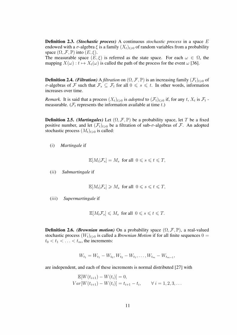
Definition 2.3. (Stochastic process) A continuous stochastic process in a space Eendowed with a σ-algebra ξ is a family (Xt)t>0 of random variables from a probabilityspace (Ω,F ,P) into (E, ξ).The measurable space (E, ξ) is referred as the state space. For each ω ∈ Ω, themapping X(ω) : t 7→ Xt(ω) is called the path of the process for the event ω [36].
Definition 2.4. (Filtration) A filtration on (Ω,F ,P) is an increasing family (Ft)t>0 ofσ-algebras of F such that Fs ⊆ Ft for all 0 6 s 6 t. In other words, informationincreases over time.
Remark. It is said that a process (Xt)t>0 is adopted to (Ft)t>0 if, for any t, Xt is Ft -measurable. (Ft represents the information available at time t.)
Definition 2.5. (Martingales) Let (Ω,F ,P) be a probability space, let T be a fixedpositive number, and let (Ft)t>0 be a filtration of sub-σ-algebras of F . An adoptedstochastic process (Mt)t>0 is called:
(ı) Martingale if
E[Mt|Fs] = Ms for all 0 6 s 6 t 6 T,
(ıı) Submartingale if
E[Mt|Fs] >Ms for all 0 6 s 6 t 6 T,
(ııı) Supermartingale if
E[MtFs] 6Ms for all 0 6 s 6 t 6 T.
Definition 2.6. (Brownian motion) On a probability space (Ω,F ,P), a real-valuedstochastic process (Wt)t>0 is called a Brownian Motion if for all finite sequences 0 =t0 < t1 < . . . < tm, the increments:
Wt1 = Wt1 −Wt0 ,Wt2 −Wt1 , . . . ,Wtm −Wtm−1 ,
are independent, and each of these increments is normal distributed [27] with
E[W (ti+1)−W (ti)] = 0,
V ar[W (ti+1)−W (ti)] = ti+1 − ti, ∀ i = 1, 2, 3, . . .
11

Definition 2.7. (Filtration for Brownian motion) According to Shreve, Filtrationfor Brownian motion is defined as follows: “Let (Ω,F ,P) be a probability space onwhich is defined a Brownian motion (Wt)t>0. A filtration for the Brownian motion isa collection of σ-algebras (Ft)t>0, satisfying:
(i) (Information accumulates) For 0 6 s 6 t, every set in Fs is also in Ft. In otherwords, there is at least as much information available at the later time Ft as thereis at the earlier time Fs.
(ii) (Adaptivity) For each t > 0, the Brownian motionWt at time t is Ft-measurable.In other words, the information available at time t is sufficient to evaluate theBrownian motion Wt at that time.
(iii) (Independence of future increments) For 0 6 t < u, the increment Wu −Wt isindependent of Ft. In other words, any increment of the Brownian motion aftertime t is independent of the information available at time t” [43].
Theorem 2.1. Brownian motion is a martingale.
Proof. A detailed proof of the theorem can be seen in Shreve [43].
2.3 Model Frameworks
A model framework by definition is not the model itself, but rather the variables of themodel. In this section, we will define two major components of the liquidity model,namely, cash flow and funding capacity. Cash flow is the flow perspective of the overallbalance sheet items. The funding capacity of a financial institution is its ability to fundthe cash outflow.
2.3.1 Cash Flow (CF)
In order to understand cash flow, let us assume that a bank which has only loans inassets and it funds those assets with deposits and equity. The composition of the bank’sbalance sheet at a point of time (t) is the stock position of the bank (see Figure 2.2).The change in those stocks over a period of time is the cash flow, which can be seen inFigure 2.3.
Since each item of the balance sheet has different maturities, the cash flow varies overtime. Incoming cash flows are the inflows to a bank, whereas outgoing cash flows arethe outflows from a bank. The netted amount of in and out flows is the stock position ofthe balance sheet. The maturity ladder of the cash flows consists of the net positionsat different time maturities. From Figure 2.4 we can observe inflows to the balancesheet in 12, 36 and 60 months of time periods, while in 6, 24 and 48 months there areoutflows from the balance.
12

Deposits(𝐷#)Loans
(𝐿#)
Equities(𝐸#)
Assets Liabilities
Figure 2.2: Balance Sheet - Stock [41].
Deposits(𝐶𝐹$%= ∆𝐷$)
Loans(𝐶𝐹$)= ∆𝐿$)
Equities(𝐶𝐹$% = ∆𝐸$)
Assets Liabilities
Figure 2.3: Balance Sheet - Cash Flow [41].
6 12 24 36 48 60
Maturity (Months)
!"#$
!"#%
T
Figure 2.4: Cash-Flow Maturity Ladder [41].
13

2.3.2 Funding Capacity (FC)
The bank in the previous example will most probably face a liquidity risk due toits distinct product maturity structure. In its assets, the bank has only loans with anaverage maturity of 3 years, which are generally fixed-term and can not be recalled,except for extreme cases10. On the other hand, deposits at the liabilities side are mainlyof short-term (3 months maturity) and have the optionality to be withdrawn dependingon the desire of the customer. The optionality of the product-cash flows represents thestochastic process. The main reason that banks utilize the products with optionality,is the lower cost of funding. In real circumstances, in order to manage the risk, banksalso have cash-equivalent assets, securities and money market receivables in theirassets, which can easily be converted into cash to fulfil obligations to depositors indaily operations. When liquid assets are not sufficient to fund outflows, banks borrowfrom external resources. The ability to fund all outflows is called as funding capacity.Banks’ main goal in liquidity management is to meet depositors’ demand: otherwise,they have to be bailed-out. In mathematical terms, the following equation should hold[41]:
FC+t > CF−t , ∀ t = 0, 1, . . . , n. (2.2)
In summary, cash flow and funding capacity are the key variables to model the liquidityof the banks. In other words, implementation of these two variables is sufficient toconstruct the basis of a bank’s liquidity structure.
2.4 Liquidity-Model Framework
In our Model Frameworks section, we have determined the key variables of theliquidity model. Now, it is time to build the model. First, we will model the cashflow of a product and then look at the whole balance sheet’s cash flow. In conclusion,the formula of the funding capacity for the total risk exposure will be derived.
2.4.1 Cash-Flow Model
In literature, there are several different cash flow models. The basis of all researcheslies on the two aspects of the customer behavior: the planned one and the unplannedone. Therefore, generally, cash-flow modeling consists of the two parts: a deterministicone and a stochastic one. The deterministic part of the model refers to liquidity, whilethe stochastic part is stated as liquidity risk. First we will analyze the modeling ofthe deterministic section, and then we will look through the stochastic approach ofliquidity-risk modeling.
10 Technically, banks can recall the facility according to credit agreements; however, in the market, recalling istreated as a signal of bankruptcy.
14
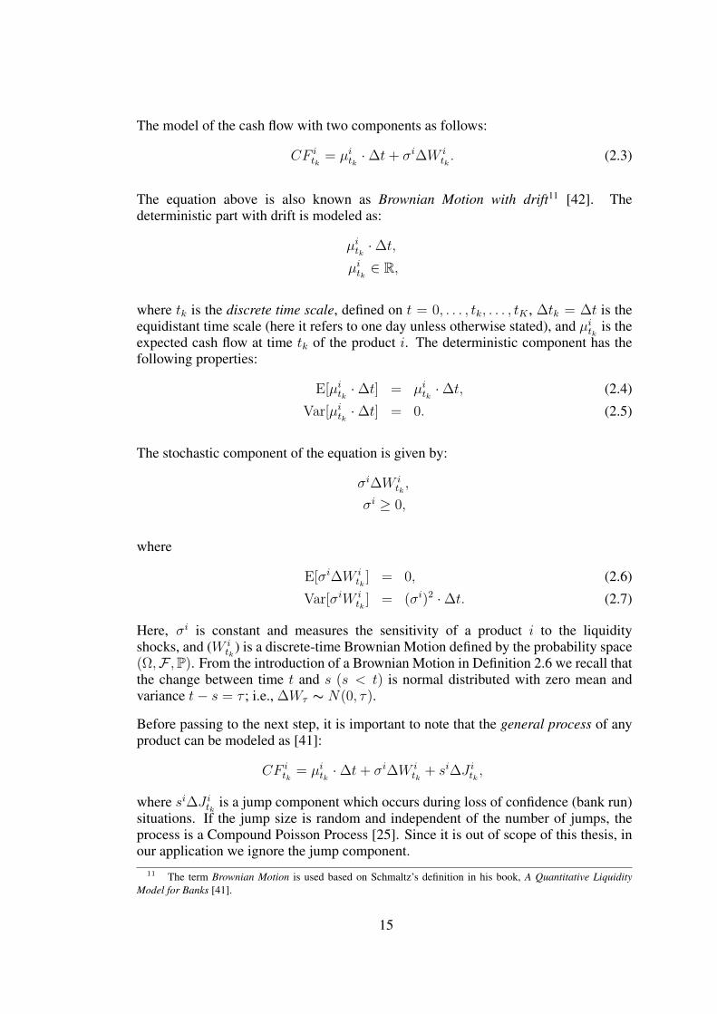
The model of the cash flow with two components as follows:
CF itk
= µitk ·∆t+ σi∆W itk. (2.3)
The equation above is also known as Brownian Motion with drift11 [42]. Thedeterministic part with drift is modeled as:
µitk ·∆t,µitk ∈ R,
where tk is the discrete time scale, defined on t = 0, . . . , tk, . . . , tK , ∆tk = ∆t is theequidistant time scale (here it refers to one day unless otherwise stated), and µitk is theexpected cash flow at time tk of the product i. The deterministic component has thefollowing properties:
E[µitk ·∆t] = µitk ·∆t, (2.4)
Var[µitk ·∆t] = 0. (2.5)
The stochastic component of the equation is given by:
σi∆W itk,
σi ≥ 0,
where
E[σi∆W itk
] = 0, (2.6)
Var[σiW itk
] = (σi)2 ·∆t. (2.7)
Here, σi is constant and measures the sensitivity of a product i to the liquidityshocks, and (W i
tk) is a discrete-time Brownian Motion defined by the probability space
(Ω,F ,P). From the introduction of a Brownian Motion in Definition 2.6 we recall thatthe change between time t and s (s < t) is normal distributed with zero mean andvariance t− s = τ ; i.e., ∆Wτ ∼ N(0, τ).
Before passing to the next step, it is important to note that the general process of anyproduct can be modeled as [41]:
CF itk
= µitk ·∆t+ σi∆W itk
+ si∆J itk ,
where si∆J itk is a jump component which occurs during loss of confidence (bank run)situations. If the jump size is random and independent of the number of jumps, theprocess is a Compound Poisson Process [25]. Since it is out of scope of this thesis, inour application we ignore the jump component.
11 The term Brownian Motion is used based on Schmaltz’s definition in his book, A Quantitative LiquidityModel for Banks [41].
15

The dependence structure of our Brownian component needs further assumptions. Inour case, we apply a factor approach and assume that the Brownian component hastwo factors: the product-specific (σi,p · ∆W i,p
tk) and the systematic (σi,m · ∆W i,p
tk).12
Factors are assumed to be independent from each other; furthermore, in order to easeour calculation, we assume that products are independent, too.13
The model of our Brownian Motion component:
σi∆W itk
= σi,p∆W i,ptk
+ σi,m∆Wmtk, (2.8)
ρ(∆W i,ptk,∆Wm
tk) = 0, ∀i = 1, . . . , n, (2.9)
ρ(∆W i,ptk,∆W j,p
tk) = 0, ∀i = 1, . . . , n, j = 1, . . . , n, i 6= j, (2.10)
where
σi,p : sensitivity of product i to ∆W i,ptk
,
∆W i,ptk
: product-specific liquidity shock,
σi,m : sensitivity of product i to the ∆Wmtk
,
∆Wmtk
: systematic liquidity shock.
The final cash flow of a product:
CF itk
= µitk ·∆t+ σi,p∆W i,ptk
+ σi,m∆Wmtk. (2.11)
After establishing the product-specific cash flow model, the next step is to aggregatethe cash flows of all products. The aggregation of deterministic parts is obtained bysimple summation, while the stochastic parts require adjustments of factors.
The total cash flow of n products can be represented in the compact martix-vectorform:
CF 1
tkCF 2
tk...CF n
tk
=
µ1tkµ2tk...µntk
·∆t+
σ1∆W 1
tkσ2∆W 2
tk...σn∆W n
tk
=
µ1tkµ2tk...µntk
·∆t+
σ1,p 0 . . . 00 σ2,p . . . 0... . . .
. . . ...0 0 . . . σn,p
∆W 1,ptk
∆W 2,ptk...
∆W n,ptk
+
σ1,m
σ2,m
...σn,m
∆Wmtk.
12 The superscripts p and m in factors stand for product and market, respectively.13 In real circumstances, there exists a significant relationship among products, and a relationship between
market and products. This assumption can be investigated and modified in further researches.
16

Hence, we get the aggregated cash-flow equation:
CFAtk
= (n∑i=1
µitk) ·∆t+ (n∑i=1
σi,p∆Wiptk
) + (n∑i=1
σi,m) ·Wmtk
= µAtk ·∆t+ σA∆WAtk,
where
µAtk =n∑i=1
µitk ,
σA =
√√√√ n∑i=1
(σi,p)2 +[ n∑i=1
σi,m]2.
2.4.2 Funding-Capacity Model (FC)
Based on the definition of the Funding Capacity, in this subsection we will derivean equation to measure the capacity of the liquidity buffer that covers the aggregateexposure σA in a confidence level p. Figure 2.5 illustrates the density function fσA∆WA
tk
of an aggregated Brownian Motion. From the setup, the required funding capacity towithstand the exposure σA during ∆t under the confidence level p is:
P (σA∆WAtk6 −FC(σA)) = 1− p. (2.12)
From Definition 2.6 of a Brownian motion, we know that the increments are normaldistributed, which results in:
Φ(∆WA
tk√∆t
6−FC(σA)
σA√
∆t
)= 1− p.
By solving the equation, we get:
FC(σA) = −√
∆t · Φ−1(1− p) · σA. (2.13)
Equation (2.13) states that σA units of Brownian standard deviation have to besupported with a funding capacity of −
√∆t · Φ−1(1 − p) · σA at the confidence level
of p. It is important to note that there is a linear relationship between risk exposure andfunding capacity.
2.5 Interest-Rate Models
In this section, we will describe the short-term interest-rate models that are widelyaccepted in practice, and select the most suitable one for this study. However, before
17

!"#∆%&'# ())
+,∆-.',
/01
2 +,∆-.',≤ −56 +, = 1− p 56(+,)
Figure 2.5: Required Funding Capacity [41].
analyzing the models, it is important to discuss the basic properties of interest rates, inparticular, the term structure of interest rate.
Mishkin states that “A plot of the yields on bonds with differing terms to maturity butthe same risk, liquidity, and tax considerations is called, a yield curve, and it describesthe term structure of interest rates” [34]. The shape of the yield curves demonstratesthe relationship between short - and long-term interest rates. When yield curves slopeupward, the long-term interest rates are above the short-term rates; when yield curvesare tending downward, the opposite is true; when yield curves are flat, this meansthat short- and long-term interest rates are the same. Moreover, historical studies haverevealed the following facts [34]:
1. The interest rates of bonds with varying maturities act together in time.2. In case of low short-term interest rates, yield curves tend to have an upward
slope; in case of high short-term rates, yield curves are likely to have adownwards slope. (In mathematical contexts, this is called as a mean revertingprocess.)
3. Yield curves are generally upward-sloped.
In the literature, there are several theories that describe the behavior of interest rates.One of the earliest theories are Expectation Theory and Segmented Markets Theory.Although they lack to explain all three facts simultaneously, they have providedfundamental ideas of their behaviors. By a combination of those fundamental ideas, theLiquidity-Premium Theory has been created. The liquidity premium theory explains allthree factual behaviors of interest rates on bonds. The main assumptions of the theoryis that bonds of different maturities are substitutes and long-term bonds bear higherinterest risk than short-term bonds. Based on those assumptions, the liquidity premium
18

Table 2.1: Yield curves and market expectations according to liquidity-premium theory[34].
Shape of the yield-curve slope Market expectation of short-term interest rates1. Steep Interest rates are expected to rise.2. Moderate Steep Interest rates are expected to stay the same.3. Flat Interest rates are expected to fall moderately.4. Inverted Interest rates expected to fall sharply.
theory is formulated as:
rnt =rt + ret+1 + ret+2 + . . .+ ret+(n−1)
n+ lnt, n > 1, (2.14)
where lnt is the liquidity premium for the n-period interest rate at time t, which isalways positive and rises as time to maturity increases [34].
Furthermore, one of the most important features of liquidity premium theory is that byusing the slope of the yield curve, one can identify the market expectation of futureshort-term interest rates. Table 2.1 gives a summary of future short-term interest rateimplications.
The forward yield curve is the curve of the expected interest rates at future time withdifferent maturities. It can be derived from the current yield curve with the followinglogic: In an Open-Market Economy, investors have equal return from investing forthe whole period, or investing up to some time and reinvesting it to the end of wholeperiod. The equation for the equal returns can be written as:
(1 + it+n)n = (1 + it+k)k · (1 + it+k, t+n)n−k, k < n. (2.15)
where
n = length of time period [0, n],k = length of time period [0, k],
n− k = length of time period [k, n],it+n = return for the whole period,it+k = return for period k,
it+k, t+n = return from period k up to period n.
In this work, forward-yield curves constitute base rates in FTP estimations. By solvingEquation (2.15), we get the forward interest rate at time t + k maturing at t + n asfollows:
it+k, t+n =
((1 + it+n)n
(1 + it+k)k
)−(n−k)
− 1. (2.16)
In short-term interest-rate modeling, the real challenge lies in the shape of theforward-yield curve. The reason is that it requires modeling of the stochastic
19
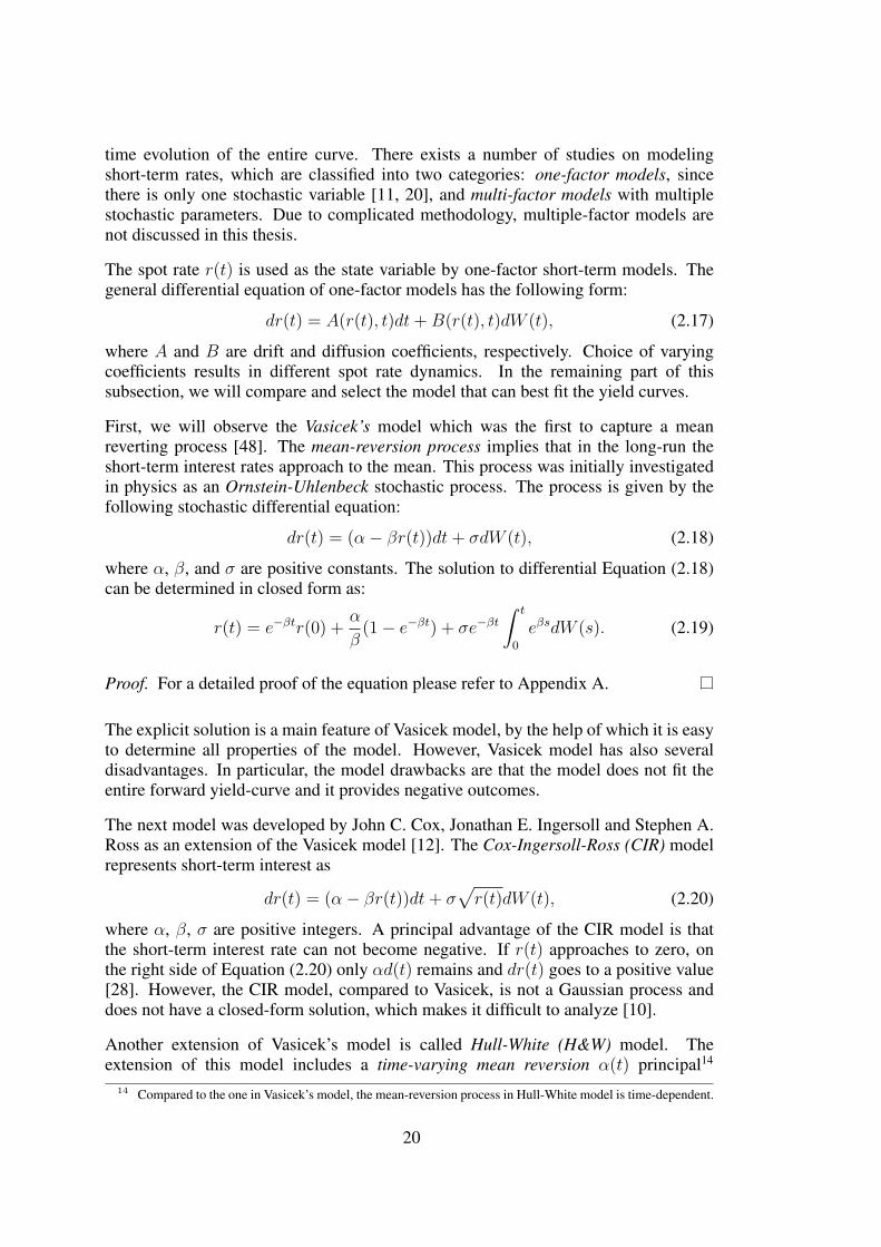
time evolution of the entire curve. There exists a number of studies on modelingshort-term rates, which are classified into two categories: one-factor models, sincethere is only one stochastic variable [11, 20], and multi-factor models with multiplestochastic parameters. Due to complicated methodology, multiple-factor models arenot discussed in this thesis.
The spot rate r(t) is used as the state variable by one-factor short-term models. Thegeneral differential equation of one-factor models has the following form:
dr(t) = A(r(t), t)dt+B(r(t), t)dW (t), (2.17)
where A and B are drift and diffusion coefficients, respectively. Choice of varyingcoefficients results in different spot rate dynamics. In the remaining part of thissubsection, we will compare and select the model that can best fit the yield curves.
First, we will observe the Vasicek’s model which was the first to capture a meanreverting process [48]. The mean-reversion process implies that in the long-run theshort-term interest rates approach to the mean. This process was initially investigatedin physics as an Ornstein-Uhlenbeck stochastic process. The process is given by thefollowing stochastic differential equation:
dr(t) = (α− βr(t))dt+ σdW (t), (2.18)
where α, β, and σ are positive constants. The solution to differential Equation (2.18)can be determined in closed form as:
r(t) = e−βtr(0) +α
β(1− e−βt) + σe−βt
∫ t
0
eβsdW (s). (2.19)
Proof. For a detailed proof of the equation please refer to Appendix A.
The explicit solution is a main feature of Vasicek model, by the help of which it is easyto determine all properties of the model. However, Vasicek model has also severaldisadvantages. In particular, the model drawbacks are that the model does not fit theentire forward yield-curve and it provides negative outcomes.
The next model was developed by John C. Cox, Jonathan E. Ingersoll and Stephen A.Ross as an extension of the Vasicek model [12]. The Cox-Ingersoll-Ross (CIR) modelrepresents short-term interest as
dr(t) = (α− βr(t))dt+ σ√r(t)dW (t), (2.20)
where α, β, σ are positive integers. A principal advantage of the CIR model is thatthe short-term interest rate can not become negative. If r(t) approaches to zero, onthe right side of Equation (2.20) only αd(t) remains and dr(t) goes to a positive value[28]. However, the CIR model, compared to Vasicek, is not a Gaussian process anddoes not have a closed-form solution, which makes it difficult to analyze [10].
Another extension of Vasicek’s model is called Hull-White (H&W) model. Theextension of this model includes a time-varying mean reversion α(t) principal14
14 Compared to the one in Vasicek’s model, the mean-reversion process in Hull-White model is time-dependent.
20

process [22]. This principal allows to fit forward yield curve by steering the volatilityof short-term interest rates. The model is the same as Vasicek’s model, except that αis time-dependent:15
dr(t) = (α(t)− βr(t))dt+ σdW (t), (2.21)
with
α(t) =∂f(0, t)
∂t+ af(0, t) +
σ2
2a(1− e−2at). (2.22)
The function f(0, t) is the forward rate function at time 0 with maturity t, whereas thefirst expression on the right-hand side of Equation (2.22) is the partial derivative of thefunction with respect to time. Since Hull-White model is a Gaussian process and hasan explicit solution, it is easy to analyze the model properties as in Vasicek’s model.The only weakness of H&W model is the positive probability of negative short-terminterest rates.
To sum up, among those three models represented above we choose the Hull-Whitemodel. The reason for such a choice is twofold. First, it fits better a forward yieldcurve than Vasicek’s model. Also, unlike CIR model, it is a Gaussian process andhas an explicit solution, which is an important implication for the simulation. Thedrawback of H&W model is in fact arguable. In the recent crisis, some central bankscharged negative interests. Let us mention that the Bank of Japan (BoJ) is still applyinga negative interest rate policy, in order to fight with Japan’s deflationary economy.
15 In later versions of Hull-White model, α, β, and σ are deterministic functions of time, which is not coveredin this work. For more details please refer to [8].
21

22

CHAPTER 3
FUND TRANSFER PRICING MODEL
In this section, we will briefly summarize the mechanics and objectives of FTP andthen move on to the analysis of the two types of FTP models, namely, Pooled Averageand Matched Maturity. Finally, we will construct the advanced FTP model in question,which includes the model of the NSFR effect (main contribution of our thesis).
In its simplest form, FTP is a process where the central unit (ALM) of a bank collectsfunds and redistributes them among the business units, acting as an internal bank [45].In case of excesses or shortages of funds, the central unit invests on or borrows fromthe money market. During the collection and redistribution processes, ALM pays andcharges the FTP rates, which results in the decomposition of net interest margin (NIM)of a bank. In addition, ALM also manages liquidity position of a bank, by investingexcess reserves into securities. The optimization process of the security portfolios isconducted by applying Conditional Value at Risk (CVaR) approaches [47].
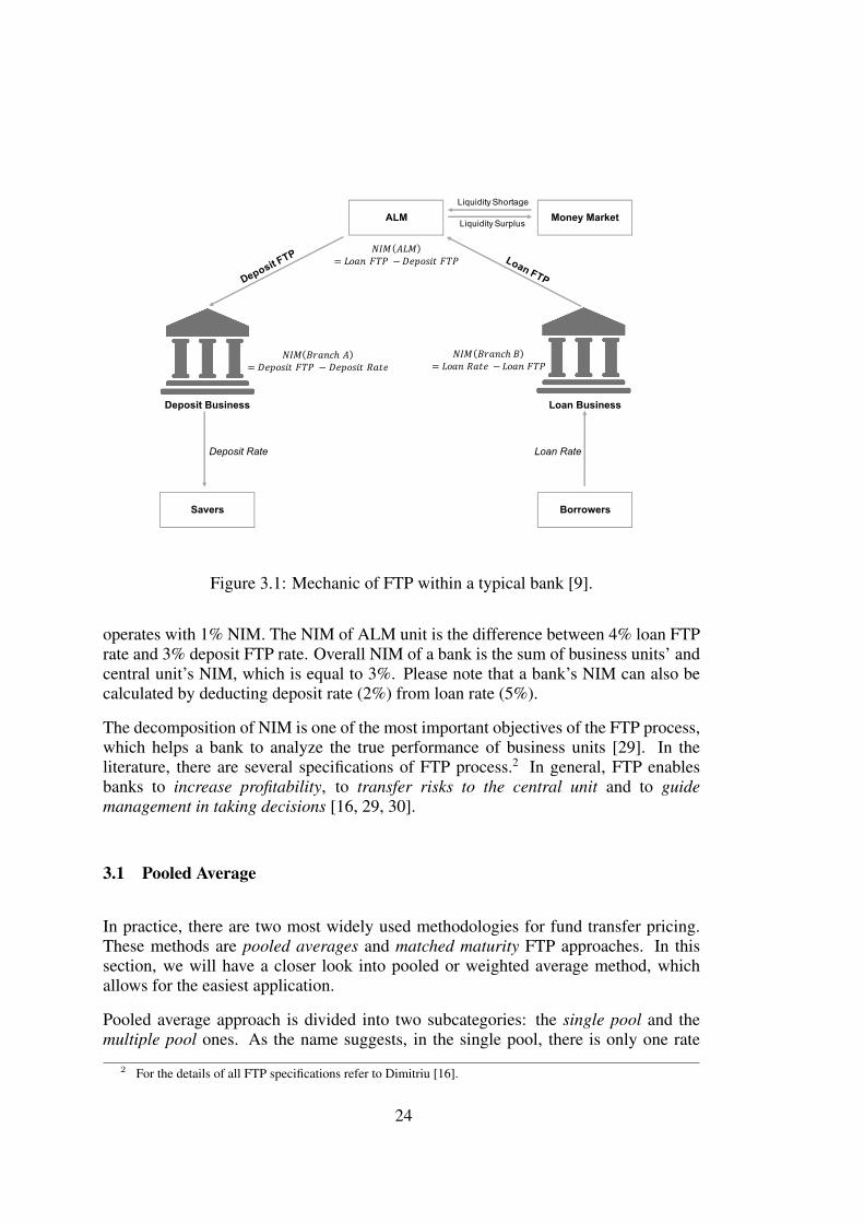
An illustrative example of the flows between ALM, business units and customersis shown in Figure 3.1. Within a bank, businesses differ by their functioningperformances. Some businesses are heavily collecting funds, while others are goodat lending. Deposit business collects funds from savers and pays interest. On the otherhand, loan business issues loans to borrowers and gets interest. As a result, one sidehas a surplus of funds, whereas the other one is in shortage. At this point, the centralunit of a bank with FTP tool comes into play. ALM of a bank borrows money from thedeposit business by paying the deposit FTP rate and lends it to the lending business at aloan FTP rate. Accordingly, there are three units benefiting from the whole transaction.The first unit is deposit business, paying deposit rate to customer and lending at depositFTP rate. The second one is ALM, borrowing at deposit FTP rate and lending at loanFTP rate. Finally, lending business issues loans at loan rate. The funding of these loansis obtained at loan FTP rate. For the bank, it is a zero-sum gain1, and the total NIM isthe difference between loan and deposit rate.
This is better to understand by a numerical example. Assume that deposit business inFigure 3.1 pays 2% deposit rate to savers and receives 3% deposit FTP rate from ALM;thus, deposit business generates 1% NIM. A bank’s lending business unit, on the otherhand, borrows at 4% loan FTP rate and charges the customer 5% loan rate, which also
1 In game theory, when the amount of one person’s gain is the same as another’s loss, the net change is zeroand this is called as zero-sum game.
23
Savers Borrowers
Deposit Business Loan Business
ALM Money Market
Loan RateDeposit Rate
Liquidity Surplus
Liquidity Shortage
𝑁𝐼𝑀 𝐵𝑟𝑎𝑛𝑐ℎ𝐵= 𝐿𝑜𝑎𝑛𝑅𝑎𝑡𝑒 − 𝐿𝑜𝑎𝑛𝐹𝑇𝑃
𝑁𝐼𝑀 𝐴𝐿𝑀= 𝐿𝑜𝑎𝑛𝐹𝑇𝑃 −𝐷𝑒𝑝𝑜𝑠𝑖𝑡 𝐹𝑇𝑃
𝑁𝐼𝑀 𝐵𝑟𝑎𝑛𝑐ℎ𝐴= 𝐷𝑒𝑝𝑜𝑠𝑖𝑡 𝐹𝑇𝑃 − 𝐷𝑒𝑝𝑜𝑠𝑖𝑡𝑅𝑎𝑡𝑒
Figure 3.1: Mechanic of FTP within a typical bank [9].
operates with 1% NIM. The NIM of ALM unit is the difference between 4% loan FTPrate and 3% deposit FTP rate. Overall NIM of a bank is the sum of business units’ andcentral unit’s NIM, which is equal to 3%. Please note that a bank’s NIM can also becalculated by deducting deposit rate (2%) from loan rate (5%).
The decomposition of NIM is one of the most important objectives of the FTP process,which helps a bank to analyze the true performance of business units [29]. In theliterature, there are several specifications of FTP process.2 In general, FTP enablesbanks to increase profitability, to transfer risks to the central unit and to guidemanagement in taking decisions [16, 29, 30].
3.1 Pooled Average
In practice, there are two most widely used methodologies for fund transfer pricing.These methods are pooled averages and matched maturity FTP approaches. In thissection, we will have a closer look into pooled or weighted average method, whichallows for the easiest application.
Pooled average approach is divided into two subcategories: the single pool and themultiple pool ones. As the name suggests, in the single pool, there is only one rate
2 For the details of all FTP specifications refer to Dimitriu [16].
24
obtained to price all balances, whereas in the multiple pool, the assets and liabilities ofa bank are grouped into different pools and are priced accordingly.
The analogy in the single-pool approach is simple: the weight of each item in apool is multiplied by its yield (assets) or cost (liabilities) to form weighted averages.Then, the average weighted yields and costs are assigned as an FTP rate. Under themultiple-pool approach, business units create pools according to some criteria and aset of dimensions: such as type, term, origination, or other fund attributes [49].
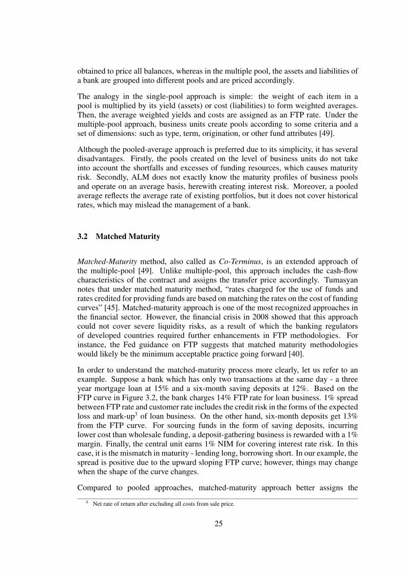
Although the pooled-average approach is preferred due to its simplicity, it has severaldisadvantages. Firstly, the pools created on the level of business units do not takeinto account the shortfalls and excesses of funding resources, which causes maturityrisk. Secondly, ALM does not exactly know the maturity profiles of business poolsand operate on an average basis, herewith creating interest risk. Moreover, a pooledaverage reflects the average rate of existing portfolios, but it does not cover historicalrates, which may mislead the management of a bank.
3.2 Matched Maturity
Matched-Maturity method, also called as Co-Terminus, is an extended approach ofthe multiple-pool [49]. Unlike multiple-pool, this approach includes the cash-flowcharacteristics of the contract and assigns the transfer price accordingly. Tumasyannotes that under matched maturity method, “rates charged for the use of funds andrates credited for providing funds are based on matching the rates on the cost of fundingcurves” [45]. Matched-maturity approach is one of the most recognized approaches inthe financial sector. However, the financial crisis in 2008 showed that this approachcould not cover severe liquidity risks, as a result of which the banking regulatorsof developed countries required further enhancements in FTP methodologies. Forinstance, the Fed guidance on FTP suggests that matched maturity methodologieswould likely be the minimum acceptable practice going forward [40].
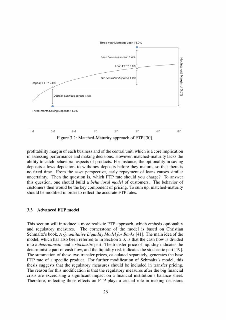
In order to understand the matched-maturity process more clearly, let us refer to anexample. Suppose a bank which has only two transactions at the same day - a threeyear mortgage loan at 15% and a six-month saving deposits at 12%. Based on theFTP curve in Figure 3.2, the bank charges 14% FTP rate for loan business. 1% spreadbetween FTP rate and customer rate includes the credit risk in the forms of the expectedloss and mark-up3 of loan business. On the other hand, six-month deposits get 13%from the FTP curve. For sourcing funds in the form of saving deposits, incurringlower cost than wholesale funding, a deposit-gathering business is rewarded with a 1%margin. Finally, the central unit earns 1% NIM for covering interest rate risk. In thiscase, it is the mismatch in maturity - lending long, borrowing short. In our example, thespread is positive due to the upward sloping FTP curve; however, things may changewhen the shape of the curve changes.
Compared to pooled approaches, matched-maturity approach better assigns the
3 Net rate of return after excluding all costs from sale price.
25
1M 3M 6M 1Y 2Y 3Y 4Y 5Y
Three-year Mortgage Loan 14.0%
Loan business spread 1.0%
The central unit spread 1.0%
Loan FTP 13.0%
Deposit FTP 12.0%
Deposit business spread 1.0%
Three-month Saving Deposits 11.0%
Net Interest M
argin of 3.0%
Figure 3.2: Matched-Maturity approach of FTP [30].
profitability margin of each business and of the central unit, which is a core implicationin assessing performance and making decisions. However, matched-maturity lacks theability to catch behavioral aspects of products. For instance, the optionality in savingdeposits allows depositors to withdraw deposits before they mature, so that there isno fixed time. From the asset perspective, early repayment of loans causes similaruncertainty. Then the question is, which FTP rate should you charge? To answerthis question, one should build a behavioral model of customers. The behavior ofcustomers then would be the key component of pricing. To sum up, matched-maturityshould be modified in order to reflect the accurate FTP rates.
3.3 Advanced FTP model
This section will introduce a more realistic FTP approach, which embeds optionalityand regulatory measures. The cornerstone of the model is based on ChristianSchmaltz’s book, A Quantitative Liquidity Model for Banks [41]. The main idea of themodel, which has also been referred to in Section 2.3, is that the cash flow is dividedinto a deterministic and a stochastic part. The transfer price of liquidity indicates thedeterministic part of cash flow, and the liquidity risk indicates the stochastic part [19].The summation of these two transfer prices, calculated separately, generates the baseFTP rate of a specific product. For further modification of Schmaltz’s model, thisthesis suggests that the regulatory measures should be included in transfer pricing.The reason for this modification is that the regulatory measures after the big financialcrisis are excercising a significant impact on a financial institution’s balance sheet.Therefore, reflecting those effects on FTP plays a crucial role in making decisions
26

[26, 46].
This section is organised as follows: In the first part, we will derive a transfer pricemodel for the deterministic part. Then, the modeling of the stochastic part will bedescribed. In the subsequent part, we will model the effects of regulatory measures andembed them into the transfer pricing. Finally, an illustrative example of an advancedFTP model will be demonstrated.
3.3.1 Deterministic Fund Transfer Pricing
From our “Cash Flow” Subsection 2.4.1, we recall that the deterministic component ofcash flow - µitk . In the literature, there is a consensus on modeling the transfer price ofthe deterministic component. The function of the deterministic transfer price is definedas follows:
TPD(µtk) := (r(0, tk)− rrf (0, tk)) · µtk ·∆t, (3.1)
wherer(0, tk) : funding curve,rrf (0, tk) : risk-free curve.
In Equation (3.1), the difference between funding curve and risk-free curve is definedas funding spread, which represents funding cost of a bank above the reference rate,and it is scaled by the expected life of the loan.
The only controversial question in the deterministic function is about which marketcurve should be used as a risk-free curve. In practice, risk-free instruments do not exist.However, banks prefer Triple-A bonds or interest-rate swaps as proxies for risk-freeinstrument. Since a bond market is not as liquid as swap markets, in practice, manybanks choose interest-rate swaps as a risk-free curve. In this thesis, we will use theTurkish-Lira swap curve as a base curve.4
The formula in Equation (3.1) indicates the transfer price of a product with only onedeterministic cash flow µ at time tk. For the product i with n deterministic cash flowsµit0 , . . . , µ
itn , the transfer price is the sum of all cash flows:
TPD(µit0 , . . . , µitk
) =n∑j=0
(r(0, tj)− rrf (0, tj))∆t · µitj · (tj − t0). (3.2)
4 For short-term rates with less than 1 year to maturity, Turkish Lira and USD cross-currency implied yields -derived from the covered interest-rate parity theorem - are used. For long-term rates Turkish Lira and USD swaprates are applied.
27
3.3.2 Stochastic Fund Transfer Pricing
In the previous sections, we have defined the Brownian component of cash flow as:
σi∆W itk
= σi,p∆W i,ptk
+ σi,m∆Wmtk.
which is the sum of the product-specific and the systematic component.
The aggregate exposure of a Brownian component has been derived in Section 2.4.1as:
σA =
√√√√ n∑i=1
(σi,p)2 +[ n∑i=1
σi,m]2
.
The funding capacity to back the aggregate exposure σA at a significance level p isstated in Equation (2.13):
FC(σA) = −√
∆t · Φ−1(1− p) · σA.
In order to simplify the notation in the above equation, we will denote it as follows:
FC(σA) = FC(1) · σA,
whereFC(1) = −
√∆t · Φ−1(1− p).
3.3.2.1 Transfer Price of Aggregate Exposure
Since the amount of funding capacity is held to back aggregate exposure carries cost,the next step is to determine the cost implied by required funding capacity FC. Recallfrom funding Section 2.1.2 that in terms of collateral the funding is divided into twocategories, namely, secured (l) and unsecured (1− l):
FC(σA) = l · FC(σA) + (1− l)FC(σA). (3.3)
The function for required cost of funding capacity is defined as follows:
TPB(σA) = CR(l · FC(1) · σA) + CU((1− l) · FC(1) · σA)
= CR(l · FC(1) · σA) + 0
= CR(−l ·√
∆t · Φ−1(1− p)) · σA, (3.4)addressing
CR : cost function of secured funds,CU : cost function of unsecured funds.
28

The cost function of secured funding costs can be expressed in linear form as:5
CR(σA) = (−l ·√
∆t · Φ−1(1− p)) · σA ·∆Y ield. (3.5)
At this point, it is important to note that the assumption which unsecured fundingincurs zero cost did not hold during the 2008 financial crisis. When Lehman Brothersfiled for bankruptcy, the LIBOR rates in interbank lending jumped by more than 360basis points [21].
3.3.2.2 Transfer Price of an Individual Product
After determining the required funding capacity to cover aggregate stochasticexposure, the next part is disaggregation of funding capacity into products. Theindependence among products, and between product-specific and market risk, is alsovalid in this part. Since the independence assumption is too simplistic, to enhancethe disaggregation approach, one has to account for diversification effects [41].6According to the diversification, the sum of required funding capacity for individualproducts exceeds the aggregate funding:
d∑i=1
FC(σp,i, σm,i) > FC(σA). (3.6)
The objective here is to adjust individual risks (σi,p, σi,m) such that:
FC(σA) =d∑i=1
FC(σi,p,adj) +d∑i=1
FC(σi,m,adj) 6d∑i=1
FC(σi,p) +d∑i=1
FC(σi,m).
(3.7)
By solving Equation (3.7) we get:
FC(σA) =d∑i=1
FC(σi,p,adj) +d∑i=1
FC(σi,m,adj)
⇔
FC(1) · σA = FC(1) ·d∑i=1
σi,p,adj + FC(1) ·d∑i=1
σm,i,adj,
σA :=d∑i=1
σi,p,adj +d∑i=1
σi,m,adj. (3.8)
5 The difference in yield indicates the risk premium of the institution, and expresses itself as the differencebetween the cost of unsecured funding and benchmark yields.
6 The Diversification Effect is measured as the relation of the required funding capacity under 0 correlation tothe funding capacity under perfect correlation.
29

Equation (3.8) states that the allocation of aggregate exposure σA is equivalent to theallocation of funding capacity. There are several approaches for the computation ofindividual risks. However, in this thesis we will use Adjustment Approach, which isalso additive [41]. The reason for such a choice is twofold: the first one it suits well fora small number of factors (in our case, there are two factors), and the second reason isthat it does not require further assumptions.
In this work, we need to calculate two adjustment factors: one measures theeffect of diversification among products, and the second assesses the effect betweenproduct-specific and systematic factors. Let us begin with an estimation of theadjustment factor among products.
By embedding Equation (3.8) into the function of Funding Capacity, we obtain:
FC(σA) = −√
∆t · Φ−1(1− p) ·
√√√√ d∑i=1
(σi,p)2 +[ d∑i=1
σi,m]2. (3.9)
At this point, it is vital to note that lower case superscripts p and m are used todistinguish products-specific and systematic Brownian risks on product level, whereasupper case superscripts P and M are referred to the risks across all products. Here,we will derive the equations for two extreme cases. In the first case, where only aproduct-specific Brownian exposure exists, it holds:
FC(σP ) = −√
∆t · Φ−1(1− p) ·
√√√√ d∑i=1
(σi,p)2 + 0
= −√
∆t · Φ−1(1− p) · σP . (3.10)
In the second case, only systematic Brownian exposure exists; then, we note
FC(σM) = −√
∆t · Φ−1(1− p) ·
√√√√0 +[ d∑i=1
σi,m]2
= −√
∆t · Φ−1(1− p) · σM . (3.11)
Under perfect correlation, the required funding capacities are additive:
FC(σP + σM) = FC(σP ) + FC(σM). (3.12)
Now we will derive the formula for the diversification factor κ - kappa, which measuresthe diversification effect between product-specific and systematic factors. Recall thatthe formula for the adjustment factor is “actual funding capacity” divided by “fundingcapacity under perfect correlation”:
30
κ =FC(σA)
FC(σP ) + FC(σM)
=σA · FC(1)
σP · FC(1) + σM · FC(1)
=σA
σP + σM. (3.13)
The adjustments for product-specific (σP ) and systematic (σM) Brownian risks arestated as:
σP,adj = κ · σP ,σM,adj = κ · σM .
Having found these adjustments, we can show that the sum of the factors would beequal to the total aggregate exposure:
FC(σP,adj) + FC(σM,adj) = FC(κ · σP ) + FC(κ · σM)
= FC(σA
σP + σM· σP ) + FC(
σA
σP + σM· σM)
= FC(σA) · ( σP
σP + σM+
σM
σP + σM)
= FC(σA).
After dividing the funding capacity into factors, the next step is to allocate the fundingcapacity into individual products (i). The allocation of the systemic factor intoindividual products is derived in the following form:
FC(σM,adj) = FC(κ · σM)
= FC(κ ·d∑i=1
σi,m)
= FC(d∑i=1
κ · σi,m)
= FC(d∑i=1
σi,m,adj).
From the last two equalities the subsequent equation is derived:
31

σi,m,adj = κ · σi,m. (3.14)
For the product-specific factor the corresponding formula results as:
FC(σP,adj) = FC(κ · σP )
= FC(κ ·
√√√√ d∑i=1
(σi,p)2)
(3.15)
6 FC(κ ·d∑i=1
σi,p) (Triangle Inequality).
The above inequality reveals that there should be further adjustments incorporatingdiversification among individual products. The second adjustment factor is defined as:
κp : =σP∑di=1 σ
i,p
⇔
σP = κp ·d∑i=1
σi,p. (3.16)
By a combination of Equations (3.15) and (3.16) we derive:
FC(σP,adj) = FC(κ · σP )
= FC(κ · κp ·d∑i=1
σi,p)
= FC(d∑i=1
κ · κp · σi,p)
=d∑i=1
FC(κ · κp · σi,p)
=d∑i=1
FC(σi,p,adj).
From the above the product-specific adjusted exposure is obtained as:
σi,p,adj = κ · κp · σi,p, ∀ i = 1, 2, . . . , d. (3.17)
32

Incorporating all factors, we receive the final equation of aggregate exposure:
FC(σA) = FC(σP,adj) + FC(σM,adj)
= FC(d∑i=1
σi,p,adj) + FC(d∑i=1
σi,m,adj)
= FC(d∑i=1
κ · κp · σi,p) + FC(d∑i=1
κ · σi,m)
=d∑i=1
FC(1) · κ · (κp · σi,p + σi,m). (3.18)
Therefore, the required funding capacity of product i, with product-specific σp andmarket σm risks, is:
FC(σi,p, σi,m) = −√
∆t · Φ−1(1− p) · κ · (κp · σi,p + σi,m). (3.19)
After deriving the required funding capacity for product i, it is trivial to show that thetransfer price of a product i with Brownian exposures, σi,m and σi,p at a confidencelevel p, equals:
TPBi (σi,p, σi,m) = cR(σi,p, σi,m, l) (3.20)
= −l ·√
∆t · Φ−1(1− p) · κ · (κp · σi,p + σi,m) ·∆Y ield.
3.3.2.3 Optionality
In Equation (3.20), the transfer price of a product is derived for one time lag ∆t,where it is assumed that there is no exercise during this period. However, as we havementioned in our Funding section, in real circumstances, indeed there is a frequentnumbers of exercises [33]. Therefore, in this subsection, we extend the assumptionand denote the full maturity as T = n ·∆t; inserting what into Equation (3.20) shows:
TPBi (σi,p, σi,m, n ·∆t) = cR(σi,p, σi,m, l)
= −l ·√n ·∆t · Φ−1(1− p) · κ
·(κp · σi,p + σi,m) ·∆Y ield.
The whole maturity time T (e.g., 1 year or 365 days), can also be denoted in termsof the average length of repayment period (e.g., 30.4 days) and the number of totalrepayments (e.g., 12 months), such that:
33
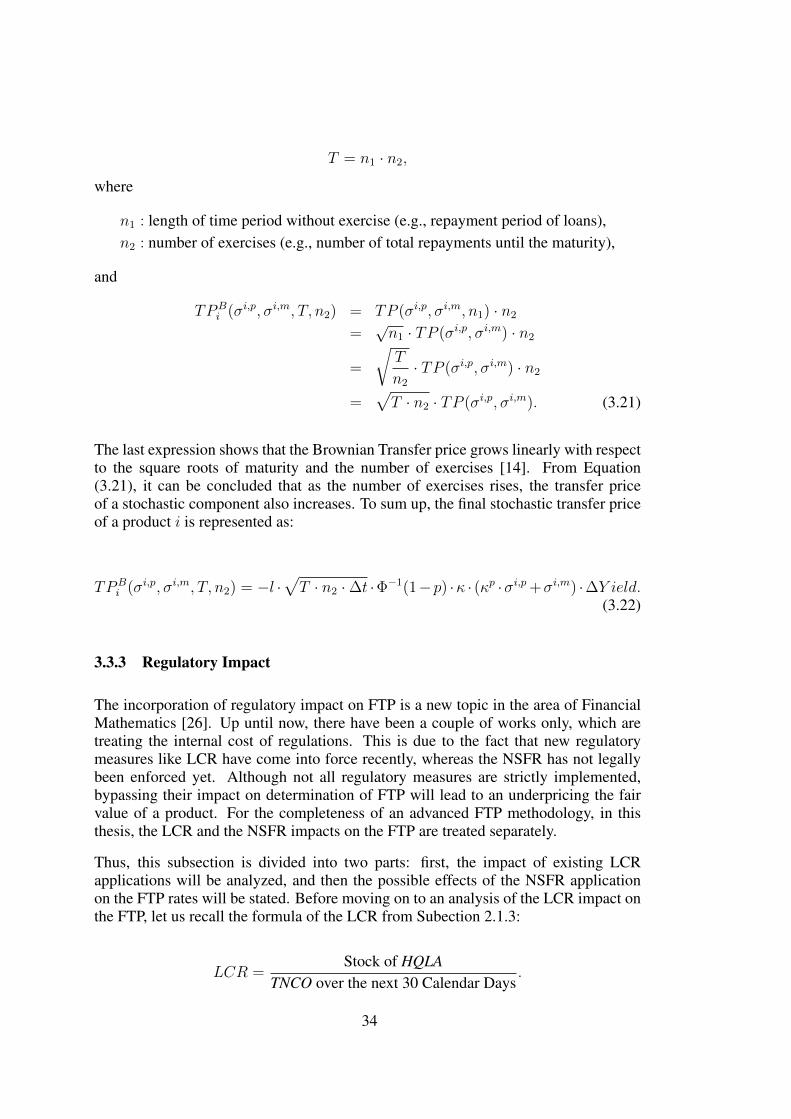
T = n1 · n2,
where
n1 : length of time period without exercise (e.g., repayment period of loans),n2 : number of exercises (e.g., number of total repayments until the maturity),
and
TPBi (σi,p, σi,m, T, n2) = TP (σi,p, σi,m, n1) · n2
=√n1 · TP (σi,p, σi,m) · n2
=
√T
n2
· TP (σi,p, σi,m) · n2
=√T · n2 · TP (σi,p, σi,m). (3.21)
The last expression shows that the Brownian Transfer price grows linearly with respectto the square roots of maturity and the number of exercises [14]. From Equation(3.21), it can be concluded that as the number of exercises rises, the transfer priceof a stochastic component also increases. To sum up, the final stochastic transfer priceof a product i is represented as:
TPBi (σi,p, σi,m, T, n2) = −l ·
√T · n2 ·∆t ·Φ−1(1−p) ·κ · (κp ·σi,p+σi,m) ·∆Y ield.
(3.22)
3.3.3 Regulatory Impact
The incorporation of regulatory impact on FTP is a new topic in the area of FinancialMathematics [26]. Up until now, there have been a couple of works only, which aretreating the internal cost of regulations. This is due to the fact that new regulatorymeasures like LCR have come into force recently, whereas the NSFR has not legallybeen enforced yet. Although not all regulatory measures are strictly implemented,bypassing their impact on determination of FTP will lead to an underpricing the fairvalue of a product. For the completeness of an advanced FTP methodology, in thisthesis, the LCR and the NSFR impacts on the FTP are treated separately.
Thus, this subsection is divided into two parts: first, the impact of existing LCRapplications will be analyzed, and then the possible effects of the NSFR applicationon the FTP rates will be stated. Before moving on to an analysis of the LCR impact onthe FTP, let us recall the formula of the LCR from Subection 2.1.3:
LCR =Stock of HQLA
TNCO over the next 30 Calendar Days.
34

The idea in applying LCR by regulators is to force banks to hold a certain amountof liquid assets against their short-term exposure. Holding liquid assets causes anopportunity cost which needs to be covered. The methodology of implementing theLCR impact on the FTP is based on reflecting those opportunity costs on the FTPrates. For the sake of simplicity, we will illustrate the methodology by the followingexample: Assume that a bank issues a mortgage loan and funds it from cash.7 Actually,this action can be replicated as an investment of cash to the mortgage-backed securities(MBS). From the above transaction, the HQLA of a bank will decrease, since the classof liquid assets has been downgraded from Level 1 to Level 2B. The fraction of adecrease in the stock of the HQLA is subject to the related haircut (φ) among assetlevels. In our example, the HQLA stock will decrease by 25% times the notionalamount of an investment (N ) due to the haircut in MBS. Herewith, the new value ofLCR after investment will look like:
LCRnew =Stock of HQLA− 0.25 ·N
TNCO over the next 30 Calendar Days.
Assuming that the initial ratio is equal to the legal required limit for the LCR, the bankneeds to fulfill the deficit amount, in our case it is 25% of the notional amount (N ), ofthe HQLA. Likewise, we assume that our bank can acquire unsecured funds and caninvest them into Level 1 assets. From the profit and loss (P and L) perspective, thisaction incurs loss for the bank, since the funding cost (fc) is higher than the return ofLevel 1 assets (rA). Otherwise, there will be an arbitrage opportunity. The maturityof this borrowing has to cover the lifetime of the issued mortgage loan (T ). However,as the monthly repayments of the mortgage loan principal are paid, the amount ofthe borrowing should also be decreased8, otherwise extra cost for the excess liquiditybuffer would occur. In order to calculate the regulatory impact more accurately, in ourthesis we would calculate the cost of the fundings’ cash-flow. As a result, the effectivecost of funding can be measured as follows:
f effc =n∑j=0
µtj ·N · (fc − rA) · φ, (3.23)
where
µt0 = 0,
µtj = principal repayments, ∀ j = 1, 2, . . . , n.
Until this point, we have assumed that the initial ratio is equal to the required limit.However, in real circumstances, this is not the case and, generally, banks with a strongliquidity basis have higher ratios. This saves the banks which have an excess HQLAstock from borrowing, and also allows them to use excess liquid assets. As a result, theeffective cost of funding will be lower, allowing banks to have a flexibility in pricing
7 Here, it is important to note that funding directly from cash or by borrowing does not affect the final outcome,since funding from cash and then replacing the amount by borrowing has the same outcome as direct borrowing.
8 In essence, the same outcome can also be reached by investing an extra reserve amount from repayments.
35

the FTP rates. The relationship between the proportion of current available HQLAand effective cost of funding (at specific time t), reflected on the FTP rates, can beexpressed in the following modified form:
f effc =n∑j=0
µtj ·N · (fc − rA) · φ · θt, (3.24)
whereθt =
Stock of HQLAt
Total available balance of HQLAt
. (3.25)
The same logic is used in measuring the NSFR effect on FTP rates. The effective costof funding, which is needed to accomplish regulatory NSFR ratio, is calculated andembedded in the FTP rate. In order to illustrate this in closer details, let us assume theprevious example in the calculation of the LCR effect: The bank issues mortgage loanwith a notional amount of N units, and the NSFR of a bank is equal to the regulatorylimit of 100%. Recalling from Subsection 2.1.3, the initial NSFR is calculated as:
NSFR =ASF
RSF, (3.26)
where
ASF: Available Stable Funding,RSF: Required Stable Funding.
After the issuance of mortgage loan funded by cash, only RSF will increase by theamount of ψ · N , since ASF will change as a result of a move in liability items.Therefore, the bank’s new value of NSFR looks as follows:
NSFRnew =ASF
RSF + ψ ·N. (3.27)
In order to encompass the decrease in the ratio, the bank needs ψ·N amount of funding,in our example, it is 65% of notional amount (N ). The effective cost of this fundingcan be demonstrated as in the LCR part:
f effc =n∑j=0
µtj ·N · (fc − rA) · ψ. (3.28)
From the above regulatory effects, one can observe that unique borrowing, coveringboth of the funding needs, can be established. Thus, all of the requirements areaccomplished by one transaction. In other words, to eliminate any double-countingeffect of regulatory cost, one should consolidate the LCR and the NSFR costs. Sincethese costs are differing by their factors φ in the LCR and ψ in the NSFR, the maximum
36

of those factors would be enough to cover both of the requirements.9 The formula forcalculating the effective cost of the consolidated regulatory is:
f effc =n∑j=0
µtj ·N · (fc − rA) ·maxψ, φ. (3.29)
The last equation approves our hypothesis that the implementation of regulatorymeasures has resulted in an increase of FTP rates, which is also shown in Jorgansen’swork [24]. The final transfer cost of regulatory measures is expressed in the followingform:
TPRi (ψ, φ) =
n∑j=0
µtj · (fc − rA) ·maxψ, φ. (3.30)
9 One of the ratios will be on its regulatory limit level, whereas the other one will be higher than the requiredlimit.
37

38
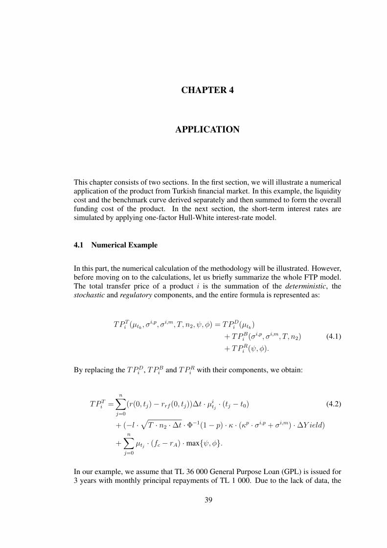
CHAPTER 4
APPLICATION
This chapter consists of two sections. In the first section, we will illustrate a numericalapplication of the product from Turkish financial market. In this example, the liquiditycost and the benchmark curve derived separately and then summed to form the overallfunding cost of the product. In the next section, the short-term interest rates aresimulated by applying one-factor Hull-White interest-rate model.
4.1 Numerical Example
In this part, the numerical calculation of the methodology will be illustrated. However,before moving on to the calculations, let us briefly summarize the whole FTP model.The total transfer price of a product i is the summation of the deterministic, thestochastic and regulatory components, and the entire formula is represented as:
TP Ti (µtk , σ
i,p, σi,m, T, n2, ψ, φ) = TPDi (µtk)
+ TPBi (σi,p, σi,m, T, n2) (4.1)
+ TPRi (ψ, φ).
By replacing the TPDi , TPB
i and TPRi with their components, we obtain:
TP Ti =
n∑j=0
(r(0, tj)− rrf (0, tj))∆t · µitj · (tj − t0) (4.2)
+ (−l ·√T · n2 ·∆t · Φ−1(1− p) · κ · (κp · σi,p + σi,m) ·∆Y ield)
+n∑j=0
µtj · (fc − rA) ·maxψ, φ.
In our example, we assume that TL 36 000 General Purpose Loan (GPL) is issued for3 years with monthly principal repayments of TL 1 000. Due to the lack of data, the
39

variables - (σi,p) and (σi,m) including their adjustment factors which are namely (κ)and (κp) - are used as given. However, the readers deeply interested in the calculationmethodologies and related researches for Turkish banking sector can refer to [1, 2, 23]and [44]. The average funding spread is assumed to be constant and the approximatecalculation1 of which is equal to 90 BPS per year. The 40% of the required Brownianfunding capacity is assumed to be secured by reserves. The Brownian exposure iscalculated at 99% confidence level, and the cost of holding reserves against Brownianexposure (∆Y ield per st. dev.) is equal to the funding spread. Since in Turkishbanking sector, a product such as GPL backed-security does not exist, it is not possibleto include GPL into the HQLA. Therefore, in our example, the haircut (φ) for the LCRis equal to 1. Assuming that the required amount for accomplishing the regulatorylimits funded via retail deposits with the maturity of 18 months (deposits are rolledduring the life-period of GPL), the NSFR factor (ψ) is 65%. The last variable thatshould also be stated is the stock proportion of the HQLA in total available HQLA attime t (θt), which is 80%. After defining all of the variables, we will put them intocomponents and compute them one by one.
The deterministic component of a GPL is equal to:
(r(0, tj)− rrf (0, tj) = 90 (BPS),
(tj − t0) =365 (Days)
12· j,
n = 36 (number of total repayments),
µt0 = −36 000 (TL),
µtj =1 000
36 000=
1
36∀tj, where j = 1, 2, . . . , T,
∆t = 1 (daily basis):
TPDi (
1
36) =
36∑j=0
90BPS
365Days· 1 · 1
36· 365Days
12· j = 138.75 (BPS).
1 The average of the difference between cost of deposits curve and swap curve, plus average cost of requiredreserves.
40

The result of stochastic component is equal to:
l = 0.4,
σi,p = 0.2,
σi,m = 0.15,
T = 3 (years),
n2 = 36,
Φ−1(1− 0.99) = −2.3263,
κ = 0.7,
κp = 0.25,
∆Y ield
st. dev.= 90 (BPS):
TPBi (0.2, 0.15, 5, 36) =− 0.4 ·
√3 · 365 · 36 · 1 · (−2.3263) · 0.7
· (0.25 · 0.2 + 0.15) · 90
365= 6.38 (BPS).
The effect of regulatory measures is equal to:
θt = 0.8,
φ = 1,
ψ = 0.65 :
TPRi (1, 0.65) =
36∑j=0
1
36· j · 60
12BPS · 0.8 ·max1, 0.65 = 74 (BPS).
According to the results, one can observe that the highest cost in our example incursthe deterministic part, whereas the stochastic part has the lowest part. The reason forsuch outcome is that our product has mainly a deterministic cash-flow and a lowervolatility. Actually, GPLs are generally short-term loans and the amount of each loanis restricted according to the banks’ internal policies2. Therefore consumers are lesswillingly to repay the remaining instalments before the maturity, compared to thelong-term loans like mortgage. However, if we analyze products such as mortgageloans, demand deposits and saving deposits, the composition of transfer price willvary, since they have higher volatility which has a positive linear relationship with
2 In Turkey, on average it is about 50 thousand Turkish Lira.
41

stochastic component of the transfer price. Another important point is that the effect ofregulatory measures has a significant weight in total liquidity cost. This result stronglysupports our hypothesis that regulatory measures will directly influence the total costof funding, which will be calculated next.
The total transfer price of a 3 years GPL is equal to:
TP Ti (
1
36, 0.2, 0.15, 5, 36, 1, 0.65) = 138.75 + 6.38 + 74 ≈ 219 BPS.
The 219 BPS is only the total cost of liquidity transfer for one unit of GPL with thematurity of 3 years (73 BPS per year). The total cost of funding actually is the sum ofrisk-free (swap) curve and the liquidity cost. The calculation methodology of the swapcurve (SC) in this thesis is conducted by replicating the cash-flow of GPL funding asstated below [13]:
SCj =n∑i=1
rrf (0, tj,i) · µtj,i · (tj,i − t0), ∀ j = 1, 2, . . . , T, (4.3)
where
rrf (0, tj,i) = swap rate with maturity j at time i.
Based on the above methodology the total funding cost of GPL is calculated andsummarized in Table 4.1. According to this table, the total cost of funding forGPL is equal to 24973 BPS. Assuming that GPL has 10% (1000 BPS) annual yield,1000 · 3 = 3000 BPS for 3 years. The net profit of a bank will be 3000− 2497 = 503BPS; in our example it is 36000 · 0.0503 ≈ 1811 TL.
4.2 Simulation
In this section, we will simulate the short-term interest rates. Concerning future yields,the market expectations are mainly indicated by the forward yield curve [13, 15]. Onthe basis of these expectations, the Hull-White model is applied for the simulation offuture possible outcomes of short-term interest rates. The data subject to the simulationis the 1 month Turkish Lira and USD implied rates, thus Turkish-Lira swap yield servesas an initial yield curve for the input of the model. Based on the Bloomberg data theswap yield curve of Turkish Lira is shown in Figure 4.1. The shape of the yield curve isinverted; therefore, by referring to Section 2.5 one can infer that the short-term interestrates are expected to fall.
The data are simulated in MATLAB tool4, by employing the following methodology.At the beginning, the data for TL interest swaps are interpolated (piecewise cubic
3 The sum of funding costs for GPL maturing in the first, second and third years with 472, 835 and 1 190 BPS,respectively.
4 The detailed MATLAB code of the simulation is presented in Appendix C.
42

Table 4.1: Summary: Total Cost of Funding.
Maturity 1 year 2 years 3 years
Swap Rates (%) 11.96 % 11.44 % 11.17 %
Replicating the cash-flow by applying Equation (4.3):
SC (BPS) 399 762 1 117
+
TP (BPS) 73 73 73
=
Funding Cost (BPS) 472 835 1 190
9,5%
10,0%
10,5%
11,0%
11,5%
12,0%
12,5%
ON 1W 2W 1M 2M 3M 6M 12M 1.5Y 2Y 3Y 4Y 5Y 6Y 7Y 8Y 9Y 10Y
Figure 4.1: Turkish Lira-Swap Yield.
43
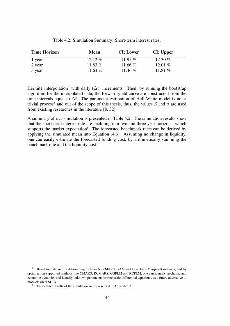
Table 4.2: Simulation Summary: Short-term interest rates.
Time Horizon Mean CI: Lower CI: Upper1 year 12.12 % 11.95 % 12.30 %2 year 11.83 % 11.66 % 12.01 %3 year 11.64 % 11.46 % 11.81 %
Hermite interpolation) with daily (∆t) increments. Then, by running the bootstrapalgorithm for the interpolated data, the forward-yield curve are constructed from thetime intervals equal to ∆t. The parameter estimation of Hull-White model is not atrivial process5 and out of the scope of this thesis, thus, the values β and σ are usedfrom existing researches in the literature [8, 32].
A summary of our simulation is presented in Table 4.2. The simulation results showthat the short term interest rate are declining in a two and three year horizons, whichsupports the market expectation6. The forecasted benchmark rates can be derived byapplying the simulated mean into Equation (4.3). Assuming no change in liquidity,one can easily estimate the forecasted funding cost, by arithmetically summing thebenchmark rate and the liquidity cost.
5 Based on data and by data-mining tools such as MARS, GAM and Levenberg-Marquardt methods, and byoptimization-supported methods like CMARS, RCMARS, CGPLM and RCPLM, one can identify stochastic andeconomic dynamics and identify unknown parameters in stochastic differential equations, as a future alternative tomore classical SDEs.
6 The detailed results of the simulation are represented in Appendix D.
44

CHAPTER 5
CONCLUSION AND OUTLOOK
In our thesis, we have modeled an advanced FTP with the implementation of thestochastic interest rates and the impact of new Basel III regulatory measures. Themodel incorporates two major parts, namely, liquidity cost and benchmark interestrates. The liquidity cost is divided into the deterministic, the stochastic and theregulatory components, the last of which forms the main contribution of this thesis.The objective of the thesis has been to introduce in Turkey the development andthe application of an advanced FTP system, which has already been applied in moredeveloped countries. FTP is an essential tool for internal banks to regulate the bankmanagement. Effectively estimated FTP curves lead to a successive management ofcosts, risks and future decisions.
In this research, the implied and the cross-currency swap rates, which are used asbenchmark rates, formed the base of the FTP curve. The modeling of the stochasticinterest rates is conducted by applying one-factor Hull-White model. Goodness offit and Gaussian characteristics is the prime reason for such kind of a choice. Thesimulation of the Hull-White provides us with the future possible outcomes of theshort-term interest rates. Incorporating future base curve with liquidity cost will helpthe management of a bank to make their strategic decisions for future periods.
In the financial markets, liquidity is the major concept. The Central bank, marketand funding liquidity are three different types of liquidity. In our thesis, the fundingliquidity is the main facet subject to the analysis. In its simplest form, the fundingliquidity is the capability of a financial institution’s assets to meet its obligations.Implementing the measurements of liquidity cost plays a crucial role in FTP modeling.During the 2008 financial crisis, the evaporation of liquidity in the market was thebreaking point of financial institutions’ bankruptcy. Therefore, the FTP model ofthis research takes into account the cost of both the deterministic and the stochasticcash-flows of all products into account. The ability to fund those cash-flows isdetermined by the funding capacity, which is another determinant of our model.Ultimately, cash-flow and funding capacity have been the two fundamental frameworksof an advanced FTP model derived in this research.
One of the significant scientific contributions of this thesis is the implementation of theregulatory measures into the FTP model. Since the NSFR metric has not entered intoforce yet, there is a lack of research in literature. This thesis initiates the modeling of
45

the NSFR effect into FTP rates and approves its hypothesis that the NSFR metric willresult in FTP increase.
The application of real data from Turkish financial market leads us to the followingresults. First, depending on the characteristics of a product, the cost of liquidity differs.If it is stable - can be determined beforehand - cash flow, the deterministic part consiststhe major part of total liquidity cost; otherwise, the stochastic cost of liquidity mayprevail. The regulatory effect has a significant impact on FTP rates. In the applicationof the model, it has been revealed that the FTP rate would be 74 BPS lower, providingthat the regulatory measures were not taken into consideration.
The application of an advanced model has also its limitations. First, it is a cumbersometask to predict short-term interest rates because it has numerous variables that shouldbe predicted. Macro indicators such as GDP, money supply, current accounts etc.,are among indicators that have a significant influence on the evolution of interest rates.Prediction of all those variables could certainly have a positive impact on the estimationof interest rates, but it is difficult to be realistic.
Insufficiency and high cost of data-generating tools is another limitation of themodel. An advanced model requires long historical data to predict actual risk factors.However, due to the lack of data, a derivation of factors is not possible. Moreover,calculation of those factors can only be executed by powerful generating tools whichhave the capacity to operate with a huge amount of data. Those tools demandhigh qualified users or further education, which in essence, means an extra cost ofdevelopment for the institution.
Finally, the effect of regulatory measures are based on simple assumptions that needfurther investigations. After the NSFR entrance into force, new products in the marketmay emerge, as a result of which, a different impact on the FTP rates may occur.
Despite the limitations, this thesis will hopefully be a guide to further researches on themodeling the effect of regulatory measures on FTP in the literature and to applicationsin the financial industry.
46
REFERENCES
[1] M. Abay, Turkish banking sector profitability: How to adjust to the new life stage,Oliver Wyman, 2016.
[2] V. V. Acharya, L. H. Pedersen, T. Philippon, and M. Richardson, Measuringsystemic risk, The Review of Financial Studies, 30(1), pp. 2–47, 2017.
[3] BCBS - Basel Committee on Banking Supervision, International convergence ofcapital measurement and capital standards: A revised framework comprehensiveversion, Bank for International Settlements, June 2006.
[4] BCBS - Basel Committee on Banking Supervision, The liquidity coverage ratioand liquidity risk monitoring tools, Bank for International Settlements, January2013.
[5] BCBS - Basel Committee on Banking Supervision, Basel III: the net stablefunding ratio, Bank for International Settlements, October 2014.
[6] O. Blanchard and D. R. Johnson, Macroeconomics, Pearson Education Inc., USA,6th edition, 2013.
[7] D. H. Boecher, How core are your deposits?, The Finance & Accounting Forumfor Financial Institutions, June 2013.
[8] D. Brigo and F. Mercurio, Interest rate models-theory and practice: with smile,inflation and credit, Springer Science & Business Media, Berlin, Germany, 2006.
[9] F. Cadamagnani, R. Harimohan, and K. Tangri, A bank within a bank: how acommercial bank’s treasury function affects the interest rates set for loans anddeposits, Bank of England Quarterly Bulletin, p. Q2, 2015.
[10] A. J. G. Cairns, Interest Rate Models: An Introduction, Princeton UniversityPress, New Jersey, USA, 2004.
[11] P. Carr, Interest rate models: Introduction, Electronic, Bloomberg LP andCourant Institute, NYU, March 2005.
[12] J. C. Cox, J. E. Ingersoll Jr, and S. A. Ross, A theory of the term structureof interest rates, Econometrica: Journal of the Econometric Society, 53(2), pp.385–407, March 1985.
[13] F. Danielsson, Implementation of a Funds Transfer Pricing model with stochasticinterest rates, Master’s thesis, Mathmematical Statistics, Lund University, Lund,Sweden, February 2014.
47
[14] J. Dermine, Fund transfer pricing for bank deposits. the case of products withundefined maturity, INSEAD Working Paper, (2016/06/FIN), January 2016.
[15] F. X. Diebold and C. Li, Forecasting the term structure of government bondyields, Journal of econometrics, 130(2), pp. 337–364, May 2006.
[16] M. C. Dimitriu, S. C. Oaca, et al., Funds transfer pricing in banking, Economia.Seria Management, 13(1), pp. 119–127, 2010.
[17] Euroclear, Understanding repos and the repo markets, Euroclear Bank SA/NV,2009.
[18] FDIC, FRB, and OCC, Interagency guidance on funds transfer pricing related tofunding and contingent liquidity risks, USA, March 2016.
[19] J. Grant, Liquidity transfer pricing: a guide to better practice, Financial StabilityInstitute [and] Bank for International Settlements, December 2011.
[20] M. Haugh, Continuous-time short rate models, Technical report, ColumbiaUniversity, Spring 2010.
[21] D. Hou and D. R. Skeie, LIBOR: origins, economics, crisis, scandal, and reform,Staff Reports 667, Federal Reserve Bank of New York, March 2014.
[22] J. Hull, A. White, et al., One-factor interest-rate models and the valuation ofinterest-rate derivative securities, Journal of financial and quantitative analysis,28(2), June 1993.
[23] IMF, Global financial stability report: Containing systemic risk and restoringfinancial soundness, World Economic and Financial Surveys, April 2008.
[24] V. B. Jorgensen, Funds Transfer Pricing under Basel III New Requirements, NewImplications, Master’s thesis, Aarhus School of Business and Social Sciences,Aarhus University, August 2012.
[25] A. Karimov, Modeling Illiquidity Premium and Bid-Ask Prices of the FinancialSecurities, Ph.D. thesis, Institute of Applied Mathematics of METU, Ankara,Turkey, December 2016.
[26] A. Katz, D. Nickson, and M. Winters, Regulatory reform in the financialindustry and end-to-end transfer pricing execution, https://www.pwc.com/gx/en/tax/publications/transfer-pricing/perspectives/assets/tpp-regulatoryreform.pdf,October 2013.
[27] D. Lamberton and B. Lapeyre, Introduction to stochastic calculus applied tofinance, CRC press, Florida, USA, 2nd edition, 2011.
[28] A. Lesniewski, 5. short rate models, https://www.math.nyu.edu/∼alberts/spring07/Lecture5.pdf, March 2008.
[29] K. Levey, Beyond funds transfer pricing to actionable decision-making, Journalof Performance Management, 21(1), p. 10, 2008.
48
[30] K. M. Levey, Extracting more value from funds transfer pricing, Journal ofPerformance Management, 25(1), p. 28, 2013.
[31] L. Matz and P. Neu, Liquidity risk measurement and management: apractitioner’s guide to global best practices, volume 408, John Wiley & Sons,2006.
[32] D. Mc Manus, D. Watt, et al., Estimating one-factor models of short-term interestrates, Working Paper 99-18, Bank of Canada, Ottawa, Canada, November 1999.
[33] W. J. McGuire, Indeterminate term deposits in FTP: Quantified solutions at last!,Journal of Performance Management, 17(2), p. 14, 2004.
[34] F. S. Mishkin, The economics of money, banking, and financial markets, Pearsoneducation, New York, USA, 7th edition, 2004.
[35] K. Nikolaou, Liquidity (risk) concepts: definitions and interactions, EuropeanCentral Bank, Working Paper Series, NO 1008, February 2009.
[36] O. J. Omole, Recent developments in portfolio optimization via dynamicprogramming, Master’s thesis, Institute of Applied Mathematics of METU,Ankara, Turkey, August 2015.
[37] J. P. Peter, A. Duchesne, and O. Slabari, Funds transfer pricing: Agateway to enhanced business performance, https://www2.deloitte.com/content/dam/Deloitte/lu/Documents/tax/lu-funds-transfer-pricing-03032015.pdf, March2015.
[38] I. Pipia and F. Bayraktar, Turkey: Banking system profile, Moody’s InvestorsService, February 2016.
[39] I. Pipia, F. Bayraktar, et al., Banking system outlook - Turkey: Slowing economy,rising funding costs drive our negative outlook, Moody’s Investors Service, April2006.
[40] PricewaterhouseCoopers, Five key points from the interagencyfunds transfer pricing guidance, http://www.pwc.com/us/en/financial-services/regulatory-services/publications/assets/funds-transfer-pricing-guidance-march-2016.pdf, March 2016.
[41] C. Schmaltz, A Quantitative Liquidity Model for Banks, Springer Science &Business Media, Heidelberg, Germany, 1st edition, 2010.
[42] S. E. Shreve, Stochastic calculus for finance I: the binomial asset pricing model,volume 1, Springer Science & Business Media, New York, USA, 2004.
[43] S. E. Shreve, Stochastic calculus for finance II: Continuous-time models,volume 11, Springer Science & Business Media, New York, USA, 2004.
[44] I. Talasli, Systemic risk analysis of turkish financial institutions with systemicexpected shortfall, Central Bank Review, 13, p. 25, February 2013.
49

[45] H. Tumasyan, Revisiting funds transfer pricing, https://ssrn.com/abstract=2257081, February 2012.
[46] S. Turner, Funds transfer pricing: cracking the code on deposit valuation,Novantas, White Paper Series, November 2008.
[47] S. Uryasev, Conditional value-at-risk: Optimization algorithms and applications,in Computational Intelligence for Financial Engineering, 2000 (CIFEr).Proceedings of the IEEE/IAFE/INFORMS 2000 Conference on, pp. 49–57, IEEE,2000.
[48] O. Vasicek, An equilibrium characterization of the term structure, Journal offinancial economics, 5(2), pp. 177–188, November 1977.
[49] R. Wyle and Y. Tsaig, Implementing high value funds transfer pricing systems,Moody’s Analytics, September 2011.
50

APPENDIX A
Proof of Vasicek’s Explicit Solution
Recall that the explicit solution is:
r(t) = e−βtr(0) +α
β(1− e−βt) + σe−βt
∫ t
0
eβsdW (s). (A.1)
In order to proof a claim, that the equation above is an explicit solution of Vasicek’smodel, we will compute the differential of the right-hand side of (A.1). Here, we usethe Ito-Doeblin formula:
f(t, x) = e−βtr(0) +α
β(1− e−βt) + σe−βtx,
where
X(t) =
∫ t
0
eβsdW (s).
Derivatives and partial derivatives of the functions f(t, x) and X(t) are:
ft(t, x) = −βe−βtr(0) + αe−βt − βσe−βtx
= α− β(e−βtr(0) +α
β(1− e−βt) + σe−βtx)
= α− βf(t, x),
fx(t, x) = σe−βt,
fxx(t, x) = 0,
dX(t) = eβtdW (t),
dX(t)dX(t) = e2βtdt.
The Ito-Doeblin states that
df(t,X(t))
= ft(t,X(t))dt+ fx(t,X(t))dX(t) +1
2fxx(t,X(t))dX(t)dX(t)
= (α− βf(t,X(t)))dt+ σdW (t).
The last equality is the Vasicek’s model, so that we completed the proof.
51

52

APPENDIX B
Derivation of Aggregate-Risk Exposure
The Brownian cash flow component of a product i is the sum of product-specific andsystemic factors:
σi∆W itk
= σi,p∆W i,ptk
+ σi,m∆Wmtk. (B.1)
Aggregated exposure is calculated by taking the summation of both sides of the aboveequation:
d∑i=1
σi∆W itk
=d∑i=1
σi,p∆W i,ptk
+d∑i=1
σi,m∆Wmtk. (B.2)
By applying the variance of the aggregate exposure in (B.2) we get:
V ar(σAd∑i=1
∆W itk
) = V ar(d∑i=1
σi,p∆W i,ptk
+d∑i=1
σi,m∆Wmtk
),
(σA)2V ar(
d∑i=1
∆W itk
) = V ar(d∑i=1
σi,p∆W i,ptk
+ ∆Wmtk
d∑i=1
σi,m),
(σA)2∆(t) = V ar(
d∑i=1
σi,p∆W i,ptk
) + V ar(∆Wmtk
d∑i=1
σi,m)
+2Cov(d∑i=1
σi,p∆W i,ptk
; ∆Wmtk
d∑i=1
σi,m).
Recall from the properties of the Brownian motion, the variance of the increments ∆Wis equal to the difference in time ∆t. From the assumption that the systematic factoris independent from product-specific factor, the covariance of the factors in the lastexpression is equal to 0. In order to simplify the expressions, let us solve the first two
53

expressions on the right-hand side, one by one:
1st term =⇒ V ar(d∑i=1
σi,p∆W i,ptk
) =d∑i=1
V ar(σi,p∆W i,ptk
)
+2d∑
16i<j6d
Cov(σi,pW i,ptk
;σj,pW j,ptk
)
=d∑i=1
(σi,p)2 ·∆t,
2nd term =⇒ V ar(∆Wmtk
d∑i=1
σi,m) = E(∆mtk
) · E(d∑i=1
σi,m)2
−[E(∆Wtk)]2 · [E(d∑i=1
σi,m)]2
= ∆t ·[ d∑i=1
(σi,m)]2
.
By combining the above the expressions, we get the final aggregate exposure asfollows:
(σA)2 ·∆t =
d∑i=1
(σi,p)2 ·∆t+[ d∑i=1
(σi,m)]2
·∆t,
hence,
σA =
√√√√ d∑i=1
(σi,p)2 +[ d∑i=1
(σi,m)]2
. (B.3)
The results implies that the aggregate volatility (σA2) is the linear sum of theproduct-specific and the market volatility under the assumption that the market andproducts, and products within themselves are independent.
54
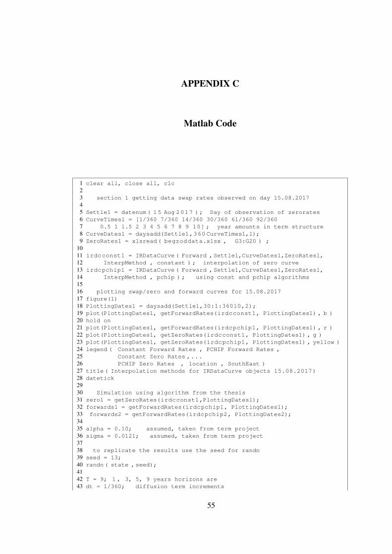
APPENDIX C
Matlab Code
1 clear all, close all, clc23 section 1 getting data swap rates observed on day 15.08.201745 Settle1 = datenum( 15 Aug 2017 ); Day of observation of zerorates6 CurveTimes1 = [1/360 7/360 14/360 30/360 61/360 92/3607 0.5 1 1.5 2 3 4 5 6 7 8 9 10] ; year amounts in term structure8 CurveDates1 = daysadd(Settle1,360 CurveTimes1,1);9 ZeroRates1 = xlsread( begzoddata.xlsx , G3:G20 ) ;
1011 irdcconst1 = IRDataCurve( Forward ,Settle1,CurveDates1,ZeroRates1,12 InterpMethod , constant ) ; interpolation of zero curve13 irdcpchip1 = IRDataCurve( Forward ,Settle1,CurveDates1,ZeroRates1,14 InterpMethod , pchip ) ; using const and pchip algorithms1516 plotting swap/zero and forward curves for 15.08.201717 figure(1)18 PlottingDates1 = daysadd(Settle1,30:1:36010,2);19 plot(PlottingDates1, getForwardRates(irdcconst1, PlottingDates1) , b )20 hold on21 plot(PlottingDates1, getForwardRates(irdcpchip1, PlottingDates1) , r )22 plot(PlottingDates1, getZeroRates(irdcconst1, PlottingDates1) , g )23 plot(PlottingDates1, getZeroRates(irdcpchip1, PlottingDates1) , yellow )24 legend ( Constant Forward Rates , PCHIP Forward Rates ,25 Constant Zero Rates ,...26 PCHIP Zero Rates , location , SouthEast )27 title( Interpolation methods for IRDataCurve objects 15.08.2017)28 datetick2930 Simulation using algorithm from the thesis31 zero1 = getZeroRates(irdcconst1,PlottingDates1);32 forwards1 = getForwardRates(irdcpchip1, PlottingDates1);33 forwards2 = getForwardRates(irdcpchip2, PlottingDates2);3435 alpha = 0.10; assumed, taken from term project36 sigma = 0.0121; assumed, taken from term project3738 to replicate the results use the seed for randn39 seed = 13;40 randn( state ,seed);4142 T = 9; 1 , 3, 5, 9 years horizons are43 dt = 1/360; diffusion term increments
55
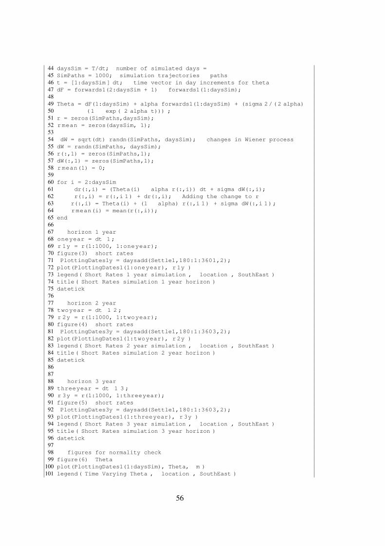
44 daysSim = T/dt; number of simulated days =45 SimPaths = 1000; simulation trajectories paths46 t = [1:daysSim ] dt; time vector in day increments for theta47 dF = forwards1(2:daysSim + 1) forwards1(1:daysSim);4849 Theta = dF(1:daysSim) + alpha forwards1(1:daysSim) + (sigma 2/(2 alpha)50 (1 exp ( 2 alpha t))) ;51 r = zeros(SimPaths,daysSim);52 rmean = zeros(daysSim, 1);5354 dW = sqrt(dt) randn(SimPaths, daysSim); changes in Wiener process55 dW = randn(SimPaths, daysSim);56 r(:,1) = zeros(SimPaths,1);57 dW(:,1) = zeros(SimPaths,1);58 rmean(1) = 0;5960 for i = 2:daysSim61 dr(:,i) = (Theta(i) alpha r(:,i)) dt + sigma dW(:,i);62 r(:,i) = r(:,i 1) + dr(:,i); Adding the change to r63 r(:,i) = Theta(i) + (1 alpha) r(:,i 1) + sigma dW(:,i 1);64 rmean(i) = mean(r(:,i));65 end6667 horizon 1 year68 oneyear = dt 1 ;69 r 1y = r(1:1000, 1:oneyear);70 figure(3) short rates71 PlottingDates1y = daysadd(Settle1,180:1:3601,2);72 plot(PlottingDates1(1:oneyear), r 1y )73 legend( Short Rates 1 year simulation , location , SouthEast )74 title( Short Rates simulation 1 year horizon )75 datetick7677 horizon 2 year78 twoyear = dt 1 2 ;79 r 2y = r(1:1000, 1:twoyear);80 figure(4) short rates81 PlottingDates3y = daysadd(Settle1,180:1:3603,2);82 plot(PlottingDates1(1:twoyear), r 2y )83 legend( Short Rates 2 year simulation , location , SouthEast )84 title( Short Rates simulation 2 year horizon )85 datetick868788 horizon 3 year89 threeyear = dt 1 3 ;90 r 3y = r(1:1000, 1:threeyear);91 figure(5) short rates92 PlottingDates3y = daysadd(Settle1,180:1:3603,2);93 plot(PlottingDates1(1:threeyear), r 3y )94 legend( Short Rates 3 year simulation , location , SouthEast )95 title( Short Rates simulation 3 year horizon )96 datetick9798 figures for normality check99 figure(6) Theta
100 plot(PlottingDates1(1:daysSim), Theta, m )101 legend( Time Varying Theta , location , SouthEast )
56

102 title( Theta )103 datetick104105 figure(7) histogram short rates106 hist(r(:,oneyear), 30)107 title( Histogram 1 year horizon short rate )108109 figure(8)110 hist(r(:,twoyear), 40)111 title( Histogram 2 year horizon short rate )112113 figure(9)114 hist(r(:,threeyear), 40)115 title( Histogram 3 year horizon short rate )116117118 Statistics of the short rates 1, 2, 3 years119 for simplicity use (approxsigma = variance of the sample)120 [muhat1,sigmahat1,muci1,sigmaci1] = normfit(r(:,oneyear));121 [muhat2,sigmahat2,muci2,sigmaci2] = normfit(r(:,twoyear));122 [muhat3,sigmahat3,muci3,sigmaci3] = normfit(r(:,threeyear));123124 max 1 = max(r 1y); max1 = max(max 1);125 max 2 = max(r 2y); max2 = max(max 2);126 max 3 = max(r 3y); max3 = max(max 3);127128 min 1 = min(r 1y); min1 = min(min 1);129 min 2 = min(r 2y); min2 = min(min 2);130 min 3 = min(r 3y); min3 = min(min 3);131132 Display the Results133134 disp( Results from Simulation 1000 trajectories )135 fprintf( 1 year horizon Means of the r short rate 3.4f . n , muhat1)136 fprintf( 2 years horizon Means of the r short rate 3.4f . n , muhat2)137 fprintf( 3 years horizon Means of the r short rate 3.4f . n , muhat3)
57

58
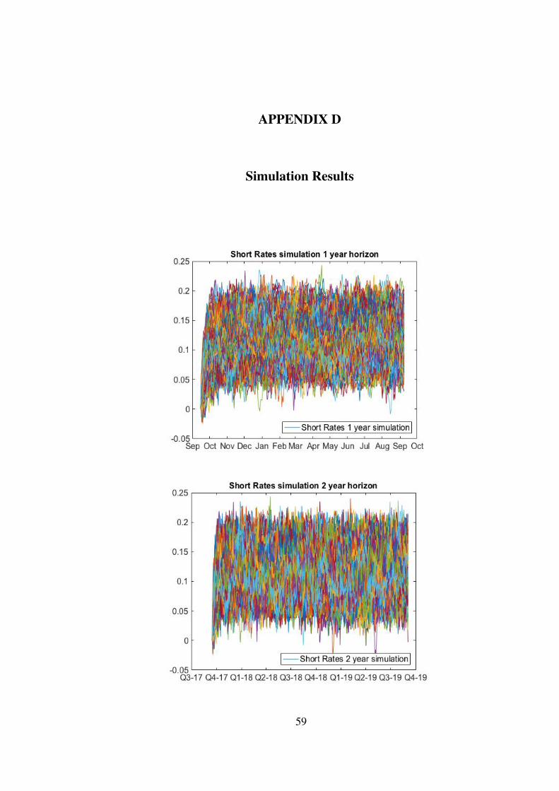
APPENDIX D
Simulation Results
59
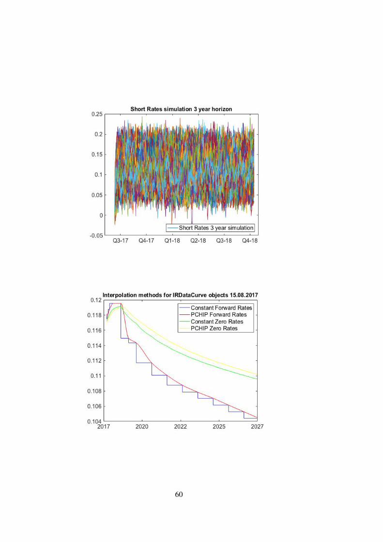
60