1

ME 310

Numerical Methods

Integration

These presentations are prepared by

Dr. Cuneyt Sert

Mechanical Engineering Department

Middle East Technical University

Ankara, Turkey

csert@metu.edu.tr

They can not be used without the permission of the author

2

Idea: Replace a complicated function or a tabulated data with an approximating (interpolating) function.

Newton-Cotes Integration Formulas

b

a

n

b

a

dx )x(f dx )x(fI

where fn(x) is an nth order interpolating polynomial.

x

f(x)

a b

2nd order polynomial

x

f(x)

1st order polynomial

a b

x

f(x)

a b

1st order with multiple segments

3

Trapezoidal Rule:

width*height age Aver )ab(2

)b(f)a(f I

h

x

f(x)

a bh

All Newton-Cotes formulas can be written in the form “Average height * width”. Different formulas will have different expressions for average height.

Newton-Cotes formulas can be derived by integrating Newton’s Interpoating Polynomials. Newton-Gregory version can be used for equispaced data points. These derivations also provide an estimate for the truncation error.

• Newton’s Divided Difference Interpolating Polynomials

fn(x) = f(x0) + (x - x0) f[x1, x0] + (x - x0)(x - x1) f[x2, x1, x0] + . . .

+ (x - x0)(x - x1) . . . (x - xn-1) f[xn, xn-1, . . ., x1, x0]

• Newton-Gregory Formula

fn(x) = f(x0) + Df(x0) a + D2f(x0) a(a - 1) / 2! + . . . + Dnf(x0) a(a - 1) . . . (a - n + 1) / n! + Rn

where a = (x - x0) / h , Rn = f (n+1)(x) hn+1 a(a - 1) . . . (a - n) / (n+1)!

and Dfn(x0) is the nth forward difference.

4

Derivation of the Trapezoidal Rule using Newton-Gregory Formula:

aax

aD

b

a

term Remainder

2

formula G-Norder 1

dx h )1(2

)(f )a(f )a(f I

st

a

a

aa

a

1

0

bx

ax

d h dx ,hddx ,h

ax

Change integration limits from x to a.

a

a

aa

xaD

1

0

2 d h h )1(2

)(f )a(f )a(f I

aaax

aaD

1

0

1

0

3 d )1(2

)(f h d )a(f )a(f h I

1

0

233

1

0

2

f(a) - f(b)

23

2

)(f h

2 )a(f )a(f h I

a

ax

aDa

)(EError Truncation

3

Rule lTrapezoida t

h )(f 12

1

2

)b(f)a(f h I x

• Trapezoidal Rule is first order accurate. It can integrate linear polynomials exactly.

5

Error Estimation for the Trapezoidal Rule:

3h )(f 12

1

2

)b(f)a(f h I x

• Usually f (x) in the error term can not be evaluated since x is not known.

• If the function f is known than f (x) can be approximated with an average 2nd derivative

)x(f 12

h E

ab

dx )x(f

)x(f )(f3

a

b

a

x

Example 35: Integrate f(x)= ex from a=1.5 to a=2.5 using the Trapezoidal Rule. Estimate the error.

True value is e2.5 – e1.5 = 7.700805

Using the trapezoidal rule:

a = 1.5, b = 2.5, h = 2.5 – 1.5 = 1.0

Et = - 0.631287, et = - 8.2 %

Estimated error: 0.641734 0.1

dx e

12

1

ab

dx )x(f

12

h E

5.2

5.1

x

3

b

a3

a

332092.8 2

ee1.0

2

)b(f)a(f h I

2.51.5

6

Multiple application of the Trapezoidal Rule:

xn

)1n(x

2x

1x

1x

0x

b

a

dx f(x) . . . dx f(x) dx f(x) dx f(x) I

In general we have n+1 points and n intervals (segments).

If the points are equispaced h = (b-a)/n

x

f(x)

x0=a

h

x1 x2 xn=b

.....

xn-1

2

)x(f)x(fh . . .

2

)x(f)x(fh

2

)x(f)x(f hI n1n2110

2n

)x(f )x(f2 )x(f

)ab( )x(f )x(f2 )x(f 2

h I

n

1n

1ii0

n

1n

1ii0

• The last equation is again of the form “Width * Average height”

7

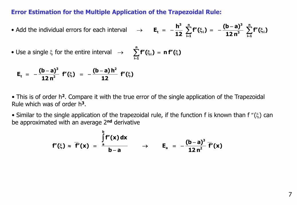
Error Estimation for the Multiple Application of the Trapezoidal Rule:

x

xn

1ii3

3n

1ii

3

t )(f n 12

)ab( )(f

12

h E

• Use a single x for the entire interval

)(f 12

h )ab( )(f

n 12

)ab( E

2

2

3

t x

x

• This is of order h2. Compare it with the true error of the single application of the Trapezoidal Rule which was of order h3.

• Similar to the single application of the trapezoidal rule, if the function f is known than f (x) can be approximated with an average 2nd derivative

)x(f n 12

)ab( E

ab

dx )x(f

)x(f )(f2

3

a

b

a

x

)(f n )(fn

1ii xx

• Add the individual errors for each interval

8

Example 36: Integrate f(x)= ex from a=1.5 to a=2.5 using the Trapezoidal Rule. Use a step size of 0.25. True value of the integral is 7.700805.

a = 1.5, b = 2.5, h = 0.25 than we have n=4 intervals.

(4) 2

e )eee( 2 e )5.15.2(

2n

)x(f )x(f 2 )x(f

)ab( I 5.225.2275.15.11

1n

1ii0

I 7.740872 , Et = - 0.040067, et = - 0.5 %

Estimated error:

Note that the calculation of Ea requires the evaluation of the same integral that the question asks for. Of course the integral in Ea can laso be calculated numerically. This approach also gives

040108.0 )0.1(

dx )x(f

(4) 12

)0.1( )x(f

n 12

)ab( E

2.5

1.5

2

3

2

3

a

040317.0 )0.1(

740872.7

(4) 12

)0.1( E

2

3

a

9

Simpson’s 1/3 Rule:

6

)x(f )x(f 4 )x(f a)-(b I

)x(f )x(f 4 )x(f 3

h I

210

210

This can be derived using the second order Newton-Gregory formula

aaaD

aaD

aD

x2

x0

vanish willterm This

03

GregoryNewton-order 2

02

00 dx Remainder )2)(1(6

)x(f )1(

2

)x(f )x(f )x(f I

nd

)(EError Truncation

5)4(

Rule 1/3 sSimpson'

210

t

h )(f 90

1 )x(f)x(f 4)x(f

3

h I x

404

h)3)(2)(1(24

)x(faaaa

Dwhere the remainder is

The derivation yields (see page 597 for details)

)x(f 2880

)ab( )x(f

90

h E )4(

5)4(

5

a

h

x

f(x)

a = x0 b = x2x1

h

10

• Simpson’s 1/3 Rule uses 3 points, therefore it is expected to integrate 2nd order polynomials exactly.

• However it can integrate cubics exactly. This is due to the vanishing third term in integrating the Newton-Gregory polynomial.

Multiple application of Simpson’s 1/3 Rule Rule:

xn

)2n(x

4x

2x

2x

0x

b

a

dx f(x) . . . dx f(x) dx f(x) dx f(x) I

In general we have n+1 points and n intervals.

If the points are equispaced h = (b-a)/n

If there are even number of points the integration can not be done with Simpson’s 1/3 rule only.

)x(f)x(f4)x(f3

h . . . )x(f)x(f4)x(f

3

h )x(f)x(f4)x(f

3

h I n1n2n432210

3n

)x(f )x(f2 )x(f4 )x(f

)ab( I n

1n

6,4,2ii

1n

5,3,1ii0

)x(f n 180

)ab( E )4(

4

5

a

x

f(x)

x0=a

h

x1 x2 xn=b

.....

xn-1

11

Example 37: Calculate using

(a) Trapezoidal Rule with n=2, n=4 and n=6.

(b) Simpson’s 1/3 Rule with n=2, n=4 and n=6.

(a) For n=2, h=p/2,

dx )xsin(0

p

570796.1 2

)sin()2/(sin 2 )0sin( 2

2/ )x(f)x(f 2 )x(f

2

h I 210

ppp

p

411234.0 0

dx )xsin(

(2) 12

)0( )x(f

n 12

)ab( E 0

2

3

2

3

a p

p

p

Note that Et = 0.429204

(b) For n=4, h=p/4,

2.004560 )sin()4/3(sin 4 )2/(sin 2 )4/(sin 4 )0sin( 3

4/

)x(f)x(f4)x(f2)x(f 4 )x(f 3

h I 43210

ppppp

004228.0 0

dx )xsin(

(4) 180

)0( )x(f

n 180

)ab( E 0

4

5)4(

4

5

a p

p

p

Note that Et = 0.004560

Exercise 38: Complete the solution of this example.

12

Simpson’s 3/8 Rule:

)(fh80

3E

8

)x(f )x(f 3 )x(f 3 )x(f a)-(b I

)x(f )x(f 3 )x(f 3 )x(f 8

3h I

)4(5t

3210

3210

x

Exercise 39: Derive this formula by integrating the proper Newton-Gregory polynomial.

Exercise 40: Derive the formula for the multiple application of Simpson’s 3/8 Rule.

• Note that 3/8 Rule uses 4 points and it is third order accurate (can integrate cubic polynomials exactly).

• 1/3 Rule does this with 3 points and it is preferred.

• 3/8 rule is useful if there are even number of points.

• 1/3 and 3/8 can be used together, but mixing them with the Trapezoidal Rule is not suggested. Because the accuracy of the Trapezoidal rule is only first order.

Exercise 41: Perform an efficient third order accurate calculation for the previous example with n=7. Use an efficient proper combiation of 1/3 and 3/8 Rules.

h

x

f(x)

x0 x2x1

h

x3

h

13

Richardson Extrapolation for Integration

Similar to the discussion we made for differentiation,

I: Exact integral (usually not known)

I = I1 + E1 where I1: Estimated integral using h=h1. E1: Error of the estimation I1.

I = I2 + E2 where I2: Estimated integral using h=h2. E2: Error of the estimation I2.

If multiple application of the Trapezoidal Rule is used to get the estimates I1 and I2, than

E1 = O(h12) , E2 = O(h2

2)

Using these, I1 and I2 can be combined to get a better estimate such as

This new estimate is O(h4) accurate.

A special case of h2 = h1/2 results in

1 h h

I I I I

221

122

12 I3

1 I

3

4 I

14

Romberg Integration

• Apply multiple Richardson Extrapolation one after the other.

• If we use Trapezoidal Rule and successively halve the step size

I1,1 is the integral obtained by h. Usually we start with a single segment, i.e, h = b - a

I2,1 is the integral obtained by h/2.

I3,1 is the integral obtained by h/4.

etc.

Combine I1,1 and I2,1 to get I1,2 I1,2 = 4/3 I2,1 - 1/3 I1,1

Combine I2,1 and I3,1 to get I2,2 I2,2 = 16/15 I3,1 - 1/15 I2,1

Combine I1,2 and I2,2 to get I1,3 I1,3 = 64/63 I2,1 - 1/63 I1,1

etc.

O(h2) O(h4) O(h6) O(h8) O(h10)

I1,1 I1,2 I1,3 I1,4 I1,4

I2,1 I2,2 I2,3 I2,4

I3,1 I3,2 I3,3

I4,1 I4,2

I5,1

1 4

I I 4 I

1k

1-kj,1-k1,j1k

k,j

Valid if Trapezoidal Rule with successive halving of the step size is used to get the first column.

100%*I

II ||

k,1

1k,1k1,a

e

15

Example 38: Perform 4 levels of Romberg Integration to integrate sin(x) over the interval [0,p].

Use Trapezoidal Rule.

h=p , I1,1 = p/2 [sin(0) + sin(p)] = 0.0

h=p/2 , I1,2 = (p/2)/2 [sin(0) + 2sin(p/2) + sin(p)] = 1.57079633

h=p/4 , I1,3 = (p/4)/2 [sin(0) + 2sin(p/4) + 2sin(p/2) + 2sin(3p/4) + sin(p)] = 1.89611890

h=p/8 , I1,4 = 1.97423160

k=1 k=2 k=3 k=4

0.00000000 2.09439511 1.99857073 2.00000555

1.57079633 2.00455976 1.99998313 Sample error calculation

1.89611890 2.00026917

1.97423160

Exercise 42: The true error of the final result is about 6x10-6. We can estimate the number of segments to be used to achieve this accuracy with the Trapezoidal Rule.

370n 10x6 0

dx )xsin(

n 12

)0( )x(f

n 12

)ab( |E| 60

2

3

2

3

a p

p

p

%07.0 100 00000555.2

99857073.100000555.2a

e

16

Gauss-Quadrature Integration

• Trapezoidal rule uses two points to perform the integration. These two points are the end points of the interval.

• What if we use some other points?

• Gauss-Quadrature uses special points in the interval [a,b] to achieve higher accuracy than Newton-Cotes formulas. But it is not suitable for integrating tabulated data, it can be used if the function is known.

• The special points (x0, x1) and the weights (c0, c1) can be determined using a technique called Method of Undetermined Coefficients.

2

)b(f)a(f a)-(b I

)f(x c )f(x c I 1100

x

f(x)

a bx0 x1

x

f(x)

a b

17

Derivation of the Two Point Gauss-Quadrature Formula Using the Method of Undetermined Coefficients

Consider the calculation of the integral of f(x) over the interval [-1,1]

I c0 f(x0) + c1 f(x1)

• We have 4 unknowns. We need 4 equations to find them.

• We will get these equations by assuming that this formula calculates constant, linear, parabolic and cubic functions exactly (Note that Trapezoidal Rule also uses two points and can only calculate constant and linear functions exactly).

x

-1 1x0 x1

f(x)

1

1

31100

1

1

21100

1

1

1100

1

1

1100

0 dx x )x(f c )x(f c

2/3 dx x )x(f c )x(f c

0 dx x )x(f c )x(f c

2 dx 1 )x(f c )x(f c

31/ x

31/- x

1 c

1 c

1

0

1

0

3

1 f

3

1- f I

18

• Note that this formula integrates over the domain xd [-1,1]. This is done to simplify the mathematics and to get a general formula that can be applied to any domain with a change of variable.

• To apply this formula to a domain of x [a,b] we need to change the variable as

dd

1

1-

dd

b

a

dx 2

abdx ,

2

x )ab()ab(x using dx )f(x dx f(x)

Example 39: Integrate sin(x) over [0,p] using two-point Gauss Quadrature.

1.9358196 )322

sin( 2

)322

sin( 2

3

1f

3

1-f I

)x22

sin( 2

)f(x

is formula Quadrature-Gauss the in use to need wefunction the Therefore

dx 2

)x22

sin( dx sin(x) dx 2/ dx ,x)2/(2/x

dd

1

1-

dd

0

dd

p

pp

p

pp

p

pp

pp

pppp

p

For this calculation |Et|= 0.064. To achieve this accuracy with the Trapezoidal Rule we approximately need 5 segments.

5n 0.064 0

dx )xsin(

n 12

)0( )x(f

n 12

)ab( |E| 0

2

3

2

3

a p

p

p

19

Higher Order Gauss-Quadrature Formulas

• The general version of Gauss-Quadrature uses n points.

I c0 f(x0) + c1 f(x1) + . . . + cn-1 f(xn-1)

• We can use the method of undetermined coefficients to get 2n equations to solve for 2n unknowns.

• Table 22.1 shows the weighting factors and integration points upto n=6.

Exercise 43: Derive the 3-point Gauss-Quadrature formula.

Exercise 44: Use this formula to integrate sin(x) over [0,p]. Approximately how many segments are necessary to get the same accuracy with the Trapezoidal Rule, Simpson’s 1/3 Rule and Simpson’s 3/8 Rule?