improved viewshed analysis algorithms for avionics - METU
99
IMPROVED VIEWSHED ANALYSIS ALGORITHMS FOR AVIONICS APPLICATIONS A THESIS SUBMITTED TO THE GRADUATE SCHOOL OF INFORMATICS OF THE MIDDLE EAST TECHNICAL UNIVERSITY BY MUSTAFA ÖZKIDIK IN PARTIAL FULFILLMENT OF THE REQUIREMENTS FOR THE DEGREE OF MASTER OF SCIENCE IN THE DEPARTMENT OF INFORMATION SYSTEMS JULY 2019
-
Upload
khangminh22 -
Category
Documents
-
view
0 -
download
0
Transcript of improved viewshed analysis algorithms for avionics - METU

IMPROVED VIEWSHED ANALYSIS ALGORITHMS FOR AVIONICS
APPLICATIONS
A THESIS SUBMITTED TO
THE GRADUATE SCHOOL OF INFORMATICS OF
THE MIDDLE EAST TECHNICAL UNIVERSITY
BY
MUSTAFA ÖZKIDIK
IN PARTIAL FULFILLMENT OF THE REQUIREMENTS FOR THE DEGREE OF
MASTER OF SCIENCE
IN
THE DEPARTMENT OF INFORMATION SYSTEMS
JULY 2019


IMPROVED VIEWSHED ANALYSIS ALGORITHMS FOR AVIONICS APPLICATIONS
Submitted by Mustafa Özkıdık in partial fulfillment of the requirements for the degree of Master of
Science in Information Systems Department, Middle East Technical University by,
Prof. Dr. Deniz Zeyrek Bozşahin
Dean, Graduate School of Informatics
Prof. Dr. Yasemin Yardımcı Çetin
Head of Department, Information Systems
Assoc. Prof. Dr. Altan Koçyiğit
Supervisor, Information Systems Dept., METU
Examining Committee Members:
Assoc. Prof. Dr. Banu Günel Kılıç
Information Systems Dept., METU
Assoc. Prof. Dr. Altan Koçyiğit
Information Systems Dept., METU
Assist. Prof. Dr. Bilgin Avenoğlu
Computer Engineering Dept., TED University
Assoc. Prof Dr. Pekin Erhan Eren
Information Systems Dept., METU
Prof. Dr. Yasemin Yardımcı Çetin
Information Systems Dept., METU
Date: July 2, 2019


iii
I hereby declare that all information in this document has been obtained and
presented in accordance with academic rules and ethical conduct. I also
declare that, as required by these rules and conduct, I have fully cited and
referenced all material and results that are not original to this work.
Name, Last name : Mustafa Özkıdık
Signature :

iv
ABSTRACT
IMPROVED VIEWSHED ANALYSIS ALGORITHMS FOR AVIONICS
APPLICATIONS
Özkıdık, Mustafa
MSc., Department of Information Systems
Supervisor: Assoc. Prof. Dr. Altan Koçyiğit
July 2019, 85 pages
Viewshed analysis is a common GIS capability used in various domains with various
requirements. In avionics, viewshed analysis is a part of accuracy critical applications and
the real time operating systems in embedded devices use preemptive scheduling
algorithms to satisfy performance requirements. Therefore, to effectively benefit from the
viewshed analysis, a method should be both fast and accurate.
Although R3 algorithm is accepted as an accuracy benchmark, R2 algorithm with lower
accuracy is preferred in many cases due to its better execution time performance. This
thesis prioritizes accuracy and presents an alternative approach to improve execution time
performance of the R3 algorithm. Considering different execution environments,
improved versions of R3 are implemented for CPU and GPU. The experiment results show
that CPU implementation of improved algorithms achieve 1.23x to 13.51x speedup
depending on the observer altitude, range and topology of the terrain. In GPU
implementation experiments up to 2.27x speedup is recorded. In addition to execution
time performance improvements, the analysis results prove that proposed algorithms are
capable of providing higher accuracy like R3.
Keywords: geographic information systems, avionic applications, viewshed analysis, line
of sight analysis, parallel programming

v
ÖZ
AVİYONİK UYGULAMALAR İÇİN GELİŞTİRİLMİŞ GÖRÜNÜRLÜK ANALİZİ
ALGORİTMALARI
Özkıdık, Mustafa
Yüksek Lisans, Bilişim Sistemleri Bölümü
Tez Yöneticisi: Doç. Dr. Altan Koçyiğit
Temmuz 2019, 85 sayfa
Görünürlük analizi, farklı gereksinimlerle farklı çalışma alanlarında kullanılan bir Coğrafi
Bilgi Sistemleri yeteneğidir. Aviyonik sistemlerde, görünürlük analizi doğruluk kritik
uygulamaların bir parçasıdır ve gömülü cihazlardaki gerçek zamanlı işletim sistemleri,
performans gereksinimlerini sağlamak için kesintili zamanlama algoritmaları
kullanmaktadır. Bu nedenle, görünürlük analizinden etkin bir şekilde yararlanmak için
kullanılan yöntemler hem hızlı hem de doğru olmalıdır.
R3 algoritması analiz sonuçlarının doğruluğu konusunda bir ölçü olarak kabul edilse de
daha iyi işleme zamanı performansı nedeniyle daha düşük doğruluğa sahip R2 algoritması
tercih edilmektedir. Bu tez analiz sonuçlarının doğruluğunu ön planda tutarak R3
algoritmasının işleme zamanı performansını geliştirmeye yönelik alternatif bir yaklaşım
sunmaktadır. Farklı çalışma ortamları gözetilerek R3 algoritmasının geliştirilmiş
versiyonları merkezi işlem birimi ve grafik işlem birimi için kodlanmıştır. Merkezi işlem
birimi ile yapılan deneylerde; analiz irtifasına, menziline ve topolojiye bağlı olarak
standart R3 algoritmasına göre 1.23 ile 13.51 kat arasında hızlanma görülmüştür. Grafik
işlem biriminde yapılan deneylerde ise tavsiye edilen algoritmalarda standart R3’e göre
2.27 kata kadar hızlanma kaydedilmiştir. İşleme zamanı performansındaki bu artışların
yanı sıra, analiz sonuçları önerilen algoritmaların R3 gibi yüksek doğruluk değerleri
sunabilme yeteneğini göstermiştir.
Anahtar Sözcükler: coğrafi bilgi sistemleri, aviyonik uygulamalar, görünürlük analizi,
görüş hattı analizi, paralel programlama

vi
DEDICATION
Dedicated to the orphans of war

vii
ACKNOWLEDGMENTS
First of all, I would like to thank my thesis advisor Assoc. Dr. Altan Koçyiğit for sharing
his time with me.
Besides my supervisor, I would like to thank to my family for supporting me in all aspects
of life.

viii
TABLE OF CONTENTS
ABSTRACT ................................................................................................................. iv
ÖZ ................................................................................................................................. v
DEDICATION.............................................................................................................. vi
ACKNOWLEDGMENTS ............................................................................................ vii
TABLE OF CONTENTS ............................................................................................ viii
LIST OF TABLES ......................................................................................................... x
LIST OF FIGURES ...................................................................................................... xi
LIST OF ABBREVIATIONS ...................................................................................... xii
CHAPTERS
INTRODUCTION ................................................................................................. 1
1.1. Motivation and Research Question ................................................................... 2
1.2. Objective and Contribution .............................................................................. 3
1.3. Thesis Organization ......................................................................................... 3
BACKGROUND INFORMATION AND PREVIOUS WORK .............................. 5
2.1 Elevation Model .............................................................................................. 5
2.2. Line of Sight .................................................................................................... 6
2.3. Viewshed Analysis Algorithms ........................................................................ 7
2.3.1. R3 ............................................................................................................. 8
2.3.2. R2 ............................................................................................................. 9
2.3.3. Blelloch .................................................................................................. 10
2.3.4. Van Kreveld’s Algorithm........................................................................ 11
2.3.5. Xdraw ..................................................................................................... 13
2.3.6 Comparison of Viewshed Analysis Algorithms ....................................... 14
3. PROPOSED SOLUTION DESIGN AND IMPLEMENTATIONS ....................... 15
3.1. Proposed Solution and Design Rationale ........................................................ 15
3.1.1. Phase-0: Prepare Processed Elevation Models ......................................... 16

ix
3.1.2. Phase-1: Detection of Invisible Groups ................................................... 19
3.1.3. Phase-2: Determine Visibility for Remaining Points ............................... 21
3.2. Proposed Granularity Algorithm Implementations ......................................... 25
3.2.1. Elevation Model Processing ................................................................... 25
3.2.2. Granularity Algorithms in CPU .............................................................. 25
3.2.3. Granularity Algorithms in GPU .............................................................. 26
3.2.4. Hybrid Granularity Algorithm ................................................................ 29
3.3. R3 and R2 Algorithm Implementations.......................................................... 30
3.3.1. R3 in CPU .............................................................................................. 30
3.3.2. R2 in CPU .............................................................................................. 30
3.3.3. R3 in GPU .............................................................................................. 30
3.3.4. R2 in GPU .............................................................................................. 31
4. EVALUATION ................................................................................................... 33
4.1. Experiments with CPU Implementation ......................................................... 34
4.1.1. Execution Time ...................................................................................... 34
4.1.2. Accuracy ................................................................................................ 38
4.2. Experiments with GPU Implementation......................................................... 41
4.2.1. Execution Time ...................................................................................... 41
4.2.2. Accuracy ................................................................................................ 46
4.3. Resource Usage ............................................................................................. 48
5. CONCLUSION AND FUTURE WORK ............................................................. 49
REFERENCES ............................................................................................................ 51
APPENDICES............................................................................................................. 55
APPENDIX A ............................................................................................................. 55
APPENDIX B ............................................................................................................. 66

x
LIST OF TABLES
Table 1: Comparison of common algorithms ................................................................ 14
Table 2: Notations for algorithm descriptions ............................................................... 18 Table 3: Processed elevation models used by algorithms .............................................. 18
Table 4: Dimensions of slope models retrieved from processed elevation models......... 20 Table 5: Phase-2 slope computation launch parameters for proposed algorithms .......... 28
Table 6: R3 kernel launch parameters .......................................................................... 31 Table 7: R2 kernel launch parameters .......................................................................... 31 Table 8: Execution time statistics of CPU algorithms on 512×512 tiles ........................ 35
Table 9: Execution time statistics of CPU algorithms on 1024×1024 tiles .................... 36 Table 10: Execution time statistics of CPU algorithms on 2048×2048 tiles .................. 37
Table 11: Accuracy of CPU algorithms ........................................................................ 39 Table 12: Accuracy statistics of algorithms (FN: False Negative, FP: False Positive) ... 39
Table 13: Accuracy statistics of experiment in Figure 24.............................................. 40 Table 14: Execution time statistics of GPU algorithms on 512×512 tiles ...................... 42
Table 15: Execution time statistics of GPU algorithms on 1024×1024 tiles .................. 43 Table 16: Execution time statistics of GPU algorithms on 2048×2048 tiles .................. 44
Table 17: Changing statistics of R2 algorithm for same analysis .................................. 47 Table 18: Resource usage of algorithms ....................................................................... 48

xi
LIST OF FIGURES
Figure 1: Viewshed analysis output ............................................................................... 1
Figure 2: Terrain model visualization using Global Mapper GIS Software ..................... 3 Figure 3: TIN and raster type DEM ............................................................................... 5
Figure 4: Line drawn by Bresenham’s algorithm............................................................ 6 Figure 5: Visibility on a line of sight.............................................................................. 7
Figure 6: Line of Sight ................................................................................................... 8 Figure 7: R3 Algorithm ................................................................................................. 8 Figure 8: R2 Algorithm ................................................................................................. 9
Figure 9: Bresenham lines for R2 Algorithm ................................................................. 9 Figure 10: Input slope data for maximum prefix scan algorithm................................... 11
Figure 11: Output of maximum prefix scan algorithm .................................................. 11 Figure 12: Events for cell in Van Kreveld's algorithm .................................................. 12
Figure 13: Active balanced tree ................................................................................... 12 Figure 14: Xdraw algorithm ......................................................................................... 13
Figure 15: Proposed approach ...................................................................................... 16 Figure 16: Forming down scaled elevation model with group by 2×2........................... 17
Figure 17: Visibility on slope model with 16×16 granularity........................................ 20 Figure 18: V_Table after phase-1 ................................................................................. 21
Figure 19: Reuse of visibility information in phase 2 ................................................... 23 Figure 20: CPU algorithm execution time comparison on 512×512 tiles ...................... 35
Figure 21: CPU algorithm execution time comparison on 1024×1024 tiles .................. 36 Figure 22: CPU algorithm execution time comparison on 2048×2048 tiles .................. 37
Figure 23: CPU algorithm execution time comparison for MSA .................................. 38 Figure 24: Visual comparison of non-matching points of R2 and DGR3 with R3 ......... 40
Figure 25: Visual comparison of non-matching points of X2 and DGR3 with R3 ......... 41 Figure 26: GPU algorithm execution time comparison on 512×512 tiles ...................... 42
Figure 27: GPU algorithm execution time comparison on 1024×1024 tiles .................. 43 Figure 28: GPU algorithm execution time comparison on 2048×2048 tiles .................. 44
Figure 29: GPU algorithm execution time comparison for MSA .................................. 45 Figure 30: Hybrid algorithm speedup with respect to R3 CPU implementation ............ 46
Figure 31: Changing pixels due to racing threads of R2 algorithm in GPU ................... 47

xii
LIST OF ABBREVIATIONS
GIS Geographic Information Systems
CPU Central Processing Unit
GPU Graphical Processing Unit
GPGPU General Purpose Graphical Processing Unit
RTOS Real Time Operating System
MSA Minimum Sector Altitude
X2 2 x 2 Granularity R3 CPU Algorithm
X4 4 x 4 Granularity R3 CPU Algorithm
X8 8 x 8 Granularity R3 CPU Algorithm
X16 16 x 16 Granularity R3 CPU Algorithm
DGR3 Dynamic Granularity R3 CPU Algorithm
DGRHYB Dynamic Granularity R3 Hybrid Algorithm
DGRGPU Dynamic Granularity R3 GPU Algorithm
R3GPU R3 GPU Algorithm
R2GPU R2 GPU Algorithm
X2GPU 2 x 2 Granularity R3 GPU Algorithm
X4GPU 4 x 4 Granularity R3 GPU Algorithm
X8GPU 8 x 8 Granularity R3 GPU Algorithm
X16GPU 16 x 16 Granularity R3 GPU Algorithm
TIN Triangulated irregular network
DEM Digital elevation model
Min Minimum value
Max Maximum value
Avg Average value

1
CHAPTER 1
INTRODUCTION
Viewshed analysis indicates visible regions on a terrain to an observer located at a certain
altitude and position. The analysis environment involves an elevation model for the terrain
and an observer with a given range of vision. The output is generally an image, as seen in
Figure 1, depicting visible and invisible areas on the terrain as a guide for decision support.
The red and green pixels on the output image represent invisible and visible points,
respectively.
Figure 1: Viewshed analysis output
If the observer is moving or changing the altitude, the whole analysis is revisited since the
output will be different. This is because view angles to all points from previous analysis
change and new elevation points will be added to range of vision while some points are
disposed due to changing observer position.
2
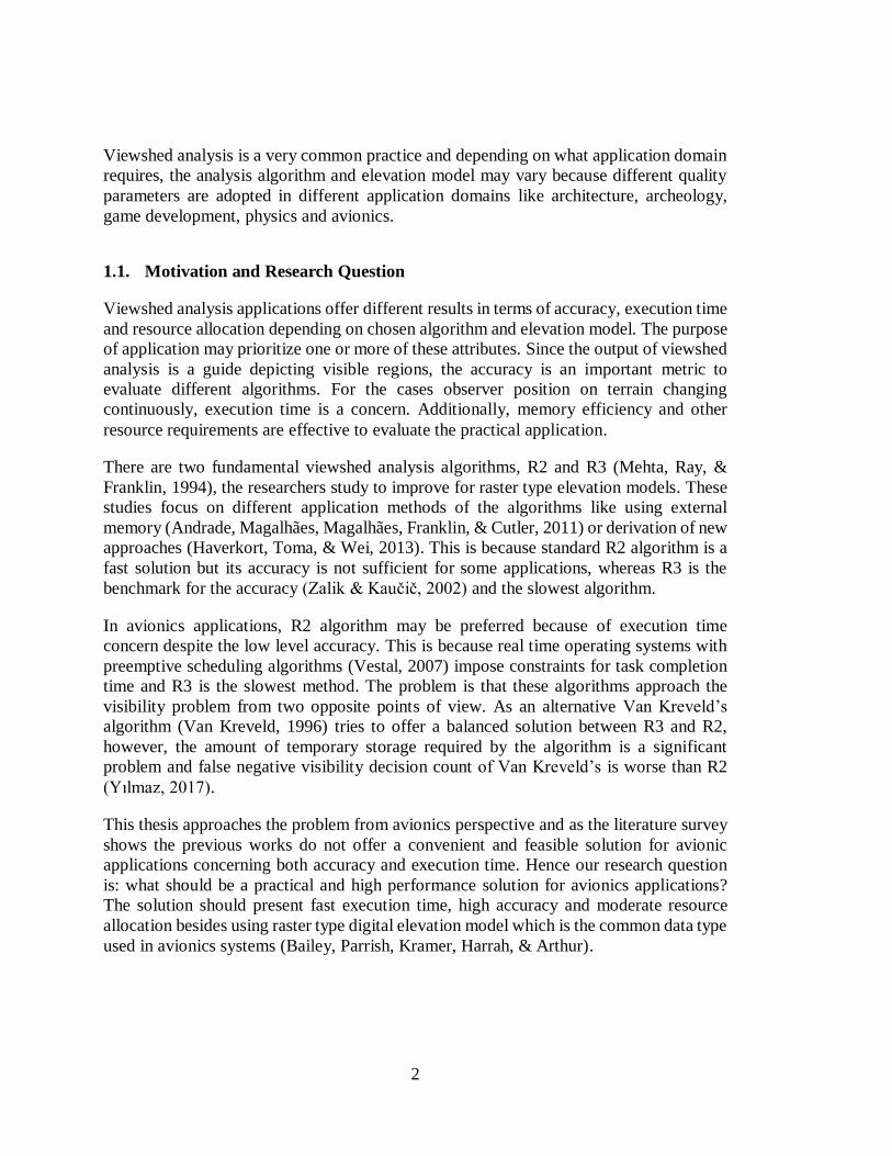
Viewshed analysis is a very common practice and depending on what application domain
requires, the analysis algorithm and elevation model may vary because different quality
parameters are adopted in different application domains like architecture, archeology,
game development, physics and avionics.
1.1. Motivation and Research Question
Viewshed analysis applications offer different results in terms of accuracy, execution time
and resource allocation depending on chosen algorithm and elevation model. The purpose
of application may prioritize one or more of these attributes. Since the output of viewshed
analysis is a guide depicting visible regions, the accuracy is an important metric to
evaluate different algorithms. For the cases observer position on terrain changing
continuously, execution time is a concern. Additionally, memory efficiency and other
resource requirements are effective to evaluate the practical application.
There are two fundamental viewshed analysis algorithms, R2 and R3 (Mehta, Ray, &
Franklin, 1994), the researchers study to improve for raster type elevation models. These
studies focus on different application methods of the algorithms like using external
memory (Andrade, Magalhães, Magalhães, Franklin, & Cutler, 2011) or derivation of new
approaches (Haverkort, Toma, & Wei, 2013). This is because standard R2 algorithm is a
fast solution but its accuracy is not sufficient for some applications, whereas R3 is the
benchmark for the accuracy (Zalik & Kaučič, 2002) and the slowest algorithm.
In avionics applications, R2 algorithm may be preferred because of execution time
concern despite the low level accuracy. This is because real time operating systems with
preemptive scheduling algorithms (Vestal, 2007) impose constraints for task completion
time and R3 is the slowest method. The problem is that these algorithms approach the
visibility problem from two opposite points of view. As an alternative Van Kreveld’s
algorithm (Van Kreveld, 1996) tries to offer a balanced solution between R3 and R2,
however, the amount of temporary storage required by the algorithm is a significant
problem and false negative visibility decision count of Van Kreveld’s is worse than R2
(Yılmaz, 2017).
This thesis approaches the problem from avionics perspective and as the literature survey
shows the previous works do not offer a convenient and feasible solution for avionic
applications concerning both accuracy and execution time. Hence our research question
is: what should be a practical and high performance solution for avionics applications?
The solution should present fast execution time, high accuracy and moderate resource
allocation besides using raster type digital elevation model which is the common data type
used in avionics systems (Bailey, Parrish, Kramer, Harrah, & Arthur).
3
1.2. Objective and Contribution
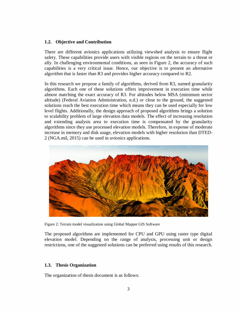
There are different avionics applications utilizing viewshed analysis to ensure flight
safety. These capabilities provide users with visible regions on the terrain to a threat or
ally. In challenging environmental conditions, as seen in Figure 2, the accuracy of such
capabilities is a very critical issue. Hence, our objective is to present an alternative
algorithm that is faster than R3 and provides higher accuracy compared to R2.
In this research we propose a family of algorithms, derived from R3, named granularity
algorithms. Each one of these solutions offers improvement in execution time while
almost matching the exact accuracy of R3. For altitudes below MSA (minimum sector
altitude) (Federal Aviation Administration, n.d.) or close to the ground, the suggested
solutions reach the best execution time which means they can be used especially for low
level flights. Additionally, the design approach of proposed algorithms brings a solution
to scalability problem of large elevation data models. The effect of increasing resolution
and extending analysis area to execution time is compensated by the granularity
algorithms since they use processed elevation models. Therefore, in expense of moderate
increase in memory and disk usage, elevation models with higher resolution than DTED-
2 (NGA.mil, 2015) can be used in avionics applications.
Figure 2: Terrain model visualization using Global Mapper GIS Software
The proposed algorithms are implemented for CPU and GPU using raster type digital
elevation model. Depending on the range of analysis, processing unit or design
restrictions, one of the suggested solutions can be preferred using results of this research.
1.3. Thesis Organization
The organization of thesis document is as follows:

4
Chapter 1 introduces viewshed analysis and presents the motivation and objective of the
thesis,
Chapter 2 provides background information about viewshed analysis and related work,
Chapter 3 introduces the proposed algorithms, alternative implementations and their
rationale,
Chapter 4 presents experiments conducted to validate the proposed algorithms and
discusses the results,
Chapter 5 presents concluding remarks and suggests directions for future work,
Appendix A includes the pseudo code for the proposed algorithms,
Appendix B presents experiment tile statistics, execution time and accuracy charts for the
evaluation of proposed algorithms.
5
CHAPTER 2
BACKGROUND INFORMATION AND PREVIOUS WORK
In this chapter components of viewshed analysis are defined and an overview of
algorithms that researchers study is presented.
2.1 Elevation Model
There are two very common data types for digital elevation models which are TIN and
raster type DEM (Trautwein, et al., 2016).
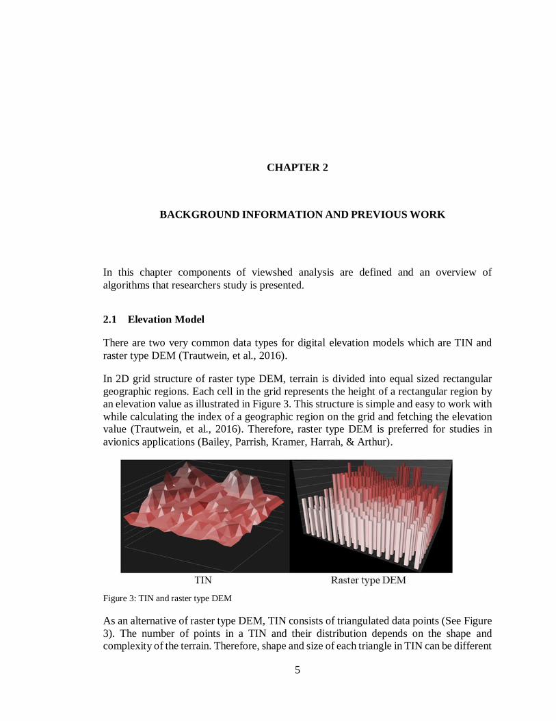
In 2D grid structure of raster type DEM, terrain is divided into equal sized rectangular
geographic regions. Each cell in the grid represents the height of a rectangular region by
an elevation value as illustrated in Figure 3. This structure is simple and easy to work with
while calculating the index of a geographic region on the grid and fetching the elevation
value (Trautwein, et al., 2016). Therefore, raster type DEM is preferred for studies in
avionics applications (Bailey, Parrish, Kramer, Harrah, & Arthur).
Figure 3: TIN and raster type DEM
As an alternative of raster type DEM, TIN consists of triangulated data points (See Figure
3). The number of points in a TIN and their distribution depends on the shape and
complexity of the terrain. Therefore, shape and size of each triangle in TIN can be different
6
and this structure provides size reduction capability. However, use of TIN requires more
effort to process for analyses (Trautwein, et al., 2016).
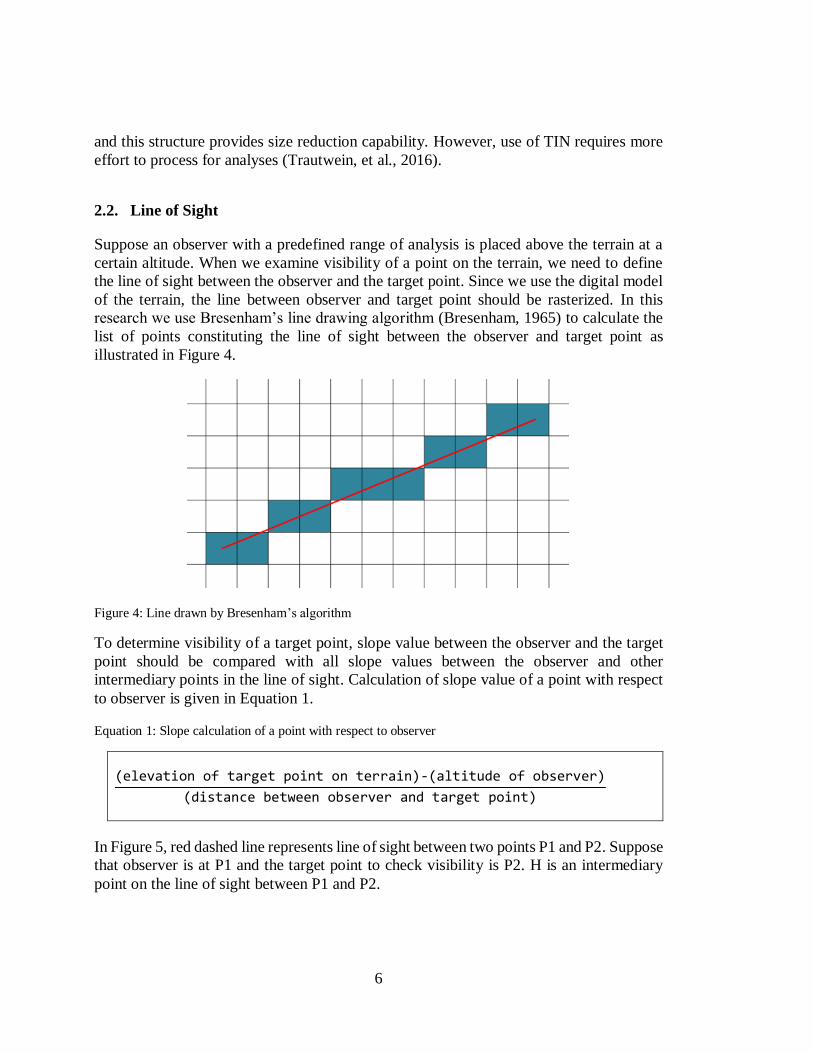
2.2. Line of Sight
Suppose an observer with a predefined range of analysis is placed above the terrain at a
certain altitude. When we examine visibility of a point on the terrain, we need to define
the line of sight between the observer and the target point. Since we use the digital model
of the terrain, the line between observer and target point should be rasterized. In this
research we use Bresenham’s line drawing algorithm (Bresenham, 1965) to calculate the
list of points constituting the line of sight between the observer and target point as
illustrated in Figure 4.
Figure 4: Line drawn by Bresenham’s algorithm
To determine visibility of a target point, slope value between the observer and the target
point should be compared with all slope values between the observer and other
intermediary points in the line of sight. Calculation of slope value of a point with respect
to observer is given in Equation 1.
Equation 1: Slope calculation of a point with respect to observer
(elevation of target point on terrain)-(altitude of observer)
(distance between observer and target point)
In Figure 5, red dashed line represents line of sight between two points P1 and P2. Suppose
that observer is at P1 and the target point to check visibility is P2. H is an intermediary
point on the line of sight between P1 and P2.

7
If the slope value between P2 and P1 is smaller than the slope value between H and P1,
P2 is marked as invisible. Otherwise, we can say that target point in P2 is visible.
Figure 5: Visibility on a line of sight
The visibility calculation for this example is given in Equation 2.
Equation 2: Visibility calculation on a line of sight
HHeight :Elevation of intermediary point H
P1Height:Observer altitude
P2Height:Target point altitude
D1:Distance between observer and intermediary point H D2:Distance between intermediary point H and P2
If HHeight- P1Height
D1≤P2Height- P1Height
D1 + D2 , P2 point is visible
If HHeight- P1Height
D1>P2Height- P1Height
D1 + D2 , P2 point is not visible
2.3. Viewshed Analysis Algorithms
Viewshed analysis investigates the visibility of all points on the terrain within the range
of vision. In line of sight based ray-casting viewshed analysis algorithms, visibility of each
target point in area is determined by examining the points in the drawn line of sight
(Mehta, Ray, & Franklin, 1994). These algorithms are also considered as ray-casting
methods (Carver & Washtell, 2012). If the line of sight from observer to the target point
is obstructed by another point on the terrain, the target point is marked as invisible. In
Figure 6 green points on the terrain refer to visible points. The red points on the terrain
refer to invisible points since their visibility is obstructed by terrain.
Blelloch, Van Kreveld, R2 and R3 presented by Franklin, Ray and Mehta are well known
examples of such ray casting algorithms (Mehta, Ray, & Franklin, 1994) computing
visibility by sending a ray from observer to the target point. Using the same approach
8
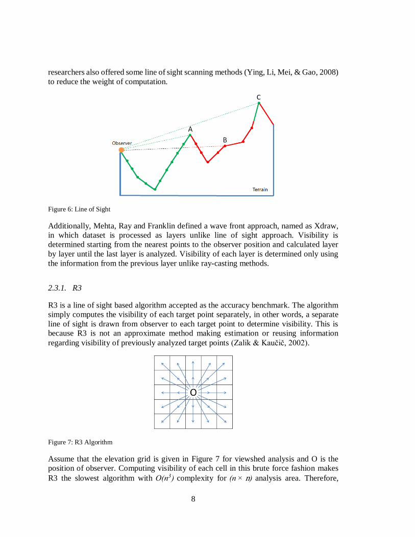
researchers also offered some line of sight scanning methods (Ying, Li, Mei, & Gao, 2008)
to reduce the weight of computation.
Figure 6: Line of Sight
Additionally, Mehta, Ray and Franklin defined a wave front approach, named as Xdraw,
in which dataset is processed as layers unlike line of sight approach. Visibility is
determined starting from the nearest points to the observer position and calculated layer
by layer until the last layer is analyzed. Visibility of each layer is determined only using
the information from the previous layer unlike ray-casting methods.
2.3.1. R3
R3 is a line of sight based algorithm accepted as the accuracy benchmark. The algorithm
simply computes the visibility of each target point separately, in other words, a separate
line of sight is drawn from observer to each target point to determine visibility. This is
because R3 is not an approximate method making estimation or reusing information
regarding visibility of previously analyzed target points (Zalik & Kaučič, 2002).
Figure 7: R3 Algorithm
Assume that the elevation grid is given in Figure 7 for viewshed analysis and O is the
position of observer. Computing visibility of each cell in this brute force fashion makes
R3 the slowest algorithm with O(n3) complexity for (n × n) analysis area. Therefore,
9
researchers try to speed up the algorithm using new technologies like GPGPU (Axell &
Fridén, 2015) or works to avoid unnecessary computations (Shrestha & Panday, 2018)
with different methods for a better execution time.
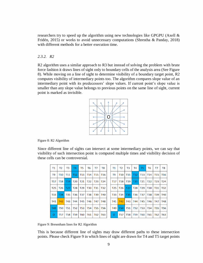
2.3.2. R2
R2 algorithm uses a similar approach to R3 but instead of solving the problem with brute
force fashion it draws lines of sight only to boundary cells of the analysis area (See Figure
8). While moving on a line of sight to determine visibility of a boundary target point, R2
computes visibility of intermediary points too. The algorithm compares slope value of an
intermediary point with its predecessors’ slope values. If current point’s slope value is
smaller than any slope value belongs to previous points on the same line of sight, current
point is marked as invisible.
Figure 8: R2 Algorithm
Since different line of sights can intersect at some intermediary points, we can say that
visibility of such intersection point is computed multiple times and visibility decision of
these cells can be controversial.
Figure 9: Bresenham lines for R2 Algorithm
This is because different line of sights may draw different paths to these intersection
points. Please check Figure 9 in which lines of sight are drawn for T4 and T5 target points

10
starting from observer position represented with O. These two lines of sight have a
common intersection point T42 and paths to T42 are different. The line of sight from O to
T4 uses slope value of T49, whereas, the line of sight from O to T5 uses slope of T50 to
determine visibility of T42. For this reason, visibility of T42 will be determined by the
last visiting line of sight and the order of visibility calculation affects the accuracy of R2.
However, the algorithm offers better execution time with complexity O(n2) compared to
R3.
2.3.3. Blelloch
To compute viewsheds for an area, each line of sight can be processed in parallel by R2
or R3 algorithms. Additionally, Blelloch parallelizes the execution of a single line of sight
using maximum prefix scan method (Blelloch, 1997).
Maximum prefix scan finds the maximum element in a given list of numbers starting from
the 0th index to the given ith index. The input for the algorithm is the slope values of cells
in a line of sight. Blelloch does maximum prefix scan in parallel with binary comparison
and it requires n/2 threads for n slope values to be compared. To find the maximum slope
for a line of sight with n elements, this procedure should be repeated 𝑙𝑜𝑔(𝑛) times.
Algorithm 1 explains how Blelloch determines viewsheds using maximum prefix scan on
a line of sight.
Algorithm 1: Application of maximum prefix scan algorithm for visibility
SlopeList: List of target slope values along a line of sight MaxPrefixScanOutput: Output of maximum prefix scan algorithm INPUT: SlopeList SlopeList = {3, 1, 5, 0, 7, 6} n: Last item index in SlopeList which is 5 n ≥ i ≥ 0, MaxPrefixScanOutput[i] is the maximum of SlopeList[0…i] MaxPrefixScanOutput = {3, 3, 5, 5, 7, 7} IF MaxPrefixScanOutput[i] > SlopeList[i] Point in index i is invisible ELSE Point in index i is visible
In Figure 10 you can see input data to be processed by maximum prefix scan algorithm
and in Figure 11 you can see the output of maximum prefix scan algorithm.

11
Figure 10: Input slope data for maximum prefix scan algorithm
Figure 11: Output of maximum prefix scan algorithm
Blelloch’s approach improves R2 by focusing on the bottleneck of the algorithm which is
the execution time spent for a line of sight. Complexity of the algorithm is
O(n/number of processors + 𝑙𝑜𝑔 𝑛 ) for (n × n) analysis area. However, Blelloch’s
method is not useful considering scalability due to required number of threads.
2.3.4. Van Kreveld’s Algorithm
Van Kreveld’s algorithm has a different approach to solve visibility problem (Van
Kreveld, 1996). Van Kreveld’s method draws a reference line from observer point to the
border of the analysis area and algorithm sweeps all cells, holding elevation value, in the
terrain grid. There are three types of events or states for each cell in the elevation grid
which are enter, center and exit (See Figure 12).
• If sweeping reference line enters the cell, it is marked as enter event for the cell.
0
1
2
3
4
5
6
7
8
1 2 3 4 5 6sl
op
e i
np
ut
index
012345678
1 2 3 4 5 6
ma
xim
um
slo
pe p
refi
x s
ca
n
ou
tpu
t
index
12
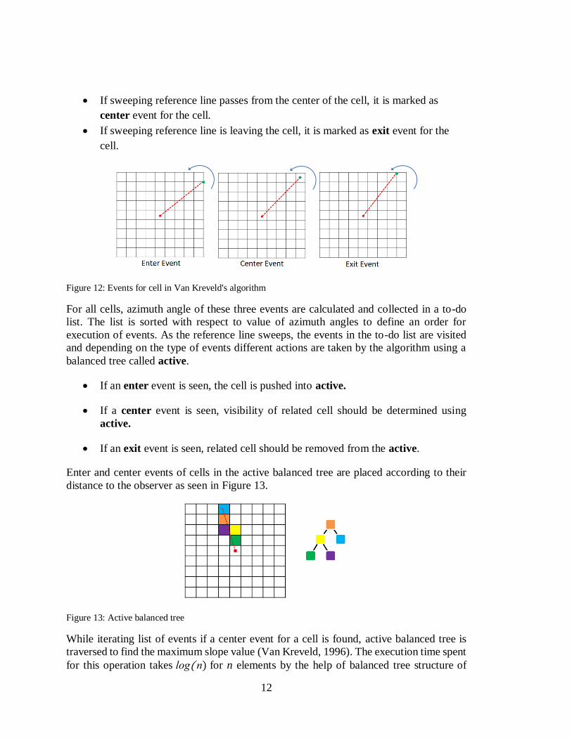
• If sweeping reference line passes from the center of the cell, it is marked as
center event for the cell.
• If sweeping reference line is leaving the cell, it is marked as exit event for the
cell.
Figure 12: Events for cell in Van Kreveld's algorithm
For all cells, azimuth angle of these three events are calculated and collected in a to-do
list. The list is sorted with respect to value of azimuth angles to define an order for
execution of events. As the reference line sweeps, the events in the to-do list are visited
and depending on the type of events different actions are taken by the algorithm using a
balanced tree called active.
• If an enter event is seen, the cell is pushed into active.
• If a center event is seen, visibility of related cell should be determined using
active.
• If an exit event is seen, related cell should be removed from the active.
Enter and center events of cells in the active balanced tree are placed according to their
distance to the observer as seen in Figure 13.
Figure 13: Active balanced tree
While iterating list of events if a center event for a cell is found, active balanced tree is
traversed to find the maximum slope value (Van Kreveld, 1996). The execution time spent
for this operation takes log( n) for n elements by the help of balanced tree structure of

13
active list. If the maximum slope value is greater than the slope value of the cell with
center event, the cell is marked as invisible. In other words; to mark a cell as visible, the
slope value of the cell in center state should be larger than all slope values of cells with
enter and center state in active tree.
Van Kreveld’s algorithm is considered as a nice option between R3 and R2 due to high
accuracy and better execution time with O(n2 log n ) complexity. There are also improved
alternatives of the method offering better execution time like HLD (Nguyen, Duy, &
Duong, 2018) and parallel sweep line algorithm implemented for GPU (Ferreira, Andrade,
Franklin, Magalhães, & Pena, 2013), however, the improvement is only in execution time.
Moreover, studies show that the algorithm tends to mark visible points as invisible
(Yılmaz, 2017). As an example; use of this algorithm to calculate the coverage of a threat
may be misleading for the user who wants to avoid visible regions to the threat. Besides,
implementation of the algorithm requires extra memory for three types of events with float
type azimuth angle for a single elevation cell in the terrain grid.
2.3.5. Xdraw
Xdraw (Mehta, Ray, & Franklin, 1994) is a wave front algorithm processing the terrain
data layer by layer and compute visibility from the inside out as seen in Figure 14. There
are many variations developed from Xdraw since it is an approximate approach offering
different estimation methods (Larsen, 2015). Mainly algorithm defines a set of
predecessor points and using their elevation values computes a horizon to address the
visibility of target point. Each target point’s visibility depends on relative points in the
previous layer. While computing visibility of the target point; minimum, maximum, mean
elevation values of relative points can be used or elevation interpolation methods can be
applied.
Figure 14: Xdraw algorithm
Xdraw is a faster alternative to R2 but its accuracy is worse. By the help of different
estimation methods, algorithm accuracy can be increased (Larsen, 2015) but it is still not
enough to use Xdraw for avionic applications with accuracy concern.

14
2.3.6 Comparison of Viewshed Analysis Algorithms
The comparison of algorithms summarized in previous sections is given in Table 1.
Execution time and accuracy comparison of algorithms are provided for both CPU and
GPU implementation. Blelloch parallel prefix scan algorithm has no CPU version.
Table 1: Comparison of common algorithms
Viewshed analysis
algorithms in CPU
Execution Time Accuracy Extra Required Memory
R2 better than Van
Kreveld’s
worse than R3
better than Xdraw -
R3 slowest algorithm best accuracy -
Van Kreveld’s
Algorithm
better than R3,
slower than R2
better than R2
worse than R3
3 FLOAT type lists for
events and a binary search
tree
Xdraw better than R2 in
some cases worse than R2 -
Viewshed analysis
algorithms in GPU
Execution Time Accuracy Extra Required Memory
R2 better than Van
Kreveld’s
worse than R3
better than Xdraw
-
R3 slowest algorithm best accuracy -
Blelloch Parallel
Prefix Scan
better than R2 same with R2 copy of line of sight data
for each target point
Van Kreveld’s
Algorithm
better than R3 better than R2
worse than R3
3 FLOAT type lists for
events and a binary search
tree
Xdraw better than R2 worse than R2 -
15
CHAPTER 3
3. PROPOSED SOLUTION DESIGN AND IMPLEMENTATIONS
In this chapter, proposed viewshed analysis algorithms and corresponding CPU/GPU
implementations are introduced. Additionally, implementation details of R2 and R3
algorithms are given in Section 3.3 for comparison.
3.1. Proposed Solution and Design Rationale
The proposed approach of this study is based on standard R3. To reach the maximum
accuracy level, we define granularity family algorithms which are derived from R3 by
making improvements to reduce the execution time. All algorithms in this family use ray
casting approach and Bresenham’s line drawing method (Bresenham, 1965). Names of
these granularity algorithms are X2, X4, X8, X16, DGRHYB and DGR3.
The complexity of proposed algorithms is O(n3). For the execution time improvement,
preprocessed elevation models are used by granularity algorithms besides the original
digital elevation model. In other words, the total amount of data used by the analysis is
increased but total amount of computation in runtime is decreased by the help of processed
elevation models while preserving the accuracy.
The implementation of granularity algorithms is done for both CPU and GPU to see
whether parallelism is a utility to be exploited by the proposed solutions. Recently GPUs
are used in avionics for such purposes due to their computing capability and limited
execution times assigned for such tasks. Besides, DGRHYB algorithm presents a different
approach by running different parts of analysis in CPU and GPU. This method might be
helpful to divide problem instead of pushing the workload to a single processing unit for
cases in which there are also other tasks.
The proposed analysis model consists of 3 phases as summarized in Figure 15. Since
preparation of processed elevation models is not done in analysis runtime, it is named as
phase-0. As these elevation models are prepared, execution of granularity algorithms starts

16
with phase-1 and then continues with phase-2. If observer altitude or position changes
phase-1 and phase-2 are executed again to update the analysis result.
Figure 15: Proposed approach
3.1.1. Phase-0: Prepare Processed Elevation Models
Since the size of digital elevation model is the most effective factor in execution time,
suggested approach focus on redesigning the elevation model to gain speedup. In this
phase, true digital elevation model with real size is processed to create smaller size models
without losing fundamental information. To retrieve the smaller version of digital
elevation model, spatially adjacent elevation values are grouped and represented as a tile
by saving the information of minimum and maximum values within the group.
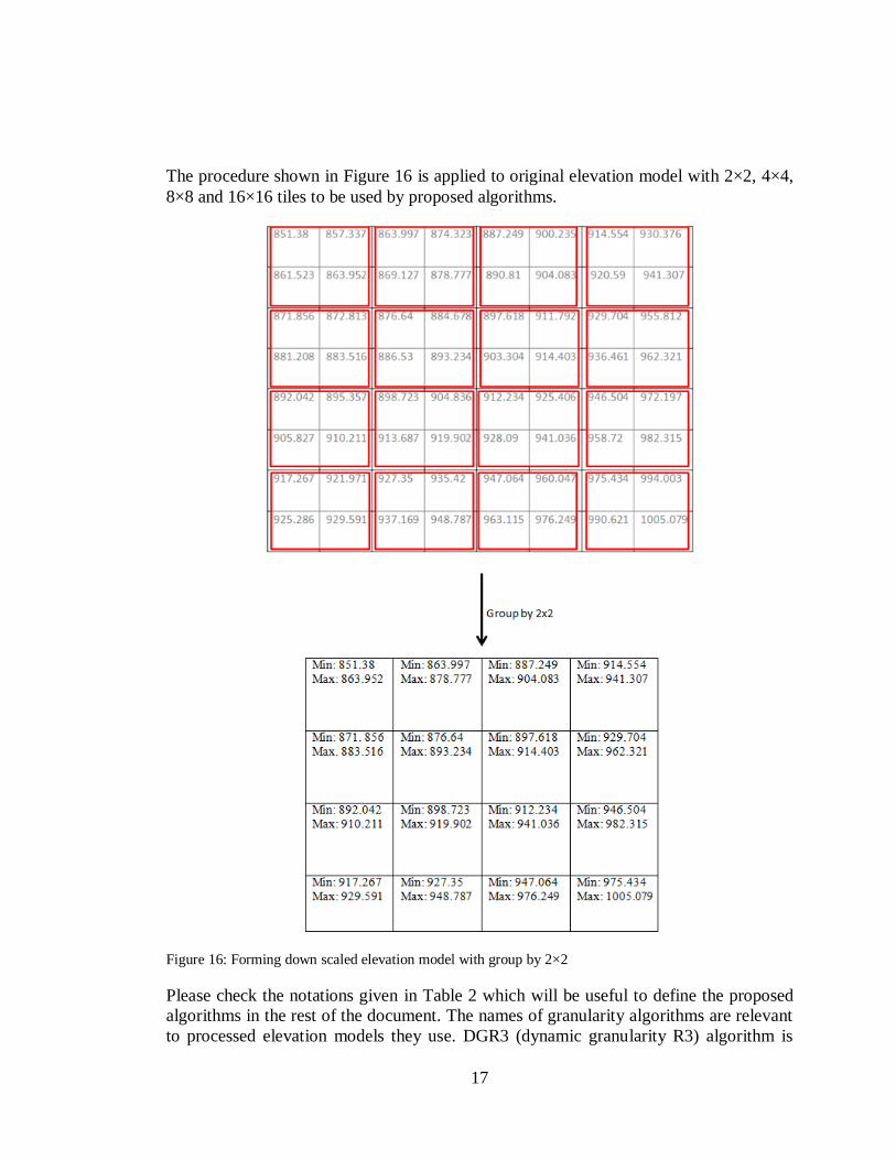
The illustration of how true elevation model is processed to create smaller size model is
given in Figure 16. Each red square in figure represents a group on elevation model. When
elevation values are grouped by 2×2 tiles, we retrieve an elevation model whose size is ¼
of the original. Each element in processed elevation model only holds the minimum and
maximum within the group of four spatially nearby elevation values.
17
The procedure shown in Figure 16 is applied to original elevation model with 2×2, 4×4,
8×8 and 16×16 tiles to be used by proposed algorithms.
Figure 16: Forming down scaled elevation model with group by 2×2
Please check the notations given in Table 2 which will be useful to define the proposed
algorithms in the rest of the document. The names of granularity algorithms are relevant
to processed elevation models they use. DGR3 (dynamic granularity R3) algorithm is

18
named considering that it uses multiple processed elevation models with different
granularities.
Table 2: Notations for algorithm descriptions
Notation Content
n Dimension of n×n analysis area
E_Model Original Elevation model
E2_Model Granularity elevation model consisting of elements with minimum and
maximum elevation values for each 2×2 tile in E_Model
E4_Model Granularity elevation model consisting of elements with minimum and
maximum elevation values for each 4×4 tile in E_Model
E8_Model Granularity elevation model consisting of elements with minimum and
maximum elevation values for each 8×8 tile in E_Model
E16_Model Granularity elevation model consisting of elements with minimum and
maximum elevation values for each 16×16 tile in E_Model
G Granularity dimension for grouping G×G points
EG_Model Refers to E2_Model, E4_Model, E8_Model, E16_Model depending on value
of G.
S_Model Slope values of target points with respect to observer.
S2_Model Minimum and maximum slope values of target points with 2×2 granularity
S4_Model Minimum and maximum slope values of target points with 4×4 granularity
S8_Model Minimum and maximum slope values of target points with 8×8 granularity
S16_Model Minimum and maximum slope values of target points with 16×16 granularity
SG_Model Refers to S2_Model, S4_Model, S8_Model, S16_Model depending on value of G.
V_Table Visibility table representing viewshed analysis result with same size of E
In Table 3, the size of each elevation model is given and algorithms using them marked
with a cross.
Table 3: Processed elevation models used by algorithms
X2 X4 X8 X16 DGR3 Elevation Model Size
E_Model X X X X X 512×512 1024×1024 2048×2048
E2_Model X 256×256 512×512 1024×1024
E4_Model X X 128×128 256×256 512×512
E8_Model X X 64×64 128×128 256×256
E16_Model X X 32×32 64×64 128×128
The dimensions of processed elevation models are calculated according to three
predefined sizes of original elevation model which are 512×512, 1024×1024 and
19
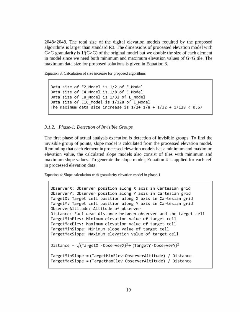
2048×2048. The total size of the digital elevation models required by the proposed
algorithms is larger than standard R3. The dimensions of processed elevation model with
G×G granularity is 1/(G×G) of the original model but we double the size of each element
in model since we need both minimum and maximum elevation values of G×G tile. The
maximum data size for proposed solutions is given in Equation 3.
Equation 3: Calculation of size increase for proposed algorithms
Data size of E2_Model is 1/2 of E_Model Data size of E4_Model is 1/8 of E_Model Data size of E8_Model is 1/32 of E_Model Data size of E16_Model is 1/128 of E_Model The maximum data size increase is 1/2+ 1/8 + 1/32 + 1/128 < 0.67
3.1.2. Phase-1: Detection of Invisible Groups
The first phase of actual analysis execution is detection of invisible groups. To find the
invisible group of points, slope model is calculated from the processed elevation model.
Reminding that each element in processed elevation models has a minimum and maximum
elevation value, the calculated slope models also consist of tiles with minimum and
maximum slope values. To generate the slope model, Equation 4 is applied for each cell
in processed elevation data.
Equation 4: Slope calculation with granularity elevation model in phase-1
ObserverX: Observer position along X axis in Cartesian grid ObserverY: Observer position along Y axis in Cartesian grid TargetX: Target cell position along X axis in Cartesian grid TargetY: Target cell position along Y axis in Cartesian grid ObserverAltitude: Altitude of observer Distance: Euclidean distance between observer and the target cell TargetMinElev: Minimum elevation value of target cell TargetMaxElev: Maximum elevation value of target cell TargetMinSlope: Minimum slope value of target cell TargetMaxSlope: Maximum elevation value of target cell
Distance = √(TargetX - ObserverX)2+ (TargetY - ObserverY)2 TargetMinSlope = (TargetMinElev-ObserverAltitude) / Distance TargetMaxSlope = (TargetMaxElev-ObserverAltitude) / Distance

20
The result of slope calculation on elevation model is one of the slope models given in
Table 4.
Table 4: Dimensions of slope models retrieved from processed elevation models
Slope Model Size
S2_Model 256×256 512×512 1024×024
S4_Model 128×128 256×256 512×512
S8_Model 64×64 128×128 256×256
S16_Model 32x32 64×64 128×128
As slope model is available we draw separate line of sight for each cell in granularity slope
model as we do in R3 algorithm. We cannot determine visible points using any granularity
slope models, however, the information of minimum and maximum slope values helps us
to find invisible group of points.
Figure 17: Visibility on slope model with 16×16 granularity
In Figure 17 we see an example of S16_Model (See Table 2) and there is a line of sight
drawn from Source_Cell to Target_Cell marked with orange color. Other intermediary

21
points are marked with blue color. Since the maximum slope of Target_Cell is smaller
than the minimum slope value of an intermediary point, Target_Cell will be marked as
invisible. Since granularity of slope model is 16×16, we can mark 16×16=256 points as
invisible in V_Table (See Table 2).
3.1.3. Phase-2: Determine Visibility for Remaining Points
Suppose that X4 algorithm is run and phase-1 is just completed. In Figure 18, we see that
observer is represented with O and red cells are marked as invisible by using S4_Model
(See Table 2). This example illustrates the recent state of viewshed analysis result just
before phase-2 starts.
Figure 18: V_Table after phase-1
The visibilities of unmarked cells will be resolved in phase-2, therefore, slope values of
all target points are calculated by applying Equation 5 using the original elevation model.

22
Equation 5: Slope calculation with original elevation model in phase-2
ObserverX: Observer position along X axis in Cartesian grid ObserverY: Observer position along Y axis in Cartesian grid TargetX: Target cell position along X axis in Cartesian grid TargetY: Target cell position along Y axis in Cartesian grid ObserverAltitude: Altitude of observer Distance: Euclidean distance between observer and the target cell TargetElev: Elevation value of target cell TargetSlope: Slope value of target cell
Distance = √(TargetX - ObserverX)2+ (TargetY - ObserverY)
2
TargetSlope = (TargetElev-ObserverAltitude) / Distance
After S_Model (See Table 2) is prepared, visibility computation for unmarked points
starts. Phase 2 works like standard R3 but it aims to reduce the amount of computation by
reusing visibility information of the previously analyzed points. Therefore, visibility
calculation of remaining points is done from the inside out. To decide visibility of each
target point, a separate line of sight is drawn and algorithm checks whether it is possible
to avoid slope comparison operations along that line of sight.
Since we draw the line of sight using Bresenham’s algorithm, we can find the position of
previous point of target cell. If the slope value of previous point on the line of sight is
larger than the target point’s slope value, we can mark the target cell as invisible.
Algorithm 2 explains how predecessor position is calculated and visibility of target point
is decided.
Algorithm 2: Detection of invisible point by checking the slope of predecessor
ObserverX: Observer position along X axis in Cartesian grid ObserverY: Observer position along Y axis in Cartesian grid TargetX: Target cell position along X axis in Cartesian grid TargetY: Target cell position along Y axis in Cartesian grid DeltaX: Absolute value of distance between observer and target along X axis DeltaY: Absolute value of distance between observer and target along Y axis PrevPointX: Position of target point’s predecessor along X axis PrevPointY: Position of target point’s predecessor along Y axis SlopeModel: 2D data holding target point slope values calculated using original elevation model. INPUT: ObserverX, ObserverY, TargetX, TargetY, SlopeModel DeltaX = |TargetX – ObserverX| DeltaY = |TargetY – ObserverY|

23
Algorithm 2 (continued)
IF (TargetX – ObserverX) > 0 THEN IteratorX = 1 IF (TargetX – ObserverX) < 0 THEN IteratorX = -1 IF (TargetY – ObserverY) > 0 THEN IteratorX = 1 IF (TargetY – ObserverY) < 0 THEN IteratorX = -1 IF (DeltaX – DeltaY) > DeltaY PrevPointX = TargetX - IteratorX
PrevPointY = TargetY ELSE IF (DeltaY – DeltaX) > DeltaX PrevPointX = TargetX
PrevPointY = TargetY - IteratorY ELSE PrevPointX = TargetX - IteratorX
PrevPointY = TargetY - IteratorY IF SlopeModel[PrevPointX][PrevPointY] > SlopeModel[TargetX][TargetY] Mark target point as invisible
If the slope of predecessor is not greater than slope of the target cell, we can determine
visibility by analyzing two relative points of the target.
Figure 19: Reuse of visibility information in phase 2
In Figure 19, three different lines of sight and list of points in them presented for three
target cells T1, T2 and T3. Comparing point list of T3 with other point lists shows that we
cannot use visibility information of T2 or T1 due to different intermediary points written
24
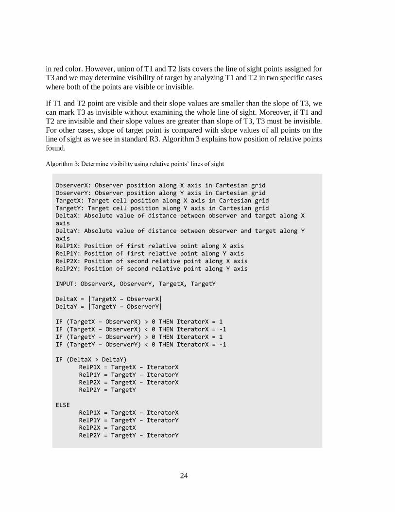
in red color. However, union of T1 and T2 lists covers the line of sight points assigned for
T3 and we may determine visibility of target by analyzing T1 and T2 in two specific cases
where both of the points are visible or invisible.
If T1 and T2 point are visible and their slope values are smaller than the slope of T3, we
can mark T3 as invisible without examining the whole line of sight. Moreover, if T1 and
T2 are invisible and their slope values are greater than slope of T3, T3 must be invisible.
For other cases, slope of target point is compared with slope values of all points on the
line of sight as we see in standard R3. Algorithm 3 explains how position of relative points
found.
Algorithm 3: Determine visibility using relative points’ lines of sight
ObserverX: Observer position along X axis in Cartesian grid ObserverY: Observer position along Y axis in Cartesian grid TargetX: Target cell position along X axis in Cartesian grid TargetY: Target cell position along Y axis in Cartesian grid DeltaX: Absolute value of distance between observer and target along X axis DeltaY: Absolute value of distance between observer and target along Y axis RelP1X: Position of first relative point along X axis RelP1Y: Position of first relative point along Y axis RelP2X: Position of second relative point along X axis RelP2Y: Position of second relative point along Y axis INPUT: ObserverX, ObserverY, TargetX, TargetY DeltaX = |TargetX – ObserverX| DeltaY = |TargetY – ObserverY| IF (TargetX – ObserverX) > 0 THEN IteratorX = 1 IF (TargetX – ObserverX) < 0 THEN IteratorX = -1 IF (TargetY – ObserverY) > 0 THEN IteratorX = 1 IF (TargetY – ObserverY) < 0 THEN IteratorX = -1 IF (DeltaX > DeltaY) RelP1X = TargetX – IteratorX
RelP1Y = TargetY – IteratorY RelP2X = TargetX – IteratorX RelP2Y = TargetY
ELSE RelP1X = TargetX – IteratorX
RelP1Y = TargetY – IteratorY RelP2X = TargetX RelP2Y = TargetY – IteratorY

25
3.2. Proposed Granularity Algorithm Implementations
In this section we define the implementation details of proposed granularity algorithms
and elevation model processing. Besides CPU and GPU implementation of each
algorithm, hybrid approach of DGRHYB is also explained.
The implementation steps are executed in the given order. To understand the notations
used for data models please check Table 2.
3.2.1. Elevation Model Processing
Since the suggested solutions use processed elevation models, we should start with
elevation model processing. These implementation steps are run before the analysis
runtime and depending on value of G; E2_Model, E4_Model, E8_Model or E16_Model
is created from E_Model.
1) Create empty EG_Model with (n/G)×(n/G) dimensions, consisting of elements with
minimum and maximum elevation attributes
2) For each G×G group in E_Model find minimum and maximum elevation values
3) Place minimum and maximum elevation values of each G×G group to respective
location in EG_Model
3.2.2. Granularity Algorithms in CPU
At the end of elevation model processing EG_Model is obtained for the granularity
algorithms. The following implementation steps are executed in analysis runtime and
they are same for X2, X4, X8, X16 and DGR3 algorithms. Firstly phase-1 steps are run
to detect invisible group of points using EG_Model.
1. Calculate SG_Model from EG_Model with respect to observer altitude and position
using Euclidean distance
2. Draw separate line of sight for each target point with G×G granularity whose
visibility is not determined yet
3. Iterate on each drawn line of sight to target groups in SG_Model
a. If minimum slope value of target point is larger than maximum slope
values of points along the line of sight, mark G×G points in target as
invisible using V_Table.
4. Prepare list of remaining points according to V_Table
At the end of phase-1 some invisible regions may be found or not. Visibility of remaining
points is resolved by phase-2 with following steps.

26
5. Calculate S_Model from E_Model with respect to observer altitude and position
using Euclidean distance
6. Draw separate line of sight to each target point remaining from phase-1
7. Iterate on each drawn line of sight to target points in S_Model
a. If slope value of target point is smaller than the slope value of
predecessor, mark target point as invisible using V_Table
b. Else if slope value of target point is smaller than the slope values of two
invisible relative points, mark target point as invisible using V_Table
c. Else if slope value of target point is larger than the slope values of two
visible relative points, mark target point as visible using V_Table
d. Else if slope value of target point is larger than slope values of all points
along the line of sight, mark target point as visible using V_Table
e. Else if slope value of the target point is smaller than slope value of any
point along the line of sight, mark target point as invisible using V_Table
DGR3 algorithm uses three types of elevation models besides the original elevation
model. Therefore, elevation model processing is applied for 16×16, 8×8 and 4×4
granularities. In analysis runtime algorithm starts phase-1 with E16_Model and repeats
the same implementation steps using E8_Model and E4_Model in order. For the
remaining points phase-2 is run once like other granularity algorithms starting from step
5.
3.2.3. Granularity Algorithms in GPU
GPU implementations of proposed algorithms are done using CUDA API developed by
NVIDIA. (NVIDIA Corporation, n.d.). In CUDA, we define kernels which are functions
executed by assigned threads in parallel with single instruction multiple data approach.
To run a kernel we firstly decide launch parameters which are the grid and block structure
for the threads (NVIDIA Corporation, n.d.).
In each phase of granularity algorithms, two kernels are defined to compute slope values
and determine visibility of points. Although same kernels are run in proposed algorithms,
calculation of launch parameters is different for DGR3 in phase-1. For the other proposed
algorithms (X2, X4, X8, X16) the equation to define grid and block structure does not
change (See Equation 6).

27
Equation 6: Launch parameters of both kernels in phase-1 for proposed algorithms except DGR3
N: Dimension of analysis area which can be 512, 1024 or 2048 G: Granularity dimension of algorithm NG: Dimension of analysis area with granularity G NG = (N / G) BlockDim = 16 GridDim = NG / BlockDim 2D Block structure = (BlockDim, BlockDim) 2D Grid structure = (GridDim, GridDim)
Since each thread works for only one target point, same launch parameters are used for
slope calculation and invisible group detection tasks in phase-1 of X2, X4, X8 and X16
algorithms. In Equation 6, you can see grid calculation where the block dimension is
assigned as 16 for both kernels of phase-1.
DGR3 repeats phase-1 three times with different granularities. For slope calculation kernel
in phase-1, the algorithm uses same launch parameters given in Equation 6. However, in
detection of invisible groups, grid and block structure depends on the count of remaining
points which are not marked as invisible. For each run of phase-1, launch parameters are
calculated again as explained in Equation 6 and Equation 7.
Equation 7: DGR3 kernel launch parameters calculation in phase-1
G: Granularity dimension of algorithm Rem: Remaining point count whose visibility is not determined in phase-1 RemG: Remaining point count whose visibility is not determined yet with granularity G RemG = Rem / G BlockDim = 16
GridDim = √RemG / (BlockDim × BlockDim) 2D Block structure = (BlockDim, BlockDim) 2D Grid structure = (GridDim, GridDim)
In phase-2 launch parameter equations are same for all proposed algorithms. The grid and
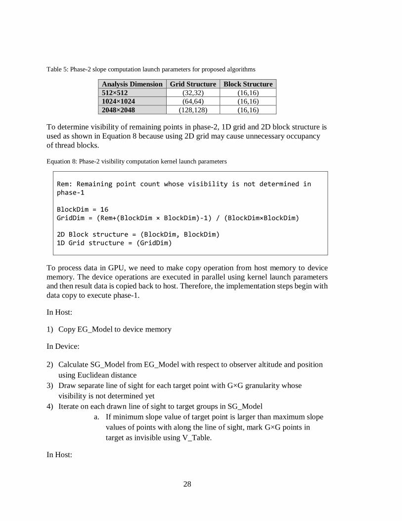
block structure for slope calculation of phase-2 is given in Table 5.
28
Table 5: Phase-2 slope computation launch parameters for proposed algorithms
Analysis Dimension Grid Structure Block Structure
512×512 (32,32) (16,16)
1024×1024 (64,64) (16,16)
2048×2048 (128,128) (16,16)
To determine visibility of remaining points in phase-2, 1D grid and 2D block structure is
used as shown in Equation 8 because using 2D grid may cause unnecessary occupancy
of thread blocks.
Equation 8: Phase-2 visibility computation kernel launch parameters
Rem: Remaining point count whose visibility is not determined in phase-1 BlockDim = 16 GridDim = (Rem+(BlockDim × BlockDim)-1) / (BlockDim×BlockDim)
2D Block structure = (BlockDim, BlockDim) 1D Grid structure = (GridDim)
To process data in GPU, we need to make copy operation from host memory to device
memory. The device operations are executed in parallel using kernel launch parameters
and then result data is copied back to host. Therefore, the implementation steps begin with
data copy to execute phase-1.
In Host:
1) Copy EG_Model to device memory
In Device:
2) Calculate SG_Model from EG_Model with respect to observer altitude and position
using Euclidean distance
3) Draw separate line of sight for each target point with G×G granularity whose
visibility is not determined yet
4) Iterate on each drawn line of sight to target groups in SG_Model
a. If minimum slope value of target point is larger than maximum slope
values of points with along the line of sight, mark G×G points in
target as invisible using V_Table.
In Host:
29
5) Copy V_Table to host memory
6) Prepare list of remaining points according to V_Table
At the end of phase-1 the visibility results are copied to host memory. In phase-2
remaining point list is prepared and copied to device memory to determine visibility of
points.
7) Copy E_Model and list of remaining points to device memory
In Device:
8) Calculate S_Model from E_Model with respect to observer altitude and position
using Euclidean distance
9) Draw separate line of sight to each target point remaining from phase-1
10) Iterate on each drawn line of sight to target point
a. If slope value of target point is smaller than the slope value of
predecessor, mark target point as invisible using V_Table
b. Else if slope value of target point is smaller than the slope values of
two invisible relative points, mark target point as invisible using
V_Table
c. Else if slope value of target point is larger than the slope values of
two visible relative points, mark target point as visible using V_Table
d. Else if slope value of target point is larger than slope values of all
points along the line of sight, mark target point as visible using
V_Table
e. Else if slope value of the target point is smaller than slope value of
any point along the line of sight, mark target point as invisible using
V_Table
In Host:
11) Copy V_Table to host memory
The implementation steps above are executed once by X2, X4, X8 and X16 algorithms.
DGR3 repeats steps 1-6 for E16_Model, E8_Model and E4_Model with given order and
then executes phase-2 starting from step 7.
3.2.4. Hybrid Granularity Algorithm
DGRHYB algorithm executes phase-1 in CPU and then switches to GPU to execute
phase-2. In phase-1, DGRHYB repeats steps 1-4 in CPU three times as DGR3. After

30
phase-1 is completed, the algorithm continues phase-2 in GPU by executing the steps 5-
10. For slope calculation DGRHYB uses launch parameters given in Table 5 and then
visibility computation of remaining points is done with grid and block structure calculated
with Equation 8.
3.3. R3 and R2 Algorithm Implementations
3.3.1. R3 in CPU
The implementation steps for standard R3 is given below:
1) Calculate S_Model from E_Model with respect to observer altitude and position
using Euclidean distance
1) Draw separate line of sight for each target point in S_Model
2) Iterate on each drawn line of sight to target points
a. If slope value of the target point is greater than slope values of all points
along the line of sight, mark target point in V_Table as visible.
b. If slope value of the target point is less than slope value of any point
along the line of sight, mark target point in V_Table as invisible.
3.3.2. R2 in CPU
The implementation steps for standard R2 is given below:
1. Calculate S_Model from E_Model with respect to observer altitude and position
using Euclidean distance
2. Draw separate line of sight only for target points on the edges of S_Model
3. Iterate on each drawn line of sight to determined target points
a. If slope value of the target point is greater than slope values of all points
along the line of sight, mark target point in V_Table as visible.
b. If slope value of the target point is less than slope value of any point
along the line of sight, mark target point in V_Table as invisible.
3.3.3. R3 in GPU
R3 algorithm runs a thread for each target point in parallel using 2D indexing since the
elevation data and viewshed output is 2D. The block size is defined as 16×16 and the grid
dimension varies depending on the size of analysis area.

31
For slope calculation and visibility computation kernels, same launch parameters are used
shown in Table 6.
Table 6: R3 kernel launch parameters
Analysis Dimension R3 Grid Structure R3 Block Structure
512×512 (32,32) (16,16)
1024×1024 (64,64) (16,16)
2048×2048 (128,128) (16,16)
GPU implementation of algorithm follows same steps with CPU implementation. Only
E_Model is copied to device memory in the beginning and visibility result data V_Table
is copied to host memory at the end of the analysis.
3.3.4. R2 in GPU
R2 algorithm computes slope values in the analysis area using the same launch parameters
with R3 as given in Table 6. However, visibility computation kernel uses 1D grid and
blocks.
Table 7: R2 kernel launch parameters
Analysis Area R2 Grid Structure R2 Block Structure
512×512 8 256
1024×1024 16 256
2048×2048 32 256
This is because R2 algorithm draws line of sight only for points on the edges of analysis
area. The block size is arranged as 256 which is equal to 16×16 which is used for 2D block
structure of compared algorithms. Table 7 shows grid and block dimensions for three
different analysis dimensions.GPU implementation of algorithm follows same steps with
CPU implementation. Only E_Model is copied to device memory in the beginning and
visibility result data V_Table is copied to host memory at the end of the analysis.

32
33
CHAPTER 4
4.EVALUATION
In this chapter we will see the comparison of implemented proposed algorithms with R3
and R2 in terms of accuracy, execution time and resource allocation. R2 and R3
implementations used in evaluations are given in Section 3.3. Digital elevation models
used in analysis experiments are retrieved from ASTER (NASA, n.d.). Experiment tiles
are chosen in three sizes which are 512, 1024 and 2048. For each size, 25 different tiles
are used to assess results in different terrain topologies. In Appendix B experiment tile
statistics are provided. Since the elevation models are extracted with Cartesian
coordinates, Euclidian distance is used in slope calculations.
For each experimented tile, the viewshed analyses are carried out for seven different
observer altitudes and the observer is located at the center of the tile in the experiments.
The altitudes are determined according to terrain elevation value at the observer’s position
and standard deviation of elevation levels in the tile. Hence, sensible changes in viewshed
can be examined, as the altitude is increased. The observer altitudes are calculated as
follows:
𝐴0 = 𝐸𝑜 + 2 Meters
and
𝐴𝑐 = 𝐸𝑜 + 𝑐 ∗ 𝑓𝑜𝑟 𝑐 = 1,2,3,4,5
Where, Ac for c=0..5 is the altitude of the observer, Eo is elevation at the observer’s
position, is the standard deviation of all elevations in the tile. Another observer altitude
level to be tested is MSA (minimum sector altitude). In aviation, MSA (Federal Aviation
Administration, n.d.) is used as a common reference to provide minimum clearance of 300
meters above the terrain (Federal Aviation Administration, n.d.).
𝐴𝑚𝑠𝑎 = 𝐸𝑜 + 300 𝑀𝑒𝑡𝑒𝑟𝑠

34
Each algorithm is run on each experiment tile with 7 different altitudes, in other words,
525 experiments are run per algorithm in this research. In each experiment, speedup ratios
for the proposed algorithms with respect to R3 are calculated to make comparisons with
R3 algorithm’s execution time. CPU versions of algorithms are implemented with single
thread. For GPU implementation CUDA parallel programming platform and API is used
(NVIDIA Corporation, n.d.). Elevation data, slope data and distance calculations use
FLOAT data type for maximum accuracy.
Hardware and software specifications of experimental setup are listed below.
OS: Windows 10
IDE: Visual Studio 2010 with C++
CUDA Version: v9.2
Architecture: x64
CPU: Intel(R) Core(TM) i7-4700QM CPU @ 2.40GHz 4 Core
GPU: NVIDIA Kepler Compute Capability 3.0
RAM: 16 GB
4.1. Experiments with CPU Implementation
4.1.1. Execution Time
In this section, execution time performances of the proposed algorithms are compared to
execution times of R3 algorithm. The speedup parameters changing by the altitude are
depicted with figures. Analyses are performed on three different tile sizes and the data
points in the charts correspond to the speedup value obtained.
According to the results presented in Figure 20, Figure 21, Figure 22 and Figure 23,
speedup per altitude graph shows that the fastest algorithms are DGR3, X4 and X8 for all
altitude levels. Execution time of X2 and X16 algorithms proves that very small and very
large granularities reduce the execution time improvement provided by phase-1.
X2 is the algorithm spending most time for phase-1 among other granularity algorithms
because E2_Model is the largest processed elevation model. On the other hand, X16 is the
algorithm using smallest input data E16_Model but increasing granularity decreases the
possibility to find invisible group of points. In this case phase-1 becomes less effective for
X16 and algorithm spends so much time for phase-2.
For analysis on 512×512 tiles, X4 and DGR3 algorithms offer best execution time with
altitude levels lower than A₃ (See Figure 20). DGR3 algorithm takes advantage of using
processed elevation models with large granularities at lowest altitude level. In contrast,
increasing observer altitude decreases wide invisible regions and causes DGR3 to lose
time in phase-1. X8 algorithm provides the best execution time for altitude levels higher
than A₃ because contribution of phase-1 dramatically reduces for all granularity algorithms

35
and X8 completes phase-1 faster than DGR3 and X4. Although X8 spends more time for
phase-2 compared to X4 and DGR3, it becomes the fastest algorithm due to small analysis
dimension (See Figure 20).
Figure 20: CPU algorithm execution time comparison on 512×512 tiles
The execution time statistics given in Table 8 for 512×512 tiles prove that DGR3 can
reach 7.77x speedup ratio. Although, X8 is the fastest algorithm at high altitude levels,
DGR3 and X4 are the best choices according to average speedup values.
Table 8: Execution time statistics of CPU algorithms on 512×512 tiles
DGR3 X2 X4 X8 X16
min 1.75 1.69 1.81 1.74 1.57
max 7.77 3.95 7.46 6.49 4.58
avg 3.30 2.62 3.30 3.21 2.65
When analysis tile size is increased to 1024×1024, DGR3 and X4 benefits from phase-1
more by the help of 4×4 granularity and X8 performs slower due to spending more time
for phase-2 by the increased analysis area dimension (See Figure 21). On the ground and
low altitude levels DGR3 is slightly faster than X4 since it uses 8×8 and 16×16
granularities besides 4×4 to determine invisible groups more quickly. For the maximum
36
altitude level, gap of speedup ratio between X4, DGR3 and X8 disappears as it can be
seen from Figure 21.
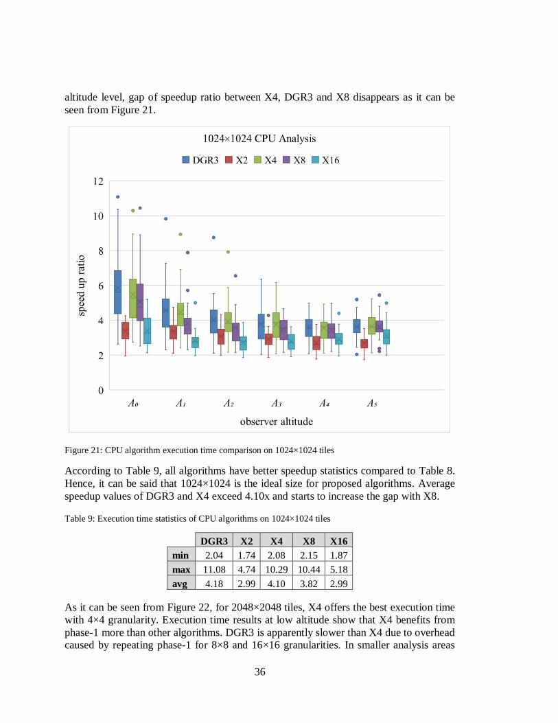
Figure 21: CPU algorithm execution time comparison on 1024×1024 tiles
According to Table 9, all algorithms have better speedup statistics compared to Table 8.
Hence, it can be said that 1024×1024 is the ideal size for proposed algorithms. Average
speedup values of DGR3 and X4 exceed 4.10x and starts to increase the gap with X8.
Table 9: Execution time statistics of CPU algorithms on 1024×1024 tiles
DGR3 X2 X4 X8 X16
min 2.04 1.74 2.08 2.15 1.87
max 11.08 4.74 10.29 10.44 5.18
avg 4.18 2.99 4.10 3.82 2.99
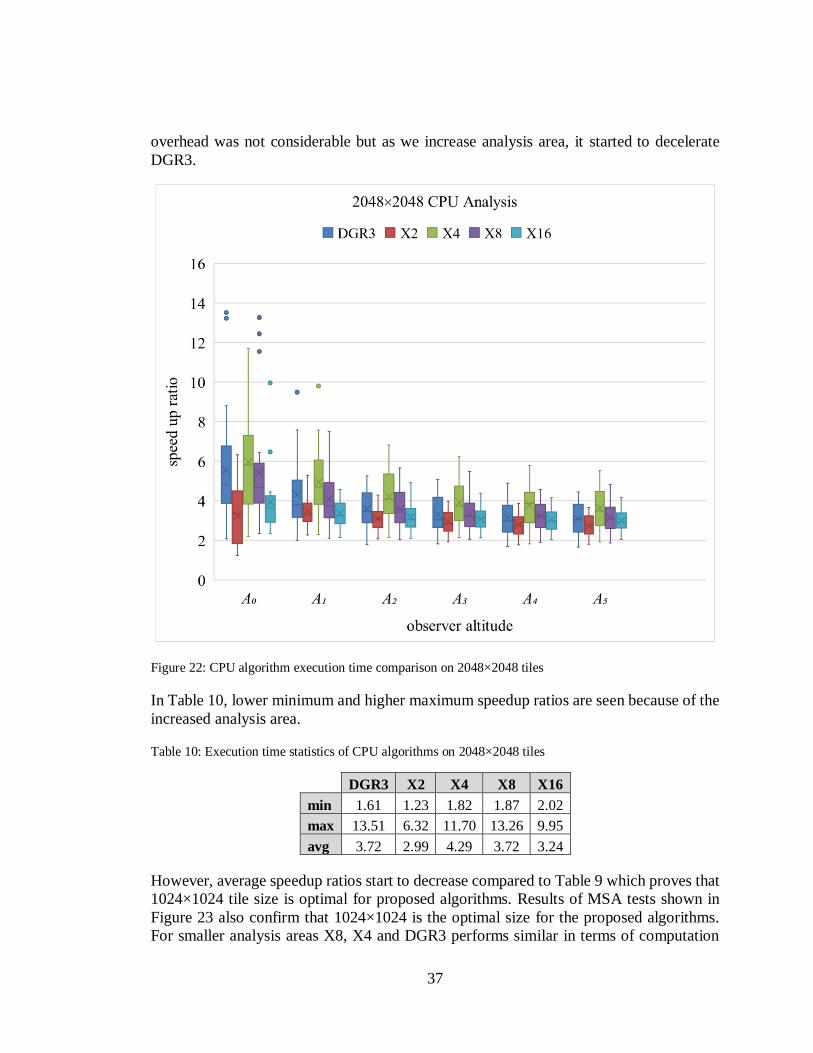
As it can be seen from Figure 22, for 2048×2048 tiles, X4 offers the best execution time
with 4×4 granularity. Execution time results at low altitude show that X4 benefits from
phase-1 more than other algorithms. DGR3 is apparently slower than X4 due to overhead
caused by repeating phase-1 for 8×8 and 16×16 granularities. In smaller analysis areas
37
overhead was not considerable but as we increase analysis area, it started to decelerate
DGR3.
Figure 22: CPU algorithm execution time comparison on 2048×2048 tiles
In Table 10, lower minimum and higher maximum speedup ratios are seen because of the
increased analysis area.
Table 10: Execution time statistics of CPU algorithms on 2048×2048 tiles
DGR3 X2 X4 X8 X16
min 1.61 1.23 1.82 1.87 2.02
max 13.51 6.32 11.70 13.26 9.95
avg 3.72 2.99 4.29 3.72 3.24
However, average speedup ratios start to decrease compared to Table 9 which proves that
1024×1024 tile size is optimal for proposed algorithms. Results of MSA tests shown in
Figure 23 also confirm that 1024×1024 is the optimal size for the proposed algorithms.
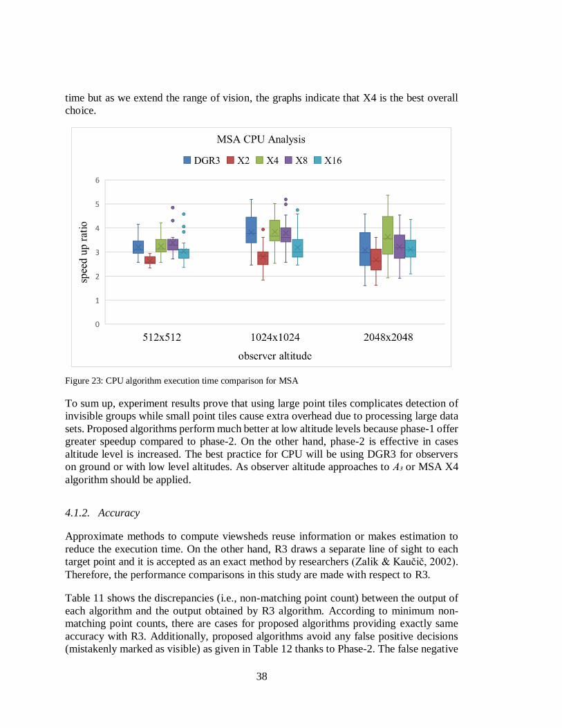
For smaller analysis areas X8, X4 and DGR3 performs similar in terms of computation
38
time but as we extend the range of vision, the graphs indicate that X4 is the best overall
choice.
Figure 23: CPU algorithm execution time comparison for MSA
To sum up, experiment results prove that using large point tiles complicates detection of
invisible groups while small point tiles cause extra overhead due to processing large data
sets. Proposed algorithms perform much better at low altitude levels because phase-1 offer
greater speedup compared to phase-2. On the other hand, phase-2 is effective in cases
altitude level is increased. The best practice for CPU will be using DGR3 for observers
on ground or with low level altitudes. As observer altitude approaches to A₃ or MSA X4
algorithm should be applied.
4.1.2. Accuracy
Approximate methods to compute viewsheds reuse information or makes estimation to
reduce the execution time. On the other hand, R3 draws a separate line of sight to each
target point and it is accepted as an exact method by researchers (Zalik & Kaučič, 2002).
Therefore, the performance comparisons in this study are made with respect to R3.
Table 11 shows the discrepancies (i.e., non-matching point count) between the output of
each algorithm and the output obtained by R3 algorithm. According to minimum non-
matching point counts, there are cases for proposed algorithms providing exactly same
accuracy with R3. Additionally, proposed algorithms avoid any false positive decisions
(mistakenly marked as visible) as given in Table 12 thanks to Phase-2. The false negative

39
decisions (mistakenly marked as invisible) are done in Phase-1 because in slope
calculation same distance value is assigned to a tile of points which may lead to wrong
minimum and maximum slope value calculation. Therefore, the largest average non-
matching point count belongs to X2 which uses the largest processed elevation model.
Table 11: Accuracy of CPU algorithms
non-matching point count
512×512=262144 1024×1024=1048576 2048×2048=4194304
min max avg min max avg min max Avg
R2 135 11028 5702.14 68 38090 20110.32 875 173843 78584.72
DGR3 0 637 15.55 0 329 27.13 0 883 113.71
X2 1 437 52.99 1 1130 185.68 6 3255 874.55
X4 0 249 8.02 0 329 22.42 0 578 86.55
X8 0 590 6.84 0 91 4.06 0 485 30.71
X16 0 176 1.72 0 67 1.16 0 497 10.37
DGR3 uses 3 types of processed elevation models and accumulates wrong decisions made
by Phase-1 of X16, X8 and X4 algorithms. However, average non-matching point count
of R2 is still 8.95x of maximum non-matching point count of DGR3 on the smallest
analysis area. Besides, DGR3 offers average 15.55 non-matching points compared to
5702.14 of R2 which is a significant difference. As the size of analysis area increases, the
distinction between granularity algorithms and R2 becomes larger.
Table 12: Accuracy statistics of algorithms (FN: False Negative, FP: False Positive)
non-matching point count
512×512 1024×1024 2048×2048
min max avg min max avg min max avg
FN R2 55 5080 2340.78 19 17816 8921.07 416 81436 35096.59
FP R2 80 5948 3361.36 49 21233 11189.25 459 92407 43488.13
FP DGR3 0 0 0.00 0 0 0.00 0 0 0.00
FN DGR3 0 637 15.55 0 329 27.13 0 883 113.71
FP X2 0 0 0.00 0 0 0.00 0 0 0.00
FN X2 1 437 52.99 1 1130 185.68 6 3255 874.55
FP X4 0 0 0.00 0 0 0.00 0 0 0.00
FN X4 0 249 8.02 0 329 22.42 0 578 86.55
FP X8 0 0 0.00 0 0 0.00 0 0 0.00
FN X8 0 590 6.84 0 91 4.06 0 485 30.71
FP X16 0 0 0.00 0 0 0.00 0 0 0.00
FN X16 0 176 1.72 0 67 1.16 0 497 10.37

40
In Figure 24, we see visual comparison of false positive and false negative decisions of
R2 and DGR3 with respect to output of R3. Orange points represent false negative
decisions (mistakenly marked as invisible) and blue points represent false positive
decisions (mistakenly marked as visible).
Figure 24: Visual comparison of non-matching points of R2 and DGR3 with R3
Total number of false negative and false positive decisions of R2 for this experiment is
5678 (See Table 13) which is lower than the average value according to Table 11 but the
difference in viewshed output looks quite misleading and this accuracy may not be
satisfactory for some applications.
Table 13: Accuracy statistics of experiment in Figure 24
False Negative False Positive
R2 3674 2004
DGR3 6 0
Proposed algorithms draw a line of sight for group of points and iterate on them. In other
words, they apply R3 with larger resolution and all points in the same target group
assumed to be on the same line of sight and distance to the observer. Therefore, detection
of invisible groups in phase-1 may cause wrong visibility decisions for some of the points
within the group. When we increase the number of groups by decreasing the granularity
of down scaled elevation models, we see more mistaken visibility decisions. This fact
explains average non-matching point count relation between X2, X4, X8 and X16. On the
other hand, increasing granularity may cause a wrong decision affecting many points in a
larger group and cause wrong decisions to accumulate in a specific region which is an
important problem. In Figure 25, we see original output of R3 and wrong visibility
decisions of X2 and DGR3. Orange points represent false negative decisions (mistakenly
marked as invisible) in output of X2 and DGR3. When we analyze the outputs of
algorithms using same approach with different granularities we see wrong decisions of X2
is dispersed unlike DGR3.

41
Figure 25: Visual comparison of non-matching points of X2 and DGR3 with R3
Van Kreveld’s algorithm is seen as considerable alternative to R3 due to accuracy. The
study of Johansson and Lundberg (Johansson & Lundberg, 2016) presents accuracy results
of Van Kreveld’s algorithm on 2001×2001 tiles. The experiment results show that there
are 50346 non-matching points, meanwhile, X2 algorithm offers the worst accuracy with
3255 unmatched points on 2048×2048 tiles (See Table 11). In other words, granularity
algorithms offer significant accuracy results compared to Van Kreveld’s algorithm.
4.2. Experiments with GPU Implementation
4.2.1. Execution Time
GPU execution time performances of the proposed algorithms are compared with respect
to R3. Parallelization of proposed algorithms sketch different execution time graphs
depending on the size of the analysis area. Since all threads run in parallel, the amount of
serial computations in an algorithm is very effective on the execution time. In this case,
execution time of R3 is determined by the visible point which is the most distant one from
the observer position. Considering that decreasing observer altitude extends the invisible
regions and cause threads to finish visibility computation quickly, R3 provides the best
execution time for the minimum altitude level. Therefore, proposed algorithms are slower
than R3 at low altitude levels as seen in Figure 26, Figure 27 and Figure 28.
The execution time results of granularity algorithms indicate sequential execution of
Phase-1 and Phase-2 cause overhead compared to parallel implementation of R3.
Especially on smallest analysis area proposed algorithms are significantly slower than R3
as shown in Figure 26.
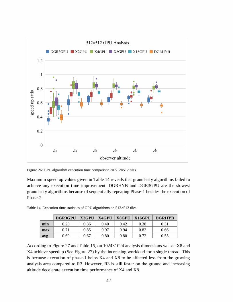
42
Figure 26: GPU algorithm execution time comparison on 512×512 tiles
Maximum speed up values given in Table 14 reveals that granularity algorithms failed to
achieve any execution time improvement. DGRHYB and DGR3GPU are the slowest
granularity algorithms because of sequentially repeating Phase-1 besides the execution of
Phase-2.
Table 14: Execution time statistics of GPU algorithms on 512×512 tiles
DGR3GPU X2GPU X4GPU X8GPU X16GPU DGRHYB
min 0.28 0.36 0.40 0.42 0.38 0.31
max 0.71 0.85 0.97 0.94 0.82 0.66
avg 0.60 0.67 0.80 0.80 0.72 0.55
According to Figure 27 and Table 15, on 1024×1024 analysis dimensions we see X8 and
X4 achieve speedup (See Figure 27) by the increasing workload for a single thread. This
is because execution of phase-1 helps X4 and X8 to be affected less from the growing
analysis area compared to R3. However, R3 is still faster on the ground and increasing
altitude decelerate execution time performance of X4 and X8.
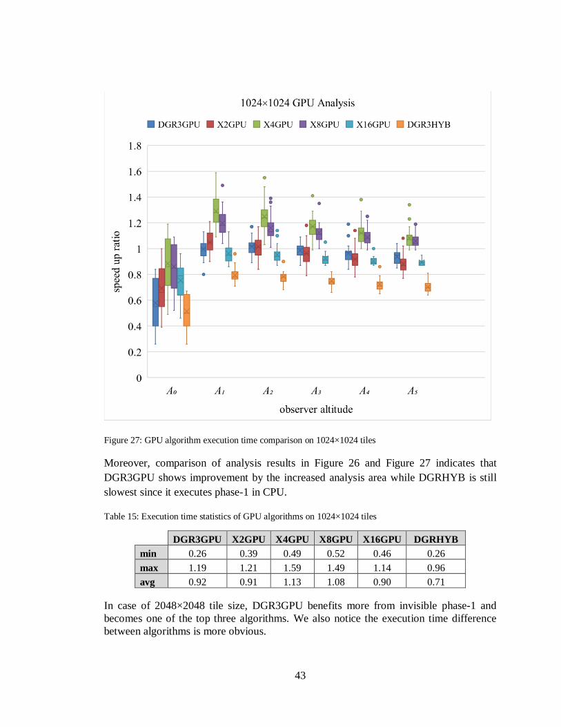
43
Figure 27: GPU algorithm execution time comparison on 1024×1024 tiles
Moreover, comparison of analysis results in Figure 26 and Figure 27 indicates that
DGR3GPU shows improvement by the increased analysis area while DGRHYB is still
slowest since it executes phase-1 in CPU.
Table 15: Execution time statistics of GPU algorithms on 1024×1024 tiles
DGR3GPU X2GPU X4GPU X8GPU X16GPU DGRHYB
min 0.26 0.39 0.49 0.52 0.46 0.26
max 1.19 1.21 1.59 1.49 1.14 0.96
avg 0.92 0.91 1.13 1.08 0.90 0.71
In case of 2048×2048 tile size, DGR3GPU benefits more from invisible phase-1 and
becomes one of the top three algorithms. We also notice the execution time difference
between algorithms is more obvious.

44
Figure 28: GPU algorithm execution time comparison on 2048×2048 tiles
The execution time graph in Figure 28 shows that granularity algorithms provide
improvement only on large analysis areas and X4 is the best algorithm with 1.41x average
speed up to 2.27x maximum (See Table 16). The second fastest algorithm is X8 with 1.31x
average speed up to 2.0x maximum thanks to 8×8 granularity and DGR3 GPU is the third
because of repeating phase-1.
Table 16: Execution time statistics of GPU algorithms on 2048×2048 tiles
DGR3GPU X2GPU X4GPU X8GPU X16GPU DGRHYB
min 0.36 0.36 0.57 0.58 0.52 0.22
max 1.87 1.63 2.27 2.00 1.50 1.21
avg 1.25 1.09 1.41 1.31 1.05 0.81
We see MSA results also support (See Figure 29) that X4GPU, X8GPU and DGR3GPU
offer execution time improvement only for 2048×2048 analysis area.

45
Figure 29: GPU algorithm execution time comparison for MSA
The reason for DGRHYB to be the slowest algorithm is the execution time overhead
caused by running phase-1 in CPU. If we compare DGRHYB with CPU version of R3,
we see amount of speedup given in Figure 30. The rationale to use hybrid approach can
be reducing the workload in CPU while using both processing units in a system.
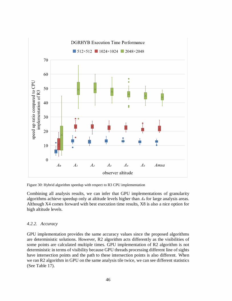
46
Figure 30: Hybrid algorithm speedup with respect to R3 CPU implementation
Combining all analysis results, we can infer that GPU implementations of granularity
algorithms achieve speedup only at altitude levels higher than A₀ for large analysis areas.
Although X4 comes forward with best execution time results, X8 is also a nice option for
high altitude levels.
4.2.2. Accuracy
GPU implementation provides the same accuracy values since the proposed algorithms
are deterministic solutions. However, R2 algorithm acts differently as the visibilities of
some points are calculated multiple times. GPU implementation of R2 algorithm is not
deterministic in terms of visibility because GPU threads processing different line of sights
have intersection points and the path to these intersection points is also different. When
we ran R2 algorithm in GPU on the same analysis tile twice, we can see different statistics
(See Table 17).
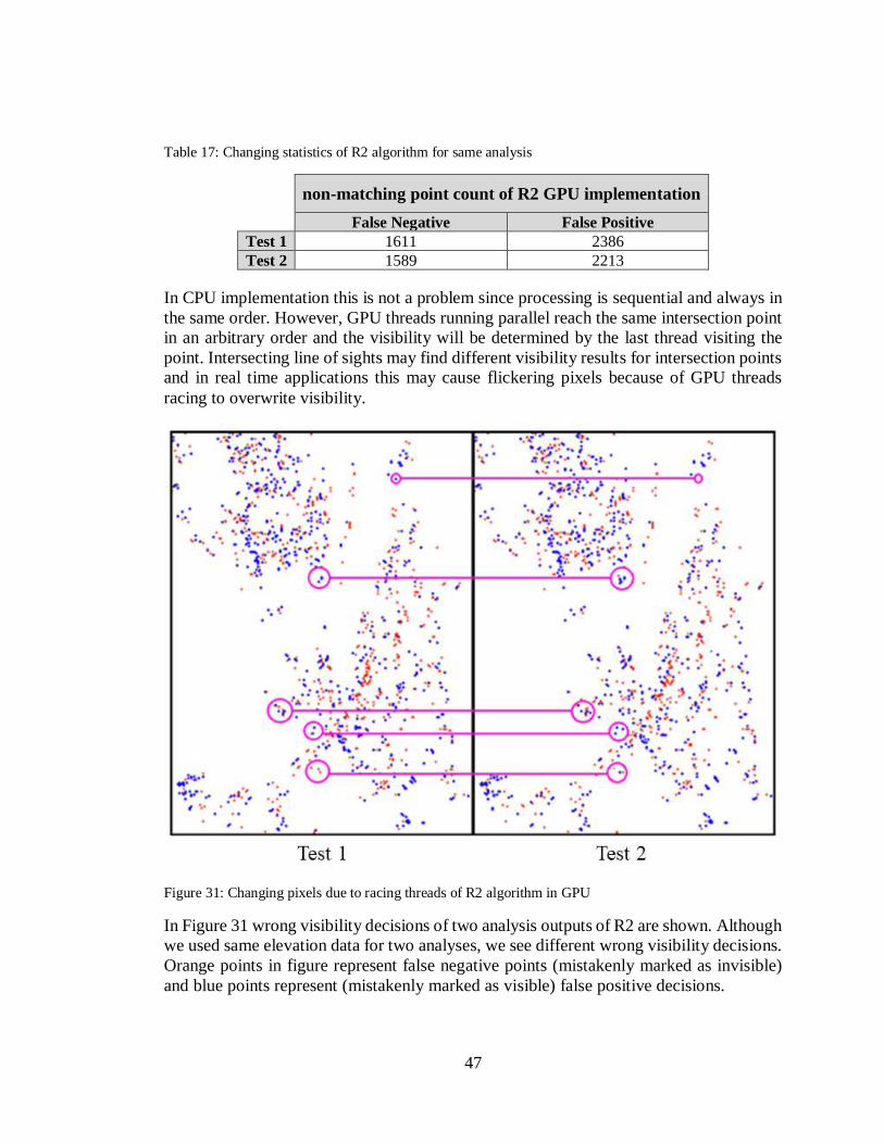
47
Table 17: Changing statistics of R2 algorithm for same analysis
non-matching point count of R2 GPU implementation
False Negative False Positive
Test 1 1611 2386
Test 2 1589 2213
In CPU implementation this is not a problem since processing is sequential and always in
the same order. However, GPU threads running parallel reach the same intersection point
in an arbitrary order and the visibility will be determined by the last thread visiting the
point. Intersecting line of sights may find different visibility results for intersection points
and in real time applications this may cause flickering pixels because of GPU threads
racing to overwrite visibility.
Figure 31: Changing pixels due to racing threads of R2 algorithm in GPU
In Figure 31 wrong visibility decisions of two analysis outputs of R2 are shown. Although
we used same elevation data for two analyses, we see different wrong visibility decisions.
Orange points in figure represent false negative points (mistakenly marked as invisible)
and blue points represent (mistakenly marked as visible) false positive decisions.

48
4.3. Resource Usage
In Table 18 the resource requirements of each algorithm are given because it is also an
important criterion in practical settings. The numbers in red color represents the external
requirement to implement the algorithms (See Table 18). Proposed algorithms require
maximum 0.67x more space in disk and 1.0x more memory.
For GPU implementation amount of data given in Table 18 is copied to device memory.
Therefore, GPU memory requirements are exactly same with CPU implementation. In
order to decrease the disk and memory requirements, the algorithm can also be
implemented with INTEGER data type.
Apart from R2, Van Kreveld’s algorithm, which is considered as a fast alternative to R3,
does not require extra disk space for implementation. However, the algorithm needs extra
temporary storage for the runtime. The event lists (enter, center and exit) and active
balanced tree require more than 3x extra memory in total (Johansson & Lundberg, 2016).
Therefore, proposed granularity methods seem more feasible compared to Van Kreveld’s,
if disk space is not a constraint.
Table 18: Resource usage of algorithms
Disk Usage Memory Usage in KB
Algorithms on
different analysis dimensions
Elevation
(FLOAT,FLOAT)
Slope
FLOAT
Remaining Point List
(SHORT,SHORT)
Visibility
BOOL
X2 512×512 512 + 1024 1024 1024 256
X2 1024×1024 2048 + 4096 4096 4096 1024
X2 2048×2048 8192 + 16384 16384 16384 4096
X4 512×512 128 + 1024 1024 1024 256
X4 1024×1024 512 + 4096 4096 4096 1024
X4 2048×2048 2048 + 16384 16384 16384 4096
X8 512×512 32 + 1024 1024 1024 256
X8 1024×1024 128 + 4096 4096 4096 1024
X8 2048×2048 512 + 16384 16384 16384 4096
X16 512×512 8 + 1024 1024 1024 256
X16 1024×1024 32 + 4096 4096 4096 1024
X16 2048×2048 128 + 16384 16384 16384 4096
DGR3 512×512 168 + 1024 1024 1024 256
DGR3 1024×1024 672 + 4096 4096 4096 1024
DGR3 2048×2048 2688 + 16384 16384 16384 4096
DGRHYB 512×512 168 + 1024 1024 1024 256
DGRHYB 1024×1024 672 + 4096 4096 4096 1024
DGRHYB 2048×2048 2688 + 16384 16384 16384 4096
49
CHAPTER 5
5. CONCLUSION AND FUTURE WORK
In this research, accuracy is considered as the primary concern in viewshed analysis.
Accordingly, a set of algorithms, which are mainly derived from R3 algorithm, are
proposed to improve the processing time performance of R3 algorithm while preserving
its accuracy. The proposed algorithms are implemented for both CPU and GPU.
Findings of the experiments confirm that CPU versions of DGR3 and X4 are considerable
options to R3 in any conditions. Besides the execution time improvement, proposed
algorithms never display an invisible point as visible unlike R2 and Van Kreveld’s
algorithm. The significant decrease in number of false negative decisions compared to
other approximate algorithms can also be a motivation to choose granularity algorithms.
On the other hand, GPU application of the suggested approach does not offer as much
speedup as CPU but on large analysis dimensions DGR3GPU, X4GPU, X8GPU can offer
speedup above 2x with respect to R3GPU. Moreover, R2GPU algorithm is not a reliable
option in terms of accuracy due to flicker effect caused by the racing threads.
Resource requirements of an algorithm are also an important issue for practical
applications. DGR3, which requires the maximum resource among proposed solutions,
can be considered as moderate compared to Van Kreveld’s and it can be revised to change
the granularity level in runtime with respect to MSA to achieve the best execution time.
To sum up DGR3, X4 and X8 are nice options to R3, if a CPU is assigned for the task.
Depending on design constraints and execution time requirements these algorithms can
be useful alternatives to R2.
To solve the execution time issues of viewshed analysis, algorithms like Xdraw and R2
are proposed. In this study, the motivation is to improve R3 while keeping the accuracy
as high as possible. However, none of the algorithms proposed is as fast as R2. In contrast
to the approach proposed in this thesis, future work may be on improvement of R2
algorithm’s accuracy while preserving execution time performance.

50
For a specific range of analysis, wrong decisions of R2 can be anticipated. This is because
the procedure to draw the line of sight and compute visibility is certain. Since there is no
estimation involved in viewshed computation, the pattern of errors can be analyzed and
wrong decision points can be found to develop a method minimizing false visibility
decisions. Nevertheless, in order to preserve the execution time performance of R2, error
correction method should not change the complexity of the algorithm.
Moreover, since different algorithms offer advantages on different terrain topologies, a
method can be developed to switch between algorithms on the fly. Implementation of such
an adaptive solution requires real time analysis of the terrain. Depending on changing
parameters like roughness and standard deviation of elevation data, we can run the optimal
algorithm to provide high accuracy and fast execution time. Additionally, making such an
analysis of the terrain can help to find points whose visibility does not change by the
vertical or horizontal movement of observer to avoid redundant visibility computations.
In conclusion, execution time requirement of real time terrain analysis should be studied
and solutions using this method should be compared with R2, R3 and granularity
algorithms in terms of performance and practicality.
51
REFERENCES
Andrade, M. V., Magalhães, S. V., Magalhães, M. A., Franklin, W. R., & Cutler, B. M.
(2011). Efficient viewshed computation on terrain in external memory.
Geoinformatica, 381-397.
Axell, T., & Fridén, M. (2015, June). Comparison between GPU and parallel CPU
optimizations in viewshed analysis. Gothenburg, Sweden: Chalmers University of
Technology.
Bailey, R. E., Parrish, R. V., Kramer, L. J., Harrah, S., & Arthur, J. (n.d.). Technical
Challenges In the Development of a NASA Synthetic Vision System Concept.
Hampton, USA: NASA Langley Research Center.
Blelloch, G. E. (1997). Prefix Sums and Their Applications. 35-59. Pittsburgh,
Pennsylvania.
Bresenham, J. E. (1965). Algorithm for computer control of a digital plotter. IBM Systems
Journal (pp. 25-30). IBM.
Carver, S., & Washtell, J. (2012). Real-time visibility analysis and rapid viewshed
calculation using a voxelbased modelling approach. GISRUK. Lancaster.
Federal Aviation Administration. (n.d.). FAA Guide to Low-Flying Aircraft. Retrieved
June 2019, 10, from FAA: https://www.faa.gov
Ferreira, C., Andrade, M. V., Franklin, R. W., Magalhães, S. V., & Pena, G. C. (2013). A
Parallel Sweep Line Algorithm for Visibility Computation. Proceedings of the
Brazilian Symposium on GeoInformatics, (pp. 85-96).
Haverkort, H., Toma, L., & Wei, B. P. (2013, November). On IO-efficient viewshed
algorithms and their accuracy. Proceedings of the 21st ACM SIGSPATIAL
International Conference on Advances in Geographic Information Systems (pp.
24-33). New York: ACM.

52
Johansson, E., & Lundberg, J. (2016, June). Distributed Viewshed Analysis. An
Evaluation of Distribution Frameworks. Gothenburg, Sweden: Chalmers
University of Technology and University of Gothenburg.
Larsen, M. V. (2015, October 30). Viewshed algorithms for strategic positioning of
vehicles. Kjeller, Norway: Norwegian Defence Research Establishment.
Mehta, S., Ray, C. K., & Franklin, R. (1994). Geometric Algorithms for Siting of Air
Defense Missile Batteries. Columbus, Ohio, USA: Battelle Columbus Division.
NASA. (n.d.). Retrieved June 8, 2019, from asterweb: https://asterweb.jpl.nasa.gov/
NGA.mil. (2015, May 18). Digital . Retrieved June 17, 2019, from NATIONAL
GEOSPATIAL-INTELLIGENCE AGENCY: https://www.nga.mil
Nguyen, T. H., Duy, T. N., & Duong, T. A. (2018). A new algorithm for viewshed
computation on raster terrain. 2nd International Conference on Recent Advances
in Signal Processing, Telecommunications & Computing (SigTelCom). Ho Chi
Minh City, Vietnam: IEEE.
NVIDIA Corporation. (n.d.). CUDA C Programming Guide. Retrieved 6 6, 2019, from
CUDA Toolkit Documentation: https://docs.nvidia.com/cuda/cuda-c-
programming-guide/
NVIDIA Corporation. (n.d.). CUDA Toolkit Documentation v9.2.148. Retrieved 6 8,
2019, from CUDA Toolkit Documentation:
https://docs.nvidia.com/cuda/archive/9.2/
NVIDIA Corporation. (n.d.). Tuning CUDA Applications for Kepler. Retrieved 6 1, 2019,
from CUDA Toolkit Documentation: https://docs.nvidia.com/cuda/kepler-tuning-
guide/
Shrestha, S., & Panday, S. P. (2018). Faster Line of Sight Computation and Faster
Viewshed Generation. 21st International Computer Science and Engineering
Conference (ICSEC). Bangkok, Thailand: IEEE.
Trautwein, F., Flitter, H., Hugentobler, M., Lüscher, P., Weckenbrock, P., Weibel, R., &
Hägi, S. (2016, 4 28). Retrieved 6 6, 2019, from http://www.gitta.info:
http://www.gitta.info/TerrainAnalyi/en/text/TerrainAnalyi.pdf
Van Kreveld, M. (1996). Variations on Sweep Algorithms: efficient computation of
extended viewsheds and class intervals. Utrecht.
Vestal, S. (2007). Preemptive Scheduling of Multi-Criticality Systems with Varying
Degrees of Execution Time Assurance. 28th IEEE International Real-Time
Systems Symposium. Tucson, AZ, USA: IEEE.

53
Yılmaz, G. (2017, May). Accelerating Line of Sight Analysis Algorithms with Parallel
Programming. Turkey.
Ying, S., Li, L., Mei, Y., & Gao, Y. (2008). Viewshed Computation Based on LOS
Scanning. 2008 International Conference on Computer Science and Software
Engineering. Hubei, China: IEEE.
Zalik, B., & Kaučič, B. (2002). Comparison of viewshed algorithms on regular spaced
points. SCCG '02 Proceedings of the 18th Spring Conference on Computer
Graphics (pp. 177-183). New York: ACM.

54

55
APPENDICES
APPENDIX A
R3 Pseudocode
Ox,y: Position of observer in cartesian coordinates
AO: Altitude of observer i: x component of point cartesian coordinate j: y component of point cartesian coordinate n: Dimension of analysis area Distancei,j: Euclidean distance between observer and point with indices
i and j E: Elevation model data S: Slope model data V: Visibility result data Ei,j: Elevation value of point with indices i and j
Si,j: Slope value from observer to point with indices i and j
Ti,j: Target point to determine visibility with indices i and j
Vi,j: Visibility result of target point with indices i and j
BresenhamPoint: Position of any point on Bresenham line between observer and Ti,j Assign Ox,y as (n/2, n/2)
// Compute Slope FOR <i,j>: <0...n, 0...n>
Si,j = (Ei,j - AO) / Distancei,j END FOR // Compute Visibility FOR <i,j>: <0...n, 0...n>
IsTargetInvisible = FALSE WHILE IsTargetInvisible is FALSE Iterate on Bresenham line points from Ox,y to Ti,j
IF Si,j < SBresenhamPoint
Vi,j = Invisible IsTargetInvisible = TRUE
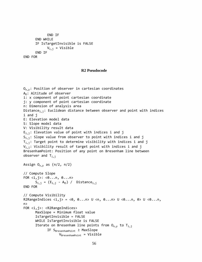
56
END IF END WHILE IF IsTargetInvisible is FALSE Vi,j = Visible
END IF END FOR
R2 Pseudocode
Ox,y: Position of observer in cartesian coordinates
AO: Altitude of observer i: x component of point cartesian coordinate j: y component of point cartesian coordinate n: Dimension of analysis area Distancei,j: Euclidean distance between observer and point with indices
i and j E: Elevation model data S: Slope model data V: Visibility result data Ei,j: Elevation value of point with indices i and j
Si,j: Slope value from observer to point with indices i and j
Ti,j: Target point to determine visibility with indices i and j
Vi,j: Visibility result of target point with indices i and j BresenhamPoint: Position of any point on Bresenham line between observer and Ti,j
Assign Ox,y as (n/2, n/2)
// Compute Slope FOR <i,j>: <0...n, 0...n>
Si,j = (Ei,j - AO) / Distancei,j
END FOR // Compute Visibility R2RangeIndices <i,j> = <0, 0...n> U <n, 0...n> U <0...n, 0> U <0...n, n> FOR <i,j>: <R2RangeIndices>
MaxSlope = Minimum float value IsTargetInvisible = FALSE WHILE IsTargetInvisible is FALSE Iterate on Bresenham line points from Ox,y to Ti,j
IF SBresenhamPoint ≥ MaxSlope VBresenhamPoint = Visible

57
MaxSlope = SBresenhamPoint ELSE VBresenhamPoint = Invisible
END IF END WHILE
END FOR
Elevation Data Preprocessing Pseudocode
AO: Altitude of observer i: x component of point cartesian coordinate j: y component of point cartesian coordinate n: Dimension of analysis area G: Dimension of group size E: Elevation model data Ei,j: Elevation value of point with indices i and j.
GroupMax: Temporary minimum elevation found GroupMin: Temporary maximum elevation found EGMin: G×G minimum elevation value model EGMax: G×G maximum elevation value model Index: Temporary iteration index /* Phase 0 - Prepare Processed Elevation Models */ Index = 0 FOR <i,j>: <0...n, 0...n> GroupMax = Ei,j
GroupMin = Ei,j
FOR <p,r>: <0...G, 0...G>
IF Ei+p,j+r > GroupMax
GroupMax = Ei+p,j+r END IF
IF Ei+p,j+r < GroupMin
GroupMin = Ei+p,j+r
END IF END FOR
EGMinIndex = GroupMin EGMaxIndex = GroupMax Index = Index + 1
i = i + G j = j + G
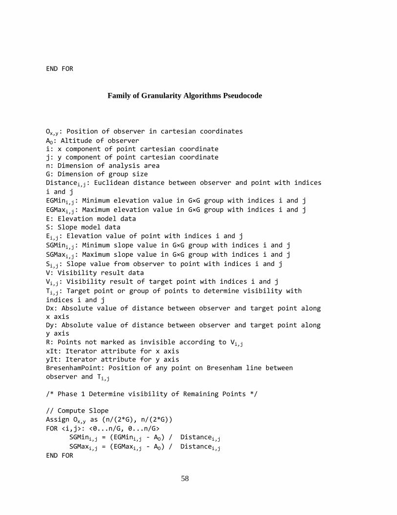
58
END FOR
Family of Granularity Algorithms Pseudocode
Ox,y: Position of observer in cartesian coordinates
AO: Altitude of observer i: x component of point cartesian coordinate j: y component of point cartesian coordinate n: Dimension of analysis area G: Dimension of group size Distancei,j: Euclidean distance between observer and point with indices
i and j EGMini,j: Minimum elevation value in G×G group with indices i and j
EGMaxi,j: Maximum elevation value in G×G group with indices i and j
E: Elevation model data S: Slope model data Ei,j: Elevation value of point with indices i and j
SGMini,j: Minimum slope value in G×G group with indices i and j
SGMaxi,j: Maximum slope value in G×G group with indices i and j
Si,j: Slope value from observer to point with indices i and j V: Visibility result data Vi,j: Visibility result of target point with indices i and j
Ti,j: Target point or group of points to determine visibility with
indices i and j Dx: Absolute value of distance between observer and target point along x axis Dy: Absolute value of distance between observer and target point along y axis R: Points not marked as invisible according to Vi,j
xIt: Iterator attribute for x axis yIt: Iterator attribute for y axis BresenhamPoint: Position of any point on Bresenham line between observer and Ti,j /* Phase 1 Determine visibility of Remaining Points */ // Compute Slope Assign Ox,y as (n/(2*G), n/(2*G))
FOR <i,j>: <0...n/G, 0...n/G> SGMini,j = (EGMini,j - AO) / Distancei,j
SGMaxi,j = (EGMaxi,j - AO) / Distancei,j
END FOR
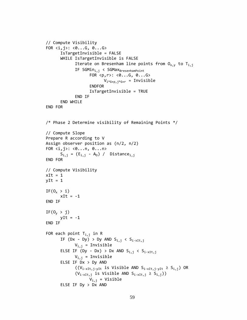
59
// Compute Visibility FOR <i,j>: <0...G, 0...G>
IsTargetInvisible = FALSE WHILE IsTargetInvisible is FALSE
Iterate on Bresenham line points from Ox,y to Ti,j
IF SGMini,j < SGMaxBresenhamPoint FOR <p,r>: <0...G, 0...G>
Vi*G+p,j*G+r = Invisible
ENDFOR IsTargetInvisible = TRUE
END IF END WHILE
END FOR /* Phase 2 Determine visibility of Remaining Points */ // Compute Slope Prepare R according to V Assign observer position as (n/2, n/2) FOR <i,j>: <0...n, 0...n>
Si,j = (Ei,j - AO) / Distancei,j
END FOR // Compute Visibility xIt = 1 yIt = 1 IF(Ox > i) xIt = -1 END IF
IF(Oy > j)
yIt = -1 END IF FOR each point Ti,j in R
IF (Dx - Dy) > Dy AND Si,j < Si-xIt,j
Vi,j = Invisible
ELSE IF (Dy - Dx) > Dx AND Si,j < Si-xIt,j
Vi,j = Invisible
ELSE IF Dx > Dy AND ((Vi-xIt,j-yIt is Visible AND Si-xIt,j-yIt ≥ Si,j) OR
(Vi-xIt,j is Visible AND Si-xIt,j ≥ Si,j))
Vi,j = Visible ELSE IF Dy > Dx AND

60
((Vi-xIt,j-yIt is Visible AND Si-xIt,j-yIt ≥ Si,j) OR
(Vi,j-yIt is Visible AND Si-xIt,j ≥ Si,j))
Vi,j = Visible ELSE
IsTargetInvisible = FALSE WHILE IsTargetInvisible is FALSE Iterate on Bresenham line points from Ox,y to Ti,j
IF Si,j < SBresenhamPoint
Vi,j = Invisible
IsTargetInvisible = TRUE END IF
END WHILE IF IsTargetInvisible is FALSE Vi,j = Visible
END IF END IF
END FOR
R3GPU Pseudocode
Ox,y: Position of observer in cartesian coordinates
AO: Altitude of observer i: x component of point cartesian coordinate j: y component of point cartesian coordinate n: Dimension of analysis area Distancei,j: Euclidean distance between observer and point with indices i and j E: Elevation model data S: Slope model data Ei,j: Elevation value of point with indices i and j
Si,j: Slope value from observer to point with indices i and j
Ti,j: Target point to determine visibility with indices i and j
V: Visibility result data Vi,j: Visibility result of target point with indices i and j
BresenhamPoint: Position of any point on Bresenham line between observer and Ti,j
COPY E to device memory Assign Ox,y as (n/2, n/2)
// Compute Slope SLOPE_CALC_KERNEL
i = (blockDim.x * blockIdx.x) + threadIdx.x

61
j = (blockDim.y * blockIdx.y) + threadIdx.y Si,j = (Ei,j - AO) / Distancei,j
END SLOPE_CALC_KERNEL // Compute Visibility R3_VISIBILITY_KERNEL
i = (blockDim.x * blockIdx.x) + threadIdx.x j = (blockDim.y * blockIdx.y) + threadIdx.y IsTargetInvisible = FALSE WHILE IsTargetInvisible is FALSE
Iterate on Bresenham line points from Ox,y to Ti,j
IF Si,j < SBresenhamPoint
Vi,j = Invisible IsTargetInvisible = TRUE
END IF END WHILE IF IsTargetInvisible is FALSE Vi,j = Visible
END IF END R3_VISIBILITY_KERNEL COPY V to device memory
R2GPU Pseudocode
Ox,y: Position of observer in cartesian coordinates
AO: Altitude of observer i: x component of point cartesian coordinate j: y component of point cartesian coordinate n: Dimension of analysis area Distancei,j: Euclidean distance between observer and point with indices
i and j E: Elevation model data S: Slope model data Ei,j: Elevation value of point with indices i and j
Si,j: Slope value from observer to point with indices i and j
Ti,j: Target point to determine visibility with indices i and j
V: Visibility result data Vi,j: Visibility result of target point with indices i and j BresenhamPoint: Position of any point on Bresenham line between observer and Ti,j

62
COPY E to device memory Assign Ox,y as (n/2, n/2)
// Compute Slope SLOPE_CALC_KERNEL
i = (blockDim.x * blockIdx.x) + threadIdx.x j = (blockDim.y * blockIdx.y) + threadIdx.y Si,j = (Ei,j - AO) / Distancei,j
END SLOPE_CALC_KERNEL // Compute Visibility R2_VISIBILITY_KERNEL
IF blockIdx.x < 2 i = (blockDim.x * blockIdx.x) + threadIdx.x j = 0
ELSE IF blockIdx.x > 1 AND blockIdx.x < 4 i = (blockDim.x * (blockIdx.x - 2)) + threadIdx.x j = n-1
ELSE IF blockIdx.x > 3 AND blockIdx.x < 6 i = 0 j = (blockDim.x * (blockIdx.x - 4)) + threadIdx.x
ELSE IF blockIdx.x > 5 AND blockIdx.x < 8 i = n - 1 j = (blockDim.x * (blockIdx.x - 6)) + threadIdx.x
END IF
MaxSlope = Minimum float value IsTargetInvisible = FALSE WHILE IsTargetInvisible is FALSE
Iterate on Bresenham line points from Ox,y to Ti,j
IF SBresenhamPoint < MaxSlope VBresenhamPoint = Invisible ELSE VBresenhamPoint = Visible
MaxSlope = SBresenhamPoint END IF
END WHILE END R2_VISIBILITY_KERNEL
Copy V to host memory
Family of Granularity Algorithms GPU Pseudocode
Ox,y: Position of observer in cartesian coordinates

63
AO: Altitude of observer i: x component of point cartesian coordinate j: y component of point cartesian coordinate n: Dimension of analysis area G: Dimension of group size (granularity dimension) Distancei,j: Euclidean distance between observer and point with indices
i and j ExMini,j: Minimum elevation value in group with indices i and j
ExMaxi,j: Maximum elevation value in group with indices i and j
E: Elevation model data S: Slope model data Ei,j: Elevation value of point with indices i and j
SGMini,j: Minimum slope value in G×G group with indices i and j
SGMaxi,j: Maximum slope value in G×G group with indices i and j
Si,j: Slope value from observer to point with indices i and j
Ti,j: Target point to determine visibility with indices i and j
V: Visibility result data Vi,j: Visibility result of target point with indices i and j Dx: Absolute value of distance between observer and target point along x axis Dy: Absolute value of distance between observer and target point along y axis R: Points not marked as invisible according to Vi,j
xIt: Iterator attribute for x axis yIt: Iterator attribute for y axis BresenhamPoint: Position of any point on Bresenham line between observer and Ti,j // Phase 1 - Detection of Invisible Groups // Compute Slope Prepare R according to V Assign Ox,y as (n/(2*G), n/(2*G))
Copy E to device memory SLOPE_G_CALC_KERNEL
i = (blockDim.x * blockIdx.x) + threadIdx.x j = (blockDim.y * blockIdx.y) + threadIdx.y SGMini,j = (EGMini,j - AO) / Distancei,j
SGMaxi,j = (EGMaxi,j - AO) / Distancei,j END SLOPE_G_CALC_KERNEL // Compute Visibility VISIBILITY_G_KERNEL

64
Ti,j = R[(blockIdx.y * gridDim.x * blockDim.x * blockDim.y) +
(blockIdx.x * blockDim.x * blockDim.y) + (threadIdx.y * blockDim.x) + threadIdx.x
IsTargetInvisible = FALSE WHILE IsTargetInvisible is FALSE Iterate on Bresenham line points from Ox,y to Ti,j
IF SGMini,j < SGMaxBresenhamPoint
FOR <p,r>: <0...G, 0...G> Vi*G+p,j*G+r = Invisible
ENDFOR IsTargetInvisible = TRUE
END IF END FOR
END VISIBILITY_G_KERNEL Copy V to host memory Prepare R accoring to V Copy R to device memory // Phase 2 Determine visibility of Remaining Points // Compute Slope Assign Ox,y as (n/2, n/2) SLOPE_CALC_KERNEL
i = blockDim.x * blockIdx.x + threadIdx.x j = blockDim.y * blockIdx.y + threadIdx.y Si,j = (Ei,j - AO) / Distancei,j
END SLOPE_CALC_KERNEL // Compute Visibility IMPR3_ VISIBILITY _KERNEL
Ti,j = R[blockIdx.x * blockDim.x * blockDim.y) + (blockDim.x * threadIdx.y) + threadIdx.x]
xIt = 1 yIt = 1
IF(Ox > i)
xIt = -1 END IF IF(Oy > j)
yIt = -1 END IF
IF (Dx - Dy) > Dy AND Si,j < Si-xIt,j
Vi,j = Invisible
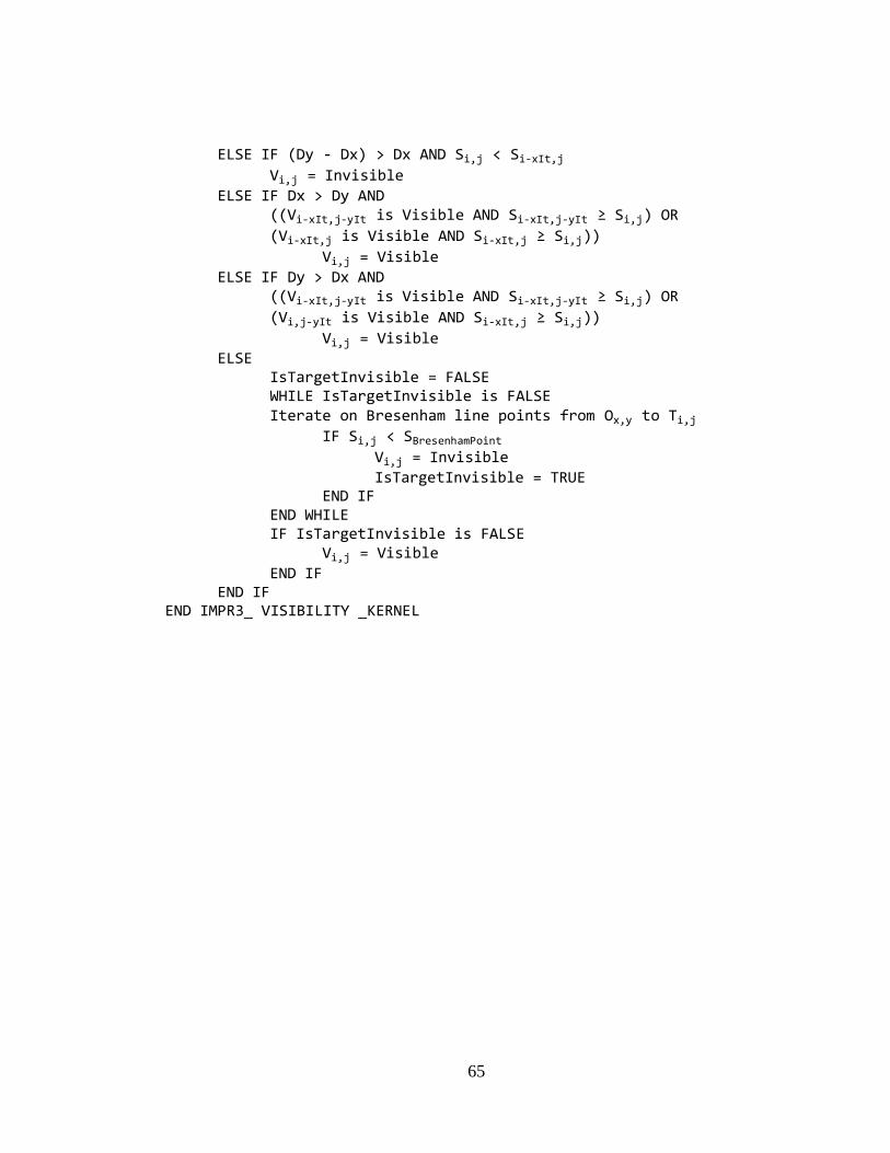
65
ELSE IF (Dy - Dx) > Dx AND Si,j < Si-xIt,j
Vi,j = Invisible
ELSE IF Dx > Dy AND ((Vi-xIt,j-yIt is Visible AND Si-xIt,j-yIt ≥ Si,j) OR
(Vi-xIt,j is Visible AND Si-xIt,j ≥ Si,j))
Vi,j = Visible
ELSE IF Dy > Dx AND ((Vi-xIt,j-yIt is Visible AND Si-xIt,j-yIt ≥ Si,j) OR
(Vi,j-yIt is Visible AND Si-xIt,j ≥ Si,j))
Vi,j = Visible ELSE
IsTargetInvisible = FALSE WHILE IsTargetInvisible is FALSE Iterate on Bresenham line points from Ox,y to Ti,j
IF Si,j < SBresenhamPoint
Vi,j = Invisible
IsTargetInvisible = TRUE END IF
END WHILE IF IsTargetInvisible is FALSE Vi,j = Visible
END IF END IF
END IMPR3_ VISIBILITY _KERNEL
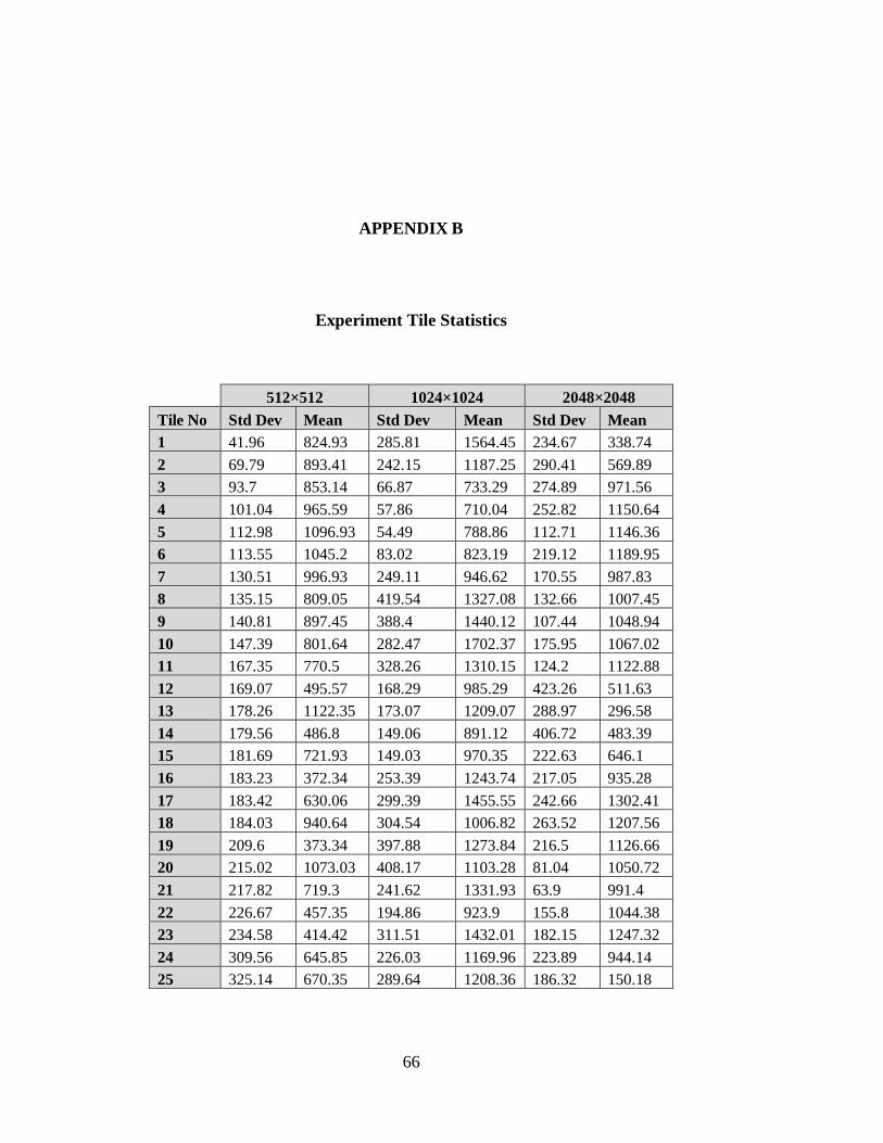
66
APPENDIX B
Experiment Tile Statistics
512×512 1024×1024 2048×2048
Tile No Std Dev Mean Std Dev Mean Std Dev Mean
1 41.96 824.93 285.81 1564.45 234.67 338.74
2 69.79 893.41 242.15 1187.25 290.41 569.89
3 93.7 853.14 66.87 733.29 274.89 971.56
4 101.04 965.59 57.86 710.04 252.82 1150.64
5 112.98 1096.93 54.49 788.86 112.71 1146.36
6 113.55 1045.2 83.02 823.19 219.12 1189.95
7 130.51 996.93 249.11 946.62 170.55 987.83
8 135.15 809.05 419.54 1327.08 132.66 1007.45
9 140.81 897.45 388.4 1440.12 107.44 1048.94
10 147.39 801.64 282.47 1702.37 175.95 1067.02
11 167.35 770.5 328.26 1310.15 124.2 1122.88
12 169.07 495.57 168.29 985.29 423.26 511.63
13 178.26 1122.35 173.07 1209.07 288.97 296.58
14 179.56 486.8 149.06 891.12 406.72 483.39
15 181.69 721.93 149.03 970.35 222.63 646.1
16 183.23 372.34 253.39 1243.74 217.05 935.28
17 183.42 630.06 299.39 1455.55 242.66 1302.41
18 184.03 940.64 304.54 1006.82 263.52 1207.56
19 209.6 373.34 397.88 1273.84 216.5 1126.66
20 215.02 1073.03 408.17 1103.28 81.04 1050.72
21 217.82 719.3 241.62 1331.93 63.9 991.4
22 226.67 457.35 194.86 923.9 155.8 1044.38
23 234.58 414.42 311.51 1432.01 182.15 1247.32
24 309.56 645.85 226.03 1169.96 223.89 944.14
25 325.14 670.35 289.64 1208.36 186.32 150.18

67
Experiments with CPU Implementation
A₀ A₁ A₂ A₃ A₄ A₅
DGR3 4.21 3.43 3.03 2.97 3.01 3.22
X2 2.63 2.78 2.59 2.55 2.53 2.61
X4 4.07 3.42 3.03 3 3.09 3.25
X8 3.58 3.06 2.86 2.98 3.17 3.47
X16 2.48 2.31 2.33 2.54 2.78 3.11
2
2.5
3
3.5
4
4.5
average s
peed
up
rati
o
512×512 CPU Analysis
A₀ A₁ A₂ A₃ A₄ A₅
DGR3 5.86 4.58 4.02 3.78 3.59 3.63
X2 3.37 3.38 3.07 2.91 2.71 2.68
X4 5.47 4.47 3.93 3.76 3.56 3.65
X8 5.06 3.84 3.58 3.48 3.42 3.61
X16 3.41 2.82 2.73 2.79 2.9 3.12
2.5
3
3.5
4
4.5
5
5.5
6
6.5
average s
peed
up
ra
tio
1024×1024 CPU Analysis
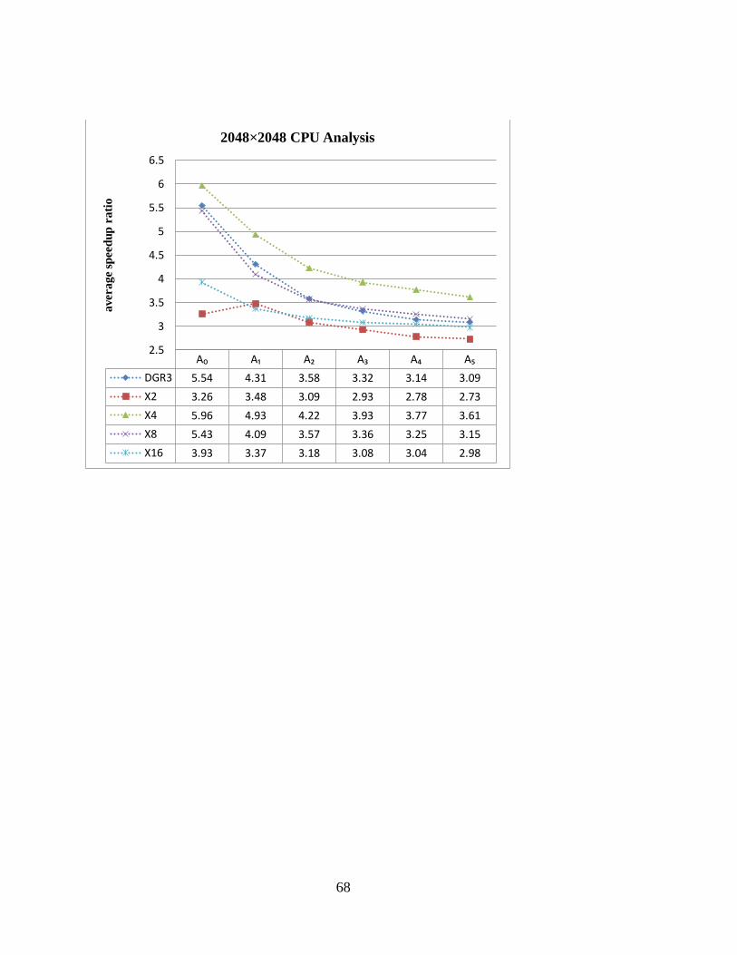
68
A₀ A₁ A₂ A₃ A₄ A₅
DGR3 5.54 4.31 3.58 3.32 3.14 3.09
X2 3.26 3.48 3.09 2.93 2.78 2.73
X4 5.96 4.93 4.22 3.93 3.77 3.61
X8 5.43 4.09 3.57 3.36 3.25 3.15
X16 3.93 3.37 3.18 3.08 3.04 2.98
2.5
3
3.5
4
4.5
5
5.5
6
6.5
average s
peed
up
rati
o
2048×2048 CPU Analysis
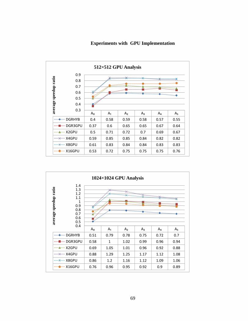
69
Experiments with GPU Implementation
A₀ A₁ A₂ A₃ A₄ A₅
DGRHYB 0.4 0.58 0.59 0.58 0.57 0.55
DGR3GPU 0.37 0.6 0.65 0.65 0.67 0.64
X2GPU 0.5 0.71 0.72 0.7 0.69 0.67
X4GPU 0.59 0.85 0.85 0.84 0.82 0.82
X8GPU 0.61 0.83 0.84 0.84 0.83 0.83
X16GPU 0.53 0.72 0.75 0.75 0.75 0.76
0.3
0.4
0.5
0.6
0.7
0.8
0.9
average s
peed
up
rati
o
512×512 GPU Analysis
A₀ A₁ A₂ A₃ A₄ A₅
DGRHYB 0.51 0.79 0.78 0.75 0.72 0.7
DGR3GPU 0.58 1 1.02 0.99 0.96 0.94
X2GPU 0.69 1.05 1.01 0.96 0.92 0.88
X4GPU 0.88 1.29 1.25 1.17 1.12 1.08
X8GPU 0.86 1.2 1.16 1.12 1.09 1.06
X16GPU 0.76 0.96 0.95 0.92 0.9 0.89
0.40.50.60.70.80.9
11.11.21.31.4
averag
e s
peed
up
ra
tio
1024×1024 GPU Analysis

70
A₀ A₁ A₂ A₃ A₄ A₅
DGRHYB 0.5 1.02 0.94 0.87 0.82 0.79
DGR3GPU 0.76 1.55 1.44 1.33 1.26 1.21
X2GPU 0.81 1.39 1.25 1.15 1.06 1.02
X4GPU 1.11 1.77 1.6 1.47 1.37 1.32
X8GPU 1.06 1.6 1.46 1.36 1.28 1.23
X16GPU 0.87 1.24 1.14 1.08 1.02 1
0.40.60.8
11.21.41.61.8
2
average s
peed
up
rati
o
2048×2048 GPU Analysis

71
Accuracy Results on 512×512 Tiles
non-matching point count with respect to R3
512×512 tile no and observer altitude R2 DGR3 X2 X4 X8 X16 R2GPU
TILE_5_1082.01 135 3 10 3 0 0 127
TILE_5_1192.99 4283 43 71 43 0 0 4127
TILE_5_1305.97 5859 12 41 4 0 8 5764
TILE_5_1418.95 6266 7 68 7 0 0 6178
TILE_5_1531.93 6732 3 63 3 0 0 6676
TILE_5_1644.92 6883 8 54 8 0 0 6828
TILE_5_1720.33 6636 9 48 8 5 0 6592
TILE_18_1026.45 896 107 1 0 74 40 781
TILE_18_1208.48 6154 17 83 17 0 0 6005
TILE_18_1392.51 8575 2 51 2 0 0 8420
TILE_18_1576.54 8572 5 55 5 0 0 8447
TILE_18_1760.58 7610 4 32 4 0 0 7560
TILE_18_1944.61 6822 2 25 2 0 0 6776
TILE_18_1798.13 7424 5 31 5 0 0 7382
TILE_3_772.619 860 0 111 0 0 0 852
TILE_3_864.315 9802 4 112 4 0 0 9682
TILE_3_958.011 10223 0 101 0 0 0 10093
TILE_3_1051.71 9428 0 71 0 0 0 9404
TILE_3_1145.4 8421 2 58 2 0 0 8388
TILE_3_1239.1 7327 3 64 3 0 0 7312
TILE_3_1541.09 4708 1 21 1 0 0 4677
TILE_4_1128.24 474 1 9 1 0 0 412
TILE_4_1227.28 4363 2 48 1 1 0 4285
TILE_4_1328.32 6725 11 77 11 0 0 6601
TILE_4_1429.36 7995 9 89 9 0 0 7926
TILE_4_1530.4 8660 9 69 9 0 0 8583
TILE_4_1631.44 8667 2 43 2 0 0 8592
TILE_4_1597.96 8652 3 43 3 0 0 8595
TILE_22_255.678 2803 14 168 13 1 0 2709
TILE_22_480.349 5883 24 88 16 8 0 5791
TILE_22_707.021 6306 13 46 9 1 3 6269
TILE_22_933.692 6302 12 52 12 0 0 6289
TILE_22_1160.36 5990 7 57 7 0 0 5951

72
TILE_22_1387.03 5678 6 43 6 0 0 5649
TILE_22_1306.86 5811 5 43 5 0 0 5767
TILE_25_653.042 1900 0 10 0 0 0 1815
TILE_25_976.186 5651 13 34 13 0 0 5570
TILE_25_1301.33 6151 4 46 4 0 0 6121
TILE_25_1626.48 6121 4 27 4 0 0 6126
TILE_25_1951.62 5840 2 28 2 0 0 5812
TILE_25_2276.76 5168 2 18 2 0 0 5132
TILE_25_1657.39 6086 4 34 4 0 0 6088
TILE_20_1213.58 830 3 9 3 0 0 743
TILE_20_1426.6 3842 0 38 0 0 0 3719
TILE_20_1641.62 5865 2 40 2 0 0 5778
TILE_20_1856.63 6158 1 42 1 0 0 6156
TILE_20_2071.65 5955 4 41 4 0 0 5964
TILE_20_2286.67 5626 3 25 3 0 0 5633
TILE_20_1730.12 6152 1 42 1 0 0 6136
TILE_6_1218.55 996 26 9 27 1 0 965
TILE_6_1330.09 5504 17 54 13 4 0 5318
TILE_6_1443.64 6896 7 59 7 0 0 6739
TILE_6_1557.19 7338 3 43 3 0 0 7231
TILE_6_1670.73 7197 2 43 2 0 0 7127
TILE_6_1784.28 6849 2 48 2 0 0 6828
TILE_6_1671.32 7188 2 47 2 0 0 7127
TILE_21_817.056 1003 30 39 18 16 0 924
TILE_21_1032.87 4886 49 59 17 35 0 4765
TILE_21_1250.69 6676 5 63 4 1 0 6556
TILE_21_1468.51 7028 3 57 1 2 0 6965
TILE_21_1686.33 6546 0 36 0 0 0 6550
TILE_21_1904.14 5810 1 24 1 0 0 5824
TILE_21_1541.14 6936 7 49 7 0 0 6869
TILE_2_846.845 1920 50 94 50 0 0 1815
TILE_2_914.637 6735 3 79 3 0 0 6555
TILE_2_984.428 7892 7 91 7 0 0 7763
TILE_2_1054.22 8283 4 94 4 0 0 8216
TILE_2_1124.01 8354 5 68 5 0 0 8290
TILE_2_1193.8 8311 5 69 5 0 0 8295
TILE_2_1451.31 6137 1 36 1 0 0 6142
TILE_1_806.641 521 0 11 0 0 0 472
TILE_1_846.606 8713 4 116 4 0 0 8527
TILE_1_888.571 10665 7 125 4 3 0 10481
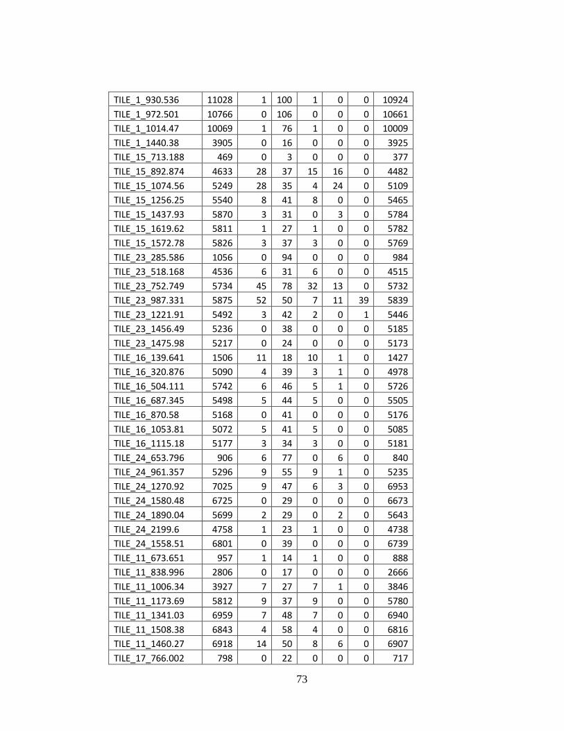
73
TILE_1_930.536 11028 1 100 1 0 0 10924
TILE_1_972.501 10766 0 106 0 0 0 10661
TILE_1_1014.47 10069 1 76 1 0 0 10009
TILE_1_1440.38 3905 0 16 0 0 0 3925
TILE_15_713.188 469 0 3 0 0 0 377
TILE_15_892.874 4633 28 37 15 16 0 4482
TILE_15_1074.56 5249 28 35 4 24 0 5109
TILE_15_1256.25 5540 8 41 8 0 0 5465
TILE_15_1437.93 5870 3 31 0 3 0 5784
TILE_15_1619.62 5811 1 27 1 0 0 5782
TILE_15_1572.78 5826 3 37 3 0 0 5769
TILE_23_285.586 1056 0 94 0 0 0 984
TILE_23_518.168 4536 6 31 6 0 0 4515
TILE_23_752.749 5734 45 78 32 13 0 5732
TILE_23_987.331 5875 52 50 7 11 39 5839
TILE_23_1221.91 5492 3 42 2 0 1 5446
TILE_23_1456.49 5236 0 38 0 0 0 5185
TILE_23_1475.98 5217 0 24 0 0 0 5173
TILE_16_139.641 1506 11 18 10 1 0 1427
TILE_16_320.876 5090 4 39 3 1 0 4978
TILE_16_504.111 5742 6 46 5 1 0 5726
TILE_16_687.345 5498 5 44 5 0 0 5505
TILE_16_870.58 5168 0 41 0 0 0 5176
TILE_16_1053.81 5072 5 41 5 0 0 5085
TILE_16_1115.18 5177 3 34 3 0 0 5181
TILE_24_653.796 906 6 77 0 6 0 840
TILE_24_961.357 5296 9 55 9 1 0 5235
TILE_24_1270.92 7025 9 47 6 3 0 6953
TILE_24_1580.48 6725 0 29 0 0 0 6673
TILE_24_1890.04 5699 2 29 0 2 0 5643
TILE_24_2199.6 4758 1 23 1 0 0 4738
TILE_24_1558.51 6801 0 39 0 0 0 6739
TILE_11_673.651 957 1 14 1 0 0 888
TILE_11_838.996 2806 0 17 0 0 0 2666
TILE_11_1006.34 3927 7 27 7 1 0 3846
TILE_11_1173.69 5812 9 37 9 0 0 5780
TILE_11_1341.03 6959 7 48 7 0 0 6940
TILE_11_1508.38 6843 4 58 4 0 0 6816
TILE_11_1460.27 6918 14 50 8 6 0 6907
TILE_17_766.002 798 0 22 0 0 0 717
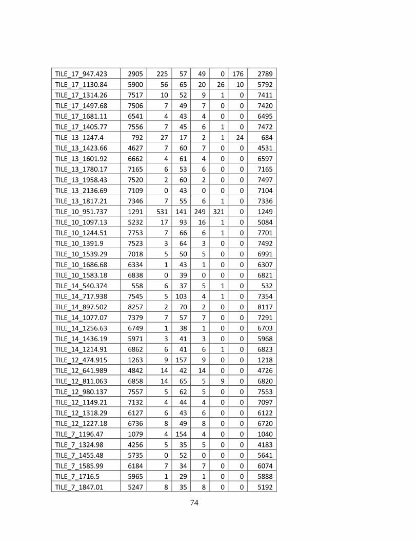
74
TILE_17_947.423 2905 225 57 49 0 176 2789
TILE_17_1130.84 5900 56 65 20 26 10 5792
TILE_17_1314.26 7517 10 52 9 1 0 7411
TILE_17_1497.68 7506 7 49 7 0 0 7420
TILE_17_1681.11 6541 4 43 4 0 0 6495
TILE_17_1405.77 7556 7 45 6 1 0 7472
TILE_13_1247.4 792 27 17 2 1 24 684
TILE_13_1423.66 4627 7 60 7 0 0 4531
TILE_13_1601.92 6662 4 61 4 0 0 6597
TILE_13_1780.17 7165 6 53 6 0 0 7165
TILE_13_1958.43 7520 2 60 2 0 0 7497
TILE_13_2136.69 7109 0 43 0 0 0 7104
TILE_13_1817.21 7346 7 55 6 1 0 7336
TILE_10_951.737 1291 531 141 249 321 0 1249
TILE_10_1097.13 5232 17 93 16 1 0 5084
TILE_10_1244.51 7753 7 66 6 1 0 7701
TILE_10_1391.9 7523 3 64 3 0 0 7492
TILE_10_1539.29 7018 5 50 5 0 0 6991
TILE_10_1686.68 6334 1 43 1 0 0 6307
TILE_10_1583.18 6838 0 39 0 0 0 6821
TILE_14_540.374 558 6 37 5 1 0 532
TILE_14_717.938 7545 5 103 4 1 0 7354
TILE_14_897.502 8257 2 70 2 0 0 8117
TILE_14_1077.07 7379 7 57 7 0 0 7291
TILE_14_1256.63 6749 1 38 1 0 0 6703
TILE_14_1436.19 5971 3 41 3 0 0 5968
TILE_14_1214.91 6862 6 41 6 1 0 6823
TILE_12_474.915 1263 9 157 9 0 0 1218
TILE_12_641.989 4842 14 42 14 0 0 4726
TILE_12_811.063 6858 14 65 5 9 0 6820
TILE_12_980.137 7557 5 62 5 0 0 7553
TILE_12_1149.21 7132 4 44 4 0 0 7097
TILE_12_1318.29 6127 6 43 6 0 0 6122
TILE_12_1227.18 6736 8 49 8 0 0 6720
TILE_7_1196.47 1079 4 154 4 0 0 1040
TILE_7_1324.98 4256 5 35 5 0 0 4183
TILE_7_1455.48 5735 0 52 0 0 0 5641
TILE_7_1585.99 6184 7 34 7 0 0 6074
TILE_7_1716.5 5965 1 29 1 0 0 5888
TILE_7_1847.01 5247 8 35 8 0 0 5192
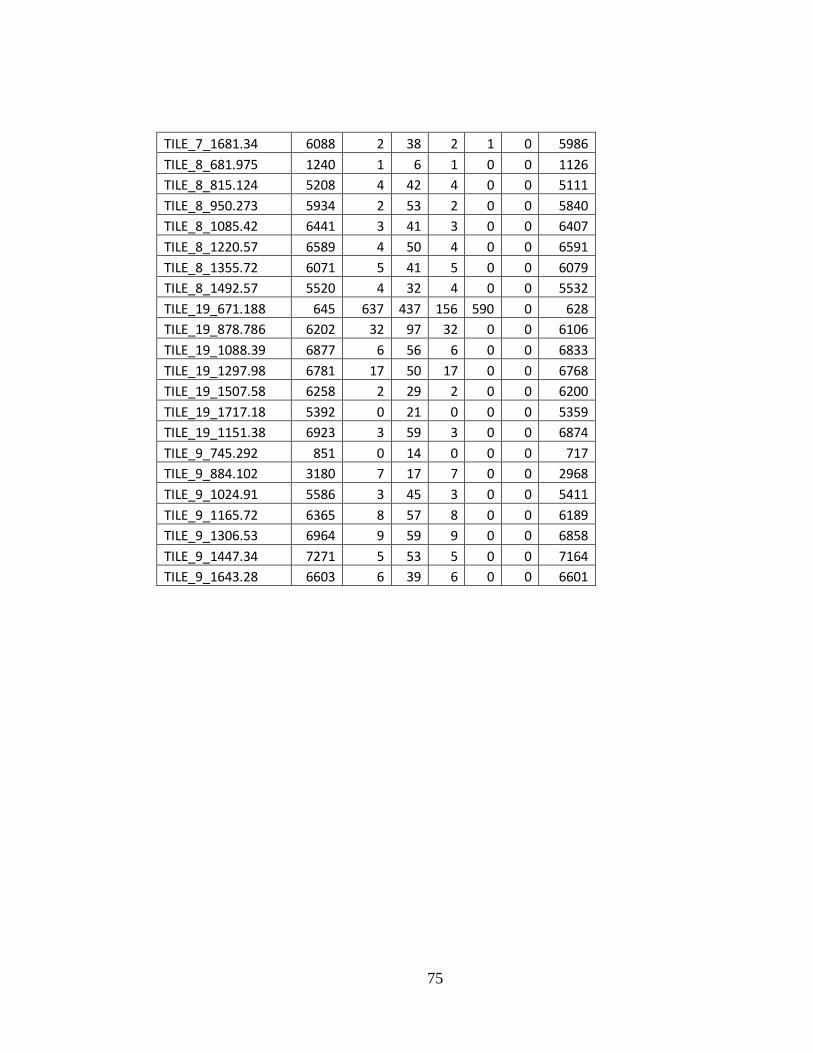
75
TILE_7_1681.34 6088 2 38 2 1 0 5986
TILE_8_681.975 1240 1 6 1 0 0 1126
TILE_8_815.124 5208 4 42 4 0 0 5111
TILE_8_950.273 5934 2 53 2 0 0 5840
TILE_8_1085.42 6441 3 41 3 0 0 6407
TILE_8_1220.57 6589 4 50 4 0 0 6591
TILE_8_1355.72 6071 5 41 5 0 0 6079
TILE_8_1492.57 5520 4 32 4 0 0 5532
TILE_19_671.188 645 637 437 156 590 0 628
TILE_19_878.786 6202 32 97 32 0 0 6106
TILE_19_1088.39 6877 6 56 6 0 0 6833
TILE_19_1297.98 6781 17 50 17 0 0 6768
TILE_19_1507.58 6258 2 29 2 0 0 6200
TILE_19_1717.18 5392 0 21 0 0 0 5359
TILE_19_1151.38 6923 3 59 3 0 0 6874
TILE_9_745.292 851 0 14 0 0 0 717
TILE_9_884.102 3180 7 17 7 0 0 2968
TILE_9_1024.91 5586 3 45 3 0 0 5411
TILE_9_1165.72 6365 8 57 8 0 0 6189
TILE_9_1306.53 6964 9 59 9 0 0 6858
TILE_9_1447.34 7271 5 53 5 0 0 7164
TILE_9_1643.28 6603 6 39 6 0 0 6601

76
Accuracy Results on 1024×1024 Tiles
non-matching point count with respect to R3
1024×1024 tile no and observer altitude R2 DGR3 X2 X4 X8 X16 R2GPU
TILE_5_755.081 6735 3 135 3 0 0 6552
TILE_5_807.567 21642 3 329 3 0 0 20988
TILE_5_862.052 30587 10 410 6 4 0 29961
TILE_5_916.538 35201 11 412 11 0 0 34733
TILE_5_971.024 37372 15 365 14 1 0 36890
TILE_5_1025.51 38090 14 345 10 4 0 37653
TILE_5_1297.05 32799 7 239 5 2 0 32767
TILE_18_869.188 564 0 81 0 0 0 523
TILE_18_1171.73 35982 20 402 18 2 0 35511
TILE_18_1476.27 35715 15 307 14 1 0 35456
TILE_18_1780.81 31049 20 224 20 0 0 30926
TILE_18_2085.35 26026 18 162 17 1 0 26035
TILE_18_2389.89 21988 19 99 19 0 0 21996
TILE_18_2860.57 17167 2 98 2 0 0 17125
TILE_3_693.999 1405 0 30 0 0 0 1184
TILE_3_758.865 9486 13 105 13 0 0 8973
TILE_3_825.731 18076 5 193 5 0 0 17615
TILE_3_892.597 24454 10 293 10 0 0 24121
TILE_3_959.464 28990 9 291 9 0 0 28592
TILE_3_1026.33 32137 21 308 20 1 0 31725
TILE_3_1540.75 30481 9 149 9 0 0 30435
TILE_4_667.636 912 1 5 1 0 0 775
TILE_4_723.497 8492 236 166 236 0 0 8131
TILE_4_781.359 21125 13 250 13 0 0 20583
TILE_4_839.22 28008 9 298 8 1 0 27417
TILE_4_897.081 31962 11 353 11 0 0 31454
TILE_4_954.943 34151 27 319 26 1 0 33667
TILE_4_1244.2 34519 10 261 10 0 0 34270
TILE_22_902.835 867 0 15 0 0 0 808
TILE_22_1095.69 17212 13 287 10 3 0 16989
TILE_22_1290.55 30506 27 403 27 0 0 29943
TILE_22_1485.41 31991 25 325 25 0 0 31602
TILE_22_1680.27 30828 9 302 9 0 0 30573
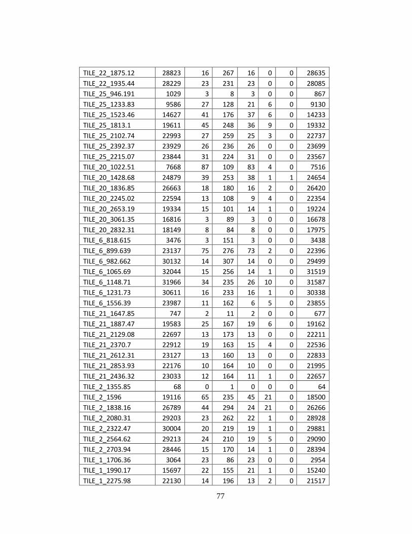
77
TILE_22_1875.12 28823 16 267 16 0 0 28635
TILE_22_1935.44 28229 23 231 23 0 0 28085
TILE_25_946.191 1029 3 8 3 0 0 867
TILE_25_1233.83 9586 27 128 21 6 0 9130
TILE_25_1523.46 14627 41 176 37 6 0 14233
TILE_25_1813.1 19611 45 248 36 9 0 19332
TILE_25_2102.74 22993 27 259 25 3 0 22737
TILE_25_2392.37 23929 26 236 26 0 0 23699
TILE_25_2215.07 23844 31 224 31 0 0 23567
TILE_20_1022.51 7668 87 109 83 4 0 7516
TILE_20_1428.68 24879 39 253 38 1 1 24654
TILE_20_1836.85 26663 18 180 16 2 0 26420
TILE_20_2245.02 22594 13 108 9 4 0 22354
TILE_20_2653.19 19334 15 101 14 1 0 19224
TILE_20_3061.35 16816 3 89 3 0 0 16678
TILE_20_2832.31 18149 8 84 8 0 0 17975
TILE_6_818.615 3476 3 151 3 0 0 3438
TILE_6_899.639 23137 75 276 73 2 0 22396
TILE_6_982.662 30132 14 307 14 0 0 29499
TILE_6_1065.69 32044 15 256 14 1 0 31519
TILE_6_1148.71 31966 34 235 26 10 0 31587
TILE_6_1231.73 30611 16 233 16 1 0 30338
TILE_6_1556.39 23987 11 162 6 5 0 23855
TILE_21_1647.85 747 2 11 2 0 0 677
TILE_21_1887.47 19583 25 167 19 6 0 19162
TILE_21_2129.08 22697 13 173 13 0 0 22211
TILE_21_2370.7 22912 19 163 15 4 0 22536
TILE_21_2612.31 23127 13 160 13 0 0 22833
TILE_21_2853.93 22176 10 164 10 0 0 21995
TILE_21_2436.32 23033 12 164 11 1 0 22657
TILE_2_1355.85 68 0 1 0 0 0 64
TILE_2_1596 19116 65 235 45 21 0 18500
TILE_2_1838.16 26789 44 294 24 21 0 26266
TILE_2_2080.31 29203 23 262 22 1 0 28928
TILE_2_2322.47 30004 20 219 19 1 0 29881
TILE_2_2564.62 29213 24 210 19 5 0 29090
TILE_2_2703.94 28446 15 170 14 1 0 28394
TILE_1_1706.36 3064 23 86 23 0 0 2954
TILE_1_1990.17 15697 22 155 21 1 0 15240
TILE_1_2275.98 22130 14 196 13 2 0 21517
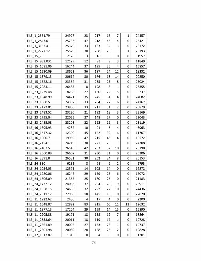
78
TILE_1_2561.79 24977 23 217 16 7 1 24457
TILE_1_2847.6 25736 47 218 45 4 0 25421
TILE_1_3133.41 25370 33 183 32 3 0 25172
TILE_1_2777.12 25529 30 258 29 1 1 25193
TILE_15_785 2120 3 16 3 0 0 1957
TILE_15_932.031 12129 12 93 9 3 3 11849
TILE_15_1081.06 16244 37 195 36 4 0 15857
TILE_15_1230.09 18652 36 197 24 12 0 18332
TILE_15_1379.13 20614 30 176 18 14 0 20250
TILE_15_1528.16 23384 31 235 23 8 0 23024
TILE_15_2083.11 26485 8 198 8 1 0 26355
TILE_23_1239.48 8268 27 1130 22 5 0 8237
TILE_23_1548.99 24421 35 245 31 4 0 24082
TILE_23_1860.5 24397 33 204 27 6 0 24162
TILE_23_2172.01 23950 33 217 31 2 0 23879
TILE_23_2483.52 23220 21 192 18 3 0 23169
TILE_23_2795.04 22055 27 148 27 0 0 22043
TILE_23_2485.08 23203 22 192 19 3 0 23119
TILE_16_1395.93 4282 10 21 6 4 0 3963
TILE_16_1647.32 12300 45 122 39 6 0 11767
TILE_16_1900.71 19959 47 215 45 4 0 19572
TILE_16_2154.1 24719 30 271 29 1 0 24308
TILE_16_2407.5 26546 42 233 32 10 0 26198
TILE_16_2660.89 26607 31 230 31 0 0 26306
TILE_16_2391.8 26531 30 252 24 8 0 26153
TILE_24_830 6231 8 68 6 2 0 5793
TILE_24_1054.03 12571 14 105 14 0 0 12272
TILE_24_1280.06 16246 29 159 23 6 0 16072
TILE_24_1506.09 21367 25 180 25 0 0 21183
TILE_24_1732.12 24063 37 204 28 9 0 23911
TILE_24_1958.15 24636 32 222 22 10 0 24436
TILE_24_2311.12 22960 18 145 18 0 0 22820
TILE_11_1222.62 2430 4 17 4 0 0 2200
TILE_11_1548.87 12892 83 215 60 11 12 12632
TILE_11_1877.13 17204 29 159 14 15 0 16890
TILE_11_2205.38 19171 18 158 12 7 5 18864
TILE_11_2533.64 20011 18 119 17 1 0 19728
TILE_11_2861.89 20006 27 133 26 1 0 19737
TILE_11_2801.98 20089 28 158 26 2 0 19828
TILE_17_1917.87 1315 0 4 0 0 0 1201
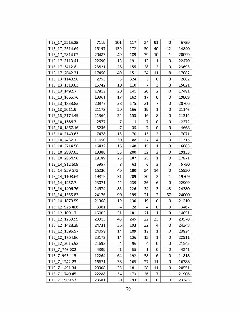
79
TILE_17_2215.25 7119 101 117 24 91 0 6759
TILE_17_2514.64 15197 130 172 50 40 42 14840
TILE_17_2814.02 20483 49 189 39 10 1 20099
TILE_17_3113.41 22690 13 191 12 1 0 22470
TILE_17_3412.8 23821 28 155 28 2 0 23693
TILE_17_2642.31 17450 49 151 34 11 8 17082
TILE_13_1148.56 2753 3 624 3 0 0 2682
TILE_13_1319.63 15742 10 110 7 3 0 15021
TILE_13_1492.7 17813 20 141 20 2 0 17481
TILE_13_1665.76 19961 17 162 17 0 0 19809
TILE_13_1838.83 20877 28 175 21 7 0 20766
TILE_13_2011.9 21173 20 166 19 1 0 21146
TILE_13_2174.49 21364 24 153 16 8 0 21314
TILE_10_1586.7 2577 7 13 7 0 0 2272
TILE_10_1867.16 5236 7 35 7 0 0 4668
TILE_10_2149.63 7478 13 70 13 2 0 7071
TILE_10_2432.1 11650 30 88 27 4 0 11315
TILE_10_2714.56 16432 16 148 15 1 0 16083
TILE_10_2997.03 19388 33 200 32 2 0 19133
TILE_10_2864.56 18189 25 187 25 1 0 17871
TILE_14_812.509 5957 8 62 6 3 0 5750
TILE_14_959.573 16230 46 180 34 14 0 15930
TILE_14_1108.64 19815 31 209 30 2 1 19709
TILE_14_1257.7 23071 42 239 36 6 0 22909
TILE_14_1406.76 24574 85 226 34 3 48 24380
TILE_14_1555.83 24176 90 199 21 2 67 24000
TILE_14_1879.59 21368 19 130 19 0 0 21210
TILE_12_925.406 3961 4 28 4 0 0 3467
TILE_12_1091.7 15003 31 181 21 1 9 14651
TILE_12_1259.99 23913 45 245 22 23 0 23578
TILE_12_1428.28 24731 36 193 32 4 0 24348
TILE_12_1596.57 24058 14 189 13 1 0 23834
TILE_12_1764.86 23172 14 136 13 1 0 22911
TILE_12_2015.92 21693 4 96 4 0 0 21542
TILE_7_746.002 4399 1 55 1 0 0 4241
TILE_7_993.115 12264 64 192 58 6 0 11818
TILE_7_1242.23 16671 38 165 27 11 0 16388
TILE_7_1491.34 20908 35 181 28 11 0 20551
TILE_7_1740.45 22288 34 173 26 7 1 21906
TILE_7_1989.57 23581 30 193 30 0 0 23343

80
TILE_7_2276.83 23582 26 164 25 1 0 23464
TILE_8_1911.89 2136 0 7 0 0 0 1942
TILE_8_2329.43 15726 39 147 38 1 0 15439
TILE_8_2748.98 25161 35 210 23 13 0 24819
TILE_8_3168.52 28609 42 203 28 15 0 28253
TILE_8_3588.06 29824 22 169 16 6 0 29672
TILE_8_4007.6 29615 17 141 15 2 0 29524
TILE_8_2680.37 23939 29 208 24 11 0 23663
TILE_19_1339.41 9040 6 21 6 0 0 8624
TILE_19_1735.29 16100 18 102 12 3 3 15561
TILE_19_2133.17 20880 21 129 17 4 0 20425
TILE_19_2531.05 23389 51 148 22 29 0 23098
TILE_19_2928.94 24460 20 162 14 6 0 24282
TILE_19_3326.82 24388 21 135 20 2 0 24318
TILE_19_2736.71 24004 22 157 21 1 0 23745
TILE_9_1893.12 4598 329 82 329 6 0 4529
TILE_9_2279.53 19544 19 153 15 4 0 19080
TILE_9_2667.93 24545 26 180 26 0 0 24168
TILE_9_3056.33 27223 21 159 19 4 0 26826
TILE_9_3444.74 27718 25 175 22 3 0 27495
TILE_9_3833.14 27470 11 147 11 0 0 27417
TILE_9_2903.67 26588 21 160 19 2 0 26200
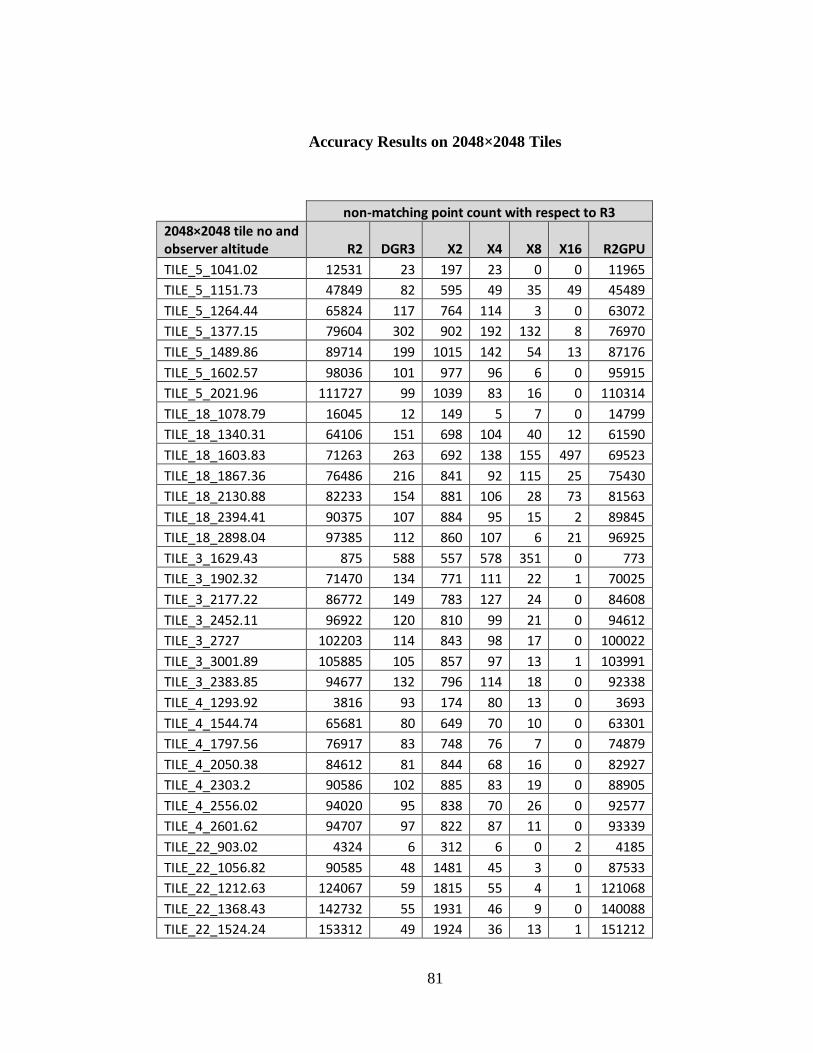
81
Accuracy Results on 2048×2048 Tiles
non-matching point count with respect to R3
2048×2048 tile no and observer altitude R2 DGR3 X2 X4 X8 X16 R2GPU
TILE_5_1041.02 12531 23 197 23 0 0 11965
TILE_5_1151.73 47849 82 595 49 35 49 45489
TILE_5_1264.44 65824 117 764 114 3 0 63072
TILE_5_1377.15 79604 302 902 192 132 8 76970
TILE_5_1489.86 89714 199 1015 142 54 13 87176
TILE_5_1602.57 98036 101 977 96 6 0 95915
TILE_5_2021.96 111727 99 1039 83 16 0 110314
TILE_18_1078.79 16045 12 149 5 7 0 14799
TILE_18_1340.31 64106 151 698 104 40 12 61590
TILE_18_1603.83 71263 263 692 138 155 497 69523
TILE_18_1867.36 76486 216 841 92 115 25 75430
TILE_18_2130.88 82233 154 881 106 28 73 81563
TILE_18_2394.41 90375 107 884 95 15 2 89845
TILE_18_2898.04 97385 112 860 107 6 21 96925
TILE_3_1629.43 875 588 557 578 351 0 773
TILE_3_1902.32 71470 134 771 111 22 1 70025
TILE_3_2177.22 86772 149 783 127 24 0 84608
TILE_3_2452.11 96922 120 810 99 21 0 94612
TILE_3_2727 102203 114 843 98 17 0 100022
TILE_3_3001.89 105885 105 857 97 13 1 103991
TILE_3_2383.85 94677 132 796 114 18 0 92338
TILE_4_1293.92 3816 93 174 80 13 0 3693
TILE_4_1544.74 65681 80 649 70 10 0 63301
TILE_4_1797.56 76917 83 748 76 7 0 74879
TILE_4_2050.38 84612 81 844 68 16 0 82927
TILE_4_2303.2 90586 102 885 83 19 0 88905
TILE_4_2556.02 94020 95 838 70 26 0 92577
TILE_4_2601.62 94707 97 822 87 11 0 93339
TILE_22_903.02 4324 6 312 6 0 2 4185
TILE_22_1056.82 90585 48 1481 45 3 0 87533
TILE_22_1212.63 124067 59 1815 55 4 1 121068
TILE_22_1368.43 142732 55 1931 46 9 0 140088
TILE_22_1524.24 153312 49 1924 36 13 1 151212
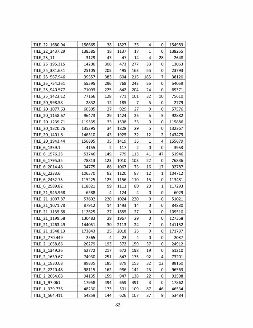
82
TILE_22_1680.04 156665 38 1827 35 4 0 154983
TILE_22_2437.29 138585 18 1137 17 1 0 138255
TILE_25_11 3129 43 47 14 4 28 2648
TILE_25_195.315 14206 306 473 277 33 0 13063
TILE_25_381.631 25105 205 495 163 55 0 23793
TILE_25_567.946 39557 383 604 215 185 7 38120
TILE_25_754.261 55595 296 768 243 55 0 54059
TILE_25_940.577 71093 225 842 204 24 0 69371
TILE_25_1423.12 77166 128 771 101 32 10 75610
TILE_20_998.58 2832 12 185 7 5 0 2779
TILE_20_1077.63 60305 27 929 27 0 0 57576
TILE_20_1158.67 96473 29 1424 25 5 5 92882
TILE_20_1239.71 119535 33 1598 33 0 0 115886
TILE_20_1320.76 135395 34 1828 29 5 0 132267
TILE_20_1401.8 146510 43 1925 32 12 2 143479
TILE_20_1943.44 156895 35 1419 35 1 4 155679
TILE_6_1359.1 4155 2 117 2 0 0 3953
TILE_6_1576.23 53746 149 779 113 41 47 51946
TILE_6_1795.35 78813 123 1010 103 22 0 76836
TILE_6_2014.48 94775 88 1067 73 16 17 92787
TILE_6_2233.6 106570 92 1120 87 12 1 104712
TILE_6_2452.73 115225 125 1156 110 15 0 113481
TILE_6_2589.82 118821 99 1113 80 20 1 117293
TILE_21_945.968 6588 4 124 4 0 0 6029
TILE_21_1007.87 53602 220 1024 220 0 0 51021
TILE_21_1071.78 87912 14 1493 14 0 0 84830
TILE_21_1135.68 112625 27 1855 27 0 0 109510
TILE_21_1199.58 130483 29 1967 29 0 0 127358
TILE_21_1263.49 144051 30 2113 24 7 0 141152
TILE_21_1548.13 173843 25 2018 25 0 0 171737
TILE_2_770.449 2565 4 23 4 0 0 2037
TILE_2_1058.86 26279 193 372 159 37 0 24912
TILE_2_1349.26 52772 217 672 198 19 0 51210
TILE_2_1639.67 74930 251 847 175 92 4 73201
TILE_2_1930.08 89835 185 879 153 32 12 88160
TILE_2_2220.48 98115 162 986 142 23 0 96563
TILE_2_2064.68 94135 159 947 138 22 0 92598
TILE_1_97.061 17958 494 659 491 3 0 17862
TILE_1_329.736 48230 173 501 109 87 46 46534
TILE_1_564.411 54859 144 626 107 37 9 53484
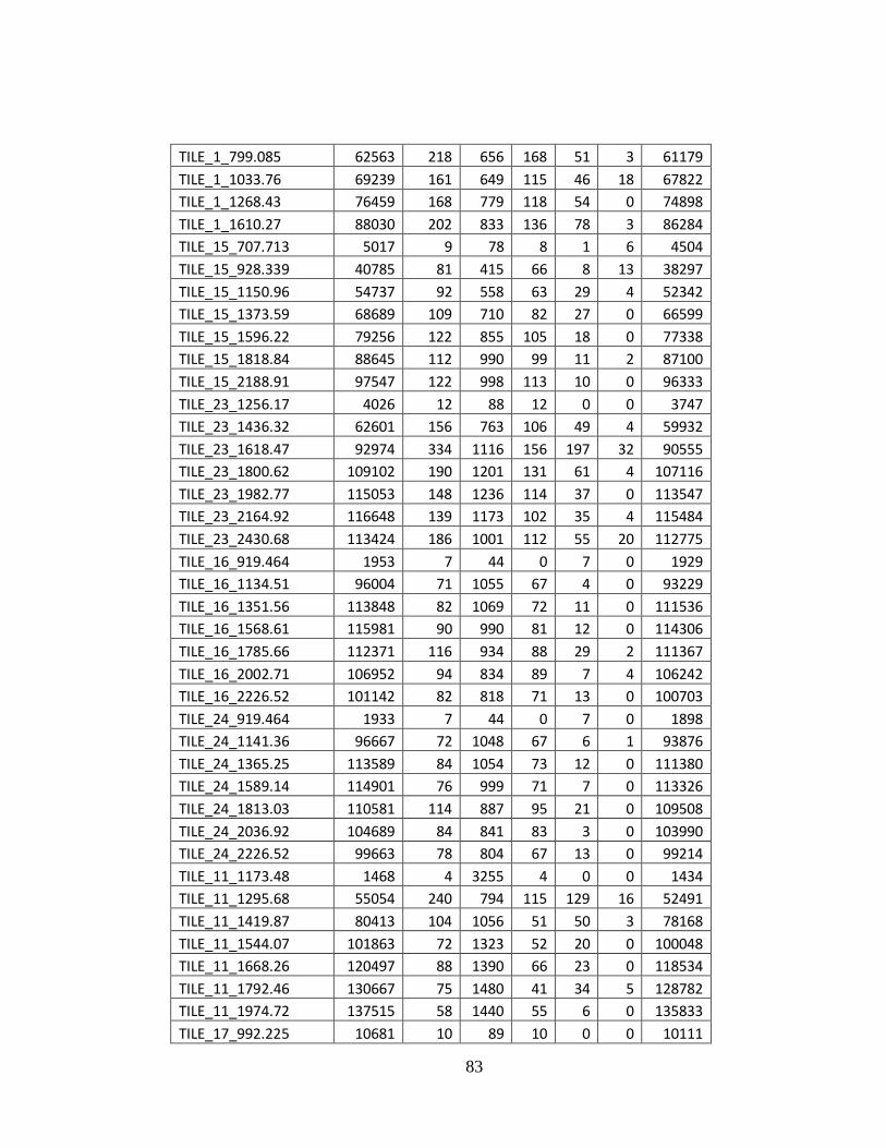
83
TILE_1_799.085 62563 218 656 168 51 3 61179
TILE_1_1033.76 69239 161 649 115 46 18 67822
TILE_1_1268.43 76459 168 779 118 54 0 74898
TILE_1_1610.27 88030 202 833 136 78 3 86284
TILE_15_707.713 5017 9 78 8 1 6 4504
TILE_15_928.339 40785 81 415 66 8 13 38297
TILE_15_1150.96 54737 92 558 63 29 4 52342
TILE_15_1373.59 68689 109 710 82 27 0 66599
TILE_15_1596.22 79256 122 855 105 18 0 77338
TILE_15_1818.84 88645 112 990 99 11 2 87100
TILE_15_2188.91 97547 122 998 113 10 0 96333
TILE_23_1256.17 4026 12 88 12 0 0 3747
TILE_23_1436.32 62601 156 763 106 49 4 59932
TILE_23_1618.47 92974 334 1116 156 197 32 90555
TILE_23_1800.62 109102 190 1201 131 61 4 107116
TILE_23_1982.77 115053 148 1236 114 37 0 113547
TILE_23_2164.92 116648 139 1173 102 35 4 115484
TILE_23_2430.68 113424 186 1001 112 55 20 112775
TILE_16_919.464 1953 7 44 0 7 0 1929
TILE_16_1134.51 96004 71 1055 67 4 0 93229
TILE_16_1351.56 113848 82 1069 72 11 0 111536
TILE_16_1568.61 115981 90 990 81 12 0 114306
TILE_16_1785.66 112371 116 934 88 29 2 111367
TILE_16_2002.71 106952 94 834 89 7 4 106242
TILE_16_2226.52 101142 82 818 71 13 0 100703
TILE_24_919.464 1933 7 44 0 7 0 1898
TILE_24_1141.36 96667 72 1048 67 6 1 93876
TILE_24_1365.25 113589 84 1054 73 12 0 111380
TILE_24_1589.14 114901 76 999 71 7 0 113326
TILE_24_1813.03 110581 114 887 95 21 0 109508
TILE_24_2036.92 104689 84 841 83 3 0 103990
TILE_24_2226.52 99663 78 804 67 13 0 99214
TILE_11_1173.48 1468 4 3255 4 0 0 1434
TILE_11_1295.68 55054 240 794 115 129 16 52491
TILE_11_1419.87 80413 104 1056 51 50 3 78168
TILE_11_1544.07 101863 72 1323 52 20 0 100048
TILE_11_1668.26 120497 88 1390 66 23 0 118534
TILE_11_1792.46 130667 75 1480 41 34 5 128782
TILE_11_1974.72 137515 58 1440 55 6 0 135833
TILE_17_992.225 10681 10 89 10 0 0 10111
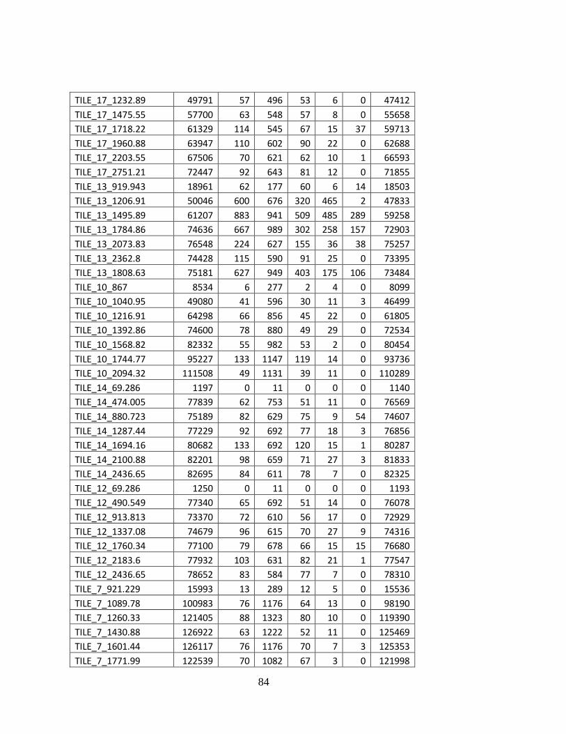
84
TILE_17_1232.89 49791 57 496 53 6 0 47412
TILE_17_1475.55 57700 63 548 57 8 0 55658
TILE_17_1718.22 61329 114 545 67 15 37 59713
TILE_17_1960.88 63947 110 602 90 22 0 62688
TILE_17_2203.55 67506 70 621 62 10 1 66593
TILE_17_2751.21 72447 92 643 81 12 0 71855
TILE_13_919.943 18961 62 177 60 6 14 18503
TILE_13_1206.91 50046 600 676 320 465 2 47833
TILE_13_1495.89 61207 883 941 509 485 289 59258
TILE_13_1784.86 74636 667 989 302 258 157 72903
TILE_13_2073.83 76548 224 627 155 36 38 75257
TILE_13_2362.8 74428 115 590 91 25 0 73395
TILE_13_1808.63 75181 627 949 403 175 106 73484
TILE_10_867 8534 6 277 2 4 0 8099
TILE_10_1040.95 49080 41 596 30 11 3 46499
TILE_10_1216.91 64298 66 856 45 22 0 61805
TILE_10_1392.86 74600 78 880 49 29 0 72534
TILE_10_1568.82 82332 55 982 53 2 0 80454
TILE_10_1744.77 95227 133 1147 119 14 0 93736
TILE_10_2094.32 111508 49 1131 39 11 0 110289
TILE_14_69.286 1197 0 11 0 0 0 1140
TILE_14_474.005 77839 62 753 51 11 0 76569
TILE_14_880.723 75189 82 629 75 9 54 74607
TILE_14_1287.44 77229 92 692 77 18 3 76856
TILE_14_1694.16 80682 133 692 120 15 1 80287
TILE_14_2100.88 82201 98 659 71 27 3 81833
TILE_14_2436.65 82695 84 611 78 7 0 82325
TILE_12_69.286 1250 0 11 0 0 0 1193
TILE_12_490.549 77340 65 692 51 14 0 76078
TILE_12_913.813 73370 72 610 56 17 0 72929
TILE_12_1337.08 74679 96 615 70 27 9 74316
TILE_12_1760.34 77100 79 678 66 15 15 76680
TILE_12_2183.6 77932 103 631 82 21 1 77547
TILE_12_2436.65 78652 83 584 77 7 0 78310
TILE_7_921.229 15993 13 289 12 5 0 15536
TILE_7_1089.78 100983 76 1176 64 13 0 98190
TILE_7_1260.33 121405 88 1323 80 10 0 119390
TILE_7_1430.88 126922 63 1222 52 11 0 125469
TILE_7_1601.44 126117 76 1176 70 7 3 125353
TILE_7_1771.99 122539 70 1082 67 3 0 121998
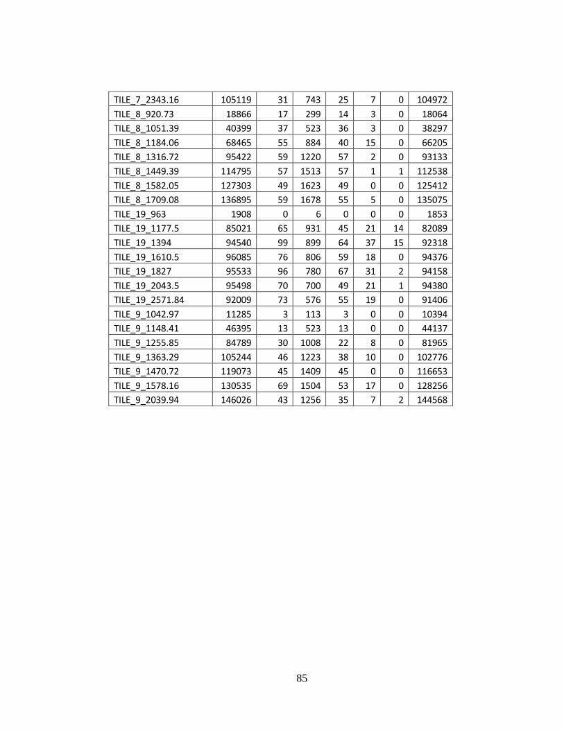
85
TILE_7_2343.16 105119 31 743 25 7 0 104972
TILE_8_920.73 18866 17 299 14 3 0 18064
TILE_8_1051.39 40399 37 523 36 3 0 38297
TILE_8_1184.06 68465 55 884 40 15 0 66205
TILE_8_1316.72 95422 59 1220 57 2 0 93133
TILE_8_1449.39 114795 57 1513 57 1 1 112538
TILE_8_1582.05 127303 49 1623 49 0 0 125412
TILE_8_1709.08 136895 59 1678 55 5 0 135075
TILE_19_963 1908 0 6 0 0 0 1853
TILE_19_1177.5 85021 65 931 45 21 14 82089
TILE_19_1394 94540 99 899 64 37 15 92318
TILE_19_1610.5 96085 76 806 59 18 0 94376
TILE_19_1827 95533 96 780 67 31 2 94158
TILE_19_2043.5 95498 70 700 49 21 1 94380
TILE_19_2571.84 92009 73 576 55 19 0 91406
TILE_9_1042.97 11285 3 113 3 0 0 10394
TILE_9_1148.41 46395 13 523 13 0 0 44137
TILE_9_1255.85 84789 30 1008 22 8 0 81965
TILE_9_1363.29 105244 46 1223 38 10 0 102776
TILE_9_1470.72 119073 45 1409 45 0 0 116653
TILE_9_1578.16 130535 69 1504 53 17 0 128256
TILE_9_2039.94 146026 43 1256 35 7 2 144568